1

Alternating Ditransitives in English:

A Corpus-Based Study

Gabriel Alejandro Ozón

UCL

PhD

2009

2

I, Gabriel Alejandro Ozón, confirm that the work presented in this thesis is my own. Where information has been derived from other sources, I confirm that this has been indicated in the thesis.

3

Abstract: Alternating Ditransitives in English

This thesis is a large-scale investigation of ditransitive constructions and their alternants

in English. Typically both constructions involve three participants: participant A

transfers an element B to participant C. A speaker can linguistically encode this type of

situation in one of two ways: by using either a double object construction or a

prepositional paraphrase. This study examines this syntactic choice in the British

component of the International Corpus of English (ICE-GB), a fully tagged and parsed

corpus incorporating both spoken and written English.

After a general introduction, chapter 2 reviews the different grammatical

treatments of the constructions. Chapter 3 discusses whether indirect objects have to be

considered necessary complements or optional adjuncts of the verb. I then examine the

tension between rigid classification and authentic (corpus) data in order to demonstrate

that the distinction between complements and adjuncts evidences gradient

categorisation effects.

This study has both a linguistic and a methodological angle. The overall design

and methodology employed in this study are discussed in chapter 4. The thesis

considers a number of variables that help predict the occurrence of each pattern. The

evaluation of the variables, the determination of their significance, and the measurement

of their contribution to the model involve reliance on statistical methods (but not

statistical software packages).

Chapters 5, 6, and 7 review pragmatic factors claimed to influence a speaker’s

choice of construction, among them the information status and the syntactic ‘heaviness’

of the constituents involved. The explanatory power and coverage of these factors are

experimentally tested independently against the corpus data, in order to highlight

several features which only emerge after examining authentic sources.

Chapter 8 posits a novel method of bringing these factors together; the resulting

model predicts the dative alternation with almost 80% accuracy in ICE-GB.

Conclusions are offered in chapter 9.

4

Table of contents 1 Introduction .............................................................................................................10 2 Review of the Literature..........................................................................................16

2.1 Diachronic Perspectives ..................................................................................16 2.2 Synchronic Approaches ..................................................................................19

2.2.1 Traditional Grammar...............................................................................19 2.2.2 Transformational Grammar.....................................................................27 2.2.3 Semantic and Cognitive Approaches ......................................................59

3 The Indirect Object as Complement of the Verb ....................................................76 3.1 Definitional Criteria ........................................................................................76

3.1.1 Notional Criterion ...................................................................................76 3.1.2 Maximum Number..................................................................................77 3.1.3 Determination of Form............................................................................78 3.1.4 Word Order .............................................................................................80 3.1.5 Noun vs. Preposition ...............................................................................81 3.1.6 Obligatoriness .........................................................................................82 3.1.7 Subcategorisation ....................................................................................84 3.1.8 Latency....................................................................................................86 3.1.9 Collocational Restrictions .......................................................................86

3.2 Constituency Tests ..........................................................................................87 3.2.1 Extraction ................................................................................................87 3.2.2 Anaphora: Substitution ...........................................................................88 3.2.3 Cleft Constructions .................................................................................89

3.3 Semantic Roles................................................................................................90 3.3.1 Locative...................................................................................................91 3.3.2 Recipient .................................................................................................91 3.3.3 Beneficiary ..............................................................................................92

3.4 The Dativus Ethicus ........................................................................................93 3.5 Gradience ........................................................................................................95

4 Dataset and Experiment Design ..............................................................................98 4.1 The Dataset......................................................................................................99 4.2 Complementation Patterns ............................................................................106

4.2.1 S V IO DO(NP).......................................................................................107 4.2.2 S V IO DO(CL).......................................................................................107 4.2.3 S V DO ‘IO’(PP) ....................................................................................107

4.3 Verb Classes..................................................................................................107 4.3.1 Class 1: V+IO+DO or V+NP+to...........................................................109 4.3.2 Class 2: V+NP+to only .........................................................................110 4.3.3 Class 3: V+NP+NP or V+NP+for.........................................................110 4.3.4 Class 4: V+NP+NP or V+NP+to/for.....................................................111 4.3.5 Class 5: V+NP+for only........................................................................111 4.3.6 Class 6: V+NP+NP only .......................................................................112 4.3.7 Class 7: V+NP+NP or V+NP+other prepositions.................................112

4.4 Fine-Tuning the Dataset: Inclusions and Exclusions ....................................112 4.4.1 Thematic Variants .................................................................................115 4.4.2 Idioms....................................................................................................125 4.4.3 Light Verbs ...........................................................................................129

4.5 Experiment Design........................................................................................134 4.5.1 Definition ..............................................................................................135 4.5.2 Sampling ...............................................................................................136 4.5.3 Analysis.................................................................................................136 4.5.4 Evaluation .............................................................................................139

5

4.6 Quantitative Analysis ....................................................................................139 4.6.1 Variables ...............................................................................................139 4.6.2 Data Distribution...................................................................................140 4.6.3 Tests ......................................................................................................141

5 Information Status.................................................................................................145 5.1 Introduction: Previous Approaches...............................................................145 5.2 Terminological Confusion ............................................................................147 5.3 Conceptions of Information Status ...............................................................148

5.3.1 Topic and Focus ....................................................................................148 5.3.2 Topic and Comment..............................................................................149 5.3.3 Theme and Rheme.................................................................................150 5.3.4 Given and New......................................................................................152 5.3.5 Pragmatic Tension: Colliding Principles?.............................................159

5.4 Accounts of the Dative Alternation...............................................................162 5.4.1 Animacy ................................................................................................163 5.4.2 Definiteness...........................................................................................165 5.4.3 Topicality, Theme, Dominance and Topicworthiness ..........................169

6 Testing the Theories: Given Before New (GBN) .................................................172 6.1 Introduction: Corpus Experimentation..........................................................172 6.2 Corpus Experiment 1: GBN by Textual Retrievability.................................172

6.2.1 The GBN Principle................................................................................172 6.2.2 Retrievability.........................................................................................173 6.2.3 Results ...................................................................................................175 6.2.4 Preliminary Consideration of the Results .............................................178

6.3 Corpus Experiment 2: GBN, Retrievability and ‘Inferrables’ ......................178 6.3.1 Textual Retrievability: Shortcomings ...................................................178 6.3.2 Inferrables .............................................................................................180 6.3.3 Results ...................................................................................................181 6.3.4 Preliminary Consideration of the Results .............................................187

6.4 Corpus Experiment 3: GBN Configurations .................................................187 6.4.1 Configurations.......................................................................................187 6.4.2 Frequency Results .................................................................................188 6.4.3 Predictors ..............................................................................................190 6.4.4 GBN Index: An Inductive Measure ......................................................193 6.4.5 Preliminary Consideration of the Results .............................................197

6.5 Conclusions...................................................................................................198 7 Testing the Theories II: Length, Weight, Complexity ..........................................199

7.1 Weight ...........................................................................................................199 7.1.1 Weight: Definitions and Assumptions ..................................................199 7.1.2 Accounts of Weight...............................................................................200 7.1.3 Corpus Experiment 4: Weight...............................................................203

7.2 Complexity....................................................................................................214 7.2.1 Complexity: Definitions and Assumptions ...........................................214 7.2.2 Complex Accounts ................................................................................214 7.2.3 Corpus Experiment 5: Complexity .......................................................216

7.3 Conclusions...................................................................................................225 8 Interacting Variables .............................................................................................226

8.1 Introduction: Resolving Competing Hypotheses ..........................................226 8.2 Weight vs. Complexity .................................................................................227

8.2.1 Interaction (i).........................................................................................228 8.2.2 Weight vs. Complexity: Results............................................................228 8.2.3 Preliminary Consideration of the Results .............................................230

6

8.3 GBN vs. Weight ............................................................................................231 8.3.1 Interaction (ii)........................................................................................231 8.3.2 GBN vs. Weight: Results ......................................................................232 8.3.3 Preliminary Consideration of the Results .............................................234

8.4 Multiple Competing Variables......................................................................235 8.4.1 Design Issues.........................................................................................237 8.4.2 Simple Majority Voting (SMV): Results ..............................................238 8.4.3 Preliminary Consideration of the Results .............................................243 8.4.4 Residual Probability or Counterexamples.............................................247

8.5 Experimental Conclusions ............................................................................252 9 Conclusions...........................................................................................................254 10 References .........................................................................................................259

List of Tables and Figures Table 1: Allerton’s Ditransitive Valency Classification (1982) .....................................26 Figure 2: Chomsky’s 1957 Model ..................................................................................28 Figure 3: Passive transformation according to Syntactic Structures (1957) ...................28 Figure 4: Chomsky’s 1965 Model ..................................................................................31 Figure 5 ...........................................................................................................................32 Figure 6 ...........................................................................................................................33 Figure 7 ...........................................................................................................................34 Figure 8: Chomsky’s 1981 Model ..................................................................................35 Figure 9 ...........................................................................................................................36 Figure 10 .........................................................................................................................36 Figure 11 .........................................................................................................................40 Figure 12 .........................................................................................................................41 Figure 13 .........................................................................................................................44 Figure 14 .........................................................................................................................45 Figure 15 .........................................................................................................................46 Figure 16 .........................................................................................................................46 Figure 17 .........................................................................................................................47 Figure 18 .........................................................................................................................47 Figure 19 .........................................................................................................................48 Figure 20 .........................................................................................................................50 Figure 21 .........................................................................................................................52 Figure 22 .........................................................................................................................52 Figure 23 .........................................................................................................................53 Figure 24 .........................................................................................................................53 Figure 25 .........................................................................................................................55 Figure 26 .........................................................................................................................57 Figure 27 .........................................................................................................................57 Figure 28: Semantic roles in ditransitives.......................................................................63 Figure 29 .........................................................................................................................66 Figure 30 .........................................................................................................................66 Figure 31: Form/meaning pairings..................................................................................68 Figure 32: Composite Fused Structure: Ditransitive construction + hand......................72 Figure 33, .......................................................................................................................74 Figure 34 .........................................................................................................................75 Figure 35: Functions in Huddleston and Pullum et al. (2002)........................................81 Table 36: Gradience between indirect objects and prepositional variants......................97 Figure 37: An FTF search pattern for DAT ..................................................................101 Figure 38: How the FTF in Figure 37 matches against a tree.......................................104

7

Figure 39: An FTF search pattern for DOC..................................................................104 Figure 40: How the FTF in Figure 39 matches against a tree.......................................105 Table 41: Occurrences of DOCs and DATs in ICE-GB ...............................................109 Table 42: Normalised occurrences of DOCs and DATs in ICE-GB ............................109 Table 43: V+IO+DO or V+NP+to ................................................................................109 Table 44: V+NP+to only...............................................................................................110 Table 45: V+NP+NP or V+NP+for ..............................................................................110 Table 46: V+NP+NP or V+NP+to/for ..........................................................................111 Table 47: V+NP+for only .............................................................................................111 Table 48: V+NP+NP only.............................................................................................112 Table 49: Unmarked Indirect Objects ...........................................................................115 Table 50: Unmarked Prepositional Paraphrases ...........................................................116 Figure 51: FTF for capturing A1 to A3 DOC cases......................................................118 Figure 52: FTF for capturing B1 to B3 DOC cases ......................................................119 Figure 53: FTF for capturing C1 to C3 DOC cases ......................................................120 Table 54: Classification of Marked Ditransitivity ........................................................121 Table 55: Classification of Marked Prepositional Alternants .......................................125 Table 56: Alternating Idioms in ICE-GB Dataset.........................................................128 Table 57: Non-Alternating Idioms in ICE-GB Dataset.................................................129 Table 58: Alternating Light Verbs in ICE-GB Dataset.................................................133 Table 59: Non-Alternating Light Verbs in ICE-GB Dataset ........................................134 Figure 60: Overall Experiment Design .........................................................................137 Table 61: Gundel's (1988) G/N Distinction ..................................................................150 Table 62: Ariel markers of accessibility (1988)............................................................155 Table 63: Prince’s Taxonomy.......................................................................................157 Table 64: Information Status Models............................................................................159 Table 65: Animacy in DAT (n=267) (A = animate, I = inanimate)..............................164 Table 66: Animacy in DOC (n=587) (A = animate, I = inanimate)..............................164 Table 67: Definiteness in DAT (n=267) (D = definite, I = indefinite) .........................168 Table 68: Definiteness in DOC (n=587) (D = definite, I = indefinite) .........................168 Table 69: Given and New in DOC: Total (n=587) .......................................................175 Table 70: Given and New in DOC: Spoken (n=365)....................................................175 Table 71: Given and New in DOC: Written (n=222)....................................................176 Table 72: Given and New in DAT: Total (n=267)........................................................176 Table 73: Given and New in DAT: Written (n=106)....................................................176 Table 74: Given and New in DAT: Spoken (n=161) ....................................................177 Table 75: Given, New, and Inferrables in DOC (n=587)..............................................181 Table 76: Given, New, and Inferrables in DAT (n=267)..............................................182 Table 77: Collins Results for DOC (1995) ...................................................................182 Table 78: Collins Results for DAT (1995)....................................................................182 Table 79: χ² Applied to Recipients ...............................................................................183 Table 80: χ² Applied to Themes ...................................................................................183 Table 81: Inferrables as New in DOC (n=587).............................................................184 Table 82: Inferrables as New in DAT (n=267) .............................................................184 Table 83: Inferrables as Given in DOC (n=587)...........................................................184 Table 84: Inferrables as Given in DAT (n=267)...........................................................185 Table 85: Variable Inferrables in DOC (n=587) ...........................................................186 Table 86: Variable Inferrables in DAT (n=267) ...........................................................186 Table 87: Configurations...............................................................................................188 Table 88: χ² applied to Configurations (Variable Inferrables) .....................................189 Table 89: χ² applied to Configurations (Retrievability, see §6.2.2) .............................189 Table 90: χ² applied to Configurations (Inferrables as Given, see §6.3.3.2) ................189

8

Table 91: Configurations as Predictors .........................................................................191 Table 92: First Position as Predictor .............................................................................192 Table 93: Second Position as Predictor.........................................................................192 Table 94: GBNα Predictions .........................................................................................194 Table 95: GBNβ Predictions .........................................................................................194 Table 96: GBNγ Predictions .........................................................................................195 Table 97: GBNα Naïve Probabilities ............................................................................195 Table 98: GBNβ Naïve Probabilities ............................................................................195 Table 99: GBNγ Naïve Probabilities.............................................................................196 Table 100: Evaluation of GBN Rules ...........................................................................197 Table 101: Results in Williams (1994) .........................................................................201 Table 102: Williams’ results revisited ..........................................................................201 Table 103: Results in Collins (1995) ............................................................................202 Table 104: Collins’ results revisited .............................................................................202 Table 105: Results in Biber et al. (1999) ......................................................................202 Table 106: Biber et al.’s results revisited......................................................................203 Figure 107: Constructional Weight...............................................................................208 Table 108: Wα Predictions............................................................................................210 Table 109: Wβ Predictions............................................................................................211 Table 110: Wγ Predictions ............................................................................................211 Table 111: Evaluation of Weight Rules ........................................................................212 Table 112: Evaluation of Weight Rules (P included) ...................................................213 Figure 113: A Complexity Finder FTF (OI= indirect object) .......................................217 Figure 114: Complexity Finder match (complexity=2) ................................................217 Figure 115: Complexity Finder match (complexity=3) ................................................218 Figure 116: Complexity Finder match (complexity=5) ................................................218 Figure 117: Constructional Complexity........................................................................219 Table 118: Cα Predictions.............................................................................................221 Table 119: Cβ Predictions.............................................................................................221 Table 120: Cγ Predictions .............................................................................................222 Table 121: Evaluation of Complexity Rules.................................................................222 Figure 122: Weight vs. Complexity..............................................................................229 Figure 123: Weight vs. Complexity in DOC ................................................................230 Figure 124: Weight vs. Complexity in DAT.................................................................230 Figure 125: GBN vs. Weight ........................................................................................232 Table 126: Inductive Rules for the Variables ...............................................................235 Table 127: Accuracy, Coverage, and Scores of Inductive Rules..................................236 Table 128: Selected Inductive Rules.............................................................................237 Table 129: Combinations of Variables .........................................................................238 Table 130: Combinations of Variables and Results......................................................238 Figure 131: Coverage....................................................................................................241 Figure 132: Accuracy....................................................................................................242 Table 133: Weight and GBN.........................................................................................244 Figure 134: Accuracy and Coverage in Weight and GBN............................................244 Table 135: Complexity and GBN .................................................................................245 Figure 136: Accuracy and Coverage in Complexity and GBN.....................................246 Figure 137: Residual Probability ..................................................................................248 Figure 138: Ditto-tagged Phrase in ICE-GB.................................................................249

9

Acknowledgements Parts of this thesis were presented in various conferences and seminars in London,

Guernsey, Verona, and Santiago de Compostela. I am very grateful to the audiences for

their comments and criticisms.

I wouldn’t have considered the possibility of doing this PhD in London without

the financial support of the ORS, which proved very helpful in the early years.

The biggest thanks must go to three persons: to Bas Aarts, for his painstaking (and

pain-giving) comments and revisions of my work; to Gerry Nelson, for his incisive

input and keen support; and to Sean Wallis, without whose expertise, enthusiasm and

inspiration this thesis would have been very much the poorer.

Thanks are also due to the many friends and colleagues who have read and

commented on different parts of this thesis, foremost among them Evelien Keizer, Dani

Kavalova, Nicole Dehé, and Jo Close.

I have received much support and encouragement over the years. In this respect, I

would like to thank Michael Barlow, Rhonwen Bowen, Judith Broadbent, Dirk Bury,

Juan Cuartero-Otal, Carmen Conti-Jiménez, Eva Eppler, Marie Gibney, Isaac Hallegua,

Anja Janoschka, Irina Koteyko, Toshi Kubota, Christian Mair, Charles Meyer,

Annabelle Mooney, Lesley Moss, Danny Mukherjee, Nelleke Oostdijk, Mariangela

Spinillo, and Evi Sifaki.

I am immensely grateful to all these people, whose input has improved this thesis

in many respects. Any remaining errors are my own.

Words are not enough to thank my parents and family for all their support. This

thesis is dedicated, with all the love I am capable of, to Carolina, Victoria and Nicole.

Gabriel Ozón

University College London

April 2009

1 Introduction

Friends, Romans, countrymen, lend me your ears Shakespeare, Julius Caesar (Act III, scene II)]

Are sentences like Eve gave Adam an apple and Eve gave an apple to Adam (or indeed

lend me your ears and lend your ears to me) truly different? An answer to that question

will have to differentiate between syntactic and semantic criteria. Assuming the

sentences are different, when did they start to be different? And why do an

overwhelming majority of speakers find them almost interchangeable? Here again, the

answer is far from clear. Finally, why is it that the more closely one looks into linguistic

categories, the more elusively data behave? This thesis is an attempt at finding answers

to the above questions in the field of syntax, more specifically in the area of

(ditransitive) verbal complementation.

A speaker referring to a situation involving three participants, whereby participant

A transfers (literally or metaphorically) an element B to participant C, can linguistically

code it in one of two ways, by using either a double object construction or a

prepositional paraphrase: this has been called the ‘dative alternation.’ The main aim of

the present study is to examine speakers’ syntactic choices in a corpus including both

written and spoken language. The research questions I propose to address lie in the

interface between syntax (form) and pragmatics (function). Description normally works

as a prelude for theory, so explanations will have to be found for empirical data. Can

corpus evidence be relevant to the study of the syntax of a construction? I am of the

opinion that corpus data are invaluable for correcting or refining linguistic descriptions,

which would in turn mean better, more accurate grammar/s.

Corpus linguistics is a relatively recent development within linguistics, giving the

researcher the possibility of going beyond their own linguistic intuitions, and testing

hypotheses and theories against actual data. Linguistic insights are thus freed from the

linguist’s armchair, and need no longer be based solely on an individual linguist’s

intuition: they can be evaluated against a systematic collection of utterances

representative of language as used by their speakers. Whether corpus linguistics is to be

considered a linguistic discipline in itself or a methodological approach is still matter

for debate. Many authors believe (Aarts 2000, McEnery and Wilson 2001) that corpus

linguistics is only a methodology, in that (a) corpus linguistics (as opposed to other

established branches of linguistics such as syntax, semantics, sociolinguistics, etc.) does

not require either explanation or description; and (b) corpus linguistic methods can be

11

employed in the analysis of many different aspects of linguistic enquiry. Still, other

authors (Sinclair 1991, Mukherjee 2004, Togninin-Bonelli 2001, inter alia) believe that

corpus linguistics has developed from being merely a means to being an end, the subject

of rather than the method for study.1 Corpus linguistics then can be viewed both as a

method and as a discipline. Personally, I side with those who consider corpus linguistics

as simply a methodology.

But what is a corpus? McEnery and Wilson (2001:75) define it as a maximally

representative finite sample, a very successful synthesis which requires some

explanation. A corpus is, first and foremost, a sample of a larger population. This

sample is not random, but has been assembled in such a way as to ensure as far as

possible that it is representative of a language, genre, text type, etc. Representativeness

–in Biber’ opinion (1993:243)— refers “to the extent to which a sample includes the

full range of variability in a population”, i.e. a sample is representative if results

obtained from the sample can validly be extrapolated to the general population. This

makes samples no more (and no less) than “scaled-down versions of a larger

population” (McEnery and Wilson 2001:19). Corpora are thus finite samples, limited

both in size and in purpose. Strictly speaking, no corpora can adequately represent

language. This is at the root of the most frequent criticisms levelled at corpora.

However, the same objection applies to the suggested alternative, i.e. the linguist’s

introspection. In Greenbaum’s words (1977:128) “[t]he linguist [also] inevitably fails to

evoke a complete sample of what would be relevant to the area being studied”.2

Finally, McEnery and Wilson (2001:31-32) also point out that a current definition

of a corpus has to include the expectation of it being machine-readable, as well as “a

tacit understanding that a corpus constitutes a standard reference for the language

variety which it represents”, which in turn entails availability to the wider research

community.

I have mentioned earlier that perhaps one of the main benefits derivable from the

advent of corpus linguistics is that it liberated linguists from their reliance on their own

(imperfect and incomplete) intuitions as their only source of linguistic information:

1 Mukherjee (2004:117 fn.) draws an analogy between corpus linguistics and microbiology, in that both can be thought of as fields “in which the development of new methods has gradually led to new insights and to the establishment of a new discipline.” In this comparison, what the development of the microscope did for microbiology is analogous to what the development and availability of the machine-readable corpus (coupled with cheap computing power) did for corpus linguistics. 2 In this respect, consider Chomsky’s facetious reply to Hatcher (as quoted in Hill 1962:31). On being challenged to name his sources for asserting that the verb perform could not be used with mass word objects, Chomsky replied that his native speaker intuition was sufficient evidence. He was wrong (e.g. you can perform magic) but very confident.

12

hypotheses and intuitions could now be tested against large corpora of naturally

occurring performance data.3 Over a relatively short period of time, a lot of authentic,

systematically organised performance data have become available, simply waiting to be

put to good use.

Many linguists working within the generative paradigm, however, flatly reject

corpus linguistics. Their objections are essentially three: (a) linguists should be

concerned with competence rather than performance, inasmuch as it is the internalised

language that determines the externalised language, which the corpus is meant to

represent; (b) performance is only a poor mirror for competence,4 (c) corpora are

skewed, not representative, and not just useless but pointless as well: Chomsky himself

is of the opinion that “arrangement of data isn’t going to get you anywhere” (in Aarts

2000:6). In turn, corpus linguists criticise the generativists for (a) their refusal to

consider performance data as valid evidence (despite there being no direct access to

competence), preferring rather to account for language introspectively; (b) failing to

appreciate linguistic insights derived from frequency data, which are not susceptible to

recovery via introspection, (c) willingly ignoring that intuitions have been proved time

and again to be as untrustworthy as they are inconsistent. However, some generativists

(Smith 2003, Wasow 2002) have indeed braved performance data and statistical

methods, and they haven’t looked back.

To my mind, there is no valid reason to opt for one kind of evidence over the

other as source of primary data. Corpus linguistics –as McEnery and Wilson suggest

(2001:19)– should be a synthesis of introspective and observational procedures, in that

both types of data complement each other. At the same time, we must not forget that “a

linguistic theory that can account for [evidence of people’s knowledge of language] is

preferable to one that cannot” (Wasow 2002:130).

It is the quantitative analysis of a corpus that allows for the findings to be

generalised to a larger population, i.e. “it enables one to discover which phenomena are

likely to be genuine reflections of the behaviour of a language or variety and which are

merely chance occurrences” (McEnery and Wilson 2001:76). Different statistical

techniques are applied to provide a rigorous analysis of complex data. Quantitative

analyses have four main goals, in Johnson’s opinion (2008:3):

3 There is, however, no escaping intuition “if you have command of the language you are investigating” (Aijmer and Altenberg 2004:47). 4 As Wasow (2002:13) points out, “generative grammarians have traditionally been concerned only with what forms are possible, not with the reasons for choosing among various grammatically well-formed alternatives”.

13

(1) a. data reduction: summarize trends, capture the common aspects of a set of

observations such as the average, standard deviation, and correlations, among

variables;

b. inference: generalize from a representative set of observations to a larger

universe of possible observations using hypothesis tests such as the t-test or

analysis of variance;

c. discovery of relationships: find descriptive or causal patterns in data which

may be described in multiple regression models or in factor analysis;

d. exploration of processes that may have a basis in probability: theoretical

modelling, say in information theory, or in practical contexts such as

probabilistic sentence parsing.

Many of these techniques require the use of computer software in order to be

made manageable. Crystal (1997:436) warns us that “it is not difficult for researchers to

be swamped with unmanageable data”, be it raw corpus data or an “unlimited number of

computer-supplied statistical analyses”. Both occurrences are equally dangerous to

corpus linguists, our Scylla and Charybdis.

In this study, the description of ditransitive constructions is entirely corpus-based.

This means that ditransitive verbs and their alternating patterns (as well as the pragmatic

reasons behind the speaker’s choice of construction) are described and analysed within a

corpus environment which allows access to the immediate context of occurrence, as

well as to the (discourse) conversational dynamics at play. It is nonetheless worth

remembering that corpus data offers no more than raw material: linguistic analyses and

theoretical significance still need to be constructed out of these humble bricks.

The present study has a dual purpose, partly descriptive, partly methodological.

The methodology part of the thesis demonstrates that the dative alternation is

happening; the theoretical part tries to show why. The overall plan of the present study

is as follows. After this general introduction to the thesis, chapter 2 provides a review of

the literature, in which we will look into the diversity of treatments bestowed upon the

construction from representatives of different grammatical traditions and perspectives.

There are two main divisions in chapter 2, a first section dealing with the evolution of

the alternating constructions in time, and a second which analyses the constructions

without recourse to grammaticalization and other processes of language evolution. In

turn, the latter section is subdivided into three subsections, each corresponding to

perhaps the most influential approaches to linguistic phenomena in the last 30 years.

14

Indirect objects in particular have an uncertain status in terms of verbal

complementation. Chapter 3 addresses the question of whether the indirect object and

their prepositional paraphrases have to be considered a necessary complement or an

optional adjunct of the verb. This in turn implies a review of the different criteria

(semantic, formal, functional) employed for the definition of complements and, more

specifically, indirect objects. These have also posed many definitional problems,

inasmuch as they sit on the boundary between formal and functional categories in the

grammar of a language. An exploration of the issues at play will therefore involve a re-

evaluation of indirect objects, taking into account (a) the thematic roles usually

attributed to the first postverbal complement in a V+NP+NP construction, (b) the

meaning of both the prototypical ditransitive construction and its prepositional alternant,

and (c) the semantic potential of verbs occurring in ditransitive patterns, whether or not

they allow for an alternative configuration. The discussion will be supported with data

extracted from ICE-GB, the British component of the International Corpus of English, a

fully tagged and parsed corpus of one million words, divided into 2,000 word text

samples which represent various kinds of spoken and written English. At the end of

chapter 3, I will examine the tension between expedient (and rigid) categorization and

real linguistic data (extracted from the corpus) with the aim of showing that the

distinction between complements and adjuncts evidences gradient categorization

effects.

The overall experimental design will be stated in chapter 4. As a first step the

available data need to be classified both in terms of the verbs being evaluated, and of

the positions in which these patterns deviate from the basic idea of the unmarked

sentence. This classification will later be supplemented with the addition of further

parameters derived from a set of criteria employed to classify speakers’ preferences in

the choice of construction. When the statistical results are compiled, they will need to be

interpreted and scanned for recurring patterns.

As Leech (1983:50) has pointed out, formal linguistic accounts cannot handle

social facts about language, which means that these kinds of linguistic descriptions

cannot extend beyond the speaker’s linguistic competence (not necessarily a bad thing,

if we go by Chomsky’s ideas). On the other hand, pragmatic explanations are primarily

functional and complement the description of the constructions in question. Pragmatic

explanations of ditransitive alternation are at the core of chapters 5 to 7, where I review

different pragmatic factors that are considered to be instrumental in influencing

speaker’s choice of construction. Among these factors we find those associated with the

15

packaging of information in the clause and those that attribute more importance to the

syntactic weight and/or complexity of the alternative constructions. The explanatory

power and coverage of each of these factors are tested independently against the corpus

data, with the intention of highlighting several features which I believe can only emerge

after examining authentic sources (i.e. not (only) by relying on the preconceived ideas

of linguists).

Chapter 8 offers a simple statistical model which combines the factors previously

discussed, all of which have some impact on the pattern alternation. This

methodological approach is claimed to be useful for (a) contrasting the explanatory

power of different principles/theories, (b) identifying different variables, (c)

demonstrating the value of having a theory incorporating more than a single variable.

The last chapter gives an overview of the chief results and conclusions.

16

2 Review of the Literature

In this chapter I discuss approaches to the ditransitive construction under three

headings: diachronic approaches, synchronic approaches, and semantic-cognitive

approaches, in accordance with the different weight given to these perspectives in the

definitions of both double object constructions and their prepositional paraphrases.

2.1 Diachronic Perspectives

A diachronic perspective seems to offer a fairly consistent view of the alternation

between the two complementation patterns in question, and agreement as to the

development of prepositional paraphrases at the expense of double object

complementation patterns is quite widespread (Curme 1931, Visser 1963-1973, Denison

1993). Vennemann (1974:339-376) even considers it part of a general and predictable

trend in language development.

Vennemann developed a universal theory of basic word order in terms of

“operator” and “operand” categories, the latter being very similar to the notion of head

in other models. He then proposed a consistency principle for all operator-operand pairs

which he calls the “Natural Serialization Principle”. This principle concerns the relative

order of operator and operand in binary constructions like P+NP, A+N, V+object, etc.;

and very roughly states that in VX languages (such as English) operands will precede

operators, the converse being true in XV languages. This generalisation allows him to

state that the word order changes in the history of English (i.e. the development of

prepositional paraphrases of double object verbs, as well as that of of-possessives at the

expense of preposed genitives) can be explained as a move towards greater consistency

as a VX language, as English was slowly becoming a head-first language.5

In the Old English period, the two objects —direct and indirect— were

distinguished by case: accusative case marked the direct object, and dative case marked

5 Givón (1979:14-15) is not very happy with Vennemann’s method, which he deems an example of a widespread malaise, ‘nomenclature as explanation’:

[B]y virtue of pointing out that the phenomenon under study is an instance of the larger class “XYZ” one has not explained the behavior of the phenomenon, but only related it to the behavior of other members of the class. Now, if this is followed by explanation of the behavior of the entire class “XYZ,” then indeed a reasonable methodological progression has been followed. Quite often, however, transformational-generative linguistics “explained” the behavior of “XYZ” either the individual or the class by positing an abstract principle which may be translated as “all XYZ’s behave in a certain way.” The tautological nature of such a procedure is transparent.

17

the indirect object. Curme (1931:103) states that dative originally meant ‘direction

toward,’ but it was not the only case with that denotation, since accusative shared that

meaning. However, the implications present in the use of each case went deeper: “both

accusative and dative indicated a goal or an object toward which an activity was

directed. (...) The accusative often indicates that a person or thing is affected in a literal,

exterior sense, while the dative indicates that a person or thing is affected in an inner

sense” (Curme 1931:108). He illustrates this with the following examples: in sentences

like He caused me pain and I preached to them (in Old English, without a preposition),

the postverbal pronouns are marked with dative case, indicating that the person is

affected inwardly. Additionally, Sweet (1891-98:50) mentions that the dative is the

“interest-case,” in that it generally denotes the person affected by or interested in the

action expressed by the verb. For example, in sentences like That man gave my brother

an orange, my brother would be put in dative case in Latin or German.

Jespersen (1924:162) is a bit more careful about the form/semantics correlation as

regards the concept of case, stating that even if it is generally true that accusatives refer

to things and datives to persons, there are instances of datives occurring when there is

only one object, and of both objects being in the accusative. He concludes that the

difference between dative and accusative is not notional, but syntactic, and depends in

each case on language-specific rules.

It is generally understood that, as pointed out by Rissanen (2000:268), the case-

marking of nominals allowed for free word order; put differently, the morphological

endings at the end of nominals were enough to indicate the function they were

performing. That is, since the formal distinction supported the semantic interpretation of

the objects, both give him a book and give a book him were possible.6

In Middle English, a great many changes take place. A gradual change in

pronunciation meant that the final syllables, which carried the inflectional case markers

(such as the dative endings in weak -e and in -um), stopped being pronounced. The

formal distinction began to vanish, i.e. case was no longer enough to stop ambiguity

from creeping into everyday language, and thus word order became increasingly and

gradually fixed. At this stage, the function of a constituent in the clause was more and

more dependent on their position. While agreeing with this view, Visser (1963-73:622)

points out that even word order was immaterial, the interpretation depending more on

“context and situation, and on the fact that in the majority of cases the indirect object

refers to a person and the direct object to a thing.” At a later stage, prepositions were

6 Nonetheless, Denison (1993:31) mentions that datives generally preceded direct objects in Old English.

18

drained of their locative meanings and became increasingly important in the

grammatical task of keeping ambiguity at bay, by taking over the discriminative task of

the difference in case forms. Of course, language changes of this sort do not occur in

one fell swoop: the roots of these changes can always be traced back to earlier periods.7

Furthermore, during the Middle English period, a new set of verbs is borrowed

from French (e.g. avail, command, escape, favour, please, profit, serve, suffice, etc.).

These verbs marked the goal phrase with the preposition à. Gropen et al. (1989:221)

mention that in the process of being assimilated to English, these verbs were given an

argument structure which was modelled on the French one, hence the preposition to (the

translation of à) as a mark of the goal argument. This argument structure was later

applied to verbs of Anglo-Saxon origin, which now had two alternative

complementation patterns: a double object form and a prepositional form. Rissanen

(2000:259) confirms this: given the gradual nature of language change, in early Middle

English, many of these verbs showed variation between the prepositional and the

prepositionless form. Returning to Gropen et al., their conclusion is that “the verbs that

take the double object form are the ones that were already in the language when that

form came into being, and the verbs that fail to take that form came into the language

more recently from French (and Latin), accompanied by a French-like argument

structure”.

In her study of indirect objects in English, Herriman (1995:3) criticizes the early

English grammarians for having been under the impression that present-day English

could still be analysed as a language with case, that is, as if Modern English were Old

English (or Latin, or German, at that), only that instead of synthetic case-markers (i.e.

inflectional endings) we now have prepositions performing that function.

Synchronically speaking Herriman holds this is a big mistake, in that only the

identity of an object’s semantic role (as opposed to its syntactic features) is used as a

defining criterion of indirect objecthood. For instance, in Curme’s grammar (1931) no

distinction is made between the formal and functional properties of noun phrases and

prepositional phrases as long as they carry the same semantic content, e.g. goal or

recipient. All the same, we can better appreciate the motivation of the early

grammarians from a diachronic perspective: historically, prepositional paraphrases of

indirect objects (in those verbs which allow an alternation) were a later development in 7 McFadden (2002) tracked the development of the to-dative construction in the Penn-Helsinki Parsed Corpus, where he found empirical confirmation for the gradual spread of the construction. He found that despite sporadic occurrences in the early Middle English period (1150-1250), the to-dative did not become common until later years (1250-1350). For additional data and a clear analysis of the gradualness of this process, see also Allen (1995:417-421).

19

English, and can be traced to an original double object structure. Furthermore, as

Vennemann claims (see above), this change is a part of a predictable trend in languages

of the VX type.

2.2 Synchronic Approaches

This section will deal with the differing views of various grammarians about

ditransitives and their prepositional paraphrases. The notion of case will not play a

(major) role in the ensuing discussion. As Jespersen most eloquently put it: “there is not

the slightest ground for speaking of a dative as separate from the accusative in Modern

English: it is just as unhistorical as it would be to speak of Normandy and New England

as parts of the British Empire” (1927:278).

Huddleston and Pullum et al. (2002:248) mention that claiming identity on the

basis of semantic role can logically lead to absurd consequences. For instance, in both

clauses in (2) Jill has the same role (recipient),

(2) a. John sent Jill a copy.

b. Jill was sent a copy.

yet no one would say that in (2)b Jill is an indirect object: it is clearly a subject. Still,

certain authors do claim that the prepositional paraphrase is an indirect object, as we

will see.

All the same, case is a die-hard idea, and terms like dative and accusative —

previously used exclusively to describe case markings— can still be found in later years

applied to the descriptions of functions (Curme 1931:96) or grammatical relations

(Sweet 1891-98:43).

2.2.1 Traditional Grammar

The old grammarians (Kruisinga, Poutsma, Sweet, Jespersen, and others) looked at the

development of the ditransitive construction over the years as a starting point for their

discussion of indirect objects. It was only natural then that the notion of morphological

case (accusative, dative, etc.) figured prominently in their descriptions. However, at

times case was invested with more descriptive and explanatory importance than the

notion of synchronic syntactic description warranted, for example “[t]he word order

now in part indicates the accusative and dative functions. (...) Sometimes the function

alone distinguishes accusative and dative: They chose him (acc) king, but They chose

20

him (dat) a wife” (Curme 1931:96). Using the word dative gives rise to confusion, and

Jespersen (1927:231) voices his criticism in no ambiguous terms: “[f]rom the modern

point of view it is of no importance whether the verb in question in OE took its object in

the accusative or in the dative, as the distinction between the two cases was obliterated

before the modern period. (...) [W]e shall have no use for the term dative”.

There is complete agreement as to the formal characteristics of indirect objects:

these are typically nominals (rarely, if at all, clauses), which appear in their objective

form if they are pronominalised. Their position is also agreed upon: objects in general

occur typically after the verb, and Kruisinga adds “[w]hen there are two objects, not

both personal pronouns,8 the indirect object stands first so as to show its function”

(1932:334). Its position next to the verb is considered to be the key identifying factor of

the indirect object. Sweet also mentions this characteristic “[i]n English, the distinction

between direct and indirect object is expressed, not by inflection, but imperfectly by

word-order, the indirect coming before the direct object (...)” (1898:43).

In semantic terms, Poutsma (1926:176) holds that the difference between the

direct object and the indirect object is that the former is a “thing-object” whereas the

latter is a “person-object” in that it usually refers to animate beings, and especially

animate beings standing in a recipient relation to the verb. On the other hand, Curme

(1935:131) states that the indirect object “indicates that an action or feeling is directed

towards a person or thing to his or its advantage or disadvantage”. His definition of the

indirect object is based on semantic, at the expense of syntactic, considerations. In

Curme’s account, a prepositional phrase headed by to can also be an indirect object, the

preposition playing merely an inflectional role indicating that its complement noun

phrase is a dative. The alternation with a prepositional phrase is also noted by Poutsma:

“[t]he indirect or person-object is mostly replaced by a complement with a preposition

when the ordinary word-order subject-predicate-indirect or person-object-direct or

thing-object is departed from” (1926:213-214).

In more recent times, Hudson (1991:333) groups Jespersen, Quirk et al.,

Huddleston, Ziv and Sheintuch, and himself as those who share a great many

assumptions with the early grammarians, except that (a) the link between indirect object

and prepositional phrases in these newer accounts is severed, and therefore (b) indirect

8 If both objects are pronominal, the syntactic function of word order becomes more relaxed, as it is influenced by other, not strictly syntactic, considerations, as Poutsma (1926:213) illustrates: “[w]hen neither object can be said to be more important than the other, either may stand first. Thus ‘I cannot lend them you now’ and ‘I cannot lend you them now’ are equally possible. It should, however, be added that in ordinary English the ‘you’ of the first sentence would be changed into ‘to you’.”

21

object is now a strictly syntactic (as opposed to semantic) category. In this vein, the

latest major grammar of English (Huddleston and Pullum et al. 2002:248) considers

prepositional paraphrases not to be indirect objects: the noun phrase Mary (in John gave

a book to Mary) is an oblique,9 and thus not a possible object of the verb.

Quirk et al. (1985:726-727) define indirect objects in terms of four different

criteria: form, position, syntactic function, and semantic properties. Their typical

indirect object is then realized by a noun phrase or nominal clause,10 and is typically

found after the subject and immediately after the verb; it carries the objective form if it

is a pronoun, while in passive paraphrases it may be retained as object or it can become

itself the subject of a passive sentence. Finally, it can generally be omitted without

affecting the semantic relations between the other elements (their example is save me a

seat),11 and it prototypically corresponds to a prepositional phrase headed by either to or

for. As regards the semantic properties of indirect objects, Quirk et al. point out that

while the direct object typically refers to an entity that is affected by the action, the

indirect object typically refers to an animate being, deemed to be the recipient of the

action.

It has long been pointed out that the standard order in English finds the indirect

object immediately following the verb, and the direct object after the indirect object.12 A

clear illustration of the fixed relative order of objects is provided by Huddleston and

Pullum et al. (2002:248). They show that inverting their relative order results in a

change of their functions, which in turn results in an anomalous sentence, or in one with

a very different meaning:13

(3) a. They offered [IO one of the experienced tutors] [DO all of the overseas

students].

b. They offered [IO all the overseas students] [DO one of the experienced tutors].

9 Obliques are defined by Huddleston and Pullum et al. (2002:215) as NPs indirectly related to the verb by a preposition, as in the example sentence in the text. These authors, however, still classify the PPs as complements, as opposed to adjuncts. 10 In general, as Biber et al. (1999:193) note, a finite nominal (wh-) clause, e.g. ‘Give whoever has it your old Cub’. 11 Although omitting the indirect object can result in ambiguity, as in the joke:

A: I say, waiter, do you serve crabs? B: Sit down, sir. We serve anybody.

12 Indirect objects are thus quite a desperate lot: they must not stray from their position if they want to go on existing as such. 13 The switch in position generally results in anomaly because in the great majority of such clauses the indirect object is human and the direct object is inanimate.

22

Jespersen (1927:278-287) considers that the use of a prepositional paraphrase

‘discards’ the indirect object from the verb. This ‘discarding’ is in fact the result of a

deeper relationship between verb and direct object. In his words “the direct object is

more essential to the verb and more closely connected with it than the indirect object, in

spite of the latter’s seemingly privileged position close to the verb”. This idea has been

expanded by Tomlin (1986:4), under the name Verb-Object Bonding. In his book, he

shows, by means of data from at wide variety of languages, that in transitive clauses it is

more difficult to interfere with the syntactic juxtaposition and semantic unity of the verb

and object, than it is to interfere with that of the verb and subject, e.g. in the case of the

placement of sentence adverbials.14

(4) a. *John cooked unfortunately the fish.

b. John unfortunately cooked the fish.

According to this basic relationship verb-direct object, the post-verbal, post-direct

object position occupied by the prepositional paraphrase will then be the natural

position for the beneficiary role. Why is it then that an indirect object can occur between

the verb and the direct object? In Jespersen’s terms, the indirect object’s ‘privileged

position’ is explained because of the ‘greatest interest felt for persons’, which leads to

their occurrence before the direct object. In this extract, Jespersen is anticipating

Givón’s idea of a topicality hierarchy (discussed in §5.4.3), whereby a human bias

present in language leads to human beings being privileged in the competition for filling

grammatical slots.

Jespersen warns the reader that even if two constructions are practically

synonymous, they can still be grammatically different.15 He goes on to explain the

alternation: whereas the to-phrase is placed in another relation to the verb than the

indirect object, and can be equated to other ‘subjuncts’ (i.e. noun phrases functioning

adverbially), the indirect object is closely connected with the verb, “though not so

intimately connected with it as either the subject or the direct object” (1927:292).

Additionally, the to-phrase can serve other purposes, such as (a) marking

emphasis, or (b) as an alternative when the indirect object position between verb and

14 See also §3.1.4. 15 Fries (1957:185) also has something to say about this: “To call such expressions as to the boy an ‘indirect object’ in the sentence the man gave the money to the boy leads to confusion. The expression to the boy does express the same meaning as that of the indirect object, but this meaning is signalled by the function word to, not by the formal arrangement which constitutes the structure ‘indirect object.’ ”

23

direct object is for some reason not possible, as in the case of Heavy Noun Phrase Shift

(HNPS). This is illustrated in the examples below:

(5) a. He gave it to him, not to her.

b. He gave it to the man in the brown suit standing near the flower-shop.

The different syntactic behaviour of indirect objects and prepositional paraphrases

in terms of their accessibility to a number of syntactic processes has been demonstrated

by Ziv and Sheintuch (1979:398-399). Some of these processes are illustrated below,

where the (a) examples are representative of indirect objects and the (b) examples of

prepositional paraphrases.

(6) Passivisation:

a. She was given a book.

b. */??She was given a book to.

(7) Tough movement:

a. *This girl is hard to tell a story.

b. ?This baby is hard to knit a sweater to/for.

(8) Relative clause formation:

a. *The girl ∅/that/which/who I gave flowers is here.

b. The girl to whom you gave flowers is here.

b’. The girl you gave flowers to is here.

(9) Topicalisation:16

a. ???My landlord, I give a check every month.

b. This girl I gave a book to.

Ziv and Sheintuch take this as evidence against considering indirect objects and their

prepositional paraphrases as members of the same grammatical category.

In a similar fashion, Hudson (1991) proves that indirect and direct objects follow

quite different rules:

16 This resistance to fronting on the part of indirect objects is considered by Huddleston (1984:195-203) to be their chief distinctive characteristic.

24

• The indirect object passivises more easily than the direct object.

(10) a. Paolo gave Harriet the duvet.

b. Harriet was given the duvet.

c. %The duvet was given Harriet.17

• The direct object can be moved by HNPS, but this is quite impossible for the

indirect object.

(11) a. Paolo gave [IO Harriet] on Sunday [DO some lovely flowers that he had bought

in the market the day before].

b. *Paolo gave [DO some flowers] [IO the girl he had met at the party the night

before].

c. *Paolo gave on Sunday [IO the girl he had met at the party the night before]

[DO some beautiful flowers he had bought in the market the day before].

• The direct object is always lexically specified in the verb’s valency (i.e.

subcategorization), but the indirect object often is not.

• Indirect objects are typically human, whereas direct objects are typically non-

human.

• Direct objects are frequently part of an idiom with the verb (e.g. lend _ a hand, give

_ the cold shoulder) but indirect objects rarely, if ever, are. There are no idioms of

the form V+IO+DO, where the indirect object is fixed and the direct object is not.

It therefore seems to be the case that indirect objects and their prepositional

paraphrases are not to be equated. But clearly there is at least some similarity between

sentences such as John gave Mary the book and John gave the book to Mary.

Transformational Grammar to be discussed in the following sections took this

similarity as evidence that the two sentences must be not just related, but

transformationally so. This claim resulted in the controversial ‘Katz-Postal hypothesis’

(see §2.2.2.2), which roughly states that sentences with the same meaning must share

the same deep structure.

From more descriptive quarters, in Quirk et al. (1985:57) transformations are

called ‘systematic correspondences between structures’, which they define as follows:

“A relation or mapping between two structures X and Y, such that if the same lexical

17 The percentage symbol in example (10)c is used by Hudson to indicate that the example is dialectally restricted.

25

content occurs in X and in Y, there is a constant meaning relation between the two

structures. This relation is often one of semantic equivalence, or paraphrase”.

The alternation indirect object/prepositional paraphrase is viewed as one example

of these correspondences, one which enables SVOO clauses to be converted into SVOA

clauses. This possibility of turning the indirect object into a prepositional phrase (which

is based on semantic considerations) is seen by Quirk et al. not as a defining criterion

for indirect object-hood, but as a distinguishing characteristic.

Huddleston (1984:197) objects to the idea of a transformational relationship

between the indirect object and a prepositional paraphrase on a number of counts: (i) the

relationship is not systematic enough; (ii) the transformation does not apply to all

prepositional phrases with to or for; (iii) there exists a variety of patterns besides

prepositional phrases with to/for; (iv) the relationship between indirect objects and their

prepositional paraphrases is based on the identity of the semantic role, not on syntactic

grounds, etc. The examples below are meant to illustrate these points.

(12) a. John gave Mary a book / John gave a book to Mary

b. John envied Mary her car / *John envied her car to Mary

c. John sent a book to Mary / John sent Mary a book

d. John sent a book to NY / *John sent NY a book

e. John blamed Mary for the crash / John blamed the crash on Mary

f. John supplied Mary with drugs / John supplied drugs to Mary

A transformational relationship indirect object/prepositional paraphrase is also

questioned by Anderson (1988:291), who believes that the different complementation

patterns a verb can take are ‘an idiosyncratic lexical property’, which needs to be

described in the lexicon (a solution TG will independently arrive at; see §2.2.2.3.3).

A thorough description of this ‘idiosyncratic lexical property’ of verbs has been

attempted by Allerton (1982) in his valency framework. It is the verb that determines

the number and type of necessary constituents. The different complementation patterns

of ditransitive verbs are therefore lexically determined and subcategorised for. Allerton

lists a large number of different complementation patterns of verbs, and his efforts are

quite noticeable in ditransitive, or rather —in his own terms— trivalent verbs.

26

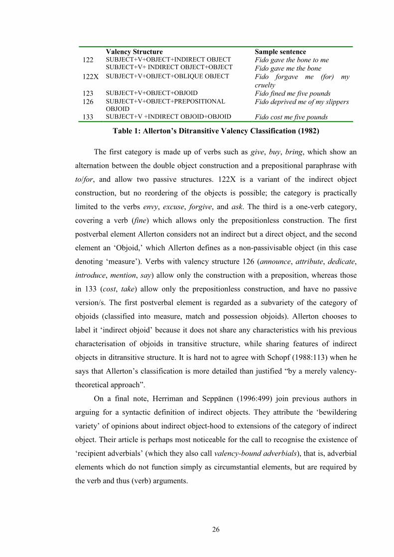
Valency Structure Sample sentence

122 SUBJECT+V+OBJECT+INDIRECT OBJECT SUBJECT+V+ INDIRECT OBJECT+OBJECT

Fido gave the bone to me Fido gave me the bone

122X SUBJECT+V+OBJECT+OBLIQUE OBJECT Fido forgave me (for) my cruelty

123 SUBJECT+V+OBJECT+OBJOID Fido fined me five pounds 126 SUBJECT+V+OBJECT+PREPOSITIONAL

OBJOID Fido deprived me of my slippers

133 SUBJECT+V +INDIRECT OBJOID+OBJOID Fido cost me five pounds

Table 1: Allerton’s Ditransitive Valency Classification (1982)

The first category is made up of verbs such as give, buy, bring, which show an

alternation between the double object construction and a prepositional paraphrase with

to/for, and allow two passive structures. 122X is a variant of the indirect object

construction, but no reordering of the objects is possible; the category is practically

limited to the verbs envy, excuse, forgive, and ask. The third is a one-verb category,

covering a verb (fine) which allows only the prepositionless construction. The first

postverbal element Allerton considers not an indirect but a direct object, and the second

element an ‘Objoid,’ which Allerton defines as a non-passivisable object (in this case

denoting ‘measure’). Verbs with valency structure 126 (announce, attribute, dedicate,

introduce, mention, say) allow only the construction with a preposition, whereas those

in 133 (cost, take) allow only the prepositionless construction, and have no passive

version/s. The first postverbal element is regarded as a subvariety of the category of

objoids (classified into measure, match and possession objoids). Allerton chooses to

label it ‘indirect objoid’ because it does not share any characteristics with his previous

characterisation of objoids in transitive structure, while sharing features of indirect

objects in ditransitive structure. It is hard not to agree with Schopf (1988:113) when he

says that Allerton’s classification is more detailed than justified “by a merely valency-

theoretical approach”.

On a final note, Herriman and Seppänen (1996:499) join previous authors in

arguing for a syntactic definition of indirect objects. They attribute the ‘bewildering

variety’ of opinions about indirect object-hood to extensions of the category of indirect

object. Their article is perhaps most noticeable for the call to recognise the existence of

‘recipient adverbials’ (which they also call valency-bound adverbials), that is, adverbial

elements which do not function simply as circumstantial elements, but are required by

the verb and thus (verb) arguments.

27

2.2.2 Transformational Grammar

Ditransitive verbs also pose a problem for linguistics in terms of their representation. It

is quite a truism of current linguistics that sequences (or linearity) are mere accidents,

and truth is to be found in (syntactic) trees. But not everybody agrees on what is an

adequate representation for ditransitives in tree diagrams.

This section will discuss the different versions of TG, paying particular attention

to the version-specific theoretical mechanisms used to account for indirect objects and

their prepositional paraphrases. The development of TG can be traced by means of

[Chomsky’s] representative publications articulating the different grammatical models.

Thus, Early Transformational Grammar is associated with Syntactic Structures (1957),

the Standard Theory with Aspects of the Theory of Syntax (1965), Government and

Binding Theory with Lectures on Government and Binding (1981), Minimalism with

The Minimalist Program (1995).18 We will start with early TG.

2.2.2.1 Early TG

A summary of the theoretical machinery of Syntactic Structures can be described in this

way: a set of phrase structure rules generates a number of underlying phrase markers,

which in turn provide the input for a set of transformations (some obligatory and some

optional) to apply to. These turn the phrase markers into their pre-final shapes. The last

step is carried out by morphophonemic rules, whose function is to put some flesh on the

structural skeleton.

This account, of course, needs further qualification. The rules of phrase structure

expand the sentence into constituents. A transformation “operates on a given string (...)

with a given constituent structure and converts it into a new string with a new derived

constituent structure” (Chomsky 1957:44). Furthermore, the order of application of

these transformations must be defined to allow later rules access to the output of earlier

rules. The insertion of the actual words is carried out by means of the phrase structure

(PS) rules,19 while they are transformed into utterances by the morphophonological

rules of the model. The following clarifies the way this model operates.

18 We will not concern ourselves with the Extended Standard Theory, nor with the so-called Revised Extended Standard Theory, inasmuch as the theoretical developments in those models (trace theory, the lexicalist hypothesis, logical form, among others) are best evaluated in the framework of GB, where they have been integrated with the component modules. 19 In the Aspects model, lexical insertion rules (LIRs) were called upon to perform this task. LIRs simply plug in a lexical item X in a socket Y, with the requirement that the (subcategorization) features of X and Y be compatible (see Figure 4 below).

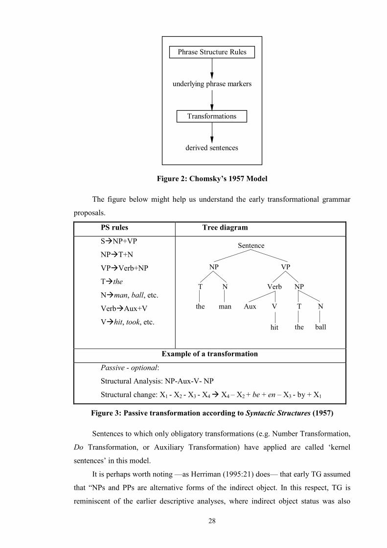
28

Phrase Structure Rules

underlying phrase markers

Transformations

derived sentences

Figure 2: Chomsky’s 1957 Model

The figure below might help us understand the early transformational grammar

proposals.

PS rules Tree diagram

S�NP+VP

NP�T+N

VP�Verb+NP

T�the

N�man, ball, etc.

Verb�Aux+V

V�hit, took, etc.

Sentence

VP

NPVerb

V T N

the ball

NP

T N

the man

hit

Aux

Example of a transformation

Passive - optional:

Structural Analysis: NP-Aux-V- NP

Structural change: X1 - X2 - X3 - X4 � X4 – X2 + be + en – X3 - by + X1

Figure 3: Passive transformation according to Syntactic Structures (1957)

Sentences to which only obligatory transformations (e.g. Number Transformation,

Do Transformation, or Auxiliary Transformation) have applied are called ‘kernel

sentences’ in this model.

It is perhaps worth noting —as Herriman (1995:21) does— that early TG assumed

that “NPs and PPs are alternative forms of the indirect object. In this respect, TG is

reminiscent of the earlier descriptive analyses, where indirect object status was also

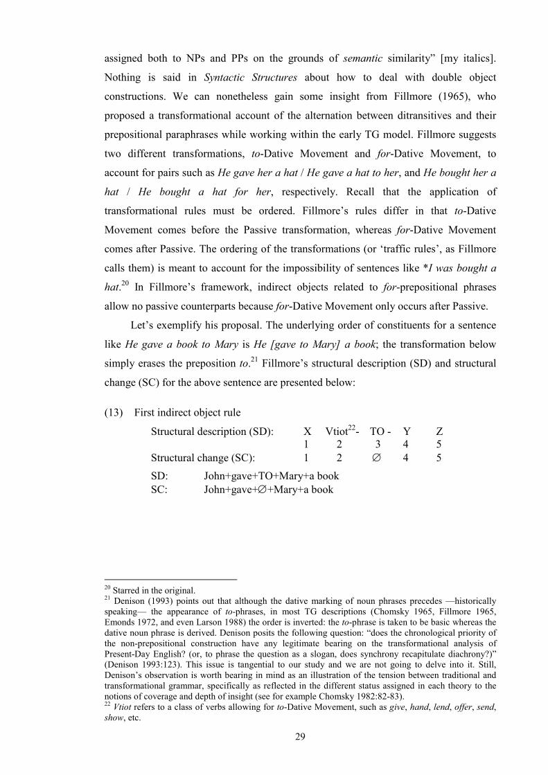
29

assigned both to NPs and PPs on the grounds of semantic similarity” [my italics].

Nothing is said in Syntactic Structures about how to deal with double object

constructions. We can nonetheless gain some insight from Fillmore (1965), who

proposed a transformational account of the alternation between ditransitives and their

prepositional paraphrases while working within the early TG model. Fillmore suggests

two different transformations, to-Dative Movement and for-Dative Movement, to

account for pairs such as He gave her a hat / He gave a hat to her, and He bought her a

hat / He bought a hat for her, respectively. Recall that the application of

transformational rules must be ordered. Fillmore’s rules differ in that to-Dative

Movement comes before the Passive transformation, whereas for-Dative Movement

comes after Passive. The ordering of the transformations (or ‘traffic rules’, as Fillmore

calls them) is meant to account for the impossibility of sentences like *I was bought a

hat.20 In Fillmore’s framework, indirect objects related to for-prepositional phrases

allow no passive counterparts because for-Dative Movement only occurs after Passive.

Let’s exemplify his proposal. The underlying order of constituents for a sentence

like He gave a book to Mary is He [gave to Mary] a book; the transformation below

simply erases the preposition to.21 Fillmore’s structural description (SD) and structural

change (SC) for the above sentence are presented below:

(13) First indirect object rule

Structural description (SD): X Vtiot22- TO - Y Z 1 2 3 4 5 Structural change (SC): 1 2 ∅ 4 5

SD: John+gave+TO+Mary+a book SC: John+gave+∅+Mary+a book

20 Starred in the original. 21 Denison (1993) points out that although the dative marking of noun phrases precedes —historically speaking— the appearance of to-phrases, in most TG descriptions (Chomsky 1965, Fillmore 1965, Emonds 1972, and even Larson 1988) the order is inverted: the to-phrase is taken to be basic whereas the dative noun phrase is derived. Denison posits the following question: “does the chronological priority of the non-prepositional construction have any legitimate bearing on the transformational analysis of Present-Day English? (or, to phrase the question as a slogan, does synchrony recapitulate diachrony?)” (Denison 1993:123). This issue is tangential to our study and we are not going to delve into it. Still, Denison’s observation is worth bearing in mind as an illustration of the tension between traditional and transformational grammar, specifically as reflected in the different status assigned in each theory to the notions of coverage and depth of insight (see for example Chomsky 1982:82-83). 22 Vtiot refers to a class of verbs allowing for to-Dative Movement, such as give, hand, lend, offer, send, show, etc.

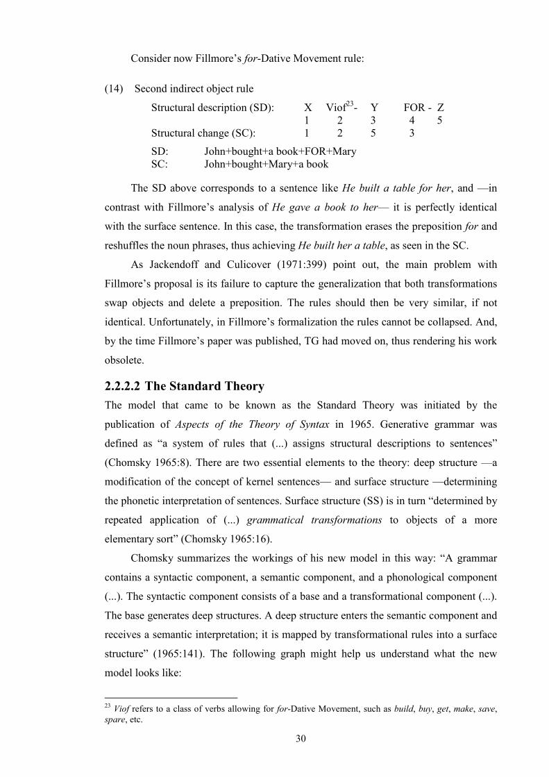
30

Consider now Fillmore’s for-Dative Movement rule:

(14) Second indirect object rule

Structural description (SD): X Viof23- Y FOR - Z 1 2 3 4 5 Structural change (SC): 1 2 5 3

SD: John+bought+a book+FOR+Mary SC: John+bought+Mary+a book

The SD above corresponds to a sentence like He built a table for her, and —in

contrast with Fillmore’s analysis of He gave a book to her— it is perfectly identical

with the surface sentence. In this case, the transformation erases the preposition for and

reshuffles the noun phrases, thus achieving He built her a table, as seen in the SC.

As Jackendoff and Culicover (1971:399) point out, the main problem with

Fillmore’s proposal is its failure to capture the generalization that both transformations

swap objects and delete a preposition. The rules should then be very similar, if not

identical. Unfortunately, in Fillmore’s formalization the rules cannot be collapsed. And,

by the time Fillmore’s paper was published, TG had moved on, thus rendering his work

obsolete.

2.2.2.2 The Standard Theory

The model that came to be known as the Standard Theory was initiated by the

publication of Aspects of the Theory of Syntax in 1965. Generative grammar was

defined as “a system of rules that (...) assigns structural descriptions to sentences”

(Chomsky 1965:8). There are two essential elements to the theory: deep structure —a

modification of the concept of kernel sentences— and surface structure —determining

the phonetic interpretation of sentences. Surface structure (SS) is in turn “determined by

repeated application of (...) grammatical transformations to objects of a more

elementary sort” (Chomsky 1965:16).

Chomsky summarizes the workings of his new model in this way: “A grammar

contains a syntactic component, a semantic component, and a phonological component

(...). The syntactic component consists of a base and a transformational component (...).

The base generates deep structures. A deep structure enters the semantic component and

receives a semantic interpretation; it is mapped by transformational rules into a surface

structure” (1965:141). The following graph might help us understand what the new

model looks like:

23 Viof refers to a class of verbs allowing for for-Dative Movement, such as build, buy, get, make, save, spare, etc.

31

Phrase Structure Rules

Lexicon Lexical InsertionRules

deep structures

Transformational Component

surface structures

Semantic Component

surface structures semantic representations

Figure 4: Chomsky’s 1965 Model

In this model, it is claimed that “the deep structure of a sentence fully determines

its meaning” (Chomsky 1975:22), which implies that (i) sentences with the same

meaning should share the same deep structure, and that (ii) transformations do not

change meaning. These claims were collectively known as the Katz-Postal Hypothesis,

which was eventually rejected when further research showed that surface structure did

play a role in the interpretation of sentences, and that some transformations did change

meaning, as the famous sentences show below.

(15) a. Everyone in Cormorant Island speaks two languages.

b. Two languages are spoken by everyone in Cormorant Island.

Sentence (15)a is the kernel of sentence (15)b; the same meaning is therefore

expected to be present in both sentences. The interaction of the passive transformation

with quantifiers, however, ensures that this is not the case. Sentence (15)a favours an

interpretation whereby everyone on the Island seem to possess the ability of speaking

any two languages, whereas the islanders in sentence (15)b are believed to speak the

same two languages. Furthermore, in terms of truth conditions, it is not difficult to

imagine a scenario in which (15)a is true and (15)b is false.

Another characteristic of the Aspects model is the claim that grammatical relations

can be defined configurationally, i.e. read off a tree. In our case, the indirect object is

defined as the first NP dominated by VP, whereas its oblique paraphrases are defined as

the NP dominated by a PP which in turn is dominated by VP. These alternative forms

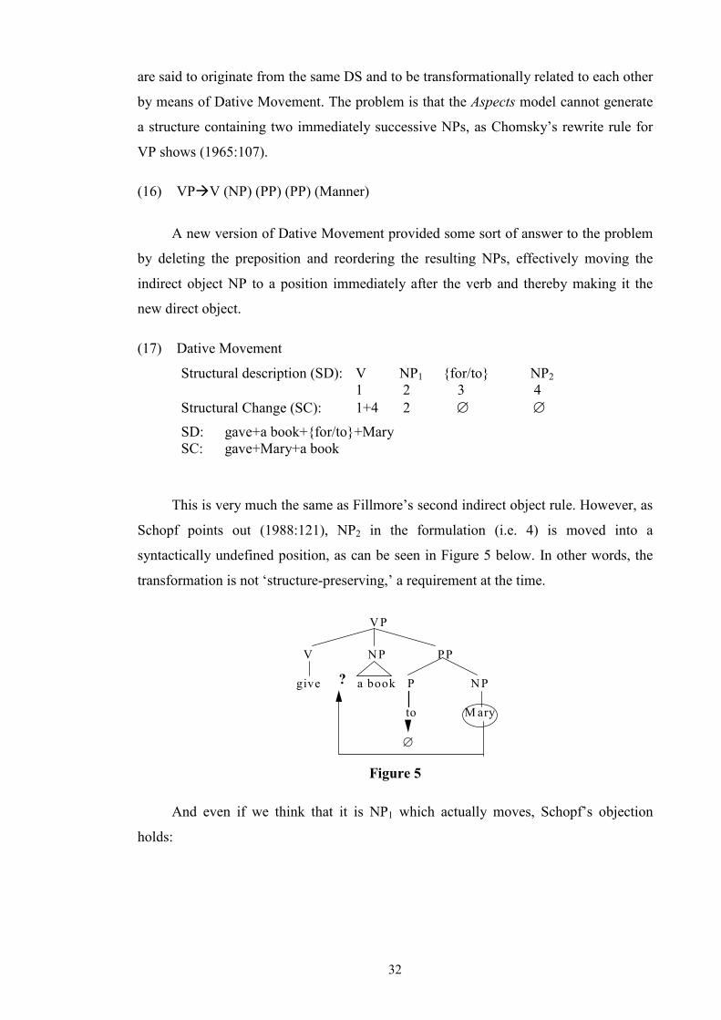
32

are said to originate from the same DS and to be transformationally related to each other

by means of Dative Movement. The problem is that the Aspects model cannot generate

a structure containing two immediately successive NPs, as Chomsky’s rewrite rule for

VP shows (1965:107).

(16) VP�V (NP) (PP) (PP) (Manner)

A new version of Dative Movement provided some sort of answer to the problem

by deleting the preposition and reordering the resulting NPs, effectively moving the

indirect object NP to a position immediately after the verb and thereby making it the

new direct object.

(17) Dative Movement

Structural description (SD): V NP1 {for/to} NP2 1 2 3 4 Structural Change (SC): 1+4 2 ∅ ∅

SD: gave+a book+{for/to}+Mary SC: gave+Mary+a book

This is very much the same as Fillmore’s second indirect object rule. However, as

Schopf points out (1988:121), NP2 in the formulation (i.e. 4) is moved into a

syntactically undefined position, as can be seen in Figure 5 below. In other words, the

transformation is not ‘structure-preserving,’ a requirement at the time.

V P

V N P PP

P N P

to M ary

give a book

∅

?

Figure 5

And even if we think that it is NP1 which actually moves, Schopf’s objection

holds:

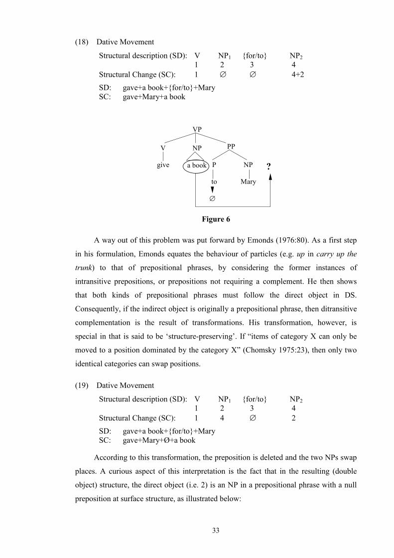
33

(18) Dative Movement

Structural description (SD): V NP1 {for/to} NP2 1 2 3 4 Structural Change (SC): 1 ∅ ∅ 4+2

SD: gave+a book+{for/to}+Mary SC: gave+Mary+a book

VP

V NP PP

P NP

to Mary

give a book

∅

?

Figure 6

A way out of this problem was put forward by Emonds (1976:80). As a first step

in his formulation, Emonds equates the behaviour of particles (e.g. up in carry up the

trunk) to that of prepositional phrases, by considering the former instances of

intransitive prepositions, or prepositions not requiring a complement. He then shows

that both kinds of prepositional phrases must follow the direct object in DS.

Consequently, if the indirect object is originally a prepositional phrase, then ditransitive

complementation is the result of transformations. His transformation, however, is

special in that is said to be ‘structure-preserving’. If “items of category X can only be

moved to a position dominated by the category X” (Chomsky 1975:23), then only two

identical categories can swap positions.

(19) Dative Movement

Structural description (SD): V NP1 {for/to} NP2 1 2 3 4 Structural Change (SC): 1 4 ∅ 2

SD: gave+a book+{for/to}+Mary SC: gave+Mary+Ø+a book

According to this transformation, the preposition is deleted and the two NPs swap

places. A curious aspect of this interpretation is the fact that in the resulting (double

object) structure, the direct object (i.e. 2) is an NP in a prepositional phrase with a null

preposition at surface structure, as illustrated below:

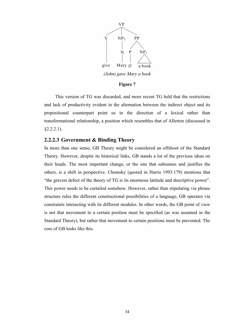
34

VP

NP2 PPV

P NP1

∅ a bookgive Mary

N

(John) gave Mary a book

Figure 7

This version of TG was discarded, and more recent TG held that the restrictions

and lack of productivity evident in the alternation between the indirect object and its

prepositional counterpart point us in the direction of a lexical rather than

transformational relationship, a position which resembles that of Allerton (discussed in

§2.2.2.1).

2.2.2.3 Government & Binding Theory

In more than one sense, GB Theory might be considered an offshoot of the Standard

Theory. However, despite its historical links, GB stands a lot of the previous ideas on

their heads. The most important change, or the one that subsumes and justifies the

others, is a shift in perspective. Chomsky (quoted in Harris 1993:179) mentions that

“the gravest defect of the theory of TG is its enormous latitude and descriptive power”.

This power needs to be curtailed somehow. However, rather than stipulating via phrase

structure rules the different constructional possibilities of a language, GB operates via

constraints interacting with its different modules. In other words, the GB point of view

is not that movement to a certain position must be specified (as was assumed in the

Standard Theory), but rather that movement to certain positions must be prevented. The

core of GB looks like this.

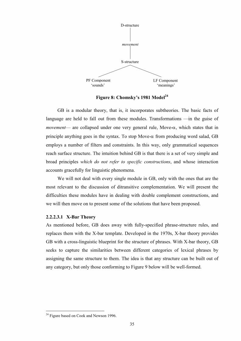
35

D-structure

movement

PF Component‘sounds’

LF Component‘meanings’

S-structure

Figure 8: Chomsky’s 1981 Model24

GB is a modular theory, that is, it incorporates subtheories. The basic facts of

language are held to fall out from these modules. Transformations —in the guise of

movement— are collapsed under one very general rule, Move-α, which states that in

principle anything goes in the syntax. To stop Move-α from producing word salad, GB

employs a number of filters and constraints. In this way, only grammatical sequences

reach surface structure. The intuition behind GB is that there is a set of very simple and

broad principles which do not refer to specific constructions, and whose interaction

accounts gracefully for linguistic phenomena.

We will not deal with every single module in GB, only with the ones that are the

most relevant to the discussion of ditransitive complementation. We will present the

difficulties these modules have in dealing with double complement constructions, and

we will then move on to present some of the solutions that have been proposed.

2.2.2.3.1 X-Bar Theory

As mentioned before, GB does away with fully-specified phrase-structure rules, and

replaces them with the X-bar template. Developed in the 1970s, X-bar theory provides

GB with a cross-linguistic blueprint for the structure of phrases. With X-bar theory, GB

seeks to capture the similarities between different categories of lexical phrases by

assigning the same structure to them. The idea is that any structure can be built out of

any category, but only those conforming to Figure 9 below will be well-formed.

24 Figure based on Cook and Newson 1996.

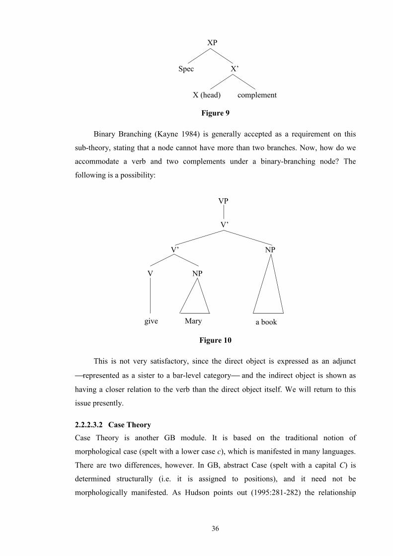
36

XP

Spec X’

X (head) complement

Figure 9

Binary Branching (Kayne 1984) is generally accepted as a requirement on this

sub-theory, stating that a node cannot have more than two branches. Now, how do we

accommodate a verb and two complements under a binary-branching node? The

following is a possibility:

VP

V’

V’ NP

V NP

give Mary a book

Figure 10

This is not very satisfactory, since the direct object is expressed as an adjunct

represented as a sister to a bar-level category and the indirect object is shown as

having a closer relation to the verb than the direct object itself. We will return to this

issue presently.

2.2.2.3.2 Case Theory

Case Theory is another GB module. It is based on the traditional notion of

morphological case (spelt with a lower case c), which is manifested in many languages.

There are two differences, however. In GB, abstract Case (spelt with a capital C) is

determined structurally (i.e. it is assigned to positions), and it need not be

morphologically manifested. As Hudson points out (1995:281-282) the relationship

37

between Case and case is an asymmetrical one: whereas Case need not be manifested by

case, every example of case is always taken to be a surface manifestation of Case.

In GB, each NP must be assigned Case, and this is stipulated by the Case Filter. If

some NP fails to be assigned Case,25 then the structure is ruled ungrammatical. If an NP

wants to survive the Case Filter, it needs to get Case somehow, and this usually means

moving to a position where Case is assigned.26 Case Theory thus provides GB with both

a reason for and a constraint on movement.

Case is assigned under adjacency, i.e. nothing may intervene between a Case

assigner and its assignee.27 Case is additionally linked with the assignment of θ-roles

(i.e. semantic roles), in that Case assignment makes an argument ‘visible’, and only

visible arguments can be θ-marked. Verbs and prepositions assign Case to their objects,

or rather to the positions their objects occupy; this is known as structural Case

assignment. Structural Case is assigned at S-structure, after movement takes place.

There is a further instantiation of Case assignment, namely inherent Case. Inherent Case

is ‘assigned’ at D-structure, before movement takes place, and does not require an

assigner, as it is considered to be a property of certain arguments of predicates. In not

requiring an assigner, inherent Case does not need to be assigned under adjacency.

Ditransitive complementation poses a problem for the requirement of adjacency in

Case-assignment. In a sentence like John gave Mary a book, the first NP can be Case-

marked by the verb, but how does the second NP get its Case? We will return to this

issue in the following sections.

2.2.2.3.3 The Projection Principle

As a point of departure for this section, consider the following quotation from Harris

(1993:109): “[m]uch work in early transformational research simply projected [back]

the wide variety of surface categories onto the underlying representation.” That is to

say, rather than reducing the enormous range of surface phenomena to a desired

minimal set of underlying categories, GB theoreticians found it easier to let ‘basic’

categories proliferate. This set of entirely new categories is licensed in GB by the

Projection Principle.

The Projection Principle is a general constraint on syntactic representation, which

states that: “[r]epresentations at each syntactic level (...) are projected from the lexicon,

in that they observe the subcategorization properties of lexical items” (Chomsky

25 Or more strictly, fails to be in a position where Case is assigned. 26 In practice, the Case Filter implies that every noun must be either a subject or a complement. 27 Case can also be assigned under Spec-head agreement, see Ouhalla (1999:194-195).

38

1981:29). Syntactic structure is thus required to accommodate the properties of each

lexical item. Complement structure is viewed as part of the properties of verbs in the

lexicon. In this light, the lexical entry for a ditransitive verb specifies two alternative

subcategorization frames: [_ NP NP] and [_ NP PP]. This renders earlier

transformations such as Dative Movement unnecessary, in that the relationship between

double object constructions and their prepositional counterparts becomes lexical, as

opposed to transformational.

The Projection Principle states that if there is an NP-position at one level, then

that NP-position must be present at all levels, even if it is not visible. This effectively

opens the floodgates for empty categories, because as a consequence, a position will

exist in syntactic structure just in case some lexical item requires it to exist. Schopf

(1988:122) has been vocal in criticizing GB solutions which resort to allowing the base

rule to generate empty nodes which will only be filled in the event of transformation, as

opposed to lexical insertion. An empty category is either an empty NP position vacated

by Move-α, or a position which is empty for an NP to move to.

Baker (1988:421) states that “the Projection Principle says that there is in some

cases more syntactic structure than meets the eye”, and the ditransitive construction is

no exception. In the next section, we will deal with the way different authors have put

empty categories to work in trying to find an answer to the problems ditransitive

complementation poses for GB.

2.2.2.3.4 Piling up the empties

All the above modules present the analyses of ditransitives within GB with a number of

problems, particularly (a) the assignment of Case to the second NP in a double object

construction, and (b) the adequate internal hierarchical structure of the VP in both

double object constructions and their prepositional paraphrases. Different authors have

proposed different solutions, but all tend to rely more and more on the use of empty

categories as an escape hatch. Empty categories are not observable, but GB treats them

just like ordinary categories. The empty categories that were called upon to account for

the behaviour of double object constructions fall into different groups: null prepositions

(Hornstein and Weinberg 1981, Czepluch 1982, Kayne 1984, Iwakura 1987), traces of

the main verb (Larson 1988), empty verbs (Aoun and Li 1989, Johnson 1991), and

traces of Preposition Incorporation (Baker 1988, Pesetsky 1995).

In §2.2.2.3.2, the question remained open: in John gave Mary a book, how does

the second NP get Case? The adjacency requirement on Case assignment, coupled with

39

the binary branching restriction on X-bar theory, does not allow a verb to Case-mark

two NPs. A GB analysis stipulates that although a book must be Case-marked, its Case

assigner must not be the verb. This leaves us with two options: either a book is

inherently Case-marked, as determined by the properties of the verb28 —an approach

which is “purely ad hoc”, in the words of Bowers (1993:644) — or we need a new

Case-assigner.

The Passive construction should allow us to decide between the alternatives. In

GB, when the passive morpheme attaches itself to the verb, it takes away the verb’s

Case-assigning properties. The object of the verb in question must then move (to the

subject position of the sentence) in order to get Case. Now, if the first NP in the VP is

the only one getting its Case from the verb, then only it should be forced to move in the

Passive construction. However, if both indirect and direct passive versions of the same

sentence are possible, the conclusion is that the second NP also gets its Case from the

verb. And this is indeed what seems to happen, at least in some dialects (as indicated by

the %):

(20) a. John gave Mary a book.

b. Mary was given a book.

c. %A book was given Mary.

However, GB places an asterisk on the third example above, and concludes that

since it is shown that the second NP is not assigned Case by the verb, a book must be

inherently Case-marked.29 This is a far from satisfactory solution for many authors who

have looked at alternative possibilities.

What the following approaches to the problem have in common is the use of an

empty category, as some sort of new Case-provider. Paradoxically, this empty category

(usually a preposition) has generally been made to Case-mark NP1, that is, the NP

which a priori does not seem to have a Case problem. As a consequence, Case

assignment to NP2 is carried out by (i) the verb, either directly (thus breaking adjacency

or binary branching requirements) or indirectly (by means of a Case-relaying empty

category); or (ii) by the empty category itself (without any intervention from the verb).

28 Chomsky himself seems to have provided for this possibility: “[t]hus we assume that certain verbs have the property of assigning a secondary Case to their secondary object, given the form of the adjacency condition” (1981:94). 29 Unlike structural Case, inherent Case is not lost but absorbed by the passive morpheme under passivisation (Haegeman 1994:188).

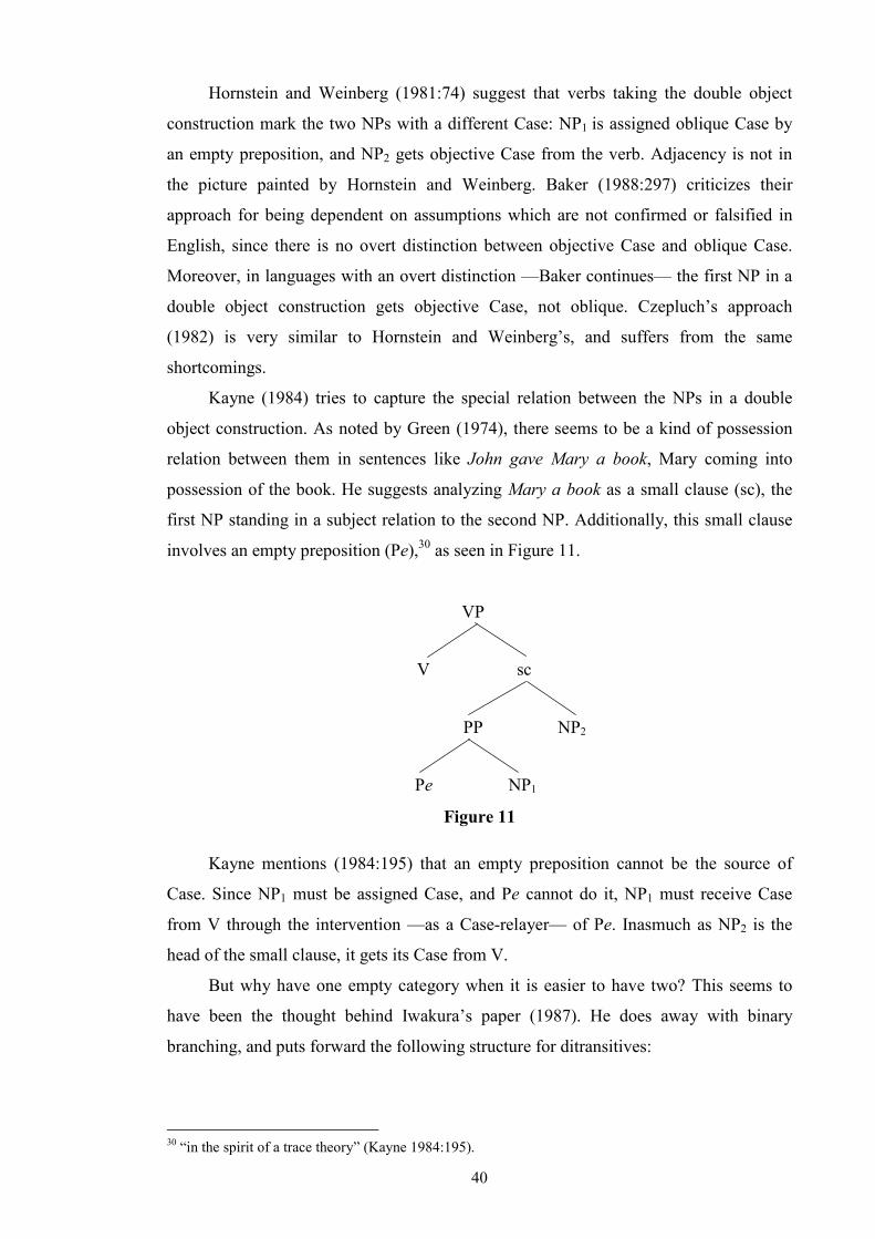
40

Hornstein and Weinberg (1981:74) suggest that verbs taking the double object

construction mark the two NPs with a different Case: NP1 is assigned oblique Case by

an empty preposition, and NP2 gets objective Case from the verb. Adjacency is not in

the picture painted by Hornstein and Weinberg. Baker (1988:297) criticizes their

approach for being dependent on assumptions which are not confirmed or falsified in

English, since there is no overt distinction between objective Case and oblique Case.

Moreover, in languages with an overt distinction —Baker continues— the first NP in a

double object construction gets objective Case, not oblique. Czepluch’s approach

(1982) is very similar to Hornstein and Weinberg’s, and suffers from the same

shortcomings.

Kayne (1984) tries to capture the special relation between the NPs in a double

object construction. As noted by Green (1974), there seems to be a kind of possession

relation between them in sentences like John gave Mary a book, Mary coming into

possession of the book. He suggests analyzing Mary a book as a small clause (sc), the

first NP standing in a subject relation to the second NP. Additionally, this small clause

involves an empty preposition (Pe),30 as seen in Figure 11.

VP

V

NP2PP

NP1Pe

sc

Figure 11

Kayne mentions (1984:195) that an empty preposition cannot be the source of

Case. Since NP1 must be assigned Case, and Pe cannot do it, NP1 must receive Case

from V through the intervention —as a Case-relayer— of Pe. Inasmuch as NP2 is the

head of the small clause, it gets its Case from V.

But why have one empty category when it is easier to have two? This seems to

have been the thought behind Iwakura’s paper (1987). He does away with binary

branching, and puts forward the following structure for ditransitives:

30 “in the spirit of a trace theory” (Kayne 1984:195).

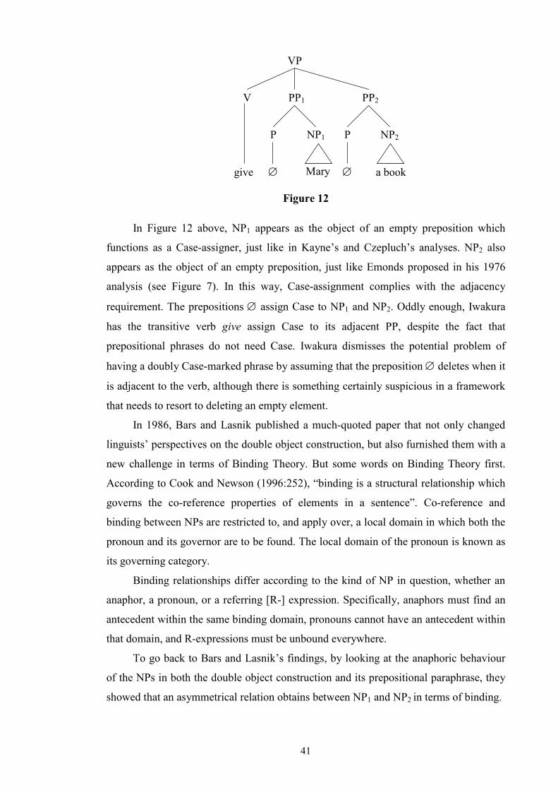
41

VP

PP1 PP2V

P NP1 P NP2

∅ ∅give Mary a book

Figure 12

In Figure 12 above, NP1 appears as the object of an empty preposition which

functions as a Case-assigner, just like in Kayne’s and Czepluch’s analyses. NP2 also

appears as the object of an empty preposition, just like Emonds proposed in his 1976

analysis (see Figure 7). In this way, Case-assignment complies with the adjacency

requirement. The prepositions ∅ assign Case to NP1 and NP2. Oddly enough, Iwakura

has the transitive verb give assign Case to its adjacent PP, despite the fact that

prepositional phrases do not need Case. Iwakura dismisses the potential problem of

having a doubly Case-marked phrase by assuming that the preposition ∅ deletes when it

is adjacent to the verb, although there is something certainly suspicious in a framework

that needs to resort to deleting an empty element.

In 1986, Bars and Lasnik published a much-quoted paper that not only changed

linguists’ perspectives on the double object construction, but also furnished them with a

new challenge in terms of Binding Theory. But some words on Binding Theory first.

According to Cook and Newson (1996:252), “binding is a structural relationship which

governs the co-reference properties of elements in a sentence”. Co-reference and

binding between NPs are restricted to, and apply over, a local domain in which both the

pronoun and its governor are to be found. The local domain of the pronoun is known as

its governing category.

Binding relationships differ according to the kind of NP in question, whether an

anaphor, a pronoun, or a referring [R-] expression. Specifically, anaphors must find an

antecedent within the same binding domain, pronouns cannot have an antecedent within

that domain, and R-expressions must be unbound everywhere.

To go back to Bars and Lasnik’s findings, by looking at the anaphoric behaviour

of the NPs in both the double object construction and its prepositional paraphrase, they

showed that an asymmetrical relation obtains between NP1 and NP2 in terms of binding.

42

(21) a. I showed John/him himself (in the mirror).

b. *I showed himself John (in the mirror).

In the sequence [V NP1 NP2], NP1 can bind NP2 but not conversely. This is

illustrated in the first pair of examples: in (21)a John binds himself, but in (21)b himself

does not bind John.

In (22), it is quantifier NPs which are related to pronouns. Pronouns can only be

anaphorically bound to quantifier NPs if they are found within the structural domain of

the quantifier NP.31

(22) a. I denied each worker his paycheck.

b. I showed every friend of mine his photograph.

c. I denied its owner each paycheck.

d. I showed its trainer every lion.

These examples from Bars and Lasnik’s illustrate that only in (22)a and (22)b, but

not in (22)c and (22)d, can the pronouns be interpreted as bound variables. The

availability of the bound pronoun reading in the above sentences posed some new

problems for the structure of the VP. In brief, in ditransitive clauses NP2 is in the

domain of NP1, but NP1 is not in the domain of NP2. It would fall to Larson (1988) to

demonstrate that this is also true in prepositional paraphrases.

The notion of ‘domain’ is explained in terms of c-command, but with a twist. C-

command is a formalization of the intuitive relation ‘higher in the tree than’. The

commonly used definitions of c-command (e.g. “X c-commands Y iff every maximal

projection that dominates X also dominates Y” (Aoun and Sportiche 1981)) fail to

define a ‘domain’ which can accommodate Bars and Lasnik’s findings. These authors

propose, instead, a definition of ‘domain’ along the following lines: “Y is in the domain

of X iff X c-commands Y and X precedes Y [my italics]”, thus bringing linear

precedence into the picture. And this is exactly the nub of the matter: without the

proviso on the definition of c-command, Bars and Lasnik’s data contradicted the

expectation that trees represent hierarchy and linearity.

Bars and Lasnik’s findings rendered a number of previous analyses obsolete

inasmuch as the relationship between the two NPs had been claimed to be symmetrical.

Larson (1988) set out to accommodate the new-found evidence into his analysis, as well

31 “[A]t S-structure”, Bars and Lasnik add.

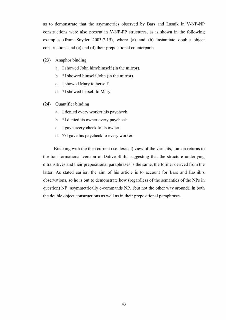
43

as to demonstrate that the asymmetries observed by Bars and Lasnik in V-NP-NP

constructions were also present in V-NP-PP structures, as is shown in the following

examples (from Snyder 2003:7-15), where (a) and (b) instantiate double object

constructions and (c) and (d) their prepositional counterparts.

(23) Anaphor binding

a. I showed John him/himself (in the mirror).

b. *I showed himself John (in the mirror).

c. I showed Mary to herself.

d. *I showed herself to Mary.

(24) Quantifier binding

a. I denied every worker his paycheck.

b. *I denied its owner every paycheck.

c. I gave every check to its owner.

d. ??I gave his paycheck to every worker.

Breaking with the then current (i.e. lexical) view of the variants, Larson returns to

the transformational version of Dative Shift, suggesting that the structure underlying

ditransitives and their prepositional paraphrases is the same, the former derived from the

latter. As stated earlier, the aim of his article is to account for Bars and Lasnik’s

observations, so he is out to demonstrate how (regardless of the semantics of the NPs in

question) NP1 asymmetrically c-commands NP2 (but not the other way around), in both

the double object constructions as well as in their prepositional paraphrases.

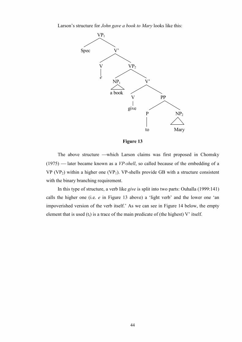
44

Larson’s structure for John gave a book to Mary looks like this:

VP1

Spec V’

V VP2

NP1 V’

V PP

NP2

e

a book

give P

Mary to

Figure 13

The above structure which Larson claims was first proposed in Chomsky

(1975) later became known as a VP-shell, so called because of the embedding of a

VP (VP2) within a higher one (VP1). VP-shells provide GB with a structure consistent

with the binary branching requirement.

In this type of structure, a verb like give is split into two parts: Ouhalla (1999:141)

calls the higher one (i.e. e in Figure 13 above) a ‘light verb’ and the lower one ‘an

impoverished version of the verb itself.’ As we can see in Figure 14 below, the empty

element that is used (ti) is a trace of the main predicate of (the highest) V’ itself.

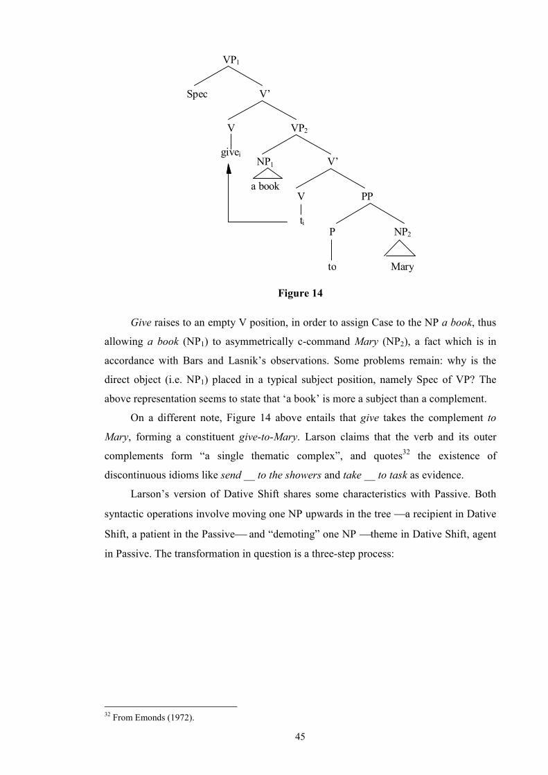
45

VP1

Spec V’

V VP2

NP1 V’

V PP

NP2

givei

a book

ti P

Mary to

Figure 14

Give raises to an empty V position, in order to assign Case to the NP a book, thus

allowing a book (NP1) to asymmetrically c-command Mary (NP2), a fact which is in

accordance with Bars and Lasnik’s observations. Some problems remain: why is the

direct object (i.e. NP1) placed in a typical subject position, namely Spec of VP? The

above representation seems to state that ‘a book’ is more a subject than a complement.

On a different note, Figure 14 above entails that give takes the complement to

Mary, forming a constituent give-to-Mary. Larson claims that the verb and its outer

complements form “a single thematic complex”, and quotes32 the existence of

discontinuous idioms like send __ to the showers and take __ to task as evidence.

Larson’s version of Dative Shift shares some characteristics with Passive. Both

syntactic operations involve moving one NP upwards in the tree a recipient in Dative

Shift, a patient in the Passive and “demoting” one NP theme in Dative Shift, agent

in Passive. The transformation in question is a three-step process:

32 From Emonds (1972).

46

• With the structure in Figure 13 as starting point, first give moves to e as before; the

transformation then absorbs the Case assigned to Mary within PP, to is absorbed and

to Mary becomes Mary; this results in Figure 15;

V P 1

S pec V ’

V V P 2

N P V ’

V

e

a bo ok

g ive

N P

M a ry

Figure 15

• the theta-role assigned to a book is demoted, the argument moving (downwards and

leftwards) to adjunct position;

V P 1

S pec V ’

V V P 2

e

N P

a b ook

V ’

V

g ive

N P

M ar y

t V’

Figure 16

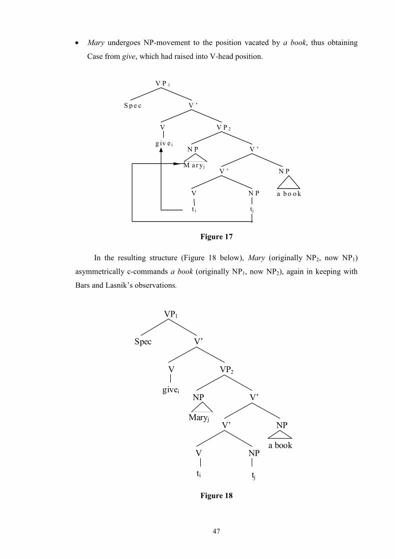
47

• Mary undergoes NP-movement to the position vacated by a book, thus obtaining

Case from give, which had raised into V-head position.

V P 1

S p e c V ’

V V P 2

N P V ’ g iv e i

M ar y j

V N P

tj t i

N P V ’

a b o o k

Figure 17

In the resulting structure (Figure 18 below), Mary (originally NP2, now NP1)

asymmetrically c-commands a book (originally NP1, now NP2), again in keeping with

Bars and Lasnik’s observations.

VP1

Spec V’

V VP2

NP V’ givei

Maryj

V NP

tj ti

NP V’

a book

Figure 18

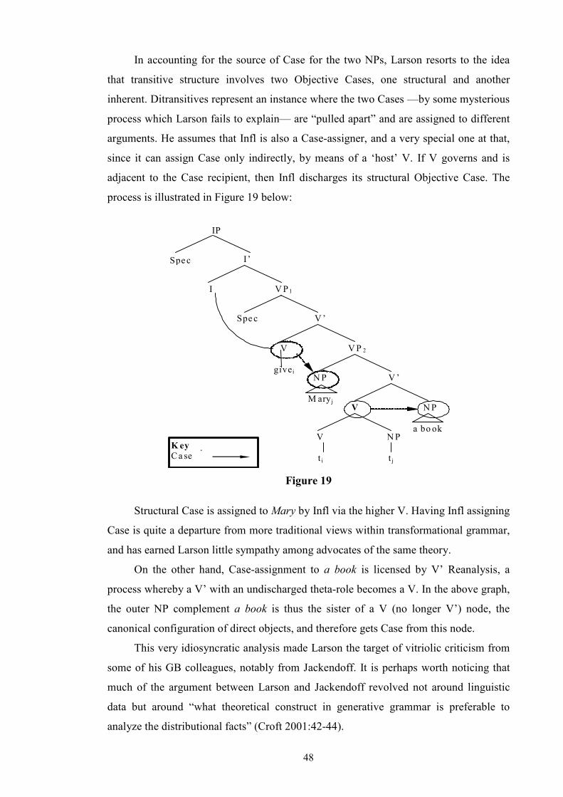
48

In accounting for the source of Case for the two NPs, Larson resorts to the idea

that transitive structure involves two Objective Cases, one structural and another

inherent. Ditransitives represent an instance where the two Cases —by some mysterious

process which Larson fails to explain— are “pulled apart” and are assigned to different

arguments. He assumes that Infl is also a Case-assigner, and a very special one at that,

since it can assign Case only indirectly, by means of a ‘host’ V. If V governs and is

adjacent to the Case recipient, then Infl discharges its structural Objective Case. The

process is illustrated in Figure 19 below:

V P1

Spe c V ’

V V P 2

N P V ’ give i

M ary j

V N P

t j t i

N P V

a bo ok

I’

I

IP

Spe c

K ey

C a se

Figure 19

Structural Case is assigned to Mary by Infl via the higher V. Having Infl assigning

Case is quite a departure from more traditional views within transformational grammar,

and has earned Larson little sympathy among advocates of the same theory.

On the other hand, Case-assignment to a book is licensed by V’ Reanalysis, a

process whereby a V’ with an undischarged theta-role becomes a V. In the above graph,

the outer NP complement a book is thus the sister of a V (no longer V’) node, the

canonical configuration of direct objects, and therefore gets Case from this node.

This very idiosyncratic analysis made Larson the target of vitriolic criticism from

some of his GB colleagues, notably from Jackendoff. It is perhaps worth noticing that

much of the argument between Larson and Jackendoff revolved not around linguistic

data but around “what theoretical construct in generative grammar is preferable to

analyze the distributional facts” (Croft 2001:42-44).

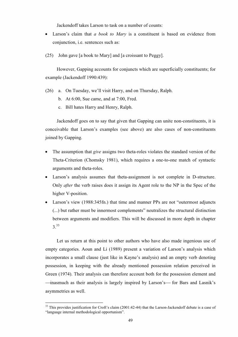
49

Jackendoff takes Larson to task on a number of counts:

• Larson’s claim that a book to Mary is a constituent is based on evidence from

conjunction, i.e. sentences such as:

(25) John gave [a book to Mary] and [a croissant to Peggy].

However, Gapping accounts for conjuncts which are superficially constituents; for

example (Jackendoff 1990:439):

(26) a. On Tuesday, we’ll visit Harry, and on Thursday, Ralph.

b. At 6:00, Sue came, and at 7:00, Fred.

c. Bill hates Harry and Henry, Ralph.

Jackendoff goes on to say that given that Gapping can unite non-constituents, it is

conceivable that Larson’s examples (see above) are also cases of non-constituents

joined by Gapping.

• The assumption that give assigns two theta-roles violates the standard version of the

Theta-Criterion (Chomsky 1981), which requires a one-to-one match of syntactic

arguments and theta-roles.

• Larson’s analysis assumes that theta-assignment is not complete in D-structure.

Only after the verb raises does it assign its Agent role to the NP in the Spec of the

higher V-position.

• Larson’s view (1988:345fn.) that time and manner PPs are not “outermost adjuncts

(...) but rather must be innermost complements” neutralizes the structural distinction

between arguments and modifiers. This will be discussed in more depth in chapter

3.33

Let us return at this point to other authors who have also made ingenious use of

empty categories. Aoun and Li (1989) present a variation of Larson’s analysis which

incorporates a small clause (just like in Kayne’s analysis) and an empty verb denoting

possession, in keeping with the already mentioned possession relation perceived in

Green (1974). Their analysis can therefore account both for the possession element and

inasmuch as their analysis is largely inspired by Larson’s for Bars and Lasnik’s

asymmetries as well.

33 This provides justification for Croft’s claim (2001:42-44) that the Larson-Jackendoff debate is a case of “language internal methodological opportunism”.

50

In Aoun and Li’s acount (in keeping with Larson’s work), the relation obtaining

between a double object construction and its prepositional paraphrase is held to be

transformational, except that the double object clause is taken as the one being base-

generated. Another difference with Larson’s account is that the empty element is not a

trace of the main verb, it is an empty verb which stays empty. Case is assigned to NP1

by the main verb, and to NP2 by the empty verb, in both cases under adjacency. Their

mechanism is in Figure 20 below:

I’

I VP1

V SC

NP1 VP2 give

Mary V NP2

a book

IP

Spec

e

Key

Case

Figure 20

Empty categories have also been assigned a slightly different job in related

proposals, such as Baker’s. This author draws an analogy between applicative

constructions and Dative Shift. An applicative construction is a type of double object

construction frequently found in Bantu languages. Applicatives change grammatical

functions. An applicative affix on the verb encodes as objects a range of roles, e.g.

benefactive and locative. By means of applicative constructions, locative, goal,

benefactives, or instrumental obliques can become objects. In other words, applicatives

allow an oblique (usually a prepositional phrase) to become the ‘object’ of the clause it

appears in.

51

Consider the following example from Chichewa (Baker 1988:229):

(27) Mbidzi zi-na -perek-a msampha kwa nkhandwe.

zebras SP-PAST-hand-AS trap to fox ‘The zebras handed the trap to the fox.’

(28) Mbidzi zi-na- perek-er-a nkhandwe msampha.

zebras SP-PAST-hand-to ASP fox trap ‘The zebras handed the fox the trap.’34

In (27), the verbs (both in the Chichewa example and in the English gloss) take a

PP complement and a NP complement. In (28), the Chichewa verb is morphologically

complex, appearing with an applicative suffix (-er). Also, a second NP replaces the

former PP complement.

Incorporation is the process whereby one word is moved by syntactic rules to a

new position ‘inside’ another word. Preposition Incorporation (PI) is a movement rule

that takes a preposition out of a prepositional phrase and plants it inside a verb.

Applicative constructions can be seen as instances of PI.

Baker (1988) considers sentences such as John gave Mary a book to be

applicative constructions derived by Preposition Incorporation, despite their not

exhibiting an applicative morpheme. The only difference between Preposition

Incorporation and Dative Shift structures is that, in the case of a closed set of verbs

(which focus on goal or benefactive arguments), the preposition is morphologically

invisible but nonetheless syntactically present. This seems like the prototypical

definition of an empty category, only in Baker’s account we have a trace of an

incorporated preposition. As illustration, the process starts in Figure 21 and ends in

Figure 22.

34 SP refers to a subject agreement prefix, PAST to past tense, and ASP to a marker of aspect or mood.

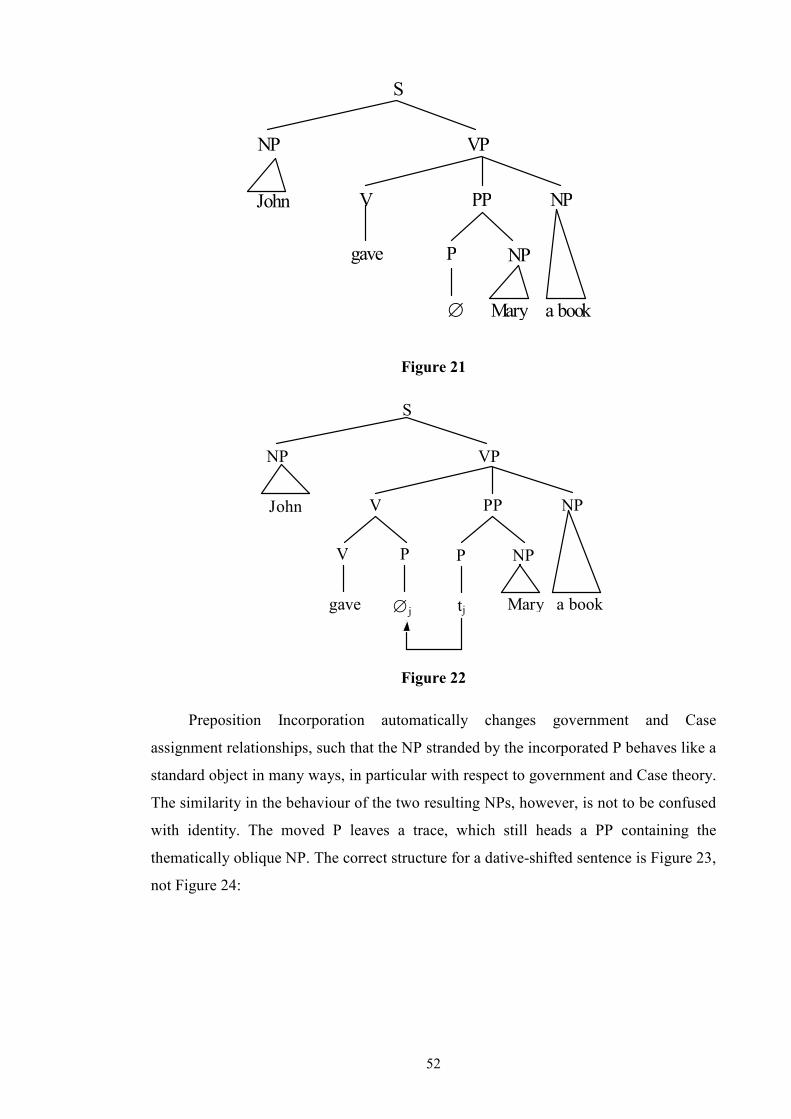
52

S

VP NP

NP V PP

NP

Mary

P gave

∅

John

a book

Figure 21

S

VP NP

NP V PP

NP P

tj Mary

P V

gave ∅j

John

a book

Figure 22

Preposition Incorporation automatically changes government and Case

assignment relationships, such that the NP stranded by the incorporated P behaves like a

standard object in many ways, in particular with respect to government and Case theory.

The similarity in the behaviour of the two resulting NPs, however, is not to be confused

with identity. The moved P leaves a trace, which still heads a PP containing the

thematically oblique NP. The correct structure for a dative-shifted sentence is Figure 23,

not Figure 24:

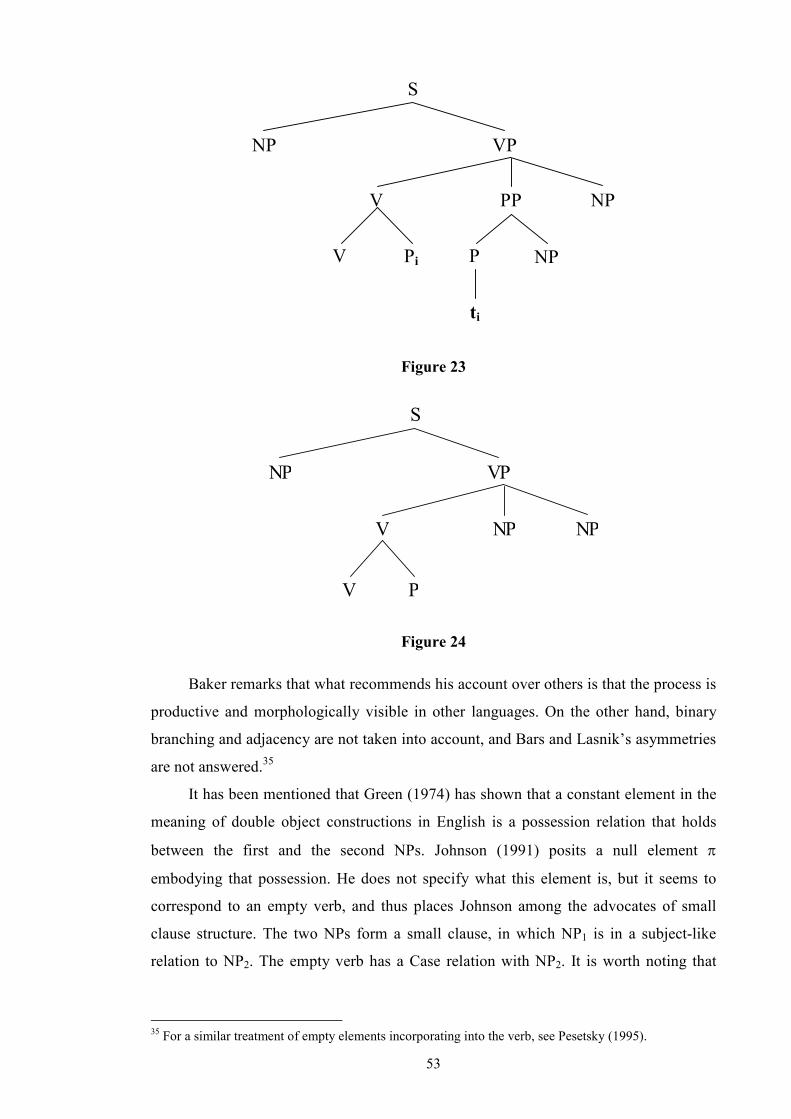
53

S

VPNP

NPV PP

NPPV

ti

Pi

Figure 23

S

VPNP

NPV NP

V P

Figure 24

Baker remarks that what recommends his account over others is that the process is

productive and morphologically visible in other languages. On the other hand, binary

branching and adjacency are not taken into account, and Bars and Lasnik’s asymmetries

are not answered.35

It has been mentioned that Green (1974) has shown that a constant element in the

meaning of double object constructions in English is a possession relation that holds

between the first and the second NPs. Johnson (1991) posits a null element π

embodying that possession. He does not specify what this element is, but it seems to

correspond to an empty verb, and thus places Johnson among the advocates of small

clause structure. The two NPs form a small clause, in which NP1 is in a subject-like

relation to NP2. The empty verb has a Case relation with NP2. It is worth noting that

35 For a similar treatment of empty elements incorporating into the verb, see Pesetsky (1995).

54

Johnson’s postulation of this null element is just a cog in his very complex theoretical

machinery.

2.2.2.4 The Minimalist Program (MP)

Minimalism is the latest of Chomsky’s projects, drawing on concepts from his late

1980s papers, such as Full Interpretation and Economy of Representation and

Derivation. Briefly expressed, the Principle of Full Interpretation states that there are no

redundant elements in a sentence, whereas the Principle of Economy requires that all

representations (and processes used to derive them) be as economical as possible.

Cook and Newson (1996:318) mention that Minimalism improved on certain

areas of GB which were becoming more and more unsustainable, for example the idea

of inflectional elements lowering onto the verb. Under the Minimalist Program, an

already ‘inflected’ Verb is inserted in the tree, which means that the verb does not have

to move anywhere to become inflected. The inflectional nodes perform the function of

‘checking’ that the inserted Verb has the appropriate features when it moves into them.

‘Checking’ a feature cancels it out so that it does not reach the expression stage. Cook

and Newson (1996:329) observe that in the Minimalist Program, “Case-marking is

reduced to Case-checking.”

It is not just verbs that check their features, the same applies to NPs (or DPs, as

they are now called). These phrases have Case features in their original positions, and

have to raise to the specifier position of an agreement projection to check them off. For

example, nominative DPs need to raise to Spec of AgrSP (Subject Agreement

Projection) in order to check their nominative-case head-feature.

The same is true of objective DPs, who also have to climb up the tree to their own

Spec of AgrOP (Object Agreement Projection). When two objects are involved as

internal arguments of a verb, both direct and indirect objects must check their features

off by moving to their projection of Spec of AgrP. Thus, DPs carrying dative Case also

raise to check their Case feature to the Spec position within an IO agreement projection

(AgrIOP) which is positioned immediately above AgrOP. To finalise matters, the verb

in question must raise first to adjoin to AgrO (a direct object agreement morpheme),

then to AgrIO (an indirect object agreement morpheme), and finally to v.36 The

operations I have just described are exemplified and illustrated by Radford (1997) over

many pages; his final tree for the sentence The crew handed back the passengers their

passports look something like this:

36 VP-shells are still present in the MP. Notice also the DP occurring in Spec of vp.

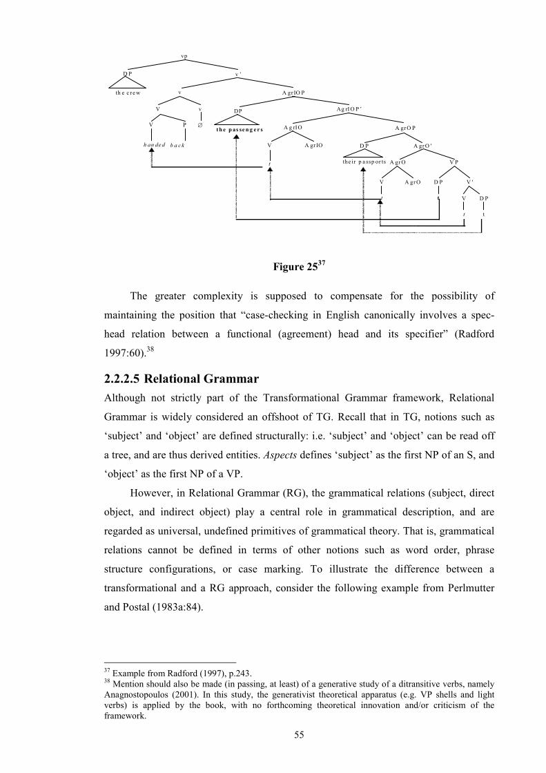
55

A gr O P

the ir p a ssp or ts

D P V A gr IO

A g rIO

Ag rI O P ’ DP

A gr IO P

th e p as se n g e r s

A gr O '

V v

th e c r e w

t

v

v ’ D P

vp

V P

h an de d b a c k

∅

A gr O V P

V A gr O

t

D P V '

t D P

t

V

t

Figure 2537

The greater complexity is supposed to compensate for the possibility of

maintaining the position that “case-checking in English canonically involves a spec-

head relation between a functional (agreement) head and its specifier” (Radford

1997:60).38

2.2.2.5 Relational Grammar

Although not strictly part of the Transformational Grammar framework, Relational

Grammar is widely considered an offshoot of TG. Recall that in TG, notions such as

‘subject’ and ‘object’ are defined structurally: i.e. ‘subject’ and ‘object’ can be read off

a tree, and are thus derived entities. Aspects defines ‘subject’ as the first NP of an S, and

‘object’ as the first NP of a VP.

However, in Relational Grammar (RG), the grammatical relations (subject, direct

object, and indirect object) play a central role in grammatical description, and are

regarded as universal, undefined primitives of grammatical theory. That is, grammatical

relations cannot be defined in terms of other notions such as word order, phrase

structure configurations, or case marking. To illustrate the difference between a

transformational and a RG approach, consider the following example from Perlmutter

and Postal (1983a:84).

37 Example from Radford (1997), p.243. 38 Mention should also be made (in passing, at least) of a generative study of a ditransitive verbs, namely Anagnostopoulos (2001). In this study, the generativist theoretical apparatus (e.g. VP shells and light verbs) is applied by the book, with no forthcoming theoretical innovation and/or criticism of the framework.

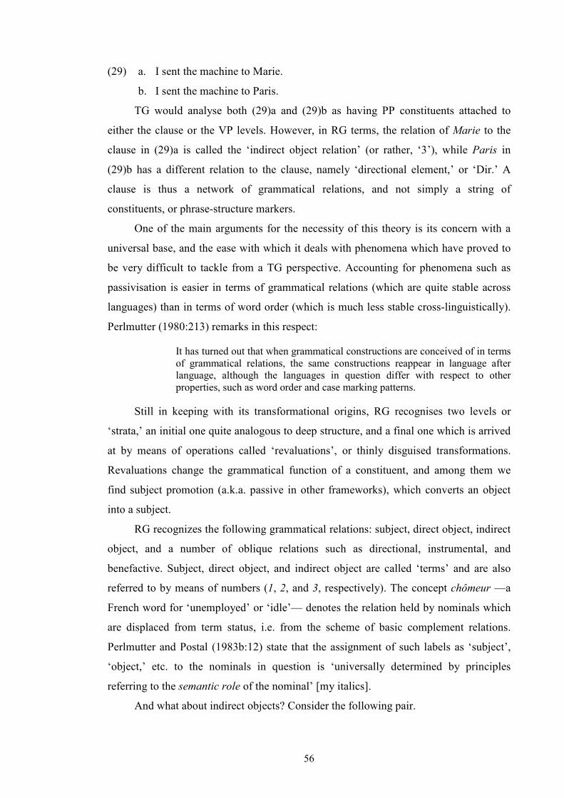
56

(29) a. I sent the machine to Marie.

b. I sent the machine to Paris.

TG would analyse both (29)a and (29)b as having PP constituents attached to

either the clause or the VP levels. However, in RG terms, the relation of Marie to the

clause in (29)a is called the ‘indirect object relation’ (or rather, ‘3’), while Paris in

(29)b has a different relation to the clause, namely ‘directional element,’ or ‘Dir.’ A

clause is thus a network of grammatical relations, and not simply a string of

constituents, or phrase-structure markers.

One of the main arguments for the necessity of this theory is its concern with a

universal base, and the ease with which it deals with phenomena which have proved to

be very difficult to tackle from a TG perspective. Accounting for phenomena such as

passivisation is easier in terms of grammatical relations (which are quite stable across

languages) than in terms of word order (which is much less stable cross-linguistically).

Perlmutter (1980:213) remarks in this respect:

It has turned out that when grammatical constructions are conceived of in terms of grammatical relations, the same constructions reappear in language after language, although the languages in question differ with respect to other properties, such as word order and case marking patterns.

Still in keeping with its transformational origins, RG recognises two levels or

‘strata,’ an initial one quite analogous to deep structure, and a final one which is arrived

at by means of operations called ‘revaluations’, or thinly disguised transformations.

Revaluations change the grammatical function of a constituent, and among them we

find subject promotion (a.k.a. passive in other frameworks), which converts an object

into a subject.

RG recognizes the following grammatical relations: subject, direct object, indirect

object, and a number of oblique relations such as directional, instrumental, and

benefactive. Subject, direct object, and indirect object are called ‘terms’ and are also

referred to by means of numbers (1, 2, and 3, respectively). The concept chômeur —a

French word for ‘unemployed’ or ‘idle’— denotes the relation held by nominals which

are displaced from term status, i.e. from the scheme of basic complement relations.

Perlmutter and Postal (1983b:12) state that the assignment of such labels as ‘subject’,

‘object,’ etc. to the nominals in question is ‘universally determined by principles

referring to the semantic role of the nominal’ [my italics].

And what about indirect objects? Consider the following pair.

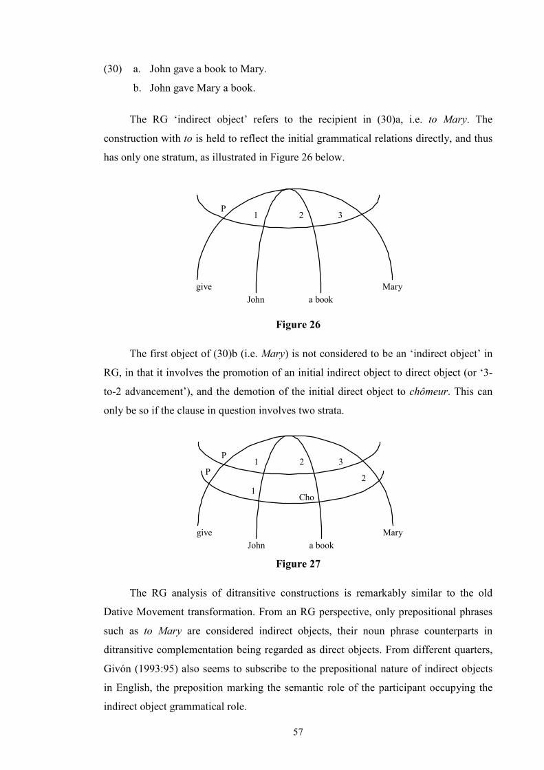
57

(30) a. John gave a book to Mary.

b. John gave Mary a book.

The RG ‘indirect object’ refers to the recipient in (30)a, i.e. to Mary. The

construction with to is held to reflect the initial grammatical relations directly, and thus

has only one stratum, as illustrated in Figure 26 below.

give Marya bookJohn

P31 2

Figure 26

The first object of (30)b (i.e. Mary) is not considered to be an ‘indirect object’ in

RG, in that it involves the promotion of an initial indirect object to direct object (or ‘3-

to-2 advancement’), and the demotion of the initial direct object to chômeur. This can

only be so if the clause in question involves two strata.

give Marya bookJohn

P31 2

P2

1Cho

Figure 27

The RG analysis of ditransitive constructions is remarkably similar to the old

Dative Movement transformation. From an RG perspective, only prepositional phrases

such as to Mary are considered indirect objects, their noun phrase counterparts in

ditransitive complementation being regarded as direct objects. From different quarters,

Givón (1993:95) also seems to subscribe to the prepositional nature of indirect objects

in English, the preposition marking the semantic role of the participant occupying the

indirect object grammatical role.

58

From the point of view of semantic roles, we find that recipients or benefactives

can be encoded either as noun phrases or as prepositional phrases (see above). Faltz

(1978:78) proposes that roles which utilize the strategy that marks them as direct objects

(i.e noun phrases) are indeed direct objects, whereas roles that utilize the strategy that

marks them as obliques (i.e. prepositional phrases) are in fact true obliques.39 Therefore,

there is no such thing as a (noun phrase) indirect object in English.

The facts offered in support of the RG analysis have to do with passivisation,

since RG considers that it is the first object but not the second that can be the subject of

a corresponding passive:

(31) a. Mary was given a book by John.

b. *A book was given Mary by John.

The kind of sentence represented by (31)b has been frowned upon and asterisked

by many linguists. Hudson (1990:337-338) mentions that although these sentences are

fine for some speakers (among them Jaeggli 1986, Zwicky 1987), it is often assumed

that everyone rejects them.40

Dryer (1986) came up with a different idea. He breaks with RG orthodoxy by

suggesting it is the double object construction (i.e. V+NP+NP) that is the basic

sentence, their prepositional counterpart being derived by demoting the first object to

peripheral status, as can be seen by its being marked by a preposition.41 This demotion

of notional indirect objects to final chômeurs he calls ‘Antidative’.42

39 Faltz later admits in a footnote that indirect objects of the oblique type sometimes manifest syntactic properties which set them apart from other obliques. Specifically, oblique indirect objects (and not other obliques) must follow the direct object, a situation which seems to highlight the fact that oblique indirect objects straddle the boundary between complements and adjuncts in English. 40 However, this does not make the use of an asterisk a less useful tool in syntactic argumentation. 41 Palmer (1994:171) mentions that even if to can indicate demotion, “there is no marker [indicating demotion] in the verb, and, more importantly, (...) if the double Object form is considered basic, the first Object ought to have the characteristics of the single, prototypical Object”, and as Hudson (1992) demonstrated, this is far from being the case. Croft (1991:296 fn) also levels some criticism at Dryer’s proposal, when he notes that in ditransitive constructions, although the possessor (recipient argument) precedes the possessed (theme argument), it is the possessor that requires a preposition if one of the arguments is absent:

i. He gives $50 every year. ii. Our relatives give *us / to us every Christmas.

42 In his analysis, Dryer (1986) introduces the terms Primary Object and Secondary Object. Secondary Object (SO) refers only to the second object (i.e. the direct object) in a double object construction, while Primary Object (PO) refers both to the first object (indirect object) of a double object construction, and to the only object (direct object) of a monotransitive clause. Notice that this classification is carried out in terms of the position of the objects in the clause, thus severing the link between objects and semantic roles. In other words, a Primary Object is the one found immediately after the verb, regardless of whether the clause is monotransitive or ditransitive. In the former case the PO will be a Patient (theme); in the latter, it will be a Recipient (beneficiary). By contrast, a Secondary Object will always have another object between its position and the verb, and will always be a Patient (theme) in a ditransitive clause.

59

Dryer claims his analysis is supported: (a) by the fact that the double object

construction is the preferred alternative across languages, and should therefore be

analysed as having only a single stratum (no revaluations); and (b) by analogy with

passivisation, where the demotion of a core relation (subject) to peripheral status is

clearly marked by a preposition (by). Hence, demotion in the case of an indirect object

in a double object construction is similar to passive, and it is also marked by a

preposition, namely to. As regards Benefactives marked by for, Dryer (1986:838)

returns to the traditional RG account, treating sentences like John bought a book for

Mary as basic.

Dryer’s proposal —says Blake (1990:55-57)— is “essentially a return to the

traditional analysis (...), and captures the fact that the recipient normally takes

precedence over the patient and the fact that the patient retains grammatical privileges

even when the recipient takes precedence”.

Relational Grammar has been taken to task by various authors. The standard RG

account of ditransitive constructions quite obviously conflicts with the traditional

analysis in which the first object of the double object construction is called the indirect

object and the second the direct object. Allerton (1982:82) voices his criticism by

pointing out that the relation between John gave Mary a book and John gave a book to

Mary is —in his opinion, at least— a minor stylistic variation, in that even if the

sequence of elements is inverted and a preposition is either inserted or deleted, both

objects remain to the right of the verb, there is no change in verb agreement, no need for

extra verbal auxiliaries, no change in grammatical case, and no change in the

obligatoriness of elements. He concludes: “[i]t therefore seems unrealistic to follow RG

in regarding a prepositional phrase as being ‘promoted’ to object position only when it

is fronted and loses its preposition” (Allerton 1982:74).

A more radical criticism of RG is made by Bhat (1991:158), who starting from

the title of his book makes no bones about his opinion of grammatical relations. This

author considers that RG (together with LFG) has failed to realise that grammatical

relations are theoretical constructs meant only to “mak[e] our descriptions of language

more explicit,” and that language in and of itself does not require their presence, even if

some theories do.

2.2.3 Semantic and Cognitive Approaches

The last quarter of the twentieth century saw the emergence and convergence of various

cognitive approaches to linguistic problems. Lakoff (1987:xi) refers to this new

60

framework as one that “brings together what is known about the mind from many

academic disciplines: psychology, linguistics, anthropology, and computer science”.

The overarching claim is that language is based on cognition.

The approach can be illustrated in terms of certain definitional characteristics.

Language is considered to be a conceptual network. Cognitive approaches do not allow

for different levels of grammar such as deep and surface structure and therefore

transformations or their functional equivalents are ruled out. Language is conceptualised

as a symbolic system, designed to express meanings produced by the cognitive

processes of human beings, with human experiences of the world feeding into these

cognitive processes. Linguistic categories are assumed to have the characteristics of

prototypes, and to be thus defined with reference to ‘best examples’ rather than in terms

of necessary and sufficient conditions.

Many authors have worked and work within this framework. In this and the next

sections we will concern ourselves mainly with the works of George Lakoff, Ronald

Langacker, Richard Hudson and Adele Goldberg. If language is part of cognition, it

follows that language structure is a special form of cognitive structure. This assumption

has been exploited in this framework by different authors in different ways, but mostly

by claiming a relationship of identity between linguistic structure (constructions being

perhaps the most obvious example) and cognitive structure (e.g. the notion of schemas).

Shibatani (1996:165) mentions that:

[t]he notion of schema is familiar to those who are exposed to the rudiments of cognitive psychology. The idea is that we tend to interpret the world according to preconceived notions and principles, sometimes imposing information or a particular structure that is not even there.

Charles Fillmore (1977) introduces the notion of ‘perspective’ or ‘schema’

on a scene, by which he means an organization imposed on the semantic content of an

utterance, a way in which the speaker conceptualizes an external, non-linguistic

situation. Fillmore (1977:73) even goes on to say that “[t]he study of semantics is the

study of the cognitive scenes that are created or activated by utterances”. By appealing

to the identity between conceptual and linguistic structure, Lakoff (1987:68) can claim

that “the structure of language can be compared to the structure of cognitive models”,

and postulate the existence of idealized cognitive models (ICMs), which are pairs of

form-content. Coming from a different perspective, Langacker (1987, 1991) talks of

‘symbolic assemblies’ or ‘sentence schemas’ that have become ‘entrenched’ through

repeated use.

61

In turn, Goldberg (1995:5) also identifies cognitive and linguistic structure when

asserting that “[s]imple clause constructions are associated directly with semantic

structures which reflect scenes basic to human experience.” In the next sections we will

see how these different and, at the same time, similar conceptions have been further

elaborated.

2.2.3.1 Cognitive Grammar

Syntax has its basis in a codification of semantic relationships. (P.H. Matthews 1982:124)

Cognitive Grammar (CG) is a theory of language structure which is embedded in a

theory of human knowledge. Modular views of language have long been paying lip-

service to the idea of linguistics as an integral part of a larger psychological enterprise,

while simultaneously holding that language is different from everything else. CG

opposes this idea, claiming that language knowledge is just a particular kind of

knowledge, and is closely integrated with the rest of cognition. Linguistic knowledge is

claimed to share the cognitive structures found in other kinds of knowledge.

Another point in which CG clashes with the Chomskyan paradigm is in its stance

on the so-called ‘autonomy of syntax’ issue. On the second page of his monumental

‘Foundations of Cognitive Grammar’, Langacker, one of the founding fathers of CG,

states with programmatic force that “[g]rammar (or syntax) does not constitute an

autonomous formal level of representation. Instead, grammar is symbolic in nature,

consisting in the conventional symbolization of semantic structure” [my italics].

This quote also gives a clear indication of CG’s stand on the role of grammar in

language. CG sees grammar as a means whereby cognitive content is given

(phonological) shape. By linking semantics and phonology, the role of grammar is

merely ‘symbolic,’ limited to the structuring and symbolization of conceptual content.

By the same token, syntax and semantics are also yoked together. The units in language

are ‘signs’, construed as pairings of sound and meaning.

Transformations, or indeed different levels of representation, are not allowed in

CG’s framework. As regards indirect objects, Langacker points out that while they are

closely associated with particular semantic roles (recipient with verbs of transfer,

addressee with verbs of communication; see below), the nominals which instantiate

these roles often do not provide solid grammatical clues as to the distinct grammatical

relation they represent.

62

Let’s consider the following examples.

(32) a. John sent the book to Mary.

b. John sent Mary the book.

(33) a. John nailed the notice to the wall.

b. *John nailed the wall the notice.

(34) a. John delivered the book to Mary.

b. *John delivered Mary the book.

From a strictly syntactic point of view, Mary in (32)a is a nominal that can

participate in Dative Shift (i.e. move to an immediate postverbal position and lose the

preposition), and as such can be said to be an indirect object. From the same viewpoint,

the wall in (33)a is not an indirect object, given the impossibility of (33)b. Notice that

analysing each sentence in isolation gives us no grounds to think that Mary is an

(oblique) object in (32)a while being an indirect object in (32)b. It is only when we

compare the two that we can arrive at a separate notion of indirect-objecthood.

However, this comparison is not always possible, as sentences (34)a-b show.

While (34)a is semantically parallel to (32)a, so that Mary can be regarded as an indirect

object, the impossibility of (34)b leaves this analysis without grammatical support.

Langacker (1991:326) states CG’s position regarding indirect objects clearly: he

believes that the alternation shown in sentences (32)a-b has to be regarded as “simply a

matter of coexisting constructions”. Mary is thus considered to be the direct object in

(32)b, not an indirect object “masquerading” as a direct object. This belief has more

than a passing resemblance to the stance of RG and Givón’s regarding indirect

objects.

Despite this syntactic lack of cohesion, Langacker believes that indirect objects

nonetheless evidence clear semantic consistency. To understand this consistency, we

need to have a look at his modelling of the connections among the typical semantic

roles in a ditransitive clause.

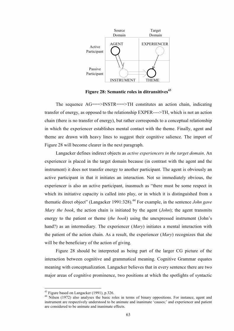
63

Source

DomainTarget

Domain

PassiveParticipant

ActiveParticipant

AGENT EXPERIENCER

INSTRUMENT THEME

Figure 28: Semantic roles in ditransitives43

The sequence AG===>INSTR===>TH constitutes an action chain, indicating

transfer of energy, as opposed to the relationship EXPER---->TH, which is not an action

chain (there is no transfer of energy), but rather corresponds to a conceptual relationship

in which the experiencer establishes mental contact with the theme. Finally, agent and

theme are drawn with heavy lines to suggest their cognitive salience. The import of

Figure 28 will become clearer in the next paragraph.

Langacker defines indirect objects as active experiencers in the target domain. An

experiencer is placed in the target domain because (in contrast with the agent and the

instrument) it does not transfer energy to another participant. The agent is obviously an

active participant in that it initiates an interaction. Not so immediately obvious, the

experiencer is also an active participant, inasmuch as “there must be some respect in

which its initiative capacity is called into play, or in which it is distinguished from a

thematic direct object” (Langacker 1991:328).44 For example, in the sentence John gave

Mary the book, the action chain is initiated by the agent (John); the agent transmits

energy to the patient or theme (the book) using the unexpressed instrument (John’s

hand?) as an intermediary. The experiencer (Mary) initiates a mental interaction with

the patient of the action chain. As a result, the experiencer (Mary) recognizes that she

will be the beneficiary of the action of giving.

Figure 28 should be interpreted as being part of the larger CG picture of the

interaction between cognitive and grammatical meaning. Cognitive Grammar equates

meaning with conceptualization. Langacker believes that in every sentence there are two

major areas of cognitive prominence, two positions at which the spotlights of syntactic

43 Figure based on Langacker (1991), p.326. 44 Nilsen (1972) also analyses the basic roles in terms of binary oppositions. For instance, agent and instrument are respectively understood to be animate and inanimate ‘causes;’ and experiencer and patient are considered to be animate and inanimate effects.

64

saliency are aimed. In a simple transitive clause, the subject corresponds to the clausal

trajector (or figure), the object to the clausal landmark (or ground), and the verb

expresses the relationship in which these two elements stand to each other. For example,

ditransitive verbs such as give, receive and take are closely related to each other,

inasmuch as they denote the transfer of a certain entity from one person to another. The

fact that speakers can choose between three different verbs is explained in CG as the

result of several cognitive processes governed by different arrangements of figure and

ground. Langacker (1987:3) points out that grammar

(...) embodies conventional imagery. By this I mean that it structures a scene in a particular way for purposes of linguistic expression, emphasizing certain facets of it at the expense of others, viewing it from a certain perspective, or construing it in terms of a certain metaphor.

In accordance with this statement, two sentences with the same propositional

content (and even the same words) which differ in their grammatical structures are

claimed to be semantically distinct, precisely because of their different symbolic

structure. Let’s see how this applies in our earlier pair of sentence, repeated here.

(35) a. John sent the book to Mary.

b. John sent Mary the book.

Sentence (35)a employs the preposition to, and thus emphasizes the path of the

book with Mary as goal. In contrast, sentence (35)b emphasizes the possession relation

which obtains between Mary and the book. In this sentence, the indirect object, rather

than the theme, is the secondary figure in the clause (the primary figure being the

subject). The English construction requires in particular that the theme’s movement

results in a possessive relationship between theme and recipient. Langacker assumes

that this possessive relationship is symbolized (grammatically) by both the juxtaposition

and linear ordering of the two nominals.

Langacker goes on to qualify this difference in meaning: it is not the case that the

notion of a path is lacking in sentence (35)b, or the notion of possession in sentence

(35)a: rather, it is the relative salience of these notions which differs in the two

sentences, a difference rooted in their different grammatical encoding. It is this

difference which enables a speaker to present the (same) scene through different

images.

65

2.2.3.2 Word Grammar

Word Grammar (WG) has been created and developed by Richard (Dick) Hudson. The

main claim of this theory, as part of a larger cognitive grammar enterprise, is that

language is a conceptual network, linking —and incorporating into the analysis of a

sentence— not just words but a vast array of different kinds of knowledge. The analysis

is monostratal, i.e. there is no recourse either to deep and surface structures, as in TG, or

to strata as in RG. Nonetheless, WG is related to RG in that both theories consider

syntactic structure to be based on grammatical relations, rather than on constituent

structure (Hudson 1990:10-11). Thus, concepts such as ‘subject’ and ‘object’ do not

need to be read off a tree —as in TG— for two main reasons: (a) there are no trees, (b)

grammatical relations are explicitly shown.

The two main tenets of the theory are dependency structure and default

inheritance. Dependency structure is essential to WG, inasmuch as WG is a theory

which does not recognise phrases, the longest unit admitted being the word. Syntactic

structure is thus handled in terms of relations between single words. Also, dependency

structure allows WG to incorporate grammatical functions into the syntactic analysis,

since they are all sub-divisions of ‘dependent’.

The concept of default inheritance —which states that “words inherit all the

characteristics of a super-category unless these are overridden”— is a very useful

mechanism both for making generalisations, and for capturing the contrast between

kernel (i.e. unmarked or underlying) sentence patterns, and marked ones. Default

inheritance is allowed for by an important relationship which obtains between words,

and in general between nodes, namely the ‘isa’ relationship, whereby the lexical form

‘dog’ isa (i.e. is linked to the meaning ) ‘animal’ and the lexeme DOG isa common

noun.

A WG analysis of a sentence is basically, in Hudson’s words (1990:12-13), “an

analysis of each word, in terms of a hierarchy (...) of word categories, plus an analysis

of each word’s relations to at least one other word, again done in a hierarchy of

categories (namely, relational categories)”. The WG hierarchy of categories is

illustrated in Figure 29 below.

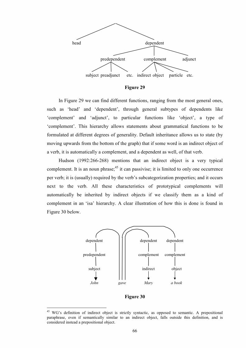
66

head dependent

complement adjunctpredependent

subject preadjunct etc. indirect object particle etc.

Figure 29

In Figure 29 we can find different functions, ranging from the most general ones,

such as ‘head’ and ‘dependent’, through general subtypes of dependents like

‘complement’ and ‘adjunct’, to particular functions like ‘object’, a type of

‘complement’. This hierarchy allows statements about grammatical functions to be

formulated at different degrees of generality. Default inheritance allows us to state (by

moving upwards from the bottom of the graph) that if some word is an indirect object of

a verb, it is automatically a complement, and a dependent as well, of that verb.

Hudson (1992:266-268) mentions that an indirect object is a very typical

complement. It is an noun phrase;45 it can passivise; it is limited to only one occurrence

per verb; it is (usually) required by the verb’s subcategorization properties; and it occurs

next to the verb. All these characteristics of prototypical complements will

automatically be inherited by indirect objects if we classify them as a kind of

complement in an ‘isa’ hierarchy. A clear illustration of how this is done is found in

Figure 30 below.

John gave Mary a book

indirect objectsubject

predependent complement complement

dependent dependent dependent

Figure 30

45 WG’s definition of indirect object is strictly syntactic, as opposed to semantic. A prepositional paraphrase, even if semantically similar to an indirect object, falls outside this definition, and is considered instead a prepositional object.

67

2.2.3.3 Construction Grammar

Traditionally, the object of grammar has been considered to be the “description and

analysis of structures (...) in terms of recurrent patterns (...)” (Robins 1964:190).

However, during the second half of the twentieth century, the importance of this notion

of ‘construction’ has been downgraded, mainly as a result of the views emanating from

the Chomskyan paradigm. From this perspective, constructions were (and still are) seen

as a by-product of the interaction of rules and constraints with the lexicon, and as such

of no theoretical import due to their lack of explanatory power.46

Pioneering work in the field can be found in early Construction Grammar papers

such as Fillmore et al. (1988) on the let alone construction, as well as Kay (1990) on

even constructions. Of late, constructions have been resurrected, placed in a different

framework, and invested with a new significance. In his book Radical Construction

Grammar, Croft (2001:14) recognises four different strands in the treatment of

constructions, represented by the works of Charles Fillmore, George Lakoff, Ronald

Langacker, and Adele Goldberg. All of these authors have cognitivist proclivities, and

thus the old construction (a kind of skeleton, an ordered sequence of slots) is now taken

to represent a unit not just of grammatical but of cognitive value as well. In Taylor’s

words (1995:197): “[f]or the cognitive linguist (...) syntactic constructions provide some

of the most compelling evidence for the similar structuring of linguistic categories on

the one hand, and the categories of non-linguistic reality on the other”.

It is thus not surprising that Construction Grammar is as a theory at

loggerheads with the central tenets of transformational grammar, and closely related to

the claims of cognitive linguists. Construction Grammar holds that language is, by and

large, idiosyncratic, and thus must be learned, i.e. cannot be innate. The theory has been

described as monostratal (i.e. there is just one level of grammar, no deep or surface

structure), non-derivational (there are no transformations or similar operations47) and

non-modular (language is considered to be an integral part of cognition).

Construction Grammar holds that language is a repertoire of constructions (or

‘constructicon’). A central implication of the theory is that words and phrases are the

46 A very important aspect of generative grammar from the GB model onwards is the assumption that there are no construction-specific rules. While early TG had rules (transformations) of e.g. Passive, in GB this construction is decomposed into more elementary operations which are motivated without recourse to the notion of construction. In Chomsky’s words (2002:94-95): “there aren’t any constructions anyway, no passive, no raising: there is just the option of dislocating something somewhere else under certain conditions, and in certain cases it gives you a question and so on, but the grammatical constructions are left as artifacts. In a sense they are real; it is not that there are no relative clauses, but they are a kind of taxonomic artifact. (…) It’s the interaction of several things (…).” 47 As Langacker (1987:46) points out, ‘general structure is almost entirely overt.’

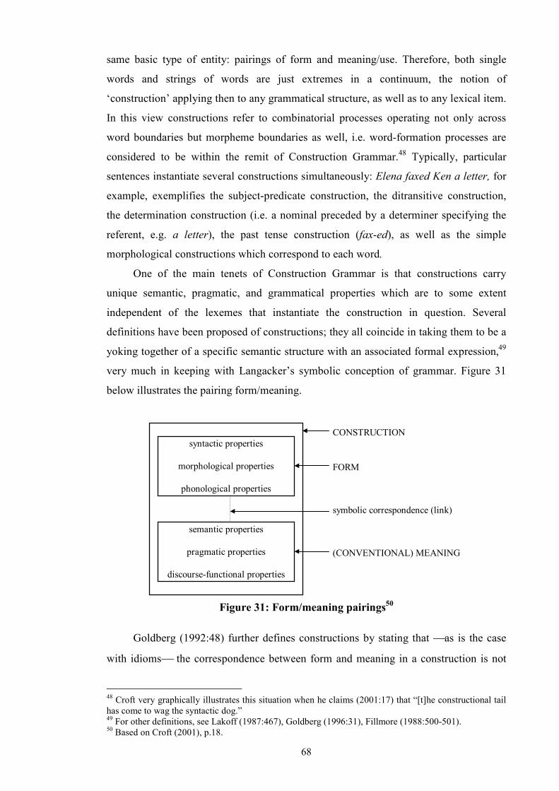
68

same basic type of entity: pairings of form and meaning/use. Therefore, both single

words and strings of words are just extremes in a continuum, the notion of

‘construction’ applying then to any grammatical structure, as well as to any lexical item.

In this view constructions refer to combinatorial processes operating not only across

word boundaries but morpheme boundaries as well, i.e. word-formation processes are

considered to be within the remit of Construction Grammar.48 Typically, particular

sentences instantiate several constructions simultaneously: Elena faxed Ken a letter, for

example, exemplifies the subject-predicate construction, the ditransitive construction,

the determination construction (i.e. a nominal preceded by a determiner specifying the

referent, e.g. a letter), the past tense construction (fax-ed), as well as the simple

morphological constructions which correspond to each word.

One of the main tenets of Construction Grammar is that constructions carry

unique semantic, pragmatic, and grammatical properties which are to some extent

independent of the lexemes that instantiate the construction in question. Several

definitions have been proposed of constructions; they all coincide in taking them to be a

yoking together of a specific semantic structure with an associated formal expression,49

very much in keeping with Langacker’s symbolic conception of grammar. Figure 31

below illustrates the pairing form/meaning.

syntactic properties

morphological properties

phonological properties

semantic properties

pragmatic properties

discourse-functional properties

CONSTRUCTION

FORM

symbolic correspondence (link)

(CONVENTIONAL) MEANING

Figure 31: Form/meaning pairings50

Goldberg (1992:48) further defines constructions by stating that as is the case

with idioms the correspondence between form and meaning in a construction is not

48 Croft very graphically illustrates this situation when he claims (2001:17) that “[t]he constructional tail has come to wag the syntactic dog.” 49 For other definitions, see Lakoff (1987:467), Goldberg (1996:31), Fillmore (1988:500-501). 50 Based on Croft (2001), p.18.

69

predictable either from the component parts, or from knowledge of the rest of the

grammar; i.e. as Croft (2001:18) points out, constructions are at least partially arbitrary.

As can be seen from Figure 31, the ‘meaning’ part of the construction includes both

pragmatic and discourse-related matters.

Constructions are claimed to “reflect scenes basic to human experience”

(Goldberg 1992:4). If we think of them as a cognitive construct, we have to concur with

Taylor’s view (1995:197) that constructions need to be regarded as prototype categories,

with some instantiations counting as better examples of the construction than others.

Both the meaning and the form of a construction have to be stated with reference to

central cases, so much so that prototype effects become evident. A construction may be

used to express meanings which differ to a greater or lesser extent from the central

specification.

Let us move on to the ditransitive construction. In a widely quoted paper and a

case of Construction Grammar avant la lettre Gropen et al. (1989:206) establish a

number of semantic conditions for the acceptability of a ditransitive construction. The

most important is the one which requires that the (referent of the) indirect object must

be the prospective possessor of the (referent of the) direct object. Possession is a very

important semantic property which determines the well-formedness of ditransitive

expressions.

Gropen et al. (1989:206) posit a rather complex theory to account for the

alternation of complementation patterns. In their view, dative shift turns out to be an

operation changing semantic structure. Each grammatical construction is made up of

two parts: the semantic structure itself, and a syntactic argument structure, associated to

each other “according to universal linking rules” (1989:206). The meanings of the two

different alternatives is considered to be as follows:

• Meaning of the prepositional dative: X causes Y to go to Z

• Meaning of the double object dative: X causes Z to have Y51

Following their argument, the dative rule changes one of these structures into the

other, thus causing a reinterpretation of facts: from understanding an event as causing a

thing to change location to construing it as causing a person to change their possessions.

A problem with their proposal is that, while providing a neat categorisation of

51 Evidence for the existence of a difference in meaning between the two constructions can be found from the process of generalisation in child language. See Lee (2001:74-78).

70

alternating and non-alternating verbs, it does not actually explain why verbs fall into the

different classes.

Anna Wierzbicka (1988:359), not a construction grammarian herself, offers a

different analysis of the same construction. She represents ditransitives with the

following formula:

• NP1 (human) V (action) NP2 (human) NP3 (concrete)

The double object construction (or ‘internal dative’ in her terms) implies a

comparison of NP2 and NP3. A sentence with an internal dative construction has two

direct objects instead of one, neither of these being a ‘full’ direct object. The presence

of two ‘objects’ represents an instance of what this author calls ‘divided transitivity’:

instead of one entity presented as affected by the action, the construction presents two

entities, each affected to a certain degree.52 When using a double object construction,

the speaker’s attention is focused primarily on the effect of the action on the target

person.53

The speaker is thus faced with a choice: will s/he focus on the effect of the action

on the patient, or will s/he focus on the effect of the action on the target? Wierzbicka

(1988:363) mentions that English constrains this choice in two ways, by means of what

she names the target condition and the patient condition. The target person can be

focused “upon, over and above” the patient if:

• the effect of the action on the target person is tangible, i.e. specifiable and

potentially desirable (see below for an example);

• the effect of the action upon the patient does not involve a drastic change of

state. Sentences like ?Kill me a spider are therefore unacceptable for

Wierzbicka.

‘Exceptions’ to this framework (i.e. verbs that do not alternate between the

ditransitive and the prepositional paraphrase constructions) are understood as violations

of either of the above conditions. To be successful, the ditransitive construction requires

a specifiable effect of the action on the target, and is incompatible with the presence of a

52 Incidentally, this accounts for the non-omissibility of NP3, since a comparison requires two objects to be compared. 53 This seems to be what Groefsema (2001:536 fn.) has in mind when stating that in a ditransitive construction we ‘zoom in’ on what happens to the patient, whereas in the prepositional alternant we zoom in on the recipient.

71

component which either implies the relative unimportance of the target or stresses the

special importance of the patient. This is the reason why verbs such as announce,

donate, and select (as opposed to their nearly synonymous counterparts tell, give and

choose) cannot alternate between the two constructions.

To spell out the implications, Wierzbicka (1988:373-374) holds that donate

implies that the target is not really a person but an institution, and as such it is not easy

to see it significantly affected by a single donation, thereby violating the target

condition. Announce focuses on the object of the communication, i.e. the focus is on the

message, therefore we have a violation of the target condition. The fact that it is the

message that is focused upon can be appreciated from the fact that the addressee can be

deleted. Lastly, one selects a few items out of many by comparing all the items with one

another; but one chooses one or more items based on the personal inclination of the

intended recipient. For example, you may select a wine out of many, but you normally

do not select your spouse; rather you choose him/her. Select then focuses on the objects

compared and thus violates the target condition.

The meanings of these Latinate verbs indicate a different perspective, one which

is incompatible with the meaning of the construction, and the result —according to this

account— has to be infelicitous.54 This seems to fit nicely with Lakoff’s dictum

(1987:582): “[a] great many syntactic properties of grammatical constructions are

consequences of their meanings”.

Let’s see how all these theoretical considerations apply to the case of ditransitive

complementation. A verb can occur in more than one syntactic argument structure, and

can adapt its meaning, chameleon-like, to its syntactic context. To restate the claim,

each verb carries its own obligatory participant roles (e.g. for the verb to give: giver,

receiver, thing given), just as every construction carries its own argument roles (e.g. in

the ditransitive construction: ‘agent’, ‘recipient’, ‘patient’), thereby specifying a

semantic macro-structure. For a construction to be felicitous, the roles a verb brings to

the construction structure must blend (or ‘fuse’) with the roles of the construction itself.

Additionally, the semantic macro-structure of the construction links each of its

argument roles with the typical syntactic roles (subject/object/oblique) which instantiate

it.

54 Groefsema (2001:548) adds that Latinate verbs tend to encode more specific meanings (than Anglo-Saxon verbs) and are often specifically concerned with the effect of the action described by the verb on one of the two affected participants (i.e. target and patient), whereas the effect on the remaining participant is covered by the native verb, as observed in pairs such as give-donate and tell-report. As we can see from Wierzbicka’s discussion of donate, announce, and select, these Latinate verbs focus on the effect of the action on the patient, and as such are incompatible with the construction’s target condition.

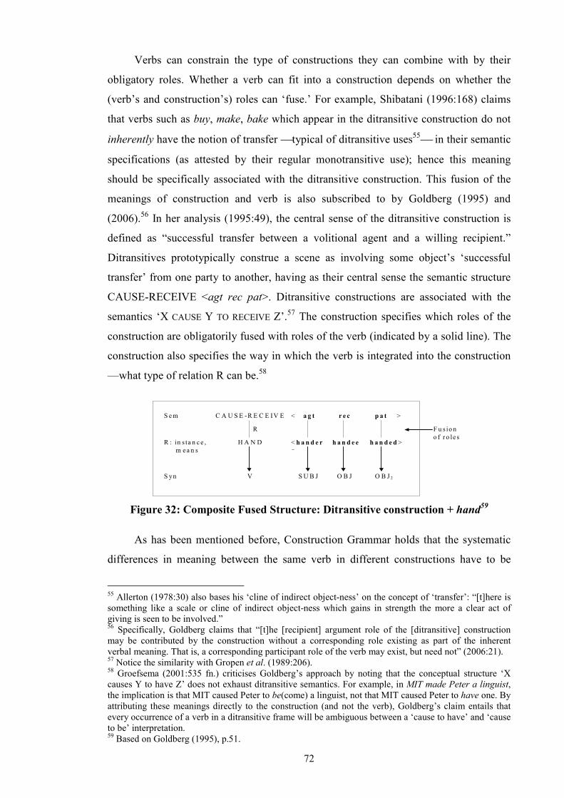
72

Verbs can constrain the type of constructions they can combine with by their

obligatory roles. Whether a verb can fit into a construction depends on whether the

(verb’s and construction’s) roles can ‘fuse.’ For example, Shibatani (1996:168) claims

that verbs such as buy, make, bake which appear in the ditransitive construction do not

inherently have the notion of transfer typical of ditransitive uses55 in their semantic

specifications (as attested by their regular monotransitive use); hence this meaning

should be specifically associated with the ditransitive construction. This fusion of the

meanings of construction and verb is also subscribed to by Goldberg (1995) and

(2006).56 In her analysis (1995:49), the central sense of the ditransitive construction is

defined as “successful transfer between a volitional agent and a willing recipient.”

Ditransitives prototypically construe a scene as involving some object’s ‘successful

transfer’ from one party to another, having as their central sense the semantic structure

CAUSE-RECEIVE <agt rec pat>. Ditransitive constructions are associated with the

semantics ‘X CAUSE Y TO RECEIVE Z’.57 The construction specifies which roles of the

construction are obligatorily fused with roles of the verb (indicated by a solid line). The

construction also specifies the way in which the verb is integrated into the construction

—what type of relation R can be.58

S e m C A U S E -R E C E IV E < a g t r e c p a t >

R : in s ta n c e ,m e a n s

H A N D < h a n d e r

g

h a n d e e h a n d e d >

S yn V S U B J O B J O B J 2

R F u s io no f r o le s

Figure 32: Composite Fused Structure: Ditransitive construction + hand59

As has been mentioned before, Construction Grammar holds that the systematic

differences in meaning between the same verb in different constructions have to be

55 Allerton (1978:30) also bases his ‘cline of indirect object-ness’ on the concept of ‘transfer’: “[t]here is something like a scale or cline of indirect object-ness which gains in strength the more a clear act of giving is seen to be involved.” 56 Specifically, Goldberg claims that “[t]he [recipient] argument role of the [ditransitive] construction may be contributed by the construction without a corresponding role existing as part of the inherent verbal meaning. That is, a corresponding participant role of the verb may exist, but need not” (2006:21). 57 Notice the similarity with Gropen et al. (1989:206). 58 Groefsema (2001:535 fn.) criticises Goldberg’s approach by noting that the conceptual structure ‘X causes Y to have Z’ does not exhaust ditransitive semantics. For example, in MIT made Peter a linguist, the implication is that MIT caused Peter to be(come) a linguist, not that MIT caused Peter to have one. By attributing these meanings directly to the construction (and not the verb), Goldberg’s claim entails that every occurrence of a verb in a ditransitive frame will be ambiguous between a ‘cause to have’ and ‘cause to be’ interpretation. 59 Based on Goldberg (1995), p.51.

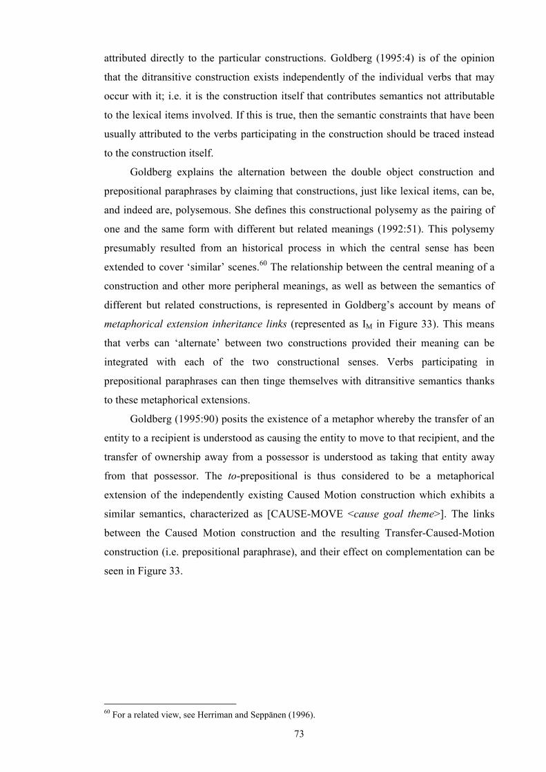
73

attributed directly to the particular constructions. Goldberg (1995:4) is of the opinion

that the ditransitive construction exists independently of the individual verbs that may

occur with it; i.e. it is the construction itself that contributes semantics not attributable

to the lexical items involved. If this is true, then the semantic constraints that have been

usually attributed to the verbs participating in the construction should be traced instead

to the construction itself.

Goldberg explains the alternation between the double object construction and

prepositional paraphrases by claiming that constructions, just like lexical items, can be,

and indeed are, polysemous. She defines this constructional polysemy as the pairing of

one and the same form with different but related meanings (1992:51). This polysemy

presumably resulted from an historical process in which the central sense has been

extended to cover ‘similar’ scenes.60 The relationship between the central meaning of a

construction and other more peripheral meanings, as well as between the semantics of

different but related constructions, is represented in Goldberg’s account by means of

metaphorical extension inheritance links (represented as IM in Figure 33). This means

that verbs can ‘alternate’ between two constructions provided their meaning can be

integrated with each of the two constructional senses. Verbs participating in

prepositional paraphrases can then tinge themselves with ditransitive semantics thanks

to these metaphorical extensions.

Goldberg (1995:90) posits the existence of a metaphor whereby the transfer of an

entity to a recipient is understood as causing the entity to move to that recipient, and the

transfer of ownership away from a possessor is understood as taking that entity away

from that possessor. The to-prepositional is thus considered to be a metaphorical

extension of the independently existing Caused Motion construction which exhibits a

similar semantics, characterized as [CAUSE-MOVE <cause goal theme>]. The links

between the Caused Motion construction and the resulting Transfer-Caused-Motion

construction (i.e. prepositional paraphrase), and their effect on complementation can be

seen in Figure 33.

60 For a related view, see Herriman and Seppänen (1996).

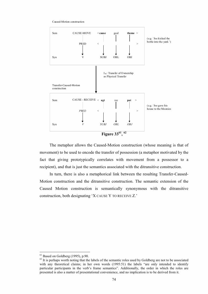
74

Sem CAUSE-MOVE < cause goal theme >

PRED < >

Syn V SUBJ OBL OBJ

( e.g. ‘Joe kicked the bottle into the yard.’)

Caused-Motion construction

I M : Transfer of Ownership as Physical Transfer

Transfer-Caused-Motion construction

Sem CAUSE - RECEIVE < agt rec pat >

PRED < >

Syn V SUBJ OBL OBJ

( e.g. ‘Joe gave his house to the Moonies

Figure 33

61,

62

The metaphor allows the Caused-Motion construction (whose meaning is that of

movement) to be used to encode the transfer of possession (a metaphor motivated by the

fact that giving prototypically correlates with movement from a possessor to a

recipient), and that is just the semantics associated with the ditransitive construction.

In turn, there is also a metaphorical link between the resulting Transfer-Caused-

Motion construction and the ditransitive construction. The semantic extension of the

Caused Motion construction is semantically synonymous with the ditransitive

construction, both designating ‘X CAUSE Y TO RECEIVE Z.’

61 Based on Goldberg (1995), p.90. 62 It is perhaps worth noting that the labels of the semantic roles used by Goldberg are not to be associated with any theoretical claims; in her own words (1995:51) the labels “are only intended to identify particular participants in the verb’s frame semantics”. Additionally, the order in which the roles are presented is also a matter of presentational convenience, and no implication is to be derived from it.

75

Sem CAUSE - RECEIVE < agt rec pat >

PRED < >

Syn V SUBJ OBJ OBJ 2

Ditransitive construction

Semantically synonymous

Transfer-Caused-Motion construction

Sem < agt rec pat >

PRED < >

Syn V SUBJ OBL OBJ

CAUSE - RECEIVE

Figure 34

Goldberg points out that semantic synonymity is not to be confused with

pragmatic synonymity: she agrees with Erteschik-Shir’s analysis (1979) in considering

that the ditransitive construction is used when the recipient is ‘nondominant’, therefore

placing the patient in focus; the converse is true in the case of the Transfer-Caused-

Motion construction, which focuses on the recipient.

As Snyder (2003:3) points out, Goldberg’s key insight is to be found in her idea

that speakers in fact choose from the range of (syntactic) options available to them

based on processing considerations, and as such “a speaker’s choice of form (but not a

language’s range of options) is in fact motivated by the discourse function of her

utterance”.

This chapter has provided an overview of (some of) the problems ditransitives

have caused to linguists, especially to those more interested in building linguistic

theories, very often at the expense of the simple job of accounting for facts. The indirect

object in particular has exercised linguists’ minds across many decades, given this

element’s notorious refusal to conform to (formal and functional) categories. The

following chapter looks in more detail into some of the challenges indirect objects have

posed for syntactic analysis.

76

3 The Indirect Object as Complement of the

Verb

In a sentence like John gave Mary a book we will have no problems in calling both

post-verbal noun phrases complements to the verb. But what about John gave a book to

Mary? Can we call the prepositional phrase to Mary a complement? Or is it better to call

it an adjunct? In ICE-GB, the wide range of post-verbal ditransitive complements boils

down to two patterns: NP+NP/CL, and NP+PP. In order to determine which structures

can accurately be called complements, a number of syntactic and semantic criteria have

been used. Before discussing these criteria, however, a short general introduction on

complements and adjuncts is required in order to illustrate a number of different

approaches to the issue at hand.

This chapter discusses various criteria and tests instrumental for the identification

of complements. In so doing, it attempts to answer two questions: (i) what is a

complement?, and (ii) is the indirect object a complement? Later sections specify the

criteria employed for determining constituency in indirect objects (especially when

postmodification is involved), the semantic roles typical of indirect objects, and the

possibility of positing a gradient continuum in the classification of indirect objects.

3.1 Definitional Criteria

Huddleston and Pullum et al. (2002:219) mention that complements are more closely

related to the verb (in its role as clausal head) and more clearly differentiated by their

syntactic properties than adjuncts are.63 However, there is also widespread agreement on

the fact that complements seem to be required in clause structure for both syntactic and

semantic reasons. It is therefore only natural to proceed to an examination of both types

of properties. The following discussion dwells mainly on points raised in Huddleston

and Pullum et al. (2002) and Hudson (1990).

3.1.1 Notional Criterion

The first criterion for differentiating complements from adjuncts is a notional one,

arising from Tesnière’s discussion (1959:102) of ‘actants’. In his account, the clause is

said to express a performance (“tout un petit drame”) which may be characterised by its

setting and the behaviour of the performers. Participants in the performance are called

63 Adjuncts, on the other hand, are easier to identify and classify by their semantic properties, as we can see by their nomenclature (e.g. adjuncts of time, duration, manner, degree, etc.).

77

actants and typically correspond to arguments/complements; the setting, props and

other optional items describing the circumstances of the performance are called

circonstants, and typically correspond to non-arguments/adjuncts.

To illustrate, a ditransitive verb such as give describes an event in which three

participants are usually present or required: a giver, a gift, and a recipient of the gift. To

use an example from Matthews (1984), in I gave you the book yesterday there is a sense

in which any of the three participants (I, you, and the book) is a more essential or

necessary part of the event than yesterday is. The noun is only providing a temporal

indication for the event described by give.

Croft (2001:124) holds that the notional criterion is only useful as some sort of

rule of thumb throwing light on the semantic distinction between complements and

adjuncts, having nothing to contribute to the analysis of their syntactic behaviour.64

3.1.2 Maximum Number

The verb determines both the minimum and maximum number of complements.

Adjuncts, on the other hand, are ‘stackable’: there is no maximum number which a

clause can tolerate, they can be added ad infinitum.

(36) I gave Peter the book (on Monday) (in the rain) (in Cambridge), etc.

Since complements of a particular kind can occur in a clause to the maximum of

one, Matthews (1981:127) suggests another test for complementhood, this time by

assessing the possibility of grafting a constituent onto a clause. Applying Matthews’s

test yields examples such as (37)d and (37)e.

(37) a. ?He gave an example.

b. He gave an example to the students.

c. He gave an example to the dog.

d. *He gave an example to the dog to the students.

e. *John carved a figurine to Mary.

Adding to the students to (37)a brings to the surface the latent participant in the

event of giving, but adding the same phrase to (37)c leads to ungrammaticality, as (37)d

shows, which is evidence that to the dog in (37)d is actually a complement of the verb,

64 See also §3.1.7.

78

although of a different type from the other verbal complement, i.e. an example.

Example (37)e illustrates that to-phrases cannot be added freely.

3.1.3 Determination of Form

Borsley (1999:67) states that a clearly important difference between complements and

adjuncts is that “complements are associated with specific words in a way that adjuncts

are not. Particular words co-occur with particular complements, whereas an adjunct (…)

is generally possible in any phrase of a particular kind whatever its head is”. Put

differently, heads impose restrictions on their complements, but not on the adjunct/s

which may be present. Example (38) below illustrates how the head verb requires its

complement to have a certain form.

(38) I saw him / *he.

Certain verbs can occur only with certain attending complements (and vice versa),

whereas adjuncts can join virtually any phrase or clause. This criterion is especially

relevant for prepositional phrases. In prepositional complements, the choice of

preposition heading the phrase is highly restricted. Poutsma (1926:177) defined these

prepositional complements as those “whose relation to the predicate is expressed by a

preposition”. The situation is compounded by the fact that very often adjuncts also take

the form of prepositional phrases. The difference between prepositional complements

and adjuncts headed by a preposition has proved to be rather elusive. Curme (1931:113)

attributes this difficulty to the fact that between prepositional complements and

prepositional adjuncts “there is never a difference in form and no fundamental

difference in function.” Nonetheless, Poutsma (1926:29ff) has provided some

guidelines.

• If the element is “felt” to be a necessary complement of the verb, it is then an

object, i.e. a complement. This is no more than a reformulation of the notional

criterion discussed in §3.1.1.

• If a (pro)noun in a prepositional object can be passivised (thus leaving the

preposition stranded), the prepositional phrase is very likely to be a complement,

since this syntactic operation is notoriously more difficult in the case of adjuncts

(see also §3.2.1).

• If the preposition is vague in meaning, “conveying little or none of the relations

of time, place, cause, purpose, agency, instrumentality, etc.”, the prepositional

79

phrase is very likely to be a complement. The function of the preposition in

prepositional objects is, rather, geared towards the identification of the semantic

role of the noun phrase.65

Huddleston and Pullum et al. (2002:220) further state that the preposition in

prepositional objects/complements is often specified by the verb, e.g.

(39) a. It consists of egg and milk.

b. He didn’t look at her.

c. I blame it on Kim.

d. He gave it to Pat.

Additionally, these authors demonstrate that just as a head selects its

complement/s, a complement can also be dependent on the occurrence of the

appropriate head. They illustrate the point with prepositional objects, by altering the

verb and keeping the preposition intact, e.g. *it contains of egg and milk, *he bought it

to Pat.

Additional difficulties surface when the prepositional phrase is headed by to, as it

can be difficult to find where the directional component (typical of adjuncts) of the

preposition starts, and where it yields to the vague meaning identified by Poutsma as

typical of complements. Examples (40) and (41) below, for instance, lead Matthews

(1981:130) to believe that the indirect object tends to merge with other elements that are

not participants.66

(40) a. I sent some books to Jill.

b. I sent Jill some books.

c. Jill was sent some books.

(41) a. I dispatched some books to my sister.

b. ?My sister was dispatched some books.

c. ?I dispatched my sister some books.

65 Givón (1993:95) subscribes to the idea of certain prepositions marking the semantic role of a participant, typically one occupying the indirect object grammatical role. Sag and Wasow also claim that in some uses, prepositions in English simply function as argument markers, i.e. “they indicate what role their object plays in the situation denoted by the verb of the clause they appear in” (1999:155-156). 66 In order to distinguish (terminologically, at least) prepositional objects/complements from prepositional phrases functioning as adverbials, Biber et al. (1999:129-130) suggest analysing to-phrases corresponding to indirect objects as recipient adverbials.

80

3.1.4 Word Order

When both complements and adjuncts are present, complements are generally both

closer and more closely linked to the head.67 In general, there is a basic or default

position for complements: subject complements tend to follow the verb, indirect objects

tend to follow the verb and precede the direct object, and so on. By contrast, adjuncts

are more mobile. An adverbial like yesterday can occur in any of the positions indicated

by an x in (42) below.

(42) x John x gave the book x to the assistant librarian x.

The idea of a default position for complements is not to be interpreted as meaning

that word order is completely fixed. Deviations from the unmarked linear order head +

complement are not hard to find in corpus data, and subsequent chapters provide more

detailed explanations in terms of both information structure (whereby given information

tends to precede relatively new information), and weight (whereby heavier constituents

tend to occur towards the end of the clause).

Consider the latter: it is a well known fact that the heavier a constituent is

(especially in relation to other clausal elements), the higher are its chances of being

postponed. This is usually known as the principle of end weight (PEW), of which

Heavy NP Shift (HNPS) is one of the manifestations. For example, in (43)b below, the

direct object has been shifted over the adjunct on Saturday towards the end of the

sentence.

(43) a. Paolo kicked [DO the ball] on Saturday.

b. Paolo kicked on Saturday [DO the ball that his parents said had belonged to a

renowned serial killer turned professional football player in Italy].

The indirect object, however, cannot be moved by HNPS: no matter how heavy it

is, it still needs to stay in immediately post-verbal position, as can be seen in (44).

(44) a. Paolo gave [IO the girl] some flowers.

b. *Paolo gave some flowers [IO the girl he had met at the party the night

before].

67 See, among others, Huddleston (1984:264); Tomlin (1986:4); Radford (1988:178, 191); Haegeman (1991:95).

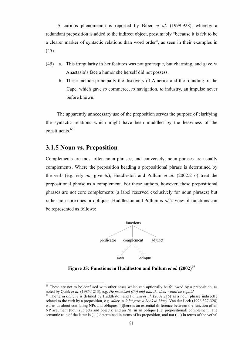
81

A curious phenomenon is reported by Biber et al. (1999:928), whereby a

redundant preposition is added to the indirect object, presumably “because it is felt to be

a clearer marker of syntactic relations than word order”, as seen in their examples in

(45).

(45) a. This irregularity in her features was not grotesque, but charming, and gave to

Anastasia’s face a humor she herself did not possess.

b. These include principally the discovery of America and the rounding of the

Cape, which gave to commerce, to navigation, to industry, an impulse never

before known.

The apparently unnecessary use of the preposition serves the purpose of clarifying

the syntactic relations which might have been muddled by the heaviness of the

constituents.68

3.1.5 Noun vs. Preposition

Complements are most often noun phrases, and conversely, noun phrases are usually

complements. Where the preposition heading a prepositional phrase is determined by

the verb (e.g. rely on, give to), Huddleston and Pullum et al. (2002:216) treat the

prepositional phrase as a complement. For these authors, however, these prepositional

phrases are not core complements (a label reserved exclusively for noun phrases) but

rather non-core ones or obliques. Huddleston and Pullum et al.’s view of functions can

be represented as follows:

functions

complement adjunctpredicator

core oblique

Figure 35: Functions in Huddleston and Pullum et al. (2002)69

68 These are not to be confused with other cases which can optionally be followed by a preposition, as noted by Quirk et al. (1985:1213), e.g. He promised ((to) me) that the debt would be repaid. 69 The term oblique is defined by Huddleston and Pullum et al. (2002:215) as a noun phrase indirectly related to the verb by a preposition, e.g. Mary in John gave a book to Mary. Van der Leek (1996:327-328) warns us about conflating NPs and obliques “[t]here is an essential difference between the function of an NP argument (both subjects and objects) and an NP in an oblique [i.e. prepositional] complement. The semantic role of the latter is (…) determined in terms of its preposition, and not (…) in terms of the verbal

82

3.1.6 Obligatoriness

Huddleston and Pullum et al. (2002:221) define an element as obligatory “if it cannot be

omitted without loss of grammaticality or an unsystematic change of meaning”.

Complements are said to be obligatory and adjuncts to be optional. However, if we

invert the relationship, we find that whereas an obligatory element has to be a

complement, an optional element can be either a complement or an adjunct, as seen in

example (46) below (also from Huddleston and Pullum et al. 2002: 221).

(46) a. She perused the report. / *She perused. (obligatory complement)

c. She read the report. / She read. (optional complement)70

d. She left because she was ill. / She left. (optional adjunct)

The status of indirect objects (especially those alternating with for) is still

undetermined between that of obligatory or optional elements. Some authors have

contrasted the behaviour of indirect objects and direct objects as a way of grounding

their opinions on syntactic phenomena. For instance, Jespersen (1927:279) considers the

direct object more closely connected to the verb than the indirect object, on the evidence

that it is possible to isolate the direct object (as in (47)b), but not the indirect object (as

in (47)c). Being non-omissible makes the direct object the obligatory complement, at

the expense of the indirect object.71

(47) a. They offered the man a reward.

b. They offered _ a reward.

c. *They offered the man _.

However, there remain some problems in treating non-omissibility as criterial for

determining complement status. As Jespersen was well aware (1927:295), some verbs

allow the possibility of treating one of the two objects (but not the other) as non-

predicate, and the oblique complement as a whole does not function as an argument of the verb but as a subpredicate that pins down the verbal meaning more specifically.” 70 Matthews (1981:125) warns that omitting an element as a test of its obligatoriness can be difficult to control, due to the possibility of ellipsis (and its attendant notion, latency; cf. §3.1.8) on the one hand, as well as to the different senses of lexemes, on the other. He illustrates the former notion with the pair Are you watching football tonight? and Are you watching tonight?, the latter with I can see you this afternoon and I can see. 71 Moreover, Jespersen (1927:278) believes that it is not unusual for normally ditransitive verbs to not require two objects: “[s]ome verbs frequently or even regularly have two objects; we shall first mention the type: he gave the boy a shilling” [my emphasis]. In this, he anticipates Matthews’s (1981) notion of latent objects (see §3.1.8).

83

omissible (examples (48) and (49)); while other verbs72 never allow its objects to be

omitted (examples (50) and (51)).

(48) a. Strike him a heavy blow.

b. Strike him _ .

c. Strike _ a heavy blow.

(49) a. Ask John a few questions.

b. Ask John _ .

c. Ask _ a few questions.

(50) a. Hand Jones a hot potato.

b. *Hand _ a hot potato.

c. *Hand Jones _ .

(51) a. Promise Jones a job.

b. *Promise _ a job.

c. *Promise Jones _ .

If no object can be omitted, then both are obligatory. If both are obligatory, does

this mean that these verbs have not simply two complements but two direct objects?

Jespersen suggests that this is indeed the case. However, where one of the direct objects

can alternate with a prepositional paraphrase with to (or for), Jespersen prefers to

consider it an indirect object.

(52) a. He teaches boys _ .

b. He teaches _ French.

c. He teaches the boys French.

d. He teaches French to the boys.

(53) a. I told the teacher _ .

b. I told _ my story.

c. I told the teacher my story.

d. I told my story to the teacher.

In the above examples, both objects can appear alone, but the existence of a

prepositional paraphrase marks one of them as an indirect object.

72 On these verbs, see also Anderson (1988), and Baker (1988), inter alia.

84

3.1.7 Subcategorisation

Subcategorisation is a type of dependence between complements and (mainly) their

head verbs in clause structure. Inverting the relationship between head and

complements, Huddleston and Pullum et al. (2002:219) suggest that “complements

require the presence of an appropriate verb that licenses them”, e.g.

(54) a. She mentioned the letter.

b. *She alluded the letter.

Adjuncts, on the other hand, can occur with any kind of verb. Elements such as

yesterday, because I’m generous, and after you left can be added to virtually any

sentence containing a verb.

Sag and Wasow (1999:77) state that the semantics of a verb is closely related to

its subcategorisation or valency, but that there is some syntactic arbitrariness present in

subcategorisation as well. They illustrate with eating verbs such as eat, dine, and

devour, activities which involve food and an eater. In this light, we should expect them

to be transitives, requiring a subject (the eater) and a direct object (the food). However,

dine is intransitive, devour is transitive, and eat can be used intransitively or

transitively, as seen in (55) below.73

(55) a. The guests devoured the meal.

b. *The guests devoured.

c. *The guests dined the meal.

d. The guests dined.

e. The guests ate the meal.

f. The guests ate.

Thus, these authors conclude, despite the link between meaning and

subcategorisation, the latter is better specified syntactically. As Borsley (1999:78)

indicates, although the number of complements taken by a head is related to meaning,

“it is also clear, however, that what complements appear is not completely predictable

from semantic considerations.” This position is seen again in Government & Binding

73 See Wierzbicka (1988) and Goldberg (1995) in §2.2.3.3.

85

Theory, where it is the lexicon that takes care of postverbal complementation; i.e. the

verb’s lexical entry stipulates which complements it takes.74

Assuming that to-/for-phrases acting as paraphrases of indirect objects are indeed

complements, it is possible to say that ditransitive verbs can occur in two

subcategorisation frames: they can be followed either by two noun phrases, or by a noun

phrase and a prepositional phrase headed by to or for. However, there are some

peculiarities worth mentioning.

(56) a. I gave you the book.

b. I gave the book to you.

(57) a. I bought a book.

b. I bought Mary a book.

c. I bought a book for Mary.

(58) a. John peeled Mary a grape.

b. Sing me an aria.

c. Carolina fixed me a sandwich.75

In (56), it is plain to see that the recipient of the giving of the book is a required

participant, both semantically and syntactically. In (57), however, there is nothing in the

act of buying that requires a beneficiary, as seen in example (57)a: I can buy a book for

myself, or just buy it with no intended beneficiary in mind. These beneficiary roles

usually alternate with a prepositional phrase headed by for. The question remains: do

these transitive verbs in (58) need to be subcategorised for NP+NP as well?76 Is the first

postverbal noun phrase a complement, despite not being included in the verb’s

subcategorisation frame? This point will be taken up in §3.3.3 and §3.4.

74 Croft’s (2001:247) is a very typical example of criticism aimed at the way in which Government & Binding Theory handles complementation: “[t]he usual characterization of subcategorization in generative syntax assumes there is a particular directionality, so that the subcategorizand determines the subcategorization that it requires. This is questionable to the extent that the subcategorization [sic] is not a function in the mathematical sense, that is, there is a unique categorization for each lexical head. This is not generally the case, particularly in English.” 75 The examples in (58) are taken and/or adapted from Jackendoff (1990a). 76 Jackendoff (1990a:449) prefers to treat these immediately postverbal NPs as adjuncts, because “[t]here is nothing in the inherent meaning of singing an aria, peeling a grape, or fixing a sandwich that requires an intended Beneficiary one could just be doing these things for the hell of it.”

86

3.1.8 Latency

Latency is closely linked to the obligatory/optional distinction. Croft (2001:275) adds to

the discussion by claiming that obligatoriness and latency are cross-linguistically valid

criteria for complementhood. Matthews (1981:124-126) defines latency as “the

requirement for a definite interpretation of a dependent if that dependent is left

syntactically unexpressed”. When a constituent is omitted in order to test for its

(syntactic or semantic) necessity, the remaining elements typically produce a plainly

ungrammatical sentence (e.g. *I devoured). However, the absence of a constituent may

be filled pragmatically: the hearer then searches the preceding discourse context for a

referent to fill the position of the omitted element. Language users can arrive at a

felicitous interpretation of an incomplete syntactic sequence by resorting to the principle

of pragmatic relevance. For example, if a speaker says I didn’t finish, s/he believes that

the addressee can fill the gap by looking in the discourse or situational context for the

element that will complete the meaning of the clause (the job, the book, etc.).

Some transitive verbs can occur without an object participant role: one can say I

am eating, or I am reading without specifying what is it that goes in your mouth or

before your eyes. The same applies to ditransitive verbs, as discussed in §3.1.6: the verb

teach, for example, describes an event involving a teacher, at least one student, and the

topic being taught. However, any of the three arguments can be left out in a sentence

with teach (see example (52) above).

3.1.9 Collocational Restrictions

Matthews (1981:124-125) suggests using the presence of collocational relations as a

diagnostic for complement status. For instance, the fact that it is more natural to say

give protection but not *give defense means that there is “a direct constructional link

between the object and the predicator”, that is to say, protection is a complement of

give. This criterion is useful for ditransitive verbs, especially since give occurs with a

very large number of collocations (give an opportunity, give assurance, give credence,

give confidence, etc.). By contrast, collocational restrictions do not apply to adjuncts.

Hudson (1990:206) sums up the discussion of complements and adjuncts thus:

“the role, in both syntax and semantics, of the complement is fixed by the head, whereas

that of the adjunct is fixed by the adjunct itself”. It is the adjunct which is far more

independent, fixing its own form and function. The complement, on the other hand, is

87

always in thrall to its head, both formally and functionally. I will return to the

distinction between complements and adjuncts in §3.5.

3.2 Constituency Tests

The preceding sections introduced some instrumental criteria for determining whether a

clausal element is a complement or an adjunct. Yet, in an example like Just offered the

girl next to me 10p for one Rolo <ICE-GB:W1B-010 #78:2>, knowing which elements are

required by the verb is as important as ascertaining where each element begins and

ends. In what follows, I introduce other tests used in this study in order to establish the

constituency of both complements and adjuncts.

3.2.1 Extraction

This test involves the extraction of an (oblique) noun phrase which is the complement

of a preposition. According to Radford (1988:191), this is more easily done with

complement prepositional phrases than with adjunct prepositional phrases.77

(59) a. What field of linguistics are you a student of?

b. *What kind of personality are you a student with?

In example (59)a, the possibility of stranding the preposition indicates that the

prepositional phrase functions as a complement (of a noun phrase). In example (59)b

where the preposition introduces an adjunct prepositional phrase, the stranding is not

possible.

This test has been used to ascertain whether a prepositional phrase in the verb

phrase is functioning as a complement or as an adjunct, especially in the case of

prepositional phrases headed by for.

(60) a. John gave a book to Mary on Tuesday.

b. Who did you give a book to on Tuesday?

c. *What day did you give a book to Mary on?

(61) a. John peeled a grape for Mary in Paris.

b. Who did John peel a grape in Paris for?

c. *Which city did John peel a grape for Mary in?

77 Recall that Poutsma also used stranding (although via passivisation) as a guideline for the identification of prepositional complements (§3.1.3). See also §3.3.

88

This test was used where possible, but the resulting sentences varied greatly in

acceptability, thereby making it necessary to supplement it with other tests.

3.2.2 Anaphora: Substitution

Substitution by a proform has long been used to determine constituent structure.

Huddleston and Pullum et al. (2002:222-223) advocate the use of the do so anaphoric

test: “[t]he fact that complements are more closely related to the verb than adjuncts is

reflected in the scope of certain anaphoric expressions, notably do so. (…) The

antecedent of do so must embrace all internal complements of the verb.” The

functionality of this test relies on the fact that in a structural analysis of

complementation, the verb and its complement/s form a constituent together.

(62) a. John bought Mary flowers on Friday.

b. John [bought Mary flowers] on Friday and James did so on Saturday.

c. *John [bought Mary] flowers on Friday and James did so a watch on

Saturday.78

A comparison between examples (62)b and (62)c shows that both Mary and

flowers must be within the scope of do so, thereby making both qualify for

complementhood, whereas on Saturday does not necessarily have to be within the scope

of the expression. If other elements (e.g. on Saturday) can combine with do so, this is

sufficient to show that they are adjuncts.

The same is true of the examples in (63).

(63) a. John peeled Mary a grape on Friday.

b. John [peeled Mary a grape] on Friday and James did so on Saturday.

c. John [peeled a grape for Mary] on Friday and James did so on Saturday.

d. *John [peeled a grape] for Mary on Friday and James did so for Jane on

Saturday.

Example (63)d is particularly interesting, in that it is not ungrammatical with a

deputive reading, i.e. where the activity is performed not for the enjoyment of a

beneficiary, but rather so that the said beneficiary does not have to do something

78 All the same, it is not unusual for an adjunct to be included in the scope of the do so proform. For example, in John bought [Mary flowers on Friday] and James did so too, we can see that on Friday (clearly and adjunct) can still occur within the scope of do so.

89

him/herself, e.g. John peeled a grape for Mary on Friday, and James peeled a grape for

Mary on Saturday so that Jane didn’t have to (peel Mary a grape). Examples like these

are further discussed in §3.3.3 and §3.5.

3.2.3 Cleft Constructions

These constructions serve the purpose of highlighting clausal elements, but it is only

constituents which can occur in the focus position of a cleft or pseudo-cleft. And there

lies its usefulness, for as Aarts (2001:227) suggests these constructions can be

employed as tests for syntactic constituency.

The cleft construction can be described using the following template: it + be +

focused element + clause. Like the pseudo-cleft, it is a flexible construction in that the

highlighted item may consist of an array of different elements. As mentioned earlier, the

focus position in the cleft is reserved for constituents only.79

Indirect objects do not sit very comfortably in the focus position of cleft sentences

(as in (64)), but their prepositional paraphrases seem to be less choosy, as can be seen in

(65).

(64) a. John gave Mary a book.

b. ?It was Mary John gave a book.

(65) a. John gave a book to Mary.

b. It was Mary John gave a book to.

c. It was to Mary John gave a book.

The pseudo-cleft construction, on the other hand, consists of the verb to be and a

wh-clause.80 The position following the verb to be is called the focus position, and it

hosts different kinds of constituents:

79 Grammars, however, do not agree as to what elements can be focused in a cleft sentence. Jackendoff (1977:17) claims that only NPs and PPs can occur in this position whereas Baker (1989:376) gives examples of NPs and adverb phrases in focus position. Quirk et al. (1985:1385) include a list of possible elements but clearly state that predicatives, indirect objects and verbs are excluded:

i. ?It’s very tall you are. ii. ?It’s me (that) he gave the book. iii. *It’s wore that John a white suit at the dance.

80 The wh-word is the fused relative what, which is understood to mean roughly ‘that which’, i.e. antecedent + relative pronoun.

90

(66) a. John gave Mary a book on Tuesday.

b. What John gave Mary on Tuesday was a book.

c. What John did was give Mary a book on Tuesday.

d. What John did on Tuesday was give Mary a book.

e. ?Who gave Mary a book on Tuesday was John.

f. ?Who John gave a book on Tuesday was Mary.

Pseudo-clefts are more limited than clefts proper, say Quirk et al. (1985:1388),

since the wh-clause can very rarely start with who, where and when. However, they also

suggest this difficulty can be bypassed by using noun phrases of general reference in

place of the wh-item in question. Therefore, examples (66)e and (66)f can be patched as

in (67)a and (67)b.

(67) a. The person who gave Mary a book on Tuesday was John.

b. ?The person John gave a book on Tuesday was Mary.

Still, sentence (67)b is still not very natural. Pseudo-clefts are more amenable to

prepositional objects (headed by to or for) than they are to plain noun phrase indirect

objects, as illustrated in (68) and (69) below.

(68) a. John gave a book to Mary on Tuesday.

b. The person John gave a book to on Tuesday was Mary.

(69) a. John bought a book for Mary on Tuesday.

b. The person John bought a book for on Tuesday was Mary.

Clearly, some of the resulting sentences seem dubious when taken out of context.

Nonetheless, the validity of each test is not compromised if we consider them as

indicators rather than as absolute proof of constituency.

These criteria were applied in a principled way to the corpus examples. All the

same, it is worth noting that in clear cases of ditransitivity, one criterion was usually

enough, whereas in unclear or ambiguous cases, several criteria had to be employed.

3.3 Semantic Roles

Most frameworks have to deal with meaning in one way or another, and thus it is

generally recognised that the type of complement a head takes has something to do with

meaning.

91

At first (syntactic) blush, there is no obvious way of distinguishing between, e.g. a

prepositional phrase encoding a locative role from a prepositional phrase encoding a

recipient role. However, this difference in roles has consequences for the behaviour of

the phrases in question in relation to the verb they co-occur with: while a locative can be

a complement with certain verbs, it is not required by others, thus acting as an adjunct.

In this light, semantic roles have some bearing on the complement/adjunct distinction.

Verbs are generally classified by the number of arguments they take. In

Government & Binding Theory, the arguments of propositions are assigned thematic

relations or theta roles (i.e. semantic roles) such as Agent, Patient and Theme. The

ultimate semantic role of a noun phrase depends on the lexical properties of its head.

Borsley (1999:77) mentions that Government & Binding Theory assumes that “word

level heads are associated with a specific number of theta-roles and that every

complement must be assigned one and only one theta-role.” 81 In summary, a verb

subcategorises for its complement/s and assigns one (and only one) theta-role to each.

3.3.1 Locative

The preposition to can be used to encode either a recipient or a locative role.

Ditransitive complementation is only normally possible with a recipient reading of

prepositional phrases headed by to. Consider the following examples:

(70) a. John sent the book to London.

b. *John sent London the book.

Example (70)b is clearly unacceptable, unless London is considered to be animate,

for example, as shorthand for ‘the people at the London branch of a company.’ By

personifying London, the prepositional phrase in (70)a stops being a locative to become

a recipient.82

3.3.2 Recipient

Quirk et al. (1985:741-753) state that indirect objects typically have the role of

‘recipient participant’, i.e. of the animate being that is passively implicated by the

happening or state. This recipient role is particularly evident with verbs instantiating

81 Theta-role assignment is intimately related to subcategorisation, since in Government & Binding Theory the latter is usually assumed to presuppose the former. 82 See also Baker (1988) and Hornstein and Weinberg (1981) for a discussion of ‘inner’ (i.e. argument) locative PPs, and ‘outer’ (i.e. adjunct) locative PPs, and their difference in syntactic behaviour.

92

actual transfer, such as give, hand, and throw. Recipient indirect objects are the most

amenable to prepositional paraphrases, usually involving the preposition to.

3.3.3 Beneficiary

If we apply the criteria presented in §3.1 to (71)a below, there is enough evidence to say

that the indirect object is a very typical complement. It is a noun phrase, it occurs

immediately after the verb head (and before the direct object), and it is limited to one

occurrence per verb. However, it is not a typical complement in not being invariably

required by the verb’s subcategorisation. Examples (71)b, (71)c, and (71)d show the

indirect object added on to run-of-the-mill transitive verbs.

(71) a. I bought Mary a present. [i.e. I bought a present for Mary]

b. John peeled Mary a grape.

c. Sing me an aria.

d. Carolina fixed me a sandwich.

Considering then that these transitive verbs subcategorise for a direct object and

do not subcategorise for a beneficiary role, the ‘add-on’ element should not be expected

to occur in such a privileged position next to the verb, a position that is expected to

correspond to the direct object. Still, the complements are ordered just like they are in a

prototypical ditransitive clause. These ‘guest’ indirect objects usually alternate with a

prepositional phrase headed by for.

(72) a. John peeled a grape for Mary.

b. Sing an aria for me.

c. Carolina fixed a sandwich for me.

The role of the guest indirect objects and of their for-phrase counterpart is called

benefactive or beneficiary in the literature, to distinguish it from recipient. Traditional

grammarians such as Kruisinga (1932:186ff) and Poutsma (1926:29ff) suggested calling

them pseudo-object or adjunct of benefit. They refuse to grant them complement status

because: (a) they are not required by the verb, and can therefore be omitted,83 (b) they

83 Marantz (1984) is another author who agrees that beneficiaries are adjuncts, based on subcategorisation evidence. However, he does point out that if it is true that beneficiaries are not required by any verbs, it is also true that no verbs clearly forbid them either.

93

do not passivise easily, (c) and their contribution is more adjunct-like than object-like,

in that they state in whose behalf an action is said to take place.

Huddleston and Pullum et al. (2002:310-311) distinguish between beneficiaries of

goods and beneficiaries of services, the difference being syntactically relevant in that

prepositional paraphrases of indirect objects tend to be “restricted to cases where it is a

matter of goods rather than services”, perhaps because the notion of transfer (inherent in

ditransitive constructions) is much more evident and concrete when goods (not services)

are involved. That is, “a goods-beneficiary is much closer to a recipient, the most

central semantic role for indirect object” (ibid.).

(73) a. I’ll do you a quiche. (goods)

b. *I’ll do you the washing up. (services)

These authors also note that a for-phrase may have a wider range of

interpretations than a recipient indirect object:

(74) a. He made the cake for Mary. Beneficiary or ultimate recipient

b. He made Mary the cake. Beneficiary

Example (74)a has two possible interpretations: he could have made the cake for

Mary to eat, or simply so that Mary did not have to make it herself. This second reading

(which involves a role sometimes referred in the literature as deputive) is not possible in

(74)b: he made the cake for Mary’s enjoyment.

A few verbs can take either a recipient or a goods-beneficiary; in the prepositional

variant the roles are distinguished by the preposition, but in the ditransitive alternant the

distinction is not encoded.

(75) a. He wrote her a letter. (recipient or beneficiary)

b. He wrote a letter to her. (recipient)

c. He wrote a letter for her. (beneficiary)

3.4 The Dativus Ethicus

Closely related to the adjuncts of benefit (§3.3.3) are what Kruisinga called obliques of

interest, Jespersen affective (or emotional) indirect objects, and are more usually known

as ethical datives. The term refers to a particular use of the dative case in Latin (which

was rather successfully imported into Old and Middle English) to denote “the person

94

who takes an interest in the action or whose interest is appealed to” (Kruisinga

1932:190), but who does not have an “intimate interest or participation in the action or

state denoted by the predicate” (Poutsma 1926:177). Textually, Jespersen points out, it

is used “to enliven the style by introducing a personal element” (Jespersen 1927:284-

285). Examples like those in (76) below are very common in literature.84

(76) a. Nothing introduces you a heroine like soft music.

b. Come me to what has done to her.

c. He could knock you off forty Latin verses in an hour.

d. She smiled him her thanks.

e. One Colonna cuts me the throat of Orsini’s baker.

f. Do not preach me sermons tonight.

g. He pluck’d me ope his doublet and offered them his throat to cut.

h. This septuagenarian youngster peppers you his page with allusions.

i. Ann flowered me a most lovely collar.

j. Give me leave to introduce you the amiable Lady C.

The italicised noun phrases in (76) fly in the face of subcategorisation

requirements, even more than the beneficiaries mentioned in §3.3.3 do. Clearly, they are

not part of the verb subcategorisation: they do not fulfill a participant role and as such

are easily omissible. Another shared characteristic with beneficiaries is the fact that they

cannot passivise. What’s more, ethical datives are subject to a number of surprising

restrictions:

• They are typically associated with offers and commands, as pointed out by

Davidse (1998:176-177).

• They are almost always 1st and 2nd person (and then only pronominal, i.e. me and

you), although occasionally a 3rd person occurs as a proper name (but see (76)d).

• They can only occur in the prototypical indirect object position, i.e. immediately

after the verb (Davidse 1998:176-177).

• They cannot be informationally new (by virtue of the fact that they are realised

mostly as pronouns).

• They cannot be thematised (topicalised).

84 Examples (76)a-d are from Jespersen (1927:282), (76)e-g from Poutsma (1928:237), (76)h from Kruisinga (1932:190), and (76)i-j from Kirchener (1936:220).

95

To illustrate the last bullet point, as well as their inability to passivise, Halliday

(1967 [part I]:55-56) offers the following examples.

(77) a. He expressed me his opinions.

b. *I was expressed his opinions.

c. *Me he expressed his opinions.

An additional point can be made, and that is the fact that ethical datives do not

seem to have a prepositional paraphrase.

3.5 Gradience The best way to approach the distinction between complements and adjuncts is probably (...) to expect each of the categories to be organized round a prototypical centre, with more or less deviant subcategories related to it. (Hudson 1990:203)

Having discussed semantic roles and ethical datives, I would like to return now to the

complement-adjunct distinction. In light of the previous discussion, it is apparent that

attempting to apply the definitional criteria to language examples shows that this

complement-adjunct distinction is far from a clear-cut dichotomy, with many gray

areas. This is made more complex by the fact that not all criteria are applicable to all

verbs.

Allerton (1978b), Hawkins (1980), Hudson (1990), and Halliday (1994) are

among those who hold that there is indeed fluidity in the categorical boundary between

complements and adjuncts, and their conclusion seems unavoidable.85

Allerton devised an acceptability test (which incorporated variables such as the

semantics of the verb, the role of the object, the determiner in the object noun phrase) in

order to test for grammaticality judgements and acceptability of both indirect objects

and prepositional paraphrases. The results led him to believe that speakers’ acceptability

judgements of ditransitive structures depend “not on the V-NP-NP pattern alone, not on

the definiteness (etc). of the NP object alone, but on the total semantic configuration

produced by the interaction of these and perhaps other factors” (1978b:30). This ‘total

semantic configuration’ hinges on a general notion of giving, which Allerton finds

instrumental for postulating a cline of “indirect-objectiness”: the more an act of giving

85 Aarts (2007:79) calls this fluidity ‘intersective gradience.’

96

is perceived, the more the elements in question are considered to be indirect objects, and

thus complements.86

Hawkins (1980) uses evidence from subcategorisation to argue for the existence

of a cline of ‘benefactivity’ (rather than Allerton’s “indirect-objectiness”) affecting the

dative alternation. By recasting Allerton’s argument in terms of thematic relations,

Hawkins is able to claim (1980:8) that “[t]he more an NP can be interpreted as a

Benefactive [e.g. example (74)b, where the cake is for Mary to eat] and the less like a

Deputive [e.g. example (74)a, where Mary is the ultimate recipient of the cake but will

not (necessarily) ingest it], the more it is likely to be under Dative Movement”, and thus

the more it will thought of as a complement.

It seems that, indeed, some notion of gradience is present in the classification of

indirect objects and their prepositional paraphrases, but I think searching for the

ultimate classificatory principle (whether syntactic, semantic, or thematic) is misguided,

in that (necessarily) other factors end up being eclipsed by the one favoured by the

framework in question. I propose below my own version of gradient classification in

ditransitives, taking into account various definitional elements of both constructions

(without giving any one of them precedence over the other) and using the resulting set

to build a matrix chart. The criteria employed are (a) whether the element in question is

a noun phrase (prototypical complement), (b) whether the element usually appears in

immediately postverbal position, (c) whether the semantic notion of transfer is present

in the construction, (d) whether the element is subcategorised for by the verb, and (e)

whether the element (nominal or oblique) can passivise. The more of these criteria an

element meets, the more strongly its claim to complementhood would be.

The elements subjected to these criteria are: (1) noun phrases encoding recipients,

(2) noun phrases encoding beneficiaries, (3) noun phrases deemed to be ethical datives,

(4) prepositional phrases headed by to encoding recipients, (5) prepositional phrases

headed by for encoding beneficiaries, and (6) prepositional phrases headed by for

encoding deputives (alternatively known as ultimate recipients).

86 ‘Subsective gradience,’ in Aarts’ framework (2007:79).

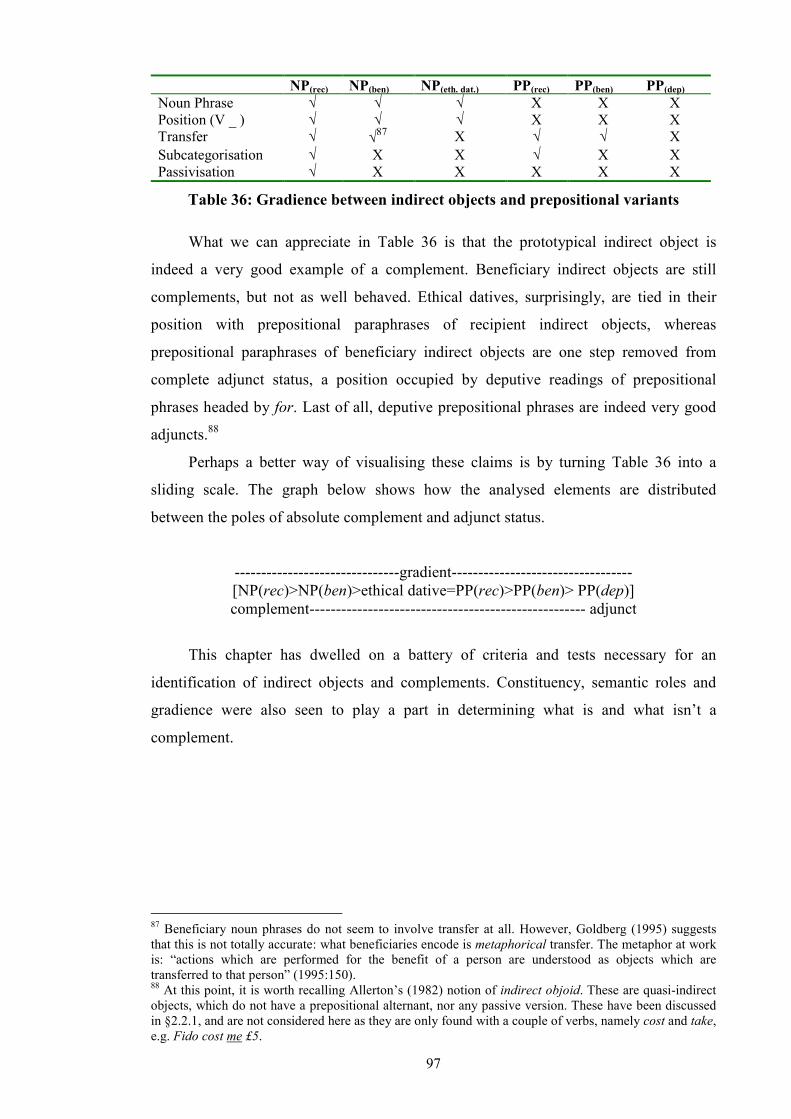
97

NP(rec) NP(ben) NP(eth. dat.) PP(rec) PP(ben) PP(dep)

Noun Phrase √ √ √ X X X Position (V _ ) √ √ √ X X X Transfer √ √87 X √ √ X Subcategorisation √ X X √ X X Passivisation √ X X X X X

Table 36: Gradience between indirect objects and prepositional variants

What we can appreciate in Table 36 is that the prototypical indirect object is

indeed a very good example of a complement. Beneficiary indirect objects are still

complements, but not as well behaved. Ethical datives, surprisingly, are tied in their

position with prepositional paraphrases of recipient indirect objects, whereas

prepositional paraphrases of beneficiary indirect objects are one step removed from

complete adjunct status, a position occupied by deputive readings of prepositional

phrases headed by for. Last of all, deputive prepositional phrases are indeed very good

adjuncts.88

Perhaps a better way of visualising these claims is by turning Table 36 into a

sliding scale. The graph below shows how the analysed elements are distributed

between the poles of absolute complement and adjunct status.

-------------------------------gradient---------------------------------- [NP(rec)>NP(ben)>ethical dative=PP(rec)>PP(ben)> PP(dep)] complement---------------------------------------------------- adjunct

This chapter has dwelled on a battery of criteria and tests necessary for an

identification of indirect objects and complements. Constituency, semantic roles and

gradience were also seen to play a part in determining what is and what isn’t a

complement.

87 Beneficiary noun phrases do not seem to involve transfer at all. However, Goldberg (1995) suggests that this is not totally accurate: what beneficiaries encode is metaphorical transfer. The metaphor at work is: “actions which are performed for the benefit of a person are understood as objects which are transferred to that person” (1995:150). 88 At this point, it is worth recalling Allerton’s (1982) notion of indirect objoid. These are quasi-indirect objects, which do not have a prepositional alternant, nor any passive version. These have been discussed in §2.2.1, and are not considered here as they are only found with a couple of verbs, namely cost and take, e.g. Fido cost me £5.

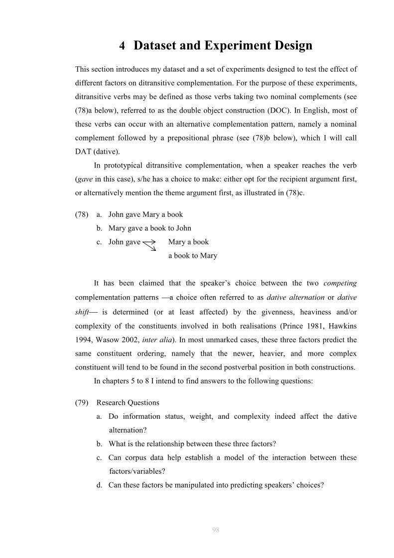
98

4 Dataset and Experiment Design

This section introduces my dataset and a set of experiments designed to test the effect of

different factors on ditransitive complementation. For the purpose of these experiments,

ditransitive verbs may be defined as those verbs taking two nominal complements (see

(78)a below), referred to as the double object construction (DOC). In English, most of

these verbs can occur with an alternative complementation pattern, namely a nominal

complement followed by a prepositional phrase (see (78)b below), which I will call

DAT (dative).

In prototypical ditransitive complementation, when a speaker reaches the verb

(gave in this case), s/he has a choice to make: either opt for the recipient argument first,

or alternatively mention the theme argument first, as illustrated in (78)c.

(78) a. John gave Mary a book

b. Mary gave a book to John

c. John gave Mary a book

a book to Mary

It has been claimed that the speaker’s choice between the two competing

complementation patterns a choice often referred to as dative alternation or dative

shift is determined (or at least affected) by the givenness, heaviness and/or

complexity of the constituents involved in both realisations (Prince 1981, Hawkins

1994, Wasow 2002, inter alia). In most unmarked cases, these three factors predict the

same constituent ordering, namely that the newer, heavier, and more complex

constituent will tend to be found in the second postverbal position in both constructions.

In chapters 5 to 8 I intend to find answers to the following questions:

(79) Research Questions

a. Do information status, weight, and complexity indeed affect the dative

alternation?

b. What is the relationship between these three factors?

c. Can corpus data help establish a model of the interaction between these

factors/variables?

d. Can these factors be manipulated into predicting speakers’ choices?

99

In this chapter, I describe the criteria, assumptions and definitions instrumental in

the building of my dataset (§4.1); I provide a characterisation of the different

complementation patterns and verbs appearing in ditransitive complementation in ICE-

GB (§4.2 and §4.3); I discuss the relevant exclusions (§4.4) and the overall design of

the experiments described in subsequent chapters (§4.5). Finally, the statistical tests

employed throughout are also introduced (§4.6).

4.1 The Dataset

The methodology applied in this study was partly inspired by Herriman (1995). A list of

ditransitive verbs allowing for alternation was compiled from the literature (Jespersen

1927, Quirk et al. 1985, Levin 1993, Herriman 1995, Huddleston and Pullum et al.

2002). A first selection was then made so as to exclude cases (verbs and/or

complementation patterns) which were not relevant to our purposes in this study (see

§4.2 below). A matrix chart was then built based on these verbs.

Only verbs which could and did alternate between the two constructions (i.e. DOC

and DAT) were considered for statistical purposes. These verbs were first investigated

using the British component of the International Corpus of English (ICE-GB), and then

grouped quantitatively according to a series of parameters (defined below).

ICE-GB is a fully parsed corpus of approximately one million words. One of the

first advantages of employing ICE-GB is its size: at slightly over a million words, it

allows for manual, unmediated analysis of the data.89 Both spoken and written language

are represented in ICE-GB, with over 600,000 words recorded in spoken language, and

400,000-odd words in written language. The grammatical structure of every sentence

(or, to be more precise, of every parsing unit) in ICE-GB is represented by a syntactic

tree: ICE-GB contains approximately 84,000 trees. In turn, every node of every tree is

annotated for three different aspects: form, function, and additional features (if

available). For example, in the sentence I am the walrus, I is analysed as a pronoun

(form), which acts as head of a noun phrase (function), and carries the features personal

and singular. In addition, this noun phrase is assigned the function subject.

The dedicated retrieval software, called the ICE Corpus Utility Program

(ICECUP), allows the user to conduct searches in ICE-GB using syntactic features (for

example, ‘retrieve all instances of transitive verbs’), as well as topological searches for

portions of tree structures by means of so-called Fuzzy Tree Fragments, or FTFs (see

89 This advantage is often overlooked. Indeed, “there is no point in having bigger and bigger corpora if you cannot work with the output” (Kennedy 1998:68).

100

Aarts et al. 1998, Nelson et al. 2002). FTFs can be thought of as a grammatical query

system, allowing users to construct templates of structures (or partial structures) which

ICECUP matches against similar structures in the corpus. Nodes can be exactly or

inexactly specified (hence fuzzy), thus enabling searches for specific categories or

structures, regardless of the lexical items instantiating them. In this study, FTFs (as

illustrated in Figure 37 and Figure 39 below) are to be read left to right rather than top

to bottom.

The parsing scheme of ICE-GB is based on Quirk et al. (1985). Since the

experiments reported in this study lean heavily on ICE-GB’s parsing scheme, special

attention was paid to the grammatical definitions built into ICE-GB: statistical results

are considerably more difficult to obtain without accepting most of these definitions. In

the case of prepositional paraphrases of indirect objects (i.e. DAT), however, other

definitions had to be taken on board which override those provided in the parsing

scheme of ICE-GB. Thus the experiments both exploit and deviate from ICE-GB’s

grammar, especially in DAT cases. In other words, what could not be retrieved by

relying on automatic searches based on (ICE-GB’s) fixed grammatical definitions had

to be obtained by working around these definitions and specifying our searches/cases by

means of purpose-built FTFs. This will be made clearer when considering the FTFs

employed in these experiments.

A major problem for retrieval was the fact that prepositional paraphrases of

indirect objects (DATs in our parlance) are not coded in ICE-GB. For example, in I sent

the book to Mary and I sent the book to Finsbury Park, the function of both

prepositional phrases is consistently analysed in ICE-GB as adverbial, despite the fact

that one but not the other allows for an alternative construction. There is no principled

way to automatically distinguish between (and therefore to automatically retrieve) the

two in the corpus (i.e. semantic roles are not part of the annotation of ICE-GB). In other

words, both are automatically retrievable but not distinguishable. To overcome this, an

FTF was necessary so as to find an identifiable formal/syntactic structure which could

be associated with DATs.

The FTF in Figure 37 below consists of an empty node which functions as an

anchor from which three children branch out: a verbal element, followed by an

element functioning as direct object, followed in turn by a prepositional phrase with an

adverbial function. This prepositional phrase has a daughter node, a preposition (with its

attendant prepositional function), and not just any preposition: to and for were specified

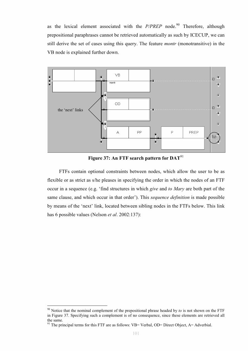
101

as the lexical element associated with the P/PREP node.90 Therefore, although

prepositional paraphrases cannot be retrieved automatically as such by ICECUP, we can

still derive the set of cases using this query. The feature montr (monotransitive) in the

VB node is explained further down.

Figure 37: An FTF search pattern for DAT91

FTFs contain optional constraints between nodes, which allow the user to be as

flexible or as strict as s/he pleases in specifying the order in which the nodes of an FTF

occur in a sequence (e.g. ‘find structures in which give and to Mary are both part of the

same clause, and which occur in that order’). This sequence definition is made possible

by means of the ‘next’ link, located between sibling nodes in the FTFs below. This link

has 6 possible values (Nelson et al. 2002:137):

90 Notice that the nominal complement of the prepositional phrase headed by to is not shown on the FTF in Figure 37. Specifying such a complement is of no consequence, since these elements are retrieved all the same. 91 The principal terms for this FTF are as follows: VB= Verbal, OD= Direct Object, A= Adverbial.

the ‘next’ links

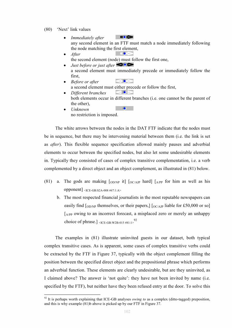
102

(80) ‘Next’ link values

• Immediately after any second element in an FTF must match a node immediately following the node matching the first element,

• After the second element (node) must follow the first one,

• Just before or just after a second element must immediately precede or immediately follow the first,

• Before or after a second element must either precede or follow the first,

• Different branches both elements occur in different branches (i.e. one cannot be the parent of the other),

• Unknown no restriction is imposed.

The white arrows between the nodes in the DAT FTF indicate that the nodes must

be in sequence, but there may be intervening material between them (i.e. the link is set

as after). This flexible sequence specification allowed mainly pauses and adverbial

elements to occur between the specified nodes, but also let some undesirable elements

in. Typically they consisted of cases of complex transitive complementation, i.e. a verb

complemented by a direct object and an object complement, as illustrated in (81) below.

(81) a. The gods are making [OD/NP it] [OC/AJP hard] [A/PP for him as well as his

opponent] <ICE-GB:S2A-008 #67:1:A>

b. The most respected financial journalists in the most reputable newspapers can

easily find [OD/NP themselves, or their papers,] [OC/AJP liable for £50,000 or so]

[A/PP owing to an incorrect forecast, a misplaced zero or merely an unhappy

choice of phrase.] <ICE-GB:W2B-015 #81:1>92

The examples in (81) illustrate uninvited guests in our dataset, both typical

complex transitive cases. As is apparent, some cases of complex transitive verbs could

be extracted by the FTF in Figure 37, typically with the object complement filling the

position between the specified direct object and the prepositional phrase which performs

an adverbial function. These elements are clearly undesirable, but are they uninvited, as

I claimed above? The answer is ‘not quite’: they have not been invited by name (i.e.

specified by the FTF), but neither have they been refused entry at the door. To solve this

92 It is perhaps worth explaining that ICE-GB analyses owing to as a complex (ditto-tagged) preposition, and this is why example (81)b above is picked up by our FTF in Figure 37.

103

problem, we could either (i) tighten up the node sequence in the FTF, thus closing the

gaps between the specified nodes to every kind of material (even pauses), or (ii) specify

the kind of complementation required. At this point, I took advantage of a particular

characteristic in the design of ICE-GB: feature duplication.

There is a certain amount of duplication built into the design of ICE-GB. Along

with a forgiving sequence specification, it allows the user a great degree of flexibility,

which, as long as s/he accepts the ICE-GB grammatical definitions, can be exploited in

different manners. Take, for example, the case of transitivity. A node containing a verb

which is complemented by a direct object is tagged as monotransitive, but this feature

does not occur just in the said verb node: it percolates up to the verb phrase containing

the verb, and to the clause containing the verb phrase.93

More specifically, if one wanted to build an FTF to retrieve transitive cases, one

could simply specify a direct object node. This would retrieve all direct objects in the

corpus, but not necessarily all cases of (purely) monotransitive complementation:94

other complementation patterns including a direct object (e.g. ditransitives, complex

transitives) would also be present in the results. If the purpose of the search is to study

only typical monotransitive complementation, the alternative is to specify the feature

montr in a verb or clause node. This would extract all and only those cases of typical

monotransitive complementation, to the exclusion of complex transitive and ditransitive

complementation.

Given that verbs occurring in prepositional versions of ditransitive

complementation are considered monotransitives by the ICE-GB parsing scheme, the

FTF employed to retrieve them has been restricted to look for monotransitive verbal

elements as can be appreciated in the feature specification montr in the first daughter

node in Figure 37 so as to exclude complex transitive verbs. The DAT FTF in Figure

37 yielded 1,260 hits. A similar FTF was built to look for PPs headed by for, and it

extracted 930 hits.95

When an FTF is applied to the corpus, ICECUP compiles an exhaustive list of

matching cases and visualises this index as a sequence of cases. It identifies each

matching configuration in a tree view by highlighting the matched area in the tree. The

FTF in Figure 37 retrieved examples such as the one below:

93 At this point, it should perhaps be made clear —as Mukherjee (2005:78) points out— that transitivity in ICE-GB is “entirely syntactic in nature,” i.e. it is based on elements required and attested in a given clause. 94 The label monotransitive in ICE-GB is applied to verbs complemented only by a direct object. 95 These figures were obtained with ICECUP 3.0.

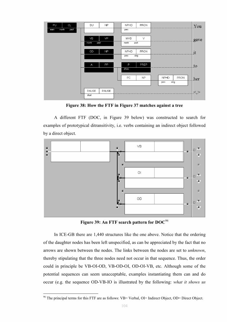
104

Figure 38: How the FTF in Figure 37 matches against a tree

A different FTF (DOC, in Figure 39 below) was constructed to search for

examples of prototypical ditransitivity, i.e. verbs containing an indirect object followed

by a direct object.

Figure 39: An FTF search pattern for DOC96

In ICE-GB there are 1,440 structures like the one above. Notice that the ordering

of the daughter nodes has been left unspecified, as can be appreciated by the fact that no

arrows are shown between the nodes. The links between the nodes are set to unknown,

thereby stipulating that the three nodes need not occur in that sequence. Thus, the order

could in principle be VB-OI-OD, VB-OD-OI, OD-OI-VB, etc. Although some of the

potential sequences can seem unacceptable, examples instantiating them can and do

occur (e.g. the sequence OD-VB-IO is illustrated by the following: what it shows us

96 The principal terms for this FTF are as follows: VB= Verbal, OI= Indirect Object, OD= Direct Object.

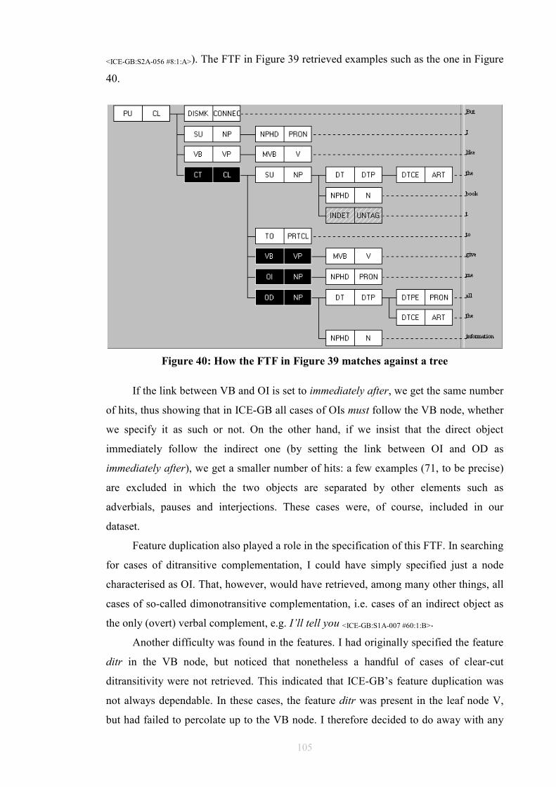
105

<ICE-GB:S2A-056 #8:1:A>). The FTF in Figure 39 retrieved examples such as the one in Figure

40.

Figure 40: How the FTF in Figure 39 matches against a tree

If the link between VB and OI is set to immediately after, we get the same number

of hits, thus showing that in ICE-GB all cases of OIs must follow the VB node, whether

we specify it as such or not. On the other hand, if we insist that the direct object

immediately follow the indirect one (by setting the link between OI and OD as

immediately after), we get a smaller number of hits: a few examples (71, to be precise)

are excluded in which the two objects are separated by other elements such as

adverbials, pauses and interjections. These cases were, of course, included in our

dataset.

Feature duplication also played a role in the specification of this FTF. In searching

for cases of ditransitive complementation, I could have simply specified just a node

characterised as OI. That, however, would have retrieved, among many other things, all

cases of so-called dimonotransitive complementation, i.e. cases of an indirect object as

the only (overt) verbal complement, e.g. I’ll tell you <ICE-GB:S1A-007 #60:1:B>.

Another difficulty was found in the features. I had originally specified the feature

ditr in the VB node, but noticed that nonetheless a handful of cases of clear-cut

ditransitivity were not retrieved. This indicated that ICE-GB’s feature duplication was

not always dependable. In these cases, the feature ditr was present in the leaf node V,

but had failed to percolate up to the VB node. I therefore decided to do away with any

106

feature specification in this FTF, especially in view of the fact that it was clear from the

topology of the FTF itself that I required an indirect object followed by a direct object

in my results. All the same, the extracted cases did include a handful of undesirable

ones (see §4.2).

The results of the queries made with FTFs had to be very carefully revised, in

more than one way, particularly those extracted by Figure 37. All clauses showing

examples of the alternation were entered in a database. Each entry in the database was

individually classified for several variables, such as the informational status of each

complement, number of words, number of nodes, type of determiner used, whether the

occurrence had been registered in written or in spoken language, and many others. The

database itself made it simpler for the constituents to be sorted according to these

variables.

The corpus examples of the verbs in the dataset have been used as a basis for the

statistics discussed in the following chapters. Naturally, as all the experiments are based

on the alternation DOC-DAT, the corpus examples of prepositional phrases which were

considered to be paraphrases of indirect objects (i.e. DAT) were also included in the

investigation.

What follows are the final figures of ditransitive complementation patterns

extracted from ICE-GB and admitted to our dataset. Of a total of 854 cases, of which

587 instantiate the double object construction, while 267 represent the prepositional

alternant with to of for. As will be seen in the following section, the results of this study

do not claim that all the verbs that take indirect objects are exemplified in this study.

Therefore, the statistics provided here do not necessarily represent the total number of

instances of DOC and/or DAT in the corpus.

4.2 Complementation Patterns

Indirect objects and their prepositional paraphrases were investigated in terms of (i)

their word order, (ii) the verbs selecting them, and (iii) the prepositions involved. What

follows is a quick overview of the complementation patterns involving ditransitivity

found in ICE-GB. The identified patterns were later classified according to their

potential for alternation with a different complementation pattern (see §4.3).

107

4.2.1 S V IO DO(NP)

This pattern was investigated searching for indirect objects followed by nominal (as

opposed to clausal) direct objects. A search in ICE-GB yielded 967 cases, but after

exclusions, only 860 of them made it to the dataset.

4.2.2 S V IO DO(CL)

Clausal direct objects are very common in ICE-GB, and ditransitive complementation

was no exception. Specifying a clausal direct object preceded by an indirect object

yielded 462 cases, before exclusions.97

4.2.3 S V DO ‘IO’(PP)

This pattern was rather more complex to search for, given that there is no coding

available in ICE-GB for recipients or beneficiaries. As a consequence, this had to be

done manually, a difficult and time-consuming task (as can be seen in the difference

between cases found and cases eventually incorporated to the dataset). Searching for a

direct object followed by a prepositional phrase headed by to yielded 1,260 cases,

before exclusions. A similar search, but with a prepositional phrase headed by for

following the direct object, gave 930 hits, also before exclusions.

4.3 Verb Classes

Ditransitive verbs were organized into three classes in the dataset, according to certain

variations in their behaviour, i.e. the alternation between their indirect objects and

different prepositions heading the prepositional alternant. The prototypical indirect

object occurs in the SVOO complementation pattern, which is typically realized as

NP+NP. It alternates with a PP headed by to or for. In this study, I focused on verbs

allowing the alternation between double object complements (DOC) and prepositional

phrases (DAT) headed by to (§4.3.1), for (§4.3.3), or headed either by to or for (§4.3.3).

The examples below instantiate the three complementation patterns of verbs found in

the dataset.

97 There were also a handful of cases (11, to be precise) of ditransitive complementation involving coordination of one of the objects which were extracted from the corpus and included in the dataset (but not listed in this section).

108

(82) a. …you write of giving you encouragement and support and not telling you

what a wally you are. <ICE-GB:W1B-003 #167:2> → DOC to

b. Since the Theatre is a Department of University College we only offer this

casual work to students. <ICE-GB:W1B-021 #126:10> → DAT to

c. Yeah we used to buy Mum a vase every year for her birthday <ICE-GB:S1A-019

#106:1:E> → DOC to/for

d. And I brought these books for Sarah … <ICE-GB:S1A-013 #246:1:B> → DAT for

e. They brought me a bottle of Croft’s Original <ICE-GB:S1A-057 #25:1:B> → DAT to

As regards the alternation with a prepositional paraphrase, there are a number of

verbs which only occur in DOC (e.g. afford, grant, quote) while many more occur only

in DAT (e.g. forward, post).

Lend and pay occur with similar frequency in both constructions. In contrast, give,

offer, show and tell (those that contribute the larger numbers towards the final count)

occur much more frequently in the double object construction. Those occurring more

frequently with prepositional paraphrases than with indirect objects are do1 (impart),

hand and sell.

Other types of verbs were also found in the corpus but excluded, given that they

did not allow for variants (see §4.3.2, §4.3.5, §4.3.6). Finally, it is perhaps obvious, but

worth pointing out, that a verb can and does convey different meanings in the corpus,

e.g. leave is used as a synonym for bequeath and for leave behind. These meanings have

an effect on the verb’s complementation pattern: both meanings of leave can occur in

ditransitive complementation, but only the first leave (which we will code as leave1) can

alternate with a prepositional paraphrase headed by to (as in example (83)a), while the

other (leave2) alternates only with a prepositional paraphrase headed by for (as in

example (83)b). To make matters more interesting, in some cases (example (83)c) leave

could potentially take either preposition. The semantic coding of verbs is not present in

the tagging of ICE-GB and had to be carried out manually.

(83) a. Uhm now at this point I’m going to leave some more work to you <ICE-GB:S1B-

014 #1:1:A>

b. Leaves it [i.e. the ball] for Geoff Thomas who plays it square to Derigo on the

far left <ICE-GB:S2A-001 #127:1:A>

c. The awful thing was that we just left it in the end to Gillian Bernard’s sister

and my Mum and they worked like blacks <ICE-GB:S1A-056 #307:4:A>

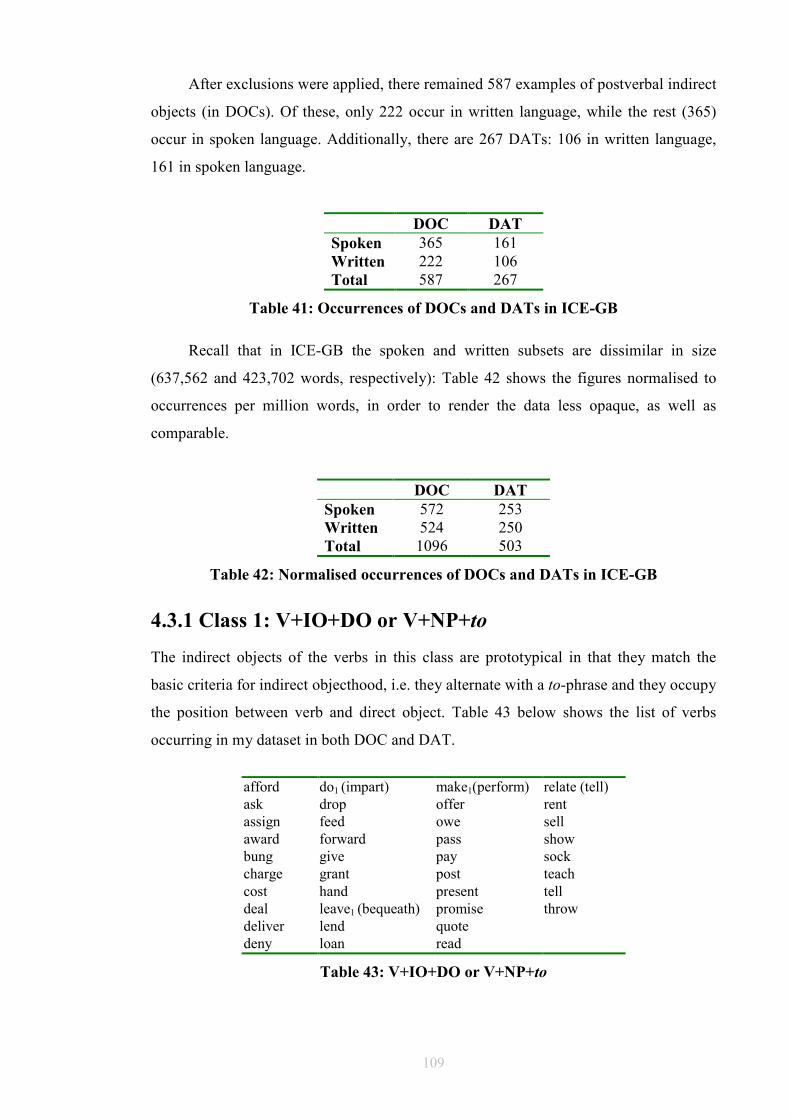
109

After exclusions were applied, there remained 587 examples of postverbal indirect

objects (in DOCs). Of these, only 222 occur in written language, while the rest (365)

occur in spoken language. Additionally, there are 267 DATs: 106 in written language,

161 in spoken language.

DOC DAT

Spoken 365 161 Written 222 106 Total 587 267

Table 41: Occurrences of DOCs and DATs in ICE-GB

Recall that in ICE-GB the spoken and written subsets are dissimilar in size

(637,562 and 423,702 words, respectively): Table 42 shows the figures normalised to

occurrences per million words, in order to render the data less opaque, as well as

comparable.

DOC DAT

Spoken 572 253 Written 524 250 Total 1096 503

Table 42: Normalised occurrences of DOCs and DATs in ICE-GB

4.3.1 Class 1: V+IO+DO or V+NP+to

The indirect objects of the verbs in this class are prototypical in that they match the

basic criteria for indirect objecthood, i.e. they alternate with a to-phrase and they occupy

the position between verb and direct object. Table 43 below shows the list of verbs

occurring in my dataset in both DOC and DAT.

afford do1 (impart) make1(perform) relate (tell) ask drop offer rent assign feed owe sell award forward pass show bung give pay sock charge grant post teach cost hand present tell deal leave1 (bequeath) promise throw deliver lend quote deny loan read

Table 43: V+IO+DO or V+NP+to

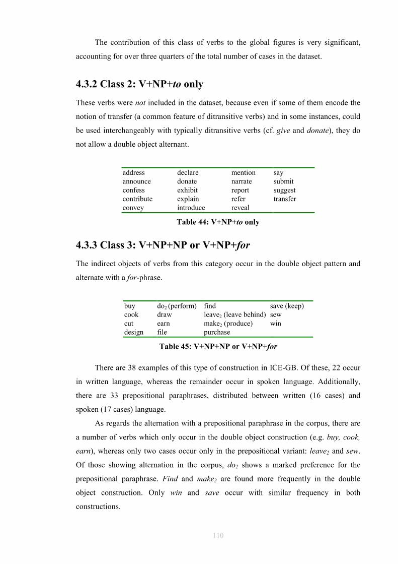
110

The contribution of this class of verbs to the global figures is very significant,

accounting for over three quarters of the total number of cases in the dataset.

4.3.2 Class 2: V+NP+to only

These verbs were not included in the dataset, because even if some of them encode the

notion of transfer (a common feature of ditransitive verbs) and in some instances, could

be used interchangeably with typically ditransitive verbs (cf. give and donate), they do

not allow a double object alternant.

address declare mention say announce donate narrate submit confess exhibit report suggest contribute explain refer transfer convey introduce reveal

Table 44: V+NP+to only

4.3.3 Class 3: V+NP+NP or V+NP+for

The indirect objects of verbs from this category occur in the double object pattern and

alternate with a for-phrase.

buy do2 (perform) find save (keep) cook draw leave2 (leave behind) sew cut earn make2 (produce) win design file purchase

Table 45: V+NP+NP or V+NP+for

There are 38 examples of this type of construction in ICE-GB. Of these, 22 occur

in written language, whereas the remainder occur in spoken language. Additionally,

there are 33 prepositional paraphrases, distributed between written (16 cases) and

spoken (17 cases) language.

As regards the alternation with a prepositional paraphrase in the corpus, there are

a number of verbs which only occur in the double object construction (e.g. buy, cook,

earn), whereas only two cases occur only in the prepositional variant: leave2 and sew.

Of those showing alternation in the corpus, do2 shows a marked preference for the

prepositional paraphrase. Find and make2 are found more frequently in the double

object construction. Only win and save occur with similar frequency in both

constructions.

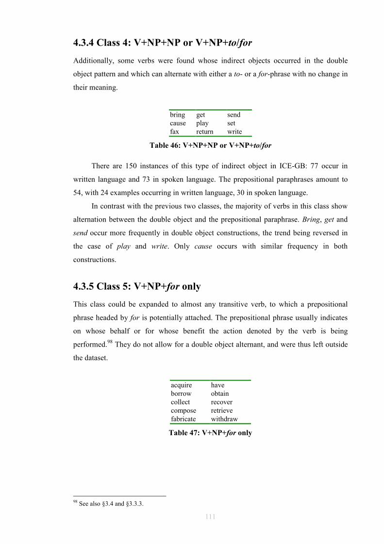
111

4.3.4 Class 4: V+NP+NP or V+NP+to/for

Additionally, some verbs were found whose indirect objects occurred in the double

object pattern and which can alternate with either a to- or a for-phrase with no change in

their meaning.

bring get send cause play set fax return write

Table 46: V+NP+NP or V+NP+to/for

There are 150 instances of this type of indirect object in ICE-GB: 77 occur in

written language and 73 in spoken language. The prepositional paraphrases amount to

54, with 24 examples occurring in written language, 30 in spoken language.

In contrast with the previous two classes, the majority of verbs in this class show

alternation between the double object and the prepositional paraphrase. Bring, get and

send occur more frequently in double object constructions, the trend being reversed in

the case of play and write. Only cause occurs with similar frequency in both

constructions.

4.3.5 Class 5: V+NP+for only

This class could be expanded to almost any transitive verb, to which a prepositional

phrase headed by for is potentially attached. The prepositional phrase usually indicates

on whose behalf or for whose benefit the action denoted by the verb is being

performed.98 They do not allow for a double object alternant, and were thus left outside

the dataset.

acquire have borrow obtain collect recover compose retrieve fabricate withdraw

Table 47: V+NP+for only

98 See also §3.4 and §3.3.3.

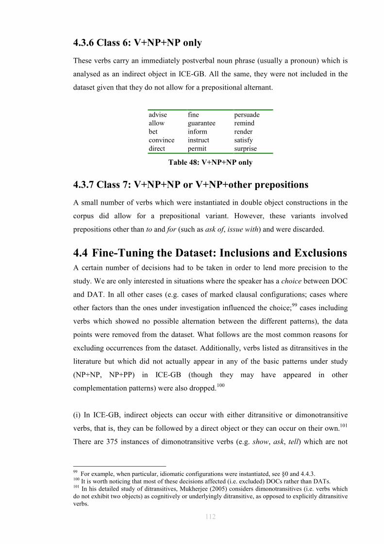
112

4.3.6 Class 6: V+NP+NP only

These verbs carry an immediately postverbal noun phrase (usually a pronoun) which is

analysed as an indirect object in ICE-GB. All the same, they were not included in the

dataset given that they do not allow for a prepositional alternant.

advise fine persuade allow guarantee remind bet inform render convince instruct satisfy direct permit surprise

Table 48: V+NP+NP only

4.3.7 Class 7: V+NP+NP or V+NP+other prepositions

A small number of verbs which were instantiated in double object constructions in the

corpus did allow for a prepositional variant. However, these variants involved

prepositions other than to and for (such as ask of, issue with) and were discarded.

4.4 Fine-Tuning the Dataset: Inclusions and Exclusions

A certain number of decisions had to be taken in order to lend more precision to the

study. We are only interested in situations where the speaker has a choice between DOC

and DAT. In all other cases (e.g. cases of marked clausal configurations; cases where

other factors than the ones under investigation influenced the choice;99 cases including

verbs which showed no possible alternation between the different patterns), the data

points were removed from the dataset. What follows are the most common reasons for

excluding occurrences from the dataset. Additionally, verbs listed as ditransitives in the

literature but which did not actually appear in any of the basic patterns under study

(NP+NP, NP+PP) in ICE-GB (though they may have appeared in other

complementation patterns) were also dropped.100

(i) In ICE-GB, indirect objects can occur with either ditransitive or dimonotransitive

verbs, that is, they can be followed by a direct object or they can occur on their own.101

There are 375 instances of dimonotransitive verbs (e.g. show, ask, tell) which are not

99 For example, when particular, idiomatic configurations were instantiated, see §0 and 4.4.3. 100 It is worth noticing that most of these decisions affected (i.e. excluded) DOCs rather than DATs. 101 In his detailed study of ditransitives, Mukherjee (2005) considers dimonotransitives (i.e. verbs which do not exhibit two objects) as cognitively or underlyingly ditransitive, as opposed to explicitly ditransitive verbs.

113

selected by DOC FTF. All dimonotransitive cases were excluded from the dataset, since

no alternation is possible.

(84) But maybe Helen can tell us <ICE-GB:S1A-055 #148:1:A>

(ii) Direct objects can be realised as noun phrases or as clauses. Verbs which require

their direct objects to be realised as a clause (e.g. convince, advise, etc.) were not taken

into account, since they do not allow alternation.102

(85) a. Dimitri has also strongly advised the British pair that weather conditions are

not right <ICE-GB:S2B-024 #62:1:A>

b. *Dimitri has also strongly advised that weather conditions are not right to the

British pair

(iii) Most variants of ditransitive complementation which involved an indirect object

followed by a clause (where, by contrast with (ii) above, the second complement was

not required to be a clause) were also excluded. These were among the most numerous,

and mainly involved the verb tell.103 In most cases, these sentences do not have a

prepositional alternative (but see chapter 7).

(86) a. For example does forty-nine show us what was happening there <ICE-GB:S1B-069

#57:1:A>

b. I’m telling you that we don’t want to be bothered to go further than Ealing

Broadway on Saturday <ICE-GB:S1A-030 #211:1:A>

(iv) Thematic variants of a clause. The typical cases of marked order clauses, such as

clefts, pseudo-clefts, fronted direct objects, extracted indirect objects (as in relative

clauses and questions), and so on were explicitly excluded from consideration by the

mere fact of the selection of nodes in the FTFs employed. For instance, example (87)a

below an interrogative passive transform of X told you that was impossible to

retrieve by means of the DOC FTF in Figure 39, given that this FTF searches (among

other things) for an indirect object, and there is no indirect object in were you told that.

Marked variants of ditransitive complementation are discussed in more detail in

§4.4.1.3 and §4.4.1.4 below.

102 In fact, only advise (6 cases) and convince (17 cases) occurred in DOC in ICE-GB exclusively with a clausal direct object. 103 Exclusions due to this particular reason amounted to 455 cases, out of which tell accounts for 292.

114

However, some marked sentences did manage to slip through the first selection

procedure, for example sentence (87)b below, which has all three nodes (i.e. a verb

phrase, a direct object, and an indirect object) required for retrieval. These and other

cases had to be manually removed, on the assumption that speakers had less room for

choice between DOC and DAT. Put differently, marked sentences were assumed a

priori to skew the choice, in that they represent a departure from a default order. In

marked clauses, the introduction of foreign (pragmatic or stylistic) factors was thus

considered to be instrumental in obscuring or affecting the constructional alternation.

(87) a. were you told that <ICE-GB:S1A-053 #151:1:C>

b. Yeah was it you that [told] me that <ICE-GB:S1A-099 #271:2:A>

(v) Idiomatic phrases presented a different problem. Levin and Rappaport-Hovav (2002)

classified idioms into two types, those that allow the possibility of alternation (“if

appropriate heaviness and discourse conditions are met”, they warn), and those that do

not.104 Some idioms were then excluded from the purpose of this study (see §0).

Example (88)a below illustrates an alternating idiom (included in the dataset), whereas

example (88)b is an idiom with no possible prepositional variant (and thus excluded

from the dataset). 79 cases of alternating idioms were included in our dataset (see Table

56).

(88) a. I still think that you find that most people who go into politics do so from a

mixture of reasons but one of those reasons is actually to do good for for

other people <ICE-GB:S1B-024 #96:1:F>

b. He didn’t give it a chance though <ICE-GB:S1A-006 #88:1:A>

(vi) ‘Affected’ indirect objects occur with semantically light (uses of) verbs (e.g. give,

do, have, make, take) and an eventive direct object (see Quirk et al. 1985:750-751).

These structures were mostly excluded, inasmuch as a prepositional paraphrase is not

normally possible. All the same, some cases of light verbs do allow a prepositional

paraphrase (see §4.4.3), as corpus examples and internet searches confirm, and were

thus duly included. Example (89)a below illustrates a non-alternating pattern, whereas

example (89)b is an instance of an alternating one.

104 See also Rappaport-Hovav and Levin (2008) for a similar, if not as focused, treatment of idioms and light verbs.

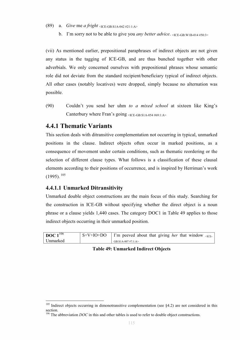
115

(89) a. Give me a fright <ICE-GB:S1A-042 #21:1:A>

b. I’m sorry not to be able to give you any better advice. <ICE-GB:W1B-014 #50:3>

(vii) As mentioned earlier, prepositional paraphrases of indirect objects are not given

any status in the tagging of ICE-GB, and are thus bunched together with other

adverbials. We only concerned ourselves with prepositional phrases whose semantic

role did not deviate from the standard recipient/beneficiary typical of indirect objects.

All other cases (notably locatives) were dropped, simply because no alternation was

possible.

(90) Couldn’t you send her uhm to a mixed school at sixteen like King’s

Canterbury where Fran’s going <ICE-GB:S1A-054 #69:1:A>

4.4.1 Thematic Variants

This section deals with ditransitive complementation not occurring in typical, unmarked

positions in the clause. Indirect objects often occur in marked positions, as a

consequence of movement under certain conditions, such as thematic reordering or the

selection of different clause types. What follows is a classification of these clausal

elements according to their positions of occurrence, and is inspired by Herriman’s work

(1995). 105

4.4.1.1 Unmarked Ditransitivity

Unmarked double object constructions are the main focus of this study. Searching for

the construction in ICE-GB without specifying whether the direct object is a noun

phrase or a clause yields 1,440 cases. The category DOC1 in Table 49 applies to those

indirect objects occurring in their unmarked position.

DOC 1

106

Unmarked S+V+IO+DO I’m peeved about that giving her that window <ICE-

GB:S1A-007 #7:1:A>

Table 49: Unmarked Indirect Objects

105 Indirect objects occurring in dimonotransitive complementation (see §4.2) are not considered in this section. 106 The abbreviation DOC in this and other tables is used to refer to double object constructions.

116

4.4.1.2 Unmarked Prepositional Alternant

Unmarked alternants in ICE-GB were no simpler to retrieve than their marked

counterparts. After exclusions, there remained 267 cases of unmarked prepositional

alternants admissible to the dataset. The category DAT1 in Table 50 applies to

prepositional paraphrases of indirect objects occurring in their unmarked position.

DAT 1

107

Unmarked S+V+ DO+PP Even giving Coppermalt to Charles has not erased

anything. <ICE-GB:W2F-018 #45:1>

Table 50: Unmarked Prepositional Paraphrases

4.4.1.3 Marked Ditransitivity

Cases of double object constructions which involved some departure from the canonical

order S+V+IO+DO were considered marked, and excluded from the dataset. Among

them, we found passivisation, relativisation, questioning, extraction, and other cases

which highlighted one position in the clause at the expense of others. Besides their

unmarked (immediately postverbal) position, Herriman distinguishes three other

available positions for indirect objects in the clause:

• DOC2: The indirect object follows the verb but does not precede the direct

object.

• DOC3: The indirect object follows both the verb and the direct object.

• DOC4: The indirect object has been moved to initial position in the clause.

This latter category (DOC4) is not to be confused with indirect passive clauses

(i.e. clauses where the recipient argument is encoded as the subject of a passive

sentence, see (91)). The distinction between DOC4 cases and indirect passive clauses

lies in the disengagement between the argument and the function: whereas in DOC4

cases, the recipient argument encoded as indirect object has been fronted but remains an

object, in indirect passive clauses the recipient argument is no longer the object and has

become the subject of the passive clause.

Indirect object clauses were well represented in the corpus, with 258 cases.

107 The abbreviation DAT in this and other tables is used to refer to prepositional paraphrases of indirect objects.

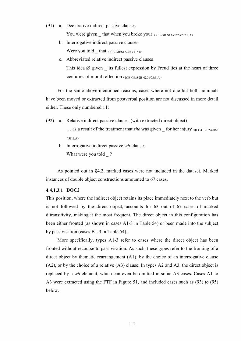
117

(91) a. Declarative indirect passive clauses

You were given _ that when you broke your <ICE-GB:S1A-022 #202:1:A>

b. Interrogative indirect passive clauses

Were you told _ that <ICE-GB:S1A-053 #151>

c. Abbreviated relative indirect passive clauses

This idea ∅ given _ its fullest expression by Freud lies at the heart of three

centuries of moral reflection <ICE-GB:S2B-029 #73:1:A>

For the same above-mentioned reasons, cases where not one but both nominals

have been moved or extracted from postverbal position are not discussed in more detail

either. These only numbered 11:

(92) a. Relative indirect passive clauses (with extracted direct object)

… as a result of the treatment that she was given _ for her injury <ICE-GB:S2A-062

#38:1:A>

b. Interrogative indirect passive wh-clauses

What were you told _ ?

As pointed out in §4.2, marked cases were not included in the dataset. Marked

instances of double object constructions amounted to 67 cases.

4.4.1.3.1 DOC2

This position, where the indirect object retains its place immediately next to the verb but

is not followed by the direct object, accounts for 63 out of 67 cases of marked

ditransitivity, making it the most frequent. The direct object in this configuration has

been either fronted (as shown in cases A1-3 in Table 54) or been made into the subject

by passivisation (cases B1-3 in Table 54).

More specifically, types A1-3 refer to cases where the direct object has been

fronted without recourse to passivisation. As such, these types refer to the fronting of a

direct object by thematic rearrangement (A1), by the choice of an interrogative clause

(A2), or by the choice of a relative (A3) clause. In types A2 and A3, the direct object is

replaced by a wh-element, which can even be omitted in some A3 cases. Cases A1 to

A3 were extracted using the FTF in Figure 51, and included cases such as (93) to (95)

below.

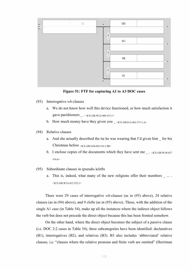
118

Figure 51: FTF for capturing A1 to A3 DOC cases

(93) Interrogative wh-clauses

a. We do not know how well this device functioned, or how much satisfaction it

gave parishioners _ . <ICE-GB:W2A-006 #31:1>

b. How much money have they given you _ <ICE-GB:S1A-062 #73:1:A>

(94) Relative clauses

a. And she actually described the tie he was wearing that I’d given him _ for his

Christmas before <ICE-GB:S1B-026 #16:1:B0>

b. I enclose copies of the documents which they have sent me _ . <ICE-GB:W1B-027

#76:6>

(95) Subordinate clauses in (pseudo-)clefts

a. This is, indeed, what many of the new religions offer their members _ ... .

<ICE-GB:W2A-012 #32:1>

There were 29 cases of interrogative wh-clauses (as in (93) above), 24 relative

clauses (as in (94) above), and 9 clefts (as in (95) above). These, with the addition of the

single A1 case (in Table 54), make up all the instances where the indirect object follows

the verb but does not precede the direct object because this has been fronted somehow.

On the other hand, where the direct object becomes the subject of a passive clause

(i.e. DOC 2:2 cases in Table 54), three subcategories have been identified: declaratives

(B1), interrogatives (B2), and relatives (B3). B3 also includes ‘abbreviated’ relative

clauses, i.e. “clauses where the relative pronoun and finite verb are omitted” (Herriman

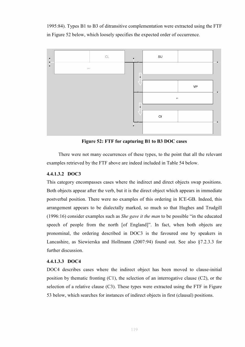
119

1995:84). Types B1 to B3 of ditransitive complementation were extracted using the FTF

in Figure 52 below, which loosely specifies the expected order of occurrence.

Figure 52: FTF for capturing B1 to B3 DOC cases

There were not many occurrences of these types, to the point that all the relevant

examples retrieved by the FTF above are indeed included in Table 54 below.

4.4.1.3.2 DOC3

This category encompasses cases where the indirect and direct objects swap positions.

Both objects appear after the verb, but it is the direct object which appears in immediate

postverbal position. There were no examples of this ordering in ICE-GB. Indeed, this

arrangement appears to be dialectally marked, so much so that Hughes and Trudgill

(1996:16) consider examples such as She gave it the man to be possible “in the educated

speech of people from the north [of England]”. In fact, when both objects are

pronominal, the ordering described in DOC3 is the favoured one by speakers in

Lancashire, as Siewierska and Hollmann (2007:94) found out. See also §7.2.3.3 for

further discussion.

4.4.1.3.3 DOC4

DOC4 describes cases where the indirect object has been moved to clause-initial

position by thematic fronting (C1), the selection of an interrogative clause (C2), or the

selection of a relative clause (C3). These types were extracted using the FTF in Figure

53 below, which searches for instances of indirect objects in first (clausal) positions.

120

Figure 53: FTF for capturing C1 to C3 DOC cases

However, not many cases were (able to be) retrieved. It seems that this position is

not very comfortable for indirect objects, and indeed Herriman points out (1995:89) that

indirect objects in this position are of doubtful acceptability for many speakers. She

remarks:

Many grammarians (Fillmore 1965:12, Kruisinga and Erades 1953:80, among others) exclude this position altogether, while others (Quirk et al. 1985:728, Jespersen 1927:138 and Nida 1960:195, among others) note that it is highly unusual. Indirect objects in initial position are examples of language fuzziness (Aitchison 1991:36), i.e. they are borderline cases which most people judge as possible but not fully acceptable.

Table 54 below lists, classifies, and exemplifies the different types of marked

ditransitivity found in ICE-GB.

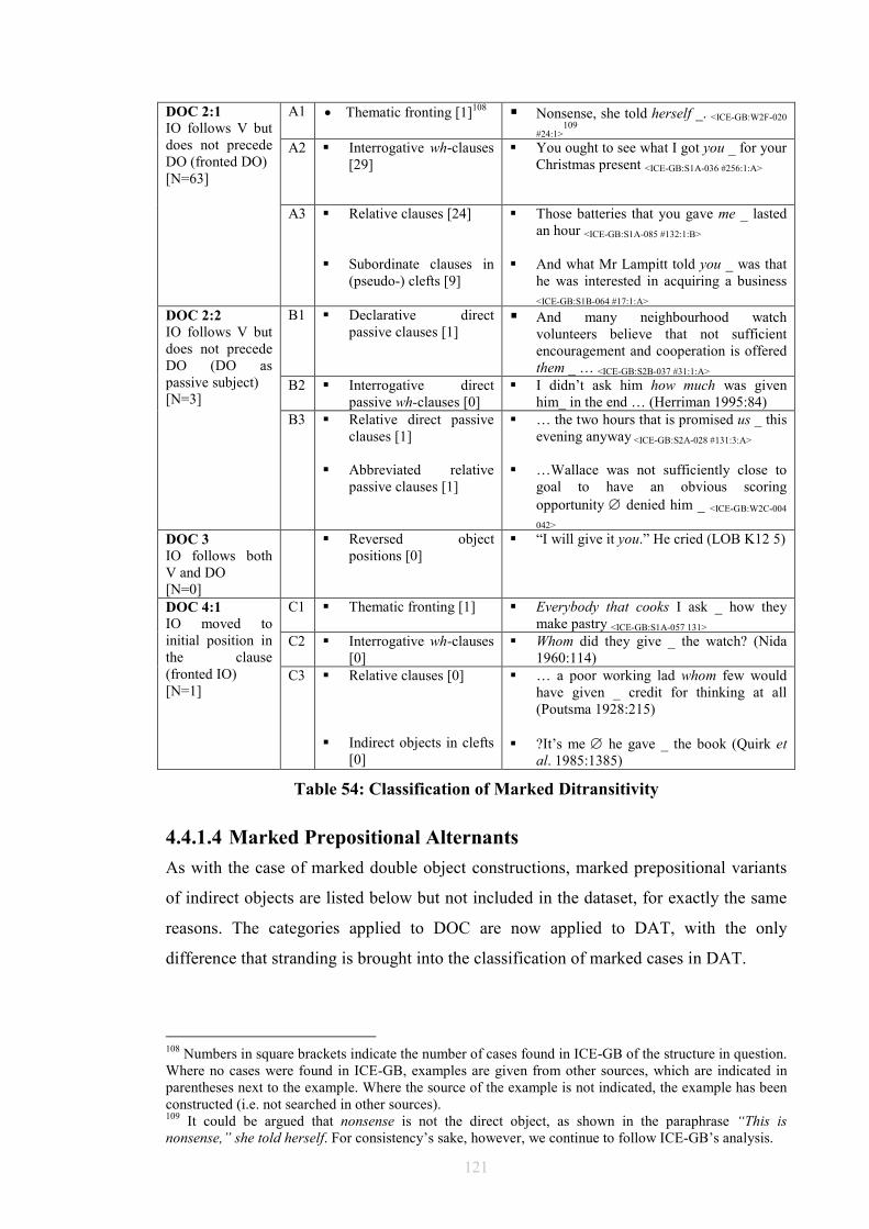
121

A1

• Thematic fronting [1]108 � Nonsense, she told herself _. <ICE-GB:W2F-020

#24:1>109

A2 � Interrogative wh-clauses [29]

� You ought to see what I got you _ for your Christmas present <ICE-GB:S1A-036 #256:1:A>

DOC 2:1

IO follows V but does not precede DO (fronted DO) [N=63]

A3 � Relative clauses [24] � Subordinate clauses in

(pseudo-) clefts [9]

� Those batteries that you gave me _ lasted an hour <ICE-GB:S1A-085 #132:1:B>

� And what Mr Lampitt told you _ was that

he was interested in acquiring a business <ICE-GB:S1B-064 #17:1:A>

B1 � Declarative direct passive clauses [1]

� And many neighbourhood watch volunteers believe that not sufficient encouragement and cooperation is offered them _ … <ICE-GB:S2B-037 #31:1:A>

B2 � Interrogative direct passive wh-clauses [0]

� I didn’t ask him how much was given him_ in the end … (Herriman 1995:84)

DOC 2:2

IO follows V but does not precede DO (DO as passive subject) [N=3]

B3 � Relative direct passive clauses [1]

� Abbreviated relative

passive clauses [1]

� … the two hours that is promised us _ this evening anyway <ICE-GB:S2A-028 #131:3:A>

� …Wallace was not sufficiently close to

goal to have an obvious scoring opportunity ∅ denied him _ <ICE-GB:W2C-004

042> DOC 3

IO follows both V and DO [N=0]

� Reversed object positions [0]

� “I will give it you.” He cried (LOB K12 5)

C1 � Thematic fronting [1] � Everybody that cooks I ask _ how they make pastry <ICE-GB:S1A-057 131>

C2 � Interrogative wh-clauses [0]

� Whom did they give _ the watch? (Nida 1960:114)

DOC 4:1

IO moved to initial position in the clause (fronted IO) [N=1]

C3 � Relative clauses [0] � Indirect objects in clefts

[0]

� … a poor working lad whom few would have given _ credit for thinking at all (Poutsma 1928:215)

� ?It’s me ∅ he gave _ the book (Quirk et

al. 1985:1385)

Table 54: Classification of Marked Ditransitivity

4.4.1.4 Marked Prepositional Alternants

As with the case of marked double object constructions, marked prepositional variants

of indirect objects are listed below but not included in the dataset, for exactly the same

reasons. The categories applied to DOC are now applied to DAT, with the only

difference that stranding is brought into the classification of marked cases in DAT.

108 Numbers in square brackets indicate the number of cases found in ICE-GB of the structure in question. Where no cases were found in ICE-GB, examples are given from other sources, which are indicated in parentheses next to the example. Where the source of the example is not indicated, the example has been constructed (i.e. not searched in other sources). 109 It could be argued that nonsense is not the direct object, as shown in the paraphrase “This is nonsense,” she told herself. For consistency’s sake, however, we continue to follow ICE-GB’s analysis.

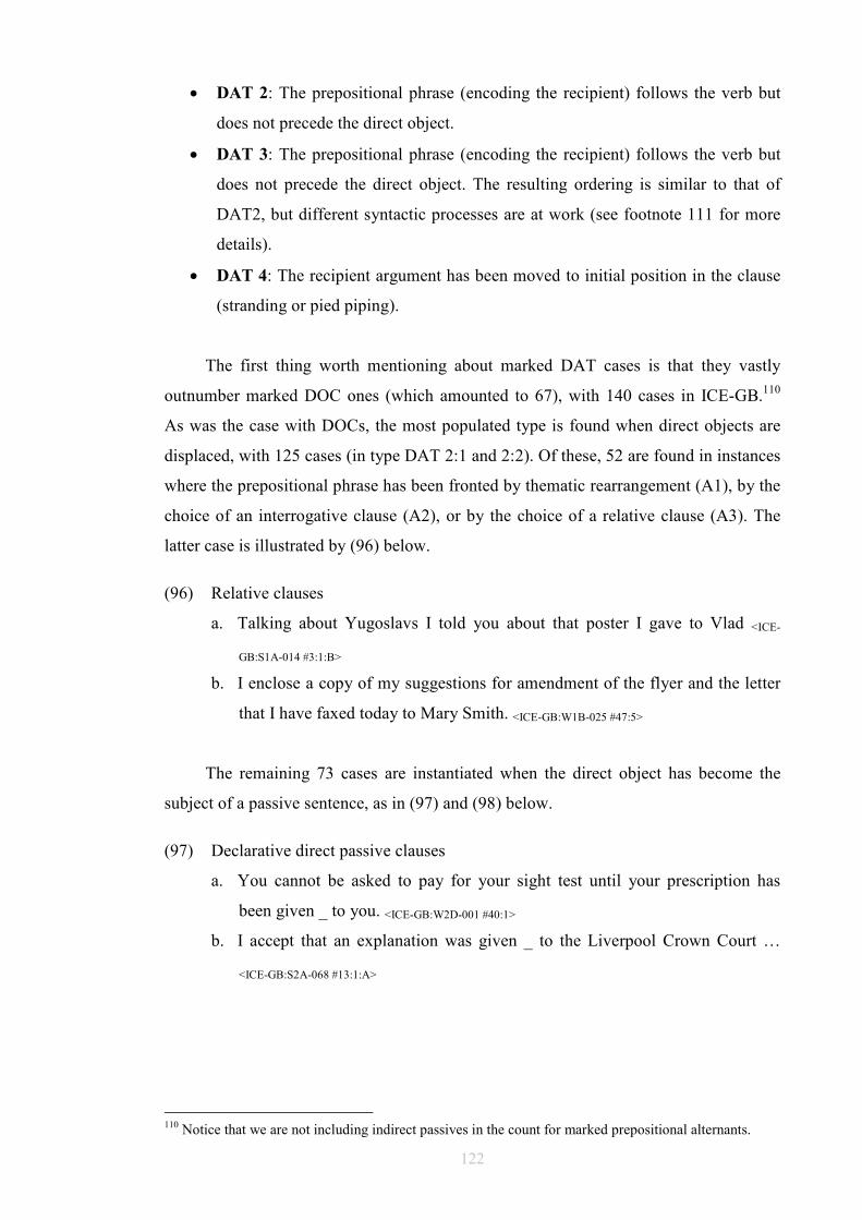
122

• DAT 2: The prepositional phrase (encoding the recipient) follows the verb but

does not precede the direct object.

• DAT 3: The prepositional phrase (encoding the recipient) follows the verb but

does not precede the direct object. The resulting ordering is similar to that of

DAT2, but different syntactic processes are at work (see footnote 111 for more

details).

• DAT 4: The recipient argument has been moved to initial position in the clause

(stranding or pied piping).

The first thing worth mentioning about marked DAT cases is that they vastly

outnumber marked DOC ones (which amounted to 67), with 140 cases in ICE-GB.110

As was the case with DOCs, the most populated type is found when direct objects are

displaced, with 125 cases (in type DAT 2:1 and 2:2). Of these, 52 are found in instances

where the prepositional phrase has been fronted by thematic rearrangement (A1), by the

choice of an interrogative clause (A2), or by the choice of a relative clause (A3). The

latter case is illustrated by (96) below.

(96) Relative clauses

a. Talking about Yugoslavs I told you about that poster I gave to Vlad <ICE-

GB:S1A-014 #3:1:B>

b. I enclose a copy of my suggestions for amendment of the flyer and the letter

that I have faxed today to Mary Smith. <ICE-GB:W1B-025 #47:5>

The remaining 73 cases are instantiated when the direct object has become the

subject of a passive sentence, as in (97) and (98) below.

(97) Declarative direct passive clauses

a. You cannot be asked to pay for your sight test until your prescription has

been given _ to you. <ICE-GB:W2D-001 #40:1>

b. I accept that an explanation was given _ to the Liverpool Crown Court …

<ICE-GB:S2A-068 #13:1:A>

110 Notice that we are not including indirect passives in the count for marked prepositional alternants.

123

(98) Relative direct passive clauses

a. And there will then be the command given to the guards … <ICE-GB:S2A-011

#41:1:A>

b. ... we can offer you a speaker’s fee of <unclear-word> which will be paid to

you within the month following the course. <ICE-GB:W1B-030 #89:5>

Another curiosity is found in type DAT 4, which describes cases when the

recipient argument moves to initial position. These cases allow for the possibility of the

argument taking the preposition with it (pied piping) or leaving it behind (stranding).

Whether this movement was caused by thematic fronting (C1), interrogative (C2) or

relative clause formation (C3), or clefting (C3), the results from the corpus seem to

suggest that whenever possible, stranding is favoured over pied piping. In C1 types, the

only found case is of stranding (see (99)); C2 cases show two stranding cases as

opposed to a single ‘unstranded’ one (see (100)); relative clauses are equally divided

between stranded and ‘unstranded’ alternatives (see (101)); whereas the only case of C3

clefting also shows stranding (see (102)).

(99) Thematic fronting

a. but beyond that any idea that the security services were deliberately seeking

to bring down the Prime Minister uh I give absolutely no credence to _ <ICE-

GB:S1B-040 #88:1:B> [with stranding]

(100) Interrogative wh-clauses

a. Now as for actually how or to whom you send the messages _ there’s a

standard convention … <ICE-GB:S2A-028 #96:2:A>

b. ... and forget that you who you’ve lent them to _ <ICE-GB:S1A-013 #86:1:E> [with

stranding]

(101) Relative clauses

a. He was a recent example of the long line of literate golden-style civil servants

to whom the English nation and its language owe so much <ICE-GB:S2B-25 #98:1>

b. I mean obviously there are some books that you can’t do that to but but I

would do that quite happily to a book <ICE-GB:S1A-013 #139:1:B> [with stranding]

124

(102) PPs in cleft

a. that’s Catholic Action for Native North Americans he does a lot of work for _

<ICE-GB:S1A-096 #106-107:1:A> [with stranding]

Due to space constraints, the remaining types of marked prepositional alternants

will not be discussed. Regardless, Table 55 classifies and offers examples of all marked

cases of DAT in ICE-GB.

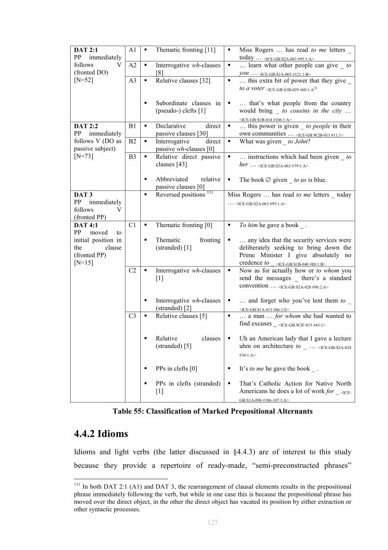
125

A1 � Thematic fronting [11] � Miss Rogers … has read to me letters _

today … <ICE-GB:S2A-063 #95:1:A> A2 � Interrogative wh-clauses

[8] � … learn what other people can give _ to

you … <ICE-GB:S1A-003 #121:1:B>

DAT 2:1

PP immediately follows V (fronted DO) [N=52] A3 � Relative clauses [32]

� Subordinate clauses in

(pseudo-) clefts [1]

� … this extra bit of power that they give _ to a voter <ICE-GB:S1B-029 #60:1:A>

� … that’s what people from the country

would bring _ to cousins in the city … <ICE-GB:S1B-014 #106:1:A>

B1 � Declarative direct passive clauses [30]

� … this power is given _ to people in their own communities … <ICE-GB:W2B-013 #11:1>

B2 � Interrogative direct passive wh-clauses [0]

� What was given _ to John?

DAT 2:2

PP immediately follows V (DO as passive subject) [N=73] B3 � Relative direct passive

clauses [43] � Abbreviated relative

passive clauses [0]

� … instructions which had been given _ to her … <ICE-GB:S2A-063 #79:1:A>

� The book ∅ given _ to us is blue.

DAT 3

PP immediately follows V (fronted PP)

� Reversed positions 111

Miss Rogers … has read to me letters _ today … <ICE-GB:S2A-063 #95:1:A>

C1 � Thematic fronting [0] � Thematic fronting

(stranded) [1]

� To him he gave a book _ . � … any idea that the security services were

deliberately seeking to bring down the Prime Minister I give absolutely no credence to _ <ICE-GB:S1B-040 #88:1:B>

C2 � Interrogative wh-clauses [1]

� Interrogative wh-clauses

(stranded) [2]

� Now as for actually how or to whom you send the messages _ there’s a standard convention … <ICE-GB:S2A-028 #96:2:A>

� … and forget who you’ve lent them to _

<ICE-GB:S1A-013 #86:1:E>

DAT 4:1

PP moved to initial position in the clause (fronted PP) [N=15]

C3 � Relative clauses [5] � Relative clauses

(stranded) [5] � PPs in clefts [0] � PPs in clefts (stranded)

[1]

� … a man … for whom she had wanted to find excuses _ <ICE-GB:W2F-015 #43:1>

� Uh an American lady that I gave a lecture

uhm on architecture to _ … <ICE-GB:S2A-024

#34:1:A> � It’s to me he gave the book _ . � That’s Catholic Action for Native North

Americans he does a lot of work for _ <ICE-

GB:S1A-096 #106-107:1:A>

Table 55: Classification of Marked Prepositional Alternants

4.4.2 Idioms

Idioms and light verbs (the latter discussed in §4.4.3) are of interest to this study

because they provide a repertoire of ready-made, “semi-preconstructed phrases”

111 In both DAT 2:1 (A1) and DAT 3, the rearrangement of clausal elements results in the prepositional phrase immediately following the verb, but while in one case this is because the prepositional phrase has moved over the direct object, in the other the direct object has vacated its position by either extraction or other syntactic processes.

126

(Sinclair 1991:109) which very often involve the verb give and other complement/s, and

alternating complementation patterns (DOC and DAT) are very often possible. In using

an idiom, however, speakers do not select a verb firstly and then its attending

complement/s, but rather there is only one choice, that of using an idiom. Moon

(1998:28) observes: “[a] single choice in one slot may be made which dictates which

elements will fill the next slot or slots, and prevents the exercise of free choice”. In this

light, speakers/writers who produced these ditransitive idioms in our database, can they

really be exercising a choice between DOC and DAT, or was the choice already

predetermined for them from the moment they chose to use the verbal idiom?112

Idioms are generally defined as multi-word expressions whose meaning cannot be

arrived at compositionally, i.e. their overall meaning is not derivable from the sum of

their parts. Moon (1998:4) provides two definitions of idioms: a narrow one, according

to which an idiom is a unit that is fixed, semantically opaque, and metaphorical, such as

kick the bucket or spill the beans; and a broad one, whereby the term is used more

generally to refer to many kinds of multi-word items, semantically opaque or not. The

fact that this author felt it necessary to provide us with these two types of definition

points at the gradient nature of idioms. Bolinger suggests (1977:168), “[t]here is no

clear boundary between an idiom and a collocation or between a collocation and a freely

generated phrase only a continuum with greater density at one end and greater

diffusion at the other”.

As mentioned earlier, give is a participant in many verbal idioms. By virtue of the

fact that this verb is prototypically ditransitive, it also takes two complements when part

of an idiom. In these cases, one of the complements usually has a beneficiary role,

rather than a recipient one. It is also not infrequent for both complements to allow the

possibility of rearrangement, thereby instantiating both double object and prepositional

variants. All the same, alternating idioms tend to favour DOC over DAT (see Table 56

below), and typically have a fixed direct object, as opposed to a fixed recipient.113 The

examples in (103) below (from Moon 1998:144) illustrate some idioms which can and

do alternate between DOC and DAT. 114

112 Huddleston and Pullum et al. (2002:273) apply the term verbal idiom to those sequences whose major element is a verb. 113 See Hudson (1991) in §2.2.1. 114 Moon (1998:144) notices that even those idioms which are strongly preferred in DOC can appear in DAT with a sufficiently heavy NP, cf. Larson (1988:341): i. Alice gives hell to anyone who uses her training wheels. ii The Count gives the creeps to anyone he’s around long enough. This phenomenon was also mentioned in Wasow (2002) and Bresnan and Nikitina (2003).

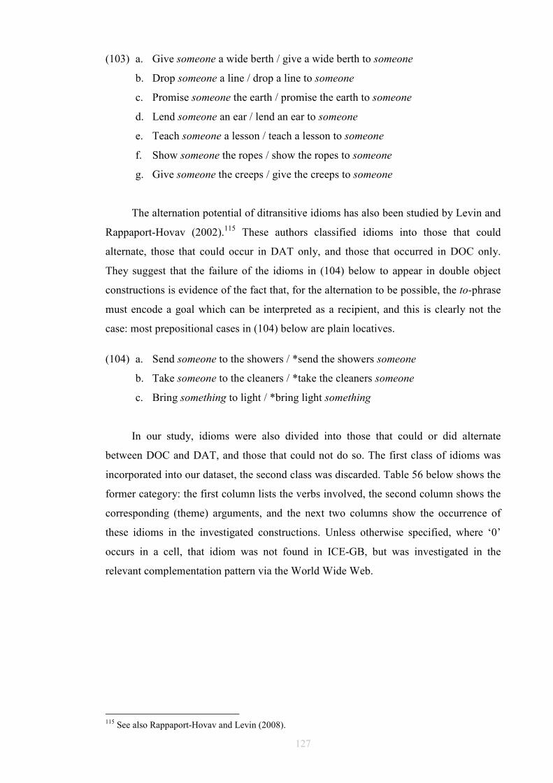
127

(103) a. Give someone a wide berth / give a wide berth to someone

b. Drop someone a line / drop a line to someone

c. Promise someone the earth / promise the earth to someone

d. Lend someone an ear / lend an ear to someone

e. Teach someone a lesson / teach a lesson to someone

f. Show someone the ropes / show the ropes to someone

g. Give someone the creeps / give the creeps to someone

The alternation potential of ditransitive idioms has also been studied by Levin and

Rappaport-Hovav (2002).115 These authors classified idioms into those that could

alternate, those that could occur in DAT only, and those that occurred in DOC only.

They suggest that the failure of the idioms in (104) below to appear in double object

constructions is evidence of the fact that, for the alternation to be possible, the to-phrase

must encode a goal which can be interpreted as a recipient, and this is clearly not the

case: most prepositional cases in (104) below are plain locatives.

(104) a. Send someone to the showers / *send the showers someone

b. Take someone to the cleaners / *take the cleaners someone

c. Bring something to light / *bring light something

In our study, idioms were also divided into those that could or did alternate

between DOC and DAT, and those that could not do so. The first class of idioms was

incorporated into our dataset, the second class was discarded. Table 56 below shows the

former category: the first column lists the verbs involved, the second column shows the

corresponding (theme) arguments, and the next two columns show the occurrence of

these idioms in the investigated constructions. Unless otherwise specified, where ‘0’

occurs in a cell, that idiom was not found in ICE-GB, but was investigated in the

relevant complementation pattern via the World Wide Web.

115 See also Rappaport-Hovav and Levin (2008).

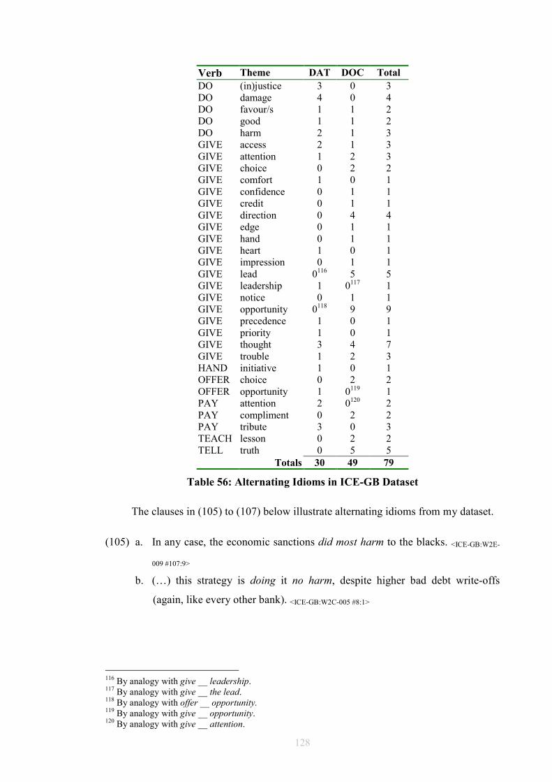
128

Verb Theme DAT DOC Total

DO (in)justice 3 0 3 DO damage 4 0 4 DO favour/s 1 1 2 DO good 1 1 2 DO harm 2 1 3 GIVE access 2 1 3 GIVE attention 1 2 3 GIVE choice 0 2 2 GIVE comfort 1 0 1 GIVE confidence 0 1 1 GIVE credit 0 1 1 GIVE direction 0 4 4 GIVE edge 0 1 1 GIVE hand 0 1 1 GIVE heart 1 0 1 GIVE impression 0 1 1 GIVE lead 0116 5 5 GIVE leadership 1 0117 1 GIVE notice 0 1 1 GIVE opportunity 0118 9 9 GIVE precedence 1 0 1 GIVE priority 1 0 1 GIVE thought 3 4 7 GIVE trouble 1 2 3 HAND initiative 1 0 1 OFFER choice 0 2 2 OFFER opportunity 1 0119 1 PAY attention 2 0120 2 PAY compliment 0 2 2 PAY tribute 3 0 3 TEACH lesson 0 2 2 TELL truth 0 5 5 Totals 30 49 79

Table 56: Alternating Idioms in ICE-GB Dataset

The clauses in (105) to (107) below illustrate alternating idioms from my dataset.

(105) a. In any case, the economic sanctions did most harm to the blacks. <ICE-GB:W2E-

009 #107:9>

b. (…) this strategy is doing it no harm, despite higher bad debt write-offs

(again, like every other bank). <ICE-GB:W2C-005 #8:1>

116 By analogy with give __ leadership. 117 By analogy with give __ the lead. 118 By analogy with offer __ opportunity. 119 By analogy with give __ opportunity. 120 By analogy with give __ attention.

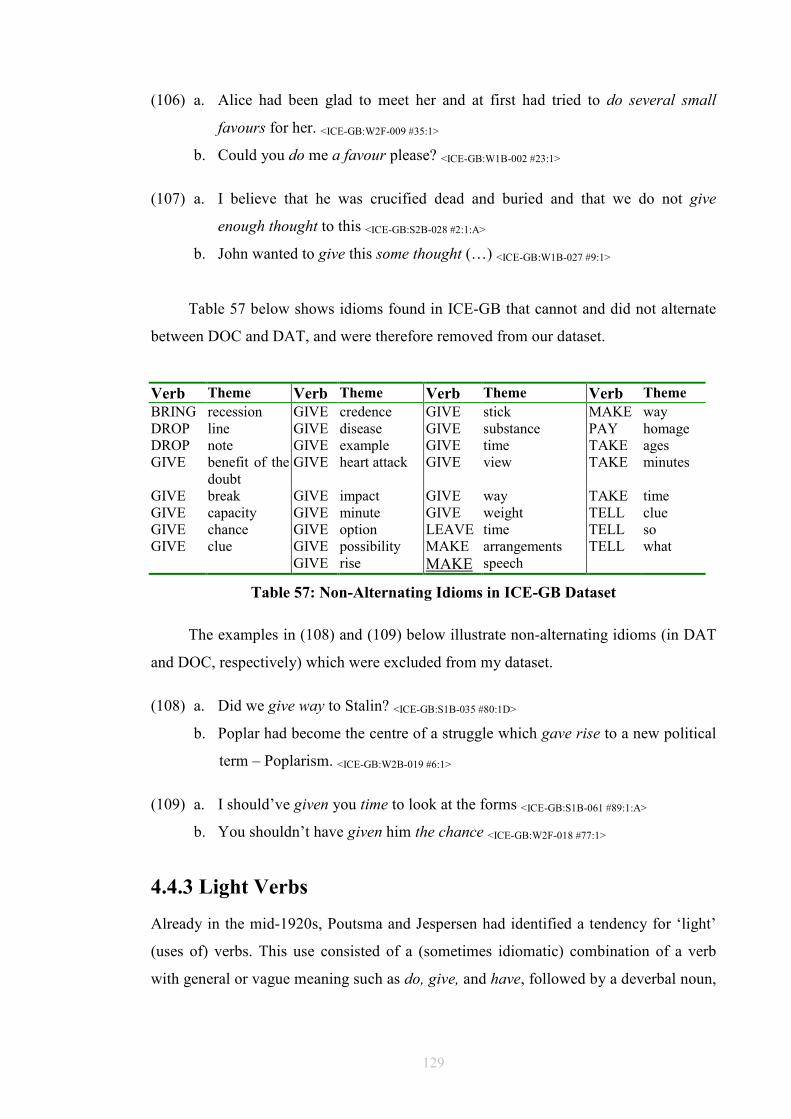
129

(106) a. Alice had been glad to meet her and at first had tried to do several small

favours for her. <ICE-GB:W2F-009 #35:1>

b. Could you do me a favour please? <ICE-GB:W1B-002 #23:1>

(107) a. I believe that he was crucified dead and buried and that we do not give

enough thought to this <ICE-GB:S2B-028 #2:1:A>

b. John wanted to give this some thought (…) <ICE-GB:W1B-027 #9:1>

Table 57 below shows idioms found in ICE-GB that cannot and did not alternate

between DOC and DAT, and were therefore removed from our dataset.

Verb Theme Verb Theme Verb Theme Verb Theme

BRING recession GIVE credence GIVE stick MAKE way DROP line GIVE disease GIVE substance PAY homage DROP note GIVE example GIVE time TAKE ages GIVE benefit of the

doubt GIVE heart attack GIVE view TAKE minutes

GIVE break GIVE impact GIVE way TAKE time GIVE capacity GIVE minute GIVE weight TELL clue GIVE chance GIVE option LEAVE time TELL so GIVE clue GIVE possibility MAKE arrangements TELL what GIVE rise MAKE speech

Table 57: Non-Alternating Idioms in ICE-GB Dataset

The examples in (108) and (109) below illustrate non-alternating idioms (in DAT

and DOC, respectively) which were excluded from my dataset.

(108) a. Did we give way to Stalin? <ICE-GB:S1B-035 #80:1D>

b. Poplar had become the centre of a struggle which gave rise to a new political

term – Poplarism. <ICE-GB:W2B-019 #6:1>

(109) a. I should’ve given you time to look at the forms <ICE-GB:S1B-061 #89:1:A>

b. You shouldn’t have given him the chance <ICE-GB:W2F-018 #77:1>

4.4.3 Light Verbs

Already in the mid-1920s, Poutsma and Jespersen had identified a tendency for ‘light’

(uses of) verbs. This use consisted of a (sometimes idiomatic) combination of a verb

with general or vague meaning such as do, give, and have, followed by a deverbal noun,

130

or a “noun of action” (Poutsma 1926:394).121,122 In the presence of a semantically vague

verb, it is this noun which carries the major part of the meaning. These constructions

have been called light verbs (Jespersen 1927:117), eventive objects (Quirk et al.

1985:750-751), expanded predicates (Algeo 1995:204), and stretched verb

constructions (Allerton 2001).

Some of the characteristics of these constructions are listed below:

• The verb in question must be one of the most frequent semantically general

verbs, such as give, have, make, take, etc. (Algeo 1995:207). The semantic

contribution of the verb to the meaning of the predication is very small: “[t]he

main semantic content is located not on the light verb, but in the noun

functioning as head of the direct object” (Huddleston and Pullum et al.

2002:290).123

• The noun phrase is “overwhelmingly indefinite” and “typically singular” (Quirk

1995:116), as well as being very often a deverbal noun.

Biber et al. (1999:1026-1027) identify a “cline of idiomaticity” in light uses of

verbs, ranging from clearly idiomatic expressions ((110)a, b), through to relatively

idiomatic expressions —where “the meanings of individual words are retained to some

extent, but the entire expression also takes on a more idiomatic meaning” (1999:1027),

and could even be replaced by a single verb ((110)c, d)—, to expressions where the

verbs retain their core meaning ((110)e, f).

121 “Semantically general verbs are those used in an idiomatic (nonpredictable) meaning, which typically have long dictionary entries because defining them requires the specification of many different senses, according to the verbal context” (Algeo 1995:206). 122 Poutsma (1926:399) makes a distinction between the elements which follow certain verbs (typically make). They can be verb-stems in their own right (e.g. make a smile, make a move), or they can be simply nouns of action “that are not to be regarded as verb-stems” such as make an examination, make a speech, make your choice, etc. 123 Poutsma (1926:394) argues that the semantic vagueness of the light verb is apparent from the fact that the same deverbal noun may be associated with more than one verb “without much difference in meaning being involved.” This was indeed confirmed in our dataset, where the object support was used almost interchangeably with light verbs such as give and lend (and offer and win too, but these are, at best, marginally light).

131

(110) a. When we go public, you’ll make a killing.

b. Do you think you can take time out to have a cup of tea.

c. Have a chance.

d. Make a deal.

e. Well, we have an extra one.

f. He made a sandwich.

It is this classification difficulty which makes Algeo (1995:204) claim that the

expanded-predicate construction is “janus-like, looking in both directions

simultaneously. It is a syntactic construction at the core of the grammar of the clause.

But it is also a lexical unit that requires entry in a dictionary”.

In view of the fact that each light verb needs at least an object, most light uses are

monotransitive. However, given that the semantic import of the verb is so small, the

combination can almost be regarded as intransitive. Consider example (111) below,

from Algeo (1995:204).

(111) a. We had to do a dive.

b. We had to dive.

The verb-object combination do a dive in (111)a above is (excluding pragmatic

considerations) the semantic equivalent of the verb to which the noun object is

morphologically related, i.e. dive. Thus, the (structurally) more complex pattern

expresses the same meaning as the simpler one.

By the same token, some light verb-object combinations which require an

additional object are semantically comparable to a monotransitive expression. Consider

examples (112) below, from Quirk et al. (1985:751).

(112) a. She gave me a push.

b. She pushed me.

These constructions allow the speaker/writer a greater “syntactic versatility,” as

Huddleston and Pullum et al. (2002:291) call it. The light verb + object combination

allows for modifiers to be added to the deverbal noun. Consider example (113) below,

where (113)b and (113)d are decidedly awkward.

132

(113) a. We had a delightful bath.124

b. ?We bathed delightfully.

c. She gave him an unusually passionate kiss.

d. ?She kissed him unusually passionately.

Additionally, light verb constructions are a convenient device to move the activity

(over the human participant) towards clause-final position, where it enjoys the focal

limelight, as can be appreciated in (114), from Quirk et al. (1985:751).

(114) a. He nudged Helen.

b. He gave Helen a nudge.

As regards the alternation potential of some light verbs, Quirk et al. (1985:751)

mention that indirect objects in light verb DOCs are not normally paraphraseable by a

prepositional phrase, as seen in example (115) below.

(115) a. I gave Helen a nudge.

b. ?I gave a nudge to Helen.

The reason for this lack of alternation with DAT is that the purpose of light verb

constructions is to focus on the deverbal noun denoting the activity. Thus, it is the direct

object and not the human participant that should receive end-focus.

As was the case with idioms, light verbs in DOC and/or DAT complementation

patterns were classified into those that could and those that could not alternate. Table 58

below shows the alternating light verbs in our dataset: the first column lists the verbs

involved, the second column shows the corresponding (theme) arguments, and the next

two columns show the number of occurrences of the idioms in the investigated

constructions. Where ‘0’ occurs in a cell, that idiom was not found in ICE-GB, but was

investigated in the relevant complementation pattern via the World Wide Web.

124 Example from Jespersen (1927:117).

133

Verb Theme DAT DOC Total

GIVE absolutions 1 0 1 GIVE appearance 1 0 1 GIVE advice 2 2 4 GIVE assurance125 0 2 2 GIVE blessing/s 1 0 1 GIVE boost 1 0 1 GIVE consideration126 1 2 3 GIVE encouragement127 0 1 1 GIVE indication128 0 4 4 GIVE look 0 2 2 GIVE response129 0 1 1 GIVE shock 0 2 2 GIVE (fore)warning 0 2 2 GIVE support 0130 7 7 LEND support 1 1 2 OFFER (re)assurance131 1 0 1 PAY visit 2 0 2 MAKE visit 1 0 1 Totals 12 26 38

Table 58: Alternating Light Verbs in ICE-GB Dataset

The clauses in (116) to (118) below illustrate alternating light verbs from my

dataset.

(116) a. And uh having recorded the matter and given certain advice to Mr Scott

Cooper … <ICE-GB:S1B-069 #49:1:A>

b. I'm sorry not to be able to give you any better advice. <ICE-GB:W1B-014 #50:3>

(117) a. It is both inevitable and right that Conservatives should give the most careful

consideration to the former Deputy Prime Minister's words …. <ICE-GB:W2E-005

#45:3>

b. Regarding the Foundation and Advanced EEC courses, we’ve given this

careful consideration … <ICE-GB:W1B-030 #135:7>

125 From Huddleston and Pullum et al. (2002:293-296). 126 See footnote 125. 127 See footnote 125. 128 See footnote 125. 129 See footnote 125. 130 By analogy with lend. 131 See footnote 125.

134

(118) a. The outcome of the constitutional confrontation was influenced by several

factors which lent support to the unitarist trend … <ICE-GB:W2B-007#45:1>

b. With Phelan lending the impressive Ince solid support in midfield and Sharpe

consistently pressing the opposition back on the left wing, United quickly

established a pattern of command … <ICE-GB:W2C-004 #32:2>

Table 59 below shows light verbs which did not alternate between DOC and

DAT, and which were removed from our dataset.

Verb Theme Verb Theme

GIVE brush-off GIVE scare GIVE call GIVE shout GIVE cuddle GIVE smile GIVE fright GIVE stare GIVE kick GIVE start GIVE miss GIVE surprise GIVE pat GIVE wink GIVE push MAKE call GIVE rebuke MAKE contribution GIVE rest MAKE decision GIVE ring MAKE speech

Table 59: Non-Alternating Light Verbs in ICE-GB Dataset

The examples in (119) below illustrate non-alternating (i.e. excluded) idioms in

DAT and DOC.

(119) a. Women might be able to make a valuable contribution to cricket <ICE-GB:S1B-

021 #79:1:B>

b. Give it a rest, Benjamin. <ICE-GB:W2F-012 #103:1>

4.5 Experiment Design All experiments are basically comparisons. (R. Langley 1968:109)

Experimental research in corpus linguistics can be defined as the conduct of

investigations which can confirm or refute hypotheses about the structure and use of

language. The role of computation is to ensure the systematic abstraction and evaluation

of data, against which hypotheses are evaluated. The role of data is in a way subsidiary

to the uses we put them to. However, as Meyer (2002:102) observes, it is not

uncommon to come across “many corpus linguists [who] have regarded the gathering of

evidence as a primary goal”, the be-all and end-all of corpus research. There have been

many lengthy papers, full of graphs and tables, signifying very little; i.e. with not

135

enough attention paid to the significance of the reported findings. Aarts (2000:7) notes

that these studies

invariably [elicit] a “so what” response: so what if we know that there are 435 instances of the conjunction “because” in a particular category of written language, whereas there are only 21 instances in conversations? So what if we are told that subordination is much more common in women’s speech than in men’s speech?

That is why it is essential to start corpus-based investigations with a particular

linguistic purpose, and to constantly remind ourselves that frequency and statistical

significance do not, in and of themselves, answer ‘why’ questions. A qualitative

analysis must therefore be considered a (post-) requisite of quantitative research.

As mentioned earlier, in this study, the research questions addressed were the

following:

(120) Research Questions

a. Do information status, weight, and complexity indeed affect the dative

alternation?

b. What is the relationship between these three factors?

c. Can corpus data help establish a model of the interaction between these

factors/variables?

d. Can these factors be manipulated into predicting speakers’ choices?

The following sections compartmentalise and break down the experiment design

applied to the corpus investigation. The experimental process is described according to

the formalisation suggested in Wallis (2007), according to whom there are four parts to

an experiment: (a) definition, (b) sampling, (c) analysis, and (d) evaluation.

4.5.1 Definition

Research questions, variables, target cases, and queries must be specified (prior to the

conduct of any kind of analysis) based on case definitions. These ‘working definitions’

are “a way of avoiding inconsistency as the analysis proceeds” (Meyer 2002:107-108).

Naturally, this does not preclude the possibility of altering definitions as new data are

encountered. The constructions to be investigated (DOC and DAT) have been defined in

§4.1, the variables investigated will be (preliminarily) defined below.

Most theories of constituent ordering recognise the role of different principles: the

Given Before New (GBN) principle and the principle of end weight (PEW), both

136

variously defined in the literature. In this study, the definition of givenness is largely

based on retrievability, i.e. a noun phrase is given if its referent is recoverable from the

preceding context. As regards the PEW, I distinguish between weight (defined as the

number of words in a constituent) and complexity (defined as the number of phrasal

nodes in a constituent).

4.5.2 Sampling

The second stage in the experimental process is sampling, which results from the

application of the definitional criteria as established in the previous stage. An

experimental sample (or model) is thus abstracted from the dataset/corpus, and this is

then classified according to the variables under study.132

The selection (and exclusion) criteria for our dataset were discussed in §4.1 and

§4.2. In view of the fact that neither DOC nor DAT have unique lexical content, lexical

searches would have been insufficient for extracting all instances of these constructions

from the corpus. Because ICE-GB is a parsed corpus and thus contains “annotation

describing higher-level grammatical constructions” (Meyer 2002:117-118), most cases

in our dataset could be extracted automatically from ICE-GB by means of FTFs and

other searching procedures available via ICECUP. All the same, the results had to be

manually revised to stop extraneous variables from affecting the sample.

4.5.3 Analysis

Analysis consists of assigning specific linguistic values to the target cases. In the present

study, this was carried out off-line from the corpus, i.e. cases were extracted manually

into a spreadsheet and categorised individually.133 Wallis (2007) also includes statistical

analysis at this stage, specifically the application of statistical tests to the dataset, the

search for patterns in the (abstract) model, and the ensuing refutation or confirmation of

hypotheses. Statistical analysis is further discussed in §4.6 below.

This study consists of a series of separate (mini-) experiments applied to the same

dataset, as illustrated in Figure 60 below.

132 In principle, though, the experimental dataset can consist of the entire set of cases in the dataset, or simply of a random subsample of it. 133 This allowed total frequencies to be separated from underlying data, i.e. the researcher can focus on relative frequencies rather than on number of instances of a specific construction per number of words in the corpus, a far less informative and useful ratio for inferential statistics.

137

Figure 60: Overall Experiment Design

An experimental model usually consists of two variables, one of which (the

independent one) can be used to explain the other (dependent) variable (see §4.6.1). In

Figure 60 above, my dependent variable (including cases of the dative alternation in

ICE-GB) is represented by the lozenge shape in the centre of the graph. The frequencies

obtained from the corpus via quantitative analysis are then tested against certain

communicative principles and discourse factors which allegedly influence speakers to

choose (in a particular context) one construction over the other. The variables which

could explain the abstract model (i.e. the independent variables) are represented by the

rectangles surrounding the lozenge. The solid arrows stand for individual tests

conducted to ascertain the influence each variable had on the sample (i.e. to see how

accurate GBN, weight, and complexity were at predicting the alternation), whereas the

dotted lines represent association (paired) tests which explored the interplay between

the posited explanatory factors.

Ditransitive cases in my dataset were evaluated by means of Mann-Whitney tests

(discussed in §4.6.3) for simple measures of weight (in terms of number of words) and

complexity (number of phrasal nodes). By comparing the distributions of DOC and

DAT cases as determined by the different variables (weight and complexity), this step

attempted to ascertain whether any observable differences were indeed real or simply

epiphenomenal. The GBN principle was tested against the dataset by means of a χ2 test,

given that the data was discrete.

The next step involved evaluating the interaction between weight and complexity

to see whether (i) they were coextensive, (ii) one was better than the other. The results

138

of the potential weight/complexity interaction (a likely explanation of the dative

alternation) were then contrasted with an account of the alternation based solely on the

GBN principle, in an attempt to identify the strength of the correlation between weight

and complexity on the one hand, and information status on the other. Additionally, the

potential interrelationship between weight and GBN was evaluated by means of Mann-

Whitney tests.

Notice that this is a mixed-factor design, in that the operationalisation of the

variables has not rendered uniformly linear results in all cases: while weight and

complexity are numerical, the information status (GBN) values are discrete (i.e. their

values are given or new, not numbers on a scale such as 1, 3, etc.). It is this design that

made it necessary to employ different statistical tests (χ2, Mann-Whitney, t, etc.), given

that using more uniform alternatives (such as factor analysis, or ANOVAs) would have

been less appropriate.134 We have been more careful (in our statistical assumptions) than

a conventional analysis of variance. We have carefully examined each individual

variable as well as its interaction with the other variable/s, which is a more principled

approach than just pushing the data through an automated statistical package and

relying on it to come out with a significance verdict.

The dataset is clean, in that weight, complexity, and information status (GBN) are

all competing predictive factors: all other categorical factors/values have been excluded

from it (see §4.2). The experimental design makes these three variables fight each other

in order to determine their relative strength with respect to the linguistic choice (DOC

or DAT). As in a gladiator’s duel, we consider only two factors at a time: having three

simultaneously could result in the finer details of their interaction being lost or

overlooked.

If we assumed that that weight, complexity, and information status (GBN) are

independent from one another, then these factors would explain different portions of the

dataset. If this were not strictly true, then they would explain an overlapping group of

cases, while failing to explain the remainder of the data. In the vast majority of cases,

though, these variables are indeed expected to favour the same (optimal) word order: the

prediction is that the newer, heavier, and more complex constituent will tend to be

found in the second position in both constructions (DOC and DAT).

134 There is more to be said about the decision not to use ANOVAs. ANOVAs can be described as cascades or bundles of t tests which compare more than two groups in order to look at various potential sources of variance. As such, they do not offer any additional insights to the experimental design employed in this study. Furthermore, we do not necessarily want to use t tests here, given that —as a matter of principle— we are treating any assumption of normal distribution of the dataset as suspect.

139

4.5.4 Evaluation

Once analysis has been carried out, the experimental results must be evaluated. In

Wallis (2007), this consists of two aspects: (i) verifying results against the corpus (i.e.

ensuring that observations reflect a real phenomenon in the data “rather than mistakes in

the analysis, an artefact of the grammar, variable definitions or sampling” (as Wallis

(2007) points out in §8.3 of his e-paper),135 and (ii) considering the theoretical

implications of the results by relating results to the literature.136 This meant going back

to the corpus and look at language in context. We should always remind ourselves that

our results are devoid of linguistic justification until we find one for them.

4.6 Quantitative Analysis Statistical packages tend to be used as a kind of oracle, from which you elicit a verdict as to whether you have one or more significant effects in your data. (…) After a magic button press, voluminous output tends to be produced that hides the p-values, the ultimate goal of the statistical pilgrimage, among other numbers that are completely meaningless to the user, as befits a true oracle. (Baayen 2008:x)

If we can make the assumption that the elements in the dataset are broadly

representative and broadly comparable with other elements in the English language,

then inferences can be derived from it. However, these inferences are only made

possible by relying on statistical methods. The experimental sample thus becomes the

test bed for hypotheses about language in general, an abstract model for confirmation

and refutation (as well as selection). What statistical tests essentially do is give the

researcher confidence when generalizing from a measured sample (dataset) to an

unmeasured instance (language) by confirming (or disconfirming) that the observed

results in the model are not accidental, i.e. are likely to reoccur in the world (all other

things being equal). This approach is sometimes called ‘inferential statistics.’

What follows is a brief discussion of certain key notions instrumental to the

design of the experiments.

4.6.1 Variables

As discussed earlier, a common way of setting up an experimental model is by

assuming two variables. The independent variable (IV) is the feature that (the researcher

135 When an explanatory gap resists our best efforts at closing it by refining or multiplying our explanatory factors, it is clearly a potentially interesting research subject. 136 In this regard, Wallis (2007) concentrates particularly on issues of theoretical commensurability (how the research results relate to previous reports), simplicity (i.e. Occam’s razor), causality and circularity (i.e. ensuring that research results are not circular nor the outcome of mere correlations).

140

assumes) could explain the dependent variable (DV). This setup is easily translated into

a table; statistical tests are then applied in order to verify whether a change in the values

of the IV affects the values of the DV. The default negative assumption (i.e. null

hypothesis) is made that there will be no (significant) change.137

In this study, DV is represented by DOC and DAT, i.e. the dative alternation. The

(relative) weight, (relative) complexity, and information status (GBN) of these

constructions are the IVs, and, as such, all possible predicting factors.

It is perhaps not too early to remind ourselves of the dictum ‘correlation is not

causation’. Identifying a correlation in the data is not to be equated with causation, i.e. if

A is correlated with B it does not necessarily follow that A causes B. There are

alternative interpretations (B causes A, C causes both A and B) and significance tests

are not able to decide among them. In short, an observed significant relationship

between two variables need not be causal.

4.6.2 Data Distribution

The distribution of linguistic data is relevant to the choice of the appropriate statistical

test to apply to the dataset: where the data is assumed to be normally distributed, certain

tests are available; otherwise, a different kind of test is prescribed which makes other,

different mathematical assumptions.

Most phenomena in the world tend toward a normal distribution, i.e. if we group

measurements on a continuous scale (i.e. plotting the number of times each score

occurs) we will notice that the resulting frequency graph indicates that “though the

scores span a wide range (from X to Y) the scores are generally clustered in the middle

of the range” (Johnson 2008:6), while at each end the curve would be relatively flat.

This means that scores tend to congregate around a typical value, and other, different

values become less and less likely as they deviate further from this central value. Such a

population distribution is the familiar bell-shaped curve known as the normal curve or

normal distribution. This is a pattern that approximates what would probably happen if

you created a distribution of scores for the entire population. Thus, a normal distribution

is only a theoretical distribution. As Goodwin points out, “[t]he normal curve is (…) a

hypothetical distribution of what all the scores in the population should be like if

everyone is tested” (1995:113).

137 Langley (1968:148) reminds us that “[i]n normal usage, the word significant means important (…). In [s]tatistics, significant means beyond the likelihood of chance.”

141

There seems to be a consensus about not treating linguistic data as normally

distributed (Dunning 1993, Kilgarriff 2001, Meyer 2002, Bresnan et al. 2007).138 On a

similar but more fact-based note, Meyer (2002) uses three criteria for evaluating the

assumption of normal distribution of linguistic data: kurtosis (i.e. the extent to which a

distribution deviates from the normal bell curve), skewness (i.e. the extent to which

more scores are above or below the mean of the distribution), and plain eyeballing the

resulting graph (2002:126-127). As regards kurtosis and skewness, Meyer claims that

“[i]f the data were normally distributed, the figures for kurtosis and skewness would be

“0” (or at least close to “0”).” In my experiments, the weight and complexity of both

DOC and DAT do indeed look like normal distribution, but this is not confirmed by

their respective kurtosis and skewness.139 It seems that resemblance is not a strong

enough argument for considering our dataset normally distributed.140

I therefore proceeded to treat the distribution of my dataset as not normal. Just as

normally distributed data requires parametric statistical tests for their analysis, not

normally distributed data calls for non-parametric tests. I thus employed non-parametric

tests, specifically Mann-Whitney tests and Spearman correlation coefficient at the

expense of t tests and Pearson correlation coefficient. These are all discussed in more

detail in the following section. Parametric tests were not entirely discarded, but used to

verify the significance results of Mann-Whitney and Spearman, i.e. both non-parametric

and parametric tests were employed, thus avoiding objections about the distribution of

the data.

4.6.3 Tests

As noted in the previous section, data determine the statistical tests to which they are

amenable. In turn, the tests will determine the significance of the data.141 In order to

138 In essence, these authors’ objections make up a rather purist mathematical argument, according to which a researcher is neither allowed to make assumptions about distributions, nor to make extrapolations from anything. However, see also Gries (2003b) for an argument for treating linguistic data as normally distributed. This author considers that “the resulting possibilities of interpretation outweigh the small risk to obtain slightly skewed results” (2003b:24). 139 For instance, the weight of DAT constructions has a kurtosis of 11.1 and a skewness of 1.76, while the weight of DOCs has a kurtosis of 5.6 and a skewness of -0.38. 140 Another reason for not treating the distributions of weight and complexity as normal is based on the fact that these measures consist of the difference between two distributions, both of which have a floor, i.e. the data cannot take on a value lower than some particular number (we cannot have a phrase with a negative number of nodes or words). This can cause the data to be skewed, and thus any assumptions of normal distribution are better abandoned, and non-parametric tests are better adopted. Finally, the fact that weight has been considered a ranked variable by some linguists is yet another reason for not assuming a normal distribution of weight. 141 Once again, it will be up to the researcher to turn statistical significance into linguistic significance, i.e. invest the correlations with motivation.

142

move one step closer to certainty or confidence, statistical tests have to do the job of

culling the wheat from the chaff, i.e. ascertaining whether the observed phenomena are

real (and likely to be repeated) or are simply attributable to chance. Only in the former

case are claims based on the data valid.

As mentioned by Biber et al. (1998:275), statistical techniques can be used to

measure (i) the difference between groups (for example, with t tests, Mann-Whitney

tests, or ANOVAs), or (ii) the extent of the relationship between variables (as with a

correlation). The first technique produces a test of significance, assessing the likelihood

that that the observed difference or relationship could be due to chance, whereas the

second type of technique provides the researcher with a measure of strength, assessing

the importance of the difference or relationship. Both types of techniques were used in

this study.

When assumptions of normal distributions are not met by the data, non-parametric

tests have to be resorted to. This kind of test (Mann-Whitney, χ2) is very powerful in

detecting population differences, accept weaker (i.e. less accurate) input, and can

therefore be employed in very many research disciplines. Given that the dataset was not

normally distributed, we employed the Mann-Whitney test (a.k.a. rank sum test).142

Just as the t test, the Mann-Whitney test evaluates the difference in central

tendency between two distributions. More specifically, the Mann-Whitney test

compares (the medians of) two sample distributions, in order to find out whether the

two are indeed different (in which case the difference is attributable to the independent

variable) or whether both are (part of) one and the same, larger sample (in which case

any difference between them is due to chance or sample variability, i.e. the null

hypothesis holds).

In this study, a series of pair-wise evaluations was carried out using a one-tailed

Mann-Whitney test for heaviness and complexity, and the interaction between the two

measures was also taken into account. A one-tailed (as opposed to a two-tailed) Mann-

Whitney test was used because we can predict a direction of the difference between the

two distributions and ignore any findings which are in the ‘wrong’ direction (i.e. weight

effects were expected to reinforce rather than impair GBN results). Anticipating the

results thus allows us to employ a more powerful test of significance in a more

controlled way.143

142 A parametric test can nonetheless be used for ranked and/or not normally distributed data; however, it will tend to overestimate the probability of variance; i.e. it would tend to assume that a result is significant when in fact it isn’t. 143 A two-tailed test would test for both effects, i.e. would evaluate whether weight reinforces or impairs

143

Another test that does not assume normally distributed data is χ2, one of the non-

parametric statistical tests more commonly applied in linguistics. This test compares

observed experimental frequencies with the frequencies expected if there were no

differences in the distribution on the data. If the null hypothesis is confirmed, then the

differences in the dataset are due to chance, while if the null hypotheses can be rejected,

then the difference is not due to chance, and the researcher is safe to make

generalizations based on the experimental dataset. In fact, χ2 was used in this study for

evaluating information status (the GBN principle), particularly because of the discrete,

nominal, or non-numerical values of this variable (i.e. both variables represent groups

rather than counts), and not just because of considerations about the (alleged) non-

parametric nature of the data.

Finally, in order to evaluate the strength of the correlation between constructional

weight and complexity, a measure of association was required. Correlation tests express

the strength of the correlation numerically, according to which a +1 value indicates a

perfect positive correlation (i.e. both variables are co-extensive, and/or one is

redundant), a 0 value is the null hypothesis (i.e. that there is absolutely no correlation

between the variables), and -1 expresses a perfect negative correlation (i.e. as in a see-

saw, high values in one variable are associated with low values in the other variable,

and vice versa). Notice that the value of the correlation as measured in these tests (as

Woods et al. (1986:161) point out) does not have any units, being a dimensionless

quantity, like a proportion or a percentage.

The standard correlation test is Pearson’s r. However, Oakes warns us (1998:31)

that the Pearson test assumes normally distributed data, and a linear relation between X

and Y. We have already determined to employ the tests that make fewer assumptions,

and thus to treat our data as not normally distributed. We therefore cannot use Pearson

and have to resort to an alternative test, Spearman’s rho. This test depends on a

comparison of the rank orders rather than numerical scores (i.e. numbers are first

converted to ranks and then calculations are performed on these ranks, which is a very

similar procedure to Mann-Whitney’s). Spearman’s rho (or rs) is still expressed as a

measure ranging from 1 through 0 to -1.144

My experiment design is in effect a form of multivariate analysis in that it (i)

predicts some outcome on the basis of two or more predictors, (ii) looks at the GBN. 144 Not everything is plain sailing though. A word of caution against this test is expressed by Woods et al. (1986). These authors warn us that Spearman’s rho “should not be used on data which have a more or less normal distribution” (1986:173). This is the usual caveat against Type II errors (i.e. throwing out results that may be significant). Again, if anything, we have been overcautious in our approach.

144

interrelationships between more than two variables, and (iii) allows for the assessment

of the relative strengths of variables. It differs from other state-of-the-art multivariate

procedures (such as multiple regression, factor analysis, or loglinear analysis, as offered

in statistical software packages) in that I employ mixed number types, since one of my

variables (information status) offers discrete possibilities. This design has advantages

and disadvantages. The most notable disadvantage is that the operationalisation of the

variables does not allow for full automation, and is thus open to claims of

annotator/analyst inconsistency.145 However, and to make a virtue out of necessity, this

same issue has forced us to break down the experimental process into a series of steps

which gave us the chance to look at the data (and tests) much more closely and

carefully, never losing the actual language constructions from sight. Despite it being

hugely time-consuming, we found this method preferable to simply plugging the data

into SPSS, pressing a magic button, and then reporting the results as (statistically)

significant, without considering (i) the assumptions that go into the statistics employed,

(ii) the linguistic significance of the results.

To recap: after a survey of the literature on ditransitive complementation, a

determination of the relevant cases (verbs and patterns) in ICE-GB, and an explanation

of the purpose and methods to be followed in this study, the next chapter begins to

tackle the first proposed explanatory variable, i.e. information status.

145 ICECUP 4.1 allows full automation of different types of variables, thus minimising the danger of inconsistency.

145

5 Information Status

There can be little doubt that where syntax (in the narrower sense) fails to determine some part of the sequential ordering, the choice between the available options is always significant in some way. (Taglicht 1984:18-19)

The ordering of constituents in ditransitives has been claimed to be affected by at least

two factors: the informational status of the referents of the two postverbal noun phrases,

and the weight and/or complexity of the noun phrases in question. In particular, the

correlation between information status and choice of construction and its attendant

constituent rearrangement has long been noticed. Some linguists even hold that the

principles discussed in this chapter are valid cross-linguistically (Firbas 1966, 1992;

Chafe 1976, 1987; Prince 1981, 1992; Tomlin 1986; Gundel 1988; Gundel et al. 1993;

Birner and Ward 1998, inter alia). This chapter discusses previous approaches to the

analysis of the impact of information status on the alternating complementation patterns

instantiated by prototypical ditransitive verbs. An overview of the different concepts

traditionally grouped together under notions such as Given and New becomes

necessary, in view of the fact that the treatment of this principle has somehow eluded

terminological consistency.

This chapter also feeds into the following one, where a series of corpus

experiments puts the dynamics and explanatory power of the Given Before New (GBN)

principle to the test.

5.1 Introduction: Previous Approaches

Word order is said to be regulated by at least two principles, described by Quirk et al.

(1985) as the principles of end weight (PEW) and end focus (PEF), generally found in

the literature in one guise or another. The principle of end weight stipulates that the

‘heavier’ the constituent, the higher its chances of being placed in clause-final position;

whereas the principle of end focus states that the most important information (the focus)

in the clause tends to occur towards the end of the clause, preceded by the not-so-

important information (the theme). These concepts seem to have an admirable

resilience. They still have a role to play in Huddleston and Pullum et al. (2002), the

latest major grammar of English to date. Under ‘general tendencies regarding

information structure’, these authors (2002:1372) mention that heavy constituents tend

to occur towards the end of the clause, that the focus typically appears at or towards the

end of the clause, and that information that is familiar tends to be placed before that

which is new.

146

Whatever the framework or terminology, it seems incontrovertible that the end of

the clause constitutes a very coveted position, inasmuch as both the heavier and newer

constituents are constantly vying for it. In the typical cases, both principles will make

the same predictions, given that despite their very different wordings, they are closely

interrelated in terms of the linguistic phenomena they are meant to describe, i.e. it is not

unusual for the most important information to require a fuller statement than

information that has already been established, by one means or another.

These principles have also been resorted to when attempting to account for the

ordering of elements above the clause, and indeed above the sentence. Quirk et al.

(1985:1391n.) mention that “the principle of end focus applies just as much to the

ordering of clauses within a sentence as to the ordering of elements within a clause.”

The word order predictions that fall out from the different information statuses of the

referents of noun phrases (treated as discourse referents) have allowed linguists to put

PEF to work in explaining different objects of study. Discourse analysts, for instance,

have used these distinctions to explain the organization of discourse or texts (as opposed

to the organization of clauses). A foundational text in this field is Halliday and Hasan

(1976), according to whom a text as opposed to a random collection of sentences is

‘cohesive’ inasmuch as there are syntactic and semantic ties binding the component

clauses together. Among the syntactic devices used to link a text together, anaphora

figures prominently. Anaphora is defined as the relationship between two elements in a

text whereby the interpretation of one element is dependent on the existence in the

preceding (linguistic) context of an expression of the same meaning (whether co-

referential or not). Anaphora is thus highly indicative of ‘old’ or given information, i.e.

information already established from the preceding context. Pronouns, for instance,

typically refer back to (the referent of) a preceding noun phrase. The use of pronouns

creates anaphoric chains across the clauses making up a text, in that they allow a

referent introduced into the discourse by means of a full noun phrase to be taken up later

by some sort of referential shorthand. In this light, anaphoric pronouns are considered

prototypical (informationally) given elements.

Anaphora also poses important theoretical questions relative to the way we

understand and represent discourse in our minds. This cognitive dimension of anaphora

and its attendant notions of given and new information has also been of interest to

psycholinguistics, a relatively new discipline which has provided a new perspective on

the opposition given/new.

147

Information status has been used as an explanatory tool in many different fields,

such as syntax, pragmatics, discourse analysis, and psycholinguistics. Each and every

discipline understands information status in slightly different ways, and a wide range of

terms has been proposed in order to emphasize its importance for the differing

dimensions of explanation. For example, as regards the distribution of information in

propositions (as opposed to clauses or sentences), we find theme and rheme (Firbas

1966, 1992; Halliday 1967, 1985), topic and comment (Hockett 1958), focus and

presupposition (Chomsky 1970), as well as variants and combinations: for example,

Quirk et al. (1985) use theme and focus.

Despite the overabundance of terms, the notional common ground is still there. In

Birner and Ward’s words (1998:9):

What previous approaches have in common is a general approach [sic] based on the degree to which information is assumed to be available to the hearer prior to its evocation in the current utterance. One aspect in which they differ is the source of this availability the prior discourse, for example, or the hearer’s knowledge store.

Thus, it seems that regardless of the particular theoretical assumptions needed to

shed light on the use of the terms given or new, the crux of the matter lies in the origin

of an element’s givenness: is its origin textual (whereby givenness is associated with

anaphoric retrievability) or is it rather resident in the addressee’s consciousness (and

therefore a psychological concept)? The following sections attempt to unravel these

differences.

5.2 Terminological Confusion

As we have seen, the principle of end focus makes reference to topical and focal

information. A different pair of opposites, given and new, has often been associated

with topic and focus, and this association resulted in a deep-seated terminological

confusion. Two problems can be identified: (a) different terms have been used by

different authors to refer to one and the same concept, (b) the same term has been used

by yet other linguists to refer to different concepts. As an example of the former

problem, consider the following quote from Quirk et al. (1985:1362 fn.): “[s]ome

linguists use the distinction topic/comment for our theme/focus (…) (and sometimes for

our given/new). Others speak of given information as old, shared, or presupposed

information”. The resulting situation is one where coming across terms such as ‘theme’

or ‘focus’ sends alarm bells ringing and the linguist rushes to find out in which

148

theoretical light the term is to be understood. Straightforward terminological reference

is apparently something only to be hoped for.

Problem (b) is slightly more complex: the use and definitions of given and new are

still far too numerous, a situation which vindicates Humpty Dumpty’s notion of

meaning. In the following sections I will briefly survey the different terms and

distinctions used to refer to these concepts, as well as the different uses to which they

have been put.

5.3 Conceptions of Information Status

The purpose of many authors (Prince 1981, 1992; Halliday 1967, 1985; Clark and

Haviland 1977; Gundel 1988, Gundel et al. 1993) in distinguishing between given and

new information was ultimately to capture the information status of discourse entities

(or their referents). Some of these authors differentiate essentially between two notions

of givenness (retrievability versus accessibility), as will be seen in more detail in the

following sections.

5.3.1 Topic and Focus

The principle of end focus can be seen as a reformulation of what the Prague School and

the work of linguists such as Vachek and Firbas called Communicative Dynamism (CD).

Both concepts refer to the idea that in presenting their message, speakers prefer

reserving the element/s with higher information value for the end of an utterance.

In this view, focus is quite an intuitive notion, referring to the most important,

relevant, and usually informationally new, part of the clause. As stated earlier, focal

information tends to come towards the end of the clause, and represents the

informational climax of the sentence. In the default case, focus is intonationally marked,

and in non-typical cases, syntactically so, as will be seen in §5.3.5.

The status of elements occurring before the focus, however, has always been

problematic. Topic was first introduced by Hockett (1958), for whom a sentence

consists of a topic and a comment (see §5.3.2), the typical configuration being that of

topic preceding comment. In her detailed study of noun phrases, Keizer (2007:194ff.)

reviews the three ways in which the term topic has been used in the literature. She

distinguishes D[iscourse]-topics, S[entence]-topics, and G[rammaticalized]-topics.

The term D-topic refers to the intuitive notion of ‘what the discourse is about’. D-

topics are not formally demarcated: rather, they can be conceived of as ‘floating’ over

the discourse and not anchored to any constituent. The concept of S-topic is in essence

149

equatable to that of D-topic, only that its range of application is reduced to the

sentence/clause. In other words, if D-topics are ‘what the discourse is about’, S-topics

are ‘what the sentence is about’. Finally for Keizer, G-topics perform “a fully

formalized grammatical function, distinguishable by a number of invariable formal

features” (2007:196).146

5.3.2 Topic and Comment

Related to the distinction between topic and focus is the pair topic and comment.

Straightforward definitions appear in Gundel (1988:210), where she states that these

concepts are to be understood as pragmatic relations relative to a discourse context. Her

definitions are quoted below.

Topic Definition: An entity, E, is the topic of a sentence, S, iff in using S the speaker intends to increase the addressee’s knowledge about, request information about, or otherwise get the addressee to act with respect to E.

Comment Definition: A predication, P, is the comment of a sentence, S, iff, in using S the speaker intends P to be assessed relative to the topic of S.147

Gundel next discusses the correlation between topic/comment, and given/new.

She holds that the terminological and conceptual confusion found in the literature on

information status can be traced to the latter pair. This distinction has been used in (at

least) two different senses. The first is a ‘relational sense,’ whereby topic is given

information in relation to comment, and by the same token, comment is taken to be new

in relation to topic. Put differently, the status of each element (topic or comment) is

determined by contrasting it with the other member of the pair. This sense she simply

dismisses as falling out from her own definitions of topic and comment.

The other sense in which the given/new distinction has been used falls under the

label ‘referential sense,’ inasmuch as “given/new describes the status of the referent of a

linguistic expression vis-à-vis a cognitive state of the speaker or addressee” (1988:212).

This referential sense of the given/new distinction is divided into two subcategories: (a)

assumed familiarity and (b) activation. The table below is meant to help the reader keep

track of Gundel’s claims. 146 G-topics have often been confused with subjects. However, as pointed out by Li and Thompson (1976), the distinction between [G-] topics and subjects is based on a number of formal differences. Topics are always definite; always set the framework for a clause; and always appear in clause-initial position, whereas these are non-essential characteristics of subjects. On the other hand, subjects are determined by the verb (with which they are in agreement); and they may be empty, but the same cannot be said of topics. 147 Keizer (2007:268) notes that according to Gundel’s definition, the comment always takes the form of a predication, a feature which clearly differentiates it from the related notion of focus, which is not restricted in this way.

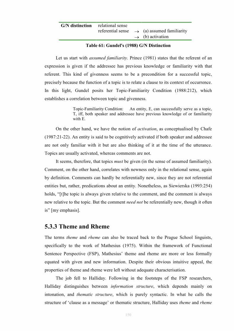
150

G/N distinction relational sense referential sense → (a) assumed familiarity → (b) activation

Table 61: Gundel's (1988) G/N Distinction

Let us start with assumed familiarity. Prince (1981) states that the referent of an

expression is given if the addressee has previous knowledge or familiarity with that

referent. This kind of givenness seems to be a precondition for a successful topic,

precisely because the function of a topic is to relate a clause to its context of occurrence.

In this light, Gundel posits her Topic-Familiarity Condition (1988:212), which

establishes a correlation between topic and givenness.

Topic-Familiarity Condition: An entity, E, can successfully serve as a topic, T, iff, both speaker and addressee have previous knowledge of or familiarity with E.

On the other hand, we have the notion of activation, as conceptualised by Chafe

(1987:21-22). An entity is said to be cognitively activated if both speaker and addressee

are not only familiar with it but are also thinking of it at the time of the utterance.

Topics are usually activated, whereas comments are not.

It seems, therefore, that topics must be given (in the sense of assumed familiarity).

Comment, on the other hand, correlates with newness only in the relational sense, again

by definition. Comments can hardly be referentially new, since they are not referential

entities but, rather, predications about an entity. Nonetheless, as Siewierska (1993:254)

holds, “[t]he topic is always given relative to the comment, and the comment is always

new relative to the topic. But the comment need not be referentially new, though it often

is” [my emphasis].

5.3.3 Theme and Rheme

The terms theme and rheme can also be traced back to the Prague School linguists,

specifically to the work of Mathesius (1975). Within the framework of Functional

Sentence Perspective (FSP), Mathesius’ theme and rheme are more or less formally

equated with given and new information. Despite their obvious intuitive appeal, the

properties of theme and rheme were left without adequate characterisation.

The job fell to Halliday. Following in the footsteps of the FSP researchers,

Halliday distinguishes between information structure, which depends mainly on

intonation, and thematic structure, which is purely syntactic. In what he calls the

structure of ‘clause as a message’ or thematic structure, Halliday uses theme and rheme

151

to refer to the (syntactic) structure of the clause. A clause, in Halliday’s view (1994:37),

is organized as a message by having a special status assigned to one part of it: “[o]ne

element in the clause is enunciated as the theme; this then combines with the remainder

so that the two parts together constitute a message”.

The theme is the point of departure for the message, the element selected by

speakers to ground their message.148 Themes usually occur clause-initially, but

Halliday adds (1994:38) position is not part of the definition of theme. Rather, he

insists, first position in the clause is the means whereby the function of theme is

realized.149

Nonetheless, there is a clear association between theme/rheme and given/new:

despite belonging to different systems in Halliday’s framework, both given and

thematic elements have been found to precede new or rhematic elements. Halliday

recognises that “[o]ther things being equal a speaker will choose the Theme from within

what is Given and locate the focus, the climax of the New, somewhere within the

Rheme” (1994:299). The difference between the concepts lies in the fact that whereas

the theme is the speaker’s point of departure, given material is what the addressee

already knows about or is familiar with. Halliday illustrates the difference as follows:

“[g]iven and new thus differ from theme and rheme (…) in that ‘given’ means ‘here is a

point of contact with what you know’ (…), whereas ‘theme’ means ‘here is the heading

to what I am saying’ ” (1970:163). Theme and rheme therefore seem to be speaker-

oriented notions, while given and new are listener-oriented.

Additionally, Theme also bears some resemblance to the notion of [S-]topic, but

the two notions are not to be equated. Halliday (1994:38) warns us that “[t]he label

‘Topic’ usually refers to only one particular kind of Theme (...). [Topic] tends to be

used as a cover term for two concepts that are fundamentally different, one being that of

Theme and the other being that of Given.” 150

148 Taglicht (1984:16) claims, however, that theme and rheme are textual as opposed to psychological entities, and that the division into thematic and rhematic is based on sequential ordering. 149 Indeed, as Firbas (1992:72) holds, neither theme nor rheme are position-bound because “[t]hey refer to interpretative arrangement. Their implementation may, but need not, coincide with the actual linear arrangement.” 150 Keizer (personal communication) points out a further restriction: whereas the function of S-topic is usually restricted to constituents, typically in argument position, Theme can be assigned to any type of element.

152

5.3.4 Given and New

The distinction between given and new elements has been held responsible for clausal

organization: given elements are claimed to precede new information. Recall that the

central problem in defining these terms lies in the source of givenness: an element can

be considered to be given (a) if it is anaphorically retrievable, or (b) if it is

psychologically present in consciousness, two notions which do not entail each other.

This difference in the source of availability of givenness has naturally resulted in many

different claims about information status. More worryingly, the possibility of reducing

these types to a single scale or factor seems unlikely. Arnold et al. (2000:29-30) believe

that the root of this evil is to be found in the fact that “the given/new contrast is a

simplified representation of accessibility”, a situation which has again resulted in an

immense variety of coding schemes used to capture these distinctions.

5.3.4.1 Conceptions of Given and New

A good survey of the given/new chaos is Prince (1981). Her survey is used here as an

introduction to the discussion of different authors’ conceptions of given and new, not

simply to her own notions. Prince identifies three levels in which the distinction has

been used in the literature on information status: saliency, shared knowledge, and

predictability/recoverability. These notions are relevant to the assumptions underlying

the design of the corpus experiments.

Saliency identifies given information with what is salient in discourse. This is the

sense of givenness regularly seen in the works of Chafe (1976, 1987, inter alia). His

definition of given information is “that knowledge which the speaker assumes to be in

the consciousness of the addressee at the time of the utterance (…). [G]ivenness is a

status decided on by the speaker (…). [I]t is fundamentally a matter of the speaker’s

belief that the item is in the addressee’s consciousness, not that it is recoverable”

(1976:30-32). Chafe further points out that given information usually carries weak

stress, can be replaced by a pronoun and even be omitted. By contrast, new information

is that which is not assumed to be in the consciousness of the addressee at the time of

the utterance.

More generally, Chafe holds (1987:21-22) that the distinction between given and

new is in fact a manifestation of basic cognitive processes. He uses the term ‘activation’

(see also Gundel’s approach in §5.3.2) to provide a scale along which other concepts

could be mapped. Concepts can therefore be active, defined as “in a person’s focus of

consciousness”, semiactive, defined as a concept “in a person’s peripheral

153

consciousness (…) which is not being directly focused upon”, or inactive, “one that is

currently in a person’s long-term memory, neither focally nor peripherally active”

(1987:25). Armed with this classification, he then proceeds to state that given elements

are elements which are already active, new elements are those which were previously

inactive, whereas accessible or inferable elements are those which were previously in a

semiactive state (i.e. available but not activated). The problem with Chafe’s approach,

as Birner and Ward (1998:10) point out, is that consciousness is “a slippery notion”.

Chafe (1980:11) defines it as “the activation of some available information in the

service of the self”, but defining consciousness in terms of activation does not appear to

shed light either on the notion of consciousness or indeed on the notion of activation.

Moreover, as Collins (1995:41) objects, by what means can an experimenter test for the

presence of an entity in the addressee’s consciousness?151

Another sense in which givenness has been used is that of shared knowledge.152 It

can best be exemplified by the work of Clark and Haviland (1977) and Clark and

Marshall (1981). In the latter’s account, the shared or mutual knowledge between

speaker and addressee determines the appropriate use of a particular linguistic marker of

givenness. For these authors, an element is deemed to be given if the speaker can

assume that its referent can be inferred from the knowledge shared by speaker and

addressee, both as participants in a conversation and as members of a linguistic

community.153 Mutual knowledge can be established (or assumed) on the basis of the

following:

(121) Mutual knowledge

a. Community membership: knowledge specific to all members of a particular

community.

b. Physical co-presence: knowledge speakers have by attending to the

immediate situation of utterance, particularly with reference to their physical

surroundings.

c. Linguistic co-presence: knowledge speakers share because it has been

mentioned in discourse.154

151 Recall Lambrecht’s dictum: “[a]ny assumption on the part of the speaker which has no formal manifestation in a sentence is irrelevant for the study of information structure” (1984:55). 152 This is in itself a concept comparable to assumed familiarity in Gundel’s framework (see §5.3.2). 153 See Sperber and Wilson (1982) for a critique of the notion of mutual knowledge. More specifically, these authors argue that mutual knowledge is of little explanatory value, given that it is inferable from (and a result of) comprehension, rather than the other way around. 154 Ariel (1988) is another author who uses a similar classification of contexts for retrievability/accessibility. In her three-way classification, “information stored as ‘general knowledge’ is

154

The source of givenness lies in the knowledge store (encyclopedic or other) of an

individual. Shared knowledge houses all three senses of givenness: both retrievable

elements (whether situational or textual) and elements in the consciousness of the

addressee are accommodated within it. And there, perhaps, lies its greatest flaw, in that

such a commodious concept proves hard to rein in and employ in an experimentally

useful way.

Finally, according to Prince’s classification (1981), the givenness of an expression

has also been equated with its predictability or recoverability, for example by Halliday

(1967), Kuno (1972), and others. This third sense of givenness covers more ground than

the first one (but less than the second), in that information is considered to be given if it

is retrievable either anaphorically or exophorically. On the other hand, new information,

naturally, is that which is not recoverable from the preceding context.

Retrievability has long been considered a representation of givenness, and it can

be found already at work in the Functional Sentence Perspective (FSP) framework. The

notion of Communicative Dynamism (CD) plays an instrumental role in FSP, inasmuch

as it provides a scale measuring the communicative contribution of discourse referents

to the communicative thrust of discourse. Thus, newly mentioned elements will carry

more CD than elements already established in discourse. Firbas states that the degree of

CD of a constituent can be assessed by means of three factors: “(i) linear modification,

(ii) the character of the semantic content of the linguistic element (…), and (iii) the

retrievability of the information from the immediately relevant preceding context”

(1992:11). The interplay of these factors “determines the distribution of CD over the

written sentence” (1992:11), the overriding factor being the contextual one.155

In this light, “what is actually in play is the retrievability/irretrievability from the

immediate relevant context” (1992:14). Information is given if it is retrievable from the

preceding context “and/or if the referent suggesting it is present in, and hence

retrievable from, the immediately relevant situational context” (1992:14). Firbas’s

criterion of givenness is thus clearly different from Chafe’s. In the latter’s approach,

givenness depends on the presence of the information in the addressee’s consciousness,

whereas in the former’s givenness revolves around the actual presence of an element in

the immediately relevant context.

not automatically accessible. Information from the physical surroundings, provided it is one [sic] that speakers are attending to, is mentally represented with a higher degree of Accessibility. Recent linguistic material is the most accessible source of information, other things being equal” (1988:68). 155 In spoken sentences, Firbas adds, intonation does play a role, but is itself highly sensitive and thus subordinated to the contextual factor.

155

Retrievability is also present in Halliday’s account. This author deviates mildly

from the givenness notions of the Prague School, enriching them with a psychological

status. Given information is specified as being treated by the speaker as “recoverable

either anaphorically or situationally” (1967:211), whereas new information is new “not

in the sense that it cannot have been previously mentioned, although it is often the case

that it has not been, but in the sense that the speaker presents it as not being recoverable

from the preceding discourse,” perhaps for rhetorical purposes [emphasis added]

(1967:204). In his framework, given elements need not be retrievable from the

preceding discourse, but are rather “options on the part of the speaker (…); what is new

is in the last resort what the speaker chooses to present as new” (1967:211).

Ariel uses recency of mention as the crucial factor in assessing givenness: the

general claim is that “referring expressions are no more than guidelines for retrieval”

(1988:68). Her classification is a detailed analysis of the behaviour of different elements

which are usually lumped together as typical representations of given elements. Ariel

classifies referential expressions according to the accessibility of antecedents. The

distinction given/new is seen as a “means to code the accessibility of the referent to the

addressee” (1988:68). Anaphoric expressions are classified into Low Accessibility (LA)

markers, Mid-Accessibility (MA) markers and High Accessibility (HA) markers. In

turn, each category is linked to three types of context general knowledge, physical

surroundings, and linguistic context which provide the textual scope where the

referential interpretation of the anaphoric form is to be found.

Accessibility

Value

Typical anaphor

Source of

antecedent

Comments

Low Full NPs/Proper names General Knowledge Often First-Mention; Long Distance

Medium Demonstratives Physical Context Deictic; Medium Distance High Pronouns Linguistic Context Anaphoric; Shorter Distance

Table 62: Ariel markers of accessibility (1988)

Ariel found out that: (a) pronouns (HA markers) tend to operate over short

distances, with antecedents generally within the same sentence; (b) demonstrative

anaphors (MA markers) tend to occur over intermediate distances; and (c) definite

descriptions and proper names (LA markers) tend to prefer antecedents in previous

sentences and beyond.156 This difference in behaviour (or acceptability at least) and the

156 This classification of nominals and their behaviour appears to mirror that provided by Binding Theory within GB, with R-expressions being equivalent to LA markers, Anaphors to MA markers, and Pronouns to HA markers.

156

characteristic patterning of different accessibility markers is dealt with by resorting to

the notion of anaphoric distance, i.e. the distance between an anaphoric expression and

its antecedent, measured over four categories: same sentence, previous sentence, same

paragraph, across paragraph (1988:72). Consider the examples in (122):

(122) a. Martin Amis wrote ‘London Fields’ in 1989. He had previously written

‘Money.’

b. Martin Amis wrote ‘London Fields’ in 1989. *? Martin Amis had previously

written ‘Money.’

The examples in (122) illustrate that pronouns are much more acceptable than full

noun phrases in a second mention of an entity introduced immediately before. In Ariel’s

framework, this is explained by the fact that pronouns are HA markers, whose context

of interpretation is found in the immediately preceding linguistic context, making them

more accessible than full noun phrases.157

5.3.4.2 Prince’s Proposals

In the preceding discussion of Prince’s survey (1981), it became quite clear that the

distinction between given and new is either not adequately defined or defined in too

extremely narrow a fashion to be useful beyond the theory-specific definition. Recall

that Prince identified three levels of givenness: saliency, shared knowledge, and

predictability/recoverability. The problem with this is that these levels are not mutually

independent, and hence deemed by her to be not very useful. Prince (1981:232-237)

proposes instead to distinguish given from new by means of a taxonomy based on a

sliding scale of assumed familiarity, where rather than given and new elements, we have

Evoked, New and Inferrable [sic] ones.158

Evoked entities are textually (anaphorically) or situationally (exophorically)

retrievable: the former are called textually evoked entities; the latter, situationally

evoked entities. In contrast, New entities are those which make a first appearance in the

text, and are subclassified into brand new those that are unfamiliar to the addressee

or unused a similar concept to Chafe’s ‘semi-active’ whereby the speaker assumes

the addressee is familiar with the entity, despite it being irretrievable either

anaphorically or situationally. The novelty comes in the guise of the Inferrables

157 For experimental support to some of Ariel’s claims, see Biber, Conrad, and Reppen (1998:106-132). 158 Inferrable with two r’s is the spelling Prince adopts for her concept. Given that I will later be using this notion for two experiments, her spelling is the one I am adopting henceforth.

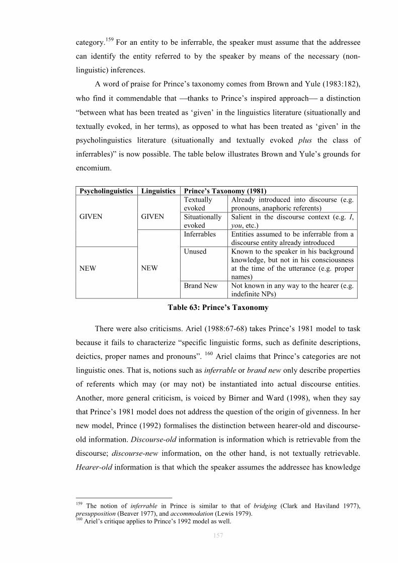
157

category.159 For an entity to be inferrable, the speaker must assume that the addressee

can identify the entity referred to by the speaker by means of the necessary (non-

linguistic) inferences.

A word of praise for Prince’s taxonomy comes from Brown and Yule (1983:182),

who find it commendable that thanks to Prince’s inspired approach a distinction

“between what has been treated as ‘given’ in the linguistics literature (situationally and

textually evoked, in her terms), as opposed to what has been treated as ‘given’ in the

psycholinguistics literature (situationally and textually evoked plus the class of

inferrables)” is now possible. The table below illustrates Brown and Yule’s grounds for

encomium.

Psycholinguistics Linguistics Prince’s Taxonomy (1981)

Textually evoked

Already introduced into discourse (e.g. pronouns, anaphoric referents)

GIVEN Situationally

evoked Salient in the discourse context (e.g. I, you, etc.)

GIVEN

Inferrables Entities assumed to be inferrable from a discourse entity already introduced

Unused Known to the speaker in his background knowledge, but not in his consciousness at the time of the utterance (e.g. proper names)

NEW

NEW

Brand New Not known in any way to the hearer (e.g. indefinite NPs)

Table 63: Prince’s Taxonomy

There were also criticisms. Ariel (1988:67-68) takes Prince’s 1981 model to task

because it fails to characterize “specific linguistic forms, such as definite descriptions,

deictics, proper names and pronouns”. 160 Ariel claims that Prince’s categories are not

linguistic ones. That is, notions such as inferrable or brand new only describe properties

of referents which may (or may not) be instantiated into actual discourse entities.

Another, more general criticism, is voiced by Birner and Ward (1998), when they say

that Prince’s 1981 model does not address the question of the origin of givenness. In her

new model, Prince (1992) formalises the distinction between hearer-old and discourse-

old information. Discourse-old information is information which is retrievable from the

discourse; discourse-new information, on the other hand, is not textually retrievable.

Hearer-old information is that which the speaker assumes the addressee has knowledge

159 The notion of inferrable in Prince is similar to that of bridging (Clark and Haviland 1977), presupposition (Beaver 1977), and accommodation (Lewis 1979). 160 Ariel’s critique applies to Prince’s 1992 model as well.

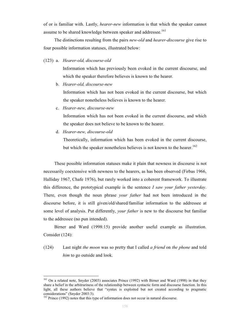
158

of or is familiar with. Lastly, hearer-new information is that which the speaker cannot

assume to be shared knowledge between speaker and addressee.161

The distinctions resulting from the pairs new-old and hearer-discourse give rise to

four possible information statuses, illustrated below:

(123) a. Hearer-old, discourse-old

Information which has previously been evoked in the current discourse, and

which the speaker therefore believes is known to the hearer.

b. Hearer-old, discourse-new

Information which has not been evoked in the current discourse, but which

the speaker nonetheless believes is known to the hearer.

c. Hearer-new, discourse-new

Information which has not been evoked in the current discourse, and which

the speaker does not believe to be known to the hearer.

d. Hearer-new, discourse-old

Theoretically, information which has been evoked in the current discourse,

but which the speaker nonetheless believes is not known to the hearer.162

These possible information statuses make it plain that newness in discourse is not

necessarily coextensive with newness to the hearers, as has been observed (Firbas 1966,

Halliday 1967, Chafe 1976), but rarely worked into a coherent framework. To illustrate

this difference, the prototypical example is the sentence I saw your father yesterday.

There, even though the noun phrase your father had not been introduced in the

discourse before, it is still given/old/shared/familiar information to the addressee at

some level of analysis. Put differently, your father is new to the discourse but familiar

to the addressee (no pun intended).

Birner and Ward (1998:15) provide another useful example as illustration.

Consider (124):

(124) Last night the moon was so pretty that I called a friend on the phone and told

him to go outside and look.

161 On a related note, Snyder (2003) associates Prince (1992) with Birner and Ward (1998) in that they share a belief in the arbitrariness of the relationship between syntactic form and discourse function. In this light, all these authors believe that “syntax is exploited but not created according to pragmatic considerations” (Snyder 2003:3). 162 Prince (1992) notes that this type of information does not occur in natural discourse.

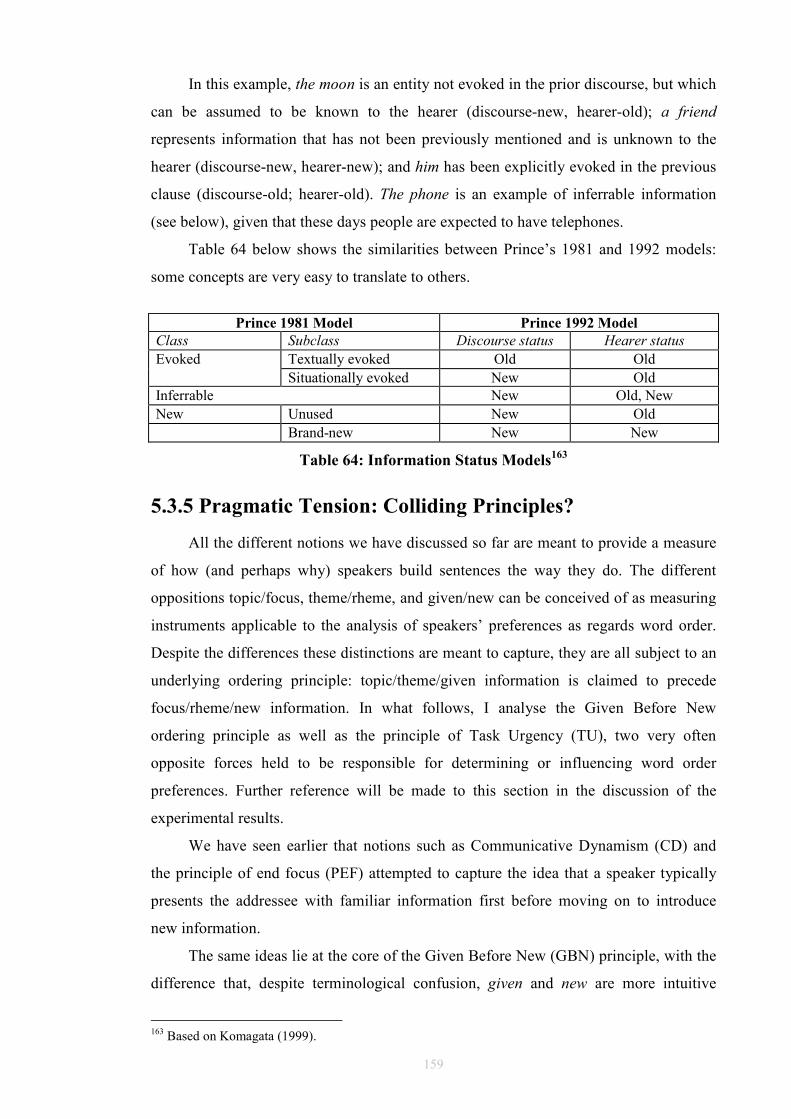
159

In this example, the moon is an entity not evoked in the prior discourse, but which

can be assumed to be known to the hearer (discourse-new, hearer-old); a friend

represents information that has not been previously mentioned and is unknown to the

hearer (discourse-new, hearer-new); and him has been explicitly evoked in the previous

clause (discourse-old; hearer-old). The phone is an example of inferrable information

(see below), given that these days people are expected to have telephones.

Table 64 below shows the similarities between Prince’s 1981 and 1992 models:

some concepts are very easy to translate to others.

Prince 1981 Model Prince 1992 Model

Class Subclass Discourse status Hearer status Textually evoked Old Old Evoked Situationally evoked New Old

Inferrable New Old, New New Unused New Old Brand-new New New

Table 64: Information Status Models163

5.3.5 Pragmatic Tension: Colliding Principles?

All the different notions we have discussed so far are meant to provide a measure

of how (and perhaps why) speakers build sentences the way they do. The different

oppositions topic/focus, theme/rheme, and given/new can be conceived of as measuring

instruments applicable to the analysis of speakers’ preferences as regards word order.

Despite the differences these distinctions are meant to capture, they are all subject to an

underlying ordering principle: topic/theme/given information is claimed to precede

focus/rheme/new information. In what follows, I analyse the Given Before New

ordering principle as well as the principle of Task Urgency (TU), two very often

opposite forces held to be responsible for determining or influencing word order

preferences. Further reference will be made to this section in the discussion of the

experimental results.

We have seen earlier that notions such as Communicative Dynamism (CD) and

the principle of end focus (PEF) attempted to capture the idea that a speaker typically

presents the addressee with familiar information first before moving on to introduce

new information.

The same ideas lie at the core of the Given Before New (GBN) principle, with the

difference that, despite terminological confusion, given and new are more intuitive

163 Based on Komagata (1999).

160

notions. If we abstract away from the coding difficulties, determining an entity’s

information status can be done more or less straightforwardly by taking into account the

preceding discourse and/or the knowledge store called upon by the participants of the

speech event.

A different principle is proposed by Givón (1988), who claims that word order

can be better accounted for with his Task Urgency principle, according to which

speakers need to tailor their utterances so as to attend first to the most urgent task.

Givón’s words, however, fail to specify an operative definition of what he means by

urgent.164 If urgent in his model can be equated with new, then this author is effectively

saying that speakers’ utterances follow a NBG pattern rather than a GBN one. Givón

observes that urgent information is that which is either less predictable, or more

important (1988:264). It is this kind of information which functionally tends to appear

in pre-posed or earlier position in a string. Consider an example from Givón,

reproduced below as (125).

(125) a. He gave the book to Mary.

b. He gave Mary the book.

Example (125) illustrates dative shift in English, whereby the noun phrase Mary is

moved out of a prepositional phrase headed by to and into immediately postverbal

position, the preposition being discarded at the same time. However, this operation

realigns not just syntactic structure, but pragmatic information as well. If the (relative)

position of (to) Mary in (125)a can be explained by claiming that it was more

predictable than the book, and thus placed later in the clause by sheer TU force, then

how to account for the possibility of (125)b with the same (functional) principle? Givón

(1988:273-274) argues that this apparent counter-example is in fact an instance of the

two subcategories of urgent information (predictability and importance) clashing with

each other. According to the predictability principle, Mary should follow the book, since

it is more predictable in context. According to the importance principle, however, Mary

should precede the book, because it is thematically more important: “the language

resolves the conflict by going with the thematic importance clause of ‘task urgency’,

and against the referential predictability clause” (1988:273-275).

164 Snyder is one author who takes exception to Givón’s loose definitions, and discards his model due to this fact. She even suggests that this absence of a precise definition even entails the possibility of the two principles (GBN and Task Urgency) being conflated, if we assume that “what is urgent for the speaker is establishing a frame of syntax and context in which entities representing new information can be more easily processed by the hearer” (2003:16-17).

161

To recap: we have two principles (GBN and TU) purporting to account for the

same range of phenomena, and at loggerheads with each other. In particular, if indeed

urgent is not the same as new, what happens when new information in a clause is also

the most important, i.e. the most urgent?

In reviewing these conflicting principles, Wasow (2002) suggests three ways out

of this quandary. The first is to prove one principle wrong and discard it; the second is

to find a more general principle under which both GBN and Task Urgency can be

subsumed; the third one is to consider both principles not as surefire determinants of

word order, but as optional constraints, a proposal as Snyder (2003:16-17) puts it

very much in line with Optimality Theory (OT). Thinking about TU in terms of

(defeasible) constraints seems indeed to be closer to Givón’s intentions (see Givón

1988:273-274).

Gundel (1988) thinks along similar lines, suggesting that the outcome of the

conflict between the two principles may vary, and that variation ensures that the speaker

is provided with larger communicative options. This author resorts to the opposition

topic/comment rather than given/new.

Recall that in her view topic is an entity about which the speaker intends to

increase the addressee’s knowledge, and comment is a predication intended by the

speaker to be assessed relative to the topic. GBN and TU clash in unmarked cases where

the comment is the most important part of the sentence. If GBN wins out, the result is

one of the constructions in (126), where the topic comes before the comment.

(126) a. The boy, he is from Hawaii. Left dislocated

b. Movies, Rina is crazy about. Topicalized

c. The one who broke the window was Taro. Pseudo-cleft

d. Your battery seems to be dead. Subject-creating165

e. George is difficult to talk to. Subject-creating166

However, if it is TU which emerges victorious, the resulting constructions will be

those in (127), where it is the new comment that precedes the given topic.

(127) a. He’s shrewd, that one. Right dislocated

b. It was Ivan I saw. It-cleft

165 Subject to Subject raising construction. 166 Object to Subject raising construction.

162

Marked sentences usually entail a departure from the canonical topic-comment

ordering, for instance, when there is a shift in topic, or when the topic is contrastive, i.e.

in cases where the topic is new.

Topics are by definition always (relationally) given. This results in a situation

where GBN and TU agree on the ordering, or in Gundel’s words (1988:229), they

“conspire (…) to put topic first”, as can be seen in (126).167

The fact that no language seems to have a syntactic construction placing new

topics after the comment is explained by Gundel by claiming that this hypothetical

construction is an impossibility because it would be inconsistent with either principle.

The experiments reported in the next chapter will make use of the GBN principle

only, for the simple reason that it seems to be the only available one, there being no

clear indication about how to develop a coding scheme for TU.

5.4 Accounts of the Dative Alternation

It was pointed out in the previous sections that certain connections have been identified

between, for instance, given and thematic elements, themes and contexts, and so on.

More specifically, Chafe (1976) compared notions such as givenness, contrastiveness,

definiteness, subjects and topics. The idea gained momentum that information structure

could be reduced to other properties.

Correlations do certainly obtain between givenness and other factors. Take

heaviness, for example. It is generally shorter NPs such as pronouns and names that are

used to refer to information already present in the discourse. By the same token,

information being introduced to the hearer and described for the first time usually needs

a lengthier statement. The question is: how can we be certain that, for instance, it is the

length of the noun phrase which is a consequence of its givenness, or for that matter,

that givenness is a consequence of length? Are these notions two different factors, is

one causing the other, or does it simply look like causation because both are so heavily

correlated? Some observed tendencies may be only secondary consequences of more

fundamental determinants.

When correlations occur between two elements, the researcher is faced with two

alternatives: either straightforwardly reducing one to the other, or teasing the two apart

in order to contrast them and ascertain which of the two is indeed subordinate to the

other. This latter alternative is useful in that it lends more precision to the research and

167 This is rather a disingenuous solution, in that the first element in the examples in (126) is considered to be both (informationally) new and (referentially) given. In this respect, Gundel seems to be attempting to have her cake and eat it too.

163

it endows one factor with a greater explanatory power over other, different factor/s. In

what follows I intend to provide some background to the question of how other factors

claimed to affect ordering preferences have been treated in some typical accounts of the

dative alternation. As will be seen, more than one factor can partially explain the same

phenomenon. These competing explanations have been treated in this study as

secondary to the more general GBN principle, for reasons to be discussed later in this

chapter.

5.4.1 Animacy

The information status of a noun phrase has also been claimed to be affected by the

inherent properties of its referent. Thus, animacy has been considered one of the factors

affecting word order. Foley and Van Valin (1985:288) place animacy in the wider

context of salience, and resort to the Silverstein Hierarchy (Silverstein 1976).

Speaker/addressee > 3rd person pronouns > human proper Ns > human common Ns > other animate Ns > inanimate Ns

This hierarchy finds a precedent in Jespersen (1927), and followers in Dowty

(1979) and Givón (1984). The basic idea is that the referents of noun phrases can be

classified in terms of their position on this sliding scale: noun phrases whose referents

rank higher in the Silverstein hierarchy tend to occupy more prominent syntactic

positions than noun phrases lower on it.168 For example, speech act participants (speaker

and addressee) are more salient than the (potentially absent) participant/s of the third

person, humans are more salient than other animate beings, and these in turn are more

salient than inanimate entities.

In Foley and Van Valin’s view, dative shift is to be understood as an operation (in

keeping with a rule noted in many languages) which takes non-undergoer arguments

(i.e. the one instantiated in the prepositional phrase) and makes them undergoers. A

verb such as give requires three core arguments, namely an actor (the giver), an

undergoer (the gift), and a recipient (the receiver). Dative shift allows the speaker to

rearrange the arguments in order to assign undergoer status to a different core argument.

Animacy has a role to play: since it is usually the case that noun phrases realising

recipient arguments refer to animate beings (i.e. they are higher up in the Silverstein

hierarchy than those noun phrases realising undergoer arguments), it is to be expected

that they occupy a more topical position closer to the verb. This rearrangement has a

168 In this light, subjects are syntactically more prominent than objects, and indirect objects more prominent than direct objects, but less so than subjects.

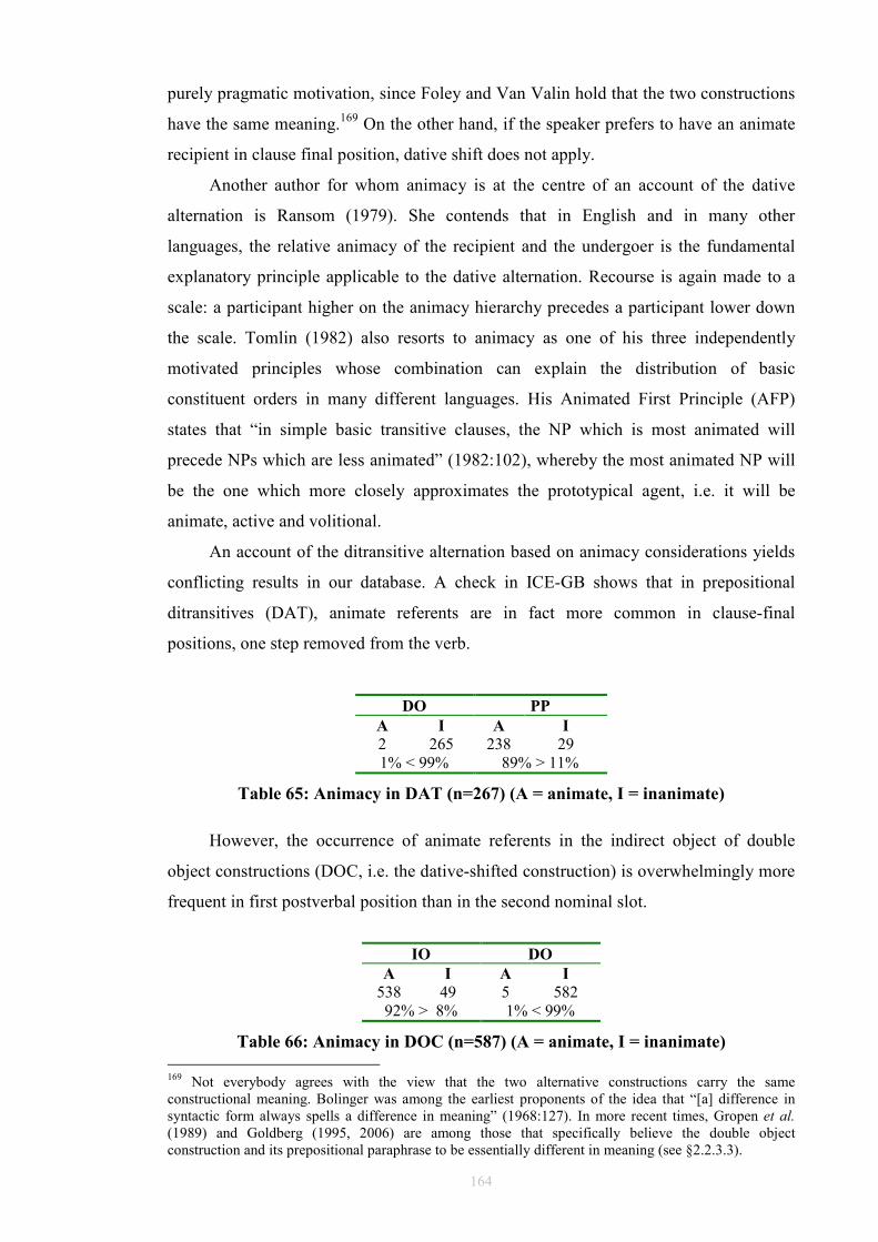
164

purely pragmatic motivation, since Foley and Van Valin hold that the two constructions

have the same meaning.169 On the other hand, if the speaker prefers to have an animate

recipient in clause final position, dative shift does not apply.

Another author for whom animacy is at the centre of an account of the dative

alternation is Ransom (1979). She contends that in English and in many other

languages, the relative animacy of the recipient and the undergoer is the fundamental

explanatory principle applicable to the dative alternation. Recourse is again made to a

scale: a participant higher on the animacy hierarchy precedes a participant lower down

the scale. Tomlin (1982) also resorts to animacy as one of his three independently

motivated principles whose combination can explain the distribution of basic

constituent orders in many different languages. His Animated First Principle (AFP)

states that “in simple basic transitive clauses, the NP which is most animated will

precede NPs which are less animated” (1982:102), whereby the most animated NP will

be the one which more closely approximates the prototypical agent, i.e. it will be

animate, active and volitional.

An account of the ditransitive alternation based on animacy considerations yields

conflicting results in our database. A check in ICE-GB shows that in prepositional

ditransitives (DAT), animate referents are in fact more common in clause-final

positions, one step removed from the verb.

DO PP

A I A I

2 265 238 29 1% < 99% 89% > 11%

Table 65: Animacy in DAT (n=267) (A = animate, I = inanimate)

However, the occurrence of animate referents in the indirect object of double

object constructions (DOC, i.e. the dative-shifted construction) is overwhelmingly more

frequent in first postverbal position than in the second nominal slot.

IO DO

A I A I

538 49 5 582 92% > 8% 1% < 99%

Table 66: Animacy in DOC (n=587) (A = animate, I = inanimate)

169 Not everybody agrees with the view that the two alternative constructions carry the same constructional meaning. Bolinger was among the earliest proponents of the idea that “[a] difference in syntactic form always spells a difference in meaning” (1968:127). In more recent times, Gropen et al. (1989) and Goldberg (1995, 2006) are among those that specifically believe the double object construction and its prepositional paraphrase to be essentially different in meaning (see §2.2.3.3).

165

It therefore seems that there is interaction between animacy and argument

structure. Animacy appears to be correlated with the recipient role, but fails to fully

explain the alternation.170 Still, an explanation of dative shift in terms of animacy

considerations is not to be straightforwardly discarded.171

5.4.2 Definiteness

New information is more often than not introduced by indefinite expressions and at later

stages referred to by means of definite expressions. Furthermore, given, identifiable

information is almost invariably represented by definite noun phrases and/or anaphoric

elements. Brown and Yule (1983:171) count the following among the syntactic forms

usually associated with given information.

• Lexical units which are mentioned for the second time, particularly those in

definite expressions, e.g. I saw a dog. The dog was black.

• Lexical units which are presented as being within the semantic field of a

previously mentioned lexical unit, again particularly those in definite

expressions, e.g. We had a picnic last Sunday. The beer was warm.

• Pronominals used anaphorically following a full lexical form in the preceding

sentence, e.g. The jewels looked expensive. I later learned they were stolen.

• Pronominals used exophorically where the referent is present, e.g. I’m not eating

that.

• Pro-verbals, e.g. He is always threatening to top himself, but he never actually

does.

There seems to be a correlation between, on the one hand, definiteness and

givenness; and on the other, between newness and indefiniteness. It is therefore not

surprising that definiteness has been taken as an indicator of givenness.

170 Attempting to arrive at inductive predictions from the dataset is a different matter. The problem can be stated rather siemply: if a recipient is animate, what are its chances of being DOC or DAT? In fact, most recipients are animate! 171 Bresnan and Hay (2008) report that recent studies involving multiple variables (Gries 2003b, Bresnan et al. 2007) have shown that the predictive power of animacy is not reducible to any of the other variables (information status, weight, complexity, etc.).

166

But this relationship is not symmetrical: while it is true that given elements are

usually definite, it is not necessarily true that definite elements are always given.172 As

Chafe points out, it not unusual to find sentences like I talked with the carpenter

yesterday, in which the carpenter is definite but somehow new (textually irretrievable).

He goes on: “[i]n such cases, the definiteness is established on some other basis than

immediately prior mention, which would create givenness as well” (1976:42), where

givenness is defined as presence in the addressee’s consciousness. The example above

(We had a picnic last Sunday. The beer was warm.) is a case in point, where the

givenness of the noun phrase is established by recourse to a set of extra-linguistic

expectations (known in other frameworks as frames or schemas, see also §6.3.2) usually

associated with a picnic.

According to Foley and Van Valin (1985), the information status of a noun phrase

in discourse is dependent on three factors: reference, definiteness and givenness (the

latter just discussed). Reference is a term used to assess whether a noun phrase refers to

an entity in the world, e.g. in (128) below, only the first noun phrase is referential.

(128) The boy saw the unicorn.

Definiteness allows the speaker to assume that the hearer can individuate the

referent of the noun phrase, a situation which obtains with the boy but not with the

unicorn.173 But when it comes to the indefinite article, reference and its attendant notion

of definiteness are not as useful as they could be, precisely because the indefinite article

can mark both referential and non-referential indefinite noun phrases, as illustrated in

(129) below.

(129) a. I’m looking for a snake (which has just escaped from my lab: referential).

b. I’m looking for a snake (for my son: non-referential).

Different frameworks have had to grapple with this uneven relation between

givenness and definiteness, and their associated theory-internal implications. For

example, in the framework of Dominance Theory (Erteschik-Shir 1979), the determiner

system plays a major role in indicating the dominance of a noun phrase, whereby

172 The same applies to new information and indefinites: while new information tends to be expressed by means of indefinites, this tendency cannot be turned into a rule, i.e. stating that indefinites can only represent new information is simply a misleading overgeneralisation. 173 Still, it can also be claimed that the unicorn is indeed referential in context, e.g. in the framework of a story.

167

dominance is the quality of a constituent towards which the speaker intends to direct the

attention of the addressee/s.174 Determiners form a hierarchy according to the degree of

specificity, a closely-related notion to that of definiteness.175 Erteschik-Shir mentions

that indefinite determiners are generally used to indicate that the noun phrase is

dominant (although it can be non-dominant too). Definites in general are used to

indicate that the noun phrase is non-dominant, whereas pronouns cannot possibly be

used dominantly.

Another example of awareness of the mismatch between given information and

definite noun phrases is found in Functional Sentence Perspective (FSP), where Firbas

(1992:14) states that “information marked by the definite article as known [given]

cannot always be regarded as such from the point of view of FSP”.

Li and Thompson (1976) and Gundel (1988) observe that in some languages

definite expressions refer necessarily to topics, and in English in particular, only

definite noun phrases can occur as dislocated topics.

(130) a. The/*A window, it’s still open.

b. It’s still open, the/*a window.

Noting that the converse is also true in many languages, i.e. that expressions

referring to topics are necessarily definite, Gundel (1988:213-215) even makes this

relation between definiteness and (by proxy, by way of topicality) givenness into a

condition, which she calls the Topic-Identifiability Condition.

Topic-Identifiability Condition: An expression, E, can successfully refer to a topic, T, iff E is of a form that allows the addressee to uniquely identify T.

In Gundel’s view, then, what distinguishes definite noun phrases from indefinite

ones is “the assumed identifiability of the referent”.

Givón is another author (2001) calling upon the notion of definiteness in his

account of the effects of the dative alternation. He notes that in ditransitive clauses the

indirect object is generally more topical than the direct object. Since topical objects are

usually highly predictable and rooted in the preceding context, indirect objects tend to

be overwhelmingly definite and anaphoric.176 The dative alternation moves the noun

phrase embedded in a prepositional phrase to a position prototypically occupied by

174 Dominance Theory is dealt with in more detail in the next section (§5.4.3). 175 For a very detailed analysis of definiteness, genericness and specificity, see Lyons (1995). 176 All the same, Hawkins (1994:111) points out that “if definite [usually shorter] items generally precede indefinite ones, this could be because short items are predicted to precede longer ones in that structure and language, or because of their information status.” Definiteness on its own cannot settle the argument.

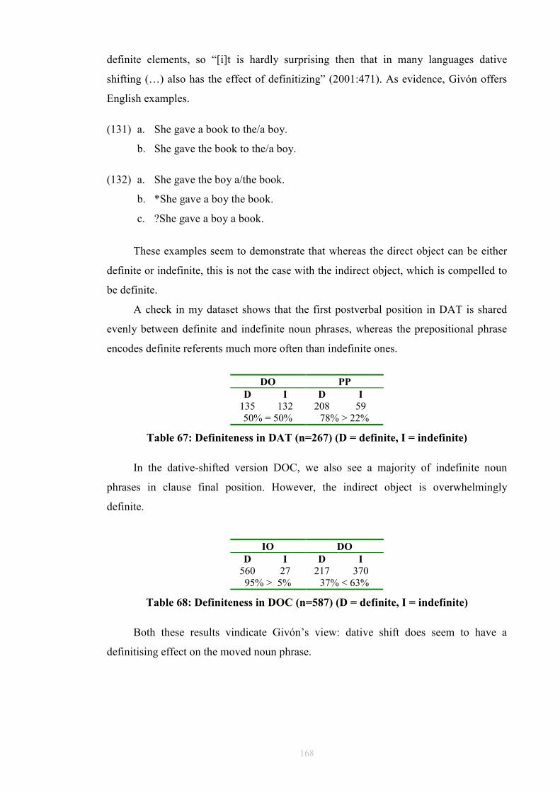
168

definite elements, so “[i]t is hardly surprising then that in many languages dative

shifting (…) also has the effect of definitizing” (2001:471). As evidence, Givón offers

English examples.

(131) a. She gave a book to the/a boy.

b. She gave the book to the/a boy.

(132) a. She gave the boy a/the book.

b. *She gave a boy the book.

c. ?She gave a boy a book.

These examples seem to demonstrate that whereas the direct object can be either

definite or indefinite, this is not the case with the indirect object, which is compelled to

be definite.

A check in my dataset shows that the first postverbal position in DAT is shared

evenly between definite and indefinite noun phrases, whereas the prepositional phrase

encodes definite referents much more often than indefinite ones.

DO PP

D I D I

135 132 208 59 50% = 50% 78% > 22%

Table 67: Definiteness in DAT (n=267) (D = definite, I = indefinite)

In the dative-shifted version DOC, we also see a majority of indefinite noun

phrases in clause final position. However, the indirect object is overwhelmingly

definite.

IO DO

D I D I

560 27 217 370 95% > 5% 37% < 63%

Table 68: Definiteness in DOC (n=587) (D = definite, I = indefinite)

Both these results vindicate Givón’s view: dative shift does seem to have a

definitising effect on the moved noun phrase.

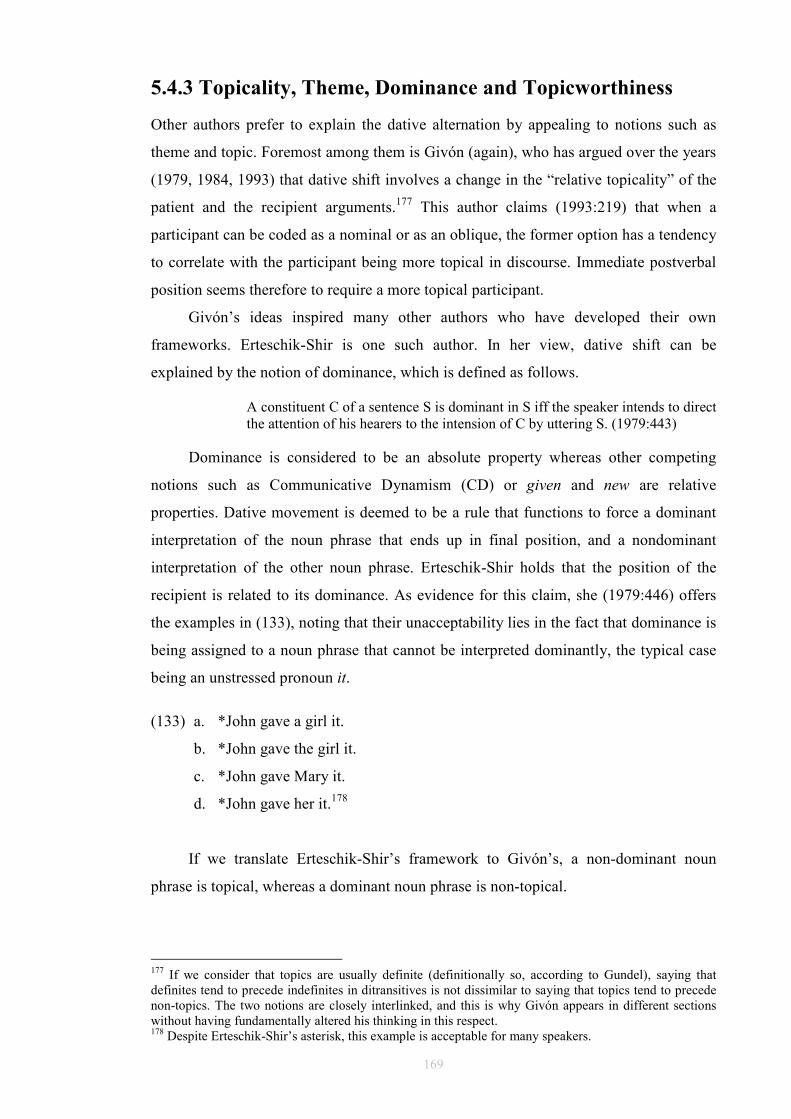
169

5.4.3 Topicality, Theme, Dominance and Topicworthiness

Other authors prefer to explain the dative alternation by appealing to notions such as

theme and topic. Foremost among them is Givón (again), who has argued over the years

(1979, 1984, 1993) that dative shift involves a change in the “relative topicality” of the

patient and the recipient arguments.177 This author claims (1993:219) that when a

participant can be coded as a nominal or as an oblique, the former option has a tendency

to correlate with the participant being more topical in discourse. Immediate postverbal

position seems therefore to require a more topical participant.

Givón’s ideas inspired many other authors who have developed their own

frameworks. Erteschik-Shir is one such author. In her view, dative shift can be

explained by the notion of dominance, which is defined as follows.

A constituent C of a sentence S is dominant in S iff the speaker intends to direct the attention of his hearers to the intension of C by uttering S. (1979:443)

Dominance is considered to be an absolute property whereas other competing

notions such as Communicative Dynamism (CD) or given and new are relative

properties. Dative movement is deemed to be a rule that functions to force a dominant

interpretation of the noun phrase that ends up in final position, and a nondominant

interpretation of the other noun phrase. Erteschik-Shir holds that the position of the

recipient is related to its dominance. As evidence for this claim, she (1979:446) offers

the examples in (133), noting that their unacceptability lies in the fact that dominance is

being assigned to a noun phrase that cannot be interpreted dominantly, the typical case

being an unstressed pronoun it.

(133) a. *John gave a girl it.

b. *John gave the girl it.

c. *John gave Mary it.

d. *John gave her it.178

If we translate Erteschik-Shir’s framework to Givón’s, a non-dominant noun

phrase is topical, whereas a dominant noun phrase is non-topical.

177 If we consider that topics are usually definite (definitionally so, according to Gundel), saying that definites tend to precede indefinites in ditransitives is not dissimilar to saying that topics tend to precede non-topics. The two notions are closely interlinked, and this is why Givón appears in different sections without having fundamentally altered his thinking in this respect. 178 Despite Erteschik-Shir’s asterisk, this example is acceptable for many speakers.

170

In his 1986 book, Tomlin contends that basic word order is ruled by three

principles, with a range of applications across languages: Verb-Object Bonding

(discussed in §2.2.1), the Animated First Principle (see §5.4.1), and the Theme First

Principle. The latter, Tomlin holds, constrains the triggering of certain syntactic

alternations, of which the dative alternation is one. Tomlin focuses on the fact that in a

double object construction, a pronominal object cannot occur in final position, e.g. in I

gave them to Mary, the nominal them occurs in an infelicitous position after dative shift

has applied, witness *I gave Mary them. If the use of dative movement is analysed in

discourse, Tomlin suggests, it can be seen that speakers “prefer dative-moved [i.e.

double object] sentences embedded in paragraphs where the text prior to the dative-

moved sentence dealt with possible recipients” (1986:68). The more established the

recipient is in the discourse (i.e. the more given it is), the higher its chances of

occupying immediate postverbal (thematic) position, leaving the focal position at the

end of the clause for the less or non-established participant, the patient. On the other

hand, when the preceding context deals with objects for giving, double object sentences

are avoided, since they would place a thematic element towards the end of the clause.

Thompson (1987, 1990) is another author using Givón’s ideas to study the dative

alternation. She revamps Givón’s notion of topicality into a new concept of

topicworthiness, defined (1990:241) as “the likelihood of a noun phrase being the topic

of discussion”, and claimed to be measurable in terms of a cluster of properties.179

Typically, then, a topicworthy entity is definite, specific, animate (usually a pronoun or

a proper noun), and relatedly, short and given.

In her experiments, based on 196 clauses extracted from two murder mysteries

and a personal narrative, Thompson sets out to demonstrate that the dative alternation is

not an optional operation but, rather, is determined by the speaker’s need to manage

information flow. The choice of formulation for a recipient (noun phrase or

prepositional phrase) is claimed to be critically influenced by information flow.

Thompson’s work confirms hypotheses which are not dissimilar to those we have

already seen in the work of Givón and Tomlin, namely that when more than one

argument is eligible for immediately postverbal position, the more topicworthy one

(with the exception of the subject) wins. This results in recipients in double object

constructions being more topicworthy (and therefore occurring earlier) than recipients in

the prepositional alternants.

179 The term topicworthiness is explained by the fact that these properties are identical to those usually found in grammatical subjects, which Thompson claims are the “grammaticization” of discourse topics.

171

In a later paper (1995), Thompson finds a new twist to her notion of

topicworthiness: iconicity.180 Her “iconicity hypothesis for dative shift” states that “[o]f

the two positions in which recipients can occur, those recipients which occur in the

earlier (i.e. postverbal) position can be shown to be conceptually closer to the preceding

discourse material than those recipients which occur in the later (i.e. the end) position”

(1995:168).181 More simply put, high topicworthiness predicts immediately postverbal

position.

Topicworthiness has not been experimentally tested in my database, simply

because it subsumes under a single name very different concepts already proposed as

likely explanations for the ditransitive alternation (e.g. definiteness, animacy, givenness

and length), most of which are more easily coded (although not always amenable to an

accurate definition).

The following chapter evaluates (against a corpus) some of the models discussed

so far which account for the dative alternation by giving a central explanatory role to the

information status of the arguments participating in ditransitive complementation. As

such, it can be viewed as a companion chapter to this one.

180 Snyder points out (2003) that Thompson is here joining other linguists such as Haiman (1985), Langacker (1991), as well as Givón (1993) who maintain that pragmatic factors and linguistic structure are iconically connected, and more importantly, cognitively significant. Snyder (2003:2) goes on: “On this view, the association between a particular linguistic form and its discourse function is non-accidental and by design: a discourse function is associated with a particular form because that form is the best possible form to convey the relevant function”. This view is opposed to those held by e.g. Prince (1992) and Birner and Ward (1998). 181 For instance, the fact that in John taught Harry maths there is an implication that Harry actually learnt something about maths (an implication which is absent in John taught maths to Harry) is a measure of the fact that Harry is “conceptually closer to the preceding discourse material.”

172

6 Testing the Theories: Given Before New (GBN)

6.1 Introduction: Corpus Experimentation

By and large, speakers have more than one alternative as regards couching the same

propositional meaning in clauses. In this chapter I explore speakers’ choice of

construction between a ditransitive verb taking, on the one hand, two nominal

complements (e.g. John gave Mary a book) which I have called the double object

construction (DOC) and on the other, a nominal complement followed by a

prepositional phrase (e.g. give a book to John), which I have called DAT (dative).182

This constructional choice will be investigated in relation with the information status of

the referents of the noun phrases involved. In §6.2.2, §6.3.2 and §6.4.1, I will proceed to

make clear which senses of the terms given and new are the ones employed in the

corpus experiments. The underlying assumption is that speakers do not toss a coin when

they have a constructional choice to make, but rather that, in Birner and Ward’s words

(1998:1), “speakers exploit their structural options to specific pragmatic ends”.

6.2 Corpus Experiment 1: GBN by Textual

Retrievability

This section introduces a corpus experiment designed to test the effect of the

informational status of (the referents of) the noun phrases involved in ditransitive

complementation, or, more specifically, to put the Given Before New principle to the

test. In this experiment, given and new are coded using the criterion of textual

retrievability. Design issues relative to the dataset, experiments, definitional criteria,

underlying assumptions, and resulting exclusions have been discussed in chapter 4.183

Can corpus studies help track and confirm or disconfirm the conditions of use of these

constructions?

6.2.1 The GBN Principle

Given that the possibility of indirect objects alternating with prepositional paraphrases

involves rearranging clause elements (rearrangement often explained in terms of

182 The use of theoretically-loaded terms such as dative, dative shift or double object construction is not synonymous with any kind of commitment on the part of the author to any specific theoretical model. 183 Parts of this section were presented at the ICAME 2003 Conference in Guernsey. An article version appeared in A. Renouf and A. Kehoe (eds.) The Changing Face of Corpus Linguistics, Amsterdam: Rodopi (2006:243-262). Some minor changes to my dataset have taken place since the paper submission deadline.

173

information status), I looked into the application of the Given Before New principle to

the corpus dataset. I used retrievability/irretrievability from context as the benchmark

for stating that a constituent (or rather, its referent) is either given or new. Since it is

very usually the case that the more firmly rooted an element is in the context, the less

(explicit) information it tends to carry, I will assume that GBN is also a measure of

accessibility.

6.2.2 Retrievability

As mentioned, textual retrievability is the sole criterion used to determine the givenness

of a referent, an idea which is in line with the framework of Functional Sentence

Perspective (FSP). Firbas, one of FSP’s leading proponents, suggested (1992:22) that

the overruling criterion for branding a nominal group as either given or new is its

retrievability (see §5.3.4.1), while at the same time warning us of a distinction between

(a) “information that not only conveys common knowledge shared by the interlocutors,

but is fully retrievable from the context”, and (b) “information that, though conveying

knowledge shared by the interlocutors, must be considered unknown (…) and in this

sense irretrievable from the context”, anticipating in this way the hearer-old/discourse-

old distinction of Prince (1992), as discussed in §5.3.4.2.184

Notice the correlation in the above quote between the textual and the

psychological spheres of givenness. If the referent of the noun phrase is textually

retrievable (i.e. explicit), it is also shared psychologically, in that it is information

common willy nilly to interlocutors. If we invert the relation, information that is

shared between speakers can be either retrievable (i.e. anaphorically present in the

preceding context) or irretrievable (I saw your father yesterday, where your father is

definitely known information to the interlocutors, despite not having been mentioned

previously).185 Using retrievability in context provides a more solid indicator of

givenness, in that it should account for more cases. This was a core assumption for the

selection of retrievability as an operational criterion.

In this experiment, the term given is subdivided into:

184 Note that Firbas (1992) is a collection of much earlier work by the same author. 185 Prince (1992) mentions that the combination ‘retrievable and not shared’ does not occur in natural discourse.

174

• Situationally given: noun phrases whose referents are salient in the discourse

context. This category was limited mainly to exophoric pronouns (e.g. I’m not

eating that), and other deictic elements (you, me).

• Textually given: noun phrases whose referents (or referential links) were present

in the preceding text. These consisted of elements which had already been

introduced in the discourse, mainly definite noun phrases and anaphoric

pronouns.

Every single (postverbal) noun phrase in my database was checked against its

context of occurrence in ICE-GB. Givón’s (1984, 1988) notion of referential distance

was instrumental in determining the coding for textual givenness of the noun phrases in

the database.186 Referential distance is determined by the distance (measured in clauses)

from the noun phrase participating in one of the constructions (DOC and/or DAT) to its

last referent in the preceding discourse. In this experiment, a noun phrase was coded as

given if its referent could be found in the preceding twenty clauses.187 For the purpose

of this experiment, given means ‘retrievable or recoverable from the discourse either

anaphorically or exophorically’. 188 All other cases were coded as new. Pragmatic

inferences and semantic connectedness between elements were not taken into account at

this stage (but see §6.3.1).

The results of this classification are meant to give an approximate measure of the

applicability or predictive power of GBN with respect to the choice of construction. The

related notions of length, weight and complexity are explored in chapter 7.

GBN predicts that (a) the first elements in both DOC and DAT will constitute

given information, and that (b) the second noun phrase in a DOC, and the prepositional

phrase in DAT will include new information. This in turn leads to a number of research

questions: are these predictions true for DOC and DAT, and in both written and spoken

language? Is there a relation between the two objects in DOC in terms of given and new

information? Is there a relation between noun phrase and prepositional phrase in DAT,

again in terms of given and new information?

186 See also Ariel’s (1988) notion of anaphoric distance, §5.3.4.1. 187 The use of an arbitrary 20 clause span was deemed necessary to achieve full coverage. While most of the referents occurred within a 7-to-10 clause span, referring expressions were often anaphorically anchored to a referent located further back. 188 By adopting this methodology, the term given can be equated with referentially given, and not at all with relationally given, if we follow Gundel’s distinction (1988), as seen in §5.3.2.

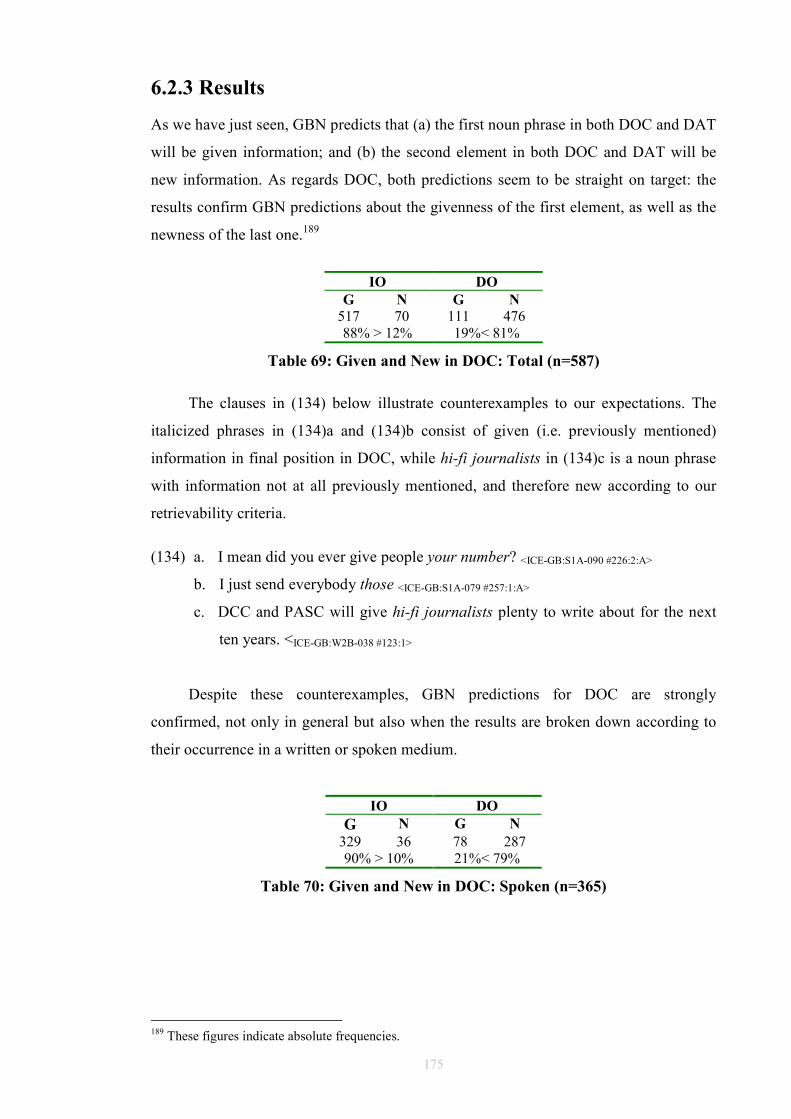
175

6.2.3 Results

As we have just seen, GBN predicts that (a) the first noun phrase in both DOC and DAT

will be given information; and (b) the second element in both DOC and DAT will be

new information. As regards DOC, both predictions seem to be straight on target: the

results confirm GBN predictions about the givenness of the first element, as well as the

newness of the last one.189

IO DO

G N G N

517 70 111 476 88% > 12% 19%< 81%

Table 69: Given and New in DOC: Total (n=587)

The clauses in (134) below illustrate counterexamples to our expectations. The

italicized phrases in (134)a and (134)b consist of given (i.e. previously mentioned)

information in final position in DOC, while hi-fi journalists in (134)c is a noun phrase

with information not at all previously mentioned, and therefore new according to our

retrievability criteria.

(134) a. I mean did you ever give people your number? <ICE-GB:S1A-090 #226:2:A>

b. I just send everybody those <ICE-GB:S1A-079 #257:1:A>

c. DCC and PASC will give hi-fi journalists plenty to write about for the next

ten years. <ICE-GB:W2B-038 #123:1>

Despite these counterexamples, GBN predictions for DOC are strongly

confirmed, not only in general but also when the results are broken down according to

their occurrence in a written or spoken medium.

IO DO

G N G N

329 36 78 287 90% > 10% 21%< 79%

Table 70: Given and New in DOC: Spoken (n=365)

189 These figures indicate absolute frequencies.

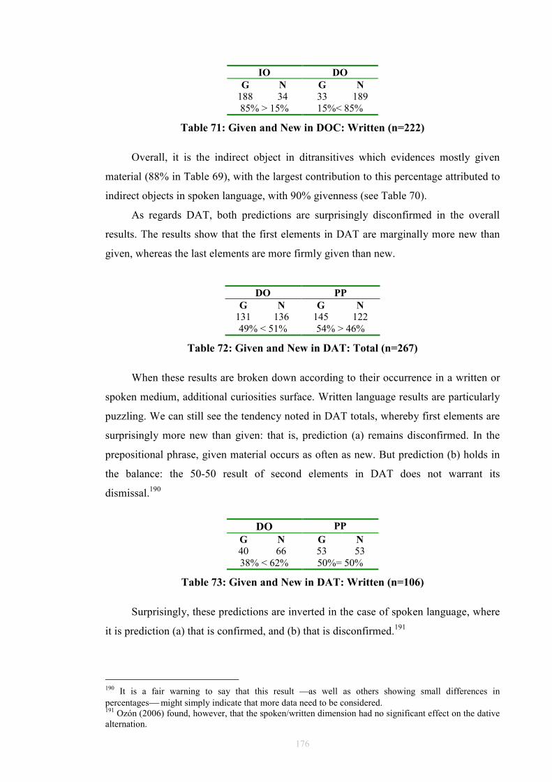
176

IO DO

G N G N

188 34 33 189 85% > 15% 15%< 85%

Table 71: Given and New in DOC: Written (n=222)

Overall, it is the indirect object in ditransitives which evidences mostly given

material (88% in Table 69), with the largest contribution to this percentage attributed to

indirect objects in spoken language, with 90% givenness (see Table 70).

As regards DAT, both predictions are surprisingly disconfirmed in the overall

results. The results show that the first elements in DAT are marginally more new than

given, whereas the last elements are more firmly given than new.

DO PP

G N G N

131 136 145 122 49% < 51% 54% > 46%

Table 72: Given and New in DAT: Total (n=267)

When these results are broken down according to their occurrence in a written or

spoken medium, additional curiosities surface. Written language results are particularly

puzzling. We can still see the tendency noted in DAT totals, whereby first elements are

surprisingly more new than given: that is, prediction (a) remains disconfirmed. In the

prepositional phrase, given material occurs as often as new. But prediction (b) holds in

the balance: the 50-50 result of second elements in DAT does not warrant its

dismissal.190

DO PP

G N G N

40 66 53 53 38% < 62% 50%= 50%

Table 73: Given and New in DAT: Written (n=106)

Surprisingly, these predictions are inverted in the case of spoken language, where

it is prediction (a) that is confirmed, and (b) that is disconfirmed.191

190 It is a fair warning to say that this result as well as others showing small differences in percentages might simply indicate that more data need to be considered. 191 Ozón (2006) found, however, that the spoken/written dimension had no significant effect on the dative alternation.

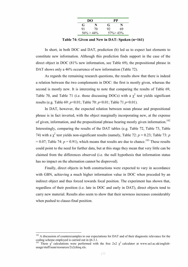
177

DO PP

G N G N

91 70 92 69 56% > 44% 57%> 43%

Table 74: Given and New in DAT: Spoken (n=161)

In short, in both DOC and DAT, prediction (b) led us to expect last elements to

constitute new information. Although this prediction finds support in the case of the

direct object in DOC (81% new information, see Table 69), the prepositional phrase in

DAT shows only a 46% occurrence of new information (Table 72).

As regards the remaining research questions, the results show that there is indeed

a relation between the two complements in DOC: the first is mostly given, whereas the

second is mostly new. It is interesting to note that comparing the results of Table 69,

Table 70, and Table 71 (i.e. those discussing DOCs) with a χ2 test yields significant

results (e.g. Table 69: p<0.01; Table 70: p<0.01; Table 71 p<0.01).

In DAT, however, the expected relation between noun phrase and prepositional

phrase is in fact inverted, with the object marginally incorporating new, at the expense

of given, information, and the prepositional phrase bearing mostly given information.192

Interestingly, comparing the results of the DAT tables (e.g. Table 72, Table 73, Table

74) with a χ2 test yields non-significant results (namely, Table 72: p = 0.23; Table 73: p

= 0.07; Table 74: p = 0.91), which means that results are due to chance.193 These results

could point to the need for further data, but at this stage they mean that very little can be

claimed from the differences observed (i.e. the null hypothesis that information status

has no impact on the alternation cannot be disproved).

Finally, direct objects in both constructions were expected to vary in accordance

with GBN, achieving a much higher information value in DOC when preceded by an

indirect object and thus forced towards focal position. The experiment has shown that,

regardless of their position (i.e. late in DOC and early in DAT), direct objects tend to

carry new material. Results also seem to show that their newness increases considerably

when pushed to clause-final position.

192 A discussion of counterexamples to our expectations for DAT and of their diagnostic relevance for the coding scheme employed is carried out in §6.3.1. 193 These χ2 calculations were performed with the free 2x2 χ2 calculator at www.ucl.ac.uk/english-usage/staff/sean/resources/2x2chisq.xls.

178

6.2.4 Preliminary Consideration of the Results

I have examined speakers’ syntactic choices in ICE-GB in order to look into the

possible application of the principle of GBN to real data. The results confirmed the

predictions for DOC. As for DAT, the experiment failed to support both the givenness

of the first element, as well as the newness of the last one. These results do not seem to

lend blind support to GBN. This could be rooted in the fact that the criterion used in this

experiment for separating given and new, i.e. textual retrievability, can be misleading

inasmuch as it can eclipse other factors which also affect the choice of construction.

In view of these results, it may be tempting to conclude that GBN does not work

with real data, which is more unruly than introspective data. However, a more cautious

approach is called for. The experimental results are better viewed as non-conclusive:

after all, they do confirm GBN predictions for DOC, and thus cannot be discarded

straightaway. On the other hand, results fail marginally at least to produce the same

confirmation in DAT. I believe this experiment shows that textual retrievability cannot

be the only measure for determining the givenness of an expression. To be more

representative, the coding scheme needs to be refined in order to distinguish other

elements. A similar category to Prince’s notion of inferrable elements (see §5.3.4.2) is

employed in the next section.

6.3 Corpus Experiment 2: GBN, Retrievability and

‘Inferrables’

The purpose of this section is still to test the validity of the GBN principle. The

definitional criteria have now been widened to incorporate a middle notion between

clearly given elements and clearly new ones. Besides given and new, inferrable

elements are now also recognised in the coding scheme. The aim of this decision is to

address the shortcomings of (strict) retrievability (discussed below), and thus to refine

and hopefully improve the experimental results.

6.3.1 Textual Retrievability: Shortcomings

Many factors are claimed to affect information ordering in the clause. The experiment

reported in §6.2 attempted to test the predictive power of the GBN principle in

determining speakers’ choices. The investigated constructions, DOC and DAT, give the

speaker the choice of selecting which of the noun phrases in question to postpone and

place in clause final position. It was expected that, regardless of the construction in

179

which they appeared, noun phrases carrying new information would favour clause-final

position. The experiment showed (even if marginally) that this is not necessarily the

case (particularly in DAT constructions), perhaps because it did not take other notions

and principles into account.

Wasow and Arnold (2003:130) suggest that there is another mechanism

underlying GBN: “the desire to put focused, important information at the end i.e.

save the punch line for the end”. Accordingly, speakers will also tend to reserve the

final spot for what they consider to be the focus, the most important part of their

message. Quirk et al. (1985:1356-1357) call this the principle of end focus (PEF). The

problem is, focal information need not be coextensive with new information.

Huddleston and Pullum et al. (2002:1370) illustrate this with the following exchange,

where her is clearly given information in focal position.

(135) A: Did they give the job to you or to Mary?

B: They gave it to her.

These authors hold that this “apparent paradox can be resolved by distinguishing

between the familiarity status of Mary considered as an entity (…), and Mary

considered as the value assigned to the variable in the focus frame They gave it to X”

(2002:1370).194 In (135) the noun phrase Mary is given because she has been mentioned

earlier and is thus identifiable for the addressee, but it is also (focally) new because the

speaker cannot assume that the addressee knows it was Mary who got the job. However,

this type of focal newness went unregistered in the previous experiment, and pronouns

were unfailingly coded as given information. The coding scheme only recognized new,

at the expense of focal, information, as a consequence of using textual retrievability as

the sole criterion.

The unexpected results of the previous experiment may therefore be instantiating

cases in which the dimensions of new and focal information diverge, cases in which

focal information wins the competition with textually (ir)retrievable information for

clause final position, i.e. cases in which PEF outweighs GBN.

The examples below illustrate unexpected patterns in the findings of the previous

experiment. They also illustrate (i) other shortcomings of using textual retrievability as

194 Huddleston and Pullum et al. distinguish between (informational) focus, defined as “an intonationally marked constituent, which typically represents addressee-new information” and the focus-frame, defined in turn as “the residue of the proposition, typically representing addressee-old information” (2002:1370). Other authors have used the same mechanism under different names, e.g. Davidse (1996:303) prefers to use constant/variable instead of focus/focus-frame.

180

a benchmark for determining the givenness of a constituent, and (ii) the interaction of

information status with other notions.

(136) a. I’ve given the title to this lecture of The Immunological Compact Disc <ICE-

GB:S2A-042 #1:1:A>

b. If somebody has just done something to you that you don’t like then you

would <ICE-GB:S1A-037 #250:1:A>

c. I was disappointed that the Belgians felt they shouldn’t supply ammunition to

us <ICE-GB:S2B-013 #90:1:E>

Examples (136)a and (136)b instantiate discontinuous (heavy) noun phrases: the

title … of The Immunological Compact Disc, and something … that you don't like.

These were not excluded from consideration, given that alternation between DOC and

DAT is allowed. However, they presented a problem for the coding: are these

discontinuous noun phrases given or new? Using textual retrievability allows only the

preceding context to make the decision: if a phrase was mentioned previously, it is

given; in all other cases, it is new. Both noun phrases in italics in (136)a and (136)b

were coded as new, since both the title and something were irretrievable from either text

or situation.

Example (136)c illustrates the necessity for taking notions of semantic

connectedness into account when coding for information status. In the preceding twenty

clauses, there was no previous mention of ammunition to consider it a given element.

However, there was talk of armaments and foreign policy, and ammunition clearly has a

place in that semantic field. Despite this, ammunition was coded as a new element.

6.3.2 Inferrables

In view of the issues just discussed in the previous section, a middle notion (between

given and new) was thought necessary. Prince (1981:236) suggests the concept of

inferrables: “[a] discourse entity is Inferrable if the speaker assumes the hearer can infer

it, via logical or, more commonly, plausible reasoning, from discourse entities

already Evoked or from other Inferrables”. Inferrables make up an in-between class,

consisting of elements which are not as firmly established in the preceding context as

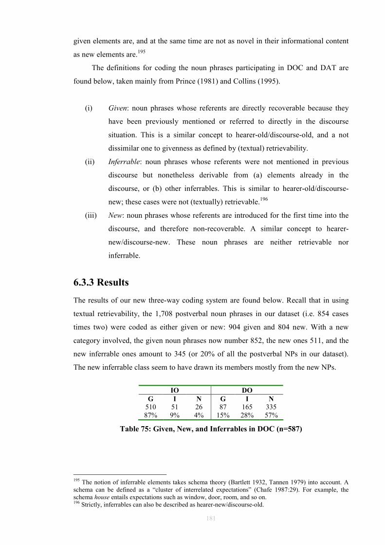
181

given elements are, and at the same time are not as novel in their informational content

as new elements are.195

The definitions for coding the noun phrases participating in DOC and DAT are

found below, taken mainly from Prince (1981) and Collins (1995).

(i) Given: noun phrases whose referents are directly recoverable because they

have been previously mentioned or referred to directly in the discourse

situation. This is a similar concept to hearer-old/discourse-old, and a not

dissimilar one to givenness as defined by (textual) retrievability.

(ii) Inferrable: noun phrases whose referents were not mentioned in previous

discourse but nonetheless derivable from (a) elements already in the

discourse, or (b) other inferrables. This is similar to hearer-old/discourse-

new; these cases were not (textually) retrievable.196

(iii) New: noun phrases whose referents are introduced for the first time into the

discourse, and therefore non-recoverable. A similar concept to hearer-

new/discourse-new. These noun phrases are neither retrievable nor

inferrable.

6.3.3 Results

The results of our new three-way coding system are found below. Recall that in using

textual retrievability, the 1,708 postverbal noun phrases in our dataset (i.e. 854 cases

times two) were coded as either given or new: 904 given and 804 new. With a new

category involved, the given noun phrases now number 852, the new ones 511, and the

new inferrable ones amount to 345 (or 20% of all the postverbal NPs in our dataset).

The new inferrable class seem to have drawn its members mostly from the new NPs.

IO DO

G I N G I N

510 51 26 87 165 335 87% 9% 4% 15% 28% 57%

Table 75: Given, New, and Inferrables in DOC (n=587)

195 The notion of inferrable elements takes schema theory (Bartlett 1932, Tannen 1979) into account. A schema can be defined as a “cluster of interrelated expectations” (Chafe 1987:29). For example, the schema house entails expectations such as window, door, room, and so on. 196 Strictly, inferrables can also be described as hearer-new/discourse-old.

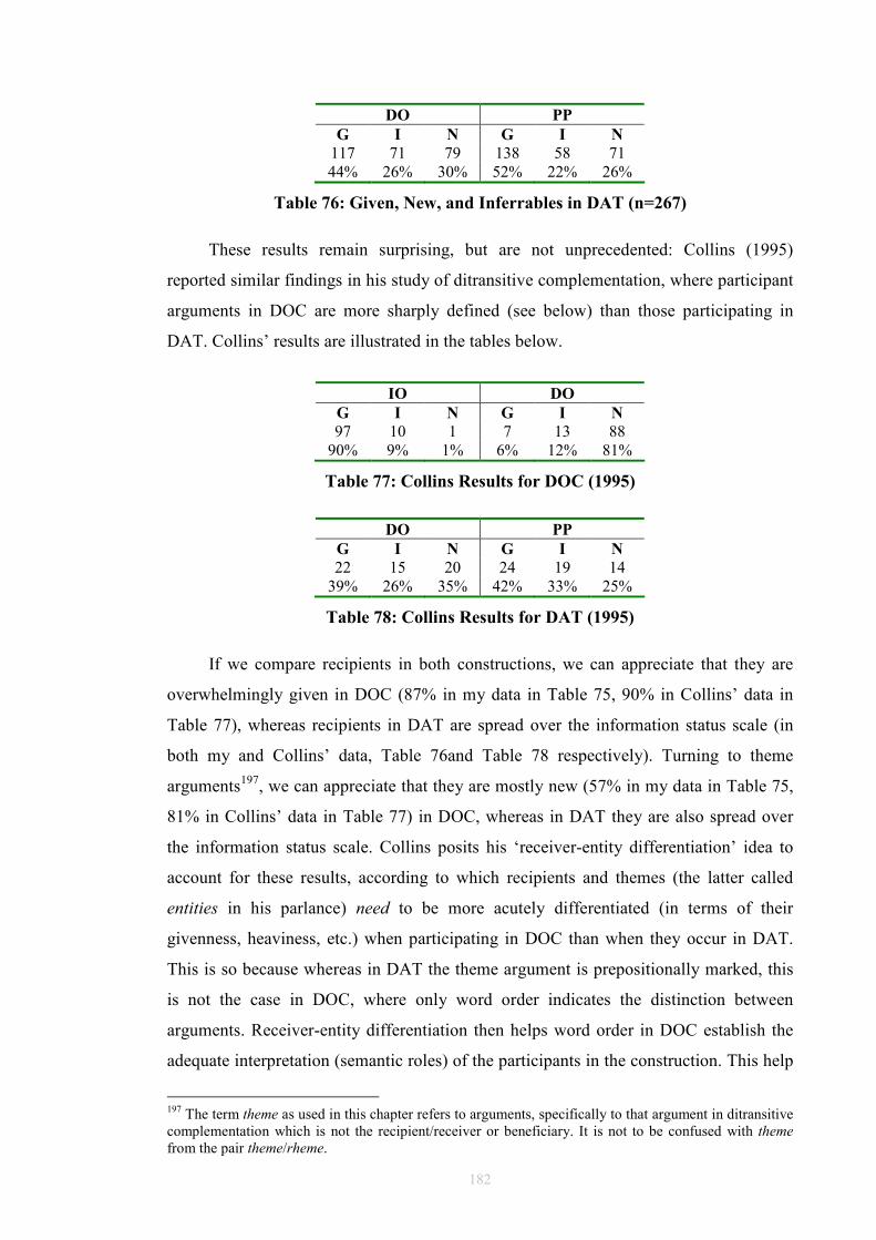
182

DO PP

G I N G I N

117 71 79 138 58 71 44% 26% 30% 52% 22% 26%

Table 76: Given, New, and Inferrables in DAT (n=267)

These results remain surprising, but are not unprecedented: Collins (1995)

reported similar findings in his study of ditransitive complementation, where participant

arguments in DOC are more sharply defined (see below) than those participating in

DAT. Collins’ results are illustrated in the tables below.

IO DO

G I N G I N

97 10 1 7 13 88 90% 9% 1% 6% 12% 81%

Table 77: Collins Results for DOC (1995)

DO PP

G I N G I N

22 15 20 24 19 14 39% 26% 35% 42% 33% 25%

Table 78: Collins Results for DAT (1995)

If we compare recipients in both constructions, we can appreciate that they are

overwhelmingly given in DOC (87% in my data in Table 75, 90% in Collins’ data in

Table 77), whereas recipients in DAT are spread over the information status scale (in

both my and Collins’ data, Table 76and Table 78 respectively). Turning to theme

arguments197, we can appreciate that they are mostly new (57% in my data in Table 75,

81% in Collins’ data in Table 77) in DOC, whereas in DAT they are also spread over

the information status scale. Collins posits his ‘receiver-entity differentiation’ idea to

account for these results, according to which recipients and themes (the latter called

entities in his parlance) need to be more acutely differentiated (in terms of their

givenness, heaviness, etc.) when participating in DOC than when they occur in DAT.

This is so because whereas in DAT the theme argument is prepositionally marked, this

is not the case in DOC, where only word order indicates the distinction between

arguments. Receiver-entity differentiation then helps word order in DOC establish the

adequate interpretation (semantic roles) of the participants in the construction. This help

197 The term theme as used in this chapter refers to arguments, specifically to that argument in ditransitive complementation which is not the recipient/receiver or beneficiary. It is not to be confused with theme from the pair theme/rheme.

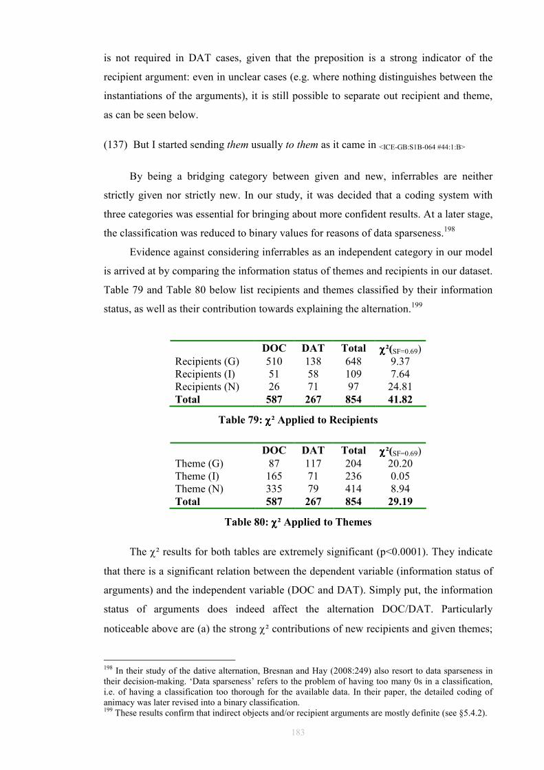
183

is not required in DAT cases, given that the preposition is a strong indicator of the

recipient argument: even in unclear cases (e.g. where nothing distinguishes between the

instantiations of the arguments), it is still possible to separate out recipient and theme,

as can be seen below.

(137) But I started sending them usually to them as it came in <ICE-GB:S1B-064 #44:1:B>

By being a bridging category between given and new, inferrables are neither

strictly given nor strictly new. In our study, it was decided that a coding system with

three categories was essential for bringing about more confident results. At a later stage,

the classification was reduced to binary values for reasons of data sparseness.198

Evidence against considering inferrables as an independent category in our model

is arrived at by comparing the information status of themes and recipients in our dataset.

Table 79 and Table 80 below list recipients and themes classified by their information

status, as well as their contribution towards explaining the alternation.199

DOC DAT Total χχχχ²(SF=0.69) Recipients (G) 510 138 648 9.37 Recipients (I) 51 58 109 7.64 Recipients (N) 26 71 97 24.81 Total 587 267 854 41.82

Table 79: χχχχ² Applied to Recipients

DOC DAT Total χχχχ²(SF=0.69) Theme (G) 87 117 204 20.20 Theme (I) 165 71 236 0.05 Theme (N) 335 79 414 8.94 Total 587 267 854 29.19

Table 80: χχχχ² Applied to Themes

The χ² results for both tables are extremely significant (p<0.0001). They indicate

that there is a significant relation between the dependent variable (information status of

arguments) and the independent variable (DOC and DAT). Simply put, the information

status of arguments does indeed affect the alternation DOC/DAT. Particularly

noticeable above are (a) the strong χ² contributions of new recipients and given themes;

198 In their study of the dative alternation, Bresnan and Hay (2008:249) also resort to data sparseness in their decision-making. ‘Data sparseness’ refers to the problem of having too many 0s in a classification, i.e. of having a classification too thorough for the available data. In their paper, the detailed coding of animacy was later revised into a binary classification. 199 These results confirm that indirect objects and/or recipient arguments are mostly definite (see §5.4.2).

184

and (b) the very poor χ² contribution of inferrables, which are much lower (especially in

the case of themes) than those of given and new recipients or themes. In this light,

grouping inferrables together with other GBN values seems a valid solution to reinforce

predictive accuracy. Indeed, this involves taking a step back, but only in terms of

procedure, not in terms of knowledge discovery. For our model, a new issue raises its

head: where to place this new category?

6.3.3.1 Inferrables as New

As was predictable from §6.3.1, (and is visible in Table 75 and Table 76), the bulk of

the inferrable category had been coded as new with the earlier coding system.

Therefore, treating inferrables as new information is not very fruitful, in that the results

do not offer any improved predictions if compared with strict retrievability, and in fact

revert to very similar figures: notice the similarities between Table 69 and Table 81, on

the one hand; and Table 72 and Table 82, on the other.

IO DO

G N G N

510 77 87 500 87% > 13% 15% < 85%

Table 81: Inferrables as New in DOC (n=587)

DO PP

G N G N

117 150 138 129 44 % < 56% 52% > 48%

Table 82: Inferrables as New in DAT (n=267)

6.3.3.2 Inferrables as Given

Wasow (2002:70) decided to group inferrables together with given entities, since the

inferrable noun phrases in his dataset were not many.200 Let us see the implications of

such a decision for our purposes.

IO DO

G N G N

561 26 252 335 95% > 5% 43% < 57%

Table 83: Inferrables as Given in DOC (n=587)

200 In fact, so few were his inferrables that he suggests in a footnote (2002:70) that he might as well have left them out altogether, since no significant changes would have resulted from that decision.

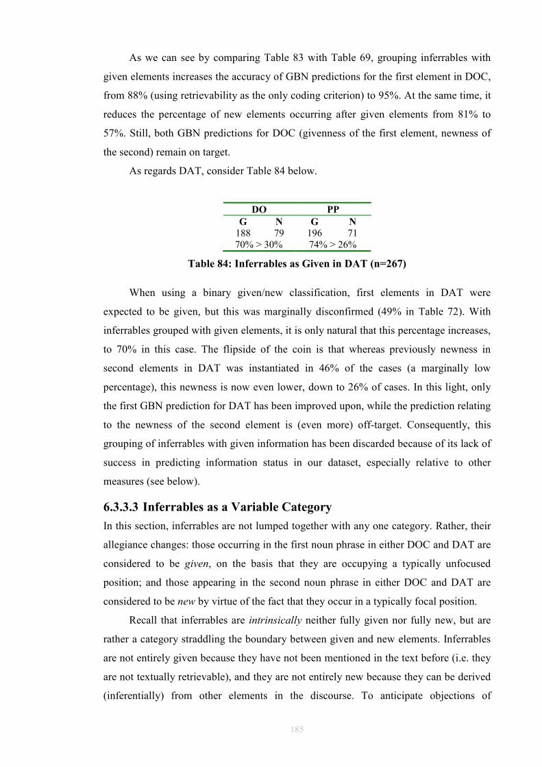
185

As we can see by comparing Table 83 with Table 69, grouping inferrables with

given elements increases the accuracy of GBN predictions for the first element in DOC,

from 88% (using retrievability as the only coding criterion) to 95%. At the same time, it

reduces the percentage of new elements occurring after given elements from 81% to

57%. Still, both GBN predictions for DOC (givenness of the first element, newness of

the second) remain on target.

As regards DAT, consider Table 84 below.

DO PP

G N G N

188 79 196 71 70% > 30% 74% > 26%

Table 84: Inferrables as Given in DAT (n=267)

When using a binary given/new classification, first elements in DAT were

expected to be given, but this was marginally disconfirmed (49% in Table 72). With

inferrables grouped with given elements, it is only natural that this percentage increases,

to 70% in this case. The flipside of the coin is that whereas previously newness in

second elements in DAT was instantiated in 46% of the cases (a marginally low

percentage), this newness is now even lower, down to 26% of cases. In this light, only

the first GBN prediction for DAT has been improved upon, while the prediction relating

to the newness of the second element is (even more) off-target. Consequently, this

grouping of inferrables with given information has been discarded because of its lack of

success in predicting information status in our dataset, especially relative to other

measures (see below).

6.3.3.3 Inferrables as a Variable Category

In this section, inferrables are not lumped together with any one category. Rather, their

allegiance changes: those occurring in the first noun phrase in either DOC and DAT are

considered to be given, on the basis that they are occupying a typically unfocused

position; and those appearing in the second noun phrase in either DOC and DAT are

considered to be new by virtue of the fact that they occur in a typically focal position.

Recall that inferrables are intrinsically neither fully given nor fully new, but are

rather a category straddling the boundary between given and new elements. Inferrables

are not entirely given because they have not been mentioned in the text before (i.e. they

are not textually retrievable), and they are not entirely new because they can be derived

(inferentially) from other elements in the discourse. To anticipate objections of

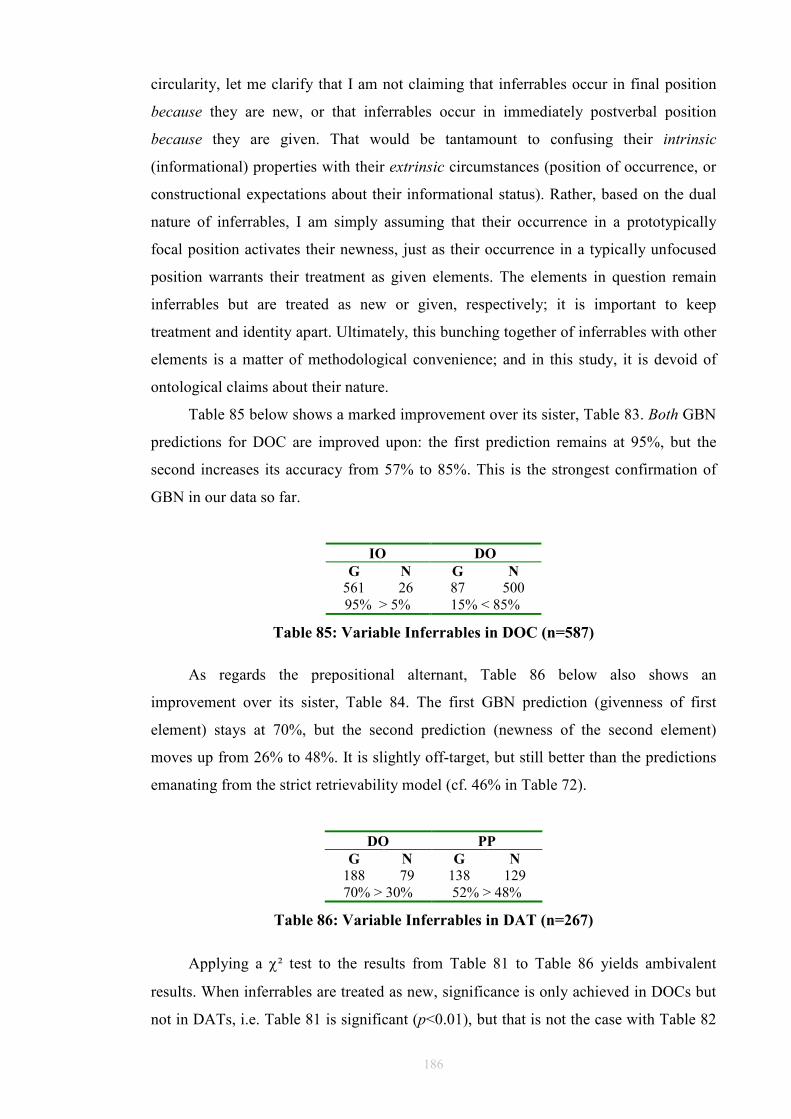
186

circularity, let me clarify that I am not claiming that inferrables occur in final position

because they are new, or that inferrables occur in immediately postverbal position

because they are given. That would be tantamount to confusing their intrinsic

(informational) properties with their extrinsic circumstances (position of occurrence, or

constructional expectations about their informational status). Rather, based on the dual

nature of inferrables, I am simply assuming that their occurrence in a prototypically

focal position activates their newness, just as their occurrence in a typically unfocused

position warrants their treatment as given elements. The elements in question remain

inferrables but are treated as new or given, respectively; it is important to keep

treatment and identity apart. Ultimately, this bunching together of inferrables with other

elements is a matter of methodological convenience; and in this study, it is devoid of

ontological claims about their nature.

Table 85 below shows a marked improvement over its sister, Table 83. Both GBN

predictions for DOC are improved upon: the first prediction remains at 95%, but the

second increases its accuracy from 57% to 85%. This is the strongest confirmation of

GBN in our data so far.

IO DO

G N G N

561 26 87 500 95% > 5% 15% < 85%

Table 85: Variable Inferrables in DOC (n=587)

As regards the prepositional alternant, Table 86 below also shows an

improvement over its sister, Table 84. The first GBN prediction (givenness of first

element) stays at 70%, but the second prediction (newness of the second element)

moves up from 26% to 48%. It is slightly off-target, but still better than the predictions

emanating from the strict retrievability model (cf. 46% in Table 72).

DO PP

G N G N

188 79 138 129 70% > 30% 52% > 48%

Table 86: Variable Inferrables in DAT (n=267)

Applying a χ² test to the results from Table 81 to Table 86 yields ambivalent

results. When inferrables are treated as new, significance is only achieved in DOCs but

not in DATs, i.e. Table 81 is significant (p<0.01), but that is not the case with Table 82

187

(p = 0.07). Similar results are obtained when inferrables are treated as given: Table 83

(p<0.01) is significant, but not Table 84 (p = 0.44). The only case in which both DOC

and DAT are significant is when inferrables are considered a variable category (Table

85: p<0.01; Table 86: p<0.01).201 Thus, treating inferrables as a variable category yields

the best GBN predictors of the three measures considered.

6.3.4 Preliminary Consideration of the Results

In view of the results obtained in §6.3.3, we now have a classification with stronger

predictions. We can therefore now discard both strict retrievability and inferrability as a

subcategory of givenness/newness from our study, since both have been outperformed

at predicting GBN by variable inferrables. At this stage, however, it becomes apparent

that DATs remain rather unmanageable and difficult to predict, especially when

compared with DOCs.

6.4 Corpus Experiment 3: GBN Configurations

This section changes the viewpoint: rather than looking at the information status of each

individual noun phrase in each construction, we now attempt to look at GBN

configurations; i.e. the information status of both noun phrases involved in DOC and

DAT. Section 6.4.4 describes the assignment of a numerical value to these GBN

configurations, and how this index can be used as an indicator of constructional choice.

As in the previous experiment, inferrables are treated as a variable category.

This experiment again puts the GBN principle to the test. Among the questions to

be addressed we find: what can and does happen to, say, a noun phrase in first position

in DAT carrying given information? What elements does it combine with? Can

configurations be better GBN predictors than the individual elements participating in

the constructions? Does the GBN principle really affect the DOC/DAT choice? And if

that is the case, can we predict a rule?

6.4.1 Configurations

As mentioned earlier, inferrables occurring in first position in both DOC and DAT are

treated as given, on the basis that they are occupying a typically unfocused position. By

the same token, whenever an inferrable appeared in second position in either DOC and

201 These χ2 calculations were performed with the free 2x2 χ2 calculator at www.ucl.ac.uk/english-usage/staff/sean/resources/2x2chisq.xls.

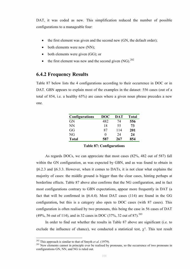
188

DAT, it was coded as new. This simplification reduced the number of possible

configurations to a manageable four:

• the first element was given and the second new (GN, the default order);

• both elements were new (NN);

• both elements were given (GG); or

• the first element was new and the second given (NG).202

6.4.2 Frequency Results

Table 87 below lists the 4 configurations according to their occurrence in DOC or in

DAT. GBN appears to explain most of the examples in the dataset: 556 cases (out of a

total of 854, i.e. a healthy 65%) are cases where a given noun phrase precedes a new

one.

Configurations DOC DAT Total

GN 482 74 556

NN 18 55 73

GG 87 114 201

NG 0 24 24

Total 587 267 854

Table 87: Configurations

As regards DOCs, we can appreciate that most cases (82%, 482 out of 587) fall

within the GN configuration, as was expected by GBN, and as was found to obtain in

§6.2.3 and §6.3.3. However, when it comes to DATs, it is not clear what explains the

majority of cases: the middle ground is bigger than the clear cases, hinting perhaps at

borderline effects. Table 87 above also confirms that the NG configuration, and in fact

most configurations contrary to GBN expectations, appear more frequently in DAT (a

fact that will be confirmed in §6.4.4). Most DAT cases (114) are found in the GG

configuration, but this is a category also open to DOC cases (with 87 cases). This

configuration is often realised by two pronouns, this being the case in 56 cases of DAT

(49%, 56 out of 114), and in 32 cases in DOC (37%, 32 out of 87).203

In order to find out whether the results in Table 87 above are significant (i.e. to

exclude the influence of chance), we conducted a statistical test, χ². This test result

202 This approach is similar to that of Smyth et al. (1979). 203 New elements cannot in principle ever be realised by pronouns, so the occurrence of two pronouns in configurations GN, NN, and NG is ruled out.

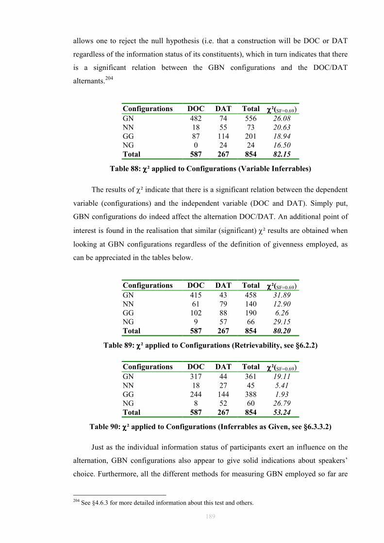
189

allows one to reject the null hypothesis (i.e. that a construction will be DOC or DAT

regardless of the information status of its constituents), which in turn indicates that there

is a significant relation between the GBN configurations and the DOC/DAT

alternants.204

Configurations DOC DAT Total χχχχ²(SF=0.69) GN 482 74 556 26.08 NN 18 55 73 20.63 GG 87 114 201 18.94 NG 0 24 24 16.50 Total 587 267 854 82.15

Table 88: χχχχ² applied to Configurations (Variable Inferrables)

The results of χ² indicate that there is a significant relation between the dependent

variable (configurations) and the independent variable (DOC and DAT). Simply put,

GBN configurations do indeed affect the alternation DOC/DAT. An additional point of

interest is found in the realisation that similar (significant) χ² results are obtained when

looking at GBN configurations regardless of the definition of givenness employed, as

can be appreciated in the tables below.

Configurations DOC DAT Total χχχχ²(SF=0.69) GN 415 43 458 31.89 NN 61 79 140 12.90 GG 102 88 190 6.26 NG 9 57 66 29.15 Total 587 267 854 80.20

Table 89: χχχχ² applied to Configurations (Retrievability, see §6.2.2)

Configurations DOC DAT Total χχχχ²(SF=0.69) GN 317 44 361 19.11 NN 18 27 45 5.41 GG 244 144 388 1.93 NG 8 52 60 26.79 Total 587 267 854 53.24

Table 90: χχχχ² applied to Configurations (Inferrables as Given, see §6.3.3.2)

Just as the individual information status of participants exert an influence on the

alternation, GBN configurations also appear to give solid indications about speakers’

choice. Furthermore, all the different methods for measuring GBN employed so far are

204 See §4.6.3 for more detailed information about this test and others.

190

validated by the strong results obtained, since the value of the different χ² is very high

in all cases.

6.4.3 Predictors

Another way in which the significance of configurations can be confirmed is by

employing naïve probabilities. It is possible to arrive at an estimation of the probability

of an event occurring based on data in a sample, by dividing the occurrences of the

event in question by the total number of events. This calculation is based on an

assumption of sample representativeness; i.e. we assume that the sample is

representative of the population, and that some change in the (sample) dataset will

reflect almost exactly to the population. With a very large number of data points, we can

be confident that dividing one by the other the sample is going to be representative of

the population.

Table 91 below (based on Table 88) lists the values for p(DOC) and p(DAT). In

short, p(DOC) is the probability of DOC for every configuration. As discussed above,

we can come up with a crude rule that states that ‘if the configuration is GN, then it is

realized as DOC (and not DAT)’; this is then formalized by taking the 482 correct

examples of GN configurations instantiated as DOC in our dataset and dividing them by

556, which is the total of all GN configurations in the dataset. p(DOC) for GN thus

amounts to 87%. Also, in order to measure our degree of confidence in the value, we

may use the binomial confidence interval (C.I. in Table 91 to Table 93 below)

expressed as a probability (see below).205 This interval is the strongest, most statistically

sound measure of the confidence on the prediction (should the experiment be

reproduced). It also represents a measure of how confident the researcher can be about

their data. Naturally, the smaller the error margin, the higher the confidence (the better

the results). This means, for example that the probability of DOC given a GN

configuration equals 0.87 plus or minus 0.03, which in itself expresses a very confident

result.

205 See www.ucl.ac.uk/english-usage/resources/ftfs/experiment2.htm. The function simplifies to z x sqrt[p(DOC) x p(DAT)/total], where z = 1.96 for an error of 0.05.

191

Configs. DOC DAT Total χχχχ²(SF=0.69) p(DOC) p(DAT) C.I.

GN 482 74 556 26.08 0.87 0.13 +/-0.03 NN 18 55 73 20.63 0.25 0.75 +/-0.10

GG 87 114 201 18.94 0.43 0.57 +/-0.07 NG 0 24 24 16.50 0.00 1.00 +/-0.00

Total 587 267 854 82.15

Table 91: Configurations as Predictors

The formula for p(DAT) is not dissimilar to that for p(DOC), only that it is the

DAT cases which are divided by the total cases of the configuration. Observing the p

columns, we can tell that apart from GG (which is rather flat, and thus unable to make

strong predictions), the remaining configurations are interesting, in that they are all over

70%. As mentioned, GN is accurate as a predictor of DOC 87% of the time; NN is

accurate as a predictor of DAT 75% of the time; and NG is accurate as a predictor of

DAT 100% of the time (but is only based on 24 cases).

We can arrive at a rule which would cover everything and thus would enable to

assess the predictive power of the Table 91. The strongest candidate for such a rule is

“if GN => DOC, otherwise DAT”, and we can also tell that this rule is correct 79% of

time [(482+55+114+24)/854].

By using naïve probabilities, we can also find out whether the speaker’s choice

between the two constructions can indeed be predicted by looking at the first element in

the configuration. In other words, is it possible that it is the givenness of the first

element (or the newness of the second element) which determines DOC or DAT? We

will evaluate whether the information status of each element affects the alternation, as

seen in Table 92 (for the first element) and Table 93 (for the second one).

Naturally, considering separate elements causes the probability to drop, because

the rule for determining the predictive power of the table is cruder. For example, in

looking at first position, I am combining the p(DOC)GN (i.e. 0.87 in Table 91) and

p(DOC)GG (i.e. 0.43 in Table 91 too).

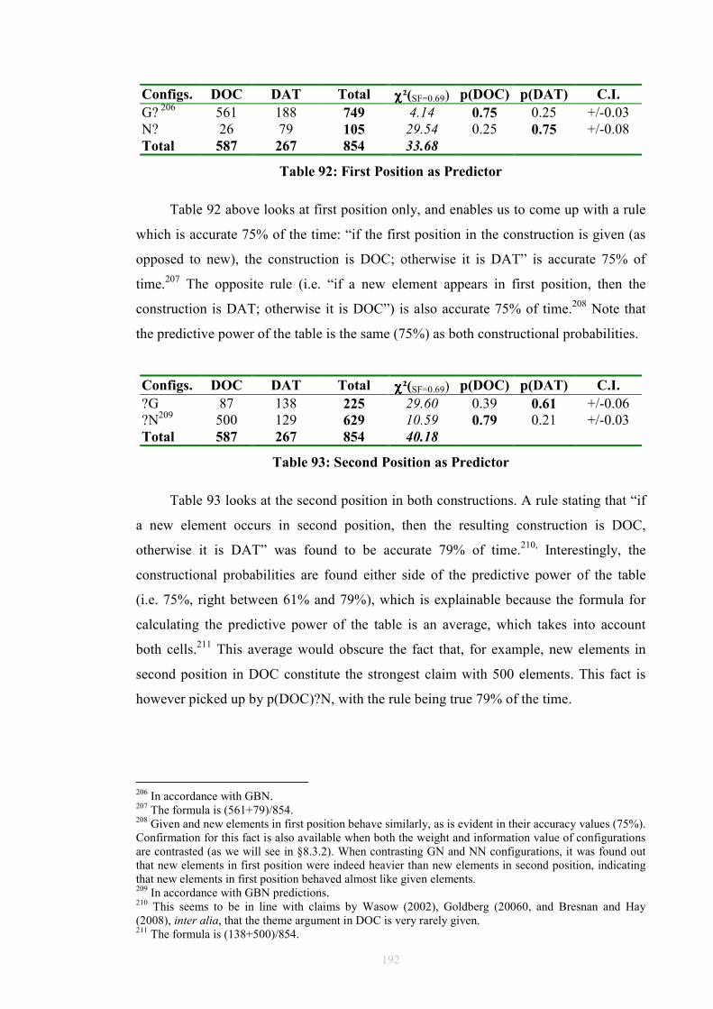
192

Configs. DOC DAT Total χχχχ²(SF=0.69) p(DOC) p(DAT) C.I.

G? 206 561 188 749 4.14 0.75 0.25 +/-0.03 N? 26 79 105 29.54 0.25 0.75 +/-0.08

Total 587 267 854 33.68

Table 92: First Position as Predictor

Table 92 above looks at first position only, and enables us to come up with a rule

which is accurate 75% of the time: “if the first position in the construction is given (as

opposed to new), the construction is DOC; otherwise it is DAT” is accurate 75% of

time.207 The opposite rule (i.e. “if a new element appears in first position, then the

construction is DAT; otherwise it is DOC”) is also accurate 75% of time.208 Note that

the predictive power of the table is the same (75%) as both constructional probabilities.

Configs. DOC DAT Total χχχχ²(SF=0.69) p(DOC) p(DAT) C.I.

?G 87 138 225 29.60 0.39 0.61 +/-0.06 ?N209 500 129 629 10.59 0.79 0.21 +/-0.03

Total 587 267 854 40.18

Table 93: Second Position as Predictor

Table 93 looks at the second position in both constructions. A rule stating that “if

a new element occurs in second position, then the resulting construction is DOC,

otherwise it is DAT” was found to be accurate 79% of time.210, Interestingly, the

constructional probabilities are found either side of the predictive power of the table

(i.e. 75%, right between 61% and 79%), which is explainable because the formula for

calculating the predictive power of the table is an average, which takes into account

both cells.211 This average would obscure the fact that, for example, new elements in

second position in DOC constitute the strongest claim with 500 elements. This fact is

however picked up by p(DOC)?N, with the rule being true 79% of the time.

206 In accordance with GBN. 207 The formula is (561+79)/854. 208 Given and new elements in first position behave similarly, as is evident in their accuracy values (75%). Confirmation for this fact is also available when both the weight and information value of configurations are contrasted (as we will see in §8.3.2). When contrasting GN and NN configurations, it was found out that new elements in first position were indeed heavier than new elements in second position, indicating that new elements in first position behaved almost like given elements. 209 In accordance with GBN predictions. 210 This seems to be in line with claims by Wasow (2002), Goldberg (20060, and Bresnan and Hay (2008), inter alia, that the theme argument in DOC is very rarely given. 211 The formula is (138+500)/854.

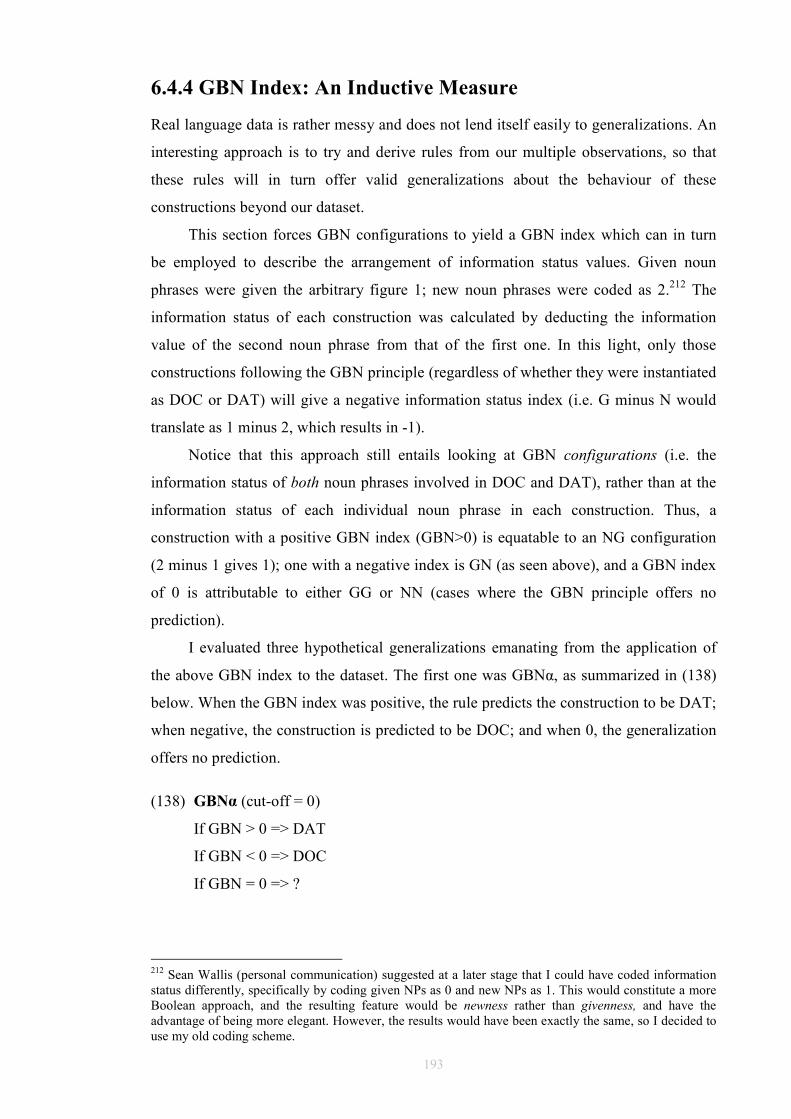
193

6.4.4 GBN Index: An Inductive Measure

Real language data is rather messy and does not lend itself easily to generalizations. An

interesting approach is to try and derive rules from our multiple observations, so that

these rules will in turn offer valid generalizations about the behaviour of these

constructions beyond our dataset.

This section forces GBN configurations to yield a GBN index which can in turn

be employed to describe the arrangement of information status values. Given noun

phrases were given the arbitrary figure 1; new noun phrases were coded as 2.212 The

information status of each construction was calculated by deducting the information

value of the second noun phrase from that of the first one. In this light, only those

constructions following the GBN principle (regardless of whether they were instantiated

as DOC or DAT) will give a negative information status index (i.e. G minus N would

translate as 1 minus 2, which results in -1).

Notice that this approach still entails looking at GBN configurations (i.e. the

information status of both noun phrases involved in DOC and DAT), rather than at the

information status of each individual noun phrase in each construction. Thus, a

construction with a positive GBN index (GBN>0) is equatable to an NG configuration

(2 minus 1 gives 1); one with a negative index is GN (as seen above), and a GBN index

of 0 is attributable to either GG or NN (cases where the GBN principle offers no

prediction).

I evaluated three hypothetical generalizations emanating from the application of

the above GBN index to the dataset. The first one was GBNα, as summarized in (138)

below. When the GBN index was positive, the rule predicts the construction to be DAT;

when negative, the construction is predicted to be DOC; and when 0, the generalization

offers no prediction.

(138) GBNα (cut-off = 0)

If GBN > 0 => DAT

If GBN < 0 => DOC

If GBN = 0 => ?

212 Sean Wallis (personal communication) suggested at a later stage that I could have coded information status differently, specifically by coding given NPs as 0 and new NPs as 1. This would constitute a more Boolean approach, and the resulting feature would be newness rather than givenness, and have the advantage of being more elegant. However, the results would have been exactly the same, so I decided to use my old coding scheme.

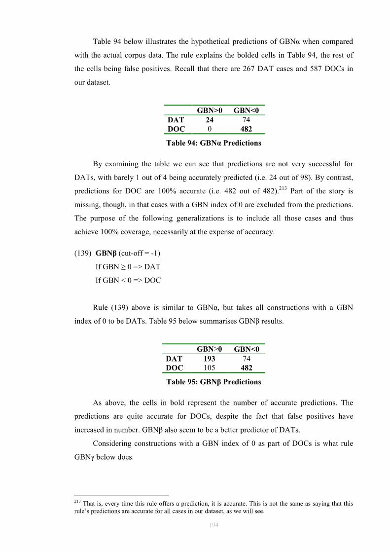
194

Table 94 below illustrates the hypothetical predictions of GBNα when compared

with the actual corpus data. The rule explains the bolded cells in Table 94, the rest of

the cells being false positives. Recall that there are 267 DAT cases and 587 DOCs in

our dataset.

GBN>0 GBN<0

DAT 24 74 DOC 0 482

Table 94: GBNα Predictions

By examining the table we can see that predictions are not very successful for

DATs, with barely 1 out of 4 being accurately predicted (i.e. 24 out of 98). By contrast,

predictions for DOC are 100% accurate (i.e. 482 out of 482).213 Part of the story is

missing, though, in that cases with a GBN index of 0 are excluded from the predictions.

The purpose of the following generalizations is to include all those cases and thus

achieve 100% coverage, necessarily at the expense of accuracy.

(139) GBNβ (cut-off = -1)

If GBN ≥ 0 => DAT

If GBN < 0 => DOC

Rule (139) above is similar to GBNα, but takes all constructions with a GBN

index of 0 to be DATs. Table 95 below summarises GBNβ results.

GBN≥0 GBN<0

DAT 193 74 DOC 105 482

Table 95: GBNβ Predictions

As above, the cells in bold represent the number of accurate predictions. The

predictions are quite accurate for DOCs, despite the fact that false positives have

increased in number. GBNβ also seem to be a better predictor of DATs.

Considering constructions with a GBN index of 0 as part of DOCs is what rule

GBNγ below does.

213 That is, every time this rule offers a prediction, it is accurate. This is not the same as saying that this rule’s predictions are accurate for all cases in our dataset, as we will see.

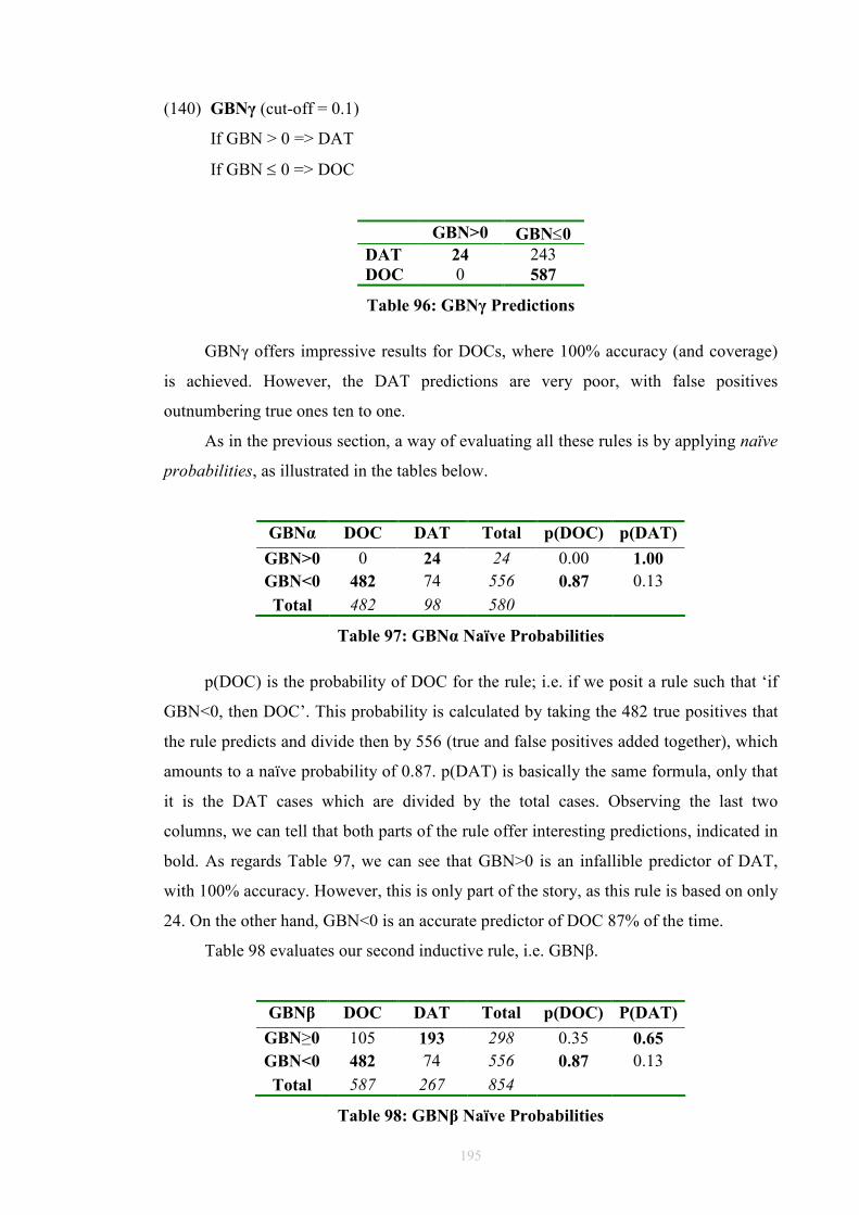
195

(140) GBNγ (cut-off = 0.1)

If GBN > 0 => DAT

If GBN ≤ 0 => DOC

GBN>0 GBN≤0

DAT 24 243 DOC 0 587

Table 96: GBNγ Predictions

GBNγ offers impressive results for DOCs, where 100% accuracy (and coverage)

is achieved. However, the DAT predictions are very poor, with false positives

outnumbering true ones ten to one.

As in the previous section, a way of evaluating all these rules is by applying naïve

probabilities, as illustrated in the tables below.

GBNα DOC DAT Total p(DOC) p(DAT)

GBN>0 0 24 24 0.00 1.00

GBN<0 482 74 556 0.87 0.13

Total 482 98 580

Table 97: GBNα Naïve Probabilities

p(DOC) is the probability of DOC for the rule; i.e. if we posit a rule such that ‘if

GBN<0, then DOC’. This probability is calculated by taking the 482 true positives that

the rule predicts and divide then by 556 (true and false positives added together), which

amounts to a naïve probability of 0.87. p(DAT) is basically the same formula, only that

it is the DAT cases which are divided by the total cases. Observing the last two

columns, we can tell that both parts of the rule offer interesting predictions, indicated in

bold. As regards Table 97, we can see that GBN>0 is an infallible predictor of DAT,

with 100% accuracy. However, this is only part of the story, as this rule is based on only

24. On the other hand, GBN<0 is an accurate predictor of DOC 87% of the time.

Table 98 evaluates our second inductive rule, i.e. GBNβ.

GBNβ DOC DAT Total p(DOC) P(DAT)

GBN≥0 105 193 298 0.35 0.65

GBN<0 482 74 556 0.87 0.13

Total 587 267 854

Table 98: GBNβ Naïve Probabilities

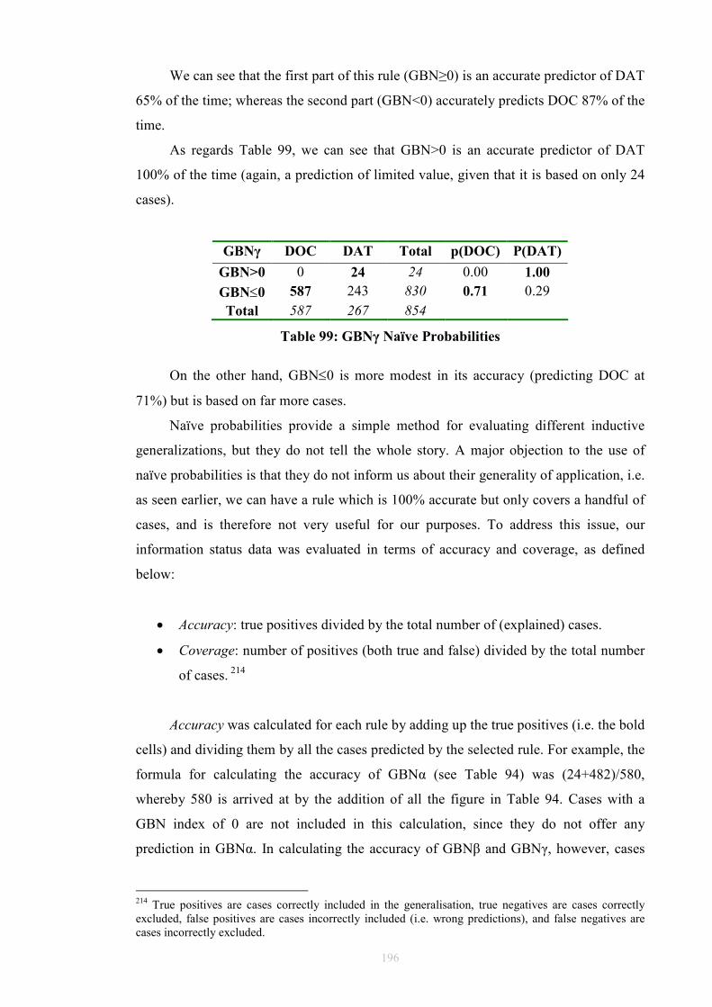
196

We can see that the first part of this rule (GBN≥0) is an accurate predictor of DAT

65% of the time; whereas the second part (GBN<0) accurately predicts DOC 87% of the

time.

As regards Table 99, we can see that GBN>0 is an accurate predictor of DAT

100% of the time (again, a prediction of limited value, given that it is based on only 24

cases).

GBNγ DOC DAT Total p(DOC) P(DAT)

GBN>0 0 24 24 0.00 1.00

GBN≤0 587 243 830 0.71 0.29 Total 587 267 854

Table 99: GBNγ Naïve Probabilities

On the other hand, GBN≤0 is more modest in its accuracy (predicting DOC at

71%) but is based on far more cases.

Naïve probabilities provide a simple method for evaluating different inductive

generalizations, but they do not tell the whole story. A major objection to the use of

naïve probabilities is that they do not inform us about their generality of application, i.e.

as seen earlier, we can have a rule which is 100% accurate but only covers a handful of

cases, and is therefore not very useful for our purposes. To address this issue, our

information status data was evaluated in terms of accuracy and coverage, as defined

below:

• Accuracy: true positives divided by the total number of (explained) cases.

• Coverage: number of positives (both true and false) divided by the total number

of cases. 214

Accuracy was calculated for each rule by adding up the true positives (i.e. the bold

cells) and dividing them by all the cases predicted by the selected rule. For example, the

formula for calculating the accuracy of GBNα (see Table 94) was (24+482)/580,

whereby 580 is arrived at by the addition of all the figure in Table 94. Cases with a

GBN index of 0 are not included in this calculation, since they do not offer any

prediction in GBNα. In calculating the accuracy of GBNβ and GBNγ, however, cases

214 True positives are cases correctly included in the generalisation, true negatives are cases correctly excluded, false positives are cases incorrectly included (i.e. wrong predictions), and false negatives are cases incorrectly excluded.

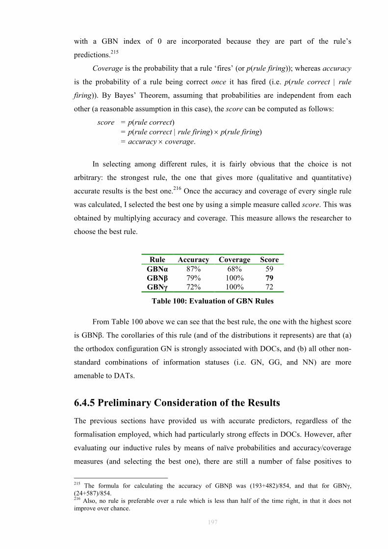
197

with a GBN index of 0 are incorporated because they are part of the rule’s

predictions.215

Coverage is the probability that a rule ‘fires’ (or p(rule firing)); whereas accuracy

is the probability of a rule being correct once it has fired (i.e. p(rule correct | rule

firing)). By Bayes’ Theorem, assuming that probabilities are independent from each

other (a reasonable assumption in this case), the score can be computed as follows:

score = p(rule correct) = p(rule correct | rule firing) × p(rule firing) = accuracy × coverage.

In selecting among different rules, it is fairly obvious that the choice is not

arbitrary: the strongest rule, the one that gives more (qualitative and quantitative)

accurate results is the best one.216 Once the accuracy and coverage of every single rule

was calculated, I selected the best one by using a simple measure called score. This was

obtained by multiplying accuracy and coverage. This measure allows the researcher to

choose the best rule.

Rule Accuracy Coverage Score

GBNα 87% 68% 59 GBNβ 79% 100% 79

GBNγ 72% 100% 72

Table 100: Evaluation of GBN Rules

From Table 100 above we can see that the best rule, the one with the highest score

is GBNβ. The corollaries of this rule (and of the distributions it represents) are that (a)

the orthodox configuration GN is strongly associated with DOCs, and (b) all other non-

standard combinations of information statuses (i.e. GN, GG, and NN) are more

amenable to DATs.

6.4.5 Preliminary Consideration of the Results

The previous sections have provided us with accurate predictors, regardless of the

formalisation employed, which had particularly strong effects in DOCs. However, after

evaluating our inductive rules by means of naïve probabilities and accuracy/coverage

measures (and selecting the best one), there are still a number of false positives to

215 The formula for calculating the accuracy of GBNβ was (193+482)/854, and that for GBNγ, (24+587)/854. 216 Also, no rule is preferable over a rule which is less than half of the time right, in that it does not improve over chance.

198

explain. These are represented by the unbolded cells in the tables from the previous

section. If we leave aside a few outliers in the NG configuration, questions remain

unanswered, particularly about what determines the DOC/DAT alternation in the

configurations GG and NN. These cases will be discussed in chapter 8.

6.5 Conclusions

This chapter has tested the GBN principle in different ways, by employing different

coding schemes (textual retrievability in §6.2; inferrables in §6.3 onwards), by

considering the information status of individual elements (§6.2 and §6.3) and of

configurations (§6.4), and by applying different tests and measures to the results.

Strong predictions are derivable from looking at the overall (constructional)

distribution of information status, as well as by looking at the individual information

status of the noun phrases in first and/or second position. This is indicative of a strong

correlation between information status and this particular grammatical choice (DOC or

DAT). The significant results in the studies reported in this chapter also indicate that all

the different classificatory methods for information status are valid. However, as was

pointed out time and again, statistics do not answer why questions: for that, further

investigation is required to evaluate what is going on (and whether the data predicts

anything else).

The next chapter is concerned with the impact of heaviness on the dative

alternation. Different measures for evaluating heaviness are discussed and implemented

in the analysis of corpus data.

199

7 Testing the Theories II: Length, Weight,

Complexity

7.1 Weight

As we have seen earlier (§5.1), word order is claimed to be affected by the principles of

end weight (PEW) (Quirk et al. 1985:1361-1362) and end focus (PEF) (Quirk et al.

1985:1356-1357). In this chapter we will concern ourselves with the principle of end

weight, which stipulates that the ‘heavier’ the constituent, the higher its chances of

appearing after a lighter one. Weight is variously defined in the literature, many times

vaguely so. The idea is intuitively clear, but that does not make it easy to operationalise,

particularly when conducting data-driven experimentation. The chapter is organized in

the following manner: §7.1 provides a definition of weight, discusses a number of

accounts of the dative alternation based on weight, and conducts an experiment to

evaluate weight measures in ICE-GB. Section 7.2 follows the same structure, but rather

than applying it to weight, we use a different measure of heaviness, namely complexity.

Conclusions are offered in §7.3.

7.1.1 Weight: Definitions and Assumptions

In his discussion of Heavy Noun Phrase Shift (HNPS), Wasow (1997a:84-85) discusses

eight definitions of heaviness, quoted below. Unfortunately for the purposes of this

study, most of these definitions tend to conflate what I will call weight (defined as the

number of words in a constituent, as seen in (141)d and (142)a below) and complexity

(defined as the number of phrasal nodes in a constituent, as glimpsed in the rest of the

definitions, with the exception of (141)e, which does not seem to fit either weight or

complexity, but see footnote 218 below). In the rest of this chapter, I will keep weight

and complexity apart (see Altenberg 1982 and Rosenbach 2005 for a similar approach).

(141) (Categorical) Heaviness

a. An NP is heavy if it “dominates S” (Ross 1967, rule 3.26).

b. “The condition on complex NP shift is that the NP dominate an S or a PP”

(Emonds 1976:112).217

c. “Counting a nominal group as heavy means either that two or more nominal

groups (…) are coordinated (…), or that the head noun of a nominal group is

postmodified by a phrase or clause” (Erdmann 1988:328). 217 For Emonds, complexity and heaviness are coextensive concepts.

200

d. “The dislocated NP [in HNPS] is licensed when it contains at least two

phonological phrases” (Zek and Inkelas 1990:377).

e. “It is possible to formalize the intuition of ‘heaviness’ in terms of an aspect of

the meaning of the constituents involved, namely their givenness in the

discourse” 218 (Niv 1992:3).

(142) (Graduated) Weight

a. Number of words dominated (Hawkins 1990).

b. Number of nodes dominated (Hawkins 1994).219

c. Number of phrasal nodes (i.e. maximal projections) dominated (Rickford,

Wasow, Mendoza-Denton, and Espinoza 1995:111).

Wasow (1997a:85) classifies the above definitions into (a) categorical ones, i.e.

those that “consider only properties of the shifted [i.e. heavy] NP”, and (b) graduated

ones, i.e. those that “compare the weight of the [heavy] NP to the weight of the

constituents it gets shifted over [lighter by definition]”. Arnold et al. (2000:29) found

two advantages to this approach: (a) recent work has shown that it is the relative weight

that is important in accounts of weight-motivated phenomena (Hawkins 1994, Wasow

1997a),220 (b) the graded nature of weight effects is brought to the fore with this

approach. This study will make use of graduated measures for both weight and

complexity. I will be concerned with situations in which the speaker has a choice

between alternative orders, both of which are syntactically and semantically acceptable

(DOC vs. DAT).

7.1.2 Accounts of Weight

Williams (1994) conducted a corpus study (with spoken and written, American English

data) to evaluate the dative alternation. In the 168 cases he found of the alternation, he

discovered that goal [i.e. recipient] arguments tended to occur 84% of the time in

immediately postverbal position (i.e. DOC) when they were shorter in prosodic length

218 Although not explicitly stated as such in Niv’s framework, given information is equated to light information (i.e. not heavy), while new information is considered to be heavy. 219 Hawkins (1994) defines syntactic complexity as involving “the number of structural relations within different portions of a tree, measured in terms of sets of structurally related nodes” (1994:29). However, as in Hawkins (1990), he continues to use number of words as a more easily computable surrogate. 220 In other words, “weight effects depend on the relative weights of constituents, not only on the weight of any one” (Wasow 2002:57).

201

than the theme argument.221 On the other hand, goal arguments favoured end positions

(i.e. DAT) 80% of the time when they were longer than their theme counterparts. His

results are presented in Table 101 below.222

Length DOC DAT

G<T 41 (84%) 8 (16%) G>T 2 (20%) 8 (80%)

Table 101: Results in Williams (1994)

In the above table, ‘G<T’ indicate that the Goal element is shorter than the Theme

element, whereas ‘G>T’ indicates the opposite. Williams’ results seem to robustly

confirm the predictions arising from the PEW. I was able to reproduce his study, but

using number of words (instead of number of moras) as the criterion for weight. As we

can see in Table 102 below, the tendencies found are not dissimilar, with the majority of

themes in DOC longer than goals, and the reverse being true in DAT cases.

Weight DOC DAT

G<T 96% 4% G>T 47% 53%

Table 102: Williams’ results revisited

With a much larger dataset (854 cases of alternation) and a different measure for

weight, the results for DOC are not just repeated but actually strengthened to almost

categorical status: when goals (recipients) are shorter than themes, DOC is preferred

96% of the times. However, the results cannot be said to be replicated when it comes to

DAT, in that the predictions emanating from PEW seem to (barely) hang in the balance,

confirmed but only marginally.

In a later study, Collins (1995) put PEW predictions to the test in his analysis of

the dative alternation. Using a reduced dataset (108 cases) of spoken and written

Australian English, he compared the length of the constituents involved, measuring this

in terms of number of words. His findings are copied in Table 103 below.

221 Williams used a very complex measure of prosodic length, based on moraic theory as described in Hyman (1985). Moras are prosodic elements similar in extent to syllables, but not necessarily so. 222 Williams does not indicate what to do in situations when the goal and the theme have the same number of moras, which is unfortunate, in that this is rather a common occurrence.

202

Receiver Entity

DOC 1.1 words < 3.6 words DAT 3.0 words > 2.2 words

Table 103: Results in Collins (1995)

In Collins’ study, ‘entity’ refers to the postverbal element which is not the

Receiver. As we can see, his results confirm Williams’ findings, i.e. in DOC cases, the

average number of words of receivers [recipients] occurring in immediately postverbal

position is considerably (more than three times) shorter than the length of entities

[theme arguments]. In DAT cases, again the shorter argument appears closer to the verb,

but the difference in length between the two is not as marked as in DOC cases. I

managed to replicate his experiment, the results are presented in Table 104 below.

Receiver Entity

DOC 1.28 words < 3.05 words DAT 1.28 words > 1.09 words

Table 104: Collins’ results revisited

My results appear to confirm Collins’ findings (and, simultaneously, PEW

predictions), but the differences in weight between the different arguments are not as

marked, particularly in the case of DAT. It is curious to find out that in my dataset the

average length for receivers in both DOC and DAT is exactly the same, at 1.28 words.

In their impressive grammar, Biber et al. also discuss the dative alternation

(1999:927-930). They conducted a corpus study (in the massive Longman Grammar of

Spoken and Written English corpus, with over forty million words) to evaluate the effect

of the length of constituents in the three most common lexical verbs that allow for both

patterns, e.g. give, offer and sell.223 Their results are reproduced below.

Length of NP

DOC 1 word 2 words 3+ words

DO 15% 35% 50% IO 85% 10% 5% Length of NP

DAT 1 word 2 words 3+ words

DO 55% 25% 20% to-phrase 45% 30% 25%

Table 105: Results in Biber et al. (1999)

223 It is worth noting that with these verbs, the DOC pattern is much more common than DAT.

203

In DOC, the majority of indirect objects are indeed very short, with 85% of them

being only one word long, and indirect objects longer than a word seeming to be a

rarity. This weight effect is not found to be as strong in DATs, where immediately

postverbal position is accorded to direct objects. Of these, only (?!) 55% are realized as

one word, with a healthy 45% being greater than one word in length. To-phrases are not

much longer than direct objects in DAT, with 45% being one word long too (not

counting the preposition, see §7.1.3). The authors conclude that length is not such an

important factor in DATs as it is in DOCs.

When replicating Biber et al. experiment, I was surprised by the similarity

between results: my results for DOC are almost exactly the same as theirs, despite the

fact that my dataset is much smaller, and I consider many more than three verbs (in fact,

well over 50). My results can be seen in Table 106 below.

Length of NP

DOC 1 word 2 words 3+ words

DO 16% 35% 49% IO 84% 11% 5% Length of NP

DAT 1 word 2 words 3+ words

DO 47% 33% 20% to-phrase 52% 22% 26%

Table 106: Biber et al.’s results revisited

What was found in DAT is that it is not always the case that the first postverbal

element is shorter than what follows: (i) the length of DOs is found to be (marginally)

longer than one word in my data;224 and (ii) to-phrases also appear to be realized

frequently as one word.225 In conclusion, both Biber et al.’s and my results seem to

confirm PEW predictions, strongly for DOCs and not so much for DATs. Still, the

divergence found in the length (or weight) of the prepositional pattern seems to suggest

that there is something else at work. We must investigate further.

7.1.3 Corpus Experiment 4: Weight

In DOC and DAT, the choice of which constituent ordering is used appears to be

determined by the weight (and/or complexity) of the phrases in question. Aarts (1992:

224 As can be appreciated in Table 106, in DAT cases, 33% of direct objects are 2 words long, and 20% of direct objects are 3 or more words long. 225 As will be seen in §7.1.3, prepositions in DATs are considered simply case-marking devices and not counted as words.

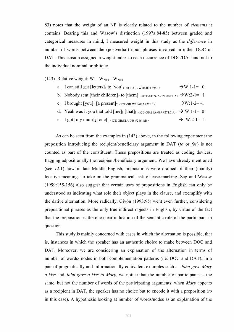
204

83) notes that the weight of an NP is clearly related to the number of elements it

contains. Bearing this and Wasow’s distinction (1997a:84-85) between graded and

categorical measures in mind, I measured weight in this study as the difference in

number of words between the (postverbal) noun phrases involved in either DOC or

DAT. This ecision assigned a weight index to each occurrence of DOC/DAT and not to

the individual nominal or oblique.

(143) Relative weight: W = WNP1 - WNP2

a. I can still get [letters]1 to [you]1 <ICE-GB:W1B-003 #98:1> �W:1-1= 0

b. Nobody sent [their children]2 to [them]1 <ICE-GB:S2A-021 #80:1:A> �W:2-1= 1

c. I brought [you]1 [a present]2 <ICE-GB:W2F-002 #220:1> �W:1-2= -1

d. Yeah was it you that told [me]1 [that]1 <ICE-GB:S1A-099 #271:2:A> � W:1-1= 0

e. I got [my mum]2 [one]1 <ICE-GB:S1A-048 #286:1:B> � W:2-1= 1

As can be seen from the examples in (143) above, in the following experiment the

preposition introducing the recipient/beneficiary argument in DAT (to or for) is not

counted as part of the constituent. These prepositions are treated as coding devices,

flagging adpositionally the recipient/beneficiary argument. We have already mentioned

(see §2.1) how in late Middle English, prepositions were drained of their (mainly)

locative meanings to take on the grammatical task of case-marking. Sag and Wasow

(1999:155-156) also suggest that certain uses of prepositions in English can only be

understood as indicating what role their object plays in the clause, and exemplify with

the dative alternation. More radically, Givón (1993:95) went even further, considering

prepositional phrases as the only true indirect objects in English, by virtue of the fact

that the preposition is the one clear indication of the semantic role of the participant in

question.

This study is mainly concerned with cases in which the alternation is possible, that

is, instances in which the speaker has an authentic choice to make between DOC and

DAT. Moreover, we are considering an explanation of the alternation in terms of

number of words/ nodes in both complementation patterns (i.e. DOC and DAT). In a

pair of pragmatically and informationally equivalent examples such as John gave Mary

a kiss and John gave a kiss to Mary, we notice that the number of participants is the

same, but not the number of words of the participating arguments: when Mary appears

as a recipient in DAT, the speaker has no choice but to encode it with a preposition (to

in this case). A hypothesis looking at number of words/nodes as an explanation of the

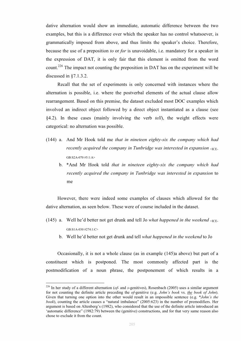
205

dative alternation would show an immediate, automatic difference between the two

examples, but this is a difference over which the speaker has no control whatsoever, is

grammatically imposed from above, and thus limits the speaker’s choice. Therefore,

because the use of a preposition to or for is unavoidable, i.e. mandatory for a speaker in

the expression of DAT, it is only fair that this element is omitted from the word

count.226 The impact not counting the preposition in DAT has on the experiment will be

discussed in §7.1.3.2.

Recall that the set of experiments is only concerned with instances where the

alternation is possible, i.e. where the postverbal elements of the actual clause allow

rearrangement. Based on this premise, the dataset excluded most DOC examples which

involved an indirect object followed by a direct object instantiated as a clause (see

§4.2). In these cases (mainly involving the verb tell), the weight effects were

categorical: no alternation was possible.

(144) a. And Mr Hook told me that in nineteen eighty-six the company which had

recently acquired the company in Tunbridge was interested in expansion <ICE-

GB:S2A-070 #5:1:A>

b. *And Mr Hook told that in nineteen eighty-six the company which had

recently acquired the company in Tunbridge was interested in expansion to

me

However, there were indeed some examples of clauses which allowed for the

dative alternation, as seen below. These were of course included in the dataset.

(145) a. Well he’d better not get drunk and tell Jo what happened in the weekend <ICE-

GB:S1A-030 #274:1:C>

b. Well he’d better not get drunk and tell what happened in the weekend to Jo

Occasionally, it is not a whole clause (as in example (145)a above) but part of a

constituent which is postponed. The most commonly affected part is the

postmodification of a noun phrase, the postponement of which results in a

226 In her study of a different alternation (of- and s-genitives), Rosenbach (2005) uses a similar argument for not counting the definite article preceding the of-genitive (e.g. John’s book vs. the book of John). Given that turning one option into the other would result in an impossible sentence (e.g. *John’s the book), counting the article causes a “natural imbalance” (2005:623) in the number of premodifiers. Her argument is based on Altenberg’s (1982), who considered that the use of the definite article introduced an ‘automatic difference” (1982:79) between the (genitive) constructions, and for that very same reason also chose to exclude it from the count.

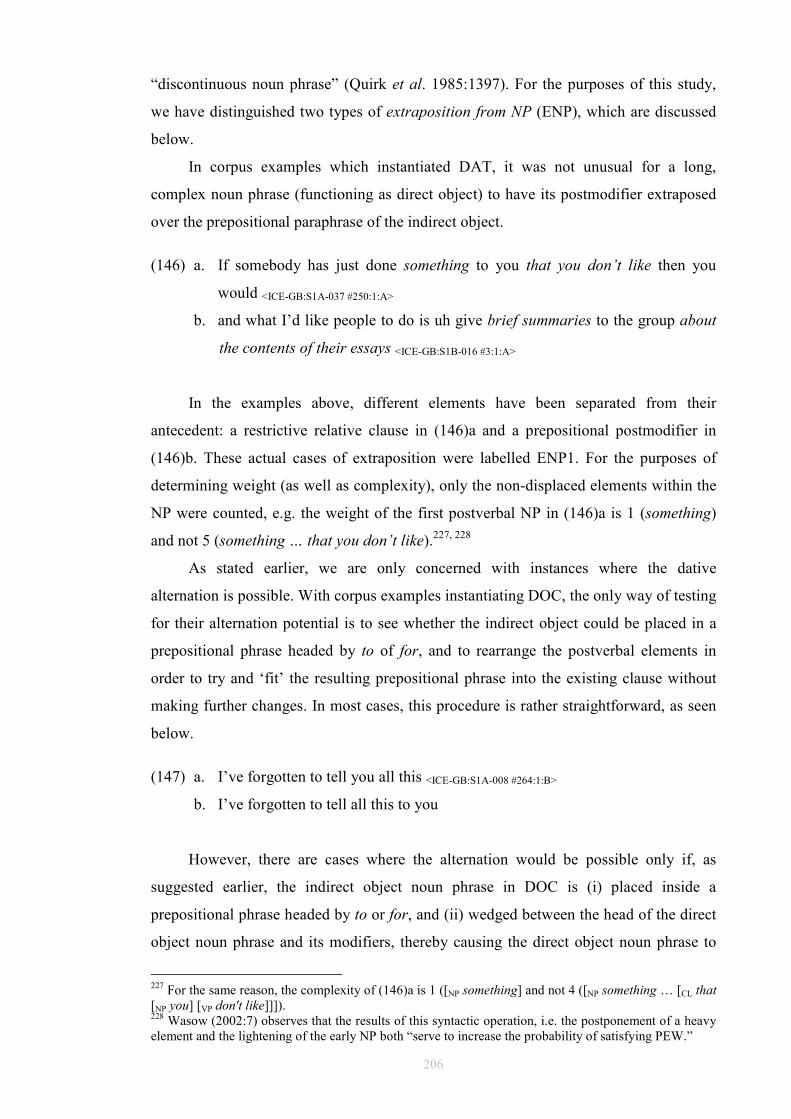
206

“discontinuous noun phrase” (Quirk et al. 1985:1397). For the purposes of this study,

we have distinguished two types of extraposition from NP (ENP), which are discussed

below.

In corpus examples which instantiated DAT, it was not unusual for a long,

complex noun phrase (functioning as direct object) to have its postmodifier extraposed

over the prepositional paraphrase of the indirect object.

(146) a. If somebody has just done something to you that you don’t like then you

would <ICE-GB:S1A-037 #250:1:A>

b. and what I’d like people to do is uh give brief summaries to the group about

the contents of their essays <ICE-GB:S1B-016 #3:1:A>

In the examples above, different elements have been separated from their

antecedent: a restrictive relative clause in (146)a and a prepositional postmodifier in

(146)b. These actual cases of extraposition were labelled ENP1. For the purposes of

determining weight (as well as complexity), only the non-displaced elements within the

NP were counted, e.g. the weight of the first postverbal NP in (146)a is 1 (something)

and not 5 (something … that you don’t like).227, 228

As stated earlier, we are only concerned with instances where the dative

alternation is possible. With corpus examples instantiating DOC, the only way of testing

for their alternation potential is to see whether the indirect object could be placed in a

prepositional phrase headed by to of for, and to rearrange the postverbal elements in

order to try and ‘fit’ the resulting prepositional phrase into the existing clause without

making further changes. In most cases, this procedure is rather straightforward, as seen

below.

(147) a. I’ve forgotten to tell you all this <ICE-GB:S1A-008 #264:1:B>

b. I’ve forgotten to tell all this to you

However, there are cases where the alternation would be possible only if, as

suggested earlier, the indirect object noun phrase in DOC is (i) placed inside a

prepositional phrase headed by to or for, and (ii) wedged between the head of the direct

object noun phrase and its modifiers, thereby causing the direct object noun phrase to

227 For the same reason, the complexity of (146)a is 1 ([NP something] and not 4 ([NP something … [CL that [NP you] [VP don't like]]]). 228 Wasow (2002:7) observes that the results of this syntactic operation, i.e. the postponement of a heavy element and the lightening of the early NP both “serve to increase the probability of satisfying PEW.”

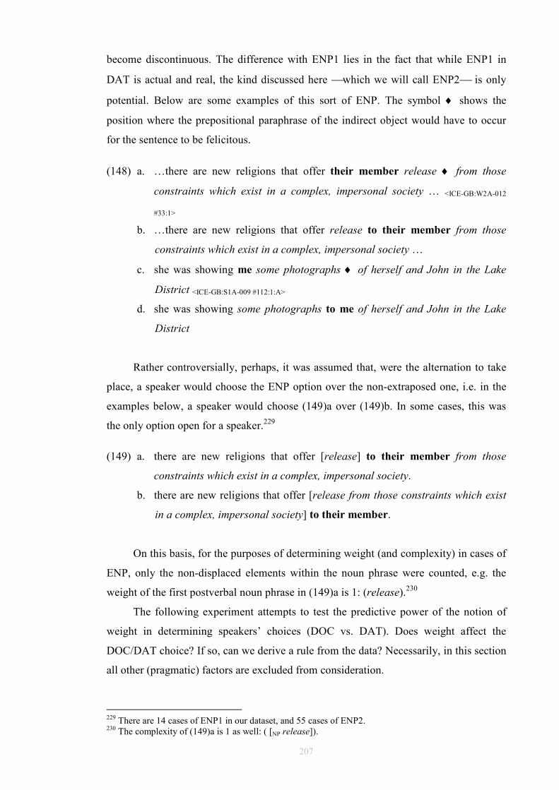
207

become discontinuous. The difference with ENP1 lies in the fact that while ENP1 in

DAT is actual and real, the kind discussed here which we will call ENP2 is only

potential. Below are some examples of this sort of ENP. The symbol ♦ shows the

position where the prepositional paraphrase of the indirect object would have to occur

for the sentence to be felicitous.

(148) a. …there are new religions that offer their member release ♦ from those

constraints which exist in a complex, impersonal society … <ICE-GB:W2A-012

#33:1>

b. …there are new religions that offer release to their member from those

constraints which exist in a complex, impersonal society …

c. she was showing me some photographs ♦ of herself and John in the Lake

District <ICE-GB:S1A-009 #112:1:A>

d. she was showing some photographs to me of herself and John in the Lake

District

Rather controversially, perhaps, it was assumed that, were the alternation to take

place, a speaker would choose the ENP option over the non-extraposed one, i.e. in the

examples below, a speaker would choose (149)a over (149)b. In some cases, this was

the only option open for a speaker.229

(149) a. there are new religions that offer [release] to their member from those

constraints which exist in a complex, impersonal society.

b. there are new religions that offer [release from those constraints which exist

in a complex, impersonal society] to their member.

On this basis, for the purposes of determining weight (and complexity) in cases of

ENP, only the non-displaced elements within the noun phrase were counted, e.g. the

weight of the first postverbal noun phrase in (149)a is 1: (release).230

The following experiment attempts to test the predictive power of the notion of

weight in determining speakers’ choices (DOC vs. DAT). Does weight affect the

DOC/DAT choice? If so, can we derive a rule from the data? Necessarily, in this section

all other (pragmatic) factors are excluded from consideration.

229 There are 14 cases of ENP1 in our dataset, and 55 cases of ENP2. 230 The complexity of (149)a is 1 as well: ( [NP release]).

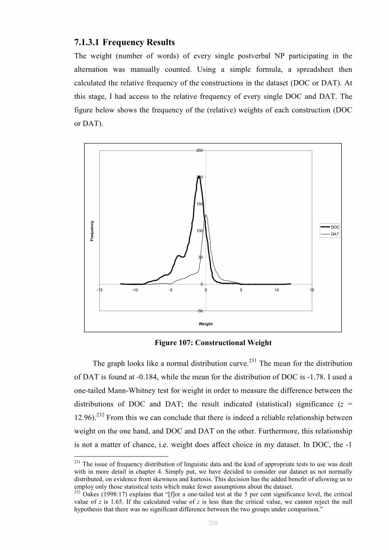
208

7.1.3.1 Frequency Results

The weight (number of words) of every single postverbal NP participating in the

alternation was manually counted. Using a simple formula, a spreadsheet then

calculated the relative frequency of the constructions in the dataset (DOC or DAT). At

this stage, I had access to the relative frequency of every single DOC and DAT. The

figure below shows the frequency of the (relative) weights of each construction (DOC

or DAT).

-50

0

50

100

150

200

250

-15 -10 -5 0 5 10 15

Weight

Frequency

DOC

DAT

Figure 107: Constructional Weight

The graph looks like a normal distribution curve.231 The mean for the distribution

of DAT is found at -0.184, while the mean for the distribution of DOC is -1.78. I used a

one-tailed Mann-Whitney test for weight in order to measure the difference between the

distributions of DOC and DAT; the result indicated (statistical) significance (z =

12.96).232 From this we can conclude that there is indeed a reliable relationship between

weight on the one hand, and DOC and DAT on the other. Furthermore, this relationship

is not a matter of chance, i.e. weight does affect choice in my dataset. In DOC, the -1

231 The issue of frequency distribution of linguistic data and the kind of appropriate tests to use was dealt with in more detail in chapter 4. Simply put, we have decided to consider our dataset as not normally distributed, on evidence from skewness and kurtosis. This decision has the added benefit of allowing us to employ only those statistical tests which make fewer assumptions about the dataset. 232 Oakes (1998:17) explains that “[f]or a one-tailed test at the 5 per cent significance level, the critical value of z is 1.65. If the calculated value of z is less than the critical value, we cannot reject the null hypothesis that there was no significant difference between the two groups under comparison.”

209

value of the mean indicates that indirect objects tend to be shorter than direct objects,

thus confirming PEW predictions and our a priori expectations. In DAT, however, the

-0.184 mean indicates that both constituents (direct object and to-/for-phrase) tend to

have the same weight, i.e. number of words. This goes against our expectations, but not

necessarily against PEW.

7.1.3.2 An Inductive Measure of Weight

Figure 107 above indicates the distribution of the relative weight of DOCs and DATs in

our dataset. An interesting approach is to try and derive rules from our multiple

observations, so that these rules will in turn offer valid generalizations about the

behaviour of these constructions. Based on the distributions in Figure 107, I tried to

arrive at a cut-off point in order to distinguish and separate the two distributions as

much as possible. Naturally, the bigger the skew, the better the cut-off point is (and the

more reliable the ensuing rule would be).

Generating this type of rule is an engineering exercise, in that the only available

guidelines are (a) separating maximally the means of the two distributions, and (b)

minimizing the error rate of the rule (i.e. the number of unexplained cases). I evaluated

three cut-off points (0, -1, and 0.1) in terms of their predictive power (accuracy) and

their coverage.233 For the purposes of this section, predictive accuracy (i.e. probability

that the rule is correct) is calculated as the number of correct predictions divided by the

number of explained cases; coverage was calculated as total number of cases minus

unexplained cases (see also §6.4.4). The latter measure was employed to complement

the former, given that naïve predictive accuracy does not tell us much (if anything at all)

about how general the rule might be in practice. This is not quite a statistical question,

but rather a methodological one.

The first rule evaluated was Wα, based on a cut-off point located at 0. This would

indicate that if the weight of a construction (notice that we do not specify between DOC

and DAT) is positive, then the rule predicts that the construction in question would be

DAT. If the constructional weight is negative, then the construction would be DOC. If

the constructional weight is right on the cut-off (i.e. 0), the rule offers no prediction.

This is summarized in (150) below.

233 We could have tested many different cut-off points for their contribution to the model (e.g. -0.1, -0.2, etc.). This proved to be unnecessary by virtue of the fact that only a few cut-off points were able to (a) maximally separate the means of the two distributions, and (b) provide a suitable solution to cases of zero constructional weight.

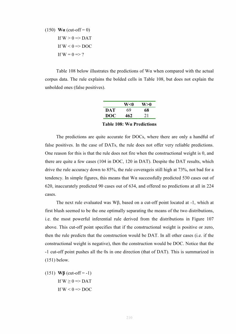
210

(150) Wα (cut-off = 0)

If W > 0 => DAT

If W < 0 => DOC

If W = 0 => ?

Table 108 below illustrates the predictions of Wα when compared with the actual

corpus data. The rule explains the bolded cells in Table 108, but does not explain the

unbolded ones (false positives).

W<0 W>0

DAT 69 68

DOC 462 21

Table 108: Wα Predictions

The predictions are quite accurate for DOCs, where there are only a handful of

false positives. In the case of DATs, the rule does not offer very reliable predictions.

One reason for this is that the rule does not fire when the constructional weight is 0, and

there are quite a few cases (104 in DOC, 120 in DAT). Despite the DAT results, which

drive the rule accuracy down to 85%, the rule coverageis still high at 73%, not bad for a

tendency. In simple figures, this means that Wα successfully predicted 530 cases out of

620, inaccurately predicted 90 cases out of 634, and offered no predictions at all in 224

cases.

The next rule evaluated was Wβ, based on a cut-off point located at -1, which at

first blush seemed to be the one optimally separating the means of the two distributions,

i.e. the most powerful inferential rule derived from the distributions in Figure 107

above. This cut-off point specifies that if the constructional weight is positive or zero,

then the rule predicts that the construction would be DAT. In all other cases (i.e. if the

constructional weight is negative), then the construction would be DOC. Notice that the

-1 cut-off point pushes all the 0s in one direction (that of DAT). This is summarized in

(151) below.

(151) Wβ (cut-off = -1)

If W ≥ 0 => DAT

If W < 0 => DOC

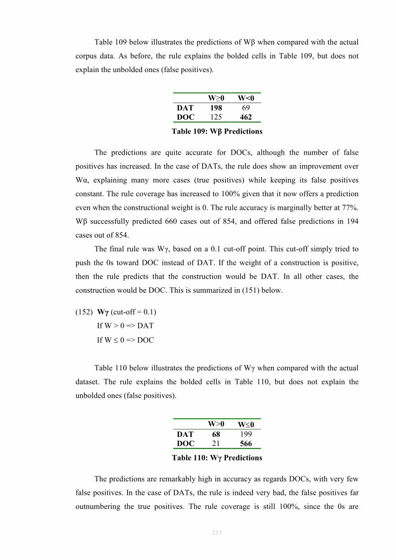
211

Table 109 below illustrates the predictions of Wβ when compared with the actual

corpus data. As before, the rule explains the bolded cells in Table 109, but does not

explain the unbolded ones (false positives).

W≥0 W<0

DAT 198 69 DOC 125 462

Table 109: Wβ Predictions

The predictions are quite accurate for DOCs, although the number of false

positives has increased. In the case of DATs, the rule does show an improvement over

Wα, explaining many more cases (true positives) while keeping its false positives

constant. The rule coverage has increased to 100% given that it now offers a prediction

even when the constructional weight is 0. The rule accuracy is marginally better at 77%.

Wβ successfully predicted 660 cases out of 854, and offered false predictions in 194

cases out of 854.

The final rule was Wγ, based on a 0.1 cut-off point. This cut-off simply tried to

push the 0s toward DOC instead of DAT. If the weight of a construction is positive,

then the rule predicts that the construction would be DAT. In all other cases, the

construction would be DOC. This is summarized in (151) below.

(152) Wγ (cut-off = 0.1)

If W > 0 => DAT

If W ≤ 0 => DOC

Table 110 below illustrates the predictions of Wγ when compared with the actual

dataset. The rule explains the bolded cells in Table 110, but does not explain the

unbolded ones (false positives).

W>0 W≤0

DAT 68 199 DOC 21 566

Table 110: Wγ Predictions

The predictions are remarkably high in accuracy as regards DOCs, with very few

false positives. In the case of DATs, the rule is indeed very bad, the false positives far

outnumbering the true positives. The rule coverage is still 100%, since the 0s are

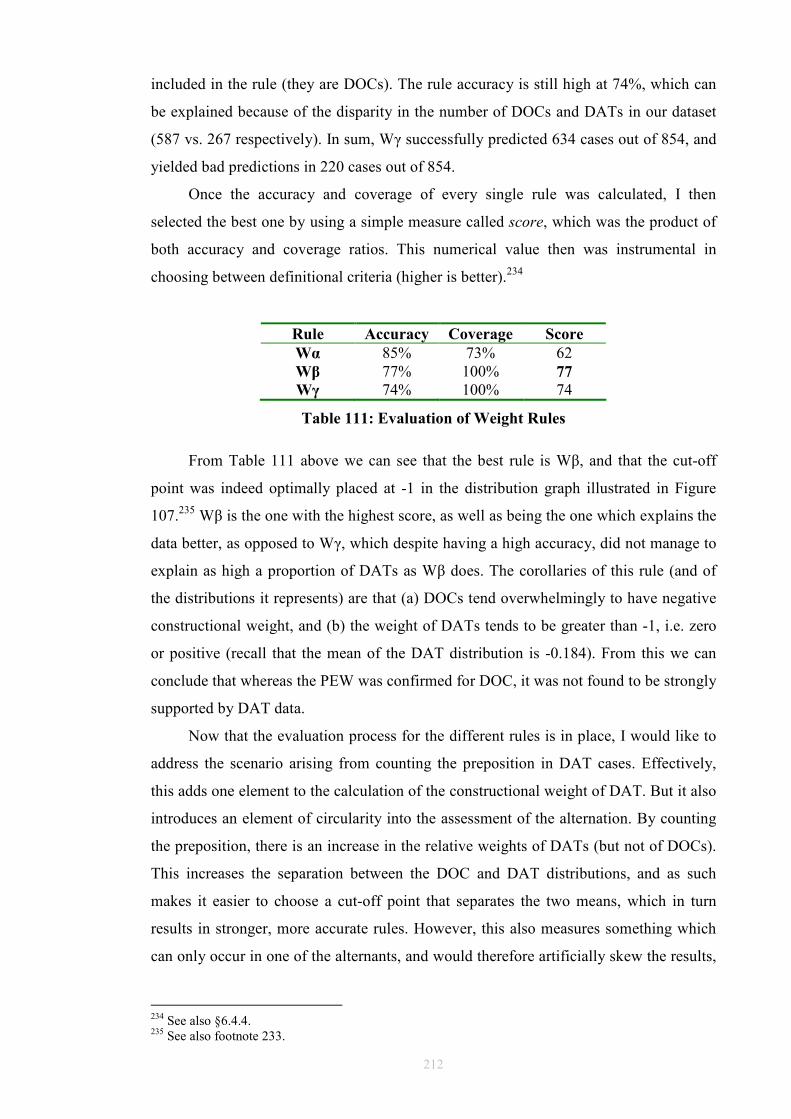
212

included in the rule (they are DOCs). The rule accuracy is still high at 74%, which can

be explained because of the disparity in the number of DOCs and DATs in our dataset

(587 vs. 267 respectively). In sum, Wγ successfully predicted 634 cases out of 854, and

yielded bad predictions in 220 cases out of 854.

Once the accuracy and coverage of every single rule was calculated, I then

selected the best one by using a simple measure called score, which was the product of

both accuracy and coverage ratios. This numerical value then was instrumental in

choosing between definitional criteria (higher is better).234

Rule Accuracy Coverage Score

Wα 85% 73% 62 Wβ 77% 100% 77

Wγ 74% 100% 74

Table 111: Evaluation of Weight Rules

From Table 111 above we can see that the best rule is Wβ, and that the cut-off

point was indeed optimally placed at -1 in the distribution graph illustrated in Figure

107.235 Wβ is the one with the highest score, as well as being the one which explains the

data better, as opposed to Wγ, which despite having a high accuracy, did not manage to

explain as high a proportion of DATs as Wβ does. The corollaries of this rule (and of

the distributions it represents) are that (a) DOCs tend overwhelmingly to have negative

constructional weight, and (b) the weight of DATs tends to be greater than -1, i.e. zero

or positive (recall that the mean of the DAT distribution is -0.184). From this we can

conclude that whereas the PEW was confirmed for DOC, it was not found to be strongly

supported by DAT data.

Now that the evaluation process for the different rules is in place, I would like to

address the scenario arising from counting the preposition in DAT cases. Effectively,

this adds one element to the calculation of the constructional weight of DAT. But it also

introduces an element of circularity into the assessment of the alternation. By counting

the preposition, there is an increase in the relative weights of DATs (but not of DOCs).

This increases the separation between the DOC and DAT distributions, and as such

makes it easier to choose a cut-off point that separates the two means, which in turn

results in stronger, more accurate rules. However, this also measures something which

can only occur in one of the alternants, and would therefore artificially skew the results,

234 See also §6.4.4. 235 See also footnote 233.

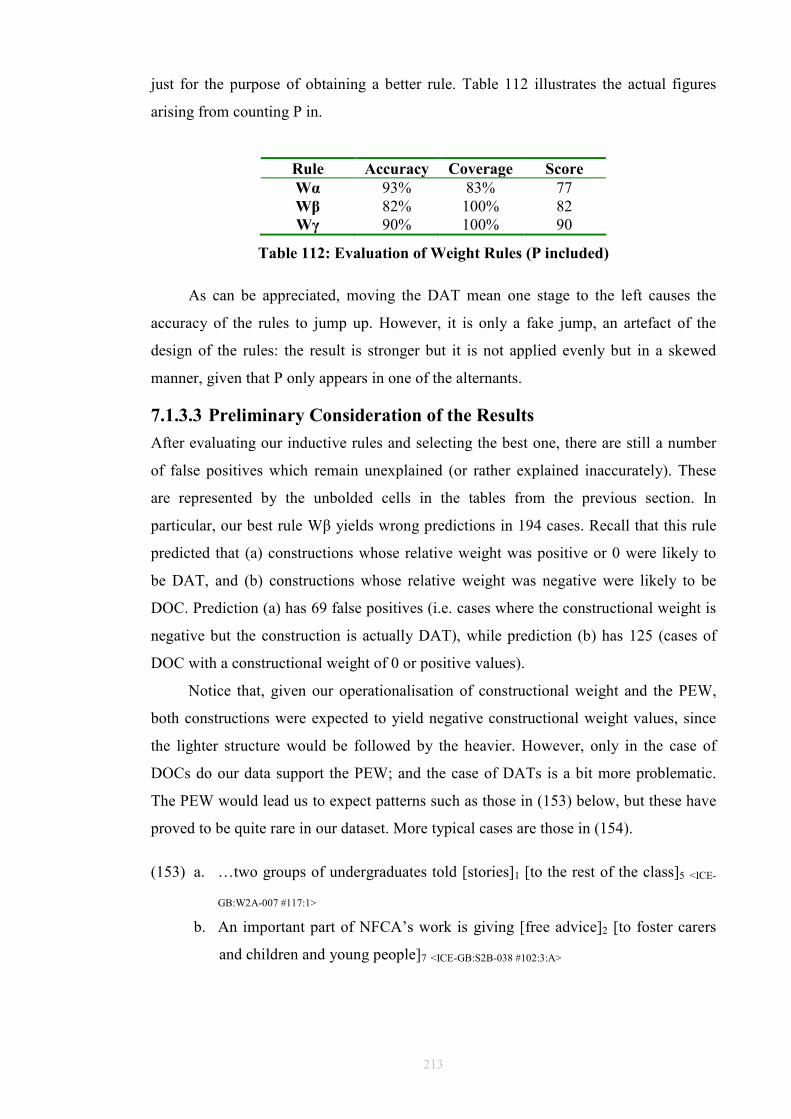
213

just for the purpose of obtaining a better rule. Table 112 illustrates the actual figures

arising from counting P in.

Rule Accuracy Coverage Score

Wα 93% 83% 77 Wβ 82% 100% 82 Wγ 90% 100% 90

Table 112: Evaluation of Weight Rules (P included)

As can be appreciated, moving the DAT mean one stage to the left causes the

accuracy of the rules to jump up. However, it is only a fake jump, an artefact of the

design of the rules: the result is stronger but it is not applied evenly but in a skewed

manner, given that P only appears in one of the alternants.

7.1.3.3 Preliminary Consideration of the Results

After evaluating our inductive rules and selecting the best one, there are still a number

of false positives which remain unexplained (or rather explained inaccurately). These

are represented by the unbolded cells in the tables from the previous section. In

particular, our best rule Wβ yields wrong predictions in 194 cases. Recall that this rule

predicted that (a) constructions whose relative weight was positive or 0 were likely to

be DAT, and (b) constructions whose relative weight was negative were likely to be

DOC. Prediction (a) has 69 false positives (i.e. cases where the constructional weight is

negative but the construction is actually DAT), while prediction (b) has 125 (cases of

DOC with a constructional weight of 0 or positive values).

Notice that, given our operationalisation of constructional weight and the PEW,

both constructions were expected to yield negative constructional weight values, since

the lighter structure would be followed by the heavier. However, only in the case of

DOCs do our data support the PEW; and the case of DATs is a bit more problematic.

The PEW would lead us to expect patterns such as those in (153) below, but these have

proved to be quite rare in our dataset. More typical cases are those in (154).

(153) a. …two groups of undergraduates told [stories]1 [to the rest of the class]5 <ICE-

GB:W2A-007 #117:1>

b. An important part of NFCA’s work is giving [free advice]2 [to foster carers

and children and young people]7 <ICE-GB:S2B-038 #102:3:A>

214

(154) a. …I propose to send [your description]2 to [them]1 <ICE-GB:W1B-030 #46:3>

b. …the Government agreed to pay [all the compensation costs]4 [to redundant

workers]2 <ICE-GB:W2C-001 #27:2>

c. …the NCC will send [its recommendations for 14 to 16-year-olds ]8 [to

MacGregor]1 <ICE-GB:W2C-002 #14:1>

These cases cannot be explained by weight considerations alone, but other notions

need to be resorted to. Perhaps complexity? This is what Chomsky (1975:477) had to

say on the issue:

It is interesting to note that it is apparently not the length of words of the object that determines the naturalness of the transformation, but, rather, in some sense, its complexity. Thus “they brought all the leaders of the riot in” seems more natural that “they brought the man I saw in.” The latter, though shorter, is more complex.236

7.2 Complexity

Several authors have claimed that complexity is indeed the motivation behind the

constructional rearrangement of constituents. Foremost among these authors is Hawkins

(1994), in whose Early Immediate Constituents (EIC) model word order is subservient

to a purely syntactic processing principle, measured as the relative complexity of the

involved constituents. In this light, complexity is independent from context, identity of

discourse participants, speaker’s intentions, or indeed any other pragmatic factors.

7.2.1 Complexity: Definitions and Assumptions

As we have seen in §7.1.1, complexity has been variously defined in the literature. For

our purposes, the complexity of each constituent is considered to be the number of

phrasal nodes it dominates, and the constructional complexity will be arrived at by

deducting the complexity of the second constituent from that of the first, in keeping

with the operationalisation of our measure of weight.

7.2.2 Complex Accounts

The thrust of Hawkins (1994) is that performance considerations (i.e. an unconscious

desire on the part of participants in a conversation to recognize constituent structure

online as quickly and efficiently as possible) can explain structure, and therefore

236 Chomsky was referring to the particle movement transformation.

215

principles such as PEW or PEF are epiphenomenal. In other words, there is no such

thing as given before new, or short before long; all these preferences are explained by

the parser’s desire to ensure recognition of phrasal heads as early as possible.

In his words (Hawkins 1994:57):

[C]onstituents occur in the orders they do so that syntactic groupings and their immediate constituents (ICs) can be recognized (and produced) as rapidly and as efficiently as possible in language performance. Different orderings of elements result in more or less rapid IC recognition. 237

Hawkins comes up with a very convoluted method for calculating complexity,

whereby complexity is a ratio between the number of words in a construction and the

number of (immediate) constituents involved in it. An important notion for the EIC

model is that of Constituent Recognition Domain (CRD), which represents the number

of nodes that need to be parsed by the addressee in order to recognise the construction in

question. The CRD is instrumental in making processing decisions. Consider the

examples below, and Hawkins’ explanation (1994:57):

(155) a. I [VP gave [NP the valuable book that was extremely difficult to find] [PP to

Mary]]

b. I [VP gave [PP to Mary] [NP the valuable book that was extremely difficult to

find]]

Example (155)b provides a more rapid presentation of the three ICs of the VP (V, NP, and PP) than (155)a. The verb gave is the first IC of the VP in both examples and signals to the parser that a VP should be constructed. The PP is a two-word IC here. Its positioning to the left of the lengthy NP in (155)b makes it possible for all three daughter ICs to be recognized within a short viewing window, since the NP can be recognized on the basis of the determiner the, occurring in leftmost position within this NP. In (155)a, on the other hand, the viewing window extends all the way from gave to the preposition to, (…) and the heaviness of the intervening NP delays access to this third IC. Of the twelve total words dominated by this VP, therefore, 11 need to be examined for IC recognition in (155)a, whereas just four suffice in (155)b.

In this light, smaller CRDs are more efficient and therefore preferable, since they

reduce the processing cost for both speaker and parser. The CRD sets the framework for

Hawkins’ final notion, his IC-to-non-IC ratio, which is arrived at by dividing the

237 We will not concern ourselves with determining what the ultimate purpose and functionality of weight or complexity effects is. Some authors (e.g. Frazier and Fodor 1978; Hawkins 1990, 1994; Kimball 1973) have argued that the PEW facilitates parsing by postponing long and/or complex elements, and thus minimises the processing cost. However, Wasow (1997a:94) believes that there is an air of implausibility about parsing considerations as the ultimate explanation, given that for words and (phrasal) nodes to be counted (and for the ordering of constituents to be evaluated for communicative efficiency), it is necessary for the speaker to have the utterance fully formulated before speaking. Rather, by appealing to experimental evidence showing that utterance planning is carried out sentence-internally, the postponement of heavy, difficult phrases is better explained by virtue of the fact that this technique facilitates planning during utterance production.

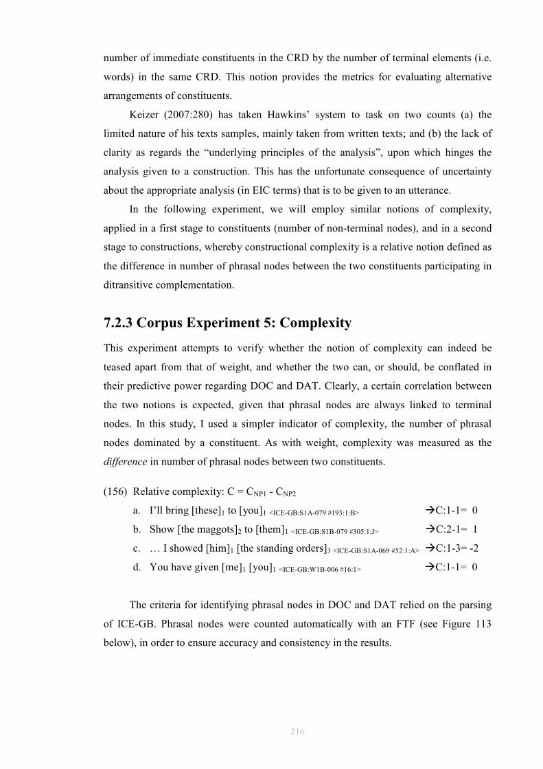
216

number of immediate constituents in the CRD by the number of terminal elements (i.e.

words) in the same CRD. This notion provides the metrics for evaluating alternative

arrangements of constituents.

Keizer (2007:280) has taken Hawkins’ system to task on two counts (a) the

limited nature of his texts samples, mainly taken from written texts; and (b) the lack of

clarity as regards the “underlying principles of the analysis”, upon which hinges the

analysis given to a construction. This has the unfortunate consequence of uncertainty

about the appropriate analysis (in EIC terms) that is to be given to an utterance.

In the following experiment, we will employ similar notions of complexity,

applied in a first stage to constituents (number of non-terminal nodes), and in a second

stage to constructions, whereby constructional complexity is a relative notion defined as

the difference in number of phrasal nodes between the two constituents participating in

ditransitive complementation.

7.2.3 Corpus Experiment 5: Complexity

This experiment attempts to verify whether the notion of complexity can indeed be

teased apart from that of weight, and whether the two can, or should, be conflated in

their predictive power regarding DOC and DAT. Clearly, a certain correlation between

the two notions is expected, given that phrasal nodes are always linked to terminal

nodes. In this study, I used a simpler indicator of complexity, the number of phrasal

nodes dominated by a constituent. As with weight, complexity was measured as the

difference in number of phrasal nodes between two constituents.

(156) Relative complexity: C = CNP1 - CNP2

a. I’ll bring [these]1 to [you]1 <ICE-GB:S1A-079 #193:1:B> �C:1-1= 0

b. Show [the maggots]2 to [them]1 <ICE-GB:S1B-079 #305:1:J> �C:2-1= 1

c. … I showed [him]1 [the standing orders]3 <ICE-GB:S1A-069 #52:1:A> �C:1-3= -2

d. You have given [me]1 [you]1 <ICE-GB:W1B-006 #16:1> �C:1-1= 0

The criteria for identifying phrasal nodes in DOC and DAT relied on the parsing

of ICE-GB. Phrasal nodes were counted automatically with an FTF (see Figure 113

below), in order to ensure accuracy and consistency in the results.

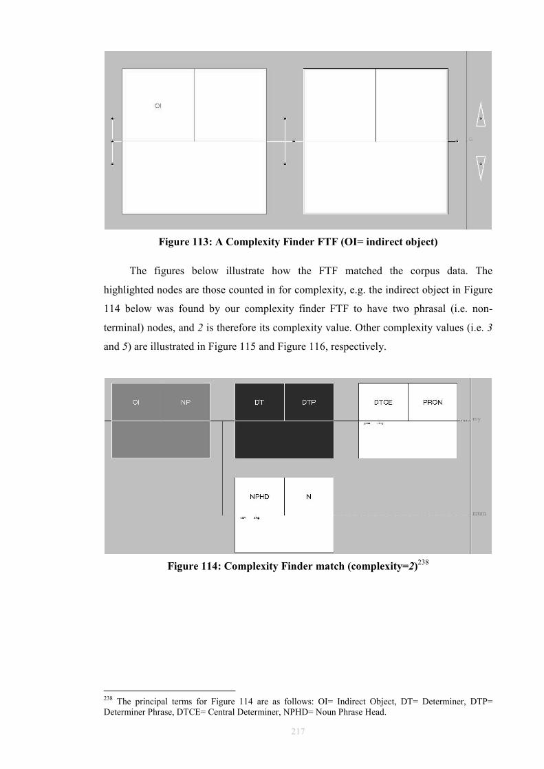
217

Figure 113: A Complexity Finder FTF (OI= indirect object)

The figures below illustrate how the FTF matched the corpus data. The

highlighted nodes are those counted in for complexity, e.g. the indirect object in Figure

114 below was found by our complexity finder FTF to have two phrasal (i.e. non-

terminal) nodes, and 2 is therefore its complexity value. Other complexity values (i.e. 3

and 5) are illustrated in Figure 115 and Figure 116, respectively.

Figure 114: Complexity Finder match (complexity=2)238

238 The principal terms for Figure 114 are as follows: OI= Indirect Object, DT= Determiner, DTP= Determiner Phrase, DTCE= Central Determiner, NPHD= Noun Phrase Head.

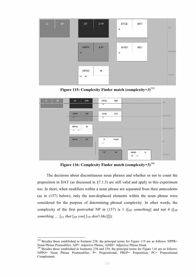
218

Figure 115: Complexity Finder match (complexity=3)239

Figure 116: Complexity Finder match (complexity=5)240

The decisions about discontinuous noun phrases and whether or not to count the

preposition in DAT (as discussed in §7.1.3) are still valid and apply to this experiment

too. In short, when modifiers within a noun phrase are separated from their antecedents

(as in (157) below), only the non-displaced elements within the noun phrase were

considered for the purpose of determining phrasal complexity. In other words, the

complexity of the first postverbal NP in (157) is 1 ([NP something] and not 4 ([NP

something … [CL that [NP you] [VP don't like]]]).

239 Besides those established in footnote 238, the principal terms for Figure 115 are as follows: NPPR= Noun Phrase Premodifier, AJP= Adjective Phrase, AJHD= Adjective Phrase Head. 240 Besides those established in footnotes 238 and 239, the principal terms for Figure 116 are as follows: NPPO= Noun Phrase Postmodifier, P= Prepositional, PREP= Preposition; PC= Prepositional Complement.

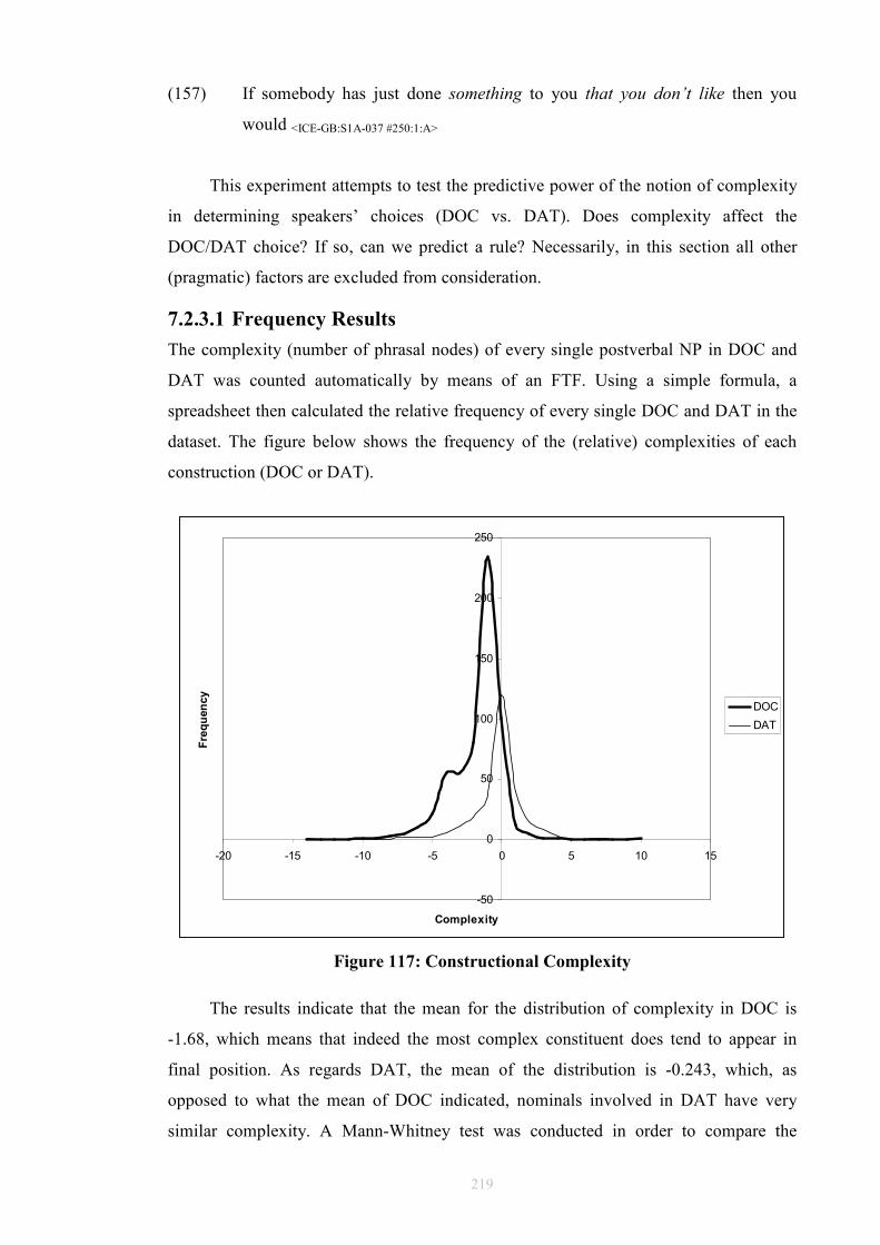
219

(157) If somebody has just done something to you that you don’t like then you

would <ICE-GB:S1A-037 #250:1:A>

This experiment attempts to test the predictive power of the notion of complexity

in determining speakers’ choices (DOC vs. DAT). Does complexity affect the

DOC/DAT choice? If so, can we predict a rule? Necessarily, in this section all other

(pragmatic) factors are excluded from consideration.

7.2.3.1 Frequency Results

The complexity (number of phrasal nodes) of every single postverbal NP in DOC and

DAT was counted automatically by means of an FTF. Using a simple formula, a

spreadsheet then calculated the relative frequency of every single DOC and DAT in the

dataset. The figure below shows the frequency of the (relative) complexities of each

construction (DOC or DAT).

-50

0

50

100

150

200

250

-20 -15 -10 -5 0 5 10 15

Complexity

Frequency

DOC

DAT

Figure 117: Constructional Complexity

The results indicate that the mean for the distribution of complexity in DOC is

-1.68, which means that indeed the most complex constituent does tend to appear in

final position. As regards DAT, the mean of the distribution is -0.243, which, as

opposed to what the mean of DOC indicated, nominals involved in DAT have very

similar complexity. A Mann-Whitney test was conducted in order to compare the

220

distributions of DOC and DAT, and the result indicated (statistical) significance (z =

12.25). This result shows that there are two different distributions in Figure 117 above.

This result allows us to claim that there is a reliable relationship between

complexity and DOC/DAT and this relationship is not a matter of chance. Complexity

tends to affect choice. At this point it is worth noting the similarities between the

complexity results described here and the weight results reported in §7.1.3. The means

are very similar (mean DOC weight: -1.78, mean DAT weight: -0.184), as is the value

of z (12.96 for weight and 12.25 for complexity).

7.2.3.2 An Inductive Measure of Complexity

We next tried to generate an inductive rule for complexity along the lines set out in

§7.1.3.2 for weight. The idea is to try and capture generalisations in the behaviour of the

alternants based on our dataset. Taking the distributions in Figure 117 as basis, I

decided to evaluate three cut-off points in order to separate the two complexity

distributions, and eventually arrive at the best inductive rule. As before, the three cut-off

points (0, -1, and 0.1) were evaluated for their accuracy and coverage.241

The first rule evaluated was Cα, based on a cut-off point located at 0. This would

indicate that if the complexity of a construction (notice that no construction is specified)

is positive, then the rule predicts that the construction in question would be DAT. When

relative complexity is negative, then the construction would be DOC. If the

constructional complexity is right on the cut-off (i.e. 0) then, the rule offers no

prediction. This is summarized in (158) below.

(158) Cα (cut-off = 0)

If C > 0 => DAT

If C < 0 => DOC

If C = 0 => ?

Table 118 below illustrates the predictions of Cα when compared with the actual

corpus data. As can be appreciated, the rule explains the bolded cells in Table 118, but

does not explain the unbolded ones (false positives).

241 As in the case of cut-off for weight (see §7.1.3.2), here again we could have tested many different cut-off points for their contribution to the model (e.g. -0.1, -0.2, etc.). This proved to be unnecessary by virtue of the fact that only a few cut-off points were able to (a) maximally separate the means of the two distributions, and (b) provide a suitable solution to cases of zero constructional complexity.

221

C>0 C<0

DAT 68 79 DOC 20 466

Table 118: Cα Predictions

The predictions are quite accurate for DOCs, where there are only 20 false

positives. In the case of DATs, the rule fails to yield anything better than 50% accuracy.

The rule does not apply for every single case in which the relative complexity falls on

the cut-off (i.e. 0), and these are not negligible (101 in DOC, 120 in DAT). The rule

coverage is 84%, its accuracy is 73%. In actual figures, Cα successfully predicted 534

cases out of 633, inaccurately predicted 99 cases out of 633, and offered no predictions

at all in 221 cases.

The next rule evaluated was Cβ, based on a cut-off point located at -1, perhaps the

optimal point for separating the means if we look at the complexity distribution figure

above. This cut-off point specifies that if the constructional complexity is positive or

zero, then the rule predicts that the construction would be DAT. In all other cases, then

the construction would be DOC. The -1 cut-off point pushes all the 0s in the direction of

DAT, thus maximizing the coverage of the rule. This is summarized in (139) below.

(159) Cβ (cut-off = -1)

If C ≥ 0 => DAT

If C < 0 => DOC

Table 119 below presents the predictions of Cβ. The rule explains the bolded

cells, but does not explain the unbolded ones (false positives).

C≥0 C<0

DAT 188 79 DOC 121 466

Table 119: Cβ Predictions

The predictions are quite accurate for DOCs, although the number of false

positives has increased dramatically (from 20 to 121). In the case of DATs, the rule

does show an improvement over Cα, explaining many more cases (true positives) while

keeping its false positives constant. The rule accuracy is better at 77%. Cβ successfully

predicted 654 cases out of 854, and wrongly predicted 200 cases out of 854.

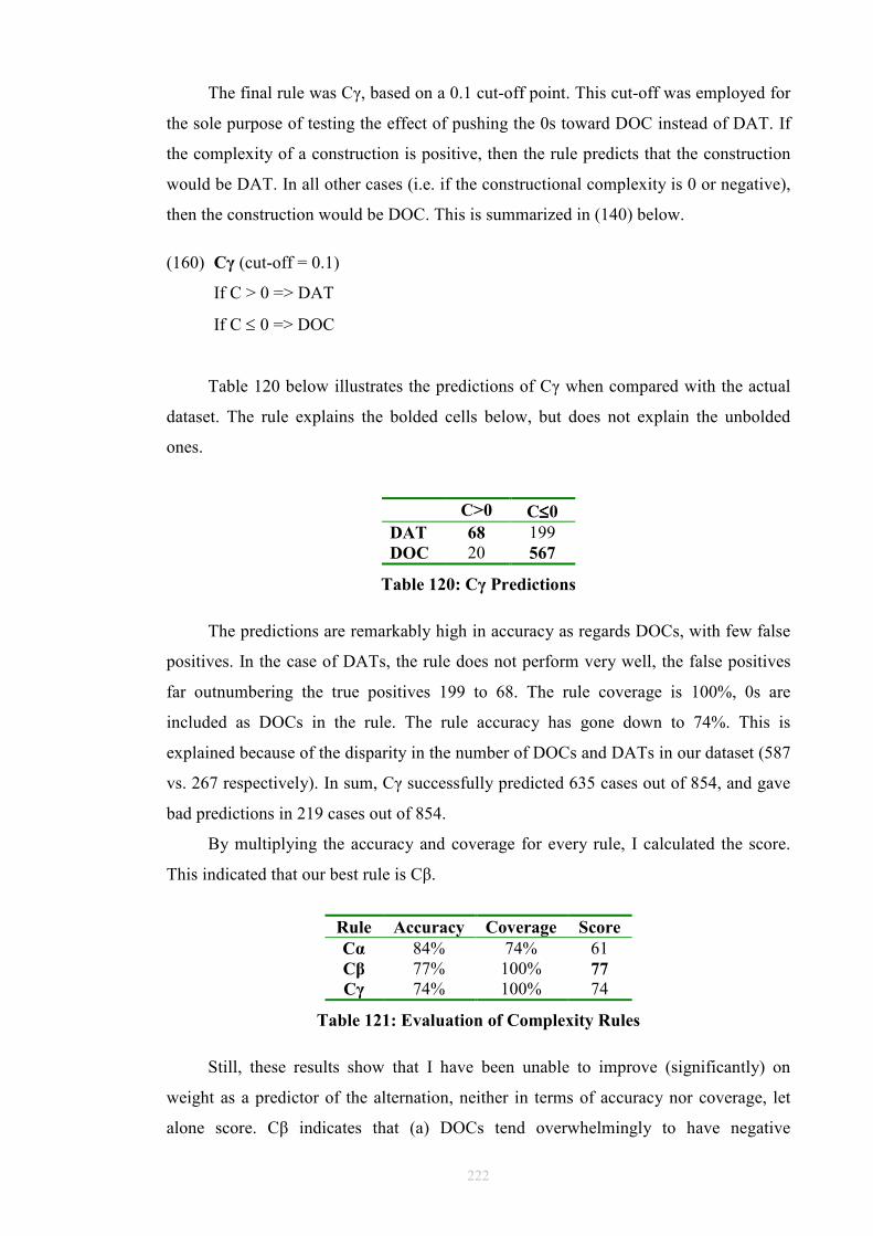
222

The final rule was Cγ, based on a 0.1 cut-off point. This cut-off was employed for

the sole purpose of testing the effect of pushing the 0s toward DOC instead of DAT. If

the complexity of a construction is positive, then the rule predicts that the construction

would be DAT. In all other cases (i.e. if the constructional complexity is 0 or negative),

then the construction would be DOC. This is summarized in (140) below.

(160) Cγ (cut-off = 0.1)

If C > 0 => DAT

If C ≤ 0 => DOC

Table 120 below illustrates the predictions of Cγ when compared with the actual

dataset. The rule explains the bolded cells below, but does not explain the unbolded

ones.

C>0 C≤≤≤≤0

DAT 68 199 DOC 20 567

Table 120: Cγ Predictions

The predictions are remarkably high in accuracy as regards DOCs, with few false

positives. In the case of DATs, the rule does not perform very well, the false positives

far outnumbering the true positives 199 to 68. The rule coverage is 100%, 0s are

included as DOCs in the rule. The rule accuracy has gone down to 74%. This is

explained because of the disparity in the number of DOCs and DATs in our dataset (587

vs. 267 respectively). In sum, Cγ successfully predicted 635 cases out of 854, and gave

bad predictions in 219 cases out of 854.

By multiplying the accuracy and coverage for every rule, I calculated the score.

This indicated that our best rule is Cβ.

Rule Accuracy Coverage Score

Cα 84% 74% 61 Cβ 77% 100% 77

Cγ 74% 100% 74

Table 121: Evaluation of Complexity Rules

Still, these results show that I have been unable to improve (significantly) on

weight as a predictor of the alternation, neither in terms of accuracy nor coverage, let

alone score. Cβ indicates that (a) DOCs tend overwhelmingly to have negative

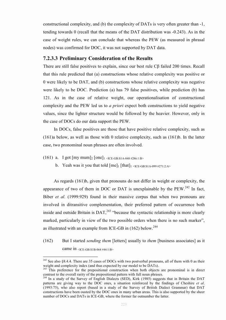
223

constructional complexity, and (b) the complexity of DATs is very often greater than -1,

tending towards 0 (recall that the means of the DAT distribution was -0.243). As in the

case of weight rules, we can conclude that whereas the PEW (as measured in phrasal

nodes) was confirmed for DOC, it was not supported by DAT data.

7.2.3.3 Preliminary Consideration of the Results

There are still false positives to explain, since our best rule Cβ failed 200 times. Recall

that this rule predicted that (a) constructions whose relative complexity was positive or

0 were likely to be DAT, and (b) constructions whose relative complexity was negative

were likely to be DOC. Prediction (a) has 79 false positives, while prediction (b) has

121. As in the case of relative weight, our operationalisation of constructional

complexity and the PEW led us to a priori expect both constructions to yield negative

values, since the lighter structure would be followed by the heavier. However, only in

the case of DOCs do our data support the PEW.

In DOCs, false positives are those that have positive relative complexity, such as

(161)a below, as well as those with 0 relative complexity, such as (161)b. In the latter

case, two pronominal noun phrases are often involved.

(161) a. I got [my mum]2 [one]1 <ICE-GB:S1A-048 #286:1:B>

b. Yeah was it you that told [me]1 [that]1 <ICE-GB:S1A-099 #271:2:A>

As regards (161)b, given that pronouns do not differ in weight or complexity, the

appearance of two of them in DOC or DAT is unexplainable by the PEW.242 In fact,

Biber et al. (1999:929) found in their massive corpus that when two pronouns are

involved in ditransitive complementation, their preferred pattern of occurrence both

inside and outside Britain is DAT,243 “because the syntactic relationship is more clearly

marked, particularly in view of the two possible orders when there is no such marker”,

as illustrated with an example from ICE-GB in (162) below.244

(162) But I started sending them [letters] usually to them [business associates] as it

came in <ICE-GB:S1B-064 #44:1:B>

242 See also §8.4.4. There are 35 cases of DOCs with two postverbal pronouns, all of them with 0 as their weight and complexity index (and thus expected by our model to be DATs). 243 This preference for the prepositional construction when both objects are pronominal is in direct contrast to the overall rarity of the prepositional pattern with full noun phrases. 244 In a study of the Survey of English Dialects (SED), Kirk (1985) suggests that in Britain the DAT patterns are giving way to the DOC ones, a situation reinforced by the findings of Cheshire et al. (1993:75), who also report (based in a study of the Survey of British Dialect Grammar) that DAT constructions have been ousted by the DOC ones in many urban areas. This is also supported by the sheer number of DOCs and DATs in ICE-GB, where the former far outnumber the latter.

224

In DOC cases, Biber et al. (1999:929) identify two patterns, which I will call

DOCi and DOCii, as seen in (163) below. DOCi instances have a very high frequency in

conversation, and are mainly found with the pronoun it as direct object. Notice that

while it is naturally construed as a direct, inanimate object, other personal pronouns

could just as easily be interpreted as an indirect or a direct object. This is why for the

speaker in (162), DAT was the only option. As regards DOCii (as seen in (163)b and c),

Biber et al. (1999:930) found it mainly occurred in conversation and fiction.245

(163) a. Give me it (DOCi)

b. Give it me (DOCii)

c. You gave him [a dog] me. <ICE-GB:W2F-001 #108:1>

According to Biber et al. (1999:929), register can be considered a strong

explanatory factor in deciding among the competing patterns when both objects are

pronominal. In their data, DOCi patterns are twice as frequent as DOCii ones, whereas in

fiction the reverse patterns prevails. Hawkins (1994:312-313) accounts for DOCi and

DOCii cases by resorting to complexity. Consider his examples below:

(164) I [VP gave it [PP to him]]

VP Constituent Recognition Domain (CRD, see §7.2.2): 3/3=100%

(165) I [VP gave [NP him] it]

VP CRD: 3/3=100%

Despite the example in (164) corresponding to the most frequent pattern, he sees

that the overall structure of the VP is simpler in (165) than in (164), given that the P and

PP nodes are no longer there. The CRDs for the VPs in both examples are not being

improved upon, both rate at 100%. This simplification by removal of nodes is also

employed to account for cases of DOCii (example (166) below), despite no CRD

improvement being made.

(166) I [VP gave it him]

VP CRD: 3/3=100%

245 Jespersen (1927:278-287) attributed the presence of the immediately postverbal it in examples such as (163)b to a tendency in all languages to place “a weakly stressed pronoun as near to the verb as possible. This may sometime lead to the direct object being placed before the indirect object.”

225

Support for Hawkins’ explanation can be provided by dialectal studies. For

example, in their study of Lancashire dialects, Siewierska and Hollmann (2007) have

found out that when both theme and recipient are personal pronouns, there is a clear

preference for positioning the theme before the recipient (i.e. DOCii cases such as

(163)b), so much so that this alternative double object construction is nearly twice as

common as the canonical one (i.e. DOCi cases such as (163)a). In fact the theme-before-

recipient order is not only dominant in the DOC cases, but is also dominant overall, as it

also obtains in the DAT ones. In Lancashire then, the most common patterns are

differentiated not in terms of ordering but simply in terms of the presence or absence of

a preposition, as we can see below.

(167) a. I’ll give it your sister.

b. I’ll give it to your sister.

7.3 Conclusions

Weight and complexity are difficult to separate. At the same time, lexical weight is

(marginally) a better predictor of the alternation. Both measures are very successful

predictors of constituent ordering, with over 75% accuracy for the alternations in our

dataset. This conclusion seem to be aligned with those of Wasow (1997a) and Hawkins

(1994). As pointed out earlier, this finding is not entirely unexpected, given that more

words usually mean more structure, and more structure usually means more words.

There still remain some unexplained cases. Weight and complexity are also

claimed to correlate with information status (GBN). I will discuss this in detail in

chapter 8.

226

8 Interacting Variables

8.1 Introduction: Resolving Competing Hypotheses

We have seen in previous chapters that information status, weight, and complexity each

explain a good percentage of cases of the dative alternation. Many linguists have tried to

employ reductive theories that essentially seek to explain linguistic phenomena by

recourse to a single, simple, underlying variable. Hawkins (1994), for instance,

considers weight/complexity to be the only significant determinant of word order

variation.

The problem is that all the different factors discussed so far in this study (which

include Hawkins’) fail to account for all instances of either DOC or DAT. This fact has

driven many efforts towards accounting for word order variation (of which the dative

alternation is a case in point) by means of an army of potential explanatory factors. For

example, Gries (2003b) used discriminant analysis (a multiple regression method) to

derive dative alternation predictions from a dataset. He coded for animacy, referential

distance, semantic process described by the verb, kind of determiner, pronominality,

and discourse status of the noun phrases instantiating DOC and DAT. His model

accurately identifies 83% of DATs and 95% of DOCs. DATs are elusive for his model

too.246

In another study of the dative alternation, Bresnan et al. (2004-2007) employed

logistic regression using variables such as (discourse) accessibility, pronominality,

definiteness, animacy, number, length, semantic class of the verb, and structural

parallelism, the first six elements being coded in both recipients and themes. Their

results are impressive: they claim their model is able to accurately predict 94% of the

actual choice (i.e. DOC/DAT) in a corpus of telephone conversations.247 In a similar

study, Bresnan and Hay (2008) also employed logistic regression, but did not code for

definiteness and number, while adding syntactic complexity (measured as number of

graphemic words) to the mix of factors.

Wasow and Arnold (2003) have praised (as well as employed) studies resorting to

multiple factors because of their adequacy for treating factor weighting (i.e. some

factors are stronger than others, no factor is categorical), as well as factor interaction.

Models employing multiple factors are susceptible to criticism precisely for the high

246 As will be seen in §8.4.2, the model introduced in this study accurately predicts 79% of DOCs and 74% of DATs. 247 Their findings also determined that givenness, animacy, definiteness, pronominality, and relative length are all associated with immediate postverbal position in both DOC and DAT.

227

factorial correlations; that is, despite factor combination models offering improved

predictions, their results are very difficult to attribute to any one explanatory factor.

Consider (168) below. It is a challenge verging on the impossible to decide whether her

is placed in immediately postverbal position because it is given, because it is animate,

because it is a pronoun, because it is short (or shorter than the next complement), or

because it is less complex (than the next complement).

(168) Paolo gave her a football top from his home team.

As a methodological aside, we need to insist yet again that correlations should not

be confused with explanations. Thus, research into correlating factors has to address the

issue of the linguistic motivation of empirical analysis. Specifically, how can we

separate (and compare) the effect that different but correlated factors have on our

dataset? How can we be certain whether or not, e.g., information status is a consequence

of weight, or for that matter, that weight is a consequence of information status? Are

these notions two different factors, or is it just that one of them looks like a causal factor

because of its high correlation with the other? In other words, are the factors under

consideration independent, or is there a fundamental one that renders the others

epiphenomenal? These questions cannot be settled by mere correlational statistics.

In sum, the three variables discussed in this study (information status, weight, and

complexity) are predictive, but (a) do they overlap to the extent that one explanation can

be subsumed under another?, and (b) if we take them together, can we get a higher

degree of coverage than with each variable on its own? Finally, is there an overarching

generalisation linking the various factors that affect the alternation? If (b) is true, that

would mean that despite their overlaps, there is some degree of independence between

them, a conclusion both important and useful: it is not the case that each prediction

reduces to the other one.

8.2 Weight vs. Complexity

In chapter 7 we considered two different implementations of the PEW separately:

weight (number of words) and complexity (number of phrasal nodes). However, long

phrases have more complex structures (more phrasal nodes and very often clausal or

228

prepositional postmodifiers), and thus it is not uncommon to find the two notions

conflated.248

8.2.1 Interaction (i)

The experiments in chapter 7 have looked at overlapping hypotheses trying to predict a

particular contingent event: the choice of DOC or DAT structures. There is apparently a

core of cases which are covered by weight and complexity measures, both variables

being plausible explanations for word order arrangements. This is reinforced by the fact

that we arrived at two inductive rules (i.e. Wβ in §7.1.3.2 and Cβ in §7.2.3.2) with very

similar accuracy and coverage (77% and 100% respectively for both measures). This

logical dependency between weight and complexity does not preclude the existence of

slightly different (explained) sample sets. In what follows I attempt to determine

whether, in considering weight and complexity as separate explanations, we are

essentially describing the same intrinsic phenomenon in different ways. Can we

demonstrate that these two notions are just alternative types of measure for heaviness?

If that is not the case, and we pit one against the other, does complexity predict the

result of the linguistic choice between DOC/DAT better than weight? Can we apply

Occam’s razor, i.e. is ‘number of words’ simpler than ‘number of phrasal nodes’? These

issues will be discussed in the following sections. A discussion of the interaction

between PEF and PEW is reserved for §8.3.

8.2.2 Weight vs. Complexity: Results

I conducted a regression test to check whether weight and complexity were measuring

the same thing (see chapter 4, particularly §4.6.3, for a description of the tests employed

in these experiments). The resulting scattergram (plotting the distribution of the relative

weight and the relative complexity of DOC and DAT in our dataset) was evaluated by

means of Spearman’s rho (a measure of linear correlation). If weight and complexity are

indeed measuring the same thing, we would expect to see a nice fit between the

distributions of weight and complexity of both DOC and DAT, with the dots in the

distribution forming an approximate line, and a positive regression value nearing 1. If

complexity and weight are measuring different things, then the scattergram should show

a cloud of dots and the regression value would be near 0.249 Figure 122 below illustrates

248 As we have seen in chapter 7, even separating PEW from PEF is sometimes difficult, given that constituents carrying new information often require lengthier statements, and thus also tend to occur later. 249 See Woods et al. (1986:160-161) and Oakes (1998:30-31) for further details on this test.

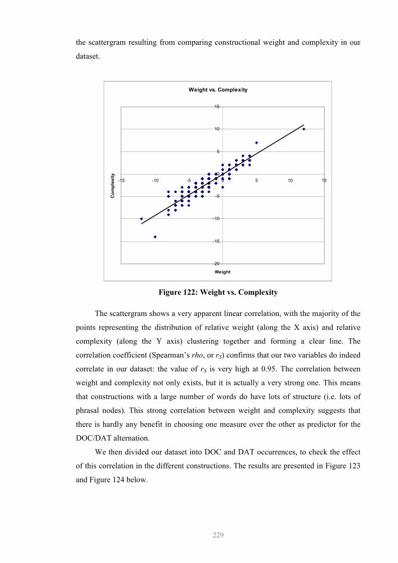
229

the scattergram resulting from comparing constructional weight and complexity in our

dataset.

Weight vs. Complexity

-20

-15

-10

-5

0

5

10

15

-15 -10 -5 0 5 10 15

Weight

Complexity

Figure 122: Weight vs. Complexity

The scattergram shows a very apparent linear correlation, with the majority of the

points representing the distribution of relative weight (along the X axis) and relative

complexity (along the Y axis) clustering together and forming a clear line. The

correlation coefficient (Spearman’s rho, or rS) confirms that our two variables do indeed

correlate in our dataset: the value of rS is very high at 0.95. The correlation between

weight and complexity not only exists, but it is actually a very strong one. This means

that constructions with a large number of words do have lots of structure (i.e. lots of

phrasal nodes). This strong correlation between weight and complexity suggests that

there is hardly any benefit in choosing one measure over the other as predictor for the

DOC/DAT alternation.

We then divided our dataset into DOC and DAT occurrences, to check the effect

of this correlation in the different constructions. The results are presented in Figure 123

and Figure 124 below.

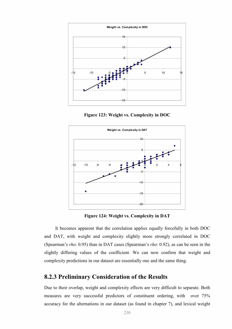
230

Weight vs. Complexity in DOC

-15

-10

-5

0

5

10

15

-15 -10 -5 0 5 10 15

Figure 123: Weight vs. Complexity in DOC

Weight vs. Complexity in DAT

-20

-15

-10

-5

0

5

10

-12 -10 -8 -6 -4 -2 0 2 4 6

Figure 124: Weight vs. Complexity in DAT

It becomes apparent that the correlation applies equally forcefully in both DOC

and DAT, with weight and complexity slightly more strongly correlated in DOC

(Spearman’s rho: 0.95) than in DAT cases (Spearman’s rho: 0.92), as can be seen in the

slightly differing values of the coefficient. We can now confirm that weight and

complexity predictions in our dataset are essentially one and the same thing.

8.2.3 Preliminary Consideration of the Results

Due to their overlap, weight and complexity effects are very difficult to separate. Both

measures are very successful predictors of constituent ordering, with over 75%

accuracy for the alternations in our dataset (as found in chapter 7), and lexical weight

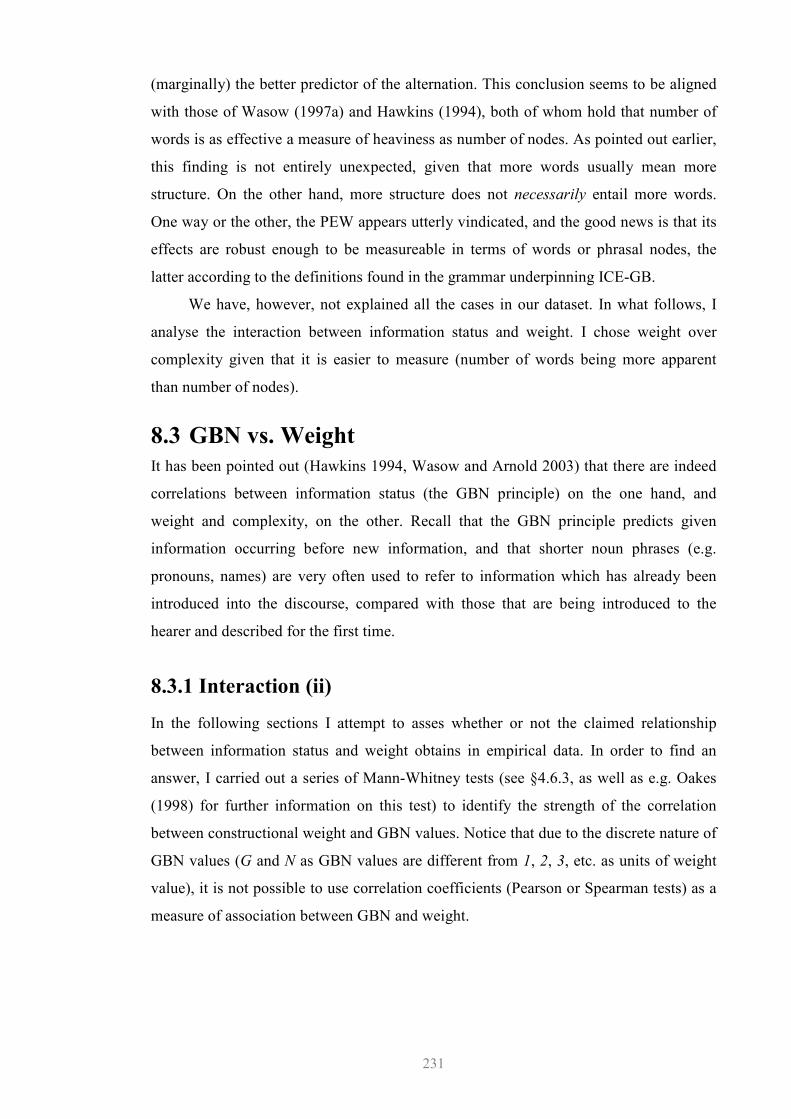
231

(marginally) the better predictor of the alternation. This conclusion seems to be aligned

with those of Wasow (1997a) and Hawkins (1994), both of whom hold that number of

words is as effective a measure of heaviness as number of nodes. As pointed out earlier,

this finding is not entirely unexpected, given that more words usually mean more

structure. On the other hand, more structure does not necessarily entail more words.

One way or the other, the PEW appears utterly vindicated, and the good news is that its

effects are robust enough to be measureable in terms of words or phrasal nodes, the

latter according to the definitions found in the grammar underpinning ICE-GB.

We have, however, not explained all the cases in our dataset. In what follows, I

analyse the interaction between information status and weight. I chose weight over

complexity given that it is easier to measure (number of words being more apparent

than number of nodes).

8.3 GBN vs. Weight

It has been pointed out (Hawkins 1994, Wasow and Arnold 2003) that there are indeed

correlations between information status (the GBN principle) on the one hand, and

weight and complexity, on the other. Recall that the GBN principle predicts given

information occurring before new information, and that shorter noun phrases (e.g.

pronouns, names) are very often used to refer to information which has already been

introduced into the discourse, compared with those that are being introduced to the

hearer and described for the first time.

8.3.1 Interaction (ii)

In the following sections I attempt to asses whether or not the claimed relationship

between information status and weight obtains in empirical data. In order to find an

answer, I carried out a series of Mann-Whitney tests (see §4.6.3, as well as e.g. Oakes

(1998) for further information on this test) to identify the strength of the correlation

between constructional weight and GBN values. Notice that due to the discrete nature of

GBN values (G and N as GBN values are different from 1, 2, 3, etc. as units of weight

value), it is not possible to use correlation coefficients (Pearson or Spearman tests) as a

measure of association between GBN and weight.

232

8.3.2 GBN vs. Weight: Results

The purpose of this section is to find out to what extent constructional weight is the

result of the GBN choice. The Mann-Whitney tests attempt to see whether the means of

the weight of different GBN configurations (e.g. GG, GN, etc.) can be separated. If they

can, then the different configurations are associated with different weights. If GBN and

weight values do correlate, then we have been measuring the same thing with different

elements.

Figure 125 below shows the frequency of the different configurations (GN, GG,

etc.) according to their weight, irrespective of DOC or DAT. That is, the X axis

represents the different constructional weights, and the Y axis plots the number of times

GBN configurations occurred in the dataset.

GBN vs. Weight

-50

0

50

100

150

200

-15 -10 -5 0 5 10 15

Weight

Frequency NN

GG

GN

NG

Figure 125: GBN vs. Weight

First of all, configuration NG does not offer enough data (only 24 cases, all

DATs) to be entered into any statistical test, so what follows are tests applied to the

distributions GN vs. GG, GG vs. NN, and GN vs. NN.

The first test contrasts the distribution of weight in GN configurations with that of

weight in GG configurations. GN configurations are instantiated 556 times in our

dataset, with over 85% of those occurring in DOC form. GG, on the other hand, occurs

233

201 times, with a majority of DAT cases (57%). The result of the Mann-Whitney test is

statistically significant (z= 9.83). In other words, GBN separates out two different

distributions vis-à-vis weight, i.e. the two tested configurations have different weights.

The mean of the weight of GN is -1.67, in keeping with expectations emanating from

our operationalisation of weight, according to which the weight of a particular instance

of a construction was calculated by deducting the weight of the second noun phrase

from that of the first noun phrase. In this light, a negative weight was expected to be the

default, a confirmation of the PEW. GN configurations appear to conform to the PEW.

The mean of the weight of GG is -0.348, very close to 0, which was the weight value

expected of this configuration, particularly when both noun phrases were realized as

pronouns.

Notice that in both GN and GG configurations the first element is given. As such,

this test is also telling us something about the effect of the second element, N in GN,

and G in GG. More specifically, it appears that the difference in the means is

attributable to this element. The occurrence of new information in the second noun

phrase of either DOC or DAT is indeed an indicator that the said noun phrase is heavier

(i.e. has more weight) than both (a) a noun phrase in immediately postverbal position

carrying given information, and (b) a noun phrase in second position carrying given

information.

The second pair tested was GG and NN. We have discussed GG configurations in

the preceding paragraph. NN configurations occurred 73 times, mostly in DAT (75%).

The result of the Mann-Whitney test is again statistically significant (z= 3.82). As in the

previous pair, GBN and weight affect the dataset in different ways and cannot be

conflated.

We have seen that GG configurations are expected to have 0 relative weight

(especially when instantiated by pronouns), and that expectation appears to have been

confirmed by the mean of their weight. NN configurations, on the other hand, have a

mean weight of -1.29.250 The negative value of this mean suggests that their relative

weight is better aligned with GN configurations than with GG ones. That is, regardless

of information status, the second noun phrase is clearly heavier than the first one, a

result which seems to support PEW. The newer, the weightier then. Also, when both

noun phrases have similar informational value (i.e. GG or NN), weight seems to be the

one tipping the scales towards DOC or DAT.

250 Notice that by definition, pronouns cannot occur in this configuration, in that their (mainly anaphoric) referring capabilities automatically brand them as carrying given information by proxy.

234

The final test pairs GN and NN, both already discussed in previous paragraphs.

The result of the Mann-Whitney test is also statistically significant (z= -1.78). Again,

GBN and weight are shown to behave differently and determine different data

distributions. As in the first case, GN and NN configurations share a second new

element. Thus, the test also touches on the effect of the first element (G in GN and N in

NN), and differences and similarities in the means could be tracked to this element.

Noun phrases in first position carrying new information appear to behave similarly to

those carrying given information (in that very same position) as regards weight; both are

lighter than the noun phrases following them. In other words, noun phrases in first

position behave similarly regardless of their information status, i.e. they are lighter than

noun phrases in second position.

8.3.3 Preliminary Consideration of the Results

Linguists have not failed to notice the correlation between information status and

heaviness/weight/complexity notions. What they make of this correlation, however,

varies. Some authors treat weight as the fundamental factor explaining the alternation,

with information status being treated as an epiphenomenal occurrence. Hawkins (1994)

is foremost among those reducing GBN effects (as well as other factors such as

animacy) to PEW ones.

Other authors are not as certain. Curiously, even contradictory results can be

found in Arnold et al. (2000) and Wasow (2002), who report that their corpus

investigation results support the dominance of weight over information status in

affecting ordering, but their experimental (psycholinguistic) results do not. This

discrepancy leads them to advocate a compromise solution, whereby neither GBN nor

PEW can be reduced to the other, and can thus cover more ground when accounting for

constituent ordering when combined.

This solution is the driving force behind Arnold et al.’s (2000) and Wasow’s

(2002) models, the former of which holds that:

[T]he role of each factor depends in part on the strength of competing factors. When there is a big weight difference between constituents, there is a strong tendency to produce the light argument early, and discourse status may not play as large a role. In contrast, when one argument is extremely accessible (…), discourse status will influence constituent ordering more than weight (Arnold et al. 2000:50).

Our tests in this section have shown that information status and weight define and

explain different subsets in our data, which means they are not coextensive. Reducing

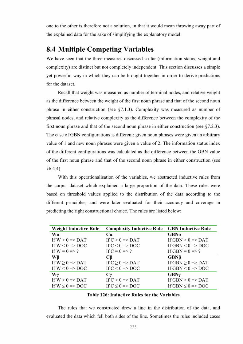
235

one to the other is therefore not a solution, in that it would mean throwing away part of

the explained data for the sake of simplifying the explanatory model.

8.4 Multiple Competing Variables

We have seen that the three measures discussed so far (information status, weight and

complexity) are distinct but not completely independent. This section discusses a simple

yet powerful way in which they can be brought together in order to derive predictions

for the dataset.

Recall that weight was measured as number of terminal nodes, and relative weight

as the difference between the weight of the first noun phrase and that of the second noun

phrase in either construction (see §7.1.3). Complexity was measured as number of

phrasal nodes, and relative complexity as the difference between the complexity of the

first noun phrase and that of the second noun phrase in either construction (see §7.2.3).

The case of GBN configurations is different: given noun phrases were given an arbitrary

value of 1 and new noun phrases were given a value of 2. The information status index

of the different configurations was calculated as the difference between the GBN value

of the first noun phrase and that of the second noun phrase in either construction (see

§6.4.4).

With this operationalisation of the variables, we abstracted inductive rules from

the corpus dataset which explained a large proportion of the data. These rules were

based on threshold values applied to the distribution of the data according to the

different principles, and were later evaluated for their accuracy and coverage in

predicting the right constructional choice. The rules are listed below:

Weight Inductive Rule Complexity Inductive Rule GBN Inductive Rule Wα If W > 0 => DAT If W < 0 => DOC If W = 0 => ?

Cα If C > 0 => DAT If C < 0 => DOC If C = 0 => ?

GBNα

If GBN > 0 => DAT If GBN < 0 => DOC If GBN = 0 => ?

Wβ If W ≥ 0 => DAT If W < 0 => DOC

Cβ If C ≥ 0 => DAT If C < 0 => DOC

GBNβ

If GBN ≥ 0 => DAT If GBN < 0 => DOC

Wγ If W > 0 => DAT If W ≤ 0 => DOC

Cγ If C > 0 => DAT If C ≤ 0 => DOC

GBNγ

If GBN > 0 => DAT If GBN ≤ 0 => DOC

Table 126: Inductive Rules for the Variables

The rules that we constructed drew a line in the distribution of the data, and

evaluated the data which fell both sides of the line. Sometimes the rules included cases

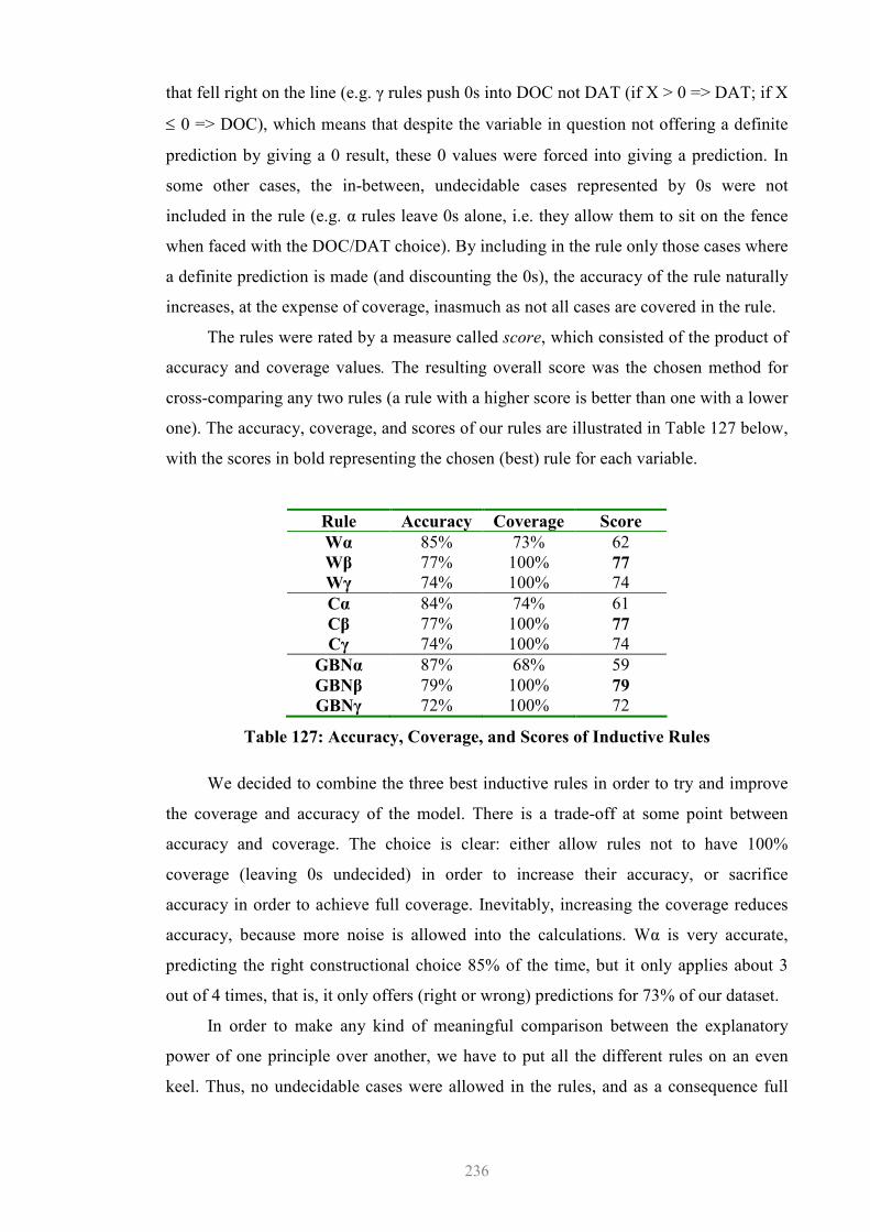
236

that fell right on the line (e.g. γ rules push 0s into DOC not DAT (if X > 0 => DAT; if X

≤ 0 => DOC), which means that despite the variable in question not offering a definite

prediction by giving a 0 result, these 0 values were forced into giving a prediction. In

some other cases, the in-between, undecidable cases represented by 0s were not

included in the rule (e.g. α rules leave 0s alone, i.e. they allow them to sit on the fence

when faced with the DOC/DAT choice). By including in the rule only those cases where

a definite prediction is made (and discounting the 0s), the accuracy of the rule naturally

increases, at the expense of coverage, inasmuch as not all cases are covered in the rule.

The rules were rated by a measure called score, which consisted of the product of

accuracy and coverage values. The resulting overall score was the chosen method for

cross-comparing any two rules (a rule with a higher score is better than one with a lower

one). The accuracy, coverage, and scores of our rules are illustrated in Table 127 below,

with the scores in bold representing the chosen (best) rule for each variable.

Rule Accuracy Coverage Score

Wα 85% 73% 62 Wβ 77% 100% 77

Wγ 74% 100% 74 Cα 84% 74% 61 Cβ 77% 100% 77

Cγ 74% 100% 74 GBNα 87% 68% 59 GBNβ 79% 100% 79

GBNγ 72% 100% 72

Table 127: Accuracy, Coverage, and Scores of Inductive Rules

We decided to combine the three best inductive rules in order to try and improve

the coverage and accuracy of the model. There is a trade-off at some point between

accuracy and coverage. The choice is clear: either allow rules not to have 100%

coverage (leaving 0s undecided) in order to increase their accuracy, or sacrifice

accuracy in order to achieve full coverage. Inevitably, increasing the coverage reduces

accuracy, because more noise is allowed into the calculations. Wα is very accurate,

predicting the right constructional choice 85% of the time, but it only applies about 3

out of 4 times, that is, it only offers (right or wrong) predictions for 73% of our dataset.

In order to make any kind of meaningful comparison between the explanatory

power of one principle over another, we have to put all the different rules on an even

keel. Thus, no undecidable cases were allowed in the rules, and as a consequence full

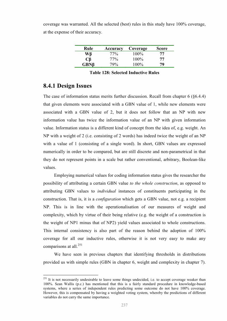
237

coverage was warranted. All the selected (best) rules in this study have 100% coverage,

at the expense of their accuracy.

Rule Accuracy Coverage Score

Wβ 77% 100% 77

Cβ 77% 100% 77

GBNβ 79% 100% 79

Table 128: Selected Inductive Rules

8.4.1 Design Issues

The case of information status merits further discussion. Recall from chapter 6 (§6.4.4)

that given elements were associated with a GBN value of 1, while new elements were

associated with a GBN value of 2, but it does not follow that an NP with new

information value has twice the information value of an NP with given information

value. Information status is a different kind of concept from the idea of, e.g. weight. An

NP with a weight of 2 (i.e. consisting of 2 words) has indeed twice the weight of an NP

with a value of 1 (consisting of a single word). In short, GBN values are expressed

numerically in order to be compared, but are still discrete and non-parametrical in that

they do not represent points in a scale but rather conventional, arbitrary, Boolean-like

values.

Employing numerical values for coding information status gives the researcher the

possibility of attributing a certain GBN value to the whole construction, as opposed to

attributing GBN values to individual instances of constituents participating in the

construction. That is, it is a configuration which gets a GBN value, not e.g. a recipient

NP. This is in line with the operationalisation of our measures of weight and

complexity, which by virtue of their being relative (e.g. the weight of a construction is

the weight of NP1 minus that of NP2) yield values associated to whole constructions.

This internal consistency is also part of the reason behind the adoption of 100%

coverage for all our inductive rules, otherwise it is not very easy to make any

comparisons at all.251

We have seen in previous chapters that identifying thresholds in distributions

provided us with simple rules (GBN in chapter 6, weight and complexity in chapter 7).

251 It is not necessarily undesirable to leave some things undecided, i.e. to accept coverage weaker than 100%. Sean Wallis (p.c.) has mentioned that this is a fairly standard procedure in knowledge-based systems, where a series of independent rules predicting some outcome do not have 100% coverage. However, this is compensated by having a weighted voting system, whereby the predictions of different variables do not carry the same importance.

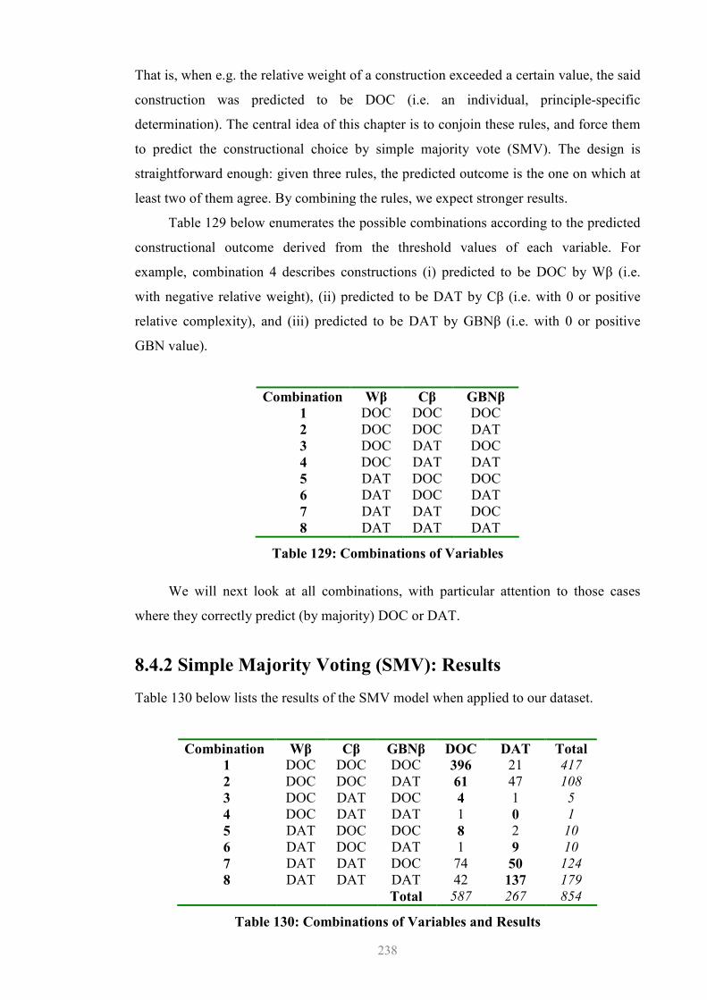
238

That is, when e.g. the relative weight of a construction exceeded a certain value, the said

construction was predicted to be DOC (i.e. an individual, principle-specific

determination). The central idea of this chapter is to conjoin these rules, and force them

to predict the constructional choice by simple majority vote (SMV). The design is

straightforward enough: given three rules, the predicted outcome is the one on which at

least two of them agree. By combining the rules, we expect stronger results.

Table 129 below enumerates the possible combinations according to the predicted

constructional outcome derived from the threshold values of each variable. For

example, combination 4 describes constructions (i) predicted to be DOC by Wβ (i.e.

with negative relative weight), (ii) predicted to be DAT by Cβ (i.e. with 0 or positive

relative complexity), and (iii) predicted to be DAT by GBNβ (i.e. with 0 or positive

GBN value).

Combination Wβ Cβ GBNβ

1 DOC DOC DOC 2 DOC DOC DAT 3 DOC DAT DOC 4 DOC DAT DAT 5 DAT DOC DOC 6 DAT DOC DAT 7 DAT DAT DOC 8 DAT DAT DAT

Table 129: Combinations of Variables

We will next look at all combinations, with particular attention to those cases

where they correctly predict (by majority) DOC or DAT.

8.4.2 Simple Majority Voting (SMV): Results

Table 130 below lists the results of the SMV model when applied to our dataset.

Combination Wβ Cβ GBNβ DOC DAT Total

1 DOC DOC DOC 396 21 417 2 DOC DOC DAT 61 47 108 3 DOC DAT DOC 4 1 5 4 DOC DAT DAT 1 0 1 5 DAT DOC DOC 8 2 10 6 DAT DOC DAT 1 9 10 7 DAT DAT DOC 74 50 124 8 DAT DAT DAT 42 137 179

Total 587 267 854

Table 130: Combinations of Variables and Results

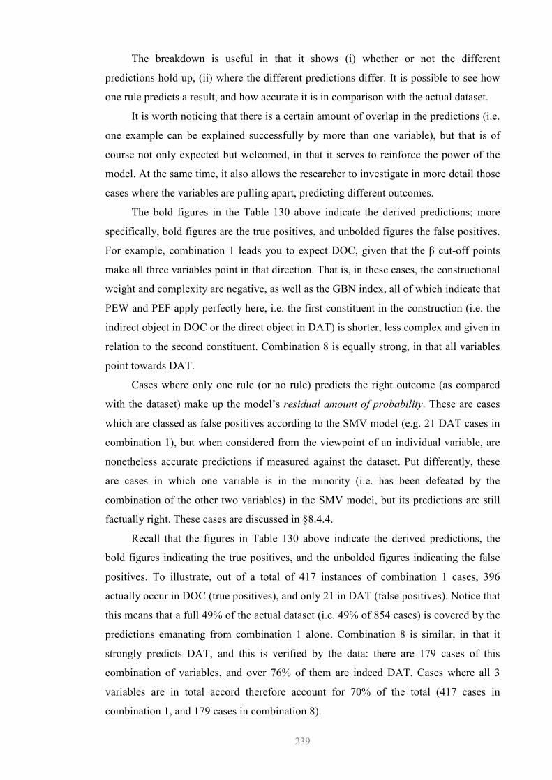
239

The breakdown is useful in that it shows (i) whether or not the different

predictions hold up, (ii) where the different predictions differ. It is possible to see how

one rule predicts a result, and how accurate it is in comparison with the actual dataset.

It is worth noticing that there is a certain amount of overlap in the predictions (i.e.

one example can be explained successfully by more than one variable), but that is of

course not only expected but welcomed, in that it serves to reinforce the power of the

model. At the same time, it also allows the researcher to investigate in more detail those

cases where the variables are pulling apart, predicting different outcomes.

The bold figures in the Table 130 above indicate the derived predictions; more

specifically, bold figures are the true positives, and unbolded figures the false positives.

For example, combination 1 leads you to expect DOC, given that the β cut-off points

make all three variables point in that direction. That is, in these cases, the constructional

weight and complexity are negative, as well as the GBN index, all of which indicate that

PEW and PEF apply perfectly here, i.e. the first constituent in the construction (i.e. the

indirect object in DOC or the direct object in DAT) is shorter, less complex and given in

relation to the second constituent. Combination 8 is equally strong, in that all variables

point towards DAT.

Cases where only one rule (or no rule) predicts the right outcome (as compared

with the dataset) make up the model’s residual amount of probability. These are cases

which are classed as false positives according to the SMV model (e.g. 21 DAT cases in

combination 1), but when considered from the viewpoint of an individual variable, are

nonetheless accurate predictions if measured against the dataset. Put differently, these

are cases in which one variable is in the minority (i.e. has been defeated by the

combination of the other two variables) in the SMV model, but its predictions are still

factually right. These cases are discussed in §8.4.4.

Recall that the figures in Table 130 above indicate the derived predictions, the

bold figures indicating the true positives, and the unbolded figures indicating the false

positives. To illustrate, out of a total of 417 instances of combination 1 cases, 396

actually occur in DOC (true positives), and only 21 in DAT (false positives). Notice that

this means that a full 49% of the actual dataset (i.e. 49% of 854 cases) is covered by the

predictions emanating from combination 1 alone. Combination 8 is similar, in that it

strongly predicts DAT, and this is verified by the data: there are 179 cases of this

combination of variables, and over 76% of them are indeed DAT. Cases where all 3

variables are in total accord therefore account for 70% of the total (417 cases in

combination 1, and 179 cases in combination 8).

240

The remaining combinations are not as strong, given that there is one variable in

disagreement with the others. In these combinations, the application of a simple

majority voting rule (2 out of 3) forces the data into supplying a prediction. In this light,

combinations 2, 3, and 5 predict DOC; whereas combinations 4, 6, and 7 predict DAT.

Let’s review some of these combinations in more detail.

• Combination 2 indicates a DOC prediction (by majority rule), and this is

supported by the data: 61 out of 108 cases are actually instantiated as DOC, but

there is a strong number of false positives (47 out of 108, or 43%). This seems to

suggest that the dissenting minority variable in this combination, i.e. GBN, does

have a strong influence on the distribution of constructions even if the other two

variables gang up against it.252

• Combination 3 indicates a DOC prediction by majority rule, and out of a total of

5 cases, 4 follow this prediction, with a single outlier.

• Combination 4 predicts DAT by majority rule, and is the only case instantiated

in our dataset that gives the lie to this prediction. This is the only combination

without true positives.

• Combination 5 predicts DOC, and we can see that this is true in 8 out of 10

cases.

• There are 10 cases covered under combination 6, and 9 out of 10 represent

accurate predictions.

• Combination 7 covers a decent number of cases (15% of the whole dataset, 124

out of 854). Still, it presents the greatest challenge to the model, in that the false

positives outnumber the true positives. In this combination, weight and

complexity are in agreement, but their agreement lies on the wrong side of the β

cut-off point. As in combination 2 (of which combination 7 is the opposite),

GBN seems to outweigh both variables in an SMV model.

Predictions derived from Table 130 have an accuracy of 78%, calculated as the

number of correct (i.e. accurately predicted) cases divided by the number of explained

cases, i.e. (396+61+4+0+8+9+50+137) / 854. The coverage in Table 130 is, naturally,

100%. The accuracy of DOCs in this model is 79%, calculated with the following

formula: (396+61+4+8) / 587. The accuracy of DATS is slightly lower at 74%,

calculated with the following formula: (0+9+50+137) / 267. The model is marginally 252 In fact this is supported by all the data, and in combination 7 with particular force.

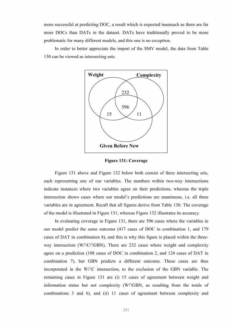
241

more successful at predicting DOC, a result which is expected inasmuch as there are far

more DOCs than DATs in the dataset. DATs have traditionally proved to be more

problematic for many different models, and this one is no exception.

In order to better appreciate the import of the SMV model, the data from Table

130 can be viewed as intersecting sets.

Figure 131: Coverage

Figure 131 above and Figure 132 below both consist of three intersecting sets,

each representing one of our variables. The numbers within two-way intersections

indicate instances where two variables agree on their predictions, whereas the triple

intersection shows cases where our model’s predictions are unanimous, i.e. all three

variables are in agreement. Recall that all figures derive from Table 130. The coverage

of the model is illustrated in Figure 131, whereas Figure 132 illustrates its accuracy.

In evaluating coverage in Figure 131, there are 596 cases where the variables in

our model predict the same outcome (417 cases of DOC in combination 1, and 179

cases of DAT in combination 8), and this is why this figure is placed within the three-

way intersection (W∩C∩GBN). There are 232 cases where weight and complexity

agree on a prediction (108 cases of DOC in combination 2, and 124 cases of DAT in

combination 7), but GBN predicts a different outcome. These cases are thus

incorporated in the W∩C intersection, to the exclusion of the GBN variable. The

remaining cases in Figure 131 are (i) 15 cases of agreement between weight and

information status but not complexity (W∩GBN, as resulting from the totals of

combinations 3 and 6), and (ii) 11 cases of agreement between complexity and

232

596

11 15

Given Before New

Weight

Complexity

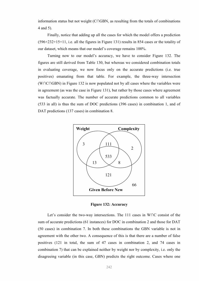
242

information status but not weight (C∩GBN, as resulting from the totals of combinations

4 and 5).

Finally, notice that adding up all the cases for which the model offers a prediction

(596+232+15+11, i.e. all the figures in Figure 131) results in 854 cases or the totality of

our dataset, which means that our model’s coverage remains 100%.

Turning now to our model’s accuracy, we have to consider Figure 132. The

figures are still derived from Table 130, but whereas we considered combination totals

in evaluating coverage, we now focus only on the accurate predictions (i.e. true

positives) emanating from that table. For example, the three-way intersection

(W∩C∩GBN) in Figure 132 is now populated not by all cases where the variables were

in agreement (as was the case in Figure 131), but rather by those cases where agreement

was factually accurate. The number of accurate predictions common to all variables

(533 in all) is thus the sum of DOC predictions (396 cases) in combination 1, and of

DAT predictions (137 cases) in combination 8.

Figure 132: Accuracy

Let’s consider the two-way intersections. The 111 cases in W∩C consist of the

sum of accurate predictions (61 instances) for DOC in combination 2 and those for DAT

(50 cases) in combination 7. In both these combinations the GBN variable is not in

agreement with the other two. A consequence of this is that there are a number of false

positives (121 in total, the sum of 47 cases in combination 2, and 74 cases in

combination 7) that can be explained neither by weight nor by complexity, i.e. only the

disagreeing variable (in this case, GBN) predicts the right outcome. Cases where one

3 111

533

121

2

8 13

Given Before New

Weight Complexity

66

243

variable is pulling away from the other two are therefore considered to be false

positives, and thus have no place in two-way intersections. This is why in Figure 132,

the 121 false positives in W∩C, for instance, appear only in the GBN set which does not

partake of any intersections. That is, those 121 cases cannot be explained either by

weight or by complexity alone, nor by a combination of the two: only our remaining

variable (i.e. information status) can account for them (see §8.4.4).

By the same token, W∩GBN cases (13 in all) consist of the sum of accurate

predictions (4 cases) for DOC in combination 3 and those for DAT (9 cases) in

combination 6. The 2 false positives in these combinations are accountable only by

complexity, since weight and information status cannot do that job. Finally, the 8 cases

present in C∩GBN consist only of accurate predictions for DOC in combination 5,

because combination 4 offers only inaccurate DAT predictions. All the same, those

cases unaccountable by the combination of the two variables in question (1 false

positive in combination 4, and 2 other false positives in combination 5) are nonetheless

accountable by the remaining variable (again, see §8.4.4).

As regards overall accuracy, measured as the number of correct predictions

(533+111+13+8) divided by the number of explained cases (854), we can see that it

rightly stays at 78%.253 Section 8.4.4 will focus on the residual probability of the model,

i.e. that 22% of false positives, in an attempt to investigate cases where predictions from

different variables part company so as to identify shortcomings in the proposed model.

8.4.3 Preliminary Consideration of the Results

We have found in §8.2 that weight and complexity were strongly correlated, which calls

into question their usefulness for a three-way SMV model. If, despite being

definitionally distinct, they determine similar datasets, isn’t considering them as

separate variables doubling the effect of the same phenomenon? In order to address this,

as well as to find out which of the two is better at predicting the alternation (when

paired with GBN), we set up two tables. The SMV model is adapted to a 2-way

prediction: in Table 133, weight is paired with information status, while in Table 135 it

is complexity which is paired with GBN.

253 Insisting on strict accuracy (i.e. cases where all three variables are not only in agreement but factually right in their predictions) causes this index to fall to 62% (533/854).

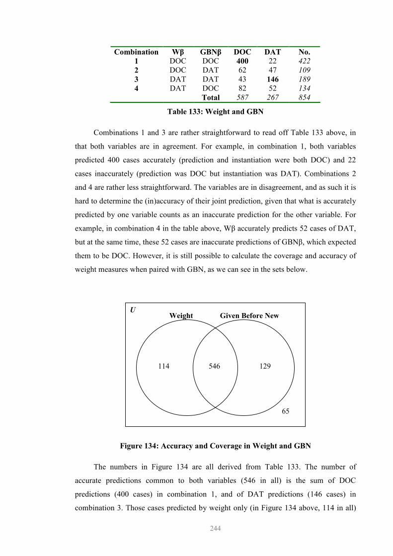
244

Combination Wβ GBNβ DOC DAT No.

1 DOC DOC 400 22 422 2 DOC DAT 62 47 109 3 DAT DAT 43 146 189 4 DAT DOC 82 52 134

Total 587 267 854

Table 133: Weight and GBN

Combinations 1 and 3 are rather straightforward to read off Table 133 above, in

that both variables are in agreement. For example, in combination 1, both variables

predicted 400 cases accurately (prediction and instantiation were both DOC) and 22

cases inaccurately (prediction was DOC but instantiation was DAT). Combinations 2

and 4 are rather less straightforward. The variables are in disagreement, and as such it is

hard to determine the (in)accuracy of their joint prediction, given that what is accurately

predicted by one variable counts as an inaccurate prediction for the other variable. For

example, in combination 4 in the table above, Wβ accurately predicts 52 cases of DAT,

but at the same time, these 52 cases are inaccurate predictions of GBNβ, which expected

them to be DOC. However, it is still possible to calculate the coverage and accuracy of

weight measures when paired with GBN, as we can see in the sets below.

Figure 134: Accuracy and Coverage in Weight and GBN

The numbers in Figure 134 are all derived from Table 133. The number of

accurate predictions common to both variables (546 in all) is the sum of DOC

predictions (400 cases) in combination 1, and of DAT predictions (146 cases) in

combination 3. Those cases predicted by weight only (in Figure 134 above, 114 in all)

546 114 129

Weight Given Before New

65

U

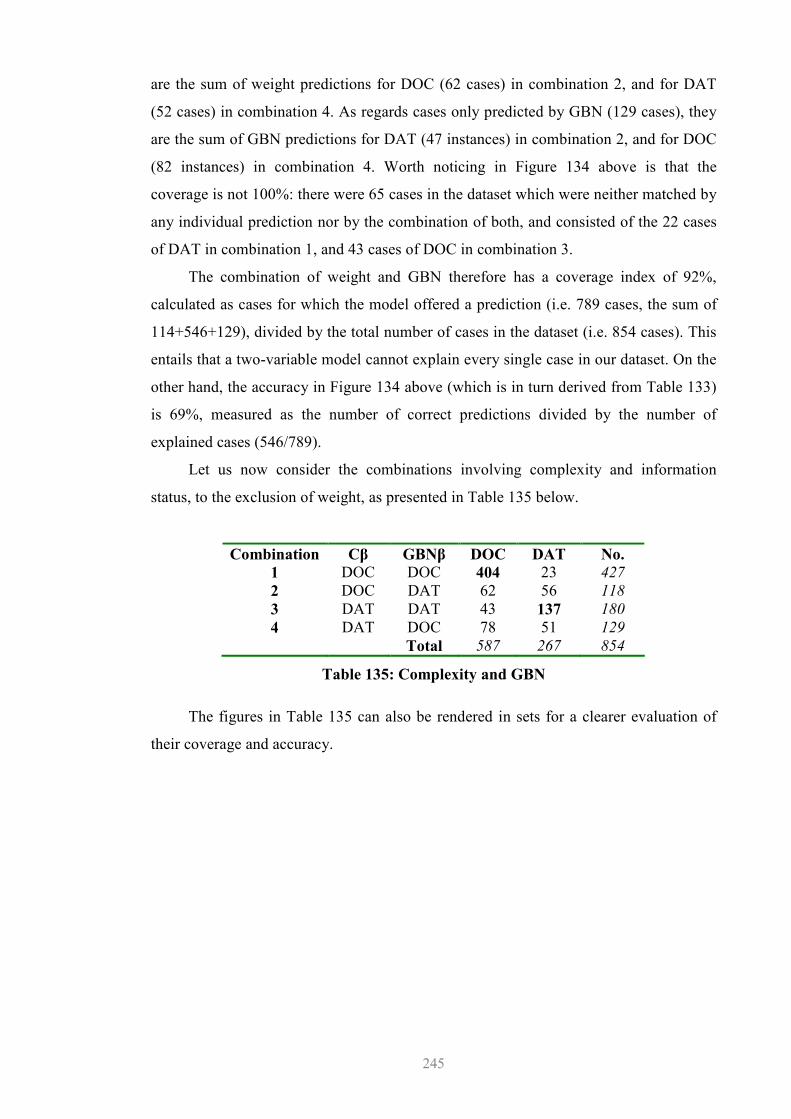
245

are the sum of weight predictions for DOC (62 cases) in combination 2, and for DAT

(52 cases) in combination 4. As regards cases only predicted by GBN (129 cases), they

are the sum of GBN predictions for DAT (47 instances) in combination 2, and for DOC

(82 instances) in combination 4. Worth noticing in Figure 134 above is that the

coverage is not 100%: there were 65 cases in the dataset which were neither matched by

any individual prediction nor by the combination of both, and consisted of the 22 cases

of DAT in combination 1, and 43 cases of DOC in combination 3.

The combination of weight and GBN therefore has a coverage index of 92%,

calculated as cases for which the model offered a prediction (i.e. 789 cases, the sum of

114+546+129), divided by the total number of cases in the dataset (i.e. 854 cases). This

entails that a two-variable model cannot explain every single case in our dataset. On the

other hand, the accuracy in Figure 134 above (which is in turn derived from Table 133)

is 69%, measured as the number of correct predictions divided by the number of

explained cases (546/789).

Let us now consider the combinations involving complexity and information

status, to the exclusion of weight, as presented in Table 135 below.

Combination Cβ GBNβ DOC DAT No.

1 DOC DOC 404 23 427 2 DOC DAT 62 56 118 3 DAT DAT 43 137 180 4 DAT DOC 78 51 129 Total 587 267 854

Table 135: Complexity and GBN

The figures in Table 135 can also be rendered in sets for a clearer evaluation of

their coverage and accuracy.

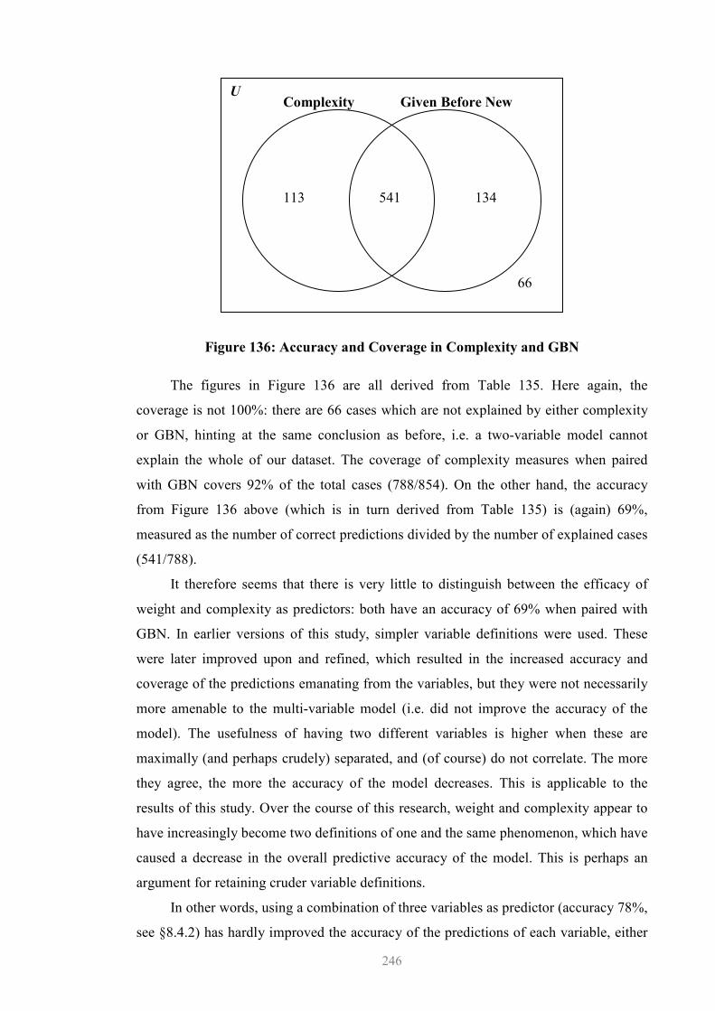
246

Figure 136: Accuracy and Coverage in Complexity and GBN

The figures in Figure 136 are all derived from Table 135. Here again, the

coverage is not 100%: there are 66 cases which are not explained by either complexity

or GBN, hinting at the same conclusion as before, i.e. a two-variable model cannot

explain the whole of our dataset. The coverage of complexity measures when paired

with GBN covers 92% of the total cases (788/854). On the other hand, the accuracy

from Figure 136 above (which is in turn derived from Table 135) is (again) 69%,

measured as the number of correct predictions divided by the number of explained cases

(541/788).

It therefore seems that there is very little to distinguish between the efficacy of

weight and complexity as predictors: both have an accuracy of 69% when paired with

GBN. In earlier versions of this study, simpler variable definitions were used. These

were later improved upon and refined, which resulted in the increased accuracy and

coverage of the predictions emanating from the variables, but they were not necessarily

more amenable to the multi-variable model (i.e. did not improve the accuracy of the

model). The usefulness of having two different variables is higher when these are

maximally (and perhaps crudely) separated, and (of course) do not correlate. The more

they agree, the more the accuracy of the model decreases. This is applicable to the

results of this study. Over the course of this research, weight and complexity appear to

have increasingly become two definitions of one and the same phenomenon, which have

caused a decrease in the overall predictive accuracy of the model. This is perhaps an

argument for retaining cruder variable definitions.

In other words, using a combination of three variables as predictor (accuracy 78%,

see §8.4.2) has hardly improved the accuracy of the predictions of each variable, either

541 113 134

Complexity Given Before New

66

U

247

individually (weight 77%, complexity 77%, information status 79%, see §8.4) or when

paired (both weight and GBN, and complexity and GBN had an accuracy of 69%, as

seen earlier). Weight and complexity are highly correlated (recall Spearman’s

correlation coefficient was very high, 0.95), and seem to be measuring the same thing.

The model’s 78% accuracy appears to be the average of the accuracies of

information status on the one hand, and weight and complexity, on the other.254

However, it is worth noticing that even if GBN’s accuracy is higher than that of our

model (78%), the latter’s is a much more robust prediction index, given that it is based

on more principles. What is important is the a posteriori empirical predictions of the

model, i.e. how many cases are correctly predicted when two or more principles agree.

8.4.4 Residual Probability or Counterexamples

Grau …ist alle Theorie, Und gruen des Lebens goldner Baum. (Goethe)

Modelling performance data is an exercise consisting in reasoned simplifications of

actual events. Furthermore, Mukherjee (2005:87) argues that “corpus-based models of

grammar should not attempt to explain all performance data in their entirety, because

the data will always include instances of, say, unacceptable language use, clear mistakes

and intended ungrammaticality”. This is of limited applicability to our dataset, but is

nonetheless a sensible reminder that it is not reasonable to aim for an explanation of

100% of all cases in performance data.

Recall that residual probability consists of cases in which one variable is not part

of the majority in the SMV model, but its predictions are still factually right. Residual

probability is thus entirely made up of false positives, and consists of four possible

scenarios, derived from Table 130 above, listed in (169) below, and illustrated in Figure

137 further down.

254 An advantage of SMV is that it corrects logical dependencies, whereby two variables overlap substantially. If variable X predicts 83% and Y, 77%, it may be the case that Y’s 77% is entirely dependent on (included in) X’s. In this case, using SMV is instrumental in demonstrating that Y adds very little to the overall accuracy of the predictions.

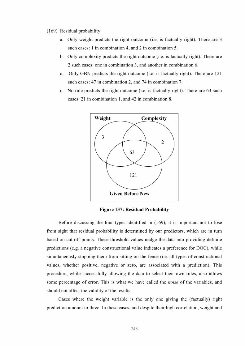
248

(169) Residual probability

a. Only weight predicts the right outcome (i.e. is factually right). There are 3

such cases: 1 in combination 4, and 2 in combination 5.

b. Only complexity predicts the right outcome (i.e. is factually right). There are

2 such cases: one in combination 3, and another in combination 6.

c. Only GBN predicts the right outcome (i.e. is factually right). There are 121

such cases: 47 in combination 2, and 74 in combination 7.

d. No rule predicts the right outcome (i.e. is factually right). There are 63 such

cases: 21 in combination 1, and 42 in combination 8.

Figure 137: Residual Probability

Before discussing the four types identified in (169), it is important not to lose

from sight that residual probability is determined by our predictors, which are in turn

based on cut-off points. These threshold values nudge the data into providing definite

predictions (e.g. a negative constructional value indicates a preference for DOC), while

simultaneously stopping them from sitting on the fence (i.e. all types of constructional

values, whether positive, negative or zero, are associated with a prediction). This

procedure, while successfully allowing the data to select their own rules, also allows

some percentage of error. This is what we have called the noise of the variables, and

should not affect the validity of the results.

Cases where the weight variable is the only one giving the (factually) right

prediction amount to three. In these cases, and despite their high correlation, weight and

3

63

121

2

Given Before New

Weight

Complexity

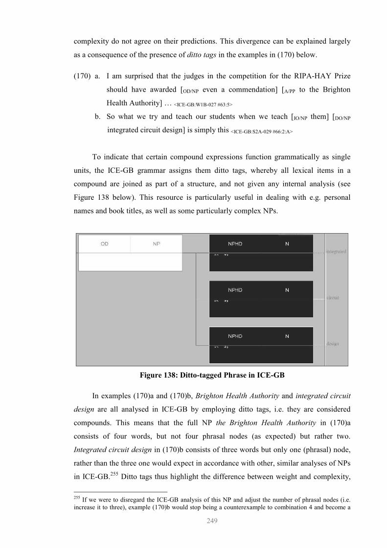
249

complexity do not agree on their predictions. This divergence can be explained largely

as a consequence of the presence of ditto tags in the examples in (170) below.

(170) a. I am surprised that the judges in the competition for the RIPA-HAY Prize

should have awarded [OD/NP even a commendation] [A/PP to the Brighton

Health Authority] … <ICE-GB:W1B-027 #63:5>

b. So what we try and teach our students when we teach [IO/NP them] [DO/NP

integrated circuit design] is simply this <ICE-GB:S2A-029 #66:2:A>

To indicate that certain compound expressions function grammatically as single

units, the ICE-GB grammar assigns them ditto tags, whereby all lexical items in a

compound are joined as part of a structure, and not given any internal analysis (see

Figure 138 below). This resource is particularly useful in dealing with e.g. personal

names and book titles, as well as some particularly complex NPs.

Figure 138: Ditto-tagged Phrase in ICE-GB

In examples (170)a and (170)b, Brighton Health Authority and integrated circuit

design are all analysed in ICE-GB by employing ditto tags, i.e. they are considered

compounds. This means that the full NP the Brighton Health Authority in (170)a

consists of four words, but not four phrasal nodes (as expected) but rather two.

Integrated circuit design in (170)b consists of three words but only one (phrasal) node,

rather than the three one would expect in accordance with other, similar analyses of NPs

in ICE-GB.255 Ditto tags thus highlight the difference between weight and complexity,

255 If we were to disregard the ICE-GB analysis of this NP and adjust the number of phrasal nodes (i.e. increase it to three), example (170)b would stop being a counterexample to combination 4 and become a

250

in that the imbalance between terminal and phrasal nodes is definitionally guaranteed.

In Figure 138 above, the phrase integrated circuit design is considered a compound, and

given a (reduced) flat analysis.

Turning now to cases where the right prediction was yielded only by complexity,

these are also few, and are listed in (171) below. In these cases weight and complexity

are pulling apart in their predictions, again as a result of ditto-tagging.

(171) a. I’m reading it [OD/NP Treasure Island] at the moment [A/PP to my son] <ICE-

GB:S1A-013 #65:1:D>

b. Thus, if Bank A ends the day owing [IO/NP Bank B] [OD/NP $100m]. <ICE-GB:W2C-

016 #26:2>

Case (171)a includes an oversight on my part: the compound Treasure Island was

mistakenly analysed as consisting of one word and two (phrasal) nodes, instead of two

words and one node, as suggested by the presence of a ditto tag. 256 As regards (171)b,

the phrase Bank B is also ditto-tagged in ICE-GB: two words, one phrasal node. It is this

disparity in the number of (terminal and phrasal) nodes which brings about the

disagreement between our weight and complexity variables. There is another peculiarity

in (171)b. This example originated in written language, and as such, the analysis given

is understandably derived from the original written text. The NP $100m is analysed as

one node and one word. Recourse is not even made to ditto tags: the three elements $,

100, and m all appear as the author wrote them, and no further analysis was given it.257

The largest contribution to the model’s residual probability (121 cases) comes

from cases where weight and complexity agree, as expected, on their predictions, but

these are not verified in the dataset, i.e. they are factually wrong. Only our GBN

variable predicts the right outcome.

Recall that in the operationalisation of GBN discussed in chapter 6 (§6.4), our cut-

off point GBNβ indicated that configurations with a negative constructional value

predicted DOC. This is essentially the same as saying that only those configurations

which consisted of a given element followed by a new one (i.e. GN) predicted DOC, all

true positive to the same combination, which would perhaps be more desirable, given that combination 4 is the only one in our model without a single true positive. 256 Correcting this error would make (171)a no longer a counterexample to combination 3, but rather a true positive for combination 7. 257 There are hardly any benefits in going against this ICE-GB analysis. However, if we did this, the complexity of the NP would be increased, and the constructional complexity would turn negative in value. Thus, while in our original analysis the construction was a counterexample to combination 6, it would now still a counterexample, but to combination 8 (where all predictions are wrong).

251

other configurations (GG, NN, NG) thus being associated with DAT. The examples in

(172) below exemplify counterexamples instantiated by the different configurations:

(172)a illustrates configuration NN; (172)b, configuration GG; and (172)c,

configuration NG.

(172) a. The outcome of the constitutional confrontation was influenced by several

factors which lent [OD/NP support] [A/PP to the unitarist trend] …<ICE-GB:W2B-007

#45:1>

b. … penalise those employers that don’t offer [OD/NP opportunities] [A/PP to

disabled people] <ICE-GB:S1B-057 #7:1:D>

c. … whenever safety was at odds with production there was a temptation to

give [OD/NP precedence] [A/PP to the latter]. <ICE-GB:W2C-007 #110:3>

All 47 DAT cases in this section have negative weight and complexity values

(which would require DOC, by Wβ and Cβ), while being correctly predicted as DAT by

their GBN value alone (either 0 or positive).

On the other hand, all 74 DOC cases in this section have a negative GBN value

(which means that given noun phrases do truly precede new ones), but weight and

complexity values associated with DAT (i.e. either 0 or positive). In fact, 57 of the 74

DOC cases have values of 0 for weight and complexity; and 40 of the 57 consist of one

word-long NPs.258 The examples in (173) below illustrate DOC cases.

(173) a. I mean if she’d really wanted to leave him she’d have sent [IO/NP you] [OD/NP

flowers] <ICE-GB:S1A-080 #171:1:B>

b. … you give [IO/NP the head] [OD/NP support] <ICE-GB:S1B-025 #98:1:B>

Example (173)a has 0 as both weight and complexity values (thus predicting

DAT), and negative GBN value (thus predicting DOC). Recall that our model predicts

DAT for cases with 0 or positive (constructional) values, and only negative values are

associated with DOCs. On the other hand, example (173)b has positive weight and

complexity values (predicting DAT), and a negative GBN value (the head analysed as

given, and support as new, thus predicting DOC).

All these counterexamples seem to point towards the need for refining GBNβ. It

does not seem a coincidence that the more crudely measured variable is the one that 258 Zero values can be considered borderline cases in that a single word would be enough to change the prediction. However, as we have seen, our cut-off points impose a sharp differentiation and borderline effects are thus not contemplated.

252

produces the most counterexamples to the model. An alternative explanation is that

information status is a different kind of beast and is indeed best kept separated from

other, more tameable concepts.

In the last category of residual probability, all our variables agree on a prediction,

only it is the wrong one, i.e. it is not supported by the data. There are 63 cases in which

every single variable offered a wrong prediction, and as such these examples would

provide a serious challenge to our model.

(174) a. They sent [OD/NP one] [A/PP to my mother] … <ICE-GB:S1A-007 #277:1:B>

b. But of course now they’re going to send [IO/NP everyone] [OD/NP one] … <ICE-

GB:S1A-007 #272:1:B>

Example (174)a is a typical example of DAT. On its own, it is able to be predicted

by GBN, weight and complexity. In our model, however, where it is outnumbered by

DOCs, its negative values for all variables predict DOC. On the other hand, example

(174)b has 0 values for all variables (predicting DAT). In fact, of the 42 examples in

this section of (wrongly) predicted DATs (i.e. examples such as (174)b), a full 37 have

0 values for all three variables, i.e. cases with minimal distinctiveness as regards DOC,

but nonetheless DAT by our β cut-offs.259

The greatest challenge to the model thus appears to consist of those cases in which

there really is no big difference between the prototypical cases of each construction (see

the examples in (174) above), at least as far as we have described/defined them in this

study by means of threshold values. When differences exist but cannot be picked up by

any of the three measures we employed, the model overgeneralises and yields false

positives. This is nonetheless to be expected, as well as accepted, in view of the fact that

the true positives far outweigh the false ones. Residual probability can be described as

the cost the researcher pays for obtaining successful predictions.

8.5 Experimental Conclusions

We have been able to identify threshholds for the inductive rules, and established that

the different factors overlap to a degree but are also semi-independent from one another.

This semi-independence results in their different explanatory powers. The factors

predict different subsets of the data, and putting them together yields a more robust and

259 Furthermore, there are 37 constructions involving 1-word long postverbal NPs, 35 of which involve two pronominal noun phrases (see also §7.2.3.3).

253

improved predictive score (though not necessarily in numerical terms) than would

otherwise be the case if we considered each variable independently.

On a methodological note, the experiments conducted appear to have reached the

limits of what the data will tell. More specifically, talking about percentages of the

distribution may be understood as going beyond what the significance tests employed

allow for. A percentage of accuracy within the dataset is not guaranteed to be replicated,

as it is likely that some variation will creep in, as a result of e.g. slightly different

distributions, difference in corpus or dataset, etc.

By using scores in an SMV model, one can predict whether an observation

belongs to DOC or to DAT. Between 70-80% of the examples are correctly predicted in

this model as belonging to either of the two constructions. We now have an estimate of

all explained data, as well as of data which remains unexplained, which is a quite useful

result from the point of view of a research programme.

254

9 Conclusions

Not everything that counts can be counted, and not everything that can be counted counts. (Sign hanging in Einstein’s office at Princeton)

This thesis set out to address the following research questions, by employing a corpus-

based methodology:

(175) Research Questions

a. Do information status, weight, and complexity indeed affect the dative

alternation?

b. What is the relationship between these three factors?

c. Can corpus data help establish a model of the interaction between these

factors/variables?

d. Can these factors be manipulated into predicting speakers’ choices?

In order to obtain questions and hypotheses to test against corpus data, a critical

review of the literature on ditransitives was conducted in chapter 2. We saw how a

diachronic approach is very much the only perspective which offers a uniform view of

the (development of) two related complementation patterns. The overview continued

with synchronic approaches, divided in two different schools of thought. Traditional

approaches were discussed first, particularly Quirk et al. (1985), with their characteristic

attempt at a “functional description of syntactic relations” (Mukherjee 2005:11), which

led these authors not to insist on a strict separation of syntax and semantics. The

transformational paradigm was reviewed next, from its early, intuitive, and sensible

postulation of a dative shift transformation which captured the similarity between the

double object construction and its prepositional paraphrase, to the theoretical

gymnastics in an attempt to account for two verbal complements by means of

apparently inadequate theoretical tools. Finally, cognitive approaches linking language

phenomena and cognition were also reviewed in chapter 2.

In chapter 3, I discussed which structures could be called complements, and

briefly discussed a battery of syntactic and semantic criteria for their identification.

Reference was also made in this chapter to constituency tests employed in the

identification of (the scope of) indirect objects. The dativus ethicus was used as a means

of exemplifying gradience in the categorisation of complements and adjuncts.

Once working hypotheses and definitions have been gleaned from the literature,

the corpus —containing real, performance data— becomes a yardstick against which to

255

measure or test them. Chapter 4 described the organization of the dataset (target cases,

exclusions, automation involved, etc.), as well as the design of the experiments,

including tests and other statistical notions employed in the quantitative analysis of the

extracted corpus data. This thesis illustrates a novel methodological approach which

both relies on, and simultaneously reins in, automation.260 The quantitative and

qualitative analysis of authentic data by means of a parsed corpus makes it possible to

describe linguistic structures “rapidly and exhaustively, empirically and reliably,

resulting in a testable and frequency-based account of authentic language use”

(Mukherjee 2005:38). Additionally, the use of authentic (i.e. corpus) data ensures the

analysis is based on empirical, realistic grounds. In this light, the methodology

employed can be construed as exploratory data analysis.

In chapter 5, previous approaches to the analysis of the impact of information

status on the ditransitive alternation were discussed. Related concepts (theme and

rheme, given and new, etc.) were evaluated, in order to clarify our standpoint in a

traditionally murky field. This chapter also provided the background for chapter 6,

where the Given Before New (GBN) principle was ionvestigated.

Chapter 6 tested the GBN principle in different ways, by employing different

coding schemes (textual retrievability, as well as the presence of inferrable elements),

by considering the information status both of individual elements and of configurations,

and finally by applying different tests and measures to the corpus results. The GBN

principle predicts that (a) the first NP would be given, and that (b) the second NP would

be new in either DOC or DAT. Using strict retrievability confirmed predictions (a) and

(b) for DOC (88% of NP1 in DOCs were given, and 81% of NP2 in DOCs were new),

but was not successful in DATs (49% and 46%, respectively). These results partially

supported GBN, but appeared to point to the need for refining our retrievability

criterion, in that other factors such as end focus seemed to be obscured by it. Inferrables

(an intermediate notion between given and new) were called upon in order to reinforce

predictive accuracy. And that was indeed the case: GBN predictions for DOC were

again confirmed (95% and 85% respectively). As regards DAT, both predictions

supported the GBN more strongly, but only one of them was verified (70% and 48%

respectively).

260 Indeed, the approach discussed in this study was used as an early model for the design of the Next Generation Tools project (www.ucl.ac.uk/english-usage/projects/next-gen/report.htm) carried out at the Survey of English Usage. In short, the NGT project developed a software environment for conducting experimental research employing (parsed) corpora. Certain research processes (e.g. the extraction of numeric variables, abstract generalisations), which in this study were carried out manually are systematised in NGT with the help of automation.

256

We then explored GBN configurations; i.e. the information status of both noun

phrases involved in DOC and DAT, from which we derived rules offering valid

generalizations about the behaviour of these constructions. Once again, strong

predictions were derivable from looking at the overall (constructional) distribution of

information status. The significant results in this chapter indicate that all the different

classificatory methods for information status are valid.

A different pragmatic factor, namely heaviness, was tested in Chapter 7. This

factor was discussed in two different guises: weight, measured as number of words, and

complexity, measured as number of nodes. Accounts of the dative alternation in terms of

heaviness were discussed, and a number of hypotheses were evaluated against the

dataset. Relative (as opposed to categorical) measures were used for both weight and

complexity, which means that weight in this study was defined as the difference in

number of words between the (postverbal) noun phrases involved in either DOC or

DAT. The frequency of the (relative) weights of each construction (DOC or DAT) was

plotted, cut-off points posited in order to try and separate the distributions of DOC and

DAT, and inductive rules were arrived at. The best rule for weight was accurate 77% of

the time, and was applicable to all cases in our dataset. The same procedure was

followed in dealing with complexity, with similar results (77% accuracy and 100%

coverage). This shows why weight and complexity have been difficult to separate (even

if lexical weight is marginally better as a predictor), but are both very successful

predictors of constituent ordering, with over 75% accuracy for the alternations in our

dataset.

The three pragmatic variables discussed were brought together in chapter 8.

Firstly, weight and complexity are different manifestations of the PEW, but had a very

similar accuracy and coverage in relation to our dataset. When tested, it was found that

our two variables were correlated, and highly so (rS = 0.95). More specifically, weight

and complexity were slightly more strongly correlated in DOC (rS = 0.95) than in DAT

cases (rS = 0.92). In a second stage, weight and GBN were also inspected for

correlational behaviour. GBN and weight behaved differently and determined different

data distributions, which means they are not coextensive and cannot be reduced to a

single factor.

Finally, a simple yet powerful method was suggested for joining our variables in

order to derive predictions for the dataset. Based on the operationalisation of the

variables, the inductive rules, and the threshold values already discussed, a table was

constructed listing all the possible combinations according to the predicted

257

constructional outcome (DOC or DAT). This breakdown was useful in that it showed (i)

whether or not the different predictions could hold up, (ii) where the different

predictions differed. It was possible to see how a rule predicted a result, and how

accurate that result was in comparison with the actual dataset. By means of a simple

majority vote (SMV) procedure, the resulting model has 100% coverage and its

predictions are successful 78% of the time. Moreover, the variables are joined in their

predictions, and thus offer a more robust and improved predictive score than would

otherwise be the case if we considered each variable independently.

The results in this study have lent support to Collins’ notion of receiver/entity

differentiation (see §6.3.3), according to which participants in DOC are more highly

differentiated than participants in DAT. While DATs have a preposition to differentiate

between receivers and entities, DOCs do not, and thus need an alternative method of

achieving this differentiation. This is carried out by means of more marked differences

in the heaviness and information status of their participants. From §6.4.3, we can see

that the GBN principle is supported by the DOCs in our dataset, 482 out of 587 (82%)

have a GN configuration. DATs are not so well behaved: most of them (114 out of 267,

or 43%) do not tend to distinguish informationally between entity and receiver.

We have also seen (§7.1.3.2) that the PEW is not confirmed for DATs, where both

participants have approximately the same weight (i.e. 120 out of 267 cases of DAT, or

45%, have 0 as their constructional weight). On the other hand, the PEW is confirmed

in DOCs, where indirect objects (receivers) tend to be shorter than direct objects

(entities), with 462 cases (out of 587, or 79%) showing this by their negative

constructional weight. This finding is replicated in evaluating complexity (see §7.2.3.1),

where we find that receivers and entities are more sharply differentiated in DOCs than

in DATs. And even when contrasting GBN and Weight (see §8.3.2), we can see

Collins’ principle supported. In discussing the mean weight of GN configurations (85%

of which are DOCs in our dataset), we appreciated that it is negative (-1.67), pointing at

an actual difference in terms of number of words. Contrast this with the mean weight of

GG configurations (57% of which are DATs), with a less marked weight difference

tending towards 0 (-0.348). Our dataset thus seems to show that (in line with Collins’

idea) the higher the differences between the participants in a construction, the more the

said construction will tend to be DOC.

At first sight, this study appears only to have confirmed theoretical claims already

in the literature. Its added value, however, lies in its innovative, principled, simple, and

yet powerful methodological approach to corpus-based research. Among the advantages

258

of the proposed model is its simplicity, which allows the researcher to accommodate

further variables (e.g. such as animacy, different NP types, speaker gender, etc.).

However, more computational support will be necessary in assessing the multivariable

interactions. Another benefit of this study is that besides having shown that speakers do

use (cross-linguistically valid) variables such as the GBN Principle and the PEW, it has

also illustrated the effects of manipulating variables in a dataset. Additionally, in

selecting hypotheses from the literature while allowing the dataset to inductively select

their own rules, this study combines a theory-down (corpus-based) approach with a

words-up (corpus-driven) method. Finally, the illustration of our SMV model with Venn

diagrams provides a useful tool for the identification of best or prototypical examples of

each construction, at least as far as they have been described/defined in our dataset by

our threshold values.

Researchers conducting quantitative analysis offline from the corpus will always

run the risk of losing from sight that the dataset under analysis consists of actual

language, and is only expressed as figures. This separation between corpus examples

and databases very often results in the overreliance on predetermined quantitative

stages/tests for the analysis of data. It need not be like this.

In the methodology proposed in this study, cases in the statistical model were

constantly inspected against the actual clauses in the corpus, in order to check what the

results actually meant from a linguistic point of view (particularly in the case of

counterexamples). Returning to the corpus to verify the accuracy and relevance of

findings also proved to be advantageous in allowing the researcher freedom to adjust

and modify their searching/analytical procedures, not in an automated way (as permitted

by many procedures common in statistical software packages) but rather by applying

linguistic (as opposed to purely statistical) expertise and reflection to the analysis of the

dataset.

259

10 References

Aarts, B. (1992), Small Clauses in English: The Nonverbal Types, Mouton de Gruyter: Berlin-New York.

Aarts, B. (1997/2001:2nd edition), English Syntax and Argumentation, Palgrave: Basingstoke. Aarts, B. (2000), ‘Corpus Linguistics, Chomsky and Fuzzy Tree Fragments’, in Mair, C.;

Hundt, M. (eds.), Corpus Linguistic and Linguistic Theory, Rodopi: Amsterdam. 5-13. Aarts, B. (2004), ‘Grammatici Certant: Review of Huddleston and Pullum (2002)’, Journal of

Linguistics 40. 365-382. Aarts, B. (2006), ‘Conceptions of Categorization in the History of Linguistics’, Language

Sciences 28. 361-385. Aarts, B. (2007), Syntactic Gradience, OUP: Oxford. Aarts, B.; Nelson, G.; Wallis, S. (1998), ‘Using Fuzzy Tree Fragments to Explore English

Grammar’, English Today 14. 52-56. Aarts, F. (1971), ‘On the Distribution of Noun-Phrase Types in English Clause Structure’,

Lingua 26. 281-293. Aarts, F.; Aarts, J. (1982), English Syntactic Structures, Pergamon Press: Oxford. Aarts, J. (1991), ‘Intuition-based and observation-based grammars’, in Aijmer, K.; Altenberg,

B. (eds.), English Corpus Linguistics: Studies in Honour of Jan Svartvik, Longman: London. 44-62.

Abney, S. (1996), ‘Statistical Methods and Linguistics’, in Klavans, J.; Resnik, P. (eds.), The Balancing Act: Combining Symbolic and Statistical Approaches to Language, MIT Press: Cambridge, MA. 1-26.

Aijmer, K.; Altenberg, B. (eds.) (2004), Advances in Corpus Linguistics, Rodopi: Amsterdam. Aitchison, J. (1991), Language Change: Progress or Decay?, CUP: Cambridge. Akmajian, A.; Heny, F.W. (1975), An Introduction to the Principles of Transformational

Syntax, MIT Press: Cambridge, MA. Algeo, J. (1995), ‘Having a Look at the Expanded Predicate’, in Aarts, B.; Meyer, C. (eds.),

The Verb in Contemporary English, CUP: Cambridge. 203-217. Allen, C.L. (1995), Case-Marking and Reanalysis: Grammatical Relations from Old to Early

Modern English, Clarendon Press: Oxford. Allerton, D.J. (1978a), ‘The Notion of Givenness and its Relation to Presuppositions and to

Theme’, Lingua 44. 133-168. Allerton, D.J. (1978b), ‘Generating Indirect Objects in English’, Journal of Linguistics 14. 21-

33. Allerton, D.J. (1982), Valency and the English Verb, Academic Press: London. Allerton, D.J. (2001), Stretched Verb Constructions in English, Routledge: London. Altenberg, B. (1982), The genitive v. the of-construction: A Study of Syntactic Variation in

17th Century English, CWK Gleerup: Malmö. Anagnostopoulou, E. (2003), The Syntax of Ditransitives: Evidence from Clitics, Mouton de

Gruyter: Berlin-New York. Anderson, J.M. (1982), ‘A Disagreeable Note on Relational Grammatical Relations’, in

Dirven, R.; Radden, F. (eds.), Issues in the Theory of Universal Grammar, Gunter Narr: Tübingen. 125-143.

Anderson, J.M. (1984), ‘The Natural History of Dative Sentences’, in Blake, N.F.; Jones, C. (eds.), English Historical Linguistics: Studies in Development, University of Sheffield: Sheffield. 241-278.

260

Anderson, S.R. (1988), ‘Objects (Direct and Not-So-Direct) in English and Elsewhere’, in Stockwell, R.P.; Duncan-Rose, C.; Vennemann, T. (eds.), On Language, Routledge: London. 287-314.

Aoun, J.; Sportiche, D. (1981), ‘On the Formal Theory of Government’, The Linguistic Review 2. 211-236.

Aoun, J.; Li, Y.A. (1989), ‘Scope and Constituency’, Linguistic Inquiry 20. 141-172. Ariel, M. (1988), ‘Referring and Accessibility’, Journal of Linguistics 24. 65-87. Ariel, M. (1990), Accessing Noun-Phrase Antecedents, Routledge: London. Arnold, J.; Wasow, T.; Losongco, A.; Ginstrom, R. (2000), ‘Heaviness vs. Newness: The

Effects of Structural Complexity and Discourse Status on Constituent Ordering’, Language 76:1. 28-55.

Arnold, M.D. (1997), ‘Double Object Constructions and Indirect Object Passives: Problems Posed by History’, in Agbayabi, B.; Tang, S.W. (eds.), West Coast Conference on Formal Linguistics (15th: 1996): Proceedings of the Fifteenth West Coast Conference on Formal Linguistics, CSLI: Stanford, CA. 1-16.

Asher, R.E.; Simpson, J.M.Y. (eds.) (1994), The Encyclopedia of Language and Linguistics, Pergamon Press: Oxford.

Baayen, R.H. (2008), Analyzing Linguistic Data, CUP: Cambridge. Baker, C.L. (1989), English Syntax, MIT Press: Cambridge, MA. Baker, M.C. (1988), Incorporation: A Theory of Grammatical Function Changing, University

of Chicago Press: Chicago. Bars, A.; Lasnik, H. (1986), ‘A Note on Anaphora and Double Objects’, Linguistic Inquiry 17.

347-354. Bartlett, F.C. (1932), Remembering, CUP: Cambridge. Basilico, D. (1997), ‘Review of Hawkins (1994)’, Journal of Linguistics 33. 192-197. Beaver, I. (1977), ‘Presupposition’, in van Benthem, J.; ter Meulem, A. (eds.), Handbook of

Logic and Language, MIT Press: Cambridge, MA. 939-1008. Berinstein, A. (1986), ‘Indirect Object Constructions and Multiple Levels of Syntactic

Representation’, Chicago Linguistic Society 22:1. 36-51. Bever, T. (1990), ‘The Cognitive Basis for Linguistic Structures’, in Hayes, J. (ed.), Cognition

and the Development of Language, Wiley: New York. 279-362. Bhat, D.N.S. (1991), Grammatical Relations, Routledge: London. Biber, D. (1986), ‘On the Investigation of Spoken/Written Differences’, Studia Linguistica 40.

1-21. Biber, D. (1988), Variation across speech and writing, CUP: Cambridge. Biber, D. (1992), ‘Using Computer-Based Text Corpora to Analyze the Referential Strategies

of Spoken and Written Texts’, in Svartvik, J. (ed.), Directions in Corpus Linguistics: Proceedings of Nobel Symposium 82, Stokholm, 4-8 August 1991, Mouton de Gruyter: New York. 213-252.

Biber, D. (1993), ‘Representativeness in Corpus Design’, Literary and Linguistic Computing 8. 243-257.

Biber, D.; Conrad, S.; Reppen, R. (1998), Corpus Linguistics: Investigating Language Structure and Use, CUP: Cambridge.

Biber, D.; Johansson, S.; Leech, G.; Conrad, S.; Finegan, E. (1999), Longman Grammar of Spoken and Written English, Longman: Harlow.

Birner, B. (1994), ‘Information Status and Word Order: An Analysis of English Inversion’, Language 70:2. 233-259.

Birner, B. (1998), ‘Recency Effects in English Inversion’, in Walker, M.; Joshi, A.; Prince, E. (eds.), Centering Theory in Discourse, Clarendon Press: Oxford. 309-323.

261

Birner, B.; Ward, G. (1998), Information Status and Noncanonical Word Order in English, John Benjamins: Amsterdam/Philadelphia.

Blake, B.J. (1990), Relational Grammar, Routledge: London. Blake, N.F. (1988), Traditional Grammar and Beyond, Macmillan: London. Bock, J.; Irwin, D. (1980), ‘Syntactic Effects of Information Availability in Sentence

Production’, Journal of Verbal Learning and Verbal Behavior 19. 467-484. Boeckx, C. (2004), ‘Review of Anagnostopoulou (2003)’, Journal of Linguistics 40. 149-153. Bolinger, D. (1968), ‘Entailment and the Meaning of Structures’, Glossa 2. 119-127. Bolinger, D. (1977), ‘Idioms Have Relations’, Forum Linguisticum 2:2. 157-169. Borsley, R. (1999), Syntactic Theory, Edward Arnold: London. Borsley, R. (2005), ‘Introduction’, Lingua 115. 1475-1480. Botha, R.P. (1989), Challenging Chomsky: The Generative Garden Game, Blackwell: Oxford. Botley, S.; McEnery, A. (2000), ‘Discourse Anaphora: The Need For A Synthesis’, in Botley,

S.; McEnery, A.(eds.), Corpus-based and Computational Approaches to Discourse Anaphora, John Benjamins: Amsterdam/Philadelphia. 1-41.

Bowers, J.S. (1981), The Theory of Grammatical Relations, Cornell University Press: Ithaca-London.

Bowers, J.S. (1993), ‘The Syntax of Predication’, Linguistic Inquiry 24. 591-656. Bresnan, J.; Nikitina, T. (2003), On the Gradience of the Dative Alternation, Stanford

University: Online. Bresnan, J.; Cueni, A.; Nikitina, T.; Baayen, R. H. (2005), ‘Predicting the Dative Alternation,’

in Proceedings of the Royal Netherlands Academy of Science Colloquium on Foundations of Interpretation, October 2004, .

Bresnan, J.; Cueni, A.; Nikitina, T.; Baayen, R. H. (2007), ‘Predicting the Dative Alternation’, in Bouma, G.; Kraemer, G.; Zwarts, J. (eds.), Cognitive Foundations of Interpretation, Royal Netherlands Academy of Science: Amsterdam. 69-94.

Bresnan, J.; Hay, J. (2007), ‘Gradient grammar: An effect of animacy on the syntax of 'give' in New Zealand and American English’, Lingua 118. 245-249.

Broderick, J.P. (1975), Modern English Linguistics: A Structural and Transformational Grammar, Thomas Y. Crowell: New York.

Brown, G.; Yule, G. (1983), Discourse Analysis, CUP: Cambridge. Butler, C. (1985), Statistics in Linguistics, Blackwell: Oxford. Buysschaert, J. (1982), Criteria for the Classification of English Adverbials, Verhandelingen

van de Koninklijke Academie voor Wetenschappen, Letteren en Schone Kunsten van Belgie, No. 99: Brussels.

Chafe, W.L. (1976), ‘Givenness, Contrastiveness, Definiteness, Subjects, Topics, and Point of View’, in Li, C., Subject and Topic, Academic Press: New York. 25-56.

Chafe, W.L. (1980), ‘The Deployment of Consciousness in the Production of a Narrative’, in Chafe, W.L. (ed.), The Pear Stories: Cognitive, Cultural, and Linguistic Aspects of Narrative Production, Ablex: New Jersey. 9-50.

Chafe, W.L. (1987), ‘Cognitive Constraints on Information Flow’, in Tomlin, R. (ed.), Coherence and Grounding in Discourse, John Benjamins: Amsterdam/Philadelphia. 21-51.

Chafe, W.L. (1994), Discourse, Consciousness, and Time: The Flow and Displacement of Conscious Experience in Speaking and Writing, University of Chicago Press: Chicago.

Chen, P. (1986), ‘Discourse and Particle Movement in English’, Studies in Language 10:1. 79-95.

262

Cheshire, J.; Edwards, V.; Whittle, P. (1993), ‘Non-standard English and dialect leveling’, in Milroy, J; Milroy, L. (eds.), Real English. The Grammar of English Dialects in the British Isles, Longman: London/New York. 53-96.

Chomsky, N. (1957/1966: 6th printing), Syntactic Structures, Mouton de Gruyter: The Hague. Chomsky, N. (1965), Aspects of the Theory of Syntax, MIT Press: Cambridge, MA. Chomsky, N. (1970), ‘Deep Structure, Surface Structure, and Semantic Interpretation’, in

Steinberg, D.; Jakobovits, L. (eds.), Semantics: An Interdisciplinary Reader in Philosophy, Linguistics and Psychology, CUP: Cambridge. 183-216.

Chomsky, N. (1975), The Logical Structure of Linguistic Theory, Plenum Press: New York. Chomsky, N. (1981), Lectures on Government and Binding, Foris: Dordrecht. Chomsky, N. (1995), The Minimalist Program, MIT Press: Cambridge, MA. Chomsky, N. (2002), On Nature and Language, CUP: Cambridge. Clark, E.; Clark, H. (1978), ‘Universals, Relativity, and Language Processing’, in Greenberg, J.

(ed.), Universals of Human Language, Vol. I: Method and Theory, Stanford University Press: Stanford, CA. 225-277.

Clark, H.; Clark, E. (1977), Psychology and Language: An Introduction to Psycholinguistics, Harcourt Brace Jovanovich: New York.

Clark, H.; Haviland, S. (1974), ‘Psychological Processes as Linguistic Explanation’, in Cohen, D. (ed.), Explaining Linguistic Phenomena, Hemisphere Press: Washington DC. 91-124.

Clark, H.; Haviland, S. (1977), ‘Comprehension and the Given-New Contract’, in Freedle, R. (ed.), Discourse Production and Comprehension, Ablex: Hillsdale, NJ. 1-40.

Clark, H.; Marshall, C. (1981), ‘Definite Reference and Mutual Knowledge’, in Joshi, A.; Webber, B.; Sag, I. (eds.), Elements of Discourse Understanding, CUP: Cambridge. 10-63.

Clark, H.; Sengul, C. (1979), ‘In Search of Referents for Nouns and Pronouns’, Memory and Cognition 7. 35-41.

Clifton, J.M. (1977), ‘On the Acceptability of Particles in Sentences to Which Indirect Object Movement Has Applied’, in Elkman, F.R. (ed.), Current Themes in Linguistics, Hemisphere Publishing Corp.: London. 109-124.

Collins, P. (1995), ‘The Indirect Object Construction in English: An Informational Approach’, Linguistics 33:1. 35-49.

Cook, S.J.; Sutter, R.W. (1980), The Scope of Grammar: A Study of Modern English, McGraw-Hill: New York.

Cook, V. (1976), ‘A Note on Indirect Objects’, Journal of Child Language 3. 435-437. Cook, V.; Newson, M. (1996), Chomsky’s Universal Grammar: An Introduction, Blackwell:

Oxford. Corder, S.P. (1968), ‘Double Object Verbs in English’, Studia Anglica Posnaniensia 1:1-2. 15-

28. Croft, W. (1990), Typology and Universals, CUP: Cambridge. Croft, W. (1991), Syntactic Categories and Grammatical Relations, University of Chicago

Press: Chicago. Croft, W. (2001), Radical Construction Grammar, OUP: Oxford. Cruse, D.A. (1980), ‘Review of Hawkins, J.A. (1978)’, Journal of Linguistics 16:2. 308-316. Crystal, D. (1997), The Cambridge Encyclopedia of the English Language, CUP: Cambridge. Curme, G. (1931), A Grammar of the English Language: vol. III Syntax, Heath and Co.:

Boston. Curme, G. (1935), A Grammar of the English Language: vol. II Parts of Speech and

Accidence, Heath and Co.: Boston.

263

Czepluch, H. (1982), ‘Case Theory and the Dative Construction’, The Linguistic Review 2:1. 1-38.

Davidse, K. (1996), ‘Ditransitivity and Possession’, in Hasan, R.; Carmel, C.; Butt, D. (eds.), Functional Descriptions: Theory in Practice, John Benjamins: Amsterdam/Philadelphia. 85-144.

Davidse, K. (1996), ‘Functional Dimensions of the Dative in English’, in Van Belle, W.; Van Langendonck, W. (eds.), The Dative, vol. 1: Descriptive Studies, John Benjamins: Amsterdam/Philadelphia. 289-338.

Davidse, K. (1998), ‘The Dative as Participant Role versus the Indirect Object: On the Need to Distinguish Two Layers of Organization’, in Van Belle, W.; Van Langendonck, W. (eds.), The Dative, vol. 2: Theoretical and Contrastive Studies, John Benjamins: Amsterdam/Philadelphia. 143-184.

De Mönnink, I. (2000), On the Move: The Mobility of Constituents in the English NP: A Multi-Method Approach, Rodopi: Amsterdam.

de Swart, P.; Lamers, M.; Lestrade, S. (2007), ‘Animacy, argument structure, and argument encoding’, Lingua 118. 131-140.

Denison, D. (1993), English Historical Syntax, Longman: London. Denison, D. (1999), ‘Syntax’, in Romaine, S. (ed.), The Cambridge History of the English

Language, Vol. IV (1776-1997), CUP: Cambridge. 92-329. Dixon, R.M.W. (1992), A New Approach to English Grammar, on Semantic Principles, OUP:

Oxford. Dodson, K.; Tomasello, M. (1998), ‘Acquiring the Transitive Construction in English: The

Role of Animacy and Pronouns’, Journal of Child Language 25. 605-622. Dowty, D.R. (1979), ‘Dative Movement and Thomason’s Extensions of Montague Grammar’,

in Davis, S.; Mithum, M. (eds.), Linguistics, Philosophy, and Montague Grammar, University of Texas Press: Austin. 153-222.

Dryer, M. (1986), ‘Primary Objects, Secondary Objects, and Antidative’, Language 62:4. 808-845.

Dunning, T. (1993), ‘Accurate Methods for the Statistics of Surprise and Coincidence’, Computational Linguistics 19:1. 61-74.

Emonds, J. (1972), ‘Evidence That Indirect Object Movement is a Structure-Preserving Rule’, Foundations of Language 8. 546-561.

Emonds, J. (1976), A Transformational Approach to English Syntax, Academic Press: New York.

Emonds, J. (1985), A Unified Theory of Syntactic Categories, Foris: Dordrecht. Erdmann, P. (1988), ‘On the Principle of 'Weight' in English’, in Duncan-Rose, C.;

Vennemann, T. (eds.), On Language, Rhetorica Phonologica Syntactica: A Festschrift for Robert P. Stockwell from his Friends and Colleagues, Routledge: London. 325-329.

Erteschik-Shir, N. (1979), ‘Discourse Constraints on Dative Movement’, in Givón, T. (ed.), Syntax & Semantics, vol. 12: Discourse and Syntax, Academic Press: New York. 441-467.

Faltz, L.M. (1978), ‘On Indirect Objects in Universal Grammar’, Chicago Linguistic Society 14. 76-87.

Ferreira, V.S. (1996), ‘Is It Better to Give Than to Donate?: Syntactic Flexibility in Language Production’, Journal of Memory and Language 35:5. 724-755.

Fillmore, C.; Kay, P.; O'Connor, M. (1988), ‘Regularity and Idiomaticity in Grammatical Constructions: The Case of 'Let Alone'’, Language 64:3. 501-538.

264

Fillmore, C. (1992), ‘Corpus Linguistics” or “Computer-aided Armchair Linguistics’, in Svartvik, J. (ed.), Directions in Corpus Linguistics: Proceedings of Nobel Symposium 82, Stokholm, 4-8 August 1991, Mouton de Gruyter: New York. 35-60.

Fillmore, C. (1977), ‘The Case for Case Reopened’, in Cole, P.; Sadock, J. (eds.), Syntax and Semantics 8: Grammatical Relations, Academic Press: New York. 59-81.

Fillmore, C. (1968), ‘The Case for Case’, in Bach, E.; Harms, R.T. (eds.), Universals of Linguistic Theory, Holt, Rinehart and Winston: New York. 1-88.

Fillmore, C. (1965), Indirect Object Constructions in English and the Ordering of Transformations, Mouton de Gruyter: The Hague.

Firbas, J. (1964), ‘On Defining the Theme in Functional Sentence Analysis’, Travaux Linguistiques de Prague 1. 267-280.

Firbas, J. (1966), ‘Non-Thematic Subjects in Contemporary English’, Travaux Linguistiques de Prague 2. 239-256.

Firbas, J. (1974), ‘Some Aspects of the Czechoslovak Approach to Problems of Functional Sentence Perspective’, in Danes, F. (ed.), Papers on Functional Sentence Perspective, Academia: Prague. 11-37.

Firbas, J. (1992), Functional Sentence Perspective in Written and Spoken Communication, CUP: Cambridge.

Fischer, K. (1993), ‘What Is an Indirect Object?’, Trivium 28. 124-138. Foley, W.A.; Van Valin, R.D. (1985), ‘Information Packaging in the Clause’, in Shopen, T.

(ed.), Language Typology and Syntactic Description, vol. I: Clause Structure, CUP: Cambridge. 282-364.

Fowler, H. (1926/1965: 2nd edition), A Dictionary of Modern English Usage, OUP: Oxford. Frazier, L.; Fodor, J. (1978), ‘The Sausage Machine: A New Two-Stage Parsing Model’,

Cognition 6. 291-325. Fries, C.C. (1957), The Structure of English, Longmans, Green and Co.: London. Fries, P. (1998), ‘Post Nominal Modifiers in the English Noun Phrase’, in Collins, P.; Lee, D.

(eds.), The Clause in English, John Benjamins: Amsterdam/Philadelphia. 93-110. Fujita, K. (1996), ‘Double Objects, Causatives, and Derivational Economy’, Linguistic Inquiry

27:1. 146-173. García Miguel, J.M. (1999), ‘Grammatical Relations in Spanish Triactant Clauses’, in de

Stadler, L.; Eyrich, C. (eds.), Issues in Cognitive Linguistics, Mouton de Gruyter: New York. 447-469.

Garside, R.; Leech, G; Sampson, G. (eds.) (1987), The Computational Analysis of English: A Corpus-based Approach, Longman: London.

Garside, R.; Leech, G.; McEnery, A. (eds.) (1997), Corpus Annotation: Linguistic Information from Computer Text Corpora, Longman: London.

Givón, T. (1979), On Understanding Grammar, Academic Press: London. Givón, T. (1984), ‘Direct Object and Dative Shifting: Semantic and Pragmatic Case’, in Plank,

F. (ed.), Objects: Towards a Theory of Grammatical Relations, Academic Press: London. 151-182.

Givón, T. (1988), ‘The Pragmatics of Word Order: Predictability, Importance and Attention’, in Hammond, M.; Moravcsik, E.; Wirth, J. (eds.), Studies in Syntactic Typology, John Benjamins: Amsterdam/Philadelphia. 243-284.

Givón, T. (1993), English Grammar: A Function-Based Introduction, John Benjamins: Amsterdam/Philadelphia.

Givón, T. (1995), Functionalism and Grammar, John Benjamins: Amsterdam/Philadelphia. Givón, T. (2001), Syntax: An Introduction, John Benjamins: Amsterdam/Philadelphia.

265

Goldberg, A.E. (1992), ‘The Inherent Semantics of Argument Structure: The Case of the English Ditransitive Construction’, Cognitive Linguistics 3:1. 37-74.

Goldberg, A.E. (1995), Constructions: A Construction Grammar Approach to Argument Structure, University of Chicago Press: Chicago.

Goldberg, A.E. (2006), Constructions at Work, OUP: Oxford. Goodwin, C.J. (1995), Research in Psychology: Methods and Design, Wiley: New

York/Chichester. Green, G. (1974), Semantics and Syntactic Regularity, Indiana University Press: Bloomington. Greenbaum, S. (1977), ‘The Linguist as Experimenter’, in Eckman, F.R. (ed.), Current Themes

in Linguistics, Hemisphere Publishing Corp.: New York. 125-144. Greenbaum, S. (1991), An Introduction to English Grammar, Longman: Harlow. Gries, S. (2000), Towards Multifactorial Analyses of Syntactic Variation: The Case of Particle

Placement, Doctoral Dissertation, University of Hamburg. Gries, S. (2002), ‘Preposition Stranding in English: Predicting Speakers’ Behaviour’, in

Samiian, V. (ed.), Proceedings of the 27th Western Conference on Linguistics, California State University: Fresno, CA. 230-241.

Gries, S. (2003a), Multifactorial Analysis in Corpus Linguistics: A Study of Particle Placement, Continuum Press: London-New York.

Gries, S. (2003b), ‘Towards a Corpus-based Identification of Prototypical Instances of Constructions’, Annual Review of Cognitive Linguistics 1. 1-28.

Gries, S.; Stefanowitsch, A. (eds.) (2006), Corpora in Cognitive Linguistics: Corpus-Based Approaches to Syntax and Lexis, Mouton de Gruyter.

Grimshaw, J. (1989), ‘Getting the Dative Alternation’, MIT Working Papers in Linguistics 10. 113-122.

Groefsema, M. (2001), ‘The Real-World Colour of the Dative Alternation’, Language Sciences 23. 525-550.

Gropen, J.; Pinker, S.; Hollander, M.; Goldberg, R.; Wilson, R. (1989), ‘The Learnability and Acquisition of the Dative Alternation in English’, Language 65:1. 203-257.

Gundel, J. (1988), ‘Universals of Topic-Comment Structure’, in Hammond, M.; Moravcsik, E.A.; Wirth, J.R. (eds.), Studies in Syntactic Typology, John Benjamins: Amsterdam/Philadelphia. 209-239.

Gundel, J.; Hedberg, N.; Zacharski, R. (1993), ‘Cognitive Status and the Form of Referring Expressions in Discourse’, Language 69:2. 274-307.

Gundel, J.; Hedberg, N.; Zacharski, R. (2001), ‘Definite Descriptions and Cognitive Status in English: Why Accommodation is Unnecessary’, English Language and Linguistics 5:2. 273-295.

Haegeman, L. (1994), Introduction to Government and Binding Theory, Blackwell: Oxford. Haegeman, L.; Guéron, J. (1999), English Grammar: A Generative Perspective, Blackwell:

Oxford. Haiman, J. (ed.) (1985), Iconicity in Syntax, John Benjamins: Amsterdam/Philadelphia. Halliday, M.A.K. (1967), ‘Notes on Transitivity and Theme in English’, Journal of Linguistics

3. 37-81, 199-244. Halliday, M.A.K. (1967), ‘Notes on Transitivity and Theme in English’, Journal of Linguistics

4. 179-215. Halliday, M.A.K. (1970), ‘Language Structure and Language Function’, in Lyons, J. (ed.), New

Horizons in Linguistics, Penguin: Hardmondsworth. 140-165. Halliday, M.A.K. (1985/1994: 2nd edition), An Introduction to Functional Grammar, Edward

Arnold: London.

266

Halliday, M.A.K. (1991), ‘Corpus Studies and Probabilistic Grammar’, in Aijmer, K.; Altenberg, B. (eds.), English Corpus Linguistics: Studies in Honour of Jan Svartvik, Longman: London. 30-43.

Halliday, M.A.K. (1992), ‘Language as System and Language as Instance: The Corpus as a Theoretical Construct’, in Svartvik, J. (ed.), Directions in Corpus Linguistics: Proceedings of Nobel Symposium 82, Stokholm, 4-8 August 1991, Mouton de Gruyter: New York. 61-77.

Halliday, M.A.K.; Hasan, R. (1976), Cohesion in English, Longman: London. Hare, M.; McRae, K.; Elman, J. (2004), ‘Admitting that Admitting Verb Sense into Corpus

Analyses Makes Sense’, Language and Cognitive Processes 19:2. 181-224. Harris, R.A. (1993), The Linguistics Wars, OUP: New York. Haspelmath, M. (2005a), ‘Argument Marking in Ditransitive Alignment Types’, Linguistic

Discovery 3:1. 1-21. Haspelmath, M. (2005b), ‘Ditransitive Constructions: The Verb ‘Give’ ’, in Haspelmath, M.;

Dryer, M.S.; Gil, D.; Comrie, B. (eds.), World Atlas of Language Structures, OUP: Oxford. 426-429.

Hawkins, J.A. (1978), Definiteness and Indefiniteness: A Study in Reference and Grammaticality Prediction, Croom Helm: London.

Hawkins, J.A. (1990), ‘A Parsing Theory of Word Order Universals’, Linguistic Inquiry 21. 223-261.

Hawkins, J.A. (1994), A Performance Theory of Order and Constituency, CUP: Cambridge. Hawkins, J.A. (2004), Efficiency and Complexity in Grammars, OUP: Oxford. Hawkins, R. (1980), ‘On “Generating Indirect Objects in English”: A Reply to Allerton’,

Journal of Linguistics 17. 1-9. Herriman, J. (1995), The Indirect Object in Present-Day English, Acta Universitatis

Gothoburgensis. Herriman, J.; Seppänen, A. (1996), ‘What is an Indirect Object?’, English Studies 77:5. 484-

499. Hill, A.A. (ed.) (1962) The Third Texas Conference on Problems of Linguistic Analysis in

English; Austin: University of Texas Press. Hockett, C. (1958), A Course in Modern Linguistics, Macmillan: New York. Hoekstra, E. (1991), ‘On Double Objects in English and Dutch’, in Leffel, K.; Bouchard, D.

(eds.), Views on Phrase Structure, Kluwer Academic Publishers: London. 83-95. Hoekstra, T. (1995), ‘To Have to Be Dative’, in Haider, H.; Olsen, S.; Vikner, S. (eds.), Studies

in Comparative Germanic Syntax, Kluwer Academic Publishers: Dordrecht. 119-137. Hoffman, M. (1995), ‘The Structure and Surface Form of Benefactives and Other Prepositional

Grammatical Relations’, in Burgess, C.S.; Dziwirek, K; Gerdts, D. (eds.), Grammatical Relations: Theoretical Approaches to Empirical Questions, CSLI: Stanford, CA. 117-129.

Holmes, J. (1994), ‘Inferring Language Change from Computer: Some Methodological Problems’, ICAME Journal 18. 27-40.

Hopper, P.J.; Thompson, S.A. (1980), ‘Transitivity in Grammar and Discourse’, Language 56:1. 251-299.

Horn, L. (1986), ‘Presupposition, Theme and Variations’, Chicago Linguistic Society 22 (Papers from the Parasession on Pragmatics and Grammatical Theory). 168-192.

Hornby, A.S. (1954/1976: 2nd edition), A Guide to Patterns and Usage in English, OUP: Oxford.

Hornstein, N.; Weinberg, A. (1981), ‘Case Theory and Preposition Stranding’, Linguistic Inquiry 12:1. 55-91.

267

Huddleston, R. (1984), Introduction to the Grammar of English, CUP: Cambridge. Huddleston, R. (1988), English Grammar: An Outline, CUP: Cambridge. Huddleston, R.; Pullum, G. (2002), The Cambridge Grammar of the English Language, CUP:

Cambridge. Hudson, R. (1984), Word Grammar, Blackwell: Oxford. Hudson, R. (1990), English Word Grammar, Blackwell: Oxford. Hudson, R. (1991), ‘Double Objects, Grammatical Relations and Proto-Roles’, UCL Working

Papers in Linguistics 3. 331-368. Hudson, R. (1992), ‘So-called “Double Objects” and Grammatical Relations’, Language 68:2.

251-276. Hudson, R. (1995), ‘Does English Really Have Case?’, Journal of Linguistics 31:2. 375-392. Hudson, R. (2007), ‘Word Grammar’, in Cuyckens, H; Geeraerts, D. (eds.), Handbook of

Cognitive Linguistics, OUP: Oxford. 509-542. Hughes, A.; Trudgill, P. (1996: 3rd edition), English Accents and Dialects: An Introduction to

the Social and Regional Varieties of English in the British Isles, Arnold: London. Hunston, S.; Francis, G. (2000), Pattern Grammar: A Corpus-driven Approach to the Lexical

Grammar of English, John Benjamins: Amsterdam. Iwakura, K. (1987), ‘A Government Approach to Double Object Constructions’, Linguistic

Analysis 17:1-2. 78-98. Jackendoff, R. (1972), Semantic Interpretation in Generative Grammar, MIT Press:

Cambridge, MA. Jackendoff, R. (1977), X-bar Syntax: A Study of Phrase Structure, MIT Press: Cambridge,

MA. Jackendoff, R. (1990a), ‘On Larson’s Treatment of the Double Object Construction’,

Linguistic Inquiry 21:3. 427-456. Jackendoff, R. (1990b), Semantic Structures, MIT Press: Cambridge, MA. Jackendoff, R.; Culicover, P. (1971), ‘A Reconsideration of Dative Movements’, Foundations

of Language 7. 397-412. Jaeggli, O. (1986), ‘Passive’, Linguistic Inquiry 17. 587-622. Jespersen, O. (1933), Essentials of English Grammar, Allen & Unwin: London. Jespersen, O. (1927), A Modern English Grammar on Historical Principles. Part III, Syntax,

vol. II, Carl Winter: Heidelberg. Jespersen, O. (1924), The Philosophy of Grammar, Allen & Unwin: London. Johnson, K. (1991), ‘Object Positions’, Natural Language and Linguistic Theory 9. 577-636. Johnson, K. (2008), Quantitative Methods in Linguistics, Blackwell: Oxford. Kay, P. (1990), ‘Even’, Linguistics and Philosophy 13:1. 59-112. Kayne, R.S. (1984), Connectedness and Binary Branching, Foris: Dordrecht. Keenan, E.; Comrie, B. (1977), ‘Noun Phrase Accessibility and Universal Grammar’,

Linguistic Inquiry 8:1. 63-99. Keizer, M.E. (2004), ‘Postnominal PP Complements and Modifiers: A Cognitive Distinction’,

English Language and Linguistics 8:2. 323-350. Keizer, M.E. (2007), The English Noun Phrase: The Nature of Linguistic Categorization,

CUP: Cambridge. Kennedy, G. (1998), An Introduction to Corpus Linguistics, Longman: London. Kilgarriff, A. (2001), ‘Comparing Corpora’, International Journal of Corpus Linguistics 6:1.

97-133. Kimball, J. (1973), ‘Seven Principles of Surface Structure Parsing in Natural Language’,

Cognition 2. 15-47.

268

Kirchener, G. (1936), ‘The Verbs with Direct and Indirect Object Re-examined’, English Studies 18-9. 1-16, 206-222; 97-112 [published in three parts].

Kirk, J.M. (1985), ‘Linguistic atlases and grammar: the investigation and description of regional variation in English syntax’, in Kirk, J.M.; Sanderson, S.; Widdowson, J.D.A. (eds.), Studies in Linguistic Geography, Croom Helm: London. 130-156.

Kittila, S. (2006), ‘The woman showed the baby to her sister: On resolving humanness-driven ambiguity in ditransitives’, in Kulikov, L.; Malchukov, A.; de Swart, P. (eds.), Case, Valency and Transitivity, John Benjamins: Amsterdam. 291-308.

Komagata, N. (1999), A Computational Analysis of Information Structure Using Parallel Expository Texts in English and Japanese, Doctoral Dissertation, University of Pennsylvania.

Koopman, W.F. (1990), ‘The Double Object Construction in Old English’, in Adamson, S.; Law, V.; Vincent, N.; Wright, S. (eds.), Papers from the 5th International Conference on English Historical Linguistics, John Benjamins: Amsterdam/Philadelphia. 225-243.

Koopman, W.F. (1994), The order of dative and accusative objects in Old English, Ms., University of Amsterdam.

Kretzschmar, W. Jr.; Schneider, E. (1996), Introduction to Quantitative Analysis of Linguistic Survey Data, Sage: Los Angeles.

Krug, M. (2002), ‘Review of ‘Longman Grammar of Spoken and Written English’ ’, English Language and Linguistics 6:2. 379-416.

Kruisinga, E. (1931-2), A Handbook of Present Day English (3 vols.), P.Noordhoff: Groningen.

Kruisinga, E.; Erades, P. (1953:8th edition), An English Grammar, Noordhof: Groningen. Kuno, S. (1972), ‘Functional Sentence Perspective: A Case Study from Japanese and English’,

Linguistic Inquiry 3. 269-320. Kuroda, S.Y. 1968, ‘Review of Fillmore (1965)’, Language 44. 374-378. Lakoff, G. (1987), Women, Fire, and Dangerous Things, University of Chicago Press:

Chicago. Lambrecht, K. (1994), Information Structure and Sentence Form, CUP: Cambridge. Langacker, R.W. (1987-91), Foundations of Cognitive Grammar (2 vols.), Stanford University

Press: Stanford, CA. Langley, R. (1971), Practical Statistics, Dover: New York. Larson, R. (1988), ‘On the Double Object Construction’, Linguistic Inquiry 19:3. 335-391. Larson, R. (1990), ‘Double Objects Revisited: Reply to Jackendoff’, Linguistic Inquiry 21:4.

589-632. Lee, D. (2001), Cognitive Linguistics: An Introduction, OUP: Oxford. Leech, G. (1983), Principles of Pragmatics, Longman: London. Leech, G.; Deuchar, M.; Hoogenraad, R. (1982), English Grammar for Today: A New

Introduction, Macmillan: London. Leech, G.; Li, L. (1995), ‘Indeterminacy between Noun Phrases and Adjective Phrases as

Complements of the English Verb’, in Aarts, B.; Meyer, C. (eds.), The Verb in Contemporary English, CUP: Cambridge. 189-202.

Levin, B. (1993), English Verb Classes and Alternations, University of Chicago Press: Chicago.

Levin, B.; Rappaport Hovav, M. (2002), ‘What alternates in the dative alternation?’, in 2002 conference on Role and Reference Grammar: new topics in Functional Linguistics: the cognitive and discoursive dimension of morphology, syntax and semantics: La Rioja: Spain.

Levinson, S. (1993), Pragmatics, CUP: Cambridge.

269

Lewis, D. (1979), ‘Scorekeeping in a Language Game’, in Bäuerle, R.; Egli, U.; von Stechow, A. (eds.), Semantics from Different Points of View, Springer-Verlag: Berlin. 172-187.

Li, C.; Thompson, S.A. (1976), ‘Subject and Topic: A New Typology of Language’, in Li, C. (ed.), Subject and Topic, Academic Press: New York. 457-489.

Lightfoot, D. (1981), ‘The History of Noun Phrase Movement’, in Baker, C.L.; McCarthy, J.J. (eds.), The Logical Problem of Language Acquisition, MIT Press: Cambridge, MA. 86-119.

Longley-Cook, L. (1970), Statistical Problems, Barnes & Noble: New York. Lyons, J. (1995), Linguistic Semantics, CUP: Cambridge. Mackenzie, J.L.; Keizer, M.E. (1991), ‘On Assigning Pragmatic Functions in English’,

Pragmatics 1:2. 169-215. Mair, C. (1990), Infinitival Complement Clauses in English, CUP: Cambridge. Mair, C. (1994), ‘Is “See” Becoming a Conjunction?: The Study of Grammaticalisation as a

Meeting Ground for Corpus Linguistics and Grammatical Theory’, in Fries, U.; Tottie, G.; Scheider, P. (eds.), Creating and Using English Language Corpora: Papers from the Fourteenth International Conference on English Language Research on Computerized Corpora, Rodopi: Amsterdam. 127-137.

Manczak Wohlfeld, E. (1986), ‘On the Construction “Give It Him”’, Kwartalnik Neofilologiczny 33:1. 61-65.

Marantz, A. (1984), On the Nature of Grammatical Relations, MIT Press: Cambridge, MA. Marchand, H. (1951), ‘The Syntactical Change from Inflectional to Word Order System and

Some Effects of This Change on the Relation Verb-Object in English: A Diachronic-Synchronic Interpretation’, Anglia 70. 70-89.

Mardirussian, G. (1975), ‘Noun-Incorporation in Universal Grammar’, Chicago Linguistic Society 11. 383-389.

Mathesius, V. (1975), A Functional Analysis of Present Day English on a General Linguistic Basis, Mouton de Gruyter: The Hague.

Matthews, P.H. (1981), Syntax, CUP: Cambridge. Mazurkewich, I. (1984), ‘The Acquisition of the Dative Alternation by Second Language

Learners and Linguistic Theory’, Language Learning 34:1. 91-109. McConnell-Ginet, S. (1982), ‘Adverbs and Logical Form’, Language 58:1. 144-184. McDonald, J.; Bock, J.; Kelly, M. (1993), ‘Word and World Order: Semantic, Phonological,

and Metrical Determinants of Serial Position’, Cognitive Psychology 25. 188-230. McEnery, T.; Wilson, A. (2001), Corpus Linguistics : An Introduction, Edinburgh University

Press: Edinburgh. McEnery, T.; Xiao, R.; Tono, Y. (2006), Corpus-Based Language Studies, Routledge: London. McFadden, T. (2002), ‘The Rise of the To Dative in Middle English’, in Lightfoot, D. (ed.),

Syntactic Effects of Morphological Change, OUP: Oxford. 107-123. Meurers, W.D. (2005), ‘On the Use of Electronic Corpora for Theoretical Linguistics’, Lingua

115. 1619-1639. Meurman Solin, A. (2000), ‘Prepositional Ditransitive Types of Verb Complementation’, in

Mair, C.; Hundt, M. (eds.), Corpus Linguistics and Linguistic Theory: International Conference on English Language Research on Computerized Corpora, Rodopi: Amsterdam. 243-254.

Meyer, C. (2002), English Corpus Linguistics, CUP: Cambridge. Michaelis, L.; Lambrecht, K. (1996), ‘Toward a Construction-Based Theory of Language

Function: The Case of Nominal Extraposition’, Language 72:2. 215-247. Miller, S. (1975), Experimental Design and Statistics, Methuen: Suffolk.

270

Mindt, D. (2002), ‘What is a grammatical rule?’, in Breivik, L.E.; Hasselgren, A. (eds.), From the COLT's Mouth... and others': Language Corpora Studies - In Honour of Anna-Brita Stenström, Rodopi: Amsterdam. 197-212.

Moon, R. (1998), Fixed Expressions and Idioms in English: A Corpus-Based Approach, Clarendon Press: Oxford.

Mukherjee, J. (2004), ‘The State of the Art in Corpus Linguistics: Three Book-Length Perspectives (review of Hunston 2002, Meyer 2002, Nelson et al. 2002)’, English Language and Linguistics 8:1. 103-119.

Mukherjee, J. (2005), English Ditransitive Verbs: Aspects of Theory, Description and a Usage-Based Model, Rodopi: Amsterdam-New York.

Napoli, D.J. (1992), ‘The Double-Object Construction, Domain Asymmetries and Linear Precedence’, Linguistics 30. 837-871.

Nelson, G.; Wallis, S.; Aarts, B. (2002), Exploring Natural Language: Working with the British Component of the International Corpus of English, John Benjamins: Amsterdam/Philadelphia.

Newman, J. (ed.) (1997), The Linguistics of Giving, John Benjamins: Amsterdam/Philadelphia. Newmeyer, F. (2000), ‘The Discrete Nature of Syntactic Categories: Against a Prototype-

Based Account’, in Borsley, R. (ed.), Syntax & Semantics 32: The Nature and Function of Syntactic Categories, Academic Press: New York. 221-250.

Nida, E. (1960), A Synopsis of English Syntax, Summer Institute of Linguistics of the University of Oklahoma: Norman.

Nilsen, D. (1972), Toward a Sematic Specification of Deep Case, Mouton de Gruyter: The Hague.

Niv, M. (1992), Right Association Revisited, Paper presented at the annual meeting of the Association for Computational Linguistics.

Oakes, M. (1998), Statistics for Corpus Linguistics, Edinburgh University Press: Edinburgh. Oehrle, R.T. (1976), The Grammatical Status of the English Dative Alternation, Doctoral

Dissertation, MIT Press: Cambridge, MA. Oehrle, R.T. (1983), ‘Czepluch on the English Dative Construction’, The Linguistic Review 3.

165-180. Ohwada, S. (1987), ‘Covert PP and English Dative Constructions’, Descriptive and Applied

Linguistics 20. 145-156. Ouhalla, J. (1994/1999: 2nd edition), Introducing Transformational Grammar: From

Principles and Parameters to Minimalism, Edward Arnold: London. Owen, F.; Jones, R. (1977), Statistics, Polytech Publishers: Stockport. Ozón, G. (2006), ‘The Given Before New Principle, and Textual Retrievability: A Corpus-

based Study’, in Renouf, A.; Kehoe, A. (eds.), The Changing Face of Corpus Linguistics, Rodopi: Amsterdam. 243-262.

Palmer, F.R. (1974/1987: 2nd edition), The English Verb, Longman: London. Palmer, F.R. (1994), Grammatical Roles and Relations, CUP: Cambridge. Partee, B.H. (1979), Subject and Object in Modern English, Garland: New York. Partington, A. (2004), ‘Review of Sinclair's (2003) "Reading Concordances"’, System 32. 459-

462. Perlmutter, D. (1980), ‘Relational Grammar’, in Moravcsik, E.A. & Wirth, J.R. (eds.), Syntax

& Semantics, Vol. 13: Current Approaches to Syntax, Academic Press: New York. 195-229.

Perlmutter, D.; Postal, P. (1983a), ‘Some Proposed Laws of Basic Clause Structure’, in Perlmutter, D. (ed.), Studies in Relational Grammar 1, University of Chicago Press: Chicago. 81-128.

271

Perlmutter, D.; Postal, P. (1983b), ‘Toward a Universal Characterization of Passivization’, in Perlmutter, D. (ed.), Studies in Relational Grammar 1, University of Chicago Press: Chicago. 3-29.

Perlmutter, D.; Rosen, C. (eds.) (1984), Studies in Relational Grammar 2, University of Chicago Press: Chicago.

Pesetsky, D.M. (1995), Zero Syntax: Experiencers and Cascades, MIT Press: Cambridge, MA. Pinker, S. (1994/2000 reissue), The Language Instinct, Penguin Books: London. Polinsky, M. (1998), ‘A Non-Syntactic Account of Some Asymmetries in the Double Object

Construction’, in Koenig, J.P. (ed.), Discourse and Cognition: Bridging the Gap, CSLI: Stanford, CA. 403-422.

Postal, P. (1974), On Raising, MIT Press: Cambridge, MA. Postal, P. (1986), Studies of Passive Clauses, State University of New York Press: Albany. Poutsma, H. (1926), A Grammar of Late Modern English, P.Noordhoff: Groningen. Prideaux, G. (1985), Psycholinguistics: The Experimental Study of Language, Guilford Press:

New York. Prince, E. (1981), ‘Toward a Taxonomy of Given/New Information’, in Cole, P. (ed.), Radical

Pragmatics, Academic Press: New York. 223-254. Prince, E. (1992), ‘The ZPG Letter: Subjects, Definiteness, and Information Status’, in

Thompson, S.; Mann, W. (eds.), Discourse Description: Diverse Analyses of a Fundraising Text, John Benjamins: Amsterdam/Philadelphia. 295-325.

Quirk, R. (1995), ‘On Having a Look in a Corpus’, in Quirk, R., Grammatical and Lexical Variance in English, Longman: London. 113-119.

Quirk, R.; Greenbaum, S.; Leech, G.; Svartvik, J. (1985), A Comprehensive Grammar of the English Language, Longman: London.

Radford, A. (1988), Transformational Grammar: A First Course, CUP: Cambridge. Radford, A. (1997), Syntactic Theory and the Structure of English: A Minimalist Approach,

CUP: Cambridge. Radford, A. (1997), Syntax: A Minimalist Introduction, CUP: Cambridge. Ransom, E. (1979), ‘Definiteness and Animacy Constraints on Passive and Double-Object

Constructions in English’, Glossa 13:2. 215-240. Rappaport Hovav, M.; Levin, B. (2008), ‘The English dative alternation: The case for verb

sensitivity’, Journal of Linguistics 44. 129-167. Rasinger, S. (2008), Quantitative Research in Linguistics, Continuum: London. Raumolin Brunberg, H. (1994), ‘Prototype Categories and Variation Studies’, in Fernández,

R.; Fuster, M.; Calvo, J.J. (eds.), English Historical Linguistics, John Benjamins: Amsterdam/Philadelphia. 287-303.

Reinhart, T. (1982), ‘Pragmatics and Linguistics: An Analysis of Sentence Topics’, Philosophica 27:1. 53-94.

Reinhart, T. (1983), Anaphora and Semantic Interpretation, Croom Helm: London. Rickford, J.; Wasow, T.; Mendoza-Denton, N.; Espinoza, J. (1995), ‘Syntactic Variation and

Change in Progress: Loss of the Verbal Coda in Topic-Restricting ‘as far as’ Constructions’, Language 71. 101-131.

Rissanen, M. (2000), ‘Syntax’, in Lass, R. (ed.), The Cambridge History of the English Language, vol. III (1476-1776), CUP: Cambridge. 187-331.

Robins, R. (1964), General Linguistics: An Introductory Survey, Longmans: London. Rosenbach, A. (2005), ‘Animacy versus Weight as Determinants of Grammatical Variation in

English’, Language 81:3. 613-644 Ross, J.R. (1967), Constraints on Variables in Syntax, Doctoral Dissertation, MIT Press:

Cambridge, MA.

272

Sag, I.; Wasow, T. (1999), Syntactic Theory: A Formal Introduction, CSLI: Stanford, CA. Schachter, P. (1976), ‘The Subject in Philippine Languages’, in Li, C. (ed.), Subject and Topic,

Academic Press: New York. 491-518. Schlesinger, I.M. (1995a), Cognitive Space and Linguistic Case, CUP: Cambridge. Schlesinger, I.M. (1995b), ‘On the Semantics of the Object’, in Aarts, B.; Meyer, C. (eds.), The

Verb in Contemporary English, CUP: Cambridge. 54-74. Schopf, R. (1988), ‘The Ditransitive Reconsidered’, in Klegraf, J.; Nehls, D. (eds.), Essays on

the English Language and Applied Linguistics, Julius Groos: Heidelberg. 110-130. Shibatani, M. (1996), ‘Applicatives and Benefactives: A Cognitive Account’, in Shibatani, M.;

Thompson, S. (eds.), Grammatical Constructions: Their Form and Meaning, Clarendon Press: Oxford. 157-194.

Siewierska, A. (1993), ‘Syntactic Weight vs Information Structure and Word Order Variation in Polish’, Journal of Linguistics 29. 233-265.

Siewierska, A. (1998), ‘Languages with and without objects’, Languages in contact 1:2. 173-190.

Siewierska, A.; Hollmann, W. (2007), ‘Ditransitive clauses in English with special reference to Lancashire dialect’, in Hannay, M.; Steen, G. (eds.), Structural-functional studies in English grammar, John Benjamins: Amsterdam/Philadelphia. 83-102.

Silverstein, M. (1976), ‘Hierarchy of Features and Ergativity’, in Dixon, R.M.W. (ed.), Grammatical Categories in Australian Languages, Australian Institute of Aboriginal Studies: Canberra. 112-171.

Sinclair, J. (1991), Corpus, concordance, collocation: Describing English language, OUP: Oxford.

Sinclair, J. (2003), Reading Concordances, Longman: London. Smith, N.V. (2003), ‘Linguistics by Numbers’, Glot International 7. 110-112. Smyth, R.; Prideaux, G.; Hogan, J. (eds.) (1979), ‘The Effect of Context on Dative Position’,

Lingua 47. 27-42. Snyder, K. (2003), The relationship between form and function in ditransitive constructions,

Doctoral Dissertation, University of Pennsylvania. Snyder, W.; Stromswold, K. (1997), ‘The Structure and Acquisition of English Dative

Constructions’, Linguistic Inquiry 28:2. 281-317. Sorace, A.; Keller, F. (2005), ‘Gradience in Linguistic Data’, Lingua 115. 1497-1524. Sperber, D.; Wilson, D. (1982), ‘Mutual Knowledge and Relevance in Theories of

Comprehension’, in Smith, N.V. (ed.), Mutual Knowledge, Academic Press: London. 61-85.

Sperber, D.; Wilson, D. (1986), Relevance, Blackwell: Oxford. Steinberg, D.; Jacobovits, L. (eds.) (1971), Semantics: An Interdisciplinary Reader in

Philosophy, Linguistics and Psychology, CUP: Cambridge. Stockwell, R.; Schachter, P.; Partee, B.H. (1973), The Major Syntactic Structures of English,

Holt, Rinehart and Winston: New York. Storm, P. (1977), ‘Predicting the Applicability of Dative Movement’, in The Book of Squibs,

Chicago Linguistic Society: Chicago. 101-102. Strawson, P. (1964), ‘Identifying Reference and Truth-Value’, in Steinberg, D.; Jacobovits, L.

(eds.), Semantics: An Interdisciplinary Reader in Philosophy, Linguistics and Psychology, CUP: Cambridge. 86-99.

Sweet, H. (1891-98/1955 impression), A New English Grammar (2 vols.), OUP: Oxford. Szmrecsanyi, B. (2007), ‘Review of Mukherjee (2005)’, English Language and Linguistics

11:1. 240-246.

273

Taglicht, J. (1984), Message and Emphasis: On Focus and Scope in English, Longman: London.

Talmy, L. (1983), ‘How Language Structures Space’, in Pick, H. Jr.; Acredolo, L. (eds.), Spatial Orientation: Theory, Research and Application, Plenum Press: New York. 225-282.

Tannen, D. (1979), ‘What’s in a Frame? Surface Evidence for Underlying Expectations’, in Freedle, R. (ed.), Discourse Processing: New Directions, Ablex: Hillsdale, NJ. 137-181.

Taylor, J.R. (1995: 2nd edition), Linguistic Categorization, OUP: Oxford. Tesnière, L. (1959), Éléments de syntaxe structurale, Klincksieck: Paris. Thomas, J.; Short, M. (eds.) (1996), Using Corpora for Language Research: Studies in Honour

of Geoffrey Leech, Longman: London. Thompson, S.A. (1990), ‘Information Flow and Dative Shift in English Discourse’, in

Edmondson, J.; Feagin, C.; Mühlhäusler, P. (eds.), Development and Diversity: Language Variation across Time and Space, Dallas, TX: Summer Institute of Linguistics. 239-253.

Thompson, S.A. (1995), ‘The Iconicity of Dative Shift in English’, Studies in Anthropological Linguistics 9. 155-176.

Thompson, S.A.; Koide, Y. (1987), ‘Iconicity and ‘Indirect Objects’ in English’, Journal of Pragmatics 11. 399-406.

Tognini-Bonelli, E. (2001), Corpus Linguistics at Work, John Benjamins: Amsterdam. Tomasello, M. (1998a), ‘One’s Child Early Talk about Possession’, in Newman, J. (ed.), The

Linguistics of Giving, John Benjamins: Amsterdam/Philadelphia. 349-373. Tomasello, M. (1998b), ‘The Return of Constructions’, Journal of Child Language 25:2. 431-

491. Tomlin, R. (1986), Basic Word Order, Routledge: London. Ungerer, F.; Schmid, H.-J (1996), An Introduction to Cognitive Linguistics, Addison Wesley

Longman Ltd.: Harlow. Vachek, J. (1966), The Linguistic School of Prague, Indiana University Press: Bloomington. Van der Gaaf, W. (1929), ‘The Conversion of the Indirect Personal Object into the Subject of a

Passive Construction’, English Studies 11:1-2. 1-11, 58-76. Van der Leek, F. (1996), ‘Rigid Syntax and Flexible Meaning: The Case of the English

Ditransitive’, in Goldberg, A.E. (ed.), Conceptual Structure, Discourse and Language, CSLI: Stanford, CA. 321-332.

Van Kemenade, A. (1984), ‘Verb Second and Clitics in Old English’, in Bennis, H.; van Lessen Kloeke, W.U.S. (eds.), Linguistics in the Netherlands 1984, Foris: Dordrecht. 101-109.

Vennemann, T. (1974), ‘Topics, Subjects, and Word Order: From SXV to SVX via TVX’, in Anderson, J.M.; Jones, C. (eds.), Historical Linguistics I, North-Holland: Amsterdam. 339-376.

Visser, F. Th (1963-73), An Historical Syntax of the English Language, Brill: Leiden. Wallis, S.; Aarts, B.; Nelson, G. (1999), ‘Parsing in reverse – Exploring ICE-GB with Fuzzy

Tree Fragments and ICECUP’, in Kirk, J.M. (ed.), Corpora Galore, papers from 19th International Conference on English Language Research on Computerised Corpora, ICAME-98, Rodopi: Amsterdam. 335-344.

Wallis, S. (2007), ‘Annotation, Retrieval and Experimentation’, in Meurman-Solin, A.; Nurmi, A. (eds.), Annotating Variation and Change, Varieng: Helsinki. E-published at www.helsinki.fi/varieng/journal/volumes/01/wallis/

Wardhaugh, R. (1995), Understanding English Grammar, Blackwell: Oxford.

274

Wasow, T. (1997a), ‘Remarks on Grammatical Weight’, Language Variation and Change 9. 81-105.

Wasow, T. (1997b), ‘End-Weight from the Speaker's Perspective’, Journal of Psycholinguistic Research 26:3. 347-361.

Wasow, T. (2002), Postverbal Behavior, CSLI: Stanford. Wasow, T.; Arnold, J. (2003), ‘Post-Verbal Constituent Ordering in English’, in Rohdenburg,

G.; Mondorf, B. (eds.), Determinants of Grammatical Variation in English, Mouton de Gruyter: Berlin-New York. 119-154.

Wasow, T.; Arnold, J. (2005), ‘Intuitions in Linguistic Argumentation’, Lingua 115. 1481-1496.

Wierzbicka, A. (1982), ‘Why can you ‘have a drink’ when you can’t *‘have an eat’?’, Language 58:4. 753-799.

Wierzbicka, A. (1988), The Semantics of Grammar, John Benjamins: Amsterdam/Philadelphia. Williams, Robert S. (1994), ‘A Statistical Analysis of English Double Object Alternation’,

Issues in Applied Linguistics 5:1. 37-58. Wolfe Quintero, K. (1998), ‘The Connection between Verbs and Argument Structures: Native

Speaker Production of the Double Object Dative’, Applied Psycholinguistics 19:2. 225-257.

Woods, A.; Fletcher, P.; Hughes, A. (1986), Statistics in Language Studies, CUP: Cambridge. Zandvoort, R.W. (1957), A Handbook of English Grammar, Longmans, Green and Co.:

London. Zec, D; Inkelas, S. (1990), ‘Prosodically Constrained Syntax’, in Zec, D; Inkelas, S. (eds.), The

Phonology-Syntax Connection, CSLI and The University Of Chicago Press: Chicago. 365-378.

Zhang, N. (1998), ‘Argument Interpretations in Ditransitive Constructions’, Nordic Journal of Linguistics 21:2. 179-209.

Zipf, G.K. (1936), The Psycho-Biology of Language: An Introduction to Dynamic Philology, Routledge: London.

Ziv, Y.; Sheintuch, G. (1979), ‘Indirect Objects Reconsidered’, Chicago Linguistic Society 15. 390-403.

Ziv, Y.; Sheintuch, G. (1981), ‘Passives of Obliques over Direct Objects’, Lingua 54. 1-17. Zwicky, A. (1987), ‘Slashes in the Passive’, Linguistics 25. 639-669.