Highly Parallel Alternating Directions Algorithm for Time DependentProblemsM. Ganzha, K. Georgiev, I. Lirkov, S. Margenov, and M. Paprzycki Citation: AIP Conf. Proc. 1404, 210 (2011); doi: 10.1063/1.3659922 View online: http://dx.doi.org/10.1063/1.3659922 View Table of Contents: http://proceedings.aip.org/dbt/dbt.jsp?KEY=APCPCS&Volume=1404&Issue=1 Published by the American Institute of Physics. Related ArticlesNon-resonant parametric amplification in biomimetic hair flow sensors: Selective gain and tunable filtering Appl. Phys. Lett. 99, 213503 (2011) The effect of electrostatic shielding using invisibility cloak AIP Advances 1, 042126 (2011) A molecular Debye-Hückel theory and its applications to electrolyte solutions J. Chem. Phys. 135, 104104 (2011) Adhesion selectivity by electrostatic complementarity. I. One-dimensional stripes of charge J. Appl. Phys. 110, 054902 (2011) Quantitative potential measurements of nanoparticles with different surface charges in liquid by open-loopelectric potential microscopy J. Appl. Phys. 110, 044315 (2011) Additional information on AIP Conf. Proc.Journal Homepage: http://proceedings.aip.org/ Journal Information: http://proceedings.aip.org/about/about_the_proceedings Top downloads: http://proceedings.aip.org/dbt/most_downloaded.jsp?KEY=APCPCS Information for Authors: http://proceedings.aip.org/authors/information_for_authors

Downloaded 09 Dec 2011 to 195.96.224.8. Redistribution subject to AIP license or copyright; see http://proceedings.aip.org/about/rights_permissions

Highly Parallel Alternating Directions Algorithm for TimeDependent Problems

M. Ganzha∗, K. Georgiev†, I. Lirkov†, S. Margenov† and M. Paprzycki∗

∗Systems Research Institute, Polish Academy of Science, ul. Newelska 6, 01-447 Warsaw, Poland†Institute of Information and Communication Technologies, Bulgarian Academy of Sciences

Acad. G. Bonchev, bl. 25A, 1113 Sofia, Bulgaria

Abstract. In our work, we consider the time dependent Stokes equation on a finite time interval and on a uniform rectangularmesh, written in terms of velocity and pressure. For this problem, a parallel algorithm based on a novel direction splittingapproach is developed. Here, the pressure equation is derived from a perturbed form of the continuity equation, in whichthe incompressibility constraint is penalized in a negative norm induced by the direction splitting. The scheme used in thealgorithm is composed of two parts: (i) velocity prediction, and (ii) pressure correction. This is a Crank-Nicolson-type two-stage time integration scheme for two and three dimensional parabolic problems in which the second-order derivative, withrespect to each space variable, is treated implicitly while the other variable is made explicit at each time sub-step. In orderto achieve a good parallel performance the solution of the Poison problem for the pressure correction is replaced by solvinga sequence of one-dimensional second order elliptic boundary value problems in each spatial direction. The parallel code isimplemented using the standard MPI functions and tested on two modern parallel computer systems. The performed numericaltests demonstrate good level of parallel efficiency and scalability of the studied direction-splitting-based algorithm.

Keywords: Navier-Stokes, time splitting, ADI, incompressible flows, pressure Poisson equation, parallel algorithmPACS: 02.60.Cb, 02.60.Lj, 02.70.Bf, 07.05.Tp, 47.10.ad, 47.11.Bc

INTRODUCTION

The objective of this article is to analyze the parallel performance of a new fractional time stepping technique, basedon a direction splitting strategy, developed to solve the incompressible Navier-Stokes equations.

Projection schemes were first introduced in [1, 2] and they have been used in Computational Fluid Dynamics (CFD)for the last forty years. During these years, these techniques have been evolving, but the main paradigm, consistingof decomposing vector fields into a divergence-free part and a gradient, has been preserved (see [3] for a reviewof projection methods). In terms of computational efficiency, projection algorithms are far superior to the methodsthat solve the coupled velocity-pressure system. This feature makes them the most popular techniques in the CFDcommunity for solving the unsteady Navier-Stokes equations. The computational complexity of each time step of theprojection methods is that of solving one vector-valued advection-diffusion equation, plus one scalar-valued Poissonequation with the Neumann boundary conditions. Note that, for large scale problems, and large Reynolds numbers,the cost of solving the Poisson equation becomes dominant.

The alternating directions algorithm proposed in [4] reduces the computational complexity of the action of theincompressibility constraint. The key idea is to modify the standard projection approach, in which the vector fields aredecomposed into a divergence-free part plus a gradient part. This variation of the projection methods has been provedto be very efficient for solving variable density flows [see, for instance 5, 6]. In the new method the pressure equationis derived from a perturbed form of the continuity equation, in which the incompressibility constraint is penalizedin a negative norm induced by the direction splitting. The standard Poisson problem for the pressure correction isreplaced by series of one-dimensional second-order boundary value problems. This technique is proved to be stableand convergent [for details see 4]. Furthermore, a very brief initial assessment, found in [4], indicates that the newapproach should be efficiently parallelizable. The aim of this paper is to experimentally investigate this claim on twodistinct parallel computers, for two and three dimensional problems.

Application of Mathematics in Technical and Natural SciencesAIP Conf. Proc. 1404, 210-217 (2011); doi: 10.1063/1.3659922

© 2011 American Institute of Physics 978-0-7354-0976-7/$30.00

210

Downloaded 09 Dec 2011 to 195.96.224.8. Redistribution subject to AIP license or copyright; see http://proceedings.aip.org/about/rights_permissions

STOKES EQUATION

Let us start by defining the problem to be solved. We consider the time-dependent Navier-Stokes equations on a finitetime interval [0,T ], and in a rectangular domain Ω. Since the nonlinear term in the Navier-Stokes equations does notinterfere with the incompressibility constraint, we focus our attention on the time-dependent Stokes equations, writtenin terms of velocity u and pressure p:

⎧⎪⎨⎪⎩

ut −νΔu+∇p = f in Ω× (0,T )∇ ·u = 0 in Ω× (0,T )u|∂Ω = 0, ∂n p|∂Ω = 0 in (0,T )u|t=0 = u0, p|t=0 = p0 in Ω

, (1)

where the f is a smooth source term, the ν is the kinematic viscosity, and the u0 is a solenoidal initial velocity fieldwith a zero normal trace. In our work, we consider homogeneous Dirichlet boundary conditions on the velocity.

To solve thus described problem, we discretize the time interval [0,T ] using a uniform mesh. Finally, let τ be thetime step used in the algorithm.

Singular perturbation analysis

The Chorin-Temam algorithm is a singular perturbation of the equation (1):⎧⎪⎨⎪⎩

∂tuε −νΔuε +∇pε = f in Ω× (0,T ),−τΔpε +∇ ·uε = 0 in Ω× (0,T ),uε |∂Ω = 0, ∂n pε |∂ Ω = 0 in (0,T ),uε |t=0 = u0, pε |t=0 = p0 in Ω,

(2)

where the perturbation parameter ε := τ .We depart from the equation (2) by considering the following alternative O(τ) perturbation of the equation (1):

⎧⎪⎨⎪⎩

∂tuε −νΔuε +∇pε = f in Ω× (0,T ),τApε +∇ ·uε = 0 in Ω× (0,T ),uε |∂Ω = 0, pε ∈ D(A) in (0,T ),uε |t=0 = u0, pε |t=0 = p0 in Ω,

(3)

where the operator A and its domain D(A) are such that the bilinear form a(p,q) :=∫

Ω qApdx satisfies the followingproperties: a is symmetric, and ‖∇q‖2

L2 ≤ a(q,q),∀q ∈ D(A).

Fractional step technique

We now construct a fractional step technique approximating equation (3) by using the alternating direction strategies.

• Pressure predictor. The algorithm is initialized by setting p−12 = 0, and for n ≥ 0 we set p∗,n+ 1

2 = pn− 12 .

• Velocity update. We update the velocity by using a direction splitting technique proposed by Douglas. Thealgorithm is initialized by setting u0 = u0, and for n ≥ 0 the velocity is updated as follows:

ξξξ n+1 −un

τ−νΔun +∇p∗,n+ 1

2 = f|t=(n+ 12 )τ , ξξξ n+1|∂Ω = 0, (4)

ηηηn+1 −ξξξ n+1

τ− ν

2∂ 2(ηηηn+1 −un)

∂x2 = 0, ηηηn+1|∂Ω = 0,

ζζζ n+1 −ηηηn+1

τ− ν

2∂ 2(ζζζ n+1 −un)

∂y2 = 0, ζζζ n+1|∂Ω = 0,

un+1 −ζζζ n+1

τ− ν

2∂ 2(un+1 −un)

∂ z2 = 0, un+1|∂ Ω = 0,

The two-dimensional version of the algorithm is obtained by omitting the last sub-step and setting un+1 = ζζζ n+1.

211

Downloaded 09 Dec 2011 to 195.96.224.8. Redistribution subject to AIP license or copyright; see http://proceedings.aip.org/about/rights_permissions

• Pressure update. The pressure is updated by solving Apn+ 12 = − 1

τ ∇ ·un+1 with the direction splitting operatorA := (1−∂xx)(1−∂yy)(1−∂zz) supplemented with appropriate boundary conditions. This is achieved as follows:

ϕ −∂xxϕ = −1τ

∇ ·un+1, ∂xϕ |∂Ω = 0,

ψ −∂yyψ = ϕ, ∂yψ|∂ Ω = 0, (5)

pn+ 12 −∂zz pn+ 1

2 = ψ, ∂z pn+ 12 |∂ Ω = 0,

Higher-order variants

It is well known that the time accuracy of the Chorin-Temam scheme is limited. To improve the accuracy of themethod we use higher-order versions of the method by using a collection of incremental schemes. We introduce thefollowing alternative O(τ2) perturbation of the equation (2), which allows for the direction splitting:

⎧⎪⎪⎪⎨⎪⎪⎪⎩

∂tuε −νΔuε +∇pε = f in Ω× (0,T ),τAφε +∇ ·uε = 0 in Ω× (0,T ),τ∂t pε = φε −χν∇ ·uε φε ∈ D(A)uε |∂Ω = 0, ∂nφε |∂ Ω = 0 in (0,T ),uε |t=0 = u0, pε |t=0 = p0 in Ω,

(6)

where χ ∈ [0,1] is an adjustable parameter.

PARALLEL ALTERNATING DIRECTIONS ALGORITHM

Let us now describe the proposed parallel solution method. Authors of [4] introduced an innovative fractional timestepping technique for solving the incompressible Navier-Stokes equations, based on a direction splitting strategy.They used a singular perturbation of the Stokes equation with the perturbation parameter τ . The standard Poissonproblem for the pressure correction was replaced by series of one-dimensional second-order boundary value problems.

Formulation of the scheme

The scheme used in the algorithm is composed of the following parts: (i) pressure prediction, (ii) velocity update,(iii) penalty step, and (iv) pressure correction. Let us now describe an algorithm that uses the direction splitting operator

A :=(

1− ∂ 2

∂x2

)(1− ∂ 2

∂y2

)(1− ∂ 2

∂ z2

).

• Pressure predictor. The algorithm is initialized by setting p−12 = p−

32 = p0. Next, for all n ≥ 0, a pressure

predictor is computed as followsp∗,n+ 1

2 = 2pn− 12 − pn− 3

2 . (7)

• Velocity update. The velocity field is initialized by setting u0 = u0, and for all n ≥ 0 the velocity update iscomputed by solving the following series of one-dimensional problems

ξξξ n+1 −un

τ−νΔun +∇p∗,n+ 1

2 = fn+ 12 = f|

t=(n+ 12 )τ , ξξξ n+1|∂Ω = 0

ηηηn+1 −ξξξ n+1

τ− ν

2∂ 2(ηηηn+1 −un)

∂x2 = 0, ηηηn+1|∂Ω = 0 (8)

ζζζ n+1 −ηηηn+1

τ− ν

2∂ 2(ζζζ n+1 −un)

∂y2 = 0, ζζζ n+1|∂ Ω = 0 (9)

un+1 −ζζζ n+1

τ− ν

2∂ 2(un+1 −un)

∂ z2 = 0, un+1|∂Ω = 0. (10)

212

Downloaded 09 Dec 2011 to 195.96.224.8. Redistribution subject to AIP license or copyright; see http://proceedings.aip.org/about/rights_permissions

• Penalty step. The intermediate parameter φ is approximated by solving Aφ =− 1τ ∇ ·un+1. This is done by solving

the following series of one-dimensional problems:

θ −θxx = − 1τ ∇ ·un+1, θx|∂ Ω = 0,

ψ −ψyy = θ , ψy|∂ Ω = 0,φ −φzz = ψ, φz|∂Ω = 0,

(11)

• Pressure update. The pressure is updated using the parameter χ =∈ [0, 12 ].

pn+ 12 = pn− 1

2 +φ −χν∇ · un+1 +un

2(12)

Parallel algorithm

In the proposed algorithm, we use a rectangular uniform mesh combined with a central difference scheme for thesecond derivatives for solving equations (8)–(11). Thus the algorithm requires only the solution of tridiagonal linearsystems. The parallelization is based on a decomposition of the domain into rectangular sub-domains. Let us associatewith each such sub-domain a set of integer coordinates (ix, iy, iz), and identify it with a given processor. The linearsystems, generated by the one-dimensional problems that need to be solved in each direction, are divided into systemsfor each set of unknowns, corresponding to the internal nodes for each block that can be solved independently by adirect method. The corresponding Schur complement for the interface unknowns between the blocks that have an equalcoordinate ix, iy, or iz is also tridiagonal and can be therefore easily inverted directly. The overall algorithm requiresonly exchange of the interface data, which allows for a very efficient parallelization with an efficiency comparable tothat of an explicit schemes.

EXPERIMENTAL RESULTS

Recall, that the aim of this paper is to experimentally verify the claim found in [4] that the proposed approach hasgood potential for parallelization. To this effect we have solved the problem (1) in the domain Ω = (0,1)d , d = 2,3, fort ∈ [0,2] with Dirichlet boundary conditions. The discretization in time was done with time step 10−2. The parameterin the pressure update sub-step was χ = 1

2 , and the kinematic viscosity was ν = 10−3. The discretization in spaceused mesh sizes hx = 1

nx−1 , hy = 1ny−1 , and hz = 1

nz−1 . Thus, the equation (8) resulted in linear systems of size nx, theequation (9) resulted in linear systems of size ny, and the equation (10) in linear systems of size nz. The total numberof unknowns in the discrete 2D problem was 600nx ny, while in the 3D problem it was 800nx ny nz.

To solve the problem, a portable parallel code was designed and implemented in C, while the parallelization hasbeen facilitated using the MPI library [7, 8]. In the code, we use the LAPACK subroutines DPTTRF and DPTTS2[see 9] for solving tridiagonal systems of equations resulting from equations (8), (9), (10), and (11) for the unknownscorresponding to the internal nodes of each sub-domain. The same subroutines are used to solve the tridiagonal systemswith the Schur complement.

The parallel code has been tested on a cluster computer system (Sooner), located in the Oklahoma SupercomputingCenter (OSCER), and on the IBM Blue Gene/P machine at the Bulgarian Supercomputing Center. In our experiments,times have been collected using the MPI provided timer and we report the best results from multiple runs. In thefollowing tables, we report the elapsed time Tc in seconds using c cores, the parallel speed-up Sc = T1/Tc, and theparallel efficiency Ec = Sc/c.

Tables 1 and 2 show the results collected on the Sooner for the 2D and 3D problems. It is a Dell Xeon E5405(“Harpertown”) quad core Linux cluster. It has 486 Dell PowerEdge 1950 III nodes, and two quad core processorsper node. Each processor runs at 2 GHz. Processors within each node share 16 GB of memory, while nodes areinterconnected with a high-speed InfiniBand network (for additional details concerning the machine, see http://www.oscer.ou.edu/resources.php). We have used an Intel C compiler, and compiled the code with thefollowing options: “-O3 -march=core2 -mtune=core2.”

The physical memory on a single node of Sooner (16GB) is not large enough for solving the 2D problem withnx = 8000, and ny = 16000. For solving problems of these sizes, virtual memory was used, and this is the reason forlarger execution times on 1–8 cores.

213

Downloaded 09 Dec 2011 to 195.96.224.8. Redistribution subject to AIP license or copyright; see http://proceedings.aip.org/about/rights_permissions

TABLE 1. Execution time for solving of 2D problem on Sooner

nx ny Cores1 2 4 8 16 32 64 128 256 512 1024

1000 1000 93.0 46.9 24.4 17.0 6.3 2.6 1.1 0.8 0.5 0.5 0.51000 2000 186.4 95.6 55.2 40.2 16.9 6.5 2.6 1.3 0.8 0.7 0.82000 2000 384.3 197.3 112.9 85.0 40.1 17.3 6.7 3.1 1.4 1.2 0.82000 4000 793.2 394.9 227.1 171.0 84.5 40.6 17.4 7.0 3.6 2.0 1.54000 4000 1739.0 848.0 464.5 346.3 170.7 85.7 41.0 18.4 7.8 3.9 2.34000 8000 4006.5 1817.0 955.3 696.9 343.2 171.7 85.7 42.5 19.5 8.3 10.18000 8000 10007.0 4240.1 2185.1 1605.1 694.8 347.8 173.2 90.7 44.8 21.8 47.28000 16000 29138.7 10952.4 6117.1 4693.7 1567.6 697.6 345.0 182.4 93.3 48.1 127.2

16000 16000 4679.1 1608.2 703.9 374.7 187.9 99.0 302.9

TABLE 2. Execution time for solving of 3D problem on Sooner

nx ny nz Cores1 2 4 8 16 32 64 128 256 512 1024

120 120 120 397.3 197.2 99.2 70.6 36.4 13.3 6.3 2.9 1.8 1.3 1.3120 120 240 825.7 423.2 271.9 213.3 106.8 37.1 13.7 7.2 3.9 2.2 1.6120 240 240 1809.1 904.5 598.5 493.2 252.5 108.4 37.9 16.5 8.3 4.2 3.3240 240 240 3811.3 1965.5 1255.4 1105.9 498.0 217.9 75.0 39.1 16.7 9.6 4.9240 240 480 7811.1 4030.9 2657.4 2356.9 1075.2 494.4 220.6 113.4 43.8 20.1 10.5240 480 480 16898.5 8442.2 5869.7 4938.2 2376.7 1079.6 504.0 265.0 118.8 46.0 20.7480 480 480 4963.8 2381.5 1122.9 515.7 233.6 86.8 44.4480 480 960 4842.0 2387.6 1114.4 553.6 237.5 124.5480 960 960 5007.6 2436.1 1156.5 532.8 288.0960 960 960 5068.8 2510.2 1209.3 543.1

The obtained execution times confirm that the communication time between processors is larger than the commu-nication time between cores within one processor. Also, the execution time for solving one and the same discreteproblem decreases with increasing the number of cores, which shows that the communication in our parallel algorithmis mainly local.

Tables 3 and 4 present execution time collected on the IBM Blue Gene/P machine at the Bulgarian SupercomputingCenter, for 2D and 3D problems. It consists of 2048 compute nodes with quad core PowerPC 450 processors(running at 850 MHz). Each node has 2 GB of RAM. For the point-to-point communications a 3.4 Gb 3D meshnetwork is used. Reduction operations are performed on a 6.8 Gb tree network (for more details, see http:

TABLE 3. Execution time for solving of 2D problem on IBM Blue Gene/P

nx 1000 1000 2000 2000 4000 4000 8000 8000 16000

Cores ny 1000 2000 2000 4000 4000 8000 8000 16000 16000

1 681.7 1415.6 2768.5 5565.9 11424.72 329.0 690.6 1408.8 2809.5 5656.4 11619.14 164.6 335.6 709.7 1472.8 2886.4 5803.2 11907.58 81.3 167.6 344.2 720.3 1468.6 2926.7 5892.0 12067.4

16 41.8 85.5 173.7 353.2 743.4 1539.9 3019.1 6066.0 12423.432 20.4 42.1 84.6 174.1 356.5 745.9 1514.6 3030.7 6090.464 10.5 21.8 42.4 85.9 174.2 353.8 747.9 1547.7 3040.7

128 5.6 10.7 21.0 43.1 85.8 175.7 360.4 751.1 1529.3256 2.9 5.7 10.8 22.3 43.7 88.2 177.8 360.5 759.2512 1.8 3.1 6.0 11.3 22.2 44.7 88.8 180.1 369.0

1024 1.0 1.9 3.3 6.3 11.8 23.8 45.5 90.8 181.92048 0.9 1.3 2.4 3.8 7.4 13.0 24.9 47.8 94.94096 0.7 1.0 1.6 2.7 4.5 7.8 14.3 27.0 51.0

214

Downloaded 09 Dec 2011 to 195.96.224.8. Redistribution subject to AIP license or copyright; see http://proceedings.aip.org/about/rights_permissions

TABLE 4. Execution time for solving of 3D problem on IBM Blue Gene/P

nx 120 120 120 240 240 240 480 480 480 960

ny 120 120 240 240 240 480 480 480 960 960

Cores nz 120 240 240 240 480 480 480 960 960 960

1 1623.6 3248.3 6582.42 769.5 1601.5 3264.9 6638.64 370.3 763.1 1621.7 3318.0 6634.48 177.5 371.1 782.0 1662.5 3320.4 6717.8

16 115.2 176.0 351.4 793.7 1647.1 3355.8 6783.032 45.4 117.9 178.8 382.5 787.4 1663.9 3384.2 6769.864 23.2 45.8 117.7 184.7 383.8 804.8 1700.4 3390.2 6847.1

128 12.5 24.4 48.5 123.1 190.0 377.8 829.6 1721.6 3497.0 6986.4256 7.0 13.8 26.5 52.1 147.7 195.6 406.7 834.2 1746.2 3512.0512 3.7 7.0 13.6 26.8 51.7 127.1 199.7 409.6 847.4 1768.8

1024 2.7 5.0 9.6 15.5 30.0 58.4 135.3 212.2 430.9 892.92048 1.9 3.6 5.8 9.3 17.9 32.6 62.2 166.2 226.1 493.24096 1.5 2.3 3.7 6.2 11.2 19.4 37.2 70.9 186.8 311.1

TABLE 5. Speed-up for solving of 2D problem

nx ny Cores2 4 8 16 32 64 128 256 512 1024

Sooner

1000 1000 1.98 3.81 5.46 14.67 36.04 84.73 121.69 184.46 170.30 192.201000 2000 1.95 3.38 4.64 11.04 28.54 71.20 147.11 227.46 272.04 244.872000 2000 1.95 3.40 4.52 9.58 22.19 57.33 125.09 270.75 328.98 471.202000 4000 2.01 3.49 4.64 9.38 19.52 45.61 112.48 258.14 405.30 532.664000 4000 2.05 3.74 5.02 10.19 20.28 42.37 94.44 223.78 440.61 739.744000 8000 2.20 4.19 5.75 11.67 23.33 46.75 94.34 205.44 481.72 397.868000 8000 2.36 4.58 6.23 14.40 28.77 57.79 110.38 223.31 458.67 211.878000 16000 2.66 4.76 6.21 18.59 41.77 84.46 159.72 312.20 606.34 229.16

IBM Blue Gene/P

1000 1000 2.07 4.14 8.38 16.29 33.45 64.90 121.70 234.70 375.71 647.921000 2000 2.05 4.22 8.45 16.56 33.63 64.89 132.01 249.18 452.59 724.392000 2000 1.97 3.90 8.04 15.94 32.74 65.21 131.56 255.28 457.45 835.702000 4000 1.98 3.78 7.73 15.76 31.97 64.82 129.11 249.57 490.29 887.074000 4000 2.02 3.96 7.78 15.37 32.04 65.58 133.14 261.13 513.36 964.43

//www.scc.acad.bg/). We have used the IBM XL C compiler and compiled the code with the following options:“-O5 -qstrict -qarch=450d -qtune=450”.

The memory of one node of IBM supercomputer is substantially smaller than on Sooner (2 GB vs. 16 GB) and is notenough for solving 2D problem with even nx = 4000, and ny = 8000; as well as 3D problem with nx = ny = nz = 240.We solved these problems on two and more cores in the SMP mode using a single core per processor.

While the obtained parallel performance is quite satisfactory, we believe that it can be further improved. To achievethis goal, we plan to develop a mixed MPI/OpenMP code and to use the nodes of the Sooner with 8 OpenMP processesper node (and 4 OpenMP processes per node of the Blue Gene). This modified code should also allow us to runefficiently on the upcoming machines with 10-core Intel processors (and future computers with ever increasing numberof cores per processor). Furthermore, we plan to synchronize the decomposition of the computational domain into sub-domains with the topology of the compute nodes in the Blue Gene connectivity network. In such way we will minimizethe communication time in the parallel algorithm.

To complete analysis of the experimental performance data, Tables 5 and 6 show the obtained speed-up while theparallel efficiency is depicted in Tables 7 and 8. Obviously, the reported performance data is limited to the cases forwhich we were able to solve the problem on a single node (see the explanations about the memory limitations, above).

215

Downloaded 09 Dec 2011 to 195.96.224.8. Redistribution subject to AIP license or copyright; see http://proceedings.aip.org/about/rights_permissions

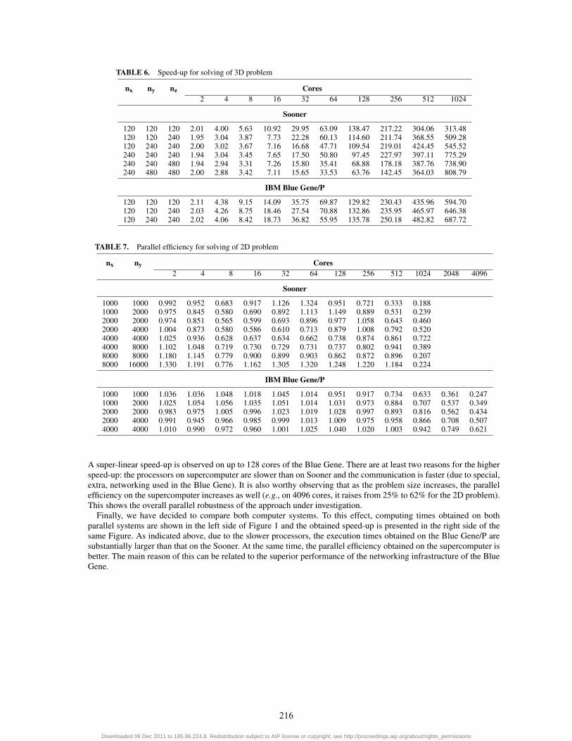
TABLE 6. Speed-up for solving of 3D problem

nx ny nz Cores2 4 8 16 32 64 128 256 512 1024

Sooner

120 120 120 2.01 4.00 5.63 10.92 29.95 63.09 138.47 217.22 304.06 313.48120 120 240 1.95 3.04 3.87 7.73 22.28 60.13 114.60 211.74 368.55 509.28120 240 240 2.00 3.02 3.67 7.16 16.68 47.71 109.54 219.01 424.45 545.52240 240 240 1.94 3.04 3.45 7.65 17.50 50.80 97.45 227.97 397.11 775.29240 240 480 1.94 2.94 3.31 7.26 15.80 35.41 68.88 178.18 387.76 738.90240 480 480 2.00 2.88 3.42 7.11 15.65 33.53 63.76 142.45 364.03 808.79

IBM Blue Gene/P

120 120 120 2.11 4.38 9.15 14.09 35.75 69.87 129.82 230.43 435.96 594.70120 120 240 2.03 4.26 8.75 18.46 27.54 70.88 132.86 235.95 465.97 646.38120 240 240 2.02 4.06 8.42 18.73 36.82 55.95 135.78 250.18 482.82 687.72

TABLE 7. Parallel efficiency for solving of 2D problem

nx ny Cores2 4 8 16 32 64 128 256 512 1024 2048 4096

Sooner

1000 1000 0.992 0.952 0.683 0.917 1.126 1.324 0.951 0.721 0.333 0.1881000 2000 0.975 0.845 0.580 0.690 0.892 1.113 1.149 0.889 0.531 0.2392000 2000 0.974 0.851 0.565 0.599 0.693 0.896 0.977 1.058 0.643 0.4602000 4000 1.004 0.873 0.580 0.586 0.610 0.713 0.879 1.008 0.792 0.5204000 4000 1.025 0.936 0.628 0.637 0.634 0.662 0.738 0.874 0.861 0.7224000 8000 1.102 1.048 0.719 0.730 0.729 0.731 0.737 0.802 0.941 0.3898000 8000 1.180 1.145 0.779 0.900 0.899 0.903 0.862 0.872 0.896 0.2078000 16000 1.330 1.191 0.776 1.162 1.305 1.320 1.248 1.220 1.184 0.224

IBM Blue Gene/P

1000 1000 1.036 1.036 1.048 1.018 1.045 1.014 0.951 0.917 0.734 0.633 0.361 0.2471000 2000 1.025 1.054 1.056 1.035 1.051 1.014 1.031 0.973 0.884 0.707 0.537 0.3492000 2000 0.983 0.975 1.005 0.996 1.023 1.019 1.028 0.997 0.893 0.816 0.562 0.4342000 4000 0.991 0.945 0.966 0.985 0.999 1.013 1.009 0.975 0.958 0.866 0.708 0.5074000 4000 1.010 0.990 0.972 0.960 1.001 1.025 1.040 1.020 1.003 0.942 0.749 0.621

A super-linear speed-up is observed on up to 128 cores of the Blue Gene. There are at least two reasons for the higherspeed-up: the processors on supercomputer are slower than on Sooner and the communication is faster (due to special,extra, networking used in the Blue Gene). It is also worthy observing that as the problem size increases, the parallelefficiency on the supercomputer increases as well (e.g., on 4096 cores, it raises from 25% to 62% for the 2D problem).This shows the overall parallel robustness of the approach under investigation.

Finally, we have decided to compare both computer systems. To this effect, computing times obtained on bothparallel systems are shown in the left side of Figure 1 and the obtained speed-up is presented in the right side of thesame Figure. As indicated above, due to the slower processors, the execution times obtained on the Blue Gene/P aresubstantially larger than that on the Sooner. At the same time, the parallel efficiency obtained on the supercomputer isbetter. The main reason of this can be related to the superior performance of the networking infrastructure of the BlueGene.

216

Downloaded 09 Dec 2011 to 195.96.224.8. Redistribution subject to AIP license or copyright; see http://proceedings.aip.org/about/rights_permissions

TABLE 8. Parallel efficiency for solving of 3D problem

nx ny nz Cores2 4 8 16 32 64 128 256 512 1024 2048 4096

Sooner

120 120 120 1.007 1.001 0.703 0.691 0.936 1.025 1.082 0.849 0.594 0.306120 120 240 0.975 0.759 0.484 0.483 0.709 0.939 0.902 0.827 0.720 0.497120 240 240 0.997 0.753 0.457 0.446 0.520 0.757 0.886 0.853 0.829 0.533240 240 240 0.967 0.757 0.430 0.477 0.545 0.795 0.766 0.888 0.776 0.757240 240 480 0.970 0.734 0.413 0.453 0.493 0.552 0.543 0.695 0.757 0.722240 480 480 1.002 0.715 0.424 0.441 0.485 0.520 0.500 0.552 0.711 0.790

IBM Blue Gene/P

120 120 120 1.055 1.096 1.143 0.881 1.117 1.092 1.014 0.900 0.851 0.581 0.420 0.267120 120 240 1.014 1.064 1.094 1.154 0.861 1.108 1.038 0.922 0.910 0.631 0.439 0.340120 240 240 1.008 1.015 1.052 1.171 1.151 0.874 1.061 0.977 0.943 0.672 0.557 0.435

100

101

102

103

104

1 4 16 64 256 1024 4096

Tim

e

number of processors

Execution time

Sooner nx=ny=2000Blue Gene nx=ny=2000

Sooner nx=ny=8000Blue Gene nx=ny=8000Sooner nx=ny=nz=120

Blue Gene nx=ny=nz=120Sooner nx=ny=nz=240

Blue Gene nx=ny=nz=240

1

4

16

64

256

1024

1 4 16 64 256 1024 4096

spee

d-up

number of processors

Speed-up

Sooner nx=ny=2000Blue Gene nx=ny=2000

Sooner nx=ny=8000Sooner nx=ny=nz=120

Blue Gene nx=ny=nz=120Sooner nx=ny=nz=240

FIGURE 1. Execution time and speed-up for 2D problem nx = ny = 2000,8000, 3D problem nx = ny = nz = 120,240

ACKNOWLEDGMENTS

Computer time grants from the Oklahoma Supercomputing Center (OSCER) and the Bulgarian SupercomputingCenter (BGSC) are kindly acknowledged. K. Georgiev, I. Lirkov, and S. Margenov were partially supported bygrants DO02-147 and DPRP7RP-02/13 of the Bulgarian NSF. Work presented here is a part of the Poland-Bulgariacollaborative grant “Parallel and distributed computing practices”.

REFERENCES

1. A. J. Chorin (1968) Math. Comp. 22, 745–762.2. R. Temam (1969) Arch. Rat. Mech. Anal. 33, 377–385.3. J.-L. Guermond, P. Minev, and J. Shen (2006) Comput. Methods Appl. Mech. Engrg. 195, 6011–6054.4. J.-L. Guermond and P. Minev (2010) Comptes Rendus Mathematique 348, 581–585.5. J.-L. Guermond and A. Salgado (2009) Journal of Computational Physics 228, 2834–2846.6. J.-L. Guermond and A. Salgado (2008) Comptes Rendus Mathematique 346, 913–918.7. M. Snir, S. Otto, S. Huss-Lederman, D. Walker, and J. Dongarra, MPI: The Complete Reference, Scientific and engineering

computation series, The MIT Press, Cambridge, Massachusetts, 1997, 2nd printing.8. D. Walker and J. Dongarra (1996) Supercomputer 63, 56–68.9. E. Anderson, Z. Bai, C. Bischof, S. Blackford, J. Demmel, J. Dongarra, J. D. Croz, A. Greenbaum, S. Hammarling,

A. McKenney, and D. Sorensen, LAPACK Users’ Guide, SIAM, Philadelphia, 1999, 3rd edn.

217

Downloaded 09 Dec 2011 to 195.96.224.8. Redistribution subject to AIP license or copyright; see http://proceedings.aip.org/about/rights_permissions