Improving the Analysis of Hyperion Red-Edge Index from an Agricultural area1

Jupp, D.L.B.1, Datt, B.1, McVicar, T.R.2, Van Niel, T.G.2, Pearlman, J.S.3, Lovell, J.L.1 and King, E.A.1

1 CSIRO Earth Observation Centre, PO Box 3023, Canberra, ACT 2601, Australia 2 CSIRO Land and Water, PO Box 1666, Canberra, ACT 2601, Australia

3 The Boeing Company, Seattle, Washington 98124, USA

ABSTRACT The benefits of EO-1 data, and especially Hyperion hyperspectral data, to agriculture are being studied at sites in the Coleambally Irrigation Area of Australia where a seasonal time series has been developed. Hyperion can provide effective measures of agricultural performance through the use of spectral indices if systematic and random noise is managed and such noise management methods have been established for Coleambally. Among the sources of noise specific to Hyperion is the spectral “smile” that affects the location of the red-edge – an important index in agricultural assessment. We show how this phenomenon, which arises from the pushbroom technology of Hyperion, affects the data and discuss how its effects can be overcome to provide stable and accurate measures of the red-edge and related indices. HyMap airborne data are used to evaluate the results of the methods studied. This paper also shows how future pushbroom instruments should consider the wavelength sampling step in their design if it is intended to remove the “smile” effects by systematic software processing.

1 INTRODUCTION The Hyperion sensor1is one of three instruments carried by NASA’s EO-1 satellite2. It is the first space-borne hyperspectral instrument that acquires both visible and near infrared (VNIR, 400 nm to 1000 nm) and shortwave infrared (SWIR, 900 nm to 2500 nm) spectra. Hyperion is based on pushbroom technology with two spectrometers (one for the VNIR data and one for the SWIR). The EO-1 satellite is in a sun-synchronous orbit at 705 km altitude, nominally one minute behind the Landsat-7 satellite. Hyperion has 256 pixels with a nominal size of 30 m over a 7.65-km swath. Hyperion has a total of 242 nominal (198 currently in use) spectral bands that are approximately equally spaced at 11 nm and with Full Width Half Maximum (FWHM) close to 10 nm over the spectral range3. Since Hyperion is an experimental instrument, it was to be expected that its data would need corrections and a new set of processing steps developed. In recent work4 the basic processing steps and their impact on the performance of agricultural indices have been discussed in some detail. In this paper, we take the study further to examine an effect called spectral “smile” that occurs most strongly in the VNIR array and has a specifically disturbing effect in the development of the “red-edge” index relating to the position in wavelength of the inflection in crop spectra. The study area, as for the previous work, is the well-studied agricultural site near Coleambally in New South Wales (NSW), Australia which we will refer to as the Coleambally Irrigation Area Site, or CIAS.

2 ACTIVITY AT THE COLEAMBALLY IRRIGATION AREA SITE The CIAS is a 95,000 ha site in southern NSW, Australia (Latitude 34° 48′ 4.3′′ S, Longitude 146° 0′ 48.96′′ E, 120 m above sea level) which has over 500 farms with large (up to 70 ha), flat, uniform fields. The CIAS is a focus of remote sensing research to determine the information content available to both landholders and irrigation companies from satellite and airborne remote sensing. The CIAS has an excellent base of geographic and agricultural management 1 Presented at the SPIE’s Third International Asia-Pacific Remote Sensing symposium, Hangzhou, China, October 2002. Included in Proceedings of SPIE Vol. 4898 (2003), Image Processing and Pattern Recognition in Remote Sensing, S.G.Ungar (Ed), p78-92.

1

information. Since December 2000, a time series of EO-1 images has been collected over two Southern Hemisphere summer growing seasons (2000/2001 and 2001/2002). There have also been a number of field campaigns to collect spectral and ancillary information for calibration and applications research. This work has been conducted as a significant part of the Australian contribution to the NASA EO-1 Science Validation Team’s evaluation of instrument performance between March 2001 and September 2002. An extensive data set was obtained for the CIAS on 12 January 2002. The data included Landsat ETM, EO-1 Hyperion and ALI data, SAC-C and TERRA platform data plus complementary ground, airborne and atmospheric data. An Analytical Spectral Devices (ASD) Fieldspec spectroradiometer was used to collect ground-based spectra for selected crops and fields. HyMap airborne scanner data5, covering the 400-nm to 2500-nm spectral range in 126 bands, with 5-m spatial resolution, and 15-nm spectral resolution, were also acquired. These data sets have been used to evaluate Hyperion sensor performance and atmospheric correction models4. Data taken by the ASD are plotted in Figure 1. These spectra display signatures and spectral features typical of green vegetation, dry vegetation and soils that are commonly found in such areas. The green reflectance peak near 550 nm, the photosynthetic chlorophyll absorption feature (680 nm), the red-edge region (700 nm to 750 nm) and leaf water absorption features near 970 nm and 1240 nm are present in the rice spectra. The soil spectra show a clay absorption feature near 2200 nm and the stubble spectra show lignin/cellulose absorption features near 2100 nm and 2300 nm and a plant wax/oil absorption feature near 1720 nm.

0

0 .1

0 .2

0 .3

0 .4

0 .5

0 .6

4 2 5 6 2 5 8 2 5 1 0 2 5 1 2 2 5 1 4 2 5 1 6 2 5 1 8 2 5 2 0 2 5 2 2 2 5 2 4 2 5

W a v e le n g th (n m )

Ref

lect

ance

S o il1S o il2S tu b b le 1S tu b b le 2G r ic eN N S o ilR ic e 1Y ric eM S o il

Figure 1. Typical spectral features occurring in the CIAS. Mean ASD spectra (convolved to 176 Hyperion bands) for the nine sampling sites are shown.

Among indices being used to assess the health and performance of the rice, corn, soybeans and other crops4 are two that involve the feature between about 680 nm and 760 nm in crops called the “red-edge”. The two indices are: 1. The red-edge wavelength (RE) is the wavelength position of the maximum slope (or zero second derivative) in the red-near-infrared (700 nm to 750 nm) reflectance of vegetation. Several studies have shown that the red-edge wavelength is correlated with chlorophyll content in leaves and canopies 6,7,8. The red-edge wavelength is therefore useful for monitoring vegetation productivity and detecting the onset of stress and senescence. The RE shifts to longer wavelengths during plant growth and shifts to shorter wavelengths during stress. 2. The first derivative value at the red-edge (dRE) is the “slope” associated with the red-edge position and has also been shown to be sensitive to green vegetation amount (percent cover and leaf area index, LAI). Filella and Peñuelas9 found the area of the red-edge peak to be a strong indicator of LAI amount.

2

The Hyperion bands used to develop both the RE and the dRE were 33 to 40 or wavelengths 681.8 nm to 753.0 nm and the indices were realized using local polynomial fitting as implemented in a package provided by the Mineral Mapping and Technology Group of CSIRO13. The fitting procedure is sensitive to noise and residual atmospheric effects and this must be taken into account in the processing described in this paper.

3 BASE IMAGE PROCESSING FOR HYPERION DATA

3.1 Hyperion noise and base processing The Hyperion VNIR sensor has 70 bands and the SWIR has 172 providing 242 potential bands. A number of the bands were intentionally not illuminated and others correspond to areas of low sensitivity of the spectrometer materials. Because of this, only 198 bands have been provided as calibrated data in Hyperion Level 1B1 products; the unused bands are set to zero values by the TRW software during the calibration stage of the processing3. Among the 198 there are four remaining bands in the overlap between the two spectrometers. It is usual to eliminate two of these to obtain 196 unique bands. Atmospheric water vapor bands that absorb most of the incident and reflected solar radiation are easily identified by visual inspection of the image data or by atmospheric modeling. Accepting this as a good criterion for band elimination for land surface applications yields a subset of about 176 bands that can be effectively used for atmospheric correction and further investigations4. Hyperion data display additional effects that arise from its pushbroom technology. In this paper, the spatial elements of one line of an image will be referred to as “pixels” and are the same as “samples” in other usage. They sample the land surface in the across-track direction. As the pushbroom moves forward, a given pixel creates a “column” of data or an along-track (vertical direction) data set. Each column in a single band corresponds to a single detector in one of the arrays. For pushbroom instruments, a poorly calibrated detector in either the VNIR or SWIR arrays will leave a vertical “stripe” in a displayed image band. Ways to correct these have been discussed in a number of papers to date, including the previous study that this paper extends4. Hyperion also has low-frequency array effects such as those due to spectral “smile”, the main topic of this paper. This arises from the optical techniques used to disperse the input imaged “slit” over the detector arrays in the wavelength dimension. They create a variation in central wavelength and bandwidth across the swath of the sensor – or in a single image line. The spectral “smile” effect, while well characterized prior to launch3, is the subject of on-going investigations to establish whether there have been changes to its form and magnitude since launch. Since HyMap is a scanning instrument it does not have these effects and provides an excellent base to discuss their magnitude and compare correction methods. The statistics of the detector arrays can be studied by accumulating mean, variance, minimum and maximum data for each pixel in each band over the lines of an image. Following the advice given in Datt et al.4, the VNIR and SWIR have been treated separately as two matrices of size: the number of pixels by the number of bands present in each case. The process of “de-striping” involves accumulating statistics and balancing the means and possibly variance to a reference. If the reference mean and variance are those of the whole image area it can be called “global” de-striping whereas if the reference means are local to a column the method can be called “local”. In this paper we assume “local” processing has been applied but will discuss global destriping as an option for overcoming spectral “smile”.

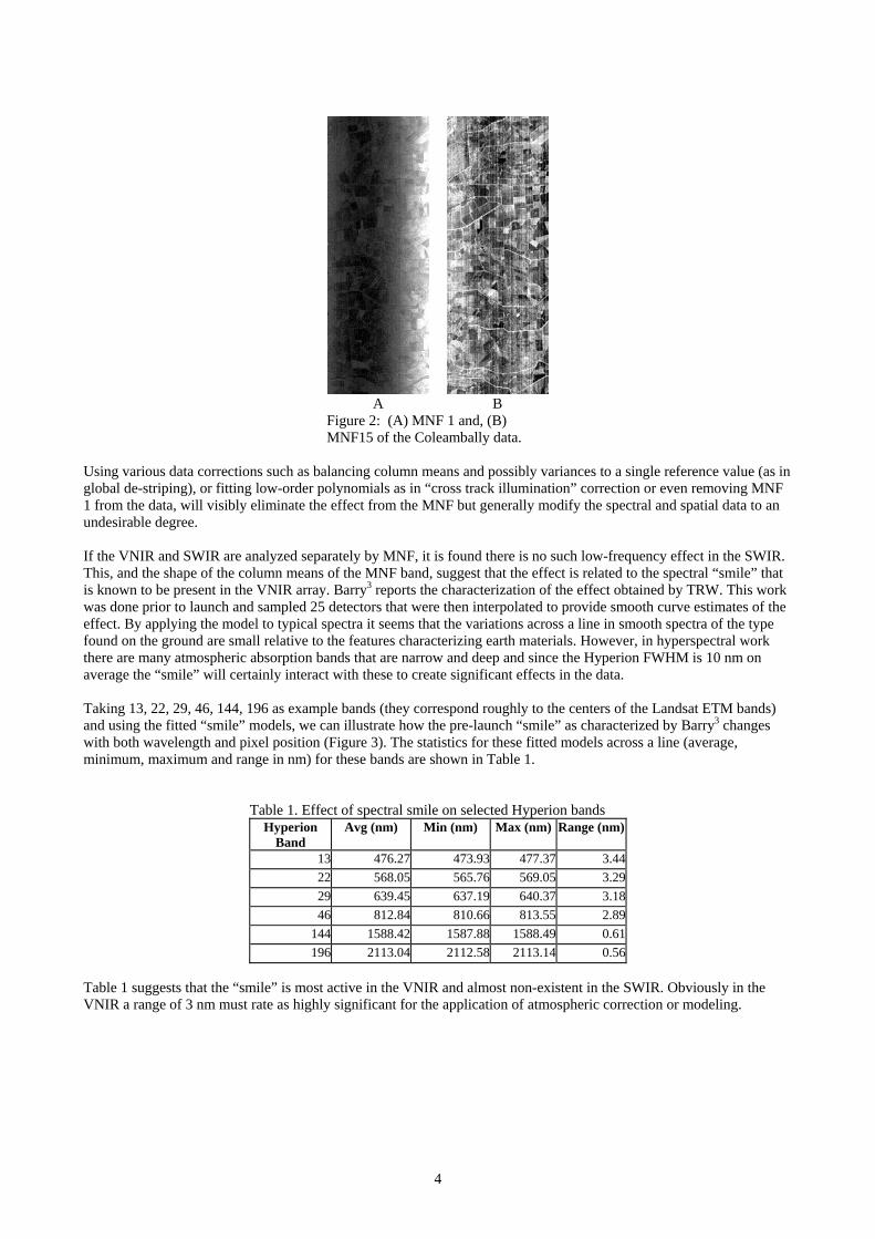
4 THE “SMILE” RADIANCE EFFECT AND ITS SIGNIFICANCE Low-frequency effects in Hyperion data are sometimes visible in displayed image data and can dominate exploratory analyses such as the Minimum Noise Fraction (MNF)14. The MNF transform consists of two Principal Components transformations; the first transformation uses an estimated noise covariance matrix to remove the band-to-band correlations present in the noise and rescales the noise to have unit variance; the second transformation is a standard Principal Components transform of the ‘noise-whitened’ data. Figures 2A and 2B for the CIAS show MNF bands 1 and 15, where there is a strong low frequency effect in MNF band 1.

3

A

B

Figure 2: (A) MNF 1 and, (B) MNF15 of the Coleambally data.

Using various data corrections such as balancing column means and possibly variances to a single reference value (as in global de-striping), or fitting low-order polynomials as in “cross track illumination” correction or even removing MNF 1 from the data, will visibly eliminate the effect from the MNF but generally modify the spectral and spatial data to an undesirable degree. If the VNIR and SWIR are analyzed separately by MNF, it is found there is no such low-frequency effect in the SWIR. This, and the shape of the column means of the MNF band, suggest that the effect is related to the spectral “smile” that is known to be present in the VNIR array. Barry3 reports the characterization of the effect obtained by TRW. This work was done prior to launch and sampled 25 detectors that were then interpolated to provide smooth curve estimates of the effect. By applying the model to typical spectra it seems that the variations across a line in smooth spectra of the type found on the ground are small relative to the features characterizing earth materials. However, in hyperspectral work there are many atmospheric absorption bands that are narrow and deep and since the Hyperion FWHM is 10 nm on average the “smile” will certainly interact with these to create significant effects in the data. Taking 13, 22, 29, 46, 144, 196 as example bands (they correspond roughly to the centers of the Landsat ETM bands) and using the fitted “smile” models, we can illustrate how the pre-launch “smile” as characterized by Barry3 changes with both wavelength and pixel position (Figure 3). The statistics for these fitted models across a line (average, minimum, maximum and range in nm) for these bands are shown in Table 1. Table 1. Effect of spectral smile on selected Hyperion bands

Hyperion Band

Avg (nm) Min (nm) Max (nm) Range (nm)

13 476.27 473.93 477.37 3.44 22 568.05 565.76 569.05 3.29 29 639.45 637.19 640.37 3.18 46 812.84 810.66 813.55 2.89

144 1588.42 1587.88 1588.49 0.61 196 2113.04 2112.58 2113.14 0.56

Table 1 suggests that the “smile” is most active in the VNIR and almost non-existent in the SWIR. Obviously in the VNIR a range of 3 nm must rate as highly significant for the application of atmospheric correction or modeling.

4

To show consistency between land covers and how similar the MNF characterizations are for Hyperion, we took data from an image of a salt lake (Lake Frome15) and the focus agricultural area (Coleambally) as test data. If the MNF-1 is in each case averaged over all lines in these images and (re-)scaled to mean zero and unit range we obtain the result plotted as Figure 4.

Figure 3: Relative spectral variation across Hyperion lines.

Figure 4: Mean MNF-1 for Coleambally and Lake Frome.

The consistency for land covers and some similarity with the average “smile” effect described by TRW are clear but the actual mechanism of its appearance in the image data needs to be better established since if individual bands, averaged over vertical columns, are plotted we do not obtain these smooth curves. That is, these are not just radiance variations across a line. A driving mechanism for the “smile” radiance effect can be investigated by plotting the factor loadings for VNIR MNF-1 against the data mean value. The factor loadings are coefficients for the linear combination of original hyperion bands producing a transformed MNF band. In Figures 5A and 5B the loadings are plotted against the (scaled) image means for comparison. Figure 5A is for Coleambally agricultural area and 5B for the Lake Frome salt lake.

Fig 5(A,B): Scaled mean radiances & MNF-1 Loadings

In each case, the MNF-1 has the mathematical structure of a mean of differences across major atmospheric absorption features which then “track” the sensor “smile” effect. The effect can, in fact, be simply obtained without recourse to MNF by using differences across any of the significant atmospheric features. In the above plots it seems that the oxygen-A area near 760nm and the two water vapor bands on each side are driving the magnitude of the effect. It would appear that a significant step in processing to overcome “smile” would be to use methods for atmospheric correction that take account of the “smile”. The only current software that has attempted this and been reported is the HATCH program developed at the University of Colorado9. However, as most people will be using available software

5

such as FLAASH10 and ACORN11 we need to consider what effect may be left in the data when “smile” is neglected in that step. For the purposes of this paper we especially need to assess whether the “smile” radiance effect can seriously affect spectral indices after atmospheric correction due to its effect on the underlying spectra or the presence of residual atmospheric features that vary across the line. To do this, basing the choice on an analysis of the MNF 1 loadings, we defined some simple test indices using the differences between column means taken either side of the vegetation features at 681 nm (the chlorophyll absorption wavelength, ) and 722 nm (the approximate location of the red-edge inflection, ) respectively. These were applied to the column means obtained as part of the de-striping process. The indices have the form:

681I

722I

691 671 732 712681 722

691 671 732 712

200 , 200L L L L

I IL L L L

− −= × = ×

+ +

where Lx denotes the radiance at wavelengths 671, 691, 712 and 732 nm. Figures 6A and 6B show the differences across the chlorophyll feature and red-edge feature as a function of pixel in a line before and after atmospheric correction using FLAASH10. They also show the TRW modeled “smile” for the center band. To make them comparable, the plots have each been rescaled to be zero at pixel 128 and have standard deviation one.

Figure 6 (A) Normalized I681 with (Refl) and without (Rad) atmospheric correction and TRW characterized “smile” effect

Figure 6 (B) Normalized I722 with (Refl) and without (Rad) atmospheric correction and TRW characterized “smile” effect

The trends in the normalized indices show great similarity to the “smile” shape and the red-edge difference shows more land cover variation as expected. The shape of the effect is not altered by the atmospheric correction when the data are normalized. The “smile” radiance effect will therefore exist in the atmospherically corrected data but the issue is - to what extent?

Table 2. ASD-based data for the indices Case I681 I722

Mean 8.26 19.36 Mean crop 34.69 53.70 Mean soil 3.76 3.38 Mean Stubble 5.29 4.43

6

Table 2 records the averaged values of the indices for crops (rice), soil and stubble calculated after averaging the nine reflectance spectra plotted in Figure 1 to three cover types. It records the magnitudes found for these different covers. The crops are distinct and separate from the soil and stubble as would be expected for these indices. To establish the variation due to the “smile” effect in these features, Table 3 lists the mean and standard deviation of the actual column mean data taken from the Hyperion image as recorded in the column means across the pixels of a line. The magnitude of the standard deviation is, in this case, largely due to the “smile” effect.

Table 3 Image-based data for the indices Case I681 I722

Image Mean 11.60 20.28 Image STD 1.49 2.91

Figures 6A and 6B, and Tables 2 and 3, suggest that the magnitude of the “smile” effect in these indices remains in the data after atmospheric correction, but is a relatively small variation compared with the variation between and, in the case of crops, within cover types. However, this conclusion does not apply to the higher derivative data and particularly to the location of the zero of the second derivative or red-edge inflection. Figure 7A illustrates the magnitude of the change in the red-edge position across the Coleambally image while Figure 7B shows that the change in red-edge first derivative value across the image is small relative to the variations within crops. We therefore need to apply some form of image processing to overcome this disturbing trend – but only in the higher order derivative data.

A

B

Figure 7. Across track variation in; (A) Red-edge wavelength and, (B) Red-edge first derivative Hyperion images.

5 METHODS FOR REDUCING THE SMILE EFFECT ON THE RED-EDGE POSITION The “smile” effect on Hyperion red-edge wavelength and slope indices was examined by comparing the January 12, 2002 Hyperion and Hymap5 images over CIAS. HyMap is not pushbroom technology and does not have striping and “smile” such as we find in Hyperion. Both images were atmospherically corrected using the FLAASH atmospheric

7

correction software. The individual Hymap image strips for each flight line were atmospherically corrected and then geo-referenced to a single image mosaic. The Hymap reflectance image was then resampled to Hyperion space and the pixels were aggregated to the Hyperion pixel size of 30 m. The Hymap and Hyperion images were then spatially subset to obtain the common area covered by both sensors. Red-edge wavelength (RE) and red-edge slope (dRE) images were produced using an ENVI_IDL module developed by CSIRO Exploration and Mining, Mineral Mapping Technologies Group13. This module fits a third-order polynomial to the red-edge region of the spectrum (680 nm to 750 nm) and returns the wavelength and first derivative value where this polynomial has an analytical inflection point. The polynomial fitting and calculation of RE and dRE was performed on six Hymap bands (from 680 nm to 756 nm) and eight Hyperion bands (from 681 nm to 752 nm). To exclude non-vegetation areas (soil, crop stubble, roads, etc.) from the analysis a mask band was created using the ratio of green (≈ 550 nm) and red (~ 680 nm) bands and masking out areas with a ratio of < 1. The mean RE values across the 256 pixels for Hymap and Hyperion are plotted in Figure 8. The “smile” effect in the Hyperion-derived RE is clearly shown as a departure from the Hymap trend, especially over pixels 150 to 256 where the mean Hyperion RE values increase significantly (2 nm to 9 nm) above the Hymap values over the same area. There also several ‘spikes’ of low RE mean values in Hyperion between pixels 1-8 and 227-256, indicating extreme RE values (i.e. values outside the RE inflection window of 700 to 740 nm) for many pixel that have been returned as zeroes, thus reducing the pixel means.

Figure 8. Across-track variation of the RE index in Hymap and Hyperion Images.

To reduce the effect of spectral smile and to make the Hyperion RE values more consistent with Hymap RE values, several data correction methods were applied to the Hyperion image. The RE indices were calculated for each of the “smile” corrected Hyperion images and compared with the Hymap RE indices.

5.1 Global de-striping In the global destriping procedure (Datt et al.4) the data for each column are modified so that the column means and variances match those for the whole image for each band. Global destriping was applied to the Hyperion reflectance image using an IDL procedure added on to the ENVI image processing software.

5.2 MNF Smoothing The MNF smoothing of Hyperion reflectance data is a two stage process as described in Datt et al.4 The MNF smoothing was applied only to the VNIR bands of the Hyperion image since the focus was on deriving the red-edge indices. First the forward MNF transform was applied to the Hyperion reflectance image in ENVI. The first MNF band showed the smile radiance effect as shown in Figure 2A. The second step was an inverse MNF transform to reproduce the reflectance data but using only the MNF bands 2 to 12. MNF band 1 was excluded to test if it reduced the “smile” effect in the red-edge indices.

8

5.3 Cross-track illumination correction Cross-track illumination correction is another procedure in ENVI used to remove variation in the cross-track illumination of an image usually caused by vignetting effects, instrument scanning, or other non-uniform illumination effects. The column mean values are calculated for all pixels in each band and fitted with a polynomial to show the mean variation in the cross-track direction. The polynomial function fitted to the means is used to remove the variation. The cross track illumination correction was applied to the Hyperion reflectance image using a polynomial of order 2.

5.4 Interpolation The action of interpolating the spectral data so that the channels correspond to the same spectral band over all the pixels can be referred to as “de-smiling”. The basic idea is simple. At each pixel (i) of a line we have calibrated radiance values { }, 1,ijL j N= for the N wavelengths recorded. At any pixel we then construct an interpolating function ( ( )L λ )

such that . Here λ( ) 1,ij ijL L jλ = = N ’ij is the actual center wavelength at pixel (i), perturbed from its nominal value as

a result of the “smile”. Then the estimated data corresponding to the standard header central wavelength (CWL) values are: . ( ) 1,j jL L j Nλ= = In practice the VNIR and SWIR need to be treated separately and we can use polynomials of various degrees that “slide” so that they combine local interpolation with properties that approximate an “ideal” interpolator as described by Brown16. The Coleambally data were “de-smiled” using a locally sliding cubic polynomial to test the utility of the process for removing the effect of “smile” on the position of the red-edge. The Hyperion central wavelengths for each pixel, as provided in the instrument calibration files, were used to interpolate the radiance data.

A

B

C

D

Figure 9. (A) Hyperion MNF1

(B) Hyperion MNF2 (C) Hymap MNF1 (D) Hymap MNF2

The effects of the four data correction methods on the smile effect were examined in three ways: 1. MNF imagesThe MNF transform was applied to the Hyperion images after “smile” corrections and compared with the Hymap MNF images. The first MNF band in the Hyperion reflectance image prior to any “smile” correction shows a “smile” effect (also shown in Figure 2) while the Hymap MNF band 1 does not show any such effect (Figure 9). The first MNF band in the Hyperion images following the “smile” correction did not show the smile effect for the Global de-striping, MNF smoothing, and cross track illumination corrections (Figure 10). The first MNF band for the “smile” correction by interpolation did, however, show a residual “smile” effect in MNF band 1 (see Figure 11A). The improvement in MNF band 1 is not a clear indication that the “smile” effect has been

9

effectively reduced in the data. The question is whether the data have also been modified in other ways, which cannot be determined by examining MNF band 1. The effects of the “smile” corrections specifically on the RE index were examined in more detail by comparing the across track trends with Hymap, as described in (2) below.

A B

A B

Figure 10. Hyperion MNF bands after “smile” correction using the global destriping method, (A) MNF 1, and (B) MNF2

Figure 11. (A) MNF 1 and (B) MNF15 of the interpolated Coleambally data.

2. Cross track variation in the red-edgeThe mean RE values across the 256 pixels for the Hyperion images following smile corrections were calculated and are compared with the Hymap RE trends in Figure 12.

Figure 12. Comparison of cross-track variations in RE index for Hymap and Hyperion without any “smile” corrections together with, (A) interpolation and MNF smoothing corrections, and (B) global de-striping and Cross Track Illumination Corrections.

A B

It can be seen from Figure 12A that the smile correction by interpolation produces the best improvement in the trend in Hyperion data. MNF smoothing produced the next best improvement. It is also seen from Figures 12A and 12B that all transformations except the global de-striping, removed the ‘spikes’ or effects of extreme RE values over pixels 227-256.

10

The global de-striping in fact introduced more ‘spikes’ in the trend. The spikes in pixels 1-8, however, were not removed by any transformation, except global de-striping. The cause of the ‘spikes’ in pixels 1-8 is not fully established at present and is the subject of further investigation. Its likely cause can, however, be seen as stripes in Figure 2D. 3. Regression of Hyperion RE and dRE column means with Hymap RE and dRE column meansA more quantitative comparison of the trends shown in Figure 12 was made by regressing the Hyperion column means with the Hymap column means across pixels 9-256 (Table 4). Columns 1-8 were not used in the regressions because, as mentioned in (2) above, the cause of the spikes in these pixels is not clear at this stage and may be due to some other effect in Hyperion data. The results show that the “smile” correction by interpolation produced the best correlation (r2 = 0.90) with Hymap RE means and the RMS error was the lowest (0.47 nm). MNF smoothing also produced a significant improvement in the consistency with Hymap data. Table 4. Regression between Hyperion and Hymap derived RE values. The column means for pixels 9 to 256 were used in the regressions. In each case the regression line was forced to an intercept of zero. Smile correction applied to Hyperion reflectance image Interpolation MNF

smoothing Cross track illumination correction

Global de-striping

No “smile” correction

r2 0.904 0.743 0.300 -0.023 0.004 RMS Error (nm) 0.47 0.85 1.43 14.92 24.03 Slope 1.0011 1.0036 1.0033 0.9983 0.9949 Regression between Hyperion and Hymap column means was also performed for the red-edge slope or dRE index (Table 5). These results show that correction for “smile” using the interpolation and cross-track illumination correction methods improves the relationship between Hyperion and Hymap-derived dRE index. The interpolation and cross track illumination corrections produced the largest improvements in R2, with the interpolation method producing the smallest RMS error. (The quoted RMS errors are in units of (Reflectance x 10000 per μm), so an error of 1618 in Table 5 is equivalent to 0.0001618 nm-1 when converted to reflectance (0 to 1.0) per nm.). Table 5. Regression between Hyperion and Hymap-derived dRE values. The column means for pixels 9 to 256 were used in the regressions. In each case the regression line was forced to an intercept of zero. Smile correction applied to Hyperion Reflectance Image Interpolation MNF

smoothing Cross track illumination correction

Global de-striping

No “smile” correction

r2 0.924 0.599 0.924 0.331 0.679 RMS Error (nm) 1618.393 5086.87 1721.826 5587.988 3786.915 Slope 1.079 1.045 1.066 1.061 1.059 As with the RE index, the smile effect in Hyperion was most prominent across pixels 150-256, with the largest deviations from the Hymap trend across pixels 227-256. The effect in pixels 1-8 was similar to the effect in the RE index described earlier and this was not reduced by the smile corrections.

6 THE POTENTIAL TO USE INTERPOLATION TO REMOVE “SMILE” IN BASE PROCESSING

As described in the introduction, Hyperion data correspond to a (Gaussian) bandpass function of close to 10 nm FWHM and are set at close to 10 or 11 nm steps apart. If we approximate the sequence of band data in either spectrometer as an equally spaced sampled data set the Hyperion data may be expressed formally as:

11

{ } ( )j hL S Lϕ= ∗ , or a sampling at equally spaced points step h apart of the convolution of the radiance with the bandpass ϕ. In this case, the issue of interpolation to a new set of CWL values simply becomes that of estimating Lϕ ∗ at a new location, or interpolating the sampled data series that has been “pre-filtered” with the bandpass function. For this problem, an interpolation operator M(λ) is used to construct the function approximating Lϕ ∗ :

( ) ( )

( )( )

h jj

L L M

L

jλ λ λ

ϕ λ

∞

=−∞

= −

≈ ∗

∑

where the index j is assumed to run over all integers and the subscript h indicates that the underlying series has sampling step h and the origin of the data series is taken at a convenient point. The interpolation operator, M(λ), has the property that:

. (0) 1

( ) 0 ( , ) 0M

M jh j j== ∈ −∞ ∞ ≠

The choice of the interpolation operator needs to consider accuracy (usually for a class of functions), stability and sensitivity to noise as well as convenience. For example, the data sequences are usually relatively short so that local interpolation operators rather than those with long “settling times” away from the wavelength of interest are preferred. The Fourier transform of the interpolated function can be written as: ˆ ˆ( ) ( ) ( )hL Mω ω φ ω= where the caret indicates Fourier transform and ( )φ ω is the “cosine polynomial” for the data series:

( )

( )

ˆˆ ( 2 ) /

i jhj

j

j

L e

L jh

ωφ ω

ϕ ω π ω π

∞−

=−∞

∞

=−∞

=

= + ≤

∑

∑ h.

The second relation between ( )φ ω and the original data is a well-known relation in Fourier analysis and shows how the cosine polynomial is the “aliased” or “folded” form of the original function’s Fourier transform. It follows from it that if the convolved data are band-limited within the range / hω π≤ then ( )φ ω will retrieve the Fourier transform exactly. This is described in Brown16. Among possible interpolation operators there is one that is called “Ideal” in that its Fourier transform is a constant in the interval / hω π≤ . Such an interpolating function will then exactly retrieve the band limited functions mentioned above. It is easy to show that M(λ) in this case is:

sin( ( ) / )( )

( ) /

( ( ) / )

jj

j

j

hM

h

Sinc h

π λ λλ λ

π λ λ

π λ λ

−− =

−

= −

.

12

This operator is, however, not easy to use in practice as it includes the influence of the interpolation for a considerable distance from its peak (it has a long “settling time”) and also is not very stable to noise that has been added after the pre-filtering. However, various approximations to the ideal operator in the form of sliding polynomials or splines can be constructed that have greater stability and shorter ranges of influence. These interpolations have been used in this paper while the ideal is mainly used to provide a theoretical baseline. In the interpolation of a general sampled data series, frequencies in the “Nyquist” range will be retrieved but higher frequencies (including random noise) will be present as “aliasing” and create problems in addition to not being retrievable. In practice, data series are pre-filtered to remove high frequency information before sampling. In our case, the bandpass function ϕ acts as the low pass pre-filter making it feasible to retrieve the filtered data if the relationship between h and the FWHM is chosen carefully. The outcome is a criterion we have used to establish the possibility of interpolation. That is, if the Fourier components of Lϕ ∗ are mostly within the bandpass / hω π≤ then very precise interpolation is possible between the sample points by interpolating functions similar to the ideal interpolating function. Since L is unknown we can consider the delta radiance as described above to be the most extreme but, in the case of data where sharp atmospheric features are present, nevertheless a very practical choice. Since in this case ˆ 1L = it follows that our criterion for the possibility of interpolation of the filtered versions of the sharp features is the extent to which the Fourier transform of ϕ is contained in the bandpass / hω π≤ . For Hyperion we have (assuming the FWHM is constant over all wavelengths):

2

2

2 2

22

1/ 2

1( )2

ˆ( )

t

t e

e

σ

σ ω

ϕπσ

ϕ ω

−

−

=

=

where [ ]1/ 22 2 2FWHM

Lnσ = . It follows that the proportion of the Gaussian within the bandpass / hω π≤ can be evaluated

as:

where

( )1/ 24 2

FWHMR Erfh

Ln

β

πβ

⎛ ⎞= ⎜ ⎟⎝ ⎠

=.

Clearly, if h is small relative to the FWHM then the possibility of interpolation (afforded by the ideal operator) will be greater. Using the appropriate data for Hyperion we have in Table 6: Table 6. Proportion of bandpass retrievable from Hyperion data.

H (nm) FWHM (nm) σ (nm) Bandpass (%) VNIR 10.17 10.92 4.64 84.8 SWIR 10.09 11.07 4.70 85.7

That is, a high level of information should be able to be interpolated from Hyperion data, but with 15% outside the interval there is still significant aliasing of higher frequency information, such as would occur in narrow band absorptions or in rapidly changing areas of a spectrum.

13

Figure 13 shows the behavior of R with the ratio of the FWHM to the sampling step h:

Figure 13: Performance of ideal interpolation

A step of 5 nm would provide 99.7% of the bandpass and allow accurate potential interpolation of Hyperion data, but this would double the number of Hyperion bands. A step of 8 nm would, however, obtain over 90% of the bandpass and significantly improve the potential to remove any pushbroom “smile” by software processing. It may be concluded that for hyperspectral sensor designs using denser sampling (or shorter wavelength step) these effects could be removed by software. The problem with such interpolation is that there is noise present that is not pre-filtered by the Hyperion bandpass and so such interpolation will need to be done after pre-processing has removed the worst of such noise.

7 CONCLUSIONS We have shown how the Hyperion sensor “smile” effect mainly affects atmospheric features and residual atmospheric features after atmospheric correction. In most cases of agricultural indices the remaining effect after atmospheric correction is small relative to variations within and between crop fields. However, in the case of the position of the red-edge the effect is serious enough to investigate how it may be resolved. A likely cause of the remaining effect is that atmospheric residuals alter the polynomial approximations used in fitting the red-edge in a systematic way across the line. Using global de-striping, fitting polynomials as in “cross track illumination” correction and removing MNF1 where this is dominated by a “smile” effect all apparently reduced the “smile” variation. However, these all alter the ground spectra and could only be considered as special approaches for the red-edge position. However, by far the most successful approach was using wavelength interpolation. Interpolation is the most sophisticated approach as it directly addresses the issues of “smile” but it does not remove the “smile” effect completely from the MNF1. In our view this is due to two reasons. One is that the current “smile” model may be inadequate on the east side of Hyperion images. The other is that we believe (with support from the work of Section 6) that the sampling step of Hyperion is too long for the FWHM. We have concluded that spectral interpolation before atmospheric correction is a promising technique for reducing the effects of spectral “smile” that improves the spectra and overcomes the specific issue for the red-edge position. We have also discussed the possibility that a denser sampling of a Hyperspectral instrument could make a software solution to “smile” by interpolation or resampling a distinct possibility – and it could be applied before the atmospheric correction. This should be considered in future hyperspectral pushbroom instrument design.

14

8 ACKNOWLEDGEMENTS Tim McVicar and Tom Van Niel were supported in part by the Cooperative Research Centre for Sustainable Rice Production, specifically Project 1105. NASA provided valuable encouragement and support for Jay Pearlman’s contribution. The Hyperion data were collected by NASA and processed by TRW for the evaluation of the experimental sensors on the New Millennium EO-1 mission through CSIRO membership in the EO-1 Science Validation Team. CSIRO EOC, as Australian PI to the SVT provided significant support and staff resources for this research. Particular acknowledgement is due to Susan Campbell for field support and the Mineral Mapping and Technology Group of CSIRO for access to their MMTG-A set of software for hyperspectral processing.

9 REFERENCES 1. J. Pearlman, S. Carman, C. Segal, P. Jarecke, and P. Barry, “Overview of the Hyperion imaging spectrometer for the NASA EO-1

mission,” in Proc. Int. Geoscience and Remote Sensing Symp. (IGARSS’01), Sydney, Australia, 2001. 2. S. G. Ungar, “Overview of EO-1, the first 120 days,” in Proc. Int. Geoscience and Remote Sensing Symp. (IGARSS’01), Sydney,

Australia, 2001. 3. P. Barry, “EO-1/ Hyperion Science Data User’s Guide,” TRW Space, Defense & Information Systems, USA, May 2001. 4. B. Datt, T.R. McVicar, T.G. Van Niel, D.L.B. Jupp, and J. S. Pearlman, “Pre-processing EO-1 Hyperion hyperspectral data to

support the application of agricultural indices,” IEEE Trans. Geosci. Remote Sensing, (In Press), 2003. 5. T. Cocks, R. Jenssen, A. Stewart, I. Wilson and T. Shields, “The HyMap airborne hyperspectral sensor: the system, calibration and

performance,” in Proc. 1st EARSEL Workshop on Imaging Spectroscopy, Zurich, pp. 37-42, October 1998. 6. D. N. H. Horler, M. Dockray, and J. Barber, “The red edge of plant leaf reflectance,” Int. J. Remote Sens., Vol. 4, pp. 273-288,

1983. 7. P. J. Curran, J. L. Dungan, B. A. Macler, and S. E. Plummer, “The effect of a red leaf pigment on the relationship between red

edge and chlorophyll concentration,” Remote Sens. Environ., vol. 35, pp. 69-76, 1991. 8. A. A. Gitelson, M. N. Merzlyak, and H. K. Lichtenthaler, “Detection of red edge position and chlorophyll content by reflectance

measurements near 700 nm,” J. Plant Physiol., vol. 148, pp. 501-508, 1996. 9. I. Filella, and J. Peñuelas, “The red edge position and shape as indicators of plant chlorophyll content, biomass, and hydric status,”

Int. J. Remote Sens., vol. 15, pp. 1459-1470, 1994. 10. A. F. H. Goetz, Z. Qu, B. Kindel, and M. Ferri, “Atmospheric correction of Hyperion data and techniques for dynamic scene

correction," in Proc. Int. Geoscience and Remote Sensing Symp. (IGARSS’02), Toronto, Canada, III: pp.1408-1410, 2002. 11. T. W. Cooley, G. Anderson, G. W. Felde, M. L. Hoke, and A. J. Ratkowski, “FLAASH, a MODTRAN-4 based atmospheric

correction algorithm, its application and validation” in Proc. Int. Geoscience and Remote Sensing Symp. (IGARSS’02), Toronto, Canada, III: pp.1414-1418, 2002.

12. http://www.aigllc.com/acorn/intro.asp13. MMTG, “MMTG A-List Hyperspectral Processing Software”, CSIRO Division of Exploration and Mining, Mineral Mapping

Technologies Group, North Ryde, NSW, Australia, 2002. 14. A. A. Green, M. Berman, P. Switzer, and M. D.Craig, “A transformation for ordering multispectral data in terms of image quality

with implications for noise removal,” IEEE Transactions on Geoscience and Remote Sensing, vol. 26, no. 1, pp. 65-74, 1988. 15. S. Campbell, J. Lovell, D. L. B. Jupp, R. D. Graetz, P. Clancy, P. Jarecke, and J. Pearlman, "The Lake Frome Field campaign in

Support of Hyperion Instrument Calibration and Validation" in Proc. Int. Geoscience and Remote Sensing Symp. (IGARSS’01), Sydney, NSW, July 2001, (CD).

16. Brown, B.M. (1965). The Mathematical Theory of Linear Systems. Science Paperbacks, Chapman & Hall.

15