Improvement of the Thermodynamic Description of Polar ...
236
Improvement of the Thermodynamic Description of Polar Molecules and Their Mixtures in the SAFT Framework by Jamie Theo Cripwell Dissertation presented for the Degree of DOCTOR OF PHILOSOPHY (Chemical Engineering) in the Faculty of Engineering at Stellenbosch University Supervisor Prof. A.J. Burger Co-Supervisor Prof. C.E. Schwarz March 2017
-
Upload
khangminh22 -
Category
Documents
-
view
4 -
download
0
Transcript of Improvement of the Thermodynamic Description of Polar ...
Improvement of the Thermodynamic Description of Polar Molecules and
Their Mixtures in the SAFT Framework
by
Jamie Theo Cripwell
Dissertation presented for the Degree
of
DOCTOR OF PHILOSOPHY (Chemical Engineering)
in the Faculty of Engineering at Stellenbosch University
Supervisor Prof. A.J. Burger
Co-Supervisor Prof. C.E. Schwarz
March 2017

Declaration
By submitting this dissertation electronically, I declare that the entirety of the work contained
therein is my own, original work, that I am the sole author thereof (save to the extent explicitly otherwise
stated), that reproduction and publication thereof by Stellenbosch University will not infringe any third
party rights and that I have not previously in its entirety or in part submitted it for obtaining any
qualification.
From the research presented in this thesis, two original papers have already been published in
peer-reviewed journals and another two papers are in preparation for publication. The development and
writing of these papers (published and unpublished) were the principal responsibility of myself and, for
each of the cases where this was not entirely true, a declaration is included in the dissertation indicating
the nature and extent of the contributions of co-authors.
Date: …March 2017……
Copyright © 2017 Stellenbosch University
All rights reserved
Stellenbosch University https://scholar.sun.ac.za

“Do or do not, there is no try…”
For Rosie
Stellenbosch University https://scholar.sun.ac.za

Abstract
i | P a g e
ABSTRACT
Chemical processes are designed around the manipulation of thermodynamic properties of
chemical species and their mixtures. The ability to predict these properties accurately has driven the
development of thermodynamic models from the humble beginnings of the van der Waals equation to the
fundamental statistical mechanical theories we have today. Despite the successes of recent years resulting
from improved fundamental understanding and availability of increased computational power, the
accurate representation of certain chemical species and some thermodynamic properties remain elusive.
This is particularly true of the holistic properties of polar components and their mixtures, which is the
focus of the work presented here.
Arguably the most successful product of the more fundamental approach to thermodynamic
modelling is the Statistical Associating Fluid Theory (SAFT). This equation of state has allowed for the
accurate representation of molecular geometries, molecular association and the accurate representation of
polar interactions. The resulting model framework produces highly accurate predictions of mixture phase
equilibria of many systems, which has been the focus of the model’s development. Exceptions still remain
however, with one such systematic fault providing specific context for model improvement in this work.
A central aim of this work was to establish whether there is deterioration in the predictive
capacity of polar sPC-SAFT when applied to the phase equilibrium of different polar isomers. This
follows from previous work, where such systematic deterioration was found for ketones, and is extended
to ethers and esters here. A lack of previously measured data for isomers of these polar functional groups
necessitated generation of such experimental data. Thus, new isobaric vapour-liquid equilibrium data were
generated for two C6 ether isomers with n-heptane, and five C6 ester isomers with n-octane at 60 kPa. The
experimental data showed that significant differences in mixture phase behaviour and resulting phase
envelopes are present for each isomer considered, consistent with the experimental trend seen for ketones.
Modelling of the experimental data using sPC-SAFT with the Jog & Chapman (JC) and Gross &
Vrabec (GV) polar terms showed that similar trends to that witnessed for ketones previously are apparent
for ethers and esters. Using pure component data alone, sPC-SAFTGV parameters were determined for all
but one considered isomer, displaying a consistent level of accuracy in the prediction of mixture VLE.
Significant parameter degeneracy was apparent for sPC-SAFTJC however, resulting in an inability to
regress unique parameter sets for less polar isomers. The results constitute the first case of systematic
superiority of the Gross & Vrabec polar term over that of Jog & Chapman.
The modelling results served to clarify the relationship between isomer identity and predictability
of the component properties. The predictive capacity of polar sPC-SAFT decreases as the behaviour of
the isomer approaches that of an equivalent size/mass nonpolar component. In the case of ketones
previously and esters here, this behaviour is linked to the shifting of the polar group centrally, while a
Stellenbosch University https://scholar.sun.ac.za

Abstract
ii | P a g e
more terminally located functional group produces this result in ethers. The incorporation of VLE data in
the parameter regression, or fixing the value of the polar parameter, were shown to be excellent mitigation
strategies for regressing accurate parameter sets.
The systematic difficulties in modelling isomer phase behaviour raises questions over the overall
predictive capacity of the sPC-SAFTJC and sPC-SAFTGV models. Combined with the previously
demonstrated inability of these models to simultaneously model phase equilibria and derivative properties
using a single parameter set lead to the decision to consider a new polar SAFT framework. To this end,
the recently developed SAFT-VR Mie equation of state provided an ideal foundation, and the new
SAFT-VR MieJC and SAFT-VR MieGV variants, using the same JC and GV polar terms, were proposed.
An extensive regression exercise demonstrated the difficulty with which polar SAFT-VR Mie
parameters are determined. This comes as a result of the more complex regression space, being a function
of five regressed parameters (σ, m, ε/k, λr and xp/np). For SAFT-VR MieJC in particular, the problem of
broad minima in the objective function was more widespread, resulting in an inability to generate
parameter sets with nonzero polar contributions. This was true for all components when considering pure
component data alone, but also for the ketone functional group when mixture data were considered. This
finding supports similar conclusions drawn for sPC-SAFT and points to an inferiority of this variant.
SAFT-VR MieGV proved a more robust model and, applied to the same phase behaviour of isomeric
systems, demonstrated that the model performs at least as well as its sPC-SAFT counterpart when a
unique parameter set was determined.
As with polar sPC-SAFT before it, accurate parameter sets were shown to be determinable for
SAFT-VR MieGV when VLE data were incorporated in the regression procedure. These optimum VLE
parameter sets were demonstrated to produce highly accurate predictions, not only for the traditional
application to mixture phase equilibria, but to derivative properties such as speed of sound in mixtures as
well. This signifies a significant improvement over the polar sPC-SAFT framework, achieving the elusive
simultaneous prediction of VLE and derivative properties using a single parameter set. Novel application
to mixture excess properties further demonstrates that, while the new polar SAFT-VR Mie models yield
similar predictions to their sPC-SAFT counterparts, room for improvement still exists. This is particularly
true for representation of the temperature dependence of Ar in SAFT type models.
The prediction results of the Correlation parameter sets represent the most significant
contribution of this work - the reliance of generating an accurate parameter set on the availability of
mixture VLE data is simply not an acceptable caveat in promoting a new predictive model. Here, the value
of the polar parameter is fixed to physically meaningful values while the remaining parameters are
regressed using pure component data alone. In particular, the pure component speed of sound is
incorporated to produce a more well-balanced parameter set. Using these parameters improves the
prediction of mixture speed of sound, while incurring only a small deterioration of the mixture VLE
prediction. However, the ability to yield such accurate, holistic predictions for polar components by
regression using pure component data alone is a characteristic of a truly predictive model.
Stellenbosch University https://scholar.sun.ac.za

Opsomming
iii | P a g e
OPSOMMING
Chemiese prosesse word rondom die manipulering van die termodinamiese eienskappe van
chemiese spesies en hul mengsels ontwerp. Die vermoë om hierdie eienskappe akkuraat te voorspel, het
die ontwikkeling van termodinamiese modelle aangespoor; van die eenvoudige Van der Waals-vergelyking,
tot die hedendaagse fundamentele statistiese meganika-modelle. Ten spyte van die sukses wat, as gevolg
van ’n verbeterde fundamentele insig en die beskikbaarheid van toenemende rekenaarvermoë, in die laaste
jare behaal is, is die akkurate voorstelling van sekere chemiese spesies en sommige termodinamiese
eienskappe nog ontwykend. Dit is veral die geval vir die holistiese eienskappe van polêre komponente en
hul mengsels, wat die fokus van hierdie ondersoek is.
Die Statistical Associating Fluid Theory (SAFT) is stellig die mees suksesvolle produk van die soeke
na ’n meer fundamentele benadering tot termodinamiese modellering. Hierdie toestandsvergelyking het
die akkurate voorstelling van molekulêre geometrie, molekulêre assosiasie, en van polêre interaksies
teweeggebring. Die modelraamwerk lewer hoogs akkurate voorspellings van die mengsel-fase-ewewig van
baie sisteme, wat die fokus van die model se ontwikkeling was. Daar is egter nog steeds uitsonderings. Een
van hierdie sistematiese foute bied die spesifieke konteks vir modelverbeterings in hierdie ondersoek.
Een van die sentrale doelwitte van hierdie ondersoek was om te bepaal of die
voorspellingsvermoë van polêre-sPC-SAFT verswak wanneer dit op die fase-ewewig van verskillende
polêre isomere toegepas word. Dit volg uit ’n vorige ondersoek, waar sistematiese verswakking vir ketone
gevind is. Hierdie ondersoek word na eters en esters uitgebrei. ’n Tekort aan literatuurdata vir isomere van
hierdie funksionele groepe het die meet van sulke eksperimentele data genoodsaak. Nuwe data vir
isobariese damp-vloeistof-ewewig (VLE) is vir twee C6-eterisomere met n-heptaan, en vyf C6-esterisomere
met n-oktaan by 60 kPa gegenereer. Die eksperimentele data wys dat merkbare verskille in die mengsel-
fasegedrag en gepaardgaande fasediagramme vir elke isomeer aanwesig is, wat in ooreenstemming is met
die tendens wat vir ketone waargeneem is.
Modellering van die eksperimentele data, deur gebruik te maak van sPC-SAFT, met die
Jog & Chapman (JC) en Gross & Vrabec (GV) polêre terme, wys dat soortgelyke tendense, wat voorheen
vir die ketone waargeneem is, ook vir die eters en esters sigbaar is. Deur slegs suiwer-komponentdata in
die regressieprosedure in te sluit, is sPC-SAFTGV parameters vir alle isomere, behalwe een, bepaal. Hierdie
parameters vertoon deurgaans dieselfde akkuraatheid wanneer mengsel-VLE voorspel word. Beduidende
parameter-ontaarding is egter duidelik vir sPC-SAFTJC, wat daartoe gelei het dat geen parameters vir
minder-polêre isomere bepaal kon word nie. Hierdie resultate vorm die eerste geval van sistematiese
superioriteit van die Gross & Vrabec-polêre term teenoor dié van Jog & Chapman.
Die modelleringsresultate verduidelik die verhouding tussen die identiteit van die isomeer en die
voorspellingsvermoë van die komponent se eienskappe. Die voorspellingsvermoë van polêre-sPC-SAFT
Stellenbosch University https://scholar.sun.ac.za

Opsomming
iv | P a g e
neem af soos die isomeergedrag streef na dié van ’n ekwivalente grootte/massa nie-polêre komponent. Vir
ketone en esters gaan hierdie gedrag gepaard met die skuif van die polêre groep na die sentrale
koolstofatoom, terwyl die eter met die polêre groep op die buitenste koolstofatoom dieselfde gedrag
voortbring. Twee verskillende strategieë het akkurate parameterstelle gelewer: deur VLE-data in die
regressieprosedure in te sluit, of die waarde van die polêre parameter vas te maak.
Die sistematiese struikelblokke in die modellering van isomeergedrag, bring vrae oor die
voorspellingsvermoë van sPC-SAFTJC en sPC-SAFTGV na vore. Hierdie vraagstuk, tesame met die
onvermoë van die modelle om met dieselfde parameterstel tegelykertyd fase-ewewig en ander
termodinamiese eienskappe te voorspel, het daartoe gelei dat ’n nuwe polêre-SAFT-raamwerk oorweeg is.
Die onlangs ontwikkelde SAFT-VR Mie toestandsvergelyking het die ideale grondslag hiervoor gebied, en,
deur gebruik te maak van dieselfde JC- en GV-polêre terme, is die nuwe SAFT-VR MieJC- en SAFT-VR
MieGV-variante voorgestel.
’n Omvattende regressie-oefening het getoon dat dit moeilik is om parameters vir die polêre-
SAFT-VR Mie modelle te bepaal. Dit is as gevolg van die meer komplekse regressieruimte wat nou uit vyf
regressieparameters (σ, m, ε/k, λr, en xp/np) bestaan. Breë minima in die doelfunksie was vir veral
SAFT-VR MieJC problematies, en het daartoe gelei dat unieke parameterstelle nie gegenereer kon word nie.
Dit was die geval vir alle komponente wanneer slegs suiwer-komponentdata in die regressieprosedure
oorweeg is, maar ook vir ketone, selfs met die toevoeging van mengseldata. Hierdie bevinding staaf
soortgelyke gevolgtrekkings wat vir sPC-SAFT gemaak is, en dui op ’n ondergeskiktheid van hierdie
modelvariant. SAFT-VR MieGV is die meer robuuste model, en wanneer dit op dieselfde fasegedrag van
isomeersisteme toegepas word, presteer die model ten minste so goed soos sPC-SAFTGV met ’n unieke
parameterstel.
Soos vir die polêre-sPC-SAFT modelle, kon akkurate parameterstelle vir SAFT-VR MieGV bepaal
word wanneer VLE-data by die regressieprosedure gevoeg is. Die optimum VLE-parameterstelle kon
hoogs akkurate voorspellings lewer, nie net vir die tradisionele toepassing op mengsel-fase-ewewig nie,
maar ook van ander termodinamiese eienskappe soos die spoed-van-klank in mengsels. Dit dui op ’n
noemenswaardige verbetering teenoor die polêre-sPC-SAFT-raamwerk: ’n enkele parameterstel kan nou
gebruik word om VLE en ander termodinamiese eienskappe tegelyk te beskryf. Die polêre-SAFT-VR Mie
modelle lewer voorspellings vir mengsel-oormaateienskappe wat soortgelyk aan dié van hul sPC-SAFT
eweknieë is, en dui daarop dat die modelle nog kan verbeter. Dit is veral die geval vir ’n akkurate
voorstelling van die temperatuurafhanklikheid van Ar in SAFT-tipe modelle.
Die resultate wat met die Korrelasie-parameterstelle verkry is, verteenwoordig die mees
noemenswaardige bydra van hierdie werkstuk – dat die generering van akkurate parameterstelle op die
beskikbaarheid van mengsel-VLE-data afhanklik is, is nie ’n aanvaarbare voorbehoud vir ’n model wat op
voorspellings gerig is nie. Daarteenoor lewer die Korrelasie-metode polêre parameters wat tot fisies-
betekenisvolle waardes vasgemaak is, terwyl die oorblywende parameters deur regressie met insluiting van
slegs suiwer-komponentdata bepaal word. Suiwer-komponent spoed-van-klankdata word gebruik om ’n
Stellenbosch University https://scholar.sun.ac.za

Opsomming
v | P a g e
meer gebalanseerde parameterstel te lewer. Hierdie parameters lewer verbeterde voorspellings van
mengsel-spoed-van-klank, terwyl mengsel-VLE voorspellings slegs ’n klein bietjie verswak. Die vermoë
om sulke akkurate, holistiese voorspellings vir polêre komponente te lewer, deur regressiesprosedures wat
slegs suiwer-komponentdata insluit, is ’n eienskap van ’n model wat werklik voorspellend is.
Stellenbosch University https://scholar.sun.ac.za

Acknowledgements
vi | P a g e
ACKNOWLEDGEMENTS
This work is based on the research supported in part by the National Research Foundation of
South Africa (Grant specific unique reference number (UID) 83966) and Sasol Technology (Pty) Ltd. The
authors acknowledge that opinions, findings and conclusions or recommendations expressed in any
publication generated by the supported research are that of the authors, and that the sponsors accepts no
liability whatsoever in this regard.
I would also like to extend personal thanks to the following people.
Prof’s A. J. Burger and C. E. Schwarz for your guiding hands, while still giving me the
freedom to choose my own direction.
Dr A. J. de Villiers for providing the basis and model framework from which this project
would grow.
Mrs H. Botha and Mrs. L. Simmers for your assistance with all of my analytical work.
The Separations Technology research group, for providing a sounding board and group
support when things get tough (as they do) during any research undertaking.
Ms Sonja Smith, my “Padawan” apprentice. Having someone who understood the journey
was invaluable – thank you for the innumerable ways you helped make this possible, and
for sharing my quirky humour.
My parents, Jonathan and Lesley, for their continuous support and unquestionable faith
in me – you always made me feel like the outcome was never in doubt.
Finally, my wife Rose, for whom this is dedicated. None of this would have been possible
without your love, support and empathy. You are my tether in rough seas, and my
inspiration every day – my love and gratitude always.
Stellenbosch University https://scholar.sun.ac.za

Nomenclature
vii | P a g e
NOMENCLATURE
Symbol Description
A/NkT Helmholtz free energy
A Homolgous group specific constant for fixing polar parameter np/xp
a van der Waalsian energy parameter
BIPs Binary Interaction Parameters
b van der Waalsian co-volume parameter
CP Isobaric heat capacity
CV Isochoric heat capacity
F State function, or dimensionless residual Helmholtz energy
fi Fugacity of component i
Gex Excess Gibbs free energy
gi(r) Radial distribution function of component i over an intermolecular distance r
Hex Excess enthalpy
Hivap Enthalpy of vaporisation for component i
k Boltzmann constant
L Parameter in Wisniak’s L/W consistency test
Mw Molecular weight
m Number of segments in the reference chain
N Avogadro’s number
n Number of moles
np Number of polar segments in the chain
OF Regression objective function
P Absolute pressure
Pivap Vapour pressure of component i
ΔSivap Entropy of vaporisation for component i
T Absolute temperature
Tisat Boiling temperature of component i
Tr Reduced temperature
uliq Speed of sound in compressed liquid
u(r) Intermolecular/pair potential function as a function of intermolecular distance r
V Molar volume
Vex Excess molar volume
W Parameter in Wisniak’s L/W consistency test
xi Mole fraction of component i in liquid phase
xp Fraction of polar segments in the chain
yi Mole fraction of component i in vapour phase
zi Mole fraction of component i in feed
γi Activity coefficient of component i
ε Dispersion energy parameter
εAB
Energy of association between sites A & B
θ Generic thermodynamic property
κAB
Volume of association between sites A & B
Stellenbosch University https://scholar.sun.ac.za

Nomenclature
viii | P a g e
λ Intermolecular potential range
λa Attractive potential range
λr Repulsive potential range
μ Dipole moment
ρi Compressed liquid density
ρisat Saturated liquid density
σ Segment diameter
Super/ Subscript
Description
r Residual property
assoc Contribution due to association
calc Calculated value
chain Contribution due to chain formation
disp Contribution due to dispersion forces
ex Experimental value/Excess property (as appropriate)
ideal Ideal gas contribution
polar Contribution due to polar forces
seg/mon Contribution inherent in monomeric segments
sat Saturation property
c,d Experimental points c and d
i Property of component i
Stellenbosch University https://scholar.sun.ac.za

Nomenclature
ix | P a g e
Abbreviation Description
AAD
Average Absolute Deviation:exp
exp
1100
calcnp
i
x xAAD
np x
EoS Equation of State
SAFT Statistical Associating Fluid Theory
SAFT-0 Statistical Associating Fluid Theory as developed by the research group of Chapman
SAFTHR Statistical Associating Fluid Theory as developed by Huang & Radosz
PC-SAFT Perturbed Chain Statistical Associating Fluid Theory
sPC-SAFT Simplified Perturbed Chain Statistical Associating Fluid Theory
sPC-SAFTGV Simplified Perturbed Chain Statistical Associating Fluid Theory with Gross & Vrabec Polar Term
sPC-SAFTJC Simplified Perturbed Chain Statistical Associating Fluid Theory with Jog & Chapman Polar Term
SAFT-VR Statistical Associating Fluid Theory for Potentials of Variable Range
SAFT-VR+D Statistical Associating Fluid Theory for Potentials of Variable Range Accounting for Dipolar Interactions
SAFT-VR Mie Statistical Associating Fluid Theory for Mie Potentials of Variable Range
SAFT-VR MieGV Statistical Associating Fluid Theory for Mie Potentials of Variable Range with Gross & Vrabec Polar Term
SAFT-VR MieJC Statistical Associating Fluid Theory for Mie Potentials of Variable Range with Jog & Chapman Polar Term
TPT-1 Thermodynamic Perturbation Theory of First Order
Stellenbosch University https://scholar.sun.ac.za

Table of Contents
x | P a g e
TABLE OF CONTENTS
Abstract ............................................................................................................................................................. i
Opsomming.................................................................................................................................................... iii
Acknowledgements ....................................................................................................................................... vi
Nomenclature ............................................................................................................................................... vii
Chapter 1: INTRODUCTION ...................................................................................................................... 1
1.1 The Thermodynamic Description of Mixtures ........................................................................ 1
1.2 Problem Identification.................................................................................................................. 4
1.3 Study Objectives & Thesis Structure ......................................................................................... 4
1.3.1 Generation of Low Pressure Phase Equilibrium Data ....................................................... 5
1.3.2 Polar sPC-SAFT: Structural Isomers & Phase Equilibrium .............................................. 5
1.3.3 Accounting for Dipolar Interactions in a SAFT-VR Mie Framework ............................ 6
Chapter 2: LITERATURE REVIEW ............................................................................................................. 8
2.1 SAFT Family of Equations of State ........................................................................................... 8
2.1.1 History of SAFT ....................................................................................................................... 8
2.1.2 Perturbed Chain SAFT ..........................................................................................................10
2.1.3 sPC-SAFT: A Mathematical Simplification .......................................................................12
2.2 Dipolar Interactions: Unique Intermolecular Forces ............................................................13
2.2.1 Polar Term of Jog & Chapman ............................................................................................13
2.2.2 Polar Term of Gross & Vrabec ...........................................................................................15
2.3 Structural Isomerism: Properties & Equilibria .......................................................................16
2.3.1 Mixture Phase Behaviour: Past Work .................................................................................18
2.3.2 Previously Measured Polar Isomer/n-Alkane VLE Data ................................................19
2.4 Thermodynamic Consistency ....................................................................................................21
2.4.1 McDermott-Ellis Consistency Test .....................................................................................22
2.4.2 L/W Consistency Test. .........................................................................................................23
Stellenbosch University https://scholar.sun.ac.za
Table of Contents
xi | P a g e
2.5 Chapter Summary ........................................................................................................................25
Chapter 3: EXPERIMENTAL METHODOLOGY .....................................................................................26
3.1 Materials ........................................................................................................................................26
3.2 Apparatus ......................................................................................................................................28
3.2.1 Unit Description .....................................................................................................................28
3.3 Experimental Procedure.............................................................................................................30
3.3.1 Preliminaries ............................................................................................................................30
3.3.2 Unit Preparation .....................................................................................................................30
3.3.3 Experimental Runs.................................................................................................................31
3.3.4 Draining and Washing ...........................................................................................................32
3.3.5 Analytical Procedure ..............................................................................................................33
3.4 Compositional Error Analysis ...................................................................................................34
3.4.1 Experimental Uncertainty .....................................................................................................34
3.4.2 Analytical Uncertainty ...........................................................................................................37
3.4.3 Total Compositional Uncertainty ........................................................................................38
Chapter 4: PHASE EQUILIBRIA MEASUREMENTS ...............................................................................39
4.1 Experimental Verification ..........................................................................................................39
4.1.1 Pure Component Vapour Pressures ....................................................................................39
4.1.2 Verification of Experimental Method.................................................................................40
4.1.3 Verification Summary ............................................................................................................42
4.2 C6 Ether/n-Heptane Systems ....................................................................................................42
4.2.1 Phase Equilibrium Results ....................................................................................................42
4.2.1.1 Di-n-Propyl Ether/n-Heptane .....................................................................................42
4.2.1.2 Butyl Ethyl Ether/n-Heptane ......................................................................................44
4.2.2 Role of Functional Group Location ...................................................................................45
4.3 C6 Ester/n-Octane Systems .......................................................................................................46
4.3.1 Phase Equilibrium Results ....................................................................................................46
Stellenbosch University https://scholar.sun.ac.za

Table of Contents
xii | P a g e
4.3.1.1 Methyl Valerate/n-Octane ............................................................................................47
4.3.1.2 Ethyl Butanoate/n-Octane ...........................................................................................48
4.3.1.3 Propyl Propanoate/n-Octane .......................................................................................49
4.3.1.4 Butyl Acetate/n-Octane ................................................................................................50
4.3.1.5 Pentyl Formate/n-Octane .............................................................................................51
4.3.2 Role of Functional Group Location ...................................................................................52
4.4 Chapter Summary ........................................................................................................................54
4.5 Scientific Contribution ...............................................................................................................54
Chapter 5: ASSESSING THE PREDICTIVE CAPACITY OF POLAR SPC-SAFT ...................................55
5.1 Determining Polar sPC-SAFT Parameters .............................................................................55
5.1.1 Choice of Pure Component Data Inclusion ......................................................................55
5.1.2 Regression Challenges ...........................................................................................................57
5.1.3 Proposed Solutions to Regression Challenges...................................................................58
5.1.4 Selected Regression Methods ...............................................................................................60
5.2 Regressed Parameters .................................................................................................................62
5.2.1 C6 Ether Parameters ..............................................................................................................62
5.2.2 C6 Ester Parameters ...............................................................................................................64
5.3 Application to Mixture Phase Behaviour ................................................................................66
5.3.1 C6 Ether Systems ....................................................................................................................66
5.3.1.1 Standard Pure Component Regression .......................................................................67
5.3.1.2 np/xp Correlation Regression ........................................................................................69
5.3.1.3 VLE Data Regression ....................................................................................................70
5.3.2 C6 Ester Systems.....................................................................................................................71
5.3.2.1 Standard Pure Component Regression .......................................................................74
5.3.2.2 np/xp Correlation Regression ........................................................................................77
5.3.2.3 VLE Data Regression ....................................................................................................80
5.4 Performance of Polar sPC-SAFT Applied to Structural Isomers .......................................82
5.4.1 C6 Ether Systems ....................................................................................................................82
Stellenbosch University https://scholar.sun.ac.za

Table of Contents
xiii | P a g e
5.4.1.1 Shortcomings of the Standard Pure Component Regression .................................83
5.4.1.2 The Role of Regression Alternatives ...........................................................................84
5.4.2 C6 Ester Systems.....................................................................................................................86
5.4.2.1 Shortcomings of the Standard Pure Component Regression .................................86
5.4.2.2 The Role of Regression Alternatives ...........................................................................87
5.5 Chapter Summary ........................................................................................................................90
Chapter 6: SAFT-VR MIE: A POTENTIAL HOLISTIC APPROACH ....................................................92
6.1 Development of SAFT-VR Mie ...............................................................................................92
6.1.1 SAFT-VR .................................................................................................................................92
6.1.2 Original SAFT-VR Mie .........................................................................................................94
6.2 Current SAFT-VR Mie ...............................................................................................................97
6.3 Accounting for Polarity with SAFT-VR ..................................................................................97
6.4 Opportunities ...............................................................................................................................98
Chapter 7: DEVELOPMENT OF POLAR SAFT-VR MIE ......................................................................99
7.1 The Question of Accounting for Polarity ...............................................................................99
7.1.1 Is There Need for a Polar Term? ........................................................................................99
7.1.2 Polar Terms for SAFT-VR Mie ........................................................................................ 100
7.2 Determining Polar SAFT-VR Mie Parameters .................................................................... 102
7.2.1 Choice of Pure Component Properties ........................................................................... 102
7.2.2 The Role of Speed of Sound ............................................................................................. 104
7.2.2.1 The Identified Problem .............................................................................................. 104
7.2.2.2 The Proposed Solution ............................................................................................... 105
7.2.3 Addressing Potential Regression Challenges .................................................................. 108
7.2.4 Selected Regression Methods ............................................................................................ 109
7.3 Validation of Coded SAFT-VR Mie ...................................................................................... 111
7.4 Polar SAFT-VR Mie Parameters ........................................................................................... 113
7.5 Analysis of Regression Results ............................................................................................... 117
Stellenbosch University https://scholar.sun.ac.za

Table of Contents
xiv | P a g e
7.5.1 Results of the Standard Pure Component Regression .................................................. 117
7.5.1.1 Multiple Minima and Parameter Degeneracy .......................................................... 117
7.5.2 Explicit vs. Implicit: Effect of Accounting for Polarity ................................................ 119
7.5.2.1 Ketones ......................................................................................................................... 119
7.5.2.2 Esters ............................................................................................................................. 122
7.5.2.3 Ethers ............................................................................................................................ 125
7.5.2.4 Summary ....................................................................................................................... 127
7.5.3 Role of Speed of Sound ..................................................................................................... 128
7.5.3.1 Hvap vs. uliq .................................................................................................................... 129
7.5.3.2 Using uliq of Isomers in Regression .......................................................................... 131
7.5.4 Accounting for Structural Isomerism .............................................................................. 133
7.6 Addressing the Dependence of Optimal Parameters on VLE Data................................ 137
7.6.1 Choice of Pure Component Properties ........................................................................... 138
7.6.2 Fixed xp/np Parameter Sets ................................................................................................ 140
7.7 Chapter Summary ..................................................................................................................... 142
Chapter 8: APPLICATION OF POLAR SAFT-VR MIE TO MIXTURE PROPERTIES ...................... 143
8.1 Vapour-Liquid Equilibrium .................................................................................................... 143
8.2 Speed of Sound ......................................................................................................................... 150
8.3 Excess Properties ..................................................................................................................... 155
8.3.1 Excess Enthalpy .................................................................................................................. 155
8.3.2 Excess Volume .................................................................................................................... 159
8.3.3 Excess Isobaric Heat Capacity .......................................................................................... 162
8.4 Holistic Predictions .................................................................................................................. 166
8.5 Chapter Summary ..................................................................................................................... 169
Chapter 9: CONCLUSIONS .................................................................................................................... 171
Chapter 10: RECOMMENDATIONS ...................................................................................................... 174
Stellenbosch University https://scholar.sun.ac.za

Table of Contents
xv | P a g e
REFERENCES .............................................................................................................................................. 176
APPENDIX A: GC-MS RESULTS FOR PENTYL FORMATE .................................................................. 188
APPENDIX B: CERTIFICATES OF CALIBRATION .................................................................................. 190
APPENDIX C: GC CALIBRATION & ERROR ANALYSIS....................................................................... 193
APPENDIX D: PURE COMPONENT VAPOUR PRESSURE MEASUREMENTS ..................................... 201
APPENDIX E: EXPERIMENTAL RESULTS: VLE & CONSISTENCY TESTS ........................................ 202
APPENDIX F: SPC-SAFT CORRELATION RESULTS ............................................................................. 210
APPENDIX G: POLAR SAFT-VR MIE WORKING EQUATIONS ........................................................ 213
APPENDIX H: SAFT-VR MIE CODE VALIDATION ............................................................................ 214
Stellenbosch University https://scholar.sun.ac.za

Stellenbosch University https://scholar.sun.ac.za

Introduction
1 | P a g e
Chapter 1: INTRODUCTION
While the long term solution to the world’s looming energy crisis may be the development and
implementation of cutting-edge technologies, a more accessible medium term solution may be the
optimisation of energy usage in existing equipment. Thermodynamics provides a means of studying and
quantifying this kind of energy transfer, while defining the limits of what is physically achievable in the
process. Thus, by employing a highly accurate thermodynamic model to describe the process, wastage of
energy can be minimised.
Distillation is still the most extensively used and one of the most energy intensive separation
technologies in process industries today. Distillation manipulates the principles of thermal and chemical
equilibrium to achieve separation of chemical mixtures into the desired pure component species. As a
result, many of the thermodynamic models developed in recent years have been geared towards the
accurate representation of phase equilibria, often exclusively so. Such developments have come at the
expense of accurate representation of other, less widely used thermodynamic properties. This focus has
made these models correlative at best and somewhat limited in their application.
A highly accurate thermodynamic model, which is the goal of the work proposed here, would
require not just correlation of thermodynamic properties, but accurate prediction of these properties.
Achieving this level of accuracy requires a fundamental approach to the development of such models.
This necessitates looking at the microscopic effects that are responsible for the macroscopic properties of
these components. Over the past three decades, the focus of thermodynamic modelling research has
shifted to explicitly account for the different intermolecular interactions of different species by
incorporating size, shape and energetic effects at the molecular level. Arguably the most successful
product of this research has been the Statistical Associating Fluid Theory (SAFT), and it is this family of
equations of state (EoSs) that forms the basis of the work proposed here.
1.1 The Thermodynamic Description of Mixtures
The driving force behind the development of thermodynamic models has historically been the
desire to accurately describe phase equilibrium. Indeed it is this focus which gives the van der Waals EoS
(van der Waals, 1873) such fundamental status:
2
RT aP
V b V
1.1
Stellenbosch University https://scholar.sun.ac.za

Introduction
2 | P a g e
Equation 1.1 was the first pressure explicit EoS capable of predicting two phase equilibria and
was the foundation upon which the development of such models as the Soave-Redlich-Kwong
(Soave, 1972) and Peng-Robinson (Peng & Robinson, 1976) equations of state were based. These
semi-empirical EoSs still enjoy widespread industrial application today due to their relative simplicity and
robustness in application to petrochemical mixtures in particular (Wei & Sadus, 2000).
The limited theoretical basis of these cubic EoSs however restricts the applicability and
performance of these models. This is demonstrated by their well-documented inability to accurately model
the complex and strongly non-ideal interactions present in polar and associating components (Wei &
Sadus, 2000). Furthermore, the semi-empirical nature of the Soave-Redlich-Kwong and Peng-Robinson
EoSs means that their performance is subject to the availability of experimental equilibrium data to which
model constants can be regressed (Cotterman et al., 1986). This last point highlights both the importance
of accurate experimental phase equilibrium data, as well as the need to develop more predictive models
for application to complex system where no such data are available or indeed measurable. This premise,
combined with the exponential growth in available processing power in the past twenty years, lead to the
development of more fundamental fluid theories and EoSs in recent years (Economou & Donohue, 1991).
The Statistical Associating Fluid Theory is one such fundamentally based model framework,
originally developed from the seminal first order thermodynamic perturbation theory (TPT-1) of
Wertheim in a series of four papers (Wertheim, 1984a & b, 1986a & b). The theory proposes that chemical
species are represented by a reference fluid comprising chains of component-specific, spherical segments
containing an inherent and unique energy contribution. The contributions of intermolecular dispersion
forces, molecular association and polar interactions to this inherent chemical energy are accounted for by
distinct mathematical functions using a sound theoretical basis. The result, and ensuing model framework,
is a summation of these contributions in the residual Helmholtz energy of the system:
r seg chain disp assoc polarA A A A A A
NkT NkT NkT NkT NkT NkT 1.2
Modelling of phase equilibria requires an accurate description of the component fugacities in
order to address the equilibrium criterion of equal fugacities for each component in each phase. In the
SAFT framework, this requires an accurate description of the compositional derivative of the residual
Helmholtz energy of equation 1.2 (Kontogeorgis & Folas, 2010):
, ,
ln ln
j i
r
i
i iT V n
Af PVNkTz P n NkT
1.3
Stellenbosch University https://scholar.sun.ac.za

Introduction
3 | P a g e
Figure 1.1: Schematic representation of the interconnectivity of thermodynamic properties using the residual Helmholtz energy as a reference point. Figure redrawn and adapted from de Villiers (2011)
While the prediction of phase equilibrium has driven the development of thermodynamic models
to date, the field of thermodynamics is not limited to this single application. Indeed, using the residual
Helmholtz energy of equation 1.2 as a starting point and employing appropriate Maxwell relations, the
interconnectivity of thermodynamic properties can be demonstrated.
Figure 1.1 shows the plethora of potential applications of thermodynamic models to properties of
industrial and practical importance. To date, the description of these properties has taken a backseat to the
accurate representation of phase equilibria resulting in separate correlative model development specific to
these properties. As the predictability of phase equilibria plateaus however, with ever increasing accuracy
in ever more complex systems, a more holistic approach to model development is beginning to emerge.
This approach takes into account the very nature of thermodynamic properties.
rA
FRT
F
V
F
T
i
F
n
2F
V V
2F
V T
2F
T T
2
i
F
n T
2
i
F
n V
2
i j
F
n n
Speed of Sound
Isothermal Compressibility
Isobaric Thermal Expansivity
Residual Isobaric Heat Capacity
Residual Isochoric Heat CapacitydP/dV
Volume
dP/dT
Fugacity Coefficient Derivatives
Fugacity Coefficient
Saturated Vapour Pressure
Heat of Vaporisation
Mass Density
Multi-Component Phase Equilibrium
Excess Enthalpy
Dependency of A on BA B
Key:
Stellenbosch University https://scholar.sun.ac.za

Introduction
4 | P a g e
1.2 Problem Identification
While much progress has been made to date to account for the different types of intermolecular
interactions that influence the macroscopic properties of pure fluids and their mixtures, room for
improvement still exists. One such consideration is the role of strong dipolar interactions of chemical
families such as ketones, esters and ethers, and the role that these strong intermolecular forces play in
defining the thermodynamic behaviour of such components. Two recent studies (de Villiers, 2011 &
Cripwell, 2014) have suggested that subtle yet physically important contributors to these physical
properties are, as yet, unaccounted for within the existing SAFT framework.
The work of Cripwell (2014) compared the predictions of the sPC-SAFT EoS with two different
polar terms, viz. that of Jog & Chapman (sPC-SAFTJC) and of Gross & Vrabec (sPC-SAFTGV), in
predicting the phase behaviour of ketone structural isomers with a common second component. The
comparative study identified a previously undocumented superiority of sPC-SAFTGV over sPC-SAFTJC.
The former provided consistently good pure predictions for the mixture VLE of each of the structural
isomers while the latter exhibited marked deterioration in predictive capacity. Specifically, the pure
predictions systematically worsened from the most to the least polar structural isomer. This study raised
two questions that still need to be addressed: the first is whether these trends extend to other polar
functional groups; the second is whether the deficiency is inherent to the parent framework or simply the
superiority of one polar term over another.
De Villiers (2011) adopted a holistic approach to addressing the thermodynamic description of
mixtures and assessed the predictive capacity of sPC-SAFT in describing the derivative and excess
properties of mixtures. For polar components in particular, it was shown that neither sPC-SAFTJC nor
sPC-SAFTGV could accurately predict both equilibrium and derivative/excess properties for mixtures
using a single parameter set. While no other SAFT variants were considered, it was concluded that this
deficiency was inherent to the sPC-SAFT framework.
The success of the SAFT family of EoSs in the prediction of phase equilibria has been extensively
reported in recent years, for ever more complex and nuanced systems (Tan et al., 2008). The holistic
predictive strength of these models is still largely unaddressed however, and is gaining more attention in
the literature. The identification of bias afforded to the phase behaviour of specific functional isomers, as
well as addressing the all-round predictive strength of SAFT-type models, represent opportunities for
investigation and further improvement of this fundamental model family.
1.3 Study Objectives & Thesis Structure
The overarching aim of this study is to identify a superior polar SAFT variant, with emphasis on
assessing the effects of structural isomerism on binary phase behaviour and the predictability of
Stellenbosch University https://scholar.sun.ac.za

Introduction
5 | P a g e
thermodynamic properties beyond phase equilibria. To this end, the study objectives are outlined and
detailed in the subsections below, with the expected original contributions highlighted.
1.3.1 Generation of Low Pressure Phase Equilibrium Data
The experimental phase of the study, presented in Chapters 3 & 4, involves the generation of
isobaric phase equilibrium data for the structural isomers of medium length esters and ethers with a
normal alkane exhibiting a similar boiling point. Specifically, the following systems will be measured:
C6 ethers with n-heptane
o butyl ethyl ether/n-heptane
o di-n-propyl ether/n-heptane
C6 esters with n-octane:
o pentyl formate/n-octane
o butyl acetate/n- octane
o propyl propanoate/n- octane
o ethyl butanoate/n- octane
o methyl valerate/n- octane
The generation of mixture data for these systems fill the gap in the literature, to be highlighted in
the literature review, regarding VLE data for structural isomers with a common second component at the
same physical conditions.
The following original contributions arise from this phase of the study:
i. New isobaric VLE data for binary systems comprising one aliphatic C6 ether structural
isomer with n-heptane
ii. New isobaric VLE data for binary systems comprising one aliphatic C6 ester structural
isomer with n-octane
1.3.2 Polar sPC-SAFT: Structural Isomers & Phase Equilibrium
The focus of Chapter 5 is to extend the assessment of the predictive capacity of sPC-SAFTJC and
sPC-SAFTGV, initiated by Cripwell (2014), to the ester and ether functional groups using the
experimentally measured data of Chapter 4. To this end, the following objectives are specified:
Thermodynamic modelling, using sPC-SAFTJC and sPC-SAFTGV, of the experimentally
measured binary phase behaviour of:
o the five C6 esters with n-octane
o the two C6 ethers with n-heptane
Assessment of the performance of each model, for the phase behaviour of each structural
isomer, in each homologous group:
Stellenbosch University https://scholar.sun.ac.za

Introduction
6 | P a g e
o Identify trends in predictive capacity of each model
o Do both models give equally good pure predictions of the mixture phase
behaviour of each isomer?
The following original contribution is made from the initial modelling phase:
i. Accounting for the effect of functional group location on mixture phase behaviour of the
structural isomers of polar, non-associating molecules with a common second
component with polar sPC-SAFT.
1.3.3 Accounting for Dipolar Interactions in a SAFT-VR Mie
Framework
As is demonstrated in Chapter 6, the SAFT-VR Mie EoS looks to be a promising variant of the
SAFT moving forward, with good all-round predictive capacity in the published work based on this model
variant so far. This work has however, been restricted in scope with limited application to real fluid
mixtures and no attempt has been made to explicitly account for the anisotropic dipolar forces present in
some of these molecules. Therefore, the goal of Chapters 7 & 8 is thus to extend the SAFT-VR Mie EoS
to the study of polar molecules by explicitly accounting for dipolar interactions using two widely accepted
dipolar terms in the SAFT formalism:
Extension of the SAFT-VR Mie EoS with the dipolar terms of Jog & Chapman and of
Gross & Vrabec
Determine pure component parameters for a range of polar, non-associating molecules
Assess the model predictions for pure component and binary mixture phase equilibria
Compare these predictions to those of the nonpolar SAFT-VR Mie variant so as to
answer the question:
“Is it necessary to explicitly account for dipolar interactions in the SAFT-VR Mie EoS?”
Given that a central aim of the study is to determine whether the properties of the structural
isomers of polar molecules and their mixtures can be accurately predicted in all cases using the SAFT
family of EoSs, it is of particular interest to:
Assess the performance of both the original, nonpolar as well as the proposed polar
SAFT-VR Mie EoS to accurately predict the binary phase behaviour of each polar
structural isomer with a common second component. This assessment is be carried out
for all functional groups under consideration.
Finally, given the demonstrated superiority of SAFT-VR Mie over its more established PC-SAFT
counterpart in accurately predicting thermodynamic derivative properties, a further objective was to:
Stellenbosch University https://scholar.sun.ac.za

Introduction
7 | P a g e
Assess the prediction of thermodynamic derivative and excess properties of polar,
non-associating compounds using the proposed polar SAFT-VR Mie EoS.
The following novel contributions are made from this final phase of the work:
i. Accounting for dipolar interactions in the SAFT-VR Mie framework: extension with two
established dipolar terms.
ii. Understanding the effect of polar functional group location on binary mixture equilibria:
a comparative study using polar sPC-SAFT and SAFT-VR Mie.
iii. Prediction of thermodynamic derivative and excess properties of polar molecules and
their mixtures using polar SAFT-VR Mie.
Stellenbosch University https://scholar.sun.ac.za

Literature Review
8 | P a g e
Chapter 2: LITERATURE REVIEW
2.1 SAFT Family of Equations of State
The Statistical Associating Fluid Theory has its roots in the fields of statistical thermodynamics
and perturbation theory, fields that came to prominence in the 1970’s and 1980’s. Like their contemporary
cubic equation of state counterparts, these theories account for the hard-sphere repulsive and dispersive
forces between molecules. However, they further consider the energy associated with, and the structural
influence of, chain formation and allow for the consideration of molecular association, previously
unaccounted for by the popularised cubic EoSs (Wei & Sadus 2000). The origin of the SAFT EoS will be
presented in the following section, before the variants and extensions of interest to this work are
highlighted.
2.1.1 History of SAFT
The origin of the consideration of molecular association in EoSs was the work of Wertheim
(Wertheim, 1984 a, b, 1986 a, b), whose seminal papers provided an analytical means of describing the
energetic contribution of association between spherical particles. Molecular association, or hydrogen
bonding, is a major source of nonideality in pure fluids and mixtures, and so the ability to explicitly
account for these interactions enhances the predictive capacity of an EoS. Further, if one considers
association between two such spherical segments, and takes the limit of infinitely strong association at
infinitely small bonding sites, the result is an approximation of a covalent bond. Algebraically, this yields
an analytically simple means for correlating the polymerisation of monomers to form chains (Müller &
Gubbins, 2001). Thus, the major contribution of Wertheim’s work was a means of explicitly accounting
for hydrogen bonding and molecular association, forces which have a major influence on intermolecular
interactions.
It was the research group of Chapman (Chapman et al., 1989, 1990) who first incorporated
Wertheim’s theory into the development of an EoS, proposing the Statistical Associating Fluid Theory.
This original SAFT, often referred to as SAFT-0 (Tan et al. 2008), proposed an EoS in the form of a
summation of contributions to the Helmholtz free energy.
ideal seg disp chain assocA A A A A A
NkT NkT NkT NkT NkT NkT 2.1
The Helmholtz free energy serves as an ideal foundation for the development of a molecular EoS
as all other equilibrium thermodynamic properties are readily calculable by appropriate differentiation
(von Solms et al., 2003).
Stellenbosch University https://scholar.sun.ac.za

Literature Review
9 | P a g e
1
m
σ
ε B
Ab
a
The physical picture of Wertheim’s TPT-1, and thus of the SAFT reference fluid, is a chain of
homonuclear, tangentially bonded spherical segments. Accounting for chain formation allows for the
effect of non-spherical molecular structure on bulk fluid properties to be quantified. Compared to the
hard-sphere representation of van der Waalsian EoSs, this physical picture is much more representative of
our understanding of molecular structure, as depicted in Figure 2.1.
[i.]
[ii.]
The reference fluid comprises spherical segments of a characteristic diameter, σ, which interact via
an intermolecular potential characterised by the depth of the potential well, ε. These monomers are then
covalently bonded, using Wertheim’s TPT-1, to form chains of m segments, where m is representative of
the chain length. Finally, hydrogen bonding between the segments of different chains is characterised by
the association strength and volume between the association sites A on segment i and B on segment j (εAB
and κAB respectively). The SAFT component parameters provided in Figure 2.1 [ii.] are the same
parameters proposed by Chapman et al. (1989, 1990) and have been retained in this form in most
subsequent variations of the theory.
Although Chapman et al.’s papers are the historical roots of the SAFT EoS, the variant most
widely referenced as the fundamental basis of subsequent modifications is that of Huang & Radosz (1990,
1991), often referred to as SAFTHR. The differences between SAFT-0 and SAFTHR are subtle,
incorporating the same overall framework but different intermolecular potentials and expressions for the
dispersion energy (Economou, 2002). This point deserves explanation, particularly in the context of this
study, where the performance of two different SAFT variants is to be assessed and compared. The
primary difference between different SAFT versions is the choice of a reference fluid and thus, the
description of the intermolecular dispersion forces (Kontogeorgis & Folas, 2010).
The reference fluid is fully described by the specification of monomer geometry and the choice of
intermolecular potential. The choice of potential function further necessitates the selection of an algebraic
function to quantify the intermolecular forces, typically in the form of a “dispersion term”. This hierarchy
Figure 2.1: Representation of 1-pentanol using [i.] van der Waalsian reference fluid with energetic (a), and co-volume (b) parameters & [ii.] SAFT type reference with segment size (σ), segment number (m) and
segment energy (ε) parameters. Two further parameters characterise association at sites A & B on the chain
Stellenbosch University https://scholar.sun.ac.za
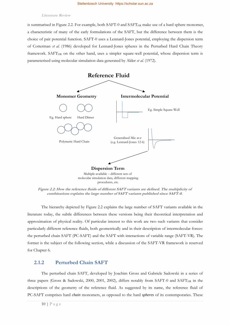
Literature Review
10 | P a g e
is summarised in Figure 2.2. For example, both SAFT-0 and SAFTHR make use of a hard sphere monomer,
a characteristic of many of the early formulations of the SAFT, but the difference between them is the
choice of pair potential function. SAFT-0 uses a Lennard-Jones potential, employing the dispersion term
of Cotterman et al. (1986) developed for Lennard-Jones spheres in the Perturbed Hard Chain Theory
framework. SAFTHR on the other hand, uses a simpler square-well potential, whose dispersion term is
parameterised using molecular simulation data generated by Alder et al. (1972).
The hierarchy depicted by Figure 2.2 explains the large number of SAFT variants available in the
literature today, the subtle differences between these versions being their theoretical interpretation and
approximation of physical reality. Of particular interest to this work are two such variants that consider
particularly different reference fluids, both geometrically and in their description of intermolecular forces:
the perturbed chain SAFT (PC-SAFT) and the SAFT with interactions of variable range (SAFT-VR). The
former is the subject of the following section, while a discussion of the SAFT-VR framework is reserved
for Chapter 6.
2.1.2 Perturbed Chain SAFT
The perturbed chain SAFT, developed by Joachim Gross and Gabriele Sadowski in a series of
three papers (Gross & Sadowski, 2000, 2001, 2002), differs notably from SAFT-0 and SAFTHR in the
descriptions of the geometry of the reference fluid. As suggested by its name, the reference fluid of
PC-SAFT comprises hard chain monomers, as opposed to the hard spheres of its contemporaries. These
Figure 2.2: How the reference fluids of different SAFT variants are defined. The multiplicity of combinations explains the large number of SAFT variants published since SAFT-0.
Reference Fluid
Monomer Geometry Intermolecular Potential
Eg. Hard sphere Hard Dimer
Polymeric Hard Chain
Eg. Simple Square-Well
Generalised Mie m-n
(e.g. Lennard-Jones 12-6)
Dispersion TermMultiple available – different sets of
molecular simulation data, different mapping
procedures, etc.
Stellenbosch University https://scholar.sun.ac.za

Literature Review
11 | P a g e
chain monomers are themselves made up of hard sphere segments, interacting with a modified square well
potential proposed by Chen & Kreglewski (1977). This modified potential, detailed in Figure 2.3, is used
to account for the phenomenon of soft repulsion exhibited by real fluids, while maintaining the
mathematical convenience of the simple square well potential.
These hard sphere segments are then covalently bonded using the TPT-1 framework common to
all SAFT variants to form the monomeric chain reference fluid. Algebraically, this is tantamount to
rearranging the terms of equation 2.1 as:
ideal seg chain disp assocA A A A A A
NkT NkT NkT NkT NkT NkT
2.2
where:
mon seg chainA A A
NkT NkT NkT
This simple reformulation of the residual Helmholtz energy has important physical consequences
for the EoS because in the SAFT framework, the pair potential is applied to the monomer fluid in the
dispersion term. Thus, because the monomer fluid comprises chains in PC-SAFT, only after the chain
monomers are formed is the dispersion term applied to the reference fluid. For SAFT variants where the
monomer fluid comprises hard spheres, Amon = Aseg in equation 2.1, and the pair potential is applied to the
hard sphere segments prior to chain formation. This results in an overlapping of the dispersion field of
the segments, conceptually illustrated in Figure 2.4, resulting in overestimation of the dispersion forces
between molecules.
This dispersion term takes the form of a second order perturbation expansion, according to the
theory of Barker & Henderson (1967a, b). The integrals in the radial distribution function and
intermolecular potential are approximated by power series, rather than analytically derived (Gross &
Sadowski, 2001). The procedure for determining the constants of the power series involves fitting the
Figure 2.3: Simplified approximations for intermolecular potentials [i.] Square well in SAFTHR, & [ii.] Modified square well PC-SAFT. The parameterisation of both models is identical, viz. σ, m & ε.
Radial Distance (r)
Po
ten
tial
En
ergy
(Γ
)
σ
ε ε
[i.] [ii.]
Stellenbosch University https://scholar.sun.ac.za

Literature Review
12 | P a g e
correlations to data for n-alkanes, using an intermediate assumption of hard chains interacting via a
Lennard-Jones potential. The authors argue that this procedure is justified and indeed preferable given
that, by “incorporating information of real substance behaviour,” the error inherent in the approximations
for the pair potential and the radial distribution function, “can be corrected to a certain extent” (Gross &
Sadowski, 2001). Thus, the choice of a somewhat simple intermolecular potential in the EoS is
compensated for by incorporating real fluid properties into the fitting procedure.
Therefore, the strength of PC-SAFT is that the dispersion term is more physically representative
of real intermolecular forces because its reference fluid is geometrically representative of real molecules.
The result of this realism is that the EoS consistently outperforms its hard-sphere monomer
contemporaries in the prediction of pure fluid and mixture behaviour (Gross & Sadowski 2001, 2002). It
has further been successful in such a variety of applications as modelling polydispersity, the description of
biological systems and characterising solid-fluid boundaries in copolymer crystallisation (Tan et al., 2008).
The success of PC-SAFT is exemplified by the fact that, apart from the fundamental SAFTHR, it is the
only variant to be included into the widely used Aspen Plus® process simulation software.
2.1.3 sPC-SAFT: A Mathematical Simplification
In an effort to reduce its computational intensity, and thus make it a more accessible option for
the engineering community at large, von Solms et al. (2003) proposed a modification of the PC-SAFT EoS.
The modification came in the form of a uniformity assumption for the temperature dependent diameter
of the reference fluid segments, which leads to two mathematically simplified expressions. The first is for
the radial distribution function, the other for the segment contribution, Aseg, to the residual Helmholtz free
Figure 2.4: Hard sphere (SAFT-0, SAFTHR) and hard chain (PC-SAFT) reference fluids. The overlapping of dispersion fields in hard-sphere monomer reference fluids is highlighted.
PC-SAFT
SAFT-0, SAFTHR
Aseg
Amon= (Aseg+Achain)
Aseg(=Amon)+Adisp Aseg+Adisp+Achain
(Aseg+Achain)+Adisp
Stellenbosch University https://scholar.sun.ac.za

Literature Review
13 | P a g e
energy. Extensive testing of this modification found that the simplified expressions, “simplify the
calculation of phase equilibrium properties… without loss of accuracy” (von Solms, 2003) and for this
reason, this variant is employed in this work rather than PC-SAFT.
2.2 Dipolar Interactions: Unique Intermolecular Forces
Molecular polarity arises as a result of the presence of lone electron pairs on certain atoms within
a molecule, resulting in a charge distribution and the generation of a permanent electric field surrounding
the molecule (Assael et al., 1998). These permanent fields result in strong electrostatic forces, the strength
and nature (attractive/repulsive) of which are highly dependent upon the orientation of the molecule, as
illustrated schematically in Figure 2.5.
When considering such polar molecules and their mixtures, earlier SAFT variants simply assumed
that the dispersion term in equation 2.1 could be numerically adjusted to account for these dipolar
interactions. The result is an artificially large value for the dispersion energy, which leads to poor
predictions of the properties of polar fluid mixtures (de Villiers, 2011). However, the strength and
anisotropic nature of the electrostatic forces between polar molecules distinguish them from the much
weaker London dispersion interactions discussed in the previous section. For this reason, a number of
authors have attempted to explicitly account for these dipolar interactions within the SAFT framework,
resulting in a number of “polar” terms to add to the residual Helmholtz energy of the system, as per
equation 2.3.
ideal seg disp chain assoc polarA A A A A
NkT NkT NkT NkT NkT
A A
NkT NkT
2.3
2.2.1 Polar Term of Jog & Chapman
While dipolar terms had been previously developed for polar hard sphere fluids, a corresponding
term for dipolar chains was first proposed by the research group of Jog & Chapman (Jog & Chapman,
1999; Jog et al., 2001) in the framework of SAFTHR. Considering the polar molecules to be dipolar hard
[i.] [ii.] [iii.]
Figure 2.5: Schematic representation of anisotropic dipolar intermolecular forces. [i.] If molecules are favourably oriented, strong attractive electrostatic forces result. [ii.] If like-poles are aligned, strong repulsive
forces result. [iii.] If poles are non-axially aligned, no significant electrostatic forces result.
Stellenbosch University https://scholar.sun.ac.za

Literature Review
14 | P a g e
spheres introduces inherent limitations of the theory, similar to the case of a hard sphere reference fluid in
van der Waalsian type EoSs (Jog et al., 2001):
the minimum distance between molecules is overestimated,
the molecule as a whole is considered polar rather than specific functional groups, and
the orientation of the dipole is unaccounted for.
All three inherent assumptions, schematically presented in Figure 2.6, limit the influence of the
dipolar interactions on fluid behaviour. This is due to the dependence of these interactions on
intermolecular distances and the position of the dipole within the chain. The success of the work of Jog &
Chapman over previous attempts is thus the ability to explicitly account for the effects of molecular
geometry and that specific functional groups (or segments) are polar, rather than the molecule as a whole.
The polar contribution to the Helmholtz free energy in equation 2.3 is determined by means of a
u-expansion. Here, the second and third order terms are given explicitly, with higher order terms
approximated by a Padé approximant (Rushbrooke et al., 1973), as per equation 2.4.
2
3
2
1
polar AA
ANkT
A
2.4
The second (A2) and third (A3) order terms are calculated as functions of the segment size and
dispersion energy parameters as well as the functional group dipole moment (μ). These terms also contain
complex integrals for the two- and three-body correlation functions, which themselves are functions of
the radial distribution and angular functions. As with the dispersion term, highlighted in the hierarchy of
Figure 2.2, there are a number of analytical expressions for these integrals which allow the second and
third order terms of equation 2.4 to be explicitly calculated. Jog & Chapman (1999) used the result of
[i.] [ii.]
Figure 2.6: Difference between [i.] dipolar hard sphere and [ii.] dipolar segmented chain approaches. The overestimation of intermolecular, or inter-dipole distances are highlighted.
Further, orientation and location of dipole are arbitrary in [i.], but explicitly accounted for in [ii.].
Stellenbosch University https://scholar.sun.ac.za

Literature Review
15 | P a g e
Rushbrooke et al. (1973), where the dipole is assumed to be aligned perpendicular to the molecular axis, to
express the integrals as simple analytical functions of the segment diameter.
A similar approach had been taken for dipolar hard sphere models, but Jog et al. (2001) accounted
for the different molecular geometry of chain molecules by introducing a new regressable parameter, xp.
This “fraction of dipolar segments” parameter has physical meaning when approximately equal to the
inverse of the component segment number (viz. m -1). This represents a single polar segment in the chain,
or physically, a single polar functional group in the carbon backbone of the molecule. In this way, the
polar term is only applied to the xp fraction of polar segments in the reference fluid from which the chain
molecules are built in the SAFT framework. Results with this new polar SAFT EoS were generally
excellent, and it was emphasised that explicitly accounting for the fundamental difference between dipolar
interactions and dispersion forces make the EoS more predictable (Jog et al., 2001).
Jog & Chapman’s polar term was later incorporated, without alteration, into the PC-SAFT
(Tumakaka & Sadowski, 2004) and sPC-SAFT (de Villiers et al., 2011) frameworks. Given that, as
highlighted earlier, PC-SAFT is a more sophisticated and recent variant than its SAFTHR counterpart, this
may at first appear a logical progression. However, this successful extension has subtle yet important
consequences for the SAFT framework as a whole and this work in particular: it shows that the Jog &
Chapman polar term is readily extendable to other SAFT variants, despite these variants having different
reference fluids and dispersion terms.
2.2.2 Polar Term of Gross & Vrabec
The research group that developed the PC-SAFT EoS went on to develop their own polar term
within the PC-SAFT framework. Gross & Vrabec (2006) drew on the success of Jog & Chapman before
them, and used the same physical picture of a chain comprised of both polar and nonpolar segments, viz.
Figure 2.6 [ii.]. They also employed the Padé approximant formulation for a third order u-expansion of the
polar contribution to the residual Helmholtz energy (equation 2.4). However, the primary difference
between the polar terms of Jog & Chapman and of Gross & Vrabec came in the way the integrals over the
two- and three-body correlation functions were approximated.
Gross & Vrabec made use of molecular simulation data for dipolar point-dipole fluids interacting
with a Lennard-Jones potential to fit correlations for the integrals over the two- and three-body
correlations functions. The point-dipole reference fluid is different to the tangent-sphere fluid used by
SAFT however. Thus a correlation between the properties of the two fluids was developed so that the
molecular simulation results could be interpreted within a TPT-1 framework (Gross & Vrabec, 2006). A
power series in the segment density, itself a function of the segment diameter, was then fitted to the
simulation data to yield approximations for the required integrals.
In the same way that Jog & Chapman introduced the xp parameter to account for the fraction of
dipolar segments in the chain, Gross & Vrabec introduced the “number of dipolar segments”, np. This
Stellenbosch University https://scholar.sun.ac.za

Literature Review
16 | P a g e
parameter was originally set equal to 1, the authors arguing that this was physically representative of the
influence of a single polar functional group in a carbon chain (Gross & Vrabec, 2006). By setting the value
of np equal to unity meant that Gross & Vrabec’s polar term did not introduce a further regressable
parameter to the nonpolar PC-SAFT’s existing parameter set. This also avoided the numerical problem of
a broad minimum in the objective function when considering models with four or more parameters, as
was found in some instances with the Jog & Chapman polar term (Al-Saifi et al., 2008; de Villiers et al.,
2011).
Similar treatments of quadrupolar molecules (Gross, 2005) and ionisable dipoles (Kleiner &
Gross, 2006) went further to demonstrate the success of this approach. In a comparative study,
incorporating both the Jog & Chapman and Gross & Vrabec polar terms into the sPC-SAFT framework,
de Villiers et al., (2011) argued that the np parameter should be left regressable in the same fashion as xp if
the two terms are to be judged on an equal footing. The study showed no clear superiority on the part of
either polar term, but the most important result was that the transferability of the polar terms between
SAFT variants was demonstrated.
2.3 Structural Isomerism: Properties & Equilibria
Structural or constitutional isomers are compounds with the same molecular formula, but
different arrangements of the atoms. As a result of the formulaic similarity between the molecules, the
properties of structural isomers are only subtly different. The ability to differentiate between such subtle
differences constitutes a stringent test for any model. Thus, the accurate prediction of, and distinction
between, the properties of structural isomers represents an interesting test of the predictive capacity of the
SAFT EoSs.
The effects of structural isomerism are more pronounced in organic molecules containing polar
or associating functional groups. The strength of the dipolar interactions are directly related to the
location of the functional group within the molecule, as schematically illustrated in Figure 2.7. When a
polar functional group is located near a terminal methyl group, the charge distribution about the molecule
is highly asymmetrical and the dipolar interactions are strongest, resulting in significant deviation from
ideality. As the polar group shifts centrally however, the charge distribution becomes symmetric about the
molecule. This culminates in a dampening of the dipolar interactions of the molecule, producing smaller
deviations from ideal behaviour.
Stellenbosch University https://scholar.sun.ac.za

Literature Review
17 | P a g e
The different intermolecular interactions of the different isomers manifest themselves on a
macroscopic level in their associated phase behaviour. This is most readily seen in the unique vapour
pressures of different structural isomers, as typified for the three structural isomers of heptanone in
Figure 2.8. This is an important result for this study in particular, as trends in pure component vapour
pressures are known to significantly influence the phase behaviour of mixtures containing these
components.
1
1 Reprinted (adapted) with permission from Cripwell et al., “Vapor–Liquid Equilibria Measurements for the Nine n-Alkane/Ketone Pairs Comprising 2-, 3-, and 4-Heptanone with n-Octane, n-Nonane, and n-Decane”, J. Chem. Eng. Data, 2015, 60 (3), 602-611. Copyright (2015) American Chemical Society.
δ- δ+ δ- δ+ δ- δ+δ+
δ- δ+ δ- δ+ δ+
δ+δ-
Figure 2.7: Schematic representation of the effect of polar functional group location on the charge distribution of the molecule (upper) and the structural impact of this charge distribution(lower). Font size
indicative of the respective strength of dipolar interactions for the structural isomers.
0
20
40
60
80
100
340 360 380 400 420 440
Pva
p (k
Pa
)
T (K)
Figure 2.8: Vapour pressures of structural isomers of heptanone: 2-heptanone, 3-heptanone and 4-heptanone. Key: Cripwell (2014) and Wu & Sandler (1988), with trend line through
reference data.1
Stellenbosch University https://scholar.sun.ac.za

Literature Review
18 | P a g e
2.3.1 Mixture Phase Behaviour: Past Work
In a previous study (Cripwell, 2014), the effect of polar functional group location on the
associated binary phase behaviour of polar structural isomers with a common second component was
investigated. Using ketones as the homologous series of interest, the three constitutional isomers of
heptanone were each paired with n-octane, n-nonane and n-decane and isobaric VLE data were generated
for each of these nine systems (Cripwell et al., 2015). It was found that the effect of the carbonyl group
location within the chain was pronounced enough to generate distinct phase envelopes and azeotropic
points for each isomer. This was particularly true for the case of mixtures where the second component
exhibited a similar vapour pressure, as shown in Figure 2.9.
2
The ability of the sPC-SAFTJC and sPC-SAFTGV EoSs to accurately predict the witnessed phase
behaviour of all nine binary systems, using parameters regressed from pure component properties alone,
was assessed. Both models were found to give accurate predictions of the phase behaviour of the most
polar isomer (2-heptanone) with all three n-alkanes, but the predictive capacity of sPC-SAFTJC was found
to decrease rapidly as the functional group moved centrally. Specifically, the quality of the sPC-SAFTJC
pure prediction worsened for the two less polar isomers (3- & 4-heptanone), to the extent that no
prediction for the 4-heptanone case was possible as a unique parameter set could not be determined. As
seen in Figure 2.10, the sPC-SAFTGV prediction did not suffer from the same shortcomings and the
quality of the pure prediction remained high for all three isomers with each alkane.
2 Reprinted (adapted) with permission from Cripwell et al., “Vapor–Liquid Equilibria Measurements for the Nine n-Alkane/Ketone Pairs Comprising 2-, 3-, and 4-Heptanone with n-Octane, n-Nonane, and n-Decane”, J. Chem. Eng. Data, 2015, 60 (3), 602-611. Copyright (2015) American Chemical Society.
383
385
387
389
391
393
0 0.2 0.4 0.6 0.8 1
T (
K)
x1, y1
Figure 2.9: Isobaric VLE data for 2-heptanone ( & ), 3-heptanone ( & ) and 4-heptanone ( & ) with n-nonane at 40 kPa. The influence of carbonyl group location in ketone chain on the phase behaviour is
highlighted.2
Stellenbosch University https://scholar.sun.ac.za

Literature Review
19 | P a g e
Given that this was the first demonstration of a clear superiority of one polar term over the other,
a natural recommendation of the study was to establish whether the observed trends hold for other polar
functional groups. For such an assessment to be made, reliable data with which to test these predictions
are necessary.
2.3.2 Previously Measured Polar Isomer/n-Alkane VLE Data
The functional groups of interest to an extended investigation of the effect of structural
isomerism on mixture phase behaviour are non-associating, unbranched, linear polar molecules. An
extension of the previous study requires that the second component in the mixture be a normal alkane.
This is to ensure that any observable difference between the phase behaviour of the different isomers are
attributable to the shifting polar functional group alone, rather than any interaction of these groups with
other polar and/or associating groups (Cripwell, 2014). The ester and ether functional groups satisfy this
requirement, with the functional group structures schematically presented in Figure 2.11. Further, these
378
380
382
384
386
388
390
392
394
0 0.2 0.4 0.6 0.8 1
Tem
pe
ratu
re (K
)
Mole Fraction n-Nonane (xi;yi)
b.Experimental DatasPC-SAFTsPC-SAFT + GV PolarsPC-SAFT + JC Polar
382
384
386
388
390
392
394
0 0.2 0.4 0.6 0.8 1
Tem
pe
ratu
re (K
)
Mole Fraction n-Nonane (xi;yi)
c.Experimental Data
sPC-SAFT
sPC-SAFT + GV Polar
Figure 2.10: Pure predictions for isobaric VLE in [i.] n-nonane/2-heptanone, [ii.] n-nonane/3-heptanone & [iii.] n-nonane/4- heptanone systems at 40kPa. The worsening predictions of the
sPC-SAFTJC parameter sets are highlighted in this progression. Figure reprinted from Cripwell (2014).
[ii.]
[iii.]
386
387
388
389
390
391
392
393
394
0 0.2 0.4 0.6 0.8 1
Tem
pe
ratu
re (K
)
Mole Fraction n-Nonane (xi;yi)
a.Experimental DatasPC-SAFTsPC-SAFT + GV PolarsPC-SAFT + JC Polar
[i.]
Stellenbosch University https://scholar.sun.ac.za

Literature Review
20 | P a g e
homologous groups omit the consideration of molecular association when considered in mixtures with
n-alkanes.
[i.]
[ii.] [iii.]
Table 2.1 summarises the availability of previously published VLE data for ether/n-alkane
systems. Only ethers with the potential of three or more structural isomers are considered, limiting the
summary to those ethers with a carbon number of 5 or greater. It is readily apparent that many more data
sets are available for the phase behaviour of branched chain ethers than for their unbranched counterparts.
This is due in large part, to the industrial relevance of branched ethers as fuel additives with good anti-
knocking properties (Marsh et al., 1999). Of significance to this study however, is that no published data
sets are available for each linear isomer of a given length ether with a common n-alkane.
Table 2.1: Available VLE data in literature for aliphatic ethers (C5 or heavier) with alkanes
Ether Alkane Reference
C5 Ethers
methyl butyl ether heptane Treszczanowiczet al.(1986)
ethyl propyl ether none
*methyl tert-butyl ether
hexane Wisniak et al. (1997a)
heptane Segovia et al.(1998)
octane Wisniak et al. (1997b)
C6 Ethers
methyl pentyl ether none
ethyl butyl ether none
dipropyl ether
heptane Gmehling et al. (1979)
octane Maripuri & Ratcliff (1972)
nonane
*methyl tert-amyl ether hexane
Mejía et al. (2011) heptane
*ethyl tert-butyl ether
hexane
Reich et al. (2000) heptane
octane
heptane Gmehling & Onken (1999)
*Branched ethers
For esters, a plethora of data are available that systematically consider the effect of varied
alkanolic or acidic chain lengths (while the other is kept constant) on the phase equilibria of these
components in mixtures with a common second component. However, as the available data sets of
Figure 2.11: Schematic representation of [i.] ketone, [ii.] ester and [iii.] ether functional group structures
Stellenbosch University https://scholar.sun.ac.za
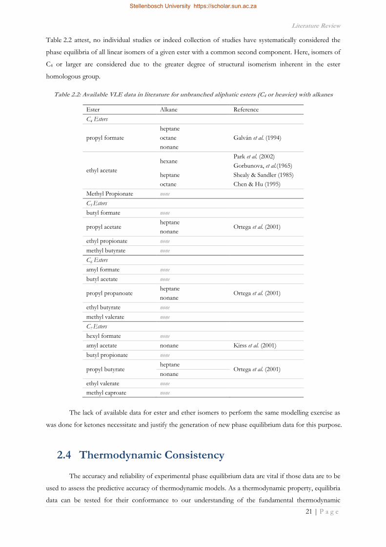
Literature Review
21 | P a g e
Table 2.2 attest, no individual studies or indeed collection of studies have systematically considered the
phase equilibria of all linear isomers of a given ester with a common second component. Here, isomers of
C4 or larger are considered due to the greater degree of structural isomerism inherent in the ester
homologous group.
Table 2.2: Available VLE data in literature for unbranched aliphatic esters (C4 or heavier) with alkanes
Ester Alkane Reference
C4 Esters
propyl formate
heptane
Galván et al. (1994) octane
nonane
ethyl acetate
hexane Park et al. (2002)
Gorbunova, et al.(1965)
heptane Shealy & Sandler (1985)
octane Chen & Hu (1995)
Methyl Propionate none
C5 Esters
butyl formate none
propyl acetate heptane
Ortega et al. (2001) nonane
ethyl propionate none
methyl butyrate none
C6 Esters
amyl formate none
butyl acetate none
propyl propanoate heptane
Ortega et al. (2001) nonane
ethyl butyrate none
methyl valerate none
C7 Esters
hexyl formate none
amyl acetate nonane Kirss et al. (2001)
butyl propionate none
propyl butyrate heptane
Ortega et al. (2001) nonane
ethyl valerate none
methyl caproate none
The lack of available data for ester and ether isomers to perform the same modelling exercise as
was done for ketones necessitate and justify the generation of new phase equilibrium data for this purpose.
2.4 Thermodynamic Consistency
The accuracy and reliability of experimental phase equilibrium data are vital if those data are to be
used to assess the predictive accuracy of thermodynamic models. As a thermodynamic property, equilibria
data can be tested for their conformance to our understanding of the fundamental thermodynamic
Stellenbosch University https://scholar.sun.ac.za

Literature Review
22 | P a g e
principles at play. In the case of phase equilibrium, this is governed by the Gibbs-Duhem equation
(Sandler, 2006):
, ,
0i i
i
P n T n
dT dP x dT P
θ θθ
2.5
This theoretical thermodynamic consistency correlation demonstrates the interconnectivity of
partial properties in a solution and that these properties are not independent. The excess Gibbs energy is
used as the hypothetical property Θ of equation 2.5, thus, application to a binary mixture in the special
case of isothermal and isobaric conditions results in (Smith et al. 2005):
1 2
1 2
1 1
ln ln0
d dx x
dx dx
γ γ 2.6
The Gibbs-Duhem equation in this form is a theoretically derived relationship adhering to strict
thermodynamic principles. However, the activity coefficient is determinable from experimental phase
equilibrium data, with the compositions easily measured. The right hand side of equation 2.6 is therefore
readily calculated for an experimental data set, but the data’s adherence to the equation’s equality criterion
is a test of that data set’s adherence to thermodynamic principles and thus its thermodynamic consistency.
Equation 2.6 also serves as the basis for a number of thermodynamic consistency tests developed in the
literature.
2.4.1 McDermott-Ellis Consistency Test
The McDermott-Ellis consistency test (McDermott & Ellis, 1965) is a point-to-point consistency
test, which assesses the thermodynamic consistency of each successive pair of data points. In this way,
inconsistent data can be identified and excluded as they arise. The test starts by numerically integrating
equation 2.6 over the whole composition range using the trapezoidal rule to yield:
, , , ,0 ln lni c i d i d i cx x γ γ 2.7
The summation is over all components in the mixture for consecutive data points, c and d. Given
the uncertainty inherent in experimental measurements, strict adherence to the need for equation 2.7 to
equal zero was considered excessively limiting in the assessment of experimental data. McDermott and
Ellis thus vaguely suggested that the criterion for judging between consistent and inconsistent data be
dependent upon the accuracy of compositional measurement. The guideline provided was a maximum
deviation of 0.01 for uncertainties of ±0.001 mole fraction. This indefinite criterion was refined by
Stellenbosch University https://scholar.sun.ac.za

Literature Review
23 | P a g e
Wisniak & Tamir (1977), who argued that this maximum should be considered a function of the
respective uncertainties in the measurable physical properties according to:
, , , ,
, , , ,
, , , , 2 2
1 1 1 10 2 ln ln
1 1
i c i d i d i c
i c i d i c i d
i c i d i c i d isat sat
c i d i
x x x xx x y y
Px x x x T
P T T
γ γ
βδ δ
Δ Δ
ΔΔ
2.8
In equation 2.8, the Δ terms are the experimental uncertainties in the relevant measure quantity,
while βi and δi are the Bi and Ci constants respectively.
Point-to-point tests, such as the McDermott-Ellis consistency test, constitute one of two broad
types of consistency tests. Unlike the point-to-point tests, area consistency tests consider the data set as a
whole and define a tolerance with which the consistency of that data set can be judged. One such area
consistency test is the L/W consistency test as described in the following section.
2.4.2 L/W Consistency Test.
The general description of the Gibbs free energy for equation 2.5 can be defined in terms of the
excess enthalpy and excess volume of the system:
20 ln
ex ex
i i
H VdT dP x d
NkT NkTγ 2.9
The starting point for such area consistency tests as the L/W test is the integration of
equation 2.9 over the entire composition range. If the special case of isobaric and isothermal conditions is
once again assumed, the result is an integral of the natural logarithm of the activity coefficient ratio over
the composition range:
1
21
10
0 ln dxγ
γ 2.10
Thus, a plot of ln(γ2/γ1) against the composition, using any experimental data set, yields a plot
crossing the x-axis along the binary composition range. For that data to be considered thermodynamically
consistent, the areas above and below the curve need to be equal (Wisniak, 1994).
For a given experimental data set however, the equality criterion of equation 2.10 can never truly
be met given that phase equilibria measurements are made at either constant temperature or constant
pressure conditions. Starting instead with the full Gibbs free energy description of equation 2.9, in the
Stellenbosch University https://scholar.sun.ac.za

Literature Review
24 | P a g e
case of isothermal operation, the excess volume can be assumed approximately constant, yielding the same
result as presented in equation 2.10 for data consistency testing (Wisniak, 1994). Excess enthalpy however,
can never be assumed constant and thus the isobaric operation case does not simply reduce to the
convenient representation of equation 2.10. The need to account for the effects of excess enthalpy is a
significant hurdle as such data are rarely for the whole composition range, at the relevant temperature and
pressure of interest.
In the development of the L/W consistency test, Wisniak (1993) sought to address this problem
by considering the Gex-T relationship at equilibrium rather than the Gibbs-Duhem equation explicitly:
lnex
i iG NkT x γ 2.11
By assuming that nonidealities are confined to the liquid phase, experimental activity coefficients
can be calculated using Raoult’s law. Similarly, assuming a constant heat of vaporisation and negligible
liquid molar volume compared to that of the vapour, the Clausius-Clapeyron equation can be used to
defined the ratio of the system pressure to the component vapour pressures, yielding the following
description of Gex (Wisniak, 1993):
vap
i iS x SΔ Δ
2.12 ln ii
i
yw x
x
lnex vap sat i
i i i i
i
yG x S T T NkT x
xΔ
Wisniak (1993) used this result to derive an expression for the mixture bubble point in terms of
the defined parameters:
i
i sati i
y P
x Pγ
2.13
ln
vap sat vap sati i i i
vap sati i
H T T S T TP
P NkT T NkT
Δ Δ
exsat sati i i
b
x S T G NkTwT
S S S
Δ
Δ Δ Δ
This bubble point relation can be manipulated to yield an equality relationship which serves the
basis for the L/W consistency test, where the index z refers to equilibrium pairs of VLE data:
Stellenbosch University https://scholar.sun.ac.za

Literature Review
25 | P a g e
exsat sati i i
z b zz
x S T G NkTwL T W
S S S
Δ
Δ Δ Δ 2.14
Integrating equation 2.14 over the composition range yields the equality criterion and area basis of
the L/W test:
1 1
1 1
0 0
z zL L dx W dx W 2.15
As with the McDermott-Ellis test previously, strict adherence to this equality constraint is
excessively limiting for real experimental data. As a result, Wisniak defined an acceptable deviation to
account for experimental uncertainty.
100L W
DL W
2.16
Wisniak proposed that thermodynamic consistency of an experimental data set is indicated by a
maximum value for D of 3 to 5. The lower limit is based on similar limits for the Herrington area test
while the upper limit accounts for errors resulting from potential uncertainty in heats of vaporisation
(Wisniak, 1993). Data not adhering to these contraints may thus be declared thermodynamically
inconsistent. The important caveat however, is that because this development was not derived from the
Gibbs-Duhem equation, data cannot be considered thermodynamically consistent using this test alone. It is
thus necessary to use a theoretically based test, such as the McDermott-Ellis test of the previous section,
in conjunction with the L/W test to rigorously assess the thermodynamic consistency of experimental data.
2.5 Chapter Summary
This chapter provided background on the development of the SAFT family of EoSs up to and
including the variants and polar terms of interest to this study. The role of the dipole moment in
distinguishing the behaviour of polar molecules from their nonpolar counterparts was discussed, and the
subtle but important role of its location in the carbon chain was highlighted. The effect of this functional
group location on mixture phase behaviour for different isomers was shown to be the focus of previous
work and the basis of the work presented here. However, the lack of available data in the literature to
extend the modelling investigation to ethers and esters was highlighted and the need to generate new
experimental VLE data for such systems was underlined. Addressing this deficiency defined the objectives
of the experimental phase of this work and the means by which these data were generated is the subject of
the following chapter.
Stellenbosch University https://scholar.sun.ac.za

Experimental Methodology
26 | P a g e
Chapter 3: EXPERIMENTAL
METHODOLOGY
The aim of this chapter is to describe the experimental approach adopted to generate isobaric
phase equilibrium data. In the sections that follow, a description of the materials will be provided while
the apparatus and methodology used will be described in detail.
3.1 Materials
Table 3.1 lists the chemicals used for both the phase equilibrium experiments, and the subsequent
analysis of the equilibrium samples. The chemical assays on a mass basis are listed, with all components
purchased from Sigma Aldrich.
Table 3.1: List of chemicals used for phase equilibrium experiments with purities on a mass basis
Component CAS Number Purity (mass%)
n-heptane 142-82-5 99%
n-octane 111-65-9 ≥99.0%
2-butanone 78-93-3 ≥99.7%
2-heptanone 110-43-0 98%
methyl valerate 624-24-8 99%
ethyl butanoate 105-54-4 99%
propyl propanoate 106-36-5 99%
butyl acetate 123-86-4 ≥99.5%
pentyl formate 638-49-3 95%
butyl- ethyl-ether 628-81-9 99%
di-n-propyl ether 111-43-3 ≥99.0%
2-ethyl-1-hexanol 104-76-7 ≥99.6%
All components listed in Table 3.1 were analysed by gas chromatography prior to experimentation
in order to verify the listed purities by looking for significant impurity peaks. The results of the analysis
indicated that all components adhered to or exceed their listed assays. All but one (pentyl formate) of the
components used during the phase equilibrium experiments were at least 99 mass% pure and were thus
considered appropriate for use.
The results for the pentyl formate indicated that a significant impurity of approximately 5 mass%
was indeed present. Subsequently, a sample of the ester was analysed by gas chromatography-mass
spectrometry (GC-MS) where the impurity was identified as 1-pentanol (see Appendix A for the GC-MS
results). The most convenient means of stripping the 1-pentanol from the pentyl formate was by means of
pot distillation, but first it was necessary to determine whether the desired separation could be achieved
via distillation. To this end, it was desirable to find existing experimental data for a binary mixture of
Stellenbosch University https://scholar.sun.ac.za

Experimental Methodology
27 | P a g e
1-pentanol/pentyl formate to determine the phase behaviour for the system at atmospheric pressure, and
whether an azeotrope is present in the systems at these conditions. However, no data for the system were
available in the literature and in lieu of using an experimental data set, it was necessary to use a
thermodynamic prediction of the system as a first approximation.
This system comprises an associating 1-alkanol and a polar ester and can thus be modelled within
a polar sPC-SAFT framework with appropriate pure component parameters. As with the experimental
data however, no parameters have been published for pentyl formate in any SAFT framework. On the
other hand, parameters have been published for two of pentyl formate’s structural isomers (de Villiers et
al., 2011a) as well as for 1-pentanol (de Villiers et al., 2011b). While modelling these systems does not give
an accurate representation of the phase behaviour of the 1-pentanol/pentyl formate system, the trends
apparent for the azeotropic point in the systems containing the ester’s isomers at least indicate whether
purification of the ester by distillation is possible. To this end, the phase behaviour of the
1-pentanol/propyl propanoate and 1-pentanol/butyl ethanoate systems were modelled at atmospheric
pressure (in Stellenbosch, ±1 bar), and the results are presented in Figure 3.1.
Given that the results in Figure 3.1 show azeotropic behaviour in the 1-pentanol/propyl
propanoate and 1-pentanol/butyl ethanoate systems, it is reasonable to assume that similar positive
deviations from ideality exist in the 1-pentanol/pentyl formate system. Furthermore, it is apparent from
Figures 3.1 [i.] and [ii.] that the azeotropic point is getting richer in 1-pentanol as the alkyl- chain of the
ester lengthens; specifically at ±14 mass% for the propyl ester and ±18 mass% for the butyl ester. Thus, it
is reasonable to assume that this trend continues for the pentyl ester and that any azeotrope present in the
system does not prevent purification of the pentyl formate by distillation. Furthermore, by analysing the
form of the phase envelopes, we can intuit that distillation of the 95 mass% pure pentyl formate will
produce a liquid phase richer in the ester, while the vapour phase will approach the azeotropic
composition with successive runs in a batch still.
392
397
402
407
412
0.00 0.20 0.40 0.60 0.80 1.00
Tem
per
atu
re (K
)
1-Pentanol Mass Fraction (x,y)
PropylPropanoate
392
397
402
407
412
0.00 0.20 0.40 0.60 0.80 1.00
Tem
per
atu
re (K
)
1-Pentanol Mass Fraction (x,y)
Butyl Acetate
[i.] [ii.]
Figure 3.1: sPC-SAFT GV predictions for the phase behaviour of [i.] 1-pentanol/propyl propanoate and [ii.] 1-pentanol/butyl ethanoate systems at 1 bar
Stellenbosch University https://scholar.sun.ac.za

Experimental Methodology
28 | P a g e
With the expectation of producing a bottoms product richer in pentyl formate, the stock material
was batch distilled four times, with the liquid product of each successive run analysed by the GC-MS to
determine the change in composition. After the fourth run, it was noted that no significant change in the
concentration had taken place compared to the results of the third run, bearing in mind the minimum
volume of purified pentyl formate required to run the VLE experiments. Thus, purification yielded a
product of 98.2 mass% purity, according to the GC-MS analysis (results in Appendix A), which was
considered acceptable for the purposes of the experimental work.
3.2 Apparatus
An all-glass dynamic recirculating still was used to measure the phase equilibrium data,
schematically presented in Figure 3.2. The full figure legend is available in the works of Pienaar (2011) and
Cripwell (2014), although appropriate descriptions are provided in Sections 3.2.1 and 3.3 that follow. The
unit is a commercially produced still, model VLE 100D from Pilodist of Germany.
3.2.1 Unit Description
Primary operation of the still takes place in the boiling chamber (1.3), where an electrical
immersion heater (10) is installed concentrically and supplies sufficient heat to partially vaporise the liquid
mixture. At the top of the boiling chamber, the unit walls converge to the base of a spirally curled Cottrell
tube (1.2) where slugs of liquid and vapour pass by a pressure differential into the separation chamber.
During this time, concentrated mass transfer between the two phases takes place and it is here that phase
equilibrium is attained. At the interface between the Cottrell pump and the separation chamber, the two
phases pass over a Pt-100 temperature probe (7) where the equilibrium temperature is measured. The two
phases split within the separation chamber; the denser liquid leaving at the base while the vapour rises to
the top of the chamber. Construction of the chamber ensures that liquid drops do not become entrained
in the rising vapour, and prevents partial condensation of the vapour phase within the chamber.
After the phases are split, the liquid flows down a graduated line to the liquid phase sampling
point (11), where a condenser (1.7) is located above the sampling point to ensure the equilibrium liquid
remains in the liquid phase for sampling. The vapour on the other hand passes through the first of two
condensers (1.12) so as to produce a condensed equilibrium vapour to be taken from the vapour sampling
point (12). As with the liquid arm of the unit, a second condenser (1.11) is present to make sure the
condensed vapour remains in the liquid phase to ensure a representative sample. Provision is made
however, at the top of the separation chamber (sampling point 1.5) to allow the extraction of an
equilibrium vapour sample in the vapour phase prior to the condenser. The shallow wells at the liquid and
condensed vapour sampling points ensure that the accumulating equilibrium phase is consistently renewed
by the flow of new material from the separation chamber. From the wells, the condensed equilibrium
phases are returned to the mixing chamber (1.1), where a magnetic stirrer serves the dual purpose of
mechanically stirring the mixture and inducing flow of the mixture back into the boiling chamber. From
here, the circulation procedure is repeated. The still was originally modified to house an ultrasonic
Stellenbosch University https://scholar.sun.ac.za

Experimental Methodology
29 | P a g e
Figure 3.2: Schematic representation of the Pilodist dynamic recirculating still used for VLE measurements. Figure reprinted with permission (Pienaar, 2011)
homogeniser (17) for the measurement of vapour-liquid-liquid equilibria. While the homogeniser was not
used in this work, it does need to be secured in its housing to keep the unit sealed during operation.
The unit as illustrated in Figure 3.2 is installed within an extraction cabinet due to the flammable
nature of the components used. Pressure is measured by means of a Wika UT-10 pressure transmitter
with an operating range of 0-1.6 bar abs and a calibrated accuracy of 0.1 % of full scale output (thus in
absolute quantities, 1.6 mbar). The maximum operating temperature of the still is rated at 250 °C, with
temperature recorded using a four-wire Pt-100 probe connected to a digital Hart Scientific thermometer
with an accuracy of 0.03 °C. The probe was calibrated by a SANAS approved laboratory prior to
commencement of this study, with the certificate of calibration (provided in Appendix B) indicating an
uncertainty in temperature measurement of 0.1 °C over the temperature range of interest to this study.
This drift was accounted for in the recorded temperatures presented in this work.
Stellenbosch University https://scholar.sun.ac.za

Experimental Methodology
30 | P a g e
3.3 Experimental Procedure
A brief description of the experimental procedure is presented in this section, giving an overall
summary of unit operation and analysis of the equilibrium samples. The numerical references in
parentheses refer to the labels of Figure 3.2 as in Section 3.2 previously.
3.3.1 Preliminaries
As alluded to in Section 3.1, accurate measurement of phase equilibrium data is contingent on
uncontaminated pure component species in the charged binary mixture. Thus, prior to operation of the
still, it was important to ensure that the unit was both clean and dry to prevent contamination. To this end,
the unit had to be washed beforehand with an appropriate volatile solvent to remove liquid residues from
previous experiments (this procedure will be described in Section 3.3.4) followed by running compressed
air through the unit to vaporise residues of the washing solvent.
Given the relatively volatile nature of some of the components used in this work, it was necessary
to use chilled water as the cooling medium in the condensers. Thus it had to be ensured that the water in
the bath had been left to cool by the chiller for an appropriate time before the pump was turned on to
circulate the water through the unit’s condenser lines. At this stage, the still could be turned on and the
controlling software opened.
3.3.2 Unit Preparation
In order to run the still under vacuum, the appropriate selection needed to be made within the
control software and using the three-way valve on the pneumatic box of the still. Before adding the
mixture of interest to the unit, the homogeniser needed to be securely fitted in its housing and the
discharge valve (1.4) closed. At this point, approximately 110 cm3 of one of the pure components in the
mixture could be charged to the feed burette, although this amount was somewhat variable and dependent
on the volatility of the components in the mixture. The fed volume needed to least completely submerge
the immersion heater (10) when the liquid was fed to the mixing chamber (1.1) from the feed burette.
With the liquid loaded, the magnetic stirrer was turned on.
The reason experiments were always started with a pure component was twofold: firstly, the pure
component boiling point could be used as a means of verification at the start of each run, ensuring no
contamination at the start of the experiment and; secondly, the most systematic way of moving across the
composition space would be to successively add small amounts of the second component to the first
already charged to the still.
Within the controller software, the heater power had to be specified, along with the set points for
the mantle temperature and the operating pressure. The heater power once again depended on the
volatility of the components in the given mixture while the mantle temperature depended on the
equilibrium temperature for the given feed composition. The heater power is set as a percentage of the
Stellenbosch University https://scholar.sun.ac.za
Experimental Methodology
31 | P a g e
total output and needed to be correctly balanced to achieve equal circulation of both equilibrium phases
for sampling. Too low a power setting and the mixture would be heated but not vaporised resulting in no
vapour return, while too high a setting would vaporise too much of the mixture and result in no liquid
circulation. The mantle heater maintained the temperature of the separation chamber wall so as to prevent
unintentional condensation of the vapour phase before the condensers (1.11 & 1.12). However, due to the
rudimentary on-off control of the mantle heater, large oscillations around its set point were evident during
experiments and thus the set point had to be set some 15 °C lower than the equilibrium temperature to
ensure the mantle temperature did not exceed the equilibrium value.
The installed pressure transmitter was a modification to the original unit and changed the means
by which the pressure was regulated. The original setup employed a Pilodist M101 pressure control system
to automatically control the system pressure under vacuum operation. This made use of simple on-off
control of the vacuum pump, but resulted in fairly large pressure oscillations (±5 mbar) around the
operating set point which, at system pressures of 600 mbar, were considered too large. Thus, the set point
on the controller was fixed at a value 50 mbar lower than the operating pressure to ensure the vacuum
pump stayed on, while the amount of vacuum drawn from the unit was manually throttled to maintain the
desired operating pressure. This produced much smaller oscillations (max ±2 mbar), resulting in a more
stable equilibrium within the unit.
3.3.3 Experimental Runs
A given experimental run was commenced once the set points had been fixed. Using appropriate
power settings, the liquid began circulating within 5 minutes while condensed vapour return was evident
within 20 minutes. Due to the concave nature of the sample collection ports beneath the sampling wells
(11 & 12), periodic flushing of the ports was necessary to clear the liquid film accumulated from previous
runs to prevent contamination. These ports were flushed after 20 and then 40 minutes in the following
manner:
The solenoid valves for both the liquid and vapour arms of the still (8 & 9) were opened
using the remote control within the unit casing. The valves were only opened to allow a
small amount of each phase to wash the walls of the ports before being closed again.
The liquid accumulated as a result of flushing was then drained into the respective glass
receiver vials (5 & 5.1) by opening the respective stop valves (1.8 & 1.16). These valves
were then immediately closed again.
After the second flushing at 40 minutes, the flushed liquid needed to be removed. To this
end, the isolation valves (1.10) for both phases needed to be closed before the vacuum
could be broken, so as to isolate the respective arms of the still. In this way, the vials
could be removed while vacuum operation of the still was maintained. To do so required
subsequently opening the aeration valves (1.18) before removing the vials and discarding
the flushed liquid.
Stellenbosch University https://scholar.sun.ac.za

Experimental Methodology
32 | P a g e
The sample vials were then swapped for clean ones for taking the equilibrium samples.
Upon replacing the vials and refitting them to the still, the aeration valves could be closed
and the isolation valves opened to bring the pressure in the arms back down to the
operating pressure.
Replacing the vials after the flushed liquid was discarded resulted in a small surge in the system
pressure (and the coupled equilibrium temperature) as the arms were brought back down to the operating
pressure. This inevitably affected the equilibrium and thus the still was left to run for a further 20 minutes
to allow for the micro-fluctuations caused by the flushing procedure to level out and for the equilibrium
to be reobtained. In this way, equilibrium was attained after 60 minutes of run time and was indicated by a
stable vapour temperature and steady return of both phases. A vapour circulation rate of 30 drops per
minute at the vapour return point (left of 12) was considered sufficient to produce a large enough
equilibrium sample to prepare analytical samples.
While a liquid phase equilibrium liquid sample was taken (11), the equilibrium vapour phase could
be taken as either a vapour (1.5) or a condensed liquid (12). Due to the complete miscibility of all binary
ester/alkane and ether/alkane mixtures considered in this study, combined with the technical difficulties
in manually extracting a large enough vapour sample, it was decided that condensed vapour samples
would be taken in this study. Samples were taken as per the procedure for flushing detailed above, with
the obvious exception that the samples were kept for preparing analytical samples rather than being
discarded. The vapour temperature was monitored while the solenoid valves were opened to ensure that
no temperature changes occurred during sampling – this constant temperature was recorded as the
equilibrium temperature for that run.
Once the equilibrium samples had been taken, the given experimental run came to an end and the
still was stopped and the aeration valves opened to bring the unit back up to ambient pressure. In the case
where additional runs were being performed on that day, more of the second component could be
introduced to the unit via the feed burette at this point. The amount of the component to be added was
simply the volume which would result in re-submersion of the immersion heater, generally ±10 cm3.
Thereafter, successive runs could be performed using the same procedure detailed above.
3.3.4 Draining and Washing
At the end of a given day of experiments, the liquid mixture could be left in the still overnight to
resume experimental runs the following day, according to Section 3.3.3 above. However, if experiments
were to start from the other side of the composition space or indeed with a new binary system, it was
necessary to drain and wash the still so as to flush any non-volatile liquids left over from the experiment
and prevent contamination of the next experimental runs. In order to drain the still, it was necessary to
allow the mixture to cool to ambient temperature before draining the contents via the discharge valve (1.4),
and to remove the homogeniser to drain any accumulated liquid in its housing. Thereafter, the
homogeniser was refitted and the discharge vial closed again so that wash acetone could be added to the
Stellenbosch University https://scholar.sun.ac.za
Experimental Methodology
33 | P a g e
still. Acetone was chosen as it met both the solvation and volatility criteria for the wash solvent
highlighted in Section 3.3.1 above. The still was then set to run at ambient pressure for 30 minutes to
allow the acetone to circulate through and “wash” both the vapour and liquid arms of the still. During this
time, the ports were flushed with the acetone as was done during the experimental runs to ensure the
sampling wells were also washed. After running and being left to cool, the acetone could also be drained
from the still and the unit left with all aeration valves open to dry overnight.
3.3.5 Analytical Procedure
The compositions of the equilibrium phases were quantified by means of gas chromatography
using a Varian CP-3380 gas chromatograph fitted with a flame ionisation detector (FID). A ZB Wax
capillary column (30m x 0.32nm x 1µm), with helium as the carrier gas, was operated using a graduated
temperature programme of 17 minutes to quantify each analytical sample. These samples were prepared as
follows:
2 mL sample vials were loaded with ±1.5 mL of the analytical solvent, i.e.
2-ethyl-1-hexanol, and weighed.
30 µL of internal standard (2-heptanone) was pipetted into the solvent, with the sample
again weighed to yield the mass of standard added.
15 µL of the experimental sample was added to the solvent, with the vial weighed a third
time to yield the mass of sample added.
Two analytical samples were prepared from each equilibrium phase of each experimental sample,
resulting in a total of four analytical samples per experimental run/equilibrium temperature. An average
was taken of the two composition results for each phase at each temperature to produce a single datum
point which is reported in this work.
Quantification of component concentrations using an internal standard was achieved by creating
a calibration curve for each component. Using an appropriate temperature profile, the GC produces
distinct peaks for each component, the area of which is directly proportional to the quantity of that
component in the sample. The calibration curves relate the peak areas of the component and the standard
to their quantities (here, masses) by the following simple proportionality equation:
i
std stdi
i
Area massk
Area mass 3.1
In equation 3.1, ki is the response factor for component i with respect to the internal standard,
and is unique for each component in a mixture, provided the same GC operating conditions are used
throughout. The calibration curve for each component was thus created by preparing samples containing
known masses of both components and the internal standard and inferring the value of the response
factor for each component using the relationship in equation 3.1. Thus, for each of the ester/alkane and
Stellenbosch University https://scholar.sun.ac.za

Experimental Methodology
34 | P a g e
ether/alkane mixtures of interest, five samples of known mass were prepared to construct the calibration
curves. Each sample contained different ratios of the two components, such that the full composition
spectrum of the binary mixture could be accounted for. Each known sample was analysed four times on
the GC, with the averages used to produce the calibration curve and yield the response factor for each
component in each mixture, detailed in Appendix C.
3.4 Compositional Error Analysis
While the pressure and temperature deviations were directly measurable through uncertainties of
calibration and observable fluctuations during experimentation, the errors associated with reporting
compositions of equilibrium samples have to be somewhat inferred. The two major factors in determining
compositional uncertainty are the effects of experimental fluctuations and errors associated with the
analytical procedure.
3.4.1 Experimental Uncertainty
The equilibrium sample compositions are outputs of the phase equilibria experiments, and, as
such, are directly influenced by errors and fluctuations in the input variables. Within the experimental
procedure, there are two such input variables; specifically the power setting to the immersion heater and
the operating pressure set point. The heater power is maintained at a constant setting throughout the
experimental run and thus its effect on the uncertainty in compositional measurement can be considered
negligible. Given the manual throttling of the vacuum drawn from the system, and the inherent pressure
oscillations mentioned in Section 3.3.2 previously, the effect of fluctuations in the system pressure cannot
be similarly neglected and must be explicitly accounted for.
As detailed in Section 3.3.2, manual throttling of the vacuum drawn from the system maintains
the system pressure to well within ±2 mbar of the desired operating pressure throughout the experimental
run. Thus it is desirable to determine the impact of this pressure oscillation on the resulting equilibrium
composition. In lieu of a means of directly measuring this effect, the effect of the worst case scenario
pressure fluctuations can be modelled and compared to the equivalent set point prediction, provided an
accurate model of the system phase behaviour is used. As will be detailed later, the sPC-SAFTGV model
yields an excellent prediction of the ethyl butanoate/n-octane system and can thus be used for the
compositional error analysis here. The reason for choosing this system as reference is explained in the
course of the discussion of the analysis results which follow. The results of modelling the system at the set
point and at the two pressure fluctuation extremes are presented in Figure 3.3 [i.] and [ii.].
Stellenbosch University https://scholar.sun.ac.za

Experimental Methodology
35 | P a g e
0.27050.260 0.281
374.5
375.0
375.5
376.0
376.5
377.0
377.5
378.0
0.22 0.24 0.26 0.28 0.30 0.32 0.34 0.36
Tem
per
atu
re (
K)
Ethyl Butanoate Mole Fraction (x,y)
598mbar sPC-SAFT + GV Polar
600mbar sPC-SAFT + GV Polar
602mbar sPC-SAFT + GV Polar
374.0
375.5
377.0
378.5
380.0
381.5
0.00 0.20 0.40 0.60 0.80 1.00
Tem
per
atu
re (
K)
Ethyl Butanoate Mole Fraction (x,y)
598mbar sPC-SAFT + GV Polar
600mbar sPC-SAFT + GV Polar
602mbar sPC-SAFT + GV Polar
Figure 3.3: Effects of worst case pressure fluctuation on resulting equilibrium composition measurements. [i.] Entire phase envelope. [ii.] Representative section of the phase envelope, highlighting the compositional
uncertainty.
[i.]
[ii.]
Stellenbosch University https://scholar.sun.ac.za

Experimental Methodology
36 | P a g e
In Figure 3.3 [ii.], a section of the full phase envelope in the region of 30 mole% ethyl butanoate
is used for the purpose of the analysis. If the equilibrium temperature is taken as reference for all three
phase envelopes, it can be seen that the 2 mbar pressure fluctuation has an associated compositional
deviation of 0.011 mole fraction at a reference mixture composition of ~0.27 mole fraction. It can be
argued that larger deviations would result if the section taken in Figure 3.3 [ii.] was closer to the azeotropic
point; however it can similarly be argued that a smaller compositional deviation would be evident for
sections closer to the pure component ends of the mixture spectrum. In the same way, performing the
analysis on the vapour phase would also yield similar trends. Thus, the section presented is chosen to be
representative of the average deviations across the entire composition range, for both equilibrium phases.
Figure 3.3 illustrates the effect of the maximum pressure oscillations, but as previously noted, the
pressure was generally controlled to well within these maximums, particularly around the time of sampling.
Thus, to get an idea of the representative effect of the average pressure fluctuations, we can consider its
impact on the instantaneous experimental output; the vapour temperature. If it is assumed that the
micro-fluctuations seen in the temperature are a direct result of the average pressure oscillations at any
given time, the temperature fluctuations can be used to infer the average pressure oscillations. Thereafter,
using a similar analysis to that performed in Figure 3.3, the effect of these average pressure oscillations on
the compositional uncertainty can be inferred. This assumption can be justified by considering that the
thermal equilibrium in the unit is slower than the mechanical equilibrium, with the chemical equilibrium
slower still. Thus, the fluctuations in temperature and equilibrium composition caused by the pressure
oscillations will be smaller than those in the pressure and will average out in a smaller range.
To perform this analysis, the average temperature fluctuations during sampling were considered,
on average found to be 0.02 °C at the time of sampling. If Figure 3.3 [ii.] is reconsidered, the average
pressure fluctuation will be inferred by modelling the system such that the phase envelope passes through
the same composition (here, 0.2705 mole fraction) at temperatures 0.02°C higher and lower (diamonds in
Figure 3.4). The resulting average pressure fluctuation is 0.3mbar; significantly less than the maximum
2 mbar listed previously. The associated effect on the composition, taken to be the true experimental
uncertainty as a result of pressure fluctuations, is calculable from the model predictions at 600.3mbar and
599.7mbar (circles in Figure 3.4) and shown to be 0.0015 mole fraction.
As mentioned, the effect of pressure fluctuations on compositional measurements is largest
around the azeotrope, with the fluctuations having a smaller influence moving further from the azeotropic
point and closer to the pure component extremes. It is for this reason that it is important to perform this
analysis on a system exhibiting azeotropic behaviour, specifically because the azeotrope exhibits the worst
case scenario which is the goal of this analysis. Further, it is evident from Figure 3.4 that the gentler the
slope of the phase envelope, or the smaller the temperature range of the system, the more pronounced the
effect of the pressure fluctuations will be on the compositional deviations. Given that the
ethyl butanoate/n-octane system exhibits azeotropic behaviour and the phase envelope is formed over a
small temperature range mean that this system is suitable for the analysis performed here.
Stellenbosch University https://scholar.sun.ac.za

Experimental Methodology
37 | P a g e
3.4.2 Analytical Uncertainty
While the experimental procedure has been shown to produce small deviations in the
compositional measurements, additional uncertainty is introduced by the analytical procedure. The highest
degree of accuracy is ensured by making use of accurate calibration curves and performing the analysis for
the entire system in the shortest possible time. The latter is of importance as the response of the GC may
drift over time due to wearing of the column with successive runs, which would render even the most
accurate of calibration curves inaccurate. Thus it is of importance to test the reproducibility of the
calibration curves, and thus the GC itself, after each system has been run to quantify the effect of drift in
the responses over time.
To this end, once all experimental samples for a given system had been analysed, samples of
known composition were prepared in the same manner as those used to establish the calibration curve
(see Section 3.3.5). These samples were then run through the GC four times each, with the compositions
predicted using the same calibration curves. In this way, the predictions could be compared to the known
concentrations for the samples, and the maximum deviation due to drift in the response factors could be
quantified. Results of this procedure are presented in Appendix C, where the maximum deviation in the
composition as a result of analytical uncertainty was found to be ±0.008 mole fraction.
0.2705
0.269 0.2720.26 0.281
375.7
375.8
375.9
376.0
376.1
376.2
376.3
376.4
0.255 0.260 0.265 0.270 0.275 0.280 0.285
Tem
per
atu
re (
K)
Ethyl Butanoate Mole Fraction (x,y)
600mbar sPC-SAFT + GV Polar
602mbar sPC-SAFT + GV Polar
598mbar sPC-SAFT + GV Polar
600.3mbar sPC-SAFT + GV Polar
599.7mbar sPC-SAFT + GV Polar
Figure 3.4: Representative section of bubble curve for the phase envelopes corresponding to the average pressure oscillations (0.3mbar). Associated uncertainty in compositional measurements (0.00105 mole
fraction) inferred from deviations indicated.
Stellenbosch University https://scholar.sun.ac.za
Experimental Methodology
38 | P a g e
3.4.3 Total Compositional Uncertainty
It is apparent from the analysis presented here that the contribution of the analytical effects to the
compositional uncertainty is almost an order of magnitude greater than that for the experimental effects.
However, the latter cannot be neglected in light of the former because these errors are additive; the errors
introduced by the pressure fluctuations during the experimental runs are present before the samples are
analysed and thus need to be added to the errors associated with the sample analysis. Thus, the total
compositional uncertainty reported for equilibrium concentrations here is ±0.010 mole fraction.
Stellenbosch University https://scholar.sun.ac.za

Phase Equilibria Measurements
39 | P a g e
Chapter 4: PHASE EQUILIBRIA
MEASUREMENTS
In this chapter, the results of the experimental study are presented. Initially, verification of the
experimental setup and procedure is presented through comparison with an independently measured
system from the literature. Thereafter, the new isobaric phase equilibria measurements for the two ether
isomer/n-heptane systems and five ester isomer/n-octane systems are presented, with a discussion of the
observable phase behaviour of these systems. Particular attention is paid to any azeotropic behaviour, as
well as the changes in phase behaviour between isomers as the functional group of interest shifts along the
carbon backbone.
4.1 Experimental Verification
Verification of the equilibrium still and experimental method are necessary to validate any new
phase equilibrium measurements resulting from this study. Given the confirmed purities of the materials
used in this study, measurement of pure component vapour pressures can serve to validate the
temperature and pressure measurements from the equilibrium still. Verification of the method for binary
systems is best achieved through the reproduction on an independently measured data set for a system
similar to those under consideration in this work.
4.1.1 Pure Component Vapour Pressures
The phase diagram of a pure component indicates that for every pressure, there is a single
temperature at which equilibrium between the vapour and liquid phases exists. This fundamental principle
is used here to verify the temperature and pressure readings of the dynamic still used in this study.
Figures 4.1 [i.] and [ii.] present a comparison between experimentally measured vapour pressures for each
component and their literature counterparts, with the data tabulated in Appendix D.
The comparisons show excellent agreement between the experimentally measured vapour
pressures and the literature data for all components. Statistically, 92% of the measured data points across
all components deviated by less than 3% from the literature data with the largest deviation being 3.64%.
More importantly, these deviations are scattered rather than systematic, with both positive and negative
deviations apparent. The high degree of agreement between the experimental and literature vapour
pressures serve to validate the temperature and pressure measurements reported in this work
Stellenbosch University https://scholar.sun.ac.za

Phase Equilibria Measurements
40 | P a g e
-3.0
-2.0
-1.0
0.0
1.0
2.0
3.0
4.0
355 365 375 385 395 405
(Plit
-Pe
xp)/
Plit
x1
00
T (K)
4.1.2 Verification of Experimental Method
Within this study, the experimental focus is on binary systems comprising a polar component and
an n-alkane of similar molecular weights, under isobaric conditions. To this end, use of the
2-butanone/n-heptane system at 94 kPa (Wisniak et al,. 1998) fits the criteria for a verification system.
Furthermore, the thermodynamic consistency of the data and the large body of phase equilibrium
measurements published by this group lend a degree of confidence to the reliability of the reference data
set. The measured 2-butanone/n-heptane data are compared to the reference data in Figure 4.2.
3.0
3.4
3.8
4.2
4.6
5.0
2.45E-03 2.55E-03 2.65E-03 2.75E-03 2.85E-03
ln(P
vap)
T-1 (K-1)
Methyl Valerate
Ethyl Butanoate
Propyl Propanoate
Butyl Ethanoate
Pently Formate
2.8
3.2
3.6
4.0
4.4
4.8
2.40E-03 2.55E-03 2.70E-03 2.85E-03 3.00E-03 3.15E-03
ln(P
vap)
T-1 (K-1)
Butyl Ethyl Ether
Di-n-Propyl Ether
n-Heptane
n-Octane
Figure 4.1: Comparison between experimentally measured and literature vapour pressures for [i.] n-alkanes and ethers, and [ii.] esters of interest to this study. Literature data (DIPPR) represented by a linear trend
line through actual points to aid in readability.
[i.]
b
.
[ii.]
-2.5
-2.0
-1.5
-1.0
-0.5
0.0
0.5
315 330 345 360 375 390
(Plit
-Pe
xp)/
Plit
x1
00
T (K)
Stellenbosch University https://scholar.sun.ac.za
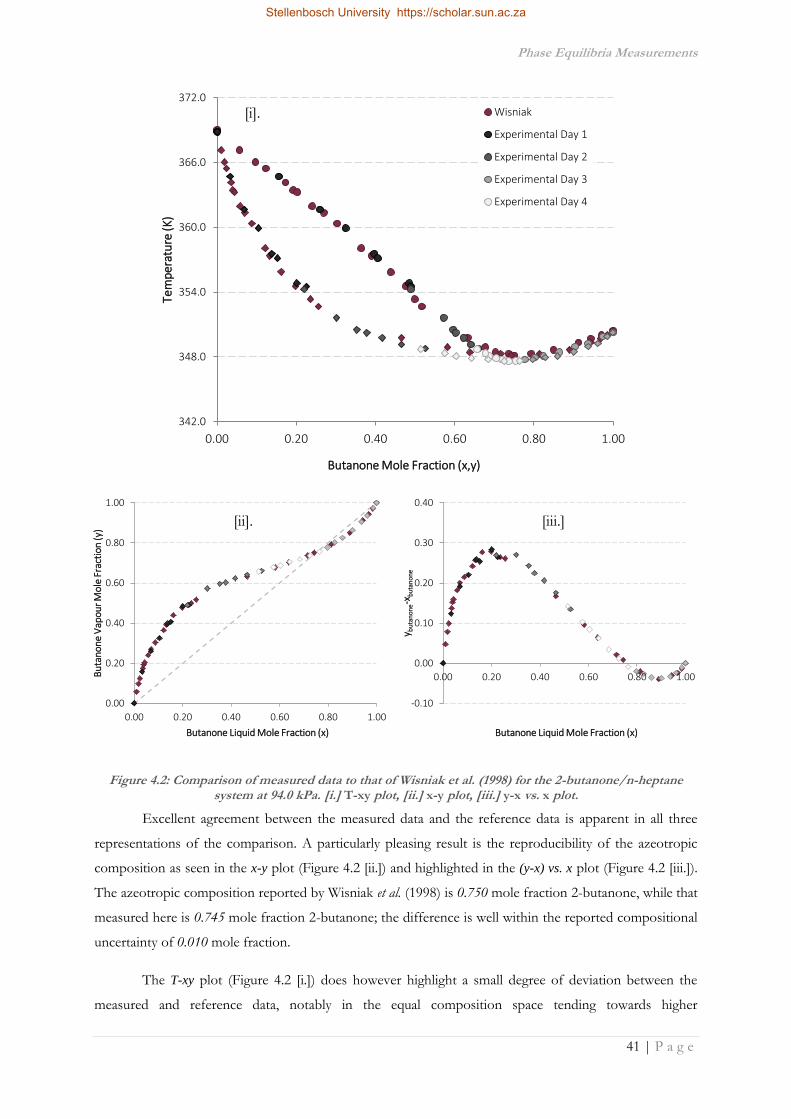
Phase Equilibria Measurements
41 | P a g e
0.00
0.20
0.40
0.60
0.80
1.00
0.00 0.20 0.40 0.60 0.80 1.00
Bu
tan
on
e V
apo
ur
Mo
le F
ract
ion
(y)
Butanone Liquid Mole Fraction (x)
-0.10
0.00
0.10
0.20
0.30
0.40
0.00 0.20 0.40 0.60 0.80 1.00
y bu
tan
on
e-x
bu
tan
one
Butanone Liquid Mole Fraction (x)
342.0
348.0
354.0
360.0
366.0
372.0
0.00 0.20 0.40 0.60 0.80 1.00
Tem
per
atu
re (
K)
Butanone Mole Fraction (x,y)
Wisniak
Experimental Day 1
Experimental Day 2
Experimental Day 3
Experimental Day 4
Excellent agreement between the measured data and the reference data is apparent in all three
representations of the comparison. A particularly pleasing result is the reproducibility of the azeotropic
composition as seen in the x-y plot (Figure 4.2 [ii.]) and highlighted in the (y-x) vs. x plot (Figure 4.2 [iii.]).
The azeotropic composition reported by Wisniak et al. (1998) is 0.750 mole fraction 2-butanone, while that
measured here is 0.745 mole fraction 2-butanone; the difference is well within the reported compositional
uncertainty of 0.010 mole fraction.
The T-xy plot (Figure 4.2 [i.]) does however highlight a small degree of deviation between the
measured and reference data, notably in the equal composition space tending towards higher
b
.
c
.
Figure 4.2: Comparison of measured data to that of Wisniak et al. (1998) for the 2-butanone/n-heptane system at 94.0 kPa. [i.] T-xy plot, [ii.] x-y plot, [iii.] y-x vs. x plot.
c
.
[i].
[ii]. [iii.]
Stellenbosch University https://scholar.sun.ac.za
Phase Equilibria Measurements
42 | P a g e
concentrations of 2-butanone, viz. ≥0.55 mole fraction 2-butanone. Given that these deviations are not
apparent in the compositional plots, where the temperature effects are excluded, it can be deduced that
these deviations are purely in the temperature measurement. The largest temperature difference is
apparent around the azeotropic point, with deviations of approximately 0.2 K, which is of the same order
of magnitude as the reported uncertainty in temperature. Furthermore, temperature measurements were
validated through reproducing literature vapour pressures in the previous section where, in particular,
deviations were found to be scattered rather than systematic. In light of these two points, the small
temperature deviations apparent in the T-xy plot can be considered within acceptable experimental limits.
4.1.3 Verification Summary
By accurately reproducing both pure component vapour pressures and an independently
measured binary system, a degree of confidence is given to the data generated in this study. Both the
equipment and the procedure employed can thus be considered verified and focus can turn to the
generation of new phase equilibrium data.
4.2 C6 Ether/n-Heptane Systems
The experimental data for both the di-n-propyl ether and butyl ethyl ether systems are presented
and their phase behaviour discussed separately. An analysis of the role of the shifting functional group on
the associated mixture behaviour follows thereafter.
4.2.1 Phase Equilibrium Results
4.2.1.1 Di-n-Propyl Ether/n-Heptane
The phase equilibrium data for the di-n-propyl ether/n-heptane system at 60 kPa are plotted in
Figure 4.3, with data tabulated in Appendix E. The reproducibility of the experimental data is good, as is
evidenced by the agreement between ‘Experimental Day 5’ data and that of the preceding days’ runs. The
system presents slight positive deviations from ideality, which results in a very narrow phase envelope, but
not significant enough to produce azeotropic behaviour. This is verified by the fact that no temperature
minimum was apparent experimentally and that the x-y plot does not cross the x = y line in Figure 4.3 [ii.]
or equivalently the x-axis in Figure 4.3 [iii.]. The data reported were shown to be thermodynamically
consistent by both the McDermott-Ellis and L/W consistency tests, exhibiting a D value of 4.28 (less than
the recommended maximum of 5).
Stellenbosch University https://scholar.sun.ac.za

Phase Equilibria Measurements
43 | P a g e
346.0
348.0
350.0
352.0
354.0
356.0
0.00 0.20 0.40 0.60 0.80 1.00
Tem
per
atu
re (
K)
Di-n-Propyl Ether Mole Fraction (x,y)
Experimental Day 1
Experimental Day 2
Experimental Day 3
Experimental Day 4
Experimental Day 5
0.00
0.20
0.40
0.60
0.80
1.00
0.00 0.20 0.40 0.60 0.80 1.00
Di-
n-P
rop
yl E
ther
Vap
ou
r M
ole
Fra
ctio
n (y
)
Di-n-Propyl Ether Liquid Mole Fraction (x)
-0.15
-0.10
-0.05
0.00
0.05
0.10
0.15
0.00 0.20 0.40 0.60 0.80 1.00
y DN
PE-x
DN
PE
Di-n-Propyl Ether Liquid Mole Fraction (x)
b
.
c
.
c
.
Figure 4.3: Experimental phase equilibrium data for the di-n-propyl ether/n-heptane system at 60 kPa. Equilibrium represented in [i.] T-xy, [ii.] x-y, and [iii.] y-x vs. x plot forms.
[i].
[ii]. [iii.]
Stellenbosch University https://scholar.sun.ac.za

Phase Equilibria Measurements
44 | P a g e
4.2.1.2 Butyl Ethyl Ether/n-Heptane
Like the di-n-propyl ether/n-heptane system before it, the butyl ethyl ether/n-heptane system at
60 kPa is seen to exhibit positive deviations from ideality with no azeotropic point, but a particularly
narrow phase envelope in Figure 4.4. The lowest recorded temperature was the pure ether boiling point,
which confirmed zeotropic behaviour in the system experimentally. Reproducibility of the data is evident
while the data were found to be thermodynamically consistent by both the L/W (D = 3.15) and
McDermott-Ellis consistency tests.
-0.15
-0.10
-0.05
0.00
0.05
0.10
0.15
0.00 0.20 0.40 0.60 0.80 1.00
y Bu
t Eth
Eth
er-x
But
Eth
Eth
er
Butyl Ethyl Ether Liquid Mole Fraction (x)
348.0
350.0
352.0
354.0
356.0
0.00 0.20 0.40 0.60 0.80 1.00
Tem
per
atu
re (
K)
Butyl Ethyl Ether Mole Fraction (x,y)
Experimental Day 1
Experimental Day 2
Experimental Day 3
Experimental Day 4
Experimental Day 5
b
.
c
.
0.00
0.20
0.40
0.60
0.80
1.00
0.00 0.20 0.40 0.60 0.80 1.00
Bu
tyl E
thyl
Eth
er V
apo
ur
Mo
le F
ract
ion
(y)
Butyl Ethyl Ether Liquid Mole Fraction (x)
c
.
Figure 4.4: Experimental phase equilibrium data for the butyl ethyl ether/n-heptane system at 60 kPa. Equilibrium represented in [i.] T-xy, [ii.] x-y, and [iii.] y-x vs. x plot forms.
[i].
[ii]. [iii.]
Stellenbosch University https://scholar.sun.ac.za

Phase Equilibria Measurements
45 | P a g e
4.2.2 Role of Functional Group Location
With neither ether/n-heptane system exhibiting azeotropic behaviour, the difference in mixture
behaviour between the two ethers manifests itself most readily in the pure component boiling points. As
the polar oxygen atom moves further from the centre of the carbon backbone, the polar forces become
more prominent, raising the boiling point of the ether, as demonstrated in Figure 4.5. Structurally, a C6
ether is not dissimilar from n-heptane – the only difference being the substitution of a CH2 group for the
polar oxygen within the carbon backbone itself.
Thus, what is interesting with the behaviour of the ethers is that as the polar ether group shifts
toward the terminal methyl group, its influence increases and the boiling point of the ether approaches that
of the equivalent sized nonpolar alkane. In fact, the boiling point of the final linear isomer (pentyl methyl
ether – not measured here) at the experimental conditions is 355.3 K (DIPPR), a mere 0.6 K higher than
that of n-heptane. One could thus argue that when the oxygen is located in the centre of the chain, the
greatest “deviation” from nonpolar behaviour is apparent. That is, the greatest difference between the
phase behaviour of the polar ether and the nonpolar alkane is in evidence for the mixture with di-n-propyl
ether. This emphasises the subtle but important role that the polar oxygen plays in distinguishing the ether
from a nonpolar alkane and the difficulty inherent in accurately describing the behaviour of components
of this functional group.
Figure 4.5: Combined T-xy plot for both ether/n-heptane systems at 60 kPa, highlighting the role of the polar functional group location in altering system behaviour. Molecular representations of the respective
ethers are included for ease of reference.
346.0
348.0
350.0
352.0
354.0
356.0
0.00 0.20 0.40 0.60 0.80 1.00
Tem
per
atu
re (
K)
Ether Mole Fraction (x,y)
Butyl Ethyl Ether
Di-n-Propyl Ether
Stellenbosch University https://scholar.sun.ac.za

Phase Equilibria Measurements
46 | P a g e
4.3 C6 Ester/n-Octane Systems
As with the ether systems in the previous section, the experimental data for and discussion of the
phase equilibrium of the five ester/n-octane systems will be presented first. This will be followed by a
discussion on the role of the shifting diatomic functional group on the associated phase behaviour.
4.3.1 Phase Equilibrium Results
The results of the vapour-liquid equilibrium experiments for each of the C6 ester isomers with
n-octane are presented in Figures 4.6 to 4.10 that follow. All five systems exhibited strong positive
deviations from ideality and a minimum boiling azeotrope, with the experimentally observed azeotropic
points listed in Table 41.
Table 4.1: Summary of experimentally measured azeotropic temperatures and compositions in the five ester/n-octane systems considered.
Azeotropic Temperature Azeotropic Composition
K mole fraction ester
methyl valerate/n-octane 377.53 0.409
ethyl butanoate/n-octane 374.60 0.605
propyl propanoate/n-octane 375.44 0.546
butyl acetate/n-octane 376.55 0.459
pentyl formate/n-octane 378.32 0.308
Reproducibility of the data was checked by performing repeat runs in all five systems, with
excellent agreement between the runs performed on different days. Thermodynamic consistency of all the
data was checked and confirmed by both the L/W and McDermott-Ellis consistency tests. In the case of
the L/W test, the largest D value of any of the five systems was found to be 0.861 – well within the
recommended maximum of 5. For the McDermott-Ellis consistency test, all data pairs exhibited
deviations smaller than their respective Dmax values. Details of the thermodynamic consistency testing can
be found in Appendix E.
Stellenbosch University https://scholar.sun.ac.za

Phase Equilibria Measurements
47 | P a g e
4.3.1.1 Methyl Valerate/n-Octane
376.0
378.0
380.0
382.0
384.0
0.00 0.20 0.40 0.60 0.80 1.00
Tem
per
atu
re (
K)
Methyl Valerate Mole Fraction (x,y)
Experimental Day 1
Experimental Day 2
Experimental Day 3
Experimental Day 4
Experimental Day 5
Experimental Day 6
b
.
c
.
c
.
Figure 4.6: Experimental phase equilibrium data for the methyl valerate/n-octane system at 60 kPa. Equilibrium represented in [i.] T-xy, [ii.] x-y, and [iii.] y-x vs. x plot forms.
0.00
0.20
0.40
0.60
0.80
1.00
0.00 0.20 0.40 0.60 0.80 1.00
Met
hyl
Val
erat
e V
apo
ur
Mo
le F
ract
ion
(y)
Methyl Valerate Liquid Mole Fraction (x)
-0.15
-0.10
-0.05
0.00
0.05
0.10
0.15
0.00 0.20 0.40 0.60 0.80 1.00
y Met
h V
al-x
Met
h V
al
Methyl Valerate Liquid Mole Fraction (x)
[i].
[ii]. [iii.]
Stellenbosch University https://scholar.sun.ac.za

Phase Equilibria Measurements
48 | P a g e
4.3.1.2 Ethyl Butanoate/n-Octane
-0.15
-0.10
-0.05
0.00
0.05
0.10
0.15
0.00 0.20 0.40 0.60 0.80 1.00
y Eth
Bu
t-x
Eth
Bu
t
Ethyl Butanoate Liquid Mole Fraction (x)
0.00
0.20
0.40
0.60
0.80
1.00
0.00 0.20 0.40 0.60 0.80 1.00
Eth
yl B
uta
no
ate
Vap
ou
r M
ole
Fra
ctio
n (y
)
Ethyl Butanoate Liquid Mole Fraction (x)
374.0
376.0
378.0
380.0
382.0
0.00 0.20 0.40 0.60 0.80 1.00
Tem
per
atu
re (
K)
Ethyl Butanoate Mole Fraction (x,y)
Experimental Day 1
Experimental Day 2
Experimental Day 3
Experimental Day 4
Experimental Day 5
Experimental Day 6
b
.
c
.
c
.
Figure 4.7: Experimental phase equilibrium data for the ethyl butanoate/n-octane system at 60 kPa. Equilibrium represented in [i.] T-xy, [ii.] x-y, and [iii.] y-x vs. x plot forms.
[i].
[ii]. [iii.]
Stellenbosch University https://scholar.sun.ac.za
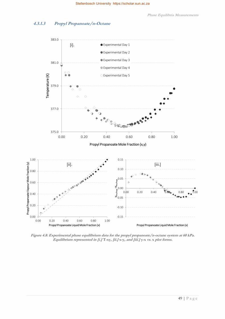
Phase Equilibria Measurements
49 | P a g e
4.3.1.3 Propyl Propanoate/n-Octane
-0.15
-0.10
-0.05
0.00
0.05
0.10
0.15
0.00 0.20 0.40 0.60 0.80 1.00
y Pro
Pro
p-x
Pro
Pro
p
Propyl Propanoate Liquid Mole Fraction (x)
0.00
0.20
0.40
0.60
0.80
1.00
0.00 0.20 0.40 0.60 0.80 1.00
Pro
pyl
Pro
pan
oat
e V
apo
ur
Mo
le F
ract
ion
(y)
Propyl Propanoate Liquid Mole Fraction (x)
375.0
377.0
379.0
381.0
383.0
0.00 0.20 0.40 0.60 0.80 1.00
Tem
per
atu
re (
K)
Propyl Propanoate Mole Fraction (x,y)
Experimental Day 1
Experimental Day 2
Experimental Day 3
Experimental Day 4
Experimental Day 5
b
.
c
.
c
.
Figure 4.8: Experimental phase equilibrium data for the propyl propanoate/n-octane system at 60 kPa. Equilibrium represented in [i.] T-xy, [ii.] x-y, and [iii.] y-x vs. x plot forms.
[i].
[ii]. [iii.]
Stellenbosch University https://scholar.sun.ac.za

Phase Equilibria Measurements
50 | P a g e
4.3.1.4 Butyl Acetate/n-Octane
-0.15
-0.10
-0.05
0.00
0.05
0.10
0.15
0.00 0.20 0.40 0.60 0.80 1.00
y Bu
t Ace
-xB
ut A
ce
Butyl Acetate Liquid Mole Fraction (x)
375.0
377.0
379.0
381.0
383.0
0.00 0.20 0.40 0.60 0.80 1.00
Tem
per
atu
re (
K)
Butyl Acetate Mole Fraction (x,y)
Experimental Day 1
Experimental Day 2
Experimental Day 3
Experimental Day 4
Experimental Day 5
Experimental Day 6
0.00
0.20
0.40
0.60
0.80
1.00
0.00 0.20 0.40 0.60 0.80 1.00
Bu
tyl A
ceta
te V
apo
ur
Mo
le F
ract
ion
(y)
Butyl Acetate Liquid Mole Fraction (x)
b
.
c
.
c
.
Figure 4.9: Experimental phase equilibrium data for the butyl acetate/n-octane system at 60 kPa. Equilibrium represented in [i.] T-xy, [ii.] x-y, and [iii.] y-x vs. x plot forms.
[i].
[ii]. [iii.]
Stellenbosch University https://scholar.sun.ac.za

Phase Equilibria Measurements
51 | P a g e
4.3.1.5 Pentyl Formate/n-Octane
-0.15
-0.10
-0.05
0.00
0.05
0.10
0.15
0.00 0.20 0.40 0.60 0.80 1.00
y Pen
Fo
rm-x
Pen
Fo
rm
Pentyl Formate Liquid Mole Fraction (x)
0.00
0.20
0.40
0.60
0.80
1.00
0.00 0.20 0.40 0.60 0.80 1.00
Pe
nty
l Fo
rmat
e V
apo
ur
Mo
le F
ract
ion
(y)
Pentyl Formate Liquid Mole Fraction (x)
378.0
380.0
382.0
384.0
386.0
388.0
0.00 0.20 0.40 0.60 0.80 1.00
Tem
per
atu
re (
K)
Pentyl Formate Mole Fraction (x,y)
Experimental Day 1
Experimental Day 2
Experimental Day 3
Experimental Day 4
Experimental Day 5
Experimental Day 6
[i].
b
.
c
.
c
.
Figure 4.10: Experimental phase equilibrium data for the pentyl formate/n-octane system at 60 kPa. Equilibrium represented in [i.] T-xy, [ii.] x-y, and [iii.] y-x vs. x plot forms.
[ii]. [iii.]
Stellenbosch University https://scholar.sun.ac.za

Phase Equilibria Measurements
52 | P a g e
4.3.2 Role of Functional Group Location
The ester functional group comprises an alkoxy group in the carbon backbone of the molecule
directly bonded to a carbonyl group, or simplistically, an ether group bonded to a ketone group. As a
result, a given linear ester has roughly 1.5 times the number of structural isomers as an equivalent length
ketone or ether, as well a larger scope for differences in their associated phase equilibrium. This is readily
apparent from both the pure ester boiling points in Figure 4.1 as well as the mixture behaviour of each
isomer with n-octane in Figures 4.6 to 4.10.
In ketones and ethers, it has already been shown that the strength of polar interactions is directly
linked to the location of the single carbonyl or alkoxy group in the carbon chain; a terminally located polar
functional group yields the most polar isomer with successively decreasing influence until the group is in
the middle of the chain. For esters the situation is a little more nuanced; here it is the relative locations of
the carbonyl and alkoxy subgroups in relation to each other and the two terminal methyl groups that
impact the strength of the polar interactions and consequently their phase behaviour. The effect of these
relative locations are highlighted in the combined T-xy and x-y plots for the five ester isomers in
Figures 4.11 and 4.12 respectively.
374.0
376.0
378.0
380.0
382.0
384.0
386.0
388.0
0.00 0.20 0.40 0.60 0.80 1.00
Tem
per
atu
re (
K)
Ester Mole Fraction (x,y)
Methyl Valerate
Ethyl Butanoate
Propyl Propanoate
Butyl Acetate
Pentyl Formate
Figure 4.11: Combined T-xy plot for ester/n-octane systems at 60 kPa, highlighting the role of the polar functional group location in altering system behaviour.
Stellenbosch University https://scholar.sun.ac.za

Phase Equilibria Measurements
53 | P a g e
Given that the carbonyl subgroup is located at the end of the chain readily explains why pentyl
formate is the most polar isomer with the highest boiling point. The interesting trend is the relative
dipolar strength of the methyl valerate-butyl acetate and propyl propanoate-ethyl butanoate pairs. To
clarify this point, the skeletal formulae of the esters considered here are presented in order of descending
boiling point in Figure 4.13.
Given that ketones are more polar molecules than ethers, one might intuit that the more
terminally located carbonyl subgroup of butyl acetate would make it more strongly polar than methyl
valerate, but based on the experimental phase behaviour the opposite seems to be true. This trend is
reversed for the latter pair, where the centrally located and thus sterically hindered carbonyl subgroup of
ethyl butanoate results in more dampened dipolar interactions than propyl propanoate. Indeed, if the
behaviour of methyl valerate is omitted, it is clear that a regular trend exists between the acid chain length
Figure 4.13: Skeletal formulae of the five linear C6 structural isomers, presented from left to right in descending order of their boiling points at the experimental pressure (60 kPa). The aim is to highlight the
location of carbonyl and alkyl subgroups of the ester group within the linear chain.
-0.15
-0.10
-0.05
0.00
0.05
0.10
0.15
0.00 0.20 0.40 0.60 0.80 1.00
y est
er-
x est
er
Ester Liquid Mole Fraction (x)
Methyl Valerate
Ethyl Butanoate
Propyl Propanoate
Butyl Acetate
Pentyl Formate
Figure 4.12: Combined (y-x) vs. x plot for ester/n-octane systems at 60 kPa, highlighting the role of the polar functional group location in altering system behaviour.
Methyl Valerate T
b: 383.1K
Ethyl Butanoate T
b: 377.0K
Propyl Propanoate T
b: 378.8K
Butyl Acetate T
b: 382.0K
Pentyl Formate T
b: 387.4K
Stellenbosch University https://scholar.sun.ac.za
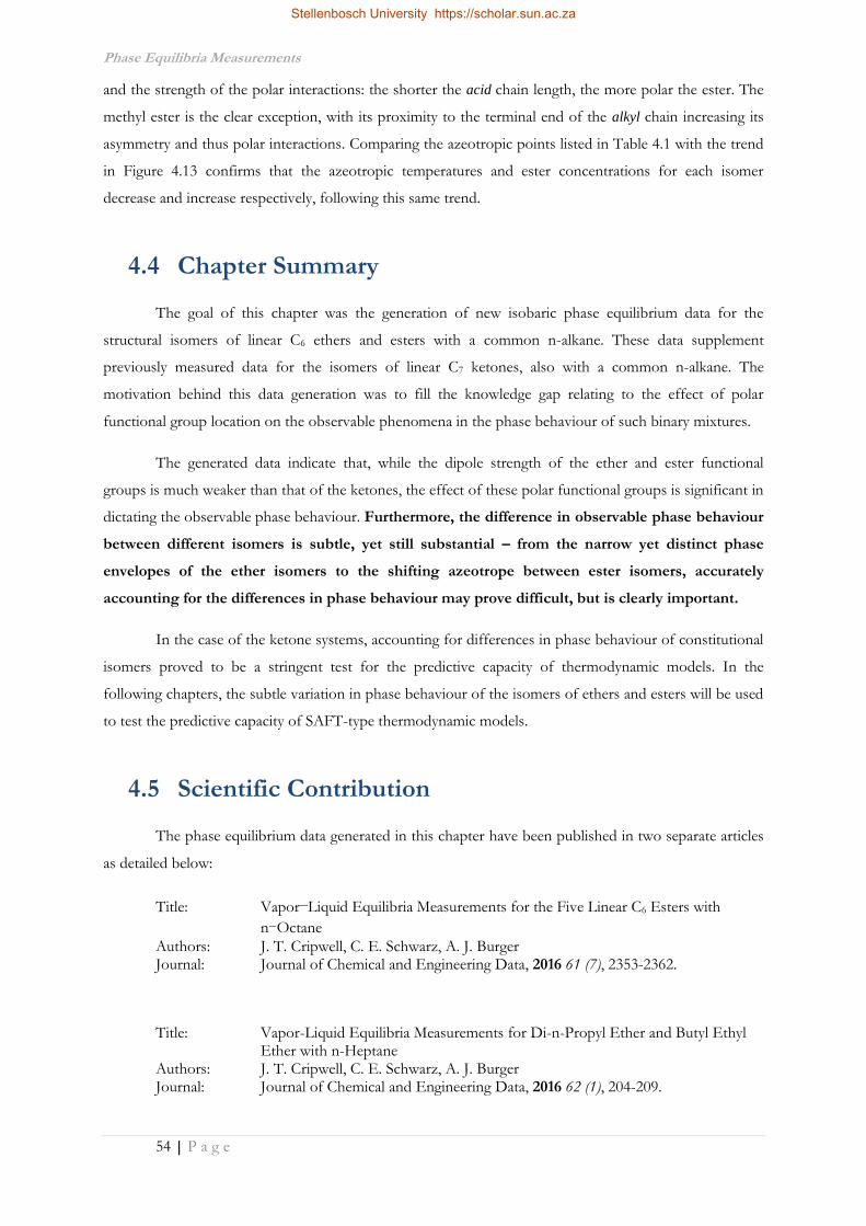
Phase Equilibria Measurements
54 | P a g e
and the strength of the polar interactions: the shorter the acid chain length, the more polar the ester. The
methyl ester is the clear exception, with its proximity to the terminal end of the alkyl chain increasing its
asymmetry and thus polar interactions. Comparing the azeotropic points listed in Table 4.1 with the trend
in Figure 4.13 confirms that the azeotropic temperatures and ester concentrations for each isomer
decrease and increase respectively, following this same trend.
4.4 Chapter Summary
The goal of this chapter was the generation of new isobaric phase equilibrium data for the
structural isomers of linear C6 ethers and esters with a common n-alkane. These data supplement
previously measured data for the isomers of linear C7 ketones, also with a common n-alkane. The
motivation behind this data generation was to fill the knowledge gap relating to the effect of polar
functional group location on the observable phenomena in the phase behaviour of such binary mixtures.
The generated data indicate that, while the dipole strength of the ether and ester functional
groups is much weaker than that of the ketones, the effect of these polar functional groups is significant in
dictating the observable phase behaviour. Furthermore, the difference in observable phase behaviour
between different isomers is subtle, yet still substantial – from the narrow yet distinct phase
envelopes of the ether isomers to the shifting azeotrope between ester isomers, accurately
accounting for the differences in phase behaviour may prove difficult, but is clearly important.
In the case of the ketone systems, accounting for differences in phase behaviour of constitutional
isomers proved to be a stringent test for the predictive capacity of thermodynamic models. In the
following chapters, the subtle variation in phase behaviour of the isomers of ethers and esters will be used
to test the predictive capacity of SAFT-type thermodynamic models.
4.5 Scientific Contribution
The phase equilibrium data generated in this chapter have been published in two separate articles
as detailed below:
Title: Vapor−Liquid Equilibria Measurements for the Five Linear C6 Esters with
n-Octane
Authors: J. T. Cripwell, C. E. Schwarz, A. J. Burger Journal: Journal of Chemical and Engineering Data, 2016 61 (7), 2353-2362.
Title: Vapor-Liquid Equilibria Measurements for Di-n-Propyl Ether and Butyl Ethyl Ether with n-Heptane
Authors: J. T. Cripwell, C. E. Schwarz, A. J. Burger Journal: Journal of Chemical and Engineering Data, 2016 62 (1), 204-209.
Stellenbosch University https://scholar.sun.ac.za

Assessing the Predictive Capacity of Polar sPC-SAFT
55 | P a g e
Chapter 5: ASSESSING THE PREDICTIVE
CAPACITY OF POLAR
SPC-SAFT
In Chapter 2, an introduction to the field of SAFT modelling was presented, highlighting the
development of the EoS, up to and including the simplified perturbed chain SAFT variant (sPC-SAFT) as
well as the Jog & Chapman (JC) and Gross & Vrabec (GV) polar terms. In this chapter, the predictive
capacity of sPC-SAFT, combined with each of these two polar terms, is assessed through the model’s
application to the vapour-liquid equilibrium data presented in Chapter 4.
Initially, the regression method is discussed. The results of the parameter regression are presented
with reference to deviations from appropriate pure component properties given as an indication of the
quality of fit. Thereafter, the pure predictions of the EoSs for the mixture phase behaviour are compared
to experimental data, to assess the predictive capacity of the models. Particular attention is paid to trends
in the success or failure of the models to accurately account for the differences in phase behaviour of each
structural isomer of each homologous group under consideration. Finally, a summary of the overall
predictive strengths and shortcomings of polar sPC-SAFT is presented.
5.1 Determining Polar sPC-SAFT Parameters
Modelling of mixture phase behaviour requires generation of pure component parameter sets for
each component in question. For a thermodynamic model to be used in the prediction of mixture
properties, the accurate representation of pure component properties is a prerequisite.
5.1.1 Choice of Pure Component Data Inclusion
Given that thermodynamic models are most widely used for the description of phase equilibria,
emphasis is generally placed on accurate description of pure component properties that will yield the best
account of the two phase region. To this end, the saturated liquid density (ρisat) and saturated vapour
pressure (Pisat) are traditionally the pure component properties of choice. The vapour pressure dictates the
T-P relationship between the vapour and liquid phases, while the liquid density provides a measure of the
phase volumes and thus the volume roots of the EoS. The ultimate goal of thermodynamic modelling
however, is the accurate description of any thermodynamic property using a single, component-specific
parameter set. In the case of SAFT type models, defining the EoS with respect to the residual Helmholtz
free energy allows determination of many other thermodynamic properties by appropriate differentiation.
This interconnectivity was first presented in Chapter 1 (Figure 1.1).
Stellenbosch University https://scholar.sun.ac.za

Assessing the Predictive Capacity of Polar sPC-SAFT
56 | P a g e
Llovell et al. (2006) argued that the parameters of a physically sound thermodynamic model
should be transferable, giving accurate predictions of all thermodynamic properties using the
thermodynamic relationships illustrated in Figure 1.1. De Villiers (2011) refined this argument by stating
that it is the optimum parameter set for such a model that should exhibit these characteristics. This is an
important distinction; the mathematical nature of parameter regression means that by fitting component
parameters against pure component data, one will always produce a parameter set capable of accurately
representing the fitted properties. Thus it is important to select pure component properties that can
provide the best balance of prediction for all properties to yield the optimum parameter set.
As is evident from Figure 1.1, incorporation of both saturated vapour pressure and saturated
liquid densities of a pure component allows for regression to test both the first compositional and first
volume derivatives of the residual Helmholtz energy function, viz: dA/dni & dA/dV. What is also evident
however, is that the temperature dependency is not tested in this procedure (dA/dT). While a degree of
temperature dependence is incorporated through the temperature range of the Pisat and ρi
sat data, some
authors have elected to include other pure component properties in the regression procedure to yield a
more balanced parameter set.
Lafitte et al. (2006) argued the merits of including pure component speed of sound data, while the
same group later advocated for the inclusion of heats of vaporisation (Lafitte et al., 2007) within a
SAFT-VR framework. It is evident from Figure 1.1 that both suggestions would serve to incorporate
temperature dependence into the resulting regressed parameter set and should yield accurate predictions
of these previously excluded properties. However, the predictive capacity of thermodynamic models is
traditionally measured in their application to mixture phase equilibrium. Thus, it is important that
increased accuracy in the prediction of derivative properties does not compromise the ability of the model
to yield accurate phase equilibrium predictions.
Within the sPC- and PC-SAFT frameworks respectively, de Villiers (2011) and de Villiers et al.
(2013) performed extensive studies on using different combinations of pure component properties in the
regression procedure. The goal of these studies was identifying the combination that would yield the
optimum parameter set. The results indicated that regardless of the choice of pure component data
included, no single combination of parameters could yield equally accurate predictions for phase
equilibrium as well as derivative properties. The authors attributed this deficit to inherent shortcomings in
the predictive behaviour of the hard sphere term, where the use of a Lennard-Jones potential function
restricts the range of repulsive intermolecular interactions.
With the emphasis here on the sPC-SAFT framework, the conclusion of de Villiers (2011) is
highlighted. In that work, the best combination of properties (with regression weights in parentheses) for
accurate representation of phase equilibrium, and with fair correlation of derivative properties, was found
to be:
Stellenbosch University https://scholar.sun.ac.za

Assessing the Predictive Capacity of Polar sPC-SAFT
57 | P a g e
saturated vapour pressures, Psat, (4),
saturated liquid densities, ρisat, (2), and
heats of vaporisation, Hvap, (1).
This combination of properties and regression weights was used to good effect in the previous
study performed on ketones (Cripwell, 2014) and is similarly employed in the regression of polar sPC-
SAFT parameter sets in this work.
Incorporating the correct pure component data is an important initial requirement for
determination of the optimum parameter set. The challenge when regressing parameters of fundamental
models like SAFT is the need to produce parameters that have physical meaning, e.g. non-negative
segment numbers and realistic segment sizes. Being able to bridge the divide between the mathematical
parameter space and their physical realism often presents the biggest challenges in the regression of SAFT
parameters.
5.1.2 Regression Challenges
A majority of SAFT variants, including the original PC-SAFT and its simplified variant, support
three pure component parameters – typically the segment diameter (σ - Å), the segment number
(m - dimensionless) and the dispersion energy (ε/k – K). Regression of n pure component parameters can
be seen as determining the global minimum in an n-dimensional space. Determination of the usual three
parameters is thus performed in the visible three dimensional space and is readily achieved using a local
optimisation type algorithm. The objective functions used in these algorithms are typically of the form
presented in equation 5.1, using the aforementioned standard pure component properties, viz. saturated
vapour pressure and liquid density data respectively.
2 2, , , ,
, ,1
np sat calc sat ex sat calc sat exi i i i
sat ex sat exi i i
P POF
P
ρ ρ
ρ
5.1
However, complications often arise once the number of parameters requiring fitting increases, as
is the case for the introduction of polar terms to the SAFT framework. In this case, the global minimum
needs to be found in a four-dimensional or higher space, where the existence of multiple local minima can
cause the search algorithms to become trapped in false solutions. This degeneracy of the parameter space
causes mathematical difficulties when trying to find the global minimum.
When applying PC-SAFTJC to ketones, ethers and esters, both Sauer & Chapman (2003) and
Dominik et al. (2005) noted degeneracy of the parameter space, resulting in multiple minima in the
objective function. This meant that, when parameters were fit only to pure component saturated vapour
pressures and liquid densities, multiple parameter sets exist that could accurately represent the pure
component properties. However, many of these sets were physically unrealistic (e.g. excessively large
Stellenbosch University https://scholar.sun.ac.za

Assessing the Predictive Capacity of Polar sPC-SAFT
58 | P a g e
segment numbers). This result highlighted the importance of stressing the physical significance of the
regressed parameters in order to obtain optimum parameter sets.
Indeed, Gross & Vrabec (2006) went further to note that, when the four PC-SAFTJC parameters
were fit to pure component data alone, the optimum parameter set was frequently that which had a zero
polar contribution. Specifically, the zero polar contribution arose when the polar parameter xp was forced
to its lower physical limit of zero. This trend was supported by similar observations by de Villiers et al.
(2011) and the precursor to this work (Cripwell, 2014), where both the Jog & Chapman and Gross &
Vrabec polar terms were incorporated in the sPC-SAFT framework. This trend seems to suggest an
inability of the polar term to distinguish between the anisotropic polar contribution and the isotropic
dispersion forces in some cases. However, the problem up to this point is that no trend in parameter space
degeneracy has yet been identified and so this suggestion has yet to be proven to be the case.
5.1.3 Proposed Solutions to Regression Challenges
In the original work for the GV polar term, Gross & Vrabec (2006) set the value of their
additional polar parameter, np, equal to unity for molecules containing a single polar group, but it could be
changed to 2 for diketones, diethers, etc. In this way, the problem of parameter multiplicity could be
avoided and the authors claimed this to be a superior aspect of the GV term compared to the JC term.
This example of employing physical considerations for fixing the value of one of the component
parameters is the first of the suggested means in the literature for avoiding parameter multiplicity by
reducing the dimensionality of the parameter space.
Such considerations were also made in the original works on the JC polar term (Jog et al., 2001),
where the value of the dipolar fraction, xp, was expected to be equal to the inverse of the segment number.
This was based on the physical consideration that the dipole moment is confined to a single group in the
carbon chain in most common polar molecules. Later, Sauer & Chapman (2003) and Dominik et al. (2005)
built on this physical consideration and showed that, for a given homologous group, the product of xp and
m is constant. This relatively simple re-working is an example of employing an empirical correlation based
on the same physical observation, which still serves to fix the value of a given parameter. In this case, if
the value of xp could be successfully regressed for one member of a homologous series, the constant xpm
correlation could be used to determine unique parameters for other members of the homologous series,
resulting in better representation of mixture behaviour.
In the same work that introduced the relationship between xp and m as a means for fixing a
parameter value, Dominik et al. (2005) also suggested the second means of overcoming problems in
regressing unique parameter sets. The problem with multiple local minima in the objective function is that
different regressed parameter sets can accurately model pure component properties but not all can
account for mixture behaviour. Thus, Dominik et al.’s (2005) argument was that by incorporating mixture
VLE data, a subtle bias could be afforded to the description of multicomponent phase equilibria, and the
true global minimum in the objective function could be found. The choice of mixture data is important
Stellenbosch University https://scholar.sun.ac.za

Assessing the Predictive Capacity of Polar sPC-SAFT
59 | P a g e
however, as the second component in the mixture needs to have had its own parameters determined and
tested, as well as being void of functionality beyond typical dispersion forces. This last point is particularly
poignant; dipolar interactions only occur between polar molecules, while dispersion forces are common to
all components. Thus, the inclusion of binary data with a nonpolar component helps differentiate between
these different intermolecular forces.
As discussed in Chapter 2, de Villiers et al. (2011) argued that an accurate comparison between the
performance of the JC and GV polar terms necessitates that each be assessed on an equal footing with the
same number of regressed parameters. To this end, polar sPC-SAFT parameter sets were determined for a
wide range of polar components where the value of np was allowed to vary in the regression procedure.
Following the line of thought proposed by Dominik et al. (2005), de Villiers et al. (2011) similarly included
VLE data in the regression procedure for both sPC-SAFTJC and sPC-SAFTGV. This resulted in parameter
sets that reproduced both pure component and mixture phase behaviour with a high degree of accuracy.
The problem with the reliance on incorporating mixture VLE data in the regression procedure is
that, for many components of industrial and academic interest, accurate phase equilibrium data is simply
not available. Indeed, one of the strongest arguments for using fundamental models like SAFT is the
models’ predictive capacity without the need for experimental data in the first place. Thus, in lieu of
experimental data, it is vital that parameter multiplicity does not hinder the use and application of these
models. De Villiers et al. (2011) acknowledged this point and looked to combine the approaches of fixing
the value of a pure component parameter with the incorporation of VLE data in the regression procedure.
Using Dominik et al.’s observation of the relationship between xp and m for a given homologous series, de
Villiers developed an empirical correlation for setting the value of both xp and np, the form of which is
presented in equations 5.2 and 5.3
2p
w
Kx
A M B μ
5.2
2
wp
K A M Bn
μ
5.3
The term in parenthesis is approximately equal to the segment number, while the molecular
dipole moment introduces further component specific dependence in the correlation. The constants K, A
and B are homologous group specific and are presented for ketones and esters in Table 5.1. Parameters
for the ether functional group were not previously determined due to a lack of “good VLE data” for this
homologous group (de Villiers et al., 2011); so determination of equivalent constants for mono ethers was
an objective of this work.
The same procedure as that adopted by de Villiers was thus to add the constants for ethers to
those for ketones and esters in Table 5.1. The constants (K, A & B) of these equations are fit to parameter
sets that have been successfully regressed using binary VLE data in the regression procedure. A and B are
Stellenbosch University https://scholar.sun.ac.za
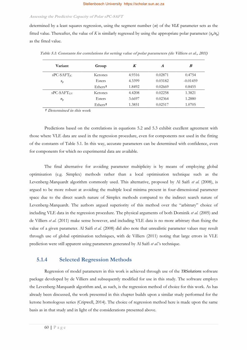
Assessing the Predictive Capacity of Polar sPC-SAFT
60 | P a g e
determined by a least squares regression, using the segment number (m) of the VLE parameter sets as the
fitted value. Thereafter, the value of K is similarly regressed by using the appropriate polar parameter (xp/np)
as the fitted value.
Table 5.1: Constants for correlations for setting value of polar parameters (de Villiers et al., 2011)
Variant Group K A B
sPC-SAFTJC Ketones 4.9316 0.02871 0.4754
xp Esters 4.3399 0.03182 -0.01459
Ethers† 1.8492 0.02669 0.8455
sPC-SAFTGV Ketones 4.4208 0.02258 1.3821
np Esters 3.6697 0.02364 1.2880
Ethers† 1.3851 0.02517 1.0705
† Determined in this work
Predictions based on the correlations in equations 5.2 and 5.3 exhibit excellent agreement with
those where VLE data are used in the regression procedure, even for components not used in the fitting
of the constants of Table 5.1. In this way, accurate parameters can be determined with confidence, even
for components for which no experimental data are available.
The final alternative for avoiding parameter multiplicity is by means of employing global
optimisation (e.g. Simplex) methods rather than a local optimisation technique such as the
Levenberg-Marquardt algorithm commonly used. This alternative, proposed by Al Saifi et al. (2008), is
argued to be more robust at avoiding the multiple local minima present in four-dimensional parameter
space due to the direct search nature of Simplex methods compared to the indirect search nature of
Levenberg-Marquardt. The authors argued superiority of this method over the “arbitrary” choice of
including VLE data in the regression procedure. The physical arguments of both Dominik et al. (2005) and
de Villiers et al. (2011) make sense however, and including VLE data is no more arbitrary than fixing the
value of a given parameter. Al Saifi et al. (2008) did also note that unrealistic parameter values may result
through use of global optimisation techniques, with de Villiers (2011) noting that large errors in VLE
prediction were still apparent using parameters generated by Al Saifi et al.’s technique.
5.1.4 Selected Regression Methods
Regression of model parameters in this work is achieved through use of the TRSolutions software
package developed by de Villiers and subsequently modified for use in this study. The software employs
the Levenberg-Marquardt algorithm and, as such, is the regression method of choice for this work. As has
already been discussed, the work presented in this chapter builds upon a similar study performed for the
ketone homologous series (Cripwell, 2014). The choice of regression method here is made upon the same
basis as in that study and in light of the considerations presented above.
Stellenbosch University https://scholar.sun.ac.za

Assessing the Predictive Capacity of Polar sPC-SAFT
61 | P a g e
To this end, the following three regression procedures are performed:
i. Standard pure component regression
Only pure component property data will be used, with all four parameters included
in the regression procedure.
ii. Fixing polar parameter
The value of xp and np for sPC-SAFTJC and sPC-SAFTGV respectively will be fixed
using the correlations of equations 5.2 and 5.3 with the constants in Table 5.1.
Thereafter, the remaining three nonpolar parameters will be regressed against the
same pure component property data as considered in the Standard pure component
regression above.
iii. Inclusion of measured VLE data in regression procedure
The appropriate isobaric VLE data for each ether and ester isomer, presented in
Chapter 4, will be included in the regression procedure for that isomer’s parameter
set.
Pure component data used in the regression procedure includes saturated vapour pressures, liquid
densities and heats of vaporisation. All such data are taken from appropriate correlations in the DIPPR
database, or from retrofitted correlations of the form presented in DIPPR for any components not
present in the database. Each component property comprises 30 equidistant data points over a
temperature range of 0.5<Tr<0.9. The objective function for regressions to pure component data alone is
of the form in equation 5.4, where τ, υ, and ω are the regression weights for each pure component
property (viz. 4, 2 and 1 respectively):
2 2 2, , , , , ,
, , ,1
np sat calc sat ex sat calc sat ex vap calc vap exi i i i i i
sat ex sat ex vap exi i i i
P P H HOF
P H
ρ ρτ υ ω
ρ
5.4
For the regression cases involving VLE data inclusion, the measured ether/n-heptane and
ester/n-octane data are included. The objective function for these cases takes the form presented in
equation 5.5, where ψ is the VLE data regression weight, and the revised approximate weights are 10, 8, 2
and 1 successively as per the recommendation of de Villiers (2011) and also used in Cripwell (2014):
2 2, , , ,
, ,1
2, ,
2,
,
np sat calc sat ex sat calc sat exi i i i
sat ex sat exi i i
vap calc vap exVLE errori iivap ex
i
P POF
P
H HX
H
ρ ρτ υ
ρ
ω ψ
5.5
Stellenbosch University https://scholar.sun.ac.za

Assessing the Predictive Capacity of Polar sPC-SAFT
62 | P a g e
5.2 Regressed Parameters
The results of the parameter regressions for each isomer of the considered ethers and esters are
presented in this section. The parameter sets corresponding to each of the regression procedures
highlighted in the previous section are reported, followed by a discussion of apparent trends in the results.
5.2.1 C6 Ether Parameters
Parameters regressed for di-n-propyl ether and butyl ethyl ether are presented in Table 5.2, along
with those used for n-heptane. Parameters for the latter are those originally derived by Gross & Sadowski
(2000) and shown to be applicable in the sPC-SAFT framework (von Solms et al., 2003). Given that
n-heptane is a nonpolar molecule, it necessarily lacks a polar parameter and a zero polar contribution,
meaning the same parameter set for sPC-SAFT applies to both sPC-SAFTJC and sPC-SAFTGV.
Table 5.2: Regressed model parameters for n-heptane and each C6 ether isomer using indicated regression procedures
MW σ m ε/k np/xp μ Psat ρsat Hvap
g/mol Å K D AAD% AAD% AAD%
n-Heptane
sPC-SAFT
sPC-SAFTGV 100.20 3.8049 3.4831 238.40 - - 0.2545 0.8738 1.407
sPC-SAFTJC
Di-n-Propyl Ether
sPC-SAFT 102.17 3.6960 3.4870 234.37 - - 0.1663 0.0547 0.5951
sPC-SAFTGV
Std. Regression 102.17 3.7070 3.4576 234.05 2.6847 1.21 0.1529 0.0780 0.5947
np Correlation 102.17 3.7119 3.4444 233.70 3.4457 1.21 0.1503 0.1035 0.5946
Exp VLE Data 102.17 3.6745 3.5748 228.21 4.0082 1.21 1.211 1.316 1.104
sPC-SAFTJC
Std. Regression 102.17 3.7140 3.4442 235.00 0.2023 1.21 0.1485 0.0510 0.6073
xp Correlation 102.17 3.7420 3.3789 235.84 0.3467 1.21 0.1534 0.0458 0.6328
Exp VLE Data 102.17 3.6995 3.5485 228.66 0.3708 1.21 1.602 2.227 1.354
Butyl Ethyl Ether
sPC-SAFT 102.17 3.6020 3.7604 226.40 - - 0.7402 0.5559 6.986
sPC-SAFTGV
Std. Regression 102.17 - - - - 1.22 - - -
np Correlation 102.17 3.6162 3.7178 225.79 3.3895 1.22 0.7794 0.5410 6.958
Exp VLE Data 102.17 3.6273 3.7064 225.28 4.1182 1.22 0.7944 1.165 6.889
sPC-SAFTJC
Std. Regression 102.17 - - - - 1.22 - - -
xp Correlation 102.17 3.6538 3.6265 227.87 0.3411 1.22 0.9386 0.5534 7.084
Exp VLE Data 102.17 3.6622 3.6374 227.29 0.3518 1.22 0.9450 1.585 7.079
Regressed parameters for the nonpolar sPC-SAFT model are included for comparison and for
illustration of the need to explicitly account for the polar forces. Starting with the parameters for
di-n-propyl ether, unique parameter sets were determined for both sPC-SAFTJC and sPC-SAFTGV, using
all three regression cases. Analysis of the AADs for the considered pure component properties, defined in
equation 5.6, indicate that excellent agreement with pure component properties is in evidence for all
regression alternatives – even in the nonpolar sPC-SAFT case.
Stellenbosch University https://scholar.sun.ac.za

Assessing the Predictive Capacity of Polar sPC-SAFT
63 | P a g e
exp
exp
1100
calcnp
i
x xAAD
np x
5.6
It is further apparent that the parameter sets regressed with the incorporation of VLE data exhibit
AADs that are an order of magnitude higher than the cases where only pure component data were
considered. These predictions are still very good however, but it remains to be seen in the prediction of
mixture data whether this larger deviation is validated.
Considering the regressed parameters for butyl ethyl ether, one is immediately drawn to the lack
of a reported parameter set for either sPC-SAFTJC or sPC-SAFTGV using the Standard pure component
regression procedure. In this case, it was found that, regardless of initial guess, the value of the polar
parameters were consistently forced to zero, yielding a zero polar contribution. This result suggests the
presence of a broad minimum in the objective function, where no distinction can be made between the
dispersion and weak polar forces at play in the ether. This argument is supported by the contributions of
each term to the residual chemical potential predicted by each model, as typified by Figure 5.1.
In Figure 5.1, the sPC-SAFTJC and sPC-SAFTGV predictions are those using the parameter sets
successfully fitted by incorporating VLE data. The figure highlights the weakness of the dipolar
interactions in butyl ethyl ether, particularly when compared to the magnitude of the dispersion
contribution and the similarity with the nonpolar model prediction. It also helps shed light on the
difficulty in successfully accounting for this contribution. It should be stressed that term contributions of
a similar magnitude to those presented in Figure 5.1 were in evidence for di-n-propyl ether, where a
unique parameter set could be obtained without the need for including mixture data. The point being
Figure 5.1: Contributions of each term to the reduced chemical potential of butyl ethyl ether at T = 298.15 K. The weak contribution of the polar term is stressed, supporting arguments for difficulties in accounting for
its contribution.
-40
-30
-20
-10
0
10
20
30
40
Hard Sphere Chain Dispersion Polar
Re
du
ced
Ch
emic
al P
ote
nti
al
sPC-SAFT
sPC-SAFT + GV Polar (VLE)
sPC-SAFT + JC Polar (VLE)
Stellenbosch University https://scholar.sun.ac.za
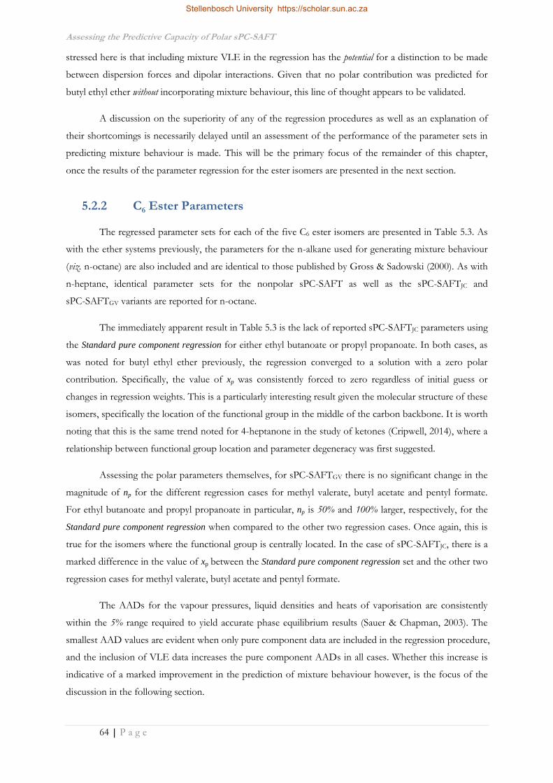
Assessing the Predictive Capacity of Polar sPC-SAFT
64 | P a g e
stressed here is that including mixture VLE in the regression has the potential for a distinction to be made
between dispersion forces and dipolar interactions. Given that no polar contribution was predicted for
butyl ethyl ether without incorporating mixture behaviour, this line of thought appears to be validated.
A discussion on the superiority of any of the regression procedures as well as an explanation of
their shortcomings is necessarily delayed until an assessment of the performance of the parameter sets in
predicting mixture behaviour is made. This will be the primary focus of the remainder of this chapter,
once the results of the parameter regression for the ester isomers are presented in the next section.
5.2.2 C6 Ester Parameters
The regressed parameter sets for each of the five C6 ester isomers are presented in Table 5.3. As
with the ether systems previously, the parameters for the n-alkane used for generating mixture behaviour
(viz. n-octane) are also included and are identical to those published by Gross & Sadowski (2000). As with
n-heptane, identical parameter sets for the nonpolar sPC-SAFT as well as the sPC-SAFTJC and
sPC-SAFTGV variants are reported for n-octane.
The immediately apparent result in Table 5.3 is the lack of reported sPC-SAFTJC parameters using
the Standard pure component regression for either ethyl butanoate or propyl propanoate. In both cases, as
was noted for butyl ethyl ether previously, the regression converged to a solution with a zero polar
contribution. Specifically, the value of xp was consistently forced to zero regardless of initial guess or
changes in regression weights. This is a particularly interesting result given the molecular structure of these
isomers, specifically the location of the functional group in the middle of the carbon backbone. It is worth
noting that this is the same trend noted for 4-heptanone in the study of ketones (Cripwell, 2014), where a
relationship between functional group location and parameter degeneracy was first suggested.
Assessing the polar parameters themselves, for sPC-SAFTGV there is no significant change in the
magnitude of np for the different regression cases for methyl valerate, butyl acetate and pentyl formate.
For ethyl butanoate and propyl propanoate in particular, np is 50% and 100% larger, respectively, for the
Standard pure component regression when compared to the other two regression cases. Once again, this is
true for the isomers where the functional group is centrally located. In the case of sPC-SAFTJC, there is a
marked difference in the value of xp between the Standard pure component regression set and the other two
regression cases for methyl valerate, butyl acetate and pentyl formate.
The AADs for the vapour pressures, liquid densities and heats of vaporisation are consistently
within the 5% range required to yield accurate phase equilibrium results (Sauer & Chapman, 2003). The
smallest AAD values are evident when only pure component data are included in the regression procedure,
and the inclusion of VLE data increases the pure component AADs in all cases. Whether this increase is
indicative of a marked improvement in the prediction of mixture behaviour however, is the focus of the
discussion in the following section.
Stellenbosch University https://scholar.sun.ac.za
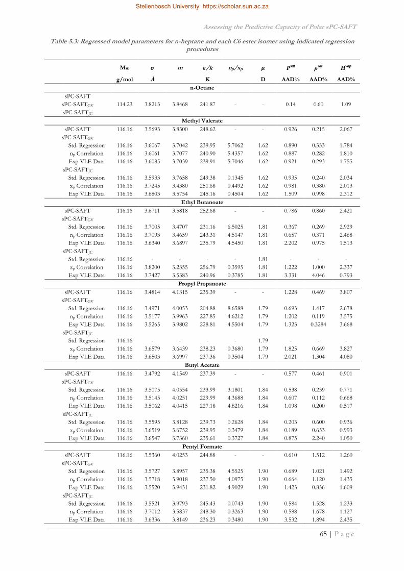
Assessing the Predictive Capacity of Polar sPC-SAFT
65 | P a g e
Table 5.3: Regressed model parameters for n-heptane and each C6 ester isomer using indicated regression procedures
MW σ m ε/k np/xp μ Psat ρsat Hvap
g/mol Å K D AAD% AAD% AAD%
n-Octane
sPC-SAFT
sPC-SAFTGV 114.23 3.8213 3.8468 241.87 - - 0.14 0.60 1.09
sPC-SAFTJC
Methyl Valerate
sPC-SAFT 116.16 3.5693 3.8300 248.62 - - 0.926 0.215 2.067
sPC-SAFTGV
Std. Regression 116.16 3.6067 3.7042 239.95 5.7062 1.62 0.890 0.333 1.784
np Correlation 116.16 3.6061 3.7077 240.90 5.4357 1.62 0.887 0.282 1.810
Exp VLE Data 116.16 3.6085 3.7039 239.91 5.7046 1.62 0.921 0.293 1.755
sPC-SAFTJC
Std. Regression 116.16 3.5933 3.7658 249.38 0.1345 1.62 0.935 0.240 2.034
xp Correlation 116.16 3.7245 3.4380 251.68 0.4492 1.62 0.981 0.380 2.013
Exp VLE Data 116.16 3.6803 3.5754 245.16 0.4504 1.62 1.509 0.998 2.312
Ethyl Butanoate
sPC-SAFT 116.16 3.6711 3.5818 252.68 - - 0.786 0.860 2.421
sPC-SAFTGV
Std. Regression 116.16 3.7005 3.4707 231.16 6.5025 1.81 0.367 0.269 2.929
np Correlation 116.16 3.7093 3.4659 243.31 4.5147 1.81 0.657 0.371 2.468
Exp VLE Data 116.16 3.6340 3.6897 235.79 4.5450 1.81 2.202 0.975 1.513
sPC-SAFTJC
Std. Regression 116.16 - - - - 1.81 - - -
xp Correlation 116.16 3.8200 3.2355 256.79 0.3595 1.81 1.222 1.000 2.337
Exp VLE Data 116.16 3.7427 3.5383 240.96 0.3785 1.81 3.331 4.046 0.793
Propyl Propanoate
sPC-SAFT 116.16 3.4814 4.1315 235.39 - - 1.228 0.469 3.807
sPC-SAFTGV
Std. Regression 116.16 3.4971 4.0053 204.88 8.6588 1.79 0.693 1.417 2.678
np Correlation 116.16 3.5177 3.9963 227.85 4.6212 1.79 1.202 0.119 3.575
Exp VLE Data 116.16 3.5265 3.9802 228.81 4.5504 1.79 1.323 0.3284 3.668
sPC-SAFTJC
Std. Regression 116.16 - - - - 1.79 - - -
xp Correlation 116.16 3.6579 3.6439 238.23 0.3680 1.79 1.825 0.669 3.827
Exp VLE Data 116.16 3.6503 3.6997 237.36 0.3504 1.79 2.021 1.304 4.080
Butyl Acetate
sPC-SAFT 116.16 3.4792 4.1549 237.39 - - 0.577 0.461 0.901
sPC-SAFTGV
Std. Regression 116.16 3.5075 4.0554 233.99 3.1801 1.84 0.538 0.239 0.771
np Correlation 116.16 3.5145 4.0251 229.99 4.3688 1.84 0.607 0.112 0.668
Exp VLE Data 116.16 3.5062 4.0415 227.18 4.8216 1.84 1.098 0.200 0.517
sPC-SAFTJC
Std. Regression 116.16 3.5595 3.8128 239.73 0.2628 1.84 0.203 0.600 0.936
xp Correlation 116.16 3.6519 3.6752 239.95 0.3479 1.84 0.189 0.653 0.993
Exp VLE Data 116.16 3.6547 3.7360 235.61 0.3727 1.84 0.875 2.240 1.050
Pentyl Formate
sPC-SAFT 116.16 3.5360 4.0253 244.88 - - 0.610 1.512 1.260
sPC-SAFTGV
Std. Regression 116.16 3.5727 3.8957 235.38 4.5525 1.90 0.689 1.021 1.492
np Correlation 116.16 3.5718 3.9018 237.50 4.0975 1.90 0.664 1.120 1.435
Exp VLE Data 116.16 3.5520 3.9431 231.82 4.9029 1.90 1.423 0.836 1.609
sPC-SAFTJC
Std. Regression 116.16 3.5521 3.9793 245.43 0.0743 1.90 0.584 1.528 1.233
np Correlation 116.16 3.7012 3.5837 248.30 0.3263 1.90 0.588 1.678 1.127
Exp VLE Data 116.16 3.6336 3.8149 236.23 0.3480 1.90 3.532 1.894 2.435
Stellenbosch University https://scholar.sun.ac.za
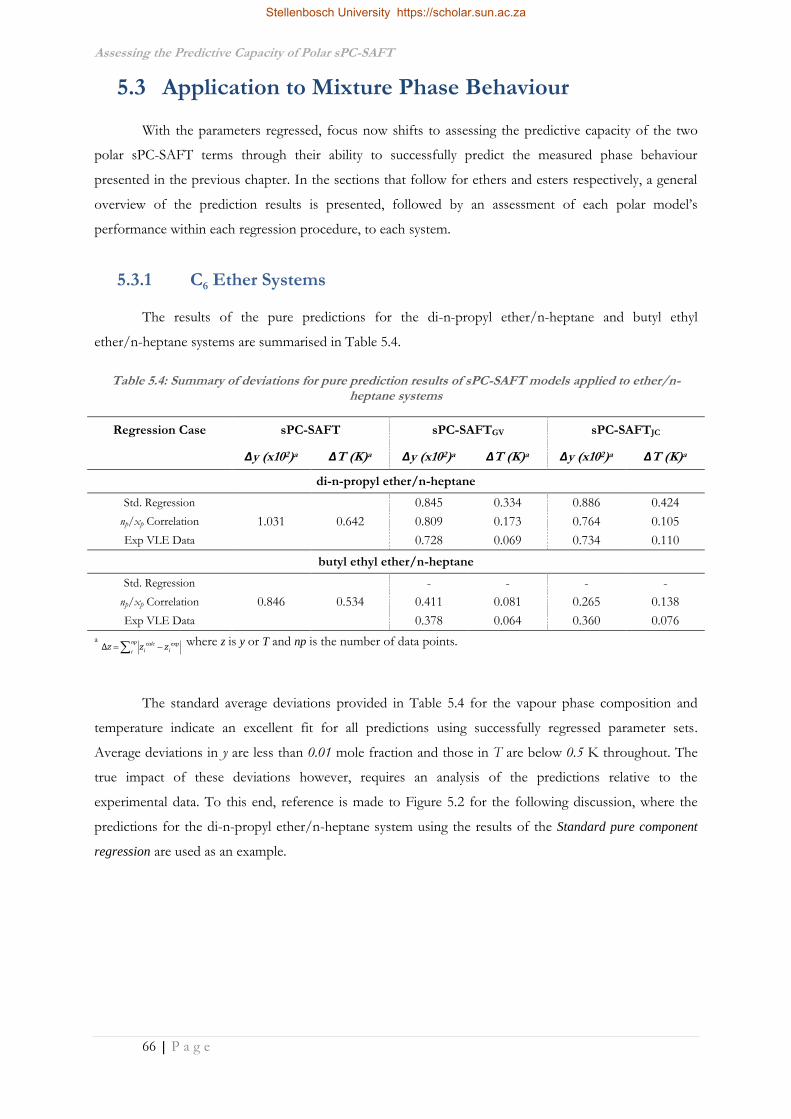
Assessing the Predictive Capacity of Polar sPC-SAFT
66 | P a g e
5.3 Application to Mixture Phase Behaviour
With the parameters regressed, focus now shifts to assessing the predictive capacity of the two
polar sPC-SAFT terms through their ability to successfully predict the measured phase behaviour
presented in the previous chapter. In the sections that follow for ethers and esters respectively, a general
overview of the prediction results is presented, followed by an assessment of each polar model’s
performance within each regression procedure, to each system.
5.3.1 C6 Ether Systems
The results of the pure predictions for the di-n-propyl ether/n-heptane and butyl ethyl
ether/n-heptane systems are summarised in Table 5.4.
Table 5.4: Summary of deviations for pure prediction results of sPC-SAFT models applied to ether/n-
heptane systems
Regression Case sPC-SAFT sPC-SAFTGV sPC-SAFTJC
Δy (x102)a ΔT (K)a Δy (x102)a ΔT (K)a Δy (x102)a ΔT (K)a
di-n-propyl ether/n-heptane
Std. Regression
1.031 0.642
0.845 0.334 0.886 0.424
np/xp Correlation 0.809 0.173 0.764 0.105
Exp VLE Data 0.728 0.069 0.734 0.110
butyl ethyl ether/n-heptane
Std. Regression
0.846 0.534
- - - -
np/xp Correlation 0.411 0.081 0.265 0.138
Exp VLE Data 0.378 0.064 0.360 0.076 a
expnp calci ii
z z zΔ where z is y or T and np is the number of data points.
The standard average deviations provided in Table 5.4 for the vapour phase composition and
temperature indicate an excellent fit for all predictions using successfully regressed parameter sets.
Average deviations in y are less than 0.01 mole fraction and those in T are below 0.5 K throughout. The
true impact of these deviations however, requires an analysis of the predictions relative to the
experimental data. To this end, reference is made to Figure 5.2 for the following discussion, where the
predictions for the di-n-propyl ether/n-heptane system using the results of the Standard pure component
regression are used as an example.
Stellenbosch University https://scholar.sun.ac.za

Assessing the Predictive Capacity of Polar sPC-SAFT
67 | P a g e
Figure 5.2: Predictions for the di-n-propyl ether/n-heptane systems at 60 kPa using parameter sets resulting from the standard pure component regression. Small but significant deviations of the model from the data are
highlighted, with the prediction of nonpolar sPC-SAFT included for comparison.
346.0
348.0
350.0
352.0
354.0
356.0
0.00 0.20 0.40 0.60 0.80 1.00
Tem
per
atu
re (
K)
Di-n-Propyl Ether Mole Fraction (x,y)
Experimental
sPC-SAFT
sPC-SAFT GV
sPC-SAFT JC
It is readily apparent that while only small deviations between the predictions of both
sPC-SAFTJC and sPC-SAFTGV with the experimental data exist, these small deviations actually result in
the predictions completely missing the phase envelope. This is a consequence of how narrow the phase
envelope is, resulting in a predicted liquid phase in agreement with the experimental vapour phase. This
does not necessarily condemn the predictive capacity of the models, but rather serves to illustrate that the
magnitude of average deviations in y and T should always be considered with respect to the system of
interest. Further, it suggests and stresses that there is no universal scale for deviations in these properties
that is indicative of an excellent model fit.
5.3.1.1 Standard Pure Component Regression
The results of the prediction based on the Standard pure component regression for each model
applied to di-n-propyl ether/n-heptane have already been presented in Figure 5.2. The results of the same
prediction applied to the x-y representation of the equilibrium data are presented in Figure 5.3. The
zeotropic behaviour of the system is well predicted in the x-y plot for this system, where even the
nonpolar sPC-SAFT prediction accurately represents the data. This suggests that errors in the model
prediction are limited to deviations in the temperature prediction.
Stellenbosch University https://scholar.sun.ac.za
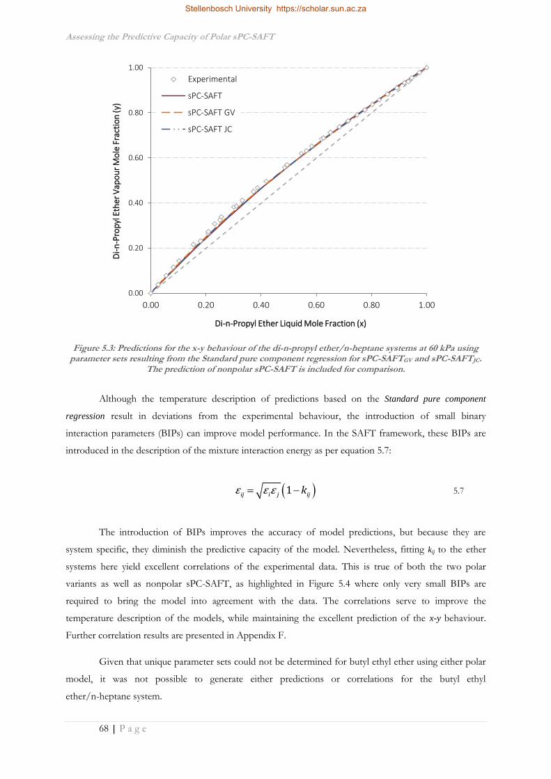
Assessing the Predictive Capacity of Polar sPC-SAFT
68 | P a g e
Although the temperature description of predictions based on the Standard pure component
regression result in deviations from the experimental behaviour, the introduction of small binary
interaction parameters (BIPs) can improve model performance. In the SAFT framework, these BIPs are
introduced in the description of the mixture interaction energy as per equation 5.7:
1ij i j ijkε ε ε 5.7
The introduction of BIPs improves the accuracy of model predictions, but because they are
system specific, they diminish the predictive capacity of the model. Nevertheless, fitting kij to the ether
systems here yield excellent correlations of the experimental data. This is true of both the two polar
variants as well as nonpolar sPC-SAFT, as highlighted in Figure 5.4 where only very small BIPs are
required to bring the model into agreement with the data. The correlations serve to improve the
temperature description of the models, while maintaining the excellent prediction of the x-y behaviour.
Further correlation results are presented in Appendix F.
Given that unique parameter sets could not be determined for butyl ethyl ether using either polar
model, it was not possible to generate either predictions or correlations for the butyl ethyl
ether/n-heptane system.
Figure 5.3: Predictions for the x-y behaviour of the di-n-propyl ether/n-heptane systems at 60 kPa using parameter sets resulting from the Standard pure component regression for sPC-SAFTGV and sPC-SAFTJC.
The prediction of nonpolar sPC-SAFT is included for comparison.
0.00
0.20
0.40
0.60
0.80
1.00
0.00 0.20 0.40 0.60 0.80 1.00
Di-
n-P
rop
yl E
ther
Vap
ou
r M
ole
Fra
ctio
n (
y)
Di-n-Propyl Ether Liquid Mole Fraction (x)
Experimental
sPC-SAFT
sPC-SAFT GV
sPC-SAFT JC
Stellenbosch University https://scholar.sun.ac.za

Assessing the Predictive Capacity of Polar sPC-SAFT
69 | P a g e
346
348
350
352
354
356
0.00 0.20 0.40 0.60 0.80 1.00
Tem
per
atu
re (K
)
Di-n-Propyl Ether Mole Fraction (x,y)
Experimental
sPC-SAFT (kij = 0.005)
sPC-SAFT GV (kij = 0.002)
sPC-SAFT JC (kij = 0.003)
0.00
0.20
0.40
0.60
0.80
1.00
0.00 0.20 0.40 0.60 0.80 1.00
Di-
n-P
rop
yl E
ther
Vap
ou
r M
ole
Fra
ctio
n (y
)
Di-n-Propyl Ether Liquid Mole Fraction (x)
Experimental
sPC-SAFT (kij = 0.005)
sPC-SAFT GV (kij = 0.002)
sPC-SAFT JC (kij = 0.003)
346
348
350
352
354
356
0.00 0.20 0.40 0.60 0.80 1.00
Tem
per
atu
re (K
)
Di-n-Propyl Ether Mole Fraction (x,y)
Experimental
sPC-SAFT
sPC-SAFT GV
sPC-SAFT JC
0.00
0.20
0.40
0.60
0.80
1.00
0.00 0.20 0.40 0.60 0.80 1.00
Di-
n-P
rop
yl E
ther
Vap
ou
r M
ole
Fra
ctio
n (y
)
Di-n-Propyl Ether Liquid Mole Fraction (x)
Experimental
sPC-SAFT
sPC-SAFT GV
sPC-SAFT JC
5.3.1.2 np/xp Correlation Regression
The resulting model predictions for the parameter sets where the polar parameters were fixed
using the correlations in equations 5.2 and 5.3 and the updated ether parameters in Table 5.1 are presented
in Figures 5.5 and 5.6 for the di-n-propyl ether/n-heptane and butyl ethyl ether/n-heptane systems
respectively. The improvement over the Standard pure component regression predictions is immediately
apparent, with both the T-xy and x-y representations in excellent agreement with the experimental data.
For the di-n-propyl ether/n-heptane system, both polar terms produce an excellent prediction of
the phase behaviour across the whole compositional range. For the butyl ethyl ether/n-heptane system,
sPC-SAFTGV similarly maintains the quality of its prediction throughout, while that of sPC-SAFTJC tends
Figure 5.4: Correlation results for di-n-propyl ether/n-heptane system at 60 kPa. [i.] Deviations in the temperature predictions are rectified. [ii.] The x-y prediction is largely unchanged.
[i.] [ii.]
Figure 5.5: [i.]T-xy and [ii.] x-y pure predictions for the di-n-propyl ether/n-heptane system at 60 kPa using the parameter set obtained by fixing the value of polar parameter (np, xp) and regression to pure
component data. The prediction of nonpolar sPC-SAFT is included for comparison.
[i.] [ii.]
Stellenbosch University https://scholar.sun.ac.za

Assessing the Predictive Capacity of Polar sPC-SAFT
70 | P a g e
0.00
0.20
0.40
0.60
0.80
1.00
0.00 0.20 0.40 0.60 0.80 1.00
Di-
n-P
rop
yl E
ther
Vap
ou
r M
ole
Fra
ctio
n (y
)
Di-n-Propyl Ether Liquid Mole Fraction (x)
Experimental
sPC-SAFT
sPC-SAFT GV
sPC-SAFT JC
348
350
352
354
356
0.00 0.20 0.40 0.60 0.80 1.00
Tem
per
atu
re (K
)
Butyl Ethyl Ether Mole Fraction (x,y)
Experimental
sPC-SAFT
sPC-SAFT GV
sPC-SAFT JC
346
348
350
352
354
356
0.00 0.20 0.40 0.60 0.80 1.00
Tem
per
atu
re (K
)
Di-n-Propyl Ether Mole Fraction (x,y)
Experimental
sPC-SAFT
sPC-SAFT GV
sPC-SAFT JC
to drift slightly as the ether concentration increases. This final observation is overly critical however, given
that no prediction was possible for this system using the results of the Standard pure component regression.
5.3.1.3 VLE Data Regression
The final results for the ether systems considered are those for the parameter sets determined
with the inclusion of VLE data in the regression procedure. The results for the di-n-propyl
ether/n-heptane and butyl ethyl ether/n-heptane systems using these parameter sets are presented in
Figures 5.7 and 5.8 respectively. The predictions of both sPC-SAFTJC and sPC-SAFTGV are identical and
in excellent agreement with the experimental data.
0.00
0.20
0.40
0.60
0.80
1.00
0.00 0.20 0.40 0.60 0.80 1.00
Bu
tyl E
thyl
Eth
er V
apo
ur
Mo
le F
ract
ion
(y)
Butyl Ethyl Ether Liquid Mole Fraction (x)
Experimental
sPC-SAFT
sPC-SAFT GV
sPC-SAFT JC
Figure 5.6: [i.]T-xy and [ii.] x-y pure predictions for the butyl ethyl ether/n-heptane system at 60 kPa using the parameter set obtained by fixing the value of polar parameter (np, xp) and regression to pure component
data. The prediction of nonpolar sPC--SAFT is included for comparison.
[i.] [ii.]
Figure 5.7: [i.]T-xy and [ii.] x-y pure predictions for the di-n-propyl ether/n-heptane system at 60 kPa using the parameter set obtained by incorporating VLE data in the regression procedure. The prediction of
nonpolar sPC-SAFT is included for comparison.
[i.] [ii.]
Stellenbosch University https://scholar.sun.ac.za

Assessing the Predictive Capacity of Polar sPC-SAFT
71 | P a g e
348
350
352
354
356
0.00 0.20 0.40 0.60 0.80 1.00
Tem
per
atu
re (K
)
Butyl Ethyl Ether Mole Fraction (x,y)
Experimental
sPC-SAFT
sPC-SAFT GV
sPC-SAFT JC
0.00
0.20
0.40
0.60
0.80
1.00
0.00 0.20 0.40 0.60 0.80 1.00B
uty
l Eth
yl E
ther
Vap
ou
r M
ole
Fra
ctio
n (y
)
Butyl Ethyl Ether Liquid Mole Fraction (x)
Experimental
sPC-SAFT
sPC-SAFT GV
sPC-SAFT JC
That this regression case provides the best prediction of the phase equilibrium results should be
no surprise, considering the parameters were fit to these data sets to begin with. The true test of these
parameter sets will be in their applicability to independently measured phase equilibria for systems other
than those considered here. This will be a focus of the discussion that follows in Section 5.4.
5.3.2 C6 Ester Systems
Discussion of the results of applying the regressed parameters for the five C6 ester isomers to the
measured mixture behaviour follows the same course as was presented for the ethers previously. The
results of the modelling exercise are summarised in Table 5.5.
Figure 5.8: [i.]T-xy and [ii.] x-y pure predictions for the butyl ethyl ether/n-heptane system at 60 kPa using the parameter set obtained by incorporating VLE data in the regression procedure The prediction of
nonpolar sPC--SAFT is included for comparison.
[i.] [ii.]
Stellenbosch University https://scholar.sun.ac.za

Assessing the Predictive Capacity of Polar sPC-SAFT
72 | P a g e
Table 5.5: Summary of deviations for pure prediction results of sPC-SAFT models applied to ester/n octane systems
Regression Case sPC-SAFT sPC-SAFTGV sPC-SAFTJC
Δy (x102)a ΔT (K)a Δy (x102)a ΔT (K)a Δy (x102)a ΔT (K)a
methyl valerate/n-octane
Std. Regression
3.972 2.494
0.970 0.083 3.665 2.198
np/xp Correlation 1.192 0.205 1.582 0.261
Exp VLE Data 1.009 0.080 1.251 0.094
ethyl butanoate/n-octane
Std. Regression
3.724 2.377
2.018 2.072 - -
np/xp Correlation 0.770 0.115 1.556 0.565
Exp VLE Data 0.785 0.083 0.770 0.154
propyl propanoate/n-octane
Std. Regression
3.060 2.295
5.402 5.035 - -
np/xp Correlation 0.437 0.296 0.638 0.552
Exp VLE Data 0.515 0.083 0.585 0.130
butyl acetate/n-octane
Std. Regression
3.929 2.960
2.374 1.609 2.052 1.216
np/xp Correlation 1.183 0.628 1.021 0.295
Exp VLE Data 0.658 0.088 0.568 0.100
pentyl formate/n-octane
Std. Regression
4.643 3.263
1.322 0.630 4.438 3.078
np/xp Correlation 1.876 1.059 2.031 0.936
Exp VLE Data 1.087 0.097 1.274 0.104
a expnp calc
i iiz z zΔ
where z is y or T and np is the number of data points.
Differences between the average deviations in y and T reported in Table 5.5 for nonpolar
sPC-SAFT and the two polar variants are more pronounced in the prediction of ester/n-alkane VLE than
for the ethers in the previous section. This is due to the presence of the minimum boiling azeotrope in all
five systems resulting from the strong positive deviations in these mixtures. The larger deviations in y and
T for the nonpolar sPC-SAFT model are due to the inability of the model to account for the azeotropic
behaviour in the system. The largest deviations are apparent for the sPC-SAFTGV prediction of the propyl
propanoate/n-octane system using the Standard pure component regression, although the nature of the
deviations is different. sPC-SAFTGV still accounts for the positive deviations in the mixture, but the
strength of these deviations are overestimated and the azeotropic temperature is under predicted, as
illustrated in Figure 5.9 [i.].
Stellenbosch University https://scholar.sun.ac.za

Assessing the Predictive Capacity of Polar sPC-SAFT
73 | P a g e
374
376
378
380
382
0.00 0.20 0.40 0.60 0.80 1.00
Tem
per
atu
re (K
)
Propyl Propanoate Mole Fraction (x,y)
Experimental
sPC-SAFT (kij = 0.017)
sPC-SAFT GV (kij = -0.036)
In cases where accurate pure predictions were not possible, BIPs were fit using the experimental
data. Figure 5.9 [ii.] highlights that even the nonpolar sPC-SAFT model can produce a qualitative fit of the
experimental data using appropriate binary interaction parameters. For the propyl propanoate example
provided, the correlation for sPC-SAFTGV provides a qualitative fit of the data, but the overall fit is not
good. This case was the exception rather than the rule in terms of successfully correlating the experimental
data, as is demonstrated in the supplementary correlation results in Appendix F. However, the relatively
poor quantitative fit of these correlations stresses the importance of generating the optimum parameter
set to begin with.
The assessment of correlation fits raises a further important point in the context of this work.
The example provided in Figure 5.9 lacks a corresponding correlation fit for sPC-SAFTJC. However, given
that no parameters could be regressed for propyl propanoate using the Standard pure component regression,
no prediction for this system was possible. Without a prediction to improve upon, or an interaction
energy parameter to fit kij to, a correlation of the system is not possible. The problem of parameter
degeneracy thus does not only affect the predictability of a system, but the ability to correlate that system
as well.
The presence of the azeotrope provides the most stringent test of the predictive capacity of the
thermodynamic models as accurate prediction of the azeotropic point is vital in industrial applications. In
light of this, the predicted azeotropic point for each model in each system, using each regression
procedure, is presented in Table 5.6. Discussion of the performance of each parameter set in representing
the azeotropic point is reserved for the following sections, where the performance of each parameter set
will be discussed as was the case for the ethers previously.
368
371
374
377
380
383
0.00 0.20 0.40 0.60 0.80 1.00
Tem
per
atu
re (K
)
Propyl Propanoate Mole Fraction (x,y)
Experimental
sPC-SAFT
sPC-SAFT GV
Figure 5.9: [i.] Pure prediction and [ii.] correlation of the propyl propanoate/n-octane system at 60 kPa using results of the standard pure component regression. The difference in the nature of the deviations in y
and T of nonpolar sPC-SAFT and polar sPC-SAFT are highlighted.
[i.] [ii.]
Stellenbosch University https://scholar.sun.ac.za

Assessing the Predictive Capacity of Polar sPC-SAFT
74 | P a g e
Table 5.6: Comparison between experimentally determined azeotropic points and the pure predictions of each model and regression case for ester/n-octane systems
Experimental
Regression Case
sPC-SAFTGV sPC-SAFTJC
Comp (mole% ester)
Temp (K) Comp
(mole% ester)
Temp (K) Comp
(mole% ester)
Temp (K)
methyl valerate/n-octane
40.9% 377.53
Std. Regression 41% 377.5 28% 380.7
np/xp Correlation 41% 377.8 41% 378.0
Exp VLE Data 41% 377.5 40% 377.7
ethyl butanoate/n-octane
60.5% 374.60
Std. Regression 55% 371.8 - -
np/xp Correlation 61% 374.5 68% 375.2
Exp VLE Data 61% 374.6 63% 374.6
propyl propanoate/n-octane
54.6% 375.44
Std. Regression 47% 369.4 - -
np/xp Correlation 58% 375.2 59% 374.8
Exp VLE Data 58% 375.5 58% 375.4
butyl acetate/n-octane
45.9% 376.55
Std. Regression 45% 378.7 45% 378.2
np/xp Correlation 45% 377.3 45% 376.9
Exp VLE Data 45% 376.5 45% 376.5
pentyl formate/n-octane
30.8% 378.32
Std. Regression 31% 378.9 NP* NP*
np/xp Correlation 28% 379.5 29% 379.5
Exp VLE Data 32% 378.3 32% 378.4
NP* - No azeotrope predicted
5.3.2.1 Standard Pure Component Regression
The results for the predictions of the parameter sets determined using the Standard pure
component regression procedure are presented graphically in Figures 5.10 to 5.14 for the five C6
ester/n-octane systems. Starting with the predictions for the methyl valerate system in Figure 5.10, the
first consideration is that the sPC-SAFTGV model produces an excellent pure prediction of the
experimental data, in both the T-xy and x-y representations of the data. The quality of this fit is reflected in
the accuracy with which the azeotropic point is predicted in Table 5.6. Considering the sPC-SAFTJC
prediction however, there is barely an improvement over the nonpolar sPC-SAFT prediction. While the
model does predict azeotropic behaviour, the azeotropic point is poorly predicted and this is reflected in
the large deviations in y and T reported in Table 5.5.
The predictions for the ethyl butanoate system in Figure 5.11 show a decline in the quality of the
sPC-SAFTGV prediction compared to the methyl valerate case. The increased deviation appears to be
predominantly in the representation of the temperature as Figure 5.11 [ii.] shows that the x-y data are still
fairly predicted. This is supported by the prediction of the azeotropic point, where the extent of the
positive deviations is over exaggerated, and the azeotropic temperature is under-predicted as a result. This
Stellenbosch University https://scholar.sun.ac.za

Assessing the Predictive Capacity of Polar sPC-SAFT
75 | P a g e
377
379
381
383
385
0.00 0.20 0.40 0.60 0.80 1.00
Tem
per
atu
re (K
)
Methyl Valerate Mole Fraction (x,y)
Experimental
sPC-SAFT
sPC-SAFT GV
sPC-SAFT JC
0.00
0.20
0.40
0.60
0.80
1.00
0.00 0.20 0.40 0.60 0.80 1.00
Met
hyl
Val
erat
e V
apo
ur
Mo
le F
ract
ion
(y)
Methyl Valerate Liquid Mole Fraction (x)
Experimental
sPC-SAFT
sPC-SAFT GV
sPC-SAFT JC
370
372
374
376
378
380
382
0.00 0.20 0.40 0.60 0.80 1.00
Tem
per
atu
re (K
)
Ethyl Butanoate Mole Fraction (x,y)
Experimental
sPC-SAFT
sPC-SAFT GV
sPC-SAFT JC
0.00
0.20
0.40
0.60
0.80
1.00
0.00 0.20 0.40 0.60 0.80 1.00
Eth
yl B
uta
no
ate
Vap
ou
r M
ole
Fra
ctio
n (y
)
Ethyl Butanoate Liquid Mole Fraction (x)
Experimental
sPC-SAFT
sPC-SAFT GV
sPC-SAFT JC
is still better than the case for sPC-SAFTJC where the inability to successfully generate a unique parameter
set meant that no prediction could be made.
The significant deviation of the sPC-SAFTGV prediction for the propyl propanoate mixture in
Figure 5.12 has already been highlighted previously. The azeotropic temperature is under-predicted by 5 K
and the x-y plot shows that these deviations are not limited to the prediction of the temperature. As with
the ethyl butanoate system however, the quality of this prediction is still an improvement over the case of
sPC-SAFTJC, where no prediction was possible given that no parameters could be regressed.
Predictions for the butyl acetate system in Figure 5.13 show a significant improvement in the
predictive capacity of the sPC-SAFTJC model, where the positive deviations are only slightly understated,
resulting in an over predicted azeotropic temperature. A similar trend is apparent for the sPC-SAFTGV
Figure 5.10: [i.]T-xy and [ii.] x-y pure predictions for the methyl valerate/n-octane system at 60 kPa using the standard pure component regression procedure. The prediction of nonpolar sPC-SAFT is included for
comparison.
[i.] [ii.]
Figure 5.11: [i.]T-xy and [ii.] x-y pure predictions for the ethyl butanoate/n-octane system at 60 kPa using the standard pure component regression procedure. The prediction of nonpolar sPC-SAFT is included for
comparison.
[i.] [ii.]
Stellenbosch University https://scholar.sun.ac.za

Assessing the Predictive Capacity of Polar sPC-SAFT
76 | P a g e
368
371
374
377
380
383
0.00 0.20 0.40 0.60 0.80 1.00
Tem
per
atu
re (K
)
Propyl Propanoate Mole Fraction (x,y)
Experimental sPC-SAFT
sPC-SAFT GV sPC-SAFT JC
0.00
0.20
0.40
0.60
0.80
1.00
0.00 0.20 0.40 0.60 0.80 1.00P
rop
yl P
rop
ano
ate
Vap
ou
r M
ole
Fra
ctio
n (y
)Propyl Propanoate Liquid Mole Fraction (x)
Experimental
sPC-SAFT
sPC-SAFT GV
sPC-SAFT JC
375
377
379
381
383
0.00 0.20 0.40 0.60 0.80 1.00
Tem
per
atu
re (K
)
Butyl Ethanoate Mole Fraction (x,y)
Experimental sPC-SAFT
sPC-SAFT GV sPC-SAFT JC
0.00
0.20
0.40
0.60
0.80
1.00
0.00 0.20 0.40 0.60 0.80 1.00
Bu
tyl E
than
oat
e V
apo
ur
Mo
le F
ract
ion
(y)
Butyl Ethanoate Liquid Mole Fraction (x)
Experimental
sPC-SAFT
sPC-SAFT GV
sPC-SAFT JC
prediction and this is the only case where sPC-SAFTJC outperforms sPC-SAFTGV. The azeotropic
composition is well correlated by both models as shown in Table 5.6 and the x-y behaviour in general is
well captured by both models in Figure 5.13 [ii.].
Finally, the results for the pentyl formate/n-octane mixture are presented in Figure 5.14, where
the sPC-SAFTGV model can be seen to maintain its good predictive capacity with an excellent prediction
of the observed equilibrium behaviour. While the azeotropic temperature is slightly over predicted, the
predicted composition is exactly right, with the x-y prediction underpinning this excellent fit. The
sPC-SAFTJC prediction on the other hand offers little improvement over the nonpolar sPC-SAFT model
predictions; no azeotrope is predicted and overall prediction of the phase behaviour is poor.
Figure 5.12: [i.]T-xy and [ii.] x-y pure predictions for the propyl propanoate/n-octane system at 60 kPa using the standard pure component regression procedure. The prediction of nonpolar sPC-SAFT is
included for comparison.
[i.] [ii.]
Figure 5.13: [i.]T-xy and [ii.] x-y pure predictions for the butyl acetate/n-octane system at 60 kPa using the standard pure component regression procedure. The prediction of nonpolar sPC-SAFT is included for
comparison.
[i.] [ii.]
Stellenbosch University https://scholar.sun.ac.za

Assessing the Predictive Capacity of Polar sPC-SAFT
77 | P a g e
378
380
382
384
386
388
0.00 0.20 0.40 0.60 0.80 1.00
Tem
per
atu
re (K
)
Pentyl Formate Mole Fraction (x,y)
Experimental
sPC-SAFT
sPC-SAFT GV
sPC-SAFT JC
0.00
0.20
0.40
0.60
0.80
1.00
0.00 0.20 0.40 0.60 0.80 1.00
Pe
nty
l Fo
rmat
e V
apo
ur
Mo
le F
ract
ion
(y)
Pentyl Formate Liquid Mole Fraction (x)
Experimental
sPC-SAFT
sPC-SAFT GV
sPC-SAFT JC
377
379
381
383
385
0.00 0.20 0.40 0.60 0.80 1.00
Tem
per
atu
re (K
)
Methyl Valerate Mole Fraction (x,y)
Experimental
sPC-SAFT (kij = 0.019)
sPC-SAFT GV (kij = 0)
sPC-SAFT JC (kij = 0.017)
378
380
382
384
386
388
0.00 0.20 0.40 0.60 0.80 1.00
Tem
per
atu
re (K
)
Pentyl Formate Mole Fraction (x,y)
Experimental
sPC-SAFT (kij = 0.025)
sPC-SAFT GV (kij = 0.004)
sPC-SAFT JC (kij = 0.023)
As previously highlighted, where poor pure predictions were in evidence, the introduction of
BIPs resulted in successful correlation of these systems. This is typified by the T-xy correlations for the
methyl valerate and pentyl formate systems in Figure 5.15 [i.] and [ii.] respectively. In particular, successful
correlation served to address the relatively poor overall predictive capacity of the sPC-SAFTJC parameter
sets based on the Standard pure component regression procedure. The correlation results and binary
interaction parameters for all systems are presented in Appendix F.
5.3.2.2 np/xp Correlation Regression
Employing the correlations developed by de Villiers (2011) for fixing the values of xp and np for
sPC-SAFTJC and sPC-SAFTGV respectively result in the VLE predictions of Figures 5.16 to 5.20. Applied
to the methyl valerate system in Figure 5.16, the improvement of the sPC-SAFTJC prediction over its
Standard pure component regression counterpart in Figure 5.10 is significant, to the point where the
Figure 5.14: [i.]T-xy and [ii.] x-y pure predictions for the pentyl formate/n-octane system at 60 kPa using the standard pure component regression procedure. The prediction of nonpolar sPC-SAFT is included for
comparison.
[i.] [ii.]
Figure 5.15: Correlation results for both models applied to the [i.] methyl valerate/n-octane and [ii.] pentyl formate/n-octane systems, highlighting the ability to introduce binary interaction parameters to produce
excellent correlation fits.
[i.] [ii.]
Stellenbosch University https://scholar.sun.ac.za

Assessing the Predictive Capacity of Polar sPC-SAFT
78 | P a g e
377
379
381
383
385
0.00 0.20 0.40 0.60 0.80 1.00
Tem
per
atu
re (K
)
Methyl Valerate Mole Fraction (x,y)
Experimental
sPC-SAFT
sPC-SAFT GV
sPC-SAFT JC
0.00
0.20
0.40
0.60
0.80
1.00
0.00 0.20 0.40 0.60 0.80 1.00
Met
hyl
Val
erat
e V
apo
ur
Mo
le F
ract
ion
(y)
Methyl Valerate Liquid Mole Fraction (x)
Experimental
sPC-SAFT
sPC-SAFT GV
sPC-SAFT JC
374
376
378
380
382
0.00 0.20 0.40 0.60 0.80 1.00
Tem
per
atu
re (K
)
Ethyl Butanoate Mole Fraction (x,y)
Experimental
sPC-SAFT
sPC-SAFT GV
sPC-SAFT JC
0.00
0.20
0.40
0.60
0.80
1.00
0.00 0.20 0.40 0.60 0.80 1.00
Eth
yl B
uta
no
ate
Vap
ou
r M
ole
Fra
ctio
n (y
)
Ethyl Butanoate Liquid Mole Fraction (x)
Experimental
sPC-SAFT
sPC-SAFT GV
sPC-SAFT JC
azeotropic point is successfully correlated to within 0.5 K. For sPC-SAFTGV, correlation of the azeotropic
point is only slightly deteriorated, maintaining good predictive capacity using this regression procedure.
The predictions for ethyl butanoate and propyl propanoate in Figures 5.17 and 5.18 respectively
offer particularly pleasing results. There is significant improvement in the performance of sPC-SAFTGV in
both cases, where the azeotropic point is no longer overshot and the data is almost perfectly predicted.
Further, sPC-SAFTJC is allowed to make good qualitative predictions for both isomers where none were
possible using the Standard pure component regression procedure. In both cases, the models slightly under
predict the pure component boiling points (consistent with the marginally increased AADs for the vapour
pressures in Table 5.3) which serve to skew their predictions in the high ester concentration space.
However, these small temperature deviations (~0.6 K) only appear significant due to the small
temperature range of the phase envelopes as a whole.
Figure 5.16: [i.]T-xy and [ii.] x-y pure predictions for the methyl valerate/n-octane system at 60 kPa using the parameter set obtained by fixing the value of polar parameter (np, xp) and regression to pure component
data. The prediction of nonpolar sPC-SAFT is included for comparison.
[i.] [ii.]
Figure 5.17: [i.]T-xy and [ii.] x-y pure predictions for the ethyl butanoate/n-octane system at 60 kPa using the parameter set obtained by fixing the value of polar parameter (np, xp) and regression to pure component
data. The prediction of nonpolar sPC-SAFT is included for comparison.
[i.] [ii.]
Stellenbosch University https://scholar.sun.ac.za

Assessing the Predictive Capacity of Polar sPC-SAFT
79 | P a g e
374
376
378
380
382
0.00 0.20 0.40 0.60 0.80 1.00
Tem
per
atu
re (K
)
Propyl Propanoate Mole Fraction (x,y)
Experimental
sPC-SAFT
sPC-SAFT GV
sPC-SAFT JC
0.00
0.20
0.40
0.60
0.80
1.00
0.00 0.20 0.40 0.60 0.80 1.00
Pro
pyl
Pro
pan
oat
e V
apo
ur
Mo
le F
ract
ion
(y)
Propyl Propanoate Liquid Mole Fraction (x)
Experimental
sPC-SAFT
sPC-SAFT GV
sPC-SAFT JC
375
377
379
381
383
0.00 0.20 0.40 0.60 0.80 1.00
Tem
per
atu
re (K
)
Butyl Ethanoate Mole Fraction (x,y)
Experimental sPC-SAFT
sPC-SAFT GV sPC-SAFT JC
0.00
0.20
0.40
0.60
0.80
1.00
0.00 0.20 0.40 0.60 0.80 1.00
Bu
tyl E
than
oat
e V
apo
ur
Mo
le F
ract
ion
(y)
Butyl Ethanoate Liquid Mole Fraction (x)
Experimental
sPC-SAFT
sPC-SAFT GV
sPC-SAFT JC
378
380
382
384
386
388
0.00 0.20 0.40 0.60 0.80 1.00
Tem
per
atu
re (K
)
Pentyl Formate Mole Fraction (x,y)
Experimental
sPC-SAFT
sPC-SAFT GV
sPC-SAFT JC
0.00
0.20
0.40
0.60
0.80
1.00
0.00 0.20 0.40 0.60 0.80 1.00
Pe
nty
l Fo
rmat
e V
apo
ur
Mo
le F
ract
ion
(y)
Pentyl Formate Liquid Mole Fraction (x)
Experimental
sPC-SAFT
sPC-SAFT GV
sPC-SAFT JC
Figure 5.18: [i.]T-xy and [ii.] x-y pure predictions for the propyl propanoate/n-octane system at 60 kPa using the parameter set obtained by fixing the value of polar parameter (np, xp) and regression to pure
component data. The prediction of nonpolar sPC-SAFT is included for comparison.
[i.] [ii.]
Figure 5.19: [i.]T-xy and [ii.] x-y pure predictions for the butyl acetate/n-octane system at 60 kPa using the parameter set obtained by fixing the value of polar parameter (np, xp) and regression to pure component
data. The prediction of nonpolar sPC-SAFT is included for comparison.
[i.] [ii.]
Figure 5.20: [i.]T-xy and [ii.] x-y pure predictions for the pentyl formate/n-octane system at 60 kPa using the parameter set obtained by fixing the value of polar parameter (np, xp) and regression to pure component
data. The prediction of nonpolar sPC-SAFT is included for comparison.
[i.] [ii.]
Stellenbosch University https://scholar.sun.ac.za

Assessing the Predictive Capacity of Polar sPC-SAFT
80 | P a g e
377
379
381
383
385
0.00 0.20 0.40 0.60 0.80 1.00
Tem
per
atu
re (K
)
Methyl Valerate Mole Fraction (x,y)
Experimental
sPC-SAFT
sPC-SAFT GV
sPC-SAFT JC
0.00
0.20
0.40
0.60
0.80
1.00
0.00 0.20 0.40 0.60 0.80 1.00
Met
hyl
Val
erat
e V
apo
ur
Mo
le F
ract
ion
(y)
Methyl Valerate Liquid Mole Fraction (x)
Experimental
sPC-SAFT
sPC-SAFT GV
sPC-SAFT JC
The phase behaviour in the butyl acetate system was qualitatively well predicted by both models
using the Standard pure component regression parameter sets and Figure 5.19 shows further improvement
in the temperature description of the predictions of both models when the values of the polar parameters
are fixed. As was the case for the previous regression procedure, it is the only system for which the
prediction of sPC-SAFTJC outperforms that of sPC-SAFTGV, but both models still accurately account for
the azeotropic point.
Predictions of the pentyl formate/n-octane phase behaviour present some mixed results. The
prediction of sPC-SAFTGV is noticeably inferior to the previous regression case, but the prediction is still
qualitatively correct. The x-y behaviour is well predicted, it is just the temperature dependence which is
has suffered using this regression alternative. This is reflected in the model’s description of the azeotropic
point in Table 5.6 where the composition is correct but the temperature is 1.5 K too high. sPC-SAFTJC
offers an identical prediction, but in this case the prediction is a marked improvement over the Standard
pure component regression case in Figure 5.14, where no azeotropic behaviour was predicted.
5.3.2.3 VLE Data Regression
The prediction results for the parameter sets determined by including the measured VLE data for
the respective ester/n-octane systems are presented in Figures 5.21 to 5.25. It is apparent that inclusion of
the VLE data brings the predictions of both sPC-SAFTJC and sPC-SAFTGV into precise agreement with
the experimental data for all five systems considered. Even the prediction of the propyl propanoate
system, where increased deviations in the pure component vapour pressure tended to skew the predictions
of both models previously, can be seen to be brought into agreement with the experimental data.
Figure 5.21: [i.]T-xy and [ii.] x-y pure predictions for the methyl valerate/n-octane system at 60 kPa using
the parameter set obtained by incorporating VLE data in the regression procedure The prediction of nonpolar sPC-SAFT is included for comparison.
[i.] [ii.]
Stellenbosch University https://scholar.sun.ac.za

Assessing the Predictive Capacity of Polar sPC-SAFT
81 | P a g e
374
376
378
380
382
0.00 0.20 0.40 0.60 0.80 1.00
Tem
per
atu
re (K
)
Ethyl Butanoate Mole Fraction (x,y)
Experimental
sPC-SAFT
sPC-SAFT GV
sPC-SAFT JC
0.00
0.20
0.40
0.60
0.80
1.00
0.00 0.20 0.40 0.60 0.80 1.00
Eth
yl B
uta
no
ate
Vap
ou
r M
ole
Fra
ctio
n (y
)
Ethyl Butanoate Liquid Mole Fraction (x)
Experimental
sPC-SAFT
sPC-SAFT GV
sPC-SAFT JC
374
376
378
380
382
0.00 0.20 0.40 0.60 0.80 1.00
Tem
per
atu
re (K
)
Propyl Propanoate Mole Fraction (x,y)
Experimental
sPC-SAFT
sPC-SAFT GV
sPC-SAFT JC
0.00
0.20
0.40
0.60
0.80
1.00
0.00 0.20 0.40 0.60 0.80 1.00
Pro
pyl
Pro
pan
oat
e V
apo
ur
Mo
le F
ract
ion
(y)
Propyl Propanoate Liquid Mole Fraction (x)
Experimental
sPC-SAFT
sPC-SAFT GV
sPC-SAFT JC
375
377
379
381
383
0.00 0.20 0.40 0.60 0.80 1.00
Tem
per
atu
re (K
)
Butyl Ethanoate Mole Fraction (x,y)
Experimental sPC-SAFT
sPC-SAFT GV sPC-SAFT JC
0.00
0.20
0.40
0.60
0.80
1.00
0.00 0.20 0.40 0.60 0.80 1.00
Bu
tyl E
than
oat
e V
apo
ur
Mo
le F
ract
ion
(y)
Butyl Ethanoate Liquid Mole Fraction (x)
Experimental
sPC-SAFT
sPC-SAFT GV
sPC-SAFT JC
Figure 5.22: [i.]T-xy and [ii.] x-y pure predictions for the ethyl butanoate/n-octane system at 60 kPa using the parameter set obtained by incorporating VLE data in the regression procedure The prediction of
nonpolar sPC-SAFT is included for comparison.
[i.] [ii.]
Figure 5.23: [i.]T-xy and [ii.] x-y pure predictions for the propyl propanoate/n-octane system at 60 kPa using the parameter set obtained by incorporating VLE data in the regression procedure The prediction of
nonpolar sPC-SAFT is included for comparison.
[i.] [ii.]
Figure 5.24: [i.]T-xy and [ii.] x-y pure predictions for the butyl acetate/n-octane system at 60 kPa using the parameter set obtained by incorporating VLE data in the regression procedure The prediction of nonpolar
sPC-SAFT is included for comparison.
[i.] [ii.]
Stellenbosch University https://scholar.sun.ac.za

Assessing the Predictive Capacity of Polar sPC-SAFT
82 | P a g e
378
380
382
384
386
388
0.00 0.20 0.40 0.60 0.80 1.00
Tem
per
atu
re (K
)
Pentyl Formate Mole Fraction (x,y)
Experimental
sPC-SAFT
sPC-SAFT GV
sPC-SAFT JC
0.00
0.20
0.40
0.60
0.80
1.00
0.00 0.20 0.40 0.60 0.80 1.00
Pe
nty
l Fo
rmat
e V
apo
ur
Mo
le F
ract
ion
(y)
Pentyl Formate Liquid Mole Fraction (x)
Experimental
sPC-SAFT
sPC-SAFT GV
sPC-SAFT JC
As with the results for the ethers previously, parameter sets of this regression procedure produced
the best predictions for all the ester mixtures considered as a group. This result is to be expected however,
as it was these same systems that were included in the regression procedure to begin with. A true test of
these parameter sets however, will be their successful application to independently measured systems
comprising these isomers, which is highlighted in the next section.
5.4 Performance of Polar sPC-SAFT Applied to
Structural Isomers
With application of the regressed parameter sets to the phase equilibrium data performed in the
previous section, it is possible to highlight and discuss observed trends in the predictive capacity of the
polar sPC-SAFT models here. As with the structure of this chapter thus far, the discussion of the ether
systems will be presented first, followed by that of the esters.
5.4.1 C6 Ether Systems
Ethers are considered particularly difficult components to model due to the very small, but still
significant contribution of this functional group’s dipole moment. The validity of this argument was
highlighted in the modelling procedure here, where the positive deviations from ideality of the di-n-propyl
ether/n-heptane and butyl ethyl ether/n-heptane systems were not easily accounted for. The emphasis of
this phase of the study however, was on the ability of the models to accurately account for the differences
in phase behaviour between different structural isomers of polar molecules. This focus was most readily
addressed in the results of the Standard pure component regression procedure.
Figure 5.25: [i.]T-xy and [ii.] x-y pure predictions for the pentyl formate/n-octane system at 60 kPa using the parameter set obtained by incorporating VLE data in the regression procedure The prediction of
nonpolar sPC-SAFT is included for comparison.
[i.] [ii.]
Stellenbosch University https://scholar.sun.ac.za

Assessing the Predictive Capacity of Polar sPC-SAFT
83 | P a g e
5.4.1.1 Shortcomings of the Standard Pure Component Regression
The inability of either polar sPC-SAFT variant to generate unique parameter sets for butyl ethyl
ether using only pure component data in the regression procedure serves to re-enforce trends witnessed
for heptanone isomers previously (Cripwell, 2014). In the case of the ketones, a systematic trend was
observed for the deterioration of model predictions and the associated ability to generate unique
component parameters (the latter specifically for sPC-SAFTJC). This trend was attributed to the shifting of
the carbonyl group from the terminal end to the centre of the carbon chain. In the case of the ethers
considered here, it is difficult to establish a trend when only two isomers are considered. Through
consultation of Figure 5.26 however, it is apparent that the “trend” for ethers is juxtaposed to that for
ketones. Here, the direction of the graduated red lines indicate deterioration of model predictions relative
to the different functional group locations.
For ketones previously, a unique parameter set could not be determined for the isomer with the
centrally located functional group, viz. 4-heptanone. For ethers here however, it is the isomer with the
more terminally located functional group, viz. butyl ethyl ether, which presents this problem. This suggests
that the trend in parameter degeneracy being linked to functional group location needs to be reassessed
and restructured.
The starting point here is the line of thought introduced in Chapter 4. It was remarked upon that
as the alkoxy group shifts from the centre of the molecule (di-n-propyl ether) to the terminal methyl
group (pentyl methyl ether), the boiling point of the ether approaches the boiling point of the equivalent
weight n-alkane. If a similar analysis is performed for the heptanone isomers, we find that as the carbonyl
group shifts from the centre of the molecule (4-heptanone) to the terminal ethyl group (2-heptanone), the
boiling point of the ketone departs from that of the equivalent weight n-alkane, as highlighted in Table 5.7.
Figure 5.26: Observable trend in the deterioration of model predictions using the standard regression procedure for ethers (top) and ketones (bottom) as a function of functional group location. Skeletal
structures presented from left to right following shift of respective functional groups from terminal end to centre of the chain.
Butyl Ethyl Ether Di-n-Propyl Ether
2-Heptanone 3-Heptanone 4-Heptanone
Deterioration
Deterioration
Stellenbosch University https://scholar.sun.ac.za
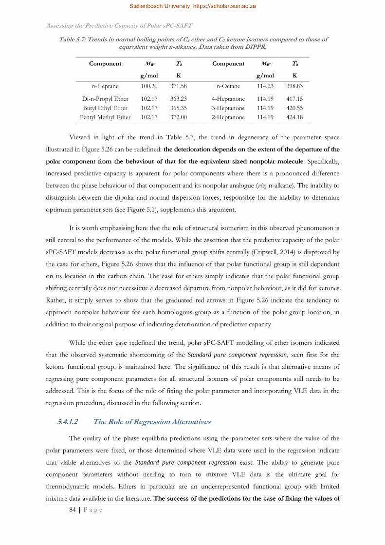
Assessing the Predictive Capacity of Polar sPC-SAFT
84 | P a g e
Table 5.7: Trends in normal boiling points of C6 ether and C7 ketone isomers compared to those of equivalent weight n-alkanes. Data taken from DIPPR.
Component MW Tb Component MW Tb
g/mol K g/mol K
n-Heptane 100.20 371.58 n-Octane 114.23 398.83
Di-n-Propyl Ether 102.17 363.23 4-Heptanone 114.19 417.15
Butyl Ethyl Ether 102.17 365.35 3-Heptanone 114.19 420.55
Pentyl Methyl Ether 102.17 372.00 2-Heptanone 114.19 424.18
Viewed in light of the trend in Table 5.7, the trend in degeneracy of the parameter space
illustrated in Figure 5.26 can be redefined: the deterioration depends on the extent of the departure of the
polar component from the behaviour of that for the equivalent sized nonpolar molecule. Specifically,
increased predictive capacity is apparent for polar components where there is a pronounced difference
between the phase behaviour of that component and its nonpolar analogue (viz. n-alkane). The inability to
distinguish between the dipolar and normal dispersion forces, responsible for the inability to determine
optimum parameter sets (see Figure 5.1), supplements this argument.
It is worth emphasising here that the role of structural isomerism in this observed phenomenon is
still central to the performance of the models. While the assertion that the predictive capacity of the polar
sPC-SAFT models decreases as the polar functional group shifts centrally (Cripwell, 2014) is disproved by
the case for ethers, Figure 5.26 shows that the influence of that polar functional group is still dependent
on its location in the carbon chain. The case for ethers simply indicates that the polar functional group
shifting centrally does not necessitate a decreased departure from nonpolar behaviour, as it did for ketones.
Rather, it simply serves to show that the graduated red arrows in Figure 5.26 indicate the tendency to
approach nonpolar behaviour for each homologous group as a function of the polar group location, in
addition to their original purpose of indicating deterioration of predictive capacity.
While the ether case redefined the trend, polar sPC-SAFT modelling of ether isomers indicated
that the observed systematic shortcoming of the Standard pure component regression, seen first for the
ketone functional group, is maintained here. The significance of this result is that alternative means of
regressing pure component parameters for all structural isomers of polar components still needs to be
addressed. This is the focus of the role of fixing the polar parameter and incorporating VLE data in the
regression procedure, discussed in the following section.
5.4.1.2 The Role of Regression Alternatives
The quality of the phase equilibria predictions using the parameter sets where the value of the
polar parameters were fixed, or those determined where VLE data were used in the regression indicate
that viable alternatives to the Standard pure component regression exist. The ability to generate pure
component parameters without needing to turn to mixture VLE data is the ultimate goal for
thermodynamic models. Ethers in particular are an underrepresented functional group with limited
mixture data available in the literature. The success of the predictions for the case of fixing the values of
Stellenbosch University https://scholar.sun.ac.za

Assessing the Predictive Capacity of Polar sPC-SAFT
85 | P a g e
325
335
345
355
365
0.00 0.20 0.40 0.60 0.80 1.00
Tem
per
atu
re (K
)
Acetone Mole Fraction (x,y)
Resa et al. (1995)
sPC-SAFT GV
sPC-SAFT JC
0.23
0.26
0.29
0.32
0.35
0.38
0.00 0.20 0.40 0.60 0.80 1.00
Pre
ssu
re (k
Pa)
2-Butanone Mole Fraction (x,y)
Garriga et al. (1999)
sPC-SAFT GV
sPC-SAFT JC
xp/np is thus a particularly important result. Improvement of the prediction behaviour compared to the
Standard pure component regression case and comparable performance with the parameter set where VLE
data were included in the regression procedure serve to validate this regression alternative.
Given that the constants for ethers (Table 5.1) were determined and applied here for the first time
is of further significance. The values for np larger than 1 again serve to validate the decision to make the
parameter adjustable in the regression, as was the case for other functional groups. This correlation has
already been shown to yield good results for aliphatic ketones, cyclic ketones, esters and aldehydes, so its
successful extension to the ether functional group is a significant next step.
The ability to successfully generate a unique parameter set does not necessarily imply universal
applicability however. This is an important point, particularly for the parameter set determined by
including the respective ether/n-heptane data sets in the regression procedure. Successful prediction of
the data used in the regression of the parameters does not guarantee that similar success will be achieved
when applied to other mixtures. To this end, the applicability of the regressed parameters was tested
through prediction of the di-n-propyl ether/acetone and di-n-propyl ether/2-butanone data of Resa et al.
(1995) and Garriga et al. (1999) respectively, the results of which are presented in Figure 5.27. A similar
test of the butyl ethyl ether parameters was not possible given the lack of mixture data for this component.
The parameters for the ketones in these systems are those published by de Villiers et al. (2011),
with the parameter set based on the inclusion of the measured VLE data chosen for di-n-propyl ether.
Predictive capacity in these polar/polar systems is maintained for both models with excellent predictions
in evidence, and the behaviour in the high ether composition space is particularly good. The quality of
these pure predictions demonstrates that the regressed parameters are in fact appropriate beyond the
system to which they were fit and gives a measure of confidence to the universal applicability of the
parameter set.
Figure 5.27: Application of the VLE Data parameter set for di-n-propyl ether to the independently measured [i.] acetone/DNPE and [ii.] 2-butanone/DNPE data. Universal applicability of the parameter
set is highlighted.
[i.] [ii.]
Stellenbosch University https://scholar.sun.ac.za

Assessing the Predictive Capacity of Polar sPC-SAFT
86 | P a g e
Figure 5.28: Contributions of each term to the reduced chemical potential of pentyl formate at T = 298.15 K using parameters of the standard pure component regression. Underestimation of the polar contribution for
sPC-SAFTJC is highlighted.
-50
-40
-30
-20
-10
0
10
20
30
40
50
Hard Sphere Chain Dispersion Polar
Re
du
ced
Ch
emic
al P
ote
nti
al
sPC-SAFT
sPC-SAFT + GV Polar (Standard)
sPC-SAFT + JC Polar (Standard)
5.4.2 C6 Ester Systems
The structure of the ester functional group inherently allows for a greater degree of structural
isomerism. This results in a less intuitive relationship with the functional group location for determining
the most and least polar isomers. These characteristics thus provide the greatest scope for testing the
predictive capacity of the polar sPC-SAFT models using structural isomerism as the assessment criterion.
As with the ether case, the predictive capacity of sPC-SAFTJC and sPC-SAFTGV were most stringently
tested by the results of the Standard pure component regression.
5.4.2.1 Shortcomings of the Standard Pure Component Regression
The sPC-SAFTJC predictions using the Standard pure component regression parameter sets provide
the most compelling results here. Broad minima in the regression function were encountered for both
ethyl butanoate and propyl propanoate, resulting in an inability to generate a prediction of the mixture
data at all. Of the remaining three isomers for which parameters could be regressed, only the prediction of
butyl acetate was in qualitative agreement with the experimental data. For methyl valerate and pentyl
formate, the strength of the polar forces was underestimated (Figure 5.28) leading the model to yield only
slightly better predictions than the nonpolar sPC-SAFT model. Analysis of the regressed parameters
(Table 5.3) reinforce this argument, where the regressed values of xp (0.13 for methyl valerate, 0.07 for
pentyl formate) are significantly smaller than those for the other two regression cases (~0.45 and ~0.34,
respectively) which yielded significantly improved predictions of the mixture behaviour.
Considering the performance of the sPC-SAFTGV model, the notably superior predictive capacity
of these predictions is evident, although a trend is apparent in the prediction quality. In fact, the quality of
Stellenbosch University https://scholar.sun.ac.za

Assessing the Predictive Capacity of Polar sPC-SAFT
87 | P a g e
the predictions follows much the same trend as the boiling point/polar strength trend for the isomers
presented in Figure 4.13 of the previous chapter. Specifically, the best predictions are in evidence for the
two most polar isomers and deteriorate systematically with decreasing strength of the polar forces as
depicted in Figure 5.29.
The systematic decline in the accuracy of sPC-SAFTGV’s predictions with the shifting functional
group maintains the trends seen for ketones and ethers previously. The same conclusion can be drawn
from the degeneracy of the parameter space for sPC-SAFTJC when considering the least polar isomers.
Specifically, the quality of the model predictions and the ability to generate unique parameter sets is
shown to once again be dependent on the polar strength of the isomer in question. Furthermore, the
case for esters mirrors that for ketones where the poorest predictions and broad minima in objective
functions are apparent for the isomers where the functional group is located in the middle of the chain.
These results lend a degree of confidence to the assertion that these trends can now be considered a
systematic problem for all polar functional groups.
5.4.2.2 The Role of Regression Alternatives
It has already been demonstrated that deviations in the model predictions based on parameters
from the Standard pure component regression can largely be overcome by the introduction of a small binary
interaction parameter to yield accurate correlation results. However, the need for accurate phase
equilibrium data to fit the binary interaction parameters to is the same caveat for including VLE data in
Figure 5.29: Deterioration of model predictions using the standard regression procedure for esters as a function of functional group location and polar strength. Structures presented from top to bottom follow
shift of functional groups from terminal end to centre of the chain and following boiling point trend.
Methyl Valerate
Ethyl ButanoatePropyl Propanoate
Butyl Acetate
Pentyl Formate
Det
erio
rati
on
Stellenbosch University https://scholar.sun.ac.za

Assessing the Predictive Capacity of Polar sPC-SAFT
88 | P a g e
the regression procedure to begin with. To this end, the results for predictions using the parameter sets
where the value of the polar parameters were fixed, or those determined by incorporating VLE data in the
regression, offer more viable and reliable alternatives.
The results based on the parameter sets where xp/np are fixed produce particularly interesting
results, given that parameter sets for other esters based on this correlation were not included in the
previous published work (de Villiers, 2011; de Villiers et al. 2014). The parameters based on the
correlations in equations 5.2 and 5.3 provide consistent qualitative predictions for all five isomers with
improved predictions in evidence for most cases. Some small bias is apparent however for isomers with
more centrally located functional groups. This can be readily explained by the nature of the generation of
the constants for the esters in Table 5.1.
The lack of experimental data for all isomers of a given molecular weight ester, and indeed other
polar functional groups, has already been cited as motivation for performing this study. Where such data
exists, it is largely limited to smaller components or systems of industrial interest (e.g. acetates).
Furthermore, the functional group constants for the correlations in equations 5.2 and 5.3 were fit to
parameter sets that were successfully regressed using such available VLE data in the regression procedure.
Thus, considering the case of esters here, de Villiers (2011) only incorporated parameters sets for
components up to C6 in the determination of the functional group constants. Of these largest esters, only
propyl propanoate and butyl acetate were considered given data availability. This work has already shown
that methyl and formate type esters exhibit notably different phase behaviour compared to the other, less
polar isomers. Thus application of these correlations to the likes of pentyl formate yields an extrapolation
of the correlation results, rather than interpolation for the more prevalent acetates and ethyl esters, which
produce larger deviations in the witnessed predictions.
Nevertheless, these deviations do not markedly dissuade the quality of the predictions given that
only pure component data are included in the regression. The ability of this regression alternative to offer
unique parameters yielding excellent predictions of mixture phase behaviour, in lieu of available
experimental data, is necessarily emphasised.
As with the ketones and ethers previously, parameter sets where VLE data is incorporated in the
regression procedure yield the best prediction of the measured phase behaviour, although their
applicability beyond the systems measured here need to be tested. To this end, the parameters were used
to predict independently measured phase behaviour, the results of which are summarised in Table 5.7.
Stellenbosch University https://scholar.sun.ac.za

Assessing the Predictive Capacity of Polar sPC-SAFT
89 | P a g e
392
399
406
413
420
427
0.00 0.20 0.40 0.60 0.80 1.00
Tem
per
atu
re (K
)
Ethyl Butanoate Mole Fraction (x,y)
Ríos et al. (2012)
sPC-SAFT GV
sPC-SAFT JC
370
377
384
391
398
0.00 0.20 0.40 0.60 0.80 1.00
Tem
per
atu
re (K
)
Propyl Propanoate Mole Fraction (x,y)
Ortega et al. (2001)
sPC-SAFT GV
sPC-SAFT JC
Table 5.8: Deviations for the predictions obtained by applying the parameter sets determined here to independently measured ester/n-alkane and ester/ester VLE data.
System sPC-SAFTGV sPC-SAFTJC
Data Reference Δy (x102)a ΔT (K)a Δy (x102)a ΔT (K)a
Ester/n-Alkane Systems
methyl valerate/n-heptane 0.833 0.326 1.028 0.397 Ortega et al. (2003)
ethyl butanoate/n-nonane 0.267 0.350 0.189 0.347 Ríos et al. (2012)
propyl propanoate/n-heptane 0.888 0.220 0.911 0.284 Ortega et al. (2001)
butyl acetate/n-hexane 1.233 1.181 1.483 1.331 Feng et al. (1998)
Ester/Ester Systems
butyl acetate/ethyl acetate 0.487 0.464 0.573 0.462 Shono & Kanazawa (1969)
butyl acetate/butyl formate 0.917 0.528 0.951 0.569 Shaburov et al. (1971)
a expnp calc
i iiz z zΔ
where z is y or T and np is the number of data points.
The parameters for ethyl acetate and butyl formate in these systems are those determined by de
Villiers et al. (2011), with their applicability thus tested in a similar fashion. From the model fits in
Figures 5.30 and 5.31, where selected systems from Table 5.8 are presented for both ester/n-alkane and
ester/ester systems respectively, it is clearly demonstrated that the determined parameters for the esters
are applicable beyond the system to which they were fit. Predictive capacity is maintained in both
ester/n-alkane systems as well as ester/ester mixtures. This incorporates the effects of both
nonpolar/polar and polar/polar interactions between different components.
Figure 5.30: Application of the VLE Data parameter sets for C6 esters to independently measured ester/n-alkane data: [i.] ethyl butanoate/n-nonane and [ii.] propyl propanoate/n-heptane. Universal applicability
of the parameter sets is highlighted.
[i.] [ii.]
Stellenbosch University https://scholar.sun.ac.za

Assessing the Predictive Capacity of Polar sPC-SAFT
90 | P a g e
377
383
389
395
401
0.00 0.20 0.40 0.60 0.80 1.00
Tem
per
atu
re (K
)
Butyl Acetate Mole Fraction (x,y)
Shaburov et al. (1971)
sPC-SAFT GV
sPC-SAFT JC
345
357
369
381
393
405
0.00 0.20 0.40 0.60 0.80 1.00
Tem
per
atu
re (K
)
Butyl Acetate Mole Fraction (x,y)
Shono & Kanazawa (1969)
sPC-SAFT GV
sPC-SAFT JC
5.5 Chapter Summary
The aim of this chapter was to test the predictive capacity of polar sPC-SAFT using the effects of
structural isomerism on mixture phase behaviour as the judgement criterion. The main objective was to
determine whether systematic deterioration of the prediction quality for both sPC-SAFTJC and
sPC-SAFTGV would result when considering structural isomers of ethers and esters, as had been the case
for ketones previously.
When attempting to regress pure component parameters using the Standard pure component
regression, the minimum in the objective function of some isomers was found to be more pronounced
than for others. The procedure for ethers and esters verified that the link between parameter space
degeneracy and polar functional group location did extend beyond the instance apparent for ketones.
However these results further demonstrated that the deterioration of the prediction quality was not simply
a result of the functional group shifting centrally.
The case for ethers in particular clarified that model predictions deteriorated as the behaviour of
the isomer approached that of an equivalent sized nonpolar molecule. This was argued to result from a
decreasing ability to distinguish between polar forces, unique to these components, and the dispersion
forces common to all polar and nonpolar molecules. For ketones and esters, this behaviour is associated
with decreasing polar interactions when the functional group shifts from the terminal end to the centre of
the molecule. Ethers are clearly the exception however, as shifting of the functional group towards the
terminal end results in the isomer’s phase behaviour approaching that of a nonpolar molecule, despite
indicating an increase in polar interactions. What remains clear from the results for all functional groups
Figure 5.31: Application of the VLE Data parameter sets for C6 esters to independently measured ester/ester data: [i.] butyl acetate/ethyl acetate and [ii.] butyl acetate/butyl formate. Universal
applicability of the parameter sets is highlighted.
[i.] [ii.]
Stellenbosch University https://scholar.sun.ac.za
Assessing the Predictive Capacity of Polar sPC-SAFT
91 | P a g e
considered is that parameter degeneracy and prediction accuracy of polar sPC-SAFT models are
intrinsically related to functional group location when considering different structural isomers.
The relative performance of both models using the Standard pure component regression
parameters was particularly interesting. The rapid deterioration of the JC polar term’s predictions, first
noted for ketones, was shown to extend to ethers and esters. Indeed, the sPC-SAFTJC model could only
produce a qualitatively good fit for the binary phase behaviour of one of the five considered ester isomers
and no parameters could be regressed for the two least polar esters. The sPC-SAFTGV model on the other
hand, when used with an adjustable polar parameter, produced consistently better predictions than its
counterpart and demonstrated the same robustness that was apparent in the investigation of ketones. The
accuracy of the predictions could be seen to decrease systematically as the influence of the polar group
diminished however, and suggests that there remains room for improvement.
The considered regression alternatives of fixing the value of xp/np or including mixture data in the
regression procedure illustrated that means of circumventing the problems associated with determining
the optimum parameter set from pure component data alone do exist. The inclusion of mixture data in the
regression, if such data are available, was shown to yield parameter sets which produce the best predictions
of phase equilibrium beyond merely the system to which they were fit. The caveat of availability of
accurate phase equilibrium data is sizable however, and thus the significant result is clearly the
performance of parameters determined by fixing the value of the polar parameter. The empirical
correlations derived for this purpose have physical significance and allow for the accurate prediction of
mixture phase behaviour in lieu of actual data. This last point is of particular significance for the
predictive capacity of polar sPC-SAFT and its application to more complex and physically obscure
systems.
Stellenbosch University https://scholar.sun.ac.za

SAFT-VR Mie: A Potential Holistic Approach
92 | P a g e
Chapter 6: SAFT-VR MIE: A
POTENTIAL HOLISTIC
APPROACH
The modelling results of the previous chapter highlighted that there are still predictive
shortcomings in the polar sPC-SAFT framework when accurately accounting for phase equilibrium of all
polar molecules. In recent studies, a particularly prominent deficiency of the sPC-SAFT model has been
brought to light: the inability to accurately account for derivative properties (Lafitte et al. 2006, de Villiers
et al. 2011, Lafitte et al. 2013). The development of thermodynamic models has shifted to an ever more
fundamental basis. With it, the focus of application has similarly gradually shifted from exclusively
accounting for phase equilibrium, to providing well balanced predictions for the full spectrum of
thermodynamic properties illustrated in Figure 1.1 of Chapter 1.
The SAFT-VR Mie model has garnered much attention recently due to its ability to seemingly
provide this holistic approach to thermodynamic properties. While not itself a new SAFT variant, the most
recent version of SAFT-VR Mie developed by Lafitte et al. (2013) has shown much promise in the short
time since its initial publication. The goal of this chapter is to summarise the development of this SAFT
variant to provide context to the modelling exercise that will follow within this model framework.
6.1 Development of SAFT-VR Mie
The SAFT-VR Mie EoS has its roots in SAFT-VR (SAFT for potentials of variable range), a
SAFT variant pioneered by Alejandro Gil-Villegas and co-workers (Gil-Villegas et al., 1996, Galindo et al.,
1998). The variant differs from SAFTHR that came before it, and PC-SAFT which came after, in the
choice and treatment of the intermolecular potential.
6.1.1 SAFT-VR
An equation of state’s reference pair potential has a significant effect on the model’s predictive
capacity. It is one of the first and biggest assumptions inherent in the development of any EoS as it is the
mathematical approximation of the fundamental forces between molecules. In the SAFT-0, SAFTHR and
sPC-SAFT EoSs, the square well and Lennard-Jones potentials used account for the different magnitudes
of interaction for different molecules. The inherent assumption of these potentials however, is that all
molecules interact over the same range of intermolecular distances. The former is accounted for through
the dispersion energy parameter, ε, represented by the potential well depth, but the range of interactions,
associated with the well width, is constant.
Stellenbosch University https://scholar.sun.ac.za

SAFT-VR Mie: A Potential Holistic Approach
93 | P a g e
The previously asserted assumption of a universal potential range, known since the 1950s to be
highly simplified (Lafitte et al., 2013), was the reason for the development of a SAFT-type EoS for
potentials of variable range (Gil-Villegas et al., 1996, Galindo et al., 1998). In this new SAFT-VR
framework, the monomer reference fluid comprised the traditional hard spheres interacting with a simple
square well potential, but of variable width through the introduction of a new parameter, λ. This new
parameter characterises the range of the potential, as illustrated in Figure 6.1. While the square well
potential of SAFTHR was also characterised by a well width, that range was constant while the λ of
SAFT-VR is an additional, regressed pure component parameter.
One may argue that the incorporation of an additional, regressed parameter merely allows more
room for flaws in the theory to be compensated for by curve fitting – even purely empirical equations can
be fit to highly non-ideal system behaviour if enough parameters are included. However, the widely held
view that a universal potential function would not be truly applicable to the different intermolecular forces
of all substances (Lafitte et al., 2013) supports, and arguably necessitates, the inclusion of a further
regressed parameter. This inclusion results in SAFT-VR’s four pure component parameters for non-
associating components (σ, m, ε and λ) compared to its contemporaries’ three.
SAFT-VR employs the full statistical mechanical theory of Barker & Henderson (1967a, b), where
a hard sphere fluid is considered the reference and the attractive term is considered a perturbation. In the
theory, a high temperature expansion can be used to approximate the dispersive free energy of the system,
Radial Distance (r)
Po
ten
tial
En
ergy
(Γ)
εb εb
λbs1
Po
ten
tial
En
ergy
(Γ)
εa εa
[i.] [ii.]
λas1
Radial Distance (r)P
ote
nti
al E
ner
gy
(Γ)
Po
ten
tial
En
ergy
(Γ)
Component “a”
Component “b”
Figure 6.1: Accounting for the range of intermolecular interactions. [i.] SAFTHR accounts for the different magnitudes of interaction of two species (εa & εb), but simplistically assumes their range to be equal (s1) [ii.] SAFT-VR accounts for both the difference in magnitude and range, yielding better overall approximation of
the true potentials.
Stellenbosch University https://scholar.sun.ac.za

SAFT-VR Mie: A Potential Holistic Approach
94 | P a g e
which is typically truncated at the second term, as in the case of PC-SAFT. Further however, an nth order
expansion in the free energy corresponds to a (n-1)th order expansion in the fluid structure, or more
specifically, the radial distribution function (Gil-Villegas et al., 1996). Thus truncating the dispersion term
at second-order necessitates the use of a first-order expansion in the radial distribution function. This
term is important for the calculation of the contribution of the chain term to the residual Helmholtz free
energy according to equation 6.1:
1 lnchain
moni i ii iii
Ax m g
NkTσ
6.1
1mon hsii ii ii ii iig g gσ σ σ
This full application of the Barker-Henderson perturbation theory is not explicitly employed in
the PC-SAFT framework. As is traditionally the case, only the zeroth order radial distribution function (i.e.
hard sphere ghs of Boublik (1970) and Mansoori et al. (1971)) is used in the chain term of PC-SAFT. Thus,
the use of a higher order approximation should arguably result in better correlation of chain effects, even
if a simpler monomer geometry is used.
Using the mean value theorem and the local compressibility approximation, Gil-Villegas et al.
(1996) present analytical functions for the first and second order dispersion terms respectively. The first
order structural term in equation 6.1 (i.e. g1) is determined analytically by a self-consistent method equating
the monomer compressibility factor from the Clausius virial theorem and the density derivative of the
Helmholtz energy. The strength of SAFT-VR is thus the theoretically derived, yet analytically simple
expressions for each term in the residual Helmholtz free energy, incorporating the range variability of
intermolecular interactions. Further, and perhaps critically, while Gil-Villegas et al. (1996) presented
predictions and correlations of SAFT-VR using a square-well potential, they showed that the procedure
for determining these analytical expressions is readily and easily generalizable to any pair potential.
6.1.2 Original SAFT-VR Mie
Application of the SAFT-VR framework using generalised Mie potentials, typified by equation 6.2,
was the next major advancement for the variant as a whole. The Mie (λa - λr) potentials, of which the
6 - 12 Lennard-Jones potential is the most recognisable, are generalised potentials which accurately
capture the curvature and magnitude of the potential energy between molecules as a function of their
intermolecular distance.
Stellenbosch University https://scholar.sun.ac.za

SAFT-VR Mie: A Potential Holistic Approach
95 | P a g e
r aλ λ
Mie σ σu r C
r r
6.2
a
r a
λ
λ λr r
r a a
λ λC
λ λ λ
The λa and λr parameters are representative of the ranges of the attractive and repulsive
interactions, respectively. With the advent of quantum mechanics, it was shown that attractive interactions
were a result of fluctuating electric dipoles, later referred to as London dispersion interactions. The
contribution of these interactions to the pair potential function is proportional to the inverse sixth power
in the intermolecular distance (Lafitte et al., 2013). This physical description serves as a fundamental basis
for setting the value of the attractive range parameter (λa) to 6, but there exists no unique value for λr
which is universally applicable. This ties in to the original assertion of this section that the popular 6 - 12
Lennard-Jones potential is oversimplified, and that the repulsive range should be a component specific
parameter.
Using this notion, and the generalised SAFT-VR framework established by Gil-Villegas et al.
(1996), Lafitte et al. (2006, 2007) proposed the SAFT-VR Mie EoS using the Mie (λa - λr) potential of
equation 6.2. In an extensive comparative study, the new EoS was found to outperform its square-well
SAFT-VR counterpart for the prediction of phase equilibria of both associating and non-associating
components and their mixtures, with these predictions comparable with those of PC-SAFT. A more
significant result however, was the ability of the SAFT-VR Mie EoS to accurately predict derivative
properties, including speed of sound as well as isobaric and isochoric heat capacities. Generally accepted
to be a stern test for any thermodynamic model, the ability to predict these second derivative properties
(compare Figure 6.2 [i.] with [ii.]) suggests that SAFT-VR Mie has a strong fundamental basis.
Stellenbosch University https://scholar.sun.ac.za

SAFT-VR Mie: A Potential Holistic Approach
96 | P a g e
Figure 6.2: Predictions for the speed of sound through 1-hexanol at 303.15 K using [i.] SAFT-VR Mie3, & [ii.] SAFTHR, PC-SAFT and two cubic EoSs4.
3
4
The authors attributed the success of the model in this regard to the use of a variable repulsive
term in the intermolecular potential. They further claimed that EoSs for which the repulsive range was
fixed, like PC-SAFT, were unable to match the accuracy of the prediction of these second derivative
properties (Lafitte et al., 2007). This claim was supported by the work of de Villiers et al., (2013), who
showed that, using sPC-SAFT, good correlation of second derivative properties was not possible while
maintaining the quality of phase equilibria predictions. Indeed, in the case of pressure-volume derivative
properties like speed of sound, a good fit of experimental data was not possible under any conditions
(Figure 6.2 [ii.]), suggesting the terms of the sPC-SAFT EoS could not accurately describe the physical
interactions governing these properties.
3 [i.] Reprinted (adapted) with permission from T. Lafitte, M. M. Piñeiro, J. Daridon & D. Bessières, “A Comprehensive
Description of Chemical Association Effects on Second Derivative Properties of Alcohols through a SAFT-VR Approach”, Journal of Physical Chemistry B, 2007, 111(13), pg 3447-3461. Copyright 2007 American Chemical Society.
4 [ii.] Reprinted from Fluid Phase Equilibria, 338, A. J. de Villiers, C. E. Schwarz, A. J. Burger & G. M. Kontogeorgis, “Evaluation of the PC-SAFT, SAFT and CPA equations of state in predicting derivative properties of selected nonpolar and hydrogen-bonding compounds”, 1-15, Copyright 2013, with permission from Elsevier.
[i.]
[ii.]
Stellenbosch University https://scholar.sun.ac.za

SAFT-VR Mie: A Potential Holistic Approach
97 | P a g e
6.2 Current SAFT-VR Mie
Lafitte et al. (2013) later further modified the SAFT-VR Mie EoS to consider a third order
expansion in the residual Helmholtz free energy and a second order expansion in the molecular structure.
Including these higher order terms in the Barker & Henderson perturbation theory has allowed even
better correlation of real fluid properties, without introducing more component specific parameters than
in the previous manifestation. Application of the refined EoS has not been limited to the aforementioned
phase equilibria and derivative properties, but includes accurate description of the supercritical region
(Lafitte et al., 2013). Such a description has previously been considered beyond the capabilities of an EoS
type thermodynamic model without employing a cross-over treatment (Tan et al. 2008), but highlights the
strength and potential of this new SAFT variant.
The apparent holistic predictive strength of this most recent SAFT-VR Mie EoS suggests that it is
a promising fundamental model moving forward. To date, application of the refined EoS to real
components has largely been limited to n-alkanes as well as smaller chain alcohols, fluoroalkanes, carbon
dioxide and water (Lafitte et al. 2013; Dufal et al., 2015). Application to mixture data has been even more
limited, with a focus on industrially relevant reservoir fluid and carbon capture mixtures (Dufal, 2013). In
fact, recent work by the originators of SAFT-VR Mie suggest its inception may have been originally
envisioned as a starting point for the group contribution type γ-SAFT EoS (Papaioannou et al., 2011;
Papaioannou et al., 2014) as much of their subsequent work has been focused on this model framework.
6.3 Accounting for Polarity with SAFT-VR
According to the most recent review of progress made in the SAFT literature, Tan et al., (2008)
highlight the fact that most research into accounting for polar interactions has been made in the PC-SAFT
formalism. Only a select few attempts at accounting for polar interactions have been made using the
SAFT-VR EoS as a basis.
The only attempt to account for dipolar interactions explicitly using SAFT-VR is in the work of
Zhao & McCabe (2006) and Zhao et al. (2007). Rather than considering an additional dipolar term in the
residual Helmholtz free energy expansion, the SAFT-VR+D EoS attempts to account for dipolar
interactions implicitly through their influence on molecular structure. Specifically, the dipolar segments are
considered part of the reference fluid, appropriately accounted for in the monomer term, and the radial
distribution function of these dipolar segments is considered in the chain term. In this way, the influence
of the dipolar segments on their nonpolar neighbours and next-nearest neighbours is accounted for. The
theory further distinguishes both the orientation of specific dipoles as well as their location in the chain
(Zhao & McCabe, 2006), features unaccounted for in PC-SAFTJC and PC-SAFTGV.
Stellenbosch University https://scholar.sun.ac.za

SAFT-VR Mie: A Potential Holistic Approach
98 | P a g e
While the SAFT-VR+D EoS showed good results when compared to molecular simulations data
of dipolar associating and non-associating fluids, application to the properties of real fluids and their
mixtures was limited to the vapour pressure and saturated liquid density of water (Zhao et al., 2007). Due
to the lack of further published results, the ability of SAFT-VR+D, or any SAFT-VR EoS where dipolar
interactions are explicitly accounted for, to predict the properties of polar organics and their mixtures,
remains untested. Whether it is thus far assumed that dipolar interactions can be assimilated into the
potential range parameter (λ) in SAFT-VR’s standard form is unclear. However, having improved the
predictive capacity of nonpolar SAFTHR and PC-SAFT, it is reasonable to assume that explicitly
accounting for polar interactions could result in a similar improvement in SAFT-VR.
6.4 Opportunities
The model in its most recent incarnation (Laffitte et al., 2013) can be considered still to be in its
infancy compared to the well-developed frameworks of PC-SAFT and sPC-SAFT considered previously.
To date, no attempt has been made to explicitly account for polar interactions using SAFT-VR Mie as the
model framework. This provides a unique opportunity to take the model in a direction in which it has yet
to see application; the prediction of thermodynamic properties of polar components and their mixtures.
Stellenbosch University https://scholar.sun.ac.za

Development of Polar SAFT-VR Mie
99 | P a g e
Chapter 7: DEVELOPMENT OF POLAR
SAFT-VR MIE
The unique opportunity to expand the existing application of SAFT-VR Mie to the properties of
real polar components and their mixtures provides the basis and rationale behind the work done in this
chapter. To this end, the approach taken to account for the polar interactions is initially discussed,
followed by a renewed analysis of the regression procedure alternatives in a SAFT-VR Mie framework.
Successfully regressed parameter sets are then applied to thermodynamic properties of pure component as
well as their mixtures where the suitability and applicability of polar SAFT-VR Mie will be assessed.
7.1 The Question of Accounting for Polarity
Whether it is necessary to explicitly account for polar interactions as distinct from their dispersion
counterparts has been a central thread in the work presented here. This is a common theme in the
thermodynamic modelling and SAFT literature as well. Use of advanced mixing rules have shown to yield
adequate results for traditional EoSs (Dahl & Michelsen 1990, Kontogeorgis & Folas 2010) while
assuming pseudo-self-association of polar components has shown similar results for SAFT-type models
(von Solms et al., 2004).
In Chapter 5, the three pure component parameters of nonpolar sPC-SAFT have already been
shown to be unable to account for the differences between polar and dispersion forces. In order to
maintain physical realism, this necessitated the incorporation of explicit polar terms. This question takes
on added significance in the SAFT-VR Mie framework due to the way in which the ranges of
intermolecular forces are treated in this model.
7.1.1 Is There Need for a Polar Term?
The use of the Mie potential introduces the possibility of an additional two pure component
parameters in the form of the attractive and repulsive range exponents, viz. λa and λr respectively. The
previous chapter highlighted that fixing the value of λa to a value of 6 has physical significance related to
the range of the London dispersion forces common to all molecules. It is the adjustable value of λr that is
frequently cited as being responsible for the model’s superiority in accounting for a wider range of
properties than other variants. The poignant question here is thus whether this variable repulsive range
can, and should be allowed to, account for dipolar interactions.
A crude mathematical argument would say that, given that the addition of a fourth (polar)
parameter to sPC-SAFT allowed for accurate description of polar components, then the fourth parameter
of SAFT-VR Mie should facilitate similar capability. The physical significance of these models and their
Stellenbosch University https://scholar.sun.ac.za

Development of Polar SAFT-VR Mie
100 | P a g e
parameters is what elevates this above a simple mathematical argument however, and adherence of the
parameters to physically meaningful values is of paramount importance in the SAFT framework. In light
of this physical emphasis, expecting the repulsive range parameter to account for dipolar interactions
immediately raises a red flag: dipolar interactions by their nature are attractive forces. Thus relying
exclusively on a variable repulsive range parameter to account for these additional forces is physically flawed.
A physically sound alternative may be to allow the dipolar interactions to be accounted for
through a variable attractive range parameter, λa. To this end, a particularly significant result is the work of
Dufal et al., (2015) who assessed different parameter sets considering λa as either adjustable or fixed for
nonpolar components. Leaving λa adjustable often yielded better correlation of component properties, but
the resulting values of λa were frequently at odds with the physical understanding of the quantity. As a
result, those parameter sets based on the London dispersion attractive range (viz. λa = 6) were favoured.
Thus, allowing SAFT-VR Mie to regress physically dubious parameter values to account for polar
interactions does not adhere to the emphasis placed on physical significance in the SAFT framework.
Nonpolar sPC-SAFT artificially exaggerates values of the dispersion energy parameter to accommodate
the fundamentally different polar forces. In the same way, allowing λa to vary from its London force value
would be tantamount to lumping dispersion and polar forces together, erroneously suggesting the nature
of these forces is the same.
In light of these considerations, it was decided to maintain the physical significance of a constant
(λa = 6) attractive range in the polar SAFT-VR Mie framework presented here. Polar interactions will be
treated separately, as befits their fundamentally different nature, through the incorporation of a polar
specific term as in the case of previous SAFT variants:
r seg disp polachain rA A A A
NkT NkT NkT N
A
Tk kT N 7.1
7.1.2 Polar Terms for SAFT-VR Mie
In lieu of a SAFT-VR Mie specific polar term, it is necessary to assess whether existing polar
terms can be used within the refined SAFT-VR Mie framework. The Jog & Chapman and Gross &
Vrabec polar terms have been the focus of the modelling exercise in this work thus far and present logical
starting points for this consideration. Whether these terms can be assimilated into SAFT-VR Mie is a
question of compatibility of the reference fluids and intermolecular potentials.
The common thread in many SAFT variants, including PC-SAFT, sPC-SAFT and SAFT-VR Mie,
is the thermodynamic perturbation theory (TPT) treatment of a chain reference fluid comprised of
tangentially bonded spheres. Thus incorporation of terms into the SAFT framework necessitates similar
treatment of the reference fluid. The GV term was developed on the basis of a two-centre Lennard-Jones
fluid rather than a tangent-sphere model, but Gross & Vrabec (2006) formulated correlations for
Stellenbosch University https://scholar.sun.ac.za

Development of Polar SAFT-VR Mie
101 | P a g e
successfully applying the model results to such fluids. This facilitated the term’s successful incorporation
into the PC-SAFT and sPC-SAFT models. Development of the JC term on the other hand, employed an
identical reference fluid geometry of tangent-sphere chains (Jog & Chapman, 1999) and was readily
applicable to the SAFTHR framework for which it was developed. In this way, the physical representation
of the molecules was maintained when considering additional terms.
The question of intermolecular potential is a little more nuanced as this is frequently the basis for
distinguishing SAFT variants and terms in the first place. This is particularly true of the SAFT-VR Mie
model, where the variable description of the potential is at the core of the model’s development. Thus,
whether polar terms rooted in a given intermolecular potential can be employed within a model
framework based on a different potential function is of particular significance here. The JC term was
developed based on a simple hard sphere potential, but was successfully employed in the SAFTHR
framework which used a square well potential (Jog et al., 2001). The same is true of the GV term, where
the Lennard-Jones based polar term is seamlessly incorporated into the modified square well PC-SAFT
framework (Gross & Vrabec, 2006). Indeed, extension of the JC term to the PC-SAFT (Tumakaka et al.,
2004) and sPC-SAFT (de Villiers et al. 2011) frameworks without appreciable difference in predictive
capacity supports this argument and serves to allay concerns over the mixing of terms based on different
pair potentials.
In light of these considerations, there appears to be no reason why the JC and GV terms
shouldn’t fit seamlessly into a polar SAFT-VR Mie framework. The modular nature of terms within the
SAFT family facilitates the unique opportunity to improve parent models with previously developed and
well tested terms. Use is made of this opportunity to propose the following polar SAFT-VR Mie models:
SAFT-VR Mie with the Jog & Chapman polar term (SAFT-VR MieJC); and
SAFT-VR Mie with the Gross & Vrabec polar term (SAFT-VR MieGV).
Given the lack of previous applications of the base nonpolar SAFT-VR Mie model to polar
components, nonpolar SAFT-VR Mie is considered in addition to these two polar models. This serves to
test the predictive capacity of the nonpolar variant in a novel environment, but also allows for the
assessment of the difference made by the explicit inclusion of polar terms in SAFT-VR MieJC and
SAFT-VR MieGV. These three models provide the basis of the extensive thermodynamic modelling
procedure presented in the remainder of this chapter.
Stellenbosch University https://scholar.sun.ac.za

Development of Polar SAFT-VR Mie
102 | P a g e
7.2 Determining Polar SAFT-VR Mie Parameters
With the means by which dipolar interactions will be accounted for in the newly defined polar
SAFT-VR Mie framework, attention turns to the determination of pure component parameters. As with
the sPC-SAFT framework, the accurate description of pure component properties is a necessary and
significant starting point.
7.2.1 Choice of Pure Component Properties
The line of thought followed in the similarly-named section in Chapter 5 is applicable for
determining the appropriate choice of pure component properties to be considered in regressing polar
SAFT-VR Mie parameters. Addressing this issue using the already discussed case for sPC-SAFT as both
reference and juxtaposition provides a suitable starting point. In the case of sPC-SAFT, a trade-off in
predictive capacity between phase equilibria and derivative properties was apparent: either phase
equilibrium or derivative properties could be accurately described, but not both using a single parameter
set. As a result, the best combination of properties for determining the optimum parameter set in
sPC-SAFT for application to phase equilibria was found to be that which omitted derivative properties in
their entirety, viz. saturated vapour pressure, saturated liquid density, and heat of vaporisation. The
resulting parameters were shown to be capable of producing accurate predictions of phase equilibria.
Given the success of this combination of properties in regressing accurate sPC-SAFT parameter sets, it
stands to reason that the same combination should yield similar results when applied to SAFT-VR Mie.
The proven superiority of SAFT-VR Mie however, is in its ability to simultaneously and
accurately predict both phase equilibrium and derivative properties using a single parameter set. Thus a
revaluation of the choice of pure component properties is warranted. The good holistic predictions
reported for SAFT-VR Mie suggest that the inclusion of derivative properties in the regression procedure
would augment the predictive capacity of the model, rather than hinder it as was the case with sPC-SAFT.
In the original SAFT-VR Mie formulation, Lafitte et al. (2006) argued that the optimum parameter set was
obtained with the inclusion of compressed liquid density (ρliq) and speed of sound (uliq) data, over and
above the standard saturated vapour pressure and liquid density. Considering the interconnectivity of
thermodynamic properties using the residual Helmholtz free energy, reintroduced in Figure 7.1, illustrates
the merit in this argument.
Stellenbosch University https://scholar.sun.ac.za

Development of Polar SAFT-VR Mie
103 | P a g e
The argument for including speed of sound is particularly poignant: equation 7.2 shows that uliq is
explicitly dependent on the dP/dV derivative as well as the isochoric (CV) and isobaric (CP) heat capacities.
These properties are themselves derivative properties of physical significance and are of practical interest.
This means that accurately accounting for these properties is not only necessary for describing uliq, but is a
priority in its own right, given the holistic approach adopted with SAFT-VR Mie. Following the arrows
and orange-shaded properties stemming from Speed of Sound in Figure 7.1, we can see that this dependency
can be traced all the way to the second derivatives of F in temperature and volume.
2
,
liq P
T nw V
CV Pu
M C V
7.2
A similar analysis of the grey shaded properties stemming from Heat of Vaporisation shows that
incorporating this property over speed of sound yields only explicit dependence on Ar and its temperature
Figure 7.1: Schematic representation of the interconnectivity of thermodynamic properties using the residual Helmholtz energy as a reference point. Figure redrawn and adapted from de Villiers (2011)
rA
FRT
F
V
F
T
i
F
n
2F
V V
2F
V T
2F
T T
2
i
F
n T
2
i
F
n V
2
i j
F
n n
Speed of Sound
Isothermal Compressibility
Isobaric Thermal Expansivity
Residual Isobaric Heat Capacity
Residual Isochoric Heat CapacitydP/dV
Volume
dP/dT
Fugacity Coefficient Derivatives
Fugacity Coefficient
Saturated Vapour Pressure
Heat of Vaporisation
Mass Density
Multi-Component Phase Equilibrium
Excess Enthalpy
Dependency of A on BA B
Key:
Stellenbosch University https://scholar.sun.ac.za

Development of Polar SAFT-VR Mie
104 | P a g e
derivative, the latter of which is already tested by including uliq. Similarly, since both regression procedures
incorporate Psat and ρsat, those properties that are accounted for through dependencies by both property
inclusion alternatives are shaded with both colours. Tracing these dependencies illustrate that the
incorporation of speed of sound in the regression procedure inherently allows for testing of a wider range
of thermodynamic derivatives without the need to include these properties in the regression explicitly.
This quality is clearly lacking for the case of including Hvap and it is thus expected that parameter sets
determined through inclusion of uliq will produce more balanced predictions than those determined by
including Hvap.
7.2.2 The Role of Speed of Sound
The intrinsic link between phase equilibrium and Psat, ρsat and even Hvap means that research of the
former goes hand-in-hand with generating experimental data for the latter. Combined with the industrial
significance of distillation in the modern era, this has resulted in the plethora of available experimental
phase equilibrium-related data for both pure components and mixtures. Unlike distillation and phase
equilibrium however, the interest in acoustic speeds in fluids and their mixtures is a relatively new
endeavour with far more limited industrial application. As a result, available experimental data is not as
abundant for uliq, nor do there exist the extensive databases of measurements and correlations that are
available for saturation properties; the DIPPR database for example does not contain any speed of sound
data. Thus while the inclusion of pure component speed of sound data in the regression of SAFT-VR Mie
parameters promises to yield balanced predictions of thermodynamic properties, a potential stumbling
point is the nature of the property itself.
7.2.2.1 The Identified Problem
The source of pure component speed of sound data used by Lafitte et al. (2013) for the
determination of SAFT-VR Mie parameters for the real components considered in that work was the
NIST Standard Reference Database Number 69 (Linstrom & Mallard, 2016). Consultation of this database
showed that, while there are indeed data available for the components of interest in Lafitte et al.’s study,
the component database is severely limited and devoid of data for even a single ketone, ester or ether.
This is not meant as an indictment of the database, but rather serves to highlight the difficulty of finding
pure component speed of sound data. To this end, use of NIST’s ThermoLit report builder (Kroenlein et
al., 2016) proved invaluable in the compilation of Table 7.1, which summarises the pure component speed
of sound data available in the literature for polar components of interest to this study.
Stellenbosch University https://scholar.sun.ac.za

Development of Polar SAFT-VR Mie
105 | P a g e
Table 7.1: Summary of available pure component speed of sound data for ketones, esters and ethers of interest in this study. Listed data sources necessarily included more than a single datum point.
Component Property
Specification Range
No. of Data Points
Reference
Ketones
acetone Isothermal 28 Azevedo et al., (2004)
2-butanone Isobaric (293.15-323.15)K 7 Varfolomeev et al. (2014)
Isobaric (293.15-303.15)K 3 Cobos et al. (2016)
2-pentanone Isobaric (293.15-303.15)K 3 Cobos et al. (2016)
2-heptanone Isobaric (293.15-303.15)K 3 Gonzálezet al. (2011)
Isobaric (293.15-303.15)K 3 Cobos et al. (2016)
Esters
methyl acetate Isobaric (288.15-308.15)K 5 Pal et al. (2013)
ethyl formate Isobaric (298.15-313.15)K 4 Rathnam et al. (2010)
methyl propanoate Isobaric (308.15-318.15)K 2 Sastry et al. (1999)
Isobaric (298.15-308.15)K 2 Sastry et al. (2013)
ethyl acetate Isobaric (288.15-308.15)K 5 Pal et al. (2013)
methyl butanoate Isobaric (308.15-318.15)K 2 Sastry et al. (1999)
ethyl propanoate Isobaric (308.15-318.15)K 2 Sastry et al. (1999)
Isobaric (298.15-308.15)K 3 Oswal et al. (2004)
Isobaric (298.15-308.15)K 2 Sastry et al. (2013)
propyl acetate Isobaric (298.15-313.15)K 4 Patwari et al. (2009)
ethyl butanoate Isobaric (293.15-343.15)K 11 Freitas et al. (2013)
butyl acetate Isobaric (288.15-308.15)K 5 Pal et al. (2013)
Ethers
diisopropyl ether Isobaric (279.15-323.15)K 23 Gonzalez-Olmos et al. (2008)
ethyl tert-butyl ether Isobaric (279.15-323.15)K 23 Gonzalez-Olmos et al. (2008)
tert-amyl methyl ether Isobaric (279.15-323.15)K 23 Gonzalez-Olmos et al. (2008)
Table 7.1 demonstrates that there is not only a lack of published speed of sound data available in
the literature for polar components, but also that data sets which have been generated typically only have
2 to 3 data points each. The reason for this is that the focus of the published data is generally towards
mixture behaviour at varying conditions, with the pure component property happening to fall in this
spectrum. Of particular significance to this study is the lack of data for all structural isomers of any given
sized functional group. For the considered ketones, only data for 2-heptanone are available; for the C6
esters there is data for ethyl butanoate and butyl acetate, while for the ethers, no data set comprising more
than a single point has been published for linear ethers at all. The viability of incorporating speed of sound
data into the regression of polar SAFT-VR Mie parameter sets is thus clearly in question.
7.2.2.2 The Proposed Solution
An analysis of that data which are available may yield an improvised solution to the problem
posed by a lack of data for all isomers. Table 7.1 shows that published pure component speed of sound
data are available for three C5 ester isomers as well as two C6 esters. These cases provide the best context
for this discussion and thus these data sets are presented in Figures 7.2 [i.] and [ii.] respectively. The
Stellenbosch University https://scholar.sun.ac.za

Development of Polar SAFT-VR Mie
106 | P a g e
notable similarity in the magnitude of uliq for each isomer in both figures leads to the following provisional
proposal:
For those components where no pure component speed of sound data are available, available data
for isomers of that component may be used in the regression of SAFT-VR Mie parameters.
Justification of this proposed solution starts with consideration of Figures 7.2 [i.], which shows
that the largest relative difference between the three C5 linear esters considered is 3%, and that data for
each component follow a similar trend with temperature. Lafitte et al. (2006) demonstrated that typical
deviations in speed of sound predictions for models other than SAFT-VR Mie are of the order of 10%. In
a later work, Lafitte et al. (2013) present SAFT-VR Mie parameter sets with deviations in uliq of ca. 3%,
where note is made of the “very small overall deviation” for speed of sound and other second derivative
thermodynamic properties. In light of this, a 3% variation between uliq of different isomers can be
considered small, as it is of the same order of magnitude as the expected deviation of a good
thermodynamic prediction. A flaw in this consideration however is the small number of data points in
these data sets, as well as the small range of physical (viz. T & P) conditions for which these measurements
were made.
These points are addressed by considering the data for ethyl butanoate and butyl acetate in
Figures 7.2 [ii.]. Data for these components, exhibiting similarly small relative differences, were tested over
larger temperature ranges than for the C5 esters and visibly follow the same trend over this increased range.
This serves to alleviate concern over markedly different behaviour for different isomers at the same
conditions, even if question marks remain over the extent of data measurement for any one component.
A similar analysis cannot be made for either ketones or the linear ethers of interest to this study as
data are simply not available for more than a single given isomer. Table 7.1 does however indicate that
extensive data are available for branched C6 ethers, which can be used for testing the proposed solution.
The speed of sound data of diisopropyl ether, ethyl tert-butyl ether and tert-amyl methyl ether are plotted in
1050
1100
1150
1200
1250
1300
285 295 305 315
u (
m.s
-1)
Temperature (K)
Butyl Acetate - Freitas et al. (2013)
Ethyl Butanoate - Pal et al. (2013)
Figure 7.2: Available pure component speed of sound data for [i.] three structural isomers of C5 ester, and [ii.] two isomers of C6 ester. Small relative differences between isomers and apparent adherence to same
trend are highlighted.
1080
1110
1140
1170
1200
295 305 315
u (
m.s
-1)
Temperature (K)
Propyl Acetate - Patwari et al. (2009)
Ethyl Propanoate - Oswal et al. (2004)
Methyl Butanoate - Sastry et al. (1999)
[i.] [ii.]
Stellenbosch University https://scholar.sun.ac.za
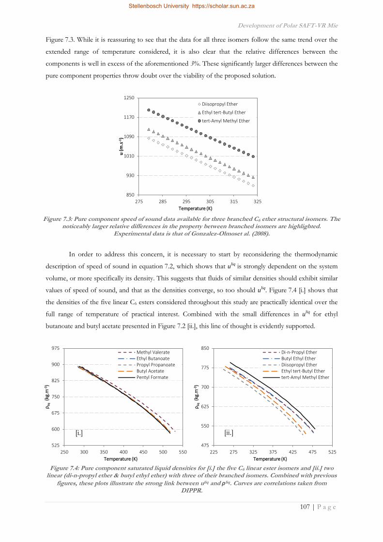
Development of Polar SAFT-VR Mie
107 | P a g e
850
930
1010
1090
1170
1250
275 285 295 305 315 325
u (
m.s
-1)
Temperature (K)
Diisopropyl Ether
Ethyl tert-Butyl Ether
tert-Amyl Methyl Ether
Figure 7.3. While it is reassuring to see that the data for all three isomers follow the same trend over the
extended range of temperature considered, it is also clear that the relative differences between the
components is well in excess of the aforementioned 3%. These significantly larger differences between the
pure component properties throw doubt over the viability of the proposed solution.
In order to address this concern, it is necessary to start by reconsidering the thermodynamic
description of speed of sound in equation 7.2, which shows that uliq is strongly dependent on the system
volume, or more specifically its density. This suggests that fluids of similar densities should exhibit similar
values of speed of sound, and that as the densities converge, so too should uliq. Figure 7.4 [i.] shows that
the densities of the five linear C6 esters considered throughout this study are practically identical over the
full range of temperature of practical interest. Combined with the small differences in uliq for ethyl
butanoate and butyl acetate presented in Figure 7.2 [ii.], this line of thought is evidently supported.
Figure 7.3: Pure component speed of sound data available for three branched C6 ether structural isomers. The noticeably larger relative differences in the property between branched isomers are highlighted.
Experimental data is that of Gonzalez-Olmoset al. (2008).
Figure 7.4: Pure component saturated liquid densities for [i.] the five C6 linear ester isomers and [ii.] two linear (di-n-propyl ether & butyl ethyl ether) with three of their branched isomers. Combined with previous
figures, these plots illustrate the strong link between uliq and ρliq. Curves are correlations taken from DIPPR.
525
600
675
750
825
900
975
250 300 350 400 450 500 550
ρliq
(kg.
m-3
)
Temperature (K)
Methyl ValerateEthyl ButanoatePropyl PropanoateButyl AcetatePentyl Formate
475
550
625
700
775
850
225 275 325 375 425 475 525
ρliq
(kg.
m-3
)
Temperature (K)
Di-n-Propyl EtherButyl Ethyl EtherDiisopropyl EtherEthyl tert-Butyl Ethertert-Amyl Methyl Ether
[i.] [ii.]
Stellenbosch University https://scholar.sun.ac.za
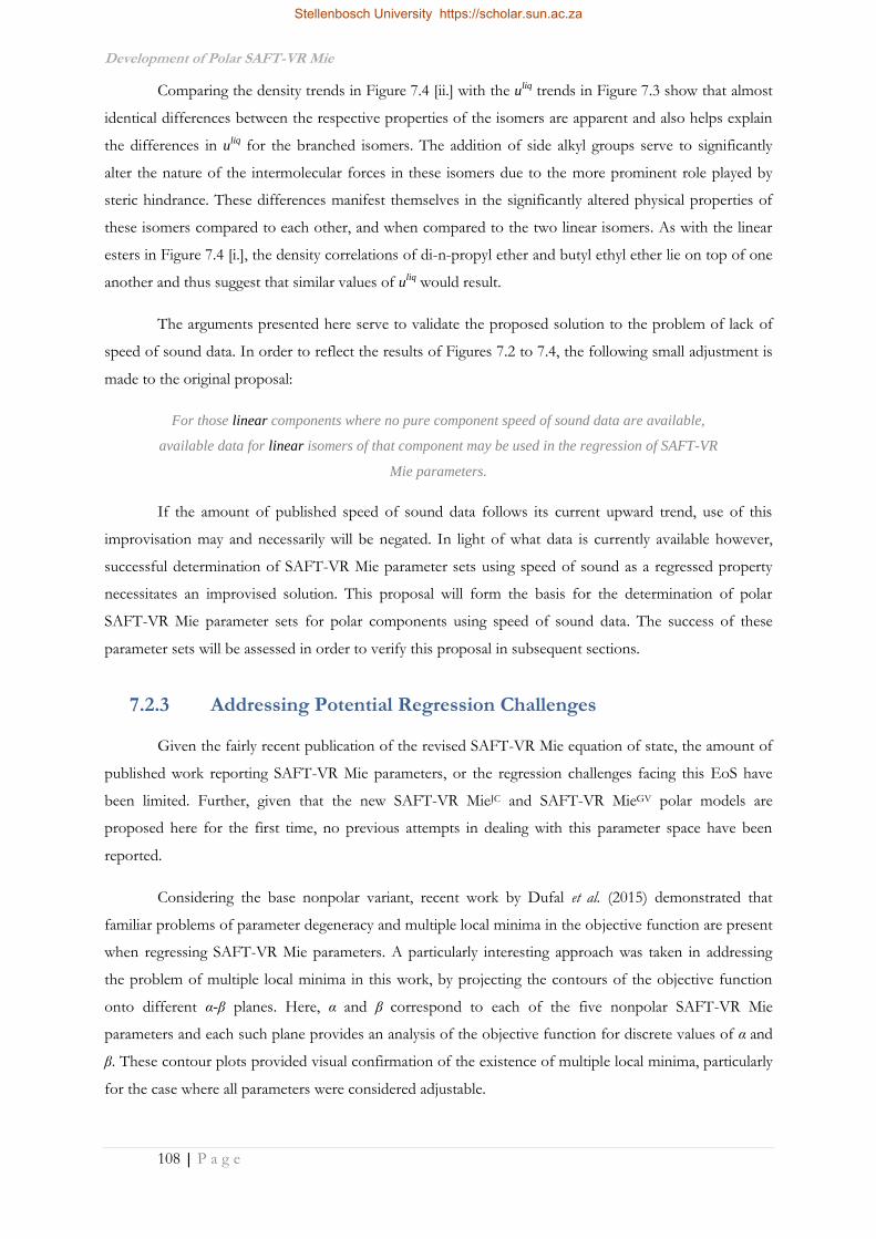
Development of Polar SAFT-VR Mie
108 | P a g e
Comparing the density trends in Figure 7.4 [ii.] with the uliq trends in Figure 7.3 show that almost
identical differences between the respective properties of the isomers are apparent and also helps explain
the differences in uliq for the branched isomers. The addition of side alkyl groups serve to significantly
alter the nature of the intermolecular forces in these isomers due to the more prominent role played by
steric hindrance. These differences manifest themselves in the significantly altered physical properties of
these isomers compared to each other, and when compared to the two linear isomers. As with the linear
esters in Figure 7.4 [i.], the density correlations of di-n-propyl ether and butyl ethyl ether lie on top of one
another and thus suggest that similar values of uliq would result.
The arguments presented here serve to validate the proposed solution to the problem of lack of
speed of sound data. In order to reflect the results of Figures 7.2 to 7.4, the following small adjustment is
made to the original proposal:
For those linear components where no pure component speed of sound data are available,
available data for linear isomers of that component may be used in the regression of SAFT-VR
Mie parameters.
If the amount of published speed of sound data follows its current upward trend, use of this
improvisation may and necessarily will be negated. In light of what data is currently available however,
successful determination of SAFT-VR Mie parameter sets using speed of sound as a regressed property
necessitates an improvised solution. This proposal will form the basis for the determination of polar
SAFT-VR Mie parameter sets for polar components using speed of sound data. The success of these
parameter sets will be assessed in order to verify this proposal in subsequent sections.
7.2.3 Addressing Potential Regression Challenges
Given the fairly recent publication of the revised SAFT-VR Mie equation of state, the amount of
published work reporting SAFT-VR Mie parameters, or the regression challenges facing this EoS have
been limited. Further, given that the new SAFT-VR MieJC and SAFT-VR MieGV polar models are
proposed here for the first time, no previous attempts in dealing with this parameter space have been
reported.
Considering the base nonpolar variant, recent work by Dufal et al. (2015) demonstrated that
familiar problems of parameter degeneracy and multiple local minima in the objective function are present
when regressing SAFT-VR Mie parameters. A particularly interesting approach was taken in addressing
the problem of multiple local minima in this work, by projecting the contours of the objective function
onto different α-β planes. Here, α and β correspond to each of the five nonpolar SAFT-VR Mie
parameters and each such plane provides an analysis of the objective function for discrete values of α and
β. These contour plots provided visual confirmation of the existence of multiple local minima, particularly
for the case where all parameters were considered adjustable.
Stellenbosch University https://scholar.sun.ac.za

Development of Polar SAFT-VR Mie
109 | P a g e
Dufal et al. (2015) demonstrated that using physical considerations to fix the values of different
parameters mitigated the problem of multiple minima, removing them in some cases while confining them
to physically unrealistic α-β combinations in others. The problem was not completely removed however,
and different parameter sets exhibiting a sliding bias to different considered properties were still presented.
These results emphasised the need to choose appropriate pure component data and to attach appropriate
regression weights to these different properties.
7.2.4 Selected Regression Methods
Given the novelty of a polar SAFT-VR Mie framework, it is necessary to generate a collection of
parameter sets for different homologous groups, which will constitute a solid core for the model moving
forward. In light of the work done here, the initial homologous groups of interest will be linear ketones,
esters and ethers. To this end, it is desirable to generate parameters starting with the smallest component
of each functional group and systematically work up to longer chain molecules, considering all relevant
structural isomers.
As has already been discussed, the value of the attractive range parameter, λa, is fixed to the
London dispersion value of 6 for all components. The value of the remaining four nonpolar parameters (σ,
m, ε/k and λr) will be left adjustable in the regression procedure for all cases. For the SAFT-VR MieJC and
SAFT-VR MieGV models, the value of the polar parameters (xp/np) is kept adjustable to allow for a fair
comparison of the terms, as was done for sPC-SAFT. The case for fixing np equal to 1 as per the original
term is also considered to provide a comparison with the regressed np case.
Use was made of available pure component speed of sound data tabulated in Table 7.1 and
employing the improvised solution above for components whose isomers have available data. In this way,
polar SAFT-VR Mie parameters can be regressed for a number of polar components, using the following
properties, with weightings in parentheses, as suggested by Lafitte et al. (2013):
saturated vapour pressures, Psat, (4),
saturated liquid densities, ρsat, (4), and
speed of sound, uliq, (1).
The problem however, is that for some components (e.g. methyl formate and the linear ethers)
uliq data are not available for either the component or its isomers. Thus, an alternative combination of
pure component properties needs to be considered. To this end, the same property combination as was
employed for polar sPC-SAFT will be considered for polar SAFT-VR Mie, viz:
saturated vapour pressures, Psat, (4),
saturated liquid densities, ρsat, (2), and
heats of vaporisation, Hvap, (1).
Stellenbosch University https://scholar.sun.ac.za
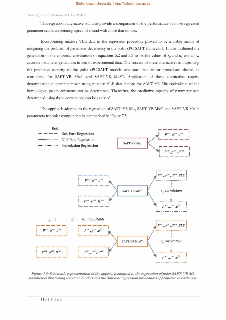
Development of Polar SAFT-VR Mie
110 | P a g e
Figure 7.5: Schematic representation of the approach adopted to the regression of polar SAFT-VR Mie parameters illustrating the three models and the different regression procedures appropriate to each case.
This regression alternative will also provide a comparison of the performance of those regressed
parameter sets incorporating speed of sound with those that do not.
Incorporating mixture VLE data in the regression procedure proved to be a viable means of
mitigating the problem of parameter degeneracy in the polar sPC-SAFT framework. It also facilitated the
generation of the empirical correlations of equations 5.2 and 5.3 to fix the values of xp and np and allow
accurate parameter generation in lieu of experimental data. The success of these alternatives in improving
the predictive capacity of the polar sPC-SAFT models advocates that similar procedures should be
considered for SAFT-VR MieJC and SAFT-VR MieGV. Application of these alternatives require
determination of parameter sets using mixture VLE data before the SAFT-VR Mie equivalents of the
homologous group constants can be determined. Thereafter, the predictive capacity of parameter sets
determined using these correlations can be assessed.
The approach adopted to the regression of SAFT-VR Mie, SAFT-VR MieJC and SAFT-VR MieGV
parameters for polar components is summarised in Figure 7.5.
, ,sat sat vapP Hρ
SAFT-VR Mie
SAFT-VR MieJC
SAFT-VR MieGV
, ,sat sat liqP uρ
, ,sat sat vapP Hρ
, ,sat sat liqP uρ
, ,sat sat vapP Hρ
, ,sat sat liqP uρ
, , ,sat sat vapP H VLEρ
, , ,sat sat vapP H VLEρ
, ,sat sat vapP Hρ
, ,sat sat liqP uρ
1pn .vs pn adjustable
, ,sat sat liqP uρ
pn correlation
, ,sat sat liqP uρ
px correlation
Std. Pure Regression
VLE Data Regression
Correlation Regression
Key:
Stellenbosch University https://scholar.sun.ac.za

Development of Polar SAFT-VR Mie
111 | P a g e
Regression of component parameters following the outline of Figure 7.5 yields up to 12
parameter sets for each component considered. The regression procedures will be assessed according to
the predictive capacity of their parameter sets when tested against thermodynamic and phase equilibrium
properties of pure components and their mixtures. This is the goal of the sections that follow.
7.3 Validation of Coded SAFT-VR Mie
Before parameters can be regressed for polar components within the new polar SAFT-VR Mie
framework and the predictive capacity of this model can be tested, it is necessary to validate the coding of
the SAFT-VR Mie EoS to corroborate modelling results presented in this chapter.
Thermodynamic modelling using SAFT type EoSs is conducted by means of the in-house
developed software, TRSolutions. The software was originally written by A.J. de Villiers to conduct
predominantly sPC-SAFT focused research and had this functionality coded and validated already. In
order to conduct the SAFT-VR Mie focused modelling suggested here, it was necessary to first code the
EoS and its derivatives in order to add them to the TRSolutions framework. Thus, starting with the model
framework presented by Lafitte et al. (2013), the appropriate thermodynamic derivatives were determined
in analytical form (the working equations are presented in Appendix G) and added to the software.
The additional code requires validation, which is achieved by:
i. Numerical Differentiation
Appropriate numerical differentiation of each term can be used to compare with the
coded analytical derivative. This allows for any error in the analytical differentiation of
the EoS terms to be identified and fixed as they arise.
ii. Reproducing Published Predictions
Using parameter sets published by Lafitte et al., (2013) and Dufal et al., (2015) to predict
pure component properties allows for direct comparison of published predictions with
literature data and deviations reported by these authors; and
iii. Regression of Published Parameters
Regressing parameters for the same components for which Lafitte et al., (2013) and Dufal
et al., (2015) published parameters allow for validation of the regression engine in the
software, the goal of which is to determine significantly similar parameter sets.
The numerical differentiation validation was written into each unit of the code, each of which was
checked via a step-through procedure of the program. Deviations between the analytical and numerical
derivatives indicated an erroneously-coded analytical derivative function, which was amended immediately.
To this end, all coded functions were verified by this numerical differentiation procedure and modelling
results presented here are mathematically correct. Details of this numerical differentiation are provided in
Appendix H.
Stellenbosch University https://scholar.sun.ac.za

Development of Polar SAFT-VR Mie
112 | P a g e
Validation of the model predictions was performed by considering the three n-alkanes of
particular interest to this study, viz. n-heptane, n-octane and n-nonane. The parameter sets published by
Lafitte et al. (2013) and those of Dufal et al. (2015) were used to generate the same pure component
predictions as were reported in those works. The results of these comparisons are provided in Table 7.2,
where the AADs of the predictions generated using TRSolutions are listed, followed by the values reported
by the original authors in parentheses. It is clear that all generated predictions yield deviations of the same
order of magnitude as those reported by the original authors. It should be noted that different sources
were used for these properties (DIPPR vs. NIST) which should account for the small discrepancies
between the values. Also, where Lafitte et al. (2013) and Dufal et al. (2015) considered uliq data over a
surface of temperatures and pressures, only those of the saturated liquid were considered here. The
comparison is adequate however as these saturation values fall within the T and P ranges considered by
those authors.
Table 7.2: Comparison of parameter sets regressed in this work and those of Lafitte et al. (2013) and Dufal et al., (2015) for the n-alkanes of interest in this study. Deviations obtained in this work, through use of the
indicated published parameters, are compared to those reported in parentheses.
σ m ε/k λa λr Psat * ρsat* usat † Hvap*
Å K AAD% AAD% AAD% AAD%
n-Heptane
Lafitte et al. (2013)
4.4282 2.3949 358.510 6 17.0920
0.886 (0.91) 0.489 (0.45) 0.922 (0.67) 2.186 (1.79)
Dufal et al. (2015
4.5427 2.2413 381.420 6 18.2520
0.462 (0.27) 0.109 (0.19) 0.339 (0.92) 2.015 (1.65)
Regressed 4.4811 2.3185 369.295 6 17.5886 0.230 0.086 0.526 2.191
n-Octane
Lafitte et al. (2013)
4.4696 2.6253 369.180 6 17.3780
0.983 (0.96) 0.683 (.052) 0.488 (0.75) 1.651 (.158)
Dufal et al. (2015
4.5708 2.4777 391.870 6 18.6540
0.386 (0.29) 0.139 (0.36) 1.954 (1.79) 1.705 (1.59)
Regressed 4.4816 2.5944 370.997 6 17.2990 0.347 0.100 0.432 1.716
n-Nonane
Lafitte et al. (2013)
4.5334 2.8099 387.550 6 18.3240 0.758 (0.82) 0.549 (0.60) 1.640 (0.45) 1.398 (1.60)
Dufal et al. (2015
4.6236 2.6665 404.830 6 19.1160 0.587 (0.34) 0.140 (0.41) 0.753 (0.60) 1.280 (1.48)
Regressed 4.5672 2.7490 394.826 6 18.6445 0.448 0.117 1.137 1.427
† uliq deviations reported by Lafitte et al. & Dufal et al. for compressed liquid; presented here for the saturated liquid * AADs based on DIPPR Correlations; † AADs based on NIST Data
The same three components were considered for validating the regression procedure, where the
Psat- ρ
sat- uliq property combination was selected to mirror the procedures followed by Lafitte et al. (2013)
and Dufal et al. (2015). The results of the regression are also listed in Table 7.2 along with their respective
AADs in the considered pure component properties. The regressed parameters are in consistent
agreement with those previously generated, with the resulting AADs exhibiting similar agreement. Indeed,
the AADs of the parameter sets regressed here are frequently the smallest of the three considered.
Stellenbosch University https://scholar.sun.ac.za

Development of Polar SAFT-VR Mie
113 | P a g e
With the numerical, predictive and regressive validations for the base nonpolar SAFT-VR Mie
case completed, focus shifts to the application of the model to polar components by incorporating the JC
and GV polar terms. Verification of the SAFT-VR MieJC and SAFT-VR MieGV models can only be
achieved by the numerical differentiation step in the validation procedure highlighted above and was
performed as such. The fully validated model could now be applied to the regression of parameter sets for
real polar components, the results of which are discussed in the following section.
7.4 Polar SAFT-VR Mie Parameters
The regression alternatives considered in Figure 7.5 illustrate the sheer volume of generated
parameter sets resulting from the regression exercise. As a result, not every parameter set generated is
reported here. Rather, regressed parameter sets that exhibit good predictive capacity are tabulated, before
a detailed assessment of the regression results is provided in the proceeding section.
As was the case with the sPC-SAFT framework, the inclusion of polar component/n-alkane VLE
data in the regression procedure yielded parameter sets that exhibited the best predictions for mixture
phase behaviour. For this reason, these parameter sets are considered the ideal starting point for the
analysis of regression results and will provide an ideal reference with which to compare the results of the
other regression cases. To this end, the parameters for the SAFT-VR MieJC and SAFT-VR MieGV models
regressed as a result of incorporating mixture VLE data in the regression procedure are tabulated in
Tables 7.3 and 7.4 respectively.
It is perhaps most notable that, in Table 7.3, the value of the polar parameter is listed as zero for a
number of the considered components. This is a result of the inability to successfully regress a parameter
set for these components with a nonzero xp, despite the inclusion of VLE data in the regression procedure.
This was particularly prevalent amongst the considered ketones although selected instances were apparent
for esters and ethers. The result was regression of a “nonpolar” parameter set for SAFT-VR MieJC and the
reported parameter sets for these components are thus the best fit nonpolar SAFT-VR Mie parameters for
those components. This appears to be a continuation of the problem of broad minima in the objective
function for the JC polar term, but will be discussed at length in subsequent sections.
The SAFT-VR MieGV model exhibits no such problems, with notable polar contributions
regressed for all components considered. Analysis of the parameters themselves indicate that they are well
behaved and follow the expected trends with changes in molecular weight; viz. molecular sizes (product of
σ and m) and dispersion energy increase as the molecular size increases. Trends in the value of the
regressed range parameters are also noteworthy; smaller values of λr are in evidence for smaller
components with a steady increase in the parameter value for larger molecules. This trend is similar to that
reported for nonpolar components by Lafitte et al., (2013) and Dufal et al., (2015). This serves to further
support the physical arguments behind allowing λr to deviate from its traditional fixed Lennard-Jones
value.
Stellenbosch University https://scholar.sun.ac.za

Development of Polar SAFT-VR Mie
114 | P a g e
Table 7.3: SAFT-VR MieJC parameters for ketones, esters and ethers determined by regression incorporating the indicated polar/n-alkane VLE data in the regression.
MW σ m ε/k λa λr xp μ VLE Data Paired Psat * ρsat * uliq † Hvap *
g.mol-1 Å K D Reference Alkane AAD% AAD% AAD% AAD%
Ketones
acetone 58.08 3.8102 1.9162 258.370 6 11.0337 0.3052 2.88 Acosta et al. (2002) n-hexane 1.918 2.275 5.783 3.035
2-butanone 72.11 4.0215 2.2107 258.347 6 11.2061 0.3517 2.76 Wisniak et al. (1998) n-heptane 3.741 11.51 0.449 1.280
2-pentanone 86.13 4.0571 2.3194 375.912 6 16.7737 0 b 2.77 Geiseler et al. (1968) n-heptane 0.359 0.479 7.537 3.322
3-pentanone 86.13 4.0341 2.3322 369.083 6 16.2708 0 b 2.82 Fuchs et al. (1984) n-heptane 1.513 0.770 -a 3.097
2-heptanone 114.1 3.9158 3.3015 307.272 6 12.9282 0 b 2.61 Cripwell et al. (2015) n-nonane 0.190 0.094 3.551 1.983
3-heptanone 114.1 3.9878 3.1163 290.571 6 12.4634 0.2222 2.81 Cripwell et al. (2015) n-nonane 0.112 0.477 -a 2.330
4-heptanone 114.1 4.3051 2.6032 392.799 6 17.2198 0 b 2.68 Cripwell et al. (2015) n-nonane 0.553 0.559 -a 1.440
Esters
methyl formate 60.05 3.4037 2.1266 221.529 6 10.2165 0.4741 1.77 Ortega et al. (2003) n-heptane 0.694 0.799 -a 2.864
ethyl formate 74.08 3.9950 1.7900 294.511 6 13.1830 0.7996 1.93 Ortega et al. (2015) n-heptane 0.743 0.940 0.884 3.285
methyl acetate 74.08 3.5142 2.4784 238.061 6 10.9886 0.4665 1.68 Fernández et al. (2013) n-heptane 0.691 0.134 2.436 2.232
propyl formate 88.11 3.6807 2.6705 244.235 6 10.8966 0.3847 1.91 Galván et al. (1994) n-heptane 0.326 0.361 -a 2.197
ethyl acetate 88.11 3.7299 2.6011 263.106 6 12.2552 0.4747 1.78 Fernández et al. (2010) n-heptane 0.437 0.247 2.859 2.373
methyl propanoate 88.11 3.4126 3.1969 230.184 6 10.7439 0.1997 1.70 Ortega et al. (2003) n-heptane 0.486 0.987 6.355 1.809
butyl formate 102.1 4.0953 2.3897 324.482 6 14.3963 0.5131 2.02 Ortega et al. (2015) n-heptane 1.375 0.204 -a 2.380
propyl acetate 102.1 3.7258 3.0506 257.864 6 11.8194 0.3642 1.79 Fernández et al. (2013) n-heptane 0.442 0.380 6.047 2.968
ethyl propanoate 102.1 3.9842 2.5737 306.267 6 14.1383 0.5589 1.75 Ríos et al. (2014) n-heptane 0.370 0.355 1.675 3.820
methyl butanoate 102.1 4.0057 2.5066 313.159 6 13.9857 0.5801 1.72 Ríos et al. (2012) n-heptane 0.204 0.179 3.408 2.245
pentyl formate 116.2 4.1631 2.6676 323.241 6 14.0702 0.5868 1.90 This work n-octane 0.947 1.264 -a 1.273
butyl acetate 116.2 4.0492 2.8374 310.894 6 14.0149 0.5105 1.84 This work n-octane 0.636 0.216 3.398 1.408
propyl propanoate 116.2 4.0740 2.7941 360.848 6 17.2044 0 b 1.79 This work n-octane 1.728 0.182 -a 4.345
ethyl butanoate 116.2 4.2815 2.4425 332.077 6 14.0531 0.6091 1.81 This work n-octane 1.376 0.712 4.315 2.163
methyl valerate 116.2 4.2810 2.4602 355.743 6 15.7938 0.6939 1.62 This work n-octane 0.923 1.420 -a 2.581
Ethers
diethyl ether 74.12 3.7964 2.4531 245.859 6 12.1527 0.5461 1.15 Klon-Palczewska et al. (1980) n-hexane 0.335 0.196 -a 1.920
di-n-propyl ether 102.18 4.1355 2.6406 302.892 6 14.0232 0.3826 1.21 This work n-heptane 0.373 0.506 -a 1.183
butyl ethyl ether 102.18 4.0085 2.8776 294.033 6 14.1005 0.2023 1.22 This work n-heptane 1.287 0.694 -a 7.745
dibutyl ether 130.23 4.3424 2.9612 362.723 6 17.3716 0 b 1.17 March et al., (1980) n-hexane 0.446 0.601 -a 1.582
† AADs in uliq calculated with reference to corresponding pure component data sets as indicated in Table 7.1 * AADs based on DIPPR Correlations a No AADs possible due to lack of published data b Nonpolar SAFT-VR Mie parameters listed (viz. zero polar contribution) due to tendency of regression to drive xp to zero regardless of initial guess
Stellenbosch University https://scholar.sun.ac.za
Stellenbosch University https://scholar.sun.ac.za

Development of Polar SAFT-VR Mie
115 | P a g e
Table 7.4: SAFT-VR MieGV parameters for ketones, esters and ethers determined by regression incorporating the indicated polar/n-alkane VLE data in the regression.
MW σ m ε/k λa λr np μ VLE Data Paired Psat * ρsat * uliq † Hvap *
g.mol-1 Å K D Reference Alkane AAD% AAD% AAD% AAD%
Ketones
acetone 58.08 3.4778 2.3593 251.047 6 12.3835 1.2389 2.88 Acosta et al. (2002) n-hexane 0.127 0.248 9.413 1.195
2-butanone 72.11 3.6394 2.5585 260.956 6 12.3040 1.5638 2.76 Wisniak et al. (1998) n-heptane 0.279 0.195 4.079 1.097
2-pentanone 86.13 3.8494 2.6093 297.363 6 13.8669 1.7869 2.77 Geiseler et al. (1968) n-heptane 0.131 0.589 3.327 2.485
3-pentanone 86.13 3.9840 2.3771 329.238 6 16.8726 2.216 2.82 Fuchs et al. (1984) n-heptane 0.541 0.885 -a 1.974
2-heptanone 114.1 3.8386 3.4465 276.968 6 11.9113 1.9211 2.61 Cripwell et al. (2015) n-nonane 0.359 0.564 6.006 1.663
3-heptanone 114.1 3.8101 3.4857 293.744 6 12.7967 0.6449 2.81 Cripwell et al. (2015) n-nonane 0.320 0.958 -a 2.176
4-heptanone 114.1 4.1391 2.7414 332.124 6 14.6402 2.1229 2.68 Cripwell et al. (2015) n-nonane 0.500 0.040 -a 1.048
Esters
methyl formate 60.05 3.1162 2.6170 208.666 6 10.3869 1.9084 1.77 Ortega et al. (2003) n-heptane 0.269 1.303 -a 1.566
ethyl formate 74.08 3.3775 2.7158 221.984 6 10.8664 2.3195 1.93 Ortega et al. (2015) n-heptane 0.312 1.395 2.285 2.140
methyl acetate 74.08 3.2320 3.0310 216.275 6 10.5774 2.2498 1.68 Fernández et al. (2013) n-heptane 0.405 1.242 3.082 1.461
propyl formate 88.11 3.4336 3.1523 226.314 6 10.5945 2.1136 1.91 Galván et al. (1994) n-heptane 0.457 1.529 -a 1.611
ethyl acetate 88.11 3.5434 2.9332 254.629 6 12.7101 3.2674 1.78 Fernández et al. (2010) n-heptane 0.239 0.992 2.201 1.452
methyl propanoate 88.11 3.2761 3.5254 216.018 6 10.3199 1.094 1.70 Ortega et al. (2003) n-heptane 0.517 1.634 7.819 1.606
butyl formate 102.1 3.9668 2.5794 332.046 6 16.5322 3.4987 2.02 Ortega et al. (2015) n-heptane 0.403 1.134 -a 2.037
propyl acetate 102.1 3.6507 3.1868 260.878 6 12.5111 3.5139 1.79 Fernández et al. (2013) n-heptane 0.502 1.009 5.436 2.406
ethyl propanoate 102.1 3.6671 3.1451 267.250 6 12.8094 3.1965 1.75 Ríos et al. (2014) n-heptane 0.335 0.807 3.845 3.345
methyl butanoate 102.1 3.6918 3.0564 272.843 6 12.6336 3.06612 1.72 Ríos et al. (2012) n-heptane 0.255 1.067 5.887 1.734
pentyl formate 116.2 3.8661 3.1884 288.207 6 13.2007 4.1093 1.90 This work n-octane 0.904 0.220 -a 1.627
butyl acetate 116.2 3.8501 3.1907 293.024 6 13.8230 4.0503 1.84 This work n-octane 0.553 0.865 3.788 0.865
propyl propanoate 116.2 4.0225 2.8671 331.304 6 16.2168 4.2672 1.79 This work n-octane 1.478 0.684 -a 4.123
ethyl butanoate 116.2 4.1891 2.5736 335.846 6 15.3695 4.3293 1.81 This work n-octane 0.681 0.201 3.185 2.208
methyl valerate 116.2 4.0646 2.7511 332.541 6 15.2862 4.3386 1.62 This work n-octane 0.681 0.914 -a 2.186
Ethers
diethyl ether 74.12 3.7032 2.6069 239.234 6 12.0284 2.2558 1.15 Klon-Palczewska et al. (1980) n-pentane 0.374 0.514 -a 1.784
di-n-propyl ether 102.18 4.3583 2.3226 356.304 6 17.3103 3.4305 1.21 This work n-heptane 0.441 0.543 -a 0.963
butyl ethyl ether 102.18 4.0139 2.8687 295.481 6 14.1883 1.6563 1.22 This work n-heptane 1.219 0.712 -a 7.745
dibutyl ether 130.23 4.3564 2.9364 363.111 6 17.4393 3.9749 1.17 March et al., (1980) n-hexane 0.486 0.621 -a 1.604
† AADs in uliq calculated with reference to corresponding pure component data sets as indicated in Table 7.1 * AADs based on DIPPR Correlations a No AADs possible due to lack of published data
Stellenbosch University https://scholar.sun.ac.za
Stellenbosch University https://scholar.sun.ac.za

Development of Polar SAFT-VR Mie
116 | P a g e
Apart from the SAFT-VR MieJC exceptions, the polar SAFT-VR Mie variants are clearly able to
accurately model the pure component properties under consideration. The reported AADs are of the
expected order of magnitude for SAFT type thermodynamic models, with particularly good correlation of
the saturation properties in evidence. The AADs in pure component speed of sound are of specific
interest in the SAFT-VR Mie framework and warrant particular attention. The magnitudes of some of the
deviations for uliq reported in Tables 7.3 and 7.4 are disappointingly high given SAFT-VR Mie’s renown
for accurate prediction of this property. A fair assessment of these AADs however, requires direct
comparison with equivalent deviations exhibited by polar sPC-SAFT; this comparison is provided in
Figure 7.6.
Comparison between the polar SAFT-VR Mie predictions and those of polar sPC-SAFT illustrate
that, apart from the smaller ketone molecules, significant improvement in the prediction of pure
component uliq is apparent for the polar SAFT-VR Mie models. The arguments of Lafitte et al., (2006,
2013) appear to hold for the polar variants of SAFT-VR Mie: explicitly accounting for variable repulsive
range serves to improve accuracy in the prediction of speed of sound. The significance of this
improvement is made even more apparent when considering that the parameter sets reported in
Tables 7.3 and 7.4 were generated without speed of sound data being included in the regression procedure
to begin with.
0
2
4
6
8
10
12
14
%A
AD
(uliq
)
sPC-SAFT GV sPC-SAFT JC
SAFT-VR Mie GV SAFT-VR Mie JC
Figure 7.6: Comparison of AADs in uliq for both polar SAFT-VR Mie and polar sPC-SAFT considering ketones and esters with available reference data. Reference data are those presented in Table 7.1.
*SAFT-VR MieJC predictions are those of nonpolar variant, given the inability to regress appropriate SAFT-VR MieJC parameters for these components.
Stellenbosch University https://scholar.sun.ac.za

Development of Polar SAFT-VR Mie
117 | P a g e
Inclusion of speed of sound data in the objective function offers just one alternative to the
regression procedures used to determine the parameters presented in Tables 7.3 and 7.4. The good
predictive capacity of these parameters however, makes them an excellent reference with which to
compare the results of these alternative regression procedures. This is the aim of the following section.
7.5 Analysis of Regression Results
The analysis performed in this section is limited to the generalised results of the different
regression procedures and how these results compare with each other. Such an analysis is necessarily
supplemented by example cases of application to pure component data and selected application to
mixtures. A more rigorous and thorough assessment of the performance of these parameter sets to
mixture data is reserved for Chapter 8, where only the optimum parameter sets will be considered.
7.5.1 Results of the Standard Pure Component Regression
Results of the Standard pure component regression constitute the largest proportion of the
regression results, with eight different cases under consideration according to Figure 7.5. As highlighted in
the Chapter 5, regression procedures of this kind are the literature standard for determination of pure
component properties given the relative availability of pure component property data.
7.5.1.1 Multiple Minima and Parameter Degeneracy
The work of Dufal et al. (2015) highlighted the prevalence of multiple, discreet local minima in the
SAFT-VR Mie objective function. It was emphasised that this was sensitive to the choice of pure
component properties, their relative regression weights, as well as initial guesses for the parameter values.
Results of the Standard pure component regression show that the problem of multiple minima extends to
the polar SAFT-VR Mie models as well.
Choosing initial values proved to be the most influential aspect in determining the parameter set
resulting from the regression. This was particularly true for the determination of the polar parameter (viz.
xp and np) as the largest adjustments between regression iterations were made to this parameter value. This
was most prevalent and problematic when initial parameter values far from those corresponding to the
objective function minimum were chosen. In these cases, the initial adjustments were largest for xp/np and
frequently resulted in the parameter being pushed to the bounded lower value of zero before significant
changes were made to the other nonpolar parameters. Once pushed in this direction, the xp/np value
would approach zero asymptotically for the remainder of the assigned iterations and yield “nonpolar”
SAFT-VR MieJC and SAFT-VR MieGV parameter sets.
In the case of SAFT-VR MieGV, this tendency was the result of multiple discrete local minima of
the kind demonstrated by Dufal et al. (2015). This conclusion was drawn based on the fact that careful
selection of parameter initial values and altering regression weightings frequently mitigated the problem of
Stellenbosch University https://scholar.sun.ac.za
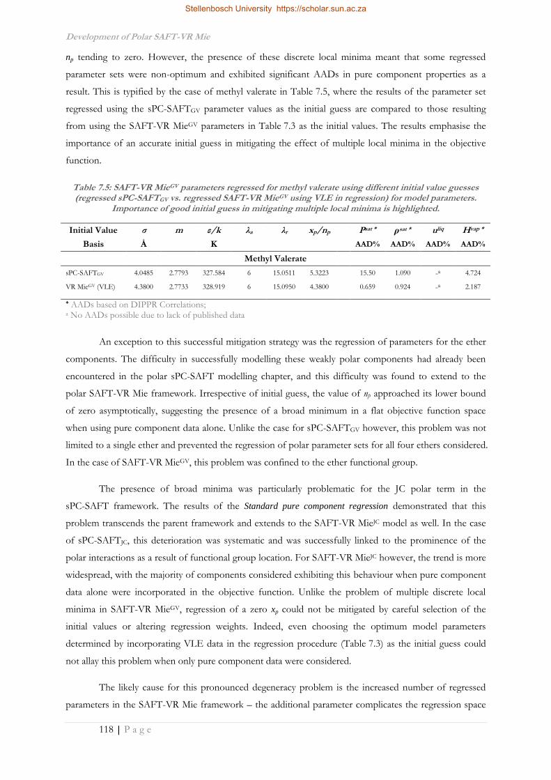
Development of Polar SAFT-VR Mie
118 | P a g e
np tending to zero. However, the presence of these discrete local minima meant that some regressed
parameter sets were non-optimum and exhibited significant AADs in pure component properties as a
result. This is typified by the case of methyl valerate in Table 7.5, where the results of the parameter set
regressed using the sPC-SAFTGV parameter values as the initial guess are compared to those resulting
from using the SAFT-VR MieGV parameters in Table 7.3 as the initial values. The results emphasise the
importance of an accurate initial guess in mitigating the effect of multiple local minima in the objective
function.
Table 7.5: SAFT-VR MieGV parameters regressed for methyl valerate using different initial value guesses (regressed sPC-SAFTGV vs. regressed SAFT-VR MieGV using VLE in regression) for model parameters.
Importance of good initial guess in mitigating multiple local minima is highlighted.
Initial Value σ m ε/k λa λr xp/np Psat * ρsat * uliq Hvap *
Basis Å K AAD% AAD% AAD% AAD%
Methyl Valerate
sPC-SAFTGV 4.0485 2.7793 327.584 6 15.0511 5.3223 15.50 1.090 -a 4.724
VR MieGV (VLE) 4.3800 2.7733 328.919 6 15.0950 4.3800 0.659 0.924 -a 2.187
* AADs based on DIPPR Correlations; a No AADs possible due to lack of published data
An exception to this successful mitigation strategy was the regression of parameters for the ether
components. The difficulty in successfully modelling these weakly polar components had already been
encountered in the polar sPC-SAFT modelling chapter, and this difficulty was found to extend to the
polar SAFT-VR Mie framework. Irrespective of initial guess, the value of np approached its lower bound
of zero asymptotically, suggesting the presence of a broad minimum in a flat objective function space
when using pure component data alone. Unlike the case for sPC-SAFTGV however, this problem was not
limited to a single ether and prevented the regression of polar parameter sets for all four ethers considered.
In the case of SAFT-VR MieGV, this problem was confined to the ether functional group.
The presence of broad minima was particularly problematic for the JC polar term in the
sPC-SAFT framework. The results of the Standard pure component regression demonstrated that this
problem transcends the parent framework and extends to the SAFT-VR MieJC model as well. In the case
of sPC-SAFTJC, this deterioration was systematic and was successfully linked to the prominence of the
polar interactions as a result of functional group location. For SAFT-VR MieJC however, the trend is more
widespread, with the majority of components considered exhibiting this behaviour when pure component
data alone were incorporated in the objective function. Unlike the problem of multiple discrete local
minima in SAFT-VR MieGV, regression of a zero xp could not be mitigated by careful selection of the
initial values or altering regression weights. Indeed, even choosing the optimum model parameters
determined by incorporating VLE data in the regression procedure (Table 7.3) as the initial guess could
not allay this problem when only pure component data were considered.
The likely cause for this pronounced degeneracy problem is the increased number of regressed
parameters in the SAFT-VR Mie framework – the additional parameter complicates the regression space
Stellenbosch University https://scholar.sun.ac.za
Development of Polar SAFT-VR Mie
119 | P a g e
further and increases the difficulty of finding a unique parameter set. Given the prevalence of this
deterioration in polar sPC-SAFT, where four pure component parameters are considered, the addition of
a fifth parameter appears to increase the occurrence of this problem when using SAFT-VR Mie.
7.5.2 Explicit vs. Implicit: Effect of Accounting for Polarity
Perhaps the most important consideration in proposing a polar SAFT-VR Mie framework is
whether the explicit polar dependence is necessary in light of the enhanced predictive capacity of this
model. Thus the focus of the discussion presented here is a comparison of the relative performance of
nonpolar SAFT-VR Mie vs. the proposed polar variants. Given the regression difficulties for the
SAFT-VR MieJC model demonstrated in the previous section, the discussion here will centre on a
comparison of nonpolar SAFT-VR Mie and SAFT-VR MieGV. Evaluation of the polar model is further
divided into the cases where np = 1 as per the original Gross & Vrabec formulation, and the case where
this parameter is variable. To this end, due consideration is given to successfully generated parameter sets
for representative components of each functional groups of interest, followed by a summary of the overall
comparison.
7.5.2.1 Ketones
Acetone is undeniably the first choice reference ketone in the literature, given the relative
abundance of pure and mixture data for this component compared to other members of the ketone family.
Due to acetone’s small molecular mass and large dipole moment however, its properties are not
necessarily representative of the ketone family as a whole. Thus, a reference component for the linear
ketones should be a longer chain molecule and is chosen to be 2-pentanone for the purposes of
illustration here. Regressed parameters of both ketones for nonpolar SAFT-VR Mie and SAFT-VR MieGV
are provided in Table 7.6. The reported parameter sets are based on the Standard pure component
regression procedure using the Hvap alternative, which thus allows for a direct comparison of the model
performance.
Stellenbosch University https://scholar.sun.ac.za
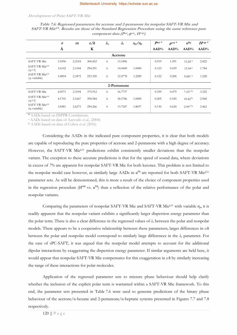
Development of Polar SAFT-VR Mie
120 | P a g e
Table 7.6: Regressed parameters for acetone and 2-pentanone for nonpolar SAFT-VR Mie and SAFT-VR MieGV. Results are those of the Standard Regression Procedure using the same reference pure
component data (Psat, ρsat, Hvap)
σ m ε/k λa λr xp/np Psat * ρsat * uliq Hvap *
Å K AAD% AAD% AAD% AAD%
Acetone
SAFT-VR Mie 3.5596 2.2518 304.452 6 13.1896
0.919 1.291 13.24 a 2.822
SAFT-VR MieGV (np=1)
3.6142 2.1544 294.291 6 14.0449 1.0000 0.123 0.439 13.94 a 1.784
SAFT-VR MieGV (np variable)
3.4854 2.3472 253.350 6 12.4778 1.2289 0.122 0.206 9.681 a 1.228
2-Pentanone
SAFT-VR Mie 4.0571 2.3194 375.912 6 16.7737 0.359 0.479 7.537 b 3.322
SAFT-VR MieGV (np=1)
4.1701 2.1667 394.584 6 18.5786 1.0000 0.205 0.185 10.42 b 2.968
SAFT-VR MieGV (np variable)
3.8381 2.6275 294.266 6 13.7247 1.8037 0.130 0.624 2.997 b 2.462
* AADs based on DIPPR Correlations; a AADs based on data of Azevedo et al., (2004) b AADs based on data of Cobos et al. (2016)
Considering the AADs in the indicated pure component properties, it is clear that both models
are capable of reproducing the pure properties of acetone and 2-pentanone with a high degree of accuracy.
However, the SAFT-VR MieGV predictions exhibit consistently smaller deviations than the nonpolar
variant. The exception to these accurate predictions is that for the speed of sound data, where deviations
in excess of 7% are apparent for nonpolar SAFT-VR Mie for both ketones. This problem is not limited to
the nonpolar model case however, as similarly large AADs in uliq are reported for both SAFT-VR MieGV
parameter sets. As will be demonstrated, this is more a result of the choice of component properties used
in the regression procedure (Hvap vs. uliq) than a reflection of the relative performance of the polar and
nonpolar variants.
Comparing the parameters of nonpolar SAFT-VR Mie and SAFT-VR MieGV with variable np, it is
readily apparent that the nonpolar variant exhibits a significantly larger dispersion energy parameter than
the polar term. There is also a clear difference in the regressed values of λr between the polar and nonpolar
models. There appears to be a cooperative relationship between these parameters; larger differences in ε/k
between the polar and nonpolar model correspond to similarly large differences in the λr parameter. For
the case of sPC-SAFT, it was argued that the nonpolar model attempts to account for the additional
dipolar interactions by exaggerating the dispersion energy parameter. If similar arguments are held here, it
would appear that nonpolar SAFT-VR Mie compensates for this exaggeration in ε/k by similarly increasing
the range of these interactions for polar molecules.
Application of the regressed parameter sets to mixture phase behaviour should help clarify
whether the inclusion of the explicit polar term is warranted within a SAFT-VR Mie framework. To this
end, the parameter sets presented in Table 7.6 were used to generate predictions of the binary phase
behaviour of the acetone/n-hexane and 2-pentanone/n-heptane systems presented in Figures 7.7 and 7.8
respectively.
Stellenbosch University https://scholar.sun.ac.za

Development of Polar SAFT-VR Mie
121 | P a g e
It is clear from Figures 7.7 and 7.8 that the inclusion of the GV polar term improves the
prediction accuracy in both ketone/n-alkane systems. It is also notable that a constant np = 1 parameter
set fails to accurately capture the effects of the strong positive deviations in these ketone molecules. This
is consistent with similar trends in sPC-SAFT that lead to the consideration of a variable np to begin with.
Fixing the value of np in this fashion limits the ability to account for dipolar interactions, resulting in
exaggerated dispersion energy parameters in the same fashion as that described for the nonpolar case. In
the same vein, the apparent cooperativity between ε/k and λr results in similarly larger values of the
repulsive range. These exaggerated values of λr are clearly responsible for the notable difference in the
predictability of uliq by the two SAFT-VR MieGV cases in Table 7.6.
Figure 7.7: Application of nonpolar SAFT-VR Mie and SAFT-VR Mie GV (np = 1 & variable) to phase behaviour of the acetone/n-hexane (Acosta et al., 2002) mixture at 101.3kPa. Nonpolar sPC-SAFT
prediction equivalent included for reference.
320
325
330
335
340
345
0.00 0.20 0.40 0.60 0.80 1.00
Tem
per
atu
re (K
)
Acetone Mole Fraction (x,y)
Acosta et al. (2002)
sPC-SAFT
SAFT-VR Mie
SAFT-VR Mie + GV
SAFT-VR Mie + GV (np=1)
Stellenbosch University https://scholar.sun.ac.za

Development of Polar SAFT-VR Mie
122 | P a g e
The quality of the nonpolar SAFT-VR Mie prediction should not so quickly be dismissed
however, as comparison with the equivalent nonpolar sPC-SAFT predictions (based on the parameters of
de Villiers (2011)) shows an improvement in prediction accuracy. Based on the predictions for the
representative ketones however, it is readily apparent that explicitly accounting for the polar interactions
is necessary to yield a good fit of their phase equilibria.
7.5.2.2 Esters
Studies on esters are generally limited to smaller (C4 ≥) members of this homologous group with
limited attention paid to larger components where wider ranges of behaviour are exhibited for the
different isomers. The ester functional group’s capacity for extensive structural isomerism has already
been highlighted in previous chapters. For these reasons it is necessary to consider multiple reference
components for this functional group. Here ethyl acetate and methyl valerate are selected to be
representative of different chain lengths as well as different functional group locations. Parameters
regressed for these components for the nonpolar SAFT-VR Mie model and the SAFT-VR MieGV polar
variant are listed in Table 7.7. As with the ketones, parameter sets are results of the Standard pure
component regression procedure using Hvap instead of uliq in the regression, allowing for direct comparison
of the predictions.
Figure 7.8: Application of nonpolar SAFT-VR Mie and SAFT-VR Mie GV (np = 1 & variable) to phase behaviour of the 2-pentanone/n-heptane (Geiseler et al., 1968) mixture at 353.15K. Nonpolar sPC-SAFT
prediction equivalent included for reference.
0.44
0.49
0.54
0.59
0.64
0.69
0.00 0.20 0.40 0.60 0.80 1.00
Pre
ssu
re (b
ar)
2-Pentanone Mole Fraction (x,y)
Geiseler et al. (1968)
sPC-SAFT
SAFT-VR Mie
SAFT-VR Mie + GV
SAFT-VR Mie + GV (np=1)
Stellenbosch University https://scholar.sun.ac.za

Development of Polar SAFT-VR Mie
123 | P a g e
Table 7.7: Regressed parameters for ethyl acetate and methyl valerate for nonpolar SAFT-VR Mie and SAFT-VR MieGV. Results are those of the Standard Regression Procedure using the same reference pure
component data (Psat, ρsat, Hvap)
σ m ε/k λa λr xp/np Psat * ρsat * uliq Hvap *
Å K AAD% AAD% AAD% AAD%
Ethyl Acetate
SAFT-VR Mie 3.6095 2.8246 289.604 6 13.7377 0.094 0.274 0.435 a 2.089
SAFT-VR MieGV (np=1)
3.5646 2.9109 275.455 6 13.0879 1.0000 0.088 0.295 0.451 a 2.058
SAFT-VR MieGV (np variable)
3.5746 2.8837 271.202 6 13.0501 1.9467 0.096 0.461 0.850 a 1.902
Methyl Valerate
SAFT-VR Mie 4.0524 2.7925 346.100 6 15.2997 0.768 0.372 -b 2.455
SAFT-VR MieGV (np=1)
4.0627 2.7741 347.228 6 15.3720 1.0000 1.006 0.370 -b 2.546
SAFT-VR MieGV (np variable)
4.0753 2.7380 337.270 6 15.3785 3.8597 0.682 0.778 -b 2.267
* AADs based on DIPPR Correlations; a AADs based on data of Pal et al., (2013) b No available experimental data with which to compare model predictions
The AADs reported in Table 7.7 illustrate that the difference between the prediction accuracy of
the polar and nonpolar SAFT-VR Mie variants is much smaller for esters than was the case for ketones.
Deviations in pure component properties are almost identical throughout and there is no marked
improvement of the model when explicitly accounting for the polar effects. Numerically, the values of the
regressed parameters for the polar and nonpolar models are very similar, with larger values of ε/k and λr
once again in evidence for the nonpolar variant and the constant np case. The smaller difference between
the dispersion energies in the polar and nonpolar models is likely a result of the markedly weaker dipole
moment of the ester functional group compared to the ketones.
The predictive capacity of these model parameters is tested against mixture phase equilibrium data
in Figures 7.9 and 7.10, where the ethyl acetate/n-heptane and methyl valerate/n-octane systems are
considered respectively.
Stellenbosch University https://scholar.sun.ac.za

Development of Polar SAFT-VR Mie
124 | P a g e
In the ethyl acetate/n-heptane case, the nonpolar SAFT-VR Mie model fit is only slightly worse
than the variable np SAFT-VR MieGV prediction. The poorest correlation of the data is visible in the high
ester concentration range, where the nonpolar model fails to account for the azeotrope at ~0.86 mole
fraction ethyl acetate. This is remedied in the case of the polar variant predictions, albeit at higher ester
concentrations (ca. 0.92 mole fraction). In Figure 7.10 the nonpolar variant similarly fails to accurately
capture the temperature dependence of the azeotrope in the methyl valerate/n-octane system and is
clearly outperformed by SAFT-VR MieGV in this system. However, the SAFT-VR Mie prediction can be
seen to maintain its superiority over nonpolar sPC-SAFT for the prediction of the phase equilibria of ester
mixtures.
Figure 7.9: Application of nonpolar SAFT-VR Mie and SAFT-VR Mie GV (np = 1 & variable) to phase behaviour of the ethyl acetate/n-heptane (Fernández et al., 2010) mixture at 101.3kPa. Nonpolar sPC-SAFT
prediction equivalent included for reference.
347
352
357
362
367
372
0.00 0.20 0.40 0.60 0.80 1.00
Tem
per
atu
re (K
)
Ethyl Acetate Mole Fraction (x,y)
Fernández et al. (2010)
sPC-SAFT
SAFT-VR Mie
SAFT-VR Mie + GV
SAFT-VR Mie + GV (np=1)
Stellenbosch University https://scholar.sun.ac.za

Development of Polar SAFT-VR Mie
125 | P a g e
The notable result from Figures 7.9 and 7.10 is the negligible improvement offered by the
constant np SAFT-VR MieGV case compared to the predictions of the nonpolar model. This is reflected in
the similarity of the two parameter sets and emphasises the need to accurately capture the polar
contribution in a variable fashion. The parameter set for the regressed np case is not markedly different
apart from the value of np itself, but the effect of limiting this parameter on the associated predictive
capacity is made clear in the ester functional group.
7.5.2.3 Ethers
The problem of broad minima in the objective functions of the ethers means that comparison of
the polar and nonpolar models can only be performed by using the SAFT-VR MieGV parameter sets of
Table 7.3. This necessitates comparing parameter sets determined by different regression procedures; viz.
Standard pure component regression for both the nonpolar model and fixed np case vs. the inclusion of
VLE data for SAFT-VR MieGV with variable np. However, the comparison still provides insight into the
question of whether polar interactions need to be explicitly accounted for. Diethyl ether and butyl ethyl
ether are used as reference components for this functional group, with their respective parameters listed in
Table 7.8.
As with the ketones and esters previously, AADs reported in Table 7.8 suggest that there is little
to distinguish between the predictive capacities of nonpolar SAFT-VR Mie and SAFT-VR MieGV. The
similarity of the parameters themselves highlights the small contribution of polar interactions to the phase
behaviour of the ethers. The exception is the variable np parameter set for butyl ethyl ether, where smaller
dispersion energy and repulsive range parameters are in evidence. The same trend is found for the other
Figure 7.10: Application of nonpolar SAFT-VR Mie and SAFT-VR Mie GV (np = 1 & variable) to phase behaviour of the methyl valerate/n-octane (This work) mixture at 60.0kPa. Nonpolar sPC-SAFT prediction
equivalent included for reference.
377
379
381
383
385
0.00 0.20 0.40 0.60 0.80 1.00
Tem
per
atu
re (K
)
Methyl Valerate Mole Fraction (x,y)
Cripwell et al. (2016)
sPC-SAFT
SAFT-VR Mie
SAFT-VR Mie + GV
SAFT-VR Mie + GV (np=1)
Stellenbosch University https://scholar.sun.ac.za

Development of Polar SAFT-VR Mie
126 | P a g e
functional groups. In those cases, the most apparent manifestation of this difference was the description
of uliq
but the lack of such data for ethers means the only appreciable difference will be noted in the
description of mixture behaviour.
Table 7.8: Regressed parameters for diethyl ether and butyl ethyl ether for nonpolar SAFT-VR Mie and
SAFT-VR MieGV. Results are those of the Standard Regression Procedure for SAFT-VR Mie with those for SAFT-VR MieGV relisted from Table 7.3.
σ m ε/k λa λr xp/np Psat * ρsat * uliq Hvap *
Å K AAD% AAD% AAD% AAD%
Diethyl Ether
SAFT-VR Mie 3.7120 2.5952 245.350 6 12.2809 0.370 0.383 -a 1.863
SAFT-VR MieGV (np=1)
3.7018 2.6120 242.328 6 12.1424 1.0000 0.368 0.436 -a 1.831
SAFT-VR MieGV (np variable)
3.7032 2.6069 239.234 6 12.0284 2.2558 0.374 0.514 -a 1.784
Butyl Ethyl Ether
SAFT-VR Mie 4.2397 2.5159 349.734 6 17.4652 1.116 0.620 -a 7.659
SAFT-VR MieGV (np=1)
4.2414 2.5129 349.511 6 17.4559 1.0000 1.117 0.623 -a 7.656
SAFT-VR MieGV (np variable)
4.0139 2.8687 295.481 6 14.1883 1.6563 1.219 0.712 -a 7.745
* AADs based on DIPPR Correlations; a No available experimental data with which to compare model predictions
The parameter sets of Table 7.8 are used to predict VLE for the binary diethyl ether/n-pentane
and butyl ethyl ether/n-heptane in Figures 7.11 and 7.12.
Figure 7.11: Application of nonpolar SAFT-VR Mie and SAFT-VR Mie GV (np = 1 & variable fit to VLE data) to phase behaviour of the diethyl ether/n-pentane (Klon-Palczewska et al., 1980) mixture at 101.3kPa.
Nonpolar sPC-SAFT prediction equivalent included for reference.
306
307
308
309
310
0.00 0.20 0.40 0.60 0.80 1.00
Tem
per
atu
re (K
)
Diethyl Ether Mole Fraction (x,y)
Klon-Palczewska et al. (1980)
sPC-SAFT
SAFT-VR Mie
SAFT-VR Mie + GV (VLE)
SAFT-VR Mie + GV (np=1)
Stellenbosch University https://scholar.sun.ac.za

Development of Polar SAFT-VR Mie
127 | P a g e
The diethyl ether/n-pentane system highlights the improvement of nonpolar SAFT-VR Mie over
its nonpolar sPC-SAFT counterpart, qualitatively accounting for the azeotropic behaviour in the system.
The prediction of the fixed np parameter set goes a step further in improving the temperature description
of the azeotrope, but the variable np case once again clearly provides the superior prediction. This is more
subtly demonstrated in the butyl ethyl ether/n-heptane system where all but the variable np parameter sets
produce near identical predictions, shifted away from the experimental data.
7.5.2.4 Summary
When considering the prediction of pure component properties, the nonpolar and polar
SAFT-VR Mie models exhibited similar predictive capacities, regardless of the functional group
considered. Analysis of the parameters themselves however, showed that the dispersion energy and
repulsive range parameters of nonpolar SAFT-VR Mie are systematically larger than their SAFT-VR
MieGV equivalents when np is regressed. These differences were most obvious for the ketones, with
systematically smaller differences as the more weakly polar ester and ether groups were considered. The
larger values of ε/k and λr in the nonpolar variant are indicative of the tendency of the model to artificially
exaggerate the contribution of the dispersion term in order to accommodate the polar interactions. This
same argument applies to the fixed np = 1 case, where limiting the value of the polar parameter leads to
exaggerated dispersion parameters. Indeed, this explains why the nonpolar SAFT-VR Mie and
SAFT-VR MieGV parameters are significantly different for the strongly polar ketones, yet almost identical
for the very weakly polar ethers.
Figure 7.12: Application of nonpolar SAFT-VR Mie and SAFT-VR Mie GV (np = 1 & variable fit to VLE data) to phase behaviour of the butyl ethyl ether/n-heptane (This work) mixture at 60.0kPa. Nonpolar
sPC-SAFT prediction equivalent included for reference.
348
350
352
354
356
0.00 0.20 0.40 0.60 0.80 1.00
Tem
per
atu
re (K
)
Butyl Ethyl Ether Mole Fraction (x,y)
Cripwell et al. (2016)
sPC-SAFT
SAFT-VR Mie
SAFT-VR Mie + GV (VLE)
SAFT-VR Mie + GV (np=1)
Stellenbosch University https://scholar.sun.ac.za

Development of Polar SAFT-VR Mie
128 | P a g e
The clearest distinction between polar and nonpolar model performances was in their application
to selected phase equilibria. As the most strongly polar of the functional groups under consideration, the
ketone homologous group most ardently demonstrated the need to account for polar interactions
explicitly. While the nonpolar SAFT-VR Mie model captured the azeotropic behaviour in the
ketone/n-alkane systems, and exhibited marked improvement over its nonpolar sPC-SAFT counterpart,
the fits were still only qualitatively correct. This functional group also most clearly showed the effect of
fixing the value of the polar parameter to 1: improved prediction of mixture behaviour is in evidence
compared to the nonpolar model, but the limitation on np similarly limits the predictive capacity of the
model.
While the difference in predictive capacity between the polar and nonpolar SAFT-VR Mie models
is smaller when considering the ester and ether functional groups, there is still a clear distinction between
them. Nonpolar SAFT-VR Mie cannot accurately capture the temperature dependence of the positive
deviations in these systems, with the fixed np case offering minimal improvement. For the esters, a
consistent trend is apparent in the predictions of these models: higher accuracy is apparent in the
nonpolar model prediction of mixture data for less polar esters (viz. acetates, propanoates) than for more
strongly polar members (viz. methyl esters, formates). This makes sense considering the less strongly polar
isomers will exhibit a smaller polar contribution to the overall system behaviour. This results in a smaller
distinction between polar and dispersion forces, the latter of which is well correlated by the nonpolar
model. This last point is even more pronounced in application to the ether functional group. As with
sPC-SAFT previously, the nonpolar SAFT-VR Mie and fixed np cases can’t account for the subtle
deviations resulting from the ether’s weak dipole.
Lafitte et al.’s SAFT-VR Mie exhibits an enhanced predictive capacity compared to nonpolar
sPC-SAFT when applied to polar components and their mixtures. While the improved theory
underpinning SAFT-VR Mie and its variable range parameter allow for better description of derivative
properties, this improvement is clearly insufficient to accurately account for dipolar interactions in the
model’s original framework. Indeed, trying to shoehorn the effects of dispersion and polar interactions
into a single contribution is fundamentally erroneous and has been proven as such by the model
predictions in this section.
7.5.3 Role of Speed of Sound
The role of speed of sound in setting SAFT-VR Mie apart from its predecessors has already been
extensively detailed in this work. The question of importance here is whether its explicit inclusion in the
regression procedure yields improved performance when applied to properties of polar components and
their mixtures. The inclusion of uliq is not itself a novel suggestion; there was a demonstrated trade-off in
predictive accuracy between phase equilibrium properties and derivative properties in the sPC-SAFT
framework (de Villiers, 2011). This meant that its inclusion in the regression procedure only served to
Stellenbosch University https://scholar.sun.ac.za
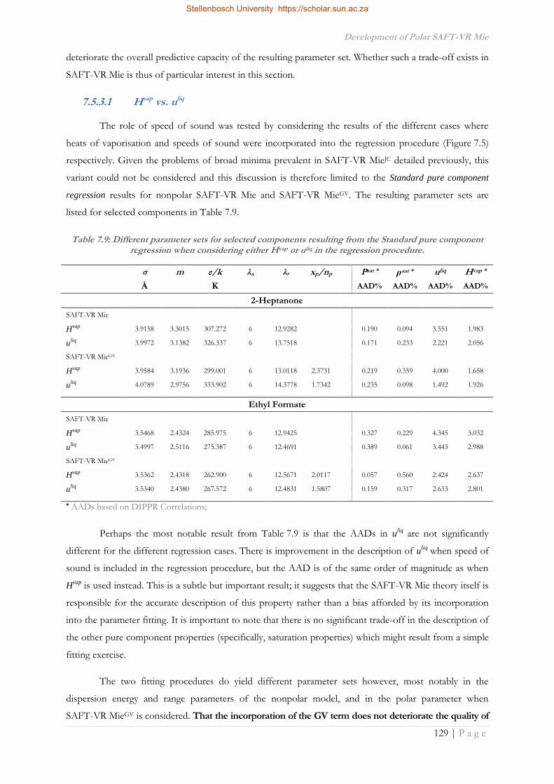
Development of Polar SAFT-VR Mie
129 | P a g e
deteriorate the overall predictive capacity of the resulting parameter set. Whether such a trade-off exists in
SAFT-VR Mie is thus of particular interest in this section.
7.5.3.1 Hvap vs. uliq
The role of speed of sound was tested by considering the results of the different cases where
heats of vaporisation and speeds of sound were incorporated into the regression procedure (Figure 7.5)
respectively. Given the problems of broad minima prevalent in SAFT-VR MieJC detailed previously, this
variant could not be considered and this discussion is therefore limited to the Standard pure component
regression results for nonpolar SAFT-VR Mie and SAFT-VR MieGV. The resulting parameter sets are
listed for selected components in Table 7.9.
Table 7.9: Different parameter sets for selected components resulting from the Standard pure component
regression when considering either Hvap or uliq in the regression procedure.
σ m ε/k λa λr xp/np Psat * ρsat * uliq Hvap *
Å K AAD% AAD% AAD% AAD%
2-Heptanone
SAFT-VR Mie
Hvap 3.9158 3.3015 307.272 6 12.9282 0.190 0.094 3.551 1.983
uliq 3.9972 3.1382 326.337 6 13.7518 0.171 0.233 2.221 2.056
SAFT-VR MieGV
Hvap 3.9584 3.1936 299.001 6 13.0118 2.3731 0.219 0.359 4.000 1.658
uliq 4.0789 2.9756 333.902 6 14.3778 1.7342 0.235 0.098 1.492 1.926
Ethyl Formate
SAFT-VR Mie
Hvap 3.5468 2.4324 285.975 6 12.9425 0.327 0.229 4.345 3.032
uliq 3.4997 2.5116 275.387 6 12.4691 0.389 0.061 3.443 2.988
SAFT-VR MieGV
Hvap 3.5362 2.4318 262.900 6 12.5671 2.0117 0.057 0.560 2.424 2.637
uliq 3.5340 2.4380 267.572 6 12.4831 1.5807 0.159 0.317 2.633 2.801
* AADs based on DIPPR Correlations;
Perhaps the most notable result from Table 7.9 is that the AADs in uliq are not significantly
different for the different regression cases. There is improvement in the description of uliq when speed of
sound is included in the regression procedure, but the AAD is of the same order of magnitude as when
Hvap is used instead. This is a subtle but important result; it suggests that the SAFT-VR Mie theory itself is
responsible for the accurate description of this property rather than a bias afforded by its incorporation
into the parameter fitting. It is important to note that there is no significant trade-off in the description of
the other pure component properties (specifically, saturation properties) which might result from a simple
fitting exercise.
The two fitting procedures do yield different parameter sets however, most notably in the
dispersion energy and range parameters of the nonpolar model, and in the polar parameter when
SAFT-VR MieGV is considered. That the incorporation of the GV term does not deteriorate the quality of
Stellenbosch University https://scholar.sun.ac.za
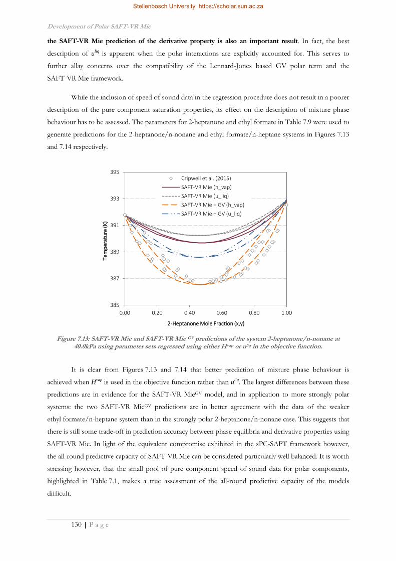
Development of Polar SAFT-VR Mie
130 | P a g e
the SAFT-VR Mie prediction of the derivative property is also an important result. In fact, the best
description of uliq
is apparent when the polar interactions are explicitly accounted for. This serves to
further allay concerns over the compatibility of the Lennard-Jones based GV polar term and the
SAFT-VR Mie framework.
While the inclusion of speed of sound data in the regression procedure does not result in a poorer
description of the pure component saturation properties, its effect on the description of mixture phase
behaviour has to be assessed. The parameters for 2-heptanone and ethyl formate in Table 7.9 were used to
generate predictions for the 2-heptanone/n-nonane and ethyl formate/n-heptane systems in Figures 7.13
and 7.14 respectively.
It is clear from Figures 7.13 and 7.14 that better prediction of mixture phase behaviour is
achieved when Hvap is used in the objective function rather than uliq. The largest differences between these
predictions are in evidence for the SAFT-VR MieGV model, and in application to more strongly polar
systems: the two SAFT-VR MieGV predictions are in better agreement with the data of the weaker
ethyl formate/n-heptane system than in the strongly polar 2-heptanone/n-nonane case. This suggests that
there is still some trade-off in prediction accuracy between phase equilibria and derivative properties using
SAFT-VR Mie. In light of the equivalent compromise exhibited in the sPC-SAFT framework however,
the all-round predictive capacity of SAFT-VR Mie can be considered particularly well balanced. It is worth
stressing however, that the small pool of pure component speed of sound data for polar components,
highlighted in Table 7.1, makes a true assessment of the all-round predictive capacity of the models
difficult.
Figure 7.13: SAFT-VR Mie and SAFT-VR Mie GV predictions of the system 2-heptanone/n-nonane at 40.0kPa using parameter sets regressed using either Hvap or uliq in the objective function.
385
387
389
391
393
395
0.00 0.20 0.40 0.60 0.80 1.00
Tem
per
atu
re (K
)
2-Heptanone Mole Fraction (x,y)
Cripwell et al. (2015)
SAFT-VR Mie (h_vap)
SAFT-VR Mie (u_liq)
SAFT-VR Mie + GV (h_vap)
SAFT-VR Mie + GV (u_liq)
Stellenbosch University https://scholar.sun.ac.za

Development of Polar SAFT-VR Mie
131 | P a g e
7.5.3.2 Using uliq of Isomers in Regression
In Section 7.2 and Table 7.1, the lack of pure component speed of sound data for polar
components was highlighted. Given the central role that this property plays in the reported SAFT-VR Mie
framework, physical arguments were made to support the following claim to account for speed of sound
data for those isomers where no experimental data have been published:
For those linear components where no pure component speed of sound data are available,
available data for linear isomers of that component may be used in the regression of SAFT-VR
Mie parameters.
Here, the aim is to test the validity of this argument by testing the predictions of the parameter
sets determined using the Standard pure component regression and employing this premise. Given the
demonstrated need to incorporate the explicit dipolar term, and the evidence given in the previous section
that including speed of sound data does not significantly improve the accuracy of phase equilibria
predictions in the nonpolar model, this discussion is limited to the results for SAFT-VR MieGV. To this
end, selected parameter sets determined in this manner are presented in Table 7.10.
Figure 7.14: SAFT-VR Mie and SAFT-VR Mie GV predictions of the system ethyl formate/n-heptane at 101.3kPa using parameter sets regressed using either Hvap or uliq in the objective function.
325
335
345
355
365
375
0.00 0.20 0.40 0.60 0.80 1.00
Tem
per
atu
re (K
)
Ethyl Formate Mole Fraction (x,y)
Ortega et al. (2015)
SAFT-VR Mie (h_vap)
SAFT-VR Mie (u_liq)
SAFT-VR Mie + GV (h_vap)
SAFT-VR Mie + GV (u_liq)
Stellenbosch University https://scholar.sun.ac.za

Development of Polar SAFT-VR Mie
132 | P a g e
Table 7.10: Regressed parameter sets for selected components using the pure component uliq data of their linear structural isomers. Parameter sets following the Hvap regression alternative listed for comparison.
σ m ε/k λa λr xp/np Psat * ρsat * uliq Hvap *
Å K AAD% AAD% AAD% AAD%
3-Pentanone
SAFT-VR MieGV
Hvap 3.9689 2.3972 324.476 6 16.5943 2.2401 0.529 0.916 6.627 a 1.952
uliq 3.9689 2.4019 326.997 6 15.8260 1.8739 0.783 0.408 5.362 a 2.417
4-Heptanone
SAFT-VR MieGV
Hvap 4.7438 2.0747 469.593 6 26.7097 4.7438 0.093 0.237 15.21 b 0.150
uliq 4.3476 2.5293 389.852 6 18.1491 4.3476 0.237 0.094 0.723 b 0.919
Pentyl Formate
SAFT-VR MieGV
Hvap 4.4929 2.2472 437.890 6 24.3903 5.0077 0.654 0.360 14.43 c 1.591
uliq 4.1976 2.6248 373.041 6 18.5101 4.4138 0.819 0.317 4.577 c 1.623
Methyl Acetate
SAFT-VR MieGV
Hvap 3.4361 2.6119 264.106 6 12.6665 2.0504 0.119 0.308 2.213 d 1.671
uliq (isomer) 3.4188 2.6478 264.830 6 12.5191 1.5344 0.093 0.181 2.095 d 1.858
uliq (self) 3.4258 2.6363 268.487 6 12.6291 1.2984 0.113 0.094 2.441 d 1.916
* AADs based on DIPPR Correlations; a AADs based on uliq data of 2-pentanone; b AADs based on uliq data of 2-heptanone; c AADs based on uliq data of butyl acetate; d AADs based on uliq data of ethyl formate
In similar fashion to that demonstrated in the previous section, incorporating the uliq data of a
linear isomer yields a SAFT-VR MieGV parameter set which differs from the Hvap alternative primarily in
the values of np and ε/k. The same trends in the numerical values of these parameters are also apparent,
with smaller dispersion energies and repulsive ranges in evidence when the isomer uliq data are considered.
The reported AADs for the uliq regression alternative are of the same order of magnitude as those in
Table 7.9 for those components where their own speed of sound data were available. The most notable
difference is the vastly improved prediction of uliq. Although the AADs are calculated with reference to
the respective isomer data, the equivalent data for these components are expected to be numerically
similar, making the improved predictions a significant result.
Table 7.10 contains two parameter sets for methyl acetate; the first of which was regressed using
uliq data of methyl acetate while the second was determined using equivalent data for ethyl formate. The
similarity of the resulting parameter sets confirm that the regression procedure is not sensitive enough to
distinguish between the numerically similar data of the two isomers. This is further reflected in the
prediction of both the pure component speed of sound data as well as mixture phase equilibrium data in
Figures 7.15 [i.] and [ii.] respectively.
Stellenbosch University https://scholar.sun.ac.za

Development of Polar SAFT-VR Mie
133 | P a g e
Predictions for mixture phase behaviour of 3-pentanone, 4-heptanone and pentyl formate using
the parameter sets in Table 7.10 are shown in Figures 7.16 [i.] to [iii.]. It is clear that there is no significant
deterioration of the VLE prediction quality when incorporating the isomer uliq data in the regression
procedure. Combined with the improved description of the isomer uliq data, these results suggest that
including data of linear isomers in the regression objective function is indeed a viable regression
alternative.
7.5.4 Accounting for Structural Isomerism
The major focus of the experimental and sPC-SAFT modelling chapters was the role of
functional group location on mixture phase behaviour and the predictability of these systems. It was here
that the numerical deficiencies of the JC polar term were systematically highlighted, and the relationship
between structural isomerism and prediction accuracy was first established. Having considered and
developed a polar SAFT-VR Mie model, a pertinent consideration is whether such trends are maintained
or indeed improved upon in the SAFT-VR Mie framework.
The superiority of sPC-SAFTGV over its sPC-SAFTJC counterpart became evident in the
determination of parameter sets using the Standard pure component regression for different isomers. The
difficulties experienced using the JC polar term came as a result of a broad flat minimum for those
isomers that exhibit behaviour closest to that of the equivalent weight nonpolar component. This resulted
in an inability to distinguish between the polar and dispersion contributions. The more general problems
encountered by SAFT-VR MieJC as a result the same numerical issues have already been discussed. Thus
of particular interest is whether the GV polar term maintains its predictive accuracy for isomers moving
from sPC-SAFT to SAFT-VR Mie.
Figure 7.15: Comparing the performance of parameter sets for methyl acetate regressed against Hvap, its own uliq data and that of its linear isomer, ethyl formate. Predictions for [i.] uliq and [ii.] methyl
acetate/n-heptane VLE (Fernández et al., 2013) at 101.3kPa.
325
335
345
355
365
375
0.00 0.20 0.40 0.60 0.80 1.00
Tem
per
atu
re (K
)
Methyl Acetate Mole Fraction (x,y)
Fernández et al. (2013)
hvap
uliq - Methyl Acetate
uliq - Ethyl Formate
[ii.]
1000
1075
1150
1225
1300
1375
275 285 295 305 315 325
u (
m.s
-1)
Temperature (K)
Pal et al. (2013)
hvap
uliq - Methyl Acetate
uliq - Ethyl Formate
[i.]
Stellenbosch University https://scholar.sun.ac.za

Development of Polar SAFT-VR Mie
134 | P a g e
The comparison between sPC-SAFTGV and SAFT-VR MieGV predictions, with parameters
regressed by the Standard pure component regression, for the three heptanone/n-nonane mixtures is
presented in Figures 7.17 [i.] to [iii.]. There is clear improvement in the predictions of SAFT-VR MieGV for
the more strongly polar 2-heptanone and 3-heptanone isomers. Predictions for the least polar
4-heptanone isomer on the other hand are practically identical. This is an important result, given the
need to regress an additional pure component parameter in the SAFT-VR Mie framework.
0.09
0.10
0.11
0.12
0.13
0.14
0.15
0.16
0.00 0.20 0.40 0.60 0.80 1.00
Pre
ssu
re (b
ar)
3-Pentanone Mole Fraction (x,y)
Fuchs et al. (1984)
SAFT-VR Mie + GV (h_vap)
SAFT-VR Mie + GV (u_liq)
381
383
385
387
389
391
393
0.00 0.20 0.40 0.60 0.80 1.00
Tem
per
atu
re (K
)
4-Heptanone Mole Fraction (x,y)
Cripwell et al. (2015)
SAFT-VR Mie + GV (h_vap)
SAFT-VR Mie + GV (u_liq)
376
378
380
382
384
386
388
0.00 0.20 0.40 0.60 0.80 1.00
Tem
per
atu
re (K
)
Pentyl Formate Mole Fraction (x,y)
This work
SAFT-VR Mie + GV (h_vap)
SAFT-VR Mie + GV (u_liq)
Figure 7.16: Assessment of the predictive capacities of parameter sets based on uliq data for linear isomers given that no such data are available for the components in question. Predictions are compared to the Hvap alternatives in the systems [i.] 3-pentanone/n-heptane (Fuchs et al., 1984) at 363.15K, [ii.] 4-heptanone/n-
nonane (Cripwell et al., 2015) at 40.0kPa and [iii.] pentyl formate/n-octane (This work) at 60.0kPa.
[ii.] [i.]
[iii.]
Stellenbosch University https://scholar.sun.ac.za

Development of Polar SAFT-VR Mie
135 | P a g e
Predictions for the phase behaviour of the five C6 ester isomers with n-octane are presented in
Figures 7.18 [i.] to [v.]. Predictive capacity of the GV polar term is maintained in the strongly polar pentyl
formate and methyl valerate cases, while a qualitatively good prediction is in evidence for ethyl butanoate.
The predictions in these systems are on par with their sPC-SAFTGV counterparts with more equal
performance of the models in evidence for the weaker ester than in the ketones previously.
The distinct difference between the models however, is in the cases of butyl acetate & propyl
propanoate and indeed both C6 ether isomers, where the presence of a broad minimum prevented
successful regression of a unique polar parameter set for SAFT-VR MieGV. In sPC-SAFTGV, this problem
was only evident for the case of butyl ethyl ether, but the problem extends to the remainder of the ether
family and a number of weakly polar esters in SAFT-VR MieGV. This is a clear demonstration of the
increased prevalence of broad minima in the regression space of higher dimensionality using SAFT-VR
Mie, which as has already been discussed.
Figure 7.17: Comparison of the sPC-SAFTGV and SAFT-VR MieGV predictions for the phase behaviour of [i.] 2-heptanone, [ii.] 3-heptanone and [iii.] 4-heptanone with n-nonane at 40.0kPa (Cripwell et al., 2015).
385
387
389
391
393
395
0.00 0.20 0.40 0.60 0.80 1.00
Tem
per
atu
re (K
)
2-Heptanone Mole Fraction (x,y)
Cripwell et al. (2015)
sPC-SAFT + GV
SAFT-VR Mie + GV
[i.]
384
386
388
390
392
394
0.00 0.20 0.40 0.60 0.80 1.00
Tem
per
atu
re (K
)
3-Heptanone Mole Fraction (x,y)
Cripwell et al. (2015)
sPC-SAFT + GV
SAFT-VR Mie + GV
[ii.]
381
383
385
387
389
391
393
0.00 0.20 0.40 0.60 0.80 1.00
Tem
per
atu
re (K
)
4-Heptanone Mole Fraction (x,y)
Cripwell et al. (2015)
sPC-SAFT + GV
SAFT-VR Mie + GV
[iii.]
Stellenbosch University https://scholar.sun.ac.za

Development of Polar SAFT-VR Mie
136 | P a g e
377
379
381
383
385
0.00 0.20 0.40 0.60 0.80 1.00
Tem
per
atu
re (K
)
Methyl Valerate Mole Fraction (x,y)
This work
sPC-SAFT + GV
SAFT-VR Mie + GV (h_vap)
370
372
374
376
378
380
382
0.00 0.20 0.40 0.60 0.80 1.00
Tem
per
atu
re (K
)
Ethyl Butanoate Mole Fraction (x,y)
This work
sPC-SAFT + GV
SAFT-VR Mie + GV (h_vap)
368
371
374
377
380
383
0.00 0.20 0.40 0.60 0.80 1.00
Tem
per
atu
re (K
)
Propyl Propanoate Mole Fraction (x,y)
This work
sPC-SAFT + GV
375
377
379
381
383
0.00 0.20 0.40 0.60 0.80 1.00
Tem
per
atu
re (K
)
Butyl Acetate Mole Fraction (x,y)
This work
sPC-SAFT + GV
377
380
383
386
389
0.00 0.20 0.40 0.60 0.80 1.00
Tem
per
atu
re (K
)
Pentyl Formate Mole Fraction (x,y)
This work
sPC-SAFT + GV
SAFT-VR Mie + GV (h_vap)
Figure 7.18: Comparison of the sPC-SAFTGV and SAFT-VR MieGV predictions for the phase behaviour of [i.] methyl valerate, [ii.] ethyl butanoate, [iii.] propyl propanoate, [iv.] butyl acetate and [v.] pentyl formate
with n-octane at 60.0 kPa (This work).
[i.]
[v.]
[ii.]
[iii.] [iv.]
Stellenbosch University https://scholar.sun.ac.za
Development of Polar SAFT-VR Mie
137 | P a g e
That polar SAFT-VR Mie could not make up for the deficiencies in describing the phase
behaviour of polar structural isomers demonstrated in polar sPC-SAFT is a disappointing result, but one
which demonstrates that the fault does not lie with the parent EoS. Rather, it is inherently linked to the
prominence of the dipolar behaviour and thus its description by the polar term as distinct from an
equivalent nonpolar molecule. Extension to the SAFT-VR Mie framework has also demonstrated the
robustness of the GV polar term in a mathematically challenging regression space and clearly established
its superiority over the JC polar term in this regard. This last point is notable as it addresses a primary aim
of this study.
As with polar sPC-SAFT before it, the numerical difficulties of determining unique parameter sets
in polar SAFT-VR Mie can be bypassed through incorporation of mixture phase behaviour in the
regression function. The resulting optimum parameter sets were presented and used as reference earlier in
this chapter. Though demonstrably accurate, a fundamental flaw in the process of determining these
parameters is the need for reliable mixture data. In lieu of such data, it is necessary to improve the
regression results based on pure component data alone.
7.6 Addressing the Dependence of Optimal Parameters
on VLE Data
In the polar sPC-SAFT framework, the reliance of accurate parameter sets on incorporating
mixture VLE data in the regression was mitigated by using the correlations of equations 5.2 and 5.3. These
functional group specific, empirical correlations fix the values of the polar parameters to physically
meaningful constant values, allowing the dimensionality of the regression space to be reduced. This allows
for determination of the remaining nonpolar parameters by regression using pure component data alone.
The success of this procedure was extensively demonstrated in Chapter 5, producing parameter sets
exhibiting comparable predictions with those where VLE data were incorporated.
2p
w
Kx
A M B μ
5.2
2
wp
K A M Bn
μ
5.3
The dependence of these correlations on pure component properties alone (viz. molecular weight
and dipole moment) suggests that employing this approach using polar SAFT-VR Mie is a viable
alternative. In polar sPC-SAFT, the equivalent constants of equations 5.2 and 5.3 were fit to values of xp
and np that had been successfully regressed as a result of incorporating VLE data in the regression
procedure. The details of this fitting procedure were given in Section 5.1.3. Extending this to polar
SAFT-VR Mie means that these functional group specific constants require refitting using the successfully
Stellenbosch University https://scholar.sun.ac.za

Development of Polar SAFT-VR Mie
138 | P a g e
regressed parameters of Tables 7.3 and 7.4. The results of this fitting procedure are presented in
Table 7.11.
Table 7.11: Functional group specific constants determined for Equations 5.2 & 5.3 for polar SAFT-VR Mie
Variant Group K A B
SAFT-VR MieJC Ketones - - -
xp Esters 3.8062 0.01056 1.4819
Ethers 1.0597 0.00668 1.9578
SAFT-VR MieGV Ketones 4.3725 0.02014 1.0405
np Esters 3.6506 0.00693 2.3156
Ethers 1.9224 0.00587 2.0837
The inability to successfully determine unique SAFT-VR MieJC parameter sets for all but two of
the ketones considered means that correlation constants could not be determined for this functional
group. This omission further reinforces the apparent superiority of the GV term over its JC counterpart
in the SAFT-VR Mie framework. With the constants of Table 7.11 successfully determined, polar SAFT-
VR Mie parameter sets could be regressed with a fixed polar parameter.
7.6.1 Choice of Pure Component Properties
An alternative regression procedure once again raises the question of which pure component
properties should be considered. In the case of polar sPC-SAFT, after fixing the value of the polar
parameter, the remaining nonpolar parameters were fit to the standard combination of saturated vapour
pressure, saturated liquid density and heat of vaporisation. This same procedure could be followed using
polar SAFT-VR Mie, but a more promising alternative exists.
The incorporation of speed of sound data in the regression procedure has already shown to
improve the description of this property by the resulting SAFT-VR Mie parameter sets. More importantly,
this improved description of uliq does not come at the expense of a notable loss in prediction accuracy of
saturation properties and phase equilibria. Thus, the final polar SAFT-VR Mie regression alternative
(Figure 7.1) is fixing the value of the polar parameter and regressing the nonpolar parameters using the
following pure component properties with approximate regression weightings as indicated:
saturated vapour pressures, Psat, (4),
saturated liquid densities, ρsat, (4), and
speed of sound, uliq, (1).
The demonstrated ability to use the speed of sound data of isomers when no such data are
available for the component in question means that this regression procedure is applicable to the majority
of the polar components of interest. A clear exception is the case of the ether components, for which the
Stellenbosch University https://scholar.sun.ac.za

Development of Polar SAFT-VR Mie
139 | P a g e
lack of data has been discussed, and methyl formate which has no available uliq data nor does it have any
linear isomers. In these cases, the same procedure used for polar sPC-SAFT will be used, viz.:
saturated vapour pressures, Psat, (4),
saturated liquid densities, ρsat, (2), and
heats of vaporisation, Hvap, (1).
The resulting parameter sets for this regression alternative are listed in Table 7.12 for SAFT-VR
MieJC and in Table 7.13 for SAFT-VR MieGV. Combined with the “VLE” parameter sets of Tables 7.3 and
7.4, these “Correlation” parameters represent the optimum parameter sets generated in this work. These
two parameter sets are extensively applied to mixture data for phase equilibria and other thermodynamic
properties in Chapter 8, where a detailed assessment of the predictive capacities of these models is
performed.
Stellenbosch University https://scholar.sun.ac.za

Development of Polar SAFT-VR Mie
140 | P a g e
7.6.2 Fixed xp/np Parameter Sets
Table 7.12: “Correlation” SAFT-VR MieJC parameters for ketones, esters and ethers determined by fixing xp according to equation 5.2.
MW σ m ε/k λa λr xp μ Psat * ρsat * uliq † Hvap *
g.mol-1 Å K D AAD% AAD% AAD% AAD%
Esters
methyl formate 60.05 3.4617 2.0248 220.010 6 10.1708 0.5742 1.77 0.646 0.365 -a 2.937
ethyl formate 74.08 3.7224 2.1468 264.689 6 11.7418 0.4513 1.93 0.814 0.483 0.397 2.982
methyl acetate 74.08 3.6334 2.2751 225.079 6 11.7172 0.5956 1.68 0.613 0.462 1.379 2.418
propyl formate 88.11 3.7861 2.4830 267.264 6 11.7890 0.4325 1.91 0.319 0.041 -a 2.338
ethyl acetate 88.11 3.8449 2.4078 295.263 6 13.7644 0.4980 1.78 0.273 0.386 0.378 2.444
methyl propanoate 88.11 3.7792 2.4793 277.077 6 12.5843 0.5460 1.70 0.148 0.209 3.386 2.262
butyl formate 102.1 4.1453 2.3269 365.456 6 16.6977 0.3643 2.02 1.183 0.126 -a 2.356
propyl acetate 102.1 3.9702 2.6012 312.972 6 14.3533 0.4640 1.79 0.345 0.229 1.803 3.152
ethyl propanoate 102.1 4.0606 2.4588 340.302 6 16.0320 0.4855 1.75 0.195 0.301 1.088 3.800
methyl butanoate 102.1 4.0274 2.4732 329.877 6 14.8501 0.5026 1.72 0.140 0.137 2.126 2.181
pentyl formate 116.2 4.2601 2.5354 380.295 6 17.3048 0.3892 1.90 0.812 1.155 -a 1.288
butyl acetate 116.2 4.2030 2.5955 370.436 6 17.3950 0.4150 1.84 0.404 0.113 1.094 1.289
propyl propanoate 116.2 4.1905 2.5990 361.945 6 17.0019 0.4385 1.79 1.947 0.117 -a 4.367
ethyl butanoate 116.2 4.4051 2.2844 387.611 6 17.0853 0.4289 1.81 1.205 0.617 0.916 2.233
methyl valerate 116.2 4.2663 2.4539 367.882 6 16.2246 0.5354 1.62 0.903 0.106 -a 2.464
Ethers
diethyl ether 74.12 3.7784 2.4826 245.136 6 12.1411 0.4812 1.15 0.337 0.236 -a 1.900
di-n-propyl ether 102.18 4.3519 2.3350 355.558 6 17.0543 0.3504 1.21 0.214 0.405 -a 1.121
butyl ethyl ether 102.18 4.2650 2.4785 351.041 6 17.4838 0.3446 1.22 1.172 0.590 -a 7.681
dibutyl ether 130.23 4.3577 2.9356 363.617 6 17.3944 0.3139 1.17 0.505 0.572 -a 1.550
† AADs in uliq calaculated with reference to corresponding pure component data sets as indicated in Table 7.1 * AADs based on DIPPR Correlations a No AADs possible due to lack of published data
Stellenbosch University https://scholar.sun.ac.za
Stellenbosch University https://scholar.sun.ac.za
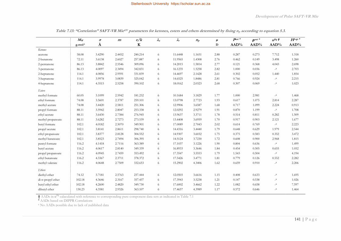
Development of Polar SAFT-VR Mie
141 | P a g e
Table 7.13: “Correlation” SAFT-VR MieGV parameters for ketones, esters and ethers determined by fixing np according to equation 5.3.
MW σ m ε/k λa λr np μ Psat * ρsat * uliq † Hvap *
g.mol-1 Å K D AAD% AAD% AAD% AAD%
Ketones
acetone 58.08 3.4290 2.4452 240.214 6 11.6448 1.1651 2.88 0.287 0.273 7.712 1.318
2-butanone 72.11 3.6138 2.6027 257.887 6 11.9565 1.4308 2.76 0.462 0.149 3.498 1.260
2-pentanone 86.13 3.8842 2.5546 309.096 6 14.2015 1.5814 2.77 0.121 0.368 4.043 2.698
3-pentanone 86.13 4.0097 2.3494 342.831 6 16.1235 1.5258 2.82 1.000 0.036 -a 2.703
2-heptanone 114.1 4.0856 2.9591 331.839 6 14.4697 2.1428 2.61 0.302 0.052 1.440 1.854
3-heptanone 114.1 3.9978 3.0839 325.042 6 14.6525 1.8486 2.81 0.766 0.924 -a 2.215
4-heptanone 114.1 4.3515 2.5258 390.102 6 18.0162 2.0323 2.68 0.307 0.069 -a 1.023
Esters
methyl formate 60.05 3.1099 2.5942 181.232 6 10.1684 3.1829 1.77 1.000 2.981 -a 1.468
ethyl formate 74.08 3.5601 2.3787 259.101 6 13.0798 2.7723 1.93 0.617 1.075 2.814 2.287
methyl acetate 74.08 3.4420 2.5811 251.306 6 12.9906 3.6587 1.68 0.717 1.099 2.224 0.913
propyl formate 88.11 3.5942 2.8047 253.338 6 12.0292 2.9279 1.91 0.870 1.199 -a 1.708
ethyl acetate 88.11 3.6430 2.7384 276.945 6 13.9637 3.3711 1.78 0.514 0.811 0.282 1.509
methyl propanoate 88.11 3.6282 2.7273 273.539 6 13.4408 3.6959 1.70 0.917 0.903 2.121 1.677
butyl formate 102.1 4.0182 2.5070 349.901 6 17.0089 2.7043 2.02 0.614 0.769 -a 2.223
propyl acetate 102.1 3.8141 2.8611 298.740 6 14.4316 3.4440 1.79 0.648 0.629 1.979 2.544
ethyl propanoate 102.1 3.8377 2.8128 304.552 6 14.9307 3.6032 1.75 0.375 0.583 0.352 3.472
methyl butanoate 102.1 3.8523 2.7494 306.395 6 14.5124 3.7230 1.72 0.608 0.900 2.968 1.815
pentyl formate 116.2 4.1418 2.7116 363.389 6 17.1037 3.1226 1.90 0.804 0.636 -a 1.499
butyl acetate 116.2 4.0617 2.8140 349.339 6 16.8933 3.3646 1.84 0.454 0.505 0.655 1.052
propyl propanoate 116.2 4.0945 2.7459 353.492 6 17.3547 3.5553 1.79 1.543 0.504 -a 4.194
ethyl butanoate 116.2 4.3367 2.3711 378.372 6 17.5426 3.4771 1.81 0.779 0.126 0.552 2.282
methyl valerate 116.2 4.0648 2.7509 332.653 6 15.2902 4.3406 1.62 0.659 0.910 -a 2.206
Ethers
diethyl ether 74.12 3.7181 2.5763 237.444 6 12.0503 3.6616 1.15 0.408 0.633 -a 1.695
di-n-propyl ether 102.18 4.3646 2.3167 357.437 6 17.3943 3.5238 1.21 0.147 0.538 -a 1.026
butyl ethyl ether 102.18 4.2600 2.4820 349.730 6 17.6002 3.4662 1.22 1.082 0.658 -a 7.597
dibutyl ether 130.23 4.3581 2.9326 363.107 6 17.4657 4.3989 1.17 0.572 0.646 -a 1.464
† AADs in uliq calaculated with reference to corresponding pure component data sets as indicated in Table 7.1 * AADs based on DIPPR Correlations a No AADs possible due to lack of published data
Stellenbosch University https://scholar.sun.ac.za
Stellenbosch University https://scholar.sun.ac.za

Development of Polar SAFT-VR Mie
142 | P a g e
7.7 Chapter Summary
The aim of this chapter was the development of a new polar SAFT model using the newly
proposed SAFT-VR Mie as a parent framework. Initially, the question of whether polar interactions
needed to be explicitly accounted for using SAFT-VR Mie was conceptually addressed using the physical
considerations of the model. Thereafter, the suitability of the Jog & Chapman and Gross & Vrabec polar
terms being incorporated into this new framework was assessed and the new SAFT-VR MieJC and
SAFT-VR MieGV models were proposed.
The effect of choosing different pure component properties to include in the parameter
regression was assessed. While the use of saturation properties is considered standard, the role of speed of
sound data in the SAFT-VR Mie framework was identified as a key factor in potentially setting the
proposed models apart from their sPC-SAFT counterparts. The lack of pure component uliq data available
in the literature however, represented a potential hurdle to testing this hypothesis. To address this obstacle,
using the speed of sound data of linear isomers as a pseudo pure component property for the regression
of model parameters was shown to be a viable alternative in lieu of data for the component of interest.
The successful incorporation of mixture VLE data in the parameter regressions of polar
sPC-SAFT in the previous chapter lead to similar regression procedures being considered here. The
development of correlations for fixing the value of the polar parameters in the same vein as done by de
Villiers (2011) was also proposed to provide an alternative for parameter regression using pure component
data alone. The result was an extensive regression exercise producing up to 12 different parameter sets for
a range of small to medium length ketones, esters and ethers, including those isomers of interest in earlier
chapters and previous work.
Regression results demonstrated that the newly proposed polar SAFT-VR MieGV performs at
least as well as its sPC-SAFTGV counterpart in the description of isomeric systems. However, problems
of parameter degeneracy and multiple minima were shown to be prevalent in the Standard pure component
regression for the polar SAFT-VR Mie framework as well, most notably for SAFT-VR MieJC. This served
as confirmation that these regression problems are inherently linked to the polar terms considered, as
suggested in the previous chapter. The increased occurrence in SAFT-VR MieGV however also suggests
the problem is intrinsically linked to the dimensionality of the parameter space. As with the polar
sPC-SAFT framework, it was demonstrated that these problems could be circumvented by the VLE and
Correlation regression procedures, for which optimum parameter sets were presented for a variety of
components.
Having developed this new model framework in this chapter and put forward two sets of
optimum parameters, the predictive capacity of SAFT-VR MieJC and SAFT-VR MieGV will be tested using
a range of mixture data in the following chapter.
Stellenbosch University https://scholar.sun.ac.za
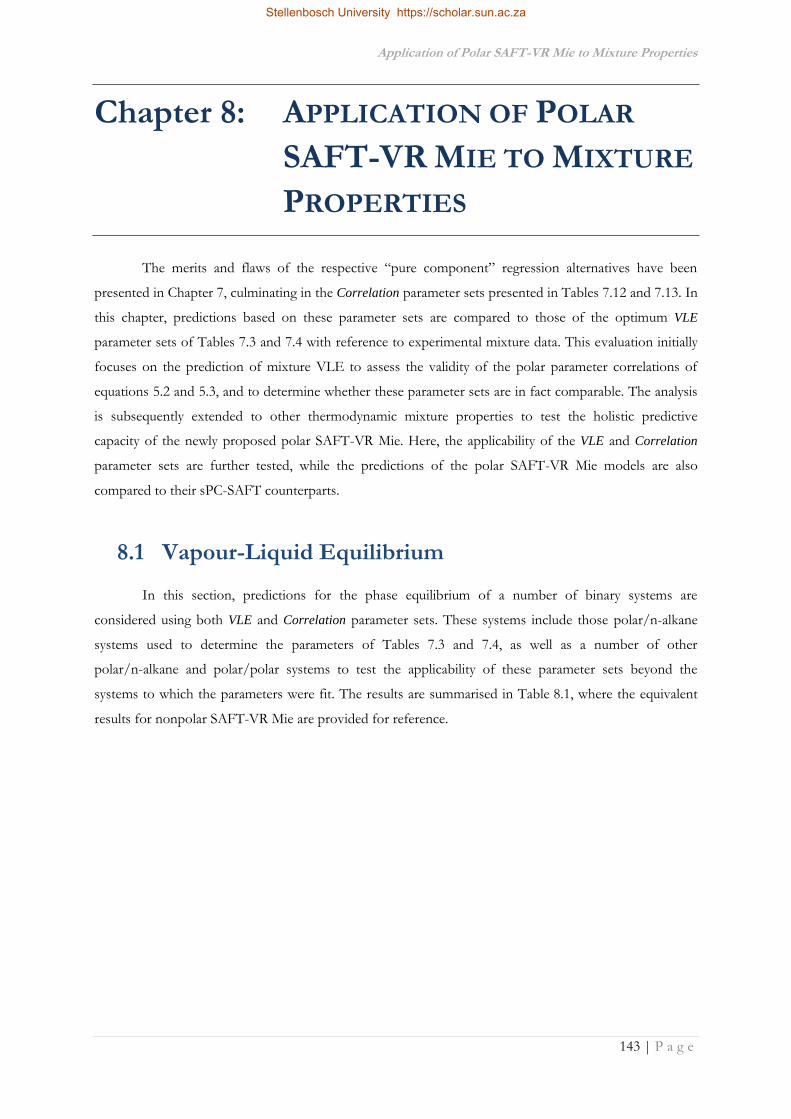
Application of Polar SAFT-VR Mie to Mixture Properties
143 | P a g e
Chapter 8: APPLICATION OF POLAR
SAFT-VR MIE TO MIXTURE
PROPERTIES
The merits and flaws of the respective “pure component” regression alternatives have been
presented in Chapter 7, culminating in the Correlation parameter sets presented in Tables 7.12 and 7.13. In
this chapter, predictions based on these parameter sets are compared to those of the optimum VLE
parameter sets of Tables 7.3 and 7.4 with reference to experimental mixture data. This evaluation initially
focuses on the prediction of mixture VLE to assess the validity of the polar parameter correlations of
equations 5.2 and 5.3, and to determine whether these parameter sets are in fact comparable. The analysis
is subsequently extended to other thermodynamic mixture properties to test the holistic predictive
capacity of the newly proposed polar SAFT-VR Mie. Here, the applicability of the VLE and Correlation
parameter sets are further tested, while the predictions of the polar SAFT-VR Mie models are also
compared to their sPC-SAFT counterparts.
8.1 Vapour-Liquid Equilibrium
In this section, predictions for the phase equilibrium of a number of binary systems are
considered using both VLE and Correlation parameter sets. These systems include those polar/n-alkane
systems used to determine the parameters of Tables 7.3 and 7.4, as well as a number of other
polar/n-alkane and polar/polar systems to test the applicability of these parameter sets beyond the
systems to which the parameters were fit. The results are summarised in Table 8.1, where the equivalent
results for nonpolar SAFT-VR Mie are provided for reference.
Stellenbosch University https://scholar.sun.ac.za

Application of Polar SAFT-VR Mie to Mixture Properties
144 | P a g e
Table 8.1: Summary of deviations in predictions of binary VLE using nonpolar SAFT-VR Mie and the VLE and Correlation variants of SAFT-VR MieGV and SAFT-VR MieJC
SAFT VR Mie SAFT VR MieGV SAFT VR MieJC Reference
VLE Correlation VLE Correlation
T(K)/ P(bar)
Δy (x102)a ΔP(%)b/ ΔT(K)a
Δy (x102)a ΔP(%)b/ ΔT(K)a
Δy (x102)a ΔP(%)b/ ΔT(K)a
Δy (x102)a ΔP(%)b/ ΔT(K)a
Δy (x102)a ΔP(%)b/ ΔT(K)a
Polar/Nonpolar Systems 2-butanone/n-heptane 0.94 bar 8.31 4.26 0.94 0.28 1.39 0.39 1.15 0.29 - - Wisniak et al. (1998) 2-pentanone/n-heptane 353.15 K 4.53 9.61 0.34 0.76 0.78 1.69 - - - - Geiseler et al. (1968) 3-pentanone/n-heptane 313.15 K 6.41 12.30 1.41 4.69 2.06 2.69 - - - - Fuchs et al. (1984) 2-heptanone/n-nonane 0.40 bar 4.60 2.10 1.30 0.20 2.58 1.02 - - - - Cripwell et al. (2015) 3-heptanone/n-nonane 0.40 bar 2.14 1.22 1.94 1.09 0.81 0.38 1.33 1.22 - - Cripwell et al. (2015) 4-heptanone/n-hexane 338.15 K 0.85 8.26 0.27 4.26 0.26 2.62 - - - - Maripuri & Ratcliff (1972) 4-heptanone/n-nonane 0.40 bar 4.26 2.61 0.94 0.19 1.95 0.86 - - - - Cripwell et al. (2015) methyl formate/n-heptane 1.013 bar 7.03 6.74 1.56 1.07 1.68 2.10 1.72 1.07 1.82 2.25 Ortega et al. (2003) ethyl formate/n-heptane 1.013 bar 5.69 5.30 0.33 0.36 0.84 0.79 0.33 0.26 1.65 1.38 Ortega et al. (2015) methyl acetate/n-heptane 1.013 bar 3.68 3.23 0.43 0.27 1.56 1.00 0.39 0.25 0.50 0.25 Fernández et al. (2013) propyl formate/n-heptane 1.013 bar 2.18 2.61 0.29 0.26 0.57 0.43 0.34 0.34 0.26 0.64 Galvan et al. (1994) ethyl acetate/n-heptane 1.013 bar 4.06 2.30 0.46 0.27 0.95 0.29 0.80 0.30 1.80 0.66 Fernández et al. (2010) methyl propanoate/n-heptane 1.013 bar 2.07 2.09 1.69 0.65 2.66 1.15 1.41 0.75 2.02 0.84 Ortega et al. (2003) butyl formate/n-heptane 1.013 bar 4.15 3.03 0.76 0.17 1.96 1.03 1.37 0.18 2.89 1.70 Ortega et al. (2015) propyl acetate/n-heptane 1.013 bar 3.20 1.92 0.65 0.26 1.63 0.71 1.00 0.14 2.02 0.91 Fernández et al. (2013) ethyl propanoate/n-heptane 1.013 bar 1.96 1.86 0.33 0.10 0.45 0.49 0.26 0.07 1.04 1.06 Ríos et al. (2014) methyl butanoate/n-heptane 1.013 bar 2.16 2.33 0.23 0.62 0.46 0.80 0.22 0.64 0.98 1.35 Ríos et al. (2012) pentyl formate/n-octane 0.60 bar 4.64 3.08 0.95 0.11 2.80 1.67 1.18 0.06 3.39 2.01 This work butyl acetate/n-octane 0.60 bar 3.93 2.74 0.70 0.08 2.10 1.25 0.81 0.07 2.61 1.58 This work propyl propanoate/n-octane 0.60 bar 3.05 2.12 0.64 0.14 1.35 0.59 - - 1.82 0.89 This work ethyl butanoate/n-octane 0.60 bar 3.69 2.23 0.91 0.10 1.89 0.79 0.98 0.20 2.73 1.43 This work methyl valerate/n-octane 0.60 bar 3.68 2.08 1.06 0.09 1.04 0.09 1.21 0.07 2.21 0.80 This work diethyl ether/n-pentane 1.013 bar 0.50 0.31 0.41 0.06 0.59 0.33 0.44 0.20 0.43 0.12 Klon-Palczewska et al. (1980) diethyl ether/n-hexane 1.013 bar 0.50 0.17 0.66 0.40 1.09 0.77 0.78 0.54 0.70 0.46 Klon-Palczewska et al. (1980) di-n-propyl ether/n-heptane 0.60 bar 1.01 0.54 0.73 0.06 0.79 0.10 0.71 0.05 0.88 0.38 This work butyl ethyl ether/n-heptane 0.60 bar 0.84 0.46 0.34 0.05 0.37 0.06 0.41 0.93 0.64 0.27 This work dibutyl ether/n-hexane 308.15 K 0.17 1.78 0.22 0.25 0.17 0.19 - - 0.11 1.01 March et al. (1980) Polar/Polar Systems dibutyl ether/2-heptanone 363.15 K 1.10 2.08 0.31 0.74 0.75 1.50 - - 0.75 1.23 Wu & Sandler (1988) dibutyl ether/3-heptanone 363.15 K 0.22 1.09 0.29 1.38 0.35 1.37 - - 0.24 1.10 Wu & Sandler (1988) dibutyl ether/4-heptanone 363.15 K 1.286 2.463 0.29 1.63 0.59 1.25 - - 0.95 1.87 Wu & Sandler (1988) ethyl formate/2-butanone 313.15 K 0.80 0.94 0.78 0.48 1.16 1.47 0.56 0.78 0.78 1.20 Macedo et al. (1984) methyl acetate/ethyl acetate 353.15 K 0.39 1.07 0.15 0.56 0.25 1.47 0.15 0.40 0.15 0.40 Lee et al. (1997) ethyl acetate/butyl acetate 1.013 bar 1.61 1.69 0.48 0.43 0.43 0.38 0.44 0.32 0.48 0.45 Shono & Kanazawa (1969) acetone/dibutyl ether 1.013 bar 0.74 0.41 0.85 0.77 0.86 0.55 - - 1.69 4.94 Resa et al. (1999) acetone/2-butanone 3.447 bar 1.46 0.42 1.76 0.54 1.72 0.46 0.60 1.34 1.60 0.46 Othmer et al. (1952) acetone/3-pentanone 1.013 bar 0.48 0.58 0.57 0.59 0.96 0.87 - - 3.75 3.34 Glukhareva et al. (1974)
a expnp calc
i iiz z zΔ
where z is y or T and np is the number of data points. b Deviations as %AAD
Stellenbosch University https://scholar.sun.ac.za
Stellenbosch University https://scholar.sun.ac.za
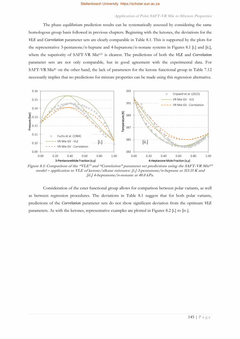
Application of Polar SAFT-VR Mie to Mixture Properties
145 | P a g e
The phase equilibrium prediction results can be systematically assessed by considering the same
homologous group basis followed in previous chapters. Beginning with the ketones, the deviations for the
VLE and Correlation parameter sets are clearly comparable in Table 8.1. This is supported by the plots for
the representative 3-pentanone/n-heptane and 4-heptanone/n-nonane systems in Figures 8.1 [i.] and [ii.],
where the superiority of SAFT-VR MieGV is clearest. The predictions of both the VLE and Correlation
parameter sets are not only comparable, but in good agreement with the experimental data. For
SAFT-VR MieJC on the other hand, the lack of parameters for the ketone functional group in Table 7.12
necessarily implies that no predictions for mixture properties can be made using this regression alternative.
Consideration of the ester functional group allows for comparison between polar variants, as well
as between regression procedures. The deviations in Table 8.1 suggest that for both polar variants,
predictions of the Correlation parameter sets do not show significant deviation from the optimum VLE
parameters. As with the ketones, representative examples are plotted in Figures 8.2 [i.] to [iv.].
383
385
387
389
391
393
0.00 0.20 0.40 0.60 0.80 1.00
Tem
per
atu
re (K
)
4-Heptanone Mole Fraction (x,y)
Cripwell et al. (2015)
VR Mie GV - VLE
VR Mie GV - Correlation
0.09
0.10
0.11
0.12
0.13
0.14
0.15
0.16
0.00 0.20 0.40 0.60 0.80 1.00
Pre
ssu
re (b
ar)
3-PentanoneMole Fraction (x,y)
Fuchs et al. (1984)
VR Mie GV - VLE
VR Mie GV - Correlation
[i.] [ii.]
Figure 8.1: Comparison of the “VLE” and “Correlation” parameter set predictions using the SAFT-VR MieGV model – application to VLE of ketone/alkane mixtures: [i.] 3-pentanone/n-heptane at 313.15 K and
[ii.] 4-heptanone/n-nonane at 40.0 kPa.
Stellenbosch University https://scholar.sun.ac.za

Application of Polar SAFT-VR Mie to Mixture Properties
146 | P a g e
In all cases, the VLE parameter sets of both SAFT-VR MieGV and SAFT-VR MieJC necessarily fit
the experimental data best, having been considered in the regression of the parameters to begin with. The
case of propyl formate/n-heptane in Figure 8.2 [i.] shows that the predictions of the Correlation parameter
sets show negligible deviations from their optimum VLE equivalents in azeotropic systems established
over larger temperature ranges. The discrepancies between the VLE and Correlation parameter predictions
are more notable in Figures 8.2 [ii.] to [iv.], where the azeotropic phase envelope is established in a much
smaller temperature range, providing a more stringent test of the predictive capacity. The np Correlation
predictions for SAFT-VR MieGV exhibit only small deviations from the data and the VLE parameter fits, in
keeping with the trends seen for ketones previously – the azeotropic compositions are well correlated,
even if the azeotropic temperatures are slightly over predicted in all three cases. The equivalent
xp Correlation predictions for SAFT-VR MieJC exhibit much larger deviations; the prediction of the ethyl
butanoate/n-octane system (Figures 8.2 [iv.]) is particularly notable in this respect as the predicted
azeotropic point is far removed from the experimental value. The method is validated by the prediction of
the propyl propanoate/n-octane system (Figures 8.2 [iii.]) however, as the inability to regress a unique VLE
parameter set for this component meant that no SAFT-VR MieJC prediction for this system would be
374
376
378
380
382
0.00 0.20 0.40 0.60 0.80 1.00
Tem
per
atu
re (K
)
Ethyl Butanoate Mole Fraction (x,y)
This work
VR Mie GV - VLE
VR Mie JC - VLE
VR Mie GV - Correlation
VR Mie JC - Correlation
374
376
378
380
382
0.00 0.20 0.40 0.60 0.80 1.00
Tem
per
atu
re (K
)
Propyl Propanoate Mole Fraction (x,y)
This work
VR Mie GV - VLE
VR Mie GV - Correlation
VR Mie JC - Correlation
365
367
369
371
373
375
0.00 0.20 0.40 0.60 0.80 1.00
Tem
per
atu
re (K
)
Ethyl Propanoate Mole Fraction (x,y)
Ríos et al. (2014)
VR Mie GV - VLE
VR Mie JC - VLE
VR Mie GV - Correlation
VR Mie JC - Correlation
349
353
357
361
365
369
373
0.00 0.20 0.40 0.60 0.80 1.00
Tem
per
atu
re (K
)
Propyl Formate Mole Fraction (x,y)
Galvan et al. (1994)
VR Mie GV - VLE
VR Mie JC - VLE
VR Mie GV - Correlation
VR Mie JC - Correlation
[i.] [ii.]
[iii.] [iv.]
Figure 8.2: Comparison of the “VLE” and “Correlation” parameter set predictions using the SAFT-VR MieGV and SAFT-VR MieJC models – application to VLE of ester/alkane mixtures: [i.] propyl formate/n-heptane at
101.3 kPa, [ii.] ethyl ropanoate/n-heptane at 101.3 kPa, [iii.] propyl propanoate/n-octane at 60.0 kPa and [iv.] methyl valerate/n-octane at 60.0 kPa.
Stellenbosch University https://scholar.sun.ac.za

Application of Polar SAFT-VR Mie to Mixture Properties
147 | P a g e
possible. In light of this, the xp Correlation prediction provides a fair description of a difficult system, even
if the prediction remains inferior to its SAFT-VR MieGV counterpart.
Comparison of the VLE and Correlation parameter predictions for ether systems yields similar
results to that seen for esters, with smaller differences in the model predictions for these systems. The
diethyl ether/n-pentane and butyl ethyl ether/n-heptane system are given in Figures 8.3 [i.] and [ii.] as
representative systems, where the former offers a particularly rigorous test of the model performance.
Here, the deviation of the np Correlation prediction from its VLE prediction counterpart is larger than that
for the xp Correlation prediction, but given the temperature range of the system, all four predictions can be
considered excellent. The xp Correlation prediction of the butyl ethyl ether/n-heptane system exhibits the
same tendency as the Standard pure component regression, where a near ideal prediction is in evidence that
oversights the experimental phase envelope.
Figures 8.1 to 8.3 clearly demonstrate that the VLE and Correlation parameter sets are suitable for
the prediction of polar/n-alkane mixture VLE, but their applicability to other industrially relevant
mixtures needs to be tested. In Figures 8.4 [i.] to [iv.], these parameter sets are used to predict the
experimental phase behaviour of the three binary systems comprising dibutyl ether and one of the three
heptanone isomers. The analysis is necessarily limited to the predictions of the SAFT-VR MieGV
alternatives, with the data presented on the same scale axes in Figures 8.4 [i.] to [iii.]. An appropriately
scaled representation of the 4-heptanone/dibutyl ether system is given in Figures 8.4 [iv.]. The model
predictions are in excellent agreement with the experimental data, with the exception of the np Correlation
prediction of the 2-heptanone system, where the presence of azeotrope in the low 2-heptanone
concentration region is not predicted by the model. Both the VLE and Correlation predictions of the
4-heptanone system are shifted from the data, but given the narrowness of the phase envelope and the
small (4 kPa) pressure range, the predictions can still be considered excellent. Accurate prediction of these
systems further serves to show that both regression alternatives, and in particular the case of fixing np,
348
350
352
354
356
0.00 0.20 0.40 0.60 0.80 1.00
Tem
pera
ture
(K)
Butyl Ethyl Ether Mole Fraction (x,y)
This work
VR Mie GV - VLE
VR Mie JC - VLE
VR Mie GV - Correlation
VR Mie JC - Correlation
305
306
307
308
309
310
0.00 0.20 0.40 0.60 0.80 1.00
Tem
pera
ture
(K)
Diethyl Ether Mole Fraction (x,y)
Klon-Palczewska et al. (1980)
VR Mie GV - VLE
VR Mie JC - VLE
VR Mie GV - Correlation
VR Mie JC - Correlation
[i.] [ii.]
Figure 8.3: Comparison of the “VLE” and “Correlation” parameter set predictions using the SAFT-VR MieGV and SAFT-VR MieJC models – application to VLE of ether/alkane mixtures: [i.] diethyl ether/n-pentane and
[ii.] butyl ethyl ether/n-heptane.
Stellenbosch University https://scholar.sun.ac.za
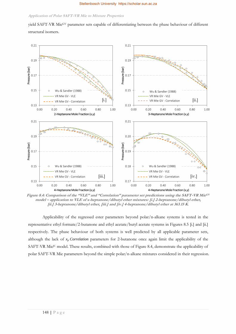
Application of Polar SAFT-VR Mie to Mixture Properties
148 | P a g e
yield SAFT-VR MieGV parameter sets capable of differentiating between the phase behaviour of different
structural isomers.
Applicability of the regressed ester parameters beyond polar/n-alkane systems is tested in the
representative ethyl formate/2-butanone and ethyl acetate/butyl acetate systems in Figures 8.5 [i.] and [ii.]
respectively. The phase behaviour of both systems is well predicted by all applicable parameter sets,
although the lack of xp Correlation parameters for 2-butanone once again limit the applicability of the
SAFT-VR MieJC model. These results, combined with those of Figure 8.4, demonstrate the applicability of
polar SAFT-VR Mie parameters beyond the simple polar/n-alkane mixtures considered in their regression.
0.13
0.15
0.17
0.19
0.21
0.00 0.20 0.40 0.60 0.80 1.00
Pre
ssu
re (b
ar)
4-Heptanone Mole Fraction (x,y)
Wu & Sandler (1988)
VR Mie GV - VLE
VR Mie GV - Correlation
0.17
0.18
0.19
0.20
0.21
0.00 0.20 0.40 0.60 0.80 1.00
Pre
ssu
re (b
ar)
4-Heptanone Mole Fraction (x,y)
Wu & Sandler (1988)
VR Mie GV - VLE
VR Mie GV - Correlation
0.13
0.15
0.17
0.19
0.21
0.00 0.20 0.40 0.60 0.80 1.00
Pre
ssu
re (b
ar)
3-Heptanone Mole Fraction (x,y)
Wu & Sandler (1988)
VR Mie GV - VLE
VR Mie GV - Correlation
0.13
0.15
0.17
0.19
0.21
0.00 0.20 0.40 0.60 0.80 1.00
Pre
ssu
re (b
ar)
2-Heptanone Mole Fraction (x,y)
Wu & Sandler (1988)
VR Mie GV - VLE
VR Mie GV - Correlation [i.] [ii.]
Figure 8.4: Comparison of the “VLE” and “Correlation” parameter set predictions using the SAFT-VR MieGV model – application to VLE of x-heptanone/dibutyl ether mixtures: [i.] 2-heptanone/dibutyl ether,
[ii.] 3-heptanone/dibutyl ether, [iii.] and [iv.] 4-heptanone/dibutyl ether at 363.15 K.
[iii.] [iv.]
Stellenbosch University https://scholar.sun.ac.za

Application of Polar SAFT-VR Mie to Mixture Properties
149 | P a g e
Accurate description of mixture phase equilibria is of primary importance in assessing the
performance of thermodynamic models. The results of this section show polar SAFT-VR Mie to be an
accurate and predictive thermodynamic model on par with polar sPC-SAFT for the description of mixture
phase behaviour. Further, the comparable predictions of the VLE and Correlation parameter sets serve
not only to validate the Correlation regression procedure, but also prove it to be a viable alternative for
parameter determination for components for which there are no experimental VLE data available.
The success of the predictions of the Correlation parameter sets are all the more important when
the nature of the regression procedure is considered. The inclusion of pure component speed of sound
data served only to deteriorate the predictive capacity of polar sPC-SAFT when mixture phase behaviour
is considered, but the integrity of polar SAFT-VR Mie’s predictions is maintained here. SAFT-VR Mie’s
ability to predict speed of sound and other derivative properties has been a constant thread in the
development of polar SAFT-VR Mie in this work. Thus, testing the proposed polar model’s ability to
accurately predict speed of sound in polar mixtures is the logical next step in assessing the predictive
capacity of the model.
0.20
0.29
0.38
0.47
0.56
0.65
0.00 0.20 0.40 0.60 0.80 1.00
Pre
ssu
re (b
ar)
Ethyl Formate Mole Fraction (x,y)
Mendinca et al. (1984)
VR Mie GV - VLE
VR Mie JC - VLE
VR Mie GV - Correlation
VR Mie JC - Correlation
350
360
370
380
390
400
410
0.00 0.20 0.40 0.60 0.80 1.00
Tem
per
atu
re (K
)
Ethyl Acetate Mole Fraction (x,y)
Shono (1969)
GV - VLE
JC - VLE
GV - Correlation
JC - Correlation
[i.] [ii.]
Figure 8.5: Comparison of the performance of the optimum parameter set fit to VLE data and that regressed using the polar parameter correlations – application to VLE of polar/polar mixtures: [i.] ethyl formate/2-
butanone at 313.15 K and [ii.] ethyl acetate/butyl acetate 101.3 kPa.
Stellenbosch University https://scholar.sun.ac.za

Application of Polar SAFT-VR Mie to Mixture Properties
150 | P a g e
8.2 Speed of Sound
Compared to the amount of published pure component data, there is a relative abundance of
mixture speed of sound data for polar components of interest to this study. In this section, the same VLE
and Correlation parameter sets used for the successful description of mixture phase behaviour are used for
the prediction of ultrasonic speed in these polar mixtures. The results are summarised in Table 8.2 below.
Table 8.2: Summary of AADs for model predictions of speed of sound in polar/n-alkane mixtures. Both the
“VLE” and “Correlation” parameter sets for polar SAFT-VR Mie are considered as indicated.
SAFT-VR Mie
sPC-SAFTGV
SAFT-VR MieGV sPC-
SAFTJC SAFT-VR MieJC Reference
VLE Corr VLE Corr
Ketone Systems
acetone/n-hexane 1.90 7.65 5.26 4.22 7.21 - - Marino et al. (2001)
2-butanone/n-heptane 0.90 9.10 1.62 1.95 8.82 1.95 - Ohomuro et al. (1987)
3-pentanone/n-heptane 2.85 10.84 2.21 1.97 10.60 - - Ohomuro et al. (1987)
Ester Systems
methyl acetate/n-heptane 0.88 11.04 3.80 1.97 10.72 3.02 2.34 Sastry et al. (1999)
ethyl acetate/n-hexane 1.98 10.12 0.99 0.49 9.78 1.14 0.75 Acosta et al. (2001)
methyl propanoate/n-heptane 2.08 11.17 5.00 1.93 10.87 4.16 2.34 Sastry et al. (1999)
ethyl propanoate/n-heptane 0.40 11.62 3.02 1.19 11.48 1.77 0.65 Sastry et al. (1999)
methyl butanoate/n-heptane 0.67 12.18 3.66 1.93 11.57 2.27 1.35 Sastry et al. (1999)
butyl acetate/n-heptane 2.09 11.83 1.83 1.02 11.53 1.59 1.41 Sastry et al. (2009)
ethyl butanoate/n-heptane 1.08 12.28 6.58 0.82 11.65 2.89 0.91 Sastry et al. (1999)
Ether Systems
diethyl ether/n-hexane 1.31 9.53 1.89 2.24 9.29 1.67 1.63 Canosa et al. (1999)
di-n-propyl ether/n-heptane 0.65 12.07 0.81 0.76 11.94 2.57 0.75 Ohomuro et al. (1987)
In Figures 8.6 to 8.11 that follow, the predictions of the optimum VLE parameter sets initially
compared to their polar sPC-SAFT equivalents. The polar sPC-SAFT parameters are those determined by
de Villiers (2011) which were similarly determined by incorporating mixture VLE data in their regression.
Thereafter, the effect of incorporating pure component uliq data in the Correlation regression procedure is
considered by comparing the VLE and Correlation predictions directly.
980
1055
1130
1205
1280
1355
0.00 0.20 0.40 0.60 0.80 1.00
u (
m.s
-1)
Mole Fraction 3-Pentanone (x)
Ohomuro et al. (1987)
SAFT-VR Mie
VR Mie GV - VLE
sPC-SAFT + GV
sPC-SAFT + JC
1000
1100
1200
1300
1400
1500
0.00 0.20 0.40 0.60 0.80 1.00
u (
m.s
-1)
Mole Fraction Acetone (x)
Marino et al. (2001)
SAFT-VR Mie
VR Mie GV - VLE
sPC-SAFT + GV
sPC-SAFT + JC
[i.] [ii.]
Figure 8.6: Predictions of mixture speed of sound using polar sPC-SAFT and polar SAFT-VR Mie– application to ketone/alkane mixtures: [i.] acetone/n-hexane at 273.15K and [ii.] 3-pentanone/n-heptane at
298.15K.
Stellenbosch University https://scholar.sun.ac.za

Application of Polar SAFT-VR Mie to Mixture Properties
151 | P a g e
Figures 8.6 [i.] and [ii.] compare the polar SAFT-VR Mie models with their sPC-SAFT
counterparts for the speed of sound in ketone mixtures. The case of acetone is particularly interesting as
the prediction quality varies distinctly over the composition range. The alkane rich region is well correlated
by the SAFT-VR Mie variants, but the prediction quality decreases as the acetone concentration increases.
The pure acetone property is surprisingly best correlated by the sPC-SAFT variants, while incorporation
of the GV polar term results in a worsened prediction compared to nonpolar SAFT-VR Mie. As the
AADs of Table 8.2 and subsequent figures show however, acetone proves to be the exception to the trend.
Figure 8.6 [ii.] for the 3-pentanone/n-heptane system is more representative of this predictive
trend, where there is notable improvement in the prediction quality of polar SAFT-VR Mie compared to
polar sPC-SAFT. Incorporation of the polar term allows for the curvature apparent in the data to be
better captured by the model compared to the nonpolar variant, even if the prediction of the pure ketone
value is slightly worse. It should be noted that these predictions are the result of parameter sets regressed
without consideration of uliq. Thus the innate superiority of SAFT-VR Mie in the prediction of speed of
sound is highlighted and shown to be unaffected by inclusion of the polar term.
The effect of incorporating pure component uliq data in the Correlation regression procedure on
the prediction quality is demonstrated for the same two ketone systems in Figures 8.7 [i.] and [ii.]. In both
systems, the model prediction is brought into closer agreement with the experimental data by using these
parameter sets. Indeed, for the 3-pentanone/n-heptane system, the pure ketone property is correlated
with the same accuracy as the nonpolar SAFT-VR Mie variant, but the curvature of the data is correctly
captured by the polar model. Considered in conjunction with the successful VLE prediction in
Figure 8.1 [i.], and the fact that the parameters were fitted to pure component data alone, the predictive
promise of SAFT-VR MieGV is demonstrated in these ketone systems.
1050
1125
1200
1275
1350
0.00 0.20 0.40 0.60 0.80 1.00
u (
m.s
-1)
Mole Fraction 3-Pentanone (x)
Ohomuro et al. (1987)
SAFT-VR Mie
VR Mie GV - VLE
VR Mie GV - Correlation
1000
1100
1200
1300
1400
1500
0.00 0.20 0.40 0.60 0.80 1.00
u (
m.s
-1)
Mole Fraction Acetone (x)
Marino et al. (2001)
SAFT-VR Mie
VR Mie GV - VLE
VR Mie GV - Correlation
[i.] [ii.]
Figure 8.7: Comparison of the “VLE” and “Correlation” parameter set predictions using the SAFT-VR MieGV model – application to speed of sound of ketone/alkane mixtures: [i.] acetone/n-hexane at 273.15K and
[ii.] 3-pentanone/n-heptane at 298.15K.
Stellenbosch University https://scholar.sun.ac.za

Application of Polar SAFT-VR Mie to Mixture Properties
152 | P a g e
The ester functional group allows for a more extensive analysis to be performed. Predictions of
the VLE parameter sets of SAFT-VR MieGV and SAFT-VR MieJC are compared to their polar sPC-SAFT
counterparts in the four representative systems of Figures 8.8 [i.] to [iv.]. These representative systems
allow us to assess the model predictions applied to the range of molecular weights of linear esters under
consideration, different functional group locations as well as differences between structural isomers.
Across all four figures, a notable result is the significant improvement of prediction quality for the
SAFT-VR Mie models compared to the sPC-SAFT equivalents; the latter clearly capture the trends but are
consistently shifted quantitatively.
The esters also allow for direct comparison of the two polar SAFT-VR Mie models, which was
not possible for ketones previously. Such a comparison suggests that the predictions of SAFT-VR MieJC
are marginally better than for SAFT-VR MieGV, although a similar analysis of the sPC-SAFT predictions
yields the same conclusions. As with the ketones, inclusion of the polar term appears to worsen the
correlation of the pure ester property, but allows for more accurate description of the curvature in the
mixture space. This is particularly notable in the ethyl butanoate/n-heptane system of Figure 8.8 [iii.]
where the nonpolar SAFT-VR Mie prediction is quantitatively much more accurate than
950
1050
1150
1250
1350
0.00 0.20 0.40 0.60 0.80 1.00
u (
m.s
-1)
Mole Fraction Butyl Acetate (x)
Sastry et al. (2009)
SAFT-VR Mie
VR Mie GV - VLE
VR Mie JC - VLE
sPC-SAFT + GV
sPC-SAFT + JC
925
975
1025
1075
1125
1175
1225
1275
0.00 0.20 0.40 0.60 0.80 1.00
u (
m.s
-1)
Mole Fraction Ethyl Butanoate (x)
Sastry et al. (1999)
SAFT-VR Mie
VR Mie GV - VLE
VR Mie JC - VLE
sPC-SAFT + GV
sPC-SAFT + JC
925
975
1025
1075
1125
1175
1225
1275
0.00 0.20 0.40 0.60 0.80 1.00
u (
m.s
-1)
Mole Fraction Ethyl Propanoate (x)
Sastry et al. (1999)
SAFT-VR Mie
VR Mie GV - VLE
VR Mie JC - VLE
sPC-SAFT + GV
sPC-SAFT + JC
925
975
1025
1075
1125
1175
1225
1275
0.00 0.20 0.40 0.60 0.80 1.00
u (
m.s
-1)
Mole Fraction Methyl Acetate (x)
Sastry et al. (2009)
SAFT-VR Mie
VR Mie GV - VLE
VR Mie JC - VLE
sPC-SAFT + GV
sPC-SAFT + JC
[i.] [ii.]
[iii.] [iv.]
Figure 8.8: Predictions of mixture speed of sound using polar sPC-SAFT and polar SAFT-VR Mie– application to ester/alkane mixtures: [i.] methyl acetate/n-heptane at 298.15K, [ii.] ethyl propanoate/n-
heptane at 308.15K, [iii.] ethyl butanoate /n-heptane at 308.15K, and [iv.] butyl acetate/n-hexane at 298.15K.
Stellenbosch University https://scholar.sun.ac.za

Application of Polar SAFT-VR Mie to Mixture Properties
153 | P a g e
SAFT-VR MieGV’s prediction, but the polar model captures the presence of the property minimum.
Indeed, the minimum is well over predicted, but as with acetone previously, this case is the exception to
the rule.
Comparing the results of the VLE and Correlation predictions for the same ester systems in
Figures 8.9 [i.] to [iv.] shows a more significant improvement in the prediction quality using the latter
parameter set. This improvement is more pronounced than was the case for the two ketone systems, most
notably for the np Correlation predictions of the ethyl butanoate/n-heptane (Figure 8.9 [iii.]) and butyl
acetate/n-heptane (Figure 8.9 [iv.]) systems. The case of ethyl butanoate demonstrates the significance of
being able to use speed of sound data of isomers in the regression procedure; without following this
procedure, the relatively poor VLE parameter set prediction would offer the best hope of a simultaneous
prediction of both phase equilibrium and speed of sound in mixtures. The drastic difference in curvature
also illustrates the complexity in describing uliq of mixtures, despite the similarity of the VLE and
Correlation parameter sets themselves.
1050
1100
1150
1200
1250
1300
0.00 0.20 0.40 0.60 0.80 1.00
u (
m.s
-1)
Mole Fraction Butyl Acetate (x)
Sastry et al. (2009)
SAFT-VR Mie
VR Mie GV - VLE
VR Mie JC - VLE
VR Mie GV - Correlation
VR Mie JC - Correlation
950
1000
1050
1100
1150
1200
1250
0.00 0.20 0.40 0.60 0.80 1.00
u (
m.s
-1)
Mole Fraction Ethyl Butanoate (x)
Sastry et al. (1999)
SAFT-VR Mie
VR Mie GV - VLE
VR Mie JC - VLE
VR Mie GV - Correlation
VR Mie JC - Correlation
1000
1050
1100
1150
1200
1250
0.00 0.20 0.40 0.60 0.80 1.00
u (
m.s
-1)
Mole Fraction Ethyl Propanoate (x)
Sastry et al. (1999)
SAFT-VR Mie
VR Mie GV - VLE
VR Mie JC - VLE
VR Mie GV - Correlation
VR Mie JC - Correlation
[i.] [ii.]
[iii.] [iv.]
Figure 8.9: Comparison of the “VLE” and “Correlation” parameter set predictions using the SAFT-VR MieGV and SAFT-VR MieJC models – application to speed of sound of ester/alkane mixtures: [i.] methyl acetate/n-heptane at 298.15K, [ii.] ethyl propanoate/n-heptane at 308.15K, [iii.] ethyl butanoate /n-heptane at 308.15K,
and [iv.] butyl acetate/n-hexane at 298.15K.
1000
1050
1100
1150
1200
1250
0.00 0.20 0.40 0.60 0.80 1.00
u (
m.s
-1)
Mole Fraction Methyl Acetate (x)
Sastry et al. (2009)
SAFT-VR Mie
VR Mie GV - VLE
VR Mie JC - VLE
VR Mie GV - Correlation
VR Mie JC - Correlation
Stellenbosch University https://scholar.sun.ac.za

Application of Polar SAFT-VR Mie to Mixture Properties
154 | P a g e
While the lack of pure ether uliq data has already been highlighted, there are some mixture data
available in the literature with which to compare the model predictions. Figures 8.10 [i.] and [ii.] illustrate
that the same innate superiority of the SAFT-VR Mie models over their sPC-SAFT counterparts in
predicting speed of sound data is maintained for this functional group. The plots further highlight the
small influence of the ether functional group, with the polar predictions yielding much more similar results
to the nonpolar case than for the ketones and esters previously.
For the ketones and esters previously, notable improvement in mixture speed of sound
predictions were apparent as a result of including uliq data in the Correlation parameter regression. The
lack of pure ether uliq data necessitated that the Correlation fits for this functional group be fitted to heat
of vaporisation data instead. The necessary change in regression procedure does not negatively affect the
prediction quality however, as shown in Figures 8.11 [i.] and [ii.], where we see near identical predictions
for the Correlation parameter sets as for the VLE sets. This is still an important result however; it shows
that the prediction integrity, for both speed of sound and phase equilibrium, can be maintained using
only pure component saturation properties without the need for mixture phase equilibria data.
900
980
1060
1140
1220
1300
0.00 0.20 0.40 0.60 0.80 1.00
u (
m.s
-1)
Mole Fraction Dipropyl Ether (x)
Ohomuro et al. (1987)
SAFT-VR Mie
VR Mie GV - VLE
VR Mie JC - VLE
sPC-SAFT + GV
sPC-SAFT + JC
875
925
975
1025
1075
1125
1175
0.00 0.20 0.40 0.60 0.80 1.00
u (
m.s
-1)
Mole Fraction Diethyl Ether (x)
Canosa et al. (1999)
SAFT-VR Mie
VR Mie GV - VLE
VR Mie JC - VLE
sPC-SAFT + GV
sPC-SAFT + JC
[i.] [ii.]
Figure 8.10: Predictions of mixture speed of sound using polar sPC-SAFT and polar SAFT-VR Mie– application to ether/alkane mixtures: [i.] diethyl ether/n-heptane at 298.15K and [ii.] di-n-propyl ether/n-
heptane at 298.15K.
Stellenbosch University https://scholar.sun.ac.za

Application of Polar SAFT-VR Mie to Mixture Properties
155 | P a g e
8.3 Excess Properties
The results of the previous section clearly demonstrate the superiority of the polar SAFT-VR Mie
models over their polar sPC-SAFT counterparts in the description of mixture speed of sound. Considered
in conjunction with the phase equilibrium results of Section 8.1, the advantage of using a polar SAFT-VR
Mie EoS for application to the properties of real fluid mixtures becomes apparent. However, it is
important to remember the fundamental basis upon which the success of SAFT-type modelling has been
based. An improvement in the prediction of one property at the expense of another does not mean that
the model has been improved – even a completely empirical model can fit one property well. Thus, while
it is not the focus of the work presented here, it is necessary to assess the application of the new model
framework to other important thermodynamic properties of mixtures such as excess properties. Indeed,
such an analysis has yet to be performed for real fluids using the SAFT-VR Mie EoS.
The purpose of the following sections is thus to perform a preliminary analysis of the predictive
capacity of the proposed polar SAFT-VR Mie models. The aim of these analyses is to assess the holistic
predictive capacity of polar SAFT-VR Mie using polar sPC-SAFT as a benchmark. The viability of the
parameters resulting from the Correlation regression procedure are also further tested, using the VLE
parameter predictions as a similar reference.
8.3.1 Excess Enthalpy
Assessing the interconnectivity of thermodynamic properties in Figure 7.1 shows that excess
enthalpy provides a good indication of the temperature dependence of the system Helmholtz energy.
More specifically, this property is defined as per equations 8.1 and 8.2, which are an extension of the
framework of Michelsen & Mollerup (2007), with F = Ar/NkT:
1000
1050
1100
1150
1200
1250
0.00 0.20 0.40 0.60 0.80 1.00
u (
m.s
-1)
Mole Fraction Dipropyl Ether (x)
Ohomuro et al. (1987)
SAFT-VR Mie
VR Mie GV - VLE
VR Mie JC - VLE
VR Mie GV - Correlation
VR Mie JC - Correlation
925
975
1025
1075
1125
1175
0.00 0.20 0.40 0.60 0.80 1.00
u (
m.s
-1)
Mole Fraction Diethyl Ether (x)
Canosa et al. (1999)
SAFT-VR Mie
VR Mie GV - VLE
VR Mie JC - VLE
VR Mie GV - Correlation
VR Mie JC - Correlation
[i.] [ii.]
Figure 8.11: Comparison of the “VLE” and “Correlation” parameter set predictions using the SAFT-VR MieGV and SAFT-VR MieJC models – application to speed of sound of ether/alkane mixtures: [i.] diethyl
ether/n-heptane at 298.15K and [ii.] di-n-propyl ether/n-heptane at 298.15K.
Stellenbosch University https://scholar.sun.ac.za

Application of Polar SAFT-VR Mie to Mixture Properties
156 | P a g e
1
, , , ,nc
ex res resi i
i
H H T P H T P n
n 8.1
2
,
, ,res
V
FH T P RT PV nNkT
T n
n 8.2
Equation 8.2 in particular shows that accurate description of mixture excess enthalpy is strongly
dependent on the accurate model description of the temperature dependence of F. Thus, an assessment of
the model predictions of excess enthalpy will provide some insight into how the SAFT-VR Mie
framework models the F-T relationship and test the accuracy of this representation.
The acetone/n-hexane and 3-heptanone/n-heptane systems are used as representative examples
for the ketone functional group, with the corresponding sPC-SAFT and SAFT-VR Mie predictions
plotted in Figures 8.12 [i.] and [ii.]. These systems account for both the size distribution of the ketones, as
well as the relative strength of the dipolar interactions of the components of interest to this study. The
difference between the nonpolar SAFT-VR Mie prediction and those of the other four models clearly
demonstrates the need to explicitly account for dipolar interactions to account for Hex in these
ketone/alkane mixtures. This large discrepancy comes as a result of the interactional contribution to Hex
arising from the significant difference between like and unlike energetic interactions (Costas & Patterson,
1987).
The choice of dipolar term, rather than model framework, appears to have the largest effect on
the prediction accuracy, with the sPC-SAFT and SAFT-VR Mie version of the respective polar terms
exhibiting similar predictions. It is further evident that the predictions of the GV variants are more
accurate than their JC counterparts, although the SAFT-VR MieGV prediction of the
3-heptanone/n-heptane system appears to contradict this observation. This exception is readily explained
by considering the parameter set for this system (Table 7.4), and in particular the value of np itself: the
0
300
600
900
1200
1500
1800
0.00 0.20 0.40 0.60 0.80 1.00
u (
m.s
-1)
Mole Fraction 3-Heptanone (x)
Urdaneta (1979) SAFT-VR Mie
VR Mie GV - VLE VR Mie JC - VLE
sPC-SAFT + GV sPC-SAFT + JC
0
500
1000
1500
2000
2500
3000
0.00 0.20 0.40 0.60 0.80 1.00
HE
(J.m
ol-1
)
Mole Fraction Acetone (x)
Schaffer (1978) SAFT-VR Mie
VR Mie GV - VLE VR Mie JC - VLE
sPC-SAFT + GV sPC-SAFT + JC
Figure 8.12: Predictions of mixture excess enthalpy using polar sPC-SAFT and polar SAFT-VR Mie– application to ketone/alkane mixtures: [i.] acetone/n-hexane at 293.15K and [ii.] 3-heptanone/n-heptane at
298.15K.
[i.] [ii.]
Stellenbosch University https://scholar.sun.ac.za

Application of Polar SAFT-VR Mie to Mixture Properties
157 | P a g e
regressed value of 0.6449 is notably different to the typical value of ~1.8 seen for the other components
and this clearly diminishes the predicted influence of the polar group.
This explanation is supported by the improved prediction of the Correlation parameter set in
Figures 8.13 [ii.], where the np value was fixed to a more representative value of 1.8486. This also explains
the more marked change in the Correlation prediction of this system compared to the acetone/n-hexane
system of Figure 8.13 [i.]. It is interesting to note the improvement, albeit small, in the prediction of the
np Correlation parameter sets in both systems, which serves to further validate this regression alternative.
Once again, the lack of an xp Correlation set for the ketones means no assessment of the change in
prediction accuracy can be made for the SAFT-VR MieJC model.
The propyl acetate/n-heptane and butyl acetate/n-heptane systems in Figures 8.14 [i.] and [ii.]
show that similar trends are in evidence for ester/alkane systems. The nonpolar SAFT-VR Mie prediction
is clearly inferior to those of the polar models, while there is still little difference between the sPC-SAFT
and SAFT-VR Mie predictions using the same polar term. There is again a marked difference between the
predictions of the polar terms themselves, although the JC polar term predictions are now superior to
those of the GV polar models.
0
300
600
900
1200
1500
1800
0.00 0.20 0.40 0.60 0.80 1.00
u (
m.s
-1)
Mole Fraction 3-Heptanone (x)
Urdaneta (1979) SAFT-VR Mie
VR Mie GV - VLE VR Mie JC - VLE
GV - Correlation
0
450
900
1350
1800
2250
2700
0.00 0.20 0.40 0.60 0.80 1.00
HE
(J.m
ol-1
)
Mole Fraction Acetone (x)
Schaffer (1978) SAFT-VR Mie
VR Mie GV - VLE VR Mie JC - VLE
GV - Correlation
Figure 8.13: Comparison of the “VLE” and “Correlation” parameter set predictions using the SAFT-VR MieGV and SAFT-VR MieJC models – application to excess enthalpy of ketone/alkane mixtures:
[i.] acetone/n-hexane at 293.15K and [ii.] 3-heptanone/n-heptane at 298.15K.
[i.] [ii.]
Stellenbosch University https://scholar.sun.ac.za
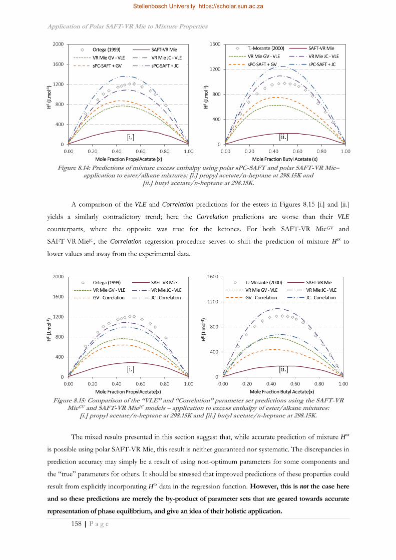
Application of Polar SAFT-VR Mie to Mixture Properties
158 | P a g e
A comparison of the VLE and Correlation predictions for the esters in Figures 8.15 [i.] and [ii.]
yields a similarly contradictory trend; here the Correlation predictions are worse than their VLE
counterparts, where the opposite was true for the ketones. For both SAFT-VR MieGV and
SAFT-VR MieJC, the Correlation regression procedure serves to shift the prediction of mixture Hex to
lower values and away from the experimental data.
The mixed results presented in this section suggest that, while accurate prediction of mixture Hex
is possible using polar SAFT-VR Mie, this result is neither guaranteed nor systematic. The discrepancies in
prediction accuracy may simply be a result of using non-optimum parameters for some components and
the “true” parameters for others. It should be stressed that improved predictions of these properties could
result from explicitly incorporating Hex data in the regression function. However, this is not the case here
and so these predictions are merely the by-product of parameter sets that are geared towards accurate
representation of phase equilibrium, and give an idea of their holistic application.
0
400
800
1200
1600
0.00 0.20 0.40 0.60 0.80 1.00
HE
(J.m
ol-1
)
Mole Fraction Butyl Acetate(x)
T.-Morante (2000) SAFT-VR Mie
VR Mie GV - VLE VR Mie JC - VLE
GV - Correlation JC - Correlation
0
400
800
1200
1600
0.00 0.20 0.40 0.60 0.80 1.00
HE
(J.m
ol-1
)
Mole Fraction Butyl Acetate (x)
T.-Morante (2000) SAFT-VR Mie
VR Mie GV - VLE VR Mie JC - VLE
sPC-SAFT + GV sPC-SAFT + JC
0
400
800
1200
1600
2000
0.00 0.20 0.40 0.60 0.80 1.00
HE
(J.m
ol-1
)
Mole Fraction PropylAcetate(x)
Ortega (1999) SAFT-VR Mie
VR Mie GV - VLE VR Mie JC - VLE
GV - Correlation JC - Correlation
0
400
800
1200
1600
2000
0.00 0.20 0.40 0.60 0.80 1.00
HE
(J.m
ol-1
)
Mole Fraction PropylAcetate (x)
Ortega (1999) SAFT-VR Mie
VR Mie GV - VLE VR Mie JC - VLE
sPC-SAFT + GV sPC-SAFT + JC
[i.] [ii.]
[i.] [ii.]
Figure 8.14: Predictions of mixture excess enthalpy using polar sPC-SAFT and polar SAFT-VR Mie– application to ester/alkane mixtures: [i.] propyl acetate/n-heptane at 298.15K and
[ii.] butyl acetate/n-heptane at 298.15K.
Figure 8.15: Comparison of the “VLE” and “Correlation” parameter set predictions using the SAFT-VR MieGV and SAFT-VR MieJC models – application to excess enthalpy of ester/alkane mixtures:
[i.] propyl acetate/n-heptane at 298.15K and [ii.] butyl acetate/n-heptane at 298.15K.
Stellenbosch University https://scholar.sun.ac.za

Application of Polar SAFT-VR Mie to Mixture Properties
159 | P a g e
Given that the same trends were evident for the polar sPC-SAFT predictions both here and in
similar assessments performed by de Villiers (2011), the mixed results are likely the result of a systematic
shortcoming in describing the temperature dependence of F within the SAFT framework as a whole. A
detailed study, where Hex was the focus of the modelling exercise, would be necessary to confirm or deny
these claims, but this is beyond the scope of the preliminary assessment performed here. In the context of
this work, the most significant result is that the predictions of polar SAFT-VR Mie are of the same order
of magnitude as their sPC-SAFT counterparts, and that accurate description of mixture speed of sound
does not come at the expense of decreased predictive capacity in excess enthalpy.
8.3.2 Excess Volume
Excess volume accounts for the changes in mixture volume resulting from size asymmetries and
differing energetic interactions between the components that constitute the mixture. In a similar fashion
to that of Hex, Vex is defined by equation 8.3 (Michelsen & Mollerup, 2007) and is strongly dependent on
the first order volume derivative of the system Helmholtz energy.
,1
, , , ,nc
exmix pure i i
i
V V T P V T P n
n 8.3
In the same fashion as the preceding sections, the VLE parameter set of SAFT-VR MieGV is used
to predict the excess volume data for the 3-pentanone/n-heptane system in Figure 8.16. In the figure,
nonpolar SAFT-VR Mie falsely predicts a negative excess volume for this system, which clearly
demonstrates the need to explicitly account for dipolar interaction in polar components. The polar
SAFT-VR Mie provides a better prediction of the experimental data than the two polar sPC-SAFT
variants, suggesting that the volume derivatives are better described in the SAFT-VR Mie framework.
Figure 8.16: Predictions of mixture excess volume using polar sPC-SAFT and polar SAFT-VR Mie– application to 3-pentanone/n-heptane at 298.15K.
-0.3
0.0
0.3
0.6
0.9
1.2
1.5
0.00 0.20 0.40 0.60 0.80 1.00
VE
(cm
3.m
ol-1
)
Mole Fraction 3-Pentanone (x)
Grolier (1984) SAFT-VR Mie
VR Mie GV - VLE sPC-SAFT + GV
sPC-SAFT + JC
Stellenbosch University https://scholar.sun.ac.za
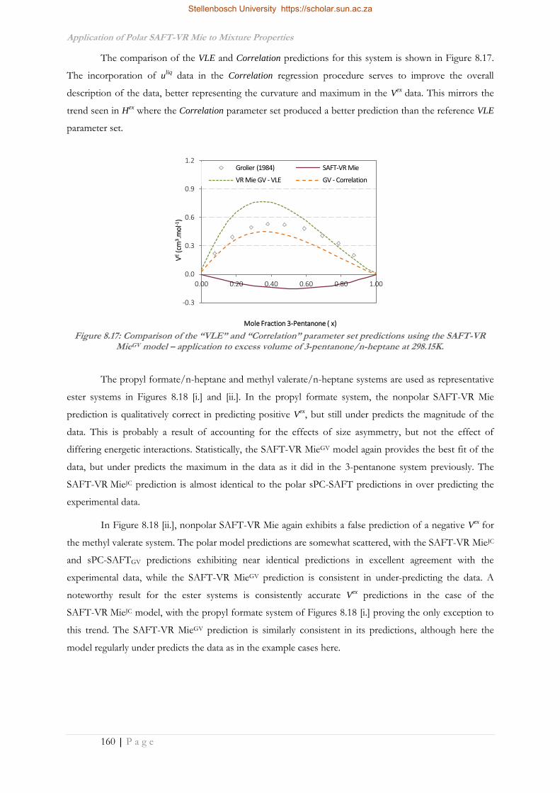
Application of Polar SAFT-VR Mie to Mixture Properties
160 | P a g e
The comparison of the VLE and Correlation predictions for this system is shown in Figure 8.17.
The incorporation of uliq data in the Correlation regression procedure serves to improve the overall
description of the data, better representing the curvature and maximum in the Vex data. This mirrors the
trend seen in Hex where the Correlation parameter set produced a better prediction than the reference VLE
parameter set.
The propyl formate/n-heptane and methyl valerate/n-heptane systems are used as representative
ester systems in Figures 8.18 [i.] and [ii.]. In the propyl formate system, the nonpolar SAFT-VR Mie
prediction is qualitatively correct in predicting positive Vex, but still under predicts the magnitude of the
data. This is probably a result of accounting for the effects of size asymmetry, but not the effect of
differing energetic interactions. Statistically, the SAFT-VR MieGV model again provides the best fit of the
data, but under predicts the maximum in the data as it did in the 3-pentanone system previously. The
SAFT-VR MieJC prediction is almost identical to the polar sPC-SAFT predictions in over predicting the
experimental data.
In Figure 8.18 [ii.], nonpolar SAFT-VR Mie again exhibits a false prediction of a negative Vex for
the methyl valerate system. The polar model predictions are somewhat scattered, with the SAFT-VR MieJC
and sPC-SAFTGV predictions exhibiting near identical predictions in excellent agreement with the
experimental data, while the SAFT-VR MieGV prediction is consistent in under-predicting the data. A
noteworthy result for the ester systems is consistently accurate Vex predictions in the case of the
SAFT-VR MieJC model, with the propyl formate system of Figures 8.18 [i.] proving the only exception to
this trend. The SAFT-VR MieGV prediction is similarly consistent in its predictions, although here the
model regularly under predicts the data as in the example cases here.
Figure 8.17: Comparison of the “VLE” and “Correlation” parameter set predictions using the SAFT-VR MieGV model – application to excess volume of 3-pentanone/n-heptane at 298.15K.
-0.3
0.0
0.3
0.6
0.9
1.2
0.00 0.20 0.40 0.60 0.80 1.00
VE
(cm
3.m
ol-1
)
Mole Fraction 3-Pentanone ( x)
Grolier (1984) SAFT-VR Mie
VR Mie GV - VLE GV - Correlation
Stellenbosch University https://scholar.sun.ac.za

Application of Polar SAFT-VR Mie to Mixture Properties
161 | P a g e
The inclusion of pure component uliq data in the Correlation parameter sets for SAFT-VR MieGV
does not result in significant changes to the resulting prediction for either ester/alkane system. As
Figures 8.19 [i.] and [ii.] show however, the Correlation parameter sets for SAFT-VR MieJC result in
notable decreases in the predicted Vex. In the case of propyl formate, this decrease brings the prediction
into better agreement with the experimental data but as already stated, this is the exception. The trend
apparent for methyl valerate is true for the majority of ester/alkane mixtures however; predictions of the
Correlation parameter sets result in notably worse predictions of the experimental data.
Considering excess volume predictions in this section yielded interesting results, most notably the
consistent accuracy with which the VLE parameter sets of SAFT-VR MieJC predicted experimental Vex
mixture data for esters. The inability to test for consistency of this trend in other functional groups due to
the already detailed lack of parameters for ketones, and lack of data for ethers is thus a particularly
frustrating result. Of significance to this work however, is that the aim of demonstrating the polar
-0.2
0.0
0.2
0.4
0.6
0.8
1.0
0.00 0.20 0.40 0.60 0.80 1.00
VE
(cm
3.m
ol-1
)
Mole Fraction Methyl Valerate ( x)
Pintos (1988) SAFT-VR Mie
VR Mie GV - VLE VR Mie JC - VLE
GV - Correlation JC - Correlation
-0.2
0.0
0.2
0.4
0.6
0.8
1.0
0.00 0.20 0.40 0.60 0.80 1.00
VE
(cm
3.m
ol-1
)
Mole Fraction Methyl Valerate (x)
Pintos (1988) SAFT-VR Mie
VR Mie GV - VLE VR Mie JC - VLE
sPC-SAFT + GV sPC-SAFT + JC
0.0
0.3
0.6
0.9
1.2
1.5
1.8
0.00 0.20 0.40 0.60 0.80 1.00
VE
(cm
3.m
ol-1
)
Mole Fraction Propyl Formate ( x)
Pintos (1988) SAFT-VR Mie
VR Mie GV - VLE VR Mie JC - VLE
GV - Correlation JC - Correlation
0.0
0.3
0.6
0.9
1.2
1.5
1.8
0.00 0.20 0.40 0.60 0.80 1.00
VE
(cm
3.m
ol-1
)
Mole Fraction Propyl Formate (x)
Pintos (1988) SAFT-VR Mie
VR Mie GV - VLE VR Mie JC - VLE
sPC-SAFT + GV sPC-SAFT + JC
[i.]
[ii.]
Figure 8.18: Predictions of mixture excess volume using polar sPC-SAFT and polar SAFT-VR Mie– application to ester/alkane mixtures: [i.] propyl formate/n-heptane at 298.15K and
[ii.] methyl valerate/n-heptane at 298.15K.
[i.]
[ii.]
Figure 8.19: Comparison of the “VLE” and “Correlation” parameter set predictions using the SAFT-VR MieGV and SAFT-VR MieJC models – application to excess isobaric heat capacity of ester/alkane mixtures:
[i.] propyl formate/n-heptane at 298.15K and [ii.] methyl valerate/n-heptane at 298.15K.
Stellenbosch University https://scholar.sun.ac.za

Application of Polar SAFT-VR Mie to Mixture Properties
162 | P a g e
SAFT-VR Mie predictions to be qualitatively similar to their polar sPC-SAFT analogues has been
achieved. Further, in the case of SAFT-VR MieGV, these predictions are improved by using the
Correlation parameter sets for ketones, while the same level of accuracy is maintained for esters.
8.3.3 Excess Isobaric Heat Capacity
The isobaric heat capacity is an extensively used property in industry, and thus accurate
description of this property is desirable in a predictive thermodynamic model. The excess isobaric heat
capacity is a particularly complex function mathematically, with dependence on both the dP/dV and dP/dT
derivatives, as well as the second temperature derivative of F. These former terms are also themselves
functions of the second volume and temperature-volume derivatives of the residual Helmholtz energy
respectively. These relationships are captured by equations 8.4 to 8.6 (Michelsen & Mollerup, 2007).
2
22,
2,,
,
, , 2r VP
VV
T
P
T F FC T P T nNk T T
P T T
V
n
nn
n
n 8.4
2
,V
P FNkT n
T T V
n n
8.5
2
2 2, ,T T
P F nNkTNkT
V V V
n n
8.6
Accurate description of CPex is thus a stringent test of the holistic predictive strength of
thermodynamic models, testing three of the six second order derivatives in F. Predictions of CPex for the
same 3-pentanone/n-heptane system considered for excess volume are presented in Figure 8.20. It is
readily apparent that none of the model predictions accurately account for the trends seen in the
experimental data. Indeed, it appears that the nonpolar model provides the best quantitative prediction,
but it does not account for the negative CPex values at low 3-pentanone concentrations. Both sPC-SAFTGV
and SAFT-VR MieGV over predict the positive maximum in CPex, while the sPC-SAFTJC model
inaccurately predicts large negative excess heat capacities over the whole composition range.
Stellenbosch University https://scholar.sun.ac.za

Application of Polar SAFT-VR Mie to Mixture Properties
163 | P a g e
Figure 8.21 shows that the predictions of the Correlation parameter set for SAFT-VR MieGV
improve the models prediction. However, the experimental trend of negative CPex values in the data is still
unaccounted for, and the maximum is still over predicted.
Considering the polar sPC-SAFT vs. polar SAFT-VR Mie comparison for esters in Figures 8.22 [i.]
and [ii.], we see that similar trends in the model predictions are apparent. The propyl formate/n-heptane
system exhibits qualitatively similar behaviour to the 3-pentanone/n-heptane system, with small negative
CPex values in the low ester concentration range. The nonpolar SAFT-VR Mie prediction once again
provides the best quantitative fit, but the both sPC-SAFTGV and SAFT-VR MieGV predictions are in much
better agreement with the data, qualitatively capturing the shift of the maximum to higher ester
concentrations. The SAFT-VR MieJC model captures the sinusoidal nature of the data, but is inverted and
quantitatively incorrect.
Figure 8.21: Comparison of the “VLE” and “Correlation” parameter set predictions using the SAFT-VR MieGV model – application to excess isobaric heat capacity of 3 pentanone/n-heptane at 298.15K.
Figure 8.20: Predictions of mixture excess isobaric heat capacity using polar sPC-SAFT and polar SAFT-VR Mie– application to 3 pentanone/n-heptane at 298.15K.
-3.0
0.0
3.0
6.0
9.0
0.00 0.20 0.40 0.60 0.80 1.00C
PE
(J.m
ol-1
K-1)
Mole Fraction 3-Pentanone (x)
Grolier (1984) SAFT-VR Mie
VR Mie GV - VLE sPC-SAFT + GV
sPC-SAFT + JC
-2.0
0.0
2.0
4.0
6.0
8.0
0.00 0.20 0.40 0.60 0.80 1.00
CP
E(J
.mo
l-1K-1
)
Mole Fraction 3-Pentanone (x)
Grolier (1984) SAFT-VR Mie
VR Mie GV - VLE GV - Correlation
Stellenbosch University https://scholar.sun.ac.za

Application of Polar SAFT-VR Mie to Mixture Properties
164 | P a g e
The methyl valerate/n-heptane system exhibits the highly complex “W-shaped” concentration
dependence of the CPex curve, with a broad flat maximum in the middle concentration range with local
minima in the extrema of the composition space. As Figure 8.22 [ii.] shows, none of the considered
models are able to predict the trends in the data with any degree of accuracy. What is consistent however
is the relative performance of the SAFT-VR Mie and sPC-SAFT predictions when the same polar term
is used in each case.
In Figures 8.23 [i.] and [ii.], we find that the choice of regression procedure using polar
SAFT-VR Mie does not significantly affect the prediction of the respective models, with the complex
behaviour still not accurately accounted for.
The predictions for mixture excess isobaric heat capacity presented in this section attest to the
difficulty of accurately modelling this highly complex property. The results suggest that, in the case of
-1.5
0.0
1.5
3.0
4.5
6.0
7.5
0.00 0.20 0.40 0.60 0.80 1.00
CP
E(J
.mo
l-1K-1
)
Mole Fraction Propyl Formate (x)
Pintos (1988) SAFT-VR Mie
VR Mie GV - VLE VR Mie JC - VLE
GV - Correlation JC - Correlation
-3.0
-1.5
0.0
1.5
3.0
4.5
6.0
0.00 0.20 0.40 0.60 0.80 1.00
CP
E(J
.mo
l-1K-1
)
Mole Fraction Propyl Formate (x)
Pintos (1988) SAFT-VR Mie
VR Mie GV - VLE VR Mie JC - VLE
sPC-SAFT + GV sPC-SAFT + JC
-3.0
-1.5
0.0
1.5
3.0
4.5
0.00 0.20 0.40 0.60 0.80 1.00CP
E(J
.mo
l-1K-1
)
Mole Fraction Methyl Valerate (x)
Pintos (1988) SAFT-VR Mie
VR Mie GV - VLE VR Mie JC - VLE
GV - Correlation JC - Correlation
-3.0
-1.5
0.0
1.5
3.0
4.5
0.00 0.20 0.40 0.60 0.80 1.00CP
E(J
.mo
l-1K-1
)
Mole Fraction Methyl Valerate (x)
Pintos (1988) SAFT-VR Mie
VR Mie GV - VLE VR Mie JC - VLE
sPC-SAFT + GV sPC-SAFT + JC
[i.] [ii.]
Figure 8.22: Predictions of mixture excess isobaric heat capacity using polar sPC-SAFT and polar SAFT-VR Mie– application to ester/alkane mixtures: [i.] propyl formate/n-heptane at 298.15K and
[ii.] methyl valerate/n-heptane at 298.15K.
[i.] [ii.]
Figure 8.23: Comparison of the “VLE” and “Correlation” parameter set predictions using the SAFT-VR MieGV and SAFT-VR MieJC models – application to excess isobaric heat capacity of ester/alkane mixtures:
[i.] propyl formate/n-heptane at 298.15K and [ii.] methyl valerate/n-heptane at 298.15K.
Stellenbosch University https://scholar.sun.ac.za

Application of Polar SAFT-VR Mie to Mixture Properties
165 | P a g e
mixtures containing polar components, the model predictions are dominated by the contribution of the
polar term rather than the parent framework - the respective polar sPC-SAFT and SAFT-VR Mie models
yield very similar predictions when the same polar term was used. It should again be stressed that these
predictions are the by-product of parameter sets geared towards accurate predictions of phase equilibrium.
A detailed study of the reason for the models’ inability to accurately predict both phase equilibria and CPex
using a single parameter set is beyond the scope of the work done here. However, a brief analysis of
possible causes of deviations is warranted.
Equations 8.4 to 8.6 show that the dP/dV derivative is the only element of the Cpex function which
is not itself a direct function of temperature. Speed of sound is also a function of the dP/dV derivative (see
equation 7.2, reintroduced below) and this property has already been shown to be well predicted by the
polar SAFT-VR Mie framework in this work.
2
,
liq P
T nw V
CV Pu
M C V
7.2
Thus it would appear that it is the temperature dependence of the state function, F, which is not
accurately captured by these models. Poor description of the complex relationship between the
temperature derivatives in the description of F results in the overall poor correlation of isobaric heat
capacities seen in this section. This conclusion is supported by the results for the excess enthalpy
predictions, where a direct relationship between Hex and the dF/dT derivative exists, and smaller
discrepancies with the data are in evidence. As further evidence, equation 7.2 shows that speed of sound is
a function of the heat capacity ratio. The contribution of CPex is small relative to the total CP, with the
same being true of CVex defined in equation 8.7. This suggests that errors in model predictions of CP
ex and
CVex, arising from the incorrect temperature dependence of F, would cancel in the heat capacity ratio. This
error cancellation would account for the demonstrated accuracy of speed of sound measurements for
polar SAFT-VR Mie, despite its poor description of Cpex, although further study would be required to
confirm
2
2
2,,
, , 2rV
VV
F FC T V T T
T T
nn
n 8.7
It is significant to note however that similar conclusions regarding erroneous temperature
dependence in SAFT-type models have been drawn by de Villiers (2011), Polishuk (2011) and Polishuk &
Molero (2011). This suggests that this is a flaw inherent in all the SAFT-type models and is not restricted
to the proposed polar SAFT-VR Mie. As with the excess enthalpy and excess volume predictions of the
previous sections however, the most significant result in the context of this work is that the model
predictions of polar SAFT-VR Mie exhibit similar accuracies to their sPC-SAFT counterparts.
Stellenbosch University https://scholar.sun.ac.za
Application of Polar SAFT-VR Mie to Mixture Properties
166 | P a g e
8.4 Holistic Predictions
In the previous sections, the predictions of the proposed polar SAFT-VR Mie models were
rigorously tested against an array of important thermodynamic properties. In each section, the aim was to
assess the relative performance of the models compared to the renowned sPC-SAFT equivalents for those
particular properties. While the models proved robust in these individual applications, it is desirable to
assess the holistic predictive capacity before drawing final conclusions. To this end, SAFT-VR MieGV and
SAFT-VR MieJC are applied to the full range of considered data for a representative ketone and ester for
which such data were available in this section.
Beginning with 2-butanone for the ketone functional group, predictions for nonpolar
SAFT-VR Mie and the VLE and Correlation parameter sets of SAFT-VR MieGV are presented in
Figures 8.24 [i.] to [v.]. The need to explicitly account for dipolar interactions by incorporating a polar
term is highlighted in the predictions of almost all the considered properties. Considered in this collective
fashion, the holistic strength of the SAFT-VR MieGV model in particular is clearly evident. Given that VLE
parameters could be determined for the SAFT-VR MieJC model for this component, these predictions are
also incorporated and exhibit similar accuracy to their GV counterparts.
The discerning factor between the models however is the viability of using the Correlation
regression procedure to determine equally accurate parameter sets using pure component data alone. In
the case of SAFT-VR MieGV, this viability has been consistently demonstrated and is maintained
throughout Figures 8.24 [i.] to [v.]. However, the inability to generate or test similar xp Correlation
parameters for this functional group underpins the weakness of SAFT-VR MieJC when comparing the two
polar SAFT-VR Mie variants.
Stellenbosch University https://scholar.sun.ac.za

Application of Polar SAFT-VR Mie to Mixture Properties
167 | P a g e
The same rounded analysis is performed using ethyl acetate as the representative component for
esters in Figures 8.25 [i.] to [v.]. The same conclusions can be drawn regarding the need to explicitly
account for dipolar interactions for this more weakly polar functional group, but the distinction between
the two polar variants is less clear than for ketones. The consistent improvement in the prediction of Hex
345
350
355
360
365
370
0.00 0.20 0.40 0.60 0.80 1.00
Tem
per
atu
re (K
)
2-Butanone Mole Fraction (x,y)
Wisniak et al. (1998)
SAFT-VR Mie
VR Mie GV - VLE
VR Mie JC - VLE
GV - Correlation
-2.0
0.0
2.0
4.0
6.0
8.0
0.00 0.20 0.40 0.60 0.80 1.00
CP
E(J
.mo
l-1K-1
)
Mole Fraction 2-Butanone (x)
Grolier (1984) SAFT-VR Mie
VR Mie GV - VLE VR Mie JC - VLE
GV - Correlation
-0.4
0.0
0.4
0.8
1.2
1.6
2.0
2.4
0.00 0.20 0.40 0.60 0.80 1.00
HE
(J.m
ol-1
)
Mole Fraction 2-Butanone (x)
Grolier (1984) SAFT-VR Mie
VR Mie GV - VLE VR Mie JC - VLE
GV - Correlation
0
500
1000
1500
2000
2500
0.00 0.20 0.40 0.60 0.80 1.00
HE
(J.m
ol-1
)
Mole Fraction 2-Butanone (x)
Kiyohara (1979) SAFT-VR Mie
VR Mie GV - VLE VR Mie JC - VLE
GV - Correlation
1050
1100
1150
1200
1250
1300
0.00 0.20 0.40 0.60 0.80 1.00
u (
m.s
-1)
Mole Fraction 2-Butanone (x)
Ohomuro (1987) SAFT-VR Mie
VR Mie GV - VLE VR Mie JC - VLE
GV - Correlation
[ii.] [iii.]
[iv.] [v.]
[i.]
Figure 8.24: Comparison of the “VLE” and “Correlation” parameter set predictions using the SAFT-VR MieGV and SAFT-VR MieJC models – application to the full spectrum of considered mixture properties for butanone/n-heptane: [i.] isobaric VLE, [ii.] speed of sound, [iii.] excess enthalpy, [iv.] excess volume and
[v.] excess isobaric heat capacity.
Stellenbosch University https://scholar.sun.ac.za

Application of Polar SAFT-VR Mie to Mixture Properties
168 | P a g e
and Vex when using SAFT-VR MieJC as opposed to SAFT-VR MieGV suggests that this is the superior
model for the description of ester thermodynamic properties. However, the decrease in SAFT-VR MieJC
prediction accuracies noted when employing the Correlation parameter is a trade-off that is not apparent
for the equivalent SAFT-VR MieGV parameters. This trade-off is seen in all the considered properties, but
perhaps most notably for phase equilibrium predictions.
345
351
357
363
369
375
0.00 0.20 0.40 0.60 0.80 1.00
Tem
per
atu
re (K
)
Ethyl Acetate Mole Fraction (x,y)
Fernández et al. (2010)SAFT-VR MieVR Mie GV - VLEVR Mie JC - VLEGV - CorrelationJC - Correlation
-2.0
0.0
2.0
4.0
6.0
0.00 0.20 0.40 0.60 0.80 1.00
CP
E(J
.mo
l-1K-1
)
Mole Fraction Ethyl Acetate(x)
Pintos (1988) SAFT-VR Mie
VR Mie GV - VLE VR Mie JC - VLE
GV - Correlation JC - Correlation
-0.3
0.0
0.3
0.6
0.9
1.2
1.5
0.00 0.20 0.40 0.60 0.80 1.00
VE
(cm
3.m
ol-1
)
Mole Fraction Ethyl Acetate(x)
Acosta (2001) SAFT-VR Mie
VR Mie GV - VLE VR Mie JC - VLE
GV - Correlation JC - Correlation
0
400
800
1200
1600
2000
2400
0.00 0.20 0.40 0.60 0.80 1.00
HE
(J.m
ol-1
)
Mole Fraction Ethyl Acetate(x)
Vidal (1997) SAFT-VR Mie
VR Mie GV - VLE VR Mie JC - VLE
GV - Correlation JC - Correlation
1000
1050
1100
1150
1200
1250
0.00 0.20 0.40 0.60 0.80 1.00
u (
m.s
-1)
Mole Fraction Ethyl Acetate (x)
Acosta (2001) SAFT-VR Mie
VR Mie GV - VLE VR Mie JC - VLE
GV - Correlation JC - Correlation
[ii.] [iii.]
[iv.] [v.]
[i.]
Figure 8.25: Comparison of the “VLE” and “Correlation” parameter set predictions using the SAFT-VR MieGV and SAFT-VR MieJC models – application to the full spectrum of considered mixture properties for
ethyl acetate/n-heptane (except uliq): [i.] isobaric VLE, [ii.] speed of sound (+n-hexane), [iii.] excess enthalpy, [iv.] excess volume and [v.] excess isobaric heat capacity.
Stellenbosch University https://scholar.sun.ac.za

Application of Polar SAFT-VR Mie to Mixture Properties
169 | P a g e
Considering the overall performance of SAFT-VR MieGV and SAFT-VR MieJC, prediction results
suggest that the former is better suited to describing the behaviour of more strongly polar components,
while the latter is better for weaker polar molecules. Such a recommendation is at odds with the goal of
espousing a single thermodynamic model capable of accurately predicting the behaviour of polar
components and their mixtures as laid out in the aims and objectives of this work.
To this end, the aim of developing a model that yields accurate predictions of equilibrium and
thermodynamic properties using parameters regressed from pure component data alone takes precedence.
Viewed in this light, the regression difficulties experienced using SAFT-VR MieJC cannot be overlooked,
even if notably better results are in evidence for some excess properties using this model. Taken as a whole,
the modelling results of this chapter clearly point to SAFT-VR MieGV being the superior variant in this
new polar framework.
8.5 Chapter Summary
The results of Sections 8.1 and 8.2, considered together, represent the most significant
contribution of the proposed polar SAFT-VR Mie models. Polar sPC-SAFT has already been shown to be
exceedingly competent in predicting the phase equilibria of polar systems, even the nuanced instances of
isomeric systems, if the same VLE and Correlation regression procedures are considered for their
parameter regression. Application of the new SAFT-VR MieGV and SAFT-VR MieJC models to the same
mixture equilibria demonstrated that this predictive capacity is maintained when moving to the
SAFT-VR Mie framework. This result was an important prerequisite for the proposal of a new model and
serves as justification for its development. The novelty and success of the proposed model is evident
however, when these successful equilibrium predictions are considered in conjunction with the vastly
improved description of speed of sound in mixtures when using the same parameter sets.
A primary focus of the work was developing a means of parameter regression that does not
necessitate the inclusion of mixture VLE data, yet still provides an accurate description of the range of
thermodynamic properties considered. To this end, the success of the Correlation regression procedure,
adapted from the sPC-SAFT equivalent of Chapter 5, was a notable and important result. The inclusion of
uliq data in this regression alternative (or equivalently, isomer uliq data) served to improve the mixture speed
of sound predictions, with only a small loss of accuracy in the description of phase equilibrium. While this
constitutes a trade-off for those components where optimum VLE data sets were regressed, it is a
significant result for those components where no such data set could be determined, as well as for the
multitude of components not considered here for which no VLE data have been measured.
To the author’s knowledge, an assessment of the excess properties of real fluids has never been
made with SAFT-VR Mie. The rationale behind performing such an analysis was to test whether the
increased accuracy in predicting speed of sound came at the expense of significantly reduced predictive
Stellenbosch University https://scholar.sun.ac.za

Application of Polar SAFT-VR Mie to Mixture Properties
170 | P a g e
capacity in other thermodynamic properties. To this end, experimental excess enthalpy, excess volume and
excess isobaric heat capacity data were used to test the predictions of the new polar SAFT-VR Mie models,
as well as those of polar sPC-SAFT. It was stressed that these predictions merely provide a holistic view of
the predictive capacity of the VLE and Correlation parameter sets, given that the focus of these parameters
is the accurate description of phase equilibrium. The results illustrated that the choice of polar term is
more significant than the parent SAFT framework in defining the model prediction, with both
sPC-SAFTGV and SAFT-VR MieGV yielding similar results. Similarly, the use of the Correlation parameter
sets was shown to yield predictions at least as good as their VLE counterparts. This preliminary analysis
also highlighted room for improvement of the model moving forward, while the aims of providing a
holistic assessment of the predictive capacity of polar SAFT-VR Mie were met.
The accurate simultaneous prediction of phase equilibria and speed of sound in polar mixtures
demonstrates that the new polar SAFT-VR Mie is an improvement over polar sPC-SAFT. Within this
new framework itself, the ability to generate unique parameter sets for all considered components, that
yield accurate predictions of the range of properties considered, sets SAFT-VR MieGV apart from its
SAFT-VR MieJC counterpart.
Stellenbosch University https://scholar.sun.ac.za
Conclusions
171 | P a g e
Chapter 9: CONCLUSIONS
The overarching aim of this work was systematic improvement of the description of
thermodynamic properties of polar components and their mixtures, within the SAFT framework.
Specifically, the effect of structural isomerism on mixture phase behaviour and non-equilibrium derivative
properties were identified as key factors to address in this pursuit.
Objective (i.) Generation of Low Pressure Phase Equilibrium Data
In order to systematically address the former, it was necessary to generate mixture phase
equilibrium data for ether and ester components. Chapter 4 presented thermodynamically consistent,
isobaric phase equilibrium data that was generated for two C6 ether isomers with n-heptane as well as five
C6 ester isomers with n-octane at 60kPa.
This new experimental data demonstrated that distinct phase envelopes are in evidence for
respective isomers. These isomeric systems exhibit qualitatively similar phase behaviour; viz. narrow,
zeotropic phase envelopes for ether/n-heptane systems and minimum boiling azeotropic behaviour for
ester/n-octane systems.
Objective (ii.) Polar sPC-SAFT: Structural Isomers & Phase Equilibrium
The experimentally measured phase behaviour data were used to test the predictive capacity of
polar sPC-SAFT models in Chapter 5. This modelling exercise was an extension of a previous study
(Cripwell, 2014) for ketone isomers, and demonstrated that structural isomerism in polar molecules
provides a stringent test of the predictive capacity of thermodynamic models. Specifically, it was
concluded that the quality of model predictions decreases as the phase behaviour of the considered isomer
approaches that of its nonpolar size equivalent. Furthermore, the prevalence of parameter degeneracy
increased following this same trend, most notably for sPC-SAFTJC. These results established the trends
seen in previous work as a systematic shortcoming of the model framework – the first time such a
systematic trend has been established.
Overall, sPC-SAFTGV was found to be a more robust and reliable polar framework than
sPC-SAFTJC, significantly outperforming its counterpart in their application to the phase behaviour of
polar structural isomers. Use of the VLE parameter sets brought the predictions of the two terms into
agreement with each other and with mixture data, but the requirement of experimental data negates the
advantage of model prediction over introducing BIPs to correlate the data in more simple semi-empirical
models. In this respect, a major finding of the work was the success of employing the Correlation
regression procedure. This alternative allows for the generation of parameter sets, capable of accurately
representing mixture phase behaviour, from pure component data alone while overcoming the
mathematical shortcomings of the Standard pure component regression.
Stellenbosch University https://scholar.sun.ac.za

Conclusions
172 | P a g e
Objective (iii.) Accounting for Dipolar Interactions in a SAFT-VR Mie Framework
The extensive modelling exercise using polar sPC-SAFT, both here and in the previous work of
de Villiers (2011), highlighted strengths as well as inherent shortcomings in the model framework. With
the primary aim of improving the thermodynamic description of polar components and their mixtures, it
was decided to conduct a similar analysis using the recently developed SAFT-VR Mie framework.
It was demonstrated that dipolar interactions need to be explicitly accounted for in the
SAFT-VR Mie framework. This was the focus of Chapter 7, where the JC and GV polar terms were
incorporated into the SAFT-VR Mie EoS to yield the new polar SAFT-VR MieJC and SAFT-VR MieGV
variants. These models comprise four regressed nonpolar parameters (σ, m, ε/k & λr) as well as a variable
polar parameter (xp or np). A range of regression alternatives were considered for determination of these
parameters, including the traditional Standard pure component regression. Choice of pure component data
in the regression procedure was shown to significantly affect the resulting parameters. Specifically, the role
of pure component speed of sound, prominent in the development of the base SAFT-VR Mie EoS, was
highlighted in producing parameter sets with well-balanced predictive capacity. This demonstrated that the
new polar SAFT-VR Mie variants maintain an excellent holistic prediction capacity for pure component
properties.
The problems of parameter degeneracy and broad minima in the objective function were found
to be more pronounced in the Standard pure component regression of polar SAFT-VR Mie, most notably
so for SAFT-VR MieJC. Considered in combination with similar results in Chapter 5, this was linked to the
choice of polar term and the dimensionality of the parameter space. The prevalence of this regression
hurdle indicates that polar SAFT-VR Mie does not inherently improve the description of phase behaviour
of isomeric systems using the same Standard pure component regression compared to polar sPC-SAFT.
However, the predictions of SAFT-VR MieGV equal or exceed those of sPC-SAFTGV in these systems.
This trend further reinforced the conclusions carried over from Chapter 5 that the GV polar term is a
more robust and reliable modelling framework.
Drawing upon the success in sPC-SAFT, it was found that mitigation of regression problems is
possible by including the binary VLE data in the regression. A more significant result however, was the
demonstrated ability to regress parameter sets by fixing the value of the polar parameter in the Correlation
regression alternative. This alternative reduces the dimensionality of the regression space and removes the
dependence on available VLE data, allowing for optimum parameter sets to be determined from pure
component data alone.
The optimum parameter sets regressed in Chapter 7 were applied to various thermodynamic
properties of polar mixtures in Chapter 8. In this fashion, the all-round predictive capacity was tested,
with model results initially compared to their sPC-SAFT analogues, followed by a comparison of the
predictions of the VLE and Correlation parameter predictions. Application to a wide range of phase
equilibria demonstrated the robust predictive strength of polar SAFT-VR Mie, particularly
Stellenbosch University https://scholar.sun.ac.za
Conclusions
173 | P a g e
SAFT-VR MieGV, displaying excellent agreement with experimental data in all considered systems. The
most significant contribution of the new model framework over polar sPC-SAFT was notable and
consistent improvement in the description of mixture speed of sound using the same parameter set. This
was demonstrated for all three functional groups considered and validated the inclusion of the GV and JC
polar terms in the SAFT-VR Mie framework.
Novel application of the SAFT-VR Mie framework to excess properties demonstrates that polar
SAFT-VR Mie predictions are comparable to those of polar sPC-SAFT. This result is significant as it
shows that improved description of mixture speed of sound does not come at the expense of worse
predictions for other thermodynamic properties. Results of the excess property analysis highlighted that
systematic shortcomings still exist in the SAFT framework, particularly the temperature dependence of Ar,
which extends to the polar SAFT-VR Mie model proposed here. However, given that the model
parameters were not geared towards accurate description of excess properties, these preliminary results
were considered satisfactory.
Addressing the Overarching Aim
Polar SAFT-VR Mie represents a predictive thermodynamic model with the capacity to
simultaneously predict both phase equilibrium and derivative properties with a higher degree of accuracy
than is achievable with previous thermodynamic models. The systematic regression problems faced by
SAFT-VR MieJC, resulting in a lack of parameters for many of the components considered here,
demonstrate the inferiority of this variant to SAFT-VR MieGV. The latter boasts a full complement of
parameter sets for all three polar functional groups considered in this work and exhibits consistently good,
holistic predictions for these components.
The most significant outcome of this work however is the results of the Correlation regression
alternative, which demonstrated that achievability of such accurate results are not limited by the
availability of mixture data. The ability to determine accurate parameter sets using pure component data
alone is a cornerstone of the ideal of a fundamental, predictive model. The ability to regress such
Correlation parameter sets is thus a notable step towards this goal. In the context of this work however,
the SAFT-VR MieGV EoS addresses the aim of improving the thermodynamic description of polar
components and their mixtures.
Stellenbosch University https://scholar.sun.ac.za
Recommendations
174 | P a g e
Chapter 10: RECOMMENDATIONS
Based on the results and finding of this work, the following are recommended for consideration
in future work to further improve the thermodynamic description of polar components and their mixtures:
Generation of Pure Component uliq Data
In Chapter 7, the severe lack of pure component speed of sound data available in the literature
was highlighted. This is particularly true for polar components, where “data sets” typically only comprise
two to three points. Given the modelling success of the Correlation approach in polar SAFT-VR Mie,
where speed of sound data are used in the regression procedure, increased access to accurate pure
component uliq data is vital. While the use of isomer data as a pseudo property was shown to be a viable
short term alternative, true data are required to improve the overall performance of these models.
Systematic Derivative Property Data Generation for Polar Isomers
The experimental aim of this work was the systematic generation of phase equilibrium data for all
isomers of a polar molecule with a common second component. Given the difficulty with which these
mixtures were accurately modelled, a recommendation is to expand the scope of study of these isomeric
components. Specifically, systematic data generation for additional properties such as mixture speed of
sound as well as excess properties for these same systems is recommended. This would provide a more
holistic picture of the role of polar functional group location on the overall thermodynamic behaviour of
these components, which may help in the accurate modelling of these components.
Mapping the Polar SAFT-VR Mie Parameter Space
The primary shortcoming of SAFT-VR MieJC compared to its SAFT-VR MieGV counterpart was
the systematic inability of the former to regress unique parameter sets with a nonzero polar contribution.
Indeed, this was also true for SAFT-VR MieGV in a select few cases. This was attributed to broad minima
in the objective function, which frequently pushed the polar parameter to zero. As highlighted in that
section, interesting work has been done by Dufal et al. (2015) to map the parameter space of nonpolar
SAFT-VR Mie in order to mitigate such regression problems. These mapping procedures help identify
what parameter combinations should be specified as initial guesses to yield parameter sets close to the
global minimum. These parameter combinations can be assessed based on their physical significance
which would systematically improve the overall regression exercise.
Stellenbosch University https://scholar.sun.ac.za

Recommendations
175 | P a g e
Extension of Polar SAFT-VR Mie to Group Contribution Basis
Considering the work of Lafitte and co-workers since the revised SAFT-VR Mie EoS was
published, it would appear that the model’s development was seen as a stepping stone in the development
of a new group contribution approach. The resulting SAFT-γ Mie model has been the focus of subsequent
work from that group, with the group contribution approach seen as superior to the component-specific
approach of SAFT-VR Mie. Whether these group contribution models are in fact superior is still a subject
of debate, especially in the accurate description of isomers which has been a focus of this work. Thus, a
recommendation of this work is to incorporate the polar SAFT-VR Mie results presented here into a polar
SAFT-γ Mie framework to assess whether the group contribution approach represents a viable alternative.
Systematic Modelling Study of Excess Properties
The modelling of mixture excess properties highlighted predictive shortcomings in both polar
sPC-SAFT and polar SAFT-VR Mie. This suggested potential fundamental discrepancies in the SAFT
framework as a whole, particularly in the temperature description of Ar, which has already been
commented on by a number of authors in the literature. A more thorough investigation of SAFT-type
modelling of these excess properties is thus required. Such a study should focus exclusively on the
accurate representation of excess properties, without consideration of mixture VLE, to determine whether
these complex properties can be accurately represented in the model framework at all. To this end,
component parameter could be fit to excess property data, with resulting parameter sets assessed for
physical significance in the same fashion as is done when fit to phase equilibria data.
Stellenbosch University https://scholar.sun.ac.za

References
176 | P a g e
REFERENCES
Acosta, J., Arce, A., Rodil, E. & Soto, A. 2001, "Densities, speeds of sound, refractive indices, and
the corresponding changes of mixing at 25 C and atmospheric pressure for systems composed by ethyl
acetate, hexane, and acetone", Journal of Chemical & Engineering Data, vol. 46, no. 5, pp. 1176-1180.
Acosta, J., Arce, A., Martínez-Ageitos, J., Rodil, E. & Soto, A. 2002, "Vapor−liquid equilibrium of
the ternary system ethyl acetate + hexane + acetone at 101.32 kpa", Journal of Chemical and Engineering Data,
vol. 47, no. 4, pp. 849-854.
Alder, B.J., Young, D.A. & Mark, M.A. 1972, "Studies in molecular dynamics. X. Corrections to
the augmented van der Waals theory for the square well fluid", Journal of Chemical Physics, vol. 56, no. 6, pp.
3013-3029.
Al-Saifi, N.M., Hamad, E.Z. & Englezos, P. 2008, "Prediction of vapor-liquid equilibrium in
water-alcohol-hydrocarbon systems with the dipolar perturbed-chain SAFT equation of state", Fluid Phase
Equilibria, vol. 271, no. 1-2, pp. 82-93.
Assael, M.J., Trusler, J.P.M. & Tsolakis, T.F. 1998, Thermophysical properties of fluids: An introduction to
their prediction, Imperial College Press, London.
Azevedo, R.G.d., Szydlowski, J., Pires, P.F., Esperança, J.M.S.S., Guedes, H.J.R. & Rebelo, L.P.N.
2004, "A novel non-intrusive microcell for sound-speed measurements in liquids. Speed of sound and
thermodynamic properties of 2-propanone at pressures up to 160 MPa", The Journal of Chemical
Thermodynamics, vol. 36, no. 3, pp. 211-222.
Barker, J.A. & Henderson, D. 1967, "Perturbation theory and equation of state for fluids. II. A
successful theory of liquids", Journal of Chemical Physics, vol. 47, no. 11, pp. 4714-4721.
Barker, J.A. & Henderson, D. 1967, "Perturbation theory and equation of state for fluids: The
square-well potential", Journal of Chemical Physics, vol. 47, no. 8, pp. 2856-2861.
Boublik, T. 1970, "Hard-sphere equation of state", Journal of Chemical Physics, vol. 53, pp. 471.
Canosa, J., Rodrı́guez, A. & Tojo, J. 1999, "Binary mixture properties of diethyl ether with
alcohols and alkanes from 288.15 K to 298.15 K", Fluid Phase Equilibria, vol. 156, no. 1–2, pp. 57-71.
Chapman, W.G., Gubbins, K.E., Jackson, G. & Radosz, M. 1990, "New reference equation of
state for associating liquids", Industrial and Engineering Chemistry Research, vol. 29, no. 8, pp. 1709-1721.
Chapman, W.G., Gubbins, K.E., Jackson, G. & Radosz, M. 1989, "SAFT: Equation-of-state
solution model for associating fluids", Fluid Phase Equilibria, vol. 52, no. C, pp. 31-38.
Stellenbosch University https://scholar.sun.ac.za

References
177 | P a g e
Chen, S.S. & Kreglewski, A. 1977, "Applications of the augmented van der Waals theory of fluids.
I. Pure fluids", Berichte der Bunsengesellschaft für Physikalische Chemie, vol. 81, no. 10, pp. 1048-1052.
Chen, Z. & Hu, W. 1995, Chinese Journal of Chemical Engineering, vol. 3, no. 3, pp. 180.
Cobos, A., Hevia, F., González, J.A., García De La Fuente, I. & Alonso Tristán, C. 2016,
"Thermodynamics of amide + ketone mixtures. 1. Volumetric, speed of sound and refractive index data
for N,N-dimethylformamide + 2-alkanone systems at several temperatures", The Journal of Chemical
Thermodynamics, vol. 98, pp. 21-32.
Costas, M. & Patterson, D. 1987, "Order destruction and order creation in binary mixtures of
non-electrolytes", Thermochimica acta, vol. 120, pp. 161-181.
Cotterman, R.L., Schwarz, B.J. & Prausnitz, J.M. 1986, "Molecular thermodynamics for fluids at
low and high densities. Part I: Pure fluids containing small or large molecules", AIChE Journal, vol. 32, no.
11, pp. 1787-1798.
Cripwell, J. 2014, Assessment of the capabilities of two polar sPC-SAFT terms through application to measured
ketone-alkane phase equilibria, Masters edn, Stellenbosch University, Stellenbosch, South Africa.
Cripwell, J.T., Schwarz, C.E. & Burger, A.J. 2016, "Vapor-liquid equilibria measurements for the
five linear C6 esters with n-octane", Journal of Chemical and Engineering Data, vol. 61, no. 7, pp. 2353-2362.
Cripwell, J.T., Schwarz, C.E. & Burger, A.J. 2015, "Vapor-liquid equilibria measurements for the
nine n-alkane/ketone pairs comprising 2-, 3-, and 4-heptanone with n -octane, n -nonane, and n -decane",
Journal of Chemical and Engineering Data, vol. 60, no. 3, pp. 602-611.
Dahl, S. & Michelsen, M.L. 1990, "High‐pressure vapor‐liquid equilibrium with a UNIFAC‐based
equation of state", AIChE Journal, vol. 36, no. 12, pp. 1829-1836.
de Villiers, A.J. 2011, Evaluation and improvement of the sPC-SAFT equation of state for complex mixtures,
Stellenbosch University.
de Villiers, A.J., Schwarz, C.E. & Burger, A.J. 2011a, "Improving vapour-liquid-equilibria
predictions for mixtures with non-associating polar components using sPC-SAFT extended with two
dipolar terms", Fluid Phase Equilibria, vol. 305, no. 2, pp. 174-184.
de Villiers, A.J., Schwarz, C.E. & Burger, A.J. 2011b, "New association scheme for 1-alcohols in
alcohol/water mixtures with sPC-SAFT: The 2C association scheme", Industrial and Engineering Chemistry
Research, vol. 50, no. 14, pp. 8711-8725.
de Villiers, A.J., Schwarz, C.E., Burger, A.J. & Konotgeorgis, G.M. 2013, "Evaluation of the PC-
SAFT, SAFT and CPA equations of state in predicting derivative properties of selected nonpolar and
hydrogen-bonding compounds", Fluid Phase Equilibria, vol. 338, pp. 1-15.
Stellenbosch University https://scholar.sun.ac.za

References
178 | P a g e
DIPPR 801 Database Design Institute for Physical Properties, Sponsored by AIChE.
Dominik, A., Chapman, W.G., Kleiner, M. & Sadowski, G. 2005, "Modeling of polar systems
with the perturbed-chain SAFT equation of state. Investigation of the performance of two polar terms",
Industrial and Engineering Chemistry Research, vol. 44, no. 17, pp. 6928-6938.
Dufal, S. 2013, Development and application of advanced thermodynamic molecular description for complex
reservoir fluids containing carbon dioxide and brines , Doctor of Philosophy edn, Imperial College London,
United Kingdom.
Dufal, S., Lafitte, T., Galindo, A., Jackson, G. & Haslam, A.J. 2015, "Developing intermolecular-
potential models for use with the SAFT-VR Mie equation of state", AIChE Journal, vol. 61, no. 9, pp.
2891-2912.
Economou, I.G. 2002, "Statistical associating fluid theory: A successful model for the calculation
of thermodynamic and phase equilibrium properties of complex fluid mixtures", Industrial and Engineering
Chemistry Research, vol. 41, no. 5, pp. 953-962.
Economou, I.G. & Donohue, M.D. 1991, "Chemical, quasi-chemical and perturbation theories
for associating fluids", AIChE Journal, vol. 37, no. 12, pp. 1875-1894.
Feng, L.C., Chou, C.H., Tang, M. & Chen, T.P. 1998, "Vapor-liquid equilibria of binary mixtures
2-butanol + butyl acetate, hexane + butyl acetate, and cyclohexane + 2 butanol at 101.3 kPa", Journal of
Chemical and Engineering Data, vol. 43, pp. 658-661.
Fernández, L., Pérez, E., Ortega, J., Canosa, J. & Wisniak, J. 2013, "Multiproperty modeling for a
set of binary systems. Evaluation of a model to correlate simultaneously several mixing properties of
methyl ethanoate + alkanes and new experimental data", Fluid Phase Equilibria, vol. 341, pp. 105-123.
Fernández, L., Pérez, E., Ortega, J., Canosa, J. & Wisniak, J. 2010, "Measurements of the excess
properties and vapor-liquid equilibria at 101.32 kPa for mixtures of ethyl ethanoate + alkanes (from C5 to
C10)", Journal of Chemical and Engineering Data, vol. 55, pp. 5519-5533.
Freitas, S.V.D., Santos, Â., Moita, M.-.C.J., Follegatti-Romero, L.A., Dias, T.P.V.B., Meirelles,
A.J.A., Daridon, J.-., Lima, Á.S. & Coutinho, J.A.P. 2013, "Measurement and prediction of speeds of
sound of fatty acid ethyl esters and ethylic biodiesels", Fuel, vol. 108, pp. 840-845.
Fuchs, R., Krenzer, L. & Gaube, J. 1984, "Excess properties of binary mixtures composed of a
polar component and an alkane", Berichte der Bunsengesellschaft für Physikalische Chemie, vol. 88, pp. 642-649.
Galindo, A., Davies, L.A., Gil-Villegas, A. & Jackson, G. 1998, "The thermodynamics of mixtures
and the corresponding mixing rules in the SAFT-VR approach for potentials of variable range", Molecular
Physics, vol. 93, no. 2, pp. 241-252.
Stellenbosch University https://scholar.sun.ac.za
References
179 | P a g e
Galván, S., Ortega, J., Susial, P. & Pena, J.A. 1994, "Isobaric vapor-liquid-equilibria for propyl
methanoate plus (n-alkanes, C-7, C-8, C-9) or n-alkanols (C-2, C-3, C-4)", Journal of Chemical Engineering of
Japan, vol. 27, no. 4, pp. 529-534.
Garriga, R., Andrés, A.C., Pérez, P. & Gracia, M. 1999, "Vapor pressures at several temperatures
and excess functions at 298.15 K of butanone with di-n-propyl ether or diisopropyl ether", Journal of
Chemical and Engineering Data, vol. 44, no. 2, pp. 296-302.
Geiseler, G. & Köhler, H. 1968, "Thermodynamisches verhalten der mischsysteme
methyläthylketoxim/n-heptan, diäthylketon/n-heptan und methyläthylketoxim/diäthylketon", Berichte der
Bunsengesellschaft für Physikalische Chemie, vol. 72, no. 6, pp. 697-706.
Gil-Villegas, A., Galindo, A., Whitehead, P.J., Mills, S.J., Jackson, G. & Burgess, A.N. 1996,
"Statistical associating fluid theory for chain molecules with attractive potentials of variable range", Journal
of Chemical Physics, vol. 106, no. 10, pp. 4168-4186.
Glukhareva, M., Taravkova, E., Chashchin, A., Kushner, T. & Serafimov, L. 1974, "Liquid-vapor
phase equilibriums in the acetone-diethyl ketone, methyl ethyl ketone-diethyl ketone, and diethyl ketone-
acetic acid systems at 760 torr", Tr.Mosk.in-ta tonkoi khim.tekhnol, vol. 4, pp. 86-89.
Gmehling, J., Onken, U. & Arlt, W. 1979, Vapour-liquid equilibrium collection. Aldehydes and Ketones.
Ethers (Volume 1), DECHEMA, Frankfurt.
González, J.A., Alonso, I., Mozo, I., García De La Fuente, I. & Cobos, J.C. 2011,
"Thermodynamics of (ketone + amine) mixtures. Part VI. Volumetric and speed of sound data at (293.15,
298.15, and 303.15) K for (2-heptanone + dipropylamine, +dibutylamine, or +triethylamine) systems",
Journal of Chemical Thermodynamics, vol. 43, no. 10, pp. 1506-1514.
Gonzalez-Olmos, R., Iglesias, M., Santos, B.M.R.P. & Mattedi, S. 2008, "Thermodynamics of
oxygenate fuel additives as a function of temperature", Physics and Chemistry of Liquids, vol. 46, no. 3, pp.
223-237.
Gorbunova, L.V., Lutugina, N.V. & Malenko, Y.I. 1965, Zhurnal Prikladnoi Khimii, vol. 38, pp. 374.
Grolier, J.P.E. & Benson, G.C. 1984, "Thermodynamic properties of binary mixtures containing
ketones. VIII. Heat capacities and volumes of some n-alkanone + n-alkane mixtures at 298.15 K",
Canadian Journal of Chemistry, vol. 62, no. 5, pp. 949-953.
Gross, J. 2005, "An equation-of-state contribution for polar components: Quadrupolar
molecules", AIChE Journal, vol. 51, no. 9, pp. 2556-2568.
Gross, J. & Sadowski, G. 2002, "Application of the perturbed-chain SAFT equation of state to
associating systems", Industrial and Engineering Chemistry Research, vol. 41, no. 22, pp. 5510-5515.
Stellenbosch University https://scholar.sun.ac.za
References
180 | P a g e
Gross, J. & Sadowski, G. 2001, "Perturbed-chain SAFT: An equation of state based on a
perturbation theory for chain molecules", Industrial and Engineering Chemistry Research, vol. 40, no. 4, pp.
1244-1260.
Gross, J. & Sadowski, G. 2000, "Application of perturbation theory to a hard-chain reference
fluid: An equation of state for square-well chains", Fluid Phase Equilibria, vol. 168, no. 2, pp. 183-199.
Gross, J. & Vrabec, J. 2006, "An equation-of-state contribution for polar components: Dipolar
molecules", AIChE Journal, vol. 52, no. 3, pp. 1194-1204.
Huang, S.H. & Radosz, M. 1991, "Equation of state for small, large, polydisperse, and associating
molecules: Extension to fluid mixtures", Industrial and Engineering Chemistry Research, vol. 30, no. 8, pp. 1994-
2005.
Huang, S.H. & Radosz, M. 1990, "Equation of state for small, large, polydisperse, and associating
molecules", Industrial and Engineering Chemistry Research, vol. 29, no. 11, pp. 2284-2294.
Jog, P.K. & Chapman, W.G. 1999, "Application of Wertheim's thermodynamic perturbation
theory to dipolar hard sphere chains", Molecular Physics, vol. 97, no. 3, pp. 307-319.
Jog, P.K., Sauer, S.G., Blaesing, J. & Chapman, W.G. 2001, "Application of dipolar chain theory
to the phase behavior of polar fluids and mixtures", Industrial and Engineering Chemistry Research, vol. 40, no.
21, pp. 4641-4648.
Kirss, H., Siimer, E., Kuus, M. & Kudryavtseva, L. 2001, "Isobaric vapor-liquid equilibria in the
system o-xylene + amyl acetate + nonane", Journal of Chemical and Engineering Data, vol. 46, no. 1, pp. 147-
150.
Kiyohara, O., Handa, Y.P. & Benson, G.C. 1979, "Thermodynamic properties of binary mixtures
containing ketones III. Excess enthalpies of n-alkanes + some aliphatic ketones", The Journal of Chemical
Thermodynamics, vol. 11, no. 5, pp. 453-460.
Kleiner, M. & Gross, J. 2006, "An equation of state contribution for polar components:
Polarizable dipoles", AIChE Journal, vol. 52, no. 5, pp. 1951-1961.
Klon-Palczewska, M., Cholinski, J. & Wyrzykowska-Stankiewicz, D. 1980, "Isobaric vapour-liquid
equilibrium in binary organic solvent mixtures", Chem.Stosow., vol. 24, pp. 197-209.
Kontogeorgis, G.M. & Folas, G.K. 2010, Thermodynamics models for industrial applications: From
classical and advanced mixing rules to association theories, John Wiley & Sons, Ltd., Wiltshire, United Kingdom.
Kroenlein, K., Diky, V., Muzny, C.D., Chirico, R.D., Magee, J.W. & Frenkel, M. , ThermoLit NIST
Literature Report Builder for Thermophysical and Thermochemical Property Measurements NIST Standard Reference
Database #171. Available: http://trc.nist.gov/thermolit/main/home.html#home [2016, 02/20].
Stellenbosch University https://scholar.sun.ac.za
References
181 | P a g e
Lafitte, T., Apostolakou, A., Avendaño, C., Galindo, A., Adjiman, C.S., Müller, E.A. & Jackson, G.
2013, "Accurate statistical associating fluid theory for chain molecules formed from Mie segments", The
Journal of Chemical Physics, vol. 139, no. 15.
Lafitte, T., Bessieres, D., Piñeiro, M.M. & Daridon, J.-. 2006, "Simultaneous estimation of phase
behavior and second-derivative properties using the statistical associating fluid theory with variable range
approach", Journal of Chemical Physics, vol. 124, no. 2.
Lafitte, T., Piñeiro, M.M., Daridon, J.-. & Bessières, D. 2007, "A comprehensive description of
chemical association effects on second derivative properties of alcohols through a SAFT-VR approach",
Journal of Physical Chemistry B, vol. 111, no. 13, pp. 3447-3461.
Lee, M., Hsiao, C. & Lin, H. 1997, "Isothermal vapor-liquid equilibria for mixtures of methyl tert-
butyl ether, methyl acetate, and ethyl acetate", Fluid Phase Equilibria, vol. 137, no. 1, pp. 193-207.
Linstrom, P.J. & Mallard, W.G. , NIST Chemistry WebBook, NIST Standard Reference Database
Number 69. Available: http://webbook.nist.gov [2016, 02/20].
Llovell, F., Peters, C.J. & Vega, L.F. 2006, "Second-order thermodynamic derivative properties of
selected mixtures by the soft-SAFT equation of state", Fluid Phase Equilibria, vol. 248, no. 2, pp. 115-122.
Macedo, E.A., Mendonca, J.M. & Medina, A.G. 1984, "Vapor-liquid equilibrium for the systems
ethyl formate-methyl ethyl ketone, ethyl formate-toluene and ethyl formate-methyl ethyl ketone-toluene:
new unifac parameters for interactions between the groups ACH/HCOO, ACCH2/HCOO and
CH2Co/HCOO", Fluid Phase Equilibria, vol. 18, no. 2, pp. 197-210.
Máchová, I., Linek, J. & Wichterle, I. 1988, "Vapour-liquid equilibria in the heptane - 1-pentanol
and heptane - 3-methyl-1-butanol systems at 75, 85 and 95 °C", Fluid Phase Equilibria, vol. 41, no. 3, pp.
257-267.
Mansoori, G.A., Carnahan, N.F., Starling, K.E. & Leland, T.W.J. 1971, "Equilibrium
thermodynamic properties of the mixture of hard spheres", Journal of Chemical Physics, vol. 54, no. 4, pp.
1523-1525.
Marino, G., Piñeiro, M.M., Iglesias, M., Orge, B. & Tojo, J. 2001, "Temperature dependence of
binary mixing properties for acetone, methanol, and linear aliphatic alkanes (C6-C8)", Journal of Chemical &
Engineering Data, vol. 46, no. 3, pp. 728-734.
Maripuri, V.C. & Ratcliff, G.A. 1972, "Isothermal vapour-liquid equilibria in binary mixtures of
ketones and alkanes", Journal of Applied Chemistry and Biotechnology, vol. 22, no. 8, pp. 899-903.
Marsh, K.N., Niamskul, P., Gmehling, J. & Bölts, R. 1999, "Review of thermophysical property
measurements on mixtures containing MTBE, TAME, and other ethers with nonpolar solvents", Fluid
Phase Equilibria, vol. 156, no. 1–2, pp. 207-227.
Stellenbosch University https://scholar.sun.ac.za
References
182 | P a g e
McDermott, C. & Ellis, S.R.M. 1965, "A multicomponent consistency test", Chemical Engineering
Science, vol. 20, no. 4, pp. 293-296.
Mejía, A., Segura, H. & Cartes, M. 2011, "Vapor-liquid equilibrium in the binary systems 2-
butanol + tert -amyl methyl ether, 2-butanol + heptane, and heptane + tert-amyl methyl ether", Journal of
Chemical and Engineering Data, vol. 56, no. 5, pp. 2256-2265.
Michelsen, M. L. & Mollerup, J.M. 2007, Thermodynamic models: Fundamental & computational aspects,
Tie-Line Publications, Holte, Denmark.
Müller, E.A. & Gubbins, K.E. 2001, "Molecular-based equations of state for associating fluids: A
review of SAFT and related approaches", Industrial and Engineering Chemistry Research, vol. 40, no. 10, pp.
2193-2211.
Ohomuro, K., Tamura, K. & Murakami, S. 1987, "Speeds of sound, excess molar volumes, and
isentropic compressibilities of "xCH3COC2H5 + (1 - x)C7H16',...", The Journal of Chemical Thermodynamics,
vol. 19, no. 2, pp. 163-169.
Ortega, J., Espiau, F., Tojo, J., Canosa, J. & Rodríguez, A. 2003, "Isobaric vapor-liquid equilibria
and excess properties for the binary systems of methyl esters + heptane", Journal of Chemical and Engineering
Data, vol. 48, no. 5, pp. 1183-1190.
Ortega, J., Fernández, L. & Sabater, G. 2015, "Solutions of alkyl methanoates and alkanes:
Simultaneous modeling of phase equilibria and mixing properties. Estimation of behavior by UNIFAC
with recalculation of parameters", Fluid Phase Equilibria, vol. 402, pp. 38-49.
Ortega, J., González, C. & Galván, S. 2001, "Vapor-liquid equilibria for binary systems composed
of a propyl ester (ethanoate, propanoate, butanoate) + an n-alkane (C7, C9)", Journal of Chemical and
Engineering Data, vol. 46, no. 4, pp. 904-912.
Ortega, J., Vidal, M., Toledo-Marante, F.J. & Plácido, J. 1999, "Thermodynamic properties of (a
propyl ester+ann-alkane). XII. Excess molar enthalpies and excess molar volumes for
{xCH3(CH2)u−1COO(CH2)2CH3+(1−x)CH3(CH2)2v+1CH3} withu=(1to 3), andv=(1to 7)", The
Journal of Chemical Thermodynamics, vol. 31, no. 8, pp. 1025-1044.
Oswal, S.L., Oswal, P., Modi, P.S., Dave, J.P. & Gardas, R.L. 2004, "Acoustic, volumetric,
compressibility and refractivity properties and Flory’s reduction parameters of some homologous series of
alkyl alkanoates from 298.15 to 333.15 K", Thermochimica Acta, vol. 410, no. 1–2, pp. 1-14.
Othmer, D.F., Chudgar, M.M. & Levy, S.L. 1952, "Binary and Ternary Systems of Acetone,
Methyl Ethyl Ketone, and Water", Ind Eng Chem Res, vol. 44, no. 8, pp. 1872-1881.
Stellenbosch University https://scholar.sun.ac.za

References
183 | P a g e
Pal, A., Kumar, H., Maan, R. & Sharma, H.K. 2013, "Volumetric and ultrasonic studies of
molecular interactions in n -alkoxypropanols + alkyl acetates mixtures at different temperatures", Journal of
Chemical and Engineering Data, vol. 58, no. 11, pp. 3190-3200.
Park, S.-., Han, K.-. & Gmehling, J. 2002, "Vapor-liquid equilibria and excess properties for
methyl tert-butyl ether (MTBE) containing binary systems", Fluid Phase Equilibria, vol. 200, no. 2, pp. 399-
409.
Patwari, M.K., Bachu, R.K., Boodida, S. & Nallani, S. 2009, "Densities, viscosities, and speeds of
sound of binary liquid mixtures of sulfolane with ethyl acetate, n-propyl acetate, and n-butyl acetate at
temperature of (303.15, 308.15, and 313.15) K", Journal of Chemical and Engineering Data, vol. 54, no. 3, pp.
1069-1072.
Peng, D.-. & Robinson, D.B. 1976, "A new two-constant equation of state", Industrial and
Engineering Chemistry Fundamentals, vol. 15, no. 1, pp. 59-64.
Pienaar, C. 2011, Evaluation of entrainers for the dehydration of C2 and C3 alcohols via azeotropic distillation,
Stellenbosch University.
Pintos, M., Bravo, R., Baluja, M.C., Paz-Andrade, M.I., Roux-Desgranges, G. & Grolier, J.P.E.
1988, "Thermodynamics of alkanoate + alkane binary mixtures. Concentration dependence of excess
heat capacities and volumes", Canadian Journal of Chemistry, vol. 66, no. 5, pp. 1179-1186.
Polishuk, I. & Mulero, A. 2011, "The numerical challenges of SAFT EoS models", Reviews in
Chemical Engineering, vol. 27, no. 5-6, pp. 241-251.
Polishuk, I. 2011, "Addressing the issue of numerical pitfalls characteristic for SAFT EOS
models", Fluid Phase Equilibria, vol. 301, no. 1, pp. 123-129.
Rathnam, M.V., Jain, K. & Kumar, M.S.S. 2010, "Physical properties of binary mixtures of ethyl
formate with benzene, isopropyl benzene, isobutyl benzene, and butylbenzene at (303.15, 308.15, and
313.15) K", Journal of Chemical and Engineering Data, vol. 55, no. 4, pp. 1722-1726.
Reich, R., Cartes, M., Segura, H. & Wisniak, J. 2000, "Isobaric vapor-liquid equilibria in the
systems ethyl 1,1-dimethylethyl ether + hexane and + heptane", Physics and Chemistry of Liquids, vol. 38, no.
2, pp. 217-232.
Resa, J.M., Betolaza, M.A., González, C. & Ruiz, A. 1995, "13th IUPAC Conference on Chemical
Thermodynamics concerning Fluid Phase Equilibria Isobaric vapor-liquid equilibria of acetone-propyl
ether and isopropyl ether-propyl ether systems. Corroboration of no reverse volatility", Fluid Phase
Equilibria, vol. 110, no. 1, pp. 205-217.
Stellenbosch University https://scholar.sun.ac.za

References
184 | P a g e
Resa, J.M., González, C., Betolaza, M.A. & Ruiz, A. 1999, "Behaviour of butyl ether as entrainer
for the extractive distillation of the azeotropic mixture propanone+diisopropyl ether. Isobaric VLE data
of the azeotropic components with the entrainer", Fluid Phase Equilibria, vol. 156, no. 1–2, pp. 89-99.
Ríos, R., Ortega, J. & Fernández, L. 2012, "Measurements and correlations of the isobaric
vapor−liquid equilibria of binary mixtures and excess properties for mixtures containing an alkyl (methyl,
ethyl) butanoate with an alkane (heptane, nonane) at 101.3 kPa", Journal of Chemical and Engineering Data, vol.
57, pp. 3210-3224.
Ríos, R., Ortega, J., Fernández, L., de Nuez, I. & Wisniak, J. 2014, "Improvements in the
experimentation and the representation of thermodynamic properties (iso-p VLE and yE) of alkyl
propanoate + alkane Binaries", Journal of Chemical and Engineering Data, vol. 59, pp. 125-142.
Rushbrooke, G.S., Stell, G. & Høye, J.S. 1973, "Theory of polar liquids I. Dipolar hard spheres",
Molecular Physics, vol. 26, no. 5, pp. 1199-1215.
Sandler, S. I. (2006). Chemical, biochemical, and engineering thermodynamics John Wiley & Sons, Inc.
Sastry, N.V., Jain, N.J., George, A. & Bahadur, P. 1999, "Viscosities, speeds of sound and excess
isentropic compressibilities of binary mixtures of alkyl alkanoate–hydrocarbons at 308.15 K and 318.15
K", Fluid Phase Equilibria, vol. 163, no. 2, pp. 275-289.
Sastry, N.V., Patel, S.R. & Soni, S.S. 2013, "Excess molar volumes, excess isentropic
compressibilities, excess viscosities, relative permittivity and molar polarization deviations for methyl
acetate +, ethyl acetate +, butyl acetate +, isoamyl acetate +, methyl propionate +, ethyl propionate +,
ethyl butyrate +, methyl methacrylate +, ethyl methacrylate +, and butyl methacrylate + cyclohexane at T
= 298.15 and 303.15 K", Journal of Molecular Liquids, vol. 183, pp. 102-112.
Sastry, N.V., Thakor, R.R. & Patel, M.C. 2009, "Excess molar volumes, viscosity deviations,
excess isentropic compressibilities and deviations in relative permittivities of (alkyl acetates (methyl, ethyl,
butyl and isoamyl) + n-hexane, + benzene, + toluene, + (o-, m-, p-) xylenes, + (chloro-, bromo-, nitro-)
benzene at temperatures from 298.15 to 313.15 K", Journal of Molecular Liquids, vol. 144, no. 1–2, pp. 13-22.
Sauer, S.G. & Chapman, W.G. 2003, "A parametric study of dipolar chain theory with
applications to ketone mixtures", Industrial and Engineering Chemistry Research, vol. 42, no. 22, pp. 5687-5696.
Schaffer, K. 1978, Dechema Heats of Mixing Collection, Volume III, Part 1, Dechema.
Segovia, J.J., Martín, M.C., Chamorro, C.R. & Villamañán, M.A. 1998, "Vapor−liquid equilibrium
of ternary mixtures containing methyl tert-butyl ether and/or substitution hydrocarbons. Methyl tert-butyl
ether + heptane + cyclohexane and methyl tert-butyl ether + cyclohexane + 1-hexene at 313.15 K",
Journal of Chemical and Engineering Data, vol. 43, no. 6, pp. 1021-1026.
Stellenbosch University https://scholar.sun.ac.za
References
185 | P a g e
Shaburov, M.A., Sorokin, V.I., Chaschin, A.M. & Lazareva, N.K. 1971, "Vapor-liquid equilibrium
of butyl acetate + butyl formate and butyl propionate + butyl formate two component systems", Gidroliz.
Lesokhim. Prom-st., vol. 24, pp. 10.
Shealy, G.S. & Sandler, S.I. 1985, "Vapor-liquid equilibria of {xCH3CH(CH3)CHO+(1-
x)C7H16}(l) and {xCH3CO2C2H5+(1-x)C7H16}(l)", The Journal of Chemical Thermodynamics, vol. 17, no. 2,
pp. 143-150.
Shono, H. & Kanazawa, N. 1969, "Vapor–liquid equilibrium in extractive distillation of ethyl
acetate–ethanol system", Kogyo Kagaku Zasshi, vol. 72, pp. 815.
Smith, J.M., Van Ness, H.C. & Abbott, M.M. 2005, Introduction to Chemical Engineering
Thermodynamics, 7th edn, McGraw-Hill, New York.
Soave, G. 1972, "Equilibrium constants from a modified Redlich-Kwong equation of state",
Chemical Engineering Science, vol. 27, no. 6, pp. 1197-1203.
Tan, S.P., Adidharma, H. & Radosz, M. 2008, "Recent advances and applications of statistical
associating fluid theory", Industrial and Engineering Chemistry Research, vol. 47, no. 21, pp. 8063-8082.
Toledo-Marante, ,F.J., Ortega, ,J., Chaar, ,M. & Vidal, M. 2000, "Thermodynamic properties of (a
butyl ester + ann-alkane). XIII. HmE and VmE for {xCH3(CH2)u−1CO2(CH2)3CH3+(1
−x)CH3(CH2)2 v+1CH3}, where u= 1 to 3 and v= 1 to 7", The Journal of Chemical Thermodynamics, vol. 32,
no. 8, pp. 1013-1036.
Treszczanowicz, T. & Lu, B.C.-. 1986, "Isothermal vapour-liquid equilibria for 11 examples of (an
ether + a hydrocarbon)", The Journal of Chemical Thermodynamics, vol. 18, no. 3, pp. 213-220.
Tumakaka, F. & Sadowski, G. 2004, "Application of the perturbed-chain SAFT equation of state
to polar systems", Fluid Phase Equilibria, vol. 217, no. 2, pp. 233-239.
Urdaneta, O., Handa, Y.P. & Benson, G.C. 1979, "Thermodynamic properties of binary mixtures
containing ketones V. Excess enthalpies of an isomeric heptanone + n-heptane", The Journal of Chemical
Thermodynamics, vol. 11, no. 9, pp. 857-860.
Varfolomeev, M.A., Zaitseva, K.V., Rakipov, I.T., Solomonov, B.N. & Marczak, W. 2014, "Speed
of sound, density, and related thermodynamic excess properties of binary mixtures of butan-2-one with
C1-C4 n-alkanols and chloroform", Journal of Chemical and Engineering Data, vol. 59, no. 12, pp. 4118-4132.
Vidal, M., Ortega, J. & Plácido, J. 1997, "Thermodynamic properties of (an ethyl ester + andn-
alkane). IX. HmE and VmE for {xCH3(CH2)uCOOCH2CH3+ (1−x)CH3(CH2)2v + 1CH3} with u= 0
to 5, and v= 1 to 7", The Journal of Chemical Thermodynamics, vol. 29, no. 1, pp. 47-74.
Stellenbosch University https://scholar.sun.ac.za
References
186 | P a g e
Von Solms, N., Michelsen, M.L. & Kontogeorgis, G.M. 2003, "Computational and physical
performance of a modified PC-SAFT equation of state for highly asymmetric and associating mixtures",
Industrial and Engineering Chemistry Research, vol. 42, no. 5, pp. 1098-1105.
Von Solms, N., Michelsen, M.L. & Kontogeorgis, G.M. 2004, "Applying association theories to
polar fluids", Industrial and Engineering Chemistry Research, vol. 43, no. 7, pp. 1803-1806.
Wei, Y.S. & Sadus, R.J. 2000, "Equations of state for the calculation of fluid-phase equilibria",
AIChE Journal, vol. 46, no. 1, pp. 169-196.
Wertheim, M.S. 1986, "Fluids with highly directional attractive forces. III. Multiple attraction
sites", Journal of Statistical Physics, vol. 42, no. 3-4, pp. 459-476.
Wertheim, M.S. 1986, "Fluids with highly directional attractive forces. IV. Equilibrium
polymerization", Journal of Statistical Physics, vol. 42, no. 3-4, pp. 477-492.
Wertheim, M.S. 1984, "Fluids with highly directional attractive forces. I. Statistical
thermodynamics", Journal of Statistical Physics, vol. 35, no. 1-2, pp. 19-34.
Wertheim, M.S. 1984, "Fluids with highly directional attractive forces. II. Thermodynamic
perturbation theory and integral equations", Journal of Statistical Physics, vol. 35, no. 1-2, pp. 35-47.
Wisniak, J., Fishman, E. & Shaulitch, R. 1998, "Isobaric vapor-liquid equilibria in the systems 2-
butanone + heptane and 2-butanone + oxolane", Journal of Chemical and Engineering Data, vol. 43, no. 4, pp.
537-540.
Wisniak, J. 1994, "The Herington test for thermodynamic consistency", Industrial and Engineering
Chemistry Research, vol. 33, no. 1, pp. 177-180.
Wisniak, J. 1993, "A new test for the thermodynamic consistency of vapor-liquid equilibrium",
Industrial and Engineering Chemistry Research, vol. 32, no. 7, pp. 1531-1533.
Wisniak, J., Embon, G., Shafir, R., Segura, H. & Reich, R. 1997, "Isobaric vapor-liquid equilibria
in the systems methyl 1,1-dimethylethyl ether + octane and heptane + octane", Journal of Chemical and
Engineering Data, vol. 42, no. 6, pp. 1191-1194.
Wisniak, J., Magen, E., Shachar, M., Zeroni, I., Reich, R. & Segura, H. 1997, "Isobaric vapor-
liquid equilibria in the systems methyl 1,1-dimethylethyl ether + hexane and + heptane", Journal of Chemical
and Engineering Data, vol. 42, no. 2, pp. 243-247.
Wolfová, J., Linek, J. & Wichterle, I. 1991, "Vapour-liquid equilibria in the heptane-2-pentanol
and heptane-2-methyl-1-butanol systems at 75, 85 and 95°C", Fluid Phase Equilibria, vol. 64, no. C, pp.
281-289.
Stellenbosch University https://scholar.sun.ac.za

References
187 | P a g e
Wolfová, J., Linek, J. & Wichterle, I. 1990, "Vapour-liquid equilibria in the heptane - 3-pentanol
and heptane - 2-methyl-2-butanol systems at constant temperature", Fluid Phase Equilibria, vol. 54, no. C,
pp. 69-79.
Wu, H.S. & Sandler, S.I. 1988, "Vapor-liquid equilibria for binary mixtures of butyl ether with 2-
furaldehyde and with 2-, 3-, and 4-heptanone", Journal of Chemical and Engineering Data, vol. 33, no. 3, pp.
316-321.
Zhao, H., Ding, Y. & McCabe, C. 2007, "Phase behavior of dipolar associating fluids from the
SAFT-VR+D equation of state", Journal of Chemical Physics, vol. 127, no. 8.
Zhao, H. & McCabe, C. 2006, "Phase behavior of dipolar fluids from a modified statistical
associating fluid theory for potentials of variable range", Journal of Chemical Physics, vol. 125, no. 10.
Stellenbosch University https://scholar.sun.ac.za

Appendix A: GC-MS Results for Pentyl Formate
188 | P a g e
APPENDIX A: GC-MS RESULTS FOR PENTYL FORMATE
Figure A.1: Pre-purification GC-MS chromatograph and report for pentyl formate
Stellenbosch University https://scholar.sun.ac.za
Stellenbosch University https://scholar.sun.ac.za
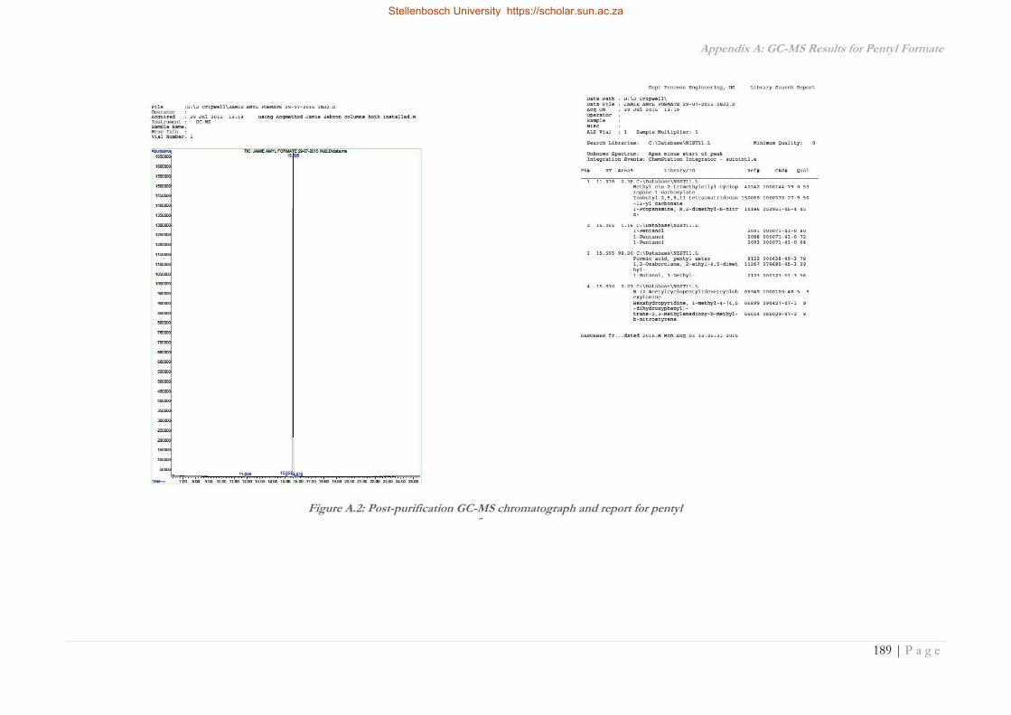
Appendix A: GC-MS Results for Pentyl Formate
189 | P a g e
Figure A.2: Post-purification GC-MS chromatograph and report for pentyl formate
Stellenbosch University https://scholar.sun.ac.za
Stellenbosch University https://scholar.sun.ac.za

Appendix B: Certificates of Calibration
190 | P a g e
APPENDIX B: CERTIFICATES OF
CALIBRATION
Stellenbosch University https://scholar.sun.ac.za

Appendix B: Certificates of Calibration
191 | P a g e
Stellenbosch University https://scholar.sun.ac.za
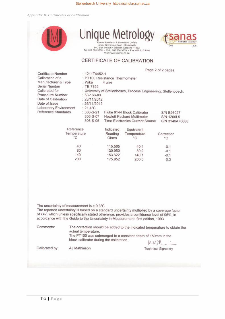
Appendix B: Certificates of Calibration
192 | P a g e
Stellenbosch University https://scholar.sun.ac.za

Appendix C: GC Calibration & Error Analysis
193 | P a g e
APPENDIX C: GC CALIBRATION &
ERROR ANALYSIS
Butyl Ethyl Ether/n-Heptane
BEHGC5
Preparation
Mass (g)
Individual
Mass (g)
Mass
Fraction
Sample Mass
(g)Area A comp /A std Area A comp /A std Area A comp /A std Area A comp /A std
Butyl Ethyl
Ether2.47290 0.03200 0.19070 0.00305125 364274 0.21713 362463 0.21641 363252 0.21653 361907 0.21743
n-Heptane 2.48100 0.00810 0.04827 0.0007723 126842 0.07561 126106 0.07529 126708 0.07553 126253 0.07585
2-Heptanone
(I.S.)2.44090 0.12770 0.76103 0.012176 1677682 1.00000 1674858 1.00000 1677618 1.00000 1664494 1.00000
Vial 2.31320 GC Mass (g) 0.016
BEHGC6
Preparation
Mass (g)
Individual
Mass (g)
Mass
Fraction
Sample Mass
(g)Area A comp /A std Area A comp /A std Area A comp /A std Area A comp /A std
Butyl Ethyl
Ether2.48860 0.02450 0.14609 0.00268813 304771 0.16542 302002 0.16527 303898 0.16527 325739 0.17213
n-Heptane 2.50370 0.01510 0.09004 0.0016568 263595 0.14307 261394 0.14304 262891 0.14297 284139 0.15015
2-Heptanone
(I.S.)2.46410 0.12810 0.76386 0.014055 1842420 1.00000 1827360 1.00000 1838817 1.00000 1892361 1.00000
Vial 2.33600 GC Mass (g) 0.0184
BEHGC7
Preparation
Mass (g)
Individual
Mass (g)
Mass
Fraction
Sample Mass
(g)Area A comp /A std Area A comp /A std Area A comp /A std Area A comp /A std
Butyl Ethyl
Ether2.48340 0.01690 0.10582 0.00170376 214728 0.12426 199401 0.11867 198085 0.11852 215002 0.12318
n-Heptane 2.50070 0.01730 0.10833 0.0017441 305158 0.17659 280485 0.16693 278242 0.16648 305024 0.17476
2-Heptanone
(I.S.)2.46650 0.12550 0.78585 0.012652 1728059 1.00000 1680300 1.00000 1671305 1.00000 1745390 1.00000
Vial 2.34100 GC Mass (g) 0.0161
BEHGC8
Preparation
Mass (g)
Individual
Mass (g)
Mass
Fraction
Sample Mass
(g)Area A comp /A std Area A comp /A std Area A comp /A std Area A comp /A std
Butyl Ethyl
Ether2.45330 0.00850 0.05346 0.00102107 109260 0.06103 109959 0.06064 108951 0.06103 108636 0.06089
n-Heptane 2.48040 0.02710 0.17044 0.0032554 497508 0.27788 503375 0.27758 497422 0.27862 496728 0.27843
2-Heptanone
(I.S.)2.44480 0.12340 0.77610 0.014824 1790366 1.00000 1813420 1.00000 1785332 1.00000 1784027 1.00000
Vial 2.32140 GC Mass (g) 0.0191
Reference BEHGC8A BEHGC8B BEHGC8C BEHGC8D
Reference BEHGC7A BEHGC7B BEHGC7C BEHGC7D
Reference BEHGC6A BEHGC6B BEHGC6C BEHGC6D
Reference BEHGC5A BEHGC5B BEHGC5C BEHGC5D
Table C.1: Sample preparation details for GC calibration in the butyl ethyl ether/n-heptane system
y = 0.8737xR² = 0.9987
0.00
0.05
0.10
0.15
0.20
0.25
0.00 0.06 0.12 0.18 0.24 0.30
Are
a Bu
tyl E
thyl
Eth
er/
Are
a Sta
nd
ard
MassButyl Ethyl Ether/MassStandard
y = 1.2514xR² = 0.9984
0.00
0.07
0.14
0.21
0.28
0.35
0.00 0.06 0.12 0.18 0.24 0.30
Are
a n-H
epta
ne/A
rea S
tand
ard
Massn-Heptane/MassStandard
Figure C.2: n-Heptane calibration curve for butyl ethyl ether/n-heptane system
Figure C.1: Butyl ethyl ether calibration curve for butyl ethyl ether/n-heptane system
Stellenbosch University https://scholar.sun.ac.za

Appendix C: GC Calibration & Error Analysis
194 | P a g e
Di-n-Propyl Ether/n-Heptane
BEHGC5
Preparation
Mass (g)
Individual
Mass (g)
Mass
Fraction
Sample Mass
(g)Area A comp /A std Area A comp /A std Area A comp /A std Area A comp /A std
Butyl Ethyl
Ether2.47290 0.03200 0.19070 0.00305125 364274 0.21713 362463 0.21641 363252 0.21653 361907 0.21743
n-Heptane 2.48100 0.00810 0.04827 0.0007723 126842 0.07561 126106 0.07529 126708 0.07553 126253 0.07585
2-Heptanone
(I.S.)2.44090 0.12770 0.76103 0.012176 1677682 1.00000 1674858 1.00000 1677618 1.00000 1664494 1.00000
Vial 2.31320 GC Mass (g) 0.016
BEHGC6
Preparation
Mass (g)
Individual
Mass (g)
Mass
Fraction
Sample Mass
(g)Area A comp /A std Area A comp /A std Area A comp /A std Area A comp /A std
Butyl Ethyl
Ether2.48860 0.02450 0.14609 0.00268813 304771 0.16542 302002 0.16527 303898 0.16527 325739 0.17213
n-Heptane 2.50370 0.01510 0.09004 0.0016568 263595 0.14307 261394 0.14304 262891 0.14297 284139 0.15015
2-Heptanone
(I.S.)2.46410 0.12810 0.76386 0.014055 1842420 1.00000 1827360 1.00000 1838817 1.00000 1892361 1.00000
Vial 2.33600 GC Mass (g) 0.0184
BEHGC7
Preparation
Mass (g)
Individual
Mass (g)
Mass
Fraction
Sample Mass
(g)Area A comp /A std Area A comp /A std Area A comp /A std Area A comp /A std
Butyl Ethyl
Ether2.48340 0.01690 0.10582 0.00170376 214728 0.12426 199401 0.11867 198085 0.11852 215002 0.12318
n-Heptane 2.50070 0.01730 0.10833 0.0017441 305158 0.17659 280485 0.16693 278242 0.16648 305024 0.17476
2-Heptanone
(I.S.)2.46650 0.12550 0.78585 0.012652 1728059 1.00000 1680300 1.00000 1671305 1.00000 1745390 1.00000
Vial 2.34100 GC Mass (g) 0.0161
BEHGC8
Preparation
Mass (g)
Individual
Mass (g)
Mass
Fraction
Sample Mass
(g)Area A comp /A std Area A comp /A std Area A comp /A std Area A comp /A std
Butyl Ethyl
Ether2.45330 0.00850 0.05346 0.00102107 109260 0.06103 109959 0.06064 108951 0.06103 108636 0.06089
n-Heptane 2.48040 0.02710 0.17044 0.0032554 497508 0.27788 503375 0.27758 497422 0.27862 496728 0.27843
2-Heptanone
(I.S.)2.44480 0.12340 0.77610 0.014824 1790366 1.00000 1813420 1.00000 1785332 1.00000 1784027 1.00000
Vial 2.32140 GC Mass (g) 0.0191
Reference BEHGC8A BEHGC8B BEHGC8C BEHGC8D
Reference BEHGC7A BEHGC7B BEHGC7C BEHGC7D
Reference BEHGC6A BEHGC6B BEHGC6C BEHGC6D
Reference BEHGC5A BEHGC5B BEHGC5C BEHGC5D
y = 0.9142xR² = 0.9995
0.00
0.06
0.12
0.18
0.24
0.30
0.00 0.07 0.14 0.21 0.28 0.35
Are
a Di-
n-P
rop
yl E
the
r/A
rea S
tan
dar
d
MassDi-n-Propyl Ether/MassStandard
y = 1.2776xR² = 1
0.00
0.07
0.14
0.21
0.28
0.35
0.00 0.07 0.14 0.21 0.28 0.35
Are
a n-H
epta
ne/
Are
a Sta
nd
ard
Massn-Heptane/MassStandard
Figure C.4: n-Heptane calibration curve for di-n-propyl ether/n-heptane system
Figure C.3: Di-n-propyl ether calibration curve for di-n-propyl ether/n-heptane system
Table C.0.2: Sample preparation details for GC calibration in the di-n-propyl ether/n-heptane system
Stellenbosch University https://scholar.sun.ac.za
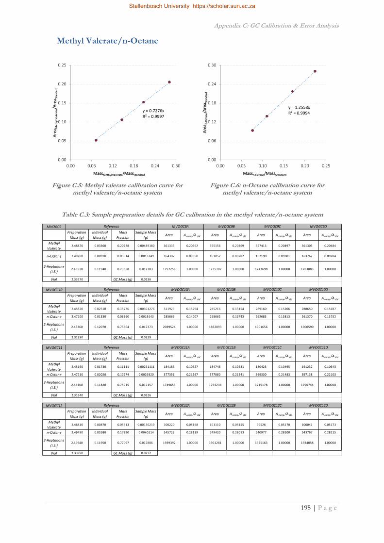
Appendix C: GC Calibration & Error Analysis
195 | P a g e
Methyl Valerate/n-Octane
MVOGC9
Preparation
Mass (g)
Individual
Mass (g)
Mass
Fraction
Sample Mass
(g)Area A comp /A std Area A comp /A std Area A comp /A std Area A comp /A std
Methyl
Valerate2.48870 0.03360 0.20728 0.00489180 361335 0.20562 355156 0.20469 357413 0.20497 361305 0.20484
n-Octane 2.49780 0.00910 0.05614 0.0013249 164307 0.09350 161052 0.09282 162190 0.09301 163767 0.09284
2-Heptanone
(I.S.)2.45510 0.11940 0.73658 0.017383 1757256 1.00000 1735107 1.00000 1743698 1.00000 1763883 1.00000
Vial 2.33570 GC Mass (g) 0.0236
MVOGC10
Preparation
Mass (g)
Individual
Mass (g)
Mass
Fraction
Sample Mass
(g)Area A comp /A std Area A comp /A std Area A comp /A std Area A comp /A std
Methyl
Valerate2.45870 0.02510 0.15776 0.00361276 311929 0.15294 285216 0.15154 289160 0.15206 288650 0.15187
n-Octane 2.47200 0.01330 0.08360 0.0019143 285669 0.14007 258662 0.13743 262683 0.13813 261370 0.13752
2-Heptanone
(I.S.)2.43360 0.12070 0.75864 0.017373 2039524 1.00000 1882093 1.00000 1901656 1.00000 1900590 1.00000
Vial 2.31290 GC Mass (g) 0.0229
MVOGC11
Preparation
Mass (g)
Individual
Mass (g)
Mass
Fraction
Sample Mass
(g)Area A comp /A std Area A comp /A std Area A comp /A std Area A comp /A std
Methyl
Valerate2.45190 0.01730 0.11111 0.00251111 184186 0.10527 184746 0.10531 180423 0.10495 191232 0.10643
n-Octane 2.47210 0.02020 0.12974 0.0029320 377351 0.21567 377880 0.21541 369330 0.21483 397138 0.22103
2-Heptanone
(I.S.)2.43460 0.11820 0.75915 0.017157 1749653 1.00000 1754234 1.00000 1719178 1.00000 1796744 1.00000
Vial 2.31640 GC Mass (g) 0.0226
MVOGC12
Preparation
Mass (g)
Individual
Mass (g)
Mass
Fraction
Sample Mass
(g)Area A comp /A std Area A comp /A std Area A comp /A std Area A comp /A std
Methyl
Valerate2.46810 0.00870 0.05613 0.00130219 100220 0.05168 101110 0.05155 99526 0.05170 100041 0.05173
n-Octane 2.49490 0.02680 0.17290 0.0040114 545722 0.28139 549420 0.28013 540977 0.28100 543767 0.28115
2-Heptanone
(I.S.)2.45940 0.11950 0.77097 0.017886 1939392 1.00000 1961281 1.00000 1925163 1.00000 1934058 1.00000
Vial 2.33990 GC Mass (g) 0.0232
Reference MVOGC12A MVOGC12B MVOGC12C MVOGC12D
Reference MVOGC11A MVOGC11B MVOGC11C MVOGC11D
Reference MVOGC10A MVOGC10B MVOGC10C MVOGC10D
Reference MVOGC9A MVOGC9B MVOGC9C MVOGC9D
Table C.3: Sample preparation details for GC calibration in the methyl valerate/n-octane system
y = 0.7276xR² = 0.9997
0.00
0.05
0.10
0.15
0.20
0.25
0.00 0.06 0.12 0.18 0.24 0.30
Are
a Met
hyl
Val
erat
e/A
rea S
tand
ard
MassMethyl Valerate/MassStandard
y = 1.2558xR² = 0.9994
0.00
0.06
0.12
0.18
0.24
0.30
0.00 0.05 0.10 0.15 0.20 0.25
Are
a n-O
ctan
e/A
rea S
tand
ard
Massn-Octane/MassStandard
Figure C.5: Methyl valerate calibration curve for methyl valerate/n-octane system
Figure C.6: n-Octane calibration curve for methyl valerate/n-octane system
Stellenbosch University https://scholar.sun.ac.za

Appendix C: GC Calibration & Error Analysis
196 | P a g e
Ethyl Butanoate/n-Octane
EBOGC1
Preparation
Mass (g)
Individual
Mass (g)
Mass
Fraction
Sample Mass
(g)Area A comp /A std Area A comp /A std Area A comp /A std Area A comp /A std
Ethyl
Butyrate2.12830 0.03400 0.21092 0.00504094 562673 0.20336 556468 0.20449 561037 0.20418 561084 0.20445
n-Octane 2.13540 0.00710 0.04404 0.0010527 206715 0.07471 202990 0.07459 204471 0.07441 204633 0.07457
2-Heptanone
(I.S.)2.09430 0.12010 0.74504 0.017806 2766937 1.00000 2721234 1.00000 2747815 1.00000 2744348 1.00000
Vial 1.97420 GC Mass (g) 0.0239
EBOGC2
Preparation
Mass (g)
Individual
Mass (g)
Mass
Fraction
Sample Mass
(g)Area A comp /A std Area A comp /A std Area A comp /A std Area A comp /A std
Ethyl
Butyrate2.47860 0.02560 0.15802 0.00336593 385160 0.15052 384330 0.15025 384824 0.14969 387634 0.15014
n-Octane 2.49210 0.01350 0.08333 0.0017750 354587 0.13857 353416 0.13816 353560 0.13753 355699 0.13777
2-Heptanone
(I.S.)2.45300 0.12290 0.75864 0.016159 2558852 1.00000 2557991 1.00000 2570764 1.00000 2581860 1.00000
Vial 2.33010 GC Mass (g) 0.0213
EBOGC3
Preparation
Mass (g)
Individual
Mass (g)
Mass
Fraction
Sample Mass
(g)Area A comp /A std Area A comp /A std Area A comp /A std Area A comp /A std
Ethyl
Butyrate2.47570 0.01690 0.10875 0.00246866 301496 0.10364 299462 0.10372 300992 0.10341 305407 0.10321
n-Octane 2.49630 0.02060 0.13256 0.0030091 640421 0.22014 637517 0.22080 639998 0.21987 648307 0.21910
2-Heptanone
(I.S.)2.45880 0.11790 0.75869 0.017222 2909104 1.00000 2887339 1.00000 2910782 1.00000 2958984 1.00000
Vial 2.34090 GC Mass (g) 0.0227
EBOGC4
Preparation
Mass (g)
Individual
Mass (g)
Mass
Fraction
Sample Mass
(g)Area A comp /A std Area A comp /A std Area A comp /A std Area A comp /A std
Ethyl
Butyrate2.46020 0.00920 0.05913 0.00124165 135430 0.05488 135345 0.05469 134557 0.05479 135658 0.05482
n-Octane 2.48670 0.02650 0.17031 0.0035765 686301 0.27811 686627 0.27743 682115 0.27774 687953 0.27800
2-Heptanone
(I.S.)2.45100 0.11990 0.77057 0.016182 2467764 1.00000 2474992 1.00000 2455922 1.00000 2474616 1.00000
Vial 2.33110 GC Mass (g) 0.021
Reference EBOGC4A EBOGC4B EBOGC4C EBOGC4D
Reference EBOGC3A EBOGC3B EBOGC3C EBOGC3D
Reference EBOGC2A EBOGC2B EBOGC2C EBOGC2D
Reference EBOGC1A EBOGC1B EBOGC1C EBOGC1D
Table C.4: Sample preparation details for GC calibration in the ethyl butanoate/n-octane system
y = 0.7208xR² = 1
0.00
0.05
0.10
0.15
0.20
0.25
0.00 0.06 0.12 0.18 0.24 0.30
Are
a Eth
yl B
uta
no
ate/A
rea S
tan
dar
d
MassEthyl Butanoate/MassStandard
y = 1.2577xR² = 1
0.00
0.06
0.12
0.18
0.24
0.30
0.00 0.06 0.12 0.18 0.24 0.30
Are
a n-O
ctan
e/A
rea S
tand
ard
Massn-Octane/MassStandard
Figure C.7: Ethyl butanoate calibration curve for ethyl butanoate/n-octane system
Figure C.8: n-Octane calibration curve for ethyl butanoate/n-octane system
Stellenbosch University https://scholar.sun.ac.za

Appendix C: GC Calibration & Error Analysis
197 | P a g e
Propyl Propanoate/n-Octane
y = 1.2706xR² = 0.9989
0.00
0.07
0.14
0.21
0.28
0.35
0.00 0.06 0.12 0.18 0.24 0.30
Are
a n-O
ctan
e/A
rea S
tand
ard
Massn-Octane/MassStandard
y = 0.7402xR² = 0.9999
0.00
0.05
0.10
0.15
0.20
0.25
0.00 0.07 0.14 0.21 0.28 0.35
Are
a Pro
pyl
Pro
pan
oat
e/A
rea S
tand
ard
MassPropyl Propanoate/MassStandard
Figure C.10: n-Octane calibration curve for propyl propanoate/n-octane system
Figure C.9: Propyl propanoate calibration curve for propyl propanoate/n-octane system
PPOGC5
Preparation
Mass (g)
Individual
Mass (g)
Mass
Fraction
Sample Mass
(g)Area A comp /A std Area A comp /A std Area A comp /A std Area A comp /A std
Propyl
Propionate2.47090 0.03970 0.22582 0.00499073 481275 0.23122 514878 0.22940 502645 0.23109 500167 0.23064
n-Octane 2.47940 0.00850 0.04835 0.0010685 175795 0.08446 186596 0.08314 182987 0.08413 181752 0.08381
2-Heptanone
(I.S.)2.43120 0.12760 0.72582 0.016041 2081456 1.00000 2244420 1.00000 2175061 1.00000 2168565 1.00000
Vial 2.30360 GC Mass (g) 0.0221
PPOGC6
Preparation
Mass (g)
Individual
Mass (g)
Mass
Fraction
Sample Mass
(g)Area A comp /A std Area A comp /A std Area A comp /A std Area A comp /A std
Propyl
Propionate2.46910 0.02780 0.16982 0.00371912 358556 0.17177 378638 0.17005 364428 0.17109 356040 0.17179
n-Octane 2.48490 0.01580 0.09652 0.0021137 342029 0.16386 361795 0.16249 347448 0.16312 340290 0.16419
2-Heptanone
(I.S.)2.44130 0.12010 0.73366 0.016067 2087366 1.00000 2226577 1.00000 2130067 1.00000 2072540 1.00000
Vial 2.32120 GC Mass (g) 0.0219
PPOGC7
Preparation
Mass (g)
Individual
Mass (g)
Mass
Fraction
Sample Mass
(g)Area A comp /A std Area A comp /A std Area A comp /A std Area A comp /A std
Propyl
Propionate2.47260 0.01990 0.11859 0.00247861 253106 0.11681 232055 0.11803 246209 0.11698 233604 0.11788
n-Octane 2.49570 0.02310 0.13766 0.0028772 499777 0.23066 462647 0.23532 490423 0.23301 465618 0.23495
2-Heptanone
(I.S.)2.45270 0.12480 0.74374 0.015544 2166755 1.00000 1966031 1.00000 2104714 1.00000 1981767 1.00000
Vial 2.32790 GC Mass (g) 0.0209
PPOGC8
Preparation
Mass (g)
Individual
Mass (g)
Mass
Fraction
Sample Mass
(g)Area A comp /A std Area A comp /A std Area A comp /A std Area A comp /A std
Propyl
Propionate2.46740 0.01030 0.06277 0.00135576 135507 0.06196 133325 0.06215 131863 0.06233 130751 0.06221
n-Octane 2.49730 0.02990 0.18221 0.0039356 674846 0.30859 665290 0.31011 657941 0.31101 654516 0.31141
2-Heptanone
(I.S.)2.45710 0.12390 0.75503 0.016309 2186848 1.00000 2145350 1.00000 2115515 1.00000 2101784 1.00000
Vial 2.33320 GC Mass (g) 0.0216
Reference PPOGC6A PPOGC6B PPOGC6C PPOGC6D
Reference PPOGC5A PPOGC5B PPOGC5C PPOGC5D
Reference PPOGC8A PPOGC8B PPOGC8C PPOGC8D
Reference PPOGC7A PPOGC7B PPOGC7C PPOGC7D
Table C.5: Sample preparation details for GC calibration in the propyl propanoate/n-octane system
Stellenbosch University https://scholar.sun.ac.za

Appendix C: GC Calibration & Error Analysis
198 | P a g e
Butyl Acetate/n-Octane
y = 0.7369xR² = 1
0.00
0.05
0.10
0.15
0.20
0.25
0.00 0.07 0.14 0.21 0.28 0.35
Are
a Bu
tyl A
ceta
te/A
rea S
tan
dar
d
MassButyl Acetate/MassStandard
y = 1.2273xR² = 0.9995
0.00
0.07
0.14
0.21
0.28
0.35
0.00 0.06 0.12 0.18 0.24 0.30
Are
a n-O
ctan
e/A
rea S
tand
ard
Massn-Octane/MassStandard
Figure C.11: Butyl acetate calibration curve for butyl acetate/n-octane system
Figure C.12: n-Octane calibration curve for butyl acetate/n-octane system
BAOGC1
Preparation
Mass (g)
Individual
Mass (g)
Mass
Fraction
Sample Mass
(g)Area A comp /A std Area A comp /A std Area A comp /A std Area A comp /A std
Butyl Acetate 2.15200 0.03430 0.21238 0.00501226 568248 0.21382 584493 0.20920 572845 0.21064 568835 0.20866
n-Octane 2.15910 0.00710 0.04396 0.0010375 201924 0.07598 201068 0.07197 198954 0.07316 196016 0.07190
2-Heptanone
(I.S.)2.11770 0.12010 0.74365 0.017550 2657543 1.00000 2793904 1.00000 2719552 1.00000 2726150 1.00000
Vial 1.99760 GC Mass (g) 0.0236
BAOGC2
Preparation
Mass (g)
Individual
Mass (g)
Mass
Fraction
Sample Mass
(g)Area A comp /A std Area A comp /A std Area A comp /A std Area A comp /A std
Butyl Acetate 2.49660 0.02620 0.16355 0.00384332 411442 0.16055 423254 0.16081 412712 0.15992 418997 0.15973
n-Octane 2.51040 0.01380 0.08614 0.0020243 357329 0.13943 368516 0.14001 357270 0.13844 361992 0.13800
2-Heptanone
(I.S.)2.47040 0.12020 0.75031 0.017632 2562761 1.00000 2631994 1.00000 2580766 1.00000 2623119 1.00000
Vial 2.35020 GC Mass (g) 0.0235
BAOGC3
Preparation
Mass (g)
Individual
Mass (g)
Mass
Fraction
Sample Mass
(g)Area A comp /A std Area A comp /A std Area A comp /A std Area A comp /A std
Butyl Acetate 2.46150 0.01720 0.11026 0.00252487 247531 0.10767 259985 0.10728 252182 0.10684 250371 0.10702
n-Octane 2.48170 0.02020 0.12949 0.0029653 478493 0.20813 503026 0.20756 487287 0.20645 485160 0.20739
2-Heptanone
(I.S.)2.44430 0.11860 0.76026 0.017410 2299003 1.00000 2423484 1.00000 2360278 1.00000 2339391 1.00000
Vial 2.32570 GC Mass (g) 0.0229
BAOGC4
Preparation
Mass (g)
Individual
Mass (g)
Mass
Fraction
Sample Mass
(g)Area A comp /A std Area A comp /A std Area A comp /A std Area A comp /A std
Butyl Acetate 2.47300 0.00910 0.05879 0.00125213 115399 0.05642 119556 0.05660 117464 0.05690 118988 0.05668
n-Octane 2.50020 0.02720 0.17571 0.0037426 576817 0.28203 599084 0.28363 589624 0.28562 595515 0.28366
2-Heptanone
(I.S.)2.46390 0.11850 0.76550 0.016305 2045266 1.00000 2112172 1.00000 2064364 1.00000 2099424 1.00000
Vial 2.34540 GC Mass (g) 0.0213
Reference BAOGC2A BAOGC2B BAOGC2C BAOGC2D
Reference BAOGC1A BAOGC1B BAOGC1C BAOGC1D
Reference BAOGC4A BAOGC4B BAOGC4C EBOGC4D
Reference BAOGC3A BAOGC3B BAOGC3C BAOGC3D
Table C.0.6: Sample preparation details for GC calibration in the butyl acetate/n-octane system
Stellenbosch University https://scholar.sun.ac.za

Appendix C: GC Calibration & Error Analysis
199 | P a g e
Pentyl Formate/n-Octane
AFOGC1
Preparation
Mass (g)
Individual
Mass (g)
Mass
Fraction
Sample Mass
(g)Area A comp /A std Area A comp /A std Area A comp /A std Area A comp /A std
Amyl
Formate2.48970 0.03540 0.21811 0.00447135 281004 0.22350 279861 0.22287 279123 0.22340 278084 0.22313
n-Octane 2.49800 0.00830 0.05114 0.0010484 107096 0.08518 106860 0.08510 106478 0.08522 106291 0.08529
2-Heptanone
(I.S.)2.45430 0.11860 0.73075 0.014980 1257267 1.00000 1255714 1.00000 1249428 1.00000 1246267 1.00000
Vial 2.33570 GC Mass (g) 0.0205
AFOGC2
Preparation
Mass (g)
Individual
Mass (g)
Mass
Fraction
Sample Mass
(g)Area A comp /A std Area A comp /A std Area A comp /A std Area A comp /A std
Amyl
Formate2.46210 0.02620 0.16385 0.00345729 210617 0.16259 211080 0.16291 210529 0.16233 209031 0.16309
n-Octane 2.47750 0.01540 0.09631 0.0020321 207390 0.16010 207936 0.16049 208281 0.16059 206151 0.16085
2-Heptanone
(I.S.)2.43590 0.11830 0.73984 0.015611 1295409 1.00000 1295670 1.00000 1296950 1.00000 1281664 1.00000
Vial 2.31760 GC Mass (g) 0.0211
AFOGC3
Preparation
Mass (g)
Individual
Mass (g)
Mass
Fraction
Sample Mass
(g)Area A comp /A std Area A comp /A std Area A comp /A std Area A comp /A std
Amyl
Formate2.46690 0.01860 0.11915 0.00238309 147074 0.11932 146593 0.11889 147581 0.11883 150549 0.11875
n-Octane 2.48840 0.02150 0.13773 0.0027546 281936 0.22873 282666 0.22925 283462 0.22824 287935 0.22711
2-Heptanone
(I.S.)2.44830 0.11600 0.74311 0.014862 1232588 1.00000 1232991 1.00000 1241943 1.00000 1267800 1.00000
Vial 2.33230 GC Mass (g) 0.02
AFOGC4
Preparation
Mass (g)
Individual
Mass (g)
Mass
Fraction
Sample Mass
(g)Area A comp /A std Area A comp /A std Area A comp /A std Area A comp /A std
Amyl
Formate2.44070 0.00950 0.06145 0.00109994 65892 0.06015 68899 0.06018 72079 0.05991 76172 0.06080
n-Octane 2.47000 0.02930 0.18952 0.0033924 340345 0.31067 353981 0.30917 370371 0.30786 387960 0.30965
2-Heptanone
(I.S.)2.43120 0.11580 0.74903 0.013408 1095515 1.00000 1144937 1.00000 1203036 1.00000 1252900 1.00000
Vial 2.31540 GC Mass (g) 0.0179
Reference AFOGC2A AFOGC2B AFOGC2C AFOGC2D
Reference AFOGC1A AFOGC1B AFOGC1C AFOGC1D
Reference AFOGC4A AFOGC4B AFOGC4C AFOGC4D
Reference AFOGC3A AFOGC3B AFOGC3C AFOGC3D
Table C.7: Sample preparation details for GC calibration in the pentyl formate/n-octane system
y = 0.7427xR² = 0.9996
0.00
0.05
0.10
0.15
0.20
0.25
0.00 0.07 0.14 0.21 0.28 0.35
Are
a Pen
tyl F
orm
ate/A
rea S
tand
ard
MassPentyl Formate/MassStandard
y = 1.2264xR² = 0.9999
0.00
0.07
0.14
0.21
0.28
0.35
0.00 0.06 0.12 0.18 0.24 0.30
Are
a n-O
ctan
e/A
rea S
tand
ard
Massn-Octane/MassStandard
Figure C.14: n-Octane calibration curve for pentyl formate/n-octane system
Figure C.13: Pentyl formate calibration curve for pentyl formate/n-octane system
Stellenbosch University https://scholar.sun.ac.za

Appendix C: GC Calibration & Error Analysis
200 | P a g e
GC Compositional Error Analysis
Table C.8 below is an example of the determination of compositional uncertainty from the analysis procedure. At the conclusion of the experimental sample
analysis procedure, four samples of known and variable mass, and thus composition, were prepared and run through the GC four times each. The reported Absolute GC
Error Mole Fraction illustrates the error induced by a drift in the response factor over the course of the analysis. WC1 and WC2 account for potential weighing error which
affects the “true” reference composition used to establish calibration curves. For WC1, the mass of the ester is increased by 0.0001g (uncertainty of scale) with the alkane
reduced by the same quantity, with the signs opposite in WC2. The reported values are thus the difference between the prediction and these worst case scenarios.
Table C.8: Sample repeatability results for GC error analysis using the pentyl formate/n-octane system
Pentyl Formate
Mass
n-Octane Mass
Standard Mass
Pentyl Formate
Mole Frac
Octane Mole Frac
Pentyl Formate
Area
Octane Area
Standard Area
Predicted Pentyl
Formate Mass Frac
Predicted n-Octane
Mass Frac
Predicted Pentyl
Formate Mole Frac
Predicted n-Octane
Mole Frac
Absolute GC Error
Mole Fraction
Absolute GC Error
Mole Fraction (WC1)*
Absolute GC Error
Mole Fraction (WC2)*
Average Absolute GC Error
Mole Fraction
KNO1A 0.0469 0.0127 0.0206 0.7841 0.2159 318322 135889 1241392 0.7946 0.2054 0.7918 0.2082 0.0077 0.0061 0.0095
0.0029 KNO1B 0.0469 0.0127 0.0206 0.7841 0.2159 328200 145740 1290165 0.7881 0.2119 0.7853 0.2147 0.0012 0.0004 0.0029
KNO1C 0.0469 0.0127 0.0206 0.7841 0.2159 326864 146053 1283292 0.7870 0.2130 0.7842 0.2158 0.0001 0.0015 0.0019
KNO1D 0.0469 0.0127 0.0206 0.7841 0.2159 325931 145724 1275344 0.7869 0.2131 0.7841 0.2159 0.0000 0.0016 0.0018
KNO2A 0.0369 0.0232 0.0212 0.6100 0.3900 236634 248723 1294805 0.6110 0.3890 0.6071 0.3929 0.0029 0.0045 0.0012
0.0021 KNO2B 0.0369 0.0232 0.0212 0.6100 0.3900 240874 251752 1325792 0.6124 0.3876 0.6084 0.3916 0.0016 0.0032 0.0002
KNO2C 0.0369 0.0232 0.0212 0.6100 0.3900 241436 252947 1327450 0.6118 0.3882 0.6078 0.3922 0.0022 0.0037 0.0004
KNO2D 0.0369 0.0232 0.0212 0.6100 0.3900 242611 253549 1334895 0.6124 0.3876 0.6084 0.3916 0.0016 0.0031 0.0002
KNO3A 0.0242 0.0351 0.0216 0.4041 0.5959 147445 359919 1388876 0.4035 0.5965 0.3995 0.6005 0.0046 0.0061 0.0028
0.0050 KNO3B 0.0242 0.0351 0.0216 0.4041 0.5959 148322 362458 1405093 0.4032 0.5968 0.3992 0.6008 0.0048 0.0064 0.0031
KNO3C 0.0242 0.0351 0.0216 0.4041 0.5959 148689 363799 1400403 0.4029 0.5971 0.3989 0.6011 0.0051 0.0067 0.0033
KNO3D 0.0242 0.0351 0.0216 0.4041 0.5959 146735 359778 1381513 0.4024 0.5976 0.3984 0.6016 0.0056 0.0072 0.0039
KNO4A 0.0144 0.0485 0.0209 0.2260 0.7740 79220 454213 1252013 0.2236 0.7764 0.2207 0.7793 0.0053 0.0068 0.0036
0.0054 KNO4B 0.0144 0.0485 0.0209 0.2260 0.7740 81690 465724 1311299 0.2246 0.7754 0.2217 0.7783 0.0043 0.0058 0.0027
KNO4C 0.0144 0.0485 0.0209 0.2260 0.7740 78632 453959 1242875 0.2224 0.7776 0.2195 0.7805 0.0065 0.0080 0.0048
KNO4D 0.0144 0.0485 0.0209 0.2260 0.7740 78551 451596 1238254 0.2231 0.7769 0.2202 0.7798 0.0057 0.0072 0.0041
Stellenbosch University https://scholar.sun.ac.za
Stellenbosch University https://scholar.sun.ac.za

Appendix D: Pure Component Vapour Pressure Measurements
201 | P a g e
APPENDIX D: PURE COMPONENT VAPOUR PRESSURE
MEASUREMENTS
Table D.1: Experimentally measured vapour pressures for components of experimental interest to this study
n-Heptane n-Octane Di-n-Propyl
Ether Butyl Ethyl
Ether Methyl Valerate Ethyl Butanoate
Propyl Propanoate
Butyl Acetate Pentyl Formate
P T P T P T P T P T P T P T P T P T
(kPa) (K) (kPa) (K) (kPa) (K) (kPa) (K) (kPa) (K) (kPa) (K) (kPa) (K) (kPa) (K) (kPa) (K)
101.30 371.28 97.58 397.28 101.30 362.87 101.30 365.25 101.3 400.48 101.3 393.78 101.3 395.51 101.3 399.09 101.3 405.12
88.40 366.87 83.70 391.91 96.32 361.18 96.36 363.47 100.4 400.07 100.4 393.63 93.37 392.74 99.03 398.35 93.45 402.19
83.45 364.95 66.74 384.28 89.30 358.73 90.59 361.44 95.08 398.03 90.84 390.23 86.38 390.13 88.69 394.58 86.56 399.55
76.47 362.11 60.05 380.83 84.25 356.85 79.60 357.31 88.17 395.42 84.14 387.65 77.90 386.81 80.09 391.20 80.16 396.89
70.24 359.38 53.65 377.27 78.97 354.82 71.58 354.01 77.71 391.14 77.20 384.82 70.32 383.56 72.71 388.06 73.50 394.01
64.60 356.78 43.33 370.71 72.36 352.11 63.63 350.44 69.02 387.18 65.75 379.65 60.83 379.07 60.15 382.08 68.46 391.65
56.20 352.58 34.91 364.35 62.30 347.55 56.24 346.80 59.35 382.55 58.98 376.28 51.21 373.82 56.43 380.10 60.50 387.67
50.97 349.68 28.95 359.12 57.75 345.34 51.67 344.21 52.83 378.84 54.40 373.83 47.90 371.88 45.02 373.32 55.79 385.08
46.80 347.16 49.98 341.15 44.96 340.35 45.81 374.53 50.00 371.33 40.92 367.30 41.42 370.90 49.42 381.35
38.89 341.94 42.54 336.55 38.60 336.22 40.47 370.86 40.41 365.24 33.58 361.75 32.95 364.47 44.06 377.87
30.59 335.45 36.71 332.57 29.99 331.51 35.06 366.70 35.41 361.56 29.92 361.85 39.15 374.41
26.15 331.39 29.35 326.73 29.41 361.82 33.67 370.04
Stellenbosch University https://scholar.sun.ac.za
Stellenbosch University https://scholar.sun.ac.za

Appendix E: Experimental Results: VLE & Consistency Tests
202 | P a g e
APPENDIX E: EXPERIMENTAL RESULTS:
VLE & CONSISTENCY
TESTS
The PRO-VLE 2.0 software was used to perform the L/W thermodynamic consistency test,
which requires inputting a number of component specific properties and correlation constants. The input
values for the components used in this study are detailed in Table E.1 below.
Table E.1: Component parameters used for thermodynamic consistency testing
Butyl Ethyl Ether
Di-n-Propyl Ether
Methyl Valerate
Ethyl Butanoate
Propyl Propanoate
Butyl Acetate
Pentyl Formate
n-Heptane n-Octane
Antoine A* 6.73327 6.72609 6.77353 6.928582 6.978531 6.864025 6.80815 6.64338 6.94182
Antoine B* 1104.422 1118.741 1220.67 1331.7852 1326.38506 1270.8518 1270.754 1105.257 1365.368
Antoine C* 194.9097 201.1184 186.2061 207.6835 201.4181 193.05968 191.36074 195.5387 210.525
Tc (K)
531 530.6 588.92 571 568.6 575.4 576 540.2 568.7
Pc (atm)
29.509 29.88403 31.609 29.11423 30.19984 30.49592 30.84134 27.04169 24.57438
Vc (cm3.mol-1)
382 382 426.4 403 389 389 389 428 486
Tb (K)
348.84 346.63 383.29 377.21 378.63 381.98 387.69 354.63 380.85
ω 0.385408 0.368756 0.35844 0.401075 0.448676 0.439393 0.515459 0.349469 0.399552
VL (cm3.mol-1)
147.702 a 147.703 a 145.276 a 147.1255 a 146.951 a 147.1297 a 147.9057 a ±158 a ±181 a
Hvap (cal.mol-1)
7854 7794 8997 8945 8970 9021 9069 7874 8580
μ (Debye)
1.22019 1.21119 1.62 1.81079 1.78981 1.84077 1.90073 0 0
*Antoine Equation as log10P(mmHg) = A – (B/(T(°C) + C)) Listed values taken from DIPPR Database unless otherwise specified a Values of VL depend on max and min temperatures for mixture of interest – tabulated values are thus averages
In the tables of experimental results that follow, the activity coefficients were generated for each
component by the PRO-VLE 2.0 software. The reported uncertainties in temperature (0.02K), pressure
(1.5mbar) and composition (0.010 mole fraction) were used to determine D and Dmax for the
McDermott-Ellis consistency test.
Stellenbosch University https://scholar.sun.ac.za

Appendix E: Experimental Results: VLE & Consistency Tests
203 | P a g e
Butyl Ethyl Ether/n-Heptane
Table E.2: Experimental data and thermodynamic consistency testing results for butyl ethyl ether/n-heptane system
Experimental Data L/W Consistency Test McDermott-Ellis Consistency
Test Sample Name
T (K) yether xether Li Wi Li/Wi Δx. ΣLi
Δx. ΣWi
γether γhept D Dmax
Hept. 354.63 0.000 0.000
Hept. 354.63 0.000 0.000
BEH11 354.37 0.035 0.026 0.109 0.089 1.220 0.001 0.001 1.127 0.998 0.0035 0.1584
BEH51 354.22 0.049 0.035 0.203 0.185 1.100 0.010 0.009 1.157 0.999 0.0041 0.1658
BEH12 353.87 0.095 0.071 0.341 0.329 1.040 0.004 0.003 1.133 0.998 0.0036 0.1580
BEH52 353.79 0.111 0.081 0.362 0.351 1.030 0.017 0.017 1.162 0.994 0.0050 0.1606
BEH53 353.41 0.160 0.121 0.514 0.510 1.010 0.003 0.003 1.144 0.993 0.0014 0.1587
BEH13 353.34 0.166 0.127 0.549 0.546 1.010 0.027 0.027 1.134 0.995 0.0035 0.1616
BEH14 352.90 0.212 0.169 0.742 0.747 0.990 0.021 0.021 1.102 1.002 0.0049 0.1610
BEH15 352.71 0.245 0.197 0.768 0.777 0.990 0.002 0.002 1.102 0.999 0.0006 0.1612
BEH54 352.68 0.248 0.195 0.810 0.819 0.990 0.034 0.034 1.128 0.993 0.0093 0.1621
BEH55 352.43 0.293 0.236 0.818 0.833 0.980 0.011 0.011 1.108 0.992 0.0010 0.1623
BEH16 352.32 0.305 0.250 0.850 0.866 0.980 0.031 0.032 1.093 0.997 0.0034 0.1630
BEH56 352.06 0.344 0.285 0.903 0.925 0.980 0.004 0.004 1.089 0.996 0.0023 0.1630
BEH17 352.00 0.348 0.289 0.940 0.963 0.980 0.047 0.048 1.088 0.998 0.0013 0.1644
BEH21 351.62 0.395 0.336 1.046 1.077 0.970 0.010 0.010 1.076 1.004 0.0004 0.1647
BEH22 351.59 0.400 0.346 1.019 1.051 0.970 0.011 0.011 1.061 1.011 0.0006 0.1646
BEH57 351.50 0.413 0.356 1.047 1.081 0.970 0.025 0.026 1.066 1.008 0.0032 0.1651
BEH23 351.39 0.436 0.381 1.015 1.051 0.970 0.022 0.023 1.056 1.011 0.0034 0.1654
BEH24 351.29 0.458 0.403 0.988 1.027 0.960 0.008 0.008 1.053 1.010 0.0043 0.1656
BEH58 351.17 0.466 0.410 1.064 1.106 0.960 0.013 0.014 1.054 1.013 0.0070 0.1659
BEH25 351.19 0.479 0.423 0.969 1.010 0.960 0.020 0.021 1.051 1.009 0.0029 0.1664
BEH26 351.05 0.504 0.444 0.989 1.033 0.960 0.011 0.011 1.057 1.002 0.0028 0.1666
BEH48 350.96 0.511 0.455 1.017 1.063 0.960 0.018 0.018 1.050 1.010 0.0018 0.1668
BEH27 350.89 0.525 0.472 0.985 1.033 0.950 0.003 0.003 1.042 1.015 0.0069 0.1668
BEH59 350.77 0.528 0.475 1.090 1.141 0.960 0.016 0.017 1.045 1.019 0.0029 0.1669
BEH47 350.73 0.543 0.490 1.041 1.092 0.950 0.002 0.002 1.043 1.018 0.0057 0.1674
BEH28 350.78 0.546 0.488 1.002 1.052 0.950 0.040 0.042 1.052 1.004 0.0039 0.1680
BEH46 350.51 0.579 0.528 1.045 1.101 0.950 0.038 0.040 1.041 1.019 0.0040 0.1681
BEH45 350.35 0.615 0.565 0.988 1.048 0.940 0.035 0.038 1.038 1.018 0.0037 0.1690
BEH44 350.22 0.644 0.603 0.902 0.965 0.930 0.037 0.040 1.024 1.033 0.0036 0.1690
BEH43 349.98 0.680 0.644 0.905 0.974 0.930 0.034 0.037 1.021 1.043 0.0027 0.1694
BEH42 349.85 0.716 0.684 0.803 0.875 0.920 0.029 0.031 1.016 1.049 0.0005 0.1697
BEH41 349.71 0.749 0.721 0.728 0.802 0.910 0.027 0.030 1.012 1.058 0.0000 0.1699
BEH37 349.55 0.783 0.760 0.666 0.744 0.900 0.021 0.024 1.010 1.064 0.0080 0.1701
BEH36 349.32 0.811 0.790 0.721 0.804 0.900 0.028 0.032 1.013 1.072 0.0059 0.1711
BEH35 349.25 0.851 0.835 0.535 0.620 0.860 0.016 0.019 1.008 1.078 0.0028 0.1708
BEH34 349.12 0.879 0.867 0.483 0.570 0.850 0.021 0.026 1.008 1.088 0.0042 0.1758
BEH33 349.01 0.927 0.921 0.282 0.371 0.760 0.008 0.012 1.004 1.103 0.0007 0.1798
BEH32 348.93 0.963 0.960 0.137 0.226 0.600 0.002 0.004 1.002 1.132 0.0025 0.1885
BEH31 348.89 0.985 0.984 0.010 0.099 0.100 0.000 0.001 1.001 1.121
BEE 348.84 1.000 1.000
L W D
0.7072 0.7532 3.1521
Stellenbosch University https://scholar.sun.ac.za

Appendix E: Experimental Results: VLE & Consistency Tests
204 | P a g e
Di-n-Propyl Ether/n-Heptane
Table E.3: Experimental data and thermodynamic consistency testing results for di-n-propyl ether/n-heptane system
Experimental Data L/W Consistency Test McDermott-Ellis Consistency
Test Sample Name
T (K) yether xether Li Wi Li/Wi Δx. ΣLi
Δx. ΣWi
γether γhept D Dmax
Hept. 354.63 0.000 0.000
DPH31 354.42 0.038 0.027 -0.006 -0.023 0.270 0.002 0.002 1.109 0.994 0.0027 0.1648
DPH32 354.01 0.078 0.055 0.173 0.165 1.050 0.007 0.006 1.120 0.995 0.0009 0.1586
DPH33 353.65 0.115 0.082 0.319 0.319 1.000 0.008 0.008 1.128 0.994 0.0000 0.1575
DPH34 353.33 0.144 0.101 0.480 0.486 0.990 0.032 0.033 1.151 0.992 0.0068 0.1603
DPH35 352.66 0.215 0.154 0.721 0.742 0.970 0.017 0.018 1.152 0.988 0.0039 0.1609
DPH36 352.55 0.232 0.180 0.629 0.655 0.960 0.017 0.018 1.072 1.000 0.0068 0.1607
DPH58 352.34 0.266 0.207 0.615 0.646 0.950 0.001 0.001 1.071 0.996 0.0076 0.1609
DPH37 352.17 0.273 0.209 0.770 0.804 0.960 0.018 0.019 1.095 0.995 0.0090 0.1614
DPH41 351.94 0.307 0.232 0.818 0.857 0.960 0.016 0.016 1.120 0.983 0.0003 0.1615
DPH42 351.75 0.325 0.250 0.858 0.900 0.950 0.005 0.005 1.105 0.987 0.0039 0.1621
DPH43 351.66 0.339 0.256 0.905 0.949 0.950 0.042 0.045 1.130 0.977 0.0024 0.1636
DPH44 351.25 0.381 0.301 0.948 1.000 0.950 0.009 0.010 1.093 0.988 0.0080 0.1636
DPH59 351.07 0.386 0.310 1.055 1.110 0.950 0.022 0.024 1.080 0.999 0.0070 0.1638
DPH45 350.92 0.411 0.332 1.032 1.091 0.950 0.040 0.043 1.082 0.993 0.0079 0.1650
DPH46 350.65 0.450 0.372 0.982 1.046 0.940 0.014 0.015 1.066 0.995 0.0025 0.1653
DPH510 350.46 0.467 0.386 1.058 1.125 0.940 0.032 0.035 1.073 0.993 0.0085 0.1662
DPH47 350.29 0.496 0.418 0.971 1.041 0.930 0.070 0.075 1.057 0.996 0.0076 0.1680
DPH48 349.60 0.558 0.485 1.127 1.207 0.930 0.010 0.011 1.048 1.010 0.0063 0.1679
DPH57 349.60 0.569 0.494 1.054 1.133 0.930 0.053 0.057 1.050 1.002 0.0068 0.1691
DPH28 349.23 0.619 0.545 1.013 1.098 0.920 0.019 0.021 1.046 0.999 0.0028 0.1697
DPH56 349.07 0.632 0.564 1.023 1.109 0.920 0.020 0.021 1.037 1.013 0.0054 0.1698
DPH27 348.96 0.652 0.583 0.978 1.064 0.920 0.034 0.037 1.039 1.004 0.0023 0.1706
DPH26 348.71 0.683 0.618 0.950 1.039 0.910 0.008 0.009 1.035 1.007 0.0038 0.1708
DPH55 348.62 0.688 0.627 0.974 1.064 0.920 0.023 0.025 1.032 1.017 0.0091 0.1712
DPH25 348.54 0.712 0.651 0.857 0.947 0.900 0.026 0.029 1.031 1.006 0.0032 0.1720
DPH24 348.35 0.738 0.683 0.791 0.882 0.900 0.024 0.027 1.024 1.015 0.0045 0.1723
DPH54 348.09 0.762 0.714 0.809 0.901 0.900 0.001 0.001 1.020 1.032 0.0022 0.1721
DPH23 348.09 0.765 0.715 0.798 0.890 0.900 0.024 0.027 1.022 1.023 0.0046 0.1728
DPH22 347.94 0.792 0.747 0.691 0.783 0.880 0.019 0.022 1.017 1.028 0.0023 0.1731
DPH21 347.74 0.813 0.776 0.664 0.756 0.880 0.017 0.020 1.013 1.046 0.0027 0.1730
DPH17 347.60 0.837 0.804 0.586 0.678 0.860 0.013 0.016 1.011 1.047 0.0011 0.1733
DPH16 347.49 0.857 0.828 0.501 0.592 0.850 0.015 0.017 1.009 1.053 0.0012 0.1743
DPH15 347.26 0.883 0.858 0.496 0.587 0.840 0.015 0.018 1.011 1.046 0.0024 0.1758
DPH14 347.11 0.910 0.892 0.371 0.461 0.810 0.009 0.011 1.007 1.065 0.0007 0.1756
DPH13 346.98 0.933 0.920 0.286 0.374 0.760 0.005 0.006 1.006 1.071 0.0109 0.1743
DPH51 346.79 0.938 0.934 0.364 0.453 0.800 0.004 0.005 1.002 1.213 0.0070 0.1751
DPH12 346.82 0.955 0.946 0.235 0.322 0.730 0.005 0.007 1.006 1.075 0.0043 0.1867
DPH11 346.72 0.979 0.974 0.115 0.200 0.580 0.001 0.003 1.004 1.069
DNPE 346.63 1.000 1.000
DNPE 346.55 1.000 1.000
L W D
0.6983 0.7609 4.2874
Stellenbosch University https://scholar.sun.ac.za
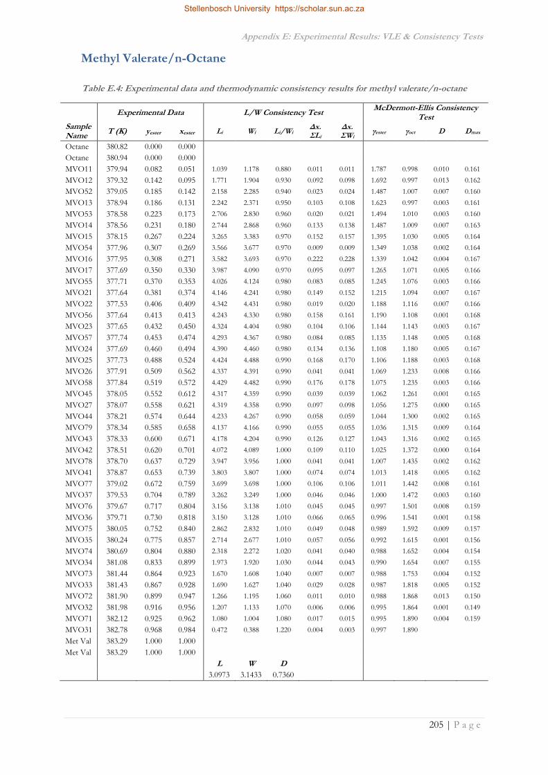
Appendix E: Experimental Results: VLE & Consistency Tests
205 | P a g e
Methyl Valerate/n-Octane
Table E.4: Experimental data and thermodynamic consistency results for methyl valerate/n-octane
Experimental Data L/W Consistency Test McDermott-Ellis Consistency
Test Sample Name
T (K) yester xester Li Wi Li/Wi Δx. ΣLi
Δx. ΣWi
γester γoct D Dmax
Octane 380.82 0.000 0.000
Octane 380.94 0.000 0.000
MVO11 379.94 0.082 0.051 1.039 1.178 0.880 0.011 0.011 1.787 0.998 0.010 0.161
MVO12 379.32 0.142 0.095 1.771 1.904 0.930 0.092 0.098 1.692 0.997 0.013 0.162
MVO52 379.05 0.185 0.142 2.158 2.285 0.940 0.023 0.024 1.487 1.007 0.007 0.160
MVO13 378.94 0.186 0.131 2.242 2.371 0.950 0.103 0.108 1.623 0.997 0.003 0.161
MVO53 378.58 0.223 0.173 2.706 2.830 0.960 0.020 0.021 1.494 1.010 0.003 0.160
MVO14 378.56 0.231 0.180 2.744 2.868 0.960 0.133 0.138 1.487 1.009 0.007 0.163
MVO15 378.15 0.267 0.224 3.265 3.383 0.970 0.152 0.157 1.395 1.030 0.005 0.164
MVO54 377.96 0.307 0.269 3.566 3.677 0.970 0.009 0.009 1.349 1.038 0.002 0.164
MVO16 377.95 0.308 0.271 3.582 3.693 0.970 0.222 0.228 1.339 1.042 0.004 0.167
MVO17 377.69 0.350 0.330 3.987 4.090 0.970 0.095 0.097 1.265 1.071 0.005 0.166
MVO55 377.71 0.370 0.353 4.026 4.124 0.980 0.083 0.085 1.245 1.076 0.003 0.166
MVO21 377.64 0.381 0.374 4.146 4.241 0.980 0.149 0.152 1.215 1.094 0.007 0.167
MVO22 377.53 0.406 0.409 4.342 4.431 0.980 0.019 0.020 1.188 1.116 0.007 0.166
MVO56 377.64 0.413 0.413 4.243 4.330 0.980 0.158 0.161 1.190 1.108 0.001 0.168
MVO23 377.65 0.432 0.450 4.324 4.404 0.980 0.104 0.106 1.144 1.143 0.003 0.167
MVO57 377.74 0.453 0.474 4.293 4.367 0.980 0.084 0.085 1.135 1.148 0.005 0.168
MVO24 377.69 0.460 0.494 4.390 4.460 0.980 0.134 0.136 1.108 1.180 0.005 0.167
MVO25 377.73 0.488 0.524 4.424 4.488 0.990 0.168 0.170 1.106 1.188 0.003 0.168
MVO26 377.91 0.509 0.562 4.337 4.391 0.990 0.041 0.041 1.069 1.233 0.008 0.166
MVO58 377.84 0.519 0.572 4.429 4.482 0.990 0.176 0.178 1.075 1.235 0.003 0.166
MVO45 378.05 0.552 0.612 4.317 4.359 0.990 0.039 0.039 1.062 1.261 0.001 0.165
MVO27 378.07 0.558 0.621 4.319 4.358 0.990 0.097 0.098 1.056 1.275 0.000 0.165
MVO44 378.21 0.574 0.644 4.233 4.267 0.990 0.058 0.059 1.044 1.300 0.002 0.165
MVO79 378.34 0.585 0.658 4.137 4.166 0.990 0.055 0.055 1.036 1.315 0.009 0.164
MVO43 378.33 0.600 0.671 4.178 4.204 0.990 0.126 0.127 1.043 1.316 0.002 0.165
MVO42 378.51 0.620 0.701 4.072 4.089 1.000 0.109 0.110 1.025 1.372 0.000 0.164
MVO78 378.70 0.637 0.729 3.947 3.956 1.000 0.041 0.041 1.007 1.435 0.002 0.162
MVO41 378.87 0.653 0.739 3.803 3.807 1.000 0.074 0.074 1.013 1.418 0.005 0.162
MVO77 379.02 0.672 0.759 3.699 3.698 1.000 0.106 0.106 1.011 1.442 0.008 0.161
MVO37 379.53 0.704 0.789 3.262 3.249 1.000 0.046 0.046 1.000 1.472 0.003 0.160
MVO76 379.67 0.717 0.804 3.156 3.138 1.010 0.045 0.045 0.997 1.501 0.008 0.159
MVO36 379.71 0.730 0.818 3.150 3.128 1.010 0.066 0.065 0.996 1.541 0.001 0.158
MVO75 380.05 0.752 0.840 2.862 2.832 1.010 0.049 0.048 0.989 1.592 0.009 0.157
MVO35 380.24 0.775 0.857 2.714 2.677 1.010 0.057 0.056 0.992 1.615 0.001 0.156
MVO74 380.69 0.804 0.880 2.318 2.272 1.020 0.041 0.040 0.988 1.652 0.004 0.154
MVO34 381.08 0.833 0.899 1.973 1.920 1.030 0.044 0.043 0.990 1.654 0.007 0.155
MVO73 381.44 0.864 0.923 1.670 1.608 1.040 0.007 0.007 0.988 1.753 0.004 0.152
MVO33 381.43 0.867 0.928 1.690 1.627 1.040 0.029 0.028 0.987 1.818 0.005 0.152
MVO72 381.90 0.899 0.947 1.266 1.195 1.060 0.011 0.010 0.988 1.868 0.013 0.150
MVO32 381.98 0.916 0.956 1.207 1.133 1.070 0.006 0.006 0.995 1.864 0.001 0.149
MVO71 382.12 0.925 0.962 1.080 1.004 1.080 0.017 0.015 0.995 1.890 0.004 0.159
MVO31 382.78 0.968 0.984 0.472 0.388 1.220 0.004 0.003 0.997 1.890
Met Val 383.29 1.000 1.000
Met Val 383.29 1.000 1.000
L W D
3.0973 3.1433 0.7360
Stellenbosch University https://scholar.sun.ac.za

Appendix E: Experimental Results: VLE & Consistency Tests
206 | P a g e
Ethyl Butanoate/n-Octane
Table E.5: Experimental data and thermodynamic consistency results for ethyl butanoate/n-octane
Experimental Data L/W Consistency Test McDermott-Ellis Consistency
Test Sample Name
T (K) yester xester Li Wi Li/Wi Δx. ΣLi
Δx. ΣWi
γester γoct D Dmax
Octane 380.85 0.000 0.000
EBO51 380.47 0.029 0.013 0.331 0.477 0.690 0.022 0.027 2.036 0.999 0.009 0.175
EBO31 379.63 0.085 0.045 1.047 1.187 0.880 0.029 0.032 1.732 0.999 0.013 0.153
EBO52 379.14 0.126 0.069 1.447 1.583 0.910 0.030 0.033 1.712 0.993 0.003 0.152
EBO32 378.58 0.155 0.087 1.940 2.070 0.940 0.133 0.140 1.707 0.995 0.016 0.160
EBO53 377.69 0.226 0.145 2.609 2.721 0.960 0.056 0.059 1.530 1.000 0.002 0.158
EBO34 377.40 0.247 0.166 2.820 2.926 0.960 0.003 0.003 1.472 1.006 0.002 0.158
EBO33 377.33 0.253 0.165 2.894 3.000 0.960 0.196 0.202 1.525 0.998 0.006 0.162
EBO54 376.60 0.312 0.227 3.389 3.470 0.980 0.026 0.027 1.390 1.017 0.001 0.161
EBO35 376.43 0.325 0.235 3.531 3.608 0.980 0.197 0.201 1.410 1.013 0.002 0.163
EBO55 375.82 0.375 0.288 3.944 3.997 0.990 0.014 0.014 1.352 1.027 0.000 0.163
EBO36 375.79 0.377 0.284 3.987 4.041 0.990 0.181 0.183 1.378 1.019 0.013 0.165
EBO56 375.66 0.405 0.330 3.948 3.981 0.990 0.016 0.016 1.281 1.043 0.007 0.165
EBO37 375.49 0.412 0.326 4.132 4.166 0.990 0.082 0.082 1.323 1.032 0.006 0.165
EBO41 375.47 0.421 0.346 4.079 4.103 0.990 0.141 0.142 1.275 1.047 0.000 0.166
EBO42 375.26 0.445 0.380 4.163 4.170 1.000 0.019 0.019 1.235 1.066 0.002 0.165
EBO57 375.29 0.447 0.385 4.116 4.121 1.000 0.100 0.100 1.224 1.070 0.003 0.166
EBO43 375.10 0.466 0.409 4.217 4.209 1.000 0.130 0.129 1.208 1.082 0.004 0.167
EBO44 374.87 0.488 0.439 4.336 4.311 1.010 0.045 0.044 1.187 1.100 0.008 0.167
EBO58 374.97 0.492 0.449 4.198 4.169 1.010 0.026 0.025 1.165 1.109 0.004 0.166
EBO45 374.87 0.497 0.455 4.276 4.242 1.010 0.102 0.101 1.165 1.113 0.003 0.167
EBO46 374.83 0.513 0.479 4.228 4.182 1.010 0.103 0.102 1.144 1.128 0.001 0.167
EBO47 374.75 0.534 0.504 4.219 4.160 1.010 0.124 0.122 1.135 1.136 0.002 0.167
EBO48 374.65 0.555 0.533 4.213 4.137 1.020 0.206 0.202 1.119 1.156 0.004 0.168
EBO28 374.66 0.591 0.583 4.022 3.921 1.030 0.207 0.201 1.088 1.192 0.001 0.168
EBO27 374.65 0.627 0.636 3.843 3.714 1.030 0.113 0.109 1.059 1.245 0.004 0.166
EBO26 374.76 0.650 0.666 3.624 3.481 1.040 0.012 0.012 1.045 1.269 0.003 0.166
EBO78 374.70 0.651 0.663 3.696 3.553 1.040 0.117 0.112 1.054 1.254 0.004 0.166
EBO25 374.82 0.672 0.696 3.459 3.302 1.050 0.099 0.094 1.033 1.300 0.005 0.165
EBO24 374.83 0.695 0.725 3.346 3.174 1.050 0.042 0.039 1.025 1.337 0.004 0.164
EBO77 374.81 0.705 0.737 3.321 3.142 1.060 0.030 0.028 1.023 1.354 0.003 0.164
EBO23 374.89 0.712 0.746 3.209 3.027 1.060 0.065 0.061 1.017 1.368 0.009 0.164
EBO22 374.85 0.729 0.767 3.177 2.983 1.060 0.038 0.036 1.015 1.403 0.000 0.163
EBO76 374.92 0.740 0.779 3.063 2.864 1.070 0.102 0.095 1.012 1.416 0.002 0.163
EBO75 375.13 0.773 0.814 2.728 2.517 1.080 0.035 0.033 1.005 1.461 0.001 0.161
EBO21 375.21 0.785 0.827 2.602 2.386 1.090 0.045 0.041 1.002 1.486 0.002 0.161
EBO17 375.32 0.802 0.845 2.429 2.208 1.100 0.020 0.018 0.999 1.518 0.007 0.160
EBO74 375.53 0.814 0.854 2.189 1.969 1.110 0.033 0.030 0.996 1.508 0.011 0.160
EBO16 375.47 0.828 0.869 2.195 1.966 1.120 0.046 0.041 0.997 1.562 0.004 0.159
EBO15 375.64 0.851 0.891 1.948 1.713 1.140 0.003 0.003 0.995 1.612 0.004 0.158
EBO73 375.75 0.855 0.893 1.832 1.600 1.150 0.038 0.033 0.994 1.593 0.002 0.158
EBO14 375.97 0.881 0.916 1.533 1.297 1.180 0.015 0.013 0.992 1.641 0.003 0.156
EBO72 376.18 0.894 0.926 1.285 1.051 1.220 0.016 0.013 0.989 1.667 0.006 0.156
EBO13 376.26 0.911 0.939 1.160 0.923 1.260 0.021 0.016 0.991 1.699 0.001 0.158
EBO12 376.57 0.940 0.961 0.775 0.539 1.440 0.010 0.007 0.990 1.754 0.007 0.158
EBO71 376.75 0.964 0.977 0.540 0.303 1.780 0.002 0.001 0.993 1.778 0.001 0.153
EBO11 376.87 0.971 0.982 0.403 0.169 2.390 0.992 1.806
Eth But 377.23 1.000 1.000
Eth But 377.21 1.000 1.000
L W D
3.0917 3.0389 0.8610
Stellenbosch University https://scholar.sun.ac.za
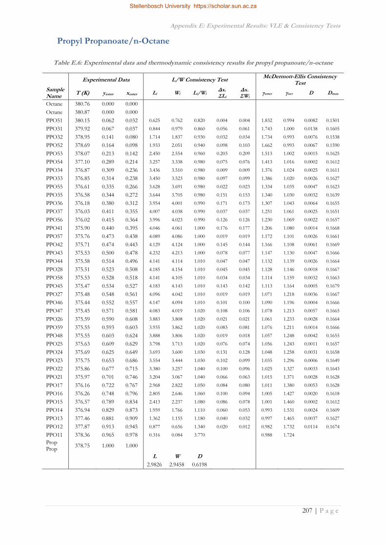
Appendix E: Experimental Results: VLE & Consistency Tests
207 | P a g e
Propyl Propanoate/n-Octane
Table E.6: Experimental data and thermodynamic consistency results for propyl propanoate/n-octane
Experimental Data L/W Consistency Test McDermott-Ellis Consistency
Test Sample Name
T (K) yester xester Li Wi Li/Wi Δx. ΣLi
Δx. ΣWi
γester γoct D Dmax
Octane 380.76 0.000 0.000
Octane 380.87 0.000 0.000
PPO51 380.15 0.062 0.032 0.625 0.762 0.820 0.004 0.004 1.832 0.994 0.0082 0.1501
PPO31 379.92 0.067 0.037 0.844 0.979 0.860 0.056 0.061 1.743 1.000 0.0138 0.1605
PPO32 378.95 0.141 0.080 1.714 1.837 0.930 0.032 0.034 1.734 0.993 0.0076 0.1538
PPO52 378.69 0.164 0.098 1.933 2.051 0.940 0.098 0.103 1.662 0.993 0.0067 0.1590
PPO53 378.07 0.213 0.142 2.450 2.554 0.960 0.203 0.209 1.513 1.002 0.0015 0.1625
PPO54 377.10 0.289 0.214 3.257 3.338 0.980 0.075 0.076 1.413 1.016 0.0002 0.1612
PPO34 376.87 0.309 0.236 3.436 3.510 0.980 0.009 0.009 1.376 1.024 0.0025 0.1611
PPO33 376.85 0.314 0.238 3.450 3.523 0.980 0.097 0.099 1.386 1.020 0.0026 0.1627
PPO55 376.61 0.335 0.266 3.628 3.691 0.980 0.022 0.023 1.334 1.035 0.0047 0.1623
PPO35 376.58 0.344 0.272 3.644 3.705 0.980 0.151 0.153 1.340 1.030 0.0032 0.1639
PPO36 376.18 0.380 0.312 3.954 4.001 0.990 0.171 0.173 1.307 1.043 0.0064 0.1655
PPO37 376.03 0.411 0.355 4.007 4.038 0.990 0.037 0.037 1.251 1.061 0.0025 0.1651
PPO56 376.02 0.415 0.364 3.996 4.023 0.990 0.126 0.126 1.230 1.069 0.0022 0.1657
PPO41 375.90 0.440 0.395 4.046 4.061 1.000 0.176 0.177 1.206 1.080 0.0014 0.1668
PPO57 375.76 0.473 0.438 4.089 4.086 1.000 0.019 0.019 1.172 1.101 0.0026 0.1661
PPO42 375.71 0.474 0.443 4.129 4.124 1.000 0.145 0.144 1.166 1.108 0.0061 0.1669
PPO43 375.53 0.500 0.478 4.232 4.213 1.000 0.078 0.077 1.147 1.130 0.0047 0.1666
PPO44 375.58 0.514 0.496 4.141 4.114 1.010 0.047 0.047 1.132 1.139 0.0026 0.1664
PPO28 375.51 0.523 0.508 4.185 4.154 1.010 0.045 0.045 1.128 1.146 0.0018 0.1667
PPO58 375.53 0.528 0.518 4.141 4.105 1.010 0.034 0.034 1.114 1.159 0.0032 0.1663
PPO45 375.47 0.534 0.527 4.183 4.143 1.010 0.143 0.142 1.113 1.164 0.0005 0.1679
PPO27 375.48 0.548 0.561 4.096 4.042 1.010 0.019 0.019 1.071 1.218 0.0036 0.1667
PPO46 375.44 0.552 0.557 4.147 4.094 1.010 0.101 0.100 1.090 1.196 0.0004 0.1666
PPO47 375.45 0.571 0.581 4.083 4.019 1.020 0.108 0.106 1.078 1.213 0.0057 0.1665
PPO26 375.59 0.590 0.608 3.883 3.808 1.020 0.021 0.021 1.061 1.233 0.0028 0.1664
PPO59 375.55 0.593 0.603 3.935 3.862 1.020 0.083 0.081 1.076 1.211 0.0014 0.1666
PPO48 375.55 0.603 0.624 3.888 3.806 1.020 0.019 0.018 1.057 1.248 0.0042 0.1655
PPO25 375.63 0.609 0.629 3.798 3.713 1.020 0.076 0.074 1.056 1.243 0.0011 0.1657
PPO24 375.69 0.625 0.649 3.693 3.600 1.030 0.131 0.128 1.048 1.258 0.0031 0.1658
PPO23 375.75 0.653 0.686 3.554 3.444 1.030 0.102 0.099 1.035 1.296 0.0006 0.1649
PPO22 375.86 0.677 0.715 3.380 3.257 1.040 0.100 0.096 1.025 1.327 0.0033 0.1643
PPO21 375.97 0.701 0.746 3.204 3.067 1.040 0.066 0.063 1.015 1.371 0.0028 0.1628
PPO17 376.16 0.722 0.767 2.968 2.822 1.050 0.084 0.080 1.011 1.380 0.0053 0.1628
PPO16 376.26 0.748 0.796 2.805 2.646 1.060 0.100 0.094 1.005 1.427 0.0020 0.1618
PPO15 376.57 0.789 0.834 2.413 2.237 1.080 0.086 0.078 1.001 1.460 0.0002 0.1612
PPO14 376.94 0.829 0.873 1.959 1.766 1.110 0.060 0.053 0.993 1.531 0.0024 0.1609
PPO13 377.46 0.881 0.909 1.362 1.155 1.180 0.040 0.032 0.997 1.465 0.0037 0.1627
PPO12 377.87 0.913 0.945 0.877 0.656 1.340 0.020 0.012 0.982 1.732 0.0114 0.1674
PPO11 378.36 0.965 0.978 0.316 0.084 3.770 0.988 1.724
Prop Prop
378.75 1.000 1.000
L W D
2.9826 2.9458 0.6198
Stellenbosch University https://scholar.sun.ac.za
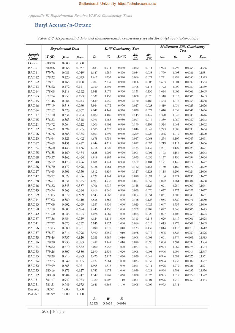
Appendix E: Experimental Results: VLE & Consistency Tests
208 | P a g e
Butyl Acetate/n-Octane
Table E.7: Experimental data and thermodynamic consistency results for butyl acetate/n-octane
Experimental Data L/W Consistency Test McDermott-Ellis Consistency
Test Sample Name
T (K) yester xester Li Wi Li/Wi Δx. ΣLi
Δx. ΣWi
γester γoct D Dmax
Octane 380.78 0.000 0.000
BAO61 380.06 0.068 0.037 0.833 0.974 0.860 0.012 0.014 1.974 0.995 0.0065 0.1536
BAO11 379.76 0.081 0.049 1.147 1.287 0.890 0.034 0.038 1.779 1.003 0.0081 0.1551
BAO12 379.32 0.120 0.073 1.617 1.752 0.920 0.066 0.071 1.771 0.999 0.0056 0.1573
BAO62 378.77 0.165 0.108 2.207 2.339 0.940 0.006 0.006 1.683 1.001 0.0032 0.1554
BAO13 378.62 0.172 0.111 2.360 2.492 0.950 0.108 0.114 1.722 1.000 0.0050 0.1589
BAO14 378.08 0.218 0.152 2.948 3.074 0.960 0.131 0.136 1.624 1.006 0.0069 0.1609
BAO63 377.74 0.257 0.193 3.337 3.456 0.970 0.068 0.070 1.518 1.016 0.0005 0.1603
BAO15 377.46 0.284 0.213 3.639 3.756 0.970 0.180 0.185 1.534 1.013 0.0055 0.1638
BAO16 377.19 0.318 0.260 3.964 4.072 0.970 0.027 0.028 1.419 1.034 0.0023 0.1626
BAO64 377.12 0.323 0.267 4.042 4.149 0.970 0.070 0.072 1.410 1.038 0.0047 0.1636
BAO17 377.10 0.334 0.284 4.082 4.185 0.980 0.145 0.149 1.370 1.046 0.0048 0.1646
BAO65 376.83 0.363 0.318 4.391 4.488 0.980 0.017 0.017 1.339 1.060 0.0059 0.1643
BAO21 376.92 0.364 0.322 4.306 4.401 0.980 0.190 0.194 1.324 1.061 0.0060 0.1662
BAO22 376.69 0.394 0.365 4.585 4.672 0.980 0.046 0.047 1.273 1.088 0.0033 0.1654
BAO66 376.76 0.388 0.355 4.503 4.592 0.980 0.219 0.223 1.286 1.079 0.0006 0.1670
BAO23 376.64 0.421 0.402 4.678 4.756 0.980 0.067 0.068 1.234 1.107 0.0047 0.1661
BAO67 376.69 0.431 0.417 4.644 4.719 0.980 0.092 0.093 1.219 1.112 0.0047 0.1666
BAO24 376.60 0.443 0.436 4.756 4.827 0.990 0.135 0.137 1.201 1.129 0.0028 0.1671
BAO25 376.55 0.460 0.464 4.838 4.902 0.990 0.001 0.001 1.173 1.154 0.0006 0.1663
BAO68 376.57 0.462 0.464 4.818 4.882 0.990 0.055 0.056 1.177 1.150 0.0094 0.1664
BAO48 376.72 0.473 0.476 4.681 4.741 0.990 0.102 0.104 1.171 1.145 0.0014 0.1677
BAO26 376.70 0.477 0.498 4.726 4.781 0.990 0.152 0.154 1.130 1.186 0.0077 0.1669
BAO27 376.65 0.501 0.530 4.812 4.859 0.990 0.127 0.128 1.118 1.209 0.0024 0.1666
BAO47 376.77 0.522 0.556 4.722 4.761 0.990 0.090 0.091 1.104 1.224 0.0135 0.1667
BAO28 376.61 0.531 0.575 4.903 4.938 0.990 0.057 0.057 1.092 1.261 0.0084 0.1658
BAO46 376.82 0.545 0.587 4.706 4.737 0.990 0.125 0.126 1.091 1.250 0.0009 0.1661
BAO45 376.94 0.565 0.614 4.616 4.640 0.990 0.069 0.070 1.077 1.273 0.0027 0.1657
BAO59 377.03 0.572 0.629 4.543 4.562 1.000 0.054 0.054 1.061 1.300 0.0040 0.1651
BAO44 377.02 0.580 0.640 4.566 4.582 1.000 0.128 0.128 1.055 1.320 0.0071 0.1650
BAO43 377.09 0.602 0.669 4.527 4.536 1.000 0.025 0.025 1.047 1.353 0.0030 0.1640
BAO58 377.18 0.605 0.674 4.443 4.450 1.000 0.209 0.209 1.042 1.360 0.0006 0.1645
BAO42 377.60 0.648 0.723 4.078 4.069 1.000 0.025 0.025 1.027 1.408 0.0063 0.1623
BAO57 377.56 0.654 0.729 4.124 4.114 1.000 0.113 0.113 1.029 1.417 0.0006 0.1628
BAO41 377.77 0.675 0.757 3.945 3.927 1.000 0.016 0.016 1.015 1.476 0.0008 0.1609
BAO56 377.83 0.680 0.761 3.890 3.870 1.010 0.133 0.132 1.014 1.478 0.0018 0.1612
BAO37 378.27 0.716 0.798 3.490 3.459 1.010 0.078 0.077 1.006 1.526 0.0050 0.1596
BAO55 378.46 0.737 0.820 3.325 3.287 1.010 0.008 0.008 1.001 1.579 0.0105 0.1583
BAO36 378.30 0.738 0.823 3.487 3.449 1.010 0.096 0.095 1.004 1.604 0.0039 0.1584
BAO54 378.82 0.770 0.852 3.000 2.952 1.020 0.077 0.076 0.994 1.669 0.0075 0.1564
BAO53 379.26 0.807 0.880 2.590 2.534 1.020 0.008 0.008 0.996 1.694 0.0014 0.1547
BAO35 379.38 0.813 0.883 2.473 2.417 1.020 0.050 0.049 0.996 1.684 0.0025 0.1551
BAO34 379.75 0.842 0.905 2.127 2.064 1.030 0.033 0.032 0.994 1.733 0.0082 0.1537
BAO52 379.99 0.865 0.921 1.905 1.838 1.040 0.011 0.011 0.996 1.779 0.0021 0.1521
BAO33 380.16 0.873 0.927 1.742 1.673 1.040 0.029 0.028 0.994 1.798 0.0032 0.1526
BAO32 380.58 0.904 0.947 1.342 1.269 1.060 0.028 0.026 0.995 1.817 0.0072 0.1572
BAO31 381.17 0.947 0.973 0.780 0.702 1.110 0.001 0.001 0.996 1.940 0.0067 0.1483
BAO51 381.31 0.949 0.973 0.641 0.563 1.140 0.008 0.007 0.993 1.911
But Ace 382.01 1.000 1.000
But Ace 381.99 1.000 1.000
L W D
3.5229 3.5655 0.6016
Stellenbosch University https://scholar.sun.ac.za

Appendix E: Experimental Results: VLE & Consistency Tests
209 | P a g e
Pentyl Formate/n-Octane
Table E.8: Experimental data and thermodynamic consistency results for pentyl formate/n-octane
Experimental Data L/W Consistency Test McDermott-Ellis Consistency
Test Sample Name
T (K) yester xester Li Wi Li/Wi Δx. ΣLi
Δx. ΣWi
γester γoct D Dmax
Octane 380.84 0.000 0.000
Octane 380.82 0.000 0.000
AFO31 380.39 0.045 0.027 0.651 0.793 0.820 0.032 0.036 2.112 0.999 0.0068 0.1659
AFO32 379.98 0.086 0.060 1.292 1.431 0.900 0.013 0.015 1.828 1.002 0.0003 0.1576
AFO61 379.97 0.088 0.049 1.227 1.368 0.900 0.114 0.122 2.289 0.989 0.0033 0.1702
AFO62 379.21 0.147 0.111 2.427 2.560 0.950 0.028 0.030 1.723 1.012 0.0019 0.1583
AFO33 379.10 0.162 0.123 2.617 2.749 0.950 0.097 0.101 1.722 1.011 0.0017 0.1619
AFO34 378.89 0.192 0.157 3.067 3.195 0.960 0.077 0.080 1.611 1.021 0.0038 0.1627
AFO63 378.82 0.211 0.181 3.306 3.430 0.960 0.052 0.054 1.533 1.029 0.0040 0.1623
AFO35 378.65 0.228 0.196 3.581 3.704 0.970 0.204 0.210 1.543 1.030 0.0017 0.1663
AFO64 378.50 0.266 0.249 4.102 4.216 0.970 0.032 0.032 1.423 1.053 0.0095 0.1647
AFO36 378.32 0.278 0.256 4.334 4.448 0.970 0.148 0.152 1.450 1.053 0.0083 0.1665
AFO37 378.39 0.298 0.290 4.496 4.605 0.980 0.095 0.097 1.372 1.069 0.0022 0.1668
AFO65 378.35 0.310 0.311 4.680 4.785 0.980 0.058 0.059 1.333 1.084 0.0001 0.1667
AFO41 378.37 0.318 0.323 4.745 4.848 0.980 0.178 0.182 1.317 1.090 0.0014 0.1681
AFO42 378.42 0.342 0.360 4.951 5.046 0.980 0.040 0.040 1.269 1.110 0.0024 0.1676
AFO66 378.47 0.345 0.368 4.955 5.049 0.980 0.172 0.175 1.251 1.117 0.0032 0.1685
AFO43 378.51 0.369 0.402 5.150 5.238 0.980 0.159 0.162 1.221 1.137 0.0043 0.1687
AFO44 378.54 0.388 0.432 5.329 5.410 0.980 0.000 0.000 1.192 1.161 0.0071 0.1679
AFO67 378.65 0.388 0.432 5.219 5.299 0.980 0.272 0.276 1.189 1.156 0.0108 0.1699
AFO45 378.69 0.417 0.483 5.527 5.597 0.990 0.109 0.110 1.142 1.208 0.0063 0.1684
AFO68 378.71 0.431 0.502 5.640 5.706 0.990 0.164 0.166 1.132 1.226 0.0055 0.1686
AFO46 378.98 0.448 0.532 5.569 5.628 0.990 0.073 0.074 1.105 1.251 0.0034 0.1675
AFO58 379.05 0.460 0.545 5.589 5.645 0.990 0.093 0.094 1.104 1.257 0.0010 0.1677
AFO47 379.18 0.470 0.561 5.573 5.624 0.990 0.202 0.204 1.089 1.277 0.0055 0.1680
AFO48 379.37 0.493 0.597 5.628 5.670 0.990 0.263 0.265 1.067 1.322 0.0048 0.1671
AFO57 379.83 0.531 0.645 5.489 5.518 0.990 0.044 0.045 1.049 1.368 0.0017 0.1654
AFO28 379.91 0.534 0.653 5.464 5.490 1.000 0.195 0.196 1.039 1.389 0.0141 0.1651
AFO56 380.16 0.565 0.689 5.455 5.472 1.000 0.057 0.057 1.034 1.433 0.0051 0.1635
AFO27 380.41 0.575 0.699 5.276 5.289 1.000 0.110 0.110 1.028 1.440 0.0007 0.1632
AFO26 380.71 0.594 0.720 5.118 5.125 1.000 0.007 0.007 1.021 1.466 0.0149 0.1625
AFO55 380.48 0.594 0.722 5.358 5.365 1.000 0.058 0.058 1.027 1.483 0.0160 0.1623
AFO25 380.90 0.604 0.733 5.014 5.016 1.000 0.099 0.099 1.014 1.490 0.0007 0.1622
AFO24 381.17 0.618 0.753 4.877 4.874 1.000 0.074 0.074 1.002 1.540 0.0116 0.1607
AFO23 381.30 0.635 0.768 4.850 4.842 1.000 0.104 0.104 1.005 1.563 0.0172 0.1600
AFO54 381.49 0.660 0.790 4.805 4.791 1.000 0.036 0.036 1.010 1.597 0.0087 0.1588
AFO22 381.77 0.668 0.798 4.577 4.560 1.000 0.154 0.153 1.003 1.606 0.0006 0.1585
AFO21 382.62 0.712 0.834 3.968 3.940 1.010 0.027 0.027 0.996 1.654 0.0099 0.1564
AFO53 382.53 0.716 0.840 4.102 4.073 1.010 0.059 0.059 0.996 1.705 0.0107 0.1560
AFO17 383.00 0.731 0.856 3.734 3.700 1.010 0.067 0.066 0.984 1.761 0.0106 0.1543
AFO16 383.44 0.761 0.874 3.417 3.379 1.010 0.057 0.057 0.989 1.773 0.0178 0.1531
AFO52 383.79 0.792 0.892 3.183 3.139 1.010 0.033 0.032 0.999 1.773 0.0105 0.1523
AFO15 384.22 0.805 0.903 2.825 2.779 1.020 0.060 0.059 0.990 1.823 0.0109 0.1515
AFO14 384.90 0.848 0.926 2.301 2.250 1.020 0.005 0.005 0.995 1.841 0.0127 0.1498
AFO51 384.69 0.848 0.928 2.526 2.474 1.020 0.054 0.053 0.999 1.909 0.0058 0.1513
AFO13 385.78 0.897 0.955 1.610 1.554 1.040 0.021 0.020 0.994 1.970 0.0083 0.1484
AFO12 386.28 0.927 0.969 1.208 1.149 1.050 0.010 0.009 0.997 2.036 0.0087 0.1463
AFO11 386.51 0.947 0.978 1.036 0.976 1.060 0.011 0.011 1.001 2.072
Pen For 387.46 1.000 1.000
Pen For 387.40 1.000 1.000
L W D
4.0200 4.0747 0.6763
Stellenbosch University https://scholar.sun.ac.za

Appendix F: sPC-SAFT Correlation Results
210 | P a g e
346
348
350
352
354
356
0.00 0.20 0.40 0.60 0.80 1.00
Tem
per
atu
re (K
)
Di-n-Propyl Ether Mole Fraction (x,y)
Experimental
sPC-SAFT (kij=5.178E-03)
sPC-SAFT GV (kij = 2.489e-03)
sPC-SAFT JC (kij = 3.308e-03)
0.00
0.20
0.40
0.60
0.80
1.00
0.00 0.20 0.40 0.60 0.80 1.00
Di-
n-P
rop
yl E
ther
Vap
ou
r M
ole
Fra
ctio
n (y
)
Di-n-Propyl Ether Liquid Mole Fraction (x)
Experimental
sPC-SAFT (kij = 5.178e-03)
sPC-SAFT GV (kij = 2.489e-03)
sPC-SAFT JC (kij = 3.308e-03)
348
350
352
354
356
0.00 0.20 0.40 0.60 0.80 1.00
Tem
per
atu
re (K
)
Butyl Ethyl Ether Mole Fraction (x,y)
Experimental
sPC-SAFT (kij = 4.308e-03)
sPC-SAFT GV
sPC-SAFT JC
0.00
0.20
0.40
0.60
0.80
1.00
0.00 0.20 0.40 0.60 0.80 1.00
Bu
tyl E
thyl
Eth
er V
apo
ur
Mo
le F
ract
ion
(y)
Butyl Ethyl Ether Liquid Mole Fraction (x)
Experimental
sPC-SAFT (kij = 4.308e-03)
sPC-SAFT GV
sPC-SAFT JC
APPENDIX F: SPC-SAFT CORRELATION
RESULTS
The correlation results presented in this section are those for the Standard pure component
regression to demonstrate that such predictions can be brought into agreement with experimental data by
introducing small binary interaction parameters.
Ether Systems
[i.]
[ii.]
[i.]
[ii.]
Figure F.2: [i.] T-xy and [ii.] x-y correlations for the di-n-propyl ether/n-heptane system at 60 kPa using the standard pure component regression procedure. The correlation of nonpolar sPC-SAFT is included for
comparison.
Figure F.1: [i.] T-xy and [ii.] x-y correlations for the butyl ethyl ether/n-heptane system at 60 kPa using the standard pure component regression procedure. Only correlation of nonpolar sPC-SAFT is possible.
Stellenbosch University https://scholar.sun.ac.za

Appendix F: sPC-SAFT Correlation Results
211 | P a g e
377
379
381
383
385
0.00 0.20 0.40 0.60 0.80 1.00
Tem
per
atu
re (K
)
Methyl Valerate Mole Fraction (x,y)
Experimental
sPC-SAFT (kij = 0.019)
sPC-SAFT GV (kij = 0)
sPC-SAFT JC (kij = 0.017)
0.00
0.20
0.40
0.60
0.80
1.00
0.00 0.20 0.40 0.60 0.80 1.00
Met
hyl
Val
erat
e V
apo
ur
Mo
le F
ract
ion
(y)
Methyl Valerate Liquid Mole Fraction (x)
Experimental
sPC-SAFT (kij = 0.019)
sPC-SAFT GV (kij = 0)
sPC-SAFT JC (kij = 0.017)
374
376
378
380
382
0.00 0.20 0.40 0.60 0.80 1.00
Tem
per
atu
re (K
)
Ethyl Butanoate Mole Fraction (x,y)
Experimental
sPC-SAFT (kij = 0.019)
sPC-SAFT GV (kij = -0.016)
sPC-SAFT JC
0.00
0.20
0.40
0.60
0.80
1.00
0.00 0.20 0.40 0.60 0.80 1.00
Eth
yl B
uta
no
ate
Vap
ou
r M
ole
Fra
ctio
n (y
)
Ethyl Butanoate Liquid Mole Fraction (x)
Experimental
sPC-SAFT (kij = 0.019)
sPC-SAFT GV (kij = -0.016)
sPC-SAFT JC
374
376
378
380
382
0.00 0.20 0.40 0.60 0.80 1.00
Tem
per
atu
re (K
)
Propyl Propanoate Mole Fraction (x,y)
Experimental
sPC-SAFT (kij = 0.017)
sPC-SAFT GV (kij = -0.036)
sPC-SAFT JC
0.00
0.20
0.40
0.60
0.80
1.00
0.00 0.20 0.40 0.60 0.80 1.00
Pro
pyl
Pro
pan
oat
e V
apo
ur
Mo
le F
ract
ion
(y)
Propyl Propanoate Liquid Mole Fraction (x)
Experimental
sPC-SAFT (kij = 0.017)
sPC-SAFT GV (kij = -0.036)
sPC-SAFT JC
Ester Systems
Figure F.3: [i.] T-xy and [ii.] x-y correlations for the methyl valerate/n-octane system at 60 kPa using the standard pure component regression procedure.
[i.] [ii.]
Figure F.4: [i.] T-xy and [ii.] x-y correlations for the ethyl butanoate/n-octane system at 60 kPa using the standard pure component regression procedure.
[i.]
[ii.]
Figure F.5: [i.] T-xy and [ii.] x-y correlations for the ethyl butanoate/n-octane system at 60 kPa using the standard pure component regression procedure.
[i.]
[ii.]
Stellenbosch University https://scholar.sun.ac.za
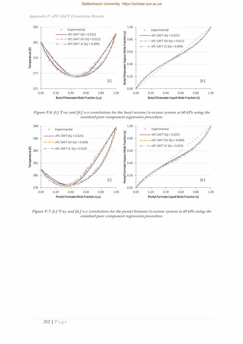
Appendix F: sPC-SAFT Correlation Results
212 | P a g e
378
380
382
384
386
388
0.00 0.20 0.40 0.60 0.80 1.00
Tem
per
atu
re (K
)
Pentyl Formate Mole Fraction (x,y)
Experimental
sPC-SAFT (kij = 0.025)
sPC-SAFT GV (kij = 0.004)
sPC-SAFT JC (kij = 0.023)
0.00
0.20
0.40
0.60
0.80
1.00
0.00 0.20 0.40 0.60 0.80 1.00
Pe
nty
l Fo
rmat
e V
apo
ur
Mo
le F
ract
ion
(y)
Pentyl Formate Liquid Mole Fraction (x)
Experimental
sPC-SAFT (kij = 0.025)
sPC-SAFT GV (kij = 0.004)
sPC-SAFT JC (kij = 0.023)
375
377
379
381
383
0.00 0.20 0.40 0.60 0.80 1.00
Tem
per
atu
re (K
)
Butyl Ethanoate Mole Fraction (x,y)
Experimental
sPC-SAFT (kij = 0.022)
sPC-SAFT GV (kij = 0.012)
sPC-SAFT JC (kij = 0.009)
0.00
0.20
0.40
0.60
0.80
1.00
0.00 0.20 0.40 0.60 0.80 1.00
Bu
tyl E
than
oat
e V
apo
ur
Mo
le F
ract
ion
(y)
Butyl Ethanoate Liquid Mole Fraction (x)
Experimental
sPC-SAFT (kij = 0.022)
sPC-SAFT GV (kij = 0.012)
sPC-SAFT JC (kij = 0.009)
Figure F.7: [i.] T-xy and [ii.] x-y correlations for the pentyl formate/n-octane system at 60 kPa using the
standard pure component regression procedure.
[i.] [ii.]
Figure F.6: [i.] T-xy and [ii.] x-y correlations for the butyl acetate/n-octane system at 60 kPa using the standard pure component regression procedure.
[i.] [ii.]
Stellenbosch University https://scholar.sun.ac.za
Appendix G: Polar SAFT-VR Mie Working Equations
213 | P a g e
APPENDIX G: POLAR SAFT-VR MIE
WORKING EQUATIONS
The working equation for the SAFT-VR Mie EoS comprise 96 pages of equations and are thus
not incorporated here for the sake of brevity. These equations can be made available on request.
Stellenbosch University https://scholar.sun.ac.za

Appendix H: SAFT-VR Mie Code Validation
214 | P a g e
APPENDIX H: SAFT-VR MIE CODE
VALIDATION
The tables presented in this appendix serve to validate the coded working equations of the polar
SAFT-VR Mie EoS’s. This was achieved by comparing the analytical derivatives of the working equations
with those calculated by numerical differentiation using the central differences technique of equation H.1:
, ,
2i i
i
f x f xf
x
ε ε
ε
x x H.1
where x ∈ {ni,…,nc, T, V}.
For the validation considered here, use is made of 2-butanone as a one component reference
system with T = 300K and V= 0.091L.mol-1.
Table H.1: Hard Sphere term code validation results
Function Analytical Derivative Numerical Derivative % Difference
F 7.7521901019 7.7521901019
∂F/∂ni 22.238267552 22.238267552 -2.7631689795e-09
∂F/∂T -0.0031236728274 -0.0031236727915 -1.1488186755e-06
∂F/∂V -159.95056941 -159.95057477 3.3497458718e-06
∂2F/∂ni∂nj 53.340014737 53.340014736 -1.9514343501e-09
∂2F/∂T∂ni -0.011501854468 -0.011501857244 2.4139341698e-05
∂2F/∂V∂ni -588.9631447 -588.96314504 5.7395196968e-08
∂2F/∂T2 3.1222034689e-06 3.1222038843e-06 1.3306786763e-05
∂2F/∂T∂V 0.092509164653 0.092509169515 5.2559470084e-06
∂2F/∂V2 6503.1400446 6503.1404711 6.5577600577e-06
Stellenbosch University https://scholar.sun.ac.za
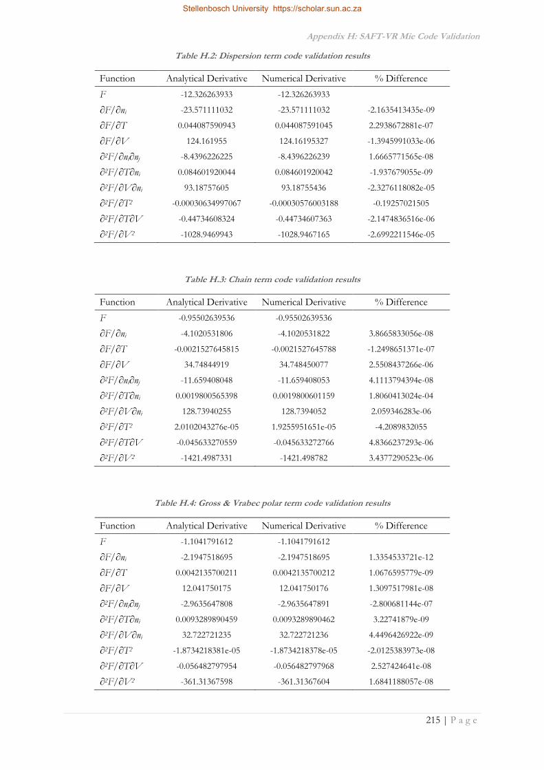
Appendix H: SAFT-VR Mie Code Validation
215 | P a g e
Table H.2: Dispersion term code validation results
Function Analytical Derivative Numerical Derivative % Difference
F -12.326263933 -12.326263933
∂F/∂ni -23.571111032 -23.571111032 -2.1635413435e-09
∂F/∂T 0.044087590943 0.044087591045 2.2938672881e-07
∂F/∂V 124.161955 124.16195327 -1.3945991033e-06
∂2F/∂ni∂nj -8.4396226225 -8.4396226239 1.6665771565e-08
∂2F/∂T∂ni 0.084601920044 0.084601920042 -1.937679055e-09
∂2F/∂V∂ni 93.18757605 93.18755436 -2.3276118082e-05
∂2F/∂T2 -0.00030634997067 -0.00030576003188 -0.19257021505
∂2F/∂T∂V -0.44734608324 -0.44734607363 -2.1474836516e-06
∂2F/∂V2 -1028.9469943 -1028.9467165 -2.6992211546e-05
Table H.3: Chain term code validation results
Function Analytical Derivative Numerical Derivative % Difference
F -0.95502639536 -0.95502639536
∂F/∂ni -4.1020531806 -4.1020531822 3.8665833056e-08
∂F/∂T -0.0021527645815 -0.0021527645788 -1.2498651371e-07
∂F/∂V 34.74844919 34.748450077 2.5508437266e-06
∂2F/∂ni∂nj -11.659408048 -11.659408053 4.1113794394e-08
∂2F/∂T∂ni 0.0019800565398 0.0019800601159 1.8060413024e-04
∂2F/∂V∂ni 128.73940255 128.7394052 2.059346283e-06
∂2F/∂T2 2.0102043276e-05 1.9255951651e-05 -4.2089832055
∂2F/∂T∂V -0.045633270559 -0.045633272766 4.8366237293e-06
∂2F/∂V2 -1421.4987331 -1421.498782 3.4377290523e-06
Table H.4: Gross & Vrabec polar term code validation results
Function Analytical Derivative Numerical Derivative % Difference
F -1.1041791612 -1.1041791612
∂F/∂ni -2.1947518695 -2.1947518695 1.3354533721e-12
∂F/∂T 0.0042135700211 0.0042135700212 1.0676595779e-09
∂F/∂V 12.041750175 12.041750176 1.3097517981e-08
∂2F/∂ni∂nj -2.9635647808 -2.9635647891 -2.800681144e-07
∂2F/∂T∂ni 0.0093289890459 0.0093289890462 3.22741879e-09
∂2F/∂V∂ni 32.722721235 32.722721236 4.4496426922e-09
∂2F/∂T2 -1.8734218381e-05 -1.8734218378e-05 -2.0125383973e-08
∂2F/∂T∂V -0.056482797954 -0.056482797968 2.527424641e-08
∂2F/∂V2 -361.31367598 -361.31367604 1.6841188057e-08
Stellenbosch University https://scholar.sun.ac.za

Appendix H: SAFT-VR Mie Code Validation
216 | P a g e
Analysis of the ∂2F/∂T2 results shows fairly large deviations between the numerical and analytical
derivatives, particularly when compared to the orders of magnitude of other derivative deviations. Closer
inspection shows these instances are confined to the SAFT-VR Mie terms and not the polar contribution.
These deviations are thus readily explained by the fact that the temperature dependent diameter in
SAFT-VR Mie is calculated by means of 10-point Gauss-Legendre quadrature – thus the numerical
derivative of the temperature dependent properties is taking the numerical derivative of a numerical
integral. This procedure is inherently error-prone which leads to the larger deviations between analytical
and numerical derivatives. Considering the total model deviations in Table H.5, rather than the individual
terms, provides a measure of reassurance regarding these deviations however, with a significantly lower
overall deviation in evidence.
Table H.5: Total SAFT-VR MieGV prediction validation results
Function Analytical Derivative Numerical Derivative % Difference
F -6.6332793876600 -6.6332793876600
∂F/∂ni -7.6296485301000 -7.6296485317000 2.09708235717E-08
∂F/∂T 0.0430247235552 0.0430247236959 3.27021276688E-07
∂F/∂V 11.0015849550 11.0015787530 -5.63736954573E-05
∂2F/∂ni∂nj 30.2774192857 30.2774192700 -5.18537999196E-08
∂2F/∂T∂ni 0.0844091111617 0.0844091119601 9.45869454024E-07
∂2F/∂V∂ni -334.313444865 -334.313464244 5.79665586911E-06
∂2F/∂T2 -3.01859942E-04 -3.02116095E-04 0.0848580353667
∂2F/∂T∂V -0.456952987100 -0.456952974849 -2.68101979714E-06
∂2F/∂V2 3691.38064122 3691.38129656 1.77532490592E-05
The validation of the Jog & Chapman polar term is presented in Table H.6, where a different
volume root of v = 0.104L.mol-1 was solved at the reference temperature of T = 300K.
Table H.6: Jog & Chapman polar term code validation results
Function Analytical Derivative Numerical Derivative % Difference
F -1.4874880008 -1.4874880008
∂F/∂ni -3.1967520486 -3.1967520485 -2.7766966542e-09
∂F/∂T 0.0081340854198 0.0081340854209 1.3710292278e-08
∂F/∂V 16.494002153 16.494002155 1.4934017608e-08
∂2F/∂ni∂nj -4.198135944 -4.1981359435 -1.191004884E-08
∂2F/∂T∂ni 0.016519066644 0.016519066645 9.2171317844e-09
∂2F/∂V∂ni 45.054100951 45.054100961 2.1272848624e-08
∂2F/∂T2 -6.8990402257e-05 -6.8990402274e-05 2.4998304835e-08
∂2F/∂T∂V -0.080913126634 -0.080913126646 1.5087819201e-08
∂2F/∂V2 -390.92214745 -390.92214758 3.4011886423e-08
Stellenbosch University https://scholar.sun.ac.za

Appendix H: SAFT-VR Mie Code Validation
217 | P a g e
Stellenbosch University https://scholar.sun.ac.za