
Resonance phenomena in macroscopic quantum tunneling for an rf SQUID
Upload
khangminh22Category
view
5download
0
IMPROVED TUNNELING KNOWLEDGE
THROUGH ROBUST MACHINE
LEARNING
by
James I. Maher Jr.

A thesis submitted to the Faculty and the Board of Trustees of the Colorado School
of Mines in partial fulfillment of the requirements for the degree of Doctor of Philosophy
(Computer Science).
Golden, Colorado
Date
Signed:James I. Maher Jr.
Signed:Dr. Tracy CampThesis Advisor
Golden, Colorado
Date
Signed:Dr. Randy Haupt
Professor and HeadDepartment of Electrical Engineering and Computer Science
ii

ABSTRACT
Earth Pressure Balance Machines (EPBMs) are essential equipment for excavating and
constructing underground tunnels in urban environments with soft ground conditions. As
examples, EPBMs are used for subways, underground highways, and water conduits. Our
work utilizes data collected from hundreds of sensors on an EPBM to understand which
systems affect the EPBM’s performance. The ultimate goal is to optimize these systems in
future tunneling projects, reducing project costs and construction time. We apply machine
learning techniques to two data sets from EPBM excavated tunnels in the Seattle, WA,
University Link subway project (U230 Contract). Specifically, we apply ensemble feature
selection to identify sensor readings that are correlated with changes in the EPBM’s advance
rate. We found that current ensemble feature selection methods are insufficient for our
data sets; thus, we created a novel ensemble feature selection method, JENNA Ensemble
Network Normalization Algorithm (JENNA). JENNA allows diversity in the configurations
of Feature Selection Algorithms, allows for regression FSAs, and enables both subset and
ranker FSAs to be used simultaneously. JENNA also introduces a novel ensemble feature
selection aggregation function that weights each feature by predicted accuracy performance
and feature stability, in addition to average feature selection algorithm ranking.
During our initial work, we identified a time delay between changes to some EPBM
machine parameters and when these changes affect the EPBM’s advance rate. In order to
account for the time delay, we trained Recurrent Neural Networks (RNNs) to the data set.
We then created a novel anomaly detection algorithm Recurrent Neural Network Anomaly
Detection Algorithm (ReNN AnD) based on the trained RNNs. ReNN AnD varies from
traditional anomaly detection, because it accounts for time delays in the data set. We used
ReNN AnD to successfully detect soil at the front of an EPBM. This soil type information
could be used to improve an EPBM’s performance in future tunneling projects.
iii
TABLE OF CONTENTS
ABSTRACT . . . . . . . . . . . . . . . . . . . . . . . . . . . . . . . . . . . . . . . . . iii
LIST OF FIGURES . . . . . . . . . . . . . . . . . . . . . . . . . . . . . . . . . . . . viii
LIST OF TABLES . . . . . . . . . . . . . . . . . . . . . . . . . . . . . . . . . . . . . . xii
LIST OF SYMBOLS . . . . . . . . . . . . . . . . . . . . . . . . . . . . . . . . . . . . xiii
LIST OF ABBREVIATIONS . . . . . . . . . . . . . . . . . . . . . . . . . . . . . . . . xiv
ACKNOWLEDGMENTS . . . . . . . . . . . . . . . . . . . . . . . . . . . . . . . . . . xv
DEDICATION . . . . . . . . . . . . . . . . . . . . . . . . . . . . . . . . . . . . . . . . xvi
CHAPTER 1 INTRODUCTION . . . . . . . . . . . . . . . . . . . . . . . . . . . . . . . 1
1.1 Background and Related Work . . . . . . . . . . . . . . . . . . . . . . . . . . . . 2
1.2 Description of an Earth Pressure Balance Machine (EPBM) . . . . . . . . . . . 3
1.3 Performance Prediction of EPBMs . . . . . . . . . . . . . . . . . . . . . . . . . 9
1.3.1 Computer Model or Laboratory Simulation . . . . . . . . . . . . . . . . . 9
1.3.2 Soil and Rock Property Regression Models . . . . . . . . . . . . . . . . 11
1.3.3 Analyze Soil and TBM Data through Machine Learning Techniques . . 14
1.4 Seattle Project Case Study Description . . . . . . . . . . . . . . . . . . . . . . 21
1.4.1 Geology Description . . . . . . . . . . . . . . . . . . . . . . . . . . . . 22
1.4.2 Data Preparation . . . . . . . . . . . . . . . . . . . . . . . . . . . . . . 22
1.5 Feature Selection Algorithms (FSAs) . . . . . . . . . . . . . . . . . . . . . . . 28
1.5.1 Filter FSAs . . . . . . . . . . . . . . . . . . . . . . . . . . . . . . . . . 33
1.5.2 Wrapper FSAs . . . . . . . . . . . . . . . . . . . . . . . . . . . . . . . 37
iv

1.5.3 Ensemble Methods . . . . . . . . . . . . . . . . . . . . . . . . . . . . . 39
1.6 Contributions . . . . . . . . . . . . . . . . . . . . . . . . . . . . . . . . . . . . 41
CHAPTER 2 FSA APPLICATION TO EPBM DATA . . . . . . . . . . . . . . . . . . 42
2.1 Input Feature Selection Methods Applied . . . . . . . . . . . . . . . . . . . . . 45
2.2 Assessment of the Prediction Power of the Selected Features . . . . . . . . . . 48
2.3 Results and Analysis . . . . . . . . . . . . . . . . . . . . . . . . . . . . . . . . 51
2.3.1 RReliefF Filter FSA . . . . . . . . . . . . . . . . . . . . . . . . . . . . 52
2.3.2 R2 Estimation Filter FSA . . . . . . . . . . . . . . . . . . . . . . . . . 53
2.3.3 F-statistic Filter FSA . . . . . . . . . . . . . . . . . . . . . . . . . . . . 60
2.3.4 CFS Wrapper FSA . . . . . . . . . . . . . . . . . . . . . . . . . . . . . 62
2.3.5 MLP ANN Wrapper FSA . . . . . . . . . . . . . . . . . . . . . . . . . 66
2.3.6 SVM Regression Wrapper FSA . . . . . . . . . . . . . . . . . . . . . . 68
2.3.7 Comparison of the Best FSA Configurations . . . . . . . . . . . . . . . 71
2.3.8 Number of Features Selected . . . . . . . . . . . . . . . . . . . . . . . . 78
2.4 Conclusions . . . . . . . . . . . . . . . . . . . . . . . . . . . . . . . . . . . . . 80
CHAPTER 3 JENNA ENSEMBLE NETWORK NORMALIZATIONALGORITHM (JENNA) . . . . . . . . . . . . . . . . . . . . . . . . . . 81
3.1 Related Work . . . . . . . . . . . . . . . . . . . . . . . . . . . . . . . . . . . . 82
3.2 JENNA Ensemble Network Normalization Algorithm (JENNA) . . . . . . . . 85
3.3 Experimental Procedure . . . . . . . . . . . . . . . . . . . . . . . . . . . . . . 86
3.4 Methodology . . . . . . . . . . . . . . . . . . . . . . . . . . . . . . . . . . . . 89
3.4.1 JENNA Aggregation Equation . . . . . . . . . . . . . . . . . . . . . . . 89
3.4.2 Saeys Method . . . . . . . . . . . . . . . . . . . . . . . . . . . . . . . . 93
v

3.5 JENNA FSA Types . . . . . . . . . . . . . . . . . . . . . . . . . . . . . . . . . 95
3.5.1 Correlation Based Feature Selection (CFS) . . . . . . . . . . . . . . . . 96
3.5.2 mRMR . . . . . . . . . . . . . . . . . . . . . . . . . . . . . . . . . . . . 96
3.5.3 l1-norm . . . . . . . . . . . . . . . . . . . . . . . . . . . . . . . . . . . 98
3.5.4 Bias and Variance in FSAs and MLAs . . . . . . . . . . . . . . . . . . 99
3.5.5 Validation-Machine Learning Algorithms (V-MLA) . . . . . . . . . . 101
3.6 Consistency and Repeatability . . . . . . . . . . . . . . . . . . . . . . . . . . 102
3.7 Experimental Results . . . . . . . . . . . . . . . . . . . . . . . . . . . . . . . 102
3.7.1 JENNA FSA Instance Performance Analysis . . . . . . . . . . . . . . 106
3.7.2 JENNA Selected EPBM Machine Parameter Analysis . . . . . . . . . 107
3.7.3 Ground Conditioning System (GCS) . . . . . . . . . . . . . . . . . . 112
3.7.4 Cutterhead Torque . . . . . . . . . . . . . . . . . . . . . . . . . . . . 121
3.8 Conclusions . . . . . . . . . . . . . . . . . . . . . . . . . . . . . . . . . . . . 124
CHAPTER 4 TIME DELAYED DATA . . . . . . . . . . . . . . . . . . . . . . . . . 126
4.1 Deep Learning . . . . . . . . . . . . . . . . . . . . . . . . . . . . . . . . . . . 127
4.1.1 Long Short-Term Memory (LSTM) . . . . . . . . . . . . . . . . . . . 128
4.1.2 Generalized Long Short-Term Memory (LSTM-g) . . . . . . . . . . . 132
4.2 Proposed Method . . . . . . . . . . . . . . . . . . . . . . . . . . . . . . . . . 134
4.2.1 Calibrate the RNN to the Data set . . . . . . . . . . . . . . . . . . . 134
4.2.2 Anomaly Thresholding . . . . . . . . . . . . . . . . . . . . . . . . . . 138
4.2.3 Anomaly Detection . . . . . . . . . . . . . . . . . . . . . . . . . . . . 139
4.3 ReNN AnD Application Experiment . . . . . . . . . . . . . . . . . . . . . . 140
4.4 Experimental Results . . . . . . . . . . . . . . . . . . . . . . . . . . . . . . . 140
vi

4.4.1 Calibration Results . . . . . . . . . . . . . . . . . . . . . . . . . . . . 141
4.4.2 Soil Detection Results . . . . . . . . . . . . . . . . . . . . . . . . . . 143
4.5 Conclusions . . . . . . . . . . . . . . . . . . . . . . . . . . . . . . . . . . . . 146
CHAPTER 5 CONCLUSION . . . . . . . . . . . . . . . . . . . . . . . . . . . . . . . 151
5.1 Research Questions . . . . . . . . . . . . . . . . . . . . . . . . . . . . . . . . 154
5.2 Contributions . . . . . . . . . . . . . . . . . . . . . . . . . . . . . . . . . . . 156
5.3 Future Work . . . . . . . . . . . . . . . . . . . . . . . . . . . . . . . . . . . . 157
5.4 Summary . . . . . . . . . . . . . . . . . . . . . . . . . . . . . . . . . . . . . 159
REFERENCES CITED . . . . . . . . . . . . . . . . . . . . . . . . . . . . . . . . . . 160
APPENDIX A - TBM AND MACHINE LEARNING DEFINITIONS . . . . . . . . . 167
APPENDIX B - COMMON ML ALGORITHM BACKGROUND INFORMATION . 171
B.1 Linear Regression . . . . . . . . . . . . . . . . . . . . . . . . . . . . . . . . . 176
vii

LIST OF FIGURES
Figure 1.1 Photos of an EPBM and concrete tunnel segments. . . . . . . . . . . . . . . 3
Figure 1.2 Cross-sectional view of an Earth Pressure Balance (EPB) TunnelBoring Machine (TBM). . . . . . . . . . . . . . . . . . . . . . . . . . . . . 4
Figure 1.3 Illustration of how soil and water pressures are balanced at the front ofthe EPBM. . . . . . . . . . . . . . . . . . . . . . . . . . . . . . . . . . . . . 5
Figure 1.4 Schematic of the GCS on an EPBM. . . . . . . . . . . . . . . . . . . . . . . 8
Figure 1.5 GBR soil diagram of predicted soil types along the Seattle projecttunnel alignment. . . . . . . . . . . . . . . . . . . . . . . . . . . . . . . . 23
Figure 1.6 NB advance rate histogram before and after outlier removal. . . . . . . . 25
Figure 1.7 SB advance rate histogram before and after outlier removal. . . . . . . . . 26
Figure 2.1 Feature selection and feature validation workflow. . . . . . . . . . . . . . 50
Figure 2.2 Comparison of the mean correlation coefficients for the RReliefF (10neighbors) for the NB Seattle tunnel data. . . . . . . . . . . . . . . . . . 54
Figure 2.3 Comparison of the mean correlation coefficients for the RReliefF (100neighbors) for the NB Seattle tunnel data. . . . . . . . . . . . . . . . . . 54
Figure 2.4 Comparison of the mean correlation coefficients for the RReliefF (350neighbors) for the NB Seattle tunnel data. . . . . . . . . . . . . . . . . . 55
Figure 2.5 Comparison of the mean correlation coefficients for the RReliefF (700neighbors) for the NB Seattle tunnel data. . . . . . . . . . . . . . . . . . 55
Figure 2.6 Comparison of the mean correlation coefficients for the RReliefF (10neighbors) for the SB Seattle tunnel data. . . . . . . . . . . . . . . . . . . 56
Figure 2.7 Comparison of the mean correlation coefficients for the RReliefF (100neighbors) for the SB Seattle tunnel data. . . . . . . . . . . . . . . . . . . 56
Figure 2.8 Comparison of the mean correlation coefficients for the RReliefF (350neighbors) for the SB Seattle tunnel data. . . . . . . . . . . . . . . . . . . 57
viii

Figure 2.9 Comparison of the mean correlation coefficients for the RReliefF (700neighbors) for the SB Seattle tunnel data. . . . . . . . . . . . . . . . . . . 57
Figure 2.10 Comparison of the mean correlation coefficients for the R2 Estimationfor the NB Seattle tunnel data. . . . . . . . . . . . . . . . . . . . . . . . . 58
Figure 2.11 Comparison of the mean correlation coefficients for the R2 Estimationfor the SB Seattle tunnel data. . . . . . . . . . . . . . . . . . . . . . . . . 58
Figure 2.12 Comparison of the mean correlation coefficients for the R2 Estimationfor the NB Seattle tunnel data using new training data. . . . . . . . . . . 59
Figure 2.13 Comparison of the mean correlation coefficients for the F-statistic forthe NB Seattle tunnel data. . . . . . . . . . . . . . . . . . . . . . . . . . . 62
Figure 2.14 Comparison of the mean correlation coefficients for the F-statistic forthe SB Seattle tunnel data. . . . . . . . . . . . . . . . . . . . . . . . . . . 63
Figure 2.15 Comparison of the mean correlation coefficients for the CFS wrapperfor the NB Seattle tunnel data. . . . . . . . . . . . . . . . . . . . . . . . . 63
Figure 2.16 Comparison of the mean correlation coefficients for the CFS wrapperfor the SB Seattle tunnel data. . . . . . . . . . . . . . . . . . . . . . . . . 64
Figure 2.17 Comparison of the mean correlation coefficients for the MLP ANNwrapper for the NB Seattle tunnel data. . . . . . . . . . . . . . . . . . . . 67
Figure 2.18 Comparison of the mean correlation coefficients for the MLP ANNwrapper for the SB Seattle tunnel data. . . . . . . . . . . . . . . . . . . . 67
Figure 2.19 Comparison of the mean correlation coefficients for the SVM Regressionfor the NB Seattle tunnel data. . . . . . . . . . . . . . . . . . . . . . . . . 69
Figure 2.20 Comparison of the mean correlation coefficients for the SVM Regressionfor the SB Seattle tunnel data. . . . . . . . . . . . . . . . . . . . . . . . . 70
Figure 3.1 Flowchart of our experimental procedure for training and testing aSaeys ensemble and a JENNA ensemble with the Seattle project casestudy data. . . . . . . . . . . . . . . . . . . . . . . . . . . . . . . . . . . . 88
Figure 3.2 Illustration of the division of data within our experiment. . . . . . . . . . 91
Figure 3.3 Chart of the V-MLA error versus the number of selected features usedto train the V-MLA for the JENNA Method and the Saeys Methodensembles in the NB tunnel. . . . . . . . . . . . . . . . . . . . . . . . . 103
ix

Figure 3.4 Chart of the V-MLA error versus the number of selected features usedto train the V-MLA for the JENNA Method and the Saeys Methodensembles in the SB tunnel. . . . . . . . . . . . . . . . . . . . . . . . . 104
Figure 3.5 Schematic of GCS lines facing the front of the EPBM, looking at thecutterhead face. . . . . . . . . . . . . . . . . . . . . . . . . . . . . . . . 113
Figure 3.6 Foam Volume per Ring in the NB and SB tunnels. . . . . . . . . . . . . 115
Figure 3.7 Solution Volume per Ring in the NB and SB tunnels. . . . . . . . . . . 117
Figure 3.8 Additive Volume per Ring in the NB and SB tunnels. . . . . . . . . . . 118
Figure 3.9 Line #1 Foam Flow in the NB and SB tunnels. . . . . . . . . . . . . . . 120
Figure 3.10 Cutter Torque in the NB and SB tunnels. . . . . . . . . . . . . . . . . . 122
Figure 3.11 Average Cutter Motor Torque in the NB and SB tunnels. . . . . . . . . 123
Figure 4.1 Detailed diagram of a single LSTM memory cell. . . . . . . . . . . . . . 129
Figure 4.2 Comparison of the LSTM memory cell architecture to the LSTM-gmemory cell architecture. . . . . . . . . . . . . . . . . . . . . . . . . . . 133
Figure 4.3 Graph of the RMSE of varying memory cells and break-in data lengthsin the NB tunnel. . . . . . . . . . . . . . . . . . . . . . . . . . . . . . . 142
Figure 4.4 Graph of the RMSE of varying memory cells and break-in data lengthsin the SB tunnel. . . . . . . . . . . . . . . . . . . . . . . . . . . . . . . 143
Figure 4.5 ReNN AnD soil change detection results for chainage 108,200 to107,000 in both tunnels. . . . . . . . . . . . . . . . . . . . . . . . . . . . 148
Figure 4.6 ReNN AnD soil change detection results for chainage 107,000 to106,000 in both tunnels. . . . . . . . . . . . . . . . . . . . . . . . . . . . 149
Figure 4.7 ReNN AnD soil change detection results for chainage 106,000 to104,600 in both tunnels. . . . . . . . . . . . . . . . . . . . . . . . . . . . 150
Figure B.1 An example FFBP ANN configuration. . . . . . . . . . . . . . . . . . . 171
Figure B.2 Contour plots of an example gradient descent iterative search for aglobal minimum and an example gradient descent iterative search. . . . 177
x

Figure B.3 Illustration of the margin between support vectors (of opposite classes)that SVMs are optimizing in a two class classification example. . . . . . 178
xi

LIST OF TABLES
Table 1.1 Comparison of R2 and RMSE values among TBM performance predictionstudies. . . . . . . . . . . . . . . . . . . . . . . . . . . . . . . . . . . . . . . 21
Table 2.1 Description of the properties of FSAs applied to the Seattle EPBM data. . 47
Table 2.2 A comparison of all FSAs tested. . . . . . . . . . . . . . . . . . . . . . . . . 72
Table 2.3 The number of significant wins and losses for the best performing FSAconfiguration in the NB tunnel. . . . . . . . . . . . . . . . . . . . . . . . . . 72
Table 2.4 The number of significant wins and losses for the best performing FSAconfiguration in the SB tunnel. . . . . . . . . . . . . . . . . . . . . . . . . . 73
Table 2.5 Features selected by FSAs that significantly outperformed at least oneother FSA in the NB tunnel. . . . . . . . . . . . . . . . . . . . . . . . . . . 74
Table 2.6 Table 2.5 continued. . . . . . . . . . . . . . . . . . . . . . . . . . . . . . . . 75
Table 2.7 Features selected by FSAs that significantly outperformed at least oneother FSA in the SB tunnel. . . . . . . . . . . . . . . . . . . . . . . . . . . 76
Table 2.8 The number of features selected by each FSA configuration that did notutilize an artificial halting criteria. . . . . . . . . . . . . . . . . . . . . . . . 79
Table 3.1 FSA instances created for each of the five cross validation folds. . . . . . . . 90
Table 3.2 Comparison of the similarity of the features selected by the JENNA andSaeys methods across the five cross validation folds. . . . . . . . . . . . . 106
Table 3.3 Average RMSE of each FSA instance in the JENNA ensemble, in the NBtunnel. . . . . . . . . . . . . . . . . . . . . . . . . . . . . . . . . . . . . . 108
Table 3.4 Average RMSE of each FSA instance in the JENNA ensemble, in the SBtunnel. . . . . . . . . . . . . . . . . . . . . . . . . . . . . . . . . . . . . . 109
Table 3.5 Top 50 EPBM machine parameters selected by JENNA in the NB and SBtunnels. . . . . . . . . . . . . . . . . . . . . . . . . . . . . . . . . . . . . . 110
Table 3.6 Machine parameters selected by JENNA in both tunnels of the Seattleproject. . . . . . . . . . . . . . . . . . . . . . . . . . . . . . . . . . . . . . 111
xii

LIST OF SYMBOLS
correlation coefficient . . . . . . . . . . . . . . . . . . . . . . . . . . . . . . . . . . . . . R2
cost function . . . . . . . . . . . . . . . . . . . . . . . . . . . . . . . . . . . . . . . . J(·)
hypothesis function . . . . . . . . . . . . . . . . . . . . . . . . . . . . . . . . . . . . . f(·)
index of input feature . . . . . . . . . . . . . . . . . . . . . . . . . . . . . . . . . . . . . l
input feature ranking in an FSA ensemble instance . . . . . . . . . . . . . . . . . . . . f
input feature vector . . . . . . . . . . . . . . . . . . . . . . . . . . . . . . . . . . . . . x
mean of x (Note: x can be replaced by any variable) . . . . . . . . . . . . . . . . . . . x
number of examples . . . . . . . . . . . . . . . . . . . . . . . . . . . . . . . . . . . . . m
number of input features . . . . . . . . . . . . . . . . . . . . . . . . . . . . . . . . . . . n
number of instances in an FSA ensemble . . . . . . . . . . . . . . . . . . . . . . . . . . . k
output target column vector . . . . . . . . . . . . . . . . . . . . . . . . . . . . . . . . . y
output target value . . . . . . . . . . . . . . . . . . . . . . . . . . . . . . . . . . . . . . . y
similarity function . . . . . . . . . . . . . . . . . . . . . . . . . . . . . . . . . . . . . S(·)
time . . . . . . . . . . . . . . . . . . . . . . . . . . . . . . . . . . . . . . . . . . . . . . . t
tuning parameter . . . . . . . . . . . . . . . . . . . . . . . . . . . . . . . . . . . . . . . λ
vector features selected by an ensemble FSA instance . . . . . . . . . . . . . . . . . . . . f
xiii

LIST OF ABBREVIATIONS
Geotechnical Baseline Report . . . . . . . . . . . . . . . . . . . . . . . . . . . . . . GBR
Interquartile Range outlier identification method . . . . . . . . . . . . . . . . . . . . IQR
Feature Selection Algorithm . . . . . . . . . . . . . . . . . . . . . . . . . . . . . . . . FSA
Earth Pressure Balance Machine . . . . . . . . . . . . . . . . . . . . . . . . . . . EPBM
Support Vector Machine Recursive Feature Elimination . . . . . . . . . . . . . SVM-RFE
Correlation-based Feature Selection . . . . . . . . . . . . . . . . . . . . . . . . . . . . CFS
JENNA Ensemble Network Normalization Algorithm . . . . . . . . . . . . . . . . JENNA
Validation-Machine Learning Algorithm . . . . . . . . . . . . . . . . . . . . . . . V-MLA
xiv

ACKNOWLEDGMENTS
The views expressed in this dissertation are those of the author and do not reflect the
official policy or position of the United States Air Force, Department of Defense, or the U.S.
Government.
Thank you to Jay Dee Contractors for use of the EPBM data studied throughout this
dissertation. Thank you to my advisor Tracy Camp for her support, ideas, and careful
reading of my many, many drafts. I also would like to thank my committee for always being
there to help me along the way: Michael Mooney, William Navidi, Christopher Painter-
Wakefield, and Hua Wang.
Finally, I would like to thank my wonderful wife Ashley and my two children James and
Jenna for their support of me throughout this program.
xv

“I believe in speed and power. Power and speed solves many things.” –Jeremy Clarkson
xvi

CHAPTER 1
INTRODUCTION
Modern tunneling projects increasingly rely on Tunnel Boring Machines (TBMs), rather
than traditional Drill and Blast (D&B) methods, because of TBMs’ increased tunneling
efficiency [1]. TBMs have a circular drill bit, commonly referred to as the cutterhead, which
can range in diameter from 1 meter to 19.25 meters, depending on the desired use of the
completed tunnel. Applications of tunnels dug by TBMs range from underground water
and sewer conduits to subway lines and double-decker, 3-lane wide highways. Most TBM
contractors monitor the performance of their TBMs with sensors that send data back to
a central data collection system. While the number of sensors installed varies by TBM
manufacturer, TBMs usually contain 400-800 sensors that are sampled every 10 seconds
over tunneling projects that can last over a year [2]. Clearly, an immense amount of data is
collected, which can be stored for future analysis.
Underground construction and tunneling projects can incur project costs from tens of
millions of dollars to well over one billion dollars. Project costs are estimated based on prior
experience, or a best guess, of the advance rate. The advance rate of a TBM is defined by
the tunnel distance excavated divided by the time to excavate and is commonly measured
in metershour
. A scientific model for understanding the factors that affect the advance rate of a
TBM can lead to improved cost prediction and lower overall cost to complete the tunnel [3].
Data collected by TBMs is visible to human operators as the TBM constructs the tunnel,
and is also recorded in a database for later analysis. Applying machine learning algorithms
to this large data set provides an opportunity to find long-term trends that may not be
visible during operation of the TBM.
1

1.1 Background and Related Work
Much of our research focuses on studying methods for predicting and improving TBM
performance. TBM performance can be defined by several factors, including the TBM’s ad-
vance rate, the TBM’s production rate, the soil surface settlement, and the TBM cutterhead
wear, which are all factors that impact the monetary and temporal cost of building a tunnel.
In TBM literature, advance rate and penetration rate are often used as synonyms. In our
work, we use the term advance rate to define the amount of time the TBM is excavating,
and we exclude construction of tunnel rings and maintenance interventions. The TBM’s
production rate includes the time spent excavating soil, constructing tunnel rings, and
maintenance interventions. Our research focuses on advance rate, because it is a problem
that can be optimized by machine learning algorithms. Production rate estimation is a more
difficult performance prediction problem than advance rate, because many factors that affect
the production rate are probability based, e.g., unscheduled maintenance, concrete liner con-
struction time, and TBM accidents. Since the advance rate only examines when the TBM
is actively excavating soil, these three examples of probability-based factors are not present;
however, some probability-based factors still exist, e.g., soil type at the cutterhead face.
There are two major categories of TBMs: hard-rock and soft-soil. Most prior research fo-
cused on hard-rock TBMs; however, we focus on data collected from soft-soil TBMs. There
are two major types of soft-soil TBMs: Earth Pressure Balance Machines (EPBMs) and
slurry shield TBMs. Photographs of an EPBM are shown in Figure 1.1. Our research specif-
ically focuses on EPBMs, and we were unable to locate research on advance rate prediction of
EPBMs in the literature; therefore, we compare the results of our research to hard-rock TBM
advance rate prediction research. While previous work from hard-rock TBMs is relevant, be-
cause hard-rock TBMs are performing a similar function to soft-soil TBMs, the fundamental
differences between excavating a tunnel in soft-soil vs. hard-rock must be understood when
predicting the performance of an EPBM.
2

(a) EPBM cutterhead face (b) Top view of an EPBM shield (c) Concrete tunnel segments
Figure 1.1: Photos of an EPBM and concrete tunnel segments from the U230 Seattle Uni-versity Link Extension Project. Used with permission from Jay Dee Contractors.
1.2 Description of an Earth Pressure Balance Machine (EPBM)
Figure 1.2 illustrates the major components of an EPBM. A list of common tunneling and
TBM terms are defined in Appendix A. The cutterhead face (shown in Figure 1.2, number 1)
rotates in a clockwise or counterclockwise direction to loosen soil, which then passes through
the cutterhead face and into the muck chamber (shown in Figure 1.2, number 2). As the
name Earth Pressure Balance Machine (EPBM) implies, the machine must balance earth and
water pressure that is pushing on the cutterhead face of the machine with the pressures of the
excavated soil maintained in the muck chamber. The excavated soil is referred to as muck,
because it has been mixed with ground conditioning chemicals to change its consistency.
A diagram of the EPBM balancing the soil and water pressure with the pressure of the
excavated soil, which is stored in the muck chamber, is shown in Figure 1.3. The Ground
Conditioning System (GCS), which controls the chemicals that are mixed with the excavated
soil, is discussed later in this section.
The pressure balance between the cutterhead face and the soil and water pressure must
be maintained even when the EPBM is stopped for maintenance. In order to allow for main-
tenance of the cutterhead face, the muck chamber is emptied and filled with compressed air.
The compressed air replaces the muck that was balancing the soil and water pressure. Com-
mercial scuba divers then enter the muck chamber through the airlock (shown in Figure 1.2,
3

Figure 1.2: Cross-sectional view of an Earth Pressure Balance (EPB) Tunnel Boring Machine(TBM). Image reproduced as non-copyrighted material from the Federal Highway Adminis-tration [4].
number 3) to perform maintenance on the cutterhead.
When the machine is operating, a screw conveyor (shown in Figure 1.2, number 4) in-
creases or decreases the pressure in the muck chamber by adjusting its rate of rotation.
Increasing the rotation speed of the screw conveyor will remove a greater amount of muck
and, thus, decrease the pressure in the muck chamber. If the pressure in the muck chamber
is significantly lower than the earth and water pressure, too much soil will flow into the
muck chamber causing a pressure vacuum in front of the cutterhead face. The soil in front
of the cutterhead face will then collapse into this vacuum. Since EPBMs generally tunnel
in urban environments, it is possible that the soil collapse will cause a collapse of buildings
at the surface. The opposite of soil collapse is soil bulge, which occurs when too much
pressure builds up in the muck chamber. Furthermore, soil bulge at the surface can also
damage buildings. The screw conveyor is also partially responsible for the advance rate of
4

Figure 1.3: Illustration of how soil and water pressures are balanced at the front of the EPBMwith excavated soil in the muck chamber. Image reproduced as non-copyrighted materialfrom the Federal Highway Administration [4].
the EPBM. As the screw conveyor increases the rate of muck removed from the chamber, the
advance rate generally increases; however, the pressure balance at the front of the EPBM
must be maintained to avoid any damage at the surface.
In order to propel the EPBM forward, propulsion cylinders (shown in Figure 1.2, number
5) push against the already completed concrete tunnel liner (shown in Figure 1.2, number 6).
The gray rings at number 6 are pre-cast concrete segments that are placed by the segment
erector (shown in Figure 1.2, number 7). Once these segments are placed, they are bolted
together and a grout compound is sprayed between the concrete tunnel liner and the soil.
The grout compound provides the finished tunnel a watertight seal and prevents the soil
from further settling around the concrete ring. The EPBM constructs the tunnel in a cyclic
manner. The propulsion cylinders push the machine forward until it excavates approximately
5 linear feet of soil. The cylinders then retract, giving the segment erector room to place the
concrete tunnel segments and bolt them together. Each of these sections is called a tunnel
ring. The tunnel construction portion of the cycle, i.e., not including excavation, usually
5

takes between 30 and 45 minutes to complete, then the cycle repeats itself until the EPBM
has excavated and constructed the entire tunnel. As mentioned previously, our research only
focuses on when the EPBM is being pushed forward through the soil.
In addition to a potential soil collapse or soil bulge in front of the EPBM, the machine
must prevent soil from collapsing into the excavated portion of the soil until the concrete
tunnel liner is constructed and grouted. Notice the metal shield in Figure 1.2, number
8. This shield is a metal cylinder that surrounds the excavation and tunnel construction
portion of the EPBM from the rear of the cutterhead to the last tunnel ring that has been
constructed and grouted. As the EPBM advances, grout is expelled behind the machine to
seal the concrete liner. Without this metal linear and pressurized grouting process, it would
be impossible to tunnel in soft ground conditions.
Another challenge to the excavation process is the removal of materials in front of the
cutterhead face of the machine. Since the machine is excavating in soft soils, soil that is too
loose will be difficult to push into the muck chamber and for the screw conveyor to remove
from the muck chamber. Soil that is too loose will also leak out of the dump trucks that are
removing the soil from the job site. On the other hand, soil that is not pliable enough slows
the screw conveyor and could eventually clog the machine, bringing excavation to a halt.
To prevent these issues, EPBMs utilize a Ground Conditioning System (GCS) that alters
the consistency of the soil in front of the machine, in the muck chamber, and in the screw
conveyor. There are three locations where nozzles can spray ground conditioning chemicals:
through the front of the cutterhead face (foam), into the muck chamber (additive), or into
the screw conveyor (additive). The liquids used in the GCS are extremely expensive, so
it is beneficial to only use the necessary amount of GCS fluids to maintain the desired
soil consistency. The challenges of (1) maintaining balances of pressures in front of and
surrounding the EPBM and (2) controlling the GCS are unique to soft-soil TBMs.
Figure 1.4 is a schematic view of the Ground Conditioning System (GCS), which adds
chemicals to the excavated soil as previously discussed. Reading from right to left in Fig-
6

ure 1.4, ground conditioning chemicals are contained in the additive and agent tanks1. Water
is mixed with both the additive and the agent chemicals in a ratio defined by the EPBM
operator. When the agent is mixed with water it is referred to as a solution. This solution
is then mixed with air to become GCS foam that is sprayed through nozzles in the front
of the cutterhead. The purpose of the GCS foam is to lubricate the cutterhead as it is
excavating soil and to change the consistency of the soil before it enters the muck chamber.
The additive mixture is sprayed into the muck chamber to change the consistency of the soil
already excavated. Changing the consistency of the soil in the muck chamber is another way
to adjust the pressure of the soil, in addition to adjusting the speed of the screw conveyor.
Adjusting the soil consistency in the muck chamber also helps the soil flow out of the EPBM
more efficiently. The additive mixture can also be sprayed into the screw conveyors. Additive
mixture is sprayed into the screw conveyor if the screw conveyors are starting to clog.
Before a tunneling project begins, hundreds of geotechnical tests are performed along the
proposed path of the tunnel. The proposed path of the tunnel is referred to as the tunnel
alignment. These tests are often focused on projected problem areas for the project. An
example problem area in the U230 Seattle Project (described in Section 1.4) was crossing
under a segment of Interstate 5, with only 10 feet of clearance, in an area that contained many
types of compacted soils. To determine the properties of the subsurface (e.g., at locations
of concern), 6 inch diameter boreholes are drilled along the tunnel alignment, in-situ soil
tests are performed to determine the soil properties at each borehole, and an extrapolation
is made about the soil properties between the boreholes. Because most of these boreholes are
focused on project problem areas in the tunnel alignment, soil conditions in areas that are
not considered problem areas are often not predicted correctly. For example, in the Seattle
project, we have found several incorrectly predicted changes in soil conditions in the data.
1We note that, in our project, the same chemicals were used in both additive and agent tanks, but the optionexists to use different chemicals in these tanks.
7
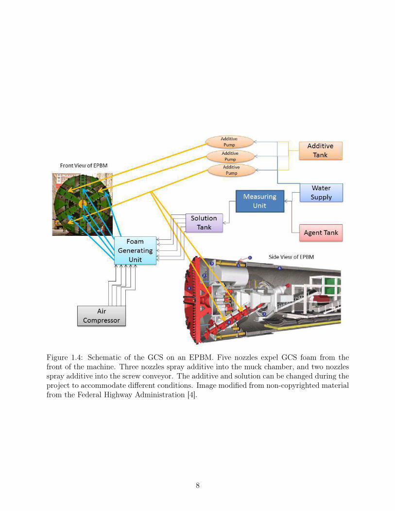
Figure 1.4: Schematic of the GCS on an EPBM. Five nozzles expel GCS foam from thefront of the machine. Three nozzles spray additive into the muck chamber, and two nozzlesspray additive into the screw conveyor. The additive and solution can be changed during theproject to accommodate different conditions. Image modified from non-copyrighted materialfrom the Federal Highway Administration [4].
8

1.3 Performance Prediction of EPBMs
Researchers use several approaches to predict a TBM’s production or advance rate. Al-
though our work focuses on advance rate prediction, we also examined production rate
research to gain a complete picture of the TBM performance prediction field. There are
three major categories of research that attempts to predict the production or advance rate
of TBMs. We discuss each of these three categories in the following three subsections:
1. Create a computer simulation or laboratory model of the TBM’s interactions with the
soil or rock.
2. Model the TBM’s performance by applying regressions to soil and rock properties
obtained from geotechnical reports.
3. Analyze soil and TBM data through machine learning techniques.
In the following three subsections, we review related research in both hard-rock and
soft-soil TBMs for these three categories.
1.3.1 Computer Model or Laboratory Simulation
Dubugnon and Barendsen attempted to simulate a hard-rock TBM without computer
simulation [5]. They hypothesized that some of the early simulations were too theoretical,
and thus real-world testing was needed in order to create an accurate assessment of the TBM’s
performance. The researchers created a small-scale model TBM and used laws of scaling to
extrapolate the predicted real-world machine values from observations in the small-scale test.
The model was then used to predict the performance of two tunnels dug in Austria.
TBM performance prediction studies often compute the error between the predicted ad-
vance rate or production rate of the model and the advance rate or production rate observed
by the TBM data monitoring system. In order to compare an average error value to other
studies, the Root Mean Squared Error (RMSE) is reported by Dubugnon and Barendsen
9

and several other TBM performance prediction studies. RMSE is defined as:
RMSE =
√√√√ 1
m
m∑j=1
(yj,observed − yj,predicted)2, (1.1)
where yj,predicted is the advance rate or production rate predicted by the model or simulation,
yj,observed is the advance rate or production rate observed by the TBM data monitoring
system, and m is the number of data points used to compute the RMSE. The RMSE of
Dubugnon and Barendsen’s model (when compared to the real data) was 0.733 metershour
for the
first analyzed tunnel and 0.675 metershour
for the second tunnel. The range of observed advance
rates were 1.3 metershour
- 3.7 metershour
for the first tunnel, and 3.8 metershour
- 5.2 metershour
for the second
tunnel. TBM data monitoring systems were not as prevalent in the early 1980’s and, thus,
the researchers were only able to measure the TBM at six points in the first tunnel and
four points in the second tunnel. A linear relationship between torque and advance rate was
identified in multiple hard-rock samples.
In another laboratory experiment conducted by Peila et al., the researchers created an
EPBM simulator that contained a soil tank simulating the pressurized muck chamber and
constructed a screw conveyor to extract soil from that pressurized chamber [6]. The Ground
Conditioning System (GCS) was simulated by mixing different amounts of GCS foam with
the test soil in a cement mixer. This system was intended to simulate the nozzles, which
are in the cutterhead face of the EPBM, that spray GCS foam into the soil as the soil is
excavated. One soil sample was completely saturated with water as a control test. The
torque exerted by the screw conveyor was measured with soil that was saturated versus soil
that was enhanced with GCS foam. When the screw conveyor removed the saturated soil,
significantly more torque was required by the screw conveyor than was required by the foam
conditioned soil. Since the advance rate of an EPBM partially depends on the speed that soil
can be removed from the muck chamber, this experiment indicates that the screw conveyor
torque, GCS foam, water content in the soil, and the type of soil can all have a direct impact
on the EPBM’s advance rate. Recently Peila and others have conducted more research with
10

this EPBM simulator [7], using several soil samples from a tunnel project in Italy. Peila
et al. determined soil conditioning parameters that will not only reduce the torque at the
screw conveyor, but also manage the conditioned soils’ pressure in the muck chamber. As
previously discussed, it is important for the bulkhead soil chamber to present a consistent
pressure to the face of the EPBM in order to balance the soil and water pressure at the
cutterhead face. The tests in [7] modified three independent variables2: the soil’s water
content, the Foam Injection Ratio (FIR), and the Foam Expansion Ratio (FER). The study
found that these independent variables have ideal points that decrease screw conveyor torque
and provide consistent pressure across the bulkhead soil chamber, but these ideal points are
different for different types of soil.
Maynar and Rodriguez modeled part of a subway extension project in Madrid, Spain,
using a Discrete-Element Method (DEM) [8]. In-situ tests were conducted to determine
the soil properties of borehole soil samples along the proposed tunnel alignment. The soil
properties were used to create a DEM model of the soil and the EPBM. The authors used
this model to analyze the thrust and torque necessary to maintain a desired advance rate and
determined factors that impact surface settlement when the machine is drilling and when
the machine is stopped. It was found that a high initial thrust and torque are necessary
after the construction of a ring is completed and the machine must be restarted. It was
also found that there is not a clear relationship between the type of soil or the depth of the
EPBM to the amount of torque necessary to maintain a particular advance rate. For reasons
previously discussed, the torque and thrust forces are not as dependent on the soil type in
soft soils as they are in hard-rock. The researchers stated that the DEM modeled the torque
and thrust of the EPBM satisfactorily, but did not provide results to substantiate this claim.
1.3.2 Soil and Rock Property Regression Models
Gong and Zhao investigated rock mass properties and TBM parameters during the con-
struction of two sewage tunnels in Singapore [9]. These tunnels were drilled with a hard-rock
2A description of common tunneling terms can be found in Appendix A.
11

TBM and the only rock type encountered was a granite formation. Parameters of this granite
formation such as rock brittleness, joint spacing, and joint orientation varied throughout the
project and had an impact on the advance rate of the TBM. The authors created a rock mass
model that consisted of: compressive strength of the rock material, rock brittleness, joint
spacing, and joint orientation. During periods when the TBM was stopped for maintenance,
rock conditions were measured and recorded. Parameters were obtained from sensors on the
TBM to determine the advance rate of the machine. Because the type of TBM can affect the
advance rate, the Specific Rock Mass Boreability Index (SRMBI) was chosen (rather than
the actual advance rate of the machine) to normalize these effects [10]. The rock mass model
was used to predict the SRMBI using a multivariate linear regression.
Gong and Zhao computed the R2 value between the advance rates predicted by their
model (X) and the observed advance rate (Y). Computing R2 is a common measure of
model performance and is used in several of the studies discussed herein. The R2 value
indicates the amount of variance from the mean of the data explained by the model, i.e.,
the mean squared error divided by the amount of variance in the original observations.
Equation 1.2 shows how the R2 value is computed:
R2 = 1−∑m
i=1 (yi − yi)2∑mi=1 (yi − y)2
, (1.2)
where m is the number of data points (i.e., examples), yi is observed output, yi is the model
predicted output, and y is the mean of all observations. The R2 value of Gong and Zhao’s
regression was 0.749. The study indicated that the rock’s Uniaxial Compressive Strength
(UCS) and joint count have the most effect on advance rate. This model did not consider
machine parameters, which are more important for a soft-soil TBM than a hard-rock TBM.
The use of the SRMBI as a prediction target instead of the advance rate of a hard-rock
TBM is common, although different authors have called the SRMBI by different names [11].
For example, Delisio et al. predicted the Field Penetration Index (FPI) of a hard-rock TBM,
such that the FPI uses the same units as the SRMBI: kNewtons/cuttermillimeters/revolution
. Delisio et al. also
12

modified the FPI equations in conditions where the TBM does not encounter a solid wall
of rock at the cutterhead face, called blocky conditions. In these conditions, each cutter
will not always maintain contact with the rock face due to gaps in the rock. Therefore the
FPI utilizes the total applied thrust force instead of the force at each cutterhead cutter:
FPIblocky = TotalThrust(kNewtons)millimeters/revolution
. Using FPIblocky for blocky conditions showed that, like
Gong and Zhao’s experiment, the UCS and joint count had a high correlation with the FPI,
but the joint count was correlated more with the FPI in blocky conditions. Delisio et al.,
ran a multi-linear regression with the same input parameters as Gong and Zhao, but used
FPIblocky as the target values; in this study, the regression returned an R2 value of 0.78.
In addition, the author conducted linear regressions comparing the thrust and cutterhead
RPMs to the advance rate of the TBM. These parameters returned R2 values of 0.35 and
0.13, respectively. An inverse correlation between the cutterhead face thrust and RPMs was
noted, but it is not a conclusive result due to the low reported R2 values.
Several other studies [12–15] have used the same approach as Gong and Zhao [10] and
Delisio et al. [11]. These studies focused primarily on utilizing different rock classification
systems to express the strength of the rock and the number and orientation of gaps in the
rock. Two rock classification systems are often referenced as comparison models. Specifically,
the Colorado School of Mines model (CSM) [16] and the Norwegian University of Science and
Technology model (NTNU) [17, 18] are the most commonly cited, and most researchers apply
a modification of these classification systems in their research. Both models use geotechnical
tests on the rocks along the path of the proposed tunnel and a few additional parameters that
describe the TBM’s characteristics (e.g., TBM cutterhead diameter). These systems are then
used to make predictions about torque, thrust, and advance rate of hard-rock TBMs. The
difference between the models is that the NTNU model uses specialized tests, whereas the
CSM model uses tests that are commonly available in standard geotechnical reports. It has
been shown that both models make similar predictions [19]; thus, the choice of either model
is a project contractor’s preference. After classifying the rock and TBM type, a regression is
13

calculated from the results of these rating systems to predict the advance rate index: SRMBI
or FPI. The computed regression model then becomes an equation for predicting the advance
rate of the TBM. The R2 values of these regressions are normally in the 0.70 to 0.80 range.
The regression modeling technique provides insight into the factors that affect the advance
rate of the machine, because the regression assigns a weight to each of the input parameters.
A larger weight identifies a correlation between a particular input parameter and the advance
rate, and also provides whether it is a positive or negative correlation. While this research
has been primarily focused on hard-rock TBMs, the basic methodology can be extended to
EPBMs.
Yagiz used a similar approach using core samples from a hard-rock TBM tunnel project
in New York [20]. Yagiz produced multi-linear regression equations, and also utilized forward
stepwise regression analysis. Forward stepwise regression analysis is a statistical and machine
learning technique for identifying input features that are relevant to predicting the output
target value. Yagiz used the results of the stepwise regression function to show which input
parameters had the greatest impact on predicting the production rate of the TBM. This
automated feature selection methodology was extended to EPBMs in our research, and
additional feature selection algorithms were added. See Section 1.5 for more details about
the Feature Selection Algorithms (FSAs) applied in our work.
1.3.3 Analyze Soil and TBM Data through Machine Learning Techniques
Analyzing TBM data with machine learning techniques is not as prevalent in the tunnel-
ing community as the prior two methods, but a few studies have attempted to apply multiple
machine learning algorithms to the TBM performance prediction problem. A. Benardos con-
ducted two studies (with assistance from D. Kaliampakos in the first study) that applied an
Artificial Neural Network (ANN) to predict the advance rate of TBM projects [21, 22]. The
first study analyzed two tunnels in the Italian Alps (both were hard-rock projects), and the
second study, in Athens, Greece, analyzed a tunnel with both hard-rock and soft-soil; we
note, however that a hard-rock TBM was used for the second project (not an EPBM). The
14

authors assumed that TBM operating parameters have minimal effects on the advance rate
of a hard-rock TBM; thus, the authors only used geotechnical parameters as inputs to the
ANN. In the Athens, Greece project, the input parameters were normalized in an unconven-
tional method, which is shown in Equation 1.3. In Equation 1.3, E[X] is the expected value
of the nominal input feature X.
E[X] =x∑i=1
Pi · Vi, (1.3)
where x is the number of possible values of X, Pi is the probability of observing the ith value
of the possible values of the input feature X (∑n
i=1 Pi = 1), and Vi is the value of x. We note
that the authors chose to bin each continuous input feature into four discrete bins, which
caused data loss. Unfortunately, the probability distribution of Pi is not defined in [22].
Although Pi appears to be an attempt at normalization, some of the input parameters have
values that are much larger than the other parameters, and Equation 1.3 does not account for
the difference in magnitudes of the input parameters. In addition, Pi may induce additional
biases to the input data; however, these biases are difficult to determine since the probability
distribution is unknown. The output prediction rate was averaged over the segment in metersday
,
and the error rate was biased by heavily averaging the data. More information about ANNs
and back-propagation algorithms can be found in Appendix B.
In the first study, the authors presented RMSE values that were labeled as training data
results, and they presented R2 values that were not labeled as testing or training data results.
Without R2 results from the testing data set, it is impossible to determine the accuracy of
the first study’s results. In the second study, the RMSE of three testing segments are
presented, and the average RMSE of these three segments was 0.0713 metersday
. Even though
testing, training, and validation data was used to build and test the models, heavy averaging,
attribute binning, and the application of an unknown probability distribution may have
caused an artificially low RMSE.
15

Other researchers have conducted a similar application of ANNs to geotechnical data to
predict the advance rate of hard-rock TBMs. Javad and Narges [23] applied ANNs in a
nearly identical method to [21] and [22], except fewer input parameters were utilized and
Equation 1.3 was not applied to the data before applying an ANN model. Javad and Narges
found a model with an R2 value of 0.939, but it appears that the R2 value was computed
on a linear curve fitted to their predicted vs. observed values chart, rather than applying
Equation 1.2.
Another interesting application of ANNs to production rate prediction was taken by Lau
et al. [24]. Lau et al. combined probability theory with a Radial Basis Function (RBF)
ANN. While related, we note the tunneling project examined in this study was a drill and
blast project rather than a TBM project. Also, all sources of delay were considered, not
just when excavation was occurring; in other words, the model predicted production rate
rather than advance rate. Lau et al. first applied k-means clustering to the input data, then
created a Gaussian distribution of each of these clusters. Equation 1.4 shows the Gaussian
distribution using the Euclidean Square Distance from the mean of the cluster and a weight
obtained from the RBF ANN, where f(x) is the predicted production rate for the given
tunnel cycle3:
f(x) =M∑j=1
wj exp(‖ x− uj ‖2
−2v2j), (1.4)
where M is the number of clusters created by k-means, wj are the weights of each cluster
from the RBF ANN, x is the vector of input values, uj is the center of the cluster j, and
vj is the standard deviation of the examples within the jth cluster. Applying a Gaussian
distribution to the input values allows for uncertainty in human controlled processes, such as
setting blast charges and building the tunnel framework after blasting. To apply this method,
the researchers used the previously completed tunnel cycle to predict the next tunnel cycle’s
production rate. The Root Mean Squared Error (RMSE) over 56 tunnel cycles was calculated
3A tunnel cycle is defined as 12 hours in Lau et al.’s research.
16

as 0.61metersday
. RMSE is defined in Equation 1.1, where yj is the output value (production rate
in Lau et al.’s work) for each observation j and n is the number of observations calculated
in the RMSE value.
Although 0.61 metersday
is a good RMSE value (when compared to other studies), the re-
searchers were only able to predict the advance rate for the next tunnel cycle, and the model
missed some of the larger changes in production rate that may be of most interest to a
project manager. Also, the 0.61metersday
RMSE was only achieved at the last tunnel cycle; the
RMSE ranged from a high of approximately 1.1metersday
at the 13th tunnel cycle to 0.61metersday
at the last cycle. It is also important to note that drill and blast project production rates
are significantly slower than TBM projects. The range of production rates for this project
was only 1.20metersday
- 7.50metersday
. Although Lau et al.’s RBF ANN model has a good RMSE,
the best RMSE was only achieved after using the entire data set. It is also likely that Lau et
al.’s model is overfitted to the training data, because the results are based only on training
data.
Zhao et al. extended the ANN approach by leveraging an ensemble of Feed Forward
Back Propagation (FFBP) Aritficial Neural Networks (ANNs) to predict cutter wear and
advance rate performance in hard-rock TBMs [25]. The input parameters to the ANN were
geotechnical characteristics of the rock (e.g., Uniaxial Compressive Strength (UCS) and
joint spacing). Ensemble methods are techniques to create multiple input data sets from
one training data set (see Section 1.5.3). These ensemble instances can then be used to
train multiple machine learning algorithms, and the results of each of these algorithms is
combined through voting methods. Zhao et al.’s work applied the FFBP ANN algorithm
to ensemble methods. Specifically, this study used a method called bootstrapping, where
N input data records are randomly sampled from the training data to create the ensemble
instances and an input record can be used across multiple ensemble instances (repetition
allowed). This work extended traditional bootstrapping by also creating a set of FFBP
ANNs, with varying hidden layer configurations, for each ensemble instance. In classification
17

problems, each bootstrapped FFBP ANN instance contributes a vote and these votes are
tallied; the output class with the most votes then becomes the predicted output. Because
advance rate prediction is a regression problem, Zhao et al. averaged each predicted advance
rate from the hidden layer configuration that produced the lowest RMSE across all ensemble
instances. (It is unclear which hidden layer FFBP ANNs were chosen when the ensemble
network was trained.) Zhao et al. predicted the Specific Rock Mass Boreability Index
(SRMBI) rather than the advance rate, because it normalized the effects of hard-rock TBMs
of different cutterhead sizes and from different manufacturers. The R2 value for the model,
comparing the predicted SRMBI to the observed SRMBI, was 0.75 for non-linear regression
and 0.81 for the best ensemble model.
We note the R2 value did not increase much for the ensemble method when compared
to standard non-linear regression, which may be caused by the bootstrap ensemble method
used by Zhao et al. Boosting is another ensemble method that could have been used instead
of bootstrapping [26], and it may have provided better results. To explain boosting, we use
the FFBP ANN algorithm; however, we note that any machine leaning algorithm could be
substituted for FFBP ANN. The first boosted FFBP ANN instance is created by applying
the bootstrap method (i.e., a random subset of the input data records are selected and used to
train the initial FFBP ANN instance). The initial training instance is then assigned a weight.
The assigned weight is the RMSE, which means that higher weights are assigned to instances
with high error rates. A high error rate increases the probability that a training instance will
be selected when boosting creates the next ensemble instance. By making it more probable
that misclassified training instances (i.e., high error rate instances in regression problems) are
selected for constructing the next ensemble instance, boosting focuses on creating ensemble
instances that are trained on the training examples that are difficult to predict. Additional
FFBP ANNs are trained via boosting until the RMSE of a validation data set is below a
threshold or a user-defined number of FFBP ANNs are created.
18

Ensemble methods are usually applied to classification problems rather than regression
problems. As previously discussed, in order to combine the results of an ensemble of FFBP
ANNs, a majority rules voting scheme is used to select the output class; alas, this voting
scheme is not possible in a regression problem, because the output of each ensemble instance
is a continuous value rather than a class value. Zhao et al. averages the regression output
of the FFBP ANNs to determine the output advance rate of the TBM; however, since input
instances used in each ensemble instance were selected randomly, the average could have
been potentially biased by interspersing difficult training instances, which skews the average
for easier training instances.
Grima et al. presents research that utilized the University of Texas, Austin’s database
of over 640 hard-rock TBM projects to predict the advance rates of these projects through
neuro-fuzzy methods [27]. A similar, comprehensive data set has not yet been compiled for
EPBM projects. Most research on EPBMs rely on laboratory tests or a few tunneling projects
where the researchers have been able to obtain access to the contractor’s data collection
system. The parameters selected as inputs to the model in [27] were: two parameters based
on rock strength, three parameters based on the type of TBM, the maximum cutterhead
torque, and cutterhead RPMs. Grima et al. picked these parameters based on previous
studies of rock classification systems, which are discussed in Section 1.3.2. The number of
input parameters was then reduced with the Principle Component Analysis (PCA) method,
which created three new inputs from the original seven. Each of these three new inputs was
a weighted sum of the original seven inputs, where the weights were generated by PCA. Ten
sets of testing data (of unknown size) were used to ensure the model was not overfitted.
The RMSE of these testing data sets was also compared to the RMSE of the training data
to ensure there was not a large increase from the RMSE of the training data to the RMSE
of the test data. (A large increase in the RMSE of the test data would indicate a model
overfitted to the training data.) The RMSE of the training data was 0.888 metershour
, and the
RMSE of the testing data was 0.900 metershour
. The testing data consisted of 20% of the 640
19

TBM projects, and one advance rate value was calculated for each of these projects. These
results were combined to find the overall RMSE (see Equation 1.1).
Recently, Mahdevari et al. applied Regression Support Vector Machines to the hard-
rock TBM prediction problem in the same manner (and with the same weaknesses) as prior
hard-rock TBM prediction studies [28]. Mahdevari et al. applied a Regression Support
Vector Machine to data from the Queens Water Tunnel Number 3 in Queens, NY. The
researchers selected features based on a combination of the properties of the hard-rock and
TBM machine parameters, for a total of nine input features. Instead of using the entire data
set, as we do in our work, Mahdevari et al. used 150 measurements from the tunnel. Ten
fold cross validation was implemented, but the Support Vector Machine parameters were
selected without using a separate validation set, which may have caused overfitting. The
Regression Support Vector Machine seemed to return a low error4: a mean squared error
(MSE) of 0.0013, an RMSE of 0.0361, and R2 = 0.9903 in one of the cross validation folds;
however, the authors admit that they do not know how the features impact the penetration
rate, the algorithms may be overfitted, and the results are based on a very small sample size.
Since little research on the prediction of advance or production rates in EPBMs could be
found, the research results from hard-rock TBM and Drill and Blast projects are our best
comparison points when analyzing the RMSE of new EPBM advance rate models. Table 1.1
compares the R2 values and the RMSE values for the various performance prediction studies
discussed in Sections 1.3.2 and 1.3.3. The range of observed production or advance rates
for each TBM project is listed in the “Range of Values” column. If data was not available
in the article, the range of values was estimated based on figures and tables within each
article. Several authors predicted values other than the production rate, penetration rate,
or advance rate of the machine, but the methodology is other performance studies and,
therefore, valuable to our discussion of previous work conducted in the field.
4The penetration rate was normalized (0,1); therefore, MSE and RMSE have no units.
20

Table 1.1: Comparison of R2 and RMSE values among TBM performance prediction studies.Only studies that included valid R2 or RMSE values are included in the table. If multiple R2
or RMSE values were reported, the best value is shown in the table. We note that the 0.94R2 value from Javad and Narges’s work appears to be computed incorrectly (a line fitted tothe data points rather than the line y = x+ 0).
Author(s) Output Predicted R2 Testing Data RMSE Testing Data Range of ValuesGong and Zhao SRMBI 0.749 not recorded 108 to 211Delisio et al. FPI 0.78 not recorded 750 to 4600Yagiz advance rate 0.82 3.218 m
h 1.4 mh to 2.93 m
h
A. Benardos advance rate Not recorded 0.0713 mday 4.54 m
day to 16.67 mday
Javad and Narges advance rate 0.939 0.329 mh 1.38 m
h to 10.30 mh
Lau et al. production rate Not recorded 0.61 mday 1.20 m
day to 7.50 mday
Z. Zhao et al. SRMBI 0.81 11.290 110 to 240A. M. Grima et al. advance rate Not recorded 0.900 m
h 0.5 mh to 7.6 m
h
Mahdevari et al. penetration rate 0.9903 0.0361 0 to 1 (normalized)
1.4 Seattle Project Case Study Description
We studied two light rail tunnels excavated and constructed with a Hitachi-Zosen EPBM
with a 6.44 meter diameter cutterface in Seattle, WA, USA, as part of the University Link
subway extension project. The entire University Link subway extension project included two
stations (the University of Washington station and the Capital Hill station), two parallel
subway tunnels that connect the stations, two parallel subway tunnels that connect the
Capitol Hill Station to the Pine Street Stub Tunnel (PSST), and various cross-passages and
supporting structures for these tunnels. The subway stations were constructed using cut
and cover methods, while the length of the parallel twin tunnels was excavated by launching
closed-shield, EPBMs from the subway stations.
The full project was divided into five contracts and our work uses data from one of these
five contracts: the U230 contract. The U230 contract constructed the 3,000 foot, parallel
tunnels that connected the Capital Hill Station to the PSST, and the contract included
excavating at shallow depth beneath Interstate 5 (I-5), a major roadway in Seattle. We
hereafter refer to the U230 contract as the Seattle Project for brevity.
21

1.4.1 Geology Description
A subsurface exploratory project drilled boreholes to explore the subsurface conditions
in the area of the Seattle project. Adams et al. described the geology at the Seattle project
area as, “...[laying] near the southern end of the Seattle basin, a depression in the volcanic
bedrock that is filled with middle to late Tertiary (36 to 2 million years before present)
sedimentary and volcanic rock, and Quaternary (last 2 million years) sediments [29].” In
addition, Adam et al. described the geology predicted along the tunnel alignment,
“In general, the ground conditions along the alignment consist of glacially consol-
idated pre-Vashon deposits consisting of hard cohesive clay and silt, very dense
cohesionless silt and fine sand, very dense glacial till and till-like deposits, and
very dense cohesionless sand and gravel. The glacial till and till-like deposits
consist of a heterogeneous mixture of clay, silt, sand, gravel, cobble and boul-
ders. The predominant soil type within the tunnel is expected to consist of hard
cohesive silt and clay and very dense cohesionless silt and silty sand. Boulders
may be present in all of these glacial deposits [29].”
Figure 1.5 shows the Geotechnical Baseline Report (GBR) soil map for the tunnel align-
ment of the Seattle project. We note that the EPBM excavated through a variety of glacial
soil types and mixed face soil conditions. We also note the subsurface I-5 crossing on the
left side of the GBR soil map, where jet grouting and extra pre-cautions reduced the ad-
vance rate to ensure the stability of I-5. The twin, parallel tunnels were named Northbound
(NB) and Southbound (SB) (in accordance with the direction the light rail trains travel in
the completed tunnels); however, both the NB and SB tunnels were excavated in the same
direction (from right to left in Figure 1.5) to take advantage of a downward slope.
1.4.2 Data Preparation
The raw data from the Seattle Project contains over two million examples, per tunnel,
and over 700 input features (i.e., input sensor readings). We created the advance rate output
22

Figure 1.5: GBR soil diagram of predicted soil types along the Seattle project tunnel align-ment (the Capital Hill Station is on the right side of the map and the PSST is on the leftside of the map; I-5 is annotated near the PSST). The tunnel path is marked by three blacklines running from the right to the left side of the map; the top line is the top of the tunnel,the bottom line is the bottom of the tunnel, and the center line is the position of the subwaytrack.
target value using the equation: Arate =Average Jack Stroke(t)−Average Jack Stroke(t−1)
(t)−(t−1) . The average
jack stroke is the average position of the 16 hydraulic jacks that push the cutterhead face of
the EPBM into the soil. The variables (t) and (t − 1) represent the time that the current
example (t) and the example at the previous recorded time step (t− 1) were measured.
We then removed all examples when the EPBM was not excavating or when the jack
strokes were retracted for tunnel lining construction. Removing these examples resulted in
199,193 examples in the NB tunnel and 228,788 examples in the SB tunnel.
In our initial work (see Chapter 2), several of the FSAs identified features that correlated
with advance rate, but were a result of changes in the advance rate (e.g., belt scale weight
and grout expelled). Because we want to determine features that affect the advance rate
(i.e., input features that do not change as a result of advance rate changes), we consulted
with experts on the EPBM’s features to remove features that all parties agreed were caused
by changes in the advance rate. After removing these features from the initial set of 756
features, the data sets contained 537 features, including the advance rate.
The resulting features were a mixture of binary and numeric features. The binary features
represented “on” and “off” switches or indicator lights (e.g., a methane gas warning light) in
the EPBM. These were recorded as “1” and “0” in the data sets, representing “on” and “off”
23

states, respectively. We then visualized the data by plotting histograms of each of the 537
attributes, which provided an approximation of the feature distributions and we discovered
the impact the outliers had on the data sets. Because there were several extreme outliers
in the data, Figure 1.6 and Figure 1.7 each contained one very large “spike” of data points
instead of a normal data distribution. By removing the outliers the advance rate followed
a distribution much closer to a normal data distribution. In the NB tunnel we remove 188
outliers (resulting in 199,005 examples remaining), and in the SB tunnel we remove 144
outliers (resulting in 228,644 examples remaining).
In Chapter 3 and Chapter 4, our visualizations revealed that most of the numeric input
attributes did not follow a normal distribution (i.e., many of the measurements were clustered
in a small area within the range of possible values for the input attribute); therefore, we
standardized the input attributes so that all values would have a mean of zero and unit
variance. In other words, standardizing the input features “spreads” the measurements closer
to a normal distribution, making it easier for the FSAs and MLAs to find a model that
accurately predicts the output target value. In addition, we found that the EPBM’s advance
rate contained several severe outlier values. Figure 1.6 and Figure 1.7 shows histograms of the
advance rates (before and after removing negative and outlier values) in the Seattle project
NB tunnel and SB tunnel, respectively.
In order to identify advance rate outliers, we used the Interquartile Range (IQR) outlier
identification method. The median advance rate example (i.e., the Quartile 2 dividing line)
was determined before the negative advance rate examples were removed. We then removed
all examples where the advance rate exceeded 10 times the Quartile 3 value; the Quartile
3 value was computed as the median advance rate value between the Quartile 2 value and
the maximum observed advance rate. The threshold of 10 times the Quartile 3 value was
chosen to eliminate the very high advance rate readings that occurred when the EPBM was
not moving; however, realistic high advance rates when the EPBM is moving are retained.
Figure 1.6(b) and Figure 1.7(b) show the histograms after removing the outlier advance rate
24

Histogram of Advance Rate in the NB Tunnel Before Outlier Removal
Advance Rate (mm/sec)
log1
0(F
requ
ency
)
−400 −200 0 200 400
01
23
45
(a) NB advance rate histogram before outlier removal.The x axis range indicates that there are outlier advancerate values up to 376.75 mm
sec . We note that the scale ofthe y-axis is log10.
Histogram of Advance Rates in the NB Tunnel After Outlier Removal
Advance Rate (mm/sec)
Fre
quen
cy
0.0 0.5 1.0 1.5 2.0
050
0010
000
1500
020
000
(b) NB advance rate histogram after outlier removal. TheEPBM’s advance rate values for the NB tunnel are nowcontained within a more realistic range of up to 1.8 mm
sec .
Figure 1.6: NB advance rate histogram before and after outlier removal.
25

Histogram of Advance Rate in the SB Tunnel Before Outlier Removal
Advance Rate (mm/sec)
log1
0(F
requ
ency
)
−20 −10 0 10 20 30 40
01
23
45
(a) SB advance rate histogram before outlier removal.The range of advance rate values in the SB tunnel wasnot as severe as the NB tunnel; however, both negativeadvance rates and outlier advance rates up to 33.6 mm
secexisted in the SB tunnel. We note that the scale of they-axis is log10.
Histogram of Advance Rates in the SB Tunnel After Outlier Removal
Advance Rate (mm/sec)
Fre
quen
cy
0.0 0.2 0.4 0.6 0.8 1.0 1.2 1.4
050
0010
000
1500
020
000
2500
030
000
(b) SB advance rate histogram after outlier removal.The EPBM’s advance rate values for the SB tunnel arenow contained within a more realistic range of up to 1.4mmsec .
Figure 1.7: SB advance rate histogram before and after outlier removal.
26

values.
We further examined the NB tunnel raw data to better understand the severe outlier
values. We found that all of the severe outlier values occurred during the excavation of
concrete tunnel Ring #23. We then looked at data for the “Net Stroke (mm)” sensor, which
measured the average number of millimeters that the propulsion jacks had expanded in the
current tunnel ring under excavation. In Ring #23, the “Net Stroke (mm)” values oscillate
back and forth between 0 and 1507; however, the individual jack strokes do not move. We,
therefore, conclude that the “Net Stroke (mm)” oscillation in Ring #23 is a sensor error,
validating our removal of these outlier values.
Figure 1.7(a) shows the histogram of advance rates in the SB tunnel with the y-axis
adjusted to a logarithmic scale. As with the NB tunnel, several negative advance rate
measurements exist and, thus, we investigated these measurements in the raw data. We,
again, found that during the excavation of one concrete tunnel ring (#162) the advance rate
exhibited the same oscillating behavior between measurements in the “Net Stroke (mm)”
input feature; however, the oscillation in the SB tunnel was only 1mm (between 1529 and
1530). Because, the range of oscillation was smaller in the SB tunnel, the outlier values in
the SB tunnel were not as extreme as in the NB tunnel. The IQR outlier removal procedure
accounts for differing magnitudes of outliers; we, thus, applied the IQR outlier procedure to
both tunnels to remove the outliers and maintain consistency.
In summary, the following preprocessing steps were applied to both the NB and SB
Seattle project data sets:
1. removal of outliers using the IQR outlier removal method,
2. removal of examples with advance rates less than or equal to zero,
3. standardization of numeric input features to a mean of zero and unit variance, and
4. removal of input features with very small variances, i.e., “useless features”.
27

We note that we applied the IQR outlier method before removing examples with an advance
rate less than or equal to zero, because of the oscillating behavior in the negative values
discussed earlier. We included the negative values so that the extreme oscillation outliers
would be removed.
The results from our experiments are more accurate than other TBM performance studies,
because we use the entire data set without any averaging. Many studies average the advance
rate over a tunnel ring, an entire day of tunneling, or some other defined section of the tunnel,
which provides unrealistically optimistic error rates. Even with other authors’ unrealistically
optimistic error rates, our feature stabilization work is able to predict advance rates with a
lower error than most previous advance rate studies. Furthermore, our work provides a more
precise model of the EPBM than studies with less error and heavily averaged TBM advance
rates.
After pre-processing the Seattle project data sets, we utilized five-fold cross validation
to prove that the accuracy of our work statistically improves upon state-of-the-art feature
stability methods. Cross validation is a method of dividing the data set into testing and
training data where no examples used to train an algorithm are used to test the algorithm;
thus, we avoid one source of overfitting in MLA and FSA algorithms. In five-fold cross
validation, 80% of the data is selected as the training data and 20% of the data is selected
as the testing data. The selection process is repeated a total of five times, such that each
example is used as a testing example in exactly one of the folds. As a reminder, a description
of common machine learning and tunneling terms can be found in Appendix A. We now
describe how FSAs use the pre-processed data to select the input features most important
in predicting the output target value.
1.5 Feature Selection Algorithms (FSAs)
EPBM data collection systems present a machine learning challenge, often referred to as
the “Curse of Dimensionality [30].” The “Curse of Dimensionality” occurs when a machine
learning algorithm trains on a large number of input features. Machine learning researchers
28

generally attempt to record as many input features as possible to better understand their
prediction domain, but too many inputs can cause the machine learning algorithm to focus
on input attributes that are not relevant in predicting the output target value. Definitions
vary on the number of input attributes required before the number of input attributes has
reached the “Curse of Dimensionality,” but the literature discussed previously shows that
researchers believe hard-rock TBMs have the “Curse of Dimensionality”; these researchers,
therefore, attempt to select important input attributes through literature search and prior
knowledge. Methods used to select a subset of important input attributes from the set of all
input attributes are referred to as Feature Selection Algorithms (FSAs) in machine learning
terminology. Many automated FSAs exist and we research these FSAs to determine the
input features that are significant in the prediction of an EPBM’s advance rate.
A common theorem in data mining and machine learning is called the “No Free Lunch
Theorem,” which states that there is no single algorithm that will provide the most relevant
set of features to all machine learning problems. Because there is no single best Feature
Selection Algorithm (FSA), research has focused on finding the best FSAs for individual
ML problems. The purpose of an FSA is to determine which input features are relevant,
but first the concept of relevance must be defined. Blum and Langley’s seminal paper [31]
on applications of FSAs presents multiple definitions of relevance and these definitions have
been used throughout FSA literature [32, 33]. We define relevance next; other definitions of
common ML terminology used in this work can be found in Appendix A.
• Strong Relevance: A feature xi is strongly relevant if there exists a pair of examples A
and B where changing only the value of feature xi will change the output target class
(c(·)) value such that c(A) 6= c(B).
• Weak Relevance: A feature xi is weakly relevant if xi is not relevant, but it is possible
to create a subset X ′ (X ′ ⊂ X|xi ∈ X ′) such that X ′ is strongly relevant. X ′ contains
one or more features, xj, (xj ∈ X), and xi.
29

• Incremental Usefulness: Given a feature set X, a feature xi is incrementally useful if
{xi} ∪X increases the prediction accuracy of the ML algorithm.
• Relevance as a Complexity Measure: the smallest number of relevant features to an
output target class c from sample S is defined as r(S, c).
These definitions of relevance provide a framework for creating FSAs, which are a com-
putational approach to identifying relevant features [33]. We note, however, that these defi-
nitions are often loosely applied in the design of FSAs. For example, when designing FSAs
for regression ML problems (as opposed to classification), the strict definition of strong rel-
evance, weak relevance, and relevance as a complexity measure cannot be used, because
each relies on differentiating features by the output target class; in other words, a regression
problem’s output target is a continuous value.
Blum and Langley also describe four properties that all FSAs must define in [31]. These
properties are:
1. Starting Point: Define which features are included in the beginning feature set. For
example, forward feature selection starts with no features (X ′ = {∅}) and backwards
feature selection starts with the entire feature set (X ′ = {X}).
2. Search Organization: Define which combinations of individual features X ′|X ′ ⊂ X
and xi ∈ X ′ will be evaluated by the FSA. An exhaustive search will evaluate 2n
combinations of X, where X ∈ Rn. An exhaustive search is often computationally
infeasible; thus, other approaches such as stepwise selection are used to incrementally
add and remove features at each step, which avoids searching all possible X ′ subsets.
3. Subset Evaluation Function: Define an algorithm that evaluates the relevance of the
subset X ′ to the output target. These algorithms can be equations from information
theory, such as entropy, or a measure of accuracy like RMSE.
30
4. Halting Criteria: Define when the search for the optimal X ′ subset will stop. The
experimenter can stop once a pre-defined number of features is reached, stop when
the subset evaluation function no longer improves, or stop when the end of the search
space is reached.
FSAs can be divided into three categories: filters, wrappers, and embedded FSAs. Filer
and wrapper FSAs differ in their subset evaluation function. Wrappers use an ML algorithm
(usually the ML algorithm that will be trained with the testing data) as the subset evalu-
ation function. Filters create subset evaluation functions that measure relevance using the
definitions of relevance previously discussed, independent of an ML algorithm. Embedded
algorithms integrate FSAs into the ML algorithm. Some examples of embedded algorithms
are decision trees, which use information theory to determine which features to prune after
the decision tree has been created. Feed-Forward, Back-Propagation, Artificial Neural Net-
works (FFBP ANNs) are also embedded FSAs that select relevant features by penalizing the
synaptic weights of features that contribute the most to the error in predicting the output
target. We do not use embedded methods in our work, because embedded FSAs are targeted
at classification problems and we have chosen to apply FSAs to regression problems. Thus,
only filter and wrapper FSAs are discussed in the following sections.
Molina et al. [33] reviewed Bloom and Langley’s work in [31], but also analyzed 42 FSAs
to determine how well each detected relevant, irrelevant, and redundant features using syn-
thetic data and a scoring metric. As discussed previously, FSAs require a subset evaluation
function to differentiate the performance of subsets of selected features; Molina et al. outlines
several evaluation functions and each evaluation function is related to one of the measures
of relevance discussed previously. The authors then take the properties of an FSA and ar-
range the properties in 3-d space, with each application of an FSA being a point within
this space. The three dimensions in this space are: subset evaluation function, search or-
ganization, and next subset generation. Starting and ending criteria are not listed in the
3-d space, which implies that these criteria are defined in the search organization and next
31

subset generation dimensions. A scoring system was created to determine if the algorithm
left out redundant and irrelevant features while selecting relevant features. Weights were
assigned to these properties, because it was considered less harmful if the algorithm selected
irrelevant features rather than missing a relevant feature. Choosing a redundant feature was
also considered less harmful than choosing an irrelevant feature. (Guyon and Elisseef showed
that redundant variables can actually be helpful in reducing noise in data [34].) Of the 42
FSAs analyzed, Molina et al. concluded that ReliefF performed best when differentiating
relevant and irrelevant features, while the Las Vegas Filtering (LVF) algorithm performed
best at detecting redundant features.
Another, more recent, review of FSAs is Saeys et al.’s review of applying FSAs to bioin-
formatics [35]. Much of Saeys et al.’s review is similar to other FSA review articles, but the
authors sub-categorize the three categories of FSAs discussed previously. Filter FSAs are
sub-categorized into univariate or multivariate FSAs. Multivariate, filter FSAs were created
to find dependencies among features instead of only considering each feature’s relation to
the target variable. In terms of relevance, multivariate FSAs identify strongly and weakly
related features whereas univariate FSAs can only identify strongly related features. Wrap-
per FSAs are sub-categorized into deterministic and randomized FSAs, based on the feature
space search method. A deterministic, wrapper FSA will search the feature space in a pre-
determined order, while a random, wrapper FSA will randomly create subsets of features.
The randomly created subsets of features may be randomly generated at each iteration, or
a genetic algorithm can be used to evolve the random subsets that perform the best. The
feature selection methods listed in this work are the same methods listed in other review
papers. These review papers also discuss the evaluation of FSAs. Researchers will often
apply an FSA to an entire data set and then evaluate the FSA’s performance with the same
data set. Saeys et al. [35], however, suggest using a training and test set when applying an
FSA, such that the test set is used for evaluating the performance of the FSA. If the set of
examples is too small, researchers can apply ensemble techniques to create more example
32

sets for training the FSAs.
1.5.1 Filter FSAs
The choice between filter FSAs and wrapper FSAs is somewhat controversial. Kohavi and
John argue that a major disadvantage of using a filter FSA instead of a wrapper FSA is that
the filter FSA completely ignores the ML algorithm the researcher is trying to optimize [32].
On the other hand, there may be problem instances where filter algorithms will perform
as well or better than wrapper algorithms [34]. The filter algorithm is computationally
efficient, because it does not need to run an ML algorithm for each candidate subset X ′.
Filter algorithms can introduce bias, but are less prone to overfitting the training data.
Guyon and Elisseeff present a review of FSAs that balances coverage of filter and wrapper
FSAs [34]. Because our research is a supervised, regression ML problem, we focus on super-
vised, regression methods for feature selection. Guyon and Elisseeff present 10 steps that
are intended as guidelines to the application of ML algorithms to prediction problems. Step
5 of this procedure specifically refers to the decision of whether or not to use a filter FSA.
The answer is unequivocally “yes,” regardless of your end prediction goals. If the researcher’s
prediction goals are only to assess the impact of the features on the output target, and not
build a predictor, the filter FSA will provide these results. If the research also needs to build
a predictor, the filter FSA will provide baseline results to assist in determining if the final
selected features are overfitted.
Guyon and Elisseeff examined a category of filter FSAs called variable ranking. The
authors defined a data set as {xk,i, yk}(k = 1, . . . ,m), (i = 1, . . . , n), where xk,i is the value
of an example k for the input feature i, yk is the output target value for example k, m is
the number of training examples, and n is the number of input features. Variable ranking
uses a scoring function, S(i), that creates a score for each input feature (i), using xi and
y, where xi is a column vector containing all m training examples for each input feature i,
and y is a column vector containing the output value of each example. A commonly used
scoring function is Pearson’s Correlation Coefficient (or the R2 value) of each input feature.
33

Pearson’s correlation coefficient is defined by Equation 1.5. Pearson’s Correlation Coefficient
of each input feature identifies the estimated fraction of total variance around the mean of Y
that is explained by the linear relation between the input feature Xi and the output target
Y .
R2 = (cov(Xi,Y)√var(Xi)var(Y)
)2 (1.5)
Note that the capital X and Y vectors represent the entire population of potential observa-
tions (which is infinite), but we are taking samples of the random variables X and Y in an
ML problem (represented by the lowercase x and y variables). Equation 1.6 shows how to
estimate theR2 value based on these samples (or examples in machine learning terminology).
R2i = (
∑mk=1(xk,i − xi)(yk − y)√∑m
k=1(xk,i − xi)2∑m
k=1(yk − y)2)2, (1.6)
where xi represents the mean input feature value for feature i across the m examples, and
y represents the mean output target value across the m examples. In order to determine
non-linear relationships between the input features and the output target, attributes can be
fitted to the target using a non-linear function, or the attributes can be pre-processed with
a non-linear function and then a correlation coefficient is calculated for the non-linear fit.
These methods increase the risk of overfitting to the training data and, thus, the selected
variables may not generalize well to a test data set.
Estimating the R2 value of each input feature allows for an exhaustive search of the
feature space in O(n) time, but the features are only ranked and there is no mechanism
that specifies a stopping point for the number of features selected. A common method for
determining the number of features to select from the ranked list of input features is to
retain a testing set of data and then see how well different numbers of features performs
with an MLA [31]; however, this method partially transforms a filter FSA into a wrapper
FSA. Stoppiglia et al., [36] suggests an alternative method for ranking features, while also
automatically determining a stopping point. Specifically, the algorithm first determines the
input feature that most explains the output target by determining the magnitude of the
34

angle between the input feature’s vector and the output feature’s vector in Rn space (where
n is the number of input features). The cos2 of the angle between the vector of each input
feature and the target vector is computed using Equation 1.7:
cos2(xi,y) =(xi · y)2
‖xi‖2‖y‖2, (1.7)
where (i = 1, . . . , n) and n in the number of input features. The input feature with the
greatest result from Equation 1.7 is the selected feature. To remove the effects of the se-
lected feature, the remaining input features are projected onto the subspace of the selected
feature using the Gram-Schmidt algorithm [37]. In order to determine the stopping point, a
random variable, called a probe variable, is used. The random variable is not instantiated,
but the cumulative distribution function of the angle between the random variable and the
target output is computed, where the distribution of the random variable is assumed to
be normal. From the cumulative distribution function of the random probe, the chance of
an instantiation of the random probe having more relevance to the output target than the
selected feature can be found. (This chance is called the risk by Stoppiglia et al. [36].) The
researcher then defines a threshold for the amount of risk he or she is willing to accept, and
if the calculated risk is greater than this threshold, the selected variable is discarded and
the FSA stops. This process seems to be a precise method for determining when to stop a
regression, filter FSA.
We note, however, that Bi et al. were also successful with a stopping criteria that uses
three instantiations of the random variable instead of the cumulative probability distribution
function [38]. The three random variables, i.e., input features, were generated from a normal
distribution with a mean of zero and a standard deviation of one. Bi et al. stated that
any distribution could replace the normal distribution. We also note that Bi et al. used
a random probe variable as an additional measure to exclude non-relevant features; the
primary method was to use a sparse norm regularized Support Vector Machine (SVM) with
a linear kernel.
35

Another type of filter FSAs is the Relief algorithm originally created by Kira and Ren-
dell [39]; instead, many researchers use the modified algorithm (ReliefF) created by Kononenko
[40]. Since Relief and ReliefF are only valid for classification problems, Robnik-Sikonja and
Kononenko extended ReliefF into an algorithm (RReliefF) that can also rank input features
in regression problems, where the input features and output target is a continuous value [41].
All Relief algorithms are based on randomly selecting an example (R) from the training
data set and then examining the nearest neighbors to that example. Relief examines the
nearest neighbor that is misclassified (MISS) and the nearest neighbor that is correctly
classified (HIT ). The distance between each of R’s input features and each of the MISS
and HIT ’s input features is then calculated. Each input feature (A) is assigned a weight
(W [A]), which is initialized to 0. A larger distance between R[A] and MISS[A] increases
the weight of A, while a larger distance between R[A] and HIT [A] decreases the weight.
The researcher can specify how many R[A] examples to examine (the examples are called
neighbors in Relief), and ReliefF allows the researcher to examine multiple MISS and HIT
nearest neighbors. Also in ReliefF, a σ term specifies the standard deviation of a Gaussian
distribution that sharpens the decrease (or increase) in the weight parameter with a change
in distance from R.
In ReliefF, W [A] is based on the distance between an input feature A and whether the
selected example’s class is the same or different than its neighbors. Instead of categorizing
the examples into HIT or MISS, RReliefF computes the Euclidean distance between the
predicted output target and the output target of the example’s neighbors, allowing RReliefF
to be used in regression problems with a continuous output target. The distance between the
attributes and the distance between the output targets of the examples is applied to Bayes’
Rule to create a probability that a feature is related to the output target. Specifically,
Equation 1.8,
W [A] =PC|APAPC
−(1− PC|A)PA
1− PC, (1.8)
36

computes the probability that a feature is relevant to the output target, where PA represents
the probability the selected example’s feature A is different than its neighbors and PC rep-
resents the probability that the selected example’s output value is different than its nearest
neighbors. Using Equation 1.8, input features that are close in examples with similar output
target values are given increased weights.
Another filter FSA applied in our work is a stepwise regression algorithm called the F-
statistic FSA. The F-statistic FSA searches for a good subset of features by using a greedy
stepwise search method instead of individually ranking each feature. Starting from the subset
of no features, a linear regression line is fitted for each of the input features. An F-test is
computed on these linear regressions and the feature with the smallest p-value is added
to the selected feature subset. The p-value represents the likelihood the feature will not
contribute to reducing the prediction error (over the subset of features that does not include
the feature). At each step of the greedy stepwise search, the linear regression is refitted with
the selected feature subset and each remaining feature; features will be removed from the
selected feature subset if their p-value is greater than the exit criteria, and a feature will
be added to the selected feature subset if its p-value is less than the entrance criteria. At
the extremes of the entrance and exit criteria values, a researcher can configure the FSA to
select all features or no features.
1.5.2 Wrapper FSAs
Kohavi and John introduced a concept called optimality, stating that an input feature
can be relevant to the output target, but may not be optimal with regard to the underly-
ing distribution [32]. Researchers do not have access to the underlying distribution of the
problem space, as they are only making finite observations on an infinite domain. Therefore,
a feature that is relevant to the observations made by the researcher may not be optimal
with regard to the underlying distribution. Kohavi and John argue that since relevance is
not always the same as optimality, researchers should always use wrapper methods. The
wrapper methods should adjust for the biases of the ML algorithm being optimized by be-
37

ing aware of and compensating for overfitting. In our work, we compare the performance
between wrapper and filter FSAs to our problem domain.
In order to test the impact of wrappers on the performance of ML algorithms, Kohavi
and John tested several real and synthetic data sets using ID3 decision trees and Naive Bayes
wrappers. The wrappers started with an empty set of features, and used both hill-climbing
and best first search methods to traverse the feature space. To avoid selecting features
overfitted to the data, five fold cross validation was used within the selection evaluation
algorithm. The selection evaluation algorithm was the ML algorithm (Naive Bayes or ID3)
and the accuracy of the five cross validation folds were averaged together. The standard
deviation of these folds was also calculated and if the standard deviation of the accuracy was
greater than 1%, the feature selection algorithm was re-run. To determine the final accuracy
of the selected features, ten fold cross validation was used.
In real data sets, it was found that the wrapper methods (when compared to no feature
selection) increased the accuracy of the predictors, because the reduction of available features
reduced the variance in the ML algorithm [32]. The artificial data sets did not see an increase
in accuracy with the wrapper methods; the authors argue this result exists because there
are higher level interactions between the features in these data sets.
Hall introduces a wrapper FSA called Correlation-based Feature Selection (CFS) [42]
that extends the R2 filter method (see Section 1.5.1). CFS is a subset evaluation function
that identifies features that are highly-correlated to the output target value, but are not
correlated to other variables. CFS assumes that redundancy does not improve prediction
accuracy and, therefore, seeks to remove redundant and irrelevant features. The evaluation
function used by CFS is:
MS =ircf√
n+ n(n− 1)rff, (1.9)
where MS is the merit of the feature subset S, n is the number of features in subset S, rcf
is the mean correlation of each feature to the output class, and rff is the mean correlation
between all features in subset S. Pearson’s Correlation Coefficient is used to calculate rcf
38

and rff , and the output class can be a continuous value (which means this method can
be used with regression problems). CFS is only the subset evaluation function; any search
method, starting point, and halting criteria can be used with CFS. Several performance tests
of CFS were run, using both artificial and real data sets. The results for the real data sets
were mixed, i.e., some data sets showed significant improvement in performance after the
application of CFS and others showed a significant decrease in performance. Hall attributes
this result to CFS’s bias towards smaller data sets and suggests combining some of the top
data sets identified by CFS to include more features. The disadvantage of this approach is
that it may reintroduce redundant features that the algorithm sought to eliminate.
CFS can also apply another method (as an additional step to greedy stepwise and best
first) called locally predictive. Hall found that CFS has a bias toward eliminating features
that predict well on a small percentage of the examples and predict poorly on the remaining
examples. After CFS selects a feature subset (through best first or greedy stepwise search),
the locally predictive algorithm searches the non-selected features; if a non-selected feature
has a higher correlation to the output target than the non-selected feature’s correlation to any
of the selected features, the feature is added to the selected feature subset. The limitation
requiring the non-selected feature to be more correlated with the output target than the
selected features prevents the locally predictive method from introducing redundancy into
the selected feature subset. The locally predictive method was also used when applying the
CFS wrapper FSA to our data, and it was applied to the best first search method.
1.5.3 Ensemble Methods
An ensemble method is a method used to combine the results of multiple MLA instances
together into a single predictor. Since an ensemble method increases the number of MLAs
trained to predict a machine learning problem, processing time for an ensemble will be greater
than training an individual MLA; however, the prediction accuracy of the ensemble will be
greater than an individual MLA as long as certain conditions are met. Tan et al. show that
if the conditions are not met, ensemble accuracy is less than the accuracy of an individual
39

MLA [43]. Tan et al. states the two conditions, “. . . (1) the base classifiers [MLAs] should
be independent of each other, and (2) the base classifiers should do better than a classifier
[MLA] that performs random guessing.”
Although it is difficult to achieve true MLA independence in real data sets, diversity of
the ensemble instances increases the independence among the ensemble instances. Multiple
methods exist for increasing diversity within an ensemble, e.g., input data diversity, MLA
diversity, input feature manipulation, and output target manipulation [43, 44]. In order
to create an MLA ensemble, one must decide on two architectural considerations: (1) how
will the ensemble instances be modified to achieve diversity, and (2) how will the ensemble
combine the outputs of each ensemble instance?
Bagging [45] and boosting, e.g., AdaBoost [46], are common methods of manipulating
the input data to create ensemble instances. Bagging creates a “bag” of training examples
the same size as the original set of training examples. The examples for the “bag” are
chosen at random and repetition of examples is allowed and nearly impossible to avoid. The
repetition of training examples forces the ensemble instance to give greater importance to
those training examples that are repeated. We note that the bagging method is used by
the Saeys Method [47], which we compare to our method (called the JENNA Method) in
Chapter 3.
Boosting assigns a weight to each training example instead of creating “bags" of examples.
An MLA is trained with all of the training examples, and then the examples are assigned a
weight that is large if the example is classified correctly and small if the example is classified
incorrectly. Training the MLA is repeated several times and the training example weights are
updated at each iteration. The resulting weights can be used when deciding which training
examples to pick for each ensemble instance [43].
Another method of ensuring ensemble instance diversity is to use the same training data
for each ensemble instance, but modify the configuration of the MLA (e.g., selecting different
learning rate or starting weights in an ANN) [43, 44]. In our JENNA Method, we modify
40

the configuration of FSAs (instead of MLAs) in addition to using different types of FSAs to
increase ensemble diversity.
Once the ensemble instance configuration is determined, one must choose a method of
combining the ensemble instances’ results. Typically ensemble method used for classification
problems implement a “majority rules” voting method for aggregating the ensemble instances’
outputs. In a binary classification problem, each ensemble instance votes for “0” or “1”; the
binary digit with the most votes wins and, thus, the winning class is the ensemble’s output.
In a multi-class classification problem, the ensemble instances vote for each class, and in the
regression problem the mean of the ensemble instances’ output replaces the voting method.
1.6 Contributions
Our work is an interdisciplinary project focused on improving machine learning algo-
rithms and improving understanding of EPBMs used in underground tunneling projects.
We successfully implemented and tested improvements in both fields. The research ques-
tions we seek to answer are:
1. What EPBM systems impact the EPBM’s performance as it is excavating?
2. How do EPBM systems impact the EPBM’s performance as it is excavating?
3. Can we improve machine learning methods to better understand an EPBM’s perfor-
mance?
We answer these questions in the following chapters. In Chapter 2 we apply Feature
Selection Algorithms to identify the machine parameters that are important to EPBM per-
formance, and in Chapter 3 we propose a novel feature stabilization algorithm to address
feature stability issues identified in our preliminary work (Chapter 2). In Chapter 4, we cre-
ate a method for detecting anomalies in data sets with a time delay and apply our algorithm
to detecting EPBM soil changes. Lastly, we conclude our work in Chapter 5.
41

CHAPTER 2
FSA APPLICATION TO EPBM DATA
Previous studies have focused on the performance prediction of hard-rock TBMs, but
our research focuses on soft-soil EPBMs. Because EPBMs face different challenges than
hard-rock TBMs, it is hypothesized that the input features of an accurate, EPBM perfor-
mance prediction model will be different than the input features of accurate, hard-rock TBM
performance models. As previously discussed, the input parameters for hard-rock TBM per-
formance models are usually (1) rock or soil geotechnical properties and (2) static properties
of the TBM (such as cutterhead diameter or machine manufacturer). Instead of relying on
traditional rock and soil classification models, our research utilized automated Feature Selec-
tion Algorithms (FSAs) to determine the input features that are important in the prediction
of the EPBM’s advance rate. Once the input features that most affect the EPBM’s advance
rate are identified, machine learning algorithms can then be applied to these features to
validate they accurately predict the EPBM’s advance rate. We present the FSAs we applied
to the NB and SB tunnel data in Section 2.1. We also provide our associated error rate for
comparison with hard-rock TBM research, as well as details of our validation methodology,
in Section 2.2. Lastly, in Section 2.3, we present comparison results on the different FSAs
considered.
FSAs are implemented to address the “Curse of Dimensionality” (discussed in Section 1.5),
which is a machine learning challenge where machine learning algorithms perform well in
small feature spaces, but performance degrades significantly in large feature spaces. Two
common categories of algorithms that alleviate the “Curse of Dimensionality” challenge are
(1) dimensionality reduction and (2) feature selection. Dimensionality reduction seeks to
represent input data in a lower dimension subspace through the application of linear or
non-linear projections (e.g., Principle Component Analysis (PCA) [48]). The dimensionality
42

reduction algorithms focus on creating features that increase class separability; however, it
is then difficult to assess the impact of the original input feature in the lower dimensional
subspace. As with many other real-world applications, our work focuses on feature selection,
because feature selection focuses on identifying a subset of the input features; therefore, the
impact of the individual input features is not lost.
FSAs reduce the input feature space by assigning an importance value to each input
feature (or subset of input features), which is based on the feature’s relation to the output
target, and then eliminates features with a low importance score. Often researchers will
train several FSAs, because different types of FSAs have different biases and adjusting the
configuration of an FSA can cause variations in the features that the FSA selects. Our
work seeks to stabilize the set of features selected by the FSAs while also achieving high
prediction accuracy. In addition, our work ranks FSAs (in addition to ranking individual
features), which allows proportional contributions from all FSA instances with a focus on
maximizing accuracy and feature stability.
If a researcher’s purpose is to develop an MLA with the best possible prediction accuracy,
the researcher can train an MLA (or an ensemble of MLAs) using features selected by multiple
FSA instances (assuming FSA types and configurations are varied). The researcher would
then chose the trained MLA with the lowest testing error, and ignore the selected features
from the other, less accurate FSAs; however, only picking the features selected by one of the
FSAs and ignoring features selected by similarly performing FSAs may cause the researcher
to miss insights into the causes of increased prediction accuracy. Our work seeks to identify
the best performing features selected across multiple FSAs. The selected input features are
robust input features, because multiple FSAs identified the input features as important. The
identified features can then be further analyzed to determine their impact on changes to the
output target value.
We apply FSAs to EPBM operating parameter data and geotechnical data obtained
from two tunnels that were previously excavated in Seattle, WA, USA, as part of the U-230
43

University Link subway extension project (hereafter referred to as the Seattle project)5. The
two EPBMs analyzed are Hitachi EPBMs with cutterhead diameters of 21 feet. One tunnel
is referred to as the northbound tunnel and the other tunnel is referred to as the southbound
tunnel; we note, however, that the TBMs drilled these tunnels in the same direction to take
advantage of a downward slope. TBM operating parameters are measurements of how the
machine is performing as it is running, such as torque exerted to turn the cutterhead, amount
of liquid used in the Ground Conditioning System (GCS), forward thrust of the propulsion
system, and weight of the material excavated on the belt conveyor.
The machine learning techniques applied to the geotechnical and TBM operating data in
previous hard-rock TBM studies are: Artificial Neural Networks (ANNs), ensemble methods,
multi-linear regression, fuzzy logic, and neuro-fuzzy methods (a combination of ANNs and
fuzzy logic). Some of the EPBM’s operating features are known to have a linear dependence
on the advance rate of the TBM. For example, as an EPBM excavates faster, more soil
is removed from in front of the machine. Furthermore, as the advance rate increases, the
weight of muck on the conveyor belt also increases linearly. The linear parameters exhibit
strong relevance to the output target value; however, adding weakly related parameters could
increase the prediction accuracy of the strongly related parameters. In order to search for
these strongly and weakly related parameters, we applied FSAs that are known to be efficient
in searching for subsets of strongly and weakly related input features.
As mentioned in Section 1.2, the EPBM excavates the distance of a new concrete tunnel
ring during each excavation cycle. The EPBM is propelled forward by propulsion cylinders
which are pushing on the previously constructed concrete tunnel ring. Once the excavation
of one tunnel ring is complete, the propulsion cylinders are retracted to make room for the
segment erector to construct the next tunnel ring. Sensors are attached to each propulsion
cylinder to measure their extension in millimeters. A smoothing algorithm computes the
average advance rate (per ring) by dividing the millimeters the propulsion cylinders advanced
5The Seattle project is discussed further in Section 1.4.
44

by the time it took for the propulsion cylinders to advance. The output target value was set
to the smoothed advance rate of each tunnel ring, and the input sensor values were averaged
by tunnel ring as well.
Our research explored two hypotheses. First, we predict that applying FSAs to the full
data set will identify features that better predict the EPBM’s advance rate than using the
full set of EPBM features. Second, we predict that some of the FSAs will be able to identify
weakly related features that improve the prediction accuracy of the strongly related features.
We used FSAs to identify the input features that are most related to the advance rate of each
EPBM. Previous research, on the other hand, utilized a literature search to determine which
input features are most related to the advance rate of the machine. We do not discount
the value of a literature search, but we do not use it in the initial feature selection phase;
instead, we use a literature search to analyze the results of the FSAs that we applied.
2.1 Input Feature Selection Methods Applied
Based on our review of the feature selection literature, a mix of wrapper and filter methods
were selected. The following feature selection methods were each applied to the sensor data
from the NB and SB tunnels:
• RReliefF (filter),
• Estimation of the R2 value (filter),
• F-statistic (filter),
• CFS Subset evaluation (wrapper),
• Multilayer Perceptron Artificial Neural Network (MLP ANN) (wrapper), and
• Support Vector Machine (SVM) Regression (wrapper).
Table 2.1 lists the FSAs and their properties that we applied to the Seattle EPBM data.
The four properties of the FSAs are represented by the columns in Table 2.1 and were dis-
cussed in Section 1.5. The filter methods assign a rank to each input feature based on each
45

algorithm’s subset evaluation function. Two of the FSA properties do not apply to most
of the filter FSAs; these properties are marked as not applicable, annotated in Table 2.1
as “N/A”. Specifically, there is no starting point or search organization with RReliefF and
estimation of the R2 value, because these two filter FSAs (1) evaluate each feature individ-
ually, instead of as part of a subset, and (2) evaluate all features. Also, while there is no
subset evaluation function for some filter FSAs, there is a feature evaluation which replaces
the subset evaluation function. Lastly, for filter FSAs that do not have a halting criteria, we
chose an artificial halting criteria of 5, 10, 15, and 20 top ranked features. The performance
of each of these subsets will be evaluated using the same method as the wrapper methods,
which is described in Section 2.2.
The wrapper methods were tested using forward feature selection, which means that the
starting subset is ∅ for CFS and SVM; the MLP ANN’s starting subset is the first feature
in the data set, because the MLP ANN algorithm fails with a subset of ∅. Greedy stepwise
and best first search strategies were applied to each wrapper FSA, and the locally predictive
search strategy was applied to CFS. The best first search traverses the feature subset space by
expanding the most promising node until there is no improvement in the result of the subset
evaluation function. In our work, the best first search was allowed to backtrack up to five
previous nodes to prevent the algorithm from stopping at a local minima. A greedy stepwise
search uses the same algorithm as best first search, but it does not implement backtracking.
Both SVM and MLP ANN FSAs use the RMSE value as the subset evaluation function, and
this is a valid measure because the data is normalized to a range of [0, 1] before applying
the FSAs. That is, some FSA objective functions are dependent on distances between data
points; thus, normalization ensures that a feature with a larger range of values will not
dominate a feature with a smaller range of values. In other words, if the feature with the
smaller range of values was more relevant than the feature with the larger range of values,
the smaller range feature may be missed by the FSA without normalization [49].
46

Table 2.1: Description of the properties of FSAs applied to the Seattle EPBM data. EachFSA was applied to the NB and SB Seattle data. The number after RReliefF is the numberof neighbors used to compute the RReliefF equations. Not applicable is denoted as N/A inthe table. We note that the locally predictive method also utilized a best first search.
FSA Properties
FSA StartingPoint
Search Organization Subset orFeatureEvaluationFunction
Halting Criteria
Filter FSAsRReliefF 10 N/A N/A Equation 1.8 5 featuresRReliefF 100 N/A N/A Equation 1.8 5 featuresRReliefF 350 N/A N/A Equation 1.8 5 featuresRReliefF 700 N/A N/A Equation 1.8 5 featuresRReliefF 10 N/A N/A Equation 1.8 10 featuresRReliefF 100 N/A N/A Equation 1.8 10 featuresRReliefF 350 N/A N/A Equation 1.8 10 featuresRReliefF 700 N/A N/A Equation 1.8 10 featuresRReliefF 10 N/A N/A Equation 1.8 15 featuresRReliefF 100 N/A N/A Equation 1.8 15 featuresRReliefF 350 N/A N/A Equation 1.8 15 featuresRReliefF 700 N/A N/A Equation 1.8 15 featuresRReliefF 10 N/A N/A Equation 1.8 20 featuresRReliefF 100 N/A N/A Equation 1.8 20 featuresRReliefF 350 N/A N/A Equation 1.8 20 featuresRReliefF 700 N/A N/A Equation 1.8 20 featuresR2 N/A N/A Equation 1.6 5 featuresR2 N/A N/A Equation 1.6 10 featuresR2 N/A N/A Equation 1.6 15 featuresR2 N/A N/A Equation 1.6 20 featuresF-Statistic ∅ Greedy Stepwise F-statistic all p-values > 0.001
Wrapper FSAsCFS ∅ Best First Equation 1.9 No MS improvementCFS ∅ Greedy Stepwise Equation 1.9 No MS improvementCFS ∅ Locally Predictive Equation 1.9 No MS improvementMLP ANN x0 Best First Equation 1.1 No RMSE improve-
mentMLP ANN x0 Greedy Stepwise Equation 1.1 No RMSE improve-
mentSVM RegressionLinear Kernel
∅ Best First Equation 1.1 No RMSE improve-ment
SVM RegressionLinear Kernel
∅ Greedy Stepwise Equation 1.1 No RMSE improve-ment
SVM RegressionSecond DegreeKernel
∅ Best First Equation 1.1 No RMSE improve-ment
SVM RegressionSecond DegreeKernel
∅ Greedy Stepwise Equation 1.1 No RMSE improve-ment
47

After averaging the input features and output target value of the Seattle EPBM tunnels
by tunnel ring, each tunnel contained approximately 750 examples. A training data set
and test data set were created to implement the FSA. A split of 66% training data and 33%
testing data was chosen. Cross validation was not chosen because each fold would potentially
identify a different set of features, and there is no valid way to combine the selected features.
2.2 Assessment of the Prediction Power of the Selected Features
After the feature selection algorithms determined the important input features, the se-
lected features were used to create a model of the EPBM’s advance rate. The algorithms
used to create the machine learning models (hereafter referred to as ML algorithms) follow.
• Linear Regression generates a linear regression model using all selected input fea-
tures. When solving the linear equation y = mx + b, y is a column vector of output
target values, m is a vector of weights for the selected input features, and x is a matrix
of training data containing all selected input features.
• Multilayer Perceptron (MLP) ANN generates a non-parametric, non-linear re-
gression model when used with a linear activation function. MLP ANNs are organized
into an input layer, a number of hidden layers, which is specified by the user, and
an output layer. Each layer contains nodes that are connected to nodes in the other
layers by weights. The input layer contains a node for each input feature, the number
of nodes in each hidden layer is specified by the user (in our work this value was de-
termined by multiple iterative tests using a validation data set), and the output layer
contains a node for each class of output (e.g., one node for regression problems). The
organization of an MLP ANN is meant to simulate the synaptic connections among
neurons in the human brain. An activation function is used in classification problems
to convert a continuous value from the hidden layers into a binary value for the output
layer. We note that Feedforward Backpropagation (FFBP) ANNs are a subset of MLP
ANNs.
48
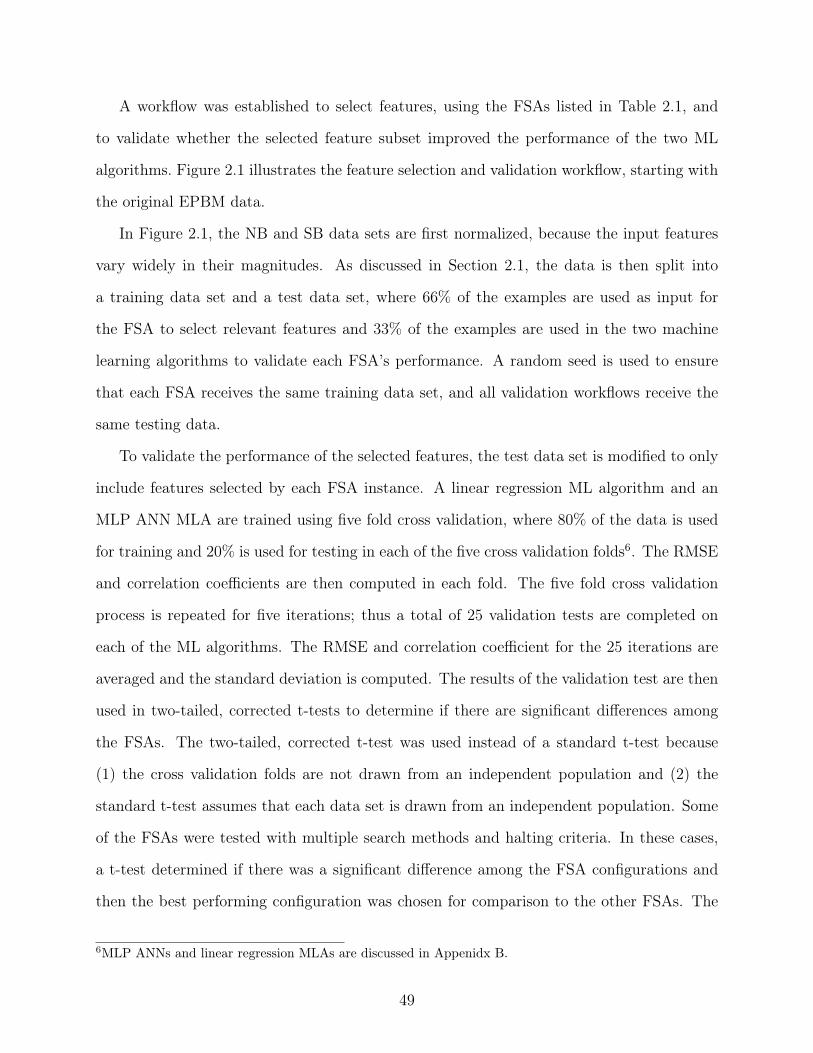
A workflow was established to select features, using the FSAs listed in Table 2.1, and
to validate whether the selected feature subset improved the performance of the two ML
algorithms. Figure 2.1 illustrates the feature selection and validation workflow, starting with
the original EPBM data.
In Figure 2.1, the NB and SB data sets are first normalized, because the input features
vary widely in their magnitudes. As discussed in Section 2.1, the data is then split into
a training data set and a test data set, where 66% of the examples are used as input for
the FSA to select relevant features and 33% of the examples are used in the two machine
learning algorithms to validate each FSA’s performance. A random seed is used to ensure
that each FSA receives the same training data set, and all validation workflows receive the
same testing data.
To validate the performance of the selected features, the test data set is modified to only
include features selected by each FSA instance. A linear regression ML algorithm and an
MLP ANN MLA are trained using five fold cross validation, where 80% of the data is used
for training and 20% is used for testing in each of the five cross validation folds6. The RMSE
and correlation coefficients are then computed in each fold. The five fold cross validation
process is repeated for five iterations; thus a total of 25 validation tests are completed on
each of the ML algorithms. The RMSE and correlation coefficient for the 25 iterations are
averaged and the standard deviation is computed. The results of the validation test are then
used in two-tailed, corrected t-tests to determine if there are significant differences among
the FSAs. The two-tailed, corrected t-test was used instead of a standard t-test because
(1) the cross validation folds are not drawn from an independent population and (2) the
standard t-test assumes that each data set is drawn from an independent population. Some
of the FSAs were tested with multiple search methods and halting criteria. In these cases,
a t-test determined if there was a significant difference among the FSA configurations and
then the best performing configuration was chosen for comparison to the other FSAs. The
6MLP ANNs and linear regression MLAs are discussed in Appenidx B.
49

Figure 2.1: Feature selection and feature validation workflow. Tan rectangles represent datapre or post processing, white rectangles represent data, blue diamonds represent data splits,and red rectangles represent applying FSAs or ML algorithms to the data.
50

FSA that significantly outperformed the most other FSAs was declared the best performing
FSA.
To determine the predictive power of the selected features, each test example’s observed
output target was compared to the example’s output target value predicted by the ML
algorithm (created with the selected features). If we were to visualize this comparison, the
observed values would be plotted on the x-axis and the ML algorithm predicted values would
be plotted on the y-axis. An R2 value (i.e., the correlation coefficient) was computed for
each of the cross-validation folds and iterations, in order to determine how well the results
fit the line y = x+ 0, which describes a model that perfectly predicts every observed testing
value.
In order to determine which features could be optimized to improve the advance rate
performance of the EPBM, the selected input features were compared across the NB and SB
data sets. Features that could not be modified by the EPBM operator (such as the weight
of the material on the rear belt scale) were eliminated from consideration. The remaining
input features were examined on a time series plot to determine their effects on the advance
rate.
2.3 Results and Analysis
The FSAs tested in our work did not select the same features, but some difference in fea-
tures selected was expected due to our FSA literature review. In other words, we expected
the FSA configurations to select different features and, therefore, developed a validation
workflow to determine which FSA configuration best predicted EPBM advance rate. As
previously discussed, our validation workflow contained five iterations of five fold cross val-
idation to determine if an FSA configuration performed statistically better than no feature
selection or other FSA configurations.
Before comparing the FSAs to each other, the best FSA configuration for each FSA type
was determined. The best FSA configuration was determined from the results of the five-fold
cross validation and five iteration loop depicted in Figure 2.1. A two-tailed, corrected t-test
51

compared each FSA’s correlation coefficient against the correlation coefficient of the same
data with no feature selection. The corrected t-test relaxes the independence constraint and
reduces type I errors caused by cross validation [50]. Although the correlation coefficient
and the RMSE were computed for each FSA, we chose to use the correlation coefficient
due to the large variance in the RMSE when no feature selection was applied. Specifically,
when no feature selection was applied, at least one cross validation fold returned an RMSE
several orders of magnitude larger than the maximum advance rate of the EPBM. Instead
of removing the large cross-validation folds in our analysis, we leave it in our analysis to
illustrate how FSAs reduce the variance in the EPBM data set.
2.3.1 RReliefF Filter FSA
Four configurations of the RReliefF neighbors were tested against four halting criteria.
The 5, 10, 15, and 20 selected features were chosen as halting criteria for two filter FSAs
(i.e., RReliefF and R2), because the accuracy of the validation ML algorithms decreased
significantly when 20 features (or more) were selected. The four configurations of neighbors
(10, 100, 350, and 700) were chosen to test claims by Khoavi and John [32] that RReli-
efF must use almost all of the available neighbors to identify an accurate set of features.
The configurations with 700 neighbors utilized all of the examples in the calculation of
feature weights. Figure 2.2, Figure 2.3, Figure 2.4, and Figure 2.5 show the mean correla-
tion coefficient value and standard deviations (each figure represents 10, 100, 350, and 700
neighbors used, respectively) for the NB tunnel when the RReliefF Filter FSA is applied;
Figure 2.6, Figure 2.7, Figure 2.8, and Figure 2.9 show the same data for the SB tunnel.
Configurations that performed significantly better than applying no feature selection are
highlighted with a red box and the R2 and σ values are shown; we note that some figures do
not contain an FSA that outperformed no feature selection and, thus, do not contain any
red boxes.
A linear regression algorithm and an MLP ANN algorithm were trained using (1) data
without feature selection and (2) data resulting from the features selected by each of the
52

16 RReliefF configurations. When a linear regression algorithm was trained, 6 of the 16
configurations outperformed no feature selection and 1 of the 16 configurations performed
worse. When an MLP ANN algorithm was trained, 12 of the 16 configurations outperformed
no feature selection and 1 of the 12 configurations performed worse.
To understand which configuration to test against the other FSAs, the corrected t-test
determined if there existed significant differences in the mean correlation coefficient (R2)
among the 16 configurations. The null hypothesis, i.e., that two configurations did not
contain a significant difference between their correlation coefficients, was rejected if the p-
value was less than 0.05. A rank was created for each of the RReliefF configurations by
calculating the number of other configurations that were statistically better than a given
configuration, as well as the number of configurations that were statistically worse than
the given configuration. Each configuration lost one point if it was worse than another
configuration and gained one point if it was better than another configuration. The results
showed that Khoavi and John’s assertions were correct, i.e., the highest scoring configurations
used all neighbors. In the NB tunnel, RReliefF with all neighbors and 10 features selected was
the highest ranked; in the SB tunnel, RReliefF with all neighbors and 5 features selected
was the highest ranked. These two configurations competed against the other FSAs in
Section 2.3.7.
2.3.2 R2 Estimation Filter FSA
Figure 2.10 and Figure 2.11 show the mean correlation coefficients for the features
selected by the R2 Estimation FSA configurations. As with the RReliefF FSA, an artificial
halting criteria (5, 10, 15, and 20 features) was created, because the R2 Estimation FSA
ranks individual features rather than searching for the best subset.
In the SB tunnel, the mean correlation coefficient of all configurations (except the 15
features, linear regression ML algorithm configuration) performed significantly better than
no feature selection. In the NB tunnel, no configurations of R2 Estimation improved the
mean correlation coefficient when training a linear regression ML algorithm or an MLP ANN
53

No FSA Applied 5 Features 10 Features 15 Features 20 Features0
0.1
0.2
0.3
0.4
0.5
0.6
0.7
0.8
0.9
1Comparison of the Correlation Coefficient for the RReliefF (10 Neighbors) Filter FSA Configurations Applied to the NB EPBM Data
FSA Configuration Applied
Mea
n C
orre
latio
n C
oeffi
cien
t
Linear RegressionMLP ANN
R2 = 0.52σ = 0.18
Figure 2.2: Comparison of the mean correlation coefficients for the RReliefF (10 neighbors)FSA over five cross validation folds and five iterations (each data point encompasses 25simulations) for the NB Seattle tunnel data. The x-axis contains the number of featuresselected.
No FSA Applied 5 Features 10 Features 15 Features 20 Features0
0.1
0.2
0.3
0.4
0.5
0.6
0.7
0.8
0.9
1
Comparison of the Correlation Coefficient for the RReliefF (100 Neighbors) Filter FSA Configurations Applied to the NB EPBM Data
FSA Configuration Applied
Mean C
orr
ela
tion C
oeffic
ient
Linear RegressionMLP ANN
R2 = 0.63
σ = 0.18
R2 = 0.70
σ = 0.21
R2 = 0.66
σ = 0.18
R2 = 0.71
σ = 0.20
Figure 2.3: Comparison of the mean correlation coefficients for the RReliefF (100 neighbors)FSA over five cross validation folds and five iterations (each data point encompasses 25simulations) for the NB Seattle tunnel data. The x-axis contains the number of featuresselected.
54

No FSA Applied 5 Features 10 Features 15 Features 20 Features0
0.1
0.2
0.3
0.4
0.5
0.6
0.7
0.8
0.9
1
Comparison of the Correlation Coefficient for the RReliefF (350 Neighbors) Filter FSA Configurations Applied to the NB EPBM Data
FSA Configuration Applied
Mean C
orr
ela
tion C
oeffic
ient
Linear RegressionMLP ANN
R2 = 0.71
σ = 0.20R2 = 0.73
σ = 0.19
R2 = 0.74
σ = 0.19
R2 = 0.72
σ = 0.20
R2 = 0.75
σ = 0.20
Figure 2.4: Comparison of the mean correlation coefficients for the RReliefF (350 neighbors)FSA over five cross validation folds and five iterations (each data point encompasses 25simulations) for the NB Seattle tunnel data. The x-axis contains the number of featuresselected.
No FSA Applied 5 Features 10 Features 15 Features 20 Features0
0.1
0.2
0.3
0.4
0.5
0.6
0.7
0.8
0.9
1
Comparison of the Correlation Coefficient for the RReliefF (700 Neighbors) Filter FSA Configurations Applied to the NB EPBM Data
FSA Configuration Applied
Mean C
orr
ela
tion C
oeffic
ient
Linear RegressionMLP ANN
R2 = 0.75
σ = 0.20R2 = 0.74
σ = 0.21
R2 = 0.64
σ = 0.19
R2 = 0.74
σ = 0.19
R2 = 0.71
σ = 0.20
Figure 2.5: Comparison of the mean correlation coefficients for the RReliefF (700 neighbors)FSA over five cross validation folds and five iterations (each data point encompasses 25simulations) for the NB Seattle tunnel data. The x-axis contains the number of featuresselected.
55
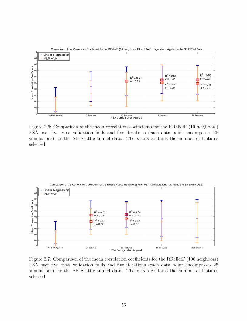
No FSA Applied 5 Features 10 Features 15 Features 20 Features0
0.1
0.2
0.3
0.4
0.5
0.6
0.7
0.8
0.9
1
Comparison of the Correlation Coefficient for the RReliefF (10 Neighbors) Filter FSA Configurations Applied to the SB EPBM Data
FSA Configuration Applied
Mean C
orr
ela
tion C
oeffic
ient
Linear RegressionMLP ANN
R2 = 0.55
σ = 0.23
R2 = 0.49
σ = 0.28
R2 = 0.55
σ = 0.22
R2 = 0.50
σ = 0.29
R2 = 0.53
σ = 0.23
Figure 2.6: Comparison of the mean correlation coefficients for the RReliefF (10 neighbors)FSA over five cross validation folds and five iterations (each data point encompasses 25simulations) for the SB Seattle tunnel data. The x-axis contains the number of featuresselected.
No FSA Applied 5 Features 10 Features 15 Features 20 Features0
0.1
0.2
0.3
0.4
0.5
0.6
0.7
0.8
0.9
1
Comparison of the Correlation Coefficient for the RReliefF (100 Neighbors) Filter FSA Configurations Applied to the SB EPBM Data
FSA Configuration Applied
Mean C
orr
ela
tion C
oeffic
ient
Linear RegressionMLP ANN
R2 = 0.54
σ = 0.22
R2 = 0.47
σ = 0.27
R2 = 0.53
σ = 0.24
R2 = 0.42
σ = 0.22
Figure 2.7: Comparison of the mean correlation coefficients for the RReliefF (100 neighbors)FSA over five cross validation folds and five iterations (each data point encompasses 25simulations) for the SB Seattle tunnel data. The x-axis contains the number of featuresselected.
56

No FSA Applied 5 Features 10 Features 15 Features 20 Features0
0.1
0.2
0.3
0.4
0.5
0.6
0.7
0.8
0.9
1
Comparison of the Correlation Coefficient for the RReliefF (350 Neighbors) Filter FSA Configurations Applied to the SB EPBM Data
FSA Configuration Applied
Mean C
orr
ela
tion C
oeffic
ient
Linear RegressionMLP ANN
R2 = 0.53
σ = 0.24
R2 = 0.42
σ = 0.22
R2 = 0.53
σ = 0.26
R2 = 0.49
σ = 0.27
Figure 2.8: Comparison of the mean correlation coefficients for the RReliefF (350 neighbors)FSA over five cross validation folds and five iterations (each data point encompasses 25simulations) for the SB Seattle tunnel data. The x-axis contains the number of featuresselected.
No FSA Applied 5 Features 10 Features 15 Features 20 Features0
0.1
0.2
0.3
0.4
0.5
0.6
0.7
0.8
0.9
1Comparison of the Correlation Coefficient for the RReliefF (700 Neighbors) Filter FSA Configurations Applied to the SB EPBM Data
FSA Configuration Applied
Mea
n C
orre
latio
n C
oeffi
cien
t
Linear RegressionMLP ANN
R2 = 0.48σ = 0.24
R2 = 0.45σ = 0.29
R2 = 0.53σ = 0.23
R2 = 0.47σ = 0.26
R2 = 0.55σ = 0.22
R2 = 0.53σ = 0.28
Figure 2.9: Comparison of the mean correlation coefficients for the RReliefF (700 neighbors)FSA over five cross validation folds and five iterations (each data point encompasses 25simulations) for the SB Seattle tunnel data. The x-axis contains the number of featuresselected.
57

No FSA Applied 5 Features 10 Features 15 Features 20 Features0
0.1
0.2
0.3
0.4
0.5
0.6
0.7
0.8
0.9
1
Comparison of the Correlation Coefficient for the R2 Estimation Filter FSA Configurations Applied to the NB EPBM Data
FSA Configuration Applied
Mean C
orr
ela
tion C
oeffic
ient
Linear RegressionMLP ANN
Figure 2.10: Comparison of the mean correlation coefficients for the R2 Estimation FSA overfive cross validation folds and five iterations (each data point encompasses 25 simulations)for the NB Seattle tunnel data. The x-axis contains the number of features selected.
No FSA Applied 5 Features 10 Features 15 Features 20 Features0
0.1
0.2
0.3
0.4
0.5
0.6
0.7
0.8
0.9
1Comparison of the Correlation Coefficient for the R2 Estimation Filter FSA Configurations Applied to the SB EPBM Data
FSA Configuration Applied
Mea
n C
orre
latio
n C
oeffi
cien
t
Linear RegressionMLP ANN
R2 = 0.53σ = 0.23
R2 = 0.41σ = 0.22
R2 = 0.55σ = 0.21
R2 = 0.49σ = 0.27
R2 = 0.55σ = 0.23
R2 = 0.45σ = 0.29
R2 = 0.49σ = 0.27
Figure 2.11: Comparison of the mean correlation coefficients for the R2 Estimation FSA overfive cross validation folds and five iterations (each data point encompasses 25 simulations)for the SB Seattle tunnel data. The x-axis contains the number of features selected.
58

No FSA Applied 5 Features 10 Features 15 Features 20 Features0
0.1
0.2
0.3
0.4
0.5
0.6
0.7
0.8
0.9
1
Comparison of the Correlation Coefficient for the R2 Estimation Filter FSA Applied to the NB EPBM Data (New Training Data)
FSA Configuration Applied
Mean C
orr
ela
tion C
oeffic
ient
Linear RegressionMLP ANN
Figure 2.12: Comparison of the mean correlation coefficients for the R2 Estimation FSA overfive cross validation folds and five iterations (each data point encompasses 25 simulations)for the NB Seattle tunnel data. The x-axis contains the number of features selected. Adifferent training and testing data set were used to test whether the training and testingdata in Figure 2.10 is representative of the underlying population.
ML algorithm. This result was unexpected; that is, we expected at least one of the linear
regression ML algorithms would show improvement sinceR2 Estimation FSA selects features
linearly related to the output target.
We, therefore, investigated the NB tunnel further. The features selected by the FSA (in
the NB tunnel) did not include the rear or front side belt scales, which have a strong linear
relation to the output target. Examining the R2 estimate for each feature showed that none
of the features in the NB tunnel returned an R2 value of more than 0.45, whereas the SB
tunnel returned several R2 values of 1.0. We re-sampled the training and testing data to
determine if the training or testing data did not provide the R2 filter with a representative
sample of the underlying population. Figure 2.12 shows the results of selecting a new training
and testing data set. Although none of the configurations performed significantly better than
no feature selection, the correlation coefficients in Figure 2.12 were an improvement over the
correlation coefficients in Figure 2.10; in addition, the front side belt scale and rear side
belt scale were selected as predictors of advance rate with the different training and testing
data sets. The non-significant improvement using a different testing and training data set
59

indicates that: (1) The R2 Estimation Filter was not able to find highly correlated patterns
in the original training and testing data split, and (2) the NB tunnel data may contain
weakly related features that significantly improve predictive power.
In the SB tunnel, the R2 Estimation FSA configurations with a halting criteria of 5,
10, 15, and 20 features tied in the rankings, i.e., each configuration significantly improved
no feature selection in at least one of the ML algorithms, but none of these configurations
were able to significantly improve upon the other configurations. If we only examine mean
correlation coefficient scores, the features selected when halting at 10 features performed the
best in the SB tunnel. We, therefore, compare this configuration against the other FSAs
in Section 2.3.7. Since none of the R2 Estimation FSA configurations improved upon no
feature selection in the NB tunnel, the 20 feature halting criteria was selected as our best
configuration (for comparison against the other FSAs) because it returned the highest mean
correlation coefficient score.
2.3.3 F-statistic Filter FSA
In order to select between 5 and 20 features (similar to the 5, 10 , 15, and 20 feature
halting criteria of other filter FSAs) we found that an entrance criteria of p < 0.001 and exit
criteria of p > 0.01 provided the number of features within our bounds in both tunnels. The
resulting features were used in the validation workflow, described in Section 2.1; the results
are shown in Figure 2.13 and Figure 2.14. As noted in Table 2.1, only one configuration of
the F-statistic FSA was tested, i.e., the greedy stepwise search method. Configurations that
performed significantly better than applying no feature selection are highlighted with a red
box, and the R2 and σ values are shown. The number of input features selected by each
search method is shown below the mean and error bars and labeled “n features selected,"
where n is the number of input features selected.
In the NB tunnel, the F-statistic FSA performed significantly better than no feature
selection when a linear regression algorithm was trained with the selected features, but the
MLP ANN ML algorithm did not perform significantly better than no feature selection.
60

Significantly better results were obtained in the SB tunnel when the F-statistic selected
features were applied to the MLP ANN, but the linear regression ML algorithm did not
produce significantly better results than no feature selection.
We now consider why the linear regression algorithm performed significantly better in
the NB tunnel and the MLP ANN ML algorithm performed significantly better in the SB
tunnel. In the NB tunnel, linear regression with no feature selection returned a correlation
coefficient of 0.10; however, in the SB tunnel, linear regression with no feature selection
returned a correlation coefficient of 0.23. Because of the low correlation coefficient value in
the NB tunnel, the performance of the linear regression algorithm does not need to improve
as much in the NB tunnel as it does in the SB tunnel. The MLP ANN ML algorithm
preformed better in the NB tunnel than the SB tunnel with no feature selection, returning a
correlation coefficient of 0.26 in the NB tunnel and 0.06 in the SB tunnel. These differences
in the correlation coefficient with no feature selection illustrate why the linear regression
algorithm performed significantly better than no feature selection in the NB tunnel, whereas
the MLP ANN ML algorithm performed significantly better than no feature selection in the
SB tunnel.
We note there was a stronger linear relationship between the input features in the SB
tunnel than in the NB tunnel. The SB tunnel had sharper changes in advance rate than the
NB tunnel, and these changes align with changes in the GCS system. The linear regression
algorithm was then able to focus on a few features that predicted the advance rate changes
and ignore the rest, providing better performance without feature selection. The NB tunnel
showed a more consistent advance rate, which means that a more complex ML algorithm, i.e.,
the MLP ANN, performed better. In other words, the amount of variation in the advance
rate caused a different ML algorithm to perform better in the NB tunnel than in the SB
tunnel.
The F-statistic FSA identified strong linear features, such as the front and rear belt scale
weight and the grout expelled, in both tunnels. In the NB tunnels, more features were
61

identified, including the soil type, as important features; however, the soil type was not
shown to have a significant impact in the SB tunnel. Visualizations of the data indicate that
the advance rate of the EPBM was more consistent when the soil type was constant in the
NB tunnel than in the SB tunnel, which confirms why the soil type was only identified in
the NB tunnel. We had several discussions with project managers and conclude the advance
rate was more consistent in the SB tunnel because the SB tunnel was excavated after the NB
tunnel; in other words, the operators were more familiar with the tunnel alignment during
the SB excavation, allowing the operators to achieve a consistently high advance rate despite
the varying soil conditions.
No FSA Applied Greedy Stepwise0
0.1
0.2
0.3
0.4
0.5
0.6
0.7
0.8
0.9
1
Comparison of the Correlation Coefficient for the F−statistic Filter FSA Configurations Applied to the NB EPBM Data
FSA Configuration Applied
Mean C
orr
ela
tion C
oeffic
ient
Linear RegressionMLP ANN
R2 = 0.60
σ = 0.29
16 featuresselected
Figure 2.13: Comparison of the mean correlation coefficients for the F-statistic FSA overfive cross validation folds and five iterations (each data point encompasses 25 simulations)for the NB Seattle tunnel data.
2.3.4 CFS Wrapper FSA
Three search methods were utilized when selecting feature subsets with CFS: best first,
greedy stepwise, and the locally predictive method was applied to a best first search. Fig-
ure 2.15 and Figure 2.16 compare the mean correlation coefficients for each CFS FSA con-
figuration across the NB and SB tunnels, respectively. In the NB tunnel, when the features
trained an MLP ANN ML algorithm, the best first and greedy stepwise search methods
62

No FSA Applied Greedy Stepwise0
0.1
0.2
0.3
0.4
0.5
0.6
0.7
0.8
0.9
1Comparison of the Correlation Coefficient for the F−statistic Filter FSA Configurations Applied to the SB EPBM Data
FSA Configuration Applied
Mea
n C
orre
latio
n C
oeffi
cien
t
Linear RegressionMLP ANN
R2 = 0.51σ = 0.35
8 featuresselected
Figure 2.14: Comparison of the mean correlation coefficients for the F-statistic FSA overfive cross validation folds and five iterations (each data point encompasses 25 simulations)for the SB Seattle tunnel data.
No FSA Applied Best First Greedy Stepwise Locally Predictive0
0.1
0.2
0.3
0.4
0.5
0.6
0.7
0.8
0.9
1
Comparison of the Correlation Coefficient for the CFS Wrapper FSA Configurations Applied to the NB EPBM Data
FSA Configuration Applied
Mean C
orr
ela
tion C
oeffic
ient
Linear RegressionMLP ANN
5 features selected
5 features selected
7 features selected
Figure 2.15: Comparison of the mean correlation coefficients for the CFS wrapper FSA overfive cross validation folds and five iterations (each data point encompasses 25 simulations)for the NB Seattle tunnel data. We note that the locally predictive method also utilized abest first search.
63

No FSA Applied Best First Greedy Stepwise Locally Predictive0
0.1
0.2
0.3
0.4
0.5
0.6
0.7
0.8
0.9
1
Comparison of the Correlation Coefficient for the CFS Wrapper FSA Configurations Applied to the SB EPBM Data
FSA Configuration Applied
Mean C
orr
ela
tion C
oeffic
ient
Linear RegressionMLP ANN
R2 = 0.46
σ = 0.26
R2 = 0.46
σ = 0.26R
2 = 0.41
σ = 0.21
11 featuresselected
11 featuresselected
12 featuresselected
Figure 2.16: Comparison of the mean correlation coefficients for the CFS wrapper FSA overfive cross validation folds and five iterations (each data point encompasses 25 simulations)for the SB Seattle tunnel data. We note that the locally predictive method also utilized abest first search.
selected the same feature subset, and the selected subset resulted in a statistically significant
improvement over no feature selection. The best first, locally predictive search method did
not show a statistically significant improvement in the NB tunnel, perhaps because of its bias
towards removing redundant features. That is, the subset in the NB tunnel that performed
statistically better than no feature selection contained a redundant feature that may have
reduced noise in the data. Because some of the features have a strong linear correlation to
the output target (e.g., front and rear side belt scales), it may have been difficult for CFS to
identify other features with a stronger correlation than these features and, thus, caused CFS
to select a small feature set. It is also important to note that the features selected by CFS
have a much larger variance than the subsets selected by other FSAs. The large variance is
usually seen when a model is overfitting the training data; however, since very few features
were selected by CFS, we suspect the selected subset is underfitting the training data. We
note that overfitting occurs when an overly complex model is trained and performs well on
the training data, but does not perform well on the testing data. Underfitting occurs when a
model is trained that is not complex enough to properly model the training data and, thus,
64

also performs poorly on the testing data.
There is no absolute method to determine if an ML algorithm is overfitting or underfitting
the training data. As the complexity of a model increases, it is more likely to overfit the data;
similarly, as the complexity of the model decreases, it is more likely to underfit the data. We
seek to find a balance between overfitting and underfitting the training data. Comparing the
correlation coefficient of the training data to the testing data is one method for determining
a model’s balance between overfitting and underfitting. If the correlation coefficient of the
testing data is much lower than the correlation coefficient of the training data, i.e., the model
fits the training data much better than the testing data, the model is either underfitted or
overfitted to the training data. To determine whether the model is overfitted or underfitted,
we examine the complexity of the model: a low complexity model is underfitted and a high
complexity model is overfitted.
The CFS configurations in the NB tunnel identified low complexity models, i.e., models
that utilized a small number of input features, which means that the CFS models in the
NB tunnel are underfitted if the correlation coefficient difference between the training data
and the testing data is large. In the NB data set, the linear regression algorithm had
an average correlation coefficient difference of 0.26 in the best first and greedy stepwise
configurations and 0.32 in the locally predictive configuration. The MLP ANN ML algorithm
fared better with a difference of 0.06 in the best first and greedy stepwise configurations and
0.13 in the locally predictive configuration. In the SB tunnel, more features were selected
and the smaller correlation coefficient differences between the training and testing data
indicates that the models did not overfit or underfit the data. The linear regression model
performed 0.04 better in the testing data set in all configurations. The MLP ANN ML
algorithm’s training data correlation coefficient performed 0.01 better in the best first and
greedy stepwise configurations and 0.05 better in the locally predictive configuration. The
correlation coefficients in the NB tunnel suggest that the smaller feature set is underfitting
the data, and the correlation coefficients in the SB tunnel suggest that the configurations
65

are neither overfitting or underfitting the data.
In the SB tunnel, all search methods identified a sets of features that were significantly
better than no feature selection, but only when validated with the MLP ANN ML algorithm.
Best first and greedy stepwise identified the same subset of features and this subset of features
outperformed the set of features identified by the locally predictive search method. The best
first and greedy stepwise feature subset were, therefore, chosen to compete against the best
subsets selected by the other FSAs. In the NB tunnel, no selected subset outperformed no
feature selection. Therefore, the tie breaker method (discussed in Section 2.3) was used to
select the best subset. Specifically, the locally predictive search method slightly outperformed
the best first and greedy stepwise search methods (i.e., had higher correlation coefficients),
so the locally predictive subset was chosen to compete against other FSA selected subsets.
2.3.5 MLP ANN Wrapper FSA
The MLP ANN wrapper FSA selected features using the method described by Khoavi and
John [32] for training wrapper algorithms. As discussed in Section 2.1, each wrapper method
was tested with two search strategies: best first and greedy stepwise, and additionally, locally
predictive search was used with CFS. At each step of the search, five-fold cross validation
trained five MLP ANN FSAs. If the standard deviation of the RMSE (from the five cross
validation folds) was greater than a threshold, the cross validation folds were run again.
The subset with the lowest RMSE was then selected as the final set of features. We set
the threshold as low as possible without causing the algorithm to cycle into an infinite loop.
Specifically, we set the MLP ANNs to use a threshold of 0.01. Each MLP ANN also utilized
a hidden layer and the number of nodes in the hidden layer was equal to one half the number
of features. The learning rate of the MLP ANN was set to 0.3 for all trials.
Figure 2.17 and Figure 2.18 show the mean correlation coefficient of all configurations for
the MLP ANN FSA in the NB and SB tunnels, respectively. The mean correlation coefficient
only increased significantly in the NB tunnel when a linear regression ML algorithm was
used. In the SB tunnel, no significant improvement was found with any of the MLP ANN
66

No FSA Applied Best First Greedy Stepwise0
0.1
0.2
0.3
0.4
0.5
0.6
0.7
0.8
0.9
1Comparison of the Correlation Coefficient for the MLP ANN Wrapper FSA Configurations Applied to the NB EPBM Data
FSA Configuration Applied
Mea
n C
orre
latio
n C
oeffi
cien
t
Linear RegressionMLP ANN
R2 = 0.64σ = 0.19
R2 = 0.64σ = 0.19
5 features selected
7 features selected
Figure 2.17: Comparison of the mean correlation coefficients for the MLP ANN wrapperFSA over five cross validation folds and five iterations (each data point encompasses 25simulations) for the NB Seattle tunnel data.
No FSA Applied Best First Greedy Stepwise0
0.1
0.2
0.3
0.4
0.5
0.6
0.7
0.8
0.9
1Comparison of the Correlation Coefficient for the MLP ANN Wrapper FSA Configurations Applied to the SB EPBM Data
FSA Configuration Applied
Mea
n C
orre
latio
n C
oeffi
cien
t
Linear RegressionMLP ANN 9 features
selected5 features selected
Figure 2.18: Comparison of the mean correlation coefficients for the MLP ANN wrapperFSA over five cross validation folds and five iterations (each data point encompasses 25simulations) for the SB Seattle tunnel data.
67

wrapper configurations when compared to no feature selection. We did not expect the linear
regression ML algorithm to perform better than the MLP ANN ML algorithm (in the NB
tunnel), because the features were selected by an MLP ANN wrapper FSA. The linear
regression ML algorithm is biased towards less variance (i.e., more likely to underfit the test
data set because of the simplicity of the model), which means the underlying distribution
may be less complex than the model created by the MLP ANN ML algorithm. The linear
regression ML algorithm performed better than the MLP ANNML algorithm with no feature
selection only in the NB tunnel, which may indicate that the conditions in the NB tunnel
do not require as complex of a model as the SB tunnel.
The ranking method, described in Section 2.1, was used to asses the performance of
each of the FSA configurations (within the same tunnel). In the NB tunnel, both FSA
configurations training a linear regression ML algorithm performed significantly better than
no feature selection and both configurations of the FSA (i.e., greedy stepwise search and
best first search) were tied in outperforming no feature selection (i.e., R2 = 0.64 and σ =
0.19). To break the tie, the sums of the mean correlation coefficients of all tests (MLP ANN
and linear regression ML algorithms) were calculated, and the FSA configuration with the
largest sum was selected. The greedy stepwise subset was chosen for the NB tunnel, because
its correlation coefficient total means were 0.01 greater than best first. In the SB tunnel,
the greedy stepwise subset was also selected, because greedy stepwise performed better (i.e.,
had a higher correlation coefficient) than best first search (but not significantly better than
no feature selection).
2.3.6 SVM Regression Wrapper FSA
The SVM wrapper FSA required much more computing time than both the MLP ANN
wrapper FSA and the CFS wrapper FSA. In fact, some of the SVM wrapper configuration
settings had to be adjusted so that the algorithm would complete. The standard deviation
threshold value (i.e., cross validation stops when the standard deviation of the cross validation
folds is less than the threshold value) was increased from 0.01 to 0.5, because the algorithm
68

was not converging to a solution with the lower threshold. Cross validation folds were also
reduced from five to two folds. In addition to testing two subset search methods (best first
and greedy stepwise), each of these search configurations was tested with a linear kernel and
a second degree polynomial kernel. The polynomial kernel was tested to detect non-linear
dependencies between the features and the output target, and a second degree polynomial
was chosen to avoid overfitting the training data with a higher order polynomial. Even
with a higher threshold and two cross validation folds, the SVM wrapper FSA was able to
significantly outperform no feature selection in at least one configuration in both the NB
and SB tunnels.
No FSA Applied Linear Kernel, Best First Linear Kernel, Greedy Stepwise Second Degree Kernel, Best First Second Degree Kernel, Greedy Stepwise0
0.1
0.2
0.3
0.4
0.5
0.6
0.7
0.8
0.9
1
Comparison of the Correlation Coefficient for the SVM Regression Wrapper FSA Configurations Applied to the NB EPBM Data
FSA Configuration Applied
Mean C
orr
ela
tion C
oeffic
ient
Linear RegressionMLP ANN
R2 = 0.80
σ = 0.29
21 featuresselected
21 featuresselected
R2 = 0.65
σ = 0.30
33 featuresselected
5 featuresselected
Figure 2.19: Comparison of the mean correlation coefficients for the SVM Regression FSAover two cross validation folds and five iterations (each data point encompasses 10 simula-tions) for the NB Seattle tunnel data.
Figure 2.19 and Figure 2.20 show changes in the mean correlation coefficient for the
SVM wrapper FSA configurations. Configurations that performed significantly better than
applying no feature selection are highlighted with a red box, and the R2 and σ values
are shown. None of the SVM wrapper FSAs utilizing a second degree polynomial kernel
returned features that significantly outperformed no feature selection (in both the NB and
SB tunnels). In the NB tunnel, an SVM wrapper (linear kernel and greedy stepwise subset
search) identified features that performed significantly better than no feature selection.
69

No FSA Applied Linear Kernel, Best First Linear Kernel, Greedy Stepwise Second Degree Kernel, Best First Second Degree Kernel, Greedy Stepwise0
0.1
0.2
0.3
0.4
0.5
0.6
0.7
0.8
0.9
1
Comparison of the Correlation Coefficient for the SVM Regression Wrapper FSA Configurations Applied to the SB EPBM Data
FSA Configuration Applied
Mean C
orr
ela
tion C
oeffic
ient
Linear RegressionMLP ANN
R2 = 0.53
σ = 0.30
R2 = 0.54
σ = 0.31
22 featuresselected
23 featuresselected
13 featuresselected
13 featuresselected
Figure 2.20: Comparison of the mean correlation coefficients for the SVM Regression FSAover two cross validation folds and five iterations (each data point encompasses 10 simula-tions) for the SB Seattle tunnel data.
In the NB tunnel, the SVM wrapper that performed significantly better than no feature
selection (linear kernel, greedy stepwise subset search) identified 33 features; the SVM using
a different subset search method (linear kernel, best first subset search) only returned five
features and the performance of the five selected features is not significantly better than no
feature selection. The difference in features may be explained by best first’s backtracking
method, which biases the search towards a smaller subset. Greedy stepwise, on the other
hand, adds a feature to the subset of selected features if there is any improvement in the
performance of the ML algorithm, leading to a larger subset of features. The SVM wrapper
with a linear kernel identified several features that increased the RMSE by a small amount,
and this combination of weakly related features led to a feature subset that significantly
improved the accuracy of the ML algorithms when applied to test data.
The SB tunnel did not show a large difference in the number of features selected by
the best first and greedy stepwise search methods in the SVM wrapper utilizing the linear
70

kernel. The SVM wrapper FSA utilizing the linear kernel showed a significant improvement
over no feature selection when applied to the MLP ANN ML algorithm (with best first and
greedy stepwise search strategies), but no significant improvement over no feature selection
using the linear regression ML algorithm. None of the SVM wrapper FSAs were signifi-
cantly better than any of the other FSAs in the SB tunnel; thus, the greedy stepwise, linear
kernel configuration was selected, because it returned a slightly higher mean correlation co-
efficient. In the NB tunnel the greedy stepwise, linear kernel was also chosen because it
outperformed (although, not significantly) the best first, linear kernel SVM wrapper FSA as
well as significantly outperformed the data set with no feature selection.
2.3.7 Comparison of the Best FSA Configurations
Table 2.2 shows that most of the FSA types tested were able to improve the performance
of the ML algorithms in at least one of the tested configurations. A checkmark indicates
that at least one configuration of the FSA outperformed no feature selection for the FSA
listed in the column. There were only three exceptions where the FSA type did not per-
form significantly better than no feature selection: R2 Estimation (NB tunnel, discussed in
Section 2.3.2), CFS (NB tunnel, discussed in Section 2.3.4), and MLP ANN (SB Tunnel,
discussed in Section 2.3.5). The biases of each of these FSAs may have caused the FSAs
to return a feature set that was not significantly better than no feature selection, which
illustrates the “No Free Lunch Theorem”. Even though each FSA type did not return a
significantly better set of features, we conclude that our first hypothesis (see Section 2.0)
was proven. Specifically, in both tunnels, at least one FSA configuration returned a set of
features that was significantly better than not applying feature selection.
Each of the previously discussed FSA configurations were then ranked; the highest ranked
FSA configuration for each FSA type (e.g., RReliefF, CFS, etc.) was then compared to the
other highest ranked FSA types. This FSA comparison is repeated for the NB and SB
tunnel data. A two-tailed, corrected t-test compares each combination (chose two) of the
FSAs, and a p-value less than 0.05 is considered to have a statistically significant difference
71

in performance.
Table 2.2: A comparison of all FSAs tested. An FSA is checked if at least one configurationof the FSA performed better (in terms of the correlation coefficient) than no feature selection.
Tunnel RReliefF R2 Estimation F-statistic CFS MLP ANN SVM RegressionNB X X X XSB X X X X X
Table 2.3: The number of significant wins and losses for the best performing FSA configura-tion in the NB tunnel. A positive integer indicates a significant win for the algorithm overother algorithms. A negative integer indicates a significant loss for the algorithm over theother algorithms.
Northbound TunnelFSA # Correlation
Coefficient Wins# RMSE Wins
RReliefF 2 0R2 Estimation -5 -1F-statistic 1 -1CFS 0 0MLP ANN 1 -1SVM Regression 1 3
Table 2.3 and Table 2.4 compare the best FSA configurations and show which algorithms
performed significantly better than other algorithms for the NB and SB tunnels respectively.
An FSA that performed significantly better than another FSA was given a score of +1
and the FSA that performed significantly worse than another FSA was given a score of -1; if
neither FSA performed significantly better than the other, a score of 0 was assigned. Table 2.3
and Table 2.4 show the sum of scores from comparing each FSA to every other FSA. We
tested for significant performance differences in terms of the correlation coefficient and the
RMSE. In the NB table (Table 2.3), R2 Estimation is scored lowest (-5), while in the SB
tunnel (Table 2.4) it is tied for the highest score (1). The variation in this result is expected
because of the more consistent excavation of the SB tunnel than the NB tunnel. The R2
Estimation method looks for linearly correlated relationships between the input feature and
72

Table 2.4: The number of significant wins and losses for the best performing FSA configu-ration in the SB tunnel. A positive integer indicates a significant win for the algorithm overother algorithms. A negative integer indicates a significant loss for the algorithm over otheralgorithms.
Southbound TunnelFSA # Correlation
Coefficient Wins# RMSE Wins
RReliefF 1 1R2 Estimation 1 0F-statistic 0 1CFS 0 -3MLP ANN -2 1SVM Regression 0 0
the output target; however, a linear relationship is not clear in the NB tunnel as the EPBM
operator was learning the subsurface conditions.
Table 2.5, Table 2.6, and Table 2.7 show the NB and SB tunnel features that were selected
by FSAs with a positive score in Table 2.3 and Table 2.4. RMSE, CC, or CC+RMSE, is
noted in the parenthesis next to each FSA’s name to indicate whether the FSA performs
significantly better than other FSAs in Root Mean Squared Error (RMSE), Correlation
Coefficient (CC), or both, respectively. Features within these tables are highlighted as gray
or yellow. Gray highlights indicate a feature common across multiple FSAs and is a result
of the changing EPBM advance rate; yellow highlights indicate a feature common across
multiple FSAs but is not a result from the changing EPBM advance rate. Only features that
were exactly the same were highlighted; in other words, features that took readings for the
same system, but at different locations, are not highlighted.
In the NB tunnel, the gray highlighted features in Table 2.5 are either part of: (1) the soil
removal system (i.e., Rear Side Belt Scale, Front Side Belt Scale, Calculated Muck Weight,
and Belt Conveyor Fault) or (2) the grouting system (i.e., Grout Fill Rate, Grout Component
A+B Flow, and #2 Grout Component B Liquid Flow). We expected the soil removal system
to have a strong relation to the advance rate, i.e., when more soil is removed the EPBM is
73

Table 2.5: Features selected by FSAs that significantly outperformed at least one other FSAin the NB tunnel. Features are highlighted as gray or yellow; gray highlights indicate afeature common across multiple FSAs and is a result of the changing EPBM advance rate;yellow highlights indicate a feature common across multiple FSAs but is not a result fromthe changing EPBM advance rate. CC, RMSE, and CC+RMSE represent whether the FSAoutperformed at least one other FSA in Correlation Coefficient (CC), Root Mean SquaredError (RMSE), or both (CC+RMSE).
Northbound Tunnel Correlation Coefficient (CC) and RMSE WinnersRReliefF (CC) F-statistic (CC) MLP ANN (CC) SVM Regression
(CC+RMSE)Rear Side Belt Scale(tons/hour)
Soil Type Pitching-Front-Body(deg)
Soil Type
Front Side Belt Scale(tons/hour)
#1 Screw SoilPressure-Front (bar)
Front Side Belt Scale(tons/hour)
Total Thrust Force(kNewtons)
Foam Fill Rate (%) Rear Side Belt Scale(tons/hour)
#2 Grout ComponentB Liquid Flow (liter-s/minute)
Rear Side Belt Scale(tons/hour)
Grout Fill Rate (%) #4 Foam Flow (liter-s/minute)
Grout Fill Rate (%) #5 Cutter Motor Out-put Frequency (Hz)
#1 Air Pressure (bar) Belt Conveyor Fault(on/off)
Foam Fill Rate (%) #2 Grout ComponentA Liquid Flow (liter-s/minute)
Grout ComponentA+B Flow (liter-s/minute)
#1 BF Injection PipeOpen (on/off)
#2 Grout ComponentB Liquid Flow (liter-s/minute)
Calculated MuckWeight (tons)
#1 Injection PipeClosed (on/off)
#2 Foam Flow (liter-s/minute)
#2 Air Pressure (bar) #3 Additive Injection(on/off)
#4 Air Flow (liter-s/minute)
#5 Air Pressure (bar) #2 Grout ComponentB Liquid Pump Fault(on/off)
#4 Air Pressure (bar)
#3 Air Pressure (bar) Net Stroke Difference(millimeters)
#4 Foam Counter(liters)
Grout ComponentA+B Flow (liter-s/minute)
#3 Additive Flow(liters/minute)
Muck Chamber-Bottom-Left-Minimum (bar)
#2 Screw RotationCounterclockwise(on/off )
Rear Side Belt ScaleWeight (tons)
Belt Conveyor Fault(on/off)
Methane Gas Monitor#2 Level (%)
Gas Alarm (on/off)
Pressure Body-Upper-Front (bar)
#1 Back Fill DeviceClosed (on/off)
Total Water Volume(m3)
#4 BF Injection PipeOpen (on/off)#4 Injection PipeOpen (on/off)Excavation FinishCondition (on/off)
74

Table 2.6: Table 2.5 continued.
Northbound Tunnel Correlation Coefficient (CC) and RMSE WinnersRReliefF (CC) F-statistic (CC) MLP ANN (CC) SVM Regression
(CC+RMSE)Gross ExcavationTime (minutes)Net Excavation Time(minutes)Grout ComponentA+B Flow (liter-s/minute)Screw Muck Volume(m3/minutes)Foam Volume Average(m3/number of Rings)03SJ Select Time (min-utes)05SJ Select Time (min-utes)08SJ Select Time (min-utes)R Back Distance (feet)Vertical Deviation-Tail(inches)Screw Conveyor Outlet1 Minimum (bar)Muck Chamber-Top-Maximum (bar)Flow Air Line 5 (m3)Flow Mix Line 3 (m3)Calculated MuckWeight (tons)
75

Table 2.7: Features selected by FSAs that significantly outperformed at least one other FSAin terms of the correlation coefficient in the SB tunnel. Features highlighted in gray arefeatures that change because the advance rate has changed. CC, RMSE, and CC+RMSErepresent whether the FSA outperformed at least one other FSA in Correlation Coefficient(CC), Root Mean Squared Error (RMSE), or both (CC+RMSE).
Southbound Tunnel Correlation Coefficient (CC) and RMSE WinnersRReliefF(CC+RMSE)
R2 (CC) F-Statistic (RMSE) MLP ANN (RMSE)
Rear Side Belt Scale(tons/hour)
Rear Side Belt Scale(tons/hour)
Rear Side Belt Scale(tons/hour)
Pitching-Front Body(degrees)
Front Side Belt Scale(tons/hour)
Grout ComponentA+B Flow (liter-s/minute)
#3 Grout ComponentA Liquid Pressure(bar)
#2 Grout ComponentA Liquid Flow (liter-s/minute)
Grout ComponentA+B Flow (liter-s/minute)
Front Side Belt Scale(tons/hour)
#2 Foam Pressure(bar)
#2 Solution Flow(liters/minute)
Belt Conveyor Fault(on/off)
#2 Grout ComponentA Liquid Flow (liter-s/minute)
#1 Additive Pressure(bar)
Str Jack Stroke-Left(millimeter)
#2 Grout ComponentA Liquid Flow (liter-s/minute)
#3 Grout ComponentA Liquid Flow (liter-s/minute)
Grout Component ALiquid Tank Level-Low(on/off)
Grout Volume LCL(m3/number of rings)
#2 Grout ComponentB Liquid Flow (liter-s/minute)
Tail Clear-Bottom(millimeters)
Tail Clear-Bottom(millimeters)
Grout ComponentA+B Flow (liter-s/minute)
Belt Conveyor Fault(on/off)
Flow Mix Line 4 (m3)
#3 Grout ComponentB Liquid Flow (liter-s/minute)Foam Calculated Stan-dard Deviation (σ)
76

excavating quicker. We also expected the grouting system to have a strong relation to the
advance rate; as the EPBM excavates faster, more grout is required to seal the completed
concrete tunnel rings. The Foam Fill Rate and Soil Type are highlighted yellow in the tables
because these features are not a result of the EPBM excavating faster. The Foam Fill Rate
is part of the GCS and is controlled by the EPBM operator. The soil type is not controlled
by the operator, but likely influences advance rate changes. We discuss the soil type further
later in this section.
We note that the non-highlighted features selected in the NB tunnel are still important
to examine, even though these features were not selected by multiple FSAs. Many additional
GCS features were selected by one of the FSAs, e.g., #1 through #5 Air Pressure, #4 and
#2 Foam Flow, #1 and #4 BF Injection Pipe Open, #1 Injection Pipe Closed, #4 Injection
Pipe Open, #3 Additive Injection, #3 Additive Flow, Total Water Volume, Foam Volume
Average, Flow Air Line 5, and Flow Mix Line 3. Further investigation into the placement of
the sensors is necessary to understand why only particular sensors in the GCS were selected
by the FSAs, i.e., only the #3 Additive Injection and #3 Additive Flow sensors were selected.
In other words, why does only certain portions of the GCS impact the advance rate of the
EPBM?
Furthermore, we note that several features selected for the NB tunnel are not part of the
soil removal system, grouting system, or GCS: #1 Screw Soil Pressure-Front, Muck Chamber-
Bottom-Left-Minimum, Methane Gas Monitor #2 Level, Pressure Body-Upper-Front, Total
Thrust Force, #5 Cutter Motor Output Frequency, #2 Screw Rotation Counterclockwise,
Gas Alarm, Excavation Finish Condition, Gross Excavation Time, Net Excavation Time,
R Back Distance, Vertical Deviation-Tail, Screw Conveyor Outlet 1 Minimum, and Muck
Chamber-Top-Maximum. We note that features directly related to the propulsion system
were excluded from this list, as it is unclear what type of relationship these features have
on the advance rate; the features we previously discussed have a near linear relationship
with the advance rate. Some of the features clearly do not have a relationship with the
77

advance rate and were selected by the FSAs because they remain close to a constant value,
i.e., Methane Gas Monitor #2 Level and Gas Alarm.
Most of the features that were not part of the soil removal system, grouting system,
or GCS were not selected by any of the best performing FSAs in the SB tunnel as shown
in Table 2.7. We note, however, that the FSAs in the SB tunnel did not perform as well as
the FSAs in the NB tunnel; the best performing FSA in the NB tunnel returned R2 = 0.80
and σ = 0.29, whereas the best performing FSA in the SB tunnel returned R2 = 0.55 and
σ = 0.21. The variance in prediction performance, however, was higher in the NB tunnel
than in the SB tunnel. The performance difference between the NB and SB tunnels can
be explained by the EPBM operator learning the subsurface conditions, which caused more
perturbations in the NB tunnel input data than in the SB tunnel input data.
In Table 2.7, the SB tunnel only contains gray highlighted features, which are features
that change because the advance rate changed. The features highlighted in the SB tunnel
are almost all part of the soil removal system (i.e., Rear Side Belt Scale, Front Side Belt
Scale, and Belt Conveyor Fault) or the grouting system (i.e., Grout Component A+B Flow
or #2 Grout Component A Liquid Flow). The Tail Clear-Bottom feature is an exception;
it is highlighted gray, but is not part of the soil removal system or the grouting system. We
believe Tail Clear-Bottom was selected because it is an indirect indicator of how much soil
is removed. Although GCS features are not highlighted in Table 2.7, GCS features were
selected by individual FSAs, e.g., Foam Calculated Standard Deviation, #2 Foam Pressure,
#1 Additive Pressure, Flow Mix Line 4, and #2 Solution Flow.
2.3.8 Number of Features Selected
As expected, the FSAs selected a different number of features depending on the FSA
type and FSA configuration. Table 2.8 shows the number of features selected by each of the
FSAs that did not have an artificial halting criteria (i.e., the 5, 10, 15, and 20 feature halting
criteria used for RReliefF and R2 Estimation FSAs). If an FSA did not utilize one of the
search configurations, the value for that search configuration in the table is blank; otherwise,
78
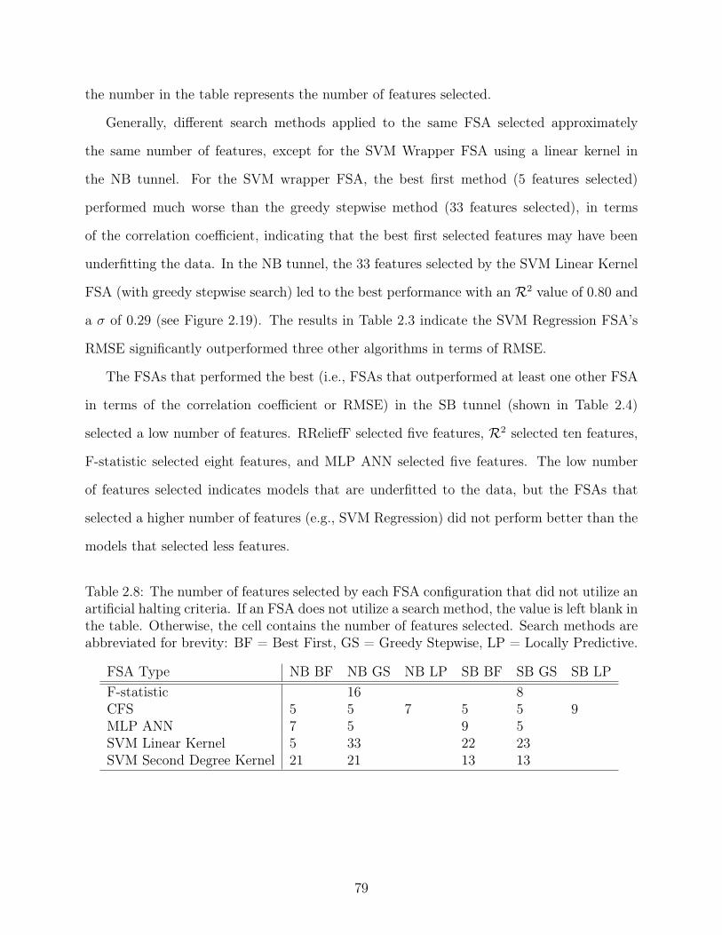
the number in the table represents the number of features selected.
Generally, different search methods applied to the same FSA selected approximately
the same number of features, except for the SVM Wrapper FSA using a linear kernel in
the NB tunnel. For the SVM wrapper FSA, the best first method (5 features selected)
performed much worse than the greedy stepwise method (33 features selected), in terms
of the correlation coefficient, indicating that the best first selected features may have been
underfitting the data. In the NB tunnel, the 33 features selected by the SVM Linear Kernel
FSA (with greedy stepwise search) led to the best performance with an R2 value of 0.80 and
a σ of 0.29 (see Figure 2.19). The results in Table 2.3 indicate the SVM Regression FSA’s
RMSE significantly outperformed three other algorithms in terms of RMSE.
The FSAs that performed the best (i.e., FSAs that outperformed at least one other FSA
in terms of the correlation coefficient or RMSE) in the SB tunnel (shown in Table 2.4)
selected a low number of features. RReliefF selected five features, R2 selected ten features,
F-statistic selected eight features, and MLP ANN selected five features. The low number
of features selected indicates models that are underfitted to the data, but the FSAs that
selected a higher number of features (e.g., SVM Regression) did not perform better than the
models that selected less features.
Table 2.8: The number of features selected by each FSA configuration that did not utilize anartificial halting criteria. If an FSA does not utilize a search method, the value is left blank inthe table. Otherwise, the cell contains the number of features selected. Search methods areabbreviated for brevity: BF = Best First, GS = Greedy Stepwise, LP = Locally Predictive.
FSA Type NB BF NB GS NB LP SB BF SB GS SB LPF-statistic 16 8CFS 5 5 7 5 5 9MLP ANN 7 5 9 5SVM Linear Kernel 5 33 22 23SVM Second Degree Kernel 21 21 13 13
79

2.4 Conclusions
Our work automatically identifies EPBM features that affect an EPBM’s advance rate;
we note that these selected features are different than the features affecting the performance
of hard-rock TBMs. The automatic feature detection was achieved through testing and
validation of multiple FSAs. Testing multiple configurations of each FSA found the optimal
configuration for the NB and SB tunnel data sets; these features were then compared to find
feature sets that performed well.
Most FSAs outperformed no feature selection in at least one configuration, which proves
our first hypothesis that using FSAs outperforms no feature selection. Our second hypothesis,
i.e., that some FSAs would identify weakly related features in addition to strongly related
features was also proven. Specifically, strongly related features were identified in both the
NB and SB tunnels. These identified features are part of the soil removal system and
grouting system. Identifying features in the soil removal system and grouting systems is
logical, because both must increase production as the advance rate increases. These features,
however, result from the advance rate changing rather than causing the advance rate to
change. Input features that are components within the GCS were identified as weakly related
features to the EPBM’s advance rate. It seems that changes in the GCS would change the
advance rate, but the FSAs evaluated did not consistently select these parameters. Several
other features were identified that were not part of the soil removal system, grouting system,
or GCS, and the relationship between these parameters and the advance remains unclear,
pending further work.
Although we identified a set of important features in the NB and SB tunnels, the features
identified were not the same features across FSA algorithms. Also, some of the identified
features are caused by a change in advance rate rather than causing an advance rate change
(e.g., Front and Rear Side Belt Scales). In Chapter 3, we present our novel robust ensemble
feature selection method that eliminates irrelevant features and identifies a robust set of
features that can be generalized to other EPBM projects.
80

CHAPTER 3
JENNA ENSEMBLE NETWORK NORMALIZATION ALGORITHM (JENNA)
Our prior work applied FSAs to the Seattle project data; however, we found that the input
features identified by different FSAs are not a consistent set of input features. This problem of
fusing features identified by FSAs has been referred to as Feature Stability, Robust Feature
Selection, or Ensemble Feature Selection; henceforth, we refer to this problem as feature
stability. We note that several models exist that can model EPBM data with acceptable error
rates and without the complexity of feature stability; however, our purpose is to identify a
generalizable set of input features important to an EPBM’s performance; thus, we pursue
feature stability in the EPBM data set. We review the state-of-the-art in feature stability
research and propose an improved algorithm (JENNA Ensemble Network Normalization
Algorithm (JENNA)) that increases feature stability and accuracy when using an ensemble
of FSAs.
We prove JENNA’s effectiveness by applying JENNA to an EPBM case-study (i.e., the
Seattle project, discussed in Section 1.4), in order to identify the EPBM machine parameters
(i.e., input features) that best describe which systems in an EPBM cause changes to the
EPBM’s advance rate. Knowledge of the features that affect the EPBM’s advance rate can
help project managers reduce tunnel project costs or time to complete the tunnel. We also
seek algorithms that will identify a set of features that not only cause changes in the EPBM’s
advance rate (i.e., the output target value), but are generalizable to other EPBM projects.
As a reminder, a list of common machine learning and EPBM terminology can be found in
Appendix A.
In order to find features that are generalizable to other projects, we seek a stable set
of selected features through the application and improvement of ensemble feature selection
methods. We measure the similarity between cross validation folds in the NB and SB Seattle
81

project tunnels (using established similarity metrics [43, 51]) to determine how well the
features will generalize to other projects. Large similarity values indicates features that are
generalizable across EPBM projects and should be monitored closely to realize efficiencies
in EPBM operations.
3.1 Related Work
Most work on feature stability is conducted in the bioinformatics field, because bioinfor-
matics data sets also have many features and a small number of examples. The bioinformatics
field has intensely focused on feature stability [52–54] since the review of Saeys et al. intro-
duced the use of robust feature selection to the field [35, 47]. Feature stability is important
to the bioinformatics field, because perturbations in the small example space can cause large
variance in the features selected by FSAs. To reduce the variance in the output features
selected, the bioinformatics field has modified MLA ensemble methods and applied these
modified methods to ensembles of FSAs.
To reduce variance in the training data, Han and Yu [55] proposed decomposing selected
input features into their bias and variance components. The bias error component is caused
by biases present in the FSA, and the variance error component is caused by perturbations
in the training data. Han and Yu, therefore, created a method of weighting examples from
the training data set based on how likely the examples are to cause a significant change in
the function learned by the FSA. Han and Yu’s method focuses on a binary classification
problem, but can be adapted to regression problems. First, all training data examples are
transformed into margin-based feature space, represented as x′, using Equation 3.1
x′j =z∑l=1
|xj − xlj| −h∑k=1
|xj − xkj |, (3.1)
where xj is the value of input feature j for the example that is being translated into x′j
space, z is the number of examples incorrectly classified, xlj is the value of input feature j for
example l, h is the number of examples correctly classified, xkj is the value of input feature j
for example k. Equation 3.1 is computed across all input features and computed separately
82

for each training example. The weight of each training example is then determined to be
the inverse average distance of that training example to all other training examples. In
other words, training examples in sparse regions are assigned lower weights than training
examples in dense regions, which decreases the variance error component in FSAs that use
the weighted training examples.
Han and Yu conducted experiments to determine if their algorithm increased stability
in the features selected by the Support Vector Machine Recursive Feature Elimination
(SVM-RFE) FSA. The researchers measured variance in the selected feature weights (across
500 training data sets), and used the Kuncheva index [56] to measure the similarity among
the feature subsets selected. Han and Yu concluded that feature weighting significantly
increased stability, decreased variance, increased accuracy, and decreased dependency on a
large number of training examples.
Saeys et al. leveraged data diversity created by ensemble methods (traditionally applied
to MLAs) to propose the concept of Ensemble Feature Selection [47]. Ensemble methods
reduce variance by creating artificial data sets from the original training data set. The
additional diversity in the data sets reduces variance by making the MLA more resilient to
perturbations in the input data. Saeys et al.’s method (henceforth referred to as the Saeys
Method) uses bootstrapping to generate additional data sets for the FSA and then averages
the resulting rankings of the features identified by the FSAs. We use the Saeys Method for
comparison to JENNA, and we discuss the implementation details of the Saeys Method in
Section 3.4.2.
A research group at Florida Atlantic University investigated improvements to the Saeys
Method [57–60]. Dittman et al. [57] (members of the Florida Atlantic University research
group) implemented an improved ensemble feature selection based upon the original ensem-
ble feature selection method, the Saeys Method [47]. In Saeys et al., improved prediction
accuracies are the result of creating bootstrapped data sets, i.e., data diversity. Dittman et
al. identified two other types of ensemble diversity: (1) functional diversity and (2) hybrid
83

diversity. Functional diversity uses the same training data set to train various FSA types
(i.e., no bootstrapping), and then the rankings identified by each FSA are combined using
the mean ranking among the FSAs.
The hybrid method combines data diversity and algorithm diversity by using boot-
strapped data sets to train different FSA types. The hybrid method creates ensemble in-
stances by first choosing the algorithm configurations that will be present in the ensemble,
then a synthetic data set is created for each ensemble instance using a data diversity method
(e.g., bootstrapping). The results of the ensemble instances can then be combined with the
same methods that have been previously used for data and algorithm diversity ensembles.
We note that the output type of an FSA can be divided into two categories, (1) ranker
FSAs and (2) subset FSAs. Ranker FSAs output a complete rank-ordered list (the rank is
based on the relevance of the input feature to the output target value) for all input features;
subset FSAs, on the other hand, only output a portion of the input features. FSA types are
discussed in more detail in Section 1.5.
Although Dittman et al.’s work is similar to our work (i.e., we use functional diversity
in our FSA ensemble), there are several areas where JENNA improves upon the work by
Dittman et al. Specifically, our improvements are that:
1. we include different FSA configurations in addition to different FSA types,
2. we allow and account for both ranker FSAs and subset FSAs,
3. our algorithm can be applied to regression problems, and
4. our aggregation algorithm uses error and similarity measurements to weigh robust and
accurate FSAs.
Dittman et al. experimented on 26 bioinformatics data sets, but the results are difficult
to understand. In particular, similarity values are computed between different approaches
to ensemble feature selection (i.e., functional diversity versus hybrid diversity, functional
84

diversity versus data diversity, and data diversity versus hybrid diversity). We believe,
however, that a better measurement would have been to compute the similarity measure
among cross-validated folds of the same approach; in this case, the similarity of each approach
is measured without interference from other, possibly inferior, approaches.
In both Khoshgoftaar et al.’s and Dittman et al.’s work [59, 60], the Florida Atlantic
University research group examined the effect of modifying the feature rank aggregation
algorithm beyond the typical mean rank aggregation algorithm (i.e., the mean ranking of
a feature among all FSAs is the ensemble’s ranking of that feature). Khoshgoftaar et al.
examined using FSAs that produced a score of each feature instead of a rank; then, if a
feature shows a much stronger relationship to the output target than the next strongest
feature, the scoring metric will show the difference in strength whereas the ranking of the
feature will not. We note, however, that the results did not show a clear advantage in
choosing ranking or scoring.
Guan et al. published an extensive survey on the state of ensemble feature selection algo-
rithms [61]. Their work divides ensemble feature selection into two categories: (1) creating
an ensemble of FSAs and (2) using feature selection to improve the prediction accuracy of
a traditional ensemble of MLAs. Our work focuses on the first category, because we want
to analyze the features selected rather than increasing the performance of a prediction algo-
rithm. Guan et al. also outlines current feature ranking (or scoring) aggregation algorithms
which are: highest rank, lowest rank, average rank, and arithmetic mean. JENNA’s aggre-
gation algorithm (discussed in Section 3.2) improves upon the arithmetic mean aggregation
algorithm, which is the most commonly used feature ranking aggregation algorithm.
3.2 JENNA Ensemble Network Normalization Algorithm (JENNA)
JENNA is an FSA ensemble method that seeks to gain information from functional
diversity applied to data sets containing a large number of examples. JENNA combines
the results of multiple FSAs in a way that maximizes the stability and accuracy of the
selected features, while also reducing individual FSA bias; we discuss the bias and variance
85

components of error, as well as methods to measure bias and variance, in Section 3.5.4.
As a reminder, JENNA varies from Dittman et al.’s recent work [57], because JENNA can
utilize FSAs that provide a rank-order of all input features and FSAs that provide a subset of
selected features; Dittman et al. can only utilize FSAs that provide a rank-order of all input
features, limiting functional diversity in the ensemble. JENNA provides a novel aggregation
algorithm that combines rank-order FSAs and subset selection FSAs. Each instance in the
JENNA ensemble is a unique configuration of an FSA; in other words, we do not repeat any
FSA [type, configuration] tuple in our ensemble, and we do not change the ensemble’s inputs
through bootstrapping. Our approach differs from other previous work in the field [47, 55],
because previous work implements the same FSA type and configuration with different input
data sets. The purpose of varying the input data sets is to reduce the effects of perturbations
in small training data sets (i.e., variance) on the output model [45]. Since JENNA focuses
on data sets with a large number of examples, these input perturbations do not affect the
FSAs as they would in small examples data sets; therefore, we do not explore the hybrid
method of Dittman et al. [57].
Because of the magnitude of examples, we are also not concerned about variance among
the training examples; we are, however, more concerned with reducing the effects of biases
inherent in FSAs. We, therefore, measure variance to ensure that our data has been properly
pre-processed (and will, therefore, generalize to other tunneling projects). Methods for
measuring bias are focused on MLAs instead of FSAs; however, we use the results of our
Validation-MLAs (V-MLAs) to determine the bias and variance in the FSA ensemble selected
features. (V-MLAs are further discussed in Section 3.5.5.)
3.3 Experimental Procedure
We list the steps of our experimental procedure for applying the JENNA method and
the Saeys method to a data set, and we reference the section(s) where each step is discussed
in detail. Our experiment applied the experimental procedure to the Seattle project case
studies (discussed in Section 1.4). Figure 3.1 shows a flowchart of the experimental procedure
86

steps (i.e., the same steps listed in this section).
1. We first pre-processed the full Seattle project data; we discuss details on pre-processing
the data in Section 1.4.2. After the data was pre-processed, we created five cross-
validation folds for each tunnel to prevent overfitting the data (i.e., 80% of the data
is selected for training, 20% of the data is selected for testing, repeated five times).
Details of the cross-validation split are also discussed in Section 1.4.2.
2. We created 40 bootstrapped samples from each of the cross validation training folds.
The bootstrapping procedure is described in Section 3.4.2. We only utilized the boot-
strapped data when testing the Saeys method, as the Saeys method reduces variance
by creating artificial data sets; JENNA, on the other hand, utilizes the original cross
validation training data.
3. We trained two ensembles on each Seattle project tunnel: (1) a Saeys Correlation-based
Feature Selection (CFS) ensemble and (2) a JENNA ensemble. Table 3.1 describes
the FSA type, FSA configuration, and feature search method used to create the FSA
instances for each of the ensembles. We note that the FSA instances shown in Table 3.1
were created for each of the five cross-validation folds.
4. We combined the results of each ensemble instance (again, shown in Table 3.1) using
the mean feature rank aggregation algorithm (described in Section 3.4.2) for the Saeys
Method ensembles, or the JENNA aggregation algorithm (described in Section 3.2) for
the JENNA ensembles. The Saeys and JENNA Methods were applied individually to
each cross-validation fold; thus, a single, ordered list of input features is produced for
each cross-validation fold in each tunnel (i.e., the NB and SB tunnels).
5. We compared the similarity of the features (identified by each FSA ensemble) across
the cross validation folds. We used the Jaccard similarity measure for both ensembles.
We further discuss the similarity function computations in Section 3.4.2.
87

Figure 3.1: Flowchart of our experimental procedure for training and testing a Saeys en-semble and a JENNA ensemble with the Seattle project case study data. Abbreviationsin parenthesis (i.e., TR, TS, and JA) are the abbreviations for data divisions explainedin Figure 3.2. 88

6. We determined the accuracy of the Saeys Method and JENNA Method selected fea-
tures by training a Validation-Machine Learning Algorithm (V-MLA) with the cross
validation fold’s training data set. (V-MLAs are discussed in Section 3.5.5.) We
trained a V-MLA for each cross-validation fold and then determined RMSE using a
testing data set. We used the average RMSE and 95% confidence intervals of the five
cross-validation folds to determine the bias and variance of each ensemble.
3.4 Methodology
To prove our new FSA ensemble method, JENNA, improves state-of-the-art feature sta-
bility methods, we mirrored the methodologies used by Saeys et al. [47] as closely as possible.
Instead of using data sets from the bioinformatics domain, we applied the feature stability
methods to our case studies from the Seattle project. The small number of examples in
bioinformatics data causes researchers to either seek ways of artificially increasing the num-
ber of examples (e.g., by using bootstrapping or boosting [47]) or weighting the importance
of each example [54]. The Seattle project data contains over 100,000 examples in each of
the two tunnels, so perturbations in the examples do not have as large of an effect on the
results (assuming only Gaussian white noise is present). Therefore, JENNA utilizes an en-
semble of permutations (i.e., FSA instances) of 16 regression FSA types and configurations
(see Table 3.1 for a complete listing and see Section 3.5 for a description of each FSA type),
rather than an ensemble of bootstrapped examples utilizing the same FSA configuration.
By weighting the contribution of various FSA instances, we average or cancel out the biases
of the various FSAs while increasing the stability and accuracy of the ensemble’s selected
features.
3.4.1 JENNA Aggregation Equation
At JENNA’s core is the aggregation algorithm for combining the rankings of the FSA
ensemble. Typically feature rankings are aggregated by selecting each feature’s highest
rank, lowest rank, average rank, or the arithmetic mean of the feature’s rank among the
89

Table 3.1: FSA instances created for each of the five cross validation folds. The number ofinstances represents how many instances of each FSA type, configuration, and search methodtuple were created for the ensemble (indicated by the bold-faced ensemble name above thedouble line). Section 3.5 describes the FSA types.
JENNA EnsembleFSA Type FSA Instances FSA Configuration Feature Search MethodCFS 1 Locally Predictive Best first, backward searchCFS 1 Not Locally Predictive Best first, backward searchCFS 1 Locally Predictive Best first, forward searchCFS 1 Not Locally Predictive Best first, forward searchCFS 1 Locally Predictive Greedy stepwise, backward
searchCFS 1 Not Locally Predictive Greedy stepwise, backward
searchCFS 1 Locally Predictive Greedy stepwise, forward
searchCFS 1 Not Locally Predictive Greedy stepwise, forward
searchmRMR 1 mRMRD RankermRMR 1 mRMRQ Rankerl1-norm, regularized 1 λ = 0.25 ∗ λmax Rankerl1-norm, regularized 1 λ = 0.5 ∗ λmax Rankerl1-norm, regularized 1 λ = 0.7 ∗ λmax Rankerl1-norm, regular-ized, non-negativeconstraint
1 λ = 0.25 ∗ λmax Ranker
l1-norm, regular-ized, non-negativeconstraint
1 λ = 0.5 ∗ λmax Ranker
l1-norm, regular-ized, non-negativeconstraint
1 λ = 0.7 ∗ λmax Ranker
Saeys Method CFS EnsembleCFS 40 Not Locally Predictive Best first, forward search
90

FSA instances in the FSA ensemble [61]. JENNA’s aggregation method utilizes the feature’s
arithmetic mean ranking; however, the mean ranking is also weighted by the similarity score
of the feature within the ensemble and the predicted error of the FSA that selected the
feature. To determine a predicted error without overfitting the data set, we implemented
more data splits to the common training, testing, and validation data splits. Figure 3.2 shows
how JENNA splits the data set; the abbreviations used for the data splits in Figure 3.2 are
also annotated in the flowchart of our experimental procedure (Figure 3.1). The data division
abbreviations are also used in JENNA’s aggregation function (Equation 3.2).
TR: 80% JA: 10% TS: 10%
TR: 66% TS: 34%TR: 66% TS: 34%
FSA JENNA V-MLA
Figure 3.2: Illustration of the division of data within our experiment. The large, solidrectangle represents the full data set for one cross validation fold. TR represents trainingdata, TS represents testing data, and JA represents validation data only used by the JENNAmethod (i.e., the Saeys method never uses this piece of the data). Note that the JENNAaggregation equation and V-MLA (Step 6) further splits its associated data into trainingand testing data (represented by the dashed rectangle) to prevent overfitting.
91

Equation 3.2 shows the novel feature rank aggregation equation used by the JENNA
method:
W (f l) =
1
k[k∑i=1
(f li ) ∗ J(xJAi ,yJA)∗
|cv|∑a=1,b=1,a6=b
Ssp(fai , f
bi )
|cv| − 1] if fi ∈ ranker FSA, or
1
k[k∑i=1
(f li ) ∗ J(xJAi ,yJA)∗
|cv|∑a=1,b=1,a6=b
Sja(fai , f
bi )
|cv| − 1] if fi ∈ subset FSA
(3.2)
where W (f l) is the JENNA weight of feature f l (lower weights indicate better features), k
is the number of FSA instances in the ensemble, f li is the rank of f l in FSA instance i, J(·)
is a cost function, xJAi and yJA are the validation data set and the output target values,
respectively (illustrated as the “JA” portion of the cross validation fold in Figure 3.2), xJAi
only contains the input data of features selected by the FSA instance i, |cv| is the number
of cross validation folds, fai is a vector of the features selected by FSA instance i at cross
validation fold a, f bi is a vector of the features selected by FSA instance i at cross validation
fold b, Ssp(·) is the Spearman similarity function, and Sja(·) is the Jaccard similarity function.
The Spearman and Jaccard similarity functions are discussed in Section 3.4.2. W (·) is
computed for all input features.
In other words, JENNA first finds the arithmetic mean rank of each selected feature. The
cost function J(·) is computed for each FSA instance by training an Ordinary Least Squares
(OLS) Linear Regression MLA utilizing validation data (“JA” in Figure 3.2)7. The average
Area over the Curve (AOC) of the Regression Error Characteristic (REC) curve [62] is used
in our cost function implementation, which gives a result in the range [0, 1] where smaller
values indicate less error. The AOC function could be replaced with another error function
that outputs error values in the same range, such that smaller values indicate lower error.
7The validation data set (“JA”) only contains data from the features selected by the FSA.
92

We modified the Saeys stability function that we discuss in Section 3.4.2, Equation 3.3,
so that we could measure the stability in each FSA instance rather than the stability of
the entire ensemble. Our stability equation includes the Spearman similarity equation for
rank-order FSA instances (Equation 3.4) and the Jaccard similarity equation for subset FSA
instances (Equation 3.5).
Once we computed the weight W (f l) of all input features F , the weights were ordered in
ascending order, where the lowest feature weight is the most important feature. The ensem-
ble’s feature rankings were then used to train and test V-MLAs (discussed in Section 3.5.5)
to analyze the accuracy, bias, and variance of the ensemble selected features.
3.4.2 Saeys Method
We compare the results from our JENNA Method ensemble to the results of a Saeys
Method ensemble, because it is the state-of-the-art method in the field; the Sayes Method
is also a reproducible method due to the availability of its source code. We apply the Saeys
Method and JENNA Method to the Seattle project data set to see if the JENNA Method’s
performance can improve upon the Saeys Method performance in large example data sets.
In Saeys et al. [47], the authors’ ensemble weighting method outperformed a single FSA in
terms of the stability of the selected features. Unfortunately, the prediction accuracy of the
selected features was not measured, and a high stability metric does not necessarily correlate
with high accuracy. For each of the Seattle project tunnels we created two ensembles of 40
FSA instances (called “bags” by Saeys et al.). In Saeys et al., an ensemble of 40 instances (or
bags) was created for each of the following FSAs: (1) Symmetric Uncertainty, (2) RELIEF,
(3) Support Vector Machine-Recursive Feature Elimination (SVM-RFE), and (4) Random
Forest. We implemented the Saeys Method on the Seattle project data set by creating an
ensemble of 40 instances using CFS [42]. The FSAs used to create our ensembles varied
from Saeys et al. original work; specifically, the EPBM advance rate prediction problem
is a regression problem, while Saeys et al. looked at classification problems. We did not
implement the regression version of SVM-RFE because the processing time was too large
93

for the size of our data set; we also did not implement RELIEF because the processing time
was large and it is a less accurate algorithm. CFS was chosen for its fast processing speed
and the high accuracy of CFS we found in the SB tunnel in our prior work (see Chapter 2).
When implementing CFS for the Saeys Method, we selected configuration parameters
that worked best in our prior FSA work. In the Saeys Method CFS ensemble, we selected
the best first subset search method; we note that the best first and greedy stepwise subset
search performed exactly the same in our prior work. We also disabled the locally predictive
option in CFS, because our prior work showed that the FSA instances with locally predictive
search enabled performed worse than when locally predictive was disabled.
As discussed, each FSA instance in the Saeys Method is exactly the same type and
configuration; only the examples that are inputted to the FSA are different (i.e., Saeys
method only implements data diversity). To implement data diversity, we created 40 artificial
data sets using the same bagging method implemented in Saeys et al. [47]. The data set
for each FSA instance are exactly the same size as the original data set (i.e., the training
data set discussed in Section 1.4.2). Training examples were selected at random, using the
standard Java package java.util.Random with a seed, and we allowed training examples
to be repeated in the ensemble instance’s data set. Each instance was then trained by the
ensemble’s FSA method, using 1 of the 40 “bags,” i.e., one of the training data sets that
resulted from bootstrapping the original training data set.
In order to assess the stability of the features selected by the ensemble, the stability
metric by Saeys, et al. was computed using Equation 3.3:
Stot =2∑k
i=1
∑kj=i+1 S(fi, fj)
k(k − 1), (3.3)
where k is the number of instances in the FSA ensemble, S(·) is a similarity function, fi
represents the features selected by ensemble instance i, and fj represents the features selected
by ensemble instance j. In other words, the stability score was computed by averaging the
pairwise comparison of each instance in the ensemble to every other instance in the ensemble.
94

Several similarity functions exist; we chose to use the same similarity functions used in Saeys
et al.. Specifically, we used the Spearman similarity function on FSAs that rank-order the
features, and we used the Jaccard similarity function for FSAs that select a subset of the
features (i.e., CFS). Equation 3.4 is the Spearman similarity function:
S(fi, fj) = 1− 6n∑l=1
(f li − f lj)2
k(k2 − 1), (3.4)
where n is the number of input features, k is the number of instances in the FSA ensemble,
f li represents the rank of feature l from the features selected by FSA ensemble instance i,
and f lj represents the rank of feature l from the features selected by FSA ensemble instance
j. The Jaccard similarity function, shown in Equation 3.5, examines whether a feature is a
member of the subset selected by an instance or not.
S(fi, fj) =|fi ∩ fj||fi ∪ fj|
, (3.5)
where |fi ∩ fj| is the number of features selected by both FSA instance fi and FSA instance
fj, and |fi ∪ fj| is the number of features selected by FSA instance fi or FSA instance fj (i.e.,
the total number of features selected by the FSA instances).
In addition to computing the similarity values of the Saeys Method ensembles, we mea-
sured the accuracy of the features selected, because, as discussed previously, a feature set
with high stability does not necessarily correlate with high accuracy. We trained V-MLAs
based on the features that were selected by the Saeys Method ensemble to determine the
accuracy that the selected features provide. (V-MLAs are discussed in Section 3.5.5.) Saeys
Method V-MLAs are trained and tested with the same data as the JENNA Method V-MLAs
to ensure an accurate error comparison result.
3.5 JENNA FSA Types
In our implementation of JENNA we created instances of the FSAs listed in Table 3.1. In
this section, we describe each FSA type and how the FSA type determines the importance
of the relationship between an input feature and the output target value. The biases of each
95

FSA type are also discussed, showing how these biases contribute diversity to the JENNA
ensemble.
3.5.1 Correlation Based Feature Selection (CFS)
CFS is an FSA that identifies features that are highly-correlated to the output target
value, but are not correlated to other variables [42]. CFS assumes that redundancy does
not improve prediction accuracy and, therefore, seeks to remove redundant and irrelevant
features; therefore, CFS is biased towards non-redundant features. The evaluation function
used by CFS is given in Equation 1.9. Pearson’s Correlation Coefficient is used to calculate
rcf and rff , and the output class can be a continuous value. CFS is only the subset evaluation
function; any search method, starting point, and halting criteria can be used with CFS to
search the input feature space. See the end of Section 1.5.2 for more details on CFS. Unlike
the work in Chapter 2, our work herein uses CFS with and without locally predictive search.
3.5.2 mRMR
Minimum-Redundancy-Maximum-Relevance criteria (mRMR) is an FSA that seeks to
identify input features strongly related to the output target value and to eliminate redundant
input features that may confuse an MLA prediction algorithm [63]. Relevance of an input
feature to the output target value is determined by the Mutual Information Criterion (defined
in Equation 3.6), which uses the probabilistic densities of an input feature and the output
target to determine relevance :
I(x; y) =
∫y
∫x
p(x, y)log
(p(x, y)
p(x)p(y)
)dxdy, (3.6)
where I(x; y) is the mutual information criterion value for the random variables x and y, x
is an input feature vector, y is the output target vector, p(x) and p(y) are the probabilistic
densities of x and y, respectively, and p(x, y) is the joint probabilistic density of x and y.
Equation 3.6 is applied in Equation 3.7 in order to determine the set of input features with
the maximum dependence value between the identified set of input features and the output
96

target value:
D =1
|S|∑xi∈S
I(xi,y), (3.7)
where D is the dependency (i.e., the average mutual information criteria value) of the output
target value (y) on the input feature (xi), |S| is the size of the feature set S (where S ⊂ X and
X is the set of all input features), and xi is the ith feature in S. mRMR also seeks to remove
redundant features from the selected subset S; Equation 3.8 determines the redundancy
within S:
R =1
|S|2∑
xi,xj∈S
I(xi,xj), (3.8)
where R is the redundancy within a set of input features S, and xi, xj are input feature
vectors that are in S (1 <= i <= |S|, 1 <= j <= |S|). Once the dependency and redundancy
of every possible S ∈ X are computed, the mRMR criterion value is computed for each set S
and the maximum value is then the selected input feature subset. There are two versions of
mRMR: (1) mutual information difference (mRMRD) and (2) mutual information quotient
(mRMRQ). Equation 3.9 shows the computation of the mRMRD criterion value:
ΦD = D −R, (3.9)
where ΦD is the mRMRD criterion value and D and R are previously defined. Equation 3.10
shows the computation of the mRMRQ criterion value (ΦQ):
ΦQ = D/R, (3.10)
where D and R are previously defined. mRMR has a low computation time to identify a
relevant, non-redundant set of input features; therefore, it is an ideal FSA to use within an
ensemble method. mRMR also adds a bias towards non-redundant features, and, through
the mutual information criteria, mRMR considers the probabilistic density of the output
target value in addition to the relationship between the input feature and the output target
value.
97

3.5.3 l1-norm
Least Absolute Shrinkage and Selection Operator (LASSO) regression is an FSA that
utilizes the l1-norm to select an optimal subset of input features [64]. When an Ordinary
Least Squares (OLS) regression is fitted to a training data set it can become overfitted from
assigning a weight to each input feature. LASSO (i.e., l1-norm) regression induces sparsity
in the OLS fitted regression by adding an l1-norm regularization term. The first part of
Equation 3.11 is the OLS regression equation and the “subject to” part is the regularization
term:
(α, β) = min
M∑i=1
(yi − α−
N∑j=1
βjxij
)2 subject to
∑j
|βj| ≤ λ, (3.11)
where (α, β) is the LASSO estimated sparse feature weights, M is the number of examples
(i.e., measurements), yi is the output target value for example i, α is a bias term, N is the
number of input features, βj is the weight of input feature j, xij is the value of example i
at input feature j, and λ is a tuning parameter. Equation 3.12 shows the matrix form of
LASSO regression, which uses the l1-norm to regularize the OLS regression:
minβ1
2||βX− y||22 + λ||X||1, (3.12)
where β is a vector of input feature weights, X is an m × n matrix of input data, y is a
vector of output target values, || · ||22 is l2-norm squared, λ is the tuning parameter, and || · ||1
is the l1-norm. The regularization tuning parameter can be adjusted (and is adjusted in our
experiments) to increase the sparsity of the input feature weights (if λ is increased) or to
decrease the sparsity of the input feature weights (if λ is decreased).
We use the l1-norm FSA in our experiments because the sparsity inducing properties
decrease variances in prediction accuracy from a training data set to a testing data set. The
sparse input features are, therefore, biased towards a more general set of input features.
Some of the trials in our experiments also include a non-negative constraint, which means
that the weights (β) are not allowed to be negative.
98

3.5.4 Bias and Variance in FSAs and MLAs
In our work, we are seeking stable features with a minimal error rate. The error rate
can be decomposed into three components: (1) measurement noise, (2) variance, and (3)
bias [65]. This error rate is represented in Equation 3.13:
error = noise+ bias+ variance. (3.13)
Equation 3.14 computes the variance component of the error rate:
variance =√
(yH − yH)2, (3.14)
where yH represents the hypothesis function identified by the MLA, i.e., yH is the output
value of a testing example, and yH is the average output value of all testing examples.
Noise is often difficult or impossible to measure, because the true output value (i.e., the
output value without error) must be known. Noise is defined as the distance between the
observed output value and the actual output value in Equation 3.15:
noise =√
(yF − y)2, (3.15)
where yF is the observed output value and y is the actual output value. Bias is measured
as the distance between the hypothesis output value and the observed output value. Equa-
tion 3.16 computes the bias error component:
bias =√
(yH − yF )2, (3.16)
where yH is the average output value of the MLA generated hypothesis function for all
examples, and yF is the measured output value. We use the RMSE function to measure
bias, because it is a common bias measurement across TBM projects.
There are several common methodologies for estimating an MLA’s bias, even though the
ideal function is not known [65, 66]. Kohavi and Wolpert created a method to estimate bias in
real-world classification problems, but Kohavi and Wolpert’s equations (Equations 3.13, 3.14,
and 3.16) can also be applied to regression problems. We found the details of their methodol-
ogy unclear in their paper; however, since the method is also included in the MLC++ source
99

code [67], we were able to learn how it works. Our description of Kohavi and Wolpert’s
method is a result of [65] and the MLC++ source code [67] .
1. The data set is divided into a training data set and a testing data set.
2. Then, N data sets are generated from the training data set using uniform random
sampling without replacement.
3. Finally, an MLA is trained on each of the N data sets and the error is computed as
the sum of the N data sets.
The variance term and bias term can be computed for each of the N data sets individually
and then averaged, but the bias term requires the average output value across the N data sets
in order to estimate the ideal function. Kohavi and Wolpert use the probability distributions
in Equation 3.17 to estimate the MLA’s divergence from the ideal function, i.e., the bias:∑d
P (d|f,m, x)P (YH = y|d, x), (3.17)
where P (d|f,m, x) is the probability of the training example d occurring in the underlying,
ideal function f (given a training set of size m), and P (YH = y|d, x) is the probability that
the MLA’s output value (YH = y) will result from the example d’s input feature values x. In
a classification problem, with discrete input features and output values, the probability dis-
tributions are counts of the input feature and output target values. In a regression problem,
the probability distributions are distances from the average output values of the N data sets.
Kohavi and Wolpert discuss that their method for estimating bias is upwardly biased for a
small N , i.e., the number of data sets generated within the training data set. The authors
propose a method to remove the bias estimator’s bias. But, again, the value of the ideal
function must be known. To avoid this bias, due to a small N , we use the largest N that is
computationally possible.
Abu-Mostafa et al. further expands on using the average of hypotheses generated by an
MLA to estimate bias and variance [68]. Abu-Mostafa et al. creates an average function,
100

g(x), which represents the average of hypotheses generated from the same MLA across
multiple data sets. In our implementation, these data sets were generated through cross-
validation. Utilizing the average function, the bias equation is
bias = (g(x)− f(x))2 (3.18)
and the variance is
var(x) = ED[(g(D)(x)− g(x))2], (3.19)
where f(x) is the ideal function modeling the data x, x is a matrix of the input data, g(D)(x)
is the set of hypotheses generated from the same MLA across the datasets D, D represents
the set of generated data sets, and ED is the expected value across all generated data sets.
3.5.5 Validation-Machine Learning Algorithms (V-MLA)
Our work seeks to not only identify robust input features, but also to identify accurate
input features. To measure the accuracy of FSA ensemble selected input features, we can
use any MLA to create a model where only data from the selected input features is used to
train and test an MLA. These MLAs then serve as our measurement of the selected input
features’ accuracy, bias, and variance, and are referred to as Validation-Machine Learning
Algorithms (V-MLAs).
The V-MLAs only use testing data (to avoid bias induced by repeating examples that
trained an FSA) in measuring the accuracy of selected features. Discussed in Section 3.2,
the testing data set used to train the V-MLA is the cross validation testing data not used
in the cost function term of the JENNA algorithm (i.e., 10% of the original cross validation
data set).
For each set of features identified by an ensemble, subsets of the best performing 10, 15,
20, 25, 30, 35, 40, 45, and 50 features were created, and these subsets were used to train nine
V-MLAs (one V-MLA for each subset). CFS only identifies a subset of important features
rather than ranking all input features; thus, all V-MLA subset sizes larger than the number
of features identified by the CFS instance were only trained with the features selected by
101

the CFS instance. The Saeys Method ensemble only trains with CFS FSAs, which resulted
in less than 50 features for some cross validation folds; however, JENNA was always trained
with at least one instance of a ranker FSA, so all V-MLA feature subsets were created when
evaluating JENNA’s performance. We trained an Ordinary Least Squares MLA because
of its fast training time (compared with other MLAs, such as Regression Support Vector
Machines).
3.6 Consistency and Repeatability
We created a custom Java software package called JENNA on Java (JJ) to run our
experiments. The purpose of this software package is to (1) create a repeatable procedure
for validating our results, (2) create a modular framework for adding new algorithms for
comparison to already included feature selection algorithms, and (3) ensure the exact same
procedures are applied to all data sets. The Saeys Method was programmed into JJ, using
the Java-ML ensemble feature selections source code as a reference [69]. Specifically, we
programmed the bootstrap method used by Saeys et al. into JJ, and we integrated the
Spearman and Jaccard similarity algorithms to evaluate the similarities of the ensembles.
We added a module for computing the Area Over the Curve (AOC) for the Regression Error
Characteristic (REC) curve, as described by Bi et al. [62]. We also implemented our JENNA
algorithm (discussed in detail in Section 3.2) into JJ. Our Java package is multithreaded and
uses a minimal memory profile; thus, an ensemble of FSAs running on a large data set can
be run on a multicore system in parallel without overflowing the system memory.
3.7 Experimental Results
The results of our experiments show that applying the JENNA Method ensemble to the
Seattle project case studies decreases bias, decreases variance, and improves feature stability
when compared to the state-of-the-art Saeys Method. To prove JENNA’s performance we
show the results of training V-MLAs with the input features identified by the JENNA and
Saeys Methods. After training the JENNA Method and Saeys Method ensembles (using the
102

workflow in Figure 3.2), we trained V-MLAs with the top 10, 15, 20, 25, 30, 35, 40, 45, and
50 features in the JENNA and Saeys Method ensembles. The V-MLA that produced the
lowest average RMSE (across the five cross-validation folds) was selected as the best feature
set for each ensemble method.
We illustrate the average RMSE of the JENNA and Saeys Methods in Figure 3.3 and Fig-
ure 3.4, for the NB and SB tunnels, respectively. In both figures, the red, solid line represents
the Saeys Method ensemble, and the blue, dashed line represents the JENNA Method en-
semble; the x-axis represents the number of top features used to train the V-MLA and the
y-axis represents the RMSE in mmsec
. The error bars represent the standard deviation, based
on the RMSE values of the five cross validation folds.
Figure 3.3: Chart of the V-MLA error versus the number of selected features used to trainthe V-MLA for the JENNA Method and the Saeys Method ensembles in the NB tunnel. Theaverage RMSE, across all five cross validation folds, is represented by the red and blue lines,and the variance (i.e., standard deviation) among the folds is represented by the error bars.
103

Figure 3.4: Chart of the V-MLA error versus the number of selected features used to trainthe V-MLA for the JENNA Method and the Saeys Method ensembles in the SB tunnel. Theaverage RMSE, across all five cross validation folds, is represented by the red and blue lines,and the variance (i.e., standard deviation) among the folds is represented by the error bars.
104

From Figure 3.3, in the NB tunnel, the JENNA Method performs best with 50 features
and the Saeys Method performs best with 10 features. From Figure 3.4, in the SB tunnel, the
JENNA Method performs best with 50 features and the Saeys Method performs best with 10
features. Because JENNA consistently identified more features (with similar or better error
readings) than the Saeys Method, the JENNA Method appears to identify a more complex
set of features; furthermore, as Figure 3.3 and Figure 3.4 illustrate, the more complex model
identified by JENNA outperforms the simpler model identified by the Saeys Method.
The error bars in Figure 3.3 and Figure 3.4 illustrate 95% confidence intervals for the
V-MLA error, measured across the five cross validation folds. In the NB tunnel (Figure 3.3),
JENNA’s best average RMSE was 0.385 mmsec
with a confidence interval of ±0.005 (at 50
selected input features), which was better than the Saeys method best average RMSE of
0.393 mmsec
, with a confidence interval of ±0.001 (at 10 selected input features). We conclude
that our JENNA method outperformed the Saeys method in the NB tunnel, because (1)
JENNA’s best average RMSE was less than the Saeys method best average RMSE and (2)
the confidence intervals of the two ensemble methods do not overlap.
In Figure 3.3, the performance of the Saeys method significantly degrades when more than
20 Saeys selected features are used to train the V-MLA in the NB tunnel. We investigated
the Saeys method identified features ranked #21 to #30 to understand the relationship
between these features and the EPBM’s advance rate. The identified features were: Bentonite
injection pipe status indicators and status indicators for air compressor and solution pumps.
Saeys likely overfitted the training data by identifying these status indicators, which, in
turn, caused the Saeys method performance to degrade when training the V-MLA with
more than 20 features. A similar situation occurred in the SB tunnel (Figure 3.4) when
more than 25 Sayes selected features were used to train the V-MLA. The Saeys method also
identified status sensors for the Bentonite injection pipes, back fill device, and cutterhead
face rotation direction. The exception to the status sensors was the #1 additive flow sensor
that was identified in two of the five cross validation folds. Again, Saeys likely overfitted
105

the sensor status readings, which did not generalize well to the testing data, causing the
significant RMSE increase when the V-MLA was trained with greater than 25 features in
the SB tunnel.
In the SB tunnel (Figure 3.4), the best average RMSE for the JENNA Method was
0.314 mmsec
, with a confidence interval of ±0.002 (at 50 selected input features), and the best
average RMSE for the Saeys Method was 0.310 mmsec
, with a confidence interval of ±0.003
(at 10 selected input features). Because the confidence intervals overlap, we conclude the
two methods performed similarly in the SB tunnel. Although the accuracy measurements of
the JENNA method and Saeys Method were similar in the SB tunnel, the JENNA method’s
similarity measurements performed much better in both tunnels.
Specifically, we analyzed the stability of the chosen features for the JENNA Method
and Saeys Method using the stability equation show in Equation 3.3. We used the Jaccard
similarity equation (Equation 3.5) to compute the similarity of the features in the selected
subsets across the JENNA Method and Saeys Method ensembles. Because of JENNA’s novel
aggregation algorithm, the JENNAMethod was able to identify features that were very stable
across cross validation folds and highly accurate. Table 3.2 compares the similarity values
resulting from the analysis of stability in the JENNA and Saeys Methods.
Table 3.2: Comparison of the similarity of the features selected by the JENNA and Saeysmethods across the five cross validation folds.
Tunnel Name JENNA SaeysNB 1.0000 0.8283SB 1.0000 0.7903
3.7.1 JENNA FSA Instance Performance Analysis
JENNA’s primary objective is to identify a robust, compact, and accurate set of input
features that most impact the output target value. JENNA achieved maximum similarity
among cross-validation folds (1.0) and an RMSE similar to the best performing FSA instance.
To better understand how JENNA utilizes the FSA instances Table 3.3 and Table 3.4 shows
106

the testing error (i.e., RMSE) of each FSA trained in the JENNA ensemble. JENNA balances
input feature similarity (i.e., robustness) with accuracy; in other words, JENNA’s accuracy
may not be the best RMSE among the FSA instances, but the best possible stability was
achieved with high accuracy.
3.7.2 JENNA Selected EPBM Machine Parameter Analysis
We list the first 50 machine parameters (i.e., input features) selected by JENNA in both
the NB and SB tunnels of the Seattle project case study in Table 3.5, because the V-MLAs
trained by the first 50 JENNA identified features returned the lowest error. Machine param-
eters in Table 3.5 are ordered by importance, with the most important machine parameter
listed first. In Table 3.5, machine parameters selected by JENNA across both tunnels are
highlighted in yellow. The 25 yellow highlighted features are consolidated into Table 3.6
(i.e., only machine parameters selected by JENNA in both tunnels are listed). We highlight
this set of EPBM machine parameters as they can be generalized to other projects.
In this section, we closely examine the machine parameters that are similar across both
Seattle project case studies, in order to potentially improve the efficiency of EPBMs in future
tunneling projects. To understand how the JENNA identified machine parameters impact the
advance rate, we analyze the case-study data further. We use three dimensional histograms
to compare each machine parameter to the EPBM’s advance rate. In each histogram, the
x-axis represents the machine parameter, the y-axis represents the advance rate, and the
z-axis represents the number of measurements in each {x,y} histogram bin. Although the
machine parameters were standardized when applying the JENNA method, we note the
machine parameter values shown on the x-axis of the histograms in this section are the
actual, measured values. Also, the histograms show the entire data set (recorded in the NB
and SB tunnels) with the negative and outlier advance rate measurements removed.
Contractors who worked on the Seattle project stated that the SB excavation went
smoother than the NB tunnel, because they were learning the soil conditions during the
NB excavation [70]. Although the SB excavation went smoother, the NB tunnel exhibited
107

Table 3.3: Average RMSE of each FSA instance in the JENNA ensemble, in the NB tunnel.The Average RMSE mm
seccolumn shows the average RMSE across the five cross validation
folds. JENNA’s best RMSE is 0.385 mmsec
.
JENNA Ensemble, NB TunnelFSA Type FSA Configuration Feature Search
MethodAverageRMSE mm
sec
CFS Locally Predictive Best first, backwardsearch
0.389
CFS Not Locally Predictive Best first, backwardsearch
0.389
CFS Locally Predictive Best first, forwardsearch
0.389
CFS Not Locally Predictive Best first, forwardsearch
0.387
CFS Locally Predictive Greedy stepwise,backward search
0.409
CFS Not Locally Predictive Greedy stepwise,backward search
0.474
CFS Locally Predictive Greedy stepwise, for-ward search
0.388
CFS Not Locally Predictive Greedy stepwise, for-ward search
0.388
mRMR mRMRD Ranker 0.381mRMR mRMRQ Ranker 0.383l1-norm, regularized λ = 0.25 ∗ λmax Ranker 0.399l1-norm, regularized λ = 0.5 ∗ λmax Ranker 0.399l1-norm, regularized λ = 0.7 ∗ λmax Ranker 0.400l1-norm, regular-ized, non-negativeconstraint
λ = 0.25 ∗ λmax Ranker 0.399
l1-norm, regular-ized, non-negativeconstraint
λ = 0.5 ∗ λmax Ranker 0.401
l1-norm, regular-ized, non-negativeconstraint
λ = 0.7 ∗ λmax Ranker 0.395
108

Table 3.4: Average RMSE of each FSA instance in the JENNA ensemble, in the SB tunnel.The Average RMSE mm
seccolumn shows the average RMSE across the five cross validation
folds. JENNA’s best RMSE is 0.314 mmsec
.
JENNA Ensemble, SB TunnelFSA Type FSA Configuration Feature Search
MethodAverageRMSE mm
sec
CFS Locally Predictive Best first, backwardsearch
0.310
CFS Not Locally Predictive Best first, backwardsearch
0.309
CFS Locally Predictive Best first, forwardsearch
0.308
CFS Not Locally Predictive Best first, forwardsearch
0.308
CFS Locally Predictive Greedy stepwise,backward search
0.324
CFS Not Locally Predictive Greedy stepwise,backward search
0.376
CFS Locally Predictive Greedy stepwise, for-ward search
0.310
CFS Not Locally Predictive Greedy stepwise, for-ward search
0.310
mRMR mRMRD Ranker 0.308mRMR mRMRQ Ranker 0.306l1-norm, regularized λ = 0.25 ∗ λmax Ranker 0.316l1-norm, regularized λ = 0.5 ∗ λmax Ranker 0.314l1-norm, regularized λ = 0.7 ∗ λmax Ranker 0.315l1-norm, regular-ized, non-negativeconstraint
λ = 0.25 ∗ λmax Ranker 0.317
l1-norm, regular-ized, non-negativeconstraint
λ = 0.5 ∗ λmax Ranker 0.313
l1-norm, regular-ized, non-negativeconstraint
λ = 0.7 ∗ λmax Ranker 0.315
109

Table 3.5: Top 50 EPBM machine parameters selected by JENNA in the NB and SB tunnels.Machine parameters selected by JENNA in both tunnels are highlighted in yellow.
NB Tunnel SB TunnelSolution Vol (Ring) m3 Solution Vol (Ring) m3Additive Flow PV l/min Foam Vol (Ring) m3Foam Vol (Ring) m3 Cutter Torque kNmExcavation Length m Additive Vol (Ring) m3Cutter Torque kNm Chamber Bottom Ave BarAdditive Vol (Ring) m3 Bentonite m3Bentonite m3 Foam Flow PV l/min#2 Copy Cutter Position deg Ave Cutter Motor Torque (Power) %#3 Solution Pressure bar #2 Additive Flow lit/minTail Void m3 Flow Air Line 4 m3#1 Copy Cutter Stroke mm (1) Articulation Bottom Max mm#4 Solution Flow lit/min #1 Additive Flow lit/minScrew Conveyor Outlet 1 Min Bar Traction Right Pressure bar#2 Gate Stroke % Belt Conveyor Current AmpsHorizontal-Displace (Tail) mm/Ring #1 Foam Flow lit/minBulk Head Soil Pressure Ave Bar Tail Void m3#1 Foam Pressure bar Screw Conveyor Outlet 1 Min BarScrew Conveyor Outlet 1 Ave Bar (1) #3 Solution Pressure bar#2 Screw Revolution RPM #2 Copy Cutter Position degVertical-Displace (Tail) mm/Ring #5 Solution Pressure bar#1 Copy Cutter Position deg #4 Air Flow lit/minFlow Air Line 1 m3 Horizontal-Displace (Tail) mm/RingFlow Air Line 4 m3 Pressure Segment Lower bar#1 Foam Vol (R) m3 Additive Vol 1 (Ring) m3Foam Flow PV l/min #2 Foam Flow lit/min#3 Foam Flow lit/min Screw Muck Vol LCL m3/RingTraction Left Pressure bar #1 Copy Cutter Position deg#5 Foam Pressure bar Tail Clear (Top) mmHorizontal-Displace (Head) mm/Ring #1 Additive Pressure barFoam Vol UCL m3/nR Bearing Displace deg/RingScrew Muck Vol LCL m3/Ring #2 Screw Soil Pressure barSegment Type Day or Night Shift#4 Foam Flow lit/min Flow Air Line 1 m3Tgt str Diff Dev mm #1 Solution Pressure barDay or Night Shift #4 Solution Vol (Ring) m3#4 Foam Vol (Ring) m3 #1 Solution Vol (Ring) m3Water Injection Pressure bar Traction Left Pressure bar#1 Foam Flow lit/min Flow Mix Line 3 m3#2 Solution Flow lit/min End Level m#2 Gate Stroke % (1) Water Vol (Ring) m3#3 Additive Flow lit/min #1 Screw Revolution min-1#1 Additive Pressure bar #3 Bulk Head Soil Pressure bar#2 Solution Pressure bar Start Head Horizontal Deviation mmAve Cutter Motor Torque (Power) % Additive Vol 2 (Ring) m3Flow Mix Line 1 m3 Screw Conveyor Inlet 1 Min BarScrew Conveyor Inlet 1 Min Bar Chamber Left Ave BarScrew Muck Vol m3/min #1 Foam Pressure bar#1 Solution Flow lit/min #2 Gate Stroke %Flow Mix Line 4 m3 EPB Chamber Left Max BarScrew Conveyor Inlet 1 Ave Bar (1) #5 Foam Pressure bar
110
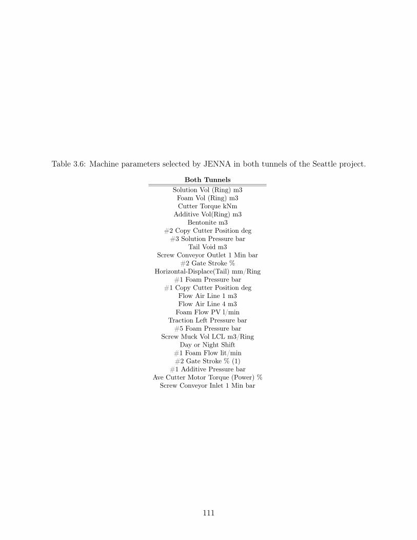
Table 3.6: Machine parameters selected by JENNA in both tunnels of the Seattle project.
Both TunnelsSolution Vol (Ring) m3Foam Vol (Ring) m3Cutter Torque kNm
Additive Vol(Ring) m3Bentonite m3
#2 Copy Cutter Position deg#3 Solution Pressure bar
Tail Void m3Screw Conveyor Outlet 1 Min bar
#2 Gate Stroke %Horizontal-Displace(Tail) mm/Ring
#1 Foam Pressure bar#1 Copy Cutter Position deg
Flow Air Line 1 m3Flow Air Line 4 m3Foam Flow PV l/min
Traction Left Pressure bar#5 Foam Pressure bar
Screw Muck Vol LCL m3/RingDay or Night Shift
#1 Foam Flow lit/min#2 Gate Stroke % (1)
#1 Additive Pressure barAve Cutter Motor Torque (Power) %
Screw Conveyor Inlet 1 Min bar
111

higher advance rates than the SB tunnel; higher advance rates can cause other issues for a
tunneling project (e.g., soil settlement and structural damage at the surface), thus, perhaps
the speed of the excavation in the SB tunnel was reduced on purpose. As a reminder, our
research goal is to understand the causes of the advance rate changes in the EPBM, not to
maximize the EPBM’s advance rate. In this section, we note the smoother operation in the
SB tunnel can be seen in most histogram figures. If a difference exists between the machine
parameter measurements in the NB tunnel and the machine parameter measurements in the
SB tunnel, it is assumed that the machine parameters in the SB tunnel produced better
results overall.
We examine two EPBM subsystems (i.e., a combination of multiple, related EPBM ma-
chine parameters) that had the clearest relationship to the advance rate in the rest of this
section. The two systems are: (1) the Ground Conditioning System (GCS) and (2) the
cutterhead movement system.
3.7.3 Ground Conditioning System (GCS)
The Ground Conditioning System (GCS) serves to lubricate the cutter tools that are
attached to the cutterface, and to change the soil consistency. Changing the soil consistency
can allow the soil to move faster through the cutterhead and into the screw conveyor; also,
changing the soil consistency assists with maintaining a steady pressure in the muck chamber
to resist earth and water pressures at the cutterhead face of the EPBM. The effects of the
GCS are often studied in laboratories [6, 7]; however, these effects are usually not studied in
real case studies. A schematic of the GCS system used in the Hitachi-Zosen EPBM can be
found in Figure 1.4.
Additives, solutions, Bentonite, and foam are individual systems that make up the liquids
used in the GCS. The GCS also contains five lines that move the GCS liquids to the front of
the cutterhead face where the GCS foam mixes with the soil. Line #1 is in the center of the
cutterhead face, and the other lines (#2 to #5) are placed at different distances from the
center of the cutterhead face; Figure 3.5 shows the locations of the GCS foam lines #1 to
112

#5 on the cutterhead face of the Hitachi-Zosen EPBM. Because the cutterhead face rotates
during excavation, the GCS lines expel the foam in circles of increasing diameter. In this
section we examine the GCS machine parameters identified as important to predicting the
EPBM’s advance rate in both tunnels.
Figure 3.5: Schematic facing the front of the EPBM, looking at the cutterhead face. Thelocations of the expelling port of the GCS foam lines are circled in red and the number ofeach line is highlighted in the red text next to the port. The line numbers are used whenidentifying GCS machine parameters.
The following machine parameters identified as important by JENNA in both tunnels
are part of the GCS:
• Solution Volume (Ring) m3
• Foam Volume (Ring) m3
• Additive Volume (Ring) m3
• Bentonite m3
• #3 Solution Pressure bar
• #1 Foam Pressure bar
113
• #1 Flow Air Line m3
• #4 Flow Air Line m3
• Foam Flow PV lit/min
• #5 Foam Pressure bar
• #1 Foam Flow lit/min
• #1 Additive Pressure bar
Figure 3.6, Figure 3.7, and Figure 3.8 show histograms of the EPBM’s measurement of
Foam Volume, Solution Volume, and Additive Volume, respectively, for both the NB and
SB tunnels. These machine parameters are counters of the total volume expelled per ring;
in other words, the volume measurements reset to zero when a new tunnel ring excavation
cycle is started and the measurement increases as the fluid is expelled in the current tunnel
ring. Because these machine parameters count the total volume of foam expelled in a tunnel
ring (i.e., the counter resets to zero at the beginning of each tunnel ring), the number of high
foam volume measurements is smaller than the number of low foam volume measurements
(as high foam volumes are only achieved at the end of the tunnel ring cycle).
The histograms shows that many zero measurements are observed, i.e., each tunnel ring
starts with a volume of 0m3. We are most interested, however, in the slope of the histograms
at each advance rate, because the slope describes the amount of foam and rate at which the
foam was used. Specifically, a steeply descending slope indicates many tunnel rings were
completed without using a lot of GCS foam; however, a shallow slope indicates many tunnel
rings were completed with a large amount of GCS foam. A shallow slope also indicates that
a large amount of GCS foam was used earlier in the tunnel ring cycle, because the high foam
volume measurement was observed for more time.
The slope of the foam volume histograms, observed in Figure 3.6, is related to the EPBM’s
advance rate. For example, in the SB tunnel (Figure 3.6(a)), the slope of the foam volume
114

(a) SB Tunnel Foam Volume (Ring) m3
(b) NB Tunnel Foam Volume (Ring) m3
Figure 3.6: Foam Volume per Ring in the NB and SB tunnels.
115

measurements (i.e., the slope before the large drop in high foam volume measurements) at
1.0 mmsec
advance rate is much shallower than the slope at 0.4 mmsec
advance rate. In the NB
tunnel (Figure 3.6(b)), a similar shallow slope is observed e.g., 1.2 mmsec
to 1.8 mmsec
advance
rate. A steep slope can also be observed in the low advance rate measurements in the NB
tunnel (i.e., 0.2 mmsec
to 1.0 mmsec
). Shallow slopes, associated with high advance rates, indicate
that more foam was applied in the tunnel ring excavation cycle than in the low advance rate
measurements.
Although the slope of the foam volume histogram bins follows a similar pattern across
the NB and SB tunnels (Figure 3.6), the NB tunnels shows several 0 m3 spikes in the low
advance rates (i.e., less than 1.2 mmsec
). As previously mentioned, the operators were learning
the soil conditions while excavating the NB tunnel and, thus, waited to see how much foam
to add when a new cycle ring was started. A clear pattern, however, of increased GCS foam
use is associated with an increased excavation rate in the NB tunnel histogram.
We observe a large spike of foam volume near an advance rate of 0.8 mmsec
in Figure 3.6(b).
This spike is observed throughout the NB tunnel data histograms, and is a result of a
monitoring well that was not removed after the geotechnical investigation was completed.
When the EPBM excavated the location of the monitoring well, a large amount of GCS
foam was expelled and created an explosive discharge of GCS foam at the surface [70]. High
advance rates occurred near the monitoring well’s location, but the high advance rates were
due to a complete break down in the composition of the soil.
The solution volume per ring histograms (Figure 3.7) exhibit an almost identical pattern
to the foam volume per ring histograms, with lower volume measurements. The identical
slopes and lower solution volumes are expected, because the solution is mixed with air to
generate the GCS foam.
The GCS additive is combined with water and added to the muck chamber to change the
consistency of the soil. Changing the consistency of the soil in the muck chamber is a good
idea when the excavated soil becomes too thick to move through the screw conveyor; however,
116

(a) SB Tunnel Solution Volume (Ring) m3
(b) NB Tunnel Solution Volume (Ring) m3
Figure 3.7: Solution Volume per Ring in the NB and SB tunnels.
117

(a) SB Tunnel Additive Volume (Ring) m3
(b) NB Tunnel Additive Volume (Ring) m3
Figure 3.8: Additive Volume per Ring in the NB and SB tunnels.
118

if the excavated soil is at the proper consistency in the muck chamber, additives should not
be used. In other words, the amount of additive used in the solution varies depending on soil
conditions. Because the GCS additive is used after the soil has been excavated, the slopes
of the additive volume histograms are similar to the foam and solution volume histograms,
but not identical. Figure 3.8 shows histograms of the GCS additive volume per ring for the
NB and SB tunnels. In the SB tunnel (Figure 3.8(a)), the slope is shallowest in advance
rates ≥ 1.0mmsec
. In the NB tunnel (Figure 3.8(b)), shallow slopes also occur at advance rates
≥ 0.8mmsec
. An increase in additive volume is associated with an increase in advance rate;
however, there are many high advance rate locations where no additive was used, indicating
another factor impacts the decision to use additive in the muck chamber. In Chapter 4
we examine an anomaly detection method to detect soil changes, as the decision to use a
different amount of additive in the muck chamber may have a time-delayed impact on the
advance rate.
We also examine the Line #1 Foam Flow measurements (see Figure 3.9), because several
features that are part of GCS Line #1 were identified as important features by JENNA
(e.g., #1 Foam Pressure (bar), Flow Air Line 1 (m3), and #1 Additive Pressure (bar)). As a
reminder, Line #1 of the GCS expels GCS foam from a port in the center of the cutterhead
face. We note the data in Figure 3.9 exhibits a different distribution than distributions of
the foam volume per ring, solution volume per ring, and additive volume per ring, because
the #1 Foam Flow is an instantaneous reading of the rate foam is flowing from the port at
the front of the cutterhead face.
The #1 Foam Flow measurements in the SB tunnel (see Figure 3.9(a)) are generally
higher than in the NB tunnel (see Figure 3.9(b)) (e.g., 150-250 liters/minute in the SB
tunnel versus 20-35 liters/minute in the NB tunnel); it, therefore, appears a higher foam
flow at the center of the EPBM resulted in a more consistent and higher advance rate in the
SB tunnel. In Figure 3.9(a), three peaks can be observed in the data: (1) a peak centered on
50 lit/min, (2) a peak centered on 175 lit/min in low advance rates, and (3) a peak centered
119

(a) SB Tunnel #1 Foam Flow (liters/minute)
(b) NB Tunnel #1 Foam Flow (liters/minute)
Figure 3.9: Line #1 Foam Flow in the NB and SB tunnels.
120

on 200 lit/min in high advance rates. In our spatial analysis of the subsurface, these peaks
indicate different foam flow rates for different soil types.
The NB tunnel (Figure 3.9(a)) also exhibits two peaks: (1) a peak near 20 lit/min and
(2) a peak near 33 lit/min. Although the foam flow is consistent within each of these peaks,
the 33 lit/min peak is associated with higher advance rates (i.e., greater than 1.6 mmsec
). In
summary, the foam flow was adjusted to soil type in both tunnels, and higher foam flow
rates were associated with higher advance rates in both tunnels. We note that the #1 Foam
Flow rate in the SB tunnel was significantly higher than in the NB tunnel, i.e., compare the
x-axes in Figure 3.9(a) and Figure 3.9(b). Because Foam Flow Line #1 is near the center of
the EPBM and the SB tunnel used a significantly higher foam flow rate than the NB tunnel,
we conclude that a higher foam flow rate at the center of the EPBM leads to a smoother
excavation environment.
3.7.4 Cutterhead Torque
Torque is the twisting force exerted by the motors to rotate the cutterhead, which loosens
the soil for excavation. We expect torque to be an important machine parameter in regard
to the EPBM’s advance rate, as higher torque should indicate soil that is more difficult
to remove. JENNA identified two torque machine parameters as important to an EPBM’s
advance rate: (1) Cutter Torque kNm and (2) Ave Cutter Motor Torque (Power) %. We
plot histograms of these parameters in Figure 3.10 and Figure 3.11.
The torque measurements in the SB tunnel (Figure 3.10(a)) are more consistent than
in the NB tunnel (Figure 3.10(b)). Although lower torque sometimes correlates with a
higher advance rate, an optimal torque level for high advance rates seems to be between
3000 and 3250 kNm in the SB tunnel. In the less consistent NB tunnel, the favored torque
measurement for high advance rates was between 2750 and 3000 kNm. The optimal torque
level can be achieved by using the GCS to condition the soil in front of the machine, and,
from our previous examination of the GCS machine parameters, expelling the GCS foam
quicker in the tunnel ring excavation cycle will allow the EPBM to reach the optimal torque
121

(a) SB Tunnel Cutter Torque (kNm)
(b) NB Tunnel Cutter Torque (kNm)
Figure 3.10: Cutter Torque in the NB and SB tunnels.
122

(a) SB Tunnel Cutter Torque (kNm)
(b) NB Tunnel Cutter Torque (kNm)
Figure 3.11: Average Cutter Motor Torque in the NB and SB tunnels.
123

conditions faster.
Figure 3.11 shows a similar torque measurement (i.e., the average cutter motor torque
power), except that the torque is measured as a percentage of maximum torque. The average
cutter motor torque is similar to cutter torque (i.e., lower torque sometimes results in a higher
advance rate, and an optimal torque point exits). In the SB tunnel, the optimal torque is near
50% and in the NB tunnel the optimal torque is near 55%. The NB tunnel contains spikes
in the number of measurements near 30% average cutter motor torque, when the EPBM was
moving at a moderate advance rate (around 1.0 mm/sec). Although the EPBM operated at
30% torque for many measurements, the 55% torque allowed higher advance rates; however,
this higher torque may have placed additional stress on the cutter bits, causing the bits to
wear faster.
3.8 Conclusions
Our work created and tested a new ensemble feature selection method (JENNA) that
outperformed the state-of-the-art feature selection method (Saeys). JENNA was created
to improve performance (i.e., decrease bias, decrease variance, and increase stability) in the
features selected by feature selection ensembles when applied to data sets with large numbers
of examples and features; previous methods, on the other hand, focused on data sets with
large numbers of features and a small number of examples. When applied to the data sets
from the Seattle project, JENNA identified features that trained an OLS V-MLA with a
statistically significantly lower or equal RMSE (i.e., bias) than previous methods, and, in
addition, stability increased to perfect stability. We, therefore, conclude that JENNA is a
better ensemble feature selection method for our data set type.
We also performed a comprehensive analysis of the machine parameters identified by
JENNA and how those machine parameters relate to the advance rate of the EPBM. In the
NB tunnel an increase in the ground conditioning foam expelled led to an increase in the
advance rate of the EPBM. The optimal amount of ground conditioning foam is dependent
on the soil type that the EPBM is excavating (e.g., hard, stiff clay requires more ground
124

conditioning foam than sandy, silty soil). A consistent, high level of foam applied early in
the tunnel cycle results in a more consistent, high advance rate. We also found an optimal
torque point (near 50% of the available torque in the cutterhead face motors) for achieving
a consistent, high advance rate.
125
CHAPTER 4
TIME DELAYED DATA
In our prior work we identified several EPBMmachine parameters that affect the EPBM’s
advance rate in a delayed manner. An example of a time-delayed feature within an EPBM is
soil pressure in the EPBM’s screw conveyor. As a reminder, the screw conveyor is attached
to the EPBM’s muck chamber, and the screw conveyor and muck chamber work together
to balance the soil and water pressure at the EPBM’s cutterface preventing soil collapse in
front of the EPBM. In Chapter 3, JENNA identified the soil pressure sensors at the inlet
and outlet of the screw conveyor as important features in predicting the EPBM’s advance
rate; furthermore, JENNA did not identify any soil pressure sensors at the cutterface or in
the muck chamber. We believe the soil pressure sensors in the screw conveyor were identified
because it takes time for changes in the soil pressure to propagate through the muck chamber
and into the screw conveyor. In other words, JENNA highlighted a time-delayed feature as
important to predicting the advance rate of the EPBM. In this chapter, we utilize state-of-
the-art machine learning techniques to account for time-delays in the EPBM data set and
increase our understanding of EPBMs.
Based on JENNA identifying time-delayed features as important in predicting an EPBM’s
advance rate, we apply deep learning methods (specifically Recurrent Neural Networks
(RNNs)) to further our understanding of how EPBM systems impact EPBM performance.
RNNs are modified ANNs (further discussed in Section 4.1). An intuitive method of utilizing
ANNs for feature selection is to weight input features based on the ANN’s weighted con-
nections; however, the weighted connections within the network are not deterministic (i.e.,
similar prediction performance can be achieved with different weights). Since it is impossible
to determine important features from applying time-delayed methods, we seek to identify
another important EPBM performance parameter: the location of changes in the soil type
126

at the front of the EPBM.
Based on our prior work, changes in the soil type at the front of the cutterface causes
changes to several EPBM machine parameters; therefore, we identify soil type changes by
creating a novel, anomaly detection algorithm that can be applied to data sets with a known
time-delay between changes to input features and resulting changes to output target values.
Our method (Recurrent Neural Network Anomaly Detection (ReNN AnD)) trains RNNs
with the current time sequence and then tests the trained RNN with the next time sequence,
marking spikes in the testing error as anomalies. The intuition behind ReNN AnD is that
RNN will achieve a steady prediction state in the current soil type and then the prediction
error will spike as the EPBM enters a different soil type and the EPBM machine parame-
ters change. ReNN AnD is designed to be used as an online anomaly detection algorithm;
therefore, ReNN AnD does not require the entire data set to identify anomalies. We are not
aware of any other work that utilizes RNNs for anomaly detection.
4.1 Deep Learning
An emerging machine learning field is representation learning, often called deep learning.
The purpose of deep learning is to make Machine Learning Algorithms (MLAs) less depen-
dent on input feature creation by crafting MLAs that are better representations of how the
human brain thinks [71]. Our work applies Recurrent Neural Networks (RNNs), which are
modified Artificial Neural Networks (ANNs) that contain a backwards or recurrent connec-
tion. In time-delay problems, the recurrent connection allows error signals from previous
time steps to affect the current weighted ANN connections. Backpropagation Through Time
(BPTT) is a common algorithm that allows an ANN containing recurrent connections to be
trained [72]. Recurrent connections do add, however, two major problems when training the
RNN with conventional BPTT: (1) if BPTT is used with more than a few (i.e., ≥ 10) prior
time steps, the processing time is intractable and (2) BPTT introduces the vanishing (or
exploding) gradient problem.
127
The exploding or vanishing gradient problem occurs because BPTT combines error flow
from all time steps through multiplication. If there are no limits on the magnitude of the
error flow, one time step with a very small or very large error flow can cause the gradient
(used to adjust the connection weights) to disappear or explode, respectively.
4.1.1 Long Short-Term Memory (LSTM)
Hochreiter and Schmidhuber [73] proposed Long Short-Term Memory (LSTM) as an
alternative to BPTT, in order to train an RNN without the two previously discussed dis-
advantages of BPTT. Specifically, the vanishing (or exploding) gradient problem is handled
through the application of a Constant Error Carousel (CEC). We detail the parts of an
LSTM memory cell, discuss conventional BPTT, show how CEC modifications attempt to
solve BPTT’s vanishing (or exploding) gradient problem, and, finally, show how LSTM solves
new problems introduced by CEC.
Figure 4.1 illustrates a common configuration of an LSTM memory cell, which is part
of the memory cell layer of an RNN (i.e., the hidden layer). We discus Figure 4.1 in the
following paragraphs.
In Figure 4.1, j represents all non-output layer nodes (i.e., neurons in the input layer
or hidden layer(s)), circles g, h, l, and m are nodes containing differentiable activation
functions (any combination of activation functions may be used), cj is the memory cell (i.e.,
the rectangular box), scj(t) is the “internal state” or “memory” of the memory cell at time
t, w = 1 represents the constant CEC weighted connection, netinjand netoutj represent the
activation value of input and output gates from other memory cells, respectively, and arrows
represent weighted connections showing the direction the activation signal flows during the
feed-forward phase. We note that Figure 4.1 illustrates an example network configuration
and not all weighted connections are mandatory.
The input and output gates are defined as gain and gaout, respectively. The input gates
restrict signals from input perturbations, and the output gates restrict the contribution of
the memory cell to the nodes in the next layer (in cases where the memory cell would increase
128
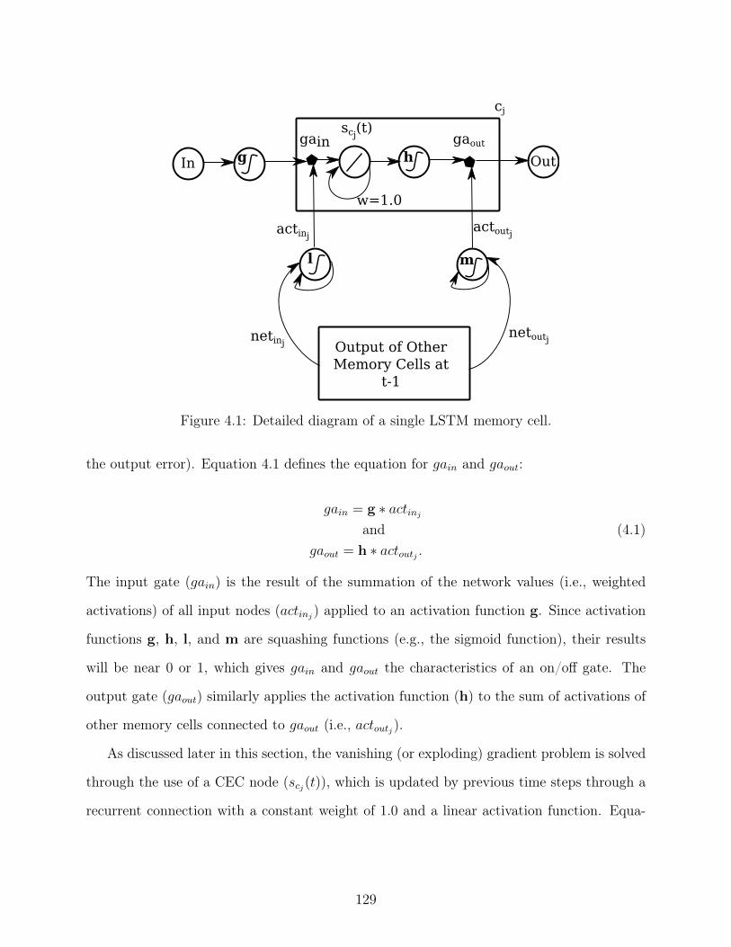
g
ml
In Outh
gainscj
(t)gaout
Output of Other
Memory Cells at
t-1
w=1.0
netoutjnetinj
cj
actinjactoutj
Figure 4.1: Detailed diagram of a single LSTM memory cell.
the output error). Equation 4.1 defines the equation for gain and gaout:
gain = g ∗ actinj
andgaout = h ∗ actoutj .
(4.1)
The input gate (gain) is the result of the summation of the network values (i.e., weighted
activations) of all input nodes (actinj) applied to an activation function g. Since activation
functions g, h, l, and m are squashing functions (e.g., the sigmoid function), their results
will be near 0 or 1, which gives gain and gaout the characteristics of an on/off gate. The
output gate (gaout) similarly applies the activation function (h) to the sum of activations of
other memory cells connected to gaout (i.e., actoutj).
As discussed later in this section, the vanishing (or exploding) gradient problem is solved
through the use of a CEC node (scj(t)), which is updated by previous time steps through a
recurrent connection with a constant weight of 1.0 and a linear activation function. Equa-
129

tion 4.2 shows the specific implementation of an CEC node inside an LSTM memory cell:
scj(t) = scj(t− 1) + actinj(t− 1) ∗ gain(t), (4.2)
where the previous time step’s activation (scj(t − 1)) is added to the internal state at the
current time step (scj(t)) if the in gate (gain(t)) is greater than 0. We note that if gain(t) is
less than 1 and greater than 0, only a portion of the previous time step’s internal state will
be added to the current time step’s internal state (e.g., if gain(t) = 0.95, only 95% of the
previous time step’s activation will be added to the current time step’s activation).
RNNs are ANNs modified by adding recurrent connections (i.e., weighted connections
that move in the opposite direction of traditional ANN weighted connections) so that signals
from prior time steps can impact the current time step. To train an RNN, BPTT modifies
ANN’s traditional backpropagation equations to include error signals from the recurrent
connections. Equations 4.3 and 4.4 describe how BPTT computes the backpropagation
error signal in output and hidden nodes, respectively. Equation 4.3 assumes an RNN with
one output node.
δk(t) = f ′k(netk(t))(dk(t)− yk(t)),defined by
acti(t) = fi(neti(t)),
and
neti(t) =∑j
wijactj(t− 1).
(4.3)
In the first portion of Equation 4.3, δk(t) is the error signal of node k at time t, k is the
output node, f ′k is the derivative of the activation function of node k (typically the sigmoid
function in classification problems or linear identity function in regression problems), netk(t)
is the sum of the activation of all nodes with a weighted connection to node k from the prior
time step (i.e., all connections from the hidden layer), dk(t) is the measured output target
value for the example, and yk(t) is the output value of node k at time t. In the second
portion of Equation 4.3, acti(t) is the output (i.e., activation) of any non-input node i and
130

fi is the differentiable activation function of node i8. In the third part of Equation 4.3, neti
is the output value (i.e., activation) of all input nodes connected to node i, j is a non-output
node, wij is a weighted connection from node i to nodej, and actj(t− 1) is the activation of
node j at time t− 1. In words, Equation 4.3 computes the error signal of the output node’s
recurrent connections to the hidden nodes (i.e., the memory cell layer in LSTM).
Nodes that are not the output node are updated in a similar manner; however, the error
term (dk(t) − yk(t)) in Equation 4.3 is replaced with the error flow from the output node
back to the non-output nodes (j). Equation 4.4 provides the BPTT error flow equation:
δj(t) = f ′j(netj(t))∑i
wijδi(t+ 1), (4.4)
where δj(t) is the error flow of non-output node j at time t, netj(t) is the sum of the activation
of all connected nodes at time t− 1 multiplied by the connection weight, wij is the weight of
the connection from node i to node j, and δi(t+ 1) is the error flow of connected, non-input
node i at time t+ 1.
Equation 4.3 and Equation 4.4 comprise the BPTT cycle that allows output values from
prior time steps to impact the RNN connection weights in the current time step. When
BPTT is scaled to multiple time steps, the error flows (δk(t) and δj(t)) become the product
of multiple time steps instead of only t−1. If there are no limits on the magnitude of the error
flow, one time step with a very small or very large error flow can cause the gradient (used
to adjust the connection weights) to disappear or explode, respectively. CEC restricts the
error flow from Equation 4.4 by adding a constraint to Equation 4.4 shown in Equation 4.5
f ′j(netj(t))wjj = 1.0, (4.5)
where f ′j is the derivative of node j’s activation function, netj(t) is the activation of the
recurrent connections to node j at time t − 1, and wjj is the constant weight from node j
to itself. Due to the constraint in Equation 4.5, wjj must be 1.0 and node j’s activation
function must be linear. We note that the 1.0 weight constraint on wjj leads to the name
8Because i represents any non-input node and k represents the output node, the i terms in the second partof the equation can be replaced with k terms.
131

“Carrousel” in Constant Error Carrousel (CEC).
CEC eliminates the exploding (or vanishing) gradient problem and is implemented in
LSTM as scj(t) in Figure 4.1. A second problem with CEC arises from many time step,
time-delayed patterns. Given a non-output node j, node j may contribute to reducing the
output error at some time steps, but may increase error at other time steps. In an ideal
network, an on/off switch would be placed at the output connection of node j to prevent
node j from increasing the error when input example perturbations would cause node j to
increase the error. A similar switch would be placed at the input connection to node j
as well. LSTM implements the input and output switches through the use of additional
neurons, which are contained within the memory cell. Figure 4.1 (see the pentagons labeled
gain and gaout) illustrates an example LSTM memory cell within a memory cell hidden layer.
Finally, LSTM implements truncated backpropagation so that no error flows will leave the
memory cell.
4.1.2 Generalized Long Short-Term Memory (LSTM-g)
Monner and Reggia [74] improved the original LSTM algorithm to allow LSTM to be
applied to second-order network architectures; the improved algorithm is called Generalized
Long Short-Term Memory (LSTM-g). A limitation of LSTM is that it must use truncated
backpropagation in order for LSTM to work across very long time lags (i.e., the error signal
from previous time steps is blocked from entering or leaving the memory cell). The truncation
prevents the error signal from transmitting between memory cells, which prevents the error
signal from getting caught in a loop that would affect the memory cells throughout time.
Truncating the backpropagation error signal causes a condition where only one hidden layer
can be trained in an RNN, because additional hidden layers would not receive the error
signal to adjust the weights of their connections.
Figure 4.2 shows the difference between LSTM and LSTM-g. In Figure 4.2(a), the input
and output gates are connected to the modulated signal within the memory cell; in other
words, the input gate either allows all input signals into the memory cell or no inputs into
132

(a) LSTM (b) LSTM-g
Figure 4.2: Comparison of the LSTM memory cell architecture to the LSTM-g memory cellarchitecture. The circles represent artificial neurons and the symbol within a given circlerepresents an expected activation function (e.g., a straight line represents a linear activationfunction and a curved line represents a squashing function). The solid black lines representweighted connections from other neurons. The gray lines represent on/off switched (or gated)connections. Figures are copyrighted material reproduced with permission from [74] underlicense number 3562570486445.
the memory cell. Similarly, the output gate allows all output signals to leave the memory
cell or no output signal to leave the memory cell. In Figure 4.2(b) the individual connections
into the input gate are modulated by the input gate9; therefore, some input connections can
be turned on while other input connections are turned off. A similar configuration on the
output gate allows some output connections to be turned on and other output connections to
be turned off. The modulation of the individual connections by the input and output gates
allows the error signals to be backpropagated through multiple layers instead of truncating
9In LSTM the input connections are summed and then modulated by the input gate, creating an all ornothing situation.
133

(i.e., removing) the error signal when it leaves the memory cell. Allowing error signals to
leave the memory cells, in turn, allows training of multiple memory cell layers in serial.
Multiple, serial memory cell layers allows for more complex time delayed functions to be
modeled by the RNN, potentially decreasing the RNN’s error. Our work utilizes Monner
and Reggia’s implementation of LSTM-g [75] to train and test the RNNs used in ReNN
AnD.
4.2 Proposed Method
We propose the RNN Anomaly Detection (ReNN AnD) method for detecting anomalies
in systems where input features have a time-delayed impact on the output target value.
ReNN AnD is implemented in three steps:
1. calibrate the RNN to the data set (Section 4.2.1),
2. determine a testing error threshold (Section 4.2.2), and
3. detect anomalies (Section 4.2.3).
4.2.1 Calibrate the RNN to the Data set
As previously discussed, the RNNs we implement for our work are trained and tested
using Monner and Reggia’s LSTM-g algorithm [74] (implemented as XLBP [75]). As with
most machine learning algorithms, several parameters of the algorithm need to be calibrated
to the current data set. The following RNN parameters are calibrated:
• the number of memory cells and
• the sequence length (i.e., the number of measurements used to recurrently train the
RNN).
Our work implements RNN as an online tool; therefore, we must also consider a start
up period. The start up period is the number of measurements used to calibrate the RNN’s
134

parameters; clearly we want to find the shortest start up period possible. Algorithm 4.1
calibrates the RNN during the start up period.
Algorithm 4.1: ReNN AnD Calibration Algorithm
class ReNNAnDCalibration {//Memory Ce l l s (mc)int mc [ ] = mcStart . . . mcStep . . . mcStop ;
//Sequence Lengths ( seq )int seq [ ] = seqSta r t . . . seqStep . . . seqStop ;//Best mc and seq l e n g t h s
int bestMC ;int bestSEQ ;// Var iab l e to t rack the b e s t c on f i g u r a t i on ’ s t e s t e r rorbestTestError double = 9999 ;
ReNNAnDCalibrate ( ) {for ( int curMc : mc) {
for ( int curSeq : seq ) {//Data c l a s s de f ined a f t e r ReNNAnDCalibration c l a s s
double [ ] [ ] trainDataX = Data . getCalibTrainDataX ( seq ) ;double [ ] [ ] testDataX = Data . getCalibTestDataX ( seq ) ;double [ ] trainDataY = Data . getCalibTrainDataY ( seq ) ;double [ ] testDataY = Data . getCalibTestDataY ( seq ) ;
//RNN c l a s s i s implemented in XLBPrnn = new RNN(mc, seq ) ;rnn . t r a i n ( trainDataX , trainDataY ) ;
double curTestError = rnn . t e s t ( testDataX , testDataY ) ;i f ( curTestError < bestTestError ) {
ReNNAnDCalibration . bes tTestError = curTestError ;ReNNAnDCalibration . bestMC = mc ;ReNNAnDCalibration . bestSeq = seq ;} //End i f
}// end seq f o r loop}// end mc fo r loop
}// end ReNNAnDCalibrate ( )
int getBestMC ( ) {return bestMC ;
}// end getBestMC
int getBestSEQ ( ) {return bestSEQ ;
}// end ge tBes tSeq}//end c l a s s ReNNAnDCalibration
135

class Data{int numExamples ; //Number o f examples in fu l lDataX and fu l lDataYint numInFeatures ; //Number o f input f e a t u r e s in fu l lDataX
// Fu l l data s e t updated from data stream .fu l lDataX double [ ] [ ] = new double [ numExamples ] [ numInFeatures ] ;fu l lDataY double [ ] = new double [ numExamples ] ;
//Define func t i on : System . arraycopy (// src : source array ,// srcPos : index in src array to s t a r t copying from ,// de s t : d e s t i n a t i o n array ,// destPos : index in de s t array to s t a r t copying to ,// l en g t h : how many array e n t r i e s to copy )
double [ ] [ ] getCalibTrainDataX ( int seqLength ) {//Copies the f i r s t 66% of seqLength examples in fu l lDataX in to a//new arrayint returnLength66 = Math . f l o o r ( seqLength ∗ 0 . 66 ) ;double [ ] [ ] returnArray = new double [ returnLength66 ] [ numInFeatures ] ;
//Copy po s i t i o n 0 to returnLength66 from fu l lDataX in to// returnArray and re turn .for ( int i =0; i<returnLength66 ; i++){
System . arraycopy (Data . ful lDataX [ i ] , 0 , returnArray [ i ] , 0 ,numInFeatures ) ;
}}//end getCalibTrainDataX
double [ ] [ ] getCalibTestDataX ( int seqLength ) {//Copies the l a s t 34% seqLength examples in fu l lDataX in to a//new arrayint returnLength66 = Math . f l o o r ( seqLength ∗ 0 . 66 ) ;int returnLength34 = seqLength − returnLength66 ;double [ ] [ ] returnArray = new double [ returnLength34 ] [ numInFeatures ] ;//Copy po s i t i o n returnLength66 to seqLength−1 from fu l lDataX to// returnArray and re turn .for ( int i = 0 ; i<returnLength34 ; i++){
System . arraycopy (Data . ful lDataX [ returnLength66+i ] , 0 ,returnArray [ i ] , 0 , numInFeatures ) ;
}}//end getCal ibTestDataX
double [ ] getCalibTrainDataY ( int seqLength ) {//Copies the f i r s t 66% seqLength examples in fu l lDataY in to a//new array
136

int returnLength66 = Math . f l o o r ( seqLength ∗ 0 . 66 ) ;double [ ] returnArray = new double [ returnLength66 ] ;System . arraycopy (Data . ful lDataY , 0 , returnArray , 0 , returnLength66 ) ;return returnArray ;
}//end getCalibTrainDataY
double [ ] getCalibTestDataY ( int seqLength ) {//Copies the l a s t 34% seqLength examples in fu l lDataY in to a//new arrayint returnLength66 = Math . f l o o r ( seqLength ∗ 0 . 66 ) ;int returnLength34 = seqLength − returnLength66 ;double returnArray = new double [ returnLength34 ] ;System . arraycopy (Data . ful lDataY , returnLength66 , returnArray , 0 ,
returnLength34 ) ;return returnArray ;
}//end getCal ibTestDataY
void s e t fu l lDataX (double [ ] [ ] dataIn ) {Data . ful lDataX = dataIn ;
}//end s e t f u l lDa taX
void s e t fu l lDataY (double [ ] dataIn ) {Data . ful lDataY = dataIn ;
}//end s e t f u l lDa taY
double [ ] [ ] getSequenceDataX ( int s eqPos i t i on , int seqLength ) {double [ ] [ ] returnArray = new double [ seqLength ] [ numInFeatures ] ;r e turnArrayPos i t i on = 0 ;for ( int i =( s eqPos i t i on ∗ seqLength )−1; i <( s eqPos i t i on +1) ∗ seqLength ;
i++){System . arraycopy ( ful lDataX [ i ] , 0 , returnArray [ r e turnArrayPos i t i on ] ,
0 , numInFeatures ) ;r e turnArrayPos i t i on++;
}// end i f o r loopreturn returnArray ;
} //end getSequenceDataX
double [ ] getSequenceDataY ( int s eqPos i t i on , int seqLength ) {double [ ] returnArray = new double [ seqLength ] ;System . arraycopy (Data . ful lDataY , ( s eqPos i t i on ∗ seqLength )−1,
returnArray , 0 , seqLength ) ;return returnArray ;
}//end getSequenceDataY}//end c l a s s Data
We train each RNN on the first 66% of the data set (of sequence length defined in the
array seq, which is the start up period) and then test the RNN on the remaining 34% of
137

the data. We split the training and testing data to (1) prevent overfitting by not testing
the RNN using training data and (2) increase calibration speed over cross validation. The
memory cell (bestMC) and sequence length (bestSEQ) combination that produces the lowest
error (e.g., RMSE) is then chosen as the RNN configuration for the rest of the data set.
4.2.2 Anomaly Thresholding
Anomaly Detection commonly relies on two assumptions: (1) the examined data follows
a normal (i.e., Gaussian) distribution and (2) an approximate likelihood of anomalies is
known for the given data set [43]. In continuous data sets, common anomaly thresholds are
µ ± σ, µ ± 2 ∗ σ, µ ± 3 ∗ σ, etc., where µ is the mean of the data and σ is the standard
deviation of the data. The approximate number of anomalies one expects in the data set
determines the σ multiplier (i.e., the less sensitive the anomaly detection, the greater the σ
multiplier). The ReNN AnD Thresholding Algorithm (Algorithm 4.2) maintains the mean,
standard deviation, and threshold of the error as data is applied to the algorithm.
Algorithm 4.2: ReNN AnD Thresholding Algorithm
class ReNNAnDThresholding{LinkedList<double> yErro rL i s t = new LinkedLis t ( ) ;int stdDevConst ;
double ReNNAnDThresh(double yCurrentError ) {yErro rL i s t . add ( yCurrentError ) ;mean = Math . mean( yErro rL i s t ) ;stdDev = Math . stdDev ( yErro rL i s t ) ;th r e sho ld = mean + ( stdDevConst ∗ stdDev ) ;return th r e sho ld ;}// end ReNNAnDThresh( )
}//end c l a s s ReNNAnDThresholding
The threshold algorithm recomputes the mean and standard deviation of the data set at
each time step. The threshold that is returned to the ReNN AnD algorithm is determined by
the current mean and of the data set plus the standard deviation of the data set multiplied
by the standard deviation constant. The anomaly detection algorithm (Algorithm 4.3) then
138

marks the testing sequence as an anomaly if the sequence’s testing error is greater than the
threshold returned from Algorithm 4.2.
4.2.3 Anomaly Detection
The anomaly detection portion of Algorithm 4.3 trains a calibrated RNN using the inputs
{xs,ys} and then tests the trained RNN using the inputs {xs+1,ys+1}. {xs,xs+1} are each
m by n matrices (where m is the sequence length and n is the number of input features),
s represents the sequence number, and {ys,ys+1} are output target vectors of length m.
If the testing error (from applying the trained RNN to {xs+1,ys+1}) exceeds the anomaly
threshold, then ReNN AnD marks sequence s + 1 as a detected anomaly. Algorithm 4.3
defines the ReNN AnD anomaly detection algorithm. We note that Algorithm 4.3 uses the
class Data, which is defined in Algorithm 4.1.
Algorithm 4.3: ReNN AnD Anomaly Detection Algorithm
class ReNNAnDAnomalyDetect{
void main ( St r ing [ ] a rgs ) {// E s t a b l i s h a data connect ionDatabaseConnector onl ineData = new DatabaseConnector ( ) ;onl ineData . connect ( ) ;
// E s t a b l i s h Alarm to t r i g g e r when an anomaly i s d e t e c t e d .AlarmStream alarm = new AlarmStream ( ) ;
// Ca l i b r a t e the RNNReNNAnDCalibration . ReNNAnDCalibrate ( ) ;bestMC = ReNNAnDCalibration . getbestMC ( ) ;bestSEQ = ReNNAnDCalibration . getbestSEQ ( ) ;
//Track curren t sequence numberint current_s = 0 ;
while ( true ) { // I n f i n i t e loop f o r on l ine a l gor i thm//Populate Data c l a s s wi th on l ine database dataData . s e t fu l lDataX ( onl ineData . pullDataX ( ) ) ;Data . s e t fu l lDataY ( onl ineData . pullDataY ( ) ) ;//RNN c l a s s i s implemented in XLBPrnn = new RNN(bestMC , bestSEQ) ;
139

//Get t r a i n i n g and t e s t i n g data from Data c l a s sdouble [ ] [ ] trainDataX = Data . getSequenceX ( current_s , bestSEQ) ;double [ ] trainDataY = Data . getSequenceY ( current_s , bestSEQ) ;double [ ] [ ] testDataX = Data . getSequenceX ( current_s + 1 , bestSEQ) ;double [ ] testDataY = Data . getSequenceY ( current_s + 1 , bestSEQ) ;rnn . t r a i n ( trainDataX , trainDataY ) ;double t e s tE r r o r = rnn . t e s t ( testDataX , testDataY ) ;double th r e sho ld = ReNNAnDThresholding .ReNNAnDThresh( t e s tE r r o r ) ;i f ( t e s tE r r o r > thre sho ld ) {
alarm . t r i g g e r ( current_s+1) ;}current_s++;
}// end wh i l e loop}//end main
}//end c l a s s ReNNAnDAnomalyDetect
4.3 ReNN AnD Application Experiment
Our ReNN AnD algorithm provides an anomaly detection method for data sets that
contain a time-delay (i.e., a delay between when an input feature value changes and when
the change affects the output target value). In order to experimentally validate our method,
we apply ReNN AnD to data sets with known time delays between changes in input feature
values and changes in output target values. Specifically, we apply ReNN AnD to the two
Seattle project data sets described in Chapter 1. We use ReNN AnD to identify changes in
the type of soil that the EPBM is excavating, and we compare the location of ReNN AnD’s
detected soil changes to the estimated position in the Geotechnical Baseline Report (GBR)
soil map. Because soil changes are estimated by drilling boreholes (i.e., small soil samples)
at largely spaced intervals, the true position of a soil change is estimated. Identifying the
true position of these soil changes with ReNN AnD will allow tunneling contractors to make
adjustments to the EPBM (in real-time); the EPBM will then excavate more efficiently,
saving project time and costs.
4.4 Experimental Results
Our experiment calibrated RNN parameters for the Seattle project data, trained the
calibrated RNNs on the Seattle project data, and detected anomalies (i.e., soil changes) for
140

the length of the Seattle project in both the NB and SB tunnels. ReNN AnD was applied to
the Seattle project data after the Seattle project was completed; however, the data set was
simulated as an online data set (i.e., the entire data set was not available to ReNN AnD as
the algorithm executed).
In order to determine if ReNN AnD is correctly detecting soil type changes, we compare
the location of the ReNN AnD identified soil type changes to the GBR, which was created
prior to excavation of the tunnels. This report is created by geotechnical engineers who drill
boreholes along the planned route of the tunnel. Soil samples are taken from the boreholes,
and then the engineers create a predicted map of the subsurface based on these soil samples
(i.e., the GBR soil map); we will see these maps for the Seattle project in Section 4.4.2. We
note that the same map is used for both tunnels, because the tunnels were excavated parallel
to each other.
4.4.1 Calibration Results
We varied the number of memory cells in the RNN’s memory cell layer, as well as the
length of the break-in period. We worked to determine the best number of RNN memory
cells without using an excessive amount of data to calibrate the RNN; that is, a smaller
break-in period means ReNN AnD can start detecting anomalies sooner. Varying the length
of the break-in period in Figure 4.3 and Figure 4.4 shows the local error minimum that is
selected as the RNNs’ configuration.
In both the NB and SB tunnels, we tested 50 to 1,000 memory cells (stepping by 25 mem-
ory cells), and sequence lengths of 50 to 500 examples (stepping by 50 examples). Figure 4.3
and Figure 4.4 graph the Root Mean Squared Error (RMSE) of the five best performing
(i.e., lowest RMSE) memory cell configurations in the NB and SB tunnels, respectively.
Equation 4.6 shows the equation we used to compute the RMSE for a given sequence:
RMSE =
√√√√ 1
m
m∑i=1
(yi − yi)2, (4.6)
141

where m is the number of examples in the sequence (i.e., the sequence length), yi is the
measured output target value (i.e., advance rate), and yi is the RNN predicted output target
value. We determine the number of examples to classify as the break-in period by looking
for the lowest RMSE after the RNN’s RMSE has stabilized.
Figure 4.3: Graph of the RMSE of varying memory cells and break-in data lengths in theNB tunnel.
In Figure 4.3, a large error (i.e., RMSE) spike occurs around 250 examples. The large
RMSE variance is caused by the EPBM operator making changes to the EPBM’s system
as the operator becomes accustomed to a new tunneling project and a new EPBM. These
variations were expected, and led us to measure various break-in periods to determine RNN
configuration stability. In the NB tunnel, Figure 4.3 shows the lowest RMSE is achieved
with an RNN memory cell layer consisting of 775 memory cells and a break-in length of 350
examples. We calibrate the RNN parameters with these values since 350 examples is after
the break-in period.
142

Figure 4.4: Graph of the RMSE of varying memory cells and break-in data lengths in theSB tunnel.
Figure 4.4 illustrates the RMSE when calibrating for the SB tunnel data set. Unlike the
NB tunnel, a spike in RMSE does not occur early in the tunneling process, likely because the
EPBM operator is more accustomed to the soil in the Seattle project. The error is minimized
with an RNN memory cell layer consisting of 325 memory cells and 100 examples. We note
that the y-axis in Figure 4.4 is a different scale than the y-axis in Figure 4.3, and shows the
lower variance at the beginning of the SB tunnel. Because variability in the RNN’s RMSE
is stabilized from the beginning onward, we pick the lowest RMSE: 100 examples and 325
memory cells.
4.4.2 Soil Detection Results
We discuss ReNN AnD’s detected soil change locations compared to the GBR’s predicted
soil change locations. We reference locations in the GBR predicted soil maps as chainage,
which is a measurement used in tunneling projects; one chainage unit represents one linear
foot. The excavation began at chainage 108,200 and continued to 104,600.
143

ReNN AnD identified several locations along the tunnel path where likely soil changes
(i.e., anomalies) occurred. It is impossible to identify the exact locations of soil changes,
because the front of the EPBM is pressurized; that is, humans cannot enter the front of the
EPBM to measure the soil (without costly and dangerous techniques to retract the EPBM
cutterhead face). As previously discussed, however, the Geotechnical Baseline Report (GBR)
contains a map of predicted soil types along the tunnel path based on pre-construction
testing. Figure 4.5, Figure 4.6, and Figure 4.7 can be combined to show the GBR soil map
for the tunnels in the Seattle project. We compare ReNN AnD’s detected soil change points
to the locations of soil changes predicted by the GBR soil map. Specifically, we marked
ReNN AnD’s detected soil change locations with a red vertical line in Figure 4.5, Figure 4.6,
and Figure 4.7. We analyze some of these locations in the following discussion.
Figure 4.5 shows a soil change detection across both tunnels at 107,800 chainage (i.e, the
4th red line from the right in the NB tunnel and the 3rd red line from the right in the SB
tunnel). We note that (1) this soil detection is in the middle of a homogeneous soil region
(i.e., the tan region) and (2) the soil change was not predicted in the GBR. The drilled
boreholes are marked as vertical black lines in the GBR soil map, and Figure 4.5 shows
that the transition from tan soil type to purple soil type is estimated to be exactly halfway
between the two boreholes at about chainage 107,800 and 107,650. In other words, ReNN
AnD concludes that the soil change occurs much earlier than the GBR predicted (i.e, almost
immediately after the 107,800 borehole). The NB and SB results from ReNN AnD match in
other homogeneous soil areas in the GBR as well. For example, a soil change detection can
also be seen at 108,000 chainage (i.e., the second line from the right in both tunnels), and
in Figure 4.7 at 104,900 chainage (i.e., the second line from the left in both tunnels).
Figure 4.6 shows a soil detection point at 107,000 chainage (i.e., the first line from the
right in both tunnels). At this soil change detection point, the GBR soil map expects the
EPBM to transition from the light blue soil type to a mixed soil type (containing the light
blue soil type and the light purple soil type). ReNN AnD detected this transition at the
144

GBR predicted location in both tunnels. For more locations where ReNN AnD detected soil
changes in both tunnels as expected by the GBR soil map, see 106,800 chainage in Figure 4.6
(i.e., the third line from the right in the NB tunnel and the 2nd line from the right in the
SB tunnel), 106,000 chainage in Figure 4.6 (i.e., the first line from the left in both tunnels),
and 105,850 chainage in Figure 4.7 (i.e., the first line from the right in both tunnels).
Figure 4.7 shows a soil detection point at 105,400 chainage in the NB tunnel and 105,300
chainage in the SB tunnel (i.e., the fourth line from the right in the NB tunnel and the
second line from the right in the SB tunnel). These two soil change detection points are near
a GBR predicted soil change location, i.e., the soil change from mixed soil (light blue and
light purple) to dark purple soil. We believe the discrepancy in detection position is due to
the knowledge of the EPBM operator gained while excavating the NB tunnel. In the NB
tunnel, the EPBM operator was unfamiliar with the project; therefore, the operator reacted
to the soil change. However, in the SB tunnel, the EPBM operator was more familiar with
the project and, therefore, was able to make changes to the EPBM machine parameters in
anticipation of the soil change. The EPBM operator’s anticipatory behavior can also be
observed in Figure 4.5 at 107,700 chainage in the NB tunnel and 107,625 chainage in the SB
tunnel (i.e., the fifth line from the right in the NB tunnel and the fourth line from the right
in the SB tunnel).
The absence of soil change detection points also indicates ReNN AnD is properly detecting
no soil changes. For example, Figure 4.7 shows, from approximately chainage 105,300 to
105,000 chainage (in both tunnels), a homogeneous soil region; thus, ReNN AnD makes
no soil change detections (after the transition into the dark purple soil type). A detection
does occur at 105,000 chainage in both tunnels; we believe this detection is associated with
the light blue soil seam. Also, Figure 4.5, from approximately chainage 107,180 to 107,000,
shows another homogeneous light blue soil region with no soil detections in either tunnel.
A few of the soil detection points by ReNN AnD did not make sense. For example,
in Figure 4.6 at 106,600 chainage (i.e., the fourth line from the right in the NB tunnel), a
145

soil change was detected in the NB tunnel, but not in the SB tunnel. Upon consulting the
project review [70], we determined that the soil change detection in the NB tunnel was due
to irregular movements of the machine that occurred because the EPBM hit a monitoring
well that was not properly capped. These irregular readings then caused ReNN AnD to
trigger a soil change detection, even though a soil change did not exist.
The GBR soil map is a predicted soil map and, thus, may not be completely accurate.
We conclude that ReNN AnD is detecting soil changes because of three observations: (1)
most soil change detections are located near the beginning of a soil change region shown on
the GBR soil map, (2) the soil change detection points in the NB and SB tunnels are similar
even though these data sets are very different, and (3) there are few detections in the GBR
predicted homogeneous soil regions. Accurately detecting these soil changes, especially as a
tunneling contractor is starting on a new project, can assist with correct EPBM configuration
for the soil type, which then increases EPBM efficiency.
4.5 Conclusions
The main contribution of our work in this chapter is a novel anomaly detection algorithm
(ReNN AnD) that can be applied to anomaly detection in data where a time-delay exists
between changes in the input feature values and when these changes affect the output target
value. Another contribution of our work is providing a tool for EPBM tunneling contractors
to detect soil changes as an EPBM excavates and constructs an underground tunnel in
real-time.
We implemented and applied ReNN AnD to two time-delayed data sets from the Seattle
project, and detected soil changes (i.e., anomalies) in several expected soil change locations.
Specifically, we found soil change detection points at locations the GBR soil map predicted
soil changes would occur. We also detected soil changes where the GBR predicted a homo-
geneous soil region; however, since the soil change detections occurred in the same location
in both tunnels, we believe an actual soil change exists. The EPBM operator was able to
anticipate soil changes in the SB tunnel (based on prior knowledge from excavating the NB
146

tunnel); ReNN AnD, however, was still able to detect soil changes despite the “smoothed
out” data in the SB tunnel. Upon examining large homogeneous regions of soil, we find that
ReNN AnD did not detect soil changes where no soil change existed, further proving the
effectiveness of ReNN AnD. ReNN AnD is a viable time-delayed, anomaly detection method
that we successfully applied to two real-world data sets.
147

(a) NB tunnel from 108,200 chainage to 107,000 chainage.
(b) SB tunnel from 108,200 chainage to 107,000 chainage.
Figure 4.5: ReNN AnD soil change detection results for chainage 108,200 to 107,000 in bothtunnels. A ReNN AnD detection event is annotated with a red vertical line.
148

(a) NB tunnel from 107,000 chainage to 106,000 chainage.
(b) SB tunnel from 107,000 chainage to 106,000 chainage.
Figure 4.6: ReNN AnD soil change detection results for chainage 107,000 to 106,000 in bothtunnels. A ReNN AnD detection event is annotated with a red vertical line.
149

(a) NB tunnel from 106,000 chainage to 104,600 chainage.
(b) SB tunnel from 106,000 chainage to 104,600 chainage.
Figure 4.7: ReNN AnD soil change detection results for chainage 106,000 to 104,600 in bothtunnels. A ReNN AnD detection event is annotated with a red vertical line.
150

CHAPTER 5
CONCLUSION
Our work seeks to improve the underground tunneling community’s understanding of
how EPBMs operate efficiently through automated machine learning methods. Specifically,
underground tunneling contractors collect massive amounts of data in each tunneling project;
however, this collected data is only analyzed in real-time or analyzed by tunnel ring. In other
words, generally, the entire data set is not analyzed to find potential efficiencies, because
traditional methods do not allow for macro level analysis of large data sets. Instead of relying
on small scale analysis, we applied automated machine learning methods that identified key
underground tunneling systems that impacted the performance of the tunneling machine.
Our work is different from other applications of machine learning to underground tun-
neling problems. Specifically, we addressed the following weaknesses in traditional tunneling
performance studies that apply machine learning methods: (1) training a predictor and de-
termining an error measurement without understanding how the input features affect the
TBM or EPBM’s performance, (2) not focusing on robust methods that discover stable fea-
tures, allowing results to be generalized to other TBM and EPBM projects, and (3) not
considering data time delays when detecting anomalies. Our work implements improved
machine learning methods to address these weaknesses.
After our initial analysis of the Seattle project EPBM data (with traditional Feature Se-
lection Algorithms (FSAs)), we found areas where current machine learning methods could
be improved to better analyze underground tunneling project data. Specifically, when we
applied multiple FSA types to predict the EPBM’s advance rate, we found that similarly
performing FSAs identified significantly different important input features (i.e., EPBM ma-
chine parameters) that affect the EPBM’s advance rate. Methods for stabilizing the features
selected by FSAs are common in the bioinformatics field; however, bioinformatics data sets
151

address the problem of feature instability caused by perturbations in a small example space
(i.e., a small number of available measurements for training the FSA). Our problem (i.e., the
Seattle project data) is different, because we have a large number of examples and, there-
fore, do not suffer from these input perturbations. Traditional feature selection methods
could not identify a stable set of input features that are important to underground tunnel-
ing, and dimensionality reduction methods would have lost data about which input features
are important. To solve this problem, we created a new robust FSA ensemble method,
called JENNA Ensemble Network Normalization Algorithm (JENNA), that is appropriate
for large feature and large example space problems (e.g., the underground tunneling prob-
lem). JENNA can also be applied to other data sets with both a large feature space and a
large example space.
We compared JENNA’s performance to the state-of-the-art ensemble feature selection
method (i.e., the Saeys Method). We found that the prediction performance of input features
selected by JENNA in the NB tunnel performed statistically better than the Saeys method,
and the input features selected by JENNA in the SB tunnel performed statistically equivalent
to the Saeys method. Most importantly, we measured the stability of the features selected
by the JENNA Method and the Saeys Method, and we found that JENNA significantly
outperformed Saeys (i.e., JENNA selected the same input features across all cross validation
folds, in both tunnels, achieving a perfect 1.0 similarity score). We also found that many of
the features identified by JENNA in the NB tunnel were also identified by JENNA in the
SB tunnel, despite significant differences between the NB and SB data sets.
We analyzed the machine parameters (i.e., input features) selected by JENNA in both
tunnels to identify a generalizable set of EPBM machine parameters that affect advance rate.
To the best of our knowledge no comprehensive analysis of machine parameters that affect
an EPBM’s advance rate exists. Our analysis found a relationship between the application of
GCS foam and the EPBM’s advance rate. The necessary amount of GCS foam varies by soil
type; however, applying the GCS foam earlier in the tunnel cycle changed the consistency
152

of the soil and allowed for a higher advance rate. We also found that reducing torque at
the cutterhead generally increases advance rate; however, an ideal torque point exists where
further reducing torque does not increase advance rate. JENNA also identified the screw
conveyor soil pressure sensors as important and did not identify the muck chamber soil
pressure sensors as important, which indicates a time-delay exists between changes to the
soil pressure and when the soil pressure changes affect the EPBM’s advance rate.
Based on our findings that a time-delay exists between changes to some of the EPBM’s
machine parameters and when the changes to the EPBM’s machine parameters affect the
EPBM’s advance rate, we investigated machine learning methods that accounts for time
delays in data sets. Deep learning is the state-of-the-art category of machine learning meth-
ods for handling time series data; however, many deep learning algorithms are focused on
solving a specific problem (e.g., facial recognition, voice recognition, or object detection).
Recurrent Neural Networks (RNNs) are modified Artificial Neural Networks (ANNs) that
can be trained on more generic data sets, such as the Seattle project data sets. RNNs cannot
be trained deterministically and, therefore, cannot be reliably used as an FSA. However, we
found that accounting for time delays in the Seattle project data can be used to create an
online soil detection algorithm.
Our time delayed anomaly detection method (ReNN AnD) successfully detects anomalies
(i.e., soil changes) in data where a time delay exists between changes to the value of the input
feature and the time when the input feature value affects the output target value. We are
not aware of any other method that applies RNNs as a time delayed anomaly detection
algorithm.
We trained and tested ReNN AnD on the NB and SB tunnels in the Seattle project and
compared ReNN AnD’s soil change detected points to the predicted soil change points on
the Seattle project’s Geotechnical Baseline Report (GBR). ReNN AnD detected anomalies
(i.e., soil changes) near most of the predicted soil change locations in the NB and SB tunnel.
ReNN AnD also detected several soil changes in locations slightly different than marked
153

on the GBR; because ReNN AnD detected soil changes at the same location across both
tunnels, we believe ReNN AnD identified the true location of the soil change.
In Section 5.1 we address each of the research questions we originally postulated in Sec-
tion 1.6. Section 5.2 then addresses our contributions to computer science and underground
tunneling, Section 5.3 proposes areas of future work, and Section 5.4 concludes our work.
5.1 Research Questions
What EPBM systems impact the EPBM’s performance as it is excavating?
Many studies have examined the factors that affect hard-rock TBMs’ penetration rates;
our work conducts a similar analysis on soft-soil EPBMs. When we initially trained FSAs,
without applying feature stability methods, the FSAs did not consistently identify the same
machine parameters; however, the FSAs did identify several machine parameters from the
same EPBM systems. For example, the grouting system and GCS foam system were high-
lighted by the initial FSAs we applied. We eliminated the grouting system from future
consideration, because a change in grouting results from a change in advance rate. We then
developed JENNA to improve the stability of features highlighted.
Applying JENNA resulted in a stable set of EPBM machine parameters, generalizable
across EPBM projects. Table 3.6 lists the EPBM machine parameters that affect the EPBM
advance rate performance as it is excavating. Further analysis of these machine parameters
led to future insights on how the EPBM’s performance was affected by the identified machine
parameters.
How do EPBM systems impact the EPBM’s performance as it is excavating?
As previously discussed, over 700 machine parameters were monitored on the Seattle
project EPBMs. The amount of impact that each of these machine parameters has on the
EPBM’s advance rate is impossible to determine from small scale analysis and visualiza-
tion techniques alone. Our JENNA method determined several EPBM machine parameters
that impacted the advance rate in the Seattle project. We then visualized these important
machine parameters to see how these machine parameters impacted the advance rate.
154

Section 3.7.2 to Section 3.7.4 provides an analysis of the JENNA parameters that affect
the EPBM’s advance rate. The identified machine parameters affect the advance rate in
expected and unexpected ways. For example, we expected that, typically, a decrease in
cutterhead torque leads to an increased advance rate. We did not expect that increasing
the GCS foam early in a tunnel ring cycle leads to increased advance rate; furthermore, we
have not seen a clear relationship between GCS foam and advance rate in the literature.
Although we used visualizations to establish these relationships, JENNA validates that the
relationships observed between the identified machine parameters and the advance rate are
valid observations. From our visualization analysis we conclude:
• the GCS system impacts how “smooth” the EPBM operates (e.g., stable, high advance
rate, lower torque),
• the center GCS port (i.e., GCS Line #1) impacts advance rate the most,
• applying GCS foam and solution early in the tunnel cycle contributes to a high, stable
advance rate,
• the ideal amount of GCS foam applied for stable, high advance rates varies with soil
type,
• the cutterhead motors should operate between 50% and 55% of maximum torque for
high advance rates,
• time-delayed features (e.g., screw conveyor soil pressure sensors) were identified as
important to the EPBM’s advance rate, and
• applying additive early in a tunnel ring cycle and applying a greater total additive
volume led to smoother, high advance rates.
Can we improve machine learning methods to better understand an EPBM’s
performance?
155

JENNA was created to address the problem of stabilizing FSA biases. We implemented
JENNA and proved that it performs better on large example space, large feature space data
sets (e.g., the Seattle project data sets) than traditional methods.
In addition, we determined that JENNA was identifying time delayed machine parame-
ters as important in predicting the EPBM’s advance rate. Although time delayed machine
learning methods (i.e., deep learning) are not able to be reliably used as FSAs, we found that
the accuracy of RNNs allowed us to create a useful time delayed anomaly detection method.
We, therefore, implemented ReNN AnD, which successfully detects soil changes. ReNN
AnD enables tunnel engineers and contractors to correctly configure EPBMs for optimal
performance in real-time (as soil changes are detected).
5.2 Contributions
This thesis presents interdisciplinary work for the progression of the machine learning
and underground tunneling fields. Our work applied traditional machine learning methods
to EPBM data sets, which have not previously been analyzed with FSAs. Based on the
stability problems we encountered from applying traditional FSAs, we contribute a new
feature stability method (JENNA) for analyzing underground tunneling data sets and any
other data set that has a large example space and large feature space structure.
We then provide an analysis of the generalizable EPBM machine parameters identified
by JENNA. Our analysis found EPBM machine parameters that we expected, as well as
machine parameters that we did not expect, to be identified. Although some parameters
may not have been expected, our analysis found that logical connections between these
machine parameters and the EPBM’s advance rate can be made within the Seattle project
data. Finally, we contribute a novel, online method for anomaly detection in time delayed
data (ReNN AnD) that we successfully applied to detect soil changes in the Seattle project
data.
In summary, we
156

1. improved the understanding of the systems in an EPBM that affect the performance
of an EPBM,
2. improved the performance of robust feature selection methods in large example, large
feature space problems by creating and testing JENNA Ensemble Network Normaliza-
tion Algorithm (JENNA),
3. applied deep learning methods to a data set outside of traditional deep learning focus
areas (e.g., image recognition, speech recognition, video recognition) to improve our
understanding of EPBM systems, and
4. developed and tested a soil change detection method using deep learning methods
(Recurrent Neural Network Anomaly Detection (ReNN AnD)).
5.3 Future Work
We found several areas where our work can be continued in the future. Our research
questions focused on improving our understanding of EPBM systems through improvements
to existing machine learning technologies. JENNA and ReNN AnD are our contributed
machine learning technology improvements, and we proved their effectiveness when applied
to EPBM data. We plan to consider how JENNA could improve the performance of other
data sets by (1) applying JENNA to synthetic and real-world data sets similar to the EPBM
data sets (i.e., large example space, large feature space data sets) and (2) applying JENNA
to dissimilar data sets. Specifically, we would like to apply JENNA to bioinformatics data
sets (that contain approximately 50 million input features) to see if JENNA can outper-
form the current state-of-the-art feature stability methods. We plan to prove ReNN AnD’s
performance by applying ReNN AnD to anomaly detection problems in (1) real-world, time-
delayed data sets and (2) synthetic, time-delayed data sets. Specific examples of real-world,
time-delayed anomaly detection data sets include earthen dam failure detection and network
intrusion detection data sets.
157

JENNA identified a greater number of important input features than the Saeys method
in the NB and SB tunnel data, indicating that higher order relationships potentially exist
between the input features and the EPBM’s advance rate. We plan to extend our work by
creating higher order features from the existing EPBM data (e.g., creating input features
that are the squared value of the original input feature). In addition, the response vari-
able (i.e., the EPBM’s advance rate) can be transformed into a higher order space, which
may increase the model’s prediction accuracy without significantly increasing the required
computing power to run JENNA.
We would also like to further prove that JENNA is identifying important features to an
EPBM’s performance by creating a randomized input feature data set and training JENNA
on this random data. The randomized input feature data set would contain the same num-
ber of input features and examples as the EPBM data, and the input features would be
randomized in the same range as the EPBM data’s input features. A large difference in the
error of JENNA trained on random data versus JENNA trained on the actual EPBM data
will further prove that JENNA is precisely identifying input features that are important to
the EPBM’s performance. Another method of further proving JENNA’s performance is to
compare JENNA to the application of FSAs without using ensemble methodologies. Our
prior work contained results from applying FSAs without using ensemble methodologies;
however, the EPBM data was pre-processed differently than the data set applied to the
ensemble methods, which does not allow for a direct comparison. In our future work, we
plan to apply different FSAs to the pre-processed data and then compare results with the
JENNA and Saeys methods.
JENNA identified a generalizable set of EPBM machine parameters that can be used
across EPBM projects. We found that JENNA performs well on the Seattle project EPBM
data sets; we plan, however, to apply JENNA to more tunneling project data sets to further
prove that the identified machine parameters are similar across projects. In addition, we
plan to test ReNN AnD in an online manner (i.e., with a tunneling project in progress) to
158

further prove ReNN AnD’s ability to identify soil changes as an EPBM excavates.
5.4 Summary
Our work discussed within this thesis advances our understanding of EPBM performance.
We created two machine learning methods to address specific problems encountered in the
underground tunneling industry. We have presented a through analysis of EPBM perfor-
mance, FSAs, and feature stability methods, and how these dissimilar methods can be amal-
gamated to produce exceptional progress in two divergent fields of study. Our work provides
a framework to increase the efficiency of EPBM operations, and better understanding of
large feature space, large example data sets in the future.
159

REFERENCES CITED
[1] P. J. Tarkoy and J. E. Byram. The advantages of tunnel boring: a qualitative/quan-titative comparison of D&B and TBM excavation. Hong Kong Engineer, 19(1):30–36,1991.
[2] M. Mooney, B. Walter, and C. Frenzel. Real-time tunnel boring machine monitoring:A state of the art review. In North American Tunneling Conference, 2012.
[3] P. P. Nelson, Y. A. Al-Jalil, and C. Laughton. Improved strategies for TBM performanceprediction and project management. In Rapid Excavation and Tunneling Conference,pages 963–980, 1999.
[4] Federal Highway Administration. Federal Highway Administration technical man-ual for design and construction of road tunnels - civil elements, Appendix D.http://www.fhwa.dot.gov/bridge/tunnel/pubs/nhi09010/appd.cfm, Access date: June19, 2013.
[5] O. Dubugnon and P. Barendsen. Small scale model testing a new approach in TBMdevelopment. In Rapid Excavation and Tunneling Conference, pages 245–263, 1985.
[6] D. Peila, C. Oggeri, and R. Vinai. Screw conveyor device for laboratory tests on condi-tioned soil for EPB tunneling operations. Journal of Geotechnical and GeoenvironmentalEngineering, 133(12):1622–1625, 2007.
[7] D. Peila, A. Picchio, and A. Chieregato. Earth pressure balance tunnelling in rockmasses: Laboratory feasibility study of the conditioning process. Tunnelling and Un-derground Space Technology, 35:55–66, 2013.
[8] M. J. Maynar and L. E. Rodríguez. Discrete numerical model for analysis of earthpressure balance tunnel excavation. Journal of Geotechnical and GeoenvironmentalEngineering, 131(10):1234–1242, 2005.
[9] Q. M. Gong and J. Zhao. Development of a rock mass characteristics model for TBMpenetration rate prediction. International Journal of Rock Mechanics and Mining Sci-ences, 46(1):8–18, 2009.
[10] Q. M. Gong, J. Zhao, and Y. S. Jiang. In-situ TBM penetration tests and rock massboreability analysis in hard rock tunnels. Tunnelling and Underground Space Technology,22(3):303–316, 2007.
160

[11] A. Delisio, J. Zhao, and H. H. Einstein. Analysis and prediction of TBM performancein blocky rock conditions at the Lötschberg Base Tunnel. Tunnelling and UndergroundSpace Technology, 33:131–142, 2013.
[12] J. Hassanpour, J. Rostami, M. Khamehchiyan, A. Bruland, and H. R. Tavakoli. TBMperformance analysis in pyroclastic rocks: a case history of Karaj Water ConveyanceTunnel. Rock Mechanics and Rock Engineering, 43(4):427–445, 2010.
[13] J. Hassanpour, J. Rostami, and J. Zhao. A new hard rock TBM performance predictionmodel for project planning. Tunnelling and Underground Space Technology, 26(5):595–603, 2011.
[14] M. Sapigni, M. Berti, E. Bethaz, A. Busillo, and G. Cardone. TBM performance es-timation using rock mass classifications. International Journal of Rock Mechanics andMining Sciences, 39(6):771–788, 2002.
[15] S. R. Torabi, H. Shirazi, H. Hajali, and M. Monjezi. Study of the influence of geotech-nical parameters on the TBM performance in Tehran–Shomal highway project usingANN and SPSS. Arabian Journal of Geosciences, pages 1–13, 2011.
[16] J. Rostami and L. Ozedemir. A new model for performance prediction of hard rockTBMs. In Rapid Excavation and Tunneling Conference, 1993.
[17] O. T. Blindheim. Boreability Predictions for Tunneling. PhD Thesis, Norweigan Insti-tute of Techonology, 1979.
[18] A. Bruland. Hard Rock Tunnel Boring. PhD thesis, Norwegian Unversity of Scienceand Technology, 2000.
[19] J. Rostami. Comparison between CSM and NTH hard rock TBM performance predic-tion models. In Annual Technical Meeting of the Institute of Shaft Drilling Technology,pages 1–10, 1996.
[20] S. Yagiz. Utilizing rock mass properties for predicting TBM performance in hard rockcondition. Tunnelling and Underground Space Technology, 23(3):326–339, 2008.
[21] A. G. Benardos and D. C. Kaliampakos. Modelling TBM performance with artificialneural networks. Tunnelling and Underground Space Technology, 19(6):597–605, 2004.
[22] A. G. Benardos. Artificial intelligence in underground development: A study of TBMperformance. Underground Spaces, pages 21–32, 2008.
[23] G. Javad and T. Narges. Application of artificial neural networks to the prediction oftunnel boring machine penetration rate. Mining Science and Technology, 20(5):727–733,2010.
161

[24] S. Lau, M. Lu, and S. T. Ariaratnam. Applying radial basis function neural networksto estimate next-cycle production rates in tunnelling construction. Tunnelling and Un-derground Space Technology, 25(4):357–365, 2010.
[25] Z. Zhao. Prediction model of tunnel boring machine performance by ensemble neuralnetworks. Geomechanics and Geoengineering: An International Journal, 2(2):123–128,2007.
[26] P. Tan, M. Steinbach, and V. Kumar. Introduction to Data Mining, 1st ed. AddisonWesley, 2006. ISBN 0-321-32136-7.
[27] M. A. Grima, P. A. Bruines, and P. N. W. Verhoef. Modeling tunnel boring machineperformance by neuro-fuzzy methods. Tunnelling and Underground Space Technology,15(3):259–269, 2000.
[28] S. Mahdevari, K. Shahriar, S. Yagiz, and M. A. Shirazi. A support vector regressionmodel for predicting tunnel boring machine penetration rates. International Journal ofRock Mechanics and Mining Sciences, 72:214–229, 2014.
[29] N. Adams, D., I. Lamb, A. Morgan, and J. Sleavin. Design of the university link tunnelsand stations. Technical report, Society for Mining, Metallurgy, and Exploration, 2008.
[30] R. Bellman. Dynamic programming and LaGrange multipliers. The National Academyof Sciences of the United States of America, 42(10):767, 1956.
[31] A. L. Blum and P. Langley. Selection of relevant features and examples in machinelearning. Artificial Intelligence, 97(1):245–271, 1997.
[32] R. Kohavi and G. H. John. Wrappers for feature subset selection. Artificial Intelligence,97(1):273–324, 1997.
[33] L. C. Molina, L. Belanche, and À. Nebot. Feature selection algorithms: A survey andexperimental evaluation. In IEEE International Conference on Data Mining, pages306–313, 2002.
[34] I. Guyon and A. Elisseeff. An introduction to variable and feature selection. The Journalof Machine Learning Research, 3:1157–1182, 2003.
[35] Y. Saeys, I. Inza, and P. Larrañaga. A review of feature selection techniques in bioin-formatics. Bioinformatics, 23(19):2507–2517, 2007.
[36] H. Stoppiglia, G. Dreyfus, R. Dubois, and Y. Oussar. Ranking a random feature forvariable and feature selection. The Journal of Machine Learning Research, 3:1399–1414,2003.
162

[37] L.N. Trefethen and D. Bau. Numerical Linear Algebra. Society for Industrial andApplied Mathematics, 1997. ISBN 9780898713619. URL https://books.google.com/books?id=4Mou5YpRD_kC&lpg=PR2&dq=numericallinearalgebra&pg=PR7#v=onepage&q=numericallinearalgebra&f=false. Access Date: June 9, 2015.
[38] J. Bi, K. Bennett, M. Embrechts, C. Breneman, and M. Song. Dimensionality reductionvia sparse support vector machines. The Journal of Machine Learning Research, 3:1229–1243, 2003.
[39] K. Kira and L. A. Rendell. The feature selection problem: Traditional methods and anew algorithm. In Association for the Advancement of Artificial Intelligence Conference,pages 129–134, 1992.
[40] I. Kononenko. Estimating attributes: analysis and extensions of Relief. In EuropeanConference on Machine Learning, pages 171–182, 1994.
[41] M. Robnik-Šikonja and I. Kononenko. An adaptation of Relief for attribute estimationin regression. In International Conference on Machine Learning, pages 296–304, 1997.
[42] M. A. Hall. Correlation-based feature selection for machine learning. PhD thesis, TheUniversity of Waikato, 1999.
[43] T. Pang-Ning, M. Steinbach, and V. Kumar. Introduction to Data Mining. 2006.
[44] T. G. Dietterich. Ensemble methods in machine learning. InMultiple Classifier Systems,pages 1–15. 2000.
[45] L. Breiman. Bagging predictors. Machine Learning, 24(2):123–140, 1996.
[46] Y. Freund and R. E. Schapire. A decision-theoretic generalization of on-line learning andan application to boosting. Journal of Computer and System Sciences, 55(1):119–139,1997.
[47] Y. Saeys, T. Abeel, and Y. Van de Peer. Robust feature selection using ensemble featureselection techniques. InMachine Learning and Knowledge Discovery in Databases, pages313–325. 2008.
[48] I. Jolliffe. Principal Component Analysis. Wiley Online Library, 2002.
[49] I. H. Witten and E. Frank. Data Mining: Practical machine learning tools and tech-niques. Morgan Kaufmann, 2005.
163

[50] M. Hall, E. Frank, G. Holmes, B. Pfahringer, P. Reutemann, and I. H. Witten. TheWeka Data Mining Software: an update. ACM SIGKDD Explorations Newsletter, 11(1):10–18, 2009.
[51] C. Spearman. The proof and measurement of association between two things. TheAmerican Journal of Psychology, 15(1):72–101, 1904.
[52] T. Abeel, T. Helleputte, Y. Van de Peer, P. Dupont, and Y. Saeys. Robust biomarkeridentification for cancer diagnosis with ensemble feature selection methods. Bioinfor-matics, 26(3):392–398, 2010.
[53] S. Van Landeghem, T. Abeel, Y. Saeys, and Y. Van de Peer. Discriminative and infor-mative features for biomolecular text mining with ensemble feature selection. Bioinfor-matics, 26(18):i554–i560, 2010.
[54] L. Yu, Y. Han, and M. E. Berens. Stable gene selection from microarray data via sampleweighting. IEEE/ACM Transactions on Computational Biology and Bioinformatics, 9(1):262–272, 2012.
[55] Y. Han and L. Yu. A variance reduction framework for stable feature selection. StatisticalAnalysis and Data Mining, 5(5):428–445, 2012.
[56] L. I. Kuncheva. A stability index for feature selection. In the 25th IASTED InternationalMulti-Conference: Artificial Intelligence and Applications, pages 390–395, 2007.
[57] D. J. Dittman, T. M. Khoshgoftaar, R. Wald, and A. Napolitano. Comparing two newgene selection ensemble approaches with the commonly-used approach. In InternationalConference on Machine Learning and Applications, volume 2, pages 184–191, 2012.
[58] R. Wald, T. M. Khoshgoftaar, and D. Dittman. Mean aggregation versus robust rankaggregation for ensemble gene selection. In International Conference on Machine Learn-ing and Applications, volume 1, pages 63–69, 2012.
[59] T. M. Khoshgoftaar, R. Wald, D. J. Dittman, and A. Napolitano. Feature list aggre-gation approaches for ensemble gene selection on patient response datasets. In IEEEInternational Conference on Information Reuse and Integration, pages 317–324, 2013.
[60] D. J. Dittman, T. M. Khoshgoftaar, R. Wald, and A. Napolitano. Comparison of rank-based vs. score-based aggregation for ensemble gene selection. In IEEE InternationalConference on Information Reuse and Integration, pages 225–231, 2013.
[61] D. Guan, W. Yuan, Y. Lee, K. Najeebullah, and M. K. Rasel. A review of ensemblelearning based feature selection. IETE Technical Review, 31(3):190–198, 2014.
164
[62] J. Bi and K. P. Bennett. Regression error characteristic curves. In International Con-ference on Machine Learning, pages 43–50, 2003.
[63] H. Peng, F. Long, and C. Ding. Feature selection based on mutual information criteria ofmax-dependency, max-relevance, and min-redundancy. IEEE Transactions on PatternAnalysis and Machine Intelligence, 27(8):1226–1238, 2005.
[64] R. Tibshirani. Regression shrinkage and selection via the LASSO. Journal of the RoyalStatistical Society. Series B (Methodological), pages 267–288, 1996.
[65] R. Kohavi and D. H. Wolpert. Bias plus variance decomposition for zero-one loss func-tions. In International Conference on Machine Learning, pages 275–283, 1996.
[66] G. M. James. Variance and bias for general loss functions. Machine Learning, 51(2):115–135, 2003.
[67] R. Kohavi, G. John, R. Long, D. Manley, and K. Pfleger. MLC++: A machine learninglibrary in C++. In International Conference on Tools with Artificial Intelligence, pages740–743, 1994.
[68] Y. S. Abu-Mostafa, M. Magdon-Ismail, and H. Lin. Learning from data. AMLBook,2012.
[69] T. Abeel, Y. Van de Peer, and Y. Saeys. Java-ML: A machine learning library. TheJournal of Machine Learning Research, 10:931–934, 2009.
[70] M. A. Diponio and C. Dixon. In Rapid Excavation and Tunneling Conference, 2013.
[71] Y. Bengio, A. C. Courville, and P. Vincent. Unsupervised feature learning and deeplearning: A review and new perspectives. CoRR abs/1206.5538, 2012.
[72] P. J. Werbos. Backpropagation through time: what it does and how to do it. Proceedingsof the IEEE, 78(10):1550–1560, 1990.
[73] S Hochreiter and J Schmidhuber. Long short-term memory. Neural computation, 9(8):1735–1780, 1997.
[74] D. Monner and J. A. Reggia. A generalized LSTM-like training algorithm for second-order recurrent neural networks. Neural Networks, 25:70–83, 2012.
[75] D. Monner. XLBP bitbucket repository, 2015. URL https://bitbucket.org/dmonner/xlbp/overview. Access Date: May 4, 2015.
165

[76] C. M. L. Burnett. Artificial neural network, 2015.http://en.wikipedia.org/wiki/File:Artificial_neural_network.svg. Access Date: June9, 2015.
[77] J. Gillis. Gradient ascent contour, 2015. http://en.wikipedia.org/wiki/File:Gradient_ascent_(contour).png. Access Date: June 9, 2015.
[78] J. Gillis. Gradient ascent surface, 2015. http://en.wikipedia.org/wiki/File:Gradient_ascent_(surface).png. Access Date: June 9, 2015.
[79] H. Yu and B. M. Wilamowski. Industrial Electronics Handbook, Volume 5 - IntelligentSystems. CRC Press, 2nd edition, 2011. Chapter 12.
[80] C. J. C. Burges. A tutorial on support vector machines for pattern recognition. DataMining and Knowledge Discovery, 2(2):121–167, 1998.
[81] C. M. Bishop. Pattern Recognition and Machine Learning. Springer Science + BusinessMedia LLC, 2006.
166

APPENDIX A - TBM AND MACHINE LEARNING DEFINITIONS
Advance Rate The distance an EPBM excavates divided by the time spent excavating.
The advance rate does not include delays due to tunnel ring construction or mainte-
nance interventions. Usually measured in metersday
.
Bagging An artificial data set created by randomly resampling the original training data
set with repetition. The bootstrapped data set contains the same number of instances
as the original training data set.
Bootstrap An artificial data set created by resampling the original data set in some manner.
The manner in which the data is resampled is defined by the bootstrapping method
implemented (e.g., bagging or boosting are common methods). Bootstrapping is used
to reduce variance caused by having a small number of measurements.
Borehole A 6-inch diameter vertical shaft drilled prior to tunnel construction to sample
soil along the tunnel alignment. The borehole analysis is compiled into a Geotechnical
Baseline Report (GBR) of predicted soil types and water level for use in EPBM project
planning.
Chainage Used in tunneling projects as a reference distance along the tunnel alignment,
measured in linear feet for the Seattle project.
Class The output target in classification ML problems. A class is a discrete set of two or
more output values. For example, an ML algorithm predicting the weather could use
the classes: cloudy, sunny, raining, and snowing.
Classification ML Problem Classification is used when the output target is a discrete set
of values. For instance, a weather prediction classification problem may predict one of
four classes: cloudy, sunny, raining, or snowing.
167

Cross-Validation A procedure to measure the accuracy of an ML algorithm using a data set
that is independent of the data set used to train the ML algorithm. Cross-validation is
referred to by the number of folds applied to the data set, e.g., 10-fold cross-validation.
In 10-fold cross-validation, 10% of the data set is set aside as the testing data and 90%
of the data set is used to train the ML algorithm for one fold. The splitting procedure
is repeated nine more times (for a total of 10 folds) so that all of the data is used to
test the ML algorithm.
Cutterhead Face The front of the EPBM that makes contact with the soil. Rotates in a
clockwise or counterclockwise direction to loosen soil. Loose soil passes through the
cutterhead face to the muck chamber.
Earth Pressure Balance Machine (EPBM) A Tunnel Boring Machine (TBM) that is
specially designed to excavate in soft-soils (as opposed to hard-rock TBMs). Our study
uses data collected from two EPBM excavations.
Example A measured data point that contains input features and an output target value
used in an MLA. Examples can be part of a training set, testing set, validation set, or
cross-validation set.
Feature Selection Algorithm (FSA) An algorithm that decreases the number of input
features by identifying the most relevant features to the output target. FSAs are
applied to data sets with many input features to increase the performance of ML
algorithms.
FSA Instance An FSA used in a Feature Selection Ensemble. Feature Selection Ensem-
bles combine the results of multiple FSAs, trained on the same data set, to improve
the robustness and stability of the selected features. In standard Feature Selection
Ensembles, FSA instances are exactly the same type and configuration. In JENNA,
we vary the type and configuration of the FSA instances.
168

Grout Similar to grout used in common masonry work. EPBM grout waterproofs the
concrete tunnel liner and prevents soil from settling around the tunnel ring when the
metal shield is removed.
Input Feature A category of physical measurements of the problem space that are inputs
to the ML algorithm when predicting the output target. For example, in this work,
the rear belt scale weight is an input feature that is measured by sensors every ten
seconds. Feature and input feature are used interchangeably.
Metal Shield Steel cylinder to prevent soil surrounding the excavated tunnel from settling
into the excavated area. The metal shield moves forward after the tunnel ring is
constructed and grouted.
Muck Excavated soil mixed with Ground Conditioning System (GCS) chemicals.
Muck Chamber Area behind the cutterhead face of an EPBM that is filled with muck.
Pressure in this chamber must balance with the pressure of soil and water pushing
against the cutterhead face.
Output Target The output target is the value the ML algorithm is attempting to predict
or has been measured in an example. In our work, the output target is always the
advance rate of the EPBM.
Overfitting An MLA that trains and performs well on training data, but performs poorly
on testing (and real-world) data.
Production Rate The distance an EPBM constructs a tunnel divided by the construction
time. The production rate includes excavation time, tunnel construction time, and
maintenance intervention times. Usually measured in ringsday
.
Regression ML Problem Regression is used when the output target is a continuous value,
which is different than classification where the output value is a discrete value.
169

Surface Settlement Caused by a pressure vacuum in front of the EPBM. Any surface
settlement can cause damage to structures above the EPBM.
Thrust Amount of force pushing the cutterhead face forward. Thrust is exerted by propul-
sion cylinders that push against the completed concrete tunnel liner.
Torque The amount of force exerted by the motor to turn the mechanical portions of the
EPBM, e.g., the cutterhead face or screw conveyor. For example, the more resistance
that is provided by the muck, the more torque will be required to make the motor turn.
Tunnel Alignment The underground path of the tunnel.
Tunnel Face The soil directly in front of the EPBM’s cutterhead face.
Tunnel Ring A circular ring of pre-cast concrete segments that are bolted together to form
the completed tunnel. Each ring is approximately 5 feet in length.
170

APPENDIX B - COMMON ML ALGORITHM BACKGROUND INFORMATION
Feed Forward, Back Propagation (FFBP) describes the methodology an Artificial
Neural Network (ANN) uses to train its network of neurons. The ANN’s network of
neurons is modeled on the network of neurons contained in the human brain. Neurons are
connected to other neurons by sending electrical impulses across a synaptic gap. The combi-
nations of these impulses lead to impulses that control human thoughts or movements. Fig-
ure B.1 shows a common ANN structure.
Figure B.1: An example FFBP ANN configuration. The tan circles represent neurons; thearrows connecting the neurons represent a synaptic connection between the neurons. Eachof these connections is associated with a weight (not shown in the figure) that determinesthe strength of the connection between neurons. Each vertical column represents a layer inthe ANN. This image was created by C. M. L. Burnett and is reproduced, with permission,under the terms of the GNU Free Documentation License [76].
The tan circles represent neurons, and the arrows between the neurons represent the
strength of the electrical impulse connection between the neurons (called the weight of the
171
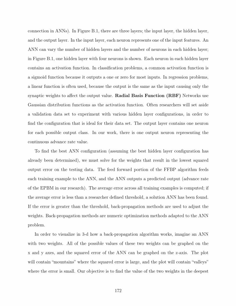
connection in ANNs). In Figure B.1, there are three layers; the input layer, the hidden layer,
and the output layer. In the input layer, each neuron represents one of the input features. An
ANN can vary the number of hidden layers and the number of neurons in each hidden layer;
in Figure B.1, one hidden layer with four neurons is shown. Each neuron in each hidden layer
contains an activation function. In classification problems, a common activation function is
a sigmoid function because it outputs a one or zero for most inputs. In regression problems,
a linear function is often used, because the output is the same as the input causing only the
synaptic weights to affect the output value. Radial Basis Function (RBF) Networks use
Gaussian distribution functions as the activation function. Often researchers will set aside
a validation data set to experiment with various hidden layer configurations, in order to
find the configuration that is ideal for their data set. The output layer contains one neuron
for each possible output class. In our work, there is one output neuron representing the
continuous advance rate value.
To find the best ANN configuration (assuming the best hidden layer configuration has
already been determined), we must solve for the weights that result in the lowest squared
output error on the testing data. The feed forward portion of the FFBP algorithm feeds
each training example to the ANN, and the ANN outputs a predicted output (advance rate
of the EPBM in our research). The average error across all training examples is computed; if
the average error is less than a researcher defined threshold, a solution ANN has been found.
If the error is greater than the threshold, back-propagation methods are used to adjust the
weights. Back-propagation methods are numeric optimization methods adapted to the ANN
problem.
In order to visualize in 3-d how a back-propagation algorithm works, imagine an ANN
with two weights. All of the possible values of these two weights can be graphed on the
x and y axes, and the squared error of the ANN can be graphed on the z-axis. The plot
will contain “mountains” where the squared error is large, and the plot will contain “valleys”
where the error is small. Our objective is to find the value of the two weights in the deepest
172
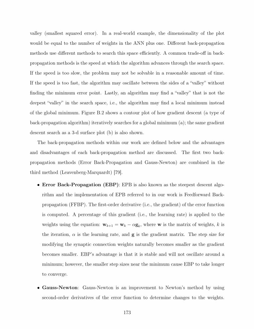
valley (smallest squared error). In a real-world example, the dimensionality of the plot
would be equal to the number of weights in the ANN plus one. Different back-propagation
methods use different methods to search this space efficiently. A common trade-off in back-
propagation methods is the speed at which the algorithm advances through the search space.
If the speed is too slow, the problem may not be solvable in a reasonable amount of time.
If the speed is too fast, the algorithm may oscillate between the sides of a “valley” without
finding the minimum error point. Lastly, an algorithm may find a “valley” that is not the
deepest “valley” in the search space, i.e., the algorithm may find a local minimum instead
of the global minimum. Figure B.2 shows a contour plot of how gradient descent (a type of
back-propagation algorithm) iteratively searches for a global minimum (a); the same gradient
descent search as a 3-d surface plot (b) is also shown.
The back-propagation methods within our work are defined below and the advantages
and disadvantages of each back-propagation method are discussed. The first two back-
propagation methods (Error Back-Propagation and Gauss-Newton) are combined in the
third method (Leavenberg-Marquardt) [79].
• Error Back-Propagation (EBP): EPB is also known as the steepest descent algo-
rithm and the implementation of EPB referred to in our work is Feedforward Back-
propagation (FFBP). The first-order derivative (i.e., the gradient) of the error function
is computed. A percentage of this gradient (i.e., the learning rate) is applied to the
weights using the equation: wk+1 = wk − αgk, where w is the matrix of weights, k is
the iteration, α is the learning rate, and g is the gradient matrix. The step size for
modifying the synaptic connection weights naturally becomes smaller as the gradient
becomes smaller. EBP’s advantage is that it is stable and will not oscillate around a
minimum; however, the smaller step sizes near the minimum cause EBP to take longer
to converge.
• Gauss-Newton: Gauss-Newton is an improvement to Newton’s method by using
second-order derivatives of the error function to determine changes to the weights.
173

Gauss-Newton uses a Jacobian matrix to eliminate the second order derivatives, and
thus decreases the required computation power at each iteration. Although Gauss-
Newton is faster than EBP, it often fails to converge on a minimum error value and
has been mostly replaced by the Leavenberg-Marquardt Algorithm.
• Leavenberg-Marquardt Algorithm: Speed and stability are the major advan-
tages of using the Leavenberg-Marquardt (LM) algorithm for back-propagation. The
LM algorithm combines the advantages of the standard EBP and the Gauss-Newton
algorithm. Leavenberg-Marquardt is generally accepted as an improvement upon
EBP and Gauss-Newton back-propagation methods. The LM equation is: wk+1 =
wk − (JTk Jk + µI)−1Jkek, where w is the matrix of weights, k is the iteration number,
J is the Jacobian of the error matrix and the weights’ matrix, µ is the combination
coefficient, and e is the error matrix. The LM equation effectively combines the EBP
and Gauss-Newton equations, such that µ adjusts how much each equation impacts the
weight change in the next iteration. Specifically, a small µ uses the effects of Gauss-
Newton, and a large µ uses the effects of EBP. The combination coefficient is adjusted
at each iteration, which allows LM to start with the speed of Gauss-Newton and then
switch to EBP to achieve convergence at an error minimum. The major disadvantage
of LM is that it requires more memory for each iteration, which is problematic for data
sets with a large number of features.
Support Vector Machines (SVMs) are popular in machine learning because of their ten-
dency to return lower error rates than most other ML algorithms in real-world problems;
lower error rates exist because there is (generally) less feature interaction complexity than
hypothetical ML problems [80]. SVMs are also solving a convex optimization problem, which
means that any solution an SVM finds will be a global solution. SVMs were developed for
classification problems, but are easily adapted to regression problems; our description exam-
ines a simple SVM classification problem. Another name for an SVM is a maximum margin
classifier, because the algorithm attempts to find a dividing boundary between two classes
174
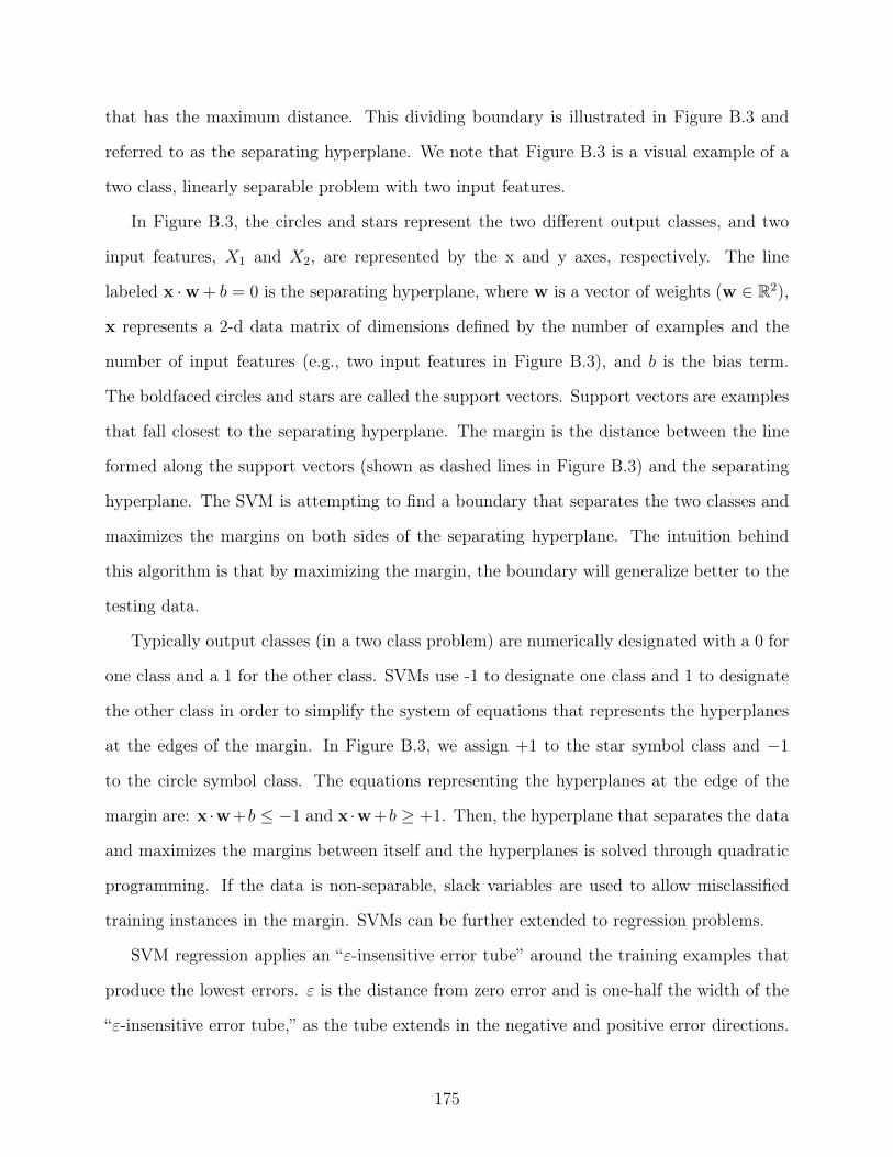
that has the maximum distance. This dividing boundary is illustrated in Figure B.3 and
referred to as the separating hyperplane. We note that Figure B.3 is a visual example of a
two class, linearly separable problem with two input features.
In Figure B.3, the circles and stars represent the two different output classes, and two
input features, X1 and X2, are represented by the x and y axes, respectively. The line
labeled x ·w + b = 0 is the separating hyperplane, where w is a vector of weights (w ∈ R2),
x represents a 2-d data matrix of dimensions defined by the number of examples and the
number of input features (e.g., two input features in Figure B.3), and b is the bias term.
The boldfaced circles and stars are called the support vectors. Support vectors are examples
that fall closest to the separating hyperplane. The margin is the distance between the line
formed along the support vectors (shown as dashed lines in Figure B.3) and the separating
hyperplane. The SVM is attempting to find a boundary that separates the two classes and
maximizes the margins on both sides of the separating hyperplane. The intuition behind
this algorithm is that by maximizing the margin, the boundary will generalize better to the
testing data.
Typically output classes (in a two class problem) are numerically designated with a 0 for
one class and a 1 for the other class. SVMs use -1 to designate one class and 1 to designate
the other class in order to simplify the system of equations that represents the hyperplanes
at the edges of the margin. In Figure B.3, we assign +1 to the star symbol class and −1
to the circle symbol class. The equations representing the hyperplanes at the edge of the
margin are: x ·w+b ≤ −1 and x ·w+b ≥ +1. Then, the hyperplane that separates the data
and maximizes the margins between itself and the hyperplanes is solved through quadratic
programming. If the data is non-separable, slack variables are used to allow misclassified
training instances in the margin. SVMs can be further extended to regression problems.
SVM regression applies an “ε-insensitive error tube” around the training examples that
produce the lowest errors. ε is the distance from zero error and is one-half the width of the
“ε-insensitive error tube,” as the tube extends in the negative and positive error directions.
175

Within the “ε-insensitive error tube,” training examples are assigned an error of 0. The
closest non-zero error training examples then become the support vectors from which the
margin hyperplanes are created. The center of this margin is the separating hyperplane
solution for the regression SVM [81].
B.1 Linear Regression
In supervised machine learning, linear regression fits a line to the training examples.
Equation B.1 represents the linear regression model:
hθ(x) = θ0 + θ1x1 + θ2x2 + · · ·+ θnxn, (B.1)
where hθ(x) is the hypothesized model based on the training data x, θ0 is the bias term,
θ1 · · · θn are the weights of each input feature, x1···n are values of the training example, and
n is the number of input features. In order to learn the θ parameters, a cost function is
established so that optimization methods can be applied. Equation B.2 shows the ordinary
least squares cost function:
J(θ) =1
2
m∑i=1
(hθ(x(i))− y(i))2, (B.2)
where J(θ) represents the cost of the current model applied to all training examples, m is the
number of training examples, hθ(x(i)) is the result of Equation B.1 for the current training
example, and y(i) is the observed value of the current training example. The Least Mean
Squares (LMS) update rule can then be applied until the cost has reached a minimum point
that is acceptable to the person training the model (i.e., convergence). Equation B.3 shows
the LMS update rule:
θj = θj + α(y(i) − hθ(x(i)))x(i)j , (repeat for all j), (B.3)
where θj is the weight of input feature j, α is the learning rate, y(i) is the observed value of
training example i, hθ(x(i)) is the model predicted value for the training example i, and x(i)j
is the value of input feature j for training example i.
176

(a) Gradient Ascent Contour
(b) Gradient Ascent Surface
Figure B.2: (a) Contour plot of an example gradient descent iterative search for a globalminimum. (b) 3-d surface plot of the same example gradient descent iterative search. Imageoriginally created by Joris Gillis and reproduced as non-copyrighted material [77, 78].
177

X1
X2
w
margin
Figure B.3: Illustration of the margin between support vectors (of opposite classes) thatSVMs are optimizing in a two class classification example.
178
Copyright © 2022 FDOKUMEN