BioMed CentralBMC Bioinformatics

ss

Open AcceMethodology articleImproved analysis of bacterial CGH data beyond the log-ratio paradigmLars Snipen*1, Otto L Nyquist2, Margrete Solheim2, Ågot Aakra2 and Ingolf F Nes2

Address: 1Biostatistics, Department of Chemistry, Biotechnology and Food Sciences, Norwegian University of Life Sciences, Ås, Norway and 2Laboratory of Microbial Gene Technology, Department of Chemistry, Biotechnology and Food Sciences, Norwegian University of Life Sciences, Ås, Norway

Email: Lars Snipen* - lars.snipen@umb.no; Otto L Nyquist - otto.nyquist@umb.no; Margrete Solheim - margrete.solheim@umb.no; Ågot Aakra - agot.aakra@umb.no; Ingolf F Nes - ingolf.nes@umb.no

* Corresponding author

AbstractBackground: Existing methods for analyzing bacterial CGH data from two-color arrays are basedon log-ratios only, a paradigm inherited from expression studies. We propose an alternativeapproach, where microarray signals are used in a different way and sequence identity is predictedusing a supervised learning approach.

Results: A data set containing 32 hybridizations of sequenced versus sequenced genomes havebeen used to test and compare methods. A ROC-analysis has been performed to illustrate theability to rank probes with respect to Present/Absent calls. Classification into Present and Absentis compared with that of a gaussian mixture model.

Conclusion: The results indicate our proposed method is an improvement of existing methodswith respect to ranking and classification of probes, especially for multi-genome arrays.

BackgroundMicroarray based comparative genomic hybridizations(CGH) is a tool for rapid investigation of the genetic con-tent of bacteria. The technique is used for comparativegenomic studies as well as screening for virulence factorsor other genomic features of interest in a population [1-3].The basic idea behind the technology is to constructmicroarrays from sequenced and annotated genomes, andthen hybridize genomic DNA from other sources to thesearrays to detect similarities and differences in genomiccontent. For two-color arrays DNA from some sampledgenome is labeled and hybridized against labeled DNA

from a reference. This reference is typically genomic DNAfrom one or several fully sequenced genomes, usuallythose from which the array was constructed.

The results obtained from such experiments can be seen asprojections of the genomes in question onto the sequencespace spanned by the microarray probe sequences. Thisprobe space may vary in size, representing only a set ofselected genomic features all the way up to pan-genomes.Probes may be short or long oligonucleotides, or PCRproducts, and we will in this paper only consider caseswhere the probe sequences are known exactly.

Published: 19 March 2009

BMC Bioinformatics 2009, 10:91 doi:10.1186/1471-2105-10-91

Received: 12 November 2008Accepted: 19 March 2009

This article is available from: http://www.biomedcentral.com/1471-2105/10/91

© 2009 Snipen et al; licensee BioMed Central Ltd. This is an Open Access article distributed under the terms of the Creative Commons Attribution License (http://creativecommons.org/licenses/by/2.0), which permits unrestricted use, distribution, and reproduction in any medium, provided the original work is properly cited.

Page 1 of 9(page number not for citation purposes)

BMC Bioinformatics 2009, 10:91 http://www.biomedcentral.com/1471-2105/10/91

The data from these experiments are qualitatively differentfrom those obtained in gene expression studies, where sig-nal intensities must be seen as a continuum due to thedynamic abundance of mRNA. In bacterial CGH (bCGH)differences in signal intensities are predominately due todifferences in sequence composition, copy number abber-ations are few and give smaller signal fluctuations. For thisreason bCGH signals tend to behave more like a categori-cal variable with two possible outcomes, usually denotedPresent and Absent. A strong signal, corresponding toPresent, means the corresponding probe sequence isfound, with sufficient similarity to yield hybridization, inthe investigated genome. A weak signal means a too smallpart of the probe sequence is found in the genome to givehybridization, and the probe is called Absent.

Some methods to analyze bCGH data of this type havebeen proposed, and some of them are reviewed and testedin a recent publication by [4]. Most of these methods basetheir results on the log-ratio of signals, which is a standardadopted from the analysis of expression data. We will inthis paper propose a new strategy for analyzing bCGHdata, that does not rely on log-ratios, which we believe isa misleading paradigm for this type of data. Also, somepreviously proposed methods utilizing more than justlog-ratios, like [5-7], are all unsupervised methods, nottaking into account the sequence information from thereference genomes. In our approach this information isalso included to aid the analysis. In the analysis of two-color microarray data demonstrated in this paper, we treatthe array signals separately, almost as two single-colorarrays, hence the method could easily be used for datafrom this technology as well. We test our method on datafrom S. aureus and E. faecalis, and compare our results tothose achieved by other effective methods.

MethodsSequence identityAny bCGH experiment starts by performing alignments ofevery array probe sequence against the fully sequencedreference genomes to establish which probes are presentand absent in these genomes. We use the term R-genomefor a reference genome. We define the identity betweenprobe and an R-genome as the number of identical basesin the best local alignment between them divided by theprobe length to obtain a value between 0 and 1. We callthis quantity Rbij for probe i against the R-genome inhybridization j. If Rbij = 1 it means an exact copy of theprobe sequence is found in the R-genome, while if probei has no significant hits in R-genome j we set Rbij = 0 evenif all probes will of course have some very short subse-quences in common with any genome.

The categorical response Present or Absent is coded as 1 or0, respectively. This require, however, that intermediateRb-values must be rounded to either 1 or 0, i.e. we need

some a priori threshold that specify the sequence identityneeded to be Present. Our analysis approach does notrequire categorical responses, and intermediate Rb-valuescan be used as is. However, if the ultimate goal is to clas-sify between Present and Absent, the analysis is usuallyfavored by having only 1 and 0 as responses from the start.

A sampled, un-sequenced, genome we call a sample-genome or S-genome. Corresponding to Rbij for the R-genome, we also have a similar Sbij for the S-genome. Themotivation behind the entire bCGH experiment is to saysomething about this Sbij, i.e. the sequence identitybetween probe i and the S-genome in hybridization j.

PreprocessingFor each array in the experiment, we assume backgroundcorrection and within-array normalization has been done.We have employed standard methods in the LIMMA pack-age [8] in R [9], available from the Bioconductor [10].Normalization of CGH arrays has recently been discussedby [11] and [12], and nothing in our downstream analysisprevent the use of these or other approaches.

The flagging of low quality spots should be done verycareful for bCGH analyses. In standard procedures forexpression data, spots with low signals are removed. ForbCGH data these spots turn out informative, because theyspan the range of array signals. Especially negative controlprobes, e.g. spots with alien or no DNA, are importantsince they carry information about which signals to expectwhen no hybridization takes place.

On microbial arrays probes are usually spotted multipletimes (replicates). We will only consider the median valueof these replicates on each array, but the number of repli-cates for each probe is kept as a weight in the final predic-tion, i.e. probes with more replicates have larger impact.

Let and be the median preprocessed log-trans-

formed signals from the R- and S-genome channel forprobe i in hybridization j.

In most cases a bCGH experiment will consist of a batchof several hybridizations to be analyzed simultaneously.For our downstream analysis some between-array nor-malization within this batch is beneficial. Let Ij0 = {i|Rbij <0.1}, i.e. the set of probes with R-genome sequence iden-tity less than 0.1. Also, let Ij1 = {i|Rbij > 0.9}. Let Raj0 andRaj1 be the median of the Raij values for the probes in Ij0and Ij1, respectively. Then the between-array normalizedR-signal is

Raij′ Saij′

RaRaij Ra jRa j Ra j

ij =′ −

−0

1 0(1)

Page 2 of 9(page number not for citation purposes)

BMC Bioinformatics 2009, 10:91 http://www.biomedcentral.com/1471-2105/10/91

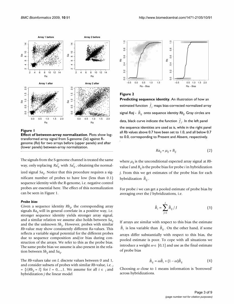
The signals from the S-genome channel is treated the same

way, only replacing with , obtaining the normal-

ized signal Saij. Notice that this procedure requires a sig-

nificant number of probes to have low (less than 0.1)sequence identity with the R-genome, i.e. negative controlprobes are essential here. The effect of this normalizationcan be seen in Figure 1.

Probe biasGiven a sequence identity Rbij, the corresponding arraysignals Raij will in general correlate in a positive way, i.e.stronger sequence identity yields stronger array signal,and a similar relation we assume also holds between Saijand the the unknown Sbij. However, probes with similarRb-value may show consistently different Ra-values. Thisreflects a variable signal potential for the different probesdue to sequence composition and/or bias during con-struction of the arrays. We refer to this as the probe bias.The same probe bias we assume is also present in the rela-tion between Sbij and Saij.

The Rb-values take on L discrete values between 0 and 1,and consider subsets of probes with similar Rb-value, i.e. l= {i|Rbij = l} for l = 0,...,1. We assume for all i ∈ l andhybridization j the linear model

Raij = μlj + Bij (2)

where μlj is the unconditional expected array signal at Rb-

value l and Bij is the probe bias for probe i in hybridization

j. From this we get estimates of the probe bias for each

hybridization .

For probe i we can get a pooled estimate of probe bias byaveraging over the J hybridizations, i.e.

If arrays are similar with respect to this bias the estimate

is less variable than . On the other hand, if some

arrays differ substantially with respect to this bias, thepooled estimate is poor. To cope with all situations we

introduce a weight ω ∈ [0,1] and use as the final estimateof probe bias

Choosing ω close to 1 means information is 'borrowed'across hybridizations.

Raij′ Saij′

Bij

B B Ji ij

j

J

==

∑ /1

(3)

Bi Bij

ˆ ( )B B Bij i ij= + −w w1 (4)

Predicting sequence identityFigure 2Predicting sequence identity. An illustration of how an

estimated function maps bias-corrected normalized array

signal Raij - onto sequence identity Rbij. Gray circles are

data, black curve indicate the function . In the left panel

the sequence identities are used as is, while in the right panel all Rb values above 0.7 have been set to 1.0, and all below 0.7 to 0.0, corresponding to Present and Absent, respectively.

−0.5 0.0 0.5 1.0 1.5

0.0

0.2

0.4

0.6

0.8

1.0

Ra − Bias

Rb

−0.5 0.5 1.0 1.5 2.0

0.0

0.2

0.4

0.6

0.8

1.0

Ra − Bias

Rb

f j

Bij

f j

Effect of between-array normalizationFigure 1Effect of between-array normalization. Plots show log-transformed array signal from S-genome (Sa) against R-genome (Ra) for two arrays before (upper panels) and after (lower panels) between-array normalization.

2 4 6 8 10 12 14

24

68

1014

Array 1 before

Ra

Sa

2 4 6 8 10 12 142

46

810

14

Array 2 before

Ra

Sa

0.0 0.5 1.0 1.5 2.0

0.0

0.5

1.0

1.5

2.0

Array 1 after

Ra

Sa

0.0 0.5 1.0 1.5 2.0

0.0

0.5

1.0

1.5

2.0

Array 2 after

Ra

Sa

Page 3 of 9(page number not for citation purposes)

BMC Bioinformatics 2009, 10:91 http://www.biomedcentral.com/1471-2105/10/91

Predicting sequence identityThe basic idea is, for each array, to fit a function thatdescribes how Rb-values depend on bias-corrected Ra-val-ues, and then use the same function to predict Sb-valuesfrom bias-corrected Sa-values.

First, we assume there is a function fj for hybridization jsuch that

We will make few assumptions about the shape of thefunction fj, but we will require it to be monotonouslyincreasing, since an increased array signal should alwaysindicate stronger sequence identity.

We have chosen to estimate fj by a weighted running

mean, where probes are weighted by their number ofwithin-array replicates. For notational simplicity, let xij =

Raij - . The range of the function is divided into N

equally spaced knots, x1,...,xN, and let D be the width

between two knots. For knot n, let Cn be the data subset

{xij, Rbij} whose value of xij falls within xn ± 3D/2. Finding

fj(x1),...,fj(xN) leads to the constrained optimization prob-

lem

This problem can be solved by first computing the uncon-strained optimum (weighted running mean), and thenresolving the violated constraints in a recursive way. If theinitial estimate of fj(xn+1) is smaller than that of fj(xn),both are replaced by the weighted average of them,weighted by the number of data points behind each initialestimate. This may again violate the constraints on theestimates of fj(xn+2) and/or fj(xn-1), and hence the recur-sion.

Given the estimates of fj(x1),...,fj(xN) the estimated func-

tion value at any point within the range is found by linear

interpolation between the knots. Let denote this esti-

mated function for array j. Figure 2 illustrates how fits

a typical data set.

For the given S-genome in hybridization j, the predictionof the sequence identity for probe i is now given as

It is not uncommon to repeat experiments, i.e. hybridizethe same S-genome to several arrays. In this case it is nat-ural to first analyze each array separately, obtain predic-

tions from each array, and in the end average these

for each S-genome. A description of uncertainty in the pre-diction is best achieved by constructing a confidenceinterval for Sbij. Since this variable is trapped between 0

and 1 it seems reasonable to avoid inference based on spe-cific distributions, and instead rely on some non-paramet-ric approach. In case of a categorical response (Present/Absent), majority vote should be used instead of average,and statements concerning uncertainty should be put for-ward as some estimate of posterior probability of Present.The proportion of Present-votes for each probe is the max-imum likelihood estimate of this probability, assumingthe repeated experiments are independent.

DataIn order to test methods we performed bCGH experi-ments using only sequenced genomes, i.e. the Sb-valuesare, contrary to a real situation, all known. Two differentarrays were used, one representing 6 genomes of Staphylo-coccus aureus available from J. Craig Venter Institute [13](JCVI), and one representing the genome of Enterococcusfaecalis strain V583. In both cases probes are 70-mer oligo-nucleotides. The S. aureus array contains 5057 differentprobes spotted six times, where 4515 are ordinary probesrepresenting genomes, and the remaining 542 negativecontrol probes include various alien DNA and the 'emptyprobe' (no DNA). The E. faecalis array contains 3218probes representing genes in the genome of V583, 10probes representing the enterococcal pathogenicity islandof strain MMH594 and 15 negative controls, giving a totalof 3243 probes, spotted three times each.

Experiments were conducted using the S. auerus strainsCOL, N315, Mu50, NCTC8325 and RF122 and E. faecalisstrains V583 and OG1RF, whose genome sequences areavailable at NCBI [14]. For the S. aureus experiments sevendifferent pairs of genomes were selected for hybridization,and for each pair a dye-swap was performed. For each ofthese 14 hybridizations both genomes involved can playthe role as R-genome and S-genome, hence there are alto-gether 28 different S. aureus data sets where we can com-pare predicted and true sequence identity. Twohybridizations of V583 versus OG1RF were conducted(dye swap), and again both genomes can play the role asR-genome and S-genome, giving 4 additional E. faecalis

E Rb f Ra Bij j ij ij( ) ( )= − (5)

Bij

min ( ( ))( ),..., ( )f x f x

ij j n

Rb Cn

N

j j Nij n

Rb f x1

2

1

−∈=

∑∑constrained to f x f xj n j n( ) ( )≤ +1

f j

f

ˆ ˆ ( ˆ )Sb f Sa Bij j ij ij= − (6)

Sbij

Page 4 of 9(page number not for citation purposes)

BMC Bioinformatics 2009, 10:91 http://www.biomedcentral.com/1471-2105/10/91

data sets. In order to compare our method against othermethods we use a categorical response, i.e. each probe isclassified as Present (1) or Absent (0). This means we haveassigned a threshold to the Rb- and Sb-values in order toround each value to 1 or 0. We have used the threshold 0.7(70% identity), i.e. an Rb- or Sb-value above 0.7 corre-sponds to Present and is rounded to 1 and values below0.7 is rounded to 0. The threshold is chosen on the basisof the histogram in Figure 3. The S. aureus arrays containprobes representing genes in 6 different strains. By BLAST-ing the probe sequences against the genome sequences ofthese strains, the identities distribute as indicated in Fig-ure 3. Thus, it seems that probes matching with approxi-mately 70% identity or more are considered Present in thegenome by JCVI who designed the arrays. This also corre-sponds well with our experience regarding the degree ofmatch giving hybridizations. This threshold will in gen-eral depend on array design and hybridization conditions,and a proper value must be decided upon for each exper-iment separately. Our method is independent of thischoice as long as it is a reasonable value for the experi-ments analyzed. Table 1 show the percent of truly Present/Absent probes in each of the genomes using our probe setand threshold.

As previously mentioned, we advocate a weak flagging ofarray spots during the preprocessing of the data. This

means only truly damaged spots should be flagged, andspots with weak signals or negative controls, should bepart of the data set through the entire analysis. When com-paring our proposed method against other approaches,we used both 'hard' and 'weak' flagging of spots to illus-trate the differences between these strategies. By 'hard'flagging we mean removing all negative controls as well asall spots flagged by the image analysis software, i.e. in ourcase all spots with negative flag value from GenePix. In the'weak' flagging only manually discarded spots wereremoved, i.e. only spots with flag value -100 from Gene-Pix.

ResultsOur proposed method predicts probe sequence similarityto a sampled genome based on a biased-corrected arraysignal. Based on observed array signal and probe sequencesimilarities to the reference genome, we estimate a probebias for each probe. Then, correcting for this probe bias,we fit a non-parametric function describing the relationbetween array signal and probe sequence similarity for thereference genome. Finally, we use this function to predictprobe sequence similarity from observed array signals forthe sampled genome. If a categorical response (Present orAbsent) is desired this is coded as Present = 1 and Absent= 0. Comparison to other approaches are here made ondata sets where true sequence similarities (Present/Absentstatus) are known.

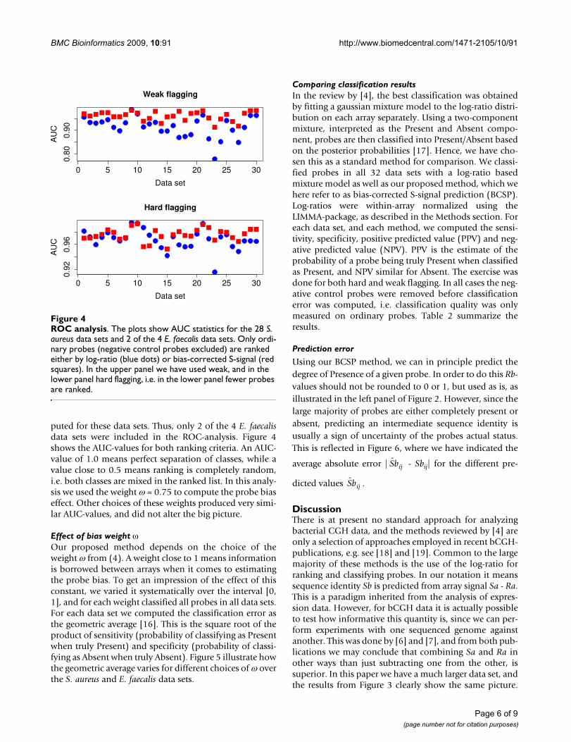
ROC-analysisMost bCGH analyses are based on the ranking of probesaccording to log-ratios. In our approach the correspond-ing ranking is according to predicted sequence similarity.The potential for correct classification was examined byranking all ordinary probes by both criteria, and the AreaUnder Curve (AUC) statistic from a ROC-analysis [15]was computed for the data sets. Under the hard flaggingregime, two of the E. faecalis data sets completely lackedabsent probes, and hence no AUC-values could be com-

Distribution of Rb valuesFigure 3Distribution of Rb values. The histogram shows the distri-bution of Rb-values when BLASTing the probe sequences against four of the genomes they are designed to represent. A majority of alignments show either Rb = 0 or Rb = 1, but a large proportion of probes also have 0.7 <Rb < 1.0. By choosing the threshold between Present and Absent at 0.7 these probes are defined as Present.

Rb

Fre

quen

cy

0.0 0.2 0.4 0.6 0.8 1.0

020

0040

0060

0080

0010

000 Table 1: Genomes and microarrays

Genome Size (Mb) Present Absent

S. aureus COL 2.81 74% 26%S. aureus N315 2.84 74% 26%S. aureus Mu50 2.90 76% 24%S. aureus NCTC8325 2.82 74% 26%S. aureus RF122 2.74 70% 30%E. faecalis V583 3.36 99% 1%E. faecalis OG1RF 2.73 73% 27%

Overview of the genomes used in the test data sets. The Present/Absent numbers indicate the percentage of probes on the arrays having sequence identity above (Present) or below (Absent) the threshold of Rb = 0.7. Percentages refer to the total number of probes, i.e. 5057 on the S. aureus array and 3243 on the E. faecalis array.

Page 5 of 9(page number not for citation purposes)

BMC Bioinformatics 2009, 10:91 http://www.biomedcentral.com/1471-2105/10/91

puted for these data sets. Thus, only 2 of the 4 E. faecalisdata sets were included in the ROC-analysis. Figure 4shows the AUC-values for both ranking criteria. An AUC-value of 1.0 means perfect separation of classes, while avalue close to 0.5 means ranking is completely random,i.e. both classes are mixed in the ranked list. In this analy-sis we used the weight ω = 0.75 to compute the probe biaseffect. Other choices of these weights produced very simi-lar AUC-values, and did not alter the big picture.

Effect of bias weight ωOur proposed method depends on the choice of theweight ω from (4). A weight close to 1 means informationis borrowed between arrays when it comes to estimatingthe probe bias. To get an impression of the effect of thisconstant, we varied it systematically over the interval [0,1], and for each weight classified all probes in all data sets.For each data set we computed the classification error asthe geometric average [16]. This is the square root of theproduct of sensitivity (probability of classifying as Presentwhen truly Present) and specificity (probability of classi-fying as Absent when truly Absent). Figure 5 illustrate howthe geometric average varies for different choices of ω overthe S. aureus and E. faecalis data sets.

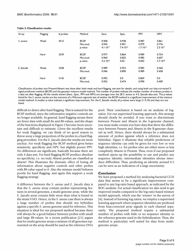
Comparing classification resultsIn the review by [4], the best classification was obtainedby fitting a gaussian mixture model to the log-ratio distri-bution on each array separately. Using a two-componentmixture, interpreted as the Present and Absent compo-nent, probes are then classified into Present/Absent basedon the posterior probabilities [17]. Hence, we have cho-sen this as a standard method for comparison. We classi-fied probes in all 32 data sets with a log-ratio basedmixture model as well as our proposed method, which wehere refer to as bias-corrected S-signal prediction (BCSP).Log-ratios were within-array normalized using theLIMMA-package, as described in the Methods section. Foreach data set, and each method, we computed the sensi-tivity, specificity, positive predicted value (PPV) and neg-ative predicted value (NPV). PPV is the estimate of theprobability of a probe being truly Present when classifiedas Present, and NPV similar for Absent. The exercise wasdone for both hard and weak flagging. In all cases the neg-ative control probes were removed before classificationerror was computed, i.e. classification quality was onlymeasured on ordinary probes. Table 2 summarize theresults.

Prediction error

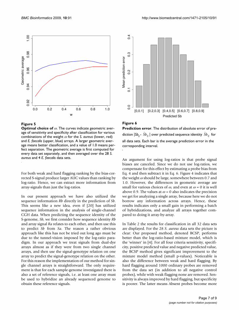
Using our BCSP method, we can in principle predict thedegree of Presence of a given probe. In order to do this Rb-values should not be rounded to 0 or 1, but used as is, asillustrated in the left panel of Figure 2. However, since thelarge majority of probes are either completely present orabsent, predicting an intermediate sequence identity isusually a sign of uncertainty of the probes actual status.This is reflected in Figure 6, where we have indicated the

average absolute error | - Sbij| for the different pre-

dicted values .

DiscussionThere is at present no standard approach for analyzingbacterial CGH data, and the methods reviewed by [4] areonly a selection of approaches employed in recent bCGH-publications, e.g. see [18] and [19]. Common to the largemajority of these methods is the use of the log-ratio forranking and classifying probes. In our notation it meanssequence identity Sb is predicted from array signal Sa - Ra.This is a paradigm inherited from the analysis of expres-sion data. However, for bCGH data it is actually possibleto test how informative this quantity is, since we can per-form experiments with one sequenced genome againstanother. This was done by [6] and [7], and from both pub-lications we may conclude that combining Sa and Ra inother ways than just subtracting one from the other, issuperior. In this paper we have a much larger data set, andthe results from Figure 3 clearly show the same picture.

Sbij

Sbij

ROC analysisFigure 4ROC analysis. The plots show AUC statistics for the 28 S. aureus data sets and 2 of the 4 E. faecalis data sets. Only ordi-nary probes (negative control probes excluded) are ranked either by log-ratio (blue dots) or bias-corrected S-signal (red squares). In the upper panel we have used weak, and in the lower panel hard flagging, i.e. in the lower panel fewer probes are ranked.

0 5 10 15 20 25 30

0.80

0.90

Weak flagging

Data set

AU

C

0 5 10 15 20 25 30

0.92

0.96

Hard flagging

Data set

AU

C

Page 6 of 9(page number not for citation purposes)

BMC Bioinformatics 2009, 10:91 http://www.biomedcentral.com/1471-2105/10/91

For both weak and hard flagging ranking by the bias-cor-rected S-signal produce larger AUC values than ranking bylog-ratio. Hence, we can extract more information fromarray-signals than just the log-ratios.

In our present approach we have also utilized thesequence information Rb directly in the prediction of Sb.This seems like a new idea, even if [20] has utilizedsequence information in the analysis of single-channelCGH data. When predicting the sequence identity of theS-genome, Sb, we first consider how sequence identity Rband array signal Ra relates to each other, and then use thisto predict Sb from Sa. The reason a rather obviousapproach like this has not be tried out long ago must bedue to the tunnel-vision imposed by the log-ratio para-digm. In our approach we treat signals from dual-dyearrays almost as if they were from two single channelarrays, and then use the signal-genotype relation on onearray to predict the signal-genotype relation on the other.For this reason the implementation of our method for sin-gle channel arrays is straightforward. The only require-ment is that for each sample-genome investigated there isalso a set of reference signals, i.e. at least one array mustbe used to hybridize an already sequenced genome toobtain these reference signals.

An argument for using log-ratios is that probe signalbiases are canceled. Since we do not use log-ratios, wecompensate for this effect by estimating a probe bias fromEq. 4 and then subtract it in Eq. 6. Figure 4 indicates thatthe weight ω should be large, somewhere between 0.7 and1.0. However, the differences in geometric average aresmall for various choices of ω, and even at ω = 0 it is wellabove 0.9. The values at ω = 0 also indicates the precisionwe get for analyzing a single array, because here we do notborrow any information across arrays. Hence, theseresults indicates only a small gain in performing a batchof hybridizations, and analyze all arrays together com-pared to doing it array-by-array.

In Table 2 the results for classification in all 32 data setsare displayed. For the 28 S. aureus data sets the picture isclear: Our proposed method, denoted BCSP, performsbetter than the log-ratio-based mixture model, which isthe 'winner' in [4]. For all four criteria sensitivity, specifi-city, positive predicted value and negative predicted value,the BCSP method gives significant improvement to themixture model method (small p-values). Noticeable isalso the difference between weak and hard flagging. Byhard flagging around 1000 ordinary probes are removedfrom the data set (in addition to all negative controlprobes), while with weak flagging none are removed. Sen-sitivity is always improved by hard flagging, but specificityis poorer. The latter means Absent probes become more

Prediction errorFigure 6Prediction error. The distribution of absolute error of pre-

diction |Sbij - | over predicted sequence identity for

all data sets. Each bar is the average prediction error in the corresponding interval.

[0,0.1] [0.2,0.3] [0.4,0.5] [0.6,0.7] [0.8,0.9]

Predicted Sb

Mea

n pr

edic

tion

erro

r

0.0

0.1

0.2

0.3

0.4

Sbij Sbij

Optimal choice of ωFigure 5Optimal choice of ω. The curves indicate geometric aver-age of sensitivity and specificity after classification for various combinations of the weight ω for the S. aureus (lower, red) and E. faecalis (upper, blue) arrays. A larger geometric aver-age means better classification, and a value of 1.0 means per-fect separation. The geometric average is first computed for every data set separately, and then averaged over the 28 S. aureus and 4 E. faecalis data sets.

0.0 0.2 0.4 0.6 0.8 1.0

0.92

0.94

0.96

0.98

1.00

w

Geo

met

ric a

vera

ge

Page 7 of 9(page number not for citation purposes)

BMC Bioinformatics 2009, 10:91 http://www.biomedcentral.com/1471-2105/10/91

difficult to detect after hard flagging. This is natural for theBCSP method, since the informative negative controls areno longer available. In general, hard flagging means thereare fewer data with small Ra and Rb-values, and the shapeof the functions displayed in Figure 2 become more uncer-tain and difficult to estimate. Given the excellent resultsfor weak flagging, we can think of no good reason tothrow away a large proportion of the probes in a hard flag-ging procedure. For the E. faecalis data the results are moreunclear. For weak flagging the BCSP method gives bettersensitivity, specificity and NPV, but slightly poorer PPV.No differences are significant, basically because there areonly 4 data sets. For hard flagging BCSP produce absoluteno specificity, i.e. no truly Absent probes are classified asabsent! This illustrates the dramatic effect of losing allinformation about negative controls and other probeswith Rb-value equal to 0. Also the mixture model behavespoorly for hard flagging, and again this support a weakflagging strategy.

A difference between the S. aureus and E. faecalis data isthat the S. aureus array contain probes representing fea-tures in several genomes, a multi-genome array, while theE. faecalis array contain little more than what is found inthe strain V583. Hence, in the S. aureus case there is alwaysa large number of probes that should not hybridizeagainst a specific S. aureus genome used for reference. Thissituation is ideal for our proposed method because therewill always be a good balance between probes with smalland large Rb-values. In a recent publication [21] arguesthat for multi-genome arrays a mixture of all genomes rep-resented on the array should be used as the reference DNA

pool. Their conclusion is based on an analysis of log-ratios. For our supervised learning approach, this strategyshould clearly be avoided. If you want to discriminatebetween Present and Absent in the S-genome channel,you must make certain you have data that show the differ-ence between Present and Absent in the R-genome chan-nel as well. Hence, there should always be a substantialamount of probes against which a reference does nothybridize. Figure 6 illustrate that reliable predictions ofsequence identity can only be given for very low or veryhigh identities, i.e. for probes who are either more or lesscompletely Absent or Present. Thus, even if our proposedmethod opens up the possibility to use and predict anysequence identity, intermediate identities always intro-duce difficulties. Thus, predicting an identity around 0.5can be seen as an indication of a large uncertainty.

ConclusionWe have proposed a method for analyzing bacterial CGHdata that seems to be a significant improvement com-pared to any log-ratio based approach, as indicated by theROC-analysis. For actual classification we also tend to getimproved results compared to the log-ratio based mixturemodel approach, which was the 'winner' in the survey of[4]. Instead of forming log-ratios, we employ a supervisedlearning approach where sequence identities are predictedfrom bias-corrected array signals in each channel sepa-rately. The proposed method require a substantialnumber of probes with little or no sequence identity tothe reference genome used in the hybridization. Thus, themethod is particulary well suited for data from multi-genome arrays.

Table 2: Classification results

Array Flagging # probes Method Sens. Spec. PPV NPV

S. aureus Weak 4515 BCSP 0.968 0.938 0.987 0.861Mix.mod. 0.945 0.901 0.979 0.776p-value 4.1·10-7 7.4·10-4 1.7·10-4 2.5·10-7

Hard 3539 BCSP 0.977 0.864 0.989 0.754Mix.mod. 0.960 0.825 0.985 0.607p-value 3.2·10-8 0.02 0.003 3.7·10-8

E. faecalis Weak 3228 BCSP 0.989 0.953 0.983 0.560Mix.mod. 0.946 0.890 0.989 0.458

Hard 3145 BCSP 0.992 0.0 0.869 0.0Mix.mod. 0.955 0.474 0.990 0.409

Classification of probes into Present/Absent was done after both weak and hard flagging, see text for details, and using both our bias-corrected S-signal prediction method (BCSP) and the gaussian mixture model method. The number of probes indicate the median number of ordinary probes in a data set after flagging. All the results shown (Sens., Spec., PPV and NPV) are averages over the 28 S. aureus or 4 E. faecalis data sets. The p-values listed for the S. aureus results are the outcome of a Wilcoxon signrank test of wether the BCSP-method is a significant improvement of the mixture model method. A smaller p-value indicate a significant improvement. For the E. faecalis results all p-values were large (> 0.10) and they are not listed.

Page 8 of 9(page number not for citation purposes)

BMC Bioinformatics 2009, 10:91 http://www.biomedcentral.com/1471-2105/10/91

Publish with BioMed Central and every scientist can read your work free of charge

"BioMed Central will be the most significant development for disseminating the results of biomedical research in our lifetime."

Sir Paul Nurse, Cancer Research UK

Your research papers will be:

available free of charge to the entire biomedical community

peer reviewed and published immediately upon acceptance

cited in PubMed and archived on PubMed Central

yours — you keep the copyright

Submit your manuscript here:http://www.biomedcentral.com/info/publishing_adv.asp

BioMedcentral

AvailabilityR code for handling bCGH data using this method, as wellas other approaches, is freely available from the corre-sponding author.

Authors' contributionsLS has proposed the methods presented, done all the pro-gramming in R and drafted the manuscript. OLN has dis-cussed the proposed methods and performed all the S.aureus hybridizations. MS has performed the E. faecalishybridizations. ÅA has supplied/constructed the arrays,and been the supervisor of OLN and MS. IFN has been theproject leader. All authors have read and approved thefinal manuscript.

AcknowledgementsOLN was financially supported by a research grant from the Norwegian University of Life Sciences. MS was financially supported by the European Union 6th Framework Programme "Approaches to Control multi-resistant Enterococci: Studies on molecular ecology, horizontal gene transfer, fitness and prevention". ÅA were supported by grants from the Research Council of Norway. S. aureus micorarrays were kindly provided by the Pathogen Functional Genomics Resource Center (PFGRC) at the J. Craig Venter Institute (JCVI), Rockville, MD, USA. We acknowledge Aksel Flack, The Norwegian Microarray Consortium, Oslo, for printing of the E. faecalis microarray slides.

References1. Dorrell N, Champion OL, Wren BW: Application of DNA Micro-

arrays for Comparative and Evolutionary Genomics. Methodsin Microbiology 2002, 33:121-136.

2. Lindsay JA, Moore CE, Day NP, Peacock SJ, Witney AA, Stabler RA,Husain PDSE, Butcher JH: Microarrays Reveal that Each of theTen Dominant Lineages of Staphylococcus aureus Has aUnique Combination of Surface-Associated and RegulatoryGenes. Journal of Bacteriology 2006, 188(2):669-676.

3. Willenbrock H, Petersen A, Sekse C, Kiil K, Wasteson Y, Ussery DW:Design of a Seven-Genome Escherichia coli Microarray forComparative Genomic Profiling. Journal of Bacteriology 2006,188(22):.

4. Carter B, Wu G, Woodward MJ, Anjum MF: A process for analysisof microarray comparative genomics hybridisation studiesfor bacterial genomes. BMC Genomics 2008, 9(53):.

5. Repsilber D, Mira A, Lindroos H, Andersson S, Ziegler A: Data rota-tion improves genomotyping efficiency. Biometrical Journal2005, 47(4):585-598.

6. Snipen L, Repsilber D, Nyquist L, Ziegler A, Aakra Å, Aastveit A:Detection of divergent genes in microbial aCGH experi-ments. BMC Bioinformatics 2006, 7(181):.

7. Feten G, Almøy T, Snipen L, Aakra Å, Nyquist OL, Aastveit AH: Mix-ture Models as a Method to Find Present and DivergentGenes in Comparative Genomic Hybridization Studies onBacteria. Biometrical journal 2007, 49(2):242-258.

8. Smyth GK, Speed TP: Normalization of cDNA microarray data.Methods 2003, 31:265-273.

9. The R project [http://www.r-project.org/]10. The Bioconductor [http://www.bioconductor.org/]11. van Hijum SAFT, Baerends RJS, Zomer AL, Karsens HA, Martin-

Requena V, Trelles O, Kok J, Kuipers OP: Supervised Lowess nor-malization of comparative genome hybridization data –application to lactococcal strain comparisons. BMC Bioinfor-matics 2008, 9:93.

12. Staaf J, Jonsson G, Ringner M, Vallon-Christersson J: Normalizationof array-CGH data: influence of copy number imbalances.BMC Genomics 2007, 8:382.

13. The J. Craig Venter Institute [http://www.jcvi.org/]14. GenBank [http://www.ncbi.nlm.nih.gov/Genomes/]

15. Hanley JA, McNeil BJ: The meaning and use of the area under areceiver operating characteristic (ROC) curve. Radiology1982, 143:29-36.

16. Kubat M, Holte R, Matwin S: Machine learning for the detectionof oil spills in satellite radar images. Machine Learning 1998,30:195-215.

17. McLachlan GJ, Peel D: Finite Mixture Models New York: John Wiley &Sons; 2000.

18. da Silva VS, Shida CS, Rodrigues FB, Ribeiro DCD, de Souza AA,Coletta-Fiho HD, Machada MA, Nunes LR, de Oliveira RC: Compar-ative genomic characterization of citrus-associated Xylellafastidiosa strains. BMC Genomics 2007, 8(474):.

19. Jayapal KP, Lian W, Glod F, Sherman DH, Hu WS: Comparativegenomic hybridizations reveal absence of large Streptomy-ces coelicolor genomic islands in Streptomyces lividans. BMCGenomics 2007, 8(229):.

20. Schuster EF, Blanc E, Partridge L, Thornton J: Correcting forsequence biases in present/absent calls. Genome Biology 2007,8:R125.

21. Pinto FR, Aguiar SI, Melo-Cristino J, Ramirez M: Optimal controland analysis of two-color genomotyping experiments usingbacterial multistrain arrays. BMC Genomics 2008, 9(230):.

Page 9 of 9(page number not for citation purposes)