Improved Accuracy of Chlorophyll-a Concentration Estimates from MODIS Imagery Using a Two-Band Ratio...

Remote Sens. 2014, 6, 421-442; doi:10.3390/rs6010421

remote sensing ISSN 2072-4292

www.mdpi.com/journal/remotesensing

Article

Improved Accuracy of Chlorophyll-a Concentration Estimates from MODIS Imagery Using a Two-Band Ratio Algorithm and Geostatistics: As Applied to the Monitoring of Eutrophication Processes over Tien Yen Bay (Northern Vietnam)

Nguyen Thi Thu Ha 1,*, Katsuaki Koike 2 and Mai Trong Nhuan 1

1 Faculty of Geology, VNU University of Science, Vietnam National University, Hanoi 334,

Nguyen Trai, Thanh Xuan, Hanoi 10000, Vietnam; E-Mail: [email protected] 2 Department of Urban Management, Graduate School of Engineering, Kyoto University,

Katsura C1-2-215, Kyoto 615-8540, Japan; E-Mail: [email protected]

* Author to whom correspondence should be addressed; E-Mail: [email protected];

Tel.: +84-4-3558-7060; Fax: +84-4-3557-3336.

Received: 24 October 2013; in revised form: 11 December 2013 / Accepted: 20 December 2013 /

Published: 30 December 2013

Abstract: Sea eutrophication is a natural process of water enrichment caused by increased

nutrient loading that severely affects coastal ecosystems by decreasing water quality. The

degree of eutrophication can be assessed by chlorophyll-a concentration. This study aims

to develop a remote sensing method suitable for estimating chlorophyll-a concentrations in

tropical coastal waters with abundant phytoplankton using Moderate Resolution Imaging

Spectroradiometer (MODIS)/Terra imagery and to improve the spatial resolution of

MODIS/Terra-based estimation from 1 km to 100 m by geostatistics. A model based on the

ratio of green and blue band reflectance (rGBr) is proposed considering the bio-optical

property of chlorophyll-a. Tien Yen Bay in northern Vietnam, a typical phytoplankton-rich

coastal area, was selected as a case study site. The superiority of rGBr over two existing

representative models, based on the blue-green band ratio and the red-near infrared band

ratio, was demonstrated by a high correlation of the estimated chlorophyll-a concentrations

at 40 sites with values measured in situ. Ordinary kriging was then shown to be highly

capable of predicting the concentration for regions of the image covered by clouds and,

thus, without sea surface data. Resultant space-time maps of concentrations over a year

clarified that Tien Yen Bay is characterized by natural eutrophic waters, because the

average of chlorophyll-a concentrations exceeded 10 mg/m3 in the summer. The temporal

changes of chlorophyll-a concentrations were consistent with average monthly air

OPEN ACCESS

Remote Sens. 2014, 6 422

temperatures and precipitation. Consequently, a combination of rGBr and ordinary kriging

can effectively monitor water quality in tropical shallow waters.

Keywords: bio-optical properties; water quality; estimation algorithm; phytoplankton;

ordinary kriging

1. Introduction

Chlorophyll-a (Chl-a) concentration is an effective measure of the trophic state of sea and land

waters, because it is related strongly to aquatic phytoplankton abundance and biomass. Estimating

Chl-a concentration is one of the most traditional and significant applications of remote sensing for

evaluating aquatic ecosystems and monitoring eutrophication [1–5]. Recently, satellite imagery with

high spectral resolution spanning the visible to thermal-infrared bands has become available for such

estimations. The main targets of substantive case studies using such imagery are environmental

assessments of ocean waters [6–9], open coastal and estuarine waters [10–15] and inland lakes [16–19].

In addition to these waters, eutrophication in coastal waters, shallow coastal bays and lagoons has been

a notable issue threatening coastal ecosystems all over the world [20]. Despite the importance of Chl-a

monitoring in such coastal areas by remote sensing, such applications have been limited, and the most

suitable methods for estimating Chl-a concentrations from satellite imagery have not yet been

identified. This lack of information is the result of several factors, including the difficulties associated

with making atmospheric corrections and the influences of detritus and dissolved organic matter on

water optical properties that may not co-vary with phytoplankton [21].

Based on the above conditions, this study aims to identify a suitable method for the estimation using

representative satellite imagery, like the Moderate Resolution Imaging Spectroradiometer Terra

(MODIS/Terra: MODIS in short hereinafter). The physical relationship between the Chl-a

concentration and reflectance spectra of the MODIS bands, but not an empirical relationship, has been

considered for the estimation. The MODIS imagery gives the best fit for Chl-a monitoring owing to the

advantages of short revisit periods for the same scene (nearly every day) and the wide swath of the

satellite [22]. These advantages also make the monitoring of coastal waters by MODIS more

convenient in data collection and in comparisons of eutrophication conditions over the world.

Tien Yen Bay in northern Vietnam was selected for the present study, because it is a typical closed

and shallow coastal water body that contains a rich and diverse aquatic ecosystem, but one that has a

high risk of eutrophication and water-quality degradation. To improve the spatial resolution of Chl-a

concentration mapping through MODIS imagery (1 km), a geostatistical technique was adopted as a

post-image process. Two common atmospheric correction procedures were compared also to identify

the best method to be used with such a MODIS application for the monitoring of Tien Yen Bay waters

under tropical weather conditions.


2. Materials

2.1. Features of the Study Area

Tien Yen Bay, adjacent to both Vietnam and China, covers an area of approximately 400 km2 and is

connected to the South China Sea by five channels (Figure 1). The most remarkable feature of the bay

is its shallowness: the sea depth generally ranges from 2 to 5 m; although it becomes deeper in the

connecting channels, the maximum depth is still only 20 m. There are five short local rivers that

usually transport small quantities of freshwater (the average water discharges of Tien Yen River and

Ha Coi River are 22.1 and 7.4 m3/s, respectively) and sediments into the bay. The sediment quantity

decreases further in the dry season to 4 mg/L of the total suspended solids. Therefore, the physical and

aquatic environment of the bay is a typical closed sea environment, which is influenced mainly by

oceanographic factors, such as tide, waves and near-shore currents.

Figure 1. Location of Tien Yen Bay in northern Vietnam and the positions of 40 sampling

points for measuring Chl-a concentrations.

According to the Vietnam Environmental Protection Agency [23], Tien Yen Bay is a nationally

significant site of biodiversity, because of the occurrence of 69 species of phytoplankton, 58 species of

zooplankton, 33 species of seaweed and four species of seagrass that have been identified in the

area [24]. The bay waters encompass a high density of phytoplankton ranging from 6,318 cells/L (dry


season) to 7,352 cells/L (rainy season) on average. The maximum density was recorded as 70,810 cells/L

in the rainy season [25]. The most abundant phytoplankton is Bacillariophyta (162 species), which

occupies 86% of the total species, and Chlorophyta (12 species), Cyanophyta (8 species) and

Pyrrophyta (6 species) follow it in descending order [25]. Therefore, eutrophication may occur and

threaten aquatic life in the bay, particularly in the rainy season (June to October). To observe this

possibility and to preserve aquatic health, monitoring of water quality in terms of the water trophic

state is indispensable. This state can be assessed primarily by Chl-a concentration. Satellite remote

sensing, in particular using MODIS imagery with its above-mentioned advantages, is the most suitable

procedure for this purpose.

2.2. Collection of Sample Data

Samples of Chl-a concentrations in Tien Yen Bay were collected at 40 locations using a speed-boat

on 6 July 2010, with a Global Positioning System (GPS) receiver used to locate the points shown in

Figure 1. These points were selected to representatively cover the whole bay. The samples were taken

at a depth of 50 cm using a Van Dorn water sampler, preserved in one liter cleaned dark-color bottles,

and then refrigerated.

In the laboratory, the water samples were filtered by a pre-washed 47 mm glass fiber filter and then

extracted into 90% acetone. The Chl-a concentrations in the extracts were determined

spectrophotometrically using a Labomed UV-Vis RS model UV-2502 spectrometer with a 2 nm

spectral bandwidth and optically matched 13 mm diameter cuvettes following the standard method of

the American Public Health Association [26]. Table 2 in Section 4.2 below includes descriptive

statistics of the resultant 40 concentration data, which indicates that the Tien Yen Bay waters have a

wide variation (8.4 mg/m3 range), and most data (80%) exceed 10 mg/m3.

The turbidity of the bay waters was also in situ measured on 6 July 2010 and ranged from 6 to 15

NTU at the 40 survey sites. The turbidity of 10 NTU approximately corresponds to the 2-m Secchi

disk depth [27]. Because the Secchi disk depths are mostly shallower than the water depths of the

40 sites based on the bathymetric map [28], the effect of the bottom reflected radiance is negligible.

2.3. MODIS Image Data

The Terra spacecraft passes over Tien Yen Bay at about 3:20 GMT (10:20 local time) each day.

This time is suitable for the acquisition of satellite imagery to compare with in situ water quality.

MODIS level 1B image data acquired on the same date as the water sampling (6 July 2010), which

were calibrated at-aperture radiances for the 36 bands and geo-located for WSG-84 N48 of the UTM

system, were used to estimate Chl-a concentrations.

The atmospheric correction of MODIS image data is a necessary part of pre-processing, because the

contributions of radiant energy from the atmosphere and from specular reflections at the sea surface

must be corrected for extracting the radiant energy from the water body only. The dark-object

subtraction (DOS), a histogram minimum method proposed by Chavez [29], was compared with the

Quick Atmospheric Correction (QUAC) that is a VNIR-SWIR atmospheric correction method [30] in

this study. The DOS was demonstrated as the most effective method for monitoring water quality

using visible bands [31,32], while QUAC showed accurate performance for infrared spectral


bands [30]. Ha and Koike [33] also identified that DOS was a more suitable atmospheric correction

method for the MODIS image data of Tien Yen Bay than the near-infrared atmospheric correction and

Fast Line-of-sight Atmospheric Analysis of Hyperspectral cubes (FLAASH).

3. Methods for Estimating Chl-a Concentration

3.1. Review of Estimation Algorithms

Light is absorbed by algal pigments, but scattered by algal cells and non-algal particles. This

phenomenon is used in most existing estimation algorithms for Chl-a concentration from optical satellite

image data [34], which emphasize the difference between the absorption and scattering by a ratio of

reflectances at two wavelength bands or in two certain wavelength ranges. The algorithms can be classified

into two groups, depending on the wavelengths used in the ratio. The first uses a ratio of reflectance in the

wavelength range between 440 and 510 nm in which Chl-a and carotenoid strongly absorb light and

another reflectance in the minimum green pigment region between 550 and 555 nm [21,35]. The second

uses a ratio of reflectance in the near-infrared (NIR) region between 685 and 710 nm, in which the water

and pigment absorption and the chlorophyll fluorescence have a minimum correlation, and another

reflectance in the red chlorophyll absorption band between 670 and 675 nm [4,36].

A representative algorithm for the first group is the blue-green band ratio, which was proposed first

by Morel and Prieur [21] for discriminating ocean color. This simple ratio has a robust and sensitive

relationship to the Chl-a concentration in ocean waters, but is known to be less sensitive for the

30 mg/m3 or more of Chl-a [4]. The algorithm has been improved in order to make it applicable to

coastal waters [7–9,35,37,38]. OC3M developed by O’Reilly et al. [9] is the most widely used

algorithm of such improvement for estimating global Chl-a concentrations, which is formulated as: = 10 (1)

where CChla is the Chl-a (mg/m3) concentration, φ = log{max[Rrs(443):Rrs(488)]/Rrs(551)}, Rrs(λ) is

reflectance at λ nm and a0, a1, a2, a3, a4 are constants derived empirically as 0.283, −2.753, 1.457,

0.659 and −1.403, respectively.

The red-NIR band ratio algorithm (RNIR) of the second group has been applied to monitoring Chl-a

in inland and coastal waters [13,14,17,18,36,39] and in turbid productive waters using mainly MODIS

imagery [34]. A representative algorithm of this group was formulated by Gilerson et al. [40] as: = (748)(667) + (2)

where c1 and c2 are constants determined by the relationship between the MODIS image data and the

measured Chl-a concentration data.

3.2. New Algorithm Development

The OC3M and RNIR algorithms have been derived empirically and are known to be of low

accuracy in coastal waters, such as those present study areas. To improve the accuracy, we have

developed a new versatile algorithm that considers the fundamental physics of the relationship between

MODIS image data and in situ Chl-a concentrations.


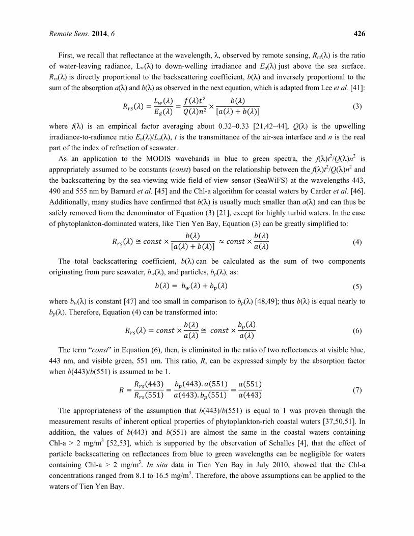
First, we recall that reflectance at the wavelength, λ, observed by remote sensing, Rrs(λ) is the ratio

of water-leaving radiance, Lw(λ) to down-welling irradiance and Ed(λ) just above the sea surface.

Rrs(λ) is directly proportional to the backscattering coefficient, b(λ) and inversely proportional to the

sum of the absorption a(λ) and b(λ) as observed in the next equation, which is adapted from Lee et al. [41]: ( ) = ( )( ) = ( )( ) × ( )( ) + ( ) (3)

where f(λ) is an empirical factor averaging about 0.32–0.33 [21,42–44], Q(λ) is the upwelling

irradiance-to-radiance ratio Eu(λ)/Lu(λ), t is the transmittance of the air-sea interface and n is the real

part of the index of refraction of seawater.

As an application to the MODIS wavebands in blue to green spectra, the f(λ)t2/Q(λ)n2 is

appropriately assumed to be constants (const) based on the relationship between the f(λ)t2/Q(λ)n2 and

the backscattering by the sea-viewing wide field-of-view sensor (SeaWiFS) at the wavelengths 443,

490 and 555 nm by Barnard et al. [45] and the Chl-a algorithm for coastal waters by Carder et al. [46].

Additionally, many studies have confirmed that b(λ) is usually much smaller than a(λ) and can thus be

safely removed from the denominator of Equation (3) [21], except for highly turbid waters. In the case

of phytoplankton-dominated waters, like Tien Yen Bay, Equation (3) can be greatly simplified to: ( ) ≅ × ( )( ) + ( ) ≈ × ( )( ) (4)

The total backscattering coefficient, b(λ) can be calculated as the sum of two components

originating from pure seawater, bw(λ), and particles, bp(λ), as: ( ) = ( ) + ( ) (5)

where bw(λ) is constant [47] and too small in comparison to bp(λ) [48,49]; thus b(λ) is equal nearly to

bp(λ). Therefore, Equation (4) can be transformed into: ( ) = × ( )( ) ≅ × ( )( ) (6)

The term “const” in Equation (6), then, is eliminated in the ratio of two reflectances at visible blue,

443 nm, and visible green, 551 nm. This ratio, R, can be expressed simply by the absorption factor

when b(443)/b(551) is assumed to be 1. = (443)(551) = (443). (551)(443). (551) = (551)(443) (7)

The appropriateness of the assumption that b(443)/b(551) is equal to 1 was proven through the

measurement results of inherent optical properties of phytoplankton-rich coastal waters [37,50,51]. In

addition, the values of b(443) and b(551) are almost the same in the coastal waters containing

Chl-a > 2 mg/m3 [52,53], which is supported by the observation of Schalles [4], that the effect of

particle backscattering on reflectances from blue to green wavelengths can be negligible for waters

containing Chl-a > 2 mg/m3. In situ data in Tien Yen Bay in July 2010, showed that the Chl-a

concentrations ranged from 8.1 to 16.5 mg/m3. Therefore, the above assumptions can be applied to the

waters of Tien Yen Bay.


In the case of water with an unknown range of in situ Chl-a concentration, b(443)/b(551) is not

assumable as 1. Then, in situ spectroradiometric measurement is necessary to determine the water surface

reflectance and inherent optical properties, such as the a(λ) and b(λ) coefficients. After this

determination, Chl-a concentration can be calculated directly using the backscattering algorithms [37,54].

For general ocean water, a(λ)can be spectrally divided into four absorption components originating

from pure water (aw), phytoplankton (ap), detritus or non-algal particles (aNAP), and gelbstoff or colored

dissolved organic matter (aCDOM) [34] as: ( ) = ( ) + ( ) + ( ) + ( ) (8)

Based on the measurement results of ap(λ), aNAP(λ) and aCDOM(λ) at the 350 stations in various

coastal waters around Europe, it was concluded that the aNAP(λ) and aCDOM(λ) were negligibly small,

and the aw(λ) was constant regardless of [55]. Accordingly, Equation (8) can be simplified as

a(λ) ≅ ap(λ) + const, and Equation (7) is transformed into: = (551)(443) = (551) + .(443) + . (9)

In this equation, Chl-a concentration is a function of ap(λ)only: ( ) = ∗( ) ∙ (10)

where a*p(λ) denotes a chlorophyll-specific absorption coefficient of phytoplankton (m2/mg) at a unit

concentration of Chl-a (1 mg/m3), as shown in Figure 2. Equation (8) can be rewritten as: = (551)(443) = ∗(551) ∙ +∗ (443) ∙ + (11)

∙ ∗ (443) − ∗(551) = − ∙ (12)

where α, β are constants.

As a*p(551) is negligible, i.e., a*

p(443) >> a*p(551) ([4]; Figure 2), the following approximation holds: ∙ ∗ (443) − ∗(551) ≅ ∙ ∗ (443) (13)

Consequently, Chl-a concentration can be estimated by: = − ∙∙ ∗ (443) = ∙ + = (551)(443) + (14)

where ωand ε are constants inversely proportional to a*p(443) and determined by the relationship

between the MODIS data and in situ Chl-a data. This algorithm, using the reflectance ratio of the green

and blue bands, is termed “rGBr” hereafter. The performance of rGBr is evaluated for Tien Yen Bay

by comparing the two existing algorithms, OC3M and RNIR, as described below.

From the absorption spectra of the phytoplankton classes in different sizes, the use of blue and

green bands (443 and 511 nm, respectively) has been demonstrated to be valid for Chl-a concentration

in tropical or low latitude waters, because micro-phytoplankton is mostly accumulated in the surface

layer [54–56]. This condition is applicable to Tien Yen Bay.

Furthermore, bottom reflectance tends to affect Rrs(λ) significantly in usual coastal shallow

waters [57,58]. A Rrs(410)/Rrs(670) algorithm then was proposed to estimate Chl-a concentration

instead of the traditional blue-to-green band-ratio algorithm [57]. This new algorithm was proven to be


accurate only for the waters with low Chl-a concentration <1 mg/m3 [58]: its availability for the

eutrophic waters with Chl-a > 10 mg/m3 has been uncertain. Therefore, in situ measurement of turbidity

or water transparency is necessary to monitor Chl-a concentration in shallow waters using rGBr.

3.3. Geostatistical Methods

Pixel-based satellite images of the Earth’s surface are often composed of spatially and temporally

irregular datasets due to missing swaths or cloud coverage. Additionally, due to limitations in spatial

resolution, maps produced directly from satellite image data may lack the detail and accuracy required

for environmental monitoring. To compensate for missing image data and to improve the spatial

resolution of MODIS image data, geostatistics has been adopted. The effectiveness of geostatistics has

been demonstrated by many case studies for improving the spatial resolution of satellite imagery [59–63]

and mapping distributions of Chl-a and total suspended solids concentrations [33,64–68]. Therefore,

geostatistics must be the most promising for the present purpose.

Geostatistics uses the semivariogram, γ(h), to quantify the spatial correlation of a regionalized

variable by the mean variability between two points:

γ(ℎ) = 12 (ℎ) { ( ) − ( + ℎ)}( ) (15)

where Z(xi) is the estimated Chl-a concentration at pixel i, h is the lag distance between two pixels of

the image and N(h) is the number of pixel pairs of (x, x + h) separated by h. The experimental γ(h) in

Equation (15) is then approximated by a model, such as the spherical model, and the parameters that

describe the structure of spatial variation, range, sill and the nugget effect are determined.

Spatial interpolation using γ(h) is termed kriging. Of the various methods, ordinary kriging (OK), as

shown in the next equation, is the most widely used univariate, non-biased method:

∗ = ( )= 1 (16)

where Z*(xp) is a satisfactory estimate of OK, λi is the weight of Z(xi) and n is the number of data used

for the interpolation. λI can be obtained by solving the linear equation related to γ(h).

4. Results and Discussion

4.1. Atmospheric Correction

The atmospheric correction methods, DOS and QUAC, were applied to the MODIS 36 band data to

obtain Rrs(λ) at the locations involving the sampling points. Table 1 summarizes the descriptive

statistics of Rrs(λ) at the five primary ocean color bands (Bands 9, 10, 12, 13 and 15). Almost all

electromagnetic reflectances are absorbed by water in the wavelength of visible red, near infrared and

short-wave infrared regions. The QUAC-corrected spectra in these regions are known to become

similar spuriously to water body spectra [63]. In fact, the Rrs(λ) data was not obtained for Bands 12, 13


and 15, corresponding to part of the visible red and near-infrared regions by QUAC, as shown by the

mark “not a number (NaN)”. Therefore, QUAC is not applicable to the MODIS image data of tropical

coastal waters. The suitability of DOS to Tien Yen Bay is proven by this study in addition to Ha and

Koike [33]. The DOS gives an effective cross-calibration for Bands 9, 10 and 12 particularly, because

there are no pixels that cannot be corrected in the sampled 40 pixels (Table 1).

Table 1. Descriptive statistics of reflectance data obtained at 40 pixels of the Moderate

Resolution Imaging Spectroradiometer (MODIS) image data corresponding to the locations

of water sampling points. Two atmospheric correction methods, dark-object subtraction

(DOS) and Quick Atmospheric Correction (QUAC), were used to determine the reflectance

at primary ocean color bands. NaN stands for “not a number”.

Data Obtained from DOS for Bands Data Obtained from QUAC for Bands

9 10 12 13 15 9 10 12 13 15

Average 0.043 0.040 0.042 0.022 0.036 0.117 0.039 NaN NaN NaN

Maximum 0.077 0.082 0.090 0.036 0.010 0.147 0.072 NaN NaN NaN

Minimum 0.026 0.021 0.015 0.010 0.024 0.065 0.039 NaN NaN NaN

Out of 40 pixels 0 0 0 13 8 0 0 40 40 40

4.2. Estimation Algorithm for Chl-a Concentrations

The 443 and 551 nm wavelengths used for estimating Chl-a concentration are equivalent to MODIS

Bands 9 and 12, respectively. Using Rrs(443) and Rrs(551) obtained through DOS and the least squares

method for the relationship between their ratio (R in Equation (7)) and the Chl-a concentrations at the

40 points (Figure 2a), the rGBr of Equation (14) was determined as: = 8.843 ∙ + 4.093 (17)

The descriptive statistics of the Chl-a concentrations estimated at 392 pixels by rGBr are shown in

Table 2, which are similar to those of the sample data. In addition, the estimated values are well fitted

to the measured values with a correlation coefficient r = 0.78, as confirmed in Figure 2b. The relative

error of this estimation ranges from zero to 15%, and the root mean square error (RMSE) is small at

1.13 mg/m3 (Table 3) against the data average of 12.5 mg/m3 (Table 2).

Table 3 compares the prediction accuracy of rGBr with that of OC3M of Equation (1) and RNIR of

Equation (2). These equations were also determined by Rrs and the measured concentration data using

the least squares method. It is evident that rGBr has the largest and the smallest mean standard error

(MSE) and RMSE.

The capabilities of the three models can be evaluated, as seen in Figure 3, which shows the

relationship between the measured and estimated Chl-a concentrations. As estimated from the value,

this relationship is the weakest in RNIR: in particular, the high and low concentrations cannot be

estimated. This result proves the overestimation problem of RNIR for the waters containing

Chl-a ≥ 6 mg/m3 by Gilerson et al. [40]. The difference between OC3M and rGBr is remarkable in the

region with concentrations higher than 14 mg/m3, in which the trend of the underestimate is stronger in

OC3M than rGBr. Consequently, rGBr was identified as the best model for estimating Chl-a

concentrations over Tien Yen Bay with small errors.


Figure 2. (a) The relationship between chlorophyll-a (Chl-a) concentration of the water

sample and the ratio of two reflectances at MODIS Band 12 (551 nm) vs. Band 9 (443 nm).

A regression line is drawn to show the relationship. (b) Scattergram of Chl-a concentrations

between the sample value and estimation by the ratio of green and blue band reflectance

(rGBr) of Equation (17). The 45-degree dotted line denotes perfect estimation.

Table 2. Descriptive statistics of three datasets of Chl-a concentrations (mg/m3): water

samples, estimations from the MODIS image data by rGBr and predictions at the MODIS

pixels by cross-validation of ordinary kriging (OK).

Sample Data Estimation from MODIS Prediction by OK Number of data 40 392 392 Mean 12.5 13.3 13.3 Median 12.7 13.3 13.3 Maximum 16.5 16.6 16.1 Minimum 8.1 9.0 9.9 Standard deviation 1.8 1.4 1.3 Range 8.4 7.6 6.3

Table 3. Comparison of three algorithms for estimating the accuracy of Chl-a

concentrations. The accuracy is evaluated by the linear correlation coefficient (r), mean

square error (MSE) and root mean square error (RMSE) for the 40 sample values. RNIR,

red-near-infrared band ratio algorithm (RNIR).

Algorithm Models with Empirical Coefficients r MSE (mg/m

3) RMSE

(mg/m3) Average Max Min

OC3M

(O’Reilly et al., 2000)

= 10 . . . . .

where = log 10 { ( ): ( )( ) } 0.65 1.19 5.48 0.03 1.70

RNIR

(Gilerson et al., 2010) = −51.212 (748)(667) + 63.084 0.43 1.48 4.19 0.23 1.82

rGBr = 8.843 (551)(443) + 4.093 0.78 0.90 2.51 0.05 1.13

7

9

11

13

15

17

0.55 0.70 0.85 1.00 1.15

Mea

sure

d C

hl-

a (m

g/m

3 )

Rrs(551)/Rrs(443)

a)

8

10

12

14

16

18

8 10 12 14 16 18

Est

imat

ed C

hl-

a (m

g/m

3 )Measured Chl-a (mg/m3)

b)

r = 0.78


Figure 3. Scattergram of Chl-a concentrations between the sample value and estimation by

three algorithms. The 45-degree dotted line denotes perfect estimation.

4.3. Spatial Distribution of Chl-a Concentrations

The spatial distribution of Chl-a concentrations within Tien Yen Bay was estimated by applying

rGBr to the MODIS image data, as illustrated in Figure 4. Although a rough trend of the distribution is

apparent in this 1 km interval estimation of the 392 pixels (e.g., the locations of the highest and lowest

values), there is no precise variation near the shoreline. Additionally, estimation is inevitably

impossible for areas covered by clouds, as shown in black in Figure 4. It can be confirmed therefore

that using only MODIS image data is not effective for monitoring the spatial-temporal changes of

Chl-a concentrations that may have large variation in bad weather conditions.

Next, the MODIS-based estimation was transformed by OK into a more precise distribution with a

100-m grid. Usually, in situ sample data are used for OK, but Chl-a concentrations cannot be estimated

on the day without sample data by this usual procedure. Instead, estimates of Chl-a concentrations

using only MODIS image data enable Chl-a monitoring on the image acquisition day. The histogram

of the 392 Chl-a concentration data is not far from a normal distribution (Figure 5). Therefore, this

dataset is suitable for geostatistical analyses that require normal distribution of regionalized random

variables as OK.

Experimental γ(h) produced from the dataset was approximated best by the exponential model with

a nugget effect of zero, a sill of 1.6 mg/m3 and a range of 17.9 km (Figure 6a). To check the spatial

estimation accuracy of OK with a cross-validation, a scattergram that represents the relationship

between the original CChla-value at a particular MODIS pixel (estimations in Table 1) and the predicted

OK value using the CChla data around the target pixel (predictions in Table 2) was produced

(Figure 6b). The resultant mean error of the prediction is close to zero (0.017 mg/m3), and the RMSE is

relatively low (0.43 mg/m3), which confirms the high capability of OK. The resultant OK distribution

8

10

12

14

16

18

8 10 12 14 16 18

Est

imat

ed C

hl-

a (m

g/m

3 )

Measured Chl-a (mg/m3)

OC3M

RNIR

rGBr


of Chl-a concentration and the kriging variance map are depicted in Figure 7. The kriging variances are

negligible over the entire bay. Only the zone covered by clouds has a relatively high variance, but its

value is smaller than 3% of the estimated CChla. Such a variance trend also supports the correctness of

the OK estimation.

Figure 4. Spatial distribution of Chl-a concentrations over Tien Yen Bay on 6 July 2010,

with a 1-km interval using MODIS image data and rGBr.

Figure 5. Histogram of Chl-a concentrations estimated from MODIS/Terra image data

and rGBr.

The OK map in Figure 7 presents much more precise spatial characteristics than the original CChla

distribution in Figure 4 and also clarifies the eutrophic conditions in the waters of Tien Yen Bay. The

Chl-a concentrations on 6 July 2010, ranged from nine to 16.6 mg/m3, which are four to 7.5 times of

0

20

40

60

80

100

9 9.8 10.5 11.3 12.1 12.8 13.6 14.3 15.1 15.9 16.6

Fre

qu

ency

Estimated Chl-a (mg/m3)


the eutrophic level, 2.21 mg/m3 [71:Table 4]. Generally, concentrations of Chl-a over 14.5 mg/m3

occur in local estuaries at the mouths of the Ha Coi and Dam Ha Rivers and along the coast from

Mong Cai to Hai Ha. The middle bay also contains high Chl-a from 13.5 to 14.5 mg/m3 from Cai Chien

to Hai Ha districts. On the contrary, the concentrations become low toward the west near Cai Bau

Island, with a minimum of 9 mg/m3 in the channels connected with the outer sea.

Figure 6. (a) Omnidirectional experimental semivariogram and exponential model (curve)

of the Chl-a concentrations estimated from MODIS data and rGBr. (b) Scattergram for

cross-validation of ordinary kriging prediction. The 45-degree dotted line is superimposed.

(a) (b)

Figure 7. (a) Spatial distribution of Chl-a concentrations produced by interpolating the

MODIS image-based estimation in Figure 4 using OK and a 100-m grid size. (b) Kriging

variance for representing the uncertainty of estimation of Chl-a concentrations by OK. in

the image, no space before and after en dash representing ranges.

(a)

0.0

0.2

0.4

0.6

0.8

1.0

1.2

1.4

1.6

1.8

2.0

0 2 4 6 8 10 12 14 16 18 20 22

Sem

ivar

iogr

am

Distance (km)

Exponential model

8

10

12

14

16

18

8 10 12 14 16 18

Pre

dic

ted

Ch

l-a

by

OK

(m

g/m

3 )

Estimated Chl-a from MODIS (mg/m3)


Figure 7. Cont.

(b)

Those spatial characteristics conform to the hydrodynamic system in the bay that is generated by

the interaction of regional surface currents ([72]; Figure 4), tides and waves. The local river estuaries

and central bay are shielded by the islands (Van Nuoc, Cai Chien and Vinh Thuc) and the tortuous

coastline, and therefore, the hydro-energy related to currents and waves is weak there. Under such

conditions, phytoplankton, the main source of high Chl-a concentrations, accumulate and grow. In

contrast, in the connection channels and the largely movable waters affected directly by the outer sea,

the hydro-energy is strong. These waters contain high amounts of re-suspended material, which

prevent the accumulation and growth of phytoplankton. Accordingly, Chl-a concentrations become

low in such high-energy zones.

4.4. Eutrophication Processes over the Course of a Year

To clarify the eutrophication process and the seasonal change of Chl-a concentrations in the waters

of Tien Yen Bay, the rGBr and OK were applied to 21 scenes of MODIS image data that were

acquired under the lowest cloud coverage conditions from late May 2010, to middle May 2011. The

resultant maps are shown in Figure 8. The general trend of the Chl-a concentrations is observed to be

similar to Figure 7 in that higher concentrations are located in the near shore and the central bay

waters, while lower concentrations are distributed in the waters connected directly to the outer sea. The

map of 5 August 2010, reveals extraordinarily high concentrations over the whole bay, which may have

been caused by the massive growth of phytoplankton, due to the strong solar energy in the midsummer.

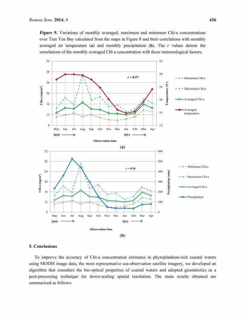
The seasonal trend is highlighted by the graphs in Figure 9 showing monthly averaged, maximum

and minimum Chl-a concentrations over Tien Yen Bay calculated from the maps in Figure 8. The Chl-a

concentrations (monthly averaged concentrations) reached a maximum of 16.6 mg/m3 in August 2010.

After that, the concentrations declined toward the winter, with a minimum of 12.0 mg/m3 in January 2011,

and then increased again toward a second maximum concentration (15.9 mg/m3) in March 2011.


Figure 8. Spatio-temporal changes of Chl-a concentrations for the year from May 2010, to

May 2011, over Tien Yen Bay produced from 21 MODIS scene data, rGBr and OK.

The monthly maximum and minimum draw similar trends to the average. These temporal changes

are coincident with the monthly averaged air temperature and monthly precipitation [73]. Because

solar energy input in the early spring is not great enough for the rapid growth of phytoplankton, the

concentrations decline to a general level soon after the second peak. In many coastal waters, such as

the southern coast of Hokkaido in northern Japan [74], Chl-a concentrations usually show a bimodal

variation with the first peak in spring and the second peak in late summer to early autumn. This trend

coincides with that observed in the waters of Tien Yen Bay.

CSTT [75] defined 10 mg/m3 of Chl-a as the Environmental Quality Standard for coastal waters. If

the Chl-a concentration of a water body frequently exceeds this criterion in the summer, it is regarded

as having a eutrophic condition. Based on this criterion, the waters of Tien Yen Bay were considered

to be eutrophic over the entire study period, with the degree of eutrophication being the strongest

midsummer. However, undesirable eutrophication disturbances, such as algae blooms, generated in the

water with Chl-a over 100 mg/m3 [76] have not been observed in Tien Yen Bay. This bay may be

eutrophic by natural processes rather than by anthropogenic causes, such as wastewater, thereby

maintaining a high ecological quality similar to other coastal areas [24]. The natural cause is suggested

by the positive moderate correlation of the Chl-a concentrations with the meteorological factors as

shown in Figure 9 (r = 0.57 and 0.54 for the air temperature and precipitation, respectively) and no

specific accumulation of Chl-a concentrations in a certain area.

Note that the remote sensing technique can detect Chl-a in surface waters only. However, Tien Yen

Bay is a shallow water body; then, Chl-a concentrations may be relatively uniform over the depth

except for the deep channels [28]. Phytoplankton, such as diatoms (Bacillariophyta), is often

accumulated at the highest level in the surface water layer within the 1-m depth for photosynthesis.


Figure 9. Variations of monthly averaged, maximum and minimum Chl-a concentrations

over Tien Yen Bay calculated from the maps in Figure 8 and their correlations with monthly

averaged air temperature (a) and monthly precipitation (b). The r values denote the

correlations of the monthly averaged Chl-a concentration with those meteorological factors.

(a)

(b)

5. Conclusions

To improve the accuracy of Chl-a concentration estimates in phytoplankton-rich coastal waters

using MODIS image data, the most representative sea-observation satellite imagery, we developed an

algorithm that considers the bio-optical properties of coastal waters and adopted geostatistics as a

post-processing technique for down-scaling spatial resolution. The main results obtained are

summarized as follows:

12

16

20

24

28

32

8

12

16

20

24

28

32

May Jun Jul Aug Sep Oct Nov Dec Jan Feb Mar Apr

Tem

per

atur

e (o C

)

Ch

l-a

(mg/

m3 )

Observation time

Minimium Chl-a

Maximium Chl-a

Averaged Chl-a

Averagedtemperature

r = 0.57

2010 2011

0

100

200

300

400

500

600

8

12

16

20

24

28

32

May Jun Jul Aug Sep Oct Nov Dec Jan Feb Mar Apr

Pre

cip

itat

ion

(m

m)

Ch

l-a

(mg/

m3 )

Observation time

Minimium Chl-a

Maximium Chl-a

Averaged Chl-a

Precipitation

r = 0.54

2010 2011


(1) Two widely-used atmospheric correction methods, DOS and QUAC, were compared to obtain

reflectance at the sea surface by excluding atmospheric contributions from the MODIS image

data. DOS was identified to be more suitable for tropical waters, such as those of Tien

Yen Bay.

(2) Consideration of the optical properties of water shows that the concentration of Chl-a can be

physically calculated by the ratio of the reflectances of the seawater surface at the visible green

and blue wavelengths. The Chl-a concentrations in phytoplankton-rich coastal waters estimated

by the proposed algorithm, rGBr, fit the measured in situ concentrations better and with smaller

errors than the two previous representative algorithms, OC3M and RNIR.

(3) The effectiveness of OK to improve the spatial resolution of the MODIS image-based

estimation of Chl-a concentration from 1 km to 100 m was demonstrated. This improvement

was possible because the OK map clarified the variation of Chl-a concentration in detail,

particularly in local estuaries. From that OK map, the hydrodynamic system in Tien Yen Bay is

suggested to be a main factor controlling the distribution of Chl-a concentrations.

(4) By applying the rGBr and OK to the 21 scenes of MODIS image data from May 2010 to

May 2011, notable features and seasonal trends were detected. In particular, the Chl-a

concentrations have a bimodal variation. Furthermore, the waters of Tien Yen Bay can be

labeled as naturally eutrophic, because of Chl-a values higher than 10 mg/m3 in the summer.

This natural cause is supported by the correlation of Chl-a concentrations with representative

meteorological factors, air temperature and precipitation.

In conclusion, the combination of the proposed rGBr and OK methods can contribute to monitoring

water quality and the eutrophication process in tropical coastal areas having similar geomorphological

conditions as Tien Yen Bay, particularly in the South China Sea coast, where this is recognized as the

global marine center of shallow-water tropical biodiversity.

Acknowledgments

We are grateful to the projects coded QGTD 10.31 TRIG-A and 105.09.82.09 NAFOSTED by the

Vietnamese National Scientific Grant for their support of the fieldwork and water sample analysis.

Thanks also go to NASA for providing the MODIS data and to four anonymous reviewers for their

valuable comments and suggestions that helped improve the clarity of the manuscript.

Conflicts of Interest

The authors declare no conflict of interest.

References

1. Matthews, A.M.; Duncan, A.G.; Davison, R.G. An assessment of validation techniques for

estimating chlorophyll-a concentration from airborne multispectral imagery. Int. J. Remote Sens.

2001, 22, 429–447.

2. Cauwer, V.D.; Ruddick, K.; Park, Y.J.; Nechad, B.; Kyramarios, M. Optical remote sensing in

support of eutrophication monitoring in the southern North Sea. EARSeL eProc. 2004, 3, 208–221.


3. Zimba, P.V.; Gitelson, A. Remote estimation of chlorophyll concentration in hyper-eutrophic

aquatic systems: Model tuning and accuracy optimization. Aquaculture 2006, 256, 272–286.

4. Schalles, J.F. Optical Remote Sensing Techniques to Estimate Phytoplankton Chlorophyll-a

Concentrations in Coastal Waters with Varying Suspended Matter and CDOM Concentrations. In

Remote Sensing of Aquatic Coastal Ecosystem Processes: Science and Management Application;

Richardson, L.L., LeDew, E.F., Eds.; Springer: Dordrecht, The Netherlands, 2006; pp. 27–78.

5. Ibrahim, A.N; Mabuchi, Y.; Murakami, M. Remote sensing algorithms for monitoring

eutrophication in Ishizuchi storm water reservoir in Kochi Prefecture, Japan. Hydrol. Sci. J. 2009,

50, 525–542.

6. Gordon, H.R; Morel, A.Y. Remote Assessment of Ocean Color for Interpretation of Satellite

Visible Imagery: A Review; Springer-Verlag: New York, NY, USA, 1983; pp. 1–114.

7. Aiken, J.; Moore, G.F.; Trees, C.C.; Hooker, S.B.; Clark, D.K. The SeaWiFS CZCS-Type

Pigment Algorithm. In SeaWiFS Technical Report Series; Hooker, S.B., Firestone, E.R., Eds.,

NASA Goddard Space Flight Center: Greenbelt, MD, USA, 1995; Volume 29, pp. 1–34.

8. O’Reilly, J.E.; Maritorena, S.; Mitchell, B.G.; Siegel, D.A.; Carder, K.L.; Garver, S.A.; Kahru, M.;

McClain, C. Ocean color chlorophyll algorithms for SeaWiFS. J. Geophys. Res. 1998, 103,

24937–24953.

9. O’Reilly, J.E.; Maritorena, S.; Mitchell, B.G.; Siegel, D.A.; Carder, K.L.; Garver, S.A.; Kahru, M.;

McClain, C. Ocean Color Chlorophyll a Algorithms for SeaWiFS, OC2, and OC4: Version 4. In

SeaWiFS Postlaunch Technical Report Series, Volume 11, SeaWiFS Postlaunch Calibration and

Validation Analyses, Part 3; Hooker, S.B., Firestone, E.R., Eds.; NASA Goddard Space Flight

Center: Greenbelt, MD, USA, 2000; pp. 9–23.

10. Carder, K.L.; Steward, R.G.; Harvey, G.R.; Ortner, P.B. Marine humic and fulvic acids: Their

effects on remote sensing of ocean chlorophyll. Limnol. Oceanogr. 1989, 34, 68–81.

11. Gallegos, C.L.; Correll, D.L.; Pierce, J.W. Modeling spectral diffuse attenuation, absorption, and

scattering coefficients in a turbid estuary. Limnol. Oceanogr. 1990, 35, 1486–1502.

12. Ritchie, J.C.; Schiebe, F.R.; Cooper, C.M.; Harrington, J.A., Jr. Chlorophyll measurements in the

presence of suspended sediment using broad band spectral sensors aboard satellites. J. Freshwater

Ecol. 1994, 9, 197–206.

13. Schalles, J.F.; Sheil, A.T.; Tycast, J.F.; Alberts, J.J.; Yacobi, Y.Z. Detection of Chlorophyll,

Seston, and Dissolved Organic Matter in the Estuarine Mixing Zone of Georgia Coastal Plain

Rivers. In Proceedings of the Fifth International Conference on Remote Sensing for Marine and

Coastal Environments, San Diego, CA, USA, 5–7 October 1998; pp. 315–324.

14. Gons, H.J. Optical tele-detection of chlorophyll a in turbid inland waters. Environ. Sci. Technol.

1999, 33, 1127–1132.

15. Hladik, C.M. Close Range, Hyperspectral Remote Sensing of Southeastern Estuaries and an

Evaluation of Phytoplankton Chlorophyll-a Predictive Algorithms. M.Sc. Thesis, Creighton

University, Omaha, NE, USA, 2004.

16. Vertucci, F.A.; Likens, G.E. Spectral reflectance and water quality of Adirondack mountain

region lakes. Limnol. Oceanogr. 1989, 34, 1656–1672.


17. Schalles, J.F.; Gitelson, A.A.; Yacobi, Y.Z.; Kroenke, A.E. Estimation of chlorophyll a from time

series measurements of high spectral resolution reflectance in an eutrophic lake. J. Phycol. 1998,

34, 383–390.

18. Thiemann, S.; Kaufmann, H. Lake water quality monitoring using hyperspectral airborne data—A

semiempirical multisensor and multitemporal approach for the Mecklenburg Lake District,

Germany. Remote Sens. Environ. 2002, 81, 228–237.

19. Kallio, K.; Koponen, S.; Pulliainen, J. Feasibility of airborne imaging spectrometry for lake

monitoring—A case study of spatial chlorophyll-a distribution in two meso-eutrophic lakes. Int. J.

Remote Sens. 2003, 24, 3771–3790.

20. McGlathery, K.J.; Sundback, K.; Anderson, I.C. Eutrophication in shallow coastal bays and

lagoons: the role of plants in coastal filter. Marine Ecol. Prog. Series 2007, 348, 1–18.

21. Morel, A.; Prieur, L. Analysis of variations in ocean color. Limnol. Oceanogr. 1977, 22, 709-722.

22. Wu, M.; Zhang, W.; Wang, X.; Luo, D. Application of MODIS satellite data in monitoring water

quality parameters of Chaohu Lake in China. Environ. Monit. Assess. 2009, 148, 255–264.

23. Vietnam Environment Protection Agency (VEPA), World Conservation Union (IUCN), Mekong

Wetlands Biodiversity Conservation and Sustainable Use Programme (MWBP). Overview of

Wetland Status in Vietnam following 15 Years of Ramsar Convention Implementation; VEPA:

Hanoi, Vietnam, 2005; pp. 1–80.

24. Hoang, V.T.; Pham, V.H. Biodiversity in Coastal Zones of Tien Yen—Dam Ha, Quang Ninh

Province and Conservation. In Proceeding of the 2nd Vietnam National Conference on

Biodiversity (in Vietnamese), Hanoi, Vietnam, 17 October 2010; pp. 61–74.

25. Thuoc, C.V. Phytoplankton in the Tien Yen, Bach Dang and Red River mouths. Marine Resour.

Environ. 1996, 3, 242–248.

26. American Public Health Association (APHA). Standard Methods for the Examination of Water

and Wastewater, 20th ed.; American Public Health Association: Washington, DC, USA, 1998;

pp. E1–E15.

27. Department of Environment, Climate Change and Water NSW. Waterwatch Estuary Field Mannual:

A Manual for On-Site Use in the Monitoring of Water Quality and Estuary Health; Department of

Environment, Climate Change and Water NSW: Sydney, Australia, 2010; pp. 2_6–2_7.

28. Vietnam Ministry of Natural Resources and Environment. Vietnam Topographic Map; Scale

1/50,000; Department of Survey Map Publishing House: Hanoi, Vietnam, 2004.

29. Chavez, J.P.S., Jr. An improved dark-object subtraction technique for atmospheric scattering

correction of multispectral data. Remote Sens. Environ. 1988, 24, 459–479.

30. Bernstein, L.S.; Adler-Golden, S.M.; Sundberg, R.L.; Levine, R.Y.; Perkins, T.C.; Berk A.;

Ratkowski, A.J.; Felde, G.; Hoke, M.L. A New Method for Atmospheric Correction and Aerosol

Optical Property Retrieval for VIS-SWIR Multi- and Hyperspectral Imaging Sensors: QUAC

(QUick Atmospheric Correction). In Proceedings of IEEE International Geosciences and Remote

Sensing Symposium, Seoul, Korea, 25–27 July 2005; pp. 3549–3552.

31. Hadjimitsis, D.G.; Clayton, C.R.I.; Hope, V.S. An assessment of the effectiveness of atmospheric

correction algorithms through the remote sensing of some reservoirs. Int. J. Remote Sens. 2004,

25, 3651–3674.


32. Hadjimitsis, D.G.; Clayton, C.R.I. Field spectroscopy for assisting water quality monitoring and

assessment in water treatment reservoirs using atmospheric corrected satellite remotely sensed

imagery. Remote Sens. 2011, 3, 362–377.

33. Ha, N.T.T.; Koike, K. Integrating satellite imagery and geostatistics of point samples for

monitoring spatio-temporal changes of total suspended solids in bay waters: application to Tien

Yen Bay (Northern Vietnam). Frontiers Earth Sci. 2011, 5, 305–316.

34. Moses, W.J.; Gitelson, A.A.; Berdnikov, S.; Povazhnyy, V. Estimation of chlorophyll-a

concentration in case II waters using MODIS and MERIS data- successes and challenges.

Environ. Res. Lett. 2009, 4, doi:10.1088/1748-9326/4/4/045005.

35. Carder, K.L.; Chen, F.R.; Cannizzaro, J.P.; Campbell, J.W.; Mitchell, B.G. Performance of the

MODIS semi-analytical ocean color algorithm for chlorophyll-a. Adv. Space Res. 2004, 33,

1152–1159.

36. Gitelson, A. The Peak near 700 nm on Radiance Spectra of algae and water - Relationships of its

magnitude and position with chlorophyll concentration. Int. J. Remote Sens. 1992, 13, 3367–3373.

37. Antoite, D.; Andre, J.M.; Morel, A. Oceanic primary production 2: Estimation of global scale

from satellite (coastal zone color scanner) chlorophyll. Glob. Biogeochem. Cy. 1996, 10, 57–69.

38. D’Sa, E.J.; Miller, R.L. Bio-optical properties in waters influenced by the Mississippi River

during low flow conditions. Remote Sens. Environ. 2002, 84, 538–549.

39. Dall’Olmo, G.; Gitelson, A.A.; Rundquist, D.C. Toward a unified approach for remote estimation

of chlorophyll-a in both terrestrial vegetation and turbid productive waters. Geophys. Res. Lett.

2003, 30, 1938–1941.

40. Gilerson, A.A; Gitelson, A.A.; Zhou, J.; Gurlin, D.; Moses, W.; Ioannou, I.; Ahmed, S.

Algorithms for remote estimation of chlorophyll-a in coastal and inland waters using red and near

infrared bands. Opt. Express. 2010, 18, 24109–24125.

41. Lee, Z.P.; Carder, K.L.; Hawes, S.H.; Steward, R.G.; Peacock, T.G.; Davis, C.O. A model for

interpretation of hyperspectral remote-sensing reflectance. Appl. Opt. 1994, 33, 5721–5732.

42. Gordon, H.R.; Brown, O.B.; Jacobs, M.M. Computed relationships between the inherent and

apparent optical properties of a flat homogeneous ocean. Appl. Opt. 1975, 14, 417–427.

43. Jerome, J.H.; Bukata, R.P.; Burton, J.E. Utilizing the components of vector irradiance to estimate

the scalar irradiance in natural waters. Appl. Opt. 1988, 27, 4012–4018.

44. Kirk, J.T.O. Volume scattering function, average cosines, and the underwater light field.

Limnol. Oceanogr. 1991, 36, 455–467.

45. Barnard, A.H.; Ronald, J.; Zaneveld, V.; Pegau, S.W. In situ determination of the remotely sensed

reflectance and the absorption coefficient: Closure and inversion. Appl. Opt. 1999, 38, 5108–5117.

46. Carder, K.L.; Chen, F.R.; Lee, Z.; Hawes, S.K.; Cannizzaro, J.P. Case 2 Chlorophyll a. In MODIS

Ocean Science Team Algorithm Theoretical Basis Document; Version 7; NASA Goddard Space

Flight Center: Greenbelt, MD, USA, 2003; pp. 4–67.

47. Morel, A. Optical Properties of Pure Water and Pure Seawater. In Optical Aspects of

Oceanography; Jerlov, N.G., Nielson, E.S., Eds.; Academic Press: London, UK, 1974; pp. 1–24.

48. Smith, R.C.; Baker, K.S. Optical properties of the clearest natural waters (200–800 nm). Appl.

Opt. 1981, 20, 177–184.


49. Twardowski, M.S.; Claustre, H.; Freeman, S.A.; Stramski, D.; Huot, Y. Optical backscattering

properties of the “clearest” natural waters. Biogeosciences 2007, 4, 1041–1058.

50. McKee, D.; Cunningham, A.; Slater, J.; Jones, K.J.; Griffiths, C.R. Inherent and apparent optical

properties in coastal waters: A study of the Clyde Sea in early summer. Estuar. Coast. Shelf Sci.

2002, 56, 369–376.

51. McKee, D.; Cunningham, A. Identification and characterisation of two optical water types in the

Irish Sea from in situ inherent optical properties and seawater constituents. Estuar. Coast. Shelf Sci.

2006, 68, 305–316.

52. Whitmire, A.L.; Boss, E.; Cowles, T.J.; Pegau, W.S. Spectral variability of the particulate

backscattering ratio. Opt. Expr. 2007, 15, 7019–7031.

53. Park, Y.J; Ruddick K. Model of remote-sensing reflectance including bidirectional effects for case

1 and case 2 waters. Appl. Opt. 2005, 44, 1236–1249.

54. Babin, M.; Stramski D.; Ferrari, G.M.; Claustre, H.; Bricaud, A.; Obolensky, G.; Hoepffner, N.

Variations in the light absorption coefficients of phytoplankton, non-algal particles, and dissolved

organic matter in coastal waters around Europe. J. Geophys. Res. 2003, 108, 4_1–4_20.

55. Fishwick, J.R.; Aiken, J.; Barlow, R.G.; Sessions, H.; Bernard, S.; Ras, J. Functional relationships

and bio-optical properties derived from phytoplankton pigments, optical and photosynthetic

parameters; a case study of the Benguela ecosystem. J. Mar. Biol. Assoc. UK 2006, 86, 1267–1280.

56. Hirata, T.; Aiken, J.; Hardman-Mountford, N.; Smyth, T.J.; Barlow, R.G. An absorption model to

determine phytoplankton size classes from satellite ocean colour. Remote Sens. Environ. 2009,

112, 3153–3159.

57. Carder, K.L.; Cannizzaro, J.P.; Lee, Z. Ocean color algorithms in optically shallow waters:

Limitation and improvements. Proc. SPIE 2005, 5885, doi:10.1117/12.615039.

58. Cannizzaro, J.P.; Carder, K.L. Estimating chlorophyll a concentration from remote-sensing

reflectance in optically shallow waters. Remote Sens. Environ. 2006, 101, 13–24.

59. Aiken, J.; Pradhan, Y.; Barlow, R.G.; Lavender, S.; Poulton, A.; Holligan, P.M.;

Hardman-Mountford, N. Phytoplankton pigments and functional types in the Atlantic Ocean: A

decadal assessment, 1995–2005. Deep-Sea Res. Part II: Top. Stud. Oceanogr. 2009, 56, 899–917.

60. Cressie, N.A.C. Statistics for Spatial Data; John Wiley & Sons, Inc: New York, NY, USA, 1993;

pp. 1–900.

61. Kanaroglou, P.S.; Soulakellis, N.A.; Sifakis, N.I. Improvement of satellite derived pollution maps

with the use of a geostatistical interpolation method. J. Geogr. Syst. 2001, 4, 193–208.

62. Zhang, C.; Li, W.; Travis, D. Restoration of clouded pixels in multispectral remotely sensed

imagery with co-kriging. Int. J. Remote Sens. 2009, 30, 2173–2195.

63. Meng, Q.; Borders, B.; Madden, M. High-resolution satellite image fusion using regression

kriging. Int. J. Remote Sens. 2010, 31, 1857–1876.

64. Petrie, G.M.; Heasler, P.G.; Perry, E.M.; Thompson, S.E.; Daly, D.S. Inverse kriging to enhance

spatial resolution of imagery. Proc. SPIE 2002, 4789, doi:10.1117/12.454822.

65. Wang, X.J.; Liu, R.M. Spatial analysis and eutrophication assessment for chlorophyll a in Taihu

Lake. Environ. Monit. Assess. 2005, 101, 167–74.

66. Müller, D. Estimation of Algae Concentration in Cloud Covered Scenes Using Geostatistical

Methods. In Proceeding of ENVISAT Symposium 2007, Montreux, Switzerland, 23–27 April 2007.


67. Georgakarakos, S.; Kitsiou, D. Mapping abundance distribution of small pelagic species applying

hydroacoustics and Co-Kriging techniques. Hydrobiologia 2008, 612, 155–169.

68. Saulquin, B.; Gohin, F.; Garrello, R. Regional objective analysis for merging high-resolution

MERIS, MODIS/Aqua, and SeaWiFS Chlorophyll-a data from 1998 to 2008 on the European

Atlantic Shelf. IEEE Trans. Geosci. Remote Sens. 2010, 49, 143–154.

69. Shehhi, M.R.A.; Gherboudj, I.; Estima, J.; Ghedira, H. Geospatial Analysis of the Red-Tide over

the Arabian Gulf. In Proceeding of the 1st Geospatial Scientific Summit, Dubai, United Arab

Emirates, 12–13 November 2012.

70. Agrawal, G.; Sarup, J. Comparision of QUAC and FLAASH atmospheric correction modules on

EO-1 Hyperion data of Sanchi. Int. J. Adv. Eng. Sci. Technol. 2011, 4, 178–186.

71. Simboura, N.; Panayotidis, P.; Papathanassiou, E. A synthesis of the biological quality elements

for the implementation of the European Water Framework Directive in the Mediterranean

ecoregion: The case of Saronikos Gulf. Ecol. Indic. 2005, 5, 253–266.

72. Morton, B.; Blackmore, G. South China Sea. Mar. Pollut. Bull. 2001, 42, 1236–1263.

73. Quangninh Province Statistics Office. Quangninh. Statistical Yearbook 1955–2011; Statistical

Publishing House: Hanoi, Vietnam, 2012; pp.1–548.

74. Lihan, T.; Mustapha, M.A.; Rahim, S.A.; Saitoh, S.; Iida, K. Influence of river plume on

variability of chlorophyll a concentration using satellite images. J. Appl. Sci. 2011, 11, 484–493.

75. CSTT (Comprehensive Study Task Team of Group Coordinating Sea Disposal Monitoring).

Comprehensive Studies for the Purposes of Article 6 & 8.5 of DIR 91/271 EEC, the Urban. Waste

Water Treatment Directive, 2nd ed.; The Scottish Environment Protection Agency and Water

Service Association: Edinburgh, UK, 1997; pp. 8–11.

76. Cannizzaroa, J.P.; Cardera, K.L.; Chena, F.R.; Heilb, C.A.; Vargoa, G.A. A novel technique for

detection of the toxic dinoflagellate, Kareniabrevis, in the Gulf of Mexico from remotely sensed

ocean color data. Cont. Shelf Res. 2008, 28, 137–158.

© 2013 by the authors; licensee MDPI, Basel, Switzerland. This article is an open access article

distributed under the terms and conditions of the Creative Commons Attribution license

(http://creativecommons.org/licenses/by/3.0/).

Improved Accuracy of Chlorophyll-a Concentration Estimates from MODIS Imagery Using a Two-Band Ratio...

Documents

Transcript of Improved Accuracy of Chlorophyll-a Concentration Estimates from MODIS Imagery Using a Two-Band Ratio...