MODIStsp: A Tool for Automatic Preprocessing of

MODIS Time Series - v1.3.3Lorenzo Busetto (busetto.l@irea.cnr.it), Luigi Ranghetti (ranghetti.l@irea.cnr.it)

2017-08-17

Contents

1 Introduction 1

2 Installation 22.1 On Windows . . . . . . . . . . . . . . . . . . . . . . . . . . . . . . . . . . . . . . . . . . . . . 22.2 On Linux systems . . . . . . . . . . . . . . . . . . . . . . . . . . . . . . . . . . . . . . . . . . 32.3 On Mac OS . . . . . . . . . . . . . . . . . . . . . . . . . . . . . . . . . . . . . . . . . . . . . . 3

3 Running the tool in Interactive Mode: the MODIStsp GUI 53.1 Selecting Processing Parameters . . . . . . . . . . . . . . . . . . . . . . . . . . . . . . . . 63.2 Saving and Loading Processing Options . . . . . . . . . . . . . . . . . . . . . . . . . . . 103.3 Starting the processing . . . . . . . . . . . . . . . . . . . . . . . . . . . . . . . . . . . . . . 10

4 Non-Interactive Execution from within R 114.1 Specifying a saved “Options file” . . . . . . . . . . . . . . . . . . . . . . . . . . . . . . . . . . 114.2 Looping on different spatial extents . . . . . . . . . . . . . . . . . . . . . . . . . . . . . . . . . 11

5 Standalone execution and scheduled processing 115.1 Standalone execution . . . . . . . . . . . . . . . . . . . . . . . . . . . . . . . . . . . . . . . . . 115.2 Scheduled Processing . . . . . . . . . . . . . . . . . . . . . . . . . . . . . . . . . . . . . . . . . 12

6 Outputs Format and Naming Conventions 126.1 Single-band outputs . . . . . . . . . . . . . . . . . . . . . . . . . . . . . . . . . . . . . . . . . 126.2 Virtual multi-band outputs . . . . . . . . . . . . . . . . . . . . . . . . . . . . . . . . . . . . . 13

7 Accessing the processed time series from R 137.1 Extracting Time Series Data on Areas of Interest . . . . . . . . . . . . . . . . . . . . . . . . . 13

8 Problems and Issues 14

9 Citation 14

10 Installing R and GDAL 1410.1 Installing R . . . . . . . . . . . . . . . . . . . . . . . . . . . . . . . . . . . . . . . . . . . . . . 1410.2 Installing GDAL >= 1.11.1 . . . . . . . . . . . . . . . . . . . . . . . . . . . . . . . . . . . . . 15

1 Introduction

MODIStsp is a novel “R” package allowing to automatize the creation of time series of rasters derived fromMODIS Land Products data. It allows to perform several preprocessing steps on MODIS data availablewithin a given time period.

Development of MODIStsp started from modifications of the ModisDownload “R” script by Thomas Hengl[-@Hengl2010], and successive adaptations by Babak Naimi [-@Naimi2014]. The basic functionalities for

1

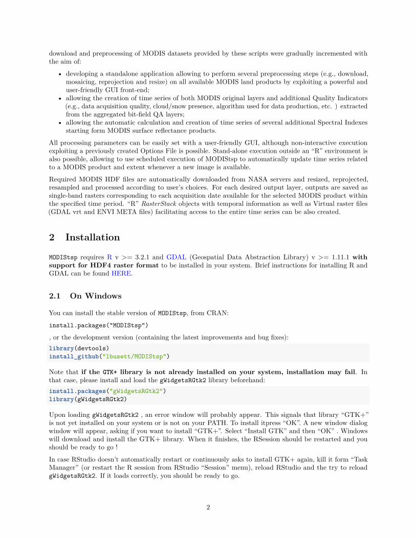
download and preprocessing of MODIS datasets provided by these scripts were gradually incremented withthe aim of:

• developing a standalone application allowing to perform several preprocessing steps (e.g., download,mosaicing, reprojection and resize) on all available MODIS land products by exploiting a powerful anduser-friendly GUI front-end;

• allowing the creation of time series of both MODIS original layers and additional Quality Indicators(e.g., data acquisition quality, cloud/snow presence, algorithm used for data production, etc. ) extractedfrom the aggregated bit-field QA layers;

• allowing the automatic calculation and creation of time series of several additional Spectral Indexesstarting form MODIS surface reflectance products.

All processing parameters can be easily set with a user-friendly GUI, although non-interactive executionexploiting a previously created Options File is possible. Stand-alone execution outside an “R” environment isalso possible, allowing to use scheduled execution of MODIStsp to automatically update time series relatedto a MODIS product and extent whenever a new image is available.

Required MODIS HDF files are automatically downloaded from NASA servers and resized, reprojected,resampled and processed according to user’s choices. For each desired output layer, outputs are saved assingle-band rasters corresponding to each acquisition date available for the selected MODIS product withinthe specified time period. “R” RasterStack objects with temporal information as well as Virtual raster files(GDAL vrt and ENVI META files) facilitating access to the entire time series can be also created.

2 Installation

MODIStsp requires R v >= 3.2.1 and GDAL (Geospatial Data Abstraction Library) v >= 1.11.1 withsupport for HDF4 raster format to be installed in your system. Brief instructions for installing R andGDAL can be found HERE.

2.1 On Windows

You can install the stable version of MODIStsp, from CRAN:

install.packages("MODIStsp")

, or the development version (containing the latest improvements and bug fixes):

library(devtools)

install_github("lbusett/MODIStsp")

Note that if the GTK+ library is not already installed on your system, installation may fail. Inthat case, please install and load the gWidgetsRGtk2 library beforehand:

install.packages("gWidgetsRGtk2")

library(gWidgetsRGtk2)

Upon loading gWidgetsRGtk2 , an error window will probably appear. This signals that library “GTK+”is not yet installed on your system or is not on your PATH. To install itpress “OK”. A new window dialogwindow will appear, asking if you want to install “GTK+”. Select “Install GTK” and then “OK” . Windowswill download and install the GTK+ library. When it finishes, the RSession should be restarted and youshould be ready to go !

In case RStudio doesn’t automatically restart or continuously asks to install GTK+ again, kill it form “TaskManager” (or restart the R session from RStudio “Session” menu), reload RStudio and the try to reloadgWidgetsRGtk2. If it loads correctly, you should be ready to go.

2

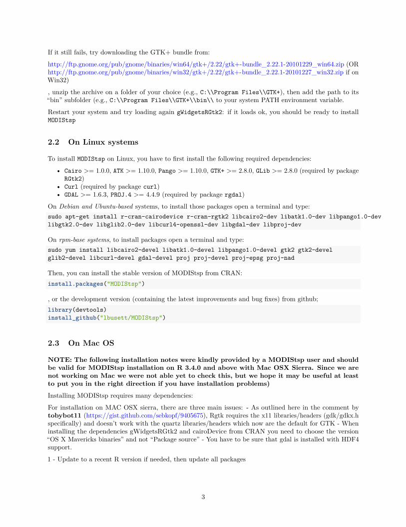
If it still fails, try downloading the GTK+ bundle from:

http://ftp.gnome.org/pub/gnome/binaries/win64/gtk+/2.22/gtk+-bundle_2.22.1-20101229_win64.zip (ORhttp://ftp.gnome.org/pub/gnome/binaries/win32/gtk+/2.22/gtk+-bundle_2.22.1-20101227_win32.zip if onWin32)

, unzip the archive on a folder of your choice (e.g., C:\\Program Files\\GTK+), then add the path to its“bin” subfolder (e.g., C:\\Program Files\\GTK+\\bin\\ to your system PATH environment variable.

Restart your system and try loading again gWidgetsRGtk2: if it loads ok, you should be ready to installMODIStsp

2.2 On Linux systems

To install MODIStsp on Linux, you have to first install the following required dependencies:

• Cairo >= 1.0.0, ATK >= 1.10.0, Pango >= 1.10.0, GTK+ >= 2.8.0, GLib >= 2.8.0 (required by packageRGtk2)

• Curl (required by package curl)• GDAL >= 1.6.3, PROJ.4 >= 4.4.9 (required by package rgdal)

On Debian and Ubuntu-based systems, to install those packages open a terminal and type:

sudo apt-get install r-cran-cairodevice r-cran-rgtk2 libcairo2-dev libatk1.0-dev libpango1.0-dev

libgtk2.0-dev libglib2.0-dev libcurl4-openssl-dev libgdal-dev libproj-dev

On rpm-base systems, to install packages open a terminal and type:

sudo yum install libcairo2-devel libatk1.0-devel libpango1.0-devel gtk2 gtk2-devel

glib2-devel libcurl-devel gdal-devel proj proj-devel proj-epsg proj-nad

Then, you can install the stable version of MODIStsp from CRAN:

install.packages("MODIStsp")

, or the development version (containing the latest improvements and bug fixes) from github;

library(devtools)

install_github("lbusett/MODIStsp")

2.3 On Mac OS

NOTE: The following installation notes were kindly provided by a MODIStsp user and shouldbe valid for MODIStsp installation on R 3.4.0 and above with Mac OSX Sierra. Since we arenot working on Mac we were not able yet to check this, but we hope it may be useful at leastto put you in the right direction if you have installation problems)

Installing MODIStsp requires many dependencies:

For installation on MAC OSX sierra, there are three main issues: - As outlined here in the comment bytobybot11 (https://gist.github.com/sebkopf/9405675), Rgtk requires the x11 libraries/headers (gdk/gdkx.hspecifically) and doesn’t work with the quartz libraries/headers which now are the default for GTK - Wheninstalling the dependencies gWidgetsRGtk2 and cairoDevice from CRAN you need to choose the version“OS X Mavericks binaries” and not “Package source” - You have to be sure that gdal is installed with HDF4support.

1 - Update to a recent R version if needed, then update all packages

3

# update packages

update.packages()

# install the development version of devtools:

install.packages(c("devtools"))

devtools::install_github("hadley/devtools")

2 - Now, install RGtk2 using Homebrew (https://gist.github.com/sebkopf/9405675). First, ensure you havecairo installed with “–with-x11”. Open a terminal and run:

brew uninstall cairo --ignore-dependencies

brew install --with-x11 cairo

next, edit the configure options for GTK to require x11 rather than Quartz:

brew edit gtk+

in the def install section, remove the reference to quartz and switch to:

--with-gdktarget=x11,

--enable-x11-backend

Now install:

brew install --build-from-source --verbose gtk+

export PKG_CONFIG_PATH=

/usr/local/lib/pkgconfig:/usr/local/lib/pkgconfig/gtk+-2.0.pc:/opt/X11/lib/pkgconfig

3 - next, install RGtk2. Since install.packages(“Rgtk2”) is not going to work, go here, downloadRGtk2_2.20.33.tar.gz and, from a terminal run:

R CMD INSTALL RGtk2_2.20.33.tar.gz

Now, open R and run:

library(RGtk2)

hopefully, RGTk2 will load without errors !

4 - Install packages gWidgetsRGtk2 and cairoDevice

Very important !!!! from CRAN, download the “OS X Mavericks binaries” for gWidgetsRGtk2 andcairoDevice( not “Package source”). Save both to Frameworks/R.framework/3.4. . . , open R and run thecode below (This will also install cairoDevice)

install.packages("gWidgetsRGtk2",

lib="~/Library/Frameworks/R.framework/Versions/3.4/Resources/library/gWidgetsRGtk2")

library(gWidgetsRGtk2)

library(cairoDevice)

(This will work for R version 3.4, mac OS X Sierra)

5 - Install GDAL with HDF4 support

Check that gdal is installed with hdf4 support. From a terminal:

> gdal-config --formats

if gdal is installed, check what drivers are installed: the list should include hdf4.

If gdal is not yet installed or hdf4 is not supproted, install/reinstall it following these notes

4

> brew install hdf4

# prefer hdf4 links over NetCDF

> brew link --overwrite hdf4

> brew install gdal --complete --enable-unsupported --with-hdf4

# check what drivers are installed, list should now include hdf4:

> gdal-config --formats

6 - Install rgdal

since rgdal is not usually looking in “/usr/local/lib”" you must include that with install.packages():

install.packages('rgdal',

type = "source",configure.args = c(

'--with-proj-include=/usr/local/include',

'--with-proj-lib=/usr/local/lib')

)

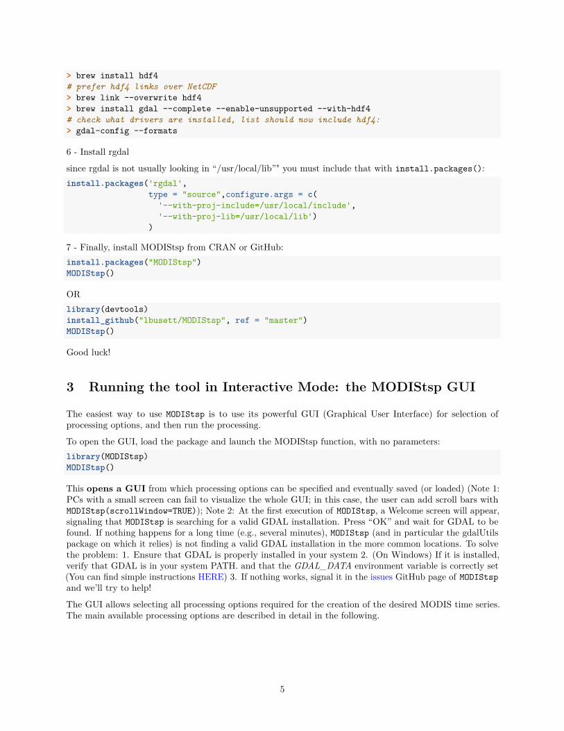
7 - Finally, install MODIStsp from CRAN or GitHub:

install.packages("MODIStsp")

MODIStsp()

OR

library(devtools)

install_github("lbusett/MODIStsp", ref = "master")

MODIStsp()

Good luck!

3 Running the tool in Interactive Mode: the MODIStsp GUI

The easiest way to use MODIStsp is to use its powerful GUI (Graphical User Interface) for selection ofprocessing options, and then run the processing.

To open the GUI, load the package and launch the MODIStsp function, with no parameters:

library(MODIStsp)

MODIStsp()

This opens a GUI from which processing options can be specified and eventually saved (or loaded) (Note 1:PCs with a small screen can fail to visualize the whole GUI; in this case, the user can add scroll bars withMODIStsp(scrollWindow=TRUE)); Note 2: At the first execution of MODIStsp, a Welcome screen will appear,signaling that MODIStsp is searching for a valid GDAL installation. Press “OK” and wait for GDAL to befound. If nothing happens for a long time (e.g., several minutes), MODIStsp (and in particular the gdalUtilspackage on which it relies) is not finding a valid GDAL installation in the more common locations. To solvethe problem: 1. Ensure that GDAL is properly installed in your system 2. (On Windows) If it is installed,verify that GDAL is in your system PATH. and that the GDAL_DATA environment variable is correctly set(You can find simple instructions HERE) 3. If nothing works, signal it in the issues GitHub page of MODIStsp

and we’ll try to help!

The GUI allows selecting all processing options required for the creation of the desired MODIS time series.The main available processing options are described in detail in the following.

5

3.1 Selecting Processing Parameters

3.1.1 MODIS Product, Platform and Layers:

The top-most menus allow to specify details of the desired output time series:

1. “Category” and “Product”: Selects the MODIS product of interest

2. MODIS platform(s): Selects if only TERRA, only AQUA or Both MODIS platforms should beconsidered for download and creation of the time series

3. version: Selects whether processing version 5 or 6 (when available) of MODIS products has to beprocessed

After selecting the product and version, clicking the “Click to Select Desired Layers” button opens theSelect Processing Layers GUI panel, from which the user must select which MODIS original layers and/orderived Quality Indexes (QI) and Spectral Indexes (SI) layers should be processed:

6

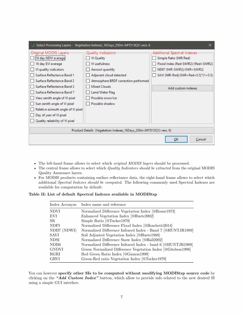
• The left-hand frame allows to select which original MODIS layers should be processed.• The central frame allows to select which Quality Indicators should be extracted from the original MODIS

Quality Assurance layers.• For MODIS products containing surface reflectance data, the right-hand frame allows to select which

additional Spectral Indexes should be computed. The following commonly used Spectral Indexes areavailable for computation by default:

Table II: List of default Spectral Indexes available in MODIStsp

Index Acronym Index name and reference

NDVI Normalized Difference Vegetation Index [@Rouse1973]EVI Enhanced Vegetation Index [@Huete2002]SR Simple Ratio [@Tucker1979]NDFI Normalized Difference Flood Index [@Boschetti2014]NDII7 (NDWI) Normalized Difference Infrared Index - Band 7 [@HUNTJR1989]SAVI Soil Adjusted Vegetation Index [@Huete1988]NDSI Normalized Difference Snow Index [@Hall2002]NDII6 Normalized Difference Infrared Index - band 6 [@HUNTJR1989]GNDVI Green Normalized Difference Vegetation Index [@Gitelson1998]RGRI Red Green Ratio Index [@Gamon1999]GRVI Green-Red ratio Vegetation Index [@Tucker1979]

You can however specify other SIs to be computed without modifying MODIStsp source code byclicking on the “Add Custom Index” button, which allow to provide info related to the new desired SIusing a simple GUI interface.

7

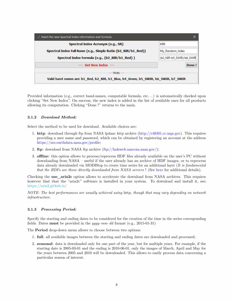
Provided information (e.g., correct band-names, computable formula, etc. . . ) is automatically checked uponclicking “Set New Index”. On success, the new index is added in the list of available ones for all productsallowing its computation. Clicking “Done !” returns to the main.

3.1.2 Download Method:

Select the method to be used for download. Available choices are:

1. http: download through ftp from NASA lpdaac http archive (http://e4ftl01.cr.usgs.gov). This requiresproviding a user name and password, which can be obtained by registering an account at the addresshttps://urs.earthdata.nasa.gov/profile;

2. ftp: download from NASA ftp archive (ftp://ladsweb.nascom.nasa.gov/);

3. offline: this option allows to process/reprocess HDF files already available on the user’s PC withoutdownloading from NASA – useful if the user already has an archive of HDF images, or to reprocessdata already downloaded via MODIStsp to create time series for an additional layer (It is fundamentalthat the HDFs are those directly downloaded from NASA servers ! (See here for additional details).

Checking the use_aria2c option allows to accelerate the download from NASA archives. This requireshowever that that the “aria2c” software is installed in your system. To download and install it, see:https://aria2.github.io/

NOTE: The best performances are usually achieved using http, though that may vary depending on networkinfrastructure.

3.1.3 Processing Period:

Specify the starting and ending dates to be considered for the creation of the time in the series correspondingfields. Dates must be provided in the yyyy–mm–dd format (e.g., 2015-01-31)

The Period drop-down menu allows to choose between two options:

1. full: all available images between the starting and ending dates are downloaded and processed;

2. seasonal: data is downloaded only for one part of the year, but for multiple years. For example, if thestarting date is 2005-03-01 and the ending is 2010-06-01, only the images of March, April and May forthe years between 2005 and 2010 will be downloaded. This allows to easily process data concerning aparticular season of interest.

8

3.1.4 Spatial Extent:

Allows to define the area of interest for the processing. Two main options are possible:

1. Full Tiles Extent: specify which MODIS tiles need to be processed using the “Start” and “End”horizontal and vertical sliders in the Required MODIS Tiles frame. During processing, data from thedifferent tiles is mosaiced, and a single file covering the total area is produced for each acquisition date(Note: pressing the “show map” button, a representation of the MODIS tiles grid is shown to facilitatethe selection).

2. Resized: specify a custom spatial extent for the desired outputs either by:

a. Manually inserting the coordinates of the Upper Left and Lower Right corners of the area of interestin the Bounding Box frame. Coordinates of the corners must be provided in the coordinatesystem of the selected output projection;

b. pressing the “Load Extent from a Spatial File” and selecting a raster or vector spatialfile. In this case, the bounding box of the selected file is retrieved, converted in the selectedoutput projection, and shown in the “Bounding Box” frame. Required input MODIS tiles are alsoautomatically retrieved from the output extent, and the tiles selection sliders modified accordingly.

3.1.5 Reprojection and Resize:

Specify the options to be used for reprojecting and resizing the MODIS images.

• “Output Projection”: select one of the predefined output projections or specify a user-defined one.To specify a user selected projection, select “User Defined” and then insert a valid “Proj4” string in thepop-up window. Validity of the Proj4 string is automatically checked, and error messages issued if thecheck fails;

• “Output Resolution”, “Pixel Size” and “Reprojection Method”: specify whether output imagesshould inherit their spatial resolution from the original MODIS files, or be resampled to a user-definedresolution. In the latter case, output spatial resolution must be specified in the measure units of theselected output projection. Resampling method can be chosen among “Nearest Neighbour” and “Mode”(Useful for down-sampling purposes). Other resampling methods (e.g., bilinear, cubic) are not currentlysupported since i) they cannot be used for resampling of categorical variables such as the QA and QIlayers, and ii) using them on continuous variable (e.g., reflectance, VI values) without performing ana-priori data cleaning would risk to contaminate the values of high-quality observations with those oflow-quality ones.

3.1.6 Processing Options:

Several processing options can be set using check-boxes:

• Output Files Format: Two of the most commonly formats used in remote sensing applications areavailable at the moment: ENVI binary and GeoTiff. If GeoTiff is selected, the type of file compressioncan be also specified among “None”, “PACKBITS”, “LZW” and “DEFLATE”.

• Create Virtual Rasters: Specify if virtual multitemporal files should be created. These virtualfiles allow access to the entire time series of images as a single file without the need of creating largemultitemporal raster images. Available virtual files formats are ENVI meta-files and GDAL “vrt” files.

• Create RasterStack: Specify if the output time series should be also saved as as “R” rasterStackobjects (with temporal information added through the “setZ” method of the raster package). This maybe useful in order to easily access the preprocessed MODIS data within “R” scripts.

9

• Change NoData values: Specify if NoData values of MODIS layers should be kept at their originalvalues, or changed to those specified within the “MODIStsp_Products_Opts” XML file. By selecting“Yes” in the “Change Original NODATA values” check-box, NoData of outputs are set to the largestinteger value possible for the data type of the processed layer (e.g., for 8-bit unsigned integer layers,NoData is set always to 255, for 16-bit signed integer layers to 32767, and for 16-bit unsigned integerlayers to 65535). Information about the new NoData values is stored both in the output rasters, and inthe XML files associated with them.

• Scale output values: Specify if scale and offset values of the different MODIS layers should be applied.If selected, outputs are appropriately rescaled on the fly, and saved in the true “measure units” of theselected parameter (e.g., spectral indexes are saved as floating point values; Land Surface Temperatureis saved in °K, etc.).

3.1.7 Main Output Folder for Time Series Storage:

Select the main folder where the pre-processed time series data will be stored. All MODIStsp outputswill be placed in specific sub-folders of this main folder (see XXX for details on MODIStsp namingconventions)-.

The “Reprocess Existing Data” check-box allows to decide if images already available should be reprocessedif a new run of MODIStsp is launched with the same output folder. If set to “No”, MODIStsp skips dates forwhich output files following the MODIStsp naming conventions are already present in the output folder. Thisallows to incrementally extend MODIS time series without reprocessing already available dates.

3.1.8 Output Folder for Original HDF Storage:

Select the folder where downloaded original MODIS HDF files downloaded from NASA servers will bestored.

The “delete original HDF files” check-box allows also to decide if the downloaded images should bedeleted from the file system at the end of the processing. To avoid accidental file deletion, this is always setto “No” by default, and a warning is issued before execution whenever the selection is changed to “Yes”.

3.2 Saving and Loading Processing Options

Specified processing parameters can be saved to a JSON file for later use by clicking on the Save Options

button.

Previously saved options can be restored clicking on the Load Options button and navigating to thepreviously saved JSON file.

(Note that at launch, MODIStsp always reloads automatically the processing options used for its

last succesfull run .

3.3 Starting the processing

Once you are happy with your choices, click on Start Processing. MODIStsp will start accessing NASAservers to download and process the MODIS data corresponding to your choices.

For each date of the specified time period, MODIStp downloads and preprocesses all hdf images required tocover the desired spatial extent. Informative messages concerning the status of the processing are providedon the console, as well as on a self-updating progress window.

10

4 Non-Interactive Execution from within R

4.1 Specifying a saved “Options file”

MODIStsp can be launched in non-interactive mode within an R session by setting the optional GUI parameterto FALSE, and the Options_File parameter to the path of a previously saved JSON Options file. Thisallows to exploit MODIStsp functionalities within generic “R” processing scripts

library(MODIStsp)

# --> Specify the path to a valid options file saved in advance from MODIStsp GUI

options_file <- "X:/yourpath/youroptions.json"

# --> Launch the processing

MODIStsp(gui = FALSE, options_file = options_file)

4.2 Looping on different spatial extents

Specifying also the spatial_file_path_ parameter overrides for example the output extent of the selectedOptions File. This allows to perform the same preprocessing on different extents using a single Options File,by looping on an array of spatial files representing the desired output extents. For example:

library(MODIStsp)

# --> Specify the path to a valid options file saved in advance from MODIStsp GUI

options_file <- "X:/yourpath/youroptions.json"

# --> Create a character array containing a list of shapefiles (or other spatial files)

extent_list <- list.files("X:/path/containing/some/shapefiles/", "\\.shp$")

# --> Loop on the list of spatial files and run MODIStsp using each of them to automatically

# define the output extent (A separate output folder is created for each input spatial file).

for (single_shape in extent_list) {

MODIStsp(gui = FALSE, options_file = options_file, spatial_file_path = single_shape )

}

5 Standalone execution and scheduled processing

5.1 Standalone execution

• MODIStsp can be also executed as a “standalone” application(i.e., without having to open R/RStudio);to do this, from R launch the function MODIStsp_install_launcher().

In a Linux operating system this function creates a desktop entry (accessible from the menu in the sections“Science” and “Geography”) and a symbolic link in a known path (default: /usr/bin/MODIStsp). In Windows,a link in the Start Menu and optionally a desktop shortcut are created. See ?install_MODIStsp_launcher

for details and path customization.

Double-clicking those files or launching them from a shell without parameters will launch MODIStsp ininteractive mode. Non-interactive mode is triggered by adding the “-g” argument to the call, and specifyingthe path to a valid Options File as “-s” argument:

• Linux: MODIStsp -g -s "/yourpath/youroptions.RData" (see MODIStsp -h for details).

11

• Windows:your_r_library\MODIStsp\ExtData\Launcher\MODIStsp.bat -g -s "yourpath/youroptions.RData"

(see C:\Users\you\Desktop\MODIStsp -h for details).

If you do not want to install any link, launchers can be found in the subdirectory “MODIStsp/ExtData/Launcher”of your library path.

5.2 Scheduled Processing

Standalone non-interactive execution can be used to periodically and automatically update the time series ofa selected product over a given study area. To do that, you should simply:

1. Open the MODIStsp GUI, define the parameters of the processing specifying a date in the future as the“Ending Date” and save the processing options. Then quit the program.

2. Schedule non-interactive execution of the launcher installed as seen before (or located in the subdirectory“MODIStsp/ExtData/Launcher” of your library path) as windows scheduled task (or linux “cron” job)according to a specified time schedule, specifying the path of a previously saved Options file as additionalargument:

5.2.0.1 On Linux

• edit your crontab by opening a terminal and type:

crontab -e

• add an entry for the launcher. For example, if you have installed it in /usr/bin and you want to runthe tool every day at 23.00, add the following row:

0 23 * * * /bin/bash /usr/bin/MODIStsp -g -s "/yourpath/youroptions.RData"

5.2.0.2 On Windows

• create a Task following these instructions; add the path of the MODIStsp.bat launcher as Action (point6), and specifying -g -s "X:/yourpath/youroptions.RData" as argument.

6 Outputs Format and Naming Conventions

6.1 Single-band outputs

Output raster files are saved in specific subfolders of the main output folder. In particular, a separatesubfolder is created for each processed original MODIS layer, Quality Indicator or Spectral Index. Eachsubfolder contains one image for each processed date, created according to the following naming conventions:

"ProdCode"_"Layer"_"YYYY"_"DOY"."ext"

(e.g.,MOD13Q1_NDVI_2000_065.dat)

, where:

• ProdCode is the code name of the MODIS product from which the image was derived (e.g., MOD13Q1);• Layer is a short name describing the dataset (e.g., b1_Red, NDII, UI);• YYYY and DOY correspond to the year and DOY (Day of the Year) of acquisition of the original

MODIS image;• ext is the file extension (.tif for GTiff outputs, or .dat for ENVI outputs).

12

6.2 Virtual multi-band outputs

ENVI and/or GDAL virtual time series files and RasterStack RData objects are instead stored in the“Time_Series” subfolder if required.

Naming convention for these files is as follow:

"ProdCode"_"Layer"_"StartDOY"_"StartYear_"EndDOY"_"EndYear_"suffix".ext"

(e.g., MOD13Q1_NDVI_49_2000_17_2015_RData.dat)

, where:

• ProdCode is the code name of the MODIS product from which the image was derived (e.g., MOD13Q1);• Layer is a short name describing the dataset (e.g., b1_Red, NDII, UI);• StartDOY , StartYear , EndDOY and EndYear indicate the temporal extent of the time serie

created;• suffix indicates the type of virtual file (ENVI, GDAL or RData);• ext is the file extension (“.vrt” for gdal virtual files, “META” for ENVI meta files or “Rdata” for R

raster stacks).

7 Accessing the processed time series from R

Preprocessed MODIS data can be retrieved within R either by accessing the single-date raster files, or byloading the saved RasterStack objects.

Any single-date image can be accessed by simply opening it with a raster command:

library(raster)

modistsp_file <- "/my_path/my_moditsp_folder/MOD13Q1_2005_137_EVI.tif"

my_raster <- raster(modistsp_file)

rasterStack time series containing all the processed data for a given parameter (saved in the “Time Series”subfolder - see here for details) can be opened by:

in_virtual_file <- "/my_moditsp_folder/Time_Series/MOD13Q1_MYD13Q1_NDVI_49_2000_353_2015_RData.RData"

indata <- get(load(in_virtual_file))

This second option allows accessing the complete data stack and analyzing it using the functionalities forraster/raster time series analysis, extraction and plotting provided for example by the raster or rasterVis

packages.

7.1 Extracting Time Series Data on Areas of Interest

MODIStsp provides an efficient function (MODIStsp\_extract) for extracting time series data at specificlocations. The function takes as input a RasterStack virtual object created by MODIStsp (see above), thestarting and ending dates for the extraction and a standard _Sp*_ object (or an ESRI shapefile name)specifying the locations (points, lines or polygons) of interest, and provides as output a xts object ordata.frame containing time series data for those locations.

If the input is of class SpatialPoints, the output object contains one column for each point specified, andone row for each date. If it is of class SpatialPolygons (or SpatialLines), it contains one column for eachpolygon (or each line), with values obtained applying the function specified as the “FUN” argument (e.g.,mean, standard deviation, etc.) on pixels belonging to the polygon (or touched by the line), and one row foreach date.

As an example the following code:

13

#Set the input paths to raster and shape file

infile <- 'in_path/MOD13Q1_MYD13Q1_NDVI_49_2000_353_2015_RData.RData'

shpname <- 'path_to_file/rois.shp'

#Set the start/end dates for extraction

startdate <- as.Date("2010-01-01")

enddate <- as.Date("2014-12-31")

#Load the RasterStack

inrts <- get(load(infile))

# Compute average and St.dev

dataavg <- MODIStsp_extract(inrts, shpname, startdate, enddate, FUN = 'mean', na.rm = T)

datasd <- MODIStsp_extract (inrts, shpname, startdate, enddate, FUN = 'sd', na.rm = T)

# Plot average time series for the polygons

plot.xts(dataavg)

loads a RasterStack object containing 8-days 250 m resolution time series for the 2000-2015 period andextracts time series of average and standard deviation values over the different polygons of a user’s selectedshapefile on the 2010-2014 period.

8 Problems and Issues

Solutions to some common installation and processing problems can be found in MODIStsp FAQ:

http://lbusett.github.io/MODIStsp/articles/faq.html

• Please report any issues you may encounter in our issues page on GitHub:

https://github.com/lbusett/MODIStsp/issues

9 Citation

To cite MODIStsp please use:

L. Busetto, L. Ranghetti (2016) MODIStsp: An R package for automatic preprocessing of MODIS LandProducts time series, Computers & Geosciences, Volume 97, Pages 40-48, ISSN 0098-3004, http://dx.doi.org/10.1016/j.cageo.2016.08.020, URL: https://github.com/lbusett/MODIStsp.

10 Installing R and GDAL

10.1 Installing R

10.1.1 Windows

Download and install the latest version of R which can be found here.

10.1.2 Linux

Please refer to the documentation which can be found here, opening the directory relative to your Linuxdistribution. The documentation provides instruction to add CRAN repositories and to install the latest Rversion. With Ubuntu 15.10 Wily (and newer) this step is not mandatory (although recommended), since

14

packaged version of R is >= 3.2.1 (although not the latest); in this case, user can install R by simply typingin a terminal

sudo apt-get install r-base

10.2 Installing GDAL >= 1.11.1

10.2.1 Windows

The easiest way to install GDAL on Windows is from the OSGeo4W Website

1. Open the OSGeo4W Website2. In the Quick Start for OSGeo4W Users section, select the download of 32bit or 64bit of OSGeo4W

network installer3. Run the installer

• Easiest Option:– Select Express Desktop Install, then proceed with the installation. This will install GDAL and

also other useful Spatial Processing software like QGIS and GRASS GIS• Advanced Option:

– Select Advanced Install, then click on “Next” a few times until you reach the “Select Packages”screen.

– Click on “Commandline_Utilities_”, and on the list look for “_gdal: The GDAL/OGR library. . . "entry

– Click on “Skip”: the word “skip” will be replaced by the current GDAL version number– Click on “Next” a few times to install GDAL

10.2.2 Debian and Ubuntu-based systems

1. Ensure that your repositories contain a version of gdal-bin >= 1.11.1. In particular, official repositoriesof Ubuntu 15.04 Vivid (or older) and Debian Jessie (or older) provide older versions of GDAL, so it isnecessary to add UbuntuGIS-unstable repository before installing. To do this, follow instructions here).With Ubuntu 15.10 Wily (and newer) this step is not mandatory, although recommended in order tohave updated version of GDAL installed.

2. To install GDAL, open a terminal and type

sudo apt-get install gdal-bin

10.2.3 ArchLinux

GDAL is maintained updated to the latest version as binary package within the community repository;although that, the support for HDF4 format is not included. To bypass this problem, ArchLinux users caninstall gdal-hdf4 package from AUR (see here or here for the package installation from AUR). This packageis updated manually after each release of gdal on the community repository, so a temporal shift between anew gdal release and the update of gdal-hdf4 could happen. If you want to manually add the support forHDF4 in case gdal-hdf4 is out-of-date, you can do it following these instructions.

10.2.4 Other Linux systems

Install the packaged binary of GDAL included in your specific distribution; if the version is older than 1.11.1,or if the support for HDF4 format is not included, you can manually install the HDF4 library and compilethe source code by adding the parameter --with-hdf4 to the configure instruction).

15