Mind the Data Gap: Identifying and Assessing Drivers of Changing Eutrophication Condition

Mind the Data Gap: Identifying and Assessing Driversof Changing Eutrophication Condition

Benjamin Fertig & Michael J. Kennish &

Gregg P. Sakowicz & Laura K. Reynolds

Received: 12 February 2013 /Revised: 8 October 2013 /Accepted: 19 November 2013 /Published online: 18 December 2013# Coastal and Estuarine Research Federation 2013

Abstract This study identified drivers of change in BarnegatBay–Little Egg Harbor Estuary, NJ, USA over multiplelong-term time periods by developing an assessmenttool (an “Eutrophication Index”) capable of handlingdata gaps and identifying the condition of and relationshipsbetween ecosystem pressures, ecosystem state, and bioticresponses. The Eutrophication Index integrates 15 indicatorsin 3 components: (1) water quality, (2) light availability, and(3) seagrass response. Annual quantitative assessments ofcondition and its consistency for three geographic segmentsrange from 0 (highly degraded) to 100 (excellent condition).Eutrophication Index values significantly declined (p <0.05)by 34 and 36 % in central and south segments from 73 and 71in the early 1990s to 48 and 45 in 2010, respectively. Ongoingdeclines despite periods of improvement (e.g., 1989–1992,

1996–2002, and 2006–2008) suggest these estuarine seg-ments are currently undergoing eutrophication. The northsegment had highest nutrient loading and lowestEutrophication Index values (2010 Eutrophication Index val-ue=37) but increased over time (from 14 in 1991 to 50 in2009) in contrast to trends in central and south segments.Rapid initial declines of Eutrophication Index values withincreasing loading highlight that the estuary is sensitive toloading. Ecosystem response to total nutrient loading, asdescribed by the Index of Eutrophication, exhibited nonline-arity at loading rates of >1,200 and <5,000 kg TN km−2 year−1

and >100 and <250 kg TP km−2 year−1, values similar toresponses of seagrass to nutrient loading in many ecosystems.While nutrient loading is initially a critical driver of ecosystemchange, other factors, e.g., light availability and drive ecosys-tem condition, yield nonlinearity. Empirical evidence forswitches in the driving factors of ecosystem stress adds com-plexity to the conceptualization of ecosystem resiliency due tofeedback from multiple dynamic, nonlinear stressors.

Keywords Eutrophication . Biotic indices . Long-term data .

Data gaps . Ecological status .Multivariate analysis

Introduction

Many coastal estuarine ecosystems undergo long-term non-linear ecosystem-scale changes and have been classified ashighly eutrophic (Bricker et al. 2007; Kennish et al. 2007;Duarte 2009; Fertig et al. 2013b). Barnegat Bay–Little EggHarbor (BB–LEH), a Mid-Atlantic shallow coastal lagoon inNew Jersey, USA, exemplifies systems exhibiting multiplebiotic responses to a myriad of stressors (Kennish et al.2011; Fertig et al. 2013a) to the extent that BB–LEH has beenused as a eutrophic end-member ecosystem to test metrics ofincipient eutrophication (Kennish and Fertig 2012). Stressors

Communicated by Mark J. Brush

Electronic supplementary material The online version of this article(doi:10.1007/s12237-013-9746-5) contains supplementary material,which is available to authorized users.

B. Fertig (*) :M. J. Kennish :G. P. Sakowicz : L. K. ReynoldsInstitute of Marine and Coastal Sciences, Rutgers University,New Brunswick, NJ 08901, USAe-mail: [email protected]

B. Fertige-mail: [email protected]

L. K. Reynoldse-mail: [email protected]

Present Address:B. FertigSchool of Math and Science, Community College of BaltimoreCounty, Essex, MD 21237, USA

Present Address:L. K. ReynoldsDepartment of Evolution and Ecology, University of CaliforniaDavis, Davis, CA 95616, USA

Estuaries and Coasts (2014) 37 (Suppl 1):S198–S221DOI 10.1007/s12237-013-9746-5

http://dx.doi.org/10.1007/s12237-013-9746-5

to BB–LEH include increases in concentrations and loads ofnutrients (Hunchak-Kariouk and Nicholson 2001; Baker et al.2013). Human population in the catchment (>575,000year-round and >1,200,000 in summertime) has rapidlyexpanded (US Census 2010), altering the catchment’sland use–land cover to >34 % developed including>10 % impervious surface (Lathrop and Conway2001). Multiple symptoms of eutrophication have beenobserved (Kennish 2001a; Kennish et al. 2007, 2012),including low dissolved oxygen concentrations, harmfuland benthic algal blooms (Anderson et al. 2002;Gastrich et al. 2004; Kennish et al. 2011), heavy epi-phytic loading, and declines in seagrass biomass(Kennish et al. 2010; Fertig et al. 2013a). A holistictool for assessing condition and identifying the driversof these changes is needed for BB–LEH.

Identifying drivers of long-term changes can be ac-complished by assessing a suite of bioindicators. Manytechniques and tools are available (Bricker et al. 2007;Williams et al. 2009; Ferreira et al. 2011) includingstatistical methods for establishing reference nutrientconditions (Dodds and Oakes 2004), comparing indica-tors to threshold values (Wazniak et al. 2007), andsampling benthic community composition with respectto the degree of sensitivity/tolerance to a stressor toindicate local condition across ecosystems (Borja et al.2000, 2008).

Synthesizing existing datasets to evaluate the ecolog-ical condition of shallow estuarine systems can provideextensive information globally (Srebotnjak et al. 2012),but they are often time consuming, labor-intensive, cost-ly, and often target individual stressors. To avoid thesedeficiencies, there has been an effort to develop analyt-ical techniques and environmental indicators that spanthe multiple levels of ecosystem components (Carvalhoet al. 2011), biological organization, and are broadlyapplicable (Niemi and McDonald 2004). Relatively fewecosystems are extensively studied globally, and datagaps (both paucity and spatiotemporal inconsistencies)pose a major challenge for extensive assessments formany ecosystems including shallow coastal lagoonssuch as BB–LEH. Long-term ecosystem-wide datasetsfor BB–LEH exist but have not previously been synthe-sized to assess drivers of change in ecosystem condi-tion, and, as with many systems, available data containsgaps and spatiotemporal inconsistencies.

The goal of this study was to identify drivers ofchange in BB–LEH over multiple long-term time pe-riods by developing an assessment tool (an “Index ofEutrophication”) capable of handling data gaps andidentifying the condition of and relationships betweenecosystem pressures, ecosystem state, and bioticresponses.

Methods

Study Location

The BB–LEH catchment covers an area of 1,730 km2 (catch-ment, estuary areal ratio is 6.5:1) approximately overlappingOcean County, NJ, USA. Population density and developmentdecrease along a north–south gradient (Conway and Lathrop2005), as does nutrient loading to the estuary (Hunchak-Kariouk and Nicholson 2001; Seitzinger et al. 2001; Wiebenand Baker 2009; Baker et al. 2013). Nitrogen loadingfrom the BB–LEH catchment is positively correlatedwith total nitrogen concentrations in the estuary (Kennishand Fertig 2012).

BB–LEH estuary (Fig. 1) is a back-bay basin complexforming an irregular contiguous lagoonal system with a sur-face area of 280 km2 and a volume of 3.54×108 m3 (Kennish2001a, b). Water residence time is 74 days in summer (Guoet al. 2004), semidiurnal tides range from <0.5 to 1.5 m, andthe estuary is well-mixed by wind and currents (<0.5 to1.5 m s−1). Water temperatures range from −1.5 to 30 °C,and salinity ranges from 10 to 32.

Significant differences in long-term catchment, estuarinewater quality, and sediment indicators (Psuty 2004; Psuty andSilveira 2009) indicated the necessity of partitioning the estuaryinto three spatial segments (north, central, and south; Fig. 1),differing from previous assessment (Kennish et al. 2007).

Index Calculation

Fifteen biotic and abiotic indicators were selected at the outsetbased on potential response to total nitrogen and total phos-phorus loadings and organized into three components: (1)water quality, (2) light availability, and (3) seagrass(Table 1). Annual mean (or median) data (1989–2010) foreach indicator in each of the three spatial segments (north,central, and south; Fig. 1) were input to calculate “raw scores”,“weighted scores” , component indices , and the“Eutrophication Index”.

First, each variable was rescaled by comparing the mea-sured value to “threshold” values (Tables 2 and 3). Thesethresholds were defined to distinguish optimal conditionsfrom degraded conditions for each variable based upon (a)the literature, (b) data analysis, (c) best professional judgment,and (d) some combination of a–c (Table 2). Best professionaljudgment was reserved only for indicators where previousthresholds are not established in the literature and data analy-sis yielded limited insight. Thresholds were set at values ofindicators that indicated a change in response values—such aschanges in the slope or abrupt breaks in response indicators(Table 2). As a result, this rescaling transforms each variableinto common spatial and temporal units and intervals. Data for2011 were calculated independently for validation.

Estuaries and Coasts (2014) 37 (Suppl 1):S198–S221 S199

Component scores are comprised of “raw” and “weighted”Scores, each contributing 50 % to the component’s index.Raw scores for each indicator are calculated by rescalingannual means (Table 4) according to an equation describedby a set of threshold values (Tables 2 and 3; see below). Rawscores range from 0 (degraded) to 50 (excellent) for eachvariable. Component raw scores were determined by comput-ing the mean of these raw scores.

Weighted scores are calculated independently from variablesmeasured in each year and each component (e.g., water quality,light availability, and seagrass; Table 1). For each component,covariance matrices are computed from raw scores for all mea-surements in a given decade. Principal component analysis

(PCA) is then applied to these covariance matrices to find theeigenvector (first principle component) that gives the linearcombination of model variables that explain most of the vari-ance in the given system in a given decade (∼50–75 % of thevariability in our data). The larger the magnitude in an elementof the eigenvector, the more the corresponding variable explainsthe variability in the system. Therefore, weightings are deter-mined for each variable by squaring the elements of the eigen-vector (Table 5). Weighted scores were then calculated for eachyear by multiplying the raw scores in a given year by theseweightings. The resulting scores also range from 0 (degraded) to50 (excellent) for each variable and are summed to obtain aweighted component score.

Fig. 1 Map of Barnegat Bay–Little Egg Harbor Estuary and itslocation within New Jersey, USA.The boundaries for the north,central, and south segments areindicated, as well as the arealextent of seagrass beds (green)and locations of transects used forseagrass sampling (black dots)

S200 Estuaries and Coasts (2014) 37 (Suppl 1):S198–S221

Table1

Availableindicatordataforpotentialinclusion

intheEutrophicationIndexforBarnegatB

ay–L

ittleEgg

HarborEstuary

summarized

byyear

(1989–2010)andestuarinesegm

ent

Com

ponent

Variable

1989

1990

1991

1992

1993

1994

1995

1996

1997

1998

1999

2000

2001

2002

2003

2004

2005

2006

2007

2008

2009

2010

2011

Water

quality

Temperature

aa

ac

aa

aa

aa

aa

aa

aa

aa

aa

aa

a

Dissolved

oxygen

aa

ac

aa

aa

aa

aa

aa

aa

aa

aa

aa

a

Totaln

itrogen

concentratio

n

aa

ac

aa

aa

aa

aa

aa

aa

aa

aa

aa

a

Totalp

hosphorus

concentratio

n

cc

cc

cc

cc

cc

aa

aa

aa

aa

aa

aa

a

Light

availability

Chlorophylla

cc

cc

cc

cc

aa

aa

aa

aa

aa

aa

aa

a

Totalsuspended

solid

sa

aa

ca

cc

ca

aa

aa

aa

aa

aa

aa

aa

Secchi

depth

aa

ac

aa

aa

aa

aa

aa

aa

aa

aa

aa

a

Macroalgaepercent

cover

ca

aa

aa

aa

aa

aa

aa

ab

aa

cb

bb

a

Percentsurface

light

cc

cc

cc

cc

cc

cc

cc

cb

bb

cb

bb

a

Epiphytebiom

ass

cc

cc

cc

cc

cc

cc

cc

cb

bb

cb

bb

a

Seagrass

response

Zosteraaboveground

biom

ass

cc

cc

cc

cc

cc

cc

cc

cb

bb

cb

bb

b

Zosterabelowground

biom

ass

cc

cc

cc

cc

cc

cc

cc

cb

bb

cb

bb

b

Zosteradensity

cc

cc

cc

cc

cc

cc

cc

cc

cc

cb

bb

b

Zosterapercentcover

cc

cc

cc

cc

cc

cc

cc

cc

cc

cb

bb

b

Zosteralength

cc

cc

cc

cc

cc

cc

cc

cb

cc

cc

cc

c

aDataavailablein

north

,central,andsouth

bDataavailablein

centraland

south

cDatanotavailable


Table2

Determinationof

thresholds

Water

component

Threshold

indicator

Threshold

values

Threshold

valuedeterm

ined

by:

Summaryof

methods

used

todeterm

inethreshold

Threshold

limitations

Biotic

responsesshow

ninBarnegat

Bay

todeterm

inethresholdvalues

References

Ecosystem

Pressures

TotalN

itrogen

(kgTN

yr-1

estuarine

km-2)

50kg

TNestuary

km-2yr

-1=100

250kg

TNestuary

km-2yr

-1=75

1000

kgTNestuary

km-2yr

-1=50

3000

kgTNestuary

km-2yr

-1=25

Thresholds

fortotalnitrogenandphosphorus

loadingweredeterm

ined

byexam

iningbiotic

responsestonutrientloading

reportedinthe

literature,andby

dataanalysisof

thenutrient

loadingmodelingoutputfro

mPL

OADandits

relationshiptoecosystemstateandbiotic

response.Inexam

iningandcompiling

inform

ationfro

mtheliterature,loadingratesfor

totalnitrogen

andtotalphosphoruswere

convertedtokg

Nyear-1

forcom

parison

with

common

units

tomodeled

loadsfro

mBB-

LEH.Inlookingforpotentialthresholdsamong

theserelationships,w

esoughtvaluesofnutrient

loadings

thatmarkachange

inrateofdeclineof

seagrassresponses.How

ever,w

ealso

looked

forv

aluesthatmarkthestartofd

eclines

(regardlessof

rate),andvalues

aboveor

below

which

itappearsthatnitrogenloadingisno

longeradominantfactorinthechange

ofthe

bioticresponse.First,weexam

ined

relationships

betweennutrientloading

and

estuarineresponsesintheliterature(see

for

exam

ple,Wazniak

etal.,2007;B

rickeretal.,

1999;B

rickeretal.,2007;T

omasko

etal.,

1996;ShortandBurdick,1996;Deegan,2002;

Valielaetal.,2000;B

urkholderetal.2007;

Boynton

etal.,1996;K

ennish

andFertig,2012;

Stevensonetal.,1993;D

uarte

1995;and

Kiddonetal.2003).Pertinentfigures

fromthe

literaturewereincluded

inKennish

etal.,2012.

Tomasko

etal.(1996)and

Burkholderetal.

(2007)

reportthatas

nutrientloading

increases,

seagrassbiom

assandproductivity

decline

exponentially

with

very

sharpdeclines

starting

at~50kg

Nday-1,an

inflectionpointinthe

curveat~100

kgNday-1andaslow

errateof

declineabove~225

kgNday-1(Figure3-10).

Asimilartypeof

response

isseen

forseagrass

arealcoverageinthattheinflectionpointofthe

curvewasbelow1,000kg

Nkm

-2year-1anda

slow

errateof

declinewas

observed

above

5,000kg

Nkm

-2year-1

(Figure3-11in

Kennish

etal.2012,Shortand

Burdick,1996,

Valielaetal.,2000,B

urkholderetal.2007)

Also,seagrassarealcoveragedeclined

most

dram

aticallyatincipientlevelsof

eutrophication,early

oninthelong-term

analysis(Valielaetal.,2000).Seagrassshoot

density

ishighlyvariableanddeclines

rapidly

with

nitrogenloadingaslowas50

kgNyear-1,

which

slow

swith

greaterthan1,000kg

Nyear-

1though

atthishigherloadingratethedensity

approaches

(butdoes

notreach)0

shootsm-2

(Deeganetal.2002,Burkholderetal.2007,

Figure3-1

2inKennish

etal.2012).Seagrass

declines

aremediatedby

linearincreases

in

Thresholds

fortotalnitrogenand

phosphorus

loadingwere

determ

ined

byexam

iningbiotic

responsestonutrientloading

reportedintheliterature,andby

dataanalysisof

thenutrient

loadingmodelingoutputfro

mPL

OADandits

relationshipto

ecosystem

stateandbiotic

response.First,weexam

ined

relationships

betweennutrient

loadingandestuarineresponsesin

theliterature(see

forexample,

Wazniak

etal.,2007;B

rickeret

al.,1999;B

rickeretal.,2007;

Tomasko

etal.,1996;S

hortand

Burdick,1996;Deegan,2002;

Valielaetal.,2000;B

urkholderet

al.2007;Boynton

etal.1996;

Kennish

andFertig,2012;

Stevensonetal.,1993;D

uarte

1995;and

Kiddonetal.2003).A

snutrientloading

increases,

seagrassbiom

assandproductivity

declineexponentially

(Tom

asko

etal.,1996,alsoFigure3-9

inKennish

etal.2012),asdoesareal

coverage

(ShortandBurdick,

1996,alsoFigure3-1

0in

Kennish

etal.2012andValielaet

al.,2000,alsoFigure3-11in

Kennish

etal.2012).Seagrass

shootdensitysimilarly

declines

(Deeganetal.2002,also

Figure3

-11inKennish

etal.2012).

Seagrassdeclinesaremediatedby

linearincreases

inestuarinetotal

nitrogenconcentrations,ashas

been

foundinMaryland’scoastal

bays

(Boynton

etal.,1996,also

Figure3-1

2inKennish

etal.

2012)and

inBB-LEH

(Kennish

andFertig,2012,alsoFigure3-

13inKennish

etal.2012).In

lookingforthresholdsam

ong

theserelationships,w

ehave

looked

forv

aluesof

nutrient

loadings

thatmarkachange

inrate

ofdeclineof

seagrassresponses.

How

ever,w

ehave

also

looked

for

values

thatmarkthestartof

declines

(regardlessof

rate),and

valuesabovewhich

itappearsthat

nitrogenloadingisno

longera

dominantfactorinthechange

ofthebioticresponse.Similarly,w

e

Thresholdsandrescalingequations

have

been

calibratedforBB-

LEHas

acoastallagoon.

How

ever,w

hiletheremay

beapplicability

ofthesethresholds

toothersimilarcoastallagoons

inNew

Jersey

orelsewhere

(suchas

GreatSo

uthBay,N

Y,

ChincoteagueBay,M

D/VA,

Hog

Island

Bay,V

A,etc.),

the

thresholds

establishedmay

beof

limitedutilityforotherNew

Jersey

waters(e.g.R

aritanBay,

NY/NJHarbor,andDelaw

are

Bay)thatdonotshareim

portant

characteristics.BB-LEHisin

partextremelysusceptibleto

even

smallamountsof

nutrient

loadingdueto

itsenclosed

geom

orphologyandslow

water

circulationandflu

shingtim

e.In

contrast,coastalwatersalong

the

AtlanticCoast,R

aritanBay,and


are

Bay

have

muchquickerand

strongercirculationpatternsand

thereforerespondto

nutrient

enrichmentatd

ifferenttim

escales.A

dditionally,w

hile

heavymetals,inorganic,and

organictoxicantsmay

beim

portant

considerations

for

ecologicalhealth

insomeNew

Jersey

waters,they

may

beof

lowerpriorityforBB-LEH.

Toxicologicalanalysisof

sedimentsandthewatercolumn

arebeyond

thescopeof

this

projectand

have

notb

een

included

intheIndexof

Eutrophicationor

itscomponent

indices.

Weexam

ined

totaln

itrogen

loading

impactson

waterquality

indicatorsincluding

temperature,dissolved

oxygen,

andestuarytotaln

itrogen

and

totalp

hosphorusconcentrations

(Figure3-14

inKennish

etal.

2012),light

indicatorsincluding

totalsuspended

solids,

chlorophylla,S

ecchid

epth,the

ratio

ofepiphytebiom

assto

seagrass

biom

ass,macroalgae

percentcover,and

thepercentof

light

reaching

seagrass

leaves

(Figure3-15

inKennish

etal.

2012),andseagrass

indicators

includingabovegroundand

belowground

biom

ass,shoot

density,percentcover,andblade

length(Figure3-1

6inKennish

etal.2012).A

dditionalpotential

thresholds

fortotaln

itrogen

loadingwereidentifiedfrom

changesin

response

indicators

with

changesin

loading.

Wazniak

etal.2007,Brickeretal.

1999,2007To

masko

etal1996,

Shortand

Burdick

1996,D

eegan

2002,V

alielaetal2000,

Burkholderetal2007,B

oynton

etal1996,K

ennish

andFertig

2012,S

tevenson

etal1993,

Duarte

1995,K

iddonetal.2003,

dataanalysisby

thisstudy

TotalPhosphorus

(kgTPyr

-1

estuarine

km-2)

25kg

TPestuarykm

-2yr-1

=100;50

kgTPestuary

km-2

yr-1

=75;100

kgTPestuarykm

-2yr-1

=50;250

kgTPestuary

km-2

yr-1

=25

Weexam

ined

totaln

itrogen

loading

impactson

waterquality

indicatorsincluding

temperature,dissolved

oxygen,

andestuarytotaln

itrogen

and

totalp

hosphorusconcentrations

(Figure3-14

inKennish

etal.

2012),light

indicatorsincluding

totalsuspended

solids,

chlorophylla,S

ecchid

epth,the

ratio

ofepiphytebiom

assto

seagrass

biom

ass,macroalgae

percentcover,and

thepercentof

light

reaching

seagrass

leaves

(Figure3-15

inKennish

etal.

2012),andseagrass

indicators


belowground

biom

ass,shoot


length(Figure3-1

6inKennish

etal.2012).A

dditionalpotential

thresholds

fortotaln

itrogen

loadingwereidentifiedfrom

changesin

response

indicators

with

changesin

loading.

Brickeretal.1999,2007

Tomasko

etal1996,S

hortandBurdick

1996,D

eegan2002,V

alielaetal

2000,B

urkholderetal2007,

Boynton

etal1996,K

ennish

and

Fertig2012,S

tevenson

etal.

1993,K

iddonetal.2003,

Wazniak

etal.2007,Duarte

1995,dataanalysisby

thisstudy


Table2

(contin

ued)

Water

component

Threshold

indicator

Threshold

values

Threshold

valuedeterm

ined

by:

Summaryof

methods

used

todeterm

inethreshold

Threshold

limitations

Biotic

responsesshow

ninBarnegat

Bay

todeterm

inethresholdvalues

References

estuarinetotalnitrogen

concentrations,w

ithtotalnitrogen

concentrationinμM

=39.4+

0.53

*theannualtotalnitrogen

load

ingNm-2

year-1,ash

asbeen

foundinMaryland’scoastal

bays

(Boynton

etal.,1996,B

urkholderetal.,

2007,Figure3-13inKennish

etal.2012)and

inBB-LEH

,with

totalnitrogen

concentrations

inμg

NL-1=52.42+1.76

*theareal

norm

alized

subw

atershed

totalnitrogen

loading

inkg

TNkm

-2year-1(Figure3-14inKennish

etal.2012).Inan

analysisof

62estuarine

embaym

ents,L

atimerandRego(2010)

found

that≤50

kgTN

loadingha-1

year-1,seagrass

extentisvariableandislikelycontrolledby

otherecosystem

factorsunrelatedtonutrient

loading,butabove

thatrateeelgrasscoverage

declined

markedlyandwasessentially

absentat

loadinglevels≥100kg

TNloadingha-1year-1

(Figure3-15inKennish

etal.2012).Thereare

fewerestuarinestudiesthatexam

inethe

relationshipbetweentotalphosphorusloading

andbioticresponsesthan

forthe

relationship

betweentotalnitrogen

loadingsinceingeneral,

nitrogen–notphosphorus–isthelim

iting

nutrientfor

estuarinesystem

s.Nevertheless,

bothphosphorus

andnitrogenareimportantto

controlfor

estuarinewatersheds,particularly

thosewith

high

levelsofnutrientloading,asthe

receivingestuariescanbe

phosphorus

limited,

nitrogenlim

ited,or

co-limited,andthenutrient

thatismostlimiting

canchange

bothseasonally

andspatially

(Conleyetal.2009,Conley,1999,

Maloneetal.1996).T

heanalyses

ondata

assembled

forthisp

rojectdescribed

abovewere

also

perfo

rmed

fortotalphosphorus.Similarly,

weexam

ined

therelationships

between

seagrassresponsesandnutrientloadings

observed

inBB-LEH

compiledforthisproject.

Additionalpotentialthresholdsfortotal

nitrogenloadingwereidentifiedfro

mchanges

inresponse

indicatorswith

changesinloading.

Thisisparticularly

importanttocalibratethe

thresholds

tobe

relevantforB

B-LEH

.We

exam

ined

totalnitrogen

loadingimpactson

waterquality

indicators:tem

perature,dissolved

oxygen,and

estuarinetotalnitrogen

andtotal

phosphorus

concentrations

(Figure3-1

6in

Kennish

etal.2012),lightindicatorsas

wellas

from

totalphosphorusloading.Similarly,w

eexam

ined

theimpacton

lightindicators:

chlorophylla,totalsuspendedsolids,Secchi

depth,macroalgaepercentcover,and

theratio

ofepiphytetoseagrassbiom

assfro

mtotal

nitrogenloading(Figure3-19inKennish

etal.

2012)and

totalphosphorusloading(Figure3-

20inKennish

etal.2012).A

lso,weexam

nined

exam

ined

therelationships

betweenseagrassresponsesand

nutrientloadingsobserved

inBB-

LEHcompiledforthisproject.

Thisisparticularly

importantto

calibratethethresholds

tobe

relevantforB

B-LEH

.We

exam

ined

totalnitrogen

loading

impactson

waterquality

indicatorsincludingtemperature,

dissolvedoxygen,and

estuary

totalnitrogen

andtotalphosphorus

concentrations

(Figure3-1

4in

Kennish

etal.2012),light

indicatorsincludingtotal

suspendedsolids,chlorophylla,

Secchidepth,theratio

ofepiphyte

biom

asstoseagrassbiom

ass,

macroalgaepercentcover,and

the

percentoflightreaching

seagrass

leaves(Figure3-15inKennish

etal.2012),and

seagrassindicators


belowground

biom

ass,shoot


length(Figure3-16inKennish

etal.2012).A

dditionalpotential

thresholds

fortotalnitrogen

loadingwereidentifiedfro

mchangesinresponse

indicators

with

changesinloading.


Table2

(contin

ued)

Water

component

Threshold

indicator

Threshold

values

Threshold

valuedeterm

ined

by:

Summaryof

methods

used

todeterm

inethreshold

Threshold

limitations

Biotic

responsesshow

ninBarnegat

Bay

todeterm

inethresholdvalues

References

theimpacton

seagrassindicators:aboveground

andbelowground

biom

ass,shootdensity,

percentcover,and

bladelengthfro

mtotal

nitrogenloading(Figure3-21inKennish

etal.

2012)and

fromtotalphosphorusloading

(Figure3-2

2inKennish

etal.2012).A

gain,

herewelooked

forv

aluesof

nutrientloadings

thatmarkedachange

intherateof

declineof

response

indicatorsandforv

aluesof

nutrient

loadings

thatmarkedthestartofd

eclines

(regardlessofrate),andforvaluesabovewhich

itappeared

thatnutrientloading

wasno

longera

dominantfactorinthechange

ofthebiotic

response.Totalnitrogenconcentrations

increasedwith

totalnitrogen

loadingandwith

totalphosphorusloadingintheNorthsegm

ent

(Figure3-1

8inKennish

etal.2012).

Chlorophyllaconcentrations

didnotappearto

vary

below2,000kg

totalnitrogen

km-2

yr-1,

butincreased

linearly

above~5,000

kgtotal

nitrogenkm

-2yr-1

andabove~250

kgtotal

phosphorus

km-2

yr-1

(Figure3-1

9in

Kennish

etal.2012).A

llseagrassindicators

declined

substantially

with

increasedtotal

nitrogenloadingandtotalphosphorusloading

(Figure3-2

1,Figure3-2

2inKennish

etal.

2012).Th

esedeclines

wereexponential

decreasesforb

iomass(bothabovegroundand

belowground

(Fertig

etal.2013a)aswellas

bladelengthandshootdensity(Figure3-21in

Kennish

etal.2012,Figure3-22inKennish

etal.2012).B

ased

ontheaboveobservations

and

analyses,thresholdsfortotalnitrogenloading

andtotalphosphorusloadingweredefined.

Defined

thresholds

forE

cosystem

Pressuresare

listedinTable3-11inKennish

etal.2012.Th

erescalingequations

thataregeneratedfro

mthesethresholds

arelistedinTable3-4

inKennish

etal.2012.Notethatsincethe

EcosystemPressuresonlyreceiveRaw

Scores,

thescores

forthese

indicatorsrangefro

m0to

100.Th

isisbecausethereareonlytwo

indicatorsandthus

PCAisnotm

eaningfuland

weightings

arethus

notcalculated.Raw

Scores

forthese

indicatorsareaveraged

togetherto

createthePressureIndex.Maximum

and

minimum

nutrientloading

values

forrescaling

arelistedinTable3-2inKennish

etal.2012.As

described

inmoredetailbelow,E

cosystem

Pressurescoresarekeptseparatefro

mtheother

indicatorsused

intheIndexof

Eutrophication

toavoidconfoundingassessmentofcausal

indicatorsfro

mresponse

indicators.

Water Quality

Temperature(°C)

18°C

=50;22°C=38;26°C

=25;3

0°C=13

Welooked

foro

ptim

altemperaturesforseagrass

grow

thandphotosynthesis,m

inim

umoxygen

concentrations

required

Waterquality

thresholds

werealso

defin

edby

exam

iningthe

literatureandthroughanalysisof

Temperaturedataareonly

available

from

quarterly

insitu

observations

form

anyyears.

effectsof

increasedtemperatureon

seagrass

condition

(including

density,percentcover,biom

ass)

Borjaetal.2004,Lee

etal.2007,

Wazniak

etal.2007,Williamset


Table2

(contin

ued)

Water

component

Threshold

indicator

Threshold

values

Threshold

valuedeterm

ined

by:

Summaryof

methods

used

todeterm

inethreshold

Threshold

limitations

Biotic

responsesshow

ninBarnegat

Bay

todeterm

inethresholdvalues

References

physiologically

fora

varietyoffish,shellfish,

andinvertebratespecies,andnutrient

concentrations

thatspur

phytoplanktonand

macroalgalg

rowth

(Table3-3in

Kennish

etal.2012).K

empetal.(2004)liststatistically

deriv

edconcentrations

ofdissolved

inorganicnitro

gen(D

IN)anddissolved

inorganicphosphorus

(DIP)beyond

which

subm

ergedaquatic

vegetationisnotp

resent

atavariety

ofsalinity

regimes

(Table3-4in

Kennish

etal.2012).A

roughguidelinehas

been

oneforChincoteagueBay,w

hich

isa

shallow,w

ell-m

ixed

coastallagoon

ecosystem,sim

ilarto

BB-LEH.W

azniak

etal.(2007)summarized

pertinentthresholds

regardingdissolvedoxygen,and

fortotal

nitro

gen,totalphosphorus,andchlorophylla

(Table3-9in

Kennish

etal.2012)

for

Maryland’scoastalb

ays.Optim

altemperaturesforg

rowth

andphotosynthesis

ofseagrass(Lee

etal.2007)

guided

determ

inationof

temperaturethresholds

(Table3-10).Fo

rBB-LEH,dissolved

oxygen

thresholds

weredefin

edrelativeto

theNew

Jersey

standard

ofim

pairm

ent,

which

isestablishedat4mgL-1.D

eviations

from

optim

altemperatureswereconsidered

forthresholdvalues.Tem

peraturefrom

April

toOctober(in

clusive)was

considered

with

respecttothesevalues

fordeterm

ining

thresholds.Ingeneral,seagrass

haspeak

abovegroundbiom

assdurin

gsummer

monthsandminim

alabovegroundbiom

ass

durin

gwintermonths(see

Com

ponent

2in

Kennish

etal.2012).L

eeetal.(2007)report

theoptim

altemperatureforeelgrass

grow

this15.3±1.6°C

andtheoptim

altemperature

foreelgrassphotosynthesisis23.3±1.8°C

(Table3-10

inKennish

etal.2012).

Temperaturesabove30

°Cstress

eelgrass

though

even

prolongedexposureto

26°C

canalso

induce

physiologicalstress

(Burkholderetal.2007,Lee

etal.2007).In

additionto

physiologicalstressof

seagrass

reportedintheliterature,analysisof

theBB-

LEHdatabase

revealed

severalrelationships

with

temperature.T

herewas

greater

variabilityof

chlorophylla

concentrations

above15

°C(Figure3-23

inKennish

etal.

2012).To

talsuspended

solidsandSecchi

depthwereinverselyrelatedto

temperature

(Figure3-2

3in

Kennish

etal.2012).T

here

was

anapparent

inflectionpointo

fmacroalgaepercentcoverat~12°C

(Figure3

-23in

Kennish

etal.2012).S

eagrassshoot

dataassembled

inthisproject.

Specifically,w

elooked

for

optim

altemperaturesfor

seagrassgrow

thand

photosynthesis,m

inim

umoxygen

concentrations

required

physiologically

fora

variety

offish,shellfish,and

invertebrate

species,andnutrient

concentrations

thatspur

phytoplanktonandmacroalgal

grow

th(Table3-3in

Kennish

etal.2012).K

empetal.(2004)list

statistically

deriv

edconcentrations

ofdissolved

inorganicnitro

gen(D

IN)a

nddissolvedinorganicphosphorus

(DIP)beyond

which

subm

erged

aquatic

vegetationisnotp

resent

atavariety

ofsalinity

regimes

(Table3-4in

Kennish

etal.

2012).Aroughguidelinehas

been

oneforChincoteagueBay,

which

isashallow,w

ell-m

ixed

coastallagoonecosystem,

similartoBB-LEH.W

azniak

etal.(2007)sum

marized

pertinent

thresholds

regardingdissolved

oxygen

(Table3-5in

Kennish

etal.2012),and

fortotal

nitro

gen,totalp

hosphorus,and

chlorophylla

(Table3-6in

Kennish

etal.2012)

for

Maryland’scoastalb

ays.

Optim

altemperaturesforgrow

thandphotosynthesisof

seagrass

(Lee

etal.2007)

guided

determ

inationof

temperature

thresholds

(Table3-7in

Kennish

etal.2012).F

orBB-

LEH,dissolved

oxygen

thresholds

weredefin

edrelative

totheNew

Jersey

standard

ofim

pairment,which

isestablished

at4mgL-1.

Light

availabilityiscriticalto

maintainathigh

levelsfor

shallowcoastallagoon

ecosystemsin

orderto

maintain

healthydominance

ofbenthic

communities

(Figure3-18

inKennish

etal.2012).Indeed,

Burkholder(2001)

foundthat

light

reductionhadagreater

negativeeffecton

seagrassshoot

Thisfrequency

ofdatacollection

isnotsufficienttocapture

naturald

aily

fluctuations.

Furth

er,thisdatacollection

frequencyintro

ducesbias

with

theconfoundingwith

sunlight

irradiance.Continuous

monitorin

g(observations

recorded

at15

minuteintervals)

would

bettercharacterize

temperature;h

owever,such

measurementsareoftenonly

abletobe

madeinshallowwater

alongshorelines

dueto

capacity

forsondedeployments,and

sosuch

observations

wouldneed

tobe

reconciledwith

observations

atdepthorinopen

waterareaso

ftheestuary.

al.2009,,dataanalysisby

this

study


Table2

(contin

ued)

Water

component

Threshold

indicator

Threshold

values

Threshold

valuedeterm

ined

by:

Summaryof

methods

used

todeterm

inethreshold

Threshold

limitations

Biotic

responsesshow

ninBarnegat

Bay

todeterm

inethresholdvalues

References

density

hadan

apparentinflectionpointat

~12°C

(Figure3-24inKennish

etal.2012).

productionthan

didincreased

nitro

genavailability(Figure3-

19inKennish

etal.2012).L

ight

availabilitythresholds

are

determ

ined

from

theliterature

associated

with

physiological

requirementsof

seagrass

(Dennisonetal.1993,Figure3-

20in

Kennish

etal.2012)

and

associated

light

attenuationby

vario

usfactorssuch

asplankton

(chlorophylla),totalsuspended

solids,macroalgae(K

ennish

etal.2011,Table3-9in

Kennish

etal.2012),and

epiphytic

cover

(Brush

andNixon,2002;

Figure

3-21

inKennish

etal.2012,

Figure3-22

inKennish

etal.

2012),as

wellasmeasuresof

waterclarity

such

asSecchi

depthandthepercento

fsurface

irradianceavailableto

seagrass

leaves.L

ight

availability(%

oflight

availableto

seagrass

leaves,’PL

L’)isim

portantanda

potentially

bettermeasurement

than

Secchi

depthbecauselight

oftenpenetratestothebottomof

BB-LEHsuch

thatSecchi

disks

canbe

seen

atthebottom,

renderingSecchi

depthreadings

inaccuratewhilealso

not

providingagood

measurement

ofhowmuchlight

isactually

available.PL

Liscalculated

accordingto

equations

deriv

edfrom

empiricalobservations

describ

edby

Kem

petal.2004

show

nin

Appendix3-1in

Kennish

etal.2012.Additional

analysison

availabledata

indicatesthatseagrassindicators

respondednegativelyto

increasesin

chlorophylla

(Figure3-23

inKennish

etal.

2012)and

totalsuspended

solids

(Figure3-24

inKennish

etal.

2012).

Dissolved

Oxygen

(mgL-1)

10mgL-1

=50;9

mgL-1

=38;7

.5mgL-1

=25;

4mgL-1

=13

Dissolved

oxygen

isaphysiologicalrequirement

forfish,shellfish,and

otherinvertebrates.A

sdissolvedoxygen

concentrations

reach

hypoxicandanoxicconditions,lethality

increases(Figure3-25

inKennish

etal.

2012)andbenthiccommunities

become

stressed,decreasingbiom

assanddiversity

(Figure3-2

6inKennish

etal.2012,Table3

-7in

Kennish

etal.2012,Ritterand

Montagna1999)Weexam

ined

theliterature

andtheBB-LEHdatabase

forphysiological

stress

andlethalminim

umoxygen

concentrations

(Breitburg2002,D

iazand

Solow1999).Wazniak

etal.(2007)report

cutoffvalues

ford

issolved

oxygen

(Table3-

8inKennish

etal.2012)as<3mgL-1‘D

oes

notm

eeto

bjectives’,3-5mgL-1

‘Com

munity

threatened’,5-6mgL-1

‘Borderline’,>6mgL-1

‘Meetsobjectives’,

and>7mgL-1

‘Betterthan

objectives’.

Breitburg(2002)

reports

seasonalpatternsof

dissolvedoxygen

inthebottom

layero

fa

seasonally

stratifiedtemperateestuarythat

hasundergonesubstantiald

egradationand

experiences

seasonalhypoxia(Figure3-27

inKennish

etal.2012).W

hennotseasonally

stressed

(i.e.in

winterm

onths),dissolved

oxygen

concentrations

canreach~10to

14mgL-1

inthebottom

layer.Due

toits

shallowdepthandthorough

mixing,BB-

LEHdoes

notstratifyseasonallyandismore

similarto

thesurfacelayerof

stratified

estuariesandso

dissolvedconcentrations

inBB-LEHshould

exceed

thoseof

bottom

layersof

stratifiedestuaries.Thresholdsfor

dissolvedoxygen

inBB-LEHconsidered

the

aboveliteratureinform

ation,theNew

Jersey

standard

ofim

pairm

entthatiscurrently

establishedat4mgL-1,and

analysisof

the

assembled

database.Y

etlim

itations

ofthe

dissolvedoxygen

monitorin

gprogram

noted

abovein

previous

sections

createa

system

aticbias

thattendsto

misslow

nighttimeconcentrations.T

hese

differences,

inconjunctionwith

acomparison

ofthe

prim

aryproductionin

BB-LEHto

thatof

similarcoastallagoons

(Fertig

etal.2009,

2013a,Kennish

andFertig2012)

necessitatedadjustingthedissolvedoxygen

thresholds

upwards

from

theliteraturevalues

inaccordance

with

values

ofdissolved

oxygen

observed

inBB-LEH.C

hlorophylla

concentrations

wereinverselyrelatedto

dissolvedoxygen

concentrations,but

total

Dissolved

oxygen

dataareonly

availablefrom

quarterly

insitu

observations

formanyyears.

Thisfrequency

ofdatacollection

isnotsufficient

tocapture

naturald

aily

fluctuatio

nsdueto

processessuch

asphotosynthesisandrespiration.

Further,thisdatacollection

frequencyintro

ducesbias

with

theconfoundingof

temperature

andsunlight

irradiance.

Continuous

monito

ring

(observations

recorded

at15

minuteintervals)would

better

characterizedissolvedoxygen;

however,suchmeasurements

areoftenonlyabletobe

madein

shallowwateralongshorelines

dueto

capacity

forsonde

deployments,and

sosuch

observations

would

need

tobe

reconciledwith

observations

atdepthor

inopen

waterareasof

theestuary.

effectof

dissolvedoxygen

concentrationon

stress

and

survivalof

aquatic

fauna

includingfish,benthic

invertebrates

(including

shellfish)

Brickeretal.1999,2007Wazniak

etal.2007,Williamsetal.2009,

How

elland

Simpson

1994,

Boynton

etal.1996,Diazand

Solow1999,B

reitburg2002,

Breitburgetal.2001,Breitburg

2002,K

iddonetal.2003,Borja

etal.2004,dataanalysisby

this

study


Table2

(contin

ued)

Water

component

Threshold

indicator

Threshold

values

Threshold

valuedeterm

ined

by:

Summaryof

methods

used

todeterm

inethreshold

Threshold

limitations

Biotic

responsesshow

ninBarnegat

Bay

todeterm

inethresholdvalues

References

suspendedsolids,Secchi

depth,macroalgae

percentcover,and

epiphyteto

seagrass

biom

assratio

wereallcorrelatedpositively

with

dissolvedoxygen

(Figure3-2

9in

Kennish

etal.2012,Figure3-3

1inKennish

etal.2012).

TotalN

itrogen

Concentra-

tion(ugL-1)

135TNug

L-1

=50;1

75TNug

L-1

=38;2

50TNug

L-1

=25;4

00TNug

L-1

=13

Elevatednutrientconcentrations

spur

phytoplanktonandmacroalgalgrowth

and

degradeseagrass

(Burkholderetal.2007).

Kem

petal.(2004)documentstatistically

deriv

edconcentrations

ofdissolved

inorganicnitro

gen(D

IN)anddissolved

inorganicphosphorus

(DIP)beyond

which

subm

ergedaquatic

vegetationisnotp

resent

(<0.15

mgL-1

and<0.01

mgL-1,

respectively,which

equatesto

<150μgL-1

DIN

and<10

μgL-1

DIP)in

mesohaline

regions(Table3-6in

Kennish

etal.2012).

Kem

petal.(2004)n

otethatthesethresholds

aretobe

appliedtomedianvaluesofrawdata

collected

durin

gthegrow

ingseason

(April-

October,inclusive).Fu

rther,K

empetal.

show

thelogarithm

icrelationshipbetween

increasing

TotalD

INconcentrationand

increasing

epiphytebiom

assunderavariety

ofdimensionless

opticaldepthregimes,

whereopticaldepth=Kd*Z=the

attenuationcoefficient*depth(Figure3-4

4in

Kennish

etal.2012).Inflectionpointsfor

theserelatio

nships

rangefrom

10μM

Total

DIN

(equivalentto140μgL-1

totalD

IN)

whereopticaldepthisgreatest(i.e.clearer

water)to

30μM

TotalD

IN(equivalentto

420μgL-1

totalD

IN)inmoreopaque

water

(Figure3-44

inKennish

etal.2012).

Dissolved

inorganicnitrogen,how

ever,only

comprises

asm

allfractionof

thetotal

nitro

genin

thewatercolumnthatcanbe

bioavailable,undergouptake

andrecycling

viathemicrobialloop

andfood

webs,and

thus

thresholds

fortotaln

itrogen

concentrationin

BB-LEHmustaccount

for

this.W

azniak

etal.(2007)reportcutoff

values

fortotalnitro

genandtotalphosphorus

concentrations

used

forMaryland’sCoastal

Bays(Table3-9in

Kennish

etal.2012)

asfollows(inmgL-1):To

talN

itrogen

<0.55

mgL-1,<

0.64

mgL-1,0.65–1.0mgL-1,

1.0–2.0mgL-1,>

2.0mgL-1

(thisis

equivalent

to<550μgL-1,<

640μgL-1,

650–1000

μgL-1,1000-2

000μgL-1,and

>2000

μgL-1)andTo

talP

hosphorus<

0.025mgL-1,<

0.037mgL-1,0.038

–0.043

mgL-1,0.044

–0.100mgL-1,and

>0.100

mgL-1

(thisisequivalent

to<25

μgL-1,<

37μgL-1,38-4

3μgL-1,44-1

00μgL-1,

Nutrient

concentrations

weremade

quarterlyin

theearlieryearsof

theprojectstudy

perio

d(1989-

2010)and

thus

confidence

ofthe

assessmentislowerdurin

gthese

earlieryearswith

morelim

ited

data.C

ollectionfrequency

increasedovertim

eandthus

confidence

increasesas

wellfor

lateryearsof

thestudyperio

d.Thresholdsandrescaling

equations

have

been

calibrated

forB

B-LEHas

acoastallagoon.

How

ever,w

hiletheremay

beapplicability

ofthesethresholds

toothersimilarcoastallagoons

inNew

Jersey

orelsewhere

(suchas

GreatSo

uthBay,N

Y,

ChincoteagueBay,M

D/VA,

Hog

Island

Bay,V

A,etc.),

the

thresholds

establishedmay

beof

limitedutility

forotherNew

Jersey

waters(e.g.R

aritanBay,


are

Bay)thatdonotshareim

portant

characteristics.BB-LEHisin

partextremelysusceptibleto

even

smallamountsof

nutrient

loadingdueto

itsenclosed

geom

orphologyandslow

water

circulationandflushing

time.In

contrast,coastalwatersalong

the

AtlanticCoast,R

aritanBay,and


are

Bay

have

muchquickerand

strongercirculationpatternsand

thereforerespondto

nutrient

enrichm

entatd

ifferenttim

escales.A

dditionally,w

hile

heavymetals,inorganic,and

organictoxicantsmay

beim

portant

considerations

for

ecologicalhealth

insomeNew

Jersey

waters,they

may

beof

lowerpriorityforBB-LEH.

Toxicologicalanalysisof

sedimentsandthewatercolumn

arebeyond

thescopeof

this

projectand

have

notb

een

included

intheIndexof

bioavailabilityandnutrient

recyclingresulting

inincreases

infrequencyandintensity

ofmacroalgalbloom

swhich

isan

indicatoro

feutro

phication,as

wellasotherprim

aryproducers

inclduingmicroalgae(as

indicatedby

chlorophylla

concentration)

Brickeretal.1999,2007,

Burkholderetal.2007

Kiddonet

al.2003,Kem

petal.2004,

Wazniak

etal.2007,Boynton

etal.1996,Duarte

1995,

Stevensonetal1993,K

ennish

andFertig2012,K

iddonetal.

2003,B

orjaetal.2004,

Williamsetal.2009,data

analysisby

thisstudy


Table2

(contin

ued)

Water

component

Threshold

indicator

Threshold

values

Threshold

valuedeterm

ined

by:

Summaryof

methods

used

todeterm

inethreshold

Threshold

limitations

Biotic

responsesshow

ninBarnegat

Bay

todeterm

inethresholdvalues

References

and>100μgL-1).Analysisof

the

assembled

database

revealed

thatin

BB-

LEH,seagrassbiom

ass(bothaboveground

andbelowground)decreasedmarkedlyat

totalnitrogen

concentrations

greaterthan400

μgL-1

(Figure2-1

4inKennish

etal.2012,

Fertigetal.2013a).How

ever,sum

mertim

echlorophylla

inMaryland’sC

oastalBaysh

ashistoricallyandrecently

been

measuredat>

40μgL-1

(Boynton

etal.1996,Fertigetal.

2013a),w

hich

is~5tim

eshigher

concentrationthan

the<8μgL-1

observed

inBB-LEHsince2004

(Fertig

etal.2013a)

andarealcoverageof

seagrass

isroughly

twiceas

largein

ChincoteagueBay

(Orth

etal.2006)

than

itisinBB-LEH(Lathrop

etal.

2001).

Eutrophicationor

itscomponent

indices.

Total

Phosphorus

Concentration

(ugL-1 )

10TPu

gL-1=50;13TPug

L-1

=38;2

2TPu

gL-1

=25;40TPug

L-1

=13

Elevatednutrientconcentrations

spur

phytoplanktonandmacroalgalg

rowth

and

degradeseagrass

(Burkholderetal.2007).

Kem

petal.(2004)documentstatistically

deriv

edconcentratio

nsof

dissolved

inorganicnitro

gen(D

IN)anddissolved

inorganicphosphorus

(DIP)beyond

which

subm

ergedaquatic

vegetationisnotp

resent

(<0.15

mgL-1

and<0.01

mgL-1,

respectively,which

equatesto

<150μgL-1

DIN

and<10

μgL-1

DIP)in

mesohaline

regions(Table3-6in

Kennish

etal.2012).

Kem

petal.(2004)n

otethatthesethresholds

aretobe

appliedtomedianvaluesofrawdata

collected

durin

gthegrow

ingseason

(April-

October,inclusive).Fu

rther,K

empetal.

show

thelogarithm

icrelationshipbetween

increasing

TotalD

INconcentrationand

increasing

epiphytebiom

assundera

variety

ofdimensionless

opticaldepthregimes,

whereopticaldepth=Kd*Z=the

attenuationcoefficient*depth(Figure3-4

4in

Kennish

etal.2012).Inflectionpointsfor

theserelationships

rangefrom

10μM

Total

DIN

(equivalentto140μgL-1

totalD

IN)

whereopticaldepthisgreatest(i.e.clearer

water)to

30μM

TotalD

IN(equivalentto

420μgL-1

totalD

IN)inmoreopaque

water

(Figure3-44

inKennish

etal.2012).

Dissolved

inorganicnitro

gen,however,only

comprises

asm

allfractionof

thetotal

nitro

genin

thewatercolumnthatcanbe

bioavailable,undergouptake

andrecycling

viathemicrobialloop

andfood

webs,and

thus

thresholds

fortotalnitrogen

concentrationin

BB-LEHmustaccount

for

this.W

azniak

etal.(2007)reportcutoff

valuesfortotalnitro

genandtotalphosphorus

concentrations

used

forMaryland’sCoastal

bioavailabilityandnutrient

recyclingresulting

inincreases

infrequencyandintensity

ofmacroalgalb

loom

swhich

isan

indicatorof

eutro

phication,as

wellasotherprim

aryproducers

inclduingmicroalgae(as

indicatedby

chlorophylla

concentration)

Burkholderetal.2007,B

rickeretal.

1999,K

iddonetal.2003,Kem

petal.2004,Wazniak

etal.2007,

Boynton

etal.1996,Stevenson

etal.1993,Kiddonetal.2003,

Borjaetal.2004,Duarte

1995,

Kennish

andFertig2012,

Williamsetal.2009,data

analysisby

thisstudy


Table2

(contin

ued)

Water

component

Threshold

indicator

Threshold

values

Threshold

valuedeterm

ined

by:

Summaryof

methods

used

todeterm

inethreshold

Threshold

limitations

Biotic

responsesshow

ninBarnegat

Bay

todeterm

inethresholdvalues

References

Bays(Table3-9in

Kennish

etal.2012)

asfollows(in

mgL-1):To

talN

itrogen

<0.55

mgL-1,<

0.64

mgL-1,0.65–1.0mgL-1,

1.0–2.0mgL-1,>

2.0mgL-1

(thisis

equivalent

to<550μgL-1,<

640μgL-1,

650–1000

μgL-1,1000-2

000μgL-1,and

>2000

μgL-1)andTo

talP

hosphorus<

0.025mgL-1,<

0.037mgL-1,0.038

–0.043

mgL-1,0.044

–0.100mgL-1,and

>0.100

mgL-1

(thisisequivalentto

<25

μgL-1,<

37μgL-1,38-4

3μgL-1,44-1

00μgL-1,

and>100μgL-1).Analysisof

the

assembled

database

revealed

thatin

BB-

LEH,seagrassbiom

ass(bothaboveground

andbelowground)decreasedmarkedlyat

totalnitrogen

concentrations

greaterthan400

μgL-1

(Figure2-1

4inKennish

etal.2012,

Fertigetal.2013a).How

ever,sum

mertim

echlorophylla

inMaryland’sC

oastalBaysh

ashistoricallyandrecently

been

measuredat>

40μgL-1

(Boynton

etal.1996,Fertigetal.

2013a),w

hich

is~5tim

eshigher

concentrationthan

the<8μgL-1

observed

inBB-LEHsince2004

(Fertig

etal.2013a)

andarealcoverageof

seagrass

isroughly

twiceas

largein

ChincoteagueBay

(Orth

etal.2006)

than

itisinBB-LEH(Lathrop

etal.

2001).

Light

Availability

TotalS

uspended

Solids

(mgL-1)

10mgL-1=50;12.5mgL-

1=38;1

5mgL-1

=25;

17.5mgL-1

=13

Kem

petal.2004,Brickeretal.1999,2007

Stevensonetal.1993,Lee

etal.2007,

Wazniak

etal.2007,Ralph

etal.2007,

Williamsetal.2009,Brush

andNixon

2002,

dataanalysisby

thisstudy

samplingfrequencyandlocationis

limited

degraded

conditionsof

seagrassand

otherb

enthicprim

aryproducers,

smotherin

gof

benthicfauna

(especially

sessile

species

includingfilterfeeders)

Kem

petal.2004,Brickeretal.

1999,2007Stevensonetal.

1993,L

eeetal.2007,Wazniak

etal.2007,Ralph

etal.2007,


and

Nixon

2002,dataanalysisby

thisstudy

Chlorophylla

(ugL-1)

2.5ugL-1

=50;3

ugL-1

=38;4

ugL-1

=25;6

ugL-1=1

3

Kem

petal.2004,Burkholderetal.2007,

Wazniak

etal.2007,Boynton

etal.1996,

Brickeretal.1999,2007,K

iddonetal.2003,

Stevensonetal.1993,Borjaetal.2004,Lee

etal.2007,Ralph

etal.2007,Duarte

1995,


andNixon

2002,

dataanalysisby

thisstudy

samplingfrequencyislim

ited

reducedlight

conditionsforbenthic

prim

aryproducersincluding

seagrass

andbenthicmicroalgae

insediem

nts.Discolorationof

water.D

ecreased

dissolved

oxygen

follo

wing

decompositionof

microalgal

detrituswhich

followscrashof

algalbloom

s

Kem

petal.2004,Burkholderetal.

2007,W

azniak

etal.2007,

Boynton

etal.1996,Brickeret

al.1999,2007,K

iddonetal.

2003,S

tevenson

etal.1993,

Borjaetal.2004,Lee

etal.2007,

Ralph

etal.2007,Duarte

1995,


and

Nixon

2002,dataanalysisby

thisstudy

Macroalgaeareal

cover

(%cover)

3%=50;5

%=38;8

%=

25;1

4%=13

Kennish

etal.2011,Lee


al.2009,Brush

andNixon

2002,data

analysisby

thisstudy

Macroalgaeandseagrass

dataare

notavailablepriorto

2004,

creatingsomeuncertainty

regarding‘reference’or

‘pristine’conditionsof

seagrass

inBB-LEH,thoughthesecanbe

estim

ated

basedon

empirical

relationships

describ

edin

the

literatureforothersimilartypes

ofcoastallagoonestuaries.

shadingandlight

reductionfor

benthicprim

aryproducers

inclusingseagrass

andbenthci

microalgae.Sm

otherin

gof

benthicinvertebrates.N

oxious

odorsupon

decomposition

resulting

from

macroalgal

bloom

populationcrash

Kennish

etal.2011,Lee

etal.2007


and

Nixon

2002,dataanalysisby

thisstudy


Table2

(contin

ued)

Water

component

Threshold

indicator

Threshold

values

Threshold

valuedeterm

ined

by:

Summaryof

methods

used

todeterm

inethreshold

Threshold

limitations

Biotic

responsesshow

ninBarnegat

Bay

todeterm

inethresholdvalues

References

Epiphyteto

seagrass

ratio

(gdrywt

epiphytesper

gdrywt

seagrass)

0.25gdrywtepiphytes

per

gdrywtseagrass=50;

0.50

gdrywtepiphytes

perg

drywtseagrass=

38;1

.0gdrywt

epiphytesperg

drywt

seagrass

=25;1

.5gdry

wtepiphytes

perg

dry

wtseagrass=13

Brush

andNixon

2002,K

empetal2004,L

eeet

al.2007,dataanalysisby

thisstudy

Epiphyticdatahave

been

calculated

basedon

empiricalobservations

andstatisticalrelationships

with

otheravailableobservations,and

though

thereisvery

good

agreem

entb

etweenvalidation

datasetsandthecalculations,

additionaly

earsof

measurementswould

strengthen

theconfidence

inthese

estim

ates.

shadinig

andlight

reductionto

seagrass.N

oxious

odorsupon

decomposition

Brush

andNixon

2002,K

empetal

2004,L

eeetal.2007,data

analysisby

thisstudy

Secchi

depth(m

)0.5m

=50;0.4m=38;0.3m

=25;0

.2m

=13

Dennisonetal.1993,Kem

petal.2004,

Burkholderetal.2007,Brickeretal.

1999,2007,Kiddonetal.2003,Stevensonet

al.1993,Boynton

etal.1996,Borjaetal.

2004,L

eeetal.2007,Ralph

etal.2007,

Wazniak

etal.2007,Williamsetal.2009,

Brush

andNixon

2002,dataanalysisby

this

study

Secchidepthmustbeconsidered

atype

of‘censoreddata’–

atechnicalstatisticalterm

defined

asdatathathave

cutoffpointsdueto

someexternalfactor

resulting

ina

discreteendpointon

oneendof

thedatadistribution.In

thiscase,

data‘censorship’

isduetothe

Secchidisk

hitting

thebottom,

which

thus

placesan

externallim

it(i.e.,w

aterdepth)totheupperend

oftheobservations

ofSecchi

depth.Given

thesameconditions

indeeperwater,the

recordings

(and

theirm

eans)forSecchidepth

may

have

been

ofgreater

magnitude.

decreasedlightavailabilty

tobenthic

popiulations

Dennisonetal.1993,Kem

petal.

2004,B

urkholder2

001,Bricker

etal.1999,2007,K

iddonetal.

2003,S

tevenson

etal.1993,

Boynton

etal.1996,Borjaetal.

2004,L

eeetal.2007,Ralph

etal.

2007,W

azniak

etal.2007,


and

Nixon

2002,dataanalysisby

this

study

PercentL

ight

Reaching

Seagrass

Leaves(%

)

32%=5

0;23%=3

8;19%=2

5;15%=1

3Kem

petal.2004,Burkholderetal.2007,

Dennisonetal.1993,Stevensonetal.1993,

Boynton

etal.1996,Lee

etal.2007,Ralph

etal.2007,Wazniak

etal.2007,Williamsetal.

2009,B

rush

andNixon

2002,dataanalysis

bythisstudy

calculated

estim

ates

basedon

availabledata

physiologicallight

requirem

ents

Kem

petal.2004,Burkholderetal.

2007,D

ennisonetal.1993,

Stevensonetal.1993,Boynton

etal.1996,Lee

etal.2007,

Ralph

etal2007,W

azniak

etal.

2007,W

illiamsetal.2009,

Brush

andNixon

2002,data

analysisby

thisstudy

Seagrass

Aboveground

Biomass(g

m-2)

400g

m-2=5

0;300g

m-

2=38;2

00gm-2=2

5;100g

m-2=1

3

Burkholderetal.2007,Kem

petal.2004,

Stevensonetal.1993,Kennish

etal.2011,

Kennish

andFertig2012,L

eeetal.2007,

Wazniak

etal.2007,Duarte

1995,W

illiams

etal.2009,Dennisonetal.1993,Lea

etal.

2003,dataanalysisby

thisstudy

Thresholds

forseagrassresponsewere

defined

throughdataanalysiswith

thisproject.Because

few

extensivedataexistonseagrassin

BB-LEH

priorto2004,itis

difficulttoestablishstable

referenceconditionsforthis

estuary.Asdiscussedin

Com

ponent2inKennish

etal.

2012,eelgrassbiom

asshasbeen

ingeneraldeclinesince

monitoringcommencedin2004.

Datawereanalyzed

toidentifyif

changesinratesof

declinewere

evidentw

ithrespecttototal

nitrogenloading(Figure13

-16in

Kennish

etal.2012),to

chlorophylla

(Figure3-2

3in

Kennish

etal.2012),and

total

suspendedsolids(Figure3-24in

Eelgrassdatado

notstartuntil

2004

anddo

notextendfarback

enough

tocaptureinform

ation

durin

gsteady

state,andthus

referenceconditionsfor

BarnegatB

ay-LittleEgg

Harbor

aredifficulttoestim

ate.

Com

parisons

tohistorical

coverage

have

been

madefor

datacollected

durin

gthestudy

perio

d(1989-2010).Sp

atially,

eelgrass

arenotd

ominantinthe

north

segm

ento

fBB-LEHdue

tophysiologicalsalinity

requirements,although

they

have

been

observed

indiscrete

patchy

areasthatarenot

necessarily

locatedalong

establishedtransects.T

hecomparison

towidgeongrass

populationdemographics,biom

ass

declines

Burkholderetal.2007,K

empetal.

2004,Stevenson

etal.1993,

Kennish

etal.2011,Kennish

and

Fertig2012,L

eeetal.2007,

Wazniak

etal.2007,Duarte

1995,

Williamsetal.2009,Dennisonet

al.1993,Leaetal. 2003,data

analysisby

thisstudy

Below

ground

Biomass

(gm

-2)

800g

m-2=5

0;600g

m-

2=38;4

00gm-2=2

5;200g

m-2=1

3

Burkholderetal.2007,Kem

petal.2004,

Stevensonetal.1993,Duarte

1995,K

ennish

andFertig2012,L

eeetal.2007,Wazniak

etal.2007,Dennisonetal.1993,Lea

etal.

2003,dataanalysisby

thisstudy

populationdemographics,biom

ass

declines


empetal.

2004,S

tevenson

etal.1993,

Duarte

1995,K

ennish

andFertig

2012,L

eeetal.2007,Wazniak

etal.2007,Dennison1993,L

eaetal.2003,dataanalysisby

this

study

AreaCover(%

)50%=5

0;25%=3

8;10%=2

5;5%

=13

Lee

etal.2007,Burkholderetal.2007,K

empet

al.2004,Valielaetal2000,D

uarte

1995,

Deegan2002,Stevenson

etal1993,K

ennish

andFertig2012,W

azniak

etal.2007,

populationdemographics,coverage

ofseagrass

Lee

etal.2007,Burkholderetal.

2007,K

empetal.2004,Valiela

etal2000,D

uarte

1995,D

eegan

2002,S

tevenson

etal1993,


The final index was computed annually by summing the rawand weighted component scores to account for both the condition(mean) and consistency (variability). Thus, the final index rangesfrom 0 (degraded) to 100 (excellent) for each component. Indicesfor the components were then averaged to calculate theEutrophication Index, which thus also ranges from 0 (degraded)to 100 (excellent). All analyses were performed using SAS.

Assembling the Database

Existing and generated datasets were assembled together intoSAS libraries (SAS Inc., Table 1; Electronic SupplementaryMaterial (ESM)). Variables were selected for analysis of po-tential ecosystem impacts of nutrient loading. Nutrient loadingwas modeled by the U.S. Geological Survey generating out-puts for 1989–2011 in the three segments of the catchment, asa collaborating project (Baker et al. 2013). Water quality,chlorophyll a , total suspended solids, and Secchi depth datawere obtained from the New Jersey Department ofEnvironmental Protection (http://www.nj.gov/dep/bmw). Theratio of epiphyte to seagrass biomass is available asmeasurements throughout central and south BB–LEH from2009 to 2011 and is estimated backwards to 1997 based onempirical relationships (Kemp et al. 2004). Percent lightavailable to seagrass leaves are estimated according to empir-ical relationships (Kemp et al. 2004) from 1997 to 2011 data.Macroalgae and seagrass data were assembled from previous-ly collected datasets (Fertig et al. 2013a, b).

Analyzing Sensitivity of the Index of Eutrophication

Sensitivity to (a) the length of time over which variability ismeasured and (b) availability of indicators for a given segmentin a given year was assessed. Note that PCA—used forcalculating weightings—cannot handle missing data. Also,the power of the index increases with the size of the referencedataset. Two scenarios were considered: (1) annual weightingand annual assessment and (2) multiyear weighting and annu-al assessment. The two scenarios test sensitivity for waterquality because most data were available for that component(except 1992 for temperature, dissolved oxygen, and totalnitrogen and except for 1999–2010 for total phosphorus).Raw, weighted, and index scores for each scenario are plottedagainst each other and the slope was tested for difference from1.0. This enables examining a component’s response to theinclusion/omission of an indicator. Eigenvectors give higherweighting for higher variability. Variability of unavailable datais null and thus the weighting is defined as 0 %.

To assess sensitivity under scenario 1, eigenvectors andweightings are calculated for each metric for each year. Forscenario 2, eigenvectors and weightings are calculated in twosets: 1989–1998 (except 1992) and 1999–2010. These sets ofyears were determined by availability of total phosphorusTa

ble2

(contin

ued)

Water

component

Threshold

indicator

Threshold

values

Threshold

valuedeterm

ined

by:

Summaryof

methods

used

todeterm

inethreshold

Threshold

limitations

Biotic

responsesshow

ninBarnegat

Bay

todeterm

inethresholdvalues

References

Kennish

etal.2012).H

owever,

declines

hadbegunpriorto

monitoringandso

assessments

wereadjusted

giventhe

uncertaintyassociated

with

identifying

‘reference’conditions

ofseagrassinBB-LEH

.

(Ruppiamaritima)ultim

ately

needsmoretim

eforthis

secondaryspecieswith

lower

salinity

requirementsto

beutilizedas

acomparable

biologicalindicatordueto

physiologicald

ifferences

betweenthesetwospecies.

Williamsetal.2009,Dennisonetal.1993,

Lea


thisstudy

Kennish

andFertig2012,

Wazniak


al.2009,Dennisonetal.1993,

Lea


thisstudy

ShootD

ensity

(shootsm-2)

1910

shootsm-2=5

0;1146shootsm-2=3

8;764shootsm-2=2

5;382shootsm-2=1

3

Burkholderetal.2007,L

eeetal.2007Kem

pet

al.2004,Kennish

andFertig2012,W

azniak

etal.2007,Duarte

1995,L

eaetal.2003,

Williamsetal.2009,Dennisonetal.1993,

dataanalysisby

thisstudy

populationdemographics,shoot

density

ofseagrrass

Burkholderetal.2007,Lee

etal.

2007

Kem

petal.2004,Kennish

andFertig2012,W

azniak

etal.

2007,D

uarte

1995,L

eaetal.

2003,W

illiamsetal.2009,

Dennisonetal.1993,data

analysisby

thisstudy

Blade

Length

(cm)

80cm

=50;6

0cm=3

8;40cm

=25;

20cm

=13


ennish

andFertig2012,

Lee

etal.2007,Wazniak

etal.2007,Duarte

1995,L

eaetal.2003,Dennisonetal.1993,

Williamsetal.2009,,dataanalysisby

this

study

populationdemographics,length

ofseagrass


ennish

and

Fertig2012,L

eeetal.2007,

Wazniak

etal.2007,Duarte

1995,L

eaetal.2003,Dennison

etal.1993,Williamsetal.2009,,

dataanalysisby

thisstudy


http://www.nj.gov/dep/bmw

data. Effectively, the weighting for all metrics of water qualityin 1992 is 0. Note that in both scenarios, indicators receivemultiple weightings over the course of the entire study period(1989–2010) due to data availability.

Results

Summary Data Available as ESM

Annual means (or medians), 1989–2011, for each indicator ineach of the three spatial segments used for calculating index

values are available online as ESM. Outputs of nutrient load-ing models are available in a U.S. Geological Survey Report(Baker et al. 2013).

Sensitivity Analysis

Although weighted scores for each water quality indicator (tem-perature, dissolved oxygen, total nitrogen, and total phosphorus)differed between the annual weighting vs. multiyear weighting(slope≠1.00, p<0.05; Fig. 2a–d), the weighted scores for theWater Quality Index did not differ (slope=0.89, p=0.4; Fig. 2e)between these two scenarios. The range of the weighted scores

Table 3 Equations used to rescale mean annual indicator data into unitless unweighted scores for each component of the Eutrophication Index

Component Metric Units Rescalingequation

Maximumscore

Minimumscore

Reference

Pressures Total nitrogenloading

kg TN estuarykm−2 year−1

y=−19*ln(x)+177.52 x ≤50 x ≥10,000 Boynton et al. (1996),Short and Burdick (1996),Tomasko et al. (1996),Valiela et al. (2000),Deegan et al. (2002),Burkholder et al. (2007),Kennish and Fertig (2012),this study

Pressures Total phosphorusloading

kg TP estuarykm−2 year−1

y=−32.81*ln(x)+204.01 x ≤25 x ≥500

Water quality Temperature °C y=−3.125*x+106.25 x ≤18 x ≥34 Stevenson et al. (1993),Howell and Simpson (1994),Boynton et al. (1996),Bricker et al. (1999),Diaz and Solow (1999),Breitburg et al. (2001, 2002),Kiddon et al. (2003),Borja et al. (2004),Kemp et al. (2004),Burkholder et al. (2007),Kennish and Fertig (2012),Lee et al. (2007),Wazniak et al. (2007),Williams et al. (2009),this study

Water quality Dissolved oxygen mg L−1 y=4.8641*e0.228*x x ≥10 x ≤4Water quality Total nitrogen μg L−1 y=26,721*x−1.274 x ≤135 x ≥750Water quality Total phosphorus μg L−1 y=475.95*x−0.977 x ≤10 x ≥45

Light availability % surface irradianceavailable

% y=50.084*ln(x)−122.18 x ≥32 x ≤7.818 Dennison et al. (1993),Burkholder (2001),Brush and Nixon (2002),Kemp et al. (2004),Burkholder et al. (2007),Lee et al. (2007),Ralph et al. (2007),Kennish et al. (2011),this study

Light availability Chlorophyll a μg L−1 y=−41.67*ln(x)+85.351 x ≤2.5 x ≤100Light availability Total suspended solids mg L−1 y=−5*x +100 x ≤10 x ≥20Light availability Secchi depth cm y=0.125*x −12.5 x ≥500 x ≤100Light availability Macroalgae

percent cover% y=−24.52*ln(x)+76.782 x ≤3 x ≥20

Light availability Epiphyte/seagrassbiomass

g epiphyte/gseagrass

y=−20.32*ln(x)+22.744 x ≤2.5 x ≥2.0

Seagrass response Abovegroundbiomass

g m−2 y=0.125*x x ≥400 x ≤0 Dennison et al. (1993),Duarte (1995),Valiela et al. (2000),Deegan et al. (2002),Lea et al. (2003),Kemp et al. (2004),Burkholder et al. (2007),Lee et al. (2007),Ralph et al. (2007),this study

Seagrass response Belowgroundbiomass

g m−2 y=0.0625*x x ≥800 x ≤0

Seagrass response Percent cover % x=15.925*ln(x)−12.713 x ≥50 x ≤0Seagrass response Shoot density shoots m−2 y=0.0243*x +5.7143 x ≥1910 x ≤0Seagrass response Blade length cm y=0.625*x x ≥80 x ≤0


Table 4 Mean ± standard deviation of raw scores and weighted scores for each indicator in each of the three segments of Barnegat Bay–Little Egg Harbor. Seagrass and macroalgae percent cover data wereunavailable in the North segment

Measurements Raw scores Weighted scores

Units North Central South North Central South North Central South

Water quality 1989–2010 Temperature °C 14.3±3.8 14.5±2.9 14.2±3.5 41±5 39±4 41±7 15±10 15±10 15±10

Dissolved oxygen mg L−1 7.9±1.0 7.9±1.3 7.7±1.5 26±4 25±5 24±8 5±3 5±3 4±3

Total nitrogen μg L−1 598±141 408±93 433±141 10±5 17±6 15±5 1±1 1±1 1±1

Total phosphorus μg L−1 27±6 32±14 44±15 18±5 18±8 15±7 12±3 12±5 10±5

Light availability 1998–2010 Chlorophyll a μg L−1 4.8±1.9 4.0±1.7 4.9±3.9 36±8 37±12 41±7 1±0 1±0 1±0

TSS mg L−1 12.1±3.7 19.5±18.0 19.4±5.1 43±5 33±15 37±10 14±2 10±5 12±3

Secchi depth 3.6±1.2 4.0±1.5 4.1±1.0 25±11 23±12 26±13 1±0 1±0 1±1

Macroalgae cover % No data 5.9±4.8 10.4±4.0 25±23 13±17 0±0 0±0

Epiphyte/seagrass g epiphyte g−1

seagrass0.9±0.2 0.7±0.4 1.0±0.6 32±9 26±15 31±13 9±3 8±4 9±4

% Light at seagrass % 12.6±4.1 19.5±4.6 15.7±11.5 16±13 18±14 23±16 5±4 6±4 7±5

Seagrass 2004–2010 Aboveground biomass g m−2 No data 18.9±10.4 21.7±23.2 2±1 2±3 0±0 0±0

Belowground biomass g m−2 No data 51.6±23.7 48.4±21.9 3±1 3±1 0±0 0±0

Shoot density shoots m−2 No data 318±121 276±161 8±2 6±2 0±0 0±0

Percent cover % No data 21.8±2.9 25.1±7.1 19±3 24±6 10±2 13±3

Blade length cm No data 25.2±7.5 21.7±10.0 9±3 9±6 3±1 3±2

Estuaries

andCoasts

(2014)37(Suppl1):S198–S221

S213

was greater for each indicator under scenario 1 (100 for totalnitrogen, 93 for dissolved oxygen, 87 for total phosphorus, and40 for temperature) than scenario 2 (92 for dissolved oxygen, 56for total phosphorus, 11 for temperature, 4 for total nitrogen).Weighted scores for total nitrogen and temperaturewere very lowunder scenario 2 (0–4 and 2–12, respectively; Fig. 2a–e).

Including or omitting an indicator (total phosphorus)changed the weighting for the other three water quality indi-cators during 1999–2010. When total phosphorus was includ-ed, temperature, dissolved oxygen, and total nitrogen wereweighted 0.15, 0.08, and 0.13, with the remaining 0.65 ofweighting for total phosphorus. When total phosphorus wasexcluded from the 1999 to 2010 data, temperature, dissolvedoxygen, and total nitrogen were weighted 0.34, 0.21, and0.45, respectively. If total phosphorus was excluded entirelyfrom the study period (1989–2010), the weightings were 0.61temperature, 0.29 dissolved oxygen, and 0.10 total nitrogen.

Indicator Scores and Weightings

Of the water quality indicators, total nitrogen had the lowestmean raw score and weighted score in all estuarine segments

(Table 4). Of the light availability indicators, the lowestmean rawscore was the percent of light reaching seagrass in the north andcentral segments and was the percent of macroalgae cover in thesouth segment (Table 4). The lowest mean weighted scores weremacroalgae percent cover in the central and south segments (0±0), chlorophyll a (1±0 in all segments), and Secchi depth (1±0in the north and central segments, and 1±1 in the south segment;Table 4). Aboveground biomass (central, 2±1; south, 2±3) andbelowground biomass (3±1 in central and south segments) hadthe lowest seagrass indicator raw scores while these and shootdensity has the lowest weighted scores (0±0 for each indicator inboth the central and south segments; Table 4).

Eigenvectors of water quality (Fig. 3a, b), light availability(Fig. 3c), and seagrass (Fig. 3d) indicators were plotted byeigenvectors calculated through PCA to determine the dominantcontributors to each component. During 1989–1999, the firstprincipal component correlated positively with temperature (r=0.42, p<0.05) and total nitrogen (r=0.54, p<0.01); the secondprincipal component correlated positively with dissolved oxygen(r=0.42, p<0.05) and total nitrogen (r=0.62, p<0.01; Fig. 3a).During 2000–2010, the first principal component for water qual-ity indicators correlated positively with temperature (r=0.83, p<0.01) and total phosphorus (r=0.57, p<0.01) but negativelywith dissolved oxygen (r=−0.70, p<0.01), while the secondprincipal component correlated positively with dissolved oxygen(r=0.38, p<0.05) and total nitrogen (r=0.47, p<0.01; Fig. 3b).The first principal component for the light availability indicators(1998–2010) correlated positively with the ratio of epiphyte toseagrass biomass (r=0.80, p<0.01) while the second principalcomponent positively correlated with total suspended solids(r =0.54, p <0.01) and chlorophyll a (r =0.62, p <0.01;Fig. 3c). The first principal component for seagrass indicatorspositively correlated with eelgrass aboveground and below-ground biomass (r=0.91, p<0.01 and r=0.93, p<0.01, respec-tively), blade length (r=0.73, p<0.05), and percent cover (r=0.81, p<0.01). The second principal component for seagrassindicators positively correlated with eelgrass shoot density (r=0.86, p<0.01; Fig. 3d).

During 1989–1999, the highest weighting of the waterquality indicators was temperature (0.66), but this changedto total phosphorus (0.64) during 2000–2010 (Table 5). Lightavailability indicators were nearly evenly weighted amongtotal suspended solids (0.32), percent light reaching seagrass(0.31), and the ratio of epiphytes to seagrass biomass (0.30)during 1998–2010 (Table 5). Eelgrass percent cover wasweighted 0.53, the highest of the seagrass indicators during2004–2010 (Table 5).

Barnegat Bay–Little Egg Harbor Estuary Is Degraded

Though raw scores of the Water Quality Index did not changeover time, weighted scores in all segments decreased over time,leading to significant declines over time in the final Water

Table 5 Weighting for each indicator in each component and for eachcomponent within the Eutrophication Index

Component Years Variable Weighting

Water quality 1989–1999 Temperature 0.66

Water quality 1989–1999 Dissolved oxygen 0.33

Water quality 1989–1999 Total nitrogen 0.02

Water quality 1989–1999 Total phosphorus 0.00

Water quality 2000–2010 Temperature 0.15

Water quality 2000–2010 Dissolved oxygen 0.08

Water quality 2000–2010 Total nitrogen 0.13

Water quality 2000–2010 Total phosphorus 0.64

Light availability 1998–2010 Chlorophyll a 0.02

Light availability 1998–2010 TSS 0.32

Light availability 1998–2010 Secchi depth 0.04

Light availability 1998–2010 Epiphyte/seagrass 0.30

Light availability 1998–2010 Macroalgae % cover 0.00

Light availability 1998–2010 % Light reaching seagrass 0.31

Seagrass 2004–2010 Aboveground biomass 0.08

Seagrass 2004–2010 Belowground biomass 0.02

Seagrass 2004–2010 Shoot density 0.01

Seagrass 2004–2010 Percent cover 0.53

Seagrass 2004–2010 Blade length 0.35

Eutrophication 1989–1997 Water quality 1.00


Eutrophication 1998–2003 Light availability 0.50


Eutrophication 2004–2010 Light availability 0.33

Eutrophication 2004–2010 Seagrass 0.33


Quality Index values for the north (p <0.01) and central seg-ments (p <0.05), but not in the south segment (Fig. 4a–c). Rawscores, weighted scores, and final Light Availability Indexvalues increased significantly (p <0.01) in the north segmentbut not the other two segments (Fig. 4d–f). Raw scores, weight-ed scores, and final Seagrass Index values did not change overtime in either central or south segments (Fig. 4g–i). None ofthese index values differed between segments.

Values of the Index of Eutrophication in the central andsouth segments significantly declined (p <0.01 and p <0.05,respectively) 34 and 36 %, respectively, over time, yet valuesincreased (p <0.01) over time in the north segment (Fig. 5a).The rates of change in Eutrophication Index values over timedid not differ between the central and south segments.

Nutrient loading to the catchment from the north segmentwas significantly higher than loading rates from the central orsouth segments of the catchment. Eutrophication Index valuesexhibited a significant logarithmic decline in values as nutrientloading from the catchment increased (Fig. 5b).

Discussion

Advantages, Limitations, and Comparisons of the Tool

The “Index of Eutrophication” described here (Tables 2 and 3;Figs. 3 and 4) builds upon the myriad of existing eutrophica-tion assessment tools and indices (Borja et al. 2004; Ferreira

Central

North

South

0

20

40

60

80

100

Scenerio 1

Sce

nerio

2

Water Qualitym = 0.89F = 0.68p = 0.4

e

100806040200

1:1 line

Sce

nerio

2

0

20

40

60

80

100

Scenerio 1

TPm = -0.06F = 230p < 0.001

d

100806040200

1:1 lineS

cene

rio 2

Scenerio 1

TNm = -0.0003F = 28,000p < 0.001

c

100806040200

100

80

60

40

20

0

1:1 line

Sce

nerio

2

0

20

40

60

80

100

Scenerio 1

DOm = 0.66F = 5.4p = 0.02

b

100806040200

1:1 lineS

cene

rio 2

0

20

40

60

80

100

Scenerio 1

Temperaturem = -0.13F = 530p < 0.001

a

100806040200

1:1 line

Fig. 2 Sensitivity analysiscomparing annual weighting(scenario 1) on x-axis tomultiyearweighting on y-axis (scenario 2).The symbols represent weightedscores for a temperature, bdissolved oxygen, c totalnitrogen, d total phosphorus, ande the Water Quality Index in thenorth (gray square), central(white circle), and south (blacktriangle) segments of BarnegatBay–Little Egg Harbor. Statisticsrefer to the slope (m), F statistic(F), and p value (p) forcomparison of regression slope tothe 1:1 line (shown)


et al. 2011) by integrating multiple data types (Tables 1 and 2)to assess condition of water quality, light availability, andseagrass (Fig. 4) while addressing data gaps (Table 1) andidentifying drivers of ecosystem-level change (Table 5 andFig. 5). This index reduces the number of dimensions at theecosystem level similar to other uses of PCA to integratemultimetric analyses of indicators (Oliva et al. 2012).

An indicator’s “weighting” (Table 5) and “weighted score”(Fig. 4b, e, and h; Table 4) can be used to identify drivers ofchange in eutrophication condition. Combining a direct com-parison of indicators to thresholds along with the variabilityidentifies estuarine condition and its consistency. Utilizationof PCA to generate a weighting maintains the flexibility ofadding additional components or indicators, providedrescaling equations could be established based on thresholds.Weighted scores, particularly for total nutrient concentrations(Table 4), drove declines in Water Quality Index values overtime, since raw scores did not change in any segment (Fig. 4),consistent with the general conceptual model of eutrophica-tion (Cloern 2001). Identification of dominant drivers of con-dition in a particular system (e.g., temperature during 1989–1999 and total phosphorus during 2000–2010; Table 5) mayhelp rank stressors in order of importance and thus increaseefficiency of management efforts (Duarte 2009; Fertig et al.2013b). Future statistical studies should consider the relativeimpact of raw scores and weighted scores, and ascertain theweighting between the two that optimizes the accuracy ofthese rankings in controlled experimental systems with knownstressors.

Integrating multiple indicators representing components ofthe ecosystem, e.g., water quality, light availability, and seagrass(Borja et al. 2004) into multiple indices enables handling of datagaps through weighting each indicator (Table 5) yet limits thesensitivity of each index to variability in theweighting (Fig. 2) byusing the eigenvectors calculated from the multiyear scenario.Potentially, data availability could limit the practicality ofconducting assessments of Barnegat Bay–Little Egg Harborand many other data-poor estuaries, even though data quantitygenerally increases over time (Table 1) yet the quality of analysisis ultimately constrained by data quality (Kimmel et al. 2010).

Analyzing data with shared spatiotemporal resolutionsamong datasets required aggregation to the three segments(Fig. 1) at annual intervals (Table 3) to minimize data gaps(see ESM). Yet sampling intervals widely varied with respect toecological variability (e.g., quarterly in situ dissolved oxygenmeasurements, frequent depth limitation for Secchi disk read-ings, etc., http://www.nj.gov/dep/bmw/; (Fertig et al. 2013a)).Epiphytic data (see ESM) were estimated from empirical rela-tionships (Kemp et al. 2004) while historical macroalgae(Kennish et al. 2011) and seagrass (Fertig et al. 2013a) coverand biomass have undergone rate changes but not years ofstable “reference conditions”, and species-specific salinity tol-erance yields varying distributions of primary producers.

Consistency is important to include in an Index ofEutrophication because it highlights times and places whenand where conditions of each indicator are changing (eitherpositively or negatively) so that these indicators can be targetedfor attention (e.g., for monitoring, management, or research).

Water Quality 1999-2010

PC 1-1.0 -0.5 0.0 0.5 1.0

PC

2

-1.0

-0.5

0.0

0.5

1.0Water Quality 1989-1998

PC 1-1.0 -0.5 0.0 0.5 1.0

PC

2

-1.0

-0.5

0.0

0.5

1.0

Light

PC 1-1.0 -0.5 0.0 0.5 1.0

PC

2

-1.0

-0.5

0.0

0.5

1.0Seagrass

PC 1-1.0 -0.5 0.0 0.5 1.0

PC

2

-1.0

-0.5

0.0

0.5

1.0

TN

DO

DO

DOT

TT

TN

TNDO

DODO

TT

T

TN

TNTN

TPTP

TP

Density Density

LengthLength

Below

CoverCoverAboveAbove

Below SecchiSecchi

BeBe

Be ChlChl TSS

Chl

TSSTSS

Ke

BdeBde

Ke

BdeKe

Secchi

North SouthCentral

a b

c d

Fig. 3 Principle component (PC)analysis of indicators for eachcomponent for each multiyeardataset used: a water quality(1989–1998), b water quality(1999–2010), c light availabilityexcept macroalgae percent cover(1998–2010), d seagrass (2004–2006 and 2008–2010). Ttemperature, DO dissolvedoxygen, TN total nitrogen, TPtotal phosphorus, Chl chlorophylla , TSS total suspended solids, Keattenuation due to epiphytes, Beepiphyte biomass, Bde ratio ofepiphyte to seagrass biomass


http://www.nj.gov/dep/bmw/

Calculating unique weightings for each segment would bestatistically inappropriate and would invalidate comparisonsacross segments (Sokal and Rohlf 1981; Quinn and Keough2002; Underwood 1997). Therefore, a single weighting foreach indicator is applied to data from each segment. We notethat imbalances in sampling in given segments may result inweighting variables that explain the most variance in data-richregions.Moreover, estimates of the covariancematrices input tothe PCA may have greater error when all segments are data-poor, which occur frequently in under observed systems.Therefore, future studies should determine the minimum num-ber of observations for and impact of imbalanced data avail-ability on the resulting Water Quality Index.

The substantial data gaps required that we compute thePCA based weighting in the index independently for each

decade, instead of all years of the study. Comparisons acrossyears to assess spatiotemporal variability would ideally com-pute PCA across complete datasets for all years. Nonetheless,our analyses comparing the Water Quality Index resultingfrom annual and decadal weightings for the 1999–2010 periodsuggested the robustness of that index. Changes in annualversus multiyear weightings could either implicate temporalvariability in ecosystem stressors or measurement errors inthat variable for a given year. Similarly, missing variableschange the relative weighting of other data points, and there-fore potentially impact the overall Water Quality Index albeitless than it would in a univariate index. Therefore, futurestatistical studies should formally assess the sensitivity ofmissing or biased data from a given year or variable on theWater Quality Index.

ssargaeSytilibaliavA thgiLytilauQ retaW

Raw

Val

ue

0

10

20

30

40

50W

eigh

ted

Val

ue

0

10

20

30

40

50

FIN

AL

Val

ue

0

20

40

60

80

100

Raw

Val

ue

0

10

20

30

40

50

Wei

ghte

d V

alue

0

10

20

30

40

50F

INA

L va

lue

0

20

40

60

80

100

FIN

AL

Val

ue

0

20

40

60

80

100

Wei

ghte

d V

alue

0

10

20

30

40

50

Raw

Val

ue

0

10

20

30

40

50

1990 2000 2010 1990 2000 2010 1990 2000 2010

N: R2 = 0.033 NS C: R2 = 0.001 NSS: R2 = 0.86 NS

N: R2 = 0.52 ** C: R2 = 0.40 **S: R2 = 0.25 *

N: R2 = 0.37 ** C: R2 = 0.20 *S: R2 = 0.05 NS

N: R2 = 0.51 ** C: R2 = 0.037 NSS: R2 = 0.095 NS

N: R2 = 0.63 ** C: R2 = 0.001 NSS: R2 = 0.25 NS

N: R2 = 0.60 ** C: R2 = 0.007 NSS: R2 = 0.20 NS

C: R2 = 0.27 NSS: R2 = 0.35 NS

C: R2 = 0.28 NSS: R2 = 0.39 NS

C: R2 = 0.28 NSS: R2 = 0.38 NS

CentralNorth South

1990 2000 2010 1990 2000 2010 1990 2000 2010

1990 2000 2010 1990 2000 2010 1990 2000 2010

b

a

c

e

c

f

h

g

i

Fig. 4 Raw Values (top), weighted values (middle), and final values (bottom) of Water Quality Index (left), Light Availability Index (middle), andSeagrass Index (right). N north segment (gray squares), C central segment (white circles), S south segment (black triangles). *p <0.05; **p <0.01. NSdenotes nonsignificant relationship


As with other indices of ecosystem health (Williams et al.2009), the Index of Eutrophication (Fig. 5) provides a flexibleframework and integrates observations by converting all indica-tors to a common unit and scale based on comparison of theobservations to defined thresholds for each indicator (raw scores;Tables 2 and 3, references therein). This approach is somewhatdifferent from identifying direct/indirect effects on symptoms ofeutrophication (Bricker et al. 2003; OSPAR 2008; HELCOM2010). Additionally, there a limited possibility when creatingmultimetric indices that there is an element of double countingand circularity in the arguments—e.g., a change in water qualitywill influence light availability and seagrass response. Hence,

quantifying eutrophication and ecosystem response may bereflected by several elements and over-emphasize eutrophicationand continues to need to be addressed by future studies.

Threshold definition (Tables 2 and 3), unlike multiple linearregression analysis (Dodds and Oakes 2004), requires a prioriknowledge of the ecosystem to be assessed, and ecosystemsmay vary in their susceptibility or resilience due to characteris-tics such as residence time (Dettmann 2001; Daskin et al. 2008;Fertig et al. 2013a). As such, locality matters (Fig. 5) andcalibration of the defined thresholds is required for applicationin other systems, unlike studies conducted at much larger scales(Bricker et al. 2003, 2007). Determining and quantifying how

a

b

Nitrogen Loading (kg TN km-2y-1)

0 2,000 4,000 6,000 8,000 10,000

Eut

roph

icat

ion

Inde

x

0

20

40

60

80

100

Phosphorous Loading (kg TP km-2y-1)0 100 200 300 400 500

CentralNorth

South

1985 1990 1995 2000 2005 2010

Eut

roph

icat

ion

Inde

x

0

20

40

60

80

100

Central y= –1.03x + 2100 R2=0.51 p<0.01North y= 0.76x – 1500 R2=0.34 p<0.01

South y= –0.51x + 1100 R2=0.21 p=0.03

y=31.7 + (23700x-1) R2=0.63 p<0.0001

Fig. 5 Eutrophication Index forBarnegat Bay–Little Egg HarborEstuary a vs. time (1989–2010),b vs. total nitrogen loading (kgTN km−2 year−1), and vs. totalphosphorus loading (kg TPkm−2 year−1). Total nutrientloading data from (Baker et al.2013)


co-factors of locality interact with nutrient loading may yieldcapacity for predictions of ecosystem state and/or trajectory.Currently, the existence and quantification of ecosystem stateand nonlinearity of ecosystem change remains an active area ofresearch (Steckbauer et al. 2011).

Eutrophication Index Values Reveal Degradation of BarnegatBay–Little Egg Harbor

Decline in values of the Index of Eutrophication in the Centraland South segments since the 1990s (Fig. 5a) indicated continu-ing eutrophication in those segments, beyond the extent ofprevious assessments that characterized the estuary as “moder-ately eutrophic” (Bricker et al. 2007; Kennish et al. 2012). Smallincreases of total nutrient loading were associated with increasesin estuarine total nitrogen concentration (Kennish and Fertig2012) and sharp decreases in values of the Index ofEutrophication (Fig. 5b), indicating these areas are highly sensi-tive and have been undergoing eutrophication since the early1990s, as development (Fig. 1) has increased (Lathrop andConway 2001). Land use–land cover in the BB–LEH catchmenthas changed rapidly over the past three decades, and is nowmorethan 30 % urban with more than 10 % impervious cover. Suchchanges in land use and land cover alter hydrologic dynamics byincreasing the percentage of impervious surface resulting indecreases in recharge, increases in runoff, and more extremehydrologic peaks and low-flow events in streams and rivers.Nutrient loading from the catchment is an important driver ofbiotic change in the estuary. Nutrient enrichment and resultingeutrophic effects are leading to long-term, ecosystem-wide de-cline, impacting biotic resources, essential habitats (e.g., seagrassand shellfish beds), ecosystem services, and human uses(Kennish and de Jonge 2011).

The north segment of BB–LEH has historically been themost degraded segment (Fig. 5) but values of the Index ofEutrophication increased significantly (p <0.05) over time,generally with increasing light availability scores. There, wa-ter quality conditions deteriorated (Fig. 4a–c) as nutrient load-ing increased (Baker et al. 2013). The highest nutrient loadingin the BB–LEH catchment occurs via the Toms River andMetedeconk River, located in the north segment, containingthe peak human population and delivering >60 % of totalnitrogen load to the estuary (Wieben and Baker 2009). Yetthis area was not subject to the severity of macroalgae bloomsfound elsewhere in the estuary (Kennish et al. 2011). LightAvailability generally increased over time (Fig. 4d–f), andZostera marina is largely absent due to oligohalinity, all ofwhich contribute to the modest increases in Index ofEutrophication scores in the northern segment. Dramatic yettemporary declines of light availability during 2004–2007were observable in the decline of the Eutrophication Indexscores in the central segment during that time period.Concurrently, as the influential light availability indicators

were improving in the north, Eutrophication Index scores inthe north improved.

Eutrophication Driven by Nutrient Loading and LightAvailability

The different response of the Index of Eutrophication in thenorth as compared to the central and south segments (Fig. 5) isalso reflected in a nonlinearity of ecosystem response tonutrient loading (>1,200 and <5,000 kg TN km−2 year−1 and>100 and <250 kg TP km−2 year−1; Baker et al. 2013) similarto nonlinearities observed for seagrass condition (Short andBurdick 1996; Tomasko et al. 1996; Deegan 2002; Valiela andCole 2002; Hauxwell et al. 2003; Hauxwell and Valiela 2004;Burkholder et al. 2007; Latimer and Rego 2010). Thus, whilenutrient loading was initially a critical driver of ecosystemchange in BB–LEH, another set of factors, such as lightavailability indicators (Fig. 4, Table 4), drive ecosystem con-dition once this ecosystem threshold has been crossed. Moregenerally, empirical evidence for switches in the driving fac-tors of ecosystem stress (Fig. 5) adds complexity to the con-ceptualization of ecosystem resiliency (Elliott et al. 2007;Elliott and Quintino 2007) as ecosystem response may bedynamically and nonlinearly related to multiple stressors.

Acknowledgments We acknowledge technical support and construc-tive comments by R. Baker, R. Nicholson, and C. Wieben (U.S. Geolog-ical Survey New Jersey Water Resources Center), R. Lathrop (Center forRemote Sensing and Spatial Analysis, Rutgers University), and D. Ad-ams, T. Belton, R. Connell, M. Ferco, L.S. Hales, D. Hammond, S. King,D. Ringel, R. Schuster, B. Spinweber, and J. Vasslides (Technical Advi-sory Committee of the New England Interstate Water Pollution ControlCommission, NEIWPCC). We thank E. Fertig for reviewing statisticalsections of this contribution. This work was conducted with researchawards from the Estuarine Reserves Division, Office of Ocean andCoastal Resource Management, National Ocean Service, National Oce-anic and Atmospheric Administration, the New Jersey Department ofEnvironmental Protection, and NEIWPCC. This is Contribution Number13-257 of the Institute of Marine and Coastal Sciences, Rutgers Univer-sity, New Brunswick, New Jersey.

References

Anderson, D.M., P.M. Glibert, and J.M. Burkholder. 2002. Harmful algalblooms and eutrophication: nutrient sources, composition, and con-sequences. Estuaries 25: 704–726.

Baker, R.J., C.M. Wieben, R.G. Lathrop, and R.S. Nicholson. 2013.Determination of concentrations, loads, and yields of nitrogen andphosphorus species within the Barnegat Bay–Little Egg HarborWatershed, New Jersey, 1989–2011. In Support of investigatingspatial and temporal variability of conditions in the estuary. 128pp. U.S. Geological Survey, Trenton, New Jersey.

Borja, A., J. Franco, andV. Perez. 2000.Amarine biotic index to establish theecological quality of soft-bottom benthoswithin European estuarine andcaoastal environments.Marine Pollution Bulletin 40: 1100–1114.

Borja, A., V. Valencia, J. Franco, I. Muxika, J. Bald, M.J. Belzunce, andO. Solaun. 2004. The water framework directive: water alone, or in


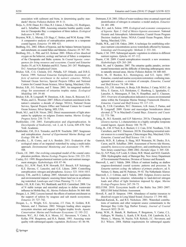
association with sediment and biota, in determining quality stan-dards?Marine Pollution Bulletin 49: 8–11.

Borja, A., D.M. Dauer, R.J. Diaz, R.J. Llanso, I. Muxika, J.G. Rodriguez,and L. Schaffner. 2008. Assessing estuarine benthic quality condi-tion in Chesapeake Bay: a comparison of three indices. EcologicalIndicators 8: 395–403.

Boynton, W.R., L. Murray, J.D. Hagy, C. Stokes, andW.M. Kemp. 1996.A comparative analysis of eutrophication patterns in a temperatecoastal lagoon. Estuaries 19: 408–421.

Breitburg, D.L. 2002. Effects of hypoxia, and the balance between hypoxiaand enrichment, on coastal fishes and fisheries. Estuaries 25: 767–781.

Breitburg, D.L., L. Pihl, and S.E. Kolesar. 2001. Effects of low dissolvedoxygen on the behavior, ecology and harvest of fishes: a comparisonof the Chesapeake and Baltic systems. In Coastal hypoxia: conse-quences for living resources and ecosystems. Coastal and EstuarineStudies 58, ed. N.N. Rabalais and R.E. Turner, 241–267.Washington,D.C: American Geophysical Union.

Bricker, S.B., C.G. Clement, D.E. Pirhalla, S.P. Orlando, and D.R.G.Farrow. 1999. National Estuarine Eutrophication Assessment: ef-fects of nutrient enrichment in the nation's estuaries . NOAA,National Ocean Service, Special Projects Office and NationalCenters for Coastal Ocean Science, Silver Spring, Maryland, USA.

Bricker, S.B., J.G. Ferreira, and T. Simas. 2003. An integrated method-ology for assessment of estuarine trophic status. EcologicalModelling 169: 39–60.

Bricker, S.B., B. Longstaff, W. Dennison, A.B.. Jones, K. Boicourt, E.C.Wicks, and J.L. Woerner. 2007. Effects of nutrient enrichment in thenation’s estuaries: a decade of change. NOAA, National OceanService, Special Projects Office and National Centers for CoastalOcean Science, Silver Spring, MD, USA.

Brush, M.J., and S.M. Nixon. 2002. Direct measurements of light atten-uation by epiphytes on eelgrass Zostera marina. Marine EcologyProgress Series 238: 73–79.

Burkholder, J.M. 2001. Eutrophication and oligotrophication. InEncyclopedia of biodiversity, vol. 2, ed. S. Levin, 649–670. NewYork: Academic.

Burkholder, J.M., D.A. Tomasko, and B.W. Touchette. 2007. Seagrassesand eutrophication. Journal of Experimental Marine Biology andEcology 350: 46–72.

Carvalho, L., R. Cortes, and A.A. Bordalo. 2011. Evaluation of theecological status of an impaired watershed by using a multi-indexapproach. Environmental Monitoring and Assessment 174: 493–508.

Cloern, J.E. 2001. Our evolving conceptual model of the coastal eutro-phication problem. Marine Ecology Progress Series 210: 223–253.

Conley, D.J. 1999. Biogeochemical nutrient cycles and nutrient manage-ment strategies. Hydrobiologia 410: 87–96.

Conley, D.J., H.W. Paerl, R.W. Howarth, D.F. Boesch, S.P. Seitzinger,K.E. Havens, C. Lancelot, and G.E. Likens. 2009. Controllingeutrophication: nitrogen and phosphorus. Science 323: 1014–1015.

Conway, T.M., and R.G. Lathrop. 2005. Alternative land use regulationsand environmental impacts: assessing future land use in an urbaniz-ing watershed. Landscape and Urban Planning 71: 1–15.

Daskin, J.H., K.R. Calci, W.I. Burkhardt, and R.H. Carmichael. 2008. Useof N stable isotope and microbial analyses to define wastewaterinfluence inMobile Bay, AL.Marine Pollution Bulletin 56: 860–868.

Deegan, L.A. 2002. Lessons learned: the effects of nutrient enrichment onthe support of nekton by seagrass and salt marsh ecosystems.Estuaries 25: 727–742.

Deegan, L., A. Wright, S.G. Ayvazian, J.T. Finn, H. Golden, R.R.Merson, and J. Harrison. 2002. Nitrogen loading alters seagrassecosystem structure and support of higher trophic levels. AquaticConservation: Marine and Freshwater Ecosystems 12: 193–212.

Dennison, W.C., R.J. Orth, K.A. Moore, J.C. Stevenson, V. Carter, S.Kollar, P.W. Bergstrom, and R.A. Batiuk. 1993. Assessing waterquality with submerged aquatic vegetation. BioScience 43: 86–94.

Dettmann, E.H. 2001. Effect of water residence time on annual export anddenitrification of nitrogen in estuaries: a model analysis. Estuaries24: 481–490.

Diaz, R.J., and A. Solow. 1999. Ecological and economic consequencesof hypoxia. Topic 2. Gulf of Mexico hypoxia assessment. NationalOceanic and Atmospheric Administration, Coastal Ocean ProgramDecision Analysis Series. NOAA Coastal Ocean Program, SilverSpring, Maryland, USA.

Dodds, W.K., and J.M. Oakes. 2004. A technique for establishing refer-ence nutrient concentrations across watersheds affected by humans.Limnology and Oceanography: Methods 2: 333–341.

Duarte, C.M. 1995. Submerged aquatic vegetation in relation to differentnutrient regimes. Ophelia 41: 87–112.

Duarte, C.M. 2009. Coastal eutrophication research: a new awareness.Hydrobiologia 629: 263–269.

Elliott, M., and V. Quintino. 2007. The estuarine quality paradox, environ-mental homeostasis and the difficulty of detecting anthropogenic stressin naturally stressed areas.Marine Pollution Bulletin 54: 640–645.

Elliott, M., D. Burdon, K.L. Hemingway, and S.E. Apitz. 2007.Estuarine, coastal andmarine ecosystem restoration: confusingman-agement and science—a revision of concepts. Estuarine, Coastaland Shelf Science 74: 349–366.

Ferreira, J.G., J.H. Andersen, A. Borja, S.B. Bricker, J. Camp, M.H.C. daSilva, E. Garces, A.S. Heiskanen, C. Humborg, L. Ignatiades, C.Lancelot, A. Menesguen, P. Tett, N. Hoepffner, and U. Claussen.2011. Overview of eutrophication indicators to assess environmentalstatus within the European Marine Strategy Framework Directive.Estuarine, Coastal and Shelf Science 93: 117–131.

Fertig, B., T.J.B. Carruthers, W.C. Dennison, A.B. Jones, F. Pantus, andB. Longstaff. 2009. Oyster and macroalgae bioindicators detectelevated Δ15N in Maryland's Coastal Bays. Estuaries and Coasts32: 773–786.

Fertig, B., M.J. Kennish, and G.P. Sakowicz. 2013a. Changing eelgrass(Zostera marina L.) characteristics in a highly eutrophic temperatecoastal lagoon. Aquatic Botany 104: 70–79.

Fertig, B., J.M. O’Neil, K.A. Beckert, C.J. Cain, D.M. Needham, T.J.B.Carruthers, and W.C. Dennison. 2013b. Elucidating terrestrial nutri-ent sources to a coastal lagoon, Chincoteague Bay, Maryland, USA.Estuarine, Coastal and Shelf Science 116: 1–10.

Gastrich, M.D., R. Lathrop, S. Haag, M.P. Weinstein, M. Danko, D.A.Caron, and R. Schaffner. 2004. Assessment of brown tide blooms,caused by Aureococcus anophagefferens, and contributing factors inNew Jersey coastal bays: 2000–2002. Harmful Algae 3: 305–320.

Guo, Q., N.P. Psuty, G.P. Lordi, S. Glenn, M.R. Mund, and M.D. Gastrich.2004. Hydrographic study of Barnegat Bay. New Jersey Departmentof Environmental Protection, Division of Science and Research.

Hauxwell, J., and I. Valiela. 2004. Effects of nutrient loading on shallowseagrass-dominated coastal systems: patterns and processes. InEstuarine nutrient cycling: the influence of primary producers, ed. S.Nielsen, G. Banta, and M. Pedersen, 59–92. The Netherlands: Kluwer.

Hauxwell, J., J. Cebrian, and I. Valiela. 2003. Eelgrass Zostera marinaloss in temperate estuaries: relationship to land-derived nitrogenloads and effect of light limitation imposed by algae. MarineEcology-Progress Series 247: 59–73.

HELCOM. 2010. Ecosystem health of the Baltic Sea 2003–2007:HELCOM Initial Holistic Assessment.

Howell, P., and D. Simpson. 1994. Abundance of marine resources todissolved oxygen in Long Island Sound. Estuaries 17: 394–402.

Hunchak-Kariouk, K., and R.S. Nicholson. 2001. Watershed contribu-tions of nutrients and other nonpoint source contaminants to theBarnegat Bay–Little Egg Harbor Estuary. Journal of CoastalResearch SI32: 28–81.

Kemp, W.M., R. Batuik, R. Bartleson, P. Bergstrom, V. Carter, C.L.Gallegos, W. Hunley, L. Karrh, E.W. Koch, J.M. Landwehr, K.A.Moore, L. Murray, M. Naylor, N.B. Rybicki, J.C. Stevenson, andD.J. Wilcox. 2004. Habitat requirements for submerged aquatic


vegetation in Chesapeake Bay: water quality, light regime, andphysical–chemical factors. Estuaries 27: 363–377.

Kennish, M.J. (ed.). 2001a. Barnegat Bay–Little Egg Harbor. NewJersey: Estuary and Watershed Assessment.

Kennish, M.J. 2001b. Status of the estuary and watershed: an overview.Journal of Coastal Research SI 32: 243–273.

Kennish, M.J., and V.N. de Jonge. 2011. Chemical introductions to thesystems: diffuse and nonpoint source pollution from chemicals(nutrients: eutrophication). In Treatise on estuarine and coastalscience , ed. E. Wolanski and D.S. McLusky, 113–148. Waltham,MA, USA: Elsevier.

Kennish, M.J., and B. Fertig. 2012. Application and assessment of anutrient pollution indicator using eelgrass (Zostera marina L.) inBarnegat Bay–Little Egg Harbor estuary, New Jersey. AquaticBotany 96: 23–30.

Kennish, M.J., S.B. Bricker, W.C. Dennison, P.M. Glibert, R.J.Livingston, K.A. Moore, R.T. Noble, H.W. Paerl, J.M. Ramstack,S. Seitzinger, D.A. Tomasko, and I. Valiela. 2007. Barnegat Bay–Little Egg Harbor Estuary: case study of a highly eutrophic coastalbay system. Ecological Applications 17: S3–S16.

Kennish, M.J., S.M. Haag, and G.P. Sakowicz. 2010. Seagrass decline inNew Jersey coastal lagoons: a response to increasing eutrophication.In Coastal lagoons: critical habitats of environmental change, ed.M.J. Kennish and H.W. Paerl, 167–201. Boca Raton, FL, USA:Taylor and Francis.

Kennish, M.J., B. Fertig, and G.P. Sakowicz. 2011. Benthic macroalgalblooms as an indicator of system eutrophy in the Barnegat Bay–Little Egg Harbor estuary. Bulletin of the New Jersey Academy ofSciences 56: 1–5.

Kennish, M.J., B. Fertig, and R.G. Lathrop. 2012. Assessment of nutrientloading and eutrophication in Barnegat Bay–Little EggHarbor, NewJersey in support of nutrient management planning. Draft finalreport. Rutgers University, Institute of Marine and CoastalSciences, New Brunswick, NJ, USA.

Kiddon, J.A., J.F. Paul, H.W. Buffum, C.S. Strobel, S.S. Hale, D. Cobb,and B.S. Brown. 2003. Ecological condition of US Mid-Atlanticestuaries, 1997-1998. Marine Pollution Bulletin 46: 1224–1244.

Kimmel, D.G., H. Townsend, T.J.B. Carruthers, and B. Fertig. 2010.Environmental statistics: balancing simplicity and explanatory pow-er. In Integrating and applying science: a practical handbook foreffective coastal ecosystem assessment, ed. B.J. Longstaff, T.J.B.Carruthers, W.C. Dennison, T.R. Lookingbill, J.M. Hawkey, J.E.Thomas, E.C. Wicks, and J.L. Woerner, 113–132. Cambridge, MD:IAN Press.

Lathrop, R.G., and T.M. Conway. 2001. A buildout analysis of theBarnegat Bay watershed . New Brunswick, NJ, USA: RutgersUniversity, Center of Remote Sensing and Spatial Analysis.

Latimer, J.S., and S.A. Rego. 2010. Empirical relationship betweeneelgrass extent and predicted watershed-derived nitrogen loadingfor shallow New England estuaries. Estuarine, Coastal and ShelfScience 90: 231–240.

Lea, C., R.L. Pratt, T.E. Wagner, E.W. Hawkes, and A.E. Almario. 2003.Use of submerged aquatic vegetation habitat requirements as tar-gets for water quality in Maryland and Virginia Coastal Bays .Assateague Island National Seashore, Maryland and Virgina.National Parks Service Technical Report NPS/NRWRD/NRTR-2003/316. National Parks Service Water Resources Division, FortCollins, Colorado, USA.

Lee, K.-S., S.R. Park, and Y.K. Kim. 2007. Effects of irradiance, temper-ature, and nutrients on growth dynamics of seagrasses: a review.Journal of Experimental Marine Biology and Ecology 350: 144–175.

Malone, T.C., D.J. Conley, T.R. Fisher, P.M. Glibert, L.W. Harding, andK.G. Sellner. 1996. Scales of nutrient-limited phytoplankton pro-ductivity in Chesapeake Bay. Estuaries 19: 371–385.

Niemi, G.J., andM.E.McDonald. 2004. Application of ecological indicators.Annual Review of Ecology and Evolutionary Systematics 35: 89–111.

Oliva, S., O. Mascaró, I. Llagostera, M. Pérez, and J. Romero. 2012.Selection of metrics based on the seagrass Cymodocea nodosa anddevelopment of a biotic index (CYMOX) for assessing ecologicalstatus of coastal and transitional waters. Estuarine, Coastal andShelf Science 114: 7–17.

Orth, R.J., Luckenbach, M.L., Marion, S.R., Moore, K.A., Wilcox, D.A.2006. Seagrass recovery in the Delmarva Coastal Bays, USA.Aquatic Botany 84: 26–36

OSPAR. 2008. Second OSPAR integrated report on the eutrophicationstatus of the OSPAR Maritime Area, 2008-372. OSPAR.

Psuty, N.P. 2004. Morpho-sedimentological characteristics of theBarnegat Bay-Little Egg Harbor Estuary. In The coastal zone:Papers in honor of H. Jesse Walker, Geoscience and Man SeriesNo. 38, eds. D.W. Davis, and M. Richardson, 81-92. Baton Rouge:Louisiana State University.

Psuty, N.P., and T.M. Silveira. 2009. Geomorphological evolution ofestuaries: the dynamic basis for morpho-sedimentary units in select-ed estuaries in the northeastern United States. Marine FisheriesReview 71: 34–45.

Quinn, G. and M. Keough. 2002. Experimental design and data analysisfor biologists . Cambridge University Press.

Ralph, P.J., M.J. Durako, S. Enriques, C.J. Collier, and M.A. Doblin.2007. Impact of light limitation on seagrasses. Journal ofExperimental Marine Biology and Ecology 350: 176–193.

Seitzinger, S.P., R.M. Styles, and I.E. Pilling. 2001. Benthic microalgaland phytoplankton production in Barnegat Bay, New Jersey (USA):microcosm experiments and data synthesis. Journal of CoastalResearch SI 32: 144–162.

Short, F.T., and D.M. Burdick. 1996. Quantifying eelgrass habitat loss inrelation to housing development and nitrogen loading in WaquoitBay, Massachusetts. Estuaries 19: 730–739.

Sokal, R., and F. Rohlf. 1981. Biometry. San Francisco: W.H. Freemanand Co.

Srebotnjak, T., G. Carr, A. de Sherbinin, and C. Rickwood. 2012. AglobalWater Quality Index and hot-deck imputation of missing data.Ecological Indicators 17: 108–119.

Steckbauer, A., C.M. Duarte, J. Carstensen, R. Vaquer-Sunyer, and D.J.Conley. 2011. Ecosystem impacts of hypoxia: thresholds of hypoxiaand pathways to recovery. Environmental Research Letters 6:025003.

Stevenson, J.C., L.W. Staver, and K.W. Staver. 1993. Water qualityassociated with survival of submersed aquatic vegetation along anestuarine gradient. Estuaries 16: 346–361.

Tomasko, D.A., C.J. Dawes, and M.O. Hall. 1996. The effects of anthro-pogenic nutrient enrichment on turtle grass (Thalassia testudinum)in Sarasota Bay, Florida. Estuaries 19: 448–456.

Underwood AJ (1997). Experiments in ecology: Their logical design andinterpretation using analysis of variance. Cambridge University Press.

US Census Bureau. 2000. Summary File 1 (SF 1) and Summary File 3(SF 3).

Valiela, I., and M.L. Cole. 2002. Comparative evidence that salt marshesand mangroves may protect seagrass meadows from land-derivednitrogen loads. Ecosystems 5: 92–102.

Valiela, I., M. Geist, J. McClelland, and G. Tomasky. 2000. Nitrogenloading from watersheds to estuaries: verification of the WaquoitBay Nitrogen Loading Model. Biogeochemistry 49: 277–293.

Wazniak, C.E., M.R. Hall, T.J.B. Carruthers, B. Sturgis, W.C. Dennison,and R.J. Orth. 2007. Linking water quality to living resources in amid-Atlantic lagoon system, USA. Ecological Applications 17:S64–S78.

Wieben, C.M., and R.J. Baker. 2009. Contributions of nitrogen to theBarnegat Bay–Little Egg Harbor Estuary: Updated loading esti-mates . New Jersey, USA: West Trenton.

Williams, M., B. Longstaff, C. Buchanan, R. Llanso, and W. Dennison.2009. Development and evaluation of a spatially-explicit index ofChesapeake Bay health. Marine Pollution Bulletin 59: 14–25.


Mind the Data Gap: Identifying and Assessing Drivers of Changing Eutrophication Condition

Documents

Transcript of Mind the Data Gap: Identifying and Assessing Drivers of Changing Eutrophication Condition