Master Thesis

Electrical Engineering

November 2007

Implementation of a Soft Output Sphere Decoder by Rapid

Prototyping Methodology

Krishnakumar Radhakrishnan

Department of Signal Processing Institute of Communications &

Blekinge Institute of Technology Radio frequency Engineering

Box 520 Vienna University of Technology

SE - 372 25 Ronneby Gußhausstraße 25/389

Sweden A - 1040 Vienna

Austria

Abstract

During the last decade there has been tremendous growth in wireless communication,

with focus on broadband wireless LAN and mobile phones. To meet the demand for

faster wireless access there is a need to change from the traditional Single-Input-Single

Output (SISO) antenna systems. There has been significant progress in recent times in

developing systems that use multiple antennas at the transmitter and receiver to achieve

better performance.

Multiple-input-multiple-output (MIMO) uses multiple antennas in both transmitter and

receiver ends to achieve high spectral efficiency. However the implementation of MIMO

systems comes at the cost of increased complexity in the receiver design. The detection

of vector of symbols drawn from a finite alphabet when transmitted over a MIMO system

poses a challenging implementation task.

The aim of this thesis is to use sphere detection algorithm as an efficient means to detect

the spatially multiplexed symbols. This thesis discusses the evaluation of the performance

and implementation aspects of a Soft output sphere decoder as an efficient detection

means for MIMO systems. The implementation is done in MATLAB and C and discusses

the prospects of rapid prototyping methodology as an efficient approach towards further

implementation.

Acknowledgements

I would like to thank many people involved in bringing up this course work to this very

point. Firstly I would thank my parents who have been a constant source of support; their

love and encouragement have brought me this far in life.

I thank Sebastian Caban for inviting me to Vienna to work on my thesis. My sincere

thanks to my thesis advisor Christian Mehlfuehrer for providing me with this topic,

sharing his viewpoint, his encouragement and support in pursuing this work. I would

further like to express my gratitude to Christian for his extended patience when it came to

making the report. The atmosphere at the MIMO Lab was just perfect and I truly had a

great experience being part of it for a whole summer.

The time spent in Vienna would not be complete without mentioning the support from the

folks met during the stay. Those joyful moments that helped take a breather and later

providing with the zeal to work further. A special thanks to Dr.N.Z.A for the

unforgettable experience that was Vienna.

Contents

Introduction ..................................................................................................................... 2

1.1 Background .......................................................................................................... 2 1.1.1 Available detection algorithms ........................................................................ 3 1.1.2 A Possible Solution ......................................................................................... 3

1.2 Objective ............................................................................................................... 4 2.1 MIMO Overview .................................................................................................. 5

2.1.1 Why MIMO-OFDM ....................................................................................... 6 2.1.2 Basic principle................................................................................................ 7

2.2 Physical layer Implementation Aspects .................................................................. 8 3.1 Sphere decoder (SD)........................................................................................... 10

3.1.1 MIMO Channel Model .................................................................................. 11 3.2 Sphere Decoding Algorithm ............................................................................... 11

3.2.1 Hard detection .............................................................................................. 12 3.2.2 Soft-output SD ............................................................................................. 13 3.2.3 Schnorr-Euchner SD (SESD) ........................................................................ 18 3.2.4 Tree traversal Algorithm............................................................................... 19

4.1 Classical Design Methodology ........................................................................... 24 4.2 Rapid prototyping ............................................................................................... 25

4.2.1 Motivation for Rapid prototyping ................................................................. 25 4.2.2 Key to Rapid prototyping ............................................................................. 26

5.1 Challenges toward Algorithm Implementation .................................................... 28 5.2 Implementation in MATLAB ............................................................................. 30 5.3 Implementation in „C‟ ........................................................................................ 34 6.1 Background ........................................................................................................ 37

6.1.1 Partitioning between FPGA and DSP ........................................................... 38 6.2 Digital Signal Processors .................................................................................... 39

6.2.1 Introduction .................................................................................................. 39 6.2.2 Development Tools ....................................................................................... 41 6.2.3 Fixed point Issues ......................................................................................... 45

Conclusion .................................................................................................................... 46 Abbreviations ................................................................................................................ 47 Bibliography ................................................................................................................. 48

LIST OF FIGURES

Figure 1: A basic 2 x 2 Communication system. .............................................................. 2 Figure 2: Overview of a MIMO Communication system.................................................. 5 Figure 3: A simple modulation-demodulation block diagram. .......................................... 7 Figure 4: Model of an OFDM system. ............................................................................. 8 Figure 5: Geometrical representation of the sphere decoding algorithm. ........................ 10 Figure 6: Simple flowchart of the Soft-output sphere decoder algorithm. ....................... 15 Figure 7: Sphere decoding as a Tree-search problem, with m = 4 as the number of

Transmit antennas. ........................................................................................................ 18 Figure 8: Example of a Single Tree Search pruning criterion (M = 5 and two bits per

symbol). ........................................................................................................................ 21 Figure 9: Example of calculating the LLR for the bit . ................................................ 22 Figure 10: Example of calculating the LLR for the bit . .............................................. 22 Figure 11: Typical product development strategy diagram. ............................................ 24 Figure 12: Rapid prototyping design flow (taken from [9]). .......................................... 27 Figure 13: A simple receiver, represented as a block diagram with blocks containing

algorithm specified by symbols. .................................................................................... 29 Figure 14: Performance evaluation for soft-output sphere decoder with symbols

compared....................................................................................................................... 31 Figure 15: Performance evaluation for soft-output sphere decoder with the bits compared.

...................................................................................................................................... 32 Figure 16: Performance evaluation in terms of computational speed, MATLAB vs. „C‟. 36 Figure 17: Basic DSP system. ........................................................................................ 39 Figure 18: Different phases of the CCS development cycle. ........................................... 41 Figure 19: Process involving creation of an executable file after compiling C file. ......... 42

2

CHAPTER 1

Introduction

1.1 Background

Since the early nineties till the recent present, technological advancements concerning

Multiple Input Multiple Output (MIMO) wireless communication have undergone

unprecedented growth and are still growing. This urge has been spurted by the demand

for high speed data communication overcoming problems such as noise and fading. The

great deal of attention towards MIMO Wireless systems is mainly due to the promise of

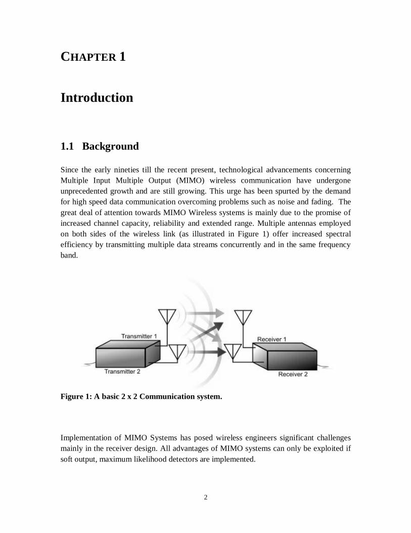
increased channel capacity, reliability and extended range. Multiple antennas employed

on both sides of the wireless link (as illustrated in Figure 1) offer increased spectral

efficiency by transmitting multiple data streams concurrently and in the same frequency

band.

Figure 1: A basic 2 x 2 Communication system.

Implementation of MIMO Systems has posed wireless engineers significant challenges

mainly in the receiver design. All advantages of MIMO systems can only be exploited if

soft output, maximum likelihood detectors are implemented.

3

1.1.1 Available detection algorithms

A wide range of algorithms offering various trade-offs between performance and

computational complexity has been developed.

Maximum likelihood detection (MLD): This detector finds the transmitted signal points

by minimising the Euclidean distance. However, such a search is exponential in finding

the number of constellation points, making MLD unsuitable for practical purposes when

aiming at high spectral efficiency.

Linear detection & Successive Interference Cancellation (SIC): producing hard or soft

decision output and performance is limited by the strongest detected signal, which leads

to poor diversity. The main advantage of this detector is the very low complexity

compared to the MLD.

A Posteriori Probabilty (APP): is a computationally efficient algorithm with optimal

performance when implemented in group detector by soft output sphere decoder (SD).

The overall decoding effort is typically constrained by system bandwidth, latency

requirements, and limitations on power consumption. Implementing different algorithms,

each optimized for a maximum allowed decoding effort and/or a particular system

configuration, would entail a considerable hardware overhead.

1.1.2 A Possible Solution

Recently sphere detection has emerged as a powerful means of finding the maximum

likelihood solution to detection problem for MIMO systems. The computational

complexity of the sphere decoder would depend on the symbol constellation size and the

number of spatially multiplexed data streams, as well as on the instantaneous MIMO

channel realization and the signal-to-noise ratio (SNR). Sphere decoder lowers the

computational complexity by limiting the search to the closest lattice point to the

received signal within a sphere radius. In a 2-D problem, we can restrict the search by

drawing a circle around the received signal just small enough to enclose one signal point

and eliminate the search of all points outside the circle. By using the soft output sphere

decoder and using the counter hypotheses it is possible to obtain better results.

4

1.2 Objective

This Masters project aims at evaluating the performance and implementation aspects of a

soft output sphere decoder algorithm for a MIMO system using rapid prototyping

methodology. The performance gain of using soft output sphere detection is to be

discussed while implementing it in MATLAB and C. Further the porting of the code onto

a DSP by following the rapid prototyping methodology would be the key objective in this

thesis.

5

CHAPTER 2

MIMO-OFDM

This chapter sheds light on MIMO Technology, how MIMO-OFDM has become the best

choice for implementing this concept, and the principles of the underlying MIMO-

OFDM.

2.1 MIMO Overview

Multipath propagation has been part of all wireless communication environments.

Traditional radio systems rely on the strong primary signal and employ multipath

mitigation techniques to combat multipath propagation and interference. One technique

used for this purpose is beamforming technology or smart antenna technology. A smart

antenna is able to steer a transmitted beam by accurately controlling the phase of the

signal at each element of the antenna array to the receiver. Another technique is receive

diversity, which uses multiple antennas at the receiver and combines all receive signal to

improve the signal reliability. These techniques help reduce the multipath propagation

effect. Additionally, MIMO rather than combating makes use of multipath propagation in

its favor to increase throughput, range and reliability.

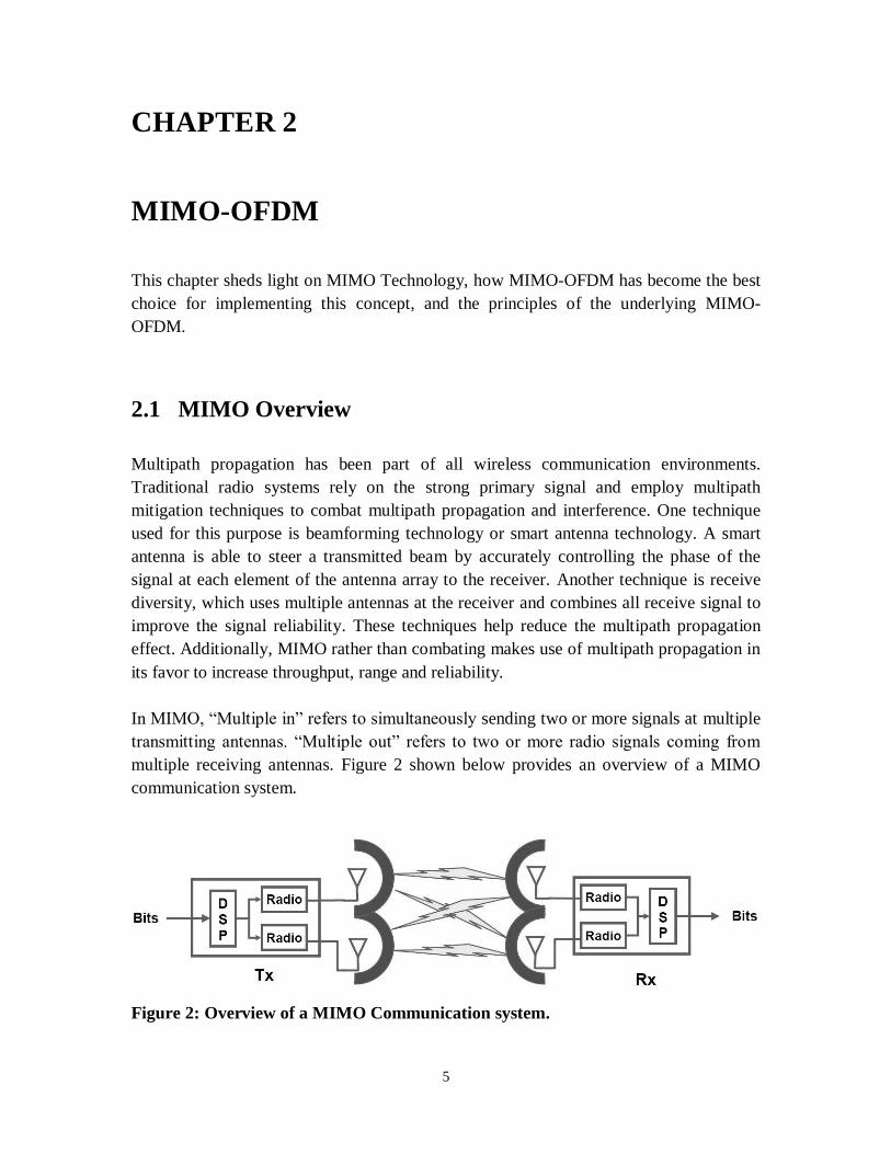
In MIMO, “Multiple in” refers to simultaneously sending two or more signals at multiple

transmitting antennas. “Multiple out” refers to two or more radio signals coming from

multiple receiving antennas. Figure 2 shown below provides an overview of a MIMO

communication system.

Figure 2: Overview of a MIMO Communication system.

6

This has been known to increase spectral efficiency and link reliability by combining the

goodness of Beamforming and Diversity. Common forms of diversity are antenna

diversity (or spatial diversity), time diversity (due to Doppler spread) and frequency

diversity (due to delay spread). In recent years the use of antenna diversity has become

very popular, this is mostly due to the fact that it can be provided without loss in spectral

efficiency.

Driven by mobile wireless applications, where it is difficult to deploy multiple antennas

in the handset, the use of multiple antennas on the transmit side combined with signal

processing and coding has become known under the name of Space Time Coding [3].

MIMO takes advantage of multipath by multiplexing these signals with advanced DSP

algorithms to boost wireless bandwidth efficiency and range. MIMO antenna

configuration has shown to achieve extraordinary data rates and this technology is known

as Spatial Multiplexing. In spatial multiplexing, a high rate signal is split into multiple

lower rate streams and each stream is transmitted from a different transmit antenna in the

same frequency channel. If these signals arrive at the receiver antenna array with

sufficiently different spatial signatures, the receiver can separate these streams, creating

parallel channels for free. Spatial multiplexing is very powerful technique for increasing

channel capacity at higher SNR.

2.1.1 Why MIMO-OFDM

MIMO can be used with any modulation or access technique. Today, many digital radio

systems use CDMA (e.g. UMTS) or OFDM (e.g. WLAN, WiMAX). Time division

systems transmit bits over a narrowband channel, using time slots to segregate bits for

different user or purposes. Code division systems transmit bits over a wideband (spread

spectrum) channel, using codes to segregate bits for different user or purposes. OFDM is

also a wideband system, but unlike CDMA which spreads the signal continuously over

the entire channel, OFDM employs multiple, discrete, lower data rate subchannels.

MIMO-OFDM technology has been adopted by the IEEE 802.11 standards group as the

foundation for a high throughput amendment to the multimedia wireless fidelity (WiFi)

applications.

When it comes to implementation point of view, particularly at higher data rates, MIMO

OFDM signals can be processed using relatively straightforward matrix algebra. In other

words use of OFDM will significantly reduce the receiver complexity in wireless

communication systems. The main motivation for using OFDM in a MIMO channel is

the fact that OFDM modulation turns a frequency-selective MIMO channel into a set of

7

parallel frequency flat MIMO channels. This renders multi-channel equalization

particularly simple, since for each OFDM-tone only a constant matrix has to be inverted

[4]. Therefore the use of MIMO technology in combination with OFDM, MIMO-OFDM

is an attractive solution for future wireless communication systems design

2.1.2 Basic principle

OFDM can be viewed as a form of frequency division multiplexing (FDM) with the

special property that each tone is orthogonal with every other tone, but it is different from

FDM in several ways. On one hand, FDM requires typically the existence of frequency

guard bands between the frequencies so that they do not interfere with each other. On the

other hand, OFDM allows spectrum of each tone to overlap, and because they are

orthogonal, they do not interfere with each other. Furthermore, the overall amount of

required spectrum is reduced due to the overlapping of the tones. Figure 3 shown below

gives an idea of the process of modulation and demodulation of OFDM signals. OFDM

signals are typically generated digitally due to the difficulty in creating large banks of

phase lock oscillators and receivers in the analog domain.

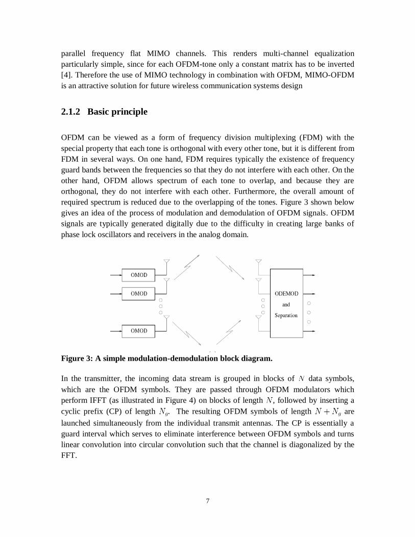
Figure 3: A simple modulation-demodulation block diagram.

In the transmitter, the incoming data stream is grouped in blocks of data symbols,

which are the OFDM symbols. They are passed through OFDM modulators which

perform IFFT (as illustrated in Figure 4) on blocks of length , followed by inserting a

cyclic prefix (CP) of length . The resulting OFDM symbols of length are

launched simultaneously from the individual transmit antennas. The CP is essentially a

guard interval which serves to eliminate interference between OFDM symbols and turns

linear convolution into circular convolution such that the channel is diagonalized by the

FFT.

8

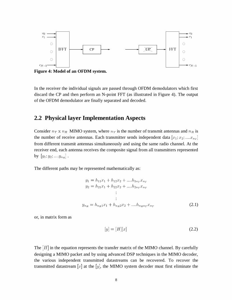
Figure 4: Model of an OFDM system.

In the receiver the individual signals are passed through OFDM demodulators which first

discard the CP and then perform an N-point FFT (as illustrated in Figure 4). The output

of the OFDM demodulator are finally separated and decoded.

2.2 Physical layer Implementation Aspects

Consider MIMO system, where is the number of transmit antennas and is

the number of receive antennas. Each transmitter sends independent data

from different transmit antennas simultaneously and using the same radio channel. At the

receiver end, each antenna receives the composite signal from all transmitters represented

by .

The different paths may be represented mathematically as:

:

:

(2.1)

or, in matrix form as

(2.2)

The in the equation represents the transfer matrix of the MIMO channel. By carefully

designing a MIMO packet and by using advanced DSP techniques in the MIMO decoder,

the various independent transmitted datastreams can be recovered. To recover the

transmitted datastream at the , the MIMO system decoder must first eliminate the

9

individual channel transfer coefficient to determine the channel transfer matrix

during the MIMO preamble of the packet. Once the estimated has been produced, the

transmitted datastream can be reconstructed by multiplying the vector with the

inverse of transfer matrix . This is represented by:

(2.3)

The process, in principle, is equivalent to solving a set of unknowns with linear

equations. To ensure that the channel matrix is invertible, MIMO systems require an

environment rich in multipath. It is important to note that unlike traditional methods of

increasing throughput by increasing bandwidth, MIMO systems can increase throughput

without increasing bandwidth. This is accomplished in a MIMO system by exploiting

spatial dimensions and increasing the number of signal paths between the transmitters

and the receivers [22]. As each independent datastream is transmitted in parallel from

separate antennas, the data throughput increases linearly with every pair of antennas

added to the MIMO system.

10

CHAPTER 3

Sphere decoding

At the receiver, detection is performed that computes and delivers the estimates of the

transmitted data bits. The detector operates on the received signal in each separate

transmission symbol interval and produces a number or a set of numbers that represent an

estimate of a transmitted Quadrature Amplitude Modulation (QAM) symbol. The

decoding methods are used for decision metrics with the aim of making a decision about

which bit, „zero‟ or „one‟ was transmitted. This decision metric can be as simple as hard

decision, or more sophisticated, being a soft decision.

3.1 Sphere decoder (SD)

Techniques like Maximum likelihood decoding require an exhaustive search over all

possible code words used. The computational complexity of these techniques is

exponential in the length of the codeword. A promising approach called the sphere

decoding algorithm was proposed to lower the computational complexity. The principle

of the sphere decoding algorithm is to search the closest lattice point to the received

signal within a sphere radius, where each codeword is represented by a lattice point in a

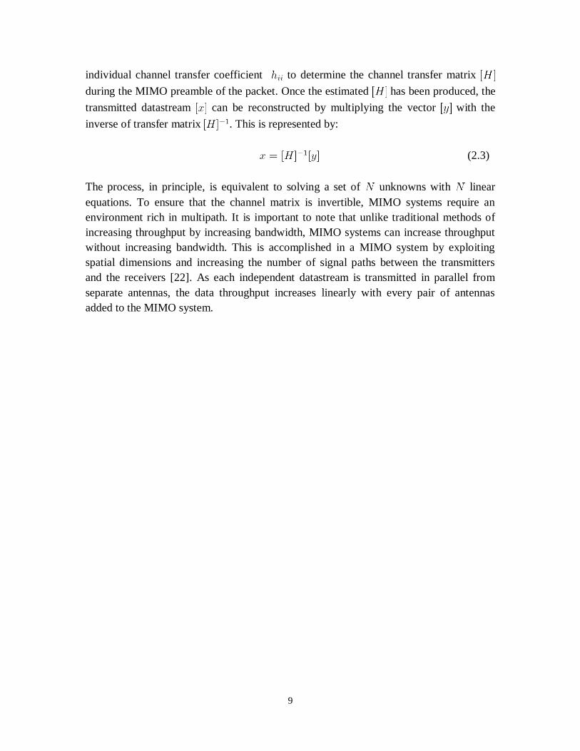
lattice field [6]. In 2-D the search can be represented by drawing a circle around the

received signal just small enough to enclose one lattice point and eliminate the search of

other points outside the circle as shown in Figure 5 below.

Figure 5: Geometrical representation of the sphere decoding algorithm.

11

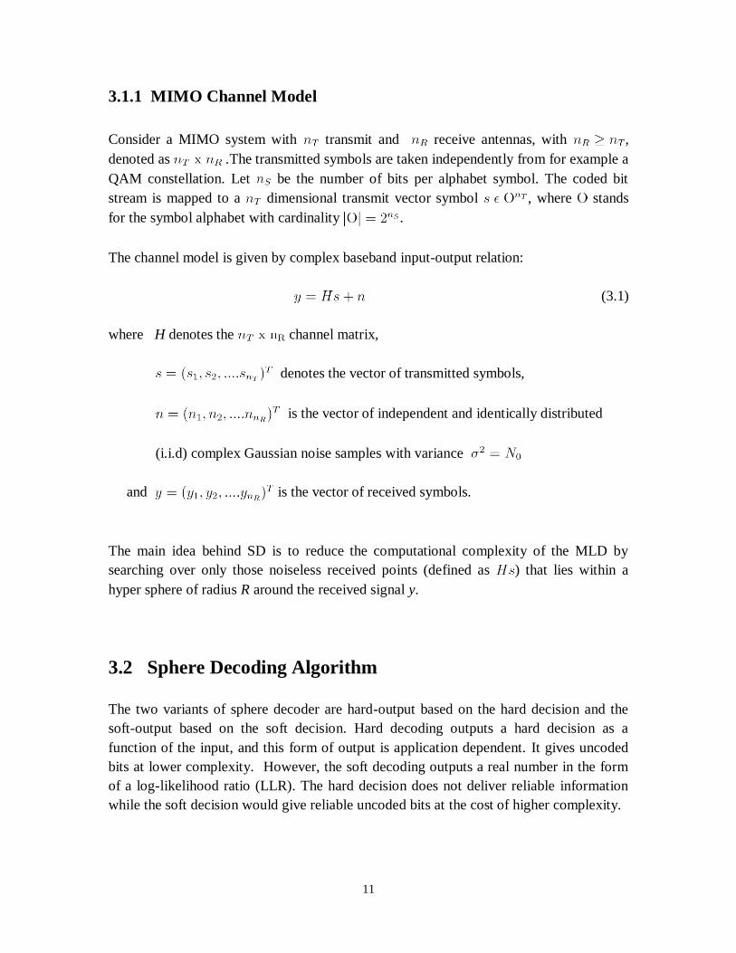
3.1.1 MIMO Channel Model

Consider a MIMO system with transmit and receive antennas, with ,

denoted as .The transmitted symbols are taken independently from for example a

QAM constellation. Let be the number of bits per alphabet symbol. The coded bit

stream is mapped to a dimensional transmit vector symbol , where stands

for the symbol alphabet with cardinality .

The channel model is given by complex baseband input-output relation:

(3.1)

where H denotes the channel matrix,

denotes the vector of transmitted symbols,

is the vector of independent and identically distributed

(i.i.d) complex Gaussian noise samples with variance

and is the vector of received symbols.

The main idea behind SD is to reduce the computational complexity of the MLD by

searching over only those noiseless received points (defined as ) that lies within a

hyper sphere of radius R around the received signal y.

3.2 Sphere Decoding Algorithm

The two variants of sphere decoder are hard-output based on the hard decision and the

soft-output based on the soft decision. Hard decoding outputs a hard decision as a

function of the input, and this form of output is application dependent. It gives uncoded

bits at lower complexity. However, the soft decoding outputs a real number in the form

of a log-likelihood ratio (LLR). The hard decision does not deliver reliable information

while the soft decision would give reliable uncoded bits at the cost of higher complexity.

12

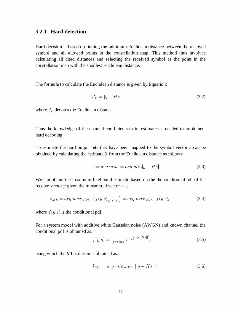
3.2.1 Hard detection

Hard decision is based on finding the minimum Euclidean distance between the received

symbol and all allowed points in the constellation map. This method thus involves

calculating all cited distances and selecting the received symbol as the point in the

constellation map with the smallest Euclidean distance.

The formula to calculate the Euclidean distance is given by Equation:

(3.2)

where denotes the Euclidean distance.

Thus the knowledge of the channel coefficients or its estimates is needed to implement

hard decoding.

To estimate the hard output bits that have been mapped to the symbol vector can be

obtained by calculating the estimate from the Euclidean distance as follows:

(3.3)

We can obtain the maximum likelihood estimate based on the the conditional pdf of the

receive vector given the transmitted vector as:

, (3.4)

where is the conditional pdf.

For a system model with additive white Gaussian noise (AWGN) and known channel the

conditional pdf is obtained as:

, (3.5)

using which the ML solution is obtained as:

(3.6)

13

But this minimisation yields only hard output of the transmit symbol vector. It does not

offer reliable information and omits a large part of the information contained in the

receive symbol vector.

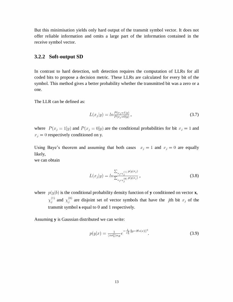
3.2.2 Soft-output SD

In contrast to hard detection, soft detection requires the computation of LLRs for all

coded bits to propose a decision metric. These LLRs are calculated for every bit of the

symbol. This method gives a better probability whether the transmitted bit was a zero or a

one.

The LLR can be defined as:

, (3.7)

where and are the conditional probabilities for bit and

respectively conditioned on y.

Using Baye‟s theorem and assuming that both cases and are equally

likely,

we can obtain

, (3.8)

where is the conditional probability density function of y conditioned on vector x,

and are disjoint set of vector symbols that have the jth bit of the

transmit symbol s equal to 0 and 1 respectively.

Assuming y is Gaussian distributed we can write:

. (3.9)

14

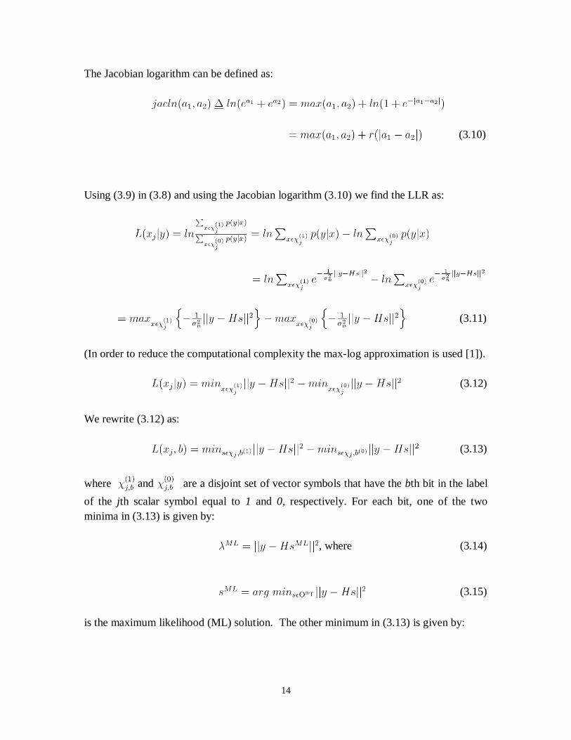
The Jacobian logarithm can be defined as:

(3.10)

Using (3.9) in (3.8) and using the Jacobian logarithm (3.10) we find the LLR as:

(3.11)

(In order to reduce the computational complexity the max-log approximation is used [1]).

(3.12)

We rewrite (3.12) as:

(3.13)

where and are a disjoint set of vector symbols that have the bth bit in the label

of the jth scalar symbol equal to 1 and 0, respectively. For each bit, one of the two

minima in (3.13) is given by:

, where (3.14)

(3.15)

is the maximum likelihood (ML) solution. The other minimum in (3.13) is given by:

15

(3.16)

where the counter hypothesis denotes the binary complement of the bth bit in the

binary label of the jth entry of .

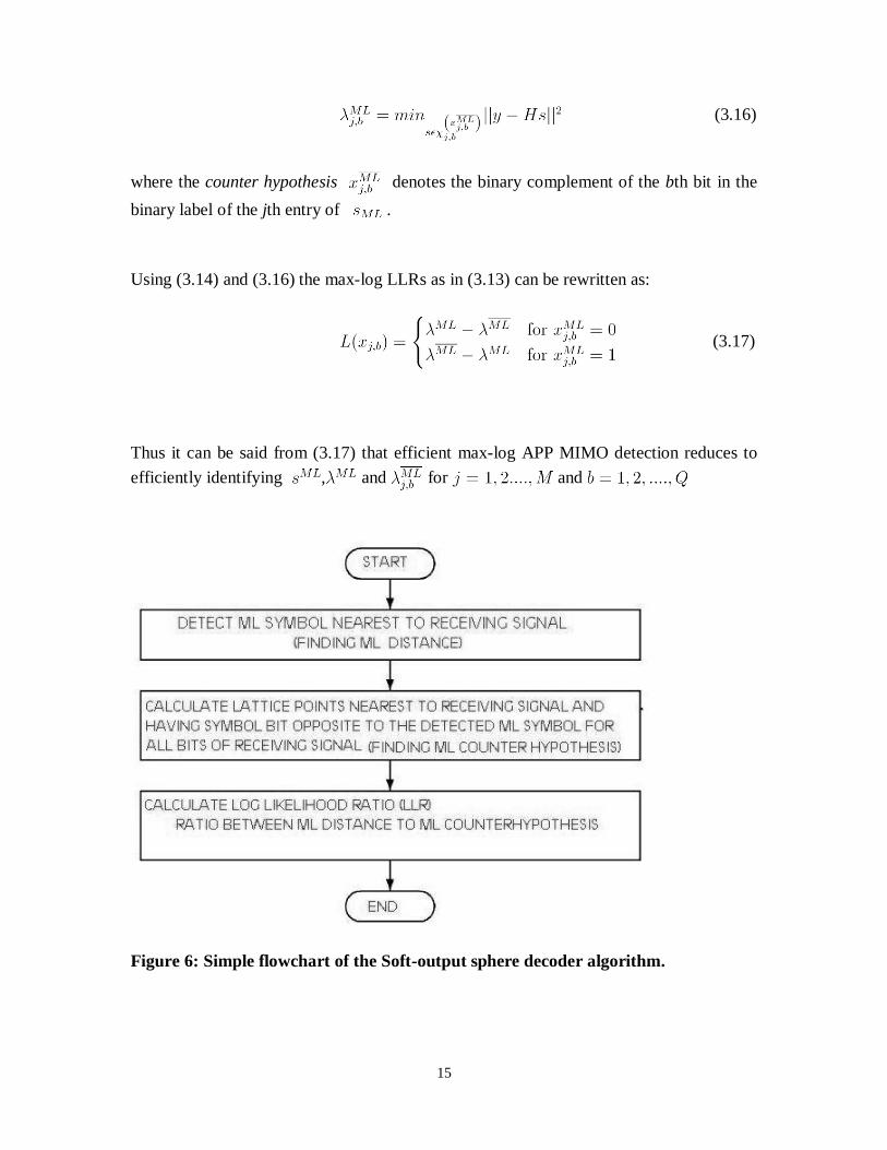
Using (3.14) and (3.16) the max-log LLRs as in (3.13) can be rewritten as:

(3.17)

Thus it can be said from (3.17) that efficient max-log APP MIMO detection reduces to

efficiently identifying , and for and

Figure 6: Simple flowchart of the Soft-output sphere decoder algorithm.

16

As the next step, QR-decomposition is done on the channel matrix H is according to

, where Q is unitary, ie and R is the upper-triangular with real-valued

positive entries on its main diagonal.

Multiplying (3.1) by HQ leads to the modified input-output relation:

with (3.18)

Noting that has the same statistics as n gives an equivalent formulation of

and as :

(3.19)

(3.20)

The computation of the distances can be transformed into a tree search problem and then

using the sphere decoding algorithm (as described in the flowchart shown in Figure 6)

leads to an efficient computation of LLRs.

Define partial symbol vectors (PSVs) as . PSVs are arranged

in a tree that has its root just above level i = M and leaves, on level i = 1, which

corresponds to possible candidate symbol vectors s [2].

In the following, the label associated with is denoted by .

The Euclidean distance is calculated as:

(3.21)

Initialise distance and using (3.21) to compute distance for (3.19) and (3.20) is

done recursively as with partial Euclidean distances (PEDs)

, where (3.22)

17

and the distance increments (DIs)

(3.23)

As the dependence of the PEDs on the symbol vector s is only through , ML

detection and computation of the max-log LLRs have been transformed into a weighted

tree-search problem.

PSVs and PEDs are associated with nodes while branches correspond to DIs. Each path

from root down to a leaf corresponds to a symbol vector . The leaf associated with

the smallest metric in and corresponds to the solution of (3.19) and (3.20)

respectively.

18

3.2.3 Schnorr-Euchner SD (SESD)

Depth First Traversal

Using SESD no initial radius to limit the search is selected; instead the radius to start the

search is initially kept at infinity. Later it updates the radius based on PEDs. Using this,

the search is constrained to nodes which lie within the updated radius and traverses the

tree depth first, visiting the children of a given node in ascending order of their PEDs.

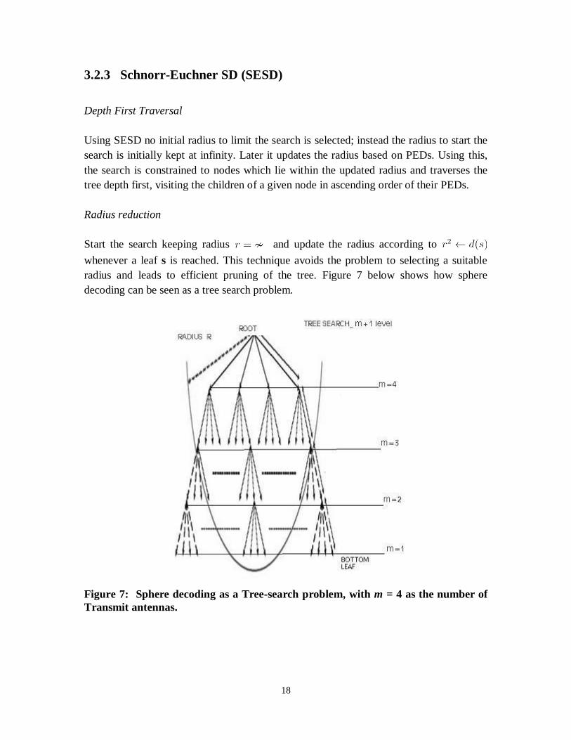
Radius reduction

Start the search keeping radius and update the radius according to

whenever a leaf s is reached. This technique avoids the problem to selecting a suitable

radius and leads to efficient pruning of the tree. Figure 7 below shows how sphere

decoding can be seen as a tree search problem.

Figure 7: Sphere decoding as a Tree-search problem, with m = 4 as the number of

Transmit antennas.

19

3.2.4 Tree traversal Algorithm

The tree traversal (based on [1]) to find solution to (3.19) and (3.20) can be be done in

two different ways:

Repeated Tree Search

The traversal starts by solving (3.19) using SESD and to rerun the SESD to solve (3.20)

for each coded bit in the vector symbol. As solving (3.20) by traversing those parts of the

tree that has leaves in has to be done for every coded bit; leading to repeated tree

traversals with increased complexity. In repeated tree search when rerunning SESD to

determine , the search tree is prepruned by forcing the decoder to exclude all nodes

and the corresponding subtrees from the search for which . However this

search leads to repeated traversal of large parts of the tree while finding the counter

hypotheses, leading to higher computational complexity.

Single Tree Search

This is a more efficient tree search that ensures that every node in the tree is visited at

most once. This can be accomplished by searching for the ML solution and all counter-

hypotheses concurrently. The key lies in formulating update rules and a pruning criterion

based on a list containing the distance metrics and .

The algorithm is initialized with . Whenever leaf with

corresponding binary label x has been reached, the decoder distinguishes between two

cases:

1) If a new ML hypothesis is found, i.e., , all for which

are set to followed by the updates and . In other

words, for each bit in the ML hypothesis that is changed in the process of the

update, the distance metric of the former ML hypothesis becomes the distance

metric of the new counter-hypothesis, followed by an update of the ML

hypothesis.

2) In the case where , only the counter-hypotheses have to be checked.

For all j and b for which and , the decoder updates

20

Pruning criterion

The key aspect of this algorithm is the following pruning criterion. A given node on

level i and the subtree originating from that node have the partial binary label

consisting of the bits and . The remaining bits

corresponding to the subtree are unknown at this point. The

pruning criterion for along with its subtree is compiled from two conditions. First, the

bits in the partial binary label are compared with the corresponding bits in the binary

label of the current ML hypothesis. In this comparison, for all j, b with , the

corresponding counter-hypotheses might be affected when further searching the

node‟s subtree. Second, all counter-hypotheses corresponding to the subtree of with

the associated distance metrics may also be updated since the

corresponding bits are not known yet.

Summarising, the distance metrics which may be affected during further search in the

subtree emanating from a node are given by the set

(3.24)

The node along with its subtree is pruned if its PED satisfies

(3.25)

This pruning criterion (as illustrated in Figure 8) ensures that the subtree of a given node

is explored only if it can lead to an update of either the ML hypothesis or of at least one

of the counter-hypotheses. Note that does not appear in (3.24) as

.

21

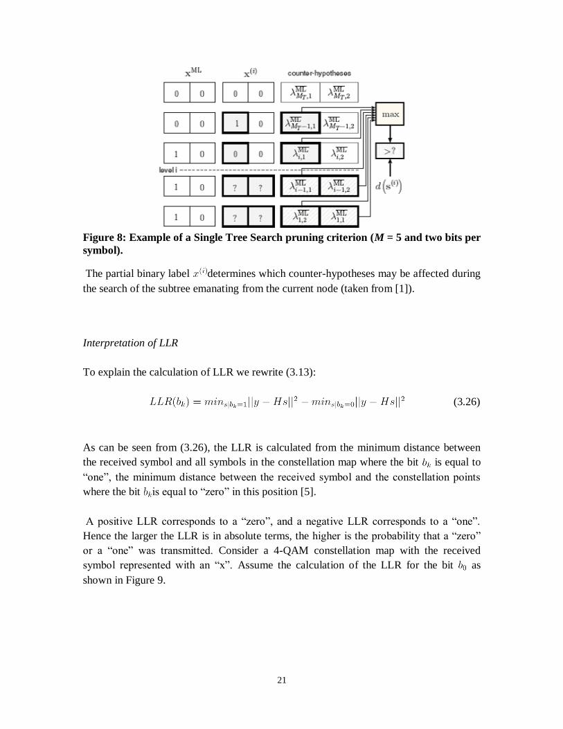
Figure 8: Example of a Single Tree Search pruning criterion (M = 5 and two bits per

symbol).

The partial binary label determines which counter-hypotheses may be affected during

the search of the subtree emanating from the current node (taken from [1]).

Interpretation of LLR

To explain the calculation of LLR we rewrite (3.13):

(3.26)

As can be seen from (3.26), the LLR is calculated from the minimum distance between

the received symbol and all symbols in the constellation map where the bit is equal to

“one”, the minimum distance between the received symbol and the constellation points

where the bit is equal to “zero” in this position [5].

A positive LLR corresponds to a “zero”, and a negative LLR corresponds to a “one”.

Hence the larger the LLR is in absolute terms, the higher is the probability that a “zero”

or a “one” was transmitted. Consider a 4-QAM constellation map with the received

symbol represented with an “x”. Assume the calculation of the LLR for the bit as

shown in Figure 9.

22

Figure 9: Example of calculating the LLR for the bit .

In subfigure (a), the minimum distance between the received bit and = 1 is calculated.

Subfigure (b) makes the same calculation for = 0.

is the minimum distance between the received bit and the points in the constellation

map that have a bit equal to “one” in the position of the bit . The same operation is

performed for the bit equal to “zero”, obtaining the distance . The numerical values

of and are 1.56 and 0.92 respectively. The LLR can be calculated as the difference

between both distances: LLR = – . Replacing the numerical values gives a result of

0.64 for LLR ( ).

Using the same steps to get the LLR value for bit is shown in Figure 10.

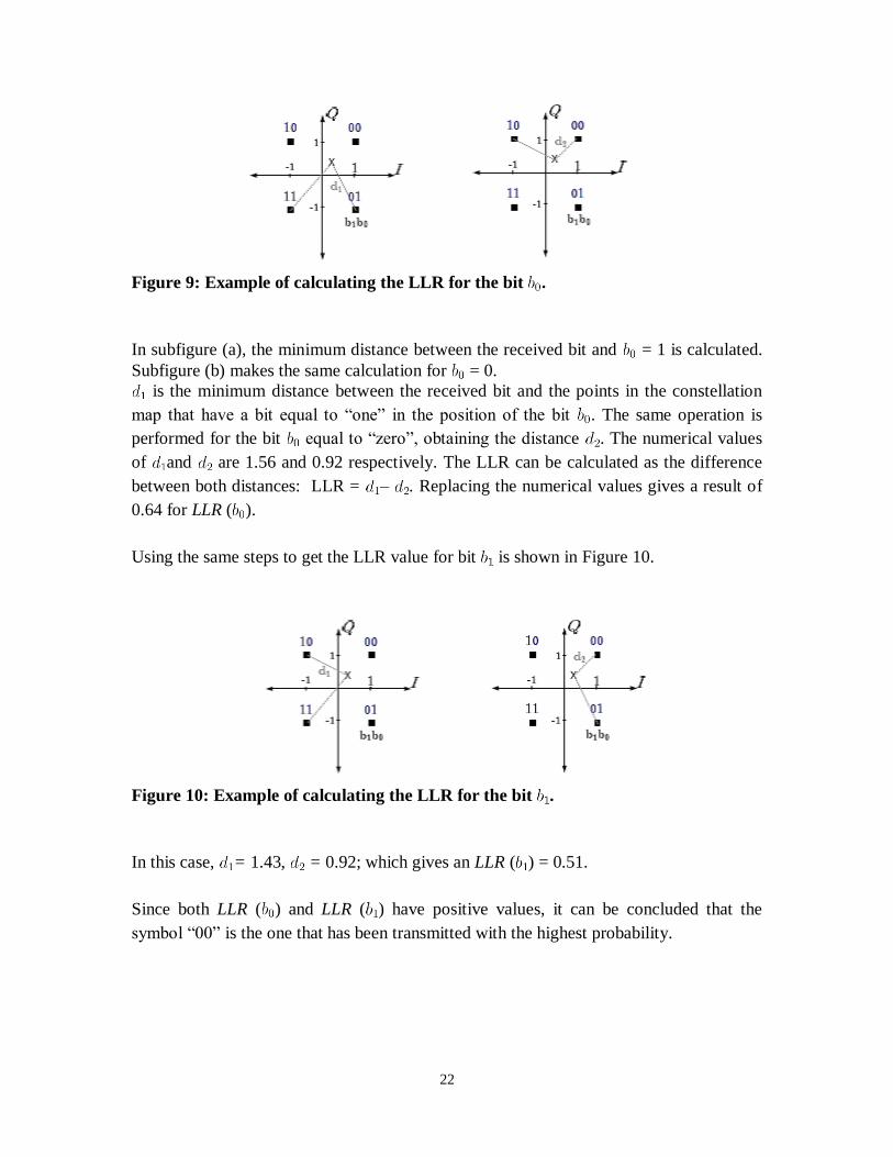
Figure 10: Example of calculating the LLR for the bit .

In this case, = 1.43, = 0.92; which gives an LLR ( ) = 0.51.

Since both LLR ( ) and LLR ( ) have positive values, it can be concluded that the

symbol “00” is the one that has been transmitted with the highest probability.

23

CHAPTER 4

Rapid prototyping methodology

Digital signal processing (DSP) algorithms are used in an ever increasing number of

embedded real-time applications that include systems as simple as consumer products to

very sophisticated control systems. Prototyping of these systems include a number of

steps, which usually start with a high-level description and simulations using common

engineering tools such as MATLAB and Simulink for at least a part of the application.

One of the major issues in embedded DSP systems prototyping and implementation is the

number of abstraction levels used to express the same functionality. Each of these

description levels introduces modification of the algorithms that may influence the final

outcome [10].

For example, say we are investigating the performance of highly sophisticated wireless

systems involving multiple-transmit and receive antennas. Let us start the simulation of

the algorithms using MATLAB that has a highly accurate double-precision numerical

environment, which is an ideal tool for this purpose; while many imperfections of the

real-world neglected [7]. A first evaluation of the performance of a novel idea is usually

done mathematically based on very basic, typically simplistic assumptions. Gaining

confidence in algorithms developed with theoretical models by means of simulations is

an essential part of the early development stage, since wireless channels suffer from a

wide variety of effects that are often difficult to model accurately [12]. The next step that

aims at the algorithm implementation requires further algorithm modification in order to

meet the capabilities of future products (that uses fixed point arithmetic. All this requires

repeated verification before the final step of algorithm synthesis for the target platform.

Target platforms include technologies such as ASICs, FPGAs, general-purpose

processors and Digital Signal Processors (DSPs). The final step involves either

transformation into synthesisable hardware description (behavioural or Register Transfer

Level, RTL) or machine code of the target processor.

24

4.1 Classical Design Methodology

The design process, leading from concept to realization passes through three general

levels of refinement, namely the algorithmic, the architectural and the implementation

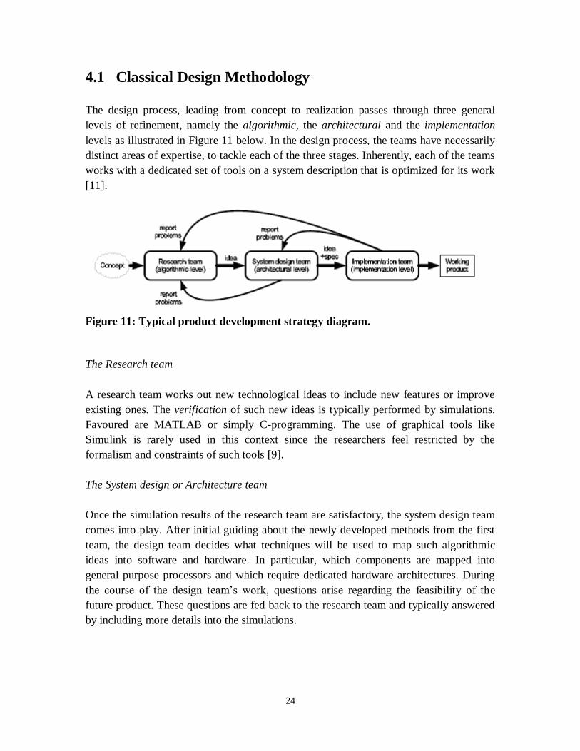
levels as illustrated in Figure 11 below. In the design process, the teams have necessarily

distinct areas of expertise, to tackle each of the three stages. Inherently, each of the teams

works with a dedicated set of tools on a system description that is optimized for its work

[11].

Figure 11: Typical product development strategy diagram.

The Research team

A research team works out new technological ideas to include new features or improve

existing ones. The verification of such new ideas is typically performed by simulations.

Favoured are MATLAB or simply C-programming. The use of graphical tools like

Simulink is rarely used in this context since the researchers feel restricted by the

formalism and constraints of such tools [9].

The System design or Architecture team

Once the simulation results of the research team are satisfactory, the system design team

comes into play. After initial guiding about the newly developed methods from the first

team, the design team decides what techniques will be used to map such algorithmic

ideas into software and hardware. In particular, which components are mapped into

general purpose processors and which require dedicated hardware architectures. During

the course of the design team‟s work, questions arise regarding the feasibility of the

future product. These questions are fed back to the research team and typically answered

by including more details into the simulations.

25

The Implementation team

The primary task of the implementation team is to build all required components from

outside vendors and to join them with existing parts; they have to make the product work.

The implementation team has knowledge of the specific tools that are required to

program DSPs, FPGAs and to design ASICs. They need to be taught the innovations of

the first team, supplemented by the implementation guidelines of the design team. Further

the algorithm implementation requires a permanent co-simulation of the actual

implementation code with the original high-level simulation. There is interaction between

the two teams and once the implementation team is confident of having a good reference

code, they can start building an ASIC or programming DSPs. From here on, co-

simulation for the purpose of verification is mostly what defines their work. Hence it is

most helpful when a design environment supports co-simulation [9].

4.2 Rapid prototyping

4.2.1 Motivation for Rapid prototyping

As described in the Classical design technique on the design flow that is used to realizing

the product; due to severe time constraints, prototypes are often skipped and it is mostly

the simulation results and experience from the previous product that is relied upon.

However the advantage of prototyping was to reduce the investment risk of the new

product in case the new technology would hide unforeseen challenges [7]. Also, one

often obtained a flavour of how the new technology needs to be realized and a feeling for

how the future product would look like. It could be used to present to the potential

customers or to work on potential features long before the final product was available.

Next-generation mobile technology keeps updating with such rapid pace, bringing added

pressure on the time to market. Since prototyping is cumbersome work, both the time and

cost factor, with the development of the prototype with all features as costly as the final

product itself. As a result telecommunication equipment companies often decide to focus

more on simulation and trust the expertise of their research team.

26

4.2.2 Key to Rapid prototyping

From the classical design approach, it can be seen that the section often exhibits

discontinuous phases. Typically, at the time when the design is handled from one team to

the next, an entire new set of tools, languages and formalisms is used and the previous

code not even used for reference purposes. Further when there is a problem in the code, a

team cannot return their design to the previous team as the current code is not backwards

compatible. Thus the classical approach is a feed-forward structure where the refined

product and corresponding responsibility is moved in one direction while necessary

expertise and information revealing discussions are only made possible by backward

loops.

To make a prototype rapidly could mean to bring out a partial set of features of the final

product in a rapid way if not the whole product. In this way only the technical parts that

are new to the implementation team are implemented.

Rapid prototyping is in a way similar to product design, requiring a team with almost the

same set of skills. The only difference being that fewer people are required with skill sets

mainly in electronic design.

The key essentials to make prototyping rapid (and possibly speed up production) can be

followed by the Five-Ones Approach [9]:

one environment

one automatic documentation by specification

one forward-backward compatible code revision tool

one code to be worked on by refinement steps

one team to improve communication

27

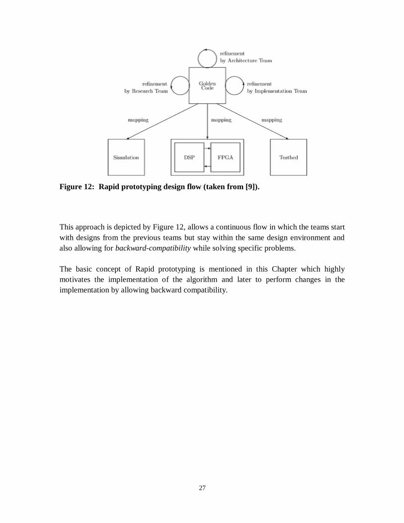
Figure 12: Rapid prototyping design flow (taken from [9]).

This approach is depicted by Figure 12, allows a continuous flow in which the teams start

with designs from the previous teams but stay within the same design environment and

also allowing for backward-compatibility while solving specific problems.

The basic concept of Rapid prototyping is mentioned in this Chapter which highly

motivates the implementation of the algorithm and later to perform changes in the

implementation by allowing backward compatibility.

28

CHAPTER 5

Implementation in high-level language

The implementation in high-level language tends to produce a less efficient code, but it is

still preferred over assembly language programming due to several advantages like:

It helps the developer or the developers to achieve structure and consistency.

Complex operations are often easier to describe in a high-level language.

High-level language development does not require very specialized skills or in-

depth knowledge of the target processor. Engineers who are not specialist can

readily undertake the development of the high-level language modules sharing the

workload of the few specialized engineers who are able to develop in assembly

language on a particular platform [18].

5.1 Challenges toward Algorithm Implementation

While designing next-generation communication systems with newer features, there is

stiff challenge in the development and integration of several computationally-intensive

algorithms towards enabling the new features. Designers are faced with two major

problems while designing these systems. First, block diagrams and equations compose

typical communication systems; however prototype hardware must be programmed in C

or assembly, an awkward and error prone means to implement block diagrams and

equations. Second, designers develop simulations which execute on a host, while other

engineers create hardware prototypes [13]. However, the host and prototype platforms

remain isolated from each other; the simulator‟s power cannot be combined with the real-

time constraints of the prototype.

In the design process, the designer must integrate algorithms into a communication

system executing on prototype hardware. Each algorithm, usually expressed as a set of

equations, must be tested to insure it operates as expected. The algorithm blocks in the

block diagram must be checked to verify that each block is properly connected and

29

operates correctly with its neighbouring blocks. Finally, the resulting block diagram of

the system must be translated into a program suitable for execution on the prototype

hardware.

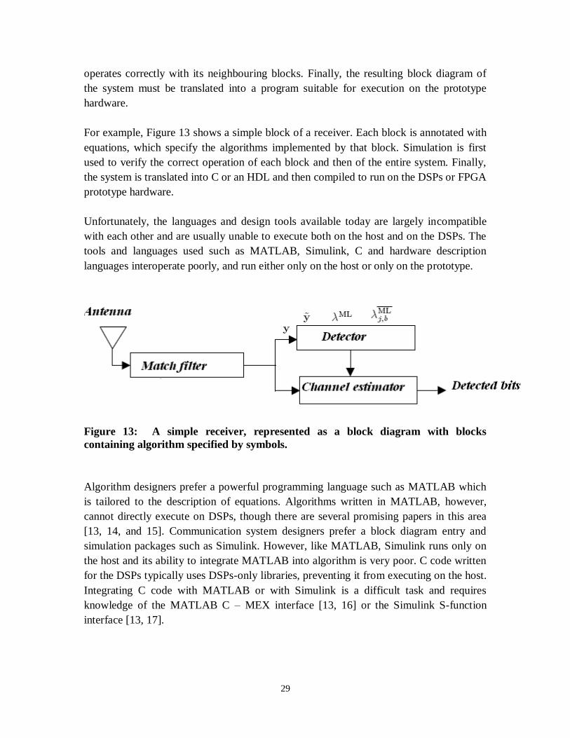
For example, Figure 13 shows a simple block of a receiver. Each block is annotated with

equations, which specify the algorithms implemented by that block. Simulation is first

used to verify the correct operation of each block and then of the entire system. Finally,

the system is translated into C or an HDL and then compiled to run on the DSPs or FPGA

prototype hardware.

Unfortunately, the languages and design tools available today are largely incompatible

with each other and are usually unable to execute both on the host and on the DSPs. The

tools and languages used such as MATLAB, Simulink, C and hardware description

languages interoperate poorly, and run either only on the host or only on the prototype.

Figure 13: A simple receiver, represented as a block diagram with blocks

containing algorithm specified by symbols.

Algorithm designers prefer a powerful programming language such as MATLAB which

is tailored to the description of equations. Algorithms written in MATLAB, however,

cannot directly execute on DSPs, though there are several promising papers in this area

[13, 14, and 15]. Communication system designers prefer a block diagram entry and

simulation packages such as Simulink. However, like MATLAB, Simulink runs only on

the host and its ability to integrate MATLAB into algorithm is very poor. C code written

for the DSPs typically uses DSPs-only libraries, preventing it from executing on the host.

Integrating C code with MATLAB or with Simulink is a difficult task and requires

knowledge of the MATLAB C – MEX interface [13, 16] or the Simulink S-function

interface [13, 17].

30

The monolingual and uni-location nature of today‟s languages and tools limits the

complexity of designs achievable. First, they restrict a designer to the use of only one

language for the entire design, though the use of an alternate language for parts of the

design is preferable. For example, a MIMO receiver designed in MATLAB implies that

all block diagrams must be expressed as text in MATLAB‟s programming language,

rather than representing the diagrams graphically. This text representation obscures the

block diagram structure of the system, which also hinders the compiler‟s ability to

understand and optimize the design. Second, today‟s languages and tools force the

designer to rewrite the entire design when moving between languages or locations.

Moving a system based on algorithms written in MATLAB from the host to a prototype

requires all MATLAB code to be rewritten in C. Finally, modern languages and tools

isolate the host-based simulation environment from the DSP-based execution

environment. Real-time data acquired by the prototype hardware cannot be easily passed

back to the host for analysis; likewise, simulated data generated on the host cannot be

processed on the prototype.

5.2 Implementation in MATLAB

MATLAB [8], a popular tool for DSP engineers, is an excellent candidate for designing

algorithms based on a set of equations. MATLAB‟s language allows these equations to

be easily entered in its text-based language. However, as a text-only language, it lacks the

ability to graphically represent block diagrams. In addition, it cannot yet produce efficient

code for execution on a hardware prototype. MATLAB‟s programming language

contains several features making it uniquely suited for algorithm design as illustrated in

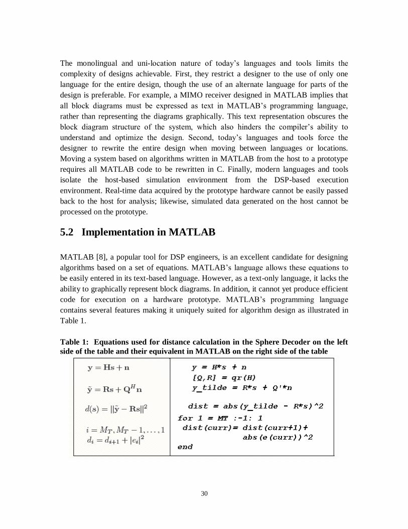
Table 1.

Table 1: Equations used for distance calculation in the Sphere Decoder on the left

side of the table and their equivalent in MATLAB on the right side of the table

31

Most importantly, MATLAB allows the user to easily enter complex equations, by

defining common arithmetic operators such as addition and multiplication for scalars,

vectors and matrices over both real and complex numbers. In addition, MATLAB

supports a wide range of toolboxes for standard signal processing operations. Its powerful

language and flexible plotting features allow the user to quickly develop and debug new

algorithms.

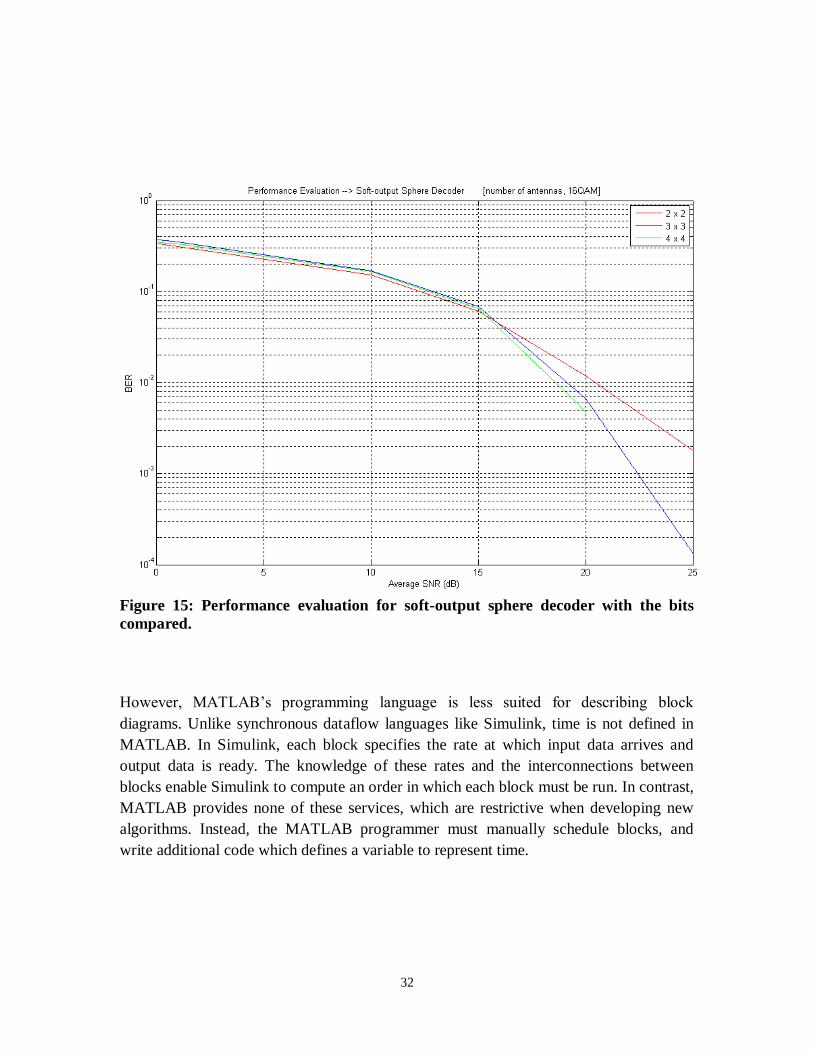
The Sphere decoder was implemented in MATLAB – both the hard and soft output was

evaluated for performance. Figure 14 below evaluates the performance for a soft output

sphere decoder for symbols compared with 16 QAM and 4 Bits per symbol. The plot

shows the Bit Error Ratio (BER) with Average Signal to Noise Ratio (SNR) in dB for

different antenna configurations. Also the performance is evaluated with bits compared

for the same parameters are shown in Figure 15. In both cases it can be seen that at lower

SNR different antenna configurations show similar BER till around 15 dB. As the SNR

increases further, the higher antenna configuration start to give reduced BER.

Figure 14: Performance evaluation for soft-output sphere decoder with symbols

compared.

32

Figure 15: Performance evaluation for soft-output sphere decoder with the bits

compared.

However, MATLAB‟s programming language is less suited for describing block

diagrams. Unlike synchronous dataflow languages like Simulink, time is not defined in

MATLAB. In Simulink, each block specifies the rate at which input data arrives and

output data is ready. The knowledge of these rates and the interconnections between

blocks enable Simulink to compute an order in which each block must be run. In contrast,

MATLAB provides none of these services, which are restrictive when developing new

algorithms. Instead, the MATLAB programmer must manually schedule blocks, and

write additional code which defines a variable to represent time.

33

Summary

Implementing an entire communication system using traditional design methodology

suffers from segregation. An idea captured as a rough sketch of a block diagram, with

equations noted beside each block, cannot be entered into a computer; the block diagram

tool is incompatible with the equation tool. When debugging the system, particularly on

embedded hardware, the best analysis and debug tools available on the host must be

abandoned for less usable hardware-specific tools designed for the embedded hardware.

Rapid prototyping methodology helps tackle these problems by unifying these classes of

tools, providing both block diagram design and equation entry in the same environment.

It provides an easy path to migrate from equations coded in MATLAB, which cannot be

executed on most embedded hardware platforms, to equations written in C or C++,

languages which are supported by most embedded hardware platforms. With each block

coded in C, a C program can then be generated and compiled on the embedded hardware.

It also enables a development environment that runs partly on the host, with its improved

analysis and debug tools, and partly on the embedded hardware.

In this way, the communication system can be build by following the Rapid prototyping

methodology. The Sphere Decoder is a part of the MIMO-OFDM WIMAX Receiver that

is being implemented using Simulink. This thesis work is restricted to the implementation

of the Sphere Decoder by Rapid prototyping methodology. First the sphere decoder is

implemented in MATLAB and then verified with a C implementation.

34

5.3 Implementation in ‘C’

When it comes to implementation for embedded applications, the high-level language of

choice is C and recently C++. It is usually advantageous to write the higher hierarchical

levels of the software applications in C or C++ because it is often the place where the

most complexity is found, and at the same time it often represents the less critical

portions of the code.

.

The C programming language produces the highest-performance executables on DSPs.

Most modern DSPs provide compilers with excellent support for the C programming

language. Also it is almost always necessary to develop some modules of code directly in

assembly language. Generally the following factors contribute to the development of

code in assembly language:

The C standard is not well defined for many functions that are important in

numerical computation and signal processing applications. For instance the

overflow behaviour during an integer addition (saturation or rollover) is not

defined in the C standard. For certain combinations of compiler and CPU, the

behaviour may even change with the context of execution during the same

application.

A code developed in C or C++ is almost always less efficient than the same code

[well] developed in assembly language.

The developer normally chooses to write the code in a high-level language to

avoid being concerned with the low-level implementation of the code. High-level

languages therefore do not give the developer access to low-level functions of the

CPU or its ALU. However, it is precisely by getting access to these low-level

functions that the developer is usually able to optimize the efficiency of the code.

A C or C++ compiler does not have as much information as the developer about

the process that has to be implemented. Many details of the process simply cannot

be specified in C or C++. For instance when performing a floating point division,

the C standard requires that the divisor be tested for zero. In a particular

application, the developer may know that a certain divisor can never be zero and

be able to skip the test. Usually a C or C++ compiler chooses general solutions

that are applicable in a wide range of conditions, rather than specialized solutions

that are often the most efficient ones [18].

35

While writing in assembly language produces the most efficient executables, C compilers

provide most of the efficiency necessary for prototyping while significantly reducing the

development time spent on implementing a given algorithm. However, unlike MATLAB,

the C language poorly supports equation entry, with complex operations involving

matrix-vector products, addition and transposition quite difficult to develop and debug.

The Sphere decoder algorithm is rewritten in C and performance is compared with that of

MATLAB in terms of time taken for computation. The C generated code can be turned

into a compiled MEX file to be called from MATLAB. Using MATLAB C-MEX

interface, the complex operations involving transposition etc was done in MATLAB and

passed on to MEX file. This MEX wrapper function helps exchange data between

MATLAB and C. The result after computation was put back into MATLAB that has a

good interface to plot the result.

As the MEX file is already compiled they are quite fast and similar to any other function

called in MATLAB. But the disadvantage lies in the process of writing the MEX file

which is quite time consuming and error prone. The memory allocation in C being

sensitive, the MEX wrapper has to allocate and access the data properly which otherwise

would lead to crashes, segmentation violation or incorrect results.

The distinct advantage is the verification of the algorithm in C with a faster execution

time. This is due to the MATLAB interpreter having unnecessary memory allocation

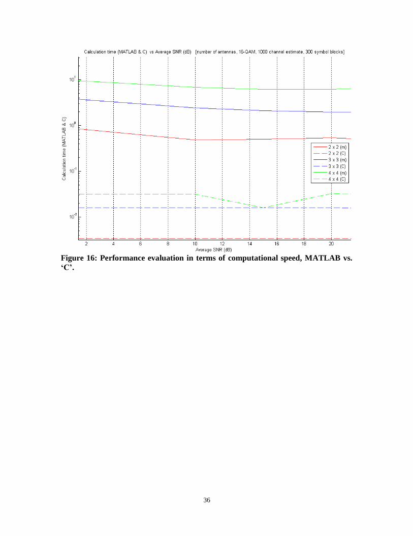
overhead when compared to the faster C compiled executables. The Figure 16 shows the

Calculation time for the algorithm in both MATLAB and C with the Average SNR in dB.

This was obtained using different antenna configurations, by averaging over 1000

channel realizations, 16 QAM and with 300 symbol blocks. As evident from Figure 16, C

implementation gives a much better performance in terms of computation speed as

compared to MATLAB.

36

Figure 16: Performance evaluation in terms of computational speed, MATLAB vs.

‘C’.

37

CHAPTER 6

Implementation on Digital Signal Processor

To further investigate the performance of the algorithm as part of a WiMAX Receiver for

MIMO systems, the verification of the algorithm on the target platform is the next step.

The target platform includes technologies such as ASICs, FPGAs, general purpose

processors and DSPs. Higher performance implementations of specific DSP algorithms

are increasingly available through implementation within FPGA.

6.1 Background

In a Software Defined Radio (SDR), functions that were formerly carried out solely in

hardware, such as the generation of the transmitted signal and tuning and detection of

received radio signals, are performed by software that controls high-speed signal

processors. With the advent of SDR in wireless segments, the usefulness of Field

programmable logic (FPGAs) as reprogrammable DSP, has led to SDR taking on

increased importance. In traditional software radio systems, the translated and filtered

baseband signal is sent into the DSP as a stream of complex samples of a time-domain

waveform. The DSP must handle all the demodulation tasks as well as higher-level

decisions based on the analysis of the signals being received. In a cell phone base station,

the number of DSP tasks grows with each new communication standard. The

proliferation of sophisticated digital voice and data protocols require decoding,

convolution, framing, error correction and vocoding.

While MIMO combined with OFDM is considered a key to achieve better throughput

which involves use of complex signal processing techniques, this comes at the cost of

added hardware. These enabling technologies pose significant challenges for OEMs

needing to design basestations that are not only scalable and cost-effective but also

flexible and re-usable across multiple evolving standards. Wireless system designers need

to meet a number of critical requirements which includes processing speed, flexibility

and time-to-market. These stringent requirements ultimately drive the hardware platform

choice. Some of the major challenges include:

Processing Bandwidth: To support WiMAX systems providing high data rates,

the underlying hardware platform must have significant processing bandwidth.

Additionally, several advanced signal processing techniques such as Turbo

38

coding/decoding and front-end functions including fast Fourier transform/inverse

fast Fourier transform (FFT/IFFT), beamforming, MIMO, crest factor reduction

(CFR) and digital predistortion (DPD) are computationally intensive and require

several billion multiply and accumulate (MAC) operations per second.

Flexibility: As WiMAX and other mobile broadband technologies such as Long

Term Evolution (LTE) specifications are being defined and standardised , and still

going through numerous revisions before being finalized; there is need to have

flexibility and re-programmability in the end product to provide for a standards-

agnostic or multi-protocol basestation.

Cost-reduction path: While WiMAX and LTE standards are expected to stabilize,

this will likely lead to a situation where cost of the final product will be more

important than flexibility for OEMs and service providers, to remain competitive

in the marketplace. Choosing the right hardware platform for prototyping would

provide seamless cost-reduction in engineering segment that would otherwise

require system re-design [19].

Thus potential advantages to implementing a DSP function within an FPGA include:

Performance Improvements

Design Implementation Flexibility

System Level Integration

Reduced Cost and Schedule

6.1.1 Partitioning between FPGA and DSP

Signal-processing data path and control operations make up the bulk of the processing

load in a wireless basestation. Most architectures implement the system control,

configuration and the signal processing data path using a combination of microcontrollers

(MCUs), FPGAs and programmable DSPs. The MCUs control the system, while the

FPGA and DSP handle the data-flow processing. Systems with light processing demands

and control-oriented tasks are implemented in software on a DSP; heavier loads are best

implemented in FPGAs that provide significant parallel processing benefits. The

combination of DSPs and FPGAs ensures complete flexibility and offers

reprogrammability to fix bugs or even support new standard. The exact partitioning

between FPGAs and DSPs depends on the processing requirements; system bandwidth as

well as system configuration; and the number of transmit and receive antennas [19].

39

Since the receiver block would require huge amount of bit level manipulations at a fairly

high rate, general purpose DSPs are very inefficient to implement those. FPGAs offer the

right amount of flexibility at the cost of higher turnaround times for algorithmic

modifications. On the other hand DSPs are very well suited for mul/add operations on

irregular code as it is common especially for decoder algorithms that rely on matrix

inversions. Hence it was decided to implement the decoder algorithm on DSPs.

6.2 Digital Signal Processors

6.2.1 Introduction

DSPs are specialized microprocessors designed specifically for digital signal processing,

generally in real-time computing. It is a special purpose CPU (Central Processing Unit)

that provides ultra-fast instruction sequences, such as shift and add, and multiply and add,

which are commonly used in math-intensive signal processing applications. They are

used for a wide range of applications, from communications and control to speech and

image processing. They have become the product of choice for various consumer

applications as cellular phones, modems, fax machines, sound cards, high capacity hard

disks, digital TVs.

DSPs are concerned primarily with real-time signal processing. Real-time processing

means that the processing must keep pace with some external event; whereas non-real

time processing has no such timing constraint. The external event to keep pace with is

usually the analog input. The basic DSP system would consist of an analog-to-digital

converter (ADC) to capture an input signal. The resulting digital representation of the

captured signal is then processed by DSPs and then output through a digital-to-analog

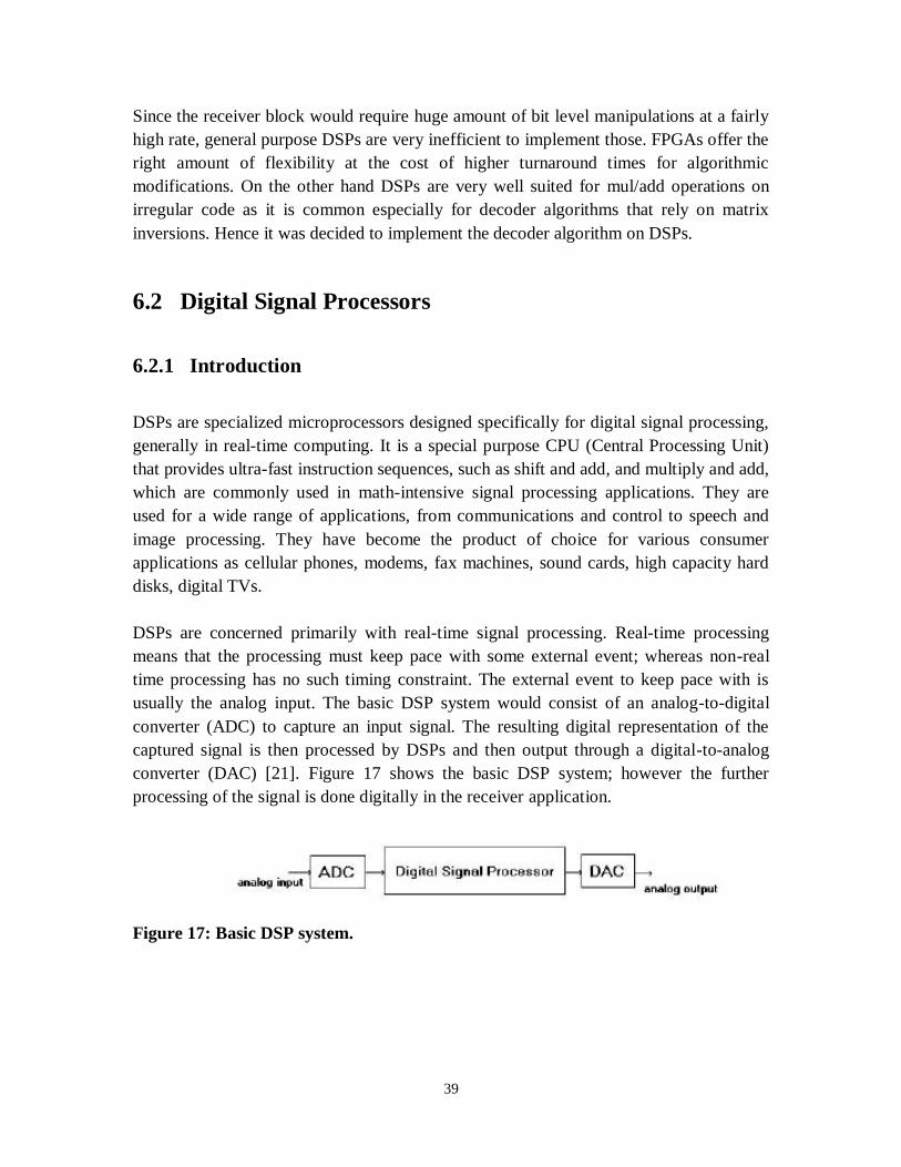
converter (DAC) [21]. Figure 17 shows the basic DSP system; however the further

processing of the signal is done digitally in the receiver application.

Figure 17: Basic DSP system.

40

TMS320C6000 Platform of DSPs

The TMS320C6000 family of processors from the company Texas Instruments (TI) is

designed to meet the real-time requirements of high performance DSP. With a

performance of up to 2000 million instructions per second (MIPS) at 250 MHz and a

complete set of development tools, the TMS320C6000 DSPs offer cost effective

solutions to higher-performance DSP programming challenges [23].

The TMS320 family consists of 16-bit and 32-bit fixed and floating-point devices. These

DSPs possess the operational flexibility of high-speed controllers and the numerical

capacity of array processors. The TMS320 family consists of three supported platforms

including the TMS320C2000, TMS320C5000 and TMS320C6000. Within the C6000

platform there are two generations, the TMS320C62x and TMS302C67x. The C62x

processors are fixed-point processors whereas the C67x are floating-point processors.

These refer to the format used to store and manipulate numbers within the device. The

architecture of C6x DSPs is very well suited for numerically intensive calculations.

Based on a very-long-instruction word (VLIW) architecture, the C6x is considered to be

TI‟s most powerful processor [20].

Each generation of TMS320 devices uses a core Central Processing Unit (CPU) that is

combined with a variety of on-chip memory and peripheral configurations. When

memory and peripherals are integrated with a CPU into one chip, the overall system cost

is greatly reduced, and circuit board space is reduced.

TMS320C6713 DSP

The TMS320C67 DSPs (including the TMS320C713) compose the floating-point DSPs

generation in TMS320C6000 DSP platform. The TMS320C6713 is based on the high-

performance, advanced VelociTI VLIW architecture developed by TI, making this an

excellent choice for multichannel and multifunction applications [23].

It has operational frequency of 225 MHz, and is thus capable to execute up to 1800 MIPS

and 1350 million floating-point operations per second (MFLOPS) on a 32-bit word

length. It has two sets of 32 general-purpose registers and eight independent functional

units capable to fetch up to eight instructions every cycle. These eight functional units are

composed of six arithmetic-logic units (ALUs) and of two multiplier units. Other features

include Real Time Data Exchange (RTDX) capability and Embedded JTAG support via

USB. Software designers can readily target the TMS320C6713 DSPs through TI‟s robust

and comprehensive Code Composer Studio (CCS) development platform.

41

6.2.2 Development Tools

Code Composer Studio

The CCS provides an integrated development environment (IDE) to incorporate the

software tools. CCS includes tools for code generation, such as a C compiler, an

assembler, and a linker. Once the generated machine code is loaded and run on the target,

the IDE also offers some analysis tools with graphical capabilities to visualize processes

running on the DSPs. CCS extends the basic code generation tools with a set of

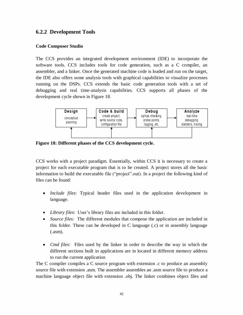
debugging and real time-analysis capabilities. CCS supports all phases of the

development cycle shown in Figure 18.

Figure 18: Different phases of the CCS development cycle.

CCS works with a project paradigm. Essentially, within CCS it is necessary to create a

project for each executable program that is to be created. A project stores all the basic

information to build the executable file (“project”.out). In a project the following kind of

files can be found:

Include files: Typical header files used in the application development in

language.

Library files: User‟s library files are included in this folder.

Source files: The different modules that compose the application are included in

this folder. These can be developed in C language (.c) or in assembly language

(.asm).

Cmd files: Files used by the linker in order to describe the way in which the

different sections built in applications are in located in different memory address

to run the current application

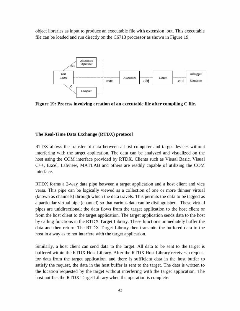
The C compiler compiles a C source program with extension .c to produce an assembly

source file with extension .asm. The assembler assembles an .asm source file to produce a

machine language object file with extension .obj. The linker combines object files and

42

object libraries as input to produce an executable file with extension .out. This executable

file can be loaded and run directly on the C6713 processor as shown in Figure 19.

Figure 19: Process involving creation of an executable file after compiling C file.

The Real-Time Data Exchange (RTDX) protocol

RTDX allows the transfer of data between a host computer and target devices without

interfering with the target application. The data can be analyzed and visualized on the

host using the COM interface provided by RTDX. Clients such as Visual Basic, Visual

C++, Excel, Labview, MATLAB and others are readily capable of utilizing the COM

interface.

RTDX forms a 2-way data pipe between a target application and a host client and vice

versa. This pipe can be logically viewed as a collection of one or more thinner virtual

(known as channels) through which the data travels. This permits the data to be tagged as

a particular virtual pipe (channel) so that various data can be distinguished. These virtual

pipes are unidirectional; the data flows from the target application to the host client or

from the host client to the target application. The target application sends data to the host

by calling functions in the RTDX Target Library. These functions immediately buffer the

data and then return. The RTDX Target Library then transmits the buffered data to the

host in a way as to not interfere with the target application.

Similarly, a host client can send data to the target. All data to be sent to the target is

buffered within the RTDX Host Library. After the RTDX Host Library receives a request

for data from the target application, and there is sufficient data in the host buffer to

satisfy the request, the data in the host buffer is sent to the target. The data is written to

the location requested by the target without interfering with the target application. The

host notifies the RTDX Target Library when the operation is complete.

43

Link for CCS Development Tools

This supports verification, debugging, visualization and validation of the application

running on TI DSPs by establishing real-time bidirectional data transfer links among

MATLAB, CCS and TI DSPs hardware. Links are established via RTDX which allows

transfer of data to and from DSPs without halting the running application. This tool

provides automation of CCS behaviour and full computational and visualization

capabilities of MATLAB can be used on real-time data.

Thus using links for RTDX it is possible to:

Send and retrieve data from memory on the processor.

Change the operating characteristics of the program.

Make changes to the algorithm as needed without stopping the program or setting

break points in the code.

These tools help ease the job of taking algorithms from the model realm to the real world

of the target DSPs on which the algorithm will run.

The next step in the thesis was to port the C implementation of the sphere decoder onto

the simulation TI board provided by CCS and by using RTDX link to evaluate

performance in MATLAB.

The following RTDX commands were tried using the CCS link in MATLAB to configure

the settings:

Create an RTDX link to the desired target and load the program to the processor.

Construct the link to the target board and processor using the command,

cc = ccsdsp('boardnum',0) where boardnum defines which board the link

accesses while „0’ connects the link to the first processor on the board.

Configure channels to communicate with the target.

The task is to open as many channels as required to support data transfer for the

development work and also to configure channel buffers to hold data when the

data rate from the target exceeds the rate at which MATLAB can capture the data.

44

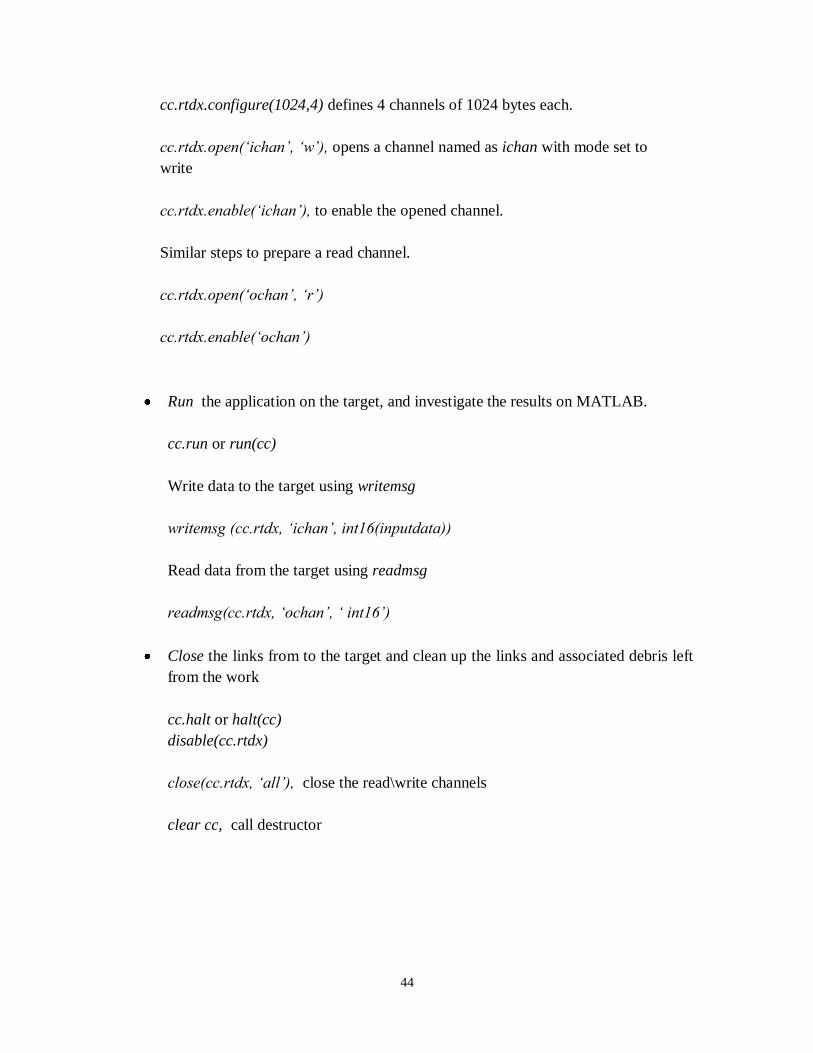
cc.rtdx.configure(1024,4) defines 4 channels of 1024 bytes each.

cc.rtdx.open(‘ichan’, ‘w’), opens a channel named as ichan with mode set to

write

cc.rtdx.enable(‘ichan’), to enable the opened channel.

Similar steps to prepare a read channel.

cc.rtdx.open(‘ochan’, ‘r’)

cc.rtdx.enable(‘ochan’)

Run the application on the target, and investigate the results on MATLAB.

cc.run or run(cc)

Write data to the target using writemsg

writemsg (cc.rtdx, ‘ichan’, int16(inputdata))

Read data from the target using readmsg

readmsg(cc.rtdx, ‘ochan’, ‘ int16’)

Close the links from to the target and clean up the links and associated debris left

from the work

cc.halt or halt(cc)

disable(cc.rtdx)

close(cc.rtdx, ‘all’), close the read\write channels

clear cc, call destructor

45

6.2.3 Fixed point Issues

To go further with the implementation in MATLAB and C to be ported onto the DSP, the

need arises for fixed point implementation. The study requires more time and that brings

my thesis study to a conclusion with the results obtained.

46

CHAPTER 7

Conclusion

This thesis gives an insight into MIMO systems and the implementation of the soft output

sphere decoder. Initially the performance of a hard output sphere decoder was done in

MATLAB and later compared with the soft output decoder for various antenna

configurations such as 2x2 systems etc. The hard output was found to give uncoded bits

at lower complexity for higher antenna system compared to a soft output which was more

accurate in the form of LLR at the cost of higher complexity.

The soft output sphere decoder algorithm was implemented in MATLAB and later the

performance evaluated by implementing in C. MATLAB was found to be the ideal tool

for such implementation that required complex mathematical operations such as

transposition etc. Using the MATLAB C-mex interface the complex mathematical

operation was done in MATLAB and passed on to mex file. The C implementation

proved to be efficient in terms of computational time for higher antenna configuration.

It was decided to implement further onto a DSP and to use the RTDX protocol for the

data transfer. However the implementation required the use of fixed point computation

unlike MATLAB that has floating point. The fixed point implementation requires further

investigation and due to lack of time the thesis was concluded with the above results.

However the fixed point implementation and later the performance evaluation of the

algorithm on a DSP would be an interesting future work.

47

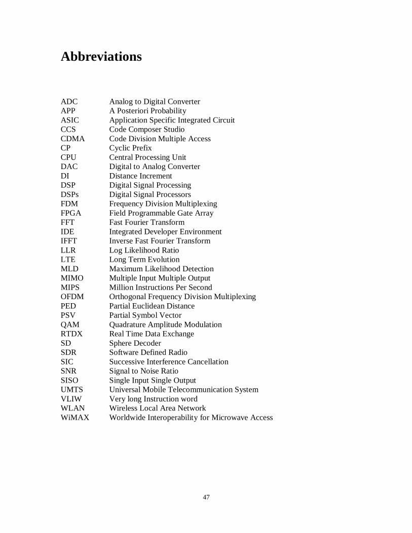
Abbreviations

ADC Analog to Digital Converter

APP A Posteriori Probability

ASIC Application Specific Integrated Circuit

CCS Code Composer Studio

CDMA Code Division Multiple Access

CP Cyclic Prefix

CPU Central Processing Unit

DAC Digital to Analog Converter

DI Distance Increment

DSP Digital Signal Processing

DSPs Digital Signal Processors

FDM Frequency Division Multiplexing

FPGA Field Programmable Gate Array

FFT Fast Fourier Transform

IDE Integrated Developer Environment

IFFT Inverse Fast Fourier Transform

LLR Log Likelihood Ratio

LTE Long Term Evolution

MLD Maximum Likelihood Detection

MIMO Multiple Input Multiple Output

MIPS Million Instructions Per Second

OFDM Orthogonal Frequency Division Multiplexing

PED Partial Euclidean Distance

PSV Partial Symbol Vector

QAM Quadrature Amplitude Modulation

RTDX Real Time Data Exchange

SD Sphere Decoder

SDR Software Defined Radio

SIC Successive Interference Cancellation

SNR Signal to Noise Ratio

SISO Single Input Single Output

UMTS Universal Mobile Telecommunication System

VLIW Very long Instruction word

WLAN Wireless Local Area Network

WiMAX Worldwide Interoperability for Microwave Access

48

Bibliography

[1] C. Studer, M. Wenk, A. Burg, and H. Bölcskei : "Soft-Output Sphere Decoding:

Performance and Implementation Aspects", ASSC ’06 Fortieth Asilomar

Conference on Signals, Systems and Computers, 2006

[2] C. Studer, M. Wenk, A. Burg, and H. Bölcskei: "Soft-Output Sphere Decoding:

Algorithms and VLSI Implementation", IEEE Journal on Selected Areas in

Communication, Vol 26, No:2, pp290-300.

[3] Helmut Bölcskei : "Principles of MIMO-OFDM Wireless Systems", Chapter in

CRC Handbook on Signal Processing for Communications, M. Ibnkahla, Ed.,

2004

[4] H. Bölcskei, D. Gesbert, and A. J. Paulraj: "On the capacity of OFDM-based

spatial multiplexing systems" , IEEE Trans. Commun., vol. 50, no. 2, pp. 225-

234, Feb. 2002.

[5] Amalia ROCA: "Implementation of a WIMAX simulator in Simulink",

MasterThesis at Institut für Nachrichtentechnik und Hochfrequenztechnik, 2007

[6] Shi Chen: "The Sphere Decoding Algorithm Applied to Space-Time Block

Codes", Master Thesis at Department of Signals, Sensors and Systems, KTH,

Sweden,2004

[7] Sebastian Caban, Christian Mehlfuehrer, Robert Langwieser, Arpad L.Scholtz,

and Markus Rupp: "Vienna MIMO Testbed", EURASIP Journal on Applied

Signal Processing, Vol 2006, No 1, pp. 142, 2006

[8] The MathWorks,MATLAB,http://www.mathworks.com/.

[9] M. Rupp, A. Burg, and E. Beck: “Rapid prototyping for wireless designs: the

five-ones approach,” Signal Processing, vol. 83, no. 7, pp. 1427–1444, 2003.

[10] Zoran Salcic: "Prototyping Embedded DSP Systems – From Specification to

Implementation", Department of Electrical and Computer Engineering,

University of Auckland,in Proceedings of European Signal Processing

conference, Vienna, 2004

[11] P. Belanovic, M. Holzer, D. Micusik and M. Rupp: "Design Methodology of

Signal Processing Algorithms in Wireless Systems", in Proceedings of

International Conference on Computer, Communication and Control

Technologies, 2003

49

[12] A. Burg, B. Haller, E. Beck, M. Guillaud, M. Rupp, L. Mailaender: "A Rapid

Prototyping Methodology for Algorithm Development in Wireless

Communications" in Proceedings of Design, Automation and Test in Europe,

2001

[13] Bryan A. Jones: "Rapid Prototyping of Wireless Communications Systems",

Master Thesis at Department of Electrical and Computer Engineering, Rice

University, 2002

[14] P. Banerjee, N. Shenoy, A. Choudhary, S. Hauck, M. Haldar, P. Joisha, A.

Jones, A. Kanhare, A. Nayak, S. Periyacheri, M. Walkden, and D. Zaretsky, "A

MATLAB compiler for distributed heterogeneous recongurable computing

systems,"; in IEEE Symposium on FPGA Custom Computing Machine (FCCM-

2000), (Napa Valley, CA), pp. 39-48, April 2000.

[15] L. DeRose, K. Gallivan, E. Gallopoulos, B. Marsolf, and D. Padua,

"FALCON: An environment for the development of scientic libraries and

applications," in Proceedings of the First International Workshop on

Knowledge-Based System for the (re)Use of Program Libraries (KBUP),

(Sophia Antipolis, France), November 1995.

[16] The MathWorks, Inc., Natick, MA, Application Program Interface Reference,

June 2001. Revised for MATLAB 6.1 (Release 12.1).

[17] The MathWorks, Inc., Natick, MA, Writing S-Functions, June 2001. Revised

for Simulink 4.1 (Release 12.1).

[18] Bruno Paillard : "An Introduction to Digital Signal Processors"

[19] Deepak Boppana: "How to combine FPGAs and DSPs to get the best base station

performance", Altera Corp.

[20] TMS320C6000 Technical Brief, Texas Instruments

[21] Rulph Chassaing : "DSP Applications using C and the TMS320C6x DSK"

[22] Fan Liang, “The challenges of testing MIMO”, Demystifying Physical layer Issues

with MIMO

http://mobiledevdesign.com/hardware_news/radio_challenges_testing_mimo/

[23] Luis Zarzo Fuertes, “OFDM PHY Layer Implementation based on the 802.11 a

Standard and system performance analysis”, Bachelor Thesis in Electronic Systems

at Linkoping University, 2005