Implementation of a Fuzzy Logic Based Set-Point ... - MSpace

Implementation of a Fuzzy Logic Based Set-Point

Modulation Scheme with SVC System Applications

By:

Steven Lawrence Howell

A thesis submitted to the Faculty of Graduate Studies of

The University of Manitoba

in partial fulfillment of the requirements for the degree of:

Master of Science

Department of Electrical and Computer Engineering

University of Manitoba

Winnipeg, Manitoba

© Copyright by Steven Lawrence Howell, 2013

ii

Acknowledgements

I would like to express my sincere gratitude to Dr. Shaahin Filizadeh for his guidance and

support throughout the completion of my research. It was a privilege to work under his

supervision.

I wish to thank Dr. David Jacobson and Mr. Pei Wang from Manitoba Hydro and Dan

Kell from TransGrid Solutions (TGS) for their guidance and knowledge regarding the

Ponton SVC system.

I would also like to thank the academic and technical staff of the Electrical and Computer

Engineering department, and specifically Mr. Erwin Dirks and Dr. Aniruddha Gole, for

their help and technical discussions.

iii

Dedication

To my family and friends for their support.

iv

Abstract

This thesis introduces a novel online set-point modulation (SPM) technique that

employs fuzzy logic to adjust the timing and magnitude of control system set-points.

After first applying fuzzy logic-enabled SPM to underdamped second order systems for

testing purposes, the new scheme is then applied to an electromagnetic transient

simulation model of Manitoba Hydro’s existing Ponton SVC system, and the results are

then compared to the original SVC system that uses traditional control approaches.

Conclusions show that fuzzy logic-based SPM improves the controlled voltage’s transient

overshoot response to changes in the voltage set-point.

v

Table of Contents

Acknowledgements ............................................................................................................. ii

Dedication .......................................................................................................................... iii

Abstract .............................................................................................................................. iv

Table of Contents ................................................................................................................ v

List of Figures ................................................................................................................... vii

List of Tables ...................................................................................................................... x

List of Symbols .................................................................................................................. xi

Chapter 1 Introduction ................................................................................................... 1

1.1 Objectives of Reactive Power Compensation ...................................................... 6

1.2 Controller Tuning for Reactive Power Compensators ......................................... 7

1.3 Problem Definition ............................................................................................. 10

1.4 Motivation for Research ..................................................................................... 11

1.5 Thesis Organization ............................................................................................ 11

Chapter 2 Reactive Power and Static Var Compensators ............................................ 13

2.1 SVC Apparatus ................................................................................................... 17

2.1.1 Anti-parallel Thyristor Pair ......................................................................... 17

2.1.2 Thyristor Controlled Reactor ...................................................................... 20

2.1.3 Fixed Capacitor-Thyristor Controlled Reactor (FC-TCR) ......................... 27

2.1.4 Thyristor Switched Capacitor (TSC) .......................................................... 30

2.1.5 Thyristor Switched Capacitor-Thyristor Controlled Reactor (TSC-TCR) . 39

2.1.6 Practical Considerations .............................................................................. 41

2.2 SVC Control System .......................................................................................... 42

2.2.1 Measurement System .................................................................................. 42

2.2.2 Synchronization System.............................................................................. 43

2.2.3 Voltage Regulator ....................................................................................... 44

2.2.4 Gate-Pulse Generator .................................................................................. 45

Chapter 3 Fuzzy Logic ................................................................................................ 47

3.1 Fundamental of Fuzzy Logic .............................................................................. 48

3.1.1 Membership Functions................................................................................ 48

3.1.2 Fuzzy Operators .......................................................................................... 50

3.1.2.1 Intersection .......................................................................................... 51

3.1.2.2 Union ................................................................................................... 53

vi

3.1.2.3 Complement ........................................................................................ 55

3.1.2.4 Implication ........................................................................................... 56

3.2 Fuzzy Inference Systems .................................................................................... 60

3.2.1 Step One: Fuzzification............................................................................... 62

3.2.2 Step Two: Application of Fuzzy Operators ................................................ 64

3.2.3 Step Three: Implication ............................................................................... 66

3.2.4 Step Four: Aggregation ............................................................................... 68

3.2.5 Step 5: Defuzzification ............................................................................... 70

Chapter 4 Set-Point Modulation .................................................................................. 72

4.1 Feedforward Posicast Control ............................................................................ 73

4.2 Feedback Posicast Control ................................................................................. 82

4.3 Set-Point Automatic Adjustment (SPAA).......................................................... 85

4.4 Set-Point Automatic Adjustment-Correction Enabled (SPAACE) .................... 90

4.5 Set-Point Modulation with Fuzzy Logic ............................................................ 95

Chapter 5 Application of Fuzzy SPM to the Ponton SVC System ............................ 103

5.1 Ponton SVC ...................................................................................................... 103

5.2 Application of Fuzzy SPM to Ponton SVC Voltage Regulator ....................... 104

5.2.1 System Characteristic ................................................................................ 105

5.2.2 Initial Attempt ........................................................................................... 109

5.2.3 Membership Function Tuning................................................................... 110

5.2.4 Modifying Fuzzy Inference System .......................................................... 114

5.2.5 Results ....................................................................................................... 116

Chapter 6 Conclusion and Recommendations ........................................................... 119

6.1 Contributions and Conclusions ........................................................................ 119

6.2 Future Work ..................................................................................................... 120

References ....................................................................................................................... 122

vii

List of Figures

Figure 1.1: Transmission system without reactive power compensation ........................... 2 Figure 1.2: Series and shunt compensated transmission line configurations ...................... 4 Figure 1.3: Load compensation configuration .................................................................... 5 Figure 1.4: System with both transmission line and load compensation ............................ 6 Figure 1.5: Block diagram of an SVC voltage controller ................................................... 7 Figure 1.6: Model-based controller tuning ......................................................................... 8 Figure 1.7: Simulation-based controller tuning .................................................................. 9 Figure 1.8: Set-point modulation diagram ........................................................................ 10 Figure 1.9: Different types of SPM ................................................................................... 11 Figure 2.1: Three phase voltage waveforms ..................................................................... 13 Figure 2.2: Apparent power triangle ................................................................................. 14 Figure 2.3: Apparent power triangle illustrating power factor correction ........................ 15 Figure 2.4: Anti-parallel thyristor and associated waveforms .......................................... 18 Figure 2.5: Voltage produced by anti-parallel thyristor pair for different thyristor firing angles ................................................................................................................................ 19 Figure 2.6: Single-phase TCR schematic and associated waveforms ............................... 20 Figure 2.7: TCR current waveforms with varying firing angles ....................................... 22 Figure 2.8: TCR reactive power vs. firing angle .............................................................. 24 Figure 2.9: TCR's V-Q characteristic ............................................................................... 25 Figure 2.10: TCR harmonics as a percent of TCR fundamental current magnitude ........ 26 Figure 2.11: TCR fundamental current and total harmonic current .................................. 27 Figure 2.12: Single-phase fixed capacitor TCR (FC-TCR) .............................................. 28 Figure 2.13: Single-phase FC-TCR's V-Q characteristic .................................................. 29 Figure 2.14: Single-phase FC-TCR with multiple fixed capacitors ................................. 30 Figure 2.15: V-Q characteristic for FC-TCR with multiple fixed capacitors ................... 30 Figure 2.16: Single-phase TSC ......................................................................................... 31 Figure 2.17: Magnification factor as a function of r ......................................................... 34 Figure 2.18: TSC voltage waveform ................................................................................. 37 Figure 2.19: Effect of capacitor size on a single-phase TSC V-Q characteristic ............. 37 Figure 2.20: Multiple TSCs .............................................................................................. 38 Figure 2.21: V-Q characteristic of k single-phase TSCs................................................... 39 Figure 2.22: TSC-TCR...................................................................................................... 40 Figure 2.23: V-Q characteristic for a TCR multiple TSC arrangement ............................ 41 Figure 2.24: A typical SVC control block diagram .......................................................... 42 Figure 2.25: PLL model for SVC controller ..................................................................... 43 Figure 2.26: SVC V-Q characteristic with droop ............................................................. 45 Figure 2.27: Gate-Pulse Generator Flowchart .................................................................. 46 Figure 3.1: A comparison of traditional set theory and fuzzy set theory .......................... 48 Figure 3.2: A possible membership function for fast speeds ............................................ 49 Figure 3.3: Membership function for determining fast speed ........................................... 50 Figure 3.4: Illustrative sets ................................................................................................ 51 Figure 3.5: Venn diagram of the intersection of two sets in traditional set theory ........... 51 Figure 3.6: Venn diagram of the union of two sets in traditional set theory .................... 53 Figure 3.7: Venn diagram of the complement of a set in traditional set theory ............... 55

viii

Figure 3.8: Single premise fuzzy if-then rule ................................................................... 58 Figure 3.9: Multiple premise fuzzy if-then rule ................................................................ 59 Figure 3.10: Multiple premise fuzzy if-then rule calculation ........................................... 59 Figure 3.11: Block diagram of the generalized fuzzy inference process .......................... 60 Figure 3.12: Employing Boolean logic to score a dive produces absurd results .............. 60 Figure 3.13: FIS diving example using fuzzy logic .......................................................... 61 Figure 3.14: Execution membership functions ................................................................. 63 Figure 3.15: Difficulty membership functions.................................................................. 63 Figure 3.16: Step 1 involves fuzzifying execution and difficulty inputs .......................... 64 Figure 3.17: Step 2 evaluates fuzzified inputs by applying fuzzy operators .................... 66 Figure 3.18: Scoring membership functions ..................................................................... 67 Figure 3.19: Application of the implication ...................................................................... 68 Figure 3.20: Aggregation of all of the rules ...................................................................... 69 Figure 3.21: Defuzzification for diving example .............................................................. 70 Figure 3.22: Defuzzification calculation for diving example ........................................... 71 Figure 4.1: PID controller block diagram without SPM ................................................... 72 Figure 4.2: PID controller block diagrams with SPM ...................................................... 73 Figure 4.3: Underdamped second-order system response ................................................ 75 Figure 4.4: Half-cycle Posicast block diagram ................................................................. 75 Figure 4.5: Posicast command .......................................................................................... 76 Figure 4.6: Application of Posicast control to eliminate overshoot .................................. 77 Figure 4.7: Pole-zero plot of the generalized Posicast transfer function .......................... 78 Figure 4.8: Pole-zero plot of Posicast cancelling out poles of second order system ........ 79 Figure 4.9: Pole-zero plot of example second order system ............................................. 80 Figure 4.10: Second-order system response with and without Posicast ........................... 81 Figure 4.11: Feedback Posicast control ............................................................................ 82 Figure 4.12: Pole-zero plot of lightly damped system with Posicast ................................ 83 Figure 4.13: Comparison between feedforward and feedback Posicast control ............... 84 Figure 4.14: Intermediate set-points and associated second order system response ........ 86 Figure 4.15: SPAA flowchart ........................................................................................... 88 Figure 4.16: Application of SPAA to a second order system ........................................... 89 Figure 4.17: SPAACE example without prediction .......................................................... 92 Figure 4.18: Prediction-based SPAACE example ............................................................ 94 Figure 4.19: Fuzzy process for SPM................................................................................. 95 Figure 4.20: Membership functions for the slope input to the FIS ................................... 95 Figure 4.21: Membership functions for the error input to the FIS.................................... 96 Figure 4.22: Modulation membership functions for the FIS ............................................ 97 Figure 4.23: Fuzzy logic-enabled SPM applied to second order underdamped system ... 98 Figure 4.24: Response of second order system with 10% damping ratio change............. 99 Figure 4.25: Response of second order system with damping ratio of 0.2 ..................... 100 Figure 4.26: Response of a second order system with a negative damping ratio ........... 101 Figure 5.1: Ponton SVC single line diagram .................................................................. 104 Figure 5.2: Ponton SVC voltage regulator with fuzzy logic-based SPM ....................... 104 Figure 5.3: Response of Ponton SVC to a step change in reference voltage .................. 105 Figure 5.4: Slope waveform as a result of 0.05 pu step change in reference voltage ..... 106 Figure 5.5: Error waveform as a result of 0.05 pu step change in reference voltage ..... 107

ix

Figure 5.6: Slope membership functions used for initial attempt ................................... 108 Figure 5.7: Error membership functions used for initial attempt.................................... 108 Figure 5.8: Modulation membership functions used for initial attempt ......................... 109 Figure 5.9: Initial attempt at improving step change performance ................................. 110 Figure 5.10: Modified slope membership functions ....................................................... 111 Figure 5.11: Modified error membership function ......................................................... 112 Figure 5.12: Modified modulation membership functions ............................................. 112 Figure 5.13: Results after re-tuning fuzzy logic-based SPM algorithm ......................... 113 Figure 5.14: System response if SPM algorithm is enabled for a short duration after step change ............................................................................................................................. 114 Figure 5.15: New slope membership functions .............................................................. 115 Figure 5.16: New error membership functions ............................................................... 116 Figure 5.17: New modulation membership functions..................................................... 116 Figure 5.18: Results after major changes to the original fuzzy logic enabled SPM algorithm ......................................................................................................................... 117 Figure 5.19: Different magnitude of step change with and without fuzzy logic based SPM algorithm ......................................................................................................................... 118

x

List of Tables

Table 2.1: Possible SVC system measurements ............................................................... 43 Table 3.1: Boolean intersection truth table ....................................................................... 52 Table 3.2: Minimum operator for fuzzy and Boolean logic values .................................. 53 Table 3.3: Boolean union truth table ................................................................................. 54 Table 3.4: Maximum operator for fuzzy and Boolean logic values ................................. 55 Table 3.5: Boolean complement truth table ...................................................................... 56 Table 3.6: Complement operator for fuzzy and Boolean logic values ............................. 56 Table 3.7: Boolean implication truth table ....................................................................... 57 Table 3.8: Boolean rules for diving example .................................................................... 61 Table 3.9: Fuzzy rules for diving example ....................................................................... 61 Table 4.1: Calculated set-points using SPAA ................................................................... 89 Table 4.2: Rules for fuzzy logic SPM ............................................................................... 96 Table 5.1: Rules for modified fuzzy inference system ................................................... 115

xi

List of Symbols

α thyristor firing angle

ζ damping ratio of a second order system

θ power factor angle

µ(x) membership function

σ thyristor conduction interval

ψ phase shift of second order system response

ω angular frequency

ω0 system nominal frequency

ωd damped frequency of a second order system

ωn natural frequency of a second order system

ωr resonant frequency

ac alternating current

B susceptance

C capacitance

CLR current limiting reactor

FC-TCR fixed capacitor-thyristor controller reactor

FIS fuzzy inference system

G conductance

GPG gate pulse generator

Irms root mean squared current

j imaginary number

KI integral gain

xii

Kp proportional gain

Ksl SVC droop

L inductance

Mp overshoot of a second order system

P real power

PLL phase locked loop

pf power factor

pu per unit

Q reactive power

S apparent power

SPAA set-point automatic adjustment

SPAACE set-point automatic adjustment-correction enabled

SPM set-point modulation

SVC static var compensator

Td oscillation period of a second order system response

tp time to peak of a second order system

TCR thyristor controlled reactor

TSC thyristor switched capacitor

Vm voltage magnitude

Vrms root mean squared voltage

Y admittance

Z integer

¬ complement

xiii

implication

∩ intersection operator

union operator

1

Chapter 1 Introduction

Transmission lines conduct electrical power over the distances that separate energy

sources such as generating stations from demand centers such as cosmopolitan areas.

Although these transmission lines must transmit more energy as power demand increases,

cost and regulatory restrictions often render new transmission line construction

infeasible, thereby necessitating more efficient use of existing transmission infrastructure

[1].

Alternating current (ac) transmission systems transmit apparent power, which

comprises both real, or active, and imaginary, or reactive, components in order to meet

customer demand, or load. Real power is dissipated in the course of providing everyday

functions such as heating, lighting, and electric motor operation. Some real power is also

lost due to the resistance of the transmission line.

In contrast to the apparent power’s real component, its reactive component does not

dissipate but is instead temporarily stored throughout the transmission system in the form

of electric and magnetic fields. Although technically incorrect, such reactive power

storage is colloquially said to be generated or consumed. A component that stores energy

in the form of electric fields is capacitive and is said to generate, or inject, reactive

power. A component that stores energy in the form of magnetic fields is inductive and is

said to absorb, or consume reactive power.

Although transmission lines exhibit both capacitive and inductive traits depending

upon the amount of current flowing in the line [2], practical transmission lines tend to be

inductive and therefore absorb rather than generate reactive power [3]. This is because

2

utilities load transmission lines to their maximum allowable limit during peak load

periods in order to maximize asset utilization, and inductive characteristics become

increasingly predominant as a transmission line carries more apparent power. Moreover,

in addition to the transmission line’s physical characteristics, the majority of load

connected to the ac transmission system’s terminal end is also inductive, which causes a

further voltage drop at the terminal end of the transmission line. Reactive power is

therefore absorbed both throughout the transmission line and at its terminal ends, as

illustrated in Figure 1.1.

Figure 1.1: Transmission system without reactive power compensation

Although non-dissipative power is precluded from producing useful output, reactive

power’s presence helps maintain system voltage stability and is therefore necessary for

the electrical system’s successful operation. Despite this, the transmission line’s fixed

apparent power capacity results in reactive power storage reducing the amount of real

power that can be transmitted and also decaying the voltage profile along the line.

3

Utilities therefore try to maximize real power transmission while supplying reactive

power locally instead of transmitting it.

Reactive power compensation refers to the set of corrective measures undertaken to

improve the transmission system’s reactive power utilization. These methods employ

reactive elements that can be either fixed or controllable in nature depending upon system

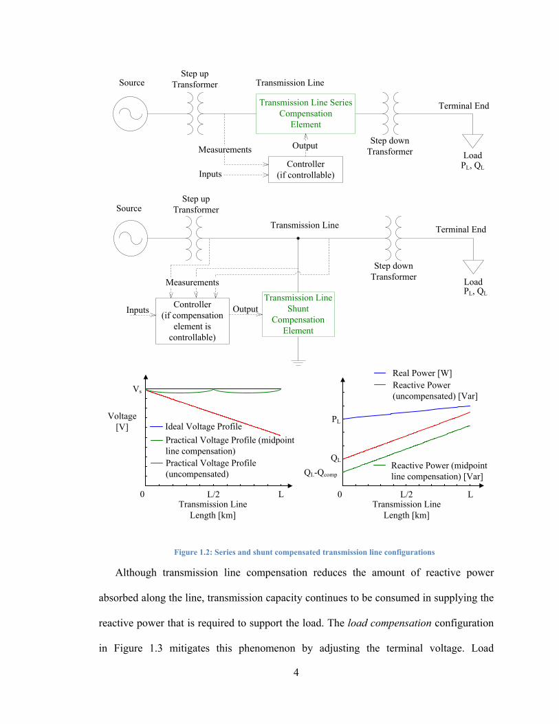
requirements. Figure 1.2 illustrates transmission line compensation’s ability to provide

local reactive power through either series or shunt reactive elements that are connected

somewhere along a transmission line. These elements alter the transmission line’s voltage

profile by either reducing its reactive power consumption or by causing it to behave as a

reactive power source [4].

4

Source Transmission Line

Load

Transmission Line SeriesCompensation

Element

Controller(if controllable)Inputs

Terminal End

Measurements Output

PL, QL

0 L

QL-Qcomp

PL

Real Power [W]

Reactive Power (midpoint line compensation) [Var]

QLPractical Voltage Profile(uncompensated)

Voltage [V]

L0

Vs

Ideal Voltage Profile

Practical Voltage Profile (midpoint line compensation)

Transmission Line Length [km]


Reactive Power(uncompensated) [Var]

Source

Transmission Line

Load

Transmission Line Shunt

CompensationElement

Controller(if compensation

element is controllable)

Inputs

Step down Transformer

Step up Transformer

Terminal End

Output

MeasurementsPL, QL


Step up Transformer

L/2L/2

Figure 1.2: Series and shunt compensated transmission line configurations

Although transmission line compensation reduces the amount of reactive power

absorbed along the line, transmission capacity continues to be consumed in supplying the

reactive power that is required to support the load. The load compensation configuration

in Figure 1.3 mitigates this phenomenon by adjusting the terminal voltage. Load

5

compensation reduces the transmission line’s reactive power requirement by adding

either reactive power sources or sinks, normally in shunt, at the line’s terminal end in

order to locally meet the load’s required reactive power. This approach reduces the

amount of reactive power that must be transmitted to support the load, but the

transmission line itself remains highly inductive and therefore continues to absorb

reactive power.

Source

Transmission Line

Load

Controller(if controllable)

Inputs

Shunt LoadCompensation

Element

Step up Transformer


Terminal EndMeasurements

PL, QL

Voltage [V]

L0

Vs

Ideal Voltage ProfilePractical Voltage Profile (load compensation)

0 L

QL-Qcomp

PL

Real Power [W]

QL



Practical Voltage Profile (uncompensated)

Reactive Power (load compensation) [Var]


L/2L/2

Figure 1.3: Load compensation configuration

Although systems would ideally employ both transmission line and load

compensation, cost considerations normally prohibit such a combination, and so the

compensation method shown in Figure 1.4 is rarely employed. Specific system objectives

dictate the type of reactive power compensation techniques that are actually

implemented.

6

Source Transmission Line

Load

Transmission Line Series

Compensation


Step up Transformer Terminal End

Transmission Line Shunt

Compensation

Load ShuntCompensation

0 LQL-Qcomp

PL

Real Power [W]


QL

Practical Voltage Profile (load compensation)Practical Voltage Profile (uncompensated)


Vol

tage

[V

]

L0

Vs

Ideal Voltage Profile

Practical Voltage profile (midpoint line compensation)

Reactive Power (midpoint line and load compensation) [Var]


Practical Voltage profile (midpoint line and load compensation)

PL, QL

L/2L/2

Figure 1.4: System with both transmission line and load compensation

1.1 Objectives of Reactive Power Compensation

Providing reactive power compensation is essential along long transmission lines for

maintaining terminal voltages within acceptable limits, enhancing the power system’s

stability, and increasing the system’s power transfer capability [2]. Capacitors and other

switched passive elements suffice as compensation devices when relatively wide voltage

ranges are acceptable. However, controllable elements such as static var compensators

(SVCs) are employed when more restricted voltage ranges are required.

Reactive power compensation device controllers compare user-defined inputs to

measured system parameters and then adjust the reactive power elements’ characteristics

in order to meet predetermined objectives. For example, a controller that must maintain a

7

specified system voltage compares a provided voltage reference value, Vref, with the

measured system voltage, Vmeasured. Depending upon the voltage difference, Ve, between

them, the controller then signals the device to generate or absorb reactive power in order

to maintain the desired voltage, Vref. A simplified block diagram of an SVC voltage

controller is illustrated in Figure 1.5.

+-

Vref

Vmeasured

Ve SVC Controller

SVC Apparatus

If Ve < 0, inject reactive power

If Ve > 0, absorb reactive power

SVC: Purpose is to maintain system voltage at Vref

SystemOutput

Figure 1.5: Block diagram of an SVC voltage controller

1.2 Controller Tuning for Reactive Power Compensators

The controller response describes the speed and accuracy with which the controller

obtains its objectives. Controller designs involve trading off improved settling time with

overshoot and undershoot considerations. This tradeoff can be adjusted by varying the

control system parameters.

Controller tuning is the process of adjusting control parameters to obtain an

acceptable controller response, and it is typically accomplished via either a model-based

or a simulation-based approach. Model-based tuning is an analytical technique that is

primarily used to tune simple control systems and to analyze the mathematical

approximations of complex control systems that were obtained through prior system

knowledge or measurements. It involves developing a mathematical construct of a

controller and its associated system. The controller is then designed and tuned to

determine the control system parameters based upon specified performance criteria. The

8

model-based tuning process is illustrated in Figure 1.6. Model-based tuning becomes

impractical as the underlying system’s sophistication increases due to the corresponding

mathematical model’s additional complexity.

Implement controllerwith user-

defined parameters

Analytical response

Mathematical model of system

and controller

User manually adjusts

parameters

No

Yes Obtain actual response

User-definedparameters (i.e gains and time

constants)

Is analytical response

satisfactory?

Figure 1.6: Model-based controller tuning

Simulation-based controller tuning uses simulation software to construct a controller

model. Different controller parameters are simulated, and the results are then compared to

specified performance criteria until an acceptable set of controller parameters are

determined. The simulation-based tuning process is illustrated in Figure 1.7. This can be

accomplished either by trial and error or else through exhaustive parameter testing.

Simulation-based optimization is an extension of simulation-based modeling that

employs software to optimize controller parameters based upon a user-defined objective

function [5], [6].

9

Figure 1.7: Simulation-based controller tuning

Both model-based and simulation-based controller tuning techniques are typically

used in feedback control systems whose controller parameters are determined by their

response to a predetermined input such as a step function. Both approaches suffer from

the controller tuning’s high dependence upon the properties being controlled and require

precise models to create a well performing control system.

Set-point modulation (SPM) is an emerging control technique that circumvents these

drawbacks. Rather than relying on access to the control variables, SPM is implemented as

an outer control loop as shown in Figure 1.8, that modifies the control system’s reference

value, or set-point, based solely upon the system’s output error and trajectory [7], [8], [9].

If the control system response sufficiently deviates from the set-point, the SPM control

scheme modifies the set-point to reduce the output overshoot and settling time. This

scheme therefore enhances system controllability without requiring direct access to the

underlying control system [10]. Manipulating the set-point enables SPM to

simultaneously reduce the settling time and improve the overshoot/undershoot.

Additionally, a control scheme that manipulates its set-point based upon its output

10

properties may provide better performance than traditional non-SPM control schemes [7],

[11].

+-

Vrefset

Vmeasured

Ve SVC Controller

SVC Apparatus

SystemOutput

SPM AlgorithmPurpose:(1) Limit overshoot/undershoot(2) Reduce settling time

Control variable slope and error measurements

Timing and magnitude of set-point adjustment

+ -Vref

SVC: Purpose is to maintain system voltage at Vref

Figure 1.8: Set-point modulation diagram

1.3 Problem Definition

SPM algorithms have thus far been limited to adjusting set-points through a fixed

scaling multiplier known as a modulation index [9]. Traditional SPM scales, or

modulates, the set-point by a predetermined amount depending upon the control

variable’s error and slope. This thesis aims to further improve SPM performance by using

fuzzy logic to determine a variable modulation index. A fuzzy logic-based SPM

algorithm is applied to simulated SVC control systems in order to produce set-point

adjustments that simultaneously limit the controlled variable’s overshoot or undershoot

while reducing its settling time. A comparison of traditional SPM and fuzzy-logic based

SPM is shown in Figure 1.9. The fuzzy logic-based SPM algorithm is then applied to

Manitoba Hydro’s Ponton SVC control system in order to quantitatively evaluate its

performance.

11

Figure 1.9: Different types of SPM

1.4 Motivation for Research

Modulating the control system’s set-point with fuzzy SPM algorithms instead of

sharply defined decision-making algorithms would further enhance SPM’s existing

performance superiority over traditional control schemes by increasing operational and

decision-making flexibility. Implementing this SPM control scheme to SVC controllers

in particular would therefore improve transmission line voltage overshoots and

undershoots and reduce settling times. This in turn enables designers to devise more

robust SVCs and allow utilities to more efficiently utilize the existing transmission

infrastructure by operating the system closer to its theoretical and operational limits.

1.5 Thesis Organization

The design and implementation of an SVC fuzzy logic-based set-point modulation

system requires an understanding of the underlying concepts of static var compensators,

fuzzy logic, and set-point modulation.

Chapter two provides a general SVC background, including SVCs’ benefits, their

constituent devices, various topologies, and control system considerations.

Chapter three discusses fuzzy logic and its potential ability to replace more traditional

control system methodologies.

12

Chapter four covers SPM in-depth, describes its compatibility with fuzzy logic-based

algorithms, and applies a fuzzy logic-based SPM control scheme to a generalized

representative second order system.

Chapter five analyzes the results obtained from applying fuzzy logic-based SPM

control methods to Manitoba Hydro’s Ponton SVC controller.

Chapter six summarizes this thesis’ contributions and provides future work

recommendations.

13

Chapter 2 Reactive Power and Static Var Compensators

A balanced steady state ac power system is characterized by three single phase

alternating voltage waveforms that are electrically separated from each other by 120°

phase shifts, as shown in Figure 2.1.

Figure 2.1: Three phase voltage waveforms

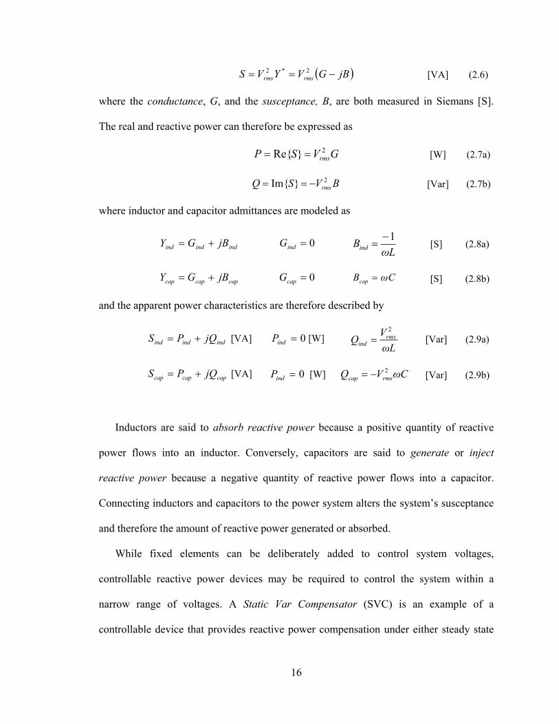
Voltage and current phasors are complex quantities, and the total apparent power, S,

which is measured in Volt-Amperes [VA], can therefore be expressed as the vector sum

of a real component, P, and an imaginary component, Q. The real power is also called

active power and is measured in Watts [W], while imaginary power is referred to as

reactive power and is measured in Volt-Amperes Reactive, or Vars [Var]. Reactive

power is stored both everywhere along the transmission line and at the load. Active

power that is not dissipated along the transmission line as heat is consumed by customers

to produce work.

*rmsrms IVS [VA] (2.1)

}Im{}Re{ SjSS [VA] (2.2a)

14

jQPS [VA] (2.2b)

Steady state transmission line and load characteristics can be modeled as complex

impedances or admittances arising from a combination of resistances, inductances and

capacitances. These complex impedances produce a phase shift, θ, between the voltage

and current waveforms.

θIjVθIVS rmsrmsrmsrms sincos [VA] (2.2c)

where

P

Q

S

Sθ

}Re{

}Im{tan 1 [rad] (2.3)

The relationships between these power components are shown in Figure 2.2.

Figure 2.2: Apparent power triangle

15

Because the transmission line’s apparent power capacity is fixed, power factor

correction is employed to minimize the reactive power consumed and therefore

maximize the amount of real power that can be transmitted. Power factor correction

reduces the net reactive power by introducing inductive or capacitive elements to the

system in order to bring θ, and therefore the imaginary portion of the impedance and the

reactive power, as close to zero as possible as depicted in Figure 2.3, thereby reducing the

phase angle between the voltage and current waveforms.

Figure 2.3: Apparent power triangle illustrating power factor correction

P

Q(θpf 1tancos)cos (2.4)

Substituting the complex form of Ohm’s law

YVI [A] (2.5)

into equation (2.1) yields:

16

jBGVYVS rmsrms 2*2 [VA] (2.6)

where the conductance, G, and the susceptance, B, are both measured in Siemans [S].

The real and reactive power can therefore be expressed as

GVSP rms2}Re{

[W] (2.7a)

BVSQ rms2}Im{ [Var] (2.7b)

where inductor and capacitor admittances are modeled as

indindind jBGY 0indG Lω

Bind

1 [S] (2.8a)

capcapcap jBGY 0capG CωBcap [S] (2.8b)

and the apparent power characteristics are therefore described by

indindind jQPS [VA] 0indP [W] Lω

VQ rms

ind

2

[Var] (2.9a)

capcapcap jQPS [VA] 0indP [W] CωVQ rmscap2 [Var] (2.9b)

Inductors are said to absorb reactive power because a positive quantity of reactive

power flows into an inductor. Conversely, capacitors are said to generate or inject

reactive power because a negative quantity of reactive power flows into a capacitor.

Connecting inductors and capacitors to the power system alters the system’s susceptance

and therefore the amount of reactive power generated or absorbed.

While fixed elements can be deliberately added to control system voltages,

controllable reactive power devices may be required to control the system within a

narrow range of voltages. A Static Var Compensator (SVC) is an example of a

controllable device that provides reactive power compensation under either steady state

17

or transient system conditions. It accomplishes this by connecting a continually varying

susceptance to either absorb or generate various amounts of reactive power depending

upon system requirements. By providing reactive power compensation, an SVC can

rapidly regulate or control the power system’s terminal voltage [12], [13] while

maintaining synchronism. Utilities employ SVCs in order to:

correct phase imbalances [14], [15] improve the power factor of loads [13], [14] improve the system’s steady state transmission capacity and transient stability

[16], [17], [18] dampen power oscillations [18], [19], [20], [21] and subsynchronous oscillations

[13] reduce voltage flicker caused by load fluctuations [12], [13] improve HVDC terminal performance [13] support system voltages [18]

Practical SVCs consist of various combinations of standard devices depending upon

design objectives, size restrictions, and installation costs.

2.1 SVC Apparatus

2.1.1 Antiparallel Thyristor Pair

A thyristor is a circuit element that acts as a diode by only allowing unidirectional

current conduction. However, unlike a diode, a thyristor will not conduct even when

forward biased unless a gate pulse signal is also provided to enable it. An anti-parallel

thyristor arrangement functions as a fully controllable bidirectional switch that enables

current conduction during both of the supply voltage’s positive and negative half-cycles.

Thyristors can begin to conduct, or fire, at any point while the thyristor is forward biased

and will continue conducting until the current flowing through the thyristor reverses

direction. Varying the timing of the thyristor’s firing therefore controls the amount of

18

voltage in the system, as depicted in Figure 2.4 for a resistive load. This provides a

controllable way to insert and remove devices from the power system, which enables

reactive power manipulation, according to equation (2.7b).

Figure 2.4: Anti-parallel thyristor and associated waveforms

The timing of the thyristor firing is referenced in terms of radians and is referred to as

the thyristor firing angle, α. Figure 2.5 illustrates the voltage waveform generated by the

anti-parallel thyristor pair for various values of α.

19

Figure 2.5: Voltage produced by anti-parallel thyristor pair for different thyristor firing angles

20

2.1.2 Thyristor Controlled Reactor

A Thyristor Controlled Reactor (TCR) is the fundamental SVC building block and

comprises an inductor, or reactor, in series with an anti-parallel thyristor pair as shown in

Figure 2.6. The anti-parallel thyristors enable the reactor to be inserted into the power

system for a fraction of the power system’s fundamental period. The reactor’s inclusion

introduces a phase shift between the supply voltage and the fundamental current

waveform through the inductor.

i(ωt)

v(ωt) = Vmsin(ωt)

Fixed reactorfor reactive

power absorption

Anti-parallelthyristor switches

combine to act as

bidirectional switch

T1 T2vT(ωt)

vL(ωt)

+

+

-

-

+

-

α

0 π 2π

i(ωt) [A]

ωt [rad]

0 π 2π ωt [rad]

α

T2conducts

vT(ωt) [V]

T1conducts

0π 2π

ωt [rad]

vL(ωt) [V]

α

Vm

T1 can fire

T2 can fire

v(ωt) [V]

π 2π 0 ωt [rad]

σ

σ

σ

T1fires

T2fires

Figure 2.6: Single-phase TCR schematic and associated waveforms

The TCR’s current conduction interval, σ, which describes the angular interval over

which a specific thyristor conducts and is varied by controlling the thyristor firing angle,

α, as measured from the zero crossing of the voltage v(t) applied across the TCR

21

terminals1. The current conduction interval is defined in terms of a thyristor’s firing angle

by2:

παπ

απσ 2

),(2 [rad] (2.10)

Varying the firing angle produces a current waveform with a controllable

fundamental component, where α = π/2 causes the anti-parallel thyristors to act as a short

circuit that enables full current conduction and α = π causes the anti-parallel thyristors to

act as an open circuit that blocks all current conduction. A firing angle of α < π/2 creates

an asymmetrical TCR current, which in turn produces a current waveform with overly

high harmonic content and a dc bias, both of which are unacceptable in ac power

networks [2]. A firing angle α > π is also impossible because the thyristors would be

reverse-biased and therefore unable to conduct.

With an applied system voltage of v(ωt) = Vmsin(ωt), the instantaneous current i(ωt)

produced is shown in equation (2.11) and illustrated in Figure 2.7.

rad 2rad )(,)cos()cos(

rad )(rad )2(,0

rad )2(rad ,)cos()cos(

rad rad )(,0

rad )(rad 0,)cos()cos(

)(

πtωαπLω

αtωV

απtωαπ

απtωαLω

αtωV

αtωαπ

απtωLω

αtωV

tωi

m

m

m

[A] (2.11)

1 Some authors measure the firing angle from the supply voltage’s peak Vm instead of its zero crossing. This phase shifts the expressions for the TCR’s fundamental and the harmonic currents [15]. 2 Because the firing angle and current conduction interval can be defined in terms of each other, the firing angle will be used exclusively throughout the remainder of this thesis for consistency.

22

Figure 2.7: TCR current waveforms with varying firing angles

23

Applying Fourier analysis to equation (2.11) allows the amplitude of the current’s

fundamental component to be expressed as a function of the thyristor firing angle:

rad rad 2

,)2sin(22

)(1 παπ

Lπω

ααπVαI mTCR

[A] (2.12)

At the fundamental frequency, the TCR current can be interpreted as the product of a

constant voltage, Vm, and a purely inductive susceptance, B1TCR, whose magnitude varies

as a function of the anti-parallel thyristors’ selected firing angle:

rad rad 2

,)()( 11 παπ

αBVαI TCRmTCR

[A] (2.13a)

where

rad rad 2

,)2sin(22

)(1 παπ

Lπω

ααπαB TCR

[S] (2.13b)

From equation (2.7b), QTCR = 2RMSV BTCR, and the TCR circuit can therefore absorb a

variable amount of reactive power depending upon the firing angle, α as shown in Figure

2.8.

24

α < π/2 Thyristors not

properly biased for conduction

α > π Thyristors not

properly biased for conduction

ωL

V 2RMS

(0.8)ωL

V 2RMS

(0.4)ωL

V 2RMS

(0.2)ωL

V 2RMS

(0.6)ωL

V 2RMS

π/2 2π/3 5π/6 π 0

α [rad]

Figure 2.8: TCR reactive power vs. firing angle

The TCR’s voltage-reactive power characteristic is illustrated in Figure 2.9. The TCR

can maintain the system voltage by varying the thyristor firing angle and therefore the

fundamental current’s magnitude. If the system voltage exceeds the desired voltage, Vref,

the ensuing firing angle reduction will increase the TCR’s reactive power absorption and

reduce the voltage back to Vref. Conversely, if the system voltage dips below Vref, the

TCR’s firing angle will increase to absorb less reactive power and cause the voltage to

rise back to Vref.

25

Figure 2.9: TCR's V-Q characteristic

The thyristor firing angle, α, affects the TCR-generated current harmonics as well as

the fundamental. Applying Fourier analysis to equation (2.11) shows that the current

amplitude, In, of the nth order harmonic differs greatly depending upon α:

evennI

oddnnnn

παn

παn

παn

πα

Lω

V

πI

n

mn

,0

,3 ,1

)2

(sin2

cos)2

(cos2

sin4

2

[A] (2.14)

Harmonics of order 3n, which are known as triple-n harmonics, are generated by the

TCR but do not appear on the transmission system when three-phase TCRs are connected

in a delta configuration, as is typically the case [4]. Figure 2.10 compares the harmonic

current magnitudes as a percentage of the fundamental magnitude over the TCR’s

operational range.

26

%10

0*

I

|)α(

I|

max

1n

Figure 2.10: TCR harmonics as a percent of TCR fundamental current magnitude

Figure 2.11 illustrates the total harmonic current magnitude’s variation as a

percentage of the current fundamental’s maximum value over the operational TCR range.

A filter is usually connected to the TCR to provide a ground path for the 5th and higher

order harmonics in order to minimize their effect on the power system [18]. Because all

non-fundamental harmonics are either filtered or cancelled out, subsequent analysis can

be limited to the TCR current’s fundamental component.

27

% o

f m

axim

um f

unda

men

tal m

agni

tude

27

25 IIIhar

Figure 2.11: TCR fundamental current and total harmonic current

2.1.3 Fixed CapacitorThyristor Controlled Reactor (FCTCR)

Although TCRs can only provide varying amounts of reactive power absorption,

power systems usually require reactive power generation. A TCR is therefore rarely used

on its own but is instead combined with fixed shunt capacitors to produce a continuously

variable reactive power source. This configuration is called a Fixed Capacitor-Thyristor

Controlled Reactor (FC-TCR), and is illustrated in Figure 2.12.

28

Figure 2.12: Single-phase fixed capacitor TCR (FC-TCR)

The capacitor bank is mathematically modeled by adding the fixed capacitor’s

susceptance to the TCR’s fundamental susceptance. Combining (2.8b) and (2.13b) yields:

)2sin(22)(

)()(

1

11

Lπω

ααπCωαB

αBBαB

TCRFC

TCRFCTCRFC

[S] (2.15)

By equation (2.6b), the FC-TCR’s reactive power characteristic may be modeled as

shown in equation (2.16), and depicted graphically in Figure 2.13

Lπω

ααπVCωVαQ

αBVαQ

αQQαQ

rmsrmsTCRFC

TCRFCrmsTCRFC

TCRFCTCRFC

)2sin(22)(

)()(

)()(

221

12

1

11

[Var] (2.16)

29

FC-TCRFC-TCR

TCR

Figure 2.13: Single-phase FC-TCR's V-Q characteristic

This modified susceptance essentially biases the original TCR’s voltage-reactive

power characteristic towards the generation portion of the reactive power region, and the

TCR’s reactive power rating is therefore designed to be greater than its fixed capacitor

reactive power rating to ensure its ability to operate in the inductive region when

required. This enables the FC-TCR to either generate or absorb a net amount of reactive

power depending upon system requirements.

Increasing the fixed capacitance term in equation (2.16) increases the reactive power

generation. A system that requires a large amount of reactive power may therefore

require an FC-TCR comprising multiple fixed shunt capacitors shown in Figure 2.14,

which the SVC employs to generate a continuous range of reactive power shown in

Figure 2.15. The mechanical switches shown in Figure 2.14 are required to place the

fixed capacitors into and out of the system.

30

Figure 2.14: Single-phase FC-TCR with multiple fixed capacitors

Figure 2.15: V-Q characteristic for FC-TCR with multiple fixed capacitors

2.1.4 Thyristor Switched Capacitor (TSC)

The power system exhibits transients whenever an FC-TCR’s fixed capacitors

connect to or disconnect from it because the capacitor voltage does not exactly match the

system voltage at the time of connection. The Thyristor Switched Capacitor (TSC)

31

illustrated in Figure 2.16 provides a theoretical operational improvement by enabling a

capacitive element to rapidly switch into and out of the power system in a transient-free

manner under certain conditions. The TSC consists of a pair of anti-parallel thyristors

series connected to a fixed capacitor and a series reactor known as a current limiting

reactor (CLR).

Figure 2.16: Single-phase TSC

The theoretical operational benefit introduced by the series capacitive element is

offset by increased cost and additional design challenges. This is because placing the

TSC into service is operationally equivalent to connecting a capacitor to a voltage source.

Any difference between the capacitor’s stored voltage and the voltage across the

capacitor at the time of switching produces an inrush current whose magnitude or rate of

32

change in magnitude may damage the thyristors. Provisions are normally taken to both

minimize the likelihood of inrush current and to reduce the severity of its occurance.

Because it is impossible to completely prevent current inrush, TSC designs require a

CLR, whose inductance protects the thyristors by limiting the rate of change of current

through the TSC branch to

L

tv

dt

tdi LL )()( [A/s] (2.17)

Despite the CLR’s necessity, its inclusion risks producing oscillations in the TSC-

generated current at the specific frequency for which the capacitor’s impedance cancels

the reactor impedance. This resonant frequency, ωr, can be mathematically expressed in

terms of the system’s fundamental frequency, ω0, as:

0

1ωr

LCωr [rad/s] (2.18)

where

cap

ind

B

Br (2.19)

Applying the Laplace transform to the TSC’s governing second order differential

equation produces the expression for the current, i(t), that flows during the TSC’s

conduction. Assuming a system voltage of v(t) = Vmsin(ωt) and a voltage VC(ωt=α)

across the capacitor during the TSC’s initial conduction, i(t) can be expressed as the sum

of a fundamental frequency component, iac, and a resonant frequency component caused

by the presence of the fixed capacitor and series CLR [22]:

33

response) (transient response) statesteady (

TermFrequency Resonant TermFrequency lFundamenta

cos)cos(

sin12

2)sin()()cos()(

ff

ωrωαtrωαaci

ωrωαtrω

r

rαmVtωcVcrBtωaciti

αtω

[A] (2.20)

where iac is the current amplitude of the TSC’s circuit steady state response:

12

2

r

rBVi Cmac [A] (2.21)

The r2/(r2-1) term is referred to as the magnification factor and is a function of the

TSC’s reactive element parameters. The TSC’s resonant frequency is normally designed

for a value that is between four and five times that of the fundamental frequency as

shown in Figure 2.17 in order to provide a magnification factor sufficiently close to unity

[22]. Tuning the TSC branch’s resonant frequency to ωr < 3ω produces a magnification

factor that is appreciably greater than one, thereby creating current magnitudes that may

exceed the SVC’s component ratings. Conversely, tuning the TSC branch’s resonant

frequency to ωr > 5ω produces unacceptably large transient current amplitudes.

34

12

2

r

r

Figure 2.17: Magnification factor as a function of r

Although equation (2.20) appears to suggest that TSCs should employ very large

reactors in order to reduce the current inrush to a negligible amount, three practical

considerations limit the CLR size. First, increasing the inductor size also increases the

time required for the voltage across the TSC to reach a steady state value. Moreover, the

additional reactive power absorbed by the CLR offsets the TSC’s intended purpose of

injecting reactive power. Finally, equation (2.19) implies that increasing the reactor size

would also necessitate increasing the capacitor size in order to keep the magnification

factor within the desired range.

While CLRs limit the severity of current inrush, other techniques are simultaneously

employed to reduce the likelihood of inrush occurring at all. Such techniques curtail or

ideally eliminate the current transients resulting from the TSC’s connection to the power

35

system and reduce the CLR’s inclusion to merely a necessary precautionary protective

design measure.

One method for eliminating possible transient currents involves timing the switching

to minimize the resonant frequency term of equation (2.20). This can be theoretically

accomplished by simultaneously satisfying the following conditions, neither of which is

perfectly realizable in a practical system:

0,1,2,...n ,

2)12(0)cos(

πnαtω

αtω [rad] (2.22a)

1)sin( α

1))(

2

2

r

rVtωV mαtωC [V] (2.22b)

Since the system voltage is v(t) = Vmsin(ωt), equation (2.22a) implies that the switch

may only be permitted to close at the supply voltage waveform’s positive or negative

peak values, which corresponds to ωt = π/2 or ωt = 3π/2, respectively. Similarly, the TSC

can only be removed from service at the point in every half-cycle at which i(ωt) = 0. The

TSC is removed from service by blocking the firing pulses to both thyristors in order to

naturally extinguish the current at the subsequent zero crossing. Therefore, unlike the

TCR, which operates for any firing angle in the range between π/2 ≤ α ≤ π, a TSC acts as

discrete device that can only enter service at α = π/2 or α = 3π/2 and be removed from

service at α = π or α = 2π.

While equation (2.22a) restricts the TSC’s instant of switching, equation (2.22b)

confines the capacitor charge to a specific value at that switching instant. Simultaneously

satisfying both of these equations precludes inrush from occurring by ensuring that the

36

TSC is only inserted into the power system when the system and the capacitor voltages

are identical.

It is impossible to physically realize either of the conditions dictated by equations

(2.22a) and (2.22b). The former condition cannot be met in practice due to the

impossibility of timing the exact switching instants, and the latter criterion cannot be met

because the voltage across a practical capacitor slowly decays over time, as illustrated in

Figure 2.18. The inability to meet either condition renders transients inevitable whenever

the TSC switches into the transmission circuit, thereby requiring the CLR’s inclusion in

the TSC design in order to protect the power electronics. SVC designs therefore employ

specialized switching schemes to further minimize the inevitable switching transients and

better approach these ideal criteria [22].

An alternative technique exists to reduce or eliminate transient currents altogether

without restricting the TSC’s range of operation, but this method is rarely used in

practice. A shunt-connected charging circuit that charges the capacitor when it is

disconnected from the system can ensure that the voltage across the capacitor matches the

system voltage at the instant of switching. Although a charging circuit would ideally be

added to the TSC circuit to maintain the capacitor’s charge at this level, such circuits are

expensive to implement and are therefore rarely installed [22].

37

Figure 2.18: TSC voltage waveform

Figure 2.19: Effect of capacitor size on a single-phase TSC V-Q characteristic

38

More practical TSCs employ multiple capacitor branches, each of which can be

independently switched into and out of operation. Although this resulting configuration

continues to lack full reactive power control, it at least provides multiple discrete levels

of reactive power. An SVC with k TSC branches will normally comprise k-1 branches of

susceptance BC and one branch of susceptance BC/2 to enable finer control between

branches A single line diagram of this configuration is shown in Figure 2.20. A voltage

deadband is also employed to ensure that TSC branches do not continuously switch on

and off while the voltage remains within the deadband as illustrated in Figure 2.21.

BC2

v(ωt) = Vmsin(ωt)

+

-

TSC1

...Anti-parallel

thyristor switches

CLR to limit current inrush

Capacitorfor reactive

power generation

T1 T2vT(ωt)

-

+

-

+

vL(ωt)-

+

vC1(ωt)

TSC2 TSCk

BC1 BC/2

i(ωt)

-

+vCk(ωt)

...TSCk-1

BCk-1-

+

...

vCk-1(ωt)vC2(ωt)-

+

Figure 2.20: Multiple TSCs

39

V [V]

-Q [Var]

Vref

Capacitive (Generation)

ΔV/2ΔV/2

C1C2

Ck-1

….

No Operation within Deadband

Q [Var]

Inductive (Absorption)

BC1+B

C2 , α = π/2 Impossible

because no reactive power absorption device is present

C1C2

Ck-1

c

...

Figure 2.21: V-Q characteristic of k single-phase TSCs

2.1.5 Thyristor Switched CapacitorThyristor Controlled Reactor

(TSCTCR)

The TSC’s advantage of reduced transient response is offset by their discrete

operational characteristics, which limit their use in systems that require continuous

reactive power control. Adding a TCR to the TSC provides sufficient controllability to

produce a Thyristor Switched Capacitor-Thyristor Controlled Reactor (TSC-TCR) with a

continuous V-Q characteristic. This arrangement is illustrated in Figure 2.22. Not only

does the TSC-TCR have greater operational flexibility than a TSC, it also produces fewer

steady state losses than an FC-TCR [22], [23].

40

Figure 2.22: TSC-TCR

The TSC-TCR’s reactor is typically sized with a slightly higher reactive power rating

than an individual TSC component to provide the SVC with overlapping reactive power

ranges over the discrete TSCs. This effectively creates a reactive power deadband and

limits unnecessary switching. The TSC-TCR’s V-Q characteristic is shown in Figure

2.23.

During large system disturbances, an FC-TCR behaves as a parallel LC branch that

may resonate with the transmission system. In contrast, the TSC-TCR can remove itself

from service sufficiently quickly to preclude it from resonating with the transmission

system during or immediately after large disturbances [22].

41

Figure 2.23: V-Q characteristic for a TCR multiple TSC arrangement

2.1.6 Practical Considerations

The idealized SVC configurations discussed thus far have ignored many design

considerations required for practical implementation. For example, an SVC does not

directly connect to the transmission system, but is rather connected through a step-down

transformer whose windings behave as reactors that introduce additional susceptance to

the idealized V-Q characteristics discussed [22]. An SVC can also employ filter banks

that assist in steady state reactive power compensation in addition to filtering out

unwanted current harmonics. This is accomplished by tuning LC filters so that the

capacitors’ reactive power generation is much larger than the inductors’ reactive power

absorption, thereby causing the filter to function like a capacitor connected to the SVC

terminals [17]. This shifts the already discussed idealized V-Q characteristics towards the

generation region of the V-Q characteristic.

42

2.2 SVC Control System

A practical SVC also requires a control system to effectively employ its constituent

components. General SVC control systems typically consist of a measurement system, a

voltage regulator, a gate pulse generator (GPG), and a synchronizing system as shown in

Figure 2.24 [22]. Auxiliary control functionality is also sometimes included when

required for cases such as power oscillation damping.

Figure 2.24: A typical SVC control block diagram

2.2.1 Measurement System

The measurement system provides the inputs that the control system requires to

perform its desired operations. Some of these values are directly measured while others

are derived from basic current and voltage measurements. The required measurement

parameters depend upon the type of SVC control employed.

43

Table 2.1: Possible SVC system measurements

Voltages Currents Auxiliary Measurements Individual Phases Individual Phases Individual Phase Reactive Power

3-phase RMS 3-phase RMS Transmission Line Real Power

Transmission Line Reactive Power Positive and Negative

Sequence Transmission Line

Bus Angles Bus Frequency

Magnitude Squared Synchronous Generator Angular

Velocity

2.2.2 Synchronization System

The synchronization system generates reference signals that are synchronized to the

system voltage’s fundamental frequency. The gate pulse generator (GPG) uses these

references to produce the SVC’s TCR and TSC firing pulses, and although it typically

uses a phase locked loop (PLL) to do so, other reference signals such as the thyristor

voltages have also been used [22]. A model of of PLL for an SVC controller is depicted

in Figure 2.25.

Figure 2.25: PLL model for SVC controller

Irrespective of the method employed, all synchronization systems must minimize the

generation of non-characteristic harmonics while accurately tracking the system’s phase

and frequency. They must also remain insensitive to events such as supply voltage

44

distortions and severe system disturbances, and they must rapidly resynchronize upon

fault clearing in order to maintain system reliability [22].

2.2.3 Voltage Regulator

The SVC voltage regulator uses the voltage error, Ve, to produce the reference

susceptance value, Bref, required to obtain the desired SVC bus voltage.

A slope, or droop, of KSL is typically included in the SVC voltage-current

characteristics as shown in Figure 2.26 [22]. This droop reduces the SVC’s reactive

power rating, prevents the SVC from reaching its reactive power limits too frequently,

and facilitates reactive power sharing between multiple parallel compensators. Droop is

implemented by multiplying the measured SVC current by the droop value KSL when

SVC current measurements can be reliably obtained. If SVC current measurements are

unattainable, the SVC voltage is assumed to be near unity, thereby producing a reference

susceptance that is approximately equal to the SVC current. Typical KSL values lie

between 3-5%, but they can sometimes range as wide as 1-10% [22].

45

Figure 2.26: SVC V-Q characteristic with droop

2.2.4 GatePulse Generator

The gate-pulse generator (GPG) receives a reference susceptance signal from the

voltage regulator and translates this into firing pulses that the SVC thyristor devices use

to generate the required susceptance. In SVCs consisting of only a TCR and fixed

capacitors, the GPG calculates the susceptance needed by the TCR to cancel the excess

capacitance. In SVCs comprising a TCR, fixed capacitors and a TSC, the GPG must also

determine the number of TSCs to be switched in order to meet the reactive power

requirements, calculate the corresponding TCR firing angles to realize this susceptance,

and then determine the TSC connection sequence that ensures minimal transient

capacitive switching [24].

The GPG accomplishes its tasks by first dividing the required susceptance, BC, by the

susceptance of a single TSC. This value, kC, is rounded up to the next largest integer

value to ensure that sufficient capacitive susceptance exists in the circuit. The required

46

inductive susceptance is computed by taking the difference between kCBC and Bref. The

GPG then calculates the required TCR firing angle to realize this susceptance. Switching

transients are minimized by employing the methodology outlined in [22] and illustrated

in Figure 2.27.

Figure 2.27: Gate-Pulse Generator Flowchart

The fundamental SVC system principles that have been briefly introduced in this

chapter can be better optimized for operational performance by employing more complex

control algorithms. Chapter three provides an overview of the fuzzy logic and fuzzy

inference systems that can be utilized in order to do so.

47

Chapter 3 Fuzzy Logic

This chapter introduces fuzzy logic, its basic operators, and its applicability to

decision making processes.

In set theory, an element is the label assigned to an abstract object, and a set is an

arbitrarily defined grouping of possible elements. Traditional set theory requires that each

element be rigidly categorized as either completely belonging to a set or entirely

excluded from it. For example, a car can be classified as an element within the set of

motorized vehicles and excluded from the set of Latin American coffee beans.

Traditional set theory’s classification method suffices for elements that have well-

defined properties, but it becomes more problematic when applied to context sensitive

classifications. For example, a particular car whose speed cannot physically exceed 200

km/h could have this property mathematically described by a set whose elements contain

all possible speeds between 0 km/h and 200 km/h. To categorize these speeds, traditional

set theory requires defining a threshold speed such as 100 km/h as a boundary above

which all speeds would be considered fast and below which all speeds would be

considered slow. However, the negligible practical distinction between 99.999 km/h and

100.001 km/h makes it intuitively inconsistent to classify such speeds differently.

Fuzzy logic is a more generalized form of set theory that is better suited to

mathematically describe a system’s qualitative properties [23], [25], [26]. It does so by

employing a class of objects called fuzzy sets whose elements may have varying degrees

of membership. This degree of membership is usually determined by a membership

function (MF) that maps an element to a value between zero and one.

48

In fuzzy set theory, a fuzzy element for the above car example would be defined as

possible car speeds, x km/h. A membership function µfast(x) would then be defined to

create a continuous grade of membership that relates speeds with the term fast.

3.1 Fundamental of Fuzzy Logic

3.1.1 Membership Functions

An element x has a degree of membership y in a fuzzy set that is defined by a

membership function y=µ(x), where y lies on the interval [0, 1] and is said to be the

fuzzified value of x.

Consider again the definition of “fast”, which could be defined by a simple

membership function such as equation (3.1) and depicted in Figure 3.2.

km/h 200km/h 0,005.0)( xxxμy fast (3.1)

Figure 3.1: A comparison of traditional set theory and fuzzy set theory

49

Figure 3.2: A possible membership function for fast speeds

Although the above example fuzzifies a car’s speed in an elementary way,

membership functions can be as simple or as complicated as an application requires. For

example, defining speeds between 0 and 50 km/h to be even remotely fast when

considering driving speeds along the Trans-Canada Highway would be inappropriate. In

this instance, it would be preferable to define any speed below 50 km/h as having a

membership value of zero in the set of fast speeds and to assign a unity membership

value to all speeds above 150 km/h. The membership function between these two

extremes could smoothly transition from “not at all fast” to “fast” to reflect the intuitive

notion that the degree of membership to the set of fast speeds increases proportionately

with increasing car speeds. Such a membership function is expressed mathematically in

Equation (3.2) and is illustrated in Figure 3.3. Using this membership function, a 70 km/h

speed is given a value of 0.2, indicating a “slightly fast” speed. Conversely, a 140 km/h

speed is assigned a value of 0.9, indicating a speed that is quite a bit more fast than slow.

50

km/hr 200km/hr 150,1

km/hr 150km/hr 50),50(01.0

km/hr 50km/hr 0,0

)(

x

xx

x

xμy fast (3.2)

Figure 3.3: Membership function for determining fast speed

3.1.2 Fuzzy Operators

Just as arithmetic operators such as addition and multiplication combine and

manipulate numbers, fuzzy operators are used to combine and manipulate fuzzified

elements. The intersection (AND, ∩), union (OR, ), negation (NOT, ⌐), and implication

(IF-THEN, ) operators are the four fundamental traditional logic operators that form

the foundation of Boolean logic and traditional set theory. The underlying concepts

conveyed by the first three of these operators can be extended into the fuzzy domain with

varying degrees of ease. For such cases, fuzzy logic becomes a superset of traditional

Boolean logic, and fuzzy operators reduce to traditional set theory operators when

specific elements within a fuzzy set have the traditional Boolean membership values of

51

either zero or one. The following sets A and B as shown in Figure 3.4 will be used to

compare and contrast Boolean and fuzzy operators.

A B

x1

x2

x3

x4

x5

x6

x7

x8

x9

x10

Axxxxx 54321 ,,,,

Bxxxxx 87654 ,,,,

Figure 3.4: Illustrative sets

3.1.2.1 Intersection

The intersection of two sets A and B is mathematically described by the expression

below and illustrated in Figure 3.5.

BxandAxxBA

Figure 3.5: Venn diagram of the intersection of two sets in traditional set theory

Under Boolean logic, any element that belongs to both set A and set B is a member of

the intersection set and assigned a value of 1, whereas any element that belongs

exclusively to either set A or set B, or that belongs to neither set A nor set B, is excluded

from this set and assigned a value of 0. The elements x4 and x5 in Figure 3.5 belong to

both sets A and B and therefore belong to the intersection of the two sets. The intersection

of the two sets of Figure 3.5 is shown in Table 3.1.

52

Table 3.1: Boolean intersection truth table

Element A B A∩Bx1 1 0 0 x2 1 0 0 x3 1 0 0 x4 1 1 1 x5 1 1 1 x6 0 1 0 x7 0 1 0 x8 0 1 0 x9 0 0 0 x10 0 0 0

Many methods exist for extending this Boolean intersection operator into the fuzzy

domain [26], but this thesis restricts the fuzzy intersection operator to the minimum value

of two quantities. This minimum operator, Min(A,B), maintains the traditional set theory

boundary conditions while enabling its extension to the membership values between 0

and 1 that are typically encountered in fuzzy logic. The highlighted entries in Table 3.2

indicate the minimum operator’s reduction to the Boolean logic intersection when the

memberships to a fuzzy set are Boolean values.

53

Table 3.2: Minimum operator for fuzzy and Boolean logic values

A B A∩B 0 0 0 0 1 0 1 0 0 1 1 1

A B Min(A,B)0 0 0 0 0.33 0 0 0.66 0 0 1 0

0.33 0 0 0.33 0.33 0.33 0.33 0.66 0.33 0.33 1 0.33 0.66 0 0 0.66 0.33 0.33 0.66 0.66 0.66 0.66 1 0.66

1 0 0 1 0.33 0.33 1 0.66 0.66 1 1 1

3.1.2.2 Union

The union operator in traditional set theory can be described mathematically by the

below expression and illustrated in Figure 3.6.

BxorAxxBA

Figure 3.6: Venn diagram of the union of two sets in traditional set theory

Under Boolean logic, any element that belongs to either set A or set B, or to both set A

and set B, is a member of the union set and assigned a value of 1, whereas any element

54

that belongs to neither set A nor set B is not a member of this set and assigned a value of

0. The Boolean union operator can be described in Table 3.3.

Table 3.3: Boolean union truth table

Element A B A∪Bx1 1 0 1 x2 1 0 1 x3 1 0 1 x4 1 1 1 x5 1 1 1 x6 0 1 1 x7 0 1 1 x8 0 1 1 x9 0 0 0 x10 0 0 0

As with the fuzzy intersection operator, many fuzzy union definitions can be

employed [26]. However, this thesis applies the maximum operator, Max(A,B) when

discussing the fuzzy union operator in order to maintain traditional logic and still permit

varying degrees of membership. Table 3.4 illustrates the maximum operator for

membership values that lie between 0 and 1.

55

Table 3.4: Maximum operator for fuzzy and Boolean logic values

A B A∪B 0 0 0 0 1 1 1 0 1 1 1 1

A B Max(A,B)0 0 0 0 0.33 0.33 0 0.66 0.66 0 1 1

0.33 0 0.33 0.33 0.33 0.33 0.33 0.66 0.66 0.33 1 1 0.66 0 0.66 0.66 0.33 0.66 0.66 0.66 0.66 0.66 1 1

1 0 1 1 0.33 1 1 0.66 1 1 1 1

3.1.2.3 Complement

The complement in traditional set theory can be mathematically described by the

expression below and illustrated in Figure 3.7.

AxxA

Figure 3.7: Venn diagram of the complement of a set in traditional set theory

Under Boolean logic, any element that does not belong set A is a member of the

complement of A and assigned a value of 1, whereas any element that belongs to set A is

56

not a member of the complement of A and is assigned a value of 0. Boolean logic

expresses the complement operator as shown in Table 3.5.

Table 3.5: Boolean complement truth table

Element A ¬Ax1 1 0 x2 1 0 x3 1 0 x4 1 0 x5 1 0 x6 0 1 x7 0 1 x8 0 1 x9 0 1 x10 0 1

The fuzzy complement operator can be defined as 1-µ(x) where µ(x) is the

membership value of the fuzzy set. This definition maintains the traditional logic operator

while extending its meaning into the fuzzy domain, and it is normally the only definition

used. Table 3.6 provides illustrative values of sample complement operations on fuzzy

logic values.

Table 3.6: Complement operator for fuzzy and Boolean logic values

A 1-A 0 1

0.25 0.750.5 0.5 0.75 0.25

1 0

A ¬A0 1 1 0

3.1.2.4 Implication

Implication in traditional set theory is also known as a conditional sentence.

Implications are of the form “if P, then Q” and can be mathematically represented as

57

QP

where P is the antecedent, or premise, and Q is the consequent, or conclusion.

Implications can also have multiple premises of the form “If P and R, then Q”. Boolean

logic expresses the implication operator as shown in Table 3.7.

Table 3.7: Boolean implication truth table

P Q P Q0 0 1 0 1 1 1 0 0 1 1 1

Unlike previous operators discussed, the fuzzy implication operator does not reduce

to the traditional set theory implication. Because the fuzzified values of the premises,

which are known as partial premises, may assume any value over the range [0, 1], fuzzy

logic requires a more complex implication operator than Boolean logic, whose element

values are limited to either 0 or 1. The existence of partial premises implies the

impossibility of drawing a fixed conclusion. Instead, partial premises are combined into a

single fuzzified premise, which then combines with an entire conclusion set to yield a set

representing the conclusion. Several techniques for implementing the fuzzy implication

exist, with the two most commonly used methods being the minimum and product

functions. This thesis arbitrarily uses the minimum method first introduced by Mamdani

[27].

Fuzzy logic applies if-then rules to relate fuzzy sets to each other. If A and B are fuzzy

sets represented by linguistic variables, then fuzzy logic applies an if-then rule of the

form:

If x is A, then y is B.

58

For example, a driver who encounters a stop sign may apply an if-then rule illustrated

in Figure 3.8.

Figure 3.8: Single premise fuzzy if-then rule

where speed is the input x to the if-then rule, braking is the output y, and A and B are

fuzzy sets corresponding to fast and abrupt, respectively.

In this example, a driver’s speed maps to a fuzzified input value of between 0 and 1

depending upon the degree to which the speed input is considered fast. The conclusion

“braking is abrupt” is the assignment of the entire fuzzy set abrupt to the output braking.

A fuzzy if-then statement can also have multiple premises, such as:

If x1 is A1 and x2 is A2, then y is B.

This type of statement is illustrated in Figure 3.9.

59

Figure 3.9: Multiple premise fuzzy if-then rule

The multiple premises are combined to produce a single value representing the entire

premise. This value can then be used to draw a conclusion or inputted into a fuzzy

inference process. The output of a fuzzy if-then rule is itself a fuzzy set whose

membership function represents the qualities of the conclusion.

For example, motorists driving at 100 km/h who sees a stop sign 4.5 meters away and

utilizing the minimum implication method results in the braking conclusion set shown in

Figure 3.10.

If the speed is fast and the stop sign is close, then braking is abrupt.

Membership function

undefined in this range

0 50 100 150 200

0.20.4

0.60.8

1

x1 = speed [km/h]

A1

= μ

fast(x

1)

0 4 8 12 16 20

0.20.40.60.8

1

x2 = proximity [m]

0 4 8 12 16 20

0.20.40.60.8

1

y = deceleration [m/s2]

If x1 is A1 and x2 is A2, then y is B.

x1 = 100 km/hμfast(x1) = 0.5

x2 = 4.5 mμclose(x2) = 0.8

min (μfast(x1),μclose(x2)) = 0.5

B =

μab

rupt

(y)

A2

= μ

clos

e(x 2

)

Figure 3.10: Multiple premise fuzzy if-then rule calculation

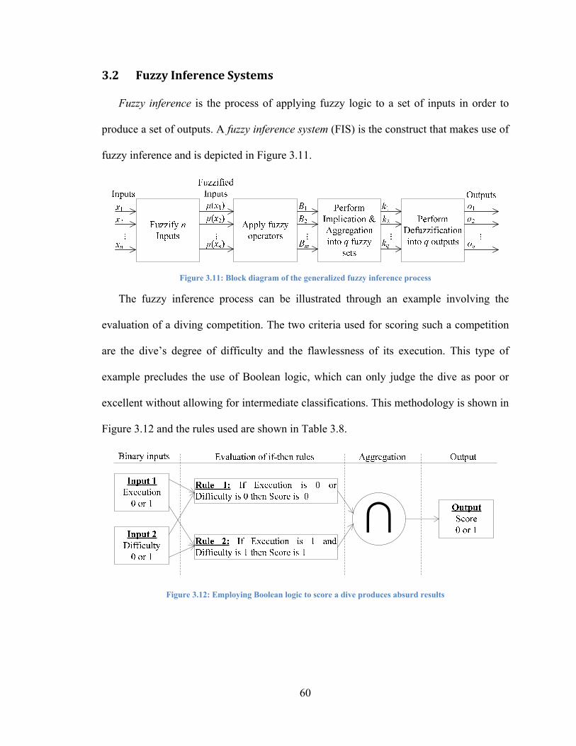
60

3.2 Fuzzy Inference Systems

Fuzzy inference is the process of applying fuzzy logic to a set of inputs in order to

produce a set of outputs. A fuzzy inference system (FIS) is the construct that makes use of

fuzzy inference and is depicted in Figure 3.11.

Figure 3.11: Block diagram of the generalized fuzzy inference process

The fuzzy inference process can be illustrated through an example involving the

evaluation of a diving competition. The two criteria used for scoring such a competition

are the dive’s degree of difficulty and the flawlessness of its execution. This type of

example precludes the use of Boolean logic, which can only judge the dive as poor or

excellent without allowing for intermediate classifications. This methodology is shown in

Figure 3.12 and the rules used are shown in Table 3.8.

Figure 3.12: Employing Boolean logic to score a dive produces absurd results

61

Table 3.8: Boolean rules for diving example

Poor Excellent

Low 0 0

High 0 1

In contrast to the above Boolean system, a fuzzy system can assign scores along a

continuum between very poor and very good. Both inputs may be evaluated on a scale of

0 to 10, where 0 is assigned to a very poor dive and 10 denotes a very good dive. The FIS

uses each of the input values to determine the final score is shown in Figure 3.13, and the

rules are shown in tabular form in Table 3.9.

Figure 3.13: FIS diving example using fuzzy logic

Table 3.9: Fuzzy rules for diving example

Poor Satisfactory Excellent

Easy Low Low/Medium Low

Average Low Medium

Hard Low Medium High

62

3.2.1 Step One: Fuzzification

The FIS begins by determining each input’s degree of membership in each of the

problem’s fuzzy sets. This is determined by first ranking the dive’s qualitative

descriptions between 0 and 10 and then applying the membership functions to each of

these rankings to fuzzify the inputs between 0 and 1. In this case, the input values for

execution and difficulty are each ranked from 0 to 10 and then mapped to the interval

between 0 and 1 using membership functions. Each of the three rules that are applied in

this example requires that each input be resolved into fuzzy sets corresponding to the

qualitative descriptions:

difficulty is easy difficulty is average difficulty is hard

execution is poor execution is satisfactory execution is excellent

The shape of the membership functions shown in Figure 3.14 and 3.15 were chosen to

reflect how these qualitative descriptors are perceived. The diving judges could select

different membership functions depending upon their view as to what constitutes easy,

average, hard, poor, satisfactory, and excellent.

63

Figure 3.14: Execution membership functions

Figure 3.15: Difficulty membership functions

For example, a dive with an execution rating of 8 and a difficulty rating of 3 would

produce the following fuzzified values shown in Figure 3.16.

64

Difficulty is Easy

Execution is Poor

0.2222

Execution is Satisfactory

Difficulty is Hard

Execution is

Excellent

0.2

0.4

0.6

0.8

1

0 2 4 6 8 10 0 2 4 6 8 10

0.2

0.4

0.6

0.8

1

0.2

0.4

0.6

0.8

1

0 2 4 6 8 10

0.2

0.4

0.6

0.8

1

0 2 4 6 8 10

0.2

0.4

0.6

0.8

1

0 2 4 6 8 10

0.2

0.4

0.6

0.8

1

0 2 4 6 8 10

Execution = 8Fuzzify input 1 y1 = μ(x1)

Fuzzify input 2 y2 = μ(x2)Difficulty = 3

Difficulty is Average

x1

x1

x1 x2

x2

x2Score

Score

Score

Score

Score

Score

Apply membership functions to Input 1

Apply membership functions to Input 2

0

0.26110.2301

00.9047

Figure 3.16: Step 1 involves fuzzifying execution and difficulty inputs

3.2.2 Step Two: Application of Fuzzy Operators

Once the inputs have all been fuzzified by their respective membership functions,

rules with multiple premises can be evaluated. When the premise has multiple parts, the

corresponding fuzzy operators linking each partial premise are applied such that a single

value can be assigned to the entire premise.

Figure 3.17 illustrates the use of fuzzy operators: OR, or maximum, AND, or

minimum, and a rule without a fuzzy operator. Because the OR function is applied to the

multiple-premised Rule 1 that “If Execution is poor or Difficulty is easy, then the Score is

65

low”, the maximum fuzzy value obtained from “Execution is poor” and “Difficulty is

easy” is used as the fuzzy value of the entire premise. Conversely, because the AND

function is applied to the multi-premised Rule 3, “If Execution is excellent and Difficulty

is hard, then the Score is high”, the minimum value obtained from “Execution is

excellent” and “Difficulty is hard” is used as the fuzzy value of the entire premise.

Finally, because Rule 2 lacks multiple premises, the fuzzy value of the premise is simply

the fuzzy value of “Execution is satisfactory”.

If a particular dive’s execution is rated an 8 and the difficulty of the dive is graded as

3, these inputs are fuzzified using the appropriate membership functions (the poor

membership function for execution and the easy membership function for difficulty) to

obtain membership values of 0 and 0.2222 respectively. The fuzzy OR operator selects

the maximum of the two values, or 0.2222. This completes the fuzzification of this

particular rule. The results of applying fuzzy operators are summarized in Figure 3.17.

66

Figure 3.17: Step 2 evaluates fuzzified inputs by applying fuzzy operators

3.2.3 Step Three: Implication

Once the fuzzy operators combine all of the premise’s components into a single

value, the FIS performs the implication step to translate each rule’s premise into a

conclusion. This process combines the premise’s single value with the consequent’s

membership function. The curves in Figure 3.18 illustrate the consequent’s membership

functions, which in this example correspond to the scoring of a dive. As with the

67

membership functions describing difficulty and execution, the membership function

shapes are constructed at the user’s discretion and can assume any form.

Figure 3.18: Scoring membership functions

This combination is performed for each FIS rule. In Rule 1, for example, the

implication process combines the result of the premise 0.2222 with the membership

function representing the consequent of Rule 1, which in this case is “Score is low”. The

membership function representing this consequent is in Figure 3.19.

68

or Difficulty is Easy

Step 1: Fuzzify Inputs Step 2:Apply fuzzy

operator

0.2222

Execution is Poor

Step 3:Apply implication

operator (min)

Result of Implication

Score is Low

Input 1: Execution = 8

Input 2: Difficulty = 3

Fuzzify input 1 y1 = μ(x1)

Fuzzify input 2 y2 = μ(x2)

OR (max)

ScoreScore x1 x2

AND (min)

Execution is Satisfactory

Difficulty is Hard

Execution is Excellent

Difficulty is Average

x1

x1 x2

x2Score

Score

Score

Score

No operator for this

rule

Score is medium


Score is high


0.22220

0.2301 0.2611 0.2301

0.9047 0 0

and

Figure 3.19: Application of the implication

3.2.4 Step Four: Aggregation

The aggregation procedure combines all of the fuzzy sets produced by the

implication process into a single fuzzy conclusion set. Each output variable is aggregated

once to produce a single fuzzy set for each output variable. This thesis uses the maximum

aggregation method. Figure 3.20 illustrates how the aggregation method combines the

69

results of each rule to produce a resultant fuzzy conclusion set. Figure 3.21 shows the

result of aggregation with its corresponding numerical boundaries.

Figure 3.20: Aggregation of all of the rules

70

3.2.5 Step 5: Defuzzification

Upon aggregation, the conclusion set is defuzzified into a single output value. Several

methods can be used to defuzzify the set, but this thesis employs the centroid

defuzzification method due to its widespread use in fuzzy logic applications and its ease

of implementation [28]. The object’s centroid can be calculated by:

b

a

dxxxf )(centroid (3.3)

The integration limits a and b are defined by the centroid’s boundaries, which typically

correspond to the defuzzified output’s minimum and maximum values.

Figure 3.21: Defuzzification for diving example

Defuzzification produces the diver’s final score based upon the inputs classifying the

dive’s difficulty and execution. Using equation (3.3) to defuzzify the diving example

conclusion set produces

71

53.3output ddefuzzifie

02

7

2

12222.0

2

3

2

1

23

22222.0

3

2output ddefuzzifie

10

7

7

5556.6

5556.6

4444.3

4444.3

3

3

6667.2

6667.2

3333.0

3333.0

0

dxdxxxdxxdxxx

dxxxdxxdxxx

(3.3)

xy3

2 2

3

2 xy

2

3

2

1 xy 2

7

2

1 xy

2222.0y

Figure 3.22: Defuzzification calculation for diving example

Fuzzy logic’s applicability to systems that rely upon qualitative evaluations makes it

useful for a wide range of applications spanning multiple disciplines. The intuitive

explanations discussed in this chapter have illustrated the procedure for applying a FIS to

simple decision making process. The next chapter introduces set-point modulation (SPM)

and combines fuzzy logic with SPM to produce a decision-making control scheme that

improves a generic second order system’s performance.

72

Chapter 4 SetPoint Modulation

In discussing the reactive power characteristic’s impact on real power transmission

and voltage profiles, Chapter two limited its treatment to steady state operational limits.

These regulatory and procedural limits restrict the transmission line’s minimum and

maximum terminal voltages for stability reasons and include other constraints such as the

maximum amount of power that can flow on transmission lines without violating thermal

limits. The power system is generally operated close to its steady state operational limits

in order to maximize utilization of the existing infrastructure. This causes equipment

ratings or regulatory restrictions to be temporarily exceeded during uncontrolled events

such as fault-induced transients.

The power system includes many controllable devices to mitigate such violations.

One approach involves improving the performance of traditional set-point tracking

controllers such as typical Proportional-Integral-Derivative (PID) controllers shown in

Figure 4.1. Such control improvements include simulation-based optimization of typical

set-point tracking systems and online PID controller gain adjustments [29].

Figure 4.1: PID controller block diagram without SPM

An alternative approach enhances the power system’s dynamic performance by

manipulating the traditional control systems’ set-points, or reference values, in real time.

This method is generically referred to as set-point modulation (SPM) and is depicted in

73

Figure 4.2. Several SPM methods have been devised to improve overshoot/undershoot

performance while simultaneously decreasing settling time of the system variable being

controlled [7], [9].

Figure 4.2: PID controller block diagrams with SPM

4.1 Feedforward Posicast Control

A second order system’s transfer function, G(s), with unity dc gain can be described in

terms of its damping ratio, ζ, which is a unitless value that describes how second order

system oscillations decay over time, and its natural frequency of oscillations, ωn:

22

2

2)(

nn

n

sssG

(4.1)

The response, y(t), of the transfer function G(s) to a unit step change, u(t), can be

calculated as shown in equation (4.2) and shown graphically in Figure 4.3.

)sin(

11)(

2

te

ty d

tn

(4.2)

where the damped frequency, ωd, and the phase shift, ψ, can be expressed as the

following functions of ζ and ωn:

21 nd [rad/s] (4.3a)

74

2

1 1tan [rad] (4.3b)

A system characterized by ζ < 1 is underdamped and will exhibit an overshoot, Mp. The

underdamped transfer function, G(s), has poles at

dnnn ωjζωζωjζωωjσs 2

2,1 1 (4.4)

The peak value of the system response will be

ppeak My 1 (4.5)

where

21 ζ

ζπ

p eM

(4.6)

The oscillation period of the response, Td, which denotes the time between successive

response peaks, is

21

222

ζω

π

ω

πtT

ndpd

(4.7)

where tp is the length of time required for the response to attain its peak value.

75

Figure 4.3: Underdamped second-order system response

The concept of improving transient behavior via set-point manipulation was first

published in 1957 as Posicast control [7]. This predefined feedforward control

methodology acts independently of the controller output and can completely eliminate a

second order system’s overshoot or undershoot response to an input step change in the

system. It does so by employing the control method shown in Figure 4.4 to divide the

input step into two parts that are separated by a fixed time delay, tp.

Figure 4.4: Half-cycle Posicast block diagram

76

pM1

1

Figure 4.5: Posicast command

The first part scales the step change, u(t), in such a way as to cause the response’s

peak value to reach the desired final output value of unity, as shown in Figure 4.5. The

second part of the input, which is time-delayed by tp, fixes this response to this desired

value instead of oscillating about it. This second part’s magnitude is devised such that the

oscillations produced by the second step completely cancel those produced by the initial

step. The resulting output attains its final value in half of the natural response period, Td,

and exhibits neither overshoot nor undershoot. Figure 4.6 illustrates the Posicast

technique.

77

Figure 4.6: Application of Posicast control to eliminate overshoot

78

The feedforward Posicast method transfer function

11

1)(1

pst

p

p eM

MsP (4.8)

has roots of the form s=σ+jω, where

nd

ζωδT

σ )ln(2

[rad/s] (4.9a)

,)12(21122

nζn

ωnd

T

πω Zn [rad/s] (4.9b)

From the Laplace domain perspective, Posicast is an all-zero filter, meaning that its

transfer function has both no poles and an infinite set of zeros at odd multiples of ωn as

depicted in Figure 4.7.

….

….

)12(1 2 nζωn

nζω

)12(1 2 nζωn

)12(13 2 nζωn

)12(13 2 nζωn

Figure 4.7: Pole-zero plot of the generalized Posicast transfer function

Feedforward Posicast control in underdamped second order systems will therefore

introduce zeros that cancel the second order system’s poles, which in turn eliminates any

overshoot in the output response as shown in Figure 4.8. Posicast control can also be used

79

to cancel the dominant poles of higher order systems, although some overshoot or

undershoot will remain in such cases [30].

)12(1 2 nζωn

)12(1 2 nζωn

)12(13 2 nζωn

)12(13 2 nζωn

….

….

nζω

Figure 4.8: Pole-zero plot of Posicast cancelling out poles of second order system

To better understand feedforward Posicast’s application to ideal second order

systems, consider a second order system with ωn = √26, and ζ = 1/√26. From equation

(4.1), this produces a transfer function with two poles at s = -1±j5 as shown in Figure 4.9.

262

26)(

20

sssG (4.10)

The Posicast parameters can be computed using equations (4.6) and (4.7)

526

11

26

1

2

2π

π

ζ

ζπ

p eeeM

(4.11)

and

5

2

26

1126

2

1

222

ππ

ζω

πT

n

d

(4.12)

80

Figure 4.9: Pole-zero plot of example second order system

Substituting these values into equations (4.8) and (4.9) and applying feedforward Posicast

control to the second order system yields a feedforward control system whose response

exhibits no overshoot and settles immediately to the desired set-point, as shown in Figure

4.10b.

81

Figure 4.10: Second-order system response with and without Posicast

82

4.2 Feedback Posicast Control

The feedforward Posicast control suffers from the drawback of requiring advance

knowledge of the precise location of a second order system’s poles, or a highly accurate

knowledge of a higher order system’s dominant poles. Attempts have been made to

reduce this sensitivity by decomposing the step change into multiple steps [7]. This

extends feedforward Posicast by using multiple transitions to achieve faster than half-

cycle response time [8].

Posicast control implementation has also recently been utilized within the feedback

control structure illustrated in block diagram form in Figure 4.11 [30]. The resulting

system is less sensitive to traditional Posicast parameters and yields better performance

than traditional Posicast control when applied either to higher order systems with

multiple sets of lightly damped poles or to systems with unmodeled lightly damped poles

[30].

Figure 4.11: Feedback Posicast control

The feedback Posicast method can be illustrated by considering a lightly damped

system with transfer function

)1012(

101

)262(

26

1012

101)()(

22201

sssssssGsG (4.13)

83

The transfer function G1(s) has sets of poles located at s = -1 ± j5 at s = -1 ± j10. The first

set represents the system’s known poles while the latter set represents unmodeled lightly

damped poles.

‐20 ‐15 ‐10 ‐5 0 5 10 15 20

‐15

‐10

‐5

5

10

15

imaginary axis

σreal axis

jω

Instability region

Zeros of Posicast control system

Poles of lightly damped system

Figure 4.12: Pole-zero plot of lightly damped system with Posicast

The Posicast portion of the control method would be designed for G0(s) in order to

eliminate the lower frequency poles. Feedback Posicast control also requires a

compensator to lessen the effect of a mismatch between the actual system and the

Posicast compensation. A compensator C(s) can be a simple integrator of the form

s

KsC )( (4.14)

This type of compensator is chosen because it not only reduces sensitivity to mismatch,

but it additionally ensures zero steady state error to constant reference commands and

reduces high frequency gain. Figure 4.13 shows the transfer function G1(s) response to a

unit step change using the feedforward and feedback Posicast methods for an integrator

gain of K = 1.1.

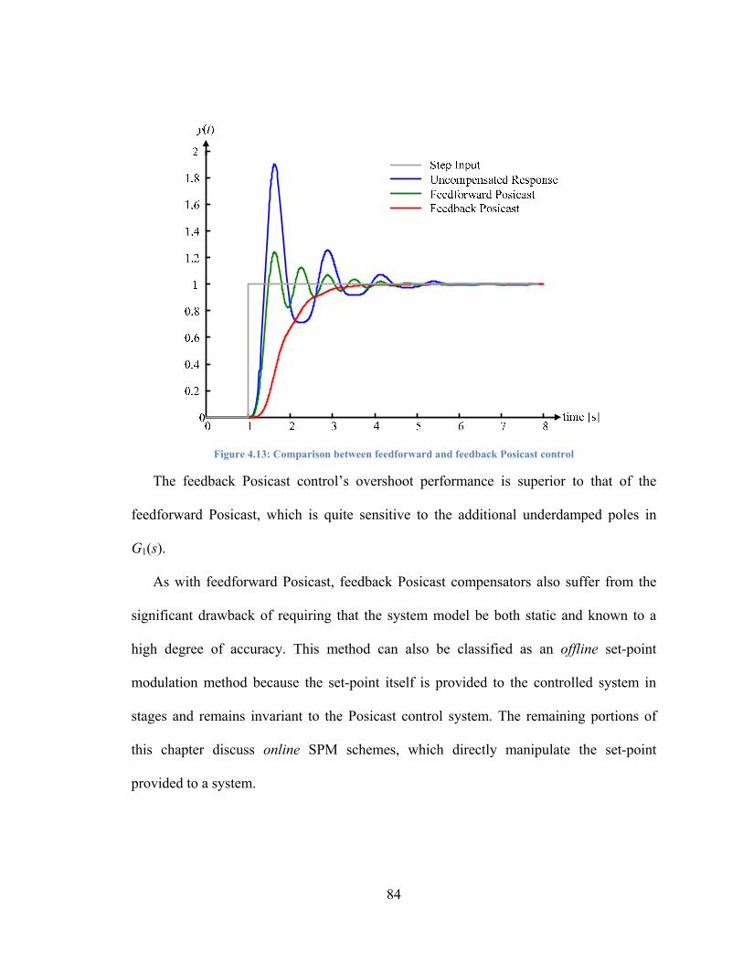
84

Figure 4.13: Comparison between feedforward and feedback Posicast control

The feedback Posicast control’s overshoot performance is superior to that of the

feedforward Posicast, which is quite sensitive to the additional underdamped poles in

G1(s).

As with feedforward Posicast, feedback Posicast compensators also suffer from the

significant drawback of requiring that the system model be both static and known to a

high degree of accuracy. This method can also be classified as an offline set-point

modulation method because the set-point itself is provided to the controlled system in

stages and remains invariant to the Posicast control system. The remaining portions of

this chapter discuss online SPM schemes, which directly manipulate the set-point

provided to a system.

85

4.3 SetPoint Automatic Adjustment (SPAA)

The Set-Point Automatic Adjustment (SPAA) SPM technique was first proposed and

implemented for mitigating large disturbances that occur when starting Distributed

Energy Resources. The SPAA method can be used for second order systems or for

systems where a second-order model is valid [9]. This method calculates intermediate

set-points, which are denoted as sp, such that a set-point change will not exceed a

specified maximum value, ymax. These calculations employ equation (4.6) to compute the

overshoot that would occur by applying a step change between two points sp1 and spfinal.

If the response variable’s computed overshoot exceeds a specified maximum value ymax,

then intermediate set-points are computed such that the set-point changes will not violate

ymax. Once the calculated overshoot does not violate ymax, then no further intermediate set-

points are required, and the transition from sp1 to spfinal can be applied without

modification. This procedure is illustrated in Figure 4.14.

86

Figure 4.14: Intermediate set-points and associated second order system response

87

The time evolution of an underdamped response variable corresponding to a step

change from sp1 to spfinal is

)()()( 11 tyspspspts final (4.15)

Therefore the peak value of the response would be

peakfinalpeak yspspsps )( 11 (4.16)

No intermediate set-points are required if speak < ymax. However, if speak > ymax, an

intermediate set-point 2sp (sp1 < 2sp < sp2final < ymax) will be calculated such that speak ≤

ymax. Combining equations (4.5), (4.6) and (4.16) results in equation (4.17), which is used

for calculating intermediate set-points.

p

p

M

spMysp

11max

2 (4.17)

Several intermediate set-points may be required to achieve an acceptable response

depending upon how restrictive ymax is with respect to the change being applied to the

system. Figure 4.15 shows a flowchart of the SPAA technique.

88

Figure 4.15: SPAA flowchart

To illustrate the series of intermediate set-point calculations, consider a second order

transfer function of the form expressed in equation (4.1) with a damping ratio of ζ =

0.2155 and a natural frequency of ωn = 82 rad/s:

6724342.35

6724

82822155.02

82)(

222

2

sssssG

89

If it is desirable to change the set-point from 0.9 to 1.09 pu and the predetermined

steady state limits are ymin = 0.9 pu and ymax = 1.1 pu, which are chosen by the user of the

algorithm, equation (4.17) and the method shown in Figure 4.15 can be used to devise the

set-points shown in Table 4.1.

Table 4.1: Calculated set-points using SPAA

Iteration Set-point

0 0.9001 1.0332 1.0783 1.090

Figure 4.16 shows the second order system’s response to these set-point changes.

Figure 4.16: Application of SPAA to a second order system

This method shows that calculating intermediate set-points and applying them

sequentially prevents violations from occurring for any system that can be modeled as a

second order system.

90

4.4 SetPoint Automatic AdjustmentCorrection Enabled (SPAACE)

The primary drawback to the SPAA method is that it requires an accurate second

order system model before its intermediate set-points can be calculated. In contrast, the

Set-Point Automatic Adjustment-Correction Enabled (SPAACE) method only requires

limits of operation such as maximum allowable values instead of also requiring advanced

knowledge of system parameters.

The SPAACE technique was originally primarily intended for microgrid applications

[9]. By monitoring the controller output’s response and modifying the control system’s

set-point when necessary to improve controller performance, SPAACE can respond to a

wide variety of perturbations such as load fluctuations, electrical system faults, and other

system disturbances.

Both predictive and non-predictive SPAACE methods exist [10]. In either case, the

set-point is scaled by a fixed percentage of its original value. The response variable is the

only monitored quantity of the non-predictive algorithm, and the set-point is adjusted to

maintain the response variable within predefined limits as soon as the output crosses a

predetermined threshold. The prediction-enabled SPAACE algorithm monitors both the

response variable’s actual response and the trend of the response, and it uses an

extrapolation algorithm to project the response variables’ trajectory. If a criterion

violation is expected, SPAACE manipulates the set-point to either prevent its occurrence

or to reduce the length of time of the violation [9]. As this is accomplished by choosing

appropriate sampling and trajectory projection intervals, designers require sufficient

understanding of the system to determine appropriate sampling times and the trajectory

projection interval.

91

Consider again an underdamped second order system with ζ = 0.5169, ωn = 82 rad/s,

which has a transfer function of the form:

67247716.84

6724)(

2

sssG

This example assumes a modulation index of m = 0.2 and the response variable’s

minimum and maximum permissible values of ymin = 0.9 pu and ymax = 1.10 pu,

respectively. Figure 4.17 illustrates the application of SPAACE without prediction for a

step change u(t) applied from 0.9 pu to 1.09 pu at time t = 0. Once the response variable

crosses the ymax threshold of 1.10 pu, the algorithm modifies the set-point from 1.09 pu to

0.872 pu at t = 0.033 s. In doing so, the algorithm forcibly reduces the response and

produces less overshoot. Once the response variable lies within permissible limits, the

set-point reverts to its original value.

92

Step 1: Set-point adjusted to desired value0 0.02 0.04 0.06 0.08 0.1 0.12 0.14 0.16 0.18 0.2

0.9

0.95

1

1.05

1.1

uncompensated responseset-point

y(t)

time [s]

0 0.02 0.04 0.06 0.08 0.1 0.12 0.14 0.16 0.18 0.20.8

0.85

0.9

0.95

1

1.05

1.1

set-point valueintermediate SPAACE response withoutprediction system

y(t)

time [s]

uncompensated system response

Step 2: Set-point reduced from 1.09 pu to 0.872 pu to bring response below maximum value

0 0.02 0.04 0.06 0.08 0.1 0.12 0.14 0.16 0.18 0.2

0.9

0.95

1

1.05

1.1 ymax

y(t)

time [s]

uncompensated system responseset-point valueSPAACE response withoutprediction

Step 3: Set-point returned to 1.09 pu once response is below the maximum allowable value

ymax

ymax

Figure 4.17: SPAACE example without prediction

93

Figure 4.18 shows the prediction-based SPAACE algorithm applied to the same

underdamped second order system described above. The predictive algorithm monitors

the response variable’s trend and projects its trajectory to anticipate when the unaltered

set-point response variable will violate the maximum threshold. As a result, the algorithm

alters the set-point at t = 0.03 s, which is earlier than the case where SPAACE without

prediction was used. The set-point then reverts to its original value at t = 0.032 s in order

to force the response variable to more closely track the desired value. Not only does

prediction-based SPAACE cause the response variable to attain its final value faster with

less overshoot, but it also does so while remaining completely within the limits

prescribed by the problem.

94

Figure 4.18: Prediction-based SPAACE example

95

4.5 SetPoint Modulation with Fuzzy Logic

This thesis introduces fuzzy logic to set-point modulation as an alternative to the

previously described SPM algorithms. This was accomplished utilizing the

MATLAB/Simulink software package. The control system response’s slope and error

measurements are inputted into a fuzzy inference system (FIS) that determines not only

when to modify the set-point, but also to determine the scaling (modulation) of the

system’s set-point in order to improve the system response.

Figure 4.19: Fuzzy process for SPM

Figures 4.20 and 4.21 show the FIS membership functions used for the slope and

error functions. The horizontal axis is not shown because it is modified depending upon

the compensated system’s characteristics.

Figure 4.20: Membership functions for the slope input to the FIS

96

Figure 4.21: Membership functions for the error input to the FIS

These fuzzified inputs are then combined using the twenty-five if-then rules

summarized in table 4.2.

Table 4.2: Rules for fuzzy logic SPM

Very

Negative Medium Negative

Small Medium Positive

Very Positive

Very Negative

None Medium Positive

Very Positive

Very Positive

Very Positive

Medium Negative

Medium Negative

None Very

Positive Very

Positive Very

Positive

Small Very

Negative Medium Negative


Very Positive

Medium Positive

Very Negative

Very Negative

Very Negative


Very Positive

Very Negative

Very Negative

Very Negative

Medium Negative

None

Slo

pe

Once the rules have been evaluated using the fuzzified inputs, implication is performed

according to the modulation membership functions shown in Figure 4.22. Once again, the

horizontal axis is undefined due to the dependence on the phenomenon and the system

being compensated.

97

0

0.2

0.4

0.6

0.8

1

very negativemedium negativenonemedium positivevery positive

Figure 4.22: Modulation membership functions for the FIS

The results produced by the modulation membership functions are aggregated using the

minimum method, and then a final modulation output value is determined by applying the

centroid defuzzification calculation.

The membership functions employed vary according to the system being

compensated in order to improve system response, but the general membership function

shape and FIS rules are not manipulated. To illustrate this method, consider again a step

change from 0.9 pu to 1.09 pu applied at t = 0 s to an underdamped second order system

of damping ratio ζ = 0.5169 and natural frequency ωn = 82 rad/s:

67247716.84

6724)(

2

sssG

The FIS samples the slope and error of the response every millisecond and determines

the timing and the modulation required to improve the system response. Figure 4.23

shows the set-point waveform provided to the system and the system’s response both

with and without fuzzy SPM.

98

Figure 4.23: Fuzzy logic-enabled SPM applied to second order underdamped system

At t = 0.008 s, the FIS increases the set-point from 1.09 pu to 1.293 pu in order to

increase the rate of rise of the underdamped second order system response and reduce the

error magnitude. As the response approaches the desired value at a sufficient rate, the FIS

reverts the set-point to 1.09 pu at t = 0.014 s. The FIS then determines that the magnitude

of the error is too small for the slope at time t = 0.019 s, and it reduces the set-point to

0.5387 pu to mitigate or eliminate the overshoot. Once the slope and the error are

sufficiently small to prevent significant overshoot from occurring, the FIS reverts the set-

point back to 1.09 pu at t = 0.022 s. As illustrated in Figure 4.23, the fuzzy logic-enabled

SPM control scheme decreases settling time and overshoot compared with an

uncompensated system. This shows that in addition to SPAA and SPAACE, fuzzy logic-

99

enabled SPM can reduce underdamped second order system overshoots and settling

times.

Different damping ratios are simulated to illustrate the robustness of applying the

fuzzy SPM scheme to second order systems. Figure 4.24 illustrates the effect of reducing

the above example’s damping ratio by 10 percent to a value of ζ = 0.46521. A small

change in the damping ratio does not significantly affect the compensated system’s

response.

Figure 4.24: Response of second order system with 10% damping ratio change

Figure 4.25 shows a second order system response with the damping ratio changed

from ζ = 0.5169 to ζ = 0.2.

100

Figure 4.25: Response of second order system with damping ratio of 0.2

Finally, the fuzzy logic-enabled SPM method can even be used to stabilize unstable

systems. Figure 4.26 illustrates the response of a second order system with a damping

ratio of ζ = -0.1

101

Figure 4.26: Response of a second order system with a negative damping ratio

102

Having demonstrated that the fuzzy SPM scheme improves underdamped second

order system responses, it can now be applied to improve the Manitoba Hydro Ponton

SVC control system’s overshoot in response to control actions.

103

Chapter 5 Application of Fuzzy SPM to the Ponton SVC System

Chapter four limited its discussion of SPM’s ability to improve control system

responses to underdamped second order systems for simplicity. This chapter overviews

the Ponton SVC control system as modeled in PSCAD/EMTDC and shows fuzzy SPM’s

ability to improve the Ponton SVC voltage control loop’s response to overshoot to SVC

voltage set-point changes. The fuzzy logic-based SPM algorithm developed in

MATLAB/Simulink was interfaced with PSCAD/EMTDC in order to model step changes

in the Ponton SVC and determine how fuzzy SPM improves the response.

5.1 Ponton SVC

The Ponton SVC is located in northern Manitoba, and its purpose is to increase the

power transfer capability between Northern Manitoba and Southern Manitoba while

maintaining the INCO mining company bus voltage level during transients [31]. The

Ponton SVC consists of a 67.63 MVar delta-connected fixed capacitor bank, an 88.3

MVar delta-connected TCR and a 54.0 MVar delta-connected TSC, and it connects to the

Manitoba Hydro 230 kV transmission network through a 230/9.3/13.8 kV transformer. A

single line diagram of the Ponton SVC is shown in Figure 5.1.

104

Figure 5.1: Ponton SVC single line diagram

5.2 Application of Fuzzy SPM to Ponton SVC Voltage Regulator

A fuzzy logic-based SPM scheme was added to the Ponton SVC’s voltage regulator

to improve its response to reference voltage step changes,.

Figure 5.2: Ponton SVC voltage regulator with fuzzy logic-based SPM

105

5.2.1 System Characteristic

Tuning the fuzzy SPM algorithm and improving its response to set-point

modifications requires a thorough understanding of the Ponton SVC system. Figure 5.3

illustrates the Ponton SVC’s response to a reference voltage step change from 1.03 pu to

1.08 pu for a given system topology and PI controller gains.

5.9 6 6.1 6.2 6.3 6.4 6.51.03

1.04

1.05

1.06

1.07

1.08

1.09

1.1

time [s]

Voltage [pu]

Figure 5.3: Response of Ponton SVC to a step change in reference voltage

The initial difference between the step-input voltage and the voltage response is due

to the strong system voltage. This is because the modeled voltage level in the area is too

high for the SVC to reduce to the desired set-point. The fuzzy SPM algorithm aims to

reduce the maximum overshoot value of 1.1 pu. The relative slope and error magnitudes

that can be expected from the step change must be obtained before tuning the SPM

system. Figures 5.4 and 5.5 show the slope and error waveforms produced with a 1 ms

106

sampling interval. These figures also show that the maximum slope produced from a 0.05

pu step change in Vref is approximately 3 and the maximum error is approximately 0.05

pu.

Figure 5.4: Slope waveform as a result of 0.05 pu step change in reference voltage

107

Figure 5.5: Error waveform as a result of 0.05 pu step change in reference voltage

Applying fuzzy if-then rules described in the previous chapter and knowing the above

information, the prior chapter’s membership functions can be scaled to produce fuzzy

values that in turn produce acceptable modulation. The modulation membership functions

are also scaled such that the algorithm does not excessively modulate the reference value.

Figures 5.6 to 5.8 show the membership functions used to implement the fuzzy SPM.

108

-5 -4 -3 -2 -1 0 1 2 3 4 50

0.1

0.2

0.3

0.4

0.5

0.6

0.7

0.8

0.9

1

Slope

very negativemedium negativesmallmedium positivevery positive

Figure 5.6: Slope membership functions used for initial attempt

Figure 5.7: Error membership functions used for initial attempt

109

Figure 5.8: Modulation membership functions used for initial attempt

5.2.2 Initial Attempt

Once the membership functions are appropriately modified and incorporated into the

algorithm, the step change shown in Figure 5.3 is applied to the Ponton SVC system, but

this time with the fuzzy SPM algorithm applied. As Figure 5.9 illustrates, the algorithm

has a negative effect on the Ponton voltage response compared to the uncompensated

system shown in Figure 5.3.

110

Figure 5.9: Initial attempt at improving step change performance

5.2.3 Membership Function Tuning

The response exhibits a sizeable and problematic delay 10 ms delay between the time

that the Ponton SVC voltage regulator’s step change occurs in reference value and the

time at which the actual response of the controlled voltage begins to track the change.

During this time, the algorithm receives large error values and small slope values and

increases the set-point to increase the rate of rise in the Ponton voltage response.

However, the delay in responding to set-point changes delays the effect of this

modulation, thereby compounding the overshoot problem. Once the algorithm recognizes

and attempts to compensate for this overshoot, the delayed action occurs too late to be

effective.

111

An attempt to solve this problem involves modifying the membership functions and

rules to modulate the set-point sooner in order to improve the timing of the set-point

changes and the system response. The primary algorithm changes include altering the

membership function shapes and reinterpreting the terms large, medium, and small to

improve the system response. Because the delay essentially causes the slope to lag the

error in time, smaller slope magnitudes must be reinterpreted as large in order to improve

the fuzzy SPM algorithm’s output. These resulting membership functions changes are

depicted in Figures 5.10 to 5.12.

-5 -4 -3 -2 -1 0 1 2 3 4 50

0.1

0.2

0.3

0.4

0.5

0.6

0.7

0.8

0.9

1

Slope

μ Slo

pe(x

) very negativemedium negativesmallmedium positivevery positive

Figure 5.10: Modified slope membership functions

112

Figure 5.11: Modified error membership function

-0.05 -0.04 -0.03 -0.02 -0.01 0 0.01 0.02 0.03 0.04 0.050

0.1

0.2

0.3

0.4

0.5

0.6

0.7

0.8

0.9

1

Modulation

very negativemedium negativenonemedium positivevery positive

Figure 5.12: Modified modulation membership functions

113

Figure 5.13: Results after re-tuning fuzzy logic-based SPM algorithm

The re-simulated results illustrated in Figure 5.13 shows a reduction of the initial

peak of the uncompensated response from approximately 1.1 pu to approximately 1.095

pu, but the algorithm produced sustained non-decaying modulation changes resulting

from the 10 ms controller delay. One option for eliminating this characteristic is to enable

the fuzzy SPM algorithm for only a fixed time after the step change in the voltage

reference value, as shown in Figure 5.14. This reduces the initial voltage peak and

removes the sustained oscillations, but it requires advanced knowledge of the timing of

the step change that would be required to properly enable the algorithm. Another attempt

at retuning the membership functions of the fuzzy inference system and altering some

fuzzy if-then rules are required to ensure the algorithm works for the step change without

requiring enabling and disabling.

114

Figure 5.14: System response if SPM algorithm is enabled for a short duration after step change

5.2.4 Modifying Fuzzy Inference System

Accomplishing this requires changing both the membership functions and the rules

that govern the Fuzzy Inference System itself. By emphasizing the error parameter over

the slope parameter, the membership functions prevent the algorithm from modulating

the set-point once the error reduces to a value below a critical threshold irrespective of

the slope. This diminishes the effect of the other rules when the error is small, which

allows the algorithm to stop modulating. Another change eliminates rules that were

designed to quickly dampen oscillations, which are counterproductive due to the system

delay and the relatively slow response when compared with the second order system

115

described in Chapter four. Table 5.1 shows the complete set of new rules utilized in the

revised fuzzy inference system.

Table 5.1: Rules for modified fuzzy inference system

Very

NegativeMedium Negative

Small Medium Positive

Very Positive

Small

Very Negative


None Very

Positive None

Medium Negative

Medium Negative


None None None

Small None Medium Positive

None

Medium Positive

Very Negative

Very Negative

Very Negative

Medium Negative

Medium Negative

None

Very Positive

Very Negative

None None Medium Negative

None None

Figures 5.15 to 5.17 illustrate the retuned membership functions that accompany the

new rules.

Figure 5.15: New slope membership functions

116

Figure 5.16: New error membership functions

Figure 5.17: New modulation membership functions

5.2.5 Results

The results of the retuned algorithm are shown in Figure 5.18. The fuzzy SPM algorithm

reduces the system overshoots and once the oscillation magnitudes reach a sufficiently

small amplitude, the algorithm no longer modulates the reference voltage and the system

117

reaches a steady state operating point. Because the algorithm should be valid for different

set-point magnitude changes, a step change from 1.03 pu to 1.05 pu is applied to the

Ponton SVC system using the same FIS as above. The results with and without the SPM

algorithm are shown in Figure 5.19.

5.9 6 6.1 6.2 6.3 6.4 6.5 6.61.03

1.04

1.05

1.06

1.07

1.08

1.09

1.1

Reference value

Compensated responseUncompensated response

time [s]

Figure 5.18: Results after major changes to the original fuzzy logic enabled SPM algorithm

118

Figure 5.19: Different magnitude of step change with and without fuzzy logic based SPM algorithm

Figure 5.19 shows that the fuzzy SPM algorithm achieves its purpose of reducing the

Ponton SVC system overshoot and demonstrates the ability of a fuzzy logic-enabled SPM

algorithm to improve an SVC voltage regulator’s performance in response to reference

voltage step changes.

119

Chapter 6 Conclusion and Recommendations

6.1 Contributions and Conclusions

This thesis discusses several topics relating to fuzzy logic and set-point modulation

and makes the following contributions:

1. Provides a comprehensive overview of existing set-point modulation techniques

2. Introduces a novel set-point modulation technique that improves control system

performance by employing fuzzy logic to determine the timing and magnitude of

the set-point modulation. Existing SPM methodologies have never been

documented to have utilized fuzzy logic.

3. Develops and tests the fuzzy SPM algorithm in MATLAB/Simulink. The fuzzy

SPM algorithm was initially developed and tested using second order systems.

The results of these second order system tests include:

Development of a tuning procedure for the fuzzy SPM algorithm, which

improves the performance of the system to which it was applied. This

tuning procedure includes:

o Observing the control system’s response to set-point changes

o Scaling the membership functions corresponding to the slope and

error magnitudes so that the membership functions fuzzify the

slope and error corresponding to the application

o Scaling the modulation membership functions to provide

acceptable range of modulations, and

o Reviewing the fuzzy if-then rules to ensure adequate algorithm

operation

120

Once tuned, the fuzzy SPM algorithm showed insensitivity to both small

and large changes in the damping ratio of the second order system to

which it was applied

The fuzzy SPM algorithm also showed an ability to stabilize an unstable

second order system characterized by a negative damping ratio

4. Upon developing and testing in MATLAB/Simulink, the fuzzy SPM algorithm

was developed and implemented in PSCAD/EMTDC

5. Upon implementation in PSCAD/EMTDC, the fuzzy SPM algorithm was applied

to the model of Manitoba Hydro’s Ponton SVC.

6. Once applied to the Ponton SVC model, the fuzzy logic-enabled SPM was shown

to be capable of improving SVC control system performance in response to

control changes such as set-point changes. However, the inherent delays in the

control circuit made it difficult to tune the algorithm to satisfactorily improve

SVC performance. As a result, this work shows that control systems that have

large delays between changing reference values and system responses are

unsuitable candidates for this application.

6.2 Future Work

The following future work suggestions may allow for ease of application of this idea

and widen its possible applicability:

1. Create a Fuzzy Inference System component in PSCAD/EMTDC to enable

easier investigations and eliminate concerns from having to interface

MATLAB with PSCAD/EMTDC.

121

2. Quantitatively compare the fuzzy SPM to existing SPAA and SPAACE

methods.

3. Investigate whether fuzzy SPM can be utilized in other applications such as

HVDC, STATCOMs, and motor drive control systems.

4. Determine this approach’s utility to other power system disturbances such as

fault recovery or load shedding.

In summary, the implementation of a fuzzy-logic enabled SPM method allows for the

intuitive modulation of a control system’s set-point to obtain better performance of the

control system to which it is applied.

122

References

[1] H. Saadat, Power System Analysis, 3rd ed. United States of America: PSA

Publishing, 2010.

[2] P. Kundur, Power System Stability and Control, N. J. Balu and M. G. Lauby, Eds.

New York, United States of America: McGraw-Hill, 1994.

[3] C. W. Taylor, Power System Voltage Stability, 1st ed., N. J. Balu and D.

Maratukulam, Eds. United States: McGraw-Hill, 1994.

[4] T. J. E. Miller, Reactive Power Control In Electric Systems. United States of

America: John Wiley & Sons, 1982.

[5] S. Filizadeh, A. M. Gole, D. A. Woodford, and G. D. Irwin, "An Optimization-

Enabled Electromagnetic Transient Simulation-Based Methodology for HVDC

Controller Design," IEEE Transactions on Power Delivery, vol. 22, no. 4, pp. 2559-

2566, Oct. 2007.

[6] A. M. Gole, S. Filizadeh, R. W. Menzies, and P. L. Wilson, "Optimization-Enabled

Electromagnetic Transient Simulation," IEEE Transactions on Power Delivery, vol.

20, no. 1, pp. 512-518, Jan. 2005.

[7] O. J. M. Smith, "Posicast Control of Damped Oscillatory Systems," Proceedings of

the IRE, vol. 45, no. 9, pp. 1249-1255, Sep. 1957.

[8] G. H. Tallman and O. J. M. Smith, "Analog Study of Dead-Beat Posicast Control,"

IRE Transactions on Automatic Control, vol. 4, no. 1, pp. 14-21, Mar. 1958.

[9] A. Mehrizi-Sani and R. Iravani, "Online Set Point Adjustment for Trajectory

Shaping in Microgrid Applications," IEEE Transactions on Power Systems, vol. 27,

123

no. 1, pp. 216-223, 2012.

[10] A. Mehrizi-Sani and R. Iravani, "Online Set Point Modulation to Enhance Microgrid

Dynamic Response: Theoretical Foundation," IEEE Transactions on Power Systems,

vol. PP, no. 99, pp. 1-8, 2012.

[11] G. Cook, "An Application of Half-Cycle Posicast," IEEE Transactions on Automatic

Control, vol. 11, no. 3, pp. 556-559, Apr. 1966.

[12] L. Gyugyi and E. R. Taylor, "Characteristics of Static, Thyrsitor-Controlled Shunt

Compensators for Power System Transmission Applications," IEEE Transactions on

Power Apparatus and Systems, vol. PAS-99, no. 5, pp. 1795-1804, Sep. 1980.

[13] R. T. Byerly, D. T. Poznaniak, T. Jr., and E.R., "Static Reactive Compensation for

Power Transmission Systems," IEEE Transactions on Power Apparatus and

Systems, vol. PAS-101, no. 10, pp. 3997-4005, Oct. 1982.

[14] L. Gyugyi, R. A. Otto, and T. H. Putman, "Principles and Applications of Static,

Thyristor-Controlled Shunt Compensators," IEEE Transactions on Power Apparatus

and Systems, vol. PAS-97, no. 5, pp. 1935-1945, Sep. 1978.

[15] L. Gyugyi, "Reactive Power Generation and Control by Thyristor Circuits," IEEE

Transactions on Industry Applications, vol. IA-15, no. 5, pp. 521-532, Sep. 1979.

[16] R. L. Hauth, S. A. Miske Jr., and F. Nozari, "The Role and Benefits of Static Var

Systems in High Voltage Power System Applications," IEEE Transactions on Power

Apparatus and Systems, vol. PAS-101, no. 10, pp. 3761-3770, Oct. 1982.

[17] N. G. Hingorani and L. Gyugyi, Understanding FACTS Concepts and Technology of

Flexible AC Transmission Systems, 1st ed., M. El-Hawary, Ed. New York, United

124

States: IEEE Press, 2000.

[18] L. Gyugyi, "Power Electronics in Electric Utilities: Static Var Compensators,"

Proceedings of the IEEE, vol. 76, no. 4, pp. 483-494, Apr. 1988.

[19] A. Olwegard, K. Walve, G. Waglund, H. Frank, and S. Torseng, "Improvement of

Transmission Capacity by Thyristor Controlled Reactive Power," IEEE Transactions

on Power Apparatus and Systems, vol. PAS-100, no. 8, pp. 3930-3939, Aug. 1981.

[20] T. Ohyama, K. Yamashita, T. Maeda, H. Suzuki, and S. Mine, "Effective

Application of Static Var Compensators to Damp Oscillations," IEEE Transactions

onPower Apparatus and Systems, vol. PAS-104, no. 6, pp. 1405-1410, Jun. 1985.

[21] L. Gyugi, "Power Transmission Control: Basic Theory; Problems and Needs;

FACTS Solutions," in Flexible AC Transmission Systems (FACTS). Stevenage,

United Kingdom: The Institution of Electrical Engineers, 1999, ch. 1, pp. 1-72.

[22] R. M. Mathur and R. K. Varma, Thyristor-based FACTS Controllers for Electrical

Transmission Systems, 1st ed., M. E. El-Hawary, Ed. Danvers, United States of

America: Wiley-Interscience, 2002.

[23] L. A. Zadeh, "Outline of a New Approach to the Analysis of Complex Systems and

Decision Processes," IEEE Transactions on Systems, Man, and Cybernetics, vol.

SMC-3, no. 1, pp. 28-44, Jan. 1973.

[24] R. M. Mathur, Static Compensators for Reactive Power Control, 1st ed. Winnipeg,

Canada: Cantext Publications, 1984.

[25] L. A. Zadeh, "Fuzzy Sets," Information and Control, vol. 8, pp. 338-353, 1965.

[26] W. Pedrycz, Fuzzy Control and Fuzzy Systems, 2nd ed., M. J. H. Sterling, Ed.

125

Somerset, England: Research Studies Press LTD., 1993.

[27] E. H. Mamdani, "Application of Fuzzy Logic to Approximate Reasoning Using

Linguistic Synthesis," IEEE Transactions on Computers, vol. C-26, no. 12, pp.

1182-1191, Dec. 1977.

[28] M. Inc., Fuzzy Logic Toolbox User's Guide, 5th ed. Natick, United States of

America: Mathworks, 2010.

[29] H. P. Huang, M. L. Roan, and J. C. Jeng, "On-line Adaptive Tuning for PID

Controllers," IEE Proceedings, Control Theory and Applications, vol. 149, no. 1, pp.

60-67, Jan. 2002.

[30] J. Y. Hung, "Feedback Control with Posicast," IEEE Transactions on Industrial

Electronics, vol. 50, no. 1, pp. 94-99, Feb. 2003.

[31] D. A. N. Jacobson, "Northern AC Transmission System Requirements," Manitoba

Hydro, Winnipeg, System Planning Report, 2002.

Implementation of a Fuzzy Logic Based Set-Point ... - MSpace

Documents

Transcript of Implementation of a Fuzzy Logic Based Set-Point ... - MSpace