Impact of radar-rainfall error structure on estimated flood magnitude across scales: An...

Impact of radar-rainfall error structure on estimated flood magnitudeacross scales: An investigation based on a parsimonious distributedhydrological model

Luciana K. Cunha,1,2 Pradeep V. Mandapaka,3 Witold F. Krajewski,1 Ricardo Mantilla,1

and Allen A. Bradley1

Received 15 March 2012; revised 4 August 2012; accepted 8 August 2012; published 9 October 2012.

[1] The goal of this study is to diagnose the manner in which radar-rainfall input affectspeak flow simulation uncertainties across scales. We used the distributed physically basedhydrological model CUENCAS with parameters that are estimated from available data andwithout fitting the model output to discharge observations. We evaluated the model’sperformance using (1) observed streamflow at the outlet of nested basins ranging in scalefrom 20 to 16,000 km2 and (2) streamflow simulated by a well-established and extensivelycalibrated hydrological model used by the US National Weather Service (SAC-SMA).To mimic radar-rainfall uncertainty, we applied a recently proposed statistical model ofradar-rainfall error to produce rainfall ensembles based on different expected errorscenarios. We used the generated ensembles as input for the hydrological model andsummarized the effects on flow sensitivities using a relative measure of the ensemble peakflow dispersion for every link in the river network. Results show that peak flow simulationuncertainty is strongly dependent on the catchment scale. Uncertainty decreases withincreasing catchment drainage area due to the aggregation effect of the river network thatfilters out small-scale uncertainties. The rate at which uncertainty changes depends on theerror structure of the input rainfall fields. We found that random errors that are uncorrelatedin space produce high peak flow variability for small scale basins, but uncertainties decreaserapidly as scale increases. In contrast, spatially correlated errors produce less scatter in peakflows for small scales, but uncertainty decreases slowly with increasing catchment size.This study demonstrates the large impact of scale on uncertainty in hydrological simulationsand demonstrates the need for a more robust characterization of the uncertainty structure inradar-rainfall. Our results are diagnostic and illustrate the benefits of using the calibration-free, multiscale framework to investigate uncertainty propagation with hydrological models.

Citation: Cunha, L. K., P. V. Mandapaka, W. F. Krajewski, R. Mantilla, and A. A. Bradley (2012), Impact of radar-rainfall error

structure on estimated flood magnitude across scales: An investigation based on a parsimonious distributed hydrological model, WaterResour. Res., 48, W10515, doi:10.1029/2012WR012138.

1. Introduction[2] In this paper we explore the effects that uncertainties

in radar-estimated rainfall have on streamflow simulationby a distributed hydrologic model at a range of spatialscales. Rainfall is the main input to many hydrological mod-els, and its uncertainties affect streamflow simulation [e.g.,

Arnaud et al., 2011]. While a number of direct and indirectmethods are available to estimate rainfall rate and accumu-lation, weather radars remain the only operational instru-ments capable of providing rainfall quantities over largedomains with the space-time resolution required for floodprediction across a large range of scales (�0.1–100,000 km2).Radar-rainfall estimates are subject to significant uncertainty(see Villarini and Krajewski [2010] for a review), and theiruse for flood prediction requires a better understanding ofhow the estimation errors propagate through hydrologicalmodels and affect streamflow prediction across scales.

[3] The main goal of this study is to evaluate the impactthat radar-rainfall uncertainties, associated with rainfallmaps (products) that were generated by the Next-Genera-tion Radar (NEXRAD) system of WSR-88D weather radars[e.g., Fulton et al., 1998], have on flood simulation. As ourgoal is to have the capability to predict potential floodingconditions anywhere within a large region (basin), we havebeen developing a distributed, data-intensive rainfall-runoffmodel. It is clear that for such a model to have useful

1IIHR-Hydroscience & Engineering, University of Iowa, Iowa City,Iowa, USA.

2Now at Department of Civil and Environmental Engineering, Schoolof Engineering and Applied Science, Princeton University, Princeton, NewJersey, USA.

3MeteoSwiss, Switzerland.

Corresponding author: L. K. Cunha, Department of Civil and Environ-mental Engineering, School of Engineering and Applied Science, PrincetonUniversity, E422 Engineering Quad, Princeton, NJ 08544, USA. ([email protected])

©2012. American Geophysical Union. All Rights Reserved.0043-1397/12/2012WR012138

W10515 1 of 22

WATER RESOURCES RESEARCH, VOL. 48, W10515, doi:10.1029/2012WR012138, 2012

http://dx.doi.org/10.1029/2012WR012138

predictive skill in many places within the basin, the mod-el’s parameterizations (physics-based) should depend ondata that characterize details of the domain and the forcingrather than the parameter calibration (e.g., Gupta, 2004).However, since there is no hydrologic theory that couldguide the development of such a model, and due to thedata’s limitations, it is difficult to know which processesshould be represented in detail and which could beneglected or simplified. The importance of various proc-esses depends on the location and the hydrologic ‘‘circum-stances’’ such as seasons and antecedent conditions. On theother hand, there is plenty of evidence documented in the lit-erature that rainfall variability, resolution, and accuracy playcrucial roles in the model’s development and performance.Given the above circumstances, we pose the following ques-tion: given a hydrologic model characterized by a certainskill level, what is the effect of radar-rainfall uncertainty onthe model’s prediction ability? We seek to answer this ques-tion across a range of spatial scales for continuous real-timesimulation. To obtain meaningful answers, we need to avoidcalibrating the model to discharge data because such fittingwould compensate for the uncertainty due to the rainfallinput and thereby compromise our objectives.

[4] Our methodology can be viewed as a data-based simu-lation. It consists of generating ensembles of ‘‘equally proba-ble’’ rainfall fields that have the same error structure as theNEXRAD products. These fields are then propagated througha rainfall-runoff hydrological model that simulates stream-flow for each stream link in a watershed. This approachrequires two main components: (1) a rainfall ensemble gen-erator that provides maps of rainfall input that mimic theactual radar-rainfall uncertainty and (2) a parsimonioushydrological model whose parameters can be prescribed apriori using physical properties of the watershed, therebyeliminating the need for parameter calibration. The modelincludes nonlinearities in the system, and its simulated dis-charge agrees reasonably well with observations. We discussthe main features of these two components below.

[5] Uncertainties in radar rainfall estimates have been stud-ied for more than 30 years [Grayman and Eagleson, 1971;Wilson and Brandes, 1979; Cluckie and Collier, 1991; Ciachand Krajewski, 1999a, 1999b; Seed et al., 1999; Pegram andClothier, 2001; Jordan et al., 2003; Chumchean et al., 2006;Ciach et al., 2007; Habib et al., 2008; Krajewski et al.,2010; AghaKouchak et al., 2010a, 2010b], and several mod-els have been proposed for the statistical description of radar-rainfall errors (see reviews by Villarini and Krajewski, 2009;Mandapaka and Germann, 2010]). Early methods of simulat-ing synthetic radar-rainfall fields, i.e., rainfall fields that arecorrupted by radar-like systematic and random errors, werebased on a conceptual understanding of the uncertaintiesinvolved [Krajewski and Georgakakos, 1985; Krajewski,1993; Anagnostou and Krajewski, 1997; Carpenter andGeorgakakos, 2004]. While these methods attempted to cap-ture the main aspects of the factors that caused uncertainty,they lacked an empirically based quantification of the devia-tions between the true and radar-estimated rainfall. Therefore,there was no guarantee that actual radar-rainfall uncertaintywas realistically represented in studies that used these meth-ods [e.g., Sharif et al., 2002; Sharif et al., 2004]. To over-come this weakness, recent developments focus on theempirically based modeling of radar-rainfall uncertainty

[e.g., Ciach et al., 2007; Germann et al., 2009]. In this studywe adopted the radar-rainfall generator proposed by Villariniet al. [2009], which is based on the empirical radar rainfallerror model by Ciach et al. [2007]. This model characterizesthe statistical structure of radar-rainfall errors with three com-ponents: (1) an overall multiplicative bias factor estimatedusing long-term accumulated radar-rainfall and gauge-rainfallvalues; (2) a systematic distortion function, conditioned onthe radar-estimated rainfall value; and (3) a stochastic factorquantifying residual random errors. The model accounts forrange dependency and for spatial and temporal correlation inerrors. The generator uses a conditional simulation frame-work: Given the estimates provided by a specific radar-rainfallestimation algorithm, the method returns rainfall fields thathave the same error structure as that observed empiricallyfor that algorithm. In our case, the algorithm is the precipi-tation processing system [Fulton et al., 1998] that convertsthe reflectivity data from the WSR-88D weather radars tothe hourly accumulation with approximately 4 km by 4 kmspatial resolution (see Ciach et al. [2007] and Villariniet al. [2009] for details). The fact that the generator is con-ditional on actual radar-rainfall fields ensures relevance topractical applications and allows analysis of real events.

[6] Once realistic radar-rainfall ensembles are generated,they are used as input to a hydrological model that simulatesstreamflow. Each member of the ensemble will result in asomewhat different hydrograph. Does the spread of differentcharacteristics of the resultant hydrographs (such as the peakvalue or the time-to-peak) depend on the scale of the basin?How does the spread compare to the difference between themodel output obtained using the ‘‘observed’’ field (i.e., the oneon which the conditional simulation was based) and thestreamflow observations? We address these questions herein.

[7] Previous studies have demonstrated, albeit indirectly,that a fair investigation of how rainfall errors affect floodsimulation requires a calibration-free hydrological modelsince calibration camouflages uncertainties related to boththe hydrologic model structure and the rainfall input datauncertainty. Carpenter and Georgakakos [2004] investi-gated the impacts of rainfall input and rainfall-runoff modelparametric uncertainty on flow simulation using a cali-brated distributed hydrological model. Their results showedthat errors due to model parameter estimation are of thesame order of magnitude or even larger than the errors dueto rainfall uncertainties. Schröter et al. [2011] used a prob-abilistic model to generate an ensemble of precipitationfields that were then used as input to a hydrological model.The authors calibrated the model based on the differentrainfall ensembles and demonstrated that rainfall uncertain-ties might have a significant impact on the estimated pa-rameter estimates. He et al. [2011] evaluated the impact ofradar rainfall uncertainties on water resource modelingusing a model that was calibrated based on rain gauge data.According to these authors, if radar precipitation were usedto calibrate the model, sensitivity of simulated stream dis-charge to rainfall input would have changed. Fu et al.[2011] investigated the impact of precipitation spatial reso-lution on the hydrological response of an integrated distrib-uted water resource model and concluded that, ‘‘the effectsof precipitation input are so dominant that it could potentiallyimpact the estimates of model parameters when the hydro-logical model is calibrated.’’ The study further concluded

W10515 CUNHA ET AL.: IMPACT OF RADAR-RAINFALL ERROR ON SIMULATED FLOOD W10515

2 of 22

that model parameters estimated by calibration would bebiased in order to compensate for errors introduced by low-resolution precipitation. These studies demonstrate the needfor a simulation framework that isolates uncertainties due toparameter estimation, model structure, and various inputs.

[8] For the above data-based simulation framework toprovide meaningful results (i.e., with respect to the goal ofdeveloping model with predictive skill across scales and atmultiple locations), it is necessary to have a hydrologicmodel with a certain level of skill that results merely fromits structure and ability to mimic the dominant processes ofhydrologic response to rainfall. The numerical values ofthe required coefficients (parameters) should be ‘‘observ-able’’ from the characteristics of the basin, including topog-raphy, land cover, land use, soils, etc. The level of skillshould be such that given a more accurate input, the modelshould provide better output. This is not always the casewith calibrated models that adjust their parameter values tocompensate for uncertainties in the input.

[9] In this study we use a fully distributed, physicallybased, and calibration-free hydrological model that allowsthe isolation of errors due to the rainfall input. A large vari-ety of distributed hydrological models exist whose parame-ters can be derived from physical data. Twelve suchmodels were included in the Distributed Model Intercom-parison Project (DMIP) that evaluated the capabilities ofexisting distributed hydrologic models forced with opera-tional radar-based precipitation [Reed et al., 2004]. In theDMIP project, several research groups compared the resultsfrom calibrated and uncalibrated versions of the modelsand concluded that calibration significantly improves simu-lation results. In our study, we opted to use the term cali-bration-free since we recognize that calibration is notfeasible due to the dynamic parametric complexity problem[Gupta, 2004] that arises when highly spatially explicit ter-rain decomposition is applied. With explicit considerationof spatial variability, the number of parameters increasesexponentially. A large number of error-free observationsthat covers all spectra of hydrological functions and spatio-temporal scales would be required to properly estimatethese parameters through calibration [Sawicz et al., 2011].When streamflow at the outlet of the basin is the only infor-mation used to calibrate these models, the large number ofdegrees of freedom results in equifinality, i.e., a limited abil-ity to uniquely identify parameters [e.g., Ebel and Loague,2006]. In that case, we can never be sure if the model is‘‘right for the right reasons’’ or if errors in the data andmodel structure are being compensated for by errors in pa-rameter values [e.g., Refsgaard, 2004; Ajami et al., 2004].

[10] Hossain et al. [2004] and Heistermann and Kneis[2011] used Monte Carlo simulation to evaluate the effectof rainfall on hydrological simulations without the need todefine optimal parameter sets based on calibration. Bothstudies demonstrated the viability of the approach for smallto medium sized basins; Heistermann and Kneis [2011]identified limitations related to the model’s computationtime even for the small catchment adopted in the study(15 km2). Therefore, a similar approach is not computation-ally feasible for large basins using fine decomposition ofthe terrain (at the hillslope level). In this study we avoidcalibration by adopting a different modeling approach, andinstead of calibrating parameters to achieve better results,

we systematically improved the model’s structure. Duringthe iterative process of adding new components and evalu-ating their impact on the model’s overall performance, werealized the importance of understanding how much of thediscrepancy between the model’s simulated and observedresponses could be due to uncertainty in the rainfall. Thisis, in fact, the main motivation behind our study. We havebeen developing a calibration-free model to enable predic-tion everywhere, in the spirit of the PUB (prediction inungauged basins) initiative [Sivapalan et al., 2003]. Whilea full description of our developments is beyond the scopeof this paper, we illustrate the expected streamflow predic-tion uncertainties due to the errors in the radar-providedinput across a range of spatial scales.

[11] The model provides an impartial evaluation of howrainfall errors propagate through hydrological models andaffect flood prediction across a large range of scales. Calibra-tion is avoided through the use of parameters that are directlyor indirectly linked to the physical properties of the water-shed (e.g., soil water storage capacity, hillslope shape, andchannel flow velocity). Direct methods use spatial informa-tion of physical properties (e.g., DEM), while indirect meth-ods adopt a combination of empirical equations (e.g.,Manning’s formula) and spatial maps of basin properties.The fine decomposition of the terrain into hillslopes and linksresults in a realistic representation of the stream and riverdrainage network, which allows us to apply model equationsthat represent processes close to the scales as they occur innature [Mantilla and Gupta, 2005]. Runoff is generated athillslopes, and water is transported via the drainage networkof connected links. Model equations at the hillslope-link scaleare based on mass and momentum conservation principles.

[12] Previous studies have also demonstrated that flowsimulation uncertainty is strongly dependent on catchmentscale, with uncertainty decreasing as basin scale increases[e.g., Carpenter, 2006; Nikolopoulos and Anagnostou, 2010].This is expected since the river network filters out small-scalevariability and uncertainties [e.g., Mandapaka et al., 2009a].In previous studies [e.g., Carpenter and Georgakakos, 2004;He et al., 2011] this conclusion was reached based on theanalysis of midsize basins, including a limited number ofpoints in the watershed for which streamflow observationswere available and used to calibrate the model. In order tocharacterize the scales for which radar data provide good in-formation for flood prediction, a more comprehensive studyinvolving a large number of sites covering a large range ofscales (from few to thousands of square kilometers) isrequired. The basin decomposition method used in this studyprovides flow simulation for every link in the basin, whichallows us to investigate error scale dependency using a largenumber of locations in the basin (more than 70,000 hillslopelinks) covering a wide range of spatial scales, from hillslope(�0.1 km2) to large watersheds (�17,000 km2).

[13] The study area and data sources are described insection 2. In section 3 we present methodological aspects ofthis work, focusing on the rainfall generator and the hydro-logical model. Section 4 includes the main results of thisstudy, including: (1) the validation of the hydrologicalmodel across multiple scales, (2) the rainfall error scenariosand statistics for the generated rainfall ensembles, and (3)flow sensitivity to different rainfall error scenarios. Section 5presents the main conclusions of this work.


3 of 22

2. Study Area and Data Source[14] The study is carried out for two adjacent basins, the

Iowa and the Cedar River basins, located almost entirely inthe state of Iowa. The total drainage area is 7234 km2 forthe Iowa River (in Marengo) and 16,853 km2 for the CedarRiver (in Cedar Rapids). The climate in this region is char-acterized by cold winters, hot summers, and wet springs,with a mean annual precipitation of nearly 900 mm(source: Oregon Climate Service), potential evapotranspi-ration (PE) of 1060 mm, and actual evaporation of 580 mm(based on MOD16 product [see Mu et al., 2011]). The dom-inant land use is agriculture, consisting mainly of corn-soybean rotations. The agricultural practice imposes a strongseasonality in land cover dynamics. The growing seasonusually starts in May and ends in November.

[15] We chose this study area for two main reasons.First, the region is rich in hydrologic information. FourNEXRAD weather radars (in Des Moines and Davenport inIowa, La Cross, Wisconsin, and Minneapolis, Minnesota)cover the two basins; also 24 USGS streamflow gaugescollect data at the outlet of drainage areas ranging fromapproximately 22 to 16,853 km2. Figure 1 presents a mapof the study area with the location of the weather radarsand the USGS streamflow sites. The second reason forselecting the area is its frequent flooding. The region wasthe center of an extreme flood event in 2008 that affectedapproximately 4800 km2 of Iowa’s agricultural land and

many communities throughout the state. About 1300 blocksin the city of Cedar Rapids were flooded, which affectedmore than 5000 homes and 900 businesses. In Iowa City,16 buildings on The University of Iowa campus werereported flooded and the total cost of recovery from theflood reached $750M. We will use the 2008 flood event todemonstrate the hydrological model’s ability to simulatefloods across scales and to investigate the effect of rainfalluncertainty on the prediction of floods.

[16] We used numerous sources of data in this study.Table 1 summarizes the data sets used as model input, forparameter estimation, and for model validation. Modelinput includes rainfall and potential evapotranspiration(PET). For rainfall we used the stage IV rainfall product,which represents hourly accumulation on approximately4 km by 4 km grids. Stage IV products are provided by theNational Weather Service. Fulton et al. [1998] describe themethods and data used to produce the different multisensorprecipitation products provided by the NWS. Stage IV is apostprocessed product based on the merging of radar andrain gauge data, in particular to remove the mean-field biasin the radar-only estimates. Hereafter, we refer to theseoverall bias corrected fields as reference rainfall. We usedNEXRAD’s stage IV products as a reference in this studyto compare how different rainfall error sources and scenar-ios affect hydrological prediction across scales.

[17] For PET we use the product produced by the NorthAmerican Regional Reanalysis NLDAS-2 with 1 h resolu-tion in time and 0.125� (�13 km) resolution in space. PETis used to estimate the actual evaporation from the surfaceand from the unsaturated and saturated layers of the soil.Dingman [2002] defines PET as ‘‘the rate at which evapo-transpiration would occur from a large area completely anduniformly covered with growing vegetation which hasaccess to an unlimited supply of soil water and withoutadvection or heat-storage effect.’’ Using PET to calculateactual evaporation presumes that the only factor limitingevapotranspiration is water availability. No limitations areimposed on the evaporation of water from the surfacestorage.

[18] We used the National Elevation Data set (NED) with90 m resolution to extract the stream and river network. Ourprocedure [Mantilla and Gupta, 2005] resulted in 78,503hillslopes for the Cedar River basin with an average hill-slope area of 0.20 km2 and 44,527 hillslopes for the IowaRiver basin with an average hillslope area of 0.16 km2. Weused the USGS hydraulic measurements to estimate the pa-rameters of hydraulic geometry equations based on the for-mulation proposed by Dodov [2004], Paik and Kumar[2004], and Mantilla [2007]. To estimate soil hydraulicproperties and water storage availability, we used the SoilSurvey Geographic (SSURGO) Database. To estimate theroughness coefficient (Manning’s) for the overland watertransport equations, we used the high-resolution nationalland cover data set [Homer et al., 2007].

[19] Finally, we used two data sets to evaluate the model’sperformance. First, we used the USGS streamflow data for atotal of 24 sites to compare observed and simulated discharge.It is important to point out that we did not use this informationto calibrate the model’s parameters; therefore, the comparisonconstitutes an independent evaluation of the model’s perform-ance. We also compared the streamflow simulations from

Figure 1. Study area with radar coverage and streamflowsites.


4 of 22

CUENCAS with those from the Sacramento Soil MoistureAccounting (SAC-SMA) model [Burnash, 1995], which isused by the National Weather Service as the main componentof their flood forecasting system [Welles et al., 2007].

3. Methodology[20] To demonstrate our model, we selected a month-

long period with rainfall and streamflow data immediatelypreceding the 2008 flood in Iowa. Our flood predictionmodel is a physically based rainfall-runoff model that sim-ulates response to rainfall forcing at a wide range of scales,with the smallest being at hillslope scale. The geometry ofthe hillslope elements of the model is irregular, but eachhillslope is connected to a channel link whose location isdetermined by analysis of the high-resolution topographydata, as described above. The model uses the informationon land cover and land use, soil types, and topographybased on readily available data that are mapped to the scaleof the hillslopes. This mapping is one of the possible sour-ces of uncertainty in the model, and investigating theseuncertainties will be the focus of future studies. The func-tion of the hillslopes is to partition the rainfall input intosurface runoff, infiltration, and evapotranspiration. This isaccomplished by using empirically based parameterizationsof the relevant processes documented in the literature. Wedo not perform local adjustments (calibration) of the coeffi-cients to force better agreement with the observed stream-flow. Surface runoff and subsurface quick flow feed thechannels, and the water is transported down the drainagenetwork. The discharge is aggregated as the water flows tohigher order streams. The aggregated discharge is attenu-ated by the selected water velocity model. The model has apower law functional form with the velocity dependent onthe magnitude of the discharge and the upstream drainagearea. We estimated the coefficients of the velocity modelby multivariate regression using the USGS collected andpublished discharge and water velocity data [Hirsch andCosta, 2004]. We did this independently of our rainfall-runoff model.

[21] The fact that the model’s parameters are not cali-brated to fit the discharge data implies that we haveavoided favoring the scales at which we have available dis-charge observations. Our model is, in principle, suitable for

prediction at any scale provided that the velocity model isable to correctly simulate transport through the river net-work. For more information on the validity of the velocitymodel applied in this study, please refer to Paik and Kumar[2004], Mantilla [2007], and Mandapaka et al. [2009a].

[22] We evaluated the model performance prior to per-forming our simulation experiment. Clearly if the modeldoes not provide accurate results, it should not be used tostudy the effects of uncertainty in the input data. On the otherhand, if the model’s parameters are fitted to a particular input(rainfall) product, it would, by construction, bias the per-formance of a competing input product. For a calibratedmodel it would be possible to perform better when forced byan inferior input product. Moreno et al. [2012] recently pre-sented a study in which calibration, performed based on aspecific data set, biases model performance when forced by adifferent input. The author calibrated the model based on theNWS stage II radar rainfall data set and concluded that themodel forced by rain gauge data tends to overestimate simu-lated streamflow. This is expected since these authors alsopointed out that stage II products underestimated rainfallcompared to the rain gauge (bias equal to 0.9).

[23] Following our methodology, we forced our modelwith the radar-rainfall input generated by a recently devel-oped error model of the NEXRAD-based hourly rainfallmaps [Ciach et al., 2007; Villarini and Krajewski, 2009].The model is based on a large sample of empirical data andhas a flexible structure, where the total error in radar-rainfall estimate is separated into systematic and randomerrors. Therefore, the model is suitable for studying theimpact of systematic and random errors separately. Usingthe error model, we generated multiple realizations (equallyprobable) of radar-rainfall fields that were conditional onthe observed (reference) field. Each of the generated real-izations has the same statistical error structure as the refer-ence field.

[24] We applied the generated ensemble of the radar-rainfall input to the hydrologic rainfall-runoff model andthus simulated multiple realizations of the discharge. Wethen calculated several performance measures to evaluatethe spread of the obtained discharge values and comparedit with the discrepancy (errors) between the dischargeobtained using the reference input and the observed dis-charge. We calculated these measures at a range of spatial

Table 1. Data Set Used for the Simulations (Model Input, Estimation of Model Parameters, Setting Soil Initial Condition, and ModelValidation)

Physical Processes and Properties Data Setsa

Rainfall Radar Stage IV, NWS (�T ¼ 1 h and �S ¼ 0.05�, almost real time)Potential Evapotranspiration PE from North American Regional Reanalysis, NLDAS-2 Model Input

(�T ¼ 1 h; �S ¼ 0.125�, �13 km)DEM National Elevation Data Set, �S ¼ 90 mHydraulic Measurements USGS Hydraulic MeasurementsSoil Properties SSURGO, �S ¼ polygons with 1 to 10 acres (�0.05 km2) size map delineationLand Cover National Land Cover Database (NLCD), �S ¼ 30 m, 2001Soil Moisture (Initial Condition) Total soil column wetness (0–200 cm), NLDAS-2 Model Output

(�T ¼ 1 h; �S ¼ 0.125�, �13 km)Streamflow USGS streamflow measurements for a total of 24 sites in the study area

(�T¼ 1/4 or 1 h)Simulated Streamflow, SAC-SMA Model

a�S ¼ spatial resolution in minutes (0), arc-seconds (00), degrees (�), or km. �T ¼ temporal resolution in minutes, hours, days, or years.


5 of 22

scales from very small to fairly large (�20,000 km2). Wethen repeated the above ensemble simulation for a differentscenario of the radar-rainfall model.

[25] In the following sections we will focus on thedescription of the two main components of this work: (1) thedistributed physically based hydrological model and (2)the radar-rainfall error model and the ensemble generatorused to produce equally probable rainfall fields based on thereference rainfall (stage IV) and the radar-rainfall error struc-ture scenarios (SCs).

3.1. Hydrological Model

[26] We adopted a hillslope-linked based model thatcompartmentalizes the landscape into small areas whererunoff generation occurs (hillslopes) and that are connectedby the river network (links). Hillslope-link models providea more accurate representation of the river basins and havelower computational requirements than grid-based models[e.g., Yang et al., 2002]. The river network plays an impor-tant role in flood generation by delineating how peak flowchanges across scales [e.g., Gupta et al., 1996; Gupta,2004; Menabde et al., 2001]. Therefore, a correct represen-tation of the river network is essential for simulating floodsacross multiple scales.

[27] We use a set of four coupled nonlinear ordinary dif-ferential equations that describe changes in mass balance ineach control volume to represent hydrological and hydrau-lic processes at hillslopes and links. The four equationsaccount for water balance in the (1) link; (2) surface hill-slope storage; (3) saturated soil zone, and (4) unsaturatedsoil layers. All state variables are solved simultaneouslyusing a time-adaptive numerical method to avoid numericalinconsistencies [Kavetski, 2011]. The solutions to theseequations provide hydrographs at each channel junction inthe network and continuously account for moisture states inthe surface, saturated and unsaturated soil layers, and chan-nels over the entire basin domain.

[28] We reduce complexities on the hillslope dynamics byparameterizing known macroscale hydrological behavior[McGlynn et al., 2002; Graham and McDonnell, 2010].Since we estimate parameters based on observations of rele-vant processes, complexities in the model’s formulation arelimited by data availability. We acknowledge that some im-portant processes are not represented in the model (e.g., soilmacropores). For the reasons previously mentioned, we optedfor a simplified model formulation that does not require cali-bration instead of using a complex conceptualization that suf-fers from equifinality. In this section we provide a generaldescription of the model. A more detailed description includ-ing all the equations is provided by Cunha [2012].

[29] Figure 2a presents a schematic representation of allthe fluxes in the model. Weather radar rainfall is the maininput to the model. We remap the radar rainfall grid to thehillslope-link structure adopted in the model. Once rainfallreaches the surface, it is transformed into surface ponding.Ponding water infiltrates, evaporates, or runs to the chan-nel. The model accounts for infiltration excess (Hortonian),overland flow (HOF), and saturation excess overland flow(SEOF). HOF occurs when ponding water exceeds the infil-tration capacity at the areas of the basin where soil is notsaturated (the permeable area, represented by green in Fig-ure 2). In this region, the percentage of surface water that

infiltrates depends on the deficit of water in the soil (soilvolumetric moisture) and on the soil infiltration capacity.Soil properties are provided by SSURGO. SEOF occurs inthe areas of the basin where soil is saturated (impermeableareas, represented by gray in Figure 2 [Freeze, 1980]). Asin nature, HOF and SEOF might occur simultaneously inthe same hillslope. The transport of the ponding water issimulated using Manning’s equations with roughness pa-rameters estimated based on land cover data.

[30] We adopt a simplified conceptualization of the hill-slope subsurface geometry to estimate impermeable area as afunction of hillslope shape and water volume in the saturatedsoil layer. In Figure 2 we present a schematic representationof this geometry for convex (b-1) and concave (b-2) hill-slopes. Hillslope shape is an important factor affecting rain-fall-runoff partitioning. Convex hillslopes exhibit a highertransport power (due to higher slope) and a lower saturationcapacity than concave hillslopes [Sabzevari et al., 2010] (seeFigures 2(b-1) and 2(b-2)). We assume that the bedrock sur-face is parallel to the hillslope surface, so the water table iscalculated as a function of the volume of water in the satu-rated soil layer. We use the topography data (DEM) to esti-mate a relationship between the water table and thepercentage of impermeable area (for an example, see plots inFigures 2(b-1) and 2(b-2)).

[31] Once the water enters into the soil, it percolates downto recharge the groundwater reservoir. We use the extensionof Darcy’s law, proposed by Buckingham [1907], to simulateflow in the partially saturated layer of the soil. The authorpostulated that Darcy’s law is also valid for soils that are par-tially saturated and, in this case (unsaturated), hydraulic con-ductivity is a function of water content. The rate of changeof unsaturated hydraulic conductivity with soil water contentis a function of soil properties [Davidson et al., 1969]. Waterin the saturated layer of the soil flows to the channel as baseflow. We estimated unsaturated hydraulic conductivity basedon soil water content and soil properties [Davidson et al.,1969]. The flux from the saturated layer to the channel isalso simulated by Darcy’s equation, using saturated hydrau-lic conductivity and terrain slope.

[32] Part of the water is removed from the surface, andfrom the unsaturated and saturated soil layers as evapotrans-piration. Evapotranspiration strongly affects soil moisturecontent, especially between rainfall events in the summerand spring seasons, and consequently plays an importantrole in runoff generation. We use potential evapotranspira-tion (PE) to estimate the actual evaporation from the surfaceand soil. Dingman [2002] defines PE as ‘‘the rate at whichevapotranspiration would occur from a large area completelyand uniformly covered with growing vegetation which hasaccess to an unlimited supply of soil water and withoutadvection or heat-storage effect.’’ Using PE to calculateactual evaporation corresponds to assuming that the only li-mitation for evaporation is water availability. We impose nolimitations on the evaporation of water from the surface stor-age. Evaporation from the soil’s unsaturated layers is limitedby the soil’s volumetric moisture and relative depth of watercompared to the total depth of soil. When a large amount ofwater is available, PE limits maximum evaporation. As inputto the model, we use potential evapotranspiration providedby NLDAS-2 [Xia et al., 2012], with hourly resolution intime and 1/8� resolution in space.


6 of 22

[33] We implemented the model’s equations as part ofthe code built into CUENCAS, initially introduced byMantilla and Gupta [2005] as a research tool to investigatethe morphological characteristics of the river networks andtheir roles in peak flow scaling. The model has been usedin previous studies. Mandapaka et al. [2009a] applied asimplified version of the model to investigate the effect ofrainfall variability on the statistical structure of peak flow.To investigate land cover changes’ effects on flood risk,Cunha et al. [2011] applied a more complete version of themodel that includes surface and subsurface processes.Gupta et al. [2010] refer to CUENCAS as an important toolto perform theoretical investigations that would explain thelink between peak flow versus area scaling parameters andphysical properties of the inputs and the watershed.

[34] As we mentioned earlier, the model is not calibratedto fit the observed discharge. The fact that, in the process ofsolving the governing equations, we have to track the watertransport in all links and hillslopes implies that the model’sstructure is amenable to prediction everywhere. Similarly,there is no imposed temporal scale. In principle, the rainfallrate input could be provided and integrated with any temporal

resolution. At this point, the temporal scale is being definedby the sampling frequency of the observations.

3.2. Radar Rainfall Error (RRE) Model and EnsembleGenerator

[35] We employed the RRE generator proposed byVillarini et al. [2009] to produce ensembles of equallyprobable rainfall fields. The method uses an empiricallyderived error model to generate synthetic probable rainfallfields conditioned on a given rainfall map. The uncertaintymodel adopted in the generator was proposed by Ciachet al. [2007]. In this model, the true pixel-scale averagerainfall RA(x,y) at a location (x,y) within the basin isexpressed as the product of a deterministic component anda random component, both conditioned on reference rain-fall, RR(x,y),

RA ¼ hðRRÞ"ðRRÞ: (1)

[36] The deterministic distortion function hðRRÞ accountsfor the conditional (i.e., on rainfall magnitude) biases,whereas the stochastic factor "ðRRÞ describes the random

Figure 2. Schematic representation of the fluxes among (a) control volume and the simplified concep-tualization hillslope geometric properties for (b-1) convex and (b-2) concave hillslope. In the figure, thefollowing are properties of the hillslope: HT is the total hillslope relief, Hwmax is the maximum watertable, Hb is the depth to the bedrock, Sh is the hillslope average slope, and AH is the hilllslope area. Thefollowing are state variables: hw is the water table level and ai is the hillslope impermeable area.


7 of 22

deviations from the true but unknown rainfall. Note thatboth components are a function of the reference rainfallrate ðRRÞ. This feature has important implications that wereveal later. The deterministic distortion function isapproximated by the two-parameter power law

hðRRÞ ¼ a½B0 � RR�b (2)

and the random component is approximated by a Gaussiandistribution with the mean of 1 and its standard deviationmodeled as a rapidly decreasing hyperbolic function of thereference rainfall :

�½RRðx; yÞ� ¼ cþ d½B0RRðx; yÞ�e: (3)

[37] In equations (2) and (3) B0 is the overall (time inte-grated) bias, defined as the ratio of time-integrated gaugeestimates to time-integrated radar estimates. The parame-ters a and b describe the deterministic distortion function,and c; d; and e are the parameters of the random compo-nent. The parameters were estimated by Ciach et al. [2007]using six-years of level-II hourly rainfall data from theOklahoma City WSR-88D radar site (KTLX) and raingauge records from the Oklahoma Mesonet [Brock et al.,1995] and the Agricultural Research Service (ARS) Micro-net. The parameters vary with season and distance from theradar site. In addition, the authors used the radar- andgauge-rainfall data to estimate the spatial and temporal cor-relation of random errors. Villarini and Krajewski [2009]extended this work by proposing three-parameter exponen-tial functions to describe the correlations in the randomcomponent as

�ð�sÞ ¼ c1exp ��s

c2

� �c3

; (4)

where c1 is the nugget effect that characterizes the small-scale variability of the process and/or measurement errors,c2 represents the correlation length, c3 is the shape parame-ter that controls the shape of the fitted correlation functionat the origin, and x is the separation distance. Villarini et al.[2009] noted difficulties in generating random error fieldsthat simultaneously preserve spatiotemporal correlationsand the dependence of error standard deviation on the rainrates. Consequently, they simplified the generator by neglect-ing temporal correlations. In this study we also neglectedtemporal correlations in the random field generator. This isacceptable if you note that the temporal errors decorrelatemuch faster than the response scale of the basins we study.One could also argue that the spatial correlation has a moredirect effect on the scale-dependent model performance.More details about the generator are provided by Villariniet al. [2009].

[38] The generation of ensemble radar-rainfall fields canbe summarized as follows: (1) the reference rainfall fieldwas corrected for conditional bias using equation (2); (2) anensemble of spatially correlated Gaussian fields with a unitmean and standard deviation conditional on the referencerainfall field was then generated using the Cholesky decom-position method; and (3) the correlated Gaussian fieldswere then multiplied with the bias corrected reference field

from step 1 to obtain an ensemble of equally probable rain-fall fields. Note that for very weak rain rates, because of thehyperbolic nature of the random error standard deviation(equation (3)), there might be negative values in the randomerror fields (step 2). Any such pixels with negative valuesare set to zero to avoid unrealistic rainfall values in step 3.Setting negative values to zero introduces slight bias intothe generated error fields. However, this bias is negligibleand therefore would not significantly affect the general con-clusions of this study.

[39] In this work, we use as ‘‘reference’’ the stage IVrainfall map products provided by the National WeatherService [Fulton et al., 1998]. Since, by construction, theradar-rainfall error model is specific to a radar-rainfallproduct, this raises the issue of whether the parameter val-ues of the ensemble generator are appropriate for this prod-uct. Since the stage IV data set is corrected to match raingauge accumulations, we considered it to be free of overallbias; therefore, we set B0 to 1.0. We can also argue that theoverall character of the microphysical rainfall processes inIowa, especially in the summer convective storms, is simi-lar to that in Oklahoma. In support of this argument, wecite a study by Seo and Krajewski [2011], which shows asimilar behavior of the random error dependence on rainfallmagnitude. Another potential issue with the transferabilityof the Ciach et al., [2007] results is the fact that their modelis valid for a single radar, whereas stage IV is a multiradarproduct. While, in principle, combining data from multipleradars reduces the random radar error, in our case, allradars that cover the Cedar and Iowa River basins do this ata far range, where errors are significant. To mitigate, atleast partially, the problem of strict applicability of the ra-dar-rainfall model to our study area, we define and consider12 different scenarios of RRE and generate 50 ensemblesfor each one.

4. Results and Discussion4.1. Radar Rainfall Error Scenarios

[40] Table 2 presents the 12 rainfall error scenarios con-sidered in this study. We conceptualized these scenarios toallow the independent evaluation of the impacts that differ-ent aspects of the rainfall error structure, including system-atic errors, standard deviation of random errors, and spatialcorrelation of random errors, have on flood simulation.Since we do not know much about the error properties forthe radar-rainfall for eastern Iowa for June 2008, we canget a better idea about the range of sensitivities involved byexploring multiple scenarios. As we mentioned in section3.1, our rainfall ensemble is obtained by imposing Gaussianrandom error fields on the bias corrected reference rainfallfields. For each scenario, we used the generator to producean ensemble of 50 equally probable rainfall fields.

[41] Ciach et al. [2007] and Villarini et al. [2009] pro-vided values of the RRE parameters for Oklahoma thatwere empirically estimated based on a dense rain gaugenetwork over a six year period. Since rainfall in Oklahomaduring summer presents patterns similar to rainfall in Iowa,we use those parameters to represent a realistic scenario ofradar rainfall error. The estimation of the RRE model pa-rameters for Iowa would require data from a dense networkof rain gauges and is outside of the scope of this study. The


8 of 22

Oklahoma parameters provide a realistic description of theexpected error in radar rainfall data obtained with the NEX-RAD system and can be applied for the scope of this study.The radar rainfall error parameters for Oklahoma are pre-sented in SC 1, Table 2. To obtain the remaining scenarios,we systematically altered the Oklahoma parameter valuesto obtain RRE scenarios that isolated the effect of differentcomponents of the RRE model. Note that when we altereda particular component in the model, the parameter valuesfor other components remain fixed to the Oklahoma values.

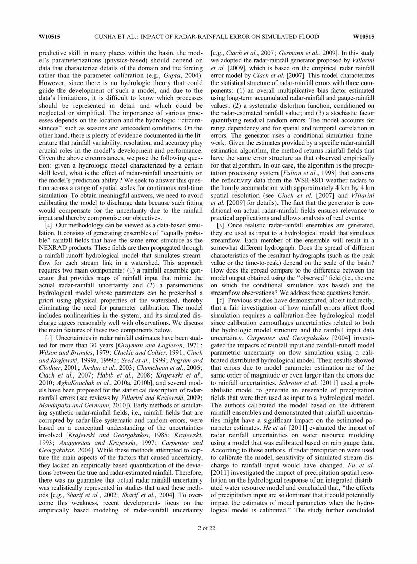
[42] In section 3.1 we have seen that the systematic errorsare characterized by the deterministic distortion function,which is a power law with a coefficient a and an exponent b(equation (3)). The effect of coefficient a on simulatedhydrographs is trivial because it is just a multiplicative fac-tor. Therefore, we focused on the exponent b and altered itsvalues such that we have one scenario with systematic over-estimation (SC 2; b ¼ 0.85) and another scenario withunderestimation by radars (SC 3, b ¼ 1.15). We emphasizethat in all three scenarios (SC 1–3), the systematic errors arenonlinearly related to the radar-rainfall estimate, as demon-strated in Figure 3a.

[43] For the remaining scenarios we isolate the effects ofrandom errors by setting parameters a and b to 1 and vary-ing the parameters that control the standard deviation andspatial correlation structure of the random errors. For SC 4we adopted the empirically estimated parameters for ran-dom error, and for SC 5 and 6 we removed the dependenceof standard deviation on radar-rainfall estimates by settingparameters d and e to zero. While for SC 5 the value of pa-rameter c was fixed to the Oklahoma value of 0.45, for SC6 it was changed to 0.2. Therefore, SC 4, 5, and 6 togetherquantify the effect of standard deviation of random errorsboth when it is conditional and when it is not conditionalon the radar-rainfall estimate. We then gradually increasedthe spatial correlation distance (C2) of random errors from0 to 100 km to obtain SC 7–11. Scenarios 7–11 thereforequantify the effect of spatial coherence of random errors onthe simulated peak hydrographs. For SC 12 we changed theshape parameter (C3) that controls the rate of decrease ofthe spatial correlation with distance. Smaller values of C3

result in a faster decrease in the correlation close to theorigin. Therefore, the effect of small-scale spatial structure

of random errors can be quantified by comparing simula-tions from SC 11 and 12. Figure 3b presents the standarddeviation of the random error, and Figure 3c presents thespatial correlation of the random error adopted for the dif-ferent scenarios.

[44] Figure 4 shows the time series of the accumulatedmean areal precipitation (AMAP) for all ensemble mem-bers and scenarios for the 2008 event, along with the refer-ence AMAP (black line). Different uncertainty scenariostranslate into a different spread of the ensemble AMAP anddifferent biases between the median of the ensemble andthe reference value. Note that in Figure 4 we are looking atthe spread in the time series of (space-time) accumulatedprecipitation fields (or AMAPs). Therefore, the determinis-tic distortion function also affects the spread of AMAPs.This is why SC 3 appears to have larger spread than SC 2even though both scenarios have the same random errorstructure. To reduce the effect of the deterministic distor-tion function on the spread of the ensemble, we calculatedstatistics for the time series of spatial averages (withouttemporal accumulation). In the bottom right of each plot, inblue font, we present a measure of the dispersion (�P) anda measure of the bias (P�) calculated based on the time se-ries of rainfall :

�P ¼ 1

nt

Xnt

i¼1

P95ðtÞ � P5ðtÞP50ðtÞ

for all t for which P50ðtÞ > 0;

(5)

P� ¼

Xt

i¼1

P50ðtÞ � Pref ðtÞ

Xt

i¼1

Pref ðtÞ; (6)

where P5ðtÞ, P50ðtÞ, and P95ðtÞ are the 5th, 50th, and 95thpercentiles of the ensemble of AMAP over Cedar Rapids,and Pref ðtÞ is the accumulated mean area precipitation forthe reference data set. Note that from here on we use theterm dispersion as a synonym for the spread of the ensem-ble. In equation (5) we first normalize the time series ofdispersion by the median value to avoid the effect of biasand then we calculate the average value for the dispersion.

Table 2. Rainfall Error Scenarios

DeterministicDistortionand Bias Bias

Par. SC 1 SC 2 SC 3 SC 4 SC 5 SC 6 SC 7 SC 8 SC 9 SC 10 SC 11 SC 12

Deterministic Biasa 1.34 1 1 1 1 1 1 1 1 1 1 1b 0.84 0.85 1.15 1 1 1 1 1 1 1 1 1

Random Error, SDc 0.45 0.45 0.45 0.45 0.45 0.2 0.45 0.45 0.45 0.45 0.45 0.45d 0.59 0.59 0.59 0.59 0 0 0.59 0.59 0.59 0.59 0.59 0.59e �0.62 �0.62 �0.62 �0.62 0 0 �0.62 �0.62 �0.62 �0.62 �0.62 �0.62

Random Error, Spatial CorrelationC1 1 1 1 1 1 1 0 1 1 1 1 1C2 37 37 37 37 37 37 0 15 37 60 100 100C3 0.39 0.39 0.39 0.39 0.39 0.39 0 1 1 1 1 0.39


9 of 22

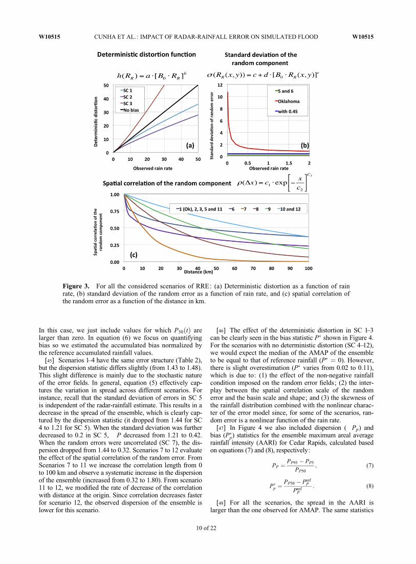
In this case, we just include values for which P50ðtÞ arelarger than zero. In equation (6) we focus on quantifyingbias so we estimated the accumulated bias normalized bythe reference accumulated rainfall values.

[45] Scenarios 1–4 have the same error structure (Table 2),but the dispersion statistic differs slightly (from 1.43 to 1.48).This slight difference is mainly due to the stochastic natureof the error fields. In general, equation (5) effectively cap-tures the variation in spread across different scenarios. Forinstance, recall that the standard deviation of errors in SC 5is independent of the radar-rainfall estimate. This results in adecrease in the spread of the ensemble, which is clearly cap-tured by the dispersion statistic (it dropped from 1.44 for SC4 to 1.21 for SC 5). When the standard deviation was furtherdecreased to 0.2 in SC 5, �P decreased from 1.21 to 0.42.When the random errors were uncorrelated (SC 7), the dis-persion dropped from 1.44 to 0.32. Scenarios 7 to 12 evaluatethe effect of the spatial correlation of the random error. FromScenarios 7 to 11 we increase the correlation length from 0to 100 km and observe a systematic increase in the dispersionof the ensemble (increased from 0.32 to 1.80). From scenario11 to 12, we modified the rate of decrease of the correlationwith distance at the origin. Since correlation decreases fasterfor scenario 12, the observed dispersion of the ensemble islower for this scenario.

[46] The effect of the deterministic distortion in SC 1–3can be clearly seen in the bias statistic P� shown in Figure 4.For the scenarios with no deterministic distortion (SC 4–12),we would expect the median of the AMAP of the ensembleto be equal to that of reference rainfall (P� ¼ 0). However,there is slight overestimation (P� varies from 0.02 to 0.11),which is due to: (1) the effect of the non-negative rainfallcondition imposed on the random error fields; (2) the inter-play between the spatial correlation scale of the randomerror and the basin scale and shape; and (3) the skewness ofthe rainfall distribution combined with the nonlinear charac-ter of the error model since, for some of the scenarios, ran-dom error is a nonlinear function of the rain rate.

[47] In Figure 4 we also included dispersion (�Pp) andbias (P�p) statistics for the ensemble maximum areal averagerainfall intensity (AARI) for Cedar Rapids, calculated basedon equations (7) and (8), respectively:

�PP ¼PP95 � PP5

PP50; (7)

P�p ¼PP50 � Pref

P

PrefP

: (8)

[48] For all the scenarios, the spread in the AARI islarger than the one observed for AMAP. The same statistics

Figure 3. For all the considered scenarios of RRE: (a) Deterministic distortion as a function of rainrate, (b) standard deviation of the random error as a function of rain rate, and (c) spatial correlation ofthe random error as a function of the distance in km.


10 of 22

will be used to quantify dispersion and bias for simulatedpeak flow in section 4.3.2, where we evaluate how uncer-tainty in rainfall propagates through the hydrological modeland affects simulated peak flow.

[49] While it is probable that none of the scenarios wehave considered (except SC 1, whose parameters were empir-ically estimated) represents real radar-rainfall error structurestructures, collectively they allow us to develop a betterunderstanding of the radar-rainfall uncertainty on basin-scalerainfall. The results demonstrate that the rainfall generatoremployed in this work is a useful tool to develop rainfalluncertainty scenarios for hydrologic error propagation stud-ies. The generated rainfall fields will allow us to map rainfalluncertainty to the response of the hydrological system.

4.2. Validation of Hydrological Simulations

[50] Before we used our hydrologic rainfall-runoff modelto study the effects of uncertainty propagation of the rain-fall input, we needed to establish that the model accuratelyrepresents the hydrologic response to heavy rainfall. We didthis by evaluating the model’s performance using observedstreamflow data for 24 sites in Iowa and by comparing thesimulated streamflow with that generated by a semidistrib-uted version of the SAC-SMA. Since 1960, the Sacramentosoil moisture accounting model [Burnash, 1995] has beenused by most of the NWS River Forecast Centers as the mainflood prediction model [Welles et al., 2007]. The model is

classified as semidistributed, deterministic, continuous, andnonlinear. SAC-SMA contains parameters that describe therainfall-runoff and evaporation dynamics as well as parame-ters that describe channel flow transport between two subba-sins [Ajami et al., 2004]. In the semidistributed version, thewatershed is decomposed in multiple subbasins, and one setof parameters is calibrated for each subbasin using 6 h meanareal precipitation (MAP) products produced by the NationalWeather Service [Johnson et al., 1999]. The model uses 14parameters to describe the rainfall-runoff processes and twoparameters to describe channel routing, if the kinematic wavemethod is used. The results presented in this study were gen-erated based on the parameters and SAC-SMA model versioncurrently in use by the North Central River Forecast Centerof the NWS for flood prediction in the study area.

[51] In Table 3 we present goodness-of-fit statistics forboth models. We begin with the mean streamflow valuesbased on observations, CUENCAS simulations, and SAC-SMA simulations. We then present the correlation coeffi-cient and the Nash-Sutcliffe coefficient for both models[Nash and Sutcliffe, 1970]. We present these statistics sincethey are commonly used to evaluate the results of hydro-logical models [Krause et al., 2005]. However, they do notprovide a comprehensive view of how well model simula-tions represent reality. Based on these evaluation statistics,we conclude that both models represent a very similar levelof performance.

Figure 4. Accumulated mean areal precipitation for the 12 rainfall error scenarios for the Cedar Riverbasin. The values indicated in brackets in the bottom right of each plot are the �PA and P�A (see equa-tions (5) and (6)).


11 of 22

[52] Figures 5 and 6 present the observed and simulatedhydrographs produced by CUENCAS and SAC-SMA forall streamflow sites in the Cedar River and Iowa Riverbasins, respectively. We normalized the hydrographs bythe mean annual flood that is used as an approximation forthe bankfull discharge (red line) [Leopold et al. 1964]. Wecalculated the mean annual flood as a function of drainagearea using USGS historical data for the Cedar and IowaRivers. Values above this line approximate flow levelsabove the riverbank. The area of each site is shown in theleft corner, while the statistics and the site number (refer toFigure 1) are shown in the right corner. In the plots, darkblue lines represent the observed hydrographs; black linesshow discharge simulated by CUENCAS using the refer-ence rainfall ; light blue lines show the hydrographs simu-lated by SAC-SMA; and red lines indicate mean annualflood. Differences between observed and predicted stream-flow are due to uncertainties in the input, output, and modelformulation and parameterization. In this study we focus onevaluating uncertainties that arise particularly from rainfallinput errors.

[53] If rainfall input and observed streamflow are used tocalibrate model parameters, uncertainties due to the differ-ent factors cannot be isolated. Since we did not calibrateour model’s parameters, we will demonstrate in this studythat, depending on the basin area and on the error structureof the radar rainfall data, uncertainties due to input uncer-tainty can be as large as the discrepancies between simu-lated and observed streamflow.

[54] It is important to point out that CUENCAS was notcalibrated to fit the hydrographs at specific locations. Inthis sense, sometimes the model is able to reproduce thepeak of the event rather well, but it is not able to correctlyreproduce the time to peak (e.g., CR 7). In such cases, the

performance statistics are reduced dramatically. When themodel is calibrated to fit a specific hydrograph, the timingof the response is probably the most important criterionsince it has a significant impact on the commonly usedmean square error objective functions. Another importantaspect is the presence of uncertainties in the streamflowobservations. Many of the streamflow time series presentedlong periods of missing data (e.g., CR 8, CR 2, and CR 5).To estimate the statistics using observed time series con-taining missing values, we adopted a simple linear interpo-lation procedure to fill the gaps in the time series.

[55] Values of the performance statistics are higher for theCedar Rapids basin for both models. The lower values forthe Iowa River basin are probably due to a large number ofsites for small drainage areas and a large number of sites thatexperienced the backwater effect, which is not accounted forin the formulation of channel dynamics of both hydrologicalmodels. Another reason could be due to the spatially corre-lated errors in the input data that have a large effect oversmall basins. Better performance is expected for large basinssince small-scale error and variability are averaged out bythe effect of the river network. In general, we deem theresults of the noncalibrated model acceptable in the contextof this work.

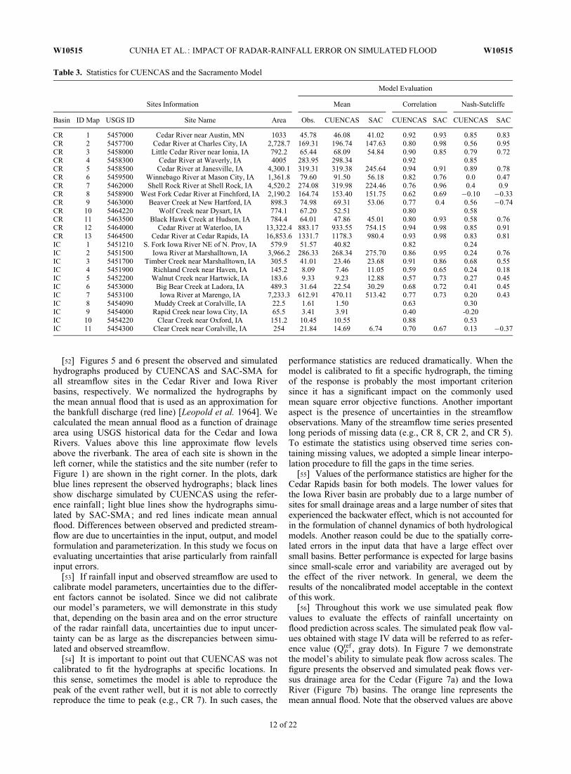
[56] Throughout this work we use simulated peak flowvalues to evaluate the effects of rainfall uncertainty onflood prediction across scales. The simulated peak flow val-ues obtained with stage IV data will be referred to as refer-ence value (Qref

P , gray dots). In Figure 7 we demonstratethe model’s ability to simulate peak flow across scales. Thefigure presents the observed and simulated peak flows ver-sus drainage area for the Cedar (Figure 7a) and the IowaRiver (Figure 7b) basins. The orange line represents themean annual flood. Note that the observed values are above

Table 3. Statistics for CUENCAS and the Sacramento Model

Model Evaluation

Sites Information Mean Correlation Nash-Sutcliffe

Basin ID Map USGS ID Site Name Area Obs. CUENCAS SAC CUENCAS SAC CUENCAS SAC

CR 1 5457000 Cedar River near Austin, MN 1033 45.78 46.08 41.02 0.92 0.93 0.85 0.83CR 2 5457700 Cedar River at Charles City, IA 2,728.7 169.31 196.74 147.63 0.80 0.98 0.56 0.95CR 3 5458000 Little Cedar River near Ionia, IA 792.2 65.44 68.09 54.84 0.90 0.85 0.79 0.72CR 4 5458300 Cedar River at Waverly, IA 4005 283.95 298.34 0.92 0.85CR 5 5458500 Cedar River at Janesville, IA 4,300.1 319.31 319.38 245.64 0.94 0.91 0.89 0.78CR 6 5459500 Winnebago River at Mason City, IA 1,361.8 79.60 91.50 56.18 0.82 0.76 0.0 0.47CR 7 5462000 Shell Rock River at Shell Rock, IA 4,520.2 274.08 319.98 224.46 0.76 0.96 0.4 0.9CR 8 5458900 West Fork Cedar River at Finchford, IA 2,190.2 164.74 153.40 151.75 0.62 0.69 �0.10 �0.33CR 9 5463000 Beaver Creek at New Hartford, IA 898.3 74.98 69.31 53.06 0.77 0.4 0.56 �0.74CR 10 5464220 Wolf Creek near Dysart, IA 774.1 67.20 52.51 0.80 0.58CR 11 5463500 Black Hawk Creek at Hudson, IA 784.4 64.01 47.86 45.01 0.80 0.93 0.58 0.76CR 12 5464000 Cedar River at Waterloo, IA 13,322.4 883.17 933.55 754.15 0.94 0.98 0.85 0.91CR 13 5464500 Cedar River at Cedar Rapids, IA 16,853.6 1331.7 1178.3 980.4 0.93 0.98 0.83 0.81IC 1 5451210 S. Fork Iowa River NE of N. Prov, IA 579.9 51.57 40.82 0.82 0.24IC 2 5451500 Iowa River at Marshalltown, IA 3,966.2 286.33 268.34 275.70 0.86 0.95 0.24 0.76IC 3 5451700 Timber Creek near Marshalltown, IA 305.5 41.01 23.46 23.68 0.91 0.86 0.68 0.55IC 4 5451900 Richland Creek near Haven, IA 145.2 8.09 7.46 11.05 0.59 0.65 0.24 0.18IC 5 5452200 Walnut Creek near Hartwick, IA 183.6 9.33 9.23 12.88 0.57 0.73 0.27 0.45IC 6 5453000 Big Bear Creek at Ladora, IA 489.3 31.64 22.54 30.29 0.68 0.72 0.41 0.45IC 7 5453100 Iowa River at Marengo, IA 7,233.3 612.91 470.11 513.42 0.77 0.73 0.20 0.43IC 8 5454090 Muddy Creek at Coralville, IA 22.5 1.61 1.50 0.63 0.30IC 9 5454000 Rapid Creek near Iowa City, IA 65.5 3.41 3.91 0.40 -0.20IC 10 5454220 Clear Creek near Oxford, IA 151.2 10.45 10.55 0.88 0.53IC 11 5454300 Clear Creek near Coralville, IA 254 21.84 14.69 6.74 0.70 0.67 0.13 �0.37


12 of 22

this line for all sites with a drainage area larger than approxi-mately 100 km2, which indicates that water levels wereabove river banks throughout the watershed. The line in redcorresponds to a nonparametric regression between peakflow and the drainage area. This figure demonstrates that ourmodel is able to capture the scaling of peak flows for the2008 event for the Cedar and Iowa River basins since thesimulated and observed peak flow values follow the samescaling patterns. Streamflow observations present manymissing data, especially during the time of highest flow (e.g.,Figure 6, sites CR 3 and CR 8). Therefore, the direct compar-ison of the observed and simulated results based solely on

the peak flow values can be misleading. Unfortunately, thereare no observed data for small scale sites to confirm the va-lidity of the scaling relationships for small areas. The sitewith the smallest area is located in the Iowa River (inferiorrectus (IR) 1 with approximately 22 km2 of drainage area).

4.3. Analysis of Error Propagation

[57] The hydrological model is executed using each rain-fall error scenario listed in Table 2 as input to obtain an en-semble of streamflow hydrographs. We evaluate the rainfallerror effects on hydrological prediction by comparing the en-semble of simulated hydrographs and the corresponding

Figure 5. Observed (dark blue line) and simulated hydrographs produced by the CUENCAS (grayline) and SAC-SMA (light blue line) models for the Iowa River basin. The basin drainage area is pre-sented on the left side, and the site number (refer to Figure 1) and Nash coefficients are presented on theright side [CUENCAS, SAC-SMA].


13 of 22

peak flows, with the streamflows obtained using the refer-ence rainfall. We also evaluate peak flow variability for eachrainfall scenario ensemble and how it changes with basindrainage area.4.3.1. Comparisons With the USGS StreamflowObservations

[58] We propagate the resulting ensemble rainfall mapsthrough the hydrological model to produce ensembles offlood hydrographs. Results obtained for the Iowa River andCedar River basins are presented in Figures 8 and 9, respec-tively. Both figures present results for error rainfall scenar-ios 2 (Figures 8a and 9a) and 7 (Figures 8b and 9b). SC 2presents random errors correlated in space and determinis-tic bias, and SC 2 consists of random errors not correlatedin space. For the sake of simplicity and brevity, we opted toinclude only four hydrographs for the Iowa River and sixhydrographs for the Cedar River out of a total of 24 simulatedhydrographs. The selected hydrographs cover a wide spectrumof basin areas and are spread around the study area. The loca-tion of the sites is represented in Figure 1 by the blue dots.

[59] Figures 8 and 9 use the same symbol convention asFigures 4 and 5, with the addition of gray shadows that rep-resent the range of values simulated by CUENCAS using the50 ensembles of rainfall. The range of values represented bythe gray shadowed region represents uncertainty in stream-

flow simulation as a result of uncertainty in rainfall. Recallthat the streamflow ensemble presented in these plots weregenerated using hypothetical scenarios of rainfall error con-structed to isolate known aspects of the error (deterministicor random) and to help us understand how each componentcontributes to error in streamflow across scales. Therefore,one should expect that the ensemble does not always capturethe observed flow. Moreover, differences between observedand simulated streamflow might be due to errors in theparameterization of the model, model structure, or uncertain-ties in streamflow time series, the last one being especiallylarge during extreme events due to extrapolation of ratingcurves and hysteresis. Errors can also arise from the mappingof land cover and land use, soil types, and topography fea-tures to the scale of the hillslopes. Investigating these uncer-tainties will be the focus of future studies.

[60] For the Cedar River basin in Cedar Rapids, thehydrograph ensemble reflects the findings of the evaluationin terms of AMAP for SC 7: small spread and a biasbetween the median of the ensemble and the reference dataset. For scenario 2, which considers the radar overestimaterainfall, peaks were reduced across scales, and some spreadis still observed at the scale of the Cedar River basin. Com-paring both scenarios, we can see that the spread for the Ce-dar River is much smaller for scenario 7 than for scenario 2.

Figure 6. Same as Figure 3 but for the Cedar River basin.


14 of 22

However, when we look at the small-scale sites, the spreadfor scenario 7 is larger. This demonstrates that scale depend-ence of streamflow uncertainty changes for different charac-teristics of rainfall error structure.

[61] In Figure 10 we present the relative differencebetween the ensemble and the reference AMAP (plots aand b) and maximum rainfall intensity (plots c and d), nor-malized by the reference values, for scenarios 2 and 7, forall the USGS sites in the Iowa and Cedar River basins. Thespread for AMAP is small since, in this case, the data wereaggregated in space and time, and random errors were can-celed out. On the other hand, we observe significant variabil-ity for the maximum rainfall intensity for each watershed.Due to the purely random character of scenario 7, variabilityin AMAP and maximum rainfall intensity decreases withdrainage area. Rainfall variability also decreases with drain-age area for scenario 2, but some spread is still observed forthe largest basin due to the spatial correlation of the randomerror. These errors are propagated through the hydrologicalmodel. In Figures 10e and 10f, gray dots represent therelative difference between the ensemble rainfall (gray dots)and observed peak flow for the same scenarios (SC 2 and 7),normalized by the observed peak flow. The variabilityobserved in simulated peak flow is closer to the variabilityobserved for maximum rainfall intensity than it is to theone observed for AMAP.

[62] The black dots in Figures 10e and 10f represent therelative difference between the simulated peak flow usingthe reference rainfall and observed peak flow, normalizedby the observed peak flow. For some of the basins, the dif-ference is around 50%. It is important to point out that aconsiderable part of these differences might result frominconsistencies in the series of observed streamflow. Due tothe extreme magnitude of the event, many of these streamgauges malfunctioned or even stopped working during theperiods of large flow. Another source of error in streamflowis due to the extrapolation of the rating curves. Some of thesites experienced water levels much higher than the maxi-mum water levels used to define the rating curve. Modelstructural and parametric uncertainties also contribute tothe differences between observed and simulated values.

[63] The results presented in this section demonstrate thedependence of the error on basin area. However, due to thelimited number of points, it is difficult to understand howerrors change with scale for different scenarios. In the nextsection we present a more comprehensive analysis thatinvolves results for all links in the river network and a rela-tive measure of the dispersion of the flow ensemble.4.3.2. Peak Flow Structure in the River Network

[64] In this section we evaluate the range of simulatedpeak flow for all the links in the river network using a nor-malized measure of peak flow spread. For each link in thewatershed (1) we calculate the difference between the 95th[QP95ðiÞ] and 5th [QP5ðiÞ] percentiles of the ensemble flowvalues normalized by the median [QP50ðiÞ] ensemble flowvalue:

�QPðiÞ ¼QP95ðiÞ � QP5ðiÞ

QP50ðiÞ: (9)

[65] We also calculated the normalized differencebetween the median ensemble value and the reference peakdischarge Qref

P ðiÞ :

Q�PðiÞ ¼QP50ðiÞ � Qref

P ðiÞQref

P ðiÞ: (10)

[66] Results for equations (9) and (10) are presented inFigures 11 and 12, respectively, for all of the rainfall errorscenarios and basin scales ranging from hillslopes (<0.1 km2)to the total basin area (�16,000 km2). �QPðiÞ (Figure 11)represents the extension of the streamflow uncertainty band atthe time of peak for each site. Bias does not affect this vari-able since it is normalized by the median value. Values equalto one mean that the error band extension is as large as themedian of the peak flow simulation. Values equal to zeromean that rainfall data is ‘‘error-free’’ or that errors do notaffect streamflow prediction for that specific site.

[67] We also added a nonparametric regression linebetween �QPðiÞ and the basin area to the plots in order todemonstrate the tendency of �QPðiÞ values to decreasewith basin area (blue for SC 1 and gray for the remainingSCs). This means that as the basin area increases, small-scale uncertainties are filtered out by the aggregation effectof the river network. To help the visual comparison amongSCs, the nonparametric regression for SC 1 (blue line) isincluded in all the plots. The rate at which �QPðiÞdecreases as the basin area increases is not the same for allthe scenarios. We included in the top right of each plot the

Figure 7. Peak flow scaling for the Cedar and IowaRivers. Gray dots are simulated by CUENCAS, dark bluerepresent observed, and light blue represent those simulatedby SAC-SMA. The red line was obtained by nonparametricregression between the drainage area and peak flow simu-lated by CUENCAS. The orange line represents mean an-nual flood.


15 of 22

values of �QPðiÞ for the outlet of Cedar River basin tofacilitate a direct comparison with the values included inFigure 4 for AMAP and AARI.

[68] Scenarios 1–4 have the same random error structure,and therefore the spreads in the values of normalized dis-persion are almost identical (Figure 11). There is a slightvariation in the dispersion statistic among these scenarios,which could be due to different deterministic distortionfunctions (although the dispersion statistic is normalizedwith the median of the ensemble’s values). Scenario 5,whose random errors are not conditional on the radar-rain-fall estimate, displayed similar spread in normalized disper-sion as scenarios 1–4. This is because of the hyperbolicdependence of the error standard deviation on the radar-rainfall estimate (see equation (3)) and demonstrates thatthe conditional dependence of the error standard deviationdoes not have a major impact on the hydrologic response ofthe basin. When the standard deviation is decreased to aconstant value of 0.2 (SC 6), the values of normalizeddispersion and their spread decreased considerably. Overall,

from scenarios 4 to 6, it can be inferred that the absolute valueof standard deviation (either conditional or unconditional) is akey factor in controlling the behavior of peak flows acrossscales. For scenarios 7 to 12 we systematically increase thecorrelation length from 0 to 100 km. The values of normal-ized differences (gray dots in Figure 11) and their spread arelarger for the uncorrelated error scenario (SC 7, c2 ¼ 0 km) atsmall scales. The spread decreased slowly between 0.1 and10 km2 and rapidly thereafter to reach a value close to zero atthe largest scales. The mean value of dispersion (i.e., the non-parametric regression line in Figure 11) drops from �1.4 atthe smallest scale to �0.1 at the largest scale. This indicatesthat the impact of uncorrelated radar-rainfall errors is mainlyfor the watersheds with a size <10 km2, and the river basinfilters out the errors for larger scales. The behavior changedsignificantly with the introduction of correlations in the radarerrors. Even for a smaller correlation length of 15 km (SC 8),the normalized differences failed to reach zero at the largerscales. However, the spread in errors is lower compared tothe uncorrelated scenario. In other words, it is beyond the

Figure 8. Hydrographs for four sites on the Iowa River showing results of the simulation for rainfallerror scenarios (a) 2 and (b) 7. The discharge is normalized by mean annual flood. The dark blue line rep-resents observed hydrographs; the black line is simulated by CUENCAS using the reference rainfall ; thegray shadow represents the lowest and highest values for the ensemble hydrographs simulated by CUEN-CAS using the 50 ensembles of rainfall ; the dash gray line is the median of the ensemble; the light blueline represents the hydrographs simulated by SAC; and the red line reflects mean annual flood.


16 of 22

‘‘capacity’’ of the Cedar River basin to filter out radar-rainfallerrors if the errors are correlated. The effect of correlations onthe simulated peak flows is more evident for c2 valuesbetween 0 and 37 km (scenarios 7–9) and less clear for c2 val-ues between 37 and 100 km (scenarios 9–11). These resultsshow that the spatial correlation of precipitation errorsreduced the rate at which errors decreased with drainage area,as has been demonstrated by Nijssen [2004].

[69] For small scales, �QPðtÞ presents a high range ofvalues for all scenarios. For basin areas close to the hillslopearea, it can go from very low values (approximately 0.4) to

values of more than 3. This means that small-scale basinscan go from receiving almost no water to receiving a largeamount of water. The uncertainty for small scale basins willdepend on the rainfall characteristics for the specific area,the rainfall error structure, and the properties of the basin.

[70] The same convention of Figure 11 is adopted forFigure 12, which presents the measure of bias QP � ðtÞ. Thebias in peak flow caused by the deterministic error is pre-sented for SC 1 to 3. For SC 1, the deterministic erroraffects only large values of rainfall, and the effect for theCedar River is negligible. For SC 2 and 3, the deterministic

Figure 9. Same as Figure 6 but for six sites in the Cedar River basin.


17 of 22

error shifts the median of the sample, depending onwhether the radar is expected to overestimate or underesti-mate rainfall. For SC 4 to 12, we would expect no bias.However, some bias is introduced due to the reasons wementioned in section 4.1. For all the scenarios, the effectsof the bias decreases with drainage area and is negligible atthe outlet for SC 4 to 6 and SC 8 to 12. The bias is still sig-nificant (�11%) at the outlet for SC 7, which presents ran-dom errors not correlated in space.

[71] It is important to include here a discussion about thepossible effect of ignoring the temporal correlation of theradar estimation error on peak flow across scales. Villariniet al. [2009] estimated the temporal correlation of the radarerror for Oklahoma for the hot season. The authors obtainedcorrelation equal to 0.5 for 1 h and 0.35 for 2 h. Based on thisinformation, the temporal correlation is not significant for thegeneration of ensemble radar rainfall maps with a temporalresolution of 1 h. Moreover, the temporal scale of hydrologi-cal response is often larger than 1 h. The inclusion of tempo-ral correlations in radar-rainfall errors would solely affecttime to peak of very small scales that present a concentrationtime on the order of hours. The effect of temporal correlation

would probably be negligible for larger basins since the mag-nitude of this effect depends on the relation between thedecorrelation time of temporal errors (lower than 2 h) and thetime to peak of the hydrograph (that is in the order of daysfor medium to large basins).

5. Conclusions[72] This study was motivated by the need to better

understand the impacts of radar rainfall uncertainties onflood forecasting that emerged during the process of devel-oping a data intensive hydrological model that does notrely on calibration. In the processes of building, modifying,evaluating, and improving a hydrological model with thesefeatures and that focuses on flood prediction across scales,logical questions arise: how much of the discrepanciesbetween simulated and observed discharge are due exclu-sively to rainfall errors? And how well can we simulateobserved values, at different basin scales, based on thebest currently available rainfall products that cover largeareas? This study is an initial attempt to answer thesequestions.

Figure 10. (a and b) Differences between the ensemble and the reference areal mean accumulated pre-cipitation. (c and d) Maximum rainfall intensity normalized by the reference values. (e and f) Differencebetween simulated peak flow using the reference rainfall (black dots) as input and the ensemble rainfall(gray dots) and observed peak flow, normalized by the observed peak flow values. Figures 1a, 1c, and 1eare for scenario 2, while Figures 1b, 1d, and 1f are for scenario 5, Cedar River basin. In the bottom left ofeach line, we added the equations used to generate each plot.


18 of 22

[73] Our methodology consisted of propagating radarderived rainfall uncertainties through a fully distributedhydrological model. We used a calibration-free hydrologi-cal model and evaluated different sources of error that arelikely to occur when precipitation is estimated using radarobservations of rainfall. We found that flood peak uncer-tainty is sensitive to both the deterministic and randomcomponents of rainfall error.

[74] The effect of systematic biases on radar-rainfall esti-mates is to shift the peak flows up or down depending on thetype of bias (overestimation versus underestimation). Theeffect of the random component on simulated peak flows ismore complex. In general, the random errors are filtered outby the aggregation effect of the river network, and uncer-tainty decreases as catchment area increases. When the errorsare not correlated in space, uncertainty decreases consider-ably with basin area, and the peak flow error at the outlet ofthe Cedar River basin is practically negligible (this resultwas consistent for all 50 ensemble members). The dispersionin the simulated peak flow in this case was �140% (of refer-ence value) at the smallest scale and �8% at the largest scale(�17,000 km2) for the Cedar River in Cedar Rapids.

[75] However, we found the efficiency of the river basinin filtering out random errors to be highly sensitive to thepresence of spatial correlation in errors. When rainfallerrors are correlated in space, the process of aggregation

and attenuation by the river network is not as effective infiltering out uncertainties. We found that the Cedar Riverbasin could not filter out errors even with a correlation dis-tance as short as 15 km. Compared to uncorrelated errors,the bias and dispersion decreased at smaller scales andincreased at larger scales. As we further increased the cor-relation length to 100 km, the dispersion was found to be�40% for the largest scale. The shape parameter also has astrong effect since it controls the rate of decrease of thespatial correlation with distance.

[76] The deterministic component of the error tends toproduce a shift in the value of simulated peak flow up ordown, but the width of the error band is still determined bythe magnitude of the random error component and its spa-tial correlation. It is important to point out that these resultsimprove our understanding of how rainfall errors propagatethrough a hydrological model and affect flood predictionacross a large range of scales. Some conclusions are gen-eral and can be applied qualitatively for any radar with anerror structure similar to the one applied here. However,quantitative error assessment depends on the specific radar-rainfall estimation algorithm and, thus, error model param-eters for the radar and area of interest.

[77] Our results are limited to the effect of hourly rainfallaccumulation given on a 4 km by 4 km grid. Higher resolu-tion of radar rainfall is unlikely to change our conclusions

Figure 11. Gray dots [�QPðiÞ, see equation (9)]: the difference between the 95th (QP95) and 5th (QP5)percentile ensemble flow values normalized by the median (QP50) ensemble flow value. The values indi-cated in brackets in the top right of each plot are the �QPðoutletÞ for the outlet of the Cedar River basin(see equation (7)).


19 of 22

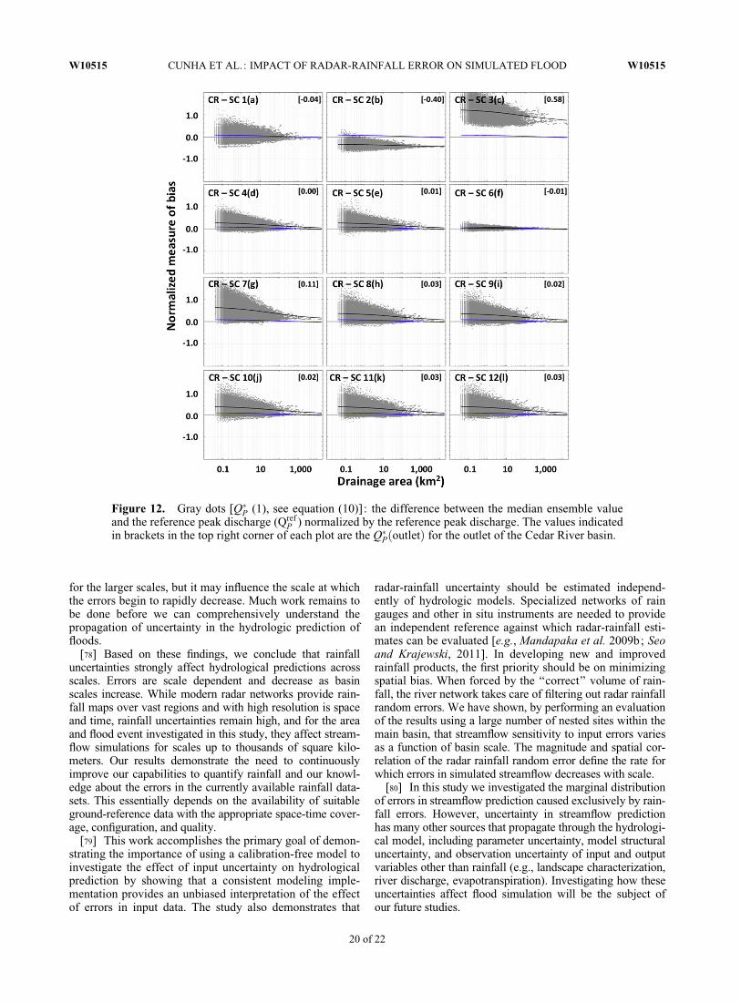
for the larger scales, but it may influence the scale at whichthe errors begin to rapidly decrease. Much work remains tobe done before we can comprehensively understand thepropagation of uncertainty in the hydrologic prediction offloods.

[78] Based on these findings, we conclude that rainfalluncertainties strongly affect hydrological predictions acrossscales. Errors are scale dependent and decrease as basinscales increase. While modern radar networks provide rain-fall maps over vast regions and with high resolution is spaceand time, rainfall uncertainties remain high, and for the areaand flood event investigated in this study, they affect stream-flow simulations for scales up to thousands of square kilo-meters. Our results demonstrate the need to continuouslyimprove our capabilities to quantify rainfall and our knowl-edge about the errors in the currently available rainfall data-sets. This essentially depends on the availability of suitableground-reference data with the appropriate space-time cover-age, configuration, and quality.

[79] This work accomplishes the primary goal of demon-strating the importance of using a calibration-free model toinvestigate the effect of input uncertainty on hydrologicalprediction by showing that a consistent modeling imple-mentation provides an unbiased interpretation of the effectof errors in input data. The study also demonstrates that

radar-rainfall uncertainty should be estimated independ-ently of hydrologic models. Specialized networks of raingauges and other in situ instruments are needed to providean independent reference against which radar-rainfall esti-mates can be evaluated [e.g., Mandapaka et al. 2009b; Seoand Krajewski, 2011]. In developing new and improvedrainfall products, the first priority should be on minimizingspatial bias. When forced by the ‘‘correct’’ volume of rain-fall, the river network takes care of filtering out radar rainfallrandom errors. We have shown, by performing an evaluationof the results using a large number of nested sites within themain basin, that streamflow sensitivity to input errors variesas a function of basin scale. The magnitude and spatial cor-relation of the radar rainfall random error define the rate forwhich errors in simulated streamflow decreases with scale.

[80] In this study we investigated the marginal distributionof errors in streamflow prediction caused exclusively by rain-fall errors. However, uncertainty in streamflow predictionhas many other sources that propagate through the hydrologi-cal model, including parameter uncertainty, model structuraluncertainty, and observation uncertainty of input and outputvariables other than rainfall (e.g., landscape characterization,river discharge, evapotranspiration). Investigating how theseuncertainties affect flood simulation will be the subject ofour future studies.

Figure 12. Gray dots [Q�P (1), see equation (10)]: the difference between the median ensemble valueand the reference peak discharge (Qref

P ) normalized by the reference peak discharge. The values indicatedin brackets in the top right corner of each plot are the Q�PðoutletÞ for the outlet of the Cedar River basin.


20 of 22

[81] Acknowledgments. The authors acknowledge support from theIA Flood Center and the NSF Award DMS-1025483 to conduct this study.Luciana Cunha was supported by NASA Headquarters under the Earth Sci-ence Fellowship grant NNX10AI46G. The third author acknowledges thesupport of the Rose & Joseph Summers Chair endowment. The authorsalso acknowledge many useful comments and suggestions of two anony-mous reviewers and Alan Seed from the Australian Bureau of Meteorologyon the original version of this paper. This revised version hopefully com-municates more effectively the findings of our study.

ReferencesAghaKouchak, A., E. Habib, and A. Bardossy (2010a), Modeling radar

rainfall estimation uncertainties: Random error model, J. Hydrolog.Eng., 15(4), 265–274.

AghaKouchak, A., E. Habib, and A. Bardossy (2010b), Copula-baseduncertainty modeling: Application to multi-sensor precipitation esti-mates, Hydrol. Processes, 24(15), 2111–2124.

Ajami, N. H., H. Gupta, T. Wagener, and S. Sorooshian (2004), Calibrationof a semi-distributed hydrologic model for streamflow estimation along ariver system, J. Hydrol., 298, 112–135, doi:10.1016/j.hydrol.2004.03.033.

Anagnostou, E. N., and W. F. Krajewski (1997), Simulation of radar reflec-tivity fields: Algorithm formulation and evaluation, Water Resour. Res.,33(6), 1419–1429.

Arnaud, P., J. Lavabre, C. Fouchier, S. Diss, and P. Javelle (2011), Sensitiv-ity of hydrological models to uncertainty in rainfall input, Hydrolog. Sci.J., 56(3), 397–410, doi:10.1080/02626667.2011.563742.

Brock, F. V., K. C. Crawford, R. L. Elliot, G. W. Cuperus, S. J. Stadler, H. L.Johnson, and M. D. Eilts (1995), The Oklahoma Mesonet—A TechnicalOverview, J. Atm. Ocean. Technol., 12(1), 5–19.

Buckingham, E. (1907). Studies on the movement of soil moisture, Bull. 38,USDA, Bureau of Soils, Washington, DC.

Burnash, R. J. C. (1995), The NWS river forecast system—Catchment mod-eling, in Computer Models of Watershed Hydrology, edited by V. P.Singh, pp. 311–366, Water Resources Publications, Littleton, CO.

Carpenter, T. M. (2006), Discretization scale dependencies of the ensembleflow range versus catchment area relationship in distributed hydrologic mod-eling, J. Hydrol., 328(1–2), 242–257, doi:10.1016/j.jhydrol.2005.12.008.

Carpenter, T. M., and K. Georgakakos (2004), Impacts of parametric and ra-dar rainfall uncertainty on the ensemble streamflow simulations of a dis-tributed hydrologic model, J. Hydrol., 298(1–4), 202–221, doi:10.1016/j.jhydrol.2004.03.036.

Chumchean, S., A. Sharma, and A. Seed (2006), An integrated approach toerror correction for real-time radar-rainfall estimation, J. Atm. Ocean.Technol., 23(1), 67–79.

Ciach, G. J., and W. F. Krajewski (1999a), Radar-rain gauge comparisonsunder observational uncertainties, J. Appl. Meteorol., 38(10), 1519–1525.

Ciach, G. J., and W. F. Krajewski (1999b), On the estimation of radar rain-fall error variance, Adv. in Water Resour., 22(6), 585–595.

Ciach, G. J., W. F. Krajewski, and G. Villarini (2007), Product-error-drivenuncertainty model for probabilistic quantitative precipitation estimationwith NEXRAD data, J. Hydrometeorol., 8(6), 1325–1347, doi:10.1175/2007JHM814.1.

Cluckie, I. D., and C. G. Collier (1991), Hydrological Applications ofWeather Radar, World Meteorological Organization Bulletin, Chichester.

Cunha, L. K. (2012), Exploring the benefits of Satellite Remote Sensing forflood prediction across scales, Ph.D. thesis, The University of Iowa, IowaCity, IA.

Cunha, L. K., W. F. Krajewski, and R. Mantilla (2011), A framework forflood risk assessment under nonstationary conditions or in the absence ofhistorical data, J. Flood Risk Manage., 4(1), 3–22.

Davidson, J. M., L. R. Stone, D. R. Nielsen, and M. E. Larue (1969), Fieldmeasurement and use of soil-water properties, Water Resour. Res., 5(6),1312–1321, doi:10.1029/WR005i006p01312.

Dingman, S. L. (2002), Physical Hydrology, 2nd ed., Prentice Hall, Engle-wood Cliffs, NJ.

Dodov, B. (2004), Generalized hydraulic geometry: Derivation based on amultiscaling formalism, Water Resour. Res., 40, W06302, doi:10.1029/2003WR002082.

Ebel, B. A., and K. Loague (2006), Physics-based hydrologic-response sim-ulation: Seeing through the fog of equifinality, Hydrolog. Process, 20,2887–2900.

Freeze, R. (1980), A stochastic-conceptual analysis of rainfall-runoff proc-esses on a hillslope, Water Resour. Res., 16(2), 391–408.

Fu, S., T. O. Sonnenborg, K. H. Jensen, and X. He (2011), Impact of precipita-tion spatial resolution on the hydrological response of an integrated distrib-uted water resources model, Vadose Zone J., 10(1), 25–36, doi:10.2136/vzj2009.0186.

Fulton, R., J. Breidenbach, D. Seo, and D. Miller (1998), The WSR-88Drainfall algorithm, Weather Forecasting, 13, 377–395.

Germann, U., M. Berenguer, D. Sempere-Torres, and M. Zappa (2009),REAL-ensemble radar precipitation estimation for hydrology in a moun-tainous region, Q. J. R. Meteorolog. Soc., 135, 445–456.

Graham, C. B., and J. J. McDonnell (2010), Hillslope threshold response torainfall: (2) Development and use of a macroscale model, J. Hydrol.,393, 77–93, doi:10.1016/j.jhydrol.2010.03.008.

Grayman, W. M., and P. S. Eagleson (1971), Evaluation of radar and rain-gage systems for flood forecasting, R. M. Parsons Lab. Rep. 138, 324pp., Mass. Inst. of Technol., Cambridge, MA.

Gupta, V. K. (2004), Emergence of statistical scaling in floods on channelnetworks from complex runoff dynamics, Chaos, Soliton Fract, 19(2),357–365, doi:10.1016/S0960-0779(03)00048-1.

Gupta, V. K., S. Castro, and T. Over (1996), On scaling exponents of spatialpeak flows from rainfall and river network geometry, J. Hydrol., 187,81–104.

Gupta, V. K., R. Mantilla, B. M. Troutman, D. Dawdy, and W. F. Krajewski(2010), Generalizing a nonlinear geophysical flood theory to median-sized river networks, Geophys. Res. Lett., 37(11), L11402, doi:10.1029/2009GL041540.

Habib, E., A. V. Aduvala, and E. A. Meselhe (2008), Analysis of radar-rain-fall error characteristics and implications for stream flow simulationuncertainty, Hydrol. Sci. J., 53, 568–587.

He, X., J. C. Refsgaard, T. O. Sonnenborg, F. Vejen, and K. H. Jensen (2011),Statistical analysis of the impact of radar rainfall uncertainties on waterresources modeling, Water Resour. Res., 47(9), W09526, doi:10.1029/2011WR010670.

Heistermann, M., and D. Kneis (2011), Benchmarking quantitative precipi-tation estimation by conceptual rainfall-runoff modeling, Water Resour.Res., 47(6), W06514, doi:10.1029/2010WR009153.

Hirsch, R. M., and J. E. Costa (2004), U.S. stream flow measurement anddata dissemination improve, Eos Trans. AGU, 85(20), 197–203.

Homer, C., J. Dewitz, J. Fry, and M. Coan (2007), Completion of the 2001National Land Cover Database for the Conterminous United States, Pho-togram. Eng. Remote Sensing, 73, 337–341.

Hossain, F., E. Anagnostou, and T. Dinku (2004), Sensitivity analyses ofsatellite rainfall retrieval and sampling error on flood prediction uncer-tainty, IEEE Trans. Geosci. Remote Sensing, 42, 130–139.

Johnson, D., M. Smith, V. Koren, and B. Finnerty (1999), Comparing meanareal precipitation estimates from NEXRAD and rain gauge networks,J. Hydrol. Eng., 4(2), 117–124.

Jordan, P. W., A. W. Seed, and P. E. Weinmann (2003), A stochastic modelof radar measurement errors in rainfall accumulations at catchment scale,J. Hydrometeorol., 4, 841–855.

Kavetski, D. (2011), Numerical troubles in conceptual hydrology: Approxi-mations, absurdities and impact on hypothesis testing, Hydrol. Processes,25, 661–670, doi:10.1002/hyp.7899.

Krajewski, W. F. (1993), Hydrology, in Encyclopedia of Applied Physics,Vol. 7, pp. 563–579, VCH, Berlin.

Krajewski, W. F. and K. Georgakakos (1985), Synthesis of radar rainfalldata, Water Resour. Res., 21(5), 764–768.

Krajewski, W. F., G. Villarini, and J. A. Smith (2010), Radar-rainfall uncer-tainties: Where are we after thirty years of efforts?, Bull. Am. Meteoro-log. Soc., 91(1), 87–94.

Krause, P., D. P. Boyle, and F. Bäse (2005), Comparison of different effi-ciency criteria for hydrological model assessment, Adv. Geosci., 5, 89–97.

Leopold, L. B., M. G. Wolman, and J. P. Miller (1964), Fluvial Processesin Geomorphology. W.H. Freeman, New York.

Mandapaka, P. V., and U. Germann (2010), Radar-rainfall error models andensemble generators, in Rainfall: State of Science, edited by M. Gebre-michael and F. Testik, Geophysical Monograph Series, 191, pp. 247–264, American Geophysical Union, Washington, DC.

Mandapaka, P., W. F. Krajewski, and R. Mantilla (2009a), Dissecting theeffect of rainfall variability on the statistical structure of peak flows, Adv.Water Resour., 32, 1508–1525.

Mandapaka, P. V., W. F. Krajewski, G. J. Ciach, G. Villarini, and J. A.Smith (2009b), Estimation of radar-rainfall error spatial covariance, Adv.Water Resour., 32(7), 1020–1030.

Mantilla, R. (2007), Physical basis of statistical scaling in peak flows andstream flow hydrographs for topologic and spatially embedded random


21 of 22

self-similar channel networks, Ph.D. thesis, University of Colorado,Boulder, CO.

Mantilla, R., and V. K. Gupta (2005), A GIS numerical framework to studythe process basis of scaling statistics in river networks, IEEE Geosci.Remote Sensing Lett., 2(4), 404–408, doi:10.1109/LGRS.2005.853571.

McGlynn, B., J. McDonnel, and D. Brammer (2002), A review of the evolv-ing perceptual model of hillslope flowpaths at the Maimai catchments,New Zealand, J. Hydrol., 257, 1–26.

Menabde, M., S. Veitzer, and V. Gupta (2001), Tests of peak flow scalingin simulated self-similar river networks, Adv. Water Resour., 24,991–999.

Moreno, H. A., E. R. Vivoni, and D. J. Gochis (2012), Utility of quantitativeprecipitation estimates for high resolution hydrologic forecasts in moun-tain watersheds of the Colorado Front Range, J. Hydrol., 438–439, 66–83, doi:10.1016/j.jhydrol.2012.03.019.

Mu, Q., M. Zhao, and S. W. Running (2011), Improvements to a MODISglobal terrestrial evapotranspiration algorithm, Remote Sensing Environ.,115, 1781–1800.

Nash, J. E. and J. Sutcliffe (1970), Flow forecasting through conceptualmodels part I—A discussion of principles, J. Hydrol., 10, 282–290.

Nijssen, B. (2004), Effect of precipitation sampling error on simulatedhydrological fluxes and states: Anticipating the Global PrecipitationMeasurement satellites, J. Geophys. Res., 109, D02103, doi:10.1029/2003JD003497.

Nikolopoulos, E., and E. Anagnostou (2010), Understanding the scale rela-tionships of uncertainty propagation of satellite rainfall through a distrib-uted hydrologic model, J. Hydrometeorol., 11, 520–532.

Paik, K., and P. Kumar (2004), Hydraulic geometry and the nonlinearity ofthe network instantaneous response, Water Resour. Res., 40, W03602,doi:10.1029/2003WR002821.

Pegram, G. and A. Clothier (2001), Downscaling rainfields in space andtime using the string of beads model in time series mode, Hydrol. EarthSyst. Sci., 5, 175–186.

Reed, S., V. Koren, M. Smith, Z. Zhang, F. Moreda, D. Seo, and DMIP Par-ticipants (2004), Overall distributed model intercomparison projectresults, J. Hydrol., 298, 27–60.

Refsgaard, J. (2004), Modelling guidelines—Terminology and guidingprinciples, Adv. Water Resour., 27, 71–82.

Sabzevari, T., A. Talebi, R. Ardakanian, and A. Shamsai (2010), A steady-state saturation model to determine the subsurface travel time (STT) incomplex hillslopes, Hydrol. Earth Syst. Sci., 14(6), 891–900, doi:10.5194/hess-14-891-2010.

Sawicz, K., T. Wagener, M. Sivapalan, and P. Troch (2011), Catchment classi-fication: Empirical analysis of hydrologic similarity based on catchmentfunction in the eastern USA, Hydrol. Earth Syst. Sci. Discuss., 8, 4495–4534.

Schröter, K., X. Llort, C. Velasco-Forero, M. Ostrowski, and D. Sempere-Torres (2011), Implications of radar rainfall estimates uncertainty on dis-tributed hydrological model predictions, Atm. Res., 100(2–3), 237–245,doi:10.1016/j.atmosres.2010.08.014.

Seed, A. W., R. Srikanthan, and M. Menabde (1999), A space and timemodel for design storm rainfall, J. Geophys. Res., 24, 31623–31630.

Seo, B.-C., and W. F. Krajewski (2011), Investigation of the scale-depend-ent variability of radar-rainfall and rain gauge error correlation, Adv.Water Resour., 34(2), 152–163.

Sharif, H. O., F. L. Ogden, W. F. Krajewski, and M. Xue (2002), Numericalsimulations of radar-rainfall error propagation, Water Resour. Res.,38(8), 1140, doi:10.1029/2001WR000525.

Sharif, H. O., F. L. Ogden, W. F. Krajewski, and M. Xue (2004), Statisticalanalysis of radar-rainfall error propagation, J. Hydrometeorol., 5(1),199–212.

Sivapalan, M. (2003), Prediction in ungauged basins: A grand challengefor theoretical hydrology, Hydrol. Processes, 17, 3163–3170.

Villarini, G., and W. F. Krajewski (2009), Empirically based modelling ofradar-rainfall uncertainties for a C-band radar at different time-scales, Q.J. R. Meteorol. Soc., 135(643), 1424–1438, doi:10.1002/qj.454.

Villarini, G., and W. F. Krajewski (2010), Review of the different sourcesof uncertainty in single polarization radar-based estimates of rainfall,Surveys Geophys., 31(1), 107–129.

Villarini, G., W. F. Krajewski, G. J. Ciach, and D. L. Zimmerman (2009), Prod-uct-error-driven generator of probable rainfall conditioned on WSR-88Dprecipitation estimates, Water Resour. Res., 45(1), W01404, doi:10.1029/2008WR006946.

Welles, E., S. Sorooshian, G. Carter, and B. Olsen (2007), Hydrologic veri-fication: A call for action and collaboration, Bull. Am. Meteorol. Soc.,88, 503–511.

Wilson, J. W., and E. A. Brandes (1979), Radar measurement of rainfall—A Summary, Bull. Am. Meteorol. Soc., 60, 1–11.

Xia, Y., et al., (2012), Continental-scale water and energy flux analysis andvalidation for the North American Land Data Assimilation System pro-ject phase 2 (NLDAS-2): 1. Intercomparison and application of modelproducts, J. Geophys. Res., 117, D03109, doi:10.1029/2011JD016048.

Yang, D., S. Herath, and K. Musiake (2002), A hillslope-based hydrologicalmodel using catchment area and width functions, Hydrolog. Sci. J.,47(1), 49–65, doi:10.1080/02626660209492907.


22 of 22

Impact of radar-rainfall error structure on estimated flood magnitude across scales: An...

Documents

Transcript of Impact of radar-rainfall error structure on estimated flood magnitude across scales: An...