Impact of adaptive thermal comfort criteria on building energy use and cooling equipment size using...

This article appeared in a journal published by Elsevier. The attachedcopy is furnished to the author for internal non-commercial researchand education use, including for instruction at the authors institution

and sharing with colleagues.

Other uses, including reproduction and distribution, or selling orlicensing copies, or posting to personal, institutional or third party

websites are prohibited.

In most cases authors are permitted to post their version of thearticle (e.g. in Word or Tex form) to their personal website orinstitutional repository. Authors requiring further information

regarding Elsevier’s archiving and manuscript policies areencouraged to visit:

http://www.elsevier.com/copyright

http://www.elsevier.com/copyright

Author's personal copyJournal Identification = ENB Article Identification = 3186 Date: July 19, 2011 Time: 7:28 pm

Energy and Buildings 43 (2011) 2055–2067

Contents lists available at ScienceDirect

Energy and Buildings

j ourna l ho me p age: www.elsev ier .com/ locate /enbui ld

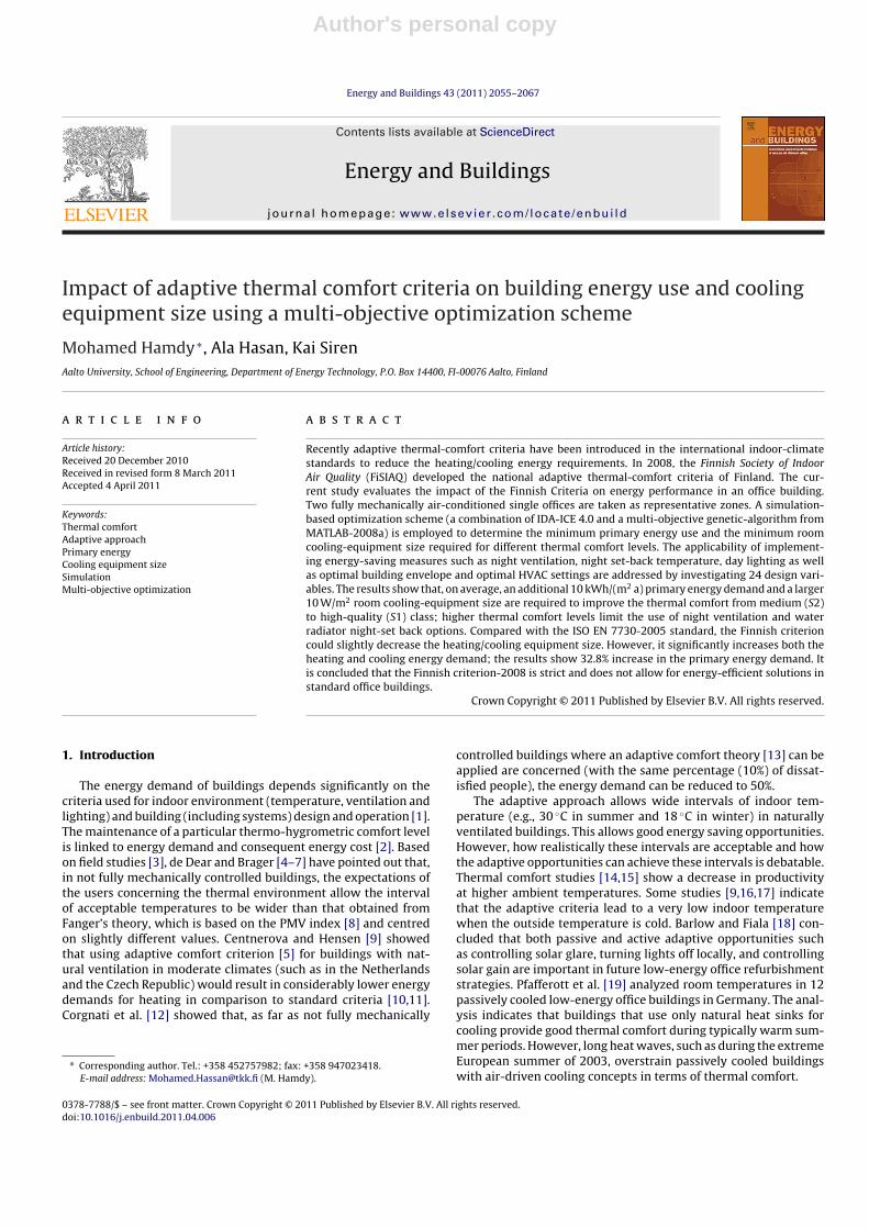
Impact of adaptive thermal comfort criteria on building energy use and coolingequipment size using a multi-objective optimization scheme

Mohamed Hamdy ∗, Ala Hasan, Kai SirenAalto University, School of Engineering, Department of Energy Technology, P.O. Box 14400, FI-00076 Aalto, Finland

a r t i c l e i n f o

Article history:Received 20 December 2010Received in revised form 8 March 2011Accepted 4 April 2011

Keywords:Thermal comfortAdaptive approachPrimary energyCooling equipment sizeSimulationMulti-objective optimization

a b s t r a c t

Recently adaptive thermal-comfort criteria have been introduced in the international indoor-climatestandards to reduce the heating/cooling energy requirements. In 2008, the Finnish Society of IndoorAir Quality (FiSIAQ) developed the national adaptive thermal-comfort criteria of Finland. The cur-rent study evaluates the impact of the Finnish Criteria on energy performance in an office building.Two fully mechanically air-conditioned single offices are taken as representative zones. A simulation-based optimization scheme (a combination of IDA-ICE 4.0 and a multi-objective genetic-algorithm fromMATLAB-2008a) is employed to determine the minimum primary energy use and the minimum roomcooling-equipment size required for different thermal comfort levels. The applicability of implement-ing energy-saving measures such as night ventilation, night set-back temperature, day lighting as wellas optimal building envelope and optimal HVAC settings are addressed by investigating 24 design vari-ables. The results show that, on average, an additional 10 kWh/(m2 a) primary energy demand and a larger10 W/m2 room cooling-equipment size are required to improve the thermal comfort from medium (S2)to high-quality (S1) class; higher thermal comfort levels limit the use of night ventilation and waterradiator night-set back options. Compared with the ISO EN 7730-2005 standard, the Finnish criterioncould slightly decrease the heating/cooling equipment size. However, it significantly increases both theheating and cooling energy demand; the results show 32.8% increase in the primary energy demand. Itis concluded that the Finnish criterion-2008 is strict and does not allow for energy-efficient solutions instandard office buildings.

Crown Copyright © 2011 Published by Elsevier B.V. All rights reserved.

1. Introduction

The energy demand of buildings depends significantly on thecriteria used for indoor environment (temperature, ventilation andlighting) and building (including systems) design and operation [1].The maintenance of a particular thermo-hygrometric comfort levelis linked to energy demand and consequent energy cost [2]. Basedon field studies [3], de Dear and Brager [4–7] have pointed out that,in not fully mechanically controlled buildings, the expectations ofthe users concerning the thermal environment allow the intervalof acceptable temperatures to be wider than that obtained fromFanger’s theory, which is based on the PMV index [8] and centredon slightly different values. Centnerova and Hensen [9] showedthat using adaptive comfort criterion [5] for buildings with nat-ural ventilation in moderate climates (such as in the Netherlandsand the Czech Republic) would result in considerably lower energydemands for heating in comparison to standard criteria [10,11].Corgnati et al. [12] showed that, as far as not fully mechanically

∗ Corresponding author. Tel.: +358 452757982; fax: +358 947023418.E-mail address: [email protected] (M. Hamdy).

controlled buildings where an adaptive comfort theory [13] can beapplied are concerned (with the same percentage (10%) of dissat-isfied people), the energy demand can be reduced to 50%.

The adaptive approach allows wide intervals of indoor tem-perature (e.g., 30 ◦C in summer and 18 ◦C in winter) in naturallyventilated buildings. This allows good energy saving opportunities.However, how realistically these intervals are acceptable and howthe adaptive opportunities can achieve these intervals is debatable.Thermal comfort studies [14,15] show a decrease in productivityat higher ambient temperatures. Some studies [9,16,17] indicatethat the adaptive criteria lead to a very low indoor temperaturewhen the outside temperature is cold. Barlow and Fiala [18] con-cluded that both passive and active adaptive opportunities suchas controlling solar glare, turning lights off locally, and controllingsolar gain are important in future low-energy office refurbishmentstrategies. Pfafferott et al. [19] analyzed room temperatures in 12passively cooled low-energy office buildings in Germany. The anal-ysis indicates that buildings that use only natural heat sinks forcooling provide good thermal comfort during typically warm sum-mer periods. However, long heat waves, such as during the extremeEuropean summer of 2003, overstrain passively cooled buildingswith air-driven cooling concepts in terms of thermal comfort.

0378-7788/$ – see front matter. Crown Copyright © 2011 Published by Elsevier B.V. All rights reserved.doi:10.1016/j.enbuild.2011.04.006


2056 M. Hamdy et al. / Energy and Buildings 43 (2011) 2055–2067

To guarantee high thermal comfort levels, most probably anair-conditioning system is required. In air-conditioned buildings,the clothing of occupants changes according to the weather [20].Other adaptive comfort opportunities such as an adjusting controland/or location might be available. This leads to proposing adaptivethermal comfort criteria in fully mechanically controlled buildings[21–23]. In such buildings, few studies have investigated the adap-tive approach. One criticism of the adaptive comfort approach is itsinherent complexity, which makes it difficult to apply to buildingdesigns (i.e., a special controller is needed for the air-conditioningsystems). In response to this criticism, the adaptive control algo-rithm (ACA) was developed and applied to two air-conditionedbuildings [17]. The ACA showed potential for energy-saving. How-ever, since the time schedule of the test was limited, it was notedthat the ACA must be extensively tested over a long term witha wider range of building types before it can be fully marketedas an alternative solution to fixed set-point temperature controls.Dynamic simulation is used to evaluate the impact of the com-fort approach on the energy demand in fully mechanically controlledand not fully mechanically controlled typical office rooms [12]. Theevaluation addressed a 1-year period, assuming the operative tem-perature set points of the HVAC system control as a function of themean monthly outdoor temperature.

The exponentially weighted mean outside temperature hasbeen found to be a more accurate outdoor temperature indexthan the monthly mean outdoor temperature [16,24]. In 2008, theFinnish Classification of Indoor Climate [25] has introduced adaptivethermal comfort criteria for naturally ventilated and mechanicallyair-conditioned environments. The criteria use the 24-h averageoutdoor temperature as the outdoor temperature index, see Sec-tion 2. The current study evaluates the impact of the Finnishcriterion not only on the energy demand but also on the roomcooling-equipment size. The study addresses two fully mechani-cally air-conditioned single offices as representative zones (Section3). A simulation-based optimization scheme is used to find an opti-mal relation between the energy demand and thermal comfortlevel. Section 4 presents the simulation-based optimization schemeand its objectives, constraints, and design variables. The resultsare presented in Section 5 and discussed in Section 6. Section 7compares the Finnish criterion and EN ISO 7730:2005 in terms ofprimary energy demand and applicability of using energy savingmeasures such as night ventilation and night-setback. The conclu-sion of the study is in Section 8.

2. The Finnish adaptive thermal comfort criterion

The significance of indoor climate for health, comfort and pro-ductivity has been well recognized in Finland in recent decades.Kurnitski and Seppänen [26] briefly summarized the developmentof the indoor climate classifications in Finland. In late 2008, theFinnish Society of Indoor Air Quality (FiSIAQ) released a new Clas-sification [25]. The classification includes three thermal comfortclasses. The first class (S1) corresponds to the best quality, meaninghigher satisfaction with indoor environment. The second class (S2)corresponds to a normal level of expectation. S1 and S2 are pro-posed for fully mechanically air-conditioned environments. WhileS3 is stipulated for naturally ventilated buildings, it is out of thescope of the current study.

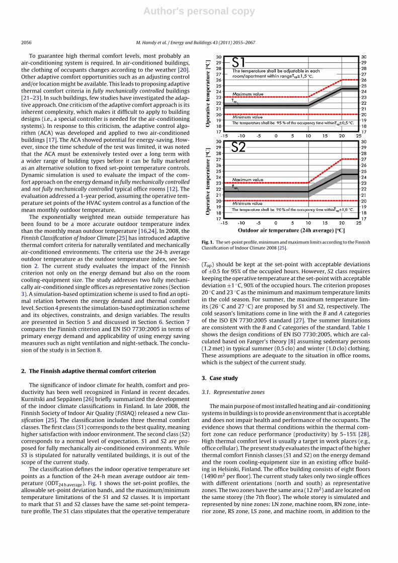
The classification defines the indoor operative temperature setpoints as a function of the 24-h mean average outdoor air tem-perature (ODT24 h average). Fig. 1 shows the set-point profiles, theallowable set-point deviation bands, and the maximum/minimumtemperature limitations of the S1 and S2 classes. It is importantto mark that S1 and S2 classes have the same set-point tempera-ture profile. The S1 class stipulates that the operative temperature

Fig. 1. The set-point profile, minimum and maximum limits according to the FinnishClassification of Indoor Climate 2008 [25].

(Top) should be kept at the set-point with acceptable deviationsof ±0.5 for 95% of the occupied hours. However, S2 class requireskeeping the operative temperature at the set-point with acceptabledeviation ±1 ◦C, 90% of the occupied hours. The criterion proposes20 ◦C and 23 ◦C as the minimum and maximum temperature limitsin the cold season. For summer, the maximum temperature lim-its (26 ◦C and 27 ◦C) are proposed by S1 and S2, respectively. Thecold season’s limitations come in line with the B and A categoriesof the ISO EN 7730:2005 standard [27]. The summer limitationsare consistent with the B and C categories of the standard. Table 1shows the design conditions of EN ISO 7730:2005, which are cal-culated based on Fanger’s theory [8] assuming sedentary persons(1.2 met) in typical summer (0.5 clo) and winter (1.0 clo) clothing.These assumptions are adequate to the situation in office rooms,which is the subject of the current study.

3. Case study

3.1. Representative zones

The main purpose of most installed heating and air-conditioningsystems in buildings is to provide an environment that is acceptableand does not impair health and performance of the occupants. Theevidence shows that thermal conditions within the thermal com-fort zone can reduce performance (productivity) by 5–15% [28].High thermal comfort level is usually a target in work places (e.g.,office cellular). The present study evaluates the impact of the higherthermal comfort Finnish classes (S1 and S2) on the energy demandand the room cooling-equipment size in an existing office build-ing in Helsinki, Finland. The office building consists of eight floors(1490 m2 per floor). The current study takes only two single officeswith different orientations (north and south) as representativezones. The two zones have the same area (12 m2) and are located onthe same storey (the 7th floor). The whole storey is simulated andrepresented by nine zones: LN zone, machine room, RN zone, inte-rior zone, RS zone, LS zone, and machine room, in addition to the


M. Hamdy et al. / Energy and Buildings 43 (2011) 2055–2067 2057

Table 1Three categories of thermal environment, ISO EN 7730, 2005 [27].

Category Thermal state of the body Operative temperature◦C

PPD PMV Summer Winter

A <6 −0.2 < PMV < +0.2 23.5–25.5 21–23B <10 −0.5 < PMV < +0.5 23–26 20–24C <15 −0.7 < PMV < +0.7 22–27 19–25

RN Zone

LS Zon e

South Zon e

North Zone

LN Zon e

Interior Zone

RS Zone

Toilet Zone

Machine Room

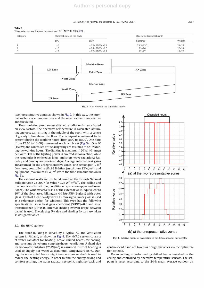
Fig. 2. Plan view for the simplified model.

two representative zones as shown in Fig. 2. In this way, the inter-nal wall-surface temperatures and the mean radiant temperatureare calculated.

The simulation program established a radiation balance basedon view factors. The operative temperature is calculated assum-ing one occupant sitting in the middle of the room with a centreof gravity 0.6 m above the floor. The occupant is assumed to bepresent during the working hours (from 8:00 to 18:00). One hour(from 12:00 to 13:00) is assumed as a lunch break (Fig. 3a). One PC(150 W) and controlled artificial lighting are assumed to be ON dur-ing the working hours. (The lighting is maximum 150 W, 40 lumenper watt; 30% of the lighting power is emitted as convection, whilethe remainder is emitted as long- and short-wave radiation.) Sat-urday and Sunday are weekend days. Average internal heat gainsare assumed for the unrepresentative zones: one person per 12 m2

floor area, controlled artificial lighting (maximum 12 W/m2), andequipment (maximum 10 W/m2) with the time schedule shown inFig. 3b.

The external walls are insulated based on the Finnish NationalBuilding Code C3-2007 (U-value = 0.24 W/(m2 K)). The ceiling andthe floor are adiabatic (i.e., conditioned spaces on upper and lowerfloors). The window area is 35% of the external walls, equivalent to20% of the floor area. Pilkington 4-15Ar-SN6 (2-glass) with outerglass Optifloat Clear, cavity width 15 mm argon, inner glass is usedas a reference design for windows. This type has the followingspecifications: solar heat gain coefficient (SHGC) = 0.6 and solartransmittance (T) = 0.48. Internal shading (woven drape betweenpanes) is used. The glazing U-value and shading factors are takenas design variables.

3.2. The HVAC systems

The office building is served by a typical AC and ventilationsystem in Finland, as shown in Fig. 4. The HVAC system consistsof water radiators for heating, active chilled beams for cooling,and constant air volume supply/exhaust ventilation. A fixed sizefor hot-water radiators (25 W/m2) is assumed. District heating isused to supply hot water at maximum temperature 55 ◦C. Dur-ing the unoccupied hours, night temperature set-back is used toreduce the heating energy. In order to find the energy-saving andcomfort settings, the water radiator set-point, night set-back, and

Fig. 3. Relative profile of occupation in the different zones during 24 h.

control-dead band are taken as design variables via the optimiza-tion scheme.

Room cooling is performed by chilled beams installed on theceiling and controlled by operative temperature sensors. The set-point is reset according to the 24-h mean average outdoor air



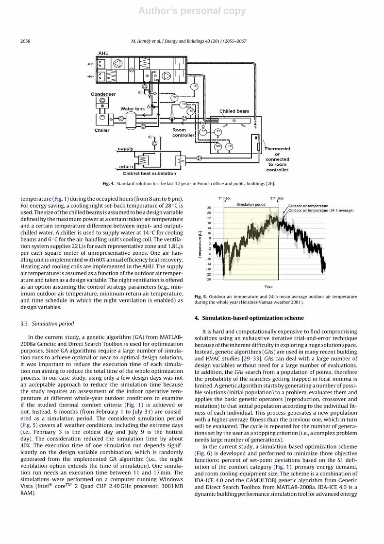
Fig. 4. Standard solution for the last 12 years in Finnish office and public buildings [26].

temperature (Fig. 1) during the occupied hours (from 8 am to 6 pm).For energy saving, a cooling night set-back temperature of 28 ◦C isused. The size of the chilled beams is assumed to be a design variabledefined by the maximum power at a certain indoor air temperatureand a certain temperature difference between input- and output-chilled water. A chiller is used to supply water at 14 ◦C for coolingbeams and 6 ◦C for the air-handling unit’s cooling coil. The ventila-tion system supplies 22 L/s for each representative zone and 1.8 L/sper each square meter of unrepresentative zones. One air han-dling unit is implemented with 60% annual efficiency heat recovery.Heating and cooling coils are implemented in the AHU. The supplyair temperature is assumed as a function of the outdoor air temper-ature and taken as a design variable. The night ventilation is offeredas an option assuming the control strategy parameters (e.g., min-imum outdoor air temperature, minimum return air temperature,and time schedule in which the night ventilation is enabled) asdesign variables.

3.3. Simulation period

In the current study, a genetic algorithm (GA) from MATLAB-2008a Genetic and Direct Search Toolbox is used for optimizationpurposes. Since GA algorithms require a large number of simula-tion runs to achieve optimal or near-to-optimal design solutions,it was important to reduce the execution time of each simula-tion run aiming to reduce the total time of the whole optimizationprocess. In our case study, using only a few design days was notan acceptable approach to reduce the simulation time becausethe study requires an assessment of the indoor operative tem-perature at different whole-year outdoor conditions to examineif the studied thermal comfort criteria (Fig. 1) is achieved ornot. Instead, 6 months (from February 1 to July 31) are consid-ered as a simulation period. The considered simulation period(Fig. 5) covers all weather conditions, including the extreme days(i.e., February 3 is the coldest day and July 9 is the hottestday). The consideration reduced the simulation time by about40%. The execution time of one simulation run depends signif-icantly on the design variable combination, which is randomlygenerated from the implemented GA algorithm (i.e., the nightventilation option extends the time of simulation). One simula-tion run needs an execution time between 11 and 17 min. Thesimulations were performed on a computer running WindowsVista (Intel® coreTM 2 Quad CUP 2.40 GHz processor, 3061 MBRAM).

Fig. 5. Outdoor air temperature and 24-h mean average outdoor air temperatureduring the whole year (Helsinki-Vantaa weather 2001).

4. Simulation-based optimization scheme

It is hard and computationally expensive to find compromisingsolutions using an exhaustive iterative trial-and-error techniquebecause of the inherent difficulty in exploring a huge solution space.Instead, genetic algorithms (GAs) are used in many recent buildingand HVAC studies [29–33]. GAs can deal with a large number ofdesign variables without need for a large number of evaluations.In addition, the GAs search from a population of points, thereforethe probability of the searches getting trapped in local minima islimited. A genetic algorithm starts by generating a number of possi-ble solutions (initial population) to a problem, evaluates them andapplies the basic genetic operators (reproduction, crossover andmutation) to that initial population according to the individual fit-ness of each individual. This process generates a new populationwith a higher average fitness than the previous one, which in turnwill be evaluated. The cycle is repeated for the number of genera-tions set by the user as a stopping criterion (i.e., a complex problemneeds large number of generations).

In the current study, a simulation-based optimization scheme(Fig. 6) is developed and performed to minimize three objectivefunctions: percent of set-point deviations based on the S1 defi-nition of the comfort category (Fig. 1), primary energy demand,and room cooling-equipment size. The scheme is a combination ofIDA-ICE 4.0 and the GAMULTOBJ genetic algorithm from Geneticand Direct Search Toolbox from MATLAB-2008a. IDA-ICE 4.0 is adynamic building performance simulation tool for advanced energy



Simul ation re sults (water and air flow ra tes, inlet and outlet water temperatures, supply and return air te mper atures )

Input file (IDALISP)

Outp uts fil es

(Primary powers)

S1, S2, and S3 Classification (m-file)

Optimi zer (Multi-objective GA algorithm)

Data source (sys tems efficienc y and primar y energy fac tors)

Write

MATLAB E nvironment

Primary Power Macros:

Venti lati on Powe r(AHU heating and cooling + fan energy)

Coo ling Power (absor bed by cooling beam + pumpin g power )

Heati ng Powe r (emitt ed by water radiator + pumpin g power )

Lighting Power Constants (wate r an d air pr opert ies)

IDA ICE 4.0 Environment

Outputs fi les

(indoor operative air temperature s)

Read

Primary Energy

(m-file)

Sim ulati on Sol ver sS1 and S2 class ificati on

(m-fil e)

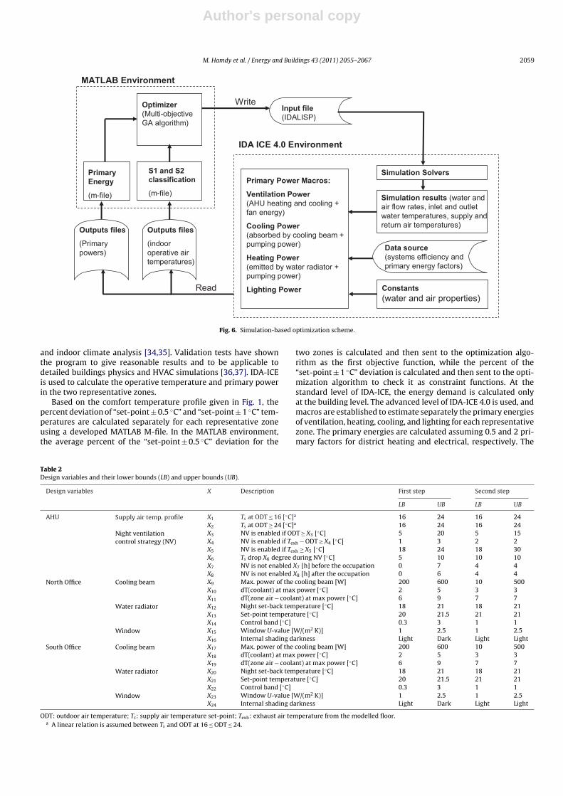
Fig. 6. Simulation-based optimization scheme.

and indoor climate analysis [34,35]. Validation tests have shownthe program to give reasonable results and to be applicable todetailed buildings physics and HVAC simulations [36,37]. IDA-ICEis used to calculate the operative temperature and primary powerin the two representative zones.

Based on the comfort temperature profile given in Fig. 1, thepercent deviation of “set-point ± 0.5 ◦C” and “set-point ± 1 ◦C” tem-peratures are calculated separately for each representative zoneusing a developed MATLAB M-file. In the MATLAB environment,the average percent of the “set-point ± 0.5 ◦C” deviation for the

two zones is calculated and then sent to the optimization algo-rithm as the first objective function, while the percent of the“set-point ± 1 ◦C” deviation is calculated and then sent to the opti-mization algorithm to check it as constraint functions. At thestandard level of IDA-ICE, the energy demand is calculated onlyat the building level. The advanced level of IDA-ICE 4.0 is used, andmacros are established to estimate separately the primary energiesof ventilation, heating, cooling, and lighting for each representativezone. The primary energies are calculated assuming 0.5 and 2 pri-mary factors for district heating and electrical, respectively. The

Table 2Design variables and their lower bounds (LB) and upper bounds (UB).

Design variables X Description First step Second step

LB UB LB UB

AHU Supply air temp. profile X1 Ts at ODT ≤ 16 [◦C]a 16 24 16 24X2 Ts at ODT ≥ 24 [◦C]a 16 24 16 24

Night ventilationcontrol strategy (NV)

X3 NV is enabled if ODT ≥ X3 [◦C] 5 20 5 15X4 NV is enabled if Texh − ODT ≥ X4 [◦C] 1 3 2 2X5 NV is enabled if Texh ≥ X5 [◦C] 18 24 18 30X6 Ts drop X6 degree during NV [◦C] 5 10 10 10X7 NV is not enabled X7 [h] before the occupation 0 7 4 4X8 NV is not enabled X8 [h] after the occupation 0 6 4 4

North Office Cooling beam X9 Max. power of the cooling beam [W] 200 600 10 500X10 dT(coolant) at max power [◦C] 2 5 3 3X11 dT(zone air − coolant) at max power [◦C] 6 9 7 7

Water radiator X12 Night set-back temperature [◦C] 18 21 18 21X13 Set-point temperature [◦C] 20 21.5 21 21X14 Control band [◦C] 0.3 3 1 1

Window X15 Window U-value [W/(m2 K)] 1 2.5 1 2.5X16 Internal shading darkness Light Dark Light Light

South Office Cooling beam X17 Max. power of the cooling beam [W] 200 600 10 500X18 dT(coolant) at max power [◦C] 2 5 3 3X19 dT(zone air − coolant) at max power [◦C] 6 9 7 7

Water radiator X20 Night set-back temperature [◦C] 18 21 18 21X21 Set-point temperature [◦C] 20 21.5 21 21X22 Control band [◦C] 0.3 3 1 1

Window X23 Window U-value [W/(m2 K)] 1 2.5 1 2.5X24 Internal shading darkness Light Dark Light Light

ODT: outdoor air temperature; Ts: supply air temperature set-point; Texh: exhaust air temperature from the modelled floor.a A linear relation is assumed between Ts and ODT at 16 ≤ ODT ≤ 24.



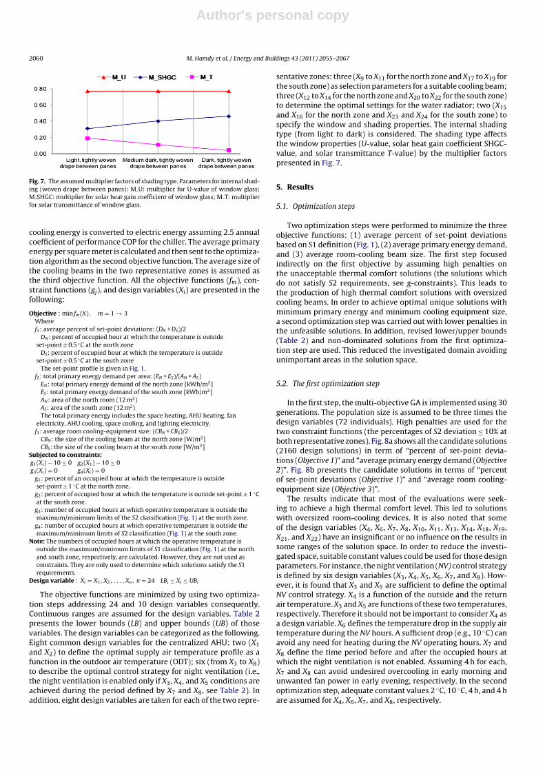
Fig. 7. The assumed multiplier factors of shading type. Parameters for internal shad-ing (woven drape between panes): M U: multiplier for U-value of window glass;M SHGC: multiplier for solar heat gain coefficient of window glass; M T: multiplierfor solar transmittance of window glass.

cooling energy is converted to electric energy assuming 2.5 annualcoefficient of performance COP for the chiller. The average primaryenergy per square meter is calculated and then sent to the optimiza-tion algorithm as the second objective function. The average size ofthe cooling beams in the two representative zones is assumed asthe third objective function. All the objective functions (fm), con-straint functions (gj), and design variables (Xi) are presented in thefollowing:

Objective : min fm(X), m = 1 → 3Wheref1: average percent of set-point deviations: (DN + DS)/2

DN: percent of occupied hour at which the temperature is outsideset-point ± 0.5 ◦C at the north zone

DS: percent of occupied hour at which the temperature is outsideset-point ± 0.5 ◦C at the south zone

The set-point profile is given in Fig. 1.f2: total primary energy demand per area: (EN + ES)/(AN + AS)

EN: total primary energy demand of the north zone [kWh/m2]ES: total primary energy demand of the south zone [kWh/m2]AN: area of the north room (12 m2)AS: area of the south zone (12 m2)The total primary energy includes the space heating, AHU heating, fan

electricity, AHU cooling, space cooling, and lighting electricity.f3: average room cooling-equipment size: (CBN + CBS)/2

CBN: the size of the cooling beam at the north zone [W/m2]CBS: the size of the cooling beam at the south zone [W/m2]

Subjected to constraints:g1(Xi) − 10 ≤ 0 g2(X1) − 10 ≤ 0g3(Xi) = 0 g4(Xi) = 0

g1: percent of an occupied hour at which the temperature is outsideset-point ± 1 ◦C at the north zone.g2: percent of occupied hour at which the temperature is outside set-point ± 1 ◦Cat the south zone.g3: number of occupied hours at which operative temperature is outside themaximum/minimum limits of the S2 classification (Fig. 1) at the north zone.g4: number of occupied hours at which operative temperature is outside themaximum/minimum limits of S2 classification (Fig. 1) at the south zone.

Note: The numbers of occupied hours at which the operative temperature isoutside the maximum/minimum limits of S1 classification (Fig. 1) at the northand south zone, respectively, are calculated. However, they are not used asconstraints. They are only used to determine which solutions satisfy the S1requirements.

Design variable : Xi = X1, X2, . . . , Xn, n = 24 LBi ≤ Xi ≤ UBi

The objective functions are minimized by using two optimiza-tion steps addressing 24 and 10 design variables consequently.Continuous ranges are assumed for the design variables. Table 2presents the lower bounds (LB) and upper bounds (UB) of thosevariables. The design variables can be categorized as the following.Eight common design variables for the centralized AHU: two (X1and X2) to define the optimal supply air temperature profile as afunction in the outdoor air temperature (ODT); six (from X3 to X8)to describe the optimal control strategy for night ventilation (i.e.,the night ventilation is enabled only if X3, X4, and X5 conditions areachieved during the period defined by X7 and X8, see Table 2). Inaddition, eight design variables are taken for each of the two repre-

sentative zones: three (X9 to X11 for the north zone and X17 to X19 forthe south zone) as selection parameters for a suitable cooling beam;three (X12 to X14 for the north zone and X20 to X22 for the south zone)to determine the optimal settings for the water radiator; two (X15and X16 for the north zone and X23 and X24 for the south zone) tospecify the window and shading properties. The internal shadingtype (from light to dark) is considered. The shading type affectsthe window properties (U-value, solar heat gain coefficient SHGC-value, and solar transmittance T-value) by the multiplier factorspresented in Fig. 7.

5. Results

5.1. Optimization steps

Two optimization steps were performed to minimize the threeobjective functions: (1) average percent of set-point deviationsbased on S1 definition (Fig. 1), (2) average primary energy demand,and (3) average room-cooling beam size. The first step focusedindirectly on the first objective by assuming high penalties onthe unacceptable thermal comfort solutions (the solutions whichdo not satisfy S2 requirements, see g-constraints). This leads tothe production of high thermal comfort solutions with oversizedcooling beams. In order to achieve optimal unique solutions withminimum primary energy and minimum cooling equipment size,a second optimization step was carried out with lower penalties inthe unfeasible solutions. In addition, revised lower/upper bounds(Table 2) and non-dominated solutions from the first optimiza-tion step are used. This reduced the investigated domain avoidingunimportant areas in the solution space.

5.2. The first optimization step

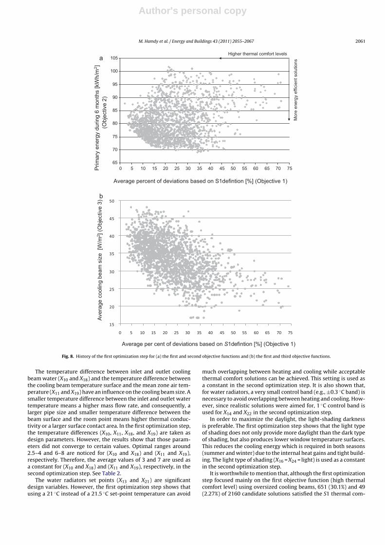
In the first step, the multi-objective GA is implemented using 30generations. The population size is assumed to be three times thedesign variables (72 individuals). High penalties are used for thetwo constraint functions (the percentages of S2 deviation ≤ 10% atboth representative zones). Fig. 8a shows all the candidate solutions(2160 design solutions) in term of “percent of set-point devia-tions (Objective 1)” and “average primary energy demand (Objective2)”. Fig. 8b presents the candidate solutions in terms of “percentof set-point deviations (Objective 1)” and “average room cooling-equipment size (Objective 3)”.

The results indicate that most of the evaluations were seek-ing to achieve a high thermal comfort level. This led to solutionswith oversized room-cooling devices. It is also noted that someof the design variables (X4, X6, X7, X8, X10, X11, X13, X14, X18, X19,X21, and X22) have an insignificant or no influence on the results insome ranges of the solution space. In order to reduce the investi-gated space, suitable constant values could be used for those designparameters. For instance, the night ventilation (NV) control strategyis defined by six design variables (X3, X4, X5, X6, X7, and X8). How-ever, it is found that X3 and X5 are sufficient to define the optimalNV control strategy. X4 is a function of the outside and the returnair temperature. X3 and X5 are functions of these two temperatures,respectively. Therefore it should not be important to consider X4 asa design variable. X6 defines the temperature drop in the supply airtemperature during the NV hours. A sufficient drop (e.g., 10 ◦C) canavoid any need for heating during the NV operating hours. X7 andX8 define the time period before and after the occupied hours atwhich the night ventilation is not enabled. Assuming 4 h for each,X7 and X8 can avoid undesired overcooling in early morning andunwanted fan power in early evening, respectively. In the secondoptimization step, adequate constant values 2 ◦C, 10 ◦C, 4 h, and 4 hare assumed for X4, X6, X7, and X8, respectively.



15

20

25

30

35

40

45

50

757065605550454035302520151050

Aver

age

cool

ing

beam

siz

e [W

/m2 ]

(Obj

ectiv

e 3)

Average per cent of deviations based on S1de fintion [%] (Objective 1)

65

70

75

80

85

90

95

100

105a

b

757065605550454035302520151050Prim

ary

ener

gy d

urin

g 6

mon

ths

[kW

h/m

]2

(Obj

ectiv

e 2)

Average percent of deviations based on S1defintion [%] (Objective 1)

High er th ermal comfo rt levels

Mor

e en

ergy

effi

cien

t sol

utio

ns

Fig. 8. History of the first optimization step for (a) the first and second objective functions and (b) the first and third objective functions.

The temperature difference between inlet and outlet coolingbeam water (X10 and X18) and the temperature difference betweenthe cooling beam temperature surface and the mean zone air tem-perature (X11 and X19) have an influence on the cooling beam size. Asmaller temperature difference between the inlet and outlet watertemperature means a higher mass flow rate, and consequently, alarger pipe size and smaller temperature difference between thebeam surface and the room point means higher thermal conduc-tivity or a larger surface contact area. In the first optimization step,the temperature differences (X10, X11, X18, and X19) are taken asdesign parameters. However, the results show that those param-eters did not converge to certain values. Optimal ranges around2.5–4 and 6–8 are noticed for (X10 and X18) and (X11 and X19),respectively. Therefore, the average values of 3 and 7 are used asa constant for (X10 and X18) and (X11 and X19), respectively, in thesecond optimization step. See Table 2.

The water radiators set points (X13 and X21) are significantdesign variables. However, the first optimization step shows thatusing a 21 ◦C instead of a 21.5 ◦C set-point temperature can avoid

much overlapping between heating and cooling while acceptablethermal comfort solutions can be achieved. This setting is used asa constant in the second optimization step. It is also shown that,for water radiators, a very small control band (e.g., ±0.3 ◦C band) isnecessary to avoid overlapping between heating and cooling. How-ever, since realistic solutions were aimed for, 1 ◦C control band isused for X14 and X22 in the second optimization step.

In order to maximize the daylight, the light-shading darknessis preferable. The first optimization step shows that the light typeof shading does not only provide more daylight than the dark typeof shading, but also produces lower window temperature surfaces.This reduces the cooling energy which is required in both seasons(summer and winter) due to the internal heat gains and tight build-ing. The light type of shading (X16 = X24 = light) is used as a constantin the second optimization step.

It is worthwhile to mention that, although the first optimizationstep focused mainly on the first objective function (high thermalcomfort level) using oversized cooling beams, 651 (30.1%) and 49(2.27%) of 2160 candidate solutions satisfied the S1 thermal com-



60

65

70

75

80

85

90

95a

b

0 5 10 15 20 25 30 35 40 45 50 55 60 65 70 75 80 85 90 95 100

All ca ndidate solutionsS2 so lutionsS1 so lutionsOptimal so lutions

Prim

ary

ene

rgy

dur

ing

6 m

onth

s [k

Wh/

m2 ]

(Obj

ectiv

e 2)

Average percen t of de via tions ba sed on S1defintion [%] (Ob jective 1)

Higher thermal comfort levels

Mor

e en

ergy

effi

cien

t sol

utio

ns

S1 Unique solution

S2 Unique solution

5

10

15

20

25

30

35

40

0 5 10 15 20 25 30 35 40 45 50 55 60 65 70 75 80 85 90 95 100

All candidate solutionsS2 so lutionsS1 so lutionsOptimal solutions

Average percent of deviations ba sed on S1defintion [%] (O bjec tive 1)

Ave

rage

coo

ling

beam

siz

e [W

/m2 ]

(Obj

ectiv

e 3)

S2 Unique solution

S1 Unique solution

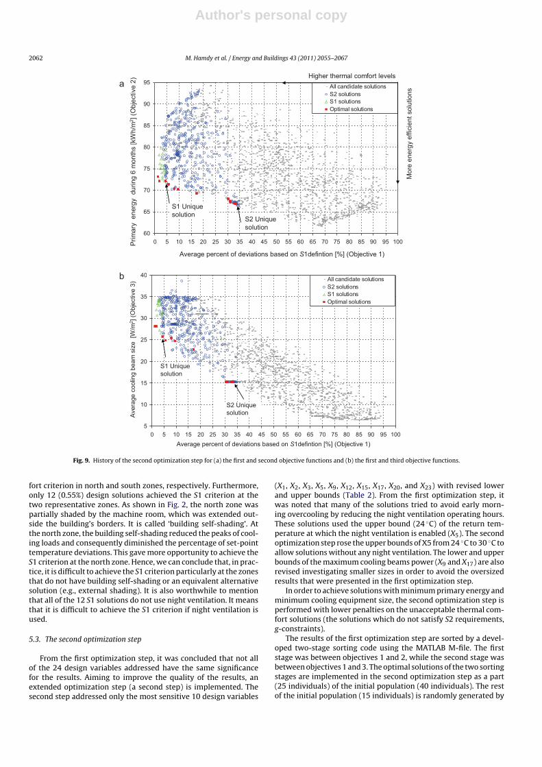
Fig. 9. History of the second optimization step for (a) the first and second objective functions and (b) the first and third objective functions.

fort criterion in north and south zones, respectively. Furthermore,only 12 (0.55%) design solutions achieved the S1 criterion at thetwo representative zones. As shown in Fig. 2, the north zone waspartially shaded by the machine room, which was extended out-side the building’s borders. It is called ‘building self-shading’. Atthe north zone, the building self-shading reduced the peaks of cool-ing loads and consequently diminished the percentage of set-pointtemperature deviations. This gave more opportunity to achieve theS1 criterion at the north zone. Hence, we can conclude that, in prac-tice, it is difficult to achieve the S1 criterion particularly at the zonesthat do not have building self-shading or an equivalent alternativesolution (e.g., external shading). It is also worthwhile to mentionthat all of the 12 S1 solutions do not use night ventilation. It meansthat it is difficult to achieve the S1 criterion if night ventilation isused.

5.3. The second optimization step

From the first optimization step, it was concluded that not allof the 24 design variables addressed have the same significancefor the results. Aiming to improve the quality of the results, anextended optimization step (a second step) is implemented. Thesecond step addressed only the most sensitive 10 design variables

(X1, X2, X3, X5, X9, X12, X15, X17, X20, and X23) with revised lowerand upper bounds (Table 2). From the first optimization step, itwas noted that many of the solutions tried to avoid early morn-ing overcooling by reducing the night ventilation operating hours.These solutions used the upper bound (24 ◦C) of the return tem-perature at which the night ventilation is enabled (X5). The secondoptimization step rose the upper bounds of X5 from 24 ◦C to 30 ◦C toallow solutions without any night ventilation. The lower and upperbounds of the maximum cooling beams power (X9 and X17) are alsorevised investigating smaller sizes in order to avoid the oversizedresults that were presented in the first optimization step.

In order to achieve solutions with minimum primary energy andminimum cooling equipment size, the second optimization step isperformed with lower penalties on the unacceptable thermal com-fort solutions (the solutions which do not satisfy S2 requirements,g-constraints).

The results of the first optimization step are sorted by a devel-oped two-stage sorting code using the MATLAB M-file. The firststage was between objectives 1 and 2, while the second stage wasbetween objectives 1 and 3. The optimal solutions of the two sortingstages are implemented in the second optimization step as a part(25 individuals) of the initial population (40 individuals). The restof the initial population (15 individuals) is randomly generated by



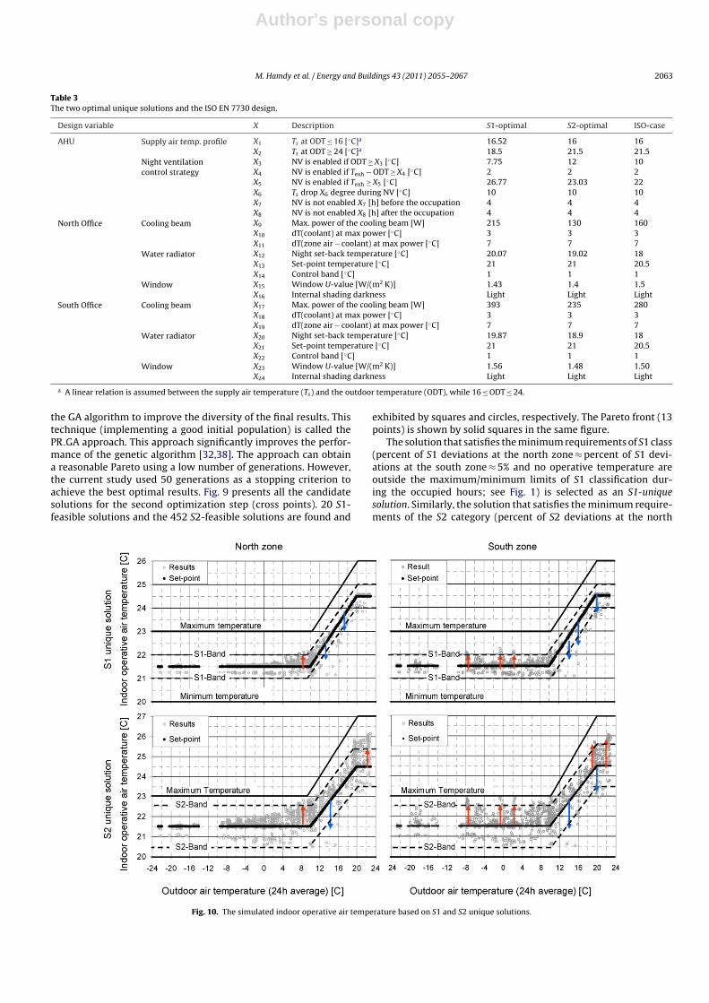
Table 3The two optimal unique solutions and the ISO EN 7730 design.

Design variable X Description S1-optimal S2-optimal ISO-case

AHU Supply air temp. profile X1 Ts at ODT ≤ 16 [◦C]a 16.52 16 16X2 Ts at ODT ≥ 24 [◦C]a 18.5 21.5 21.5

Night ventilationcontrol strategy

X3 NV is enabled if ODT ≥ X3 [◦C] 7.75 12 10X4 NV is enabled if Texh − ODT ≥ X4 [◦C] 2 2 2X5 NV is enabled if Texh ≥ X5 [◦C] 26.77 23.03 22X6 Ts drop X6 degree during NV [◦C] 10 10 10X7 NV is not enabled X7 [h] before the occupation 4 4 4X8 NV is not enabled X8 [h] after the occupation 4 4 4

North Office Cooling beam X9 Max. power of the cooling beam [W] 215 130 160X10 dT(coolant) at max power [◦C] 3 3 3X11 dT(zone air − coolant) at max power [◦C] 7 7 7

Water radiator X12 Night set-back temperature [◦C] 20.07 19.02 18X13 Set-point temperature [◦C] 21 21 20.5X14 Control band [◦C] 1 1 1

Window X15 Window U-value [W/(m2 K)] 1.43 1.4 1.5X16 Internal shading darkness Light Light Light

South Office Cooling beam X17 Max. power of the cooling beam [W] 393 235 280X18 dT(coolant) at max power [◦C] 3 3 3X19 dT(zone air − coolant) at max power [◦C] 7 7 7

Water radiator X20 Night set-back temperature [◦C] 19.87 18.9 18X21 Set-point temperature [◦C] 21 21 20.5X22 Control band [◦C] 1 1 1

Window X23 Window U-value [W/(m2 K)] 1.56 1.48 1.50X24 Internal shading darkness Light Light Light

a A linear relation is assumed between the supply air temperature (Ts) and the outdoor temperature (ODT), while 16 ≤ ODT ≤ 24.

the GA algorithm to improve the diversity of the final results. Thistechnique (implementing a good initial population) is called thePR GA approach. This approach significantly improves the perfor-mance of the genetic algorithm [32,38]. The approach can obtaina reasonable Pareto using a low number of generations. However,the current study used 50 generations as a stopping criterion toachieve the best optimal results. Fig. 9 presents all the candidatesolutions for the second optimization step (cross points). 20 S1-feasible solutions and the 452 S2-feasible solutions are found and

exhibited by squares and circles, respectively. The Pareto front (13points) is shown by solid squares in the same figure.

The solution that satisfies the minimum requirements of S1 class(percent of S1 deviations at the north zone ≈ percent of S1 devi-ations at the south zone ≈ 5% and no operative temperature areoutside the maximum/minimum limits of S1 classification dur-ing the occupied hours; see Fig. 1) is selected as an S1-uniquesolution. Similarly, the solution that satisfies the minimum require-ments of the S2 category (percent of S2 deviations at the north

Fig. 10. The simulated indoor operative air temperature based on S1 and S2 unique solutions.



14

15

16

17

18

19

20

21

22

23

2827262524232221201918171615141312

S1 unique s oluti on

S2 unique s oluti on

Supp

ly a

ir te

mpe

ratu

re (T

S) [o C

]

Outdoor air temper ature (ODT) [oC]

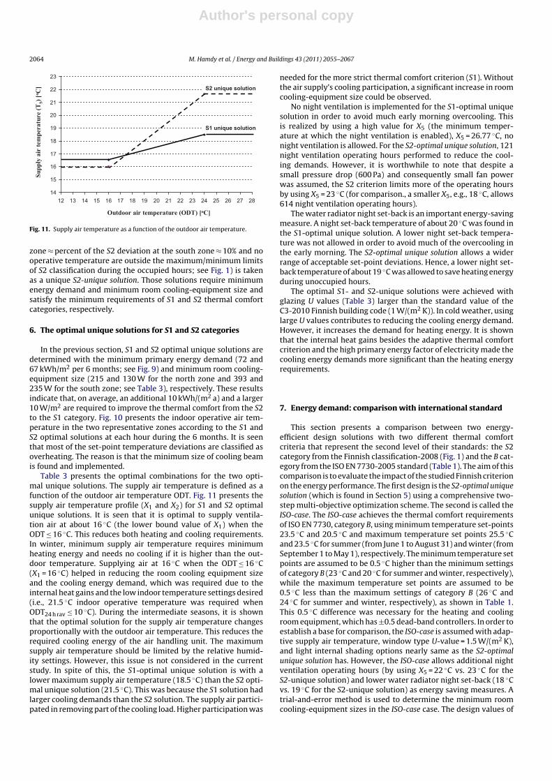
Fig. 11. Supply air temperature as a function of the outdoor air temperature.

zone ≈ percent of the S2 deviation at the south zone ≈ 10% and nooperative temperature are outside the maximum/minimum limitsof S2 classification during the occupied hours; see Fig. 1) is takenas a unique S2-unique solution. Those solutions require minimumenergy demand and minimum room cooling-equipment size andsatisfy the minimum requirements of S1 and S2 thermal comfortcategories, respectively.

6. The optimal unique solutions for S1 and S2 categories

In the previous section, S1 and S2 optimal unique solutions aredetermined with the minimum primary energy demand (72 and67 kWh/m2 per 6 months; see Fig. 9) and minimum room cooling-equipment size (215 and 130 W for the north zone and 393 and235 W for the south zone; see Table 3), respectively. These resultsindicate that, on average, an additional 10 kWh/(m2 a) and a larger10 W/m2 are required to improve the thermal comfort from the S2to the S1 category. Fig. 10 presents the indoor operative air tem-perature in the two representative zones according to the S1 andS2 optimal solutions at each hour during the 6 months. It is seenthat most of the set-point temperature deviations are classified asoverheating. The reason is that the minimum size of cooling beamis found and implemented.

Table 3 presents the optimal combinations for the two opti-mal unique solutions. The supply air temperature is defined as afunction of the outdoor air temperature ODT. Fig. 11 presents thesupply air temperature profile (X1 and X2) for S1 and S2 optimalunique solutions. It is seen that it is optimal to supply ventila-tion air at about 16 ◦C (the lower bound value of X1) when theODT ≤ 16 ◦C. This reduces both heating and cooling requirements.In winter, minimum supply air temperature requires minimumheating energy and needs no cooling if it is higher than the out-door temperature. Supplying air at 16 ◦C when the ODT ≤ 16 ◦C(X1 = 16 ◦C) helped in reducing the room cooling equipment sizeand the cooling energy demand, which was required due to theinternal heat gains and the low indoor temperature settings desired(i.e., 21.5 ◦C indoor operative temperature was required whenODT24 h rav ≤ 10 ◦C). During the intermediate seasons, it is shownthat the optimal solution for the supply air temperature changesproportionally with the outdoor air temperature. This reduces therequired cooling energy of the air handling unit. The maximumsupply air temperature should be limited by the relative humid-ity settings. However, this issue is not considered in the currentstudy. In spite of this, the S1-optimal unique solution is with alower maximum supply air temperature (18.5 ◦C) than the S2 opti-mal unique solution (21.5 ◦C). This was because the S1 solution hadlarger cooling demands than the S2 solution. The supply air partici-pated in removing part of the cooling load. Higher participation was

needed for the more strict thermal comfort criterion (S1). Withoutthe air supply’s cooling participation, a significant increase in roomcooling-equipment size could be observed.

No night ventilation is implemented for the S1-optimal uniquesolution in order to avoid much early morning overcooling. Thisis realized by using a high value for X5 (the minimum temper-ature at which the night ventilation is enabled), X5 = 26.77 ◦C, nonight ventilation is allowed. For the S2-optimal unique solution, 121night ventilation operating hours performed to reduce the cool-ing demands. However, it is worthwhile to note that despite asmall pressure drop (600 Pa) and consequently small fan powerwas assumed, the S2 criterion limits more of the operating hoursby using X5 = 23 ◦C (for comparison., a smaller X5, e.g., 18 ◦C, allows614 night ventilation operating hours).

The water radiator night set-back is an important energy-savingmeasure. A night set-back temperature of about 20 ◦C was found inthe S1-optimal unique solution. A lower night set-back tempera-ture was not allowed in order to avoid much of the overcooling inthe early morning. The S2-optimal unique solution allows a widerrange of acceptable set-point deviations. Hence, a lower night set-back temperature of about 19 ◦C was allowed to save heating energyduring unoccupied hours.

The optimal S1- and S2-unique solutions were achieved withglazing U values (Table 3) larger than the standard value of theC3-2010 Finnish building code (1 W/(m2 K)). In cold weather, usinglarge U values contributes to reducing the cooling energy demand.However, it increases the demand for heating energy. It is shownthat the internal heat gains besides the adaptive thermal comfortcriterion and the high primary energy factor of electricity made thecooling energy demands more significant than the heating energyrequirements.

7. Energy demand: comparison with international standard

This section presents a comparison between two energy-efficient design solutions with two different thermal comfortcriteria that represent the second level of their standards: the S2category from the Finnish classification-2008 (Fig. 1) and the B cat-egory from the ISO EN 7730-2005 standard (Table 1). The aim of thiscomparison is to evaluate the impact of the studied Finnish criterionon the energy performance. The first design is the S2-optimal uniquesolution (which is found in Section 5) using a comprehensive two-step multi-objective optimization scheme. The second is called theISO-case. The ISO-case achieves the thermal comfort requirementsof ISO EN 7730, category B, using minimum temperature set-points23.5 ◦C and 20.5 ◦C and maximum temperature set points 25.5 ◦Cand 23.5 ◦C for summer (from June 1 to August 31) and winter (fromSeptember 1 to May 1), respectively. The minimum temperature setpoints are assumed to be 0.5 ◦C higher than the minimum settingsof category B (23 ◦C and 20 ◦C for summer and winter, respectively),while the maximum temperature set points are assumed to be0.5 ◦C less than the maximum settings of category B (26 ◦C and24 ◦C for summer and winter, respectively), as shown in Table 1.This 0.5 ◦C difference was necessary for the heating and coolingroom equipment, which has ±0.5 dead-band controllers. In order toestablish a base for comparison, the ISO-case is assumed with adap-tive supply air temperature, window type U-value = 1.5 W/(m2 K),and light internal shading options nearly same as the S2-optimalunique solution has. However, the ISO-case allows additional nightventilation operating hours (by using X5 = 22 ◦C vs. 23 ◦C for theS2-unique solution) and lower water radiator night set-back (18 ◦Cvs. 19 ◦C for the S2-unique solution) as energy saving measures. Atrial-and-error method is used to determine the minimum roomcooling-equipment sizes in the ISO-case case. The design values of



Table 4The annual primary energy demand.

Design Thermal comfort Criterion The annual primary energy demand [kWh/m2]

Cooling Heating Electricity Total

Space AHU Total Space AHU Total Fan HVAC

ISO-case ISO EN 7730-2005 (Category B) 8.4 2.7 11.1 10.8 10.6 21.4 22.6 55.1S2-optimal unique solution Finnish adaptive criterion-2008

(Class S2)22.1 2.6 24.7 15.4 11.8 27.2 21.4 73.3

Percentage of energy increase[%] ISO-case 100%

163 −3 122 42 11 27 −6 33

the S2-optimal unique solution and the ISO-case are presented inTable 3.

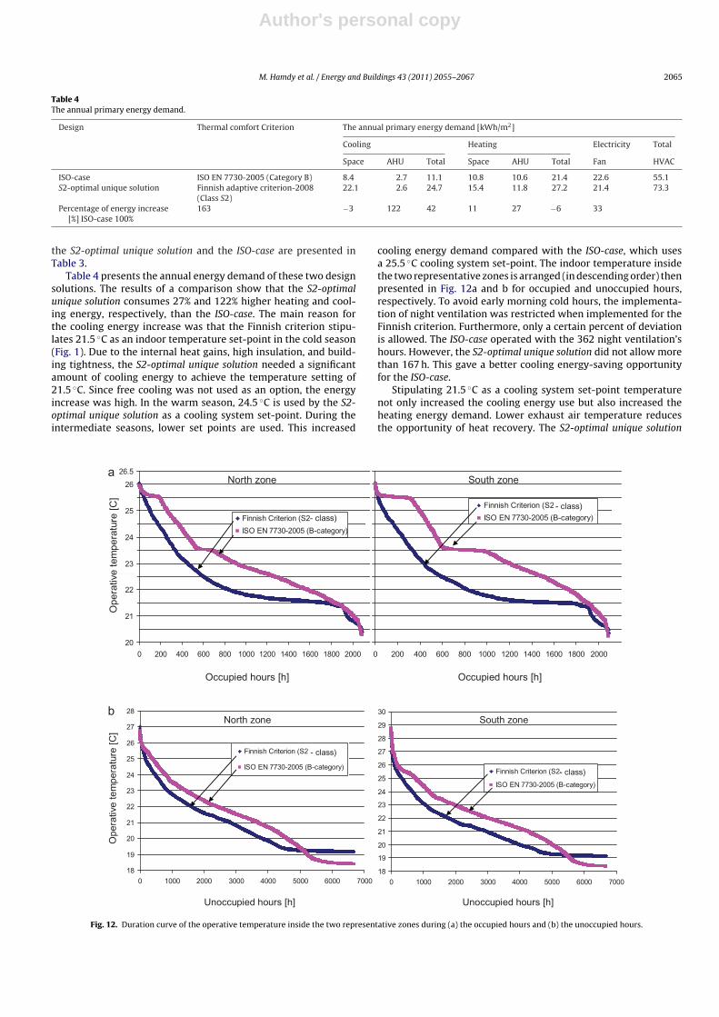
Table 4 presents the annual energy demand of these two designsolutions. The results of a comparison show that the S2-optimalunique solution consumes 27% and 122% higher heating and cool-ing energy, respectively, than the ISO-case. The main reason forthe cooling energy increase was that the Finnish criterion stipu-lates 21.5 ◦C as an indoor temperature set-point in the cold season(Fig. 1). Due to the internal heat gains, high insulation, and build-ing tightness, the S2-optimal unique solution needed a significantamount of cooling energy to achieve the temperature setting of21.5 ◦C. Since free cooling was not used as an option, the energyincrease was high. In the warm season, 24.5 ◦C is used by the S2-optimal unique solution as a cooling system set-point. During theintermediate seasons, lower set points are used. This increased

cooling energy demand compared with the ISO-case, which usesa 25.5 ◦C cooling system set-point. The indoor temperature insidethe two representative zones is arranged (in descending order) thenpresented in Fig. 12a and b for occupied and unoccupied hours,respectively. To avoid early morning cold hours, the implementa-tion of night ventilation was restricted when implemented for theFinnish criterion. Furthermore, only a certain percent of deviationis allowed. The ISO-case operated with the 362 night ventilation’shours. However, the S2-optimal unique solution did not allow morethan 167 h. This gave a better cooling energy-saving opportunityfor the ISO-case.

Stipulating 21.5 ◦C as a cooling system set-point temperaturenot only increased the cooling energy use but also increased theheating energy demand. Lower exhaust air temperature reducesthe opportunity of heat recovery. The S2-optimal unique solution

20

20.5

21

21.5

22

22.523

23.5

24

2525.5

26a

b

26.5

0 20 0 40 0 60 0 80 0 10 00 120 0 14 00 160 0 1800 200 0

Finni sh Criterion (S2- class)ISO EN 7730 -2005 (B-catego ry)

0 200 400 600 800 10 00 12 00 14 00 160 0 180 0 20 00

Finnish Criterio n (S2-catego ry)ISO EN 773 0-2005 (B-catego ry)

South zoneNorth zone

Ope

rativ

e te

mpe

ratu

re [C

]

- class)

]h[sruohdeipuccO]h[sruohdeipuccO

18

19

20

21

22

23

24

25

26

27

28

0 100 0 200 0 300 0 400 0 500 0 600 0 700 0

Finni sh Criterion (S2-catego ry)

ISO EN 7730 -2005 (B-categ ory)

18

19

20

21

22

23

24

25

26

27

28

29

30

0 100 0 200 0 300 0 400 0 500 0 600 0 700 0

Finni sh Criterion (S2-catego ry)

ISO EN 7730 -2005 (B-catego ry)

South zone

Ope

rativ

e te

mpe

ratu

re [C

]

North zone

]h[sruohdeipucconU]h[sruohdeipucconU

- class)

- class)

Fig. 12. Duration curve of the operative temperature inside the two representative zones during (a) the occupied hours and (b) the unoccupied hours.



increased the AHU heating energy by about 11%. The ISO-case used23.5 ◦C as a maximum temperature for the cold season. This pro-vided a slightly warm exhaust air temperature and consequentlybetter heat recovery.

Using a single indoor temperature set-point increases the over-lapping between heating and cooling [6]. The Finnish criteriastipulated single set-point temperature with a certain percent ofset-point deviations. Although the S2-optimal unique solution mini-mized the heating/cooling overlapping by using a dual temperaturesetting (21 ◦C for water radiations and 21.5 ◦C for room-coolingdevices) and by implementing a suitable size of cooling beams, asignificant increase was noted in the space heating energy demand(42.1%), compared with the ISO-case. The overlapping was not theonly reason of this increase. The setting of the water radiator nightset-back was the second reason. A lower night set-back tempera-ture provides more energy saving. However, in order to achieve anacceptable percent of set-point deviations, the S2-optimal uniquesolution could not use a night set-back lower than 19 ◦C, while theISO-case allowed an 18 ◦C night set-back temperature.

8. Conclusions

The adaptive thermal-comfort criterion of the Finnish Indoor-Climate Classification 2008 for a fully mechanically air-conditionedenvironment is the subject of the current study. The impact of theadaptive criterion on the energy performance of an office buildingis evaluated. The study determines the minimum energy require-ments needed to improve the thermal comfort from a mediumquality class (S2) to a high quality class (S1). A simulation-basedoptimization scheme is employed, and trade-off relations betweenprimary energy demand and thermal comfort level are found. Inaddition, two optimal unique solutions with minimum primaryenergy demand and minimum room cooling-equipment size arefound for S2 and S1 classes. The optimal results show that, onaverage, an additional 10 kWh/(m2 a) primary energy demand anda larger 10 W/m2 room cooling-equipment size are required toimprove the thermal comfort from the S2 to the S1 class. The S1 classlimits the applicability of night ventilation and the night set-backtemperature as energy saving measures (small early morning over-cooling due to using night ventilation and/or night temperatureset-back is inconsistent with the strict S1 requirements). Moreover,maintaining a narrow temperature range (S1) requires more accu-rate control instruments than for maintaining a broad range (S2).This invites questions. Is the so-called S1-class thermal environ-ment worth its inherent energy penalty and its inherent controlcomplexity? Is it even more comfortable than S2-class in a realisticenvironment?

This study is extended to compare the Finnish classification(S2-class) with the ISO EN 7730-2005 standard (B-category). Thesimulation results show that the S2-optimal unique solution (min-imum primary energy and cooling equipment-size S2 solution)consumes significantly higher heating and cooling energy than theISO-case. In order to achieve the Finnish criterion, both heatingand cooling systems are required to be in operation during mostof the year. A cooling device with a sophisticated controller isneeded to trace the adaptive set-point profile. Since heating andcooling are required most of the time, a suitable simulation opti-mization approach is needed in the first stages of design to findcompromise solutions (e.g., a compromise U value for the externalfacades). Correct room-equipment size and a small control-bandare both necessary to reduce the heating/cooling overlap. Energydemand can be significantly reduced if the supply air temperatureis optimally defined as a function of outside temperature (i.e., com-pared with the ISO standard, the adaptive Finnish classification-2008)increases the cooling use during winter and reduces the coolingdemand during the summer. Hence, supplying air at a temper-

ature of 16 ◦C (minimum acceptable temperature) in winter and22 ◦C (near the maximum acceptable temperature) in summer canreduce both heating and cooling energy demands.

It is worthwhile to note that the studied classification does notdifferentiate between overheating and overcooling (i.e., it does notdifferentiate if the indoor temperature is above or below the desiredset-point). This could lead to unfair solutions. It is noted that themajority of the set-point temperature deviations belonging to theoptimal solutions are classified as overheating. On the other hand, itis noted that the studied criterion significantly increases the needfor cooling during the winter and intermediate seasons. The freecooling can be used to mitigate that increase. However, it increasesthe operating hours of the cooling system and as a consequence itincreases the maintenance work of the auxiliary equipment (thesupply pump and free cooling fan). Using energy-efficient officeequipment (e.g., laptops instead of computers) can also mitigatethat increase in cooling. However, it could increase the capital cost.The authors concluded that the Finnish classification-2008 is strictand does not allow for energy-efficient solutions in office buildingswith standard heat gains and a tight building envelope, particularlyif a free cooling option is not applicable.

Acknowledgments

The authors would like to acknowledge the financial supportof the Finnish National Technology Agency (TEKES), as well as thefollowing supporting companies: Optiplan Oy, Pöyry Building Ser-vicees Oy, Saint-Gobain Isover Oy, Skanska Oy, and YIT Oy. Thesecond author would like to thank the Academy of Finland forfunding his work as part of a Research Fellow position.

References

[1] EN15251: 2007, Indoor Environmental Input Parameters for Design and Assess-ment of Energy Performance of Buildings Addressing Indoor Air Quality,Thermal Environment, Lighting and Acoustics, 2007.

[2] S.P. Corgnati, E. Fabrizio, M. Filippi, Costs and comfort: mutual relation betweencomfort conditions and energy demand in office buildings, in: AICARR Interna-tional Conference AICARR 2006 HVAC&R: Technology, Rules and Market, Milan,March, 2006.

[3] R.J. de Dear, A global database of thermal comfort field experiments, ASHRAETransactions 104 (1b) (1998) 1141–1152 (Reprinted in G. Schiller Brager (Ed.),Field studies of thermal comfort and adaptation, ASHRAE Technical Data Bul-letin 14 (1) (1998) 15–26).

[4] G.S. Brager, R.J. de Dear, Thermal adaptation in the built environment: a liter-ature review, Energy and Buildings 27 (1998) 83–96.

[5] R.J. de Dear, G.S. Brager, Developing an adaptive model of thermal comfort andpreference, ASHRAE Transactions 104 (1) (1998) 27–49.

[6] G.S. Brager, R.J. de Dear, A standard for natural ventilation, ASHRAE Journal 42(10) (2000) 21–27.

[7] G.S. Brager, R.J. de Dear, Climate, comfort & natural ventilation: a new adaptivecomfort standard for ASHRAE Standard 55, in: Proc. Int. Conf. Moving ThermalComfort Standards into the 21st Century, Oxford Brookes University, Windsor,2001.

[8] P.O. Fanger, Thermal Comfort Analyses and Applications in EnvironmentalEngineering, McGraw-Hill, London, 1970.

[9] L. Centnerova, J. Hensen, Energy and indoor temperature consequences ofadaptive thermal comfort standards, in: Proc. 4th Int. Conf. Indoor Climate ofBuildings, 2001, pp. 391–402.

[10] ISO 7730: 1993, Moderate Thermal Environments—Determination of the PMVand PPD Indices and Specification of the Conditions for Thermal Comfort, Inter-national Standardization Organization, 1993.

[11] ANSI/ASHRAE 55-1992, Thermal Environmental Conditions for Human Occu-pancy, American Society of Heating, Refrigerating and Air-conditioningEngineers, Atlanta, GA, 1992.

[12] S. Corgnati, E. Fabrizio, M. Filippi, The impact of indoor thermal conditions,system controls and building types on the building energy demand, Energyand Buildings 40 (2008) 627–636.

[13] R.J. de Dear, Adaptive thermal comfort in building management and perfor-mance, in: Proceedings of the Healthy Buildings, vol. 1, 2006, pp. 31–35.

[14] D.P. Wyon, Individual control at each workplace: the means and the potentialbenefits, in: D. Croome (Ed.), Creating the Productive Workplace, 1999, London,NY.

[15] M. Hannula, R. Niemela, S. Rautio, K. Reijula, The effect of indoor climate onproductivity, Proceedings of Healthy Buildings 1 (2000) 659–664.



[16] M.A. Humphreys, J.F. Nicol, in: J.F. Nicol, et al. (Eds.), An Adaptive Guide-line for UK Office Temperatures. Standards for Thermal Comfort: Indoor AirTemperature Standards for the 21st Century, E & FN Spon, London, UK,1995.

[17] K.J. McCartney, J.F. Nicol, Developing an adaptive control algorithm for Europe,Energy and Buildings 34 (2002) 623–635.

[18] D. Stuart Barlow, Fiala Occupant comfort in UK offices—how adaptive com-fort theories might influence future low energy office refurbishment strategies,Energy and Buildings 39 (2007) 837–846.

[19] J.U. Pfafferott, S. Herkel, D.E. Kalz, A. Zeuschner, Comparison of low-energyoffice buildings in summer using different thermal comfort criteria, Energyand Buildings 39 (2007) 750–757.

[20] R.J. de Dear, G.S. Brager, Thermal comfort in naturally ventilated buildings:revisions to ASHRAE Standard 55, Energy and Buildings 34 (6) (2002) 549–561.

[21] R.J. de Dear, G.S. Brager, Developing an adaptive model of thermal comfort andpreference, Final report, ASHRAE RP-884, March 1997.

[22] A.C. van der Linden, A.C. Boerstra, A.K. Raue, S.R. Kurvers, R.J. de Dear, Adaptivetemperature limits: a new guideline in the Netherlands. A new approach forthe assessment of building performance with respect to thermal indoor climate,Energy and Buildings 38 (2006) 8–17.

[23] J.F. Nicol, M.A. Humphreys, Maximum temperatures in European office build-ings to avoid heat discomfort, Solar Energy 81 (2007) 295–304.

[24] J.F. Nicol, I.A. Raja, Thermal Comfort Time Posture: Explanatory Studies in theNature of Adaptive Thermal Comfort, Oxford Brookes University, UK, 1996.

[25] Finnish Society of Indoor Air Quality (FiSIAQ), Classification of Indoor Cli-mate, 2008, Publication 5, Finnish Society of Indoor Air Quality (FiSIAQ), Espoo,Finland, 2008.

[26] J. Kurnitski, O. Seppänen, Trends and Drivers in the Finnish Ventilation andAC Market, International Energy Agency, Energy Conservation in Buildings andCommunity Systems Programme, Air Infiltration and Ventilation Centre, 2008.

[27] ISO EN 7730: 2005, Moderate Thermal Environments—Determination of thePMV and PPD Indices and Specification of the Conditions for Thermal Comfort,International Standards Organisation, 2005.

[28] D.P. Wyon, Indoor environment effects on productivity, in: Proceedings of IAQ1996 Path to Better Building Environments, ASHRAE, USA, 1996, pp. 5–15.

[29] W. Wang, R. Zmeureanu, H. Rivard, Applying multi-objective genetic algo-rithms in green building design optimization, Building and Environment 40(2005) 1512–1525.

[30] J.A. Wright, H.A. Loosemore, R. Farmani, Optimization of building thermaldesign and control by multi-criterion genetic algorithm, Energy and Buildings34 (9) (2002) 959–972.

[31] M. Palonen, A. Hasan, K. Siren, A genetic algorithm for optimization of build-ing envelope and HVAC system parameters, in: IBPSA 2009, 11th InternationalBuilding Performance Simulation Association Conference, Glasgow, UK, 2009.

[32] M. Hamdy, A. Hasan, K. Siren, Combination of optimization algorithms for amulti-objective building design problem, in: IBPSA 2009, 11th InternationalBuilding Performance Simulation Association Conference, Glasgow, UK, 2009.

[33] L.G. Caldas, L.K. Norford, Genetic algorithms for optimization of buildingenvelopes and the design and control of HVAC systems, Journal of Solar EnergyEngineering 125 (2003) 343.

[34] A. Bring, P. Sahlin, M. Vuolle, Models for Building Indoor Climate and EnergySimulation, Royal Institute of Technology, Stockholm, Sweden, 1999.

[35] EQUA, IDA Indoor Climate and Energy 3.0 User‘s Guide, EQUA Simulation AB,Stockholm, Sweden, 2002.

[36] M. Achermann, G. Zweifel, RADTEST—Radiant Heating and Cooling Test Cases,IEA Task 22 Subtask C, Building Energy Analysis.

[37] M. Achermann, Validation of IDA ICE Version 2.11.06, HTA (Hochschule Tech-nik + Architektur), Luzern, Switzerland, 2000.

[38] M. Hamdy, A. Hasan, K. Siren, Applying a multi-objective optimization approachfor design of low-emission cost-effective dwellings, Building and Environment46 (2011) 109–123.

Impact of adaptive thermal comfort criteria on building energy use and cooling equipment size using...

Documents

Transcript of Impact of adaptive thermal comfort criteria on building energy use and cooling equipment size using...