Immigration Effects on Economic Systems Through Dynamic Inequality Indices

Electronic copy available at: http://ssrn.com/abstract=1874848

GLOBAL JOURNAL OF BUSINESS RESEARCH ♦ VOLUME 5 ♦ NUMBER 5 ♦ 2011

11

IMMIGRATION EFFECTS ON ECONOMIC SYSTEMS THROUGH DYNAMIC INEQUALITY INDICES

Guglielmo D’Amico, University “G. D’Annunzio” of Chieti, Italy Giuseppe Di Biase, University “G. D’Annunzio” of Chieti, Italy

Raimondo Manca, University “La Sapienza” of Rome, Italy

ABSTRACT In this paper we propose a stochastic model to analyze the time evolution of inequality within an economic system. The classical inequality indices (Herfindahl-Hirschman, Gini and Theil’s entropy) are thereby turned into a dynamic form. We show, by using a simulative approach, how it is possible to study the time evolution of inequality in a closed or open economy. We pay particular attention to immigration effects on the inequality. The model is able to manage different behaviors of the inequality indices and it may help decision makers calibrate the economic policies of inequality containment. JEL: C63 KEYWORDS: Income distribution, Dynamic inequality index, semi-Markov reward processes. INTRODUCTION

elevant economic problems include the measure of changes in economic inequality. This measure can be examined by computing inequality indices. In this paper we propose a stochastic model that makes dynamic those classical inequality indices applied in a static framework. We simulate a

model and compute the dynamic indices for different economic scenarios. Additionally we show useful of the model for analyzing the impact of immigration with respect to the concentration of wealth distribution in the economic system. We focus on effects caused by a population increase of 10% as a consequence of immigration. To this end we use computer code, programmed in the Mathematica language, to give results for any immigration level and economic scenario. The paper is organized as follows. We start by describing the literature review in Section 2. Then we describe, in Section 3, the stochastic model and the way in which it is possible to compute the dynamic inequality indices. In Section 4 we present a numerical experience by showing the applicability of the model. Moreover we give some results with a particular attention to the immigration effects on the inequalities. Finally, we give some conclusions and further research suggestions in Section 5. LITERATURE REVIEW Income inequality can be measured by means of econometric indices. The most common methods are the Herfindahl-Hirschman index, the Gini index and the Theil’s entropy. The Herfindahl-Hirschman index is used mainly in industrial economic as a measure of market concentration. It is calculated by squaring the market share of each firm competing in the market and then summing the resulting numbers. Because the index measures market concentration, it is an inverse inequality measure. It takes into account the relative size and distribution of the agents in an economy. It approaches zero when the economy consists of a large number of agents of relatively equal size. It increases both as the number of agents in the economy decreases and as the disparity in size between those agents increases. This index has been proposed and studied by Hirschman (1964). Since then many applications appeared (see i.e. Kwoka, 1977;.Tirole, 1988; Kooleman and Van Doorslaer, 2004).

R

Electronic copy available at: http://ssrn.com/abstract=1874848

G. D'Amico et al | GJBR ♦ Vol. 5 ♦ No. 5 ♦ 2011

12

The Gini index is attributed to Gini (1912). Formally it is derived as one half of the mean of the absolute values of differences between all pairs of income relative to the mean income. It has values between zero and one. If the index value is equal to zero, then, the wealth is equidistributed in the population. On the contrary a value equal to one indicates that one economic agent possesses all the wealth. Among the properties we recall the scale independence and the invariance to replication of population. Moreover it meets the Pigou-Dalton principle of transfers (Athanasopoulos and Vahid, 2003). The last quoted properties are satisfied also by the Theil’s Entropy, introduced by Theil (1967). This index is defined as the sum of the products of the shares of the total income of each individual (denoted by xi) times the logarithm of nxi where n is the number of agents in the economic system. Besides the above mentioned properties, the index satisfies the strong principle of transfers and, moreover, it is additively decomposable (Cowell, 1995). The range of values is between 0 and ln(n). The index gives 0 when the wealth is equidistributed among the agents whereas it reaches the value of ln(n) when one agent holds all the wealth. More details about economic indices are available in Dagum (1990) and Davies and Hoy (1995). Recently, the themes of inequality and wealth concentration in a subclass of an economic system have acquired increasing relevance and have been extensively studied (Quah, 1993, 1994, 1995; Shahrestani and Bidabad 2010). In particular many papers make use of Markov chain modelling to describe income dynamics (Quah, 1993, 1994, 1995). Nevertheless, Markov chains do not consider properly the randomness in the waiting times in the states. Indeed, in the authors opinion, the elapsed time in a class of income, influences the probability distributions of the income. If an agent is in the rich class for long time, there is a stronger likelihood of remaining than that of an individual who is rich for a shorter period of time. The inadequacy of the Markov chain model has been outlined by Bickenbach and Bode (2003) without proposing any new model able to surmount this inadequacy. These drawbacks have been overcome in a recent paper by D’Amico and Di Biase (2010) in where the authors proposed the use of a semi-Markov process to compute inequality indices dynamically. Generalization of the indices was made possible by considering a population that evolves over time according to a semi-Markov process and by considering the production of each economic agent as a reward process. Therefore it is possible to justify changes in the indices when the population composition varies over time and if other relevant economic events do not occur. The semi-Markov approach has been used because it is able to treat the phenomena of real life by considering explicitly the randomness in waiting times. It is worth noticing that the Markov chain model is a special case of our model and as such, our model should always work at least as well as the Markov chain model. A complete treatment of the semi-Markov models is available for example in Janssen and Manca (2006, 2007). THE MODEL Consider a system of N economic agents which can be countries, regions or individuals. At each time t∈ each agent {1,2,..., }i N∈ produces a quantity ( )iy t of a good. Suppose that the N time series of productions are observed up to time T. Then data available, in general, are represented by the following N time series:


13

1 1 1 1

2 2 2 2

(0) (1) (2) ( )(0) (1) (2) ( )

(0) (1) (2) ( )N N N N

y y y y Ty y y y T

y y y y T

(1)

The quantity ( )iy s represents the wealth produced (in terms of good production) by agent i at time s. In order to make things as simple as possible we classify each agent by means of its wealth. To this end each agent is allocated, at each time, in one of K mutually exclusive classes:

1 2{ , , , }KE C C C= (2) through an allocation map. The allocation is done using some criterion, for example: 1)consider a partition of the positive real line through a sequence of real numbers { } 1,2,...,i i Kl

= such that

0 1 10 ... K Kl l l l−= < < < < < ∞ 2)if the wealth produced by agent i at time t belongs to the j-th interval, then agent will be allocated in the jC class. In symbols:

)1( ) , at .i j j jy t l l i C t−∈ ⇔ ∈ (3) Using the allocation map the N income time series are transformed in N time series of states of E:

1 1 1 1

2 2 2 2

(0) (1) (2) ( )(0) (1) (2) ( )

(0) (1) (2) ( )N N N N

C C C C TC C C C T

C C C C T

(4)

From these sequences we define {1,2,..., }:h N∀ ∈

{ }1 0inf : ( ) ( ) , 0

( )

h h h h hn n

h h hn n

T t C t C T T

J C T−= ∈ ≠ =

=

(5)

In this way we obtain N time series of states-times ( )

1,...,h h

n n h NJ T

=

Such time series can be considered as realizations of a random process. Therefore the following hypothesis is formulated: Assumption 1 The ( ),h h

n nJ T are N independent trajectories of a discrete time Markov renewal process.


14

A Markov renewal process is stochastic process which generalize both Markov chains and renewal processes. The process behaviour is described by the kernel Q which is a matrix of functions. The probabilistic meaning of the element Qij(t) has been described in the following relation:

( ), 1 1( ) , , , 0,...,nJ j n n n k kQ t P J j T T t J T k n+ +

= = − ≤ = (6)

In this model Qij(t) denotes the probability that an agent now allocated in wealth class iC will receive with next allocation wealth class jC within a time t. The kernel can be estimated using techniques developed by Ouhbi and Limnios (1999)

{ }1 1, ,1 1

1ˆ ( ) .h

h h h hl l l l

N N

ij J i J j T T ti h lQ t

N − −= = − ≤= =

= ∑∑ 1 (7)

where { }( ) sup :h h h

nN N t n T T= = ∈ ≤ is the total number of transitions held by the h-th agent. This identity consists of computing the number of times a transition from state i towards state j occurred in a time no longer than t in the whole dataset, divided by the total number of transitions in state i. For each jC E∈ set

{ }

{ }

1 0 ( )

1 0 ( )

( ).

hj

jh

j

N Thh t C t C

C N Th t C t C

y ty

= = =

= = =

=∑ ∑

∑ ∑

1

1 (8)

It represents the average wealth of agent in class jC estimated from data. Therefore the following hypothesis is formulated: Assumption 2 Each time an agent is in state jC it produces a wealth equal to

jCy which can be considered as a

permanence reward in the class jC . In order to define dynamic inequality indices we introduce a population structure at some starting time, denoted by zero. At starting time t = 0 we have the configuration of the population

{ }1 2(0), (0),..., (0)

kC C Cn n n . (9)

We would analyze the time evolution of some indices (stochastic processes) which describe the inequality of the total wealth in the K classes. To this end, for each class jC E∈ , let (0, )

jCa n be the initial share

of production (wealth) due to class jC :


15

1

(0) (0)(0, ) .

(0),(0)j j j j

jh h

C C C CC K

C Ch

n y n ya n

n yn y=

= =< >∑

(10)

We define the multivariate stochastic process

( )1 2( , ) ( , ), ( , ),..., ( , )

KC C Ca t n a t n a t n a t n= (11) which describes the time evolution of the shares of production among the classes of population:

( )( , ) .

( ),j j

j

C CC

n t ya t n

n t y=< >

(12)

It is a function of the multivariate counting process

( )1 2( ) ( ), ( ),..., ( ) ,

KC C Cn t n t n t n t= (13) and of the vector of rewards

( )1 2( ) , ,..., .

KC C Cy t y y y= (14)

Economists have shown it is important to have measures of how concentrated the production of the wealth inside an economic system is. Indeed for economic growth considerations and for social welfare needs, it is necessary to execute economic policies aimed to an increase of the average gross domestic product but also lead to lower income distribution inequality in the society, see for instance Campano and Salvatore (2006), Dasgupta et al. (1973). The literature includes many indices useful for the measurement of concentration and inequality of wealth. In this section we define and analyze some dynamic inequality indices usually computed in the economic analyses in a static way, see for instance Hirschman (1964), Gini (1912), Theil (1967). Concentration indices have been mainly used in the industrial organization literature to provide information on the degree of competition inside an industry. A book by Tirole (1988) constitutes a key reference. Concentration indices consider as relevant factors inequality with respect to size of the firms and the number of the firms. So it is evident that some connections should exist between concentration and inequality indices. Marfels (1971) was one of the first to investigate the relationship between concentration and inequality measures. A more recent contribution to this subject is given by Bajo and Salas (2002) were a connection between concentration and inequality indices is provided. For this reason, henceforth, we will refer only to inequality indices. The Herfindahl-Hirschman index This index is widely used as a measure of inequality and it was defined by Hirschman (1964) as

21

KHH iiC a

==∑ (15)


16

In order to measure the time evolution of the inequality of wealth in an economic system, it is necessary to replace the static Herfindahl-Hirschman index with a dynamic one. It is possible to reach this goal because the shares of production among the classes of population are considered a multivariate stochastic process through formula (12). DEFINITION Given the population configuration { }1 2

(0), (0),..., (0)kC C Cn n n at the starting time t = 0

and the vector of mean productions ( )1 2( ) , ,...,

KC C Cy t y y y= , the dynamic Herfindahl-Hirschman index

is the stochastic process:

2

21 1

( )( ) : ( , ) .

( ),i i

iK K C C

HH Ci i

n t yC t a t n

n t y= =

= = < >

∑ ∑ (16)

Because it is difficult to characterize the evolution of the process ( )HHC t , we concentrate on its first moment:

2

1

( )( ) .

( ),i iK C C

HH i

n t yE C t E

n t y=

= < > ∑ (17)

In D’Amico and Di Biase (2010) it has been proved that

( ) ( )

( )

'

'

'

2'1 '

112' '

1

!( ) ( ) ( , )!

( ) | (0) ( , )

Ch

ih

i

nKKHH h CKi

hn pc Ch

KCi

n pc

NE C t P t a t nn

P n t n n n a t n

==∈ =

=∈

=

= = =

∑ ∑ ∏∏

∑ ∑ (18)

where by pc we denoted the set of all possible population configuration. The cardinality of the population configuration set is given by the following binomial coefficient:

1( ) .

1N K

card pcK+ −

= − (19)

The joint distribution of each population configuration in the classes, as stated by Mehata and Selvam (1986), follows multinomial distribution with parameters { }1 2, ( ), ( ),..., ( )kN P t P t P t , where for each i = 1, 2,..., K:

1(0)( ) ( )K h

i hihnP t t

N==∑ ϕ (20)

being ( )hi tϕ the transition probabilities of the semi-Markov process associate to the Markov renewal process. These transition probabilities can be obtained by solving the following evolution equations:


17

( )1( ) (1 ( )) ( ) ( 1) ( ).thi hi hr hr hr ris

r E r Et Q t Q s Q s t s

=∈ ∈

= − + − − −∑ ∑∑ϕ δ ϕ (21)

Algorithms able to solve the evolution equation (21) are well known in literature, for instance Janssen and Manca (2006). The Gini Index The Gini index is one of the most used inequality index since it satisfies common criteria of inequality measures, see Sen (1993): a)Invariance to unit of measurement of incomes. If the incomes of all the economic agents increase (decrease) of the same percentage, then the inequality measure should not change. b)Invariance to replication of population. It means that if, for instance population size is doubled by adding an exact replica of every individual to the population, then the inequality measure does not change. c)Compliance with the Pigou-Dalton principle of transfers, see for instance Dalton (1920), Quah (1996). This principle requires the inequality measure to not increase any time that income is redistributed from a richer agent to a poorer agent and vice versa. A computationally efficient representation of the Gini index is the following, see Gini (1912):

( )2 11 21 ,K

iiG iaK K a =

= + −

∑ (22)

where ( )ia is the i-th highest share and a is the average population share. A sorting of shares is required first for computing the index. The Gini index has values between zero and one. If the index value is equal to zero then the wealth is equidistributed in the population. On the contrary a value equal to one denotes the fact that only one economic agent possesses all the wealth. DEFINITION Given the population configuration { }1 2



KC C Cy t y y y= , the dynamic Gini index is the stochastic

process:

( )12 ( , )1( ) : 1 .K

ii ia t nG t

K K=

= + −

∑ (23)

First moment can be written, see D’Amico and Di Biase (2010), as

[ ] ( ) ( )'

'

'1 '

11

1 2 !( ) 1 ( ) ( , ) .!

Ch

ih

nKKh CKi

hn pc Ch

i NE G t P t a t nK K n=

=∈ =

⋅= + − ∑ ∑ ∏

∏ (24)

The Theil’s Entropy This measure has been proposed by Theil (1967) and is derived from the mathematical theory of communication founded by Shannon (1948). In its static form the Theil's entropy is defined in Theil (1967) by:


18

( )1 log .Ke i iiT a Ka

==∑ (25)

This index satisfies the following criteria: a) Strong principle of transfers. It is more sensitive to transfers of wealth in the lower tail of the wealth distribution than it is to the transfers in the upper tail, see Cowell (1995). b) It is additively decomposable. This means that for any significant grouping of the population (for example by age, region, occupation) the Theil measure in the entire population can be additively decomposed to inequality between subgroups and an appropriately weighted average of inequality within each group. DEFINITION Given the population configuration { }1 2



KC C Cy t y y y= , the dynamic Theil's Entropy is the

stochastic process:

( )1( ) : ( , ) log ( , ) .i i

Ke C CiT t a t n Ka t n

==∑ (26)

First moment has been evaluated by D’Amico and Di Biase (2010), as:

[ ] ( )'

'

'

1 '1 '11

log ( , )!( ) ( ) .( , )!

Chi

ih

nKK Ce hKi

h Cn pc Ch

K a t nNE T t P ta t nn −=

=∈ =

=

∑ ∑ ∏∏

(27)

SIMULATION RESULTS In this section we provide numerical examples performed by MATHEMATICA software. In our Mathematica session we loaded the adds-on packages MultivariateStatistics and Combinatorica able to

compute in a direct way the binomial coefficient 1

1N K

K+ −

− and the multinomial distribution values

necessary in order to evaluate the joint distribution of each population configuration in the classes. In the following simulations we classify the economic agents in 5 different classes

1 2 3 4 5{ , , , , }.E C C C C C= (28) Economic agents are allocated in the classes depending on their wealth. In 1C we can find the poorest agents and in 5C the richest according to the allocation map described by formula (3). In order to describe the time evolution of the population we need the semi-Markov kernel (6). To this end we considered the transition probability matrix estimated by Quah (1996):

0.97 0.03 0.00 0.00 0.000.04 0.92 0.04 0.00 0.000.00 0.04 0.92 0.04 0.000.00 0.00 0.04 0.94 0.020.00 0.00 0.00 0.01 0.99

=

P (29)


19

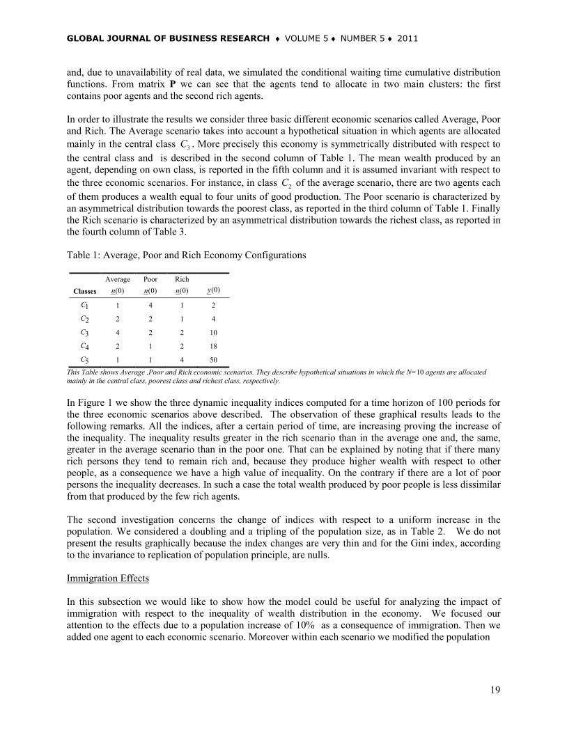
and, due to unavailability of real data, we simulated the conditional waiting time cumulative distribution functions. From matrix P we can see that the agents tend to allocate in two main clusters: the first contains poor agents and the second rich agents. In order to illustrate the results we consider three basic different economic scenarios called Average, Poor and Rich. The Average scenario takes into account a hypothetical situation in which agents are allocated mainly in the central class 3C . More precisely this economy is symmetrically distributed with respect to the central class and is described in the second column of Table 1. The mean wealth produced by an agent, depending on own class, is reported in the fifth column and it is assumed invariant with respect to the three economic scenarios. For instance, in class 2C of the average scenario, there are two agents each of them produces a wealth equal to four units of good production. The Poor scenario is characterized by an asymmetrical distribution towards the poorest class, as reported in the third column of Table 1. Finally the Rich scenario is characterized by an asymmetrical distribution towards the richest class, as reported in the fourth column of Table 3. Table 1: Average, Poor and Rich Economy Configurations

Average Poor Rich Classes (0)n (0)n

(0)n

(0)y

1C 1 4 1 2

2C 2 2 1 4

3C 4 2 2 10

4C 2 1 2 18

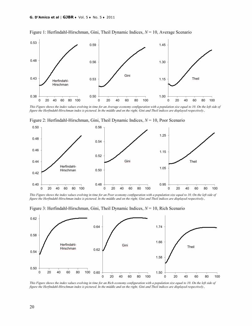
5C 1 1 4 50 This Table shows Average ,Poor and Rich economic scenarios. They describe hypothetical situations in which the N=10 agents are allocated mainly in the central class, poorest class and richest class, respectively. In Figure 1 we show the three dynamic inequality indices computed for a time horizon of 100 periods for the three economic scenarios above described. The observation of these graphical results leads to the following remarks. All the indices, after a certain period of time, are increasing proving the increase of the inequality. The inequality results greater in the rich scenario than in the average one and, the same, greater in the average scenario than in the poor one. That can be explained by noting that if there many rich persons they tend to remain rich and, because they produce higher wealth with respect to other people, as a consequence we have a high value of inequality. On the contrary if there are a lot of poor persons the inequality decreases. In such a case the total wealth produced by poor people is less dissimilar from that produced by the few rich agents. The second investigation concerns the change of indices with respect to a uniform increase in the population. We considered a doubling and a tripling of the population size, as in Table 2. We do not present the results graphically because the index changes are very thin and for the Gini index, according to the invariance to replication of population principle, are nulls. Immigration Effects In this subsection we would like to show how the model could be useful for analyzing the impact of immigration with respect to the inequality of wealth distribution in the economy. We focused our attention to the effects due to a population increase of 10% as a consequence of immigration. Then we added one agent to each economic scenario. Moreover within each scenario we modified the population


20

Figure 1: Herfindahl-Hirschman, Gini, Theil Dynamic Indices, N = 10, Average Scenario

This Figure shows the index values evolving in time for an Average economy configuration with a population size equal to 10. On the left side of figure the Herfindahl-Hirschman index is pictured. In the middle and on the right, Gini and Theil indices are displayed respectively., Figure 2: Herfindahl-Hirschman, Gini, Theil Dynamic Indices, N = 10, Poor Scenario

This Figure shows the index values evolving in time for an Poor economy configuration with a population size equal to 10. On the left side of figure the Herfindahl-Hirschman index is pictured. In the middle and on the right, Gini and Theil indices are displayed respectively., Figure 3: Herfindahl-Hirschman, Gini, Theil Dynamic Indices, N = 10, Rich Scenario

This Figure shows the index values evolving in time for an Rich economy configuration with a population size equal to 10. On the left side of figure the Herfindahl-Hirschman index is pictured. In the middle and on the right, Gini and Theil indices are displayed respectively.,

0.38

0.43

0.48

0.53

0 20 40 60 80 100

Herfindahl-Hirschman

0.50

0.53

0.56

0.59

0 20 40 60 80 100

Gini

1.00

1.15

1.30

1.45

0 20 40 60 80 100

Theil

0.40

0.42

0.44

0.46

0.48

0.50

0 20 40 60 80 100


0.48

0.50

0.52

0.54

0.56

0 20 40 60 80 100

Gini

0.95

1.05

1.15

1.25

0 20 40 60 80 100

Theil

0.50

0.54

0.58

0.62

0 20 40 60 80 100


0.60

0.62

0.64

0 20 40 60 80 100

Gini

1.50

1.58

1.66

1.74

0 20 40 60 80 100

Theil


21

Table 2: Configurations under Different Population Sizes

Scenario Agents 1 (0)Cn

2 (0)Cn 3 (0)Cn

4 (0)Cn 5 (0)Cn

A 20 2 4 8 4 2 30 3 6 12 6 3

P 20 8 4 4 2 2 30 12 6 6 3 3

R 20 2 2 4 4 8 30 3 3 6 6 12

This Table shows the configurations used in the simulations with respect to an uniform increase in the population.. In particular doubling and tripling of number of the agents has been considered. configuration through the increase of one unit allocated first in the poorest class 1C , next in average class

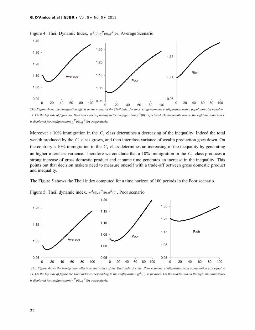
3C and finally in the richest class 5C . The mean wealth produced by an agent, depending on own class, is reported in the eleventh column and we suppose that the mean wealth is invariant with respect to immigration and economic scenarios. To arrive at this point we computed the indices for each of the nine population configurations collected in Table 3. Due to paper length constraints we are not able to report all the results. Additional results are available from the authors by request. Here after we discuss only the results concerning the Theil index. The Figure 4 shows the Theil index computed for a time horizon of 100 periods in the Average scenario. Table 3: The Average, Poor, Rich Economy Configurations Due to Immigration

Average Poor Rich Classes (0)An (0)Pn (0)Rn (0)An (0)Pn (0)Rn (0)An (0)Pn (0)Rn

(0)y

1C 1 2 1 4 5 4 1 2 1 2

2C 2 2 2 2 2 2 1 1 1 4

3C 5 4 4 3 2 2 3 2 2 10

4C 2 2 2 1 1 1 2 2 2 18

5C 1 1 2 1 1 2 4 4 5 50

This Table shows the configurations of the population modified in the following way: a) within the Average scenario one additional entry in the

Average class (configuration (0)An in the second column), one additional entry in the Poor class (configuration (0)Pn in the third column)

and one additional entry in the Rich class (configuration (0)Rn in the fourth column); b) within the Poor scenario one additional entry in the

Average class (configuration (0)An in the fifth column), one additional entry in the Poor class (configuration (0)Pn in the sixth column) and

one additional entry in the Rich class (configuration (0)Rn in the seventh column); c) within the Rich scenario one additional entry in the

Average class (configuration (0)An in the eighth column), one additional entry in the Poor class (configuration (0)Pn in the ninth column)

and one additional entry in the Rich class (configuration (0)Rn in the tenth column).

In the Average economic scenario we remark that there is an increase of the inequality with regard to the early periods because a new additional agent in the class 3C leads to a wealth production with a lower interclass variance. Afterward, thanks also to the kernel structure, the population tends towards two distinct clusters. Later like in the case without immigration, there is an increase in inequality. Therefore it seems that a 10% immigration in the class 3C leads to an increase in gross domestic product but without a corresponding increase in the long term inequality. Indeed for the second column configuration of Table 1 we have GDP 1 2 2 4 4 10 2 18 1 50 136= × + × + × + × + × = , whereas for the configuration in the second column of Table 3, GDP = 146.


22

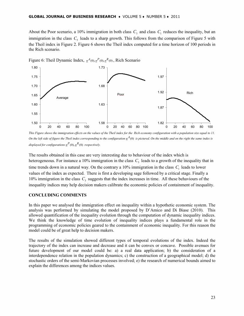
Figure 4: Theil Dynamic Index, (0), (0), (0)A P Rn n n , Average Scenario

This Figure shows the immigration effects on the values of the Theil index for an Average economy configuration with a population size equal to

11. On the left side of figure the Theil index corresponding to the configuration (0)An is pictured. On the middle and on the right the same index

is displayed for configurations (0), (0)P Rn n respectively. Moreover a 10% immigration in the 1C class determines a decreasing of the inequality. Indeed the total wealth produced by the 1C class grows, and then interclass variance of wealth production goes down. On the contrary a 10% immigration in the 5C class determines an increasing of the inequality by generating an higher interclass variance. Therefore we conclude that a 10% immigration in the 5C class produces a strong increase of gross domestic product and at same time generates an increase in the inequality. This points out that decision makers need to measure oneself with a trade-off between gross domestic product and inequality. The Figure 5 shows the Theil index computed for a time horizon of 100 periods in the Poor scenario. Figure 5: Theil dynamic index, (0), (0), (0)A P Rn n n , Poor scenario

This Figure shows the immigration effects on the values of the Theil index for the Poor economy configuration with a population size equal to

11. On the left side of figure the Theil index corresponding to the configuration (0)An is pictured. On the middle and on the right the same index

is displayed for configurations (0), (0)P Rn n respectively.

0.90

1.00

1.10

1.20

1.30

1.40

0 20 40 60 80 100

Average

0.95

1.05

1.15

1.25

1.35

0 20 40 60 80 100

Poor

0.95

1.15

1.35

0 20 40 60 80 100

Rich

0.95

1.05

1.15

1.25

0 20 40 60 80 100

Average

0.95

1.00

1.05

1.10

1.15

1.20

0 20 40 60 80 100

Poor

0.95

1.05

1.15

1.25

1.35

0 20 40 60 80 100

Rich


23

About the Poor scenario, a 10% immigration in both class 3C and class 1C reduces the inequality, but an immigration in the class 5C leads to a sharp growth. This follows from the comparison of Figure 5 with the Theil index in Figure 2. Figure 6 shows the Theil index computed for a time horizon of 100 periods in the Rich scenario. Figure 6: Theil Dynamic Index, (0), (0), (0)A P Rn n n , Rich Scenario

This Figure shows the immigration effects on the values of the Theil index for the Rich economy configuration with a population size equal to 11.

On the left side of figure the Theil index corresponding to the configuration (0)An is pictured. On the middle and on the right the same index is

displayed for configurations (0), (0)P Rn n respectively. The results obtained in this case are very interesting due to behaviour of the index which is heterogeneous. For instance a 10% immigration in the class 5C leads to a growth of the inequality that in time trends down in a natural way. On the contrary a 10% immigration in the class 1C leads to lower values of the index as expected. There is first a developing sage followed by a critical stage. Finally a 10% immigration in the class 3C suggests that the index increases in time. All these behaviours of the inequality indices may help decision makers calibrate the economic policies of containment of inequality. CONCLUDING COMMENTS In this paper we analysed the immigration effect on inequality within a hypothetic economic system. The analysis was performed by simulating the model proposed by D’Amico and Di Biase (2010). This allowed quantification of the inequality evolution through the computation of dynamic inequality indices. We think the knowledge of time evolution of inequality indices plays a fundamental role in the programming of economic policies geared to the containment of economic inequality. For this reason the model could be of great help to decision makers. The results of the simulation showed different types of temporal evolutions of the index. Indeed the trajectory of the index can increase and decrease and it can be convex or concave. Possible avenues for future development of our model could be: a) a real data application; b) the consideration of a interdependence relation in the population dynamics; c) the construction of a geographical model; d) the stochastic orders of the semi-Markovian processes involved; e) the research of numerical bounds aimed to explain the differences among the indices values.

1.50

1.55

1.60

1.65

1.70

1.75

1.80

0 20 40 60 80 100

Average

1.58

1.63

1.68

1.73

0 20 40 60 80 100

Poor

1.82

1.87

1.92

1.97

0 20 40 60 80 100

Rich


24

REFERENCES Athanasopoulos, G. & Vahid, F. (2003) “Statistical Inference on Changes in Income Inequality in Australia,” The Economic Record, 79(247), p. 412-424. Bajo, Salas (2002) "Inequality foundations of concentration mesasures: an application to the Hannah-Kay indices," Spanish economic review 4, p. 311-316. Bickenbach, F. & Bode, E. (2003) “Evaluating the Markov Property in Studies of Economic Convergence,” International Regional Science Review, 26(3), p. 363-392. Campano, F. & Salvatore, D. (2006). Income distribution. Oxford University Press, New York. Cowell, F. (1995). Measuring Inequality. LSE Handbook in Economics Series, 2nd edn, Prentice Hall, London. Dagum, C. (1990) “Relationship between income inequality measures and social welfare functions,” Journal of Econometrics, 43(1-2), p. 91-102. 22 Dalton (1929) "The measurement of the inequality incomes," Economic journal 30, p. 348-361. D'Amico, G. & Di Biase, G. (2010) "Generalized Concentration/Inequality Indices of Economic systems Evolving in Time," Wseas Transactions on Mathematics, 9(2), February, p. 140-149. Dasgupta, Partha, Sen, Starret (1973) "Notes on the measurement of income inequality," Journal of economic theory 6, p. 180-187. Davies, J. B. & Hoy, M. (1995) “Making inequality comparisons when Lorenz curves intersect,” American Economic Review, 85(4), p. 980-986. Gini, C. (1912). Variabilità e mutabilità. Bologna. Hirschman (1964) "The paternity of an index," The American Economic review 54, p. 761. Janssen, J. &Manca, R. (2006). Applied Semi-Markov Processes. Springer, New York. Janssen, J. & Manca, R. (2007). Semi-Markov risk models for Finance, Insurance and Reliability. Springer, New York. Kooleman, X. & Van Doorslaer, E. (2004) “On the interpretation of a concentration index of inequality,” Health Economics, 13(7), p. 649-656. Kwoka, J. E. Jr. (1974) “Large Firm Dominance and Price-Cost Margins in Manufacturing Industries," Southern Economic Journal 44 (1), p. 183–189. Marfels (1971) "Absolute and Relative Measures of Concentration Reconsidered", Kyklos 24, p. 753-756. Mehata, Selvam (1986) "A class of general stochastic compartmental systems," Bulletin of Mathematical Biology, 48, p. 509-523.


25

Ouhbi, Limnios (1999) "Nonparametric estimation for semi-Markov processes based on its hazard rate functions," Statistical Inference for Stochastic Processes. 2, p. 151-173. Quah (1996) "Empiric for economic growth and convergence", European Economic Review 40, p. 951-958. Quah (1993) "Galton's fallacy and tests of the convergence hypothesis", The Scandinavian Journal of Economics, 95(4), p. 427-443. Quah (1994) "One business cycle and one trend from many, many disaggregates", European Economic Review, 38, p. 605-613. Quah, D. (1995). Ideas determining convergence clubs. Economics Department, LSE, London, Working Paper. Sen, A. (1993). On economic Inequality. Clarendon Press, Oxford. Shahrestani and Bidabad (2010) “An implied income inequality index using L1 norm estimation of Lorentz curve,” Global Journal of Business Research, 4(1), p. 29-46. Shannon (1948) "A mathematical theory of communication," Bell System Technical Journal, 27, p. 379-423. Theil, H. (1967). Economics and Information Theory. North Holland, Amsterdam. Tirole, J. (1988). The theory of industrial organization. The MIT Press Cambrige Mass. BIOGRAPHY Dr. Guglielmo D’Amico, is assistant professor of Mathematical Methods in Economics, Finance and Insurance at the “G. D’Annunzio” University of Chieti-Pescara, Italy. He can be reached at: Department of Drug Sciences, University “G. D’Annunzio”, via dei Vestini 31, 66013, CHIETI, ITALY. E-mail: [email protected]. Dr. Giuseppe Di Biase, is associate professor of Mathematical Methods in Economics, Finance and Insurance at the “G. D’Annunzio” University of Chieti-Pescara, Italy. He can be reached at: Department of Drug Sciences, University “G. D’Annunzio”, via dei Vestini 31, 66013, CHIETI, ITALY. E-mail: [email protected]. Dr. Raimondo Manca, is full professor of Mathematical Methods in Economics, Finance and Insurance at the “La Sapienza” University of Rome, Italy. He can be reached at: MEMOTEF Department, University “La Sapienza”, via del Castro Laurenziano 9, 00161, ROMA, ITALY. E-mail: [email protected].

Immigration Effects on Economic Systems Through Dynamic Inequality Indices

Documents

Transcript of Immigration Effects on Economic Systems Through Dynamic Inequality Indices