1 2019 ASME

Proceedings of the ASME 2019 International Mechanical Engineering Congress and Exposition

IMECE2019 November 8-14, Salt Lake City, UT, USA

IMECE2019-10318

INVESTIGATION OF FLASHING FLOW IN A SIPHON TO EXTRACT CONDENSATE IN PAPER DRYER APPLICATION

Hamed Abdul Majeed and Ting Wang

Energy Conversion and Conservation Center University of New Orleans

New Orleans, Louisiana, USA

ABSTRACT The paper industry uses steam to dry paper web through

cylinder dryers. As steam condenses inside the cylinder dryer,

the condensate is removed by means of either a stationary or a

rotary siphon. However, during the siphoning process for

transporting the condensate, flashing of the condensate occurs,

which could cause backflow or discontinuity in the siphoning

process. To resolve this flashing issue, two approaches have

been employed: (a) increasing the amount of steam supplied to

the cylinder to "blow-through" the stalled condensate-steam

mixture and (b) reducing the back pressure by inducing

"suction" through a thermocompressor from downstream. This

practice of employing push from the upstream and suction

from the downstream requires excessively large amounts of

high-grade steam, resulting in an estimated 10 to 15 %, 15 to

25%, and 40 to 90 % of blow-through steam for stationary

siphons, rotary siphons, and Yankee dryers respectively. The

objective of this study is to investigate and improve

understanding of the flashing phenomena during condensate

transport through the siphon and piping system in order to

develop means to reduce this excessive steam consumption

during the paper drying process. A computational fluid

dynamics (CFD) simulation is performed that uses the

Eulerian-Eulerian multiphase method. The steady-state case is

first solved to obtain the flow field without flashing. Then the

transient method is initiated by employing flashing and

condensation models. The results show that reduction of local

pressure triggers flashing, however, flashing in turn reduces

local temperature, and subsequently induces condensation,

resulting in an alternating flashing and condensation behavior.

To maintain continuity of the siphon flow, the inlet pressure

fluctuates corresponding to the variation of total vapor volume

ratio inside the siphon. The results will be used to modify the

current siphon system design and operating practices to reduce

steam consumption.

Keywords: Two-phase flows, flashing, paper dryers,

siphons.

NOMENCLATURE D Droplet size, (m)

h Convective heat transfer coefficient, (W/m2K)

H Enthalpy, (J)

Nu Nusselt number (hL/k)

P Pressure, (Pa)

Re Reynolds number (u D/ν)

𝑚 Mass flow rate (kg/s)

Greek Letters μ Dynamic viscosity, (Pa-s) or microns, (10

-6 meter)

ν Kinematic viscosity, (m2/s)

ρ Density, (kg/m3)

τ Particulate relaxation time (s)

τ Strain tensor

α Volume fraction

Subscripts p p

th phase

q qth

phase

l liquid

v vapor

b bubble

sat saturation

i interface

1. INTRODUCTION

1.1 Paper Drying in Paper Industry Paper industry typically uses contact drying with

multicylinder paper dryers as the primary means for drying [1].

In multicylinder drying, slightly superheated steam is fed

inside the paper dryers. As steam condenses, it heats the

cylinder walls, which dries the paper web in contact with the

outer surface of the dryer [2].

The current Steam and Condensate (S & C) system uses

the push-pull method to control the drying process. As steam

enters the dryers it condenses to saturated liquid water, which

needs to be removed from the cylinder. Typically, a "push

and pull" approach is practiced by using the blow-through

steam to "push" the condensate in the front end and

thermocompressors (or vacuum pumps) down the line in the

back end to create a suction or low-pressure region to pull the

condensate out. Since the condensate is at the saturated liquid

state, it quickly flashes if the local pressure reduces even

slightly below the saturated pressure during the transportation

process, for example, due to climbing upward in the piping

system. Therefore, two-phase flow occurs in the siphon pipe

2 2019 ASME

consisting of the blow-through steam, the condensate, the flash

steam, and non-condensable gases.

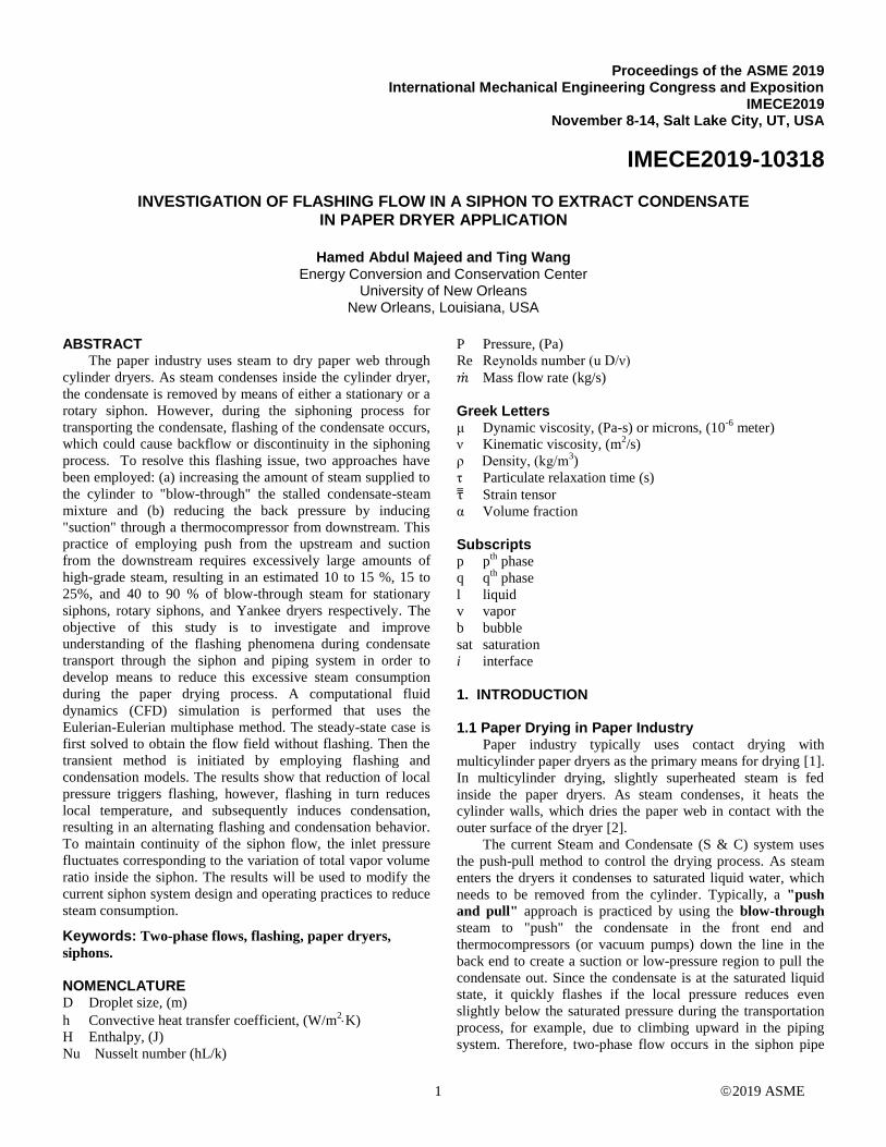
Condensate removal in paper dryers is done either through

rotary siphons or stationary siphons (see Fig. 1). Rotary siphon

rotates with the dyer and is fixed inside the dryer and bolted by

springs to the dryer shell. Rotary siphon requires higher

differential pressure to operate and could lead to dryer flooding

if the higher differential is not maintained. Stationary siphon is

stationary as the dryer rotates and require better mechanical

support to avoid failure, typically due to collision between the

siphon tip and the dryer's wall. As the condensate has an inlet

velocity with respect to the stationary siphon the kinetic energy

plays a favorable role in removing condensate, thus, stationary

siphons have a lower differential pressure requirement.

Additionally, dryer flooding is not an issue in case of

stationary siphon as it maintains its contact with the

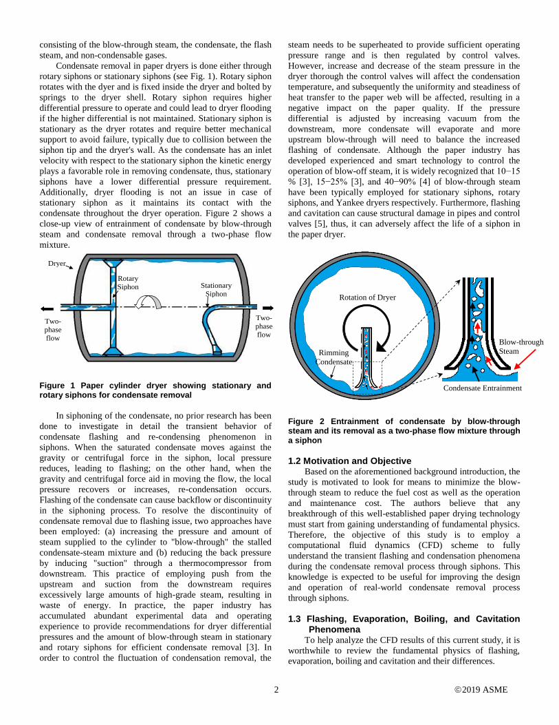
condensate throughout the dryer operation. Figure 2 shows a

close-up view of entrainment of condensate by blow-through

steam and condensate removal through a two-phase flow

mixture.

Rotary

Siphon Stationary

Siphon

Dryer

Two-

phase

flow

Two-

phase

flow

Figure 1 Paper cylinder dryer showing stationary and rotary siphons for condensate removal

In siphoning of the condensate, no prior research has been

done to investigate in detail the transient behavior of

condensate flashing and re-condensing phenomenon in

siphons. When the saturated condensate moves against the

gravity or centrifugal force in the siphon, local pressure

reduces, leading to flashing; on the other hand, when the

gravity and centrifugal force aid in moving the flow, the local

pressure recovers or increases, re-condensation occurs.

Flashing of the condensate can cause backflow or discontinuity

in the siphoning process. To resolve the discontinuity of

condensate removal due to flashing issue, two approaches have

been employed: (a) increasing the pressure and amount of

steam supplied to the cylinder to "blow-through" the stalled

condensate-steam mixture and (b) reducing the back pressure

by inducing "suction" through a thermocompressor from

downstream. This practice of employing push from the

upstream and suction from the downstream requires

excessively large amounts of high-grade steam, resulting in

waste of energy. In practice, the paper industry has

accumulated abundant experimental data and operating

experience to provide recommendations for dryer differential

pressures and the amount of blow-through steam in stationary

and rotary siphons for efficient condensate removal [3]. In

order to control the fluctuation of condensation removal, the

steam needs to be superheated to provide sufficient operating

pressure range and is then regulated by control valves.

However, increase and decrease of the steam pressure in the

dryer thorough the control valves will affect the condensation

temperature, and subsequently the uniformity and steadiness of

heat transfer to the paper web will be affected, resulting in a

negative impact on the paper quality. If the pressure

differential is adjusted by increasing vacuum from the

downstream, more condensate will evaporate and more

upstream blow-through will need to balance the increased

flashing of condensate. Although the paper industry has

developed experienced and smart technology to control the

operation of blow-off steam, it is widely recognized that 10−15

% [3], 15−25% [3], and 40−90% [4] of blow-through steam

have been typically employed for stationary siphons, rotary

siphons, and Yankee dryers respectively. Furthermore, flashing

and cavitation can cause structural damage in pipes and control

valves [5], thus, it can adversely affect the life of a siphon in

the paper dryer.

Rotation of Dryer

Condensate Entrainment

Rimming

Condensate

Blow-through

Steam

Figure 2 Entrainment of condensate by blow-through steam and its removal as a two-phase flow mixture through a siphon

1.2 Motivation and Objective Based on the aforementioned background introduction, the

study is motivated to look for means to minimize the blow-

through steam to reduce the fuel cost as well as the operation

and maintenance cost. The authors believe that any

breakthrough of this well-established paper drying technology

must start from gaining understanding of fundamental physics.

Therefore, the objective of this study is to employ a

computational fluid dynamics (CFD) scheme to fully

understand the transient flashing and condensation phenomena

during the condensate removal process through siphons. This

knowledge is expected to be useful for improving the design

and operation of real-world condensate removal process

through siphons.

1.3 Flashing, Evaporation, Boiling, and Cavitation Phenomena

To help analyze the CFD results of this current study, it is

worthwhile to review the fundamental physics of flashing,

evaporation, boiling and cavitation and their differences.

3 2019 ASME

Flashing Flashing is the vaporization of liquid into vapor due to

reduced pressure. Depressurization can occur due to total

pressure losses, pressure release, or flow acceleration.

Examples of depressurizing of liquid are liquid flow in a

convergent divergent nozzle, sudden opening of a valve for a

pressurized liquid, flashing in an atomizer, or moving against

gravity or centrifugal force. Evaporation, boiling, and

condensation all involve change of liquid phase to vapor

phase. However, they are different in some aspects, as

explained below.

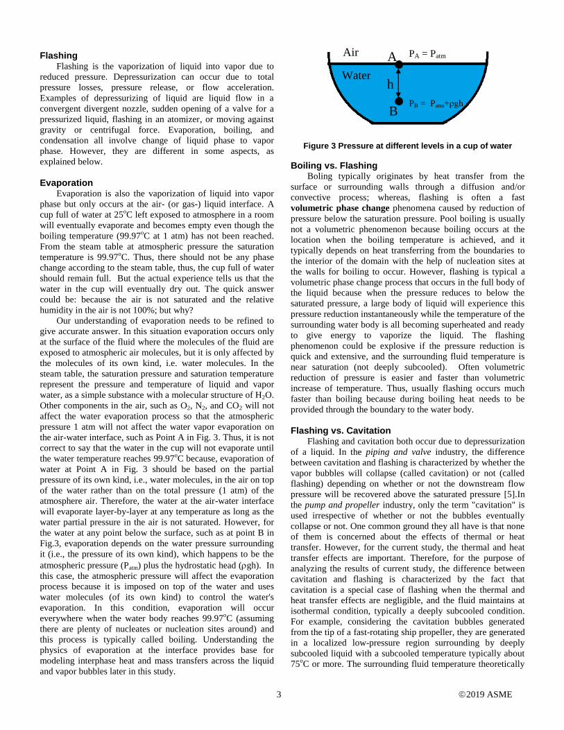
Evaporation Evaporation is also the vaporization of liquid into vapor

phase but only occurs at the air- (or gas-) liquid interface. A

cup full of water at 25oC left exposed to atmosphere in a room

will eventually evaporate and becomes empty even though the

boiling temperature (99.97oC at 1 atm) has not been reached.

From the steam table at atmospheric pressure the saturation

temperature is 99.97oC. Thus, there should not be any phase

change according to the steam table, thus, the cup full of water

should remain full. But the actual experience tells us that the

water in the cup will eventually dry out. The quick answer

could be: because the air is not saturated and the relative

humidity in the air is not 100%; but why?

Our understanding of evaporation needs to be refined to

give accurate answer. In this situation evaporation occurs only

at the surface of the fluid where the molecules of the fluid are

exposed to atmospheric air molecules, but it is only affected by

the molecules of its own kind, i.e. water molecules. In the

steam table, the saturation pressure and saturation temperature

represent the pressure and temperature of liquid and vapor

water, as a simple substance with a molecular structure of H2O.

Other components in the air, such as O2, N2, and CO2 will not

affect the water evaporation process so that the atmospheric

pressure 1 atm will not affect the water vapor evaporation on

the air-water interface, such as Point A in Fig. 3. Thus, it is not

correct to say that the water in the cup will not evaporate until

the water temperature reaches 99.97oC because, evaporation of

water at Point A in Fig. 3 should be based on the partial

pressure of its own kind, i.e., water molecules, in the air on top

of the water rather than on the total pressure (1 atm) of the

atmosphere air. Therefore, the water at the air-water interface

will evaporate layer-by-layer at any temperature as long as the

water partial pressure in the air is not saturated. However, for

the water at any point below the surface, such as at point B in

Fig.3, evaporation depends on the water pressure surrounding

it (i.e., the pressure of its own kind), which happens to be the

atmospheric pressure (Patm) plus the hydrostatic head (gh). In

this case, the atmospheric pressure will affect the evaporation

process because it is imposed on top of the water and uses

water molecules (of its own kind) to control the water's

evaporation. In this condition, evaporation will occur

everywhere when the water body reaches 99.97oC (assuming

there are plenty of nucleates or nucleation sites around) and

this process is typically called boiling. Understanding the

physics of evaporation at the interface provides base for

modeling interphase heat and mass transfers across the liquid

and vapor bubbles later in this study.

h

PB = Patm+ρgh

PA = Patm

Water

Air A

B

Figure 3 Pressure at different levels in a cup of water

Boiling vs. Flashing Boling typically originates by heat transfer from the

surface or surrounding walls through a diffusion and/or

convective process; whereas, flashing is often a fast

volumetric phase change phenomena caused by reduction of

pressure below the saturation pressure. Pool boiling is usually

not a volumetric phenomenon because boiling occurs at the

location when the boiling temperature is achieved, and it

typically depends on heat transferring from the boundaries to

the interior of the domain with the help of nucleation sites at

the walls for boiling to occur. However, flashing is typical a

volumetric phase change process that occurs in the full body of

the liquid because when the pressure reduces to below the

saturated pressure, a large body of liquid will experience this

pressure reduction instantaneously while the temperature of the

surrounding water body is all becoming superheated and ready

to give energy to vaporize the liquid. The flashing

phenomenon could be explosive if the pressure reduction is

quick and extensive, and the surrounding fluid temperature is

near saturation (not deeply subcooled). Often volumetric

reduction of pressure is easier and faster than volumetric

increase of temperature. Thus, usually flashing occurs much

faster than boiling because during boiling heat needs to be

provided through the boundary to the water body.

Flashing vs. Cavitation Flashing and cavitation both occur due to depressurization

of a liquid. In the piping and valve industry, the difference

between cavitation and flashing is characterized by whether the

vapor bubbles will collapse (called cavitation) or not (called

flashing) depending on whether or not the downstream flow

pressure will be recovered above the saturated pressure [5].In

the pump and propeller industry, only the term "cavitation" is

used irrespective of whether or not the bubbles eventually

collapse or not. One common ground they all have is that none

of them is concerned about the effects of thermal or heat

transfer. However, for the current study, the thermal and heat

transfer effects are important. Therefore, for the purpose of

analyzing the results of current study, the difference between

cavitation and flashing is characterized by the fact that

cavitation is a special case of flashing when the thermal and

heat transfer effects are negligible, and the fluid maintains at

isothermal condition, typically a deeply subcooled condition.

For example, considering the cavitation bubbles generated

from the tip of a fast-rotating ship propeller, they are generated

in a localized low-pressure region surrounding by deeply

subcooled liquid with a subcooled temperature typically about

75oC or more. The surrounding fluid temperature theoretically

4 2019 ASME

will reduce to provide vaporization energy for cavitation, but

its effect is negligible. However, if the change in the liquid due

to depressurization causes considerable changes in the

temperature surrounding the vapor, this process is flashing.

Cavitation bubble sizes are mainly controlled by

mechanical non-equilibrium i.e. due to pressure difference

across the interface with negligible thermal effects. Cavitation

also occurs at relatively lower saturation conditions as in this

case the superheat level is not high enough which results in

low vapor density and quicker collapse of vapor bubbles

(localized formation of bubbles). In contrast, flashing is

characterized by high thermal non-equilibrium (temperature

difference across the interface). The bubble growth in flashing

is dictated by the interface heat transfer rate and not by the

pressure difference at the interface. Flashing has vapor forming

and due to considerable thermal effect than pressure effect

retain downstream of the flow. In flashing steam flow, vapor

bubbles can "recondense" and shrink due to cooling in contrast

to abrupt "collapse" of vapor bubbles in a cavitation flow with

pressure recovering in a deeply subcooled fluid. Thus, for

modeling flashing and cavitation processes the physics of the

bubble formation and growth are controlled by the thermal or

mechanical effects, respectively [6].

2. MODELING OF FLASHING FLOWS IN COMPUTATIONAL FLUID DYNAMICS (CFD)

Flashing flows have been extensively studied using

computational simulation with phase-change models [7]. In

most of the published work, the vapor phase is treated as

discrete spherical bubbles dispersed in a liquid domain. The

bubble sizes in most of the research are considered constant i.e.

mono-dispersed analysis is performed. The CFD work in

modeling flashing can also be distinguished on the basis of

whether the simulation has nucleation model in use [8]. A brief

literature review of CFD used to model flashing is presented in

this section.

Giese and Laurien [9−11] and Laurien [12] simulated

flashing flow in pipelines by considering both vaporization and

condensation. They used the Eulerian-Eulerian 5-equation

model with two continuity equations, two momentum

equations, and one energy equation for the two-phase flow.

The heat transfer in the vapor phase was neglected by

considering vapor fixed at saturation temperature. The

commercial code ANSYS CFX was used in this study. Drag

force was considered for the interphase momentum transfer. In

Laurien’s later work [12], a constant bubble number density

was considered instead of the constant bubble size. This

allowed the bubble size to grow, which better explains the

physics of the flow. Their study neglected nucleation process

and was limited by the absence of bubble coalescence and

breakout model and only valid for narrow nucleation zones.

The simulation of Eulerian-Eulerian two-fluid model for

flashing flows in pipes and nozzles was performed by Maksic

and Mewes [13] in ANSYS CFX. The bubble number density

was solved using a scalar transport equation with wall

nucleation defined as a source term. The model had conduction

dominated interfacial heat transfer, which is a drawback for

flows with dominant convection heat transfer effect. It was

shown that in most flashing expansion cases the convective

contribution due to relative motion of bubbles dominated the

heat transfer. The nucleation rate was determined by the Jones

model [14]. Inter-phase mass, momentum, and energy transfer

due to nucleation was ignored in their study.

Frank [15] performed CFD simulations for the Edwards’

blow-down test. In this study the bubble size was assumed to

be Db = 1mm which was fixed through the simulation. The

model was based similar to the work performed by Laurien

and coworkers [8−11]. The bubbles were assumed to be at

saturation conditions corresponding to the saturation pressure;

this assumption is typically valid for low values of

depressurization rates. The nucleation process was ignored in

the simulation. In this study ANSYS CFX was used to model

the problem and the Eulerian-Eulerian model was used.

Marshand O’Mahony [16] used ANSYS Fluent for the

three-dimensional study of industrial flashing flows. They used

the Eulerian-Eulerian six-equation model: two continuity

equations, two momentum equations, and two energy

equations, which had one energy equation than Laurien's five-

equation model [12]. The interphase mass and momentum

transfer resulting from nucleation and phase change were both

considered in this study. However, only drag force was

considered for the momentum interphase transfer. A transport

equation was used to track the bubbles with source terms used

for heterogeneous nucleation. In this simulation, the nucleation

model used was a modification of the Blander and Katz

nucleation model [17]. Moreover, a transport equation was

used for the bubbles with a source term to account for

heterogeneous nucleation.

Mimouni et al. [18] simulated cavitation using the

Eulerian-Eulerian six-equation model in commercial code

NEPTUNE CFD. The bubble temperature was assumed to be

close to saturation temperature and a heat transfer coefficient,

was assumed to make the vapor temperature close to the

saturation temperature. The nucleation of vapor in the domain

is considered and modeled using a modified Jones model [14]

for nucleation. The interphase momentum transfer is

contributed through drag, lift, and the virtual mass forces. The

―virtual mass effect‖ occurs when a secondary phase

accelerates relative to the primary phase. The inertia of the

primary-phase mass encountered by the accelerating particles

(or droplets or bubbles) exerts a ―virtual mass force‖ on the

particles. The bubble size was considered a constant value. The

simulation results were compared to experimental results for

benchmarking of the solution.

A CFD study in ANSYS Fluent v 12.0 was performed by

Yazdani [19]. The method of "mixture model" was used to

model the two-phase flow where a single momentum equation

was used for the two phases and a velocity slip was

considered. The simulation was performed for a convergent

divergent nozzle and compared to experimental results. The

nucleation model was ignored in this study.

Liao et al. [20] simulated flashing of water in a vertical

pipe flow using Eulerian-Eulerian model in ANSYS CFX. In

the experiment the vertical pipe had a blow-off valve that

opened to release the high-pressure liquid and caused flashing.

In the simulation the bubble size was considered constant and

nucleation was neglected in this study. The interphase

momentum contribution of drag, lift, wall lubrication, virtual

mass effect, and turbulence dispersion forces were considered.

The mass transfer at the interface between the two phases was

5 2019 ASME

based on the interfacial heat transfer; this represents the

flashing phenomenon which is based on thermal effects. An

important conclusion of their research was that the bubble size

should be carefully selected based on experimental evaluation

otherwise it would lead to large deviations. For variable bubble

sizes, poly-dispersed simulation employing the

inhomogeneous multiple size group (IMUSIG) model [21] was

used which had improved the accuracy of the simulation.

Janet et al. [22] studied flashing in a convergent-divergent

nozzle using ANSYS CFX. They suggested using Jones' model

[14] for nucleation as it was more accurate compared to

Rensselaer Polytechnic Institute (RPI) [23] and Riznic models

[24]. Eulerian-Eulerian 5-equation model was used with vapor

temperature fixed to saturation temperature. A similar study

was performed by Liao and Lucas [25] for the similar

convergent-divergent geometry. The results showed the

comparison of axial and radial volume fraction and pressures.

The cross-section averaged axial profiles of vapor volume

fraction and pressure showed good agreement with the

experimental results. A comparison of different nucleation

models was also presented in this study. Their work concluded

that the Blinkov nucleation model [26] and RPI nucleation

model gave good agreement of axial pressure data with the

experiment. Moreover, the Riznic nucleation model did not

provide close agreement with the experiment results. Liao and

Lucas [8] reviewed the limitations of CFD modeling of

flashing flows. In their study of flashing due to

depressurization in a vertical pipe is considered with bubble

dynamics using the model presented by Liao et al. [27].

Pelletingeas [28] studied the flashing with nucleation

using the commercial software STAR-CD. In this study the

bubble growth is governed by the Rayleigh-Plessent equation

[29]. The surface tension between the phases was also

considered in this study. The mixture model was used for

modeling the two phases and the phase change was based on

pressure. The literature review presented above focuses on

study of flashing in applications, such as convergent-divergent

nozzle and pipe blowdown, using either Eulerian-Eulerian

model or mixture model.

In this present study the simulation of flashing in a siphon

is performed. As fluid flows upward in a vertical siphon the

region of low static pressure is created wherein if pressure

reduces to below the saturation pressure, flashing will occur. If

no phase change occurs inside the siphon, the gravitational

force created by the elevation difference between the inlet and

outlet of a stationary siphon will keep the liquid fluid moving

forever. However, if flashing occurs inside the siphon, the flow

could be interrupted, and additional pressure needs to be

provided at the inlet to push through the flow. Hence, one of

the objectives is to monitor the variation of the required inlet

pressure to sustain the siphon flow when flashing and re-

condensation occur inside the siphon. The detailed model

formulation, assumptions, sub-models, boundary conditions,

and computational methodologies are described below.

3. NUMERICAL SIMULATION This study simulates flashing as saturated liquid enters the

siphon. The two phases, liquid water and water vapor, are

modeled using the Eulerian-Eulerian model. The simulation

consists of two-phase flows with mono-dispersed vapor

bubbles, i.e. the bubble diameter is fixed in the domain. The

interphase drag force between the phases is modeled using the

Schiller-Naumann correlation for drag coefficient [30]. The

interphase heat transfer between vapor bubbles and liquid is

based on designed heat transfer coefficients on both sides of

the interface. The heat transfer coefficients are based on

Nusselt numbers calculated from the Ranz-Marshall

correlation [31]. The interfacial area density is based on an

algebraic relation considering the effect of volume fraction

from both the phases. The turbulence is modeled using the

realizable k-ε turbulent model with scalable wall functions. In

this study we are simulating flashing, so the interphase mass

transfer is based on thermal non-equilibrium between the two

phases. The nucleation and bubble dynamics (bubble growth,

coalescence, and breakups) are not considered in this study.

The CFD simulation is performed in ANSYS Fluent V. 19.0 in

a transient state. A description of the fundamental governing

and closure equations is presented below.

3.1 Fundamental Transport Equations The fundamental transport equations represent the

Eulerian-Eulerian formulation. It is also known as the two-

fluid model or the six-equation model for two-phase flow

simulation.

Continuity Equation The volume fraction of each phase (p or q) is calculated

from the continuity equation. For example, vapor can be

assigned to phase p and liquid to phase q. For phase q the

continuity equation is given by,

1

𝜌𝑟𝑞 𝜕

𝜕𝑡 𝛼𝑞𝜌𝑞 + ∇ ⋅ 𝛼𝑞𝜌𝑞𝑣 𝑞 = 𝑚 𝑝𝑞 −𝑚 𝑞𝑝

𝑛

𝑝=1 (1)

𝜌𝑟𝑞 = Reference density of phase q or volume average of

density of phase q.

𝑣 𝑞 = Velocity of the phase q.

𝑚 𝑝𝑞= Mass transfer from the pth

to qth

phase.

𝑚 𝑞𝑝= Mass transfer from the qth

to pth

phase.

Momentum conservation equation The momentum for phase q is governed by, 𝜕

𝜕𝑡 𝛼𝑞𝜌𝑞𝑣 𝑞 + ∇ ⋅ 𝛼𝑞𝜌𝑞𝑣 𝑞𝑣 𝑞

(2) = −𝛼𝑞∇𝑝 + ∇ ⋅ 𝜏 𝑞 + 𝛼𝑞𝜌𝑞𝑔 + 𝐾𝑝𝑞 𝑣 𝑝 − 𝑣 𝑞 𝑛

𝑝=1

+𝑚 𝑝𝑞𝑣 𝑝𝑞 −𝑚 𝑞𝑝𝑣 𝑞𝑝 + 𝐹 𝑞 + 𝐹 𝑙𝑖𝑓𝑡 ,𝑞 + 𝐹 𝑤𝑙 ,𝑞 + 𝐹 𝑣𝑚 ,𝑞 + 𝐹 𝑡𝑑 ,𝑞

where,

𝑝 = Pressure. All phases share same pressure.

𝜏 𝑞 = qth

phase stress-strain tensor.

𝑔 = Acceleration due to gravity.

𝐾𝑝𝑞= Interphase momentum exchange coefficient.

𝐹 𝑞 = Body force on phase q such as buoyancy.

𝐹 𝑙𝑖𝑓𝑡 ,𝑞 = Lift force on phase q.

𝐹 𝑤𝑙 ,𝑞 = Wall lubrication force on phase q.

𝐹 𝑣𝑚 ,𝑞 = Virtual mass force on phase q.

𝐹 𝑡𝑑 ,𝑞 = Turbulence dispersion force on phase q.

𝑣 𝑝𝑞 = Interphasevelocity.

6 2019 ASME

The interphase velocity 𝑣 𝑝𝑞 will be equal to 𝑣 𝑝 if mass is

transferred from phase p to phase q, likewise, if mass is

transferred from phase q to phase p then the interface velocity

will be equal to 𝑣 𝑞 .

The qth

phase stress strain tensor 𝜏𝑞 is given by,

𝜏 𝑞 = 𝛼𝑞𝜇𝑞 ∇𝑣 𝑞 + ∇𝑣 𝑞𝑇 + 𝛼𝑞 𝜆𝑞 −

2

3𝜇𝑞 ∇ ⋅ 𝑣 𝑞𝐼 (3)

where,

𝜇𝑞 = Molecular viscosity of phase q.

𝜆𝑞= Bulk viscosity of phase q.

Conservation of energy equation In the two-fluid model, the enthalpy equation can be

written for each phase. Thus, for phase q,

𝜕

𝜕𝑡 𝛼𝑞𝜌𝑞𝑕𝑞 + 𝛻 ⋅ 𝛼𝑞𝜌𝑞𝑢 𝑞𝑕𝑞 = 𝛼𝑞

𝑑𝑝𝑞

𝑑𝑡+ 𝜏 𝑞 :𝛻𝑢 𝑞 − 𝛻 ⋅ 𝑞 𝑞

(4) + 𝑄𝑞𝑝 +𝑚 𝑝𝑞𝑕𝑝𝑞 −𝑚 𝑞𝑝𝑕𝑞𝑝

𝑛

𝑝=1

where,

𝑕𝑞= Specific enthalpy of qth

phase.

𝑞 𝑞 = Heat flux of qth

phase.

𝑄𝑞𝑝 = Intensity of heat exchange between pth

and qth

phase.

𝑕𝑝𝑞 = Interphase enthalpy.

In case of evaporation, hpq is the enthalpy of vapor at the

temperature of liquid droplets, where, p is the liquid phase and

q is the vapor phase.

3.2 Closure Models The closure models provide additional equations needed to

solve the governing equations.

Interphase mass transfer The interphase mass transfer between the phases is

modeled using Thermal Phase Change Model. The model is

based on calculation of the volumetric heat transfer for

evaporation and condensation. The mass transfer is calculated

from the ratio of heat transferring to the phase from the

interface over the latent heat (Hv-Hl). The mass transfer is

given below for the cases of evaporation or condensation.

If 𝑚 𝑙𝑣 ≥ 0 (evaporation, where liquid is the outgoing phase):

𝑚 𝑙𝑣 = −𝑕𝑙𝐴𝑖 𝑇𝑠𝑎𝑡 − 𝑇𝑙 + 𝑕𝑣𝐴𝑖 𝑇𝑠𝑎𝑡 − 𝑇𝑣

𝐻𝑣 𝑇𝑠𝑎𝑡 − 𝐻𝑙(𝑇𝑙) (5)

Here, Tsat is the saturation temperature based on the local

pressure, which is the liquid pressure as well as the vapor

pressure because the pressure equilibrium model is assumed

between the vapor and liquid phrases. Tv is the vapor

temperature.

If 𝑚 𝑙𝑣 < 0 (condensation, where liquid is the incoming phase):

𝑚 𝑙𝑣 = −𝑕𝑙𝐴𝑖 𝑇𝑠𝑎𝑡 − 𝑇𝑙 + 𝑕𝑣𝐴𝑖 𝑇𝑠𝑎𝑡 − 𝑇𝑣

𝐻𝑣 𝑇𝑣 − 𝐻𝑙(𝑇𝑠𝑎𝑡 ) (6)

Interfacial area density The interfacial area density is defined as the ratio of

surface area of the bubble to the volume of the bubble. In this

case we assume the water vapor phase (secondary phase) as

bubbles of constant diameter dispersed in the liquid water

phase (primary phase). The interfacial area considering the

volume fraction of both phases is given by:

𝐴𝑖 =6𝛼𝑝𝛼𝑞

𝑑𝑏 (7)

Interphase heat transfer In this study the two-resistance heat transfer model is used

to model the interphase heat transfer. In this method the heat

transfer coefficients for either side of the interface are

considered. This is a more general approach than using the

overall heat transfer coefficient method. The interphase heat

transfer is given by,

𝑄𝑞 = −𝑄𝑝 = 𝑕𝑝𝑞𝐴𝑖 𝑇𝑝 − 𝑇𝑞 (8)

1

𝑕𝑝𝑞=1

𝑕𝑝+1

𝑕𝑞 (9)

In the current study, the interface heat transfer coefficient

for each phase is determined form the –Nusselt number (h =

Nukd) calculated from the Ranz-Marshall correlation [31] for

Nusselt number (for pth

phase) given by,

𝑁𝑢𝑝 = 2.0 + 0.6𝑅𝑒𝑝1/2

𝑃𝑟1/3 (10)

where, Rep is the relative Reynolds number for pth

phase based

on diameter of the phase p, relative velocity 𝑣𝑝 − 𝑣𝑞 , and

molecular viscosity 𝜇𝑝 . Prandtl number for the qth

phase is

given by,

𝑃𝑟 = 𝑐𝑝𝑞𝜇𝑝/𝜅𝑞 (11)

where, 𝑐𝑝𝑞 is the specific heat capacity, 𝜇𝑞 is the molecular

viscosity, and 𝜅𝑞 is the thermal conductivity for phase q.

Equations 8 and 9 provide a means to limit the amount of

flashing or condensation through Eqs. 5 and 6. This implies

that even though the local pressure reduces below the

saturation pressure, flashing can only occur when there is

sufficient heat transfer to bring the thermal energy to the

bubble sites to feed the latent heat.

Nucleation model In this study the nucleation model was not used. Instead,

an initial value of volume fraction for the vapor phase is

provided at the inlet of the computational domain. Both 5%

and 10% are used to study its effect on the simulation results

Turbulence model Realizable k-ε model with scalable wall functions are

applied for the mixture. The scalable wall functions use the log

law in conjunction with the standard wall functions and give

good results for y+<11 compared to the standard wall

functions.

7 2019 ASME

Interphase momentum transfer The momentum exchange between the phases is based on

the value of fluid-fluid exchange coefficient 𝐾𝑝𝑞 . All

interphase exchange coefficients are empirically based. In this

flow modeling, the interphase momentum transfer coefficient

is given by:

𝐾𝑝𝑞 =𝜌𝑝𝑓

6𝜏𝑝𝑑𝑝𝐴𝑖 (12)

where,

𝐴𝑖 = Interfacial area density.

𝑓 = Drag function, it includes a drag coefficient (CD) and

relative Reynolds number (Re). It can be modeled using

various drag coefficient models.

𝑑𝑝 = Diameter of the bubbles or droplets of phase p.

𝜏𝑝 = Particulate relaxation time. It is defined as:

𝜏𝑝 =𝜌𝑝𝑑𝑝

2

18𝜇𝑞 (13)

In the present study Schiller and Naumann model is used to

determine the drag coefficient [31]. The following empirical

relation is used:

𝑓 =𝐶𝐷𝑅𝑒

24 (14)

𝐶𝐷 = 24 1 + 0.15𝑅𝑒0.687

𝑅𝑒,𝑅𝑒 ≤ 1000

0.44 ,𝑅𝑒 > 1000

(15)

The relative Reynolds number for primary phase p and

secondary phase q is given by:

𝑅𝑒 =𝜌𝑞 𝑣𝑝 − 𝑣𝑞 𝑑𝑝

𝜇𝑞 (16)

3.3 Computational Domain and Methodology

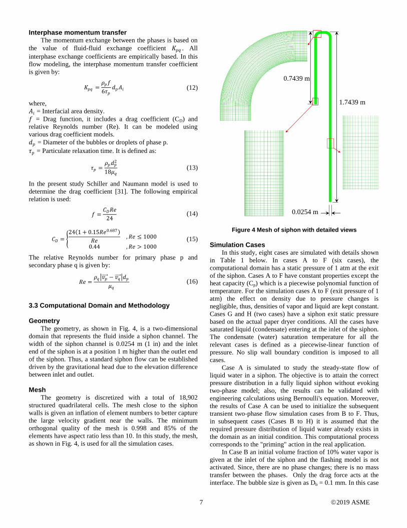
Geometry The geometry, as shown in Fig. 4, is a two-dimensional

domain that represents the fluid inside a siphon channel. The

width of the siphon channel is 0.0254 m (1 in) and the inlet

end of the siphon is at a position 1 m higher than the outlet end

of the siphon. Thus, a standard siphon flow can be established

driven by the gravitational head due to the elevation difference

between inlet and outlet.

Mesh The geometry is discretized with a total of 18,902

structured quadrilateral cells. The mesh close to the siphon

walls is given an inflation of element numbers to better capture

the large velocity gradient near the walls. The minimum

orthogonal quality of the mesh is 0.998 and 85% of the

elements have aspect ratio less than 10. In this study, the mesh,

as shown in Fig. 4, is used for all the simulation cases.

0.0254 m

0.7439 m

1.7439 m

Figure 4 Mesh of siphon with detailed views

Simulation Cases In this study, eight cases are simulated with details shown

in Table 1 below. In cases A to F (six cases), the

computational domain has a static pressure of 1 atm at the exit

of the siphon. Cases A to F have constant properties except the

heat capacity (Cp) which is a piecewise polynomial function of

temperature. For the simulation cases A to F (exit pressure of 1

atm) the effect on density due to pressure changes is

negligible, thus, densities of vapor and liquid are kept constant.

Cases G and H (two cases) have a siphon exit static pressure

based on the actual paper dryer conditions. All the cases have

saturated liquid (condensate) entering at the inlet of the siphon.

The condensate (water) saturation temperature for all the

relevant cases is defined as a piecewise-linear function of

pressure. No slip wall boundary condition is imposed to all

cases.

Case A is simulated to study the steady-state flow of

liquid water in a siphon. The objective is to attain the correct

pressure distribution in a fully liquid siphon without evoking

two-phase model; also, the results can be validated with

engineering calculations using Bernoulli's equation. Moreover,

the results of Case A can be used to initialize the subsequent

transient two-phase flow simulation cases from B to F. Thus,

in subsequent cases (Cases B to H) it is assumed that the

required pressure distribution of liquid water already exists in

the domain as an initial condition. This computational process

corresponds to the "priming" action in the real application.

In Case B an initial volume fraction of 10% water vapor is

given at the inlet of the siphon and the flashing model is not

activated. Since, there are no phase changes; there is no mass

transfer between the phases. Only the drag force acts at the

interface. The bubble size is given as Db = 0.1 mm. In this case

8 2019 ASME

an adiabatic wall (qwall = 0) is used. The temperature of the

water and water vapor entering the domain is 369.41 K which

is the saturation temperature corresponding to the pressure

expected at the inlet, which is obtained from Bernoulli’s

equation by assigning the outlet pressure at 1 atm. The purpose

of this case is to verify if the complex Eulerian-Eulerian

method is appropriately set up and can correctly do the

calculations without activating the phase change model. As

expected in Case B the energy equation has no contribution to

the flow physics.

Case C is the baseline case for two-phase flashing flow

and its results can be used for comparison of subsequent cases.

The initial volume fraction of water vapor at the inlet is 0.1

with a constant bubble size of Db = 0.1 mm, same as in Case B.

In this case flashing of the water liquid is considered and the

mass transfer is based on the thermal non-equilibrium between

the two phases. The saturation temperature is defined as linear-

piecewise function of pressure. The temperature of water

liquid and water vapor at the inlet is 369.41 K. The walls are

considered adiabatic (qwall = 0) to obtain a clear view of

thermal field and heat transfer behavior inside the siphon

without interference of heat transfer through the siphon walls.

Case D is simulated with the volume fraction of water

vapor at the inlet of the siphon as 0.05. All other parameters

for Case D are like Case C. Thus, Case C and D can be

compared to see the effect of inlet volume fraction of water

vapor. Case E is simulated with a bubble diameter Db = 1 mm

with all other parameters same as Case D. Thus, Cases D and

E are compared to highlight the effects of bubble size on

flashing in a siphon. In Case F the wall temperature is set as

the saturation temperature, 369.41 K which equals the

condensate temperature at the inlet of siphon. A comparison of

Case C and F is performed to study the effect of adiabatic and

heated siphon walls on flashing result.

In cases G and H, the pressure of actual paper dryer is

considered to simulate real world situations. In Case G, the

pressure at the exit of the siphon is 634,190 Pa; this is based on

the actual paper dryer conditions. Case G is simulated with

water vapor volume fraction at the inlet as0.05 and water vapor

bubble diameter Db = 0.1 mm. The heat transfer through the

siphon wall is zero i.e. qwall = 0. The temperature at the inlet of

the siphon is 433.605 K, which is the saturation temperature

based on the pressure at the inlet estimated from Bernoulli’s

equation. Case H is simulated with similar settings as Case G,

however, the temperature of the siphon wall is fixed at 433.605

K. In real world, the siphon is placed inside the paper dryer,

thus, Case H represents the actual saturation conditions at the

siphon wall when outside steam condenses on the siphon

external walls.

Table 1 Details of siphon simulation cases

Cases Details (Inlet velocity = 0.276m for all cases)

Case A Liquid water (single-phase).

Steady-state analysis.

No flashing: Evaporation-condensation model is off.

Exit pressure = 101,325 Pa (1 atm).

Temperature at the inlet of the siphon is 369.41 K.

Adiabatic walls: qwall = 0.

Case B Two-phase flow (Water vapor and liquid water).

Transient analysis.

The flow field is initialized with the results of steady-state

case of Case A.

No flashing: Evaporation-condensation model is off.

Water vapor (secondary phase) bubble diameter = 0.1

mm.

Volume fraction of water vapor (secondary phase) at inlet

= 0.1.

Temperature at the inlet of the siphon is Twall = 369.41 K

(96.26oC). Exit pressure = 101,325 Pa (1 atm).

Adiabatic walls: qwall = 0.

Case C Two-phase flow (Water vapor and liquid water).

Transient analysis.

The flow field is initialized with a steady-state case of

Case A.

Flashing is simulated: Evaporation-condensation model is

turned on.

Water vapor (secondary phase) bubble diameter = 0.1

mm.

Volume fraction of water vapor (secondary phase) at inlet

= 0.1.

Temperature at the inlet of the siphon is 369.41 K

(96.26oC). Exit pressure = 101,325 Pa (1 atm).

Adiabatic walls: qwall = 0.

Saturation temperature (Tsat) is defined as a piecewise-

linear function of pressure.

Case D Same as Case C, except the vapor volume fraction

(secondary phase) at the inlet of the siphon = 0.05.

Case E

Same as Case D, except the water vapor (secondary

phase) bubble diameter Db = 1mm.

Case F Same as Case C, except the wall is not insulated by

maintaining at saturation temperature: Twall = 369.41 K

(based on the steady-state inlet pressure condition).

Case G Two-phase flow (Water vapor and liquid water).

Transient analysis.

Flow and temperature fields are initialized with the

results of a steady-state case of liquid water at

temperature of 433.605 K (160.455 oC).

Flashing is simulated: Evaporation-condensation model is

turned on.

Water vapor (secondary phase) diameter = 0.1 mm.

Volume fraction of water vapor (secondary phase) at inlet

= 0.05.

Exit pressure = 634,190 Pa (6.26 atm)

Temperature at the inlet of the siphon is 433.605 K

(160.455 oC).

Adiabatic walls: qwall = 0.

Saturation temperature (Tsat) is defined as a piecewise-

linear function of pressure.

Case H Same as Case G, except the wall is not insulated by

maintaining at saturation temperature: Twall = 433.605 K

(based on the steady-state inlet pressure condition).

Boundary Conditions The computational domain boundaries consist of an inlet,

outlet, and the walls. The walls have no-slip boundary

condition and are defined as adiabatic i.e. heat flux through the

walls is zero (qwall = 0) for the Cases A to E and G. However,

for Case F, temperature at the wall is specified with a constant

value of 369.41 K (96.26oC) to allow heat transfer through the

wall. Similarly, for Case H a temperature of 433.605 K

(160.455oC) is specified at the wall, to supply energy for

flashing. At the inlet of the domain, a velocity of 0.276 m/s

(with a mass flow rate of 6.7 kg/s) is specified for the liquid

water and water vapor. Based on engineering calculations in

the siphon geometry the static pressure is also specified at the

9 2019 ASME

inlet of the domain as an initial value. The inlet static pressure

will be replaced with the calculated pressures that are needed

to push the flow through the siphon at various flashing

conditions. This simulates the situation when additional

pressure is needed to push the two-phase flow through the

siphon. The turbulence parameters are defined at the inlet in

terms of turbulence intensity (1%) and hydraulic diameter

(0.0254 m). The value of liquid water and water vapor

temperature is specified at the inlet of the domain. At the outlet

of the domain the static pressure of 101,325 Pa (1atm) is

specified for Cases A to F, while for Cases G and H, the static

pressure is 634,190 Pa; which is based on actual dryer

conditions. In two-phase simulation cases the volume fraction

of water vapor (secondary phase) is defined at the inlet as

shown in Table 1. The volume fraction of vapor at the inlet

represents the actual dryer conditions: (a) where steam entrains

the condensate and (b) where a suction pressure presents which

will make the condensate to flash, resulting in a two-phase

phase mixture entering the siphon.

Computational Methodology In the simulation pressure-velocity coupling is performed

using a ―coupled scheme‖ which solves the momentum and

pressure-based continuity equation together. The momentum,

turbulent kinetic energy, and energy terms are discretized

spatially as 2nd

order upwind scheme. The volume fraction

equation is discretized using QUICK scheme [32]. The

pressure is interpolated using PRESTO (PREssure STaggering

Option) scheme [33]. For temporal discretization the 1st order

implicit scheme is used. The flow Courant number is 0.25. The

Courant number is defined as Courant uΔt/Δx, where u is the

characteristic flow speed of the system, Δt is the time-step of

the numerical process, and Δx is the characteristic size of the

numerical cell.

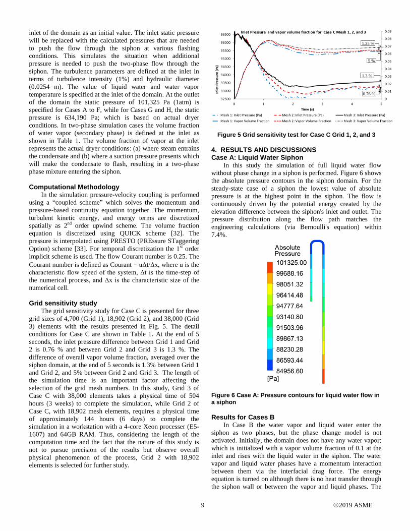
Grid sensitivity study The grid sensitivity study for Case C is presented for three

grid sizes of 4,700 (Grid 1), 18,902 (Grid 2), and 38,000 (Grid

3) elements with the results presented in Fig. 5. The detail

conditions for Case C are shown in Table 1. At the end of 5

seconds, the inlet pressure difference between Grid 1 and Grid

2 is 0.76 % and between Grid 2 and Grid 3 is 1.3 %. The

difference of overall vapor volume fraction, averaged over the

siphon domain, at the end of 5 seconds is 1.3% between Grid 1

and Grid 2, and 5% between Grid 2 and Grid 3. The length of

the simulation time is an important factor affecting the

selection of the grid mesh numbers. In this study, Grid 3 of

Case C with 38,000 elements takes a physical time of 504

hours (3 weeks) to complete the simulation, while Grid 2 of

Case C, with 18,902 mesh elements, requires a physical time

of approximately 144 hours (6 days) to complete the

simulation in a workstation with a 4-core Xeon processer (E5-

1607) and 64GB RAM. Thus, considering the length of the

computation time and the fact that the nature of this study is

not to pursue precision of the results but observe overall

physical phenomenon of the process, Grid 2 with 18,902

elements is selected for further study.

1.3 %

0.76 %

1.35 %

5 %

Figure 5 Grid sensitivity test for Case C Grid 1, 2, and 3

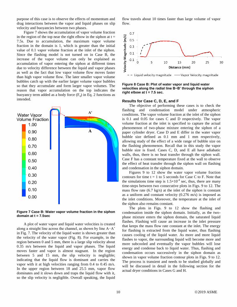
4. RESULTS AND DISCUSSIONS Case A: Liquid Water Siphon

In this study the simulation of full liquid water flow

without phase change in a siphon is performed. Figure 6 shows

the absolute pressure contours in the siphon domain. For the

steady-state case of a siphon the lowest value of absolute

pressure is at the highest point in the siphon. The flow is

continuously driven by the potential energy created by the

elevation difference between the siphon's inlet and outlet. The

pressure distribution along the flow path matches the

engineering calculations (via Bernoulli's equation) within

7.4%.

Figure 6 Case A: Pressure contours for liquid water flow in a siphon

Results for Cases B In Case B the water vapor and liquid water enter the

siphon as two phases, but the phase change model is not

activated. Initially, the domain does not have any water vapor;

which is initialized with a vapor volume fraction of 0.1 at the

inlet and rises with the liquid water in the siphon. The water

vapor and liquid water phases have a momentum interaction

between them via the interfacial drag force. The energy

equation is turned on although there is no heat transfer through

the siphon wall or between the vapor and liquid phases. The

10 2019 ASME

purpose of this case is to observe the effects of momentum and

drag interactions between the vapor and liquid phases on slip

velocity and buoyancies between two phases.

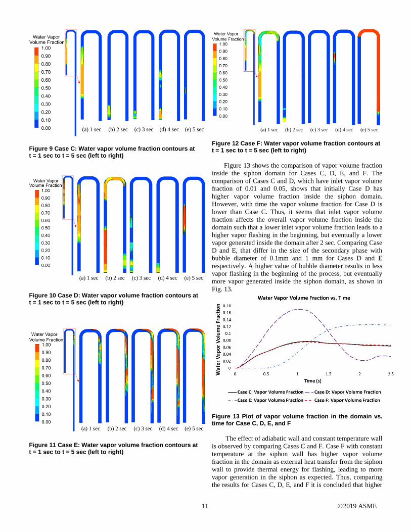
Figure 7 shows the accumulation of vapor volume fraction

in the region of the top near the right elbow in the siphon at t =

7.5s. Due to accumulation, the maximum vapor volume

fraction in the domain is 1, which is greater than the initial

value of 0.1 vapor volume fraction at the inlet of the siphon.

Since the flashing model is not turned on in Case B, the

increase of the vapor volume can only be explained as

accumulation of vapor entering the siphon at different times

due to velocity difference between the liquid and vapor phases

as well as the fact that low vapor volume flow moves faster

than high vapor volume flow. The later smaller vapor volume

bubbles catch up with the earlier larger volume vapor bubbles

so that they accumulate and form larger vapor volumes. The

reason that vapor accumulation on the top indicates the

buoyancy term added as a body force (Fq) in Eq. 2 functions as

intended.

A

A’

Figure 7 Case B: Water vapor volume fraction in the siphon domain at t = 7.5sec

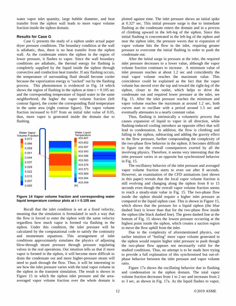
A plot of water vapor and liquid water velocities is created

along a straight line across the channel, as shown by line A−A’

in Fig. 7. The velocity of the liquid water is shown greater than

the velocity of the water vapor (Fig. 8). For example, in the

region between 0 and 5 mm, there is a large slip velocity about

0.35 m/s between the liquid and vapor phases. The liquid

moves faster and vapor is almost stagnant. In the region

between 5 and 15 mm, the slip velocity is negligible;

indicating that the liquid flow is dominant and carries the

vapor with it at high velocities ranging from 0.4 to 0.45 m/s.

In the upper region between 18 and 25.5 mm, vapor flow

dominates and it slows down and traps the liquid flow with it,

so the slip velocity is negligible. Overall speaking, the liquid

flow travels about 10 times faster than large volume of vapor

flow.

Figure 8 Case B: Plot of water vapor and liquid water velocities along the radial line B−B’ through the siphon right elbow at t = 7.5 sec.

Results for Case C, D, E, and F The objective of performing these cases is to check the

flashing and condensation model under atmospheric

conditions. The vapor volume fraction at the inlet of the siphon

is 0.1 and 0.05 for cases C and D respectively. The vapor

volume fraction at the inlet is specified to capture the actual

phenomenon of two-phase mixture entering the siphon of a

paper cylinder dryer. Case D and E differ in the water vapor

bubble size defined as 0.1 mm and 1 mm respectively,

allowing study of the effect of a wide range of bubble size on

the flashing phenomenon. Recall that in this study the vapor

bubble size is fixed. Cases C, D, and E all have adiabatic

walls, thus, there is no heat transfer through the siphon wall.

Case F has a constant temperature fixed at the wall to observe

the effect of heat transfer through the siphon wall on flashing

and condensation in the siphon domain.

Figures 9 to 12 show the water vapor volume fraction

contours for time t = 1 to 5 seconds for Case C to F. Note that

the simulations time step is 1.5×10-4

sec, thus, there are many

time-steps between two consecutive plots in Figs. 9 to 12. The

mass flow rate (6.7 kg/s) at the inlet of the siphon is constant

as a uniform and constant velocity (0.276 m/s) is imposed as

the inlet conditions. Moreover, the temperature at the inlet of

the siphon also remains constant.

The plots in Figs. 9 to 12 show the flashing and

condensation inside the siphon domain. Initially, as the two-

phase mixture enters the siphon domain, the saturated liquid

flashes. Flashing will cause an increase in the inlet pressure

that keeps the mass flow rate constant at the inlet. The energy

for flashing is extracted from the liquid water, thus flashing

causes cooling of the liquid water. As more and more liquid

flashes to vapor, the surrounding liquid will become more and

more subcooled and eventually the vapor bubbles will lose

energy and condense back to liquid water. Thus, flashing and

condensation occurs successively in the siphon domain as

shown in vapor volume fraction contour plots in Figs. 9 to 12.

The process is transient and needs to be studied globally and

will be discussed in detail in the following section for the

actual dryer conditions in Cases G and H.

11 2019 ASME

(a) 1 sec (b) 2 sec (c) 3 sec (d) 4 sec (e) 5 sec

Figure 9 Case C: Water vapor volume fraction contours at t = 1 sec to t = 5 sec (left to right)

(a) 1 sec (b) 2 sec (c) 3 sec (d) 4 sec (e) 5 sec

Figure 10 Case D: Water vapor volume fraction contours at t = 1 sec to t = 5 sec (left to right)

(a) 1 sec (b) 2 sec (c) 3 sec (d) 4 sec (e) 5 sec

Figure 11 Case E: Water vapor volume fraction contours at t = 1 sec to t = 5 sec (left to right)

(a) 1 sec (b) 2 sec (c) 3 sec (d) 4 sec (e) 5 sec

Figure 12 Case F: Water vapor volume fraction contours at t = 1 sec to t = 5 sec (left to right)

Figure 13 shows the comparison of vapor volume fraction

inside the siphon domain for Cases C, D, E, and F. The

comparison of Cases C and D, which have inlet vapor volume

fraction of 0.01 and 0.05, shows that initially Case D has

higher vapor volume fraction inside the siphon domain.

However, with time the vapor volume fraction for Case D is

lower than Case C. Thus, it seems that inlet vapor volume

fraction affects the overall vapor volume fraction inside the

domain such that a lower inlet vapor volume fraction leads to a

higher vapor flashing in the beginning, but eventually a lower

vapor generated inside the domain after 2 sec. Comparing Case

D and E, that differ in the size of the secondary phase with

bubble diameter of 0.1mm and 1 mm for Cases D and E

respectively. A higher value of bubble diameter results in less

vapor flashing in the beginning of the process, but eventually

more vapor generated inside the siphon domain, as shown in

Fig. 13.

Figure 13 Plot of vapor volume fraction in the domain vs. time for Case C, D, E, and F

The effect of adiabatic wall and constant temperature wall

is observed by comparing Cases C and F. Case F with constant

temperature at the siphon wall has higher vapor volume

fraction in the domain as external heat transfer from the siphon

wall to provide thermal energy for flashing, leading to more

vapor generation in the siphon as expected. Thus, comparing

the results for Cases C, D, E, and F it is concluded that higher

12 2019 ASME

water vapor inlet quantity, large bubble diameter, and heat

transfer from the siphon wall leads to more vapor volume

fraction inside the siphon domain.

Results for Case G Case G presents the study of a siphon under actual paper

dryer pressure conditions. The boundary condition at the wall

is adiabatic, thus, there is no heat transfer from the siphon

wall. As the condensate enters the siphon in the region of

lower pressure, it flashes to vapor. Since the wall boundary

conditions are adiabatic, the thermal energy for flashing is

completely supplied by the liquid inside the siphon through

convective and conduction heat transfer. If any flashing occurs,

the temperature of surrounding fluid should become cooler

because the vaporization energy is "sucked" out by the flashing

process. This phenomenon is evidenced in Fig. 14 which

shows the region of flashing in the siphon at time t = 0.105 sec

and the corresponding temperature of liquid water in the same

neighborhood, the higher the vapor volume fraction (left

contour figure), the cooler the corresponding fluid temperature

in the same area (right contour figure). The vapor volume

fraction increased to 0.07 from an initial inlet value of 0.05,

thus, more vapor is generated inside the domain due to

flashing.

Figure 14 Vapor volume fraction and corresponding water liquid temperature contour plots at t = 0.105 sec Recall that the inlet condition is set at a fixed velocity,

meaning that the simulation is formulated in such a way that

the flow is forced to enter the siphon with the same velocity

regardless how much vapor is formed via flashing in the

siphon. Under this condition, the inlet pressure will be

calculated by the computational code to satisfy the continuity

and momentum equations. This arrangement of inlet

conditions approximately simulates the physics of adjusting

blow-through steam pressure through pressure regulating

valves in the real operations. Our intuition tells us that if more

vapor is formed in the siphon, it will become more difficult to

drain the condensate out and more higher-pressure steam will

need to push through the flow. Thus, it will be interesting to

see how the inlet pressure varies with the total vapor volume in

the siphon in the transient simulation. The result is shown in

Figure 15 in which the siphon inlet pressure and the area-

averaged vapor volume fraction over the whole domain is

plotted against time. The inlet pressure shows an initial spike

at 0.327 sec. This initial pressure surge is due to immediate

flashing as the condensate enters the domain and in a process

of climbing upward in the left-leg of the siphon. Since this

initial flashing is concentrated in the left-leg of the siphon and

near the siphon inlet, the pressure waves due to expansion of

vapor volume hits the flow in the inlet, requiring greater

pressure to overcome the initial flashing in order to push the

condensate out.

After the initial surge in pressure at the inlet, the required

inlet pressure decreases to a lower value, although the vapor

volume fraction continues to increase. A minimum value of

inlet pressure reaches at about 1.2 sec and coincidently the

total vapor volume reaches the maximum value. This

coincidence could be explained as the fact that the vapor

volume has moved over the top and toward the right-leg of the

siphon, closer to the outlet, which helps to drive the

condensate out and required lower pressure at the inlet, see

Fig. 15. After the inlet pressure reaches the minimum and

vapor volume reaches the maximum at around 1.2 sec, both

curves start to oscillate with a period around 1.5 sec and

eventually attenuates to a nearly constant value.

Thus, flashing is intrinsically a volumetric process that

causes expansion of liquid to vapor in all direction, while

flashing-induced cooling introduce an opposite effect that will

lead to condensation. In addition, the flow is climbing and

falling in the siphon, subtracting and adding the gravity effect

to the flow pressure, further compounding the complexity of

the two-phase flow behavior in the siphon. It becomes difficult

to figure out the overall consequences exerted by all the

involving physics. Therefore, it seems very interesting that the

inlet pressure varies in an opposite but synchronized behavior

in Fig. 15.

The oscillatory behavior of the inlet pressure and averaged

vapor volume fraction starts to even out after 8 seconds.

However, an examination of the CFD animations (not shown

in this paper) reveals that the local vapor volume fraction is

still evolving and changing along the siphon from 8 to 15

seconds even though the overall vapor volume fraction seems

to reach a steady-state value in Fig. 15. The two-phase flow

inside the siphon should require a higher inlet pressure as

compared to the liquid siphon case. This is shown in Figure 15,

which shows that the pressure for a liquid siphon (the blue

dashed line) is lower than that for the two-phase flow inside

the siphon (the black dashed line). The green dashed line at the

bottom of Fig. 15 shows the lowest pressure occurring at the

highest point inside the siphon, which creates a suction region

to move the flow uphill from the inlet.

Due to the complexity of aforementioned physics, our

earlier intuition of "feeling" more vapor volume generated in

the siphon would require higher inlet pressure to push though

the two-phase flow appears not necessarily valid for the

studied conditions. Thus, no attempt is to be made here trying

to provide a full explanation of this synchronized but out-of-

phase behavior between the inlet pressure and vapor volume

ratio.

Figure 17a shows the oscillating behavior due to flashing

and condensation in the siphon domain. The total vapor

volume fraction decreases from 1 to 2 sec and increases from 2

to 3 sec, as shown in Fig. 17a. As the liquid flashes to vapor,

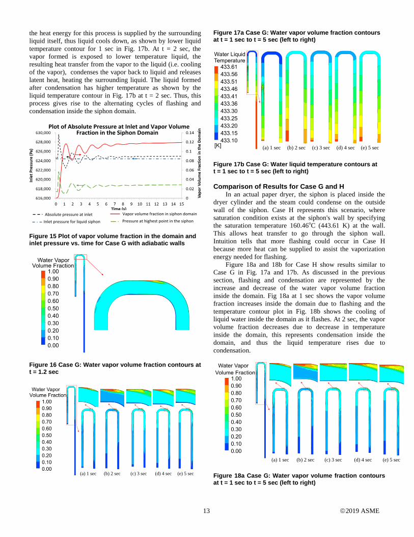
13 2019 ASME

the heat energy for this process is supplied by the surrounding

liquid itself, thus liquid cools down, as shown by lower liquid

temperature contour for 1 sec in Fig. 17b. At t = 2 sec, the

vapor formed is exposed to lower temperature liquid, the

resulting heat transfer from the vapor to the liquid (i.e. cooling

of the vapor), condenses the vapor back to liquid and releases

latent heat, heating the surrounding liquid. The liquid formed

after condensation has higher temperature as shown by the

liquid temperature contour in Fig. 17b at t = 2 sec. Thus, this

process gives rise to the alternating cycles of flashing and

condensation inside the siphon domain.

Inlet pressure for liquid siphon Pressure at highest point in the siphon

Absolute pressure at inlet Vapor volume fraction in siphon domain

Fraction in the Siphon Domain Plot of Absolute Pressure at Inlet and Vapor Volume

Figure 15 Plot of vapor volume fraction in the domain and inlet pressure vs. time for Case G with adiabatic walls

Figure 16 Case G: Water vapor volume fraction contours at t = 1.2 sec

(a) 1 sec (b) 2 sec (c) 3 sec (d) 4 sec (e) 5 sec

Figure 17a Case G: Water vapor volume fraction contours at t = 1 sec to t = 5 sec (left to right)

(a) 1 sec (b) 2 sec (c) 3 sec (d) 4 sec (e) 5 sec

Figure 17b Case G: Water liquid temperature contours at t = 1 sec to t = 5 sec (left to right)

Comparison of Results for Case G and H In an actual paper dryer, the siphon is placed inside the

dryer cylinder and the steam could condense on the outside

wall of the siphon. Case H represents this scenario, where

saturation condition exists at the siphon's wall by specifying

the saturation temperature 160.46oC (443.61 K) at the wall.

This allows heat transfer to go through the siphon wall.

Intuition tells that more flashing could occur in Case H

because more heat can be supplied to assist the vaporization

energy needed for flashing.

Figure 18a and 18b for Case H show results similar to

Case G in Fig. 17a and 17b. As discussed in the previous

section, flashing and condensation are represented by the

increase and decrease of the water vapor volume fraction

inside the domain. Fig 18a at 1 sec shows the vapor volume

fraction increases inside the domain due to flashing and the

temperature contour plot in Fig. 18b shows the cooling of

liquid water inside the domain as it flashes. At 2 sec, the vapor

volume fraction decreases due to decrease in temperature

inside the domain, this represents condensation inside the

domain, and thus the liquid temperature rises due to

condensation.

(a) 1 sec (b) 2 sec (c) 3 sec (d) 4 sec (e) 5 sec

Figure 18a Case G: Water vapor volume fraction contours at t = 1 sec to t = 5 sec (left to right)

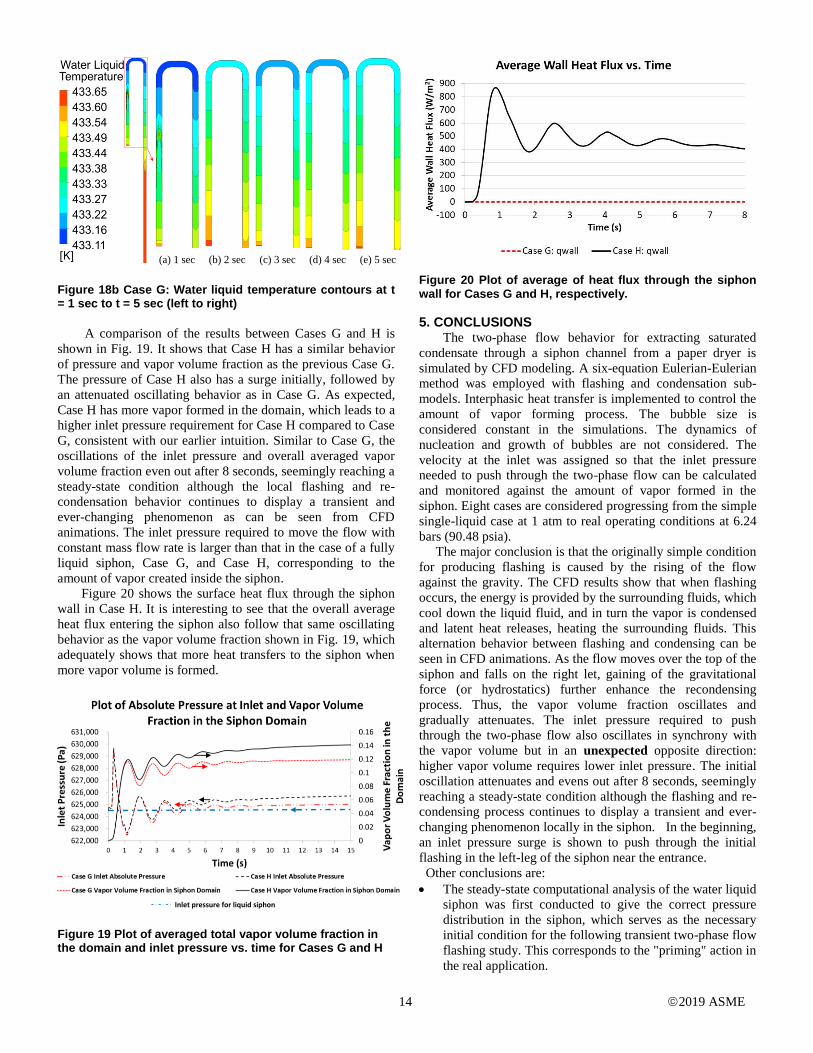
14 2019 ASME

(a) 1 sec (b) 2 sec (c) 3 sec (d) 4 sec (e) 5 sec

Figure 18b Case G: Water liquid temperature contours at t = 1 sec to t = 5 sec (left to right)

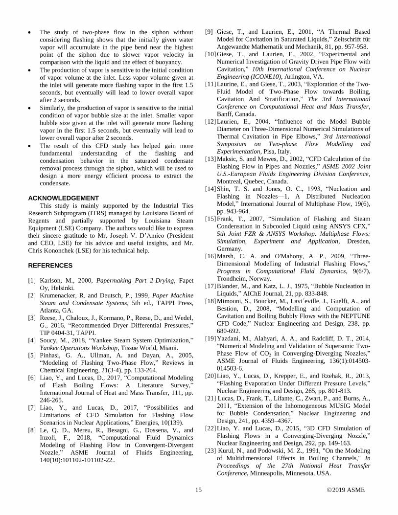
A comparison of the results between Cases G and H is

shown in Fig. 19. It shows that Case H has a similar behavior

of pressure and vapor volume fraction as the previous Case G.

The pressure of Case H also has a surge initially, followed by

an attenuated oscillating behavior as in Case G. As expected,

Case H has more vapor formed in the domain, which leads to a

higher inlet pressure requirement for Case H compared to Case

G, consistent with our earlier intuition. Similar to Case G, the

oscillations of the inlet pressure and overall averaged vapor

volume fraction even out after 8 seconds, seemingly reaching a

steady-state condition although the local flashing and re-

condensation behavior continues to display a transient and

ever-changing phenomenon as can be seen from CFD

animations. The inlet pressure required to move the flow with

constant mass flow rate is larger than that in the case of a fully

liquid siphon, Case G, and Case H, corresponding to the

amount of vapor created inside the siphon.

Figure 20 shows the surface heat flux through the siphon

wall in Case H. It is interesting to see that the overall average

heat flux entering the siphon also follow that same oscillating

behavior as the vapor volume fraction shown in Fig. 19, which

adequately shows that more heat transfers to the siphon when

more vapor volume is formed.

Inlet pressure for liquid siphon

Figure 19 Plot of averaged total vapor volume fraction in the domain and inlet pressure vs. time for Cases G and H

Figure 20 Plot of average of heat flux through the siphon wall for Cases G and H, respectively.

5. CONCLUSIONS The two-phase flow behavior for extracting saturated

condensate through a siphon channel from a paper dryer is

simulated by CFD modeling. A six-equation Eulerian-Eulerian

method was employed with flashing and condensation sub-

models. Interphasic heat transfer is implemented to control the

amount of vapor forming process. The bubble size is

considered constant in the simulations. The dynamics of

nucleation and growth of bubbles are not considered. The

velocity at the inlet was assigned so that the inlet pressure

needed to push through the two-phase flow can be calculated

and monitored against the amount of vapor formed in the

siphon. Eight cases are considered progressing from the simple

single-liquid case at 1 atm to real operating conditions at 6.24

bars (90.48 psia).

The major conclusion is that the originally simple condition

for producing flashing is caused by the rising of the flow

against the gravity. The CFD results show that when flashing

occurs, the energy is provided by the surrounding fluids, which

cool down the liquid fluid, and in turn the vapor is condensed

and latent heat releases, heating the surrounding fluids. This

alternation behavior between flashing and condensing can be

seen in CFD animations. As the flow moves over the top of the

siphon and falls on the right let, gaining of the gravitational

force (or hydrostatics) further enhance the recondensing

process. Thus, the vapor volume fraction oscillates and

gradually attenuates. The inlet pressure required to push

through the two-phase flow also oscillates in synchrony with

the vapor volume but in an unexpected opposite direction:

higher vapor volume requires lower inlet pressure. The initial

oscillation attenuates and evens out after 8 seconds, seemingly

reaching a steady-state condition although the flashing and re-

condensing process continues to display a transient and ever-

changing phenomenon locally in the siphon. In the beginning,

an inlet pressure surge is shown to push through the initial

flashing in the left-leg of the siphon near the entrance.

Other conclusions are:

The steady-state computational analysis of the water liquid

siphon was first conducted to give the correct pressure

distribution in the siphon, which serves as the necessary

initial condition for the following transient two-phase flow

flashing study. This corresponds to the "priming" action in

the real application.

15 2019 ASME

The study of two-phase flow in the siphon without

considering flashing shows that the initially given water

vapor will accumulate in the pipe bend near the highest

point of the siphon due to slower vapor velocity in

comparison with the liquid and the effect of buoyancy.

The production of vapor is sensitive to the initial condition

of vapor volume at the inlet. Less vapor volume given at

the inlet will generate more flashing vapor in the first 1.5

seconds, but eventually will lead to lower overall vapor

after 2 seconds.

Similarly, the production of vapor is sensitive to the initial

condition of vapor bubble size at the inlet. Smaller vapor

bubble size given at the inlet will generate more flashing

vapor in the first 1.5 seconds, but eventually will lead to

lower overall vapor after 2 seconds.

The result of this CFD study has helped gain more

fundamental understanding of the flashing and

condensation behavior in the saturated condensate

removal process through the siphon, which will be used to

design a more energy efficient process to extract the

condensate.

ACKNOWLEDGEMENT This study is mainly supported by the Industrial Ties

Research Subprogram (ITRS) managed by Louisiana Board of

Regents and partially supported by Louisiana Steam

Equipment (LSE) Company. The authors would like to express

their sincere gratitude to Mr. Joseph V. D’Amico (President

and CEO, LSE) for his advice and useful insights, and Mr.

Chris Kononchek (LSE) for his technical help.

REFERENCES

[1] Karlson, M., 2000, Papermaking Part 2-Drying, Fapet

Oy, Helsinki.

[2] Krumenacker, R. and Deutsch, P., 1999, Paper Machine

Steam and Condensate Systems, 5th ed., TAPPI Press,

Atlanta, GA.

[3] Reese, J., Chaloux, J., Kormano, P., Reese, D., and Wedel,

G., 2016, ―Recommended Dryer Differential Pressures,‖

TIP 0404-31, TAPPI.

[4] Soucy, M., 2018, ―Yankee Steam System Optimization,‖

Yankee Operations Workshop, Tissue World, Miami.

[5] Pinhasi, G. A., Ullman, A. and Dayan, A., 2005,

―Modeling of Flashing Two-Phase Flow,‖ Reviews in

Chemical Engineering, 21(3-4), pp. 133-264.

[6] Liao, Y., and Lucas, D., 2017, ―Computational Modeling

of Flash Boiling Flows: A Literature Survey,‖

International Journal of Heat and Mass Transfer, 111, pp.

246-265.

[7] Liao, Y., and Lucas, D., 2017, ―Possibilities and

Limitations of CFD Simulation for Flashing Flow

Scenarios in Nuclear Applications,‖ Energies, 10(139).

[8] Le, Q. D., Mereu, R., Besagni, G., Dossena, V., and

Inzoli, F., 2018, ―Computational Fluid Dynamics

Modeling of Flashing Flow in Convergent-Divergent

Nozzle,‖ ASME Journal of Fluids Engineering,

140(10):101102-101102-22..

[9] Giese, T., and Laurien, E., 2001, ―A Thermal Based

Model for Cavitation in Saturated Liquids,‖ Zeitschrift für

Angewandte Mathematik und Mechanik, 81, pp. 957-958.

[10] Giese, T., and Laurien, E., 2002, ―Experimental and

Numerical Investigation of Gravity Driven Pipe Flow with

Cavitation,‖ 10th International Conference on Nuclear

Engineering (ICONE10), Arlington, VA.

[11] Laurine, E., and Giese, T., 2003, ―Exploration of the Two-

Fluid Model of Two-Phase Flow towards Boiling,

Cavitation And Stratification,‖ The 3rd International

Conference on Computational Heat and Mass Transfer,

Banff, Canada.

[12] Laurien, E., 2004, ―Influence of the Model Bubble

Diameter on Three-Dimensional Numerical Simulations of

Thermal Cavitation in Pipe Elbows,‖ 3rd International

Symposium on Two-phase Flow Modelling and

Experimentation, Pisa, Italy.

[13] Maksic, S. and Mewes, D., 2002, ―CFD Calculation of the

Flashing Flow in Pipes and Nozzles,‖ ASME 2002 Joint

U.S.-European Fluids Engineering Division Conference,

Montreal, Quebec, Canada.

[14] Shin, T. S. and Jones, O. C., 1993, ―Nucleation and

Flashing in Nozzles—1, A Distributed Nucleation

Model,‖ International Journal of Multiphase Flow, 19(6),

pp. 943-964.

[15] Frank, T., 2007, ―Simulation of Flashing and Steam

Condensation in Subcooled Liquid using ANSYS CFX,‖

5th Joint FZR & ANSYS Workshop: Multiphase Flows:

Simulation, Experiment and Application, Dresden,

Germany.

[16] Marsh, C. A. and O'Mahony, A. P., 2009, ―Three-

Dimensional Modelling of Industrial Flashing Flows,‖

Progress in Computational Fluid Dynamics, 9(6/7),

Trondheim, Norway.

[17] Blander, M., and Katz, L. J., 1975, ―Bubble Nucleation in

Liquids,‖ AIChE Journal, 21, pp. 833-848.

[18] Mimouni, S., Boucker, M., Lavi´eville, J., Guelfi, A., and

Bestion, D., 2008, ―Modelling and Computation of

Cavitation and Boiling Bubbly Flows with the NEPTUNE

CFD Code,‖ Nuclear Engineering and Design, 238, pp.

680-692.

[19] Yazdani, M., Alahyari, A. A., and Radcliff, D. T., 2014,

―Numerical Modeling and Validation of Supersonic Two-

Phase Flow of CO2 in Converging-Diverging Nozzles,‖

ASME Journal of Fluids Engineering, 136(1):014503-

014503-6.

[20] Liao, Y., Lucas, D., Krepper, E., and Rzehak, R., 2013,

―Flashing Evaporation Under Different Pressure Levels,‖

Nuclear Engineering and Design, 265, pp. 801-813.

[21] Lucas, D., Frank, T., Lifante, C., Zwart, P., and Burns, A.,

2011, ―Extension of the Inhomogeneous MUSIG Model

for Bubble Condensation,‖ Nuclear Engineering and

Design, 241, pp. 4359–4367.

[22] Liao, Y. and Lucas, D., 2015, ―3D CFD Simulation of

Flashing Flows in a Converging-Diverging Nozzle,‖

Nuclear Engineering and Design, 292, pp. 149-163.

[23] Kurul, N., and Podowski, M. Z., 1991, "On the Modeling

of Multidimensional Effects in Boiling Channels," In

Proceedings of the 27th National Heat Transfer

Conference, Minneapolis, Minnesota, USA.

16 2019 ASME

[24] Riznic, J., and Ishii, M., 1989, ―Bubble Number Density

in Vapor Generation and Flashing Flow,‖ International

Journal of Heat and Mass Transfer, 32, pp. 1821–1833.

[25] Janet, J. P., Liao, Y., and Lucas, D., 2015, ―Heterogeneous

Nucleation in CFD Simulation of Flashing Flows in

Converging–Diverging Nozzles,‖ International Journal of

Multiphase Flow, 74, pp.106-117.

[26] Blinkov, V. N., Jones, O. C., and Nigmatulin, B. I., 1993,

―Nucleation and Flashing in Nozzles—2,‖ International

Journal of Multiphase Flow, 19, pp. 965–986.

[27] Liao, Y., Rzehak, R., Lucas, D. and Krepper, E., 2015,

―Baseline Closure Model for Dispersed Bubbly Flow:

Bubble Coalescence and Breakup,‖ Chemical Engineering

Science, 122, pp. 336-49.

[28] Pelletingeas, A., Dufresne, L. and Seers, P., 2016,

―Characterization of Flow Structures in a Diesel Injector

for Different Needle Lifts and a Fluctuating Injection

Pressure,‖ ASME Journal of Fluid Engineering,

138(8):081105-081105-11.

[29] Rayleigh, L., 1917, "On the Pressure Developed in a

Liquid During the Collapse of a Spherical Cavity,‖ Phil.

Mag. 34 (200), pp. 94–98

[30] Schiller, L., and Naumann, A., 1935, ―A Drag Coefficient

Correlation,‖ Zeitschrift des Vereins Deutscher

Ingenieure, 77, pp. 318–320.

[31] Ranz, W. E., and Marshall, W. R. Jr., 1952, "Evaporation

from Drops, Part I,‖ Chemical Engineering Progress,

48(3), pp. 141–146.

[32] Leonard, B. P., and Mokhtari, S., 1990, "ULTRA-SHARP

Non-oscillatory Convection Schemes for High-Speed

Steady Multidimensional Flow" NASA TM1-2568

(ICOMP-90-12), NASA Lewis Research Center.

[33] Patankar, S. V., 1980, Numerical Heat Transfer and Fluid

Flow, 1st Edition, CRC Press, Washington, DC.