Viscous dampers: testing, modeling and application in vibration and seismic isolation

1 Copyright © 2010 by ASME
Proceedings IMECE2010 2010 ASME International Mechanical Engineering Congress and Exposition
November 12-18, 2010, British Columbia, Vancouver, CANADA
IMECE2010-40380
RESONANCE MODELLING AND CONTROL IN STRUCTURES BY MEANS OF MAGNETORHEOLOGICAL DAMPERS
Mario F. Letelier Department of Mechanical Engineering
University of Santiago of Chile [email protected]
Dennis A. Siginer Department of Mechanical Engineering
The Petroleum Institute [email protected]
Juan S. Stockle Department of Mechanical Engineering
University of Santiago of Chile [email protected]
Cristian Herrera Department of Mechanical Engineering
University of Santiago of Chile [email protected]
ABSTRACT
Many structures such as automobile bodies, bridges and
buildings are subjected to external forces due to the nature of
the environment in which they exist. When the external
excitation frequency is similar to the structure's natural
frequency a resonance effect is generated, increasing the energy
and the amplitude of the oscillation, often causing catastrophic
situations.
This paper presents a method to decrease such resonant
oscillations using magnetorheological dampers.
INTRODUCTION
The phenomenon of resonance appears very often in nature,
in biological, chemical, mechnical systems, etc. Some of these
systems are subjected to different kinds of external loads with
oscillation frequencies often hard to predict on time when there
are high frequencies loads. One example of this is a car driver
who finds an uneven road that causes decreased vehicle control
[1].
This paper presents a method to dissipate the effect of
resonance by the application of magnetic fields arranged
around the edges of a circular tube that transports a fluid whose
properties change when a magnetic field is applied.
Assuming the pressure gradient as a function of parameters
that model the resonance behavior, the physical problem can be
studied. The purpose is to find the form that the flow stress
characterized by the magnetic field must take to decrease the
resonant effect on the flow.
ANALYSIS
Using the momentum equation along the axial coordinate
for a circular tube
� ���� + �
� + ���� = − �
�� (1)
where � is the density of the fluid, � is the sheer stress, � is the
axial velocity, and − ��� is the pressure gradient,
The flow is assumed to behave as a Bingham plastic,
represented by the following equation:
� = �� + � �− ���� � (2)
where � is the sheer stress, �� is the yield stress, and � is the
viscosity. The flow term �� is the unknown that must be
determined in this work, which is in charge of reducing the
resonance.
Substituing (2) in (1) and writing − ��� = � we have
� ���� − �∇�� = � − ��
� (3)
Taking the following factor scale:
� = ���∗
2 Copyright © 2010 by ASME
� = ���∗ (4) � = !�∗
where �� represents a reference velocity, �� is a reference time,
and ! is the radius of the circular tube.
Substituting (4) in (3) and dividing by "��
�� we have
��∗��∗ − ���!� �∇��∗ = ����� � − ��!���
���∗ (5)
Taking the following considerations:
���!� � = 1 → �� = �!�� (6)
y
��"�� � = �∗ → where ��� = "��
�� (7)
��'"�� �� = ��∗ → where ��� = '"��
�� (8)
we get the momentum equation in its nondimensional form:
��∗��∗ − ∇�w∗ = ϕ∗ − τ�∗r∗ (9)
In what follows, the asterisks are omitted in nondimensional
equations.
Incorporating the following model for the pressure gradient
function that simulates the resonance:
�(�) = ���./01�234(5�) (10)
we can get a variety of behaviors by varying parameters ��, 8, 5, 4, where ��, 4 represent the amplitude, 5 the
frequency, and 8 is a direct relation of the resonance period.
This function is shown graphically in the following plot.
Fig. 1 Graphic representation of the pressure gradient that
models the resonance phenomenon.
The resonance effect can be decreased postulating a function 9(�, �) formed by the pressure gradient and the yield stress.
9(�, �) = �(�) − :(�)� (11)
:(�) in equation (11) represents the yield stress in a
nonadimensional form of Bingham constitutive model, which
takes a form determined by the change in the magnetic field.
This is the function to be determined to stop the increase of the
pressure gradient's amplitude that is caused by the forces acting
on the system.
Applying the operator ( )∫1
0
2 rdr to equation (11)
2 ;(9(�, �)�)<� = �(�) − 2:(�)=
� (12)
and assuming
2 ;(9(�, �)�)<� = >234(5�) (13)=
�
we can solve for the yield stress term that was sought:
:(�) = �(�) − > sin(5�)2 (14)
As already mentioned, the function > 234 (5�) has the purpose
of decreasing the effect of the pressure gradient, keeping the
same frequency value, but including a smaller amplitude
modified by parameter >. Its graphic representation is shown in
Figure 2.
Fig. 2. > 234 (5�) function
The solution of Eq. (9) is found using a superposition method.
Deleting the yield stress term in (9) gives
���� − ∇�w = ϕ(t) (15)

3 Copyright © 2010 by ASME
The solution of this equation can be divided into a particular
solution and a homogeneous solution. The particular solution is
found by expanding it as a series:
�C(�, �) = D=(�)(1 − �) + D�(1 − ��) + DE(� − �) + ⋯ (16)
Replacing (16) in (15) and arranging in terms of powers of the
radius we can get the time functions D=(�), D�(�), DE(�) … ., where the odd values, i.e., D=(�), DE(�), DI(�) …. are null and
the even values D�(�), DJ(�), DK(�) …. agree with the following
relation:
4D� + <D�<� + <DJ<� + <DK<� + ⋯ = �(�) (17)
DJ = 14�
<D�<� (18)
DK = 16�
<DJ<� (19)
DL = 18�
<DK<� (20)
Replacing equations (18), (19), (20) in Eq. (17) we get an
equation in terms of a single unknown:
4 MD� + 12�
<D�<� + 12�4�
<�D�<�� + 12�4�6�
<ED�<�E + ⋯ N = �(�) (21)
Eq. (21) is written in terms of D�, proposing the following
solution:
D� = /01�(OP2(5�)(!� + !=� + !��� + ⋯ ) + (22) + sin(5�) (Q� + Q=� + Q���+. . . ))
The degree of the polynomials in Eq. (22) was determined by
comparing solutions, i.e., first polynomials of the 8th
degree
were taken, finding a solution for the velocity, then a solution
was found for polynomials of the 9th
degree, and when the
results were compared it was estimated that for the range of
parameters used in this paper the solutions are equivalent.
Replacing Eq. (22) in Eq. (21) and giving values to the
parameters of function �(�) we can determine the polynomial's
coefficients by means of a system of equations arranged in
terms of t, and replacing D�(�) in Eqs. (18), (19), (20),… we
solve for the values of DJ(�), DK(�)DL(�), getting the
expression for the velocity �C(�, �).
Once the solution of equation (15) is obtained, the stress term
that appears in Eq. (9) is included, and then replacing (16) in
(9) and arranging in terms of powers of r, the following set of
equations is obtained.
D=(�) = −:(�) (23)
4D� + RSTR� + RSU
R� + RSVR� + RSW
R� + RSXR� + ⋯ = �(�) (24)
DE = 13�
<D=<� (25)
DJ = 14�
<D�<� (26)
DI = 15�
<DE<� (27)
DK = 16�
<DJ<� (28)
DY = 17�
<DI<� (29)
DL = 18�
<DK<� (30)
Replacing equations (23), (25), (26), (27), (28), (29), (30) in Eq
(24) we get again an equation in terms of D�:
4 MD� + 12�
<D�<� + 12�4�
<�D�<�� + 12�4�6�
<ED�<�E + ⋯ N = �(�)
(31)
+ M<:(�)<� + 1
3�<�:(�)
<�� + 13�5I
<E:(�)<�E +N
This equation can be rearranged separating the right side terms.
On one hand we get
4 MD� + 12�
<D�<� + 12�4�
<�D�<�� + 12�4�6�
<ED�<�E + ⋯ N = �(�) (32)
whose answer is already known because it does not incorporate
any new term, so its solution is the same as that of equation
(21)
The other part of the equation is written in terms of the yield
stress:
4 MD� + 12�
<D�<� + 12�4�
<�D�<�� + 12�4�6�
<ED�<�E + ⋯ N = (<:(�)<� +
(33) 13�
<�:(�)<�� + 1
3�5I<E:(�)
<�E + ⋯ )
Again this solution is divided into two because the term N(t)
contains the terms �(t) and >234(5�), so there will be two
equations of the following form:
4 [D� + =�U
RSUR� + =
�UJURUSUR�U + =
�UJUKURVSUR�V + ⋯ \ = =
� (R](�)R� +
(34) 13�
<��(�)<�� + 1
3�5I<E�(�)
<�E + ⋯ )

4 Copyright © 2010 by ASME
4 [D� + =�U
RSUR� + =
�UJURUSUR�U + =
�UJUKURVSUR�V … \ = =
� (Acos(5�) +
(35) 234(5�)a)
Taking the values of the constants that go with the sine and
cosine terms in Eq. (35) as
D = M5> − 5E>3�5� + 5I>
3�5�7�9� − 5Y>3�5�7�9�11�13�N (36)
a = (− 5�>3� + 5J>
3�5�7� − 5K>3�5�7�9�11� +
(37) 5L>3�5�7�9�11�13�15�)
we propose the following solution for Eq. (34):
D�= = /01�bOP2(5�)(!� + !=� + !��� + ⋯ ) + 234(5�)(Q� +Q=� + Q��� + ⋯ )c (38)
Which is solved in the same way as Eq. (21). Now the
remaining terms of :(�), associated with the >234(5�) term
are solved proposing a solution of the type
D�� = ! 234(5�) + Q cos(5�) (39)
The same above considerations are applied, the pressure
gradient variables as well as the flow term are assigned values,
and in this way, replacing Eqs. (34) and (35) we get the
coefficients of the D�=(�) and D��(�) terms and a second
profile of the velocities �� is determined, adding these
solutions to term D�(�) found earlier.
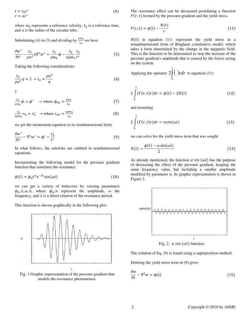
RESULTS
The pressure gradient function that describes the
resonance, and function F, which includes the flow term in
charge of decreasing the resonance effect, are presented. Each
graph is shown with the corresponding velocity profile.
Fig. 3. Pressure gradient versus time for ∅� = 2, 8 = 2, 5 = 3, 4 = 4
Fig. 4. Velocity profile versus radius for ∅� = 2, 8 = 2, 5 = 3, 4 = 4
Fig. 5. F versus time for ∅� = 2, 8 = 2, 5 = 3, 4 = 4

5 Copyright © 2010 by ASME
Fig. 6. Velocity profile versus radius for ∅� = 2, 8 = 2, 5 = 3, 4 = 4
Fig. 7. Pressure gradient versus time for ∅� = 2, 8 = 2, 5 = 3, 4 = 6
Fig. 8. Velocity profile versus radius for ∅� = 2, 8 = 2, 5 = 3, 4 = 6
Fig. 9. F versus time for ∅� = 2, 8 = 2, 5 = 3, 4 = 6
Fig. 10. Velocity profile versus radius for ∅� = 2, 8 = 2, 5 = 3, 4 = 6
Fig. 11. Pressure gradient versus time for ∅� = 2, 8 = 2, 5 = 3, 4 = 8
6 Copyright © 2010 by ASME
Fig. 12. Velocity profile versus radius for ∅� = 2, 8 = 2, 5 = 3, 4 = 8
Fig. 13. F versus time for ∅� = 2, 8 = 2, 5 = 3, 4 = 8
Fig. 14. Velocity profile versus radius for ∅� = 2, 8 = 2, 5 = 3, 4 = 8
Fig. 15. Pressure gradient versus time for ∅� = 2, 8 = 2, 5 = 10, 4 = 4
Fig. 16. Velocity profile versus radius for ∅� = 2, 8 = 2, 5 = 10, 4 = 4
Fig. 17. F versus time for ∅� = 2, 8 = 2, 5 = 10, 4 = 4

7 Copyright © 2010 by ASME
Fig. 18. Velocity profile versus radius for ∅� = 2, 8 = 2, 5 = 10, 4 = 4
Fig. 19. Pressure gradient versus time for ∅� = 2, 8 = 2, 5 = 10, 4 = 6
Fig. 20. Velocity profile versus radius for ∅� = 2, 8 = 2, 5 = 10, 4 = 6
Fig. 21. F versus time for ∅� = 2, 8 = 2, 5 = 10, 4 = 6
Fig. 22. Pressure gradient versus time for ∅� = 2, 8 = 2, 5 = 10, 4 = 6
Fig. 19. Pressure gradient versus time for ∅� = 2, 8 = 2, 5 = 10, 4 = 8

8 Copyright © 2010 by ASME
Fig. 22. Pressure gradient versus time for ∅� = 2, 8 = 2, 5 = 10, 4 = 8
Fig. 23. F versus time for ∅� = 2, 8 = 2, 5 = 10, 4 = 8
Fig. 24. Pressure gradient versus time for ∅� = 2, 8 = 2, 5 = 10, 4 = 8
Fig. 25. Pressure gradient versus time for ∅� = 2, 8 = 0.5, 5 = 3, 4 = 4
Fig. 26. Velocity profile versus radius for ∅� = 2, 8 = 0.5, 5 = 3, 4 = 4
Fig. 27. F versus time for ∅� = 2, 8 = 0.5, 5 = 3, 4 = 4

9 Copyright © 2010 by ASME
Fig. 28. Velocity profile versus radius for ∅� = 2, 8 = 0.5, 5 = 3, 4 = 4
Fig. 29. Pressure gradient versus time for ∅� = 2, 8 = 0.5, 5 = 3, 4 = 6
Fig. 30. Velocity profile versus radius for ∅� = 2, 8 = 0.5, 5 = 3, 4 = 6
Fig. 31. F versus time for ∅� = 2, 8 = 0.5, 5 = 3, 4 = 6
Fig. 32. Velocity profile versus radius for ∅� = 2, 8 = 0.5, 5 = 3, 4 = 6
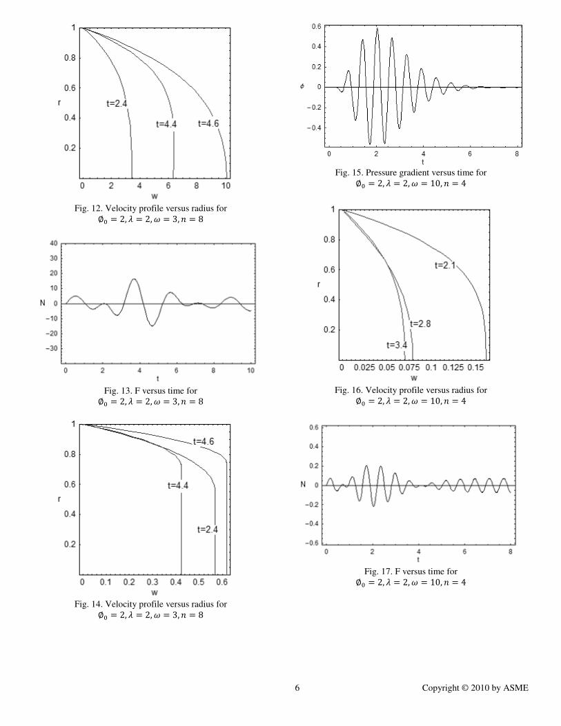
Fig. 33. Pressure gradient versus time for ∅� = 2, 8 = 0.5, 5 = 3, 4 = 8
10 Copyright © 2010 by ASME
Fig. 34. Velocity profile versus radius for ∅� = 2, 8 = 0.5, 5 = 3, 4 = 8
Fig. 31. F versus time for ∅� = 2, 8 = 0.5, 5 = 3, 4 = 8
Fig. 34. Velocity profile versus radius for ∅� = 2, 8 = 0.5, 5 = 3, 4 = 8
CONCLUSIONS
Has been found the form of the yield stress, for to decrease
the effect of the resonance produced by external forces.
This work can be used for to configurate the values of
yield stress in new design of devices that want to null the effect
of resonance.
REFERENCES
[1] Spencer Jr., B.F., Dyke, S.J., Sain, M.K., and Carlson, J.D.,
(1998). “Phenomenological Model for Magnetorheological
Dampers, “Journal of Engineering Mechanics, ASCE, Vol. 123,
No. 3, pp 9.
[2] S.J. Dyke, B. F. Spencer, M. K. Sain, and J.D.
Carlson.Modeling and control of magnetorheological dampers
for seismic response reduction. Smart Materials and Structures,
5:565 575, 1996.
Copyright © 2022 FDOKUMEN