applied sciences

Article

Image Segmentation Approaches for Weld PoolMonitoring during Robotic Arc Welding

Zhenzhou Wang *, Cunshan Zhang, Zhen Pan, Zihao Wang, Lina Liu, Xiaomei Qi, Shuai Maoand Jinfeng Pan

College of Electrical and Electronic Engineering, Shandong University of Technology, China;zcs@sdut.edu.cn (C.Z.); pz15615732790@163.com (Z.P.); 13110473098@stumail.sdut.edu.cn (Z.W.);linaliu-126@163.com (L.L.); qixiaomei@sdut.edu.cn (X.Q.); maoshuai04965@sdut.edu.cn (S.M.);pjfbysj@163.com (J.P.)* Correspondence: wangzz@sdut.edu.cn

Received: 3 November 2018; Accepted: 29 November 2018; Published: 1 December 2018�����������������

Abstract: There is a strong correlation between the geometry of the weld pool surface and thedegree of penetration in arc welding. To measure the geometry of the weld pool surface robustly,many structured light laser line based monitoring systems have been proposed in recent years.The geometry of the specular weld pool could be computed from the reflected laser lines based ondifferent principles. The prerequisite of accurate computation of the weld pool surface is to segmentthe reflected laser lines robustly and efficiently. To find the most effective segmentation solutionsfor the images captured with different welding parameters, different image processing algorithmsare combined to form eight approaches and these approaches are compared both qualitatively andquantitatively in this paper. In particular, the gradient detection filter, the difference method andthe GLCM (grey level co-occurrence matrix) are used to remove the uneven background. The splinefitting enhancement method is used to remove the fuzziness. The slope difference distribution-basedthreshold selection method is used to segment the laser lines from the background. Both qualitativeand quantitative experiments are conducted to evaluate the accuracy and the efficiency of theproposed approaches extensively.

Keywords: Image processing; segmentation; spline; grey level co-occurrence matrix; gradientdetection; threshold selection

1. Introduction

ARC welding is a widely used process for joining various metals. The electric current is transferredfrom the electrode to the work piece through the arc plasma, which has been modeled to control theweld quality in the past research [1,2]. However, the direct factor that affects the weld quality isthe geometry of the weld pool instead of arc plasma because the skilled welders achieve good weldquality mainly based on the visual information of the weld pool. During arc welding, the incompleteweld pool penetration will reduce the effective working cross-sectional area of the weld bead andsubsequently reduce the weld joint strength. It also causes stress concentrations in some cases, e.g.,the fillet and T-joints. On the contrary, excessive weld pool penetration might cause melt-through.The skilled welder needs to adjust the position and travelling speed of the weld torch based on theinformation of the observed weld pool surface to achieve complete penetration. The shortage of skilledwelders and a need for welds of a consistently high quality fuels an increasing demand for automatedarc welding systems. It is believed that machine vision techniques will lead the development of thenext generation intelligent automated arc welding systems.

Appl. Sci. 2018, 8, 2445; doi:10.3390/app8122445 www.mdpi.com/journal/applsci

Appl. Sci. 2018, 8, 2445 2 of 16

In recent years, great efforts have been put to develop the automated and high-precision weldingequipment to achieve high quality welded joints consistently. The important parts of this kindof automated welding equipment include the seam tracking system [3–6], the weld penetrationmonitoring system [7–9] and the control system. Desirably, the seam tracking system or the monitoringsystem and control system are in a closed loop. Thus, the tracking result or the monitoring resultcould serve as feedback for the control system to ensure high quality of welding. In the past studies,it has been shown that weld pool surface depression has a major effect on weld penetration [10–14].The geometry of the weld pool surface will affect the convection in the pool. The primary weldingparameter, the welding current density is also affected by the geometry of the weld pool greatly.In return, the plasma and the welding current affect the geometry of the weld pool. Both the arc plasmaand the molten weld pool are affected by the current density distribution. Therefore, it is fundamentalfor the automated welding systems to take quantitative measurements of the weld pool surface.

In the past decades, a lot of research has been conducted to measure the shape of the arc weldingweld pool by structured light methods [9,15–23]. In Reference [15], the authors pioneered to measurethe deformation of the weld pool by inventing a novel sensing system. Their sensing system projectsa short duration pulsed laser light through a frosted glass with a grid onto the specular weld pool.The reflected laser stripes are imaged in a CCD camera and the geometry of the reflected stripes containthe weld pool surface information. This method might be the earliest method that made good useof the reflective property of the weld pool surface and achieved state of the art accuracy at that time.In Reference [16], the authors improved the structured light method for gas tungsten arc weld (GTAW)pool shape measurement by reflecting the structured light onto an imaging plane instead of ontothe image plane of the camera directly. The imaging plane is placed at a properly selected distance.Thus, the imaged laser patterns are clear enough while the effect of the arc plasma has attenuatedsignificantly, because the propagation of the laser light is much longer than that of the arc plasma.Ever since then, this weld pool sensing technique has become the mainstream of weld pool imagingtechnology [17–23]. In References [17,18], the authors tried to increase the accuracy of measuringthe 3D shape of the GTAW weld pool sensed by the same imaging system as [16]. In Reference [19],the authors came up with an approach for segmentation of the reflected laser lines for pulsed gas metalarc weld (GMAW-P). In References [9,20], the reflected laser lines from the GMAW-P weld pool weresegmented manually to measure the weld pool oscillation frequency. In Reference [21], two cameraswere used to measure the shape of the weld pool for GMAW-P and an unsupervised approach wasproposed to segment and cluster the reflected laser lines. In Reference [22], three cameras are used tomeasure the specular shape from the projected laser rays and an unsupervised approach was proposedto reconstruct the GTAW weld pool shape with closed form solutions. It achieved on line robustmeasurement of GTAW weld pool shape with three calibrated cameras.

There is one major difference for the used laser pattern among these structured lightmethods [9,15–23]. The laser dot pattern is used for the measurement of the GTAW weld poolsurface while the laser line pattern is used for the measurement of the GMAW weld pool surface.Compared to the GTAW weld pool surface, the GMAW weld pool surface is much more dynamicand fluctuating, because GMAW process transfers additional metallic and liquid droplets into theweld pool, which increases the fluctuation and dynamics of the pool surface greatly. The positionand geometry of the local specular surface changes rapidly and greatly, which causes the reflectedrays to change their trajectories rapidly and greatly. If the laser dot pattern is used, the reflected laserdots might interlace irregularly, which makes it impossible for the unsupervised clustering method toidentify these dots robustly. Therefore, the laser line patterns are used in measuring the weld poolsurface of the GMAW process [19–21]. Robust segmentation and clustering of the reflected laser linesbecome the most important and challenging part in the whole monitoring system, because of theuncertainty of the weld pool geometry. The quality of the captured image is significantly affected bythe welding parameters. Due to the lack of generality and robustness, the proposed image processingmethods might work for the images captured in some specifically designed welding experiments,

Appl. Sci. 2018, 8, 2445 3 of 16

while might not work for the images captured in other experiments. For instance, the reflected laserlines were filtered by the top-hat transform and then segmented by thresholding in Reference [19].It yields acceptable segmentation results in many cases. However, it fails completely when it is used tosegment the images captured in Reference [21] with different welding parameters. The reflected laserlines were filtered by the fast Fourier transform (FFT) and then segmented by a manually specifiedthreshold in Reference [20]. It also fails completely in segmenting the images shown in Reference [21].To segment the reflected laser lines more robustly, a difference method and an effective thresholdselection method are proposed in Reference [21]. The segmented laser lines were then clustered basedon their slopes. One big problem that could be seen from the experimental figures in References [19–21]is that quite a few of the laser line parts are missing, because of the limitations of their proposedimage processing methods. One direct consequence of missing a significant part of the reflected laserline is the inaccurate characterization of the weld pool shape, since the length of the reflected laseris proportional to the size of the weld pool. Another drawback is that the segmented small part ofthe laser line might be deleted as noise blobs or some large noise blobs might be recognized as partof the reflected laser line during the unsupervised clustering. As a result, the laser line might beclustered incorrectly.

In Reference [23], a new approach was proposed, and it achieved significantly better segmentationaccuracy compared to the past research [19–21]. It comprises several novel image processing algorithms:A difference operation, a two-dimensional spline fitting enhancement operation, a gradient featuredetection filter and the slope difference distribution-based threshold selection. The major goal of [23] isto cluster and characterize the laser lines under extremely harsh welding conditions. As a result, it omitsthe image processing methods for the images captured under less harsh welding conditions with mildwelding parameters. In addition, quantitative results and comparisons to validate the effectivenessof the proposed segmentation approach were also not given. Due to the page limit, the reasons whythe segmentation approach should contain these image processing algorithms were not explainedadequately. One goal of this paper is to complement the research work conducted in Reference [23]and conduct a more thorough experiment to find the most effective solution both qualitatively andquantitatively. Another goal is to come up with more efficient segmentation approaches for imageswith relatively high quality that are captured under mild welding parameters.

In the past research, the visual inspection of the weld pool surface was mainly used to understandthe complex arc welding processes. The obtained data were used to validate and improve the accuracyof the numerical models and to gain insight into the complex arc welding processes. Few are used forin-process welding parameter adjustment and on-line feedback control, due to the lack of a robustand efficient approach that is capable of extracting meaningful feedback information on-line frommost of the captured images. The proposed approaches in this paper are promising to accomplish thischallenging task in the future.

This paper is organized as follows. Section 2 describes the established monitoring system.In Section 3, state of the art methods for laser line segmentation are evaluated and compared.In Section 4, the combination approach proposed previously is explained theoretically. In Section 5,we propose different segmentation approaches by combining different image processing algorithms.In Section 6, the experimental results and discussions are given. Section 7 concludes the paper.

2. The Structured Light Monitoring System

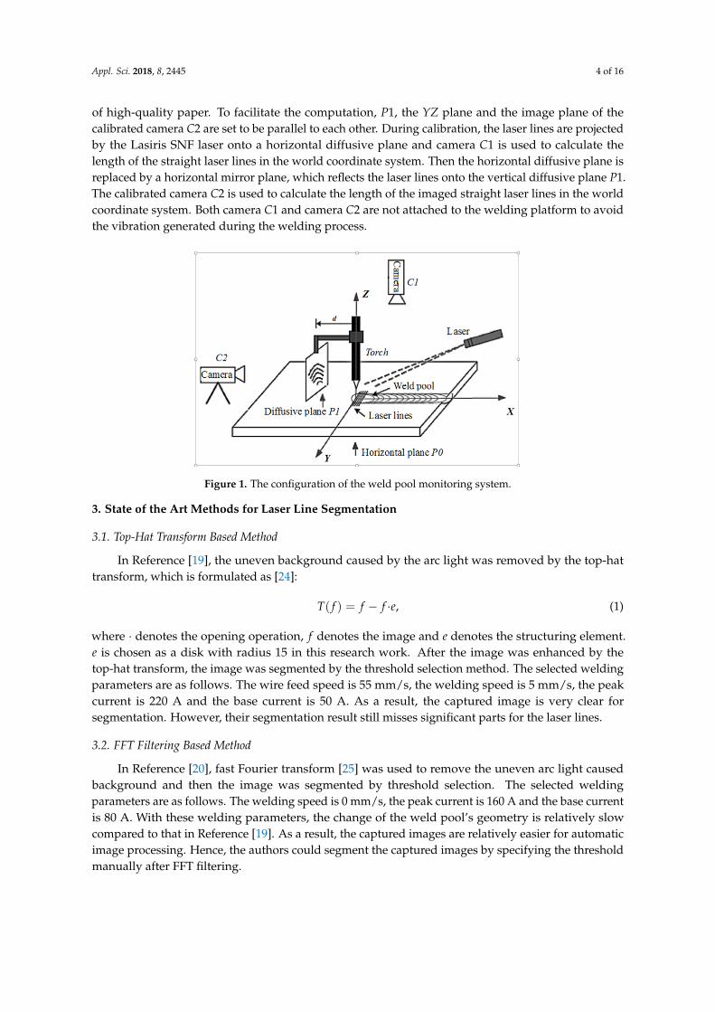
Figure 1 shows the configuration of the popular weld pool monitoring system that has beenadopted in References [9,15–23]. The major parts of the system include two point grey cameras,C1 and C2, and one Lasiris SNF with the wavelength at 635 nm. A linear glass polarizing filter withthe wavelength from 400 nm to 700 nm is mounted on camera C2 to remove the strong arc light.The structured light laser line pattern is projected by the Lasiris SNF laser generator onto the weldpool surface and reflected onto the diffusive imaging plane P1. The calibrated camera C2 viewsthe reflected laser lines from the back side of P1, which is made up of a piece of glass and a piece

Appl. Sci. 2018, 8, 2445 4 of 16

of high-quality paper. To facilitate the computation, P1, the YZ plane and the image plane of thecalibrated camera C2 are set to be parallel to each other. During calibration, the laser lines are projectedby the Lasiris SNF laser onto a horizontal diffusive plane and camera C1 is used to calculate thelength of the straight laser lines in the world coordinate system. Then the horizontal diffusive plane isreplaced by a horizontal mirror plane, which reflects the laser lines onto the vertical diffusive plane P1.The calibrated camera C2 is used to calculate the length of the imaged straight laser lines in the worldcoordinate system. Both camera C1 and camera C2 are not attached to the welding platform to avoidthe vibration generated during the welding process.

Appl. Sci. 2018, 8, x FOR PEER REVIEW 4 of 16

calibrated camera C2 are set to be parallel to each other. During calibration, the laser lines are projected by the Lasiris SNF laser onto a horizontal diffusive plane and camera C1 is used to calculate the length of the straight laser lines in the world coordinate system. Then the horizontal diffusive plane is replaced by a horizontal mirror plane, which reflects the laser lines onto the vertical diffusive plane P1. The calibrated camera C2 is used to calculate the length of the imaged straight laser lines in the world coordinate system. Both camera C1 and camera C2 are not attached to the welding platform to avoid the vibration generated during the welding process.

Figure 1. The configuration of the weld pool monitoring system.

3. State of the Art Methods for Laser Line Segmentation

3.1. Top-Hat Transform Based Method

In Reference [19], the uneven background caused by the arc light was removed by the top-hat transform, which is formulated as [24]: ( ) = − º , (1)

where º denotes the opening operation, denotes the image and denotes the structuring element. is chosen as a disk with radius 15 in this research work. After the image was enhanced by the top-hat transform, the image was segmented by the threshold selection method. The selected welding parameters are as follows. The wire feed speed is 55 mm/s, the welding speed is 5 mm/s, the peak current is 220A and the base current is 50 A. As a result, the captured image is very clear for segmentation. However, their segmentation result still misses significant parts for the laser lines.

3.2. FFT Filtering Based Method

In Reference [20], fast Fourier transform [25] was used to remove the uneven arc light caused background and then the image was segmented by threshold selection. The selected welding parameters are as follows. The welding speed is 0 mm/s, the peak current is 160A and the base current is 80 A. With these welding parameters, the change of the weld pool’s geometry is relatively slow compared to that in Reference [19]. As a result, the captured images are relatively easier for automatic image processing. Hence, the authors could segment the captured images by specifying the threshold manually after FFT filtering.

3.3. Difference Operation Based Method

In Reference [21], the difference method was proposed to reduce the unevenly distributed background. The differenced image is obtained by the following operation. ( , ) = ( + ∆ , ) − ( , ), (2)

Figure 1. The configuration of the weld pool monitoring system.

3. State of the Art Methods for Laser Line Segmentation

3.1. Top-Hat Transform Based Method

In Reference [19], the uneven background caused by the arc light was removed by the top-hattransform, which is formulated as [24]:

T( f ) = f − f ·e, (1)

where · denotes the opening operation, f denotes the image and e denotes the structuring element.e is chosen as a disk with radius 15 in this research work. After the image was enhanced by thetop-hat transform, the image was segmented by the threshold selection method. The selected weldingparameters are as follows. The wire feed speed is 55 mm/s, the welding speed is 5 mm/s, the peakcurrent is 220 A and the base current is 50 A. As a result, the captured image is very clear forsegmentation. However, their segmentation result still misses significant parts for the laser lines.

3.2. FFT Filtering Based Method

In Reference [20], fast Fourier transform [25] was used to remove the uneven arc light causedbackground and then the image was segmented by threshold selection. The selected weldingparameters are as follows. The welding speed is 0 mm/s, the peak current is 160 A and the base currentis 80 A. With these welding parameters, the change of the weld pool’s geometry is relatively slowcompared to that in Reference [19]. As a result, the captured images are relatively easier for automaticimage processing. Hence, the authors could segment the captured images by specifying the thresholdmanually after FFT filtering.

Appl. Sci. 2018, 8, 2445 5 of 16

3.3. Difference Operation Based Method

In Reference [21], the difference method was proposed to reduce the unevenly distributedbackground. The differenced image is obtained by the following operation.

fd(x, y) = f (x + ∆d, y)− f (x, y), (2)

where ∆d denotes the step size of the operation and it is determined by off line analysis of the averagewidth of the laser lines. The step size should be greater than or equal to the width of the laser line inthe captured images and it is selected as 10 in this research work. The laser lines are then segmentedfrom the differenced image by the threshold selection method.

3.4. Grey Level Co-Occurrence Matrix Based Method

Grey level co-occurrence matrix (GLCM) [26] computes the frequencies of different combinationsof pixel values or grey levels occurring in an image and then forms a matrix to represent thesefrequencies. Therefore, it is usually used to segment textured images or objects with an unevenlydistributed background. The second order GLCM is usually used for segmentation and it isformulated as:

P(i, j|d, θ) =#{k, l ∈ D| f (k) = i, f (l) = j, ‖ k− l ‖= d, ∠(k− l) = θ}

#{m, n ∈ D|‖ m− n ‖= d,∠(m− n) = θ} , (3)

where d is the distance of pixel k and pixel l. θ is the angle of vector (k − l) with the horizontal lineor vertical line. The combination of d and θ represents the relative position of pixel k and pixel l,which have gray-scale value i and j respectively.

During our implementation, we update all the intensity values in the moving window bysubtracting its minimal intensity value and then adding one. The quantization level of the GLCMmatrix becomes one and the maximal intensity value of the updated moving window. Following thecomputation of the GLCM, the contrast measure is used to form the GLCM image. Then, the GLCMimage is segmented by a global threshold.

3.5. Combination Method

In Reference [23], a combination approach was used to segment the laser lines. The combinedimage processing algorithms include a difference operation, a two-dimensional spline fittingenhancement operation, a gradient feature detection filter and the slope difference distribution-basedthreshold selection. In both [21,23], the laser lines are segmented by the slope differencedistribution-based threshold selection method that could be summarized as follows. Firstly,the gray-scales of the original image is rearranged in the interval from 1 to 255 and its normalizedhistogram distribution P(x) is computed. Secondly, the normalized histogram P(x) is smoothed by thefast Fourier transform (FFT) [25] based low pass filter with the bandwidth W = 10. Thirdly, two slopes,the right slope and the left slope, are computed for each point on the smoothed histogram distribution.The slope difference distribution is computed as the differences between the right slopes and theircorresponding left slopes. In the slope difference distribution, the position where the valley with themaximum absolute value occurs is selected as the threshold. The slope difference distribution-basedthreshold selection method is critical in this application. For the comparison with state of the art imagesegmentation methods, please refer to the related research work [21], where this threshold selectionmethod is compared with the state of the art method using the same type of images. The comparisonswith state of the art image segmentation methods showed that the slope difference distribution basedthreshold selection method is significantly more accurate in segmenting some specific types of images,including the laser line images.

Appl. Sci. 2018, 8, 2445 6 of 16

3.6. Performance Evaluation

Figure 2a shows a typical image captured by the structured light monitoring system with thefollowing welding parameters. The wire feed speed is 84.67 mm/s, the welding speed is 3.33 mm/s,the peak current is 230 A and the base current is 70 A. As can be seen, these parameters are significantlyhigher than those used in References [19,20]. With these parameters, the resultant weld pool surfacechanges more rapidly and irregularly. Hence, the quality of the captured image in this study ismuch reduced. The results by top hat method, FFT method, difference method, GLCM method andcombination method are shown in Figure 2b–f respectively. Compared to the segmentation result bycombination method, the segmentation results by other state of the art methods appear to be veryinaccurate. Although the difference method achieves the second best result, there is one big segmentedline on the top caused by the edge of the imaging plane. It costs additional effort for the subsequentunsupervised clustering. In addition, there are noise blobs that are hard to be distinguished from thelaser line parts.

Appl. Sci. 2018, 8, x FOR PEER REVIEW 6 of 16

methods appear to be very inaccurate. Although the difference method achieves the second best result, there is one big segmented line on the top caused by the edge of the imaging plane. It costs additional effort for the subsequent unsupervised clustering. In addition, there are noise blobs that are hard to be distinguished from the laser line parts.

(a) (b) (c)

(d) (e) (f)

Figure 2. Evaluation of state of the art methods (a) one typical captured image; (b) segmentation result by the top hat method; (c) segmentation result by the FFT method; (d) segmentation result by the difference method; (e) segmentation result by the GLCM method; (f) segmentation result by combination method.

4. Analysis of the Combination Approach

In Reference [23], a combination approach is proposed to segment the reflected laser lines as accurate as possible. The flowchart of this segmentation approach comprises a difference operation, a two-dimensional spline fitting enhancement operation, a gradient feature detection filter and the slope difference distribution-based threshold selection. However, the reasons why the segmentation approach should contain these image processing algorithms were not explained adequately in Reference [23]. Quantitative results to validate the effectiveness of this segmentation approach were also not given. Here, we will theoretically explain why the proposed two-dimensional spline fitting enhancement method and the gradient feature detection filter work well in segmenting the laser lines.

The intensity distribution, of the captured image caused by the arc light could be modeled mathematically by the following equation [21]: ( ) = τ 2ℎ − 1 = ( ), (4)

where τ is the intensity mapping function of the CCD camera [27]. is the surface normal at position . is the angle between the surface normal and the incident light. denotes the color value. is the distance between the arc light center and position . is the distance from the arc light center to the diffusive imaging plane P1. is the spectral frequency of arc light and ℎ is the planck’s constant. is the speed of the light and is the boltzmann’s constant. is the temperature of arc light source, which is determined by the welding current that alternates with the frequency of 10 Hz. The frame rate of the camera C2 is set to 300 frames per second during the experiment. Hence, 30 images are captured with different sampled currents at one period of the current wave. The temperature is determined by the value of the current and thus it changes with the current from frame to frame in the time domain. In the same frame, the temperature is a constant. At each image point, both the intensity mapping function and the angle remain the same in all the captured image sequences. Thus, is a constant at each specific image point in one

Figure 2. Evaluation of state of the art methods (a) one typical captured image; (b) segmentationresult by the top hat method; (c) segmentation result by the FFT method; (d) segmentation resultby the difference method; (e) segmentation result by the GLCM method; (f) segmentation result bycombination method.

4. Analysis of the Combination Approach

In Reference [23], a combination approach is proposed to segment the reflected laser lines asaccurate as possible. The flowchart of this segmentation approach comprises a difference operation,a two-dimensional spline fitting enhancement operation, a gradient feature detection filter and theslope difference distribution-based threshold selection. However, the reasons why the segmentationapproach should contain these image processing algorithms were not explained adequately inReference [23]. Quantitative results to validate the effectiveness of this segmentation approach werealso not given. Here, we will theoretically explain why the proposed two-dimensional spline fittingenhancement method and the gradient feature detection filter work well in segmenting the laser lines.

The intensity distribution, Ia of the captured image caused by the arc light could be modeledmathematically by the following equation [21]:

Ia(T) = τ

∣∣∣∣∣∣2hv3

c2 ×→N × cosβ×O

ehvγT − 1

∣∣∣∣∣∣× dr3 =

Ca(T)r3 , (4)

Appl. Sci. 2018, 8, 2445 7 of 16

where τ is the intensity mapping function of the CCD camera [27].→N is the surface normal at position

p. β is the angle between the surface normal and the incident light. O denotes the color value. r is thedistance between the arc light center and position p. d is the distance from the arc light center to thediffusive imaging plane P1. v is the spectral frequency of arc light and h is the planck’s constant. cis the speed of the light and γ is the boltzmann’s constant. T is the temperature of arc light source,which is determined by the welding current that alternates with the frequency of 10 Hz. The framerate of the camera C2 is set to 300 frames per second during the experiment. Hence, 30 images arecaptured with different sampled currents at one period of the current wave. The temperature T isdetermined by the value of the current and thus it changes with the current from frame to frame inthe time domain. In the same frame, the temperature T is a constant. At each image point, both theintensity mapping function τ and the angle α remain the same in all the captured image sequences.Thus, Ca is a constant at each specific image point in one frame and it varies from frame to frame withthe value of T. From Equation (4), it becomes much obvious that the intensity distribution producedby the arc light effect on the captured image is inversely proportional to the r3. Thus, the intensitydistribution caused by the arc light can be modeled as:

a(x, y) =Ca(T)

[(x− x0)2 + (y− y0)

2 + d2]3/2 , (5)

where (x0, y0) denotes the center of arc light distribution and it may lie outside of the image. The arclight is affected by the additional laser line and can be modeled as:

f (x, y) = l(x, y) + a(x, y), (6)

where l(x, y) denotes the intensity distribution of the laser line and it is formulated as:

l(x, y) =

{wµ(x, y); (x, y) ∈ A0; (x, y) /∈ A

, (7)

where A denotes the laser line area, w is a constant whose value is higher than the average value of thearc light distribution, Ia. µ(x, y) is the membership function that represents the fuzziness of the laserline and is formulated as:

µ(x, y) = Exp

(− (L(x, y)− µL)

2

2σL2

), (8)

where L(x, y) denotes the ideal intensity distribution of the laser line. µL is its mean and σL is itsvariance respectively.

Combining Equations (5)–(8), we get the model of the intensity distribution for the image withreflected laser lines.

f (x, y) =

wµ(x, y) + Ca(T)

[(x−x0)2+(y−y0)

2+d2]3/2 ; (x, y) ∈ A

Ca(T)

[(x−x0)2+(y−y0)

2+d2]3/2 ; (x, y) /∈ A

. (9)

From the above model, we see that the fuzziness caused by µ(x, y) should be reduced effectively toobtain high segmentation accuracy. However, the moving average filter can only reduce the Gaussiannoise instead of removing the fuzziness. Thus, a new enhancement method is required.

After the image fuzziness has been added in the derived image model (Equation (9)), we need totheoretically find the reasons that why the fuzziness causes parts of the segmented laser lines missing.To this end, the mathematical explanation of how the gradient detection filter works for segmenting

Appl. Sci. 2018, 8, 2445 8 of 16

the objects from the uneven background is described at first. According to Equation (9), the gradientvalue at the position (x, y) that is caused by the arc light background can be formulated as:

ga = Ca(T)[( N−1

2 +x−x0)2+( N−1

2 +y−y0)2+d2

]3/2 −Ca(T)[

(x−x0− N−12 )

2+(y−y0− N−1

2 )2+d2

] 32

. (10)

The gradient values caused by the laser line can be formulated as:

gl =

wµ(x, y) + ga; i f top part o f Kg /∈ A−wµ(x, y) + ga i f bottompart o f Kg /∈ Aga; i f whole part o f Kg ∈ A

. (11)

For the designed filter Kg(N, θ) in this research work, the following conditions need to be met.

wµ(x, y)� ga. (12)

Since ga is the gradient of a small part of the background with a range of N, its value is muchreduced compared to the variation of the total background. Thus, the condition of Equation (12) canbe easily satisfied if µ is a constant to make the laser line gradient distinguished from the backgroundvariation. However, µ is the membership function and its value is random between 0 and 1. It isimpossible to make Equation (12) true for every point. Hence, if the local fuzzy membership µ(x, y)could be fitted as a global function for the whole image to remove the randomness, Equation (12) couldbe easily satisfied. A two-dimensional spline function is an ideal global function to the image and thusit is used. The fitting process is implemented by minimizing the following energy function to get anenhanced image, s(x, y) from the original image f (x, y).

E =12

x(s(x, y)− f (x, y))2dxdy +

12

x ∣∣∣∣d2s(x, y)dxdy

∣∣∣∣2dxdy. (13)

5. The Proposed Approaches

Although the same weld pool monitoring system has been adopted in References [9,15–23],the monitoring algorithms have been proposed differently and divergently. In addition, most proposedmonitoring approaches only work for the specifically designed welding scenario. As described inSection 3, either the proposed monitoring approach in Reference [19] or the proposed monitoringapproach in Reference [20] could not work for the weld pool scenario in Reference [23]. On thecontrary, the proposed monitoring approach in Reference [23] works better for the weld pool scenarioin both [19,20] than their proposed monitoring approaches. The reason lies in that the quality ofthe captured laser line images in References [19,20] is much higher than that of the captured imagesin Reference [23]. When the quality of the captured image is reduced greatly, the requirement forthe monitoring algorithms increases significantly. The proposed monitoring approach is the mostrobust one for the structured laser line based weld pool monitoring systems shown in Figure 1 upto date. However, it might be redundant for monitoring of simple weld pool scenarios as describedin References [19,20]. In Reference [19], GTAW process is used. The wire feed speed is 55 mm/s,the welding speed is 5 mm/s, the peak current is 220A and the base current is 50 A. In Reference [20],GMAW-P process is used. The welding speed is 0 mm/s, the peak current is 160 A and the base currentis 80 A. In Reference [23], GMAW-P process is used. The wire feed speed is 84.67 mm/s, the weldingspeed is 3.33 mm/s, the peak current is 230A and the base current is 70 A. As a result, the producedweld pools in References [19,20] are much more stable than that produced in Reference [23]. Thus,the quality of the captured images in References [19,20] is much better than that of the images capturedin Reference [23]. On the other hand, the processing time is also important for on line monitoring.Therefore, the combination approach proposed in Reference [23] is not always optimum when both

Appl. Sci. 2018, 8, 2445 9 of 16

accuracy and efficiency are considered. The monitoring approach should be designed as fast as possibleafter the accuracy has been met.

In this paper, we combine the previously proposed image processing algorithms in differentgroups and form different segmentation approaches. We then evaluate their segmentation accuracyand segmentation efficiency quantitatively. Besides the five image processing algorithms proposedrecently, we also add the traditional GLCM as an additional component. We name the segmentation bycombining the difference method and threshold selection as approach 1, the segmentation by combiningGLCM and threshold selection as approach 2, the segmentation by combining GLCM, the differencemethod and threshold selection as approach 3, the segmentation by combining the gradient detectionfilter and threshold selection as approach 4, the segmentation by combining the gradient detectionfilter, the difference method and threshold selection as approach 5, the segmentation by combiningthe gradient detection filter, spline fitting and threshold selection as approach 6, the segmentationby combining GLCM, spline fitting, the difference method and threshold selection as approach 7,the segmentation by combining the gradient detection filter, spline fitting, the difference method andthreshold selection as approach 8.

As can be seen, there are five basic image processing methods that consist of (1), the differencemethod; (2), the GLCM; (3) the spline fitting; (4) the gradient detection filter; and (5), the thresholdselection method. The difference method, the GLCM and the spline fitting have been explained byEquations (2), (3) and (13) respectively.

The gradient feature detection filter is formulated as:

Kg = R(VH, θ), (14)

whereV = [−k; v1; v2; . . . ; vN−1; k], (15)

H = [h0, h1, . . . , hN−1, hN ], (16)

hi = wh(i); i = 0, . . . , N, (17)

vi = wv(i); i = 1, . . . , N − 1, (18)

where N equals the width of the laser line and determines the size of the kernel. k is a constant. wh andwv are two weighting functions. As can be seen, the product VH is a N by N matrix. R(VH, θ) isto rotate the matrix VH by θ degrees in the counterclockwise direction around its center point. θ isorthogonal to the line direction and is chosen as 90◦ in this research.

The threshold selection method is implemented as follows. The histogram distribution of theimage is computed, normalized and filtered by a low pass Discrete Fourier Transform (DFT) filter withthe bandwidth 10. A line model is fitted with N adjacent points at each side of the sampled point.The slopes of the fitted lines at point i, a1(i) and a2(i), are then obtained. The slope difference, s(i),at point i is computed as:

s(i) = a2(i)− a1(i); i = 16, . . . , 240, (19)

The continuous function of the above discrete function, s(i) is the slope difference distribution,s(x). To find the candidate threshold points, the derivative of s(x) is set to zero.

ds(x)dx

= 0, (20)

Solving the above equation, the valleys Vi; i = 1, . . . , Nv of the slope difference distributionare obtained. The position where the valley Vi yields the maximum absolute value is chosen as theoptimum threshold in this specific application.

Appl. Sci. 2018, 8, 2445 10 of 16

6. Results and Discussion

6.1. Experimental Results

To rank the accuracy and the efficiency the proposed approaches with different algorithmcombinations, we show the qualitative results in Figures 3–12 for visual comparison. As can beseen, the performances of the proposed approaches vary depending on the quality of the capturedimages. For some images (e.g., Figures 11 and 12), most approaches work well. Considering thecomputation time, approach 8 is not always the optimum solution in monitoring different weldingprocesses with different welding parameters.

Appl. Sci. 2018, 8, x FOR PEER REVIEW 10 of 16

pool monitoring system in Reference [23] while approach 1 or approach 5 is the best choice for the monitoring systems developed in References [19,20]. approach 1 might be the best choice to segment the reflected laser lines in good quality images. From the quantitative results, we could conclude that the recently proposed image processing algorithms are the most effective steps to form effective

(a) (b) (c) (d) (e)

(f) (g) (h) (i) (j)

Figure 3. Performance comparison of the eight methods with image 1; (a) original image; (b) filtered image; (c) approach 1; (d) approach 2; (e) approach 3; (f) approach 4; (g) approach 5; (h) approach 6; (i) approach 7; (j) approach 8.

(a) (b) (c) (d) (e)

(f) (g) (h) (i) (j)

Figure 4. Performance comparison of the eight methods with image 2; (a) original image; (b) filtered image; (c) approach 1; (d) approach 2; (e) approach 3; (f) approach 4; (g) approach 5; (h) approach 6; (i) approach 7; (j) approach 8.

(a) (b) (c) (d) (e)

(f) (g) (h) (i) (j)

Figure 5. Performance comparison of the eight methods with image 3; (a) original image; (b) filtered image; (c) approach 1; (d) approach 2; (e) approach 3; (f) approach 4; (g) approach 5; (h) approach 6; (i) approach 7; (j) approach 8.

Figure 3. Performance comparison of the eight methods with image 1; (a) original image; (b) filteredimage; (c) approach 1; (d) approach 2; (e) approach 3; (f) approach 4; (g) approach 5; (h) approach 6; (i) approach7; (j) approach 8.

Appl. Sci. 2018, 8, x FOR PEER REVIEW 10 of 16

pool monitoring system in Reference [23] while approach 1 or approach 5 is the best choice for the monitoring systems developed in References [19,20]. approach 1 might be the best choice to segment the reflected laser lines in good quality images. From the quantitative results, we could conclude that the recently proposed image processing algorithms are the most effective steps to form effective segmentation approaches. These image processing algorithms are all proposed based on the analysis of the modeling of the image intensity distribution.

(a) (b) (c) (d) (e)

(f) (g) (h) (i) (j)

Figure 3. Performance comparison of the eight methods with image 1; (a) original image; (b) filtered image; (c) approach 1; (d) approach 2; (e) approach 3; (f) approach 4; (g) approach 5; (h) approach 6; (i) approach 7; (j) approach 8.

(a) (b) (c) (d) (e)

(f) (g) (h) (i) (j)

Figure 4. Performance comparison of the eight methods with image 2; (a) original image; (b) filtered image; (c) approach 1; (d) approach 2; (e) approach 3; (f) approach 4; (g) approach 5; (h) approach 6; (i) approach 7; (j) approach 8.

(a) (b) (c) (d) (e)

(f) (g) (h) (i) (j)

Figure 5. Performance comparison of the eight methods with image 3; (a) original image; (b) filtered image; (c) approach 1; (d) approach 2; (e) approach 3; (f) approach 4; (g) approach 5; (h) approach 6; (i) approach 7; (j) approach 8.

Figure 4. Performance comparison of the eight methods with image 2; (a) original image; (b) filteredimage; (c) approach 1; (d) approach 2; (e) approach 3; (f) approach 4; (g) approach 5; (h) approach 6; (i) approach7; (j) approach 8.

Appl. Sci. 2018, 8, 2445 11 of 16

Appl. Sci. 2018, 8, x FOR PEER REVIEW 10 of 16

pool monitoring system in Reference [23] while approach 1 or approach 5 is the best choice for the monitoring systems developed in References [19,20]. approach 1 might be the best choice to segment the reflected laser lines in good quality images. From the quantitative results, we could conclude that the recently proposed image processing algorithms are the most effective steps to form effective segmentation approaches. These image processing algorithms are all proposed based on the analysis of the modeling of the image intensity distribution.

(a) (b) (c) (d) (e)

(f) (g) (h) (i) (j)

Figure 3. Performance comparison of the eight methods with image 1; (a) original image; (b) filtered image; (c) approach 1; (d) approach 2; (e) approach 3; (f) approach 4; (g) approach 5; (h) approach 6; (i) approach 7; (j) approach 8.

(a) (b) (c) (d) (e)

(f) (g) (h) (i) (j)

Figure 4. Performance comparison of the eight methods with image 2; (a) original image; (b) filtered image; (c) approach 1; (d) approach 2; (e) approach 3; (f) approach 4; (g) approach 5; (h) approach 6; (i) approach 7; (j) approach 8.

(a) (b) (c) (d) (e)

(f) (g) (h) (i) (j)

Figure 5. Performance comparison of the eight methods with image 3; (a) original image; (b) filtered image; (c) approach 1; (d) approach 2; (e) approach 3; (f) approach 4; (g) approach 5; (h) approach 6; (i) approach 7; (j) approach 8.

Figure 5. Performance comparison of the eight methods with image 3; (a) original image; (b) filteredimage; (c) approach 1; (d) approach 2; (e) approach 3; (f) approach 4; (g) approach 5; (h) approach 6; (i) approach7; (j) approach 8.Appl. Sci. 2018, 8, x FOR PEER REVIEW 12 of 16

(a) (b) (c) (d) (e)

(f) (g) (h) (i) (j)

Figure 6. Performance comparison of the eight methods with image 4; (a) original image; (b) filtered image; (c) approach 1; (d) approach 2; (e) approach 3; (f) approach 4; (g) approach 5; (h) approach 6; (i) approach 7; (j) approach 8.

(a) (b) (c) (d) (e)

(f) (g) (h) (i) (j)

Figure 7. Performance comparison of the eight methods with image 5; (a) original image; (b) filtered image; (c) approach 1; (d) approach 2; (e) approach 3; (f) approach 4; (g) approach 5; (h) approach 6; (i) approach 7; (j) approach 8.

(a) (b) (c) (d) (e)

(f) (g) (h) (i) (j)

Figure 8. Performance comparison of the eight methods with image 6; (a) original image; (b) filtered image; (c) approach 1; (d) approach 2; (e) approach 3; (f) approach 4; (g) approach 5; (h) approach 6; (i) approach 7; (j) approach 8.

Figure 6. Performance comparison of the eight methods with image 4; (a) original image; (b) filteredimage; (c) approach 1; (d) approach 2; (e) approach 3; (f) approach 4; (g) approach 5; (h) approach 6; (i) approach7; (j) approach 8.

Appl. Sci. 2018, 8, x FOR PEER REVIEW 12 of 16

(a) (b) (c) (d) (e)

(f) (g) (h) (i) (j)

Figure 6. Performance comparison of the eight methods with image 4; (a) original image; (b) filtered image; (c) approach 1; (d) approach 2; (e) approach 3; (f) approach 4; (g) approach 5; (h) approach 6; (i) approach 7; (j) approach 8.

(a) (b) (c) (d) (e)

(f) (g) (h) (i) (j)

Figure 7. Performance comparison of the eight methods with image 5; (a) original image; (b) filtered image; (c) approach 1; (d) approach 2; (e) approach 3; (f) approach 4; (g) approach 5; (h) approach 6; (i) approach 7; (j) approach 8.

(a) (b) (c) (d) (e)

(f) (g) (h) (i) (j)

Figure 8. Performance comparison of the eight methods with image 6; (a) original image; (b) filtered image; (c) approach 1; (d) approach 2; (e) approach 3; (f) approach 4; (g) approach 5; (h) approach 6; (i) approach 7; (j) approach 8.

Figure 7. Performance comparison of the eight methods with image 5; (a) original image; (b) filteredimage; (c) approach 1; (d) approach 2; (e) approach 3; (f) approach 4; (g) approach 5; (h) approach 6; (i) approach7; (j) approach 8.

Appl. Sci. 2018, 8, 2445 12 of 16

Appl. Sci. 2018, 8, x FOR PEER REVIEW 12 of 16

(a) (b) (c) (d) (e)

(f) (g) (h) (i) (j)

Figure 6. Performance comparison of the eight methods with image 4; (a) original image; (b) filtered image; (c) approach 1; (d) approach 2; (e) approach 3; (f) approach 4; (g) approach 5; (h) approach 6; (i) approach 7; (j) approach 8.

(a) (b) (c) (d) (e)

(f) (g) (h) (i) (j)

Figure 7. Performance comparison of the eight methods with image 5; (a) original image; (b) filtered image; (c) approach 1; (d) approach 2; (e) approach 3; (f) approach 4; (g) approach 5; (h) approach 6; (i) approach 7; (j) approach 8.

(a) (b) (c) (d) (e)

(f) (g) (h) (i) (j)

Figure 8. Performance comparison of the eight methods with image 6; (a) original image; (b) filtered image; (c) approach 1; (d) approach 2; (e) approach 3; (f) approach 4; (g) approach 5; (h) approach 6; (i) approach 7; (j) approach 8.

Figure 8. Performance comparison of the eight methods with image 6; (a) original image; (b) filteredimage; (c) approach 1; (d) approach 2; (e) approach 3; (f) approach 4; (g) approach 5; (h) approach 6; (i) approach7; (j) approach 8.Appl. Sci. 2018, 8, x FOR PEER REVIEW 13 of 16

(a) (b) (c) (d) (e)

(f) (g) (h) (i) (j)

Figure 9. Performance comparison of the eight methods with image 7; (a) original image; (b) filtered image; (c) approach 1; (d) approach 2; (e) approach 3; (f) approach 4; (g) approach 5; (h) approach 6; (i) approach 7; (j) approach 8.

(a) (b) (c) (d) (e)

(f) (g) (h) (i) (j)

Figure 10. Performance comparison of the eight methods with image 8; (a) original image; (b) filtered image; (c) approach 1; (d) approach 2; (e) approach 3; (f) approach 4; (g) approach 5; (h) approach 6; (i) approach 7; (j) approach 8.

(a) (b) (c) (d) (e)

(f) (g) (h) (i) (j)

Figure 11. Performance comparison of the eight methods with image 9; (a) original image; (b) filtered image; (c) approach 1; (d) approach 2; (e) approach 3; (f) approach 4; (g) approach 5; (h) approach 6; (i) approach 7; (j) approach 8.

Figure 9. Performance comparison of the eight methods with image 7; (a) original image; (b) filteredimage; (c) approach 1; (d) approach 2; (e) approach 3; (f) approach 4; (g) approach 5; (h) approach 6; (i) approach7; (j) approach 8.

Appl. Sci. 2018, 8, x FOR PEER REVIEW 13 of 16

(a) (b) (c) (d) (e)

(f) (g) (h) (i) (j)

Figure 9. Performance comparison of the eight methods with image 7; (a) original image; (b) filtered image; (c) approach 1; (d) approach 2; (e) approach 3; (f) approach 4; (g) approach 5; (h) approach 6; (i) approach 7; (j) approach 8.

(a) (b) (c) (d) (e)

(f) (g) (h) (i) (j)

Figure 10. Performance comparison of the eight methods with image 8; (a) original image; (b) filtered image; (c) approach 1; (d) approach 2; (e) approach 3; (f) approach 4; (g) approach 5; (h) approach 6; (i) approach 7; (j) approach 8.

(a) (b) (c) (d) (e)

(f) (g) (h) (i) (j)

Figure 11. Performance comparison of the eight methods with image 9; (a) original image; (b) filtered image; (c) approach 1; (d) approach 2; (e) approach 3; (f) approach 4; (g) approach 5; (h) approach 6; (i) approach 7; (j) approach 8.

Figure 10. Performance comparison of the eight methods with image 8; (a) original image; (b) filteredimage; (c) approach 1; (d) approach 2; (e) approach 3; (f) approach 4; (g) approach 5; (h) approach 6; (i) approach7; (j) approach 8.

Appl. Sci. 2018, 8, 2445 13 of 16

Appl. Sci. 2018, 8, x FOR PEER REVIEW 13 of 16

(a) (b) (c) (d) (e)

(f) (g) (h) (i) (j)

Figure 9. Performance comparison of the eight methods with image 7; (a) original image; (b) filtered image; (c) approach 1; (d) approach 2; (e) approach 3; (f) approach 4; (g) approach 5; (h) approach 6; (i) approach 7; (j) approach 8.

(a) (b) (c) (d) (e)

(f) (g) (h) (i) (j)

Figure 10. Performance comparison of the eight methods with image 8; (a) original image; (b) filtered image; (c) approach 1; (d) approach 2; (e) approach 3; (f) approach 4; (g) approach 5; (h) approach 6; (i) approach 7; (j) approach 8.

(a) (b) (c) (d) (e)

(f) (g) (h) (i) (j)

Figure 11. Performance comparison of the eight methods with image 9; (a) original image; (b) filtered image; (c) approach 1; (d) approach 2; (e) approach 3; (f) approach 4; (g) approach 5; (h) approach 6; (i) approach 7; (j) approach 8.

Figure 11. Performance comparison of the eight methods with image 9; (a) original image; (b) filteredimage; (c) approach 1; (d) approach 2; (e) approach 3; (f) approach 4; (g) approach 5; (h) approach 6; (i) approach7; (j) approach 8.Appl. Sci. 2018, 8, x FOR PEER REVIEW 14 of 16

(a) (b) (c) (d) (e)

(f) (g) (h) (i) (j)

Figure 12. Performance comparison of the eight methods with image 10; (a) original image; (b) filtered image; (c) approach 1; (d) approach 2; (e) approach 3; (f) approach 4; (g) approach 5; (h) approach 6; (i) approach 7; (j) approach 8.

Table 1. Comparison of computation accuracy for eight methods.

Approaches F-Measure Approach 1 0.5380 Approach 2 0.2074 Approach 3 0.2276 Approach 4 0.5011 Approach 5 0.8546 Approach 6 0.4743 Approach 7 0.4469 Approach 8 0.9176

Table 2. Comparison of computation time for eight methods.

Approaches Computation Time Approach 7 0.05 s Approach 3 0.045 s Approach 2 0.042 s Approach 8 0.031 s Approach 6 0.028 s Approach 5 0.0145 s Approach 4 0.0138 s Approach 1 0.01 s

6.2. Discussion

The major contributions of the work include:

(1) We combine the recently proposed image processing algorithms and the traditional GLCM to propose different approaches to segment the reflected laser lines. Their performances including accuracy and processing time are evaluated and compared thoroughly in this paper, which is critical in implementing the on-line weld pool monitoring system;

(2) The image processing algorithms proposed previously are explained theoretically in this paper, which serves as a complementation to the previous research [23];

(3) More efficient segmentation approaches for images captured under mild welding parameters with relatively high quality are proposed in this paper.

Image segmentation is fundamental and challenging in many machine vision applications. The most effective methods are usually obtained from the formulated mathematical model and address the characteristics of the captured image sequences well. As a result, the best solution usually needs to combine different image processing algorithms and forms a heuristic approach to achieve the best accuracy and required efficiency. As a typical example of visual intelligent sensing, the research

Figure 12. Performance comparison of the eight methods with image 10; (a) original image; (b) filteredimage; (c) approach 1; (d) approach 2; (e) approach 3; (f) approach 4; (g) approach 5; (h) approach 6; (i) approach7; (j) approach 8.

We use 30 images to compare the accuracy of these eight approaches quantitatively and thecomparison is shown in Table 1. As can be seen, approach 8 achieves the best segmentation accuracy.Since the computation time is also critical for on line monitoring, we compare the average computationtimes of processing the images by these eight approaches programmed with VC++ and Matrox imageprocessing library on the computer with Intel i7-3770 3.4 GHz dualcore CPU. The comparison is shownin Table 2. As can be seen, approach 1 using the difference operation proposed in Reference [21] is fastestwhile its segmentation accuracy is not acceptable for some images, e.g., Figure 8. The second fastest isapproach 4 using the gradient detection filter proposed in this paper and its segmentation accuracy isbetter than approach 1. The third fastest is approach 5, which combines the gradient dection filter andthe difference operation and it achieves adequate segmentation accuracy for subsequent unsupervisedprocessing. On the other hand, approach 5 has achieved the second-best segmentation accuracy.Hence, approach 5 is the optimum method for on line processing when the requirement for processingtime is strict. In summary, approach 8 is the best choice to segment the reflected laser lines with thehighest accuracy for the developed GMAW weld pool monitoring system in Reference [23] whileapproach 1 or approach 5 is the best choice for the monitoring systems developed in References [19,20].approach 1 might be the best choice to segment the reflected laser lines in good quality images. From thequantitative results, we could conclude that the recently proposed image processing algorithms are themost effective steps to form effective segmentation approaches. These image processing algorithmsare all proposed based on the analysis of the modeling of the image intensity distribution.

Appl. Sci. 2018, 8, 2445 14 of 16

Table 1. Comparison of computation accuracy for eight methods.

Approaches F-Measure

Approach 1 0.5380Approach 2 0.2074Approach 3 0.2276Approach 4 0.5011Approach 5 0.8546Approach 6 0.4743Approach 7 0.4469Approach 8 0.9176

Table 2. Comparison of computation time for eight methods.

Approaches Computation Time

Approach 7 0.05 sApproach 3 0.045 sApproach 2 0.042 sApproach 8 0.031 sApproach 6 0.028 sApproach 5 0.0145 sApproach 4 0.0138 sApproach 1 0.01 s

6.2. Discussion

The major contributions of the work include:

(1) We combine the recently proposed image processing algorithms and the traditional GLCM topropose different approaches to segment the reflected laser lines. Their performances includingaccuracy and processing time are evaluated and compared thoroughly in this paper, which iscritical in implementing the on-line weld pool monitoring system;

(2) The image processing algorithms proposed previously are explained theoretically in this paper,which serves as a complementation to the previous research [23];

(3) More efficient segmentation approaches for images captured under mild welding parameterswith relatively high quality are proposed in this paper.

Image segmentation is fundamental and challenging in many machine vision applications.The most effective methods are usually obtained from the formulated mathematical model and addressthe characteristics of the captured image sequences well. As a result, the best solution usually needsto combine different image processing algorithms and forms a heuristic approach to achieve the bestaccuracy and required efficiency. As a typical example of visual intelligent sensing, the researchconducted in this work might benefit other researches that need to automatically and robustly extractvisual information from the image sequences in different industrial applications.

7. Conclusions

For the image segmentation of the reflected laser lines during on line monitoring of weld poolsurface, both accuracy and the efficiency are important. In this paper, we propose eight approaches tosegment the reflected laser lines by combining different image processing algorithms. We evaluatetheir accuracy and efficiency extensively with both qualitative and quantitative results. Experimentalresults ranked the accuracy and the efficiency of the proposed approaches objectively. The quantitativeresults showed that the recently proposed image processing methods, including the difference method,the threshold selection method, the gradient detection method and the spline fitting method, are themost effective steps to form the effective segmentation approaches. The quality of the captured imageis mainly determined by the welding process. During monitoring weld pool with violent changes, e.g.,

Appl. Sci. 2018, 8, 2445 15 of 16

GMAW weld pool, all these recently proposed image processing methods should be combined as anapproach to achieve the required accuracy. During monitoring gently changing weld pool, e.g., GTAWweld pool, only the difference method, the gradient detection method and the threshold selectionmethod are required to form approach 5 that could meet the required accuracy while achievinghigher efficiency.

Author Contributions: Conceptualization, Z.W. (Zhenzhou Wang); Methodology, Z.W. (Zhenzhou Wang);Software, Z.P. and Z.W. (Zihao Wang); Validation, X.Q., L.L. and J.P.; Formal Analysis, C.Z. and S.M.;Investigation, Z.W. (Zhenzhou Wang); Resources, Z.W. (Zhenzhou Wang); Data Curation, Z.W. (ZhenzhouWang); Writing-Original Draft Preparation, Z.W. (Zhenzhou Wang); Writing-Review & Editing, C.Z., Z.P., Z.W.(Zihao Wang), X.Q, L.L., J.P. and S.M.; Visualization, Z.W. (Zhenzhou Wang); Supervision, Z.W. (Zhenzhou Wang);Project Administration, Z.W. (Zhenzhou Wang); Funding Acquisition, Z.W. (Zhenzhou Wang).

Conflicts of Interest: The authors declare no conflict of interest.

References

1. Xu, G.; Hu, J.; Tsai, H.L. Three-dimensional modeling of arc plasma and metal transfer in gas metal arcwelding. Int. J. Heat Mass Transf. 2009, 52, 1709–1724. [CrossRef]

2. Wang, X.X.; Fan, D.; Huang, J.K.; Huang, Y. A unified model of coupled arc plasma and weld pool for doubleelectrodes TIG welding. J. Phys. D Appl. Phys. 2014, 47, 275202. [CrossRef]

3. Chen, X.H.; Dharmawan, A.G.; Foong, S.H.; Soh, G.S. Seam tracking of large pipe structures for an agilerobotic welding system mounted on scaffold structures. Robot. Comput. Integr. Manuf. 2018, 50, 242–255.[CrossRef]

4. Liu, W.; Li, L.; Hong, Y.; Yue, J. Linear Mathematical Model for Seam Tracking with an Arc Sensor inP-GMAW Processes. Sensors 2017, 17, 591. [CrossRef] [PubMed]

5. Xu, Y.L.; Lv, N.; Zhong, J.Y.; Chen, H.B.; Chen, S.B. Research on the Real-time Tracking Information ofThree-dimension Welding Seam in Robotic GTAW Process Based on Composite Sensor Technology. J. Intell.Robot. Syst. 2012, 68, 89–103. [CrossRef]

6. Zou, Y.B.; Chen, T. Laser vision seam tracking system based on image processing and continuous convolutionoperator tracker. Opt. Lasers Eng. 2018, 105, 141–149. [CrossRef]

7. Chen, Z.; Chen, J.; Feng, Z. Monitoring Weld Pool Surface and Penetration Using Reversed Electrode Images.Weld. J. 2017, 96, 367S–375S.

8. Lv, N.; Zhong, J.Y.; Chen, H.B.; Lin, T.; Chen, S.B. Real time control of welding penetration during roboticGTAW dynamical process by audio sensing of arc length. Int. J. Adv. Manuf. Technol. 2014, 74, 235–249.[CrossRef]

9. Li, C.K.; Shi, Y.; Du, L.M.; Gu, Y.F.; Zhu, M. Real-time Measurement of Weld Pool Oscillation Frequency inGTAW-P Process. J. Manuf. Process. 2017, 29, 419–426. [CrossRef]

10. Yang, M.X.; Yang, Z.; Cong, B.Q.; Qi, B. A Study on the Surface Depression of the Molten Pool with PulsedWelding. Weld. J. 2014, 93, 312S–319S.

11. Ko, S.H.; Choi, S.K.; Yoo, C.D. Effects of surface depression on pool convection and geometry in stationaryGTAW. Weld. J. 2001, 80, 39.

12. Qi, B.J.; Yang, M.X.; Cong, B.Q.; Liu, F.J. The effect of arc behavior on weld geometry by high-frequency pulseGTAW process with 0Cr18Ni9Ti stainless steel. Int. J. Adv. Manuf. Technol. 2013, 66, 1545–1553. [CrossRef]

13. Rokhlin, S.; Guu, A. A study of arc force, pool depression and weld penetration during gas tungsten arcwelding. Weld. J. 1993, 72, S381–S390.

14. Zhang, Y.M.; Li, L.; Kovacevic, R. Dynamic estimation of full penetration using geometry of adjacent weldpools. J. Manuf. Sci. Eng. 1997, 119, 631–643. [CrossRef]

15. Kovacevic, R.; Zhang, Y.M. Real-time image processing for monitoring of free weld pool surface. J. Manuf.Sci. Eng. 1997, 119, 161–169. [CrossRef]

16. Saeed, G.; Lou, M.J.; Zhang, Y.M. Computation of 3D weld pool surface from the slope field and pointtracking of laser beams. Meas. Sci. Technol. 2004, 15, 389–403. [CrossRef]

17. Zhang, W.J.; Wang, X.W.; Zhang, Y.M. Analytical real-time measurement of three-dimensional weld poolsurface. Meas. Sci. Technol. 2013, 24, 115011. [CrossRef]

Appl. Sci. 2018, 8, 2445 16 of 16

18. Zhang, Y.M.; Song, H.S.; Saeed, G. Observation of a dynamic specular weld pool surface. Meas. Sci. Technol.2006, 17, 9–12. [CrossRef]

19. Ma, X.J.; Zhang, Y.M. Gas tungsten arc weld pool surface imaging: Modeling and processing. Weld. J. 2011,90, 85–94.

20. Shi, Y.; Zhang, G.; Ma, X.J.; Gu, Y.F.; Huang, J.K.; Fan, D. Laser-vision-based measurement and analysis ofoscillation frequency in GMAW-P. Weld. J. 2015, 94, 176–187.

21. Wang, Z.Z. Monitoring of GMAW weld pool from the reflected laser lines for real time control. IEEE Trans.Ind. Inform. 2014, 10, 2073–2083. [CrossRef]

22. Wang, Z.Z. An imaging and measurement system for robust reconstruction of weld pool during arc welding.IEEE Trans. Ind. Electron. 2015, 62, 5109–5118. [CrossRef]

23. Wang, Z.Z. Unsupervised recognition and characterization of the reflected laser lines for robotic gas metalarc welding. IEEE Trans. Ind. Inform. 2017, 13, 1866–1876. [CrossRef]

24. Dougherty, E.R. An Introduction to Morphological Image Processing; SPIE International Society for OpticalEngine: Bellingham, WA, USA, 1992.

25. Edelman, A.; Mccorquodale, P.; Toledo, S. The future fast Fourier transform. SIAM J. Sci. Comput. 1999, 20,1094–1114. [CrossRef]

26. Haralick, R.M.; Shanmugam, K.; Dinstein, I. Textural Features for Image Classification. IEEE Trans. Syst.Man Cybern. 1973, 6, 610–621. [CrossRef]

27. Grossberg, M.; Nayar, S. Determining the Camera Response from Images: What is Knowable? IEEE Trans.Pattern Anal. Mach. Intell. 2003, 25, 1455–1467. [CrossRef]

© 2018 by the authors. Licensee MDPI, Basel, Switzerland. This article is an open accessarticle distributed under the terms and conditions of the Creative Commons Attribution(CC BY) license (http://creativecommons.org/licenses/by/4.0/).