
Image Acquisition and Scattering Reduction in X-ray imaging
205
DOCTORAL T HESIS Digital radiography: Image Acquisition and Scattering Reduction in X-ray imaging Author: Elena MARIMÓN MUÑOZ A thesis submitted in fulfilment of the requirements for the degree of Engineering Doctorate in the Centre for Digital Entertainment Media School, Bournemouth University January 28, 2019
-
Upload
khangminh22 -
Category
Documents
-
view
0 -
download
0
Transcript of Image Acquisition and Scattering Reduction in X-ray imaging
DOCTORAL THESIS
Digital radiography: Image Acquisition andScattering Reduction in X-ray imaging
Author:Elena MARIMÓN MUÑOZ
A thesis submitted in fulfilment of the requirementsfor the degree of Engineering Doctorate
in the
Centre for Digital EntertainmentMedia School, Bournemouth University
January 28, 2019

i
Copyright Statement
This copy of the thesis has been supplied on condition that anyone who consults it is un-derstood to recognise that its copyright rests with its author and due acknowledgementmust always be made of the use of any material contained in, or derived from, this thesis.
ii
Abstract
Since the discovery of the X-rays in 1895, their use in both medical and industrial imag-ing applications has gained increasing importance. As a consequence, X-ray imagingdevices have evolved and adapted to the needs of individual applications, leading to theappearance of digital image capture devices. Digital technologies introduced the pos-sibility of separating the image acquisition and image processing steps, allowing theirindividual optimization. This thesis explores both areas, by seeking the improvement inthe design of the new family of Varex Imaging CMOS X-ray detectors and by developinga method to reduce the scatter contribution in mammography examinations using imagepost-processing techniques.
During the CMOS X-ray detector product design phase, it is crucial to detect any short-comings that the detector might present. Image characterization techniques are a veryefficient method for finding these possible detector features. This first part of the the-sis focused in taking these well-known test methods and adapt and optimize them, sothey could act as a red flag indicating when something needed to be investigated. Themethods chosen in this study have proven to be very effective in finding detector short-comings and the designs have been optimised in accordance with the results obtained.With the aid of the developed imaging characterization tests, new sensor designs havebeen successfully integrated into a detector, resulting in the recent release into the marketof a new family of Varex Imaging CMOS X-ray detectors.
The second part of the thesis focuses in X-ray mammography applications, the gold stan-dard technique in breast cancer screening programmes. Scattered radiation degradesthe quality of the image and complicates the diagnosis process. Anti-scatter grids, themain scattering reduction technique, are not a perfect solution. This study is concernedwith the use of image post-processing to reduce the scatter contribution in the image, byconvolving the output image with kernels obtained from simplified Monte Carlo simula-tions. The proposed semi-empirical approach uses three thickness-dependant symmetrickernels to accurately estimate the environment contribution to the breast, which has beenfound to be of key importance in the correction of the breast-edge area. When using a sin-gle breast thickness-dependant kernel to convolve the image, the post-processing tech-nique can over-estimate the scattering up to 60%. The method presented in this studyreduces the uncertainty to a 4-10% range for a 35 to 70 mm breast thickness range, mak-ing it a very efficient scatter modelling technique.
The method has been successfully proven against full Monte Carlo simulations and mam-mography phantoms, where it shows clear improvements in terms of the contrast to noiseratio and variance ratio when the performance is compared against images acquired withanti-scatter grids.

iii
Acknowledgements
I would like to express my most sincere gratitude to my official and not so official super-visors, Philip A. Marsden, Hammadi Nait-Charif and Oliver Díaz Montesdeoca, for theirsupport, time, patience and enthusiasm that kept me motivated all these years. Specialthanks also goes to the Centre for Digital Entertainment, Bournemouth University, Uni-versity of Bath and Dexela Ltd. and, of course, to all the people behind these institutions,who gave me this opportunity for which I will always be grateful.
Gratitude is extended, with no particular order, to Unitive Design and Analysis, TonySedivy and FilmLight Ltd. for sharing their servers, to the medical physics departmentsof Barts NHS Trust and of the University Hospital Parc Taulí (specially to Amy Rose,Mandy Price and Eduard Bardaji for aiding me in the acquisition of the clinical data), toMark Williams and Andrew Polemi from the University of Virginia and to John Hazel-wood and all the other people that helped me with the udders experiment. With specialmention to Phil’s parents and Alex for sharing their freezer space for months.
Last but not least, to my family, friends and all the people with whom I had helpfuldiscussions, great time and laugh - Thanks!
iv
Contents
Copyright Statement i
Abstract ii
Acknowledgements iii
1 Introduction 11.1 Introduction to the field . . . . . . . . . . . . . . . . . . . . . . . . . . . . . 1
1.1.1 Image acquisition: Digital X-ray detectors . . . . . . . . . . . . . . . 21.1.2 Image processing: Scattering reduction in mammography . . . . . 3
1.2 Project overview . . . . . . . . . . . . . . . . . . . . . . . . . . . . . . . . . . 31.3 Industrial Partner . . . . . . . . . . . . . . . . . . . . . . . . . . . . . . . . . 51.4 Structure of the thesis . . . . . . . . . . . . . . . . . . . . . . . . . . . . . . . 51.5 Achievements and major contributions . . . . . . . . . . . . . . . . . . . . 6
1.5.1 Image characterization techniques . . . . . . . . . . . . . . . . . . . 61.5.2 Scatter estimation in mammography . . . . . . . . . . . . . . . . . . 71.5.3 List of Publications . . . . . . . . . . . . . . . . . . . . . . . . . . . . 8
2 X-ray systems 92.1 X-rays . . . . . . . . . . . . . . . . . . . . . . . . . . . . . . . . . . . . . . . . 9
2.1.1 Bremsstrahlung radiation . . . . . . . . . . . . . . . . . . . . . . . . 102.1.2 Characteristic radiation . . . . . . . . . . . . . . . . . . . . . . . . . 102.1.3 X-ray tube characteristics . . . . . . . . . . . . . . . . . . . . . . . . 12
2.2 Photon interaction with matter . . . . . . . . . . . . . . . . . . . . . . . . . 132.2.1 Photoelectric effect . . . . . . . . . . . . . . . . . . . . . . . . . . . . 132.2.2 Coherent or elastic scattering . . . . . . . . . . . . . . . . . . . . . . 132.2.3 Inelastic (Compton) scattering . . . . . . . . . . . . . . . . . . . . . 142.2.4 Image formation . . . . . . . . . . . . . . . . . . . . . . . . . . . . . 14
2.3 Digital X-ray detectors . . . . . . . . . . . . . . . . . . . . . . . . . . . . . . 162.3.1 Screen-Film . . . . . . . . . . . . . . . . . . . . . . . . . . . . . . . . 182.3.2 Photostimulable storage phosphor computed radiography (PSP-CR) 192.3.3 Thin-film transistor (TFT) based detectors or Active Matrix Flat Panel
Imagers . . . . . . . . . . . . . . . . . . . . . . . . . . . . . . . . . . 202.3.3.1 Amorphous silicon-based technology . . . . . . . . . . . . 202.3.3.2 Amorphous selenium-based technology . . . . . . . . . . 20
2.3.4 Charge Couple Device (CCD) . . . . . . . . . . . . . . . . . . . . . . 212.3.5 Complementary Metal Oxide Semiconductor (CMOS) imagers . . 22
2.3.5.1 CMOS image sensor . . . . . . . . . . . . . . . . . . . . . . 232.3.5.2 CMOS APS X-ray detector . . . . . . . . . . . . . . . . . . 25
2.3.6 Scintillator technology . . . . . . . . . . . . . . . . . . . . . . . . . . 252.4 General design requirements for the next generation of detectors . . . . . 26
v
2.5 Detector evaluation . . . . . . . . . . . . . . . . . . . . . . . . . . . . . . . . 282.5.1 Electro-optical performance . . . . . . . . . . . . . . . . . . . . . . . 29
2.5.1.1 Noise . . . . . . . . . . . . . . . . . . . . . . . . . . . . . . 292.5.1.2 Conversion Gain . . . . . . . . . . . . . . . . . . . . . . . . 312.5.1.3 Full Well Capacity (FWC) . . . . . . . . . . . . . . . . . . . 312.5.1.4 Dynamic Range . . . . . . . . . . . . . . . . . . . . . . . . 31
2.5.2 X-ray performance . . . . . . . . . . . . . . . . . . . . . . . . . . . . 322.5.2.1 Contrast Resolution . . . . . . . . . . . . . . . . . . . . . . 322.5.2.2 Spatial Resolution: Modulation Transfer Function . . . . 332.5.2.3 Noise Power Spectrum . . . . . . . . . . . . . . . . . . . . 352.5.2.4 Detective Quantum Efficiency (DQE) . . . . . . . . . . . . 36
2.6 Chapter summary and discussion . . . . . . . . . . . . . . . . . . . . . . . . 37
3 Characterization of CMOS X-ray detectors 39
4 Scatter Reduction 404.1 Mammography . . . . . . . . . . . . . . . . . . . . . . . . . . . . . . . . . . 40
4.1.1 Breast anatomy . . . . . . . . . . . . . . . . . . . . . . . . . . . . . . 404.1.2 Breast cancer . . . . . . . . . . . . . . . . . . . . . . . . . . . . . . . 414.1.3 Screening . . . . . . . . . . . . . . . . . . . . . . . . . . . . . . . . . 444.1.4 Technology and geometry . . . . . . . . . . . . . . . . . . . . . . . . 46
4.1.4.1 Mammography X-ray systems . . . . . . . . . . . . . . . . 464.1.4.2 Mammography X-ray detectors . . . . . . . . . . . . . . . 48
4.2 Techniques for scatter estimation . . . . . . . . . . . . . . . . . . . . . . . . 504.2.1 Overview . . . . . . . . . . . . . . . . . . . . . . . . . . . . . . . . . 504.2.2 Physical methods . . . . . . . . . . . . . . . . . . . . . . . . . . . . . 53
4.2.2.1 Edge spread methodology . . . . . . . . . . . . . . . . . . 534.2.2.2 Beam stop methodology . . . . . . . . . . . . . . . . . . . 534.2.2.3 Scatter medium reposition methodology . . . . . . . . . . 544.2.2.4 Slat methodology . . . . . . . . . . . . . . . . . . . . . . . 55
4.2.3 Simulations . . . . . . . . . . . . . . . . . . . . . . . . . . . . . . . . 564.2.3.1 Monte Carlo simulations (MC) . . . . . . . . . . . . . . . . 564.2.3.2 Scatter convolution methodology . . . . . . . . . . . . . . 56
4.3 Scattering dependencies . . . . . . . . . . . . . . . . . . . . . . . . . . . . . 594.3.1 X-ray energy: . . . . . . . . . . . . . . . . . . . . . . . . . . . . . . . 594.3.2 Position in the field of view (FOV) . . . . . . . . . . . . . . . . . . . 604.3.3 Air gap . . . . . . . . . . . . . . . . . . . . . . . . . . . . . . . . . . . 604.3.4 Breast thickness . . . . . . . . . . . . . . . . . . . . . . . . . . . . . . 604.3.5 Breast tissue composition . . . . . . . . . . . . . . . . . . . . . . . . 614.3.6 Detector cover plate, detector compression plate and breast support
plate . . . . . . . . . . . . . . . . . . . . . . . . . . . . . . . . . . . . 614.3.7 Source to image distance (SID) . . . . . . . . . . . . . . . . . . . . . 624.3.8 Backscatter . . . . . . . . . . . . . . . . . . . . . . . . . . . . . . . . 624.3.9 Detector composition . . . . . . . . . . . . . . . . . . . . . . . . . . . 62
4.4 Chapter summary and discussion . . . . . . . . . . . . . . . . . . . . . . . . 62
5 PSF scatter reduction and validations 645.1 Scatter convolution methodology . . . . . . . . . . . . . . . . . . . . . . . . 645.2 Geant4 simulation tool-kit . . . . . . . . . . . . . . . . . . . . . . . . . . . . 64

vi
5.2.1 Geant4 architecture . . . . . . . . . . . . . . . . . . . . . . . . . . . . 655.2.1.1 G4VUserDetectorConstruction . . . . . . . . . . . . . . . . 665.2.1.2 G4VUserPhysicsList . . . . . . . . . . . . . . . . . . . . . . 675.2.1.3 G4VUserActionInitialization . . . . . . . . . . . . . . . . . 675.2.1.4 TrackerSD . . . . . . . . . . . . . . . . . . . . . . . . . . . . 685.2.1.5 Random Number Generator . . . . . . . . . . . . . . . . . 695.2.1.6 General Particle Source (GPS) macros . . . . . . . . . . . . 69
5.2.2 Number of simulations and uncertainties . . . . . . . . . . . . . . . 715.2.3 Preliminary validation . . . . . . . . . . . . . . . . . . . . . . . . . . 72
5.3 System Geometry . . . . . . . . . . . . . . . . . . . . . . . . . . . . . . . . . 755.3.1 Geometry and full MC validation . . . . . . . . . . . . . . . . . . . 76
5.4 Kernel calculation . . . . . . . . . . . . . . . . . . . . . . . . . . . . . . . . . 785.4.1 Kernel validation . . . . . . . . . . . . . . . . . . . . . . . . . . . . . 80
5.4.1.1 SPR validation against published data . . . . . . . . . . . 805.4.1.2 Ring validation . . . . . . . . . . . . . . . . . . . . . . . . . 82
5.5 Convolution and analysis . . . . . . . . . . . . . . . . . . . . . . . . . . . . 835.5.1 One kernel . . . . . . . . . . . . . . . . . . . . . . . . . . . . . . . . . 855.5.2 Two kernels: Object and background . . . . . . . . . . . . . . . . . 87
5.6 Proposed scatter reduction implementation . . . . . . . . . . . . . . . . . . 895.6.1 Background contribution to the object scattering . . . . . . . . . . . 90
5.6.1.1 Additional correction: column to column . . . . . . . . . . 935.6.1.2 Object to background contribution . . . . . . . . . . . . . 94
5.6.2 Object scattering . . . . . . . . . . . . . . . . . . . . . . . . . . . . . 955.6.2.1 Thin breasts (T < 50 mm) . . . . . . . . . . . . . . . . . . . 955.6.2.2 Thick breasts (T>50 mm) . . . . . . . . . . . . . . . . . . . 96
5.6.3 Method robustness and convolution validation . . . . . . . . . . . . 995.6.3.1 Scatter estimation . . . . . . . . . . . . . . . . . . . . . . . 995.6.3.2 Method limitations and conclusion . . . . . . . . . . . . . 102
5.6.4 Method schematic . . . . . . . . . . . . . . . . . . . . . . . . . . . . 1025.7 Chapter summary and discussion . . . . . . . . . . . . . . . . . . . . . . . . 102
6 PSF scatter reduction: Clinical evaluation with phantoms 1056.1 Scatter estimation methodology . . . . . . . . . . . . . . . . . . . . . . . . . 1056.2 Detector geometry: impact on the scatter contribution . . . . . . . . . . . . 1066.3 Spatial resolution . . . . . . . . . . . . . . . . . . . . . . . . . . . . . . . . . 1096.4 Evaluation with phantoms designed for mammography . . . . . . . . . . 114
6.4.1 CDMAM . . . . . . . . . . . . . . . . . . . . . . . . . . . . . . . . . . 1146.4.2 TOR-MAS and TOR-MAM phantoms . . . . . . . . . . . . . . . . . 121
6.4.2.1 TOR-MAS . . . . . . . . . . . . . . . . . . . . . . . . . . . . 1236.4.2.2 TOR-MAM . . . . . . . . . . . . . . . . . . . . . . . . . . . 130
6.4.3 CIRS phantom . . . . . . . . . . . . . . . . . . . . . . . . . . . . . . 1326.4.3.1 Uniformity . . . . . . . . . . . . . . . . . . . . . . . . . . . 1346.4.3.2 Uniform step wedge tester . . . . . . . . . . . . . . . . . . 1356.4.3.3 Circular details tester . . . . . . . . . . . . . . . . . . . . . 1376.4.3.4 Microcalcifications tester . . . . . . . . . . . . . . . . . . . 138
6.5 Realistic clinical images . . . . . . . . . . . . . . . . . . . . . . . . . . . . . 1406.5.1 Sheep mammary glands . . . . . . . . . . . . . . . . . . . . . . . . . 1406.5.2 Experimental set up . . . . . . . . . . . . . . . . . . . . . . . . . . . 1426.5.3 Results . . . . . . . . . . . . . . . . . . . . . . . . . . . . . . . . . . . 146

vii
6.5.4 Discussion . . . . . . . . . . . . . . . . . . . . . . . . . . . . . . . . . 1506.6 Chapter summary and discussion . . . . . . . . . . . . . . . . . . . . . . . . 151
7 Conclusions and future work 1537.1 CMOS X-ray detector characterization and qualification . . . . . . . . . . . 1537.2 Scatter removal by image processing in digital mammography . . . . . . . 1547.3 Future work . . . . . . . . . . . . . . . . . . . . . . . . . . . . . . . . . . . . 157
A Complementary information 158A.1 Chapter 5: Additional data . . . . . . . . . . . . . . . . . . . . . . . . . . . . 158A.2 Chapter 6: Additional data . . . . . . . . . . . . . . . . . . . . . . . . . . . . 160
A.2.1 CDMAM . . . . . . . . . . . . . . . . . . . . . . . . . . . . . . . . . . 160A.2.1.1 Thickness = 20 mm . . . . . . . . . . . . . . . . . . . . . . 160A.2.1.2 Thickness = 30 mm . . . . . . . . . . . . . . . . . . . . . . 161A.2.1.3 Thickness = 40 mm . . . . . . . . . . . . . . . . . . . . . . 161A.2.1.4 Thickness = 50 mm . . . . . . . . . . . . . . . . . . . . . . 162A.2.1.5 Thickness = 70 mm . . . . . . . . . . . . . . . . . . . . . . 162
A.2.2 TOR-MAS . . . . . . . . . . . . . . . . . . . . . . . . . . . . . . . . . 163A.2.2.1 5.6 mm circular detail tester . . . . . . . . . . . . . . . . . 163A.2.2.2 0.5 mm circular detail tester . . . . . . . . . . . . . . . . . 165A.2.2.3 0.25 mm circular detail tester . . . . . . . . . . . . . . . . . 166A.2.2.4 Microparticle step wedge tester . . . . . . . . . . . . . . . 168A.2.2.5 Uniform step wedge tester . . . . . . . . . . . . . . . . . . 171A.2.2.6 High contrast resolution tester . . . . . . . . . . . . . . . . 173
A.2.3 Realistic clinical images . . . . . . . . . . . . . . . . . . . . . . . . . 175
B Research Ethics Checklist 177
Bibliography 183
viii
List of Figures
2.1 Schematic of the Electromagnetic spectrum . . . . . . . . . . . . . . . . . . 102.2 Dependency of the X-ray spectrum with photon energy and beam filtration. 112.3 Photon interaction with matter, energy dependency plot. . . . . . . . . . . 142.4 Schematic of the photoelectric effect and Compton scattering. . . . . . . . 152.5 Absorption coefficient dependency with photon energy. . . . . . . . . . . . 162.6 Schematic of TFT detectors. . . . . . . . . . . . . . . . . . . . . . . . . . . . 212.7 Schematics of CCD layout . . . . . . . . . . . . . . . . . . . . . . . . . . . . 222.8 Overall CMOS architecture schematic. . . . . . . . . . . . . . . . . . . . . . 232.9 CMOS 3T Pixel schematic. . . . . . . . . . . . . . . . . . . . . . . . . . . . . 242.10 CMOS APS X-ray detector schematic. . . . . . . . . . . . . . . . . . . . . . 252.11 Visual explanation of the SNR calculation. . . . . . . . . . . . . . . . . . . . 322.12 Visual explanation of the MTF calculation. . . . . . . . . . . . . . . . . . . . 33
4.1 Structure of the female breast. . . . . . . . . . . . . . . . . . . . . . . . . . . 414.2 Plot of the probability of photoelectric and Compton interactions as a func-
tion of the photon energy. . . . . . . . . . . . . . . . . . . . . . . . . . . . . 474.3 Mammography X-ray spectrum for Mo/Mo and Rh/Rh anode/filter com-
binations. . . . . . . . . . . . . . . . . . . . . . . . . . . . . . . . . . . . . . . 474.4 Schematic of a Mammography X-ray system with an α-Se detector. . . . . 494.5 Diagram including all the technologies available for X-ray mammography. 504.6 Visualization of the geometry and analsis method of the edge spread method-
ology. . . . . . . . . . . . . . . . . . . . . . . . . . . . . . . . . . . . . . . . . 534.7 Geometry of the beam stop methodology . . . . . . . . . . . . . . . . . . . 544.8 Geometry of the scatter medium reposition methodology. . . . . . . . . . . 554.9 Geometry of the slat methodology. . . . . . . . . . . . . . . . . . . . . . . . 55
5.1 Diagram showing the architecture of Geant4 . . . . . . . . . . . . . . . . . 665.2 Flowchart of the X-ray photon tracking process in the TrackerSD class of
Geant4. . . . . . . . . . . . . . . . . . . . . . . . . . . . . . . . . . . . . . . . 685.3 Example of three beam shapes used in Geant4 . . . . . . . . . . . . . . . . 705.4 Geometry and ROIs used in the validation against the AAPM task group
195 - Case 3 report. . . . . . . . . . . . . . . . . . . . . . . . . . . . . . . . . 735.5 Plot with the results of the validation against the AAPM task group 195 -
Case 3 . . . . . . . . . . . . . . . . . . . . . . . . . . . . . . . . . . . . . . . . 745.6 Schematics of the full MC and PB general mammography geometries. . . 765.7 Image used for the validation of the kernel calculation. . . . . . . . . . . . 775.8 Plot with the results of the validation of the kernel calculation. . . . . . . . 775.9 Schematic showing the ring sampling and kernel interpolation methods. . 79

ix
5.10 Plot of the SPR against the distance to the centre of the kernel to illustratethe minimum kernel size. . . . . . . . . . . . . . . . . . . . . . . . . . . . . 80
5.11 Plot of the SPSF curve for two breast compositions showing the results ofthe validation exercise. . . . . . . . . . . . . . . . . . . . . . . . . . . . . . . 81
5.12 Plot of the SPSF curve for four breast thicknesses showing the results ofthe validation exercise. . . . . . . . . . . . . . . . . . . . . . . . . . . . . . . 82
5.13 Plot showing the validation of the ring sampling, compared against thepixel sampling method. . . . . . . . . . . . . . . . . . . . . . . . . . . . . . 83
5.14 Example of simulated breast phantoms using the PolyCone volume in Geant4. 845.15 Entire image processed with one kernel. Predicted scatter intensity profile
validated against full MC simulations. . . . . . . . . . . . . . . . . . . . . . 865.16 Phantom area processed with one kernel. Predicted scatter intensity profile
validated against full MC simulations. . . . . . . . . . . . . . . . . . . . . . 865.17 Schematic of the phantom and background kernel calculations . . . . . . . 875.18 Image processed with 2 kernels, phantom and background. Predicted scat-
ter intensity profile validated against full MC simulations. . . . . . . . . . 885.19 Image processed with 2 kernels, phantom and background. Full MC and
processed primary images compared. . . . . . . . . . . . . . . . . . . . . . 895.20 Schematic showing the scatter spreading in two media with different ab-
sorption coefficients. . . . . . . . . . . . . . . . . . . . . . . . . . . . . . . . 895.21 Abstracted schematic of the scatter contributions in an image. . . . . . . . 905.22 X-ray beam profile changes with a change in the absorption material. . . . 915.23 Visualization of the 100% and 0% background kernels calculation. . . . . . 925.24 Comparison of the results obtained with the 2 kernels method and the
background correction method in one and two directions. . . . . . . . . . . 945.25 Schematic of the thickness reduction as encountered by the photon beam. 955.26 Method used to delimit the inner and outer, i.e. edge, areas of the breast. . 965.27 Intensity profile across the inner area of the phantom, showing the impor-
tance of the contribution of the outer area. . . . . . . . . . . . . . . . . . . . 985.28 Procedure followed to estimate the scatter of the outer area of the phantom. 985.29 Evaluation of the proposed scatter reduction method for breast thicknesses
of 35 mm and 50 mm. . . . . . . . . . . . . . . . . . . . . . . . . . . . . . . . 1005.30 Evaluation of the proposed scatter reduction method for breast thicknesses
of 60 mm, 70 mm and 85 mm. . . . . . . . . . . . . . . . . . . . . . . . . . . 1015.31 Diagram explaining the proposed scatter contribution estimation method. 104
6.1 Schematic showing the work-flow of the scatter removal method chosenin this study. . . . . . . . . . . . . . . . . . . . . . . . . . . . . . . . . . . . . 106
6.2 Comparison of the SPSF curves obtained using three different detector ge-ometries. . . . . . . . . . . . . . . . . . . . . . . . . . . . . . . . . . . . . . . 108
6.3 Plot of the results obtained in the study of the detector geometry’s impacton the scatter contribution. . . . . . . . . . . . . . . . . . . . . . . . . . . . . 109
6.4 Experimental set up used for the MTF measurements. . . . . . . . . . . . . 1106.5 MTF curves resulting from the analysis of full MC simulated images. . . . 1116.6 MTF curves resulting from the analysis of clinical phantom images. . . . . 1136.7 Photography of the Hologic Selenia system used in this chapter. . . . . . . 1156.8 X-ray image of the CDMAM phantom. . . . . . . . . . . . . . . . . . . . . . 1166.9 Results with the CDMAM phantom, comparison of the unprocessed vs.
processed grid-less results. . . . . . . . . . . . . . . . . . . . . . . . . . . . . 117
x
6.10 Results with the CDMAM phantom, comparison of the grid vs. processedgrid-less results using the higher dose settings. . . . . . . . . . . . . . . . . 119
6.11 Results with the CDMAM phantom, comparison of the grid vs. processedgrid-less results using the lower dose settings. . . . . . . . . . . . . . . . . 120
6.12 Results with the CDMAM phantom, comparison against previous publi-cations. . . . . . . . . . . . . . . . . . . . . . . . . . . . . . . . . . . . . . . . 121
6.13 X-ray images of the TOR-MAS and TOR-MAM phantoms, from Leeds TestObjects. . . . . . . . . . . . . . . . . . . . . . . . . . . . . . . . . . . . . . . . 122
6.14 TOR-MAS X-ray images showing a comparison between the grid, grid-lessand processed grid-less images. . . . . . . . . . . . . . . . . . . . . . . . . . 124
6.15 Intensity profile plot of the grid, grid-less and processed grid-less TOR-MAS images for horizontal non-uniformity comparison. . . . . . . . . . . 124
6.16 Processed grid-less images of increasing thickness to illustrate changes inthe non-uniformity introduced by the testers. . . . . . . . . . . . . . . . . . 125
6.17 Plot of the TOR-MAS phantom results, 5.6 mm circular detail tester. . . . . 1266.18 Plot of the TOR-MAS phantom results, 0.5 mm circular detail tester. . . . . 1266.19 Plot of the TOR-MAS phantom results, 0.25 mm circular detail tester. . . . 1276.20 Plot of the TOR-MAS phantom results, microparticle step wedge tester
(125 µm). . . . . . . . . . . . . . . . . . . . . . . . . . . . . . . . . . . . . . . 1276.21 Plot of the TOR-MAS phantom results, microparticle step wedge tester
(238 µm). . . . . . . . . . . . . . . . . . . . . . . . . . . . . . . . . . . . . . . 1286.22 Plot of the TOR-MAS phantom results, uniform step wedge tester. . . . . . 1296.23 Plot of the TOR-MAS phantom results, HCR tester. . . . . . . . . . . . . . . 1296.24 Illustration of the TOR-MAM’s ROI areas selected for the evaluation. . . . 1316.25 X-ray image of the CIRS phantom. . . . . . . . . . . . . . . . . . . . . . . . 1336.26 Images illustrating the uniformity evaluation of the CIRS phantom. . . . . 1346.27 Intensity profile plot of the grid, grid-less and processed grid-less CIRS
images for horizontal non-uniformity comparison. . . . . . . . . . . . . . . 1356.28 Intensity profile plot of the grid, grid-less and processed grid-less CIRS
images for vertical non-uniformity comparison. . . . . . . . . . . . . . . . 1356.29 Plot of the CIRS phantom results, step wedge tester. . . . . . . . . . . . . . 1366.30 Plot of the CIRS phantom results, circular detail tester. . . . . . . . . . . . . 1386.31 Plot of the CIRS phantom results, microcalcifications tester. . . . . . . . . . 1396.32 Internal structure of an udder and a human breast. . . . . . . . . . . . . . . 1426.33 Illustration of the experimental set up using an Hologic Lorad Selenia sys-
tem for the measurements taken with sheep mammary glands. . . . . . . . 1436.34 Enhanced mammograms of the sheep mammary glands used in this study. 1456.35 Illustration of the six ROIs selected for each of the three sheep mammary
glands . . . . . . . . . . . . . . . . . . . . . . . . . . . . . . . . . . . . . . . 1466.36 Evaluation of the small sized udder, results tables and plots at three inci-
dent doses. . . . . . . . . . . . . . . . . . . . . . . . . . . . . . . . . . . . . . 1476.37 Evaluation of the medium sized udder, results tables and plots at three
incident doses. . . . . . . . . . . . . . . . . . . . . . . . . . . . . . . . . . . . 1486.38 Evaluation of the big sized udder, results tables and plots at three incident
doses. . . . . . . . . . . . . . . . . . . . . . . . . . . . . . . . . . . . . . . . . 149

xi
List of Tables
2.1 Performance parameters of the main digital radiography technologies. . . 28
4.1 Geometry information for digital mammography systems. . . . . . . . . . 48
5.1 X-ray source/spectrum combinations used for the validation against theAAPM task group 195 - Case 3 report. . . . . . . . . . . . . . . . . . . . . . 73
5.2 Results of the validation against the AAPM task group 195 - Case 3 . . . . 745.3 Information about the geometry of the α-Se X-ray mammography system
used in this study. . . . . . . . . . . . . . . . . . . . . . . . . . . . . . . . . . 755.4 Results of the SPR validation against published data. . . . . . . . . . . . . 815.5 Dimension information of the simulated breast phantoms. . . . . . . . . . 855.6 Results obtained in the validation of the proposed scatter reduction method. 99
6.1 Parameters of the experimental set up used in the study of the detectorgeometry’s impact on the scatter contribution. . . . . . . . . . . . . . . . . 107
6.2 Results obtained in the study of the detector geometry’s impact on thescatter contribution. . . . . . . . . . . . . . . . . . . . . . . . . . . . . . . . . 108
6.3 MTF results obtained from the analysis of full MC simulated images. . . . 1126.4 MTF results obtained from the analysis of clinical phantom images. . . . . 1136.5 Parameters of the experimental set up used in the CDMAM clinical study. 1166.6 Parameters of the experimental set up used in the study with the TOR-
MAS and TOR-MAM phantoms. . . . . . . . . . . . . . . . . . . . . . . . . 1236.7 TOR-MAM phantom evaluation results. . . . . . . . . . . . . . . . . . . . . 1326.8 Information of the composition and size of the CIRS testers. . . . . . . . . 1326.9 CIRS phantom evaluation results, step wedge tester. . . . . . . . . . . . . . 1366.10 CIRS phantom evaluation results, circular detail tester. . . . . . . . . . . . 1376.11 CIRS phantom evaluation results, microcalcifications tester. . . . . . . . . 1396.12 Parameters of the experimental set up used in the study with sheep mam-
mary glands. . . . . . . . . . . . . . . . . . . . . . . . . . . . . . . . . . . . . 1446.13 Table with a summary of the results found in the study with sheep mam-
mary glands. . . . . . . . . . . . . . . . . . . . . . . . . . . . . . . . . . . . . 150
A.1 Validation against AAPM TG195 - Case 3 report. . . . . . . . . . . . . . . . 159A.2 CDCOM results with unprocessed and processed grid-less images, using
a phantom of T=20 mm. . . . . . . . . . . . . . . . . . . . . . . . . . . . . . 160A.3 CDCOM results with unprocessed and processed grid-less images, using
a phantom of T=30 mm. . . . . . . . . . . . . . . . . . . . . . . . . . . . . . 161A.4 CDCOM results with unprocessed and processed grid-less images, using
a phantom of T=40 mm. . . . . . . . . . . . . . . . . . . . . . . . . . . . . . 161
xii
A.5 CDCOM results with unprocessed and processed grid-less images, usinga phantom of T=50 mm. . . . . . . . . . . . . . . . . . . . . . . . . . . . . . 162
A.6 CDCOM results with unprocessed and processed grid-less images, usinga phantom of T=70 mm. . . . . . . . . . . . . . . . . . . . . . . . . . . . . . 162
A.7 TOR-MAS data, 5.6 mm circular detail tester, using a phantom of T=30 mm. 163A.8 TOR-MAS data, 5.6 mm circular detail tester, using a phantom of T=50 mm. 164A.9 TOR-MAS data, 5.6 mm circular detail tester, using a phantom of T=70 mm. 164A.10 TOR-MAS data, 0.5 mm circular detail tester, using a phantom of T=30 mm. 165A.11 TOR-MAS data, 0.5 mm circular detail tester, using a phantom of T=50 mm. 165A.12 TOR-MAS data, 0.5 mm circular detail tester, using a phantom of T=70 mm. 166A.13 TOR-MAS data, 0.25 mm circular detail tester, using a phantom of T=30 mm.166A.14 TOR-MAS data, 0.25 mm circular detail tester, using a phantom of T=50 mm.167A.15 TOR-MAS data, 0.25 mm circular detail tester, using a phantom of T=70 mm.167A.16 TOR-MAS data, microparticle step wedge tester, phantom of T=30 mm. . 168A.17 TOR-MAS data, microparticle step wedge tester, phantom of T=50 mm. . 169A.18 TOR-MAS data, microparticle step wedge tester, phantom of T=70 mm. . 170A.19 TOR-MAS data, uniform step wedge tester, using a phantom of T=30 mm. 171A.20 TOR-MAS data, uniform step wedge tester, using a phantom of T=50 mm. 171A.21 TOR-MAS data, uniform step wedge tester, using a phantom of T=70 mm. 172A.22 TOR-MAS data, HCR tester, using a phantom of T=30 mm. . . . . . . . . . 173A.23 TOR-MAS data, HCR tester, using a phantom of T=50 mm. . . . . . . . . . 174A.24 TOR-MAS data, HCR tester, using a phantom of T=70 mm. . . . . . . . . . 175A.25 p-values in the CNR study of realistic clinical phantoms. . . . . . . . . . . 176A.26 p-values in the variance ratio study of realistic clinical phantoms. . . . . . 176

xiii
List of Abbreviations
1D one dimension2D two dimensions3D three dimensionsα-Se amorphous Seleniumα-Si amorphous SiliconAAPM American Association of Physicists in MedicineABP Animal By-ProductaC amorphous CarbonACR American College of RadiologyADC Analogue to Digital ConverterAEC Automatic Exposure ControlAg SilverALARP As Low As Reasonably PracticableAPS Active Pixel SensorASP Analogue Signal ProcessorAutoPIA Automatic Phantom Image AnalysisBI-RADS Breast Imaging Reporting and Data SystemCAD Computer-Aided DiagnosisCB Cone BeamCCD Charge-Coupled DeviceCDE Centre for Digital EntertainmentCDMAM Contrast Detail MAMmographyCMOS Complementary Metal-Oxide SemiconductorCNR Contrast to Noise RatioCR Computed RadiographyCsI Cesium IodineCsI:Tl Thallium activated Cesium IodineCT Computer TomographyDAK Detector Air KermaDBT Digital Breast TomosynthesisDCC Detail Compacted ContrastDCIS Ductal Carcinoma In SituDDS Delta Double SamplingDQE Detective Quantum EfficiencyDN Digital NumberDSNU Dark Signal Non-UniformityEM ElectroMagneticESF Edge Spread FunctionfASKS Fast Adaptive Scatter Kernel SuperpositionFcc Fractional concavityFD Fractal Dimension

xiv
FF Fourier FactorFFT Fast Fourier TransformFOP Fibre Optic PlateFOV Field Of ViewFPN Fixed Pattern NoiseFWC Full Well CapacityGadox GADolinium OXysulfide ceramic screenGOS Gadolinium Oxysulfide ceramic ScreenGPS General Particle SourceHCR High Contrast ResolutionHRT Hormone Replacement TherapyHVL Half Value LayerIEC International Electrotechnical CommissionLHS Left Hand Sidelp line pairsLSF Line Spread FunctionMC Monte CarloMo MolybdenumMRE Mean Radial ExtentMRI Magnetic Resonance ImagingMTF Modulation Transfer FunctionMV Mean VarianceN/A Not ApplicableNHS National Health ServiceNNPS Normalised Noise Power SpectrumNPS Noise Power SpectrumPMMA Polymethyl methacrylate or acrylic or perspexPRNG Pseudo-Random Number GeneratorPB Pencil BeamPPS Passive Pixel SensorPRNU Photo-Response Non-UniformityPSF Point Spread FunctionPSP-CR Photostimulable Storage Phosphor Computed RadiographyQC Quality ControlRh RhodiumRHS Right Hand SideROI Region Of InterestRQA Radiation QualitySEM Standard Error of the MeanSF Scatter FractionSI Spiculation IndexSID Source to Imager DistanceSNR Signal to Noise RatioSPID Support Paddle to Imager DistanceSPR Scatter to Primary RatioSPSF Scatter Point Spread FunctionStD Standard DeviationTFT Thin-Film TransistorUCL University College London

xv
Vr. Variance ratioW TungstenWHO World Health Organization
1
Chapter 1
Introduction
This chapter provides an introduction to the thesis, including a brief description of digitalradiography and the project overview and motivations. The structure of the thesis is thendefined and the achievements and major contributions are presented at the end.
1.1 Introduction to the field
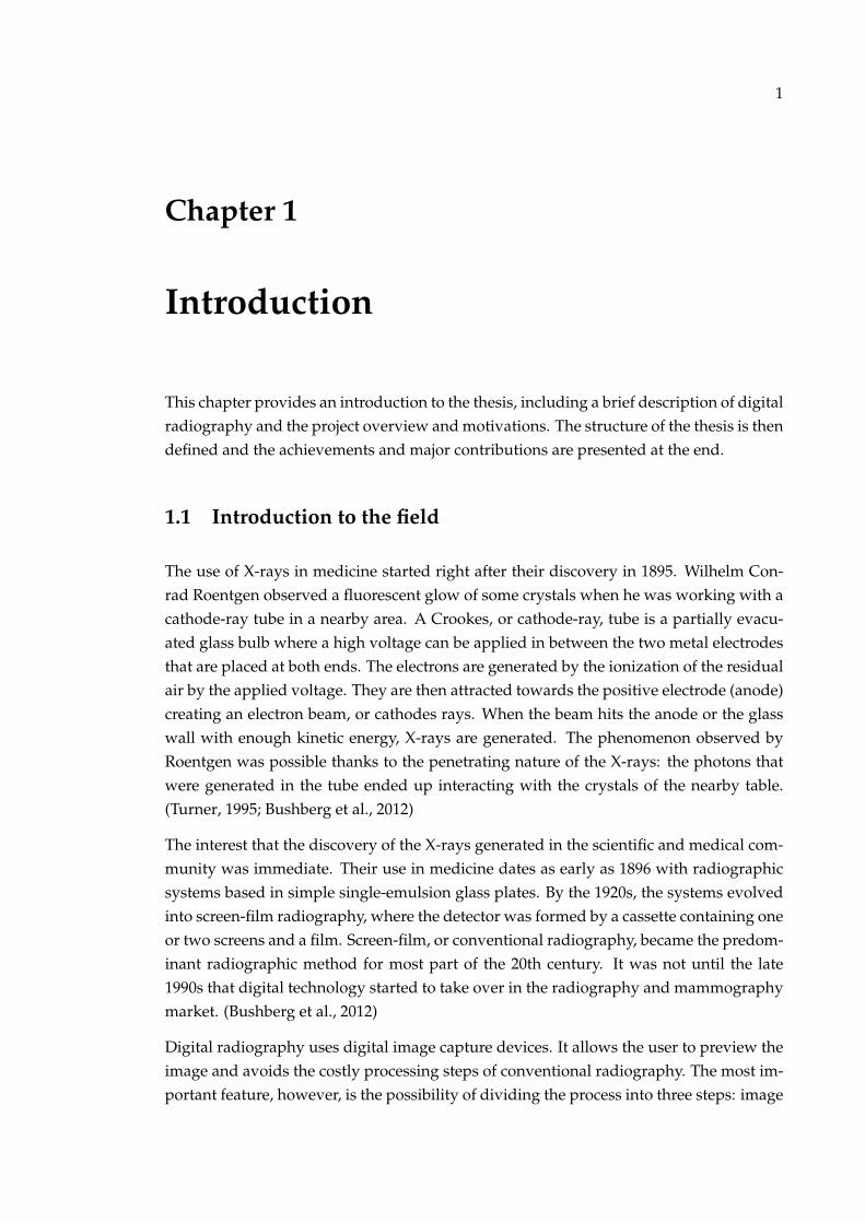
The use of X-rays in medicine started right after their discovery in 1895. Wilhelm Con-rad Roentgen observed a fluorescent glow of some crystals when he was working with acathode-ray tube in a nearby area. A Crookes, or cathode-ray, tube is a partially evacu-ated glass bulb where a high voltage can be applied in between the two metal electrodesthat are placed at both ends. The electrons are generated by the ionization of the residualair by the applied voltage. They are then attracted towards the positive electrode (anode)creating an electron beam, or cathodes rays. When the beam hits the anode or the glasswall with enough kinetic energy, X-rays are generated. The phenomenon observed byRoentgen was possible thanks to the penetrating nature of the X-rays: the photons thatwere generated in the tube ended up interacting with the crystals of the nearby table.(Turner, 1995; Bushberg et al., 2012)
The interest that the discovery of the X-rays generated in the scientific and medical com-munity was immediate. Their use in medicine dates as early as 1896 with radiographicsystems based in simple single-emulsion glass plates. By the 1920s, the systems evolvedinto screen-film radiography, where the detector was formed by a cassette containing oneor two screens and a film. Screen-film, or conventional radiography, became the predom-inant radiographic method for most part of the 20th century. It was not until the late1990s that digital technology started to take over in the radiography and mammographymarket. (Bushberg et al., 2012)
Digital radiography uses digital image capture devices. It allows the user to preview theimage and avoids the costly processing steps of conventional radiography. The most im-portant feature, however, is the possibility of dividing the process into three steps: image
Chapter 1. Introduction 2
acquisition, image processing and image display. The physical separation of the acqui-sition process and the processing of the raw image allows their individual optimization,leading to improvements in image quality:
1.1.1 Image acquisition: Digital X-ray detectors
As a result of the very positive response to the advent of digital radiography, differenttechnologies have been developed and are available for use in hospitals and industry.The wide range of choice in digital radiography has led to more specialised devices, al-lowing the possibility of defining different imaging requirements for different medicalprocedures, i.e. which organ to be imaged, which details are more important, the possi-bility of accounting for body motion, etc. Chest radiography, for example, requires a largedetector size (being 43 cm x 43 cm the standard size) and relatively high energies. Mam-mography needs high spatial resolution in order to detect microcalcifications, a lowerenergy range (25-30 keV) and a small pixel size (between 25 and 70 µm preferrably).While cardiology needs high frame rates, as the system must follow the motion of theheart (Hoheisel, 2006).
By the optimization of the X-ray systems either the image quality can be improved orthe radiation dose minimized, following the ALARP principle that stablishes that theionizing radiation has to be kept "As Low As Reasonable Practicable" (Bushberg et al.,2012). Due to the damaging effects that radiation has on the living tissue, a trade-offbetween image quality and delivered dose has always to be found and dedicated X-rayequipment and imaging technologies can help to find the best possible outcome.
The main digital radiography technologies currently available are Thin-Film Transis-tor (TFT) based detectors, Charge Couple Devices (CCD), Complementary Metal OxideSemiconductors with Active Pixel Sensors (CMOS APS). As these technologies can targetdifferent applications, a critical performance study is necessary in order to allow the enduser to make an objective decision when choosing the device.
The basic imaging performance of X-ray detector systems can be characterized by thestudy of the resolution, efficiency, noise and contrast. A series of parameters can be mea-sured in order to assess the characteristics of the detector and, therefore, can be used tocompare between technologies and industries and/or to find design problems. Some ofthese parameters are the response curve, dynamic range, signal to noise ratio, photontransfer curve, modulation transfer function, noise power spectrum and detective quan-tum efficiency.
Chapter 1. Introduction 3
1.1.2 Image processing: Scattering reduction in mammography
Image processing algorithms manipulate raw radiographies in order to adapt them tothe radiologist’s requirements. These algorithms are designed to optimize the quality ofthe output, minimizing the degradation of the image and avoiding the introduction ofartefacts that might lead to misdiagnosis. There are many different types of algorithms,indeed each manufacturer or system typically has their own, and they are focused onsolving particular issues that the raw images present for the application chosen.
In mammography applications, new scatter reduction techniques based on image post-processing have been emerging in the last years. A mammography test requires goodcontrast, good resolution, low dose and large dynamic range (NHS, 2016). The breastis composed of soft tissue, fat, blood vessels and it may have calcifications or tumours.Some of these tissues have very similar composition, therefore a X-ray scan must be sen-sitive to small differences in order to obtain enough contrast to distinguish them.
Scattered radiation limits the quantitative usefulness of radiographic images by degrad-ing the contrast and "signal-to-noise" ratio and decreasing the dynamic range. Therefore,the presence of scatter reduces the quality of the image and affects the diagnosis of lowcontrast lesions (Boone and Cooper, 2000; Cooper et al., 2000; Ahn, Cho, and Jeon, 2006;Ducote and Molloi, 2010). In addition to the risk of misdiagnosis, X-ray scatter also causesunderestimation in the measurement of the attenuation coefficients and the thickness es-timation (Ahn, Cho, and Jeon, 2006; Ducote and Molloi, 2010).
To reduce the scattered radiation in mammography the most widespread technique, atthe moment, is the use of anti-scatter grids. Anti-scatter grids are, however, an incom-plete solution that ends up adding complexity and cost to the mammography process.Although they help to improve the quality of the image they also attenuate primary ra-diation, leading to an increase in the delivered dose (up to a factor of 3) (Krol et al., 1996;Wang et al., 2015; Binst et al., 2015). The limitations of the anti-scatter grids combinedwith the introduction of new mammography screening techniques that do not allow theuse of grids, such most digital breast tomosynthesis systems, justify the interest and in-crease in research for new post-processing scatter reduction techniques.
1.2 Project overview
This EngD thesis presents the work undertaken in collaboration with Dexela Ltd. (VarexImaging London, former PerkinElmer Medical Imaging London), the Centre for DigitalEntertainment (CDE), Bournemouth University and University of Bath. The project is
Chapter 1. Introduction 4
based in the field of digital radiography, focusing more specifically on detector charac-terization of CMOS X-ray detectors and on studying image post-processing techniquesfor scatter reduction in mammography applications.
For the last five years PerkinElmer Medical Imaging first and Varex Imaging Londonnow, has been developing new products to include to their family of CMOS digital X-raydetectors. The main components of a CMOS X-ray detector are a scintillator, i.e. to con-vert the X-rays into light photons, a CMOS sensor and electronics. The new engineeringprogramme included a close interaction in the sensor development process, technologythat was previously acquired from a third-party company. Integral to this developmentprocess is a tight regime of testing and performance verification and evaluation. Newtesting procedures had to be defined for the purposes of design optimisation and prod-uct qualification. Most of the research done in the image characterization part of thisthesis has focused on this task, which is a critical input into the design cycle.
Although radiographic image quality testing is a well-known subject, it is usually fo-cused in final product characterization. There is little information about image charac-terization during the product design phase, as it is not in the private companies’ interestto share this kind of information. The main challenge has been to adapt well-known testmethods to try to identify detector or sensor issues, while mapping those issues to theirroot cause. This step is necessary to complete and challenge the initial modelling of thesensor performance, done during the first stages of the design cycle. The optical responseevaluation is a crucial test stage of the sensor development and it is achieved thanks to aclose collaboration between the imaging, sensor design and engineering teams.
Each detector prototype must be challenged in terms of image quality, to obtain a finalproduct that is suitable for medical or industrial applications and competitive in the mar-ket. The image characterization process closes the design loop.
The final image, however, is always delivered to the user after a certain amount of imageprocessing on the raw image. The second part of this thesis is based on the image pro-cessing side of digital radiography, focusing on scattering reduction in mammography.Scattering is produced when the original trajectory of the X-ray particle is deviated as aconsequence of the photon interaction with matter. It is important to minimise this effect,as it causes an increase in noise in the acquired image. The idea behind this study is toreduce the scatter component of an acquired mammogram using post-processing tech-niques, aiming to obtain equal or better image quality to the one obtained with the useof anti-scatter grids. The main objective is to determine if anti-scatter grids can be maderedundant.
Anti-scatter grids are currently the main method for scatter reduction in mammographyapplications; the motivation behind getting rid of them is multiple. The main advantagebeing the possibility of reducing the dose delivered to the patient, i.e. the grid absorbs
Chapter 1. Introduction 5
approximately 20% of the primary (non-scattered) beam so the dose needs to be increasedto maintain a good image quality. In the same way, the scattered radiation is not com-pletely absorbed, 30 to 60% will still be transmitted to the detector (Wang et al., 2015).Moreover, they are an expensive addition to the mammography system and either theyappear in the image, introducing an additional post-processing step to remove the pat-tern, or the system needs to include an additional mechanism to move the grid aroundits central position, making it invisible to the eye but increasing its size and price (Wanget al., 2015; Ahn, Cho, and Jeon, 2006; Binst et al., 2015; Krol et al., 1996).
1.3 Industrial Partner
Varex Imaging Corporation is a X-ray imaging solution provider that covers medical toindustrial applications. The extensive catalogue of products includes X-ray tubes, flatpanel digital detectors, high-voltage connectors, X-ray collimators, ionization chambers,mammography paddles, solid state automatic exposure control systems and buckies fordigital imaging.
Varian Medical Systems created Varex Imaging Corporation as a "spin-off" company inJanuary 2017. Varex Imaging completed the acquisition of the medical imaging branchof PerkinElmer in May 2017, the area of the company that was in charge of developing,manufacturing and selling digital X-ray detectors.
The CMOS flat panel detectors are currently being developed in Dexela Ltd, Varex Imag-ing - London. Dexela Ltd was founded in 2005 as a software and X-ray detector MedicalImaging Company and was acquired in June 2011 by PerkinElmer, adding CMOS tech-nology to the company’s medical and industrial imaging portfolio.
1.4 Structure of the thesis
This thesis is divided into seven chapters, including the present introduction. As it is anEngD thesis, the project covers two research topics that were of interest of the industrialpartner, both under the area of digital radiography: Chapters 2 and 3 focus on imagecharacterization analysis for the CMOS X-ray detector design phase. Chapters 4, 5 and6 look into using image post-processing techniques for reduction of scattered radiationin mammography. The conclusions of the findings and future work suggestions are pre-sented in Chapter 7. Chapters 2 to 6 are explained below.
• Chapter 2 starts with a theoretical background introduction about X-rays photonsto help in the interpretation of the results obtained in subsequent chapters. The

Chapter 1. Introduction 6
chapter follows with a description of the available digital X-ray detector technolo-gies and introduces the methods for performing a complete detector evaluationusing image characterization techniques.
• In Chapter 3 the image characterization techniques previously introduced in Chap-ter 2 are adapted and optimized to find sensor and detector shortcomings in the de-sign phase of CMOS X-ray detectors. The chapter describes the process of methodoptimization, giving examples of the failures found in the prototype evaluation andtheir root causes.
• Chapter 4 introduces the topic of scatter reduction in mammography applications.It presents some initial background information about breast cancer, mammogra-phy screening programmes and the mammography X-ray systems used for breastcancer detection. It continues with a description of the contribution of the scat-ter radiation in an image and presents the different alternatives to the anti-scattergrids available for scatter estimation, including physical detection methods andsimulated techniques. Finally, the system contribution to the scatter is evaluatedin order to identify the key areas that need to be carefully controlled in the studypresented in the following chapters.
• The point spread function (PSF) post-processing technique, based on the convo-lution of the output image with a set of scatter kernels, is the scattered reductionmethod chosen in this study. Chapter 5 explains the simulation process, startingwith an introduction to Geant4 (the chosen simulation tool-kit) and includes anoverview of the experimental set up and validation of the simulations and geome-try chosen. The proposed scatter correction method is then introduced, describingthe optimisation process and the robustness analysis that was carried out in thisstudy by comparing the results against full Monte Carlo simulations.
• Chapter 6 expands the validation of the chosen methodology to clinical imagesobtained with real mammography systems where the grid has been removed. Theresults obtained with a series of mammography phantoms are challenged againstthe images acquired with the use of an anti-scatter grid. A one to one comparisonbetween processed grid-less and grid images is performed for each of the examples.
1.5 Achievements and major contributions
1.5.1 Image characterization techniques
Prototypes of CMOS X-ray detectors under development have been been challenged interms of image quality. Image characterization methods were adapted and optimized for
Chapter 1. Introduction 7
the task of finding design shortcomings that needed to be fixed before the product wasfinalised and released into the market.
The techniques defined in this research project have been key to the development of anew family of CMOS X-ray detectors that are being released by Dexela Ltd. (Varex Imag-ing Corporation - London). The project required to work in close contact with a multi-national engineering team, providing them with the imaging science that they requiredduring the design cycle.
These test methods have a foundation in well-known image analysis techniques, but ad-ditional tools had to be developed to stretch the performance limits of these state-of-the-art custom, wafer-scale image sensor designs. The techniques adopted have beenimplemented in the company’s quality system to be used in the image quality evaluationof future products.
1.5.2 Scatter estimation in mammography
A convolution based post-processing technique has been chosen as scatter estimationmethod in this study. The scatter image is the convolution result of the input image witha point spread function (PSF) kernel. The primary image can then be calculated by justsubtracting the scatter to the input image.
It was established that, in order to account for variations in the image, the use of a singlesymmetric PSF for the convolution of the whole image was not a viable solution. Themain sources of discrepancies found were introduced by the scatter produced outsidethe breast area, i.e. background scatter produced mainly by the compression paddle, thethickness variation introduced by the angle of the X-ray beam at the edge of the breastand, in a smaller amount, the thickness reduction of the breast-edge area.
The proposed semi-empirical model accounts for the described discrepancies by intro-ducing three additional kernels: two for estimating the background contribution to thebreast and one for the thickness variations of the breast-edge. It was also seen that forbreasts thinner than 50 mm the background contribution was enough to reduce the un-certainty to less than 5%. For thicker breasts, the three kernels were necessary and thediscrepancy introduced by the model increased with the thickness, up to 10% for 70 mmthick breasts.
The final model was tested with a range of phantoms in clinical mammography systemsand the resulting images were compared with images acquired with an anti-scatter grid.The results obtained were very positive, indicating that the technique has a lot of po-tential. Although limitations were found, this semi-empirical method is relatively fast,easily optimised, verified and extendible.

Chapter 1. Introduction 8
1.5.3 List of Publications
The following publications have resulted from the work published in this thesis:
• Elena Marimon, Hammadi Nait-Charif, Asmar Khan, Philip A. Marsden and OliverDiaz. Detailed Analysis of Scatter Contribution from Different Simulated Geome-tries of X-ray Detectors. In Proc. of IWDM, LNCS 9699, pp. 203-210, 2016.
• Elena Marimon, Hammadi Nait-Charif, Asmar Khan, Philip A. Marsden and OliverDiaz. Scatter reduction for grid-less mammography using the convolution-basedimage post-processing technique. In Proc. of SPIE Medical Imaging 10132, 10132-4D,2017.
9
Chapter 2
X-ray systems
This chapter defines the theory behind digital X-ray systems. It starts giving some back-ground information about the X-ray spectrum and defining the main widespread digitalX-ray detector technologies. The chapter finishes with an introduction to image qualitycharacterization and detector evaluation.
2.1 X-rays
X-rays form part of the high frequency end of the electromagnetic spectrum, see Fig-ure 2.1. They are considered ionising radiation as their energy is high enough to liberatean electron from an atom, creating and ion pair and causing the atom to be positivelycharged.
The discovery of the X-rays in 1895 by Roentgen can be considered as the starting point ofionizing radiation in physics. X-rays can traverse most objects, including human tissue,characteristic that makes them very useful in medical applications. In fact, their use inmedicine started within six months after their discovery; they were used at the frontlinein battlefields to help locate bullets in injured soldiers. From 1913, when a X-ray tube wasdesigned to allow the use of high voltages, the improvements in the image quality wereenough to start being used extensively in medicine (Reed, 2011).
X-rays can be produced when a beam of electrons strikes a target of high atomic num-ber, e.g. Tungsten. Most of these electrons, up to 99 %, interact with the target’s orbitalelectrons, mainly producing heat but also, in smaller proportions, characteristic radiationif the interaction occurs in the inner orbitals K and L shells. The remaining < 1 % inter-acts with the atomic nuclei of the target, producing a continuous poly-energetic X-rayspectrum known as bremsstrahlung. (Turner, 1995; Dowsett, Kenny, and Johnston, 2006;Knoll, 2010).
Chapter 2. X-ray systems 10
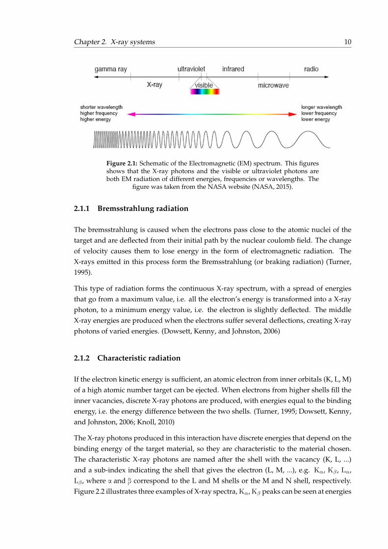
Figure 2.1: Schematic of the Electromagnetic (EM) spectrum. This figuresshows that the X-ray photons and the visible or ultraviolet photons areboth EM radiation of different energies, frequencies or wavelengths. The
figure was taken from the NASA website (NASA, 2015).
2.1.1 Bremsstrahlung radiation
The bremsstrahlung is caused when the electrons pass close to the atomic nuclei of thetarget and are deflected from their initial path by the nuclear coulomb field. The changeof velocity causes them to lose energy in the form of electromagnetic radiation. TheX-rays emitted in this process form the Bremsstrahlung (or braking radiation) (Turner,1995).
This type of radiation forms the continuous X-ray spectrum, with a spread of energiesthat go from a maximum value, i.e. all the electron’s energy is transformed into a X-rayphoton, to a minimum energy value, i.e. the electron is slightly deflected. The middleX-ray energies are produced when the electrons suffer several deflections, creating X-rayphotons of varied energies. (Dowsett, Kenny, and Johnston, 2006)
2.1.2 Characteristic radiation
If the electron kinetic energy is sufficient, an atomic electron from inner orbitals (K, L, M)of a high atomic number target can be ejected. When electrons from higher shells fill theinner vacancies, discrete X-ray photons are produced, with energies equal to the bindingenergy, i.e. the energy difference between the two shells. (Turner, 1995; Dowsett, Kenny,and Johnston, 2006; Knoll, 2010)
The X-ray photons produced in this interaction have discrete energies that depend on thebinding energy of the target material, so they are characteristic to the material chosen.The characteristic X-ray photons are named after the shell with the vacancy (K, L, ...)and a sub-index indicating the shell that gives the electron (L, M, ...), e.g. Kα, Kβ , Lα,Lβ , where α and β correspond to the L and M shells or the M and N shell, respectively.Figure 2.2 illustrates three examples of X-ray spectra, Kα, Kβ peaks can be seen at energies
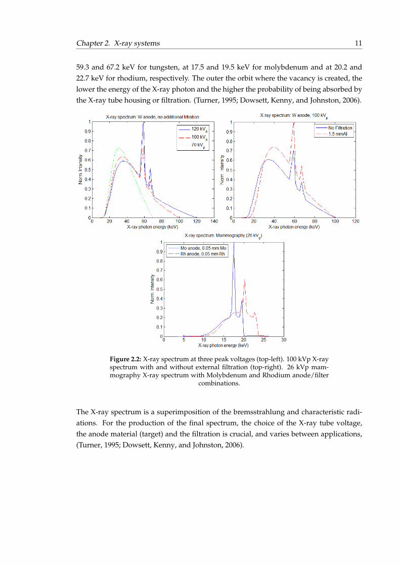
Chapter 2. X-ray systems 11
59.3 and 67.2 keV for tungsten, at 17.5 and 19.5 keV for molybdenum and at 20.2 and22.7 keV for rhodium, respectively. The outer the orbit where the vacancy is created, thelower the energy of the X-ray photon and the higher the probability of being absorbed bythe X-ray tube housing or filtration. (Turner, 1995; Dowsett, Kenny, and Johnston, 2006).
Figure 2.2: X-ray spectrum at three peak voltages (top-left). 100 kVp X-rayspectrum with and without external filtration (top-right). 26 kVp mam-mography X-ray spectrum with Molybdenum and Rhodium anode/filter
combinations.
The X-ray spectrum is a superimposition of the bremsstrahlung and characteristic radi-ations. For the production of the final spectrum, the choice of the X-ray tube voltage,the anode material (target) and the filtration is crucial, and varies between applications,(Turner, 1995; Dowsett, Kenny, and Johnston, 2006).
Chapter 2. X-ray systems 12
2.1.3 X-ray tube characteristics
Voltage
A X-ray tube is formed by an enclosure sealing a cathode and an anode under high vac-uum conditions. The electrons are emitted from the cathode, a heated tungsten filament,and accelerated towards the anode in a strong electric field, that is produced by a largepotential difference. The spectrum produced is directly related with the electron’s kineticenergy and, therefore, with the X-ray tube voltage. The maximum energy will delimitthe bremsstrahlung spectrum while the characteristic spectrum will be seen only if theelectrons have enough kinetic energy to remove an electron from the inner orbital of thetarget.
The choice of voltage determines the X-ray penetration and image quality: higher con-trast is achieved using low kilovoltages, e.g. being able to distinguish subtle soft tissuedifferences in mammography applications, while higher voltages, which produce X-rayswith increased overall energy, have higher penetration levels needed in general radiog-raphy applications.
Target
The anode material needs to have a high atomic number, as heavy nuclei cause strongerelectron deflections and are more efficient in producing Bremsstrahlung radiation. Thematerial needs high melting points, as 99+% of the electron’s energy is converted intoheat, and their contribution to the characteristic radiation needs to be taken into accountand balanced with housing and additional filtrations.
The most common target materials are tungsten and molybdenum, with binding energiesat the K shell of 69.5 and 59.3 keV, and 20.0 and 17.3 keV respectively.
Filtration
The beam filtration is needed for removing the lower X-ray energies (reducing the pa-tient dose) and "hardening" the beam by increasing the effective energy, e.g. acting as ahigh-pass filter. The choice of filtration depends on the application. For general radiog-raphy, the most common material is aluminium, which has a very low K-edge (1.6 keV),i.e. K-edge is the binding energy of the electrons situated in the innermost shell of anatom. For higher energy medical exams, such as Computed Tomography (CT), a combi-nation of aluminium and copper (8.0 keV) is used. For mammography, however, metalswith higher K-edge are needed, as they remove unneeded higher energy photons, e.g.Molybdenum (20.0 keV) or Rhodium (23.2 keV), as well as the lower X-ray energies.
Chapter 2. X-ray systems 13
2.2 Photon interaction with matter
When the X-ray beam passes through an absorber, the incident photons can be transmit-ted without interacting with the material, totally absorbed or scattered from their originaldirection. The beam is attenuated, i.e. its intensity is reduced, as a consequence of theseinteractions.
The interactions of the X-ray beam with matter take place at the atomic level and caninvolve collisions with the electrons (photoelectric effect and scattered radiation) or withthe nuclei (pair production). For nuclear interaction the incident photon needs to havea very high energy (E > 1.022 MeV) in comparison with the energies used in diagnosticimaging (20 to 150 keV), as illustrated in Figure 2.3. Therefore only the electron interac-tions are going to be discussed in this work, i.e. photoelectric effect and coherent andincoherent scattering. (Turner, 1995; Dowsett, Kenny, and Johnston, 2006; Knoll, 2010)
2.2.1 Photoelectric effect
In the photoelectric absorption, the incident photon loses all its energy in the interactionwith the atom. One electron is ejected (photoelectron), as illustrated in Figure 2.4, withenergy equal to the incident photon minus the electron binding energy and the energygiven to the recoiling atom (energy that can usually be neglected). This interaction onlyaffects electrons with high binding energy, i.e. K-shell and (sometimes) L-shell, in orderto satisfy both the conservation of energy and of momentum. (Dowsett, Kenny, andJohnston, 2006)
The probability of a photoelectric effect event decreases with the photon energy and in-creases with the target’s atomic number, ∝ Z3
E3 . Therefore, its contribution is very strongat low diagnostic energies, i.e. mammography. (Turner, 1995)
The energy given to the photoelectron is usually completely deposited in the absorber,contributing to the radiation dose, as the range of the electron is short and interacts inthe surrounding atoms. The photoelectric effect is the major contribution to dose in thetissue. (Dowsett, Kenny, and Johnston, 2006)
2.2.2 Coherent or elastic scattering
Coherent scattering takes place when the incident photon undergoes a change in direc-tion without transferring energy or ionizing the atom. The scatter can happen with boundelectrons (Rayleigh scattering) or with loosely bound electrons (Thomson scattering). Inthe diagnostic energy range, only 10% of the photon interaction events are due to elasticscattering. (Turner, 1995; Dowsett, Kenny, and Johnston, 2006)

Chapter 2. X-ray systems 14
Rayleigh scattering
Rayleigh scattering events are more important at low incident photon energies for tar-gets with high atomic numbers. Its probability is proportional to ∝ Z2
E . (Turner, 1995;Dowsett, Kenny, and Johnston, 2006)
2.2.3 Inelastic (Compton) scattering
This interaction takes place with loosely bound electrons. The incident photon, of energyE1, interacts with the electron which is ejected with energy e and at an angle φ. Thephoton is scattered at an angle θ and energy E2 = E1 − e, as depicted in Figure 2.4.The energy received by the Compton electron and the direction of the scattered photonis related to the incident photon energy; as the incident photon’s energy increases, theenergy fraction given to the electron increases and a forward scatter angle is favoured.(Turner, 1995; Dowsett, Kenny, and Johnston, 2006)
The probability to have a Compton scattering event slightly decreases with the energyand is independent on the atomic number, ∝ 1
E .(Dowsett, Kenny, and Johnston, 2006)
Figure 2.3: The plot shows the range of importance of the three principalX-ray modes of interaction as a function of the photon energy and target’s
atomic number. Image taken from (Hendee and Ritenour, 2002).
2.2.4 Image formation
The final image is formed by the photons that are absorbed by the X-ray detector. Thosephotons can be the ones that have been transmitted without interacting along the path(useful information) or scattered photons that increase the noise in the image. The objectsthat are placed in between the X-ray beam and the imager are shown in the final imagebecause of the difference in the photon intensity, as each material attenuates the beamdifferently.

Chapter 2. X-ray systems 15
Figure 2.4: Schematics of the Photoelectric Effect interaction (left) and theCompton scattering process (right). In the image the photons are referred
as γ and the electrons as e− .
The initial beam intensity (I0) is reduced as the photon beam passes through differentabsorbers, following the exponential law (Turner, 1995; Dowsett, Kenny, and Johnston,2006):
I = I0e−µx (2.1)
where, x is the thickness of the absorber and µ is the linear attenuation coefficient.
The value of the attenuation coefficient depends on the absorber’s density and atomicnumber, but also on the energy of the beam. Equation 2.1 is valid for describing theattenuation of a mono-energetic beam. An energy dependant formula would be neededfor describing the poly-energetic process:
I =
∫ Emax
Emin
I0(E)e−µ(E)x (2.2)
At a given energy, it is possible to write µ as a combination of the linear attenuation coeffi-cients of all the X-ray interaction processes (photoelectric, Compton and elastic scatteringin the diagnostic imaging range), see equation 2.3.
µ = µPE + µComp + µRay (2.3)
It is also possible to write it as a sum of the coefficients of different absorbers, see equation2.4 (Dowsett, Kenny, and Johnston, 2006).
Chapter 2. X-ray systems 16
µ =∑i
wiµi (2.4)
where, wi is a weighting factor to account for the proportion of each material (i).
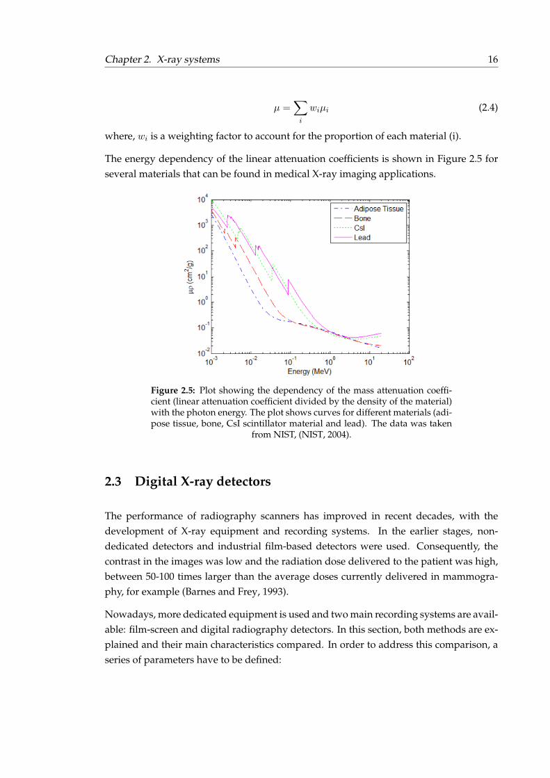
The energy dependency of the linear attenuation coefficients is shown in Figure 2.5 forseveral materials that can be found in medical X-ray imaging applications.
Figure 2.5: Plot showing the dependency of the mass attenuation coeffi-cient (linear attenuation coefficient divided by the density of the material)with the photon energy. The plot shows curves for different materials (adi-pose tissue, bone, CsI scintillator material and lead). The data was taken
from NIST, (NIST, 2004).
2.3 Digital X-ray detectors
The performance of radiography scanners has improved in recent decades, with thedevelopment of X-ray equipment and recording systems. In the earlier stages, non-dedicated detectors and industrial film-based detectors were used. Consequently, thecontrast in the images was low and the radiation dose delivered to the patient was high,between 50-100 times larger than the average doses currently delivered in mammogra-phy, for example (Barnes and Frey, 1993).
Nowadays, more dedicated equipment is used and two main recording systems are avail-able: film-screen and digital radiography detectors. In this section, both methods are ex-plained and their main characteristics compared. In order to address this comparison, aseries of parameters have to be defined:
Chapter 2. X-ray systems 17
• Signal-to-Noise Ratio (SNR): It is the ratio between the intensity of the signal andthe noise at a given region of interest (ROI). The higher the SNR, the better theimage quality obtained (James, 2004).
• Dynamic Range: It is the ratio between the maximum signal that the detector canread and the signal equivalent to the noise of the detector (Muller, 1999).
• Spatial Resolution: It is the parameter that describes the ability of an imaging sys-tem to individually discriminate two adjacent high-contrast objects.
• Modulation Transfer Function (MTF): It is the measurement of the spatial resolutionin the spatial frequency domain.
• Detective Quantum Efficiency (DQE): It is the quantity that measures the efficiencywith which the information is transferred from the imaging system to the final dis-played image, allowing to quantify how good the imaging system is (James, 2004).
The terms described above are some of the parameters needed to assess the quality of theimages. They will be defined further in Section 2.5.
Digital radiography was introduced in the mid-1980s and, with increasing popularity,is currently taking over the conventional film-screen radiography market in all radio-graphic applications (Bansal, 2006).
The main characteristic and advantage of digital radiography is the separation of imageacquisition, image processing and image display. This allows the individual optimizationof these three steps, avoiding the compromise in the performance that would be neededotherwise (Muller, 1999; Noel and Thibault, 2004).
Other advantages are a wider dynamic range, increased linearity, higher contrast reso-lution and higher DQE. This allows either to reduce the delivered dose to the patientmaintaining the SNR or to improve the image quality, compensating for the lower spa-tial resolution that digital systems typically have (James, 2004; Muller, 1999). All theseimprovements, together with easier processing and data storage, management and vi-sualization, and the possibility of increasing the scope of medical applications, such asin computer-aided diagnosis (CAD) or three-dimensional mammography, makes digitalradiography the best system for radiographic screening (James, 2004; Muller, 1999).
There are also drawbacks to a digital radiography system. In addition to the lower imageresolution observed, there is a possibility of introducing image artefacts during the pro-cessing stage, increasing the number of false positive diagnoses. Although some of theartefacts can be corrected, like the non-uniformity in the response, there are others whichare difficult to avoid, e.g. dead areas in the images caused by the gap between two imagesensors when they are joined together to make a large area detector. The detector itselfcan also lead to problems, if the detector field of view is not large enough to cover the
Chapter 2. X-ray systems 18
absorber, for example. Finally, there are also some minor disadvantages such as the needof multiple monitors of large dimensions, with large contrast resolution and high lumi-nescence, that increases the price of the system (although it also introduces a powerfulltool by allowing the reader to zoom in or change the image contrast if needed). Monitorsare needed to allow radiologists to review the mammograms in an easy way and to allowthe comparison between different images at the same time and with high speed (Muller,1999).
As mentioned above, manufacturers have adopted different approaches and introducedseveral detector technologies into the market, each of them capable of producing high-quality performance. The main technologies that are currently available are film-screen,photostimulable storage phosphor computed radiography (PSP CR) and solid state de-tectors, including thin film transistor, i.e. TFT: Amorphous silicon (α-Si) or amorphous se-lenium (α-Se), CCD and CMOS detectors. Newer technologies that have not been widelyadapted yet, such as photon-counting detectors, will not be discussed in this chapter.
2.3.1 Screen-Film
In general, film-screen cassettes consist of a film emulsion layer located between two flu-orescent screens and loaded into a light-tight cassette. The fluorescent screens, made ofscintillator material, convert the incident X-ray photons into visible or ultraviolet pho-tons that are detected by the film (for a presentation of the differences between types ofElectromagnetic (EM) radiation, in particular the X-ray and visible or ultraviolet radia-tion, refer to Figure 2.1). The film is a sheet of thin plastic with a photosensitive silverhalide emulsion coated onto both sides and it is the part of the detector that forms thelatent image when the detector is exposed with the X-rays, i.e. it records the X-ray inten-sity pattern. The final image is obtained by chemically processing of the film, reducingthe silver halide into metallic silver grains (Bushberg et al., 2012).
For mammography applications, this configuration is changed to a one sided high def-inition screen, used as a back screen, in contact with a single emulsion film, which actssimultaneously as an image acquisition detector, as a storage medium and as a displaydevice (Muller, 1999). This combination reduces the light diffusion, which is one of themain causes of blurring (Barnes and Frey, 1993).
The choice of the type of film and screen, the processing conditions (i.e. chemical formu-lation of the solutions employed), the time of exposure, the dose employed and even theambient conditions (temperature or humidity) will affect the performance of the detec-tor (Barnes and Frey, 1993). It is, therefore, very important to choose correctly betweenmaterials and ways of operations, to optimize the outcome.

Chapter 2. X-ray systems 19
The principal advantage of film-screen imaging systems is its excellent spatial resolution.The films are also physically handled, allowing the radiographer to display more thanone image at the same time, for comparative analysis, and can be stored for long periodsof time suffering almost no degradation. The detectors can be large and have continuossensitive surfaces and are directly sensitive to the impact of the X-ray beam (Muller, 1999;Noel and Thibault, 2004).
On the other hand, the main drawback is in the image quality; film-screen systems usu-ally have low SNR and low dynamic range. There is a compromise between the spa-tial resolution and the detection efficiency of the X-ray image and between the dynamicrange and the contrast resolution that limits the quality of the images. Moreover, the filmlayer is fragile and cannot be duplicated without loss of quality (Muller, 1999; Noel andThibault, 2004). In applications such as mammography, conventional film-screen imag-ing is not precise enough, missing approximately 10% of the breast cancers that can bedetected by physical examinations (Muller, 1999).
2.3.2 Photostimulable storage phosphor computed radiography (PSP-CR)
In this system the screen-film combination is replaced by a storage phosphor imagingplate, also contained inside a cassette. Irradiation excites electrons in the phosphor andthe crystalline structure traps them, keeping them stable until the exposure is finished.The number of excited electrons is proportional to the intensity of the beam so, after theexposure, the phosphor plate can be processed and the pattern of the absorbed X-raysread. In the processing step, the phosphor plate is inserted into a reader and scanned bya laser of appropriate wavelength. The phosphor plate can be reused after the residuallatent image is erased (James, 2004; Noel and Thibault, 2004).
The main advantage that CR systems have over full digital radiography systems, is thelower investment cost required, as it is possible to re-purpose existing conventional ra-diography systems just by changing the screen and film of the cassettes by the CR phos-phor plates. However, if new installations are required, the cost difference between CRand other digital mammography systems stops being significant. On the other hand, CRneeds higher dose to obtain an acceptable image quality, mainly due to lower overallDQE and to the impossibility of changing and optimizing the exposure parameters (Bickand Diekmann, 2007).
Chapter 2. X-ray systems 20
2.3.3 Thin-film transistor (TFT) based detectors or Active Matrix Flat PanelImagers
TFT panels have been used extensively for medical imaging applications since the 1990s.There are two main types: Amorphous Silicon and Amorphous Selenium detectors, whichare indirect and direct conversion detectors, respectively.
2.3.3.1 Amorphous silicon-based technology
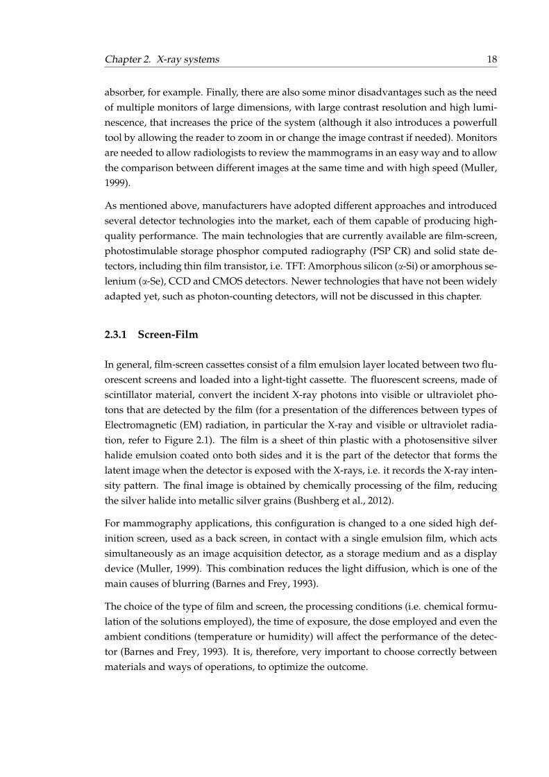
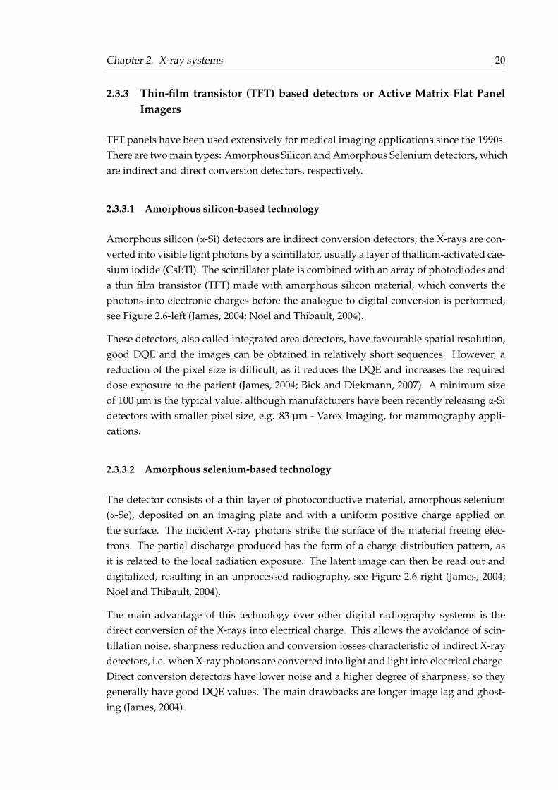
Amorphous silicon (α-Si) detectors are indirect conversion detectors, the X-rays are con-verted into visible light photons by a scintillator, usually a layer of thallium-activated cae-sium iodide (CsI:Tl). The scintillator plate is combined with an array of photodiodes anda thin film transistor (TFT) made with amorphous silicon material, which converts thephotons into electronic charges before the analogue-to-digital conversion is performed,see Figure 2.6-left (James, 2004; Noel and Thibault, 2004).
These detectors, also called integrated area detectors, have favourable spatial resolution,good DQE and the images can be obtained in relatively short sequences. However, areduction of the pixel size is difficult, as it reduces the DQE and increases the requireddose exposure to the patient (James, 2004; Bick and Diekmann, 2007). A minimum sizeof 100 µm is the typical value, although manufacturers have been recently releasing α-Sidetectors with smaller pixel size, e.g. 83 µm - Varex Imaging, for mammography appli-cations.
2.3.3.2 Amorphous selenium-based technology
The detector consists of a thin layer of photoconductive material, amorphous selenium(α-Se), deposited on an imaging plate and with a uniform positive charge applied onthe surface. The incident X-ray photons strike the surface of the material freeing elec-trons. The partial discharge produced has the form of a charge distribution pattern, asit is related to the local radiation exposure. The latent image can then be read out anddigitalized, resulting in an unprocessed radiography, see Figure 2.6-right (James, 2004;Noel and Thibault, 2004).
The main advantage of this technology over other digital radiography systems is thedirect conversion of the X-rays into electrical charge. This allows the avoidance of scin-tillation noise, sharpness reduction and conversion losses characteristic of indirect X-raydetectors, i.e. when X-ray photons are converted into light and light into electrical charge.Direct conversion detectors have lower noise and a higher degree of sharpness, so theygenerally have good DQE values. The main drawbacks are longer image lag and ghost-ing (James, 2004).
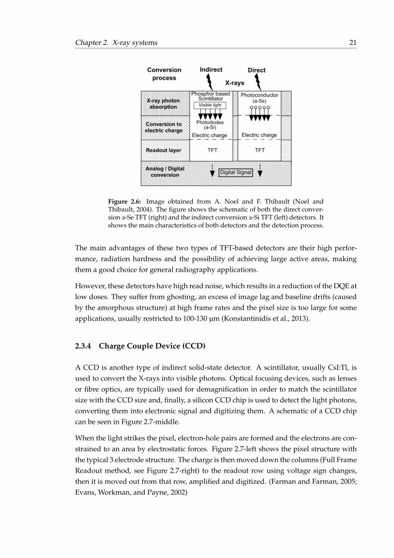
Chapter 2. X-ray systems 21
Figure 2.6: Image obtained from A. Noel and F. Thibault (Noel andThibault, 2004). The figure shows the schematic of both the direct conver-sion α-Se TFT (right) and the indirect conversion α-Si TFT (left) detectors. Itshows the main characteristics of both detectors and the detection process.
The main advantages of these two types of TFT-based detectors are their high perfor-mance, radiation hardness and the possibility of achieving large active areas, makingthem a good choice for general radiography applications.
However, these detectors have high read noise, which results in a reduction of the DQE atlow doses. They suffer from ghosting, an excess of image lag and baseline drifts (causedby the amorphous structure) at high frame rates and the pixel size is too large for someapplications, usually restricted to 100-130 µm (Konstantinidis et al., 2013).
2.3.4 Charge Couple Device (CCD)
A CCD is another type of indirect solid-state detector. A scintillator, usually CsI:Tl, isused to convert the X-rays into visible photons. Optical focusing devices, such as lensesor fibre optics, are typically used for demagnification in order to match the scintillatorsize with the CCD size and, finally, a silicon CCD chip is used to detect the light photons,converting them into electronic signal and digitizing them. A schematic of a CCD chipcan be seen in Figure 2.7-middle.
When the light strikes the pixel, electron-hole pairs are formed and the electrons are con-strained to an area by electrostatic forces. Figure 2.7-left shows the pixel structure withthe typical 3 electrode structure. The charge is then moved down the columns (Full FrameReadout method, see Figure 2.7-right) to the readout row using voltage sign changes,then it is moved out from that row, amplified and digitized. (Farman and Farman, 2005;Evans, Workman, and Payne, 2002)
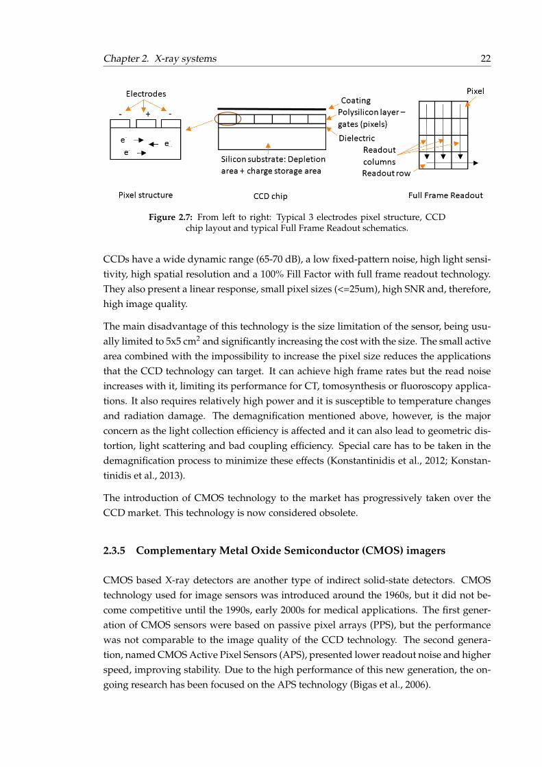
Chapter 2. X-ray systems 22
Figure 2.7: From left to right: Typical 3 electrodes pixel structure, CCDchip layout and typical Full Frame Readout schematics.
CCDs have a wide dynamic range (65-70 dB), a low fixed-pattern noise, high light sensi-tivity, high spatial resolution and a 100% Fill Factor with full frame readout technology.They also present a linear response, small pixel sizes (<=25um), high SNR and, therefore,high image quality.
The main disadvantage of this technology is the size limitation of the sensor, being usu-ally limited to 5x5 cm2 and significantly increasing the cost with the size. The small activearea combined with the impossibility to increase the pixel size reduces the applicationsthat the CCD technology can target. It can achieve high frame rates but the read noiseincreases with it, limiting its performance for CT, tomosynthesis or fluoroscopy applica-tions. It also requires relatively high power and it is susceptible to temperature changesand radiation damage. The demagnification mentioned above, however, is the majorconcern as the light collection efficiency is affected and it can also lead to geometric dis-tortion, light scattering and bad coupling efficiency. Special care has to be taken in thedemagnification process to minimize these effects (Konstantinidis et al., 2012; Konstan-tinidis et al., 2013).
The introduction of CMOS technology to the market has progressively taken over theCCD market. This technology is now considered obsolete.
2.3.5 Complementary Metal Oxide Semiconductor (CMOS) imagers
CMOS based X-ray detectors are another type of indirect solid-state detectors. CMOStechnology used for image sensors was introduced around the 1960s, but it did not be-come competitive until the 1990s, early 2000s for medical applications. The first gener-ation of CMOS sensors were based on passive pixel arrays (PPS), but the performancewas not comparable to the image quality of the CCD technology. The second genera-tion, named CMOS Active Pixel Sensors (APS), presented lower readout noise and higherspeed, improving stability. Due to the high performance of this new generation, the on-going research has been focused on the APS technology (Bigas et al., 2006).
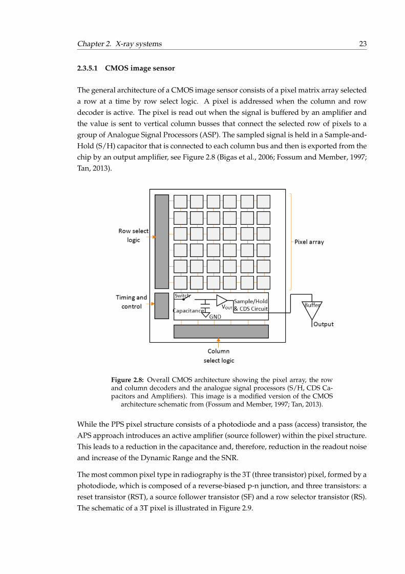
Chapter 2. X-ray systems 23
2.3.5.1 CMOS image sensor
The general architecture of a CMOS image sensor consists of a pixel matrix array selecteda row at a time by row select logic. A pixel is addressed when the column and rowdecoder is active. The pixel is read out when the signal is buffered by an amplifier andthe value is sent to vertical column busses that connect the selected row of pixels to agroup of Analogue Signal Processors (ASP). The sampled signal is held in a Sample-and-Hold (S/H) capacitor that is connected to each column bus and then is exported from thechip by an output amplifier, see Figure 2.8 (Bigas et al., 2006; Fossum and Member, 1997;Tan, 2013).
Figure 2.8: Overall CMOS architecture showing the pixel array, the rowand column decoders and the analogue signal processors (S/H, CDS Ca-pacitors and Amplifiers). This image is a modified version of the CMOS
architecture schematic from (Fossum and Member, 1997; Tan, 2013).
While the PPS pixel structure consists of a photodiode and a pass (access) transistor, theAPS approach introduces an active amplifier (source follower) within the pixel structure.This leads to a reduction in the capacitance and, therefore, reduction in the readout noiseand increase of the Dynamic Range and the SNR.
The most common pixel type in radiography is the 3T (three transistor) pixel, formed by aphotodiode, which is composed of a reverse-biased p-n junction, and three transistors: areset transistor (RST), a source follower transistor (SF) and a row selector transistor (RS).The schematic of a 3T pixel is illustrated in Figure 2.9.
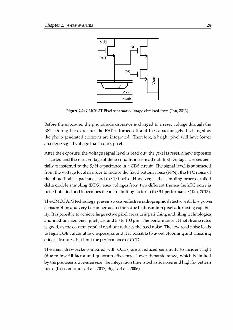
Chapter 2. X-ray systems 24
Figure 2.9: CMOS 3T Pixel schematic. Image obtained from (Tan, 2013).
Before the exposure, the photodiode capacitor is charged to a reset voltage through theRST. During the exposure, the RST is turned off and the capacitor gets discharged asthe photo-generated electrons are integrated. Therefore, a bright pixel will have loweranalogue signal voltage than a dark pixel.
After the exposure, the voltage signal level is read out, the pixel is reset, a new exposureis started and the reset voltage of the second frame is read out. Both voltages are sequen-tially transferred to the S/H capacitance in a CDS circuit. The signal level is subtractedfrom the voltage level in order to reduce the fixed pattern noise (FPN), the kTC noise ofthe photodiode capacitance and the 1/f noise. However, as the sampling process, calleddelta double sampling (DDS), uses voltages from two different frames the kTC noise isnot eliminated and it becomes the main limiting factor in the 3T performance (Tan, 2013).
The CMOS APS technology presents a cost-effective radiographic detector with low powerconsumption and very fast image acquisition due to its random pixel addressing capabil-ity. It is possible to achieve large active pixel areas using stitching and tiling technologiesand medium size pixel pitch, around 50 to 100 µm. The performance at high frame ratesis good, as the column parallel read out reduces the read noise. The low read noise leadsto high DQE values at low exposures and it is possible to avoid blooming and smearingeffects, features that limit the performance of CCDs.
The main drawbacks compared with CCDs, are a reduced sensitivity to incident light(due to low fill factor and quantum efficiency), lower dynamic range, which is limitedby the photosensitive-area size, the integration time, stochastic noise and high fix patternnoise (Konstantinidis et al., 2013; Bigas et al., 2006).
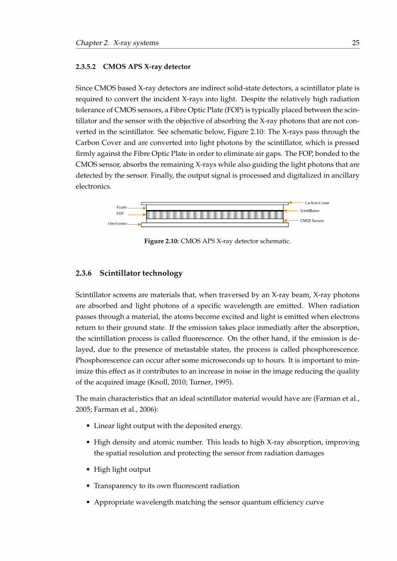
Chapter 2. X-ray systems 25
2.3.5.2 CMOS APS X-ray detector
Since CMOS based X-ray detectors are indirect solid-state detectors, a scintillator plate isrequired to convert the incident X-rays into light. Despite the relatively high radiationtolerance of CMOS sensors, a Fibre Optic Plate (FOP) is typically placed between the scin-tillator and the sensor with the objective of absorbing the X-ray photons that are not con-verted in the scintillator. See schematic below, Figure 2.10: The X-rays pass through theCarbon Cover and are converted into light photons by the scintillator, which is pressedfirmly against the Fibre Optic Plate in order to eliminate air gaps. The FOP, bonded to theCMOS sensor, absorbs the remaining X-rays while also guiding the light photons that aredetected by the sensor. Finally, the output signal is processed and digitalized in ancillaryelectronics.
Figure 2.10: CMOS APS X-ray detector schematic.
2.3.6 Scintillator technology
Scintillator screens are materials that, when traversed by an X-ray beam, X-ray photonsare absorbed and light photons of a specific wavelength are emitted. When radiationpasses through a material, the atoms become excited and light is emitted when electronsreturn to their ground state. If the emission takes place inmediatly after the absorption,the scintillation process is called fluorescence. On the other hand, if the emission is de-layed, due to the presence of metastable states, the process is called phosphorescence.Phosphorescence can occur after some microseconds up to hours. It is important to min-imize this effect as it contributes to an increase in noise in the image reducing the qualityof the acquired image (Knoll, 2010; Turner, 1995).
The main characteristics that an ideal scintillator material would have are (Farman et al.,2005; Farman et al., 2006):
• Linear light output with the deposited energy.
• High density and atomic number. This leads to high X-ray absorption, improvingthe spatial resolution and protecting the sensor from radiation damages
• High light output
• Transparency to its own fluorescent radiation
• Appropriate wavelength matching the sensor quantum efficiency curve
Chapter 2. X-ray systems 26
• Short decay time without phosphorescence
• Low cost
• Mechanical and chemical ruggedness
Unfortunately, a material with all the above properties does not exist. The most com-mon materials used in X-ray detectors are Thallium-activated structured Caesium Iodidecrystals (CsI:Tl) and Gadolinium Oxysulfide (GOS or Gadox) ceramic screens.
CsI:Tl scintillators are grown in a needle-like columnar structure, perpendicular to a sub-strate (usually carbon or aluminium). The light is channelled to the sensor when thescintillation fluorescence direction is within the acceptance cone of the CsI light guide.If the angle is bigger, the light is scattered to neighbour needles until the incident angleis acceptable to be channelled (Moy, 1998). A general restriction of scintillator materialsis their thickness: a thick material leads to a higher X-ray absorption but, at the sametime, substantially increases the light scattering and image blur. The needle structure ofCsI scintillators reduces the light scattering, allowing an increase of the thickness of thescreen without losing spatial resolution quality. This material emits green light and hasa response time in the region of 1 to 3 ms (Farman et al., 2005). It has one of the highestscintillation yields and, for the energies used in diagnostic imaging, the number of opti-cal photons emitted per absorbed X-ray is large (>1000) (Granfors and Aufrichtig, 2000).It also has high detectability, due to the K-absorption edge of the Iodine and Caesium,33.2 keV and 36.0 keV respectively (Konstantinidis et al., 2013). For all these reasons, thismaterial is widely used in X-ray diagnostic imaging.
Gadox screens, Gd202S:Tb, present high efficiency (a response time between 1 and 3 ms)green light emission (peak around 545 nm) and a main absorption edge at 50 keV. It is avery stable and easily handled material (Farman et al., 2005). Its main drawbacks are thethickness limitation (the light scatter increases considerably with the thickness due to itsunstructured nature) and the deep notch in sensitivity right at the peak of the X-ray beamspectrum for radiography diagnosis applications (Farman et al., 2006). Although CsI:Tlscreens are a better option, the low cost of Gadox screens makes them a good alternativefor some applications.
2.4 General design requirements for the next generation of de-tectors
The objective of acquiring images for medical use is to achieve an accurate diagnosis. Thelast word about the quality of the image is given by the radiologists, who are the subjec-tive receptors. However, there are a series of parameters that define the performance ofthe X-ray detector and have to be optimized before the product is released.

Chapter 2. X-ray systems 27
Any ideal detector would have:
• No dark current, i.e. no electrons generated and collected without light input
• Infinite dynamic range
• 100% of quantum efficiency, i.e. ratio of incident photons to converted electronsequal to 1
• 100% of fill factor
• No fixed pattern noise, i.e. no non-uniformities on dark current generation or pixelresponse, threshold variations or gain and offset differences
• No sensor noise
• High frame rate
• High resolution
• High signal to noise ratio
• High sensitivity
• No power consumption
• Linear response
• Radiation hardness
• Choice of active area (length)
• Choice of pixel size
• Absence of image lag or ghosting
The limitations present in every sensor technology make it impossible to achieve thisideal case. But in order to develop a product that can be sold in the medical market, themanufacturers have to optimize these parameters to obtain a minimum quality standard,e.g. low dark current, noise and power consumption and high dynamic range, quantumefficiency, frame rate, resolution and sensitivity.
Each digital detector technology has a series of strengths and weaknesses that can bereferred to the parameters described above. The choice of technology will be decided de-pending on the desired medical application and, therefore, the performance optimizationwill be affected by the targeted requirements.
The most restrictive parameters, that are decisive when choosing between technologies,are shown in the Table 2.1. Some parameters, like the fixed pattern noise or the linearity,
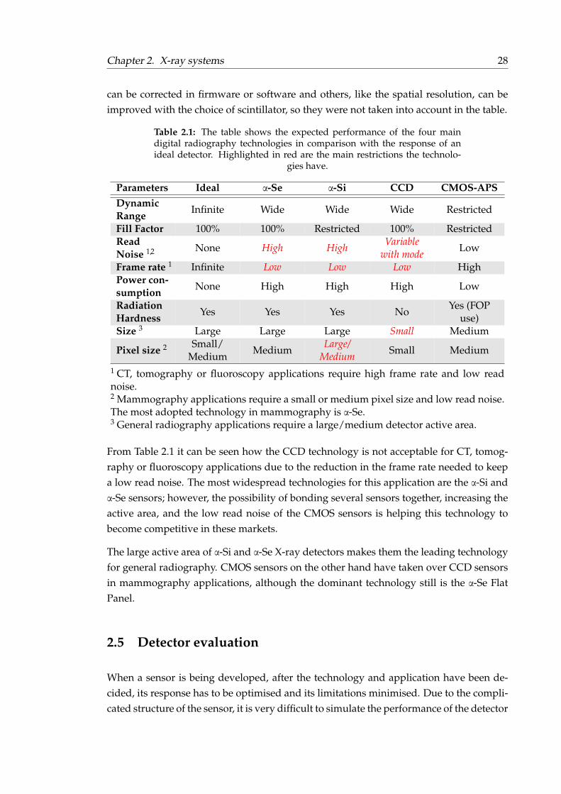
Chapter 2. X-ray systems 28
can be corrected in firmware or software and others, like the spatial resolution, can beimproved with the choice of scintillator, so they were not taken into account in the table.
Table 2.1: The table shows the expected performance of the four maindigital radiography technologies in comparison with the response of anideal detector. Highlighted in red are the main restrictions the technolo-
gies have.
Parameters Ideal α-Se α-Si CCD CMOS-APSDynamicRange
Infinite Wide Wide Wide Restricted
Fill Factor 100% 100% Restricted 100% RestrictedReadNoise 1,2 None High High Variable
with mode Low
Frame rate 1 Infinite Low Low Low HighPower con-sumption
None High High High Low
RadiationHardness
Yes Yes Yes NoYes (FOP
use)Size 3 Large Large Large Small Medium
Pixel size 2 Small/Medium
MediumLarge/
Medium Small Medium
1 CT, tomography or fluoroscopy applications require high frame rate and low readnoise.2 Mammography applications require a small or medium pixel size and low read noise.The most adopted technology in mammography is α-Se.3 General radiography applications require a large/medium detector active area.
From Table 2.1 it can be seen how the CCD technology is not acceptable for CT, tomog-raphy or fluoroscopy applications due to the reduction in the frame rate needed to keepa low read noise. The most widespread technologies for this application are the α-Si andα-Se sensors; however, the possibility of bonding several sensors together, increasing theactive area, and the low read noise of the CMOS sensors is helping this technology tobecome competitive in these markets.
The large active area of α-Si and α-Se X-ray detectors makes them the leading technologyfor general radiography. CMOS sensors on the other hand have taken over CCD sensorsin mammography applications, although the dominant technology still is the α-Se FlatPanel.
2.5 Detector evaluation
When a sensor is being developed, after the technology and application have been de-cided, its response has to be optimised and its limitations minimised. Due to the compli-cated structure of the sensor, it is very difficult to simulate the performance of the detector

Chapter 2. X-ray systems 29
with high accuracy. This leads to a series of sensor versions that have to be tested againstthe product specifications. The quality of the image characterization tests will define thequality of the final product, so it is critical for the manufacturer to cover all the possibleerrors that the sensor might encounter before freezing the design.
2.5.1 Electro-optical performance
2.5.1.1 Noise
Noise is a variation in the pixel value of an acquired image that is not caused by theoriginal object. There are many factors that contribute to the final noise observed in animage and they have to be minimized in order to improve the image quality. The mainnoise sources in a digital detector are:
Electronic Temporal Noise: In electronic detectors, it is the flow of electrons that con-veys the output signal. These electrons can be produced by the input signal or be artifi-cially introduced, causing electronic noise (Hoheisel, 2006).
The electronic temporal noise is composed of (Konstantinidis et al., 2012):
• Read noise: It is mainly comprised of pixel source follower noise and it is not func-tion of the signal.
• Reset or kTC noise: It appears due to the uncertainty of the capacitor’s amount ofcharge after it has been charged through a resistor.
• Thermal noise: It is generated in resistors and MOS transistors.
• 1/f noise or flicker noise: It is a low frequency noise that appears in MOS transis-tors.
• Dark current shot noise: It is the statistical variation on the amount of electronsgenerated in dark (without light input).
• ADC quantization noise: Analogue to Digital convertors produce discrete outputlevels. Therefore, some analogue inputs give the same output value.
• Phase noise: It comes from external sources rather than being caused in the sensor,e.g. power supply.
Temporal noise is especially problematic at low signal levels, in particular when thenoise-electrons are added to the system before the amplification circuits (Bushberg et al.,2012).
Chapter 2. X-ray systems 30
Input Signal Noise: Photon shot noise, or quantum noise, is the variation of the num-ber of X-ray photons detected. These counting statistics follow the Poisson distributionand it can be approximated to the normal or Gaussian distribution if the variance (σ2) isassumed to be equal to the mean number of photons detected, N. Therefore, the noise isequal to the square root of N and the relative noise, i.e. noise to signal ratio, shows howan increase of the number of detected photons lead to a reduction of the noise (Bushberget al., 2012). The total photon shot noise is a mixture of both, X-ray photon shot noiseand, in less proportion, scintillated photon shot noise.
Fixed Pattern Noise (FPN): FPN, also called structured noise, refers to two parameters:the dark signal non uniformity (DSNU) and the photo response non uniformity (PRNU).The DSNU noise is the offset between pixels in a dark image, i.e. no illumination level, ata specific temperature and exposure time. The PRNU is the response variation betweenpixels under illumination.
The FPN is usually caused by the read out channels of pixelated detectors, althoughdust or imperfections in the sensor can also contribute to the noise. CMOS detectors, forexample, have parallel read out channels with their own amplification circuits, so theycannot be perfectly matched with respect each other, creating a different offset and gainresponse between pixels (Bushberg et al., 2012).
The main advantage of the FPN is that it is a correlated non-stochastic noise, i.e. relativelyconstant in time, so the gain and offset factors of each pixel can be characterized and theimage corrected. The gain and offset correction algorithm is described in equation 2.5,
Icorr = gIraw − Ioffset
Igain − Ioffset(2.5)
where,
g = Mean Pixel Value of the offset corrected gain image, Igain − Ioffset
Iraw = Raw image to correct
Ioffset = Offset or dark image, acquired with no illumination. Usually 20 dark images areaveraged
Igain = Gain or flat image, typically acquired at a similar illumination level that the imageto correct
All the images have to be taken using the same exposure time. It is recommended tocollect the Ioffset and Igain images at regular time intervals to account for temperature orposition variations (Bushberg et al., 2012; Konstantinidis et al., 2012)

Chapter 2. X-ray systems 31
2.5.1.2 Conversion Gain
The Conversion Gain gives the conversion factor to transform the digital numbers (DN),i.e. count unit (ADC) given by the detector which is meaningless by itself, to electrons.
A way of calculating it is following the mean-variance analysis, described by (Konstan-tinidis et al., 2012):
σ2S = GS + σ2
R (2.6)
where,
σ2S is the total measured temporal noise (signal independent and dependent). The way of
calculating this variable is acquiring a number (N) of images at a constant signal level andquantifying the temporal variation of each pixel around its averaged value. The mean ofthe resulting 2D matrix gives the total measured temporal noise.
σ2R is the signal independent read noise in [DN2]
S is the signal level in [DN2]
G is the conversion gain in [DN/e−]
Plotting the total measured temporal noise versus the signal level and fitting the straightarea of the curve will lead to the Conversion Gain (slope of the curve) and the signalindependent read noise (y-intercept).
2.5.1.3 Full Well Capacity (FWC)
The FWC is the maximum electronic charge that each pixel’s photodiode sense node canaccommodate before the pixel is saturated.
It can be obtained using the mean-variance analysis of the conversion gain calculation,by multiplying the conversion gain with the mean signal level that corresponds to thehigher variance level, without previously subtracting the dark level (Konstantinidis etal., 2012).
2.5.1.4 Dynamic Range
The dynamic range is the ratio between the largest and smallest value of the signal. Itis given by the ratio between the FWC and the read noise. It can be described by theequation below, 2.7 (Konstantinidis et al., 2012; Zanella, 2002).

Chapter 2. X-ray systems 32
DR[dB] = 20 logFWC[e−]
σ2R[e−]
(2.7)
2.5.2 X-ray performance
2.5.2.1 Contrast Resolution
Contrast resolution is a measurement of the imaging system’s ability to detect subtlechanges in the grey scale, i.e. structures that cause small changes in the signal intensitythat are difficult to be distinguished from the background.
The SNR is a parameter used for the evaluation of the contrast resolution. It measuresthe ratio between the signal integrated over an object of interest, i.e. sum of the pixelsignal amplitude (for pixel i: (xi − xbg)), and the noise background (σbg). Therefore, theSNR studies the integrated signal, obtained from a ROI that encloses the object, dividedby the noise, see Figure 2.11. This metric describes how well an object can be observedby including its size and shape, while being independent of its distribution, i.e. it doesnot require the signal to be homogeneous. (Bushberg et al., 2012).
The SNR can be described as:
SNR =∑i
(xi − xbg)σbg
(2.8)
Figure 2.11: Example of a non-homogeneous bright object and the param-eters needed for the Signal to Noise Ratio (SNR) calculation. The idea of
the image was obtained from (Bushberg et al., 2012).
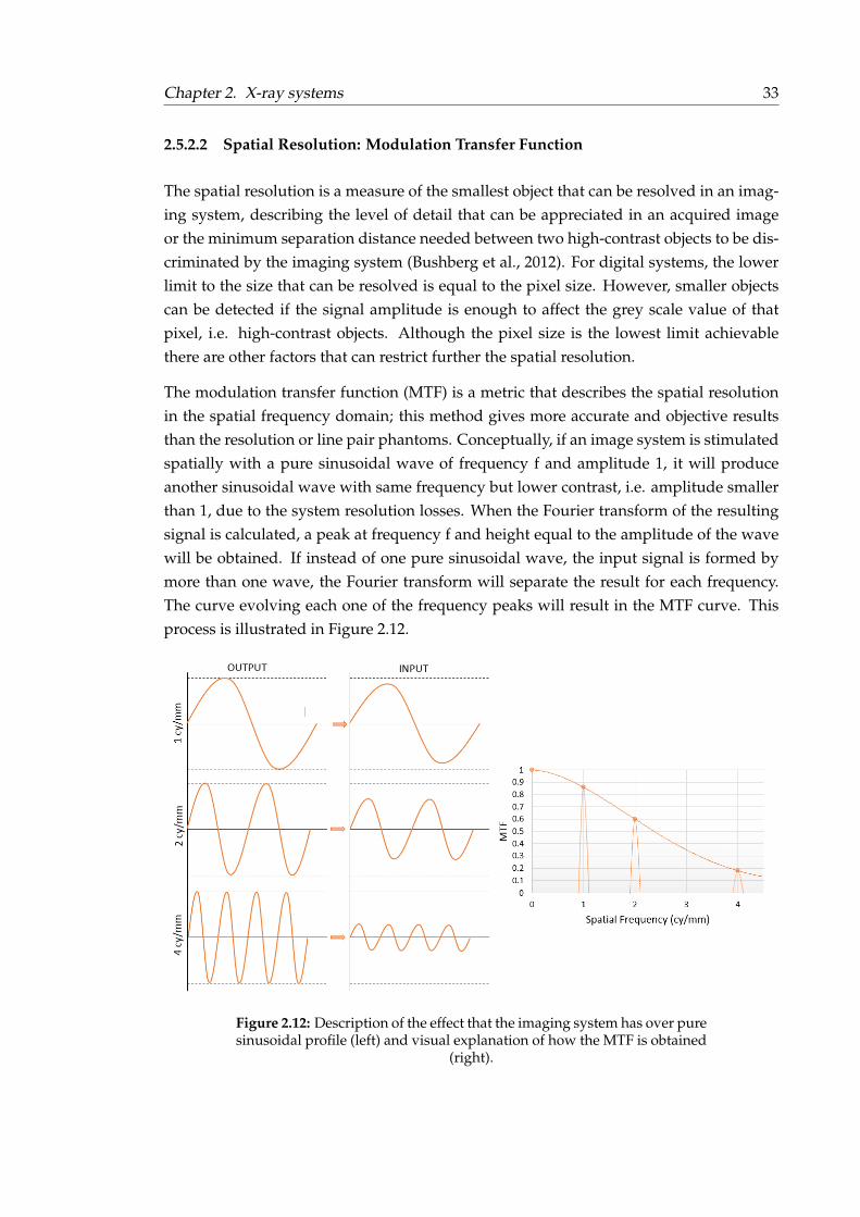
Chapter 2. X-ray systems 33
2.5.2.2 Spatial Resolution: Modulation Transfer Function
The spatial resolution is a measure of the smallest object that can be resolved in an imag-ing system, describing the level of detail that can be appreciated in an acquired imageor the minimum separation distance needed between two high-contrast objects to be dis-criminated by the imaging system (Bushberg et al., 2012). For digital systems, the lowerlimit to the size that can be resolved is equal to the pixel size. However, smaller objectscan be detected if the signal amplitude is enough to affect the grey scale value of thatpixel, i.e. high-contrast objects. Although the pixel size is the lowest limit achievablethere are other factors that can restrict further the spatial resolution.
The modulation transfer function (MTF) is a metric that describes the spatial resolutionin the spatial frequency domain; this method gives more accurate and objective resultsthan the resolution or line pair phantoms. Conceptually, if an image system is stimulatedspatially with a pure sinusoidal wave of frequency f and amplitude 1, it will produceanother sinusoidal wave with same frequency but lower contrast, i.e. amplitude smallerthan 1, due to the system resolution losses. When the Fourier transform of the resultingsignal is calculated, a peak at frequency f and height equal to the amplitude of the wavewill be obtained. If instead of one pure sinusoidal wave, the input signal is formed bymore than one wave, the Fourier transform will separate the result for each frequency.The curve evolving each one of the frequency peaks will result in the MTF curve. Thisprocess is illustrated in Figure 2.12.
Figure 2.12: Description of the effect that the imaging system has over puresinusoidal profile (left) and visual explanation of how the MTF is obtained
(right).
Chapter 2. X-ray systems 34
The MTF values are between 0 and 1, where 1 means a complete transmission of theobject’s contrast to the output image and 0 means no transmission of the contrast. Highspatial resolution results in an improvement of image sharpness and a better detection ofsmall details (very useful in analysis of microcalcifications, for example). Therefore theMTF is desired to be as high as possible for all frequencies.
While the MTF describes the spatial resolution in the frequency domain, there are threeother functions that help to define it in the spatial domain: point spread function (PSF),line spread function (LSF) and edge spread function (ESF):
• The PSF is the 2D response of the system to a point source that is, approximately,five to ten times smaller than the pixel pitch.
• The LSF describes the response of the system to a test device that has a narrow slit(1D).
• The ESF is the response of the detector to a sharp edge (1D). A straight edge is theeasier device to make, so the MTF is usually obtained from a measurement of theESF.
There is a direct relationship between these four parameters, see equations 2.9, 2.10 and2.11, so it is possible to choose the simplest and easier function to measure and calculatethe MTF.
LSF(x) =
∫ ∞y=−∞
PSF(x, y)dy (2.9)
ESF(x) =
∫ ∞y=−∞
LSF(x′)dx′ (2.10)
MTF(f) = FFT(LSF(x)) (2.11)
The MTF evaluation is very sensitive to the measurement acquisition method, the analy-sis process and the measurement settings. The International Electrotechnical Comissioncreated the documents: "IEC 62220-1: Medical Electrical Equipment - Characteristics ofDigital X-ray Imaging Devices - Part 1: Determination of the Detective Quantum Effi-ciency", (IECP, 2007b), and "IEC 62220-1-2: Medical Electrical Equipment - Characteris-tics of Digital X-ray Imaging Devices - Part 1-2: Determination of the Detective QuantumEfficiency – Detectors used in mammography", (IECP, 2007a), in order to standardise andcontrol the MTF measurement method, reducing the number of variables that hinders thecomparison between systems.
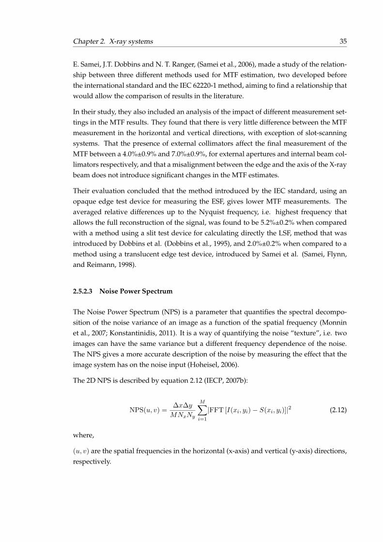
Chapter 2. X-ray systems 35
E. Samei, J.T. Dobbins and N. T. Ranger, (Samei et al., 2006), made a study of the relation-ship between three different methods used for MTF estimation, two developed beforethe international standard and the IEC 62220-1 method, aiming to find a relationship thatwould allow the comparison of results in the literature.
In their study, they also included an analysis of the impact of different measurement set-tings in the MTF results. They found that there is very little difference between the MTFmeasurement in the horizontal and vertical directions, with exception of slot-scanningsystems. That the presence of external collimators affect the final measurement of theMTF between a 4.0%±0.9% and 7.0%±0.9%, for external apertures and internal beam col-limators respectively, and that a misalignment between the edge and the axis of the X-raybeam does not introduce significant changes in the MTF estimates.
Their evaluation concluded that the method introduced by the IEC standard, using anopaque edge test device for measuring the ESF, gives lower MTF measurements. Theaveraged relative differences up to the Nyquist frequency, i.e. highest frequency thatallows the full reconstruction of the signal, was found to be 5.2%±0.2% when comparedwith a method using a slit test device for calculating directly the LSF, method that wasintroduced by Dobbins et al. (Dobbins et al., 1995), and 2.0%±0.2% when compared to amethod using a translucent edge test device, introduced by Samei et al. (Samei, Flynn,and Reimann, 1998).
2.5.2.3 Noise Power Spectrum
The Noise Power Spectrum (NPS) is a parameter that quantifies the spectral decompo-sition of the noise variance of an image as a function of the spatial frequency (Monninet al., 2007; Konstantinidis, 2011). It is a way of quantifying the noise “texture”, i.e. twoimages can have the same variance but a different frequency dependence of the noise.The NPS gives a more accurate description of the noise by measuring the effect that theimage system has on the noise input (Hoheisel, 2006).
The 2D NPS is described by equation 2.12 (IECP, 2007b):
NPS(u, v) =∆x∆y
MNxNy
M∑i=1
|FFT [I(xi, yi)− S(xi, yi)]|2 (2.12)
where,
(u, v) are the spatial frequencies in the horizontal (x-axis) and vertical (y-axis) directions,respectively.
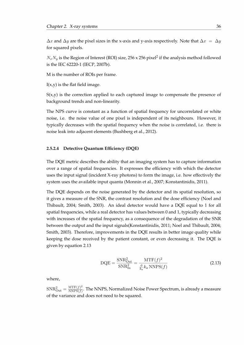
Chapter 2. X-ray systems 36
∆x and ∆y are the pixel sizes in the x-axis and y-axis respectively. Note that ∆x = ∆y
for squared pixels.
NxNy is the Region of Interest (ROI) size, 256 x 256 pixel2 if the analysis method followedis the IEC 62220-1 (IECP, 2007b).
M is the number of ROIs per frame.
I(x,y) is the flat field image.
S(x,y) is the correction applied to each captured image to compensate the presence ofbackground trends and non-linearity.
The NPS curve is constant as a function of spatial frequency for uncorrelated or whitenoise, i.e. the noise value of one pixel is independent of its neighbours. However, ittypically decreases with the spatial frequency when the noise is correlated, i.e. there isnoise leak into adjacent elements (Bushberg et al., 2012).
2.5.2.4 Detective Quantum Efficiency (DQE)
The DQE metric describes the ability that an imaging system has to capture informationover a range of spatial frequencies. It expresses the efficiency with which the detectoruses the input signal (incident X-ray photons) to form the image, i.e. how effectively thesystem uses the available input quanta (Monnin et al., 2007; Konstantinidis, 2011).
The DQE depends on the noise generated by the detector and its spatial resolution, soit gives a measure of the SNR, the contrast resolution and the dose efficiency (Noel andThibault, 2004; Smith, 2003). An ideal detector would have a DQE equal to 1 for allspatial frequencies, while a real detector has values between 0 and 1, typically decreasingwith increases of the spatial frequency, as a consequence of the degradation of the SNRbetween the output and the input signals(Konstantinidis, 2011; Noel and Thibault, 2004;Smith, 2003). Therefore, improvements in the DQE results in better image quality whilekeeping the dose received by the patient constant, or even decreasing it. The DQE isgiven by equation 2.13
DQE =SNR2
Out
SNR2In
=MTF(f)2
φkaka NNPS(f)
(2.13)
where,
SNR2Out = MTF(f)2
NNPS(f) . The NNPS, Normalized Noise Power Spectrum, is already a measureof the variance and does not need to be squared.

Chapter 2. X-ray systems 37
SNR2In = φ
kaka is the fluence per exposure ratio, φ
ka, multiplied by the exposure kerma (in
µGy).
There are different ways of calculating the fluence per exposure ratio. The InternationalStandard IEC 62220-1 gives a photon-counting approximation, assuming that an idealdetector behaves like an ideal photon counter. It can be calculated following the equation2.14 (Konstantinidis et al., 2012).
φ
ka=
∫ kV
0φnorm(E)
WQ
(µen(E)ρ )airEe108
dE (2.14)
where,
φnorm(E) is the normalized spectrum.
W = 33.97[eV/ionpair] is an accurate value for X-rays in dry air, (Konstantinidis et al.,2012).
Q = 2.58104[C/Kg/R] is the charge liberated in air by one R.
e = 1.602210−19[C] is the electronic charge.
As mentioned, the standard gives a photon-counting approximation. For energy inte-grating detectors it is possible to perform an energy-weighted calculation of the fluenceper exposure ratio. However, previous studies mentioned by Konstantinidis et al. ((Kon-stantinidis et al., 2012)) proved that the difference at radiation quality RQA-5 (explainedbelow) is less than 3%, decreasing further for lower voltage spectra.
The International Standard dictates the DQE assessment at different radiation qualities,which correspond to different radiographic applications. The measurement settings andthe photon-counting approximation vary with each radiation quality; the IEC 62220-1-2document provides the radiation qualities for mammography (RQA-M) while the IEC62220-1 document gives radiation qualities RQA3 (paediatrics), RQA5 (general radiogra-phy) and RQA7 (higher energy applications), among others.
2.6 Chapter summary and discussion
This chapter presented a critical review of the theory behind digital X-ray detector tech-nologies. To set the basic knowledge needed to understand the concepts that will beintroduced in this thesis, the chapter started with a theoretical introduction of X-ray pro-duction, photon interaction with matter and X-ray image formation.

Chapter 2. X-ray systems 38
The main widespread digital X-ray detector technologies such as TFT panels, i.e. α-Se andα-Si, CCDs or CMOS were then introduced, including their general design requirementsand comparing them against the performance of an ideal X-ray detector.
The chapter finished giving detailed information about the techniques and parametersinvolved in the evaluation and quality control of X-ray panels. It was defined that acharacterization exercise needs to focus in the study of the electro-optical performanceof the detector as well as its response to incoming photons. Therefore, the chapter ex-plained the theory behind the different types of noise (e.g. electronic temporal noise,input signal noise and fix pattern noise), introduced the concept of conversion gain, dy-namic range and contrast resolution, and gave the theoretical background and analysismethods needed for measuring the MTF (for spatial resolution analysis), NPS (for noisestructure analysis) and DQE (gold standard that describes the ability that the imagingsystem has to capture the incoming information).
The parameters explained in this section allow to fully characterize the performance of adetector and set the basis for the comparison between technologies and manufacturers.

39
Chapter 3
Characterization of CMOS X-raydetectors
This chapter has been excised for industrial IP confidentiality reasons.

40
Chapter 4
Scatter Reduction
This chapter introduces the second part of the thesis. It begins with some backgroundinformation about breast cancer and mammography systems. It continues with a mathe-matical interpretation of the scatter distribution in an image to then focus in defining thedifferent grid-less scatter reduction methodologies available for mammography applica-tions.
4.1 Mammography
4.1.1 Breast anatomy
The femmale mammary gland lies partly on the ribs and partly on the pectoralis muscle,a large fan-shaped muscle that covers the chest and stretches up into the armpit. Thebreast is formed by three different type of tissue: glandular, fibrous and fatty tissue,surrounded by a thin skin layer. The glandular tissue is composed by 15-20 lobes, each ofwhich is formed by lobules, smaller gland structures that radiate around the nipple andproduce milk in nursing women. Each lobule opens into small ducts that join togetherto form the excretory or lactiferous ducts. Towards the centre of the breast, these ductsform dilatations, lactiferous sinus, that act as milk reservoir which, at the same time, areconnected to the nipple by narrow ducts (Seeley, Stephens, and Tate, 1998; Waugh et al.,2014; Kopans, 2007). An illustration of the structure of the breast can be seen in Figure 4.1.
The lobes are supported by the fibrous tissue and covered by adipose tissue, which givesthe breast its form. The breast is supplied with blood with the thoracic branches ofthe axillary artery, the internal mammary and intercostal arteries and the axillary andmammary veins. The lymphatic channels run towards the armpit, passing through thelymph nodes, which are in charge of filtering the germs contained in the lymph.(Seeley,Stephens, and Tate, 1998)
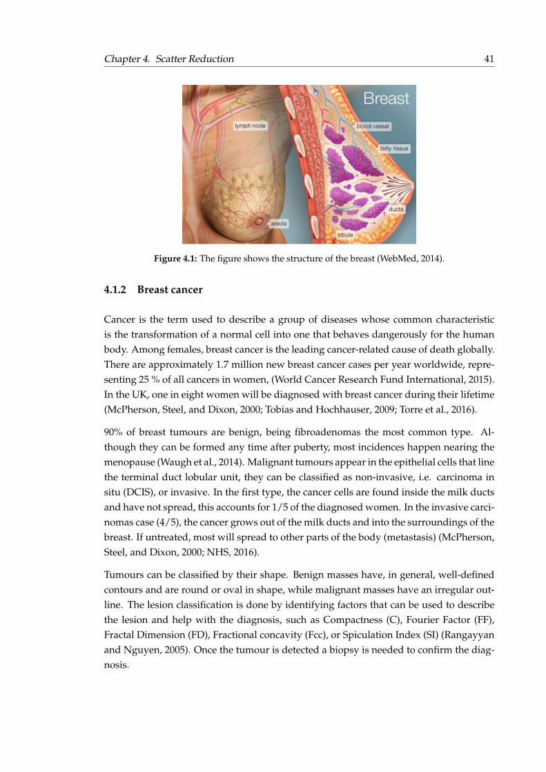
Chapter 4. Scatter Reduction 41
Figure 4.1: The figure shows the structure of the breast (WebMed, 2014).
4.1.2 Breast cancer
Cancer is the term used to describe a group of diseases whose common characteristicis the transformation of a normal cell into one that behaves dangerously for the humanbody. Among females, breast cancer is the leading cancer-related cause of death globally.There are approximately 1.7 million new breast cancer cases per year worldwide, repre-senting 25 % of all cancers in women, (World Cancer Research Fund International, 2015).In the UK, one in eight women will be diagnosed with breast cancer during their lifetime(McPherson, Steel, and Dixon, 2000; Tobias and Hochhauser, 2009; Torre et al., 2016).
90% of breast tumours are benign, being fibroadenomas the most common type. Al-though they can be formed any time after puberty, most incidences happen nearing themenopause (Waugh et al., 2014). Malignant tumours appear in the epithelial cells that linethe terminal duct lobular unit, they can be classified as non-invasive, i.e. carcinoma insitu (DCIS), or invasive. In the first type, the cancer cells are found inside the milk ductsand have not spread, this accounts for 1/5 of the diagnosed women. In the invasive carci-nomas case (4/5), the cancer grows out of the milk ducts and into the surroundings of thebreast. If untreated, most will spread to other parts of the body (metastasis) (McPherson,Steel, and Dixon, 2000; NHS, 2016).
Tumours can be classified by their shape. Benign masses have, in general, well-definedcontours and are round or oval in shape, while malignant masses have an irregular out-line. The lesion classification is done by identifying factors that can be used to describethe lesion and help with the diagnosis, such as Compactness (C), Fourier Factor (FF),Fractal Dimension (FD), Fractional concavity (Fcc), or Spiculation Index (SI) (Rangayyanand Nguyen, 2005). Once the tumour is detected a biopsy is needed to confirm the diag-nosis.

Chapter 4. Scatter Reduction 42
In order to reduce the uncertainty and standardize the diagnosis in mammography, theAmerican College of Radiology (ACR) developed, published and registred in 1992 a ra-diographic tool called BI-RADS (Breast Imaging Reporting and Data System) (Sickles,2013). The BI-RADS atlas helps to describe, classify and categorise the findings and ithas been widely adopted in clinical practice throughout the world and in screening pro-grammes in the US and Europe (Timmers et al., 2012).
The causes of breast cancer are not completely understood. However, there are differentfactors that have been linked with an increase of the probability of developing breastcancer (NHS, 2016; Dixon, 2012; Waugh et al., 2014; Tobias and Hochhauser, 2009):
Age: The risk of developing breast cancer increases with age, up to 8 in 10 breast cancercases are developed in women that are over 50 years old.
Previous diagnosis of breast cancer: Women who have developed breast cancer in onemammary gland have higher probability of developing a new breast cancer.
Previous diagnosis of a benign breast lump: Benign changes in breast tissue may in-crease the risk in developing future breast cancer. Some examples are: atypical ductalhyperplasia - cells growing abnormally in ducts; or lobular carcinoma in situ - abnormalcells inside the breast lobes.
Family history: Although most breast cancer cases do not run in families, some genesthat can be passed on from a parent to their child are associated with an increase in thebreast cancer risk, i.e. BRCA1, BRCA2, TP53 and CHEK2 . Up to 10% of breast cancerscases in Western countries are due to genetic predisposition .
Oestrogen - Menarche, menopause and breast feeding: Oestrogen is a female hormonethat can stimulate breast cancer cells and cause them to grow. Therefore, a higher oestro-gen exposure level might slightly increase the risk of breast cancer, for example in casesof late menopause, late or non offspring breastfeeding or a menarche age of 12 years oryounger.
In addition, studies have shown a protective effect for those women who have their chil-dren at an early age. This effect is seen in those women who have a full-term pregnancywith an age of 32 years or less, being more clear if the pregnancy takes place before 25years old.

Chapter 4. Scatter Reduction 43
Breast density: This effect is not fully known. One of the possible explanations is theincrease of lobules, i.e. glandular tissue that contains higher concentration of breast cells,which increase the number of cells that can become cancerous.
Lifestyle and health: Breast cancer is more frequent in women suffering from obesity,especially after the menopause, as being overweight causes more oestrogen to be pro-duced.
Alcoholics are also more likely to develop breast cancer. In fact, studies show that thereare three more cases for every 200 women if these women drink two alcoholic drinks aday.
Exercise has been proved to have a protective effect. A reduction of breast cancer inci-dence can be observed just with 30 minutes of exercise per week.
Radiation: X-rays, Computed Tomography (CT) scans or previous radiotherapy treat-ments, like the treatment of Hodgkin lymphoma, may increase the risk of breast cancervery slightly.
Hormone Replacement Therapy (HRT): This treatment is associated with an increasedrisk. Patients treated with combined HRT for 10 years show an increase of 19 cases forevery 1000 women.
Contraceptive pill: Research shows a slight increase in women that take contraceptivepills. The risk starts decreasing the moment the woman stops taking the contraceptivepill. After 10 years the risk is back to normal.
Although there are no definite conclusions, studies suggest that maintaining a healthylifestyle, i.e. healthy weight, regular exercise, low intake of saturated fat and alcohol, canreduce the risk of developing breast cancer by as much as a third (NHS, 2016).
More extreme measures can be considered for women that are in a high-risk group, suchas performing a mastectomy, which can reduce the risk up to 90 %, or the use of medica-tion, e.g. tamoxifen, anastroxole or raloxifene. These are not ideal solutions as it impliesundergoing major and invasive surgery or taking medication with many side effects,some as serious as osteoporosis, blood clots or uterine cancer (NHS, 2016). For each indi-vidual case it will be necessary to balance the risk and benefits of the treatment.
In any case, if a breast cancer is developed, an early diagnosis can improve the outcome ofthe treatment, increasing the chances of survival and reducing the need of a mastectomy

Chapter 4. Scatter Reduction 44
or chemotherapy. For this reason, breast cancer awareness is very important; it is keyto be familiarised with the symptoms and seek medical opinion if they appear. The firstnoticeable effects of breast cancer are usually the presence of a lump or thickened breasttissue. It is important to note that breast pain is not a symptom. Some indications can be(NHS, 2016):
• Change in size or shape of the breast(s)
• Change in appearance of the nipple(s)
• Nipple discharge
• Nipple rash
• Lump or swelling of one of the armpits
• Dimpling on the breast skin
However, a breast cancer in an early stage does not usually show any symptoms. For thatreason, after a certain age and to increase the chances of early detection, some countriesimplement regular breast screening programmes.
4.1.3 Screening
Screening is the procedure of checking for the presence of potential health disorders inan asymptomatic population group (National Cancer Institute, 2015; WHO, 2014).
It is not possible to carry out screening programmes for all types of diseases, for examplesome health disorders cannot be detected before causing a symptom and some screeningprogrammes present more disadvantages than benefits to the overall population. There-fore, screening programmes are limited to specific types of diseases, to certain populationgroups and/or to people with specific genetic risks.
To be considered valid, a screening programme needs to take the following aspects intoconsideration (Tobias and Hochhauser, 2009; WHO, 2014):
• Sensitivity of the test: It needs to be able to detect early stages of the disease andhave a low index of false-positive results.
• Usefulness: The disease has to be treatable and curable if detected in an early stage.
• Incidence of the disease: The disease has to be common and have a high incidenceto justify the programme.

Chapter 4. Scatter Reduction 45
Breast cancer is considered a suitable disease for a screening programme. It has high in-cidence in women population, there are high risk groups and it is easy to examine. Mam-mography is the only breast screening programme that has proved to be cost-effectiveso far. Several studies have shown that while self-examination does not show improve-ments in the mortality rate, there is approximately 20 % of relative mortality reduction,for patients over 50 years old, when a mammogram is done every two or three years(Tobias and Hochhauser, 2009; Whitman et al., 2006). However, the World Health Orga-nization (WHO) (WHO, 2014) warns that, for mammography being an effective solution,the screening programme has to be implemented in an "organized population-based":the programme has to be of high standard, targeted at all the population at risk and thewhole screened group needs to benefit equally of the screening, diagnosis and treatmentservices. Programmes that lack the necessary quality control, are opportunistic or notpopulation-based can cause more harm than benefits and should not be implemented.
Younger women that have higher-than-average risk of breast cancer, might be referredfor genetic testing and, if appropriate, for yearly MRI scans or mammograms, dependingon age and level of risk. An ultrasound or a MRI scan will be performed if the womanhas dense breast tissue, as lesions are harder to spot. (NHS, 2016)
Mammography screening programmes have a narrow balance of benefits and harm, es-pecially in younger and older women. The risks or drawbacks that need to be taken intoconsideration are, among others (NHS, 2016; WHO, 2014):
• Prevention: Breast screening is only used for diagnostic purposes, it does not pre-vent the development of the cancer and may not be of much help if the cancer is atan advanced stage.
• Over-diagnosis: some women will be diagnosed and treated for a breast cancer thatwould have never caused them harm.
• False-positive/distress: 1 every 25 women will be called back for further assess-ment. From those, only the 25 % will be diagnosed, causing unnecessary worry tothe rest 75 %.
• False-negatives: Missed tumours cause false security and delay in the diagnosis.The risk of false-negatives increase for dense breasts and young women.
• Radiation: A mammogram is a type of X-ray scan, which involves the use of ioniz-ing radiation. However, the dose delivered in a mammogram is low, e.g. 5.5 timeslower than the yearly dose received from natural background radiation, and thebenefits of an early diagnosis outweigh the risk of having an X-ray scan performed.
There have been many studies published lately in favour and against mammographyscreening programmes, showing a significant uncertainty in the results and presenting

Chapter 4. Scatter Reduction 46
estimates that vary greatly between studies (Welch and Passow, 2014; Nikola and Peter,2014; Miller et al., 2012). Reviews of observational studies entail a risk of bias in the in-terpretation of the available evidence, while specific trials can be outdated, not reflectingcurrent practices and providing wrong estimates, (WHO, 2014).
The statistics presented by the National Health Service (NHS) and Cancer Research UK(NHS, 2016) show that while screening saves 1 every 200 women screened, 3 every 200will be misdiagnosed and treated. This translates into 1300 lives saved and 4000 misdiag-nosis per year in the UK; for every one woman saved, 3 will be diagnosed with a cancerthat would never have become life-threatening. However, even if over-diagnosis is ofgreat concern for policy-makers, qualitative research has shown that women see it as lesspersonally relevant than a possible under-diagnosis (WHO, 2014).
In the UK, the NHS Breast Screening Programme was set up by the Department of Healthin 1988. This programme was pioneering in the world, and currently performs aroundone and a half million mammograms each year (NHS, 2016). Women aged 50-70 areinvited for breast cancer screening every three years, although at the moment the NHSis preparing a trial for extending their screening period to 47-73 years old women. Therecommendation given by the WHO (WHO, 2014) is to keep mammography screeningprogrammes in those countries that can guarantee an organized population-based pro-gramme. Their recommendation is to image women between 50 and 69 years old with afrequency of two years. Therefore, the benefits of the mammography screening are stillconsidered to be higher than the shortcomings. The implementation of a risk-based strat-ification screening protocol is currently being studied, where the type of breast imagingmodality is chosen based on the risk of each specific woman.
4.1.4 Technology and geometry
4.1.4.1 Mammography X-ray systems
The breast is composed of very similar soft tissues (fat, glandular or fibrous tissue), inopposition to conventional radiography applications where air, bone and soft tissue havevery different attenuation properties. For this reason, mammography examinations aredone using low energy X-rays, i.e. 25-30 keV, in the range that is most sensitive to smalldifferences in tissue attenuation, where the effect of Compton scatter is minimum andthe photoelectric effect is dominant, as illustrated in Figure 4.2.
In addition to the low energy photons, the contrast is maximized by selecting the rightanode/filter material combination. The most typical materials used are combinations ofMolybdenum (Mo), Tungsten (W), rhodium (Rh) or, in case of large breasts, Silver (Ag).Refer to Figure 4.3 for a comparison of Mo/Mo and Rh/Rh X-ray spectrum.

Chapter 4. Scatter Reduction 47
Figure 4.2: The figure shows the probability of photoelectric and Comptoninteractions as a function of the energy; highlighting the typical energyranges for mammography examinations (M), conventional radiographyand the high range examinations (H). The figure was taken from (Dowsett,
Kenny, and Johnston, 2006).
Figure 4.3: 26 kV X-ray spectrum for Mo/Mo (blue continued curve) andRh/Rh (red dotted curve)anode/filter combinations. The Siemens on-line tool for the simulation of X-ray Spectra was used to obtain the data
(Siemens, 2018).
A mammography system is comprised, from top to bottom, of: X-ray tube, additional fil-tration, collimator, breast compression paddle, support paddle, and X-ray detector. Thetypical geometry can be seen in Figure 4.4 and the typical parameters used in mammog-raphy examinations can be found in Table 4.1.
The image is formed by the photons that arrive at the X-ray detector sensor. Due to thelow energy that is needed in mammography, the photon transmission is low, i.e. for 5cmbreast thickness and a practical kilovoltage level of 28kV the transmitted photon fractionis around 20% (Dowsett, Kenny, and Johnston, 2006). As breast density increases, the

Chapter 4. Scatter Reduction 48
transmission decreases and the scatter radiation increases.
Table 4.1: The table shows the typical dimension values and material typesof the geometry of digital mammography systems. Most of the parametersdepend on the manufacturer and/or the breast thickness of the patient, the
values shown in the table are only indicative.
Simulation Parameters Value/Range Material Ref.Anatomy Breast Thickness 20-80 mm 4
SID 1 650-660 mm 5, 6SPID 2 15-20 mm 4, 6Compression paddle 2-3 mm thick Polycarbonate 5, 6
Geometry Support paddle 2.5-3.5 mm thick Carbon fibre 5Divergence angle Up to 8 deg. 7
Anode/Filter
Mo/Mo,Mo/Rh,W/Rh,W/Ag 3
4
Settings Energy24-35 kVp
(2-8 cm breastthickness)
4
1 SID = Source to Imager Distance2 SPID = Support Paddle to Imager Distance3 Mo=Molybdenum, Rh=Rhodium, W=Tungsten, Ag=Silver4 (Boone et al., 2000)5 (Sechopoulos et al., 2007b)6 (Leon, Brateman, and Wagner, 2014)7 (Boone and Cooper, 2000)
For this reason, breast compression is key to improve image quality and reduce the dosedelivered to the patient. With the compression, the breast tissue is more homogeneouslydistributed, the thickness becomes constant towards the centre of the breast and there isscatter reduction. In addition, low energy photons are absorbed in the paddle, hardeningthe beam and reducing the dose absorbed in the breast. Therefore, the image resolutionand subject contrast are considerably improved (Dowsett, Kenny, and Johnston, 2006).
4.1.4.2 Mammography X-ray detectors
The improvements that radiography examinations have undergone in the last 50 yearshave been especially significant in mammography. The first mammography systemsmade use of non-dedicated equipment, that gave low contrast images and a dose 50 to100 higher than the delivered in current mammography systems (Barnes and Frey, 1993).
Dedicated mammography equipment started to be developed in 1972, with the firstscreen-film combination coupled into a plastic vacuum bag. A few years later, mam-mography film-screen cassettes with a single emulsion layer were introduced into the

Chapter 4. Scatter Reduction 49
Figure 4.4: Schematic of a Mammography X-ray system with an α-Se de-tector.
market and finally, in the late 1980s, digital mammography started to overcome its draw-backs and became competitive (Barnes and Frey, 1993; Muller, 1999; Bick and Diekmann,2007).
Digital mammography solved some of the issues that film-screen mammography pre-sented, compensating for the lower spatial resolution of these systems. Improvementsin the dynamic range, the contrast resolution, the DQE values and a reduction of thedelivered dose to the patient, in combination with the possibility of separate image pro-cessing and data management, make digital mammography the best system for breastcancer screening at present (Muller, 1999; Bick and Diekmann, 2007; James, 2004). Im-provements in the diagnosis are of particular importance among women under the ageof 50 years, women with dense breasts and premenopausal or perimenopausal women,(Pisano et al., 2005). Different digital mammography technologies are available in themarket, see Figure 4.5. For more information about these technologies see Chapter 2.
Computed Radiography (CR) was the first digital imaging system to be used for mam-mography in the early 1980s. It was a desirable choice as it makes use of a cassette that canbe integrated in old screen-film systems, a characteristic that made it a very cost-effectivesolution, even though the performance is similar to screen-film technology. When com-pared with other digital mammography techniques, CR has lower MTF, SNR and DQE,leading to lower cancer detection rates, particularly for ductal carcinoma in situ (DCIS).
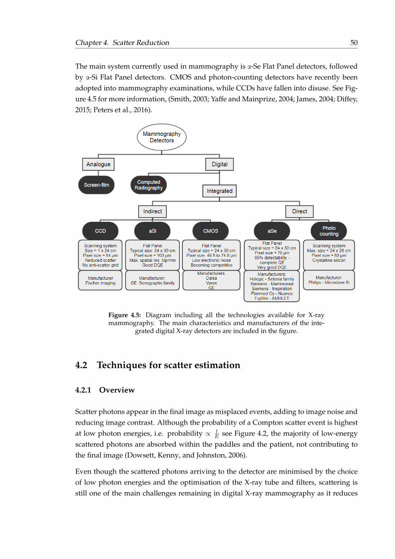
Chapter 4. Scatter Reduction 50
The main system currently used in mammography is α-Se Flat Panel detectors, followedby α-Si Flat Panel detectors. CMOS and photon-counting detectors have recently beenadopted into mammography examinations, while CCDs have fallen into disuse. See Fig-ure 4.5 for more information, (Smith, 2003; Yaffe and Mainprize, 2004; James, 2004; Diffey,2015; Peters et al., 2016).
Figure 4.5: Diagram including all the technologies available for X-raymammography. The main characteristics and manufacturers of the inte-
grated digital X-ray detectors are included in the figure.
4.2 Techniques for scatter estimation
4.2.1 Overview
Scatter photons appear in the final image as misplaced events, adding to image noise andreducing image contrast. Although the probability of a Compton scatter event is highestat low photon energies, i.e. probability ∝ 1
E see Figure 4.2, the majority of low-energyscattered photons are absorbed within the paddles and the patient, not contributing tothe final image (Dowsett, Kenny, and Johnston, 2006).
Even though the scattered photons arriving to the detector are minimised by the choiceof low photon energies and the optimisation of the X-ray tube and filters, scattering isstill one of the main challenges remaining in digital X-ray mammography as it reduces
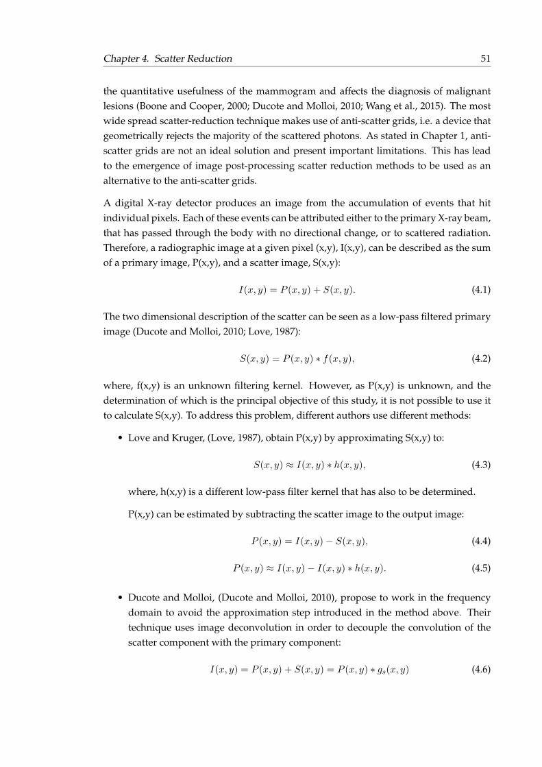
Chapter 4. Scatter Reduction 51
the quantitative usefulness of the mammogram and affects the diagnosis of malignantlesions (Boone and Cooper, 2000; Ducote and Molloi, 2010; Wang et al., 2015). The mostwide spread scatter-reduction technique makes use of anti-scatter grids, i.e. a device thatgeometrically rejects the majority of the scattered photons. As stated in Chapter 1, anti-scatter grids are not an ideal solution and present important limitations. This has leadto the emergence of image post-processing scatter reduction methods to be used as analternative to the anti-scatter grids.
A digital X-ray detector produces an image from the accumulation of events that hitindividual pixels. Each of these events can be attributed either to the primary X-ray beam,that has passed through the body with no directional change, or to scattered radiation.Therefore, a radiographic image at a given pixel (x,y), I(x,y), can be described as the sumof a primary image, P(x,y), and a scatter image, S(x,y):
I(x, y) = P (x, y) + S(x, y). (4.1)
The two dimensional description of the scatter can be seen as a low-pass filtered primaryimage (Ducote and Molloi, 2010; Love, 1987):
S(x, y) = P (x, y) ∗ f(x, y), (4.2)
where, f(x,y) is an unknown filtering kernel. However, as P(x,y) is unknown, and thedetermination of which is the principal objective of this study, it is not possible to use itto calculate S(x,y). To address this problem, different authors use different methods:
• Love and Kruger, (Love, 1987), obtain P(x,y) by approximating S(x,y) to:
S(x, y) ≈ I(x, y) ∗ h(x, y), (4.3)
where, h(x,y) is a different low-pass filter kernel that has also to be determined.
P(x,y) can be estimated by subtracting the scatter image to the output image:
P (x, y) = I(x, y)− S(x, y), (4.4)
P (x, y) ≈ I(x, y)− I(x, y) ∗ h(x, y). (4.5)
• Ducote and Molloi, (Ducote and Molloi, 2010), propose to work in the frequencydomain to avoid the approximation step introduced in the method above. Theirtechnique uses image deconvolution in order to decouple the convolution of thescatter component with the primary component:
I(x, y) = P (x, y) + S(x, y) = P (x, y) ∗ gs(x, y) (4.6)
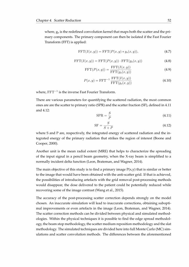
Chapter 4. Scatter Reduction 52
where, gs is the redefined convolution kernel that maps both the scatter and the pri-mary components. The primary component can then be isolated if the Fast FourierTransform (FFT) is applied:
FFT(I(x, y)) = FFT(P (x, y) ∗ gs(x, y)), (4.7)
FFT(I(x, y)) = FFT(P (x, y)) · FFT(gs(x, y)) (4.8)
FFT(P (x, y)) =FFT(I(x, y))
FFT(gs(x, y))(4.9)
P (x, y) = FFT−1 FFT(I(x, y))
FFT(gs(x, y))(4.10)
where, FFT−1 is the inverse Fast Fourier Transform.
There are various parameters for quantifying the scattered radiation, the most commonones are are the scatter to primary ratio (SPR) and the scatter fraction (SF), defined in 4.11and 4.12:
SPR =S
P(4.11)
SF =S
S + P(4.12)
where S and P are, respectively, the integrated energy of scattered radiation and the in-tegrated energy of the primary radiation that strikes the region of interest (Boone andCooper, 2000).
Another unit is the mean radial extent (MRE) that helps to characterize the spreadingof the input signal in a pencil beam geometry, when the X-ray beam is simplified to anormally incident delta function (Leon, Brateman, and Wagner, 2014).
The main objective of this study is to find a primary image P(x,y) that is similar or betterto the image that would have been obtained with the anti-scatter grid. If that is achieved,the possibilities of introducing artefacts with the grid removal post-processing methodswould disappear, the dose delivered to the patient could be potentially reduced whilerecovering some of the image contrast (Wang et al., 2015).
The accuracy of the post-processing scatter correction depends strongly on the modelchosen. An inaccurate simulation will lead to inaccurate corrections, obtaining subopti-mal improvements or even artefacts in the image (Leon, Brateman, and Wagner, 2014).The scatter correction methods can be divided between physical and simulated method-ologies. Within the physical techniques it is possible to find the edge spread methodol-ogy, the beam stop methodology, the scatter medium reposition methodology and the slatmethodology. The simulated techniques are divided here into full Monte Carlo (MC) sim-ulations and scatter convolution methods. The differences between the aforementioned
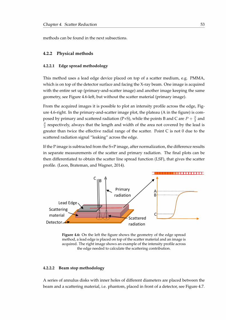
Chapter 4. Scatter Reduction 53
methods can be found in the next subsections.
4.2.2 Physical methods
4.2.2.1 Edge spread methodology
This method uses a lead edge device placed on top of a scatter medium, e.g. PMMA,which is on top of the detector surface and facing the X-ray beam. One image is acquiredwith the entire set up (primary-and-scatter image) and another image keeping the samegeometry, see Figure 4.6-left, but without the scatter material (primary image).
From the acquired images it is possible to plot an intensity profile across the edge, Fig-ure 4.6-right. In the primary-and-scatter image plot, the plateau (A in the figure) is com-posed by primary and scattered radiation (P+S), while the points B and C are P + S
2 andS2 respectively, always that the length and width of the area not covered by the lead isgreater than twice the effective radial range of the scatter. Point C is not 0 due to thescattered radiation signal “leaking” across the edge.
If the P image is subtracted from the S+P image, after normalization, the difference resultsin separate measurements of the scatter and primary radiation. The final plots can bethen differentiated to obtain the scatter line spread function (LSF), that gives the scatterprofile. (Leon, Brateman, and Wagner, 2014).
Figure 4.6: On the left the figure shows the geometry of the edge spreadmethod, a lead edge is placed on top of the scatter material and an image isacquired. The right image shows an example of the intensity profile across
the edge needed to calculate the scattering contribution.
4.2.2.2 Beam stop methodology
A series of annulus disks with inner holes of different diameters are placed between thebeam and a scattering material, i.e. phantom, placed in front of a detector, see Figure 4.7.
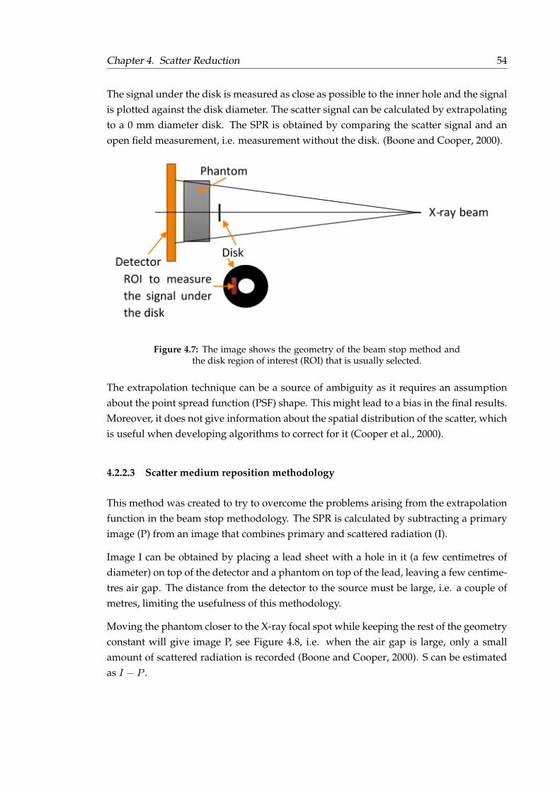
Chapter 4. Scatter Reduction 54
The signal under the disk is measured as close as possible to the inner hole and the signalis plotted against the disk diameter. The scatter signal can be calculated by extrapolatingto a 0 mm diameter disk. The SPR is obtained by comparing the scatter signal and anopen field measurement, i.e. measurement without the disk. (Boone and Cooper, 2000).
Figure 4.7: The image shows the geometry of the beam stop method andthe disk region of interest (ROI) that is usually selected.
The extrapolation technique can be a source of ambiguity as it requires an assumptionabout the point spread function (PSF) shape. This might lead to a bias in the final results.Moreover, it does not give information about the spatial distribution of the scatter, whichis useful when developing algorithms to correct for it (Cooper et al., 2000).
4.2.2.3 Scatter medium reposition methodology
This method was created to try to overcome the problems arising from the extrapolationfunction in the beam stop methodology. The SPR is calculated by subtracting a primaryimage (P) from an image that combines primary and scattered radiation (I).
Image I can be obtained by placing a lead sheet with a hole in it (a few centimetres ofdiameter) on top of the detector and a phantom on top of the lead, leaving a few centime-tres air gap. The distance from the detector to the source must be large, i.e. a couple ofmetres, limiting the usefulness of this methodology.
Moving the phantom closer to the X-ray focal spot while keeping the rest of the geometryconstant will give image P, see Figure 4.8, i.e. when the air gap is large, only a smallamount of scattered radiation is recorded (Boone and Cooper, 2000). S can be estimatedas I − P .
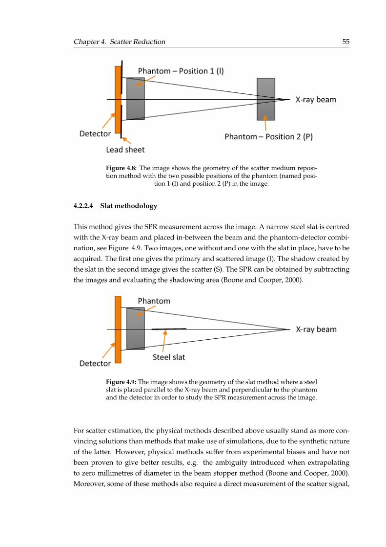
Chapter 4. Scatter Reduction 55
Figure 4.8: The image shows the geometry of the scatter medium reposi-tion method with the two possible positions of the phantom (named posi-
tion 1 (I) and position 2 (P) in the image.
4.2.2.4 Slat methodology
This method gives the SPR measurement across the image. A narrow steel slat is centredwith the X-ray beam and placed in-between the beam and the phantom-detector combi-nation, see Figure 4.9. Two images, one without and one with the slat in place, have to beacquired. The first one gives the primary and scattered image (I). The shadow created bythe slat in the second image gives the scatter (S). The SPR can be obtained by subtractingthe images and evaluating the shadowing area (Boone and Cooper, 2000).
Figure 4.9: The image shows the geometry of the slat method where a steelslat is placed parallel to the X-ray beam and perpendicular to the phantomand the detector in order to study the SPR measurement across the image.
For scatter estimation, the physical methods described above usually stand as more con-vincing solutions than methods that make use of simulations, due to the synthetic natureof the latter. However, physical methods suffer from experimental biases and have notbeen proven to give better results, e.g. the ambiguity introduced when extrapolatingto zero millimetres of diameter in the beam stopper method (Boone and Cooper, 2000).Moreover, some of these methods also require a direct measurement of the scatter signal,

Chapter 4. Scatter Reduction 56
increasing the delivered radiation dose to the patient, or need specific configurations forthe medical examination (Ducote and Molloi, 2010; Seibert and Boone, 2006).
4.2.3 Simulations
4.2.3.1 Monte Carlo simulations (MC)
Direct MC simulations give very accurate values of the scatter and primary contributionsand are conceptually simpler than the rest of the methods, (Boone and Cooper, 2000).However, if the scattering reduction is intended to be extended to all medical examina-tions, it would be necessary to implement one simulation per examination, as they arestrongly dependent on the geometry and the part of the body being imaged. Moreover,these simulations are computationally expensive as reported by Díaz et al. (Díaz et al.,2012).
For all these reasons, full MC simulations are usually adopted purely for data verificationand methodological validation purposes (Boone and Cooper, 2000).
4.2.3.2 Scatter convolution methodology
Convolution-based digital filtration techniques are based on the idea that the scatter inthe system is spatially diffuse. Thus it can be approximated to a two-dimensional low-pass convolution filter of the primary image, as seen in equation 4.2 (Ducote and Molloi,2010). As explained below, these 2D low pass filters can be obtained with simulations(point spread function) or adopting pre-defined kernel shapes:
Point spread function kernels:
PSF kernels are obtained from simplified MC simulations where the X-ray beam is a nor-mally incident delta function, i.e. the X-ray tube is simulated following the narrow pencilbeam method as a monochromatic point source (Boone and Cooper, 2000; Sechopoulos etal., 2007b; Díaz et al., 2014). This method is useful for the accurate assessment of the SPRfor small apertures and large field of views, as it reduces the computation time (Booneand Cooper, 2000).
The programme computes the point spread function (PSF) of scattered radiation for aspecific spectrum or for different energy steps, e.g. 1 keV steps from a 9.5 to 31.5 keVrange (Sechopoulos et al., 2007b). For this last option the monochromatic data, stored ina precomputed library, is combined to form the desired X-ray spectra for each individualcase. Once the PSF is obtained, it can be convolved with the field of view (FOV) in orderto obtain the scatter distribution (Boone et al., 2000).

Chapter 4. Scatter Reduction 57
Results from MC simulations show that the PSF distribution can be taken as rotationallysymmetric (Ahn, Cho, and Jeon, 2006). However, the assumption of symmetry can beargued against. Wang et al. (Wang et al., 2015) suggest that it would be better to adaptthe kernel to local variations in object thickness and attenuation. The authors say thatasymmetric kernels give better results than symmetric kernels, especially in areas closeto the edge of the breast, where the symmetric ones tend to over-correct the scatter signal.The idea behind the asymmetric kernels is to account for elevated or depressed scatterdue to thinner or thicker neighbouring regions, respectively. Wang et al. propose a fastadaptive scatter kernel superposition method (fASKS) in the frequency domain.
Moreover, if the kernel is chosen spatially invariant, it will risk overestimation of scat-tering around the edge area of the breast, leading to up to 50% of discrepancies whencompared with pure Monte Carlo simulations (Díaz et al., 2012).
Pre-defined shaped kernels:
The kernel, h(x,y), used to convolve the output image can be calculated following thepoint spread function method, as explained above, or it can be a pre-defined low-passfilter kernel. Authors like Love (Love, 1987), Ducote and Molloi (Ducote and Molloi,2010) or Boone and Seibert (Boone and Seibert, 1988) used this last option in their studies.
Love and Kruger (Love, 1987) studied four generic kernel shapes, 2D boxes, pyramid,Gaussian and exponential profiles, limiting their investigation to closed form functionsto simplify the process and allow reproducibility. They used kernels that were function-ally separable in the x and y directions, so instead of applying a 2D convolution theyapplied two consecutive 1D convolutions in order to speed up the process. Their studyfocused on finding the optimal kernel shape and size and their findings suggested that anexponential shape gave slightly better results when the size was big enough, i.e. 75 x 75pixel kernel.
Ducote and Molloi (Ducote and Molloi, 2010), and Boone and Seibert (Seibert and Boone,2006; Boone and Seibert, 1988) made use of a radially symmetric scattering kernel inorder to have a better approximation to physical reality. The formula that describes thekernel used by Ducote and Molloi has a first term with a delta function, that representsthe mapping of the primary component, and a second term that is a function of the scatterfraction (SF) and the scatter radial extent or the mean propagation distance (k):
gsi(r) =δ(r)
r+
SF
(1− SF )2kre
−rk (4.13)
To obtain the values of the SF and k both Ducote and Molloi, and Boone and Seibert usedthe beam stopping physical method.

Chapter 4. Scatter Reduction 58
The studies made with pre-defined shaped kernel shapes were always combined withthe use of anti-scatter grids, so they were focused on further reductions in the scatter.Therefore, the results in the absence of an anti-scatter grid could be completely differentto the ones presented in the papers above. In fact, a recently published paper by Leonand Wagner, (Leon, Brateman, and Wagner, 2014), combines the kernel shape proposedby Ducote and Molloi with the simulated PSF method, which they use to calculate the SFand the mean propagation distance (MRE). They applied this method with and withoutan anti-scatter grid and studied different dependencies, like breast glandularity, size andthickness, or X-ray spectra. Their results show a perfect fit between the kernel shape andthe grid data. However, when applied to grid-less measurements, the reported PSF formturned out to be less accurate, and they found that a bi-exponential PSF shape would bea better fit. Their explanation is related to the Compton scattering contribution: The gridscatter absorption makes coherent scattering to dominate over the Compton scattering.However, the Compton contribution becomes larger when the grid is not used, and sothe bi-exponential equation accounts for both factors.
The 2D low pass filters, independently of how they have been obtained, can be assumedto be shift invariant, i.e. the same kernel is used to convolve the whole image, or can beoptimised in shape and size and operated on a pixel by pixel basis (Ducote and Molloi,2010; Ahn, Cho, and Jeon, 2006).
Size optimization can be performed by selecting a kernel with radial dependency, as ex-plained in the Ducote and Molloi method. These authors also present a way of takinginto account the breast thickness variations using a look up table with kernels calculatedat different thicknesses, gs(t), for example using 1mm steps. After the mammogram isacquired, the apparent breast thickness can be estimated in a pixel by pixel basis, using aset of binary masks illustrating all corresponding pixels from 0 to maximum thickness insteps of 1 mm. Each mask is then convolved with its corresponding kernel and n partialprimary images are obtained. The primary image is finally obtained by adding all thepartial images (Ducote and Molloi, 2010).
Ahn et al. (Ahn, Cho, and Jeon, 2006) present a different algorithm to account for thethickness contribution, also creating a look up table with the PSF simulated as a functionof the thickness. They later use them to correct the image in a pixel by pixel basis: startingfrom pixel (0,0) the thickness is estimated and the image is convolved with the PSF of thecorresponding thickness; the process is repeated for all pixels. Their algorithm also takesinto account possible errors in the thickness estimation, as they report that the scatteringaffects the estimations when using general algorithms for dual-energy imaging. Theypropose an iterative method that recalculates the thickness estimation with the scatteredcorrected image obtained from the first iteration. The iteration stops when a pre-definedoptimisation value is achieved.
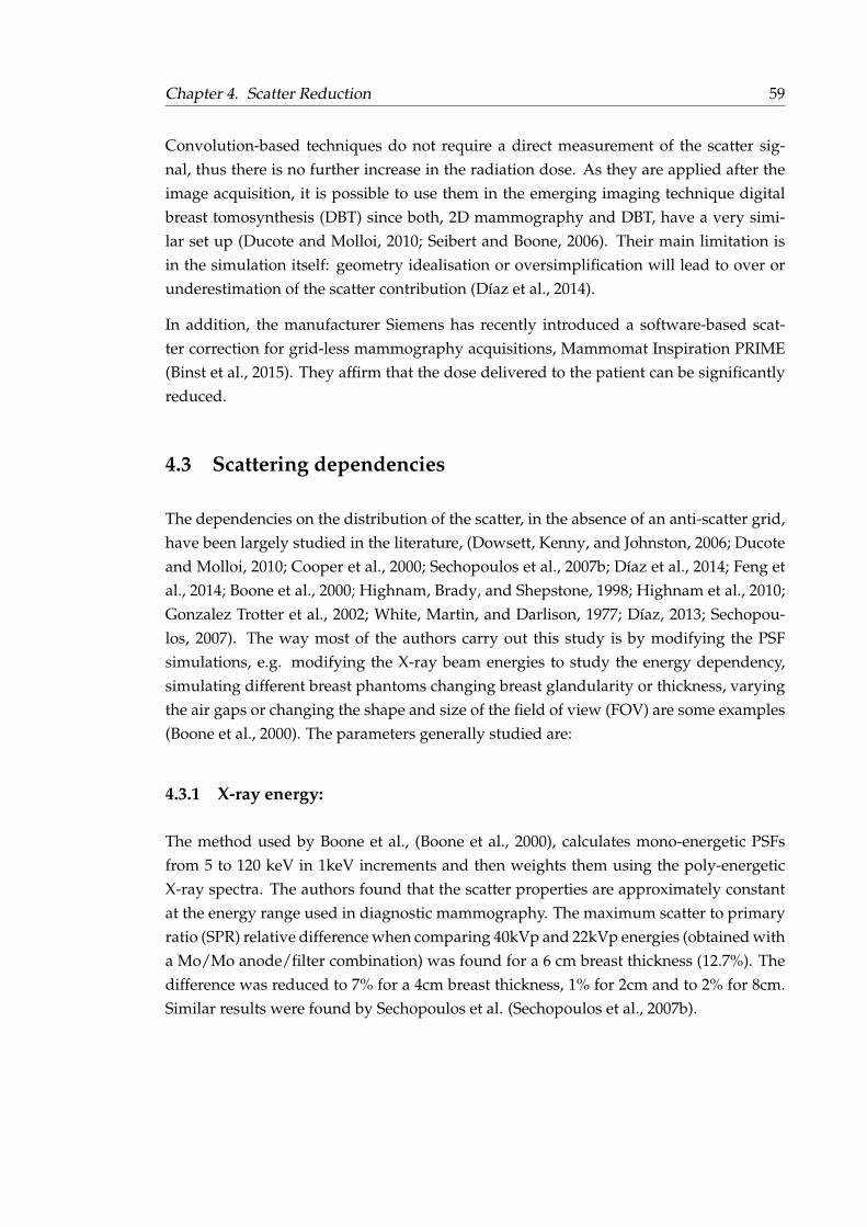
Chapter 4. Scatter Reduction 59
Convolution-based techniques do not require a direct measurement of the scatter sig-nal, thus there is no further increase in the radiation dose. As they are applied after theimage acquisition, it is possible to use them in the emerging imaging technique digitalbreast tomosynthesis (DBT) since both, 2D mammography and DBT, have a very simi-lar set up (Ducote and Molloi, 2010; Seibert and Boone, 2006). Their main limitation isin the simulation itself: geometry idealisation or oversimplification will lead to over orunderestimation of the scatter contribution (Díaz et al., 2014).
In addition, the manufacturer Siemens has recently introduced a software-based scat-ter correction for grid-less mammography acquisitions, Mammomat Inspiration PRIME(Binst et al., 2015). They affirm that the dose delivered to the patient can be significantlyreduced.
4.3 Scattering dependencies
The dependencies on the distribution of the scatter, in the absence of an anti-scatter grid,have been largely studied in the literature, (Dowsett, Kenny, and Johnston, 2006; Ducoteand Molloi, 2010; Cooper et al., 2000; Sechopoulos et al., 2007b; Díaz et al., 2014; Feng etal., 2014; Boone et al., 2000; Highnam, Brady, and Shepstone, 1998; Highnam et al., 2010;Gonzalez Trotter et al., 2002; White, Martin, and Darlison, 1977; Díaz, 2013; Sechopou-los, 2007). The way most of the authors carry out this study is by modifying the PSFsimulations, e.g. modifying the X-ray beam energies to study the energy dependency,simulating different breast phantoms changing breast glandularity or thickness, varyingthe air gaps or changing the shape and size of the field of view (FOV) are some examples(Boone et al., 2000). The parameters generally studied are:
4.3.1 X-ray energy:
The method used by Boone et al., (Boone et al., 2000), calculates mono-energetic PSFsfrom 5 to 120 keV in 1keV increments and then weights them using the poly-energeticX-ray spectra. The authors found that the scatter properties are approximately constantat the energy range used in diagnostic mammography. The maximum scatter to primaryratio (SPR) relative difference when comparing 40kVp and 22kVp energies (obtained witha Mo/Mo anode/filter combination) was found for a 6 cm breast thickness (12.7%). Thedifference was reduced to 7% for a 4cm breast thickness, 1% for 2cm and to 2% for 8cm.Similar results were found by Sechopoulos et al. (Sechopoulos et al., 2007b).
Chapter 4. Scatter Reduction 60
4.3.2 Position in the field of view (FOV)
Boone et al., (Boone et al., 2000), found that the SPR depends strongly on the positionwithin the FOV, being maximum in the centre of the breast and dropping off towards theedges, due to the amount of scattering material in nearby regions.
4.3.3 Air gap
Again Boone et al., (Boone et al., 2000), found that the PSF shape depends on the air gap,i.e. space between the support paddle and the detector surface. The PSF values in thecentral area decrease with the increase of the air gap while the curve fall off becomes lesssteep. Therefore, the air gap contributes to the spread of the scatter; the thicker the airgap, the larger the area affected.
Diaz et al., (Díaz et al., 2012; Díaz et al., 2014), introduce a second air gap contribution,present between the lower curved breast edge and the detector. The authors believe thatthe extended path length of the photons have an important contribution in the discrepan-cies that appear close to the breast edge, reported when using a spatial invariant kernel.It is therefore important to correct for this contribution, as the scattered photons do notencounter the same attenuation path and scattering than the ones that go through thecentre of the breast. In cases where the breast is simulated, the breast curvature is aknown parameter. However, if this correction is to be applied to clinical data, the breastcurvature will need to be estimated during the examination (Díaz et al., 2012).
4.3.4 Breast thickness
It has been found that the SPR is nearly linear as a function of breast thickness. The slopeof this function being dependent on the air gap and the selected FOV diameter (Booneet al., 2000; Seibert and Boone, 2006; Sechopoulos et al., 2007b).
It is therefore essential to estimate the breast thickness with accuracy. The compressionthickness that is reported by the mammography unit can be used as an initial referencemeasurement but the thickness calibration is sometimes inaccurate, and the breast thick-ness changes towards the periphery. A software based algorithm to calculate the thick-ness is recommended for obtaining reliable results (Leon, Brateman, and Wagner, 2014;Highnam, Brady, and Shepstone, 1998; Mawdsley et al., 2009).
Chapter 4. Scatter Reduction 61
The breast compression in general mammography allows the achievement of a relativelyconstant breast thickness, excluding the periphery where the thickness decreases. How-ever, the pressure applied to the compression paddles ends up deforming them and cre-ating a tilt in the area without breast (Mawdsley et al., 2009). This effect introduces vari-ations in the breast thickness. If these variations are assumed to be negligible within thecompressed breast, the thickness calculation is then reduced to an estimate of the av-eraged value, (Highnam, Brady, and Shepstone, 1998; Highnam et al., 2010; GonzalezTrotter et al., 2002). However, this assumption introduces some errors that add up in thefinal scattering simulation. For this reason, some other authors calculate a pixel by pixelthickness map and use kernels that are a function of the thickness, K(t), (Mawdsley et al.,2009; Leon, Brateman, and Wagner, 2014).
4.3.5 Breast tissue composition
The study of the contribution of breast tissue composition has been commonly carriedout by using phantoms with different glandular percentage, with 0, 50 and 100% beingthe most common choices. The literature presents very little dependency between SPRchanges and breast composition, (Boone et al., 2000; Sechopoulos et al., 2007b), the majorimpact found to be in the apparent thickness calculation (Leon, Brateman, and Wagner,2014). Due to the small glandular contribution it is possible to use a PSF simulated for ahomogeneous breast (Sechopoulos et al., 2007b; Díaz et al., 2014). The scatter kernel canbe calculated, for example, as the linear combination of the scatter response with 0% and100% of glandularity (Díaz et al., 2014).
4.3.6 Detector cover plate, detector compression plate and breast support plate
The detector cover plate and the compression and breast support plates were found tohave a significant contribution to the scattered signal (Sechopoulos et al., 2007b; Ducoteand Molloi, 2010; Díaz et al., 2014), especially for thicker breasts, i.e. 5-7cm, close to theedges of the compressed breast. The reason, found by Sechopoulos et al. (Sechopouloset al., 2007b) and studied further by Diaz et al. (Díaz et al., 2014), was related to thescattering contribution of the plates in the area without breast tissue. Some of that scat-ter is detected under the shadow of the breast, producing a high contribution due to theabsorption of the primary photons by the breast tissue. If the breast is thin enough, thatabsorption is decreased and the SPR is therefore reduced. This contribution can be pre-corrected by simulating the measurements at zero thickness (Ducote and Molloi, 2010).A more precise method, reported by Díaz et al. (Díaz et al., 2014), is to include the platesin the simulations. To account for the scattering contribution of the area without breast,i.e. system contribution, a second simulation can be done keeping the same geometry but
Chapter 4. Scatter Reduction 62
removing the scattering material, i.e. breast phantom. The system kernel will be appliedto the areas outside the breast, while the breast kernel (that has been calculated taking theplates into account) is applied within the breast areas. However, an additional correctionis needed. The scattered photons produced outside, but near, the breast, might be scat-tered towards the breast. In that case, the system scattered radiation will be attenuatedby the breast tissue. In order to compensate for this effect, Diaz et al. proposed to weightthe system kernel with a weight map, α, where α = 1 outside the scattering material andα < 1 when the beam passes through the breast. It is therefore very important not to ex-clude the plates in the simulation. If they are not taken into account the scatter can beunderestimated by as much as 31% (Sechopoulos et al., 2007b; Díaz et al., 2014).
4.3.7 Source to image distance (SID)
The SID has been reported not to affect the scattered radiation distribution (Boone andCooper, 2000).
4.3.8 Backscatter
Backscatter from the body or the detector can affect the scatter estimation, as reported bySechopoulos et al. (Sechopoulos et al., 2007b).
4.3.9 Detector composition
The detectors are commonly simplified to a scintillator plate or an ideal geometry. Ac-counting for the scattering produced after the detector cover plate could lead to moreprecise SPR estimations, introducing an advantage when compared with the anti-scattergrid method (Marimon et al., 2016).
4.4 Chapter summary and discussion
This chapter introduces the second part of this thesis, focused in post-processing scat-ter reduction for mammography applications. The theoretical framework, necessary forthe development of an adequate scatter reduction methodology, was developed in thischapter.
After an initial discussion about breast cancer, breast cancer screening programmes andmammography systems, a mathematical interpretation of the scatter contribution to the

Chapter 4. Scatter Reduction 63
image was defined and the most common techniques for scatter estimation were evalu-ated, i.e. physical and simulation methods, paying special attention to the scatter convo-lution methodology, as it will be the foundation of the technique developed and proposedin this thesis.
The chapter finished with a study of the scattering dependencies with the geometry ofthe system, evaluating how sensitive the scattering is to changes in the X-ray energyspectrum or in the dimensions and compositions of the different layers of the geometry,as encountered by the photon beam’s path.
64
Chapter 5
PSF scatter reduction and validations
A post-processing scatter estimation methodology, which is based on scatter convolutionusing simulated point spread function kernels, is developed, optimised and validated(against full Monte Carlo simulations and previously published data) in this chapter.
5.1 Scatter convolution methodology
The point spread function (PSF) post-processing scatter reduction technique is the method-ology chosen to estimate the scatter in this study. As explained in Chapter 4, this methodassumes that the scatter in the system is spatially diffuse, thus it can be approximatedby a two-dimensional low-pass convolution filter of the primary image. The scatter PSF(SPSF) filters, or scatter kernels, are calculated with a simplified MC simulation, by usinga narrow pencil beam.
This methodology has proven to be accurate, non-invasive (in opposition to some of thephysical scatter estimation methods, where the dose has to be increased or the systemset up modified) and less time consuming that full Monte Carlo simulations. From thedifferent options presented in Chapter 4, the author has chosen to follow Love’s approx-imation, see equation 4.3 (Love, 1987), using a set of symmetric kernels with special em-phasis on the treatment of the background scatter contribution to the breast, as a way ofcorrectly estimating the scatter in the breast edge area of the image, easily overestimated.
5.2 Geant4 simulation tool-kit
There are several particle physics MC software packages available that allow the study ofparticle interactions with matter in the medical physics range, e.g. GEANT4, Penelope,FLUKA, EGSx/EGSnrc and MCNP/MCNPX, (Díaz, 2013). GEANT4, in particular, hasbeen chosen by many authors, i.e Sechopoulos et al. (Sechopoulos, 2007; Sechopoulos etal., 2007b; Sechopoulos et al., 2007a), Feng et al. (Feng and Sechopoulos, 2011; Feng et al.,
Chapter 5. PSF scatter reduction and validations 65
2014), Wang et al. (Wang et al., 2015) and Diaz et al. (Díaz et al., 2012; Díaz, 2013; Díazet al., 2014), as it is a free software supported by the European Organization for NuclearResearch (CERN), where it is possible to obtain active assistance, (Agostinelli et al., 2003;Díaz, 2013).
GEANT4 provides detector and physics modeling, simulating the interaction and pas-sage of particles through matter. This simulation toolkit includes all aspects of the sim-ulation process, i.e. the system geometry and materials, the fundamental particles of in-terest, including a tracking system of them and their interactions, the detector response,etc. (Agostinelli et al., 2003; Allison et al., 2006) . Although GEANT4 was initially de-signed for high energy physics, its object-oriented structure has allowed the adaptationto a wider range of energies, including medical physics, i.e. mammography, brachyther-apy or hadron therapy, and radiation protection (Díaz, 2013).
When applied to mammography, GEANT4 has been validated in a number of publi-cations. Sechopoulos (Sechopoulos, 2007) modified the code to simulate X-rays pass-ing through only breast tissue, activating and deactivating the interaction process tostudy each individual case. That way, the attenuation coefficients were calculated andcompared to the values reported by the National Institute of Standards and Technology(NIST) and by other authors finding excellent agreements in all cases. Feijó and Hoff,(Feijó Pery and Hoff, 2008), validated the software comparing results to previously pub-lished data. They report less than 5% difference between the compared values. AlsoDiaz, (Díaz, 2013), validated the toolkit with published and clinical data, arriving to theconclusion that GEANT4 is suitable for modelling X-ray mammography systems.
For the mentioned reasons, GEANT4 (version 10.01.p02) will be the toolkit used in thiswork.
5.2.1 Geant4 architecture
The Geant4 toolkit architecture is composed by a set of modules written in C++. It is theuser’s responsibility to build the application architecture, a characteristic that contributesto Geant4’s flexibility. The Geant4 information has been obtained from the Geant4 usermanuals published by CERN, (CERN, 2016; collaboration, 2016).
The main architecture structure can be seen in the diagram of Figure 5.1. A main()method, required to build the programme, is implemented by two manager classes,G4RunManager and G4UIManager. The run manager class controls the flow of the pro-gramme, manages the event loop(s) and the initialization procedures. Therefore, it hasto receive all the information needed to build and run the simulation. The three maininitialization classes directly set to the run manager are:

Chapter 5. PSF scatter reduction and validations 66
Figure 5.1: Diagram showing the main modules that form the architectureof Geant4.
5.2.1.1 G4VUserDetectorConstruction
In this class, the user defines the entire detector geometry, from the chemical elements tothe distribution of the materials in the volume.
The detector construction needs:
• Definition of the chemical elements that compose the materials used in the simula-tion. The elements are defined by their atomic number and weight.
e.g. elH = new G4Element("Hydrogen", "H", z=1., a=1.01*g/mole);
• Definition of the materials, either by using their chemical formula or their densityand fractional mass of the components. The information needed to define the ma-terials was taken from the NIST website (NIST material composition [online]).
e.g. CsI = new G4Material("CsI",density=4.53*g/cm3,2);
CsI->AddElement(elCs,1);
CsI->AddElement(elI,1);
• Definition of the dimensions of the mother volume (or world).

Chapter 5. PSF scatter reduction and validations 67
• Definition of the materials:
– Create a solid defining its dimensions and geometrical shape. The materialscan have simple shapes as box/tube/cylinder/parallelepiped, or more com-plex designs, combining shapes or loading voxelised geometries.
– Define a logical volume, where the solid is filled with the appropriate materialcomposition.
– Place the volume in the desired position in the world volume.
• Set sensitive detectors: Information of the interactions that occur within a volumewill be provided if the volume is marked as sensitive. More information about thetracking is given below in the explanation of the TrackerSD class.
5.2.1.2 G4VUserPhysicsList
This class registers all the physics processes and all the particle types required in the sim-ulation. It also defines a threshold on particle production, where no secondary particlesare generated if they are unable to travel at least the cut-off range distance. In this studythe cut-off threshold was chosen to be 1 mm.
The electromagnetic (EM) physics constructor chosen in this work is the "emstandard_opt4",which has been designed for applications that require higher accuracy of electrons, hadronsand ion tracking and uses the most accurate standard and low-energy models available,(CERN, 2017).
5.2.1.3 G4VUserActionInitialization
In this class the user defines the user action classes that are invoked during the run phaseof the simulation. There is one mandatory class, the Primary Generator Action, and fiveadditional classes that the user can decide to use, the Run Action, the Event Action, theStacking Action, the Tracking Action and the Stepping Action.
The G4UserPrimaryGeneratorAction specifies how a primary event should be generated.The generation of the primary particles is done in the Primary Generator class.
Other modules used for the simulations of this work that are worth mentioning are:

Chapter 5. PSF scatter reduction and validations 68
5.2.1.4 TrackerSD
The tracker sensitive detector class allows to follow each individual particle as it passesthrough the sensitive volumes, tracking the interactions that the particle undergoes andsaving any relevant information for the user, e.g. classify the particles in primary orscattered or quantify the energy deposited in the volume of interest.
In this study, the primary particles are X-ray photons and, therefore, they can either suffera Compton, photoelectric or Rayleigh interaction or exit the sensitive volumes withoutinteraction. The last sensitive layer corresponds to the sensor of the detector. The par-ticle that has undergone any type of interaction before arriving to the sensor volume isclassified as a scatter event, otherwise the particle is counted as a primary event.
If the mammography detector is considered ideal, all the particles that arrive to its surfaceare taken into account, and the interactions within the detector volume are not consid-ered. If a more realistic geometry is needed, only those particles that suffer a Compton orphotoelectric interaction in the sensor volume are taken into account and their positionrecorded; the particles will be recorded as scatter or primary events depending on theclassification of the particle before interacting with the sensor, Figure 5.2 illustrates thisprocess with a flowchart. In this study the use of one type of detector or another will bespecified for each individual experiment.
Figure 5.2: Flowchart of the X-ray photon tracking process. The scatterinteractions, i.e. photoelectric (P.E.), Compton (Comp.) or Rayleigh (Ray.),and deposited energy of each X-ray photon is accounted up to the detectorsurface volume, where it is divided in Primary or Scatter type and sorted.
Chapter 5. PSF scatter reduction and validations 69
In the TrackerSD class, the position of the particles as they interact in the sensor volumeare also recorded and exported to a file. There are different options as to the way theparticles can be stored. The most precise method is to save the (x,y) coordinates of eachparticle. This option is, however, very expensive in terms of memory, and time, as manysimulations need to be run to obtain values statistically significant. An intermediate solu-tion is to sample the photons in an array, mimicking the pixel matrix of digital detectors.The full MC simulations executed in this study use this last option. For the pencil beamsimulations the data storage can be simplified even further without compromising thefinal results, by assuming cylindrical symmetry and binning the energy into concentricannuli of radius equal to half the chosen pixel size.
5.2.1.5 Random Number Generator
Random numbers are sequences of numbers that must be produced by a random physicalprocess and that cannot be predicted better than by random chance. Due to the difficultyto generate completely random numbers, MC simulation software tool-kits make use ofpseudo-random number generators (PRNGs), which are produced by using a numericalalgorithm based in a periodic cycle. An initial value, known as seed or key, that is definedin each cycle is used to determine the sequence of pseudo-random numbers.
Geant4 makes use of the HEPRandom module from CLHEP, a PRNG C++ class libraryfor high-energy physics. The Random package uses well-known algorithms (or engines)to produce the pseudo-random numbers, the most common engines implemented inHepRandom are HepJamesRandom, DRand48Engine, MixMaxRng, RanluxEngine andRanecu.
In this study, the engine selected was Ranecu, the one recommended by CERN (CERN,2016; collaboration, 2016). This engine has a relatively long period, 2 x 10¹⁸, providingreproducibility and good statistical properties (Díaz, 2013; Demchik, 2011). In Ranecu,the initialisation is carried out using a multiplicative congruential generator that uses theformula constants of L’Ecuyer. An index integrer, set by the execution time in seconds, isused to obtain two seeds from a seed table (collaboration, 2016).
5.2.1.6 General Particle Source (GPS) macros
The GPS class allows to specify the spectral, spatial and angular distribution of the pri-mary source particles.
In this work, the GPS commands have been specified in a macro file, among the numberof particles simulated, the visualization drivers and the amount of information displayed
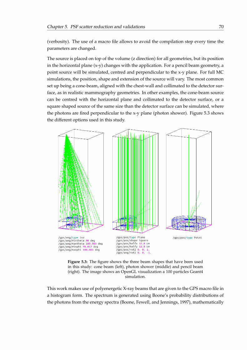
Chapter 5. PSF scatter reduction and validations 70
(verbosity). The use of a macro file allows to avoid the compilation step every time theparameters are changed.
The source is placed on top of the volume (z direction) for all geometries, but its positionin the horizontal plane (x-y) changes with the application. For a pencil beam geometry, apoint source will be simulated, centred and perpendicular to the x-y plane. For full MCsimulations, the position, shape and extension of the source will vary. The most commonset up being a cone-beam, aligned with the chest-wall and collimated to the detector sur-face, as in realistic mammography geometries. In other examples, the cone-beam sourcecan be centred with the horizontal plane and collimated to the detector surface, or asquare shaped source of the same size than the detector surface can be simulated, wherethe photons are fired perpendicular to the x-y plane (photon shower). Figure 5.3 showsthe different options used in this study.
Figure 5.3: The figure shows the three beam shapes that have been usedin this study: cone beam (left), photon shower (middle) and pencil beam(right). The image shows an OpenGL visualization a 100 particles Geant4
simulation.
This work makes use of polyenergetic X-ray beams that are given to the GPS macro file ina histogram form. The spectrum is generated using Boone’s probability distributions ofthe photons from the energy spectra (Boone, Fewell, and Jennings, 1997), mathematically
Chapter 5. PSF scatter reduction and validations 71
attenuated by the different material layers, e.g. filtration or Beryllium window, and con-sidering its half value layer (HVL). Some of the validations make use of mono-energeticX-ray beams. For this case, instead of the histogram the source has to be defined as "typeMono".
The visualization drivers are a key point in the geometry and GPS set up, to ensure thatno mistake has been introduced in the process. In this study the software interface that isused is OpenGL, a module that enables direct visualization from GEANT4 of 2D and 3Dvolumes.
5.2.2 Number of simulations and uncertainties
The precision of the results is obtained by reducing the statistical uncertainty which isdirectly related with the number of simulations and the number of particles run per sim-ulation. It is key to correctly choose the total number of particles used, i.e. number ofsimulations multiplied by the number of particles in each simulation. Too few will in-crease the uncertainty of the final results, while too many will imply a big computationalstrain. In this study, the number of particles per simulation was set to 109 and the numberof simulations was adjusted accordingly to the needs of each particular case.
To select the right number, the uncertainties need to be evaluated. Due to the randombehaviour of the X-ray photon interaction and to the large number of particles used, it ispossible to describe the uncertainties with a Gaussian distribution (central limit theorem).The method used for the evaluation is the Standard Error of the Mean (SEM), the standarddeviation of the sample mean (Sempau et al., 2001; Díaz et al., 2014). It is estimated bythe standard deviation of the population, i.e. energy deposited, qi(x,y), divided by thesize of the sample, i.e. number of simulations, N:
SEM =σ√N. (5.1)
where,
σ =
√√√√ 1
N
N∑i=1
(qi − q
)2, (5.2)
µ =1
N
N∑i=1
qi. (5.3)
Additional ways to reduce the computational time, without compromising the statisticaluncertainty, are increasing the sampling area, i.e. pixel size, or applying a smoothingspatial filter, such as a median filter, to the data.
Chapter 5. PSF scatter reduction and validations 72
The pixel size of a mammography X-ray detector is 70-75 µm. It has been found that toachieve a SEM lower than 1%, using this pixel size range and a pencil beam geometry, 15to 20 simulations are needed. This number does not imply a big computational constraintand so the smoothing spatial filter does not need to be used in combination with thepencil beam geometry.
In full MC simulation applications, the number of simulations needed is increased con-siderably. This is because the beam is spread in a bigger area and the data sampling isrestricted to an array ("pixelated") sampling, as it is not safe to assume spatial symme-try. As full MC simulations have been only used for validation applications, the aid of abigger pixel size has been used when possible.
5.2.3 Preliminary validation
The first set of validations that were performed were aimed to validate the Geant4 code,to make sure the different classes described above were properly configured.
With this objective in mind, the American Association of Physicists in Medicine (AAPM)task group 195 presented a report with a series of Monte Carlo data sets to be used as areference to validate different Monte Carlo simulations (Sechopoulos et al., 2015; AAPM,2015). The report encompasses MC simulations of a variety of medical examinations,from half value layer calculations to dose calculation in computed tomography examples.The values given in case number 3 (Mammography and breast tomosynthesis) of thereport are the ones used as a benchmark in this validation exercise.
The geometry followed included breast compression and support paddles, both made of2 mm thick PMMA material, a semi-circular cylinder as breast phantom (46 mm thick,composed by 80/20% of adipose/glandular tissue and surrounded by a 2 mm thick skinlayer) and a 13 mm air gap placed between the support paddle and an idealized detec-tor surface. The Source to Image Distance (SID) was 660 mm. A patient body made ofwater was also included, adjacent to the breast phantom’s chest wall side, and centredin the vertical direction with the breast phantom. Figure 5.4-left shows a diagram of thegeometry.
A combination of two X-ray beams (cone and pencil beam) and two X-ray spectra (mo-noenergetic and polyenergetic) were used for the validation. To reduce the uncertainty,the spectrum values were the same as the ones used by the AAPM group, (AAPM, 2015).For each of the combinations, the primary radiation, Compton scattering, Rayleigh scat-tering and multiple scattering events were measured in 7 different regions of interest(ROIs), as described by (AAPM, 2015), see Figure 5.4-right. Table 5.1 gives the source
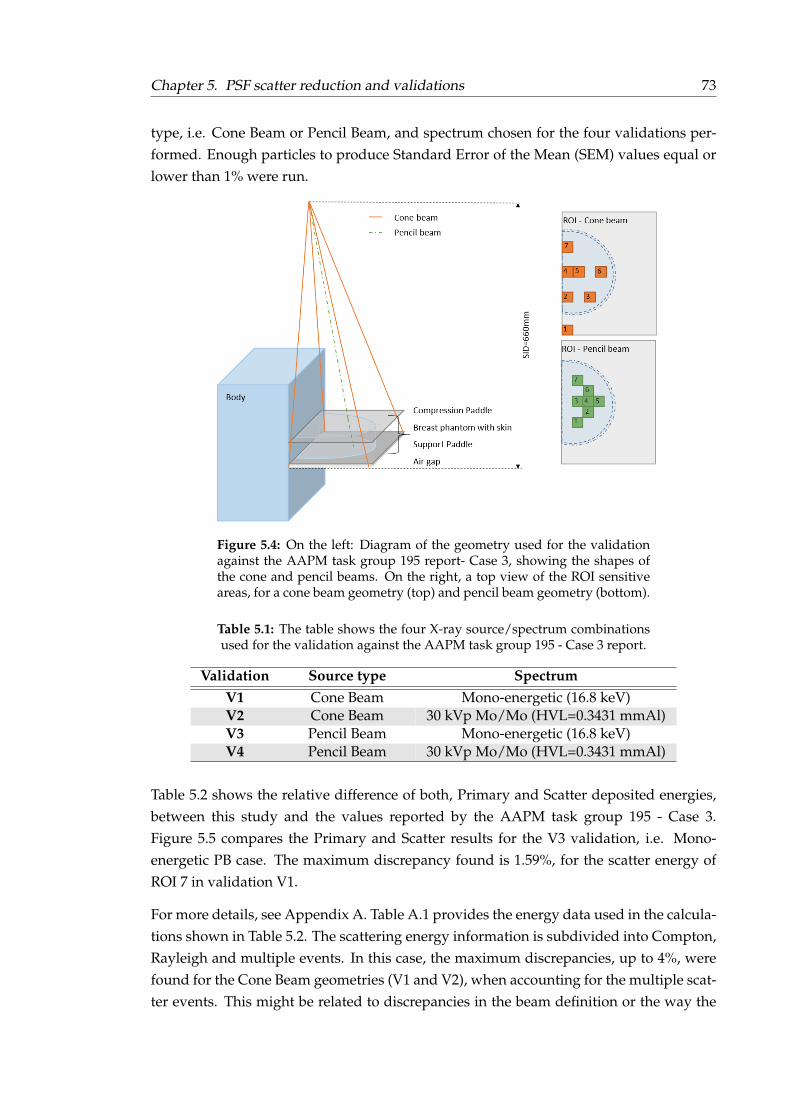
Chapter 5. PSF scatter reduction and validations 73
type, i.e. Cone Beam or Pencil Beam, and spectrum chosen for the four validations per-formed. Enough particles to produce Standard Error of the Mean (SEM) values equal orlower than 1% were run.
Figure 5.4: On the left: Diagram of the geometry used for the validationagainst the AAPM task group 195 report- Case 3, showing the shapes ofthe cone and pencil beams. On the right, a top view of the ROI sensitiveareas, for a cone beam geometry (top) and pencil beam geometry (bottom).
Table 5.1: The table shows the four X-ray source/spectrum combinationsused for the validation against the AAPM task group 195 - Case 3 report.
Validation Source type SpectrumV1 Cone Beam Mono-energetic (16.8 keV)V2 Cone Beam 30 kVp Mo/Mo (HVL=0.3431 mmAl)V3 Pencil Beam Mono-energetic (16.8 keV)V4 Pencil Beam 30 kVp Mo/Mo (HVL=0.3431 mmAl)
Table 5.2 shows the relative difference of both, Primary and Scatter deposited energies,between this study and the values reported by the AAPM task group 195 - Case 3.Figure 5.5 compares the Primary and Scatter results for the V3 validation, i.e. Mono-energetic PB case. The maximum discrepancy found is 1.59%, for the scatter energy ofROI 7 in validation V1.
For more details, see Appendix A. Table A.1 provides the energy data used in the calcula-tions shown in Table 5.2. The scattering energy information is subdivided into Compton,Rayleigh and multiple events. In this case, the maximum discrepancies, up to 4%, werefound for the Cone Beam geometries (V1 and V2), when accounting for the multiple scat-ter events. This might be related to discrepancies in the beam definition or the way the

Chapter 5. PSF scatter reduction and validations 74
particles are followed in the TrackerSD class. For the Pencil Beam geometry the agree-ment is better, with a minimum value of 98.1% and an average agreement of 99.7%. It is,therefore, safe to assume that the risk of using the Geant4 code is very small.
Table 5.2: The table shows the relative difference between this studyand the AAPM task group 195 - Case 3, comparing the primary andscatter deposited energy (eV/ph) in 7 pre-defined ROIs for four X-ray
source/spectrum combinations, i.e. V1 to V4.
eV/ph - Relative difference (%) against AAPM T.G. 195 Case 3ROI no. Type V1 V2 V3 V4
1Primary 0.59 0.00 0.62 0.00
Scattering 0.30 -0.90 0.19 -1.10Primary 0.20 0.00 0.67 0.00
2Scattering -1.50 -0.16 -1.19 -0.29
3Primary 0.64 0.00 0.65 0.00
Scattering -1.47 -0.53 -0.95 -0.49Primary 0.53 0.00 0.51 0.00
4Scattering -0.74 -0.21 -0.73 -0.19
5Primary 0.48 -0.08 0.77 -0.02
Scattering -0.85 -0.04 -0.70 -0.03Primary 0.55 0.00 0.53 0.00
6Scattering -1.31 -0.32 -0.54 -0.28
7Primary 0.36 0.00 0.58 0.00
Scattering -1.59 -1.06 -1.18 -0.74
Figure 5.5: Comparison against the AAPM task group 195 - Case 3. Theplots show the primary (left) and scatter (right) deposited energy in eachof the 7 ROIs defined in the scoring plane. The scatter energy is the sum of
the single Compton, single Rayleigh and multiple scatter events.
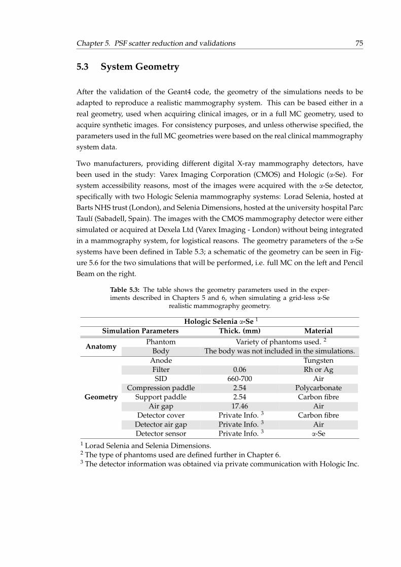
Chapter 5. PSF scatter reduction and validations 75
5.3 System Geometry
After the validation of the Geant4 code, the geometry of the simulations needs to beadapted to reproduce a realistic mammography system. This can be based either in areal geometry, used when acquiring clinical images, or in a full MC geometry, used toacquire synthetic images. For consistency purposes, and unless otherwise specified, theparameters used in the full MC geometries were based on the real clinical mammographysystem data.
Two manufacturers, providing different digital X-ray mammography detectors, havebeen used in the study: Varex Imaging Corporation (CMOS) and Hologic (α-Se). Forsystem accessibility reasons, most of the images were acquired with the α-Se detector,specifically with two Hologic Selenia mammography systems: Lorad Selenia, hosted atBarts NHS trust (London), and Selenia Dimensions, hosted at the university hospital ParcTaulí (Sabadell, Spain). The images with the CMOS mammography detector were eithersimulated or acquired at Dexela Ltd (Varex Imaging - London) without being integratedin a mammography system, for logistical reasons. The geometry parameters of the α-Sesystems have been defined in Table 5.3; a schematic of the geometry can be seen in Fig-ure 5.6 for the two simulations that will be performed, i.e. full MC on the left and PencilBeam on the right.
Table 5.3: The table shows the geometry parameters used in the exper-iments described in Chapters 5 and 6, when simulating a grid-less α-Se
realistic mammography geometry.
Hologic Selenia α-Se 1
Simulation Parameters Thick. (mm) Material
AnatomyPhantom Variety of phantoms used. 2
Body The body was not included in the simulations.
Geometry
Anode TungstenFilter 0.06 Rh or AgSID 660-700 Air
Compression paddle 2.54 PolycarbonateSupport paddle 2.54 Carbon fibre
Air gap 17.46 AirDetector cover Private Info. 3 Carbon fibre
Detector air gap Private Info. 3 AirDetector sensor Private Info. 3
α-Se1 Lorad Selenia and Selenia Dimensions.2 The type of phantoms used are defined further in Chapter 6.3 The detector information was obtained via private communication with Hologic Inc.
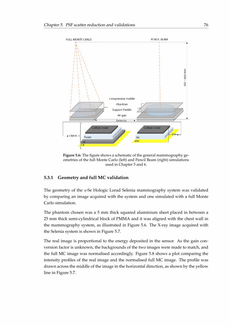
Chapter 5. PSF scatter reduction and validations 76
Figure 5.6: The figure shows a schematic of the general mammography ge-ometries of the full Monte Carlo (left) and Pencil Beam (right) simulations
used in Chapter 5 and 6.
5.3.1 Geometry and full MC validation
The geometry of the α-Se Hologic Lorad Selenia mammography system was validatedby comparing an image acquired with the system and one simulated with a full MonteCarlo simulation.
The phantom chosen was a 5 mm thick squared aluminium sheet placed in between a25 mm thick semi-cylindrical block of PMMA and it was aligned with the chest wall inthe mammography system, as illustrated in Figure 5.6. The X-ray image acquired withthe Selenia system is shown in Figure 5.7.
The real image is proportional to the energy deposited in the sensor. As the gain con-version factor is unknown, the backgrounds of the two images were made to match, andthe full MC image was normalised accordingly. Figure 5.8 shows a plot comparing theintensity profiles of the real image and the normalised full MC image. The profile wasdrawn across the middle of the image in the horizontal direction, as shown by the yellowline in Figure 5.7.
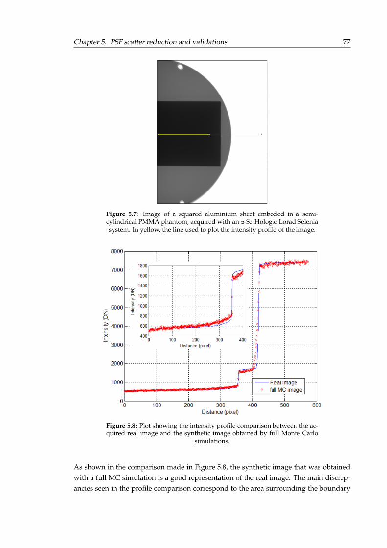
Chapter 5. PSF scatter reduction and validations 77
Figure 5.7: Image of a squared aluminium sheet embeded in a semi-cylindrical PMMA phantom, acquired with an α-Se Hologic Lorad Seleniasystem. In yellow, the line used to plot the intensity profile of the image.
Figure 5.8: Plot showing the intensity profile comparison between the ac-quired real image and the synthetic image obtained by full Monte Carlo
simulations.
As shown in the comparison made in Figure 5.8, the synthetic image that was obtainedwith a full MC simulation is a good representation of the real image. The main discrep-ancies seen in the profile comparison correspond to the area surrounding the boundary

Chapter 5. PSF scatter reduction and validations 78
between materials inside the phantom, showing a maximum discrepancy of 12%. This isdue to the mismatch between the simulated and real phantom sizes and the introductionof a non-simulated air gap when the phantom changes from the PMMA plus aluminiumarea to a pure PMMA area.
It can be assumed that the results provided by the MC simulation developed in this workaccurately reproduce the primary and scatter radiation distribution observed in the clin-ical images.
5.4 Kernel calculation
The energy and position of scatter and primary events at the detector’s volume is theinformation generated by the simulations, once the Geant4 software is run. This infor-mation is enough to calculate the PSF kernel needed to convolve the image and, in con-sequence, to obtain the predicted scatter and primary images, as shown in equations 4.3and 4.4.
The analysis of the simulations and image post-processing has been done with the aid ofMATLAB software (R2013b, version 8.2 with image processing toolbox, version 8.3) andwith ImageJ (version 1.47v).
To obtain the kernel, the method chosen uses a point spread function that is calculatedfrom the scatter and primary information obtained with the pencil beam geometry. Thescatter matrix gives information on the energy deposited per pixel, while the primaryvalue comes from the central point where the pencil beam is pointed and gives the energyof all the particles that have not suffered any interaction before arriving to the sensorsurface.
The kernel, or Scatter Point Spread Function (SPSF) is calculated by dividing the scattermatrix with the sum of the primary value and the total scatter energy (STOT):
SPSF(x, y) =S(x, y)
P (0, 0) + STOT(5.4)
where,
STOT =∑x
∑y
S(x, y) (5.5)
The term of the total scatter sum is added into the equation to compensate for the ap-proximation of equation 4.3 (Boone and Cooper, 2000). If the correction was not to beadded, the predicted scatter would be overestimated.
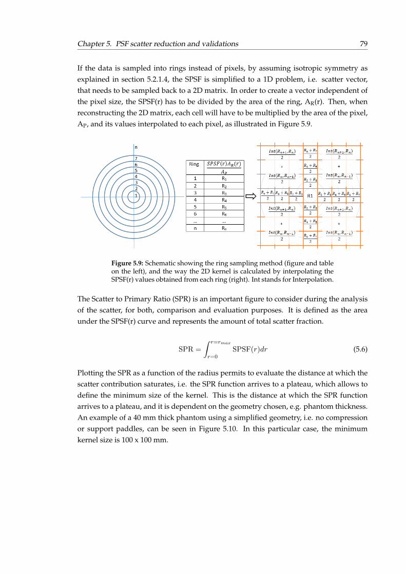
Chapter 5. PSF scatter reduction and validations 79
If the data is sampled into rings instead of pixels, by assuming isotropic symmetry asexplained in section 5.2.1.4, the SPSF is simplified to a 1D problem, i.e. scatter vector,that needs to be sampled back to a 2D matrix. In order to create a vector independent ofthe pixel size, the SPSF(r) has to be divided by the area of the ring, AR(r). Then, whenreconstructing the 2D matrix, each cell will have to be multiplied by the area of the pixel,AP, and its values interpolated to each pixel, as illustrated in Figure 5.9.
Figure 5.9: Schematic showing the ring sampling method (figure and tableon the left), and the way the 2D kernel is calculated by interpolating theSPSF(r) values obtained from each ring (right). Int stands for Interpolation.
The Scatter to Primary Ratio (SPR) is an important figure to consider during the analysisof the scatter, for both, comparison and evaluation purposes. It is defined as the areaunder the SPSF(r) curve and represents the amount of total scatter fraction.
SPR =
∫ r=rmax
r=0SPSF(r)dr (5.6)
Plotting the SPR as a function of the radius permits to evaluate the distance at which thescatter contribution saturates, i.e. the SPR function arrives to a plateau, which allows todefine the minimum size of the kernel. This is the distance at which the SPR functionarrives to a plateau, and it is dependent on the geometry chosen, e.g. phantom thickness.An example of a 40 mm thick phantom using a simplified geometry, i.e. no compressionor support paddles, can be seen in Figure 5.10. In this particular case, the minimumkernel size is 100 x 100 mm.
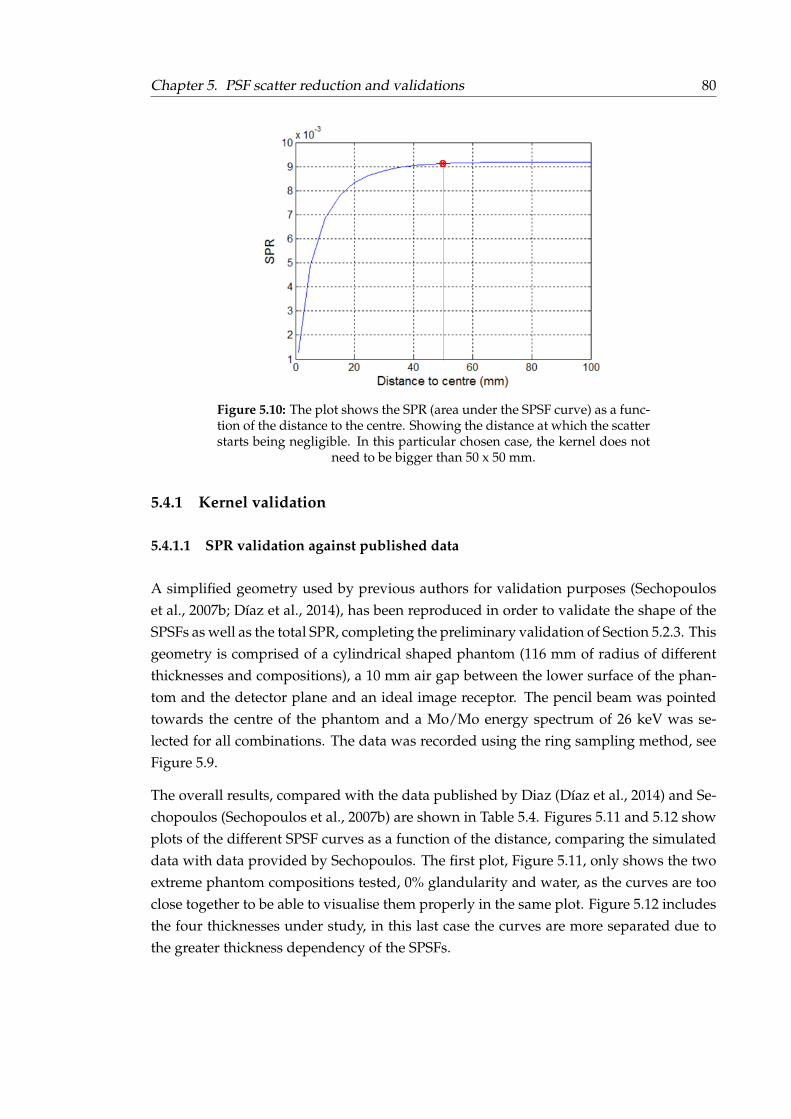
Chapter 5. PSF scatter reduction and validations 80
Figure 5.10: The plot shows the SPR (area under the SPSF curve) as a func-tion of the distance to the centre. Showing the distance at which the scatterstarts being negligible. In this particular chosen case, the kernel does not
need to be bigger than 50 x 50 mm.
5.4.1 Kernel validation
5.4.1.1 SPR validation against published data
A simplified geometry used by previous authors for validation purposes (Sechopouloset al., 2007b; Díaz et al., 2014), has been reproduced in order to validate the shape of theSPSFs as well as the total SPR, completing the preliminary validation of Section 5.2.3. Thisgeometry is comprised of a cylindrical shaped phantom (116 mm of radius of differentthicknesses and compositions), a 10 mm air gap between the lower surface of the phan-tom and the detector plane and an ideal image receptor. The pencil beam was pointedtowards the centre of the phantom and a Mo/Mo energy spectrum of 26 keV was se-lected for all combinations. The data was recorded using the ring sampling method, seeFigure 5.9.
The overall results, compared with the data published by Diaz (Díaz et al., 2014) and Se-chopoulos (Sechopoulos et al., 2007b) are shown in Table 5.4. Figures 5.11 and 5.12 showplots of the different SPSF curves as a function of the distance, comparing the simulateddata with data provided by Sechopoulos. The first plot, Figure 5.11, only shows the twoextreme phantom compositions tested, 0% glandularity and water, as the curves are tooclose together to be able to visualise them properly in the same plot. Figure 5.12 includesthe four thicknesses under study, in this last case the curves are more separated due tothe greater thickness dependency of the SPSFs.
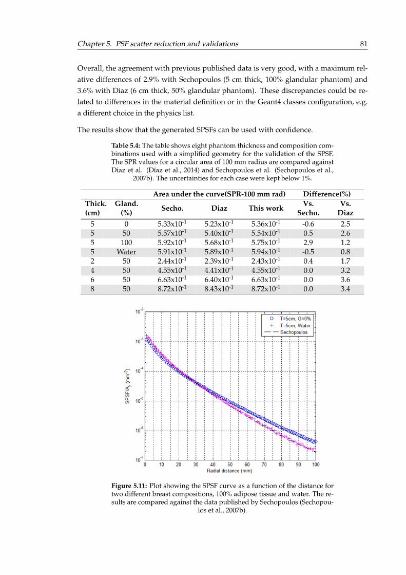
Chapter 5. PSF scatter reduction and validations 81
Overall, the agreement with previous published data is very good, with a maximum rel-ative differences of 2.9% with Sechopoulos (5 cm thick, 100% glandular phantom) and3.6% with Diaz (6 cm thick, 50% glandular phantom). These discrepancies could be re-lated to differences in the material definition or in the Geant4 classes configuration, e.g.a different choice in the physics list.
The results show that the generated SPSFs can be used with confidence.
Table 5.4: The table shows eight phantom thickness and composition com-binations used with a simplified geometry for the validation of the SPSF.The SPR values for a circular area of 100 mm radius are compared againstDiaz et al. (Díaz et al., 2014) and Sechopoulos et al. (Sechopoulos et al.,
2007b). The uncertainties for each case were kept below 1%.
Area under the curve(SPR-100 mm rad) Difference(%)Thick.(cm)
Gland.(%)
Secho. Diaz This workVs.
Secho.Vs.
Diaz5 0 5.33x10⁻¹ 5.23x10⁻¹ 5.36x10⁻¹ -0.6 2.55 50 5.57x10⁻¹ 5.40x10⁻¹ 5.54x10⁻¹ 0.5 2.65 100 5.92x10⁻¹ 5.68x10⁻¹ 5.75x10⁻¹ 2.9 1.25 Water 5.91x10⁻¹ 5.89x10⁻¹ 5.94x10⁻¹ -0.5 0.82 50 2.44x10⁻¹ 2.39x10⁻¹ 2.43x10⁻¹ 0.4 1.74 50 4.55x10⁻¹ 4.41x10⁻¹ 4.55x10⁻¹ 0.0 3.26 50 6.63x10⁻¹ 6.40x10⁻¹ 6.63x10⁻¹ 0.0 3.68 50 8.72x10⁻¹ 8.43x10⁻¹ 8.72x10⁻¹ 0.0 3.4
Figure 5.11: Plot showing the SPSF curve as a function of the distance fortwo different breast compositions, 100% adipose tissue and water. The re-sults are compared against the data published by Sechopoulos (Sechopou-
los et al., 2007b).
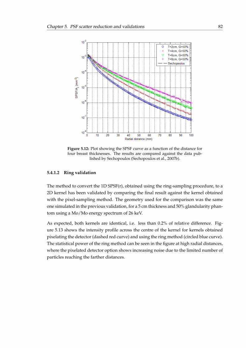
Chapter 5. PSF scatter reduction and validations 82
Figure 5.12: Plot showing the SPSF curve as a function of the distance forfour breast thicknesses. The results are compared against the data pub-
lished by Sechopoulos (Sechopoulos et al., 2007b).
5.4.1.2 Ring validation
The method to convert the 1D SPSF(r), obtained using the ring-sampling procedure, to a2D kernel has been validated by comparing the final result against the kernel obtainedwith the pixel-sampling method. The geometry used for the comparison was the sameone simulated in the previous validation, for a 5 cm thickness and 50% glandularity phan-tom using a Mo/Mo energy spectrum of 26 keV.
As expected, both kernels are identical, i.e. less than 0.2% of relative difference. Fig-ure 5.13 shows the intensity profile across the centre of the kernel for kernels obtainedpixelating the detector (dashed red curve) and using the ring method (circled blue curve).The statistical power of the ring method can be seen in the figure at high radial distances,where the pixelated detector option shows increasing noise due to the limited number ofparticles reaching the farther distances.
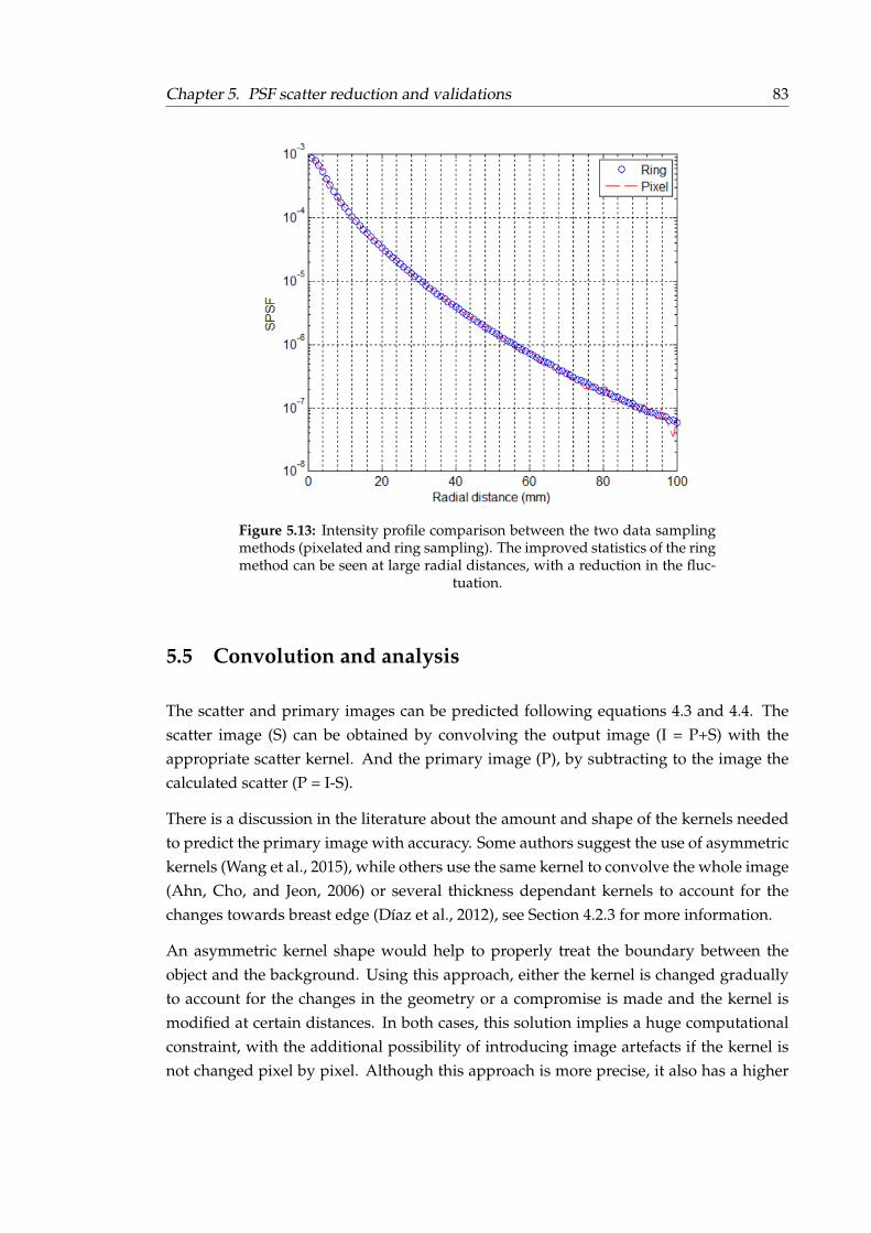
Chapter 5. PSF scatter reduction and validations 83
Figure 5.13: Intensity profile comparison between the two data samplingmethods (pixelated and ring sampling). The improved statistics of the ringmethod can be seen at large radial distances, with a reduction in the fluc-
tuation.
5.5 Convolution and analysis
The scatter and primary images can be predicted following equations 4.3 and 4.4. Thescatter image (S) can be obtained by convolving the output image (I = P+S) with theappropriate scatter kernel. And the primary image (P), by subtracting to the image thecalculated scatter (P = I-S).
There is a discussion in the literature about the amount and shape of the kernels neededto predict the primary image with accuracy. Some authors suggest the use of asymmetrickernels (Wang et al., 2015), while others use the same kernel to convolve the whole image(Ahn, Cho, and Jeon, 2006) or several thickness dependant kernels to account for thechanges towards breast edge (Díaz et al., 2012), see Section 4.2.3 for more information.
An asymmetric kernel shape would help to properly treat the boundary between theobject and the background. Using this approach, either the kernel is changed graduallyto account for the changes in the geometry or a compromise is made and the kernel ismodified at certain distances. In both cases, this solution implies a huge computationalconstraint, with the additional possibility of introducing image artefacts if the kernel isnot changed pixel by pixel. Although this approach is more precise, it also has a higher

Chapter 5. PSF scatter reduction and validations 84
dependency with the simulated geometry, risking the introduction of errors if it is notproperly computed.
The aim of this study is to find a simpler method, without the intrinsic complications ofthe asymmetric kernels but with good precision. The different options considered for theanalysis are discussed below.
Unless specified otherwise, the geometry used in this study corresponds to the α-Se Ho-logic Lorad Selenia in combination with a realistic synthetic breast phantom, see Fig-ure 5.6 and Table 5.3. For full MC simulations, the dimensions and shape of the breastphantom were based in the study published by Rodríguez-Ruiz et al. (Rodríguez-Ruiz,Agasthya, and Sechopoulos, 2017), where the shape of the compressed breast for mam-mography and breast tomosynthesis was characterised and modelled. For the simulationitself, the "PolyCone" volume available in Geant4 was chosen as a good approximation.Figure 5.14 shows an example of the breast phantom geometry and Table 5.5 gives thedimensions used for different thicknesses, all obtained with the aid of the Matlab codeprovided by Rodríguez-Ruiz. For simplification, the compression paddles were approxi-mated to rigid and non-inclined paddles. The chosen breast composition was 30% glan-dular tissue, a value that approximately represents breasts of thickness 5-6 cm in womenaged 50-64 (Dance et al., 2000; Yaffe et al., 2009). As shown in Section 4.3, changes inbreast composition do not introduce large variations in the scattering estimation, there-fore the chosen glandular percentage was kept constant for all the thicknesses studied. Inaddition, the phantom was surrounded by a 2 mm thick layer of skin and it was alignedwith the chest wall.
Figure 5.14: The figure shows different views of a simulated breast phan-tom that makes use of the "PolyCone" volume in Geant4.
For the pencil beam (PB) simulations the phantom kept the same composition and thick-ness to aid in the comparison against the full MC simulations. The phantom shape wasmodified to a cylinder and it was centred in the middle of the detector area, see Figure 5.6.A 50 mm breast phantom was chosen for the initial study. For statistic purposes, the pixelsize was increased from 70 µm to 280 or 560 µm, depending on each particular case.

Chapter 5. PSF scatter reduction and validations 85
Table 5.5: Table with the dimensions (height and radius) of the simulatedbreast phantoms at five different thicknesses. The dimensions have beenobtained following the study published by Rodríguez-Ruiz (Rodríguez-
Ruiz, Agasthya, and Sechopoulos, 2017).
H (mm) h4 (mm) r1 (mm) r4 (mm) r6 (mm)35 18.3 64.7 71.7 65.350 20.0 80.0 97.0 86.060 25.3 94.7 112.0 104.370 25 100 133 12285 32.0 136.0 164.0 153.0
5.5.1 One kernel
The first option to consider is the use of only one symmetric kernel for the convolutionanalysis (specific to the phantom thickness). For this case, the PB simulation geometrywould need to include the object of interest, centred with the pencil beam. To gain statis-tics, the pixel size of the full MC and PB images was increased to 280 µm, resulting in a600 x 600 pixel2 kernel that was used to convolve a 856 x 856 pixel2 image.
There are two possibilities for performing the image convolution when using this ap-proach. The kernel can be used to convolve the whole image, or the breast area can bemasked from the background to force the kernel only to act in the region of interest. Bothoptions present problems, especially close to the breast edge area:
• Using the whole image: Convolving the whole image leads to overestimation, start-ing 100 pixels after the chest-wall. When compared against the scatter obtainedwith a full MC simulation ("ground truth"), the predicted scatter is up to 2.6 timeshigher at the edge of the object, as shown in Figure 5.15.
• Using the phantom area: If the breast area is segmented from the background, thescatter originated in the phantom is underestimated up to 50% towards the edgeof the phantom. Figure 5.16 shows the intensity profiles (across the centre of thephantom) of the predicted scatter and the scatter obtained with a full MC simula-tion ("ground truth").
The results obtained by using only one kernel to predict the scatter are far from beingsensitive enough.
It is necessary to highlight the importance of accounting for the background contributionto the image (note that all area of the image that is outside the breast or phantom regionis denominated background; the scattering proceeding from this area comes mainly fromthe compression and support paddles). An inappropriate background treatment can lead
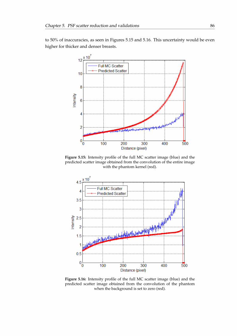
Chapter 5. PSF scatter reduction and validations 86
to 50% of inaccuracies, as seen in Figures 5.15 and 5.16. This uncertainty would be evenhigher for thicker and denser breasts.
Figure 5.15: Intensity profile of the full MC scatter image (blue) and thepredicted scatter image obtained from the convolution of the entire image
with the phantom kernel (red).
Figure 5.16: Intensity profile of the full MC scatter image (blue) and thepredicted scatter image obtained from the convolution of the phantom
when the background is set to zero (red).
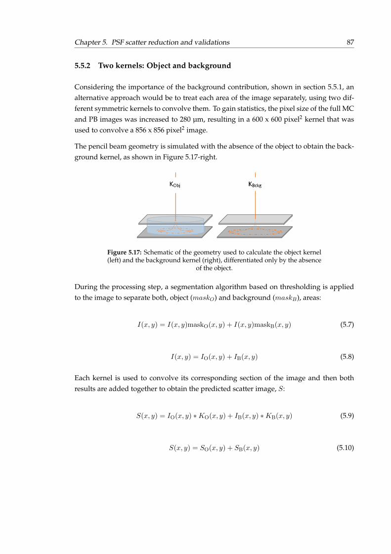
Chapter 5. PSF scatter reduction and validations 87
5.5.2 Two kernels: Object and background
Considering the importance of the background contribution, shown in section 5.5.1, analternative approach would be to treat each area of the image separately, using two dif-ferent symmetric kernels to convolve them. To gain statistics, the pixel size of the full MCand PB images was increased to 280 µm, resulting in a 600 x 600 pixel2 kernel that wasused to convolve a 856 x 856 pixel2 image.
The pencil beam geometry is simulated with the absence of the object to obtain the back-ground kernel, as shown in Figure 5.17-right.
Figure 5.17: Schematic of the geometry used to calculate the object kernel(left) and the background kernel (right), differentiated only by the absence
of the object.
During the processing step, a segmentation algorithm based on thresholding is appliedto the image to separate both, object (maskO) and background (maskB), areas:
I(x, y) = I(x, y)maskO(x, y) + I(x, y)maskB(x, y) (5.7)
I(x, y) = IO(x, y) + IB(x, y) (5.8)
Each kernel is used to convolve its corresponding section of the image and then bothresults are added together to obtain the predicted scatter image, S:
S(x, y) = IO(x, y) ∗KO(x, y) + IB(x, y) ∗KB(x, y) (5.9)
S(x, y) = SO(x, y) + SB(x, y) (5.10)
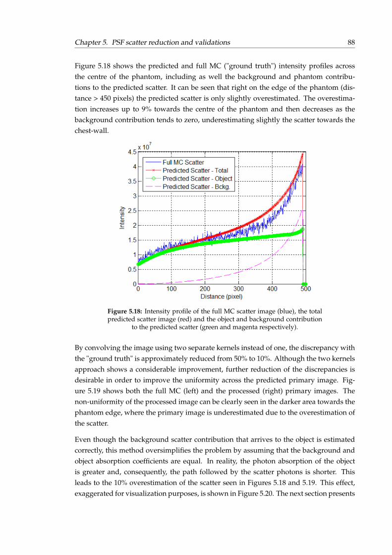
Chapter 5. PSF scatter reduction and validations 88
Figure 5.18 shows the predicted and full MC ("ground truth") intensity profiles acrossthe centre of the phantom, including as well the background and phantom contribu-tions to the predicted scatter. It can be seen that right on the edge of the phantom (dis-tance > 450 pixels) the predicted scatter is only slightly overestimated. The overestima-tion increases up to 9% towards the centre of the phantom and then decreases as thebackground contribution tends to zero, underestimating slightly the scatter towards thechest-wall.
Figure 5.18: Intensity profile of the full MC scatter image (blue), the totalpredicted scatter image (red) and the object and background contribution
to the predicted scatter (green and magenta respectively).
By convolving the image using two separate kernels instead of one, the discrepancy withthe "ground truth" is approximately reduced from 50% to 10%. Although the two kernelsapproach shows a considerable improvement, further reduction of the discrepancies isdesirable in order to improve the uniformity across the predicted primary image. Fig-ure 5.19 shows both the full MC (left) and the processed (right) primary images. Thenon-uniformity of the processed image can be clearly seen in the darker area towards thephantom edge, where the primary image is underestimated due to the overestimation ofthe scatter.
Even though the background scatter contribution that arrives to the object is estimatedcorrectly, this method oversimplifies the problem by assuming that the background andobject absorption coefficients are equal. In reality, the photon absorption of the objectis greater and, consequently, the path followed by the scatter photons is shorter. Thisleads to the 10% overestimation of the scatter seen in Figures 5.18 and 5.19. This effect,exaggerated for visualization purposes, is shown in Figure 5.20. The next section presents

Chapter 5. PSF scatter reduction and validations 89
the scatter estimation method proposed in this study, in which this observed issue isaccounted for.
Figure 5.19: Full MC primary image (left) and predicted primary imageobtained from the convolution with background and object kernels (right).
The darker area of the predicted image indicates scatter overestimation.
Figure 5.20: Schematic showing the scatter spreading in two media withdifferent absorption coefficients. The incoming photon beam hits the back-ground in an area close to the object. The two kernels method assumesthat the scatter will spread equally (left figure); in reality the SPSFs will beasymmetric as the background and object absorption coefficients are differ-ent (right figure). The values are exaggerated for visualization purposes.
5.6 Proposed scatter reduction implementation
The method that has been chosen for scatter estimation in this study is a semi-empiricalmodification of the "two kernel" method, influenced by the theory behind the asymmetrickernels.
An abstracted schematic of the scatter distribution in the image is shown in Figure 5.21.The image illustrates the contributions to the scatter from the different areas of the image.
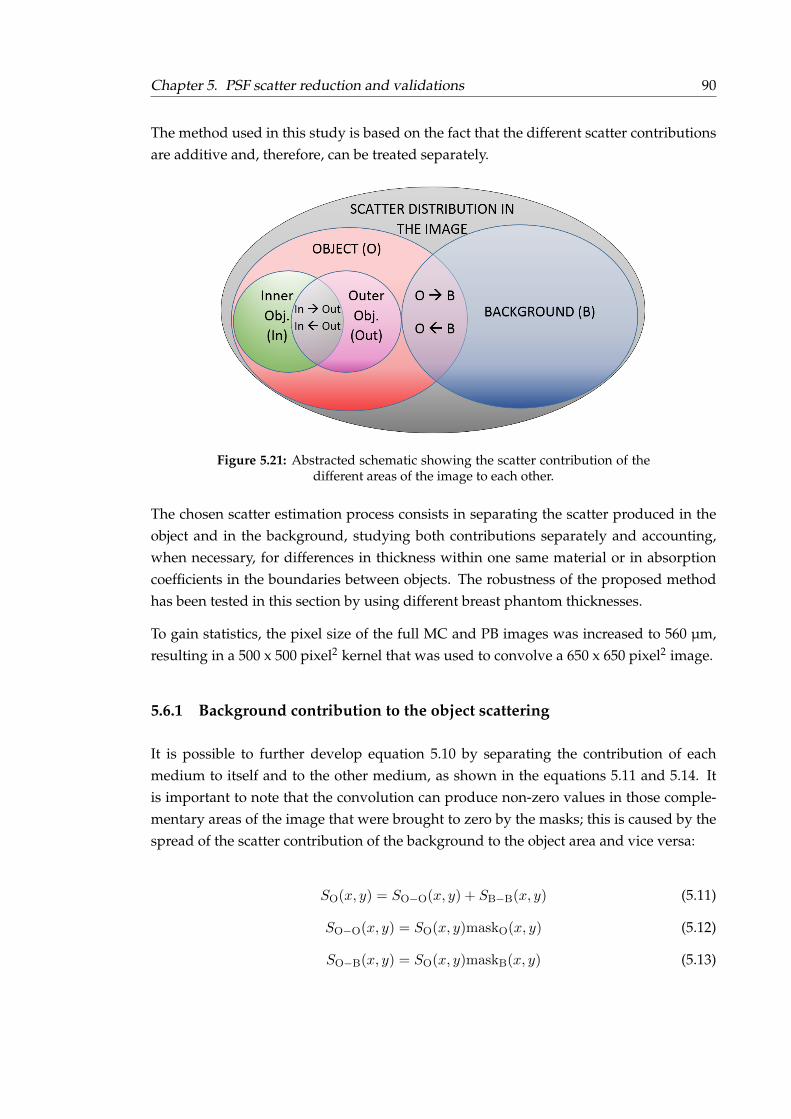
Chapter 5. PSF scatter reduction and validations 90
The method used in this study is based on the fact that the different scatter contributionsare additive and, therefore, can be treated separately.
Figure 5.21: Abstracted schematic showing the scatter contribution of thedifferent areas of the image to each other.
The chosen scatter estimation process consists in separating the scatter produced in theobject and in the background, studying both contributions separately and accounting,when necessary, for differences in thickness within one same material or in absorptioncoefficients in the boundaries between objects. The robustness of the proposed methodhas been tested in this section by using different breast phantom thicknesses.
To gain statistics, the pixel size of the full MC and PB images was increased to 560 µm,resulting in a 500 x 500 pixel2 kernel that was used to convolve a 650 x 650 pixel2 image.
5.6.1 Background contribution to the object scattering
It is possible to further develop equation 5.10 by separating the contribution of eachmedium to itself and to the other medium, as shown in the equations 5.11 and 5.14. Itis important to note that the convolution can produce non-zero values in those comple-mentary areas of the image that were brought to zero by the masks; this is caused by thespread of the scatter contribution of the background to the object area and vice versa:
SO(x, y) = SO−O(x, y) + SB−B(x, y) (5.11)
SO−O(x, y) = SO(x, y)maskO(x, y) (5.12)
SO−B(x, y) = SO(x, y)maskB(x, y) (5.13)
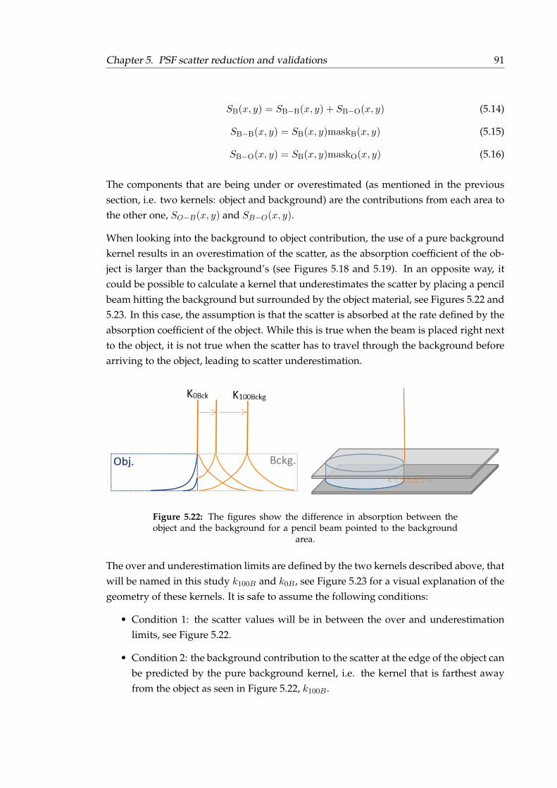
Chapter 5. PSF scatter reduction and validations 91
SB(x, y) = SB−B(x, y) + SB−O(x, y) (5.14)
SB−B(x, y) = SB(x, y)maskB(x, y) (5.15)
SB−O(x, y) = SB(x, y)maskO(x, y) (5.16)
The components that are being under or overestimated (as mentioned in the previoussection, i.e. two kernels: object and background) are the contributions from each area tothe other one, SO−B(x, y) and SB−O(x, y).
When looking into the background to object contribution, the use of a pure backgroundkernel results in an overestimation of the scatter, as the absorption coefficient of the ob-ject is larger than the background’s (see Figures 5.18 and 5.19). In an opposite way, itcould be possible to calculate a kernel that underestimates the scatter by placing a pencilbeam hitting the background but surrounded by the object material, see Figures 5.22 and5.23. In this case, the assumption is that the scatter is absorbed at the rate defined by theabsorption coefficient of the object. While this is true when the beam is placed right nextto the object, it is not true when the scatter has to travel through the background beforearriving to the object, leading to scatter underestimation.
Figure 5.22: The figures show the difference in absorption between theobject and the background for a pencil beam pointed to the background
area.
The over and underestimation limits are defined by the two kernels described above, thatwill be named in this study k100B and k0B , see Figure 5.23 for a visual explanation of thegeometry of these kernels. It is safe to assume the following conditions:
• Condition 1: the scatter values will be in between the over and underestimationlimits, see Figure 5.22.
• Condition 2: the background contribution to the scatter at the edge of the object canbe predicted by the pure background kernel, i.e. the kernel that is farthest awayfrom the object as seen in Figure 5.22, k100B .
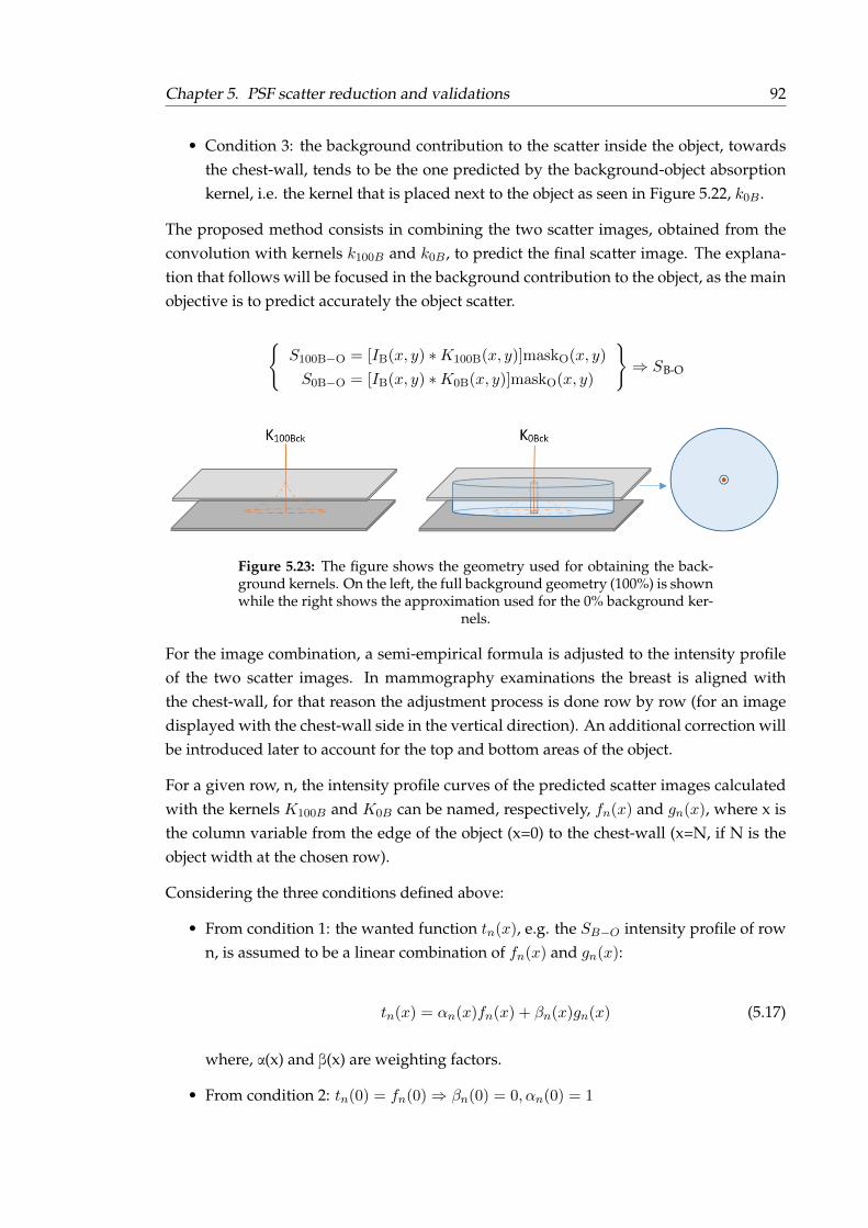
Chapter 5. PSF scatter reduction and validations 92
• Condition 3: the background contribution to the scatter inside the object, towardsthe chest-wall, tends to be the one predicted by the background-object absorptionkernel, i.e. the kernel that is placed next to the object as seen in Figure 5.22, k0B .
The proposed method consists in combining the two scatter images, obtained from theconvolution with kernels k100B and k0B , to predict the final scatter image. The explana-tion that follows will be focused in the background contribution to the object, as the mainobjective is to predict accurately the object scatter.
S100B−O = [IB(x, y) ∗K100B(x, y)]maskO(x, y)
S0B−O = [IB(x, y) ∗K0B(x, y)]maskO(x, y)
⇒ SB-O
Figure 5.23: The figure shows the geometry used for obtaining the back-ground kernels. On the left, the full background geometry (100%) is shownwhile the right shows the approximation used for the 0% background ker-
nels.
For the image combination, a semi-empirical formula is adjusted to the intensity profileof the two scatter images. In mammography examinations the breast is aligned withthe chest-wall, for that reason the adjustment process is done row by row (for an imagedisplayed with the chest-wall side in the vertical direction). An additional correction willbe introduced later to account for the top and bottom areas of the object.
For a given row, n, the intensity profile curves of the predicted scatter images calculatedwith the kernels K100B and K0B can be named, respectively, fn(x) and gn(x), where x isthe column variable from the edge of the object (x=0) to the chest-wall (x=N, if N is theobject width at the chosen row).
Considering the three conditions defined above:
• From condition 1: the wanted function tn(x), e.g. the SB−O intensity profile of rown, is assumed to be a linear combination of fn(x) and gn(x):
tn(x) = αn(x)fn(x) + βn(x)gn(x) (5.17)
where, α(x) and β(x) are weighting factors.
• From condition 2: tn(0) = fn(0)⇒ βn(0) = 0, αn(0) = 1

Chapter 5. PSF scatter reduction and validations 93
• From condition 3: tn(N) = gn(N)⇒ βn(N) = 1, αn(N) = 0
Parameters αn and βn decrease and increase respectively with the distance to the breastedge (x). It was seen experimentally that it is possible to write βn as being directly pro-portional to x, while assuming αn to be inversely proportional to the distance led to scat-ter underestimation. Therefore, to account for the experimental data and for conditionsαn(0) = 1, αn(N) = 0, βn(0) = 0 and βn(N) = 1, the parameters can be described as:
αn(x) =Kα1
Kα2 + x(5.18)
where, Kα1 has to be equal or very close to Kα2, to ensure that αn(0) = 1.
βn(x) = Kβx (5.19)
where, 1 > Kβ > 0. In particular, Kβ = 1N , to ensure that βn(N) = 1.
The constants Kα1 and Kα2 need to be adjusted across the image to obtain the final equa-tion. For the adjustment phase, the scatter images obtained from full MC simulationswere used as an aid to find the parameters, i.e. the "ground truth" results that the pre-dicted scatter needs to match.
For the adjustment of the parameters, realistic mammography geometry and breast phan-toms were used, as described at the beginning of section 5.5. The robustness of themethod and the adjusted parameters, discussed at the end of the chapter, was testedby using different breast thicknesses and additional geometries. The most reproduciblevalues found, that made the weighting factors independent of n, were Kα1 = 80 andKα2 = Kα1 − 1.
The equation adopted in this study is:
tn(x) =80
79 + xfn(x) +
x
Ngn(x) (5.20)
5.6.1.1 Additional correction: column to column
The method explained above makes use of a semi-empirical equation to calculate thescatter image in a row to row basis. The correction was applied in the horizontal directionbecause of the positioning of the object relative to the background. This correction wouldbe enough if the object was rectangular, covering the image from top to bottom. However,the breast is not only curved but it is also smaller than the image in both vertical andhorizontal directions. Therefore, even though the background contribution is larger inthe horizontal direction, the vertical contribution needs to also be considered to avoid
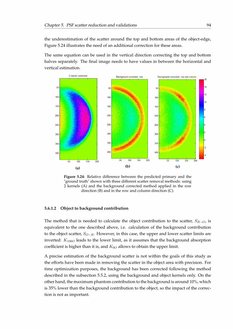
Chapter 5. PSF scatter reduction and validations 94
the underestimation of the scatter around the top and bottom areas of the object-edge,Figure 5.24 illustrates the need of an additional correction for these areas.
The same equation can be used in the vertical direction correcting the top and bottomhalves separately. The final image needs to have values in between the horizontal andvertical estimation.
(a) (b) (c)
Figure 5.24: Relative difference between the predicted primary and the"ground truth" shown with three different scatter removal methods: using2 kernels (A) and the background corrected method applied in the row
direction (B) and in the row and column direction (C).
5.6.1.2 Object to background contribution
The method that is needed to calculate the object contribution to the scatter, SB−O, isequivalent to the one described above, i.e. calculation of the background contributionto the object scatter, SO−B . However, in this case, the upper and lower scatter limits areinverted: K100O leads to the lower limit, as it assumes that the background absorptioncoefficient is higher than it is, and K0O allows to obtain the upper limit.
A precise estimation of the background scatter is not within the goals of this study asthe efforts have been made in removing the scatter in the object area with precision. Fortime optimization purposes, the background has been corrected following the methoddescribed in the subsection 5.5.2, using the background and object kernels only. On theother hand, the maximum phantom contribution to the background is around 10%, whichis 35% lower than the background contribution to the object, so the impact of the correc-tion is not as important.
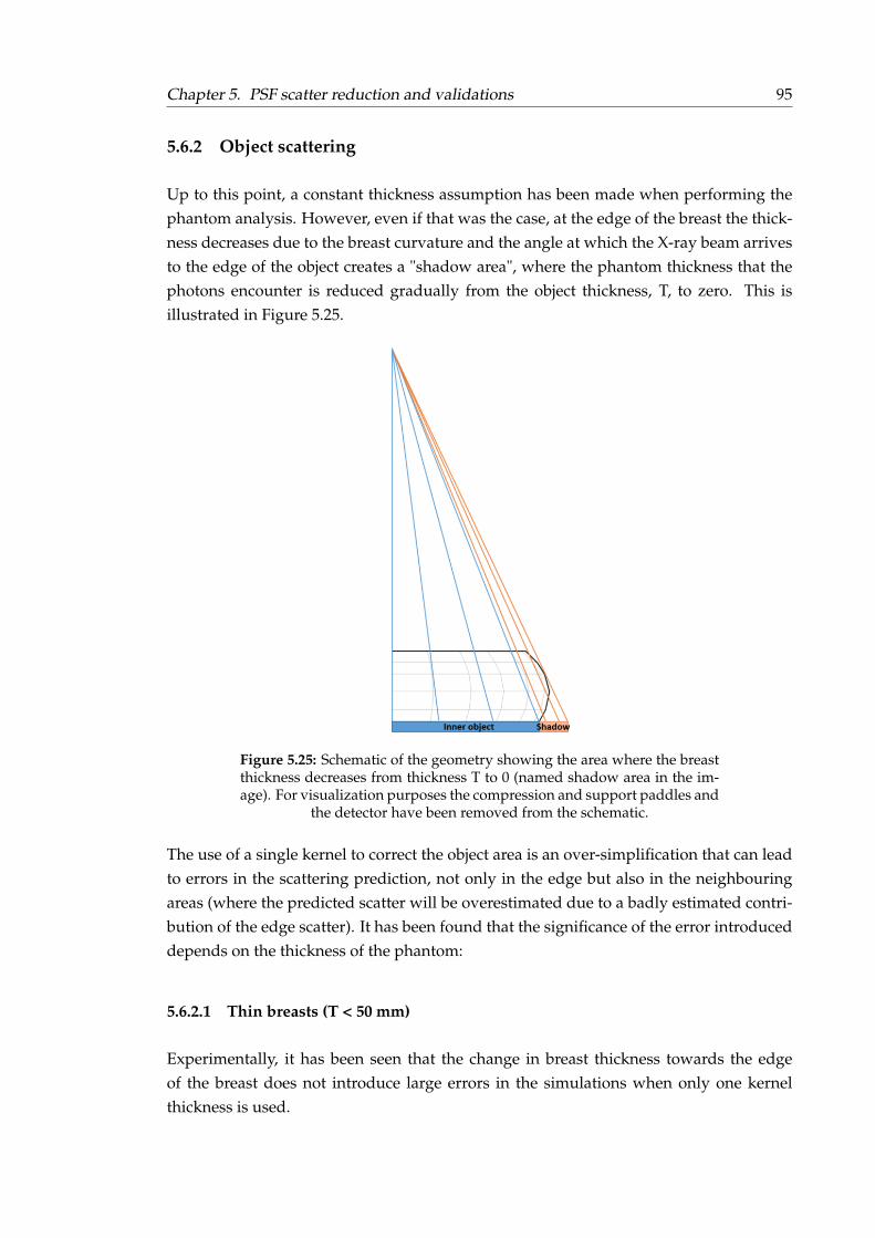
Chapter 5. PSF scatter reduction and validations 95
5.6.2 Object scattering
Up to this point, a constant thickness assumption has been made when performing thephantom analysis. However, even if that was the case, at the edge of the breast the thick-ness decreases due to the breast curvature and the angle at which the X-ray beam arrivesto the edge of the object creates a "shadow area", where the phantom thickness that thephotons encounter is reduced gradually from the object thickness, T, to zero. This isillustrated in Figure 5.25.
Figure 5.25: Schematic of the geometry showing the area where the breastthickness decreases from thickness T to 0 (named shadow area in the im-age). For visualization purposes the compression and support paddles and
the detector have been removed from the schematic.
The use of a single kernel to correct the object area is an over-simplification that can leadto errors in the scattering prediction, not only in the edge but also in the neighbouringareas (where the predicted scatter will be overestimated due to a badly estimated contri-bution of the edge scatter). It has been found that the significance of the error introduceddepends on the thickness of the phantom:
5.6.2.1 Thin breasts (T < 50 mm)
Experimentally, it has been seen that the change in breast thickness towards the edgeof the breast does not introduce large errors in the simulations when only one kernelthickness is used.
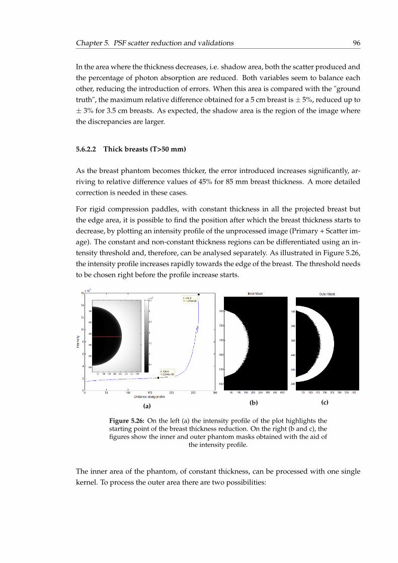
Chapter 5. PSF scatter reduction and validations 96
In the area where the thickness decreases, i.e. shadow area, both the scatter produced andthe percentage of photon absorption are reduced. Both variables seem to balance eachother, reducing the introduction of errors. When this area is compared with the "groundtruth", the maximum relative difference obtained for a 5 cm breast is± 5%, reduced up to± 3% for 3.5 cm breasts. As expected, the shadow area is the region of the image wherethe discrepancies are larger.
5.6.2.2 Thick breasts (T>50 mm)
As the breast phantom becomes thicker, the error introduced increases significantly, ar-riving to relative difference values of 45% for 85 mm breast thickness. A more detailedcorrection is needed in these cases.
For rigid compression paddles, with constant thickness in all the projected breast butthe edge area, it is possible to find the position after which the breast thickness starts todecrease, by plotting an intensity profile of the unprocessed image (Primary + Scatter im-age). The constant and non-constant thickness regions can be differentiated using an in-tensity threshold and, therefore, can be analysed separately. As illustrated in Figure 5.26,the intensity profile increases rapidly towards the edge of the breast. The threshold needsto be chosen right before the profile increase starts.
(a) (b) (c)
Figure 5.26: On the left (a) the intensity profile of the plot highlights thestarting point of the breast thickness reduction. On the right (b and c), thefigures show the inner and outer phantom masks obtained with the aid of
the intensity profile.
The inner area of the phantom, of constant thickness, can be processed with one singlekernel. To process the outer area there are two possibilities:

Chapter 5. PSF scatter reduction and validations 97
• Multiple kernel analysis: Calculate many kernels to account for the progressivechange of thickness and convolute each area with its correspondent kernel thick-ness.
• Simplification: Find an equivalent thickness to represent the outer area. The spacebetween the phantom and the support plate created by the thickness reduction isfilled with air in this case.
The first option will give more accurate results, but at a high computational time cost,as it would be equivalent to the use of asymmetric kernels. Therefore, the second optionhas been the one chosen in this study, aiming to reduce to acceptable levels the errorintroduced by the simplification while reducing the computational time.
The method is similar to the one studied for the background: both areas will have theirown scatter contribution and the scatter that arrives from the adjacent area, e.g. the scat-ter of the inner part of the phantom will be the sum of the inner scatter and the outerscatter contribution.
To compare the results with the full MC scatter image, the predicted background scatterneeds to be subtracted to isolate the phantom contribution. Using the full MC as thebenchmark result, it is possible to find empirically an equivalent thickness that givesan appropriate contribution from the outer to the inner area, see Figure 5.27. A 20%thickness reduction was found to give the better results, while being reproducible acrossdifferent phantom thicknesses.
The equivalent thickness has been introduced to calculate the scatter contribution of theouter area of the breast to the inner area, but the calculation of the scatter in the outerregion has not been included yet. The process to follow for this estimation is similarto the one introduced in the background-to-phantom scatter estimation, Section 5.6.1.However, in this case it is not necessary to use equation 5.20 as it is possible to simplifythe method by making use of a polynomial fitting, using two well-known points and theinner scatter contribution profile:
• Inner object area: Defined by the equivalent thickness method introduced above.
• Boundary between the inner and the outer object area: The scattering at the outerprofile starting point can be mapped from the inner profile end point.
• Breast edge: The breast edge corresponds to the thinner area of the outer section, ithas been seen experimentally that it corresponds to the external 25% of the profile.The kernel that describes this area is obtained using a kernel with the beam hittingthe maximum thickness but surrounded by background, i.e. 0 mm breast thickness.
It was proven experimentally that good results were obtained with a third order polyno-mial fit. An example illustrating this process is shown in Figure 5.28.

Chapter 5. PSF scatter reduction and validations 98
Figure 5.27: The figure illustrates the effect that the outer area of the phan-tom has in the scatter prediction of the inner area, considering four differ-ent cases: benchmark values (blue), 0 mm thick outer area (red), constantphantom thickness: outer = inner areas (green) and optimised equivalentouter thickness of 80% the phantom thickness (pink). All the cases include
the support and compression paddles at constant distances.
Figure 5.28: The plot on the left illustrates the procedure followed to esti-mate the scatter corresponding to the outer area of the object, marking theknown points used for the polynomial adjustment. The plot on the right
shows the adjusted profile.

Chapter 5. PSF scatter reduction and validations 99
5.6.3 Method robustness and convolution validation
Five different phantom thicknesses have been tested to validate and study the robustnessof the proposed method. Two thin phantoms (35 and 50 mm) and three thick phantoms(60, 70 and 85 mm) were analysed. The scatter of the thinner phantoms was obtainedusing one kernel to evaluate the phantom scatter while the background contribution wasanalysed following the method explained in section 5.6.1. The thicker phantoms wereanalysed by dividing the breast in an outer and an inner area and using an equivalentbreast thickness for the evaluation of the non-constant region, as explained in section5.6.2.
5.6.3.1 Scatter estimation
Figures 5.29 and 5.30 show the relative difference between primary images, comparingthe "ground truth", i.e. full MC simulated images, with the predicted image. On the leftcolumn, the positive values (blue/magenta colours) indicate scatter overestimation andthe negatives (green/red colours) point to scatter underestimation. The plots on the rightare the histograms of the images, showing the distribution of the data. Table 5.6 gives themean value, the standard deviation and the maximum values of over and underestima-tion.
It is important to take into account the photon fluctuation in the simulated images; thereis still some statistical uncertainty in the images used in the comparison, even thoughup to 80 simulations of 109 particles each were run for each of the full MC examples fora pixel size of 560 µm. In the examples evaluated, the fluctuation in the primary MCimage goes from ±1.5% for 35 mm breast thickness up to ±5% for 85 mm. To take thisinto consideration, the maximum over and underestimation values of Table 5.6 have beencorrected and the uncertainty values are included.
Table 5.6: Table showing the discrepancies between the predicted primaryimage and the "ground truth". For each thickness, the table gives the meanvalue, the standard deviation and the maximum under and overestimation
(in %).
T (mm) Mean (%) STD (%)Max. Underest.
(%)Max. Overest.
(%)35 -0.3 1.2 3.4 ± 1.5 2.8 ± 0.850 0.3 2.0 5.0 ± 3.3 4.8 ± 2.660 1.3 3.1 8.1 ± 5.2 5.6 ± 6.370 -0.4 3.3 8.1 ± 5.5 5.9 ± 5.185 -1.8 7.7 20.1 ± 14.5 23.0 ± 4.1
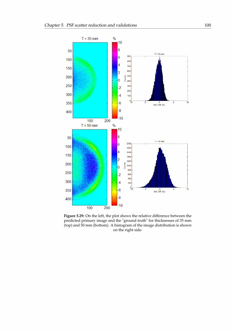
Chapter 5. PSF scatter reduction and validations 100
Figure 5.29: On the left, the plot shows the relative difference between thepredicted primary image and the "ground truth" for thicknesses of 35 mm(top) and 50 mm (bottom). A histogram of the image distribution is shown
on the right side.

Chapter 5. PSF scatter reduction and validations 101
Figure 5.30: On the left, the plot shows the relative difference between thepredicted primary image and the "ground truth" for thicknesses of 60 mm(top), 70 mm (centre) and 85 mm (bottom). A histogram of the image dis-
tribution is shown on the right side.

Chapter 5. PSF scatter reduction and validations 102
5.6.3.2 Method limitations and conclusion
The uncertainty introduced in the scatter estimation increases with the breast thickness.For thin breasts (up to 50 mm) the relative difference between the predicted primaryimage and the "ground truth" does not exceed 5%, which is considered a very good esti-mation. The error introduced increases up to 10% for thicker breasts (between 50 mm and70 mm). The method correction is still considered to work properly. For breasts that arethicker than 70 mm the correction gets more complicated and the reproducibility startsto fail, i.e. for 85 mm the error introduced is around 20-25%. This is likely linked to theequivalent thickness simplification, see section 5.6.2.
To achieve better results the method would need to be modified. For breasts thickerthan 70/75 mm it may be preferable the use of asymmetric kernels, in order to avoid aconsiderable increase in the manipulation of the image that would risk the introductionof image artefacts. For the rest of the cases, the results could be improved by modify-ing Equation 5.20 or evaluate alternative equations. For example, a thickness-dependentfactor so the scatter estimation adapts better to changes in breast thickness, making theanalysis less generic. In addition, future work will be needed to make the method moreinclusive, evaluating its effectiveness and modifying it when necessary. For example:
• New research should focus in including inclined or flexible compression paddles.
• A modification of the method would also be required to include less common com-pressed breast shapes, i.e. the suggested method works under the condition thatfrom the chest-wall to the breast-edge there are no "air/background" gaps. How-ever, breasts that present dimple areas might present these gaps when compressed.
5.6.4 Method schematic
The proposed method for estimating the scatter radiation is described in the diagram ofFigure 5.31, the schematic is a visual summary of the current section 5.6.
5.7 Chapter summary and discussion
The post-processing scatter estimation technique chosen in this thesis is based on the scat-ter convolution methodology, using as a kernel a point spread function simulated withsimplified pencil beam Monte Carlo simulations. In this chapter the proposed scatterreduction technique was defined, optimised and validated against full MC simulationsand previously published data.

Chapter 5. PSF scatter reduction and validations 103
The chapter started with an introduction to the chosen simulation tool-kit, i.e. Geant4,covering its general architecture, some of the specific adjustments made to adapt it to theneeds of this study and validation against previous publications. It continued with a def-inition and validation of the system’s geometry and kernel calculation. The validationsagainst the simulation set up were essential to the study, as they reduced the possibilityof introducing systematic errors in the kernel simulation, which would directly affect theestimation of the scatter. The agreements found indicated that it was safe to advance tothe next step: the definition of the final methodology and estimation of the scatter and ofthe primary image.
Therefore, the second part of the chapter focused on the definition and optimisation of thescatter estimation methodology. Early results showed the need of an accurate treatmentof the background contribution to the breast edge area, when background is considered tobe all areas and material layers outside the phantom/breast. Accounting for differencesin the absorption coefficients whenever there was a change of absorber, i.e. backgroundto breast, was found to be key in the treatment of the breast edge.
The suggested study simplified the asymmetric kernel methodology to the use of three in-dividual kernels for thin breasts (T < 50 mm) and five for thicker breasts (50 < T < 75 mm).In the latter case two additional kernels were needed to compensate for changes in thebreast thickness, i.e. change in the materials that the photons encounter through theirpath across the breast edge. Validations against full MC simulations suggested agree-ments between the methods of 90-97%, for 75-35 mm thicknesses respectively.

Chapter 5. PSF scatter reduction and validations 104
Figure 5.31: Diagram explaining the scatter contribution estimationmethod presented in this study, see section 5.6.
105
Chapter 6
PSF scatter reduction: Clinicalevaluation with phantoms
The scatter estimation methodology developed previously is evaluated under clinicalconditions in this chapter, testing its effectiveness against grid images acquired underthe same conditions. A broad selection of clinical phantoms is used for this purpose.
6.1 Scatter estimation methodology
The post-process scattered radiation reduction method that has been chosen, see Sec-tion 5.6, assumes that the scattered radiation in the system can be approximated to two-dimensional low-pass filters of the primary image and can be calculated with the convo-lution between the input image and the filters. The filters, or kernels, are calculated usingsimplified Monte Carlo simulations where the incident beam is approximated by a deltafunction or narrow pencil beam.
The chosen scatter estimation method has been optimised in Chapter 5. To account forvariations in the absorption coefficients within the system, i.e. background to breastboundary or thickness reduction towards the edge of the breast, the image is divided intwo or three regions of interest, depending on the thickness of the breast. Each sub-imageis analysed separately with its correspondent set of kernels, giving the scatter estimationof the analysed region and its contribution to the neighbouring areas. The final scatterimage is obtained by adding together all the scatter sub-images. From there, the pri-mary image can be calculated by subtracting the scatter image to the unprocessed (input)image, i.e. grid-less acquired image. The method work-flow can be seen in Figure 6.1.
In this chapter, the scatter reduction method is going to be further characterized andtested using two different technologies, i.e. α-Se and CMOS, with a wide range of clinicalphantoms.
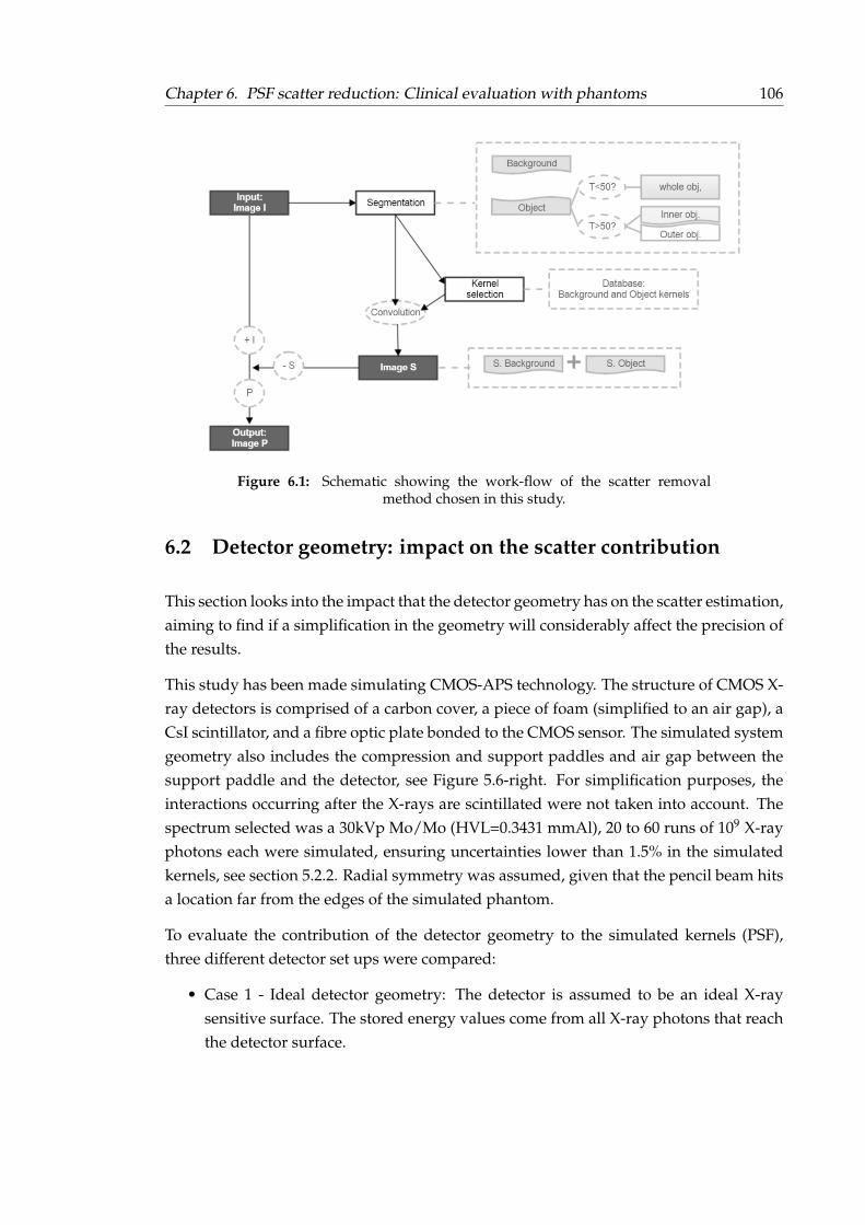
Chapter 6. PSF scatter reduction: Clinical evaluation with phantoms 106
Figure 6.1: Schematic showing the work-flow of the scatter removalmethod chosen in this study.
6.2 Detector geometry: impact on the scatter contribution
This section looks into the impact that the detector geometry has on the scatter estimation,aiming to find if a simplification in the geometry will considerably affect the precision ofthe results.
This study has been made simulating CMOS-APS technology. The structure of CMOS X-ray detectors is comprised of a carbon cover, a piece of foam (simplified to an air gap), aCsI scintillator, and a fibre optic plate bonded to the CMOS sensor. The simulated systemgeometry also includes the compression and support paddles and air gap between thesupport paddle and the detector, see Figure 5.6-right. For simplification purposes, theinteractions occurring after the X-rays are scintillated were not taken into account. Thespectrum selected was a 30kVp Mo/Mo (HVL=0.3431 mmAl), 20 to 60 runs of 109 X-rayphotons each were simulated, ensuring uncertainties lower than 1.5% in the simulatedkernels, see section 5.2.2. Radial symmetry was assumed, given that the pencil beam hitsa location far from the edges of the simulated phantom.
To evaluate the contribution of the detector geometry to the simulated kernels (PSF),three different detector set ups were compared:
• Case 1 - Ideal detector geometry: The detector is assumed to be an ideal X-raysensitive surface. The stored energy values come from all X-ray photons that reachthe detector surface.
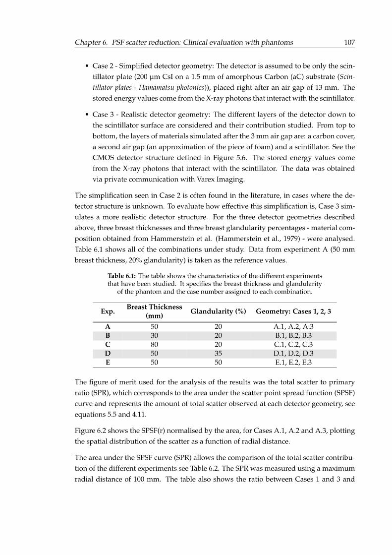
Chapter 6. PSF scatter reduction: Clinical evaluation with phantoms 107
• Case 2 - Simplified detector geometry: The detector is assumed to be only the scin-tillator plate (200 µm CsI on a 1.5 mm of amorphous Carbon (aC) substrate (Scin-tillator plates - Hamamatsu photonics)), placed right after an air gap of 13 mm. Thestored energy values come from the X-ray photons that interact with the scintillator.
• Case 3 - Realistic detector geometry: The different layers of the detector down tothe scintillator surface are considered and their contribution studied. From top tobottom, the layers of materials simulated after the 3 mm air gap are: a carbon cover,a second air gap (an approximation of the piece of foam) and a scintillator. See theCMOS detector structure defined in Figure 5.6. The stored energy values comefrom the X-ray photons that interact with the scintillator. The data was obtainedvia private communication with Varex Imaging.
The simplification seen in Case 2 is often found in the literature, in cases where the de-tector structure is unknown. To evaluate how effective this simplification is, Case 3 sim-ulates a more realistic detector structure. For the three detector geometries describedabove, three breast thicknesses and three breast glandularity percentages - material com-position obtained from Hammerstein et al. (Hammerstein et al., 1979) - were analysed.Table 6.1 shows all of the combinations under study. Data from experiment A (50 mmbreast thickness, 20% glandularity) is taken as the reference values.
Table 6.1: The table shows the characteristics of the different experimentsthat have been studied. It specifies the breast thickness and glandularity
of the phantom and the case number assigned to each combination.
Exp.Breast Thickness
(mm)Glandularity (%) Geometry: Cases 1, 2, 3
A 50 20 A.1, A.2, A.3B 30 20 B.1, B.2, B.3C 80 20 C.1, C.2, C.3D 50 35 D.1, D.2, D.3E 50 50 E.1, E.2, E.3
The figure of merit used for the analysis of the results was the total scatter to primaryratio (SPR), which corresponds to the area under the scatter point spread function (SPSF)curve and represents the amount of total scatter observed at each detector geometry, seeequations 5.5 and 4.11.
Figure 6.2 shows the SPSF(r) normalised by the area, for Cases A.1, A.2 and A.3, plottingthe spatial distribution of the scatter as a function of radial distance.
The area under the SPSF curve (SPR) allows the comparison of the total scatter contribu-tion of the different experiments see Table 6.2. The SPR was measured using a maximumradial distance of 100 mm. The table also shows the ratio between Cases 1 and 3 and

Chapter 6. PSF scatter reduction: Clinical evaluation with phantoms 108
Cases 2 and 3, giving an estimation of the change in the scattering between cases andexperiments.
Figure 6.2: Plot showing the SPSF curve obtained when using an idealdetector (Case A.1), a scintillator plate (Case A.2) and a realistic detector
geometry (Case A.3).
Table 6.2: The table shows the average SPR values and their uncertainty(in %) for the three detector geometries and the five experiments run (A-E),
including also the ratios between C1-C3 and C2-C3.
Exp.Total SPR (Error in %)
C1/C3 C2/C3Case 1 Case 2 Case 3
A 0.60 (0.04) 0.64 (0.04) 0.67 (0.04) 0.90 0.95B 0.40 (0.04) 0.43 (0.04) 0.46 (0.04) 0.86 0.94C 0.92 (0.13) 0.97 (0.14) 1.00 (0.14) 0.92 0.97D 0.61 (0.07) 0.65 (0.08) 0.68 (0.08) 0.90 0.95E 0.62 (0.08) 0.66 (0.08) 0.69 (0.08) 0.90 0.95
Considering the overall scatter contribution (see Table 6.2), the total amount of scatterincreases with additional layers of material. As expected, a more complex detector ge-ometry presents higher SPR values. If Case 1 and Case 3 are compared, a discrepancybetween 10-14% is found for the different experiments, while a discrepancy between 3-6% can be seen when comparing Cases 2 and 3. These results show that it is importantto add the real detector information into the simulations. If the dimensions and compo-nent materials are unknown, simply adding the scintillator (substrate and CsI:Tl) to thegeometry can improve the scatter simulation by 5-8%.
The changes in the ratio between the cases, as a function of variations in the glandularityor the thickness of the breast, can be seen in Figure 6.3. The figure shows the ratio (in %)between Case 1 and 2 and the reference experiment, i.e. Case 3.
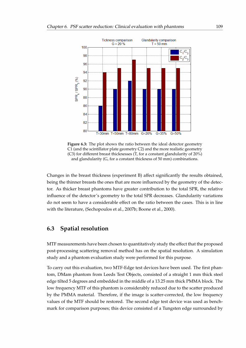
Chapter 6. PSF scatter reduction: Clinical evaluation with phantoms 109
Figure 6.3: The plot shows the ratio between the ideal detector geometryC1 (and the scintillator plate geometry C2) and the more realistic geometry(C3) for different breast thicknesses (T, for a constant glandularity of 20%)
and glandularity (G, for a constant thickness of 50 mm) combinations.
Changes in the breast thickness (experiment B) affect significantly the results obtained,being the thinner breasts the ones that are more influenced by the geometry of the detec-tor. As thicker breast phantoms have greater contribution to the total SPR, the relativeinfluence of the detector’s geometry to the total SPR decreases. Glandularity variationsdo not seem to have a considerable effect on the ratio between the cases. This is in linewith the literature, (Sechopoulos et al., 2007b; Boone et al., 2000).
6.3 Spatial resolution
MTF measurements have been chosen to quantitatively study the effect that the proposedpost-processing scattering removal method has on the spatial resolution. A simulationstudy and a phantom evaluation study were performed for this purpose.
To carry out this evaluation, two MTF-Edge test devices have been used. The first phan-tom, DMam phantom from Leeds Test Objects, consisted of a straight 1 mm thick steeledge tilted 5 degrees and embedded in the middle of a 13.25 mm thick PMMA block. Thelow frequency MTF of this phantom is considerably reduced due to the scatter producedby the PMMA material. Therefore, if the image is scatter-corrected, the low frequencyvalues of the MTF should be restored. The second edge test device was used as bench-mark for comparison purposes; this device consisted of a Tungsten edge surrounded by
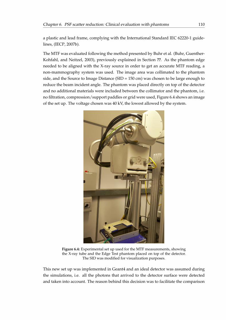
Chapter 6. PSF scatter reduction: Clinical evaluation with phantoms 110
a plastic and lead frame, complying with the International Standard IEC 62220-1 guide-lines, (IECP, 2007b).
The MTF was evaluated following the method presented by Buhr et al. (Buhr, Guenther-Kohfahl, and Neitzel, 2003), previously explained in Section ??. As the phantom edgeneeded to be aligned with the X-ray source in order to get an accurate MTF reading, anon-mammography system was used. The image area was collimated to the phantomside, and the Source to Image Distance (SID = 150 cm) was chosen to be large enough toreduce the beam incident angle. The phantom was placed directly on top of the detectorand no additional materials were included between the collimator and the phantom, i.e.no filtration, compression/support paddles or grid were used, Figure 6.4 shows an imageof the set up. The voltage chosen was 40 kV, the lowest allowed by the system.
Figure 6.4: Experimental set up used for the MTF measurements, showingthe X-ray tube and the Edge Test phantom placed on top of the detector.
The SID was modified for visualization purposes.
This new set up was implemented in Geant4 and an ideal detector was assumed duringthe simulations, i.e. all the photons that arrived to the detector surface were detectedand taken into account. The reason behind this decision was to facilitate the comparison
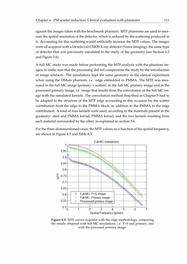
Chapter 6. PSF scatter reduction: Clinical evaluation with phantoms 111
against the images taken with the benchmark phantom. MTF phantoms are used to mea-sure the spatial resolution of the detector, which is reduced by the scattering produced init. Accounting for this scattering would artificially increase the MTF values. The imageswere all acquired with a Dexela Ltd CMOS X-ray detector (Varex Imaging), the same typeof detector that was previously simulated in the study of the geometry (see Section 6.2and Figure 5.6).
A full MC study was made before performing the MTF analysis with the phantom im-ages, to make sure that the processing did not compromise the study by the introductionof image artefacts. The simulations kept the same geometry as the clinical experimentwhen using the DMam phantom, i.e. edge embedded in PMMA. The MTF was mea-sured in the full MC image (primary + scatter), in the full MC primary image and in theprocessed primary image, i.e. image that results from the convolution of the full MC im-age with the simulated kernels. The convolution method described in Chapter 5 had tobe adapted to the structure of the MTF edge accounting in this occasion for the scattercontribution from the edge to the PMMA block, in addition to the PMMA to the edgecontribution. A total of four kernels were used, according to the materials present in thegeometry: steel and PMMA kernel, PMMA kernel, and the two kernels resulting fromeach material surrounded by the other, as explained in section 5.6.
For the three aforementioned cases, the MTF values, as a function of the spatial frequency,are shown in Figure 6.5 and Table 6.3.
Figure 6.5: MTF curves acquired with the edge methodology, comparingthe results obtained with full MC simulations, i.e. P+S and primary, and
with the processed primary image.
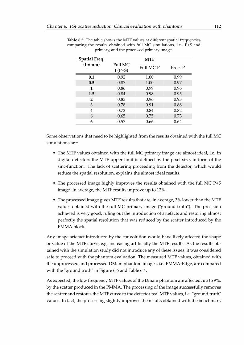
Chapter 6. PSF scatter reduction: Clinical evaluation with phantoms 112
Table 6.3: The table shows the MTF values at different spatial frequenciescomparing the results obtained with full MC simulations, i.e. P+S and
primary, and the processed primary image.
Spatial Freq.(lp/mm)
MTFFull MCI (P+S)
Full MC P Proc. P
0.1 0.92 1.00 0.990.5 0.87 1.00 0.971 0.86 0.99 0.96
1.5 0.84 0.98 0.952 0.83 0.96 0.933 0.78 0.91 0.884 0.72 0.84 0.825 0.65 0.75 0.736 0.57 0.66 0.64
Some observations that need to be highlighted from the results obtained with the full MCsimulations are:
• The MTF values obtained with the full MC primary image are almost ideal, i.e. indigital detectors the MTF upper limit is defined by the pixel size, in form of thesinc-function. The lack of scattering proceeding from the detector, which wouldreduce the spatial resolution, explains the almost ideal results.
• The processed image highly improves the results obtained with the full MC P+Simage. In average, the MTF results improve up to 12%.
• The processed image gives MTF results that are, in average, 3% lower than the MTFvalues obtained with the full MC primary image ("ground truth"). The precisionachieved is very good, ruling out the introduction of artefacts and restoring almostperfectly the spatial resolution that was reduced by the scatter introduced by thePMMA block.
Any image artefact introduced by the convolution would have likely affected the shapeor value of the MTF curve, e.g. increasing artificially the MTF results. As the results ob-tained with the simulation study did not introduce any of these issues, it was consideredsafe to proceed with the phantom evaluation. The measured MTF values, obtained withthe unprocessed and processed DMam phantom images, i.e. PMMA-Edge, are comparedwith the "ground truth" in Figure 6.6 and Table 6.4.
As expected, the low frequency MTF values of the Dmam phantom are affected, up to 9%,by the scatter produced in the PMMA. The processing of the image successfully removesthe scatter and restores the MTF curve to the detector real MTF values, i.e. "ground truth"values. In fact, the processing slightly improves the results obtained with the benchmark
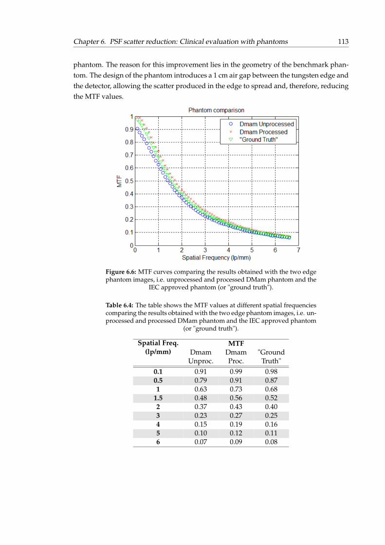
Chapter 6. PSF scatter reduction: Clinical evaluation with phantoms 113
phantom. The reason for this improvement lies in the geometry of the benchmark phan-tom. The design of the phantom introduces a 1 cm air gap between the tungsten edge andthe detector, allowing the scatter produced in the edge to spread and, therefore, reducingthe MTF values.
Figure 6.6: MTF curves comparing the results obtained with the two edgephantom images, i.e. unprocessed and processed DMam phantom and the
IEC approved phantom (or "ground truth").
Table 6.4: The table shows the MTF values at different spatial frequenciescomparing the results obtained with the two edge phantom images, i.e. un-processed and processed DMam phantom and the IEC approved phantom
(or "ground truth").
Spatial Freq.(lp/mm)
MTFDmam
Unproc.DmamProc.
"GroundTruth"
0.1 0.91 0.99 0.980.5 0.79 0.91 0.871 0.63 0.73 0.68
1.5 0.48 0.56 0.522 0.37 0.43 0.403 0.23 0.27 0.254 0.15 0.19 0.165 0.10 0.12 0.116 0.07 0.09 0.08

Chapter 6. PSF scatter reduction: Clinical evaluation with phantoms 114
6.4 Evaluation with phantoms designed for mammography
The impact that the selected scatter estimation method has in grid-less images has beenevaluated in the two previous sections using CMOS X-ray detectors, the technology de-veloped at the partner company Dexela Ltd (Varex Imaging Corporation). However,there are no Varex CMOS X-ray detectors currently being used for mammography ap-plications. Due to the difficulty in finding a mammography system with an embed-ded CMOS detector, an alternative technology was sought. The medical physics de-partment at Barts Health NHS trust (London, UK) and at the university hospital ParcTaulí (Sabadell, Spain) allocated time for continuing this study with one of their mam-mography systems. The technology chosen was α-Se. The Hologic Selenia Dimensionssystem at Parc Taulí hospital was used in combination with the CDMAM phantom (ver-sion 3.4); phantoms 010A from CIRS (CIRS) and TOR-MAS and TOR-MAM from LeedsTest Objects (TOR-MAS; TOR-MAM) were tested using the Hologic Lorad Selenia sys-tem available at Barts Health NHS trust, see Figure 6.7. The geometry of these systemswas simulated to obtain the PB kernels, following the information provided in Section5.3 and illustrated in Figure 5.6-right. The pixel size was kept at its real size, i.e. 70 µm,to analyse the images.
6.4.1 CDMAM
The CDMAM (Contrast Detail MAMography) phantom is a test object widely used forevaluating the detectability performance of mammography X-ray detectors. This contrast-detail phantom allows to assess the system ability to detect small lesions that have lowcontrast. The use of the CDMAM has been recommended in the European Protocol fordigital mammography quality assurance, as one of the ways of describing the image qual-ity of a X-ray system through contrast thresholding. (Grosjean and Muller, 2006; Díaz,2013; Binst et al., 2015)
The CDMAM phantom consists of a 2 mm thick aluminium base that holds a matrix ofgold discs and it is encased at the bottom of a 5 mm PMMA plate. Each cell of the matrixhas two identical discs; the first one is always placed at the centre of the cell while thesecond one is randomly placed in one of the four quadrants, see Figure 6.8. The diameterand thicknesses of the discs decrease logarithmically, from 2.0 to 0.06 mm and 2.0 to0.03 mm respectively, as the cells move across the rows and columns of the matrix (Díaz,2013; Binst et al., 2015).
The analysis exercise consists in detecting the position of the disc inserts in a flat noisybackground (Grosjean and Muller, 2006), starting with the cell that has thicker and big-ger discs and moving row by row towards the thinner/smaller discs. The scoring canbe made by a human reader or it can be automatized with a software. In this study the

Chapter 6. PSF scatter reduction: Clinical evaluation with phantoms 115
Figure 6.7: Example of the experimental set up used in this study. The im-age corresponds to the Hologic Selenia system located at Barts NHS trust.
analysis has been performed with the CDCOM 1.6 automated scoring method (availableat www.euref.com). The final results are normalised to the averaged human reader re-sponse, by multiplying with a given software-to-human ratio.
A set of images with and without grid were taken using different phantom thicknesses(20, 30, 40, 50 and 70 mm) and two energies per thickness. The two doses were chosenby the system’s Automatic Exposure Control (AEC) when the grid was in use (AEC wG)and removed (AEC w/oG) from the system. The dose given without the grid was 45%lower in average. See Table 6.5 for details of the chosen X-ray settings per thickness.
PMMA blocks were added to the CDMAM phantom to increase its thickness, i.e. thephantom has an equivalent PMMA thickness of 10 mm. The CDMAM phantom wasalways placed at a fixed distance of the support paddle, i.e. 20 mm, to be in line withthe experiment performed by Binst et al. (Binst et al., 2015). A 10 mm air gap betweenthe phantom and the support paddle was left in the first case, where the total phantom
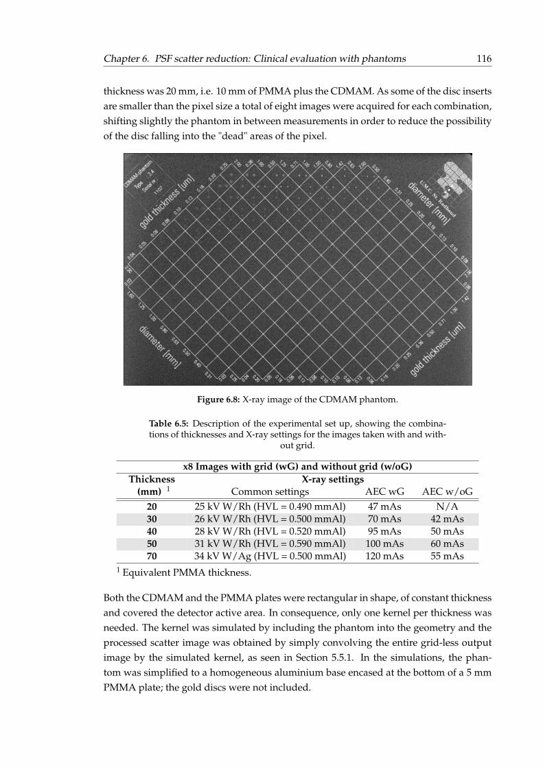
Chapter 6. PSF scatter reduction: Clinical evaluation with phantoms 116
thickness was 20 mm, i.e. 10 mm of PMMA plus the CDMAM. As some of the disc insertsare smaller than the pixel size a total of eight images were acquired for each combination,shifting slightly the phantom in between measurements in order to reduce the possibilityof the disc falling into the "dead" areas of the pixel.
Figure 6.8: X-ray image of the CDMAM phantom.
Table 6.5: Description of the experimental set up, showing the combina-tions of thicknesses and X-ray settings for the images taken with and with-
out grid.
x8 Images with grid (wG) and without grid (w/oG)Thickness X-ray settings
(mm) 1 Common settings AEC wG AEC w/oG20 25 kV W/Rh (HVL = 0.490 mmAl) 47 mAs N/A30 26 kV W/Rh (HVL = 0.500 mmAl) 70 mAs 42 mAs40 28 kV W/Rh (HVL = 0.520 mmAl) 95 mAs 50 mAs50 31 kV W/Rh (HVL = 0.590 mmAl) 100 mAs 60 mAs70 34 kV W/Ag (HVL = 0.500 mmAl) 120 mAs 55 mAs
1 Equivalent PMMA thickness.
Both the CDMAM and the PMMA plates were rectangular in shape, of constant thicknessand covered the detector active area. In consequence, only one kernel per thickness wasneeded. The kernel was simulated by including the phantom into the geometry and theprocessed scatter image was obtained by simply convolving the entire grid-less outputimage by the simulated kernel, as seen in Section 5.5.1. In the simulations, the phan-tom was simplified to a homogeneous aluminium base encased at the bottom of a 5 mmPMMA plate; the gold discs were not included.
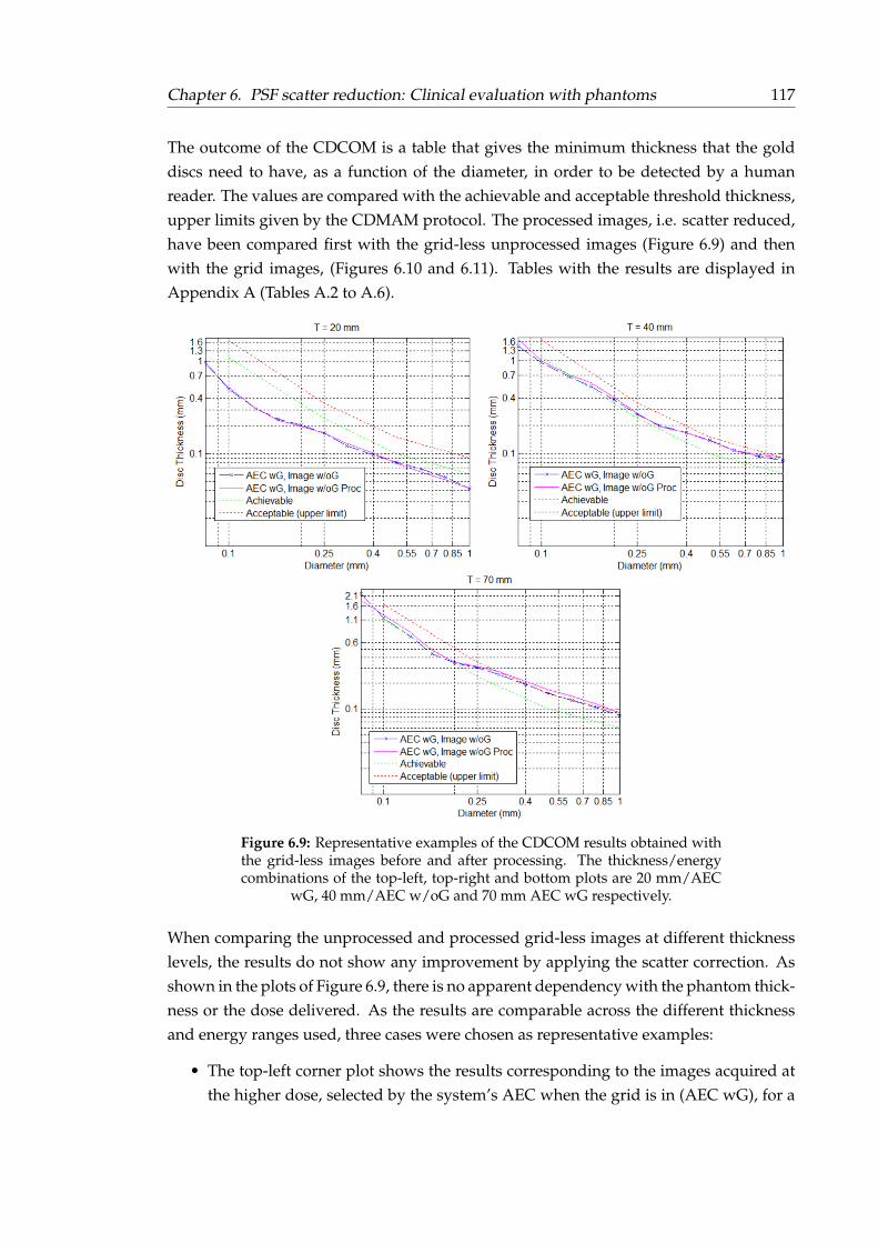
Chapter 6. PSF scatter reduction: Clinical evaluation with phantoms 117
The outcome of the CDCOM is a table that gives the minimum thickness that the golddiscs need to have, as a function of the diameter, in order to be detected by a humanreader. The values are compared with the achievable and acceptable threshold thickness,upper limits given by the CDMAM protocol. The processed images, i.e. scatter reduced,have been compared first with the grid-less unprocessed images (Figure 6.9) and thenwith the grid images, (Figures 6.10 and 6.11). Tables with the results are displayed inAppendix A (Tables A.2 to A.6).
Figure 6.9: Representative examples of the CDCOM results obtained withthe grid-less images before and after processing. The thickness/energycombinations of the top-left, top-right and bottom plots are 20 mm/AEC
wG, 40 mm/AEC w/oG and 70 mm AEC wG respectively.
When comparing the unprocessed and processed grid-less images at different thicknesslevels, the results do not show any improvement by applying the scatter correction. Asshown in the plots of Figure 6.9, there is no apparent dependency with the phantom thick-ness or the dose delivered. As the results are comparable across the different thicknessand energy ranges used, three cases were chosen as representative examples:
• The top-left corner plot shows the results corresponding to the images acquired atthe higher dose, selected by the system’s AEC when the grid is in (AEC wG), for a
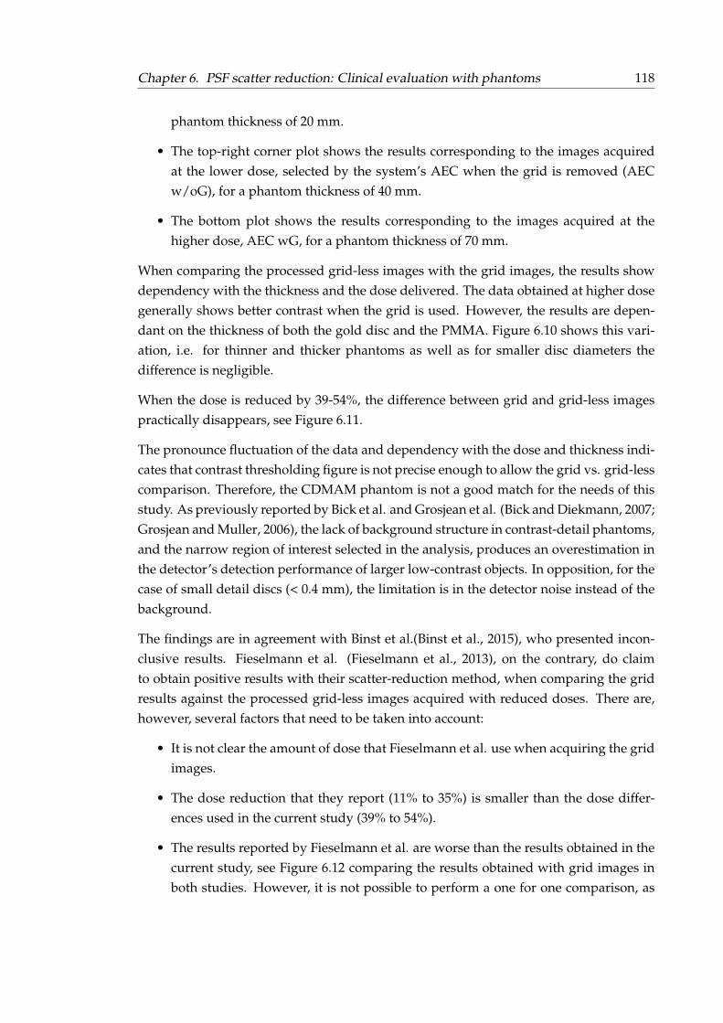
Chapter 6. PSF scatter reduction: Clinical evaluation with phantoms 118
phantom thickness of 20 mm.
• The top-right corner plot shows the results corresponding to the images acquiredat the lower dose, selected by the system’s AEC when the grid is removed (AECw/oG), for a phantom thickness of 40 mm.
• The bottom plot shows the results corresponding to the images acquired at thehigher dose, AEC wG, for a phantom thickness of 70 mm.
When comparing the processed grid-less images with the grid images, the results showdependency with the thickness and the dose delivered. The data obtained at higher dosegenerally shows better contrast when the grid is used. However, the results are depen-dant on the thickness of both the gold disc and the PMMA. Figure 6.10 shows this vari-ation, i.e. for thinner and thicker phantoms as well as for smaller disc diameters thedifference is negligible.
When the dose is reduced by 39-54%, the difference between grid and grid-less imagespractically disappears, see Figure 6.11.
The pronounce fluctuation of the data and dependency with the dose and thickness indi-cates that contrast thresholding figure is not precise enough to allow the grid vs. grid-lesscomparison. Therefore, the CDMAM phantom is not a good match for the needs of thisstudy. As previously reported by Bick et al. and Grosjean et al. (Bick and Diekmann, 2007;Grosjean and Muller, 2006), the lack of background structure in contrast-detail phantoms,and the narrow region of interest selected in the analysis, produces an overestimation inthe detector’s detection performance of larger low-contrast objects. In opposition, for thecase of small detail discs (< 0.4 mm), the limitation is in the detector noise instead of thebackground.
The findings are in agreement with Binst et al.(Binst et al., 2015), who presented incon-clusive results. Fieselmann et al. (Fieselmann et al., 2013), on the contrary, do claimto obtain positive results with their scatter-reduction method, when comparing the gridresults against the processed grid-less images acquired with reduced doses. There are,however, several factors that need to be taken into account:
• It is not clear the amount of dose that Fieselmann et al. use when acquiring the gridimages.
• The dose reduction that they report (11% to 35%) is smaller than the dose differ-ences used in the current study (39% to 54%).
• The results reported by Fieselmann et al. are worse than the results obtained in thecurrent study, see Figure 6.12 comparing the results obtained with grid images inboth studies. However, it is not possible to perform a one for one comparison, as
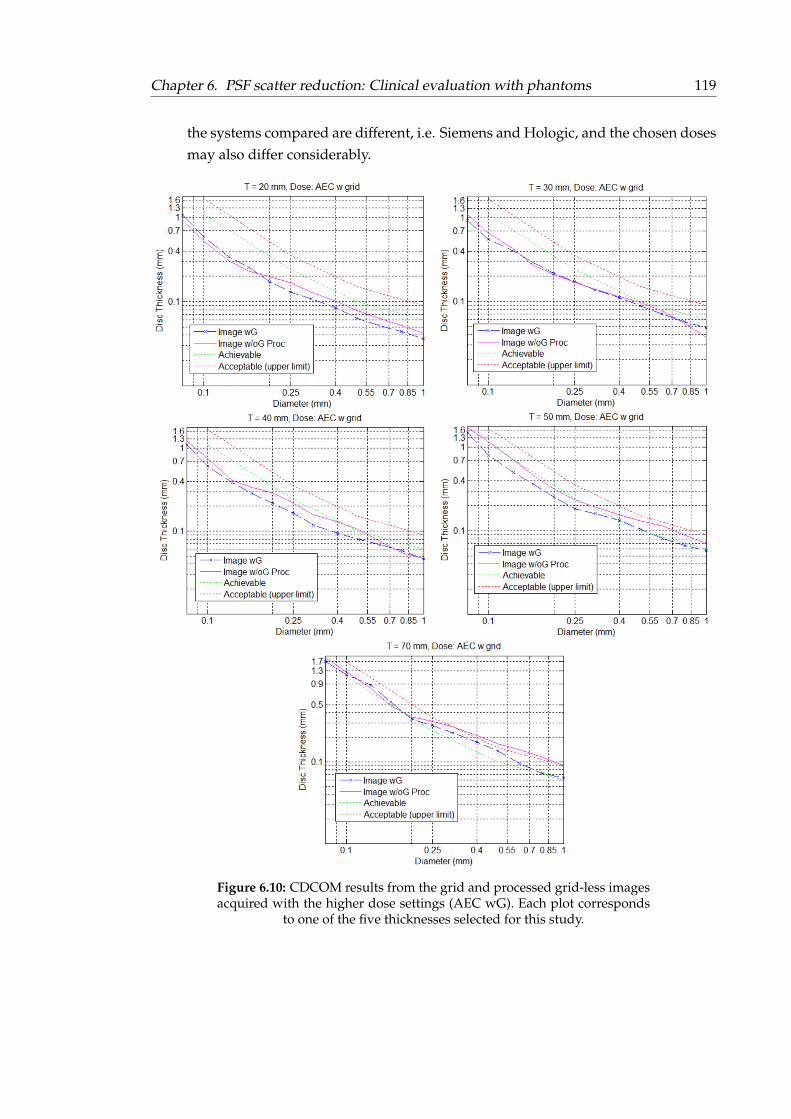
Chapter 6. PSF scatter reduction: Clinical evaluation with phantoms 119
the systems compared are different, i.e. Siemens and Hologic, and the chosen dosesmay also differ considerably.
Figure 6.10: CDCOM results from the grid and processed grid-less imagesacquired with the higher dose settings (AEC wG). Each plot corresponds
to one of the five thicknesses selected for this study.
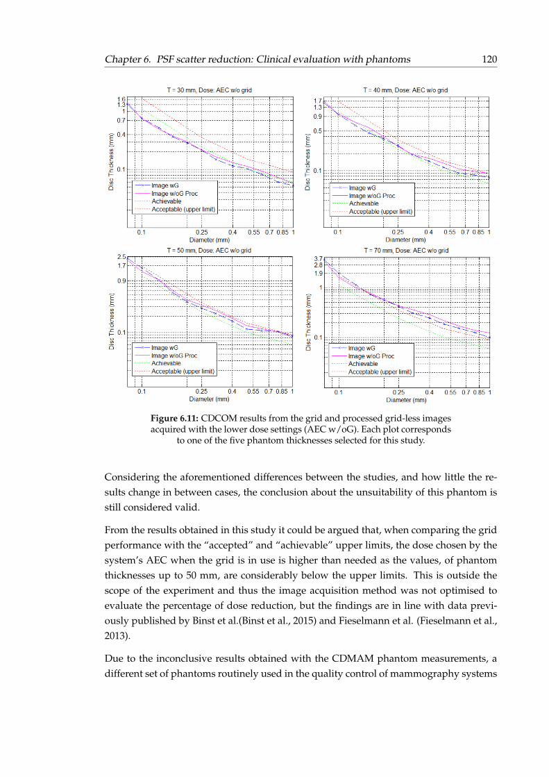
Chapter 6. PSF scatter reduction: Clinical evaluation with phantoms 120
Figure 6.11: CDCOM results from the grid and processed grid-less imagesacquired with the lower dose settings (AEC w/oG). Each plot corresponds
to one of the five phantom thicknesses selected for this study.
Considering the aforementioned differences between the studies, and how little the re-sults change in between cases, the conclusion about the unsuitability of this phantom isstill considered valid.
From the results obtained in this study it could be argued that, when comparing the gridperformance with the “accepted” and “achievable” upper limits, the dose chosen by thesystem’s AEC when the grid is in use is higher than needed as the values, of phantomthicknesses up to 50 mm, are considerably below the upper limits. This is outside thescope of the experiment and thus the image acquisition method was not optimised toevaluate the percentage of dose reduction, but the findings are in line with data previ-ously published by Binst et al.(Binst et al., 2015) and Fieselmann et al. (Fieselmann et al.,2013).
Due to the inconclusive results obtained with the CDMAM phantom measurements, adifferent set of phantoms routinely used in the quality control of mammography systems
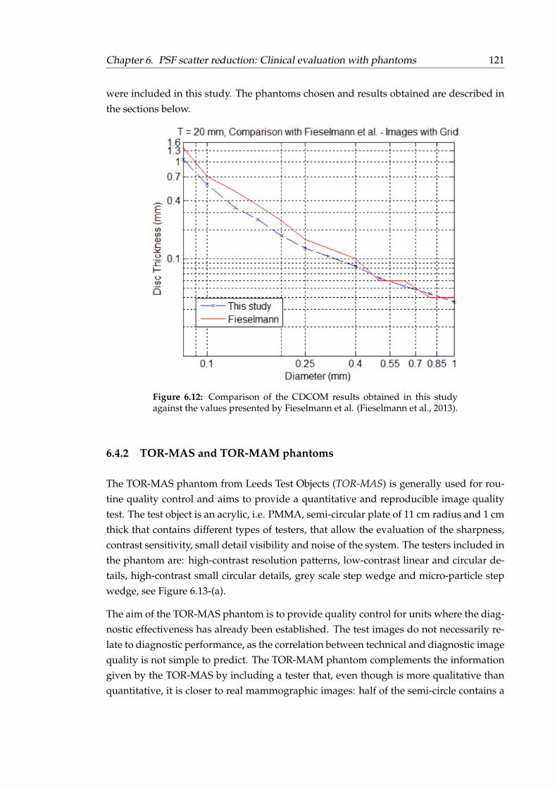
Chapter 6. PSF scatter reduction: Clinical evaluation with phantoms 121
were included in this study. The phantoms chosen and results obtained are described inthe sections below.
Figure 6.12: Comparison of the CDCOM results obtained in this studyagainst the values presented by Fieselmann et al. (Fieselmann et al., 2013).
6.4.2 TOR-MAS and TOR-MAM phantoms
The TOR-MAS phantom from Leeds Test Objects (TOR-MAS) is generally used for rou-tine quality control and aims to provide a quantitative and reproducible image qualitytest. The test object is an acrylic, i.e. PMMA, semi-circular plate of 11 cm radius and 1 cmthick that contains different types of testers, that allow the evaluation of the sharpness,contrast sensitivity, small detail visibility and noise of the system. The testers included inthe phantom are: high-contrast resolution patterns, low-contrast linear and circular de-tails, high-contrast small circular details, grey scale step wedge and micro-particle stepwedge, see Figure 6.13-(a).
The aim of the TOR-MAS phantom is to provide quality control for units where the diag-nostic effectiveness has already been established. The test images do not necessarily re-late to diagnostic performance, as the correlation between technical and diagnostic imagequality is not simple to predict. The TOR-MAM phantom complements the informationgiven by the TOR-MAS by including a tester that, even though is more qualitative thanquantitative, it is closer to real mammographic images: half of the semi-circle contains a
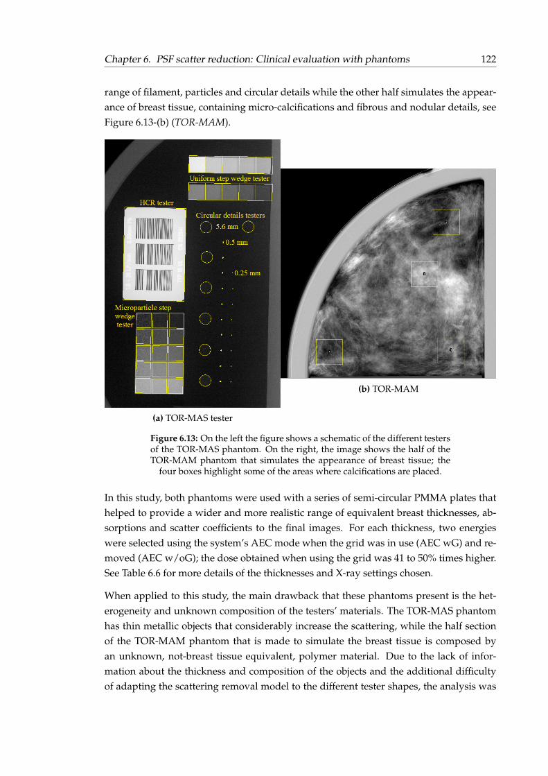
Chapter 6. PSF scatter reduction: Clinical evaluation with phantoms 122
range of filament, particles and circular details while the other half simulates the appear-ance of breast tissue, containing micro-calcifications and fibrous and nodular details, seeFigure 6.13-(b) (TOR-MAM).
(a) TOR-MAS tester
(b) TOR-MAM
Figure 6.13: On the left the figure shows a schematic of the different testersof the TOR-MAS phantom. On the right, the image shows the half of theTOR-MAM phantom that simulates the appearance of breast tissue; the
four boxes highlight some of the areas where calcifications are placed.
In this study, both phantoms were used with a series of semi-circular PMMA plates thathelped to provide a wider and more realistic range of equivalent breast thicknesses, ab-sorptions and scatter coefficients to the final images. For each thickness, two energieswere selected using the system’s AEC mode when the grid was in use (AEC wG) and re-moved (AEC w/oG); the dose obtained when using the grid was 41 to 50% times higher.See Table 6.6 for more details of the thicknesses and X-ray settings chosen.
When applied to this study, the main drawback that these phantoms present is the het-erogeneity and unknown composition of the testers’ materials. The TOR-MAS phantomhas thin metallic objects that considerably increase the scattering, while the half sectionof the TOR-MAM phantom that is made to simulate the breast tissue is composed byan unknown, not-breast tissue equivalent, polymer material. Due to the lack of infor-mation about the thickness and composition of the objects and the additional difficultyof adapting the scattering removal model to the different tester shapes, the analysis was
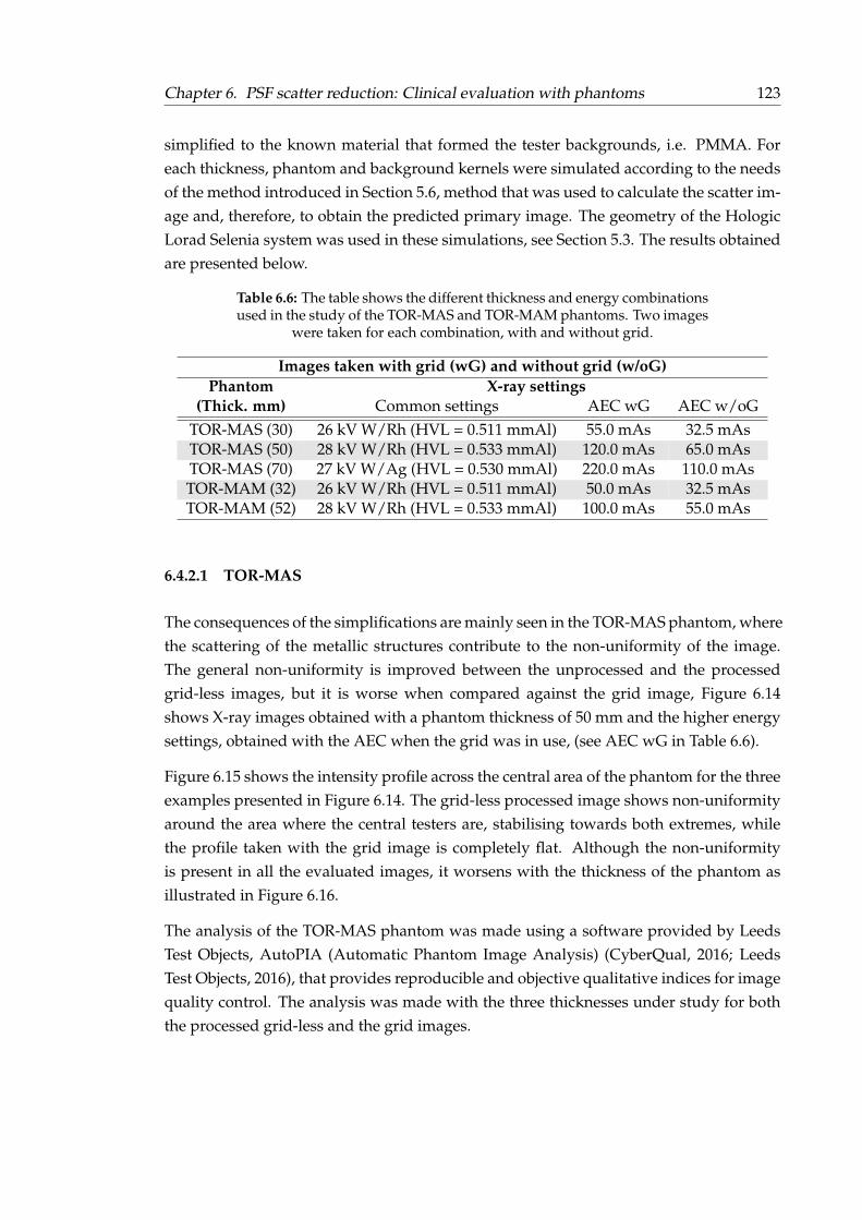
Chapter 6. PSF scatter reduction: Clinical evaluation with phantoms 123
simplified to the known material that formed the tester backgrounds, i.e. PMMA. Foreach thickness, phantom and background kernels were simulated according to the needsof the method introduced in Section 5.6, method that was used to calculate the scatter im-age and, therefore, to obtain the predicted primary image. The geometry of the HologicLorad Selenia system was used in these simulations, see Section 5.3. The results obtainedare presented below.
Table 6.6: The table shows the different thickness and energy combinationsused in the study of the TOR-MAS and TOR-MAM phantoms. Two images
were taken for each combination, with and without grid.
Images taken with grid (wG) and without grid (w/oG)Phantom X-ray settings
(Thick. mm) Common settings AEC wG AEC w/oGTOR-MAS (30) 26 kV W/Rh (HVL = 0.511 mmAl) 55.0 mAs 32.5 mAsTOR-MAS (50) 28 kV W/Rh (HVL = 0.533 mmAl) 120.0 mAs 65.0 mAsTOR-MAS (70) 27 kV W/Ag (HVL = 0.530 mmAl) 220.0 mAs 110.0 mAsTOR-MAM (32) 26 kV W/Rh (HVL = 0.511 mmAl) 50.0 mAs 32.5 mAsTOR-MAM (52) 28 kV W/Rh (HVL = 0.533 mmAl) 100.0 mAs 55.0 mAs
6.4.2.1 TOR-MAS
The consequences of the simplifications are mainly seen in the TOR-MAS phantom, wherethe scattering of the metallic structures contribute to the non-uniformity of the image.The general non-uniformity is improved between the unprocessed and the processedgrid-less images, but it is worse when compared against the grid image, Figure 6.14shows X-ray images obtained with a phantom thickness of 50 mm and the higher energysettings, obtained with the AEC when the grid was in use, (see AEC wG in Table 6.6).
Figure 6.15 shows the intensity profile across the central area of the phantom for the threeexamples presented in Figure 6.14. The grid-less processed image shows non-uniformityaround the area where the central testers are, stabilising towards both extremes, whilethe profile taken with the grid image is completely flat. Although the non-uniformityis present in all the evaluated images, it worsens with the thickness of the phantom asillustrated in Figure 6.16.
The analysis of the TOR-MAS phantom was made using a software provided by LeedsTest Objects, AutoPIA (Automatic Phantom Image Analysis) (CyberQual, 2016; LeedsTest Objects, 2016), that provides reproducible and objective qualitative indices for imagequality control. The analysis was made with the three thicknesses under study for boththe processed grid-less and the grid images.
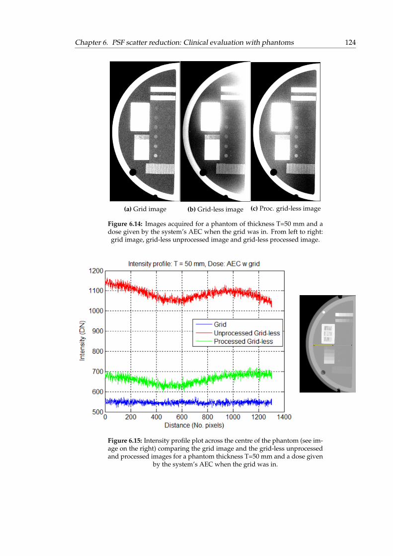
Chapter 6. PSF scatter reduction: Clinical evaluation with phantoms 124
(a) Grid image (b) Grid-less image (c) Proc. grid-less image
Figure 6.14: Images acquired for a phantom of thickness T=50 mm and adose given by the system’s AEC when the grid was in. From left to right:grid image, grid-less unprocessed image and grid-less processed image.
Figure 6.15: Intensity profile plot across the centre of the phantom (see im-age on the right) comparing the grid image and the grid-less unprocessedand processed images for a phantom thickness T=50 mm and a dose given
by the system’s AEC when the grid was in.
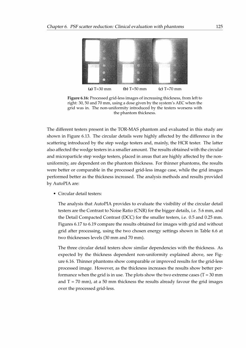
Chapter 6. PSF scatter reduction: Clinical evaluation with phantoms 125
(a) T=30 mm (b) T=50 mm (c) T=70 mm
Figure 6.16: Processed grid-less images of increasing thickness, from left toright: 30, 50 and 70 mm, using a dose given by the system’s AEC when thegrid was in. The non-uniformity introduced by the testers worsens with
the phantom thickness.
The different testers present in the TOR-MAS phantom and evaluated in this study areshown in Figure 6.13. The circular details were highly affected by the difference in thescattering introduced by the step wedge testers and, mainly, the HCR tester. The latteralso affected the wedge testers in a smaller amount. The results obtained with the circularand microparticle step wedge testers, placed in areas that are highly affected by the non-uniformity, are dependent on the phantom thickness. For thinner phantoms, the resultswere better or comparable in the processed grid-less image case, while the grid imagesperformed better as the thickness increased. The analysis methods and results providedby AutoPIA are:
• Circular detail testers:
The analysis that AutoPIA provides to evaluate the visibility of the circular detailtesters are the Contrast to Noise Ratio (CNR) for the bigger details, i.e. 5.6 mm, andthe Detail Compacted Contrast (DCC) for the smaller testers, i.e. 0.5 and 0.25 mm.Figures 6.17 to 6.19 compare the results obtained for images with grid and withoutgrid after processing, using the two chosen energy settings shown in Table 6.6 attwo thicknesses levels (30 mm and 70 mm).
The three circular detail testers show similar dependencies with the thickness. Asexpected by the thickness dependent non-uniformity explained above, see Fig-ure 6.16. Thinner phantoms show comparable or improved results for the grid-lessprocessed image. However, as the thickness increases the results show better per-formance when the grid is in use. The plots show the two extreme cases (T = 30 mmand T = 70 mm), at a 50 mm thickness the results already favour the grid imagesover the processed grid-less.

Chapter 6. PSF scatter reduction: Clinical evaluation with phantoms 126
Figure 6.17: Analysis of the 5.6 mm circular detail tester. The plots showthe CNR versus the nominal contrast for the grid and processed grid-lessimages acquired with the two dose settings at thicknesses 30 and 70 mm
(left and right respectively).
Figure 6.18: Analysis of the 0.5 mm circular detail tester. The plots showthe DCC versus the nominal contrast for the grid and processed grid-lessimages acquired with the two dose settings at thicknesses 30 and 70 mm
(left and right respectively).
• Microparticle step wedge tester:
AutoPIA’s analysis of the microparticle step wedge tester is performed by calculat-ing the variance ratio between each step and a reference value that is always keptconstant (taken from the uniform step wedge tester). The results comparing thevariance ratio versus the tester’s nominal contrast for the 30 and 70 mm images aregiven by Figures 6.20 and 6.21. The former plot refers to the smaller particle size ofthe tester (125 µm, right column of the tester) and the latter to the bigger particlesize (328 µm, left column of the tester).

Chapter 6. PSF scatter reduction: Clinical evaluation with phantoms 127
Figure 6.19: Analysis of the 0.25 mm circular detail tester. The plots showthe DCC versus the nominal contrast for the grid and processed grid-lessimages acquired with the two dose settings at thicknesses 30 and 70 mm
(left and right respectively).
Figure 6.20: Analysis of the microparticle step wedge tester for particle sizeof 125 µm. The plots show the variance ratio versus the nominal contrastfor the grid and processed grid-less images acquired with the two dose
settings at thicknesses 30 and 70 mm (left and right respectively).
As shown in the plots, the processed grid-less image performs better than the gridimage for the smaller particle size in the tester, independently of the phantom’sthickness. As the particle size increases, the results become thickness dependent,similarly to the circular detail tester: thinner breasts perform better with the pro-cessed grid-less image while thicker breasts favour the grid images. The processedimage improves in response at smaller nominal contrast, the area that is furtheraway from the HCR tester and is, therefore, less affected by the non-uniformity.For lower doses, i.e. dose given by the AEC when the grid is removed, the resultsbecome comparable and do not show dependency with the thickness.
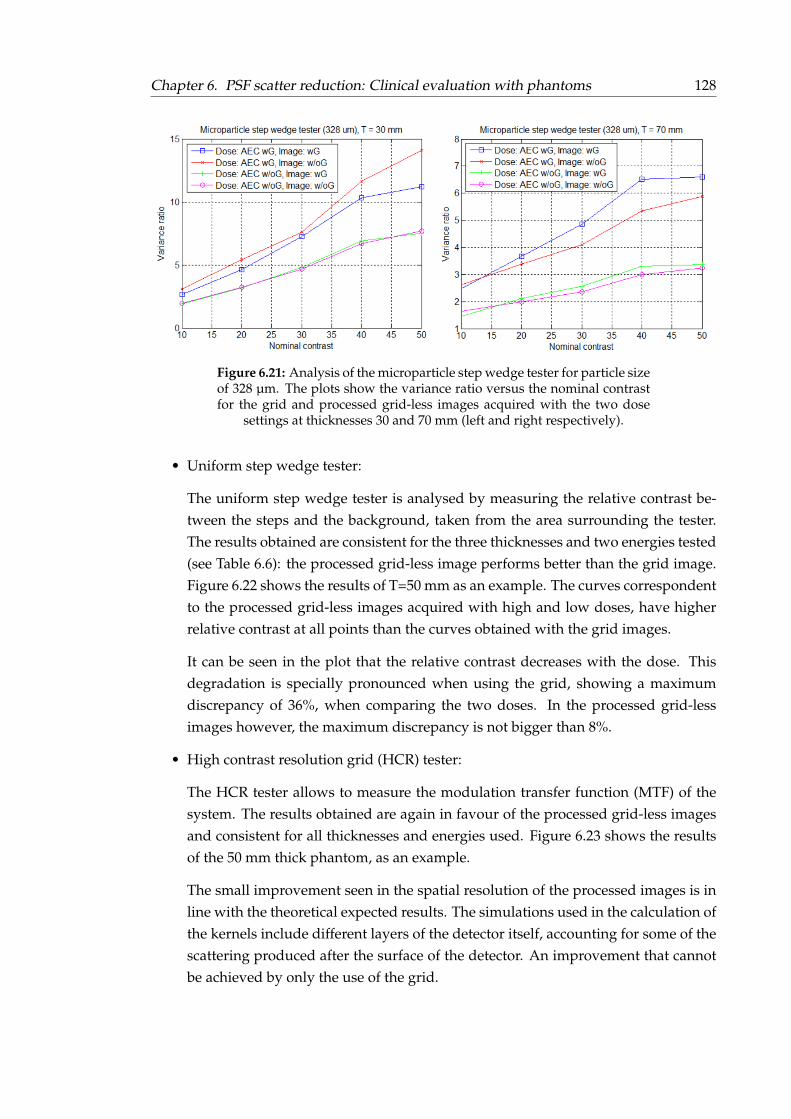
Chapter 6. PSF scatter reduction: Clinical evaluation with phantoms 128
Figure 6.21: Analysis of the microparticle step wedge tester for particle sizeof 328 µm. The plots show the variance ratio versus the nominal contrastfor the grid and processed grid-less images acquired with the two dose
settings at thicknesses 30 and 70 mm (left and right respectively).
• Uniform step wedge tester:
The uniform step wedge tester is analysed by measuring the relative contrast be-tween the steps and the background, taken from the area surrounding the tester.The results obtained are consistent for the three thicknesses and two energies tested(see Table 6.6): the processed grid-less image performs better than the grid image.Figure 6.22 shows the results of T=50 mm as an example. The curves correspondentto the processed grid-less images acquired with high and low doses, have higherrelative contrast at all points than the curves obtained with the grid images.
It can be seen in the plot that the relative contrast decreases with the dose. Thisdegradation is specially pronounced when using the grid, showing a maximumdiscrepancy of 36%, when comparing the two doses. In the processed grid-lessimages however, the maximum discrepancy is not bigger than 8%.
• High contrast resolution grid (HCR) tester:
The HCR tester allows to measure the modulation transfer function (MTF) of thesystem. The results obtained are again in favour of the processed grid-less imagesand consistent for all thicknesses and energies used. Figure 6.23 shows the resultsof the 50 mm thick phantom, as an example.
The small improvement seen in the spatial resolution of the processed images is inline with the theoretical expected results. The simulations used in the calculation ofthe kernels include different layers of the detector itself, accounting for some of thescattering produced after the surface of the detector. An improvement that cannotbe achieved by only the use of the grid.
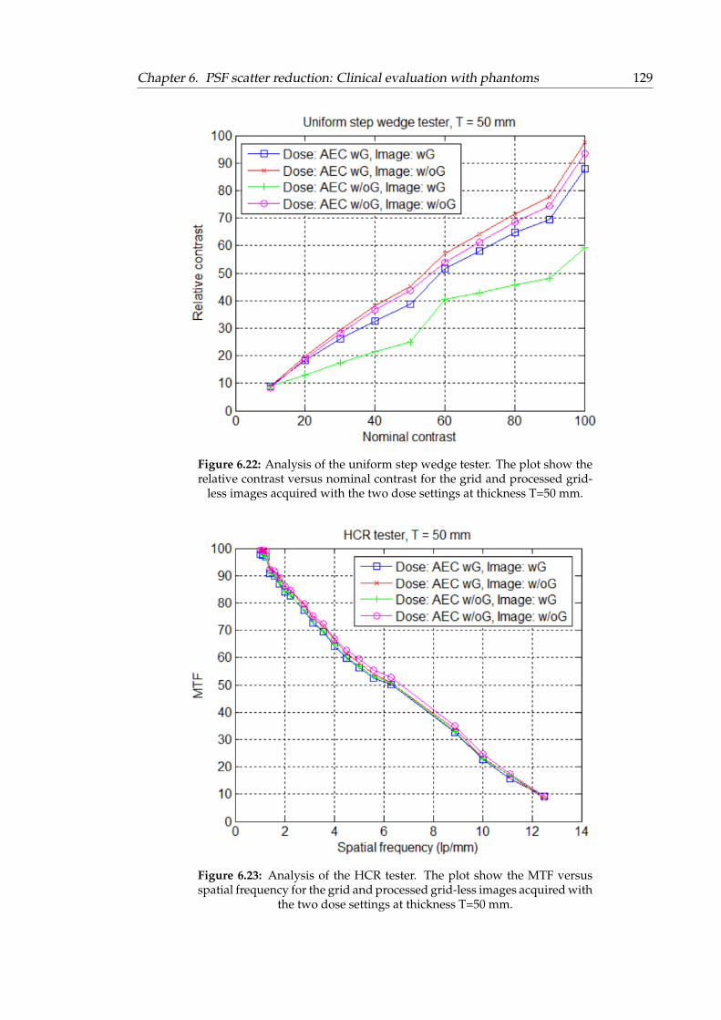
Chapter 6. PSF scatter reduction: Clinical evaluation with phantoms 129
Figure 6.22: Analysis of the uniform step wedge tester. The plot show therelative contrast versus nominal contrast for the grid and processed grid-
less images acquired with the two dose settings at thickness T=50 mm.
Figure 6.23: Analysis of the HCR tester. The plot show the MTF versusspatial frequency for the grid and processed grid-less images acquired with
the two dose settings at thickness T=50 mm.
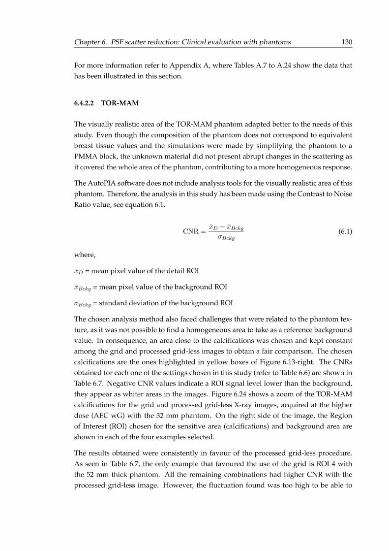
Chapter 6. PSF scatter reduction: Clinical evaluation with phantoms 130
For more information refer to Appendix A, where Tables A.7 to A.24 show the data thathas been illustrated in this section.
6.4.2.2 TOR-MAM
The visually realistic area of the TOR-MAM phantom adapted better to the needs of thisstudy. Even though the composition of the phantom does not correspond to equivalentbreast tissue values and the simulations were made by simplifying the phantom to aPMMA block, the unknown material did not present abrupt changes in the scattering asit covered the whole area of the phantom, contributing to a more homogeneous response.
The AutoPIA software does not include analysis tools for the visually realistic area of thisphantom. Therefore, the analysis in this study has been made using the Contrast to NoiseRatio value, see equation 6.1.
CNR =xD − xBckgσBckg
(6.1)
where,
xD = mean pixel value of the detail ROI
xBckg = mean pixel value of the background ROI
σBckg = standard deviation of the background ROI
The chosen analysis method also faced challenges that were related to the phantom tex-ture, as it was not possible to find a homogeneous area to take as a reference backgroundvalue. In consequence, an area close to the calcifications was chosen and kept constantamong the grid and processed grid-less images to obtain a fair comparison. The chosencalcifications are the ones highlighted in yellow boxes of Figure 6.13-right. The CNRsobtained for each one of the settings chosen in this study (refer to Table 6.6) are shown inTable 6.7. Negative CNR values indicate a ROI signal level lower than the background,they appear as whiter areas in the images. Figure 6.24 shows a zoom of the TOR-MAMcalcifications for the grid and processed grid-less X-ray images, acquired at the higherdose (AEC wG) with the 32 mm phantom. On the right side of the image, the Regionof Interest (ROI) chosen for the sensitive area (calcifications) and background area areshown in each of the four examples selected.
The results obtained were consistently in favour of the processed grid-less procedure.As seen in Table 6.7, the only example that favoured the use of the grid is ROI 4 withthe 52 mm thick phantom. All the remaining combinations had higher CNR with theprocessed grid-less image. However, the fluctuation found was too high to be able to
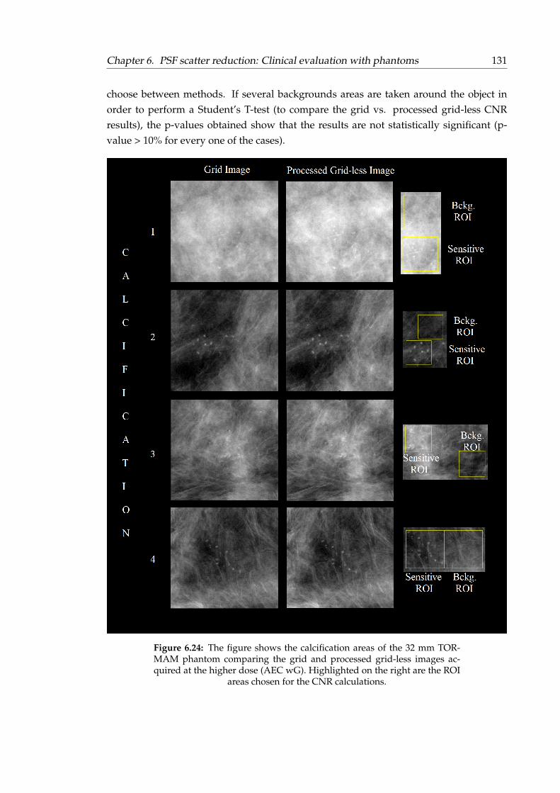
Chapter 6. PSF scatter reduction: Clinical evaluation with phantoms 131
choose between methods. If several backgrounds areas are taken around the object inorder to perform a Student’s T-test (to compare the grid vs. processed grid-less CNRresults), the p-values obtained show that the results are not statistically significant (p-value > 10% for every one of the cases).
Figure 6.24: The figure shows the calcification areas of the 32 mm TOR-MAM phantom comparing the grid and processed grid-less images ac-quired at the higher dose (AEC wG). Highlighted on the right are the ROI
areas chosen for the CNR calculations.
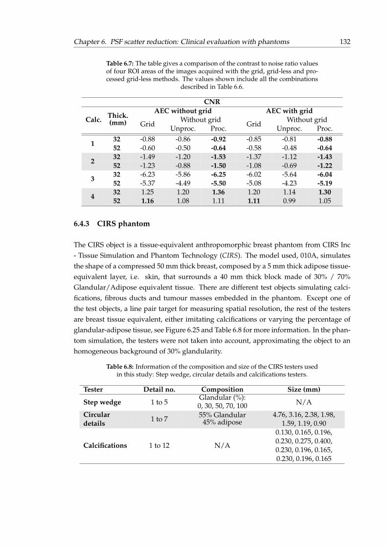
Chapter 6. PSF scatter reduction: Clinical evaluation with phantoms 132
Table 6.7: The table gives a comparison of the contrast to noise ratio valuesof four ROI areas of the images acquired with the grid, grid-less and pro-cessed grid-less methods. The values shown include all the combinations
described in Table 6.6.
CNR
Calc. Thick.(mm)
AEC without grid AEC with grid
GridWithout grid
GridWithout grid
Unproc. Proc. Unproc. Proc.
132 -0.88 -0.86 -0.92 -0.85 -0.81 -0.8852 -0.60 -0.50 -0.64 -0.58 -0.48 -0.6432 -1.49 -1.20 -1.53 -1.37 -1.12 -1.43
252 -1.23 -0.88 -1.50 -1.08 -0.69 -1.22
332 -6.23 -5.86 -6.25 -6.02 -5.64 -6.0452 -5.37 -4.49 -5.50 -5.08 -4.23 -5.1932 1.25 1.20 1.36 1.20 1.14 1.30
452 1.16 1.08 1.11 1.11 0.99 1.05
6.4.3 CIRS phantom
The CIRS object is a tissue-equivalent anthropomorphic breast phantom from CIRS Inc- Tissue Simulation and Phantom Technology (CIRS). The model used, 010A, simulatesthe shape of a compressed 50 mm thick breast, composed by a 5 mm thick adipose tissue-equivalent layer, i.e. skin, that surrounds a 40 mm thick block made of 30% / 70%Glandular/Adipose equivalent tissue. There are different test objects simulating calci-fications, fibrous ducts and tumour masses embedded in the phantom. Except one ofthe test objects, a line pair target for measuring spatial resolution, the rest of the testersare breast tissue equivalent, either imitating calcifications or varying the percentage ofglandular-adipose tissue, see Figure 6.25 and Table 6.8 for more information. In the phan-tom simulation, the testers were not taken into account, approximating the object to anhomogeneous background of 30% glandularity.
Table 6.8: Information of the composition and size of the CIRS testers usedin this study: Step wedge, circular details and calcifications testers.
Tester Detail no. Composition Size (mm)
Step wedge 1 to 5Glandular (%):0, 30, 50, 70, 100 N/A
Circulardetails
1 to 7 55% Glandular45% adipose
4.76, 3.16, 2.38, 1.98,1.59, 1.19, 0.90
Calcifications 1 to 12 N/A
0.130, 0.165, 0.196,0.230, 0.275, 0.400,0.230, 0.196, 0.165,0.230, 0.196, 0.165
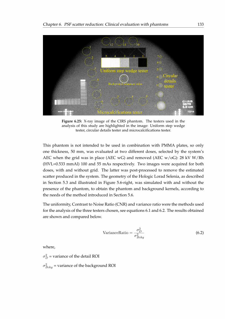
Chapter 6. PSF scatter reduction: Clinical evaluation with phantoms 133
Figure 6.25: X-ray image of the CIRS phantom. The testers used in theanalysis of this study are highlighted in the image: Uniform step wedge
tester, circular details tester and microcalcifications tester.
This phantom is not intended to be used in combination with PMMA plates, so onlyone thickness, 50 mm, was evaluated at two different doses, selected by the system’sAEC when the grid was in place (AEC wG) and removed (AEC w/oG): 28 kV W/Rh(HVL=0.533 mmAl) 100 and 55 mAs respectively. Two images were acquired for bothdoses, with and without grid. The latter was post-processed to remove the estimatedscatter produced in the system. The geometry of the Hologic Lorad Selenia, as describedin Section 5.3 and illustrated in Figure 5.6-right, was simulated with and without thepresence of the phantom, to obtain the phantom and background kernels, according tothe needs of the method introduced in Section 5.6.
The uniformity, Contrast to Noise Ratio (CNR) and variance ratio were the methods usedfor the analysis of the three testers chosen, see equations 6.1 and 6.2. The results obtainedare shown and compared below.
VarianceRatio =σ2D
σ2Bckg
(6.2)
where,
σ2D = variance of the detail ROI
σ2Bckg = variance of the background ROI
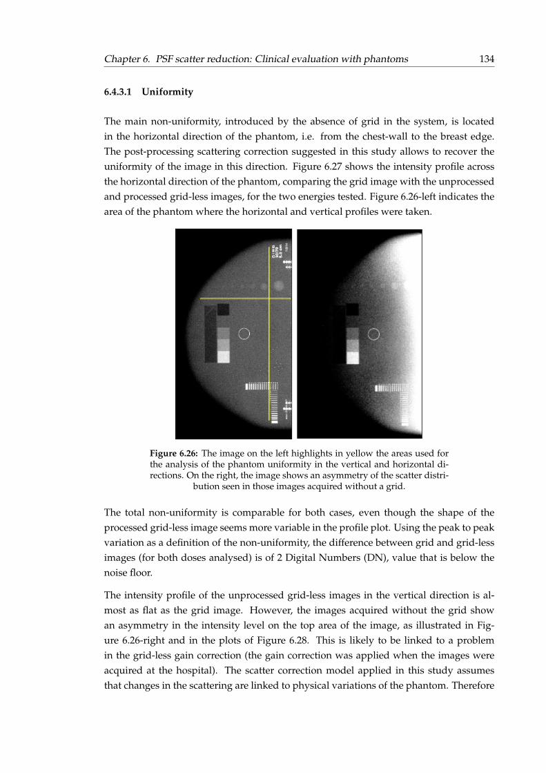
Chapter 6. PSF scatter reduction: Clinical evaluation with phantoms 134
6.4.3.1 Uniformity
The main non-uniformity, introduced by the absence of grid in the system, is locatedin the horizontal direction of the phantom, i.e. from the chest-wall to the breast edge.The post-processing scattering correction suggested in this study allows to recover theuniformity of the image in this direction. Figure 6.27 shows the intensity profile acrossthe horizontal direction of the phantom, comparing the grid image with the unprocessedand processed grid-less images, for the two energies tested. Figure 6.26-left indicates thearea of the phantom where the horizontal and vertical profiles were taken.
Figure 6.26: The image on the left highlights in yellow the areas used forthe analysis of the phantom uniformity in the vertical and horizontal di-rections. On the right, the image shows an asymmetry of the scatter distri-
bution seen in those images acquired without a grid.
The total non-uniformity is comparable for both cases, even though the shape of theprocessed grid-less image seems more variable in the profile plot. Using the peak to peakvariation as a definition of the non-uniformity, the difference between grid and grid-lessimages (for both doses analysed) is of 2 Digital Numbers (DN), value that is below thenoise floor.
The intensity profile of the unprocessed grid-less images in the vertical direction is al-most as flat as the grid image. However, the images acquired without the grid showan asymmetry in the intensity level on the top area of the image, as illustrated in Fig-ure 6.26-right and in the plots of Figure 6.28. This is likely to be linked to a problemin the grid-less gain correction (the gain correction was applied when the images wereacquired at the hospital). The scatter correction model applied in this study assumesthat changes in the scattering are linked to physical variations of the phantom. Therefore
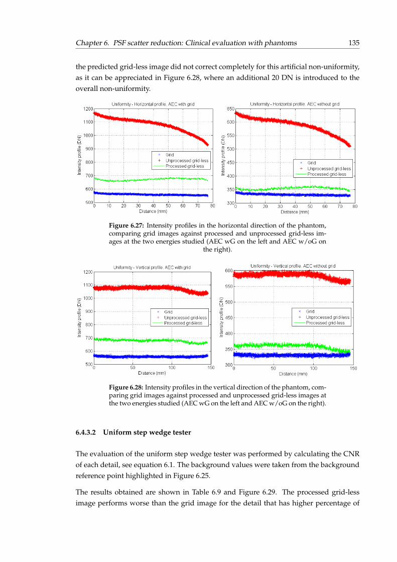
Chapter 6. PSF scatter reduction: Clinical evaluation with phantoms 135
the predicted grid-less image did not correct completely for this artificial non-uniformity,as it can be appreciated in Figure 6.28, where an additional 20 DN is introduced to theoverall non-uniformity.
Figure 6.27: Intensity profiles in the horizontal direction of the phantom,comparing grid images against processed and unprocessed grid-less im-ages at the two energies studied (AEC wG on the left and AEC w/oG on
the right).
Figure 6.28: Intensity profiles in the vertical direction of the phantom, com-paring grid images against processed and unprocessed grid-less images atthe two energies studied (AEC wG on the left and AEC w/oG on the right).
6.4.3.2 Uniform step wedge tester
The evaluation of the uniform step wedge tester was performed by calculating the CNRof each detail, see equation 6.1. The background values were taken from the backgroundreference point highlighted in Figure 6.25.
The results obtained are shown in Table 6.9 and Figure 6.29. The processed grid-lessimage performs worse than the grid image for the detail that has higher percentage of

Chapter 6. PSF scatter reduction: Clinical evaluation with phantoms 136
adipose tissue than the background, i.e step number 1 in Figure 6.25, where the changein material introduces an area with more scattering, more absorption and higher signalthan the background (positive CNR). In this case, the model does not reproduce the totalamount of scattering, leading to smaller CNR values. When the proportion of glandulartissue increases, step numbers 3 to 5, the process is inverted (negative CNR). The modelperforms better than the grid for these cases. The glandularity used in the simulation ofthe phantom, 30%, is equivalent to the step number 2, so the CNR in this case shouldbe close to zero. The grid example gives more accurate results in this case, this is likelyrelated to the difference in scattering that arrives from the neighbouring testers.
Table 6.9: Average CNR values calculated in each step of the step wedgetester for grid and processed grid-less images acquired at two energies.
The standard deviation of the measurements is shown in brackets (σ).
CNR - Step wedge testerStepno.
AEC with grid AEC without grid
Grid (σ) Proc. (σ)<p>(%)
Grid (σ) Proc. (σ)<p>(%)
1 3.66 (0.02) 3.01 (0.09) 0.28 2.69 (0.01) 2.19 (0.01) 0.012 0.06 (0.01) -0.24 (0.08) 1.07 0.08 (0.01) -0.17 (0.01) 0.013 -2.32 (0.01) -2.49 (0.08) 3.62 -1.70 (0.01) -1.72 (0.01) 0.984 -4.71 (0.02) -5.10 (0.10) 0.87 -3.45 (0.01) -3.68 (0.01) 0.015 -8.56 (0.03) -8.86 (0.08) 0.57 -6.27 (0.03) -6.50 (0.04) 0.13
Figure 6.29: Bar plot of the CNR results of Table 6.9. The grid images arecompared against the processed grid-less images at a higher (left plot) andlower (right plot) doses. The standard deviation of the measurements is
shown in the error bars.
The results obtained are reproducible at both energies. For each case, the analysis wasrepeated three times to gain statistics, by selecting different ROI sizes inside the detailsof the testers, i.e. one as big as the tester, a medium ROI and a smaller one, all cen-tred in the tester. The results presented are an average of the measurements, the errors
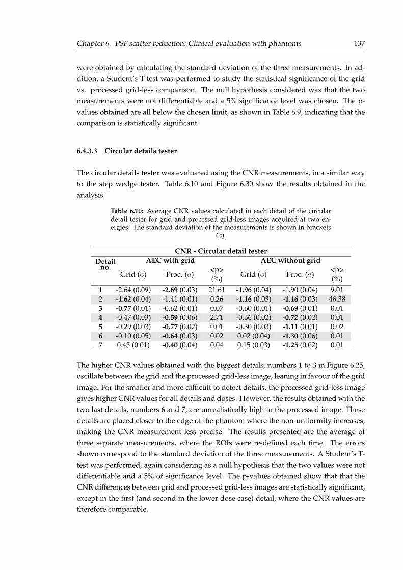
Chapter 6. PSF scatter reduction: Clinical evaluation with phantoms 137
were obtained by calculating the standard deviation of the three measurements. In ad-dition, a Student’s T-test was performed to study the statistical significance of the gridvs. processed grid-less comparison. The null hypothesis considered was that the twomeasurements were not differentiable and a 5% significance level was chosen. The p-values obtained are all below the chosen limit, as shown in Table 6.9, indicating that thecomparison is statistically significant.
6.4.3.3 Circular details tester
The circular details tester was evaluated using the CNR measurements, in a similar wayto the step wedge tester. Table 6.10 and Figure 6.30 show the results obtained in theanalysis.
Table 6.10: Average CNR values calculated in each detail of the circulardetail tester for grid and processed grid-less images acquired at two en-ergies. The standard deviation of the measurements is shown in brackets
(σ).
CNR - Circular detail testerDetail
no.AEC with grid AEC without grid
Grid (σ) Proc. (σ)<p>(%)
Grid (σ) Proc. (σ)<p>(%)
1 -2.64 (0.09) -2.69 (0.03) 21.61 -1.96 (0.04) -1.90 (0.04) 9.012 -1.62 (0.04) -1.41 (0.01) 0.26 -1.16 (0.03) -1.16 (0.03) 46.383 -0.77 (0.01) -0.62 (0.01) 0.07 -0.60 (0.01) -0.69 (0.01) 0.014 -0.47 (0.03) -0.59 (0.06) 2.71 -0.36 (0.02) -0.72 (0.02) 0.015 -0.29 (0.03) -0.77 (0.02) 0.01 -0.30 (0.03) -1.11 (0.01) 0.026 -0.10 (0.05) -0.64 (0.03) 0.02 0.02 (0.04) -1.30 (0.06) 0.017 0.43 (0.01) -0.40 (0.04) 0.04 0.15 (0.03) -1.25 (0.02) 0.01
The higher CNR values obtained with the biggest details, numbers 1 to 3 in Figure 6.25,oscillate between the grid and the processed grid-less image, leaning in favour of the gridimage. For the smaller and more difficult to detect details, the processed grid-less imagegives higher CNR values for all details and doses. However, the results obtained with thetwo last details, numbers 6 and 7, are unrealistically high in the processed image. Thesedetails are placed closer to the edge of the phantom where the non-uniformity increases,making the CNR measurement less precise. The results presented are the average ofthree separate measurements, where the ROIs were re-defined each time. The errorsshown correspond to the standard deviation of the three measurements. A Student’s T-test was performed, again considering as a null hypothesis that the two values were notdifferentiable and a 5% of significance level. The p-values obtained show that that theCNR differences between grid and processed grid-less images are statistically significant,except in the first (and second in the lower dose case) detail, where the CNR values aretherefore comparable.
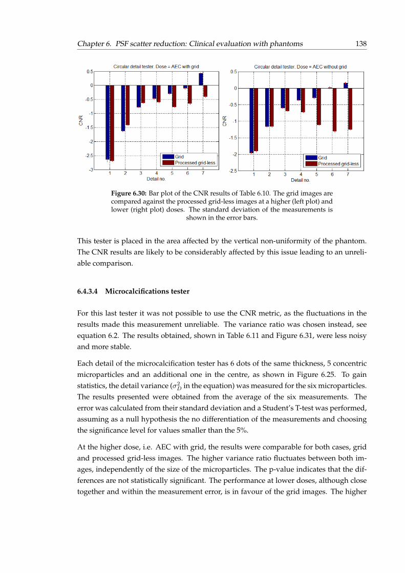
Chapter 6. PSF scatter reduction: Clinical evaluation with phantoms 138
Figure 6.30: Bar plot of the CNR results of Table 6.10. The grid images arecompared against the processed grid-less images at a higher (left plot) andlower (right plot) doses. The standard deviation of the measurements is
shown in the error bars.
This tester is placed in the area affected by the vertical non-uniformity of the phantom.The CNR results are likely to be considerably affected by this issue leading to an unreli-able comparison.
6.4.3.4 Microcalcifications tester
For this last tester it was not possible to use the CNR metric, as the fluctuations in theresults made this measurement unreliable. The variance ratio was chosen instead, seeequation 6.2. The results obtained, shown in Table 6.11 and Figure 6.31, were less noisyand more stable.
Each detail of the microcalcification tester has 6 dots of the same thickness, 5 concentricmicroparticles and an additional one in the centre, as shown in Figure 6.25. To gainstatistics, the detail variance (σ2
D in the equation) was measured for the six microparticles.The results presented were obtained from the average of the six measurements. Theerror was calculated from their standard deviation and a Student’s T-test was performed,assuming as a null hypothesis the no differentiation of the measurements and choosingthe significance level for values smaller than the 5%.
At the higher dose, i.e. AEC with grid, the results were comparable for both cases, gridand processed grid-less images. The higher variance ratio fluctuates between both im-ages, independently of the size of the microparticles. The p-value indicates that the dif-ferences are not statistically significant. The performance at lower doses, although closetogether and within the measurement error, is in favour of the grid images. The higher
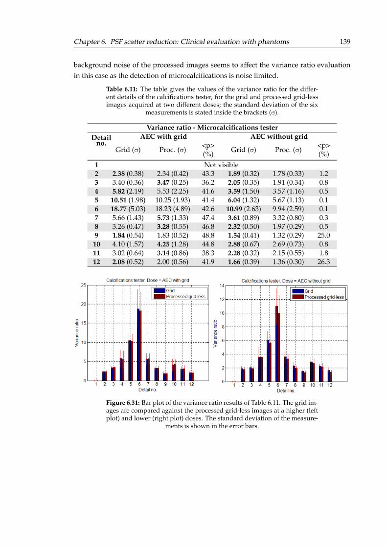
Chapter 6. PSF scatter reduction: Clinical evaluation with phantoms 139
background noise of the processed images seems to affect the variance ratio evaluationin this case as the detection of microcalcifications is noise limited.
Table 6.11: The table gives the values of the variance ratio for the differ-ent details of the calcifications tester, for the grid and processed grid-lessimages acquired at two different doses; the standard deviation of the six
measurements is stated inside the brackets (σ).
Variance ratio - Microcalcifications testerDetail
no.AEC with grid AEC without grid
Grid (σ) Proc. (σ)<p>(%)
Grid (σ) Proc. (σ)<p>(%)
1 Not visible2 2.38 (0.38) 2.34 (0.42) 43.3 1.89 (0.32) 1.78 (0.33) 1.23 3.40 (0.36) 3.47 (0.25) 36.2 2.05 (0.35) 1.91 (0.34) 0.84 5.82 (2.19) 5.53 (2.25) 41.6 3.59 (1.50) 3.57 (1.16) 0.55 10.51 (1.98) 10.25 (1.93) 41.4 6.04 (1.32) 5.67 (1.13) 0.16 18.77 (5.03) 18.23 (4.89) 42.6 10.99 (2.63) 9.94 (2.59) 0.17 5.66 (1.43) 5.73 (1.33) 47.4 3.61 (0.89) 3.32 (0.80) 0.38 3.26 (0.47) 3.28 (0.55) 46.8 2.32 (0.50) 1.97 (0.29) 0.59 1.84 (0.54) 1.83 (0.52) 48.8 1.54 (0.41) 1.32 (0.29) 25.010 4.10 (1.57) 4.25 (1.28) 44.8 2.88 (0.67) 2.69 (0.73) 0.811 3.02 (0.64) 3.14 (0.86) 38.3 2.28 (0.32) 2.15 (0.55) 1.812 2.08 (0.52) 2.00 (0.56) 41.9 1.66 (0.39) 1.36 (0.30) 26.3
Figure 6.31: Bar plot of the variance ratio results of Table 6.11. The grid im-ages are compared against the processed grid-less images at a higher (leftplot) and lower (right plot) doses. The standard deviation of the measure-
ments is shown in the error bars.

Chapter 6. PSF scatter reduction: Clinical evaluation with phantoms 140
6.5 Realistic clinical images
The method evaluation that has been used so far involved the validation with MonteCarlo simulations and different types of phantoms available for mammography applica-tions. Despite the large variety of simulated phantoms that can be generated with theaid of MC simulations, the study also needed to evaluate the performance of the methodin a realistic environment. However, the phantoms at our disposal presented a series ofdrawbacks when applied to this study. These phantoms are aimed to be used for qualitycontrol, to check for damage or degradation of the detector or the X-ray tube. Therefore,they have embedded testers of unknown materials and unrealistic shapes that allow toaccurately quantify the system performance but hinders the performance of the scatter-ing removal method presented in this study, as the analysis of the phantoms has to bemade by simplifying their structure to a single material and homogeneous shape. Al-though the overall results observed so far are positive, as seen in the previous sections,these simplifications introduced some uncertainties that complicated the analysis pro-cess, worsening the results of the processed grid-less images. These shortcomings, incombination with the need to evaluate the stability of the suggested method in a morerealistic clinical environment, led to the use of organic phantoms as a final stage of thisstudy.
The ideal solution would have been to use real mammograms of patients. However, twoimages would have been required for comparison purposes, one with grid and the otherone without a grid, resulting in an unnecessary double irradiation that goes against theALARP (As Low As Reasonably Practicable) principle and hospital ethics. The possibil-ity of using the images of women that are called back for a DBT scan (without grid) aftera first 2D mammogram (with grid) was considered, but the dose delivered at 0 degreesangle in DBT is considerably lower than in the 2D scan, compromising the comparison.After discarding human cadavers as an option, for logistic reasons and time constraints,the possibility of using mammary glands of farm animals was taken into consideration.After a study of the different possibilities, sheep were selected as the better option forthis study, for their similarity to human breast (i.e. in terms of size, structure and compo-sition) and their availability.
6.5.1 Sheep mammary glands
The reason sheep were selected as the best option for this study are multiple:
• Ethics and availability: From the range of mammals available, farm animals thatwere slaughter for food were the only possible option. Typically, the udders aredisposed with the skin and the rest of the carcass that is not processed into food, sono animal has been slaughtered to carry this study.
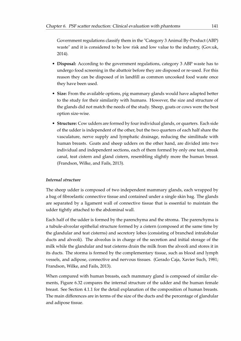
Chapter 6. PSF scatter reduction: Clinical evaluation with phantoms 141
Government regulations classify them in the "Category 3 Animal By-Product (ABP)waste" and it is considered to be low risk and low value to the industry, (Gov.uk,2014).
• Disposal: According to the government regulations, category 3 ABP waste has toundergo food screening in the abattoir before they are disposed or re-used. For thisreason they can be disposed of in landfill as common uncooked food waste oncethey have been used.
• Size: From the available options, pig mammary glands would have adapted betterto the study for their similarity with humans. However, the size and structure ofthe glands did not match the needs of the study. Sheep, goats or cows were the bestoption size-wise.
• Structure: Cow udders are formed by four individual glands, or quarters. Each sideof the udder is independent of the other, but the two quarters of each half share thevasculature, nerve supply and lymphatic drainage, reducing the similitude withhuman breasts. Goats and sheep udders on the other hand, are divided into twoindividual and independent sections, each of them formed by only one teat, streakcanal, teat cistern and gland cistern, resembling slightly more the human breast.(Frandson, Wilke, and Fails, 2013).
Internal structure
The sheep udder is composed of two independent mammary glands, each wrapped bya bag of fibroelastic connective tissue and contained under a single skin bag. The glandsare separated by a ligament wall of connective tissue that is essential to maintain theudder tightly attached to the abdominal wall.
Each half of the udder is formed by the parenchyma and the stroma. The parenchyma isa tubule-alveolar epithelial structure formed by a cistern (composed at the same time bythe glandular and teat cisterns) and secretory lobes (consisting of branched intralobularducts and alveoli). The alveolus is in charge of the secretion and initial storage of themilk while the glandular and teat cisterns drain the milk from the alveoli and stores it inits ducts. The storma is formed by the complementary tissue, such as blood and lymphvessels, and adipose, connective and nervous tissues. (Gerado Caja, Xavier Such, 1981;Frandson, Wilke, and Fails, 2013).
When compared with human breasts, each mammary gland is composed of similar ele-ments, Figure 6.32 compares the internal structure of the udder and the human femalebreast. See Section 4.1.1 for the detail explanation of the composition of human breasts.The main differences are in terms of the size of the ducts and the percentage of glandularand adipose tissue.
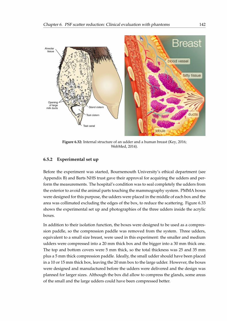
Chapter 6. PSF scatter reduction: Clinical evaluation with phantoms 142
Figure 6.32: Internal structure of an udder and a human breast (Key, 2016;WebMed, 2014).
6.5.2 Experimental set up
Before the experiment was started, Bournemouth University’s ethical department (seeAppendix B) and Barts NHS trust gave their approval for acquiring the udders and per-form the measurements. The hospital’s condition was to seal completely the udders fromthe exterior to avoid the animal parts touching the mammography system. PMMA boxeswere designed for this purpose, the udders were placed in the middle of each box and thearea was collimated excluding the edges of the box, to reduce the scattering. Figure 6.33shows the experimental set up and photographies of the three udders inside the acrylicboxes.
In addition to their isolation function, the boxes were designed to be used as a compres-sion paddle, so the compression paddle was removed from the system. Three udders,equivalent to a small size breast, were used in this experiment: the smaller and mediumudders were compressed into a 20 mm thick box and the bigger into a 30 mm thick one.The top and bottom covers were 5 mm thick, so the total thickness was 25 and 35 mmplus a 5 mm thick compression paddle. Ideally, the small udder should have been placedin a 10 or 15 mm thick box, leaving the 20 mm box to the large udder. However, the boxeswere designed and manufactured before the udders were delivered and the design wasplanned for larger sizes. Although the box did allow to compress the glands, some areasof the small and the large udders could have been compressed better.

Chapter 6. PSF scatter reduction: Clinical evaluation with phantoms 143
Figure 6.33: The picture of the left shows the experimental set up at BartsNHS trust, the udder is sealed from the exterior with a PMMA box. Thethree udders used in this study are displayed on the right side of the figure.
The sizes from top to bottom are: small, medium and large.
Images with and without grid were acquired for each of the udders at three doses: highdose (selected by the system’s AEC when the grid was in use), medium dose (selectedby the system’s AEC without the grid) and a low dose measurement, 50% of the mediumdose. All the measurements were performed at Barts NHS trust, following the geometryintroduced in Section 5.3 and illustrated in Figure 5.6-right. The simulations were donewith and without the presence of the phantom, to obtain the phantom and backgroundkernels, according to the needs of the method introduced in Section 5.6. Table 6.12 givesmore details about the experimental set up.
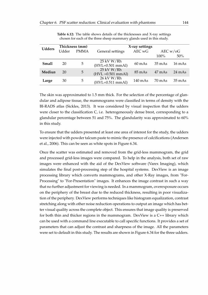
Chapter 6. PSF scatter reduction: Clinical evaluation with phantoms 144
Table 6.12: The table shows details of the thicknesses and X-ray settingschosen for each of the three sheep mammary glands used in this study.
UddersThickness (mm) X-ray settingsUdder PMMA General settings AEC wG AEC w/oG
100% 50%
Small 20 525 kV W/Rh
(HVL=0.501 mmAl) 60 mAs 35 mAs 16 mAs
Medium 20 525 kV W/Rh
(HVL =0.501 mmAl) 85 mAs 47 mAs 24 mAs
Large 30 526 kV W/Rh
(HVL=0.511 mmAl) 140 mAs 70 mAs 35 mAs
The skin was approximated to 1.5 mm thick. For the selection of the percentage of glan-dular and adipose tissue, the mammograms were classified in terms of density with theBI-RADS atlas (Sickles, 2013). It was considered by visual inspection that the udderswere closer to the classification C, i.e. heterogeneously dense brest, corresponding to aglandular percentage between 51 and 75%. The glandularity was approximated to 60%in this study.
To ensure that the udders presented at least one area of interest for the study, the udderswere injected with powder talcum paste to mimic the presence of calcifications (Andersenet al., 2006). This can be seen as white spots in Figure 6.34.
Once the scatter was estimated and removed from the grid-less mammogram, the gridand processed grid-less images were compared. To help in the analysis, both set of rawimages were enhanced with the aid of the DexView software (Varex Imaging), whichsimulates the final post-processing step of the hospital systems. DexView is an imageprocessing library which converts mammograms, and other X-Ray images, from "For-Processing" to "For-Presentation" images. It enhances the image contrast in such a waythat no further adjustment for viewing is needed. In a mammogram, overexposure occurson the periphery of the breast due to the reduced thickness, resulting in poor visualiza-tion of the periphery. DexView performs techniques like histogram equalization, contraststretching along with other noise reduction operations to output an image which has bet-ter visual quality across the complete object. This ensures that image quality is preservedfor both thin and thicker regions in the mammogram. DexView is a C++ library whichcan be used with a command line executable to call specific functions. It provides a set ofparameters that can adjust the contrast and sharpness of the image. All the parameterswere set to default in this study. The results are shown in Figure 6.34 for the three udders.
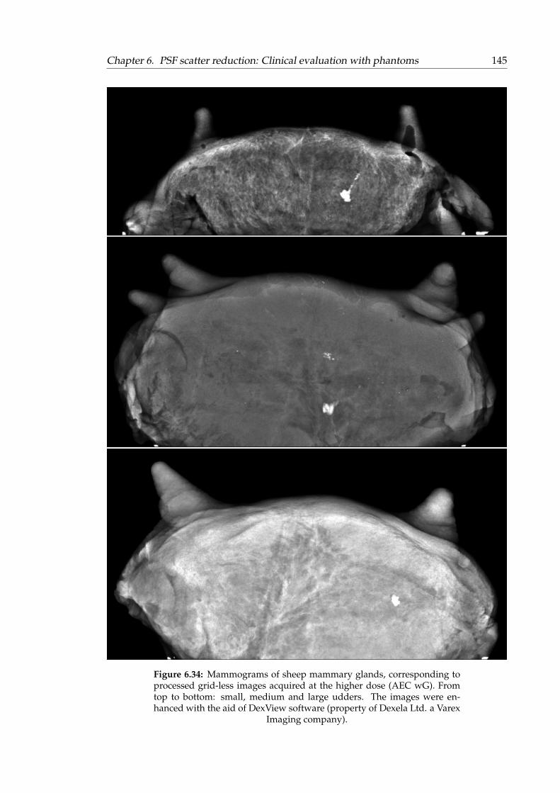
Chapter 6. PSF scatter reduction: Clinical evaluation with phantoms 145
Figure 6.34: Mammograms of sheep mammary glands, corresponding toprocessed grid-less images acquired at the higher dose (AEC wG). Fromtop to bottom: small, medium and large udders. The images were en-hanced with the aid of DexView software (property of Dexela Ltd. a Varex
Imaging company).

Chapter 6. PSF scatter reduction: Clinical evaluation with phantoms 146
6.5.3 Results
The quality of the final processed images obtained with and without the grid did notdiffer enough to be able to distinguish any difference by visual inspection with untrainedeyes. For comparison purposes, and to avoid the possibility of introducing biased results,both images were analysed quantitatively. The two figures of merit chosen to perform theanalysis were the CNR and the variance ratio (Vr), figures that were previously used inthe analysis of the commercial breast phantoms.
The measurements were performed in significant areas of the mammograms, choosinga varied selection of regions of interest in order to cover a wider analysis range. Thebackground areas were selected in nearby areas of each of the ROIs, a total of four back-ground areas were chosen for each of the six cases. The locations of the selected regionswere kept constant across the different configurations, i.e. grid and grid-less images atthe three doses used to help in the comparison. Figure 6.35 shows the six ROIs chosen foreach case and one of the background ROIs (four visualization purposes the other threebackground ROIs were excluded). The regions chosen for the study presented eithermicrocalcifications or non-homogeneous areas that were considered of interest.
Figure 6.35: The figure shows the six ROIs selected for each udder: smalleron the left, medium in the middle and larger on the right.
The CNR and variance ratio values of the six selected ROIs were compared for each case,i.e. grid vs. processed grid-less at the three selected doses, for each one of the mammaryglands. The results for the small, medium and large udder are shown in Figures 6.36 to6.38 respectively. Each one of the figures features one plot per X-ray setting (showingthe CNR on the left y-axis and the variance ratio on the right y-axis) and a table with thevalues, placed next to each plot.
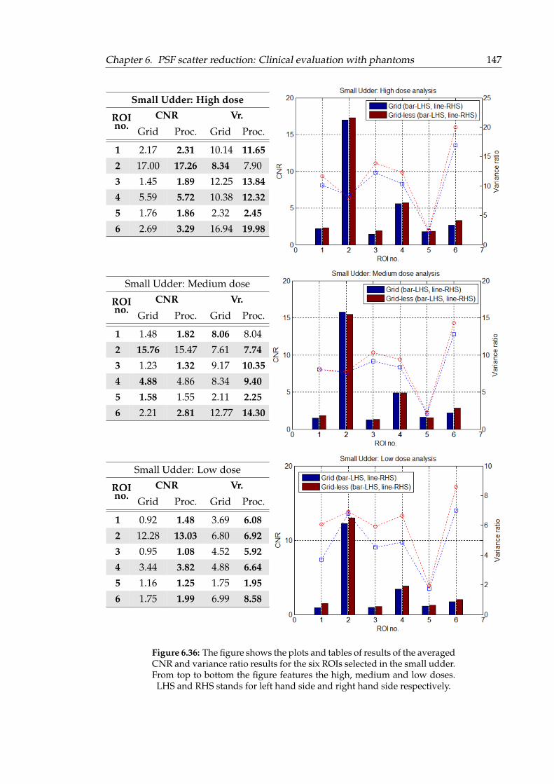
Chapter 6. PSF scatter reduction: Clinical evaluation with phantoms 147
Small Udder: High dose
ROIno.
CNR Vr.
Grid Proc. Grid Proc.
1 2.17 2.31 10.14 11.65
2 17.00 17.26 8.34 7.90
3 1.45 1.89 12.25 13.84
4 5.59 5.72 10.38 12.32
5 1.76 1.86 2.32 2.45
6 2.69 3.29 16.94 19.98
Small Udder: Medium dose
ROIno.
CNR Vr.
Grid Proc. Grid Proc.
1 1.48 1.82 8.06 8.04
2 15.76 15.47 7.61 7.74
3 1.23 1.32 9.17 10.35
4 4.88 4.86 8.34 9.40
5 1.58 1.55 2.11 2.25
6 2.21 2.81 12.77 14.30
Small Udder: Low dose
ROIno.
CNR Vr.
Grid Proc. Grid Proc.
1 0.92 1.48 3.69 6.08
2 12.28 13.03 6.80 6.92
3 0.95 1.08 4.52 5.92
4 3.44 3.82 4.88 6.64
5 1.16 1.25 1.75 1.95
6 1.75 1.99 6.99 8.58
Figure 6.36: The figure shows the plots and tables of results of the averagedCNR and variance ratio results for the six ROIs selected in the small udder.From top to bottom the figure features the high, medium and low doses.LHS and RHS stands for left hand side and right hand side respectively.

Chapter 6. PSF scatter reduction: Clinical evaluation with phantoms 148
Medium Udder: High dose
ROIno.
CNR Vr.
Grid Proc. Grid Proc.
1 18.90 20.29 26.44 35.41
2 2.48 2.71 26.77 33.42
3 1.09 1.19 5.08 6.08
4 3.95 5.03 128.58 214.11
5 0.90 1.11 8.74 11.18
6 1.95 2.07 27.46 36.04
Medium Udder: Medium dose
ROIno.
CNR Vr.
Grid Proc. Grid Proc.
1 16.12 17.76 19.76 26.47
2 2.11 2.13 19.31 19.84
3 0.98 0.93 4.18 4.17
4 3.01 3.57 69.18 97.33
5 0.97 1.07 7.37 9.15
6 1.44 1.53 16.48 19.97
Medium Udder: Low dose
ROIno.
CNR Vr.
Grid Proc. Grid Proc.
1 11.91 14.25 11.27 19.41
2 1.41 1.53 9.13 11.67
3 0.63 0.77 2.74 3.14
4 1.86 2.60 30.88 62.72
5 0.77 1.05 5.64 6.97
6 1.15 1.19 8.36 12.24
Figure 6.37: The figure shows the plots and tables of results of the averagedCNR and variance ratio results for the six ROIs selected in the mediumudder. From top to bottom the figure features the high, medium and lowdoses. LHS and RHS stands for left hand side and right hand side respec-
tively.
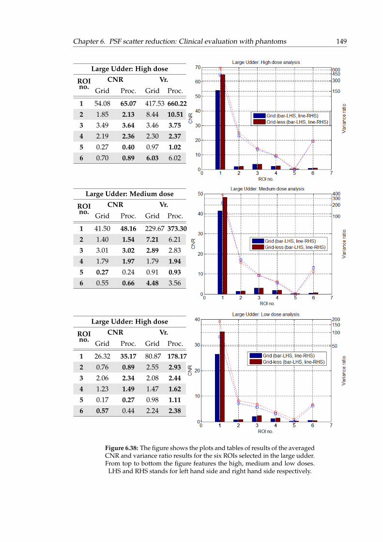
Chapter 6. PSF scatter reduction: Clinical evaluation with phantoms 149
Large Udder: High dose
ROIno.
CNR Vr.
Grid Proc. Grid Proc.
1 54.08 65.07 417.53 660.22
2 1.85 2.13 8.44 10.51
3 3.49 3.64 3.46 3.75
4 2.19 2.36 2.30 2.37
5 0.27 0.40 0.97 1.02
6 0.70 0.89 6.03 6.02
Large Udder: Medium dose
ROIno.
CNR Vr.
Grid Proc. Grid Proc.
1 41.50 48.16 229.67 373.30
2 1.40 1.54 7.21 6.21
3 3.01 3.02 2.89 2.83
4 1.79 1.97 1.79 1.94
5 0.27 0.24 0.91 0.93
6 0.55 0.66 4.48 3.56
Large Udder: High dose
ROIno.
CNR Vr.
Grid Proc. Grid Proc.
1 26.32 35.17 80.87 178.17
2 0.76 0.89 2.55 2.93
3 2.06 2.34 2.08 2.44
4 1.23 1.49 1.47 1.62
5 0.17 0.27 0.98 1.11
6 0.57 0.44 2.24 2.38
Figure 6.38: The figure shows the plots and tables of results of the averagedCNR and variance ratio results for the six ROIs selected in the large udder.From top to bottom the figure features the high, medium and low doses.LHS and RHS stands for left hand side and right hand side respectively.

Chapter 6. PSF scatter reduction: Clinical evaluation with phantoms 150
6.5.4 Discussion
The results shown in Figures 6.36 to 6.38 are summarised in Table 6.13, where it is statedwhich of the images (grid vs. grid-less) has the better performance for each case, interms of the CNR and Vr. The table color code shows green when the processed grid-less image (P) gave better results, yellow when the images were comparable or the testwas inconclusive (C) and red when the grid image (G) was better. To ensure that themeasurements were statistically relevant, a Student’s T-test was performed, choosing 5%as the significance level (the results obtained with this test are shown in Tables A.25 andA.26 of the Appendix A). A measurement was considered comparable or inconclusivewhen the p-values for both, the CNR and the Vr, were higher than 5% or when bothp-values were significant but the results contradicted each other.
Table 6.13: The table summarises the results obtained with the three real-istic phantoms analysed in this section. The table highlights which image
performs better for each of the ROIs and energies analysed.
DoseSmall udder Medium udder Large udder
ROIno.
H. M. L. H. M. L H. M. L
1 C P P P P P P P P2 C G P P C P P C P3 P C P P C P C C P4 P P P P P P C C P5 P P P P P C P C P6 P C P P P P C C C
P = Processed grid-less image.G = Grid image.C = Comparable results.
As shown in Table 6.13 the overall results obtained are very positive. The best outcomewas obtained with the medium sized udder, followed by the smaller one, with the largerudder presenting the higher amount of comparable results. This dependency with thetype of udder seems to be in line with the insufficient compression in the small and largeudders, reported in the “Experimental set up” section.
As per the energies chosen, the highest and lowest doses produce better results than themiddle dose:
• At a very low energy, the signal detected by the panel when the grid is in use is toolow to give good results. The increased signal detected as a consequence of the gridremoval is essential in the performance, as it has been seen in the results.
Chapter 6. PSF scatter reduction: Clinical evaluation with phantoms 151
• The medium dose presents the higher amount of comparable results and a negativeone in the case of the smaller udder. This indicates that the energy reduction, givenby the system’s AEC when the grid was not used, was too large.
• The results obtained with the higher dose are very positive, indicating that the re-moval of the grid would contribute to an overall improvement of the image quality,at least for the thicknesses tested.
6.6 Chapter summary and discussion
In this chapter, the post-process scattered radiation reduction method that had been pre-viously defined was evaluated and its robustness tested using a mammography system.
Prior to this evaluation, an initial study was performed to decide on the level of simpli-fications that could be implemented in the simulations. The results showed that it wasimportant to add the detector information, as the implementation of an idealised geom-etry underestimated the SPR up to 14%. Consequently, it was decided that the followingexperiments would include all the detector information up to the sensor layer, for the di-rect conversion X-ray systems, and up to the scintillator layer, for indirect detection X-raysystems, unless otherwise specified.
The first study with phantoms focused in the restoration of the low frequency spatialresolution when using a phantom highly affected by scattering. For logistical reasons, aCMOS X-ray detector placed in a radiography system was chosen for this experiment setup. The scattering reduction post-processing technique successfully recovered the totalspatial resolution lost. Moreover, the post-processed images were artefact free.
The rest of the evaluation was performed with a real mammography system, using theα-Se technology. With the aid of several mammography QC phantoms, the performanceof the post-processing scattering reduction technique was challenged by making a oneto one comparison between processed grid-less images and grid images. Overall, it wasfound that these phantoms were not fit to purpose. Due to the structure of the phantomsit was necessary to introduce a large amount of assumptions and simplifications in thesimulations used for the grid-less image processing. Therefore, the results obtained, al-though generally comparable with grid’s results, did not suggest a performance as goodas it was initially expected. It was made clear that a more clinical realistic phantom wasneeded for performing a fair comparison. For this reason, sheep mammary glands werechosen for the last study.
The results obtained in this last experiment were very encouraging and indicated thatthe scattering reduction technique (suggested in this study for processing the grid-lessimages) outperforms the performance of the anti-scatter grids when the measurements

Chapter 6. PSF scatter reduction: Clinical evaluation with phantoms 152
are taken under the same conditions. Due to lack of resources and time constraints, onlythin udders were tested. Although the performance is not expected to degrade much forthicknesses below 70 mm, another round of testing would be advisable. Suggestions forfuture research are introduced in the next chapter.
153
Chapter 7
Conclusions and future work
The work presented in this thesis covers two topics within the two main areas of digitalradiography applications:
• Image acquisition: the design cycle of new CMOS X-ray detectors has been chal-lenged in terms of their image quality.
• Image processing: a method for image scattering reduction using post-processingtechniques for grid-less mammography applications has been proposed.
A summary of the results obtained for each section is described below.
7.1 CMOS X-ray detector characterization and qualification
The main goal of this study was to contribute, with the aid of image characterisation tech-niques, to the development of new CMOS X-ray detectors. Shortcomings in the designcycle ultimately present themselves as image artefacts that compromise the quality of theproduct. For that reason, the use of image characterization to challenge the design duringthe development process is essential to ensure the final quality of the detectors. To thatend, well-known image analysis techniques were adapted, extended and optimized toqualify and debug the product at different stages of development.
The novelty in this exercise was to take the architecture of a state-of-the-art active pixelsensor CMOS imager and to develop a set of image processing tools to test it to its limit,during the design cycle. In the course of this thesis, image artefacts and performanceissues were found and addressed as a result of iterative image quality evaluation. Theproject has involved a close collaboration with a multinational team of engineers, whoseinput was required to investigate the root cause of the issues found and to address theproblems consequently. The teams involved depended on the nature of the problem,which could affect the electronics, firmware, software or sensor designs.
Chapter 7. Conclusions and future work 154
Issues encountered during the image characterization exercise have been, among others,high and low frequency noise, noise flickering, bit errors, image clipping, non-linearity,glowing rows or columns, image artefacts due to scintillator afterglow and gain hystere-sis, pixel cross-talk and unrealistic DQE values. The group of tests suggested in this thesishave been integrated in the company routine testing and detector validation and verifi-cation exercises. This study was key for the successful release of final CMOS flat paneldetectors designed and built at Dexela Ltd. (Varex Imaging Corporation - London).
7.2 Scatter removal by image processing in digital mammogra-phy
The scatter removal method that has been proposed in this thesis is based in image convo-lution with point spread function (PSF) kernels, obtained with a simplified Monte Carlosimulation using a narrow pencil beam in a symmetric environment. The simulationswere performed using the Geant4 simulation tool-kit.
The method uses a semi-empirical approach to correct the breast-edge area for the scat-ter originated outside the breast, i.e. background contribution mainly coming from thecompression paddle, and, in case of breasts of thicknesses greater than 50 mm, for thethickness variations caused by the angle of the X-ray beam at the edge of the breast andthe thickness reduction of the breast edge itself. Two additional kernels needed to be sim-ulated for performing the background correction and an additional one for the correctionof thickness reductions in the breast-edge. The novelty of the proposed method consistsin the interpolation between kernels using a semi-empirical equation. This accounts forthe impact that a change in the absorption coefficients has in the simulated scatter, e.g.background scatter contribution to the breast is affected by the change between back-ground and breast absorption and it is dependent on the distance to the breast edge.
The optimization of the semi-empirical equation and the final testing of the method wasmade by comparing, for a range of thicknesses, the results against the primary imagegenerated with full MC simulations. The uncertainty introduced by the correction wasfound to be dependent on the thickness, improving for thin breasts. The results are verypositive, showing a maximum discrepancy of 10% for a breast thickness of 70 mm, valuethat is reduced down to 3% for a 35 mm breast. For breasts that are thicker than 70 mmthe uncertainties found were too large, i.e. > 20%, showing a limitation of the method forvery thick breasts. As an alternative, an asymmetric kernel approach could reduce theuncertainties for these cases; otherwise, additional research resources would be neededto solve this issue in the method (see the "Future work" section below).
After the definition and validation of the method was completed, its robustness wastested against real images. The first step was to decide the level of detail needed in the
Chapter 7. Conclusions and future work 155
geometry of the simulations. In previous published studies the geometry of the detec-tor and compression/support paddles had not been handled with care, either for lack ofknowledge of the geometry or for simplification purposes. However, the study indicatedthat any simplification in the geometry affects the final results, as the scatter underesti-mation in the PSF kernels was found to be considerable. The underestimation goes from3-6% for a detector that is simplified to a scintillator plate to 10-14% for an ideal detectorsimplification.
The ability to recover the spatial resolution, that had been reduced by the effect of thescatter in the system, was then evaluated. Two test devices were used for this purpose:a benchmark phantom ("ground truth") that was an IEC approved edge test device de-signed to evaluate the MTF of the system and another edge test device that was em-bedded in a PMMA block (DMam from Leeds Test Objects). The PMMA increases thescattering produced in the surroundings of the edge, reducing the low frequency spa-tial resolution. The images acquired with the second phantom were processed with themethod followed in this study and the MTF obtained was compared with the "groundtruth" results. The extreme conditions of this test, where the correction focuses in theboundary between two materials with very different scatter and absorption properties,allowed not only to evaluate the quality of the method but also to ensure that the process-ing did not insert any artefacts to the image. The resulting images were clear of artefacts,as shown in the smooth MTF curves obtained, and the low frequency spatial resolutionwas restored, slightly improving the results shown by the benchmark images. As provenlater on, an additional benefit of including in the simulations the scatter that is producedin the detector layers is an improvement in the overall spatial resolution, giving post-processing scatter removal methods an advantage over anti-scatter grids.
The final goal of this study was to obtain an image quality comparable or better than theone obtained with the use of anti-scatter grids. Therefore, grid and grid-less images wereacquired under the same conditions and a one to one comparison study was made. Themeasurements from this moment onwards were made with a clinical mammography sys-tem. Due to the reduced number of mammography systems that used CMOS technology,the rest of the measurements were performed with a Hologic Lorad Selenia α-Se system.The range of phantoms chosen were: CDMAM, TOR-MAS and TOR-MAM from LeedsTest Objects, 010A from CIRS and sheep mammary glands.
The results obtained with the QA phantoms, i.e. CDMAM, TOR-MAS, TOR-MAM and010A CIRS, were mostly inconclusive:
• The CDMAM phantom was seen to be inaccurate for the type of measurementsand comparisons performed in this study, this was in agreement with previouspublications.
Chapter 7. Conclusions and future work 156
• The unknown materials and random structure of the testers inside the TOR-MASand TOR-MAM phantoms leaded to the introduction of big uncertainties, due tothe simplifications that had to be made in the simulations. The results obtainedwere, however, comparable with the grid application.
In the TOR-MAS phantom, those testers affected by the scattering of the neighbour-ing testers favoured the grid images, specially for thicker phantoms. However, thestep wedge and high contrast resolution grid testers gave better results in the grid-less cases. Results that were in line with the previous MTF experiment, indicatingthat the post-processing improves the overall spatial resolution of the system.
The calcifications of the visually realistic area of the TOR-MAM phantom gener-ally had higher contrast to noise ratio in the processed grid-less images, across thedifferent energies and thicknesses tested. Although consistent, the difference wasvery small to be considered statistically relevant, pointing to comparable results.
• Similar results were obtained with the CIRS phantom. The materials were knownin this case, so the uncertainty introduced in the simulations was lower. The grid-less images showed a non-uniformity in one of the extremes of the phantom, likelyintroduced during the gain and offset correction step at the hospital. Therefore, theresults obtained with the tester placed in that area, i.e. circular detail tester, wereaffected. The step wedge tester favoured the processed grid-less measurements forthose steps with higher glandularity percentage and the grid measurements whenthe percentage of adipose tissue was higher. The results with the microcalcificationstester, on the other hand, were inconclusive. The errors in the measurements weretoo large and the results varied across the details.
The phantoms used up to this point required the use of simplifications in the scatter es-timation method, undermining the results obtained. It became clear the need of a morerealistic clinical phantom that allowed a fair one to one grid vs. processed grid-less com-parison, while challenging the method in real-life applications. Sheep mammary glandswere chosen as a good trade-off between synthetic phantoms and female breasts.
The results obtained with the udders were in clear favour of the processed grid-less im-ages. Looking at the higher air kerma used (chosen by the AEC system when the gridwas in use) the percentage of results in favour of the grid-less methodology was 67%,100% and 50% for the small, medium and large udders respectively, with two inconclu-sive results in the small udder case (33%) and three in the larger udder (50%). During theexperimental set up it was found that the compression of the small and large udders waspoorer, explaining the better results obtained with the well-compressed gland.

Chapter 7. Conclusions and future work 157
7.3 Future work
The test procedure implemented in Dexela Ltd. to evaluate CMOS X-ray detector pro-totypes has evolved and adapted along with the development process. The re-definedtest methods have been successfully employed across a varied range of detectors and ap-plications. However, with the design of new products, or with a change in the productapplication, new features can be found that might highlight the need of a new test orthe modification of the current ones. In that case, the testing procedure will need to beadapted. A future interesting route to pursue would be to apply this study to additionaltechnologies, i.e. α-Si detectors or photon-counting detectors.
For the proposed scatter reduction technique, future work could involve research in theoptimization of the model, such as binning the images to speed up the convolution stepand then un-bin the estimated scatter image to apply the final correction. Some additionaleffort could be made to improve the model for thicker breast cases, i.e. T > 70 mm, thatcurrently suffer from large errors. Finally, further validations should be performed withclinically realistic phantoms, i.e. animal mammary glands, 3D printed phantoms or simi-lar, specially focusing in thicker samples. QC phantoms have proven to be source of largeuncertainties, so more relevant phantoms could be tested in order to gain statistics. Fur-thermore, the improvement in the image quality seen in the last test, i.e. with the sheepmammary glands, indicates that the dose could be reduced without compromising theimage quality that the grid applications give. The dose reduction would be in betweenthe higher and medium doses tested. Further efforts would be needed to identify theexact percentage of reduction, this could be done for example with the set of phantomslabs provided by CIRS (014 series). A qualitative analysis from qualified radiographerswould also be required to ensure that the dose reduction and image post-processing donot affect their diagnosis.

158
Appendix A
Complementary information
A.1 Chapter 5: Additional data
Table A.1 provides the data obtained in the validation against the AAPM task group 195- Case 3 report, introduced in Section 5.2.3.
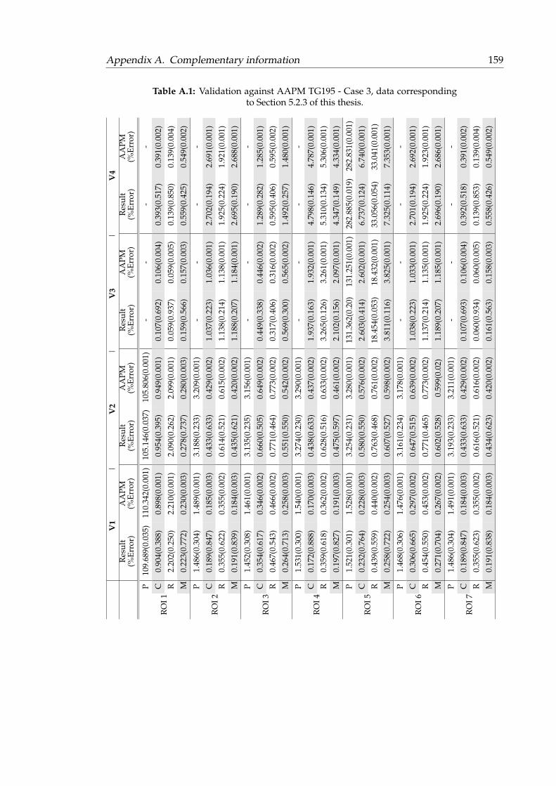
Appendix A. Complementary information 159
Table A.1: Validation against AAPM TG195 - Case 3, data correspondingto Section 5.2.3 of this thesis.
V1
|V
2|
V3
|V
4R
esul
t(%
Erro
r)A
APM
(%Er
ror)
Res
ult
(%Er
ror)
AA
PM(%
Erro
r)R
esul
t(%
Erro
r)A
APM
(%Er
ror)
Res
ult
(%Er
ror)
AA
PM(%
Erro
r)
RO
I1
P10
9.68
9(0.
035)
110.
342(
0.00
1)10
5.14
6(0.
037)
105.
806(
0.00
1)-
--
-
C0.
904(
0.38
8)0.
898(
0.00
1)0.
954(
0.39
5)0.
949(
0.00
1)0.
107(
0.69
2)0.
106(
0.00
4)0.
393(
0.51
7)0.
391(
0.00
2)
R2.
202(
0.25
0)2.
210(
0.00
1)2.
090(
0.26
2)2.
099(
0.00
1)0.
059(
0.93
7)0.
059(
0.00
5)0.
139(
0.85
0)0.
139(
0.00
4)
M0.
223(
0.77
2)0.
230(
0.00
3)0.
278(
0.73
7)0.
280(
0.00
3)0.
159(
0.56
6)0.
157(
0.00
3)0.
559(
0.42
5)0.
549(
0.00
2)
RO
I2
P1.
486(
0.30
4)1.
489(
0.00
1)3.
188(
0.23
3)3.
209(
0.00
1)-
--
-
C0.
189(
0.84
7)0.
185(
0.00
3)0.
433(
0.63
3)0.
429(
0.00
2)1.
037(
0.22
3)1.
036(
0.00
1)2.
702(
0.19
4)2.
691(
0.00
1)
R0.
355(
0.62
2)0.
355(
0.00
2)0.
614(
0.52
1)0.
615(
0.00
2)1.
138(
0.21
4)1.
138(
0.00
1)1.
925(
0.22
4)1.
921(
0.00
1)
M0.
191(
0.83
9)0.
184(
0.00
3)0.
435(
0.62
1)0.
420(
0.00
2)1.
188(
0.20
7)1.
184(
0.00
1)2.
695(
0.19
0)2.
688(
0.00
1)
RO
I3
P1.
452(
0.30
8)1.
461(
0.00
1)3.
135(
0.23
5)3.
156(
0.00
1)-
--
-
C0.
354(
0.61
7)0.
346(
0.00
2)0.
660(
0.50
5)0.
649(
0.00
2)0.
449(
0.33
8)0.
446(
0.00
2)1.
289(
0.28
2)1.
285(
0.00
1)
R0.
467(
0.54
3)0.
466(
0.00
2)0.
771(
0.46
4)0.
773(
0.00
2)0.
317(
0.40
6)0.
316(
0.00
2)0.
595(
0.40
6)0.
595(
0.00
2)
M0.
264(
0.71
3)0.
258(
0.00
3)0.
551(
0.55
0)0.
542(
0.00
2)0.
569(
0.30
0)0.
565(
0.00
2)1.
492(
0.25
7)1.
480(
0.00
1)
RO
I4
P1.
531(
0.30
0)1.
540(
0.00
1)3.
274(
0.23
0)3.
290(
0.00
1)-
--
-
C0.
172(
0.88
8)0.
170(
0.00
3)0.
438(
0.63
3)0.
437(
0.00
2)1.
937(
0.16
3)1.
932(
0.00
1)4.
798(
0.14
6)4.
787(
0.00
1)
R0.
359(
0.61
8)0.
362(
0.00
2)0.
628(
0.51
6)0.
633(
0.00
2)3.
265(
0.12
6)3.
261(
0.00
1)5.
310(
0.13
4)5.
306(
0.00
1)
M0.
197(
0.82
7)0.
191(
0.00
3)0.
475(
0.59
7)0.
461(
0.00
2)2.
102(
0.15
6)2.
097(
0.00
1)4.
347(
0.14
9)4.
334(
0.00
1)
RO
I5
P1.
521(
0.30
1)1.
528(
0.00
1)3.
254(
0.23
1)3.
280(
0.00
1)13
1.36
2(0.
20)
131.
251(
0.00
1)28
2.88
5(0.
019)
282.
831(
0.00
1)
C0.
232(
0.76
4)0.
228(
0.00
3)0.
580(
0.55
0)0.
576(
0.00
2)2.
603(
0.41
4)2.
602(
0.00
1)6.
737(
0.12
4)6.
740(
0.00
1)
R0.
439(
0.55
9)0.
440(
0.00
2)0.
763(
0.46
8)0.
761(
0.00
2)18
.454
(0.0
53)
18.4
32(0
.001
)33
.056
(0.0
54)
33.0
41(0
.001
)
M0.
258(
0.72
2)0.
254(
0.00
3)0.
607(
0.52
7)0.
598(
0.00
2)3.
811(
0.11
6)3.
825(
0.00
1)7.
325(
0.11
4)7.
353(
0.00
1)
RO
I6
P1.
468(
0.30
6)1.
476(
0.00
1)3.
161(
0.23
4)3.
178(
0.00
1)-
--
-
C0.
306(
0.66
5)0.
297(
0.00
2)0.
647(
0.51
5)0.
639(
0.00
2)1.
038(
0.22
3)1.
033(
0.00
1)2.
701(
0.19
4)2.
692(
0.00
1)
R0.
454(
0.55
0)0.
453(
0.00
2)0.
771(
0.46
5)0.
773(
0.00
2)1.
137(
0.21
4)1.
135(
0.00
1)1.
925(
0.22
4)1.
923(
0.00
1)
M0.
271(
0.70
4)0.
267(
0.00
2)0.
602(
0.52
8)0.
599(
0.02
)1.
189(
0.20
7)1.
185(
0.00
1)2.
696(
0.19
0)2.
686(
0.00
1)
RO
I7
P1.
486(
0.30
4)1.
491(
0.00
1)3.
193(
0.23
3)3.
211(
0.00
1)-
--
-
C0.
189(
0.84
7)0.
184(
0.00
3)0.
433(
0.63
3)0.
429(
0.00
2)0.
107(
0.69
3)0.
106(
0.00
4)0.
392(
0.51
8)0.
391(
0.00
2)
R0.
355(
0.62
3)0.
355(
0.00
2)0.
616(
0.52
1)0.
616(
0.00
2)0.
060(
0.93
4)0.
060(
0.00
5)0.
139(
0.85
3)0.
139(
0.00
4)
M0.
191(
0.83
8)0.
184(
0.00
3)0.
434(
0.62
3)0.
420(
0.00
2)0.
161(
0.56
3)0.
158(
0.00
3)0.
558(
0.42
6)0.
549(
0.00
2)
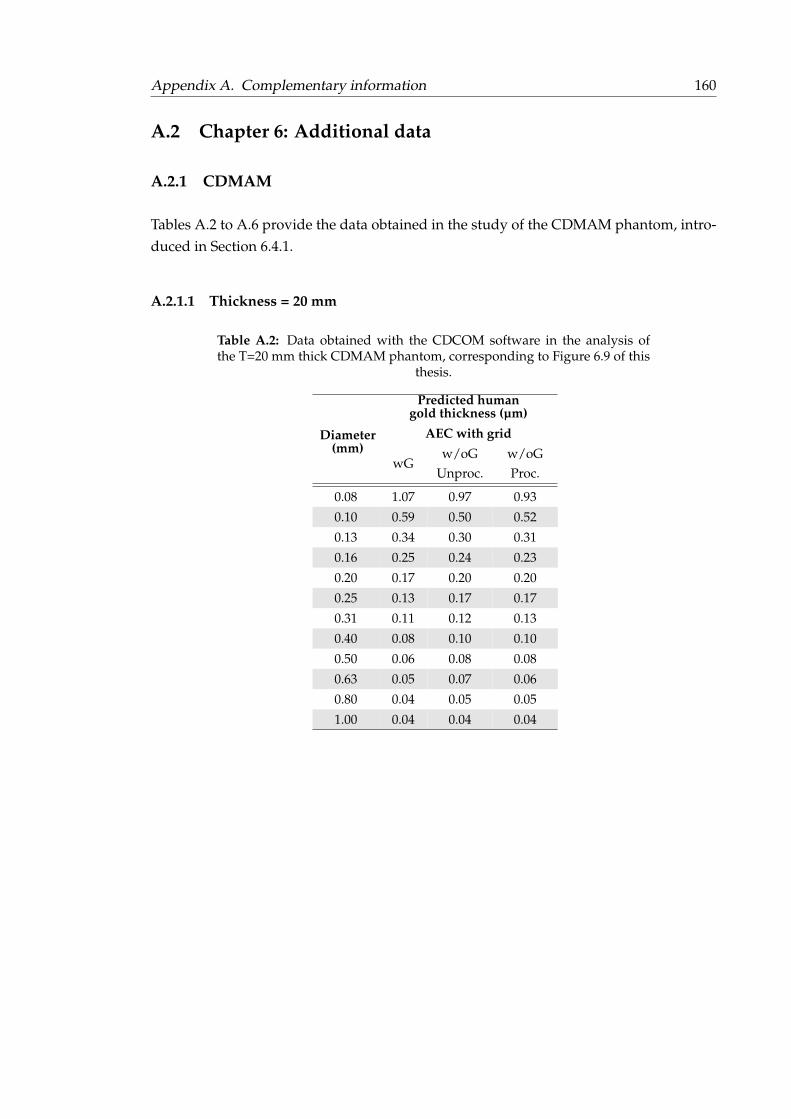
Appendix A. Complementary information 160
A.2 Chapter 6: Additional data
A.2.1 CDMAM
Tables A.2 to A.6 provide the data obtained in the study of the CDMAM phantom, intro-duced in Section 6.4.1.
A.2.1.1 Thickness = 20 mm
Table A.2: Data obtained with the CDCOM software in the analysis ofthe T=20 mm thick CDMAM phantom, corresponding to Figure 6.9 of this
thesis.
Predicted humangold thickness (µm)
Diameter(mm)
AEC with grid
wGw/oG
Unproc.w/oGProc.
0.08 1.07 0.97 0.93
0.10 0.59 0.50 0.52
0.13 0.34 0.30 0.31
0.16 0.25 0.24 0.23
0.20 0.17 0.20 0.20
0.25 0.13 0.17 0.17
0.31 0.11 0.12 0.13
0.40 0.08 0.10 0.10
0.50 0.06 0.08 0.08
0.63 0.05 0.07 0.06
0.80 0.04 0.05 0.05
1.00 0.04 0.04 0.04
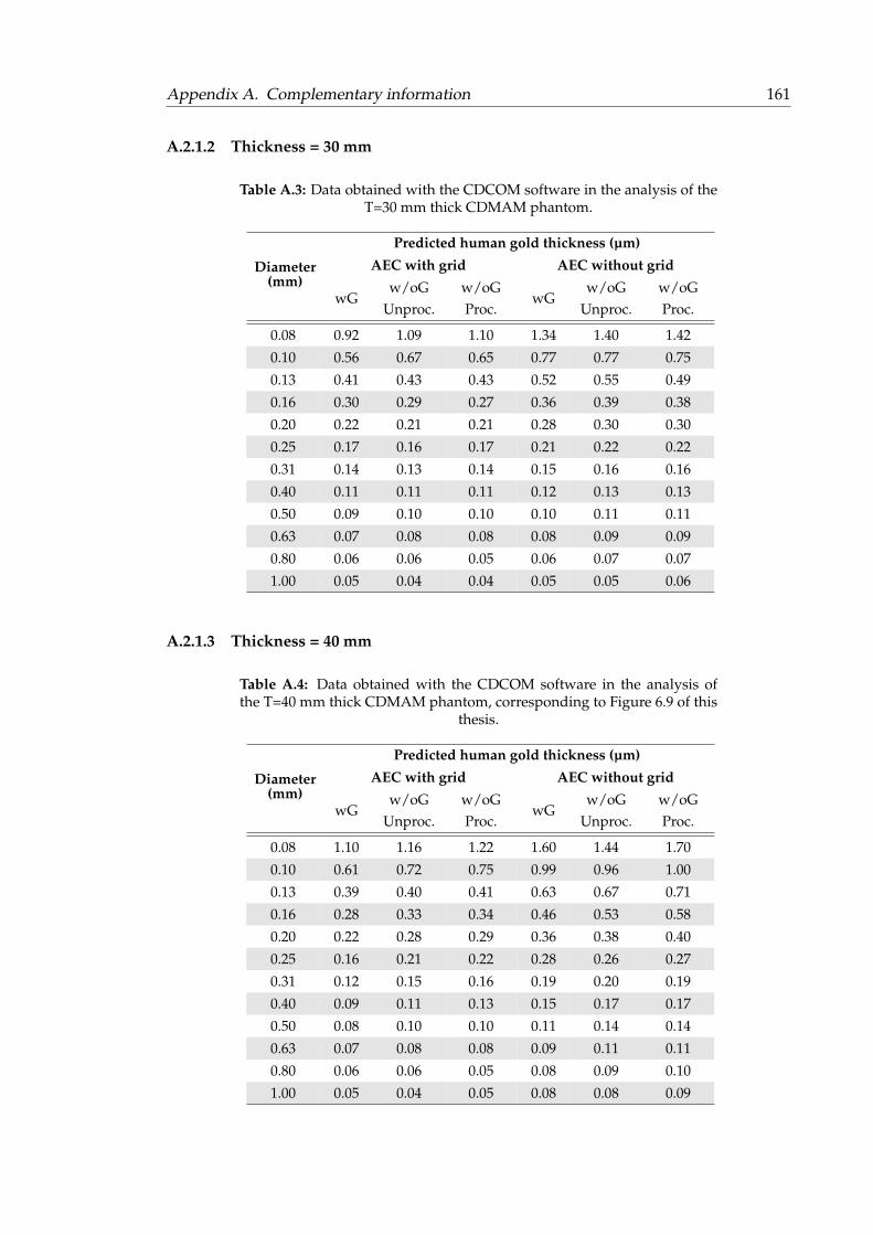
Appendix A. Complementary information 161
A.2.1.2 Thickness = 30 mm
Table A.3: Data obtained with the CDCOM software in the analysis of theT=30 mm thick CDMAM phantom.
Predicted human gold thickness (µm)
Diameter(mm)
AEC with grid AEC without grid
wGw/oG
Unproc.w/oGProc.
wGw/oG
Unproc.w/oGProc.
0.08 0.92 1.09 1.10 1.34 1.40 1.42
0.10 0.56 0.67 0.65 0.77 0.77 0.75
0.13 0.41 0.43 0.43 0.52 0.55 0.49
0.16 0.30 0.29 0.27 0.36 0.39 0.38
0.20 0.22 0.21 0.21 0.28 0.30 0.30
0.25 0.17 0.16 0.17 0.21 0.22 0.22
0.31 0.14 0.13 0.14 0.15 0.16 0.16
0.40 0.11 0.11 0.11 0.12 0.13 0.13
0.50 0.09 0.10 0.10 0.10 0.11 0.11
0.63 0.07 0.08 0.08 0.08 0.09 0.09
0.80 0.06 0.06 0.05 0.06 0.07 0.07
1.00 0.05 0.04 0.04 0.05 0.05 0.06
A.2.1.3 Thickness = 40 mm
Table A.4: Data obtained with the CDCOM software in the analysis ofthe T=40 mm thick CDMAM phantom, corresponding to Figure 6.9 of this
thesis.
Predicted human gold thickness (µm)
Diameter(mm)
AEC with grid AEC without grid
wGw/oG
Unproc.w/oGProc.
wGw/oG
Unproc.w/oGProc.
0.08 1.10 1.16 1.22 1.60 1.44 1.70
0.10 0.61 0.72 0.75 0.99 0.96 1.00
0.13 0.39 0.40 0.41 0.63 0.67 0.71
0.16 0.28 0.33 0.34 0.46 0.53 0.58
0.20 0.22 0.28 0.29 0.36 0.38 0.40
0.25 0.16 0.21 0.22 0.28 0.26 0.27
0.31 0.12 0.15 0.16 0.19 0.20 0.19
0.40 0.09 0.11 0.13 0.15 0.17 0.17
0.50 0.08 0.10 0.10 0.11 0.14 0.14
0.63 0.07 0.08 0.08 0.09 0.11 0.11
0.80 0.06 0.06 0.05 0.08 0.09 0.10
1.00 0.05 0.04 0.05 0.08 0.08 0.09
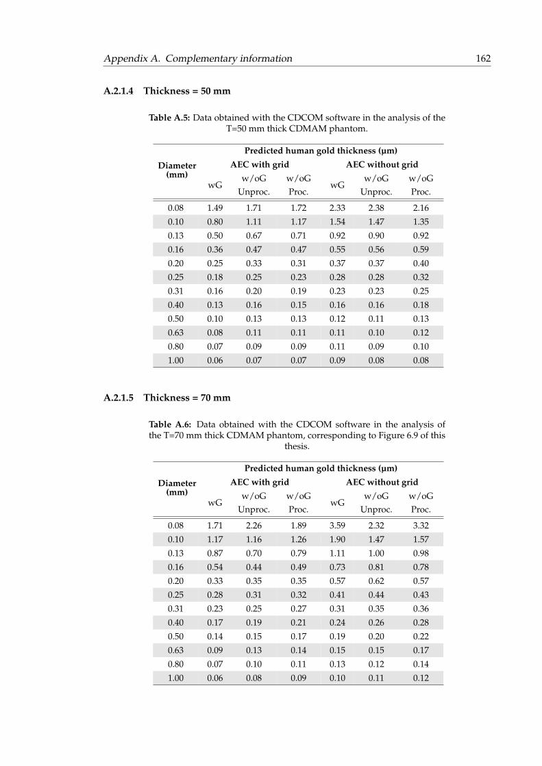
Appendix A. Complementary information 162
A.2.1.4 Thickness = 50 mm
Table A.5: Data obtained with the CDCOM software in the analysis of theT=50 mm thick CDMAM phantom.
Predicted human gold thickness (µm)
Diameter(mm)
AEC with grid AEC without grid
wGw/oG
Unproc.w/oGProc.
wGw/oG
Unproc.w/oGProc.
0.08 1.49 1.71 1.72 2.33 2.38 2.16
0.10 0.80 1.11 1.17 1.54 1.47 1.35
0.13 0.50 0.67 0.71 0.92 0.90 0.92
0.16 0.36 0.47 0.47 0.55 0.56 0.59
0.20 0.25 0.33 0.31 0.37 0.37 0.40
0.25 0.18 0.25 0.23 0.28 0.28 0.32
0.31 0.16 0.20 0.19 0.23 0.23 0.25
0.40 0.13 0.16 0.15 0.16 0.16 0.18
0.50 0.10 0.13 0.13 0.12 0.11 0.13
0.63 0.08 0.11 0.11 0.11 0.10 0.12
0.80 0.07 0.09 0.09 0.11 0.09 0.10
1.00 0.06 0.07 0.07 0.09 0.08 0.08
A.2.1.5 Thickness = 70 mm
Table A.6: Data obtained with the CDCOM software in the analysis ofthe T=70 mm thick CDMAM phantom, corresponding to Figure 6.9 of this
thesis.
Predicted human gold thickness (µm)
Diameter(mm)
AEC with grid AEC without grid
wGw/oG
Unproc.w/oGProc.
wGw/oG
Unproc.w/oGProc.
0.08 1.71 2.26 1.89 3.59 2.32 3.32
0.10 1.17 1.16 1.26 1.90 1.47 1.57
0.13 0.87 0.70 0.79 1.11 1.00 0.98
0.16 0.54 0.44 0.49 0.73 0.81 0.78
0.20 0.33 0.35 0.35 0.57 0.62 0.57
0.25 0.28 0.31 0.32 0.41 0.44 0.43
0.31 0.23 0.25 0.27 0.31 0.35 0.36
0.40 0.17 0.19 0.21 0.24 0.26 0.28
0.50 0.14 0.15 0.17 0.19 0.20 0.22
0.63 0.09 0.13 0.14 0.15 0.15 0.17
0.80 0.07 0.10 0.11 0.13 0.12 0.14
1.00 0.06 0.08 0.09 0.10 0.11 0.12
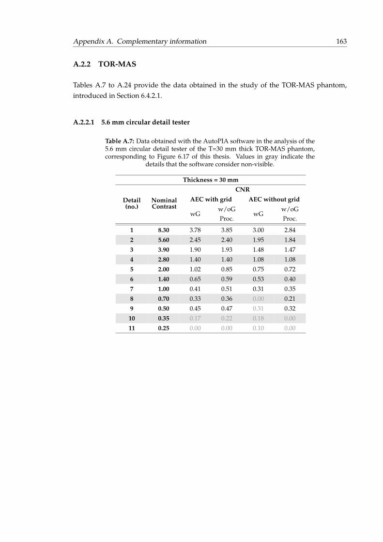
Appendix A. Complementary information 163
A.2.2 TOR-MAS
Tables A.7 to A.24 provide the data obtained in the study of the TOR-MAS phantom,introduced in Section 6.4.2.1.
A.2.2.1 5.6 mm circular detail tester
Table A.7: Data obtained with the AutoPIA software in the analysis of the5.6 mm circular detail tester of the T=30 mm thick TOR-MAS phantom,corresponding to Figure 6.17 of this thesis. Values in gray indicate the
details that the software consider non-visible.
Thickness = 30 mmCNR
Detail(no.)
NominalContrast
AEC with grid AEC without grid
wGw/oGProc.
wGw/oGProc.
1 8.30 3.78 3.85 3.00 2.84
2 5.60 2.45 2.40 1.95 1.84
3 3.90 1.90 1.93 1.48 1.47
4 2.80 1.40 1.40 1.08 1.08
5 2.00 1.02 0.85 0.75 0.72
6 1.40 0.65 0.59 0.53 0.40
7 1.00 0.41 0.51 0.31 0.35
8 0.70 0.33 0.36 0.00 0.21
9 0.50 0.45 0.47 0.31 0.32
10 0.35 0.17 0.22 0.18 0.00
11 0.25 0.00 0.00 0.10 0.00

Appendix A. Complementary information 164
Table A.8: Data obtained with the AutoPIA software in the analysis of the5.6 mm circular detail tester of the T=50 mm thick TOR-MAS phantom.Values in gray indicate the details that the software consider non-visible.
Thickness = 50 mmCNR
Detail(no.)
NominalContrast
AEC with grid AEC without grid
wGw/oGProc.
wGw/oGProc.
1 8.30 3.27 3.68 2.16 1.98
2 5.60 2.15 1.71 1.36 1.28
3 3.90 1.64 1.37 1.00 1.02
4 2.80 1.18 0.91 0.67 1.67
5 2.00 0.80 0.51 0.38 0.48
6 1.40 0.51 0.38 0.28 0.33
7 1.00 0.34 0.25 0.09 0.14
8 0.70 0.30 0.19 0.07 0.00
9 0.50 0.25 0.20 0.10 0.00
10 0.35 0.15 0.15 0.00 0.00
11 0.25 0.00 0.00 0.03 0.00
Table A.9: Data obtained with the AutoPIA software in the analysis of the5.6 mm circular detail tester of the T=70 mm thick TOR-MAS phantom,corresponding to Figure 6.17 of this thesis. Values in gray indicate the
details that the software consider non-visible.
Thickness = 70 mmCNR
Detail(no.)
NominalContrast
AEC with grid AEC without grid
wGw/oGProc.
wGw/oGProc.
1 8.30 2.57 1.92 1.73 1.32
2 5.60 1.75 1.22 1.12 1.83
3 3.90 1.26 0.87 0.83 1.63
4 2.80 0.99 0.57 0.66 1.48
5 2.00 0.67 0.28 0.42 0.24
6 1.40 0.40 0.22 0.29 0.00
7 1.00 0.32 0.32 0.22 0.19
8 0.70 0.21 0.22 0.16 0.00
9 0.50 0.29 0.00 0.00 0.00
10 0.35 0.00 0.00 0.00 0.00
11 0.25 0.00 0.00 0.00 0.00
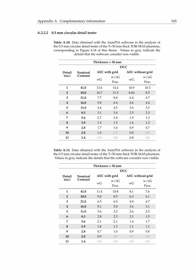
Appendix A. Complementary information 165
A.2.2.2 0.5 mm circular detail tester
Table A.10: Data obtained with the AutoPIA software in the analysis ofthe 0.5 mm circular detail tester of the T=30 mm thick TOR-MAS phantom,corresponding to Figure 6.18 of this thesis. Values in gray indicate the
details that the software consider non-visible.
Thickness = 30 mmDCC
Detail(no.)
NominalContrast
AEC with grid AEC without grid
wGw/oGProc.
wGw/oGProc.
1 41.0 13.6 14.4 10.9 10.3
2 30.0 10.7 11.5 8.60 8.5
3 21.0 7.7 8.8 6.4 6.7
4 16.0 5.8 6.4 4.6 4.4
5 11.0 4.4 4.5 3.4 3.3
6 8.3 3.1 3.4 2.5 2.3
7 5.6 2.7 2.4 1.9 1.3
8 3.9 1.9 1.5 1.6 1.2
9 2.8 1.7 3.4 0.9 0.7
10 2.0 1.0 0.7 0.8 0.6
11 1.4 0.0 0.0 0.8 0.0
Table A.11: Data obtained with the AutoPIA software in the analysis ofthe 0.5 mm circular detail tester of the T=50 mm thick TOR-MAS phantom.Values in gray indicate the details that the software consider non-visible.
Thickness = 50 mmDCC
Detail(no.)
NominalContrast
AEC with grid AEC without grid
wGw/oGProc.
wGw/oGProc.
1 41.0 11.4 10.8 8.1 7.6
2 30.0 9.0 8.5 6.3 6.1
3 21.0 6.5 6.0 4.9 4.7
4 16.0 5.1 5.0 3.6 3.1
5 11.0 3.6 3.2 2.6 2.5
6 8.3 2.8 2.3 2.1 1.5
7 5.6 2.1 2.1 1.4 1.7
8 3.9 1.8 1.3 1.1 1.1
9 2.8 0.7 1.0 0.9 0.8
10 2.0 0.9 0.0 0.0 0.0
11 1.4 0.0 0.0 0.0 0.0
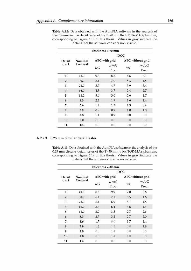
Appendix A. Complementary information 166
Table A.12: Data obtained with the AutoPIA software in the analysis ofthe 0.5 mm circular detail tester of the T=70 mm thick TOR-MAS phantom,corresponding to Figure 6.18 of this thesis. Values in gray indicate the
details that the software consider non-visible.
Thickness = 70 mmDCC
Detail(no.)
NominalContrast
AEC with grid AEC without grid
wGw/oGProc.
wGw/oGProc.
1 41.0 9.6 8.5 6.6 6.1
2 30.0 8.1 7.0 5.3 4.8
3 21.0 5.7 4.7 3.9 3.4
4 16.0 4.3 3.7 2.4 2.7
5 11.0 3.0 3.0 2.6 1.7
6 8.3 2.3 1.9 1.6 1.4
7 5.6 1.4 1.3 1.3 0.9
8 3.9 0.9 0.9 1.0 1.0
9 2.8 1.1 0.9 0.8 0.0
10 2.0 1.0 0.0 0.0 0.0
11 1.4 0.0 0.0 0.0 0.0
A.2.2.3 0.25 mm circular detail tester
Table A.13: Data obtained with the AutoPIA software in the analysis of the0.25 mm circular detail tester of the T=30 mm thick TOR-MAS phantom,corresponding to Figure 6.19 of this thesis. Values in gray indicate the
details that the software consider non-visible.
Thickness = 30 mmDCC
Detail(no.)
NominalContrast
AEC with grid AEC without grid
wGw/oGProc.
wGw/oGProc.
1 41.0 8.6 9.9 7.0 6.6
2 30.0 6.4 7.1 5.5 4.6
3 21.0 6.1 6.9 5.1 4.8
4 16.0 5.3 6.4 4.6 4.5
5 11.0 3.9 3.5 2.7 2.6
6 8.3 2.7 3.2 2.7 2.0
7 5.6 1.7 0.0 1.7 1.4
8 3.9 1.3 1.3 0.0 1.8
9 2.8 0.0 1.4 0.0 0.0
10 2.0 0.0 1.4 1.8 0.0
11 1.4 0.0 0.0 0.0 0.0
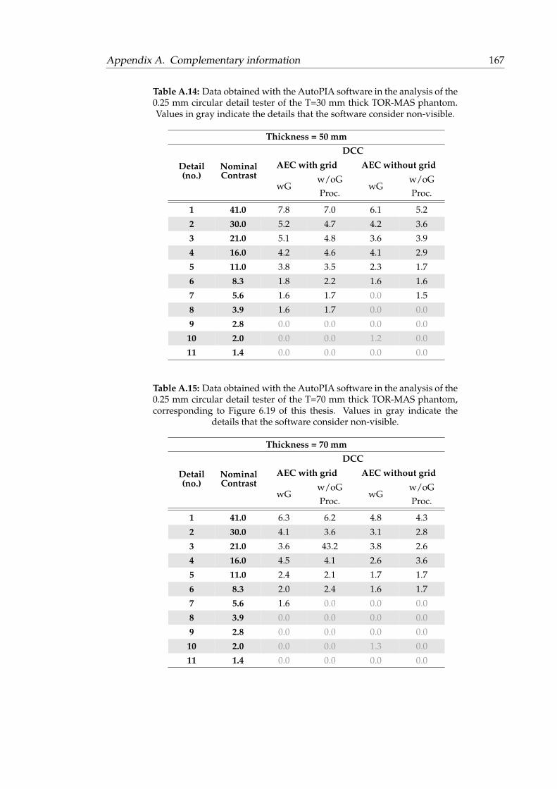
Appendix A. Complementary information 167
Table A.14: Data obtained with the AutoPIA software in the analysis of the0.25 mm circular detail tester of the T=30 mm thick TOR-MAS phantom.Values in gray indicate the details that the software consider non-visible.
Thickness = 50 mmDCC
Detail(no.)
NominalContrast
AEC with grid AEC without grid
wGw/oGProc.
wGw/oGProc.
1 41.0 7.8 7.0 6.1 5.2
2 30.0 5.2 4.7 4.2 3.6
3 21.0 5.1 4.8 3.6 3.9
4 16.0 4.2 4.6 4.1 2.9
5 11.0 3.8 3.5 2.3 1.7
6 8.3 1.8 2.2 1.6 1.6
7 5.6 1.6 1.7 0.0 1.5
8 3.9 1.6 1.7 0.0 0.0
9 2.8 0.0 0.0 0.0 0.0
10 2.0 0.0 0.0 1.2 0.0
11 1.4 0.0 0.0 0.0 0.0
Table A.15: Data obtained with the AutoPIA software in the analysis of the0.25 mm circular detail tester of the T=70 mm thick TOR-MAS phantom,corresponding to Figure 6.19 of this thesis. Values in gray indicate the
details that the software consider non-visible.
Thickness = 70 mmDCC
Detail(no.)
NominalContrast
AEC with grid AEC without grid
wGw/oGProc.
wGw/oGProc.
1 41.0 6.3 6.2 4.8 4.3
2 30.0 4.1 3.6 3.1 2.8
3 21.0 3.6 43.2 3.8 2.6
4 16.0 4.5 4.1 2.6 3.6
5 11.0 2.4 2.1 1.7 1.7
6 8.3 2.0 2.4 1.6 1.7
7 5.6 1.6 0.0 0.0 0.0
8 3.9 0.0 0.0 0.0 0.0
9 2.8 0.0 0.0 0.0 0.0
10 2.0 0.0 0.0 1.3 0.0
11 1.4 0.0 0.0 0.0 0.0
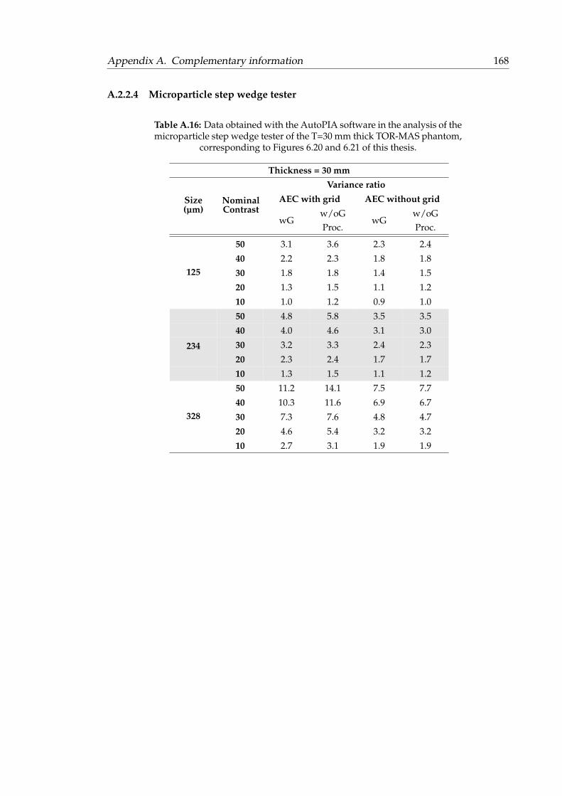
Appendix A. Complementary information 168
A.2.2.4 Microparticle step wedge tester
Table A.16: Data obtained with the AutoPIA software in the analysis of themicroparticle step wedge tester of the T=30 mm thick TOR-MAS phantom,
corresponding to Figures 6.20 and 6.21 of this thesis.
Thickness = 30 mmVariance ratio
Size(µm)
NominalContrast
AEC with grid AEC without grid
wGw/oGProc.
wGw/oGProc.
125
50 3.1 3.6 2.3 2.4
40 2.2 2.3 1.8 1.8
30 1.8 1.8 1.4 1.5
20 1.3 1.5 1.1 1.2
10 1.0 1.2 0.9 1.0
50 4.8 5.8 3.5 3.5
40 4.0 4.6 3.1 3.0
30 3.2 3.3 2.4 2.3
20 2.3 2.4 1.7 1.7234
10 1.3 1.5 1.1 1.2
328
50 11.2 14.1 7.5 7.7
40 10.3 11.6 6.9 6.7
30 7.3 7.6 4.8 4.7
20 4.6 5.4 3.2 3.2
10 2.7 3.1 1.9 1.9
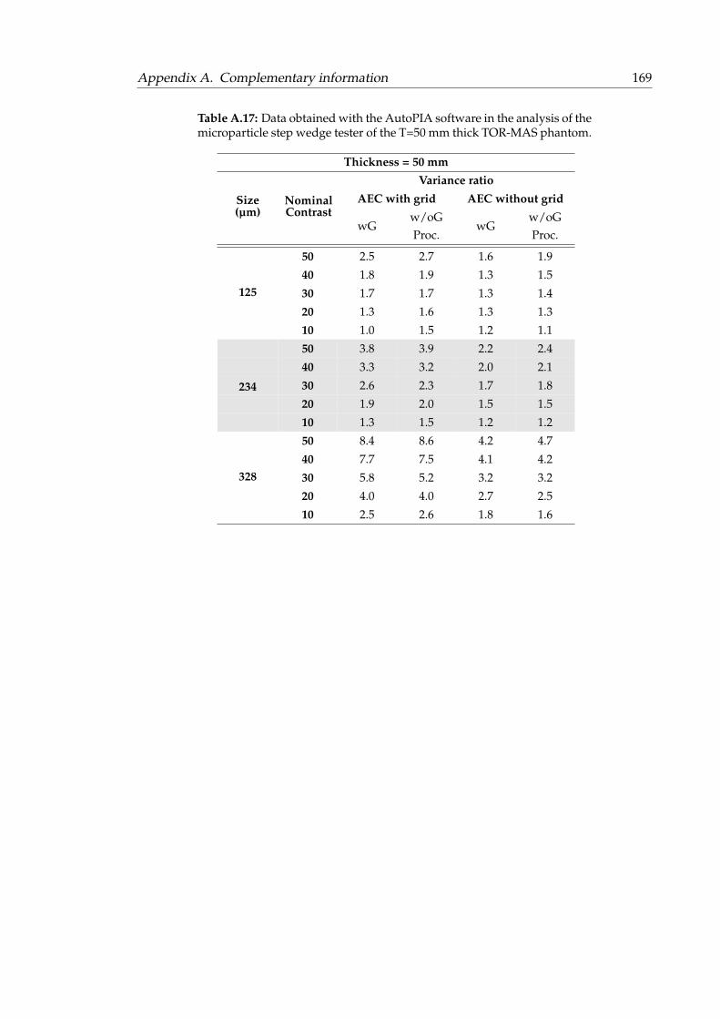
Appendix A. Complementary information 169
Table A.17: Data obtained with the AutoPIA software in the analysis of themicroparticle step wedge tester of the T=50 mm thick TOR-MAS phantom.
Thickness = 50 mmVariance ratio
Size(µm)
NominalContrast
AEC with grid AEC without grid
wGw/oGProc.
wGw/oGProc.
125
50 2.5 2.7 1.6 1.9
40 1.8 1.9 1.3 1.5
30 1.7 1.7 1.3 1.4
20 1.3 1.6 1.3 1.3
10 1.0 1.5 1.2 1.1
50 3.8 3.9 2.2 2.4
40 3.3 3.2 2.0 2.1
30 2.6 2.3 1.7 1.8
20 1.9 2.0 1.5 1.5234
10 1.3 1.5 1.2 1.2
328
50 8.4 8.6 4.2 4.7
40 7.7 7.5 4.1 4.2
30 5.8 5.2 3.2 3.2
20 4.0 4.0 2.7 2.5
10 2.5 2.6 1.8 1.6
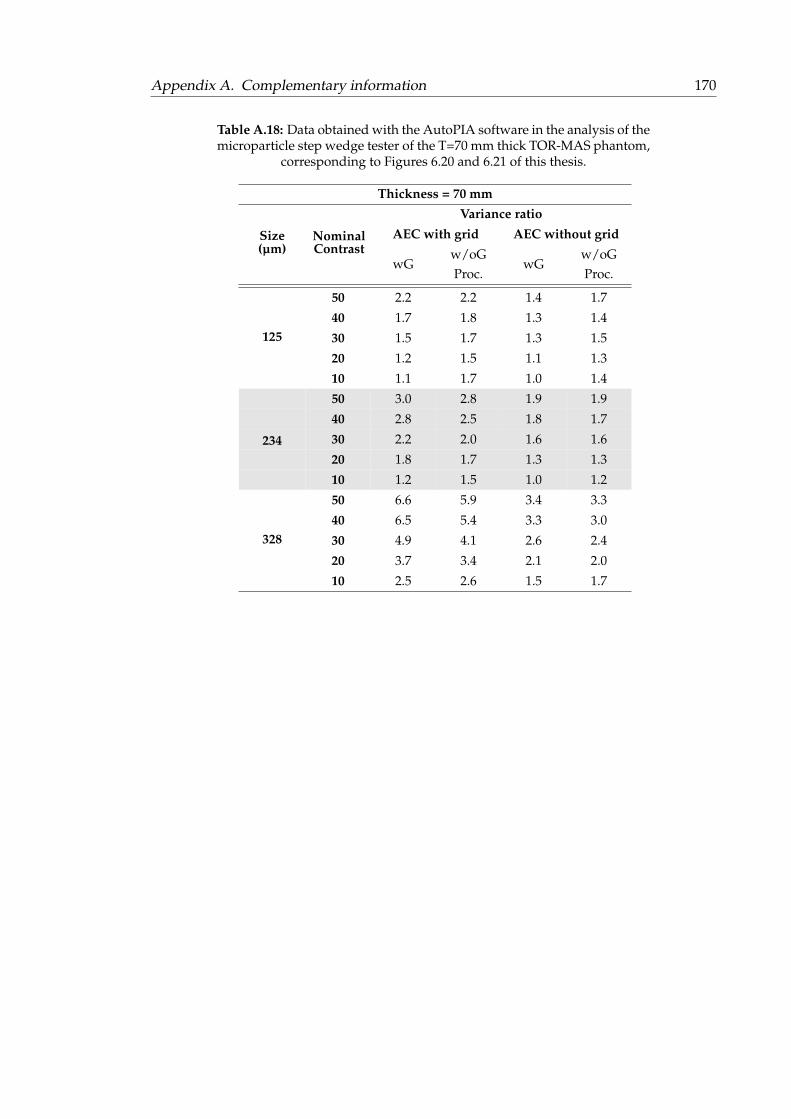
Appendix A. Complementary information 170
Table A.18: Data obtained with the AutoPIA software in the analysis of themicroparticle step wedge tester of the T=70 mm thick TOR-MAS phantom,
corresponding to Figures 6.20 and 6.21 of this thesis.
Thickness = 70 mmVariance ratio
Size(µm)
NominalContrast
AEC with grid AEC without grid
wGw/oGProc.
wGw/oGProc.
125
50 2.2 2.2 1.4 1.7
40 1.7 1.8 1.3 1.4
30 1.5 1.7 1.3 1.5
20 1.2 1.5 1.1 1.3
10 1.1 1.7 1.0 1.4
50 3.0 2.8 1.9 1.9
40 2.8 2.5 1.8 1.7
30 2.2 2.0 1.6 1.6
20 1.8 1.7 1.3 1.3234
10 1.2 1.5 1.0 1.2
328
50 6.6 5.9 3.4 3.3
40 6.5 5.4 3.3 3.0
30 4.9 4.1 2.6 2.4
20 3.7 3.4 2.1 2.0
10 2.5 2.6 1.5 1.7
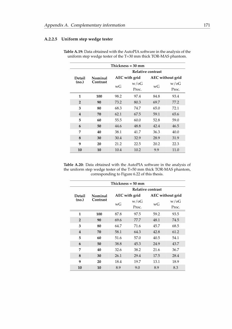
Appendix A. Complementary information 171
A.2.2.5 Uniform step wedge tester
Table A.19: Data obtained with the AutoPIA software in the analysis of theuniform step wedge tester of the T=30 mm thick TOR-MAS phantom.
Thickness = 30 mmRelative contrast
Detail(no.)
NominalContrast
AEC with grid AEC without grid
wGw/oGProc.
wGw/oGProc.
1 100 98.2 97.4 84.8 93.4
2 90 73.2 80.3 69.7 77.2
3 80 68.3 74.7 65.0 72.1
4 70 62.1 67.5 59.1 65.6
5 60 55.5 60.0 52.8 59.0
6 50 44.6 48.8 42.4 46.5
7 40 38.1 41.7 36.3 40.0
8 30 30.4 32.9 28.9 31.9
9 20 21.2 22.5 20.2 22.3
10 10 10.4 10.2 9.9 11.0
Table A.20: Data obtained with the AutoPIA software in the analysis ofthe uniform step wedge tester of the T=50 mm thick TOR-MAS phantom,
corresponding to Figure 6.22 of this thesis.
Thickness = 50 mmRelative contrast
Detail(no.)
NominalContrast
AEC with grid AEC without grid
wGw/oGProc.
wGw/oGProc.
1 100 87.8 97.5 59.2 93.5
2 90 69.6 77.7 48.1 74.5
3 80 64.7 71.6 45.7 68.5
4 70 58.1 64.3 42.8 61.2
5 60 51.6 57.0 40.5 54.1
6 50 38.8 45.3 24.9 43.7
7 40 32.6 38.2 21.6 36.7
8 30 26.1 29.4 17.5 28.4
9 20 18.4 19.7 13.1 18.9
10 10 8.9 9.0 8.9 8.3
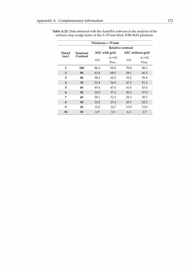
Appendix A. Complementary information 172
Table A.21: Data obtained with the AutoPIA software in the analysis of theuniform step wedge tester of the T=70 mm thick TOR-MAS phantom.
Thickness = 70 mmRelative contrast
Detail(no.)
NominalContrast
AEC with grid AEC without grid
wGw/oGProc.
wGw/oGProc.
1 100 86.3 92.0 79.0 90.3
2 90 63.6 68.5 58.1 66.3
3 80 58.2 62.2 53.2 59.4
4 70 51.8 54.9 47.3 51.3
5 60 45.4 47.6 41.6 43.4
6 50 34.5 37.4 30.2 37.9
7 40 29.1 31.3 25.3 30.7
8 30 22.8 23.4 20.1 22.2
9 20 15.2 14.7 13.9 12.9
10 10 6.9 5.0 6.4 2.7
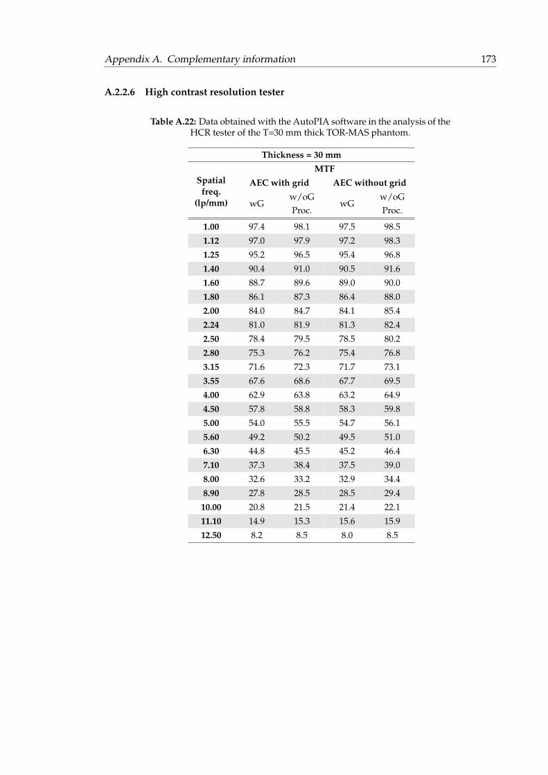
Appendix A. Complementary information 173
A.2.2.6 High contrast resolution tester
Table A.22: Data obtained with the AutoPIA software in the analysis of theHCR tester of the T=30 mm thick TOR-MAS phantom.
Thickness = 30 mmMTF
Spatialfreq.
(lp/mm)
AEC with grid AEC without grid
wGw/oGProc.
wGw/oGProc.
1.00 97.4 98.1 97.5 98.5
1.12 97.0 97.9 97.2 98.3
1.25 95.2 96.5 95.4 96.8
1.40 90.4 91.0 90.5 91.6
1.60 88.7 89.6 89.0 90.0
1.80 86.1 87.3 86.4 88.0
2.00 84.0 84.7 84.1 85.4
2.24 81.0 81.9 81.3 82.4
2.50 78.4 79.5 78.5 80.2
2.80 75.3 76.2 75.4 76.8
3.15 71.6 72.3 71.7 73.1
3.55 67.6 68.6 67.7 69.5
4.00 62.9 63.8 63.2 64.9
4.50 57.8 58.8 58.3 59.8
5.00 54.0 55.5 54.7 56.1
5.60 49.2 50.2 49.5 51.0
6.30 44.8 45.5 45.2 46.4
7.10 37.3 38.4 37.5 39.0
8.00 32.6 33.2 32.9 34.4
8.90 27.8 28.5 28.5 29.4
10.00 20.8 21.5 21.4 22.1
11.10 14.9 15.3 15.6 15.9
12.50 8.2 8.5 8.0 8.5
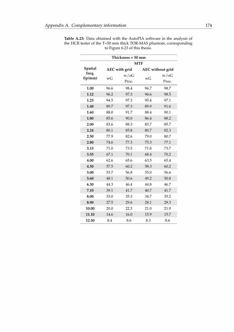
Appendix A. Complementary information 174
Table A.23: Data obtained with the AutoPIA software in the analysis ofthe HCR tester of the T=50 mm thick TOR-MAS phantom, corresponding
to Figure 6.23 of this thesis.
Thickness = 50 mmMTF
Spatialfreq.
(lp/mm)
AEC with grid AEC without grid
wGw/oGProc.
wGw/oGProc.
1.00 96.6 98.4 96.7 98.7
1.12 96.2 97.3 96.6 98.5
1.25 94.5 97.3 95.4 97.1
1.40 89.7 97.3 89.9 91.6
1.60 88.0 91.7 88.4 90.1
1.80 85.6 90.0 86.4 88.2
2.00 83.6 88.3 83.7 85.7
2.24 80.1 85.8 80.7 82.3
2.50 77.9 82.6 79.0 80.7
2.80 74.6 77.3 75.3 77.1
3.15 71.0 73.5 71.8 73.7
3.55 67.1 70.1 68.4 70.2
4.00 62.6 65.6 63.5 65.4
4.50 57.5 60.2 58.3 60.2
5.00 53.7 56.8 55.0 56.6
5.60 48.1 50.6 49.2 50.8
6.30 44.3 46.4 44.8 46.7
7.10 39.1 41.7 40.7 41.7
8.00 33.0 35.3 34.7 35.2
8.90 27.5 29.6 28.1 29.3
10.00 20.0 22.3 21.0 21.9
11.10 14.6 16.0 15.9 15.7
12.50 8.4 8.6 8.3 8.6
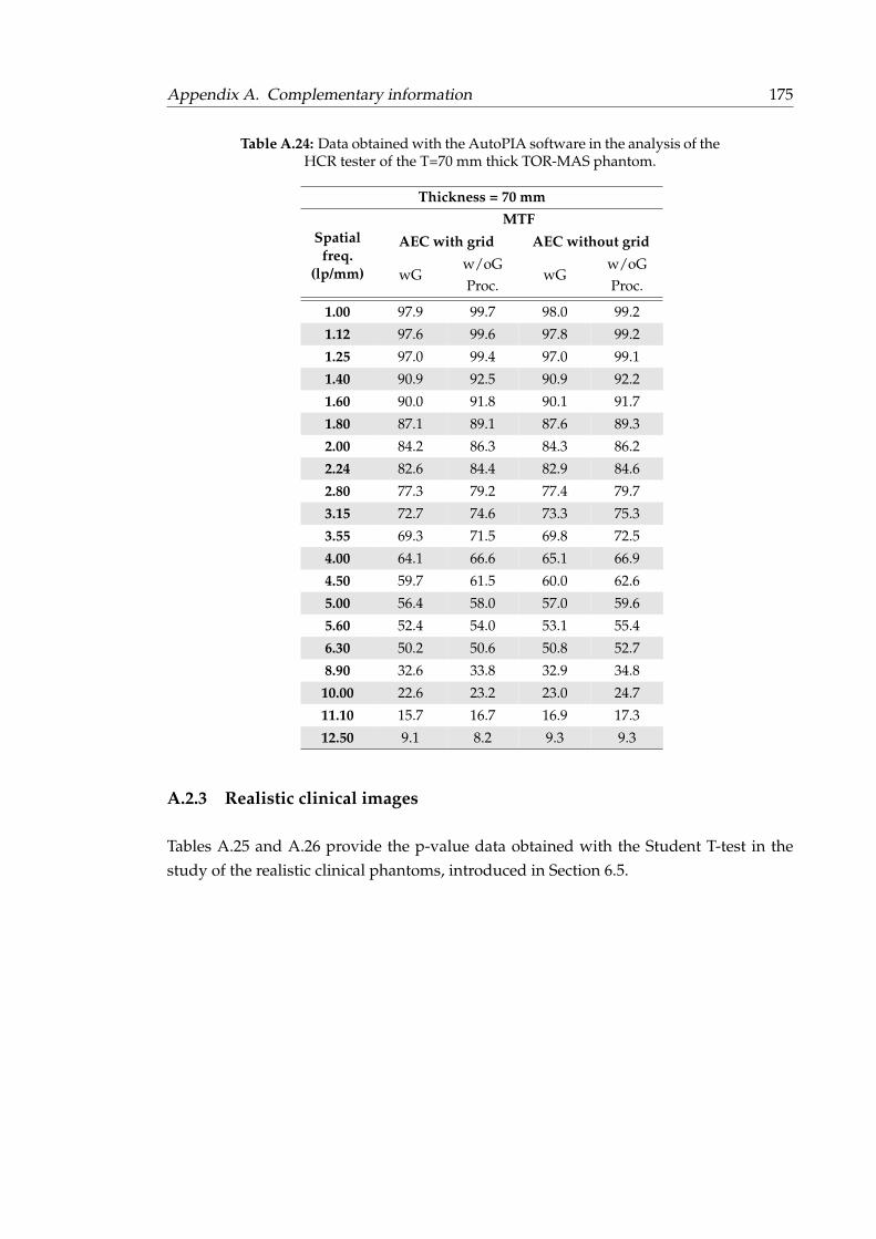
Appendix A. Complementary information 175
Table A.24: Data obtained with the AutoPIA software in the analysis of theHCR tester of the T=70 mm thick TOR-MAS phantom.
Thickness = 70 mmMTF
Spatialfreq.
(lp/mm)
AEC with grid AEC without grid
wGw/oGProc.
wGw/oGProc.
1.00 97.9 99.7 98.0 99.2
1.12 97.6 99.6 97.8 99.2
1.25 97.0 99.4 97.0 99.1
1.40 90.9 92.5 90.9 92.2
1.60 90.0 91.8 90.1 91.7
1.80 87.1 89.1 87.6 89.3
2.00 84.2 86.3 84.3 86.2
2.24 82.6 84.4 82.9 84.6
2.80 77.3 79.2 77.4 79.7
3.15 72.7 74.6 73.3 75.3
3.55 69.3 71.5 69.8 72.5
4.00 64.1 66.6 65.1 66.9
4.50 59.7 61.5 60.0 62.6
5.00 56.4 58.0 57.0 59.6
5.60 52.4 54.0 53.1 55.4
6.30 50.2 50.6 50.8 52.7
8.90 32.6 33.8 32.9 34.8
10.00 22.6 23.2 23.0 24.7
11.10 15.7 16.7 16.9 17.3
12.50 9.1 8.2 9.3 9.3
A.2.3 Realistic clinical images
Tables A.25 and A.26 provide the p-value data obtained with the Student T-test in thestudy of the realistic clinical phantoms, introduced in Section 6.5.
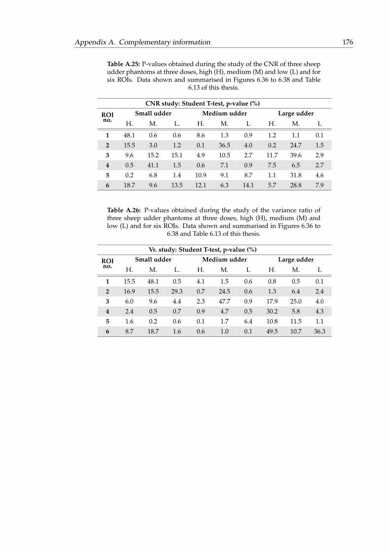
Appendix A. Complementary information 176
Table A.25: P-values obtained during the study of the CNR of three sheepudder phantoms at three doses, high (H), medium (M) and low (L) and forsix ROIs. Data shown and summarised in Figures 6.36 to 6.38 and Table
6.13 of this thesis.
CNR study: Student T-test, p-value (%)
ROIno.
Small udder Medium udder Large udder
H. M. L. H. M. L H. M. L
1 48.1 0.6 0.6 8.6 1.3 0.9 1.2 1.1 0.1
2 15.5 3.0 1.2 0.1 36.5 4.0 0.2 24.7 1.5
3 9.6 15.2 15.1 4.9 10.5 2.7 11.7 39.6 2.9
4 0.5 41.1 1.5 0.6 7.1 0.9 7.5 6.5 2.7
5 0.2 6.8 1.4 10.9 9.1 8.7 1.1 31.8 4.6
6 18.7 9.6 13.5 12.1 6.3 14.1 5.7 28.8 7.9
Table A.26: P-values obtained during the study of the variance ratio ofthree sheep udder phantoms at three doses, high (H), medium (M) andlow (L) and for six ROIs. Data shown and summarised in Figures 6.36 to
6.38 and Table 6.13 of this thesis.
Vr. study: Student T-test, p-value (%)
ROIno.
Small udder Medium udder Large udder
H. M. L. H. M. L H. M. L
1 15.5 48.1 0.5 4.1 1.5 0.6 0.8 0.5 0.1
2 16.9 15.5 29.3 0.7 24.5 0.6 1.3 6.4 2.4
3 6.0 9.6 4.4 2.3 47.7 0.9 17.9 25.0 4.0
4 2.4 0.5 0.7 0.9 4.7 0.5 30.2 5.8 4.3
5 1.6 0.2 0.6 0.1 1.7 6.4 10.8 11.5 1.1
6 8.7 18.7 1.6 0.6 1.0 0.1 49.5 10.7 36.3

177
Appendix B
Research Ethics Checklist

Appendix B. Research Ethics Checklist 178

Appendix B. Research Ethics Checklist 179

Appendix B. Research Ethics Checklist 180

Appendix B. Research Ethics Checklist 181

Appendix B. Research Ethics Checklist 182
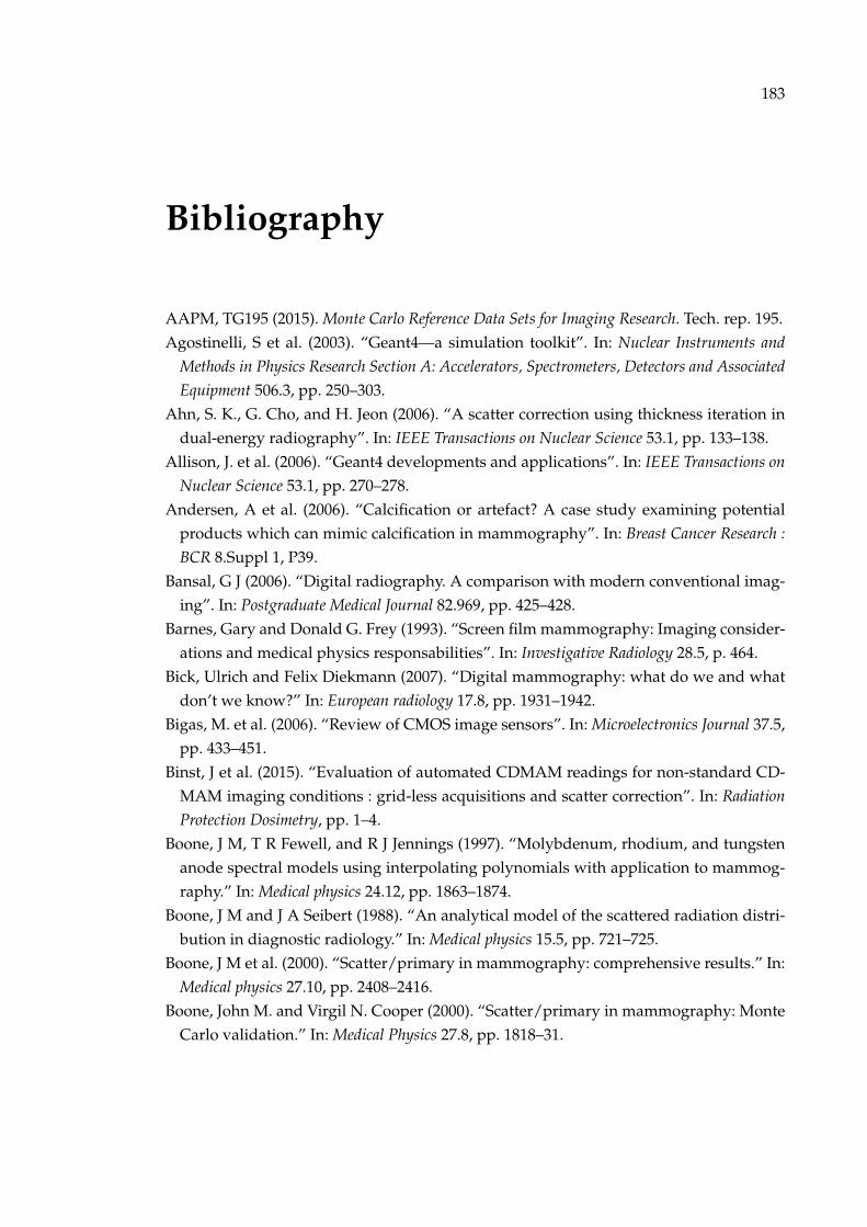
183
Bibliography
AAPM, TG195 (2015). Monte Carlo Reference Data Sets for Imaging Research. Tech. rep. 195.Agostinelli, S et al. (2003). “Geant4—a simulation toolkit”. In: Nuclear Instruments and
Methods in Physics Research Section A: Accelerators, Spectrometers, Detectors and AssociatedEquipment 506.3, pp. 250–303.
Ahn, S. K., G. Cho, and H. Jeon (2006). “A scatter correction using thickness iteration indual-energy radiography”. In: IEEE Transactions on Nuclear Science 53.1, pp. 133–138.
Allison, J. et al. (2006). “Geant4 developments and applications”. In: IEEE Transactions onNuclear Science 53.1, pp. 270–278.
Andersen, A et al. (2006). “Calcification or artefact? A case study examining potentialproducts which can mimic calcification in mammography”. In: Breast Cancer Research :BCR 8.Suppl 1, P39.
Bansal, G J (2006). “Digital radiography. A comparison with modern conventional imag-ing”. In: Postgraduate Medical Journal 82.969, pp. 425–428.
Barnes, Gary and Donald G. Frey (1993). “Screen film mammography: Imaging consider-ations and medical physics responsabilities”. In: Investigative Radiology 28.5, p. 464.
Bick, Ulrich and Felix Diekmann (2007). “Digital mammography: what do we and whatdon’t we know?” In: European radiology 17.8, pp. 1931–1942.
Bigas, M. et al. (2006). “Review of CMOS image sensors”. In: Microelectronics Journal 37.5,pp. 433–451.
Binst, J et al. (2015). “Evaluation of automated CDMAM readings for non-standard CD-MAM imaging conditions : grid-less acquisitions and scatter correction”. In: RadiationProtection Dosimetry, pp. 1–4.
Boone, J M, T R Fewell, and R J Jennings (1997). “Molybdenum, rhodium, and tungstenanode spectral models using interpolating polynomials with application to mammog-raphy.” In: Medical physics 24.12, pp. 1863–1874.
Boone, J M and J A Seibert (1988). “An analytical model of the scattered radiation distri-bution in diagnostic radiology.” In: Medical physics 15.5, pp. 721–725.
Boone, J M et al. (2000). “Scatter/primary in mammography: comprehensive results.” In:Medical physics 27.10, pp. 2408–2416.
Boone, John M. and Virgil N. Cooper (2000). “Scatter/primary in mammography: MonteCarlo validation.” In: Medical Physics 27.8, pp. 1818–31.
BIBLIOGRAPHY 184
Buhr, Egbert, Susanne Guenther-Kohfahl, and Ulrich Neitzel (2003). “Simple method formodulation transfer function determination of digital imaging detectors from edge im-ages”. In: Proceedings of SPIE, Medical Imaging 5030, p. 877.
Bushberg, J. T. et al. (2012). “The Essential Physics of the Medical Imaging, 3rd ed”. In:Lippincott Williams & Wilkins, p. 1048.
CERN, [online] (2016). Geant4 User Documentation. URL: http://geant4.cern.ch/support/userdocuments.shtml (visited on 06/08/2016).
– (2017). Geant4 physics list. URL: http : / / geant4 . cern . ch / collaboration / working\ _groups/electromagnetic/physlist10.1.shtml\#opt4 (visited on 06/08/2016).
CIRS, Tissue Simulation & Phantom Technology [online]. CIRS. URL: http : / / www.cirsinc.com/products/all/6/tissue-equivalent-phantom-for-mammography/ (visitedon 01/25/2018).
collaboration, Geant4 (2016). “Geant4 User’s Guide for Application Developers”. In: CERNDecember.
Cooper, V N et al. (2000). “An edge spread technique for measurement of the scatter-to-primary ratio in mammography.” In: Medical physics 27.5, pp. 845–853.
CyberQual, [online] (2016). AutoPIA. URL: autopia.cyberqual.it (visited on 03/20/2018).Dance, D R et al. (2000). “Additional factors for the estimation of mean glandular breast
dose using the UK mammography dosimetry protocol.” In: Physics in medicine and biol-ogy 45.11, pp. 3225–3240. ISSN: 0031-9155. DOI: 10.1088/0031-9155/45/11/308.
Demchik, Vadim (2011). “Pseudo-random number generators for Monte Carlo simula-tions on ATI Graphics Processing Units”. In: Computer Physics Communications 182.3,pp. 692–705.
Díaz, O et al. (2014). “Estimation of scattered radiation in digital breast tomosynthesis.”In: Physics in medicine and biology 59, pp. 4375–4390.
Díaz, Oliver (2013). “Scattered radiation in projection X-ray mammography and digitalbreast tomosynthesis”. PhD thesis. University of Surrey.
Díaz, Oliver et al. (2012). “A fast scatter field estimator for digital breast tomosynthesis”.In: SPIE, Medical Imaging 8313, pp. 831305–831305–9.
Diffey, J.L. (2015). “A comparison of digital mammography detectors and emerging tech-nology”. In: Radiography 21.4, pp. 1–9.
Dixon, J M (2012). ABC of Breast Diseases. ABC Series. Wiley.Dobbins, J T et al. (1995). “DQE(f) of four generations of computed radiography acquisi-
tion devices.” In: Medical physics 22.10, pp. 1581–1593.Dowsett, D, P A Kenny, and R E Johnston (2006). The Physics of Diagnostic Imaging. 2nd.
A Hodder Arnold Publication. Taylor & Francis.Ducote, J L and S Molloi (2010). “Scatter correction in digital mammography based on
image deconvolution.” In: Physics in medicine and biology 55, pp. 1295–1309.
BIBLIOGRAPHY 185
Evans, D S, A Workman, and M Payne (2002). “A comparison of the imaging properties ofCCD-based devices used for small field digital mammography”. In: Physics in Medicine& Biology 47.1, p. 117.
Farman, Allan G. and Taeko T. Farman (2005). “A comparison of 18 different x-ray de-tectors currently used in dentistry”. In: Oral Surgery, Oral Medicine, Oral Pathology, OralRadiology and Endodontology 99.4, pp. 485–489.
Farman, Taeko T et al. (2005). “Effects of scintillator on the modulation transfer function(MTF) of a digital imaging system.” In: Oral surgery, oral medicine, oral pathology, oralradiology, and endodontics 99.5, pp. 608–613.
– (2006). “Effects of scintillator on the detective quantum efficiency (DQE) of a digitalimaging system”. In: Oral Surgery, Oral Medicine, Oral Pathology, Oral Radiology, andEndodontology 101.2, pp. 219–223.
Feijó Pery, Vidal and Gabriela Hoff (2008). “Geant4 validation on mammography appli-cations”. In: IEEE Nuclear Science Symposium Conference Record, pp. 3497–3498.
Feng, Steve Si Jia and Ioannis Sechopoulos (2011). “A software-based x-ray scatter cor-rection method for breast tomosynthesis”. In: Medical Physics 38.12, pp. 6643–6653.
Feng, Steve Si Jia et al. (2014). “X-ray scatter correction in breast tomosynthesis with aprecomputed scatter map library.” In: Medical physics 41.3, p. 31912.
Fieselmann, Andreas et al. (2013). “Full-field digital mammography with grid-less acqui-sition and software-based scatter correction: investigation of dose saving and imagequality”. In: SPIE Medical Imaging: Physics of Medical Imaging 8668, 86685Y.
Fossum, Eric R and Senior Member (1997). “CMOS Image Sensors : Electronic Camera-On-A-Chip”. In: 44.10, pp. 1689–1698.
Frandson, R D, W L Wilke, and A D Fails (2013). Anatomy and Physiology of Farm Animals.Wiley.
Gerado Caja, Xavier Such, Maristela Rovai (1981). “Udder Morphology and MachineMilking Ability in Dairy Sheep”. In: Proceedings of the 6th Great Lakes Dairy Sheep Sym-posium.
Gonzalez Trotter, Dinko E et al. (2002). Thickness-dependent scatter correction algorithm fordigital mammography.
Gov.uk, [online] (2014). ABP waste. URL: https://www.gov.uk/guidance/animal- by-product-categories-site-approval-hygiene-and-disposal (visited on 07/15/2017).
Granfors, Paul and Richard Aufrichtig (2000). “DQE(f) of an amorphous-silicon flat-panelx-ray detector: detector parameter influences and measurement methodology”. In: Pro-ceedings of SPIE, Medical Imaging.
Grosjean, Bénédicte and Serge Muller (2006). “Impact of Textured Background on Scoringof Simulated CDMAM Phantom”. In: Proceeding of IWDM Digital Mammography. Ed. bySusan M Astley et al. Berlin, Heidelberg: Springer Berlin Heidelberg, pp. 460–467.
Hamamatsu, [online]. Scintillator plates - Hamamatsu photonics. URL: http://www.hamamatsu.com/jp/en/product/category/3100/3010/index.html (visited on 03/23/2016).
BIBLIOGRAPHY 186
Hammerstein, G Richard et al. (1979). “Absorbed Radiation Dose in Mammography”. In:Radiology 130.2, pp. 485–491.
Hendee, William R. and E. Russell Ritenour (2002). Medical Imaging Physics. 4th ed. Wiley-Liss.
Highnam, R. P., J. M. Brady, and B. J. Shepstone (1998). “Estimation of compressed breastthickness during mammography”. In: British Journal of Radiology 71.June, pp. 646–653.
Highnam, Ralph et al. (2010). “Robust Breast Composition Measurement - VolparaTM”.In: Digital Mammography: 10th International Workshop, IWDM 2010, Girona, Catalonia,Spain, June 16-18, 2010. Proceedings. Ed. by Joan Martí et al. Berlin, Heidelberg: SpringerBerlin Heidelberg, pp. 342–349.
Hoheisel, Martin (2006). “Review of medical imaging with emphasis on X-ray detectors”.In: Nuclear Instruments and Methods in Physics Research Section A: Accelerators, Spectrom-eters, Detectors and Associated Equipment 563.1, pp. 215–224.
IECP (2007a). IEC 62220-1-2 Medical electrical equipment - Characteristics of digital X-rayimaging devices - Part 1-2: Determination of the detective quantum efficiency - Detectors usedin mammography. Tech. rep. Geneva.
– (2007b). IEC 62220-1 Medical electrical equipment - Characteristics of digital X-ray imagingdevices - Part 1: Determination of the detective quantum efficiency. Tech. rep. Geneva.
James, J.J (2004). “The current status of digital mammography”. English. In: Clinical Ra-diology 59.1, pp. 1–10.
Key, Veterian [online] (2016). Udder structure. URL: https://veteriankey.com/the-mammary-gland-2/ (visited on 06/25/2017).
Knoll, Glenn F. (2010). Radiation detection and measurement. 4th ed. New York: Wiley.Konstantinidis, Anastasios C. (2011). “Evaluation of digital X-ray detectors for medical
imaging applications”. PhD thesis. UCL.Konstantinidis, Anastasios C et al. (2012). “The Dexela 2923 CMOS X-ray detector A flat
panel detector based on CMOS active pixel sensors for medical imaging applications”.In: Nuclear Inst. and Methods in Physics Research, A 689.C, pp. 12–21.
Konstantinidis, Anastasios C. et al. (2013). “X-ray Performance Evaluation of the DexelaCMOS APS X-ray Detector Using Monochromatic Synchrotron Radiation in the Mam-mographic Energy Range”. In: IEEE Transactions on Nuclear Science 60.5, pp. 3969–3980.
Kopans, D B (2007). Breast Imaging. Lippincott Williams & Wilkins.Krol, A et al. (1996). “Scatter reduction in mammography with air gap.” In: Medical physics
23.7, pp. 1263–1270.Leeds Test Objects, [online]. AutoPIA Leeds Test Objects. URL: https://www.leedstestobjects.
com/index.php/phantom/autopia-software/ (visited on 02/05/2018).– TOR-MAM. URL: http://www.leedstestobjects.com/index.php/phantom/tor-mam/
(visited on 01/25/2018).– TOR-MAS. URL: http://www.leedstestobjects.com/index.php/phantom/tor-mas/
(visited on 01/25/2018).
BIBLIOGRAPHY 187
Leon, Stephanie M, Libby F Brateman, and Louis K Wagner (2014). “Characterization ofscatter in digital mammography from physical measurements.” In: Medical physics 41.6,p. 061901.
Love, L. Alan (1987). “Scatter estimation for a digital radiographic system using convo-lution filtering”. In: Medical Physics 14.2, p. 178.
Marimon, Elena et al. (2016). “Detailed Analysis of Scatter Contribution from DifferentSimulated Geometries of X-ray Detectors”. In: IWDM proceedings, pp. 203–210.
Mawdsley, Gordon E. et al. (2009). “Accurate estimation of compressed breast thicknessin mammography.” In: Medical physics 36.2009, pp. 577–586.
McPherson, K, C M Steel, and J M Dixon (2000). “Breast cancer-epidemiology, risk factors,and genetics”. In: British Medical Journal 321.7261, pp. 624–628.
Miller, Scott T et al. (2012). “Summary of the evidence of breast cancer service screeningoutcomes in Europe and first estimate of”. In: Journal of Medical Screening 19, pp. 5–13.
Monnin, P et al. (2007). “A comparison of the performance of digital mammography sys-tems.” In: Medical physics 34.3, pp. 906–914.
Moy, Jean-Pierre (1998). “Image quality of scintillator-based x-ray electronic imagers”. In:Proceedings of SPIE 3336.February, pp. 187–194.
Muller, Serge (1999). “Full-field digital mammography designed as a complete system”.In: European Journal of Radiology 31.1, pp. 25–34.
NASA, [online] (2015). The electromagnetic spectrum. URL: http://imagine.gsfc.nasa.gov/science/toolbox/emspectrum1.html (visited on 09/11/2015).
National Cancer Institute, [online] (2015). Cancer screening. URL: https://www.cancer.gov/about-cancer/screening (visited on 07/20/2017).
NHS, [online] (2016). Breast Cancer NHS. URL: http://www.nhs.uk/Conditions/Cancer-of-the-breast-female/Pages/Introduction.aspx (visited on 07/05/2017).
Nikola, Biller-Andorno and Jüni Peter (2014). “Abolishing Mammography Screening Pro-grams? A View from the Swiss Medical Board”. In: New England Journal of Medicine370.21, pp. 1965–1967.
NIST. NIST material composition [online]. URL: https://physics.nist.gov/cgi-bin/Star/compos.pl (visited on 05/25/2015).
NIST, [online] (2004). NIST Linear attenuation coefficients. URL: https://www.nist.gov/pml/x-ray-mass-attenuation-coefficients (visited on 10/12/2016).
Noel, A. and Fabienne Thibault (2004). “Digital detectors for mammography: The tech-nical challenges”. In: European Radiology 14, pp. 1990–1998.
Peters, Inge M. et al. (2016). “High dynamic range CMOS-based mammography detec-tor for FFDM and DBT”. In: SPIE Medical Imaging. International Society for Optics andPhotonics 9783, p. 978316.
Pisano, Etta D et al. (2005). “Diagnostic Performance of Digital versus Film Mammog-raphy for Breast-Cancer Screening”. In: The New England Journal of Medicine 353.17,pp. 1773–1783.
BIBLIOGRAPHY 188
Rangayyan, Rangaraj M and Thanh M Nguyen (2005). “Pattern classification of breastmasses via fractal analysis of their contours”. In: International Congress Series 1281,pp. 1041–1046.
Reed, Amy B. (2011). “The history of radiation use in medicine”. In: Journal of VascularSurgery 53.1 SUPPL. Pp. 3–5.
Rodríguez-Ruiz, Alejandro, Greeshma A Agasthya, and Ioannis Sechopoulos (2017). “Thecompressed breast during mammography and breast tomosynthesis: in vivo shapecharacterization and modeling”. In: Physics in Medicine & Biology 62.17, pp. 6920–6937.
Samei, E, M J Flynn, and D a Reimann (1998). “A method for measuring the presampledMTF of digital radiographic systems using an edge test device.” In: Medical physics 25.1,pp. 102–113.
Samei, Ehsan et al. (2006). “Intercomparison of methods for image quality characteriza-tion. I. Modulation transfer function.” In: Medical physics 33.5, pp. 1454–1465.
Sechopoulos, Ioannis (2007). “Investigation of physical processes in digital x-ray tomosyn-thesis imaging of the breast”. PhD thesis. Georgia Institute of Technology.
Sechopoulos, Ioannis et al. (2007a). “Computation of the glandular radiation dose in dig-ital tomosynthesis of the breast Ioannis”. In: Medical Physics 34.1, pp. 221–232.
Sechopoulos, Ioannis et al. (2007b). “Scatter radiation in digital tomosynthesis of thebreast”. In: Medical physics 34.1, pp. 221–32.
Sechopoulos, Ioannis et al. (2015). “Monte Carlo reference data sets for imaging research:Executive summary of the report of AAPM Research Committee Task Group 195”. In:Medical physics 3834.195.
Seeley, R R, T D Stephens, and P Tate (1998). Anatomy & Physiology. WCB/McGraw-Hill.Seibert, J a and J M Boone (2006). “X-ray scatter removal by deconvolution.” In: Medical
physics 15.1988, pp. 567–575.Sempau, J et al. (2001). “Monte Carlo simulation of electron beams from an accelerator
head using PENELOPE.” In: Physics in medicine and biology 46.4, pp. 1163–1186.Sickles, EA [online] (2013). ACR BI-RADS® Mammography. URL: https://www.acr.org/
Quality-Safety/Resources/BIRADS/About-BIRADS/How-to-Cite-BIRADS (visitedon 06/23/2017).
Siemens, [online] (2018). Simulation of X-ray Spectra. URL: https : / / www. oem - xray -components.siemens.com/x-ray-spectra-simulation (visited on 05/03/2018).
Smith, A P (2003). “Fundamentals of digital mammograhpy: physiscs, technology andpractical considerations.” In: Radiology Management 25(5), pp. 18–31.
Tan, Jiaming (2013). “4T CMOS Active Pixel Sensors under Ionizing Radiation”. PhDthesis, p. 147.
Timmers, J M H et al. (2012). “The Breast Imaging Reporting and Data System (BI-RADS)in the Dutch breast cancer screening programme: its role as an assessment and stratifi-cation tool”. In: European Radiology 22.8, pp. 1717–1723.
Tobias, J S and D Hochhauser (2009). Cancer and its Management. Wiley.
BIBLIOGRAPHY 189
Torre, Lindsey A et al. (2016). “Global Cancer Incidence and Mortality Rates and Trends— An Update”. In: Cancer, Epidemiology, Biomarkers & Prevention 25.January, pp. 16–28.
Turner, James E. (1995). Atoms, radiation and radiation protection. 2nd. New York, NY: Wi-ley.
Wang, Adam et al. (2015). Asymmetric scatter kernels for software-based scatter correction ofgridless mammography.
Waugh, Anne et al. (2014). Ross and Wilson anatomy and physiology in health and illness. 12th.Edinburgh : Churchill Livingstone, 2014.
WebMed, [online] (2014). WebMD - Picture of the Breasts. URL: http://www.webmd.com/women/picture-of-the-breasts\#1 (visited on 07/17/2017).
Welch, H and H.J. Passow (2014). “Quantifying the benefits and harms of screening mam-mography”. In: JAMA Internal Medicine 174.3, pp. 448–454.
White, D R, R J Martin, and R Darlison (1977). “Epoxy resin based tissue substitutes.”eng. In: The British journal of radiology 50.599, pp. 814–821.
Whitman, Gary J. et al. (2006). “Breast Cancer Staging”. In: Seminars in Roentgenology 41.2,pp. 91–104.
WHO (2014). WHO Position Paper on Mammography Screening. Tech. rep.World Cancer Research Fund International, [online] (2015). Breast cancer statistics. URL:
https://www.wcrf.org/int/cancer-facts-figures/data-specific-cancers/breast-cancer-statistics (visited on 05/03/2018).
Yaffe, M. J. et al. (2009). “The myth of the 50-50 breast”. In: Medical Physics 36.12, p. 5437.ISSN: 00942405. DOI: 10.1118/1.3250863. URL: http://scitation.aip.org/content/aapm/journal/medphys/36/12/10.1118/1.3250863.
Yaffe, Martin J and James G Mainprize (2004). “Detectors for Digital Mammography”. In:Technology in Cancer Research & Treatment 3.4, pp. 309–324.
Zanella, G (2002). “Gray levels, dynamic range, contrast and DQE in imaging detectors”.In: Nuclear Instruments and Methods in Physics Research Section A: Accelerators, Spectrom-eters, Detectors and Associated Equipment 481, pp. 691–695.