IKM OCEAN DESIGN AS OPTIMAL - UiS Brage
310
Subsea Tie-In Design Solutions and Optimisation Methods Loyd Kjetil Helland Andersen IKM Ocean Design AS-2015 IKM OCEAN DESIGN AS AT YOUR SERVICE OPTIMAL SOLUTIONS
-
Upload
khangminh22 -
Category
Documents
-
view
2 -
download
0
Transcript of IKM OCEAN DESIGN AS OPTIMAL - UiS Brage

Subsea Tie-In
Design Solutions and Optimisation Methods
Loyd Kjetil Helland Andersen
IKM Ocean Design AS-2015
IKM OCEAN DESIGN AS
AT YOUR SERVICE
OPTIMAL SOLUTIONS


Abstract
i
Abstract
Subsea Tie-in Systems is used to connect pipes between subsea structures in the offshore oil and gas
industry. Subsea Tie-in system has been developed for many decades by the industry, and is used
throughout the world in many subsea oil and gas fields of today. Industry experience and various piping
codes have been developed and used in the design over the years. However there has been a lack of
recommended standard practice and guideline for designing such systems. In this thesis two computer
software analysis packages commonly used in the industry for structural analysis of piping systems is
explored and compared. A vertical spool design case is investigated by the use of finite element analysis.
Relevant design load cases are identified and a design basis is established for the analysis. Relevant piping
codes such as ASME and DNV are used in the design. Some of the main challenges which have a great
influence on rigid spool design are the fabrication tolerances and metrology, which has to be accounted for
in the design. This thesis gives proposal on how to implement statistical distribution of tolerances in the
analysis by use of design exploration tools included in the ANSYS Software package. Advantages and
disadvantages are described.
The thesis will present some theory and examples to gain a general understanding about the content to be
presented. An Introduction of the most common Tie-in Systems and their basic configurations and shape is
presented. Advantages and limitations are described. Recommendations and suggestions for future spool
design solutions and load mitigations are given.
In this thesis a vertical spool has been analysed with a statistical and probabilistic approach for the
metrology and tolerances, the results shows that it is beneficial to include such method in order to better
document the safety level and the conservatism in the spool design. The approach also allows the engineer
to make a better decision towards the optimisation process of the spool.
The thesis also shows that simple mitigation measures for a vertical spool such as pre-bending and
introduction of a seabed support and buoyancy onto the spool has positive effects by reducing the resulting
bending moments at connector ends, and can reduce the total stresses in the spool. The results also show
that the vertical spool design is is very sensitive to VIV and hence fatigue capacity governs the design.
The vertical spool design has also been checked by use of the commercial piping software package
AutoPIPE from Bentley. The results compared to the ANSYS analysis shows that there is a minimal
difference in utilisations when using pipe beam element technology. The software is found to be feasible
for usage in subsea spool design for small to moderate displacements and deformations, however for an
optimised weight design it is recommended to perform a FEA with solid element models in ANSYS.
Preface
ii
Preface
This thesis summarizes my post graduate master’s degree at the Dept. of Mechanical and Structural
Engineering and Material Technology at the University of Stavanger during the spring of 2015. The Thesis
has been written in co-operation with IKM Ocean Design A/S which has been my employer for the last 7
years where I have been working as a Structural and Mechanical Engineer. IKM Ocean Design Specializes in
design and engineering of subsea pipelines, subsea structures and Tie-in solutions. The company is a sub
company of the IKM Group in Norway which is a major sub supplier to the oil and gas industry. During the
years working for IKM two vertical Tie-in Spool systems for deep water applications projects have been
proven to be of great challenge when it comes to design optimization, analysis techniques and strength
verification in the project. Hence a requirement for a more standardized route and methods for these types
of spool would indeed benefit future projects. A new DNV guideline for structural design criteria for rigid
tie-in spools has been developed by Statoil and DNV. This guideline is in a preliminary version and has not
been available for the author of this thesis but it is expected that this guideline will be released during
2015. The main objective of this thesis is to investigate standard solution and identify main challenges for
engineering of subsea Tie-in Spools, and propose possible new solutions and recommendations for the
commencing of such projects.
My Intention for selecting this subject was to learn more about subsea systems and computer analysing
techniques such as finite element programs, and to explore solutions and methods based upon my project
experience in IKM within this topic. I hope that people who read it will find it interesting and inspiring, and
that the work contributes to give information and advice for future projects and development in the
industry.
I would like to thank the management and administration at IKM Ocean Design AS for the opportunity to
work on this thesis. Special thanks go to MD. Peder Hoås, Tech. Dir. Per Nystrøm and former Dept. Mngr.
Helge Nesse, who made it possible for me to post graduate with this thesis in the IKM Company.
I would also like to thank the Dept. Mngr. Samson Katuramu and my colleges at the Dept. of Structures, Tie-
in and Pressurized components, Frode Tjelta, Asle Seim Johansen, Tomas Helleren and Valgerdur
Fridriksdottir, which have given me good ideas, valuable input, good discussion and support during this
work.
I would also thank my supervisor Dr. Hirpa G. Lemu at UIS for given me guidance and comments on how to
work with this thesis.
Finally I would like to give my family and my wife Christina Andersen, a special gratitude for being so
patient and supportive for me during the working process over the years as a part time student at UIS.
Stavanger 12.06.2015
Table of Contents
iii
Table of contents
ABSTRACT ............................................................................................................................................... I
PREFACE ................................................................................................................................................ II
LIST OF FIGURES ................................................................................................................................... VI
LIST OF TABLES ...................................................................................................................................... XI
NOMENCLATURE ................................................................................................................................. XIII
1. INTRODUCTION .............................................................................................................................. 1
1.1 HISTORICAL ............................................................................................................................................ 2
1.2 PROBLEM DESCRIPTION ........................................................................................................................... 2
1.3 SCOPE AND LIMITATION ........................................................................................................................... 4
1.4 REPORT STRUCTURE ................................................................................................................................ 5
2. BACKGROUND AND THEORY ........................................................................................................... 7
2.1 STRUCTURAL ANALYSIS OF PIPING .............................................................................................................. 7
2.2 WALL THICKNESS DESIGN .......................................................................................................................... 8
2.3 COLLAPSE OF PIPE WALL UNDER EXTERNAL PRESSURE .................................................................................. 11
2.4 LONGITUDINAL STRESS ........................................................................................................................... 13
2.5 COMBINED STRESS AND VON MISES EQUIVALENT STRESS ............................................................................ 14
2.6 PIPELINE EXPANSION.............................................................................................................................. 14
2.7 FLEXIBILITY OF PIPING SYSTEM ................................................................................................................. 19
2.8 V.I.V IN PIPELINES ................................................................................................................................ 23
3. TIE-IN SPOOLS SYSTEMS ................................................................................................................ 27
3.1 OBJECTIVE AND FUNCTIONALITY .............................................................................................................. 27
3.2 CONFIGURATIONS AND GEOMETRICAL SHAPES OF SPOOLS ............................................................................ 30
3.3 TIE-IN SYSTEM DETERMINATION .............................................................................................................. 31
3.4 SPOOL FABRICATION.............................................................................................................................. 32
3.5 PIPING FABRICATION TOLERANCES ........................................................................................................... 33
3.6 PROBABILISTIC ASSESSMENT OF FABRICATION TOLERANCES ......................................................................... 35
3.7 SUMMARY ........................................................................................................................................... 37
4. CONNECTOR AND TIE-IN SYSTEMS ................................................................................................. 39
4.1 CONNECTORS ....................................................................................................................................... 39
4.2 TIE-IN SYSTEMS .................................................................................................................................... 46
5. DESIGN BASIS ............................................................................................................................... 51
5.1 APPLICABLE CODES AND REGULATIONS ..................................................................................................... 51
5.2 MATERIAL DATA ................................................................................................................................... 52
5.3 PIPE DIMENSIONS ................................................................................................................................. 52
5.4 ENVIRONMENTAL DATA ......................................................................................................................... 53
Table of Contents
iv
5.5 DESIGN PARAMETERS ............................................................................................................................. 53
5.6 SPOOL CONFIGURATION ......................................................................................................................... 54
5.7 INSTALLATION, SETTLEMENT, SPOOL FABRICATION AND METROLOGY TOLERANCES .......................................... 55
5.8 LOAD CASES ......................................................................................................................................... 56
5.9 DESIGN CODE CHECK ............................................................................................................................. 57
5.9.1 Code formulas ........................................................................................................................... 57
5.9.2 HISC Stress limits ...................................................................................................................... 60
5.9.3 Code Stress Limits ..................................................................................................................... 61
6. SPOOL OPTIMISATION AND STRENGTH VERIFICATION ................................................................... 63
6.1 FINITE ELEMENT PROGRAM ANSYS .......................................................................................................... 63
6.2 ANALYSIS DESCRIPTION .......................................................................................................................... 67
6.3 FINITE ELEMENT MODEL DESCRIPTION ..................................................................................................... 70
6.4 MATERIAL PROPERTIES .......................................................................................................................... 74
6.5 SPOOL LOADS ....................................................................................................................................... 75
7. ANALYSIS RESULTS ........................................................................................................................ 79
7.1 ANSYS DESIGN EXPLORER RESULT OPERATIONAL LOADS ............................................................................ 79
7.2 REACTION FORCES AND BENDING MOMENTS ............................................................................................ 84
7.3 STRESS RESPONSE AND SENSITIVITY ......................................................................................................... 88
7.4 OPTIMAL SPOOL CONFIGURATION ........................................................................................................... 92
7.5 ANALYSIS RESULTS OPERATIONAL ............................................................................................................ 93
7.6 ANALYSIS RESULT FAT AND OFFSHORE HYDRO TESTING ............................................................................ 100
7.7 ANALYSIS RESULT SEAL REPLACEMENT ................................................................................................... 105
7.8 SUMMARY ......................................................................................................................................... 108
8. VERIFICATION AND COMPARISON OF RESULTS ............................................................................ 109
8.1 ANSYS PIPE BEAM ELEMENT MODEL .................................................................................................... 109
8.2 ANSYS SOLID ELEMENT MODEL ........................................................................................................... 116
8.3 BENTLEY AUTOPIPE MODEL ................................................................................................................. 125
8.4 BENTLEY AUTOPIPE RESULTS ............................................................................................................... 128
8.5 SUMMARY ......................................................................................................................................... 133
9. SPOOL WEIGHT AND LOAD MITIGATION ...................................................................................... 135
9.1 BUOYANCY ELEMENTS ......................................................................................................................... 135
9.2 SEABED SUPPORT ................................................................................................................................ 142
9.3 PRE-BENDING OF SPOOL ....................................................................................................................... 146
9.4 CHAPTER SUMMARY ............................................................................................................................ 149
10. VIV CHECK OF SPOOL ............................................................................................................... 151
10.1 APPLICABLE CODES .............................................................................................................................. 151
10.2 MODAL ANALYSIS ............................................................................................................................... 152
10.3 CODE CHECK VORTEX INDUCED VIBRATIONS (VIV) ................................................................................... 156
10.4 FATIGUE ............................................................................................................................................ 160
Table of Contents
v
10.5 SUMMARY ......................................................................................................................................... 163
11. FUTURE SOLUTIONS FOR SUBSEA TIE-IN ................................................................................... 165
11.1 DIRECT TIE-IN METHOD ........................................................................................................................ 165
11.2 FLEXIBLE SPOOLS ................................................................................................................................. 170
11.3 DESIGN CONCEPT IDEAS ....................................................................................................................... 176
12. SUMMARY, CONCLUSION AND RECOMMENDATIONS ............................................................... 177
12.1 SUMMARY ......................................................................................................................................... 177
12.2 CONCLUSION ...................................................................................................................................... 180
12.3 RECOMMENDATIONS ........................................................................................................................... 181
REFERENCES ....................................................................................................................................... 182
APPENDIX 1 PRE-STUDY MASTER THESIS ............................................................................................. 185
APPENDIX 2 ANSYS DESIGN EXPLORER SPOOL DEFLECTION COMBINATIONS ........................................ 209
APPENDIX 3 HAND CALCULATIONS ..................................................................................................... 213
A 3.1 ASME B31.8 SECTION VIII PIPE WALL CALCULATION .................................................................... 214
A 3.2 BUOYANCY CALCULATION .......................................................................................................... 218
A 3.3 CURRENT FORCE CALCULATION .................................................................................................. 223
A 3.4 THICK WALL VESSEL CALCULATION ............................................................................................. 227
A 3.5 FATIGUE CALCULATION .............................................................................................................. 230
A 3.6 LOCAL BUCKLING-EXTERNAL OVERPRESSURE ............................................................................. 234
APPENDIX 4 BENTLY AUTOPIPE ........................................................................................................... 237
A 4.1 AUTOPIPE FEATURES ................................................................................................................. 238
A 4.2 AUTOPIPE STRESS OUTPUT ........................................................................................................ 242
APPENDIX 5 ANSYS DESIGN EXPLORER FEATURES ............................................................................... 279
APPENDIX 6 SPOOL TYPE COMPARISON .............................................................................................. 285
List of figures
vi
List of figures
Figure 2-1 Force balance in a pressurized pipe section pr. unit length ........................................................... 10
Figure 2-2 12” Pipe collapse curves and post collapse, Ref. /8/ ...................................................................... 11
Figure 2-3 Stress component in a pipe ............................................................................................................. 13
Figure 2-4 End Cap Force .................................................................................................................................. 14
Figure 2-5 Pipeline end expansion ................................................................................................................... 15
Figure 2-6 Frictional force from soil acting on pipeline ................................................................................... 16
Figure 2-7 Anchor point of fully restrained pipeline ........................................................................................ 16
Figure 2-8 Deformed Pipe section with internal pressure and bending radius, Ref. /11/ ............................... 17
Figure 2-9 Equivalent physical system for external pressure, Ref. /11/ .......................................................... 18
Figure 2-10 Equivalent physical system –internal pressure Ref. /11/ .............................................................. 18
Figure 2-11 Simplified system Effective force closed cylinder ......................................................................... 19
Figure 2-12 Effective force for a long pipeline ................................................................................................. 19
Figure 2-13 simple restrained pipe flexibility design ....................................................................................... 20
Figure 2-14 beam element with 6 D.O.F .......................................................................................................... 20
Figure 2-15 Bending and deflection diagram for frame ................................................................................... 21
Figure 2-16 Vortex Induced Vibrations ............................................................................................................ 23
Figure 2-17 Regimes of fluid flow across smooth circular cylinder Ref. /23/ .................................................. 24
Figure 2-18 In-line and cross-flow oscillations-in phase [SINTEF] .................................................................... 24
Figure 2-19 In-line and cross flow oscillations-out of phase [SINTEF] ............................................................. 25
Figure 3-1 Vertical spool jumper lift (Gulf Island Fabrication for BP) .............................................................. 27
Figure 3-2 Horizontal spool lift (Stord Leirvik-Thaijournal.wordpress.com) .................................................... 28
Figure 3-3 Typical Gulf Of Mexico Subsea Tie-Back Ref. /5/ ............................................................................ 28
Figure 3-4 Typical Tie-Back in the Norwegian continental shelf Ref. /5/ ......................................................... 29
Figure 3-5 Spool’s connected to subsea structures (PLEM, X-tree and Tee’- FMC Technologies) ................... 29
Figure 3-6 Tolerances for prefabricated piping assemblies, Ref. /27/ ............................................................. 33
Figure 3-7 Tolerances for prefabricated piping assemblies, Ref. /27/ ............................................................. 34
Figure 4-1 Bolted Flanged Connection (VECTOR SPO Compact Flange) .......................................................... 39
Figure 4-2 Clamped Connection subjected to external forces (Techlok by VECTOR) ...................................... 40
Figure 4-3 Clamp Connector (Techlok by VECTOR) .......................................................................................... 40
Figure 4-4 Clamp Connector (Grayloc) ............................................................................................................. 41
Figure 4-5 Typical Hub Connection (FMC Design) ............................................................................................ 41
Figure 4-6 Hub located in Tombstone subjected to Spool Forces ................................................................... 42
Figure 4-7 ROV Operated Subsea Connector (Optima VECTOR) ...................................................................... 43
Figure 4-8 ROV Operated Pipe clamp Connector (AKER) ................................................................................ 43
Figure 4-9 Optima connector exploded view (Vector) ..................................................................................... 44
Figure 4-10 KC 4.2 Connector (FMC) ................................................................................................................ 44
Figure 4-11 Collet Connector KC 4.2 high pressure and multibore (FMC) ....................................................... 45
Figure 4-12 Vertical connection collet connector (FMC) ................................................................................. 45
Figure 4-13 Icarus Tie-in System step 1 to 4 (GE-Oil & Gas-Vetco) .................................................................. 46
Figure 4-14 Icarus Tie-in System step 5 to 8 (GE-Oil & gas-Vetco) .................................................................. 47
List of figures
vii
Figure 4-15 Installation sequence for Thor Tie-in System (FMC-NEMO) ......................................................... 49
Figure 5-1 Jumper Spool Shape ........................................................................................................................ 54
Figure 5-2 Jumper spool tolerances ................................................................................................................. 56
Figure 5-3 Impact of test pressure levels on margin of safety Ref. /34/.......................................................... 61
Figure 6-1 ANSYS Classic GUI ............................................................................................................................ 64
Figure 6-2 ANSYS Workbench environment ..................................................................................................... 64
Figure 6-3 ANSYS Workbench Pipe model ....................................................................................................... 65
Figure 6-4 GUI ANSYS WB Design Explorer ...................................................................................................... 66
Figure 6-5 Boundary conditions spool “In-place model” ................................................................................. 67
Figure 6-6 normal distributions for rotations................................................................................................... 69
Figure 6-7 Linear max/min distribution of imposed deflections ...................................................................... 69
Figure 6-8 ANSYS FEA Flow chart ..................................................................................................................... 70
Figure 6-9ANSYS FEA Model ............................................................................................................................. 71
Figure 6-10 Element quality metrics ................................................................................................................ 72
Figure 6-11 ANSYS FEA model Shell Elements ................................................................................................. 73
Figure 6-12 ANSYS SHELL181 Element ............................................................................................................. 74
Figure 6-13 Spool End Constraints and Boundary Conditions ......................................................................... 75
Figure 6-14 Spool Loads ................................................................................................................................... 77
Figure 7-1 Max Reaction Forces (Abs values) ................................................................................................... 84
Figure 7-2 Max Reaction Moments (Abs. values)............................................................................................. 85
Figure 7-3 Max Reaction Moments MY and MX (Abs. values) ......................................................................... 85
Figure 7-4 Mean reaction forces ...................................................................................................................... 87
Figure 7-5 Mean reaction bending moment .................................................................................................... 87
Figure 7-6 Kriging Algorithm curve fit (Source ANSYS lectures) ....................................................................... 88
Figure 7-7 Stress Response “Max1” Configuration DxTree versus RzManifold ........................................................ 89
Figure 7-8 Stress response “Max 1” configuration Rotations Rx and Rz Manifold end ................................... 89
Figure 7-9 Stress response “Max 1” configuration Displacements DxTree and DyManifold ................................... 90
Figure 7-10 Stress response “Max 1” configuration Displacements RzTree and DyManifold ................................. 90
Figure 7-11 Goodness of fit for response algorithm ........................................................................................ 91
Figure 7-12 von Mises Stress Sensitivity “Max 1” Configuration ..................................................................... 91
Figure 7-13 ANSYS Optimisation Results and candidates for “max 1” configuration ...................................... 92
Figure 7-14 Details of Mesh FE model .............................................................................................................. 94
Figure 7-15 Max von Mises stress-operational ................................................................................................ 95
Figure 7-16 Total deformation spool ................................................................................................................ 95
Figure 7-17 location of max peak stress operational at MF end ...................................................................... 96
Figure 7-18 Max von Mises stress operational at MF end ............................................................................... 97
Figure 7-19 Cross sectional von Mises stress operational at MF end .............................................................. 97
Figure 7-20 Cross sectional max longitudinal stress in pipe operational at MF-end ....................................... 98
Figure 7-21 Von Mises stress operational at intrados of bend ........................................................................ 98
Figure 7-22 Cross sectional von Mises stress at bend ...................................................................................... 99
Figure 7-23 Cross sectional longitudinal stress at bend ................................................................................... 99
Figure 7-24 Max von Mises stress - Subsea Hydro Test ................................................................................. 101
Figure 7-25 Max stress location- Subsea Hydro test ...................................................................................... 101
List of figures
viii
Figure 7-26 Cross sectional von Mises stress-Subsea Hydro Test at bend XT- end ....................................... 102
Figure 7-27 Cross sectional longitudinal stress-Subsea Hydro Test at XT- end.............................................. 102
Figure 7-28 Max von Mises stress - FAT ......................................................................................................... 103
Figure 7-29 Max stress location- FAT ............................................................................................................. 103
Figure 7-30 Cross sectional longitudinal stress -FAT at XT- end..................................................................... 104
Figure 7-31 Cross sectional von Mises stress -FAT at bend XT- end .............................................................. 104
Figure 7-32 Stress in spool- seal replacement ............................................................................................... 105
Figure 7-33 Max stress at Seal Replacement sequence ................................................................................. 106
Figure 7-34 Max stress Seal Replacement stroking of MF end ...................................................................... 106
Figure 7-35 Max stress Seal Replacement stroking of XT end ....................................................................... 107
Figure 7-36 Max von Mises stress-Seal Replacement MF end ....................................................................... 107
Figure 7-37 Max longitudinal stress-Seal Replacement MF end .................................................................... 108
Figure 8-1 ANSYS ELBOW290 and PIPE289 Elements .................................................................................... 110
Figure 8-2 ANSYS WorkBench Pipe Model-Loads .......................................................................................... 111
Figure 8-3 ANSYS Workbench Mesh............................................................................................................... 111
Figure 8-4 ANSYS Pipe Element model ........................................................................................................... 112
Figure 8-5 Max von Mises stress Pipe Element model ................................................................................... 113
Figure 8-6 Max displacement Pipe Element model ....................................................................................... 113
Figure 8-7 Max longitudinal stress Pipe Element model ................................................................................ 114
Figure 8-8 Max von Mises Stress Pipe Element model-XT-End ...................................................................... 114
Figure 8-9 Max longitudinal stress Pipe Element model-XT End ................................................................... 115
Figure 8-10 Max von Mises stress Pipe Element model at bend ................................................................... 115
Figure 8-11 Max Longitudinal Stress Pipe Model at Bend ............................................................................. 116
Figure 8-12 ANSYS Sweep Meshing-Examples ............................................................................................... 117
Figure 8-13 Solid Mesh of Spool solid model ................................................................................................. 117
Figure 8-14 ANSYS Workbench solid model-loads ......................................................................................... 118
Figure 8-15 Max von Mises stress solid model .............................................................................................. 119
Figure 8-16 Area of max stress higher than 405 MPa .................................................................................... 119
Figure 8-17 Max displacement solid model ................................................................................................... 120
Figure 8-18 Detail max von Mises stress solid model at MF end ................................................................... 120
Figure 8-19 Linearized von Mises stress through pipe wall solid model ........................................................ 121
Figure 8-20 Cross sectional von Mises stress solid model at MF end ............................................................ 121
Figure 8-21 Cross sectional longitudinal stress solid model at MF end ......................................................... 122
Figure 8-22 von Mises stress bend solid model –XT end ............................................................................... 122
Figure 8-23 Max von Mises stress bend solid model between leg 2 and 3.................................................... 123
Figure 8-24 Cross sectional longitudinal stress solid model bend between leg 2 and 3................................ 123
Figure 8-25 Cross sectional von Mises stress solid model bend between leg 2 and 3 .................................. 124
Figure 8-26 Cross sectional longitudinal stress solid model bend XT end ..................................................... 124
Figure 8-27 Cross sectional von Mises stress solid model bend XT end ........................................................ 125
Figure 8-28 AutoPIPE spool ASME B31.8 Code stress results corroded condition ........................................ 129
Figure 8-29 AutoPIPE spool displacement ..................................................................................................... 130
Figure 8-30 AutoPIPE spool ASME B31.8 Code stress results nominal wallthickness .................................... 131
Figure 9-1 Buoyancy Element for piping –(Trelleborg Systems) .................................................................... 136
List of figures
ix
Figure 9-2 VIV Strakes on buoyancy-(Balmoral-group) .................................................................................. 137
Figure 9-3 VIV Strakes for subsea piping-(Trelleborg Systems) ..................................................................... 137
Figure 9-4 Three dimensional CFD flow around Riser (PRETech). .................................................................. 138
Figure 9-5 Three dimensional CFD flow around riser with strakes (PRETech). .............................................. 138
Figure 9-6 Spool with buoyancy uplift force .................................................................................................. 139
Figure 9-7 Max von Mises stress operational with buoyancy element.......................................................... 140
Figure 9-8 Max Displacement operational with buoyancy element .............................................................. 140
Figure 9-9 von Mises stress MF End operational with buoyancy element .................................................... 141
Figure 9-10 longitudinal stress MF end operational with buoyancy element ............................................... 141
Figure 9-11 Typical piping spring support–[Wermac.org] .............................................................................. 142
Figure 9-12 Spool with spring support loading .............................................................................................. 143
Figure 9-13 Max von Mises stress spool with spring support ........................................................................ 144
Figure 9-14 Max displacement spool with spring support ............................................................................. 144
Figure 9-15 Max cross sectional von Mises stress at MF end ........................................................................ 145
Figure 9-16 Max cross sectional longitudinal stress at MF end ..................................................................... 145
Figure 9-17 Max 1 configuration spool with pre-bending .............................................................................. 146
Figure 9-18 Spool Pre-bending loading .......................................................................................................... 147
Figure 9-19Max von Mises stress Pre-bending of spool ................................................................................ 147
Figure 9-20 Max deflection Pre-bending of spool .......................................................................................... 148
Figure 9-21 Max cross sectional von Mises stress MF end ............................................................................ 148
Figure 9-22 Max Cross section longitudinal stress MF-end ........................................................................... 149
Figure 10-1 Free spanning pipeline ................................................................................................................ 151
Figure 10-2 1’st mode frequency–spool with spring support ........................................................................ 155
Figure 10-3 2nd mode frequency –spool without spring support ................................................................... 155
Figure 10-4 2nd mode frequency- spool with spring support ......................................................................... 156
Figure 10-5 Criteria for onset of the motion in the first in line instability region (1.0<Vr<2.2 and end of
second instability region Ref. /25/ ......................................................................................................... 158
Figure 10-6 Amplitude of in-line motion as a function of Ks Ref. /25/ ........................................................... 159
Figure 10-7 Amplitude of crossflow motions as functions of Ks Ref. /25/...................................................... 159
Figure 10-8 Max principal stress 1 meter displacement at leg 4 ................................................................... 162
Figure 10-9 Max principal stress 1 meter displacement at leg 2 ................................................................... 162
Figure 11-1 sketch of reel ship and pipeline .................................................................................................. 165
Figure 11-2 Typical Skuld Pipeline residual curvature sections ..................................................................... 166
Figure 11-3 First End Direct Tie-in using the Residual Curvature Method ..................................................... 167
Figure 11-4 First End Direct Tie-in-Initiation overview .................................................................................. 167
Figure 11-5 2nd Tie In laydown position, ready for Lift, Shift and Docking operation .................................... 168
Figure 11-6 2nd end Tie-in Make up of clamp connector ................................................................................ 168
Figure 11-7 Stroke force versus distance ....................................................................................................... 168
Figure 11-8 Bending Moment vs Rotation Applied at the Pipeline End ......................................................... 169
Figure 11-9 Layers of Flexible Pipe (Wellstream) ........................................................................................... 170
Figure 11-10 Installed flexibles in Norway Ref. /31/ ...................................................................................... 171
Figure 11-11 Norway Riser failure data Ref. /31/ .......................................................................................... 172
Figure 11-12 Tordis South East Field Flexible flow lines (Statoil) ................................................................... 173

List of figures
x
Figure 11-13 Multilayer Composite flexible (DEEPFLEX) ................................................................................ 174
Figure 11-14 IPB Flexible With heat tracing and gas lift (Technip) ................................................................ 174
Figure 11-15 Jumper Solution m-pipe® (magmaglobal) ................................................................................. 175
Figure 11-16 m-pipe® spool............................................................................................................................. 175
List of Tables
xi
List of Tables
Table 3-1 Spool Shapes..................................................................................................................................... 30
Table 3-2 project risk classification .................................................................................................................. 31
Table 3-3 fabrication design considerations .................................................................................................... 32
Table 4-1 Subsea Tie-In System’s Manufacturing Companies ......................................................................... 46
Table 4-2 Comparison Tie-in systems ............................................................................................................... 47
Table 5-1 Codes, standards and regulations for pipes ..................................................................................... 51
Table 5-2 Piping material data ......................................................................................................................... 52
Table 5-3 Spool piping geometry ..................................................................................................................... 52
Table 5-4 Environmental data .......................................................................................................................... 53
Table 5-5 Design data ....................................................................................................................................... 53
Table 5-6 Spool Jumper Configurations ........................................................................................................... 54
Table 5-7 Installation Tolerances and Settlements .......................................................................................... 55
Table 5-8 Deflections and settlements............................................................................................................. 55
Table 5-9 fabrication and metrology tolerance ............................................................................................... 55
Table 5-10 Allowable stress piping X-65 grade ................................................................................................ 62
Table 5-11 Allowable stress Super Duplex piping ............................................................................................ 62
Table 6-1 Statistical Distributions .................................................................................................................... 68
Table 6-2 Distribution values ............................................................................................................................ 68
Table 6-3 Analysis Material Properties ............................................................................................................ 74
Table 6-4 Load description for jumper spool ................................................................................................... 76
Table 7-1 Spool configurations versus von Mises stress and probability level ................................................ 79
Table 7-2 von Mises stress distribution “Max” configuration .......................................................................... 80
Table 7-3 von Mises stress distribution “Nom” configuration ......................................................................... 81
Table 7-4 von Mises stress distribution “Min” configuration .......................................................................... 83
Table 7-5 Reaction Forces “Max 1”configuration 10-4 probability ................................................................... 85
Table 7-6 Reaction Forces “Min 3”configuration 10-4 probability ................................................................... 86
Table 7-7 Imposed spool end deformations (10-4 - Extremes) ......................................................................... 92
Table 7-8 Optimal Geometry for 30m long spool ............................................................................................ 93
Table 7-9 Max Spool Stresses -operational ...................................................................................................... 96
Table 7-10 Max Spool Reaction Forces -Operational ....................................................................................... 96
Table 7-11 Max Spool Stresses –FAT/Subsea test .......................................................................................... 100
Table 7-12 Reaction forces Subsea Test ......................................................................................................... 100
Table 7-13 Reaction forces FAT Test .............................................................................................................. 100
Table 7-14 Max Spool Stresses –Seal Replacement ....................................................................................... 105
Table 8-1 Max spool stress Pipe-Model ......................................................................................................... 112
Table 8-2 Reaction forces beam model .......................................................................................................... 112
Table 8-3 Max spool stress solid-Model ......................................................................................................... 118
Table 8-4 Reaction forces solid model ........................................................................................................... 118
Table 8-5 AutoPIPE ASME B31.8 code Load combinations ............................................................................ 127
Table 8-6 AutoPIPE ASME B31.8 Code stress utilisations Corroded condition .............................................. 128
List of Tables
xii
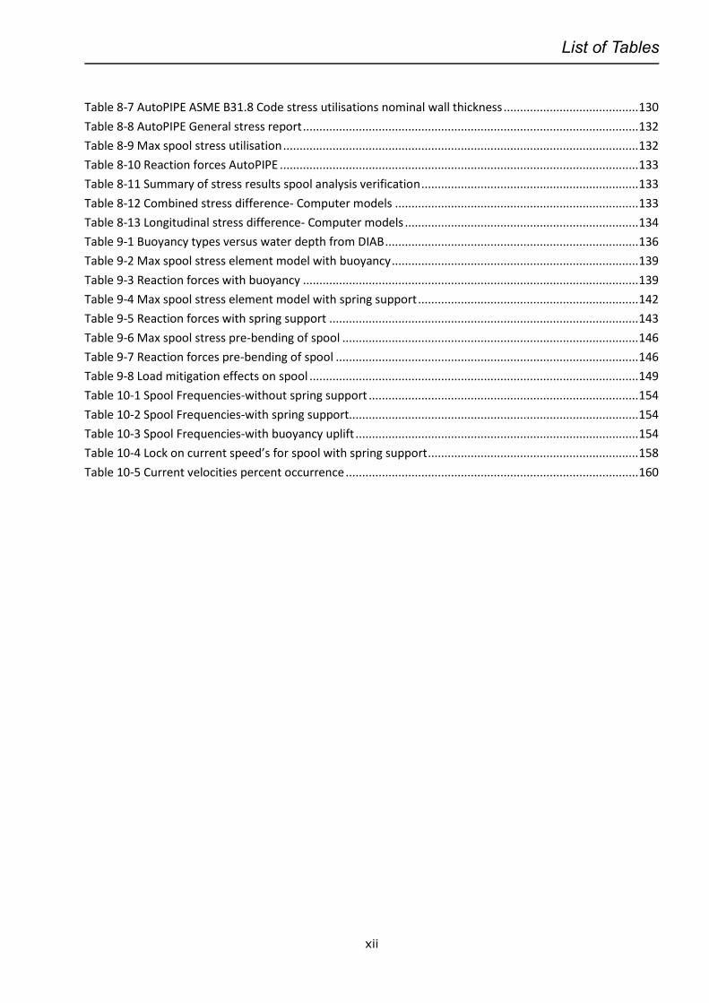
Table 8-7 AutoPIPE ASME B31.8 Code stress utilisations nominal wall thickness ......................................... 130
Table 8-8 AutoPIPE General stress report ...................................................................................................... 132
Table 8-9 Max spool stress utilisation ............................................................................................................ 132
Table 8-10 Reaction forces AutoPIPE ............................................................................................................. 133
Table 8-11 Summary of stress results spool analysis verification .................................................................. 133
Table 8-12 Combined stress difference- Computer models .......................................................................... 133
Table 8-13 Longitudinal stress difference- Computer models ....................................................................... 134
Table 9-1 Buoyancy types versus water depth from DIAB ............................................................................. 136
Table 9-2 Max spool stress element model with buoyancy ........................................................................... 139
Table 9-3 Reaction forces with buoyancy ...................................................................................................... 139
Table 9-4 Max spool stress element model with spring support ................................................................... 142
Table 9-5 Reaction forces with spring support .............................................................................................. 143
Table 9-6 Max spool stress pre-bending of spool .......................................................................................... 146
Table 9-7 Reaction forces pre-bending of spool ............................................................................................ 146
Table 9-8 Load mitigation effects on spool .................................................................................................... 149
Table 10-1 Spool Frequencies-without spring support .................................................................................. 154
Table 10-2 Spool Frequencies-with spring support........................................................................................ 154
Table 10-3 Spool Frequencies-with buoyancy uplift ...................................................................................... 154
Table 10-4 Lock on current speed’s for spool with spring support ................................................................ 158
Table 10-5 Current velocities percent occurrence ......................................................................................... 160

Nomenclature
xiii
Nomenclature
Latin symbols
ā Intercept of the design SN-curve with the log N axis
A Area
𝐴𝑖 Internal area of pipe
𝐴𝑒 External area of pipe
𝐴𝑠 Cross sectional area of pipe
b Constant polynomial
c Corrosion allowance
c Damping coeffcient
cc Critical damping
Di Inside diameter
Do Outer Diameter
D Nominal diameter
D Accumulated fatigue damage
Dk Nodal Imposed displacement in k=x, y, z global direction
d Distance
E Young’s Modulus
F Force
𝐹𝑎𝑥𝑙 Axial force
F1 ASME design factor for hoop stress
F2 ASME design factor for longitudinal stress
F3 ASME design factor for combined stress
𝐹𝑓𝑟𝑖𝑐 Frictional force
fosc Frequency forced oscillation
f0 Eigen frequency
fi Natural frequency for i’th mode
fu Ultimate strength of material
fn Shedding frequency
𝑓 ASME Fatigue factor
𝐹𝑤𝑎𝑙𝑙 Axial pipe wall force due to pressure
𝐹𝑒𝑛𝑑𝑐𝑎𝑝 Axial pipe endcap force due to pressure
g Dimensional errors
𝑖𝑜,𝑖 Stress intensification factor (SIF) out of plane or in plane
𝐼 Moment of inertia
K Stiffness
k Number of stress blocks
[𝐾] Stiffness matrix
Ks Stability factor
L Length
M Bending moment
Madd Added mass
[𝑀] Mass matrix
Nomenclature
xiv
m mass
m negative inverse slope of the S-N curve
me Effective mass
𝑀𝑖 In plane bending moment
𝑀𝑜 Out of plane bending moment
𝑀𝑡 Torsional moment
N Axial force
N Number of cycles S-N Curves
n Number of stress cycles
𝑁𝑒𝑓𝑓 Effective force in pipe
𝑁𝑡𝑟𝑢𝑒 True force in pipe wall
P Pressure
𝑃𝑐(𝑡) Collapse pressure
Pe External pressure
𝑃𝑒𝑙(𝑡) Pressure at elastic capacity perfect tube
Pi Internal pressure
Pmin Minimum internal pressure
Po Outer pressure or external pressure
𝑃𝑝(𝑡) Pressure at plastic capacity
Pn Probability during n-years
Rk Nodal imposed rotations k= x, y, z global axis
Re Reynolds number
Rp Return period
R Mean radius
Ri Internal radius
Ro Outer radius
SA ASME stress limit flexural stress
Sb ASME Longitudinal bending stresses
Sc ASME Allowable stress at cold pipe
Sh ASME hoop stress
Sh ASME Allowable stress at hot pipe
SL ASME longitudinal stress
SP ASME Longitudinal pressure stresses
Su ASME Ultimate tensile strength
Saxial ASME Axial stress
St ASME Torsional stress
S ASME Specified minimum yield strength
S Sample standard deviation
T ASME Temperature de-rating factor
t Nominal pipe wall thickness
t1 DNV definition for minimum pipe wall thickness
tmin Minimum wall thickness
tCorr Corrosion allowance
tfab Fabrication tolerance
U Current speed
V Flow velocity
Nomenclature
xv
Vr Reduced velocity
𝑊𝑠𝑢𝑏 Weight of pipe pr. meter
Wt Pipe wall thickness
y Constant polynomial
𝑌 Population random variable
Z Distance in meter
Znom ASME Section modulus, nominal wall thickness
Greek Symbols
a Thermal expansion coefficient or
am Allowable stress factor membrane stress
afab fabrication factor
𝜀𝑒𝑙 Longitudinal strain
Δ Displacement or difference
𝜎𝑎 Axial stress
𝜎𝑏 Bending stress
𝜎𝑖 Principal stress i=1,2,3
𝜎𝑗 2D-Coordinate stress j=x, y, z
𝜎𝑙 Longitudinal stress
𝜎ℎ Mean hoop stress or circumferential stress
𝜎𝑟𝑟 Radial through wall stress
𝜎𝜃𝜃 Tangential stress or Circumferential stress
𝜎𝑦 Yield strength of material
𝜏𝑖𝑗 Shear stress i=x, y, z j=x, y, z
n Poisson’s ratio
𝜈 Kinematic viscosity
𝜃 Temperature Difference
𝜇 Frictional coeffcient
γHISC
Material quality factor
r Mass density
η Usage factor
zT Total modal damping ratio
𝜔 Natural frequency
Nomenclature
xvi
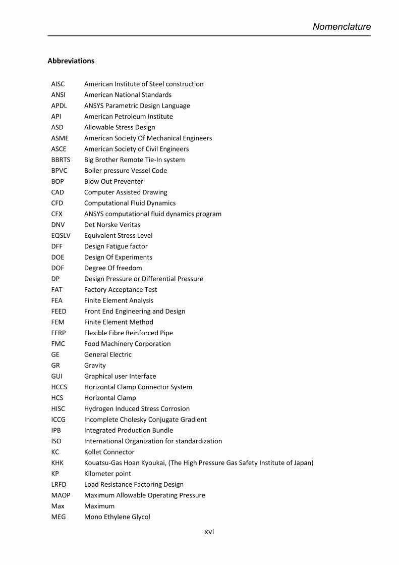
Abbreviations
AISC American Institute of Steel construction
ANSI American National Standards
APDL ANSYS Parametric Design Language
API American Petroleum Institute
ASD Allowable Stress Design
ASME American Society Of Mechanical Engineers
ASCE American Society of Civil Engineers
BBRTS Big Brother Remote Tie-In system
BPVC Boiler pressure Vessel Code
BOP Blow Out Preventer
CAD Computer Assisted Drawing
CFD Computational Fluid Dynamics
CFX ANSYS computational fluid dynamics program
DNV Det Norske Veritas
EQSLV Equivalent Stress Level
DFF Design Fatigue factor
DOE Design Of Experiments
DOF Degree Of freedom
DP Design Pressure or Differential Pressure
FAT Factory Acceptance Test
FEA Finite Element Analysis
FEED Front End Engineering and Design
FEM Finite Element Method
FFRP Flexible Fibre Reinforced Pipe
FMC Food Machinery Corporation
GE General Electric
GR Gravity
GUI Graphical user Interface
HCCS Horizontal Clamp Connector System
HCS Horizontal Clamp
HISC Hydrogen Induced Stress Corrosion
ICCG Incomplete Cholesky Conjugate Gradient
IPB Integrated Production Bundle
ISO International Organization for standardization
KC Kollet Connector
KHK Kouatsu-Gas Hoan Kyoukai, (The High Pressure Gas Safety Institute of Japan)
KP Kilometer point
LRFD Load Resistance Factoring Design
MAOP Maximum Allowable Operating Pressure
Max Maximum
MEG Mono Ethylene Glycol

Nomenclature
xvii
MF Manifold
Min Minimum
MIT Massachusetts Institute of Technology
MOP Maximum Operating Pressure
MSL Mean Sea Level
Nom Nominal
NEMA National Electrical Manufacturers Association
NORSOK Norsk Sokkels Konkurranseposisjon
NPD Norwegian Petroleum Directorate
PC Personal Computer
PCG Preconditioned Conjugate Gradient Solver
PEEK Polyetheretherketone
PLEM Pipeline End Module
PLET Pipeline End Termination
ROV Remote Operated Vehicle
RP Recommended practice
RTS Remote Tie-In System
SCF Stress Concentration Factor
SIF Stress Intensification Factor
SMYS Specified Minimum Yield Strength
SMTS Specified Minimum Tensile Strength
TR Technical Requirement
TFRP Thermoplastic Reinforced Pipe
UBC Uniform Building Code
ULS Ultimate Limit State
UTIS Universal Tie-in System
VIV Vortex Induced Vibration
WB Work Bench
WI Water Injection
WRC Welding Research Council
X-Tree Wellhead “Christmas Tree”

Nomenclature
xviii
Chapter 1 Introduction
1
1. INTRODUCTION
Subsea Tie-in solutions provided by most of the major actors in the subsea market provides various
systems for connecting pipelines to manifolds, wells and Trunk pipe lines. These pipelines are usually
called “spools” or tie in spool. This is usually a steel pipe oriented either vertically or horizontally with a
connector system in each end, other types used is of a flexible types similar to what is used in risers.
These spools are often designed to withstand large forces and displacements due to pressure and
temperature in the pipeline during installation and operation; hence the requirement for flexibility and
strength is one of the key design features. Various computer optimization techniques such as the use of
FEA and CFD are utilized in order to analyse and verify strength of these spools towards numerous load
combinations in order to document required design life and governing codes. Experience has shown that
some of these solutions are sensitive to parameter changes such as:
Flow and process data
Material choice
Metrology and fabrication tolerances
Environmental factors.
Size and shape
Connector solutions
Typically main issues related to design of rigid spools can be listed as follows:
Size
Stresses
Conflict between company standard and code requirements
Lack of recommended practice
Corrosion and (HISC) problems
Insulation
VIV
Weight
Fatigue
Erosion
Slugging
Pressure loss
Requirement for MEG inhibitors
Sour service
Seabed
Size and limitation of connector systems
Requirement for structural support equipment
Chapter 1 Introduction
2
In order to reduce project cost, time and complexity, (especially for deep water application and diver less tie-in system) the following topics should be studied such as:
Efficient computer analysis and methods
An early identification of critical values
Alternative Tie-in solutions
Reduction of complexity
Reduction of vessel installation time.
Reduction of cost by use of robust standard solutions.
Better use and understanding of recommended design standards, company practices and codes.
1.1 Historical
Since the 1980’s, when the subsea industry started moving into water depths where divers could not be used, the industry has been challenged to provide a simple cost effective method of connecting two lines without divers. The industry has responded to this challenge providing innovative methods of doing first end and second end tie-in methods including:
Stab & hinge-over’,
Rigid jumpers/spools
Flexibles,
Deflect and connect
A multitude of vertical and horizontal connectors & tools have been used. However, the use of rigid jumpers still remains the universal method of performing deep water pipeline connections, possibly due its extensive proven track record, its cost effectiveness and high reliability. However, this system still has significant drawbacks which include the requirement for metrology, topsides fabrication (which may or may not be on the critical path), installation with a multi-point lift and its limited capability to accommodate pipeline expansion and two tie-in operations. Ref. /1/ Some of the early projects during the 1980,s utilizing the deflect to connect approach was
East Frigg Project. June 1988. Connection of 2 production manifolds to a central manifold by 2 bundles in 24” carrier pipes to provide buoyancy. Bundles connected by a first time diverless Deflect to connect method.
Troll Olje Project. August 1995. Connection of 16” oil and gas export pipelines. First time diverless Deflect to Connect directly on pipelines by attaching weight and buoyancy.
1.2 Problem Description
A pipeline connection is normally used as a link between a pipeline, manifold, oil-well, storage tank, processing facility or other mechanical equipment used for the transportation of a fluid, gas, sand or a combination of all from one location to another. The pipeline link connection is called a spool which is an English terminology (in Norwegian it translates to “snelle”, which is a device for reeling something on like a fishing reel). When we use the word spool in piping terminology it is understood as piece of pipe with necessary bends tees and flanges for connection to another system. In simple terms it is the pipe from flange to flange. The concept is relatively simple. As the pipes are heated and pressurized they expand and since the piping is restrained in some way in a piping system stresses are developed. For subsea
Chapter 1 Introduction
3
pipelines the spools is usually an infield pipeline connection to a trunk exporting pipeline, manifold, oil wells or other subsea facility. The transport medium is:
Produced oil
Gas injection
Water injection
Multiphase flow (oil, gas and water)
Spools must have enough flexibility to withstand the expansion deflection from facilities such as:
Pipeline and Risers connected to subsea structures or other processing unit.
Oil-wells and manifolds
Environmental forces
Reference is also made to the Master thesis of 2012 made by Espen Slettebø Ref. /2/ the thesis assesses key requirements related to tie-in spools by a detailed review about issues related to the design, fabrication, installation and operation of tie-in spools here the definition of the Tie-in spool is described as. “Essentially spool pieces are short sections of pipeline that:
• Provide an interface between the pipeline and its connection point that bridges the inaccuracies associated with pipeline installation. For a tie-in spool to serve as intended, it needs to satisfy numerous different criteria. Principally it needs to make up the connection between the pipeline and the interconnecting part. For pipelines that are transporting hydrocarbons it is crucial that the connections are sealed. Containment of hydrocarbons is crucial to reduce the risk of pollution and ensuring safe transportation of hydrocarbons. Tie-in spools are measured, fabricated and installed after the pipeline has been laid. Mechanisms related to these operations, makes the tie-in spool a key piece of equipment in offshore field developments
• Allow the pipeline to expand during operation but also allow these pipeline expansion forces
to be dissipated/reduced at the associated connection point. The tie-in spool also needs to be a flexible element. Pipelines expand because of temperature and pressure differences between installation and operational conditions. This expansion may be in the order of several meters. Depending on how the pipeline is constrained, expansion may cause the pipeline to buckle or by it extending in axial direction. The expansion is taken up by deflection of the tie-in spool. Simultaneously as the pipeline expands, forces are induced into the tie-in spool and the connector. Making sure that induced loads are below material and connector limitations is critical in design of tie-in spools. These key requirements can have a significant impact on the overall cost of a project. A too conservative design means an oversized tie-in spool. A too large tie-in spool increases the use of materials, hampers the manufacturing process and more importantly may limit the number of vessels that can install the spools resulting in a requirement for large costly heavy lift vessels or
separate two vessels to transport the spools.”
Chapter 1 Introduction
4
1.3 Scope and Limitation
This thesis major purpose is to investigate and present some of the standard solutions of the tie-in system
as used by the major actors in the oil and gas industry. The thesis will utilize other studies, company
experience, papers and thesis on this topic. The main objective is to analyse a vertical jumper spool by use
of commercial finite element analysis software, and to study spool design such as:
Investigate the effect of a flexible joint or seabed support in order to reduce moment and forces
in a rigid spool.
Optimize the computer analysis by parametric variation
Comparison of computer models and software
Study effects of statistical distribution of tolerances and deflections
The study will also include:
Fabrication issues
Development of design basis for analysis
Theory
Use of applicable standards and codes
Other topics such as:
Conceptual ideas
Further studies and development for Tie-in
Limitations of Tie-in systems
The thesis will aim to propose recommendations for commencing of such projects and present the result
of the case study. Engineering and analysis of subsea Tie in spools normally involves a large work scope to
be investigated. In order to limit the work for this thesis, a limited number of load cases are checked, and
the focus of the work presented here is mainly for vertical spool types.
Chapter 1 Introduction
5
1.4 Report Structure
Chapter 1 (Introduction)
The introduction contains the background information, to gain an illustrative understanding about the
content of this thesis. The problem is stated followed by the purpose and scope of the thesis. A short
thesis organization is also included (this section) to make navigation in the document simple for the
reader.
Chapter 2 (Background and Theory)
This section contains presentations of some theory and examples as to gain an understanding of the basic
principles and physical behaviour of piping system
Chapter 3 (Tie-in Spools System)
This section presents examples of typical subsea Tie-in systems. The section describes typical advantages
and disadvantages for each system. Fabrication methods and considerations of tolerances are discussed.
Chapter 4 (Connector and Tie-in Systems)
This chapter describes the function of subsea connectors and the available tooling required for
performing a subsea Tie-in. A general list of the most common systems used and the manufactures is
given.
Chapter 5 (Design basis)
This chapter describes the basis for the design of the spool. The chapter describes data to be used in the
design such as the use of governing codes and standards. The chapter also describes the important
parameters such as materials, dimensions, loadings and limitations for the system.
Chapter 6 (Spool optimisation and strength verification)
This chapter describes the computer software tools used in the structural analysis of piping systems. The
boundary condition and the computer model for the FEA are given and a description of the analysis
method is outlined. Load cases for the spool is described and assigned to the analysis.
Chapter 7 (Analysis Results)
This chapter presents the analysis results from the ANSYS Design Explorer tool. Statistical distribution of
the results are presented and discussed. An optimal configuration for the spool and sensitivity to imposed
loading is studied
Chapter 8 (Verification and Comparison of Results)
Chapter 1 Introduction
6
This chapter investigates different computer models and compare results. The main purpose is to study if there are major differences between typical finite elements used in computer piping analysis. The chapter compares results from software typically used in the industry for piping analysis. (AutoPIPE). Chapter 9 (Spool Weight and Load Mitigation) In this chapter some ideas on how to minimize loading on the connectors for a vertical spool is investigated and results are presented. Typical subsea equipment used for mitigation of VIV and weight is presented. Chapter 10 (VIV Check of Spool) This chapter studies the effect and sensitivity of the spool to be excited by the sea current into a harmonic frequency with a spring seabed support. Modal analysis is performed by use of ANSYS. Typical recommended practice for the design check against VIV is discussed and a method for checking against fatigue is presented. Chapter 11 (Future Solutions) This chapter presents some developed and conceptual ideas for future subsea spool projects. The ideas are presented with the intention that it might have potential for cost savings Chapter 12 (Summary and Conclusion) The overall Summary, conclusion and recommendations from the work performed in this thesis are presented a recommended engineering practice based upon this thesis work is described. Suggestion for future studies on this topic is given.
Chapter 2 Background and theory
7
2. BACKGROUND AND THEORY
2.1 Structural analysis of piping
Structural analysis of piping systems is of great importance to study as temperature, pressure and gravity
forces is inducing stresses, strains and deformations in the pipe system when it is restrained. Furthermore
as the piping system heats up and shuts down the piping system is exposed to changes in stresses, this
causes a fatigue situation. For a piping system exposed to environmental forces such as current and
waves typically for subsea pipes, VIV (Vortex Induced Vibration) can cause the pipeline to be excited into
harmonic low frequency vibration. This can result in fatigue failure or unintentional high displacement
ranges.
The designer must calculate the stresses allowed by a particular code. One of the significant differences
between flexibility analysis and pressure design is that flexibility is related to stress range rather than a
specific stress.
For subsea spool piping the most important parameters to study is the effect of:
Pipeline expansion from pressure and temperature
Tie-in forces
Metrology and fabrication tolerances
Environmental forces.
Installation methodology
For pipelines which may vary from just a few hundred meters to several hundred kilometres it is also
important to study the effects such as those listed below. These topics are thoroughly described in
literature Ref. /10/.
Pipeline lateral buckling
Pipeline upheaval buckling
Pipeline walking
For tie-in spools these effects are not relevant as the boundary conditions required for the phenomena is
usually not present.
The pipelines are designed as to avoid buckle to be triggered at the end of a pipeline as this could
potentially damage the spools. In theory the effects might be present in the spools if the effective force in
a spool is of such a nature that large axial compression forces can be generated. Pipeline walking is a
phenomena created by the in-balance of the effective axial force during start up and shut down and
differences in the temperature gradient along the pipeline which changes the location of “virtual” anchor
(restraining point) along the pipeline.
The acceptance criteria for both spools and pipelines are usually a strain and stress based criteria set forth
by a piping code such as DNV, ISO or ASME.
Chapter 2 Background and theory
8
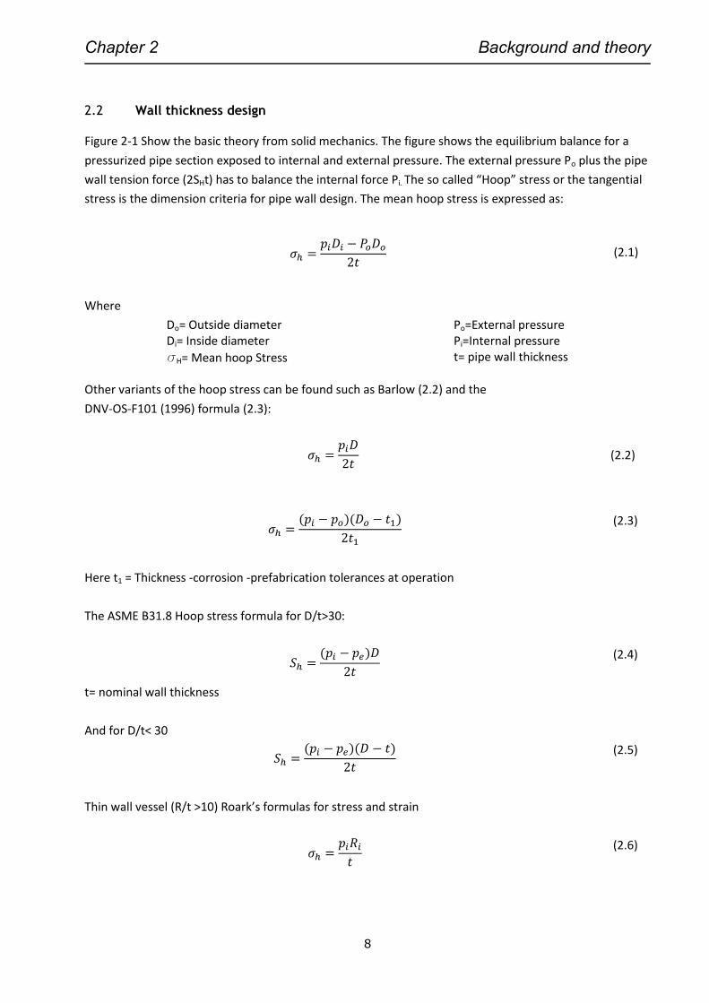
2.2 Wall thickness design
Figure 2-1 Show the basic theory from solid mechanics. The figure shows the equilibrium balance for a
pressurized pipe section exposed to internal and external pressure. The external pressure Po plus the pipe
wall tension force (2SHt) has to balance the internal force Pi. The so called “Hoop” stress or the tangential
stress is the dimension criteria for pipe wall design. The mean hoop stress is expressed as:
𝜎ℎ =𝑝𝑖𝐷𝑖 − 𝑃𝑜𝐷𝑜
2𝑡 (2.1)
Where
Do= Outside diameter Di= Inside diameter
sH= Mean hoop Stress
Po=External pressure Pi=Internal pressure t= pipe wall thickness
Other variants of the hoop stress can be found such as Barlow (2.2) and the
DNV-OS-F101 (1996) formula (2.3):
𝜎ℎ =𝑝𝑖𝐷
2𝑡 (2.2)
𝜎ℎ =(𝑝𝑖 − 𝑝𝑜)(𝐷𝑜 − 𝑡1)
2𝑡1
(2.3)
Here t1 = Thickness -corrosion -prefabrication tolerances at operation
The ASME B31.8 Hoop stress formula for D/t>30:
𝑆ℎ =(𝑝𝑖 − 𝑝𝑒)𝐷
2𝑡
(2.4)
t= nominal wall thickness
And for D/t< 30
𝑆ℎ =(𝑝𝑖 − 𝑝𝑒)(𝐷 − 𝑡)
2𝑡
(2.5)
Thin wall vessel (R/t >10) Roark’s formulas for stress and strain
𝜎ℎ =𝑝𝑖𝑅𝑖
𝑡
(2.6)
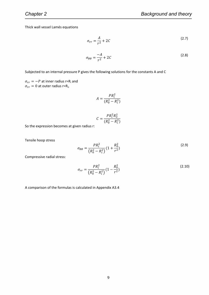
Chapter 2 Background and theory
9
Thick wall vessel Lamés equations
𝜎𝑟𝑟 =𝐴
𝑟2+ 2𝐶
(2.7)
𝜎𝜃𝜃 =−𝐴
𝑟2+ 2𝐶
(2.8)
Subjected to an internal pressure P gives the following solutions for the constants A and C 𝜎𝑟𝑟 = −𝑃 at inner radius r=Ri and 𝜎𝑟𝑟 = 0 at outer radius r=Ro
𝐴 =𝑃𝑅𝑖
2
(𝑅02 − 𝑅𝑖
2)
𝐶 =𝑃𝑅𝑖
2𝑅𝑜2
(𝑅02 − 𝑅𝑖
2)
So the expression becomes at given radius r: Tensile hoop stress
𝜎𝜃𝜃 =𝑃𝑅𝑖
2
(𝑅02 − 𝑅𝑖
2)(1 +
𝑅02
𝑟2)
(2.9)
Compressive radial stress:
𝜎𝑟𝑟 =𝑃𝑅𝑖
2
(𝑅02 − 𝑅𝑖
2)(1 −
𝑅02
𝑟2)
(2.10)
A comparison of the formulas is calculated in Appendix A3.4
Chapter 2 Background and theory
10
Figure 2-1 Force balance in a pressurized pipe section pr. unit length
Most of design codes require that the hoop stress is less than the yield stress with a safety factor SF or a
fraction of the yield stress named F1 often found in American piping codes. The factor is dependent upon
several factors such as:
The location of the system
Pressure
Fluid type and service
Fabrication methods.
This factor is then multiplied with the yield strength to get the allowable stress (ASD).
F1σy
σh≤ F1σy
The design factor or usage factor was taken as 0.72 for pipelines and 0.60 or less for risers. The figures
date back 70 years to time when standards of pipe manufactures, welding and construction were of a less
quality than what we have today Ref. /4/ .Today the limit in codes for utilising the material capacity in
pipelines is much higher such as the plastic strain limit found in the DNV–OS-F101 code Ref. /7/.( It is here
worth mention that the code does not give any limit state criteria for strain in pipe bends which is typical
for spools).
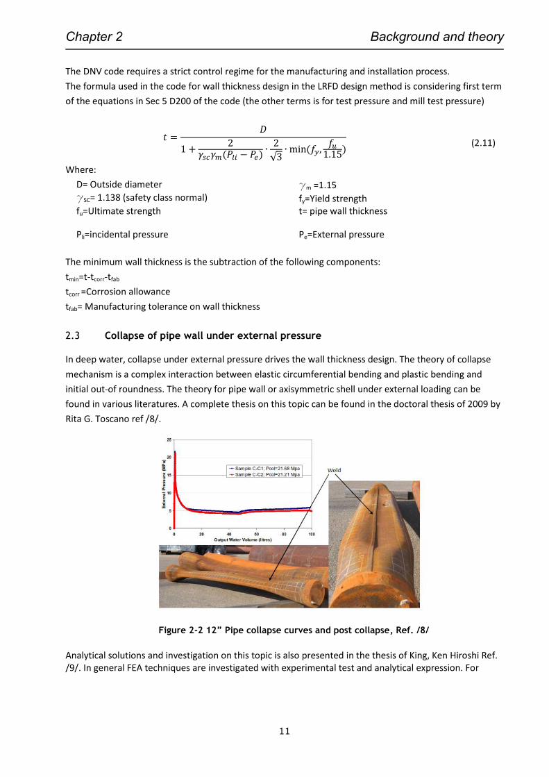
Chapter 2 Background and theory
11
The DNV code requires a strict control regime for the manufacturing and installation process.
The formula used in the code for wall thickness design in the LRFD design method is considering first term
of the equations in Sec 5 D200 of the code (the other terms is for test pressure and mill test pressure)
𝑡 =𝐷
1 +2
𝛾𝑠𝑐𝛾𝑚(𝑃𝑙𝑖 − 𝑃𝑒)∙
2
√3∙ min(𝑓𝑦,
𝑓𝑢1.15
)
(2.11)
Where:
D= Outside diameter
gSC= 1.138 (safety class normal)
fu=Ultimate strength
gm =1.15
fy=Yield strength t= pipe wall thickness
Pli=incidental pressure Pe=External pressure
The minimum wall thickness is the subtraction of the following components:
tmin=t-tcorr-tfab
tcorr =Corrosion allowance
tfab= Manufacturing tolerance on wall thickness
2.3 Collapse of pipe wall under external pressure
In deep water, collapse under external pressure drives the wall thickness design. The theory of collapse
mechanism is a complex interaction between elastic circumferential bending and plastic bending and
initial out-of roundness. The theory for pipe wall or axisymmetric shell under external loading can be
found in various literatures. A complete thesis on this topic can be found in the doctoral thesis of 2009 by
Rita G. Toscano ref /8/.
Figure 2-2 12” Pipe collapse curves and post collapse, Ref. /8/
Analytical solutions and investigation on this topic is also presented in the thesis of King, Ken Hiroshi Ref. /9/. In general FEA techniques are investigated with experimental test and analytical expression. For
Chapter 2 Background and theory
12
practical engineering the most used formula for checking against collapse is the third degree polynominal expression presented in DNV-OS-F101 ref /7/. External pressure shall meet the following criterion:
𝑃𝑒 − 𝑃𝑚𝑖𝑛 ≤𝑃(𝑡)
1.1𝛾𝑠𝑐𝛾𝑚 (2.12)
Characteristic resistance:
(𝑃𝑐(𝑡) − 𝑃𝑒𝑙(𝑡)) ∙ ((𝑃𝑐(𝑡)2 − 𝑃𝑏(𝑡)
2) = 𝑃𝑐(𝑡) ∙ 𝑃𝑒𝑙(𝑡) ∙ 𝑃𝑝(𝑡) ∙ 𝑓𝑜 ∙𝐷
𝑡 (2.13))
Where:
𝑃𝑒𝑙(𝑡) =2 ∙ 𝐸 ∙ (
𝑡𝐷)
3
1 − 𝜈2
(2.14)
𝑃𝑝(𝑡) = 𝑓𝑦 ∙ 𝛼𝑓𝑎𝑏 ∙2 ∙ 𝑡
𝐷 (2.15)
𝑓𝑜 =𝐷𝑚𝑎𝑥−𝐷𝑚𝑖𝑛
𝐷 (>0.5%) (2.16)
Where:
𝑃𝑒𝑙(𝑡)= Pressure at elastic capacity perfect tube 𝑃𝑝(𝑡)= Pressure at plastic capacity
𝑃𝑐(𝑡)=collapse pressure
E =Youngs Modulus
afab=fabrication factor
n= poisson’s ratio
The solution to the collapse pressure 𝑃𝑐(𝑡) is given in Sec 13 D700 of the code.
𝑃𝑐(𝑡) = 𝑦 −1
3b (2.17)
Where the solution to the constants y and b is given in the code and can be calculated.
For local buckling collapse check with external pressure and bending moment strains the pipe must be
checked in accordance with Sec 5. D600 in Ref. /7/
Other formulas for collapse due to external pressure can be found in the offshore code API RP111 section
4.3.2.1 Ref./32/
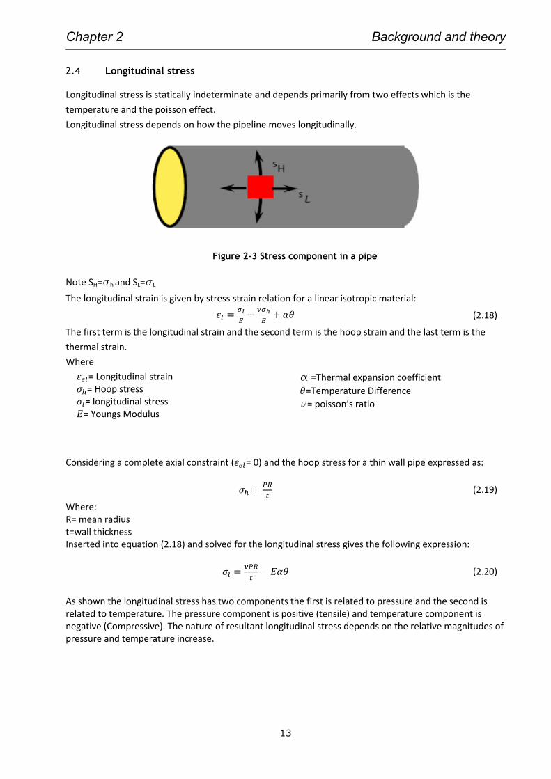
Chapter 2 Background and theory
13
2.4 Longitudinal stress
Longitudinal stress is statically indeterminate and depends primarily from two effects which is the
temperature and the poisson effect.
Longitudinal stress depends on how the pipeline moves longitudinally.
Figure 2-3 Stress component in a pipe
Note SH=sh and SL=sL
The longitudinal strain is given by stress strain relation for a linear isotropic material:
𝜀𝑙 =𝜎𝑙
𝐸−
𝜈𝜎ℎ
𝐸+ 𝛼𝜃 (2.18)
The first term is the longitudinal strain and the second term is the hoop strain and the last term is the
thermal strain.
Where
𝜀𝑒𝑙= Longitudinal strain 𝜎ℎ= Hoop stress 𝜎𝑙= longitudinal stress 𝐸= Youngs Modulus
a =Thermal expansion coefficient
𝜃=Temperature Difference
n= poisson’s ratio
Considering a complete axial constraint (𝜀𝑒𝑙= 0) and the hoop stress for a thin wall pipe expressed as:
𝜎ℎ =𝑃𝑅
𝑡 (2.19)
Where: R= mean radius t=wall thickness Inserted into equation (2.18) and solved for the longitudinal stress gives the following expression:
𝜎𝑙 =𝜈𝑃𝑅
𝑡− 𝐸𝛼𝜃 (2.20)
As shown the longitudinal stress has two components the first is related to pressure and the second is related to temperature. The pressure component is positive (tensile) and temperature component is negative (Compressive). The nature of resultant longitudinal stress depends on the relative magnitudes of pressure and temperature increase.
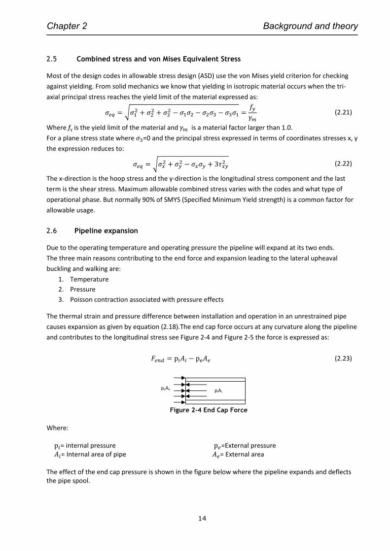
Chapter 2 Background and theory
14
piAi peAe
2.5 Combined stress and von Mises Equivalent Stress
Most of the design codes in allowable stress design (ASD) use the von Mises yield criterion for checking
against yielding. From solid mechanics we know that yielding in isotropic material occurs when the tri-
axial principal stress reaches the yield limit of the material expressed as:
𝜎𝑒𝑞 = √𝜎12 + 𝜎2
2 + 𝜎32 − 𝜎1𝜎2 − 𝜎2𝜎3 − 𝜎3𝜎1 =
𝑓𝑦
𝛾𝑚 (2.21)
Where fy is the yield limit of the material and𝛾𝑚 is a material factor larger than 1.0.
For a plane stress state where 𝜎3=0 and the principal stress expressed in terms of coordinates stresses x, y
the expression reduces to:
𝜎𝑒𝑞 = √𝜎𝑥2 + 𝜎𝑦
2 − 𝜎𝑥𝜎𝑦 + 3𝜏𝑥𝑦2 (2.22)
The x-direction is the hoop stress and the y-direction is the longitudinal stress component and the last
term is the shear stress. Maximum allowable combined stress varies with the codes and what type of
operational phase. But normally 90% of SMYS (Specified Minimum Yield strength) is a common factor for
allowable usage.
2.6 Pipeline expansion
Due to the operating temperature and operating pressure the pipeline will expand at its two ends.
The three main reasons contributing to the end force and expansion leading to the lateral upheaval
buckling and walking are:
1. Temperature
2. Pressure
3. Poisson contraction associated with pressure effects
The thermal strain and pressure difference between installation and operation in an unrestrained pipe
causes expansion as given by equation (2.18).The end cap force occurs at any curvature along the pipeline
and contributes to the longitudinal stress see Figure 2-4 and Figure 2-5 the force is expressed as:
𝐹𝑒𝑛𝑑 = pi𝐴𝑖 − pe𝐴𝑒 (2.23)
Figure 2-4 End Cap Force
Where:
p𝑖= internal pressure 𝐴𝑖= Internal area of pipe
p𝑒=External pressure 𝐴𝑒= External area
The effect of the end cap pressure is shown in the figure below where the pipeline expands and deflects the pipe spool.
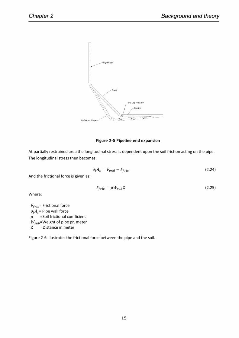
Chapter 2 Background and theory
15
Figure 2-5 Pipeline end expansion
At partially restrained area the longitudinal stress is dependent upon the soil friction acting on the pipe.
The longitudinal stress then becomes:
𝜎𝑙𝐴𝑠 = 𝐹𝑒𝑛𝑑 − 𝐹𝑓𝑟𝑖𝑐 (2.24)
And the frictional force is given as:
𝐹𝑓𝑟𝑖𝑐 = 𝜇𝑊𝑠𝑢𝑏𝑍 (2.25)
Where:
𝐹𝑓𝑟𝑖𝑐= Frictional force
𝜎𝑙𝐴𝑠= Pipe wall force
𝜇 =Soil frictional coefficient 𝑊𝑠𝑢𝑏=Weight of pipe pr. meter 𝑍 =Distance in meter
Figure 2-6 illustrates the frictional force between the pipe and the soil.
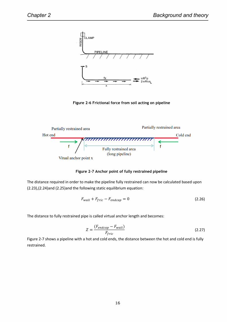
Chapter 2 Background and theory
16
Figure 2-6 Frictional force from soil acting on pipeline
Figure 2-7 Anchor point of fully restrained pipeline
The distance required in order to make the pipeline fully restrained can now be calculated based upon
(2.23),(2.24)and (2.25)and the following static equilibrium equation:
𝐹𝑤𝑎𝑙𝑙 + 𝐹𝑓𝑟𝑖𝑐 − 𝐹𝑒𝑛𝑑𝑐𝑎𝑝 = 0 (2.26)
The distance to fully restrained pipe is called virtual anchor length and becomes:
𝑍 =(𝐹𝑒𝑛𝑑𝑐𝑎𝑝 − 𝐹𝑤𝑎𝑙𝑙)
𝐹𝑓𝑟𝑖𝑐 (2.27)
Figure 2-7 shows a pipeline with a hot and cold ends, the distance between the hot and cold end is fully
restrained.
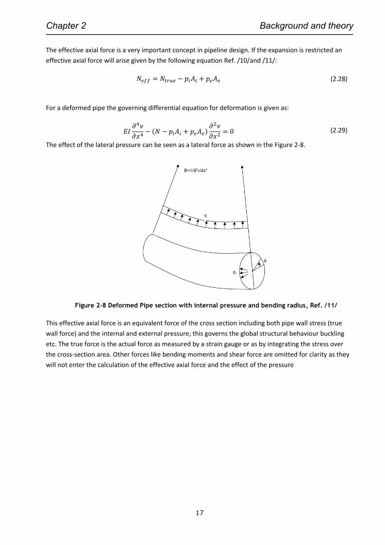
Chapter 2 Background and theory
17
The effective axial force is a very important concept in pipeline design. If the expansion is restricted an
effective axial force will arise given by the following equation Ref. /10/and /11/:
𝑁𝑒𝑓𝑓 = 𝑁𝑡𝑟𝑢𝑒 − 𝑝𝑖𝐴𝑖 + 𝑝𝑒𝐴𝑒 (2.28)
For a deformed pipe the governing differential equation for deformation is given as:
𝐸𝐼𝜕4𝜈
𝜕𝑥4− (𝑁 − 𝑝𝑖𝐴𝑖 + 𝑝𝑒𝐴𝑒)
𝜕2𝜈
𝜕𝑥2= 0 (2.29)
The effect of the lateral pressure can be seen as a lateral force as shown in the Figure 2-8.
Figure 2-8 Deformed Pipe section with internal pressure and bending radius, Ref. /11/
This effective axial force is an equivalent force of the cross section including both pipe wall stress (true
wall force) and the internal and external pressure; this governs the global structural behaviour buckling
etc. The true force is the actual force as measured by a strain gauge or as by integrating the stress over
the cross-section area. Other forces like bending moments and shear force are omitted for clarity as they
will not enter the calculation of the effective axial force and the effect of the pressure
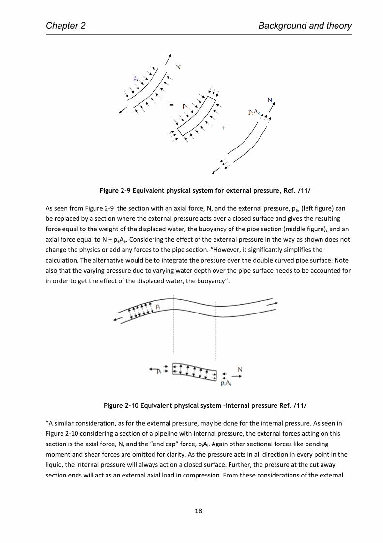
Chapter 2 Background and theory
18
Figure 2-9 Equivalent physical system for external pressure, Ref. /11/
As seen from Figure 2-9 the section with an axial force, N, and the external pressure, pe, (left figure) can
be replaced by a section where the external pressure acts over a closed surface and gives the resulting
force equal to the weight of the displaced water, the buoyancy of the pipe section (middle figure), and an
axial force equal to N + peAe. Considering the effect of the external pressure in the way as shown does not
change the physics or add any forces to the pipe section. “However, it significantly simplifies the
calculation. The alternative would be to integrate the pressure over the double curved pipe surface. Note
also that the varying pressure due to varying water depth over the pipe surface needs to be accounted for
in order to get the effect of the displaced water, the buoyancy”.
Figure 2-10 Equivalent physical system –internal pressure Ref. /11/
“A similar consideration, as for the external pressure, may be done for the internal pressure. As seen in
Figure 2-10 considering a section of a pipeline with internal pressure, the external forces acting on this
section is the axial force, N, and the “end cap” force, piAi. Again other sectional forces like bending
moment and shear forces are omitted for clarity. As the pressure acts in all direction in every point in the
liquid, the internal pressure will always act on a closed surface. Further, the pressure at the cut away
section ends will act as an external axial load in compression. From these considerations of the external
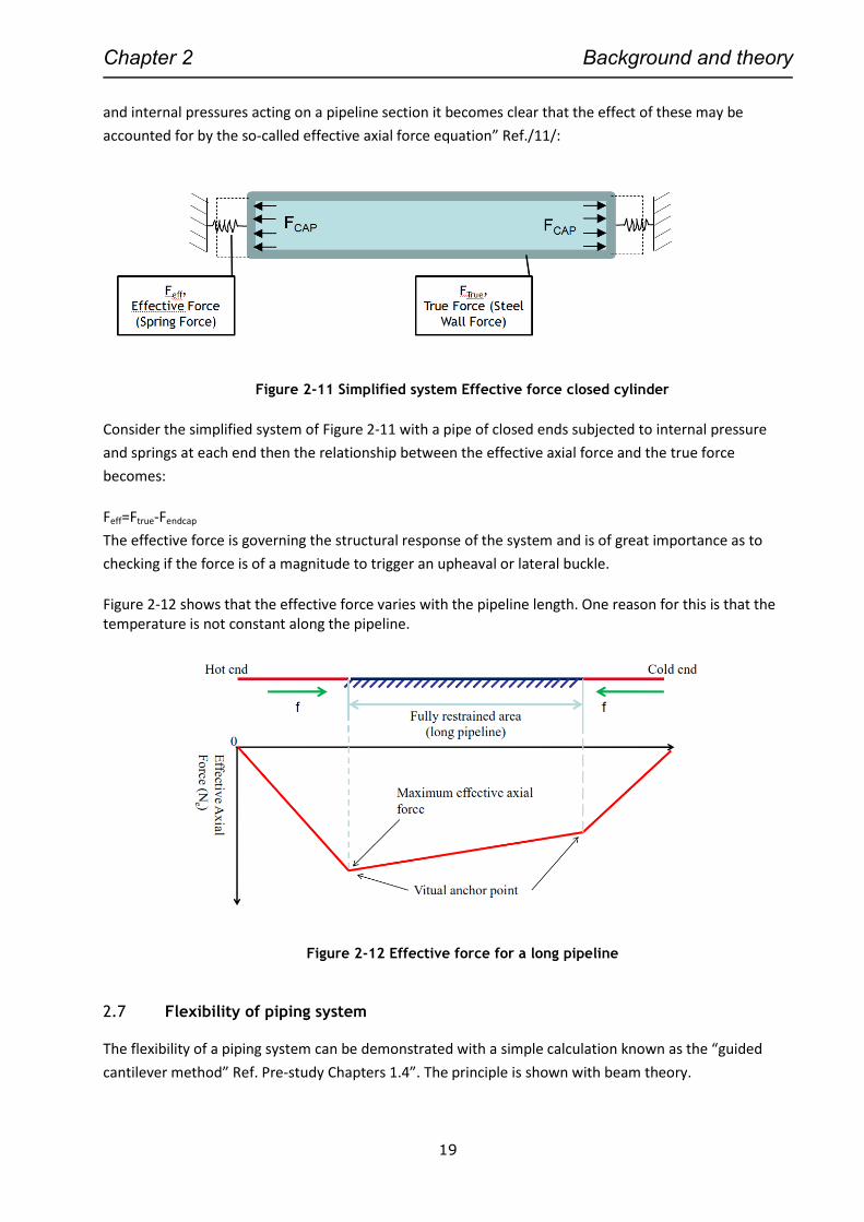
Chapter 2 Background and theory
19
and internal pressures acting on a pipeline section it becomes clear that the effect of these may be
accounted for by the so-called effective axial force equation” Ref./11/:
Figure 2-11 Simplified system Effective force closed cylinder
Consider the simplified system of Figure 2-11 with a pipe of closed ends subjected to internal pressure
and springs at each end then the relationship between the effective axial force and the true force
becomes:
Feff=Ftrue-Fendcap
The effective force is governing the structural response of the system and is of great importance as to
checking if the force is of a magnitude to trigger an upheaval or lateral buckle.
Figure 2-12 shows that the effective force varies with the pipeline length. One reason for this is that the temperature is not constant along the pipeline.
Figure 2-12 Effective force for a long pipeline
2.7 Flexibility of piping system
The flexibility of a piping system can be demonstrated with a simple calculation known as the “guided
cantilever method” Ref. Pre-study Chapters 1.4”. The principle is shown with beam theory.
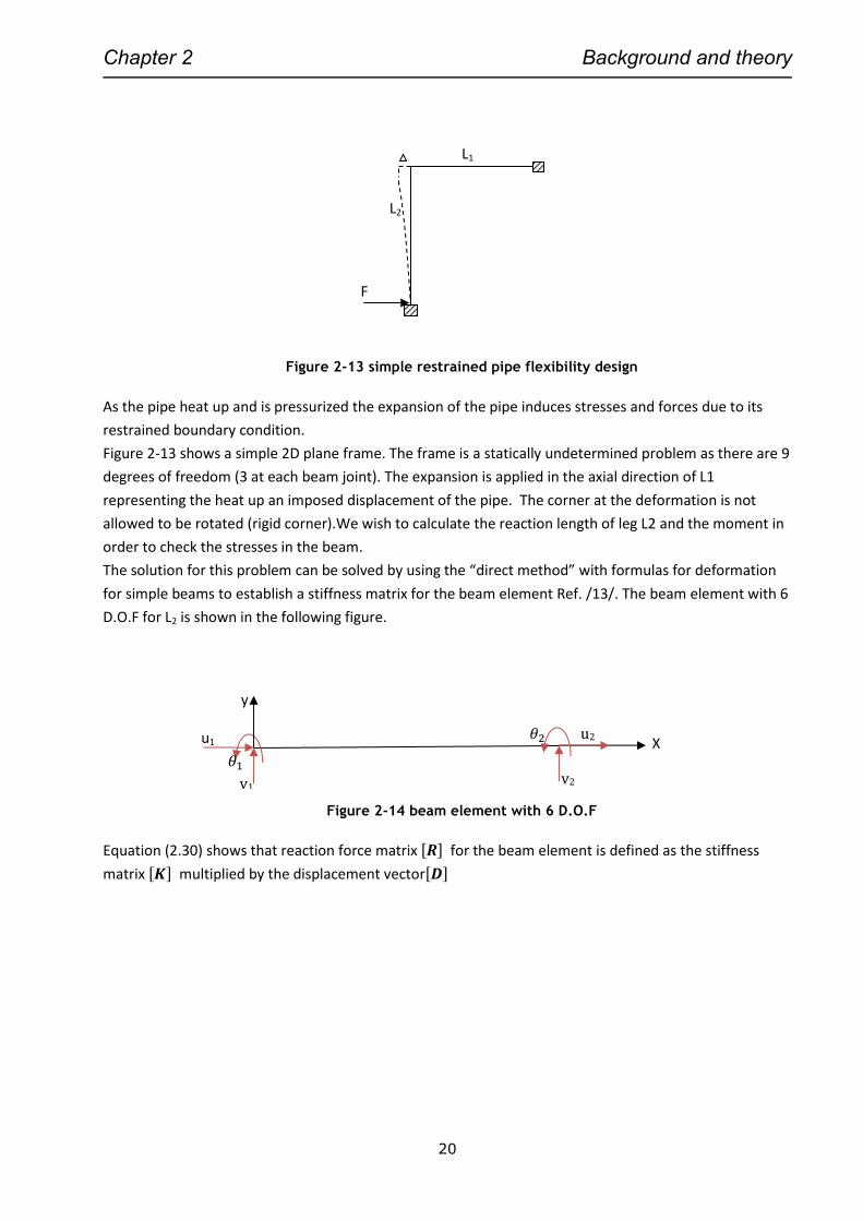
Chapter 2 Background and theory
20
Figure 2-13 simple restrained pipe flexibility design
As the pipe heat up and is pressurized the expansion of the pipe induces stresses and forces due to its
restrained boundary condition.
Figure 2-13 shows a simple 2D plane frame. The frame is a statically undetermined problem as there are 9
degrees of freedom (3 at each beam joint). The expansion is applied in the axial direction of L1
representing the heat up an imposed displacement of the pipe. The corner at the deformation is not
allowed to be rotated (rigid corner).We wish to calculate the reaction length of leg L2 and the moment in
order to check the stresses in the beam.
The solution for this problem can be solved by using the “direct method” with formulas for deformation
for simple beams to establish a stiffness matrix for the beam element Ref. /13/. The beam element with 6
D.O.F for L2 is shown in the following figure.
Figure 2-14 beam element with 6 D.O.F
Equation (2.30) shows that reaction force matrix[𝑹] for the beam element is defined as the stiffness
matrix [𝑲] multiplied by the displacement vector[𝑫]
L2
F
L1
y
X 𝜃1
u1
v1
𝜃2 u2
v2
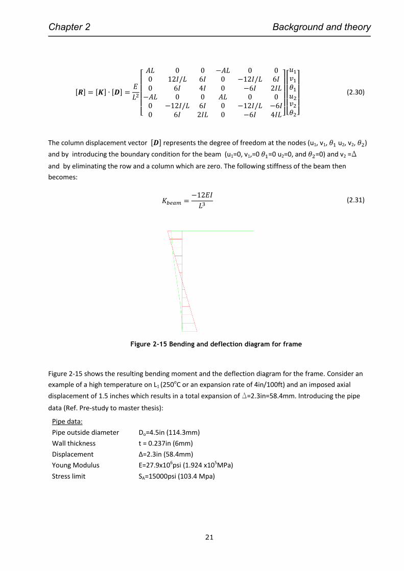
Chapter 2 Background and theory
21
[𝑹] = [𝑲] ∙ [𝑫] =𝐸
𝐿2
[
𝐴𝐿 0 0 −𝐴𝐿 0 00 12𝐼/𝐿 6𝐼 0 −12𝐼/𝐿 6𝐼0 6𝐼 4𝐼 0 −6𝐼 2𝐼𝐿
−𝐴𝐿 0 0 𝐴𝐿 0 00 −12𝐼/𝐿 6𝐼 0 −12𝐼/𝐿 −6𝐼0 6𝐼 2𝐼𝐿 0 −6𝐼 4𝐼𝐿 ]
[ 𝑢1
𝑣1
𝜃1
𝑢2𝑣2
𝜃2]
(2.30)
The column displacement vector [𝑫] represents the degree of freedom at the nodes (u1, v1, 𝜃1 u2, v2, 𝜃2)
and by introducing the boundary condition for the beam (u1=0, v1,=0 𝜃1=0 u2=0, and 𝜃2=0) and v2 =D
and by eliminating the row and a column which are zero. The following stiffness of the beam then
becomes:
𝐾𝑏𝑒𝑎𝑚 =−12𝐸𝐼
𝐿3 (2.31)
Figure 2-15 Bending and deflection diagram for frame
Figure 2-15 shows the resulting bending moment and the deflection diagram for the frame. Consider an
example of a high temperature on L1 (250oC or an expansion rate of 4in/100ft) and an imposed axial
displacement of 1.5 inches which results in a total expansion of D=2.3in=58.4mm. Introducing the pipe
data (Ref. Pre-study to master thesis):
The force is defined as:
Pipe data:
Pipe outside diameter Do=4.5in (114.3mm)
Wall thickness t = 0.237in (6mm)
Displacement Δ=2.3in (58.4mm)
Young Modulus E=27.9x10⁶psi (1.924 x10⁵MPa)
Stress limit SA=15000psi (103.4 Mpa)
Chapter 2 Background and theory
22
𝐹 = 𝐾𝑏𝑒𝑎𝑚 ∙ ∆ (2.32)
Bending stress:
𝜎 =𝑀𝑦
𝐼 (2.33)
Where y= Do/2 and M=FL/2
Inserting (2.31), (2.32) into (2.33) and rearranging for L gives the following equation for required length L2
to be within the given stress limit and give adequate flexibility:
𝐿 = √3𝐸 ∙ ∆ ∙ 𝐷
𝜎 (2.34)
Inserting values as given above and SA=s, equation (2.34) then gives the following value:
𝐿 = √3 ∙ 192400 ∙ 58.4 ∙ 114.3
103.4= 6105𝑚𝑚(20.03𝑓𝑡)
And the reaction force then becomes:
𝐹 =2 ∙ 𝜎 ∙ 𝐼
R ∙ 𝐿=
2 ∙ 103.4 ∙ 2.995 ∙ 106
54.11 ∙ 6105= 1875𝑁(422𝑙𝑏𝑓)
As seen from the calculations the flexibility of the piping is dependent upon geometry and the allowable
stress in order to be within safe limits between the heat up and cool down cycles.
Chapter 2 Background and theory
23
2.8 V.I.V in Pipelines
VIV or Vortex Induced Vibrations are common problems in offshore structures and often occur when structural components are in a free span and submitted to a flow from wind or seawater. When the flow separates from a large section of the structure surface due to its geometry (bluff structure), vortices are generated and shed alternately from one side to another side of the structure. This alternating shedding of vortices induces forces and can cause the structure to start oscillate. When the frequency of the vortex shedding is close to the natural frequency of the structure, large amplitude resonant oscillations may occur. This is a known problem for free spanning pipelines and risers. The VIV effect can generate large amplitude forces and this can lead to fatigue failure of the structural component. Figure 2-16 shows an illustration of how the pipe is displaced in the vertical and horizontal direction due to the vortex shedding generated from the sea current.
Figure 2-16 Vortex Induced Vibrations
The pipe can start to oscillate in the vertical direction (crossflow) and in the horizontal direction (In-line)
in an 8 number pattern. Figure 2-18, shows that the oscillation is in phase or it can have a D shape pattern
as seen in Figure 2-19 where the oscillation is out of phase. The behaviour and the pattern of the vortices
are very much dependent upon the flow regime. The Reynolds number Re is often used as a measure
between the laminar and turbulent flow, see Figure 2-17 and is given by equation (2.35). The
eigenfrequency of the pipe is also influenced by the change of added mass of the displaced water and this
will also influence the vortex shedding frequency. Three other important key parameters, each linked to
the frequency is the Strouhal number St, the reduced velocity UR, and the non-dimensional frequency 𝑓.
Ref. equation (2.36) to (2.38).
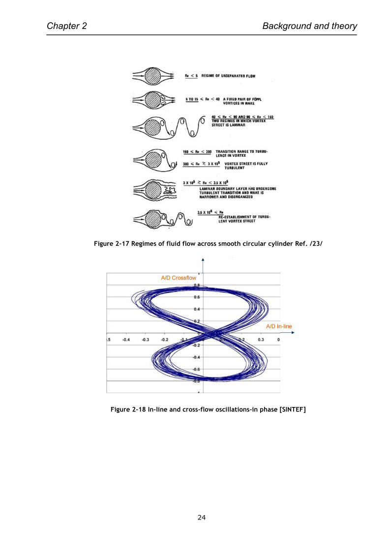
Chapter 2 Background and theory
24
Figure 2-17 Regimes of fluid flow across smooth circular cylinder Ref. /23/
Figure 2-18 In-line and cross-flow oscillations-in phase [SINTEF]
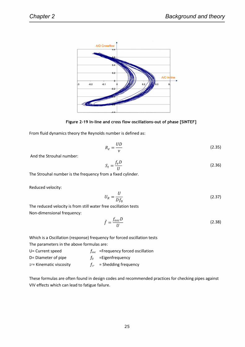
Chapter 2 Background and theory
25
Figure 2-19 In-line and cross flow oscillations-out of phase [SINTEF]
From fluid dynamics theory the Reynolds number is defined as:
𝑅𝑒 =𝑈𝐷
𝜈 (2.35)
And the Strouhal number:
𝑆𝑡 =𝑓𝑣𝐷
𝑈 (2.36)
The Strouhal number is the frequency from a fixed cylinder.
Reduced velocity:
𝑈𝑅 =𝑈
𝐷𝑓0 (2.37)
The reduced velocity is from still water free oscillation tests
Non-dimensional frequency:
𝑓 =𝑓𝑜𝑠𝑐𝐷
𝑈 (2.38)
Which is a Oscillation (response) frequency for forced oscillation tests
The parameters in the above formulas are:
U= Current speed fosc =Frequency forced oscillation
D= Diameter of pipe f0 =Eigenfrequency
n= Kinematic viscosity fn = Shedding frequency
These formulas are often found in design codes and recommended practices for checking pipes against
VIV effects which can lead to fatigue failure.

Chapter 2 Background and theory
26
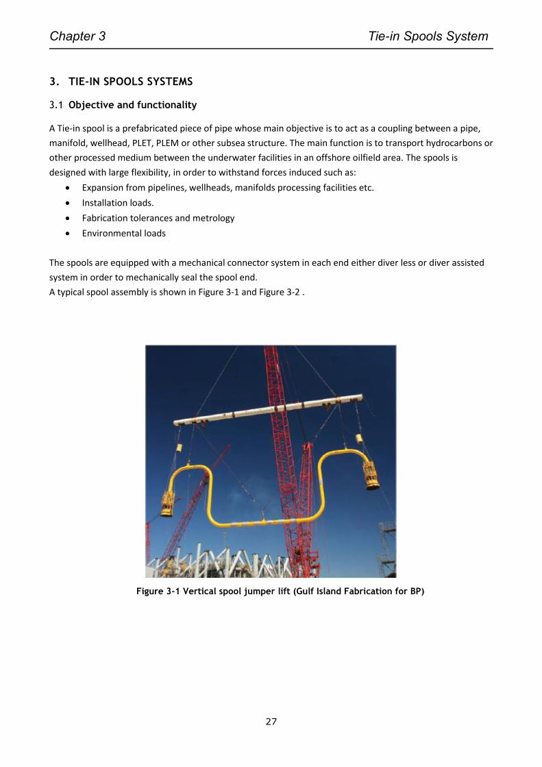
Chapter 3 Tie-in Spools System
27
3. TIE-IN SPOOLS SYSTEMS
3.1 Objective and functionality
A Tie-in spool is a prefabricated piece of pipe whose main objective is to act as a coupling between a pipe,
manifold, wellhead, PLET, PLEM or other subsea structure. The main function is to transport hydrocarbons or
other processed medium between the underwater facilities in an offshore oilfield area. The spools is
designed with large flexibility, in order to withstand forces induced such as:
Expansion from pipelines, wellheads, manifolds processing facilities etc.
Installation loads.
Fabrication tolerances and metrology
Environmental loads
The spools are equipped with a mechanical connector system in each end either diver less or diver assisted
system in order to mechanically seal the spool end.
A typical spool assembly is shown in Figure 3-1 and Figure 3-2 .
Figure 3-1 Vertical spool jumper lift (Gulf Island Fabrication for BP)
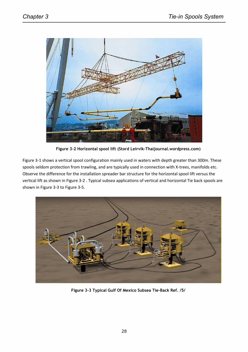
Chapter 3 Tie-in Spools System
28
Figure 3-2 Horizontal spool lift (Stord Leirvik-Thaijournal.wordpress.com)
Figure 3-1 shows a vertical spool configuration mainly used in waters with depth greater than 300m. These
spools seldom protection from trawling, and are typically used in connection with X-trees, manifolds etc.
Observe the difference for the installation spreader bar structure for the horizontal spool lift versus the
vertical lift as shown in Figure 3-2 . Typical subsea applications of vertical and horizontal Tie back spools are
shown in Figure 3-3 to Figure 3-5.
Figure 3-3 Typical Gulf Of Mexico Subsea Tie-Back Ref. /5/
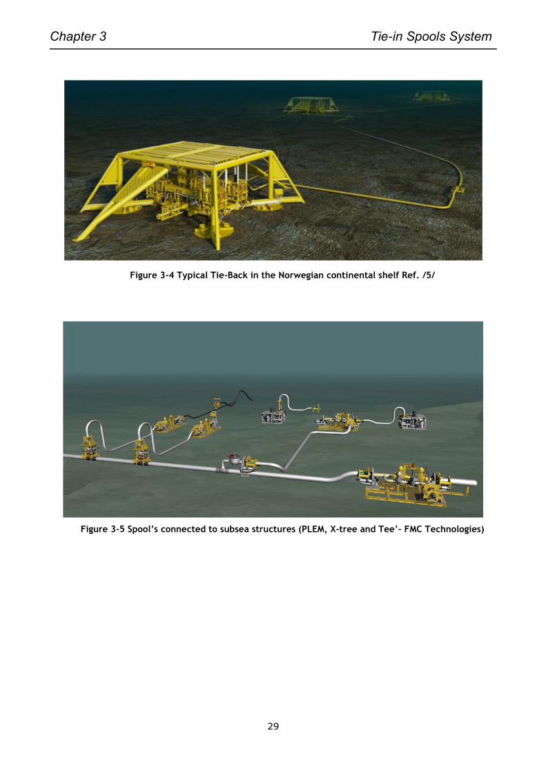
Chapter 3 Tie-in Spools System
29
Figure 3-4 Typical Tie-Back in the Norwegian continental shelf Ref. /5/
Figure 3-5 Spool’s connected to subsea structures (PLEM, X-tree and Tee’- FMC Technologies)
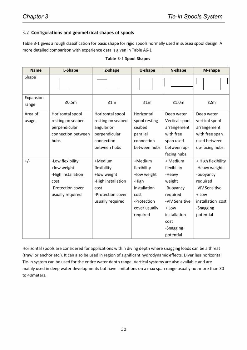
Chapter 3 Tie-in Spools System
30
3.2 Configurations and geometrical shapes of spools
Table 3-1 gives a rough classification for basic shape for rigid spools normally used in subsea spool design. A
more detailed comparison with experience data is given in Table A6-1
Table 3-1 Spool Shapes
Name L-Shape Z-shape U-shape N-shape M-shape
Shape
Expansion
range ≤0.5m ≤1m ≤1m ≤1.0m ≤2m
Area of
usage
Horizontal spool
resting on seabed
perpendicular
connection between
hubs
Horizontal spool
resting on seabed
angular or
perpendicular
connection
between hubs
Horizontal
spool resting
seabed
parallel
connection
between hubs
Deep water
Vertical spool
arrangement
with free
span used
between up-
facing hubs.
Deep water
vertical spool
arrangement
with free span
used between
up-facing hubs.
+/- -Low flexibility
+low weight
-High installation
cost
-Protection cover
usually required
+Medium
flexibility
+low weight
-High installation
cost
-Protection cover
usually required
+Medium
flexibility
+low weight
-High
installation
cost
-Protection
cover usually
required
+ Medium
flexibility
-Heavy
weight
-Buoyancy
required
-VIV Sensitive
+ Low
installation
cost
-Snagging
potential
+ High flexibility
-Heavy weight
-buoyancy
required
-VIV Sensitive
+ Low
installation cost
-Snagging
potential
Horizontal spools are considered for applications within diving depth where snagging loads can be a threat
(trawl or anchor etc.). It can also be used in region of significant hydrodynamic effects. Diver less horizontal
Tie-in system can be used for the entire water depth range. Vertical systems are also available and are
mainly used in deep water developments but have limitations on a max span range usually not more than 30
to 40meters.
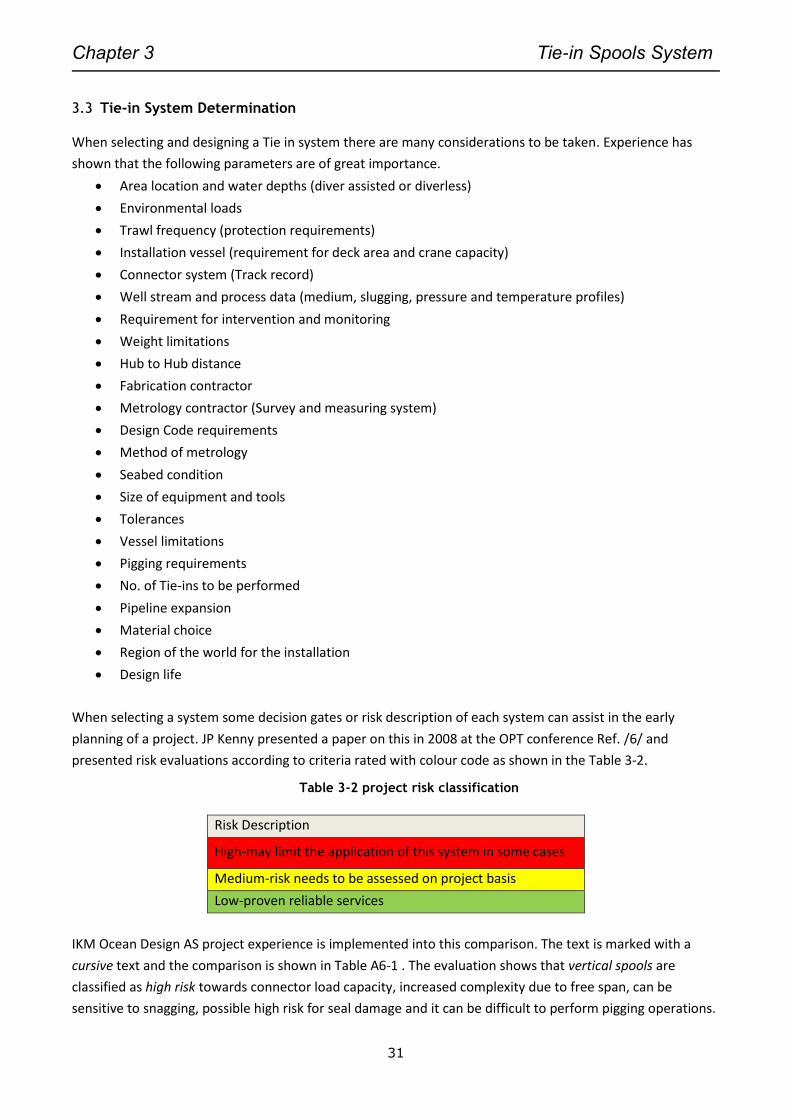
Chapter 3 Tie-in Spools System
31
3.3 Tie-in System Determination
When selecting and designing a Tie in system there are many considerations to be taken. Experience has
shown that the following parameters are of great importance.
Area location and water depths (diver assisted or diverless)
Environmental loads
Trawl frequency (protection requirements)
Installation vessel (requirement for deck area and crane capacity)
Connector system (Track record)
Well stream and process data (medium, slugging, pressure and temperature profiles)
Requirement for intervention and monitoring
Weight limitations
Hub to Hub distance
Fabrication contractor
Metrology contractor (Survey and measuring system)
Design Code requirements
Method of metrology
Seabed condition
Size of equipment and tools
Tolerances
Vessel limitations
Pigging requirements
No. of Tie-ins to be performed
Pipeline expansion
Material choice
Region of the world for the installation
Design life
When selecting a system some decision gates or risk description of each system can assist in the early
planning of a project. JP Kenny presented a paper on this in 2008 at the OPT conference Ref. /6/ and
presented risk evaluations according to criteria rated with colour code as shown in the Table 3-2.
Table 3-2 project risk classification
Risk Description
High-may limit the application of this system in some cases
Medium-risk needs to be assessed on project basis
Low-proven reliable services
IKM Ocean Design AS project experience is implemented into this comparison. The text is marked with a
cursive text and the comparison is shown in Table A6-1 . The evaluation shows that vertical spools are
classified as high risk towards connector load capacity, increased complexity due to free span, can be
sensitive to snagging, possible high risk for seal damage and it can be difficult to perform pigging operations.
Chapter 3 Tie-in Spools System
32
For horizontal spools the limitation is as for vertical spools for the connector capacity towards bending
moments and forces. However the spools are considered to have an overall lower risk compared with
vertical spools. It is worth mention here that horizontals spools normally require longer offshore installation
time and can give higher project costs.
3.4 Spool Fabrication
The fabrication of spools is normally based upon the metrology survey report which describes the location
and required dimension between the two connecting hubs. The distance between the PLET and pipeline is
measured and then the pipeline engineer designs a spool that will connect the two hubs.
Considerations relating to fabricating of spools are:
Location of fabricator and yard size requirement
Fabricator qualifications (ISO 9000 qualification, DNV OS-F101 approved, NORSOK Qualified, etc.)
Material purchasing
Production and standard requirement for testing.
Lead time for special items
Welding sequence
Number of bends
Coating methods
Fabrication tolerances
Size and weight
Number of bends
Requirement for fabrication stands
Requirement for test stands and test equipment
Requirement for lifting aids
Logistics regarding shipping of spools
Interface control
The above mentioned points are of importance to map and study in an early phase usually when fabrication
specifications and procedures are developed for the project a comparative overview is given in Table 3-3.
Table 3-3 fabrication design considerations
Issue Horizontal Tie-in Spool Vertical Tie-in spool
Size and weight Large footprint, limits amount of
spools to be transported to field.
Small footprint, scaffolding
requirement needed.
Geometry General fewer bend on horizontal
spool but complexity varies
Generally more bends are related
to vertical spool complexity varies
Fabrication and shipping stands Usually less weight for support
steel as stands do not need to
support inboard test hub.
Requirement for large weight of
supporting steel as well as tilting
function of hub
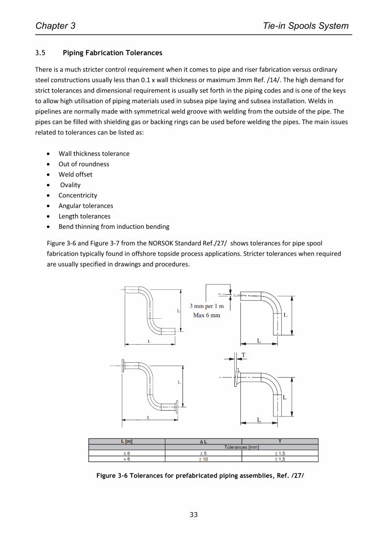
Chapter 3 Tie-in Spools System
33
3.5 Piping Fabrication Tolerances
There is a much stricter control requirement when it comes to pipe and riser fabrication versus ordinary
steel constructions usually less than 0.1 x wall thickness or maximum 3mm Ref. /14/. The high demand for
strict tolerances and dimensional requirement is usually set forth in the piping codes and is one of the keys
to allow high utilisation of piping materials used in subsea pipe laying and subsea installation. Welds in
pipelines are normally made with symmetrical weld groove with welding from the outside of the pipe. The
pipes can be filled with shielding gas or backing rings can be used before welding the pipes. The main issues
related to tolerances can be listed as:
Wall thickness tolerance
Out of roundness
Weld offset
Ovality
Concentricity
Angular tolerances
Length tolerances
Bend thinning from induction bending
Figure 3-6 and Figure 3-7 from the NORSOK Standard Ref./27/ shows tolerances for pipe spool
fabrication typically found in offshore topside process applications. Stricter tolerances when required
are usually specified in drawings and procedures.
Figure 3-6 Tolerances for prefabricated piping assemblies, Ref. /27/
Chapter 3 Tie-in Spools System
34
Figure 3-7 Tolerances for prefabricated piping assemblies, Ref. /27/

Chapter 3 Tie-in Spools System
35
3.6 Probabilistic Assessment of Fabrication Tolerances
In this chapter we take a look at the engineering practice of using the fabrication tolerances in spool design.
It is common in projects to include linear and angular tolerances of the spool in order to asses if the lock in
of the connectors at the hub will generate large stresses in the spool. The question which arises is how much
of the tolerances should be incorporated into the design and how much is taken care of by the governing
piping codes. The answer to this is not straight forward for an optimised spool design. For normal topside or
manifold piping design, the fabrication tolerances are usually incorporated into the piping design formulas.
Such as the NORSOK standard Ref. /28/ and ASME B31.3 code Ref. /17/. Below is given some discussion from
the book guide to ASME B31.3 Ref. /26/ where the question regarding alignment of pipe flanges is discussed:
Based upon the above answer from the ASME Committee, larger misalignment is allowed as long as it is
considered in the design. This would then have to be considered in the analysis. An interesting paper
regarding fabrication tolerances is found in Ref./29/ here the following problem description is given:
“Structural reliability is normally assessed by considering its converse, failure probability. Analysts often
qualify this by referring to “notional” failure probability. This is partly because the target values that
designers aim for are generally so small that calculations are sensitive to assumptions about the forms of the
Chapter 3 Tie-in Spools System
36
tails of the frequency distributions used in the mathematical models of loading and resistance variables, and
these tails are usually poorly defined.
“Much of the complexity of reliability analysis methods arises from the fact that the contributions of uncertainties in all the design parameters are combined within complex engineering design equations. However, the basic principles can be used quite directly to address practical problems, such as assessing the magnitude of the locked-in stresses due to the interaction between fabrication tolerances and assembly methods. In this case, interest is focused towards the most likely outcome rather than on rare events, and the mathematical concept is therefore more robust.”
The paper discusses the frequency distribution of dimensional errors such as the normal distribution the
Central Limit theorem and the rectangular distribution, it concludes with that the outcome is normally
distributed even if the input is of a rectangular distribution hence the total effect of the tolerances has
uncertain bounds which can only be described probabilistically.
It further gives some guide on how to set the limits for the tolerances or dimensional errors by using the
RMS or root mean square of the errors the following as the number of the variable Xi becomes large the
frequency approaches the normal distribution. And if the un-factored design condition should be taken to be
a characteristic value with 5% probability of exceedance this is obtained by taking a range between +/- 1.65
standard deviation from the mean position. Thus the characteristic effect of dimensional errors is given by
the following equation.
1.65𝑠[𝑌] ≈1.65
√3√(∑ (∆𝑔)2𝑛
𝑖=1 ≈ √(∑ (∆𝑔)2𝑛𝑖=1 (3.1)
Imperfections in element dimensions can be introduced into the structural analysis models by means of member extensions or end rotations. These can be linearly superimposed on other structural effects, so the effects of dimensional errors can be analysed independently of permanent or transient loadings.
The paper presents an analysis of a roof where over 400 different locations with the effect of tolerance was
analyzed. The results where compared to the structural building code and the ULS factor of 1.4. The result
shows that the sagging moments was increased by 8% in the ULS case due to fabrication tolerances and
considerably increase in the lateral moments by 100 %.
The paper concludes with the following:
“Computers allow us to compute load effects for structures that have much greater complexity and
indeterminacy than those that were designed using traditional methods. There is a danger that engineers
may lose sight of the important load paths when they refine their calculations to reduce apparent
overdesign. In so doing, ductility and tolerance towards imperfect erection procedures may be reduced, and
it may become increasingly unwise to trust that redistribution of local overloads will safely take care of
fabrication tolerances.
No matter what the design specifications might state, the products of different fabricators will have different
patterns of variation, and a realistic prediction of the overall effects of fabrication tolerances will require
knowledge of real processes.”
Chapter 3 Tie-in Spools System
37
3.7 Summary
A shown in this chapter there are many parameters regarding spool and pipe design which must be
considered. A Pre-Study of the planned project is advisable to commence in order to determine the best
spool design. The Pre-study or FEED should focus on the following key topics:
Subsea routing and location of spool
Spool type
Installation time and constraints
Use conservative data, previous experience is important
Define optimum spool lengths (minimum and maximum)
Identify critical values early in the project small changes can give rise to high cost later in project
For detail design :
Establish design basis for analysis and design
Perform piping analysis (FEM)
Evaluate the effect of environmental loading, process medium and flow data
Methodology for fabrication and installation
Operational aspects
Installation analysis
For the piping analysis it is advisable to incorporate a statistical tool for assessing the fabrication tolerances
in order to establish a reasonable safety level in-line with the code requirements. One question is on how
the project should handle the standard deviation based upon the critically of the system i.e. should the level
be in the range 1.65 - 3 times the standard deviation. How will the probability of exceedance be quantified
(5% or 10%)? Most of the analyzed spools today are based upon “worst case” scenario which is a very rare
event but should perhaps be analyzed with the most probably expected tolerances and loading. Different
techniques for random probabilistic and parameter correlation effects are available and can be included in
simulation software (Monte Carlo simulation is one example)

Chapter 3 Tie-in Spools System
38
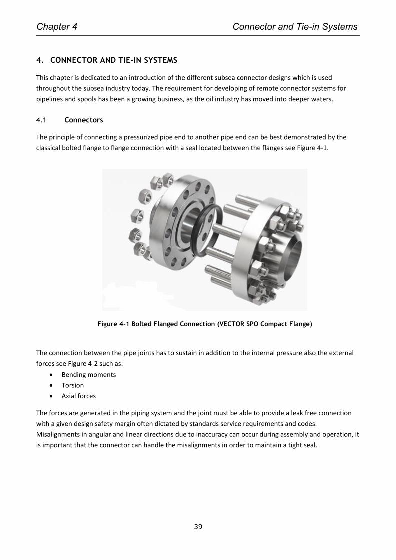
Chapter 4 Connector and Tie-in Systems
39
4. CONNECTOR AND TIE-IN SYSTEMS
This chapter is dedicated to an introduction of the different subsea connector designs which is used
throughout the subsea industry today. The requirement for developing of remote connector systems for
pipelines and spools has been a growing business, as the oil industry has moved into deeper waters.
4.1 Connectors
The principle of connecting a pressurized pipe end to another pipe end can be best demonstrated by the
classical bolted flange to flange connection with a seal located between the flanges see Figure 4-1.
Figure 4-1 Bolted Flanged Connection (VECTOR SPO Compact Flange)
The connection between the pipe joints has to sustain in addition to the internal pressure also the external
forces see Figure 4-2 such as:
Bending moments
Torsion
Axial forces
The forces are generated in the piping system and the joint must be able to provide a leak free connection
with a given design safety margin often dictated by standards service requirements and codes.
Misalignments in angular and linear directions due to inaccuracy can occur during assembly and operation, it
is important that the connector can handle the misalignments in order to maintain a tight seal.
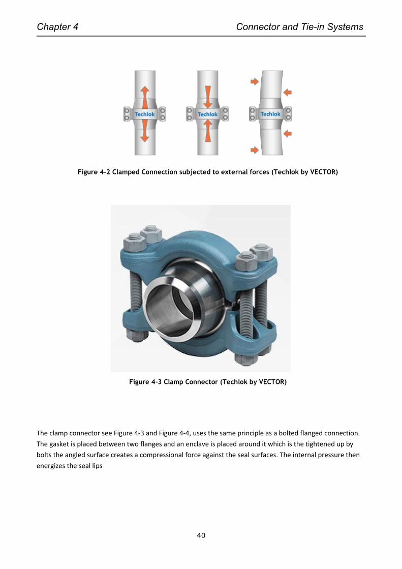
Chapter 4 Connector and Tie-in Systems
40
Figure 4-2 Clamped Connection subjected to external forces (Techlok by VECTOR)
Figure 4-3 Clamp Connector (Techlok by VECTOR)
The clamp connector see Figure 4-3 and Figure 4-4, uses the same principle as a bolted flanged connection.
The gasket is placed between two flanges and an enclave is placed around it which is the tightened up by
bolts the angled surface creates a compressional force against the seal surfaces. The internal pressure then
energizes the seal lips
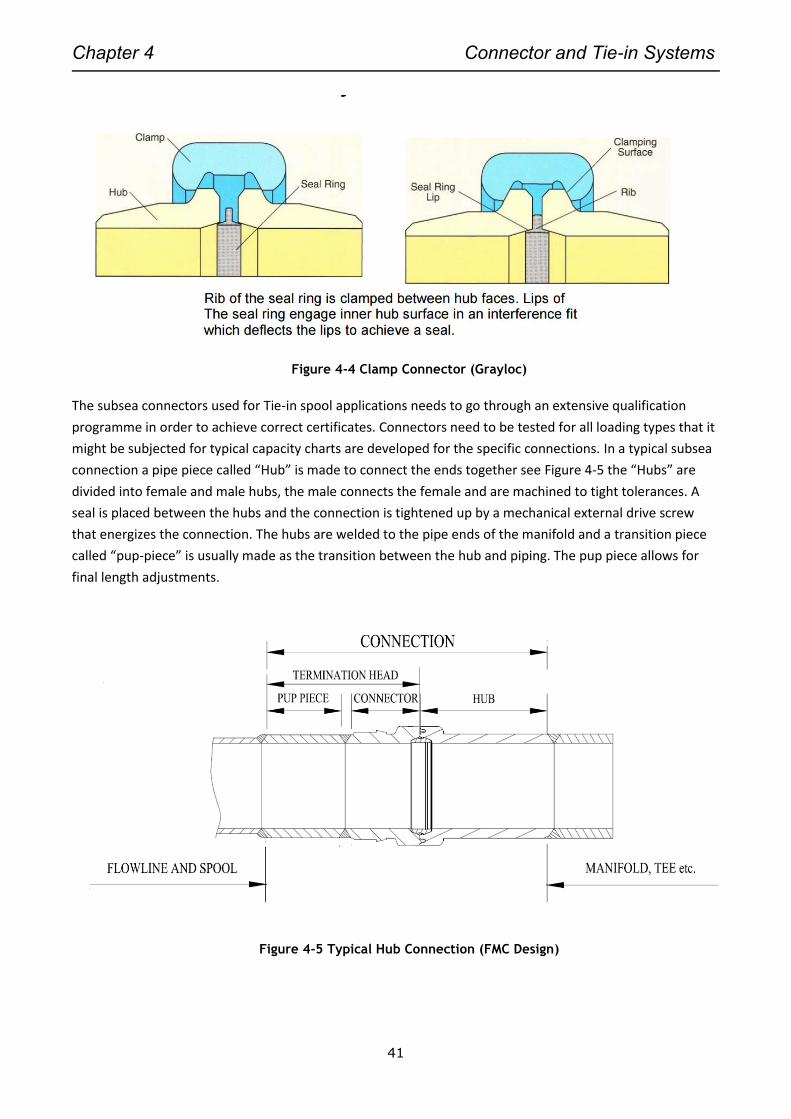
Chapter 4 Connector and Tie-in Systems
41
Figure 4-4 Clamp Connector (Grayloc)
The subsea connectors used for Tie-in spool applications needs to go through an extensive qualification
programme in order to achieve correct certificates. Connectors need to be tested for all loading types that it
might be subjected for typical capacity charts are developed for the specific connections. In a typical subsea
connection a pipe piece called “Hub” is made to connect the ends together see Figure 4-5 the “Hubs” are
divided into female and male hubs, the male connects the female and are machined to tight tolerances. A
seal is placed between the hubs and the connection is tightened up by a mechanical external drive screw
that energizes the connection. The hubs are welded to the pipe ends of the manifold and a transition piece
called “pup-piece” is usually made as the transition between the hub and piping. The pup piece allows for
final length adjustments.
Figure 4-5 Typical Hub Connection (FMC Design)
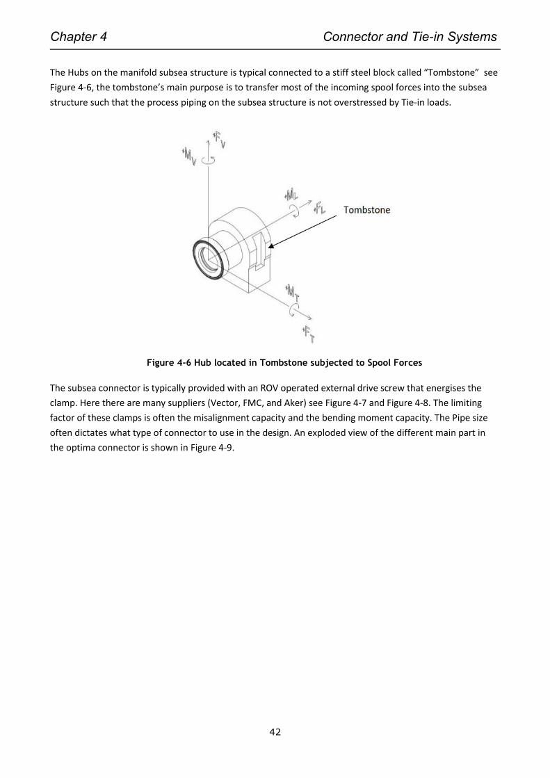
Chapter 4 Connector and Tie-in Systems
42
The Hubs on the manifold subsea structure is typical connected to a stiff steel block called “Tombstone” see
Figure 4-6, the tombstone’s main purpose is to transfer most of the incoming spool forces into the subsea
structure such that the process piping on the subsea structure is not overstressed by Tie-in loads.
Figure 4-6 Hub located in Tombstone subjected to Spool Forces
The subsea connector is typically provided with an ROV operated external drive screw that energises the
clamp. Here there are many suppliers (Vector, FMC, and Aker) see Figure 4-7 and Figure 4-8. The limiting
factor of these clamps is often the misalignment capacity and the bending moment capacity. The Pipe size
often dictates what type of connector to use in the design. An exploded view of the different main part in
the optima connector is shown in Figure 4-9.
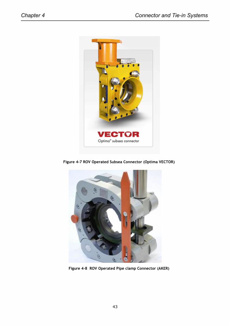
Chapter 4 Connector and Tie-in Systems
43
Figure 4-7 ROV Operated Subsea Connector (Optima VECTOR)
Figure 4-8 ROV Operated Pipe clamp Connector (AKER)
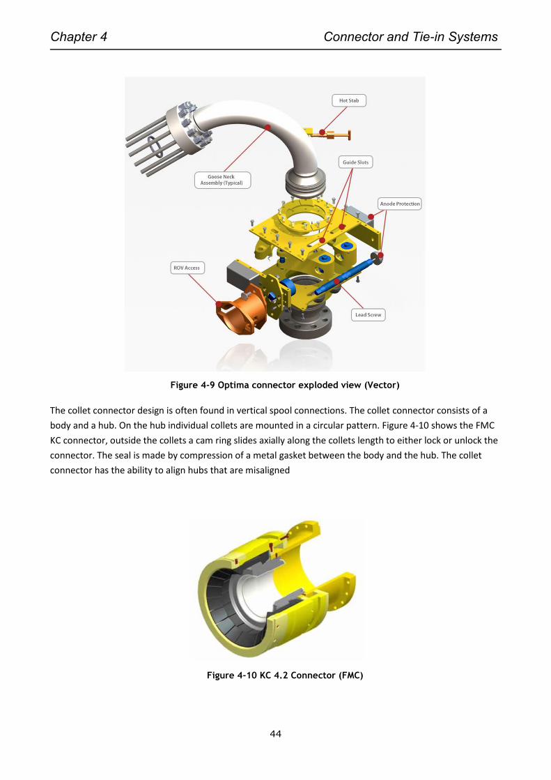
Chapter 4 Connector and Tie-in Systems
44
Figure 4-9 Optima connector exploded view (Vector)
The collet connector design is often found in vertical spool connections. The collet connector consists of a
body and a hub. On the hub individual collets are mounted in a circular pattern. Figure 4-10 shows the FMC
KC connector, outside the collets a cam ring slides axially along the collets length to either lock or unlock the
connector. The seal is made by compression of a metal gasket between the body and the hub. The collet
connector has the ability to align hubs that are misaligned
Figure 4-10 KC 4.2 Connector (FMC)
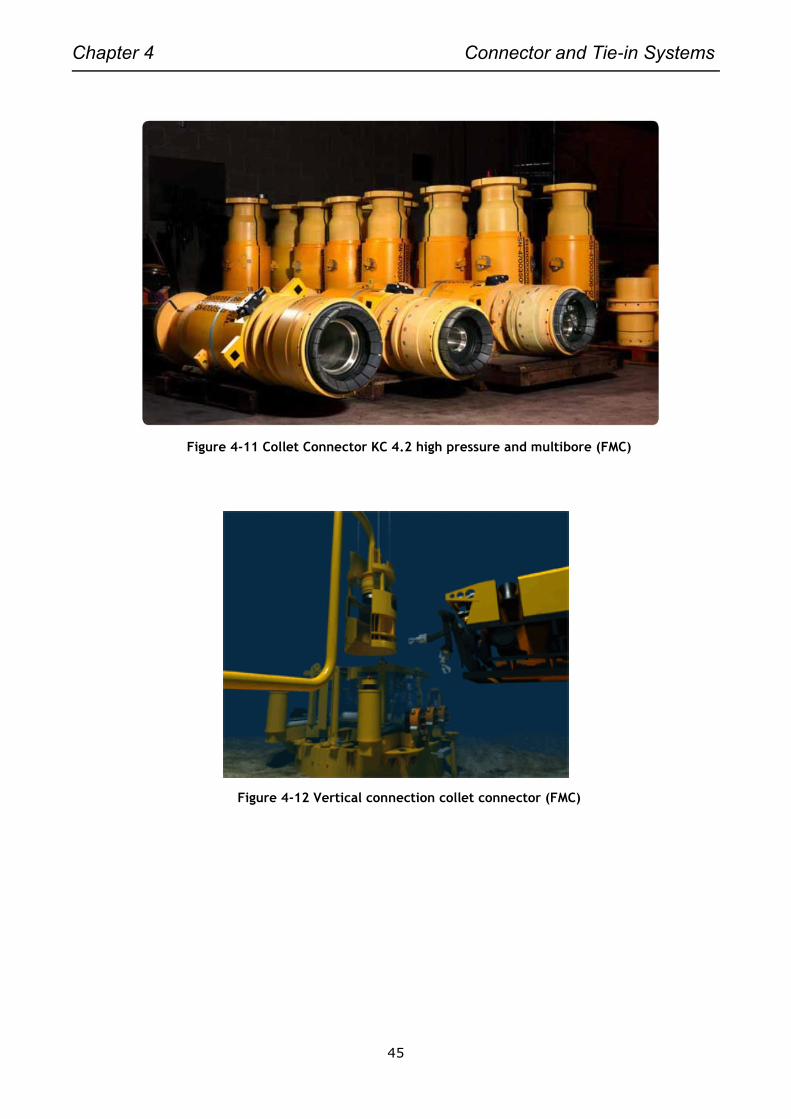
Chapter 4 Connector and Tie-in Systems
45
Figure 4-11 Collet Connector KC 4.2 high pressure and multibore (FMC)
Figure 4-12 Vertical connection collet connector (FMC)
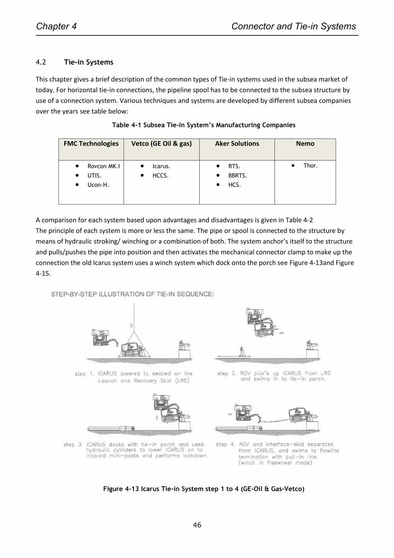
Chapter 4 Connector and Tie-in Systems
46
4.2 Tie-in Systems
This chapter gives a brief description of the common types of Tie-in systems used in the subsea market of
today. For horizontal tie-in connections, the pipeline spool has to be connected to the subsea structure by
use of a connection system. Various techniques and systems are developed by different subsea companies
over the years see table below:
Table 4-1 Subsea Tie-In System’s Manufacturing Companies
FMC Technologies
Vetco (GE Oil & gas)
Aker Solutions
Nemo
Rovcon MK.I
UTIS.
Ucon-H.
Icarus.
HCCS.
RTS.
BBRTS.
HCS.
Thor.
A comparison for each system based upon advantages and disadvantages is given in Table 4-2
The principle of each system is more or less the same. The pipe or spool is connected to the structure by
means of hydraulic stroking/ winching or a combination of both. The system anchor’s itself to the structure
and pulls/pushes the pipe into position and then activates the mechanical connector clamp to make up the
connection the old Icarus system uses a winch system which dock onto the porch see Figure 4-13and Figure
4-15.
Figure 4-13 Icarus Tie-in System step 1 to 4 (GE-Oil & Gas-Vetco)
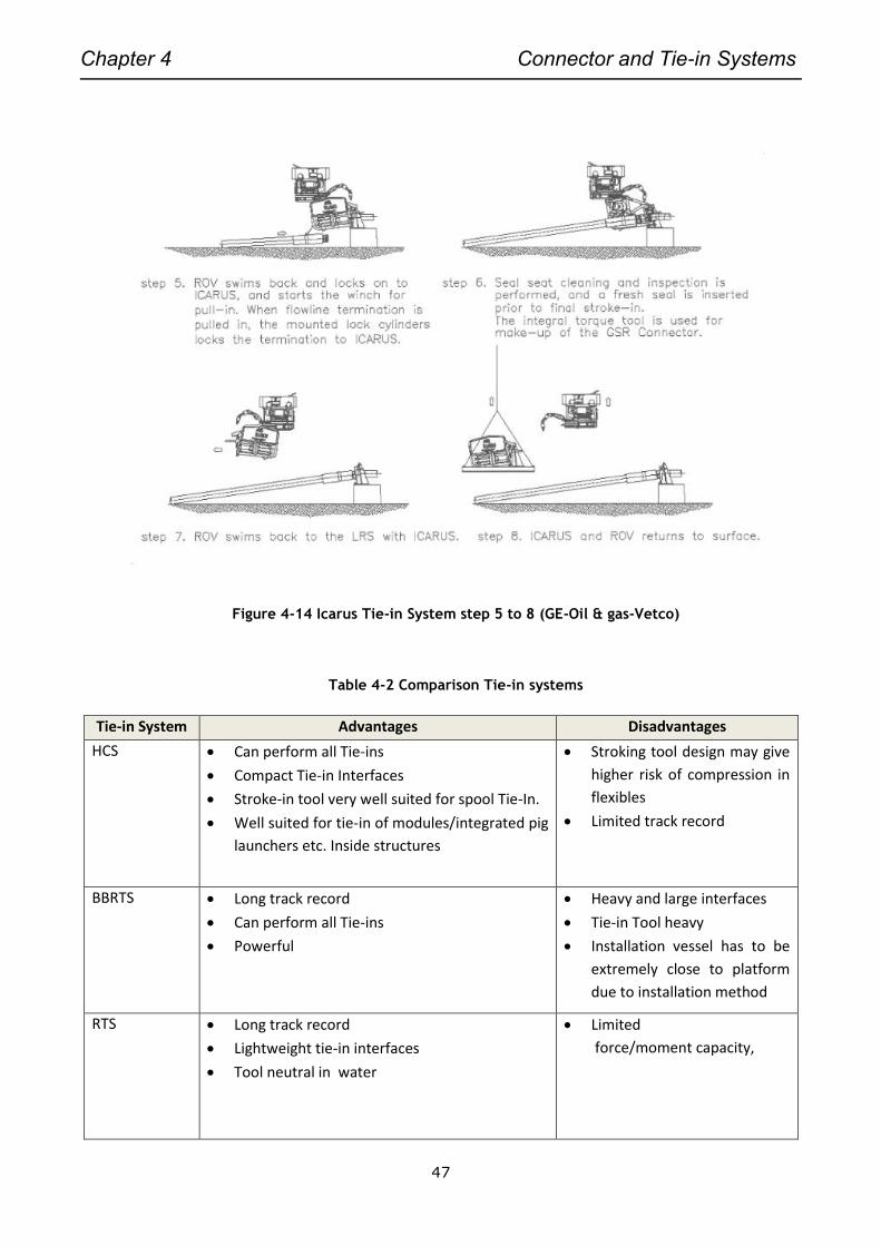
Chapter 4 Connector and Tie-in Systems
47
Figure 4-14 Icarus Tie-in System step 5 to 8 (GE-Oil & gas-Vetco)
Table 4-2 Comparison Tie-in systems
Tie-in System Advantages Disadvantages
HCS Can perform all Tie-ins
Compact Tie-in Interfaces
Stroke-in tool very well suited for spool Tie-In.
Well suited for tie-in of modules/integrated pig
launchers etc. Inside structures
Stroking tool design may give
higher risk of compression in
flexibles
Limited track record
BBRTS Long track record
Can perform all Tie-ins
Powerful
Heavy and large interfaces
Tie-in Tool heavy
Installation vessel has to be
extremely close to platform
due to installation method
RTS Long track record
Lightweight tie-in interfaces
Tool neutral in water
Limited
force/moment capacity,
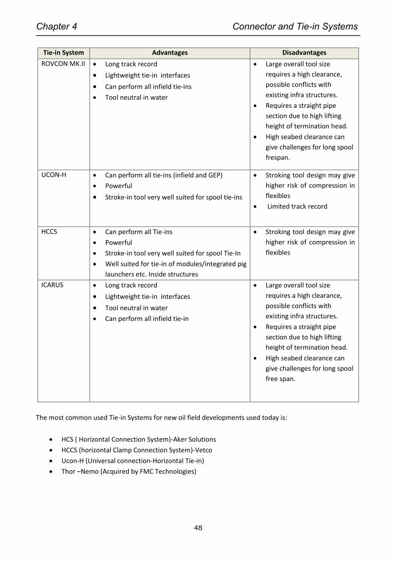
Chapter 4 Connector and Tie-in Systems
48
Tie-in System Advantages Disadvantages
ROVCON MK.II Long track record
Lightweight tie-in interfaces
Can perform all infield tie-ins
Tool neutral in water
Large overall tool size
requires a high clearance,
possible conflicts with
existing infra structures.
Requires a straight pipe
section due to high lifting
height of termination head.
High seabed clearance can
give challenges for long spool
frespan.
UCON-H Can perform all tie-ins (infield and GEP)
Powerful
Stroke-in tool very well suited for spool tie-ins
Stroking tool design may give
higher risk of compression in
flexibles
Limited track record
HCCS Can perform all Tie-ins
Powerful
Stroke-in tool very well suited for spool Tie-In
Well suited for tie-in of modules/integrated pig
launchers etc. Inside structures
Stroking tool design may give
higher risk of compression in
flexibles
ICARUS Long track record
Lightweight tie-in interfaces
Tool neutral in water
Can perform all infield tie-in
Large overall tool size
requires a high clearance,
possible conflicts with
existing infra structures.
Requires a straight pipe
section due to high lifting
height of termination head.
High seabed clearance can
give challenges for long spool
free span.
The most common used Tie-in Systems for new oil field developments used today is:
HCS ( Horizontal Connection System)-Aker Solutions
HCCS (horizontal Clamp Connection System)-Vetco
Ucon-H (Universal connection-Horizontal Tie-in)
Thor –Nemo (Acquired by FMC Technologies)
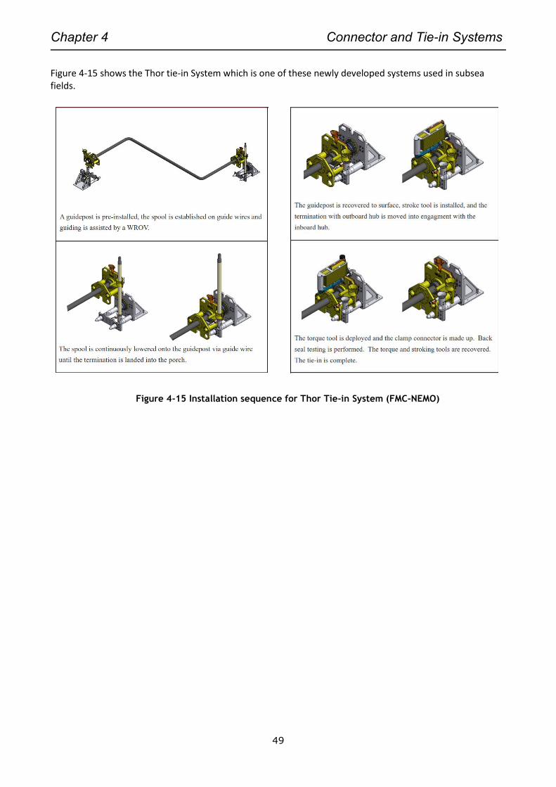
Chapter 4 Connector and Tie-in Systems
49
Figure 4-15 shows the Thor tie-in System which is one of these newly developed systems used in subsea fields.
Figure 4-15 Installation sequence for Thor Tie-in System (FMC-NEMO)

Chapter 4 Connector and Tie-in Systems
50
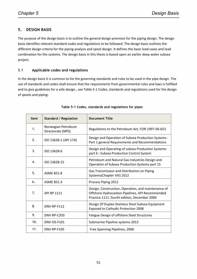
Chapter 5 Design Basis
51
5. DESIGN BASIS
The purpose of the design basis is to outline the general design premises for the piping design. The design
basis identifies relevant standard codes and regulations to be followed. The design basis outlines the
different design criteria for the piping analysis and spool design. It defines the basic load cases and load
combination for the systems. The design basis in this thesis is based upon an earlier deep water subsea
project.
5.1 Applicable codes and regulations
In the design basis it is common to list the governing standards and rules to be used in the pipe design. The
use of standards and codes shall ensure that the requirements from governmental rules and laws is fulfilled
and to give guidelines for a safe design., see Table 5-1 Codes, standards and regulations used for the design
of spools and piping:
Table 5-1 Codes, standards and regulations for pipes
Item Standard / Regulation Document Title
1. Norwegian Petroleum Directorate (NPD)
Regulations to the Petroleum Act, FOR-1997-06-653
2. ISO 13628-1 (API 17A) Design and Operation of Subsea Production Systems - Part 1 general Requirements and Recommendations
3. ISO 13628-6 Design and Operating of subsea Production Systems-part 6 : Subsea Production Control System
4. ISO 13628-15 Petroleum and Natural Gas Industries Design and Operation of Subsea Production Systems part 15
5. ASME B31.8 Gas Transmission and Distribution on Piping Systems(Chapter VIII) 2012
6. ASME B31.3 Process Piping 2012
7. API RP 1111 Design, Construction, Operation, and maintenance of Offshore Hydrocarbon Pipelines, API Recommended Practice 1111 ,fourth edition, December 2009
8. DNV-RP-F112 Design Of Duplex Stainless Steel Subsea Equipment Exposed to Cathodic Protection 2008
9. DNV-RP-C203 Fatigue Design of offshore Steel Structures
10. DNV-OS-F101 Submarine Pipeline systems 2013
11. DNV-RP-F105 Free Spanning Pipelines, 2006
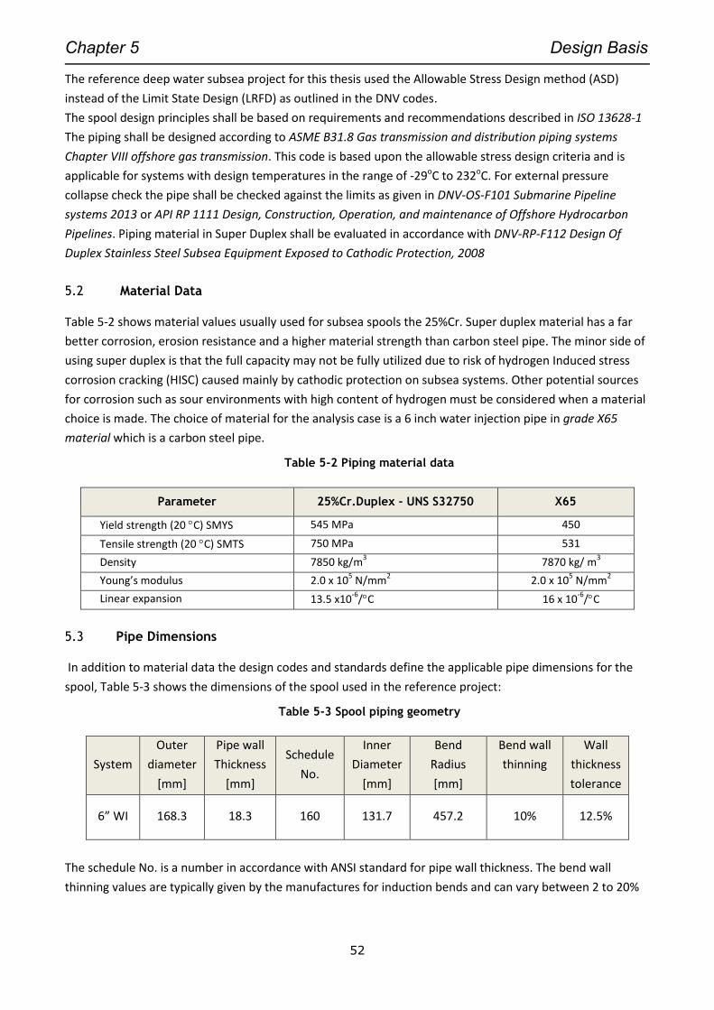
Chapter 5 Design Basis
52
The reference deep water subsea project for this thesis used the Allowable Stress Design method (ASD)
instead of the Limit State Design (LRFD) as outlined in the DNV codes.
The spool design principles shall be based on requirements and recommendations described in ISO 13628-1
The piping shall be designed according to ASME B31.8 Gas transmission and distribution piping systems
Chapter VIII offshore gas transmission. This code is based upon the allowable stress design criteria and is
applicable for systems with design temperatures in the range of -29oC to 232oC. For external pressure
collapse check the pipe shall be checked against the limits as given in DNV-OS-F101 Submarine Pipeline
systems 2013 or API RP 1111 Design, Construction, Operation, and maintenance of Offshore Hydrocarbon
Pipelines. Piping material in Super Duplex shall be evaluated in accordance with DNV-RP-F112 Design Of
Duplex Stainless Steel Subsea Equipment Exposed to Cathodic Protection, 2008
5.2 Material Data
Table 5-2 shows material values usually used for subsea spools the 25%Cr. Super duplex material has a far
better corrosion, erosion resistance and a higher material strength than carbon steel pipe. The minor side of
using super duplex is that the full capacity may not be fully utilized due to risk of hydrogen Induced stress
corrosion cracking (HISC) caused mainly by cathodic protection on subsea systems. Other potential sources
for corrosion such as sour environments with high content of hydrogen must be considered when a material
choice is made. The choice of material for the analysis case is a 6 inch water injection pipe in grade X65
material which is a carbon steel pipe.
Table 5-2 Piping material data
Parameter 25%Cr.Duplex - UNS S32750 X65
Yield strength (20 C) SMYS 545 MPa 450
Tensile strength (20 C) SMTS 750 MPa 531
Density 7850 kg/m3 7870 kg/ m
3
Young’s modulus 2.0 x 10⁵ N/mm
2 2.0 x 10
5 N/mm
2
Linear expansion 13.5 x10⁻⁶
/C 16 x 10-6
/C
5.3 Pipe Dimensions
In addition to material data the design codes and standards define the applicable pipe dimensions for the
spool, Table 5-3 shows the dimensions of the spool used in the reference project:
Table 5-3 Spool piping geometry
System
Outer
diameter
[mm]
Pipe wall
Thickness
[mm]
Schedule
No.
Inner
Diameter
[mm]
Bend
Radius
[mm]
Bend wall
thinning
Wall
thickness
tolerance
6” WI 168.3 18.3 160 131.7 457.2 10% 12.5%
The schedule No. is a number in accordance with ANSI standard for pipe wall thickness. The bend wall
thinning values are typically given by the manufactures for induction bends and can vary between 2 to 20%
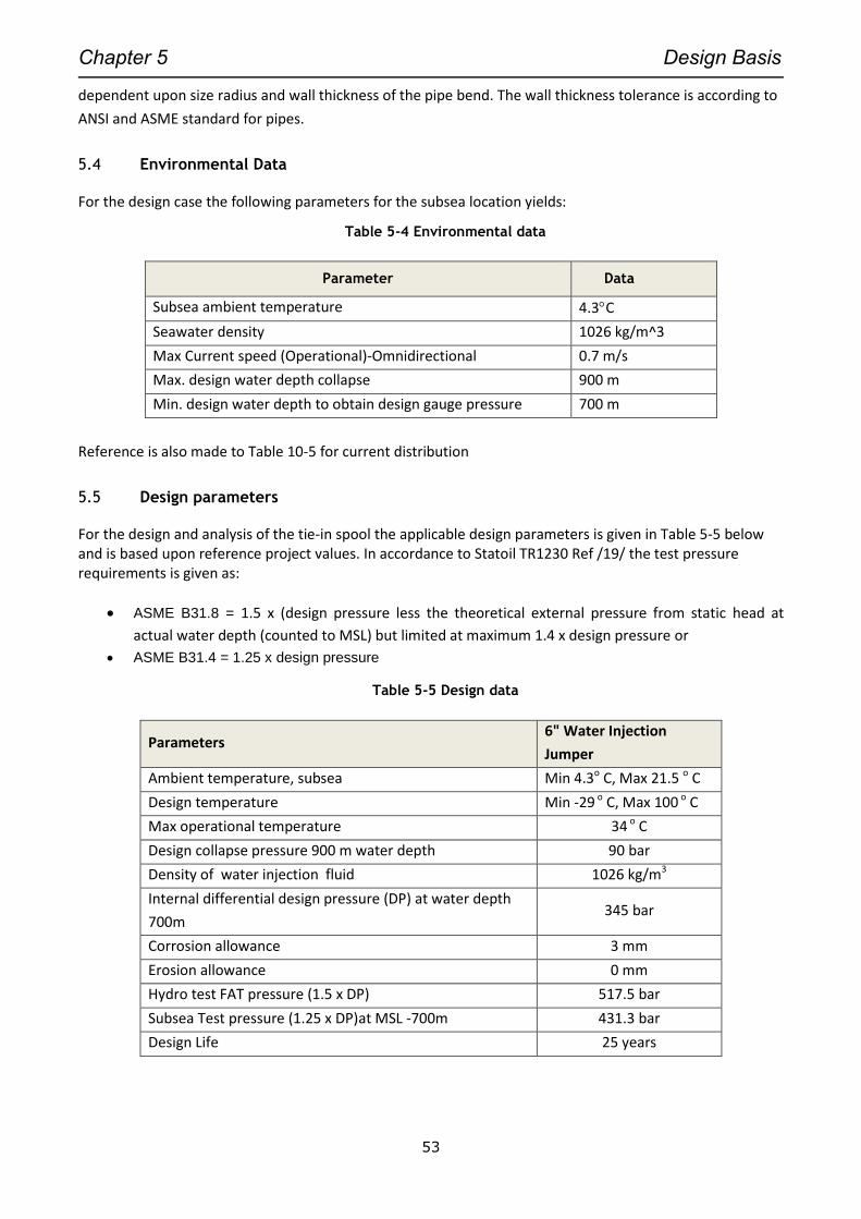
Chapter 5 Design Basis
53
dependent upon size radius and wall thickness of the pipe bend. The wall thickness tolerance is according to
ANSI and ASME standard for pipes.
5.4 Environmental Data
For the design case the following parameters for the subsea location yields:
Table 5-4 Environmental data
Parameter Data
Subsea ambient temperature 4.3C
Seawater density 1026 kg/m^3
Max Current speed (Operational)-Omnidirectional 0.7 m/s
Max. design water depth collapse 900 m
Min. design water depth to obtain design gauge pressure 700 m
Reference is also made to Table 10-5 for current distribution
5.5 Design parameters
For the design and analysis of the tie-in spool the applicable design parameters is given in Table 5-5 below and is based upon reference project values. In accordance to Statoil TR1230 Ref /19/ the test pressure requirements is given as:
ASME B31.8 = 1.5 x (design pressure less the theoretical external pressure from static head at
actual water depth (counted to MSL) but limited at maximum 1.4 x design pressure or
ASME B31.4 = 1.25 x design pressure
Table 5-5 Design data
Parameters 6" Water Injection
Jumper
Ambient temperature, subsea Min 4.3o C, Max 21.5 o C
Design temperature Min -29 o C, Max 100 o C
Max operational temperature 34 o C
Design collapse pressure 900 m water depth 90 bar
Density of water injection fluid 1026 kg/m3
Internal differential design pressure (DP) at water depth
700m 345 bar
Corrosion allowance 3 mm
Erosion allowance 0 mm
Hydro test FAT pressure (1.5 x DP) 517.5 bar
Subsea Test pressure (1.25 x DP)at MSL -700m 431.3 bar
Design Life 25 years
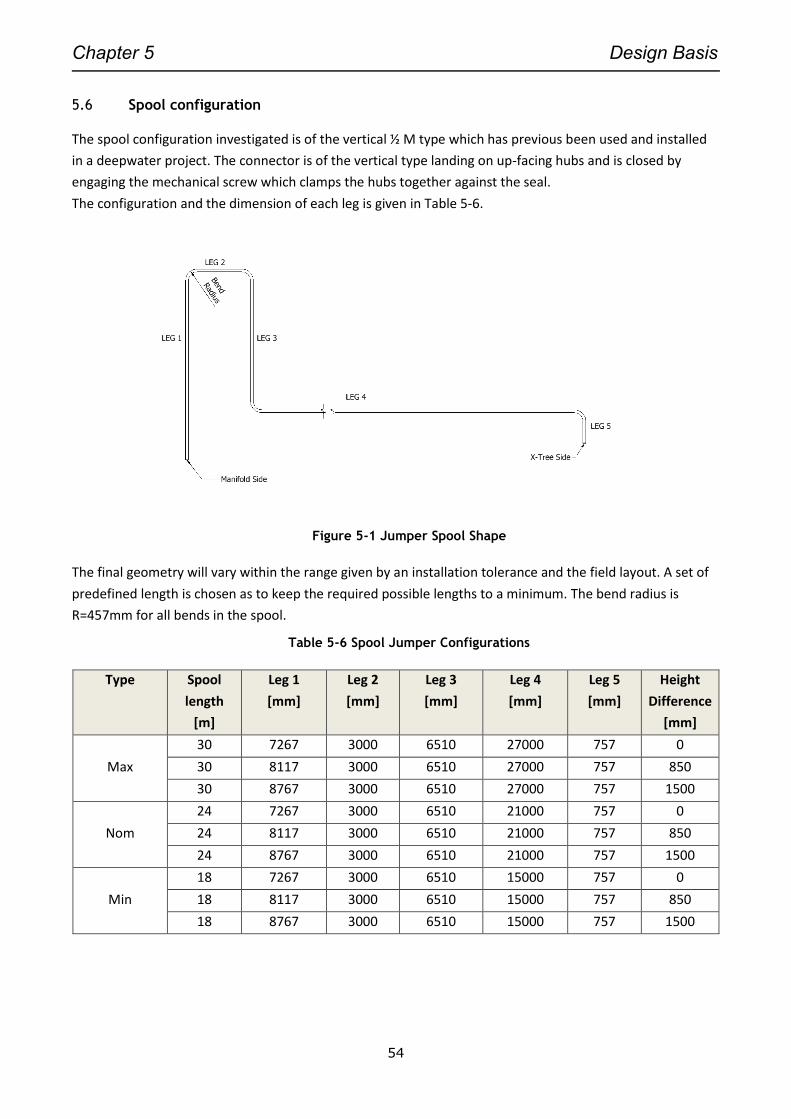
Chapter 5 Design Basis
54
5.6 Spool configuration
The spool configuration investigated is of the vertical ½ M type which has previous been used and installed
in a deepwater project. The connector is of the vertical type landing on up-facing hubs and is closed by
engaging the mechanical screw which clamps the hubs together against the seal.
The configuration and the dimension of each leg is given in Table 5-6.
Figure 5-1 Jumper Spool Shape
The final geometry will vary within the range given by an installation tolerance and the field layout. A set of
predefined length is chosen as to keep the required possible lengths to a minimum. The bend radius is
R=457mm for all bends in the spool.
Table 5-6 Spool Jumper Configurations
Type Spool
length
[m]
Leg 1
[mm]
Leg 2
[mm]
Leg 3
[mm]
Leg 4
[mm]
Leg 5
[mm]
Height
Difference
[mm]
Max
30 7267 3000 6510 27000 757 0
30 8117 3000 6510 27000 757 850
30 8767 3000 6510 27000 757 1500
Nom
24 7267 3000 6510 21000 757 0
24 8117 3000 6510 21000 757 850
24 8767 3000 6510 21000 757 1500
Min
18 7267 3000 6510 15000 757 0
18 8117 3000 6510 15000 757 850
18 8767 3000 6510 15000 757 1500
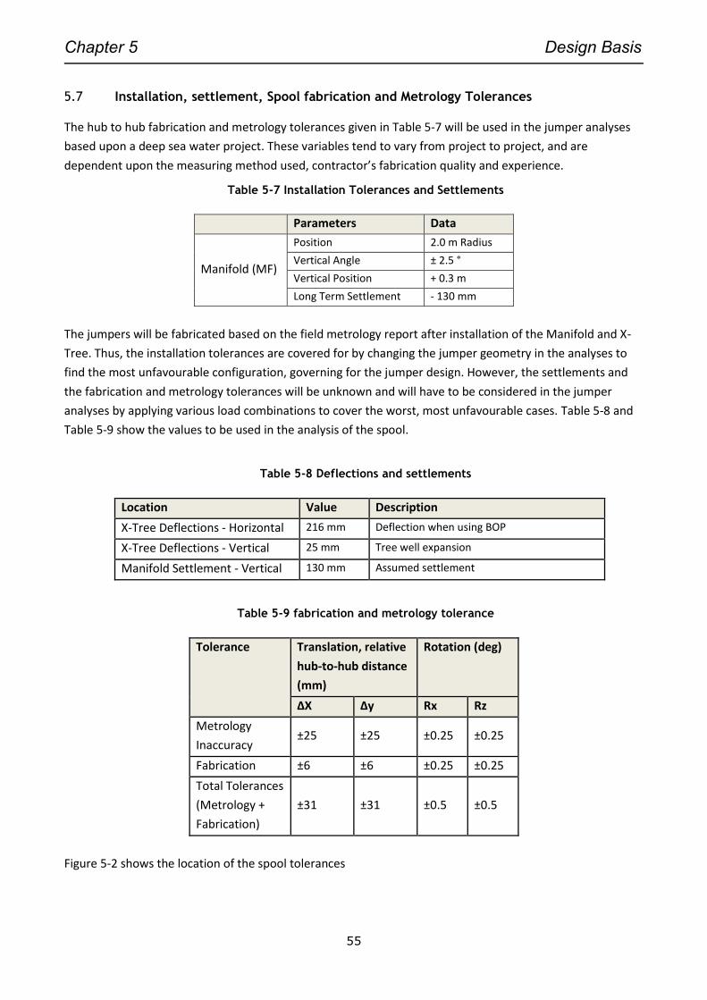
Chapter 5 Design Basis
55
5.7 Installation, settlement, Spool fabrication and Metrology Tolerances
The hub to hub fabrication and metrology tolerances given in Table 5-7 will be used in the jumper analyses
based upon a deep sea water project. These variables tend to vary from project to project, and are
dependent upon the measuring method used, contractor’s fabrication quality and experience.
Table 5-7 Installation Tolerances and Settlements
Parameters Data
Manifold (MF)
Position 2.0 m Radius
Vertical Angle ± 2.5 °
Vertical Position + 0.3 m
Long Term Settlement - 130 mm
The jumpers will be fabricated based on the field metrology report after installation of the Manifold and X-
Tree. Thus, the installation tolerances are covered for by changing the jumper geometry in the analyses to
find the most unfavourable configuration, governing for the jumper design. However, the settlements and
the fabrication and metrology tolerances will be unknown and will have to be considered in the jumper
analyses by applying various load combinations to cover the worst, most unfavourable cases. Table 5-8 and
Table 5-9 show the values to be used in the analysis of the spool.
Table 5-8 Deflections and settlements
Location Value Description
X-Tree Deflections - Horizontal 216 mm Deflection when using BOP
X-Tree Deflections - Vertical 25 mm Tree well expansion
Manifold Settlement - Vertical 130 mm Assumed settlement
Table 5-9 fabrication and metrology tolerance
Tolerance Translation, relative
hub-to-hub distance
(mm)
Rotation (deg)
ΔX Δy Rx Rz
Metrology
Inaccuracy ±25 ±25 ±0.25 ±0.25
Fabrication ±6 ±6 ±0.25 ±0.25
Total Tolerances
(Metrology +
Fabrication)
±31 ±31 ±0.5 ±0.5
Figure 5-2 shows the location of the spool tolerances
Chapter 5 Design Basis
56
Figure 5-2 Jumper spool tolerances
In the analysis the longitudinal deflection and fabrication tolerances is assumed to be of a uniform
distribution which is used when the only information known about the parameter variability is the upper and
lower bounds. For the angular tolerances a normal statistical distribution is applied. (Refer to chapters 6.2 ).
The reference project did not account for any statistical scatter in the tolerances and imposed deflections. A
range of predetermined max/min for deflections and tolerances was combined and analysed together with
the acting loads.
5.8 Load Cases
During the different phases from construction to the end of design life the jumper piping will be subject to different loads. The following loads and or load cases should be considered as potential loads during the jumper life cycle.
Pressure testing (Onshore and subsea)
Lifting/Lowering through splash zone
Connection
Operation
Slug loads
Shutdowns
Snag loads
Retrieval
Earthquake
Vortex Induced Vibration (VIV)
Fatigue Evaluation
Erosion
Seal replacement
Dropped object loads
y
x z
Chapter 5 Design Basis
57
However, the investigation of this study is limited to only the following cases:
Pressure testing onshore and subsea
Connection/operation and seal replacement (in-place)
VIV fatigue evaluation
For a more comprehensive load investigation readers of this thesis are encouraged to study Jone Lutro’s Master thesis Ref. /3/. In his thesis the main topic is a LRFD design of a vertical spool in accordance with DNV-OS-F101 Standard.
5.9 Design Code Check
5.9.1 Code formulas
Pipe wall thickness
In accordance to ASME B31.8 the allowable stress limits for Internal design pressure for the nominal wall thickness for a given design pressure is given by the following equation:
𝑊𝑡 =(𝑃𝑖 − 𝑃𝑒)
2𝑆∙
1
𝐹𝑇+ 𝑐 (5.1)
Where: Wt =Pipe wall thickness [mm] Pi =Internal design pressure [N/mm2]
Pe =External pressure [N/mm2]
S = Specified minimum yield strength [N/mm2]
F1 = Design factor [-]
T = Temperature de-rating factor [-]
c = Corrosion allowance [mm]
The design factor F1 depends on actual Location Class for the piping. The subsea manifold is defined as part of the pipeline and the design factor for hoop stress is F1 = 0.72 (Table A842.2.2-1). The temperature de-
rating factor T is equal to 1 for temperatures up to 121 C (Table 841.1.8-1 for carbon steel only)
Hoop Stress
The hoop stress due to internal design pressure must fulfil the criteria given in ASME B31.8 section A842.2.2 for D/t ≥30
𝑆𝐻 = (𝑃𝑖 − 𝑃𝑒)𝐷𝑡
2𝑡≤ 𝐹1𝑆𝑇 (5.2)
Chapter 5 Design Basis
58
And for D/t≤30:
𝑆𝐻 = (𝑃𝑖 − 𝑃𝑒)𝐷 − 𝑡
2𝑡≤ 𝐹1𝑆𝑇 (5.3)
Where: pi = Internal design pressure pe = External pressure D = Outer diameter S = Specified minimum yield strength F1 = Hoop stress design factor, here F1 = 0.72 T = Temperature de-rating factor t = Nominal wall thickness
In piping design usually the fabrication tolerances is to some degree accounted for in the stress limits and the stress intensification factors (SIF) as given in the piping code (Ref. /15/ Table E-1 and Table A842.2.2-1) . The stress limit for wall thickness design in ASME was historically developed based upon the wall thickness tolerance of 12.5% and a safety margin for hydro testing of 1.25xMOP to achieve 90% of SMYS resulting in a max usage factor of 0.72.
Longitudinal stress
For subsea pipelines the longitudinal stress shall fulfil the following
|𝑆𝐿| ≤ 𝐹2𝑆 (5.4)
Where: S = Specified minimum yield strength F2 = Longitudinal stress design factor (Table A842.2.2-1), here F2 = 0.8 SL = Maximum longitudinal stress
The maximum longitudinal stress is given as the sum of the longitudinal pressure stress, the longitudinal
bending stress and the axial stress due to sustained and thermal loads:
𝑆𝐿 = |𝑆𝑃| + |𝑆𝑏| + |𝑆𝑎𝑥𝑖𝑎𝑙| (5.5)
Where: SL = Longitudinal stresses SP = Longitudinal pressure stresses Sb = Longitudinal bending stresses Saxial= Axial stress
The bending stress is calculated by use of the following formula:
𝜎𝑏 =√(𝑖𝑖𝑀𝑖)
2 + (𝑖𝑜𝑀𝑜)2
𝑍𝑛𝑜𝑚 (5.6)
Where:
𝑀𝑖= In plane bending moment 𝑀𝑜= out of plane bending moment 𝑍𝑛𝑜𝑚= Section modulus, nominal wall thickness
𝑖𝑜,𝑖=Stress intensification factor (SIF) out of plane or in plane

Chapter 5 Design Basis
59
Combined stress
The combined stress shall not exceed the value given by the maximum shear stress equation (Tresca
combined stress) A842.2.2 (c)
2 [(𝑆𝐿 − 𝑆ℎ
2)2
+ 𝑆𝑡2]
1/2
≤ 𝐹3𝑆 (5.7)
or alternatively, the value given by the Maximum distortional energy theory (von Mises combined stress)
√𝑆ℎ2 − 𝑆ℎ𝑆𝐿 + 𝑆𝐿
2 + 3𝑆𝑡2 ≤ 𝐹3𝑆 (5.8)
Where:
SC = Combined stress St = Torsional stress SL = SLmax or SLmin, whichever is greater in magnitude SLmax= Maximum longitudinal stress (Sa+Sb) or (Sa-Sb), Sb = Bending stress
St = Tangential stresses Torsional stress=Mt/2Z (Mt= Torsional moment) Z = Section Modulus SH = Hoop stress F3 = Combined stress design factor (table A842.2.2-1), here F3 = 0.9
The wall thickness must be reduced with corrosion allowance, mill tolerance and erosion allowance for platform piping and risers when calculating combined stress. The spool is considered as part of the pipeline and hence the nominal pipe wall thickness is used in the combination stress check
Chapter 5 Design Basis
60
5.9.2 HISC Stress limits
If a pipe is made from Duplex or Super Duplex then Hydrogen Stress Induced Cracking can be a potential problem and the pipe must be checked in accordance with Ref. /32/ Section Sec. 4, D302. The RP or recommended practice presents HISC as a separate failure mode, which should be analyzed for duplex components used subsea. The design requirements in the RP include stress and strain limits, as well as a number of other factors. It is Important to note that the RP does not give load factors to the design this must be considered separately. The first step in evaluating protection against HISC is a screening criterion where the longitudinal stress from the piping analysis is used together with a calculated stress concentration factor. From this step it is possible to identify the most utilized spool configuration, and hence what type of geometry to use in further analysis in the event of this screening criterion should fail. The next step consists of a linear elastic analysis by use of FEA. Stress classification lines are added to the geometry. From the FEA analyses the membrane and membrane plus bending stresses are extracted and compared to given limits. When the linear elastic analysis criterion is not met, a non-linear analysis is required. Here the Neuber`s rule is used as a first approximation, and the corresponding non-linear stresses and strains are calculated and compared to given limits. The final step in a detailed HISC evaluation should all above criterions fail is a full elastic plastic model with as close to real geometry as possible, and different material curve for all material used in the construction. This analysis would give a deeper insight in the structures true physical behavior. The first criterion to check for piping analysis is given by eq. (5.9) and is:
𝑆𝐶𝐹 ×𝜎𝑙 < (𝑆𝑀𝑌𝑆 − 𝐷𝑒𝑟𝑎𝑡𝑖𝑛𝑔) × 𝛾𝐻𝐼𝑆𝐶 × 𝛼𝑚 (5.9)
Where:
SCF = Stress Concentration Factor (Welds, transitions, etc.)
𝜎𝑙 = Longitudinal stress extracted from the pipe element used in the analysis
SMYS = Specified Minimum yield Strength
De-rating =Temperature de-rating for yield strength at operational temperature
γHISC =Coarse austenite spacing or fine (0.85 or 1.0 Table D.2)
α𝑚 = 0.8, (Ref. /32/ Sec. 4, part 302)
A design where the membrane stress in the component is below 80% of γHISC ∙ SMYS is acceptable. The peak stress can be disregarded. (Ref. /32/ figure 2 ). The criterion is for detailed FEA linear elastic analysis of the given geometry.
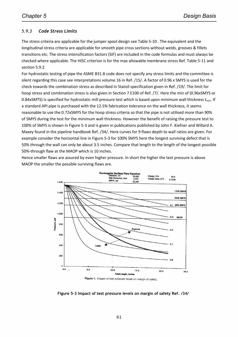
Chapter 5 Design Basis
61
5.9.3 Code Stress Limits
The stress criteria are applicable for the jumper spool design see Table 5-10 . The equivalent and the
longitudinal stress criteria are applicable for smooth pipe cross sections without welds, grooves & fillets
transitions etc. The stress intensification factors (SIF) are included in the code formulas and must always be
checked where applicable. The HISC criterion is for the max allowable membrane stress Ref. Table 5-11 and
section 5.9.2
For hydrostatic testing of pipe the ASME B31.8 code does not specify any stress limits and the committee is
silent regarding this case see interpretations volume 16 in Ref. /15/. A factor of 0.96 x SMYS is used for the
check towards the combination stress as described in Statoil specification given in Ref. /19/. The limit for
hoop stress and combination stress is also given in Section 7 E100 of Ref. /7/. Here the min of (0.96xSMYS or
0.84xSMTS) is specified for hydrostatic mill pressure test which is based upon minimum wall thickness tmin. If
a standard API pipe is purchased with the 12.5% fabrication tolerance on the wall thickness, it seems
reasonable to use the 0.72xSMYS for the hoop stress criteria so that the pipe is not utilised more than 90%
of SMYS during the test for the minimum wall thickness. However the benefit of raising the pressure test to
100% of SMYS is shown in Figure 5-3 and is given in publications published by John F. Kiefner and Willard A.
Maxey found in the pipeline handbook Ref. /34/. Here curves for 9 flaws depth to wall ratios are given. For
example consider the horizontal line in Figure 5-3 for 100% SMYS here the longest surviving defect that is
50% through the wall can only be about 3.5 inches. Compare that length to the length of the longest possible
50%-through flaw at the MAOP which is 10 inches.
Hence smaller flaws are assured by even higher pressure. In short the higher the test pressure is above
MAOP the smaller the possible surviving flaws are.
Figure 5-3 Impact of test pressure levels on margin of safety Ref. /34/
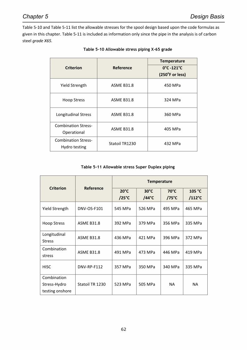
Chapter 5 Design Basis
62
Table 5-10 and Table 5-11 list the allowable stresses for the spool design based upon the code formulas as
given in this chapter. Table 5-11 is included as information only since the pipe in the analysis is of carbon
steel grade X65.
Table 5-10 Allowable stress piping X-65 grade
Criterion Reference
Temperature
0°C -121°C
(250oF or less)
Yield Strength ASME B31.8 450 MPa
Hoop Stress ASME B31.8 324 MPa
Longitudinal Stress ASME B31.8 360 MPa
Combination Stress-
Operational ASME B31.8 405 MPa
Combination Stress-
Hydro testing Statoil TR1230 432 MPa
Table 5-11 Allowable stress Super Duplex piping
Criterion Reference
Temperature
20°C
/25°C
30°C
/44°C
70°C
/75°C
105 °C
/112°C
Yield Strength DNV-OS-F101 545 MPa 526 MPa 495 MPa 465 MPa
Hoop Stress ASME B31.8 392 MPa 379 MPa 356 MPa 335 MPa
Longitudinal
Stress ASME B31.8 436 MPa 421 MPa 396 MPa 372 MPa
Combination
stress ASME B31.8 491 MPa 473 MPa 446 MPa 419 MPa
HISC DNV-RP-F112 357 MPa 350 MPa 340 MPa 335 MPa
Combination
Stress-Hydro
testing onshore
Statoil TR 1230 523 MPa 505 MPa NA NA
Chapter 6 Spool Optimisation and Strength Verification
63
6. SPOOL OPTIMISATION AND STRENGTH VERIFICATION
6.1 Finite element program ANSYS
For study of subsea flow lines and tie-in spools the most utilized FEA software used today is the ANSYS
software package. The ANSYS software package is a large tool with many capabilities. The program offers
many functions and can be used for many areas spanning from structural /mechanical fluid problems to
advanced areas within physics. Readers can visit the ANSYS Website for a comprehensive description of each
analysis packages
Some of the main products are:
Structural analysis:
ANSYS- Multiphysics
(Includes all of finite element disciplines)
ANSYS Mechanical
ANSYS Structural
ANSYS Professional
ANSYS DesignSpace
ANSYS ACT
ANSYS Rigid Body Dynamics
ANSYS Composite PrepPost
ANSYS nCode DesignLife
Explicit Dynamics
ANSYS Explicit STR
ANSYS Autodyn
ANSYS LS-DYNA
In this thesis the ANSYS Structural version 15 is used. This version has the capability to handle linear and
non-linear analysis, buckling, contact and dynamic analysis problems. The package includes the ANSYS
Workbench and ANSYS APDL classic graphical user interface. Several add-ins is provided to the package such
as CAD interface with most of the common parametric design tools (Inventor, Solidworks, CATIA, Pro
engineer etc.) in addition to the ANSYS Design modeller.
ANSYS has a large library of different element types with a variety of boundary conditions, material properties, and other relevant data. The user can determine to utilise the powerful APDL programming language and make scripts similar to what students learn by using the software CALFEM in finite elements topics. The APDL Programming language takes time to learn and to programme the input script, and has to some degree the disadvantages of being a source of programming error due a large number of options that has to be carefully checked towards the ANSYS documentation or other software. The benefit of APDL is that it is quick to change parameters, especially for simple beam and shell constructions and also to perform large numerous load combinations in one analysis run. That is also why most of the pipeline engineering is conducted with this type of programming. A simulation of a long pipeline uses contact elements and pipe elements typically CONTA175, PIPE288 PIPE289 (for Version 15 or higher). Figure 6-1 shows the vertical spool modelled in ANSYS Classic.
Fluid dynamics:
ANSYS Fluent
ANSYS CFX
ANSYS CFD
ANSYS CFD-Flo
ANSYS CFD Professional
FLUENT for CATIA V5
ANSYS CFD-Post
ANSYS Icepak
ANSYS Polyflow
ANSYS Vista TF
ANSYS BladeModeler
ANSYS TurboGrid
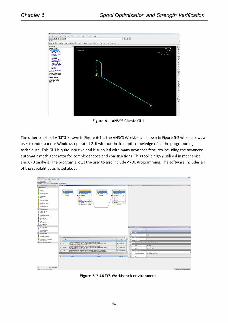
Chapter 6 Spool Optimisation and Strength Verification
64
Figure 6-1 ANSYS Classic GUI
The other cousin of ANSYS shown in Figure 6-1 is the ANSYS Workbench shown in Figure 6-2 which allows a
user to enter a more Windows operated GUI without the in depth knowledge of all the programming
techniques. This GUI is quite Intuitive and is supplied with many advanced features including the advanced
automatic mesh generator for complex shapes and constructions. This tool is highly utilised in mechanical
and CFD analysis. The program allows the user to also include APDL Programming. The software includes all
of the capabilities as listed above.
Figure 6-2 ANSYS Workbench environment
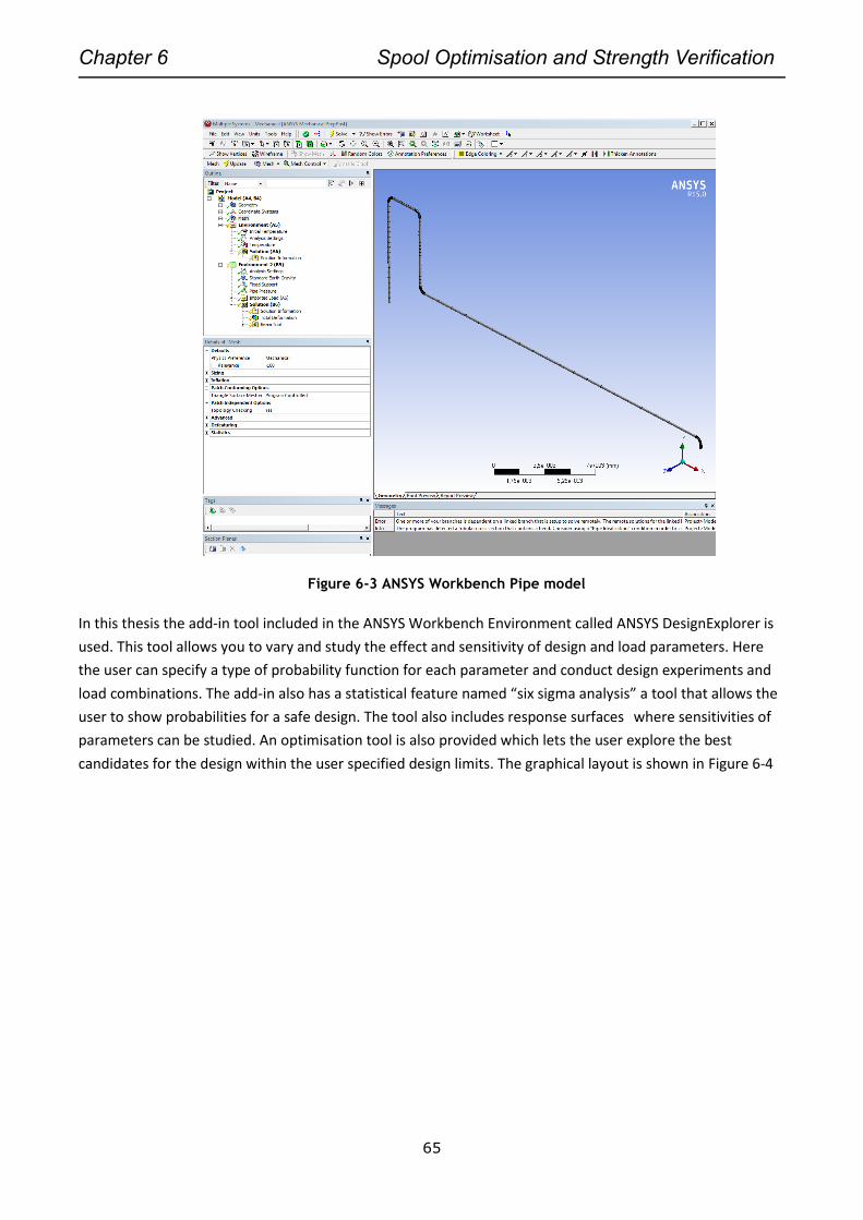
Chapter 6 Spool Optimisation and Strength Verification
65
Figure 6-3 ANSYS Workbench Pipe model
In this thesis the add-in tool included in the ANSYS Workbench Environment called ANSYS DesignExplorer is
used. This tool allows you to vary and study the effect and sensitivity of design and load parameters. Here
the user can specify a type of probability function for each parameter and conduct design experiments and
load combinations. The add-in also has a statistical feature named “six sigma analysis” a tool that allows the
user to show probabilities for a safe design. The tool also includes response surfaces where sensitivities of
parameters can be studied. An optimisation tool is also provided which lets the user explore the best
candidates for the design within the user specified design limits. The graphical layout is shown in Figure 6-4
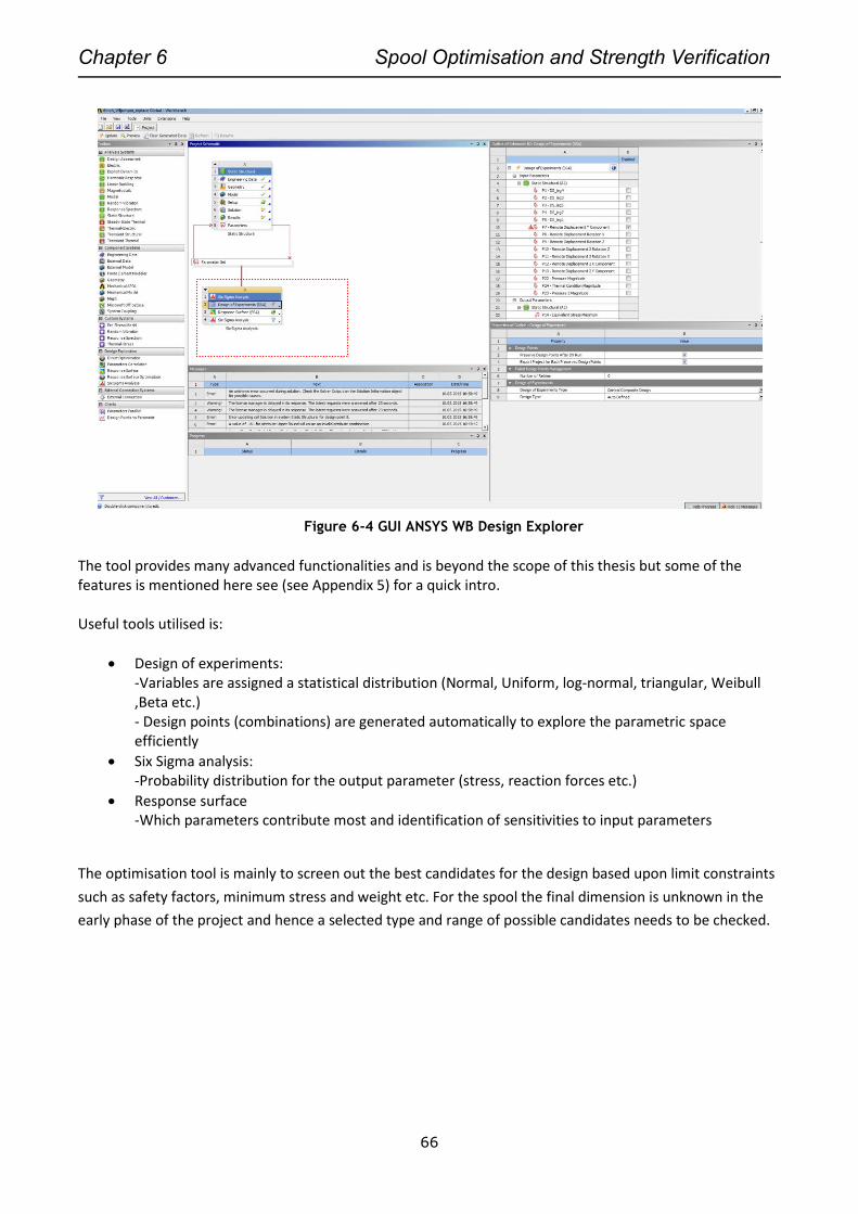
Chapter 6 Spool Optimisation and Strength Verification
66
Figure 6-4 GUI ANSYS WB Design Explorer
The tool provides many advanced functionalities and is beyond the scope of this thesis but some of the features is mentioned here see (see Appendix 5) for a quick intro. Useful tools utilised is:
Design of experiments: -Variables are assigned a statistical distribution (Normal, Uniform, log-normal, triangular, Weibull ,Beta etc.) - Design points (combinations) are generated automatically to explore the parametric space efficiently
Six Sigma analysis: -Probability distribution for the output parameter (stress, reaction forces etc.)
Response surface -Which parameters contribute most and identification of sensitivities to input parameters
The optimisation tool is mainly to screen out the best candidates for the design based upon limit constraints
such as safety factors, minimum stress and weight etc. For the spool the final dimension is unknown in the
early phase of the project and hence a selected type and range of possible candidates needs to be checked.
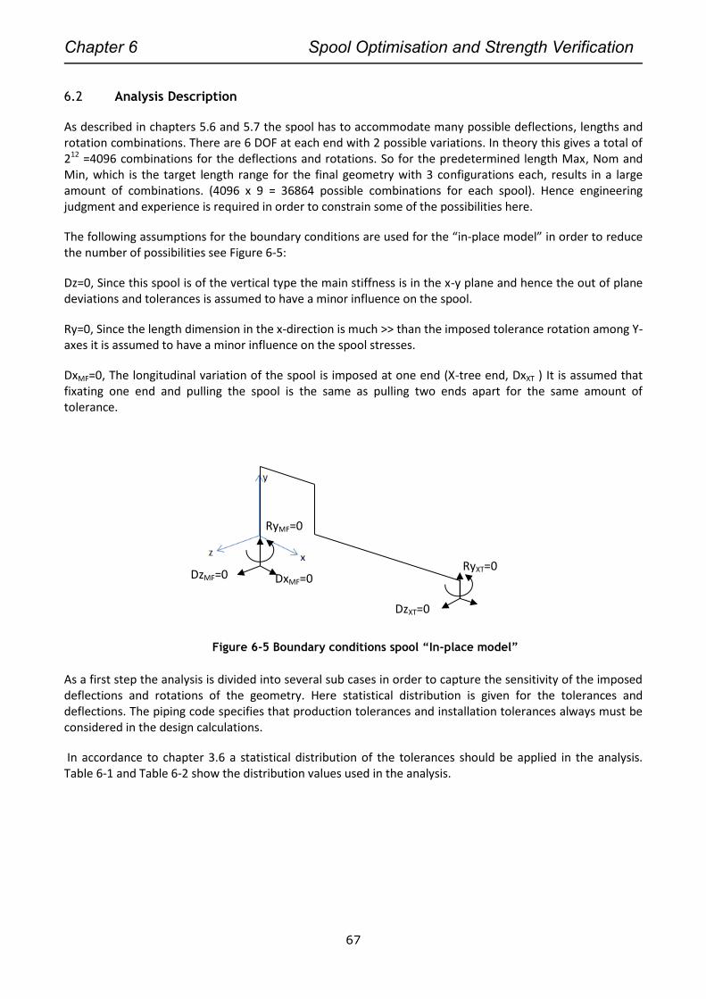
Chapter 6 Spool Optimisation and Strength Verification
67
6.2 Analysis Description
As described in chapters 5.6 and 5.7 the spool has to accommodate many possible deflections, lengths and rotation combinations. There are 6 DOF at each end with 2 possible variations. In theory this gives a total of 212 =4096 combinations for the deflections and rotations. So for the predetermined length Max, Nom and Min, which is the target length range for the final geometry with 3 configurations each, results in a large amount of combinations. (4096 x 9 = 36864 possible combinations for each spool). Hence engineering judgment and experience is required in order to constrain some of the possibilities here.
The following assumptions for the boundary conditions are used for the “in-place model” in order to reduce the number of possibilities see Figure 6-5:
Dz=0, Since this spool is of the vertical type the main stiffness is in the x-y plane and hence the out of plane deviations and tolerances is assumed to have a minor influence on the spool.
Ry=0, Since the length dimension in the x-direction is much >> than the imposed tolerance rotation among Y-axes it is assumed to have a minor influence on the spool stresses.
DxMF=0, The longitudinal variation of the spool is imposed at one end (X-tree end, DxXT ) It is assumed that fixating one end and pulling the spool is the same as pulling two ends apart for the same amount of tolerance.
Figure 6-5 Boundary conditions spool “In-place model”
As a first step the analysis is divided into several sub cases in order to capture the sensitivity of the imposed deflections and rotations of the geometry. Here statistical distribution is given for the tolerances and deflections. The piping code specifies that production tolerances and installation tolerances always must be considered in the design calculations.
In accordance to chapter 3.6 a statistical distribution of the tolerances should be applied in the analysis. Table 6-1 and Table 6-2 show the distribution values used in the analysis.
DxMF=0 DzMF=0
RyMF=0
RyXT=0
DzXT=0
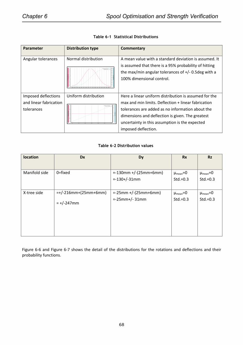
Chapter 6 Spool Optimisation and Strength Verification
68
Table 6-1 Statistical Distributions
Parameter Distribution type Commentary
Angular tolerances Normal distribution
A mean value with a standard deviation is assumed. It
is assumed that there is a 95% probability of hitting
the max/min angular tolerances of +/- 0.5deg with a
100% dimensional control.
Imposed deflections
and linear fabrication
tolerances
Uniform distribution
Here a linear uniform distribution is assumed for the
max and min limits. Deflection + linear fabrication
tolerances are added as no information about the
dimensions and deflection is given. The greatest
uncertainty in this assumption is the expected
imposed deflection.
Table 6-2 Distribution values
location Dx Dy Rx Rz
Manifold side 0=fixed =-130mm +/-(25mm+6mm)
=-130+/-31mm
µmean=0
Std.=0.3
µmean=0
Std.=0.3
X-tree side =+/-216mm+(25mm+6mm)
= +/-247mm
=-25mm +/-(25mm+6mm)
=-25mm+/- 31mm
µmean=0
Std.=0.3
µmean=0
Std.=0.3
Figure 6-6 and Figure 6-7 shows the detail of the distributions for the rotations and deflections and their probability functions.
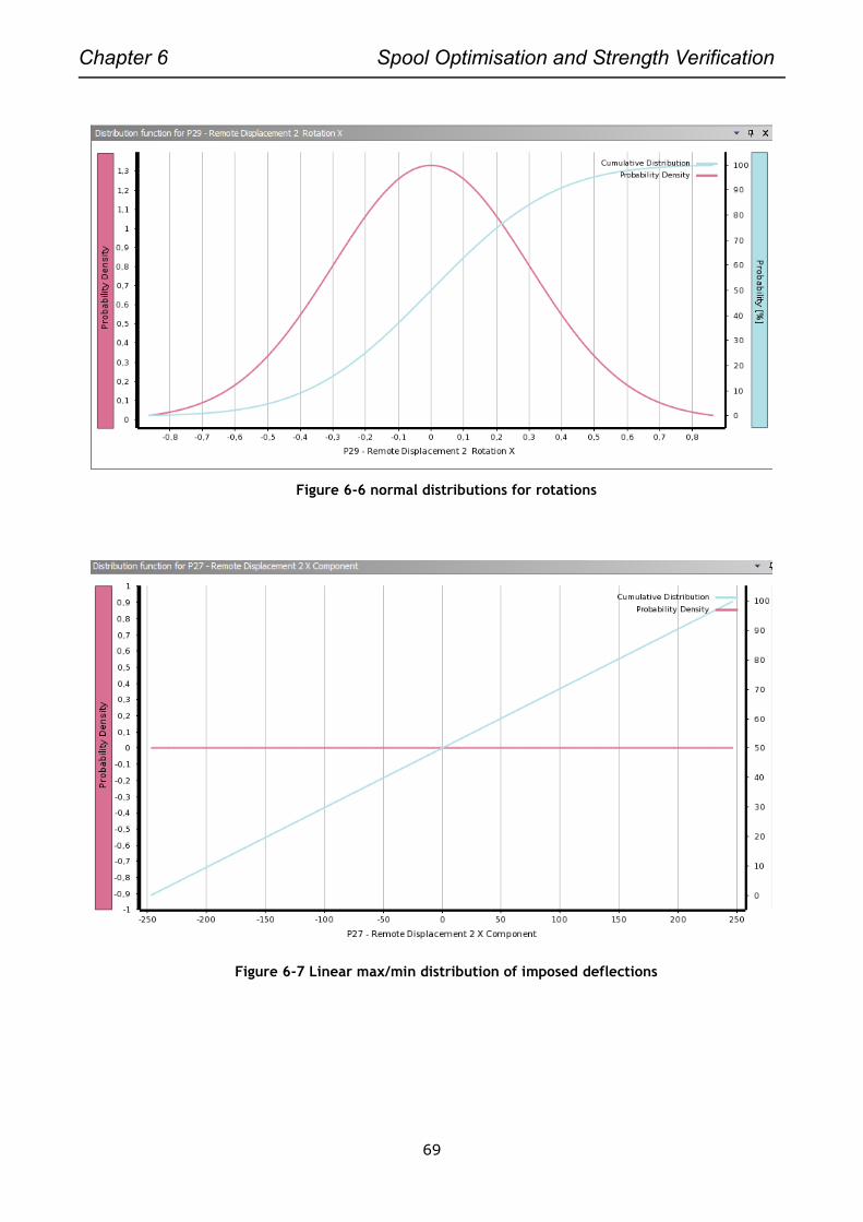
Chapter 6 Spool Optimisation and Strength Verification
69
Figure 6-6 normal distributions for rotations
Figure 6-7 Linear max/min distribution of imposed deflections
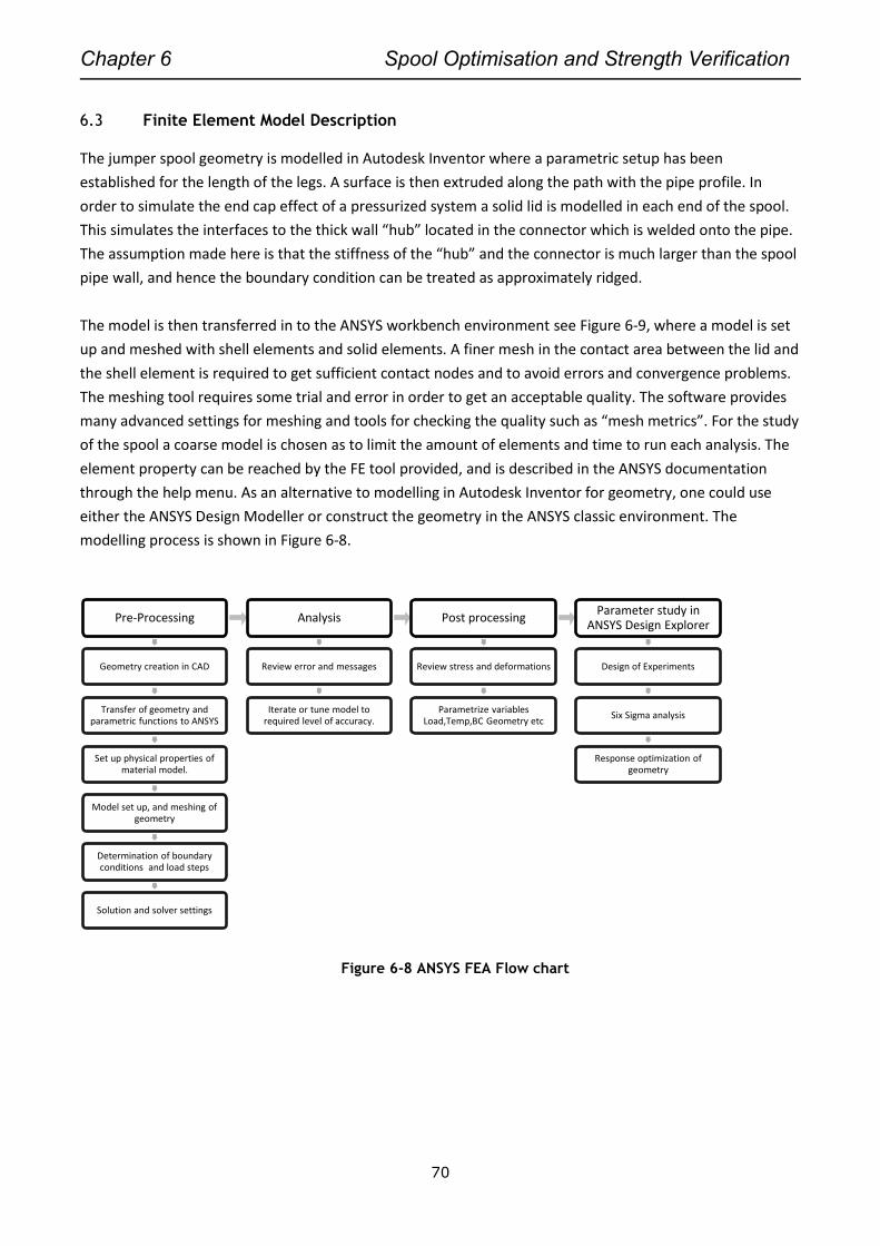
Chapter 6 Spool Optimisation and Strength Verification
70
6.3 Finite Element Model Description
The jumper spool geometry is modelled in Autodesk Inventor where a parametric setup has been
established for the length of the legs. A surface is then extruded along the path with the pipe profile. In
order to simulate the end cap effect of a pressurized system a solid lid is modelled in each end of the spool.
This simulates the interfaces to the thick wall “hub” located in the connector which is welded onto the pipe.
The assumption made here is that the stiffness of the “hub” and the connector is much larger than the spool
pipe wall, and hence the boundary condition can be treated as approximately ridged.
The model is then transferred in to the ANSYS workbench environment see Figure 6-9, where a model is set
up and meshed with shell elements and solid elements. A finer mesh in the contact area between the lid and
the shell element is required to get sufficient contact nodes and to avoid errors and convergence problems.
The meshing tool requires some trial and error in order to get an acceptable quality. The software provides
many advanced settings for meshing and tools for checking the quality such as “mesh metrics”. For the study
of the spool a coarse model is chosen as to limit the amount of elements and time to run each analysis. The
element property can be reached by the FE tool provided, and is described in the ANSYS documentation
through the help menu. As an alternative to modelling in Autodesk Inventor for geometry, one could use
either the ANSYS Design Modeller or construct the geometry in the ANSYS classic environment. The
modelling process is shown in Figure 6-8.
Figure 6-8 ANSYS FEA Flow chart
Pre-Processing
Geometry creation in CAD
Transfer of geometry and parametric functions to ANSYS
Set up physical properties of material model.
Model set up, and meshing of geometry
Determination of boundary conditions and load steps
Solution and solver settings
Analysis
Review error and messages
Iterate or tune model to required level of accuracy.
Post processing
Review stress and deformations
Parametrize variables Load,Temp,BC Geometry etc
Parameter study in ANSYS Design Explorer
Design of Experiments
Six Sigma analysis
Response optimization of geometry
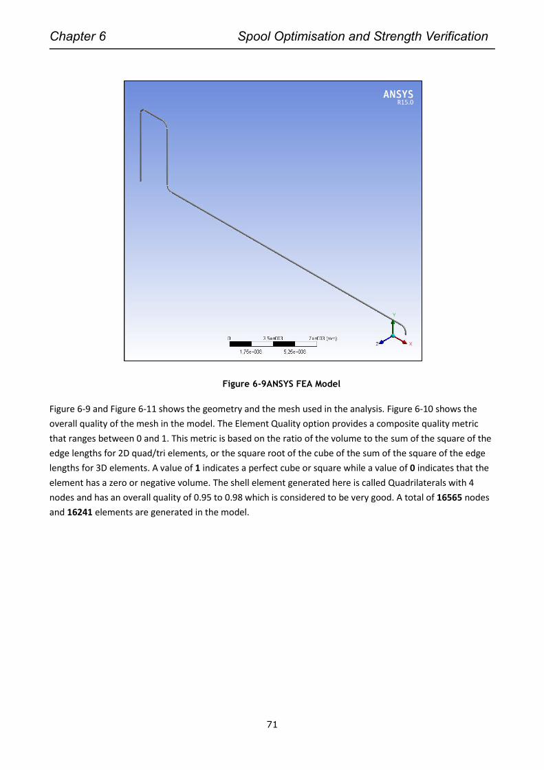
Chapter 6 Spool Optimisation and Strength Verification
71
Figure 6-9ANSYS FEA Model
Figure 6-9 and Figure 6-11 shows the geometry and the mesh used in the analysis. Figure 6-10 shows the
overall quality of the mesh in the model. The Element Quality option provides a composite quality metric
that ranges between 0 and 1. This metric is based on the ratio of the volume to the sum of the square of the
edge lengths for 2D quad/tri elements, or the square root of the cube of the sum of the square of the edge
lengths for 3D elements. A value of 1 indicates a perfect cube or square while a value of 0 indicates that the
element has a zero or negative volume. The shell element generated here is called Quadrilaterals with 4
nodes and has an overall quality of 0.95 to 0.98 which is considered to be very good. A total of 16565 nodes
and 16241 elements are generated in the model.
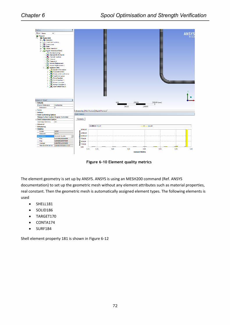
Chapter 6 Spool Optimisation and Strength Verification
72
Figure 6-10 Element quality metrics
The element geometry is set up by ANSYS. ANSYS is using an MESH200 command (Ref. ANSYS
documentation) to set up the geometric mesh without any element attributes such as material properties,
real constant. Then the geometric mesh is automatically assigned element types. The following elements is
used
SHELL181
SOLID186
TARGET170
CONTA174
SURF184
Shell element property 181 is shown in Figure 6-12
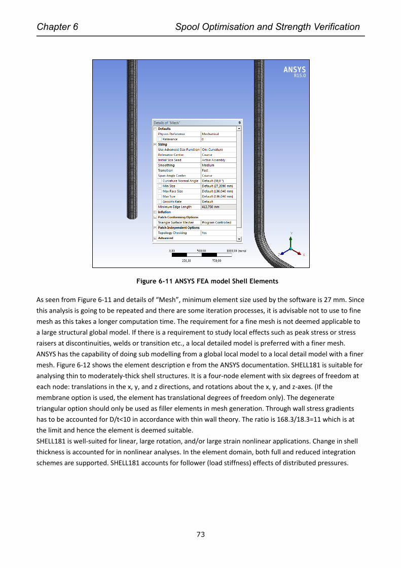
Chapter 6 Spool Optimisation and Strength Verification
73
Figure 6-11 ANSYS FEA model Shell Elements
As seen from Figure 6-11 and details of “Mesh”, minimum element size used by the software is 27 mm. Since
this analysis is going to be repeated and there are some iteration processes, it is advisable not to use to fine
mesh as this takes a longer computation time. The requirement for a fine mesh is not deemed applicable to
a large structural global model. If there is a requirement to study local effects such as peak stress or stress
raisers at discontinuities, welds or transition etc., a local detailed model is preferred with a finer mesh.
ANSYS has the capability of doing sub modelling from a global local model to a local detail model with a finer
mesh. Figure 6-12 shows the element description e from the ANSYS documentation. SHELL181 is suitable for
analysing thin to moderately-thick shell structures. It is a four-node element with six degrees of freedom at
each node: translations in the x, y, and z directions, and rotations about the x, y, and z-axes. (If the
membrane option is used, the element has translational degrees of freedom only). The degenerate
triangular option should only be used as filler elements in mesh generation. Through wall stress gradients
has to be accounted for D/t<10 in accordance with thin wall theory. The ratio is 168.3/18.3=11 which is at
the limit and hence the element is deemed suitable.
SHELL181 is well-suited for linear, large rotation, and/or large strain nonlinear applications. Change in shell
thickness is accounted for in nonlinear analyses. In the element domain, both full and reduced integration
schemes are supported. SHELL181 accounts for follower (load stiffness) effects of distributed pressures.
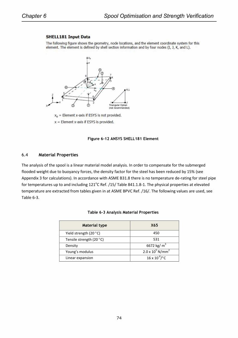
Chapter 6 Spool Optimisation and Strength Verification
74
Figure 6-12 ANSYS SHELL181 Element
6.4 Material Properties
The analysis of the spool is a linear material model analysis. In order to compensate for the submerged
flooded weight due to buoyancy forces, the density factor for the steel has been reduced by 15% (see
Appendix 3 for calculations). In accordance with ASME B31.8 there is no temperature de-rating for steel pipe
for temperatures up to and including 121oC Ref. /15/ Table 841.1.8-1. The physical properties at elevated
temperature are extracted from tables given in at ASME BPVC Ref. /16/. The following values are used, see
Table 6-3.
Table 6-3 Analysis Material Properties
Material type X65
Yield strength (20 C) 450
Tensile strength (20 C) 531
Density 6672 kg/ m3
Young’s modulus 2.0 x 10⁵ N/mm
2
Linear expansion 16 x 10-6
/C
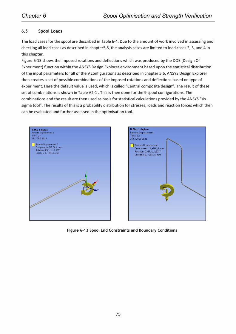
Chapter 6 Spool Optimisation and Strength Verification
75
6.5 Spool Loads
The load cases for the spool are described in Table 6-4. Due to the amount of work involved in assessing and
checking all load cases as described in chapter5.8, the analysis cases are limited to load cases 2, 3, and 4 in
this chapter.
Figure 6-13 shows the imposed rotations and deflections which was produced by the DOE (Design Of
Experiment) function within the ANSYS Design Explorer environment based upon the statistical distribution
of the input parameters for all of the 9 configurations as described in chapter 5.6. ANSYS Design Explorer
then creates a set of possible combinations of the imposed rotations and deflections based on type of
experiment. Here the default value is used, which is called “Central composite design”. The result of these
set of combinations is shown in Table A2-1 . This is then done for the 9 spool configurations. The
combinations and the result are then used as basis for statistical calculations provided by the ANSYS “six
sigma tool”. The results of this is a probability distribution for stresses, loads and reaction forces which then
can be evaluated and further assessed in the optimisation tool.
Figure 6-13 Spool End Constraints and Boundary Conditions

Chapter 6 Spool Optimisation and Strength Verification
76
Table 6-4 Load description for jumper spool
Load case Load Description Description
1 Connection
The clamp connectors are closed. This will force the pipe hub
ends into position and close the two hubs together and seal.
Hence many possible combinations of angular and linear
tolerances from fabrication, metrology and height difference
from settlements can occur. Drag loads from current is applied
2 Subsea System
Pressure Test
The subsea pressure test is simulated by applying the test
pressure and the pipeline expansion. According to the subsea
test pressure defined in Sec. A847.2 in ASME B31.8, the installed
pipeline system shall be hydrostatically tested to at least 1.25
times the maximum allowable operating pressure. A value of
1.25 x DP is applied. Drag loads from current is applied. BOP is
inactive and no deflections from XT is applied
3 Operation
The operational pressure, temperature and pipeline expansion is
simulated. The settlements, XT-deflections and the linear
fabrication and metrology tolerances are applied as deflections
at the jumper end nodes. Drag loads from current is applied
4 Seal replacement
Temperature and pressure is removed, and then the seal is
replaced by un-clamping one of the hubs end. The jumper end is
stroked 500mm in vertical direction. Drag loads from current is
applied
5 Slugging Slug loads can occur from production wells. This is not
considered applicable for water injection spools.
6 VIV
VIV effect and fatigue assessment is checked in accordance with
Ref./25/
The operational loadcase for the spool analysis is shown in Figure 6-14.
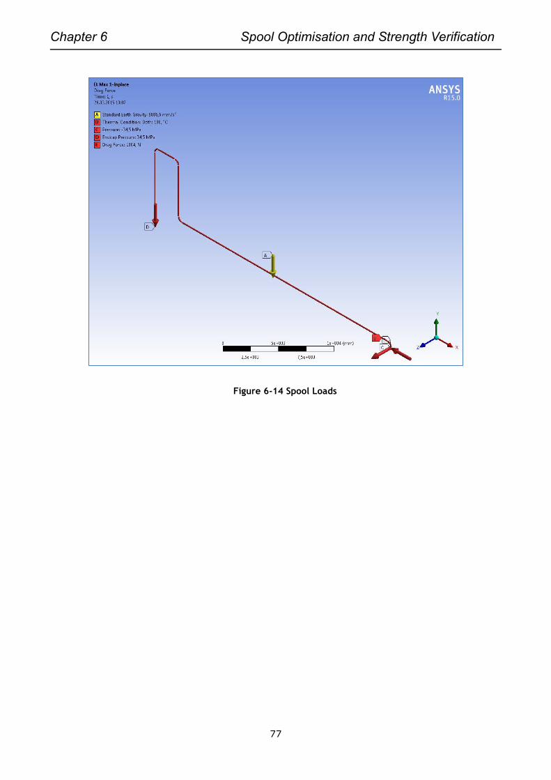
Chapter 6 Spool Optimisation and Strength Verification
77
Figure 6-14 Spool Loads
Chapter 6 Spool Optimisation and Strength Verification
78
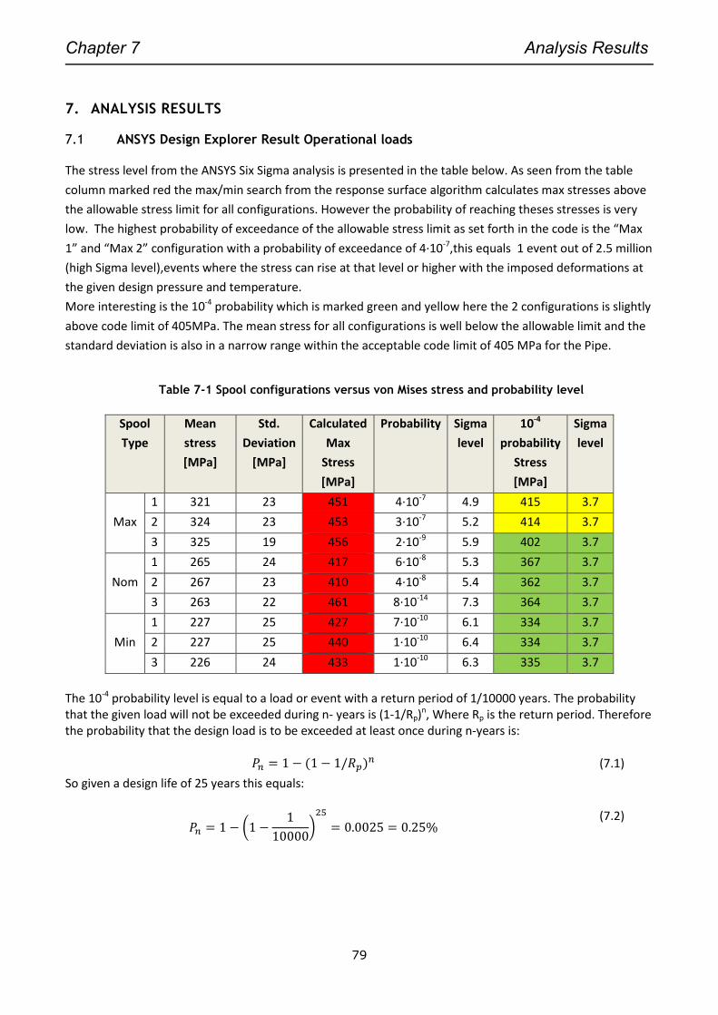
Chapter 7 Analysis Results
79
7. ANALYSIS RESULTS
7.1 ANSYS Design Explorer Result Operational loads
The stress level from the ANSYS Six Sigma analysis is presented in the table below. As seen from the table
column marked red the max/min search from the response surface algorithm calculates max stresses above
the allowable stress limit for all configurations. However the probability of reaching theses stresses is very
low. The highest probability of exceedance of the allowable stress limit as set forth in the code is the “Max
1” and “Max 2” configuration with a probability of exceedance of 4·10-7,this equals 1 event out of 2.5 million
(high Sigma level),events where the stress can rise at that level or higher with the imposed deformations at
the given design pressure and temperature.
More interesting is the 10-4 probability which is marked green and yellow here the 2 configurations is slightly
above code limit of 405MPa. The mean stress for all configurations is well below the allowable limit and the
standard deviation is also in a narrow range within the acceptable code limit of 405 MPa for the Pipe.
Table 7-1 Spool configurations versus von Mises stress and probability level
Spool
Type
Mean
stress
[MPa]
Std.
Deviation
[MPa]
Calculated
Max
Stress
[MPa]
Probability
Sigma
level
10-4
probability
Stress
[MPa]
Sigma
level
Max
1 321 23 451 4·10-7 4.9 415 3.7
2 324 23 453 3·10-7 5.2 414 3.7
3 325 19 456 2·10-9 5.9 402 3.7
Nom
1 265 24 417 6·10-8 5.3 367 3.7
2 267 23 410 4·10-8 5.4 362 3.7
3 263 22 461 8·10-14 7.3 364 3.7
Min
1 227 25 427 7·10-10 6.1 334 3.7
2 227 25 440 1·10-10 6.4 334 3.7
3 226 24 433 1·10-10 6.3 335 3.7
The 10-4 probability level is equal to a load or event with a return period of 1/10000 years. The probability that the given load will not be exceeded during n- years is (1-1/Rp)n, Where Rp is the return period. Therefore the probability that the design load is to be exceeded at least once during n-years is:
𝑃𝑛 = 1 − (1 − 1/𝑅𝑝)𝑛 (7.1)
So given a design life of 25 years this equals:
𝑃𝑛 = 1 − (1 −1
10000)25
= 0.0025 = 0.25% (7.2)
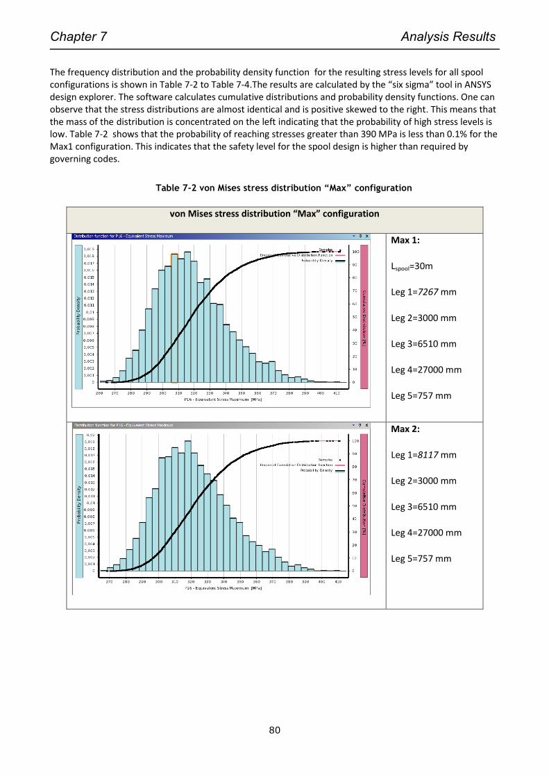
Chapter 7 Analysis Results
80
The frequency distribution and the probability density function for the resulting stress levels for all spool configurations is shown in Table 7-2 to Table 7-4.The results are calculated by the “six sigma” tool in ANSYS design explorer. The software calculates cumulative distributions and probability density functions. One can observe that the stress distributions are almost identical and is positive skewed to the right. This means that the mass of the distribution is concentrated on the left indicating that the probability of high stress levels is low. Table 7-2 shows that the probability of reaching stresses greater than 390 MPa is less than 0.1% for the Max1 configuration. This indicates that the safety level for the spool design is higher than required by governing codes.
Table 7-2 von Mises stress distribution “Max” configuration
von Mises stress distribution “Max” configuration
Max 1:
Lspool=30m
Leg 1=7267 mm
Leg 2=3000 mm
Leg 3=6510 mm
Leg 4=27000 mm
Leg 5=757 mm
Max 2:
Leg 1=8117 mm
Leg 2=3000 mm
Leg 3=6510 mm
Leg 4=27000 mm
Leg 5=757 mm
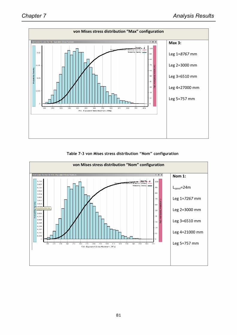
Chapter 7 Analysis Results
81
von Mises stress distribution “Max” configuration
Max 3:
Leg 1=8767 mm
Leg 2=3000 mm
Leg 3=6510 mm
Leg 4=27000 mm
Leg 5=757 mm
Table 7-3 von Mises stress distribution “Nom” configuration
von Mises stress distribution “Nom” configuration
Nom 1:
Lspool=24m
Leg 1=7267 mm
Leg 2=3000 mm
Leg 3=6510 mm
Leg 4=21000 mm
Leg 5=757 mm

Chapter 7 Analysis Results
82
von Mises stress distribution “Nom” configuration
Nom2:
Leg 1=8117 mm
Leg 2=3000 mm
Leg 3=6510 mm
Leg 4=21000 mm
Leg 5=757 mm
Nom3:
Leg 1=8767 mm
Leg 2=3000 mm
Leg 3=6510 mm
Leg 4=21000 mm
Leg 5=757 mm
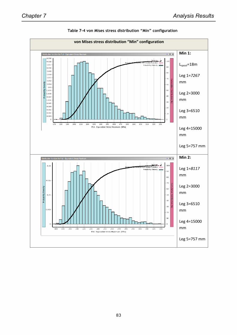
Chapter 7 Analysis Results
83
Table 7-4 von Mises stress distribution “Min” configuration
von Mises stress distribution “Min” configuration
Min 1:
Lspool=18m
Leg 1=7267
mm
Leg 2=3000
mm
Leg 3=6510
mm
Leg 4=15000
mm
Leg 5=757 mm
Min 2:
Leg 1=8117
mm
Leg 2=3000
mm
Leg 3=6510
mm
Leg 4=15000
mm
Leg 5=757 mm
Chapter 7 Analysis Results
84
von Mises stress distribution “Min” configuration
Min 3:
Leg 1=8767
mm
Leg 2=3000
mm
Leg 3=6510
mm
Leg 4=15000
mm
Leg 5=757 mm
7.2 Reaction Forces and Bending Moments
The maximum and minimum values for the reaction forces can be extracted by use of the max/min tool. The
values are shown in Figure 7-1 , Figure 7-2 and Figure 7-3 , the configurations are numbered from 1 to 9
representing 9 configurations (Max 1 to 3, Nom 1 to 3 and Min 1 to 3). Values for bending moments and
reaction forces can also be extracted by use of the “Six Sigma” probability table. Here the values can be
extracted from the Percentile-Quantile table for a specific parameter see Table 7-5 and Table 7-6 4-21 for
Max1 and Min3 configuration. The reaction forces are of interest for the installation process and to the loads
on the clamp connectors.
Figure 7-1 Max Reaction Forces (Abs values)
0,00E+00
2,00E+04
4,00E+04
6,00E+04
8,00E+04
1,00E+05
1,20E+05
1,40E+05
1,60E+05
0 2 4 6 8 10
Forc
e [
N]
Configuration No.
Max Reaction Forces
P37 FX_MF
P38 FY_MF
P39 FZ_MF
P40FX_XT
P41 FY_XT
P42 FZ_XT
Chapter 7 Analysis Results
85
Figure 7-2 Max Reaction Moments (Abs. values)
Figure 7-3 Max Reaction Moments MY and MX (Abs. values)
As seen from Figure 7-2 and Figure 7-3 , the governing bending moments is the MZ bending moments which
naturally increases with the length of the spool, (configuration Max). The other bending moments increases
when the spool becomes shorter; this is due to and increased overall structural stiffness for the spool. The
mean reaction force and moments are shown in Figure 7-4and Figure 7-5.
Table 7-5 Reaction Forces “Max 1”configuration 10-4 probability
Manifold Side
FY[kN] FX [kN] FZ [kN] MX [kNm] MY [kNm] MZ [kNm]
0,00E+00
2,00E+07
4,00E+07
6,00E+07
8,00E+07
1,00E+08
1,20E+08
0 2 4 6 8 10
Mo
me
nt
[Nm
m]
Configuration No.
Max Reaction Forces-Bending Moment
P43MX_MF
P44 MY_MF
P45 MZ_MF
P46 MX_XT
P47 MZ_XT
P48 MY_XT
0,00E+00
1,00E+06
2,00E+06
3,00E+06
4,00E+06
5,00E+06
6,00E+06
1 2 3 4 5 6 7 8 9
Mo
me
nt
[Nm
m]
Configuration No.
Max Reaction Forces-Bending Moment
P43 MX_MF
P48 MY_XT
P46 MX_XT
P44 MY_MF
Chapter 7 Analysis Results
86
35,9 -93 0,04 3,3 -0,4 87,8
X-tree Side
FY [kN] FX [kN] FZ [kN] MX [kNm] MY [kNm] MZ [kNm]
31,0 143 -0,04 -3,8 0,9 -51,0
Table 7-6 Reaction Forces “Min 3”configuration 10-4 probability
Manifold Side
FY[kN] FX [kN] FZ [kN] MX [kNm] MY [kNm] MZ [kNm]
33,9 91,8 0,023 5,0 1,1 68,6
X-tree Side
FY [kN] FX [kN] FZ [kN] MX [kNm] MY [kNm] MZ [kNm]
30,0 -94,0 -0,023 4,5 3,0 11,0
Chapter 7 Analysis Results
87
Figure 7-4 Mean reaction forces
Figure 7-5 Mean reaction bending moment
-30
-20
-10
0
10
20
30
40
0 2 4 6 8 10
Forc
e [
kN]
Configuration No.
Mean Reaction Forces
FX_MF
FY_MF
FZ_MF
FX_XT
FY_XT
FZ_XT
-0,02
0
0,02
0,04
0,06
0,08
0,1
0,12
-50
-40
-30
-20
-10
0
10
20
30
40
0 2 4 6 8 10
Mo
me
nts
MZ
[kN
m]
Configuration No.
Mean Reaction Bending Moments
MZ_MF
MZ_XT
MX_MF
MY_MF
MX_XT
MY_XT

Chapter 7 Analysis Results
88
7.3 Stress Response and Sensitivity
The sensitivity to stress increase imposed by the deformations is shown by the response plots in Figure 7-7
to Figure 7-10 for the “Max 1” configuration. One can observe how the response of stress is of a non-linear
character towards these imposed deflections and rotations. Hence a small increase of these values gives a
large stress increase.
It is important to remember that a response surface is a curve fit based on a set of data. If not enough design
points were solved or if the response surface algorithm is not appropriate then the response surface will not
be accurate. One can refine the response surface type to create a more accurate response surface based
upon more design points or type of curve fit algorithm. The technique used here is called the Kriging
algorithm see Figure 7-6. This is a multidimensional interpolation combining a polynomial model similar to
the one of the standard response surface, which provides a “global” model of the design space, plus local
deviations determined so that the Kriging model interpolates the DOE points. Output=f(inputs) + Z(inputs)
,where f is a second order polynomial (which dictates the “global” behavior of the model) and Z a
perturbation term (which dictates the “local” behavior of the model)
Since Kriging fits the response surface through all design points the “Goodness of fit metrics” will always be
good
Figure 7-6 Kriging Algorithm curve fit (Source ANSYS lectures)
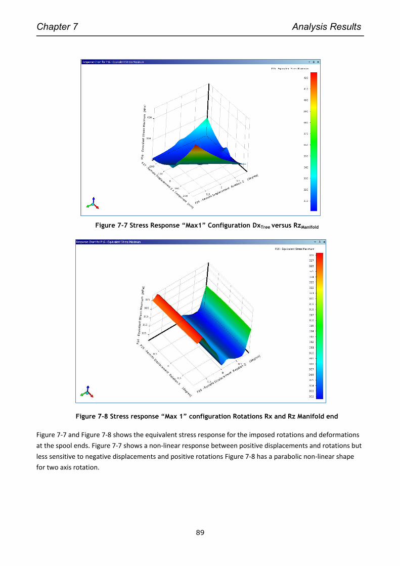
Chapter 7 Analysis Results
89
Figure 7-7 Stress Response “Max1” Configuration DxTree versus RzManifold
Figure 7-8 Stress response “Max 1” configuration Rotations Rx and Rz Manifold end
Figure 7-7 and Figure 7-8 shows the equivalent stress response for the imposed rotations and deformations
at the spool ends. Figure 7-7 shows a non-linear response between positive displacements and rotations but
less sensitive to negative displacements and positive rotations Figure 7-8 has a parabolic non-linear shape
for two axis rotation.
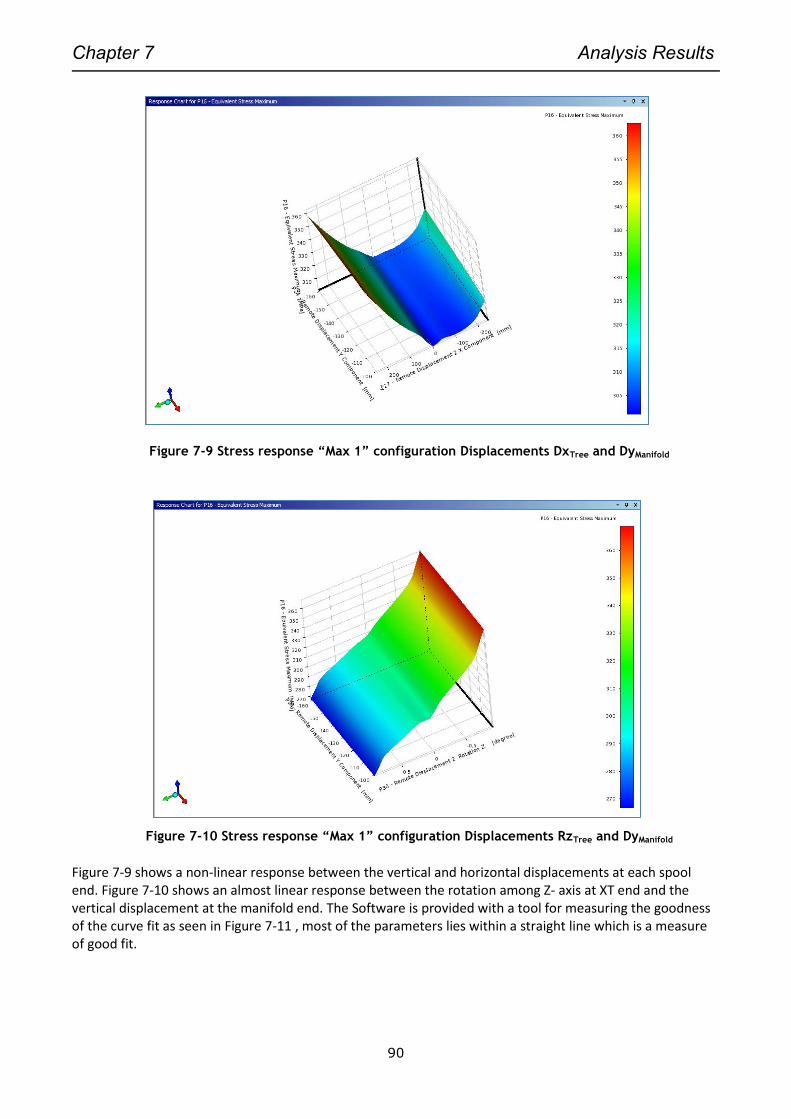
Chapter 7 Analysis Results
90
Figure 7-9 Stress response “Max 1” configuration Displacements DxTree and DyManifold
Figure 7-10 Stress response “Max 1” configuration Displacements RzTree and DyManifold
Figure 7-9 shows a non-linear response between the vertical and horizontal displacements at each spool end. Figure 7-10 shows an almost linear response between the rotation among Z- axis at XT end and the vertical displacement at the manifold end. The Software is provided with a tool for measuring the goodness of the curve fit as seen in Figure 7-11 , most of the parameters lies within a straight line which is a measure of good fit.
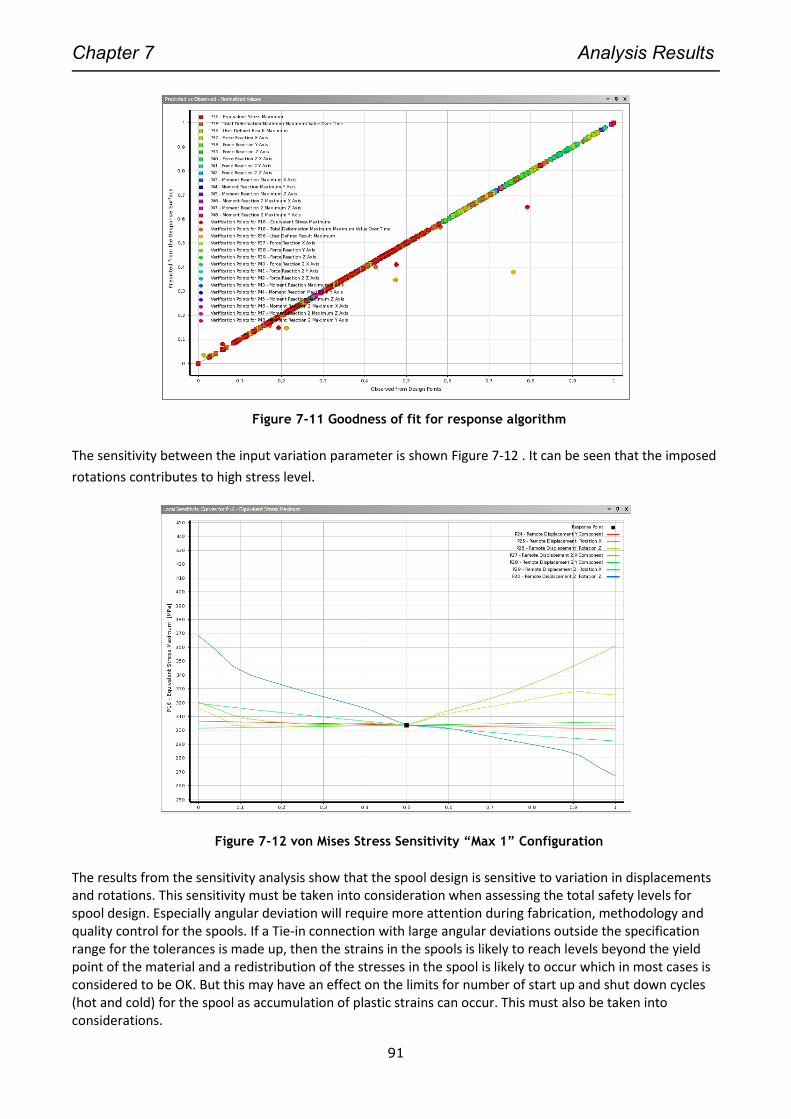
Chapter 7 Analysis Results
91
Figure 7-11 Goodness of fit for response algorithm
The sensitivity between the input variation parameter is shown Figure 7-12 . It can be seen that the imposed
rotations contributes to high stress level.
Figure 7-12 von Mises Stress Sensitivity “Max 1” Configuration
The results from the sensitivity analysis show that the spool design is sensitive to variation in displacements and rotations. This sensitivity must be taken into consideration when assessing the total safety levels for spool design. Especially angular deviation will require more attention during fabrication, methodology and quality control for the spools. If a Tie-in connection with large angular deviations outside the specification range for the tolerances is made up, then the strains in the spools is likely to reach levels beyond the yield point of the material and a redistribution of the stresses in the spool is likely to occur which in most cases is considered to be OK. But this may have an effect on the limits for number of start up and shut down cycles (hot and cold) for the spool as accumulation of plastic strains can occur. This must also be taken into considerations.

Chapter 7 Analysis Results
92
7.4 Optimal Spool Configuration
Table 7-7 shows a set of worst case rotations and displacements equivalent for 10-4 probability stress level
that has been checked with the response surface optimization tool. A value for stresses between 380MPa
and the design limit of 405 MPa, as given by the code was set as the target range. (A tolerance range for the
stress target was used in order to allow for computation for more possible geometrical candidates). The
software was also given a constraint to calculate candidates for geometrical shapes that would minimizing
the bending moments for the 30m long spool. The analysis shows that in order to be within the stress limit
for the 30meter long spool the geometry has to change to some of the candidates as suggested by the
software algorithm.
Table 7-7 Imposed spool end deformations (10-4 - Extremes)
Type Spool
length
[m]
DyMF
[mm]
RxMF
[Deg]
RZMF
[Deg]
DxXT
[mm]
DyXT
[mm]
RxXT
[Deg]
RzXT
[Deg]
Max 1 30 -160 0.9 0.9 248 -30 0.9 0.9
Figure 7-13 ANSYS Optimisation Results and candidates for “max 1” configuration
Figure 7-13 Show’s the possible candidates as calculated and verified by the optimisation tool. The output is
supplied with a samples chart, where each sample is displayed as a group of line curves where each point is
the value of one input or output parameter. This is useful to find custom candidates. The optimisation
method used is called MOGA or (Multi Objective Genetic Algorithm), which is an iterative multi objective
algorithm. Benefits of method are:
• Helps identify global and local minima
• Provides several candidates in different regions
• Accurate solution
• Can handle multiple goals
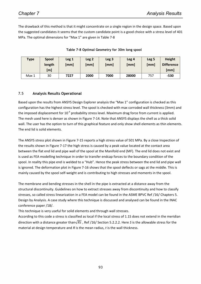
Chapter 7 Analysis Results
93
The drawback of this method is that it might concentrate on a single region in the design space. Based upon
the suggested candidates it seems that the custom candidate point is a good choice with a stress level of 401
MPa. The optimal dimensions for “Max 1” are given in Table 7-8
Table 7-8 Optimal Geometry for 30m long spool
Type Spool
length
[m]
Leg 1
[mm]
Leg 2
[mm]
Leg 3
[mm]
Leg 4
[mm]
Leg 5
[mm]
Height
Difference
[mm]
Max 1 30 7227 2000 7000 28000 757 -530
7.5 Analysis Results Operational
Based upon the results from ANSYS Design Explorer analysis the “Max 1” configuration is checked as this
configuration has the highest stress level. The spool is checked with max corroded wall thickness (3mm) and
the imposed displacement for 10-4 probability stress level. Maximum drag force from current is applied.
The mesh used here is denser as shown in Figure 7-14. Note that ANSYS displays the shell as a thick solid
wall. The user has the option to turn of this graphical feature and only show shell elements as thin elements.
The end lid is solid elements.
The ANSYS stress plot shown in Figure 7-15 reports a high stress value of 501 MPa. By a close Inspection of
the results shown in Figure 7-17 the high stress is caused by a peak value located at the contact area
between the flat end lid and pipe wall of the spool at the Manifold end (MF). The end lid does not exist and
is used as FEA modelling technique in order to transfer endcap forces to the boundary condition of the
spool. In reality this pipe end is welded to a “Hub”. Hence the peak stress between the end lid and pipe wall
is ignored. The deformation plot in Figure 7-16 shows that the spool deflects or sags at the middle. This is
mainly caused by the spool self-weight and is contributing to high stresses and moments in the spool.
The membrane and bending stresses in the shell in the pipe is extracted at a distance away from the
structural discontinuity. Guidelines on how to extract stresses away from discontinuity and how to classify
stresses, so called stress linearization in a FEA model can be found in the ASME BPVC Ref /16/ Chapters 5.
Design by Analysis. A case study where this technique is discussed and analysed can be found in the INAC
conference paper /18/.
This technique is very useful for solid elements and through wall stresses.
According to this code a stress is classified as local if the local stress of 1.1S does not extend in the meridian
direction with a distance greater than√𝑅𝑡 , Ref /16/ Section 5.2.2.2. Here S is the allowable stress for the
material at design temperature and R is the mean radius, t is the wall thickness.
Chapter 7 Analysis Results
94
Distance away from structural discontinuity can be assessed by use of equation (7.3) /18/.
𝑑 ≤ 2 ∙ √𝑅 ∙ 𝑡 (7.3)
This becomes:
𝑑 ≤ 2 ∙ √(0.5 ∙ (168.3 − 15.3)) ∙ 15.3 = 68𝑚𝑚 (7.4)
Region of local stress then becomes √𝑅𝑡 = 34𝑚𝑚
The average values from the shell element Top/Bottom, across the section at a distance d from discontinuity
is used for comparison towards the code stress limits see Figure 7-20.
Figure 7-14 Details of Mesh FE model
Chapter 7 Analysis Results
95
Figure 7-15 Max von Mises stress-operational
Figure 7-16 Total deformation spool
Chapter 7 Analysis Results
96
Figure 7-17 location of max peak stress operational at MF end
The stress utilisations (UF) towards the stress limits as described in chapter 5.9 is tabulated in Table 7-9. The ASME B31.8 code check is using formulas with bending moments, stress intensification factors (SIF) and then calculates the stresses based upon area and section modulus of the pipe. For comparison towards this limit the stresses tabulated in Table 7-9 is interpolated at cross sections by use of ANSYS surface tool.
Table 7-9 Max Spool Stresses -operational
Location Combined stress
SC (von Mises) [MPa]
Stress limit F3
[MPa]
UF Longitudinal stress SL
[MPa]
Stress limit F2
[MPa]
UF Ref.
Manifold end
313
405 0.77 364 360 1.01 Figure 7-19 Figure 7-20
Bend between leg2 /leg3
315 405 0.78 300 360 0.83 Figure 7-22 Figure 7-23
Table 7-10 Max Spool Reaction Forces -Operational
Manifold Side
FY[kN] FX [kN] FZ [kN] MX [kNm] MY [kNm] MZ [kNm]
18.3 33.7 -0.11 -3.8 1.6 64
X-tree Side
1.2 -38 0.8 -0,18 -4.6 -34
Chapter 7 Analysis Results
97
The code hoop stress criteria, is given by an analytical formula (5.1) and (5.2) , and is calculated in Appendix 3. Stress plots of longitudinal and von Mises stress are shown in Figure 7-18 to Figure 7-23.
Figure 7-18 Max von Mises stress operational at MF end
Figure 7-19 Cross sectional von Mises stress operational at MF end
Chapter 7 Analysis Results
98
Figure 7-20 Cross sectional max longitudinal stress in pipe operational at MF-end
Figure 7-21 Von Mises stress operational at intrados of bend
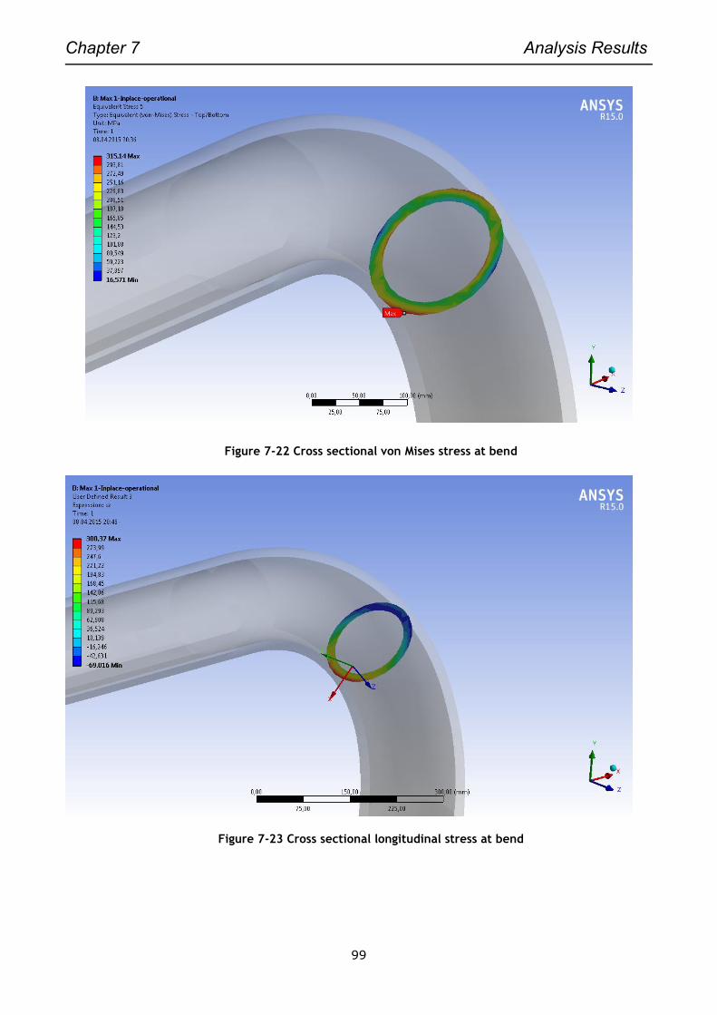
Chapter 7 Analysis Results
99
Figure 7-22 Cross sectional von Mises stress at bend
Figure 7-23 Cross sectional longitudinal stress at bend
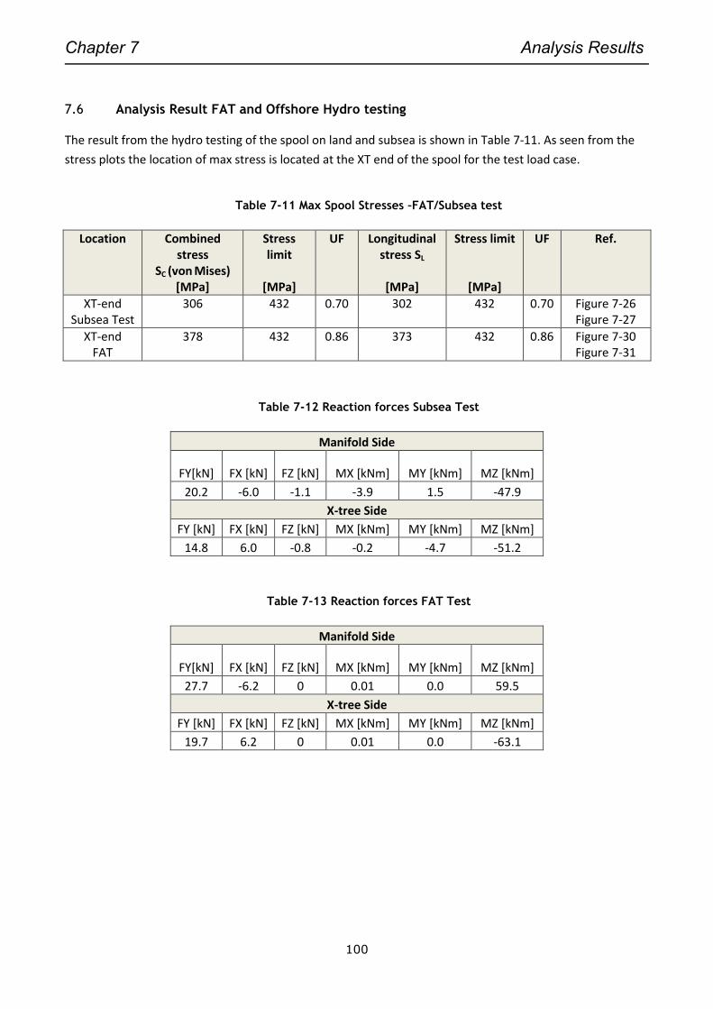
Chapter 7 Analysis Results
100
7.6 Analysis Result FAT and Offshore Hydro testing
The result from the hydro testing of the spool on land and subsea is shown in Table 7-11. As seen from the
stress plots the location of max stress is located at the XT end of the spool for the test load case.
Table 7-11 Max Spool Stresses –FAT/Subsea test
Location Combined stress
SC (von Mises) [MPa]
Stress limit
[MPa]
UF Longitudinal stress SL
[MPa]
Stress limit
[MPa]
UF Ref.
XT-end Subsea Test
306 432 0.70 302 432 0.70 Figure 7-26 Figure 7-27
XT-end FAT
378 432 0.86 373 432 0.86 Figure 7-30 Figure 7-31
Table 7-12 Reaction forces Subsea Test
Manifold Side
FY[kN] FX [kN] FZ [kN] MX [kNm] MY [kNm] MZ [kNm]
20.2 -6.0 -1.1 -3.9 1.5 -47.9
X-tree Side
FY [kN] FX [kN] FZ [kN] MX [kNm] MY [kNm] MZ [kNm]
14.8 6.0 -0.8 -0.2 -4.7 -51.2
Table 7-13 Reaction forces FAT Test
Manifold Side
FY[kN] FX [kN] FZ [kN] MX [kNm] MY [kNm] MZ [kNm]
27.7 -6.2 0 0.01 0.0 59.5
X-tree Side
FY [kN] FX [kN] FZ [kN] MX [kNm] MY [kNm] MZ [kNm]
19.7 6.2 0 0.01 0.0 -63.1

Chapter 7 Analysis Results
101
Figure 7-24 Max von Mises stress - Subsea Hydro Test
Figure 7-25 Max stress location- Subsea Hydro test
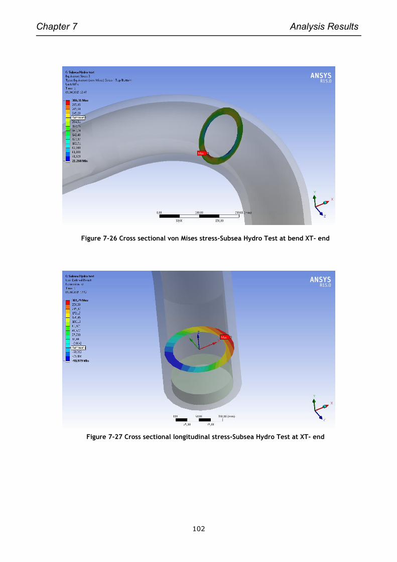
Chapter 7 Analysis Results
102
Figure 7-26 Cross sectional von Mises stress-Subsea Hydro Test at bend XT- end
Figure 7-27 Cross sectional longitudinal stress-Subsea Hydro Test at XT- end
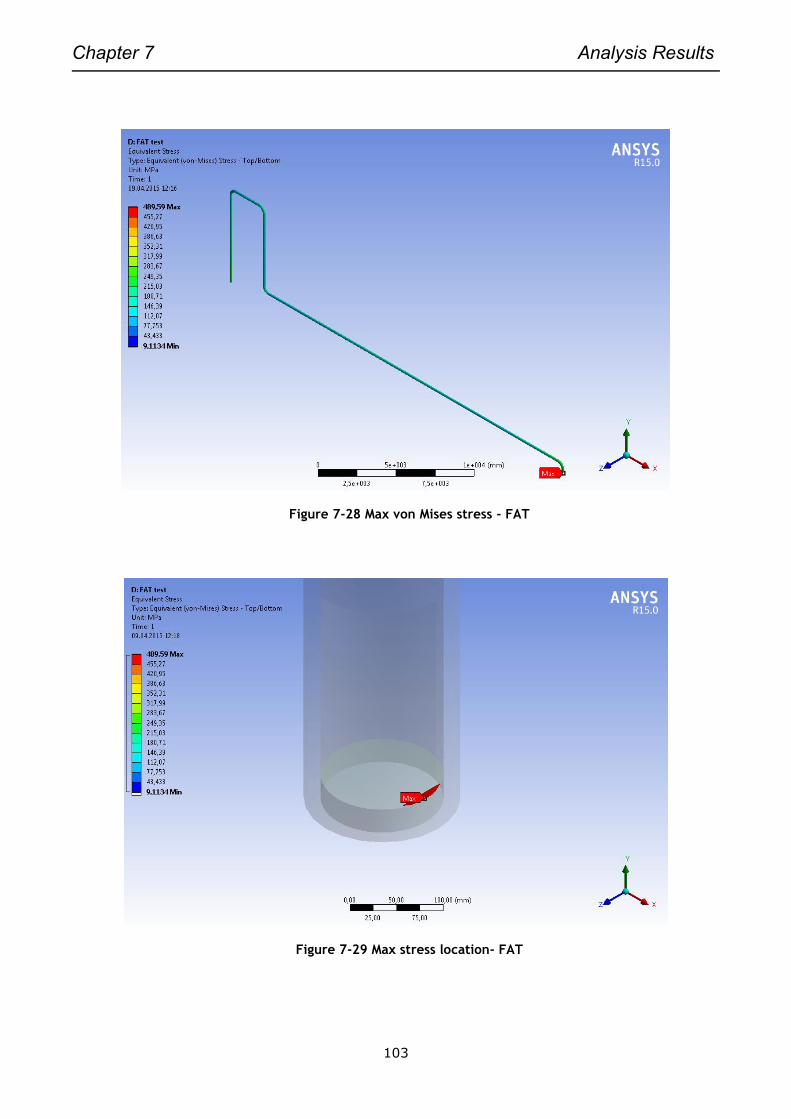
Chapter 7 Analysis Results
103
Figure 7-28 Max von Mises stress - FAT
Figure 7-29 Max stress location- FAT

Chapter 7 Analysis Results
104
Figure 7-30 Cross sectional longitudinal stress -FAT at XT- end
Figure 7-31 Cross sectional von Mises stress -FAT at bend XT- end
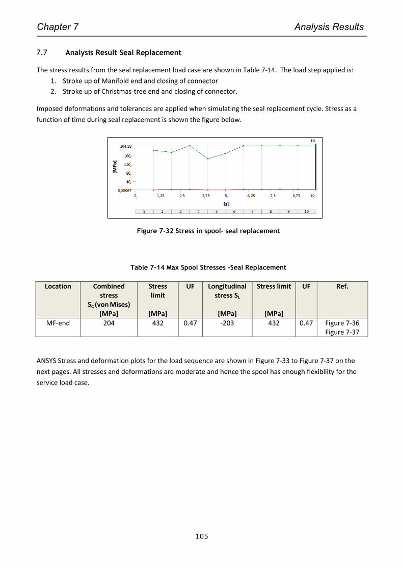
Chapter 7 Analysis Results
105
7.7 Analysis Result Seal Replacement
The stress results from the seal replacement load case are shown in Table 7-14. The load step applied is:
1. Stroke up of Manifold end and closing of connector
2. Stroke up of Christmas-tree end and closing of connector.
Imposed deformations and tolerances are applied when simulating the seal replacement cycle. Stress as a
function of time during seal replacement is shown the figure below.
Figure 7-32 Stress in spool- seal replacement
Table 7-14 Max Spool Stresses –Seal Replacement
Location Combined stress
SC (von Mises) [MPa]
Stress limit
[MPa]
UF Longitudinal stress SL
[MPa]
Stress limit
[MPa]
UF Ref.
MF-end
204 432 0.47 -203 432 0.47 Figure 7-36 Figure 7-37
ANSYS Stress and deformation plots for the load sequence are shown in Figure 7-33 to Figure 7-37 on the
next pages. All stresses and deformations are moderate and hence the spool has enough flexibility for the
service load case.
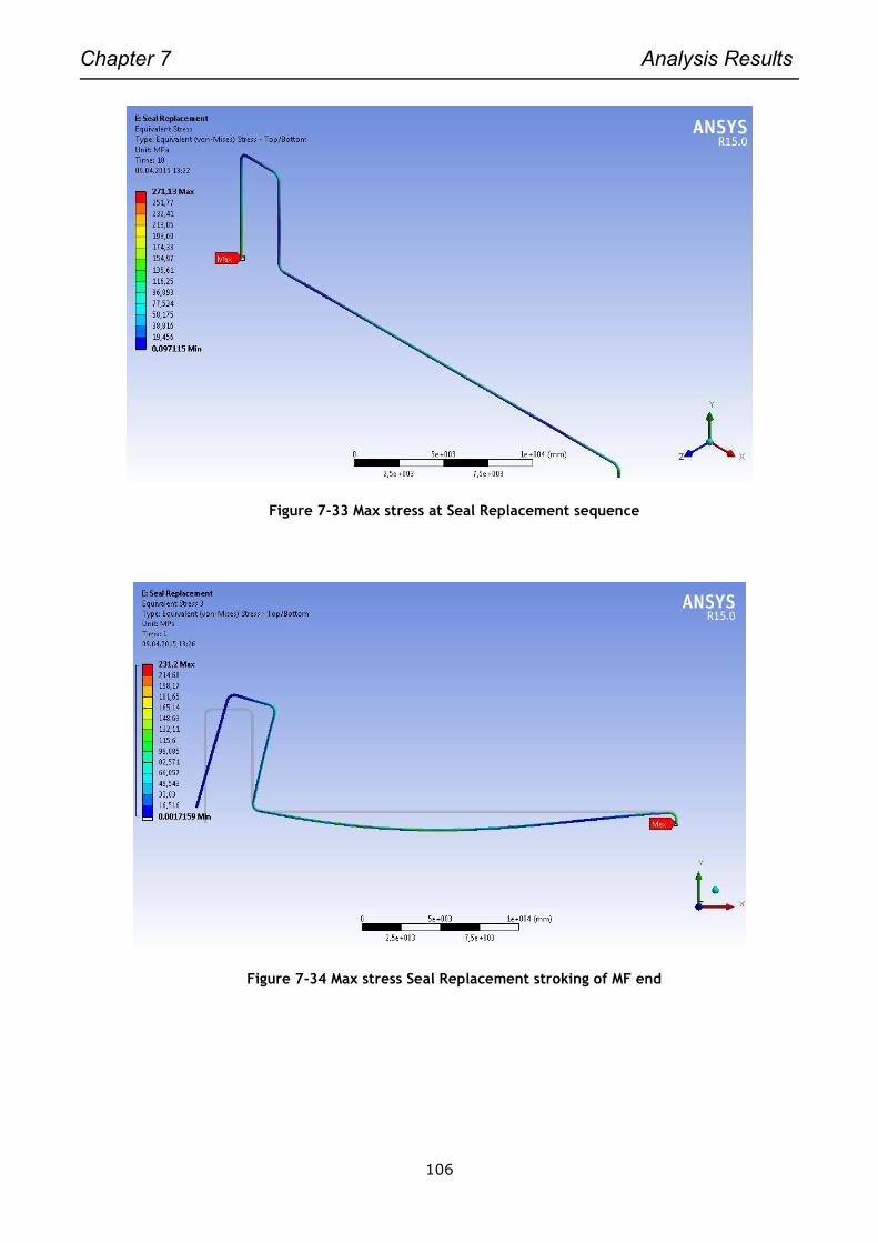
Chapter 7 Analysis Results
106
Figure 7-33 Max stress at Seal Replacement sequence
Figure 7-34 Max stress Seal Replacement stroking of MF end
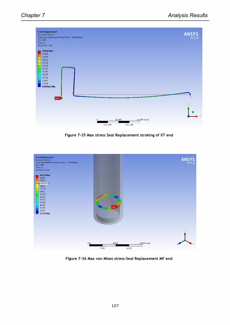
Chapter 7 Analysis Results
107
Figure 7-35 Max stress Seal Replacement stroking of XT end
Figure 7-36 Max von Mises stress-Seal Replacement MF end
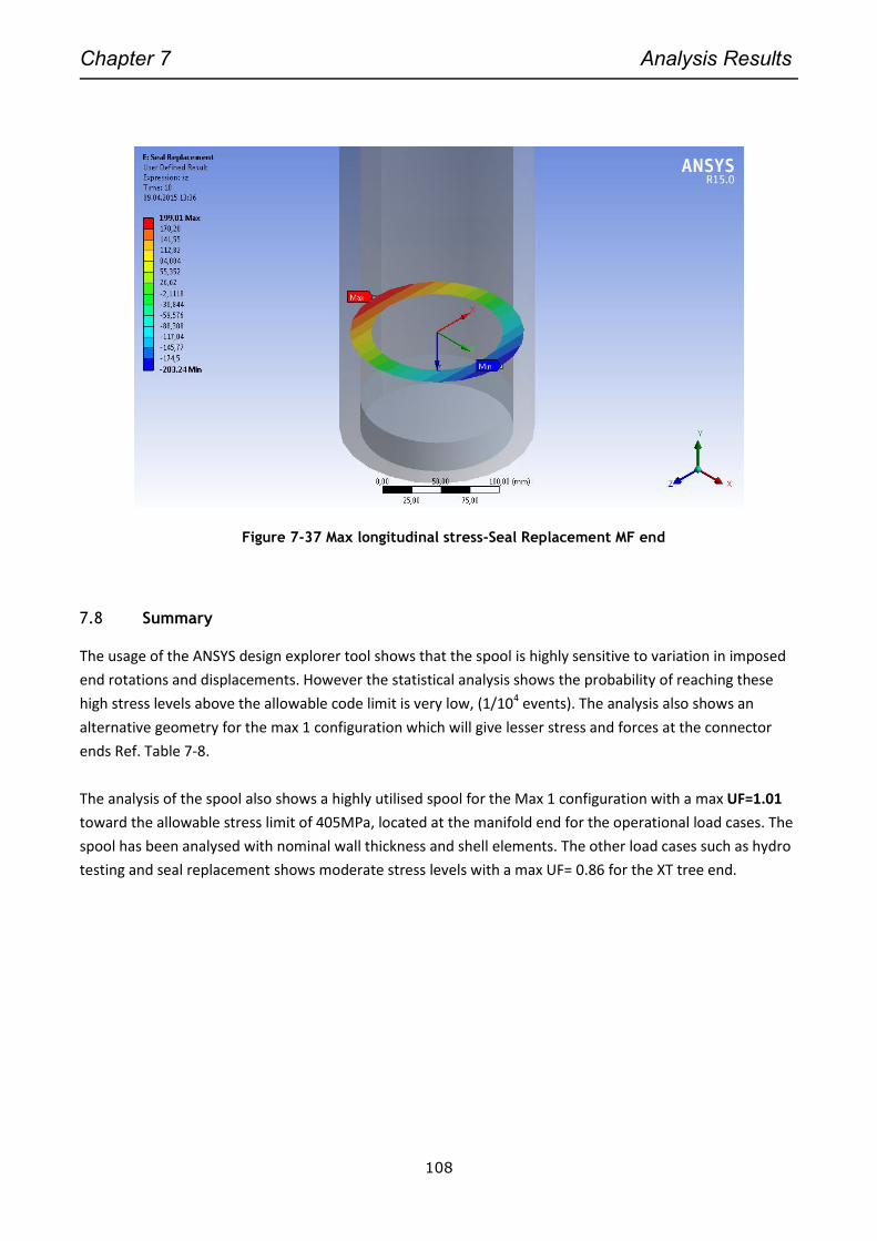
Chapter 7 Analysis Results
108
Figure 7-37 Max longitudinal stress-Seal Replacement MF end
7.8 Summary
The usage of the ANSYS design explorer tool shows that the spool is highly sensitive to variation in imposed
end rotations and displacements. However the statistical analysis shows the probability of reaching these
high stress levels above the allowable code limit is very low, (1/104 events). The analysis also shows an
alternative geometry for the max 1 configuration which will give lesser stress and forces at the connector
ends Ref. Table 7-8.
The analysis of the spool also shows a highly utilised spool for the Max 1 configuration with a max UF=1.01
toward the allowable stress limit of 405MPa, located at the manifold end for the operational load cases. The
spool has been analysed with nominal wall thickness and shell elements. The other load cases such as hydro
testing and seal replacement shows moderate stress levels with a max UF= 0.86 for the XT tree end.

Chapter 8 Verification and comparison of results
109
8. VERIFICATION AND COMPARISON OF RESULTS
In order to check and compare the shell element results from the screening and optimisation process from
ANSYS Design Explorer, three different models have been applied for the “Max1” configuration.
Pipe Element model using ANSYS PIPE289 and ELBOW290 elements
Solid Element model
Autopipe Piping Software
8.1 ANSYS Pipe Beam Element Model
The classical way of checking spools was historically made with ANSYS beam Element type PIPE16 and
PIPE18. These elements are no longer advised to use as they did not capture the thick wall effects and did
not account for cross sectional distortion or non-linear material properties. PIPE18 had the option of using
SIF factors and flexibility factors as given in Appendix E of Ref /15/. The elements are today replaced with
PIPE288 (Two nodes), PIPE289 (three nodes) and ELBOW290. The following element description is from the
ANSYS documentation.
PIPE289 is a quadratic three-node pipe element in 3-D. The element has six degrees of freedom at
each node (the translations in the x, y, and z directions and rotations about the x, y, and z
directions). The element is well-suited for linear, large rotation, and/or large strain nonlinear
applications. PIPE289 is based on Timoshenko beam theory, a first-order shear-deformation theory.
Transverse-shear strain is constant through the cross-section; that is, cross-sections remain plane
and undistorted after deformation. The element can be used for slender or stout pipes. Due to the
limitations of first-order shear-deformation theory, only moderately "thick" pipes can be analyzed.
ELBOW290 element is suitable for analyzing pipe structures with initially circular cross-sections and
thin to moderately thick pipe walls. The element accounts for cross-section distortion, which can be
commonly observed in curved pipe structures under loading. ELBOW290 is a quadratic (three-node)
pipe element in 3-D. The element has six degrees of freedom at each node (the translations in the x,
y, and z directions and rotations about the x, y, and z directions). The element is well-suited for
linear, large rotation, and/or large strain nonlinear applications. Change in pipe thickness is
accounted for in geometrically nonlinear analyses. The element accounts for follower (load stiffness)
effects of distributed pressures. ELBOW290 can be used in layered applications for modeling
laminated composite pipes. The accuracy in modeling composite pipes is governed by the first-order
shear-deformation theory (generally referred to as Mindlin-Reissner shell theory).
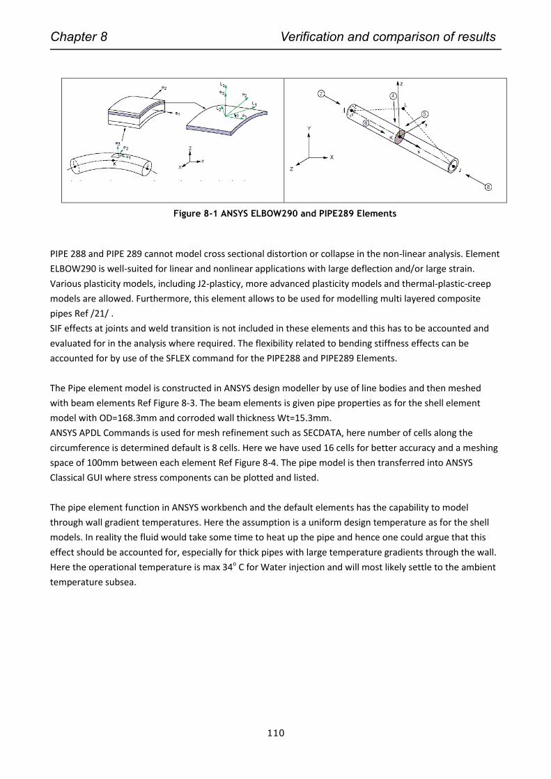
Chapter 8 Verification and comparison of results
110
Figure 8-1 ANSYS ELBOW290 and PIPE289 Elements
PIPE 288 and PIPE 289 cannot model cross sectional distortion or collapse in the non-linear analysis. Element
ELBOW290 is well-suited for linear and nonlinear applications with large deflection and/or large strain.
Various plasticity models, including J2-plasticy, more advanced plasticity models and thermal-plastic-creep
models are allowed. Furthermore, this element allows to be used for modelling multi layered composite
pipes Ref /21/ .
SIF effects at joints and weld transition is not included in these elements and this has to be accounted and
evaluated for in the analysis where required. The flexibility related to bending stiffness effects can be
accounted for by use of the SFLEX command for the PIPE288 and PIPE289 Elements.
The Pipe element model is constructed in ANSYS design modeller by use of line bodies and then meshed
with beam elements Ref Figure 8-3. The beam elements is given pipe properties as for the shell element
model with OD=168.3mm and corroded wall thickness Wt=15.3mm.
ANSYS APDL Commands is used for mesh refinement such as SECDATA, here number of cells along the
circumference is determined default is 8 cells. Here we have used 16 cells for better accuracy and a meshing
space of 100mm between each element Ref Figure 8-4. The pipe model is then transferred into ANSYS
Classical GUI where stress components can be plotted and listed.
The pipe element function in ANSYS workbench and the default elements has the capability to model
through wall gradient temperatures. Here the assumption is a uniform design temperature as for the shell
models. In reality the fluid would take some time to heat up the pipe and hence one could argue that this
effect should be accounted for, especially for thick pipes with large temperature gradients through the wall.
Here the operational temperature is max 34o C for Water injection and will most likely settle to the ambient
temperature subsea.
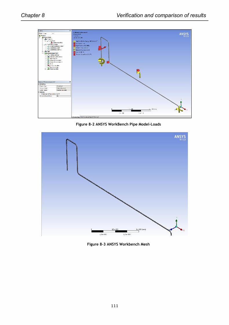
Chapter 8 Verification and comparison of results
111
Figure 8-2 ANSYS WorkBench Pipe Model-Loads
Figure 8-3 ANSYS Workbench Mesh
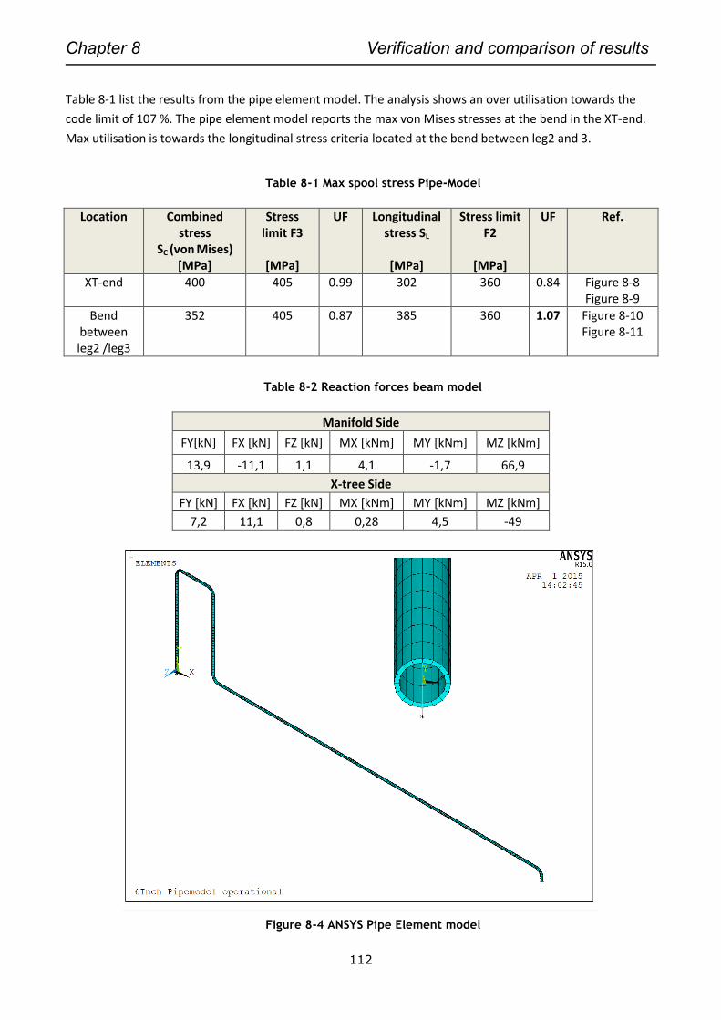
Chapter 8 Verification and comparison of results
112
Table 8-1 list the results from the pipe element model. The analysis shows an over utilisation towards the
code limit of 107 %. The pipe element model reports the max von Mises stresses at the bend in the XT-end.
Max utilisation is towards the longitudinal stress criteria located at the bend between leg2 and 3.
Table 8-1 Max spool stress Pipe-Model
Location Combined stress
SC (von Mises) [MPa]
Stress limit F3
[MPa]
UF Longitudinal stress SL
[MPa]
Stress limit F2
[MPa]
UF Ref.
XT-end 400 405 0.99 302 360 0.84 Figure 8-8 Figure 8-9
Bend between leg2 /leg3
352 405 0.87 385 360 1.07 Figure 8-10 Figure 8-11
Table 8-2 Reaction forces beam model
Manifold Side
FY[kN] FX [kN] FZ [kN] MX [kNm] MY [kNm] MZ [kNm]
13,9 -11,1 1,1 4,1 -1,7 66,9
X-tree Side
FY [kN] FX [kN] FZ [kN] MX [kNm] MY [kNm] MZ [kNm]
7,2 11,1 0,8 0,28 4,5 -49
Figure 8-4 ANSYS Pipe Element model
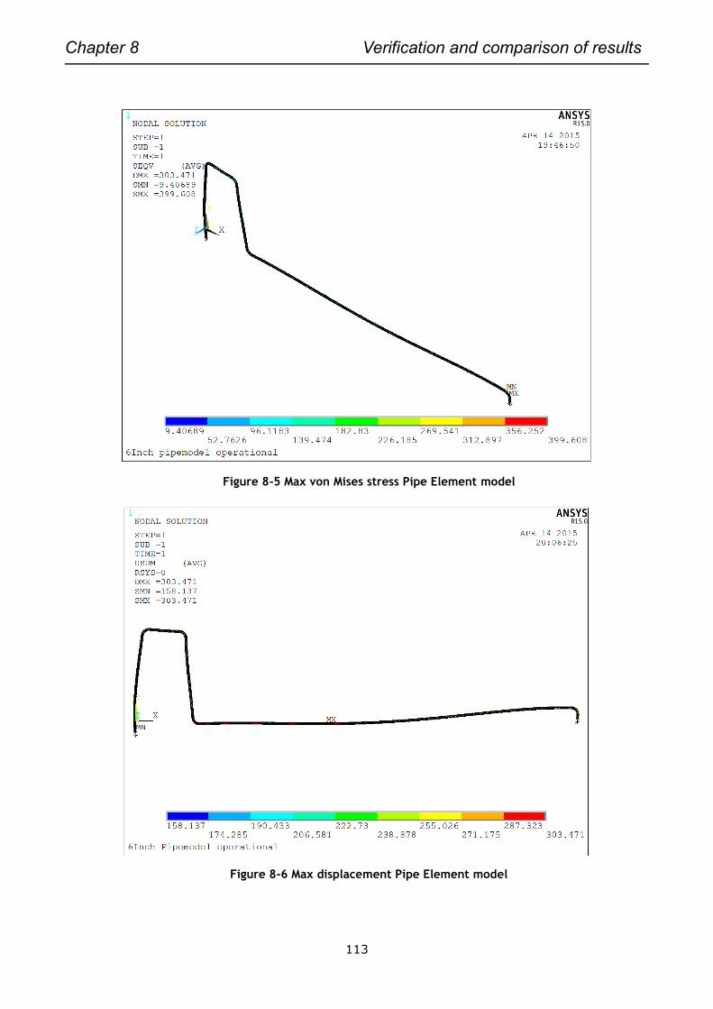
Chapter 8 Verification and comparison of results
113
Figure 8-5 Max von Mises stress Pipe Element model
Figure 8-6 Max displacement Pipe Element model
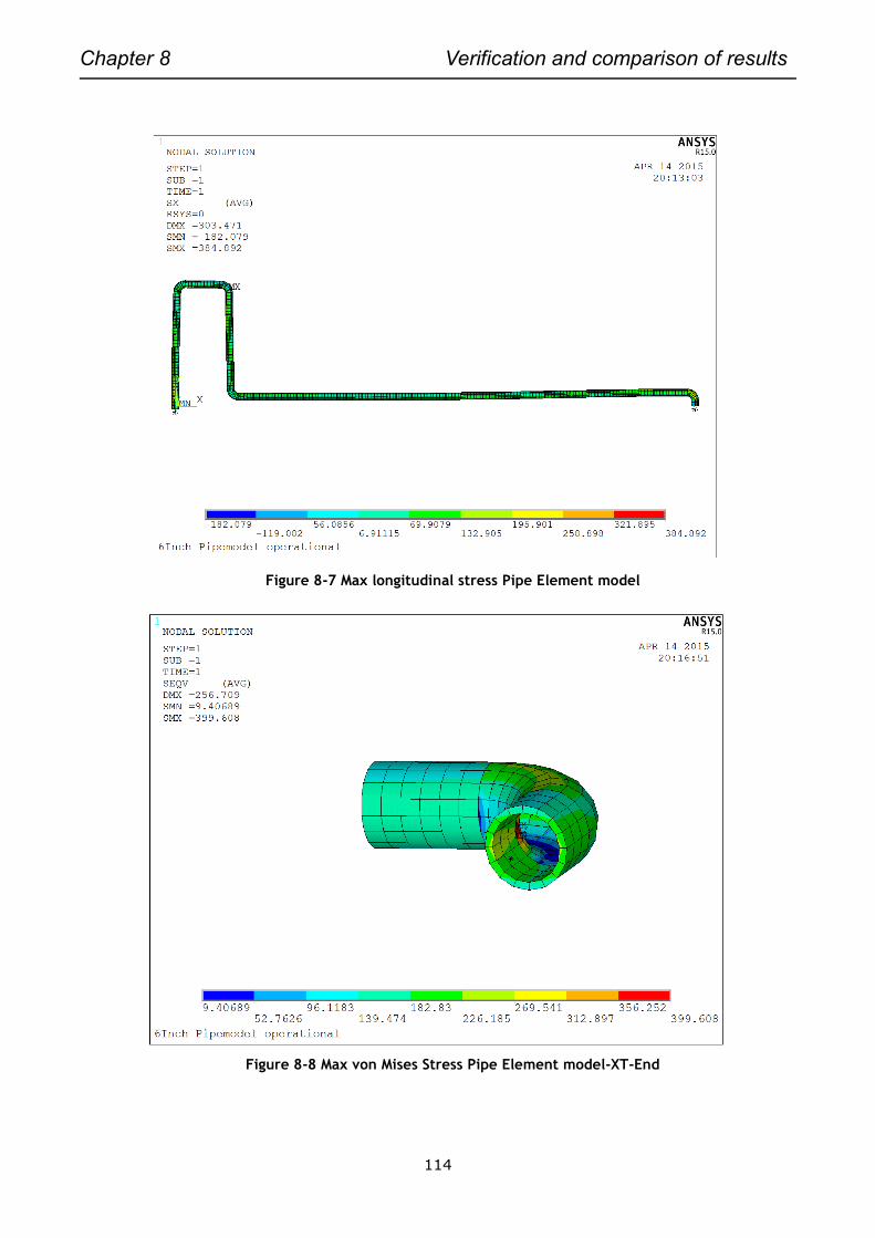
Chapter 8 Verification and comparison of results
114
Figure 8-7 Max longitudinal stress Pipe Element model
Figure 8-8 Max von Mises Stress Pipe Element model-XT-End
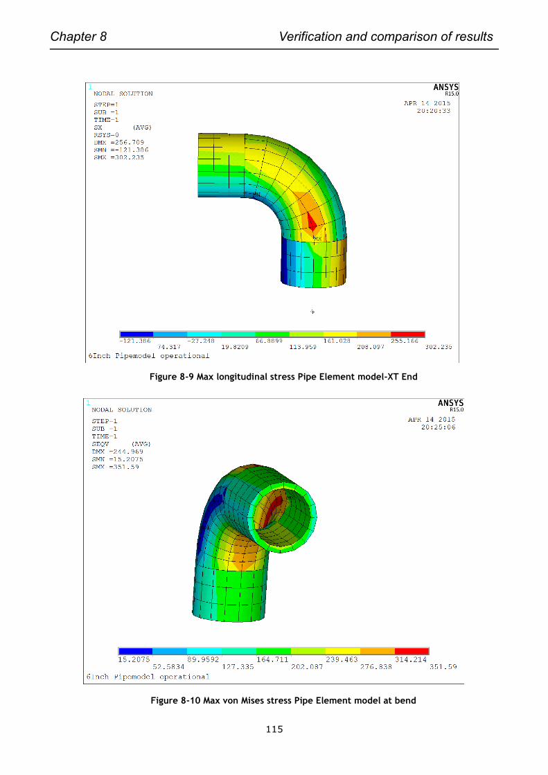
Chapter 8 Verification and comparison of results
115
Figure 8-9 Max longitudinal stress Pipe Element model-XT End
Figure 8-10 Max von Mises stress Pipe Element model at bend
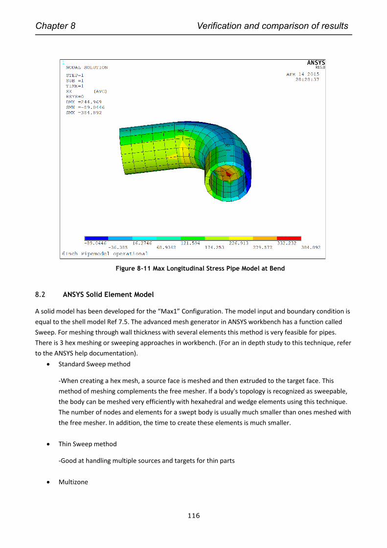
Chapter 8 Verification and comparison of results
116
Figure 8-11 Max Longitudinal Stress Pipe Model at Bend
8.2 ANSYS Solid Element Model
A solid model has been developed for the “Max1” Configuration. The model input and boundary condition is
equal to the shell model Ref 7.5. The advanced mesh generator in ANSYS workbench has a function called
Sweep. For meshing through wall thickness with several elements this method is very feasible for pipes.
There is 3 hex meshing or sweeping approaches in workbench. (For an in depth study to this technique, refer
to the ANSYS help documentation).
Standard Sweep method
-When creating a hex mesh, a source face is meshed and then extruded to the target face. This
method of meshing complements the free mesher. If a body's topology is recognized as sweepable,
the body can be meshed very efficiently with hexahedral and wedge elements using this technique.
The number of nodes and elements for a swept body is usually much smaller than ones meshed with
the free mesher. In addition, the time to create these elements is much smaller.
Thin Sweep method
-Good at handling multiple sources and targets for thin parts
Multizone
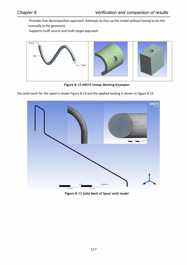
Chapter 8 Verification and comparison of results
117
-Provides free decomposition approach: Attempts to slice up the model without having to do this
manually to the geometry.
-Supports multi-source and multi target approach
Figure 8-12 ANSYS Sweep Meshing-Examples
The solid mesh for the spool is shown Figure 8-13 and the applied loading is shown in Figure 8-14
Figure 8-13 Solid Mesh of Spool solid model
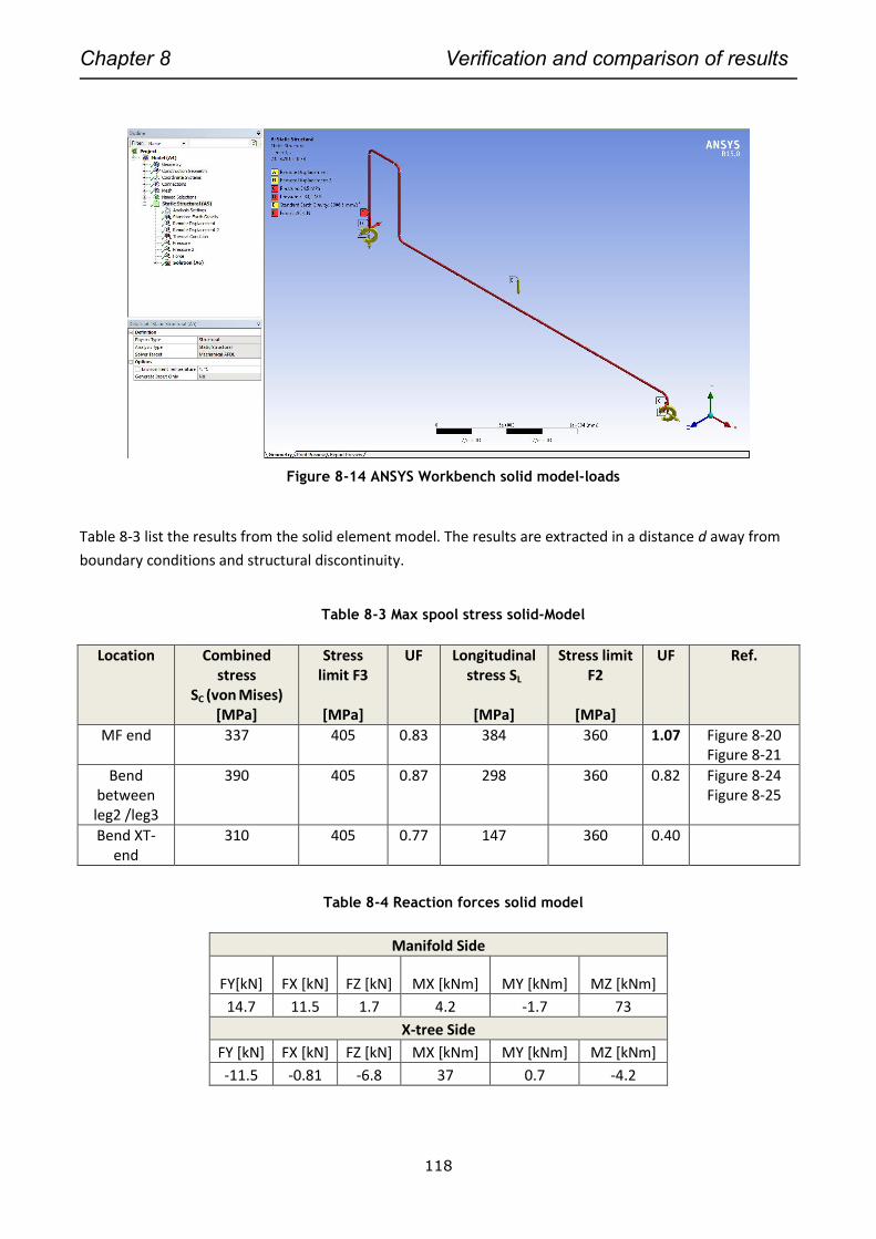
Chapter 8 Verification and comparison of results
118
Figure 8-14 ANSYS Workbench solid model-loads
Table 8-3 list the results from the solid element model. The results are extracted in a distance d away from
boundary conditions and structural discontinuity.
Table 8-3 Max spool stress solid-Model
Location Combined stress
SC (von Mises) [MPa]
Stress limit F3
[MPa]
UF Longitudinal stress SL
[MPa]
Stress limit F2
[MPa]
UF Ref.
MF end 337 405 0.83 384 360 1.07 Figure 8-20 Figure 8-21
Bend between leg2 /leg3
390 405 0.87 298 360 0.82 Figure 8-24 Figure 8-25
Bend XT-end
310 405 0.77 147 360 0.40
Table 8-4 Reaction forces solid model
Manifold Side
FY[kN] FX [kN] FZ [kN] MX [kNm] MY [kNm] MZ [kNm]
14.7 11.5 1.7 4.2 -1.7 73
X-tree Side
FY [kN] FX [kN] FZ [kN] MX [kNm] MY [kNm] MZ [kNm]
-11.5 -0.81 -6.8 37 0.7 -4.2
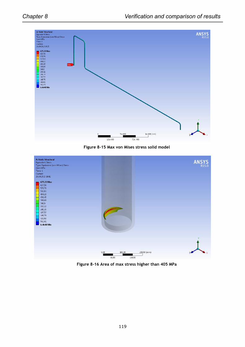
Chapter 8 Verification and comparison of results
119
Figure 8-15 Max von Mises stress solid model
Figure 8-16 Area of max stress higher than 405 MPa
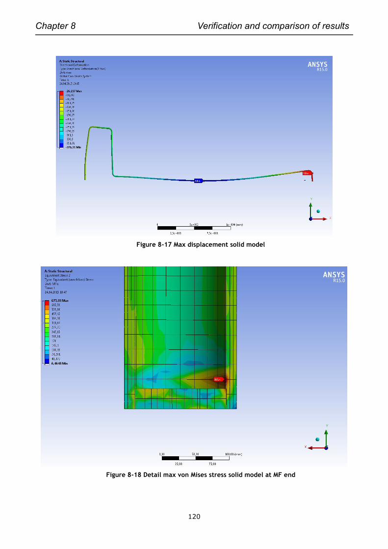
Chapter 8 Verification and comparison of results
120
Figure 8-17 Max displacement solid model
Figure 8-18 Detail max von Mises stress solid model at MF end
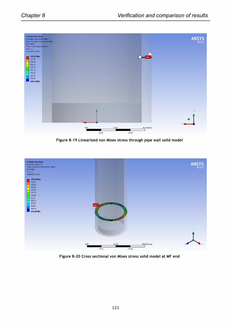
Chapter 8 Verification and comparison of results
121
Figure 8-19 Linearized von Mises stress through pipe wall solid model
Figure 8-20 Cross sectional von Mises stress solid model at MF end
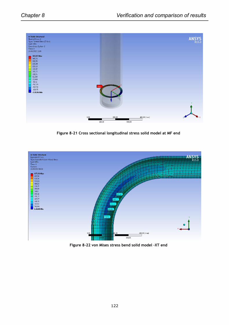
Chapter 8 Verification and comparison of results
122
Figure 8-21 Cross sectional longitudinal stress solid model at MF end
Figure 8-22 von Mises stress bend solid model –XT end
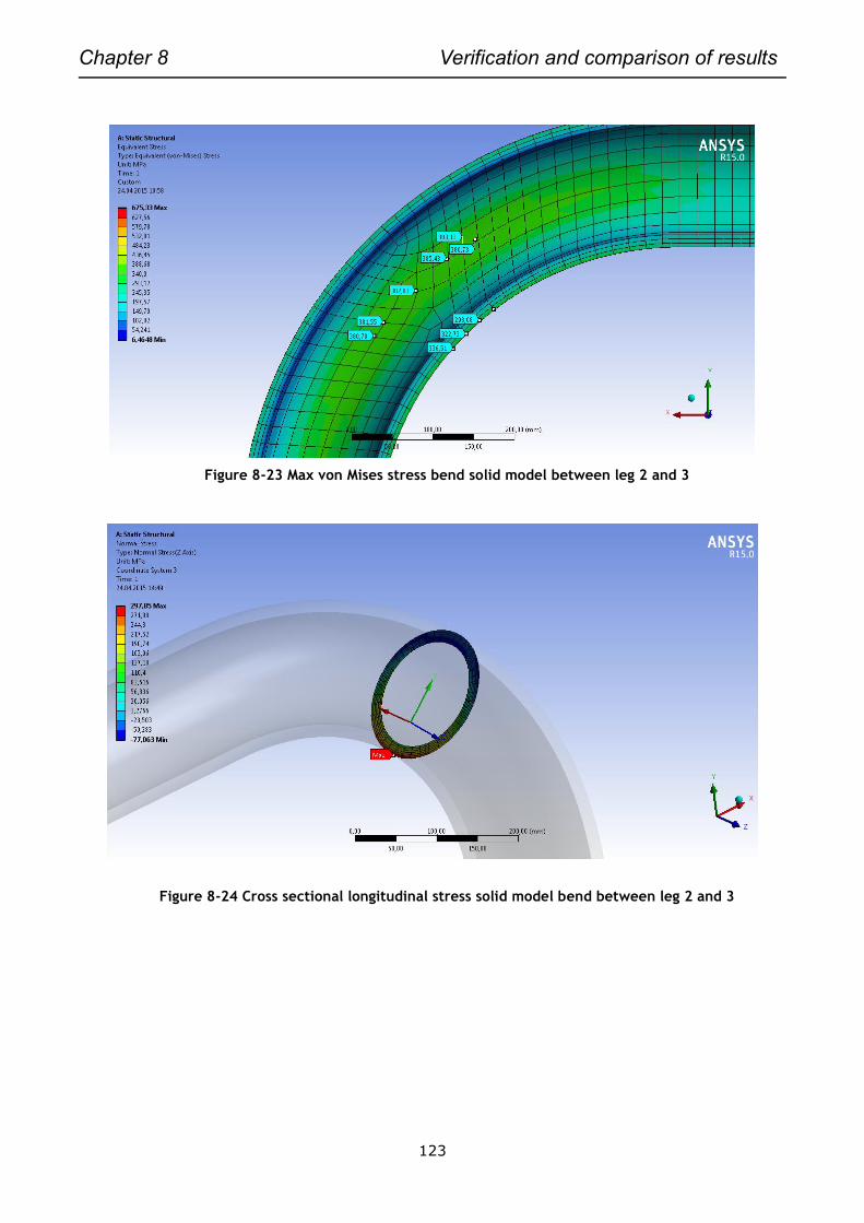
Chapter 8 Verification and comparison of results
123
Figure 8-23 Max von Mises stress bend solid model between leg 2 and 3
Figure 8-24 Cross sectional longitudinal stress solid model bend between leg 2 and 3
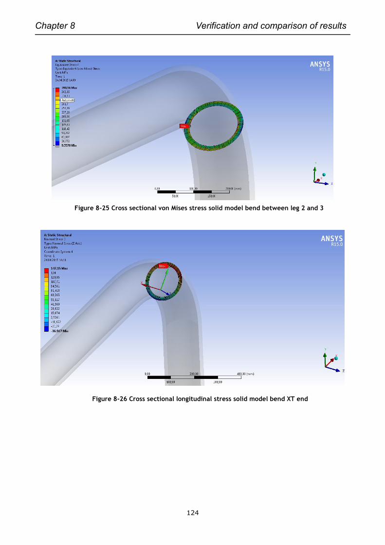
Chapter 8 Verification and comparison of results
124
Figure 8-25 Cross sectional von Mises stress solid model bend between leg 2 and 3
Figure 8-26 Cross sectional longitudinal stress solid model bend XT end
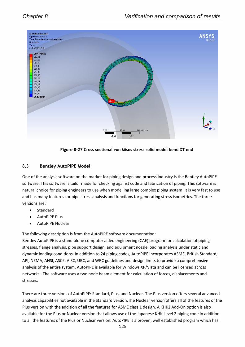
Chapter 8 Verification and comparison of results
125
Figure 8-27 Cross sectional von Mises stress solid model bend XT end
8.3 Bentley AutoPIPE Model
One of the analysis software on the market for piping design and process industry is the Bentley AutoPIPE
software. This software is tailor made for checking against code and fabrication of piping. This software is
natural choice for piping engineers to use when modelling large complex piping system. It is very fast to use
and has many features for pipe stress analysis and functions for generating stress isometrics. The three
versions are:
Standard
AutoPIPE Plus
AutoPIPE Nuclear
The following description is from the AutoPIPE software documentation:
Bentley AutoPIPE is a stand-alone computer aided engineering (CAE) program for calculation of piping
stresses, flange analysis, pipe support design, and equipment nozzle loading analysis under static and
dynamic loading conditions. In addition to 24 piping codes, AutoPIPE incorporates ASME, British Standard,
API, NEMA, ANSI, ASCE, AISC, UBC, and WRC guidelines and design limits to provide a comprehensive
analysis of the entire system. AutoPIPE is available for Windows XP/Vista and can be licensed across
networks. The software uses a two node beam element for calculation of forces, displacements and
stresses.
There are three versions of AutoPIPE: Standard, Plus, and Nuclear. The Plus version offers several advanced
analysis capabilities not available in the Standard version.The Nuclear version offers all of the features of the
Plus version with the addition of all the features for ASME class 1 design. A KHK2 Add-On option is also
available for the Plus or Nuclear version that allows use of the Japanese KHK Level 2 piping code in addition
to all the features of the Plus or Nuclear version. AutoPIPE is a proven, well established program which has
Chapter 8 Verification and comparison of results
126
been commercially available since 1986. AutoPIPE’s rigorous quality assurance practices have withstood
numerous on-site audits, making AutoPIPE one of the few PC based piping programs approved for use in
nuclear safety applications.
Since the spool is in elastic behaviour and there are no “large” non-linear effects for load and material, the
software is very versatile for piping design. The ASME codes which are one of many codes incorporated into
these softwares utilises that the goal is to ensure a safe design Ref /22/. In effect the code says that if we
calculated the stresses using a linear analysis and if we design these piping systems so that these stresses
are less than the allowable stresses, then the design has adequate factors of safety for both plastic collapse
and fatigue. The calculated stresses are not real they are based upon nominal values which are used in the
design
Piping systems can behave non-linearly because of yield and creep of the pipe, and because of non-linear
behaviour of the supports. We do not need to account for pipe non-linearity in a structural analysis because
the design procedures ensure that the pipe shakes down to elastic behaviour after one or at most a few
thermal cycles. However to calculate the stresses accurately we may need to account for support
nonlinearity.
For horizontal subsea spools the design utilises large non-linear displacements when stroking is applied and
non-linear contact between spool and seabed hence here a non-liner analysis model is mostly used and real
stresses and forces are reported and compared towards LRFD codes such as DNV-OS-F101. This feature is
not available in AutoPIPE. The recommendation from Bentley is to check the feasibility of the software by
using the following rule of thumb:
“As a check that AutoPIPE can handle large deformations, check that maximum slope angle in radians of the
deformed pipe≈sin(slope angle), then the solution should be OK. For example 0.025 radians over a large
span of 200m then the solution should be OK”
The software version which is used is the standard version. This version does not come with code check
according to ASME B31.8 2010 chapter VIII Offshore Gas Transmission Pipelines. But the standard version
does the code check in accordance with ASME B31.8 2010 Onshore Pipelines. This is the same code only
different sections within the same code.
The difference is the load combinations and criteria for calculation of longitudinal stresses and allowable
stresses. Chapter VIII specifies other loadings typical for offshore pipelines compared to onshore pipelines.
The code operates with the terminology restrained piping and unrestrained piping this dictates how one
should calculate stress and what limits to compare against.
The following table list the code load combinations for restrained piping according to the code. For the spool
checking this becomes:
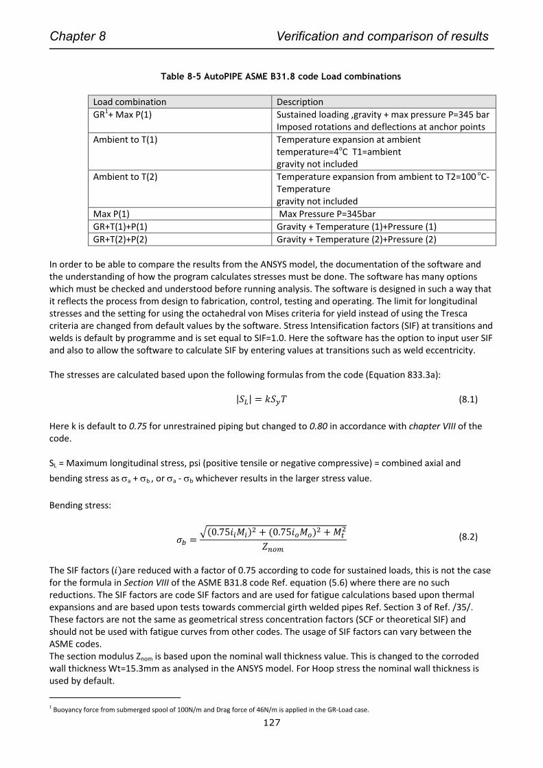
Chapter 8 Verification and comparison of results
127
Table 8-5 AutoPIPE ASME B31.8 code Load combinations
Load combination Description
GR1+ Max P(1) Sustained loading ,gravity + max pressure P=345 bar Imposed rotations and deflections at anchor points
Ambient to T(1) Temperature expansion at ambient temperature=4oC T1=ambient gravity not included
Ambient to T(2) Temperature expansion from ambient to T2=100 oC-Temperature gravity not included
Max P(1) Max Pressure P=345bar
GR+T(1)+P(1) Gravity + Temperature (1)+Pressure (1)
GR+T(2)+P(2) Gravity + Temperature (2)+Pressure (2)
In order to be able to compare the results from the ANSYS model, the documentation of the software and the understanding of how the program calculates stresses must be done. The software has many options which must be checked and understood before running analysis. The software is designed in such a way that it reflects the process from design to fabrication, control, testing and operating. The limit for longitudinal stresses and the setting for using the octahedral von Mises criteria for yield instead of using the Tresca criteria are changed from default values by the software. Stress Intensification factors (SIF) at transitions and welds is default by programme and is set equal to SIF=1.0. Here the software has the option to input user SIF and also to allow the software to calculate SIF by entering values at transitions such as weld eccentricity. The stresses are calculated based upon the following formulas from the code (Equation 833.3a):
|𝑆𝐿| = 𝑘𝑆𝑦𝑇 (8.1)
Here k is default to 0.75 for unrestrained piping but changed to 0.80 in accordance with chapter VIII of the code. SL = Maximum longitudinal stress, psi (positive tensile or negative compressive) = combined axial and
bending stress as a + b , or a - b whichever results in the larger stress value.
Bending stress:
𝜎𝑏 =√(0.75𝑖𝑖𝑀𝑖)
2 + (0.75𝑖𝑜𝑀𝑜)2 + 𝑀𝑡
2
𝑍𝑛𝑜𝑚 (8.2)
The SIF factors (𝑖)are reduced with a factor of 0.75 according to code for sustained loads, this is not the case for the formula in Section VIII of the ASME B31.8 code Ref. equation (5.6) where there are no such reductions. The SIF factors are code SIF factors and are used for fatigue calculations based upon thermal expansions and are based upon tests towards commercial girth welded pipes Ref. Section 3 of Ref. /35/. These factors are not the same as geometrical stress concentration factors (SCF or theoretical SIF) and should not be used with fatigue curves from other codes. The usage of SIF factors can vary between the ASME codes. The section modulus Znom is based upon the nominal wall thickness value. This is changed to the corroded wall thickness Wt=15.3mm as analysed in the ANSYS model. For Hoop stress the nominal wall thickness is used by default.
1 Buoyancy force from submerged spool of 100N/m and Drag force of 46N/m is applied in the GR-Load case.
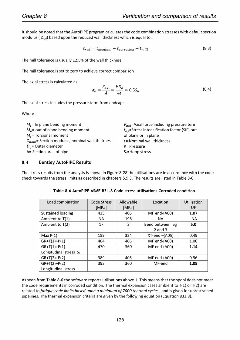
Chapter 8 Verification and comparison of results
128
It should be noted that the AutoPIPE program calculates the code combination stresses with default section modulus ( Zred) based upon the reduced wall thickness which is equal to:
𝑡𝑟𝑒𝑑 = 𝑡𝑛𝑜𝑚𝑖𝑛𝑎𝑙 − 𝑡𝑐𝑜𝑟𝑟𝑜𝑠𝑖𝑜𝑛 − 𝑡𝑚𝑖𝑙𝑙 (8.3)
The mill tolerance is usually 12.5% of the wall thickness. The mill tolerance is set to zero to achieve correct comparison The axial stress is calculated as:
𝜎𝑎 =𝐹𝑎𝑥𝑙
𝐴=
𝑃𝐷𝑜
4𝑡= 0.5𝑆ℎ (8.4)
The axial stress includes the pressure term from endcap: Where
𝑀𝑖= In plane bending moment 𝑀𝑜= out of plane bending moment 𝑀𝑡= Torsional moment 𝑍𝑛𝑜𝑚= Section modulus, nominal wall thickness 𝐷𝑜= Outer diameter
𝐹𝑎𝑥𝑙=Axial force including pressure term 𝑖𝑜,𝑖=Stress intensification factor (SIF) out of plane or in plane 𝑡= Nominal wall thickness P= Pressure
A= Section area of pipe Sh=Hoop stress 8.4 Bentley AutoPIPE Results
The stress results from the analysis is shown in Figure 8-28 the utilisations are in accordance with the code check towards the stress limits as described in chapters 5.9.3. The results are listed in Table 8-6
Table 8-6 AutoPIPE ASME B31.8 Code stress utilisations Corroded condition
Load combination Code Stress [MPa]
Allowable [MPa]
Location Utilisation UF
Sustained loading 435 405 MF end-(A00) 1.07
Ambient to T(1) NA 198 NA NA
Ambient to T(2) 17 3 Bend between leg 2 and 3
5.0
Max P(1) 159 324 XT-end –(A05) 0.49
GR+T(1)+P(1) 404 405 MF end-(A00) 1.00
GR+T(1)+P(1) Longitudinal stress SL
470 360 MF end-(A00) 1.14
GR+T(2)+P(2) 389 405 MF end-(A00) 0.96
GR+T(2)+P(2) Longitudinal stress
393 360 MF-end 1.09
As seen from Table 8-6 the software reports utilisations above 1. This means that the spool does not meet the code requirements in corroded condition. The thermal expansion cases ambient to T(1) or T(2) are related to fatigue code limits based upon a minimum of 7000 thermal cycles , and is given for unrestrained pipelines. The thermal expansion criteria are given by the following equation (Equation 833.8).
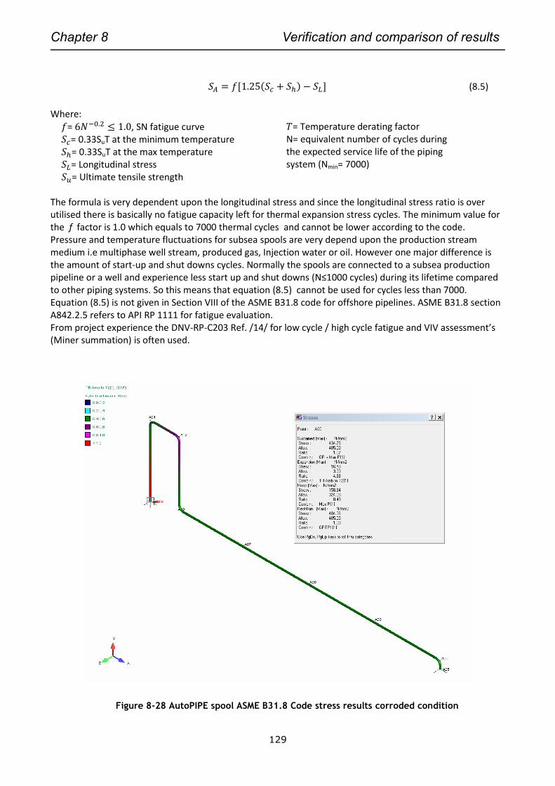
Chapter 8 Verification and comparison of results
129
𝑆𝐴 = 𝑓[1.25(𝑆𝑐 + 𝑆ℎ) − 𝑆𝐿] (8.5)
Where:
𝑓= 6𝑁−0.2 ≤ 1.0, SN fatigue curve 𝑆𝑐= 0.33SuT at the minimum temperature 𝑆ℎ= 0.33SuT at the max temperature 𝑆𝐿= Longitudinal stress 𝑆𝑢= Ultimate tensile strength
𝑇= Temperature derating factor N= equivalent number of cycles during the expected service life of the piping system (Nmin= 7000)
The formula is very dependent upon the longitudinal stress and since the longitudinal stress ratio is over utilised there is basically no fatigue capacity left for thermal expansion stress cycles. The minimum value for the f factor is 1.0 which equals to 7000 thermal cycles and cannot be lower according to the code. Pressure and temperature fluctuations for subsea spools are very depend upon the production stream medium i.e multiphase well stream, produced gas, Injection water or oil. However one major difference is the amount of start-up and shut downs cycles. Normally the spools are connected to a subsea production pipeline or a well and experience less start up and shut downs (N≤1000 cycles) during its lifetime compared to other piping systems. So this means that equation (8.5) cannot be used for cycles less than 7000. Equation (8.5) is not given in Section VIII of the ASME B31.8 code for offshore pipelines. ASME B31.8 section A842.2.5 refers to API RP 1111 for fatigue evaluation. From project experience the DNV-RP-C203 Ref. /14/ for low cycle / high cycle fatigue and VIV assessment’s (Miner summation) is often used.
Figure 8-28 AutoPIPE spool ASME B31.8 Code stress results corroded condition
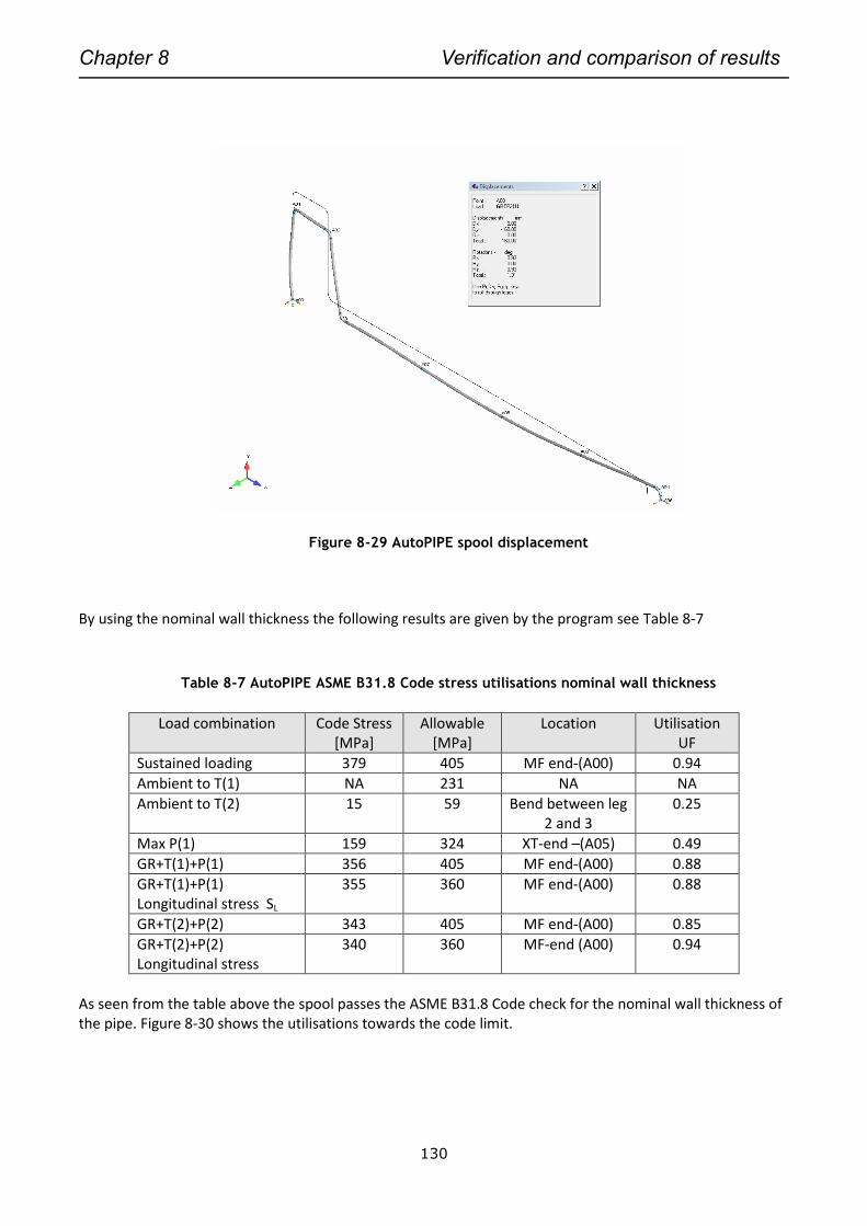
Chapter 8 Verification and comparison of results
130
Figure 8-29 AutoPIPE spool displacement
By using the nominal wall thickness the following results are given by the program see Table 8-7
Table 8-7 AutoPIPE ASME B31.8 Code stress utilisations nominal wall thickness
Load combination Code Stress [MPa]
Allowable [MPa]
Location Utilisation UF
Sustained loading 379 405 MF end-(A00) 0.94
Ambient to T(1) NA 231 NA NA
Ambient to T(2) 15 59 Bend between leg 2 and 3
0.25
Max P(1) 159 324 XT-end –(A05) 0.49
GR+T(1)+P(1) 356 405 MF end-(A00) 0.88
GR+T(1)+P(1) Longitudinal stress SL
355 360 MF end-(A00) 0.88
GR+T(2)+P(2) 343 405 MF end-(A00) 0.85
GR+T(2)+P(2) Longitudinal stress
340 360 MF-end (A00) 0.94
As seen from the table above the spool passes the ASME B31.8 Code check for the nominal wall thickness of the pipe. Figure 8-30 shows the utilisations towards the code limit.
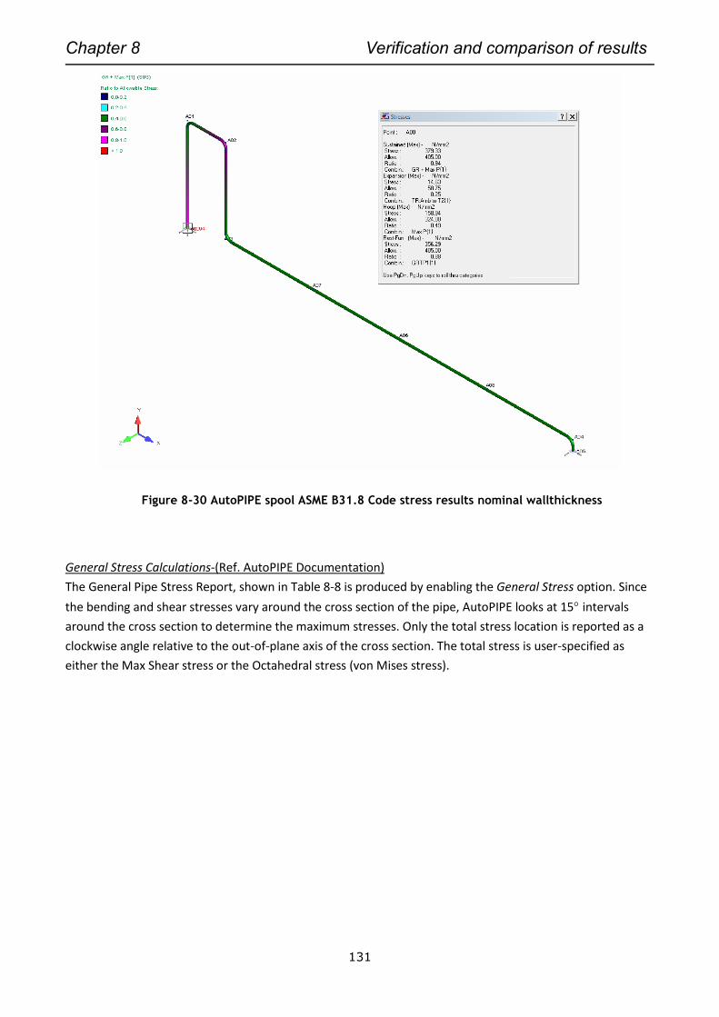
Chapter 8 Verification and comparison of results
131
Figure 8-30 AutoPIPE spool ASME B31.8 Code stress results nominal wallthickness
General Stress Calculations-(Ref. AutoPIPE Documentation)
The General Pipe Stress Report, shown in Table 8-8 is produced by enabling the General Stress option. Since
the bending and shear stresses vary around the cross section of the pipe, AutoPIPE looks at 15 intervals
around the cross section to determine the maximum stresses. Only the total stress location is reported as a
clockwise angle relative to the out-of-plane axis of the cross section. The total stress is user-specified as
either the Max Shear stress or the Octahedral stress (von Mises stress).
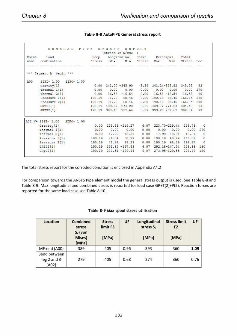
Chapter 8 Verification and comparison of results
132
Table 8-8 AutoPIPE General stress report
The total stress report for the corroded condition is enclosed in Appendix A4.2
For comparison towards the ANSYS Pipe element model the general stress output is used. See Table 8-8 and Table 8-9. Max longitudinal and combined stress is reported for load case GR+T(2)+P(2). Reaction forces are reported for the same load case see Table 8-10.
Table 8-9 Max spool stress utilisation
Location Combined stress SC (von
Mises) [MPa]
Stress limit F3
[MPa]
UF Longitudinal stress SL
[MPa]
Stress limit F2
[MPa]
UF
MF-end (A00) 389 405 0.96 393 360 1.09
Bend between leg 2 and 3
(A02) 279 405 0.68 274 360 0.76
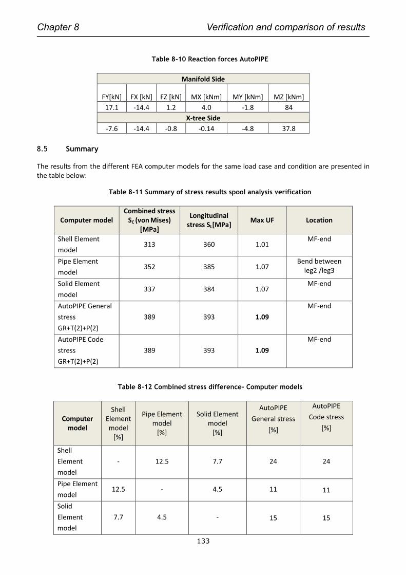
Chapter 8 Verification and comparison of results
133
Table 8-10 Reaction forces AutoPIPE
Manifold Side
FY[kN] FX [kN] FZ [kN] MX [kNm] MY [kNm] MZ [kNm]
17.1 -14.4 1.2 4.0 -1.8 84
X-tree Side
-7.6 -14.4 -0.8 -0.14 -4.8 37.8
8.5 Summary
The results from the different FEA computer models for the same load case and condition are presented in the table below:
Table 8-11 Summary of stress results spool analysis verification
Computer model Combined stress
SC (von Mises) [MPa]
Longitudinal stress SL[MPa]
Max UF Location
Shell Element
model 313 360 1.01
MF-end
Pipe Element
model 352 385 1.07
Bend between leg2 /leg3
Solid Element
model 337 384 1.07
MF-end
AutoPIPE General
stress
GR+T(2)+P(2)
389 393 1.09
MF-end
AutoPIPE Code
stress
GR+T(2)+P(2)
389 393 1.09
MF-end
Table 8-12 Combined stress difference- Computer models
Computer model
Shell Element model
[%]
Pipe Element model
[%]
Solid Element model
[%]
AutoPIPE
General stress
[%]
AutoPIPE
Code stress
[%]
Shell
Element
model
- 12.5 7.7 24 24
Pipe Element
model 12.5 - 4.5 11 11
Solid
Element
model
7.7 4.5 - 15 15
Chapter 8 Verification and comparison of results
134
Table 8-13 Longitudinal stress difference- Computer models
Computer model
Shell Element model
[%]
Pipe Element model
[%]
Solid Element model
[%]
AutoPIPE
General stress
[%]
AutoPIPE
Code
stress
[%]
Shell Element
model - 7.0 6.6 9.2 9.2
Pipe Element
model 7.0 - 0.26 2.1 2.1
Solid Element
model 6.6 0.26 - 2.3 2.3
Commentary to results:
As seen from Table 8-12 the largest utilisation is the AutoPIPE code stress calculation with an utilisation
factor of 109% towards the allowable ASME B31.8 code stress limit (9% above the limit of 405MPa). The
ANSYS model’s has an utilisation range between 101% - 107 %. The difference is the location of reported
stress location where the pipe element model reports the max longitudinal stress at the bend between leg 2
and 3. Max bending stress is however reported at the same location (MF-end). Table 8-12 also shows that
there is no difference between the calculated code stress and the general stress reported in AutoPIPE for
this case.
All models however reports utilisation above the code limits for stress in corroded condition. The lowest element stress is the shell element model and the highest stress reported is the AutoPIPE beam element model with a difference of 24%. The longitudinal stress (see Table 8-13) has less difference in results with a maximum difference of 9.2 % between AutoPIPE model and the ANSYS shell model. The minimum difference found is 0.26% and is between the ANSYS solid model and the ANSYS pipe element model. The utilisation towards the code stress limits has a good match between all computer models except for the ANSYS shell model which seems to underreport the stress levels. The spool however passes the ASME B31.8 Code check for the nominal wall thickness of the pipe max utilisation is 94% for sustained loads and GR+T(2)+P(2). See results in Table 8-6
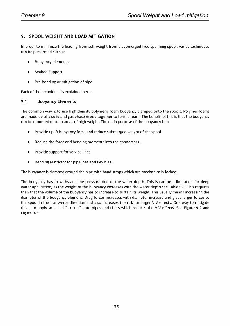
Chapter 9 Spool Weight and Load mitigation
135
9. SPOOL WEIGHT AND LOAD MITIGATION
In order to minimize the loading from self-weight from a submerged free spanning spool, varies techniques can be performed such as:
Buoyancy elements
Seabed Support
Pre-bending or mitigation of pipe
Each of the techniques is explained here.
9.1 Buoyancy Elements
The common way is to use high density polymeric foam buoyancy clamped onto the spools. Polymer foams are made up of a solid and gas phase mixed together to form a foam. The benefit of this is that the buoyancy can be mounted onto to areas of high weight. The main purpose of the buoyancy is to:
Provide uplift buoyancy force and reduce submerged weight of the spool
Reduce the force and bending moments into the connectors.
Provide support for service lines
Bending restrictor for pipelines and flexibles.
The buoyancy is clamped around the pipe with band straps which are mechanically locked.
The buoyancy has to withstand the pressure due to the water depth. This is can be a limitation for deep water application, as the weight of the buoyancy increases with the water depth see Table 9-1. This requires then that the volume of the buoyancy has to increase to sustain its weight. This usually means increasing the diameter of the buoyancy element. Drag forces increases with diameter increase and gives larger forces to the spool in the transverse direction and also increases the risk for larger VIV effects. One way to mitigate this is to apply so called “strakes” onto pipes and risers which reduces the VIV effects, See Figure 9-2 and Figure 9-3
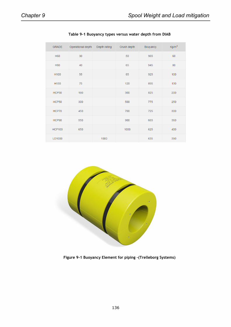
Chapter 9 Spool Weight and Load mitigation
136
Table 9-1 Buoyancy types versus water depth from DIAB
Figure 9-1 Buoyancy Element for piping –(Trelleborg Systems)

Chapter 9 Spool Weight and Load mitigation
137
Figure 9-2 VIV Strakes on buoyancy-(Balmoral-group)
Figure 9-3 VIV Strakes for subsea piping-(Trelleborg Systems)
The effect of using strakes around a cylindrical object is shown in Figure 9-4. The figure shows a complex
three dimensional flow around a bare riser Ref. PRETechnologies.com. The analysis shows high turbulent
flow and high pressure regions, (right image) red areas shows high pressure. Figure 9-5 shows the resulting
flow structures surrounding the riser with the helical strake installed. The flow is characterised by much
smaller scale structures in the vicinity of the riser surface which are less correlated than in the bare riser
configuration and hence less likely to lead to VIV. The riser surface pressures are also shown to be less
correlated in the axial direction for the rake arrangement than with the bare riser configuration.
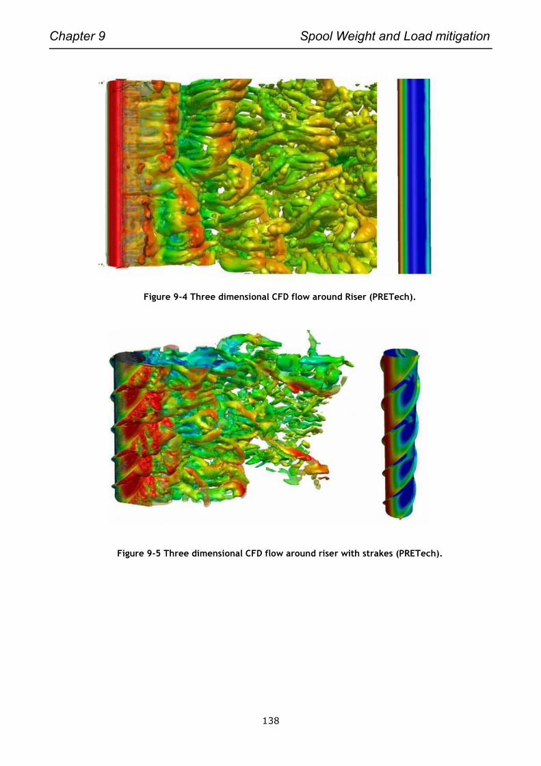
Chapter 9 Spool Weight and Load mitigation
138
Figure 9-4 Three dimensional CFD flow around Riser (PRETech).
Figure 9-5 Three dimensional CFD flow around riser with strakes (PRETech).

Chapter 9 Spool Weight and Load mitigation
139
The spool is analysed with a total calculated buoyancy uplift force of Fbuoyancy=5105 N, This reduces the spool
weight by 25% Ref. Appendix 3 for hand calculations
Table 9-2 Max spool stress element model with buoyancy
Location Combined stress
SC (von Mises) [MPa]
Stress limit F3
[MPa]
UF Longitudinal stress SL
[MPa]
Stress limit F2
[MPa]
UF Ref.
MF end 263 405 0.60 307 360 0.85 Figure 9-10 Figure 9-9
Table 9-3 Reaction forces with buoyancy
Manifold Side
FY[kN] FX [kN] FZ [kN] MX [kNm] MY [kNm] MZ [kNm]
16.7 -99 1.4 4.9 -2.3 66
X-tree Side
8.8 8.2 1.2 0.48 7.0 -9.1
Figure 9-6 Spool with buoyancy uplift force
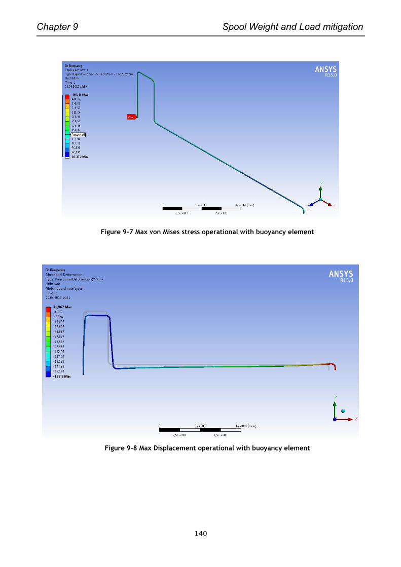
Chapter 9 Spool Weight and Load mitigation
140
Figure 9-7 Max von Mises stress operational with buoyancy element
Figure 9-8 Max Displacement operational with buoyancy element
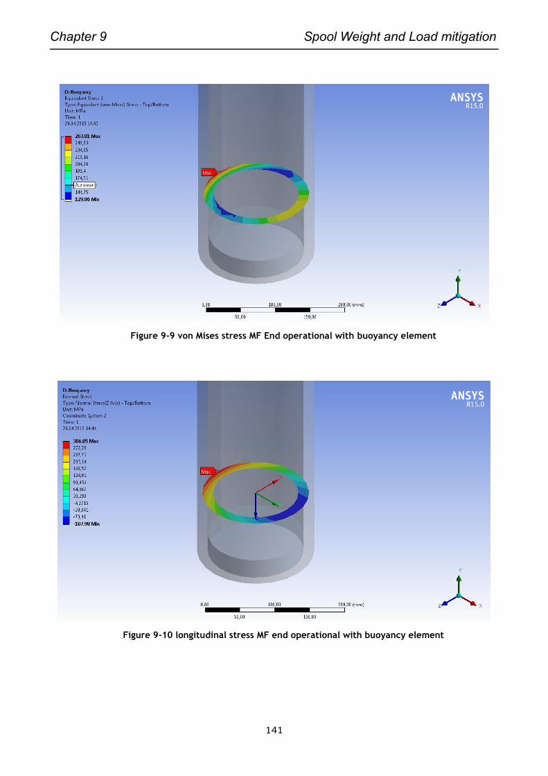
Chapter 9 Spool Weight and Load mitigation
141
Figure 9-9 von Mises stress MF End operational with buoyancy element
Figure 9-10 longitudinal stress MF end operational with buoyancy element
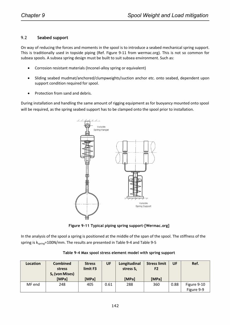
Chapter 9 Spool Weight and Load mitigation
142
9.2 Seabed support
On way of reducing the forces and moments in the spool is to introduce a seabed mechanical spring support. This is traditionally used in topside piping (Ref. Figure 9-11 from wermac.org). This is not so common for subsea spools. A subsea spring design must be built to suit subsea environment. Such as:
Corrosion resistant materials (Inconel-alloy spring or equivalent)
Sliding seabed mudmat/anchored/clumpweights/suction anchor etc. onto seabed, dependent upon support condition required for spool.
Protection from sand and debris.
During installation and handling the same amount of rigging equipment as for buoyancy mounted onto spool
will be required, as the spring seabed support has to be clamped onto the spool prior to installation.
Figure 9-11 Typical piping spring support–[Wermac.org]
In the analysis of the spool a spring is positioned at the middle of the span of the spool. The stiffness of the
spring is kspring=100N/mm. The results are presented in Table 9-4 and Table 9-5
Table 9-4 Max spool stress element model with spring support
Location Combined stress
SC (von Mises) [MPa]
Stress limit F3
[MPa]
UF Longitudinal stress SL
[MPa]
Stress limit F2
[MPa]
UF Ref.
MF end 248 405 0.61 288 360 0.88 Figure 9-10 Figure 9-9
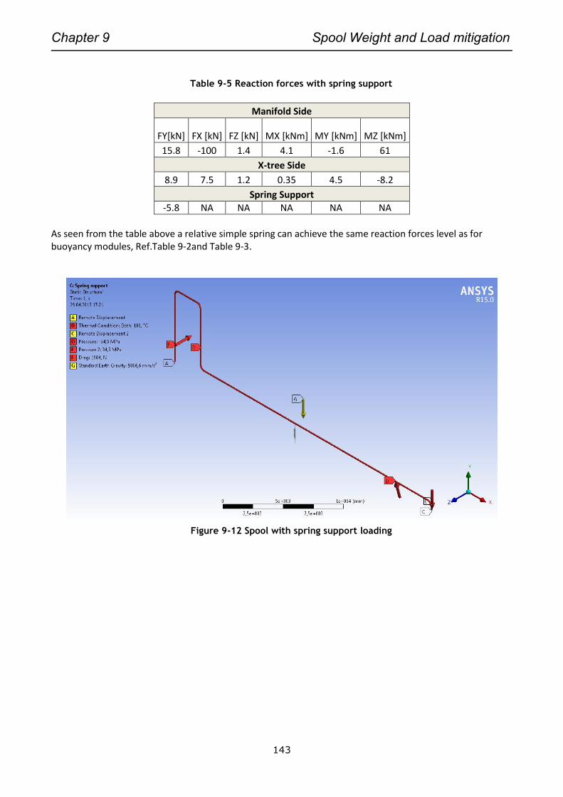
Chapter 9 Spool Weight and Load mitigation
143
Table 9-5 Reaction forces with spring support
Manifold Side
FY[kN] FX [kN] FZ [kN] MX [kNm] MY [kNm] MZ [kNm]
15.8 -100 1.4 4.1 -1.6 61
X-tree Side
8.9 7.5 1.2 0.35 4.5 -8.2
Spring Support
-5.8 NA NA NA NA NA
As seen from the table above a relative simple spring can achieve the same reaction forces level as for buoyancy modules, Ref.Table 9-2and Table 9-3.
Figure 9-12 Spool with spring support loading
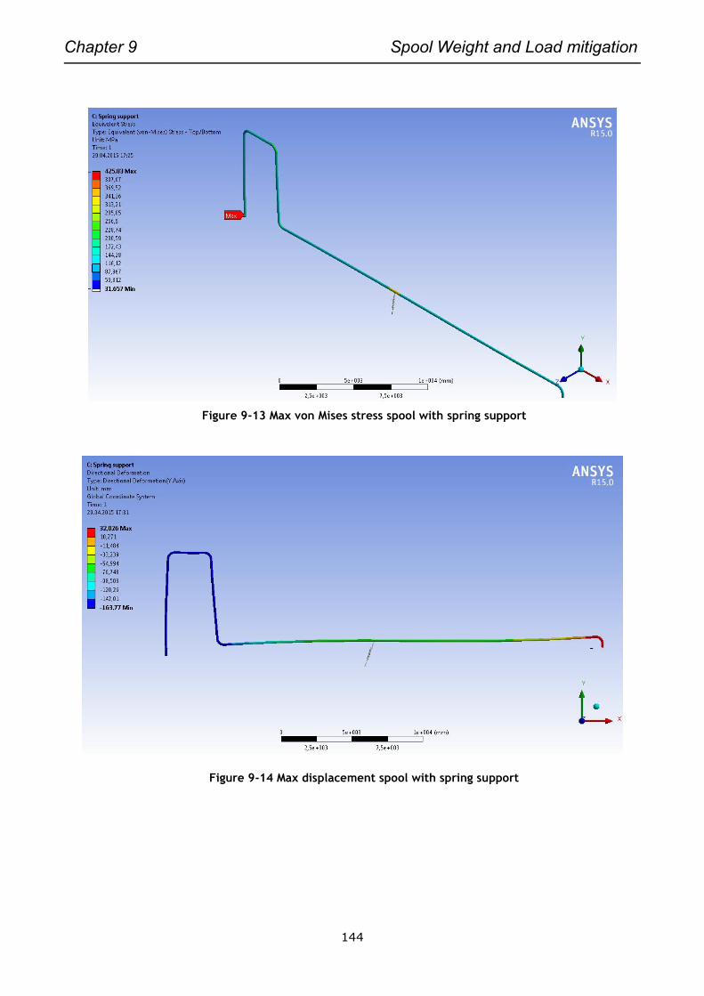
Chapter 9 Spool Weight and Load mitigation
144
Figure 9-13 Max von Mises stress spool with spring support
Figure 9-14 Max displacement spool with spring support
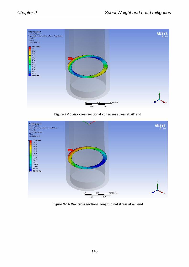
Chapter 9 Spool Weight and Load mitigation
145
Figure 9-15 Max cross sectional von Mises stress at MF end
Figure 9-16 Max cross sectional longitudinal stress at MF end
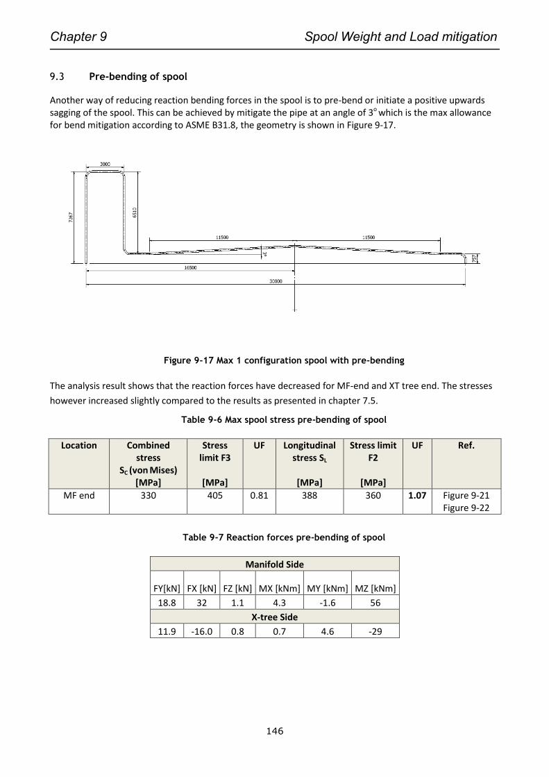
Chapter 9 Spool Weight and Load mitigation
146
9.3 Pre-bending of spool
Another way of reducing reaction bending forces in the spool is to pre-bend or initiate a positive upwards sagging of the spool. This can be achieved by mitigate the pipe at an angle of 3o which is the max allowance for bend mitigation according to ASME B31.8, the geometry is shown in Figure 9-17.
Figure 9-17 Max 1 configuration spool with pre-bending
The analysis result shows that the reaction forces have decreased for MF-end and XT tree end. The stresses
however increased slightly compared to the results as presented in chapter 7.5.
Table 9-6 Max spool stress pre-bending of spool
Location Combined stress
SC (von Mises) [MPa]
Stress limit F3
[MPa]
UF Longitudinal stress SL
[MPa]
Stress limit F2
[MPa]
UF Ref.
MF end 330 405 0.81 388 360 1.07 Figure 9-21 Figure 9-22
Table 9-7 Reaction forces pre-bending of spool
Manifold Side
FY[kN] FX [kN] FZ [kN] MX [kNm] MY [kNm] MZ [kNm]
18.8 32 1.1 4.3 -1.6 56
X-tree Side
11.9 -16.0 0.8 0.7 4.6 -29
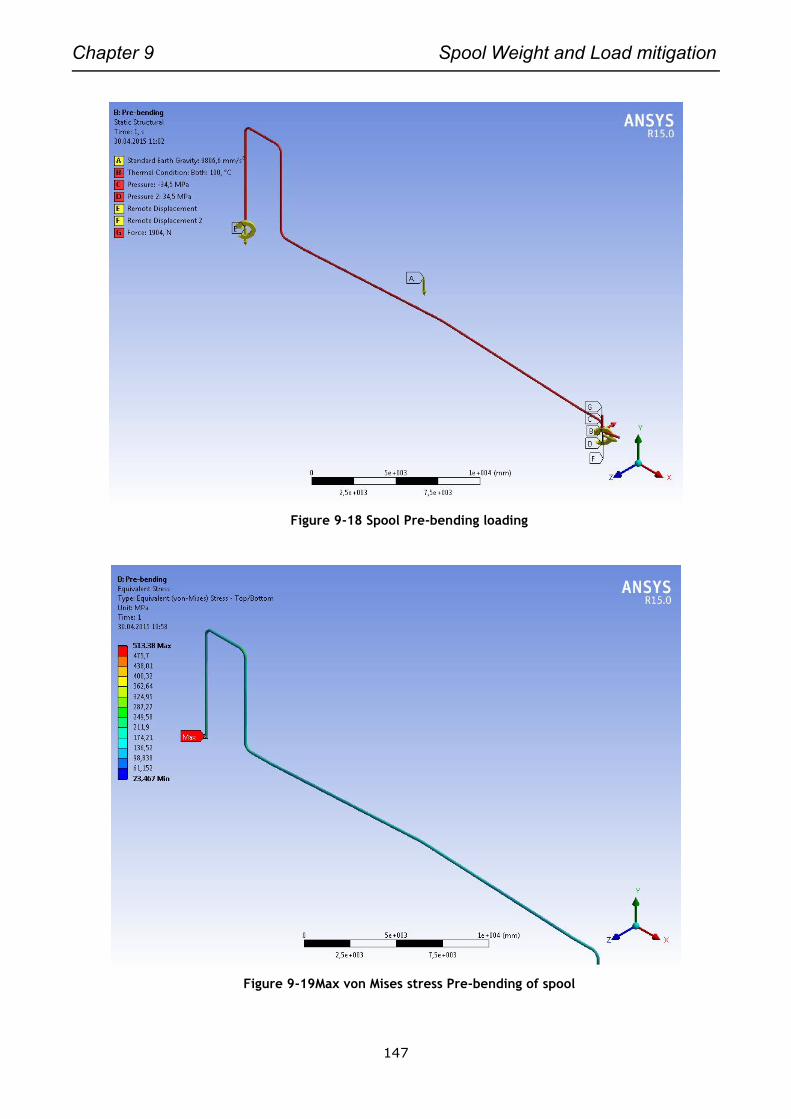
Chapter 9 Spool Weight and Load mitigation
147
Figure 9-18 Spool Pre-bending loading
Figure 9-19Max von Mises stress Pre-bending of spool
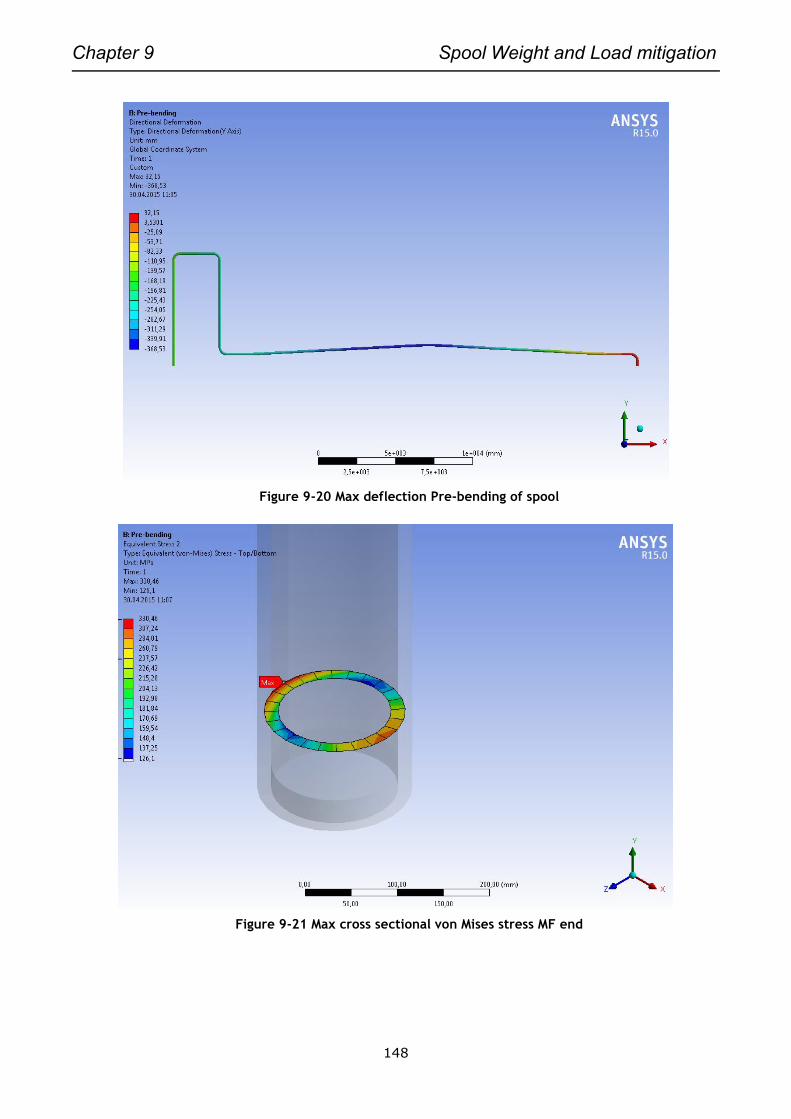
Chapter 9 Spool Weight and Load mitigation
148
Figure 9-20 Max deflection Pre-bending of spool
Figure 9-21 Max cross sectional von Mises stress MF end
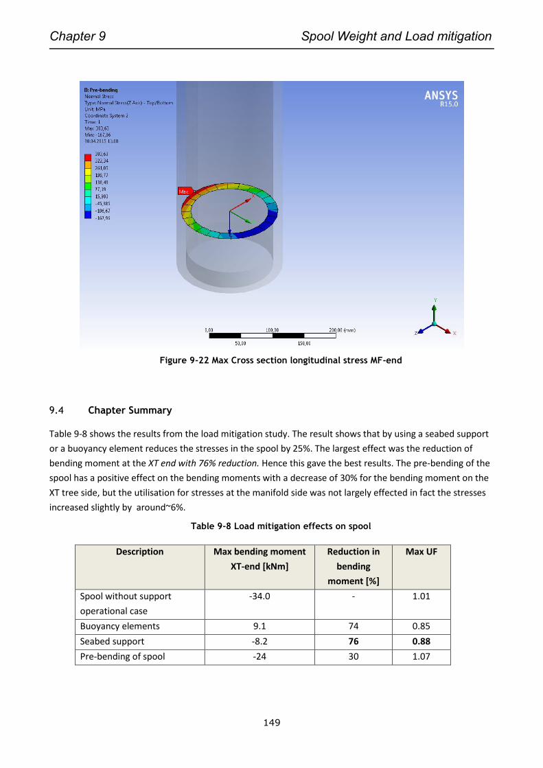
Chapter 9 Spool Weight and Load mitigation
149
Figure 9-22 Max Cross section longitudinal stress MF-end
9.4 Chapter Summary
Table 9-8 shows the results from the load mitigation study. The result shows that by using a seabed support
or a buoyancy element reduces the stresses in the spool by 25%. The largest effect was the reduction of
bending moment at the XT end with 76% reduction. Hence this gave the best results. The pre-bending of the
spool has a positive effect on the bending moments with a decrease of 30% for the bending moment on the
XT tree side, but the utilisation for stresses at the manifold side was not largely effected in fact the stresses
increased slightly by around~6%.
Table 9-8 Load mitigation effects on spool
Description Max bending moment
XT-end [kNm]
Reduction in
bending
moment [%]
Max UF
Spool without support
operational case
-34.0 - 1.01
Buoyancy elements 9.1 74 0.85
Seabed support -8.2 76 0.88
Pre-bending of spool -24 30 1.07
Chapter 9 Spool Weight and Load mitigation
150
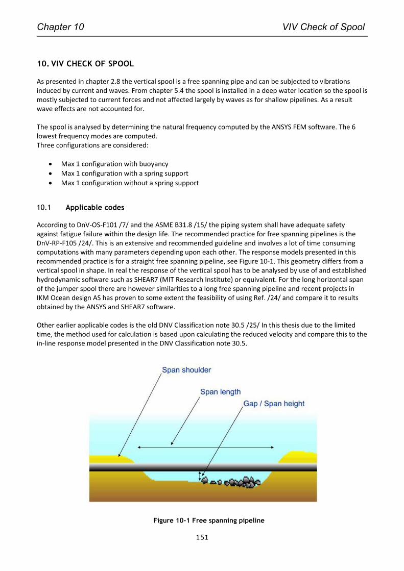
Chapter 10 VIV Check of Spool
151
10. VIV CHECK OF SPOOL
As presented in chapter 2.8 the vertical spool is a free spanning pipe and can be subjected to vibrations induced by current and waves. From chapter 5.4 the spool is installed in a deep water location so the spool is mostly subjected to current forces and not affected largely by waves as for shallow pipelines. As a result wave effects are not accounted for. The spool is analysed by determining the natural frequency computed by the ANSYS FEM software. The 6 lowest frequency modes are computed. Three configurations are considered:
Max 1 configuration with buoyancy
Max 1 configuration with a spring support
Max 1 configuration without a spring support
10.1 Applicable codes
According to DnV-OS-F101 /7/ and the ASME B31.8 /15/ the piping system shall have adequate safety against fatigue failure within the design life. The recommended practice for free spanning pipelines is the DnV-RP-F105 /24/. This is an extensive and recommended guideline and involves a lot of time consuming computations with many parameters depending upon each other. The response models presented in this recommended practice is for a straight free spanning pipeline, see Figure 10-1. This geometry differs from a vertical spool in shape. In real the response of the vertical spool has to be analysed by use of and established hydrodynamic software such as SHEAR7 (MIT Research Institute) or equivalent. For the long horizontal span of the jumper spool there are however similarities to a long free spanning pipeline and recent projects in IKM Ocean design AS has proven to some extent the feasibility of using Ref. /24/ and compare it to results obtained by the ANSYS and SHEAR7 software. Other earlier applicable codes is the old DNV Classification note 30.5 /25/ In this thesis due to the limited time, the method used for calculation is based upon calculating the reduced velocity and compare this to the in-line response model presented in the DNV Classification note 30.5.
Figure 10-1 Free spanning pipeline
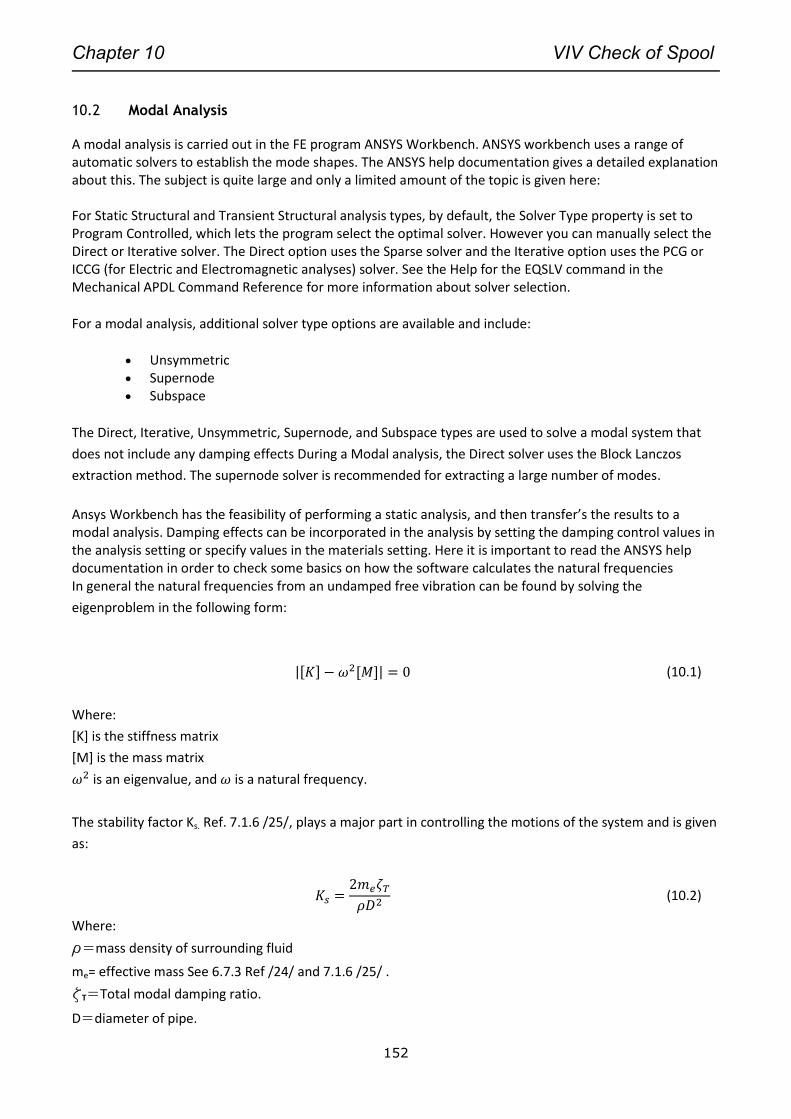
Chapter 10 VIV Check of Spool
152
10.2 Modal Analysis
A modal analysis is carried out in the FE program ANSYS Workbench. ANSYS workbench uses a range of automatic solvers to establish the mode shapes. The ANSYS help documentation gives a detailed explanation about this. The subject is quite large and only a limited amount of the topic is given here: For Static Structural and Transient Structural analysis types, by default, the Solver Type property is set to Program Controlled, which lets the program select the optimal solver. However you can manually select the Direct or Iterative solver. The Direct option uses the Sparse solver and the Iterative option uses the PCG or ICCG (for Electric and Electromagnetic analyses) solver. See the Help for the EQSLV command in the Mechanical APDL Command Reference for more information about solver selection.
For a modal analysis, additional solver type options are available and include:
Unsymmetric Supernode Subspace
The Direct, Iterative, Unsymmetric, Supernode, and Subspace types are used to solve a modal system that
does not include any damping effects During a Modal analysis, the Direct solver uses the Block Lanczos
extraction method. The supernode solver is recommended for extracting a large number of modes.
Ansys Workbench has the feasibility of performing a static analysis, and then transfer’s the results to a modal analysis. Damping effects can be incorporated in the analysis by setting the damping control values in the analysis setting or specify values in the materials setting. Here it is important to read the ANSYS help documentation in order to check some basics on how the software calculates the natural frequencies In general the natural frequencies from an undamped free vibration can be found by solving the
eigenproblem in the following form:
|[𝐾] − 𝜔2[𝑀]| = 0 (10.1)
Where:
[K] is the stiffness matrix
[M] is the mass matrix
𝜔2 is an eigenvalue, and 𝜔 is a natural frequency.
The stability factor Ks. Ref. 7.1.6 /25/, plays a major part in controlling the motions of the system and is given
as:
𝐾𝑠 =2𝑚𝑒𝜁𝑇
𝜌𝐷2 (10.2)
Where:
r=mass density of surrounding fluid
me= effective mass See 6.7.3 Ref /24/ and 7.1.6 /25/ .
zT=Total modal damping ratio.
D=diameter of pipe.
Chapter 10 VIV Check of Spool
153
The total modal damping ratio zT, comprises structural damping, soil damping and hydrodynamic damping.
The recommended practice gives some guidelines here, for instance the hydrodynamic damping in the lock
in range is set to zero and the soil damping can vary between 0,5% to 2%. Assuming a very stiff manifold and
X-tree, the damping value is assumed and set to 0.3%.
Hence (10.2) then becomes: (Ref Appendix 3 for calculation of effective mass me=82 kg/m)
𝐾𝑠 =2 ∙ 82 ∙ 0.03
1026 ∙ 0.1682= 0.17 (10.3)
The added mass from the surrounding water is dependent upon the frequency and the mode shape and are
included in the in-line response models and cross flow response models, see section 6.7.3 in Ref. /24/, In
accordance with Ref. /24/ a simplification for the added mass can also be computed as:
Madded=rpr2L
(10.4)
Where:
r=mass density of surrounding fluid
L=length of span or unit length
The added mass is calculated to be 23 kg/m and is included in the analysis (Ref. Appendix 3 for calculations) The 6 first natural frequencies from the ANSYS modal analysis is listed in the tables below since they are assumed to be the critical ones. The initial pre-stressing from the remote displacements at the MF end and XT end is included as a pre-stress effect. The Pre stress effect must be included in the modal analysis because they will affect the natural frequencies. The natural frequency is for an un-damped system, except for the spring support model where a damping coefficient for the spring is included: A more accurate analysis would be to include the structural stiffness damping effect. This is taken into account in the limits used in the response models by use of Ks Ref. /24/. The purpose of this exercise is to evaluate if the spring has a positive effect on the spool. The damping ratio of the spring is calculated based upon the following formulas, from mechanical vibrations theory:
𝜁 =𝐶
𝐶𝑐=
𝑐
2𝑚𝜔𝑛=
𝑐
2√𝑚𝑘 (10.5)
Where: 𝜔𝑛= natural frequency m= mass of system Cc=Critical damping C= damping coefficient k=stiffness of system/spring The spring constant used here is k=100N/mm and the mass of the spring used is m=50kg. A typical value for springs with good damping ratio is in the range of 𝜁 =0.2-0.4. By solving for c in equation (10.5) gives the following damping coefficient for the spring used in the analysis:
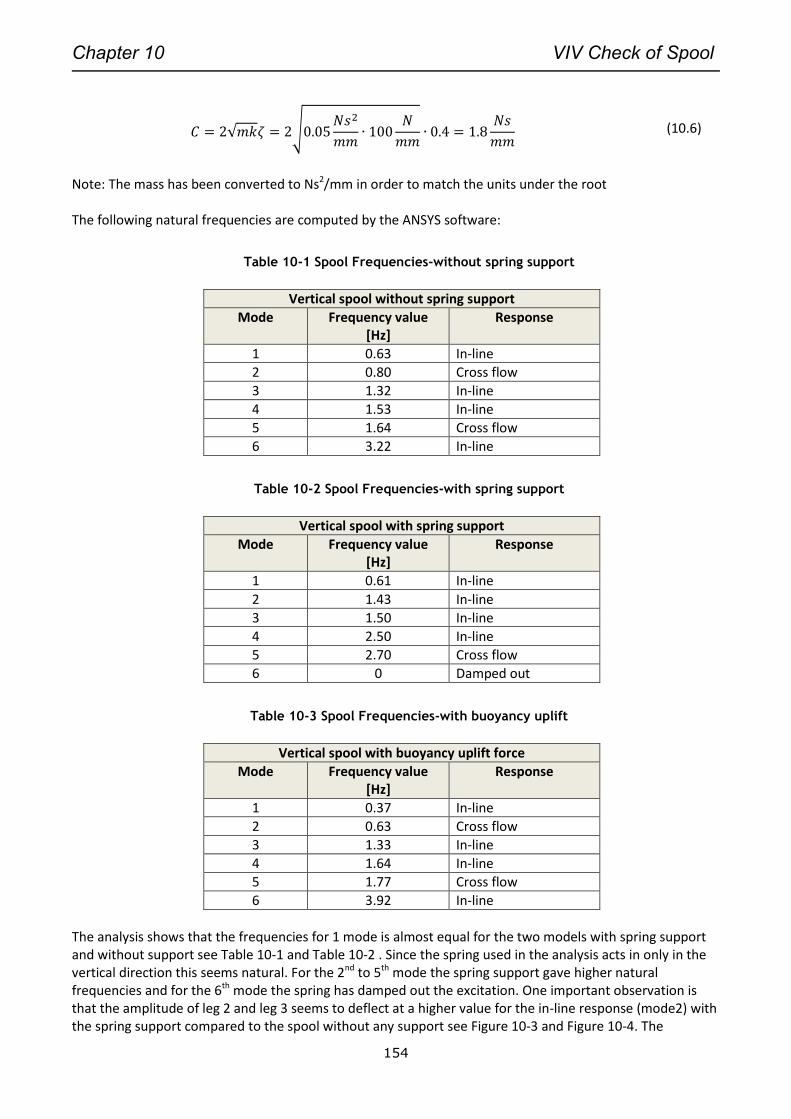
Chapter 10 VIV Check of Spool
154
𝐶 = 2√𝑚𝑘𝜁 = 2√0.05𝑁𝑠2
𝑚𝑚∙ 100
𝑁
𝑚𝑚∙ 0.4 = 1.8
𝑁𝑠
𝑚𝑚 (10.6)
Note: The mass has been converted to Ns2/mm in order to match the units under the root The following natural frequencies are computed by the ANSYS software:
Table 10-1 Spool Frequencies-without spring support
Vertical spool without spring support
Mode Frequency value [Hz]
Response
1 0.63 In-line
2 0.80 Cross flow
3 1.32 In-line
4 1.53 In-line
5 1.64 Cross flow
6 3.22 In-line
Table 10-2 Spool Frequencies-with spring support
Vertical spool with spring support
Mode Frequency value [Hz]
Response
1 0.61 In-line
2 1.43 In-line
3 1.50 In-line
4 2.50 In-line
5 2.70 Cross flow
6 0 Damped out
Table 10-3 Spool Frequencies-with buoyancy uplift
Vertical spool with buoyancy uplift force
Mode Frequency value [Hz]
Response
1 0.37 In-line
2 0.63 Cross flow
3 1.33 In-line
4 1.64 In-line
5 1.77 Cross flow
6 3.92 In-line
The analysis shows that the frequencies for 1 mode is almost equal for the two models with spring support and without support see Table 10-1 and Table 10-2 . Since the spring used in the analysis acts in only in the vertical direction this seems natural. For the 2nd to 5th mode the spring support gave higher natural frequencies and for the 6th mode the spring has damped out the excitation. One important observation is that the amplitude of leg 2 and leg 3 seems to deflect at a higher value for the in-line response (mode2) with the spring support compared to the spool without any support see Figure 10-3 and Figure 10-4. The
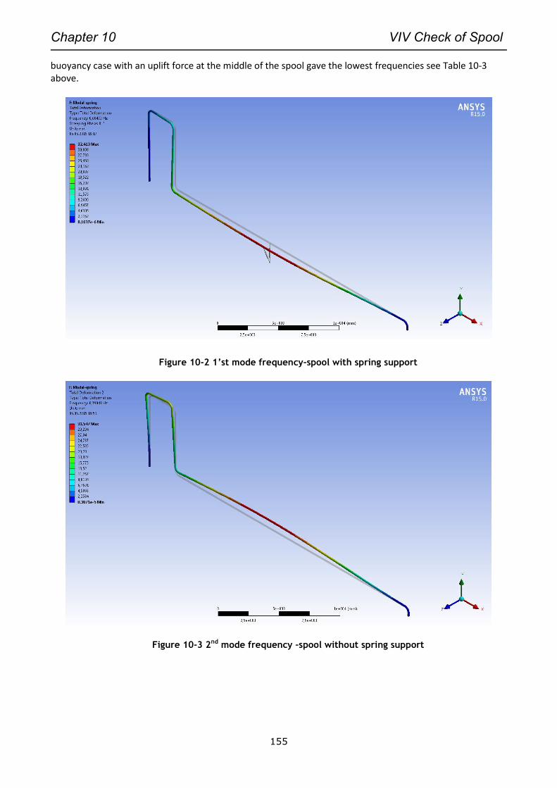
Chapter 10 VIV Check of Spool
155
buoyancy case with an uplift force at the middle of the spool gave the lowest frequencies see Table 10-3 above.
Figure 10-2 1’st mode frequency–spool with spring support
Figure 10-3 2nd mode frequency –spool without spring support
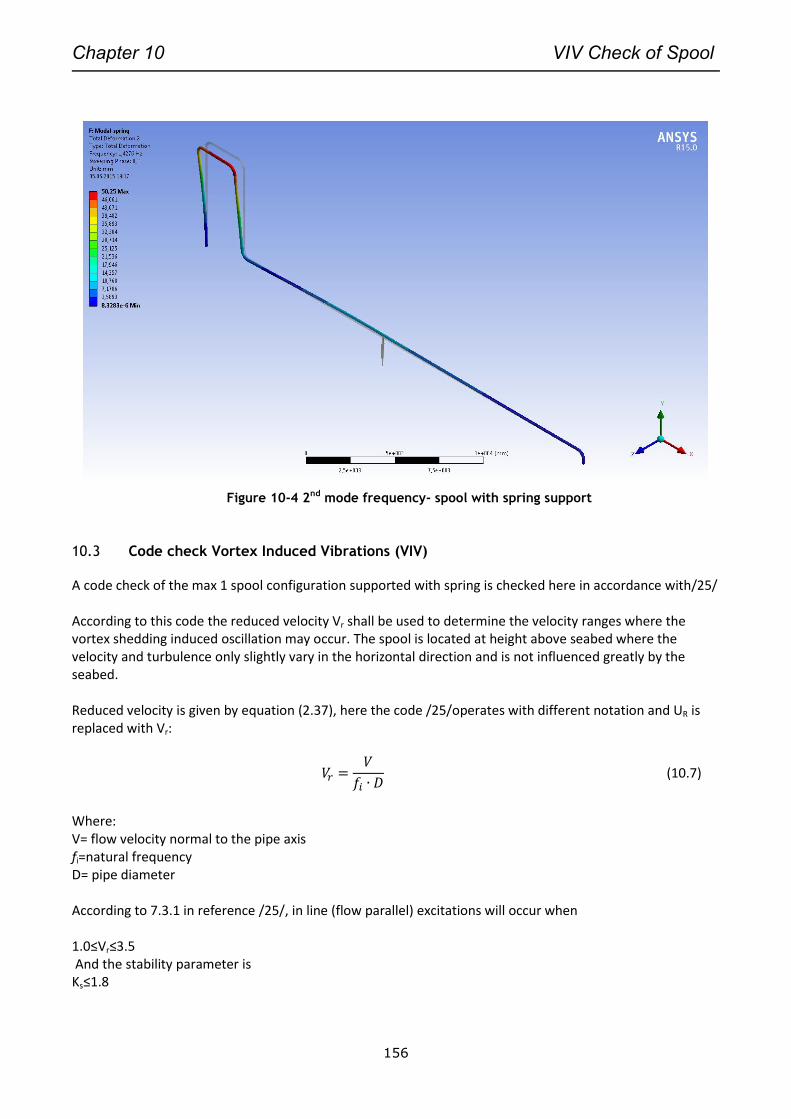
Chapter 10 VIV Check of Spool
156
Figure 10-4 2nd mode frequency- spool with spring support
10.3 Code check Vortex Induced Vibrations (VIV)
A code check of the max 1 spool configuration supported with spring is checked here in accordance with/25/ According to this code the reduced velocity Vr shall be used to determine the velocity ranges where the vortex shedding induced oscillation may occur. The spool is located at height above seabed where the velocity and turbulence only slightly vary in the horizontal direction and is not influenced greatly by the seabed. Reduced velocity is given by equation (2.37), here the code /25/operates with different notation and UR is replaced with Vr:
𝑉𝑟 =𝑉
𝑓𝑖 ∙ 𝐷 (10.7)
Where: V= flow velocity normal to the pipe axis fi=natural frequency D= pipe diameter According to 7.3.1 in reference /25/, in line (flow parallel) excitations will occur when 1.0≤Vr≤3.5 And the stability parameter is Ks≤1.8
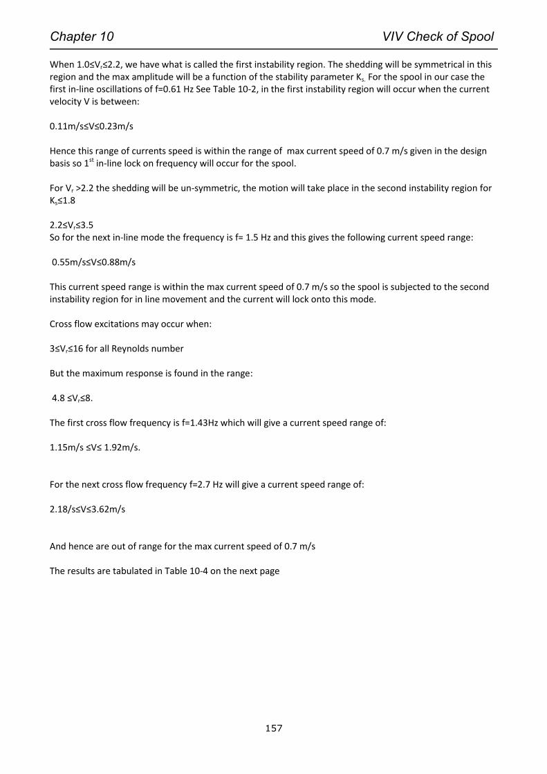
Chapter 10 VIV Check of Spool
157
When 1.0≤Vr≤2.2, we have what is called the first instability region. The shedding will be symmetrical in this region and the max amplitude will be a function of the stability parameter Ks. For the spool in our case the first in-line oscillations of f=0.61 Hz See Table 10-2, in the first instability region will occur when the current velocity V is between: 0.11m/s≤V≤0.23m/s Hence this range of currents speed is within the range of max current speed of 0.7 m/s given in the design basis so 1st in-line lock on frequency will occur for the spool. For Vr >2.2 the shedding will be un-symmetric, the motion will take place in the second instability region for Ks≤1.8 2.2≤Vr≤3.5 So for the next in-line mode the frequency is f= 1.5 Hz and this gives the following current speed range: 0.55m/s≤V≤0.88m/s This current speed range is within the max current speed of 0.7 m/s so the spool is subjected to the second instability region for in line movement and the current will lock onto this mode. Cross flow excitations may occur when: 3≤Vr≤16 for all Reynolds number But the maximum response is found in the range: 4.8 ≤Vr≤8. The first cross flow frequency is f=1.43Hz which will give a current speed range of: 1.15m/s ≤V≤ 1.92m/s. For the next cross flow frequency f=2.7 Hz will give a current speed range of: 2.18/s≤V≤3.62m/s And hence are out of range for the max current speed of 0.7 m/s The results are tabulated in Table 10-4 on the next page
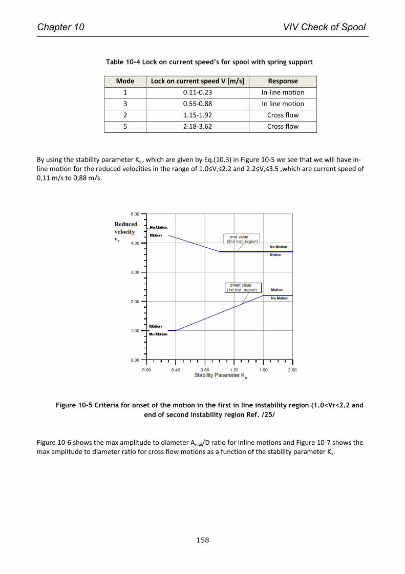
Chapter 10 VIV Check of Spool
158
Table 10-4 Lock on current speed’s for spool with spring support
Mode Lock on current speed V [m/s] Response
1 0.11-0.23 In-line motion
3 0.55-0.88 In line motion
2 1.15-1.92 Cross flow
5 2.18-3.62 Cross flow
By using the stability parameter Ks , which are given by Eq.(10.3) in Figure 10-5 we see that we will have in-line motion for the reduced velocities in the range of 1.0≤Vr≤2.2 and 2.2≤Vr≤3.5 ,which are current speed of 0,11 m/s to 0,88 m/s.
Figure 10-5 Criteria for onset of the motion in the first in line instability region (1.0<Vr<2.2 and
end of second instability region Ref. /25/
Figure 10-6 shows the max amplitude to diameter Ampl/D ratio for inline motions and Figure 10-7 shows the max amplitude to diameter ratio for cross flow motions as a function of the stability parameter Ks.
Chapter 10 VIV Check of Spool
159
Figure 10-6 Amplitude of in-line motion as a function of Ks Ref. /25/
Figure 10-7 Amplitude of crossflow motions as functions of Ks Ref. /25/
Figure 10-7 has a mode shape parameter g in the denominator of the amplitude ratio this value is listed in
table 7.2 of Ref. /25/ for some typical structural elements. As seen from the figures above the cross flow
motion gives the highest amplitude ratios.

Chapter 10 VIV Check of Spool
160
10.4 Fatigue
So by applying this in a simplified fatigue evaluation of the spool due to VIV inline motion we get the
following relation from Figure 10-7 with Ks=0.17 we get the following amplification ratio:
𝐴𝑀𝑃𝐿1
𝐷≈ 0.14 (10.8)
𝐴𝑀𝑃𝐿2
𝐷≈ 0.11 (10.9)
Where D=0.168m
The amplitude then becomes:
𝐴𝑀𝑃𝐿1 = 0.14 ∙ 0.168𝑚 = 0.024𝑚𝑓𝑜𝑟1.0 ≤ Vr ≤ 2.2
And:
𝐴𝑀𝑃𝐿2 = 0.11 ∙ 0.168𝑚 = 0.018𝑚𝑓𝑜𝑟2.2 ≤ Vr ≤ 3.5
The annual distribution and the current direction is assumed to be omnidirectional this means that the
current is likely to come from all directions. The onset for VIV in line motion will be for all currents in the
range of 0.11-0.23 m/s and 0.55-0.88 m/s with different onset frequencies. Table 10-5 shows the percent
occurrence for these currents and is from based upon values from a deep water project.
Table 10-5 Current velocities percent occurrence
Current speed
[m/s]
Percent occurrence
[%] 0.1 16
0.2 33
0.3 29
0.4 16
0.5 5
0.6 0.75
0.7 0.14
0.8 0.11
Chapter 10 VIV Check of Spool
161
The number of stress cycles can be taken as:
𝑛 = 𝑓𝑟𝑒𝑞𝑢𝑒𝑛𝑐𝑦 ∙𝑠𝑒𝑐
ℎ𝑜𝑢𝑟∙ ℎ𝑜𝑢𝑟𝑠 ∙ 𝑑𝑎𝑦𝑠 ∙
𝑝𝑟𝑜𝑏𝑎𝑏𝑖𝑙𝑙𝑖𝑡𝑦 ∙ 𝑦𝑒𝑎𝑟𝑠
𝑦𝑒𝑎𝑟 (10.10)
For the first onset with f=0.61 Hz which is in range of 0 m/s to 0.2 m/s the number of cycles then becomes:
𝑛1 = 0.61 ∙ 3600 ∙ 24 ∙ 365 ∙ (0.16 + 0.33) ∙ 25 = 2.4𝐸8
And for the second frequency f=1.5 Hz and in the current is in the range of 0.55-0.88 m/s with a limit of max
0.7 m/s is:
𝑛2 = 1.5 ∙ 3600 ∙ 24 ∙ 365 ∙ (0.05 + 0.0075 + 0.0014) ∙ 25 = 2.8𝐸7
To get the stress amplitude, the spool has been analysed with a unit displacement of 1 meter at mid span
(leg 4) and at the top of the spool (leg2) see Figure 10-8 and Figure 10-9 with fixed constraints at the ends
and zero pressure and temperature.
Max principal stress amplitude for the two conditions then becomes by multiplying with the amplitude from
Eq.(10.8):
𝜎1 =𝑀𝑎𝑥𝑠𝑡𝑟𝑒𝑠𝑠
1𝑢𝑛𝑖𝑡𝑚𝑒𝑡𝑒𝑟𝑑𝑖𝑠𝑝𝑙𝑎𝑐𝑒𝑚𝑒𝑛𝑡∙ 𝐴𝑀𝑃𝑙1 = 1573 ∙ 0.024 = 38𝑀𝑃𝑎
𝜎2 =𝑀𝑎𝑥𝑠𝑡𝑟𝑒𝑠𝑠
1𝑢𝑛𝑖𝑡𝑚𝑒𝑡𝑒𝑟𝑑𝑖𝑠𝑝𝑙𝑎𝑐𝑒𝑚𝑒𝑛𝑡∙ 𝐴𝑀𝑃𝑙2 = 605 ∙ 0.018 = 11𝑀𝑃𝑎
So max stress range then becomes:
∆𝜎1 = 2𝜎1 = 76𝑀𝑃𝑎
∆𝜎2 = 2𝜎2 = 22𝑀𝑃𝑎
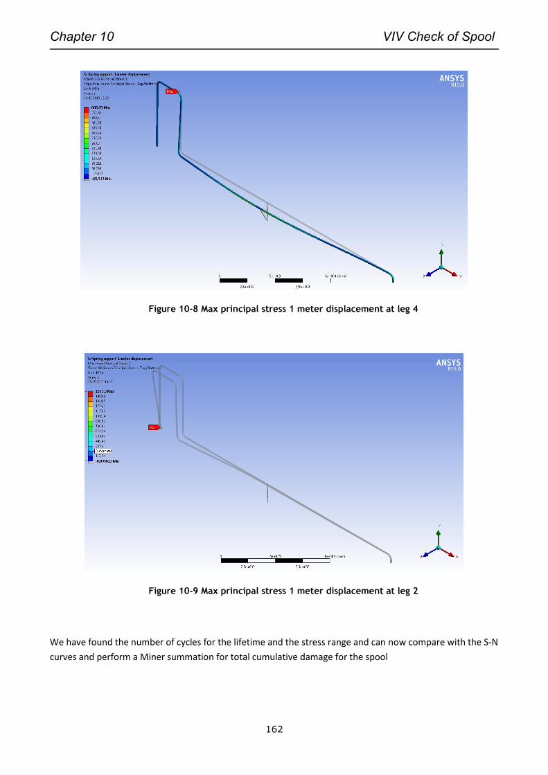
Chapter 10 VIV Check of Spool
162
Figure 10-8 Max principal stress 1 meter displacement at leg 4
Figure 10-9 Max principal stress 1 meter displacement at leg 2
We have found the number of cycles for the lifetime and the stress range and can now compare with the S-N
curves and perform a Miner summation for total cumulative damage for the spool
Chapter 10 VIV Check of Spool
163
The fatigue life is based upon the S-N curves presented in DNV-RP-C203 Ref. /14/ section 2.2.
𝐷 = ∑𝑛𝑖
𝑁𝑖
𝑘
𝑖=1
=1
�̅�∑𝑛𝑖 ∙ (∆𝜎𝑖)
𝑚
𝑘
𝑖=1
≤ 𝜂 (10.11)
Where:
D= Accumulated fatigue damage
ā = Intercept of the design SN-curve with the log N axis
m= negative inverse slope of the S-N curve
k=number of stress blocks
ni= number of stress cycles in stress block 1
Ni= number of cycles to failure at constant stress range ∆σi
η= usage factor , =1/ Design Fatigue Factor (DFF)
The DFF is set equal to 10 based upon a high risk classification as given in DNV –OS-F101.
The total accumulated fatigue damage D is calculated in appendix A 3.5. The calculation shows that D=19>>
greater than 1/10, and hence the spool does not have sufficient fatigue capacity for the 25 year lifetime.
VIV suppression strakes or other aids are required for the spool. The reason for failure is the long free span
of the spool which is very sensitive to in line 1st mode VIV motion. Hence the vertical support should also
have lateral support in order to minimize these effects.
10.5 Summary
In this chapter a VIV check have been performed based upon a modal analysis in ANSYS. The spool have
been checked for different cases of support types such as a spring located at the centre of leg 4 and by use
of buoyancy elements. The results show that the vertical spring support had a positive effect on the cross
flow response of the spool for leg 4. The eigenvalues was increased and hence the spool became less
sensitive to this motion the vibrations was also damped out for higher modes. For the inline motion there
were minimal effects of the support and buoyancy. The spool was checked for a fatigue lifetime of 25years
and the results shows that the spool does not have sufficient capacity. Mitigation measures such as VIV
suppression strakes must be included on the spool and the effect of this must be checked by new
calculations.

Chapter 10 VIV Check of Spool
164
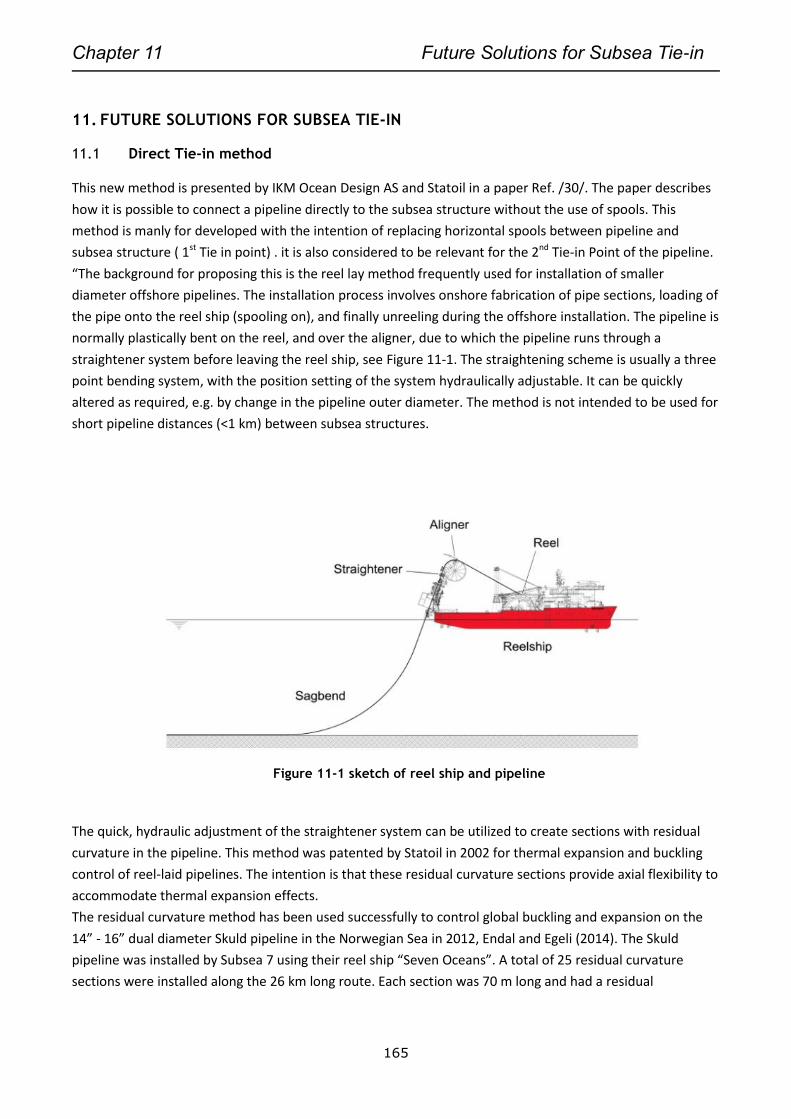
Chapter 11 Future Solutions for Subsea Tie-in
165
11. FUTURE SOLUTIONS FOR SUBSEA TIE-IN
11.1 Direct Tie-in method
This new method is presented by IKM Ocean Design AS and Statoil in a paper Ref. /30/. The paper describes
how it is possible to connect a pipeline directly to the subsea structure without the use of spools. This
method is manly for developed with the intention of replacing horizontal spools between pipeline and
subsea structure ( 1st Tie in point) . it is also considered to be relevant for the 2nd Tie-in Point of the pipeline.
“The background for proposing this is the reel lay method frequently used for installation of smaller
diameter offshore pipelines. The installation process involves onshore fabrication of pipe sections, loading of
the pipe onto the reel ship (spooling on), and finally unreeling during the offshore installation. The pipeline is
normally plastically bent on the reel, and over the aligner, due to which the pipeline runs through a
straightener system before leaving the reel ship, see Figure 11-1. The straightening scheme is usually a three
point bending system, with the position setting of the system hydraulically adjustable. It can be quickly
altered as required, e.g. by change in the pipeline outer diameter. The method is not intended to be used for
short pipeline distances (<1 km) between subsea structures.
Figure 11-1 sketch of reel ship and pipeline
The quick, hydraulic adjustment of the straightener system can be utilized to create sections with residual
curvature in the pipeline. This method was patented by Statoil in 2002 for thermal expansion and buckling
control of reel-laid pipelines. The intention is that these residual curvature sections provide axial flexibility to
accommodate thermal expansion effects.
The residual curvature method has been used successfully to control global buckling and expansion on the
14” - 16” dual diameter Skuld pipeline in the Norwegian Sea in 2012, Endal and Egeli (2014). The Skuld
pipeline was installed by Subsea 7 using their reel ship “Seven Oceans”. A total of 25 residual curvature
sections were installed along the 26 km long route. Each section was 70 m long and had a residual

Chapter 11 Future Solutions for Subsea Tie-in
166
strain of approximately 0.2%. Figure 11-2shows the as-laid survey data from two of these sections (KP 13.1
and 15.1).”
Figure 11-2 Typical Skuld Pipeline residual curvature sections
“In addition to showing the effectiveness of the method with regards to controlling global buckling, the Skuld
project also demonstrated its installation friendliness.
General: The new direct tie-in method presented herein utilizes the reel-lay installation method to create
local residual curvature in the pipeline, By installing such “prebent” sections at or close to the end of the
pipeline, direct tie-in may be enabled without the need for tie-in spools or large start-up/lay-down areas
while still achieving acceptably low tie-in and connection forces. It is believed that this approach has the
potential to enable many more tie-ins by direct connection, hence permitting large cost and schedule
savings for subsea development projects as separate spools or flexible jumpers become superfluous.
The same axial and lateral flexibility utilized for direct tie-in will be even more efficient when it comes to
absorbing and controlling expansion forces/movements caused by pressure and temperature loads during
the operating condition. In fact, pipeline expansion effects can be seen to neutralize the tie-in forces
remaining in the system.
Advantages of the technique are considered to be:
A residual curvature section can be quickly installed. Reference is made to the Skuld project where
25 pre-bent sections where installed with an average installation time of 10-20 minutes per location,
Endal et al (2014).
No straightening trials were found required, Endal et al (2014)
Is considered a robust method even if residual strains vary.
It will provide the means to efficiently reduce expansion forces for existing direct tie-in methods as
well as spool tie-ins.
Figure 11-3 below shows the concept with implementing “tie-in and expansion loop” as an integrated part of
the pipeline end section. 0.2 % to 0.3 % residual curvature strain can efficiently be created in the “tie-in and
expansion loop” sections using the straightener system on the reel ship during installation.
Buoyancy and/or additional weight should be considered installed on or close to the pipeline end to ensure
adequate rotation of the “tie-in and expansion loop”, if required.”

Chapter 11 Future Solutions for Subsea Tie-in
167
Figure 11-3 First End Direct Tie-in using the Residual Curvature Method
“A direct tie-in using the residual curvature method is considered to have more advantages at the pipelay
initiation end ( 1st tie-in) compared to the second end. At the first end, the pipeline
can for instance be initiated against a return sheave arrangement on the subsea structure an
lowered/docked in a controlled manner onto a guide post/landing frame etc. depending on the tie-in system
being employed, see Figure 11-4 The residual curvature section is introduced approximately 100 m away
from the pipeline end
Figure 11-4 First End Direct Tie-in-Initiation overview
Hub capacity is often seen to be a governing factor for pipeline tie-ins using diver-less systems. Since hubs on subsea templates typically could be elevated 2.5 m above the seabed floor, vertical alignment between pipeline end and the hub is a key parameter. In order to compensate for this, the hub can typically be tilted slightly downwards, say 3°, 5° or 7°. However, further vertical alignment will in many cases be needed. This has on several projects been solved by introducing rock supports or adjustable mechanical supports in the adjacent free span. After the pipeline is pulled down and safely landed in the tie-in porch/landing frame, the pipeline is ready for the final stroke-in and finally the clamp connector is made up and the seal can be tested”.
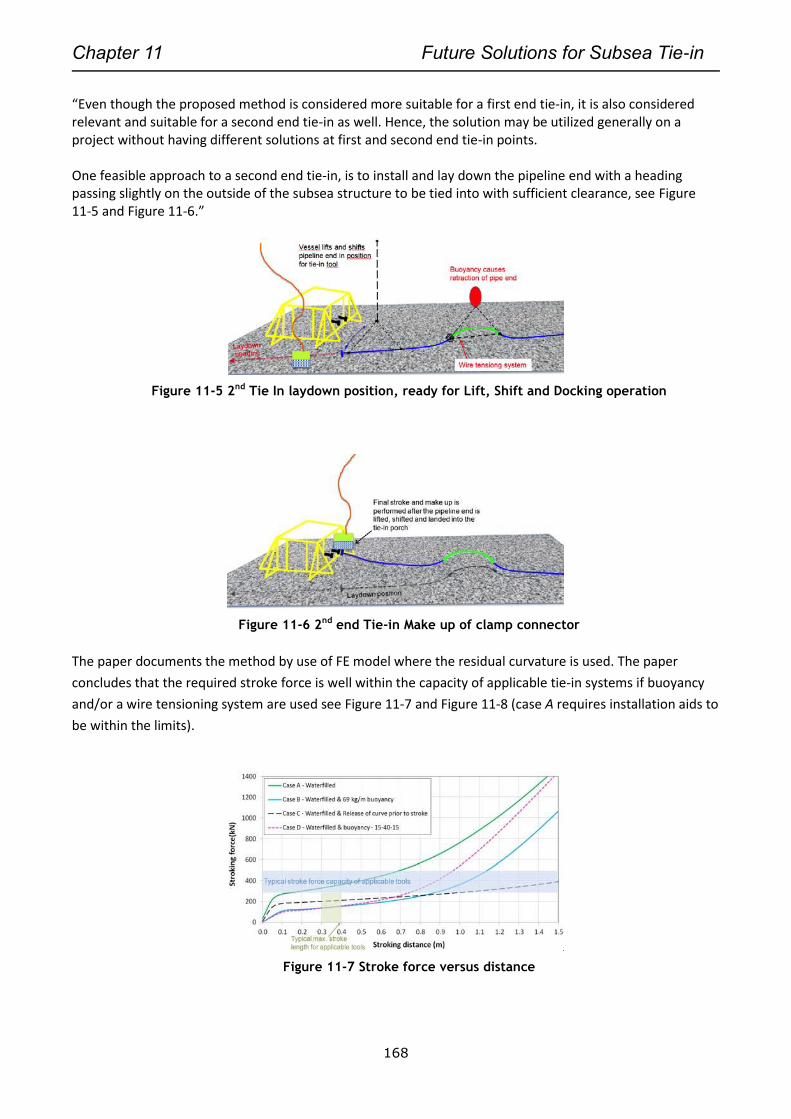
Chapter 11 Future Solutions for Subsea Tie-in
168
“Even though the proposed method is considered more suitable for a first end tie-in, it is also considered relevant and suitable for a second end tie-in as well. Hence, the solution may be utilized generally on a project without having different solutions at first and second end tie-in points. One feasible approach to a second end tie-in, is to install and lay down the pipeline end with a heading passing slightly on the outside of the subsea structure to be tied into with sufficient clearance, see Figure 11-5 and Figure 11-6.”
Figure 11-5 2nd Tie In laydown position, ready for Lift, Shift and Docking operation
Figure 11-6 2nd end Tie-in Make up of clamp connector
The paper documents the method by use of FE model where the residual curvature is used. The paper
concludes that the required stroke force is well within the capacity of applicable tie-in systems if buoyancy
and/or a wire tensioning system are used see Figure 11-7 and Figure 11-8 (case A requires installation aids to
be within the limits).
Figure 11-7 Stroke force versus distance
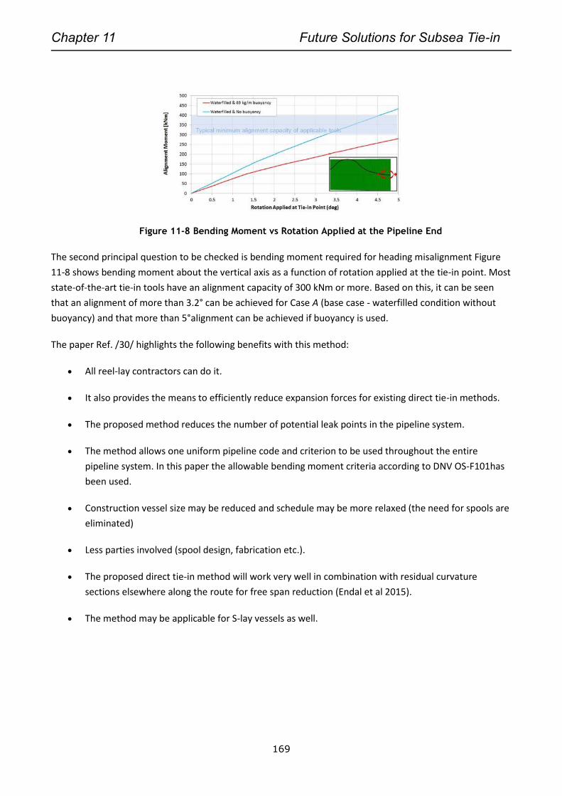
Chapter 11 Future Solutions for Subsea Tie-in
169
Figure 11-8 Bending Moment vs Rotation Applied at the Pipeline End
The second principal question to be checked is bending moment required for heading misalignment Figure
11-8 shows bending moment about the vertical axis as a function of rotation applied at the tie-in point. Most
state-of-the-art tie-in tools have an alignment capacity of 300 kNm or more. Based on this, it can be seen
that an alignment of more than 3.2° can be achieved for Case A (base case - waterfilled condition without
buoyancy) and that more than 5°alignment can be achieved if buoyancy is used.
The paper Ref. /30/ highlights the following benefits with this method:
All reel-lay contractors can do it.
It also provides the means to efficiently reduce expansion forces for existing direct tie-in methods.
The proposed method reduces the number of potential leak points in the pipeline system.
The method allows one uniform pipeline code and criterion to be used throughout the entire
pipeline system. In this paper the allowable bending moment criteria according to DNV OS-F101has
been used.
Construction vessel size may be reduced and schedule may be more relaxed (the need for spools are
eliminated)
Less parties involved (spool design, fabrication etc.).
The proposed direct tie-in method will work very well in combination with residual curvature
sections elsewhere along the route for free span reduction (Endal et al 2015).
The method may be applicable for S-lay vessels as well.
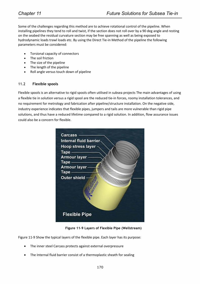
Chapter 11 Future Solutions for Subsea Tie-in
170
Some of the challenges regarding this method are to achieve rotational control of the pipeline. When installing pipelines they tend to roll and twist, if the section does not roll over by a 90 deg angle and resting on the seabed the residual curvature section may be free spanning as well as being exposed to hydrodynamic loads trawl loads etc. By using the Direct Tie-in Method of the pipeline the following parameters must be considered:
Torsional capacity of connectors The soil friction The size of the pipeline The length of the pipeline Roll angle versus touch down of pipeline
11.2 Flexible spools
Flexible spools is an alternative to rigid spools often utilised in subsea projects The main advantages of using
a flexible tie in solution versus a rigid spool are the reduced tie-in forces, roomy installation tolerances, and
no requirement for metrology and fabrication after pipeline/structure installation. On the negative side,
industry experience indicates that flexible pipes, jumpers and tails are more vulnerable than rigid pipe
solutions, and thus have a reduced lifetime compared to a rigid solution. In addition, flow assurance issues
could also be a concern for flexible.
Figure 11-9 Layers of Flexible Pipe (Wellstream)
Figure 11-9 Show the typical layers of the flexible pipe. Each layer has its purpose:
The inner steel Carcass protects against external overpressure
The Internal fluid barrier consist of a thermoplastic sheath for sealing
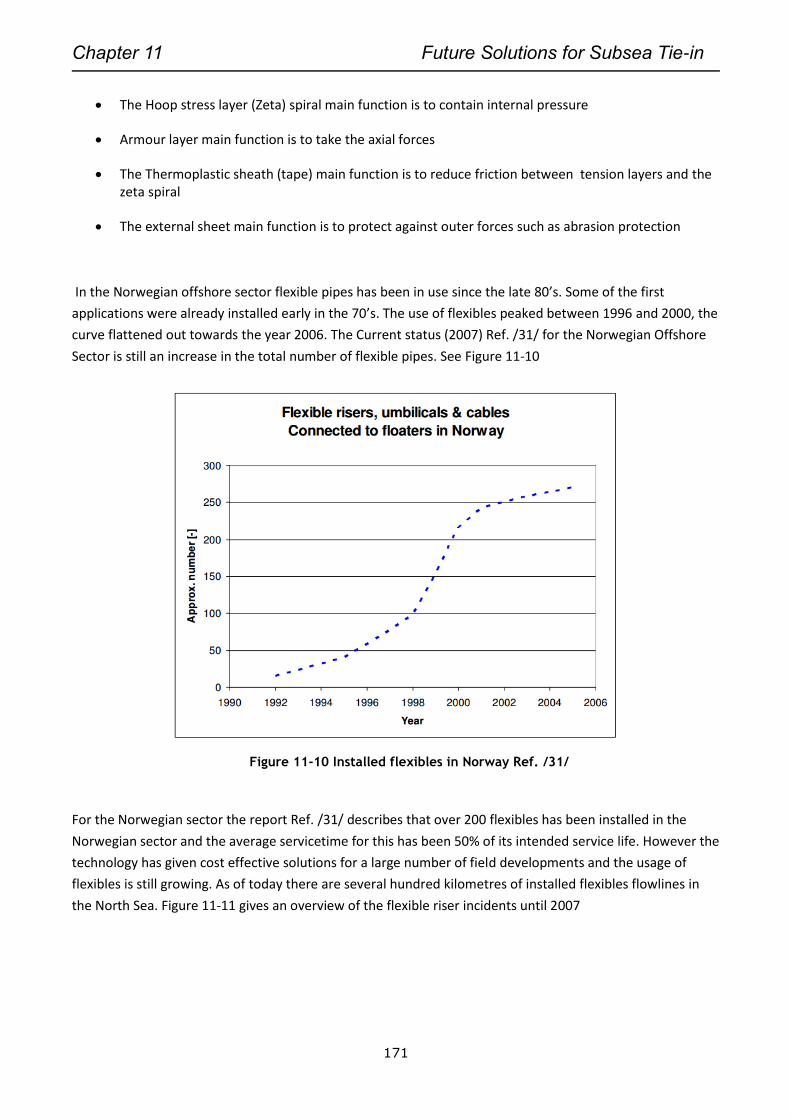
Chapter 11 Future Solutions for Subsea Tie-in
171
The Hoop stress layer (Zeta) spiral main function is to contain internal pressure
Armour layer main function is to take the axial forces
The Thermoplastic sheath (tape) main function is to reduce friction between tension layers and the zeta spiral
The external sheet main function is to protect against outer forces such as abrasion protection
In the Norwegian offshore sector flexible pipes has been in use since the late 80’s. Some of the first
applications were already installed early in the 70’s. The use of flexibles peaked between 1996 and 2000, the
curve flattened out towards the year 2006. The Current status (2007) Ref. /31/ for the Norwegian Offshore
Sector is still an increase in the total number of flexible pipes. See Figure 11-10
Figure 11-10 Installed flexibles in Norway Ref. /31/
For the Norwegian sector the report Ref. /31/ describes that over 200 flexibles has been installed in the
Norwegian sector and the average servicetime for this has been 50% of its intended service life. However the
technology has given cost effective solutions for a large number of field developments and the usage of
flexibles is still growing. As of today there are several hundred kilometres of installed flexibles flowlines in
the North Sea. Figure 11-11 gives an overview of the flexible riser incidents until 2007
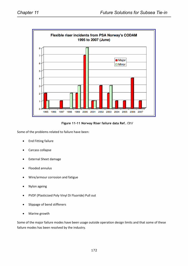
Chapter 11 Future Solutions for Subsea Tie-in
172
Figure 11-11 Norway Riser failure data Ref. /31/
Some of the problems related to failure have been:
End Fitting failure
Carcass collapse
External Sheet damage
Flooded annulus
Wire/armour corrosion and fatigue
Nylon ageing
PVDF (Plasticized Poly Vinyl Di Fluoride) Pull out
Slippage of bend stiffeners
Marine growth
Some of the major failure modes have been usage outside operation design limits and that some of these
failure modes has been resolved by the industry.
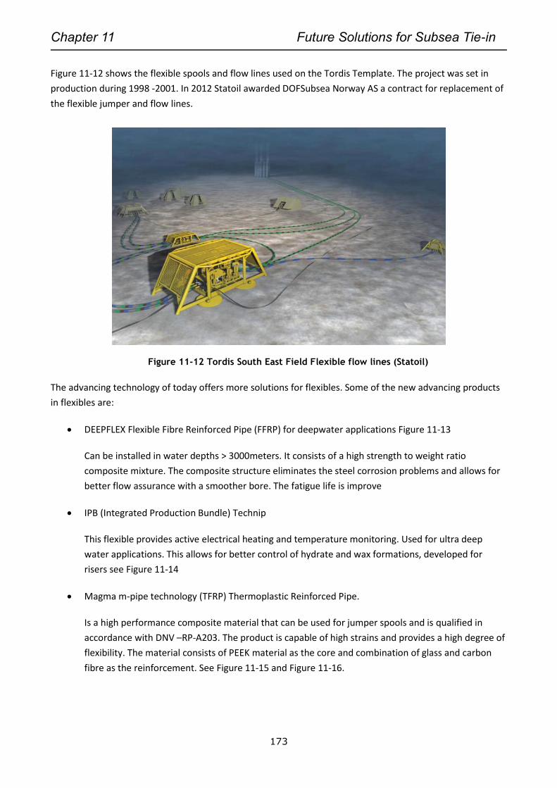
Chapter 11 Future Solutions for Subsea Tie-in
173
Figure 11-12 shows the flexible spools and flow lines used on the Tordis Template. The project was set in
production during 1998 -2001. In 2012 Statoil awarded DOFSubsea Norway AS a contract for replacement of
the flexible jumper and flow lines.
Figure 11-12 Tordis South East Field Flexible flow lines (Statoil)
The advancing technology of today offers more solutions for flexibles. Some of the new advancing products
in flexibles are:
DEEPFLEX Flexible Fibre Reinforced Pipe (FFRP) for deepwater applications Figure 11-13
Can be installed in water depths > 3000meters. It consists of a high strength to weight ratio
composite mixture. The composite structure eliminates the steel corrosion problems and allows for
better flow assurance with a smoother bore. The fatigue life is improve
IPB (Integrated Production Bundle) Technip
This flexible provides active electrical heating and temperature monitoring. Used for ultra deep
water applications. This allows for better control of hydrate and wax formations, developed for
risers see Figure 11-14
Magma m-pipe technology (TFRP) Thermoplastic Reinforced Pipe.
Is a high performance composite material that can be used for jumper spools and is qualified in
accordance with DNV –RP-A203. The product is capable of high strains and provides a high degree of
flexibility. The material consists of PEEK material as the core and combination of glass and carbon
fibre as the reinforcement. See Figure 11-15 and Figure 11-16.

Chapter 11 Future Solutions for Subsea Tie-in
174
Figure 11-13 Multilayer Composite flexible (DEEPFLEX)
Figure 11-14 IPB Flexible With heat tracing and gas lift (Technip)
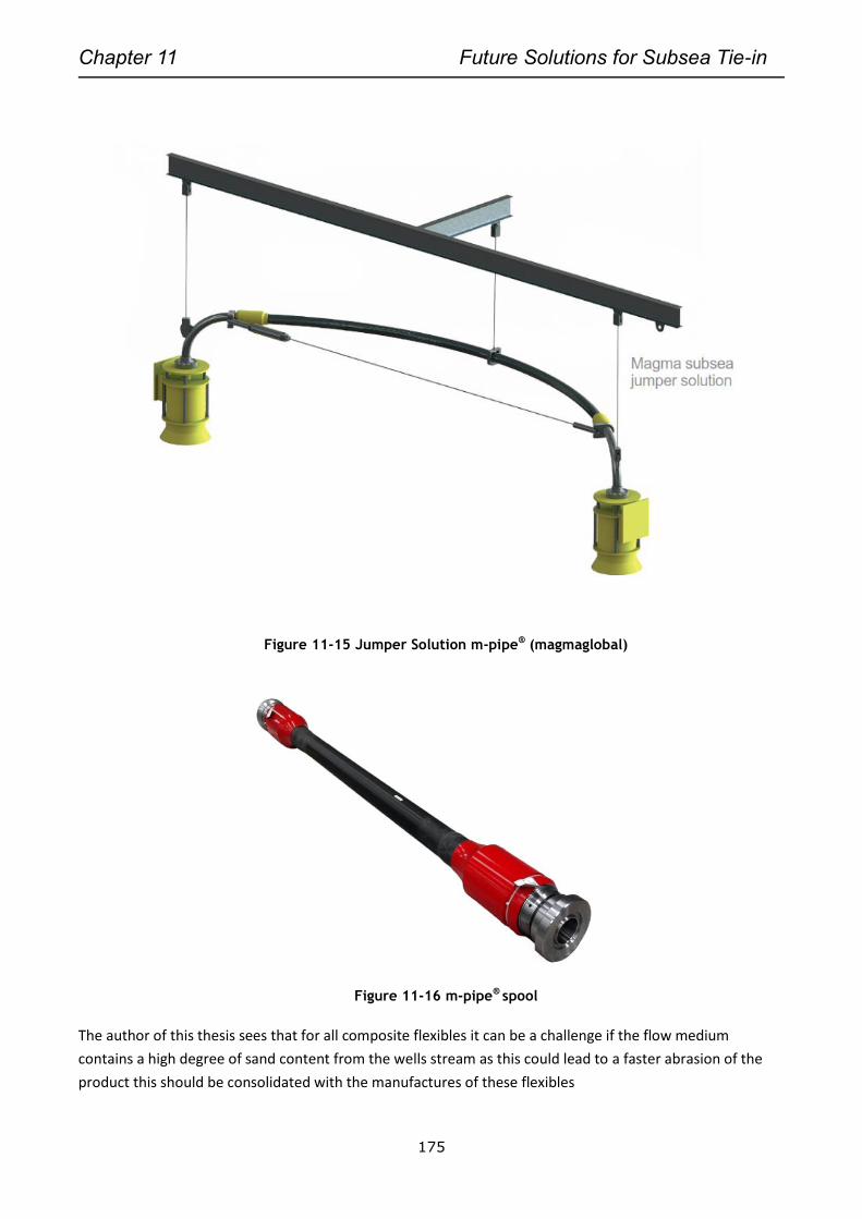
Chapter 11 Future Solutions for Subsea Tie-in
175
Figure 11-15 Jumper Solution m-pipe® (magmaglobal)
Figure 11-16 m-pipe® spool
The author of this thesis sees that for all composite flexibles it can be a challenge if the flow medium
contains a high degree of sand content from the wells stream as this could lead to a faster abrasion of the
product this should be consolidated with the manufactures of these flexibles
Chapter 11 Future Solutions for Subsea Tie-in
176
11.3 Design Concept Ideas
During the writing of this thesis some ideas regarding the improvement in the spool design has been proposed. Some of these concepts are:
Introduction of a flexible joint at each end of a rigid spool
This could potentially reduce the requirement for high flexibility and number bends in a rigid spool due to less dependent upon metrology and manufacturing tolerances.
Pre-bending of spools by weld mitigation Ref. chapters 9.3
This method is simple and reduces reaction forces at each end
Develop lighter buoyancy material for deep water applications
The buoyancy material used today is ~ ½ the density and of water and hence this causes the load mitigation aid to growth in diameter size due to increased submerged volume, this can give potential VIV issues for free span. By exploring the collapse limits for these materials or similar materials mixtures in order to optimize the density will benefit the spool design. The cost for buoyancy material may be reduced
Introduce a spring seabed support
This method is utilised in topside process piping and reduces stresses bending moments and can have positive effects on VIV sensitivity. Ref. Chapter 9.2.
Integrate flexibles on reel’s as part of subsea structures
The idea is that an integrated flexible can be a part of the subsea structure. (It is the same principle as the house garden hose). This allows for installation cost savings. The principle is that the ROV only needs to perform a 1st Tie in operation to the other structure as the flexible is already connected and the ROV is basically flying out the other end to the tie-in point
Integrate spool production facility and testing on board a pipe lay or installation vessels at regions in the world where there is lack of infrastructure for high quality pipe production. This could potentially save installation and transportation cost.
Use of tension wires anchored to the sea bed can possibly reduce VIV effects for in-line motion
Development of hybrid solutions between rigid and flexibles
Chapter 12 Summary, Conclusion and Recommendations
177
12. SUMMARY, CONCLUSION AND RECOMMENDATIONS
12.1 Summary
In this thesis subsea Tie-in systems and spools used in the oil and gas market is studied. The purpose of this
thesis was to explore the standard solutions used today and identify some of the main challenges regarding
engineering of subsea Tie-in Spools. The other purpose was to perform strength verification of a spool by use
of FEA. The study also explored and compared different computer software used in piping design. Another
objective of the thesis is to propose possible new solutions and recommendations for Tie-in spool projects.
An executive summary of the results is given here.
Tie-in Spool systems:
The study identified a variety of shapes and types used for spool design. When selecting and designing a Tie
in system there are many considerations to be taken. A Pre-Study of the planned project is advisable to
commence in order to determine the best spool design. The Pre-study or FEED should focus on the following
key topics:
Subsea routing and location of spool
Spool type
Installation time and constraints
Use conservative data, previous experience is important
Define optimum spool lengths (minimum and maximum)
Identify critical values early in the project small changes can give rise to high cost later in project
For the North-Sea region most of the spools used today is of the horizontal type. Vertical spool type is most
common for deepwater applications not exposed to risk of snagging or overtrawling. In this thesis industry
experience is collected from publications and parent company. The evaluation shows that vertical spools are
classified as high risk towards connector load capacity, increased complexity due to free span, can be
sensitive to snagging, possible high risk for seal damage, and it can be difficult to perform pigging operations.
For horizontal spools the limitation is as for vertical spools for the connector capacity towards bending
moments and forces. However the spools are considered to have an overall lower risk compared with
vertical spools. It is worth mention here that horizontals spools normally require longer offshore installation
time and can give higher project costs.
Probabilistic assessment of fabrication tolerances and metrology used in spool design:
In this thesis the effect of fabrication, metrology tolerances and deformations is studied by use of ANSYS
design explorer and the six sigma probabilistic tool. The statistical distribution of these effects has been
discussed in chapters 3 and 7. Publications and recommendations on the topic have also been reviewed and
discussed. The results in this thesis shows that the probability of reaching high stress levels due to the
fabrication and metrology tolerance is very low given a normal statistical distribution for the variables and a
uniform distribution for the displacements. It is assumed that there is a 95% probability of hitting the max
and minimum angular tolerances with a 100% dimensional control. The analysis shows that the probability of
reaching stress levels above the code allowable limits is equal or less to 10-4 (0.01%) or 1/10000 events (high
Chapter 12 Summary, Conclusion and Recommendations
178
sigma level). However the sensitivity analysis shows that the spool response is sensitive to small changes in
the tolerance and displacement values and the response is of a non-linear character. Hence this must also be
considered when addressing the required safety levels for the spool design.
For the piping analysis it is advisable to incorporate a statistical tool for assessing the fabrication tolerances
in order to establish a reasonable safety level in-line with the code requirements. One question is on how
the project should handle the standard deviation based upon the critically of the system i.e. should the level
be in the range 1.65 - 3 times the standard deviation. How will the probability of exceedance be quantified
(5% or 10%)? Most of the analyzed spools today are based upon “worst case” scenario which is a very rare
event but should perhaps be analyzed with the most probably expected tolerances and loading. Different
techniques for random probabilistic and parameter correlation effects are available and can be included in
simulation software (Monte Carlo simulation is one example)
The benefit of using the engineering tool ANSYS Design Explorer is that it is easier for projects to quantify the
uncertainty and do an optimisation decision based on a better understanding of the results. Another benefit
is that the tool also allows for “what if studies” .The ANSYS Design Explorer tool is user friendly and requires
lesser time compared to performing tedious computer programming. This can contribute to a better quality
check of the engineering work, since computer scripting is often performed by one engineer and can be a
source of human errors.
FEA software comparison:
The traditional way of analysing subsea spools by use of the recently new ANSYS Pipe elements PIPE
288, 289 and ELBOW 290 is shown to be feasible for usage in designing spools, however in some cases it
seems that max equivalent stress reported can differ in the location compared to other computer software
and solid element models. The reason is not clear it could be that the ANSYS pipe elements reports higher
stresses at bend locations due to sharp curvature or radius in pipe bends and that there is less flexibility in
ELBOW290. Here it is advisable to study more comparative models in order to conclude. If the location is
regarded as critical it is advisable to perform a finite element analysis using solid elements, fabrication
tolerances and weld should be included in the analysis. The analysis also shows that use of shell elements in
the finite element model of the spool can lead to underestimation of the reported stress levels.
The AutoPIPE software usage is proven to be a good alternative for analysis of vertical spools the results are
slightly more conservative and gives higher stress and utilisations compared to the ANSYS beam elements.
The benefit of the software is that is very versatile to use for design code checks and it is by far superior to
ANSYS when it comes to analysis time and design changes. In addition the user of the software is “forced” to
learn the code and pipe fabrication more in depth by using this type of software. The minor side is that it
does not seems to be suitable for strain based criteria’s as given in the DNV-OS-F101Pipeline codes and for
large non-linear displacements which is often used in horizontal spool design.
For the vertical spools check which was based upon the ASD criteria the utilisation towards the code stress
limits has a good match between all computer models except for the ANSYS shell model which seems to
underreport the stress levels.
Chapter 12 Summary, Conclusion and Recommendations
179
Results from strength verification of vertical Tie-in spool
The vertical spool has been checked for the hydro testing operational and seal replacement load case. The
analysis shows that the spool is utilised above the code stress limit in corroded condition with a max
utilisation of 109% using the AutoPIPE piping analysis software and max utilisation of 107% using the ANSYS
FEA software. The utilisation is largely influenced by the ASME B31.8 longitudinal stress limit criteria. The
spool also fails for the minimum fatigue criteria for flexibility stress as given in the ASME B31.8 code. The
spool however passes the ASME B31.8 Code check for the nominal wall thickness of the pipe, here max
utilisation is 94% for the sustained load case and GR+T(2)+P(2).
For the VIV and fatigue check the spool fails even with a vertical support and the accumulated damage is
calculated to D=19>> greater than fatigue limit of 1/10, and hence the spool does not have sufficient fatigue
capacity for the 25 year lifetime. The vertical support has a positive effect for the cross flow motion on leg 4
of the spool and the vibrations are damped out for higher modes. However since the VIV is dominated by in-
line motion, a possible seabed support must also include lateral support in order to reduce this motion. The
spool will require mitigation measures such as VIV suppression strakes which must be included on the spool
and the effect of this must be checked by new calculations and analysis. The spool is sensitive due to its long
free span.
Results from load mitigation study
The result shows that by using a seabed support or a buoyancy element reduces the stresses in the spool by
25%. The largest effect was the reduction of bending moment at the XT end with 76% reduction. Hence this
gave the best results. The pre-bending of the spool has a positive effect on the bending moments with a
decrease of 30% for the bending moment on the XT tree side, but the utilisation for stresses at the manifold
side was not largely effected in fact the stresses increased slightly by around~6%. The results are given in
Table 9-8.
Future solutions for Subsea Tie-in
The subsea industry and the market have challenges due to a considerable drop in the oil prises. The
industry has a large focus on how to reduce installation and development costs for future subsea oil and gas
fields. An overview of alternative solutions which has potential to reduce cost is given in chapter 11. Direct
Tie-in method for connection pipelines directly to subsea structures without the use of flow line spools is
one example. New development of better materials and flexibles spools for smaller pipe sizes is also belived
to enter the market in a larger scale. Rigid spools will however be a part of the industry for a long time due
to its proven field of record and durability. The new tie-in Systems is less complex than the old ones and this
should contribute to reduce costs. In this thesis simple measures which are adopted from the industry is
proposed in order to reduce loading on vertical connectors and spool. Some conceptual ideas are presented
which is believed to have a possibility of reducing the engineering, fabrication and installation scope such as
Chapter 12 Summary, Conclusion and Recommendations
180
using flexible joints in spool design, this could reduce the sensitivity for angular tolerance deviations. This
would again minimize subsea metrology and survey requirements.
12.2 Conclusion
Subsea spool design projects involve many tasks and considerations. It is important that issues related to the
life time cycle of the spools is understood and mapped. Each phase from project concept to end of life time
for the spool must be taken into consideration. The work requires in depth knowledge of spool design and
fabrication methods from the project members.
In this thesis a vertical spool has been analysed with a statistical and probabilistic approach for the
metrology and tolerances, the results shows that it is beneficial to include such method in order to better
document the safety level and the conservatism in the spool design. The approach also allows the engineer
to make a better decision towards the optimisation process. The ANSYS Design Explorer used in this thesis
uses an algorithm for the parametric variations. The software tool generates many possible load
combinations and gives output results based upon a statistical distribution of the input values. This results in
a faster analysis time. Another positive feature is that it is capable to perform “what if analysis” for many
design options and variations.
Other applicable software analysis program is also feasible to use such as the AutoPIPE software from
Bentley. The difference compared to ANSYS is small when it comes to piping design using beam element
technology and formulas found in a piping code such as the ASME B31.8 Ref. /15/.For a more optimised
spool design approach ANSYS solid element modelling is found to give less conservative results. The
AutoPIPE does not have the capability for strain based LRFD design according to DNV pipeline code Ref. /7/;
hence this also limits the possibility for further optimisation work. Another limitation is the software
capability to perform large non-linear displacements which is often the case for horizontal spools which relay
on stroking capability, however the software has an advantage when it comes to linking the engineering
process and the requirements given in the piping code, the software may be used in an early screening
process prior to a more optimised work by use of ANSYS.
Vertical spools have a more challenging design and gives larger engineering and fabrication scope since there
are many more considerations to be taken. This gives a higher risk level compared to horizontal spools. The
vertical spools have had a traditional advantage that they can be installed faster than horizontal spool and
require less deck space which influences the total vessel time used in an offshore campaign. When it comes
to installation time subsea this might not be true for the recently developed horizontal spool connectors, as
they have become much simpler and would logically give less subsea installation time. Documentation
regarding this has not been available and can be difficult to retrieve. An economical and technical analysis of
each system prior to a subsea field development is recommended.
The thesis also shows that simple mitigation measures for a vertical spool such as pre-bending and
introduction of a seabed support and buoyancy onto the spool has positive effects by reducing the resulting
bending moments at connector ends, and can reduce the total stresses in the spool. The result also shows
that vertical spool design is very sensitive to VIV, and hence fatigue capacity governs the design.
Chapter 12 Summary, Conclusion and Recommendations
181
12.3 Recommendations
For future subsea projects involving spool design the following practice is recommended for the design work and optimisation process.
Develop design basis
Use conservative data, previous experience is important
Identify critical values early in the project small changes can give rise to high cost later in project
Determine which FEA software is most applicable for usage regarding spool design
Use pipe beam element technology as far as possible this reduces the amount of analysis time. For a more optimised and requirement for detailed analysis of the spool, design solid element modelling is recommended.
Implement a statistical and a probabilistic tool (such as ANSYS design Explorer) for assessing the distribution of tolerances, deflections and metrology, and load combinations.
Perform parameter study and sensitivity study to changes.
The spool should be analysed for the whole life cycle.
Define optimum spool lengths (minimum and maximum)
Perform manual calculations as a benchmark and for checking results
Proposal for future studies:
Development of hybrid solutions between rigid and flexibles
Integrate spool production facility and testing on board a pipe lay or installation vessels at regions in the world where there is lack of infrastructure for high quality pipe production. This could potentially save installation and transportation cost.
Development of lighter or alternative and cheaper buoyancy material for deep water applications
Develop a software tool that integrates DNV OS-F101 LRFD design into an typical piping software such as the AutoPIPE or similar.
Perform further studies for the Direct Tie-in method for pipelines.

References
182
REFERENCES
/1/ Per Richard Nystrøm and Gawain Langford, “Jumper Arch System”, OPT-2002-
03, ABB Offshore systems presented at the Offshore Pipeline Technology
Conference, 2002
/2/ Espen Slettebø, “Tie-in Spools-A verification study”, Master Thesis , Institute of
Offshore Technology and Marine and Subsea Technology, University of
Stavanger,2012
/3/ Jone Lutro ,”Tie-in Jumper System”, Master Thesis , Institute of Offshore
Technology and Offshore Construction, College of Stavanger,2003
/4/ Dr. Phil Hopkins “High Design factor pipelines integrity issues”, Penspen
Integrity, Newcastle upon Tyne UK, Presented at the WTIA Conference
,Wollongong Australia, December2004
/5/ “Subsea Facilities Technology Developments, Incidents and Future Trends”,
2014, DNV-GL Report 2014-0113 Rev. 03, for Petroleumstilsynet
/6/ JP Kenny, “Advanced Deepwater Spools”, Analysis paper presented at OPT 2008
27-02-08
/7/ Submarine Pipeline Systems,DNV-OS-F101, October 2013
/8/ Rita G. Toscano, “Collapse and post-collapse behaviour of steel pipes under
external pressure and bending. Application to deep water pipelines”, Doctoral
Thesis Universidad de Buenos Aires- Facultad de Ingeniería, Argentina ,2009
/9/ Ken Hiroshi and O.Kenko- Waseda,-“Buckling behaviour and design of steel liner
encased in deep water tunnel under external hydrostatic pressure”, Doctoral
Thesis University of Tokyo, 2008
/10/ Andrew C. Palmer and Roger A.King -Subsea Pipeline Engineering. Tulsa
Oklahoma: PennWell Corporation, 2004
/11/ Olav Fyrileiv and Leif Collberg,” Influence of pressure in pipeline design-effective
axial force”, Presented at OMAE2005-67502 ,Det Norske Veritas ,2005
/12/ Sparks C.P, “The Influence of Tension, Pressure and Weight on Pipe and Riser
Deformations and Stresses”, Proceedings of OMAE, 1983.
/13/ Robert D. Cook, David S. Malkus, Michael E. Plesha, Robert J. Witt, Concepts and
Applications of Finite Element Analysis. Madison: John Wiley &Sons,2002
/14/ Fatigue design of Offshore Steel Structures, DNV-RP-C203 ,2011
/15/ Gas Transmission and Distribution Piping Systems, ASME B31.8 , 2012
/16/ Boiler Pressure Vessel Code (BPVC) VIII div 2- Alternative rules, ASME, 2013 and
Section II-D materials , ASME,2007
/17/ Process Piping, ASME B31.3, 2012
/18/ Carlos A. de J. Miranda, Altair A. Faloppa, Miguel Mattar Neto, Gerson Fainer
“ASME Stress linearization and classification-A Discussion Based on a Case
Study” Presented at the International Nuclear Atlantic Conference, INAC 2011

References
183
Brazil, October 24-28, 2011
/19/ Subsea Structures, Manifolds and Choke Modules, Statoil TR1230 Ver.5
/20/ Robert D. Blevins, Flow Induced vibrations second edition, Malabar: Krieger Pub.
,2001
/21/ Lingfu Zeng, Lennart G. Jansson, “On Pipe Elements Currently Available for
Nuclear Power Piping Analysis And Their Benchmark Test”, Presented at ASME
Pressure vessels & Piping Conference , Toronto Ontario Canada ,July 15-19 2012
/22/ G.H. Powell, Phd. Dept. of Structural Engineering, University of California & O.
Ashraf, Msc. Engineering Design Automation, Berkley, California USA
“Nonlinear effects in piping system analysis”, Paper C459/042, Presented at the
IMechE Conference, 1993
/23/ Lienhard John H. Ass. Professor. “Synopsis of Lift, Drag and Vortex Frequency for
Rigid Circular Cylinders”, Washington State University 1966
/24/ Free Spanning pipelines, DNV-RP-F105 February 2006
/25/ Environmental Conditions and Loads, DNV Classification note 30.5 (March 2000)
/26/ Charles Becht IV, The complete guide to ASME B 31.3 third edition, ASME Press
New York, 2009
/27/ Piping Fabrication, Installation, Flushing and Testing, NORSOK L-004 Sept 2010
/28/ Piping System Layout , Design and Structural Analysis, NORSOK L-002 , July 2009
/29/ David Copper MA ( Cantab) CEng MICE Flint and Neil partnership London
SE1ODB” Probabilistic Assessment of the Effects of Fabrication Tolerances”.
Presented at, Maritime Conference ASRANet , 2010
/30/ Per R. Nystrøm IKM Ocean Design AS, Geir Endal, Odd M. Lyngsaunet Statoil ASA “Lay Method for direct Tie-in of Pipelines”, To be presented at ISOPE Conference, Maui, Hawaii, USA, 2015.
/31/ Petroleumstilsynet-PTIL “PSA - NORWAY Flexible Pipes Failure modes, inspection, testing and monitoring”,2007.[online] available at: http://www.ptil.no/getfile.php/PDF/P5996RPT01REV02cSeaflex_JanMuren.pdf Accessed:[20.05.2015]
/32/ Design, Construction, Operation, and maintenance of Offshore Hydrocarbon Pipelines, API Recommended Practice 1111 ,fourth edition, December 2009
/33/ Design Of Duplex Stainless Steel Subsea Equipment Exposed to Cathodic
Protection,DNV-RP-F112, 2008
/34/ E.W. Mc Allister Pipeline Rules of Thumb. Burlington MA 01803 USA : Elsevier
Inc., 2005 /35/ Liang – Chaun, Tsen-Loong Pipe Stress Engineering. Houston Texas USA ASME
Press,2009

References
184

Appendixes Appendix 1-Prestudy
185
Appendix 1 Pre-Study Master Thesis

Preface
i
Preface
This is a pre-study to the Master’s Thesis to be conducted at UIS, department of Mechanical and Structural Engi-
neering and Material Science during spring 2015. The Pre-study report is made with the intention to define the
scope of work for this thesis. Key words are Subsea Tie-in spools and design methods used in the gas and oil in-
dustry. The design route for Tie-in spool used today is either the DNV-OS-F101 Submarine Pipeline Systems or
the ASME Code for Pressure Piping, B31.8, B31.4 Pipeline Transportation. A recommended practice for the design
of rigid spools is not yet set forth. According to the DNV list of Joint industry project (JIPS) a project for these
types of spools was completed in 2013. The result of this project is not known to author at present day. This The-
sis main objective is to investigate standard solutions, identify main challenges for Tie-in Spools, perform a spool
analysis, and propose possible new solutions and recommendations for the commencing of such projects.
The Thesis is written in co-operation with IKM Ocean Design A/S, which has been my employer for the last 7
years where I have been working as a Structural and Mechanical Engineer. IKM Ocean Design Specializes in de-
sign and engineering of subsea pipelines, subsea structures and Tie-in solutions. The company is a sub company
of the IKM Group in Norway which is a major sub supplier to the oil and gas industry.
During the years working for IKM two vertical Tie-in Spool systems for deepwater applications projects has been
proven to be of great challenge when it comes to design optimization, analysis techniques and strength verifica-
tion. Hence a requirement for a more standardized route and methods for these types of spool would indeed
benefit future projects.
Table of Contents
ii
Table of contents
PREFACE ................................................................................................................................................. I
TABLE OF CONTENTS .............................................................................................................................. II
1. INTRODUCTION .............................................................................................................................. 1
1.1 HISTORICAL ............................................................................................................................................ 1
1.2 BACKGROUND ........................................................................................................................................ 2
1.3 SCOPE OF WORK ..................................................................................................................................... 3
1.4 FLEXIBILITY IN PIPING DESIGN .................................................................................................................... 3
1.5 ANALYSIS SOFTWARE ............................................................................................................................... 6
2. WORK BREAK DOWN STRUCTURE (WBS) ....................................................................................... 11
2.1 PRE-STUDY AND INTRODUCTION TO MASTER THESIS ................................................................................... 12
2.2 INTRODUCTION ..................................................................................................................................... 13
2.3 TIE-IN SPOOL SYSTEMS .......................................................................................................................... 14
2.4 CONNECTOR SYSTEMS ........................................................................................................................... 15
2.5 CASE STUDY SPOOL OPTIMIZATION FEA .................................................................................................... 16
2.6 FUTURE SOLUTIONS FOR TIE-IN SYSTEMS ................................................................................................... 17
2.7 ENGINEERING ROUTE SUBSEA SPOOLS ...................................................................................................... 18
3. SCHEDULE ..................................................................................................................................... 19
4. REFERENCES.................................................................................................................................. 20
Chapter 1 Introduction to thesis
1
1. Introduction
A pipeline connection is normally used as a link between a pipeline, manifold, oil-well, storage tank, pro-cessing facility or other mechanical equipment used for the transportation of a fluid, gas, sand or a com-bination of all from one location to another. The pipeline link connection is called a spool which is an Eng-lish terminology (in Norwegian it translates to “snelle” , which is a device for reeling something on like a fishing reel). When we use the word spool in piping terminology it is understood as piece of pipe with necessary bends tees and flanges for connection to another system. In simple terms it is the pipe from flange to flange. The concept is relatively simple. As the pipes are heated and pressurized they expand and since the piping is restrained in some way in a piping system stresses are developed. For subsea pipe-lines the spools is usually an infield pipeline connection to a trunk exporting pipeline, manifold, oil wells or other subsea facility. The transport medium is:
Produced oil
Gas injection
Water injection
Multiphase flow (oil, gas and water)
Spools must have enough flexibility to withstand the expansion deflection from facilities such as:
Pipeline and Risers connected to subsea structures or other processing unit.
Oil-wells and manifolds
Environmental forces
1.1 Historical
Since the 1980’s, when the subsea industry started moving into water depths where divers could not be
used, the industry has been challenged to provide a simple cost effective method of connecting two lines
without divers.
The industry has responded to this challenge providing innovative methods of doing first end and second
end tie-in methods including:
stab & hinge-over
Rigid jumpers/spools
Flexible
Deflect and connect
A multitude of vertical and horizontal connectors & tools:
However, the use of rigid jumpers still remains the universal method of performing deepwater pipe-line connections, possibly due its extensive proven track record, its cost effectiveness and high relia-bility. However, this system still has significant drawbacks which include the requirement for metrol-ogy, topsides fabrication (which may or may not be on the critical path), installation with a multi-point lift and its limited capability to accommodate pipeline expansion and two tie-in operations. Ref. /1/
Some of the early projects during the 1980,s utilizing the deflect to connect approach was
East Frigg Project. June 1988. Connection of 2 production manifolds to a central manifold by 2
bundles in 24” carrier pipes to provide buoyancy.
Chapter 1 Introduction to thesis
2
Bundles connected by a first time diver less deflect to connect method.
Troll Olje Project. August 1995. Connection of 16” oil and gas export pipelines. First time diver less
"deflect to connect" directly on pipelines by attaching weight and buoyancy.
1.2 Background
Subsea Tie-in solutions provided by most of the major actors in the subsea market provides various sys-tems for connecting pipelines to manifolds, wells and Trunk pipe lines. These pipelines are usually called “spools” or tie in spool. This is usually a steel pipe oriented either vertically or horizontally with a con-nector system in each end, other types used is of a flexible types similar to what is used in risers. These spools are often designed to withstand large forces and displacements due to pressure and temperature in the pipeline during installation and operation; hence the requirement for flexibility and strength is one of the key design features. Various computer optimization techniques such as the use of FEA and CFD are utilized in order to analyze and verify strength of these spools towards numerous load combinations in order to document required design life and governing codes. Experience has shown that some of these solutions are sensitive to parameter changes such as:
Flow and process data
Material choice
Metrology and fabrication tolerances
Environmental factors.
Size and shape
Connector solutions
Typically main issues related to design of rigid spools can be listed as follows:
Size
Stresses
Conflict between company standard and code requirements
Lack of recommended practice
Corrosion and (HISC) problems
Insulation
VIV
Weight
Fatigue
Erosion
Slugging
Pressure loss sour service
Requirement for MEG inhibitors
Sour service
Seabed
Size and limitation of connector systems
Requirement for structural support equipment

Chapter 1 Introduction to thesis
3
In order to reduce project cost, time and complexity for subsea Tie-in projects the following areas are considered to be of interest to study in a FEED (Front End Engineering and Design) phase:
1. Computer analysis techniques and design methods 2. An early identification and mapping of critical design values and limitations 3. Other relevant Tie-in solutions 4. Mapping of complexity in the project 5. Vessel installation time. 6. Use of standard solutions and previous project experiences. 7. Usage of design standards, company practices and codes.
In order to limit the work in this Thesis, point 1, 3 and 7 is chosen as main areas to study. 1.3 Scope of work
This Thesis major purpose is to investigate some of the standard solutions of the tie-in system as used by
the major actors in the oil and gas industry.
The Thesis will utilize other studies, company experience, papers and Master Thesis on this topic.
Main objective is to analyze a vertical jumper spool by use of a commercial Finite Element Analysis Soft-
ware, and to study spool design such as:
Investigate the effect of a flexible joint or seabed support in order to reduce moment and forces
in a rigid spool.
Optimize the computer analysis by parametric variation
The study will include
Development of design basis for analysis
Theory
Use of applicable standards
Other topics such as
Conceptual ideas
Further studies and development for Tie-in
Limitations
Propose recommendations for commencing of such projects and the result of the case study
1.4 Flexibility in piping design
Flexibility design in piping systems is of great importance to study as temperature, pressure and gravity
forces are inducing stresses, strains and deformations in the pipe system when it is restrained. Further-
more as the piping system heats up and shuts down the piping system is exposed to changes in stresses,
this causes a fatigue situation. For a piping system exposed to environmental forces such as current and
waves typically for subsea pipes, VIV (Vortex Induced Vibration) can cause the pipeline to be excited into
harmonic low frequency vibration. This can result in fatigue failure or unintentional high displacement
ranges. The designer must calculate the stresses allowed by a particular code. One of the significant dif-
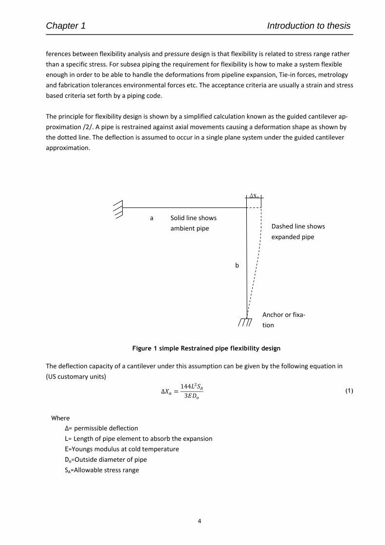
Chapter 1 Introduction to thesis
4
ferences between flexibility analysis and pressure design is that flexibility is related to stress range rather
than a specific stress. For subsea piping the requirement for flexibility is how to make a system flexible
enough in order to be able to handle the deformations from pipeline expansion, Tie-in forces, metrology
and fabrication tolerances environmental forces etc. The acceptance criteria are usually a strain and stress
based criteria set forth by a piping code.
The principle for flexibility design is shown by a simplified calculation known as the guided cantilever ap-
proximation /2/. A pipe is restrained against axial movements causing a deformation shape as shown by
the dotted line. The deflection is assumed to occur in a single plane system under the guided cantilever
approximation.
Figure 1 simple Restrained pipe flexibility design
The deflection capacity of a cantilever under this assumption can be given by the following equation in
(US customary units)
∆𝑋𝑎 =144𝐿2𝑆𝐴3𝐸𝐷𝑜
(1)
Solid line shows
ambient pipe Dashed line shows
expanded pipe
Anchor or fixa-
tion
b
a
Where
Δ= permissible deflection
L= Length of pipe element to absorb the expansion
E=Youngs modulus at cold temperature
Do=Outside diameter of pipe
SA=Allowable stress range
Δxa
Chapter 1 Introduction to thesis
5
The limitation of the method is:
The system has only two terminal points and is composed of straight legs of pipe with uniform size and thickness
All legs are parallel to the coordinate axes
Thermal expansion is absorbed only by legs in a perpendicular direction
The amount of thermal expansion that a given leg can absorb is inversely proportional to its stiffness. Because the legs are of inverse value of the cube of their lengths.
In accommodating thermal expansion the legs act as a guided cantilever, that is they are subjected to bending under end displacement no end rotation is permitted
Consider the following example as to calculate the required length of leg (b) if the system is exposed to a
displacement in x direction of 2.3in (58mm) due to thermal expansion of leg (a).
By rearranging Eq. 1.1 the required length for Leg (b) becomes in:
𝐿𝑏 = √3𝐸𝐷𝑜 ∙ ∆𝑥𝑎
144𝑆𝐴= √
3 ∙ 29.7 ∙ 106 ∙ 4.5 ∙ 2.3
144 ∙ 15000= 20.7𝑓𝑡(6298𝑚𝑚)
(2)
This simple calculation shows that Leg (b) has to be longer than that of leg (a) in order to be within a safe
stress limit for the pipe. By observing this formula one sees that the allowable deflection is depended up-
on the pipe length leg squared hence doubling the expansion ∆ of pipe length La requires the other length
Lb of the pipe to increase by a factor of: √2 = 1.41 , in order to maintain stresses within the limit.
Other flexibility criteria as given in ASME B31.4 Ref. /3/section 403.9 can also be used as a simplification. This formula is an empirical criteria for checking the expansion of unrestrained pipelines.
𝐷𝑦
(𝐿 − 𝑈)2≤ 𝐾
(3)
Pipe data:
Do=4.5 in
Δxa=2.3 in
SA=15000 psi
E=29.7x10⁶psi
La=20ft
Where
D= Outside Diameter of the pipe
L= Developed Length of the pipe between anchors
U=Straight line distance between anchors
K=numerical factor =208 (SI Units) and 0.03 for US customary units
y=Resultant of total displacement strains to be absorbed by the pipe (UaDT )
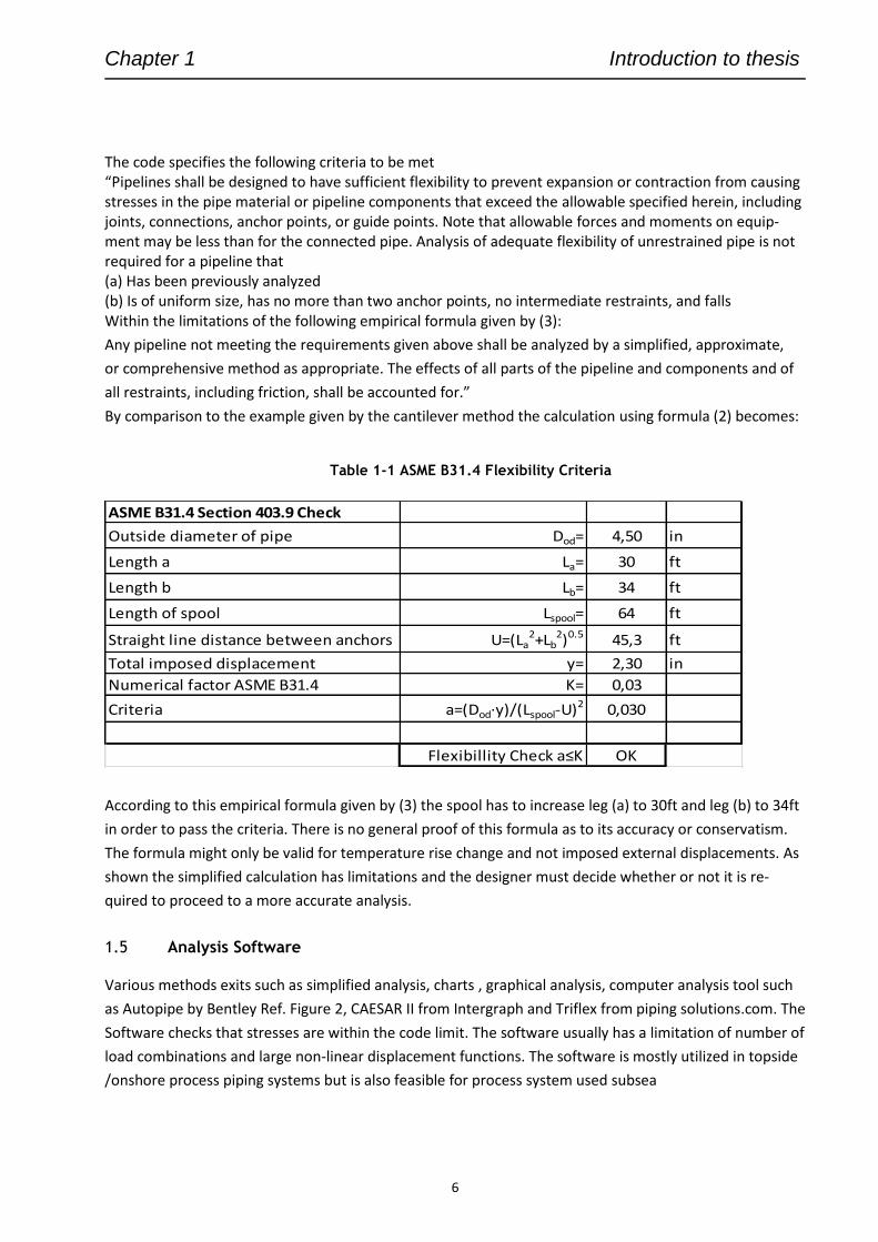
Chapter 1 Introduction to thesis
6
The code specifies the following criteria to be met “Pipelines shall be designed to have sufficient flexibility to prevent expansion or contraction from causing stresses in the pipe material or pipeline components that exceed the allowable specified herein, including joints, connections, anchor points, or guide points. Note that allowable forces and moments on equip-ment may be less than for the connected pipe. Analysis of adequate flexibility of unrestrained pipe is not required for a pipeline that (a) Has been previously analyzed (b) Is of uniform size, has no more than two anchor points, no intermediate restraints, and falls Within the limitations of the following empirical formula given by (3):
Any pipeline not meeting the requirements given above shall be analyzed by a simplified, approximate,
or comprehensive method as appropriate. The effects of all parts of the pipeline and components and of
all restraints, including friction, shall be accounted for.”
By comparison to the example given by the cantilever method the calculation using formula (2) becomes:
Table 1-1 ASME B31.4 Flexibility Criteria
ASME B31.4 Section 403.9 Check
Outside diameter of pipe Dod= 4,50 in
Length a La= 30 ft
Length b Lb= 34 ft
Length of spool Lspool= 64 ft
Straight line distance between anchors U=(La2+Lb
2)0.5 45,3 ft
Total imposed displacement y= 2,30 in
Numerical factor ASME B31.4 K= 0,03
Criteria a=(Dod·y)/(Lspool-U)2 0,030
Flexibillity Check a≤K OK
According to this empirical formula given by (3) the spool has to increase leg (a) to 30ft and leg (b) to 34ft
in order to pass the criteria. There is no general proof of this formula as to its accuracy or conservatism.
The formula might only be valid for temperature rise change and not imposed external displacements. As
shown the simplified calculation has limitations and the designer must decide whether or not it is re-
quired to proceed to a more accurate analysis.
1.5 Analysis Software
Various methods exits such as simplified analysis, charts , graphical analysis, computer analysis tool such
as Autopipe by Bentley Ref. Figure 2, CAESAR II from Intergraph and Triflex from piping solutions.com. The
Software checks that stresses are within the code limit. The software usually has a limitation of number of
load combinations and large non-linear displacement functions. The software is mostly utilized in topside
/onshore process piping systems but is also feasible for process system used subsea
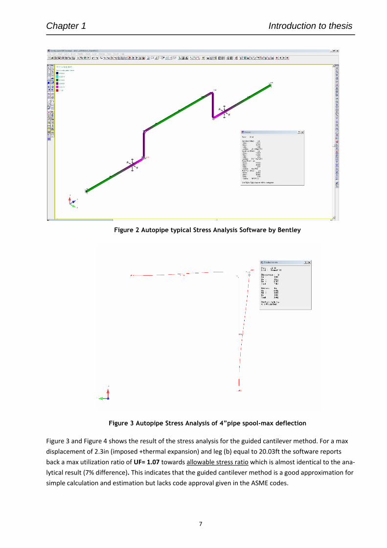
Chapter 1 Introduction to thesis
7
Figure 2 Autopipe typical Stress Analysis Software by Bentley
Figure 3 Autopipe Stress Analysis of 4”pipe spool-max deflection
Figure 3 and Figure 4 shows the result of the stress analysis for the guided cantilever method. For a max
displacement of 2.3in (imposed +thermal expansion) and leg (b) equal to 20.03ft the software reports
back a max utilization ratio of UF= 1.07 towards allowable stress ratio which is almost identical to the ana-
lytical result (7% difference). This indicates that the guided cantilever method is a good approximation for
simple calculation and estimation but lacks code approval given in the ASME codes.
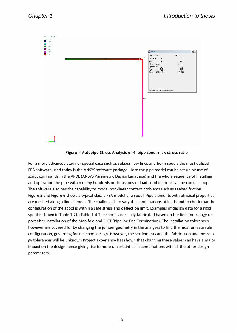
Chapter 1 Introduction to thesis
8
Figure 4 Autopipe Stress Analysis of 4”pipe spool-max stress ratio
For a more advanced study or special case such as subsea flow lines and tie-in spools the most utilized
FEA software used today is the ANSYS software package. Here the pipe model can be set up by use of
script commands in the APDL (ANSYS Parametric Design Language) and the whole sequence of installing
and operation the pipe within many hundreds or thousands of load combinations can be run in a loop.
The software also has the capability to model non-linear contact problems such as seabed friction.
Figure 5 and Figure 6 shows a typical classic FEA model of a spool. Pipe elements with physical properties
are meshed along a line element. The challenge is to vary the combinations of loads and to check that the
configuration of the spool is within a safe stress and deflection limit. Examples of design data for a rigid
spool is shown in Table 1-2to Table 1-4.The spool is normally fabricated based on the field metrology re-
port after installation of the Manifold and PLET (Pipeline End Termination). The installation tolerances
however are covered for by changing the jumper geometry in the analyses to find the most unfavorable
configuration, governing for the spool design. However, the settlements and the fabrication and metrolo-
gy tolerances will be unknown Project experience has shown that changing these values can have a major
impact on the design hence giving rise to more uncertainties in combinations with all the other design
parameters.
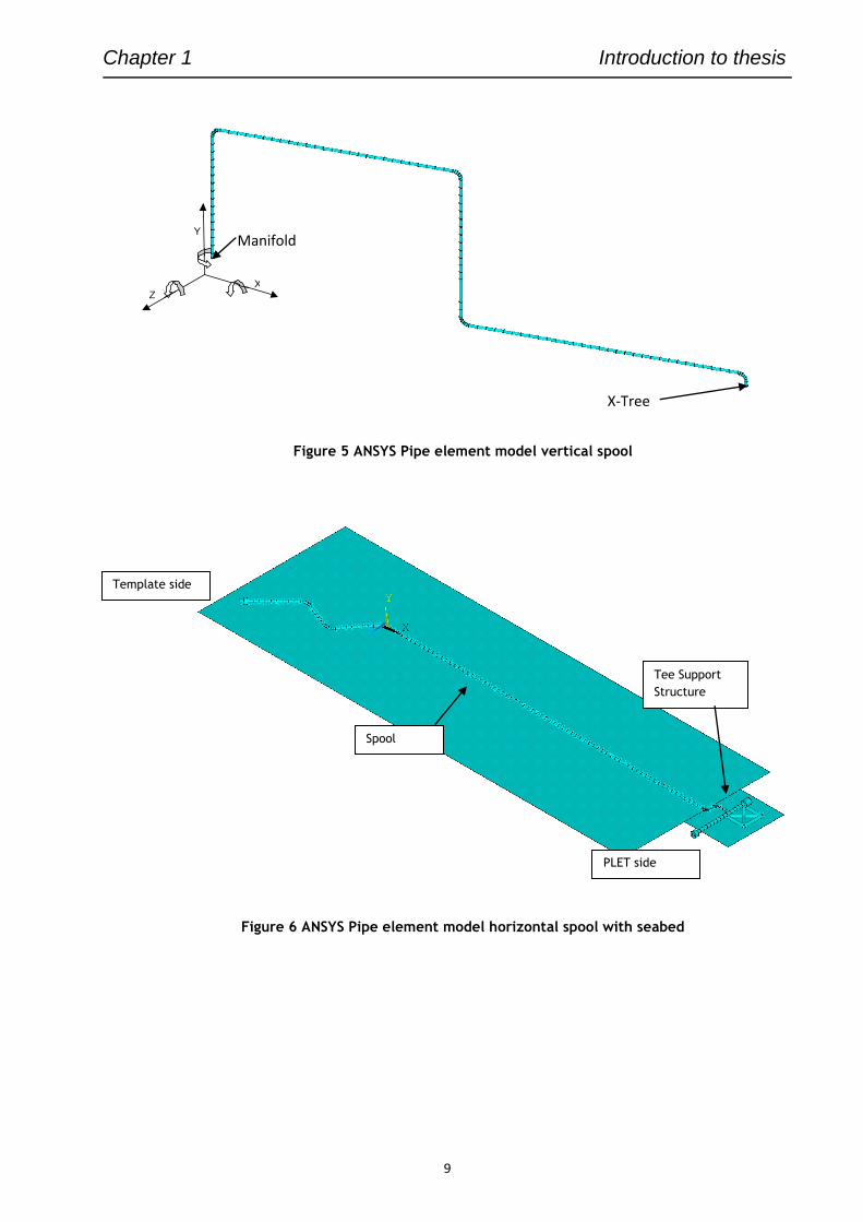
Chapter 1 Introduction to thesis
9
Figure 5 ANSYS Pipe element model vertical spool
Figure 6 ANSYS Pipe element model horizontal spool with seabed
Y
XZ
Manifold
X-Tree
Spool
Template side
Tee Support
Structure
PLET side
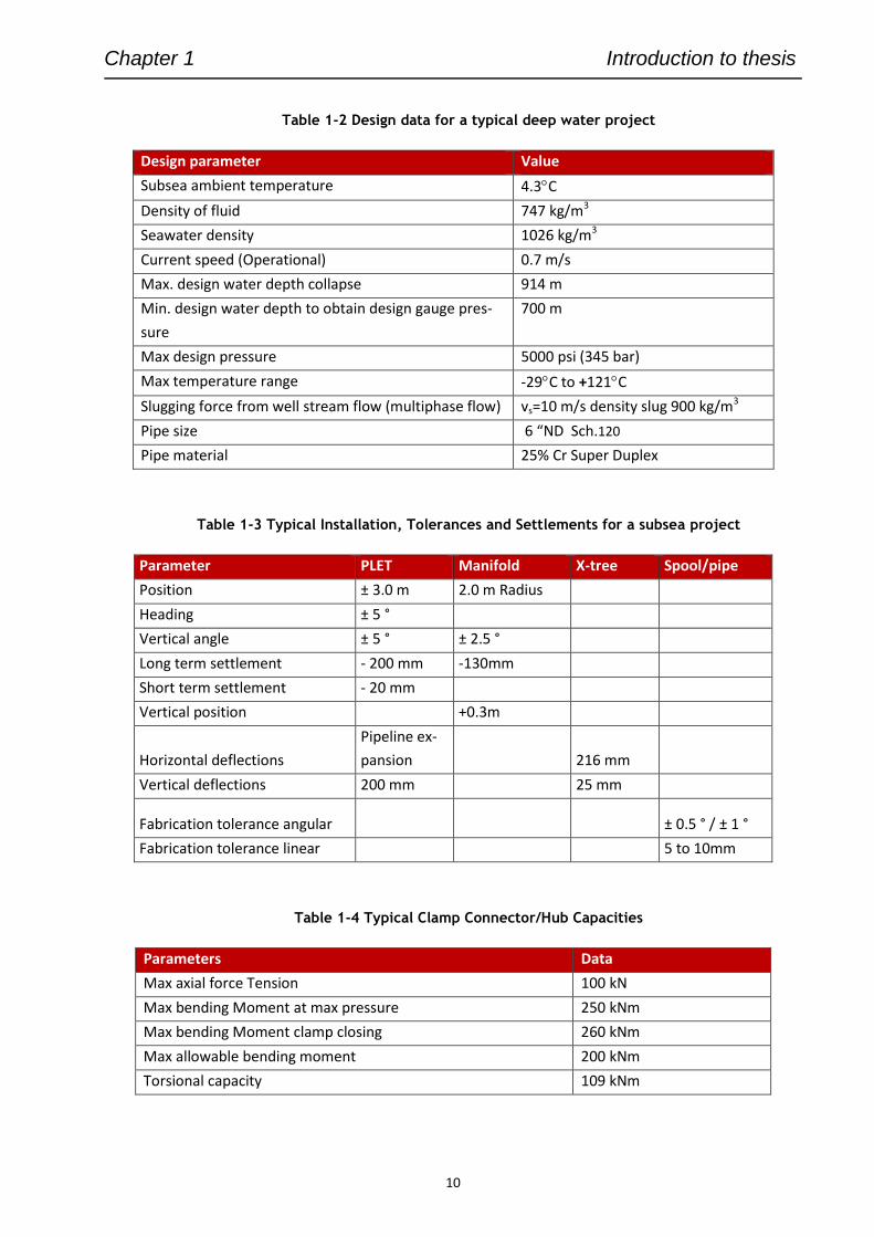
Chapter 1 Introduction to thesis
10
Table 1-2 Design data for a typical deep water project
Design parameter Value
Subsea ambient temperature 4.3C
Density of fluid 747 kg/m3
Seawater density 1026 kg/m3
Current speed (Operational) 0.7 m/s
Max. design water depth collapse 914 m
Min. design water depth to obtain design gauge pres-
sure
700 m
Max design pressure 5000 psi (345 bar)
Max temperature range -29C to +121C
Slugging force from well stream flow (multiphase flow) vs=10 m/s density slug 900 kg/m3
Pipe size 6 “ND Sch.120
Pipe material 25% Cr Super Duplex
Table 1-3 Typical Installation, Tolerances and Settlements for a subsea project
Parameter PLET Manifold X-tree Spool/pipe
Position ± 3.0 m 2.0 m Radius
Heading ± 5 °
Vertical angle ± 5 ° ± 2.5 °
Long term settlement - 200 mm -130mm
Short term settlement - 20 mm
Vertical position +0.3m
Horizontal deflections
Pipeline ex-
pansion 216 mm
Vertical deflections 200 mm 25 mm
Fabrication tolerance angular ± 0.5 ° / ± 1 °
Fabrication tolerance linear 5 to 10mm
Table 1-4 Typical Clamp Connector/Hub Capacities
Parameters Data
Max axial force Tension 100 kN
Max bending Moment at max pressure 250 kNm
Max bending Moment clamp closing 260 kNm
Max allowable bending moment 200 kNm
Torsional capacity 109 kNm
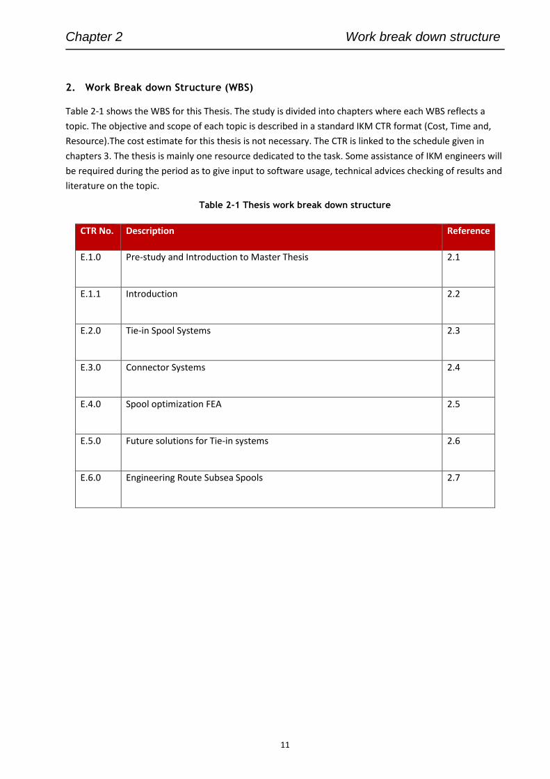
Chapter 2 Work break down structure
11
2. Work Break down Structure (WBS)
Table 2-1 shows the WBS for this Thesis. The study is divided into chapters where each WBS reflects a
topic. The objective and scope of each topic is described in a standard IKM CTR format (Cost, Time and,
Resource).The cost estimate for this thesis is not necessary. The CTR is linked to the schedule given in
chapters 3. The thesis is mainly one resource dedicated to the task. Some assistance of IKM engineers will
be required during the period as to give input to software usage, technical advices checking of results and
literature on the topic.
Table 2-1 Thesis work break down structure
CTR No. Description Reference
E.1.0 Pre-study and Introduction to Master Thesis 2.1
E.1.1 Introduction 2.2
E.2.0 Tie-in Spool Systems 2.3
E.3.0 Connector Systems 2.4
E.4.0 Spool optimization FEA 2.5
E.5.0 Future solutions for Tie-in systems 2.6
E.6.0 Engineering Route Subsea Spools 2.7
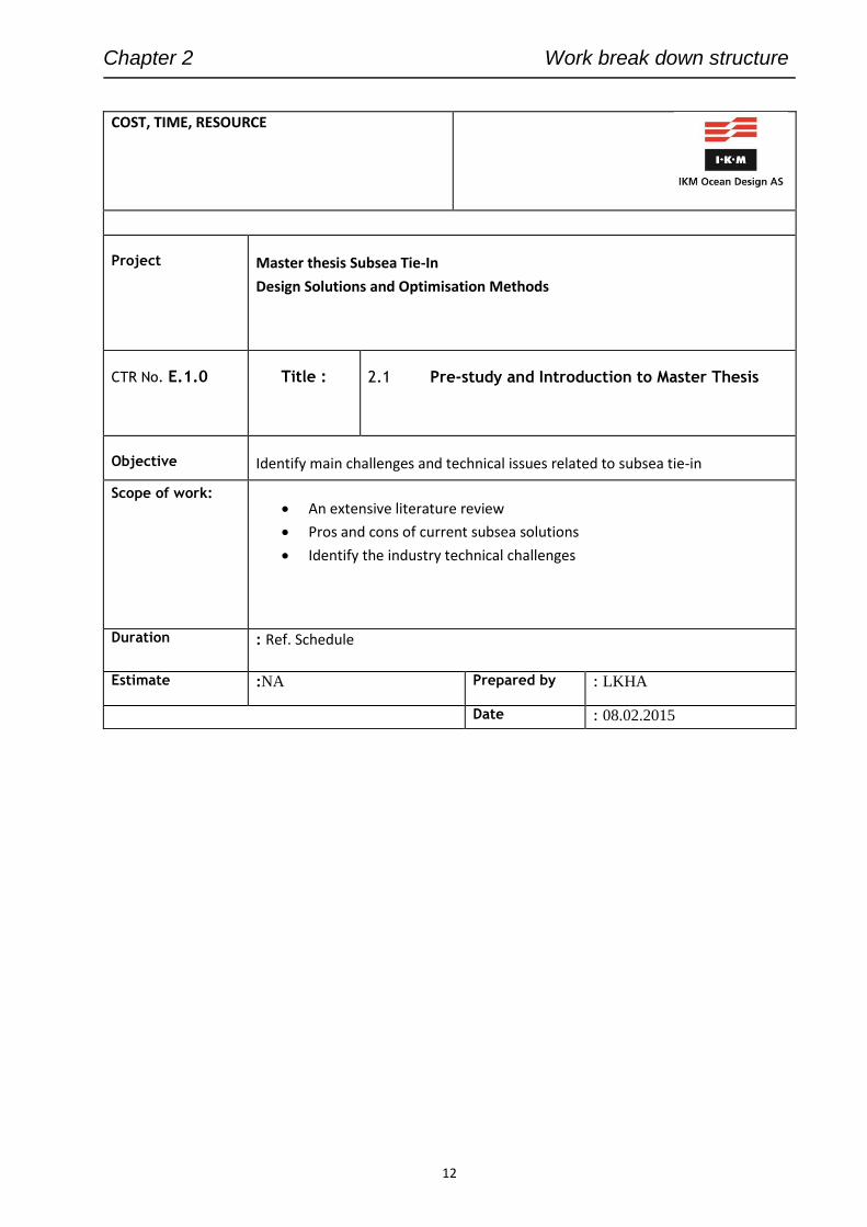
Chapter 2 Work break down structure
12
COST, TIME, RESOURCE
Project
Master thesis Subsea Tie-In
Design Solutions and Optimisation Methods
CTR No. E.1.0
Title :
2.1 Pre-study and Introduction to Master Thesis
Objective
Identify main challenges and technical issues related to subsea tie-in
Scope of work:
An extensive literature review
Pros and cons of current subsea solutions
Identify the industry technical challenges
Duration : Ref. Schedule
Estimate :NA Prepared by : LKHA
Date : 08.02.2015
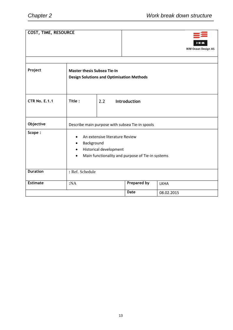
Chapter 2 Work break down structure
13
COST, TIME, RESOURCE
Project
Master thesis Subsea Tie-In
Design Solutions and Optimisation Methods
CTR No. E.1.1
Title :
2.2 Introduction
Objective
Describe main purpose with subsea Tie-in spools
Scope :
An extensive literature Review
Background
Historical development
Main functionality and purpose of Tie-in systems
Duration : Ref. Schedule
Estimate :NA Prepared by LKHA
Date 08.02.2015
Chapter 2 Work break down structure
14
COST, TIME, RESOURCE
Project
Master thesis Subsea Tie-In
Design Solutions and Optimisation Methods
CTR No. E.2.0
Title :
2.3 Tie-in Spool Systems
Objective
Identify typical Tie-in System used in today’s industry
Scope :
Classification of systems
Main purpose
Configurations and geometrical layouts
Limitations
Duration : Ref. Schedule
Estimate NA Prepared by LKHA
Date 08.02.2015
Chapter 2 Work break down structure
15
COST, TIME, RESOURCE
Project
Master thesis Subsea Tie-In
Design Solutions and Optimisation Methods
CTR No. E.3.0
Title :
2.4 Connector Systems
Objective
Identify typical Mechanical Connector Systems used for Subsea Tie-Back
Scope :
Major Suppliers
Differences
Functionality and operability
Limitations
Duration Ref. Schedule
Estimate Prepared by LKHA
Date 08.02.2015
Chapter 2 Work break down structure
16
COST, TIME, RESOURCE
Project
Master thesis Subsea Tie-In
Design Solutions and Optimisation Methods
CTR No. E.4.0
Title :
2.5 Spool optimization FEA
Objective
Verify and optimize the structural strength of a typical spool by use of FEA
Scope :
Design basis
Identification of load cases
Flexibility design
Wall thickness design
Perform computer analysis of spools
Compare different solutions
Establish criteria based upon industry standard such as ASME ,DNV
Duration Ref Schedule
Estimate NA Prepared by LKHA
Date 08.02.2015
Chapter 2 Work break down structure
17
COST, TIME, RESOURCE
Project
Master thesis Subsea Tie-In
Design Solutions and Optimisation Methods
CTR No. E.5.0
Title :
2.6 Future solutions for Tie-in systems
Objective Propose other possible Tie-in Solutions
Scope :
Describe other methods not utilised today such as Direct Tie-in
Deflect to connect etc.
Flexible spools
Other conceptual Ideas
Duration Ref. Schedule
Estimate Prepared by LKHA
Date 08.02.2015
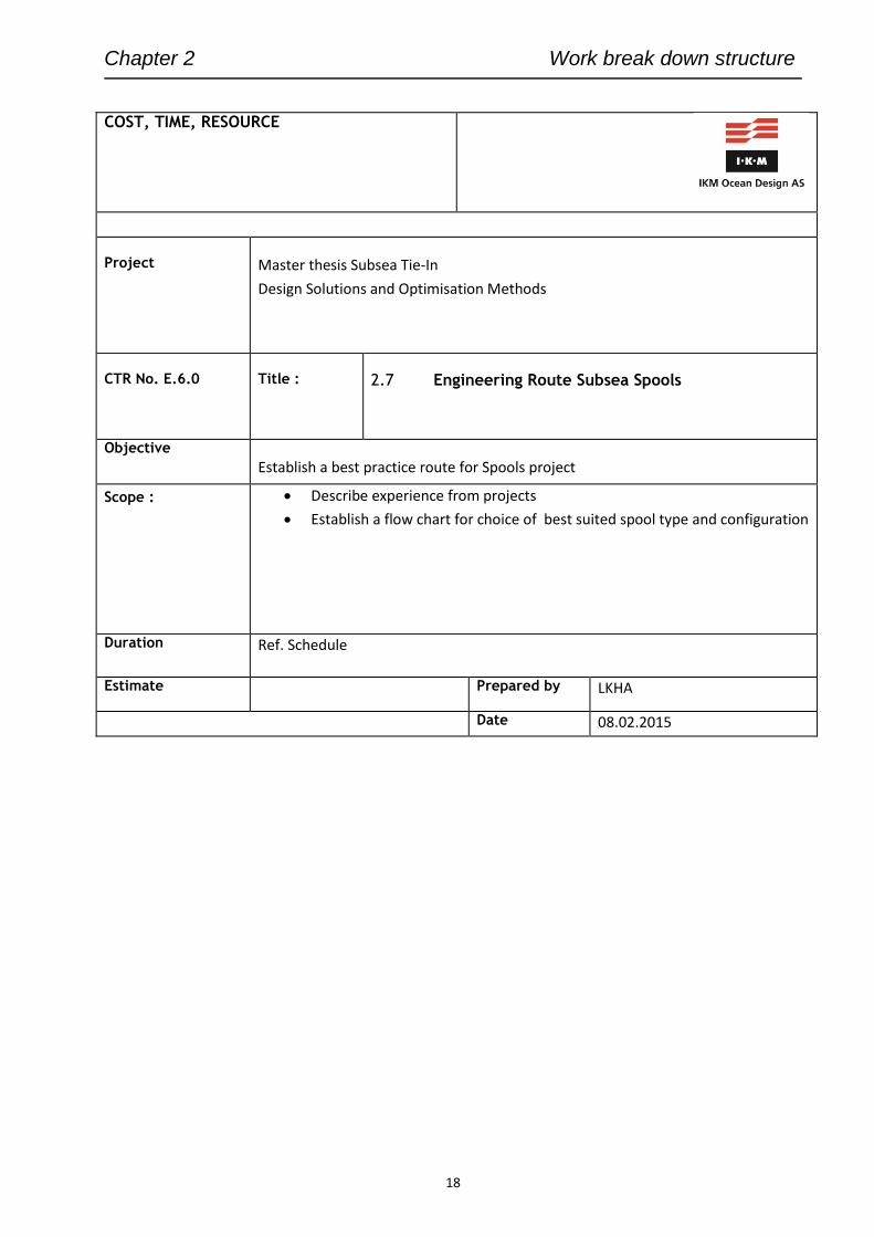
Chapter 2 Work break down structure
18
COST, TIME, RESOURCE
Project
Master thesis Subsea Tie-In
Design Solutions and Optimisation Methods
CTR No. E.6.0
Title :
2.7 Engineering Route Subsea Spools
Objective
Establish a best practice route for Spools project
Scope :
Describe experience from projects
Establish a flow chart for choice of best suited spool type and configuration
Duration Ref. Schedule
Estimate Prepared by LKHA
Date 08.02.2015
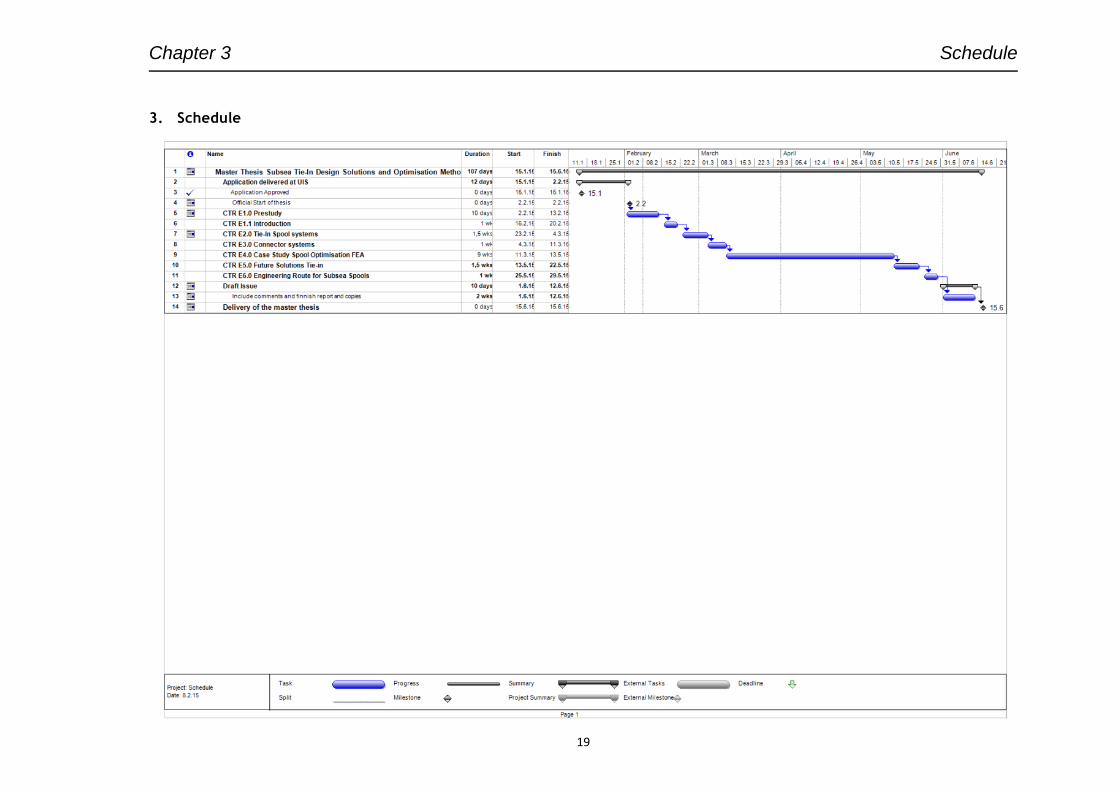
Chapter 3 Schedule
19
3. Schedule
Chapter 4 References
20
4. References
/1/ Per Richard Nystrøm and Gawain Langford, “Jumper Arch System”, OPT-2002-
03, ABB Offshore systems presented at the Offshore Pipeline Technology Con-
ference, 2002
/2/ Sam kannappan John Wiley & sons Inc. “Introduction to pipe stress analysis”
Tennessee Valley Authority, Knoxville Tennessee 1986
/3/ Pipeline Transportation systems for liquids and Slurries ,ASME B31.4, 2012

Appendixes Appendix 2 Deflection combinations
209
Appendix 2 ANSYS Design Explorer Spool Deflection Combinations
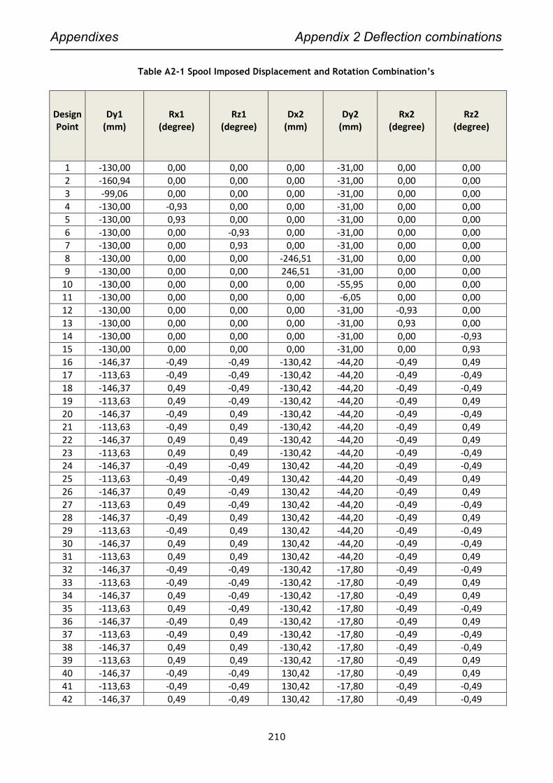
Appendixes Appendix 2 Deflection combinations
210
Table A2-1 Spool Imposed Displacement and Rotation Combination’s
Design Point
Dy1 (mm)
Rx1 (degree)
Rz1 (degree)
Dx2 (mm)
Dy2 (mm)
Rx2 (degree)
Rz2 (degree)
1 -130,00 0,00 0,00 0,00 -31,00 0,00 0,00
2 -160,94 0,00 0,00 0,00 -31,00 0,00 0,00
3 -99,06 0,00 0,00 0,00 -31,00 0,00 0,00
4 -130,00 -0,93 0,00 0,00 -31,00 0,00 0,00
5 -130,00 0,93 0,00 0,00 -31,00 0,00 0,00
6 -130,00 0,00 -0,93 0,00 -31,00 0,00 0,00
7 -130,00 0,00 0,93 0,00 -31,00 0,00 0,00
8 -130,00 0,00 0,00 -246,51 -31,00 0,00 0,00
9 -130,00 0,00 0,00 246,51 -31,00 0,00 0,00
10 -130,00 0,00 0,00 0,00 -55,95 0,00 0,00
11 -130,00 0,00 0,00 0,00 -6,05 0,00 0,00
12 -130,00 0,00 0,00 0,00 -31,00 -0,93 0,00
13 -130,00 0,00 0,00 0,00 -31,00 0,93 0,00
14 -130,00 0,00 0,00 0,00 -31,00 0,00 -0,93
15 -130,00 0,00 0,00 0,00 -31,00 0,00 0,93
16 -146,37 -0,49 -0,49 -130,42 -44,20 -0,49 0,49
17 -113,63 -0,49 -0,49 -130,42 -44,20 -0,49 -0,49
18 -146,37 0,49 -0,49 -130,42 -44,20 -0,49 -0,49
19 -113,63 0,49 -0,49 -130,42 -44,20 -0,49 0,49
20 -146,37 -0,49 0,49 -130,42 -44,20 -0,49 -0,49
21 -113,63 -0,49 0,49 -130,42 -44,20 -0,49 0,49
22 -146,37 0,49 0,49 -130,42 -44,20 -0,49 0,49
23 -113,63 0,49 0,49 -130,42 -44,20 -0,49 -0,49
24 -146,37 -0,49 -0,49 130,42 -44,20 -0,49 -0,49
25 -113,63 -0,49 -0,49 130,42 -44,20 -0,49 0,49
26 -146,37 0,49 -0,49 130,42 -44,20 -0,49 0,49
27 -113,63 0,49 -0,49 130,42 -44,20 -0,49 -0,49
28 -146,37 -0,49 0,49 130,42 -44,20 -0,49 0,49
29 -113,63 -0,49 0,49 130,42 -44,20 -0,49 -0,49
30 -146,37 0,49 0,49 130,42 -44,20 -0,49 -0,49
31 -113,63 0,49 0,49 130,42 -44,20 -0,49 0,49
32 -146,37 -0,49 -0,49 -130,42 -17,80 -0,49 -0,49
33 -113,63 -0,49 -0,49 -130,42 -17,80 -0,49 0,49
34 -146,37 0,49 -0,49 -130,42 -17,80 -0,49 0,49
35 -113,63 0,49 -0,49 -130,42 -17,80 -0,49 -0,49
36 -146,37 -0,49 0,49 -130,42 -17,80 -0,49 0,49
37 -113,63 -0,49 0,49 -130,42 -17,80 -0,49 -0,49
38 -146,37 0,49 0,49 -130,42 -17,80 -0,49 -0,49
39 -113,63 0,49 0,49 -130,42 -17,80 -0,49 0,49
40 -146,37 -0,49 -0,49 130,42 -17,80 -0,49 0,49
41 -113,63 -0,49 -0,49 130,42 -17,80 -0,49 -0,49
42 -146,37 0,49 -0,49 130,42 -17,80 -0,49 -0,49
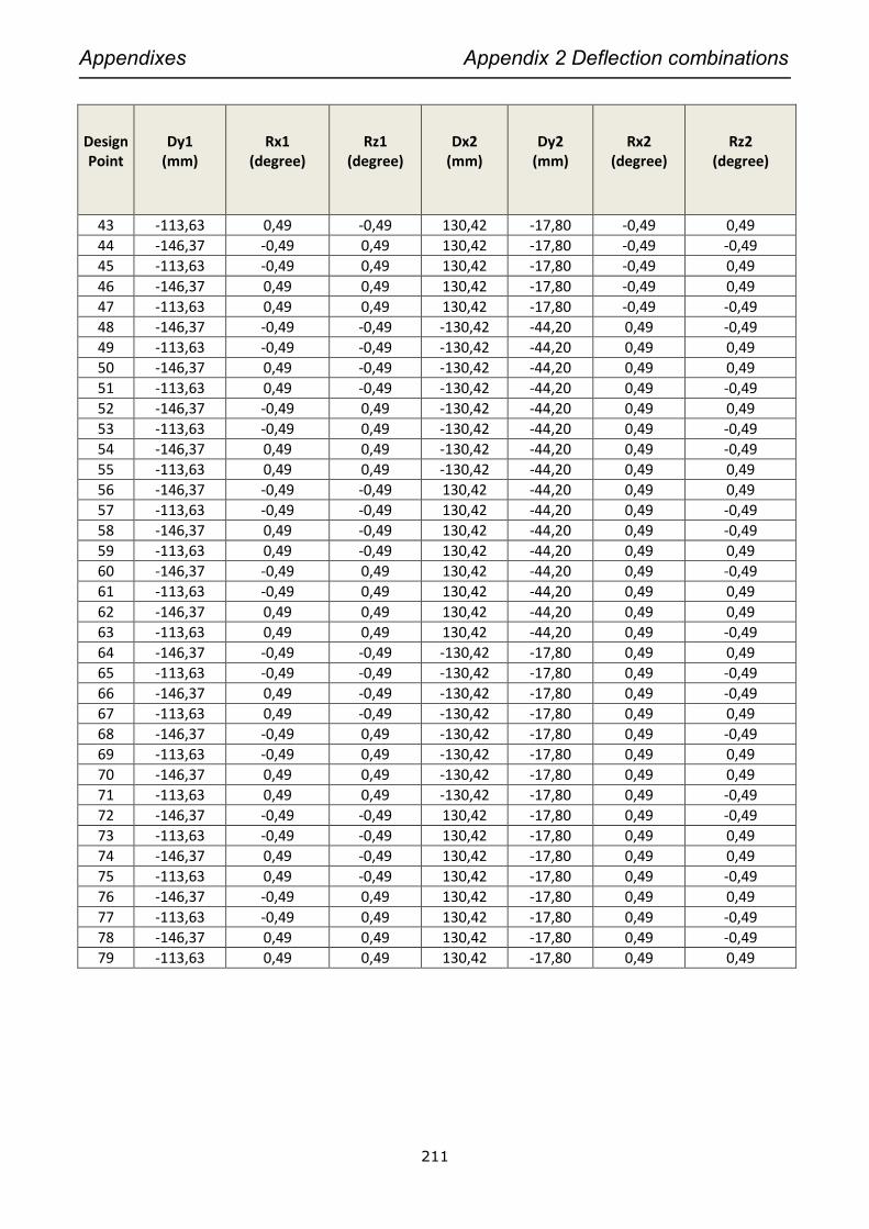
Appendixes Appendix 2 Deflection combinations
211
Design Point
Dy1 (mm)
Rx1 (degree)
Rz1 (degree)
Dx2 (mm)
Dy2 (mm)
Rx2 (degree)
Rz2 (degree)
43 -113,63 0,49 -0,49 130,42 -17,80 -0,49 0,49
44 -146,37 -0,49 0,49 130,42 -17,80 -0,49 -0,49
45 -113,63 -0,49 0,49 130,42 -17,80 -0,49 0,49
46 -146,37 0,49 0,49 130,42 -17,80 -0,49 0,49
47 -113,63 0,49 0,49 130,42 -17,80 -0,49 -0,49
48 -146,37 -0,49 -0,49 -130,42 -44,20 0,49 -0,49
49 -113,63 -0,49 -0,49 -130,42 -44,20 0,49 0,49
50 -146,37 0,49 -0,49 -130,42 -44,20 0,49 0,49
51 -113,63 0,49 -0,49 -130,42 -44,20 0,49 -0,49
52 -146,37 -0,49 0,49 -130,42 -44,20 0,49 0,49
53 -113,63 -0,49 0,49 -130,42 -44,20 0,49 -0,49
54 -146,37 0,49 0,49 -130,42 -44,20 0,49 -0,49
55 -113,63 0,49 0,49 -130,42 -44,20 0,49 0,49
56 -146,37 -0,49 -0,49 130,42 -44,20 0,49 0,49
57 -113,63 -0,49 -0,49 130,42 -44,20 0,49 -0,49
58 -146,37 0,49 -0,49 130,42 -44,20 0,49 -0,49
59 -113,63 0,49 -0,49 130,42 -44,20 0,49 0,49
60 -146,37 -0,49 0,49 130,42 -44,20 0,49 -0,49
61 -113,63 -0,49 0,49 130,42 -44,20 0,49 0,49
62 -146,37 0,49 0,49 130,42 -44,20 0,49 0,49
63 -113,63 0,49 0,49 130,42 -44,20 0,49 -0,49
64 -146,37 -0,49 -0,49 -130,42 -17,80 0,49 0,49
65 -113,63 -0,49 -0,49 -130,42 -17,80 0,49 -0,49
66 -146,37 0,49 -0,49 -130,42 -17,80 0,49 -0,49
67 -113,63 0,49 -0,49 -130,42 -17,80 0,49 0,49
68 -146,37 -0,49 0,49 -130,42 -17,80 0,49 -0,49
69 -113,63 -0,49 0,49 -130,42 -17,80 0,49 0,49
70 -146,37 0,49 0,49 -130,42 -17,80 0,49 0,49
71 -113,63 0,49 0,49 -130,42 -17,80 0,49 -0,49
72 -146,37 -0,49 -0,49 130,42 -17,80 0,49 -0,49
73 -113,63 -0,49 -0,49 130,42 -17,80 0,49 0,49
74 -146,37 0,49 -0,49 130,42 -17,80 0,49 0,49
75 -113,63 0,49 -0,49 130,42 -17,80 0,49 -0,49
76 -146,37 -0,49 0,49 130,42 -17,80 0,49 0,49
77 -113,63 -0,49 0,49 130,42 -17,80 0,49 -0,49
78 -146,37 0,49 0,49 130,42 -17,80 0,49 -0,49
79 -113,63 0,49 0,49 130,42 -17,80 0,49 0,49

Appendixes Appendix 2 Deflection combinations
212

Appendixes Appendix 3 Hand Calculations
213
Appendix 3 Hand Calculations

Appendixes Appendix 3 Hand Calculations
214
A 3.1 ASME B31.8 Section VIII Pipe wall calculation

Appendixes Appendix 3 Hand Calculations
215
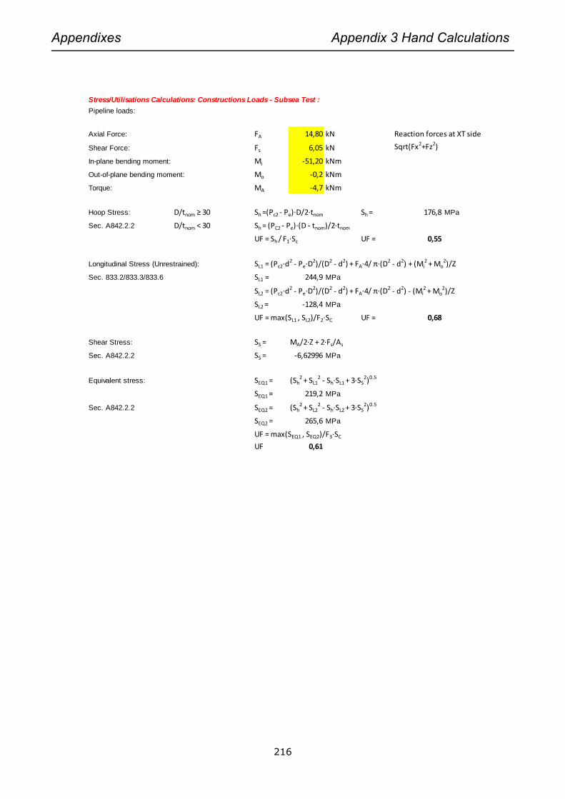
Appendixes Appendix 3 Hand Calculations
216
Stress/Utilisations Calculations: Constructions Loads - Subsea Test :
Pipeline loads:
Axial Force: FA 14,80 kN Reaction forces at XT side
Shear Force: Fs 6,05 kN Sqrt(Fx2+Fz2)
In-plane bending moment: Mi -51,20 kNm
Out-of-plane bending moment: Mo -0,2 kNm
Torque: MA -4,7 kNm
Hoop Stress: D/tnom ≥ 30 Sh =(Pc2 - Pe)∙D/2∙tnom Sh = 176,8 MPa
Sec. A842.2.2 D/tnom < 30 Sh = (PC2 - Pe)∙(D - tnom)/2∙tnom
UF = Sh / F1∙Sc UF = 0,55
Longitudinal Stress (Unrestrained): SL1 = (Pc2∙d2 - Pe∙D2)/(D2 - d2) + FA∙4/ π∙(D2 - d2) + (Mi2 + Mo
2)/Z
Sec. 833.2/833.3/833.6 SL1 = 244,9 MPa
SL2 = (Pc2∙d2 - Pe∙D2)/(D2 - d2) + FA∙4/ π∙(D2 - d2) - (Mi2 + Mo
2)/Z
SL2 = -128,4 MPa
UF = max(SL1 , SL2)/F2∙SC UF = 0,68
Shear Stress: SS = MA/2∙Z + 2∙Fs/As
Sec. A842.2.2 SS = -6,62996 MPa
Equivalent stress: SEQ1 = (Sh2 + SL1
2 - Sh∙SL1 + 3∙SS2)0.5
SEQ1 = 219,2 MPa
Sec. A842.2.2 SEQ2 = (Sh2 + SL2
2 - Sh∙SL2 + 3∙SS2)0.5
SEQ2 = 265,6 MPa
UF = max(SEQ1 , SEQ2)/F3∙SC
UF 0,61

Appendixes Appendix 3 Hand Calculations
217
Stress/Utilisations Calculations: Operational Loads :
Pipeline loads:
Axial Force: FA 18,30 kN Reaction forces at manifold side
Shear Force: Fs 33,70 kN Sqrt(Fx2+Fz2)
In-plane bending moment: Mi 64 kNm
Out-of-plane bending moment: Mo -3,8 kNm
Torque: MA 1,6 kNm
Hoop Stress: D/tnom ≥ 30 Sh =(Pd - Pe)∙D/2∙(tnom - C) Sh = 169,1 MPa
Sec. A842.2.2 D/tnom < 30 Sh = (Pd - Pe)∙(D - tnom)/2∙(tnom - C)
UF = Sh / F1∙Sd UF = 0,52
Longitudinal Stress (Unrestrained): SL1 = (Pd∙d2 - Pe∙D2)/(D2 - d2) + FA∙4/ π∙(D2 - d2) + (Mi2 + Mo
2)1/2 / ZC
Sec. 833.2/833.3/833.6/ SL1 = 304,8 MPa
SL2 = (Pd∙d2 - Pe∙D2)/(D2 - d2) + FA∙4/ π∙(D2 - d2) - (Mi2 + Mo
2)1/2 / ZC
SL2 = -195,1 MPa
UF = max(SL1 , SL2)/F2∙Sd UF = 0,85
Shear Stress: SS = MA/2∙ZC + 2∙Fs/As SS = 10,91313672 MPa
Sec. A842.2.2
Equivalent stress: SEQ1 = (Sh2 + SL1
2 - Sh∙SL1 + 3·SS2)0.5
Sec. A842.2.2 SEQ1 = 265,2 MPa
SEQ2 = (Sh2 + SL2
2 - Sh∙SL2 + 3·SS2)0.5
SEQ2 = 316,2 MPa
UF = max(SEQ1 , SEQ2)/F3∙Sd UF 0,78

Appendixes Appendix 3 Hand Calculations
218
A 3.2 Buoyancy Calculation
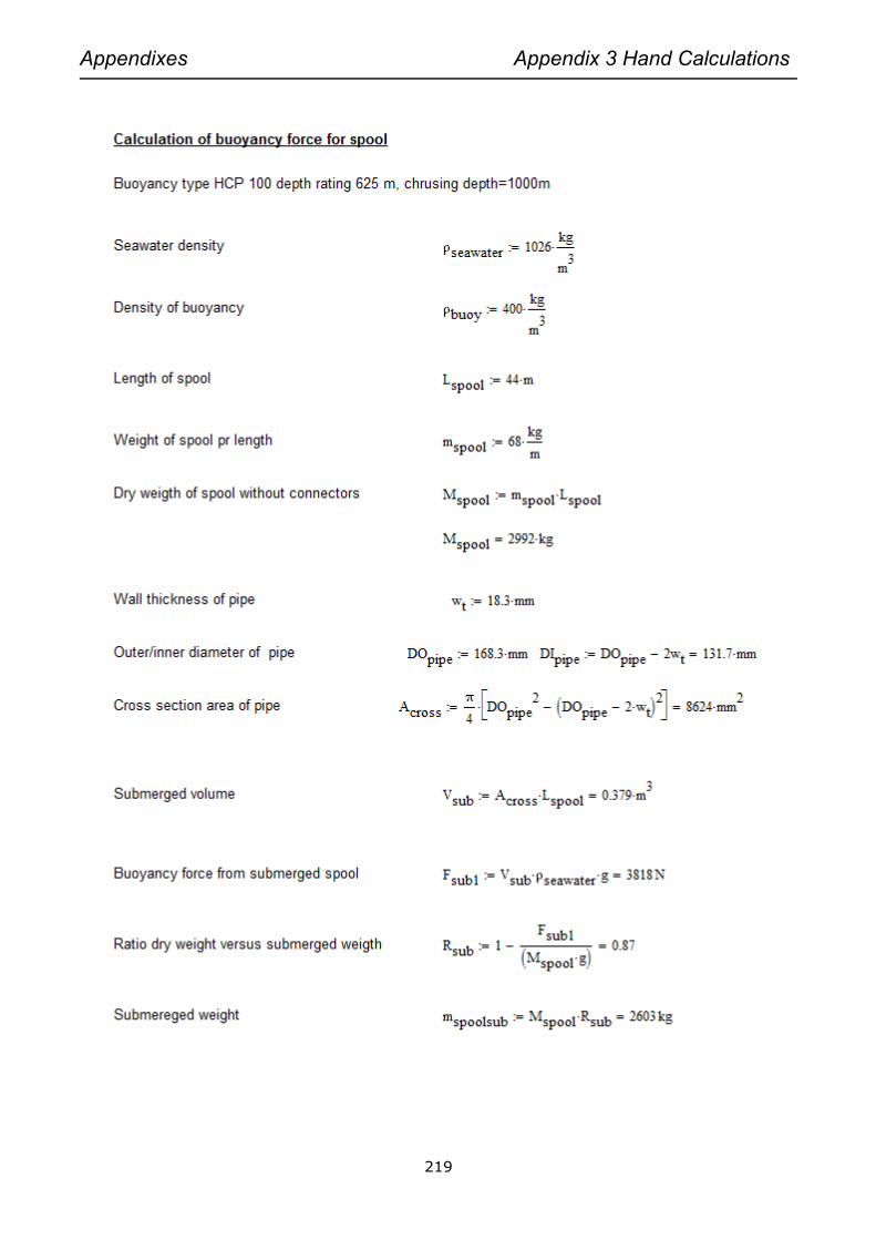
Appendixes Appendix 3 Hand Calculations
219
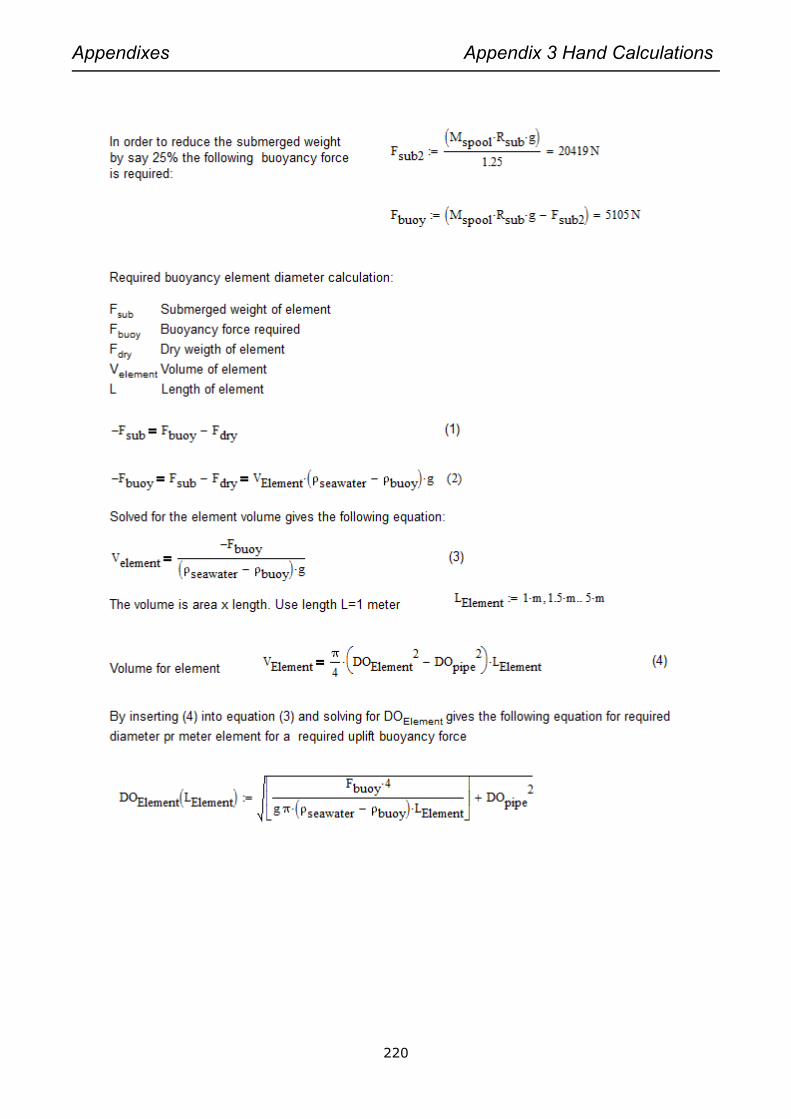
Appendixes Appendix 3 Hand Calculations
220

Appendixes Appendix 3 Hand Calculations
221
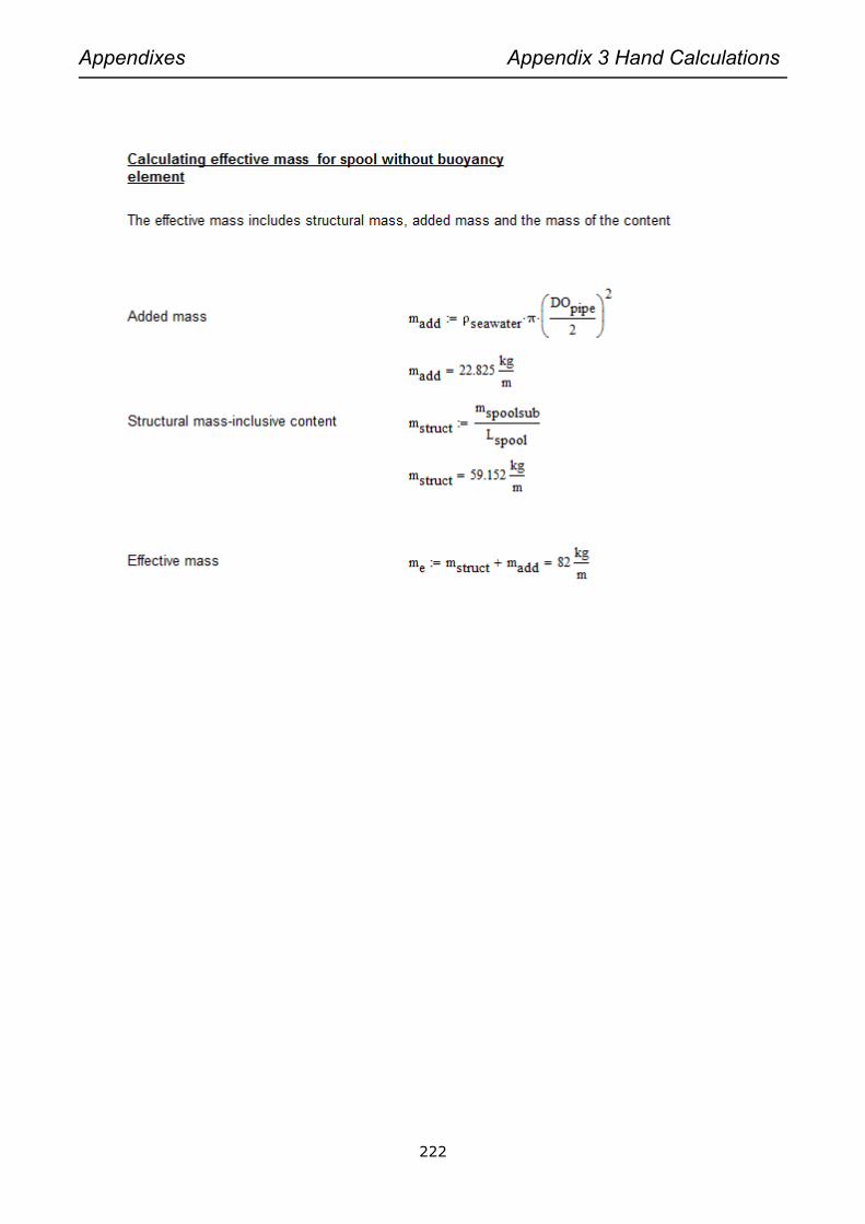
Appendixes Appendix 3 Hand Calculations
222

Appendixes Appendix 3 Hand Calculations
223
A 3.3 Current Force Calculation
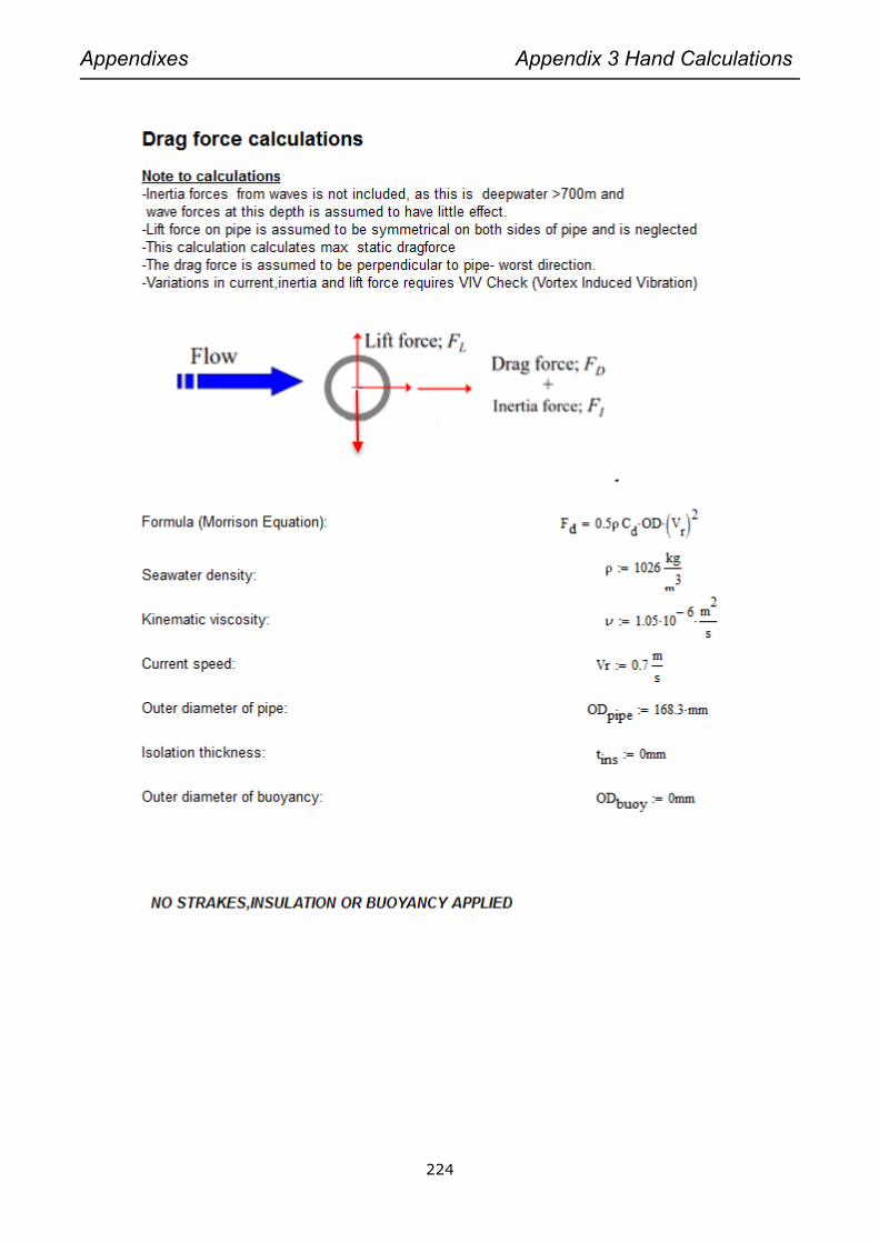
Appendixes Appendix 3 Hand Calculations
224
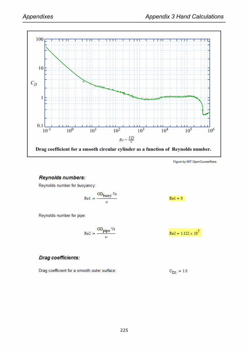
Appendixes Appendix 3 Hand Calculations
225

Appendixes Appendix 3 Hand Calculations
226

Appendixes Appendix 3 Hand Calculations
227
A 3.4 Thick Wall Vessel Calculation
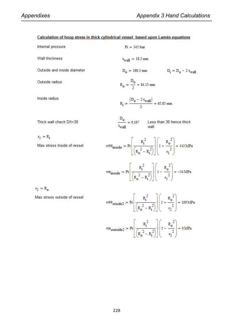
Appendixes Appendix 3 Hand Calculations
228
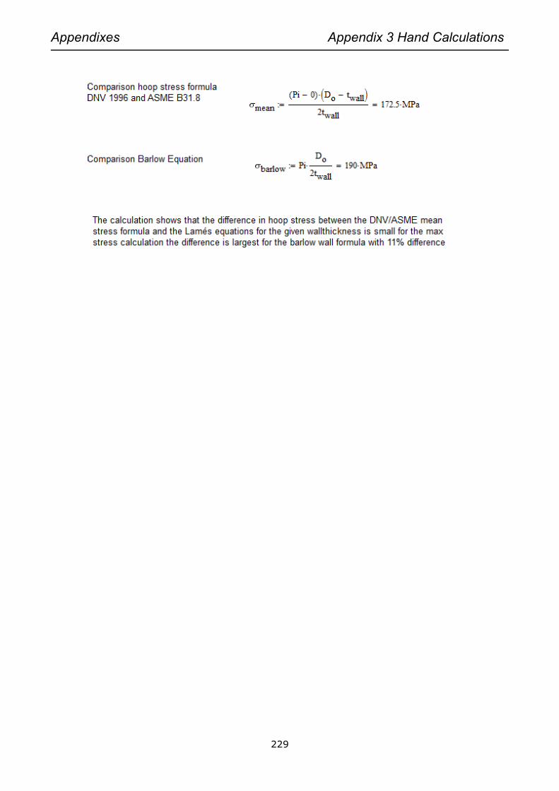
Appendixes Appendix 3 Hand Calculations
229

Appendixes Appendix 3 Hand Calculations
230
A 3.5 Fatigue calculation

Appendixes Appendix 3 Hand Calculations
231
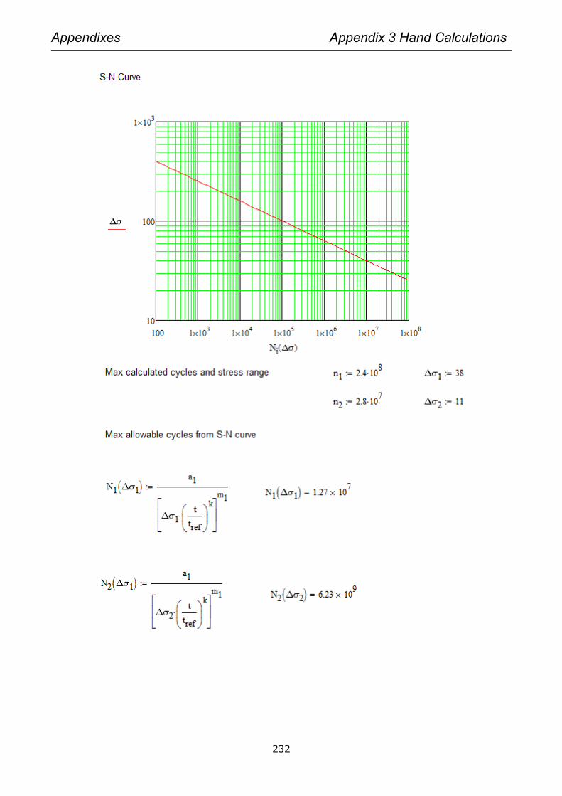
Appendixes Appendix 3 Hand Calculations
232

Appendixes Appendix 3 Hand Calculations
233

Appendixes Appendix 3 Hand Calculations
234
A 3.6 Local Buckling-External Overpressure
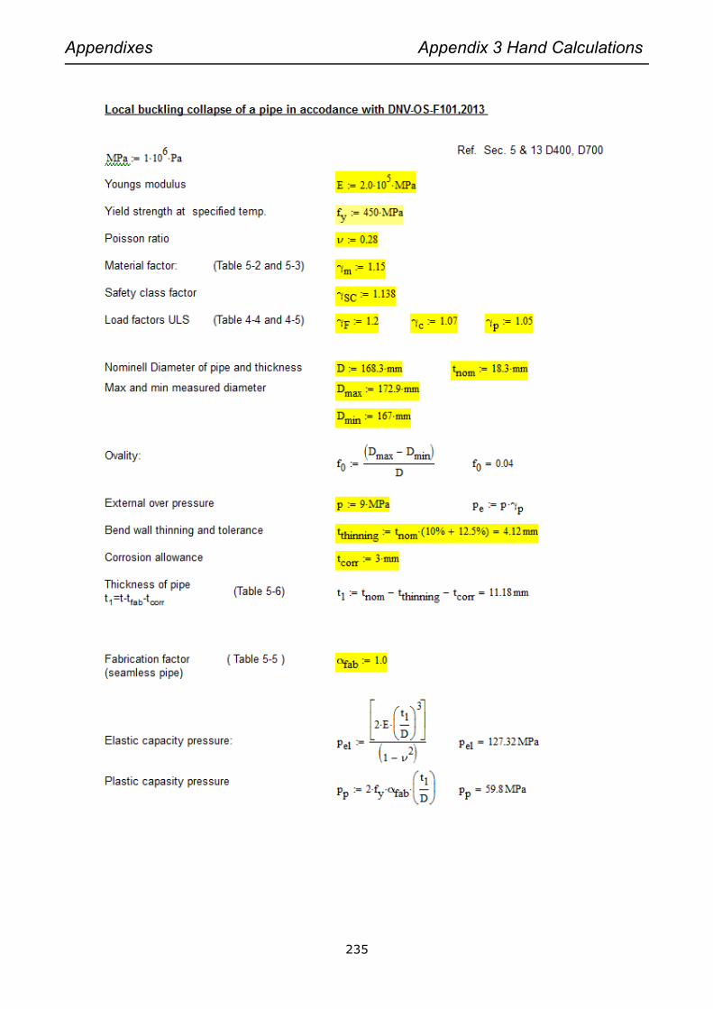
Appendixes Appendix 3 Hand Calculations
235
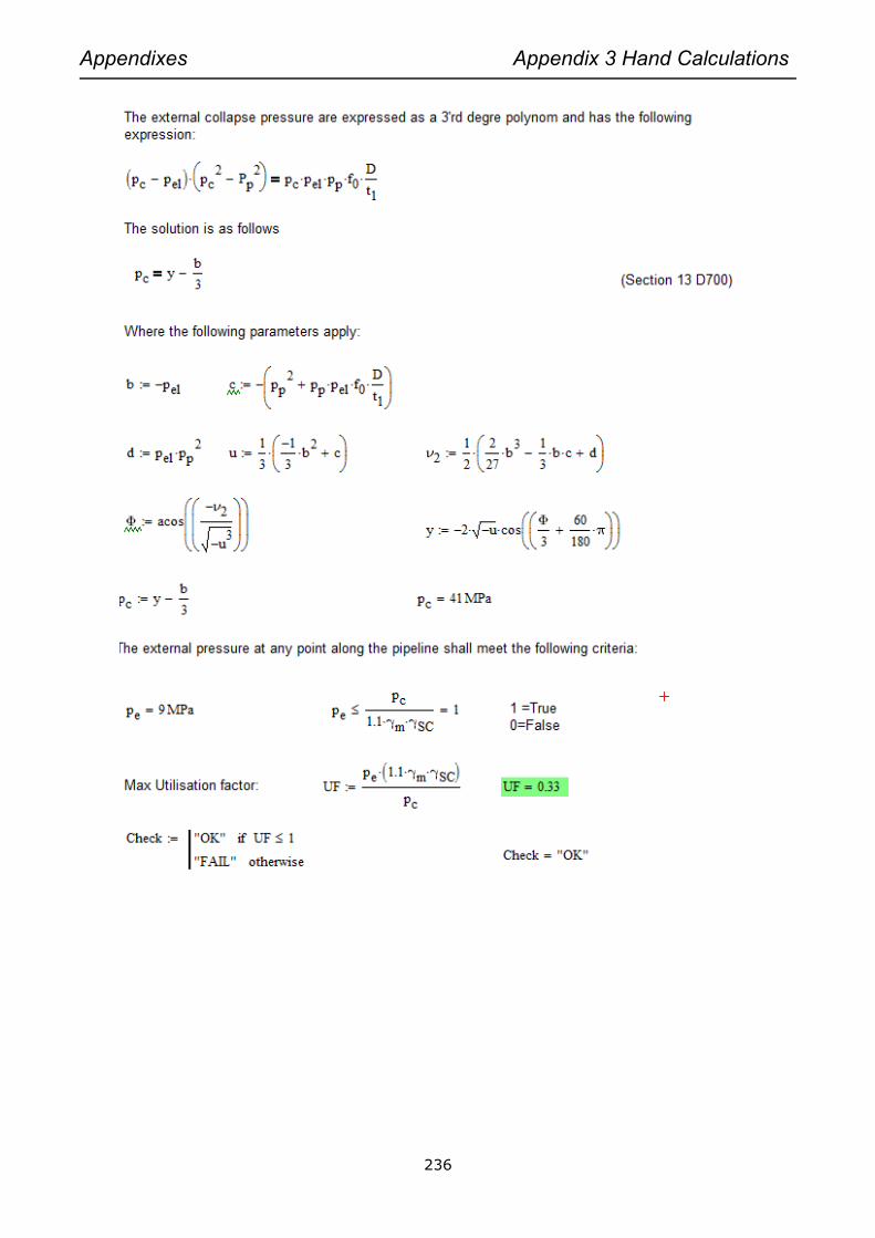
Appendixes Appendix 3 Hand Calculations
236

Appendixes Appendix 4 Bently AutoPIPE
237
Appendix 4 Bently AutoPIPE

Appendixes Appendix 4 Bently AutoPIPE
238
A 4.1 AutoPIPE Features
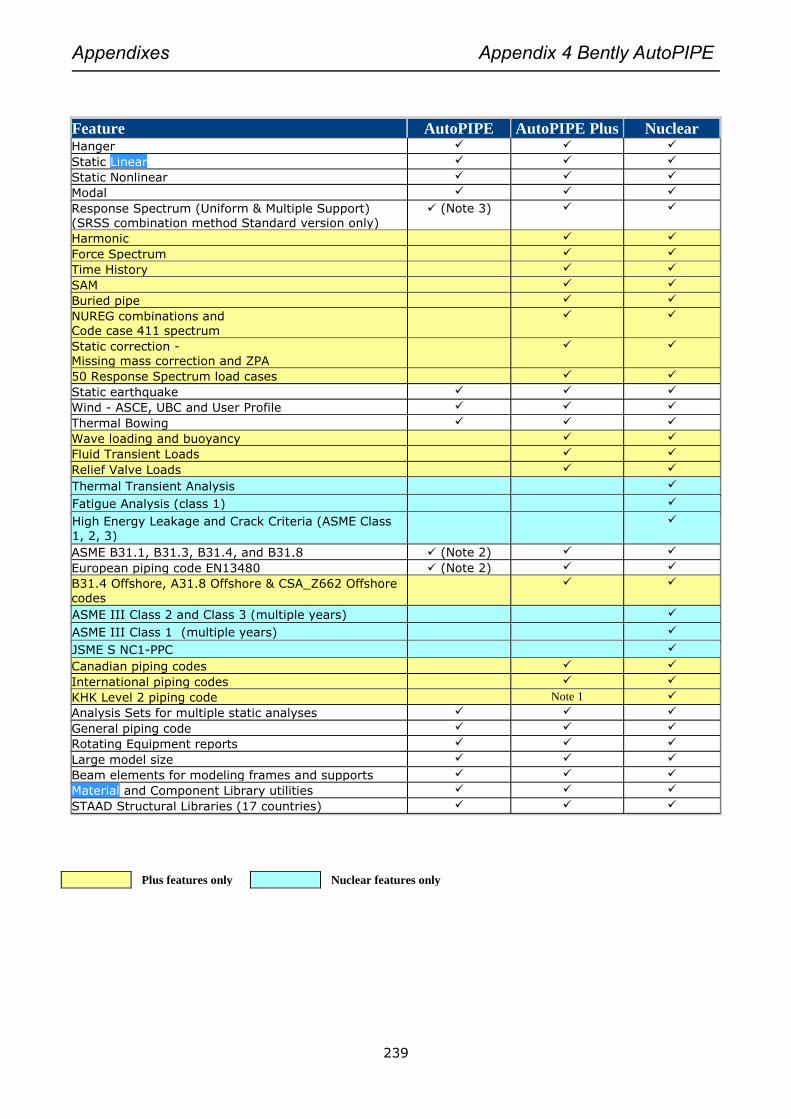
Appendixes Appendix 4 Bently AutoPIPE
239
Feature AutoPIPE AutoPIPE Plus Nuclear Hanger
Static Linear
Static Nonlinear
Modal
Response Spectrum (Uniform & Multiple Support) (SRSS combination method Standard version only)
(Note 3)
Harmonic
Force Spectrum
Time History
SAM
Buried pipe
NUREG combinations and Code case 411 spectrum
Static correction -
Missing mass correction and ZPA
50 Response Spectrum load cases
Static earthquake
Wind - ASCE, UBC and User Profile
Thermal Bowing
Wave loading and buoyancy
Fluid Transient Loads
Relief Valve Loads
Thermal Transient Analysis
Fatigue Analysis (class 1)
High Energy Leakage and Crack Criteria (ASME Class 1, 2, 3)
ASME B31.1, B31.3, B31.4, and B31.8 (Note 2)
European piping code EN13480 (Note 2)
B31.4 Offshore, A31.8 Offshore & CSA_Z662 Offshore
codes
ASME III Class 2 and Class 3 (multiple years)
ASME III Class 1 (multiple years)
JSME S NC1-PPC
Canadian piping codes
International piping codes
KHK Level 2 piping code Note 1
Analysis Sets for multiple static analyses
General piping code
Rotating Equipment reports
Large model size
Beam elements for modeling frames and supports
Material and Component Library utilities
STAAD Structural Libraries (17 countries)
Plus features only Nuclear features only

Appendixes Appendix 4 Bently AutoPIPE
240
Maximum defined static and dynamic load cases:
Load Cases Standard 9.4 Plus 9.4 Nuclear 9.4
Gravity 1 1 1
Hydrotest 1 1 1
Thermal 5 100 100
Pressure 5 100 100
Static Earthquake 5 10 10
Wind 5 10 10
User 5 140 140
Response Spectrum 5 50 50
Harmonic Not Available 10 10
Seismic Anchor
Movement
Not Available 10 10
Force Spectrum Not Available 10 10
Time History Not Available 50 50
Static Analysis Cases 27 [Note 1] 82 [Note 1] 82 [Note 1]
Note 1: Maximum number of load cases that can be analyzed in a single analysis set during a static analysis
run in v9.1 and later. However an unlimited number of analysis sets can be run in a single static analysis in
v9.1 and later.
= Gravity (1) + Hydrotest (1) + Thermal (20) + Pressure (20) + Static Earthquake (10) + Wind (10) + User (20)
= 82 cases for Plus & Nuclear (27 for Standard)
Up to 100 different thermal loadings can be defined and analyzed in a single static analysis. Only 20 thermal
load cases per analysis set e.g. if want to run 50 thermal cases then define across 3 analysis sets. Since each
analysis set can have analyze up to 82 static cases, so literally 100’s of loads can be analyzed in different
scenarios with different options, linear, non-linear, hot or cold modulus etc in the same static analysis run.
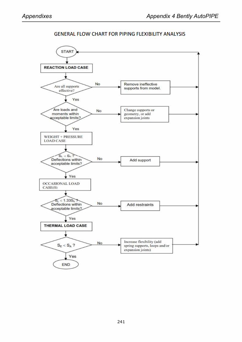
Appendixes Appendix 4 Bently AutoPIPE
241

Appendixes Appendix 4 Bently AutoPIPE
242
A 4.2 AutoPIPE Stress output

Appendixes Appendix 4 Bently AutoPIPE
243
----------------------------------------------------------------------------------------------------------------
6INCH SPOOL
05/21/2015 6INCH SPOOL BENTLEY
01:59 PM AutoPIPE Standard 9.4.0.19 RESULT PAGE 1
----------------------------------------------------------------------------------------------------------------
* ******* ** ******* *******
*** ** ** ** ** ** ** **
** ** ****** ** ** ** ** ** **
** ** ** ** ** ***** ******* ** ******* *****
********* ** ** ** ** ** ** ** ** **
** ** ** ** ** ** ** ** ** ** **
** ** ***** ** ***** ** ** ** *******
Pipe Stress Analysis and Design Program
Version: 09.04.00.19
Edition: Standard
Developed and Maintained by
BENTLEY SYSTEMS, INCORPORATED
1600 Riviera Ave., Suite 300
Walnut Creek, CA 94596
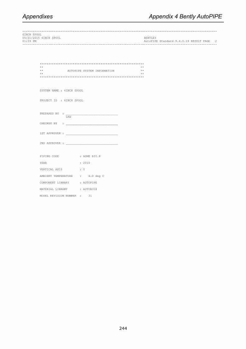
Appendixes Appendix 4 Bently AutoPIPE
244
----------------------------------------------------------------------------------------------------------------
6INCH SPOOL
05/21/2015 6INCH SPOOL BENTLEY
01:59 PM AutoPIPE Standard 9.4.0.19 RESULT PAGE 2
----------------------------------------------------------------------------------------------------------------
************************************************************
** **
** AUTOPIPE SYSTEM INFORMATION **
** **
************************************************************
SYSTEM NAME : 6INCH SPOOL
PROJECT ID : 6INCH SPOOL
PREPARED BY : ______________________________
LKA
CHECKED BY : ______________________________
1ST APPROVER : ______________________________
2ND APPROVER : ______________________________
PIPING CODE : ASME B31.8
YEAR : 2010
VERTICAL AXIS : Y
AMBIENT TEMPERATURE : 4.0 deg C
COMPONENT LIBRARY : AUTOPIPE
MATERIAL LIBRARY : AUTOB318
MODEL REVISION NUMBER : 31
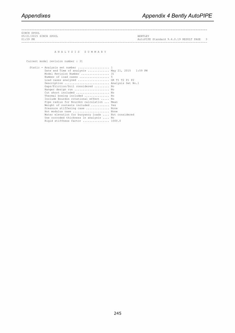
Appendixes Appendix 4 Bently AutoPIPE
245
----------------------------------------------------------------------------------------------------------------
6INCH SPOOL
05/21/2015 6INCH SPOOL BENTLEY
01:59 PM AutoPIPE Standard 9.4.0.19 RESULT PAGE 3
----------------------------------------------------------------------------------------------------------------
A N A L Y S I S S U M M A R Y
Current model revision number : 31
Static - Analysis set number ................... 1
Date and Time of analysis ............. May 21, 2015 1:59 PM
Model Revision Number ................. 31
Number of load cases .................. 5
Load cases analyzed ................... GR T1 T2 P1 P2
Description ........................... Analysis Set No.1
Gaps/Friction/Soil considered ......... No
Hanger design run ..................... No
Cut short included .................... No
Thermal bowing included ............... No
Include Bourdon rotational effect ..... No
Pipe radius for Bourdon calculation ... Mean
Weight of contents included ........... Yes
Pressure stiffening case .............. None
Hot modulus case ...................... None
Water elevation for buoyancy loads .... Not considered
Use corroded thickness in analysis .... No
Rigid stiffness factor ................ 1000.0

Appendixes Appendix 4 Bently AutoPIPE
246
----------------------------------------------------------------------------------------------------------------
6INCH SPOOL
05/21/2015 6INCH SPOOL BENTLEY
01:59 PM AutoPIPE Standard 9.4.0.19 RESULT PAGE 4
----------------------------------------------------------------------------------------------------------------
CODE COMPLIANCE COMBINATIONS
<Description> Allowable
Combination Category Method Case/Combination Factor M/S K-Factor (N/mm2) D/A/P
----------------------- ----------- -------- ------------------------ ------ --- --------- --------- -------
GR + Max P{1} Sustain Sum GR[1] 1.00 405.00 Y N Y
Max Long 1.00
Max Range Expansion Sum Temp. Range 1.00 Automatic Y Y Y
Amb to T1{1} Expansion Sum T1[1] 1.00 Automatic Y Y Y
Amb to T2{1} Expansion Sum T2[1] 1.00 Automatic Y Y Y
Max P{1} Hoop Sum Max Hoop 1.00 Automatic Y Y Y
GRTP1{1} Rest-Fun Sum Max Long 1.00 Automatic Y N Y
Max Hoop 1.00
GR[1] 1.00
T1[1] 1.00
P1[1] 1.00
GRTP2{1} Rest-Fun Sum Max Long 1.00 Automatic Y Y Y
Max Hoop 1.00
GR[1] 1.00
T2[1] 1.00
P2[1] 1.00
Notes:
D/A/P: [D]efault/[A]uto-Update/[P]rint options (Y=Yes, N=No)
Appendixes Appendix 4 Bently AutoPIPE
247
----------------------------------------------------------------------------------------------------------------
6INCH SPOOL
05/21/2015 6INCH SPOOL BENTLEY
01:59 PM AutoPIPE Standard 9.4.0.19 RESULT PAGE 5
----------------------------------------------------------------------------------------------------------------
NON-CODE COMBINATIONS
<Description>
Combination Method Case/Combination Factor D/A/P
----------------------- -------- ------------------------ ------ -------
Gravity{1} Sum GR[1] 1.00 Y Y Y
<4.00 deg C>
Thermal 1{1} Sum T1[1] 1.00 Y Y Y
<100.00 deg C>
Thermal 2{1} Sum T2[1] 1.00 Y Y Y
Pressure 1{1} Sum P1[1] 1.00 Y Y Y
Pressure 2{1} Sum P2[1] 1.00 Y Y Y
GRTP1{1} Sum GR[1] 1.00 Y Y Y
T1[1] 1.00
P1[1] 1.00
GRTP2{1} Sum GR[1] 1.00 Y Y Y
T2[1] 1.00
P2[1] 1.00
Notes:
D/A/P: [D]efault/[A]uto-Update/[P]rint options (Y=Yes, N=No)
Appendixes Appendix 4 Bently AutoPIPE
248
----------------------------------------------------------------------------------------------------------------
6INCH SPOOL
05/21/2015 6INCH SPOOL BENTLEY
01:59 PM AutoPIPE Standard 9.4.0.19 RESULT PAGE 6
----------------------------------------------------------------------------------------------------------------
CODE COMPLIANCE
Y - Factor ............................ 0.00
Weld efficiency factor ................ 1.00
Range reduction factor ................ 1.00
Design factor ......................... 0.72
Temperature derating factor ........... 1.00
Design Pressure Factor ................ 1.00
Minimum stress ratio used in reports... 0.00
Number of stress points per span ...... 0
Include corrosion in stress calcs. .... Y
Include torsion in code stress ........ N
Include axial force in code stress .... Y
Include sustain load margin ........... Only if allowable stress is exceeded
Set sustained SIF=1 no bends .......... N
Set sustained/occasional SIF = 1 ...... N
Set sustained/occasional SIF = 0.75i .. N
Apply cold/hot modulus ratio .......... N
Disable auto code combinations ........ N
Disable auto non-code combinations .... N
No. of thermal ranges to report ....... 0
Include Max Range combination ......... Y
Total stress .......................... Octahedral
Direct shear .......................... None
Longitudinal pressure calculation ..... PD/4t
Inc. Axial Str and Pcase in Sustained.. Y
Appendixes Appendix 4 Bently AutoPIPE
249
----------------------------------------------------------------------------------------------------------------
6INCH SPOOL
05/21/2015 6INCH SPOOL BENTLEY
01:59 PM AutoPIPE Standard 9.4.0.19 RESULT PAGE 7
----------------------------------------------------------------------------------------------------------------
D I S P L A C E M E N T S
Point Load TRANSLATIONS (mm ) ROTATIONS (deg )
name combination X Y Z X Y Z
------ ------------------------ ------ ------ ------ ------ ------ ------
*** Segment A begin ***
A00 Gravity{1} 0.00 -160.00 0.00 0.93 0.00 0.93
Thermal 1{1} 0.00 0.00 0.00 0.00 0.00 0.00
Thermal 2{1} 0.00 0.00 0.00 0.00 0.00 0.00
Pressure 1{1} 0.00 0.00 0.00 0.00 0.00 0.00
Pressure 2{1} 0.00 0.00 0.00 0.00 0.00 0.00
GRTP1{1} 0.00 -160.00 0.00 0.93 0.00 0.93
GRTP2{1} 0.00 -160.00 0.00 0.93 0.00 0.93
A01 N Gravity{1} 134.57 -160.06 102.76 0.89 0.18 -1.81
Thermal 1{1} 0.00 0.00 0.00 0.00 0.00 0.00
Thermal 2{1} -7.41 7.45 0.00 0.00 0.00 0.02
Pressure 1{1} -0.72 0.73 0.00 0.00 0.00 0.00
Pressure 2{1} -0.72 0.73 0.00 0.00 0.00 0.00
GRTP1{1} 133.85 -159.33 102.76 0.89 0.18 -1.81
GRTP2{1} 126.43 -151.88 102.76 0.89 0.18 -1.79
A01 F Gravity{1} 148.46 -173.46 108.45 0.92 0.19 -1.58
Thermal 1{1} 0.00 0.00 0.00 0.00 0.00 0.00
Thermal 2{1} -6.98 7.93 0.00 0.00 0.00 -0.02
Pressure 1{1} -0.68 0.78 0.00 0.00 0.00 0.00
Pressure 2{1} -0.68 0.78 0.00 0.00 0.00 0.00
GRTP1{1} 147.78 -172.68 108.45 0.92 0.19 -1.59
GRTP2{1} 140.80 -164.75 108.45 0.92 0.19 -1.60
A02 N Gravity{1} 148.48 -213.85 101.02 1.02 0.21 -0.53
Thermal 1{1} 0.00 0.00 0.00 0.00 0.00 0.00
Thermal 2{1} -4.69 5.40 0.00 0.00 0.00 -0.12
Pressure 1{1} -0.46 0.53 0.00 0.00 0.00 -0.01
Pressure 2{1} -0.46 0.53 0.00 0.00 0.00 -0.01
GRTP1{1} 148.02 -213.32 101.02 1.02 0.21 -0.54
GRTP2{1} 143.33 -207.92 101.02 1.02 0.21 -0.66
A02 F Gravity{1} 146.97 -216.53 91.09 1.05 0.20 0.00
Thermal 1{1} 0.00 0.00 0.00 0.00 0.00 0.00
Thermal 2{1} -5.40 3.79 0.00 0.00 0.00 -0.17
Pressure 1{1} -0.53 0.37 0.00 0.00 0.00 -0.02
Pressure 2{1} -0.53 0.37 0.00 0.00 0.00 -0.02
GRTP1{1} 146.45 -216.16 91.09 1.05 0.20 -0.02
GRTP2{1} 141.05 -212.37 91.09 1.05 0.20 -0.18
A03 N Gravity{1} 228.49 -216.56 -16.52 1.12 0.16 0.73
Thermal 1{1} 0.00 0.00 0.00 0.00 0.00 0.00
Thermal 2{1} -27.86 -2.34 0.00 0.00 0.00 -0.22
Pressure 1{1} -2.72 -0.23 0.00 0.00 0.00 -0.02
Pressure 2{1} -2.72 -0.23 0.00 0.00 0.00 -0.02
GRTP1{1} 225.77 -216.79 -16.52 1.12 0.16 0.71
GRTP2{1} 197.90 -219.12 -16.52 1.12 0.16 0.49

Appendixes Appendix 4 Bently AutoPIPE
250
----------------------------------------------------------------------------------------------------------------
6INCH SPOOL
05/21/2015 6INCH SPOOL BENTLEY
01:59 PM AutoPIPE Standard 9.4.0.19 RESULT PAGE 8
----------------------------------------------------------------------------------------------------------------
D I S P L A C E M E N T S
Point Load TRANSLATIONS (mm ) ROTATIONS (deg )
name combination X Y Z X Y Z
------ ------------------------ ------ ------ ------ ------ ------ ------
A03 F Gravity{1} 233.44 -212.34 -26.69 1.12 0.15 0.41
Thermal 1{1} 0.00 0.00 0.00 0.00 0.00 0.00
Thermal 2{1} -29.09 -4.51 0.00 0.00 0.00 -0.20
Pressure 1{1} -2.84 -0.44 0.00 0.00 0.00 -0.02
Pressure 2{1} -2.84 -0.44 0.00 0.00 0.00 -0.02
GRTP1{1} 230.59 -212.78 -26.69 1.12 0.15 0.39
GRTP2{1} 201.50 -217.29 -26.69 1.12 0.15 0.19
A07 Gravity{1} 233.49 -250.98 -37.82 1.07 0.03 -0.65
Thermal 1{1} 0.00 0.00 0.00 0.00 0.00 0.00
Thermal 2{1} -22.20 -16.66 0.00 0.00 0.00 -0.03
Pressure 1{1} -2.17 -1.63 0.00 0.00 0.00 0.00
Pressure 2{1} -2.17 -1.63 0.00 0.00 0.00 0.00
GRTP1{1} 231.32 -252.61 -37.82 1.07 0.03 -0.65
GRTP2{1} 209.12 -269.27 -37.82 1.07 0.03 -0.69
A06 Gravity{1} 233.55 -281.60 -30.76 1.03 -0.15 0.34
Thermal 1{1} 0.00 0.00 0.00 0.00 0.00 0.00
Thermal 2{1} -14.82 -14.05 0.00 0.00 0.00 0.06
Pressure 1{1} -1.45 -1.37 0.00 0.00 0.00 0.01
Pressure 2{1} -1.45 -1.37 0.00 0.00 0.00 0.01
GRTP1{1} 232.10 -282.98 -30.76 1.03 -0.15 0.35
GRTP2{1} 217.28 -297.02 -30.76 1.03 -0.15 0.41
A08 Gravity{1} 233.61 -159.75 -6.93 0.98 -0.23 1.61
Thermal 1{1} 0.00 0.00 0.00 0.00 0.00 0.00
Thermal 2{1} -7.44 -4.92 0.00 0.00 0.00 0.08
Pressure 1{1} -0.73 -0.48 0.00 0.00 0.00 0.01
Pressure 2{1} -0.73 -0.48 0.00 0.00 0.00 0.01
GRTP1{1} 232.88 -160.23 -6.93 0.98 -0.23 1.61
GRTP2{1} 225.45 -165.15 -6.93 0.98 -0.23 1.69
A04 N Gravity{1} 233.67 20.33 11.85 0.93 -0.07 1.29
Thermal 1{1} 0.00 0.00 0.00 0.00 0.00 0.00
Thermal 2{1} -0.55 0.75 0.00 0.00 0.00 0.01
Pressure 1{1} -0.05 0.07 0.00 0.00 0.00 0.00
Pressure 2{1} -0.05 0.07 0.00 0.00 0.00 0.00
GRTP1{1} 233.61 20.40 11.85 0.93 -0.07 1.29
GRTP2{1} 233.06 21.16 11.85 0.93 -0.07 1.31
A04 F Gravity{1} 242.81 30.00 4.85 0.93 -0.02 1.05
Thermal 1{1} 0.00 0.00 0.00 0.00 0.00 0.00
Thermal 2{1} -0.01 0.33 0.00 0.00 0.00 0.00
Pressure 1{1} 0.00 0.03 0.00 0.00 0.00 0.00
Pressure 2{1} 0.00 0.03 0.00 0.00 0.00 0.00
GRTP1{1} 242.81 30.03 4.85 0.93 -0.02 1.05
GRTP2{1} 242.81 30.36 4.85 0.93 -0.02 1.05

Appendixes Appendix 4 Bently AutoPIPE
251
----------------------------------------------------------------------------------------------------------------
6INCH SPOOL
05/21/2015 6INCH SPOOL BENTLEY
01:59 PM AutoPIPE Standard 9.4.0.19 RESULT PAGE 9
----------------------------------------------------------------------------------------------------------------
D I S P L A C E M E N T S
Point Load TRANSLATIONS (mm ) ROTATIONS (deg )
name combination X Y Z X Y Z
------ ------------------------ ------ ------ ------ ------ ------ ------
A05 Gravity{1} 248.00 30.00 0.00 0.93 0.00 0.93
Thermal 1{1} 0.00 0.00 0.00 0.00 0.00 0.00
Thermal 2{1} 0.00 0.00 0.00 0.00 0.00 0.00
Pressure 1{1} 0.00 0.00 0.00 0.00 0.00 0.00
Pressure 2{1} 0.00 0.00 0.00 0.00 0.00 0.00
GRTP1{1} 248.00 30.00 0.00 0.93 0.00 0.93
GRTP2{1} 248.00 30.00 0.00 0.93 0.00 0.93
*** Segment A end ***
Appendixes Appendix 4 Bently AutoPIPE
252
----------------------------------------------------------------------------------------------------------------
6INCH SPOOL
05/21/2015 6INCH SPOOL BENTLEY
01:59 PM AutoPIPE Standard 9.4.0.19 RESULT PAGE 10
----------------------------------------------------------------------------------------------------------------
R E S T R A I N T R E A C T I O N S
Point Load FORCES (N ) MOMENTS (N.m )
name combination X Y Z Result X Y Z Result
------ ----------------------- ------ ------ ------ ------ ------- ------- ------- -------
A00 Anchor Tag No.: <None>
Gravity{1} 15645 -17237 -1149 23307 -4018 1748 -88455 88564
Thermal 1{1} 0 0 0 0 0 0 0 0
Thermal 2{1} -1175 162 0 1186 0 0 4268 4268
Pressure 1{1} -115 16 0 116 0 0 417 417
Pressure 2{1} -115 16 0 116 0 0 417 417
GRTP1{1} 15530 -17221 -1149 23218 -4018 1748 -88038 88147
GRTP2{1} 14355 -17059 -1149 22325 -4018 1748 -83770 83885
A05 Anchor Tag No.: <None>
Gravity{1} -15645 -7395 -833 17325 -138 -4756 37180 37483
Thermal 1{1} 0 0 0 0 0 0 0 0
Thermal 2{1} 1175 -162 0 1186 0 0 573 573
Pressure 1{1} 115 -16 0 116 0 0 56 56
Pressure 2{1} 115 -16 0 116 0 0 56 56
GRTP1{1} -15530 -7410 -833 17228 -138 -4756 37236 37539
GRTP2{1} -14355 -7572 -833 16251 -138 -4756 37809 38107
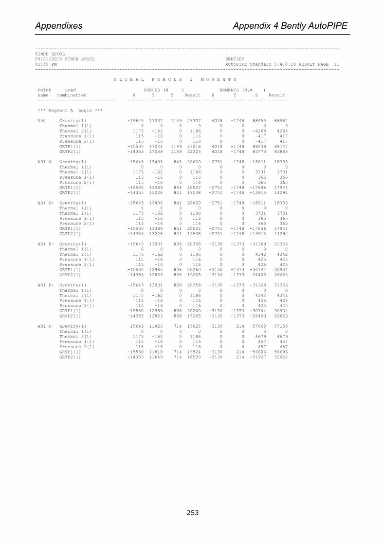
Appendixes Appendix 4 Bently AutoPIPE
253
----------------------------------------------------------------------------------------------------------------
6INCH SPOOL
05/21/2015 6INCH SPOOL BENTLEY
01:59 PM AutoPIPE Standard 9.4.0.19 RESULT PAGE 11
----------------------------------------------------------------------------------------------------------------
G L O B A L F O R C E S & M O M E N T S
Point Load FORCES (N ) MOMENTS (N.m )
name combination X Y Z Result X Y Z Result
------ ---------------------- ------ ------ ------ ------ ------- ------- ------- -------
*** Segment A begin ***
A00 Gravity{1} -15645 17237 1149 23307 4018 -1748 88455 88564
Thermal 1{1} 0 0 0 0 0 0 0 0
Thermal 2{1} 1175 -162 0 1186 0 0 -4268 4268
Pressure 1{1} 115 -16 0 116 0 0 -417 417
Pressure 2{1} 115 -16 0 116 0 0 -417 417
GRTP1{1} -15530 17221 1149 23218 4018 -1748 88038 88147
GRTP2{1} -14355 17059 1149 22325 4018 -1748 83770 83885
A01 N- Gravity{1} -15645 13405 841 20620 -2751 -1748 -18011 18303
Thermal 1{1} 0 0 0 0 0 0 0 0
Thermal 2{1} 1175 -162 0 1186 0 0 3731 3731
Pressure 1{1} 115 -16 0 116 0 0 365 365
Pressure 2{1} 115 -16 0 116 0 0 365 365
GRTP1{1} -15530 13389 841 20522 -2751 -1748 -17646 17944
GRTP2{1} -14355 13228 841 19538 -2751 -1748 -13915 14292
A01 N+ Gravity{1} -15645 13405 841 20620 -2751 -1748 -18011 18303
Thermal 1{1} 0 0 0 0 0 0 0 0
Thermal 2{1} 1175 -162 0 1186 0 0 3731 3731
Pressure 1{1} 115 -16 0 116 0 0 365 365
Pressure 2{1} 115 -16 0 116 0 0 365 365
GRTP1{1} -15530 13389 841 20522 -2751 -1748 -17646 17944
GRTP2{1} -14355 13228 841 19538 -2751 -1748 -13915 14292
A01 F- Gravity{1} -15645 13001 808 20358 -3130 -1373 -31169 31356
Thermal 1{1} 0 0 0 0 0 0 0 0
Thermal 2{1} 1175 -162 0 1186 0 0 4342 4342
Pressure 1{1} 115 -16 0 116 0 0 425 425
Pressure 2{1} 115 -16 0 116 0 0 425 425
GRTP1{1} -15530 12985 808 20260 -3130 -1373 -30744 30934
GRTP2{1} -14355 12823 808 19265 -3130 -1373 -26403 26623
A01 F+ Gravity{1} -15645 13001 808 20358 -3130 -1373 -31169 31356
Thermal 1{1} 0 0 0 0 0 0 0 0
Thermal 2{1} 1175 -162 0 1186 0 0 4342 4342
Pressure 1{1} 115 -16 0 116 0 0 425 425
Pressure 2{1} 115 -16 0 116 0 0 425 425
GRTP1{1} -15530 12985 808 20260 -3130 -1373 -30744 30934
GRTP2{1} -14355 12823 808 19265 -3130 -1373 -26403 26623
A02 N- Gravity{1} -15645 11826 714 19625 -3130 214 -57063 57150
Thermal 1{1} 0 0 0 0 0 0 0 0
Thermal 2{1} 1175 -162 0 1186 0 0 4679 4679
Pressure 1{1} 115 -16 0 116 0 0 457 457
Pressure 2{1} 115 -16 0 116 0 0 457 457
GRTP1{1} -15530 11810 714 19524 -3130 214 -56606 56693
GRTP2{1} -14355 11649 714 18500 -3130 214 -51927 52022
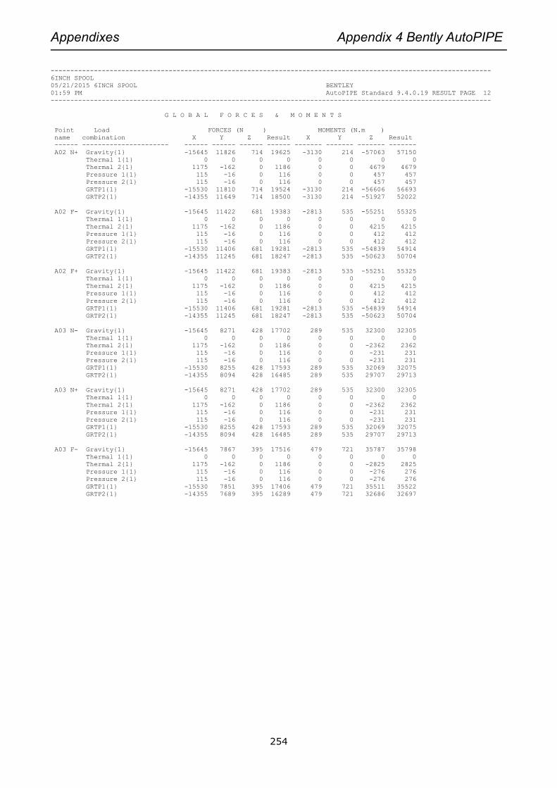
Appendixes Appendix 4 Bently AutoPIPE
254
----------------------------------------------------------------------------------------------------------------
6INCH SPOOL
05/21/2015 6INCH SPOOL BENTLEY
01:59 PM AutoPIPE Standard 9.4.0.19 RESULT PAGE 12
----------------------------------------------------------------------------------------------------------------
G L O B A L F O R C E S & M O M E N T S
Point Load FORCES (N ) MOMENTS (N.m )
name combination X Y Z Result X Y Z Result
------ ---------------------- ------ ------ ------ ------ ------- ------- ------- -------
A02 N+ Gravity{1} -15645 11826 714 19625 -3130 214 -57063 57150
Thermal 1{1} 0 0 0 0 0 0 0 0
Thermal 2{1} 1175 -162 0 1186 0 0 4679 4679
Pressure 1{1} 115 -16 0 116 0 0 457 457
Pressure 2{1} 115 -16 0 116 0 0 457 457
GRTP1{1} -15530 11810 714 19524 -3130 214 -56606 56693
GRTP2{1} -14355 11649 714 18500 -3130 214 -51927 52022
A02 F- Gravity{1} -15645 11422 681 19383 -2813 535 -55251 55325
Thermal 1{1} 0 0 0 0 0 0 0 0
Thermal 2{1} 1175 -162 0 1186 0 0 4215 4215
Pressure 1{1} 115 -16 0 116 0 0 412 412
Pressure 2{1} 115 -16 0 116 0 0 412 412
GRTP1{1} -15530 11406 681 19281 -2813 535 -54839 54914
GRTP2{1} -14355 11245 681 18247 -2813 535 -50623 50704
A02 F+ Gravity{1} -15645 11422 681 19383 -2813 535 -55251 55325
Thermal 1{1} 0 0 0 0 0 0 0 0
Thermal 2{1} 1175 -162 0 1186 0 0 4215 4215
Pressure 1{1} 115 -16 0 116 0 0 412 412
Pressure 2{1} 115 -16 0 116 0 0 412 412
GRTP1{1} -15530 11406 681 19281 -2813 535 -54839 54914
GRTP2{1} -14355 11245 681 18247 -2813 535 -50623 50704
A03 N- Gravity{1} -15645 8271 428 17702 289 535 32300 32305
Thermal 1{1} 0 0 0 0 0 0 0 0
Thermal 2{1} 1175 -162 0 1186 0 0 -2362 2362
Pressure 1{1} 115 -16 0 116 0 0 -231 231
Pressure 2{1} 115 -16 0 116 0 0 -231 231
GRTP1{1} -15530 8255 428 17593 289 535 32069 32075
GRTP2{1} -14355 8094 428 16485 289 535 29707 29713
A03 N+ Gravity{1} -15645 8271 428 17702 289 535 32300 32305
Thermal 1{1} 0 0 0 0 0 0 0 0
Thermal 2{1} 1175 -162 0 1186 0 0 -2362 2362
Pressure 1{1} 115 -16 0 116 0 0 -231 231
Pressure 2{1} 115 -16 0 116 0 0 -231 231
GRTP1{1} -15530 8255 428 17593 289 535 32069 32075
GRTP2{1} -14355 8094 428 16485 289 535 29707 29713
A03 F- Gravity{1} -15645 7867 395 17516 479 721 35787 35798
Thermal 1{1} 0 0 0 0 0 0 0 0
Thermal 2{1} 1175 -162 0 1186 0 0 -2825 2825
Pressure 1{1} 115 -16 0 116 0 0 -276 276
Pressure 2{1} 115 -16 0 116 0 0 -276 276
GRTP1{1} -15530 7851 395 17406 479 721 35511 35522
GRTP2{1} -14355 7689 395 16289 479 721 32686 32697
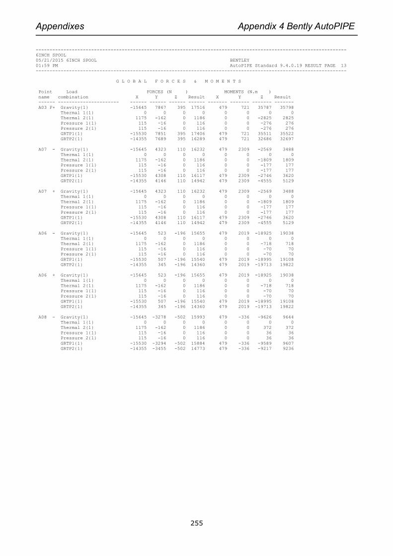
Appendixes Appendix 4 Bently AutoPIPE
255
----------------------------------------------------------------------------------------------------------------
6INCH SPOOL
05/21/2015 6INCH SPOOL BENTLEY
01:59 PM AutoPIPE Standard 9.4.0.19 RESULT PAGE 13
----------------------------------------------------------------------------------------------------------------
G L O B A L F O R C E S & M O M E N T S
Point Load FORCES (N ) MOMENTS (N.m )
name combination X Y Z Result X Y Z Result
------ ---------------------- ------ ------ ------ ------ ------- ------- ------- -------
A03 F+ Gravity{1} -15645 7867 395 17516 479 721 35787 35798
Thermal 1{1} 0 0 0 0 0 0 0 0
Thermal 2{1} 1175 -162 0 1186 0 0 -2825 2825
Pressure 1{1} 115 -16 0 116 0 0 -276 276
Pressure 2{1} 115 -16 0 116 0 0 -276 276
GRTP1{1} -15530 7851 395 17406 479 721 35511 35522
GRTP2{1} -14355 7689 395 16289 479 721 32686 32697
A07 - Gravity{1} -15645 4323 110 16232 479 2309 -2569 3488
Thermal 1{1} 0 0 0 0 0 0 0 0
Thermal 2{1} 1175 -162 0 1186 0 0 -1809 1809
Pressure 1{1} 115 -16 0 116 0 0 -177 177
Pressure 2{1} 115 -16 0 116 0 0 -177 177
GRTP1{1} -15530 4308 110 16117 479 2309 -2746 3620
GRTP2{1} -14355 4146 110 14942 479 2309 -4555 5129
A07 + Gravity{1} -15645 4323 110 16232 479 2309 -2569 3488
Thermal 1{1} 0 0 0 0 0 0 0 0
Thermal 2{1} 1175 -162 0 1186 0 0 -1809 1809
Pressure 1{1} 115 -16 0 116 0 0 -177 177
Pressure 2{1} 115 -16 0 116 0 0 -177 177
GRTP1{1} -15530 4308 110 16117 479 2309 -2746 3620
GRTP2{1} -14355 4146 110 14942 479 2309 -4555 5129
A06 - Gravity{1} -15645 523 -196 15655 479 2019 -18925 19038
Thermal 1{1} 0 0 0 0 0 0 0 0
Thermal 2{1} 1175 -162 0 1186 0 0 -718 718
Pressure 1{1} 115 -16 0 116 0 0 -70 70
Pressure 2{1} 115 -16 0 116 0 0 -70 70
GRTP1{1} -15530 507 -196 15540 479 2019 -18995 19108
GRTP2{1} -14355 345 -196 14360 479 2019 -19713 19822
A06 + Gravity{1} -15645 523 -196 15655 479 2019 -18925 19038
Thermal 1{1} 0 0 0 0 0 0 0 0
Thermal 2{1} 1175 -162 0 1186 0 0 -718 718
Pressure 1{1} 115 -16 0 116 0 0 -70 70
Pressure 2{1} 115 -16 0 116 0 0 -70 70
GRTP1{1} -15530 507 -196 15540 479 2019 -18995 19108
GRTP2{1} -14355 345 -196 14360 479 2019 -19713 19822
A08 - Gravity{1} -15645 -3278 -502 15993 479 -336 -9626 9644
Thermal 1{1} 0 0 0 0 0 0 0 0
Thermal 2{1} 1175 -162 0 1186 0 0 372 372
Pressure 1{1} 115 -16 0 116 0 0 36 36
Pressure 2{1} 115 -16 0 116 0 0 36 36
GRTP1{1} -15530 -3294 -502 15884 479 -336 -9589 9607
GRTP2{1} -14355 -3455 -502 14773 479 -336 -9217 9236
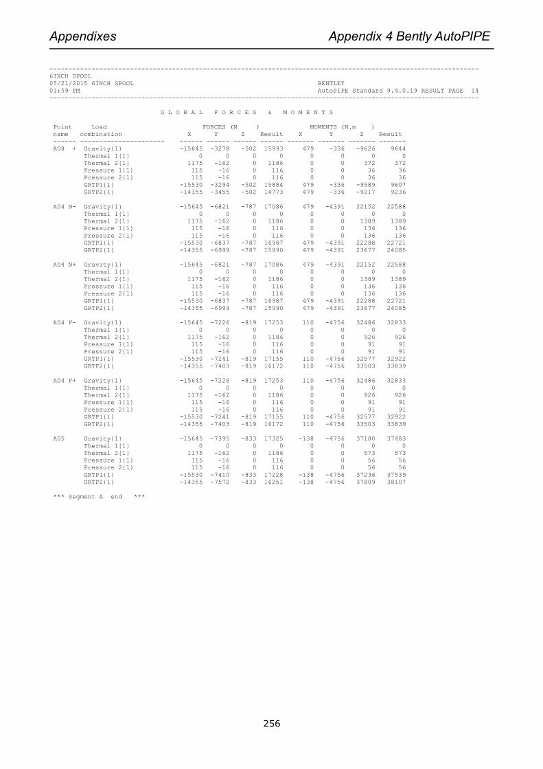
Appendixes Appendix 4 Bently AutoPIPE
256
----------------------------------------------------------------------------------------------------------------
6INCH SPOOL
05/21/2015 6INCH SPOOL BENTLEY
01:59 PM AutoPIPE Standard 9.4.0.19 RESULT PAGE 14
----------------------------------------------------------------------------------------------------------------
G L O B A L F O R C E S & M O M E N T S
Point Load FORCES (N ) MOMENTS (N.m )
name combination X Y Z Result X Y Z Result
------ ---------------------- ------ ------ ------ ------ ------- ------- ------- -------
A08 + Gravity{1} -15645 -3278 -502 15993 479 -336 -9626 9644
Thermal 1{1} 0 0 0 0 0 0 0 0
Thermal 2{1} 1175 -162 0 1186 0 0 372 372
Pressure 1{1} 115 -16 0 116 0 0 36 36
Pressure 2{1} 115 -16 0 116 0 0 36 36
GRTP1{1} -15530 -3294 -502 15884 479 -336 -9589 9607
GRTP2{1} -14355 -3455 -502 14773 479 -336 -9217 9236
A04 N- Gravity{1} -15645 -6821 -787 17086 479 -4391 22152 22588
Thermal 1{1} 0 0 0 0 0 0 0 0
Thermal 2{1} 1175 -162 0 1186 0 0 1389 1389
Pressure 1{1} 115 -16 0 116 0 0 136 136
Pressure 2{1} 115 -16 0 116 0 0 136 136
GRTP1{1} -15530 -6837 -787 16987 479 -4391 22288 22721
GRTP2{1} -14355 -6999 -787 15990 479 -4391 23677 24085
A04 N+ Gravity{1} -15645 -6821 -787 17086 479 -4391 22152 22588
Thermal 1{1} 0 0 0 0 0 0 0 0
Thermal 2{1} 1175 -162 0 1186 0 0 1389 1389
Pressure 1{1} 115 -16 0 116 0 0 136 136
Pressure 2{1} 115 -16 0 116 0 0 136 136
GRTP1{1} -15530 -6837 -787 16987 479 -4391 22288 22721
GRTP2{1} -14355 -6999 -787 15990 479 -4391 23677 24085
A04 F- Gravity{1} -15645 -7226 -819 17253 110 -4756 32486 32833
Thermal 1{1} 0 0 0 0 0 0 0 0
Thermal 2{1} 1175 -162 0 1186 0 0 926 926
Pressure 1{1} 115 -16 0 116 0 0 91 91
Pressure 2{1} 115 -16 0 116 0 0 91 91
GRTP1{1} -15530 -7241 -819 17155 110 -4756 32577 32922
GRTP2{1} -14355 -7403 -819 16172 110 -4756 33503 33839
A04 F+ Gravity{1} -15645 -7226 -819 17253 110 -4756 32486 32833
Thermal 1{1} 0 0 0 0 0 0 0 0
Thermal 2{1} 1175 -162 0 1186 0 0 926 926
Pressure 1{1} 115 -16 0 116 0 0 91 91
Pressure 2{1} 115 -16 0 116 0 0 91 91
GRTP1{1} -15530 -7241 -819 17155 110 -4756 32577 32922
GRTP2{1} -14355 -7403 -819 16172 110 -4756 33503 33839
A05 Gravity{1} -15645 -7395 -833 17325 -138 -4756 37180 37483
Thermal 1{1} 0 0 0 0 0 0 0 0
Thermal 2{1} 1175 -162 0 1186 0 0 573 573
Pressure 1{1} 115 -16 0 116 0 0 56 56
Pressure 2{1} 115 -16 0 116 0 0 56 56
GRTP1{1} -15530 -7410 -833 17228 -138 -4756 37236 37539
GRTP2{1} -14355 -7572 -833 16251 -138 -4756 37809 38107
*** Segment A end ***
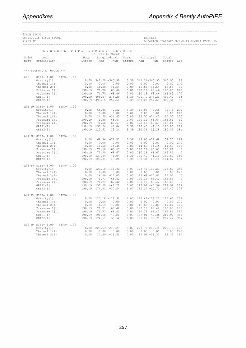
Appendixes Appendix 4 Bently AutoPIPE
257
----------------------------------------------------------------------------------------------------------------
6INCH SPOOL
05/21/2015 6INCH SPOOL BENTLEY
01:59 PM AutoPIPE Standard 9.4.0.19 RESULT PAGE 15
----------------------------------------------------------------------------------------------------------------
G E N E R A L P I P E S T R E S S R E P O R T
(Stress in N/mm2 )
Point Load Hoop Longitudinal Shear Principal Total
name combination Stress Max Min Stress Max Min Stress Loc
------ ---------------------- ------ ------ ------ ------ ------ ------ ------ ---
*** Segment A begin ***
A00 SIFI= 1.00 SIFO= 1.00
Gravity{1} 0.00 341.20 -345.90 3.39 341.24-345.93 345.95 93
Thermal 1{1} 0.00 0.00 0.00 0.00 0.00 0.00 0.00 270
Thermal 2{1} 0.00 16.58 -16.54 0.00 16.58 -16.54 16.58 90
Pressure 1{1} 190.19 71.70 68.46 0.00 190.19 68.46 166.85 270
Pressure 2{1} 190.19 71.70 68.46 0.00 190.19 68.46 166.85 270
GRTP1{1} 190.19 409.67 -274.20 3.39 409.72-274.23 404.40 93
GRTP2{1} 190.19 393.15 -257.64 3.39 393.20-257.67 389.34 93
A01 N- SIFI= 1.00 SIFO= 1.00
Gravity{1} 0.00 68.86 -72.52 3.39 69.03 -72.68 72.75 279
Thermal 1{1} 0.00 0.00 0.00 0.00 0.00 0.00 0.00 270
Thermal 2{1} 0.00 14.50 -14.45 0.00 14.50 -14.45 14.50 270
Pressure 1{1} 190.19 71.50 68.67 0.00 190.19 68.67 166.81 90
Pressure 2{1} 190.19 71.50 68.67 0.00 190.19 68.67 166.81 90
GRTP1{1} 190.19 137.54 -1.04 3.39 190.40 -1.10 190.80 279
GRTP2{1} 190.19 123.31 13.24 3.39 190.36 13.18 184.02 281
A01 N+ SIFI= 1.00 SIFO= 1.00
Gravity{1} 0.00 68.86 -72.52 3.39 69.03 -72.68 72.75 189
Thermal 1{1} 0.00 0.00 0.00 0.00 0.00 0.00 0.00 270
Thermal 2{1} 0.00 14.50 -14.45 0.00 14.50 -14.45 14.50 180
Pressure 1{1} 190.19 71.50 68.67 0.00 190.19 68.67 166.81 0
Pressure 2{1} 190.19 71.50 68.67 0.00 190.19 68.67 166.81 0
GRTP1{1} 190.19 137.54 -1.04 3.39 190.40 -1.10 190.80 189
GRTP2{1} 190.19 123.31 13.24 3.39 190.36 13.18 184.02 191
A01 F- SIFI= 1.00 SIFO= 1.00
Gravity{1} 0.00 123.18 -118.92 6.07 123.48-119.23 123.63 357
Thermal 1{1} 0.00 0.00 0.00 0.00 0.00 0.00 0.00 270
Thermal 2{1} 0.00 16.69 -17.01 0.00 16.69 -17.01 17.01 0
Pressure 1{1} 190.19 71.71 68.42 0.00 190.19 68.42 166.85 0
Pressure 2{1} 190.19 71.71 68.42 0.00 190.19 68.42 166.85 0
GRTP1{1} 190.19 191.60 -47.21 6.07 197.01 -47.36 217.92 177
GRTP2{1} 190.19 174.61 -30.54 6.07 192.27 -30.71 207.42 177
A01 F+ SIFI= 1.00 SIFO= 1.00
Gravity{1} 0.00 123.18 -118.92 6.07 123.48-119.23 123.63 177
Thermal 1{1} 0.00 0.00 0.00 0.00 0.00 0.00 0.00 270
Thermal 2{1} 0.00 16.69 -17.01 0.00 16.69 -17.01 17.01 180
Pressure 1{1} 190.19 71.71 68.42 0.00 190.19 68.42 166.85 180
Pressure 2{1} 190.19 71.71 68.42 0.00 190.19 68.42 166.85 180
GRTP1{1} 190.19 191.60 -47.21 6.07 197.01 -47.36 217.92 357
GRTP2{1} 190.19 174.61 -30.54 6.07 192.27 -30.71 207.42 357
A02 N- SIFI= 1.00 SIFO= 1.00
Gravity{1} 0.00 223.53 -219.27 6.07 223.70-219.44 223.78 180
Thermal 1{1} 0.00 0.00 0.00 0.00 0.00 0.00 0.00 270
Thermal 2{1} 0.00 17.99 -18.31 0.00 17.99 -18.31 18.31 180
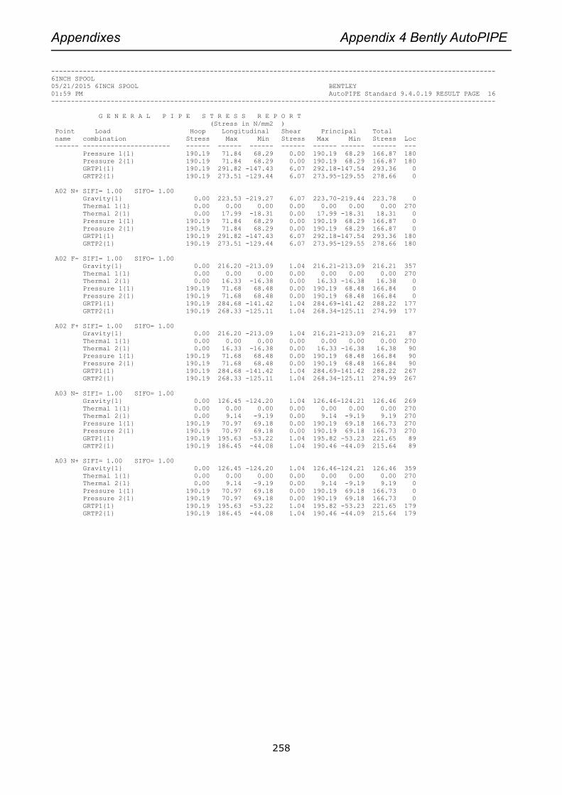
Appendixes Appendix 4 Bently AutoPIPE
258
----------------------------------------------------------------------------------------------------------------
6INCH SPOOL
05/21/2015 6INCH SPOOL BENTLEY
01:59 PM AutoPIPE Standard 9.4.0.19 RESULT PAGE 16
----------------------------------------------------------------------------------------------------------------
G E N E R A L P I P E S T R E S S R E P O R T
(Stress in N/mm2 )
Point Load Hoop Longitudinal Shear Principal Total
name combination Stress Max Min Stress Max Min Stress Loc
------ ---------------------- ------ ------ ------ ------ ------ ------ ------ ---
Pressure 1{1} 190.19 71.84 68.29 0.00 190.19 68.29 166.87 180
Pressure 2{1} 190.19 71.84 68.29 0.00 190.19 68.29 166.87 180
GRTP1{1} 190.19 291.82 -147.43 6.07 292.18-147.54 293.36 0
GRTP2{1} 190.19 273.51 -129.44 6.07 273.95-129.55 278.66 0
A02 N+ SIFI= 1.00 SIFO= 1.00
Gravity{1} 0.00 223.53 -219.27 6.07 223.70-219.44 223.78 0
Thermal 1{1} 0.00 0.00 0.00 0.00 0.00 0.00 0.00 270
Thermal 2{1} 0.00 17.99 -18.31 0.00 17.99 -18.31 18.31 0
Pressure 1{1} 190.19 71.84 68.29 0.00 190.19 68.29 166.87 0
Pressure 2{1} 190.19 71.84 68.29 0.00 190.19 68.29 166.87 0
GRTP1{1} 190.19 291.82 -147.43 6.07 292.18-147.54 293.36 180
GRTP2{1} 190.19 273.51 -129.44 6.07 273.95-129.55 278.66 180
A02 F- SIFI= 1.00 SIFO= 1.00
Gravity{1} 0.00 216.20 -213.09 1.04 216.21-213.09 216.21 357
Thermal 1{1} 0.00 0.00 0.00 0.00 0.00 0.00 0.00 270
Thermal 2{1} 0.00 16.33 -16.38 0.00 16.33 -16.38 16.38 0
Pressure 1{1} 190.19 71.68 68.48 0.00 190.19 68.48 166.84 0
Pressure 2{1} 190.19 71.68 68.48 0.00 190.19 68.48 166.84 0
GRTP1{1} 190.19 284.68 -141.42 1.04 284.69-141.42 288.22 177
GRTP2{1} 190.19 268.33 -125.11 1.04 268.34-125.11 274.99 177
A02 F+ SIFI= 1.00 SIFO= 1.00
Gravity{1} 0.00 216.20 -213.09 1.04 216.21-213.09 216.21 87
Thermal 1{1} 0.00 0.00 0.00 0.00 0.00 0.00 0.00 270
Thermal 2{1} 0.00 16.33 -16.38 0.00 16.33 -16.38 16.38 90
Pressure 1{1} 190.19 71.68 68.48 0.00 190.19 68.48 166.84 90
Pressure 2{1} 190.19 71.68 68.48 0.00 190.19 68.48 166.84 90
GRTP1{1} 190.19 284.68 -141.42 1.04 284.69-141.42 288.22 267
GRTP2{1} 190.19 268.33 -125.11 1.04 268.34-125.11 274.99 267
A03 N- SIFI= 1.00 SIFO= 1.00
Gravity{1} 0.00 126.45 -124.20 1.04 126.46-124.21 126.46 269
Thermal 1{1} 0.00 0.00 0.00 0.00 0.00 0.00 0.00 270
Thermal 2{1} 0.00 9.14 -9.19 0.00 9.14 -9.19 9.19 270
Pressure 1{1} 190.19 70.97 69.18 0.00 190.19 69.18 166.73 270
Pressure 2{1} 190.19 70.97 69.18 0.00 190.19 69.18 166.73 270
GRTP1{1} 190.19 195.63 -53.22 1.04 195.82 -53.23 221.65 89
GRTP2{1} 190.19 186.45 -44.08 1.04 190.46 -44.09 215.64 89
A03 N+ SIFI= 1.00 SIFO= 1.00
Gravity{1} 0.00 126.45 -124.20 1.04 126.46-124.21 126.46 359
Thermal 1{1} 0.00 0.00 0.00 0.00 0.00 0.00 0.00 270
Thermal 2{1} 0.00 9.14 -9.19 0.00 9.14 -9.19 9.19 0
Pressure 1{1} 190.19 70.97 69.18 0.00 190.19 69.18 166.73 0
Pressure 2{1} 190.19 70.97 69.18 0.00 190.19 69.18 166.73 0
GRTP1{1} 190.19 195.63 -53.22 1.04 195.82 -53.23 221.65 179
GRTP2{1} 190.19 186.45 -44.08 1.04 190.46 -44.09 215.64 179
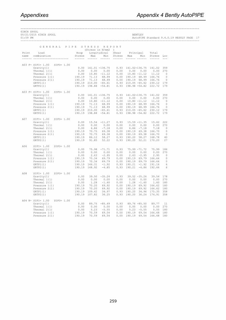
Appendixes Appendix 4 Bently AutoPIPE
259
----------------------------------------------------------------------------------------------------------------
6INCH SPOOL
05/21/2015 6INCH SPOOL BENTLEY
01:59 PM AutoPIPE Standard 9.4.0.19 RESULT PAGE 17
----------------------------------------------------------------------------------------------------------------
G E N E R A L P I P E S T R E S S R E P O R T
(Stress in N/mm2 )
Point Load Hoop Longitudinal Shear Principal Total
name combination Stress Max Min Stress Max Min Stress Loc
------ ---------------------- ------ ------ ------ ------ ------ ------ ------ ---
A03 F- SIFI= 1.00 SIFO= 1.00
Gravity{1} 0.00 141.01 -136.75 0.93 141.02-136.75 141.02 359
Thermal 1{1} 0.00 0.00 0.00 0.00 0.00 0.00 0.00 270
Thermal 2{1} 0.00 10.80 -11.12 0.00 10.80 -11.12 11.12 0
Pressure 1{1} 190.19 71.13 68.99 0.00 190.19 68.99 166.76 0
Pressure 2{1} 190.19 71.13 68.99 0.00 190.19 68.99 166.76 0
GRTP1{1} 190.19 210.00 -65.61 0.93 210.05 -65.62 230.12 179
GRTP2{1} 190.19 198.88 -54.81 0.93 198.98 -54.82 222.72 179
A03 F+ SIFI= 1.00 SIFO= 1.00
Gravity{1} 0.00 141.01 -136.75 0.93 141.02-136.75 141.02 359
Thermal 1{1} 0.00 0.00 0.00 0.00 0.00 0.00 0.00 270
Thermal 2{1} 0.00 10.80 -11.12 0.00 10.80 -11.12 11.12 0
Pressure 1{1} 190.19 71.13 68.99 0.00 190.19 68.99 166.76 0
Pressure 2{1} 190.19 71.13 68.99 0.00 190.19 68.99 166.76 0
GRTP1{1} 190.19 210.00 -65.61 0.93 210.05 -65.62 230.12 179
GRTP2{1} 190.19 198.88 -54.81 0.93 198.98 -54.82 222.72 179
A07 SIFI= 1.00 SIFO= 1.00
Gravity{1} 0.00 15.54 -11.27 0.93 15.59 -11.35 15.62 222
Thermal 1{1} 0.00 0.00 0.00 0.00 0.00 0.00 0.00 270
Thermal 2{1} 0.00 6.86 -7.18 0.00 6.86 -7.18 7.18 0
Pressure 1{1} 190.19 70.75 69.38 0.00 190.19 69.38 166.70 0
Pressure 2{1} 190.19 70.75 69.38 0.00 190.19 69.38 166.70 0
GRTP1{1} 190.19 86.12 58.27 0.93 190.20 58.27 168.78 40
GRTP2{1} 190.19 91.85 52.22 0.93 190.20 52.21 170.20 27
A06 SIFI= 1.00 SIFO= 1.00
Gravity{1} 0.00 75.98 -71.71 0.93 75.99 -71.72 75.99 186
Thermal 1{1} 0.00 0.00 0.00 0.00 0.00 0.00 0.00 270
Thermal 2{1} 0.00 2.63 -2.95 0.00 2.63 -2.95 2.95 0
Pressure 1{1} 190.19 70.34 69.79 0.00 190.19 69.79 166.64 0
Pressure 2{1} 190.19 70.34 69.79 0.00 190.19 69.79 166.64 0
GRTP1{1} 190.19 146.31 -1.92 0.93 190.21 -1.92 191.16 6
GRTP2{1} 190.19 148.92 -4.85 0.93 190.21 -4.86 192.66 6
A08 SIFI= 1.00 SIFO= 1.00
Gravity{1} 0.00 39.50 -35.24 0.93 39.52 -35.26 39.54 178
Thermal 1{1} 0.00 0.00 0.00 0.00 0.00 0.00 0.00 270
Thermal 2{1} 0.00 1.28 -1.60 0.00 1.28 -1.60 1.60 180
Pressure 1{1} 190.19 70.20 69.92 0.00 190.19 69.92 166.62 180
Pressure 2{1} 190.19 70.20 69.92 0.00 190.19 69.92 166.62 180
GRTP1{1} 190.19 109.42 34.97 0.93 190.20 34.96 175.35 358
GRTP2{1} 190.19 107.82 36.25 0.93 190.20 36.24 174.91 358
A04 N- SIFI= 1.00 SIFO= 1.00
Gravity{1} 0.00 89.75 -85.49 0.93 89.76 -85.50 89.77 11
Thermal 1{1} 0.00 0.00 0.00 0.00 0.00 0.00 0.00 270
Thermal 2{1} 0.00 5.23 -5.55 0.00 5.23 -5.55 5.55 180
Pressure 1{1} 190.19 70.59 69.54 0.00 190.19 69.54 166.68 180
Pressure 2{1} 190.19 70.59 69.54 0.00 190.19 69.54 166.68 180
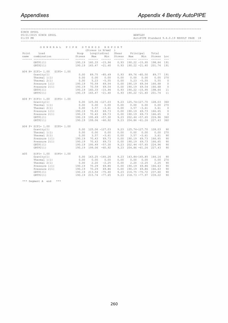
Appendixes Appendix 4 Bently AutoPIPE
260
----------------------------------------------------------------------------------------------------------------
6INCH SPOOL
05/21/2015 6INCH SPOOL BENTLEY
01:59 PM AutoPIPE Standard 9.4.0.19 RESULT PAGE 18
----------------------------------------------------------------------------------------------------------------
G E N E R A L P I P E S T R E S S R E P O R T
(Stress in N/mm2 )
Point Load Hoop Longitudinal Shear Principal Total
name combination Stress Max Min Stress Max Min Stress Loc
------ ---------------------- ------ ------ ------ ------ ------ ------ ------ ---
GRTP1{1} 190.19 160.33 -15.94 0.93 190.22 -15.95 198.64 191
GRTP2{1} 190.19 165.47 -21.40 0.93 190.22 -21.40 201.74 191
A04 N+ SIFI= 1.00 SIFO= 1.00
Gravity{1} 0.00 89.75 -85.49 0.93 89.76 -85.50 89.77 191
Thermal 1{1} 0.00 0.00 0.00 0.00 0.00 0.00 0.00 270
Thermal 2{1} 0.00 5.23 -5.55 0.00 5.23 -5.55 5.55 0
Pressure 1{1} 190.19 70.59 69.54 0.00 190.19 69.54 166.68 0
Pressure 2{1} 190.19 70.59 69.54 0.00 190.19 69.54 166.68 0
GRTP1{1} 190.19 160.33 -15.94 0.93 190.22 -15.95 198.64 11
GRTP2{1} 190.19 165.47 -21.40 0.93 190.22 -21.40 201.74 11
A04 F- SIFI= 1.00 SIFO= 1.00
Gravity{1} 0.00 125.06 -127.03 9.23 125.74-127.70 128.03 360
Thermal 1{1} 0.00 0.00 0.00 0.00 0.00 0.00 0.00 270
Thermal 2{1} 0.00 3.57 -3.61 0.00 3.57 -3.61 3.61 0
Pressure 1{1} 190.19 70.43 69.73 0.00 190.19 69.73 166.65 0
Pressure 2{1} 190.19 70.43 69.73 0.00 190.19 69.73 166.65 0
GRTP1{1} 190.19 195.49 -57.30 9.23 202.44 -57.65 224.96 360
GRTP2{1} 190.19 199.06 -60.92 9.23 204.86 -61.26 227.43 360
A04 F+ SIFI= 1.00 SIFO= 1.00
Gravity{1} 0.00 125.06 -127.03 9.23 125.74-127.70 128.03 90
Thermal 1{1} 0.00 0.00 0.00 0.00 0.00 0.00 0.00 270
Thermal 2{1} 0.00 3.57 -3.61 0.00 3.57 -3.61 3.61 90
Pressure 1{1} 190.19 70.43 69.73 0.00 190.19 69.73 166.65 90
Pressure 2{1} 190.19 70.43 69.73 0.00 190.19 69.73 166.65 90
GRTP1{1} 190.19 195.49 -57.30 9.23 202.44 -57.65 224.96 90
GRTP2{1} 190.19 199.06 -60.92 9.23 204.86 -61.26 227.43 90
A05 SIFI= 1.00 SIFO= 1.00
Gravity{1} 0.00 143.25 -145.26 9.23 143.84-145.85 146.14 90
Thermal 1{1} 0.00 0.00 0.00 0.00 0.00 0.00 0.00 270
Thermal 2{1} 0.00 2.20 -2.25 0.00 2.20 -2.25 2.25 90
Pressure 1{1} 190.19 70.29 69.86 0.00 190.19 69.86 166.63 90
Pressure 2{1} 190.19 70.29 69.86 0.00 190.19 69.86 166.63 90
GRTP1{1} 190.19 213.54 -75.40 9.23 216.75 -75.72 237.60 90
GRTP2{1} 190.19 215.74 -77.65 9.23 218.73 -77.97 239.22 90
*** Segment A end ***

Appendixes Appendix 4 Bently AutoPIPE
261
----------------------------------------------------------------------------------------------------------------
6INCH SPOOL
05/21/2015 6INCH SPOOL BENTLEY
01:59 PM AutoPIPE Standard 9.4.0.19 RESULT PAGE 19
----------------------------------------------------------------------------------------------------------------
ASME B31.8 (2010) CODE COMPLIANCE
(Moments in N.m ) (Stress in N/mm2 )
Point Load In-Pl. Out-Pl. Shear Axial Bending Code Code
name combination Moment Moment Stress Stress Stress type Stress Allow.
------ ---------------------- ------- ------- ------ ------ ------ ---- ------ ------
A00 SIFI= 1.00 SIFO= 1.00
GR + Max P{1} 4018.3888037.95 3.39 2.35 341.93 SUST 434.75 405.00**
TR:Amb to T2{1} 0.00 4267.86 0.00 0.02 16.56 DISP 16.58 3.33**
Amb to T1{1} 0.00 0.00 0.00 0.00 0.00 DISP 0.00 3.33
Amb to T2{1} 0.00 4267.86 0.00 0.02 16.56 DISP 16.58 3.33**
Max P{1} HOOP 158.94 324.00
GRTP1{1} 4018.3888037.95 0.00 67.73 341.93 RFun 404.36 405.00
LONG 409.67 360.00**
GRTP2{1} 4018.3883770.08 0.00 67.75 325.39 RFun 389.29 405.00
LONG 393.15 405.00
A02 N- SIFI= 1.00 SIFO= 1.00
GR + Max P{1} 56606.00 214.04 6.07 -2.13 219.63 SUST 317.17 405.00
TR:Amb to T2{1} 4678.78 0.00 0.00 0.16 18.15 DISP 18.31 120.90
Amb to T1{1} 0.00 0.00 0.00 0.00 0.00 DISP 0.00 120.90
Amb to T2{1} 4678.78 0.00 0.00 0.16 18.15 DISP 18.31 120.90
Max P{1} HOOP 158.94 324.00
GRTP1{1} 56606.00 214.04 0.00 72.20 219.63 RFun 293.17 405.00
LONG 291.82 360.00
GRTP2{1} 51927.22 214.04 0.00 72.04 201.47 RFun 278.47 405.00
LONG 273.51 405.00
A02 N+ SIFI= 1.00 SIFO= 1.00
GR + Max P{1} 56606.00 214.04 6.07 -2.13 219.63 SUST 317.17 405.00
TR:Amb to T2{1} 4678.78 0.00 0.00 0.16 18.15 DISP 18.31 120.90
Amb to T1{1} 0.00 0.00 0.00 0.00 0.00 DISP 0.00 120.90
Amb to T2{1} 4678.78 0.00 0.00 0.16 18.15 DISP 18.31 120.90
Max P{1} HOOP 158.94 324.00
GRTP1{1} 56606.00 214.04 0.00 72.20 219.63 RFun 293.17 405.00
LONG 291.82 360.00
GRTP2{1} 51927.22 214.04 0.00 72.04 201.47 RFun 278.47 405.00
LONG 273.51 405.00

Appendixes Appendix 4 Bently AutoPIPE
262
----------------------------------------------------------------------------------------------------------------
6INCH SPOOL
05/21/2015 6INCH SPOOL BENTLEY
01:59 PM AutoPIPE Standard 9.4.0.19 RESULT PAGE 20
----------------------------------------------------------------------------------------------------------------
ASME B31.8 (2010) CODE COMPLIANCE
(Moments in N.m ) (Stress in N/mm2 )
Point Load In-Pl. Out-Pl. Shear Axial Bending Code Code
name combination Moment Moment Stress Stress Stress type Stress Allow.
------ ---------------------- ------- ------- ------ ------ ------ ---- ------ ------
A02 N- SIFI= 1.00 SIFO= 1.00
GR + Max P{1} 56606.00 214.04 6.07 -2.13 219.63 SUST 317.17 405.00
TR:Amb to T2{1} 4678.78 0.00 0.00 0.16 18.15 DISP 18.31 120.90
Amb to T1{1} 0.00 0.00 0.00 0.00 0.00 DISP 0.00 120.90
Amb to T2{1} 4678.78 0.00 0.00 0.16 18.15 DISP 18.31 120.90
Max P{1} HOOP 158.94 324.00
GRTP1{1} 56606.00 214.04 0.00 72.20 219.63 RFun 293.17 405.00
LONG 291.82 360.00
GRTP2{1} 51927.22 214.04 0.00 72.04 201.47 RFun 278.47 405.00
LONG 273.51 405.00
A02 N+ SIFI= 1.00 SIFO= 1.00
GR + Max P{1} 56606.00 214.04 6.07 -2.13 219.63 SUST 317.17 405.00
TR:Amb to T2{1} 4678.78 0.00 0.00 0.16 18.15 DISP 18.31 120.90
Amb to T1{1} 0.00 0.00 0.00 0.00 0.00 DISP 0.00 120.90
Amb to T2{1} 4678.78 0.00 0.00 0.16 18.15 DISP 18.31 120.90
Max P{1} HOOP 158.94 324.00
GRTP1{1} 56606.00 214.04 0.00 72.20 219.63 RFun 293.17 405.00
LONG 291.82 360.00
GRTP2{1} 51927.22 214.04 0.00 72.04 201.47 RFun 278.47 405.00
LONG 273.51 405.00
A02 F- SIFI= 1.00 SIFO= 1.00
GR + Max P{1} 54838.87 2813.04 1.04 -1.56 213.05 SUST 309.71 405.00
TR:Amb to T2{1} 4215.45 0.00 0.00 0.02 16.36 DISP 16.38 128.37
Amb to T1{1} 0.00 0.00 0.00 0.00 0.00 DISP 0.00 128.37
Amb to T2{1} 4215.45 0.00 0.00 0.02 16.36 DISP 16.38 128.37
Max P{1} HOOP 158.94 324.00
GRTP1{1} 54838.87 2813.04 0.00 71.63 213.05 RFun 288.21 405.00
LONG 284.68 360.00
GRTP2{1} 50623.42 2813.04 0.00 71.61 196.72 RFun 274.98 405.00
LONG 268.33 405.00

Appendixes Appendix 4 Bently AutoPIPE
263
----------------------------------------------------------------------------------------------------------------
6INCH SPOOL
05/21/2015 6INCH SPOOL BENTLEY
01:59 PM AutoPIPE Standard 9.4.0.19 RESULT PAGE 21
----------------------------------------------------------------------------------------------------------------
ASME B31.8 (2010) CODE COMPLIANCE
(Moments in N.m ) (Stress in N/mm2 )
Point Load In-Pl. Out-Pl. Shear Axial Bending Code Code
name combination Moment Moment Stress Stress Stress type Stress Allow.
------ ---------------------- ------- ------- ------ ------ ------ ---- ------ ------
A02 F+ SIFI= 1.00 SIFO= 1.00
GR + Max P{1} 2813.0454838.87 1.04 -1.56 213.05 SUST 309.71 405.00
TR:Amb to T2{1} 0.00 4215.45 0.00 0.02 16.36 DISP 16.38 128.37
Amb to T1{1} 0.00 0.00 0.00 0.00 0.00 DISP 0.00 128.37
Amb to T2{1} 0.00 4215.45 0.00 0.02 16.36 DISP 16.38 128.37
Max P{1} HOOP 158.94 324.00
GRTP1{1} 2813.0454838.87 0.00 71.63 213.05 RFun 288.21 405.00
LONG 284.68 360.00
GRTP2{1} 2813.0450623.42 0.00 71.61 196.72 RFun 274.98 405.00
LONG 268.33 405.00
A02 F- SIFI= 1.00 SIFO= 1.00
GR + Max P{1} 54838.87 2813.04 1.04 -1.56 213.05 SUST 309.71 405.00
TR:Amb to T2{1} 4215.45 0.00 0.00 0.02 16.36 DISP 16.38 128.37
Amb to T1{1} 0.00 0.00 0.00 0.00 0.00 DISP 0.00 128.37
Amb to T2{1} 4215.45 0.00 0.00 0.02 16.36 DISP 16.38 128.37
Max P{1} HOOP 158.94 324.00
GRTP1{1} 54838.87 2813.04 0.00 71.63 213.05 RFun 288.21 405.00
LONG 284.68 360.00
GRTP2{1} 50623.42 2813.04 0.00 71.61 196.72 RFun 274.98 405.00
LONG 268.33 405.00
A02 F+ SIFI= 1.00 SIFO= 1.00
GR + Max P{1} 2813.0454838.87 1.04 -1.56 213.05 SUST 309.71 405.00
TR:Amb to T2{1} 0.00 4215.45 0.00 0.02 16.36 DISP 16.38 128.37
Amb to T1{1} 0.00 0.00 0.00 0.00 0.00 DISP 0.00 128.37
Amb to T2{1} 0.00 4215.45 0.00 0.02 16.36 DISP 16.38 128.37
Max P{1} HOOP 158.94 324.00
GRTP1{1} 2813.0454838.87 0.00 71.63 213.05 RFun 288.21 405.00
LONG 284.68 360.00
GRTP2{1} 2813.0450623.42 0.00 71.61 196.72 RFun 274.98 405.00
LONG 268.33 405.00
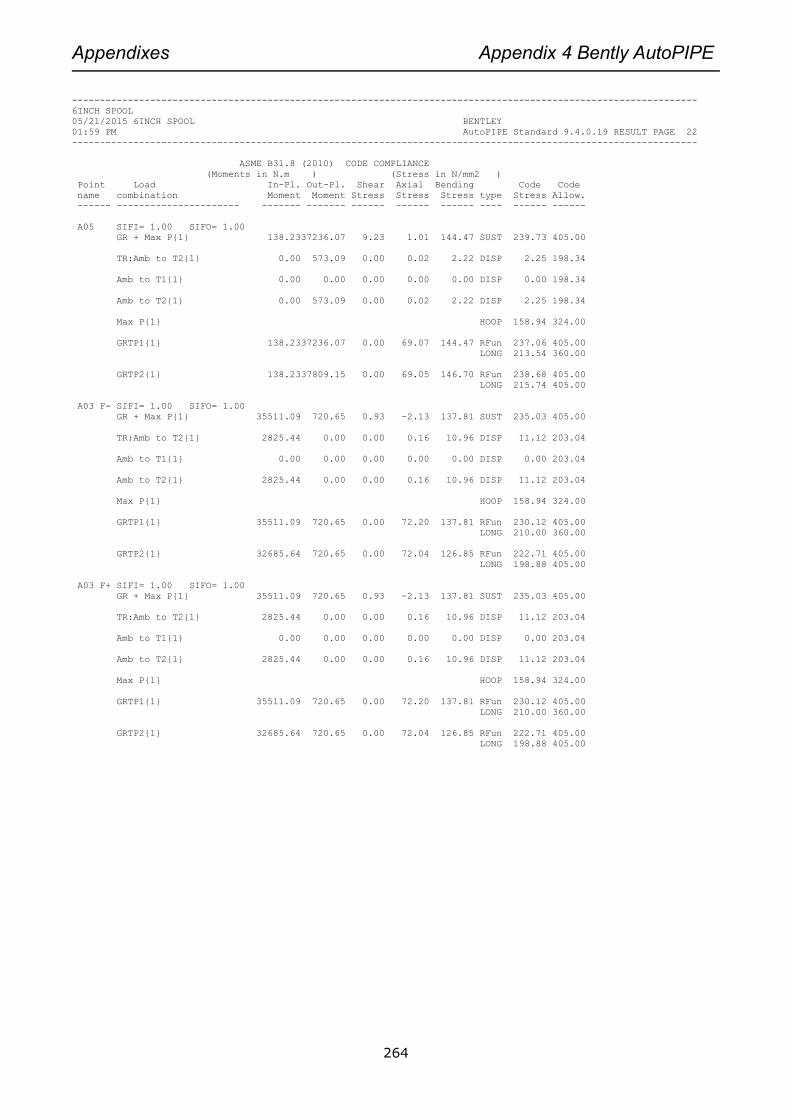
Appendixes Appendix 4 Bently AutoPIPE
264
----------------------------------------------------------------------------------------------------------------
6INCH SPOOL
05/21/2015 6INCH SPOOL BENTLEY
01:59 PM AutoPIPE Standard 9.4.0.19 RESULT PAGE 22
----------------------------------------------------------------------------------------------------------------
ASME B31.8 (2010) CODE COMPLIANCE
(Moments in N.m ) (Stress in N/mm2 )
Point Load In-Pl. Out-Pl. Shear Axial Bending Code Code
name combination Moment Moment Stress Stress Stress type Stress Allow.
------ ---------------------- ------- ------- ------ ------ ------ ---- ------ ------
A05 SIFI= 1.00 SIFO= 1.00
GR + Max P{1} 138.2337236.07 9.23 1.01 144.47 SUST 239.73 405.00
TR:Amb to T2{1} 0.00 573.09 0.00 0.02 2.22 DISP 2.25 198.34
Amb to T1{1} 0.00 0.00 0.00 0.00 0.00 DISP 0.00 198.34
Amb to T2{1} 0.00 573.09 0.00 0.02 2.22 DISP 2.25 198.34
Max P{1} HOOP 158.94 324.00
GRTP1{1} 138.2337236.07 0.00 69.07 144.47 RFun 237.06 405.00
LONG 213.54 360.00
GRTP2{1} 138.2337809.15 0.00 69.05 146.70 RFun 238.68 405.00
LONG 215.74 405.00
A03 F- SIFI= 1.00 SIFO= 1.00
GR + Max P{1} 35511.09 720.65 0.93 -2.13 137.81 SUST 235.03 405.00
TR:Amb to T2{1} 2825.44 0.00 0.00 0.16 10.96 DISP 11.12 203.04
Amb to T1{1} 0.00 0.00 0.00 0.00 0.00 DISP 0.00 203.04
Amb to T2{1} 2825.44 0.00 0.00 0.16 10.96 DISP 11.12 203.04
Max P{1} HOOP 158.94 324.00
GRTP1{1} 35511.09 720.65 0.00 72.20 137.81 RFun 230.12 405.00
LONG 210.00 360.00
GRTP2{1} 32685.64 720.65 0.00 72.04 126.85 RFun 222.71 405.00
LONG 198.88 405.00
A03 F+ SIFI= 1.00 SIFO= 1.00
GR + Max P{1} 35511.09 720.65 0.93 -2.13 137.81 SUST 235.03 405.00
TR:Amb to T2{1} 2825.44 0.00 0.00 0.16 10.96 DISP 11.12 203.04
Amb to T1{1} 0.00 0.00 0.00 0.00 0.00 DISP 0.00 203.04
Amb to T2{1} 2825.44 0.00 0.00 0.16 10.96 DISP 11.12 203.04
Max P{1} HOOP 158.94 324.00
GRTP1{1} 35511.09 720.65 0.00 72.20 137.81 RFun 230.12 405.00
LONG 210.00 360.00
GRTP2{1} 32685.64 720.65 0.00 72.04 126.85 RFun 222.71 405.00
LONG 198.88 405.00
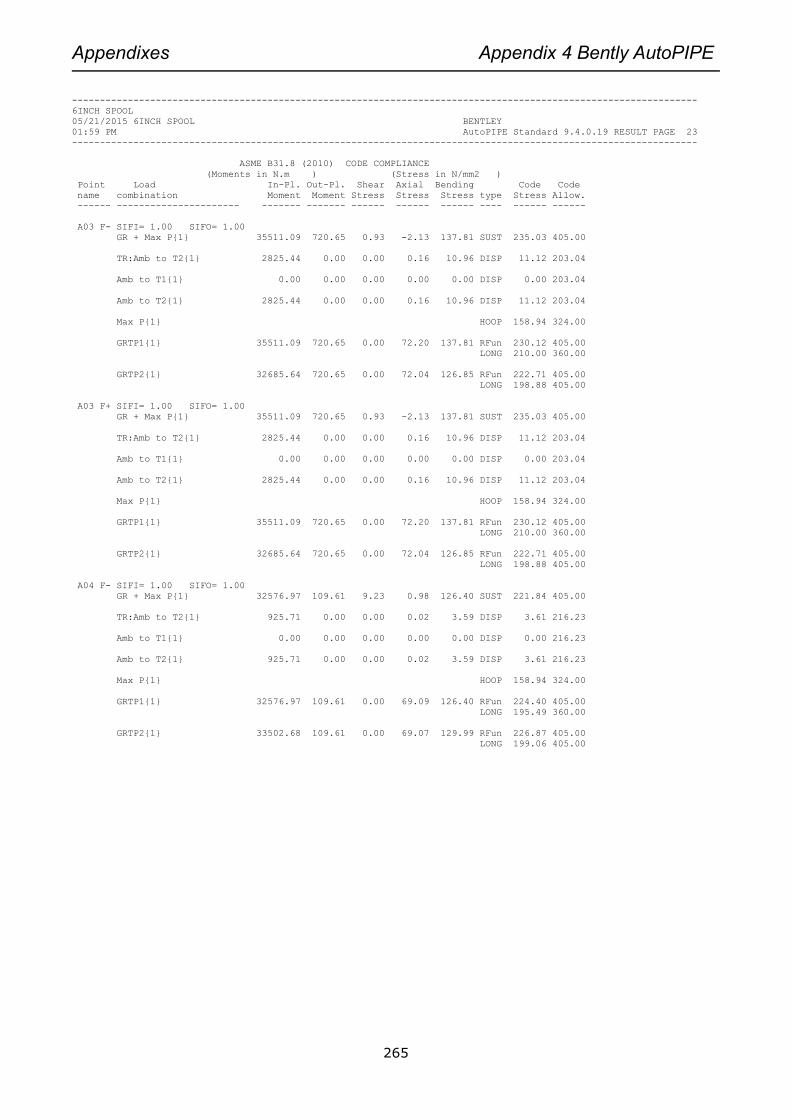
Appendixes Appendix 4 Bently AutoPIPE
265
----------------------------------------------------------------------------------------------------------------
6INCH SPOOL
05/21/2015 6INCH SPOOL BENTLEY
01:59 PM AutoPIPE Standard 9.4.0.19 RESULT PAGE 23
----------------------------------------------------------------------------------------------------------------
ASME B31.8 (2010) CODE COMPLIANCE
(Moments in N.m ) (Stress in N/mm2 )
Point Load In-Pl. Out-Pl. Shear Axial Bending Code Code
name combination Moment Moment Stress Stress Stress type Stress Allow.
------ ---------------------- ------- ------- ------ ------ ------ ---- ------ ------
A03 F- SIFI= 1.00 SIFO= 1.00
GR + Max P{1} 35511.09 720.65 0.93 -2.13 137.81 SUST 235.03 405.00
TR:Amb to T2{1} 2825.44 0.00 0.00 0.16 10.96 DISP 11.12 203.04
Amb to T1{1} 0.00 0.00 0.00 0.00 0.00 DISP 0.00 203.04
Amb to T2{1} 2825.44 0.00 0.00 0.16 10.96 DISP 11.12 203.04
Max P{1} HOOP 158.94 324.00
GRTP1{1} 35511.09 720.65 0.00 72.20 137.81 RFun 230.12 405.00
LONG 210.00 360.00
GRTP2{1} 32685.64 720.65 0.00 72.04 126.85 RFun 222.71 405.00
LONG 198.88 405.00
A03 F+ SIFI= 1.00 SIFO= 1.00
GR + Max P{1} 35511.09 720.65 0.93 -2.13 137.81 SUST 235.03 405.00
TR:Amb to T2{1} 2825.44 0.00 0.00 0.16 10.96 DISP 11.12 203.04
Amb to T1{1} 0.00 0.00 0.00 0.00 0.00 DISP 0.00 203.04
Amb to T2{1} 2825.44 0.00 0.00 0.16 10.96 DISP 11.12 203.04
Max P{1} HOOP 158.94 324.00
GRTP1{1} 35511.09 720.65 0.00 72.20 137.81 RFun 230.12 405.00
LONG 210.00 360.00
GRTP2{1} 32685.64 720.65 0.00 72.04 126.85 RFun 222.71 405.00
LONG 198.88 405.00
A04 F- SIFI= 1.00 SIFO= 1.00
GR + Max P{1} 32576.97 109.61 9.23 0.98 126.40 SUST 221.84 405.00
TR:Amb to T2{1} 925.71 0.00 0.00 0.02 3.59 DISP 3.61 216.23
Amb to T1{1} 0.00 0.00 0.00 0.00 0.00 DISP 0.00 216.23
Amb to T2{1} 925.71 0.00 0.00 0.02 3.59 DISP 3.61 216.23
Max P{1} HOOP 158.94 324.00
GRTP1{1} 32576.97 109.61 0.00 69.09 126.40 RFun 224.40 405.00
LONG 195.49 360.00
GRTP2{1} 33502.68 109.61 0.00 69.07 129.99 RFun 226.87 405.00
LONG 199.06 405.00

Appendixes Appendix 4 Bently AutoPIPE
266
----------------------------------------------------------------------------------------------------------------
6INCH SPOOL
05/21/2015 6INCH SPOOL BENTLEY
01:59 PM AutoPIPE Standard 9.4.0.19 RESULT PAGE 24
----------------------------------------------------------------------------------------------------------------
ASME B31.8 (2010) CODE COMPLIANCE
(Moments in N.m ) (Stress in N/mm2 )
Point Load In-Pl. Out-Pl. Shear Axial Bending Code Code
name combination Moment Moment Stress Stress Stress type Stress Allow.
------ ---------------------- ------- ------- ------ ------ ------ ---- ------ ------
A04 F+ SIFI= 1.00 SIFO= 1.00
GR + Max P{1} 109.6332576.97 9.23 0.98 126.40 SUST 221.84 405.00
TR:Amb to T2{1} 0.00 925.71 0.00 0.02 3.59 DISP 3.61 216.23
Amb to T1{1} 0.00 0.00 0.00 0.00 0.00 DISP 0.00 216.23
Amb to T2{1} 0.00 925.71 0.00 0.02 3.59 DISP 3.61 216.23
Max P{1} HOOP 158.94 324.00
GRTP1{1} 109.6332576.97 0.00 69.09 126.40 RFun 224.40 405.00
LONG 195.49 360.00
GRTP2{1} 109.6333502.68 0.00 69.07 129.99 RFun 226.87 405.00
LONG 199.06 405.00
A04 F- SIFI= 1.00 SIFO= 1.00
GR + Max P{1} 32576.97 109.61 9.23 0.98 126.40 SUST 221.84 405.00
TR:Amb to T2{1} 925.71 0.00 0.00 0.02 3.59 DISP 3.61 216.23
Amb to T1{1} 0.00 0.00 0.00 0.00 0.00 DISP 0.00 216.23
Amb to T2{1} 925.71 0.00 0.00 0.02 3.59 DISP 3.61 216.23
Max P{1} HOOP 158.94 324.00
GRTP1{1} 32576.97 109.61 0.00 69.09 126.40 RFun 224.40 405.00
LONG 195.49 360.00
GRTP2{1} 33502.68 109.61 0.00 69.07 129.99 RFun 226.87 405.00
LONG 199.06 405.00
A04 F+ SIFI= 1.00 SIFO= 1.00
GR + Max P{1} 109.6332576.97 9.23 0.98 126.40 SUST 221.84 405.00
TR:Amb to T2{1} 0.00 925.71 0.00 0.02 3.59 DISP 3.61 216.23
Amb to T1{1} 0.00 0.00 0.00 0.00 0.00 DISP 0.00 216.23
Amb to T2{1} 0.00 925.71 0.00 0.02 3.59 DISP 3.61 216.23
Max P{1} HOOP 158.94 324.00
GRTP1{1} 109.6332576.97 0.00 69.09 126.40 RFun 224.40 405.00
LONG 195.49 360.00
GRTP2{1} 109.6333502.68 0.00 69.07 129.99 RFun 226.87 405.00
LONG 199.06 405.00

Appendixes Appendix 4 Bently AutoPIPE
267
----------------------------------------------------------------------------------------------------------------
6INCH SPOOL
05/21/2015 6INCH SPOOL BENTLEY
01:59 PM AutoPIPE Standard 9.4.0.19 RESULT PAGE 25
----------------------------------------------------------------------------------------------------------------
ASME B31.8 (2010) CODE COMPLIANCE
(Moments in N.m ) (Stress in N/mm2 )
Point Load In-Pl. Out-Pl. Shear Axial Bending Code Code
name combination Moment Moment Stress Stress Stress type Stress Allow.
------ ---------------------- ------- ------- ------ ------ ------ ---- ------ ------
A03 N- SIFI= 1.00 SIFO= 1.00
GR + Max P{1} 288.7132068.77 1.04 -1.13 124.43 SUST 220.66 405.00
TR:Amb to T2{1} 0.00 2362.11 0.00 0.02 9.16 DISP 9.19 217.41
Amb to T1{1} 0.00 0.00 0.00 0.00 0.00 DISP 0.00 217.41
Amb to T2{1} 0.00 2362.11 0.00 0.02 9.16 DISP 9.19 217.41
Max P{1} HOOP 158.94 324.00
GRTP1{1} 288.7132068.77 0.00 71.20 124.43 RFun 221.65 405.00
LONG 195.63 360.00
GRTP2{1} 288.7129706.66 0.00 71.18 115.26 RFun 215.63 405.00
LONG 186.45 405.00
A03 N+ SIFI= 1.00 SIFO= 1.00
GR + Max P{1} 32068.77 288.71 1.04 -1.13 124.43 SUST 220.66 405.00
TR:Amb to T2{1} 2362.11 0.00 0.00 0.02 9.16 DISP 9.19 217.41
Amb to T1{1} 0.00 0.00 0.00 0.00 0.00 DISP 0.00 217.41
Amb to T2{1} 2362.11 0.00 0.00 0.02 9.16 DISP 9.19 217.41
Max P{1} HOOP 158.94 324.00
GRTP1{1} 32068.77 288.71 0.00 71.20 124.43 RFun 221.65 405.00
LONG 195.63 360.00
GRTP2{1} 29706.66 288.71 0.00 71.18 115.26 RFun 215.63 405.00
LONG 186.45 405.00
A03 N- SIFI= 1.00 SIFO= 1.00
GR + Max P{1} 288.7132068.77 1.04 -1.13 124.43 SUST 220.66 405.00
TR:Amb to T2{1} 0.00 2362.11 0.00 0.02 9.16 DISP 9.19 217.41
Amb to T1{1} 0.00 0.00 0.00 0.00 0.00 DISP 0.00 217.41
Amb to T2{1} 0.00 2362.11 0.00 0.02 9.16 DISP 9.19 217.41
Max P{1} HOOP 158.94 324.00
GRTP1{1} 288.7132068.77 0.00 71.20 124.43 RFun 221.65 405.00
LONG 195.63 360.00
GRTP2{1} 288.7129706.66 0.00 71.18 115.26 RFun 215.63 405.00
LONG 186.45 405.00

Appendixes Appendix 4 Bently AutoPIPE
268
----------------------------------------------------------------------------------------------------------------
6INCH SPOOL
05/21/2015 6INCH SPOOL BENTLEY
01:59 PM AutoPIPE Standard 9.4.0.19 RESULT PAGE 26
----------------------------------------------------------------------------------------------------------------
ASME B31.8 (2010) CODE COMPLIANCE
(Moments in N.m ) (Stress in N/mm2 )
Point Load In-Pl. Out-Pl. Shear Axial Bending Code Code
name combination Moment Moment Stress Stress Stress type Stress Allow.
------ ---------------------- ------- ------- ------ ------ ------ ---- ------ ------
A03 N+ SIFI= 1.00 SIFO= 1.00
GR + Max P{1} 32068.77 288.71 1.04 -1.13 124.43 SUST 220.66 405.00
TR:Amb to T2{1} 2362.11 0.00 0.00 0.02 9.16 DISP 9.19 217.41
Amb to T1{1} 0.00 0.00 0.00 0.00 0.00 DISP 0.00 217.41
Amb to T2{1} 2362.11 0.00 0.00 0.02 9.16 DISP 9.19 217.41
Max P{1} HOOP 158.94 324.00
GRTP1{1} 32068.77 288.71 0.00 71.20 124.43 RFun 221.65 405.00
LONG 195.63 360.00
GRTP2{1} 29706.66 288.71 0.00 71.18 115.26 RFun 215.63 405.00
LONG 186.45 405.00
A01 F- SIFI= 1.00 SIFO= 1.00
GR + Max P{1} 30744.46 1373.04 6.07 -2.13 119.40 SUST 217.23 405.00
TR:Amb to T2{1} 4341.76 0.00 0.00 0.16 16.85 DISP 17.01 220.84
Amb to T1{1} 0.00 0.00 0.00 0.00 0.00 DISP 0.00 220.84
Amb to T2{1} 4341.76 0.00 0.00 0.16 16.85 DISP 17.01 220.84
Max P{1} HOOP 158.94 324.00
GRTP1{1} 30744.46 1373.04 0.00 72.20 119.40 RFun 217.67 405.00
LONG 191.60 360.00
GRTP2{1} 26402.69 1373.04 0.00 72.04 102.58 RFun 207.15 405.00
LONG 174.61 405.00
A01 F+ SIFI= 1.00 SIFO= 1.00
GR + Max P{1} 30744.46 1373.04 6.07 -2.13 119.40 SUST 217.23 405.00
TR:Amb to T2{1} 4341.76 0.00 0.00 0.16 16.85 DISP 17.01 220.84
Amb to T1{1} 0.00 0.00 0.00 0.00 0.00 DISP 0.00 220.84
Amb to T2{1} 4341.76 0.00 0.00 0.16 16.85 DISP 17.01 220.84
Max P{1} HOOP 158.94 324.00
GRTP1{1} 30744.46 1373.04 0.00 72.20 119.40 RFun 217.67 405.00
LONG 191.60 360.00
GRTP2{1} 26402.69 1373.04 0.00 72.04 102.58 RFun 207.15 405.00
LONG 174.61 405.00
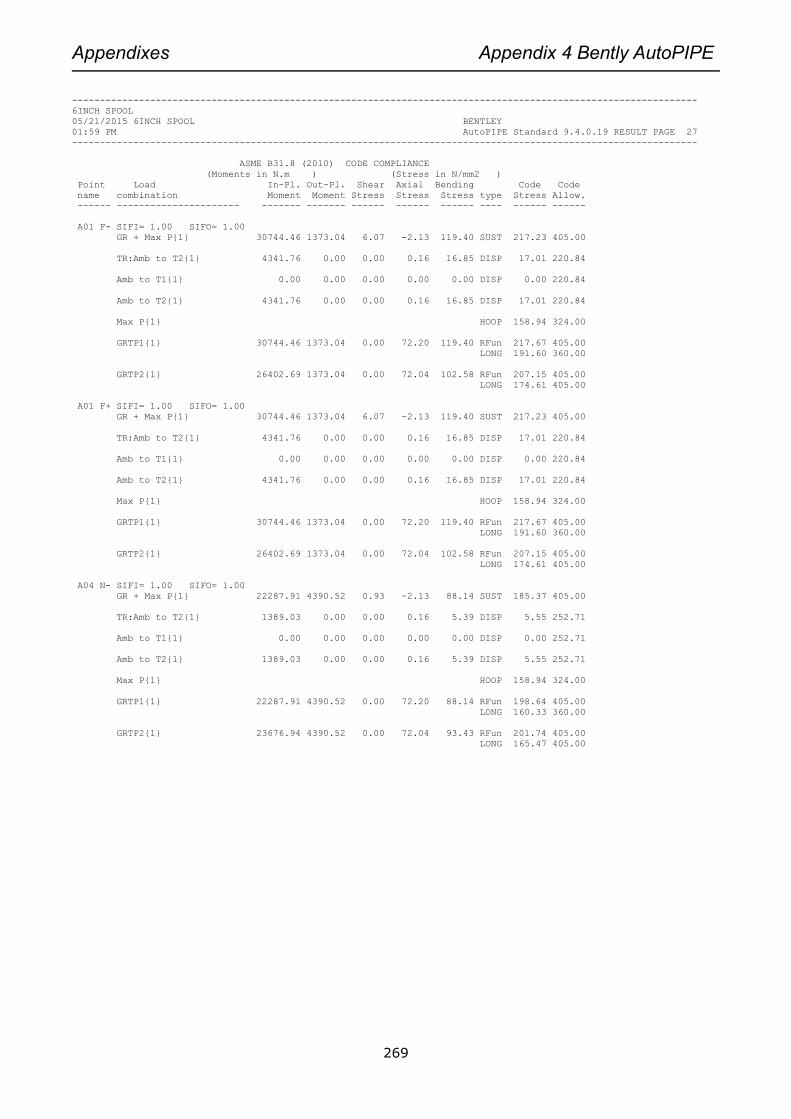
Appendixes Appendix 4 Bently AutoPIPE
269
----------------------------------------------------------------------------------------------------------------
6INCH SPOOL
05/21/2015 6INCH SPOOL BENTLEY
01:59 PM AutoPIPE Standard 9.4.0.19 RESULT PAGE 27
----------------------------------------------------------------------------------------------------------------
ASME B31.8 (2010) CODE COMPLIANCE
(Moments in N.m ) (Stress in N/mm2 )
Point Load In-Pl. Out-Pl. Shear Axial Bending Code Code
name combination Moment Moment Stress Stress Stress type Stress Allow.
------ ---------------------- ------- ------- ------ ------ ------ ---- ------ ------
A01 F- SIFI= 1.00 SIFO= 1.00
GR + Max P{1} 30744.46 1373.04 6.07 -2.13 119.40 SUST 217.23 405.00
TR:Amb to T2{1} 4341.76 0.00 0.00 0.16 16.85 DISP 17.01 220.84
Amb to T1{1} 0.00 0.00 0.00 0.00 0.00 DISP 0.00 220.84
Amb to T2{1} 4341.76 0.00 0.00 0.16 16.85 DISP 17.01 220.84
Max P{1} HOOP 158.94 324.00
GRTP1{1} 30744.46 1373.04 0.00 72.20 119.40 RFun 217.67 405.00
LONG 191.60 360.00
GRTP2{1} 26402.69 1373.04 0.00 72.04 102.58 RFun 207.15 405.00
LONG 174.61 405.00
A01 F+ SIFI= 1.00 SIFO= 1.00
GR + Max P{1} 30744.46 1373.04 6.07 -2.13 119.40 SUST 217.23 405.00
TR:Amb to T2{1} 4341.76 0.00 0.00 0.16 16.85 DISP 17.01 220.84
Amb to T1{1} 0.00 0.00 0.00 0.00 0.00 DISP 0.00 220.84
Amb to T2{1} 4341.76 0.00 0.00 0.16 16.85 DISP 17.01 220.84
Max P{1} HOOP 158.94 324.00
GRTP1{1} 30744.46 1373.04 0.00 72.20 119.40 RFun 217.67 405.00
LONG 191.60 360.00
GRTP2{1} 26402.69 1373.04 0.00 72.04 102.58 RFun 207.15 405.00
LONG 174.61 405.00
A04 N- SIFI= 1.00 SIFO= 1.00
GR + Max P{1} 22287.91 4390.52 0.93 -2.13 88.14 SUST 185.37 405.00
TR:Amb to T2{1} 1389.03 0.00 0.00 0.16 5.39 DISP 5.55 252.71
Amb to T1{1} 0.00 0.00 0.00 0.00 0.00 DISP 0.00 252.71
Amb to T2{1} 1389.03 0.00 0.00 0.16 5.39 DISP 5.55 252.71
Max P{1} HOOP 158.94 324.00
GRTP1{1} 22287.91 4390.52 0.00 72.20 88.14 RFun 198.64 405.00
LONG 160.33 360.00
GRTP2{1} 23676.94 4390.52 0.00 72.04 93.43 RFun 201.74 405.00
LONG 165.47 405.00

Appendixes Appendix 4 Bently AutoPIPE
270
----------------------------------------------------------------------------------------------------------------
6INCH SPOOL
05/21/2015 6INCH SPOOL BENTLEY
01:59 PM AutoPIPE Standard 9.4.0.19 RESULT PAGE 28
----------------------------------------------------------------------------------------------------------------
ASME B31.8 (2010) CODE COMPLIANCE
(Moments in N.m ) (Stress in N/mm2 )
Point Load In-Pl. Out-Pl. Shear Axial Bending Code Code
name combination Moment Moment Stress Stress Stress type Stress Allow.
------ ---------------------- ------- ------- ------ ------ ------ ---- ------ ------
A04 N+ SIFI= 1.00 SIFO= 1.00
GR + Max P{1} 22287.91 4390.52 0.93 -2.13 88.14 SUST 185.37 405.00
TR:Amb to T2{1} 1389.03 0.00 0.00 0.16 5.39 DISP 5.55 252.71
Amb to T1{1} 0.00 0.00 0.00 0.00 0.00 DISP 0.00 252.71
Amb to T2{1} 1389.03 0.00 0.00 0.16 5.39 DISP 5.55 252.71
Max P{1} HOOP 158.94 324.00
GRTP1{1} 22287.91 4390.52 0.00 72.20 88.14 RFun 198.64 405.00
LONG 160.33 360.00
GRTP2{1} 23676.94 4390.52 0.00 72.04 93.43 RFun 201.74 405.00
LONG 165.47 405.00
A04 N- SIFI= 1.00 SIFO= 1.00
GR + Max P{1} 22287.91 4390.52 0.93 -2.13 88.14 SUST 185.37 405.00
TR:Amb to T2{1} 1389.03 0.00 0.00 0.16 5.39 DISP 5.55 252.71
Amb to T1{1} 0.00 0.00 0.00 0.00 0.00 DISP 0.00 252.71
Amb to T2{1} 1389.03 0.00 0.00 0.16 5.39 DISP 5.55 252.71
Max P{1} HOOP 158.94 324.00
GRTP1{1} 22287.91 4390.52 0.00 72.20 88.14 RFun 198.64 405.00
LONG 160.33 360.00
GRTP2{1} 23676.94 4390.52 0.00 72.04 93.43 RFun 201.74 405.00
LONG 165.47 405.00
A04 N+ SIFI= 1.00 SIFO= 1.00
GR + Max P{1} 22287.91 4390.52 0.93 -2.13 88.14 SUST 185.37 405.00
TR:Amb to T2{1} 1389.03 0.00 0.00 0.16 5.39 DISP 5.55 252.71
Amb to T1{1} 0.00 0.00 0.00 0.00 0.00 DISP 0.00 252.71
Amb to T2{1} 1389.03 0.00 0.00 0.16 5.39 DISP 5.55 252.71
Max P{1} HOOP 158.94 324.00
GRTP1{1} 22287.91 4390.52 0.00 72.20 88.14 RFun 198.64 405.00
LONG 160.33 360.00
GRTP2{1} 23676.94 4390.52 0.00 72.04 93.43 RFun 201.74 405.00
LONG 165.47 405.00

Appendixes Appendix 4 Bently AutoPIPE
271
----------------------------------------------------------------------------------------------------------------
6INCH SPOOL
05/21/2015 6INCH SPOOL BENTLEY
01:59 PM AutoPIPE Standard 9.4.0.19 RESULT PAGE 29
----------------------------------------------------------------------------------------------------------------
ASME B31.8 (2010) CODE COMPLIANCE
(Moments in N.m ) (Stress in N/mm2 )
Point Load In-Pl. Out-Pl. Shear Axial Bending Code Code
name combination Moment Moment Stress Stress Stress type Stress Allow.
------ ---------------------- ------- ------- ------ ------ ------ ---- ------ ------
A06 SIFI= 1.00 SIFO= 1.00
GR + Max P{1} 18995.27 2018.79 0.93 -2.13 74.11 SUST 171.35 405.00
TR:Amb to T2{1} 718.21 0.00 0.00 0.16 2.79 DISP 2.95 266.73
Amb to T1{1} 0.00 0.00 0.00 0.00 0.00 DISP 0.00 266.73
Amb to T2{1} 718.21 0.00 0.00 0.16 2.79 DISP 2.95 266.73
Max P{1} HOOP 158.94 324.00
GRTP1{1} 18995.27 2018.79 0.00 72.20 74.11 RFun 191.15 405.00
LONG 146.31 360.00
GRTP2{1} 19713.47 2018.79 0.00 72.04 76.89 RFun 192.66 405.00
LONG 148.92 405.00
A01 N- SIFI= 1.00 SIFO= 1.00
GR + Max P{1} 2750.9317645.86 3.39 1.83 69.29 SUST 162.89 405.00
TR:Amb to T2{1} 0.00 3730.77 0.00 0.02 14.48 DISP 14.50 275.18
Amb to T1{1} 0.00 0.00 0.00 0.00 0.00 DISP 0.00 275.18
Amb to T2{1} 0.00 3730.77 0.00 0.02 14.48 DISP 14.50 275.18
Max P{1} HOOP 158.94 324.00
GRTP1{1} 2750.9317645.86 0.00 68.25 69.29 RFun 190.71 405.00
LONG 137.54 360.00
GRTP2{1} 2750.9313915.08 0.00 68.28 55.03 RFun 183.92 405.00
LONG 123.31 405.00
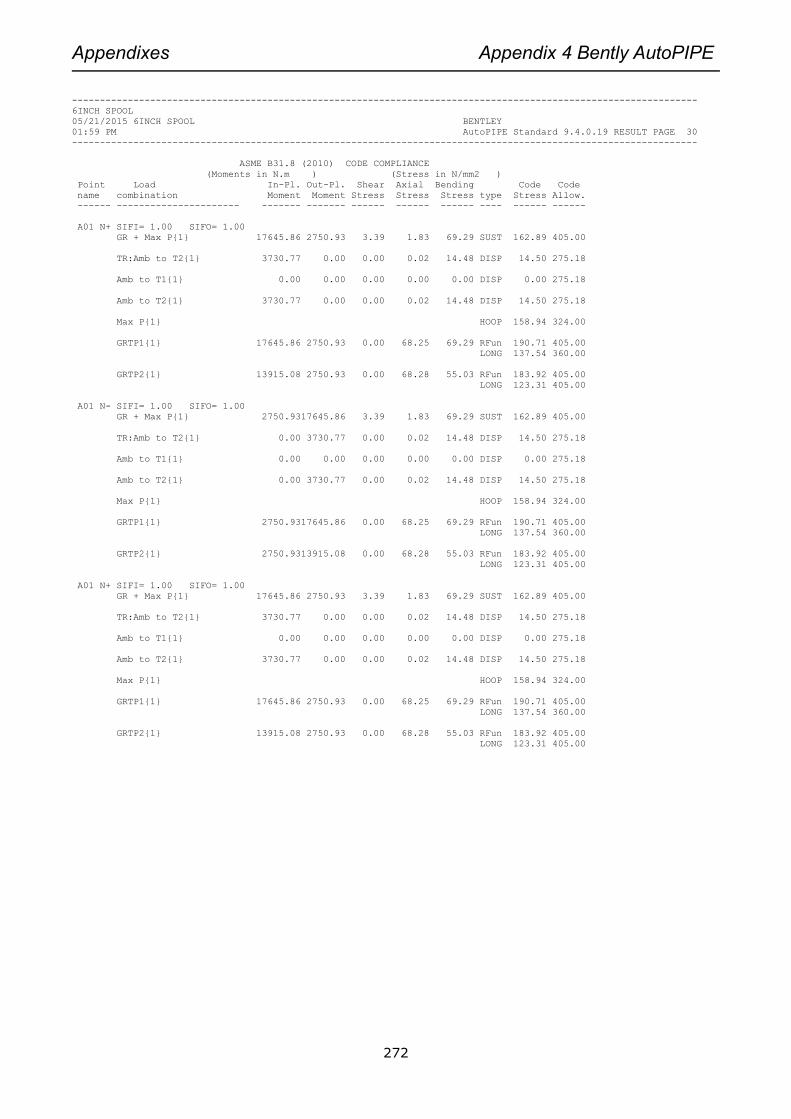
Appendixes Appendix 4 Bently AutoPIPE
272
----------------------------------------------------------------------------------------------------------------
6INCH SPOOL
05/21/2015 6INCH SPOOL BENTLEY
01:59 PM AutoPIPE Standard 9.4.0.19 RESULT PAGE 30
----------------------------------------------------------------------------------------------------------------
ASME B31.8 (2010) CODE COMPLIANCE
(Moments in N.m ) (Stress in N/mm2 )
Point Load In-Pl. Out-Pl. Shear Axial Bending Code Code
name combination Moment Moment Stress Stress Stress type Stress Allow.
------ ---------------------- ------- ------- ------ ------ ------ ---- ------ ------
A01 N+ SIFI= 1.00 SIFO= 1.00
GR + Max P{1} 17645.86 2750.93 3.39 1.83 69.29 SUST 162.89 405.00
TR:Amb to T2{1} 3730.77 0.00 0.00 0.02 14.48 DISP 14.50 275.18
Amb to T1{1} 0.00 0.00 0.00 0.00 0.00 DISP 0.00 275.18
Amb to T2{1} 3730.77 0.00 0.00 0.02 14.48 DISP 14.50 275.18
Max P{1} HOOP 158.94 324.00
GRTP1{1} 17645.86 2750.93 0.00 68.25 69.29 RFun 190.71 405.00
LONG 137.54 360.00
GRTP2{1} 13915.08 2750.93 0.00 68.28 55.03 RFun 183.92 405.00
LONG 123.31 405.00
A01 N- SIFI= 1.00 SIFO= 1.00
GR + Max P{1} 2750.9317645.86 3.39 1.83 69.29 SUST 162.89 405.00
TR:Amb to T2{1} 0.00 3730.77 0.00 0.02 14.48 DISP 14.50 275.18
Amb to T1{1} 0.00 0.00 0.00 0.00 0.00 DISP 0.00 275.18
Amb to T2{1} 0.00 3730.77 0.00 0.02 14.48 DISP 14.50 275.18
Max P{1} HOOP 158.94 324.00
GRTP1{1} 2750.9317645.86 0.00 68.25 69.29 RFun 190.71 405.00
LONG 137.54 360.00
GRTP2{1} 2750.9313915.08 0.00 68.28 55.03 RFun 183.92 405.00
LONG 123.31 405.00
A01 N+ SIFI= 1.00 SIFO= 1.00
GR + Max P{1} 17645.86 2750.93 3.39 1.83 69.29 SUST 162.89 405.00
TR:Amb to T2{1} 3730.77 0.00 0.00 0.02 14.48 DISP 14.50 275.18
Amb to T1{1} 0.00 0.00 0.00 0.00 0.00 DISP 0.00 275.18
Amb to T2{1} 3730.77 0.00 0.00 0.02 14.48 DISP 14.50 275.18
Max P{1} HOOP 158.94 324.00
GRTP1{1} 17645.86 2750.93 0.00 68.25 69.29 RFun 190.71 405.00
LONG 137.54 360.00
GRTP2{1} 13915.08 2750.93 0.00 68.28 55.03 RFun 183.92 405.00
LONG 123.31 405.00

Appendixes Appendix 4 Bently AutoPIPE
273
----------------------------------------------------------------------------------------------------------------
6INCH SPOOL
05/21/2015 6INCH SPOOL BENTLEY
01:59 PM AutoPIPE Standard 9.4.0.19 RESULT PAGE 31
----------------------------------------------------------------------------------------------------------------
ASME B31.8 (2010) CODE COMPLIANCE
(Moments in N.m ) (Stress in N/mm2 )
Point Load In-Pl. Out-Pl. Shear Axial Bending Code Code
name combination Moment Moment Stress Stress Stress type Stress Allow.
------ ---------------------- ------- ------- ------ ------ ------ ---- ------ ------
A08 SIFI= 1.00 SIFO= 1.00
GR + Max P{1} 9589.44 335.90 0.93 -2.13 37.23 SUST 134.49 405.00
TR:Amb to T2{1} 372.33 0.00 0.00 0.16 1.44 DISP 1.60 303.59
Amb to T1{1} 0.00 0.00 0.00 0.00 0.00 DISP 0.00 303.59
Amb to T2{1} 372.33 0.00 0.00 0.16 1.44 DISP 1.60 303.59
Max P{1} HOOP 158.94 324.00
GRTP1{1} 9589.44 335.90 0.00 72.20 37.23 RFun 175.34 405.00
LONG 109.42 360.00
GRTP2{1} 9217.11 335.90 0.00 72.04 35.79 RFun 174.90 405.00
LONG 107.82 405.00
A07 SIFI= 1.00 SIFO= 1.00
GR + Max P{1} 2746.19 2309.23 0.93 -2.13 13.92 SUST 111.25 405.00
TR:Amb to T2{1} 1808.74 0.00 0.00 0.16 7.02 DISP 7.18 326.82
Amb to T1{1} 0.00 0.00 0.00 0.00 0.00 DISP 0.00 326.82
Amb to T2{1} 1808.74 0.00 0.00 0.16 7.02 DISP 7.18 326.82
Max P{1} HOOP 158.94 324.00
GRTP1{1} 2746.19 2309.23 0.00 72.20 13.92 RFun 168.77 405.00
LONG 86.12 360.00
GRTP2{1} 4554.93 2309.23 0.00 72.04 19.81 RFun 170.19 405.00
LONG 91.85 405.00

Appendixes Appendix 4 Bently AutoPIPE
274
----------------------------------------------------------------------------------------------------------------
6INCH SPOOL
05/21/2015 6INCH SPOOL BENTLEY
01:59 PM AutoPIPE Standard 9.4.0.19 RESULT PAGE 32
----------------------------------------------------------------------------------------------------------------
ASME B31.8 (2010) CODE COMPLIANCE
(Moments in N.m ) (Stress in N/mm2 )
Point Load In-Pl. Out-Pl. Shear Axial Bending Code Code
name combination Moment Moment Stress Stress Stress type Stress Allow.
------ ---------------------- ------- ------- ------ ------ ------ ---- ------ ------
A07 SIFI= 1.00 SIFO= 1.00
GR + Max P{1} 2746.19 2309.23 0.93 -2.13 13.92 SUST 111.25 405.00
TR:Amb to T2{1} 1808.74 0.00 0.00 0.16 7.02 DISP 7.18 326.82
Amb to T1{1} 0.00 0.00 0.00 0.00 0.00 DISP 0.00 326.82
Amb to T2{1} 1808.74 0.00 0.00 0.16 7.02 DISP 7.18 326.82
Max P{1} HOOP 158.94 324.00
GRTP1{1} 2746.19 2309.23 0.00 72.20 13.92 RFun 168.77 405.00
LONG 86.12 360.00
GRTP2{1} 4554.93 2309.23 0.00 72.04 19.81 RFun 170.19 405.00
LONG 91.85 405.00
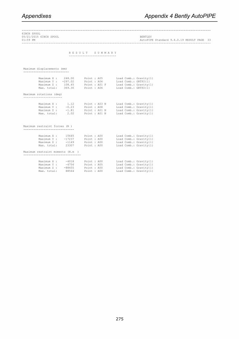
Appendixes Appendix 4 Bently AutoPIPE
275
----------------------------------------------------------------------------------------------------------------
6INCH SPOOL
05/21/2015 6INCH SPOOL BENTLEY
01:59 PM AutoPIPE Standard 9.4.0.19 RESULT PAGE 33
----------------------------------------------------------------------------------------------------------------
R E S U L T S U M M A R Y
----------------------------
Maximum displacements (mm)
---------------------------
Maximum X : 248.00 Point : A05 Load Comb.: Gravity{1}
Maximum Y : -297.02 Point : A06 Load Comb.: GRTP2{1}
Maximum Z : 108.45 Point : A01 F Load Comb.: Gravity{1}
Max. total: 369.30 Point : A06 Load Comb.: GRTP2{1}
Maximum rotations (deg)
-----------------------
Maximum X : 1.12 Point : A03 N Load Comb.: Gravity{1}
Maximum Y : -0.23 Point : A08 Load Comb.: Gravity{1}
Maximum Z : -1.81 Point : A01 N Load Comb.: Gravity{1}
Max. total: 2.02 Point : A01 N Load Comb.: Gravity{1}
Maximum restraint forces (N )
------------------------------
Maximum X : 15645 Point : A00 Load Comb.: Gravity{1}
Maximum Y : -17237 Point : A00 Load Comb.: Gravity{1}
Maximum Z : -1149 Point : A00 Load Comb.: Gravity{1}
Max. total: 23307 Point : A00 Load Comb.: Gravity{1}
Maximum restraint moments (N.m )
----------------------------------
Maximum X : -4018 Point : A00 Load Comb.: Gravity{1}
Maximum Y : -4756 Point : A05 Load Comb.: Gravity{1}
Maximum Z : -88455 Point : A00 Load Comb.: Gravity{1}
Max. total: 88564 Point : A00 Load Comb.: Gravity{1}

Appendixes Appendix 4 Bently AutoPIPE
276
----------------------------------------------------------------------------------------------------------------
6INCH SPOOL
05/21/2015 6INCH SPOOL BENTLEY
01:59 PM AutoPIPE Standard 9.4.0.19 RESULT PAGE 34
----------------------------------------------------------------------------------------------------------------
R E S U L T S U M M A R Y
----------------------------
Maximum pipe forces (N )
-------------------------
Maximum X : -15645 Point : A00 Load Comb.: Gravity{1}
Maximum Y : 17237 Point : A00 Load Comb.: Gravity{1}
Maximum Z : 1149 Point : A00 Load Comb.: Gravity{1}
Max. total: 23307 Point : A00 Load Comb.: Gravity{1}
Maximum pipe moments (N.m )
-----------------------------
Maximum X : 4018 Point : A00 Load Comb.: Gravity{1}
Maximum Y : -4756 Point : A04 F Load Comb.: Gravity{1}
Maximum Z : 88455 Point : A00 Load Comb.: Gravity{1}
Max. total: 88564 Point : A00 Load Comb.: Gravity{1}
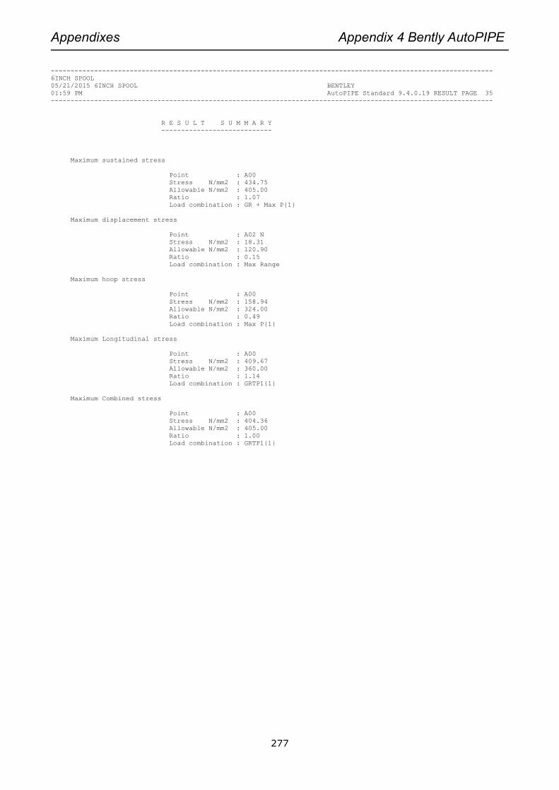
Appendixes Appendix 4 Bently AutoPIPE
277
----------------------------------------------------------------------------------------------------------------
6INCH SPOOL
05/21/2015 6INCH SPOOL BENTLEY
01:59 PM AutoPIPE Standard 9.4.0.19 RESULT PAGE 35
----------------------------------------------------------------------------------------------------------------
R E S U L T S U M M A R Y
----------------------------
Maximum sustained stress
Point : A00
Stress N/mm2 : 434.75
Allowable N/mm2 : 405.00
Ratio : 1.07
Load combination : GR + Max P{1}
Maximum displacement stress
Point : A02 N
Stress N/mm2 : 18.31
Allowable N/mm2 : 120.90
Ratio : 0.15
Load combination : Max Range
Maximum hoop stress
Point : A00
Stress N/mm2 : 158.94
Allowable N/mm2 : 324.00
Ratio : 0.49
Load combination : Max P{1}
Maximum Longitudinal stress
Point : A00
Stress N/mm2 : 409.67
Allowable N/mm2 : 360.00
Ratio : 1.14
Load combination : GRTP1{1}
Maximum Combined stress
Point : A00
Stress N/mm2 : 404.36
Allowable N/mm2 : 405.00
Ratio : 1.00
Load combination : GRTP1{1}
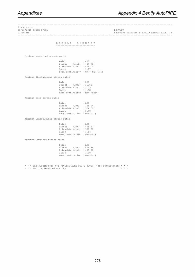
Appendixes Appendix 4 Bently AutoPIPE
278
----------------------------------------------------------------------------------------------------------------
6INCH SPOOL
05/21/2015 6INCH SPOOL BENTLEY
01:59 PM AutoPIPE Standard 9.4.0.19 RESULT PAGE 36
----------------------------------------------------------------------------------------------------------------
R E S U L T S U M M A R Y
----------------------------
Maximum sustained stress ratio
Point : A00
Stress N/mm2 : 434.75
Allowable N/mm2 : 405.00
Ratio : 1.07
Load combination : GR + Max P{1}
Maximum displacement stress ratio
Point : A00
Stress N/mm2 : 16.58
Allowable N/mm2 : 3.33
Ratio : 4.98
Load combination : Max Range
Maximum hoop stress ratio
Point : A00
Stress N/mm2 : 158.94
Allowable N/mm2 : 324.00
Ratio : 0.49
Load combination : Max P{1}
Maximum Longitudinal stress ratio
Point : A00
Stress N/mm2 : 409.67
Allowable N/mm2 : 360.00
Ratio : 1.14
Load combination : GRTP1{1}
Maximum Combined stress ratio
Point : A00
Stress N/mm2 : 404.36
Allowable N/mm2 : 405.00
Ratio : 1.00
Load combination : GRTP1{1}
* * * The system does not satisfy ASME B31.8 (2010) code requirements * * *
* * * for the selected options * * *

Appendixes Appendix 5 ANSYS Design Explorer Features
279
Appendix 5 Ansys Design Explorer Features

Appendixes Appendix 5 ANSYS Design Explorer Features
280

Appendixes Appendix 5 ANSYS Design Explorer Features
281
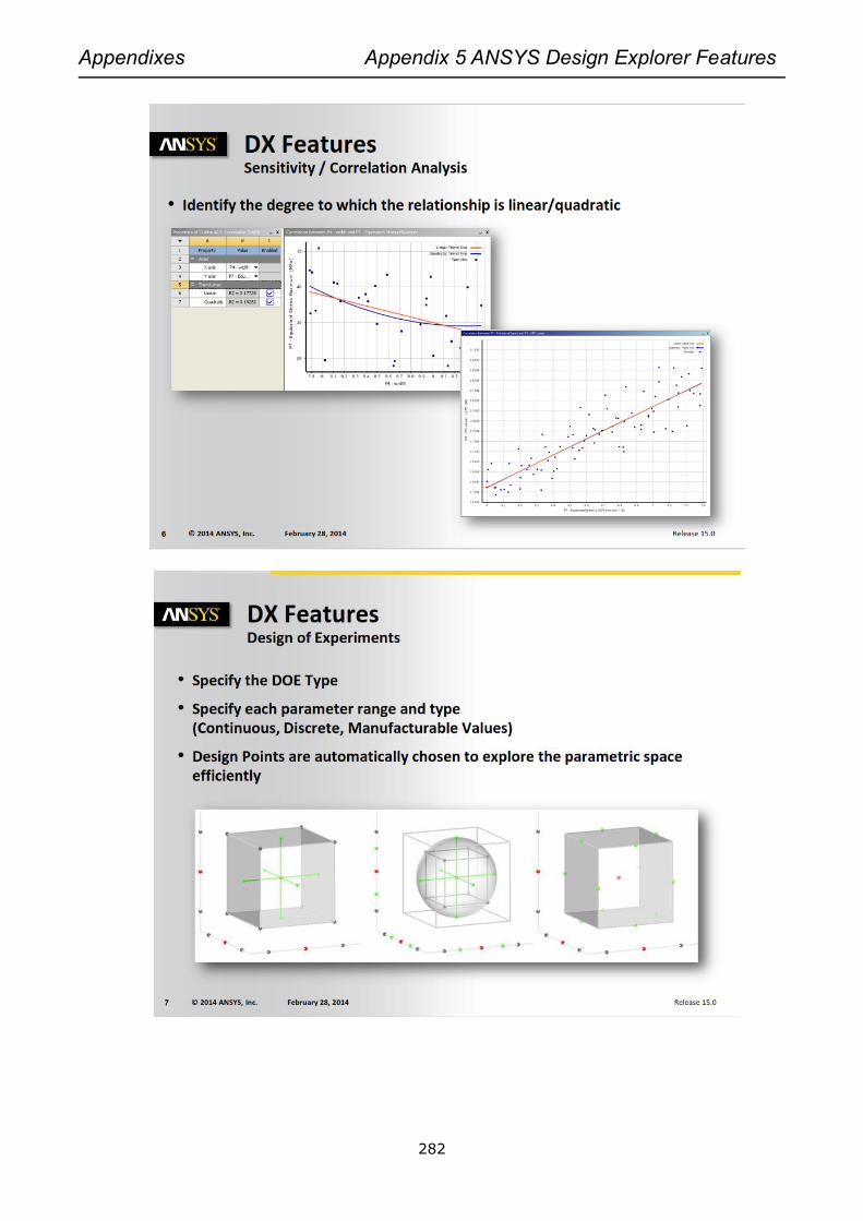
Appendixes Appendix 5 ANSYS Design Explorer Features
282
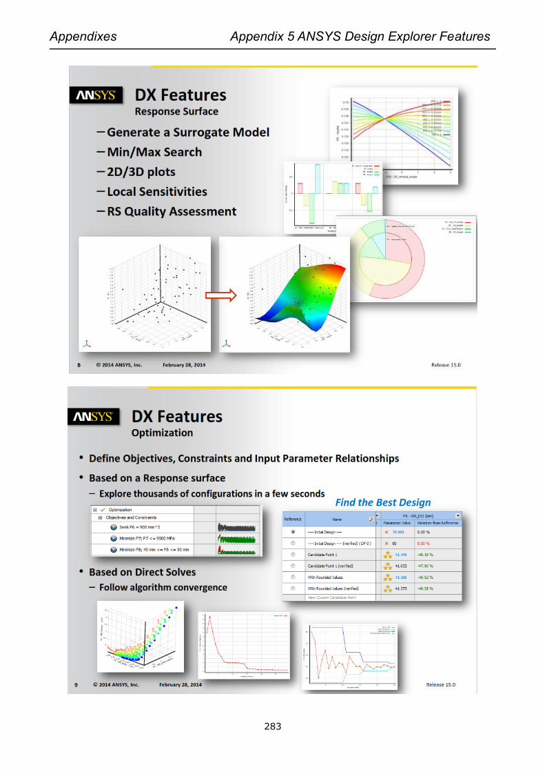
Appendixes Appendix 5 ANSYS Design Explorer Features
283
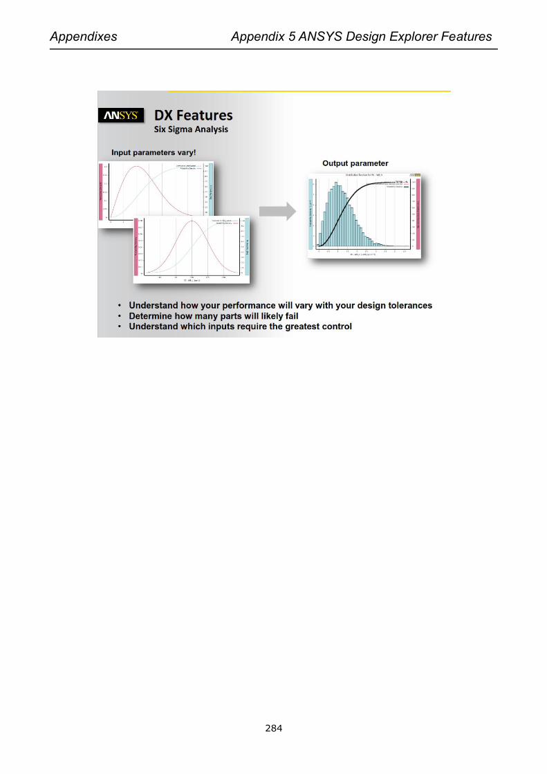
Appendixes Appendix 5 ANSYS Design Explorer Features
284

Appendixes Appendix 6 Spool Type comparison
285
Appendix 6 Spool Type Comparison
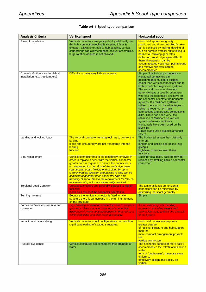
Appendixes Appendix 6 Spool Type comparison
286
Table A6-1 Spool type comparison
Analysis Criteria Vertical spool Horizontal spool Ease of Installation Vertical connectors are gravity deployed directly over
the hub, connection tooling is simpler, lighter & cheaper, allows short hub-to-hub spacing, vertical connections can allow compact receiver assemblies, large rotation of hubs is not allowed.
Horizontal spools are gravity positioned and then controlled “make-up” is achieved by tooling, docking of hub on porch is vertical but stroking is horizontal, stroking generates deflection, so short jumpers difficult, thermal expansion can be accommodated via known pull-in loads and relative hub twist can be accommodated
Controls Multibore and umbilical installation (e.g. tree jumpers)
Difficult / industry very little experience Simple / lots industry experience – Horizontal connectors can accommodate multibore designs easier than vertical connectors due to better-controlled alignment systems. The vertical connector does not generally have a specific orientation whereas the receptacle and keys on the connector orientate the horizontal systems. If a multibore system is utilised there would be advantages in using it throughout on main connections and process connections alike. There has been very little utilisation of Multibore on vertical systems whereas multibore Horizontals have been used on the block 18, Girassol and Dalia projects amongst others.
Landing and locking loads. The vertical connector running tool has to control the landing loads and ensure they are not transferred into the locking function.
The horizontal system has distinctly different landing and locking operations thus giving a high level of control over these functions
Seal replacement Vertical connector has to be completely removed in order to replace a seal. With the vertical connector greater care is required to ensure the connector is not separated too far. Most of the vertical jumpers can accommodate flexible end stroking by up to 0.5m in vertical direction and access to seal can be achieved dependent upon connector type and flexibility of spool. Hence the requirement for total re-movement of spool is not necessarily required.
Seals (or seal plate, gasket) may be replaced by stroking back a horizontal connector.
Torsional Load Capacity Vertical connectors are generally exposed to higher torsional loads as a result of the connector orientation.
The torsional loads on horizontal connectors can be minimized by optimizing the spool geometry
Turning moment Because the vertical vonnector is fitted to taller structure there is an increase in the turning moment on the structure.
Simple
Forces and moments on hub and connector
High bending moment on connectors due to jumpers geometry tolerances and make up of connection. Buoyancy elements may be required in order to keep within connector and pipe material capacity.
As for vertical spools, bending moments caused by weight and connection makeup limits the capacity of the system.
Impact on structure design Vertical connector spool configurations can result in significant loading of seabed structures.
Horizontal connectors require a greater degree of receiver structure and hub support than the more compact arrangement possible with vertical connectors,
Hydrate avoidance Vertical configured spool hampers free drainage of water
The horizontal connector more easily accommodates the retrofit of insulation in the form of “doghouses”, these are more difficult to effectively design and deploy on vertical
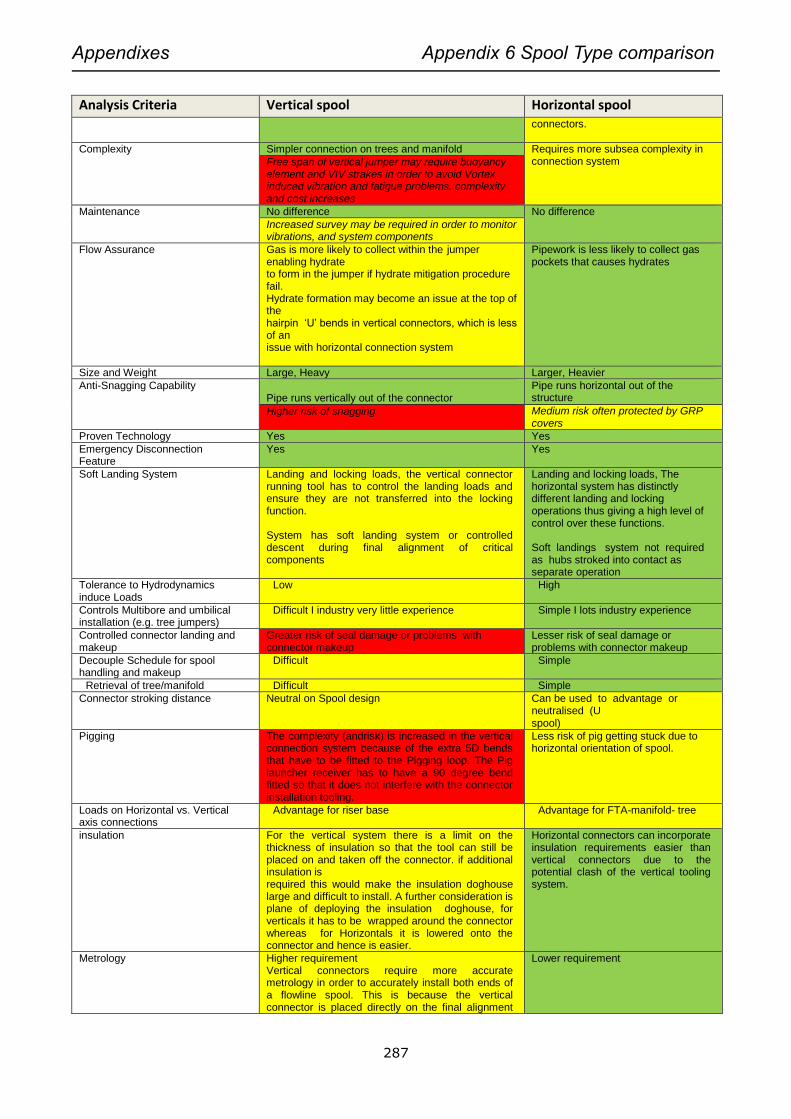
Appendixes Appendix 6 Spool Type comparison
287
Analysis Criteria Vertical spool Horizontal spool connectors.
Complexity Simpler connection on trees and manifold Requires more subsea complexity in connection system Free span of vertical jumper may require buoyancy
element and VIV strakes in order to avoid Vortex induced vibration and fatigue problems. complexity and cost increases
Maintenance No difference No difference
Increased survey may be required in order to monitor vibrations, and system components
Flow Assurance Gas is more likely to collect within the jumper enabling hydrate to form in the jumper if hydrate mitigation procedure fail. Hydrate formation may become an issue at the top of the hairpin ‘U’ bends in vertical connectors, which is less of an issue with horizontal connection system
Pipework is less likely to collect gas pockets that causes hydrates
Size and Weight Large, Heavy Larger, Heavier
Anti-Snagging Capability Pipe runs vertically out of the connector
Pipe runs horizontal out of the structure
Higher risk of snagging Medium risk often protected by GRP covers
Proven Technology Yes Yes
Emergency Disconnection Feature
Yes Yes
Soft Landing System Landing and locking loads, the vertical connector running tool has to control the landing loads and ensure they are not transferred into the locking function. System has soft landing system or controlled descent during final alignment of critical components
Landing and locking loads, The horizontal system has distinctly different landing and locking operations thus giving a high level of control over these functions. Soft landings system not required as hubs stroked into contact as separate operation
Tolerance to Hydrodynamics induce Loads
Low High
Controls Multibore and umbilical installation (e.g. tree jumpers)
Difficult I industry very little experience Simple I lots industry experience
Controlled connector landing and makeup
Greater risk of seal damage or problems with connector makeup
Lesser risk of seal damage or problems with connector makeup
Decouple Schedule for spool handling and makeup
Difficult Simple
Retrieval of tree/manifold Difficult Simple
Connector stroking distance Neutral on Spool design Can be used to advantage or neutralised (U spool)
Pigging The complexity (andrisk) is increased in the vertical connection system because of the extra 5D bends that have to be fitted to the Pigging loop. The Pig launcher receiver has to have a 90 degree bend fitted so that it does not interfere with the connector installation tooling.
Less risk of pig getting stuck due to horizontal orientation of spool.
Loads on Horizontal vs. Vertical axis connections
Advantage for riser base Advantage for FTA-manifold- tree
insulation For the vertical system there is a limit on the thickness of insulation so that the tool can still be placed on and taken off the connector. if additional insulation is required this would make the insulation doghouse large and difficult to install. A further consideration is plane of deploying the insulation doghouse, for verticals it has to be wrapped around the connector whereas for Horizontals it is lowered onto the connector and hence is easier.
Horizontal connectors can incorporate insulation requirements easier than vertical connectors due to the potential clash of the vertical tooling system.
Metrology Higher requirement Vertical connectors require more accurate metrology in order to accurately install both ends of a flowline spool. This is because the vertical connector is placed directly on the final alignment
Lower requirement
Appendixes Appendix 6 Spool Type comparison
288
Analysis Criteria Vertical spool Horizontal spool structure whereas the horizontal connector is lowered into a receptacle that gives both coarse and final alignment as well as allowing an additional tolerance during the connector final make up.
Multibore design The vertical connector does not generally have a specific orientation whereas the receptacle and keyson the connector orientate the horizontal systems. if a multibore system is utilised there would be advantages in using it throughout on main connections and process connections alike. There has been very little utilisation of Multibore on vertical systems whereas multibore Horizontals have been used on Greater Plutonio, Girassol and Dalia projects amongst others.
Horizontal connectors can accommodate multibore designs easier than vertical connectors due to better-controlled alignment systems.
IKM has participated in the ICHTHYS field in the NW of Australia. A multibore vertical connector design with piggyback was used here.
Equipment Retrieval Difficult The requirement to recover flowline / umbilical jumper in order to retrieve subsea production equipment, such as tree or manifold – horizontal connectors may be disconnected and stroked away from the equipment and left in the receptacle. Vertical connectors require to be lifted away from the equipment and either wet parked or retrieved to surface increasing total vessel time. Horizontal connectors only require one end of a flowline spool to be disconnected in order to retrieve an item of subsea equipment, whereas vertical connectors require both ends to be disconnected. Requirement for additional structure – vertical connectors require a secondary receptacle in order to wet park the flowline spool after retrieval of the subsea equipment. Alternatively a secondary connection system such as a flowbase could be utilised. A horizontal connector does not require any secondary equipment for wet parking but does require some form of structure to accommodate the guidance and/or pull in system.
Simple
Deploy to place system Not affected by seabed condition
Buoyancy application Buoyancy in some cases is required in order to reduce connector and spool stresses where nominal spools are particularly long, loads are particularly high due to structure movements and equipment are installed out with installation tolerances necessitating the design of special jumpers.
Ref. IKM Comments on requirement for buoyancy
Structural Requirements The vertical structure has a slightly smaller footprint
than the horizontal connector and this may result in a slightly reduced weight and footprint for structures using a vertical connector but they are slightly taller. Taller Structures however will mean higher moments that are acting to "turn" over the structures.
IKM experience: vertical Jumpers requires large structural test arrangement onshore and supporting equipment when deploying on barge as they need to be in an upraised position with support for lifting equipment hence required deck area increases and more labour for seafastening must be carried out.
Requires pecial installation lifting spreader which is costly, the spool requires often more deck space.
Seabed space requirement Requires larger seabed area due to bends and flexibility requirements. Can interfer with other structures and subsea equipment
Less seabed area required as this spool is in the vertical position