
IEET-2018.pdf - Instrumentation Engineering, Electronics and ...
109
“Instrumentation Engineering, Electronics and Telecommunications – 2018” Proceedings of the IV International Forum December 12–14, 2018 Izhevsk, Russia ISSN 2658–3658
-
Upload
khangminh22 -
Category
Documents
-
view
0 -
download
0
Transcript of IEET-2018.pdf - Instrumentation Engineering, Electronics and ...

“Instrumentation Engineering, Electronics and Telecommunications – 2018”
Proceedings of the IV International Forum
December 12–14, 2018Izhevsk, Russia
ISSN 2658–3658

Министерство образования и науки Российской Федерации Федеральное государственное бюджетное образовательное
учреждение высшего образования «Ижевский государственный технический университет имени М. Т. Калашникова»
«ПРИБОРОСТРОЕНИЕ, ЭЛЕКТРОНИКА И ТЕЛЕКОММУНИКАЦИИ – 2018»
Сборник статей IV Международного форума
(Ижевск, Россия, 12–14 декабря 2018 г.)
Издательство ИжГТУ имени М. Т. Калашникова Ижевск 2018

2
УДК 681.2(06)
Президиум организационного комитета В. П. Грахов – председатель, д-р экон. наук, ректор ИжГТУ имени М. Т. Калашникова; А. В. Щенятский – зам. председателя, д-р техн. наук, ИжГТУ имени М. Т. Калашникова; А. В. Абилов – зам. председателя, канд. техн. наук, ИжГТУ имени М. Т. Калашникова
Программный комитет (рецензенты)
А. В. Абилов – председатель, канд. техн. наук, ИжГТУ имени М. Т. Калашникова; К. Е. Аббакумов – д-р техн. наук, Санкт-Петербургский государственный электротехнический университет «ЛЭТИ» им. В. И. Ульянова (Ленина); М. А. Аль Аккад – канд. техн. наук, ИжГТУ имени М. Т. Калашникова; А. А. Богданов – канд. техн. наук, ИжГТУ имени М. Т. Калашникова; В. Н. Емельянов – канд. техн. наук, ИжГТУ имени М. Т. Калашникова; Я. Котон – PhD, Технический университет г. Брно, Чешская Республика; Д. Кубанек – PhD, Технический университет г. Брно, Чешская Республика; А. Кубанкова – PhD, Технический университет г. Брно, Чешская Республика; О. В. Муравьева – д-р техн. наук, ИжГТУ имени М. Т. Калашникова; С. А. Мурашов – канд. техн. наук, ИжГТУ имени М. Т. Калашникова; П. Райхерт – гл. операционный директор, CONDOR Maritime LTD., Федеративная Республика Германия; А. В. Хомченко – д-р физ.-мат. наук, Белорусско-Российский университет, г. Могилев, Республика Беларусь
Ответственные за выпуск
А. В. Абилов – канд. техн. наук, ИжГТУ имени М. Т. Калашникова; С. А. Мурашов – канд. техн. наук, ИжГТУ имени М. Т. Калашникова
«Приборостроение, электроника и телекоммуникации – 2018» [Электронный ресурс] : сб. ст. IV Междунар. форума (Ижевск, Россия, 12–14 дек. 2018 г.). – Ижевск : Изд-во ИжГТУ имени М. Т. Калашникова, 2018. – 108 с. – 8,4 Мб.
ISSN 2658-3658
Сборник содержит прошедшие рецензирование статьи на английском языке по широкому
кругу вопросов в областях приборостроения, электроники, связи и смежных им, которые обсуждались на IV Международном форуме «Instrumentation Engineering, Electronics and Telecommunications – 2018» («Приборостроение, электроника и телекоммуникации – 2018»), проводимом в рамках XIV Всероссийской научно-технической конференции «Приборостроение в XXI веке. Интеграция науки, образования и производства» (12–14 дек. 2018 года, г. Ижевск, Россия).
Материалы статей могут быть полезны ученым, специалистам, молодым исследователям, аспирантам и студентам.
Форум проведен при финансовой поддержке Российского фонда фундаментальных
исследований. Проект № 18-08-20145 Г.
УДК 681.2(06) ISSN 2658-3658
© ИжГТУ имени М. Т. Калашникова, 2018 © Оформление. Издательство ИжГТУ имени М. Т. Калашникова, 2018

The Ministry of Education and Science of the Russian Federation Kalashnikov Izhevsk State Technical University
“INSTRUMENTATION ENGINEERING, ELECTRONICS AND TELECOMMUNICATIONS – 2018”
Proceedings of the IV International forum
(Izhevsk, Russia, December 12–14, 2018)
Publishing House of Kalashnikov ISTU Izhevsk 2018

4
UDC 681.2(06)
Organizing Committee Chairmans Grakhov, Valery P. – Chairman, DSc in econ., Rector of Kalashnikov ISTU, Izhevsk, Russian Federation; Shchenyatsky, Aleksey V. – Vice-chairman, DSc in eng., Kalashnikov ISTU, Izhevsk, Russian Federation; Abilov, Albert V. – Vice-chairman, resp. org., CSc in eng., Kalashnikov ISTU, Izhevsk, Russian Federation
Scientific Committee (Peer Reviewers) Abilov, Albert V. – Chairman, CSc in eng., Kalashnikov ISTU, Izhevsk, Russian Federation; Abbakumov, Konstantin E. – DSc in eng., Saint Petersburg Electrotechnical University LETI, Saint Petersburg, Russian Federation; Al Akkad, Mhd Aiman – PhD, Kalashnikov ISTU, Izhevsk, Russian Federation; Bogdanov, Aleksey A. – CSc in eng., Kalashnikov ISTU, Izhevsk, Russian Federation; Emelyanov, Vladimir N. – CSc in eng., Kalashnikov ISTU, Izhevsk, Russian Federation; Khomchenko, Alexandr V. – DSc in phys. and math., Belarusian-Russian University, Mogilev, Republic of Belarus; Koton, Jaroslav – PhD, Brno University of Technology, Brno, Czech Republic; Kubánek, David – PhD, Brno University of Technology, Brno, Czech Republic; Kubánkova, Anna – PhD, Brno University of Technology, Brno, Czech Republic; Murav’eva, Olga V. – DSc in eng., Kalashnikov ISTU, Izhevsk, Russian Federation; Murashov, Sergey A. – CSc in eng., Kalashnikov ISTU, Izhevsk, Russian Federation; Reichert, Pavel – Chief operations officer, CONDOR Maritime LTD., Essen, Federal Republic of Germany
Editorial Board Abilov, Albert V. – CSc in eng., Kalashnikov ISTU, Izhevsk, Russian Federation; Murashov, Sergey A. – CSc in eng., Kalashnikov ISTU, Izhevsk, Russian Federation
“Instrumentation Engineering, Electronics and Telecommunications – 2018” : Proceedings of the IV International Forum (Izhevsk, Russia, December 12–14, 2018). – Izhevsk : Publishing House of Kalashnikov ISTU, 2018. – 108 p. – 8.4 Mb.
ISSN 2658-3658
This volume contains peer-reviewed papers on wide range of problems in fields of instrumental engineering, electronics, telecommunications and related areas discussed during the IV International Fo-rum “Instrumentation Engineering, Electronics and Telecommunications – 2018” held within the framework of the XIV International Scientific-Technical Conference “Instrumentation Engineering in the XXI Century. Integration of Science, Education and Production” (December 12–14, 2018, Izhevsk, Russia).
Proceedings could be useful for scientists, professionals, young researchers, students. The Forum was funded by Russian Foundation for Basic Research according to the research pro-
ject No. 18-08-20145 G. UDC 681.2(06)
ISSN 2658-3658 © Kalashnikov ISTU, 2018
© Publishing House of Kalashnikov ISTU, 2018

5
TABLE OF CONTENTS
Abbakumov K. E., Ee B. Ch. Influence of a non-rigid connection on the scattering
properties of a cylindrical inclusion ........................................................................................... 6 Arkhiphov I. O., Shelkovnikov Y. K., Meteleva A. A. The analysis of the video signal
from TV scanistor using spatial-structural parameters ............................................................ 11 Briko A., Chvanova J., Seliutina S., Ivanov E., Kobelev A., Shchukin S. Isometric
hand grab stand for neuromuscular activity research providing .............................................. 17 Chugunov А., Kulikov R., Petukhov N., Indrikov I. Technology of point focusing of
electromagnetic waves (spotforming) ...................................................................................... 24 Gevorkyan A. V. The wideband microstrip antenna with capacitive feed with the
low level of the VSWR ............................................................................................................ 33 Korobeynikov A., Kamalova Yu., Palabugin M., Basov I. The use of convolutional
neural network LeNet for pollen grains classification ............................................................. 38 Meitis D. S., Vasiliev D. S., Kaysina I., Abilov A., Khvorenkov V. Real time emula-
tion of COPE-like network coding in FANET using ns-3 ....................................................... 45 Myshkin Yu. V., Murav’eva O. V., Sannikova Yu. O., Chukhlanceva T. S. The prop-
agation of horizontally polarized shear wave in the hollow cylinder ...................................... 51 Nikitin Yu., Abramov A., Abramov I., Romanov A., Trefilov S., Turygin Yu. Diagno-
sis of mobile robots drives ....................................................................................................... 66 Parfenov D., Zaporozhko V. Implementation of genetic algorithm for forming of
individual educational trajectories for listeners of online courses ........................................... 72 Pergushev A. O., Sorotsky V. A. A time-reduced method for calculation distortions
in envelope tracking power amplifiers ..................................................................................... 83 Ponomareva O., Smirnova N., Ponomarev A. Time-domain interpolation using the
parametric DFT ........................................................................................................................ 89 Shiryaev А., Vinokurov N., Trofimov V., Karmanov V., Shilyaev А. Effect of rein-
forcing rolling on the surface properties of products made of heat-resistant alloys ................ 96

“Instrumentation Engineering, Electronics and Telecommunications – 2018”
Proceedings of the IV International Forum (Izhevsk, Russia, December 12–14, 2018)
6
DOI: 10.22213/2658-3658-2018-6-10
Influence of a Non-Rigid Connection on the Scattering Properties of a Cylindrical Inclusion
K. E. Abbakumov, B. Ch. Ee
Dept. of Electroacoustic and Ultrasonic Technics, Saint Petersburg Electrotechnical University LETI,
Saint-Petersburg, Russian Federation E-mail: [email protected]
Received: June 25, 2018
The incidence of a plane wave on a cylindrical inclusion located in a semi-infinite solid space with an inhomogeneous distribution of the rigidity at the boundary between inclusion-enclosing medium is considered. The cylindrical inclusion model is given. The solution is solved by the finite element method. Scattering indicatrices are given for different angles of incidence of a plane longitudinal wave. A significant effect of the coupling stiffness on the amplitude of the scattered field is shown.
Keywords: plane wave, cylindrical inclusion, finite element method, scattered field, scattered indicatrix.
INTRODUCTION
Nondestructive ultrasonic methods take one of the leading positions among other meth-ods of nondestructive testing. Ultrasonic methods allow solving a wide range of problems and identification of defects in various, mainly solid objects, arising during operation or during production. Wide use of ultrasonic methods is also related with the fact that the fatigue and strength properties of the monitoring object itself influence the propagation of the ultrasonic wave.
It can be noted, that the most common types of defects are nonmetallic inclusions, which are formed due to the inevitable ingress of particles of decomposing refractories into the melt.
Because of the random nature of the process of generation and growth inhomogeneities in the metal and passing through several different process steps non-metallic inclusions can re-late to the main metal scrap by means of different connection types [1, 2]. It is noted [3] that the processes of interaction of elastic waves with such a structurally complex interface be-tween the nonmetallic inclusion and the metal can’t be described using conventional boundary conditions that establish continuity of the stress tensor components and the displacement vec-tor at the boundary. In [4–7] it was proposed to consider the usual boundary, when the elastic wave interacts with boundary, the components of the stress tensor remain continuous, and the components of the displacement vector can undergo a “discontinuity”. The validity of this proposal based on the analytical relations. In [1], the existence of such boundary conditions
© Abbakumov K. E., Ee B. Ch., 2018

Abbakumov K. E., Ee B. Ch.
“Influence of a non-rigid connection on the scattering properties of a cylindrical inclusion”
7
is proved, and it is also shown that the stress at the interface generally determined by the expression: ,K u
where – stress tensor, u – vector of discontinuities in displacements, K – a positive defi-nite symmetric matrix of dimension 3×3, known as the “boundary stiffness matrix”, the ele-ments which have the dimension 3 .N m Generally, these coefficients can be in complex form, which makes it possible to model new processes in the contact zone.
Such a representation allows to consider a special phenomena in the contact zone using various combinations of dynamic flexibility elements and / or damping elements, which is ensured by the corresponding values of the imaginary and real parts. So, in this case of dry mechanical contact of rough surfaces, the values of KN (normal component of contact stiff-ness) and KT (tangential component of contact stiffness) are assumed to be purely real. In case when these surfaces are separated by a layer of a viscous liquid, KN is taken to be com-plex, and KT is purely imaginary. It follows from boundary conditions in the linear “slip” ap-proximation that the range of values of KN and KT in the general case from 0 (there is no transfer of the corresponding component of the displacement vector through the interface) to (the total transmission of the corresponding displacement vector component across the boundary section). The correspondence between the specific values of KN and KT and the structure of boundary can be established by the most suitable model [3].
FORMULATION OF THE PROBLEM
We consider the problem of normally incident plane waves diffraction on an infinite cyl-inder. We will consider a model of compact cylindrical inclusion of radius a, located in a ring layer of infinite small thickness (Figure 1).
Figure 1. Formulation of problem

“Instrumentation Engineering, Electronics and Telecommunications – 2018”
Proceedings of the IV International Forum (Izhevsk, Russia, December 12–14, 2018)
8
Let a plane wave incident on the cylinder (Figure 1) from the solid semi-infinite space I with physical parameters 1, cl1, ct1. A rectangular coordinate system XYZ arranged so that the Z axis coincides with the longitudinal axis of the cylinder and the Y axis is directed along the bisector of the opening angle of the annular layer and the circular cylindrical coordinate system r, , z associated with the rectangular of known transformation formulas. The angle between wave vector and positive direction of the Y axis will be denoted by .
Solving the problem by the finite element method, a finite region was constructed (Fig-ure 2), in which the cylindrical defect I, which is in the isotropic elastic space II. On the boundary between the defect and the elastic space in the sector of finite dimensions IV there is a nonrigid connection. The size of the sector was set as 0 ,okrL dl where okrL is the circumference in degrees, dl is a coefficient ranging from 0 to 1. It is of interest to analyze in infinite space a perfectly matched layer III is used, which absorbs all the waves entering into it.
Figure 2. Investigated area
In entire investigated region, differential equation (1) is solving:
2
2 .t
u (1)
In the stationary mode with harmonic perturbation, equation (1) can be rewritten in the following form:
2 , u
where – angular frequency, – Hamiltonian. Setting the incident wave as an additional mechanical strength of the unit amplitude,
equation (1) can be rewritten as
2 ,ext u
where ext – stress in incident plane wave. Boundary conditions for non-rigid sector are
, ,( )
, .( )
III I II Irrr r rr rr
III I II Ir
r r
KGN
KGT
u u
u u

Abbakumov K. E., Ee B. Ch.
“Influence of a non-rigid connection on the scattering properties of a cylindrical inclusion”
9
RESULTS
Figures 3–4 show the results of the calculation of a dimensionless displacement in polar coordinates, given as the ratio of the incident wave to the scattered one depending on the wavelength ,a lk c coefficient dl and angle of incidence . Figures 3a and 3b show that increase sector dimension with a non-rigid coupling, when the wave falls directly on the sec-tor, the reflection in the opposite direction increases. Figures 4a–4c show the angular distribu-tion of the dimensionless displacement, depending on the size of the sector. It is seen that for various angles of incidence, the scattering indicatrix is localized near the angle of incidence. It can also been seen that an increase sector dimension can lead both to an increase in the ampli-tude in the opposite direction (Figures 4a, 4c) and to a decrease in the amplitude (Figure 4b).
a
b
Figure 3. Dependence of the normalized amplitude of the scattered wave in polar coordinates at ka = 1.074: dl = 0 (a); dl0 = 0.04 (b)
Figure 4. Dependence of the normalized amplitude of the scattered wave in polar coordinates
at ka = 1.074: = 24° (a); = 122° (b); = 196° (c)
dl = 0 dl = 0.05 dl = 0.21
a
dl = 0 dl = 0.05 dl = 0.21
bdl = 0 dl = 0.05 dl = 0.21
c

“Instrumentation Engineering, Electronics and Telecommunications – 2018”
Proceedings of the IV International Forum (Izhevsk, Russia, December 12–14, 2018)
10
CONCLUSION
The obtained results show a significant influence of non-rigid connection on scattering properties of a cylindrical inclusion. The size of the sector leads to increase the amplitude of the scattered wave in the opposite direction, if incident plane wave falls directly on sector with non-rigid connection. When incident plane wave falls to sector with rigid connection, the increasing in size of a sector with non-rigid connection leads to localizing scattered indicatrix near the falling angle. In practice, such influence can strongly affect the results of ultrasonic control. To obtain more accurate data about the internal structure, it’s necessary to scan at dif-ferent angles.
The results can be used to develop or modify methods for ultrasonic nondestructive con-trol different objects with defects that can be approximate by cylinder.
REFERENCES
1. Margetan, F. J., Thompson, R. B., & Gray, T. A. (1988). Interfacial spring model for ultrasonic interactions with imperfect interfaces: Theory of oblique incidence and application to diffusion-bonded butt joints. Jour-nal of Nondestructive Evaluation, 7(3–4), 131–152. doi: 10.1007/BF00565998.
2. Abbakumov, K. E., & Golubev, A. S. (1982). Issledovanie fizicheskikh modeley protyazhennykh neodnorodnostey v tverdykh telakh i ikh klassifikatsiya. [Study of physical models of extended inhomogeneities in solids and their classification]. In Sb. tez. dokl. Vsesoyuz. nauch.-tekhn. konf. “Osnovnye napravleniya ul'trazvukovoy tekhnologii 1981–1990 gg.” (15–17 dekabrya 1982) [Proceedings of All-Union sci.-tech. conference “Main directions of ultrasonic technology in 1981–1990” (December 15–17, 1982)] (pp. 84–85), Suzdal', USSR : USSR Academy of Sciences (in Russian).
3. Maksimov, V. N. (1977). Prokhozhdenie akusticheskoy volny cherez tonkiy sloy mezhdu sherokhovatymi poverkhnostyami [Propagation of acoustic wave through thin layers between rough surfaces]. Prikladnaya akustika [Applied Acoustics], 1977(7), 132–135 (in Russian).
4. Huang, W., Rokhlin, S. I., & Wang, Y. J. (1997). Analysis of different boundary condition models for study of wave scattering from fiber-matrix interphases. Journal of the Acoustical Society of America, 101(4), 2031–2042. doi:10.1121/1.418135.
5. Schoenberg, M. (1980). Elastic wave behavior across linear slip interfaces. The Journal of the Acoustical Society of America, 68(5), 1516–1521. doi: 10.1121/1.385077.
6. Leiderman, R., Figueroa, J. C., Braga, A. M. B., & Rochinha, F. A. (2016). Scattering of ultrasonic guided waves by heterogeneous interfaces in elastic multi-layered structures. Wave Motion, 63, 68–82. doi: 10.1016/j.wavemoti.2016.01.006.
7. Lekesiz, H., Katsube, N., Rokhlin, S. I., & Seghic, R. R. (2013). Effective spring stiffness for a periodic array of interacting coplanar penny-shaped cracks at an interface between two dissimilar isotropic materials. Inter-national Journal of Solids and Structures, 50(18), 2817–2828. doi: 10.1016/j.ijsolstr.2013.04.006.

Arkhiphov I. O., Shelkovnikov Y. K., Meteleva A. A.
“The analysis of the video signal from TV scanistor using spatial-structural parameters”
11
DOI: 10.22213/2658-3658-2018-11-16
The Analysis of the Video Signal from TV Scanistor Using Spatial-Structural Parameters
I. O. Arkhiphov 1, Y. K. Shelkovnikov 2, A. A. Meteleva 3
1, 3 Faculty of Computer Engineering, Kalashnikov Izhevsk State Technical University
E-mail: 1 [email protected], 3 [email protected] 2 Laboratory of Information-Measuring Systems,
Institute of Mechanics of Udmurt Federal Research Center UB RAS E-mail: 2 [email protected] Izhevsk, Russian Federation
Received: June 14, 2018
The issues of the dimensions and coordinates measurement of the light zones on the TV scanistor have been considered. For this purpose we propose to use spatial-structural parameters of the trape-zoidal video signal from the scanistor. It is shown that using spatial-structural parameters makes it possible to increase accuracy of the narrow light zones measurement on the scanistor's photosensitive surface.
Keywords: TV scanistor, information-measuring system, video signal, light zone, accuracy, spatial-structural parameters.
INTRODUCTION
The most reasonable way to measure linear and angular movements of the objects in real-time scale is to use the information-measuring system (IMS) based on the TV scanistor struc-tures (continuous scanistor, discrete multiscan) in time-pulse mode which have high sensitivi-ty and coordinate resolution, small dimensions, high reliability and long service life, relatively low cost. Also it make it possible to measure many non-electrical quantities characterizing the production processes and different phenomena in physics, chemistry (dimensions, coordi-nates, motions, torque, forces, pressures, concentrations, densities, expenses, temperatures etc.) without mechanical contact with the object [1–5]. Therefore, the problem of increasing accuracy of the scanistor IMS is urgent.
INFORMATION-MEASURING SYSTEM FOR MEASURING OF DIMENSIONS AND MOTIONS OF THE LIGHT ZONES ON THE SCANISTOR
In the scanistor IMS the registration of the light relief (in the form of controlled light zones along a photosensitive surface) is carried out continuously by increasing the amplitude
© Arkhiphov I. O., Shelkovnikov Y. K., Meteleva A. A., 2018

“Instrumentation Engineering, Electronics and Telecommunications – 2018”
Proceedings of the IV International Forum (Izhevsk, Russia, December, 12–14, 2018)
12
of the unfolding sawtooth voltage and the corresponding linear movement of the equipotential zero potential line along the scanistor. To extract a video signal (VS) from the continuous scanistor the most rational way is to use interrogation circuit using sawtooth-voltage generator (SAW) and peak detector (PD) where the bias voltage of the scanistor (SC) bleeder bar is found by rectifying interrogation sawtooth-voltage (Figure 1).
Figure 1. Block diagram of scanistor IMS for measuring dimensions and movements of light zones
of the scanistor: IU – interrogation unit TS; VSEU – video signal extraction unit
The automatic ensuring of the equality of the bias voltage and amplitude of the saw-tooth-voltage leads to improving stability of the scanistor coordinate characteristic. The col-lector of the scanistor SC across the current-voltage converter (CVC) is connected to the differentiating divider (DA1), at the output of which a video signal V(t) is generated. Fur-ther the signal from the output of DA1 is put across the differentiating amplifiers DA2, DA3 to the block BVPS of the video-pulses shaper, which shapes pulses by beginning, end and maximum of the video signal for the SMI shaper of measuring time intervals. The duration of the formed intervals is measured by TIM, which includes pulse generator (PG), AND cir-cuit, pulse counter (PC), microprocessor control unit (MCU). Herewith the duration of the formed information intervals is proportional to the light zone (LZ) and distance of its mid-dle from beginning of the scanistor SC.
It can be shown that in a sequential interrogation of the elementary photodiode cells of the scanistor SC the video signal is formed, which can be described by the dependence [1]:
2
10
1 12 2 1 ,exp 1 exp 1
L x
s feb нe k e k x
L b l L b lV t j j KT E E T E E
(1)
where L – coefficient depending on differentiation method; b, l – width and length of the
scanistor, respectively; 1
;KTAq
K – Boltzmann's constant; q – electronic charge; A –
coefficient reflecting the degree of imperfection p n junction of the scanistor structure;
T – temperature in Kelvin degrees; 00e
xE El
– emitter potential at the interrogation point
x0; E0 – emitter constant bias voltage; 00c
tE ET
– value of the sawtooth voltage at the mo-
ment of interrogation t0; T – sawtooth-voltage time; js, Ks – dark saturation current and unbal-ance factor of the current-voltage characteristic of the photodiode cell, respectively; jfeb –increment of the saturation current of the photodiode cell under illumination; x1, x2 – coordi-nates of the beginning and the end on the scanistor of the light zone.
PD SAW PG AND PC MCU PM
CVC DA1 DA2 DA3 BVPS SMI
VSEU
IU TIM
x1
SC x2

Arkhiphov I. O., Shelkovnikov Y. K., Meteleva A. A.
“The analysis of the video signal from TV scanistor using spatial-structural parameters”
13
THE RESULTS OF THE MODELING AND THEIR DISCUSSIONS
In Figure 2 there are dependences of the light components of the video signal V(t), calcu-lated by formula (1), on its first and second derivatives for LZ with different width and equal illumination.
V(t)
V'(t)
V''(t)
Ф(х)L
x1 x2 x1' x2' x2''x1''
t/T
0 0.1 0.2 0.3 0.4 0.5 0.6 0.7 0.8 0.9 1
0
t1 t2 t1' t2' t2''t1''
0
0
0
2 xп
0
U
а б в
Figure 2. Shapes of the video signal curves and its first and second derivatives
for the light zones with different width
The analysis of these dependences has revealed the following aspects: At the constant width of the LZ of the amplitude VS from the scanistor and first and
second derivatives are directly proportional to the illumination. When expanding from the minimum LZ the amplitudes of the VS and its first and se-
cond derivatives first increase nonlinearly, and then become constant and independent of the width of the LZ (if the width x2 – x1 LZ exceeds the doubled value of the switching zone of the scanistor structure П2 x ).
Time coordinate of the midpoint of the LZ ( 2 1 П2x x x ) is uniquely determined by the moment of the first derivative of the ВС passing through zero.
Time coordinate of the middle of the wide LZ ( 2 1 П2x x x ) can be determined by the half-sum of moments of time 1 2( / 2)сt t t of the second derivative of the VS passing through zero.
It should be noted that coordinates and dimensions determination of the digital picture is an urgent and complicated task [6, 7], especially in case of small-dimensions objects [8] on

“Instrumentation Engineering, Electronics and Telecommunications – 2018”
Proceedings of the IV International Forum (Izhevsk, Russia, December, 12–14, 2018)
14
conditions of the image blur [9]. Herewith, to extract and manipulate the video signal from the scanistor it is effectual to use schematic diagram shown in Figure 3.
Figure 3. Schematic diagram of the scanistor IMS
for measuring dimensions and movements of the light zones
In this paper, we propose to use spatial-structural parameters (SSP) to solve the problems of determining the dimensions and coordinates of the trapezoidal video signal (TS) from the scanistor (Figure 2b). It is shown in the works [10, 13] that the SSP make it possible to esti-mate the width of the signal (TS), localize it in space and also determine the amplitude. SSP is calculated from the one-dimensional function of the trapezoidal video signal.
In the work [8] five SSP video signals are estimated: mass (M), centroid (C), dissipation (D), extent (E) and luminance (Y). SSP is found using one-dimensional moments W0, W1, W2 from the following formulas:
0 ,M W (2)
1 ,C W M (3)
22 ,D W M C (4)
2 3 ,E D (5)
.Y M E (6)
The physical meaning of the SSP, applying to the video signal, is as follows [11]: «mass» describes total mass of the video signal; «centroid» is a coordinate of its centre of gravity; «dissipation» describes the degree of localization of the mass of the video signal
around its centre of gravity; «extent» is numerically equal to the width of the video signal; «luminance» describes the amplitude of the video signal. The work [14] shows that short pulse duration TS is calculated with a smaller margin of
error by the SSP than by the derivatives. In Table 1 there are results of the measurements of the width of three LZ by the video
signals shown in Figure 2b. The measurements were taken by two methods. Firstly, by the second derivative signal passing through zero. Secondly, the width of the LZ was estimated by the SSP, i.e. by the value of the extent of the corresponding video signal. From the Table 1 it is clear that for LZ 0.2 width and 0.15 both of the methods give a high accuracy in measur-
PD SAW PM
CVC ADC x2
SC
x1
Ф

Arkhiphov I. O., Shelkovnikov Y. K., Meteleva A. A.
“The analysis of the video signal from TV scanistor using spatial-structural parameters”
15
ing the width values. However, for the narrow LZ the value, obtained from the zero-passing of the 2nd derivative signal, has a significantly overestimated value. Nevertheless, SSP allow obtaining a rather high accuracy when estimating the width of the narrow LZ.
Table 1. The results of the measurements of the LZ width
LZ Width Measured LZ width
By 2nd derivative By SSP 0.2 0.200 0.2 0.15 0.150 0.15 0.05 0.065 0.05
CONCLUSIONS
This paper considers possibility of using spatial-structural parameters of the unidimensional trapezoidal signal of the small-dimension structural elements of the digital pictures to estimate the parameters of the video signal from the scanistor. The analysis in Ta-ble 1 shows that using SSP makes it possible to increase the accuracy of measuring the di-mensions of the narrow LZ on the scanistor's photosensitive surface.
REFERENCES
1. Lipanov, A. M., & Shelkovnikov, Y. K. (2005). Theoretical science and technique of TV scanistor structures manufacturing. Yekaterinburg, Russia : Ural division of RAN, 133 pp.
2. Podlaskin, B. G., & Guk, E. G. (2005). The multiscan position-sensitive photodetector. Measurement Tech-niques, 48(8), 779–783. doi: 10.1007/s11018-005-0220-z.
3. Obolenskov, A. G., Latyev, S. M., Mitrofanov, S. S., & Podlaskin, B. G. (2016). Experience in creating test-and-measurement devices based on the multiscan position-sensitive detector. Journal of Optical Technology, 83(2), 119–122. doi: 10.1364/JOT.83.000119.
4. Podlaskin, B. G, & Guk, E. G. (2007). Analysis of optical signal distortion compensation with a Multiskan position-sensitie photodetector by the quasi-median technique. Technical Physics. The Russian Journal of Applied Physics, 52(2), 239–243. doi: 10.1134/S1063784207020156.
5. Egorov, S. F., Shelkovnikov, Y. K., Osipov, N. I., Kiznertsev, S. R., & Meteleva, A. A. (2017). Issledovanie optiko-elektronnykh registratorov tochki pritselivaniya strelkovykh trenazherov [Investigation of optic-electronic recorders of the aiming point of shooting simulators]. In L. E. Tonkov, V. B. Dementyev (Ed.), Problemy mekhaniki i materialovedeniya. Trudy Instituta Mekhaniki UrO RAN [Problems of Mechanics and Materials Science. Proceedings of the Institute of Mechanics UB RAS] (pp. 227–248). Izhevsk, Russia : Insti-tute of Mechanics UB RAS (in Russian).
6. Kolesnikova, T. A., Zhuk, E. Yu., & Fed’ko, U. I. (2012). Principles for determination of size of structural elements of object of the scanned image. Eastern-European Journal of Enterprise Technologies, 2(2), 38–40. Retrieved from http://journals.uran.ua/eejet/article/view/3664/3436 (in Russian).
7. Bardin, B. V., Manoylov, V. V., Chubinskiy-Nadezhdin, I. V., Vasilyeva, E. K., & Zarutskiy, I. V. (2010). Determination of sizes of local image objects for their identification. Scientific Instrumentation, 20(3), 88–94. Retrieved from http://iairas.ru/mag/2010/full3/Art12.pdf (in Russian).
8. Bodrov, A. S., & Haltobin, V. M. (2010). Automatic system of recognition small objects with usage of sim-ple and complex features. Modern problems of remote sensing of the Earth from space, 7(4), 56–63. Re-trieved from http://d33.infospace.ru/d33_conf/sb2010t4/56-63.pdf (in Russian).
9. Koltsov, P. P. (2011). Image blur estimation. Computer Optics, 35(1), 95–102. Retrieved from http://computeroptics.smr.ru/KO/PDF/KO35-1/12.pdf (in Russian).

“Instrumentation Engineering, Electronics and Telecommunications – 2018”
Proceedings of the IV International Forum (Izhevsk, Russia, December, 12–14, 2018)
16
10. Murynov, A. I., Vdovin, A. M, & Lyalin, V. E. (2002). Otsenka geometriko-topologicheskikh parametrov detaley izobrazheniya na osnove metoda tsentroidnoy fil’tratsii [Estimation of geometric-topological parame-ters of image details on the basis of the centroid filtration method]. Khimicheskaya Fizika i Mezoskopiya [Chemical Physics and Mesoscopics], 4(2), 161–177 (in Russian).
11. Arkhipov, I. O. (2014). Modeling and analysis of linear low-sized structural elements of graphics images on the basis of usage of spatially chromatic parameters. Bulletin of Kalashnikov ISTU, 2014(2), 149–152. Re-trieved from http://izdat.istu.ru/index.php/vestnik/article/view/2933/1701 (in Russian).
12. Levitskaya, L. N. (2006). Modelirovanie i analiz prostranstvennoy struktury graficheskikh izobrazheniy na osnove diskretno-planimetricheskoy modeli giperrastra [Modeling and analysis of the spatial structure of graphic images based on the discrete-planimetric model of hyperraster] (Candidate thesis), Izhevsk State Technical University, Russia (in Russian).
13. Murynov, A. I. (2002). Matematicheskiye modeli i metody analiza prostranstvennykh struktur dlya ekspertnykh geoinformatsionnykh sistem [Mathematical models and methods of analysis of spatial structures for expert geoinformation systems] (DSc in engineering thesis), Physical-Technical Institute UB RAS, Izhevsk, Russia (in Russian).
14. Arkhipov, I. O. (2015). Application specificities of derivaties for determining blurred low-sized structural elements of graphics image. In F. U. Enikeev, et al. (Eds.) Information Technologies. Problems and Solu-tions : Proceedings of the International Sci.-Pract. Conf. (vol. 2, pp. 247–252). Ufa, Russia : Eastern Print. Retrieved from http://vtik.net/konference/sb_trud/ITDAYS_2015_2.pdf (in Russian).

Briko A., Chvanova J., Seliutina S., Ivanov E., Kobelev A., Shchukin S.
“Isometric hand grab stand for neuromuscular activity research providing”
17
DOI: 10.22213/2658-3658-2018-17-23
Isometric Hand Grab Stand for Neuromuscular Activity Research Providing
A. Briko, J. Chvanova, S. Seliutina, E. Ivanov, A. Kobelev, S. Shchukin
Biomedical Engineering Department, Bauman Moscow State Technical University,
Moscow, Russian Federation E-mail: [email protected]
Received: June 25, 2018
The paper presents the results of experiments of the relationship between the change in electrical im-pedance and the force of brush compression determination. Within the framework of the research, an isometric compression stand was developed, which allows recording the brush compression parame-ters. On the developed stand, experiments were carried out, during which the simultaneous registra-tion of the impedance signal from the muscles of the forearm and the compression force of the stand was carried out. The relationship between the impedance change and the action force was determined. The use of this dependence in the development of bio-controlled devices will allow to control it more accurately.
Keywords: bioelectrical active devices, isometric hand grasping, neuromuscular activity, impedance, stand.
INTRODUCTION
Full or partial functional loss of upper limb due to amputation or some diseases has a great influence on human ability to do routine tasks. Active prosthesis and orthosis helps a disabled person to get back after losing the function of a limb. However, nowadays the us-age of such devices is limited due to the complexity of its control.
The most modern active bioelectrical devices are controlled by signals of surface electro-myogram. However, the disadvantage is the complexity of the interpretation, caused by the in-terference nature and the influence of signals from neighboring muscles. Therefore, it is impos-sible to determine the type of movement without increasing numbers of electrode systems [1].
For detection and quantifying muscle health a noninvasive electrical impedance myogra-phy (EIM) technique is generally used. It is based on sending high frequency current with low amplitude passing through the muscle area and measuring the consequent voltage [2]. Most previous EIM studies include the consideration of the stationary state of relaxed muscles without their contraction. Due to the study of the muscles anisotropy using the EIM method it is possible to determine muscle disuse or atrophy [3–6].
Some EIM studies have investigated that the muscle contraction leads to impedance sig-nal changing [1, 7, 8]. It is well known that the architecture and fiber geometry of the muscle, the pennation angle and muscle thickness changes during contraction [9–12]. The change of © Briko A., Chvanova J., Seliutina S., Ivanov E., Kobelev A., Shchukin S., 2018

“Instrumentation Engineering, Electronics and Telecommunications – 2018”
Proceedings of the IV International Forum (Izhevsk, Russia, December, 12–14, 2018)
18
such parameters as thickness of a skin-fat layer, cross section of muscles, conductivities and pressing force of the electrode system lead to an impedance value change during various ac-tions performance. Moreover, it was shown that it is possible to determine the type of move-ment in case of the electrical impedance measurement from forearm antagonistic muscles [13]. Therefore, such signal can be used for management tasks as an alternative for electro-myogram signal or these signals can be registered jointly [14].
Almost all EIM studies connected with the impedance change after muscle contraction were performed for the biceps muscle [8, 15, 16]. In a smaller number of studies, forearm muscles were explored during various actions performing [7, 17]. For the tasks of developing a control system for robotic devices, it is necessary to use reusable small electrode systems that are located on a specific area of the forearm, rather than along the entire length, as was done in the studies.
In addition, in the studies, the dependence of action strength on the impedance change was not found. To identify the dependence between change of the impedance signals and ac-tion parameters it is necessary to design the special stand for measuring the mechanical condi-tions of the movement and electrical impedance simultaneously [18]. Grasp is the most com-mon type of the hand movement. Based on the data of Federal Scientific Center of Rehabilita-tion of the Disabled named after G.A. Albrecht it was found that the most demanded grasps described in literature are end grasp (in a pinch) and palm grasp (opened) (Fig. 1). Such grasps are used in the same movements to hold different objects (isometric type of move-ment). Therefore, it is necessary to design the special stand for such movements.
The aim of this study is to develop the isometric hand grasp force measuring stand and to conduct the investigation for searching the dependence between the electrical impedance sig-nal and the hand grasp force. These results will be used in development of further bioelectric active electromyogram control systems analogues.
MATERIALS AND METHODS
Isometric hand grasping force measuring stand construction
The special stand was designed to register the force of isometric compression (Fig. 1), Mechanical scope of the stand consists of several units: handles, force sensors, pieces, guideways with linear friction bearings and guideway locks.
Force sensors located in handles register the isometric grasping force. Handle dimensions were chosen according to the average human’s hand to place it in the hand conveniently. Force sensors and guideway locks are bolted immovably with the low handle. Linear friction bearings for guideways are bolted immovably with the upper handle. Such construction pro-vides free movement of the upper handle along the guideway relative to the low handle. Therefore, it allows to regulate the stand width for different grasping degrees.
Adjustment of the width of the stand is carried out by installing pieces of different thicknesses bolted immovably with upper handle, which press on the force sensors. The use of 4 guides allows to minimize the skew-ing of the stand due to the non-center effect across the stand. The use of 2 force sensors, which are arranged in parallel and opposite direction, allows to record the distribution of force along the stand.
Figure 1. End grasp (left) and palm grasp (right)

Briko A., Chvanova J., Seliutina S., Ivanov E., Kobelev A., Shchukin S.
“Isometric hand grab stand for neuromuscular activity research providing”
19
Stand working principle is based on the transformation of the force created by hand isometric hand grasping into voltage by force sensors based on the tensoresistors arranged according to the Winston bridge scheme. Each sensor carries a load less than 20 kg. Therefore, it allows to register the grasping force up to 40 (daN) [19], which corresponds the maximal human’s force (error up to 1 N).
Force sensors are connected with the stand registration unit, which is used for registration, processing and transmission signals from sensors to the Personal Com-puter (PC). Signal is registered by 24-bit sigma-delta Analog-to-digital converter (ADC) with differential analog inputs AD7799 from Analog Devices designed for force sensing applications. Such an inte-grated circuit is based on a high-precision
instrumental amplifier with user-defined gain. Data are transmitted to the connected Micro-controller Unit (MCU) via Serial Peripheral Interface (SPI) interface. MCU processes regis-tered data and transmits it to the PC via Universal Serial Bus (USB) interface.
It is necessary to perform calibration before using the stand. Force sensors were calibrat-ed by installing laboratory weights of 100 g to 10 kg to the center of the stand handle. The common force was calculated as an average of signals from two force sensors.
Experiment
Experiments with recording the electri-cal impedance for various isometric grasp-ing forces were carried out on volunteers using a developed stand. Four volunteers participated in the experiments, with an av-erage forearm arm circumference of 29 cm at the location of the electrode systems.
One electrode system was used, which was located in the area along the extensores carpi radialis muscles of the wrist, in place, which can be used to position the electrode systems in modern bioelectric forearms of the forearm (Fig. 3). Before the installation of the electrode system, the place was scrubbed and smeared with an electrode contact gel.
The electrical impedance was regis-tered by the rheographic system “ReoKardioMonitor”. To measure the elec-trical impedance directly from the forearm Figure 3. Location of the electrode system
Figure 2. Isometric hand grasping force measur-ing stand: 1 – low handle, 2 – upper handle, 3 – piece, 4 – force sensor, 5 – guideway, 6 – linear friction bear-ing, 7 – guideway lock

“Instrumentation Engineering, Electronics and Telecommunications – 2018”
Proceedings of the IV International Forum (Izhevsk, Russia, December, 12–14, 2018)
20
region, special electrode systems have been developed (Fig. 4), including a platform and reusable electrodes in the form of rivets with a countersunk head made of stainless steel, 7 mm in diameter, arranged according to the tetrapolar lead system (two current electrodes along the edges and two measur-ing electrodes in the middle).
Electrode systems had the same dis-tance between the electrodes, equal to 10 mm, and were fixed to the forearm by means of rubber bands. The registration of the isometric compression force was per-formed with the help of the developed stand simultaneously with the measurement of the electric impedance signal.
During the experiment, the brush was located in a neutral position (between pro-nation and supination). The time of each study from the series was 1 minute, during which the following actions were per-formed: 0–5 seconds – the volunteer does not compress the stand (state without load), 5–10 seconds - the volunteer isometrically compresses the stand (load condition) (Fig. 5). The compression force increased iteratively in the framework of one study.
An example of registered signals with-in the framework of one study depending on the different degrees of compression of
the stand is shown in Fig. 6. On the graphs, midpoints of activity are marked in red, midpoints of the periods of the relaxed state – in yellow.
Com
pres
sion
forc
e [d
aN]
Bioi
mpe
danc
e [o
hm]
Figure 6. Example of registered signals within the framework of one study
depending on different degrees of the stand compression
Figure 4. Electrode system: 1 – electrodes platform, 2 – electrode, 3 – the place of the rubber band attach-ment for fixation. Pairs of electrodes located closer to the periphery - current, closer to the center - measuring. Dimensions in millimeters
Figure 5. Scheme of experiments

Briko A., Chvanova J., Seliutina S., Ivanov E., Kobelev A., Shchukin S.
“Isometric hand grab stand for neuromuscular activity research providing”
21
Results
With an iterative increase in the compression force of the stand during the experiment, an increase in the bioimpedance value was observed. For electric impedance signals, the drift of the isoline is specific, which is included in the shift of the base value of the signal over time and in the action performance, as shown in the graph (Fig. 6). Thus, for the subsequent analy-sis, the difference between the signal at the time of compression and the signal at the moment of relaxation was taken.
Based on the obtained data, a regression analysis was performed. For each volunteer re-gression curves with a confidence interval of 95 % were constructed. These curves for each volunteer is different and displaying them on one chart is not presentable. Therefore, the graph (Fig. 7) shows the regression curves for the considered case (Fig. 6).
As a result of the regression analysis and the least-interval method, it was found that the curve in the form of a second-order polynomial is more accurate for interpreting the experi-mental data.
2 4 6 8 10 12 14 16 18 20 22Compression force [daN]
0
0.5
1
1.5
2
2.5
Bioi
mpe
danc
e ch
ange
[ohm
]
Figure 7. Regression curve with confidence intervals for the change
in the electrical impedance dependence on isometric compression force
CONCLUSIONS
The need for bioelectric prosthesis according to the federal service of state statistics is in-creasing every year, and the development of control systems for robotic devices is becoming more urgent. One of the main tasks in this direction is to improve the quality of control, for which it is necessary not only to register a qualitative and stable signal, but also to know the optimal arrangement of the electrodes, their physical parameters, the contribution from the integration of the sensors when they are added, etc. To justify the requirements for the param-eters of the above features, it is necessary to organize research, for which it may be necessary to develop special stands that allow establishing the relationship between the parameters of the recorded signal and the parameters of the performed actions.
To enable the realization of studies aimed at determining the relationship between the change in the electrical impedance and the force of the grasp action, an isometric contraction

“Instrumentation Engineering, Electronics and Telecommunications – 2018”
Proceedings of the IV International Forum (Izhevsk, Russia, December, 12–14, 2018)
22
stand was developed. In the course of the research, it was possible to identify the relationship between the compression stand force by brush and the change in the electrical impedance, as a result of which it can be used to generate control signals for controlling robotic devices.
For each volunteer regression curves were different, but similar in form. It means, that in case of bioimpedance signal using as control signal it is necessary to provide a calibration of control system for the use by different operators in various physical conditions. To solve the problems of isoline drift the difference in signal during action with filtering slow signals changes could be used.
Thus, taking into account the change in the electric impedance signal during the perfor-mance of the action will allow not only to determine the type, when using several electrode systems, but also to supplement the electromyogram signal to determine the force with which it is performed.
REFERENCES
1. Moore, J., & Zouridakis, G. (2004). Biomedical technology and devices handbook. CRC Press LLC. 2. Rutkove, S. B. (2009). Electrical impedance myography: background, current state, and future directions.
Muscle & Nerve, 40(6), 936–946. doi: 10.1002/mus.21362. 3. Rutkove, S. B., Aaron, R., & Shiffman, C. A. (2002). Localized bioimpedance analysis in the evaluation of
neuromuscular disease. Muscle & Nerve, 25(3), 390–397. doi: 10.1002/mus.10048. 4. Chin, A. B., Garmirian, L. P., Nie, R., & Rutkove, S. B. (2008). Optimizing measurement of the electrical
anisotropy of muscle. Muscle & Nerve, 37(5), 560–565. doi: 10.1002/mus.20981. 5. Tarulli, A. W., Chin, A. B., Partida, R. A., & Rutkove, S. B. (2006). Electrical impedance in bovine skeletal
muscle as a model for the study of neuromuscular disease. Physiological Measurement, 27(12), 1269–1279. doi: 10.1088/0967-3334/27/12/002.
6. Li, J., Spieker, A. J., Rosen, G. D., & Rutkove, S. B. (2013). Electrical impedance alterations in the rat hind limb with unloading. Journal of Musculoskeletal & Neuronal Interactions, 13(1), 37–44.
7. Nakamura, T., Kusuhara, T., & Yamamoto, Y. (2013). Motion discrimination of throwing a baseball using forearm electrical impedance. Journal of Physics: Conference Series, 434(1), 012070. doi: 10.1088/1742-6596/434/1/012070.
8. Zagar, T., & Krizaj, D. (2007). Electrical impedance of relaxed and contracted skeletal muscle. In: H. Scharfetter, & R. Merwa (Eds.), ICEBI 2007, IFMBE Proceedings 17, 711–714. doi: 10.1007/978-3-540-73841-1_183.
9. Azizi, E., & Deslauriers, A. R. (2014). Regional heterogeneity in muscle fiber strain: the role of fiber archi-tecture. Frontiers in Physiology, 5, article 303, 1–5. doi: 10.3389/fphys.2014.00303.
10. Cuesta-Vargas, A., & González-Sánchez, M. (2014). Correlation between architectural variables and torque in the erector spinae muscle during maximal isometric contraction. Journal of Sports Sciences, 32(19), 1797–1804. doi: 10.1080/02640414.2014.924054.
11. Maganaris, C. N., & Baltzopoulos, V. (1999). Predictability of in vivo changes in pennation angle of human tibialis anterior muscle from rest to maximum isometric dorsiflexion. European Journal of Applied Physiolo-gy and Occupational Physiology, 79(3), 294–297. doi: 10.1007/s004210050510.
12. Walker, F. O., Donofrio, P. D., Harpold, G. J., & Ferrell, W. G. (1990). Sonographic imaging of muscle con-traction and fasciculations: A correlation with electromyography. Muscle & Nerve, 13(1), 33–39. doi: 10.1002/mus.880130108.
13. Briko, A. N., Kobelev, A. V., & Shchukin, S. I. (2016). Determining committed action type by dual-channel phase rheogram portrait for bioelectric forearm prosthetics. In: L. T. Sushkova, S. V. Selishev, Z. M. Yuldashev, & S. I. Schukin (Eds.), Proceedings of the 12th Russian-German Conference on Biomedi-cal Engineering (pp. 102–105). Suzdal, Russia : Vladimir State University named after Alexandr and Nikolay Stoletovs.

Briko A., Chvanova J., Seliutina S., Ivanov E., Kobelev A., Shchukin S.
“Isometric hand grab stand for neuromuscular activity research providing”
23
14. Briko, A. N., Kobelev, A.V., & Shchukin, S. I. (2018). Electrodes interchangeability during electromyogram and bioimpedance joint recording. Proceedings – 2018 Ural Symposium on Biomedical Engineering, Radioelectronics and Information Technology, USBEREIT 2018 (pp. 17–20). doi: 10.1109/USBEREIT.2018.8384539.
15. Orth, T. (2013). Impedance changes in biceps brachii due to isometric contractions and muscle fatigue using electrical impedance myography (EIM) (Master thesis). Retrieved from https://digitalcommons.georgiasouthern. edu/etd/840.
16. Coutinho, A., Jotta, B., Pino, A., & Souza, M. (2012). Behaviour of the electrical impedance myography in isometric contraction of biceps brachii at different elbow joint angles. Journal of Physics: Conference Series, 407(1), 012017. doi: 10.1088/1742-6596/407/1/012017.
17. Kashuri, H. (2008). Anisotropy of human muscle via non invasive impedance measurements. Frequency de-pendence of the impedance changes during isometric contractions (Doctoral thesis). Retrieved from http://hdl.handle.net/2047/d10016259.
18. Kim, S. C., Nam, K. C., Kim, D. W., Ryu, C. Y., Kim, Y. H., & Kim, J. C. (2003). Optimum electrode con-figuration for detection of arm movement using bioimpedance. Medical & Biological Engineering & Compu-ting, 41(2), 141–145. doi: 10.1007/BF02344881.
19. Stepanov, I. S., Evgrafov, A. N., Karunin, A. L., Lomakin, V. V., & Sharipov, V. M. (2002). Avtomobili i traktory. Osnovy ergonomiki i dizayna [Cars and tractors. Basics of ergonomics and design]. Moscow, Russia : MSTU MAMI (in Russian).

“Instrumentation Engineering, Electronics and Telecommunications – 2018”
Proceedings of the IV International Forum (Izhevsk, Russia, December, 12–14, 2018)
24
DOI: 10.22213/2658-3658-2018-24-32
Technology of Point Focusing of Electromagnetic Waves (Spotforming)
А. Chugunov, R. Kulikov, N. Petukhov, I. Indrikov
R&D center of Radiо & Electronics Department of MPEI, National Research University MPEI,
Moscow, Russian Federation E-mail: [email protected]
The article considers the technology of point focusing of electromagnetic waves, which allows to transmit electromagnetic energy to consumer more effectively than beamforming. The technology is based on the principle of operation of antenna arrays, but with the distribution of dipole antennas around the perimeter of the area under consideration, which makes it possible to obtain an increase in the power of the electromagnetic field only at one point in this area, and not in the beam. The article presents the results of theoretical studies as well as mathematical modeling that confirm the feasibility and describe the properties and characteristics of spotforming technology. The experimentally ob-tained characteristics of the generated electromagnetic fields measured by the real prototype are shown. Spotforming is technology of next-generation spatial filtering systems that can be used in high-speed data transmission systems and 5th generation mobile networks.
Keywords: phased arrays, microwave antenna arrays, transmitting antennas, electromagnetic fields, 5G mobile networks, microwave interference, wireless communication, wireless power transmission.
INTRODUCTION
The basis of spatial processing technologies is the use of separate directional antennas and antenna arrays (AA) of weakly directional elements – beamforming, MIMO (multiple in-put – multiple output) [3, 7]. The advantage of directional antennas is simplicity. The ad-vantage of antenna arrays is the ability to quickly change the radiation pattern through elec-tronic control of the channel phases and due to the absence of moving parts. These approaches provide forming a narrow beam of the radiation pattern [4].
In the case of directed radiation, electromagnetic energy is concentrated along the line of sight transmitter-receiver. It allows to reduce energy losses compared to non-directional radia-tion. At the same time, the receiver is only at one point of the line of sight, and in fact, high electromagnetic field strength is required to be provided only at the receiver location (more precisely, the receiver's antenna) [3].
This approach, which we called “spotforming”, makes the use of electromagnetic energy even more efficient than beamforming (Fig. 1).
© Chugunov А., Kulikov R., Petukhov N., Indrikov I., 2018

Chugunov А., Kulikov R., Petukhov N., Indrikov I.
“Technology of point focusing of electromagnetic waves (spotforming)”
25
Figure 1. The transition from beamforming to spotforming:
z-axis means power of electromagnetic field, x, y-axes mean planar coordinates
SPOTFORMING
Spotforming technology or the technology of point focusing of electromagnetic waves implies the use of an antenna system similar to AA. The difference from the known AA is the installation of elements of AA not in one place, but in the space around the working area (room), in which there is need to form a local peak of the field.
In the article [5] it is suggested to use a set of radiators installed along the perimeter around a given point and spatially separated at a distance of several kilometers or more, with several generators synchronized in time. Our approach is intended for the use in working are-as, the size of which ranges from a few meters to tens of meters with a single generator and control of the phases of the dipoles.
Antenna arrays as systems with a controlled radiation pattern of a complex shape, is based on a large number of simple weakly directional radiators. Symmetrical short antennas (Dipole Antenna) act as such radiators. Dipole antenna is a short thin piece of the conductor. The characteristics of symmetrical antennas are more fully described by the model of an ele-mentary electric radiator [1]. The case where the length of the conductor is equal to half the wavelength is of greatest interest. Such an antenna is called a half-wave vibrator, whose arm length is λ/4. Its radiation pattern has the form of a torus (Fig. 2), this means that maximum radiation of such an antenna is directed perpendicular to its axis, and there is no radiation along the axis.
Figure 2. The radiation pattern of a half-wave vibrator

“Instrumentation Engineering, Electronics and Telecommunications – 2018”
Proceedings of the IV International Forum (Izhevsk, Russia, December, 12–14, 2018)
26
It can be assumed that the electromagnetic wave has a flat front in the far field and con-tains mutually perpendicular components of electric and magnetic field intensities lying in a plane perpendicular to the direction of wave propagation. With the vertical position of the di-pole, the vector of the electric field intensity of the electromagnetic field in the far zone has only the vertical component and is described as follows [2]:
00, sin ,2
i t kriCI Z eE r t i e
r
(1)
where I0 – current in the arms of a dipole; ZC – wave impendance; k – wave number; λ – wave length; 0 – initial phase of electric current; – angle measured from the dipole axis; r – the distance between the dipole and the point in which the tension is calculated; i – imaginary unit.
Let us fix the moment of time. The amplitude of the electric field intensity vector de-creases inversely proportional to the distance, and the phase increases linearly in proportion to the distance from the dipole. Approximately, this can be written as follows:
0
.i kreE r
r
(2)
If the initial phase of the current in the conductor is known, the phase Ф of the electro-magnetic wave at a given distance r from the dipole calculated by the formula:
0Ф .r kr (3)
Consider the case when there are N half-wave antennas with known coordinates. The an-tennas are located around the working area (Fig. 3). All antennas are connected to the same generator via phase shifters. According to the formula (2), the field of the i-th radiator:
.ii kr
ieE r
r
(4)
Figure 3. Illustration of the point interference of waves of a large number of antennas
We specify a point within the working area with known coordinates and form a local peak of the electric field in it. Receiver’s antenna (REC) is placed in that point. The initial phases i are set with phase shifters in such a way that at a given point the phases of all indi-vidual electromagnetic waves coming from the dipoles are equal.
For example, for certainty, at a fixed point in time:
Ф 0,i i ikr (5)

Chugunov А., Kulikov R., Petukhov N., Indrikov I.
“Technology of point focusing of electromagnetic waves (spotforming)”
27
where ri is the distance between the given point and the i-th dipole antenna. We assume that ri >> (the far field for all dipoles). This condition ensures the in-phase of the electromagnet-ic waves of all dipoles at a given point. The condition of in-phase in general form:
Ф Ф 2 , 0,1, 2,i i ikr k k (6)
Under condition (6), the in-phase addition of electromagnetic waves occurs at a given point. The module of total electromagnetic field intensity:
1,
N
ii
E E
(7)
where iE – the electric field intensity, formed by the i-th dipole antenna at a given point. In the central part of the working area, the distances from all the antennas to the given
point are approximately equal 1 2 .Nr r r Then the modules of electric field intensity of each dipole antenna at this point are approximately equal to 1 2 .N dipE E E E So you can write:
max,dipE N E (8)
where dipE – the electric field intensity formed by the single dipole antenna at a given point. The module of electric field intensity at a given point in the central part of the working
area is proportional to the number of dipole antennas and the current amplitude on a single dipole.
Here and further, the point where the in-phase addition of waves occurs is called the point of maximum, or maximum, and all other points are called points of periphery, or periphery. The values of the intensities and powers of the electromagnetic field at such points will be denoted by the corresponding indices maxE or perE ( maxP or perP ).
In all the rest of the working area, except for a given point, the condition (6) is violated and the addition of N electromagnetic waves occurs with random phases:
Ф
1,i
Nj
iperi
E E e
(9)
where Фi is a random phase which has a uniform distribution on the interval [-π, π]. The module of the resulting electric field intensity in the periphery is proportional to the root of the number of dipoles and the current amplitude of the dipoles on the average.
.dipperE N E (10)
The electromagnetic field intensity of the periphery increases more slowly than this value at the maximum with increasing the number of dipoles. This is an important feature of a dis-tributed system of phase controlled antennas, and allows to form an electric field at a given point. This is due to in-phase focusing of radio waves at a given point by controlling the phase of each dipole.
The power of the electromagnetic field is proportional to the square of the electric field intensity. Therefore:
22
max max .dip
per dipper
N EEP NP E N E
(11)

“Instrumentation Engineering, Electronics and Telecommunications – 2018”
Proceedings of the IV International Forum (Izhevsk, Russia, December, 12–14, 2018)
28
The ratio of the power at the point of maximum to the power of the periphery is propor-tional to the number of dipoles. Figure 4 shows the relationship between the ratio of the pow-er of the maximum to the power of the periphery averaged over the three-dimensional space of the working zone, and the number of dipoles used, obtained by modeling in the presence of single and double reflections of radio waves from walls, ceiling and floor. That results were obtained by simulation in Matlab. Simulation conditions: operating frequency f = 2 GHz, the area under consideration is a parallelepiped size of 8 × 4 × 3 m, distribution of dipoles along the walls is uniform, the dielectric constant of the reflecting material is ε = 5, the maximum point coordinates are [3.55, 3.08, 1.74] m (asymmetric location of the point of maximum).
Figure 4. The estimated relationship between the ratio of the power of the maximum to the power of
the periphery and the number of dipoles taking into account the effect of reflection from the walls
The above relations (8), (10), (11) are approximate. In reality, as shown in the figure, in addition to direct propagation of radio waves in buildings, reflections from walls and objects in the work area play an important role. It is furthermore necessary to take into account the mutual influence of the dipoles [1, 2]. Strictly taking into account this influence in the general case is not possible. The following sections describe a prototype for verifying the characteris-tics of an approach in practice.
PROTOTYPE
For experimental confirmation of the feasibility of spotforming technology and research-ing of its properties, a prototype was developed, which is a model of a room size of 1 × 1 × 1 m. On the walls of the room there are dipoles, which are half-wave vibrators. In or-der to comply with the interference condition, – coherence of radio waves, all dipole antennas are connected to one monochromatic signal generator via system of power dividers. For in-

Chugunov А., Kulikov R., Petukhov N., Indrikov I.
“Technology of point focusing of electromagnetic waves (spotforming)”
29
vestigation the electromagnetic field formed in the area under consideration, is used receiver, which is also a half-wave vibrator. It is connected to a spectrum analyzer to measure the pow-er of the electromagnetic field at the receiver's location. The receiver is moved by means of special mechanisms, which makes it possible to analyze the generated electromagnetic field pattern entirely in any cross section. The prototype and its functional diagram are depicted in Fig. 5 and Fig. 6, respectively.
Figure 5. The prototype of spotforming technology
Figure 6. The block diagram of the spotforming system’s transmitting part

“Instrumentation Engineering, Electronics and Telecommunications – 2018”
Proceedings of the IV International Forum (Izhevsk, Russia, December, 12–14, 2018)
30
The block diagram of the prototype for an arbitrary number of dipole antennas includes a signal generator, power dividers, digital phase shifters that set the initial phase of each di-pole antenna to focus the radio waves at a given point. Their number is equal to the number of dipole antennas used. A computer carries out the control of phase shifters.
EXPERIMENTS
The prototype allowed us to observe the real field patterns, formed by a system of dis-tributed dipole antennas. Figure 7 (a, b) shows the obtained power distribution of the electro-magnetic field using 8 and 16 dipole antennas. Formed electromagnetic fields are character-ized by a clear spot peak, but also by the presence of subordinate maximum, which is inferior in magnitude to the main one. Measurement of the field pattern is carried out in a horizontal plane passing through the maximum point, and measured area located in the center of the “room” and 20 cm apart from the walls (see Fig. 7). This area corresponds to the far field for all dipole antennas. This fact allows us to assume the front of the electromagnetic wave to be flat and ensures the fulfillment of the relations (1–11). The dipole antennas are located at two different heights to avoid symmetry and the occurrence of subordinate maximum.
The working frequency of the experiment is 2 GHz. The measurements were carried out with a step several times smaller than the wavelength. For the experiment using eight dipole antennas, the grid spacing is 4 cm, for the experiment using sixteen dipole antennas – 2 cm. It should be noted that in the first experiment the point of maximum is located approximately in the center of the area under study (its coordinates are x = 54 cm, y = 50 cm), and in the se-cond – closer to its edge (its coordinates are x = 26 cm, y = 70 cm). This is done to show that the focusing of waves is attainable at any point of the area under study.
If a small number of dipole antennas are used, the field pattern will be characterized by subordinate maximum of power commensurate with the power of the point of maximum. As the number of dipole antennas used increases, the level and the number of subordinate maxi-mum decrease, and the field pattern takes the “ideal form” shown in Fig. 1. As a result of the experiments, the following values of power at the point of maximum were obtained:
max,8 0.203 ,P W
max,16 0.848 .P W
Averaged power at the periphery:
,8 0.032 ,perP W
,16 0.078 .perP W
In accordance with the formulas (8), (9), (11):
2max,16
max,8
164.17 4,8
PP
,16
,8
162.44 2.8
per
per
PP

Chugunov А., Kulikov R., Petukhov N., Indrikov I.
“Technology of point focusing of electromagnetic waves (spotforming)”
31
Figure 8. Experimentally obtained field patterns for the case of:
8 dipole antennas (a); 16 dipole antennas (b)
In fact, the power at the periphery increases more slowly than the power of the maximum when the number of dipole antennas used increases. The obtained results are correlated with the estimated dependences. Thus, an important property of spotforming technology, resulting from the expression (11), is the possibility of obtaining any ratio of the power of maximum to the power at the periphery (maximum to periphery ratio) by selecting the number of dipole antennas used depending on the tasks assigned.

“Instrumentation Engineering, Electronics and Telecommunications – 2018”
Proceedings of the IV International Forum (Izhevsk, Russia, December, 12–14, 2018)
32
CONCLUSION
We proposed Spotforming, a new approach to the spatial concentration of electromagnet-ic energy: at a given point, rather than in a ray, as in known approaches. This is achieved by in-phase focusing of waves at a given point.
Spotforming allows you to increase the radiation power at a given point without violating the electromagnetic compatibility with other devices in the rest of the space.
The increased power can be used to increase the speed of information transmission in communication networks, to increase the secrecy of communication systems, for wireless power transmission and for other tasks.
The authors are currently working on the application of this approach for the challenges of transferring video streams to virtual reality helmets in order to free the user from the cable between the helmet and the console.
In the long term, the implementation of the change of the location of the point of maxi-mum in the area under consideration in real time is considered, as well as the achievement of the antinodes of the field at several points. This is a generalization of the proposed technology in the case where there are several receivers that can be mobile.
REFERENCES
1. Balanis, C. A. (2005). Antenna theory: Analysis and design (3rd ed.). Columbus, Ohio, USA : A John Wiley & Sons.
2. Stutzman, W. L., & Thiele, G. A. (2012). Antenna theory and design (3rd ed.). Whittemore, Iowa, USA : Courier Westford.
3. Nordrum, A., & Clark, K. (2017, July 15). 5G bytes: beamforming explained. IEEE Spectrum. Re-trieved from https://spectrum.ieee.org/video/telecom/wireless/5g-bytes-beamforming-explained.
4. Haynes, T. (1998, March 26). A primer on digital beamforming. Retrieved from http://citeseerx.ist.psu. edu/viewdoc/download?doi=10.1.1.583.5008&rep=rep1&type=pdf.
5. Pronin, S., Pimenov, P., & Myrova, L. (2017). Vozdeystviye na priyemo-peredayushchiye radioelektronnyye sredstva. Raspredelennaya sistema sverkhkorotkoimpul’snogo elektromagnitnogo izlucheniya: eye komponenty i ispol’zovaniye [Impact on transceiving radio-electronic means. Distrib-uted system of ultrashort impulse electromagnetic radiation: components and use]. Radioelektronnyye tekhnologii [Radio-Electronic Technologies], 2017(5), 69–72 (in Russian).
6. Liu, L., Zhang, R., & Chua, K.-C. (2017). Multi-antenna wireless powered communication with energy beamforming. IEEE Transactions on Communications, 62(12), 4349–4361. doi: 10.1109/TCOMM.2014.2370035.
7. Golbon-Haghighi, M.-H. (2016). Beamforming in wireless networks. In: H. K. Bizaki (Ed.), Towards 5G Wireless Networks. A Physical Layer Perspective (pp. 163–192). IntechOpen. doi: 10.5772/66399.
8. Feng, J., Chang, C.-W., Sayilir, S., Lu, Y.-H., Jung, B., Peroulis, D., & Hu, Y. C. (2010). Energy-efficient transmission for beamforming in wireless sensor networks. In: 7th Annual IEEE Communica-tions Society Conference on Sensor, Mesh and Ad Hoc Communications and Networks (SECON) (pp. 1–9). doi: 10.1109/SECON.2010.5508256.

Gevorkyan A. V.
“The wideband microstrip antenna with capacitive feed with the low level of the VSWR”
33
DOI: 10.22213/2658-3658-2018-33-37
The Wideband Microstrip Antenna with Capacitive Feed with the Low Level of the VSWR
A. V. Gevorkyan
Department of Antennas and Radiotransmitters, Southern Federal University,
Taganrog, Russia E-mail: [email protected]
Received: July 07, 2018
In order to increase the operating frequency band of the microstrip antenna by the level of the VSWR ≤ 1.2, we propose to use capacitive feed. Simulation was performed using HFSS. The results showed that the use of capacitive feed can expand the operating frequency band to 16.8 %, while the antenna without capacitive feed was 10.9 %.
Keywords: microstrip antenna, wideband antenna, VSWR, capacitive feed.
INTRODUCTION
Antennas intended for onboard radio systems with a limited power reserve must have a small the VSWR. This is due to the fact that the smaller the VSWR of the antenna, the greater the radiated power (at a fixed input power) and the longer the radio range (at a fixed signal level at the input of the receiver). In addition, such antennas should be small size and not protruding (low profile). The microstrip antennas meet these requirements. However, the-se antennas often have a resonant frequency characteristic of the VSWR. As a result, the op-erating frequency band of these antennas is small and, basically, does not exceed a few per-cent. There are microstrip antennas, whose operating frequency band by level of the VSWR ≤ 2 is 10 % or more [1–5]. However, by level of the VSWR ≤ 1.2 (|S(1,1)| ≤ −20 dB) their operating frequency band is usually less than 10 %. In this regard, an actual task is to develop the wideband microstrip antennas with small the VSWR.
In the previous work [6], such the wideband microstrip antenna with the VSWR ≤ 1.2 in the frequency range of 1.87–2.07 GHz was developed (operating bandwidth – 200 MHz or 10.9 % relative to 1.87 GHz). The antenna had a square reflector with the width of 100 mm or ≈0.7 λ at the upper frequency of the operating frequency band.
The aim of this work was to increase of the width of the operating frequency band by the level of the VSWR ≤ 1.2 and reduce the operating frequencies of the previous antenna while maintaining the size of its reflector.
© Gevorkyan A. V., 2018

“Instrumentation Engineering, Electronics and Telecommunications – 2018”
Proceedings of the IV International Forum (Izhevsk, Russia, December, 12–14, 2018)
34
ANTENNA DESIGN
The antenna design is shown in Fig. 1. The antenna is the microstrip antenna having two microstrips (E and U-form) and the reflector.
In the previous work [6], a coaxial cable core was connected to an E-form microstrip. An additional rectangular microstrip was used to expand the operating frequency band (highlight-ed in color in Fig. 1b). The designation of the dimensions of an additional rectangular microstrip is shown in Fig. 1c, where w is the width and l is the length.
This microstrip is connected to a 50 Ohm coaxial cable core. The excitation of the E-form microstrip is carried out by means of a capacitive coupling between it and an additional rec-tangular microstrip. This excitation is called capacitive (capacitive feed) [7–8].
a b c
Figure 1. Antenna design: general view (a); top view (b); rectangular microstrip (c)
THE RADIATION CHARACTERISTICS OF THE ANTENNA
Let us consider the radiation characteristics of the antenna. Characteristics were studied in the frequency range 1.6–2.1 GHz with 10 MHz step. Simulation was performed using HFSS1.
Fig. 2–4 are shown the frequency characteristics of the VSWR, gain and radiated power for different values w (l = 28 mm).
1.60 1.65 1.70 1.75 1.80 1.85 1.90 1.95 2.00 2.05 2.10Freq [GHz]
1.0
1.2
1.4
1.6
1.8
2.0
VSW
R
Curve Info
w='1.6mm'w='1.8mm'w='2mm'w='2.2mm'w='2.4mm'
Figure 2. The frequency characteristics of the VSWR
1 Available at https://www.ansys.com/products/electronics/ansys-hfss

Gevorkyan A. V.
“The wideband microstrip antenna with capacitive feed with the low level of the VSWR”
35
From Fig. 2 it is seen that the largest operating bandwidth by the level of the VSWR ≤ 1.2 has the antenna with w = 1.8 mm. The decrease in w leads to a shift in the oper-ating frequency band towards the upper frequencies and an increase of the VSWR in the fre-quency range of 1.80–1.95 GHz. The increase of w leads to a significant reduction in the op-erating frequency band by the level of the VSWR≤1.2.
Fig. 2 are shown that the operating frequency band of the antenna with w = 1.8 mm is in the frequency range of 1.685–1.968 GHz (bandwidth – 283 MHz or 16.8 % relative to 1.685 GHz). For comparison, the previously developed [1] microstrip antenna had the VSWR ≤ 1.2 in the frequency range of 1.87–2.07 GHz (bandwidth – 200 MHz or 10.9 % rela-tive to 1.87 GHz). That is, the use of capacitive feed allowed reducing the operating frequen-cies of the antenna and increasing the operating frequency band by 83 MHz.
Fig. 3 are shown that the change in w leads to a slight change in the gain (less than 0.1 dB). This is because the gain is more dependent on the size of the antenna, which has not changed. Antenna gain with w = 1.8 mm (in the operating frequency band by the level of the VSWR ≤ 1.2) is in the range of 8.0–8.5 dB.
1.60 1.65 1.70 1.75 1.80 1.85 1.90 1.95 2.00 2.05 2.10Freq [GHz]
7.0
7.5
8.0
8.5
Gai
n [d
B] Curve Info
w='1.6mm'w='1.8mm'w='2mm'w='2.2mm'w='2.4mm'
Figure 3. The frequency characteristics of the gain
1.60 1.65 1.70 1.75 1.80 1.85 1.90 1.95 2.00 2.05 2.10Freq [GHz]
0.6
0.7
0.8
0.9
1.0
Rad
iate
d Po
wer
[W]
Curve Info
w='1.6mm'w='1.8mm'w='2mm'w='2.2mm'w='2.4mm'
Figure 4. The frequency characteristics of the radiated power
From Fig. 4 it is seen that increasing w leads to a decrease of the radiated power at fre-quencies of more than 1.95 GHz and an increase at frequencies of less than 1.68 GHz. These changes are associated with changes in the VSWR of the antenna.
Fig. 4 are shown that the radiated power of the antenna with w=1.8 mm (in the operating frequency band by the level of the VSWR ≤ 1.2) is in the range of 0.99–1.00 W (input pow-

“Instrumentation Engineering, Electronics and Telecommunications – 2018”
Proceedings of the IV International Forum (Izhevsk, Russia, December, 12–14, 2018)
36
er – 1 W). This makes it very profitable to use the developed antenna in onboard radio sys-tems with a limited supply of power.
Fig. 5–7 are shown the frequency characteristics of the VSWR, the gain and the radiated power for different values l (w = 1.8 mm).
Fig. 5 are shown that the maximum bandwidth of the operating frequency band by the level of the VSWR ≤ 1.2 of the antenna with l = 28 mm (283 MHz – in the frequency range of 1.685–1.968 GHz). The change in l leads to a shift in the frequency characteristics of the VSWR, an increase of the VSWR and a decrease in the bandwidth of the operating frequency.
1.60 1.65 1.70 1.75 1.80 1.85 1.90 1.95 2.00 2.05 2.10Freq [GHz]
1.0
1.2
1.4
1.6
1.8
2.0
VSW
R
Curve Info
l='26mm'l='27mm'l='28mm'l='29mm'l='30mm'
Figure 5. The frequency characteristics of the VSWR
Fig. 6 are shown that the change in l leads to a small change in the gain (less than 0.1 dB). The highest value of the gain in the operating frequency band by the level of the VSWR ≤ 1.2 is observed at l = 28 mm.
1.60 1.65 1.70 1.75 1.80 1.85 1.90 1.95 2.00 2.05 2.10Freq [GHz]
7.0
7.5
8.0
8.5
Gai
n [d
B] Curve Info
l='26mm'l='27mm'l='28mm'l='29mm'l='30mm'
Figure 6. The frequency characteristics of the gain
Fig. 7 are shown that the highest radiated power in the operating frequency band by the level of the VSWR ≤ 1.2 has an antenna with l = 28 mm – more than 0.99 W (power at the antenna input – 1 W). The increase of l leads to a shift in the frequency characteristics of the radiated power towards high frequencies, and the increase of the direction of low frequencies.
Analyzing the dependence of the radiation characteristics of the antenna can conclude that the highest the bandwidth of the antenna by the level of the VSWR ≤ 1.2 has the antenna with the dimensions of a rectangular microstrip w × l=1.8 × 28.0 mm2.

Gevorkyan A. V.
“The wideband microstrip antenna with capacitive feed with the low level of the VSWR”
37
1.60 1.65 1.70 1.75 1.80 1.85 1.90 1.95 2.00 2.05 2.10Freq [GHz]
0.6
0.7
0.8
0.9
1.0
Rad
iate
d Po
wer
[W]
Curve Info
l='26mm'l='27mm'l='28mm'l='29mm'l='30mm'
Figure 7. The frequency characteristics of the radiated power
CONCLUSION
Thus, the use of a capacitive feed with the dimensions of a rectangular microstrip w × l=1.8 × 28.0 mm2, has allowed to increase of the bandwidth of the antenna by the level of the VSWR ≤ 1.2 with 200 MHz (1.87–2.07 GHz) to 283 MHz (1.685–1.968 GHz) or 16.8 % relative to the minimum operating frequency (10.9 % at the source [6]). In the operating fre-quency band, the radiated power of the antenna exceeds 0.99 W, and the gain is in the range of 8.0–8.5 dB. The obtained characteristics make it very profitable to use the developed wide-band antenna in onboard radio systems with a limited supply of power.
This work was financially supported by Russian Science Foundation (Project No. 16-19-10537).
REFERENCES
1. Kuo, Y.-L., & Wong, K.-L. (2003). Printed double-T monopole antenna for 2.4/5.2 GHz dual-band WLAN operations. IEEE Transactions on Antennas and Propagation, 51(9), 2187–2192. doi: 10.1109/TAP.2003.816391.
2. Shabunin, S. (2003). Stacked patch antenna array on cylindrical surface. In: 17th International Conference on Applied Electromagnetics and Communications, ICECom–2003 (pp. 172–174). Dubrovnik, Croatia : IEEE. doi: 10.1109/ICECOM.2003.1290982.
3. Li, P., Lau, K. L., & Luk, K. M. (2005). A study of the wide-band L-probe fed planar patch antenna mounted on a cylindrical or conical surface. IEEE Transactions on Antennas and Propagation, 53(10), 3385–3389. doi: 10.1109/TAP.2005.856374.
4. Mueed, A., Xu, J., & Mehdi, G. (2011). Cavity backed embedded antenna on cylindrical surface for confor-mal applications. In: 2011 IEEE 14th International Multitopic Conference, INMIC (pp. 351–356). Karachi, Pakistan : IEEE. doi: 10.1109/INMIC.2011.6151502.
5. Ansari, J. A., Singh, P., Dubey, S. K., Khan, R. U., & Vishvakarma, B. R. (2008). H-shaped stacked patch antenna for dual band operation. Progress in Electromagnetics Research B, 5, 291–302. doi: 10.2528/PIERB08031203.
6. Gevorkyan, A. V. (2017). The wideband patch antenna with low level of the VSWR. In: 2017 Radiation and Scattering of Electromagnetic Waves, RSEMW–2017 (pp. 26–30). Divnomorskoe, Russia : IEEE. doi: 10.1109/RSEMW.2017.8103658.
7. Musale, P. D., Hobragade, S. V., & Anitha, V. R. (2011). A broadband microstrip antennas with different shapes of capacitive feed strip. In: 2011 3rd International Conference on Electronics Computer Technology (pp. 287–291). Kanyakumari, India : IEEE. doi: 10.1109/ICECTECH.2011.5941607.
8. Tarange, V., Gite, T., Musale, P., & Khobragade, S. V. (2011). A U slotted H-shaped micro strip antenna with capacitive feed for broadband application. In: 2011 International Conference on Emerging Trends in Networks and Computer Communications, ETNCC (pp. 182–184). Udaipur, India : IEEE. doi: 10.1109/ETNCC.2011.5958511.

“Instrumentation Engineering, Electronics and Telecommunications – 2018”
Proceedings of the IV International Forum (Izhevsk, Russia, December, 12–14, 2018)
38
DOI: 10.22213/2658-3658-2018-38-44
The Use of Convolutional Neural Network LeNet for Pollen Grains Classification
A. Korobeynikov 1, Yu. Kamalova 2, M. Palabugin 3, I. Basov 4
1 Dept. of Computer Software, 2 Dept. of Measuring, Control, Diagnostic Instruments and Techniques,
3 Dept. Physics and Optical Engineering, 4 Dept. Mathematical Support for Information Systems,
Kalashnikov Izhevsk State Technical University, Izhevsk, Russian Federation
E-mail: 1 [email protected], 2 [email protected], 3 [email protected], 4 [email protected]
Received: June 26, 2018
The convolutional neural network from the LenetMnistExample of the DeepLearning4j framework is described and applied for pollen grains classification.The selected basic topology of the LeNet neural network was not changed; the loading of images was modified, and the number of classes of the clas-sification task (outputNum) as well as the subsample size of examples (batchSize) were changed. Training (1520 photos) and test (380 photos) samples of four classes of pollen grains were formed. The quality metrics values calculated according to the results of the test sample classification are: 1) Accuracy = 0.9289; 2) Precision = 0.9306; 3) Recall = 0.9266; 4) F1 Score = 0.9282.
Keywords: computer pollen analysis, pollen of plants, image recognition, convolutional neural net-work, pollen recognition.
INTRODUCTION
In modern society, the trend towards automation and computerization of various technolog-ical processes is becoming increasingly prevalent. The number of areas using computer analysis for the recognition of various objects is very significant and continues to increase. And one of the promising areas using this technology is pollen analysis. Nowadays, there are a number of studies based on the recognition of pollen grains, determining their characteristics.
In the article [1] authors researched an automation of the process for the classification of pollen grains. An updated set of three schemes of pollen extractors and four algorithms for machine learning were implemented. This is CST, BOW, CST + BOW. With the usage of the BOW + CST method and the C-SVC classifier, the percentage of correct classifications reached 94 %. This was the best result in this research. BOW and CST individually had low accuracy.
In the work [2] there is described a semiautomatic system for pollen grains analysis with the usage of computer vision for increasing the number of processed data. Computer vision
© Korobeynikov A., Kamalova Yu., Palabugin M., Basov I., 2018

Korobeynikov A., Kamalova Yu., Palabugin M., Basov I.
“The use of convolutional neural network LeNet for pollen grains classification”
39
algorithms was used for automation. High performance was achieved with minimal parameter settings.
The authors of the paper [3] developed a method based on the detection of small shifts at the absolute direct current level of the cantilever deflection signal that occurs when the body is tied to the tip during atomic force microscopy. The addition of recognition images gives the microscope the ability to identify certain types of molecules at the level of one molecule without compromising their topographic characteristics.
In the article [4] there are results for creating an automatic system that produces micro-scopic analysis of biological particles. As a basis, the authors took an analytical approach. This system has yielded good results in the collection of pollen data. The accuracy of detect-ing pollen grains using this method is 90 %.
In the paper [5] authors carried out research in the field of automatic recognition of pollen grains. In their work they used the OpenCV recognition library and the method of point marks on the object. Accordingly, the neural network correctly recognized about 72 % of the pollen grains.
Authors of the work [6] carried out work on the development of automated recognition of pollen. The AMIT Leitz Ergolux AMC trinocular microscope was used, which was equipped with a stepped step X-Y-Z with computer-controlled Quick Step. To solve the problem asso-ciated with an intensive computational process of image processing, this work used a hierar-chical approach. In this paper, for the first time, a system was provided that has the potential to produce slides made with a microscope that contain pollen grains.
In the paper [7] authors conducted an exhaustive analysis of the conformity of the texture of the pollen grains and its taxon. They used the method of textures – an effective method for identifying pollen. The results reflect the excellent characteristics of the textures descriptors LGF and DTM, as well as the usefulness of the combined approach in the proposed problem of pollen classification. A significant classification accuracy of more than 80 % has been achieved.
Author of the paper [8] developed software for computer vision that can help researchers in the classification and analysis of pollen. Using the FLLT method, which makes up the im-plicit contours of the object, after which the segmentation procedure is performed. And then it is possible to classify pollen grains. In his view, a two-stage method is required for computer-classical classification of images. Fourier descriptors using centroid distance have been de-fined as an ideal way of determining the similarity of a figure.
In the work [9] authors used a method for classifying pollen grains, which involves deter-mining the size and density of sculptural elements grain, also paying attention to the complexity of the relief of the surface of the pollen. The results of the studies support the theory that a com-bination of high resolution microscopy and analysis of computational images can generate a classification at subtle taxonomic levels that are not available to specialists. In the paper, they also carried out the classification of textures using histograms of local quantum spots of images, which gave an accuracy of more than 85 %, but did not provide high interpretability.
Authors in paper [10] carried out work on the automation of differential blood counting (DBC). An effective automatic system for differential blood analysis was developed. It does not require user settings and any intervention in the human process. The segmentation scheme used in the system can be easily adapted for any given data set with a known magnification. Howev-er, for this method to be clinically useful, it is necessary to improve the process associated with the processing of clustered data cells. The database of blood bodies was obtained from the data-base of stained May-Grunwald Giemsa stains (IGY). The classification accuracy was 80 %.
Authors in the article [11] carried out research to automate the processing of data associated with pollen. They describe a method for classifying pollen that uses different grain attributes in the multi-layered decomposition of areas in the pollen image. Here researchers use a hierarchical classification. This method resulted in one of the highest classification rates. At the first stage, the

“Instrumentation Engineering, Electronics and Telecommunications – 2018”
Proceedings of the IV International Forum (Izhevsk, Russia, December, 12–14, 2018)
40
method first classifies pollen types into two broad groups, depending on the appearance of the tex-ture. In the second stage, the method classifies the pollen using the decomposition method, which creates several layers for each sample. The accuracy of the method is 80 %.
As we see attempts for automation of the process of classification of pollen grains on mi-crophotographs were made. Some of them has a high accuracy of recognition. However, the problem wasn’t completely solved, i.e. until now there is no method for determining the bo-tanical and geographical origin of honey and other bee products, based on a fully computer analysis of pollen grains.
Determining the grain’s belonging to the plant species by a highly qualified operator is an expensive procedure, but it is still the most accurate and effective one.
The relevance of the use of computer analysis in the control of honey can be explained, firstly, by the possibility of determining the fact of falsification of honey by identifying the correspondence between the name of honey and the belonging of pollen grains to a particular plant. It can find its application in the provision of services for analyzing the quality of honey, its belonging to a particular monoflorous sort of honey that will allow issuing certificates con-firming the quality of honey.
Computer pollen analysis is relevant in many areas of science and production, such as control of botanical and geographical honey origin, pharmaceutical industry, ecology, palinology, etc.
Palynological data are used in a wide range of areas, but the problems of classification and counting of pollen grains require high qualification and labor intensity. The development of an automated pollen identification and classification system will bring great benefits. Previous at-tempts at computer classification have used approaches that by nature were difficult to develop into fully automated systems able to operate independently to a considerable extent.
In this work, to solve the pollen grains classification problem, the convolutional neural networks were chosen, as they have been successfully used for image processing in recent years [12–14].
Artificial neural network of Fukushima (Cognitron, 1975) [15] was the first convolutional artificial neural network, which borrowed the ideas embodied by nature in the visual cortex for informatics. The convolutional network in its modern form appeared in the works of LeCun (LeNet, 1989) [15].
THE METHOD OF THE EXPERIMENT
As a base, the artificial neural network topology was chosen from the example of the Le-netMnistExample of DeepLearning4j framework1. In this example, the classification problem of handwritten digits images with size of 28×28 from the MNIST database2 training sample is solved.
During experiments, the selected basic topology of the LeNet neural network was not changed; the loading of images was modified, and the number of classes for the classification task (outputNum) and the subsample size of examples (batchSize) were changed.
Typical image processing using convolutional neural network LeNet is shown in Fig. 1 [16], where the feature maps (matrixes) obtained at the outputs of sequential layers of the neu-ral network are shown schematically.
The following parameters of the LeNet neural network layers were used in the experi-ments:
1 http://DeepLearning4j.org 2 http://yann.lecun.com/exdb/mnist/

Korobeynikov A., Kamalova Yu., Palabugin M., Basov I.
“The use of convolutional neural network LeNet for pollen grains classification”
41
0. Input image: size of 28×28, 1 RGB colors layer. The size of the input multidimensional array is 28×28×1.
1. Convolutional layer (Convolutions): the convolution kernel size of 3×3, the number of different convolutions (feature filters) 20, linear neuron activation function (Identity). At the layer output a multidimensional array of size 28×28×20 is derived.
2. Subsampling layer (Subsampling): the kernel size of 2×2, maximum function (Max). At the layer output a multidimensional array of size 14×14×20 is derived.
3. Convolutional layer (Convolutions): the convolution kernel size of 5×5, the number of different convolutions (feature filters) 50, linear neuron activation function (Identity). At the layer output a multidimensional array of size 14×14×50 is derived.
4. Subsampling layer (Subsampling): the kernel size of 2×2, maximum function (Max). At the layer output a multidimensional array of size 7×7×50 is derived.
5. Dense layer (Fully connected): number of neurons 500, ReLU (Rectified Linear Unit) neuron activation function. At the layer output an array of size 500 is derived.
6. Output layer (Output): number of neurons (classes) 4, SoftMax neuron activation func-tion. At the layer output a array of size 4 is derived.
Convolutions
Subsamling
Convolutions
Subsamling
Dense
Output
28x28x1 28x28x20 14x14x20 14x14x50 7x7x50 500 4
Feature maps Feature maps Feature maps Featuremaps
Array ArrayInput image
Figure 1. Image processing by convolutional neural network
EXPERIMENTS
Block diagram used for experiments is shown in Fig. 2. The following parameters were used during the training of convolutional neural network: 1) number of output neurons: 4; 2) the subsample size of examples (batchSize): 128; 3) number of training epochs (epochNum): 1000; 4) the number of iterations at each epoch: 1; 5) L2 regularization weight: 0.0005; 6) learning rate: 0.01. For fitting the neural network was used the optimization algo-rithm “stochastic gradient descent” with updater “Nesterovs”.
During the experiments, a pollen grains sample containing 4 classes of grains was used: 0) Centaurea scabiosa; 1) Helianthus; 2) Pisum; 3) Fagopyrum. Examples of images from each class are shown in Fig. 3. All images were split into training and test samples containing about 80% and 20% of images from each class respectively. Table 1 shows the number of im-ages from each class in the samples.
The results of the test sample classification obtained during the experiments are presented in Table 2. Let’s consider the data in table 2 for class 0: a total of 88 samples from this class are in the test sample, of these, the neural network related 79 samples to class 0, 1 sample to class 1 and 8 samples to class 2. The quality metrics values calculated according to the results of the test sample classification are: 1) accuracy = 0.9289; 2) precision = 0.9306; 3) recall = = 0.9266; 4) F1 score = 0.9282.

“Instrumentation Engineering, Electronics and Telecommunications – 2018”
Proceedings of the IV International Forum (Izhevsk, Russia, December, 12–14, 2018)
42
Initial setting
Loading and normalizing
the training sample
Building a neural network
epoch < epochNum
Fitting the neural network
epoch = epoch + 1
Loading and normalizing
the test sample
Evaluation of neural network
Begin
End
no
yes
Figure 2. Block diagram used for experiments
Class 0
(Centaurea scabiosa) Class 1
(Helianthus) Class 2 (Pisum)
Class 3 (Fagopyrum)
Figure 3. Examples of images used in the experiments
Table 1. Number of images in experiments Sample Class 0 Class 1 Class 2 Class 3
Training 352 496 352 320 Test 88 124 88 80 Total 440 620 440 400

Korobeynikov A., Kamalova Yu., Palabugin M., Basov I.
“The use of convolutional neural network LeNet for pollen grains classification”
43
Table 2. Classification results for the test sample
Neural network output Target output
Class 0 Class 1 Class 2 Class 3 Class 0 79 1 1 1 Class 1 1 119 8 0 Class 2 8 2 78 2 Class 3 0 2 1 77 Total 88 124 88 80
CONCLUSIONS
The results obtained in experiments on the test sample showed the applicability and high efficiency of the chosen apparatus of convolutional neural networks for solving the pollen grains classification problem, which is confirmed by high values of classification quality metrics.
In further researches, it is necessary to improve the sample by increasing the number of pollen grain classes, and the number of pollen images in the classes. After that, this neural network can be used in the automatic honey pollen analysis software.
ACKNOWLEDGMENT
The authors are grateful to the staff “Analytical Center APIS”, Ltd. (Moscow region) headed by Elena Yuryevna Balashova for provision of the microscopic images of pollen grains and for active cooperation and consultation.
REFERENCES
1. Gonçalves, A. B., Souza, J. S., Silva, G. G., Cereda, M. P., Pott, A., Naka, M. H., & Pistori, H. (2016). Fea-ture extraction and machine learning for the classification of Brazilian savannah pollen grains. PLoS ONE, 11(6), e0157044. doi: 10.1371/journal.pone.0157044.
2. Hwang, G. M., Riley, K. C., Christou, C. T., Jacyna, G. M., Woodard, J. P., Ryan, R. M., … Masters, D. L. (2013). Automated pollen identification system for forensic geo-historical location applications. In: 2013 IEEE International Conference on Technologies for Homeland Security (HST) (pp. 297–303). Waltham, MA, USA : IEEE. doi: 10.1109/ths.2013.6699018.
3. Stroh, C., Wang, H., Bash, R., Ashcroft, B., Nelson, J., Gruber, H., … Hinterdorfer, P. (2004). Single-molecule recognition imaging microscopy. Proceedings of the National Academy of Sciences, 101(34), 12503–12507. doi: 10.1073/pnas.0403538101.
4. Ranzato, M., Taylor, P., House, J., Flagan, R., Lecun, Y., & Perona, P. (2007). Automatic recognition of bio-logical particles in microscopic images. Pattern Recognition Letters, 28(1), 31–39. doi: 10.1016/j.patrec.2006.06.010.
5. Khanzhina, N., & Zamyatina, E. (2015). Pollen grains recognition using structural approach and neural net-works. Information Models & Analyses, 4(3), 243–258. Retrieved from http://www.foibg.com/ijima/vol04/ ijima04-03-p03.pdf.
6. France, I., Duller, A. W. G., Duller, G. A. T., & Lamb, H. F. (2000). A new approach to automated pollen analysis. Quaternary Science Reviews, 19(6), 537–546. doi: 10.1016/s0277-3791(99)00021-9.
7. Marcos, J. V., Nava, R., Cristóbal, G., Redondo, R., Escalante-Ramírez, B., Bueno, G., … Rodríguez, T. (2015). Automated pollen identification using microscopic imaging and texture analysis. Micron, 68, 36-46. doi: 10.1016/j.micron.2014.09.002.
8. Haas, N. Q. (2011). Automated pollen image classification (Master’s thesis, University of Tennessee, USA). Retrieved from https://trace.tennessee.edu/utk_gradthes/1113.

“Instrumentation Engineering, Electronics and Telecommunications – 2018”
Proceedings of the IV International Forum (Izhevsk, Russia, December, 12–14, 2018)
44
9. Mander, L., Li, M., Mio, W., Fowlkes, C. C., & Punyasena, S. W. (2013). Classification of grass pollen through the quantitative analysis of surface ornamentation and texture. Proceedings of the Royal Society B: Biological Sciences, 280(1770), 1–7. doi: 10.1098/rspb.2013.1905.
10. Sinha, N., & Ramakrishnan, A. (2003). Automation of differential blood count. In: TENCON 2003. Confer-ence on Convergent Technologies for Asia-Pacific Region (pp. 547–551). Bangalore, India : IEEE. doi: 10.1109/tencon.2003.1273221.
11. Daood, A., Ribeiro, E., & Bush, M. (2016). Pollen recognition using a multi-layer hierarchical classifier. 2016 23rd International Conference on Pattern Recognition (ICPR) (pp. 3091–3096). Cancun, Mexico : IEEE. doi: 10.1109/ICPR.2016.7900109.
12. Kamalova, Y. B. (2014). Calculation of statistical parameters in recognition of pollen grains, obtained by the scanning electron microscope. Intelligent Systems in Manufacturing, 2014(1), 120–123. Retrieved from http://izdat.istu.ru/index.php/ISM/article/download/1540/353 (in Russian).
13. Lomaev, G. V., & Kamalova, Y. B. (2014). Komp’yuterizirovannyy pyl’tsevoy analiz meda [Computerized pollen analysis of honey]. Pchelovodstvo [Beekeeping], 2014(8), 59–60 (in Russian).
14. Kamalova, Y. B. (2016). Methods and approaches to computerized pollen analysis. Intelligent Systems in Manufacturing, 14(2), 67–70. Retrieved from http://izdat.istu.ru/index.php/ISM/article/download/3275/2083 (in Russian).
15. Goodfellow, I., Bengio, Y., & Courville, A. (2016). Deep learning. Cambridge, USA : MIT Press. Retrieved from http://www.deeplearningbook.org.

Meitis D. S., Vasiliev D. S., Kaysina I., Abilov A., Khvorenkov V.
“Real time emulation of COPE-like network coding in FANET using ns-3”
45
DOI: 10.22213/2658-3658-2018-45-50
Real Time Emulation of COPE-like Network Coding in FANET using ns-3
D. S. Meitis 1, D. S. Vasiliev 2, I. Kaysina 3, A. Abilov 4, V. Khvorenkov 5
1 Development Bureau, CJSC NPO Telecom,
Izhevsk, Russian Federation E-mail: 1 [email protected]
2–4 Department of Communication Networks and Systems, 5 Department of Radio Engineering,
Kalashnikov Izhevsk State Technical University, Izhevsk, Russian Federation
E-mail: 2 [email protected], 3 [email protected], 4 [email protected]
Received: June 14, 2018
In this paper, we consider the version of network coding (COPE-like), that allow compressing data for more effective usage of the wireless medium. We discuss the possibility of its application in the net-works of Unmanned Aerial Vehicles (UAV) – Flying Ad hoc Networks. We have carried out an emu-lation of the network coding usage and analyzed its results.
Keywords: network coding, B.A.T.M.A.N, Flying Ad-hoc Networks, Unmanned Aerial Vehicles, ns-3.
INTRODUCTION
Wireless networks assume using common medium for data transmission between the nodes. Multiple access methods such as TDMA, FDMA and CDMA are used to access the transmission medium. In this case, each node hears all messages in the network but drops ones addressed to the other nodes.
Network coding (NC) is a spectral efficient aid to multicasting [1–7]. COPE-like NC [8] makes it possible to reduce the ineffective use of the transmission medium by compressing two packets transmitted on the network into one. The principle of COPE-like network coding is shown in Figure 1. Node A sends packets to node C and node C sends packets to node A. Node B is a NC-enabled relay. Using COPE-like NC we need only 3 timeslots instead of 4 timeslots in traditional approach.
Network coding in this form (COPE-like) can be used in Unmanned Aerial Vehicles (UAV) networks (Flying Ad hoc Networks, FANETs) for efficient data transmission using intermediate nodes (drones) [9–10]. In our previous articles we estimated efficiency of data delivery in FANETs using simulation setup with and without COPE-like Network Coding [11–12]. The following sections consider the emulation of an UAV network of three nodes and analyze the results and prospects of using network coding in them. © Meitis D. S., Vasiliev D. S., Kaysina I., Abilov A., Khvorenkov V. 2018

“Instrumentation Engineering, Electronics and Telecommunications – 2018”
Proceedings of the IV International Forum (Izhevsk, Russia, December, 12–14, 2018)
46
Figure 1. The principle of COPE-like network coding
EMULATION DETAILS
Network emulation scheme with the Ubuntu (Linux) virtual machines that are physically connected through the discrete-event network simulator for Internet systems called ns-3 was chosen as a testbed for network coding. The advantages of the presented solution are that the use of virtual machines instead of simulated nodes brings results closer to reality, and since the transmission medium itself is a simulation, we can implement any network topology, the movement of nodes in it, the standard of wireless data transmission and the model of trans-mission errors. Figure 2 shows the scheme and the used stack.
Figure 2. Emulation scheme
Nodes emulation details
Nodes in the scheme are implemented as virtual machines running OS Ubuntu 16.04 (Linux) with a pre-installed package B.A.T.M.A.N. [13][14] that contains the network coding algorithm. We used GStreamer package to transmit 60 seconds long video file as RTP traffic between nodes. This protocol provides the ability to determine transmission losses based on packet headers.

Meitis D. S., Vasiliev D. S., Kaysina I., Abilov A., Khvorenkov V.
“Real time emulation of COPE-like network coding in FANET using ns-3”
47
Medium simulation details
The mentioned virtual machines are physically connected through a simulator ns-3. We used 802.11ac wireless standard, “OFDM Rate 54 Mbps” signal propagation model and Con-stant Rate Wi-Fi error model as physical layer of the transmission. We also disabled channel layer frame retransmissions to see more realistic picture of losses.
STATIC NODES SCHEME
Firstly, we consider the topology of the network with three static nodes located 50 meters apart. It is shown in Figure 3. The communication between nodes A and C is carried out through the relay node B. Nodes A and C transmit data each other.
Figure 3. Static nodes scheme
Data transmission was carried out using the network coding algorithm and without it. We tested influence of the bitrate on the transmission quality in this scheme. Data is transmitted on rates 1.25, 2 and 5 Mbps. The results are shown in Figure 4.
a b
Figure 4. Results for static relay node scheme: the dependence of the PDR on bitrate (a); the dependence of the coding gain on bitrate (b)
We can estimate the transmission quality by comparing Packet Delivery Ratio (PDR). It is simple metric defined as a ratio of the number of delivered packets to the total number of sent packets:
,DPPDRSP
(1)
where PDR is Packet Delivery Ratio, DP is the count of delivered packets and SP is the total count of sent packets.
On the other hand, [15] introduces the concept of “coding gain” to measure the advantage of network coding. It is the ratio of the number of transmitted packets without applying net-work coding to the number of packets transmitted in the network using it:
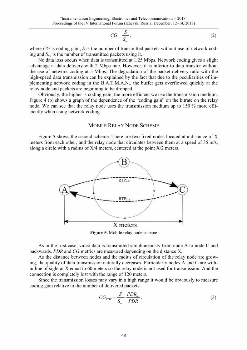
“Instrumentation Engineering, Electronics and Telecommunications – 2018”
Proceedings of the IV International Forum (Izhevsk, Russia, December, 12–14, 2018)
48
,nc
SCGS
(2)
where CG is coding gain, S is the number of transmitted packets without use of network cod-ing and Snc is the number of transmitted packets using it.
No data loss occurs when data is transmitted at 1.25 Mbps. Network coding gives a slight advantage at data delivery with 2 Mbps rate. However, it is inferior to data transfer without the use of network coding at 5 Mbps. The degradation of the packet delivery ratio with the high-speed data transmission can be explained by the fact that due to the peculiarities of im-plementing network coding in the B.A.T.M.A.N., the buffer gets overflowed quickly at the relay node and packets are beginning to be dropped.
Obviously, the higher is coding gain, the more efficient we use the transmission medium. Figure 4 (b) shows a graph of the dependence of the “coding gain” on the bitrate on the relay node. We can see that the relay node uses the transmission medium up to 150 % more effi-ciently when using network coding.
MOBILE RELAY NODE SCHEME
Figure 5 shows the second scheme. There are two fixed nodes located at a distance of X meters from each other, and the relay node that circulates between them at a speed of 35 m/s, along a circle with a radius of X/4 meters, centered at the point X/2 meters.
Figure 5. Mobile relay node scheme
As in the first case, video data is transmitted simultaneously from node A to node C and backwards. PDR and CG metrics are measured depending on the distance X.
As the distance between nodes and the radius of circulation of the relay node are grow-ing, the quality of data transmission naturally decreases. Particularly nodes A and C are with-in line of sight at X equal to 60 meters so the relay node is not used for transmission. And the connection is completely lost with the range of 120 meters.
Since the transmission losses may vary in a high range it would be obviously to measure coding gain relative to the number of delivered packets:
,ncPDR
nc
PDRSCGS PDR
(3)

Meitis D. S., Vasiliev D. S., Kaysina I., Abilov A., Khvorenkov V.
“Real time emulation of COPE-like network coding in FANET using ns-3”
49
where CGPDR – is the coding gain relative to the number of delivered packets, PDR is the packet delivery ratio without using coding gain and PDRnc is the packet delivery ratio using coding gain. Figure 6 depicts the dependencies of the PDR and the coding gain relative to PDR from the distance X between nodes A and C using network coding and without it.
a b
Figure 6. Results for mobile relay node scheme: PDR – distance dependence (a); CGPDR – distance dependence (b)
PDR is reduced by an average of 9.5 % with the use of network coding. This can be at-tributed to the fact that B.A.T.M.A.N. uses long message storage buffers for network coding and the search takes relatively long time therefore the quality of the transmission becomes worse in mobility conditions. Meanwhile Figure 6 (b) shows that the coding gain is also re-tained for the mobile scheme. The wireless medium is used at 5–70 % more efficiently de-pending on the distance using network coding. Degrading of the coding gain with the high range between the nodes as well as PDR is associated with increased delays.
CONCLUSION
According to the results of real-time emulation, we can say that network coding is a pow-erful tool that allows using the transmission medium resources more efficient. It is especially important in wireless networks. Real-time network emulation with the mobile relay node shows that network coding has the potential for both static topologies and mobile ones. Net-work coding reduces amount of the transmitted packets in network for 5–70 % depending on transmission reliability. However, we should take into account that the larger message buffers for decoding, the longer delays searching for the desired message. In the future work it is nec-essary to find a balance between the permissible delays and the efficiency of data compression.
The reported study was funded by RFBR according to the research project № 18-37-00218 mol_a.
REFERENCES
1. Ahlswede, R., Li, S.-Y., & Yeung, R. (2000). Network information flow. IEEE Transactions on Information Theory, 46(4), 1204–1216. doi: 10.1109/18.850663.
2. Yeung, R. W. (2010). Network coding theory: An introduction. Frontiers of Electrical and Electronic Engi-neering in China, 5(3), 363–390. doi: 10.1007/s11460-010-0103-1.
3. Pahlevani, P., Hundeboll, M., Pedersen, M., Lucani, D., Charaf, H., Fitzek, F., Bagheri, H., & Katz, M. (2014). Novel concepts for device-to-device communication using network coding. IEEE Communications Magazine, 52(4), 32–39. doi: 10.1109/MCOM.2014.6807944.

“Instrumentation Engineering, Electronics and Telecommunications – 2018”
Proceedings of the IV International Forum (Izhevsk, Russia, December, 12–14, 2018)
50
4. Vieira, L. F. M., Gerla, M., & Misra, A. (2013). Fundamental limits on end-to-end throughput of network coding in multi-rate and multicast wireless networks. Computer Networks, 57(17), 3267–3275. doi: 10.1016/j.comnet.2013.07.015.
5. Goseling, J., Gastpar, M., & Weber, J. H. (2015). Random access with physical layer network coding. IEEE Transactions on Information Theory, 61(7), 3670–3681. doi: 10.1109/TIT.2015.2425879.
6. Chou, P. A., & Wu, Y. (2007). Network coding for the internet and wireless networks. IEEE Signal Pro-cessing Magazine, 24(5), 77–85. doi: 10.1109/MSP.2007.904818.
7. Pyattaev, A., Galinina, O., Andreev, S., Katz, M., & Koucheryavy, Y. (2015). Understanding practical limita-tions of network coding for assisted proximate communication. IEEE Journal on Selected Areas in Commu-nications, 33(2), 156–170. doi: 10.1109/JSAC.2014.2384232.
8. Katti, S., Rahul, H., Hu, W., Katabi, D., M´edard, M., & Crowcroft, J. (2006). XORs in the air: practical wireless network coding. IEEE/ACM Transactions on Networking, 16(3), 497–510. doi: 10.1109/TNET. 2008.923722.
9. Kaysina, I. A., Vasiliev, D. S., & Abilov, A. V. (2018). Setevoe kodirovanie v setyah FANET [Network coding in FANET]. Electrosvyaz, 2018(1), 64–68 (in Russian).
10. Kaysina, I. A., Vasiliev, D. S., Abilov, A., Meitis, D. S., & Kaysin, A. E. (2018). Performance evaluation testbed for emerging relaying and coding algorithms in Flying Ad Hoc Networks. In: 2018 Moscow Work-shop on Electronic and Networking Technologies (MWENT) (pp. 1–5). Moscow, Russia : IEEE. doi: 10.1109/MWENT.2018.8337169.
11. Vasiliev, D. S., Kaysina, I. A., & Abilov, A. (2017). Performance evaluation of COPE-like network coding in Flying Ad Hoc Networks: Simulation-based study. In: O. Galinina, S. Andreev, S. Balandin, Y. Koucheryavy (Eds.), Internet of Things, Smart Spaces, and Next Generation Networks and Systems. ruSMART 2017, NsCC 2017, NEW2AN 2017. Lecture Notes in Computer Science, 10531 (pp. 577–586). Cham, Switzerland : Springer. doi: 10.1007/978-3-319-67380-6_54.
12. Vasiliev, D. S., Meitis, D. S., & Abilov, A. (2014). Simulation-based comparison of AODV, OLSR and HWMP protocols for Flying Ad Hoc Networks. In: S. Balandin, S. Andreev, Y. Koucheryavy (Eds.), Internet of Things, Smart Spaces, and Next Generation Networks and Systems. NEW2AN 2014. Lecture Notes in Computer Science, 8638 (pp. 245–252). Cham, Switzerland : Springer. doi: 10.1007/978-3-319-10353-2_21.
13. Jungic, D. A. (2011). Better Approach to Mobile Ad hoc Networking [Slides]. Retrieved from http://www2. ensc.sfu.ca/~ljilja/ENSC427/Spring11/Projects/team9/ENSC427_Group9_batman_pres.pdf.
14. Neumann, A., Aichele, C., Lindner, M., & Wunderlich, S. (2008). Better approach to mobile ad-hoc network-ing (B.A.T.M.A.N.) IETF draft (pp. 1–24). Retrieved from https://www.researchgate.net/publication/ 320172464_Better_approach_to_mobile_ad-hoc_networking_BATMAN.
15. Ngai, C. K., & Yeung, R. W. (2004). Network coding gain of combination networks. In: Information Theory Workshop (pp. 283–287). San Antonio, USA : IEEE. doi: 10.1109/ITW.2004.1405315.

Myshkin Yu. V., Murav’eva O. V., Sannikova Yu. O., Chukhlanceva T. S.
“The propagation of horizontally polarized shear wave in the hollow cylinder”
51
DOI: 10.22213/2658-3658-2018-51-65
The Propagation of Horizontally Polarized Shear Wave in the Hollow Cylinder
Yu. V. Myshkin, O. V. Murav’eva, Yu. O. Sannikova, T. S. Chukhlanceva
Department of Instruments and Techniques for Measurement, Testing, Diagnostics, Kalashnikov Izhevsk State Technical University,
Izhevsk, Russian Federation E-mail: [email protected]
Received: July 06, 2018
The paper presents studies of the velocity of propagation of a horizontally polarized shear wave (SH wave) in an aluminum hollow cylinder. The results of simulation of SH wave propagation using the finite element method are presented. Approbation was carried out on an aluminum cylinder using piezoelectric transducers with a dry point contact at a frequency of 105 kHz. Dependences of the SH wave velocity on the direction of propagation in a hollow cylinder are obtained.
Keywords: SH wave, hollow cylinder, wave velocity, finite element method, dry point contact, guided wave testing.
INTRODUCTION
The modern acoustic guided wave method in nondestructive testing is based on the use of longitudinal, torsional or flexural waves, as well as symmetric and antisymmetric modes of Lamb waves [1–3]. In studying the processes of propagation of these types of waves in plates and hollow cylinders, in most cases it is assumed that the properties of the material in which the wave propagates are isotropic. In the presence of anisotropy, as a rule, the pattern of ve-locity distribution along the directions changes [4–6]. Changes in the velocity of wave propa-gation are also caused by inhomogeneities in the cross section, structural features of the con-trol object, and various types of defects [3, 5–6].When studying the change wave velocity un-der the influence of these factors, it is necessary to take into account the qualitative state of the testing object, the presence in it of stressed-deformed sections, the design features of the transducers used, the parameters of the hardware, the size and position of the defects, and etc. [2, 5–8]
It is known from literature sources [3, 9–17] that when testing pipelines in circumferen-tial and axial directions, SH waves (or tH waves) are used. The advantage of using this type of wave is that the fundamental mode SH0 does not have dispersion, is more sensitive to defects, and has a relatively smaller attenuation [3, 18–23]. To increase the sensitivity of the guided wave method, focusing methods using phased arrays [24–30] are practiced. The most com-mon are the synthetic aperture focusing technique (SAFT) [30–36], the total focusing method
© Myshkin Yu. V., Murav’eva O. V., Sannikova Yu. O., Chukhlanceva T. S., 2018

“Instrumentation Engineering, Electronics and Telecommunications – 2018”
Proceedings of the IV International Forum (Izhevsk, Russia, December, 12–14, 2018)
52
(TFM) [25, 37–39], the common source method (CSM) [32, 40]. When using any of the methods for calculating the coordinates of the focus point, the wave propagation velocity is used, while it is assumed that it does not change depending on the direction. In the presence of anisotropy of the material properties of the pipeline, the velocity change from the direction is taken into account. Nevertheless, even in an isotropic material, in the presence of bends and deformations of the testing object, the wave velocity can have significant distinctions in dif-ferent directions.
This paper presents numerical and experimental studies of the propagation velocity of the SH0 mode of a shear wave in a hollow cylindrical aluminum isotropic testing object with a diameter of 300 mm at a frequency of 105 kHz.
GENERAL THEORY
All types of waves can exist in solids: volumetric (longitudinal and transverse waves), surface and subsurface (Rayleigh and head waves), Lamb waves in layered media, and Pochhammer waves in rods. Longitudinal oscillations are associated with the elasticity of the volume of the medium and can propagate in solid, liquid, and gaseous media. Transverse (shear) vibrations are associated with the elasticity of the shape and can only propagate in a solid medium that is capable of resisting shear deformation. Due to the polarization process, i.e. the relationship of the direction of propagation and the direction of particle oscillation, for example, transverse waves can be horizontally and vertically polarized. A horizontally polar-ized transverse (shear) wave is also called a tH-wave, in which the particles of the medium oscillate perpendicularly to the plane of incidence. Such wave represents a pure shift [28].
Guided waves (Pochhammer waves, guided longitudinal, flexural and torsional waves, Lamb waves) exist in testing objects, which are represented layered media (bars, pipes, tubes, rods, plates, etc.). Guided waves, in turn, are divided into two types: longitudinal (symmet-rical) and flexural (antisymmetric) waves. In longitudinal guided waves, the motion occurs symmetrically with respect to the axial direction of testing object and the axial (longitudinal) displacement component predominates. In flexural guided waves in the axial direction, flex-ure occurs and the transverse component of displacements predominates. In addition to sym-metrical and antisymmetrical waves, a torsional wave can propagate in extended cylindrical objects, in which there is only one azimuth displacement component. The motion of the wave is symmetrical with respect to the axial direction and represents the rotation of the cross sec-tion of the cylindrical object with respect to this axis [28].
Waves propagating along the surface of the material are called Rayleigh or surface waves. These waves have elliptical motion of particles [28].
The types of waves are shown in Table 1. As an example, in Figure 1 shows the disper-sion curves for an aluminum plate with a thickness of 5.675 mm and a hollow cylinder with an outer diameter of 300 mm, which are studied in the work.
In studies of the propagation of a horizontally polarized shear wave, the frequency was 105 kHz. From the above dispersion curves it follows that, at a given frequency, the funda-mental symmetric and antisymmetric modes of the Lamb wave and the horizontally polarized shear wave can exist in the testing object when considering it in the form of a curved plate. When considering the testing object in the form of a hollow cylinder, taking into account the wave propagation along the waveguide (in axial direction of the cylinder), there may exist in it modes of the lowest order of the longitudinal and flexural waves and the fundamental mode of the torsional wave. Since the direction of wave propagation is taken into account in this work, the velocities of the symmetric mode 5329 m/s, the antisymmetric mode 3012 m/s and the horizontally polarized shear wave of 3162 m/s are used as theoretical data (Figure 1a).

Myshkin Yu. V., Murav’eva O. V., Sannikova Yu. O., Chukhlanceva T. S.
“The propagation of horizontally polarized shear wave in the hollow cylinder”
53
Table 1. Wave type designation and description Wave Description
L(0,m) Axisymmetric mode of guided longitudinal wave, m – mode number T(0,m) Axisymmetric mode of guided torsional wave, m – mode number
F(n,m) Non-axisymmetric mode of guided flexural wave, n – circumferential order, m – mode number
Am Antisymmetrical mode of Lamb wave, m – mode order number Sm Symmetrical mode of Lamb wave, m – mode order number
SHm Horizontally polarized shear wave, m – mode order number R Rayleigh (surface) wave
Figure 1. Dispersion curves of group velocities in an aluminum plate (a) and an aluminum hollow cylinder (b): S – symmetrical mode of Lamb wave, A – antisymmetrical mode of Lamb wave, SH – horizontal-ly polarized shear wave, L – longitudinal wave, F – flexural wave, T – torsional wave (designations are present-ed in Table 1)
0
1000
2000
3000
4000
5000
6000
0 20 40 60 80 100 120 140 160 180 200
L(0,1)
L(0,2)
F(1,1)
F(1,2)
F(1,3)
T(0,1)
Group velocity, m/s
Frequency, kHz
T(0,1)
F(1,1)
F(1,2)
F(1,3)
L(0,1)
L(0,2)
Hollow cylinder parameters:External diameter 300 mmWall thickness 5.675 mm Young's modulus 71 MPaShear modulus 27 MPaDensity 2700 kg/m3
0
1000
2000
3000
4000
5000
6000
0 20 40 60 80 100 120 140 160 180 200
S0
A0
SH0 Frequency, kHz
Group velocity, m/sS0
SH0
A0
Plate parameters:Thickness 5.675 mmYoung's modulus 71 MPaShear modulus 27 MPaDensity 2700 kg/m3
a
b

“Instrumentation Engineering, Electronics and Telecommunications – 2018”
Proceedings of the IV International Forum (Izhevsk, Russia, December, 12–14, 2018)
54
FINITE ELEMENT PREDICTION
Numerical calculation was carried out using the finite element method, implemented in COMSOL Multiphysics. The model (Figure 2) included a cylindrical aluminum object with length of 1.2 m, with an internal cavity 288.65 mm in diameter, and a wall thickness of 5.675 mm (Figure 2a). The discretization step for the finite element grid (mesh) was selected based on the condition: at least five finite elements per wavelength. Thus, the grid step was no more than 5.81 mm, and the total number of finite elements is 300963 (Figure 2b).
On the outer cylindrical surface, in the middle of the object, the only (in addition to the default boundary conditions: Linear elastic material, Free, Initial values) boundary condition Point Load was set in the form of a tangential azimuth force action (Figure 2a). The form of the force action is shown in Figure 3, has a fundamental frequency in the pulse spectrum of 105 kHz and is described by the formula:
2
0 cos 2 sin ,tU t U e t t (1)
where U0 is the amplitude, is the attenuation coefficient, t is the time, ω = 2πf is the cyclic (circular) frequency.
Table 2. Material properties Parameter Value Dimension
Young’s modulus, E 71 GPa Shear modulus, G 26.7 GPa Poisson’s ratio, η 0.33 -
Shear wave velocity, С 3145 m/s Density, ρ 2700 kg/m3
Figure 2. 3D model of the pipe (a) and finite element mesh (b): pipe length is 1.2 m, point of application of tangential force is located at a distance of 0.6 m from the pipe end
Internal diameter288.65 mm
Point of applicationof tangential force
External diameter300 mm
Wall thickness5.675 mm
Total elements300963
Maximum size of elements5.81 mm
a b

Myshkin Yu. V., Murav’eva O. V., Sannikova Yu. O., Chukhlanceva T. S.
“The propagation of horizontally polarized shear wave in the hollow cylinder”
55
Table 3. Input parameters Parameter Value Dimension
External diameter of cylinder, Rext 150 mm Internal diameter of cylinder, Rint 144.325 mm Cylinder length, L 1.2 m Frequency, f 105 kHz Period, T 9.524 μs
With such force action, a SH wave directed along the cylinder, a symmetric Lamb wave
mode directed in circumferential direction, and an antisymmetric mode propagating in all di-rections were formed in the hollow cylinder. At the initial moment of time, the shape of the elastic displacements pulse has a similar shape (Figure 3) and at an amplitude of the force ac-tion of 6.6 N has a displacement amplitude of 50 pm.
As an example, in Figure 4 shows the distribution of elastic displacements at time 40 μs and 100 μs. A symmetric S0, an antisymmetric A0 of the modes of the Lamb wave, and a horizontally polarized shear wave SH0 are observed.
Figure 3. Pulse of the tangential force action (calculated by the Formula 1) and the shape of the elastic displacements pulse (calculated in the program): arrows indicate the correspondence of the graphs to the axes
To estimate the propagation velocity of the SH wave, formulas for constructing registra-tion points equidistant from the point of application of the tangential force action at a distance of 300 mm are used which describe the construction of a circle in a cylindrical coordinate sys-tem:
sin sin ,Dx RR
0 cos ,y h R (2)
cos sin ,Dz RR
-4
-2
0
2
4
6
8
0 2 4 6 8 10 12 14 16 18 20
Tangential force, N
Time, μs
Pulse parameters:Amplitude 6.6 NPeriod 9.524 μsFrequency 105 kHz
80
60
40
20
0
-20
-40
Displacement, pm

“Instrumentation Engineering, Electronics and Telecommunications – 2018”
Proceedings of the IV International Forum (Izhevsk, Russia, December, 12–14, 2018)
56
where R is the outer radius of the hollow cylinder, D is the outer diameter of the hollow cylin-der, α is the angle of propagation direction of the wave (varies from -π/2 to 3π/2 in steps of π/180), h0 is the coordinate along the y axis, where applied the tangential force (the height of the cylinder is directed along the y axis).
Figure 4. Distribution of displacements at time t = 40 s (a) and t = 100 s (b): rainbow graduation is used, the dark blue color corresponds to zero displacements, the dark red corresponds to the maximum displacements (approximately 50 pm)
Using these formulas, the amplitude of the displacements at the points on the surface of the hollow cylinder was estimated (Figure 5) and the signals were plotted for the displacement components (Figure 6). As the analyzed one, the azimuth component is chosen whose dis-placement corresponds to the displacements in the SH wave directed along the axis of the hol-low cylinder.
In the presented signals (Figure 6), displacements corresponding to the symmetric S0 and antisymmetric A0 modes of the Lamb wave and the horizontally polarized shear wave SH0 are observed. The symmetrical mode in the frequency range up to 10 to 500 kHz has a high dispersion, its velocity varies from 5200 m/s at a frequency of 10 kHz to 1760 m/s at a frequency of 440 kHz, so on the signal accepted in the axial direction, low-frequency LF and high-frequency HF symmetric mode of the Lamb wave are observed. There is also a symmetric mode of the Lamb wave of the second order S2 at a frequency of 670 kHz, whose velocity is 4730 m/s. In the circumferential direction of the cylinder, the symmetrical mode is registered in the forward direction FD and in the reverse direction RD. The distance traveled by the wave corresponds to 300 mm and 642.5 mm.
Time100 μs
Horizontally polarized shear wave SH0
Symmetrical wave S0
Antisymmetrical wave A0
Time40 μs
Horizontally polarized shear wave SH0
Symmetrical wave S0
Antisymmetrical wave A0
a b

Myshkin Yu. V., Murav’eva O. V., Sannikova Yu. O., Chukhlanceva T. S.
“The propagation of horizontally polarized shear wave in the hollow cylinder”
57
The main disadvantage in the study is the presence of an antisymmetric mode, which propagates at a velocity comparable to the velocity of a horizontally polarized shear wave. The pulse shape of the antisymmetric mode contains a whole spectrum of frequen-cies and represents a pulse with a high-frequency component that smoothly converts to a low-frequency component having a lower velocity. To avoid the influence of the antisymmetric mode on the measurement result, a band-pass filter of high order with cut-off frequencies of 90 and 120 kHz was used to analyze the propagation velocity of a horizontally polarized shear wave.
The investigated horizontally polarized shear wave had the expected maximum am-plitude of displacements in the axial direc-tion, which gradually decreased with the change in the registration coordinates of the signal. The shape of the pulse had a similar form with the shape of the probing pulse (Figure 3).
According to the arrival time of the force pulse, the propagation velocity of the SH wave was estimated on the formula:
,RP PP
LCt t
(3)
where L is the distance passed by the wave, tRP and tPP are the time recorded in the receiving and probing pulses respectively (as a rule, in the zero crossing).
It was assumed that the distance traveled by the wave was 300 mm.
EXPERIMENTAL SETUP
In experimental studies, an aluminum balloon with an external diameter of 300 mm was used. Two types of measurements were produced on the balloon: wall thickness and wave propagation velocity. Schemes of experimental setups are shown in Figure 7.
The technique for measuring the wall thickness was as follows. The balloon surface was uniformly marked (Figure 8) with step in the axial direction of 50.5 mm and step in the azi-muth direction of 12°15', corresponding to 58.9 mm. Thus, in the axial direction 13 points are marked, in the azimuth – 16, in total – 208 points. At each point, a measurement was made at a frequency of 5 MHz using a high-frequency DIO-1000PA and a contact fluid. On the re-ceived signals (Figure 9a), to increase the accuracy of the measurements, the fourth reflection from the balloon walls was evaluated. The sampling frequency was 205 MHz.
The method for measuring the velocity of wave propagation included the following steps. Marking on the surface of an aluminum cylinder in the form of a circle with a graduated scale every degree. Excitation and reception of SH waves using specialized transducers with dry point contact at a frequency of 105 kHz using a low-frequency DIO-1000LF. Measurement of
Radius300 mm
Axialdirection
Circumferentialdirection
Figure 5. Points on the outer surface of a hollow cylinder (calculated by Formulas 2) in which the amplitude of elastic displacements was registered

“Instrumentation Engineering, Electronics and Telecommunications – 2018”
Proceedings of the IV International Forum (Izhevsk, Russia, December, 12–14, 2018)
58
the propagation time of the wave according to the received signals and the translation of the time value into the velocity according to the formula (3). The distance traveled by the wave was 303 mm. To increase the accuracy of calculating the wave propagation velocity, the sam-pling frequency of the signal increased to 41 MHz, only the received signal of a horizontally polarized shear wave was recorded (Figure 9b).
Figure 6. Signals obtained at various points on the outer surface (where a – in axial direction, b – in circumferential direction (Figure 5)) of a hollow cylinder: LF – low frequency (less than 200 kHz), HF – high frequency (more than 400 kHz), FD – forward direction, RD – reverse (opposite) direction from point of application of tangential force (Figure 2a)
Both in measuring the wall thickness of the balloon and in measuring the wave propaga-tion velocity, the propagation time of the wave was estimated from the transition from the positive to the negative phase of the elastic oscillations.
RESULTS AND DISCUSSION
Figure 10 shows the results of measuring the wall thickness of an aluminum balloon. On the distribution the wall thickness is observed, and on the right side (values in the azimuth component from 150 to 300 degrees) it has higher values compared to the left part (values for the azimuth component from 0 to 120 degrees). There is also a local minimum in the region of
-4
-2
0
2
4
6
8
10
0 10 20 30 40 50 60 70 80 90 100 110 120 130 140 150
Time, ms
Displacement, pm
S2HFS0LF
SH0
A0
Wave propagation inaxial direction
S0HF
-4
-2
0
2
4
0 10 20 30 40 50 60 70 80 90 100 110 120 130 140 150
Time, ms
Displacement, pmS0FD A0
Wave propagation incircumferential direction
S0RD
a
b

Myshkin Yu. V., Murav’eva O. V., Sannikova Yu. O., Chukhlanceva T. S.
“The propagation of horizontally polarized shear wave in the hollow cylinder”
59
20 degrees in the fourth quadrant, corresponding to a wall thickness of 5.39 mm. Thus, in one direction along the azimuth from the origin, the wall thickness increases (1 and 2 quadrants) from 5.47 to 5.75 mm, on the other side (3 and 4 quadrants), first decreases, then increases and lies in the range from 5.42 to 5.63 mm. The average value of the wall thickness from the results of all measurements was 5.61 mm.
This unevenness in the wall thickness can be explained by the technological treatment of the balloon surface during its manufacture. In turn, such processing could lead to inhomoge-neity in the structure of the material.
Figure 7. The experimental setup: for measuring the wall thickness (a);
for measuring the propagation velocity of the horizontally polarized shear wave (b)
DIO1000-LFFrequency 120 kHz
Piezoelectric transducer for excitation
Piezoelectric transducer for receiving
Radius 303 mmShear wave polariza tion
Shear wave polariza tion
Aluminum balloon
Direction of wave propagation
Aluminum balloon
Piezoelectric transducer
DIO1000-PAFrequency 5 MHz
Axial step 50.5 mm
Circumferential step 22,5o (58.9 mm)
Average wall thickness 5.6 mm
a
b

“Instrumentation Engineering, Electronics and Telecommunications – 2018”
Proceedings of the IV International Forum (Izhevsk, Russia, December, 12–14, 2018)
60
Figure 8. The scanning scheme for determining wall thickness and propagation velocity
of the horizontally polarized shear wave
Figure 11 shows the dependence of the propagation velocity of a horizontally polarized shear wave on the wave propagation direction. Simulation showed that in circumferential di-rection of the hollow cylinder wave velocity is higher, which is explained by the smaller dis-tance traveled by the wave. Since the curved surface of the hollow cylinder has an inner and outer diameter, the wave overcomes a relatively smaller distance along the inner surface, which is expressed in an increase in the propagation velocity (which, as such, does not occur). In this case, the shape of the pulse is distorted and the further the wave propagates, the strong-er this distortion (for example, the longitudinal wave pulse in Figure 6b in the opposite direc-tion does not have the same form as in the forward direction). The velocity of the horizontally polarized shear wave in the axial direction was 3133 m/s, which can be assumed not to be dis-torted by the curvature of the surface of the hollow cylinder. The velocity in the circumferen-tial direction was 3220 m/s, the minimum value of 3115 m/s is observed at angles of 10-15 degrees in each quadrant. The average velocity value from the results of all measurements
22,5°
45°
67,5°
337,5°
315,0°
292,5°
0 mm 50.5 101.0 151.5 202.0 252.5 303.0- 50.5- 101.0- 151.5- 202.0- 252.5- 303.00° (360°)
Marked places where transducer was installed to measure the wall thickness
Axia l direction
Circumferentialdirection
Transducer position and scanning directionto measure the wall thickness
270,0°
247,5°
90,0°
112,5°
I quadrant
III quadrant
II quadrant
IV quadrant
270°
0°
90°
180°
Transducer position (receiving) and shear horizontal wave polarizationto measure the wave velocity
Transducer position (excitation) and shear horizontal wave polarizationto measure the wave velocity
58.9 mm
50.5 mm

Myshkin Yu. V., Murav’eva O. V., Sannikova Yu. O., Chukhlanceva T. S.
“The propagation of horizontally polarized shear wave in the hollow cylinder”
61
was 3181 m/s. Thus, the range of velocity variation based on simulation results was 95 m/s (from 3115 m/s to 3220 m/s).
Figure 9. Signals obtained at one of the points on the outer surface of a hollow cylinder when measur-ing its wall thickness (a) and when measuring the propagation velocity of the horizontally polarized shear wave (b)
When evaluating the experimental results, a similar dependence is observed with the sim-ulation results in terms of increasing the propagation velocity in circumferential direction of the hollow cylinder. Thus, the maximum velocity is observed in the circumferential direction and is 3306 m/s. A minimum velocity of 3109 m/s is observed in the direction of the mini-mum wall thickness of the aluminum balloon, with the minimum velocity range lying in the range of 325 to 350 degrees in the fourth quadrant. The decrease in the velocity of wave prop-agation is partly explained by the same principle as the change in velocity in the circumferen-tial direction: the wave travels a greater distance, since the radius of curvature of the inner
-2000
-1500
-1000
-500
0
500
1000
1500
2000
0 1 2 3 4 5 6 7 8 9 10
Time, μs
Relative amplitude
First reflection
Secondreflection
Thirdreflection
Fourthreflection
Fifthreflection
Sixthreflection
Probe pulse
-600
-400
-200
0
200
400
600
100 105 110 115 120 125 130 135 140 145 150
Time, μs
Relative amplitude
Period 9.5 μsFrequency 105 kHz
a
b

“Instrumentation Engineering, Electronics and Telecommunications – 2018”
Proceedings of the IV International Forum (Izhevsk, Russia, December, 12–14, 2018)
62
surface of the hollow cylinder increases. However, it must be taken into account that when manufacturing a cylinder as a result of technological operations, changes in the structure of the material may have occurred, which affected the elastic properties. The average velocity for all calculations was 3191 m/s. In this case, the range of variation based on the results of experimental measurements was 197 m/s (from 3109 m/s to 3306 m/s).
Figure 10. Results of thickness measurement: the markup corresponds to the Figure 8, solid lines indicate the lines of the contour with the same value of the wall thickness
CONCLUSIONS
According to the results of studies of the propagation of a horizontally polarized shear wave in a hollow aluminum cylinder, the following conclusions can be drawn.
The propagation velocity of the SH wave depends on the direction: in the axial direction, the velocity is less than in the circumferential direction of the hollow cylinder. In the investi-gated aluminum cylindrical object with an external diameter of 300 mm and a wall thickness of 5.675 mm, the difference of velocity was 95 m/s.
Experimental studies also showed an increase in the SH wave velocity in the circumfer-ential direction of a hollow cylinder, regardless of the wall thickness. As the wall thickness increases, the velocity increases: the wave travels a smaller distance along the inner surface of the hollow cylinder.
The results of the research can be used to develop methods for guided wave testing of large-sized cylindrical objects or large-diameter pipelines, when calculating the focusing laws at an angle to the axial direction of the hollow cylinder.
303.0
252.5
202.0
151.5
101.0
50.5
0
-50.5
-101.1
-151.5
-202.0
-252.5
-303.0 0° 45° 90° 135° 180° 225° 270° 315° 360°
5.7
5.7
5.7
5.7
5.65.5
5.4
5.5
5.6
5.5
Iquadrant
IIquadrant
IIIquadrant
IVquadrant
Axialdirection
Circumferentialdirection
mm

Myshkin Yu. V., Murav’eva O. V., Sannikova Yu. O., Chukhlanceva T. S.
“The propagation of horizontally polarized shear wave in the hollow cylinder”
63
Figure 11. Dependence of horizontally polarized shear wave on direction of the propagation in the hollow aluminum cylinder: upper scale (wave velocity) refers to experimental result, finite element prediction and theoretical value; lower scale (propagation distance) refers to wall thickness
This work was supported by the Russian Science Foundation (Project No. 18-79-10122).
REFERENCES
1. Zlobin, D. V., & Muravieva, O. V. (2012). Development features of electromagnetic acoustic defectoscopy equipment for bar iron using rod waves. Bulletin of Kalashnikov ISTU, (4), 99–104. Retrieved from http://izdat.istu.ru/index.php/vestnik/article/download/2682/1450 (in Russian).
2. Strizhak, V. A., Hasanov, R. R., & Pryakhin, A. V. (2018). Features of excitation of an electromagnetic acoustic transducer under a waveguide method of testing. Bulletin of Kalashnikov ISTU, 21(2), 159–166. doi: 10.22213/2413-1172-2018-2-159-166 (in Russian).
3. Muravyova, O. V., & Murashov, S. A. (2011). Use of torsional waves for detection of operational defects in pump rods and tubing. Bulletin of Kalashnikov ISTU, (2), 149–154. Retrieved from http://izdat.istu.ru/ index.php/vestnik/article/download/2279/1047 (in Russian).
3000
3050
3100
3150
3200
3250
3300
3350
Experimental result
Finite element prediction
Theoretical value
Wall thickness
5.7
5.65.5
5.5
5.6
5.4
90o
180o
270o
0oWave velocity, m/s
Propagation distance, mm
0
43
86
129
172
215
258
301
Axial direction
Circumferential direction
Iquadrant
IIquadrant
IIIquadrant
IVquadrant

“Instrumentation Engineering, Electronics and Telecommunications – 2018”
Proceedings of the IV International Forum (Izhevsk, Russia, December, 12–14, 2018)
64
4. Muravyov, V. V., Baiteriakov, A. V., & Kotolomov, A. Y. (2014). Influence of structural state of metal of gas pipelines on parameters of ultrasonic waves. Bulletin of Kalashnikov ISTU, (3), 125–128. Retrieved from http://izdat.istu.ru/index.php/vestnik/article/download/2985/1753 (in Russian).
5. Muravyov, V. V., Balobanov, E. N., & Pechina, E. A. (2013). Determination of elastic acoustic coupling coefficients of ferromagnetic metals. Bulletin of Kalashnikov ISTU, (2), 108–112. Retrieved from http://izdat.istu.ru/index.php/vestnik/article/download/2215/983 (in Russian).
6. Murav’ev, V. V., Volkova, L. V., Platunov, A. V., Buldakova, I. V., & Gushchina, L. V. (2018). Investiga-tions of the structural and strain-stress state of the rails of current production by the acoustic elasticity meth-od. Bulletin of Kalashnikov ISTU, 21(2), 13–23. doi: 10.22213/2413-1172-2018-2-13-23 (in Russian).
7. Murav’eva, O. V., & Sokov, M. Y. (2016). Influence of the defect depth on the parameters of electromagnet-ic-acoustic multiple-shadow method of the rod testing. Bulletin of Kalashnikov ISTU, 19(3), 46–50. doi: 10.22213/2413-1172-2016-3-46-50 (in Russian).
8. Petrov, K. V., Sokov, M. Y., & Muraveva, O. V. (2018). The effect of electromagnetic acoustic transducer design features on results of cylinder object testing. Bulletin of Kalashnikov ISTU, 21(2), 135–146. doi: 10.22213/2413-1172-2018-2-135-146 (in Russian).
9. Clough, M., Fleming, M., & Dixon, S. (2017). Circumferential guided wave EMAT system for pipeline screening using shear horizontal ultrasound. NDT & E International, 86, 20–27. doi: 10.1016/j.ndteint. 2016.11.010.
10. Deng, M., Gao, G., Xiang, Y., & Li, M. (2017). Assessment of accumulated damage in circular tubes using nonlinear circumferential guided wave approach: A feasibility study. Ultrasonics, 75, 209–215. doi: 10.1016/j.ultras.2016.12.001.
11. Li, M., Deng, M., Gao, G., & Xiang, Y. (2018). Modeling of second-harmonic generation of circumferential guided wave propagation in a composite circular tube. Journal of Sound and Vibration, 421, 234–245. doi: 10.1016/j.jsv.2018.01.060.
12. Howard, R., & Cegla, F. (2017). On the probability of detecting wall thinning defects with dispersive circum-ferential guided waves. NDT & E International, 86, 73–82. doi: 10.1016/j.ndteint.2016.11.011.
13. Heinlein, S., Cawley, P., & Vogt, T. K. (2018). Reflection of torsional T(0,1) guided waves from defects in pipe bends. NDT & E International, 93, 57–63. doi: 10.1016/j.ndteint.2017.09.007.
14. Khalili, P., & Cawley, P. (2018). Relative ability of wedge-coupled piezoelectric and meander coil EMAT probes to generate single-mode Lamb waves. IEEE transactions on ultrasonics, ferroelectrics, and frequency control, 65(4), 648–656. doi: 10.1109/TUFFC.2018.2800296.
15. Dobson, J., & Cawley, P. (2017). The scattering of torsional guided waves from Gaussian rough surfaces in pipework. The Journal of the Acoustical Society of America, 141(3), 1852–1861. doi: 10.1121/1.4978244.
16. Alleyne, D., Jones, R., & Vogt, T. (2017). An introduction to long-range screening using guided waves. Ma-terials Evaluation, 75(10), 1206–1213.
17. Khalili, P., & Cawley, P. (2018). The choice of ultrasonic inspection method for the detection of corrosion at inaccessible locations. NDT & E International, 99, 80–92. doi: 10.1016/j.ndteint.2018.06.003.
18. Myshkin, Y. V., & Muravieva, O. V. (2017). The features of the guided wave excitation and propagation at testing of pipes. Journal of Physics: Conference Series, 881(1), 012019. doi: 10.1088/1742-6596/881/1/012019.
19. Muravev, V. V., Muraveva, O. V., Strizhak, V. A., & Myshkin, Y. V. (2017). Acoustic guided wave testing of pipes of small diameters. IOP Conference Series: Materials Science and Engineering, 253(1), 012001. doi: 10.1088/1757-899X/253/1/012001.
20. Muravieva, O. V., Strizhak, V. A., Zlobin, D. V., Murashov, S. A., Pryakhin, A. V., & Myshkin, Y. V. (2016). Acoustic guided wave testing of downhole pumping equipment elements. Oil Industry Journal, (09), 110–115. Retrieved from https://www.onepetro.org/journal-paper/OIJ-2016-09-110-115-RU (in Russian).
21. Murav’eva, O. V., Len’kov, S. V., & Murashov, S. A. (2016). Torsional waves excited by electromagnetic–acoustic transducers during guided-wave acoustic inspection of pipelines. Acoustical Physics, 62(1), 117–124. doi: 10.1134/S1063771015060093.
22. Budenkov, G. A., Nedzvetskaya, O. V., Zlobin, D. V., & Lebedeva, T. N. (2004). The application efficiency of rod and torsional waves for checking rod-shaped roll stock. Russian Journal of Nondestructive Testing, 40(3), 147–151. doi: 10.1023/B:RUNT.0000040171.56679.6b.

Myshkin Yu. V., Murav’eva O. V., Sannikova Yu. O., Chukhlanceva T. S.
“The propagation of horizontally polarized shear wave in the hollow cylinder”
65
23. Budenkov, G. A., Nedzvetskaya, O. V., Zlobin, D. V., & Murashov, S. A. (2006). Interaction of torsion waves with longitudinal cracks in tubes. Russian Journal of Nondestructive Testing, 42(6), 392–397. doi: 10.1134/S1061830906060064.
24. Kudela, P., Radzienski, M., Ostachowicz, W., & Yang, Z. (2018). Structural health monitoring system based on a concept of Lamb wave focusing by the piezoelectric array. Mechanical Systems and Signal Processing, 108, 21–32. doi: 10.1016/j.ymssp.2018.02.008.
25. Muller, A., Robertson-Welsh, B., Gaydecki, P., Gresil, M., & Soutis, C. (2017). Structural health monitoring using Lamb wave reflections and total focusing method for image reconstruction. Applied Composite Materi-als, 24(2), 553–573. doi: 10.1007/s10443-016-9549-5.
26. Brath, A. J., Simonetti, F., Nagy, P. B., & Instanes, G. (2017). Guided wave tomography of pipe bends. IEEE transactions on ultrasonics, ferroelectrics, and frequency control, 64(5), 847–858. doi: 10.1109/TUFFC. 2017.2683259.
27. Taheri, H., Du, J., & Delfanian, F. (2017). Experimental observation of phased array guided wave application in composite materials. Materials Evaluation, 75(10), 1308–1316.
28. Rose, J. L. (2014). Ultrasonic guided waves in solid media. Cambridge, USA : Cambridge University Press. doi: 10.1017/CBO9781107273610.
29. Yu, L., & Tian, Z. (2016). Guided wave phased array beamforming and imaging in composite plates. Ultra-sonics, 68, 43–53. doi: 10.1016/j.ultras.2016.02.001.
30. Wang, W., Zhang, H., Lynch, J. P., Cesnik, C. E., & Li, H. (2018). Experimental and numerical validation of guided wave phased arrays integrated within standard data acquisition systems for structural health monitor-ing. Structural Control and Health Monitoring, 25(6), e2171. doi: 10.1002/stc.2171.
31. Vinogradov, S., Cobb, A., Bartlett, J., & Udagawa, Y. (2018). Development of a novel omnidirectional magnetostrictive transducer for plate applications. AIP Conference Proceedings, 1949(1), 090002. doi: 10.1063/1.5031565.
32. Sun, Z., Sun, A., & Ju, B. F. (2018). Guided wave imaging of oblique reflecting interfaces in pipes using common-source synthetic focusing. Journal of Sound and Vibration, 420, 1–20. doi: 10.1016/j.jsv.2018. 01.012.
33. Gaul, T., Schubert, L., Weihnacht, B., & Frankenstein, B. (2014, July). Localization of defects in pipes using guided waves and synthetic aperture focussing technique (SAFT). In: V. Le Cam, L. Mevel, F. Schoefs (Eds.), EWSHM – 7th European Workshop on Structural Health Monitoring (pp. 520–527). Nantes, France : IFFSTTAR, Inria, Université de Nantes. Retrieved from https://hal.inria.fr/hal-01020390.
34. Davies, J., & Cawley, P. (2009). The application of synthetic focusing for imaging crack-like defects in pipe-lines using guided waves. IEEE Transactions on Ultrasonics, Ferroelectrics, and Frequency Control, 56(4). 759–771. doi: 10.1109/TUFFC.2009.1098.
35. Davies, J., Simonetti, F., Lowe, M., & Cawley, P. (2006). Review of synthetically focused guided wave im-aging techniques with application to defect sizing. AIP Conference Proceedings, 820(1), 142–149. doi: 10.1063/1.2184522.
36. Davies, J., & Cawley, P. (2007). The application of synthetically focused imaging techniques for high resolu-tion guided wave pipe inspection. AIP Conference Proceedings, 894(1), 681–688. doi: 10.1063/1.2718036.
37. Liu, Z., Sun, K., Song, G., He, C., & Wu, B. (2016). Damage localization in aluminum plate with compact rectangular phased piezoelectric transducer array. Mechanical Systems and Signal Processing, 70–71, 625–636. doi: 10.1016/j.ymssp.2015.09.022.
38. Zhang, J., Drinkwater, B. W., & Wilcox, P. D. (2012). Effect of roughness on imaging and sizing rough crack-like defects using ultrasonic arrays. IEEE Transactions on Ultrasonics, Ferroelectrics, and Frequency Control, 59(5), 939–948. doi: 10.1109/TUFFC.2012.2278.
39. Petcher, P. A., & Dixon, S. (2015). Weld defect detection using PPM EMAT generated shear horizontal ul-trasound. NDT & E International, 74, 58–65. doi: 10.1016/j.ndteint.2015.05.005.
40. Fletcher, S., Lowe, M. J., Ratassepp, M., & Brett, C. (2012). Detection of axial cracks in pipes using focused guided waves. Journal of Nondestructive Evaluation, 31(1), 56–64. doi: 10.1007/s10921-011-0120-x.

“Instrumentation Engineering, Electronics and Telecommunications – 2018”
Proceedings of the IV International Forum (Izhevsk, Russia, December, 12–14, 2018)
66
DOI: 10.22213/2658-3658-2018-66-71
Diagnosis of Mobile Robots Drives
Yu. Nikitin, A. Abramov, I. Abramov, A. Romanov, S. Trefilov, Yu. Turygin
Department of Mechatronic Systems, Kalashnikov Izhevsk State Technical University,
Izhevsk, Russian Federation E-mail: [email protected]
Received: June 12, 2018
The imitation model of the mobile robot drive for diagnostics is considered. The drive is based on brushless direct current (BLDC) motor. The model was developed using the SimInTech software. Classification of signals of the mobile robot drive is performed: control signals, diagnostic signals and mixed signals. Mechanical and electrical defects in the drive are analyzed. The diagnostic parameters of the mobile robot drive are chosen: electric current, temperature and vibration. The reasons causing these defects of mobile robot drive are considered. A logical-linguistic diagnostic model of drive has been developed on basis of fuzzy logic. The calculated rules determine dependence of technical condi-tion on diagnostic parameters, their trends and utilized lifetime of mobile robot drive. Experimental results of mobile robot drive diagnostics are discussed. It is shown that in the process of degradation, the change in the state of the drive affects the diagnostic parameters.
Keywords: diagnostics, mobile robot, drive, brushless DC motor, model, fuzzy logic.
INTRODUCTION
Mobile robots work in extreme conditions. To increase the robustness of mobile robots, their diagnosis is required. Most often, the drives fail. Therefore, the paper is devoted to the diagnosis of drives of mobile robots. In modern drives of mobile robots, brushless direct cur-rent (BLDC) motors are used as electric motors.
BLDC motors are a type of electric motors that rapidly gains popularity due to its good performance and the development of microprocessor controls. In [1–2] the diagnosis of elec-tric motors using the signals of electric current and resistance is considered. New PWM switching strategy to minimize the torque ripples in BLDC motor which is based on sensored rotor position control is discussed in the paper [3]. Tuning methodology for the parameters of adaptive current and speed controllers in a permanent-magnet BLDC motor drive system is presented in paper [4]. Two Fault Detection and Diagnosis strategies for detecting BLDC mo-tor faults were considered involving wavelets and state estimation [5]. Bearing faults and sta-tor winding faults, which are responsible for the majority of motor failures, are considered [5]. A novel method using windowed Fourier ridges is proposed in paper [6] for the detection of rotor faults in BLDC motors operating under continuous non-stationarity. The use of quadrat-
© Nikitin Yu., Abramov A., Abramov I., Romanov A., Trefilov S., Turygin Yu., 2018

Nikitin Yu., Abramov A., Abramov I., Romanov A., Trefilov S., Turygin Yu.
“Diagnosis of mobile robots drives”
67
ic TFRs is presented as a solution for the diagnostics of rotor faults in BLDC motors operat-ing under constantly changing load and speed conditions [7]. Four time-frequency representa-tions are considered short-time Fourier transform (STFT), Wigner-Ville distribution (WVD), Choi-Williams distribution (CWD), and the Zhao-Atlas marks distribution (ZAM) [7]. Three new algorithms for the detection BLDC motors faults are proposed that can track and detect rotor faults in non-stationary or transient current signals [8]. Park’s vector method was used to extract the features and to isolate the BLDC motors faults from the current measured by sen-sors [9]. Proposed a model of a fault diagnosis expert system with high reliability to compare identical well-functioning BLDC motors [10]. The application of artificial intelligence for the control and diagnostics of electric motors was considered in [11–14]. In [11–13] fuzzy fault detection and diagnosis of electric motors with is considered. During the past several dec-ades, the design of model-based process monitoring systems has been a remarkable research topic. In contrast, the data-driven process monitoring techniques serve as an efficient alterna-tive way, which have gained lots of attention from both the academic and the industrial field. A straightforward way is to utilize the process history data for model identification and based on it, the well-established model-based techniques can be used to design efficient fault diag-nosis system. For this purpose, Subspace Identification Method that directly identifies the complete state-space matrices has gained more attention in the last two decades and has been successfully implemented in many industrial applications [14]. To improve the reliability of detection of mobile robot drive defects, it is suggested to use the electric current, vibration and temperature signals and the fuzzy logic.
INTEGRATION OF THE MOBILE ROBOT DRIVE CONTROL AND DIAGNOSTIC SYSTEMS
The authors propose to integrate the mobile robot drive control and diagnostic systems. The economic efficiency of diagnostic systems is due to increase in reliability and quality, accident risk and reject rate reduction, decrease of expensive equipment downtime, reduction of maintenance and repair costs and increase of service life.
Classification of signals of the mobile robot drive is performed: control signals, diagnos-tic signals and mixed signals. Control signals include: signals from sensors that determine the speed of rotation, the angle of rotation of the shaft. Diagnostic signals include vibration, tem-perature signals. Mixed signals include those signals that are used for both control and diag-nosis - electrical current. For correct diagnosis, it is also necessary to take into account the parameters that determine the mode of operation: the weight of the load, the angle of inclina-tion of the surface along which the robot moves, and the quality of the surface.
To investigate BLDC control, a simulation model of BLDC motor in natural (phase) co-ordinates has been created using SimInTech software (Fig. 1).
Simulation model of BLDC control allows to determine the relationships for phase cur-rents and back electromotive force of perfect BLDC which can be used as diagnostic parame-ters. To improve diagnostics accuracy, the analysis of faults and other BLDC diagnostic pa-rameters is required.
For the purpose of BLDC diagnostics the BLDC faults have been grouped into two clas-ses – of electrical and mechanical faults. BLDC motor faults are shown in Table 1.
Selected diagnostic parameters (electric current, vibration and temperature) are shown in Table 2.
Processing of diagnostic parameter measurements is required to make decision regarding the mobile robot drive technical condition. Fuzzy logic is the most suitable mathematical tool for diagnostic model construction.

“Instrumentation Engineering, Electronics and Telecommunications – 2018”
Proceedings of the IV International Forum (Izhevsk, Russia, December, 12–14, 2018)
68
Figure 1. Simulation model of BLDC motor
Table 1. Drive faults Electrical faults Mechanical faults
conductor break in the winding; short circuit between the winding turns; unacceptable reduction of the insulation resistance
due to insulation ageing or excessive moisture; poor contacts and connections
degradation processes in the bearings – destruction of bearing cage, balls and rollers;
poor heat transfer due to foul or dusty coils; rotor shaft deformation
Table 2. Drive diagnostic parameters
Diagnostic parameter Cause of diagnostic parameter change Electric current overload; winding break or short circuit; mains voltage change Temperature overload; winding short circuit; ambient temperature change Vibration shaft misalignment; bearing faults
LOGICAL-LINGUISTIC DIAGNOSTIC MODEL OF DRIVE
Logical-linguistic drive diagnostic model based on fuzzy logic may be represented by the following system of equations:
1 2 3, , ,
, ,
, , ,
x t F x t x t x t
D t G x t t
Z t H x t D t t
(1)
where 1 2 3, ,x t F x t x t x t – equation of diagnostic parameters; x t – vector of di-agnostic parameters; 1 2 3, ,x t x t x t – a set of diagnostic parameter measurements;
,D t G x t t – equation to calculate the trend vector of diagnostic parameters; t – uti-lized lifetime; , ,Z t H x t D t t – equation to evaluate the technical condition.

Nikitin Yu., Abramov A., Abramov I., Romanov A., Trefilov S., Turygin Yu.
“Diagnosis of mobile robots drives”
69
The model of diagnostic system (Fig. 2) is based on the mathematical apparatus of fuzzy logic. The model allows to determine the mobile robot drive condition from diagnostic pa-rameters (electric current, vibration and temperature). The simulation model of mobile robot drive diagnostics system has been designed in SimInTech software.
Fig. 2 shows the simulation model of the diagnostic system used for assessment of mo-bile robot drive condition.
Figure 2. Simulation model of mobile robot drive of the diagnostic system
Fig. 3 shows simulation results of the temporal changes (in relative units) of input signals (electric current (1), vibration (2) and temperature (3)) caused by mobile robot drive fault. Behavior of the output variable, characterizing the degree of drive defect growth, is shown in Fig. 4.
Figure 3. Simulation results of the temporal changes of input signals (electric current,
vibration and temperature) caused by drive fault (in relative units)
DISCUSSION
The resulting curve implies that on the interval 0…20 s drive is in operational condition. Development of drive degradation processes occurs on the interval 30…80 s. On the interval 90…100 s drive is in alarm condition. Dynamics of degradation processes can be judged by

“Instrumentation Engineering, Electronics and Telecommunications – 2018”
Proceedings of the IV International Forum (Izhevsk, Russia, December, 12–14, 2018)
70
the nature of the curve: change of the drive condition from operational to alarm does not hap-pen immediately; it takes place with the increase of diagnostic parameters.
In this way, by analyzing drive diagnostic parameters, trend and operating time we can foresee the emergency situation, minimize accident risk and timely schedule the drive mainte-nance and repair works. Experiments were carried out with diagnostic parameters being with-in and beyond the tolerable limits. The both experiments were performed at the same supply voltage and load torque. The simulation model of drive control and diagnostic system may be used to study the influence of diagnostic parameters on drive performance.
Figure 4. Condition of drive in the course of degradation depending on diagnostic parameters
CONCLUSIONS
It follows from the paper that a simulation model of diagnostic system built using MiTD software can be efficiently used for drive diagnostics. The model is based on mathematical apparatus of fuzzy logic. It allows to determine the drive condition from diagnostic parame-ters (electric current, vibration and temperature).
Trend of the integral parameter allows to calculate the expected time point when the limit technical condition will be reached and to minimize the risk of premature failure through ac-cident-preventive measures like scheduling of routine maintenance and repair. In case of de-velopment of drive degradation processes during the operation one can change the control ac-tion on the drive by reduction in electric current and so switch over to derated operation mode.
The simulation experiments confirmed the efficiency of the proposed diagnostic model and the prospects of its application to diagnostics of mobile robot drive. Application of to-gether electric current, vibration and temperature signals allows to detect defects of mobile robot drive. It is expected that using the fuzzy logic method will further increase the reliability of detecting defects in the mobile robot drive.
ACKNOWLEDGMENT
The reported study was funded by RFBR according to the research project No. 18-08-00772 A.
REFERENCES
1. Seera, M., Lim, C. P., Ishak, D., & Singh, H. (2012). Fault detection and diagnosis of induction motors using motor current signature analysis and a hybrid FMM-CART model. IEEE Transactions on Neural Networks and Learning Systems, 23(1), 97–108. doi: 10.1109/TNNLS.2011.2178443.

Nikitin Yu., Abramov A., Abramov I., Romanov A., Trefilov S., Turygin Yu.
“Diagnosis of mobile robots drives”
71
2. Cheng, S., Zhang, P., & Habetler, T. G. (2011). An impedance identification approach to sensitive detection and location of stator turn-to-turn faults in a closed-loop multiple-motor drive. IEEE Transactions on Indus-trial Electronics, 58(5), 1545–1554. doi: 10.1109/TIE.2010.2064276.
3. Wael, A. S., Dahaman, I., & Khaleel, J. H. (2011). PWM switching strategy for torque ripple minimization in BLDC motor. Journal of Electrical Engineering, 62(3), 141–146. doi: 10.2478/v10187-011-0023-1.
4. Mohamed, A. A., Ehab, H. E. B., & Hisham, M. S. (2009). Adaptive deadbeat controllers for brushless DC drives using PSO and ANFIS techniques. Journal of Electrical Engineering, 60(1), 3–11.
5. Zhang, W. (2013). A fault detection and diagnosis strategy for permanent magnet brushless DC motor (Mas-ters thesis, McMaster University, Hamilton, Ontario, Canada). Retrieved from https://macsphere.mcmaster. ca/bitstream/11375/12737/1/fulltext.pdf.
6. Rajagopalan, S., Habetler, T. G., Harley, R. G., Aller, J. M., & Restrepo, J. A. (2005). Diagnosis of rotor faults in brushless DC (BLDC) motors operating under non-stationary conditions using windowed Fourier ridges. In: Fourtieth IAS Annual Meeting. Conference Record of the 2005 Industry Applications Conference, 1 (pp. 26–33). Kowloon, Hong Kong, China : IEEE. doi: 10.1109/IAS.2005.1518287.
7. Rajagopalan, S., Restrepo, J. A., Aller, J. M., Habetler, T. G., & Harley, R. G. (2005). Selecting time-frequency representations for detecting rotor faults in BLDC motors operating under rapidly varying operat-ing conditions. In: 31st Annual Conference of IEEE Industrial Electronics Society, 2005. IECON 2005 (pp. 1–6). Raleigh, NC, USA : IEEE. doi: 10.1109/IECON.2005.1569314.
8. Rajagopalan, S. (2006). Detection of rotor and load faults in brushless DC motors operating under station-ary and non-stationary conditions (Doctoral thesis, Georgia Institute of Technology, USA). Retrieved from https://smartech.gatech.edu/handle/1853/11524?show=full.
9. Bae, H., Kim, S., & Vachtsevanos, G. (2009). Fault detection and diagnosis of winding short in BLDC mo-tors based on fuzzy similarity. International Journal of Fuzzy Logic and Intelligent Systems, 9(2), 99–104. doi: 10.5391/IJFIS.2009.9.2.099.
10. Baek, G., Kim, Y., & Kim, S. (2008). Fault diagnosis of identical brushless DC motors under patterns of state change. In: 2008 IEEE International Conference on Fuzzy Systems (IEEE World Congress on Computational Intelligence) (pp. 2083–2088). Hong Kong, China : IEEE. doi: 10.1109/FUZZY.2008.4630657.
11. Abramov, I., Abramov, A., Nikitin, Yu., Sosnovich, E., Božek, P., & Stollmann, V. (2015). Diagnostics of electrical drives. In: 2015 International Conference on Electrical Drives and Power Electronics (EDPE) (pp. 364–367). Tatranska Lomnica, Slovakia : IEEE. doi: 10.1109/EDPE.2015.7325321.
12. Abramov, I., Božek, P., Abramov, A., Sosnovich, E., & Nikitin, Y. (2017). Diagnostics brushless DC motors. In: F. Trebuňa, J. Bocko, P. Frankovský, R. Huňady, J. Kostka, T. Kula (Eds.), 55th International Confer-ence on Experimental Stress Analysis (EAN 2017) (pp. 156–164). Novy Smokovec, Slovakia : Curran Asso-ciates. Retrieved from http://experimentalni-mechanika.cz/konference/2017.html?download=1363: diagnostics-brushless-dc-motors.
13. Costa, B. S. J. (2016) Fuzzy fault detection and diagnosis. In: P. P. Angelov (Ed.), Handbook on computa-tional intelligence: Vol. 1. Fuzzy logic, systems, artifical neural networks, and learning systems (pp. 251–288). Singapore : World Scientific. doi: 10.1142/9789814675017_0007.
14. Luo, H. (2017). Plug-and-play monitoring and performance optimization for industrial automation process-es. Wiesbaden, Germany : Springer Vieweg. doi: 10.1007/978-3-658-15928-3.

“Instrumentation Engineering, Electronics and Telecommunications – 2018”
Proceedings of the IV International Forum (Izhevsk, Russia, December, 12–14, 2018)
72
DOI: 10.22213/2658-3658-2018-72-82
Implementation of Genetic Algorithm for Forming of Individual Educational Trajectories
for Listeners of Online Courses
D. Parfenov 1, V. Zaporozhko 2
1 Department of Applied Mathematics, 2 Department of Informatics, Orenburg State University,
Orenburg, Russian Federation E-mail: [email protected]
The widespread use of massive open online courses (MOOCs) ensures the further globalization of open education and the sustainable development of a single modern digital educational environment. However, it is certain that in the context of the implementation of mass education, the maximum con-sideration of the individual characteristics of each student is an urgent necessity. In this regard, the construction of an individual educational trajectory of the MOOC student becomes particularly im-portant. Achieving this goal is quite feasible when training students on individual learning routes. In the present work, a genetic algorithm is proposed that allows you to form an optimal learning route, designed to meet the personal educational needs and individual capabilities of each MOOC listener. The results of a computational experiment and examples of individual trajectories formed on the basis of the proposed algorithm are presented.
Keywords: massive open online course, online course, individual educational trajectory, individual learning route, genetic algorithm.
INTRODUCTION
The individual educational trajectory in massive open online courses (MOOC) is a reali-zation way of individual educational needs and abilities of students, their right to choose their personal development and self-improvement path [1]. We define an individual educational trajectory as a personal path to realize the personal potential of each MOOC listener [2]. There are several ways to realize an individual educational trajectory. For example, through the use of various educational technologies (tertiary differential education, problem-based learning, game-based learning, portfolio and others) or personalization technologies in MOOC (inquiry-based learning, personal recommender system, and others) [3, 4]. Another way is to form an individual learning route, which is a sequence of elements of the training activity of a particular student at some fixed stage of the study on the online course.
Purposefully designed an individual learning program is a technological tool for the im-plementation of an individual learning route. Individual learning routes for MOOC listeners
© Parfenov D., Zaporozhko V., 2018

Parfenov D., Zaporozhko V. “Implementation of genetic algorithm for forming of individual educational trajectories
for listeners of online courses”
73
differ not only in terms of volume but in the variability of the forms of presentation of the electronic learning content.
This is due to the individual learning styles of students and, accordingly, their activities used in the study of the same learning object. In our opinion, it is impossible to design an in-dividual learning route in advance, as it must reflect the dynamics of learning, revealing it in movement and change. Such an approach will allow timely making necessary adjustments to the educational process implemented on the basis of MOOC. For example, to fill certain gaps in the knowledge and skills of the course listeners, or vice versa, to speed up the learning pro-cess or deepen the learning program.
The task of our research is to construct an optimal individual educational trajectory based on a genetic algorithm that is as close to the real possibilities and features of each listener of the course as well as corrected, if necessary, in real time.
The remainder of this paper is organized as follows. In section 2, we present the results of a literature review devoted to the consideration of various approaches to the formation of an individual educational trajectory based on genetic algorithms. In section 3, we disclose the problem of the formation and implementation of an individual educational trajectory based on genetic algorithms. A mathematical model of the forming the optimal educational trajectory in the massive open online course is presented. Section 4 deals with the description of the practi-cal implementation of the proposed model and the evaluation of the results obtained.
RELATED WORKS
At present, the amount of research devoted to the problem of development an individual educational trajectory in the implementation of the concept of the digital educational envi-ronment is permanently growing. Here are presented various approaches to the generation of individual learning route.
Researchers from the National Taiwan Normal University [5] suggested using adaptive computer testing to identify problems in mastering individual blocks in the online course learning process. The database stores information about courses with given coefficients of dif-ficulty. Based on the results of testing, the selection of appropriate courses with the lowest coefficient of labor input is carried out. Using the obtained data, the automated system gener-ates an optimal individual training program for each student, using a genetic algorithm.
A group of researchers from Pondicherry University proposed to generate an adaptive learning scheme. The proposed approach allows to take into account the context-dependent content of learning. Depending on the educational goals and intentions of the learner, the most appropriate content is selected, which can be represented by three different types: Media, Presentation, Content. To select a particular type of content, researchers suggested using a genetic algorithm. On the basis of the data obtained, a learning path is drawn up, which best corresponds to the learner's intentions [6].
A group of Taiwan scientists in their study suggested solving the problem of identifying the ability to learn and the difficulty level of the recommended curriculums to each other. This problem is key when generate an individual learning route. To collect data within the framework of the study, the scientists conducted the assessment of students after mastering each block of educational content. The evaluation was carried out through computerized adap-tive testing. The test results were then used to form the optimal route for each student. The approach proposed in the study is based on the hybrid use of the genetic algorithm and the case-based reasoning [7].
Samia Azough et al. (Morocco) used a genetic algorithm to generate pedagogical paths which are adapted to the learner profile and to the current formation pedagogical objective. In

“Instrumentation Engineering, Electronics and Telecommunications – 2018”
Proceedings of the IV International Forum (Izhevsk, Russia, December, 12–14, 2018)
74
its study they developed the description of an adaptive e-learning system. The system pro-posed by the authors allows the learner to study courses adapted to his profile. To implement adaptive learning, researchers applied two-step work of the genetic algorithm. At the first stage, the proposed mechanism is used to form optimal trajectories for the search for learning goals, taking into account data from the student's profile. At the second stage, the results ob-tained were adapted using data obtained from social networks [8].
A team of researchers from the University of Alcala (Spain) investigated how to perform dynamic selection of learning objects based on the genetic algorithm for constructing a course structure depending on the input set of competencies (formed in the learner) and the output (planned learning outcomes) [9].
A number of studies of scientists from China are devoted to the preparation of individual tasks in the test form using genetic [10, 11]. The proposed approaches are summarized and implemented in the form of the Online Automatic Test System for various MOOC platforms.
A team of researchers from Russia proposed a method for constructing an individual learning route that meets the requirements of the user. In order to form learning paths, authors use domain ontology, on the basis of which separate learning objects are selected. Each learn-ing object is complemented by sets of input and output competences that are ranked according to the Bloom's Revised Taxonomy. The genetic algorithm is used to construct the most ap-propriate educational trajectory from the available learning objects [12].
Pragya Dwivedi et al. (India) formed individual educational trajectories in an online envi-ronment using a genetic algorithm with a variable length representation. The application of this algorithm provides a flexible duration of the recommended training course for each learn-er based on his learning style and level of knowledge. The original data is exported from the student's profile. Individual educational trajectories are built, taking into account information about the graduates of the course [13].
Thus, the conducted review of researches has shown the urgency of development optimal in-dividual learning routes and their correct in real time. At the same time, the heuristic algorithms are the main tool that allows the most effective management of individual educational trajectories.
PROBLEM FORMULATION AND IMPLEMENTATION
As part of our study, MOOC has a modular structure consisting of a certain number of units. Within each unit, there are learning objects (LOs) of different types (Table 1), which are the structural components of the course electronic learning content [14]. A certain set of LOs provides the formation of one or more relevant competencies.
It is known that each learner of the course has its own learning style [15]. Researchers distinguish the following 4 types of students, differing in the dominant style of learning: Vis-ual learners (“V”), Aural learners (“A”), Read-write learners (“R”), Kinesthetic learners (“K”). To what type each of the MOOC listeners belongs, we identify at the beginning of the learning process, using the VARK methodology1 [16]. So, in our work, each listener of the course (as an object under study) is characterized by the following input parameters (a set of attributes characterizing the state of the given object), which are presented in Table 2.
We distinguish four generalized groups of content types depending on the dominant learn-ing style (Table 1). For example, the first group consists of the types of content most suitable for students with the dominant modality “Visual”. It is established that students can also have mixed modalities. Therefore, we propose to form a course with different types of content, but at the same time taking into account the revealed dominant modality as much as possible.
1 http://vark-learn.com/the-vark-questionnaire/

Parfenov D., Zaporozhko V. “Implementation of genetic algorithm for forming of individual educational trajectories
for listeners of online courses”
75
Table 1. Composition of four generalized groups of different types of content
Type of electronic learning content
(learning objects)
Dominating learning
styles
The designation of the type of content
(learning objects)
The attribute value
coefficient
Relative attribute weight (b)
Group 1. Types of content most suitable for students with the dominant modality “Visual” (G1)
Presentations (slides), textbooks with diagrams, flowcharts, pic-tures, etc.) V LO1
1 1
Infographics (mind maps, charts, diagrams, etc.), illustrations (pic-tures, posters) V LO2
Webinars (video online meetings) V LO3 Video lessons, recording screen-
casts, animated video clips (2D &3D animation) V LO4
Group 2. Types of content most suitable for students with the dominant modality “Aural/Auditory” (G2)
Audio conferencing and online meetings A LO5
2 1 Audio notes A LO6 Audio lessons (recordings) A LO7 Workbooks audio A LO8
Group 3. Types of content most suitable for students with the dominant modality “Read/write” (G3)
Glossaries (thesaurus, dictionaries) R LO9
3 2
Reading (lecture notes, ebooks, tutorials, manuals, reports, articles, interactive textbooks, documents) R LO10
Quizzes (or tests) R LO11 Assignments (self-reports, tasks,
essays, exercises, project works, mini action researches) R LO12
Group 4. Types of content most suitable for students with the dominant modality “Kinesthetic” (G4)
Games (educational games, in-cluding simulation video games, virtual worlds) K LO13
4 2 Virtual laboratories (interactive training systems) K LO14
Interactive learning models K LO15 Workshops K LO16

“Instrumentation Engineering, Electronics and Telecommunications – 2018”
Proceedings of the IV International Forum (Izhevsk, Russia, December, 12–14, 2018)
76
Table 2. Characteristics and values of attributes for a set of students Attribute
name Attribute
(parameter) Possible attribute
values The attribute value
coefficient Relative attribute
weight (ν) a1 Gender Female a1,1 1
Male a1,2 a2 Age group under 18 a2,1
2
19–25 a2,2 26–34 a2,3 35–44 a2,4 45–54 a2,5 55+ a2,6
a3 Learning style Visual learner a3,1
3 Aural learner a3,2
Read-write learner a3,3 Kinesthetic learner a3,4
Thus, a number of LO from the list of each group must be present in each unit. Accord-
ingly, for each listener, a unit must be dynamically formed, consisting of LO, mainly corre-sponding to its learning style.
To establish a representative correlation of different types of content (learning objects) of a particular unit, depending on learning style, 15,457 respondents were surveyed. The use of the VARK methodology allowed an analysis of the real situation.
Based on the results of the survey, we will determine the ratio of different types of con-tent in the unit for each type of student (Table 3). Then the sum of the content types ratio of the different groups for each type of learner should be equal to one (1 + 2 + 3 + 4 = 1). Varying the ratio of 1, 2, 3, and 4 in the overall content structure gives different sets of LOs in the individual learning route.
Table 3. The ratio of different types of content in each unit
Types of students (by VARK)
The weight of each type of content in the course structure G1 G2 G3 G4 1 2 3 4
Visual learners 0.31 0.21 0.26 0.22 Aural learners 0.25 0.31 0.22 0.22 Read-write learners 0.24 0.18 0.34 0.24 Kinesthetic learners 0.22 0.23 0.24 0.31
Completion of the study of each unit is accompanied by the performance of a summative
test, the results of which allow one to draw a conclusion about the success of learning process or the prevalence of difficulties in the course student.
Thus, the individual learning route in MOOC is a varied set of learning objects of differ-ent types for each of the units. Their list is formed and adjusted in real time mode when the listener moves from stage to stage (from one unit to the other).

Parfenov D., Zaporozhko V. “Implementation of genetic algorithm for forming of individual educational trajectories
for listeners of online courses”
77
3.1 Mathematical model of the problem
We created a model for the formation of the individual educational trajectory in the online course. Let us presented the initial data for solving the claimed problem with the help of the mathematical tools of the genetic algorithm [17–19].
Having analyzed the subject area of the task, we have identified the following tuple, characterizing the formation process of the individual educational trajectory (IET):
IET S, C, P , (1)
where S = {sk} – the set of students learning a particular MOOC on a cloud education plat-form, k – the number of students, ;k N C = {Unitx} – MOOC, located in a cloud-based edu-cational environment and consisting of units; x – the number of units in a particular course,
.х N Each unit of the MOOC contains a specific set of content groups. Then let G = {g1, …, gn} –
the set of generalized content type groups, where n – the number of these groups, n = 4. Each group contains a certain set of learning objects gi = {LOi,j}, where LOi,j – the set of LOs in each unit, belonging to the selected generalized group gi (Table 1). Then Unitx = {G1, …, G4}.
Then P = {P1, …, Pn} is a valid set of individual routes for each student. Each individual learning route should consist of a specific set of LOi,j different types (according to the Ta-ble 1). Each learning object LOi,j can take part in the formation of an individual learning route with its mandatory entry into a generalized group gi. For the purposes of formalization, we introduce the Boolean variables 0 or 1, which describe alternatives to the selection of learning objects, i.e. LOi,j = {0, 1}.
Each object of the sets G and S can be represented as a set of attributes that numerically characterize these objects. Attributes are defined on a limited set of positive values. The defi-nition of characteristics and values of attributes (parameters) for the identified sets is present-ed in Table 1 and 2, respectively. The task of determining the value of the attribute coefficient and the relative weight of the attribute is solved using empirical data, obtained as a result of the questionnaire, and expert estimates. To identify the relative weights of these attributes, experts were asked who ranked attribute values in increasing order of importance.
The weight of each unit in the course is determined by the following formula:
,1,h
x k
bDUnit h sh
W
(2)
where , kh s – attribute coefficient value h for unit х depending on the particular type of stu-dent sk; hb – relative weight of attribute hg for unit х (Table 1).
To select an individual educational trajectory in MOOC, you also need to find the weight of the student. The weight of each student is determined by the following formula:
,1,y
k k
vZs y sy
W a
, (3)
where , ky sa – attribute coefficient value ay for student sk; yv – relative weight of attribute ay (Table 2).
In the process of optimization under consideration, the parameter space under study is sufficiently large. The task does not require a strict global optimum, so it is sufficient to find an acceptable, most suitable (effective) solution in a short time. To find an acceptable (opti-mal) individual training route P in a cloud-based educational environment (depending on pa-rameters a1, …, a3, 1, …, 4), we use the classical genetic algorithm.

“Instrumentation Engineering, Electronics and Telecommunications – 2018”
Proceedings of the IV International Forum (Izhevsk, Russia, December, 12–14, 2018)
78
3.2 Individual educational trajectory generation based on genetic algorithm
We consider a genetic algorithm that works with a population (a finite set of individuals). The set of optimized parameters is represented in the form of genes that form a chromosomal filament. In the chromosome of each individual, a possible solution of the problem is encod-ed. This algorithm consists of the following steps:
Step 1. Initialization (formation) of the initial population from P chromosomes. The pop-ulation is a collection of several vectors P. The size of the population is set before the genetic algorithm begins work. The individual is one element of the vector P. The gene is an element of LOi,j from the vector P. In our model, the chromosome consists of LO genes, in which the alleles of each of the genes are the values of {0, 1}.
Step 2. Calculate the fitness function of the chromosome in the population F(P). The objective function numerically characterizes the result of selecting an individual edu-
cational trajectory in MOOC by the following formula:
max 1,
x k
xUnit s x k xF P F P W W T S Z P (1)
where P – vector of selection of individual learning route; Unit xW – the weight of each unit in the course;
ksW – the weight of each student; x kT S – student test results in each unit; F(P)max – maximum value of the objective function; Z(Px) – function of formation a set of LOs.
Step 3. Selection of the best individuals from the current population (two parent chromo-somes) for further crossbreeding using one of the selection methods. Selection: the fittest in-dividuals have the best chance of reproducing.
Step 4. The use of the genetic operator crossover. Crossover: exchange genetic material between two individuals (see Fig. 1). Creation of a new population of descendants on the ba-sis of the original one using a crossover.
LO1 LO2 LO3 LO4 LO5 ... LO16
LO1 LO2 LO3 LO4 LO5 ... LO16
Crossover
i individual
j individual
Chromosomes 1
Figure 1. Crossover operator in a genetic algorithm
Step 5. The use of the genetic operator mutation. Mutation: randomly change part of the genetic material (see Fig. 2). Creation of a new population of descendants on the basis of the original with the help of a mutation of individuals (descendants) with a certain probability.
LO1 LO2 LO3 LO4 LO5 ... LO16
LO1 LO2 LO3 LO4 LO5 ... LO16
Mutation
i individual
j individual
Figure 2. Mutation operator in a genetic algorithm

Parfenov D., Zaporozhko V. “Implementation of genetic algorithm for forming of individual educational trajectories
for listeners of online courses”
79
Step 6. Repeat steps 3–5 until a new generation of the population containing n chromo-somes is generated.
Step 7. Repeat steps 2–6 until the end-of-process criterion is reached – the “best” chro-mosome (the optimal solution of the problem is found).
The criteria for termination of the genetic algorithm are as follows: obtaining a solution of the required quality; the solution falls into a deep local optimum of the objective function; search time expired.
EXPERIMENTAL RESULTS
In this section the results of a simulation study are presented. Using the built-in functions of Matlab, we implemented a genetic algorithm with the fol-
lowing experimental parameters. The size of the population, we have established 50 individu-als. Each chromosome is represented as a binary code. The probability of a mutation is 0.05. The probability of crossing-over is 0.8.
The Table 4 illustrates individual learning routes, which are obtained from the results of the experiment. The experimental realization of our algorithm was carried out for Information Technology MOOCs for technical specialties at the university.
The LO value is “0” if this learning object is not included in the individual learning route. The LO value is “1” if this learning object is present in the individual learning route.
Table 4. Examples of individual learning routes for one unit formed
on the basis of the genetic algorithm
Listener of MOOC Gender Age
group
Dominating learning
style
Individual learning route (the set of learning objects of different types – LO)
Student 1 Female 19–25 Aural 0 0 1 1 1 0 1 1 1 0 0 1 0 0 0 1 LO3 LO4 LO5 LO7 LO8 LO9 LO12 LO16
Student 2 Male 19–25 Aural 0 1 0 1 1 1 0 1 0 0 1 1 1 0 0 0 LO2 LO4 LO5 LO6 LO8 LO11 LO12 LO13
Student 3 Female 19–25 Read-write 0 0 1 0 0 0 0 1 1 0 0 1 1 0 1 0 LO3 LO8 LO9 LO12 LO13 LO15
Student 4 Female 19–25 Kinesthetic 0 0 0 1 1 0 0 0 1 0 0 1 1 1 1 0 LO4 LO5 LO9 LO12 LO13 LO14 LO15
Student 5 Male 19–25 Aural 0 0 0 1 0 1 1 1 1 0 1 0 0 0 1 0 LO4 LO6 LO7 LO8 LO9 LO11 LO15
Student 6 Male 19–25 Aural 0 1 0 0 1 1 1 1 1 0 0 0 1 1 0 0 LO2 LO5 LO6 LO7 LO8 LO9 LO13 LO14
Student 7 Female 19–25 Visual 1 1 0 1 1 0 1 0 1 1 0 0 1 0 0 0 LO1 LO2 LO4 LO5 LO7 LO9 LO10 LO13
Student 8 Female 19–25 Visual 1 1 1 0 0 1 0 1 1 1 0 0 1 0 0 0 LO1 LO2 LO3 LO6 LO8 LO9 LO10 LO13
Student 9 Male 19–25 Kinesthetic 0 1 1 1 0 0 1 0 1 0 1 1 1 1 1 0 LO2 LO3 LO4 LO7 LO9 LO11 LO12 LO13 LO14 LO15
Student 10 Male 19–25 Kinesthetic 0 0 1 0 0 0 1 1 0 1 1 0 1 1 0 0 LO3 LO7 LO8 LO10 LO11 LO13 LO14
Student 11 Male 19–25 Read-write 0 0 1 1 0 0 0 1 1 1 1 1 0 1 1 0 LO3 LO4 LO8 LO9 LO10 LO11 LO12 LO14 LO15

“Instrumentation Engineering, Electronics and Telecommunications – 2018”
Proceedings of the IV International Forum (Izhevsk, Russia, December, 12–14, 2018)
80
Table 4 (continued)
Listener of MOOC Gender Age
group
Dominating learning
style
Individual learning route (the set of learning objects of different types – LO)
Student 12 Female 19–25 Read-write 0 0 0 1 0 1 0 0 0 1 1 0 1 0 1 0 LO4 LO6 LO10 LO11 LO13 LO15
Student 13 Male 19–25 Visual 0 1 0 1 0 0 1 0 0 1 1 0 0 1 0 0 LO2 LO4 LO7 LO10 LO11 LO14
Student 14 Female 19–25 Read-write 0 0 1 0 0 0 1 0 1 1 1 0 0 1 1 0 LO3 LO7 LO9 LO10 LO11 LO14 LO15
Student 15 Male 19–25 Visual 0 0 1 1 1 0 1 0 0 1 0 0 1 0 0 0 LO3 LO4 LO5 LO7 LO10 LO13
Example of the one best individual learning routе formed on the basis of the genetic algo-
rithm implemented in MATHLAB is shown in Fig. 3. In this case, the individual educational trajectories of the MOOC listener (student 10) is LO3 → LO7 → LO8 → LO10 → LO11 → → LO13 → LO14.
Figure 3. Examples of the one best individual learning rout formed
on the basis of the genetic algorithm
CONCLUSION
In this article, we introduced a new algorithm that allows forming individual educational trajectories of MOOC listeners. This algorithm is proposed for the cloud educational platform, which implements the concept of personalized learning. The mathematical tools of the genetic algorithm are used in this proposed solution. The created algorithm is able to find the optimal set of course learning objects that constitute an individual learning route. The results of the computational experiment show that the proposed algorithm is able to find solutions that are very close to optimal solutions and in most cases are identical to them.
ACKNOWLEDGMENT
The research was conducted with the support of the Russian Foundation for Basic Research (Project No. 18-37-00400).

Parfenov D., Zaporozhko V. “Implementation of genetic algorithm for forming of individual educational trajectories
for listeners of online courses”
81
REFERENCES
1. Sunar, A. S., Abdullah, N. A., White, S., & Davis, H. C. (2015). Personalisation of MOOCs: The state of the art. In: Proceedings of the 7th International Conference on Computer Supported Education: Vol. 1. CSEDU (pp. 88–97). Lisbon, Portugal : SciTePress. doi: 10.5220/0005445200880097.
2. Parfenov, D., & Zaporozhko, V. (2018). Developing SMART educational cloud environment on the basis of adaptive massive open online courses. In: I. Bolodurina, K. Hänßgen (Eds.), CEUR Workshop Proceedings: Vol. 2093. Proceedings of the Workshop on Internationalization of Education in Applied Mathematics and Informatics for HighTech Applications (pp. 35–41). Leipzig, Germany : CEUR. Retrieved from http://ceur-ws.org/Vol-2093/paper4.pdf.
3. Yousef, A. M. F., & Sunar, A. S. (2015). Opportunities and challenges in personalized MOOC experience. In: ACM WEB Science Conference 2015, Web Science Education Workshop 2015 (pp. 1–2). United King-dom : Web & Internet Science. Retrieved from https://eprints.soton.ac.uk/378576/.
4. Hong, C. M., Chen, C. M., & Chang, M. H. (2005). Personalized learning path generation approach for web-based learning. In: 4th WSEAS International Conference on E-ACTIVITIES (pp. 62–68). Miami, Florida, USA. Retrieved from http://www.wseas.us/e-library/conferences/2005miami/papers/501-165.pdf.
5. Bhaskar, M., Das, M. M., Chithralekha, T., & Sivasatya, S. (2010). Genetic algorithm based adaptive learning scheme generation for context aware e-learning. International Journal on Computer Science and Engineering, 2(4), 1271–1279. Retrieved from https://pdfs.semanticscholar.org/63c0/ 774206b34b328698ca25b5ea7403cfe4c69b.pdf.
6. Huang, M. J., Huang, H. S., & Chen, M. Y. (2007). Constructing a personalized e-learning system based on genetic algorithm and case-based reasoning approach. Expert Systems with Applications, 33(3), 551–564. doi: 10.1016/j.eswa.2006.05.019.
7. Azough, S., Bellafkih, M. & Bouyakhf, El H. (2010). Adaptive e-learning using genetic algorithms. Interna-tional Journal of Computer Science and Network Security, 10(7), 237–244. Retrieved from http://paper.ijcsns.org/07_book/201007/20100730.pdf.
8. de-Marcos, L., Martinez, J. J., Gutierrez, J. A., Barchino, R., Hilera, J. R., Oton, S., & Gutierrez, J. M. (2011). Genetic algorithms for courseware engineering. International Journal of Innovative Computing, In-formation and Control, 7(7), 1–24. Retrieved from http://www.ijicic.org/10-02037-1.pdf.
9. Yao, X., & Gong, D. (2014). Genetic algorithm-based test data generation for multiple paths via individual sharing. Computational Intelligence and Neuroscience, 2014, 591294, 1–12. doi: 10.1155/2014/591294.
10. Zhang, X., Cao, L., & Yin, Y. (2016). Individualized learning through MOOC: Online automatic test system based on genetic algorithm. Proceedings of the 2016 International Conference on Intelligent Information Processing (pp. 13:1–13:6). Wuhan, China : ACM. doi: 10.1145/3028842.3028855.
11. Shmelev, V., Karpova, M., & Dukhanov, A. (2015). An approach of learning path sequencing based on re-vised bloom’s taxonomy and domain ontologies with the use of genetic algorithms. Computer Science, 66, 711–719. doi: 10.1016/j.procs.2015.11.081.
12. Dwivedi, P., Kant, V., & Bharadwaj, K. K. (2018). Learning path recommendation based on modified varia-ble length genetic algorithm. Education and Information Technologies, 23(2), 819–836. doi: 10.1007/s10639-017-9637-7.
13. Yu, H., Miao, C., Leung, C., & White, T. J. (2017). Towards AI-powered personalization in MOOC learning. npj Science of Learning, 2, 1–5. doi: 10.1038/s41539-017-0016-3.
14. Zaporozhko, V., Parfenov, D., & Parfenov, I. (2017). Approaches to the description of model massive open online course based on the cloud platform in the educational environment of the university. In: V. L. Uskov, R. J. Howlett, L. C. Jain (Eds.), Smart Innovation, Systems and Technologies: Vol. 75. Smart Education and e-Learning 2017 (pp. 177–187). Cham, Switzerland : Springer International Publishing. doi: 10.1007/978-3-319-59451-4_18.
15. Zapalska, А., & Brozik, D. (2006). Learning styles and online education. Campus-Wide Information Systems, 23(5), 325–335. doi: 10.1108/10650740610714080.

“Instrumentation Engineering, Electronics and Telecommunications – 2018”
Proceedings of the IV International Forum (Izhevsk, Russia, December, 12–14, 2018)
82
16. Fleming, N. D. (1995). I’m different; not dumb. Modes of presentation (VARK) in the tertiary classroom. In: A. Zelmer (Ed.), Research and Development in Higher Education. Proceedings of the 1995 Annual Confer-ence of the Higher Education and Research Development Society of Australasia (HERDSA), Vol. 18 (pp. 308–313). Rockhampton, Queensland, Australasia.
17. McCall, J. (2005). Genetic algorithms for modelling and optimization. Computational and Applied Mathe-matics, 184(1), 205–222. doi: 10.1016/j.cam.2004.07.034.
18. Goldberg, D. E. (1989). Genetic algorithms in search, optimization, and machine learning. Boston, USA : Addison-Wesley Longman Publishing.
19. Holland, J. H. (1992). Adaptation in natural and artificial systems. An introductory analysis with applica-tions to biology, control, and artificial intelligence. Cambridge, USA : MIT Press.

Pergushev A. O., Sorotsky V. A.
“A time-reduced method for calculation distortions in envelope tracking power amplifiers”
83
DOI: 10.22213/2658-3658-2018-83-88
A Time-Reduced Method for Calculation Distortions in Envelope Tracking Power Amplifiers
A. O. Pergushev 1, V. A. Sorotsky 2
Peter the Great St. Petersburg Polytechnic University, St. Petersburg, Russian Federation
E-mail: 1 [email protected], 2 [email protected]
Received: June 20, 2018
To increase the efficiency of power amplifiers in wireless telecommunications systems, whose signals have a high peak to average power ratio, the envelope tracking method can be used. This method in-volves forming of a low-frequency envelope signal by a switched-mode power amplifier (SPA), which is then used as a supply voltage for a RF power amplifier. A specific feature of the SPA is that its output signal has high level of harmonic distortions. To evaluate these harmonic distortions, com-puter simulation can be used. However, time required to perform one cycle of simulation can be as much as several hours because of high complexity of SPA models. To reduce the simulation time of signal spectrum, approximate method that allows to represent the output voltage of a SPA in analyti-cal form can be used. However, in known publications, the non-zero switching time of transistors is not taken into consideration, which leads to an appreciable error in the determination of the spectral components. This paper presents a method of analytic calculation of SPA output signal spectrum that considers the linear and exponential approximations of non-zero switching times of transistor. It allows to decrease the error in determining the harmonic distortions from 30…35 dB to 1…6 dB and to reduce the time expenditure as compared with computer simulation as much as 300 through 800 times.
Keywords: Envelope tracking, multiphase switched-mode power amplifier, approximate analytic method, computer simulation, harmonic distortions, time expenditure reduction.
INTRODUCTION
The signals being applied in wireless telecommunication systems (LTE, W-CDMA, etc.) have rather high peak to average power ratio. To increase efficiency of power amplifiers of such signals the envelope tracking method can be used. This method assumes forming low frequency envelope signal with switched-mode power amplifier (SPA). In that case, SPA should not make any appreciable distortions in this low-frequency signal. As is known, to reduce distortions, it is expedient to use multiphase SPA [1, 6] in which intermodulation products of a reference volt-age and an envelope signal can be shifted to the point on the frequency axis determined by the product Nq where N – quantity of the SPA phases, q – the ratio of the reference voltage fre-quency to the envelope signal frequency. It allows to lower requirements to the low-pass filter (LPF) by means of which attenuation of the harmonic distortion and intermodulation compo-nents in output SPA signal is carried out. The Figure 1 represents an example of a test signal (a), a reference voltage for a four-phase SPA (b) and the output voltage of the SPA (c). © Pergushev A. O., Sorotsky V. A., 2018

“Instrumentation Engineering, Electronics and Telecommunications – 2018”
Proceedings of the IV International Forum (Izhevsk, Russia, December, 12–14, 2018)
84
Figure 1. The test signal (a), the reference voltage of the four-phase SPA (b)
and the output voltage of the SPA (c) – in relative units
The most significant problem arises due to harmonic distortions in SPA, which can get to the LPF bandwidth.
In [2–5], where the principles of SPA implementation are considered, the problem of en-velope signal harmonic distortions caused by imperfect features of transistors (non-zero switching time, forward on voltage drop, influence of parasitic inductance of outputs of tran-sistors and elements of the printed circuit board, etc.) isn’t raised. Influence of the said pa-rameters can be considered by means of computer simulation. It is favored by that many com-panies provide the tested simulation models of their electronic devices. Unfortunately, as it was revealed in practice, the total time expenditure for simulation in case of different combi-nations of the varied parameters can reach noticeable value (tens of minutes through hours) as the SPA model usually include dozens of transistors.
The replacement of transistors’ complex models with idealized switches of course allows to lower time expenditure, but at the same time simulation accuracy significantly reduces. It can be seen on the spectral diagrams in Figure 3 (a), (c), (e) and Figure 4 (a), (c), (e), which represent the harmonic distortions amplitudes calculated using the SPA simulation model (dark tone histogram) and similar characteristics obtained on the assumption that the transis-tors have zero switching times (light-tone histogram). These spectral diagrams correspond to q = 10 and N = 4 (a), 6 (c) and 8 (e). The abscissas of the diagrams indicate the harmonics’ number.
The error in determining the amplitudes of the harmonic distortion components which in the diagrams are located to the left of a set of intermodulation products (its position is deter-mined by the product of qN) reaches 30…35 dB. In addition, in order to assess the effect of the transistors' none-zero switching times on the SPA output voltage spectrum, it is useful to compare the simulation related histograms shown in Figures 3 (a), (c), (e) and 4 (a), (c), (e) with each other. As follows from this comparison, in the histograms in Figure 4, which were obtained using simulation model with transistors whose switching times are less as much as
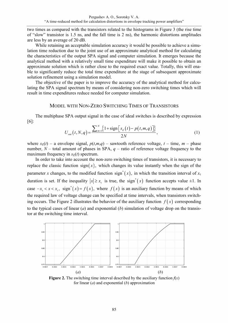
Pergushev A. O., Sorotsky V. A.
“A time-reduced method for calculation distortions in envelope tracking power amplifiers”
85
two times as compared with the transistors related to the histograms in Figure 3 (the rise time of “slow” transistor is 1.5 ns, and the fall time is 2 ns), the harmonic distortions amplitudes are less by an average of 20 dB.
While retaining an acceptable simulation accuracy it would be possible to achieve a simu-lation time reduction due to the joint use of an approximate analytical method for calculating the characteristics of the output SPA signal and computer simulation. It emerges because the analytical method with a relatively small time expenditure will make it possible to obtain an approximate solution which is rather close to the required exact value. Totally, this will ena-ble to significantly reduce the total time expenditure at the stage of subsequent approximate solution refinement using a simulation model.
The objective of the paper is to improve the accuracy of the analytical method for calcu-lating the SPA signal spectrum by means of considering non-zero switching times which will result in time expenditures reduce needed for computer simulation.
MODEL WITH NON-ZERO SWITCHING TIMES OF TRANSISTORS
The multiphase SPA output signal in the case of ideal switches is described by expression [6]:
1
1 sign , ,, , ,
2
NEm
out
s t p t m qU t N q
N
(1)
where sE(t) – a envelope signal, p(t,m,q) – sawtooth reference voltage, t – time, m – phase number, N – total amount of phases in SPA, q – ratio of reference voltage frequency to the maximum frequency in sE(t) spectrum.
In order to take into account the non-zero switching times of transistors, it is necessary to replace the classic function sign ,x which changes its value instantly when the sign of the parameter x changes, to the modified function *sign ,x in which the transition interval of x duration is set. If the inequality x x is true, the *sign x function accepts value ±1. In case ,x x x *sign ,x f x where f x is an auxiliary function by means of which the required law of voltage change can be specified at time intervals, when transistors switch-ing occurs. The Figure 2 illustrates the behavior of the auxiliary function f x corresponding to the typical cases of linear (a) and exponential (b) simulation of voltage drop on the transis-tor at the switching time interval.
(a) (b)
Figure 2. The switching time interval described by the auxiliary function f(x) for linear (a) and exponential (b) approximation

“Instrumentation Engineering, Electronics and Telecommunications – 2018”
Proceedings of the IV International Forum (Izhevsk, Russia, December, 12–14, 2018)
86
RESULTS
With the use of this method the SPA output signal spectrum was calculated for the cases when the voltage drop across transistors at the stage of their commutation is approximated either linearly or exponentially.
The SPA output signal spectral diagrams corresponding to the linear approximation of the switching times (light-tone histogram) are shown in Figures 3 (b), (d), (f) and 4 (b), (d), (f).
Figure 3. Spectral diagrams of the SPA output signal for “slow” transistors: (a), (c) and (e) – SPA simu-lation model (dark tone) and an approximate model with zero switching times of the transistors (light tone); (b), (d) and (f) – the modified model with linear switching times approximation (light tone) and the approximate model with zero switching times(dark tone)

Pergushev A. O., Sorotsky V. A.
“A time-reduced method for calculation distortions in envelope tracking power amplifiers”
87
Figure 4. Spectral diagrams of the SPA output signal for “fast” transistors: (a), (c) and (e) – SPA simula-tion model (dark tone) and an approximate model with zero switching times of the transistors (light tone); (b), (d) and (f) – the modified model with linear switching times approximation (light tone) and the approximate model with zero switching times(dark tone)
Here, to make comparison more convenient, diagrams corresponding to inertia-free tran-sistors (dark tone histograms), which were calculated with the help of (1), are given. Compar-ing these results with the results of simulation, it is easy to see that the error in determining the amplitudes of the harmonics has decreased from 30…35 dB to 1…6 dB.
Analysis of the results corresponding to linear and exponential voltage drop approxima-tions revealed that the difference in the amplitudes of the harmonics does not exceed 1 dB.

“Instrumentation Engineering, Electronics and Telecommunications – 2018”
Proceedings of the IV International Forum (Izhevsk, Russia, December, 12–14, 2018)
88
CONCLUSION
The proposed method reduces the error in determining the harmonic distortion amplitudes in comparison with (1) by 4…5 times and it should be taken into account that it requires as much as 300…800 times less simulation time to determine SPA output signal spectrum. It can especially be useful for optimization procedures and, as it was shown, a linear function f x will suit in most cases.
REFERENCES
1. Vasic, M., Cheng, P., Garcia, O., Oliver, J. A., Alou, P., Cobos, J. A., … Ortega-Gonzalez, F. J. (2016). The design of a multilevel envelope tracking amplifier based on a multiphase buck converter. IEEE Transactions on Power Electronics, 31(6), 4611–4627. doi: 10.1109/tpel.2015.2476517.
2. Jin, Q., & Ruan, X. (2013). Switch-linear hybrid envelope-tracking power supply with multilevel structure. In: IECON 2013 – 39th Annual Conference of the IEEE Industrial Electronics Society (pp. 1325–1330). Vi-enna, Austria : IEEE. doi: 10.1109/iecon.2013.6699324.
3. Sankman, J., Song, M. K., & Ma, D. (2016). Switching-converter-only multiphase envelope modulator with slew rate enhancer for LTE power amplifier applications. IEEE Transactions on Power Electronics, 31(1), 817–826. doi: 10.1109/tpel.2015.2406710.
4. Sung, S., Hong, S., Bang, J., Paek, J., Lee, S., Cho, T. B., & Cho, G. (2016). Envelope modulator for 1.5-W 10-MHz LTE PA without AC coupling capacitor achieving 86.5% peak efficiency. IEEE Transactions on Power Electronics, 31(12), 8282–8292. doi: 10.1109/tpel.2016.2519243.
5. Meng, F., Zhu, X.-W., Jin, Q., Wang, Y., & Ruan, X. (2015). Digitally-controlled high-efficiency series form switch-linear hybrid supply modulator for envelope tracking power amplifiers. 2015 Asia-Pacific Microwave Conference (APMC), 3 (pp. 1–3). Nanjing, China : IEEE. doi: 10.1109/apmc.2015.7413431.
6. Kobzev, A. V., Mikhalchenko, G. Y., & Muzychko, N. M. (1990). Modulyatsionnyye istochniki pitaniya REA [Modulated power supplies for radio electronic devices]. Tomsk, Russia : Radio and communication (in Russian).

Ponomareva O., Smirnova N., Ponomarev A.
“Time-domain interpolation using the parametric DFT”
89
DOI: 10.22213/2658-3658-2018-89-95
Time-Domain Interpolation Using the Parametric DFT
O. Ponomareva, N. Smirnova, A. Ponomarev
Kalashnikov Izhevsk State Technical University, Izhevsk, Russian Federation
E-mail: [email protected]
Received: June 28, 2018
The main directions of application of digital signal processing methods in classical discrete spectral analysis based on the discrete Fourier transform are considered. An algorithm for interpolating a time signal based on a discrete Fourier transform is given. The disadvantages of the existing interpolation algorithm for the time signal based on the discrete Fourier transform are revealed. Based on the analy-sis of the matrix structure of the inverse discrete Fourier transform, a modified parametric discrete Fourier transform is proposed. The properties of the basis of the modified parametric discrete Fourier transform are investigated.
Keywords: digtal Fourier transform, inversed digital Fourier transform, parametric fast Fourier trans-form, modified parametric discrete exponential functions.
INTRODUCTION
One of the main areas of application of digital signal processing (DSP) methods is the classical discrete spectral analysis (CDSA) based on the discrete Fourier transform (DFT) [1–31].
Algebraic form of DFT:
1
0
1 ,N
knN N
nS k x n W
N
0, 1;k N (1)
where x n is a discrete signal, 0, 1;n N NS k – DFT coefficients, the set of which de-termines the amplitude-frequency and phase-frequency signal spectra (the coefficients of the
DFT are often called bins); 2exp ,NW jN
0, 1.k N
TIME-DOMAIN INTERPOLATION USING THE DFT
In the papers [2] time-domain interpolation using the FFT is described. According to the papers, we compute the FFT of an N-point x t time sequence to produce its S k frequen-cy-domain samples. © Ponomareva O., Smirnova N., Ponomarev A., 2018

“Instrumentation Engineering, Electronics and Telecommunications – 2018”
Proceedings of the IV International Forum (Izhevsk, Russia, December, 12–14, 2018)
90
Next, we stuff 1N r zeros in the middle of NS k to yield the Nr -length intS k frequency samples, where Nr is an integer power of two.
Then we perform an Nr -point inverse FFT on intS k to obtain the interpolated-by-r
intx n times samples. Using this frequency-domain zero stuffing to implement time-domain signal interpolation
involves two important issues. The first issue: to ensure the interpolated intx n time sequence is real only, conjugate
symmetry must be maintained in the zero-stuffed intS k frequency samples. Here's the second issue regarding time-domain real signal interpolation: this exact inter-
polation algorithm provides correct results only if the original x n sequence is periodic within its full time interval. If S k exhibits any spectral leakage, like the signals with which we usually work, the interpolated intx n sequence can contain noticeable amplitude errors in its beginning and ending samples. As shown in Fig. 1(a) [2] where an 24N sample x n sequence is interpolated by 2.r In that figure, squares (both white and black) represent the 48-point interpolated intx n sequence, white squares are the original x n samples, and cir-cles represent the exactly correct interpolated sample values. (In the center portion of the fig-ure, the circles are difficult to see because they're hidden behind the squares.) The interpola-tion error, the difference between the correct samples and int ,x n is given in Fig. 1(b) [2].
Figure 1. Interpolation results for N = 24, r = 2:
interpolated int ,x n original ,x n and correct interpolation (a); interpolation error (b)
DFT and IDFT are the base of CDSA of signals in the matrix form, and described by the following relationships [1–5]:
1DFT ;N N NS F XN
(2)
1IDFT .N N NX F SN
(3)

Ponomareva O., Smirnova N., Ponomarev A.
“Time-domain interpolation using the parametric DFT”
91
where 0 , 1 , , 1 TNX x x x N – representation of a discrete signal ,x n
0, 1,n N in the form of a vector N-dimensional linear space; T is a sign of transposition;
0 , 1 , , 1 TNS s s s N is the vector of expansion coefficients NX in the system of
discrete exponential functions (DEF): 2, exp ;plNdef p l j pl W
N
which is given by
the matrix :NF
11
1 1 1
0 1 . . 11 1 . . 10
1 1 . .. . . . . .. . . . . .
1 1 . .
NN N
N
N N NN N
N n
W WF
N W Wk
. (4)
Zero-padding technique in the frequency domain (method of adding the spectrum of a discrete signal x n ( 0, 1n N ) with 1N r zero-valued samples ( 1, 2r ) in the frequency domain (ZPFD) [1, 2]. With ZPFD, the discrete spectrum NS of the real signal
,x n 0, 1,n N is represented in the form of a vector of M-dimensional ( M N r ) linear space:
1
0 , , 2 1 ,0, , 0, 2 , , 1 .
T
M
N r
S s s N s N s N
(5)
As a result of performing the IDFT of the vector XM, the values of the discrete-frequency Fourier transform (DFFT) of the discrete signal x n at M points uniformly distributed on the time axis are obtained.
The discrete-frequency Fourier transform is the inverse z-transform :NS k
1
0exp 2 .
N
Nk
x t S k j k t
(6)
The zero-padding technique, applied to the spectrum of a discrete signal x n with N samples in the frequency domain (ZPFD) allows us to find the values of the MDPF-P only for the parameter values 0, 1 , , 1 .r r r ZPFD has the following significant short-comings, which manifest themselves in its implementation of the processor instruments (PI):
• the need for a significant expansion of the RAM memory PI for storing zero spectrum values;
• conducting non-productive calculations of PI with zero spectrum values; • fixed time step in the discretization.

“Instrumentation Engineering, Electronics and Telecommunications – 2018”
Proceedings of the IV International Forum (Izhevsk, Russia, December, 12–14, 2018)
92
The purpose of this work
The purpose of this paper is to develop a method for eliminating the above mentioned shortcomings of signal interpolation in the time domain using a modified parametric discrete Fourier transform.
In the papers [1, 9–16], a generalization of the inverse DFT (IDFT) (1) in the form of a modified parametric discrete Fourier transform (MDFT-P), which is essentially the evolu-tion of the IDFT, is proposed.
MDFT-P in the matrix form is described by the following relation [1]:
, ,1 ,C
N N NX F SN 0 1; (7)
where the vector of N-dimensional linear space is the result of multiplying the second half of the vector SN (1) by a factor: ,M N
NC W
where ,NX is the vector of expansion coefficients CNS in the system of modified parametric
discrete exponential functions (MDEF-P):
2, , exp ,k npM Ndef k n W j k n
N
, 0, 1 , 0 1,k n N
which is given by the matrix , :NF
1
1 1 1
,
1 1 1
110 . . .0 1 . . .1 1 . . .
.. . . . . . .. . . . . . .
1 1 . . .
NN N
NN N
N
N N NN N
N kW W
W WF
N W Wn
(8)
MAIN PROPERTIES OF MDEF-P
1. MDEF-P, like DEF-P, are not functions of equivalent variables k and n. Consequently, the MDEF-P matrix ,NF is asymmetric.
2. MDEF-P are periodic in a variable n and parametrically periodic in a variable k with a period N:
, , , , ,
, , , , .pM pM
N ppM pM N
def k n pN def k n
def k pN n def k n W
3. MDEF-P system is non-multiplicative in the variable n:
, , , , , , , , 0, 1;pM pM pMdef k n def k m def k n m n m N n m

Ponomareva O., Smirnova N., Ponomarev A.
“Time-domain interpolation using the parametric DFT”
93
and multiplicative in the variable k:
, , , , , , , , 0, 1; .pM pM pMdef k n def l n def k l n k l N k l
4. Average value of MDEF-P with respect to the variable n is equal to zero when k 0:
1
0
1 exp 22, , exp ,21 exp
N
pMn
j kdef k n j k
N j kN
and with respect the variable k is not zero:
1
0
1 exp 2, , .
21 exp
N
pMk
j k ndef k n
j nN
5. The MDEF-P system is orthogonal in both variables:
1 *
0
,10, ;1
n m NNn k m k N
N N n mk N
N n mWW Wn mW
1 *
0
,10,1
l k NNn k n l N
N N l kn N
N l kWW Wl kW
6. The MDEF-P system is a complete system, since the number of linearly independent functions is equal to the dimension of the set of discrete signals.
CONCLUSION
Applying the modified parametric discrete transformation, we have the opportunity to eliminate the following essential deficiencies of the zero-padding technique, applied to the spectrum of a discrete signal x n with N samples in the frequency domain:
• the need for a significant expansion of the RAM memory PI for storing zero spectrum values;
• Conducting non-productive calculations of PI with zero spectrum values; • fixed time step in the discretization. With the advent of fast hardware DSP chips and pipelined parametric FFT (FFT-P) tech-
niques, the above time-domain interpolation algorithm may be viable for a number of applica-tions, such as computing selectable sample rate time sequences of a test signal that has a fixed spectral envelope shape; providing interpolation, by selectable factors, of signals that were filtered in the frequency domain using the fast convolution method; or digital image resampling.
REFERENCES
1. Ponomareva, O. V. (2016). Razvitiye teorii i razrabotka metodov i algoritmov tsifrovoy obrabotki informatsionnykh signalov v parametricheskikh bazisakh Fur’ye [Development of the theory and develop-ment of methods and algorithms for digital processing of information signals in parametric Fourier bases] (Doctoral thesis, Kalashnikov Izhevsk State Technical University, Izhevsk, Russian Federation) (in Russian).

“Instrumentation Engineering, Electronics and Telecommunications – 2018”
Proceedings of the IV International Forum (Izhevsk, Russia, December, 12–14, 2018)
94
2. Lyons, R. G. (2004). Understanding digital signal processing (2nd ed.). Upper Saddle River, USA : Prentice Hall PTR.
3. Crochiere, R. E., & Rabiner, L. R. (1983). Multirate digital signal processing (4th ed.). Englewood Cliffs, USA : Prentice-Hall.
4. Zoran Corp. (1989). Vernier spectral analysis with the ZR34161 vector signal processor: Tech. note ZAN34003. Santa Clara, CA, USA : Author.
5. Gumas, C. (1997, July). Window-presum FFT achieves high-dynamic range, resolution. Personal Engineer-ing and Instrumentation News (pp. 58–64).
6. Aldoshina, I., & Pritts, R. (2006). Muzykal’naya akustika [Musical acoustics]. Saint-Petersburg, Russia : Kompozitor – Sankt-Peterburg (in Russian).
7. Kuznetsov, L. A. (1989). Akustika muzykal’nykh instrumentov [Acoustics of musical instruments]. Moscow, USSR : Legprombytizdat (in Russian).
8. Trakhtman, A. M., & Trakhtman, V. A. (1975). Osnovy teorii diskretnykh signalov na konechnykh interva-lakh [Fundamentals of the theory of discrete signals on finite intervals]. Moscow, USSR : Soviet Radio (in Russian).
9. Yaglom, A. M. (1981). Korrelyatsionnaya teoriya statsionarnykh sluchaynykh funktsiy s primerami iz meteorologii [Correlation theory of stationary random functions with examples from meteorology]. Lenin-grad, USSR : Gidrometeoizdat (in Russian).
10. Ponomareva, O. V., Ponomarev, A. V., & Ponomareva, N. V. (2012). Sliding parametric DFT in problems of detection of tonal components. Digital Signal Processing, (4), 2–7. Retrieved from http://www.dspa.ru/ articles/year2012/jour12_4/art12_4_1.pdf (in Russian).
11. Ponomareva, O. V., & Ponomarev, A. V. (2015). Restoration of values of continuous frequency spectra of discrete signals by the method of parametric discrete Fourier transform. Bulletin of Kalashnikov ISTU, 18(3), 88–91. Retrieved from http://izdat.istu.ru/index.php/vestnik/article/download/3037/1805 (in Russian).
12. Ponomarev, V. A., Ponomareva, O. V., Ponomarev, A. V., & Ponomareva, N. V. (2014). A generalization of Hertzel's algorithms and a sliding parametric discrete Fourier transform. Digital Signal Processing, (1), 3–11. Retrieved from http://www.dspa.ru/articles/year2014/jour14_1/art14_1_1.pdf (in Russian).
13. Ponomareva, O. V. (2014). Noninvariance of the sliding energy parametric Fourier spectrum of real tonal signals. Digital Signal Processing, (2), 7–14. Retrieved from http://www.dspa.ru/articles/year2014/jour14_2/ art14_2_2.pdf (in Russian).
14. Ponomareva, O. V., Alekseyev, V. A., & Ponomarev, A. V. (2014). Fast algorithm for measuring the spec-trum of real signals by the method of an aperiodic discrete Fourier transform. Bulletin of Kalashnikov ISTU, (2), 106–109. Retrieved from http://izdat.istu.ru/index.php/vestnik/article/view/2920/1688 (in Russian).
15. Ponomareva, O. V., Ponomarev, A. V., & Ponomarev, V. A. (2014). Measurement of the sliding weighted energy discrete-time spectrum of tonal components. Intelligent Systems in Manufacturing, (2), 126–132. Re-trieved from http://izdat.istu.ru/index.php/ISM/article/download/1883/698 (in Russian).
16. Ponomarev, V. A., & Ponomareva, O. V. (2014). Invariance of the current Fourier energy spectrum of com-plex discrete signals at finite intervals. Journal of the Russian Universities: Radioelectronics, (2), 8–16. Re-trieved from https://etu.ru/assets/files/university/izdatelstvo/radioelektronika/Radioelektronika-2-2014.pdf (in Russian).
17. Ponomarev, V. A., & Ponomareva, O. V. (2014). Invariance of the current Fourier energy spectrum of real discrete signals on finite intervals. Tekhnologiya i Konstruirovanie v Elektronnoi Apparature, (1), 15–22. doi: 10.15222/tkea2014.1.15 (in Russian).
18. Courtney, C. R. P., Neild, S. A., Wilcox, P. D., & Drinkwater, B. W. (2010). Application of the bispectrum for detection of small nonlinearities excited. Journal of Sound and Vibration, 329(20), 4279–4293. doi: 10.1016/j.jsv.2010.04.031.
19. Akçay, H. (2012). Frequency domain subspace-based identification of discrete-time singular power spectra. Signal Processing, 92(9), 2075–2081. doi: 10.1016/j.sigpro.2012.01.019.
20. Beck, R., Dempster, A. G., & Kale, I. (2000). Characterisation of finite-precision resonators used in recursive filter DFT implementations. Signal Processing, 80(1), 161–183. doi: 10.1016/S0165-1684(99)00119-X.

Ponomareva O., Smirnova N., Ponomarev A.
“Time-domain interpolation using the parametric DFT”
95
21. Chaparro, L. F. (2015). Signals and systems using MATLAB (2nd ed.). Boston, USA : Academic Press. doi: 10.1016/B978-0-12-394812-0.00016-4.
22. Chu, C.-P., Shen, L.-T., & Hwang, S.-H. (2014). A new algorithm for tone detection. AASRI Procedia, 8, 118–122. doi: 10.1016/j.aasri.2014.08.020.
23. Onchis, D. M., & Rajmic, P. (2014). Generalized Goertzel algorithm for computing the natural frequencies of cantilever beams. Signal Processing, 96, Part A, 45–50. doi: 10.1016/j.sigpro.2013.07.026.
24. Fan, C.-P., & Su, G.-A. (2007). Pruning fast Fourier transform algorithm design using group-based method. Signal Processing, 87(11), 2781–2798. doi: 10.1016/j.sigpro.2007.05.012.
25. Fam, A. T. (2010). Efficient matched filters for DFT based codes. Signal Processing, 90(11), 2996–2998. doi: 10.1016/j.sigpro.2010.04.018.
26. Fraile, R., & Godino-Llorente, J. I. (2014). Cepstral peak prominence: A comprehensive analysis. Biomedical Signal Processing and Control, 14, 42–54. doi: 10.1016/j.bspc.2014.07.001.
27. Gronczyński, J. (2007). Recursive Fourier transform algorithms with integrated windowing. Signal Pro-cessing, 87(5), 1003–1013. doi: 10.1016/j.sigpro.2006.09.005.
28. Hajnayeb, A., Ghasemloonia, A., Khadem, S. E., & Moradi, M. H. (2011). Application and comparison of an ANN-based feature selection method and the genetic algorithm in gearbox fault diagnosis. Expert Systems with Applications, 38(8), 10205–10209. doi: 10.1016/j.eswa.2011.02.065.
29. Hoang, V. D. (2014). Wavelet-based spectral analysis. TrAC Trends in Analytical Chemistry, 62, 144–153. doi: 10.1016/j.trac.2014.07.010.
30. Chicharo, J. F., & Kilani, M. T. (1996). A sliding Goertzel algorithm. Signal Processing, 52(3), 283–297. doi: 10.1016/0165-1684(96)00066-7.
31. Ming, A. B., Qin, Z. Y., Zhang, W., & Chu, F. L. (2013). Spectrum auto-correlation analysis and its application to fault diagnosis of rolling element bearings. Mechanical Systems and Signal Processing, 41(1–2), 141–154. doi: 10.1016/j.ymssp.2013.08.004.
“Instrumentation Engineering, Electronics and Telecommunications – 2018”
Proceedings of the IV International Forum (Izhevsk, Russia, December, 12–14, 2018)
96
DOI: 10.22213/2658-3658-2018-96-106
Effect of Reinforcing Rolling on the Surface Properties of Products Made of Heat-Resistant Alloys
А. Shiryaev 1, N. Vinokurov 1, V. Trofimov 1, V. Karmanov 1, А. Shilyaev 2
1 PNRPU, Perm National Research Polytechnic University, Perm, Russia
E-mail: [email protected], [email protected] 2 LLC “Transet”,
Saint_Petersburg, Russia E-mail: [email protected]
Received: June 24, 2018
The process of surface plastic deformation – hardening rolling by a ball is one of the most widespread processes of finishing machining products, allowing to obtain the required mechanical characteristics of the surface of products – hardness, strength, corrosion resistance and wear resistance. The results of the investigation of the effect of rolling modes on the characteristics of the surface layer of samples of high-temperature alloys VZhL14-VM and VZhM-4 are presented: the residual stresses, roughness, microhardness, and the depth of surface crushing. For rolling, a hydrostatic tool installed instead of a rotating assembly on a friction welding machine was used. The analysis of the results shows that the step and the scheme of the tool movement have the most significant influence on the residual stress level, microhardness and roughness. It is shown that, after rolling, the depth of the surface crushing after rolling increases slightly the geometrical dimensions of the samples. The microhardness of the surface is increased by 25–33 %, and the microroughness decreases by 2–4 times. After rolling in the surface layer, compressive residual stresses are recorded, reaching the maximum values in a direction perpendicular to the direction of movement of the tool.
Keywords: residual stresses, surface hardening, surface plastic deformation, roughness, microhard-ness, heat-resistant alloys.
INTRODUCTION
Typically, the operational properties of the part can be improved by performing heat treatment (HT): quenching, tempering, annealing, etc. Despite their high cost and time costs, maintenance is sometimes not enough to obtain the necessary properties of the material. That is why, in the production of processes of surface plastic deformation (SPD), such as rolling around with a roller or a ball. Due to local plastic deformation, surface topography changes, surface layers are ground and there are compressive residual stresses (RS) [1–4]. Processing of SPD increases fatigue strength, which remains the main cause of the destruction of parts. Therefore, it is important to choose such a SPD technology and processing modes to ensure the required surface quality indicators.
© Shiryaev А., Vinokurov N., Trofimov V., Karmanov V., Shilyaev А., 2018

Shiryaev А., Vinokurov N., Trofimov V., Karmanov V., Shilyaev А.
“Effect of reinforcing rolling on the surface properties of products made of heat-resistant alloys”
97
This technology can be used on cylindrical, flat, complex surfaces, areas of sharp changes in the cross-section, etc. The main limitation of this process is mainly geometric. Despite the complexity of programming processes in the five-axis region, the use of a turning center, CNC milling machine or robot can cope with this limitation.
In [3–5] the influence of the feed, the depth of penetration, the distance between the tool and the residual stress level for steel 45 is shown. [6] shows the change in microhardness from the rolling force, the diameter of the ball for VT1-1. The procedure for selecting and calculating the parameters of the mode of finishing the SPD is shown in [7]. Depending on the surface force P of rolling around the ball, it follows that the hardness of HV increases with increasing P for steel 12X18H9T from the initial 181 to 342, for the titanium alloy VTZ-1 from 319 to 390 and for the nickel alloy KhN67BMTU from 282 to 412 [8, p. 63]. When studying RS [9], the influence of pressure, feed, velocity, tool dimensions, number of passes, structure and properties of the material was studied.
It was shown in [10] that the parameters of speed, feed, ball pressing force, its radius and number of passes affect the roughness and hardness. The force of pressing the tool af-fects the depth of the hardened layer. However, with a force > 100 N, the risk of peeling and microcracking of the surface layer increases. The best roughness result is achieved for 3–4 passes.
In [11], for the Ti-6Al-4V material, the optimization problem was investigated-the estab-lishment of maximum residual compressive stresses. To simulate the process, a model of a nonlinear finite element was developed with high accuracy of three-dimensional nonlineari-ty. According to the results, a large compressive OH on the surface of the components can be achieved either by reducing the diameter of the ball, or by increasing the number of passes. In addition, to increase the depth of the residual compressive stress, it is necessary to increase the diameter of the ball.
The main parameters affecting the rolling process are the ball diameter, the burning force, the ball speed, the number of tool passes and the initial roughness of the workpiece [12]. Loll et al. [13] studied the effect of machining parameters on the roughness of the structure during deep cold rolling for AISI 1045. Analogous studies of the polishing of roll-ers were carried out for steel 37 [14] and Al 6061-T6 [15], in which influence of rolling pa-rameters on hardness, roughness and fatigue strength of the part. Taweel and Axir [16] also experimentally studied the influence of the main parameters of the rolling process on the surface microhardness and roughness using the Taguchi method. Klocke et al. [17] investi-gated the effect of the ball diameter, superposition, pressing force and geometry of a nickel alloy preform on the roughness and the OH value during ball processing. Fretting strength and RS profile were studied for Ti-6Al-4V [18]. In [19] it was studied the effect of various polishing materials and ball pressing forces on the roughness of a steel product with an ini-tial hardness of 64 HRC. The main producers of the instrument are ECOROLL AG and Lambda Technologies.
A review of the literature shows that the changing parameters on the surface are different: the pressing force and the speed of the tool. Sometimes other factors are introduced, such as the number of passes, the diameter of the ball. The result depends mainly on the combination of various parameters depending on the rigidity of the tool, the properties of the material to be treated, the required processing time, operating conditions and the initial state of the surface layers, and the type of lubricant.

“Instrumentation Engineering, Electronics and Telecommunications – 2018”
Proceedings of the IV International Forum (Izhevsk, Russia, December, 12–14, 2018)
98
EXPERIMENTAL PROCEDURE
Samples and equipment
Samples: plates 120×48×8 mm; 160×28×14 mm (Fig. 1). Material: VZhL14-VМ, VZhM-4.
а b
Figure 1. Samples: а – VZhL14-VM (samples No. 1–2); b – VZhM-4 (sample No. 3)
The chemical composition of the high-temperature alloys is shown in Tables 1–2.
Table 1. Chemical composition of alloy VZhL14-VM Fe С Si Mn Ni S P Cr Ce Mo Ti Al B
8-10 0.05–0.08 ≤ 0.4 ≤ 0.4 59.1–63.7 ≤ 0.01 ≤ 0.01 18–20 ≤ 0.02 4.5–5.5 2.8–2.9 1.2–1.5 ≤ 0.005
Table 2. Chemical composition of alloy VZhM-4 Ni P La Al Re Cr Co Mo Ru Ta W
36.7 13.3 9.3 0.7 3.3 4.7 6.7 7.7 4.7 10.2 1.5 The residual stress was measured by X-ray diffractometry using a robotic complex
XStress 3000 G3 and a collimator with a diameter of 4 mm. Determination of the depth of the rolled bed was carried out using the coordinate measur-
ing machine CARL ZEISS ACCURA II 9/14/8. The roughness measurement was carried out using the Mahr MarSurf PS1 device based
on 5.6 mm. The microhardness was measured by the Shimadsu HMV-G21S, a load of 19.61 N. Samples were measured in the initial state and after rolling in the control points according
to the schemes indicated in Fig. 2.
Modes of strengthening processing
The reinforcing rolling was carried out with a hydrostatic tool HG6-9_SL (K) (Ecoroll) fixed in a special tooling in the friction welding machine I-ISTIR PDS-5, equipped with feed-back sensors. Information on the force of the tool pressing is obtained from these sensors. As coolant, I-20 oil was used.
Modes of hardening rolling are given in Tables 3–5. The mesh rolling was carried out: 1) direction 0° (along the axis of the tool movement);
2) direction 90° (perpendicular to the movement of the tool) (see Figure 7).

Shiryaev А., Vinokurov N., Trofimov V., Karmanov V., Shilyaev А.
“Effect of reinforcing rolling on the surface properties of products made of heat-resistant alloys”
99
b
а c
Figure 2. Points for determining the OH value of the surface layer: points on the surface of samples from VZhL14-BM (a); points on the surface of a specimen from VZhM-4 (b); diagram of the location of points on the run-in area (c)
Figure 3. Hydrostatic tool
HG6-9_SL (K) from Ecoroll Figure 4. Scheme of fixing the sample
Table 3. Knurling modes on sample No. 1 Mode No. Effort, kgf Step, mm Speed, mm / min
1 100 0.1 500 2 75
3 50

“Instrumentation Engineering, Electronics and Telecommunications – 2018”
Proceedings of the IV International Forum (Izhevsk, Russia, December, 12–14, 2018)
100
Table 4. Knurling modes on sample No. 2 Mode No. Effort, kgf Step, mm Speed, mm / min Direction of processing
4 75
0.2 500 0°
5 Mesh 6 0.05 1000 0°
Table 5. Knurling modes on sample No. 3
Mode No. Effort, kgf Step, mm Speed, mm / min Direction of processing 1
75 0.2
500 0°
2 Mesh 3 0.05 0°
RESULTS AND DISCUSSION
Samples after hardening rolling
а
b
Figure 5. Samples after hardening rolling: No. 1–2 (a); No. 3 (b)

Shiryaev А., Vinokurov N., Trofimov V., Karmanov V., Shilyaev А.
“Effect of reinforcing rolling on the surface properties of products made of heat-resistant alloys”
101
Residual stresses
The location of the monitoring object in the Xstress Robot X-ray diffractometer chamber with the directions of measurement is shown in Figures 6–7.
Graphs of RS distribution in the surface layer prior to rolling are presented in Figure 8.
а b Figure 6. Location of samples No. 1–2 in the diffractometer chamber: before processing (a); after treatment (b); 90° – transverse direction (perpendicular to the movement of the instrument); 0° – longitudinal direction (along the axis of the tool movement)
Figure 7. The location of sample No. 3 in the diffractometer chamber: 90° – longitudinal direction (along the axis of the tool movement); 0° – transverse direction (perpendicular to the movement of the tool)
а b
Figure 8. The distribution of RS on the surface of samples from VZhL14: No. 1 (a); No. 2 (b)
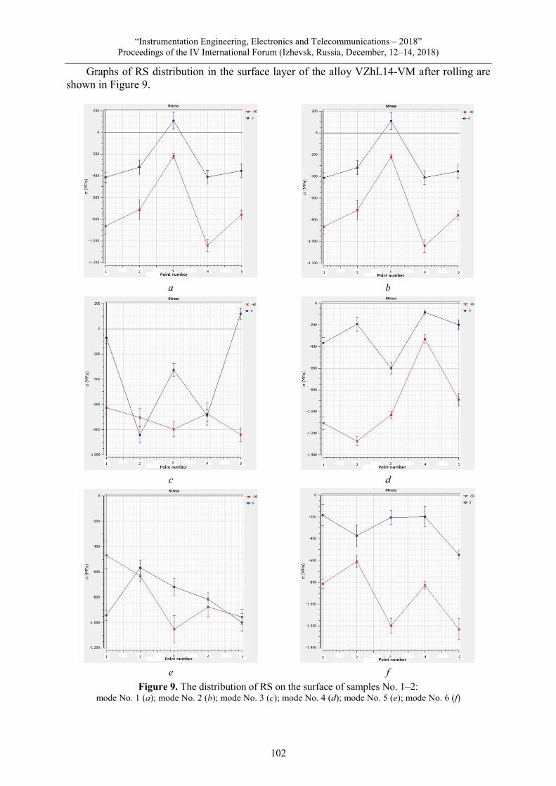
“Instrumentation Engineering, Electronics and Telecommunications – 2018”
Proceedings of the IV International Forum (Izhevsk, Russia, December, 12–14, 2018)
102
Graphs of RS distribution in the surface layer of the alloy VZhL14-VM after rolling are shown in Figure 9.
а b
c d
e f
Figure 9. The distribution of RS on the surface of samples No. 1–2: mode No. 1 (a); mode No. 2 (b); mode No. 3 (c); mode No. 4 (d); mode No. 5 (e); mode No. 6 (f)

Shiryaev А., Vinokurov N., Trofimov V., Karmanov V., Shilyaev А.
“Effect of reinforcing rolling on the surface properties of products made of heat-resistant alloys”
103
Graphs of OH distribution in the surface layer of sample No. 3 (VZhM-4) after rolling are shown in Figure 10.
а b
c
Figure 10. The distribution of RS on the surface of samples No. 3: mode No. 1 (a); mode No. 2 (b); mode No. 3 (c)
Depth of crumple of the surface layer
The depth of the crushing of the layer was measured as the average value over 9 points.
Roughness
The values of Ra are the average of 5 measurements (Table 7), where 0° is a direction along the axis of movement of the tool (VZhL); 90° is a direction perpendicular to the axis of movement of the tool (VZhL). For sample No. 3 (VZhM-4), the values are opposite.
For Mode 4, the roughness (0°) varies over a wide range of 0.129–0.621 μm. This is due to the large step (0.2 mm) during processing, because the larger value of Ra corresponds to the crest between the depressions.

“Instrumentation Engineering, Electronics and Telecommunications – 2018”
Proceedings of the IV International Forum (Izhevsk, Russia, December, 12–14, 2018)
104
Table 6. The results of the measurement of the depth of crushing of the surface layer upon rolling Material Sample No. Mode No. Depth of layer crushing, μm
VZhL14-VM
1 1 12 2 12 3 7
2 4 14 5 14 6 9
VZhM-4 3 1 3 2 3 3 2
Table 7. Results of measuring the roughness of samples
Material Sample No. Mode No. Ra, μm (0°) Ra, m (90°)
VZhL14-VM
1
Before processing 0.768 0.359 1 0.142 0.156 2 0.178 0.186 3 0.167 0.175
2
Before processing 0.757 0.265 4 0.351 0.265 5 0.362 0.122 6 0.281 0.249
VZhM-4 3
Before processing 0.406 0.629 1 0.090 0.522 2 0.141 0.096 3 0.052 0.108
Microhardness
The HV values are obtained as an average of 5 points.
Table 8. Results of measuring the roughness of samples Material Sample No. Mode No. HV
VZhL14-VM
1
Before processing 322.93 1 488.70 2 489.73 3 483.38
2
Before processing 346.65 4 469.79 5 508.12 6 473.42
VZhM-4 3
Before processing 435.52 1 576.08 2 609.68 3 619.36

Shiryaev А., Vinokurov N., Trofimov V., Karmanov V., Shilyaev А.
“Effect of reinforcing rolling on the surface properties of products made of heat-resistant alloys”
105
The reinforcing rolling leads to an increase in the microhardness of the surface by 25-33 %. The value of HV for the alloy VZhL14-VM is not affected by the pressure and processing step. The microhardness is affected by the rolling pattern.
For the alloy VZhM-4, the value of HV depends on the rolling pattern and the pitch.
CONCLUSIONS
The results of the study showed that: – for all samples and processing modes, strengthening knurling leads to the formation of
squeezing OH and equalization of their values, and also virtually eliminates stretching OH; – the depth of the crushing of the surface layer depends on the rolling force and is com-
parable to the tolerances for the manufacture of engineering parts, which does not lead to a significant distortion of their geometry;
– microhardness of the surface of the samples, depending on the regimes of hardening rolling, increases by 25–33 %;
– the roughness depends on the rolling force, the processing step, the rolling pattern and leads to a 2-fold or more decrease in the Ra parameter.
The results of the work show that the reinforcing rolling has a positive effect on the prop-erties of the surface layers of the samples and this technology can be used for finishing the parts made of high-temperature alloys of the VZhL14-VM and VZhM-4 grades.
REFERENCES
1. Podzey, A. V. (1973). Tekhnologicheskiye ostatochnyye napryazheniya [Technological residual stresses]. Мoscow, USSR : Mashinostroenie (in Russian).
2. Blyumenshtein, V. Yu., & Smelyanskiy, V. М. (2007). Mekhanika tekhnologicheskogo nasledovaniya na stadiyah obrabotki i ekspluatatsii mashin [Technological inheritance mechanics at stages of machine parts machining and operation]. Мoscow, Russia : Mashinostroenie (in Russian).
3. Zaides, S. A., & Ngo, C. C. (2018). The influence of new kinematics of the rolling roller on the quality of the hardened layer under surface plastic deformation. Proceedings of Higher Educational Institutions. Маchine Building, 2(695), 58–67. doi: 10.18698/0536-1044-2018-2-58-67 (in Russian).
4. Zaides, S. A., & Ngo, C. C. (2017). New technological potentialities of finish-strengthening by surface plas-tic deformation. Science Intensive Technologies in Mechanical Engineering, 2(3), 25–30. doi: 10.12737/24961 (in Russian).
5. Zaides, S. A., & Ngo, C. C. (2017). Increasing the stress state in the deformation zone for cylindrical parts under surface plastic deformation. Proceedings of Higher Educational Institutions. Маchine Building, 5(686), 52–59. doi: 10.18698/0536-1044-2017-5-52-59 (in Russian).
6. Gorohov, V. А. (1975). Chistovaya obrabotka titanovyh splavov [Finishing of titanium alloys]. Мoscow, USSR : Mashinostroenie (in Russian).
7. Gorohov, V. А., & Spiridonov, N. V. (2003). Sposoby otdelochno-uprochnyayushchey obrabotki materialov [Methods of finishing-strengthening processing of materials]. Minsk, Belarus : Tekhnoprint (in Russian).
8. Gorohov, V. А. (1978). Obrabotka detaley plasticheskim deformirovaniyem [Processing of parts by plastic deformation]. Kiev, USSR : Tekhnika (in Russian).
9. Papshev, D. D. (1968). Uprochneniye detaley obkatkoy sharikami [Hardening of details by rolling balls]. Мoscow, USSR : Mashinostroenie (in Russian).
10. Hamadache, H., Zemouri, Z., Laounar, L., & Dominiak, S. (2014). Improvement of surface conditions of 36 Cr Ni Mo 6 steel by ball burnishing process. Journal of Mechanical Science and Technology, 28(4), 1491–1498. doi: 10.1007/s12206-014-0135-1.

“Instrumentation Engineering, Electronics and Telecommunications – 2018”
Proceedings of the IV International Forum (Izhevsk, Russia, December, 12–14, 2018)
106
11. Mohammadi, F., Sedaghati, R., & Bonakdar, A. (2014). Finite element analysis and design optimization of low plasticity burnishing process. The International Journal of Advanced Manufacturing Technology, 70(5–8), 1337–1354. doi: 10.1007/s00170-013-5406-y.
12. Rao, D. S., Hebbar, H. S., Komaraiah, M., & Kempaiah, U. N. (2008). Investigations on the effect of ball burnishing parameters on surface hardness and wear resistance of HSLA dual-phase steels. Materials and Manufacturing Processes, 23(3), 295–302. doi: 10.1080/10426910801937306.
13. Loll, N. H., Tam, S. C., & Miyazawa, S. (1991). Investigations on the surface roughness produced by ball burnishing. International Journal of Machine Tools and Manufacture, 31(1), 75–81. doi: 10.1016/0890-6955(91)90052-5.
14. El-Axir, M. H. (2000). An investigation into roller burnishing. International Journal of Machine Tools and Manufacture, 40(11), 1603–1617. doi: 10.1016/S0890-6955(00)00019-5.
15. El-Taweel, T. A., & El-Axir, M. H. (2009). Analysis and optimization of the ball burnishing process through the Taguchi technique. The International Journal of Advanced Manufacturing Technology, 41(3–4), 301–310. doi: 10.1007/s00170-008-1485-6.
16. Klocke, F., Bäcker, V., Wegner, H., Feldhaus, B., Baron, H. U., & Hessert, R. (2009). Influence of process and geometry parameters on the surface layer state after roller burnishing of IN718. Production Engineering, 3(4), 391–399. doi: 10.1007/s11740-009-0182-0.
17. Golden, P. J., & Shepard, M. J. (2007). Life prediction of fretting fatigue with advanced surface treatments. Materials Science and Engineering: A, 468–470, 15–22. doi: 10.1016/j.msea.2006.10.168.
18. Laouar, L., Hamadache, H., Saad, S., Bouchelaghem, A., & Mekhilef, S. (2009). Mechanical surface treat-ment of steel. Optimization parameters of regime. Physics Procedia, 2(3), 1213–1221. doi: 10.1016/j.phpro. 2009.11.084.
19. Luca, L., Neagu-Ventzel, S., & Marinescu, L. (2005). Effects of working parameters on surface finish in ball-burnishing of hardened steels. Precision Engineering, 29(2), 253–256. doi: 10.1016/j.precisioneng.2004. 02.002.

Продолжающееся электронное научное издание
«ПРИБОРОСТРОЕНИЕ, ЭЛЕКТРОНИКА И ТЕЛЕКОММУНИКАЦИИ – 2018»
Сборник статей IV Международного форума
(Ижевск, Россия, 12–14 декабря 2018 года)
Адрес в информационно-телекоммуникационной сети: http://ieet.istu.ru/proceedings/IEET-2018.pdf
Дата размещения на сайте: 11.12.2018
Технический редактор С. В. Звягинцова
Корректор И. В. Ганеева Верстка Н. В. Паклиной
Дизайн обложки К. Сабура
Подписано к использованию 10.12.2018. Объем 8,4 Мб. Заказ № 422 Издательство Ижевского государственного технического университета
имени М. Т. Калашникова. 426069, Ижевск, Студенческая, 7

Serial scientific electronic edition
“INSTRUMENTATION ENGINEERING, ELECTRONICS AND TELECOMMUNICATIONS – 2018”
Proceedings of the IV International Forum (Izhevsk, Russia, December 12–14, 2018)
Internet address:
http://ieet.istu.ru/proceedings/IEET-2018.pdf
Web publication date: 11.12.2018
Technical editor S. V. Zvyagintsova Proofreader I. V. Ganeeva Layout by N. V. Paklina
Cover design by K. Sabour
Signed to use on December 10, 2018. Size: 8.4 Mb. Order No. 422 Publishing House of Kalashnikov Izhevsk State Technical University
Studencheskaya St. 7, 426069 Izhevsk, Russia