Identifying States of a Financial MarketMichael C. Munnix1,2, Takashi Shimada1,3, Rudi Schafer2, Francois Leyvraz4, Thomas H. Seligman4,

Thomas Guhr2 & H. Eugene Stanley1

1Center of Polymer Studies, Boston University, USA, 2Faculty of Physics, University of Duisburg-Essen, Germany, 3Department ofApplied Physics, Graduate School of Engineering, The University of Tokyo, Japan, 4Instituto de Ciencias Fısicas, UniversidadNacional Autonoma de Mexico and Centro Internacional de Ciencias, Cuernavaca, Mexico.

The understanding of complex systems has become a central issue because such systems exist in a wide rangeof scientific disciplines. We here focus on financial markets as an example of a complex system. In particularwe analyze financial data from the S&P 500 stocks in the 19-year period 1992–2010. We propose a definitionof state for a financial market and use it to identify points of drastic change in the correlation structure.These points are mapped to occurrences of financial crises. We find that a wide variety of characteristiccorrelation structure patterns exist in the observation time window, and that these characteristic correlationstructure patterns can be classified into several typical ‘‘market states’’. Using this classification we recognizetransitions between different market states. A similarity measure we develop thus affords means ofunderstanding changes in states and of recognizing developments not previously seen.

Time series are typical experimental results we have about complex systems. In the analysis of such time series,stationary situations have been extensively studied and correlations have been found to be a very powerfultool. Yet most natural processes are non-stationary. In particular, in times of crisis, accident or trouble,

stationarity is lost. As examples we may think of financial markets, biological systems, reactors (both chemicaland nuclear) or the weather. In non-stationary situations analysis becomes very difficult and noise is a severeproblem. Following a natural urge to search for order in the system, we endeavor to define states through whichsystems pass and in which they remain for short times. Success in this respect would allow to get a betterunderstanding of the system and might even lead to methods for controlling the system in more efficient ways.We here concentrate on financial markets because of the easy access we have to good data, because of our previousexperience and last but not least because of the strong non-stationary effects recently seen.

ResultsUsing a similarity measure we were able to classify several typical market states between which the market jumpsback and forth. Some of these states can easily be identified in this similarity measure. However, there are severalstates in which the market only stays for a short period. Thus, these states are sparsely embedded in time. With a k-means clustering analysis, we were able to identify these states and disclose a detailed dynamics of the market’sstate.

Our findings offer insight for constructing an ‘‘early warning system’’ for financial markets. By providing asimple instrument to identify similarities to previous states during an upcoming crisis, one can judge the currentsituation properly and be prepared to react if the crisis materializes. Certainly, an indication for a crisis is alsogiven when the correlation structure undergoes rapid changes.

Another possible application of the similarity measure is risk management. Given the similarity measure, theportfolio manager is aware of periods in which the market behaved completely differently and thus can choose notto include them in his calculations. He can furthermore identify regions in which the market behaved similarlyand refer to these regions when estimating the correlation matrix.

Our empirical study is a first step towards the identification of states in financial markets which are a prominentexample of complex non-stationary systems.

DiscussionThe effort to understand the dynamics in financial markets is attracting scientists from many fields1–8. Statisticaldependencies between stocks are of particular interest, because they play a major role in the estimation of financialrisk9. Since the market itself is subject to continuous change, the statistical dependencies also change in time. Thisnon-stationary behavior makes an analysis very difficult10,11. Changes in supply and demand can even lead to atwo phase behavior of the market12,13. Here, we use the correlation matrix to identify and classify the market state.

SUBJECT AREAS:STATISTICAL PHYSICS,

THERMODYNAMICS ANDNONLINEAR DYNAMICS

MODELLING AND THEORY

STATISTICS

THEORETICAL PHYSICS

Received

30 July 2012

Accepted

21 August 2012

Published

10 September 2012

Correspondence andrequests for materials

should be addressed toM.C.M. (michael@

muennix.com)

SCIENTIFIC REPORTS | 2 : 644 | DOI: 10.1038/srep00644 1

In particular we ask: How similar is the present market state, com-pared to previous states? To calculate this similarity we measuretemporal changes in the statistical dependence between stockreturns.

For stationary systems described by a (generally large) number Kof time series, the Pearson correlation coefficient is extremely useful.It is defined as

Cij:rirj! "

{ rih i rj! "

sisj: !1"

Here the ri and rj represent the time series of which the averages Æ…æare taken over a given time horizon T. si and sj are their respectivestandard deviations. When calculating the correlation coefficients ofK stocks, we obtain the K 3 K correlation matrix C, which gives aninsight into the statistical interdependencies of the time series understudy.

It is necessary to consider data over large time horizons T so as toobtain reliable statistics. This leads to a fundamental problem thatarises in the case of non-stationary systems: To extract usefulinformation from empirical data we seek a correlation matrix fromvery recent data, in order to provide a good description of currentcorrelation structure. This is because correlations change dynam-ically due to the non-stationarity of the process, making it very dif-ficult to estimate them precisely14–17. However, if the length T of thetime series is short, the correlation matrices C are noisy. On the otherhand, to keep the estimation error low, T can be increased, but thisleads to a correlation matrix that generally does not describe thepresent state very well. Various noise reduction techniques providemethods to conquer noise18–22.

In several non-stationary systems, it is possible to obtain a largenumber of correlated data over time. Such systems include, but arenot restricted to, financial markets (which show non-stationarybehavior due to crises), biological or medical time series (such asEEG), chemical and nuclear reactors (non-stationary behaviorincludes, in particular, accidents) or weather data. In the follow-ing, we only consider the financial markets, since we have studiedextensively some very high quality data of this system, the non-stationary features of which have been quite striking in the last

years. We propose a definition of a state which is appropriate forsuch systems and suggest a method of analysis which allows for aclassification of possible behaviors of the system. When T/K , 1,which is the case we are interested in, the correlation matrixbecomes singular. However, one can still make significant statist-ical statements, e.g., for the average correlation level whoseestimation error decreases as 1/K. In the following, we focus oncorrelation matrices C(t1) and C(t2) at different times t1 and t2

measured over a short time horizon. These have therefore a pro-nounced random element. We take these objects as the fun-damental states of our system. We now propose, as a centralelement, to introduce the following concept of distance betweentwo states. We define the similarity measure

f t1, t2! ": Cij t1! "{Cij t2! "## ##! "

ij !2"

to quantify the difference of the correlation structure for twopoints in time, where j…j denotes the absolute value and Æ…æij

denotes the average over all components. Note that in this case,the random component that is unavoidable in the definition of thestates of the system is strongly suppressed by the average overK2?1 numbers.

To apply the above general statements to a specific example, weanalyze two datasets: (i) we calculate f(t1, t2) based on the daily returnsof those S&P 500 stocks that remained part of the S&P during the 19-year period 1992–2010, and (ii) we study the four-year period 2007–2010 in more detail based on intraday data from the NYSE TAQdatabase. Since the noise increases for very high-frequency data23–25,we extract one-hour returns for dataset (ii). For one-hour returns, weconsider this market microstructure noise as reasonably weak.

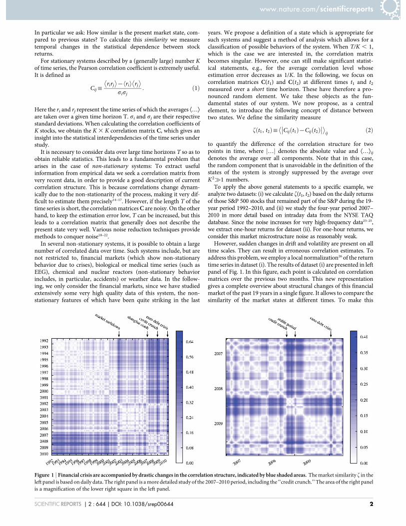
However, sudden changes in drift and volatility are present on alltime scales. They can result in erroneous correlation estimates. Toaddress this problem, we employ a local normalization26 of the returntime series in dataset (i). The results of dataset (i) are presented in leftpanel of Fig. 1. In this figure, each point is calculated on correlationmatrices over the previous two months. This new representationgives a complete overview about structural changes of this financialmarket of the past 19 years in a single figure. It allows to compare thesimilarity of the market states at different times. To make this

Figure 1 | Financial crisis are accompanied by drastic changes in the correlation structure, indicated by blue shaded areas. The market similarity f in theleft panel is based on daily data. The right panel is a more detailed study of the 2007–2010 period, including the ‘‘credit crunch.’’ The area of the right panelis a magnification of the lower right square in the left panel.

www.nature.com/scientificreports

SCIENTIFIC REPORTS | 2 : 644 | DOI: 10.1038/srep00644 2

procedure concrete, consider the following example. Pick a point onthe diagonal of this panel and designate it as ‘‘now’’. From this pointthe similarity to previous times can be found on the vertical lineabove this point, or the horizontal line to the left of this point.Light shading denotes similar market states and dark shadingdenotes dissimilar states. We can furthermore identify times of fin-ancial crises with dark shaded areas. This indicates that the correla-tion structure completely changes during a crisis. There are alsosimilarities between crises, as between the ‘‘credit crunch’’ thatinduced the 2008–2009 financial crisis and the ‘‘market meltdown’’,the burst of the ‘‘dot-com bubble’’ in 2002. A further example is theoverall rise in correlation level in the beginning of 2007. This eventcan be mapped to drastic events on the Shanghai stock exchange27.

Using dataset (ii) we are able to obtain a more detailed insight intorecent market changes, as shown in the right panel of Fig. 1. This areais represented by the lower right square of the left panel. Using intra-day data we calculate the correlation matrices on shorter time scales.We choose a time horizon of one week because it provides insightinto changes in the correlation structure on a much finer time scale.

This enables us to identify a short sub-period within the 2008–2009crisis (in the beginning of 2009) during which the market tempor-arily stabilizes before it returns to the crisis state. While the correla-tion structure during the crisis displays an overall high correlationlevel, the correlation structure of the stable period is similar to theperiod before the crisis, one of the typical states in a calm period,which is identified from daily data in dataset (i). This phenomenonmight be related to the market’s reaction to news about the progressin rescuing the American International Group (A.I.G.)28. The cor-relation structure of the stable period and the 2008–2009 crisis isshown in Supplementary Fig. S2 online.

The evolutionary structure presented in Fig. 1 illustrates that thecorrelation matrix sometimes maintains its structure for a long time(bright regions), sometimes changes abruptly (sharp blue stripes),and sometimes returns to a structure resembling a structure themarket has experienced before (white stripes). This suggests thatthe market might move among several typical market states. Toextract such typical market states, we perform a clustering analysisin the results of dataset (i). From our clustering analysis (see section

Figure 2 | The correlation between different industry branches as well as the intra-branch correlation characterize the different market states (a-h).The inter-branch correlation is represented by the off-diagonal blocks, and the intra-branch correlation is represented by the blocks on the diagonal.Legend: E: Energy, M: Materials, I: Industrials, CD: Consumer Discretionary, CS: Consumer Staples, H: Health Care, F: Financials, IT: InformationTechnology, C: Communication, U: Utilities. (i) Similarity tree structure of the 8 market states. (j) Illustration of the overall average correlation matrix.

www.nature.com/scientificreports

SCIENTIFIC REPORTS | 2 : 644 | DOI: 10.1038/srep00644 3

Methods), we find that there are ‘‘hidden’’ states sparsely embeddedin time, in addition to regimes that dominate the market during acontinuous period and are easily found by eye. The clustering ana-lysis separates the set of all correlation matrices, which are measuredon short disjoint subintervals of the observation period, into distinctclusters. The cluster centers then correspond to distinct correlationstructures which we identify as market states. We note that thisdefinition of market state depends on the length of the full obser-vation period to some extend. Enlarging the observation periodmight join previously distinct clusters, reducing it might furtherdivide a cluster.

For the clustering analysis, we use disjunct two-month timewindows ending at the respective dates. Because of the windowlength, some financial crashes cannot be resolved. Our aim israther to identify the evolution of the market, which is, in somecases, induced by financial crisis. We can confirm in Fig. 2 that thetypical states obtained from the clustering analysis indeed corre-spond to different characteristic correlation structures. To visualizethe characteristic structures of each state, we calculate its averagecorrelation matrix and sort the companies according to theirindustry branch, as defined by the Global Industry ClassificationStandard (GICS)29. In the resulting matrices, the industry branchescorrespond to the blocks on the diagonal. The correlation betweentwo branches are given by the off-diagonal blocks. The results areillustrated in Fig. 2. We can confirm that the typical states

obtained from the clustering analysis indeed correspond to differ-ent characteristic correlation structures.

Our analysis also offers insight into market structure dynamics.Figure 4 shows the temporal behavior of the market state. The marketsometimes remains for a long time in the same state, and sometimesstays only for a short time. The typical duration depends upon thestate: Some states (e.g., state 1 and state 2) appear in clusters in timewhile other states appear more sparsely in time (e.g., state 4). Thereseems to exist a global trend on a long time scale, although the marketstate is switching back and forth between states.

In Fig. 2, we can see differences between the states in the correla-tion between branches as well as in the correlation within a branch.The correlation within the energy, information technology, and util-ities branches is very strong in all states. State 1 shows an overall weakcorrelation, while states 3 and 4 feature in addition a strong correla-tion of the finance branch to other branches. State 2 shows veryunusual behavior: In the period of the dot-com bubble, manybranches are anti-correlated with one another. In states 5, 6 and 7,the overall correlation level rises, although certain branches, such asenergy, consumer staples, and utilities, are either strongly or weaklycorrelated with other branches. While some distinct characteristicsof states can be easily identified, some states look quite similar by eye.Their unique properties can be illustrated when subtracting the mar-ket’s overall correlation structure, as illustrated in Fig. 3. Forexample, state 3 and 4 look very similar in Fig. 2. However, Fig. 3

Figure 4 | Temporal evolution of the market state. The horizontal axis represents the observation time and the vertical axis denotes the market stateobtained from top-down clustering. The market state sometimes remains in the same state for a long time, and sometimes only for a short time. It also canreturn to a state that it has previously visited. Some states (e.g., state 1 and state 2) appear to cluster in time, while other states appear more sparsely andintermittently in time (e.g., state 4).

Figure 3 | (a)–(h): Difference of the states’ correlation matrices to the average correlation matrix. The color-scale is identical to Fig. 2.

www.nature.com/scientificreports

SCIENTIFIC REPORTS | 2 : 644 | DOI: 10.1038/srep00644 4

unveils that the correlation within the Energy sector (E) is completelydiverse.

We observe that the energy branch (E) is either strongly correlatedto the rest of the market, weakly correlated, or even anti-correlated.To analyze this behaviour we study the histogram of the correlationcoefficients Cij(t). We present the results in Fig. 5. In the monthsleading up to the credit crunch in October 2008, we observe a bimo-dal structure in the histogram (see also Ref. [30]). It corresponds tothe time period when the Energy branch shows a strong anti-cor-relation with other branches. The bimodality suggests that a subset ofstocks – in this case, predominantly the Energy stocks – decouplesfrom the rest of the market. During the crash, the histogram shows avery narrow distribution around large values of the correlation coef-ficients, which corresponds to state 8 in Fig. 2, where the branchstructure is lost almost completely in an overall strongly correlatedmarket.

MethodsConstruction of stock returns. Let S be the price of a specific stock andDt the intervalon which the return is calculated. For our study, we chose the arithmetic return,defined as

r t! ": S tzDt! "{S t! "S t! "

: !3"

For dataset (i), we chose Dt to be 1 day and calculate the stock returns of each day. Fordataset (ii), we choseDt as 1 hour. Furthermore, we obtain this 1-hour return for everyminute of a trading day between 10:45 am and 2:45 pm. We obtained the daily data ofdataset (i) from finance.yahoo.com. The intraday data are obtained from the NewYork Stock Exchange’s TAQ database.

Local normalization. Sudden changes in drift and volatility can result in erroneouscorrelation estimates. To address this problem, we employ a local normalizationmethod26. For each return r(t) we subtract the local mean and divide by the localstandard deviation,

~r t! ": r t! "{ r t! "h in$$$$$$$$$$$$$$$$$$$$$$$$$$$$$$$$$r2 t! "h in{ r t! "h i2n

q : !4"

The local average Æ…æn runs over the n most recent sampling points. For daily data,n 5 13 yields nearly normal distributed time series, as discussed in Ref. [26].

Outline of top-down clustering. Our clustering analysis is based on a top-downscheme: All m correlation matrices are initially regarded as a single cluster and thendivided into sub-clusters by a procedure based on the k-means algorithm31–33. Theprocess can be described as follows:

1. Choose two initial cluster centers from all matrices. Label all other matrices by themore similar cluster center in terms of j(L).

(a) Recast two new sub-cluster centers to the ‘‘center of mass’’ of the matricesin the sub-cluster.

(b) Re-label all matrices to the new sub-cluster center.(c) Repeat this process until there is no change in labeling.

Figure 5 | Footprint of the state transition in the 2008 crisis by histograms of the correlation coefficients Cij(t). (a) Surface plot for the time periodSeptember 2007 to March 2009. We use a logarithmic scale to show the bimodal structure more clearly. (b) Histograms for September 2008 (black solidline) and December 2008 (red dashed line).

Figure 6 | The entire tree of the clustering analysis presented here for thethreshold 0: No termination of the division process takes place until allthe correlation matrices are identified as different components. The largebold numbers represent the market states each of which consists of thematrices in the sub-trees below. Each right end of the tree corresponds toeach 2-month term (year-term). Terms 1, 2, …, 6 correspond to January toFebruary, March to April, …, November to December, respectively. Thelength of each branch represents the distance from the center of thesubcluster to the center of the original cluster before the last dual division.

www.nature.com/scientificreports

SCIENTIFIC REPORTS | 2 : 644 | DOI: 10.1038/srep00644 5

2. Take the best division out of all possible m(m – 1)/2 initial choices, which gives theleast average (j(L))2 to the cluster centers.

We stop this division process when the average distance from each cluster center toits members becomes smaller than a certain threshold. To identify the typical marketstates presented in the manuscript, we chose the threshold at 0.1465 as it represents(approximately) the best ratio of the distances between clusters and their intrinsicradius. One can obtain finer structures by choosing smaller threshold values, ulti-mately until all the matrices are identified as different components. The completeresults of the clustering analysis is illustrated in Fig. 6.

A possible alternative method for obtaining the states may be choosing a certainnumber of cluster centers from the beginning. However, of besides being morecomputationally intense, we believe that predefining the number of states would be asignificant disadvantage compared to our dynamic approach.

Alternative measure: Difference of largest eigenvalue of correlation matrices. Asimilar result can be archived using a different approach. The largest eigenvalue lmaxof the correlation matrix C describes the collective motion of all stocks. We can alsodefine the similarity measure by the distance of these eigenvalues,

jalt t1,t2! ": lmax C t1! "! "{lmax C t2! "! "j j: !5"

The advantage of this technique is that the noise in the correlation matrix onlycontributes to small eigenvalues (See Refs. [18] and [19]). Thus, by only taking intoaccount the largest one, we filter out the noise. However, this approach also presumesthat the corresponding eigenvector does not change. Our results indicate that thelargest eigenvalue almost remains constant, but this might not always be the case.Especially in financial crises. An alternative distance measure which takes intoaccount the changes in the eigenvectors is considered in Refs. [34, 35]. The obtainedsimilarity measure is shown in Supplementary Fig. S1 online.

1. Voit, J. The Statistical Mechanics of Financial Markets (Springer, Heidelberg,2001).

2. Mantegna, R. N. & Stanley, H. E. Stock market dynamics and turbulence: parallelanalysis of fluctuation phenomena. Physica A 239, 255–266 (1997).

3. Borghesi, C., Marsili, M. & Micciche, S. Emergence of time-horizon invariantcorrelation structure in financial returns by subtraction of the market mode.Physical Review E 76, 026104 (2007).

4. Cooley, T. F. & Quadrini, V. Financial markets and firm dynamics. The AmericanEconomic Review 91, 1286–1310 (2001).

5. Pelletier, D. Regime switching for dynamic correlations. Journal of Econometrics131, 445–473 (2006).

6. Xu, X. E., Chen, P. & Wu, C. Time and dynamic volume-volatility relation. Journalof Banking & Finance 30, 1535–1558 (2006).

7. King, M. & Wadhwani, S. Transmission of volatility between stock markets. TheReview of Financial Studies 3, 5–33 (1990).

8. Lee, S. The stability of the co-movements between real estate returns in the uk.Journal of Property Investment & Finance 24, 434–442 (2006).

9. Bouchaud, J. & Potters, M. Theory of Financial Risks (Cambridge University Press,Cambridge, 2000).

10. Eckmann, J.-P., Kamphorst, S. O. & Ruelle, D. Recurrence plots of dynamicalsystems. EPL (Europhysics Letters) 4, 973 (1987).

11. Casdagli, M. C. Recurrence plots revisited. Physica D: Nonlinear Phenomena 108,12–44 (1997).

12. Plerou, V., Gopikrishnan, P. & Stanley, E. Econophysics: Two-phase behaviour offinancial markets. Nature 421 (2003).

13. Plerou, V., Gopikrishnan, P. & Stanley, H. E. Two phase behaviour and thedistribution of volume. Quantitative Finance 5, 519–521 (2005).

14. Rosenow, B., Gopikrishnan, P., Plerou, V. & Stanley, H. E. Dynamics of cross-correlations in the stock market. Physica A 324, 241–246 (2003).

15. Tastan, H. Estimating time-varying conditional correlations between stock andforeign exchange markets. Physica A 360, 445–458 (2006).

16. Drozdz, S., Kwapien, J., Grmmer, F., Ruf, F. & Speth, J. Quantifying the dynamicsof financial correlations. Physica A 299, 144–153 (2001).

17. Schafer, R., Nilsson, N. & Guhr, T. Power mapping with dynamical adjustment forimproved portfolio optimization. Quantitative Finance (2009).

18. Laloux, L., Cizeau, P., Bouchaud, J.-P. & Potters, M. Noise dressing of financialcorrelation matrices. Physical Review Letters 83, 1467–1470 (1999).

19. Plerou, V. et al. Random matrix approach to cross correlations in financial data.Physical Review E 65, 066126 (2002).

20. Guhr, T. & Kalber, B. A new method to estimate the noise in financial correlationmatrices. Journal of Physics A: Mathematical and General 36, 3009–3032 (2003).

21. Schafer, J. & Strimmer, K. A shrinkage approach to large-scale covariance matrixestimation and implications for functional genomics. Statistical applications ingenetics and molecular biology 4 (2005).

22. Ledoit, O. & Wolf, M. Improved estimation of the covariance matrix of stockreturns with an application to portfolio selection. Journal of Empirical Finance 10,603–621 (2003).

23. Epps, T. W. Comovements in stock prices in the very short run. Journal of theAmerican Statistical Association 74, 291–298 (1979).

24. Munnix, M. C., Schafer, R. & Guhr, T. Compensating Asynchrony Effects in theCalculation of Financial Correlations. Physica A 389, 767–779 (2010).

25. Munnix, M. C., Schafer, R. & Guhr, T. Impact of the Tick-size on FinancialReturns and Correlations. Physica A 389, 4828–4843 (2010).

26. Schafer, R. & Guhr, T. Local normalization: Uncovering correlations in non-stationary financial time series. Physica A 389, 3856–3865 (2010).

27. What The Market Is Telling Us. Bloomberg Businessweek (2007). Cover story.28. A.I.G. Sells $39.3 Billion in Assets to N.Y. Fed’s Fund’. The New York Times

(2008).29. http://www.standardandpoors.com/indices/gics/en/us. accessed on 16 Aug 2012.30. Wyart, M. & Bouchaud, J.-P. Self-referential behaviour, overreaction and

conventions in financial markets. Journal of Economic Behavior & Organization63, 1–24 (2007).

31. MacQueen, J. B. Some methods for classification and analysis of multivariateobservations. In Cam, L. M. L. & Neyman, J. (eds.) Proc. of the fifth BerkeleySymposium on Mathematical Statistics and Probability, vol. 1, 281–297(University of California Press, 1967).

32. Faber, V. Clustering and the continuous k-means algorithm. Los Alamos Science22, 138–144 (1994).

33. Tanaka, N. K., Awasaki, T., Shimada, T. & Ito, K. Integration of chemosensorypathways in the drosophila second-order olfactory centers. Current biology 14,449–457 (2004).

34. Reigneron, P.-A., Allez, R. & Bouchaud, J.-P. Principal regression analysis and theindex leverage effect. Physica A 390, 3026–3035 (2011).

35. Allez, R. & Bouchaud, J.-P. Eigenvector dynamics: theory and some applicationsPreprint: arXiv:1108.4258. (2011).

AcknowledgmentsMCM acknowledges financial support from the Fulbright program and fromStudienstiftung des Deutschen Volkes. TS acknowledges support from the JSPSInstitutional Program for Young Researcher Overseas Visits, Grant-in-Aid for YoungScientists (B) no. 21740284 MEXT, Japan, and the Aihara Project, the FIRST program fromJSPS, initiated by CSTP. THS acknowledges support from project 79613 of CONACYT,Mexico. HES thanks the NSF for support.

Author contributionMCM, TS and RS performed the calculations and analyzed the results. MCM and RSprepared the figures. All authors designed the research and wrote and reviewed the paper.

Additional informationSupplementary information accompanies this paper at http://www.nature.com/scientificreports

Competing financial interests: The authors declare no competing financial interests.

License: This work is licensed under a Creative CommonsAttribution-NonCommercial-NoDerivative Works 3.0 Unported License. To view a copyof this license, visit http://creativecommons.org/licenses/by-nc-nd/3.0/

How to cite this article: Munnix, M.C. et al. Identifying States of a Financial Market. Sci.Rep. 2, 644; DOI:10.1038/srep00644 (2012).

www.nature.com/scientificreports

SCIENTIFIC REPORTS | 2 : 644 | DOI: 10.1038/srep00644 6