Identifying the Relative Importance of Stock Characteristics in the UK Market

Electronic copy available at: http://ssrn.com/abstract=2474175

1

Identifying the relative importance of stock characteristics in the UK market

Declan Frencha

Yuliang Wub*

Youwei Lic

This draft May 2014

Abstract

We address an important empirical question as to which firm-level characteristic best predicts stock returns in the UK equity market. To answer this question, we employ a semiparametric characteristic-based factor model first introduced by Connor, Hagmann and Linton (2012). We also augment their model by including the liquidity characteristic together with the market, size, momentum, volatility and book-to-market factors. We find that momentum is the most important factor and liquidity the least important based on their relative contribution to the fit of the model and the proportion of sample months for which factor returns are significant. Our main results are robust to the states of the economy and to the inclusion of the monthly reversal factor.

JEL classifications: G12

Key words: stock characteristics and factor models

a,b,c Queens University Belfast, School of Management, 185 Stranmillis Road, Belfast, BT9 5EE

*Correspondent author email address: [email protected]

Telephone: 0044-2890974717 Fax: 0044-2891974201

Acknowledgement: We are grateful to Gregory Connor and Oliver Linton for providing helpful comments.

Electronic copy available at: http://ssrn.com/abstract=2474175

2

Introduction

According to the one-factor Sharpe-Linter-Black capital asset pricing model (CAPM), stock

returns are only determined by stock price co-movements with the market portfolio.

Nevertheless, the vast majority of empirical evidence shows that cross-sectional stock returns

are additionally and significantly related to factors that are based on firm-level characteristics,

such as size (Banz, 1981; Reinganum, 1981 and Fama and French, 2012), book-to-market

equity (Fama and French, 1992; 1996; and Lakonishok et al., 1994), momentum (Jegadeesh

and Titman, 1993) and liquidity (Pastor and Stamagh 2003). A number of studies have

assessed the relative importance of these firm-level characteristics in predicting stock returns.

Asness et al. (2013) find that the momentum and value characteristics are more significant

than other characteristics in driving global equity returns. Ang et al. (2006) report that stock

volatility is an important characteristic for predicting future returns and the prediction power

of volatility cannot be explained by the three-factor (Fama and French, 1993) and the four-

factor (Carhart, 1997) models. Liu (2006) contends that firm-level liquidity can subsume the

value effect, indicating that value and growth stocks have, respectively, illiquid and liquid

features. This study employs the semiparametric characteristic-based factor model developed

by Connor, Hagmann and Linton (2012) (hereafter CHL) to identify the relative importance

among these characteristics using data on stocks listed on the London Stock Exchange (LSE).

Departing from CHL, we include the firm-level liquidity characteristic (Liu, 2006), which

combines the number of non-trading days with the turnover ratio, in the characteristic-based

factor model in addition to the market, size, book-to-market equity, momentum, and volatility

characteristics. This study is the first empirical analysis to apply the CHL approach outside

U.S. equity markets.

The CHL methodology builds upon an existing literature on characteristic-based factor

models. Following the stochastic factor model first introduced by Rosenberg (1974) , Fama

and French (1993) modify the Rosenberg approach by specifying the factors as the market

portfolio and two zero net-investment portfolios, one of which is long in high book-to-market

and short in low book-to-market stocks, while the other is long in small firms and short in

large firms. Daniel and Titman (1997) find that portfolios of firms with similar characteristics

(e.g. size and book-to-market), but with different loadings on the Fama and French factors,

have similar average returns, consistent with the notion that characteristic-based factors can

explain expected returns. Connor and Linton (2007) employ multivariate kernel methods to

obtain returns for factor-mimicking portfolios, which are used as independent variables to

3

estimate factor returns and betas from a parametric nonlinear regression. CHL (2012) modify

the Conor and Linton (2007) approach by estimating factor returns and beta directly from

individual stock characteristics instead of constructing factor-mimicking portfolios. The CHL

characteristic-based factor model is a weighted additive regression model in which each beta

function is a time-invariant unknown function of one stock characteristic while the

corresponding factor return is a time-varying parametric weight for the beta function.

The CHL methodology is implemented in the following three steps. First, stock returns are

cross-sectionally regressed on multiple stock characteristics as in Fama-MacBeth (1973).

Second, the coefficients associated with each stock characteristic act as factor returns in a

nonparametric regression to estimate each characteristic’s beta function. Finally, the factor

returns are re-estimated on the basis of the given beta function. The last two steps iterate until

estimates converge. This process is different to the procedure of creating factor-mimicking

portfolios (Fama and French 1993; 1996). Fama and French (1993) estimate the size and

value factor returns by double-sorting stocks in terms of size and the book-to-market ratio.

Then, factor betas are estimated by running a time-series regression on the factor returns. The

factor returns used in the Fama-French procedure lack rigorous statistical theory to justify

their consistency and also standard errors do not fully account for all sampling error. In

addition, when the estimated factor returns serve as explanatory variables in the time-series

regression, there is a potential errors-in-variables problem in the subsequent process of

estimating factor betas. In contrast, since the CHL approach uses all sample stocks’

characteristics to estimate each factor return and its associated beta, it is able to generate

consistent and asymptotically normal estimates for factor returns and betas that are not

obtainable by using the Fama-French procedure.

The other motivation in applying the CHL methodology is that this procedure allows any

number of characteristics in the factor model with no theoretical loss of efficiency. According

to the Fama-French approach, the value and size premia are obtained through double-sorting

stocks into size and value categories. In this way, adding a third characteristic requires triple-

sorting while quadruple-sorting is needed if adding a fourth factor. When factor numbers

increase, the number of stocks in a given characteristic-based portfolio will significantly

decrease, leading to less statistically reliable factor returns especially in the case of more than

three factors. One typical example is the work of Daniel et al. (1997) who formulate 125 (i.e.

5 5 5 ) characteristic-based benchmark portfolios for size, past one-year return and book-to-

market ratio. The method needs at least 3750 (i.e.30 125 ) sample stocks to eliminate

4

idiosyncratic risk in a given characteristic portfolio, making this method less implementable

to adjust raw returns for stocks outside U.S. equity markets. In contrast, in the CHL model,

the factor returns are obtained through estimating a nonlinear function for a given stock

characteristic without imposing any cut-off rate to define extreme stock characteristics.

We evaluate the relative importance of five stock characteristics (size, book-to-market equity,

momentum, volatility, and liquidity) in two ways. First, we consider the incremental

contribution of the characteristic of interest to the fit of the model. Each of the five stock

characteristics is combined with the market factor and the R2 is then compared to assess

explanatory power. In addition, we drop each of the characteristics from the complete model

and compare the reduction in R2 in each case. Second, since the CHL method can generate a

time-series of estimates for each factor return, we can test whether the factor return is

statistically different from zero in a given month. Then, the percentage of sample months in

which each factor return is significant can be a yardstick to evaluate the relative importance

among the five characteristics.

Our primary results show that the relationships between stock characteristics and their factor

betas are nonlinear. Consistent with the findings of Connor and Linton (2007), the evidence

suggests that factor premia exist in the full spectrum of sample stocks rather than just in

stocks with an extreme characteristic. However, the liquidity-beta function has a relatively

flat slope among the five characteristic-beta functions, implying that stocks returns are not as

sensitive to the liquidity premium as to other characteristics’ premia. In the R2 analysis, the

two-factor model that combines the market and momentum factors has the highest R2,

indicating the primacy of momentum in explaining variations in returns. In contrast, the

liquidity based two-factor model has the lowest R2, indicating its relative unimportance. Also

our results show that the momentum factor is statistically significant in a higher proportion of

sample months than other factors while the liquidity factor is significant least often. We

undertake various robustness tests to check the consistency of our results. When we separate

sample months according to the state of the economy, the results reveal that the momentum

and liquidity characteristics are the most and least important factors respectively even in a

downturn of the economy. Finally, we include stock previous month returns, as the month-

by-month reversal factor in addition to the six-factor model, to check the robustness of our

results. The result shows that the momentum characteristic remains the most important one.

While the study employs the new semiparametric technique to estimate factor returns and

5

betas for LSE listed stocks, our results are consistent with Hou et al. (2011) and Asness et al.

(2013) who emphasize the importance of momentum in explaining equity returns.

The paper proceeds as follows. Section 2 presents the methodology. Section 3 describes the

data. Section 4 reports results and Section 5 concludes.

2. Methodology

Rosenberg (1974) first models expected return as a linear combination of book-to-market

ratio and market value of equity. The factor returns are estimated by cross-sectional

regression of returns according to the betas. Thus, excess returns ity for stock i at time t is

linearly dependent on stock characteristics jX

1

,J

it ut jit jt itj

y f X f

(1)

where jtf is the factor returns for characteristic j and it are the mean zero asset specific

returns.

Fama and French (1993) modify the Rosenberg approach by approximating factor returns by

returns of constructed portfolios. Fama and French (1993) propose a two-stage method for

estimating characteristic-based factor models. In the first stage they sort assets into percentile

portfolios based on book-to-market ratio and market value characteristics. The differences

between returns on the percentile portfolios are proxies for the factor returnsjtF . The market

factor is a capitalization-weighted market index. In the second stage, the factor betas are

estimated by a time series regression of stock excess returns on the factors in Eq (2).

(2)

Connor and Linton (2007) combine the two approaches. They assume the factor betas are

smooth nonlinear functions of security characteristics. In a model with factors analogous to

Fama and French, they form a grid of equally spaced characteristic pairs. They use

multivariate kernel methods (see, e.g., Pagan and Ullah, 1999) to form factor-mimicking

portfolios for the characteristic pairs from each point on the grid. Then they estimate factor

returns and factor betas simultaneously using bilinear regression on the set of factor-

mimicking portfolio returns. More precisely, they specify a model of the form

01

J

it j jt itj

y F

6

1

J

it ut j ji jt itj

y f G X F

(3)

where the jtF are factor-mimicking portfolios constructed from a grid of characteristic pairs

using multivariate kernel approaches, and each jG is a smooth time-invariant function of

characteristic j, but they do not assume a particular functional form. The curse of

dimensionality (see Pagan and Ullah, 1999) limits the number of distinct factors that can be

used in Eq(3). The required portfolio sorting in the Fama and French model to create these

factors becomes infeasible for more than three factors with typical sample sizes.

CHL develop a new estimation methodology that efficiently uses both the time series and

cross-sectional dimensions of the data. By restricting the factor betas to be non-linear

functions of the security characteristics ,jiX they specify the following model

1

.J

it ut j ji jt itj

y f g X f

(4)

The univariate nonparametric functions jg are time-invariant while the factor returns jtf

vary over time. Given time period t, Eq (4) is a weighted additive nonparametric regression

model for panel data with time-varying parametric weights (jtf ).

CHL assume that the characteristic J-vectors of the assets ,jiX 1,...,i n are independent and

identically distributed across i. Under the identifying restriction that for each factor the cross

sectional average beta equals zero and the cross sectional variance of beta equals one,

[ ( )] 0j jiE g X and var[ ( )] 1,j jig X Connor et al. (2012) propose an iterative procedure to

estimate both the characteristic-beta functions and the factor returns in Eq (4) simultaneously

from data. It starts with period-by-period cross-sectional least squares regression of Eq (1),

and next the estimated factor returns ,ut jtf f are used to solve for jg by nonparametric

regression (see Connor et al., 2012 for details). Then the estimated functions jg are

inserted in Eq (4) and the factor returns ,ut jtf f are re-estimated by cross sectional regressions.

These last two steps iterate until a convergence criterion is satisfied. Connor et al. (2012)

establish the asymptotic theory for the suggested estimation procedure. In contrast to the

traditional portfolio approach, the recursive estimation procedure in Connor et al. (2012) does

not need any portfolio grouping or multivariate kernels in estimating the model. By avoiding

7

the curse of dimensionality the Connor et al. (2012) model allows for any number of factors

with no theoretical loss of efficiency.

3. Data and variables

Our sample includes all London Stock Exchange (LSE) listed stocks from October 1986 to

December 2011. The stock monthly return series, stock market capitalisation, stock book-to-

market ratio, and stock trading volume are extracted from Thomson Reuters Datastream. We

include only common stocks listed in LSE and exclude preferred stocks, unit trust, close-end

and open-end funds through filtering on data type. In addition, we check stock-quoted

currency and remove those that are not quoted in Sterling. This screening procedure filters

out stocks with American Depository Receipts traded in the LSE. Finally, we have a total

number of 7485 stocks with 528,539 firm-month observations.

The construction of size and value characteristics follows Fama and French (1993). We

require that each sample stock must have valid information for market capitalisation and

book-to-market ratio in June of each year. The size characteristic in each month equals the

logarithm of the previous June’s market value of equity. Likewise, the value characteristic

equals the ratio of the book value of equity to the market value of equity in the previous June.

In addition to the Fama-French size and value characteristics, we construct three additional

characteristics, namely momentum, volatility and liquidity. The effect of the three additional

characteristics on cross-sectional stock returns are well documented in the asset pricing

literature (e.g. Jegadeesh and Titman, 1993; Goyal and Santa-Clara, 2003 and Liu, 2006).

The momentum variable is measured as the cumulative twelve month return up to and

including the previous month. The volatility variable is defined as the standard deviation of

the stock return over twelve months up to and including the previous month. We use Liu’s

(2006) liquidity measure (LM12) which is defined as follows

12 [number of zero daily trading volumes in prior 12-month

1/12-month turnover 21 12 + ]

1,000,000

LM

NoTD

(5)

The first term in the bracket is the number of non-trading days for a given stock in the

previous 12- month period. The 12-month turnover is the sum of daily stock turnover over the

prior 12 months ending in the previous month. Daily stock turnover is the ratio of the number

of shares traded on a particular day to the number of shares outstanding at the end of the day.

8

The value of 1,000,000 is chosen as a deflator to constrain the term (1/ (12-month turnover)

1,000,000)

between zero and one1. NoTD is the number of trading days in prior 12 months. LM12

incorporates the number of non-trading days with the stock turnover ratio, making it ideal for

capturing trading continuity. For each stock, the size and value characteristics are held

constant from July to June while the momentum, volatility, and liquidity characteristics

change each month based on prior 12- month information. Accordingly, the empirical

analysis starts from October 1987, one year after the starting point of the dataset. Finally,

when we estimate the factor return function in Eq(4), the five characteristics are standardised

in each month to have zero mean and unit variance.

The construction of traditional factor-mimicking portfolios uses a predetermined cut-off rate

on stock characteristics. For example, stocks within the top and bottom 30% of book-to-

market ratio are defined as value and growth portfolios respectively in Fama and French

(1993). The value premium is the return difference between the value and growth portfolios.

The process of our factor return generation as specified in Eq(4) does not impose any cut-off

rate for a given stock characteristic. Rather, the factor return function is estimated

simultaneously from all sample stocks not only just from two particular portfolios with

strongest and weakest stock characteristics. This approach can potentially improve estimation

efficiency.

4. Results

4.1 Summary statistics

Insert Table 1 here

Table 1 reports firm characteristics for 7485 stocks from October 1987 to December 2011.

For each of five characteristics, we obtain each one’s cross-sectional mean in each month and

report their time-series averages across the sample period. Panel A is for the whole sample

period, while Panel B and C are for two sub-sample periods, October 1987 to December 1999

and January 2000 to December 2011, respectively. First, the average firm size in the UK

stock market has nearly doubled from a half million to one million pounds across the two

sub-sample periods. In contrast, the average of the book-to-market ratio remains relatively

1 By using the deflator, the number of non-trading days carries more importance than the stock turnover ratio. It is also equivalent to dependent double-sort on non-trading days first and then on the stock turnover ratio (Liu, 2006).

9

stable during the two periods (0.68 in the first period and 0.73 in the second period), although

in the later sample period the book-to-market ratio has a larger variation than in the earlier

one (standard deviation is 0.11 in the first period versus 0.33 in the second period). Whilst the

average of return volatility across all sample months is 0.13, it has also increased from the

first period (0.11) to the second period (0.14). In addition, the volatility measure in the

second period exhibits large positive skewness. Finally, while the overall liquidity measure in

the UK stock market is around 115.12, it has significantly decreased in the second sub-period

from 162 days in the first sub-period to 66 days in the second sub-period2.

4.2 Characteristic-beta functions

Insert Table 2 here

Table 2 reports the estimates of the characteristic-beta functions at selected percentiles and

the heteroskedasticity-consistent standard errors for each of these estimates.3 Across size,

book-to-market, momentum, volatility, and LM12, the standard errors are small in the middle

range of standardised characteristics where data is denser and are larger in the two tails where

the data is sparser. Estimates for the liquidity characteristic-beta in the bottom and top

quintiles do not vary because the data points for LM12 do not change below the 20th

percentile and beyond the 80th percentile. These values of the LM12 measure reflect that

some stocks have no zero-trading days in the previous 12-months while other stocks were

never traded during this period.

Insert Fig 1 here

The characteristic-beta functions across characteristic points are also plotted in Figure 1.

These characteristic-beta functions satisfy the equally-weighted zero mean and unit variance

identification conditions (in Section 2). Fig 1 shows that all five characteristic-beta functions

are generally upward-sloping but nonlinear. The positive relationships between book-to-

market, liquidity, volatility and momentum and betas are consistent with the existing

literature indicating that an increase in one stock characteristic raises its associated beta. The

relationship between size and beta is defined inversely to the Fama-French model in which a

stock’s size beta means its return sensitivity to the size premium between small and large

2 In Oct 1987, there are 289 firms with trading volume information. In December 2011, this number has increased to 1302. 3 Throughout this paper, semiparametric estimates were calculated using the bandwidth selection approach developed in Mammen and Park (2005) which relies on a penalised least squares framework. On this basis a bandwidth of 0.07 was selected in each application.

10

firms. A large firm should have a small size beta in the Fama-French model while in our

model large firms have large size betas by construction. The liquidity-beta function tends to

have a less steep slope than the other four beta functions. The result suggests that the liquidity

premium is not as significant as other characteristics’ premia. The value-beta function is

downward sloping at the high end of the value characteristic implying that the marginal

increase in the value premium is negative in this region. Fama and French (1993, 1996) claim

that the book-to-market ratio is a proxy for distress risk which is more prevalent in high

book-to-market firms. We find that the value-beta function has a rising slope for most firms

but not for extremely high book-to-market firms4.

Our finding of the nonlinearity of five characteristic-beta functions has implications for

analysis of characteristic-based return premia in equity markets. Our results suggest that

stock characteristics can be directly embedded in beta functions to estimate returns. It also

implies that the marginal return premium for each characteristic is not linearly proportional to

the difference in return premia between firms with extreme characteristics.

4.3 Factor correlations

In this subsection, we compare the estimated factors to the factor portfolio returns from the

original Fama-French procedure. RMRF is a market factor which is the value-weighted

market return over the 3-month UK Treasury bill rate. SMB is the monthly return difference

between small capitalisation portfolios minus large capitalisation portfolios. HML is the

monthly return difference between high book-to-market portfolios and low book-to-market

portfolios (Fama and French, 1993). FF_Mom is a momentum factor and is calculated as the

monthly return difference between past 12-month winner portfolios and loser portfolios

(Carhart, 1997). These factors are provided by Gregory et al. (2013)5. Liquidity is the return

difference between the top 30% of stocks and the bottom 30% of stocks in terms of Liu’s

liquidity measure (Liu, 2006) which is provided for the UK by Wu et al. (2012). The simple

correlation analysis can evaluate whether our semiparametric estimated factors are similar to

the Fama-French factors and whether the liquidity and volatility factors can provide

4 In addition, Dichev (1998) and Griffin and Lemmon (2002) find that most distressed stocks are growth stocks with low book-to-market ratios suggesting that the value feature is not a proxy for distress. 5 We are grateful to Gregory et al. (2013) for providing the UK Fama-French factors on their website, http://business-school.exeter.ac.uk/research/areas/centres/xfi/research/famafrench/files/.

11

additional information beyond the Fama-French factors. The correlation matrix in Table 3

shows results.

Insert Table 3 here

The estimated market factor has a correlation coefficient of 0.77 with RMRF6 while the

estimated momentum factor has a correlation coefficient of 0.64 with FF_Mom. The

correlation coefficient between the estimated book-to-market factor and HML is 0.60.

Liquidity has a correlation coefficient with LM12 of 0.31. The evidence reveals that although

we do not impose any predetermined cut-off rate to define extreme stock characteristics, the

semiparametric estimated factors share a large amount of similarities with the factors

generated by factor-mimicking portfolios. SMB has a negative correlation with size at -0.21.

This negative correlation is attributable to the model specification that the semiparametric

estimation procedure uses standardised firm size information to estimate the premium as

explained earlier. The estimated volatility factor has a positive correlation (0.57) with the

Fama-French market factor, implying that the volatility premium likely increases in a bull

market. However, the volatility factor has low correlations with SMB (0.41), HML (-0.19) and

FF_Mom (-0.06). Finally, LM12 has moderate correlations with RMRF (-0.32), SMB (-0.20),

HML(-0.25), and FF_Mom (0.20). The correlation analysis reveals that the estimated factors

are correlated with the factor-mimicking portfolios and that the two additional factors,

volatility and liquidity, contain some information outside the Fama-French three factors.

4.4 The explanatory power of estimated factors

4.4.1 Regression R2 of characteristic-based factor models

We use the average R2 of the cross-sectional regressions after convergence to assess the fit of

the model. Then, we evaluate the relative explanatory power of each characteristic in the

model in two ways. First, we singly add one of five factors along with the market factor to

formulate a two-factor model. Second, we take the difference in R2 between the 6-factor

model (by including all five characteristics) and the 5-factor model by dropping one of the

five factors except for the market factor. The R2 difference then can be interpreted as each

factor’s incremental explanatory power in the full model. Panel A in Table 4 shows results.

6 Connor and Korajczyk (1988) show that the dominant statistical factor in a large asset market is approximately identical to the equally-weighted index return. The market factor in our model is derived from the regressions with equal weights amongst a large sample of stocks. It is not surprising that the equally weighted market factor has a high correlation with the value weighted index return.

12

Insert Table 4 here

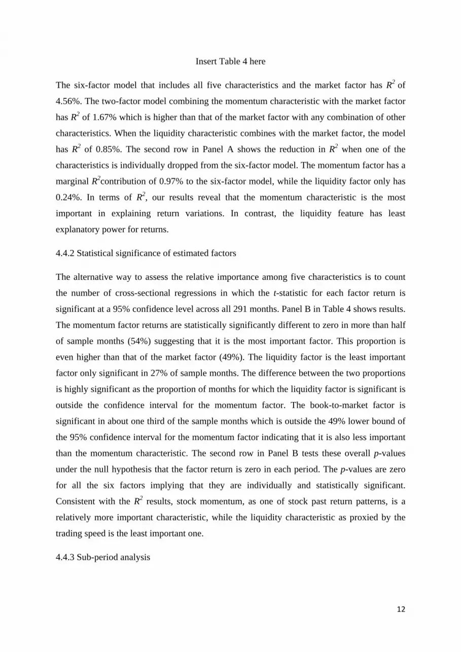
The six-factor model that includes all five characteristics and the market factor has R2 of

4.56%. The two-factor model combining the momentum characteristic with the market factor

has R2 of 1.67% which is higher than that of the market factor with any combination of other

characteristics. When the liquidity characteristic combines with the market factor, the model

has R2 of 0.85%. The second row in Panel A shows the reduction in R2 when one of the

characteristics is individually dropped from the six-factor model. The momentum factor has a

marginal R2contribution of 0.97% to the six-factor model, while the liquidity factor only has

0.24%. In terms of R2, our results reveal that the momentum characteristic is the most

important in explaining return variations. In contrast, the liquidity feature has least

explanatory power for returns.

4.4.2 Statistical significance of estimated factors

The alternative way to assess the relative importance among five characteristics is to count

the number of cross-sectional regressions in which the t-statistic for each factor return is

significant at a 95% confidence level across all 291 months. Panel B in Table 4 shows results.

The momentum factor returns are statistically significantly different to zero in more than half

of sample months (54%) suggesting that it is the most important factor. This proportion is

even higher than that of the market factor (49%). The liquidity factor is the least important

factor only significant in 27% of sample months. The difference between the two proportions

is highly significant as the proportion of months for which the liquidity factor is significant is

outside the confidence interval for the momentum factor. The book-to-market factor is

significant in about one third of the sample months which is outside the 49% lower bound of

the 95% confidence interval for the momentum factor indicating that it is also less important

than the momentum characteristic. The second row in Panel B tests these overall p-values

under the null hypothesis that the factor return is zero in each period. The p-values are zero

for all the six factors implying that they are individually and statistically significant.

Consistent with the R2 results, stock momentum, as one of stock past return patterns, is a

relatively more important characteristic, while the liquidity characteristic as proxied by the

trading speed is the least important one.

4.4.3 Sub-period analysis

13

The impact of stock characteristics on stock returns can also be dependent on economic

conditions. For example, Zhang (2005) contends that high book-to-market firms behave as

distressed firms in a downturn of the economy when the price of risk is high implying that the

value effect should be more pronounced in economic downturns rather than upturns. Petkova

and Zhang (2005) provide further empirical evidence that the value premium is higher in bad

times in support of Zhang (2005). Thus, it is worth examining whether the relative

importance among the factors will be changed dependent on economic conditions. To shed

light on this issue, we re-test the relative importance amongst the characteristics in different

states of the economy. We define up and downturns of the economy in three different ways

as the top and bottom quintile of sample months based on the UK GDP growth rate, the UK

industrial production growth rate and the UK term spread defined as the yield difference

between 10-year UK government bonds and T-bill respectively7. The three macro-economic

variables are widely used to indicate macro-economic conditions (e.g. Fama and French,

1988; 1989). Our choice of a cut-off rate of 20% to define the up- and down-turn of the

economy is consistent with Petkova and Zhang (2005). Table 5 shows results.

Insert Table 5 here

In terms of the GDP growth rate in Panel A, the market characteristic is significant in 57% of

the economy upturn months, while the momentum and size characteristics are significant in

exactly half of the economy upturns, followed by the volatility (45%), the book-to-market

(43%) and the liquidity (33%) characteristics. In times of economy downturns, the

momentum characteristic is statistically significant in 67% of months which is higher than the

market factor (52%). The difference of 15% is also statistically significant because 67% is

outside the upper bound of the 95% confidence interval for the market factor. Inconsistent

with Zhang (2005)’s explanations for the book-to-market effect, we find that the book-to-

market characteristic is more significant in economy upturns than in downturns (43% against

32%). The characteristic of stock liquidity is significant only in 37% of the downturn months

which is roughly the same as that of the upturn months (33%). The result suggests that

liquidity is relatively less important for stock returns regardless of the state of the economy.

We then use an alternative definition of states of the economy. Panel B separates the sample

months according to the industrial production growth rate. The momentum factor is

significant in 58% of the upturn months and 53% for the downturn months. For the book-to-

7 The information on the three variables was downloaded from Datastream.

14

market characteristic, there is no statistical difference between up and downturns. The

liquidity characteristic is only significant in 32% and 29% of the upturn and downturn

months, respectively, which are the two lowest ratios among the six characteristics. It should

be noted that the momentum effect is significantly different to the liquidity effect (58%

against 32%) indicating that the momentum characteristic is more important than liquidity in

predicting stock returns. When we use the term spread to define up and downturns in Panel C,

our main results are nearly unchanged. The momentum characteristic is of similar importance

to that of the market, while the liquidity characteristic remains the least important.

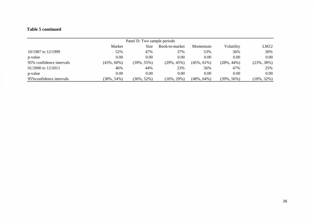
Since Datastream provides few firms’ information on trading volume at the start of sample

period, we separate the whole sample into the earlier period (10/1987 to 12/1999) and the

later period (01/2000 to 12/2011) when the trading volume information has a wide coverage.

Panel D reports results. In the earlier period, the momentum characteristic is significant in 53%

of the sub-period months and this ratio is roughly the same as that of the market factor. In the

later period, the momentum effect seems to be more important than the market effect, since

the ratio of 56% is significantly higher than 46%. In both periods, the liquidity characteristic

is significant in less than one-third of sample months. We also find that the book-to-market

effect is also relatively weaker in the second sample period. Overall, our results indicate that

the characteristics of book-to-market and liquidity are less important than other four

characteristics, while the momentum characteristic is the most important one in the two

periods.

4.5 Robustness check

Our primary result show the importance of the momentum characteristic in predicting stock

returns, implying that past return information may affect investor behaviour in making

investments. To check the robustness of the importance of momentum, we include the lagged

monthly return as an additional control factor together with previous factors. We call the new

factor the monthly reversal factor8. If investors are more responsive to the most recent return

information, the momentum effect, as an aggregate of past 12-month information, may

become weak. We repeat the previous analysis in Table 4 by including the new monthly

8 Stock returns also exhibit a negative autocorrelation across two consecutive months (Hameed and Mian, 2013; Jegadeesh, 1990 and Da et al. 2014), which is called month-by-month return reversals. This return irregularity implies that a stock’s previous month return is also an important characteristic in influencing the next month’s returns.

15

reversal factor, and our full model is the seven-factor model. New results are reported in

Table 69.

Insert Table 6 about here

Panel A reports that R2 for the full model is 4.95%, which is slightly higher than the six-

factor model of 4.56% in Table 4. In the second row, if one of factors is dropped from the

seven-factor model, the R2 is less affected by liquidity (0.26%) and lagged returns (0.35%)

and more by momentum. Therefore, by including the new monthly reversal factor as a control,

the importance of momentum remains the same as in our previous results. Panel B shows the

percentage of months in which each factor is statistically significant. The market factor is

significant in 49% of sample months. Amongst other characteristics, the momentum factor

has the highest percentage ratio at 53% indicating that it is relatively more important than

others. In contrast, the characteristics of liquidity and lagged returns are significant in only 28%

and 13% of sample months respectively. The second last row tests the null hypothesis that

each of the monthly factor returns is zero. The results show that we can reject this null

hypothesis for all seven factors. The evidence that the importance of the momentum

characteristic is robust to the monthly reversal factor suggests that investors are likely to

make investment decisions according to past price trends.

5. Conclusions

This study addresses an important empirical question as to which firm-level characteristic

best predicts stock returns in the UK market. To answer this question, we employ a

semiparametric approach to estimate the characteristic-based factor model first introduced by

CHL. While this study is the first out-of-sample analysis to apply the new method, we also

augment the CHL model by including the liquidity characteristic (Liu, 2006) along with the

market, size, book-to-market, volatility and momentum factors. Following the CHL

methodology, we find that factor betas exhibit nonlinear relationships with stock

characteristics consistent with Connor and Linton (2007) and CHL. The nonlinearity implies

that the marginal return premium for each characteristic is not linearly proportional to the

difference in return premia between firms with extreme characteristics. We also find that the

liquidity-beta function is relatively flat compared to other characteristic-beta functions

9 Results based on the state of the economy are omitted to save space. These results are generally consistent with our main results and are available upon request.

16

suggesting that stock returns are not as sensitive to the liquidity premium as to other

characteristics’ premia.

We evaluate the relative importance among stock characteristics in terms of the fit of the

model and the percentage of months in which each factor is significant. We find that the

momentum characteristic is relatively more important and gives a greater contribution to R2

than other characteristics. In contrast, the liquidity characteristic contributes least to R2. The

momentum factor is significant in half of the sample months, while the liquidity factor is

significant in less than one third of the sample months. The result that the momentum and

liquidity characteristics are most and least important holds when we separate the sample

months according to the economy downturns and upturns and the earlier and later sample

periods. Finally, when we add the monthly reversal factor to check the robustness of the

momentum effect, we still find strong return explanatory power for momentum and relatively

weak explanatory power for liquidity.

Since the momentum characteristic is typically classified as a non-risk characteristic

(Brennan et al. 1998) , our evidence supports the view that a stock’s past return pattern can

significantly influence investment decisions consistent with investor irrational behaviour

driving stock returns. However, the liquidity characteristic that is proxied by stock trading

continuity shows its relative unimportance in explaining stock returns after controlling for

other characteristics. The evidence implies that investors might consider past return patterns

as one of their first line criteria when making investments rather than how fast they can sell

stocks.

17

References:

Ang, A., Hodrick, R. J., Xing, Y., & Zhang, X. (2006). The cross‐section of volatility and expected returns. The Journal of Finance, 61(1), 259-299.

Asness, C. S., Moskowitz, T. J., & Pedersen, L. H. (2013). Value and momentum everywhere. The Journal of Finance, 68(3), 929-985.

Banz, R. W. (1981). The relationship between return and market value of common stocks. Journal of Financial Economics, 9(1), 3-18.

Brennan, M. J., Chordia, T., & Subrahmanyam, A. (1998). Alternative factor specifications, security characteristics, and the cross-section of expected stock returns. Journal of Financial Economics, 49(3), 345-373.

Carhart, M. M. (1997). On persistence in mutual fund performance. The Journal of Finance, 52(1), 57-82.

Connor, G., Hagmann, M., & Linton, O. (2012). Efficient semiparametric estimation of the Fama–French model and extensions. Econometrica, 80(2), 713-754.

Connor, G., & Korajczyk, R. A. (1988). Risk and return in an equilibrium APT: Application of a new test methodology. Journal of Financial Economics, 21(2), 255-289.

Connor, G., & Linton, O. (2007). Semiparametric estimation of a characteristic-based factor model of common stock returns. Journal of Empirical Finance, 14(5), 694-717.

Da, Z., Liu, Q., & Schaumburg, E. (2013). A closer look at the short-term return reversal. Management Science, 60(3), 658-674.

Daniel, K., & Titman, S. (1997). Evidence on the characteristics of cross sectional variation in stock returns. The Journal of Finance, 52(1), 1-33.

Daniel, K., Grinblatt, M., Titman, S., & Wermers, R. (1997). Measuring mutual fund performance with characteristic‐based benchmarks. The Journal of Finance, 52(3), 1035-1058.

Dichev, I. D. (1998). Is the risk of bankruptcy a systematic risk? The Journal of Finance, 53(3), 1131-1147.

Fama, E. F., & French, K. R. (1988). Dividend yields and expected stock returns, Journal of Financial Economics, 21(1), 3-25

Fama, E. F., & French, K. R. (1989). Business conditions and expected returns on stocks and bonds, Journal of Financial Economics, 25(1), 23-49

Fama, E. F., & French, K. R. (1992). The cross‐section of expected stock returns. The Journal of Finance, 47(2), 427-465.

18

Fama, E. F., & French, K. R. (1993). Common risk factors in the returns on stocks and bonds. Journal of Financial Economics, 33(1), 3-56.

Fama, E. F., & French, K. R. (1996). Multifactor explanations of asset pricing anomalies. The Journal of Finance, 51(1), 55-84.

Fama, E. F., & French, K. R. (2012). Size, value, and momentum in international stock returns. Journal of Financial Economics, 105(3), 457-472.

Fama, E. F., & MacBeth, J. D. (1973). Risk, return, and equilibrium: Empirical tests. The Journal of Political Economy, , 607-636.

Goyal, A., & Santa‐Clara, P. (2003). Idiosyncratic risk matters! The Journal of Finance, 58(3), 975-1008.

Gregory, A., Tharyan, R., & Christidis, A. (2013). Constructing and testing alternative versions of the Fama–French and Carhart models in the UK. Journal of Business Finance & Accounting, 40(1-2), 172-214.

Griffin, J. M., & Lemmon, M. L. (2002). Book–to–market equity, distress risk, and stock returns. The Journal of Finance, 57(5), 2317-2336.

Hameed, A., Huang, J., & Mian, G. M. (2014). Industries and stock return reversals. Journal of Financial and Quantitative analysis, forthcoming

Hou, K., Karolyi, G. A., & Kho, B. (2011). What factors drive global stock returns? Review of Financial Studies, 24(8), 2527-2574.

Jegadeesh, N. (1990). Evidence of predictable behavior of security returns. The Journal of Finance, 45(3), 881-898.

Jegadeesh, N., & Titman, S. (1993). Returns to buying winners and selling losers: Implications for stock market efficiency. The Journal of Finance, 48(1), 65-91.

Lakonishok, J., Shleifer, A., & Vishny, R. W. (1994). Contrarian investment, extrapolation, and risk. The Journal of Finance, 49(5), 1541-1578.

Liu, W. (2006). A liquidity-augmented capital asset pricing model. Journal of Financial Economics, 82(3), 631-671.

Mammen, E., & Park, B. U. (2005). Bandwidth selection for smooth backfitting in additive models. Annals of Statistics, 1260-1294.

Pagan, A., & Ullah, A. (1999). Nonparametric econometrics Cambridge university press.

Pastor, L. & Stambaugh, R.F. (2003). Liquidity risk and expected stock returns. Journal of Political Economy, 111(3), 642-685.

Petkova, R., & Zhang, L. (2005). Is value riskier than growth? Journal of Financial Economics, 78(1), 187-202.

19

Reinganum, M. R. (1981). Misspecification of capital asset pricing: Empirical anomalies based on earnings' yields and market values. Journal of Financial Economics, 9(1), 19-46.

Rosenberg, B. (1974). Extra-market components of covariance in security returns. Journal of Financial and Quantitative Analysis, 9(02), 263-274.

Wu, Y., Li, Y., & Hamill, P. (2012). Do Low‐Priced stocks drive Long‐Term contrarian performance on the London stock exchange? Financial Review, 47(3), 501-530.

Zhang, L. (2005). The value premium. The Journal of Finance, 60(1), 67-103.

20

Table 1 Summary statistics

This table reports summary statistics for 7485 stocks between October 1987 and December 2011 in the UK market. The variable size is a stock’s total market capitalisation. The variable book-to-market is a stock’s book value equity over its market value equity. The variable momentum is a stock’s cumulative prior twelve monthly returns including the previous month. The measure of volatility is defined as the standard deviation of the stock return over twelve months up to and including the previous month. The liquidity variable (LM12) is defined as

1/12-month turnover 21 1212 [number of zero daily trading volumes in prior 12-month+ ]

1,000,000LM

NoTD

The first term in the bracket is the number of non-trading days for a given stock in prior 12- month period. 12-month turnover is the sum of daily stock turnover over the prior 12 months ending in the previous month. Daily stock turnover is the ratio of the number of shares traded on a particular day to the number of shares outstanding at the end of the day. The value of 1,000,000 is chosen as a deflator

to constrain the term (1/ (12-month turnover)

1,000,000) between zero and one. NoTD is the number of trading

days in prior 12 months. For each of five stock characteristics, we obtain the cross-sectional mean in each month and report their time-series averages across the sample period in the table.

Size(£1,000) Book-to-market Mom. Volatility LM12Mean 741.7 0.7036 -0.0399 0.1252 115.13Median 744.8 0.7015 0.0015 0.1226 101.55Std. 312.75 0.2461 0.2506 0.0305 58.19Skewness 0.0165 1.3349 -0.8512 0.9520 0.65

Mean 490.04 0.6804 0.0115 0.1071 162.77Median 461.43 0.6692 0.0170 0.1046 148.88Std. 188.02 0.1088 0.1807 0.0206 42.85Skewness 0.9834 0.2986 0.1646 0.4016 0.40

Mean 1002.17 0.7277 -0.0931 0.1440 66.4Median 1021.08 0.7684 -0.0080 0.1386 64.25Std. 169.62 0.332 0.2981 0.0278 15.71Skewness -0.3514 0.9059 -0.7327 1.4976 0.45

Panel A: The whole sample

Panel B: October 1987 to December 1999

Panel C: January 2000 to December 2011

21

Table 2 Characteristic beta functions

This table shows the estimated factor betas for each point on the selected percentiles of characteristic values. The model is estimated by weighted nonlinear regression using a 6-factor model. The factor betas are restricted to have average zero and variance one for identification condition.

CharacteristicPercentile Coef. Std.error Coef. Std.error Coef. Std.error Coef. Std.error Coef. Std.error

2.5% -1.856 0.097 -1.817 0.066 -2.636 0.144 -1.140 0.067 -0.917 0.0765% -1.445 0.081 -1.122 0.064 -2.513 0.088 -1.052 0.064 -0.917 0.076

10% -1.182 0.069 -0.871 0.064 -1.406 0.061 -0.960 0.061 -0.917 0.07620% -1.080 0.058 -0.606 0.064 -0.837 0.049 -0.831 0.057 -0.917 0.07630% -0.593 0.053 -0.393 0.063 -0.345 0.046 -0.715 0.055 -0.919 0.07440% -0.354 0.050 -0.189 0.063 -0.126 0.046 -0.517 0.053 -0.812 0.06750% -0.225 0.049 0.047 0.063 0.046 0.046 -0.261 0.051 -0.588 0.06060% 0.113 0.049 0.253 0.063 0.434 0.047 0.002 0.050 0.031 0.05970% 0.615 0.052 0.488 0.063 0.643 0.048 0.338 0.051 0.570 0.07480% 1.064 0.058 0.684 0.064 0.769 0.051 0.807 0.053 1.443 0.09190% 1.634 0.078 0.998 0.065 1.019 0.058 1.677 0.066 1.443 0.09195% 1.704 0.110 1.191 0.067 1.292 0.069 2.425 0.098 1.443 0.091

97.5% 1.568 0.160 0.768 0.072 1.881 0.090 3.446 0.165 1.443 0.091

Size Book-to-market Momentum Volatiltiy LM12

22

Figure 1 Non-linear characteristic beta functions

The figure shows characteristic beta functions for size, book-to-market, momentum, volatility, and liquidity. Results for each function are displayed over a support ranging from the 2.5% to the 97.5% percentile of the respective stock characteristic.

-3.0

-2.0

-1.0

0.0

1.0

2.0

3.0

4.0

-1.7 -1.2 -0.7 -0.2 0.3 0.8 1.3 1.8

Size beta function

-3.0

-2.0

-1.0

0.0

1.0

2.0

3.0

4.0

-0.5 -0.25 0 0.25 0.5

Value beta function

-3.0

-2.0

-1.0

0.0

1.0

2.0

3.0

4.0

-2.2 -1.7 -1.2 -0.7 -0.2 0.3 0.8 1.3

Momentum beta function

-3.0

-2.0

-1.0

0.0

1.0

2.0

3.0

4.0

-1.1 -0.6 -0.1 0.4 0.9 1.4 1.9

Volatility beta function

-3.0

-2.0

-1.0

0.0

1.0

2.0

3.0

4.0

-1.1 -0.6 -0.1 0.4 0.9

Liquidity beta function

23

Table 3 Correlations between estimated factor returns and factor mimicking portfolio returns

This table provides correlations between the semiparametric approach to estimating factors with the Fama-French (e.g. RMRF, SMB, and HML), the liquidity (liquidity) and the momentum factor (FF_Mom) mimicking portfolio returns. RMRF is a market factor which is the value-weighted market return over the 3-month UK Treasury bill rate. SMB is the monthly return difference between small capitalisation portfolios and large capitalisation portfolios. HML is the monthly return difference between high book-to-market portfolios and low book-to-market portfolios. FF_Mom is the monthly return difference between past 12-month winner portfolios and loser portfolios. Liquidity is the return difference between low liquidity portfolios and high liquidity portfolios based on zero trading days and the share turnover ratio during past 12 months.

Market Size Book-to-market Mom. Volatility LM12 RMRF SMB HML FF_Mom LiquidityMarket 1Size 0.18 1Book-to-market -0.15 0.41 1Mom. -0.42 -0.11 -0.17 1Volatility 0.67 0.18 -0.25 -0.17 1LM12 -0.34 0.21 -0.02 0.17 -0.27 1RMRF 0.77 0.53 -0.01 -0.24 0.57 -0.32 1SMB 0.50 -0.21 -0.19 -0.30 0.41 -0.20 0.01 1HML 0.07 0.15 0.60 -0.41 -0.19 -0.25 0.05 -0.03 1FF_Mom -0.17 -0.29 -0.30 0.64 -0.06 0.20 -0.15 -0.12 -0.51 1Liquidity 0.05 0.60 0.27 -0.06 0.11 0.31 0.41 -0.31 0.14 -0.36 1

24

Table 4 Regression R2 analysis and statistical significance of factors

This table shows the time-series averages of R2 statistics as a measure of the explanatory power of the factor model and the percentage of months in which each factor is statistically significant. The six-factor model includes the market, size, book-to-market, momentum, volatility and LM12 factors. The first row in Panel A shows average R2 from cross-sectional regressions when one factor is combined with the market factor. The second row in Panel A shows changes of average R2 from cross-sectional regressions when one factor is dropped from the six-factor model. Panel B shows the percentage of months in which each factor is statistically significant. The 95% confidence interval and the associated p-value are based on count statistics with binomial distributions under the null hypothesis that the factor return is zero in each period.

Six-factor model Size Book-to-market Momentum Volatility LM12Adding first in the one-factor model 4.56% 1.26% 0.78% 1.67% 1.63% 0.85%Dropping first in the six-factor model 0.60% 0.50% 0.97% 0.70% 0.24%

Market Size Book-to-market Momentum Volatility LM12Number of periods statistically sig. 49% 45% 30% 54% 42% 27%p -value 0.00 0.00 0.00 0.00 0.00 0.0095% confidence intervals (43%, 55%) (40%, 51%) (25%, 35%) (49%, 60%) (36%, 47%) (22%, 33%)

Panel A:Marginal R-square statistics when adding first or dropping first in the model

Panel B: Number of period sig.

25

Table 5 Sub-period analysis

The table reports the percentage of months in which each characteristic-based factor is statistically significant at the 5% level. We use three variables to define up and downturns of the economy in Panels A, B, and C by the GDP growth, the industrial production growth and the term spread respectively. ‘Upturns’ and ‘downturns’ are the top and bottom 20% of months according to one of the above macro-economic variables. In Panel D, we further separate the sample into the earlier period (10/1987 to 12/1999) and the later period (01/2000 to 12/2011). The 95% confidence interval and the associated p-value are based on count statistics with binomial distributions under the null hypothesis that the factor return is zero in each period.

Market Size Book-to-market Momentum Volatility LM12Upturns % significant 57% 50% 43% 50% 45% 33%

p -value 0.00 0.00 0.00 0.00 0.00 0.0095% confidence intervals (44%, 69%) (37%, 63%) (31%, 56%) (37%, 63%) (32%, 58%) (21%, 45%)

Downturns % significant 52% 50% 32% 67% 42% 37%p -value 0.00 0.00 0.00 0.00 0.00 0.0095% confidence intervals (39%, 64%) (37%, 63%) (20%, 43%) (55%, 79%) (29%, 54%) (24%, 49%)

Upturns % significant 45% 53% 33% 58% 45% 32%p -value 0.00 0.00 0.00 0.00 0.00 0.0095% confidence intervals (32%, 58%) (41%, 66%) (21%, 45%) (46%, 71%) (32%, 58%) (20%, 43%)


Upturns % significant 47% 47% 36% 56% 34% 24%p -value 0.00 0.00 0.00 0.00 0.00 0.0095% confidence intervals (35%, 60%) (35%, 60%) (23%, 48%) (43%, 69%) (22%, 46%) (13%, 35%)


Panel A: GDP Growth

Panel B: Industrial Production Growth

Panel C: Term Spread

26

Table 5 continued

Market Size Book-to-market Momentum Volatility LM1210/1987 to 12/1999 52% 47% 37% 53% 36% 30%p-value 0.00 0.00 0.00 0.00 0.00 0.0095% confidence intervals (43%, 60%) (39%, 55%) (29%, 45%) (45%, 61%) (28%, 44%) (23%, 38%)01/2000 to 12/2011 46% 44% 23% 56% 47% 25%p-value 0.00 0.00 0.00 0.00 0.00 0.0095%confidence intervals (38%, 54%) (36%, 52%) (16%, 29%) (48%, 64%) (39%, 56%) (18%, 32%)

Panel D: Two sample periods

27

Table 6 Robustness check

This table shows the time-series averages of R2 statistics as a measure of the explanatory power of the factor model and the percentage of months in which each factor is statistically significant. The seven-factor model includes the market, size, book-to-market, momentum, volatility, LM12 and monthly reversal factors. The monthly reversal factor (Lag_ret) is a stock’s previous monthly return which is used to control for month-by-month return reversals. The first row in Panel A shows average R2 from cross-sectional regressions when one factor is combined with the market factor. The second row in Panel A shows changes of average R2 from cross-sectional regressions when one factor is dropped from the seven-factor model. Panel B shows the percentage of months in which each factor is statistically significant. The 95% confidence interval and the associated p-value are based on count statistics with binomial distributions under the null hypothesis that the factor return is zero in each period.

Seven-factor model Size Book-to-market Momentum Volatility LM12 Lag_ret

Adding first in the one-factor model 4.95% 1.27% 0.79% 1.68% 1.62% 0.89% 0.80%

Dropping first in the seven-factor model 0.56% 0.54% 0.85% 0.64% 0.26% 0.35%

Market Size Book-to-market Momentum Volatility LM12 Lag_ret

% Number of periods statistically sig. 49% 47% 31% 53% 39% 28% 13%

p -value 0.00 0.00 0.00 0.00 0.00 0.00 0.00

95% confidence intervals (43%, 55%) (41%, 53%) (26%, 36%) (47%, 59%)(34%, 45%) (22%, 33%) (9%, 17%)

Panel A:Marginal R -square statistics when adding first or dropping first in the model

Panel B: Number of period sig.

Identifying the Relative Importance of Stock Characteristics in the UK Market

Documents

Transcript of Identifying the Relative Importance of Stock Characteristics in the UK Market