The financial accelerator in the housing

market via collateral effects and the role

of monetary policy in an estimated New

Keynesian DSGE model

A Norwegian case study

Dior Kurta

Master thesis for the Master of Philosophy in Economics

degree

Department of Economics

UNIVERSITY I OSLO

May 2011

II

© Dior Kurta

2010

The financial accelerator in the housing market through collateral effects and the role of

monetary policy in an estimated New Keynesian DSGE model: A Norwegian case study

Dior Kurta

http://www.duo.uio.no/

Trykk: Reprosentralen, Universitetet i Oslo

IV

Preface

This master thesis marks the end of my master degree in Economics at the University of Oslo.

Als meus pares

I would like to express my gratitude towards my supervisor Tommy Sveen for coming up

with the idea of writing about the financial accelerator within the housing market, teaching

me the programming tool Dynare and for answering my countless e-mails. I would also like to

thank Norges Bank for providing me with data. Ragnar Nymoen, Asbjørn Rødseth, Steinar

Holden and Nina Midthjell from the university were also of great assistance in the process.

I am eternally grateful to my good friend Kenneth for reading through my thesis and giving

me invaluable pointers; let`s call it even mate. On that note, I would also like to thank Ellen

for proofreading parts of my thesis, and for encouraging my caffeine addiction with coffee

breaks these 5 years at the Uni. Lastly, I would like to thank my family for the great support I

have received.

All remaining errors and weaknesses are my own responsibility.

Dior Kurta, May 2011

VI

Abstract

This thesis aims to show the financial accelerator mechanism in the housing sector using

Norwegian data for the period 1995-2010. Housing is the most important investment decision

an agent makes during his/her lifetime. Most Norwegian households own their own home and

have during the last 15 years experienced an astonishing 400% nominal rate of return on their

investment. Mortgage Equity Withdrawal (MEW) is a relatively new phenomenon that allows

households to withdraw money from increasing housing markets to finance increased

spending today. Seeing that more than 50% of household assets are tied to housing, adverse

changes in the housing market will consequently have severe repercussions for the rest of the

economy through the MEW channel. Real and monetary shocks hitting the economy affect

the net worth of households and therefore amplify and propagate the initial shock, making it

more persistent and longer lasting. This is known as the financial accelerator in the literature.

This thesis is divided into two parts. First, I estimate a closed economy New

Keynesian Dynamic Stochastic General Equilibrium (DSGE) model for Norwegian data using

a Bayesian framework. I then look into the importance of collateral effects in amplifying

monetary shocks to the economy and hypothesise what would happen if the wage share of the

credit constrained consumers increase. I find that during the last decade, there has been a

liberalisation of credit markets and it has become increasingly easier to obtain credit, leading

to the consumption boom we are experiencing. Having realised that the sheer size of

household debt has grown substantially more than income the last couple of decades, it is a

concerning development and one that should not be taken easily. Second, I look into the

monetary policy rule and theorise whether central banks should aim to stabilise asset prices as

well as keeping inflation and output stable. I find that incorporating asset prices in the policy

specification of the central bank leads to a statistically insignificant coefficient. This is not in

contrast to the literature on this field of research, although some studies have conversely

found that it will be welfare enhancing for the central bank to stabilise asset prices as well.

Content

1 Introduction ............................................................................................................................. 1

2 Defining the financial accelerator and financial frictions ....................................................... 2

2.1 The financial accelerator .................................................................................................. 2

2.2 The financial accelerator in the housing sector ................................................................ 4

3 Key Characteristics of the Housing Sector ............................................................................. 8

3.1 Household saving and investment .................................................................................... 8

3.2 Developments in the housing sector............................................................................... 11

3.3 Determinants of the housing market .............................................................................. 14

3.4 Similarities and differences between housing and other financial assets ....................... 16

3.5 Bubbles ........................................................................................................................... 17

4 Modelling Housing Spillovers .............................................................................................. 20

4.1 Current modelling approaches and monetary policy rules ............................................. 20

4.2 The New Keynesian Dynamic Stochastic General Equilibrium Model ......................... 22

4.2.1 Households .............................................................................................................. 23

4.2.2 Entrepreneurs .......................................................................................................... 25

4.2.3 Retailers ................................................................................................................... 26

4.2.4 The central bank ...................................................................................................... 27

4.2.5 Equilibrium .............................................................................................................. 27

5 Quantitative Policy Analyses and Estimation ....................................................................... 31

5.1 Methodology and data .................................................................................................... 31

5.2 Calibrated parameters ..................................................................................................... 32

5.3 Bayesian estimation ........................................................................................................ 33

5.3.1 Prior distribution ..................................................................................................... 35

5.3.2 Posterior distribution ............................................................................................... 36

5.4 Properties of the estimated DSGE model ....................................................................... 39

5.5 Central bank reacting to house prices ............................................................................ 46

6 Limitations and Areas of Further Research ........................................................................... 50

7 Conclusion ............................................................................................................................. 52

References ................................................................................................................................ 54

Appendix .................................................................................................................................. 57

VIII

Figure 1 – Illustrated the financial accelerator effect ................................................................. 3

Figure 2 – Financial accelerator in the housing market ............................................................. 7

Figure 3 – Cross-country savings rates ...................................................................................... 8

Figure 4 – Total financial assets for Norwegian household ....................................................... 9

Figure 5 – Financial liabilities of Norwegian households ........................................................ 10

Figure 7 – The housing market in a 20 year perspective ......................................................... 12

Figure 8 – Percentage change in house prices on a year to year basis ..................................... 12

Figure 10 – Cross-country comparison of real changes in house prices .................................. 14

Figure 11 – Different measures normally undertaken in the case of housing price bubbles ... 19

Figure 12 – Prior distributions of some of the parameters ....................................................... 35

Figure 13 – Posterior distribution along with prior distribution .............................................. 38

Figure 14 – Percentage deviations from steady state for the period 1995Q1 – 2010Q4 .......... 40

Figure 15 – Fluctuations around trend shown in the data for 1995Q1-2010Q4 ...................... 40

Figure 16 – Impulse responses to an iid. monetary policy shock. ........................................... 41

Figure 17 – Impulse responses to preference shock ................................................................. 42

Figure 18 – Impulse responses to a positive technology (supply) shock ................................. 43

Figure 19 – Impulse responses to cost-push shock .................................................................. 44

Figure 20 – Impulse responses for different scenarios ............................................................. 45

Figure 22 – Impulse responses to a negative monetary policy shock ...................................... 48

Figure 23 – Impulse responses to a positive technology shock ............................................... 49

1 Introduction

“Ever tried. Ever failed. No matter. Try again. Fail again. Fail better.”

Samuel Beckett

Housing is the most important single asset in most households’ portfolios. The biggest

investment decision households make is whether or not to enter the housing market. Adverse

changes in the housing market will therefore have severe repercussions for the rest of the

economy. The main goal of this paper is to estimate and analyse a DSGE model incorporating

financial frictions in a closed economy using Norwegian data. There is a large literature with

a primary focus on the financial accelerator mechanism going through the balance sheet

channel of firms, and some also focus on the less known, the exchange rate channel

amplification mechanism. I will, however, focus on the financial accelerator within the

housing sector and the effect going through collateral constraints. I wish to see how the

financial accelerator applies to Norwegian data in a DSGE model incorporating

heterogeneous consumers; households following a permanent income hypothesis (PIH) and

households displaying a Rule-of-Thumb (ROT) type behavioural pattern. The financial

accelerator theory postulates that positive real and monetary shocks to the economy that lead

to increased asset prices will, through a collateral effect, also lead to increased consumption

today. The mechanism in play here is as follows. When house prices increase, the net wealth

of households with a mortgage increases as well. Households will then have more negotiation

power and can demand lower interest rates or even withdraw equity through a Home Equity

Loan. The increased purchasing power will then lead to increased consumption today. The

amplification and propagation mechanism at work here is called the financial accelerator. I

estimate a closed economy New Keynesian DSGE model using a Bayesian approach. I

calibrate the relevant parameters and estimate the others for the period 1995Q1-2010Q4. I

then move on to implement asset prices (residential and non-residential prices) into the

monetary policy specification.

I find that the impulse responses are amplified when collateral effects are present. This

is most clear when we look at monetary and real shocks since these types of shocks directly

affect asset prices and hence affect the balance sheet of the households. I also take a closer

look at the wage share of the unconstrained households. I believe that a reduction in this wage

share proxies for increased ROT consumers or even the case of restricting the ease of credit

unrelated to housing. I find that increased ROT type consumers amplify the shock and lead to

a marginal effect on GDP, increased effect on real house prices and also increased effect on

consumption when compared to the case of no collateral effects.

2

2 Defining the financial accelerator and

financial frictions

2.1 The financial accelerator

Defining the financial accelerator is not an easy task, isolating the financial effect is not

exactly a walk in the park either. Loosely spoken, the financial accelerator theory postulates

that shocks that increase (decrease) the net worth of an agent also lead to an additional effect,

other than the wealth effect, through the increased (decreased) credit worthiness of agents and

hence to reduced (increased) cost of borrowing. The change in the cost of borrowing will then

amplify and propagate the initial business cycle leading to more persistent and stronger effects

on the general economy. Bernanke et al. (1996) refer to this amplification of initial shocks

brought about by changes in credit-market conditions as the financial accelerator.

The Modigliani-Miller theorem states that when there are no market frictions, like complete

markets with perfect information and no transaction costs, it is irrelevant how a corporation

finances itself; be it by debt or equity. This is, nonetheless, a restricting assumption as without

market frictions financial markets have no reason to exist. The recent financial crisis is a clear

indicator that market frictions are in fact present and can have drastic consequences for the

world economy. Modelling the real world as if there are no market frictions is a naïve point of

view. The Financial accelerator is largely due to financial frictions arising from imperfect

information such as asymmetric information leading to Principal – Agency problems.

Asymmetric information is defined as a case where one party in a transaction has more

information than the other. The corresponding agency problems are more severe when the

incentives of the principal and the agent do not align.

An important channel financial crises affect the real economy is through the creditworthiness

of borrowers. A borrower gets extra liquidity through posting collateral, i.e. the accessibility

of collateral give support to credit extension. Posting collateral for a loan reduces the lender`s

risk and therefore makes sure that the borrower (agent) and the lender (principal) both have

the same incentives towards the collaboration. It is this risk that is given value in the market

and its very own definition, of which we turn to next. Bernanke et al. (1999) introduce

asymmetric information and agency costs in lending relationships, and hence, define a wedge

between the opportunity cost of funds raised internally and the cost of funds raised externally,

called the external finance premium (EFP). In other words it is the difference between

financing a project internally, like withholding dividend pay-outs, and obtaining external

financing, like a bank loan. Due to agency problems, obtaining external credit is almost

always more expensive than internal finance; debt versus equity. This will in most cases be

true unless the debt is fully collateralised. Hence, the external finance premium is in most

cases a positive number. And as such, the external finance premium depends heavily on the

financial position of the borrower; the premium charged is then said to be inversely related to

the net worth of the borrower. The richer an agent is, i.e. the more collateral he can post, the

less risk the lender takes on and will therefore require a lower premium. The other way

around, if the borrower is in a dire financial position, the lender will charge a higher premium

as he faces higher default risk, the so called “flight to quality”. A borrower in a better

financial position has also greater incentives towards making better informed decisions and

evaluating the risk accordingly and will therefore also require less monitoring costs. He is said

to have more “skin in the game”.

Events that change financial and credit conditions of agents, like real or monetary

shocks, are important in the propagation of the business cycle, i.e. it amplifies the initial effect

into bigger static and dynamic multipliers in the different periods, as shown in Kiyotaki and

Moore (1997). The oil crisis in the 70`s are often used as an example of small initial shocks

that led to persistent fluctuations. Changes in financial conditions may intensify the effect of

monetary policy on the economy; this is often called the credit channel of the monetary-policy

transmission.

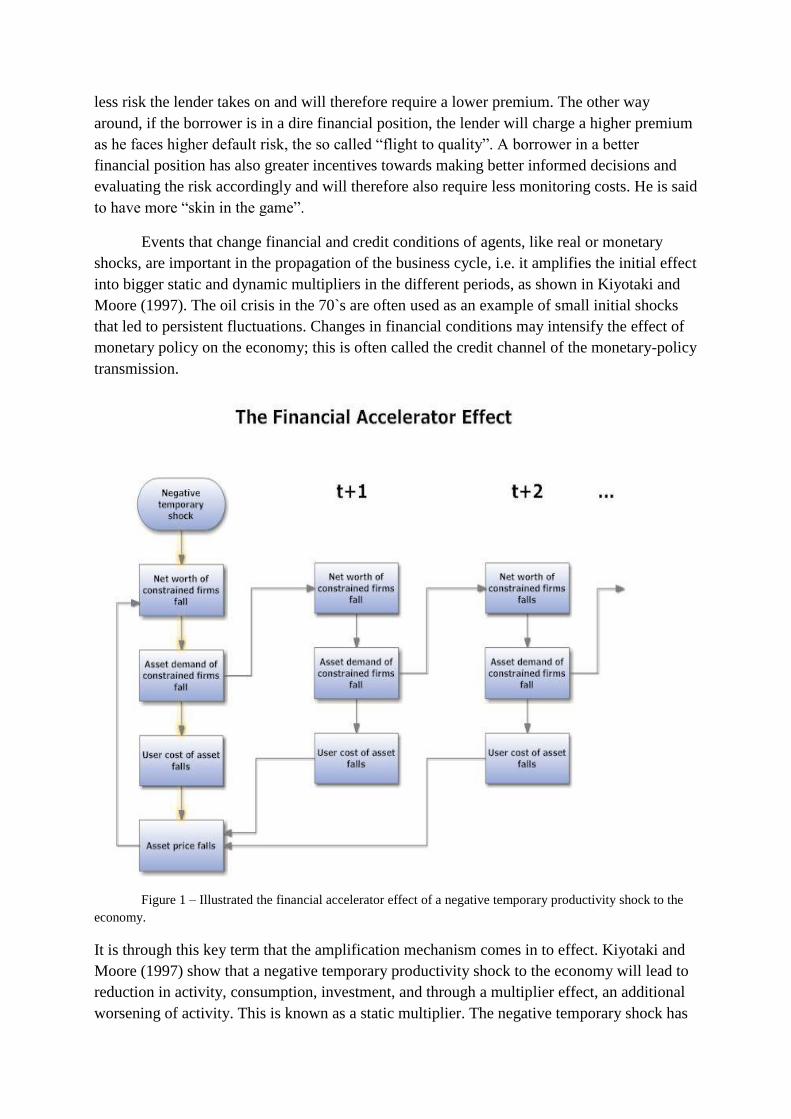
Figure 1 – Illustrated the financial accelerator effect of a negative temporary productivity shock to the

economy.

It is through this key term that the amplification mechanism comes in to effect. Kiyotaki and

Moore (1997) show that a negative temporary productivity shock to the economy will lead to

reduction in activity, consumption, investment, and through a multiplier effect, an additional

worsening of activity. This is known as a static multiplier. The negative temporary shock has

4

then led to reduced asset prices. This effect goes through the reduction in the net worth of

liquidity constrained firms and households asset demand falling user cost of assets fall

since the marginal productivity falls for the liquidity constrained agents.

The authors also incorporate a dynamic multiplier mechanism that comes into play in the

second period and stays around for several other periods. The asset prices fall further due to

the reduced asset in the previous period net worth of constrained firms and households fall

yet again (increasing the EFP) because of higher default probability further fall in asset

demand further fall in user cost, and this goes on and on until the small temporary shock to

the economy has been dramatically increased, propagated and amplified the business cycle.

This affects the first period asset price because the asset price is simply the discounted value

of future user costs.

A reasonable assumption is that net worth is procyclical, seeing that profits and asset prices

are generally greater in good times. The external finance premium, on the other hand, is

generally considered countercyclical as it amplifies the cycle through the accelerator effect on

aggregates like investment, production and consumption. Gelain (2010), however, casts doubt

on the generally assumed countercyclicality of the EFP. He found out that depending on the

shock hitting the economy, the EFP may in fact turn out to be procyclical. While agency costs

in credit markets will generally be countercyclical since a monetary relaxation that leads to

lower interest rates also generates a real economic boom that improves the balance sheets of

firms. This then lowers agency costs and thereby raises the efficiency of allocation.

2.2 The financial accelerator in the housing sector

Empirical findings suggest that there is an economic link to house prices and consumption,

suggesting that they move together. If increases in housing prices lead to increased housing

transactions then this link may be explained by the increased demand for housing appliances;

like furniture and curtains for instance. Housing goods and consumption goods are likely to

increase if agents are rather optimistic regarding future economic prospects. This link is,

perhaps, best explained through the credit market effect, suggesting the importance of the

collateral effect in obtaining credit from intermediaries. There is every reason to believe that

the financial accelerator also applies to households and their consumption of housing and

housing services. It is this latter effect that gives rise to the term “the financial accelerator

theorem in the market for housing.” Households generally have most of their wealth tied up in

the house they own and are therefore quite perceptible to shocks and events that change their

net-worth. Aoki et al. (2004) argue that in the case of financial assets, an increase in the price

would lead to an outward budgetary shift. While in the case of house prices on the other hand,

this wealth effect may not be present. They notice that even in a finitely lived household, an

increase in house prices just leads to a redistribution away from a first time borrower to the

last-time seller, not an increase in aggregate per se. And since most home owners live in their

own house they optimise until the benefits of an increase in house price is directly offset by

the opportunity costs of housing services.

Quite like firms, households face an external finance premium that is inversely related to their

financial position as well. The higher the loan-to-value (henceforth LTV) ratio is the higher

the premium the households face. The financial accelerator is in fact amplifying the effect to

account for more than the traditional theory around wealth effects suggest. Collateral is fairly

important as consumers are in reality using the value of their house to obtain higher

consumption through increased borrowing to the face value of the house, so called mortgage

equity withdrawal (MEW). Soaring house prices lead to more collateral being available to the

households and therefore more money can be borrowed from intermediaries to finance

increased consumption and investment. House prices are in this respect exceedingly cyclical,

leading to large discrepancies in the net worth of households and then to large discrepancy in

consumption through the MEW effect. Another important mechanism to remember is that

households that are not able, or willing, to withdraw equity may still benefit from increasing

housing prices due to decreasing LTV ratios, and hence, benefit from lower interest rate

spreads. The reduced cost of borrowing may then signal households to consume more or

perhaps even take up more loans. The EFP will here benefit them in good times, and of course

harm their financial position in bad times. An underlying assumption within MEW is that

households are said to be smoothing consumption over their lifetime, so called permanent

income hypothesis (PIH). Empirically, however, there is evidence for some households

actually behaving according to a rule-of-thumb/constrained manner (see Gali et al. (2004)). I

will of course embellish on this in later chapters.

Is there evidence for rising housing prices having led to the consumption boom of the

last decades? In Iacoviello (2005), the author lists several elasticities found from other papers

suggesting positive long-run elasticities of consumption to housing prices of around 0,06 for a

panel of US data, and a long-run elasticity of consumption to housing wealth of 0,08. He

raises concern regarding the life-cycle model; whether it is being too constrained in the belief

that rising housing prices lead to gains being equally distributed, when we should in fact have

unchanged demand with the assumption of same propensity to consume for both types of

consumers. In fact, according to Iacoviello, the impatient households will, ceteris paribus, end

up increasing consumption more than their patient counterparts due to their more impatient

nature.

The housing sector is a tricky thing to isolate. First of all, just like other assets

households hold, an increase in house prices leads to a direct wealth effect and should

according to micro theory lead to increased consumption. It is, however, not as easy as that.

Campbell and Cocco (2007) noticed that the theoretical rationale for a large housing wealth

effect is rather vague. They go on to further argue for their view: “If we define financial

wealth as the sum of liquid financial assets and the value of real estate minus debt

outstanding, it is clear that an increase in house prices leads to an increase in homeowners`

financial wealth. But this doesn`t necessarily mean that their real wealth is also higher.”

6

Housing is considered a consumption good, and therefore an increase in house prices must be

seen as increased benefits of not having to pay higher rent in the rental market. In this view

there are no real wealth effects and should consequently not have any effect on consumption

either, conditioned of course on substitution effects being absent as well. Second, as already

argued above, the borrowing constrained households wish to withdraw the increased equity of

the house to smooth consumption over time, and thereby increasing consumption now.

According to a household survey in Norway completed in 2006, about 4 out of 10 households

are actually willing to do a Mortgage Equity Withdrawal, MEW1. Half of them do this to

increase their consumption today, one quarter do so to transfer funds to their heirs, and one in

ten wish to save the money instead.

Most mortgage contracts in Norway are in fact variable mortgage rates. Unlike the

case of the United States and Denmark, the cost of refinancing a mortgage contract in Norway

are slightly higher and therefore allows the borrower to a lesser degree to adjust mortgage

rates when interest rates fall. We could look into how big effect monetary policy has on

different households with different mortgage contracts. Theory suggests that Norway, which

has a higher fraction of homeowners with flexible interest rates contracts, will be more

susceptible to changes in monetary policy than in the US, where a fixed interest rate is more

common.

“…In countries like the United Kingdom, for example, where most mortgages have

adjustable rates, changes in short-term interest rates (whether induced by monetary policy or

some other factor) have an almost immediate effect on household cash flows. If household

cash flows affect access to credit, then consumer spending may react relatively quickly. In an

economy where most mortgages carry fixed rates, such as the United States, that channel of

effect may be more muted.” Bernanke (2007)

Rubio (2009) reach the same conclusion as Bernanke in her study of variable versus fixed

rates mortgage contracts.

One can also distinguish between predictable and unpredictable changes in house

prices. Campbell and Cocco (2007) argue that forward looking households may in fact realise

the wealth effects of house price changes well in advance of the actual change, as soon as they

form the expectation of the change coming. A predictable change, however, will still help

relax the borrowing constraints, even if there is no wealth effect. The reason is that the

predictable change has already been anticipated. This is in contradiction to the permanent

income hypothesis which postulates that consumption is only affected by unpredictable

changes in income. This will of course complicate the effect considerably, and as such will

require two assumptions. First, only when increased house prices are realised will housing

become available as collateral, and not when it can be predicted. Second, and lastly,

borrowing capacity depends on current house prices, and not on the purchase price of the

1 The survey and the report is found here, albeit in Norwegian:

http://www.sparebankforeningen.no/id/13456.1

house. They also estimate the house price elasticities of consumption both for an old cohort

and for younger consumers. The main conclusion to be had from this paper is that the old

have a higher elasticity of consumption, while the younger consumers have an elasticity that

is insignificantly different from zero. This may be due to the notion that increased house

prices will lead to younger/first-time-buyers ending up with a lot less liquidity, and will not be

able to achieve the high consumption the permanent income hypothesis suggests. This leads

to the conclusion that as the baby boom grow older, the old will stand for a greater portion of

the population, and then consumption will also be more responsive to changes in house prices.

However important as this fact may be, it is also something I will disregard in this paper due

to the complications of modelling it in my highly stylised model.

Figure 2 – Financial accelerator in the housing market, only static effects are displayed.

What I will focus on here will be mainly on unpredictable house price movements, on

the collateral effect, and how this may be affected by borrowing constraints; leading to

changes in the borrowing opportunities of households.

Expansionary Monetary Policy Shock

Increased Housing Demand

Increased Housing Prices and Homeowners` Net Worth

Reduced EFP

Further Increase in Housing Demand and Consumption

8

3 Key Characteristics of the Housing

Sector

3.1 Household saving and investment

In this section I will take a closer look at the savings behaviour among Norwegian households

and do a cross-country comparison of the savings rate and investment choice, and try to

characterise Norwegian households’ asset holdings and liabilities. Most importantly I will

look at the how the acquired Home Equity Loan is spent among the households; saving the

proceeds or spending it on increased consumption today.

Figure 3 depicts the savings rate during the last two decades for Norwegian households and

several other countries that it is natural to compare us with. Norwegian households save in

several different ways. Norwegian saving ratio was in the early 2000s quite volatile in

comparison to the other countries saving ratios. Notice also the large drop in the savings rate

from 10% in 2005 to 0.1% in 2006, only to rise again to around 7% in 2010. This big fall in

the saving ratio was mostly because of the change in dividend tax that was announced in

2006.

Figure 3 – Cross-country savings rates. Data: OECD, Economic Outlook No. 88

Saving is defined as the net amount of labour income, net capital income and net transfers that

is not consumed. For the Norwegian population the government is doing most of the saving as

ridiculous amounts of money are extracted from the North Sea every day. In fact, 4 out of 5

0

2

4

6

8

10

12

14

%

Household and non-profit institutions serving households net saving ratio including forecasts for 2011

and 2012

Japan

Norway

Sweden

UnitedStates

NOK saved are done by the government. This saving is, however, not depicted in figure 3 as

it only depicts households and non-profit institutions. The government’s claims have

increased a lot more than its obligations, while the households claim versus obligations has

been relatively constant. A significant portion of household wealth is tied to deposit accounts

and claims to money from insurance and pension funds; of which are highly illiquid in the

short and medium term. The households are investing only a small portion of their wealth in

the stock market, and are therefore to a certain degree not exposed to the volatility in the stock

market. Norwegian households saving ratio was negative in the 80`s and turned positive and

relatively stable in the 90`s. Last decade it turned more volatile and reached a level of 7,4% in

2010. A concerning factor regarding the recent developments in the financial statements of

households is that the growth in income has lately not kept up with the growth in household

debt. The last decade brought about a period of low interest rates and liberal lending practices.

Norwegian households save in several different respects. While until recently only a small

portion saved in the stock market, an increasing part of the population is now also investing in

shares and bonds. We also see a trend towards more complicated portfolios as well. This may

be due to the need for diversification of risk or even because of the ever-lasting search for

yield due to low interest rates in the aftermath of the financial turmoil. The Norwegian

households are still heavily built up of “safe” investments, as more than half of the financial

assets of the households are tied to housing. Housing, as an asset, is in itself rather safe

investment for the individual household, but it is also fundamentally unsafe for the general

economy. As will be elaborated more in later chapters.

Figure 4 – Total financial assets for Norwegian household

0

500000

1000000

1500000

2000000

2500000

3000000

 1995  2000  2006  2007  2008  2009

Total Financial Assets in NOK million

 Other financial assets

 Insurance technicalreserves

 Loans

 Mutual fund shares

 Shares and other equity

 Securities other than shares

 Notes, coins and deposits

10

Figure 4 – Financial liabilities of Norwegian households2

Figure 6 shows the structure of the debt for Norwegian households over a 15 year period.

Mortgage backed loans and other loans using homes as collateral stand for approximately

71% of the household debt. One of the main contributors for this development is the increased

popularity of Home Equity Loans (HEL). This is also the channel through which households

are withdrawing money from the housing market, the so called MEW. In March 2010 the

Financial Supervisory Authority of Norway (FSA), Finanstilsynet (2011), established

guidelines they suggested the banks to follow. They recommended that the LTV ratio should

generally not exceed 90% on market value of the home, and in the case of HEL this rate

should be fixed at 75%. The regulatory authorities gather data from annual bank surveys they

conduct. Based on these surveys they found that in 2010 approximately 21% of mortgages

had a LTV ratio exceeding 90%, and shockingly 9% of the mortgages had in reality an

outstanding mortgage above the home market value. The mortgages the households are

getting are in almost all cases flexible interest rate contracts, and an increasing proportion

include a no annuity period. Considering HEL, 89% of the cases in 2010 were under the 75%

the authorities suggested, implying a sound financial state of the economy. The survey also

concludes that a large portion of the households withdrawing equity from their homes are in

fact spending the proceeds on buying a car, boat or even a cabin. HELs are, according to the

report, used mostly on goods other than housing services and investment in own home. It is

however alarming that the increase in HEL usage has also led to decreasing down payments

of the total outstanding mortgages in Norway.

2 The table with the associated values for graph 4 and 5 can be found here, albeit in Norwegian:

http://www.ssb.no/emner/08/05/10/oa/201101/08hushold.pdf

0

500000

1000000

1500000

2000000

2500000

 1995  2000  2006  2007  2008  2009

Total Liabilities in NOK million  Other liabilities

 Other loans

 Loans from insurancecompanies

 Loans from financecooperation

 Loans from state lendinginstitutions

 Loans from banks

Figure 6 – Graph depicting the components of household liabilities over a 15 year period. Source: SSB.

3.2 Developments in the housing sector

The Housing market has increased fourfold since the 90`s. Early 2011, it was about 7% higher

than the peak in 2008, the weeks prior to the Lehman collapse and the beginning of the

financial crisis that led to crashing housing markets in several different parts of the world. In

comparison, the CPI has only increased by 45% during this same period, and the costs of

construction about 82%. Clearly, the price increase in the housing sector is not even remotely

due to construction costs only. One might argue that because of people’s aversion towards

selling at a loss, house prices are generally sticky on the way down, as opposed when the

market is booming. Norway has one of the most deregulated housing markets in Europe as

well. Sweden, Denmark, United Kingdom, Netherlands and Austria, all have government

regulated housing markets. All of which provide price regulated government constructed

housing. Norwegian authorities deregulated a heavily regulated housing market up until the

1980s leading to people’s savings and private equity entering the equation. The housing

market was liberalized; the prohibition against pre-emptive regulation and other price

regulations was launched, as well as selective instruments directed towards first-time buyers.

12

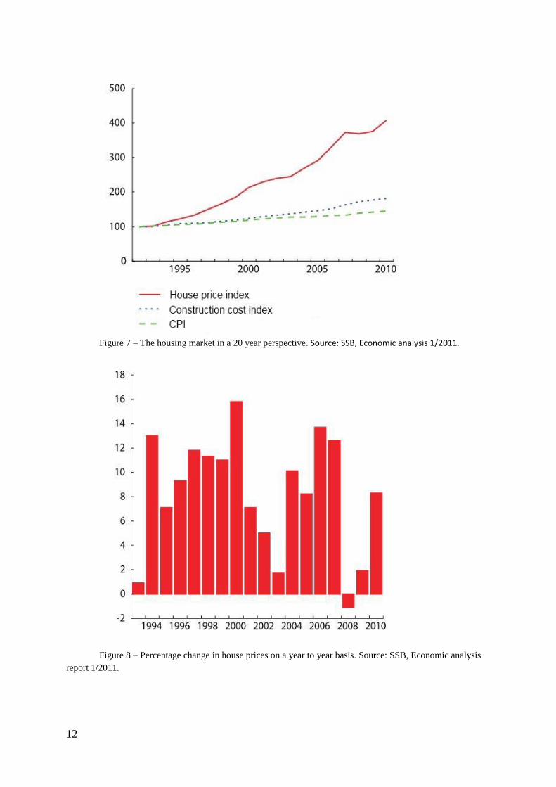
Figure 7 – The housing market in a 20 year perspective. Source: SSB, Economic analysis 1/2011.

Figure 8 – Percentage change in house prices on a year to year basis. Source: SSB, Economic analysis

report 1/2011.

Graph 8 depicts the percentage deviation on a year to year basis. As we clearly see from the

graph, in the period of the boom preceding the dot-com bubble the growth in the housing

market was quite high, 14% in 2006 and 13% in 2007. The financial crisis brought about a

year of negative growth, only to pick up again a year later.

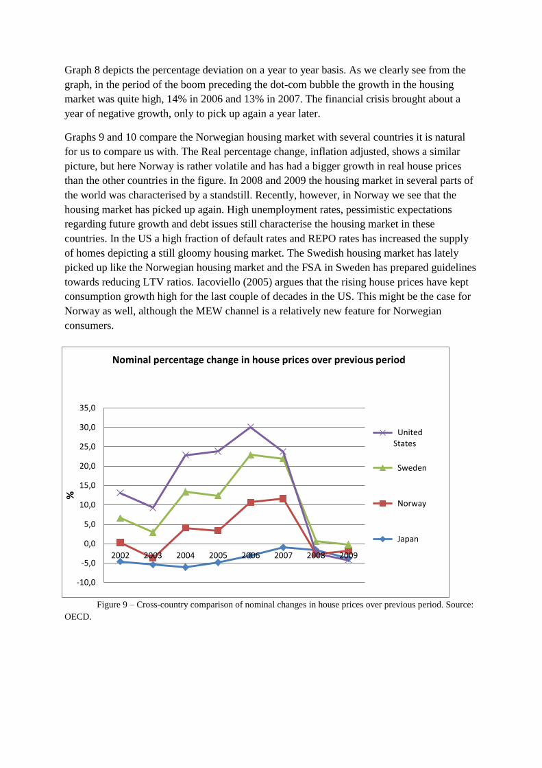
Graphs 9 and 10 compare the Norwegian housing market with several countries it is natural

for us to compare us with. The Real percentage change, inflation adjusted, shows a similar

picture, but here Norway is rather volatile and has had a bigger growth in real house prices

than the other countries in the figure. In 2008 and 2009 the housing market in several parts of

the world was characterised by a standstill. Recently, however, in Norway we see that the

housing market has picked up again. High unemployment rates, pessimistic expectations

regarding future growth and debt issues still characterise the housing market in these

countries. In the US a high fraction of default rates and REPO rates has increased the supply

of homes depicting a still gloomy housing market. The Swedish housing market has lately

picked up like the Norwegian housing market and the FSA in Sweden has prepared guidelines

towards reducing LTV ratios. Iacoviello (2005) argues that the rising house prices have kept

consumption growth high for the last couple of decades in the US. This might be the case for

Norway as well, although the MEW channel is a relatively new feature for Norwegian

consumers.

Figure 9 – Cross-country comparison of nominal changes in house prices over previous period. Source:

OECD.

-10,0

-5,0

0,0

5,0

10,0

15,0

20,0

25,0

30,0

35,0

2002 2003 2004 2005 2006 2007 2008 2009

%

Nominal percentage change in house prices over previous period

  UnitedStates

  Sweden

  Norway

  Japan

14

Figure 10 – Cross-country comparison of real changes in house prices over previous period. Source:

OECD

3.3 Determinants of the housing market

One may ask which factors play an important role for the developments in the housing

market. In the short run the growth in the housing market may be determined by, as indicated

by Tsatsaronis and Zhu (2004) as well:

Availability, cost and flexibility of debt financing

Number of potential housing consumers and their financial resources and tastes

Transaction costs such as inheritance tax, registration duties, and the level of value

added tax (VAT)

Different ways of measuring user cost of housing that account for deductibility of

mortgage interest rates

Uncertainty, periods of high volatility in the housing market will often lead to reduced

future predictions and more cautious construction behaviour

Length of planning and construction stages

-8,0

-6,0

-4,0

-2,0

0,0

2,0

4,0

6,0

8,0

10,0

12,0

14,0

2002 2003 2004 2005 2006 2007 2008 2009

%

Real percentage change in house prices over previous period

  Japan

  Norway

  Sweden

  UnitedStates

Existing land and planning systems

In the longer term the housing market is determined by:

Average level of the interest rate set by the central bank

Demographics

Household disposable income

Permanent changes in the tax system that encourages investing in housing rather than

other financial assets

Availability and cost of land

Production costs and the cost of investments that aim to improve the quality of

existing housing stock

Tsatsaronis and Zhu (2004) use a structural vector autoregression (SVAR) framework on

cross country data and find that the most prominent explanation for what drives house prices

is the inflation rate. Inflation is the driver of housing prices and on average it explains almost

half of the total variation in the house prices at the five-year horizon. Being even larger in the

short run, almost 90% of the variation is driven by inflation. The authors reason that this may

be due to the interlinkage of housing; acting both as a consumption good and an investment

good. Households are believed to hedge against risks of rising inflation through real estate.

The BIS authors also argue that a second explanation for inflation being such an important

driver of housing prices is because inflation affects the cost of mortgage financing and it may

also act as a proxy for the prevailing financing conditions.

The second most important factors determining the developments in the housing market are:

spreads, bank credit and short-term interest rates. The authors conclude that they are equally

important and that they together stand for approximately one third of the variation in the

housing market in the long run. Income, on the other side, is of shockingly small relevance in

explaining the variations. In other words, it matters less what the income of the household is

as long as the mortgage payments are low enough when deciding whether to purchase a new

home or not. This is also the case for Norwegian consumers. What matters is the capability of

households in taking on and servicing new debt, and to a lesser degree the income of the

households.

In countries with more flexible interest rate mortgage contracts and more market based

property valuation practices for loan valuation, the authors find evidence for a stronger

feedback mechanism from property prices to credit growth. As is also the case for Norway,

since most of these determinants are present in the Norwegian housing market. In fact, only

3% of total mortgages in 2010 were on fixed rate contracts.

16

One might wonder if housing prices need to decrease at all and if they generally do so

in practice. The housing market was a contributing factor in dampening the slowdown in

global activity early in the 2000s, and now in the aftermath of the credit crunch we see similar

tendencies in several parts of the world as house prices continue to soar. In a study by Borio

and McGuire (2004) the authors find that equity price peaks have considerable predictive

power for subsequent housing price peaks, in a cross-country study for the period 1970-early

2000s. This indicates perhaps a boom and bust cycle in the housing market that feeds onto

itself. As opposed to imposing a “natura non facit saltum” condition on housing, one

generally finds that the housing market instead grows at a slower pace as the economy

recovers after a recession, or even a downturn in production. The authors also check whether

this predictive power is somewhat reduced if output growth, unemployment and interest rates

are included. They find that:

“…housing price peaks have tended to follow periods of comparatively strong

economic activity …For example, the coefficients on the lag of GDP growth, while not always

individually significant when multiple lags are included, indicate that the overall effect is

positive and statistically significant. Similarly, the effect of unemployment is negative,

implying that a fall in unemployment in the periods preceding a peak in equity prices leads to

a higher probability of experiencing a peak in housing prices in the quarters ahead.

…increases in interest rates were a factor bringing the rise in housing prices to a halt”

Borio and McGuire (2004) pp. 86 - 87

They come to the conclusion that the predictive content of this relationship between equity

and housing is fairly robust to the presence of other macro economic variables as well.

Housing demand takes up most of the literature on reasons why we have booms and

bust. Lately, nevertheless, there has been an increasing concern over whether the researchers

are too narrowly concentrating on the demand side. Clearly, one must understand the supply

side as well if one wants to determine the reasons for booms and busts in the economy. There

is a concern that there are too few homes being built where people want to live, and unless

this is corrected the prices will continue to soar. New government regulation, together with

new energy requirements launched in July 2010, put heavy restrictions on the standard of new

homes and this made new homes more costly than with previous regulation.

3.4 Similarities and differences between housing and

other financial assets

I have already discussed how Norwegian households have a lot of their wealth tied up in

housing and how some see it as an investment good as well, but how closely related is the

housing market to other financial assets, e.g. shares and other equity? What are the similarities

and differences? These are the questions I wish to address now.

There is a close relationship between equity prices and housing prices. As already noted,

housing price peaks tend to come after an equity price peak, and also after a beneficial

economic environment. Traditional economic theory states that both equity and housing are

somewhat similar long lived assets, in the sense that they both are claims to goods and

services. They both have several determinants in common. Both will benefit from

comparatively strong advantages in economic activity. At the same time they are different in

several ways. First, real estate is more illiquid than private equity; people generally don’t

borrow money to invest in shares and bonds and if they do, the leverage ratio is way lower

than for housing. Second, we cannot always determine if housing is an investment good rather

than consumption good. There are multiple reasons why people buy homes. Wanting to

provide a safe environment for their offspring, having more control of their living space and

financial motives, such as return, are some of them. This mixture leads to problems for the

financial system because if housing was truly a consumption good, increasing the price should

then lead to falling demand. As a financial asset, the increase in price actually motions a buy

now signal. Third, Norwegian houses are not widely traded internationally. Hence, the

Norwegian consumers cannot realise, in aggregate, their capital gains and increase their

consumption therein. Fourth, differing economic environments may shift demand for one

asset in favour of the other. We are here talking about portfolio shifts that drive a wedge

between this relationship. Lastly, there is no way someone who believes that the housing

market is overpriced may benefit from this by short-selling the asset and this therefore leads

to the momentum in the property market. The short-comings of the market to provide a

possibility for short-selling in the housing market may in fact be leading to the bubbles in the

housing market.

3.5 Bubbles

What makes houses such an unsafe asset for the economy? It is perhaps the most dangerous

asset of all; looking at the absolute size of the asset class.

“The five big banking blow-ups in the rich world before the latest crisis (Spain in the

1970s, Norway in the 1980s and Sweden, Finland and Japan in the 1990s) had property at

their heart.”3

Houses are the most important single asset of most households, but it is also the backbone of

the financial intermediaries since the value of real estate is incorporated in their portfolios. In

3 “A special report on property: Bricks and slaughter.” From the online version of The Economist,

http://www.economist.com/node/18250385

18

fact, there is a double leverage as both the banks and property are leveraged. House prices are

in effect not only affecting the business cycle through the financial accelerator, but they also

influence the performance of the financial sector. It is this interlinkage that determines the

soundness of the economy.

Considering the Norwegian economy, a reasonable question to ask is whether there are

bubble tendencies in Norway. I will not speculate whether the housing market is experiencing

a bubble. It is rather difficult to assess whether the price increases are coming from

underlying economic fundamentals or perhaps irrational exuberance. While western countries

are experiencing deflating house prices in the aftermath of the financial crisis (Norway and

Sweden being notable exceptions), eastern countries are essentially still experiencing ever-

increasing house prices, China is a good example of this. The close ties the housing market

has with the financial sector leads to crises that affect the whole economy, and this boils down

to an extreme bill that is disproportionately shared among the population and among

countries. Newspapers in Norway have long been monitoring the developments in the housing

market. There is a growing concern there is a shortage of houses and that building new homes

is quite expensive, in fact construction of new homes has not been this low in 100 years,

pushing the prices further up the sky. We have, nonetheless, seen that construction costs did

not play a big role in the fourfold increase in house prices from 1995-2010. House prices are

predicted to increase by another 30% by 2014. Norges Bank has declared it is going to double

its current policy rate by 2013-14, and although this should in practice lead to lower asset

prices, the fact remains that higher rates will also lead to lower profitability in the

construction of new homes, due to higher opportunity cost. Clearly, the market is not learning

from its own mistakes, and time and again one ends up thinking that “this time it`s different”,

but it rarely is. And if the market is not going to regulate and fix its own problems, then that

leaves the government with the unpopular job of pulling the strings. The authorities have

several ways of giving disincentives towards investing in an already inflated housing market.

First, institutional changes like altering the tax system towards making housing a less

attractive investment object. Svein Gjedrem, former governor of Norges Bank, has long been

a proponent for reforming the taxation of housing to counter credit cycles and achieve a more

stable housing market; proclaiming that increased taxation of homes, in a similar manner as

other financial assets, will lead to a dampening effect on housing prices. Second, the mortgage

financing is a cause for concern. The subprime crisis originated and escalated due to credit

being to easy at hand, and this drove up the prices creating a bubble that burst. This led to

falling housing prices, and in some places the housing market is still characterised by great

scepticism regarding future economic prospects, like USA. There are some drawbacks,

however, in changing the ease of credit. First-time borrowers and self-employed will suffer

because of this, and this may lead them to find alternative, and perhaps more expensive,

financing.

Third, macroprudential regulation works great in theory, but is rather hard to implement in

practice. Generally bubbles are known to be a fact only when they burst. These are

instruments like changing the LTV ratio according to the current cycle, changing the reserve

requirements and thereby reducing the amount of credit that banks can lend out. Angelini et

al. (2011) find that macroprudential policy, like the LTV ratio, contribute little in normal

times, but have substantial macroeconomic advantages in the case of adverse shocks. Catte et

al. (2010) instead ask:

“Was US monetary policy too expansionary for too long in the wake of the 2001

recession? Would a tighter monetary stance have prevented (or at least contained) the

housing bubble?“ Catte et al. (2010) pp. 6

They reach the conclusion that regulatory failures, low perceived risk and abundant liquidity

helped inflate the price bubble prior to the 2003-2007 period. Svenson (2004), conversely,

takes on a different approach. He claims that asset prices should generally not be the concern

of the monetary authorities unless they have an impact on target variables, inflation and

output gap.

Figure 11 – Different measures normally undertaken in the case of housing price bubbles

20

4 Modelling Housing Spillovers

4.1 Current modelling approaches and monetary

policy rules

Dynamic stochastic general equilibrium models are micro-founded optimisation models based

on rational expectations of agents at the micro level. They have, nevertheless, grown in

popularity in macro economics the last couple of decades and are now widely used in central

banks. Using a general equilibrium framework, how does one go about incorporating

borrowing and lending, without losing manageability and comparability with the benchmark

macro models? Modelling the dynamic optimisation problem for heterogeneous households

under liquidity constraints without losing the distinctive features of the credit channel, is

rather complex. And by using a representative agent model we will not even have any lending

in equilibrium. In other words, we want to incorporate liquidity constraints for heterogeneous

households in a simplistic model and still be able to generate useful conclusions. When

studying household savings behaviour many studies have resulted in using an overlapping

generation’s model to ensure both lending and borrowing occurs in equilibrium. Another

frequently used model is the separation of the households into two behavioural types. We

distinguish between a patient and an impatient group; one following a Permanent Income

hypothesis and one Rule-of-thumb consumer type. This separation makes the model

significantly simpler without losing the essence of the financial accelerator mechanism.

Aoki et al. (2004) study the interlinkage between the housing market and the general economy

and postulate whether house prices merely reflect the macroeconomic conditions, or if there

are indeed important feedback effects from house prices to other economic variables. The

authors consider two behavioural types of households, homeowners and consumers. The

homeowners buy houses with private equity and borrow from financial intermediaries, facing

an external finance premium. The consumers consume goods and housing services. They rent

housing services from the homeowners and supply their labour to a competitive labour

market. The producers of the consumption good follow a sticky pricing regime, as is standard

in the New Keynesian framework. They conclude that an expansionary monetary policy shock

leads to increased housing demand, increased housing prices and therefore increased net

worth of homeowners. The increase in net worth reduces the external finance premium and

this then leads to a further increase in housing demand, and through a spillover effect to

increased consumption. Aoki et al. (2004) argue further that a deregulated mortgage market

will to lesser extent have an effect on housing prices, while the effect on consumption will be

amplified.

Iacoviello (2005) setup the model with two key characteristics that define his work;

collateral constraints, for firms and households, tied to real estate values, and nominal debt.

Quite like Christensen and Dibs (2008) Iacoviello finds that supply shocks decelerate the

economy, and demand shocks work the opposite way, amplifying and propagating the shocks.

He concludes with the notion that there is little to be gained by a monetary authority actively

seeking to stabilise output and inflation through responding to movements in asset prices, and

that implementing nominal debt actually improves the output-inflation variance trade-off for

the central banks since it acts as redistributing wealth between borrowers and lenders.

Mendicino and Pescatori (2005) try to find a link between the design of an optimal

monetary policy rule and movements in housing prices. Unlike Iacoviello and Neri (2010) the

authors direct attention to the welfare of the lenders and the borrowers. Like most other

authors in this field of research, Mendicino and Pescatori focus on the households` sector

instead of regarding housing as just another asset in the portfolio of households. In doing so,

the authors find out how housing prices could be a variable of interest for the interest rate

setting authority, instead of just looking at general movements in generic asset prices. Ibid. set

up a simple model with two distinctive household types, a monopolistic competitive good

producing firm with sticky pricing, and a monetary authority. Mendicino and Pescatori reach

the conclusion that targeting housing prices for the monetary authority is welfare reducing.

This result is in contrast to both Iacoviello and Neri (2010), and Faia and Monacelli (2004) in

a different study.

Christensen and Dibs (2008) estimate a closed market DSGE model with rigidities

such as sticky prices, capital adjustment costs and financial frictions. They embed a model

with these rigidities and show that the financial accelerator improves the model`s fit with the

data. They find that incorporating a financial accelerator actually reduces the effect on

investment when considering a supply shock, it amplifies and propagates demand shocks and

plays an important role in the transmission of monetary shocks. They also find that the same

effect is rather miniscule on output, but this is mainly due to the monetary authorities reacting

aggressively to output fluctuations in order to stabilize the economy. They also use a

representative agent model, and in doing so they focus on the financial accelerator going

through the balance sheet of firms instead of through housing prices.

Kannan et al. (2009) start off by asking several questions regarding the role of the

monetary authority in a model with house price booms. They also ascertain whether the

central bank should also focus on asset prices as well as CPI and output gap in a similar

manner as Mendicino and Pescatori, and what I will do in later chapters. It is not always the

case that the central bank can react to changes in different economic variables; take for

example a state of high inflation and low economic activity. They therefore also consider the

use of a macroprudential policy tool alone, or together with the monetary policy tool already

in use, and its impact on the economy after a shock. Ibid. use a similar model as in the

aforementioned papers. They find that when considering a demand shock to the economy, the

monetary policy tool and a macroprudential policy tool can, and will, help to stabilise the

economy. They notice that a macroprudential policy tool is unambiguously useful when

dealing with financial shocks and that even though the monetary policy rule is more

22

aggressive, the volatility in the interest rate is lower as well. When the economy is hit by a

productivity shock the best policy for the monetary authority is to accommodate the

improvement in the productivity as much as possible. This is in contrast to the case of a

demand shock; macroprudential policy tool is unwarranted.

Gerali et al. (2010), unlike me and the rest of these authors, incorporate a banking

sector into the DSGE model. They look at the effects of an expansionary technology shock,

and a contractionary monetary policy shock. They find that macroeconomic shocks play a

minor role in explaining the fall in output in 2008 in the Euro area, while the shocks to the

banking sector explain a lot more. The most important result to be had from their study is that

much is lost in excluding explicitly financial and credit shocks in DSGE models designed to

analyse fluctuations in business cycles.

Iacoviello and Neri (2010) also consider the spillovers from the housing market to the

wider economy. But they also try to find out what types of shocks are hitting the housing

market, and how the dynamics of residential investment and housing prices are clarified by

shocks and frictions in the market. The authors’ model is to some extent similar to those

above, but instead of a supply side with a manufacturing sector with final- and intermediate

goods, they model sectoral heterogeneity with a housing and a nonhousing sector. This

modelling approach yields an additional effect from an increase in house prices, other than the

traditional effect on borrowing constraints; the relative profitability of producing new homes

is increased. This addition to the model generates an additional feedback mechanism that

propagates and amplifies the cycle. Another key feature to this model is that it incorporates

the collateral effects and that these effects help generate a positive and persistent response of

consumption following an increase in housing demand. Without this effect the authors state

that the increase in demand for housing would generate an increase in housing investment and

housing prices, but a fall in consumption. A monetary shock leads in this model to a drop in

real house prices, due mainly to nominal stickiness, and that both the collateral effect and

nominal rigidities amplify the response to consumption. A positive technology shock leads to

a decline in housing prices due to a rise in investment coming from a fall in construction

costs. The main results to note are that technology shocks and housing demand shocks each

explain about a quarter of the cyclical volatility in the housing investment and housing prices,

and that the spillovers to the rest of the economy are quite important, but that the effect is

concentrated on consumption rather than business investment.

4.2 The New Keynesian Dynamic Stochastic General

Equilibrium Model

I ended up using the model of Matteo Iacoviello (2005), “House Prices, Borrowing

Constraints, and Monetary Policy in the Business Cycle” from the American Economic

review. The model was found in the American Economic review, but the Dynare Code was

taken from the Macro Model Database, Wieland (2009). There are several similarities to the

Iacoviello and Neri (2010) as well. While the paper is overly simplistic and stylised, relative

to several of the other papers I have considered, it still gets the message through. Note that the

main goal regarding my thesis will not be discovering a brand new model as this is PhD

material at this level, but mainly estimating and analysing the results of an old one with

Norwegian data. Hence, I will shortly explain the model I use.

There are several ways in which economists in this field of research are able to

generate borrowing and lending within a dynamic stochastic general equilibrium framework,

and still be able to isolate the desired effects. In order to apply the financial accelerator

approach to the data one has to identify the different sectors on beforehand and give them

certain characteristics that are easy to model, and which are expected to yield reasonable

results. Having a household sector that maximises utility with respect to consumption, holding

of housing, labour and money balances subject to a budget constraint; one ads a

microfoundation to a macroeconomic framework. I further make the assumption that

households are either patient; following a permanent income hypothesis behavioural pattern,

or impatient; following something similar to a Rule-of-Thumb consumption pattern.

Incorporating ROT consumers has gained a hold in the literature lately. There will also be an

entrepreneurial sector and a retail sector, of which is rather standard in these types of New

Keynesian DSGE models. I further argue that the entrepreneurial sector and the impatient

type of households are the key element in this model, due to the two sectors facing borrowing

constraints. Hence, they borrow funds from intermediaries in accordance with their net worth,

of which depends on the house prices in any given period. In addition to the households, the

entrepreneurs and the retailers there will also be a central bank following a Taylor type rule.

4.2.1 Households

The households are infinitely lived, along with the entrepreneurs, and are further divided into

a patient type and an impatient type. The impatient type is only separated from the patient

ones through different discount rate; impatient households are assumed to have a higher

discount rate. The impatient households are hence assumed to be more myopic and face

borrowing constraints, indicating that they can in fact take advantage of MEW in the case of

equity price increases, but no other way of borrowing is available for these types. The patient

households maximize the following utility function

∑

)

(

))

subject to the budget constraint

24

With respect to consumption , holding of housing

, labour supply in hours , and money

balances divided by the price level is given by

. The household sector is denoted with a

prime and the impatient households are denoted with a double prime, just like in Iacoviello

(2005).

The impatient household maximization problem is then, in a similar manner

∑ )

)

(

))

Subject to the budget constraint

)

Where (

)

is the way we denote the housing adjustment cost, but it plays a

minor role in my further analysis and can therefore be disregarded with ease.

E0 is the expectations operator, is the discount factor, q is the real housing price

(Gross price Q divided by price level P), w is the real wage (Gross wage W divided by price

level P). I further assume that households borrow in real terms –b, and receive back

,

where is the nominal interest rate on loans between t-1 and t. is the difference operator

in the budget constraint,

denotes the gross inflation rate, F denotes the lump sum

transfers received from the retailers, T - M/P denotes the net transfers from the central bank

financed through printing new money. j is the weight one puts on housing services, also the

demand shock, and is the labour supply aversion.

The housing preference shock may be regarded as a shock that captures other social

and institutional changes that shift housing preferences, or even cyclical deviations in the

availability of resources needed to purchase housing, h, relative to other goods, c.

Maximizing the utility function, with respect to c, h, L and M/P, subject to the budget

constraint, one arrives to the first order conditions. In a similar fashion to Iacoviello (2005) I

will disregard the money demand. Since I use a separable utility function, ignoring the

quantity of money will not have any consequences for the rest of the model.

4.2.2 Entrepreneurs

Using only labour, capital and real estate as inputs the entrepreneurs produce the intermediate

good according to a constant returns-to-scale Cobb-Douglas production function:

) ) )

We further make the assumption that the entrepreneur, similar to a consumer, wishes to

maximize consumption with respect to the borrowing constraint condition, technology, and

the corresponding budget constraint.

∑

(

)

) ) )

Where A is the random technology parameter, and are the labour supply of the

different types of households, α denotes the wage share of the unconstrained agents, and µ

denotes the capital share in the economy. K is capital and δ is the depreciation rate. ξ denotes

the adjustment costs for both the sectors, defined as in Iacoviello (2005). m is the loan-to-

value ratio and will in most cases define how much one can borrow, with collateral. I further

make the assumption that the entrepreneurial discount factor is lower than the patient

household discount factor, but still as high as the impatient household discount factor. This

implies for the model I use that the entrepreneurs and the impatient household are in fact

bounded by the borrowing constraint around the steady state. in fact makes

sure that entrepreneurs and borrowing constrained households decumulate wealth quick

enough to a lower bound such that the borrowing constraint is binding. One complication with

this model, as Iacoviello notes, is that we want to avoid that the entrepreneurs and the

impatient households amass wealth and self-insure. In order to get the desired effects of

26

collateral one needs that these ROT consumers hit the borrowing constraints. Iacoviello

makes good arguments why the probability of this this may be small enough that I disregard

this nuisance fact.

4.2.3 Retailers

As in most of the models we have covered in this paper, the retail sector is mostly brought

along in order to introduce price rigidities and monopolistic competition into the model and to

render the model linear. Price stickiness guarantees that monetary policy has real effects to the

economy and is introduced through a Calvo-pricing regime. A Calvo price setting rule

assumes that each firm resets its price only with probability 1-θ in any given period, no matter

when it last reset its price. In other words, in each period a fraction 1-θ resets its price, while a

fraction θ keep their prices unchanged. The average duration of a price then becomes

and

in this context θ is then considered a natural price index of price stickiness. Assuming a

continuum of retailers and that they purchase intermediate goods from entrepreneurs and

(inducing the fact that only the retail sector is characterised by monopolistic behaviour)

differentiate the goods at no extra costs. Their production function, final goods, is given by:

∫ )

)

And the price index is then given by:

∫ ) )

Each retailer faces then an individual demand curve derived to be:

) ( )

)

Adding just another equation to the retail sector one is then able to derive the maximisation

problem, the price evolution is:

)

) )

θ denotes the staggered price setting à la Calvo (1983). A fraction (1-θ) is allowed to re-

optimise its price in any given period, given by .

Firms chose output, prices and labour input in order to maximise expected profits subject to

the individual demand curves, production technology function and the different Calvo-states.

Setting up the Lagrangian and deriving the first order conditions with respect to prices,

output and labour input and we get the following condition:

∑ ( (

)

)

))

Where (

) is the relevant discount, and

is the markup of final goods

over intermediate goods in steady state. Assuming zero inflation in steady state and log-

linearizing we get the New Keynesian forward looking Phillips Curve (NKPC). The forward

looking Phillips Curve postulates that inflation depends positively on expected inflation and

negatively on the markup.

4.2.4 The central bank

The central bank in this model is assumed to follow a backward looking interest rate rule,

according to a Taylor principle. The Taylor principle states that the central bank reacts to

inflation shock more than one-to-one in order to affect the real interest rate.

)

(

)

)

Where I denote rr and Y as steady state values of real rate and output, just as in Iacoviello

(2005). is the inflation shock, or white noise shock process that is identically and

independently distributed with variance and zero mean.

4.2.5 Equilibrium

The first order conditions obtained from the households’ maximisation problem, firm

maximisation problem, as well as the central bank interest rate rule, make up the DSGE model

in a stylised manner. The equilibrium model is derived using market clearing conditions in the

housing market, labour market, real estate, goods market and market for loans. Log-

linearizing the complete model around a steady state in order to reduce the computational

difficulty for the system of equations that need to be solved simultaneously is a frequently

used method in DSGE macro models. This method of transforming non-linear equations into

linear in terms of log-deviation of the related variables from their steady state values is

intensely used in macroeconomics, as well as microeconomics. For small enough deviations

from steady state we interpret the log-deviations as percentage deviations from steady state,

28

hence the “hat” in the following model. The complete log-linearized model is as follows,

taken directly from Iacoviello (2005), Appendix A page 760-761:

Aggregate demand

) )

)

)

The first equation is the clearing condition in the goods market, while the second equation is

the first order condition (FOC) for the patient households. The last equation defines the

investment.

Housing/consumption margin

) ) ) )

)( ) )

) )

)

)

The first equation here denotes the optimal condition for entrepreneurs, the second the

optimality condition for impatient household and the last one the non-myopic households

demand.

Borrowing constraints for the firm and the households

Aggregate supply

) )

) ) )

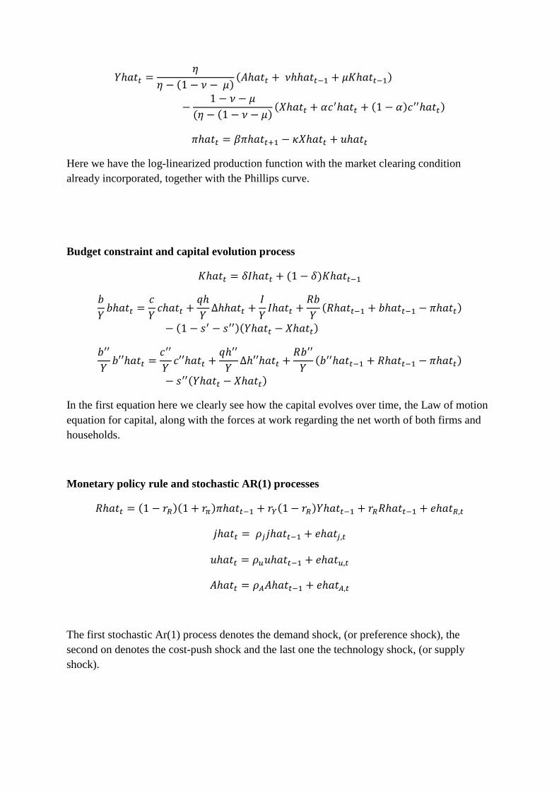
Here we have the log-linearized production function with the market clearing condition

already incorporated, together with the Phillips curve.

Budget constraint and capital evolution process

)

)

) )

)

)

In the first equation here we clearly see how the capital evolves over time, the Law of motion

equation for capital, along with the forces at work regarding the net worth of both firms and

households.

Monetary policy rule and stochastic AR(1) processes

) ) )

The first stochastic Ar(1) process denotes the demand shock, (or preference shock), the

second on denotes the cost-push shock and the last one the technology shock, (or supply

shock).

30

Where is the real ex ante interest rate. )

, )

,

), ) )

and

and noticing that

)

and

) )

in the log-linearized equation, where they denote the

income share of the patient and impatient households, respectively. Iacoviello (2005) defines

) as the average discount factor for the returns to entrepreneurial real

estate investment.

5 Quantitative Policy Analyses and

Estimation

5.1 Methodology and data

I will use a Bayesian New Keynesian Synthesis (NNS) estimation approach and choose both

calibrated parameters and appropriate prior distributions for the parameters that I estimate.

“Bayesian NNS models, therefore, combine a sound, microfounded structure suitable

for policy analysis with a good probalistic description of the observed data and good

forecasting performance” Smets and Wouters (2007) pp. 587

The likelihood function is assessed using a Kalman filter. The posterior distributions are then

done using a Metropolis Hastings algorithm, within the free software Dynare4.2.0 along with

Matlab version R2010b, to draw the posterior distribution of the parameters. I estimate the

model using four observable variables; GDP in fixed prices, CPI adjusted for taxes and energy

prices (hereafter CPI-ATE), nominal house prices deflated by the CPI-ATE and the 3 Month

NIBOR for the period 1995Q1 – 2010Q4. For the period I wish to examine I have come to the

conclusion that GDP and real house prices will most likely have a trend, inflation and NIBOR

are assumed to be without a trend and are therefore not filtered. They are, nonetheless,

demeaned. Hence, both real GDP and real house prices have been detrended using a Hodrick-

Prescott filter (HP) after first having been recalculated to log values. More on this in the

Appendix.

After doing this I intend to go on to do some comparative analysis through showing the

impulse responses to different shocks to real GDP, nominal interest rates, real house prices,

inflation and consumption. Using the baseline model as a benchmark I will then plot the

impulse responses with no collateral effects for constrained households (m = m’’= 0). Doing

so, I can estimate the spillovers from the housing market to consumption. I intend to measure

the spillovers to the general economy through the notion that the conventional wealth effect

on consumption is greater when collateral effects are indeed present. Also, another large part

of the spillovers come from the notion of the wage share of the constrained households. These

are the financial frictions mentioned in the beginning of my thesis. I will also check what

would happen if the central bank, in addition to reacting to last period nominal interest rates,

32

activity in the economy and last period inflation, keep an eye on current asset prices as well.

The reason is that asset prices that are let to overinflate will have large repercussions for the

economy. In this manner, one can check whether it would be beneficial for a central bank to

implementing asset prices into the monetary policy rule. The limited gains of asset prices in

the policy specification are already noted in the literature. I will elaborate on this on a later.

5.2 Calibrated parameters

One important reason why we often calibrate certain parameters is that some parameters are

known to be hard to pin-point and therefore hard to estimate, or that other papers have already

identified the relevant value of the parameters in question. Calibration necessitates that the

values of the parameters are collected from other sources independent of the phenomenon

under study.

“This controversial step is driven by three main concerns. First, identification of deep

parameters in estimated large dynamic systems can be troublesome. Second, there is often a

conceptual mismatch between the theoretical variables and their sample counterparts. …And

third, in practice the classical estimation of macro models can be plagued by badly-behaved

likelihoods – the researcher typically has very few business cycle fluctuations with which to

estimate the highly abstract model.” Karagedikli et al. (2008) pp. 10

The parameters that I chose to calibrate for the Norwegian data are also the ones that are most

commonly calibrated, such as the discount rate for the different types of households, capital

share and wage share of the economy, depreciation rate of capital and mark-up of final- over

intermediate goods and LTV ratios.

Table 1 – Parameter calibration

Parameter Description Value

β Discount factor for patient household 0.9994

β’’ Discount factor for impatient household 0.97

γ Discount factor for entrepreneurial sector 0.97

m’’ Loan-to-value ratio for households 0.8

m Loan-to-value ratio for entrepreneurs 0.35

j Weight on housing services 0.2

η Labour supply aversion 1.01

ν Housing share 0.03

Ψ Variable capital adjustment cost 2

δ Variable capital depreciation rate 0.0180

Housing adjustment cost, entrepreneurs 0

Housing adjustment cost, impatient HH 0

The parameters that I have calibrated are given on Table 2, with their corresponding value.

Most of the time these calibrated values will be close to or taken directly from US or

European studies on the literature. I have, nonetheless, also used Norwegian studies where

this was possible. I further make the assumption that using estimates from literature on the

subject based on American or European studies will not have significant impact on my

estimation procedure and my estimation results. I calibrate β to be 0.9994 based on a

Norwegian study by Bache et al. (2010), implying an annual steady state real return on

financial assets of about 0.25%. This seems rather intuitive since Norwegian consumers have

a higher savings ratio than their American counterparts in Iacoviello`s study. The impatient

households discount factor, β’’, is calibrated to 0.97 just as in Iacoviello and Neri (2010) and

this will enable the ROT consumers to hit the borrowing constraints. Iacoviello (2005) sets γ

to be 0.97 as it proxies for the internal rate of return for the firms. Considering that Norwegian

firms have higher wage costs and lower productivity than their American counterparts, I have

reason to believe this to be different from the one Iacoviello uses. In a working paper

estimating a DSGE model for the Euro area with a data set from ECB, Gerali et al. (2010)

calibrate this value to 0.97, similar to the impatient households discount factor. Lacking

Norwegian estimates on the subject I will, nevertheless, stick with these authors choice here

as well. The LTV parameter is calibrated to be 0.8 for Norway based on a cross country study

by Tasatsaronis and Zhu (2004). I calibrate the entrepreneurial LTV ratio to 0.35, following

Gerali et al. (2010). This implies that non-residential property is more easily collaterisable

than residential property. I believe this parameter does not differ a lot from Norway and,

hence, will calibrate the same value for the LTV. These calibrated values of the LTV ratios

are meant to measure the typical credit constrained borrowers LTV ratios and define the

maximum possible amount they can borrow against their home/collateral. The weight on the

housing services is set to 0.2 as in Gerali et al. (2010); Norwegian consumers are by

assumption putting no more weight on housing services than their European counterparts. δ is

calibrated to 0.0180 in accordance with the capital depreciation rate for Norwegian data in

Bache et al. (2009), implying a quarterly depreciation rate of capital of 1.8%.

η, ψ, φ and ν are the parameters that I will be following Iacoviello (2005) on as well and

calibrate them to 1.01, 2, 0 and 0.03, respectively. This is due to the complication of

estimating these parameters in my relatively stylised model.

5.3 Bayesian estimation

In the Bayesian framework the parameters are considered random variables and hence the

objective is to make conditional probalistic statements about the parameters. Conditional on

the structure of the model, observed data and the prior distribution specified for the

parameters. The first two are then used to form a likelihood function; the result is then, along

with the prior distribution, used to get the associated posterior distribution using Bayes` Rule.

34

In these types of models, New Keynesian DSGE-models, one often ends up estimating key

parameters using prior information, which is a clever way of avoiding the calibration

problems number one and three from above. Here the priors will act as a catch-all for

information that is not in the sample data. One might even argue that the calibration method is

an extreme variant of Bayesian procedure since we focus on one single value of the

parameter. Using such a strong prior, the observations of the data series add nothing to our

knowledge of the parameter values and the posterior density overlaps with the prior one.

“While, in principle, priors can be gleaned from personal introspection to reflect

strongly held beliefs about the validity of economic theories, in practice most priors are

chosen based on some observations.” An and Schorfheide (2007) pp. 127

The main advantages of using priors; using all the relevant information from past studies and

estimations makes sense since it makes the model and estimation more robust than it would

have been for a single sample, and it makes sure that less new testing is needed to confirm

confidence intervals when priors are encouraging. There are of course drawbacks to using

priors; prior information may in some cases not be accurate and this will lead to misleading

conclusions and results; for example if priors are from models with different characteristics

and cannot be compared as such, and the results are not in any way objective since they

represent the researchers subjective opinion on the choice of prior. The priors express the

researcher’s opinion about the likely value of the parameter in question. And by using Bayes

formula one derives the posterior probability of the value of the parameter, revising the

starting assessment. One might say that the posterior density summarises what we know about

a parameter after observing the data. And since we are considering structural parameters, it is

also the basis for probalistic statements about them. In Dynare this is done using Kalman

Filter to find numerical values that maximise the prior and the sum of the likelihood. It is,

nonetheless, important to notice that the posterior of one parameter is dependent of the priors

of all the other parameters; changing one prior will change the rest of the estimated posterior

distributions as well. Specifying a prior necessitates a lot of other information, and it may as

such be difficult doing so. This is because one does not only specify the mean value of the

parameter one expects the parameter to have, but also the distribution of the prior and the

standard deviation. Avoiding the headache that is choosing a prior and prior distribution one

can use un-informative priors, using rather vague information, but this is to say that one

misrepresents one`s knowledge about a parameter.

Following the convention of recent papers estimating similar DSGE models using prior

information; I will use the inverse gamma distribution for parameter values that need to be

constrained by the zero lower bound and are relatively small in value (mostly reserved for the

distribution of the standard deviation of the shocks), beta distribution for parameters that are

restricted between zero and one, gamma distribution for parameters restricted to be positive,

normal distribution for values of other dimensions.

Figure 12 – Prior distributions of some of the parameters.

5.3.1 Prior distribution

The priors I have chosen for the estimation are given in table 3. These are overall in the same

range as previous studies. As for the monetary policy specification, I chose priors conveying

different weight on inflation deviations, (output deviations) and interest rate according to a

Taylor rule. I have assumed prior means, based on the posteriors of a Norwegian DSGE

study, Bache et al. (2010), prior means for the policy weight parameters of 0.67, 1.5 and 0.45

were used for , respectively. These are almost identical to the Gerali et al. study

on European soil. Note, however, that Bache et al. (2010) consider an open economy, and also

incorporate exchange rate. The patient household wage share prior mean is set to 0.65 with a

standard error of 0.05, as in Iacoviello and Neri (2010). Bache et al. (2010) calibrate capital

share to be 0.3, I chose their value as prior mean along with a standard error of 0.02. θ, the

staggered price setting parameter is set 0.75 with a beta distribution, implying that retailers re-

optimise their price every 4 quarters. Choosing this value from a US study, I believe, will not

stultify the posterior distribution of the parameter. The steady state mark-up is set to be 5% in

Iacoviello (2005) and a 15% mark-up is assumed in Iacoviello and Neri (2010), I have,

nevertheless, reason to believe there to be a lesser degree of competition in Norway, so this

might just be higher for Norwegian data. Setting it to be in the ballpark of these estimates, I

set prior mean of the mark-up, X, to 1.20. Prior mean of 0.8 has been chosen for the AR (1)

36

coefficients with a standard error 0.1, implying a great degree of persistence in the shocks,

following Iacoviello and Neri (2010). The standard deviations of the shocks are set to 0.01

with a standard deviation of 0.05 as in the model of Gerali et al. (2010).

5.3.2 Posterior distribution

Now that I have used frequently calibrated parameters and estimated other parameters such as

patient household wage share, capital share, Calvo parameter and monetary policy

parameters, using Bayesian estimation, I will go on to discuss whether my estimation results

are reasonable prima facie. The posteriors are estimated with 20 000 Metropolis Hastings

draws, yielding an almost ideal acception rate of 0.248 (25% being ideal).

Table 3 also displays the posterior mean and the 95% probability intervals for the parameters.

I find a wage share of about 0.73 for unconstrained agents for the Norwegian economy,

implying that the constrained agents wage share is about 0.27. Overall this is above the prior

mean that is set to 0.65. If this value is large enough that it yields the desired results that the

elasticity of consumption with respect to house prices for constrained agents is positive and

large enough stands to see. Capitals share in the Cobb-Douglas production function is

estimated to 0.31 which is satisfyingly close to the prior mean. This means that the labour

income share in this model of Norwegian economy is about 69%. My estimate for the

staggered price setting parameter implies that firms re-optimise their price on average almost

every year. The mark-up of final goods over intermediate goods is estimated to 1.21, which

says that the estimated mark-up is about 21%. As for the policy parameters, the importance

assigned to output deviation, inflation deviation and interest rate smoothing are what should

be expected for an inflation targeting central bank. These estimates imply that the central bank

allots a lot of importance towards keeping inflation stable, although less than prior mean

suggests. Relatively less importance is assigned to output stabilisation, while interest rate

smoothing is assigned more stressed than the interest rate smoothing coefficient imply. Bache

et al. (2010) estimated these parameters to 1.5, 0.67 and 0.45, respectively. We see that my

estimates, although not directly comparable since we use different models (open versus closed

economy) and different data, are somewhat close to their estimates. Their estimates suggest

that the central bank stresses inflation deviations more than my estimates would imply. They

also find that less importance is assigned to interest rate smoothing and output stabilisation

than my estimates suggest. This is in line with the inflation targeting regime that the

Norwegian central bank accords to, as one of few central banks with an explicit inflation

target. This explicit inflation target Norges bank adheres to is set at 2.5% over time. The

AR(1) persistence parameters are quite high, implying a high degree of pass-through to the

next period. The autoregressive demand shock coefficient is estimated to almost 0.95,

indicating a great degree of persistence. The cost-push shock is estimated to almost unity,

meaning an almost complete pass-through of the shock to the next period. In other words,

these shocks are extremely persistent. The technology shock AR(1) persistence parameter is

estimated to about 0.75, implying that about three quarter of the shock is passed over to the

next period. These are not in contradiction to the ones Gerali et al. (2010) estimate for

European data, Iacoviello and Neri (2010) estimates on US data, and also around the prior

means of Bache et al. (2009) on Norwegian data. The standard deviations of the shock are

reasonably low, as is also the case in Iacoviello (2010) paper.

Table 2 - Prior and Posterior distribution of the parameters

Description Parameter Prior

distribution

Prior

mean

Prior

se.

Posterior

mean

95%

Confidence

interval

Factor shares, LTV ratios and other deep parameters

Unconstrained

agents wage share

α Beta 0.65 0.05 0.7318 0.67 – 0.80

Variable capital

share μ Beta 0.3 0.02 0.3086 0.27 – 0.34

Calvo-parameter θ Beta 0.75 0.05 0.7500 0.66 – 0.83

Mark-up X Gamma 1.2 0.1 1.2096 1.04 – 1.36

Interest rate

smoothing – CB`s

own lag

Beta 0.67 0.1 0.9129 0.89 – 0.93

Output deviations

Gamma 0.45 0.1 0.6315 0.51 – 0.75

Inflation deviation Gamma 1.5 0.1 1.3603 1.21 – 1.50

Reaction to asset

prices***

Normal 0.15 0.1 0.0338 0.00 – 0.07

AR(1) coefficients

Cost-push Beta 0.8 0.1 0.9769 0.96 – 0.99

Demand Beta 0.8 0.1 0.9491 0.92 – 0.98

Supply /tech. shock Beta 0.8 0.1 0.7500 0.69 – 0.81

St.d. of shocks

Cost-push Inv.

gamma

0.01 0.05 0.0019 0.0015 – 0.0023

Demand Inv.

gamma

0.01 0.05 0.5817 0.43 – 0.72

Supply –tech. shock Inv.

gamma

0.01 0.05 0.0457 0.04 – 0.05

Interest rate shock Inv.

gamma

0.01 0.05 0.0018 0.0016 – 0.0021

*** Was estimated separately as the rest of the estimates above. Prior means for the policy weight parameters of 0.67, 1.5

0.45 and 0.15 were used for respectively.

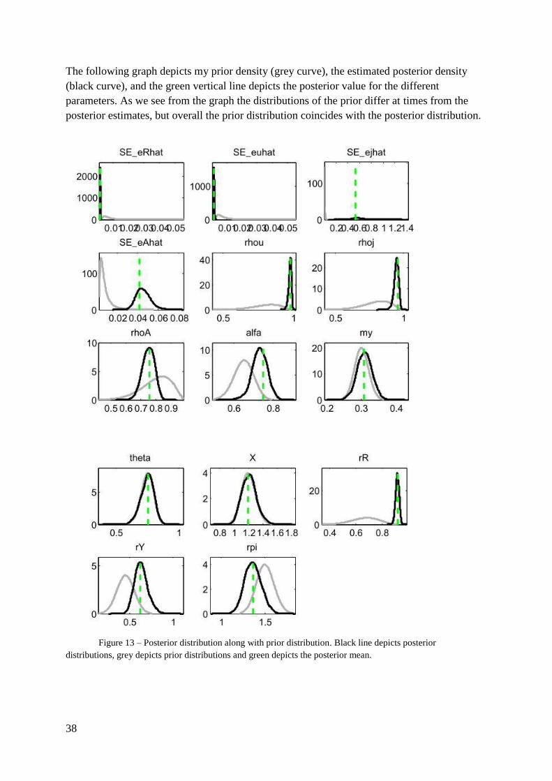
38

The following graph depicts my prior density (grey curve), the estimated posterior density

(black curve), and the green vertical line depicts the posterior value for the different

parameters. As we see from the graph the distributions of the prior differ at times from the

posterior estimates, but overall the prior distribution coincides with the posterior distribution.

Figure 13 – Posterior distribution along with prior distribution. Black line depicts posterior

distributions, grey depicts prior distributions and green depicts the posterior mean.

5.4 Properties of the estimated DSGE model

Table 3 - Correlation matrix of the simulated variables

Variable Yhat Rhat qhat pihat chat c’’hat

Yhat 1.0000 -0.9919 0.9609 -0.8725 0.9791 0.8695

Rhat -0.9919 1.0000 -0.9661 0.9241 -0.9818 -0.8114

qhat 0.9609 -0.9661 1.0000 -0.8506 0.9180 0.7323

pihat -0.8725 0.9241 -0.8506 1.0000 -0.8993 -0.6158

chat 0.9791 -0.9818 0.9180 -0.8993 1.0000 0.8259

c’’hat 0.8695 -0.8114 0.7323 -0.6158 0.8259 1.0000

The correlation matrix of the simulated variables indicates that there is a large positive

correlation between the consumption of the entrepreneurial sector (chat) and house prices of

0.92, as well as a positive correlation between constrained household consumption (c2hat)

and residential prices of the magnitude 0.73. I also find that real house prices are almost

positively correlated with real GDP, but a strong negative correlation between real house

prices and inflation rate. These results are similar to the ones obtained by Ahearne et al.

(2005), although they find that real house prices are co-moving with inflation as well. Also,

when assigning m’’ and m a value of 0, i.e. no collateral constraint, we see that the correlation

between real house prices and impatient household consumption is increased to 0.89,

implying a larger correlation between them. For the entrepreneurial consumption, this

correlation is slightly reduced. The correlation matrix to this simulated scenario is given in the

Appendix C.

In the following graphs, figure 14 and 15, depicting smoothed variables, we see how

the data portrays the quarter to quarter changes. We see that the house prices move strongly

with output and that it lags the cycle slightly. When GDP is above trend then so are the real

house prices. Real house prices are on the other hand a lot more volatile than the real GDP.

Norway experienced a great economic boom in the period of 2003-2007. The low interest

rates made sure that people were able and could afford to buy new houses or upgrade to a

better one, leading to increased demand and, since supply is very inelastic in the short to

medium run, increased house prices. After about 50 quarters we see that real house prices start

their strong descent and drop to more than 0.08% below trend. This fall may largely be

explained by the gradual increase in the policy rate from 1.75 in mid 2005 to 5.75 in the fall

of 2008 along with increased scepticism regarding future prospects.

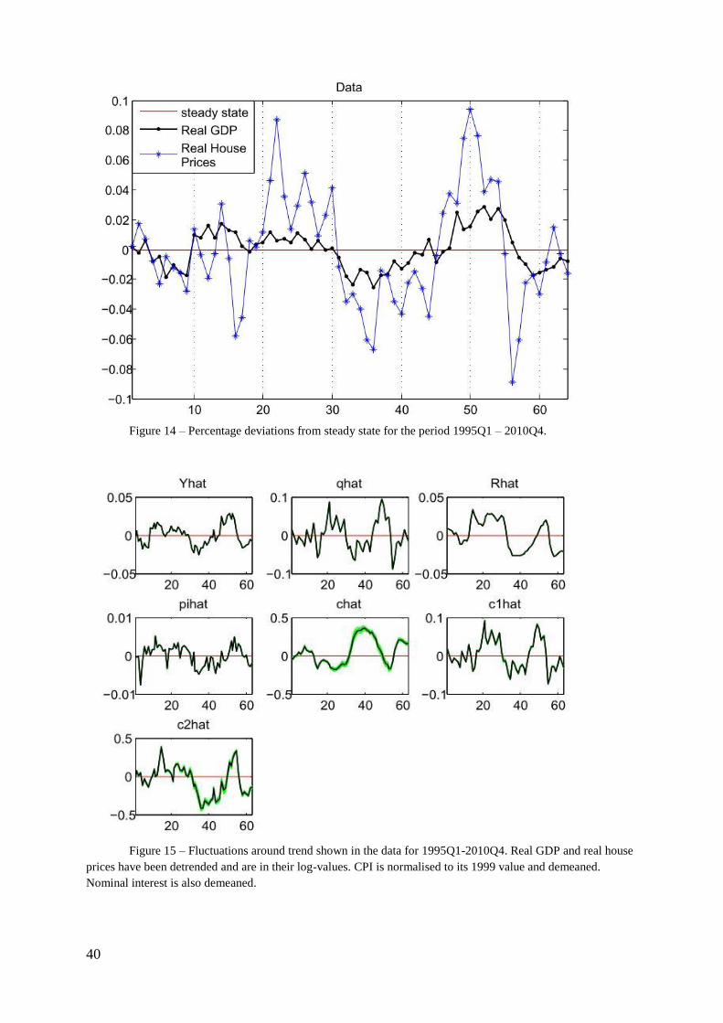
40

Figure 14 – Percentage deviations from steady state for the period 1995Q1 – 2010Q4.

Figure 15 – Fluctuations around trend shown in the data for 1995Q1-2010Q4. Real GDP and real house

prices have been detrended and are in their log-values. CPI is normalised to its 1999 value and demeaned.

Nominal interest is also demeaned.

The impulse response functions of the estimated model are next on the list. I show the

impulse responses of a contractionary monetary policy shock, a positive demand shock, a

positive supply shock (technology shock) and an inflation surprise (cost-push shock). I also

introduce a second curve in the same graphs incorporating a no-collateral constraint

(m=m’’=0). The reason why I do this is because one easy, and perhaps simplistic way, of

showing the spillovers of house prices to consumption is to show the reinforced effects when

there are collateral effects present. Increased house prices should therefore in my model lead

to more consumption when households are able to withdraw more equity from their home, up

to a LTV ratio of unity. This effect is perhaps strongest when considering monetary policy

shocks. The credit channel effect of house prices on consumption is present only when we

consider monetary and real shocks to the economy. The monetary policy shock is therefore

my main concern; although I will, briefly, explain the other impulse responses as well. The

impulse responses for 20 quarters are simulated using estimated parameters and calibrated

parameters, yielding the following results:

Monetary shock. – A contractionary monetary policy shock to the economy, shown as the

initial increase in nominal interest rate, leads initially to a fall in real GDP.

Figure 16 – Impulse responses to an iid. monetary policy shock.

Real GDP declines due to the shock, but moves towards the steady state within 5 quarters.

The situation is quite similar when there are no collateral effects. Real house prices initially

42

drop and hence worsen the cycle, as is reasonable due to fewer agents wishing to buy homes

when the cost of financing increases, but it then overshoots the steady state after the economic

recovery. In the no collateral effects case, real house prices display a bigger initial drop and it

stabilises after around 5 quarters. The drop in real house prices is quite intuitive since asset

prices generally decrease when interest rates increase. Overall on consumption, we see that

the constrained households’ reaction to the policy shock shows a smaller initial drop in

consumption, compared to the case when collateral effects are present. The effects are as

follows: Increased interest rates reduce asset prices and affect the borrowing constraints

negatively. Increased LTV ratio and the effect on the borrowing constraint lead to lower

borrowing opportunities for these households. We clearly see an amplification mechanism in

the case of a negative monetary shock.

Housing preference shock. – A positive nominal demand shock to the economy is shown as

a small initial drop in GDP in both scenarios. Normally a demand shock leads to an increase

in activity, in my model; however, I have the opposite effect, although it is rather small. This

is the same result as Iacoviello (2005) finds for US data.

Figure 17 – Impulse responses to preference shock. Black curve is the baseline model, blue curve

depicts when LTV ratios are set to 0.

A housing preference shock leads to a negative, albeit small, response of aggregate demand.

From above we remember that a housing preference shock may also be regarded as a

measurement of cyclical deviations of the availability of resources needed to purchase

housing and institutional changes that affect housing demand. This is not directly comparable

to a demand shock to output in different models, hence output falls and real house prices

increase initially. Inflation falls initially, leading the central bank to react by reducing the

policy rate. The lower policy rates lead to increased demand and consumption, as is shown in

the graph. Real house prices increase initially and move towards the steady state after a while,

displaying a hump-shaped pattern. In the case of no collateral effects, the effect is greater on

house prices and marginally greater on consumption. Most of the time the two scenarios co-

align with each other and there is no clear financial accelerator effect in play here.

Technology shock. – The positive technology shock to the economy has real effects, as we

see on the real GDP. Real GDP displays a positive hump-shaped pattern after a couple

quarters in both of the scenarios. Unlike the case of a demand shock, a supply shock generates

a trade-off for the central bank.

Figure 18 – Impulse responses to a positive technology (supply) shock. Black curve is the baseline

model, blue curve depicts when LTV ratios are set to 0.

The positive technology shock leads to increased activity in the economy as well as deflation.

Notice that the favourable technology shock is partly accommodated by the central bank, as

the interest rate is decreased. The nominal interest rate should increase in order to dampen the

supply shock on GDP, but it should decrease in order to increase inflation. We see, however,

that it is reduced and should, according to a Taylor rule, imply that the policy rate is reduced

more than the inflation in order to reduce the real interest rate. This is because the central

bank is by assumption not frantically concerned with small output deviations. Instead we see

44

that as the inflation rate starts its climb back towards steady state, the central bank increases

the interest rate accordingly. The consumption of the constrained households displays a

greater negative effect when there are collateral effects in play. This is in contrast to a

monetary shock, as shown above. And as is already noted in Iacoviello (2005) for US data, I

find for Norwegian data that a technology shock decelerates the economy.

Cost-push shock. – An inflation surprise is captured by the positive initial effect on real

GDP, house prices, and as expected, a positive effect on inflation as well. The inflation

pressure in the economy leads to a monetary tightening. As noted above, Tsatsaronis and Zhu

found that inflation is the main driver of house prices. Since households are assumed to hedge

against rising inflation with housing and due to inflation being regarded as a proxy for

financial condition, we clearly see that rising inflation leads to reduced real house prices, in a

hump-shaped pattern. The authors also argued that in the short run almost 90% of the

variation in house prices may be due to inflation. There is a good reason why they are

correlated indeed, seeing that a form of house prices/renting prices is incorporated in the CPI.

The impulse response functions clearly show this effect in play. The collateral case here

almost aligns with the no-collateral constraint scenario, except housing prices and

consumption. We also see a clear difference between the collateral and the no-collateral effect

case. Collateral effects lead to increased effect on consumption, displaying the spillovers of

increased house prices.

Figure 19 – Impulse responses to cost-push shock. Black curve is the baseline model, blue curve depicts

when LTV ratios are set to 0.

Higher wage share of the constrained individuals –As explained above, the fraction of

constrained to unconstrained agents in the economy matters a lot. Increasing the fraction of

ROT consumers should, in theory, lead to increased effect of monetary policy shocks on asset

prices, and therefore on consumption. The intuition is as follows: an unanticipated negative

monetary shock to the economy leads to increased house prices improving the financial

position for the consumer reduced LTV ratio increased borrowing on the face value of

the home increase in consumption. Developments that increase the fraction of constrained

to unconstrained households should therefore amplify this effect. ROT consumers are by

definition consuming their entire income every period, they should in theory react more

strongly to changes in house prices than their more patient counterparts. Reducing the wage

share of the unconstrained agents, decreasing α, should proxy for more ROT consumers as

well as a case of restricting the ease of credit unrelated to housing. I reduce α from 0.73 to 0.2

and analyse the impulse responses to a negative monetary policy shock.

Figure 20 – Impulse responses for different scenarios. Separated the effect of a small monetary policy

shock in the baseline scenario (Black curve), reduced constrained household wage share (Green curve) and no-

collateral effects (Blue curve).

I obtained similar results as Aoki et al. (2001) in their Bank of England Quarterly Bulletin.

Note, however, that they consider instead a reduction in the wage share of ROT consumers.

An unanticipated monetary tightening leads to an initial reduction in house prices. This

worsens the financial position of the borrowers through increased LTV ratio and therefore

reduces their consumption as well. Since impatient households react more strongly to changes

in their current income, increased wage share of ROT consumers will therefore lead to an

46

increased effect on aggregate demand, as shown in the real GDP graph. Aggregate effect on

consumption is not shown as consumption in this model is separated into three different

segments; entrepreneurial consumption, PIH type consumption and ROT consumption. As we

see from figure 20, the effect of increased ROT consumers leads to a much larger initial effect

on real house prices, and therefore a larger effect on inflation as well (not shown in the

graph). Clearly, the wage share of the consumers also displays an amplification mechanism

that leads to increased consumption for constrained agents when compared to the case of no

collateral effect. Comparing reduced alpha to the baseline case (black curve) we see that the

effect on ROT consumption is smaller. This may be due to the dual identity of alpha; proxies

for number of ROT consumers as well as the case of restricting the ease of credit unrelated to

housing. In the recent years we have, nonetheless, seen quite a different trend. While I look at

what happens when the number of ROT consumers increase, the developments in Norway are

rather conflicting. First, average maturing time for mortgage debt has increased from 15 to 23

years during the last decade. Second, the size of the mortgage does not matter as much

anymore; instead a more common practice for banks is to look at the capability of agents in

servicing and taking on new debt. The increased popularity of the no-annuity period in has

also contributed on this matter. Opposing these effects are the stricter guidelines from the

Financial Supervisory Authority for Norway, requiring additional collateral for loans with

exceeding 90% LTV ratio.

Also note that the correlation between ROT consumers’ consumption and real house prices

turns negative and near zero after lowering α from 0.73 to 0.2 (Appendix C). A negative,

although small, correlation implies that as one variable goes up the other goes down. Perhaps

counter intuitively, this says that an increase in the house prices from steady state is

accompanied by reduced consumption for ROT consumers when the fraction of ROT

consumers increases.

5.5 Central bank reacting to house prices

I now turn my attention to the central bank and their role. In this section I intend to add house

prices to the reaction function of the central banks to see if and how monetary policy is

affected by this. I check weather introducing a central bank reaction towards asset price

stabilisation leads to higher volatility in output and inflation in this model. The central bank

will now focus on large variations in asset prices (residential and non-residential prices in this

model), last period’s inflation, output deviations and interest rate smoothing. The following

interest rate rule is implemented in the Dynare4.2.0 estimation procedure:

)( ) )

Note, nonetheless, that I will use the same priors for both types of monetary policy choice

functions. In doing so I follow the lead of Bache et al. (2010) in their study: “This is meant to

reflect the heroic assumption that these parameters are truly structural.”

There is a large literature of researchers including asset prices in their respective

policy specification. A thorough insight into the literature will go beyond the scope of this

thesis, I will, however, briefly go through some main results. As noted above, Iacoviello

(2005) finds that there are gains in targeting asset prices in terms of output and inflation

stabilisation. He argues for a positive weight on asset price deviations, , around 0.1-0.15,

although his results are not statistically significant. Mendicino and Pescatori (2005) also

arrive to the same conclusion in their stylised DSGE model. Svenson (2004) reasons in a

similar manner as the authors above, claiming (in a briefing paper for the ECB governor) that

central banks should not include asset prices in their policy rule in normal times. In normal

times it is up to the supervisory authorities to monitor the market for indicators of financial

instability and report well ahead with appropriate regulatory and supervisory action. This is a

benefit as a whole because it only applies in times of crisis or great instability. Financial

stability becomes then a constraint only when expansionary monetary policy is required,

affecting monetary policy only in gloomy times. He goes on to discuss the limited amount of

information the central bank has prior to excessive asset price surges and the hardship in

identifying the consequences of bubbles bursting. Pre-emptive action to moderate asset price

movements, therefore, will not be usable in practice, ibid.: “Furthermore, whereas the

principles for good monetary policy are simple, the practice of good monetary policy is

difficult.”

Faia and Monacelli (2007) instead find (perhaps counter intuitively) that the monetary

authorities should respond to increased asset prices by lowering the interest rate. The intuition

behind their finding is that the asset price is analogous to a tax that distorts the dynamic

evolution for investment. A central bank with a stark distaste for inflation will, though, not

experience any welfare gains in targeting asset prices. Only those with a specific Taylor type

rule with coefficient on inflation ranging between 1 and 2 experience a gain in welfare. This is

however not different from what is found in central banks around the world, as well as

Norway. This is illustrated in their 3D graph, figure 21, depicting welfare, inflation and asset

prices. When the coefficient of inflation deviation is low, then there are gains in reacting to

asset prices.

Estimating the model with the asset prices, I found, led several of the other parameters t-

statistics to decrease in magnitude. obtained a low t-value (0.21), implying statistical

insignificance just like Iacoviello (2005) in his US study. Most of the posteriors remained

around their prior means, while the standard deviation of the shocks did in fact increase

slightly in magnitude. The policy coefficients were estimated to 0.91, 0.67, 1.38 and 0.03 for

, respectively. These indicate that interest rate smoothing is actively sought

48

out for the monetary policy authorities, although less importance is assigned to output

deviations interest smoothing than for. A great deal of importance is also assigned to inflation

stabilisation, which is to be expected as the central bank is still considered following a

flexible inflation targeting regime. A flexible inflation targeting regime implies that the

central bank aims to keep inflation low and stable, yet still assigning weight to output

deviations. It is assumed to partly accommodate inflationary pressures in the short run in

order to avoid excessive instability of output and unemployment.

I illustrate the impulse responses to three cases of monetary policy specification. One where

is set to zero, one where is set to the estimated value of 0.0348 and one in which I use

the one Iacoviello (2005) suggests in his study, namely 0.15.

We see from the impulse response functions that a monetary tightening leads to no

significant effect on the impulse responses. The impulse responses of the cost-push shock and

the technology shock are given in appendix C, as they reveal the same pattern. The situation is

slightly different when considering a shock to technology, however. These impulse responses

are illustrated in figure 22 and 23, respectively.

Figure 22 – Impulse responses to a negative monetary policy shock. Black curve depicts the case when

rq=0, blue curve when rq=0.03 (estimated value) and green curve when rq=0.15 (as implied by Iacoviello

(2005)).

Reacting to asset prices, here residential and non-residential prices, leads to greater effect on

output, consumption and inflation. My simulation results reveal that the variance of aggregate

output does decrease slightly from reacting to asset prices, but the variance of the inflation

rate is instead increased marginally as well. If these changes are statistically different remains

unknown in this thesis.

Figure 23 – Impulse responses to a positive technology shock. Black curve depicts the case when rq=0, blue

curve when rq=0.04 (estimated value) and green curve when rq=0.15 (implied by Iacoviello (2005)).

This was a rather simplistic way of analysing the effects of incorporating asset prices

into the policy function. I arrive to the similar result as Iacoviello (2005), in that introducing

asset prices into the policy specification is statistically insignificant at the 1%, 5% as well as

the 10% significance level.

50

6 Limitations and Areas of Further

Research

I started off with a plan of incorporating an open economy model for Norway, of which is an

economy that is heavily affected by the developments from the rest of the world. The

financial market is starkly interlinked with the rest of the world as well. The size of the oil

sector in Norway will also be of great importance. And we will have an interlinkage between

the oil producing sector and companies that deliver goods and services to the sector. This

means that Norway will be heavily exposed to oil price shocks that adversely affect our

trading partners. The decrease of the oil price to $20-30 per barrel, among other notable

events, during the financial crisis led to declining stock markets. The Norwegian stock

market is very reliant on the oil producing sector and a large portion of stocks on the OBX are

directly affected by the oil price. In the fall of 2007 until Feb. 2009 the stocks on OBX

experienced a reduction in value of more than 50%. Due to the complexity of finding a

relevant and simple enough model I could work with, I ended up using a closed economy

model instead, developed by Matteo Iacoviello for the US economy. Another possible

extension to the model may be including a housing construction sector in the model as Neri

and Iacoviello (2010) do in their model. They also add land as another input into the

production function for new homes. Something that could be of importance since it ads

another financial accelerator effect in the supply side, in addition to the collateral effects on

the demand side.

I also implemented asset prices into the monetary policy specification in a simplistic

manner. This was never the main part of this thesis; it is rather meant as an addition to the

analysis of the financial accelerator and was rather intended as the discussion part of the

thesis. In the literature on the subject, there are many ways of measuring the effects.

Iacoviello (2005) uses inflation-output volatility frontiers to measure these effects. Mendicino

and Pescatori (2005), as well as Faia and Monacelli (2007), measure these effects through a

welfare function consisting of goods consumption of the households.

I have not done any extensive sensitivity analysis of my estimates and data, although I

had my mind set on doing this from the beginning. Shutting off the shocks and rigidities one

at the time could have provided me with better insight into how robust my estimates really

are. Another possible way of doing this is to estimate my model using different data on house

prices or GDP, use the GDP deflator instead of CPI-ATE, or even use a larger and/or different

dataset than was used in my model. I looked into the option of using data from further back

than 1995, and perhaps incorporate more cycles into the model estimation. This option was

sadly not pursued further due to time limitations. Due to the small sample period in my data, I

was also sceptic regarding a division of my data into subsamples and see how this may affect

my estimates. The closest I got to a sensitivity analysis was re-estimating the model using the

posterior estimates from the Bache et al. (2010) paper for the monetary policy function and

inserting a policy specification incorporating residential and non-residential prices.

Including more shocks to the economy has proven its worth in replicating the real

world in a more precise manner than a model consisting of just a few shocks. A more

complex and realistic model incorporating more shocks is perhaps better at replicating the

business cycles in the data. It goes without saying that more shocks lead to more explanatory

power, but it also leads to problems regarding which shocks account for what. This is also a

possible area of improvement for future analysis. Incorporating more shocks, though, requires

more observable variables if one wants to avoid the problem of stochastic singularity,

something I did not pursue further either. Smets and Wouters (2007) use seven types of

structural shocks, as well as several types of nominal rigidities. Other models, Neri and

Iacoviello (2010), also incorporate wage rigidities for instance, as well as 6 types of structural

shocks.

52

7 Conclusion

“Science is facts; just as houses are made of stones, so is science made of facts; but a pile of

stones is not a house and a collection of facts is not necessarily science.”

Henri Poincare, French mathematician and physicist

The financial accelerator effect is a recently discovered phenomenon and, as noted in the

introduction, there are several different channels the financial accelerator amplification

mechanism works through. I have chosen to focus on the financial accelerator mechanism

within the housing market. Having used a DSGE framework and incorporated heterogeneous

consumers in a model with financial frictions, I measured the importance of the collateral

effects via the entrepreneurial sector along with constrained consumers. I then estimated the

model using a Bayesian approach, calibrated the relevant parameters and estimated the rest.

The estimation procedure yielded results similar to other research on the area of financial

accelerators. It is a remarkable fact that there has not been much research going extensively

into the financial accelerator effect within the Norwegian housing market. This paper is meant

to shine a light on this area of research and perhaps contribute with some new insights into the

spillovers from the housing market to the general economy.

I found that the collateral effects are very important in amplifying and propagating the

effects of monetary shocks to the economy. Absent the collateral effects, an increase in the

demand for housing would produce an increase in housing prices and a reduction in

consumption. The collateral effects are able to amplify the initial shock through the change in

the LTV ratio and the capability of borrowers to obtain more financing. This is something the

traditional wealth effect is not able to explain. The traditional wealth effect postulates that

developments in the housing market do not yield any aggregate wealth effect per se. The

reason behind this assumption is because developments in the housing market are just

considered as a re-distribution away from a first-time borrower to the last-time seller, and not

an increase in aggregate. This is especially the case since houses are not built to be exported.

Through the impulse response functions I have shown that consumers displaying ROT type

behaviour, facing collateral constraints, increase their consumption via Home-Equity-Loans

following an increase house prices after an iid. monetary policy shock. I also found that a

technology shock instead decelerates the fluctuations in the economy, shown by the impulse

responses on consumption. Regulations aimed at restricting the ease of credit for households

will, ceteris paribus, have greater impact in aggregate demand as well as real house prices, as

shown through a monetary tightening. The effect on consumption for ROT type consumers is

greater than the no-collateral scenario, yet below baseline case with LTV ratios of 80% for

impatient households and 35% for entrepreneurs. In other words, collateral effects and a high

wage share of unconstrained households lead to the greatest effect on consumption. Lastly, I

implemented asset prices in the policy specification of the central bank and found that the

coefficient assigned to asset prices is not statistically significant at the 1%, 5% or even 10%

level. This is similar to Iacoviello (2005) study I followed heartily.

54

References

Books

D. N. DeJong and C. Dave, Structural Macroeconometrics, The University Press Group Ltd,

2007

J. Gali, Monetary Policy, Inflation, and the Business Cycle: An Introduction to the New

Keynesian Framework, 2008. Princeton University Press.

J. A. Rice, Mathematical Statistics and Data Analysis, third edition 2007, Thomson –

Brooks/Cole

C. E. Walsh, Monetary Theory and Policy, 2003 third ed. 2010, The MIT Press.

Papers

Ahearne A. G., Ammer J., Doyle B.M., Kole L.S. and Martin R. F., House Prices and

monetary policy: A cross country study, International Finance Discuccion papers, Number

841, Sept. 2005

An S. and Schorfheide F., Bayesian Analysis of DSGE Models, Econometric Reviews, 26(2–

4):113–172, 2007

Angelini P., Neri S. and Panetta F., Monetary and Macroprudential Policies, Banca d’Italia -

Economic Outlook and Monetary Policy Department, September 2010.

Aoki K., Proudman J. and Vlieghe G., House Prices, consumption, and monetary policy: a

financial accelerator approach, Journal of Financial Intermediation 13 (2004) 414-435

Aoki K., Proudman J. and Vlieghe G., Why house prices matter, Bank of England Quarterly

Bulletin, Winter 2001

Bache I. W., Jore A. S., Mitchell J. and Vahey S.P., Combining VAR and DSGE forecast

densities by 2009, Working Paper at Norges Bank No. 23/2009

Bache I. W., Brubakk L. and Maih J., Simple rules versus optimal policy: what fits?, Working

Paper at Norges Bank No. 03/2010

Bernanke B., The Financial Accelerator and the Credit Channel, Speech at The Credit

Channel of Monetary Policy in the Twenty First Century Conference, Federal Reserve bank

of Atlanta, Atlanta, Georgia, June 15, 2007.

http://www.federalreserve.gov/newsevents/speech/bernanke20070615a.htm

Bernanke B., Gertler M. and Gilchrist S., Chapter 21 - The Financial Accelerator in a

Quantitative Business Cycle Framework, Handbook of Macroeconomics, Volume 1

Bernanke B., Gertler M. and Gilchrist S., The Financial Accelerator and the Flight to Quality,

The Review of Economics and Statistics, Vol. 78, No. 1 (feb., 1996), pp. 1-15

Borio C. and McGuire P., Twin peaks in equity and housing prices?, BIS Quarterly Review,

March 2004

Campbell J. Y. and Cocco J.F., How do house prices affect consumption? Evidence from

micro data, Journal of Monetary Economics 54 (2007) pp. 591-621

Christensen I. and Dib A., The financial accelerator in an estimated New Keynesian model,

Review of Economic Dynamics 11 (2008) pp. 155-178

Clarida R., Galì J. and Gertler M., The Science of Monetary Policy: A new Keynesian

Perspective, Journal of Economic Literature, Vol. 37, No. 4 (Dec., 1999), pp. 1661-1707

Faia E. and Monacelli T., Optimal interest rate rules, asset prices, and credit frictions,

Journal of Economic Dynamics & Control 31 (2007) pp. 3228–3254

Finanstilsynet, Finansielt utsyn 2011, downloaded 14.04.2011 at 15.00.

http://www.finanstilsynet.no/Global/Venstremeny/Rapport/2011/Finansielt_utsyn_2011.pdf

Galì J., Lòpez-Salido J. D. and Vallès J., Rule-of-Thumb Consumers and the Design of

Interest Rate Rules, Journal of Money, Credit, and Banking, Vol. 36, No. 4 (August 2004)

Gelain P., The external finance premium in the euro area: A useful indicator for monetary

policy, Working Paper at European Central bank – No. 1171 / April2010

Gerali A., Neri S., Sessa L. and Signoretti F.M., Credit and banking in a DSGE model of the

euro area, Temi di Discussione (Working Papers) No. 740

Iacoviello M., House Prices, Borrowing Constraints, and Monetary Policy in the Business

Cycle, The American economic Review, Vol. 95, No. 3 (Jun., 2005), pp. 739-764

Iacoviello M. and Neri S., Housing Market Spillovers: Evidence from an Estimated DSGE

Model, American Economic Journal: Macroeconomics, Vol. 2, No. 2 (Apr., 2010) pp. 125-

164

Kannan P., Rabanal P. and Scott A.M., Monetary and Macroprudential Policy Rules in a

Model with House Price Booms, IMF Working Paper No. 09/251

Karagedikli Ö., Matheson T., Smith C. and Vahey S., RBCs and DSGEs: The computational

approach to business cycle theory and evidence, Working Paper Norges bank 17/2008

Kiyotaki N. and Moore J., Credit Cycles, The Journal of Political Economy, Vol. 105, No. 2

(April 1997), pp. 211-248

56

Kriwoluzky A., Matching Theory and Data: Bayesian Vector Autoregression and Dynamic

Stochastic General Equilibrium Models, EUI Working Papers MWP 2009/27

Mendicino C. and Pescatori A., Credit Frictions, Housing Prices and Optimal Monetary

Policy Rules, Working Paper No. 42/2004 Universita’ Roma Tre

Rubio M., Fixed and Variable-Rate Mortgages, Business Cycles and Monetary Policy, Banco

de Espana Working Paper No. 0903, 2009

Smets F. and Wouters R., Shocks and Frictions in US Business Cycles: A Bayesian DSGE

Approach, The American Economic Review, Vol. 97, No. 3 (Jun., 2007) pp. 586-606

SSB, Økonomiske analyser 1/2011: 8. Husholdningene, Økonomisk utsyn

http://www.ssb.no/emner/08/05/10/oa/201101/08hushold.pdf

Svenson L., Asset Prices and ECB Monetary Policy, briefing paper for the committee on

Economic and Monetary Affairs (ECON) of the European Parliament for the quarterly

dialogue with the President of the European Central Bank.

Tsatsaronis K. and Zhu H., What drives housing price dynamics: cross country evidence, BIS

Quarterly Review, March 2004

Wieland V., Cwik T., Müller G.J, Schmidt S. and Wolters M., A New Comparative Approach

to Macroeconomic Modeling and Policy Analysis, Working Paper, Goethe University of

Frankfurt, August 2009

Woodford M., Financial Intermediation and Macroeconomic Analysis, Journal of Economic

Perspectives (2010), 24(4), pp. 21-44

Articles and Newspapers

A special report on property: Between a rock and a living space, Economist.com, Mar 3rd

2011

http://www.economist.com/node/18250431?story_id=18250431&fsrc=rss

A special report on property: Bricks and slaughter, Mar 3rd 2011

http://www.economist.com/node/18250385

Appendix

Appendix A Data sources

Seasonally adjusted mainland GDP in fixed prices (in million NOK), i.e. excluding the oil

producing sector Source: SSB, created Fri Apr 08 16:02:00 CEST 2011

Seasonally adjusted consumer price index – adjusted for taxes and energy prices.

Source: SSB, created Fri Apr 08 16:05:58 CEST 2011.

Seasonally adjusted Nominal House Price Index (in thousand NOK, per square meter).

Source: NEF, NFF, Finn.no and Econ Pöyry, created Fri Apr 08 16:10:23 CEST 2011.

3 Month NIBOR rate, average value from daily notations. Source: Norges Bank

Savings ratios for several OECD countries, Economic Outlook No. 88 – December 2010 –

Annual Projections for OECD Countries. www.OECD.org

http://stats.oecd.org/Index.aspx?DataSetCode=EO88_INTERNET

Financial assets and liabilities for Norwegian households per 31 December 2010.

www.SSB.no

http://www.ssb.no/english/yearbook/tab/tab-302.html

Estimation was done using Dynare 4.2.0, a freeware programming code usable inside Matlab

or Octave, downloadable from here: http://www.dynare.org/download

Data was handled using Matlab R2010b, http://www.mathworks.com/

Graphs and charts were drawn using MS Excel, MS Words and SmartDraw VP (can be

downloaded from http://www.smartdraw.com/ )

58

Appendix B HP-filter

Hodrick-Prescott Filter is a smoothing technique used to detrend dataseries, ie. it removes

short-term fluctuations that are related to business cycles. It therefore is a neat trick to reveal

long term trends in the data.

Mathematically it can be expressed as:

or

{ }

∑ ) ∑( ) ))

Where the first sum denotes the goodness of fit and the second term denotes the penalty for

Roughness. λ denotes the smoothing parameter and is in the literature 1600 when considering

quarterly data.

Real GDP and real house prices have been detrended using HP-filter. If x is the m x m matrix

I wish to detrend, I first take log of x and then run it through a Matlab code using the

following command: ) ) ) where 1600 is the smoothing

number.

The Matlab code can be found here:

http://www.krannert.purdue.edu/faculty/knaknoi/Econ635/matlab_filter.html

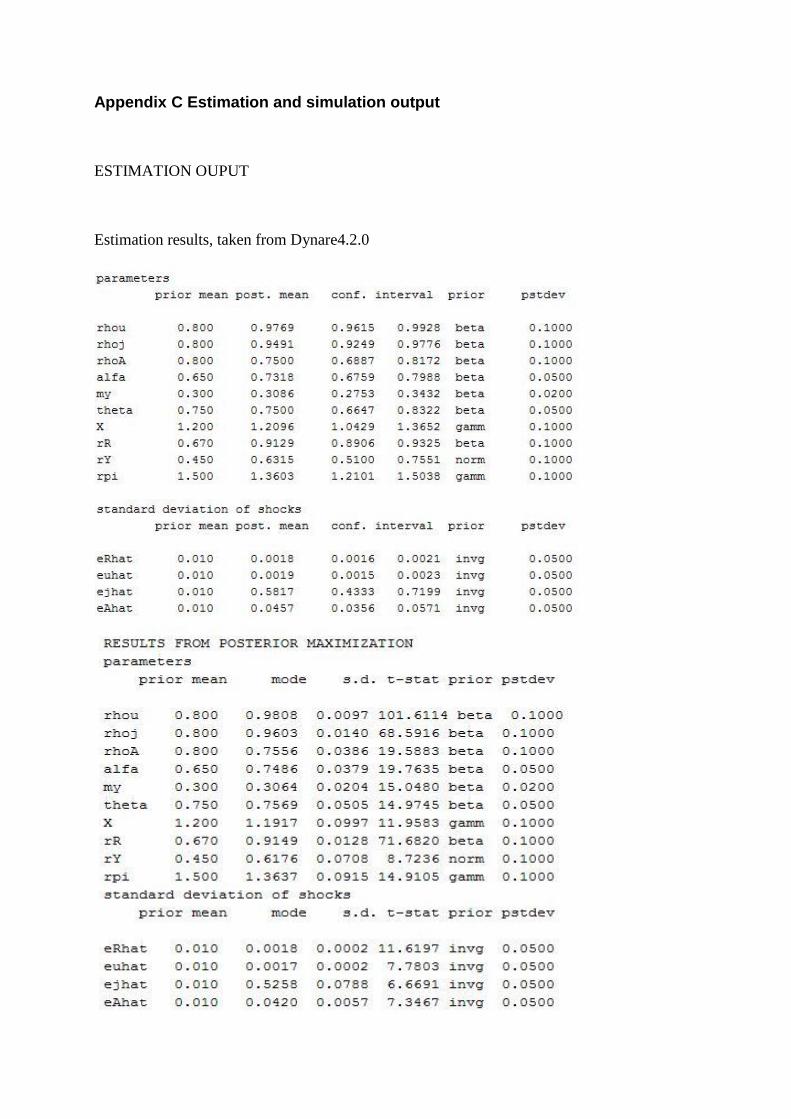
Appendix C Estimation and simulation output

ESTIMATION OUPUT

Estimation results, taken from Dynare4.2.0

60

Graphs of the the check_plot function in Dynare4.2.0, showing that maximum is truly found

The vertical line should coincide with the maximum of the log post (blue) curve, as is the case

for all except the AR(1) coefficient for cost-push shock:

Smoothed shocks, these should be around zero. They are indeed around zero.

Estimation results when with alternative policy specification

62

Check-plots:

Prior- and posterior distributions:

64

Smoothed Shocks: The shocks are around zero as is expected.

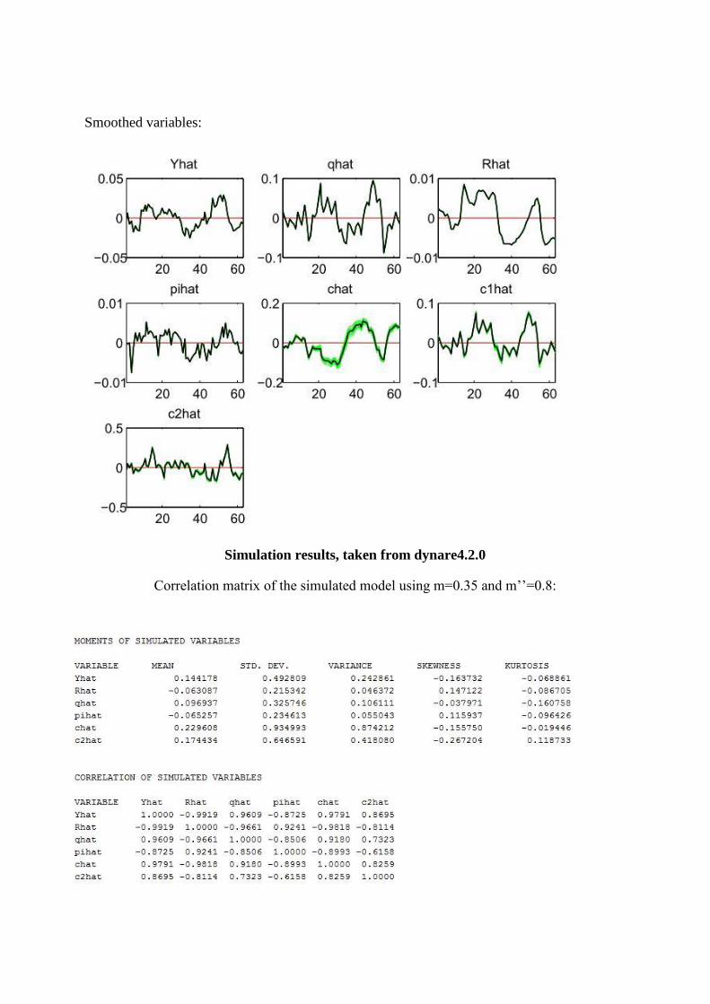
Smoothed variables:

Simulation results, taken from dynare4.2.0

Correlation matrix of the simulated model using m=0.35 and m’’=0.8:

66

Correlation matrix of the simulated model using m=m’’=0:

Correlation matrix of the simulated model using α=0.2, m=0.35 and m’’=0.8

Simulation results from estimated model incorporating asset prices in the policy specification.

Impulse responses to a technology shock. Black curve depicts the case when rq=0, blue curve when

rq=0.04 (estimated value) and green curve when rq=0.15 (implied by Iacoviello (2005)).

Impulse responses to a cost-push shock. Black curve depicts the case when rq=0, blue curve when

rq=0.04 (estimated value) and green curve when rq=0.15 (implied by Iacoviello (2005)).

68

Simulation when rq=0

Simulation when rq=0.03

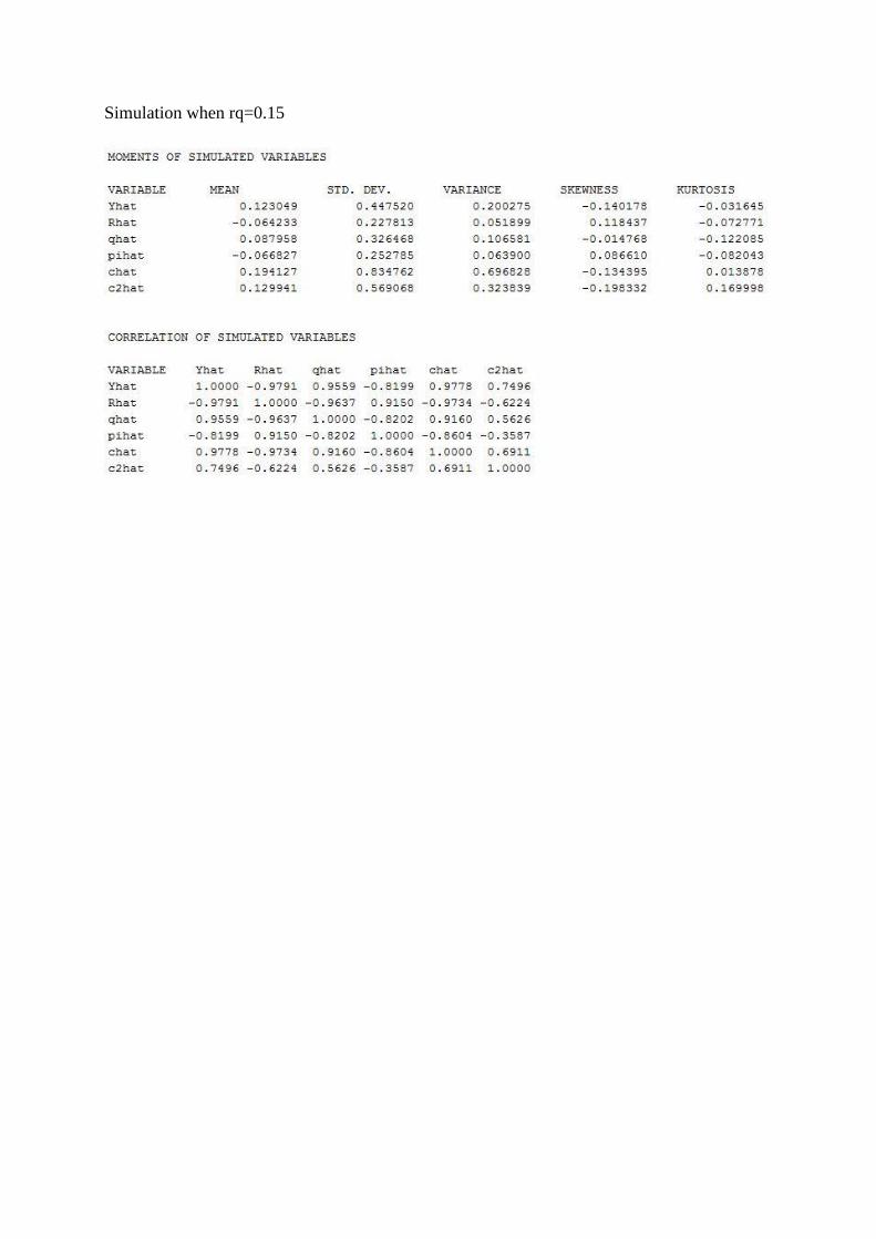
Simulation when rq=0.15

70

Dynare4.2.0 Model Code obtained through the macro model database

// Model: US_IAC05

// Further references: // Matteo Iacoviello. 2005. "House Prices, Borrowing Constraints, and

Monetary Policy in the Business Cycle" // the American Economic Review 95, pp. 739-764.

//% basic endogenous variable var Yhat chat c1hat c2hat Ihat Khat Xhat qhat bhat b2hat hhat h2hat Rhat

pihat rrhat

//% Endogenous variables with exogenous dynamics jhat Ahat uhat;

//% Declaration of exogenous variables (shocks) varexo ejhat, euhat, eAhat, eRhat;

parameters

//% deep parameters beta, beta2, gamma, j, eta, my, ypsilon, psi, delta, fie, fih, X, theta, alfa, m, m2, rhou, rhoj, rhoA, rR, rpi, rY, gammae, gammah,

omega, kappa, s1, s2, qhtoY, btoY, c1toY, qh1toY, qh2toY, htoh1, h2toh1, b2toY, c2toY, ctoY, ItoY, jota, jota2, h1ss, sigmau, sigmaj, sigmaA, sigmaR, R;

//% Setting of numerical values for parameters

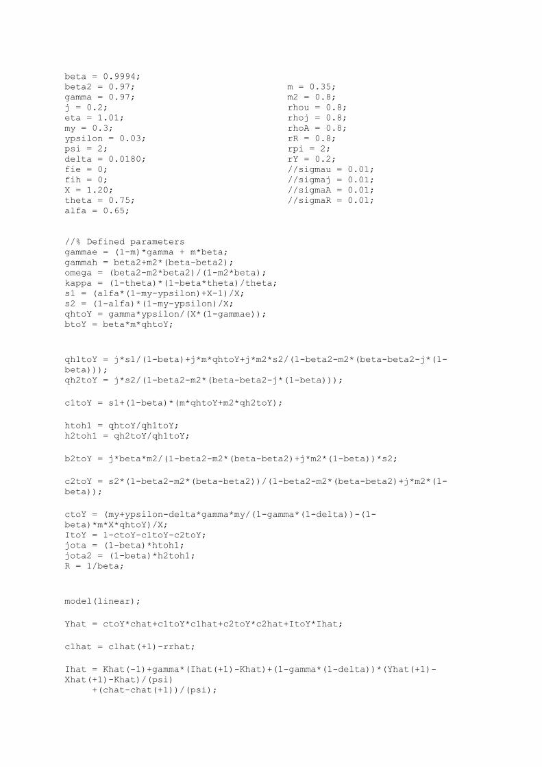
beta = 0.9994; beta2 = 0.97; gamma = 0.97; j = 0.2; eta = 1.01; my = 0.3; ypsilon = 0.03; psi = 2; delta = 0.0180; fie = 0; fih = 0; X = 1.20; theta = 0.75; alfa = 0.65;

m = 0.35; m2 = 0.8; rhou = 0.8; rhoj = 0.8; rhoA = 0.8; rR = 0.8; rpi = 2; rY = 0.2; //sigmau = 0.01; //sigmaj = 0.01; //sigmaA = 0.01; //sigmaR = 0.01;

//% Defined parameters gammae = (1-m)*gamma + m*beta; gammah = beta2+m2*(beta-beta2); omega = (beta2-m2*beta2)/(1-m2*beta); kappa = (1-theta)*(1-beta*theta)/theta; s1 = (alfa*(1-my-ypsilon)+X-1)/X; s2 = (1-alfa)*(1-my-ypsilon)/X; qhtoY = gamma*ypsilon/(X*(1-gammae)); btoY = beta*m*qhtoY;

qh1toY = j*s1/(1-beta)+j*m*qhtoY+j*m2*s2/(1-beta2-m2*(beta-beta2-j*(1-

beta))); qh2toY = j*s2/(1-beta2-m2*(beta-beta2-j*(1-beta)));

c1toY = s1+(1-beta)*(m*qhtoY+m2*qh2toY);

htoh1 = qhtoY/qh1toY; h2toh1 = qh2toY/qh1toY;

b2toY = j*beta*m2/(1-beta2-m2*(beta-beta2)+j*m2*(1-beta))*s2;

c2toY = s2*(1-beta2-m2*(beta-beta2))/(1-beta2-m2*(beta-beta2)+j*m2*(1-

beta));

ctoY = (my+ypsilon-delta*gamma*my/(1-gamma*(1-delta))-(1-

beta)*m*X*qhtoY)/X; ItoY = 1-ctoY-c1toY-c2toY; jota = (1-beta)*htoh1; jota2 = (1-beta)*h2toh1; R = 1/beta;

model(linear);

Yhat = ctoY*chat+c1toY*c1hat+c2toY*c2hat+ItoY*Ihat;

c1hat = c1hat(+1)-rrhat;

Ihat = Khat(-1)+gamma*(Ihat(+1)-Khat)+(1-gamma*(1-delta))*(Yhat(+1)-

Xhat(+1)-Khat)/(psi) +(chat-chat(+1))/(psi);

2

qhat = gammae*qhat(+1)+(1-gammae)*(Yhat(+1)-Xhat(+1)-hhat)-m*beta*rrhat -(1-m*beta)*(chat(+1)-chat)-fie*(hhat-hhat(-1)-gamma*(hhat(+1)-hhat));

qhat = gammah*qhat(+1)+(1-gammah)*(jhat-h2hat)-m2*beta*rrhat+(1-

m2*beta)*(c2hat-omega*c2hat(+1)) -fih*(h2hat-h2hat(-1)-beta2*(h2hat(+1)-h2hat));

qhat = beta*qhat(+1)+(1-beta)*jhat+jota*hhat+jota2*h2hat+c1hat-

beta*c1hat(+1) +fih*(htoh1*(hhat-hhat(-1))+h2toh1*(h2hat-h2hat(-1))-

beta*htoh1*(hhat(+1)-hhat)-beta*h2toh1*(h2hat(+1)-h2hat));

bhat = qhat(+1)+hhat-rrhat;

b2hat = qhat(+1)+h2hat-rrhat;

Yhat = eta*(Ahat+ypsilon*hhat(-1)+my*Khat(-1))/(eta-(1-ypsilon-my)) -(1-ypsilon-my)*(Xhat+alfa*c1hat+(1-alfa)*c2hat)/(eta-(1-ypsilon-my));

pihat = beta*pihat(+1)-kappa*Xhat+uhat;

Khat = delta*Ihat+(1-delta)*Khat(-1);

btoY*bhat = ctoY*chat+qhtoY*(hhat-hhat(-1))+ItoY*Ihat+R*btoY*(Rhat(-

1)+bhat(-1)-pihat) -(1-s1-s2)*(Yhat-Xhat);

b2toY*b2hat = c2toY*c2hat+qh2toY*(h2hat-h2hat(-1))+R*b2toY*(b2hat(-

1)+Rhat(-1)-pihat)-s2*(Yhat-Xhat);

Rhat = (1-rR)*(1+rpi)*pihat(-1)+rY*(1-rR)*Yhat(-1)+rR*Rhat(-1)+eRhat;

//*************************************************************************

//Alternative policy specification

//Rhat = rR*Rhat(-1)+(1-rR)*(rq*qhat+(1+rpi)*pihat(-1)+rY*Yhat(-1))+eRhat;

//*************************************************************************

//% Defined variable(s) rrhat = Rhat-pihat(+1);

//% equations for variables with exogenous AR(1)-dynamics jhat = rhoj*jhat(-1)+ejhat; uhat = rhou*uhat(-1)+euhat; Ahat = rhoA*Ahat(-1)+eAhat;

end;

//************************************************************************* //Needed to simulate the model

//shocks; //var eRhat; //stderr sigmaR; //var euhat; //stderr sigmau;

//var ejhat; //stderr sigmaj; //var eAhat; //stderr sigmaA; //end;

//stoch_simul(periods=5000,simul_seed=1, irf=20) Yhat Rhat qhat

pihat chat c2hat;

//*************************************************************************

estimated_params;

stderr eRhat, inv_gamma_pdf,0.01,0.05; stderr euhat, inv_gamma_pdf,0.01,0.05; stderr ejhat, inv_gamma_pdf,0.01,0.05; stderr eAhat, inv_gamma_pdf,0.01,0.05; rhou, beta_pdf, 0.8, .1; rhoj, beta_pdf, 0.8, .1; rhoA, beta_pdf, 0.8, .1; alfa, beta_pdf, 0.65, 0.05; my, beta_pdf, 0.3, .02; theta, beta_pdf, 0.75, 0.05; rR, beta_pdf, 0.8, 0.1; //rY, normal_pdf, 0.2, 0.15; rpi, gamma_pdf, 2, 0.1;

end;

estimated_params_bounds; stderr eRhat, 0.0001, 100; stderr euhat, 0.0001, 100; stderr ejhat, 0.0001, 100; stderr eAhat, 0.0001, 100; rhou, .001,.9999; rhoj, .001,.9999; rhoA, .0001,.9999; alfa, 0,.99; my, 0,.99; theta, 0,.99; rR, 0,.9999; //rY, 0,10; rpi,0,10;

end;

estimated_params_init; stderr eRhat, 0.01; stderr euhat, 0.01; stderr ejhat, 0.01; stderr eAhat, 0.01; rhou, 0.8; rhoj, 0.8; rhoA, 0.8;

4

alfa, 0.65; my, 0.3; theta, 0.75; rR, 0.9; //rY, 0.2; rpi, 2; end;

varobs Yhat pihat qhat Rhat;

// bayesestimation

estimation(datafile=”filename”,conf_sig

=.95,smoother,mode_check,mode_compute=1,mh_replic=2000,mh_jscale=0.55,mh_nb

locks=1,prior_trunc=0) Yhat Rhat pihat qhat chat c1hat c2hat;

Appendix D Data manipulation

Real GDP was log transformed and HP-filtered via Matlab R2010b

Real house prices were found by using the following formula: Real Houseprices = Nominal Houseprices/Price Index

Real house prices were then log transformed and HP-filtered

3-Month annualised NIBOR was given in monthly values, from daily notations. Quarter average was found and demeaned by deducting the average of the time series from 1995-2010. Was then multiplied by 3 and divided by 12 in order to de-annualise them. Was also divided by 100 in order to be directly compared to the other time-series.

CPI-ATE was seasonally adjusted and given in monthly values. Quarter average was found and demeaned by deducting the mean of the time series. Divided by 100 in order to be directly compared to GDP and house prices. The inflation rate was found using the following formula: Inflation Rate = ( )

The first observation is therefore lost using this transformation, yielding me 63 observations instead of

64.

CPI-ATE NIBOR GDP House price index

01.01.1995 91.30 januar 95 5.76 01.01.1995 257113 1995Q1 40.3 01.02.1995 91.50 februar 95 5.46 01.04.1995 258120 1995Q2 42 01.03.1995 91.70 mars 95 5.39 01.07.1995 262294 1995Q3 42.7 01.04.1995 91.80 april 95 5.36 01.10.1995 260635 1995Q4 43.2 01.05.1995 91.90 mai 95 5.67 01.01.1996 263442 1996Q1 43.7

01.06.1995 92.00 juni 95 5.79 01.04.1996 261907 1996Q2 45.7 01.07.1995 92.10 juli 95 5.62 01.07.1996 266038 1996Q3 46.6 01.08.1995 92.30 august 95 5.34 01.10.1996 266835 1996Q4 47.7

01.09.1995 92.40 september

95 5.36 01.01.1997 268386 1997Q1 48.4 01.10.1995 92.60 oktober 95 5.34 01.04.1997 277845 1997Q2 51.8 01.11.1995 92.60 november 95 5.22 01.07.1997 279446 1997Q3 52.3 01.12.1995 92.80 desember 95 5.43 01.10.1997 283821 1997Q4 52.9 01.01.1996 92.40 januar 96 5.48 01.01.1998 283573 1998Q1 55.2 01.02.1996 92.30 februar 96 5.26 01.04.1998 288195 1998Q2 58.6 01.03.1996 92.40 mars 96 4.92 01.07.1998 288959 1998Q3 58 01.04.1996 92.50 april 96 4.70 01.10.1998 290378 1998Q4 56.5 01.05.1996 92.70 mai 96 4.76 01.01.1999 289421 1999Q1 58.7

01.06.1996 92.70 juni 96 4.93 01.04.1999 290163 1999Q2 63.4 01.07.1996 93.10 juli 96 4.99 01.07.1999 293346 1999Q3 64.7 01.08.1996 93.30 august 96 5.02 01.10.1999 295339 1999Q4 67

01.09.1996 93.40 september

96 5.09 01.01.2000 299104 2000Q1 71 01.10.1996 93.50 oktober 96 5.04 01.04.2000 298979 2000Q2 75.7 01.11.1996 93.70 november 96 4.39 01.07.2000 300975 2000Q3 73.5 01.12.1996 93.90 desember 96 4.14 01.10.2000 301616 2000Q4 73.5

6

01.01.1997 94.20 januar 97 3.52 01.01.2001 305141 2001Q1 76.2

01.02.1997 94.40 februar 97 3.52 01.04.2001 305315 2001Q2 79.5 01.03.1997 94.40 mars 97 3.51 01.07.2001 304797 2001Q3 79.5 01.04.1997 94.60 april 97 3.50 01.10.2001 308003 2001Q4 79.2 01.05.1997 94.70 mai 97 3.46 01.01.2002 307654 2002Q1 81.8 01.06.1997 95.00 juni 97 3.51 01.04.2002 309520 2002Q2 84.8 01.07.1997 95.10 juli 97 4.00 01.07.2002 309260 2002Q3 81.9 01.08.1997 95.40 august 97 4.04 01.10.2002 307074 2002Q4 81.4

01.09.1997 95.50 september

97 3.94 01.01.2003 306999 2003Q1 83.3 01.10.1997 95.70 oktober 97 3.97 01.04.2003 312079 2003Q2 83.9 01.11.1997 95.90 november 97 3.95 01.07.2003 313408 2003Q3 83.7 01.12.1997 96.10 desember 97 3.87 01.10.2003 312233 2003Q4 84.7 01.01.1998 96.50 januar 98 3.82 01.01.2004 317103 2004Q1 91

01.02.1998 96.80 februar 98 3.84 01.04.2004 319578 2004Q2 92.4 01.03.1998 97.10 mars 98 4.08 01.07.2004 324773 2004Q3 92.6 01.04.1998 97.30 april 98 4.15 01.10.2004 325733 2004Q4 93.6 01.05.1998 97.40 mai 98 4.47 01.01.2005 329575 2005Q1 97.5 01.06.1998 97.60 juni 98 4.82 01.04.2005 334540 2005Q2 100.2 01.07.1998 97.90 juli 98 5.35 01.07.2005 336781 2005Q3 101.1 01.08.1998 98.10 august 98 6.74 01.10.2005 343155 2005Q4 101.2

01.09.1998 98.40 september

98 8.03 01.01.2006 340826 2006Q1 107.5 01.10.1998 98.60 oktober 98 7.92 01.04.2006 345999 2006Q2 112.8 01.11.1998 98.80 november 98 7.96 01.07.2006 349666 2006Q3 116.5 01.12.1998 99.00 desember 98 8.24 01.10.2006 360878 2006Q4 117.9 01.01.1999 99.10 januar 99 7.72 01.01.2007 359610 2007Q1 125.3

01.02.1999 99.10 februar 99 7.27 01.04.2007 362955 2007Q2 130 01.03.1999 99.80 mars 99 6.88 01.07.2007 369173 2007Q3 129.8 01.04.1999 99.90 april 99 6.55 01.10.2007 372767 2007Q4 126.9 01.05.1999 99.90 mai 99 6.66 01.01.2008 372161 2008Q1 129.9 01.06.1999 100.00 juni 99 6.48 01.04.2008 376986 2008Q2 131.5 01.07.1999 100.00 juli 99 6.35 01.07.2008 376285 2008Q3 127 01.08.1999 99.90 august 99 6.09 01.10.2008 372626 2008Q4 118.1

01.09.1999 100.20 september

99 5.97 01.01.2009 370826 2009Q1 123 01.10.1999 100.50 oktober 99 6.37 01.04.2009 370841 2009Q2 129.5 01.11.1999 100.70 november 99 6.15 01.07.2009 369872 2009Q3 131.8 01.12.1999 100.80 desember 99 5.97 01.10.2009 372285 2009Q4 131.8 01.01.2000 101.10 januar 00 5.88 01.01.2010 374866 2010Q1 136.3

01.02.2000 101.30 februar 00 5.89 01.04.2010 377350 2010Q2 141.3 01.03.2000 101.40 mars 00 6.00 01.07.2010 381035 2010Q3 140.6 01.04.2000 101.70 april 00 6.23 01.10.2010 382163 2010Q4 140.5 01.05.2000 101.80 mai 00 6.50

01.06.2000 102.20 juni 00 6.72

01.07.2000 102.30 juli 00 6.91

01.08.2000 102.70 august 00 7.12

01.09.2000 103.00 september

00 7.33

01.10.2000 103.10 oktober 00 7.52

01.11.2000 103.30 november 00 7.43

01.12.2000 103.50 desember 00 7.42

01.01.2001 103.80 januar 01 7.41

01.02.2001 104.30 februar 01 7.32

01.03.2001 104.20 mars 01 7.39

01.04.2001 104.30 april 01 7.48

01.05.2001 104.50 mai 01 7.45

01.06.2001 104.70 juni 01 7.42

01.07.2001 104.90 juli 01 7.37

01.08.2001 105.20 august 01 7.31

01.09.2001 105.40 september

01 7.14

01.10.2001 105.60 oktober 01 6.94

01.11.2001 105.90 november 01 6.90

01.12.2001 106.20 desember 01 6.59

01.01.2002 106.40 januar 02 6.32

01.02.2002 106.50 februar 02 6.57

01.03.2002 106.90 mars 02 6.72

01.04.2002 106.80 april 02 6.77

01.05.2002 107.30 mai 02 6.90

01.06.2002 107.50 juni 02 7.12

01.07.2002 107.80 juli 02 7.25

01.08.2002 107.70 august 02 7.26

01.09.2002 107.70 september

02 7.15

01.10.2002 107.80 oktober 02 7.12

01.11.2002 107.90 november 02 7.09

01.12.2002 108.10 desember 02 6.62

01.01.2003 108.40 januar 03 5.99

01.02.2003 108.70 februar 03 5.69

01.03.2003 108.40 mars 03 5.49

01.04.2003 108.50 april 03 5.26

01.05.2003 108.60 mai 03 4.92

01.06.2003 108.50 juni 03 4.04

01.07.2003 108.60 juli 03 3.45

01.08.2003 108.60 august 03 3.14

01.09.2003 108.60 september

03 2.81

01.10.2003 108.60 oktober 03 2.86

01.11.2003 108.50 november 03 2.89

01.12.2003 108.50 desember 03 2.64

01.01.2004 108.50 januar 04 2.26

01.02.2004 108.60 februar 04 2.01

01.03.2004 108.70 mars 04 1.84

01.04.2004 108.70 april 04 1.97

01.05.2004 108.70 mai 04 1.99

01.06.2004 108.80 juni 04 2.03

8

01.07.2004 108.90 juli 04 2.02

01.08.2004 108.80 august 04 2.02

01.09.2004 109.10 september

04 1.96

01.10.2004 109.20 oktober 04 2.00

01.11.2004 109.40 november 04 1.99

01.12.2004 109.50 desember 04 1.99

01.01.2005 109.40 januar 05 1.96

01.02.2005 109.40 februar 05 1.92

01.03.2005 109.50 mars 05 2.02

01.04.2005 109.70 april 05 2.05

01.05.2005 109.90 mai 05 2.08

01.06.2005 110.00 juni 05 2.15

01.07.2005 110.10 juli 05 2.22

01.08.2005 110.30 august 05 2.25

01.09.2005 110.40 september

05 2.35

01.10.2005 110.50 oktober 05 2.45

01.11.2005 110.50 november 05 2.54

01.12.2005 110.50 desember 05 2.55

01.01.2006 110.50 januar 06 2.52

01.02.2006 110.50 februar 06 2.57

01.03.2006 110.40 mars 06 2.72

01.04.2006 110.60 april 06 2.82

01.05.2006 110.70 mai 06 2.94

01.06.2006 110.90 juni 06 3.03

01.07.2006 110.90 juli 06 3.09

01.08.2006 110.70 august 06 3.23

01.09.2006 111.00 september

06 3.37

01.10.2006 111.30 oktober 06 3.48

01.11.2006 111.50 november 06 3.62

01.12.2006 111.60 desember 06 3.80

01.01.2007 111.60 januar 07 3.98

01.02.2007 111.80 februar 07 4.20

01.03.2007 112.10 mars 07 4.43

01.04.2007 112.10 april 07 4.54

01.05.2007 112.20 mai 07 4.60

01.06.2007 112.20 juni 07 4.75

01.07.2007 112.30 juli 07 4.89

01.08.2007 112.70 august 07 5.18

01.09.2007 112.80 september

07 5.50

01.10.2007 112.90 oktober 07 5.67

01.11.2007 113.20 november 07 5.78

01.12.2007 113.60 desember 07 5.96

01.01.2008 113.80 januar 08 5.79

01.02.2008 114.20 februar 08 5.91

01.03.2008 114.50 mars 08 6.18

01.04.2008 114.70 april 08 6.30

01.05.2008 114.90 mai 08 6.48

01.06.2008 114.90 juni 08 6.41

01.07.2008 115.60 juli 08 6.46

01.08.2008 115.90 august 08 6.53

01.09.2008 116.20 september

08 6.82

01.10.2008 116.60 oktober 08 6.92

01.11.2008 116.40 november 08 6.18

01.12.2008 116.60 desember 08 4.64

01.01.2009 117.00 januar 09 3.70

01.02.2009 117.60 februar 09 3.48

01.03.2009 117.60 mars 09 3.17

01.04.2009 117.90 april 09 2.87

01.05.2009 118.10 mai 09 2.40

01.06.2009 118.60 juni 09 2.10

01.07.2009 118.60 juli 09 1.87

01.08.2009 118.60 august 09 1.88

01.09.2009 119.00 september

09 1.93

01.10.2009 119.00 oktober 09 2.03

01.11.2009 119.20 november 09 2.05

01.12.2009 119.40 desember 09 2.08

01.01.2010 119.70 januar 10 2.25

01.02.2010 119.80 februar 10 2.27

01.03.2010 119.70 mars 10 2.30

01.04.2010 119.80 april 10 2.39

01.05.2010 120.00 mai 10 2.50

01.06.2010 120.10 juni 10 2.67

01.07.2010 120.10 juli 10 2.69

01.08.2010 120.20 august 10 2.65

01.09.2010 120.10 september

10 2.64

01.10.2010 120.30 oktober 10 2.56

01.11.2010 120.40 november 10 2.51

01.12.2010 120.60 desember 10 2.59

01.01.2011 120.50 januar 11 2.59

01.02.2011 120.60 februar 11 2.61

Yhat qhat Rhat pihat

10

1995Q2 -0.00208 0.01717 0.002315 -2.5E-06

1995Q3 0.00621 0.00711 0.001902 -0.00038

1995Q4 -0.00789 -0.00785 0.001631 -3.9E-05

1996Q1 -0.00494 -0.02297 0.001356 -0.00761

1996Q2 -0.01854 -0.00489 0.000294 -0.00149

1996Q3 -0.01065 -0.01210 0.000882 0.002463

1996Q4 -0.01541 -0.01552 -0.00039 0.000272

1997Q1 -0.01732 -0.02772 -0.0029 0.002385

1997Q2 0.00969 0.01341 -0.00298 0.00022

1997Q3 0.00792 -0.00371 -0.00171 0.001606

1997Q4 0.01609 -0.01895 -0.00187 0.00157

1998Q1 0.00803 -0.00293 -0.00191 0.005011

1998Q2 0.01722 0.03045 -0.0005 0.002169

1998Q3 0.01312 -0.00602 0.005076 0.00281

1998Q4 0.01149 -0.05818 0.008401 0.002419

1999Q1 0.00189 -0.04567 0.006528 0.001024

1999Q2 -0.00163 0.00600 0.004705 0.001666

1999Q3 0.00341 0.00137 0.003647 -0.00337

1999Q4 0.00450 0.01189 0.003716 0.001957

2000Q1 0.01168 0.04609 0.003114 0.001586

2000Q2 0.00595 0.08710 0.004512 0.00188

2000Q3 0.00744 0.03528 0.0061 0.00315

2000Q4 0.00452 0.01371 0.006947 0.001795

2001Q1 0.01120 0.02896 0.006732 0.00337

2001Q2 0.00689 0.05124 0.006925 -0.00053

2001Q3 0.00033 0.03179 0.006486 0.002006

2001Q4 0.00591 0.00915 0.005326 0.002599

2002Q1 -0.00017 0.02308 0.004642 0.002236

2002Q2 0.00082 0.04111 0.005622 0.001254

2002Q3 -0.00525 -0.01141 0.006347 0.000601

2002Q4 -0.01777 -0.03513 0.005661 -0.00252

2003Q1 -0.02370 -0.02968 0.002613 0.000876

2003Q2 -0.01327 -0.04025 0.000146 -0.00407

2003Q3 -0.01530 -0.06061 -0.00386 -0.00376

2003Q4 -0.02566 -0.06701 -0.0047 -0.00499

2004Q1 -0.01711 -0.01387 -0.00661 -0.00376

2004Q2 -0.01657 -0.01753 -0.00672 -0.00315

2004Q3 -0.00795 -0.03460 -0.00671 -0.00253

2004Q4 -0.01276 -0.04338 -0.00671 -0.0004

2005Q1 -0.00899 -0.02230 -0.00678 -0.00376

2005Q2 -0.00215 -0.01488 -0.00646 -0.00041

2005Q3 -0.00369 -0.02590 -0.006 -0.00073

2005Q4 0.00680 -0.04484 -0.00542 -0.00226

2006Q1 -0.00826 -0.00422 -0.00519 -0.00468

2006Q2 -0.00138 0.02444 -0.00437 -0.00196

2006Q3 0.00110 0.03768 -0.00362 -0.00317

2006Q4 0.02479 0.03118 -0.00261 0.001038

2007Q1 0.01364 0.07428 -0.00119 -0.00108

2007Q2 0.01556 0.09411 -0.00012 -0.00139

2007Q3 0.02553 0.07638 0.001277 -0.00051

2007Q4 0.02855 0.03840 0.002813 0.001251

2008Q1 0.02060 0.04711 0.003206 0.003869

2008Q2 0.02752 0.04535 0.00429 0.001465

2008Q3 0.02002 -0.00296 0.004804 0.004915

2008Q4 0.00490 -0.08872 0.003096 0.00109

2009Q1 -0.00505 -0.06094 -0.00307 0.003063

2009Q2 -0.00994 -0.02216 -0.00555 0.00244

2009Q3 -0.01735 -0.01718 -0.00697 0.000138

2009Q4 -0.01556 -0.02975 -0.00656 -0.00044

2010Q1 -0.01331 -0.00872 -0.00601 0.0001

2010Q2 -0.01133 0.01479 -0.0054 -0.00243

2010Q3 -0.00622 -0.00267 -0.00505 -0.00298

2010Q4 -0.00787 -0.01586 -0.00532 -0.00188