Collateral constraint and news-driven cycles∗

Keiichiro Kobayashi†, Tomoyuki Nakajima‡, and Masaru Inaba§

July 2010 (First version: August 2007)

Abstract

We develop business-cycle models with financial constraints, the driving force of

which is news about the future (i.e., changes in expectations). We assume that an

asset with fixed supply (“land”) is used as collateral, and firms need to hold collateral

to finance their input costs. The latter feature introduces an interaction between the

inefficiencies in the financial market and in the factor market. Good news raises the

price of land today, which relaxes the collateral constraint. It, in turn, reduces the

inefficiency in the labor market. If this force is sufficiently strong, the equilibrium

labor supply increases. So do output, investment and consumption. Our models

also generate procyclical movement in Tobin’s Q. We also show that when the news

turns out to be wrong, the economy may fall into a recession.

Keywords: News-driven cycles; collateral constraints; Tobin’s q; bankruptcies.

JEL Classifications: E22, E32, E37, G12.

1 Introduction

In this paper we develop models of business cycles driven by “news shocks” (i.e., changes

in expectations) through financial frictions. The current financial crisis from 2007 through∗We thank seminar participants at RIETI, University of Tokyo, the 2007 SED Annual Meeting

(Prague) for their helpful comments. All remaining errors are ours. The views expressed herein are

those of the authors and not necessarily those of the Research Institute of Economy, Trade and Industry.†Research Institute of Economy, Trade and Industry. E-mail: kobayashi-keiichiro@rieti.go.jp‡Institute of Economic Research, Kyoto University§The Canon Institute for Global Studies

1

today might be a good example that shows the relevance of such a model. It originated

with the collapse of the boom in the U.S. real estate market. On the one hand, it is likely

that such a large fluctuation in real estate prices reflects, to a large extent, changes in

expectations about returns in the future. On the other hand, it would be difficult to un-

derstand the large impact on the real economy that the real-estate collapse has brought

about, without considering some form of financial-market frictions. This is our major

motivation to build a expectation-driven business-cycle model with financial constraints.

Recently there has been a growing interest in examining the role of such news shocks

as a driving force of business cycles. The literature includes, among others, Beaudry and

Portier (2004, 2007), Christiano, Motto, and Rostagno (2007), Christiano and Fujiwara

(2006), Jaimovich and Rebelo (2009), Den Haan and Kaltenbrunner (2009) and Lorenzoni

(2009). As is well known, in the standard real business cycle model, news shocks move

consumption and labor in opposite directions due to the wealth effect. For instance,

if an increase in the expected level of future productivity raises the present discounted

value of income, the consumer increases both consumption and leisure today, and hence

reduces labor supply. It follows that output and investment decline as well.

In order for news shocks to generate business cycles (i.e, comovement between con-

sumption, investment, labor, and output), the papers listed above modify preferences

and/or technology from the standard model. For instance, Beaudry and Portier (2004,

2007) introduce a certain type of complementarity between production technologies in

a two-sector model; Christiano, Motto, and Rostagno (2007) introduce habit persis-

tence in consumers’ preference and a specific form of the adjustment costs in investment;

Jaimovich and Rebelo (2009) assume preferences without income effect on labor sup-

ply, the same adjustment cost as Christiano, Motto and Rostagno, and variable capital

utilization.

In this paper, we propose a different mechanism to generate news-driven cycles. Our

story is based on collateral constraint and fluctuations in asset prices play a key role

in generating news-driven cycles. We consider an economy with a productive asset with

fixed supply (“land”). Producers must pay the costs for inputs, such as labor, in advance

2

of production, and they need external funds to finance them. The amount that they can

borrow is limited by the value of the collateral (land and/or capital). Its important

consequence is that the collateral constraint makes the allocation of labor inefficient by

introducing a wedge between the marginal product of labor and the marginal rate of

substitution between leisure and consumption. Furthermore, the wedge becomes greater

as the collateral constraint binds more tightly. Thus, the labor market inefficiency and

the financial market inefficiency are closely linked with each other.

We consider two models of collateral constraint. For the sake of exposition, we start

with a very simple model of collateral constraint, which has a representative household.

In this model, news of a productivity increase in the future generates a boom today as

follows. The news raises the price of land today, which relaxes the collateral constraint.

Since the input finance is collateral constrained, the relaxation of the collateral constraint

reduces the inefficiency in the labor market (the gap between the wage rate and the

marginal product of labor becomes lower). It shifts the labor demand curve outward.

If this force is sufficiently strong, it overcomes the wealth effect on the labor supply

schedule, and the equilibrium labor supply increases. So do output and investment.

Consumption increases because the wealth effect of the good news. With augmented by

adjustment cost of investment, the model also generates procyclical movement in Tobin’s

Q.

We then consider a version of Carlstrom and Fuerst’s (1998) model, which has two

types of agents: households (lender) and entrepreneurs (borrowers). Having two types of

agents brings about a new feature. In the representative-household model, when the news

actually turns out to be false, the economy essentially jumps back to the initial steady

state, although there are some transitional dynamics. In particular, false information

does not cause a recession: the level of output does not get lower than the steady state

level. In our second model with two types of agents, however, if the information turns

out to be wrong, the economy falls into a recession. This is because, when the good

news arrives, the price of the collateral asset increases, and hence entrepreneurs need

a less share of land to achieve the desired value of collateral. Hence, in response to

3

the good news about future, entrepreneurs sell their land. When the news turns out to

be wrong, the land price essentially goes back to its steady state level. However, since

the share of land held by entrepreneurs is lower than the steady state level, the value of

their collateral is lower than the steady state level. It follows that the financial constraint

becomes tighter, which increases the labor market inefficiency, and reduces labor, output,

and consumption.

In addition to the papers cited above, our paper is also closely related to a recent

paper by Jermann and Quadrini (2007). In their model, good news about the future pro-

ductivity stimulates the current economic activity because of financial constraint, just

as in our model. However, the mechanism is very different. Their economy consists of

heterogeneous firms with decreasing returns, whose sizes are constrained by borrowing

constraint. The good news about the future productivity relaxes the borrowing con-

straint, and thereby makes the size distribution of firms in the economy more efficient.

This is how such news may generate a boom in their economy. However, given the fact

that the firm-size distribution changes only gradually over time, their model is more

suitable to account for medium to long run fluctuations, compared to our model. In this

sense, their model and ours should be viewed as complementary rather than substitutes.

The organization of the paper is as follows. In the next section, we describe our first

model. The collateral constraint is formalized in the manner of Kiyotaki and Moore

(1997). In Section 3, we describe the second model in which the collateral constraint is

formalized in the manner of Carlstrom and Fuerst (1998). Section 4 provides concluding

remarks.

2 Model 1: Lack of commitment

In this section we describe our first model of collateral constraint. The collateral con-

straint arises because borrowers cannot credibly commit to repay their debt. For sim-

plicity, the first model is set up so that we can use a representative household framework.

Thanks to this, the dynamics of the model would be easily and clearly understood. We

shall see that what is crucial in our model is the interaction between the financial market

4

inefficiency and the labor market inefficiency. We also see that, with adjustment costs of

investment, our model naturally generates procyclical movement in Tobin’s Q.

2.1 Basic model

Our model economy is a closed economy that consists of continua of identical households

and banks, whose measures are both normalized to one. A representative household

consists of a worker-manager pair. At the beginning of each period, the worker and the

manager split, and act separately until the end of the period. The worker supplies labor

nt to a firm owned by another household at the wage rate wt. The manager hires labor

nt and purchases intermediate input mt from other households to produce output, yt,

using the following production technology:

yt = A(1−η)(1−α)t mη

t a(1−η)νt k

(1−η)αt n

(1−η)(1−α−ν)t , (1)

where kt is capital and at is land, both of which the manager owns at the beginning of

period t. Parameter At represents the level of productivity. The productivity growth

rate, ζt ≡ lnAt − lnAt−1, evolves stochastically following an AR(1) process:

ζt = (1 − ρ)ζ + ρζt−1 + ϵt, (2)

where ρ > 0, and ϵt is an i.i.d. noise with mean zero.

We assume that a bank can issue bank notes that can be circulated in the economy

as payment instruments. The manager needs to borrow bank notes because we assume

that he must pay for the inputs in advance of production. Let bt be the amount that the

manager borrows. Then, given bt, the manager’s choice of nt and mt is constrained by

wtnt + mt ≤ bt. (3)

Borrowing and lending are intra-period; if Rt is the gross rate of bank loans, the man-

ager is supposed to repay Rtbt after production. (As discussed below, since borrowing

and lending are intra period, Rt = 1 in equilibrium.) As in Kiyotaki and Moore (1997),

however, the manager cannot fully commit himself to repay the debt. He can abscond

5

without repayment at the end of period t, and the bank cannot keep track of the abscon-

der’s identity from the next period on. Instead, an imperfect commitment technology is

available for the manager and the bank: The manager can put up a part of capital and

land that he owns as collateral, and the bank can seize the collateral when the borrower

absconds. Therefore, the value of collateral gives the upper limit of bank loan:

bt ≤ ϕkt + ψqtat, (4)

where ϕ and ψ (0 ≤ ϕ, ψ ≤ 1) are the ratios of respective assets that can be put up as

collateral, and qt is the price of land in period t. The bank’s problem is to maximize

the return on the loan, (Rt − 1)bt. Since the bank faces no risk of default if the intra-

period loan bt satisfies (4), competition among banks implies that the return on the loan

should be zero (Rt − 1 = 0) in equilibrium. Therefore, in equilibrium, the banks become

indifferent to the amount of bt, and work as passive liquidity suppliers to the households.

So we can neglect the banks’ decision-making, since it has no effect on the equilibrium

dynamics of this economy. Conditions (3) and (4) together imply the following collateral

constraint on the manager’s purchase:

wtnt + mt ≤ ϕkt + ψqtat. (5)

At the end of period t, after production, the household sells yt, repays Rtbt, and

determines consumption, ct, investment, it, and land, at+1, subject to the flow budget

constraint:

ct + it + qtat+1 + Rtbt = qtat + wtnt + bt + πt,

where πt is the profit from the firm owned by this household: πt = yt − mt − wtnt, and

Rt = 1 in the equilibrium. The reduced form of the budget constraint is

ct + it + qtat+1 = qtat + wtnt + yt − mt − wtnt. (6)

A representative household maximizes its lifetime utility, U , defined over sequences

of consumption and leisure, 1 − nt. To ensure the existence of a balanced growth path,

we assume the following class of utility functions:

U = E0

∞∑t=0

βt 11 − σ

[ct(1 − nt)γ ]1−σ, (7)

6

where E0 denotes the expectation conditional on the information available at time 0.

The law of motion for capital accumulation is

kt+1 = it + (1 − δ)kt, (8)

where δ is the rate of capital depreciation.

The dynamics of this economy are determined as the solution to the representative

household’s problem, in which the household maximizes (7) subject to (1), (2), (5), (6),

and (8). The market clearing conditions are

yt = ct + it + mt, (9)

nt = nt, (10)

at = 1. (11)

Note that the final output is also used as the intermediate input in this model, as usually

assumed in the literature (see, for example, Rotemberg and Woodford [1995], Chari,

Kehoe, and McGrattan [2007], and Comin and Gertler [2006]).

The role of the collateral constraint: Our model departs from the standard real

business cycle model in a minimal way. The only difference is the collateral constraint on

input finance.1 For instance, if ϕ and ψ in (5) are so large that the collateral constraint

does not bind at all, our model would reduce simply to the standard model. How does our

collateral constraint affect the economy? The key is the interaction between inefficiencies

in the labor market and in the financial market.

To see this, let λt and µt be the Lagrange multipliers associated with (6) and (5),

respectively, and form the Lagrangian as (for the sake of exposition ignore the other

constraints for now):∞∑

t=0

βt

{1

1 − σ

[ct(1 − nt)γ

]1−σ+ µt

[ϕkt + ψqtat − wtnt − mt

]+ λt

[qtat + wtnt + yt − mt − wtnt − ct − it − qtat+1

]}1Our model is close in spirit to Mendoza (2010). He assumes that payment for inputs is collateral

constrained, while capital is used as collateral.

7

The labor supply decision implies that the marginal rate of substitution equals the wage

rate:

γct

1 − nt= wt,

which is standard. The labor demand decision, however, is different from the standard

model and it does not imply that the marginal product of labor equals the wage rate.

Using the equilibrium condition nt = nt, the labor demand condition is expressed as

(1 − η)(1 − α − ν)yt

nt= (1 + xt)wt, (12)

where xt ≡ µt

λtmeasures how tightly the collateral constraint (5) binds. Since the left-

hand side of (12) is the marginal product of labor, xt is the wedge between the marginal

product of labor and the wage rate. We have xt > 0 if the collateral constraint binds,

and xt can be viewed as a measure of the financial market inefficiency. At the same time,

it is the wedge between the marginal product of labor and the wage rate, and hence it is

a measure of the labor market inefficiency.

Notice that the effect of a reduction in xt on the labor demand function is similar

to the effect of a positive productivity shock. As long as a higher price of a collateral

asset today relaxes the collateral constraint, it affects the labor demand curve in the

same way as a positive productivity shock today, by reducing the inefficiency in the

labor market. It is then clear how our collateral constraint helps generate news-driven

cycles. Suppose that a piece of news arrives that there is a positive productivity shock

in the future. Such news raises the land price today, and tends to relax the collateral

constraint.2 Other things being equal, it reduces the labor/financial market inefficiency,

xt, and shifts the labor demand curve outward. If this force is strong enough to overcome

the wealth effect on the labor supply curve, the equilibrium labor supply rises, and so

do consumption, investment, and output.

Our result implies that the collateral constraint on input payment may be a powerful

tool to reproduce business cycles, in contrast to the formulation by Kiyotaki and Moore

(1997). In their model, consumption smoothing and capital accumulation are distorted,

2For this to be the case, the elasticity of intertemporal substitution, 1/σ, must be sufficiently high.

8

because the agents cannot issue optimal amounts of intertemporal debt, since debt is-

suance is constrained by collateral. These intertemporal distortions in consumption and

capital accumulation are said to have quantitatively insignificant effects in business fluc-

tuations (See Cordoba and Ripoll [2004]). Our result show, however, that when working

capital expenditure (or input payment) is constrained, the collateral constraint may have

a significant effect on business fluctuations.

The role of intermediate inputs: The requirement of intermediate inputs, mt, in

the production technology (1) is not necessary to generate news-driven cycles in our

model. The collateral constraint (5) is enough for that purpose. However, it reinforces

the effect of the collateral constraint and does increase the set of parameter values which

are consistent with news-driven cycles.

To see this, note that the first-order condition for mt is

ηyt

mt=

λt + µt

λt= 1 + xt (13)

As the demand for labor, the demand for the intermediate good, mt, is also distorted

when the collateral constraint (5) binds (i.e., when xt > 0). Equation (13) shows that

in response to a fall in the financial market inefficiency, xt, the intermediate input,

mt, increases more than proportionally to the increase in gross output, yt. This is an

additional force shifting the labor demand curve (12) outward, and hence reinforces the

mechanism described above. Indeed, using (13) to eliminate mt, the marginal product

of labor can be expressed as

(1 − η)(1 − α − ν)yt

nt= (1 − η)(1 − α − ν)

(η

1 + xt

) η1−η

A1−αt aν

t kαt n−α−ν

t .

As long as η > 0 and xt > 0, a fall in the financial market inefficiency, xt, expands the

marginal product of labor.

The above mechanism can also be seen by looking at the total factor productivity

(TFP) in the production of value added, yt −mt. By eliminating mt from (1), the gross

output production function can be written as

yt =(

η

1 + xt

) η1−η

A1−αt aν

t kαt n1−α−ν

t .

9

It follows that the production function for value added is

yt − mt =(

1 − η

1 + xt

) (η

1 + xt

) η1−η

A1−αt aν

t kαt n1−α−ν

t . (14)

Then, TFP for the production of value added, A(At, xt), is defined as

A(At, xt) ≡(

1 − η

1 + xt

)(η

1 + xt

) η1−η

A1−αt , (15)

where ∂A/∂x < 0 if η, xt > 0. Thus, a fall in the financial market inefficiency increases

TFP in the production of value added.3

Numerical experiments: Our numerical experiments follow Christiano, Motto, and

Rostagno (2007). For t ≤ 0, the economy is at the deterministic steady state, where

the representative agent believes that there shall be no productivity shock at all in the

future: ϵt = 0 for all t. In period t = 1, the agent receives news that there will be a

positive productivity shock at t = T : ϵT = ϵ > 0. The agent is totally confident about

the news, so that, for t = 1, . . . , T − 1, she believes that ϵT = ϵ with probability one.

At t = T , however, the news may or may not turn out to be true, and both cases are

considered. There is no productivity shock except possibly at t = T : ϵt = 0 for t = T .

The unit of time is a quarter, and we set T = 5 so that the news received in period 1

says that the productivity shock occurs in a year later. The parameter values are set as

follows: β = .99; γ = .5; σ = .5; δ = .025; η = .5; α = .3; ν = .03; ϕ = 0; ψ = .1; ζ = 0;

ρ = .95; ϵ = .0025. Most of these values seem standard. As a benchmark, we consider the

case where only land is used as collateral (ϕ = 0), but including capital in the collateral

(ϕ > 0) does not change the main result. We focus on the former case because the

banking practices in the US show that nearly a half of the commercial and industrial

loans made by US banks are secured by collateral (Federal Reserve Survey of Terms

of Business Lending, 2010). Especially for commercial loans, the typical asset used as

collateral is real estate (Survey of Consumer Finances, Board of Governors of the Federal3It is pointed out by Chari, Kehoe, and McGrattan (2007) that frictions in financing intermediate

inputs are observed as changes in the TFP in a standard growth model. The same mechanism works in

our model.

10

Reserve System, 2004). The value of ψ is chosen so that the collateral constraint binds

tightly enough to generate the news-driven cycle.4 With this value, the steady-state

value of xt = µt/λt is 0.085.

For our story of news-driven cycles to work, the elasticity of intertemporal substitu-

tion (EIS), σ−1, must be greater than one. This is because, if the EIS is less than one, a

higher rate of productivity growth tends to increase the real interest rate so much that

the value of land relative to output declines. Thus, in order for a future productivity

shock to relax the collateral constraint, we need the EIS to be greater than one. In our

simulation, we set the EIS equal to two (σ = 0.5). Here, we’d like to stress that what

matters in our model is a high EIS rather than a low risk aversion coefficient (there is

nothing stochastic in our simulation), although our utility function does not distinguish

them. The empirical evidence seems to be mixed regarding the size of the EIS. But the

empirical studies supporting that the EIS is greater than one include, among others,

Mulligan (2002), Gruber (2006), and Vissing-Jorgensen and Attanasio (2003). In addi-

tion, Bansal and Yaron (2004), for instance, show that assuming an EIS greater than

one helps to explain the equity premium puzzle in their long-run risk model.

The model is first detrended by At, and then solved numerically by log-linearization

using the method of Uhlig (1999). Figures 1-2 plot the dynamic responses of the economy

to the news shock. They correspond to the case where the news turns out to be wrong,

and the case where it turns out to be correct, respectively.5 Both figures show that the

positive news shock raises output, consumption, investment, and labor for t = 1, . . . , 4.

This comovement of the main macro variables can be understood by looking at the

behavior of the Lagrange multipliers, λt and µt. When the news of a future increase

4Note that our model reduces to the standard real business cycle model if ψ is so large that the

collateral constraint does not bind. This is why setting ψ at a small enough value is necessary to produce

the news-driven cycle. For instance, if we set ψ ≥ .15 in our benchmark model, the consumption and the

investment move to the opposite directions in response to the news shock.5The plotted values are detrended ones. This is why variables such as value added, consumption, etc.

decline for t ≥ 5 in Figure 2, that is, in the case where the productivity shock does hit the economy in

period five as the news has suggested.

11

in productivity arrives in period 1, the value of land held by the representative agent

rises, and also her expected future wage rates go up. As a result, her marginal utility of

wealth, λ1, falls, and consumption increases. Other things being equal, it tends to reduce

labor supply. Thanks to the collateral constraint, however, in our model, the higher land

price relaxes the collateral constraint, and hence lowers µ1 and x1 = µ1/λ1. As discussed

above, a lower x1 reduces the inefficiency in the factor markets, which increases both the

wage rate, w1, and the TFP. With this effect sufficiently strong, labor supply increases

and so do output and investment.

It may be interesting to look at how the yield curve spread responds to a news shock

in our model. Let rTt denote the T period real interest rate from date t to t + T , which

is defined implicitly by (1

1 + rTt

)T

= Et

[βT Uc(t + T )

Uc(t)

],

where Uc(t) = ∂∂c

11−σ [ct(1 − nt)γ ]1−σ. The news of an increase in productivity causes an

increase in consumption and a decrease in leisure, which leads to a rise in the interest

rate. As agents attempt to smooth their consumption and leisure, the short rate rises

more than the long rate. Hence the yield curve negatively responds to a positive news.

The empirical evidence (Stock and Watson 1999, Table 2, Series 51: Yield curve spread

(long-short)) shows that the yield curve indeed responds negatively to a positive output

shock. Therefore, the prediction of our model concerning the yield curve seems to be

consistent with the empirical data.6

Figure 1 shows that if the news turns out to be false in period 5, the economy goes

back to the initial steady state almost immediately. In particular, the level of output

does not fall below the steady-state level. We follow Jaimovich and Rebelo (2009) and

define a recession as an event that the level of output falls below the steady-state level.

In this sense, false information does not create a recession in this version of our model.

We shall see in Section 3 that in our second model, which is based on the costly state

verification, the economy falls into a recession when the news turns out to be false.

6We thank an anonymous referee for suggesting us to analyze the yield curve.

12

2.2 Adjustment costs and Tobin’s Q

In the previous work such as Jaimovich and Rebelo (2009) and Christiano, Motto and

Rostagno (2007), a specific form of adjustment cost of investment is necessary to generate

news-driven cycles. Following the terminology of Christiano, Motto and Rostagno (2007),

the level specification of adjustment cost is

kt+1 = (1 − δ)kt + it − H

(itkt

)kt, (16)

where

H(x) =σH

2δ(x − x)2.

Here x is the steady state level of it/kt. The flow specification of adjustment cost is

kt+1 = (1 − δ)kt + it − G

(it

it−1

)it, (17)

where

G(x) =σG

2(x − x)2.

Here x is the steady state level of it/it−1.

The models of Jaimovich and Rebelo (2009) and Christiano, Motto and Rostagno

(2007) generate news-driven cycles with the flow specification (17), but not with the

level specification (16) of adjustment cost. Furthermore, as discussed in detail by Chris-

tiano, Motto and Rostagno (2007), their model does not yield procyclical movement in

Tobin’s Q, which may not be consistent with the observation that stock prices fluctuate

procyclically.7 The model of Jaimovich and Rebelo (2009) has the same problem. In this

section, we show that our model can generate news-driven cycles with both specifications

of adjustment cost, and that Tobin’s Q fluctuates procyclically in response to the news

shock.

For the sake of simplicity, we continue to focus on the case where ϕ = 0 in the

collateral constraint (5).8 Let λc,t, µt, and λk,t be the Lagrange multipliers associated

7To make Tobin’s Q procyclical, they augment their model with sticky prices and wages, and a certain

form of monetary policy rule.8If ϕ = 0, the collateral constraint must be modified as wtnt + mt ≤ ϕpk′,tkt + ψqtat.

13

with the flow budget constraint (6), the collateral constraint (5), and the law of motions

of capital (16) or (17), respectively. Then Tobin’s Q is defined as the (shadow) price of

installed capital, pk′,t:

pk′,t =λk,t

λc,t.

Let us start with the level specification (16). The first-order condition for it implies

the familiar relationship between the level of investment and Tobin’s Q:

itkt

= δ +δ

σH

pk′,t − 1pk′,t

.

Thus, the investment-capital ratio is higher than the steady state value δ if and only if

Tobin’s Q is greater than unity. Letting it ≡ ln(it/At), kt ≡ ln(kt/At−1), pk′,t ≡ ln pk′,t,

its log-linear approximation is written as

it =1

σHpk′,t + kt − ζt,

where ζt = lnAt − lnAt−1. Hence, with this specification, procyclical investment implies

procyclical Tobin’s Q.

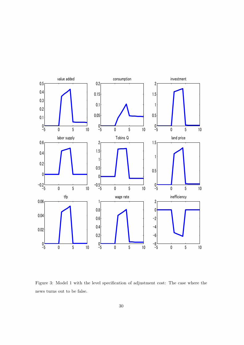
As a benchmark, we set σH = 1, that is, the elasticity of investment with respect to

Tobin’s Q is unity, which is consistent with the empirical evidence. The other parameter

values are the same as those used for Figure 1. Figure 3 shows the impulse responses

to the same news shock as in Figure 1, where the news turns out to be false. The news

shock increases Tobin’s Q, as well as other macroeconomic variables. It is worth noting

that introducing the adjustment cost of investment enlarges the set of parameter values

that are consistent with news-driven cycles. For instance, the EIS, σ−1, can be made

very close to unity. Figure 4 plots the result when σ = 0.9. The effects of the news shock

are smaller compared to the benchmark case of σ = 0.5, but we still obtain comovements

of the variables of interest.

With the flow specification (17), the relationship between the level of investment and

Tobin’s Q becomes less clear. The first-order condition for it is written as

pk′,t

[1 − G

(it

it−1

)− G′

(it

it−1

)it

it−1

]+ βpk′,t+1G

′(

it+1

it

)(it+1

it

)2

= 1

14

We set σG = 15.1 following Christiano, Motto, and Rostagno (2007). The other param-

eter values are the same as before. Figure 5 plots the impulse responses to the news

shock. Again, the model is successful in generating comovements, including Tobin’s Q.

Our success in reproducing procyclical Tobin’s Q may be explained as follows: Loos-

ening of the collateral constraint increases labor and intermediate inputs, leading to an

increase in the marginal product of capital. Therefore, capital becomes more valuable,

implying higher Tobin’s Q. On the other hand, in Christiano, Motto, and Rostagno’s

(2007) model and in Jaimovich and Rebelo’s (2009) model, when the good news arrives,

agents anticipate that they need to pay a large amount of adjustment costs during tran-

sition to the new steady state; thus, agents increase investment today to reduce the

adjustment cost that they must pay in the future; and the increase in investment makes

capital more abundant and cheaper today. Christiano et al. needs to introduce sticky

prices and a Taylor-type monetary policy rule in order to generate the procyclicality in

the price of capital. We do not need such a complication in the model to explain capital

prices. Policy implications are quite different: On one hand, Christiano et al. conclude

that the news-driven cycle, if it exists at all, should be caused by a mechanical conduct

of monetary policy and therefore the central bank is to be blamed; and on the other

hand, our model implies that the news-driven cycle may be an inevitable feature of the

economy in which agents are subject to collateral constraints.

3 Model 2: Costly state verification

In this section we consider a version of the costly-state-verification model due to Carl-

strom and Fuerst (1997, 1998). Specifically, we augment Carlstrom and Fuerst’s (1998)

model with land, and assume that only land can be used as collateral in the debt contract.

The key difference from the first model is that the second model has two types of agents:

households (lenders) and entrepreneurs (borrowers). We first show that this two-agent

model can also reproduce news-driven cycles, and that with the level specification of the

adjustment cost, it can reproduce procyclicality of Tobin’s Q. The basic mechanism that

generates this result is the same as in the first model. Furthermore, in our second model,

15

when the news of a future increase in productivity turns out to be wrong, the economy

falls into a recession (the level of output falls below the steady state level). This feature

is absent in our first model, as well as in the models of Christiano, Motto and Rostagno

(2007) and Jaimovich and Rebelo (2009).9

The economy consists of a representative household and a continuum of entrepreneurs

with unit mass. The household consumes, supplies labor, accumulates capital, holds land,

and lends to entrepreneurs. An entrepreneur produces output under idiosyncratic risk,

holds land, and borrows from the household.

Household: The household maximizes (7) subject to the flow budget constraint:

ct + it + qtat = wtnt + rk,tkt + (qt + ra,t)at + (Rt − 1)bt, (18)

and the law of motion for capital accumulation, either (16) or (17), where rk,t and ra,t

are the rental rates of capital and land, respectively, and (Rt−1)bt is the return on intra-

period loans, bt, to entrepreneurs. Although entrepreneurs are subject to idiosyncratic

risk, the loans to them are intermediated through a mutual fund so that the household

faces no risk. Since the loans are made within period, Rt = 1 must hold in equilibrium.

Thus, the household becomes indifferent to bt in the equilibrium.

Let λc,t and λk,t be the Lagrange multipliers associated with the flow budget con-

straint (18) and the law of motion of capital accumulation (16) or (17), respectively.

Then Tobin’s Q, pk′,t, is defined as

pk′,t ≡λk,t

λc,t.

Entrepreneurs: Entrepreneurs are indexed by i ∈ [0, 1]. We assume that only land can

be used as collateral in the debt contract. As a result, entrepreneurs do not hold physical

capital. Entrepreneur i holds land, a′t(i), at the beginning of period t, produces output,

yt(i), and then determines consumption, c′t(i), and land holdings, a′t+1(i). Entrepreneurs9Note that the original model of Carlstrom and Fuerst (1998) does not generate news-driven cycles.

The success of our model in this respect is due to the introduction of an asset in fixed supply (land) in

the debt contract.

16

faces an idiosyncratic productivity shock in producing output. Specifically, entrepreneur i

produces yt(i), employing intermediate input, mt(i), land services, at(i), capital services,

kt(i), and labor input, nt(i), under an idiosyncratic shock, ωt(i), using the following

production technology:

yt(i) = ωt(i)F [At,mt(i), at(i), kt(i), nt(i)], (19)

where

F (A,m, a, k, n) = A(1−η)(1−α)mηa(1−η)νk(1−η)αn(1−η)(1−α−ν).

The idiosyncratic shock ωt(i) is private information; it is i.i.d. across agents and across

time; its probability distribution and density function are denoted by Φ(ω) and ϕ(ω),

respectively; its mean is unity, and its standard deviation is denoted by σω. Note that

at(i) = a′t(i), in general. If at(i) > a′t(i), entrepreneur i rents at(i) − a′t(i) from another

entrepreneur or the household; and if at(i) < a′t(i), he rents a′t(i) − at(i) to another

entrepreneur.

The quantities of inputs, mt(i), at(i), kt(i), nt(i), are determined prior to the real-

ization of ωt(i). Therefore, the input costs, st(i) ≡ mt(i) + wtnt(i) + rk,tkt(i) + ra,tat(i),

must be paid in advance. Cost minimization and the Cobb-Douglas technology leads to

the following first-order conditions:

wtnt(i) = (1 − η)(1 − α − ν)st(i),

rk,tkt(i) = (1 − η)αst(i),

ra,tat(i) = (1 − η)νst(i),

mt(i) = ηst(i).

Let et(i) be the net worth of entrepreneur i. Since the only asset that entrepreneur

i holds at the beginning of period t is a′t(i), her net worth is given by

et(i) = (qt + ra,t)a′t(i).

Since st(i) must be paid in advance, entrepreneur i needs to borrow st(i)−et(i) from the

household. Let pt be the markup rate, that is, a project of size st(i) yields gross return

17

ptst(i)ωt(i). Let µptst(i) be the cost of monitoring a project of size st(i). As discussed

by Carlstrom and Fuerst (1997, 1998), given {pt, et(i)}, the optimal debt contract is

described by {st(i), ωt}. Here, the borrower with net worth et(i) conducts a project of

size st(i), and pays back to the lender ptst(i)ωt as long as ωt(i) ≥ ωt. If ωt(i) < ωt, then

the borrower defaults, and pays back only ptst(i)ωt(i) < ptst(i)ωt. Thus Φ(ωt) equals the

fraction of entrepreneurs who default. As shown in Appendix, the optimal debt contract

{st(i), ωt} is determined as

st(i) =et(i)

1 − ptg(ωt),

1pt

= 1 − Φ(ωt)µ + ϕ(ωt)µf(ωt)f ′(ωt)

,

where f(ω) and g(ω) are the functions defined in Appendix.

Given {pt, ωt}, entrepreneur i chooses {c′t(i)} and {a′t+1(i)} to maximize his utility:

E0

∞∑t=0

(β′)tc′t(i),

subject to the flow budget constraint:

c′t(i) + qta′t+1(i) = ptst(i)max{ωt(i) − ωt, 0},

where st(i) = (qt+ra,t)a′t(i)

1−ptg(ωt). We assume that β′ < β to ensure that entrepreneurs are

borrowing constrained in equilibrium.10

Because of the linearity in the entrepreneurs’ utility and the debt contract, the en-

trepreneur sector is easily aggregated by integration over i. Let zt denotes the aggregate

variable of zt(i) for zt(i) = st(i), c′t(i), a′t(i), etc. The aggregate variables solve

max E0

∞∑t=0

(β′)tc′t, (20)

10Strictly speaking, we need to prevent the possibility that the net worth of each entrepreneur becomes

zero. For that sake, Carlstrom and Fuerst (1997) assume that entrepreneurs supply labor. Here, however,

for simplicity, we follow Carlstrom and Fuerst (1998) and consider the limiting case where entrepreneurs’

labor income is approximately zero. Explicit consideration of entrepreneurs’ labor does not change our

result.

18

subject to

c′t + qta′t+1 = ptstf(ωt), (21)

where

st =(qt + ra,t)a′t1 − ptg(ωt)

, (22)

1pt

= 1 − Φ(ωt)µ + ϕ(ωt)µf(ωt)f ′(ωt)

. (23)

The total output produced is

yt = A(1−η)(1−α)t mη

t a(1−η)νt k

(1−η)αt n

(1−η)(1−α−ν)t . (24)

Since the price of output is unity (numeraire), pt is the mark-up rate:

yt = ptst. (25)

The market clearing conditions are

ct + c′t + it + mt = [1 − Φ(ωt)µ]yt, (26)

at = 1. (27)

The factor market equilibrium conditions are given by:

wtnt = (1 − η)(1 − α − ν)st, (28)

rk,tkt = (1 − η)αst, (29)

ra,tat = (1 − η)νst, (30)

mt = ηst. (31)

Equilibrium: The equilibrium dynamics of this economy are determined by the solu-

tion to the household’s problem, i.e., maximization of (7) subject to (18) and either (16)

or (17); the aggregate entrepreneurs’ problem, (20)–(23); and the conditions (24)–(31).11

11The total amount of loans from the household to entrepreneurs is given by bt = st − (qt + ra,t)a′t,

though it is irrelevant to the dynamics.

19

The financial-market inefficiency and the factor-market inefficiency: As in the

first model, a crucial feature of this model is the interaction between the inefficiencies in

the financial market and in the factor market. The inefficiency in the factor market is

measured by the mark up rate, pt, which is the wedge between the marginal products and

the input prices. For instance, it follows from (25) and (28) that the marginal product

of labor equals pt times the wage rate:

(1 − η)(1 − α − ν)yt

nt= ptwt;

and similar conditions hold for the other inputs.

The financial-market inefficiency may be measured by ωt, which is the threshold

value for default. Equation (23) implies that pt = p(ωt) is an increasing function of

ωt, that is, an increase in the financial market inefficiency will raise the factor market

inefficiency. In addition, the definition of g(ωt) in Appendix implies that p(ωt)g(ωt) is

an increasing function of ωt. It follows from (22) that, other things being equal, a higher

land price, qt, lowers the financial market inefficiency ωt. Therefore, this model has the

same mechanism as the first one: a higher land price qt tends to reduce the financial

market inefficiency ωt, which, in turn, decreases the factor-market inefficiency pt. This

is the basic mechanism that generates news-driven cycles.

Similarly, as in the first model, the requirement of intermediate inputs, mt, implies

that the (observed) TFP depends negatively on the inefficiency of the financial market.

The value added in this economy is given by [1−Φ(ωt)µ]yt −mt. Then, define the TFP

in this economy, A(At, pt, ωt), as

[1 − Φ(ωt)µ]yt − mt = A(At, pt, ωt)aνt k

αt n1−α−ν

t . (32)

Equations (24), (25), (31), and (32) imply that

A(At, pt, ωt) ≡[1 − Φ(ωt)µ − η

pt

](η

pt

) η1−η

A1−αt . (33)

Because of the monitoring cost, the financial market inefficiency ωt directly affects the

TFP through the term Φ(ωt)µ. But the negative dependence of At on pt is based on

20

the same mechanism as we have seen in (15). Hence, the TFP is, again, a decreasing

function of the financial-market inefficiency, ωt. As a result, other things being equal,

a higher land price, qt, tends to increase the TFP. Although η > 0 is not necessary to

generate news-driven cycles, it reinforces the mechanism that drives news-driven cycles.

Numerical experiments: We conduct the same experiments as those in Section 2:

At t = 1, the agents receive a signal that ϵT = ϵ > 0, which turns out to be true or false

at t = T . The parameter values are set as follows: β = .99; β′ = β ∗ .973; σ = .5; γ = .5;

η = .5; ν = .03; α = .3; δ = .025; σH = 1; σG = 15.1; σω = .37; µ = .15; ρ = .95;

ϵ = .0025; and T = 5. Here, the values for β′, σω and µ are taken from Carlstrom and

Fuerst (1998). The rest are the same as in Section 2.2.

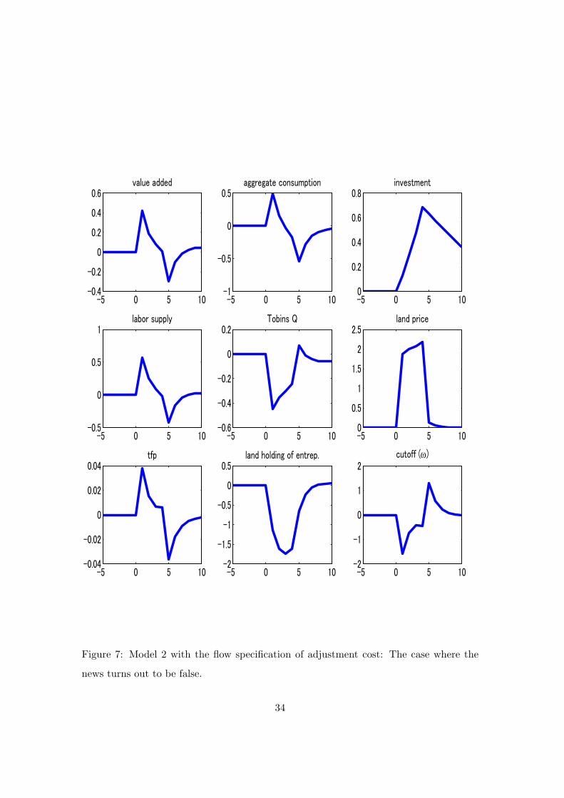
Here we report the case where the news turns out to be wrong at t = T . The

results for the level specification model (16) and for the flow specification model (17)

are shown in Figures 6 and 7, respectively. Just as in the representative-agent model of

Section 2.2, the news of a future productivity increase brings about a boom in periods

t = 1, . . . , T − 1. Aggregate consumption, value added, investment, and labor all rise

during these periods.12 The measured TFP also rises for t = 1, . . . , T−1. The mechanism

that the news shock produces the boom is the same as in the previous model. Tobin’s

Q rises with the level specification of adjustment cost, while it does not with the flow

specification.

In this model, it may be interesting to look at how the risk premium responds to a

news shock.13 Let prt denote the risk premium, which is defined implicitly by

ptωtst = (1 + prt )(st − et).

12The aggregate consumption is the sum of the household’s consumption and the entrepreneurs’ con-

sumption. As can be inferred from the dynamics of λc,t, the household’s consumption slightly declines

for t = 1, . . . , T − 1. The aggregate consumption rises because the entrepreneurs’ consumption increases

by amounts that are more than offsetting the declines in the household’s consumption.13We thank an anonymous referee for suggesting us to consider this.

21

It follows that

prt =

ωt

g(ωt)− 1.

Since prt = {1 − g′(ω)ω/g(ω)}ωt, where the variables with the hat is the percentage

deviations from the steady-state values, and {1− g′(ω)ω/g(ω)} > 0 under the parameter

values we use, it follows that the risk premium moves countercyclically in response to

the news shock. Such a movement of the risk premium appears to be consistent with

the evidence. For instance, Stock and Watson (1999, Table 2, series 52: Commercial

paper/Treasury Bill spread) show that a higher risk premium today predicts a lower

level of output in the future.

What is notable in the second model is what happens when the news turns out to

be wrong in period t = T . In the previous model with a representative household, when

the news turns out to be wrong in period t = T , the economy essentially jumps back to

the initial steady state, although there are some transitional dynamics (see Figures 1, 3,

5). In particular, after the news turns out to be wrong, the economic activity does not

fall below the steady state level. This implies that the wrong news does not cause the

economy to fall into a recession by Jaimovich and Rebelo’s (2009) definition. That is not

true in our second model. In period t = T , when the news turns out to be false, value

added, consumption, and labor supply get lower than their steady state levels.

What causes this remarkable difference is the fact that there are two types of agents

in the second model: borrowers and lenders. Look at the dynamics of the share of land

held by entrepreneurs, {a′t+1} (note that in the figures, the plotted value of a′ at t is a′t+1,

rather than a′t). When the good news hits the economy in period t = 1, entrepreneurs

sell their land to households so that a′2 is lower than the steady state level, a′, which is

reflected in the sharp decline in a′ occurring at t = 1 in Figures 6 and 7. Entrepreneurs

sell their land in period 1, because, given the increase in the land price caused by the

good news, entrepreneurs need less land to achieve their desired level of net worth (or

collateral). So the share of land held by entrepreneurs becomes lower than the steady

state level as long as the price of land is higher than its steady state level. It follows

that, when the news turns out to be wrong in period T , the share of land held by

22

entrepreneurs at the beginning of period T is lower than the steady state value: a′T < a′.

The entrepreneurs’ borrowing constraint (22) and the markup equation (25) imply that,

at t = T , gross output equals:

yT =p(ωT )

1 − p(ωT )g(ωT )(qT + ra,T )a′T

Here, p(ω)/(1 − p(ω)g(ω)) is increasing in ω. Since at this point our agents realize that

the productivity increase does not happen, the land price goes back to the steady state

value: qT ≈ q. Then, the fact that entrepreneurs hold a share of land which is less than

the steady state level, a′T < a′, implies that the financial market inefficiency gets higher,

ωT > ω, which, in turn, raises the factor market inefficiency, pT . (Recall that (23) implies

that pT = p(ωT ) is an increasing function of ωT .) As a result, the economy falls into a

recession in period t = T , as the figures show. Note also that the countercyclicality in ωt

in the figures can be interpreted as the countercyclicality in bankruptcies, which seems

realistic but is not reproduced in the original models of Carlstrom and Fuerst (1997,

1998).

4 Conclusion

We proposed two models of the business cycles, which are driven by changes in expecta-

tions or news about the future through financial constraints. The global financial crisis

in 2008 has shown dramatically that the financial frictions, interacting with the collapse

of asset bubbles, can cause a large impact on real activities. The asset-price collapse

might have been caused by a change in the expectations about the future. Our aim in

this paper is to shed some light on the interaction between expectational changes and

financial frictions that appears to be a key to understand the current financial crisis.

We have seen that such news-driven cycles can be reproduced by models with collateral

constraint.

Our main assumptions are that an asset with fixed supply (“land”) is used as col-

lateral, and that firms are collateral constrained to finance the input costs. The first

assumption is to ensure that the price of a collateralized asset fluctuates enough in re-

23

sponse to news about future productivity growth. The second assumption is to introduce

an interaction between the financial market inefficiency and the factor market inefficiency.

A positive news about the future productivity growth raises the asset price today and

relaxes the collateral constraint. Since the input finance is collateral constrained, the

relaxation of the collateral constraint reduces the inefficiency in the factor market. This

interaction can generate the news-driven cycles. Augmented by the adjustment cost of

investment, the models can generate procyclical movement on Tobin’s Q. Furthermore,

in our second model, the economy can fall into a recession when a good news turns out

to be false.

In comparison with the existing models of the news-driven cycles, our collateral con-

straint models are simpler and exhibit more realistic performance. Collateral constraint

on input finance by a fixed-supply asset may be a good ingredient to develop a com-

prehensive theory of the business cycles from a point of the “News” view (Beaudry and

Portier [2005]).

Appendix

Following Carlstrom and Fuerst (1998), we derive the optimal contract for intra-period

debt for an entrepreneur that faces an idiosyncratic risk.

We consider an entrepreneur with his own fund x. If he undertakes a project of size s,

it generates stochastic return pωs units of output, where p is a constant that represents

the market rate of mark-up, and ω is a unit-mean iid random variable. The probability

distribution of ω is Φ(ω) and the probability density is ϕ(ω). The entrepreneur must

borrow s − x from the household, while ω is private information for the entrepreneur.

The lender must pay µps to monitor the outcome of the project, where µ is a constant.

As Carlstrom and Fuerst (1998) argue briefly, it is well known that in this costly-

state-verification setting, the optimal financial contract is a risky debt. Given (p, x), the

optimal contract is characterized by (s, ω), where s is the size of the project, i.e., the size

24

of the borrowing is s − x; and the amount that the borrower repay is

ps × min{ω, ω}. (34)

ω can be viewed as the threshold value for default: The lender will monitor the project

outcome if and only if the entrepreneur reports that ω is less than ω; and in such a case

the lender will confiscate all the returns from the project, psω.

Define f(ω) and g(ω) as the expected shares of output for the entrepreneur and the

lender, respectively:

f(ω) ≡∫ ∞

0(ω − min{ω, ω})Φ(dω), (35)

g(ω) ≡∫ ∞

0min{ω, ω}Φ(dω) − Φ(ω)µ. (36)

We assume that lending is fully diversified across projects, so that the lender only

cares about the expected rate of return, and that borrowing and lending are intra-period,

so that the equilibrium rate of return is unity. Under these assumptions, the optimal

contract (s, ω) is determined as the solution to the following problem, given (p, x):

maxs,ω

psf(ω) s.t. psg(ω) ≥ (s − x). (37)

The solution is (implicitly) given as

1p

= 1 − Φ(ω)µ + ϕ(ω)µf(ω)f ′(ω)

, (38)

s =1

1 − pg(ω)x. (39)

References

[1] Bansal, R. and A. Yaron (2004). “Risks for the Long Run: A Potential Resolution

of Asset Pricing Puzzles.” Journal of Finance 59(4): 1481–1509.

[2] Beaudry, P. and F. Portier (2004). “An exploration into Pigou’s theory of cycles.”

Journal of Monetary Economics 51(6): 1183–1216.

25

[3] Beaudry, P. and F. Portier (2007). “When can changes in expectations ccause busi-

ness cycle fluctuations in Neo-Classical settings?” Journal of Economic Theory

135(1), 458–477.

[4] Beaudry, P. and F. Portier (2005). “The ‘News’ view of economic fluctuations: Evi-

dence from aggregate Japanese data and sectoral U.S. data.” Journal of the Japanese

and International Economies 19(4): 635–652.

[5] Carlstrom, C. T., and T. S. Fuerst (1997). “Agency costs, net worth, and busi-

ness fluctuations: A computable general equilibrium analysis.” American Economic

Review 87(5): 893–910.

[6] Carlstrom, C. T., and T. S. Fuerst (1998). “Agency costs and business cycles.”

Economic Theory 12: 583–97.

[7] Chari, V. V., P. J. Kehoe, and E. R. McGrattan (2007). “Business cycle accounting.”

Econometrica 75(3): 781–836.

[8] Christiano, L. J., and I. Fujiwara (2006). “Bubbles, excess investments, working-

hour regulation, and the lost decade.” Bank of Japan Working Paper Series 06–J–8.

[9] Christiano, L. J., R. Motto, and M. Rostagno (2007). “Monetary policy and a stock

market boom-bust cycle.” European Central Bank Working Paper Series 955.

[10] Comin, D., and M. Gertler (2006). “Medium-term business cycles.” American Eco-

nomic Review 96(3): 523–51.

[11] Cordoba, J.-C., and M. Ripoll (2004). “Credit Cycles Redux,” International Eco-

nomic Review 45(4): 1011-46.

[12] Den Haan, W. J. and G. Kaltenbrunner (2009). “Anticipated growth and business

cycles in matching models.” Journal of Monetary Economics 56(3): 309–327.

[13] Gruber, J. (2006). “A tax-based estimate of the elasticity of intertemporal substi-

tution,” NBER Working Paper 11945.

26

[14] Jaimovich, N. and S. Rebelo (2009). “Can news about the future drive the business

cycle?” American Economic Review 99(4): 1097-1118.

[15] Jermann, U. J., and V. Quadrini (2007). “Stock market boom and the productivity

gains of the 1990s.” Journal of Monetary Economics 54: 413–32.

[16] Kiyotaki, N., and J. Moore (1997). “Credit cycles.” Journal of Political Economy

105 (2): 211–48.

[17] Lorenzoni, G. (2009). “A Theory of Demand Shocks.” American Economic Review

99 (5): 2050–2084.

[18] Mendoza, E. G. (2010). “Sudden Stops, Financial Crises and Leverage.” American

Economic Review, forthcoming.

[19] Mulligan, C. (2002). “Capital, interest, and aggregate intertemporal substitution,”

NBER Working Paper 9373.

[20] Rotemberg, J. J., and M. Woodford (1995). “Imperfectly competitive markets,” in

Cooley, T. F. ed. Frontiers of business cycle research, Princeton: Princeton Univ.

Press.

[21] Stock, J. H., and M. W. Watson (1999) “Business Cycle Fluctuations in US Macroe-

conomic Time Series.” in Taylor, J. B., and M. Woodford ed. Handbook of Macroe-

conomics, Volume 1A, Elsevier.

[22] Uhlig, H. (1999). “A Toolkit for Analysing Nonlinear Dynamic Stochastic Models

Easily,” in Marimon, R., and A. Scott, eds., Computational methods for the study

of dynamic economies. Oxford: Oxford University Press.

[23] Vissing-Jorgensen, A., and O. Attanasio (2003). “Stock-market participation, in-

tertemporal substitution, and risk aversion.” American Economic Review 93(2):

383-391.

27

-5 0 5 100

0.1

0.2

0.3

0.4

0.5value added

-5 0 5 100

0.5

1

1.5

2land price

-5 0 5 100

0.1

0.2

0.3

0.4

0.5consumption

-5 0 5 10-0.5

0

0.5

1investment

-5 0 5 10-0.2

0

0.2

0.4

0.6labor supply

-5 0 5 100

0.02

0.04

0.06

0.08

0.1tfp

-5 0 5 100

0.5

1

1.5wage rate

-5 0 5 10-10

-8

-6

-4

-2

0inefficiency

Figure 1: Model 1: The case where the news turns out to be false. (Percent deviations

from the steady state. The same applies hereafter.)

28

-5 0 5 100

0.1

0.2

0.3

0.4

0.5value added

-5 0 5 100

0.5

1

1.5

2land price

-5 0 5 10-0.5

0

0.5consumption

-5 0 5 100

1

2

3investment

-5 0 5 100

0.2

0.4

0.6

0.8labor supply

-5 0 5 100

0.02

0.04

0.06

0.08

0.1tfp

-5 0 5 100

0.5

1

1.5wage rate

-5 0 5 10-10

-8

-6

-4

-2

0inefficiency

Figure 2: Model 1: The case where the news turns out to be correct.

29

-5 0 5 100

0.1

0.2

0.3

0.4

0.5value added

-5 0 5 100

0.5

1

1.5land price

-5 0 5 100

0.05

0.1

0.15

0.2consumption

-5 0 5 100

0.5

1

1.5

2investment

-5 0 5 10-0.2

0

0.2

0.4

0.6labor supply

-5 0 5 10-0.5

0

0.5

1

1.5

2Tobins Q

-5 0 5 100

0.02

0.04

0.06tfp

-5 0 5 100

0.2

0.4

0.6

0.8

1wage rate

-5 0 5 10-8

-6

-4

-2

0

2inefficiency

Figure 3: Model 1 with the level specification of adjustment cost: The case where the

news turns out to be false.

30

-5 0 5 100

0.02

0.04

0.06

0.08value added

-5 0 5 100

0.05

0.1

0.15

0.2

0.25land price

-5 0 5 100

0.005

0.01

0.015consumption

-5 0 5 100

0.1

0.2

0.3

0.4investment

-5 0 5 10-0.05

0

0.05

0.1labor supply

-5 0 5 10-0.1

0

0.1

0.2

0.3

0.4Tobins Q

-5 0 5 100

0.002

0.004

0.006

0.008

0.01tfp

-5 0 5 100

0.05

0.1

0.15

0.2wage rate

-5 0 5 10-1.5

-1

-0.5

0

0.5inefficiency

Figure 4: Model 1 with the level specification of adjustment cost and σ = 0.9: The case

where the news turns out to be false.

31

-5 0 5 100

0.1

0.2

0.3

0.4

0.5value added

-5 0 5 10-0.5

0

0.5

1

1.5

2land price

-5 0 5 10-0.4

-0.2

0

0.2

0.4consumption

-5 0 5 100

0.5

1

1.5investment

-5 0 5 100

0.2

0.4

0.6

0.8labor supply

-5 0 5 10-0.2

-0.1

0

0.1

0.2Tobins Q

-5 0 5 10-0.02

0

0.02

0.04

0.06

0.08tfp

-5 0 5 10-0.5

0

0.5

1

1.5wage rate

-5 0 5 10-10

-5

0

5inefficiency

Figure 5: Model 1 with the flow specification of adjustment cost: The case where the

news turns out to be false.

32

-5 0 5 10-0.4

-0.2

0

0.2

0.4

0.6value added

-5 0 5 100

0.5

1

1.5

2land price

-5 0 5 10-0.4

-0.2

0

0.2

0.4aggregate consumption

-5 0 5 100

0.5

1

1.5investment

-5 0 5 10-0.4

-0.2

0

0.2

0.4

0.6labor supply

-5 0 5 10-0.5

0

0.5

1

1.5Tobins Q

-5 0 5 10-0.04

-0.02

0

0.02

0.04tfp

-5 0 5 10-1.5

-1

-0.5

0

0.5land holding of entrep.

-5 0 5 10-2

-1

0

1

2cutoff (ω)

Figure 6: Model 2 with the level specification of adjustment cost: The case where the

news turns out to be false.

33

-5 0 5 10-0.4

-0.2

0

0.2

0.4

0.6value added

-5 0 5 100

0.5

1

1.5

2

2.5land price

-5 0 5 10-1

-0.5

0

0.5aggregate consumption

-5 0 5 100

0.2

0.4

0.6

0.8investment

-5 0 5 10-0.5

0

0.5

1labor supply

-5 0 5 10-0.6

-0.4

-0.2

0

0.2Tobins Q

-5 0 5 10-0.04

-0.02

0

0.02

0.04tfp

-5 0 5 10-2

-1.5

-1

-0.5

0

0.5land holding of entrep.

-5 0 5 10-2

-1

0

1

2cutoff (ω)

Figure 7: Model 2 with the flow specification of adjustment cost: The case where the

news turns out to be false.

34