Yale University Yale University

EliScholar – A Digital Platform for Scholarly Publishing at Yale EliScholar – A Digital Platform for Scholarly Publishing at Yale

Yale Graduate School of Arts and Sciences Dissertations

Spring 2021

Essays on Financial Intermediation and Collateral Requirements Essays on Financial Intermediation and Collateral Requirements

Chuan Du Yale University Graduate School of Arts and Sciences, chuandu1988@yahoo.co.uk

Follow this and additional works at: https://elischolar.library.yale.edu/gsas_dissertations

Recommended Citation Recommended Citation Du, Chuan, "Essays on Financial Intermediation and Collateral Requirements" (2021). Yale Graduate School of Arts and Sciences Dissertations. 39. https://elischolar.library.yale.edu/gsas_dissertations/39

This Dissertation is brought to you for free and open access by EliScholar – A Digital Platform for Scholarly Publishing at Yale. It has been accepted for inclusion in Yale Graduate School of Arts and Sciences Dissertations by an authorized administrator of EliScholar – A Digital Platform for Scholarly Publishing at Yale. For more information, please contact elischolar@yale.edu.

Abstract

Essays on Financial Intermediation and Collateral Requirements

Chuan Du

2021

This collection of essays examines �nancial intermediation and collateral require-

ments in economies where limited enforcement of repayment necessitates loans to be

backed by eligible collateral. Collateralized lending was a key feature of the 2008 �nan-

cial crisis, with signi�cant policy interventions in major economies directed towards

restoring leverage and �nancial intermediation. Similarly, given the unprecedented

shock of the COVID-19 pandemic, �rms that face binding collateral constraints and

�nd it di�cult to secure loans on a�ordable terms may struggle to weather the crisis.

Governments and central banks worldwide have instigated large scale policy responses

to ease credit conditions. Theoretical models of �nancial frictions that account for

endogenous variations in leverage across the business cycle are thus important for

guiding policy design and for analyzing the propagation and ampli�cation of shocks

through the �nancial sector.

In Chapter 1, I examine how central banks should intervene to improve credit

conditions during a downturn. Speci�cally, I analyze the setting of collateral require-

ments in central bank lending facilities. Traditionally, central bank lending during

times of crisis followed Bagehot's rule. That is to lend freely to solvent institutions,

against collateral that is good in normal times, and at �high interest rates�. The rule

is designed so that the central bank can improve credit conditions without taking on

any credit risk. Lately, central banks began to deviate from this approach, conducting

more direct lending to �rms, against a broader class of collateral, and reducing the

haircuts imposed on the collateral posted. Which is the more appropriate response?

Should central banks take on greater credit risk in order to provide a larger stimulus?

i

To answer the question, I develop a model of central bank intervention in collat-

eralized credit markets. I �nd that when the downturn is severe it is optimal for the

central bank to take on greater credit risk. The analysis suggests that credit facilities

set up by the Federal Reserve in response to COVID-19, such as the Main Street

Lending Program, can achieve greater participation and e�ectiveness by easing their

terms of lending.

In Chapter 2, I present joint work with Agostino Capponi and Stefano Giglio

on the determinants of collateral requirements in central clearinghouses for credit

default swaps (CDSs). The empirical results in Capponi et al. (2020) demonstrate

that extreme tail risk measures have higher explanatory power for observed collateral

requirements than the standard Value-at-Risk rule. To provide a theoretical foun-

dation for these �ndings, we develop a model of endogenous collateral requirements

in the CDS market, where counterparties trade state-contingent promises backed by

cash as collateral. Trading occurs due to di�erences in market participants' beliefs

about the uncertain states of the world.

We show that it is the nature � rather than the degree � of these belief di�erences

that determines collateral requirements in equilibrium. For instance, the equilibrium

level of collateral increases both when the optimist becomes more pessimistic (which

reduces the extent of the disagreement), and when the pessimist becomes more

concerned about tail events (which increases the extent of the disagreement). We can

thus point to the clearinghouse's concerns about extreme tail events as an explanation

for the highly conservative levels of collateral observed in practice.

In Chapter 3, I propose a generalization of the Binomial No-Default Theorem

of Fostel and Geanakoplos (2015). The Binomial No-Default Theorem states that

�in binomial economies with �nancial assets serving as collateral, any equilibrium

is equivalent in real allocations and prices to another equilibrium in which there

is no default�. I extend this theorem to economies with more than two states of

ii

nature when debt can be ordered by seniority. For instance, with three states of

nature, borrowers can issue both senior secured debt and junior unsecured debt. The

senior secured debt is explicitly backed by the risky �nancial asset held by the �rm,

whereas the junior unsecured debt is implicitly backed by the residual value of the

�rm after the senior creditors satisfy their claims. The interest rates and credit risks

associated with each creditor tier are endogenously determined in equilibrium. The

Multinomial Max-Min theorem I prove states that any equilibrium is equivalent to

another equilibrium where the senior tranche never defaults, and the junior tranche

only defaults in the worst state of the world. The expanded theorem allows for the

application of the endogenous leverage framework to a richer set of models with more

than two states and where some loans are not contractually secured.

Finally, in a joint paper with David Miles presented in Chapter 4, I examine

the interaction between the real interest rate and capital requirements in the risk

taking behavior of banks. In this model, banks can undertake costly screening to

discover private information about the probability of success on their potential lending

projects. Once this probability is known, each bank sets a cut-o� threshold for the

likelihood of success on a project that determines whether or not to lend. When banks

are highly leveraged, a combination of asymmetric information and limited liability

means that banks screen too little (insu�cient �participation�) and accept projects

that are too risky (insu�cient �prudence�) relative to the �rst-best benchmark.

We show that the real interest rate and capital requirements function as imperfect

substitutes. Qualitatively, raising either the real interest rate or the capital require-

ment on banks can increase �prudence� at the cost of decreased �participation�. But

the two policy instruments work through very di�erent mechanisms. An increase in

capital requirements forces banks to hold �more skin in the game� and is targeted

at the subset of poorly capitalized banks in the population. In contrast, an increase

in the real interest rate increases the opportunity cost of lending for all banks, and

iii

is thus a much blunter instrument. The interaction between these two policy levers

means that the optimal capital requirement on banks rises as the interest rate falls,

suggesting tougher macro-prudential capital standards in a �lower-for-longer� interest

rate environment.

iv

Essays on Financial Intermediation and Collateral Requirements

A Dissertation

Presented to the Faculty of the Graduate School

of

Yale University

in Candidacy for the Degree of

Doctor of Philosophy

by

Chuan Du

Dissertation Director: John Geanakoplos

June 2021

© 2021 by Chuan Du

All rights reserved.

Contents

Acknowledgments ix

1 Collateral Requirements in Central Bank Lending 1

1.1 Introduction . . . . . . . . . . . . . . . . . . . . . . . . . . . . . . . . 1

1.2 The Model . . . . . . . . . . . . . . . . . . . . . . . . . . . . . . . . . 9

1.3 Characterizing the Collateral Equilibrium . . . . . . . . . . . . . . . . 18

1.4 Central Bank Intervention . . . . . . . . . . . . . . . . . . . . . . . . 32

1.5 Concluding Remarks . . . . . . . . . . . . . . . . . . . . . . . . . . . 43

1.6 Appendices . . . . . . . . . . . . . . . . . . . . . . . . . . . . . . . . 54

2 The Collateral Rule - Theory for the Credit Default Swap Market1 69

2.1 Introduction . . . . . . . . . . . . . . . . . . . . . . . . . . . . . . . . 69

2.2 Model Setup . . . . . . . . . . . . . . . . . . . . . . . . . . . . . . . . 70

2.3 Existence and Uniqueness of the Collateral Equilibrium . . . . . . . . 73

2.4 Characterizing the Equilibrium . . . . . . . . . . . . . . . . . . . . . 76

2.5 Comparative Statics and Illustrative Example . . . . . . . . . . . . . 79

2.6 Concluding Remarks . . . . . . . . . . . . . . . . . . . . . . . . . . . 82

2.7 Appendices . . . . . . . . . . . . . . . . . . . . . . . . . . . . . . . . 85

3 From Binomial No-Default to Multinomial Max-Min 100

3.1 Introduction . . . . . . . . . . . . . . . . . . . . . . . . . . . . . . . . 100

3.2 Set-up . . . . . . . . . . . . . . . . . . . . . . . . . . . . . . . . . . . 101

3.3 The Multinomial Max-Min Theorem . . . . . . . . . . . . . . . . . . 104

3.4 Concluding Remarks . . . . . . . . . . . . . . . . . . . . . . . . . . . 106

3.5 Appendix - Proof . . . . . . . . . . . . . . . . . . . . . . . . . . . . . 108

1This is joint work with Agostino Capponi and Stefano Giglio.

vii

4 Capital requirements, the safe real interest rate and the fundamental

problem of bank risk taking2 118

4.1 Introduction . . . . . . . . . . . . . . . . . . . . . . . . . . . . . . . . 118

4.2 The Model . . . . . . . . . . . . . . . . . . . . . . . . . . . . . . . . . 124

4.3 The First-Best - the model under perfect information . . . . . . . . . 129

4.4 The Model with Asymmetry of Information . . . . . . . . . . . . . . 135

4.5 Policy Tools and Their Transmission . . . . . . . . . . . . . . . . . . 140

4.6 Numerical Simulations . . . . . . . . . . . . . . . . . . . . . . . . . . 148

4.7 Concluding Remarks . . . . . . . . . . . . . . . . . . . . . . . . . . . 155

4.8 Appendices . . . . . . . . . . . . . . . . . . . . . . . . . . . . . . . . 159

2Joint work with David Miles.

viii

Acknowledgements

I am grateful to my advisors Prof. John Geanakoplos, Prof. Stefano Giglio, and Prof.

William English for their guidance, support and accommodation for late night panic

calls. I am also indebted to my other co-authors Prof. David Miles and Prof. Agostino

Capponi for their invaluable contributions and incredible patience. I thank my family

for their unconditional support, and lastly my dad for making me (unnecessarily and

perpetually) stressed. All remaining mistakes are my own.

ix

1 Collateral Requirements in Central Bank Lending

1.1 Introduction

Central bank lending during times of crisis traditionally followed Bagehot's rule: lend

freely to solvent institutions, against collateral that is good in normal times, and

at high interest rates. The rule is designed so that the central bank can improve

credit conditions without taking on any credit risk while also limiting moral hazard.

Lately, central banks have begun to deviate from this approach in their response

to COVID-19, conducting more direct lending to �rms, against a broader class of

collateral, and reducing the haircuts imposed on the collateral posted. Which is the

more appropriate response? Should central banks take on greater credit risk in order

to provide a larger stimulus?

I develop a model of central bank intervention in collateralized credit markets that

combines the Credit Cycles in Kiyotaki and Moore (1997) and the Leverage Cycle

in Geanakoplos (1997). I �nd that when the downturn is severe, it is optimal for

the central bank to take on greater credit risk. Speci�cally, the central bank should

intervene by lending at more favorable interest rates compared to the private market,

while simultaneously lowering collateral requirements. The potential losses for the

central bank on the loans extended falls on taxpayers.

In the model, �rms borrow in order to purchase capital for production. There

are two sources of �nancial frictions. First, �rms can only borrow using simple debt

contracts that are non-state-contingent. Second, each debt contract must be backed

by one unit of capital as collateral in order to enforce repayment. Crucially, �rms can

choose one or more contracts from an entire spectrum of such simple debt contracts

that di�er only in the size of the promised repayment. When the promise exceeds the

value of the collateral at the point of delivery, �rms default. Since all debt contracts

are backed by one unit of capital as collateral, a debt contract with a higher promised

1

repayment implies greater credit risk for the lender. The price of each debt contract,

the �rms' choice of contracts, and thus the credit risk faced by the lenders are fully

endogenized in competitive equilibrium. This is in contrast to many papers in the

literature where the amount the �rm can borrow against each unit of collateral is

exogenously given and the lenders face �xed value-at-risk when lending.

The borrowing constraints faced by �rms amplify negative aggregate productivity

shocks. During a downturn, �rms experience an endogenous reduction in their liquid

wealth and their ability to borrow. As a consequence, �rms hold too little capital in

the downturn relative to the socially e�cient level.

A central bank can intervene in this case by lending to �rms against collateral at

more favorable terms relative to the market. Central bank loans are funded through

the issuance of a public liability to households that carries the safe rate of interest,

and crucially, without the need to post collateral. The central bank is able to borrow

at the risk-free rate without posting collateral because it is backed by the ability of

the government to tax. As such, any ex post losses incurred on central bank loans

will need to be recouped through recourse to the Treasury.

Since the amount �rms can borrow against each unit of collateral is fully endog-

enized in the model, we can assess two di�erent types of central bank interventions.

The central bank can either reduce the risk-free interest rate on low loan-to-value

debt contracts, or subsidize riskier loans with high loan-to-value. If the central bank

is unwilling to bear any credit risk, then the size of the stimulus may be limited.

Instead, optimal intervention during severe downturns requires the central bank to

take on greater risk in order to provide a larger stimulus. By o�ering contracts that

private lenders are able, but unwilling, to make during a downturn, the central bank

can achieve signi�cant gains in productive e�ciency through its intervention.

2

The paper suggests that credit facilities set up by the Federal Reserve in response

to COVID-19, such as the Main Street Lending Program, can achieve greater partic-

ipation and e�ectiveness by easing their terms of lending.

Background: Central banks response to COVID-19

Given the enormous e�ect of the COVID-19 pandemic on the real economy, central

banks across the world are intervening aggressively in credit markets to cushion the

impact. In addition to pushing the benchmark policy rate to historic lows and

conducting very large asset purchases, the Federal Reserve launched a number of

new credit facilities in March 2020. For instance, the Primary and Secondary Market

Corporate Credit Facilities are joint programs set up by the Federal Reserve and

the US Treasury, whereby a Special Purpose Vehicle (SPV) is established to purchase

qualifying bonds from eligible issuers either directly, or through the secondary market.

The Treasury made the initial $10bn equity investment and the Federal Reserve com-

mitted to lend to the SPV on a recourse basis.3 The stated goal of these facilities is to

�support credit to employers� through either bond issuance, or by providing liquidity

to the market for outstanding corporate bonds.4 Similarly, the Term Asset-Backed

Securities Loan Facility extends loans secured by eligible asset-backed securities; and

the Main Street Lending Program purchases participations in loans originated by

eligible lenders. In the UK, the Bank of England and HM Treasury announced a

similar suite of measures, including the COVID-19 Corporate Financing Facility and

the Term Funding Scheme with additional incentives for SMEs.

This paper joins a growing literature that examines the design and e�cacy of

these dramatic interventions.

3Source: Primary Market Corporate Credit Facility Term Sheet(original version published on March 23, 2020), available at:https://www.federalreserve.gov/newsevents/pressreleases/�les/monetary20200323b1.pdf

4More details can be found at: www.federalreserve.gov

3

Key Themes and Related Literature

The analytical framework in this paper draws from two seminal models that study how

�nancial frictions amplify shocks to the real economy: Credit Cycles by Kiyotaki and

Moore (1997); and The Leverage Cycle by Geanakoplos (1997, 2003, 2010). In Credit

Cycles, borrowers secure loans subject to a borrowing constraint that is tied to their

net worth. During a downturn, the fall in borrower's net worth reduces their ability

to borrow, leading to a fall in their capital holdings which reduces future revenue

and net worth, thus completing a dynamic feedback loop to even lower asset prices

and net worth today. Crucially however, in the Credit Cycles model the collateral

constraint faced by borrowers is exogenously given: the loan to value (LTV) against

each unit of collateral is �xed, and the interest rate always equals the lender's rate

of time preference (i.e. the risk-free interest rate). Geanakoplos (1997) provides a

natural framework for endogenizing the collateral constraint. In the Leverage Cycle,

loan to value - and equivalently leverage - is too high in normal times, and crashes

when bad news arrive. The bad news about the value of borrower's collateral also

reduce their liquid wealth and further restricts their purchasing power today.

In this paper I combine the key features of both the Credit Cycle and the Leverage

Cycle frameworks. Firms and households are di�erentially productive with a durable

capital good, and �rms face an endogenous borrowing constraint when they try to

secure loans against capital as collateral. A key theme here is that �rms have the

option to choose from an entire spectrum of collateralized debt contracts that di�er in

LTV and the contractual/promised interest rate. For given collateral, a high LTV debt

contract trades o� a larger loan today at the cost of a higher promised rate of interest.

Plotting the promised interest rate against the LTV on each debt contract that arises

in the competitive collateral equilibrium generates the credit surface (Figure 1.1).

The credit surface summarizes the prevailing credit condition at each point in time;

and shifts in the credit surface re�ect changing circumstances. During a downturn,

4

credit conditions deteriorate and the corresponding credit surface shifts inwards and

upwards. So for a �rm that was originally highly leveraged, it must now either

accept a much larger haircut on the same collateral in order to maintain the same

interest rate; or retain a similar (albeit slightly reduced) LTV at the cost of a much

higher interest rate. Figure 1.2 plots the option-adjusted spread on US corporate

debt against credit rating, and highlights how credit conditions - especially for riskier

loans - could deteriorate during recessions in this fashion, in spite of central bank

interventions.

The analytical framework in this paper accounts for the richer picture of credit

market conditions that we observe in practice. Firms optimize simultaneously over

their desired capital holding and the type of debt contract they wish to issue. Choos-

ing a high LTV contract means a lower haircut and a larger sized loan today, in

return for a higher promised interest rate to compensate lenders for the increased

credit risk. Importantly, �rms' choices over leveraged debt contracts determine what

the optimal central bank intervention should look like during a downturn (Figure 1.3).

Interventions targeted at the low-LTV end of the credit surface can reduce the risk-free

interest rate faced by �rms without exposing the central bank to signi�cant credit

risk. In contrast, subsidizing riskier high-LTV loans can provide a larger stimulus,

but at the cost of potential losses for the central bank that will ultimately fall on

taxpayers. I show that when the downturn is severe �rms demand larger and riskier

loans against their dwindling pool of collateral. In such cases, it is optimal for the

central bank to take on more credit risk.

Figure 1.4 shows that during the current COVID-19 recession high-yield corporate

debt issuance in the US, as a proportion of investment grade issuance, �rst collapsed

at the onset of the crisis before recovering quickly after the Federal Reserve intervened

aggressively in the credit markets. Gilchrist et al. (2020) �nd that the Federal

Reserve's Secondary Market Corporate Credit Facility (SMCCF) has been e�ective

5

Figure 1.1: Model generated Credit Surface

The Credit Surface plots the promised interest rate on a collateralized debt contract against its loanto value (LTV) - both of which are determined endogenously in equilibrium. The haircut imposedon the collateral posted is de�ned as one minus the loan to value. The credit surface is composed ofthree parts. The horizontal segment to the left represents the risk-free spectrum of the market wherethe haircut is so high on the collateral posted that the loan is e�ectively risk-free. The increasingfunction in the middle of the credit surface captures the fact that as the haircut falls (and the LTVrises), the lender starts to take on more credit risk and must be compensated through a higherpromised interest rate. Lastly, the credit surface becomes vertical once the maximum loan-to-valueis reached. During normal times, interest rates are low across the credit surface. In a downturn,credit conditions deteriorate and the corresponding credit surface shifts inwards and upwards. Sofor a �rm that was originally highly leveraged, it must now either accept a much larger haircut onthe same collateral in order to maintain the same interest rate; or retain a similar (albeit slightlyreduced) LTV at the cost of a much higher interest rate.

6

Figure 1.2: US Corporate Index Option-Adjusted Spread

Source: Federal Reserve Economic Data.Figure 1.2 plots the option-adjusted spread on US corporate debt against credit rating, for the threemost recent recessions in the US. It compares the average spread during each recession against theaverage in the preceding years. The �gure shows that, in spite of central bank interventions, creditconditions deteriorate during recessions. The interest rate spreads on riskier loans are especiallyelevated.

in reducing credit spreads on corporate bonds. The �ndings in my paper support

calls for the Federal Reserve to further ease lending terms on existing facilities, such

as the Main Street Lending Program (English and Liang (2020), Anderson (2020)),

in order to increase participation and e�cacy.

Hanson et al. (2020) is a recent and closely related paper which models the business

credit programs conducted by the Federal Reserve during the current recession. The

authors also conclude that �in contrast to the classic lender-of-last-resort thinking that

underpinned much of the response to the 2007�2009 global �nancial crisis, an e�ective

policy response to the pandemic will require the government to accept the prospect

of signi�cant losses on credit extended to private sector �rms�. Similarly, Koulischer

and Struyven (2014) argued for looser central bank collateral requirements during

credit crunches to reduce risk spreads and increase output. In both of these papers,

the collateral constraints faced by borrowers are exogenously �xed. By endogenizing

7

Figure 1.3: Central Bank Intervention during a downturn

In the model, a central bank can intervene in the collateralized debt market during a downturn byeither reducing the interest rate on low loan-to-value (LTV) debt contracts (blue dashed line); orby reducing the interest rate on high LTV loans (red dotted line). Interventions aimed at the highLTV end of the market entail greater credit risk for the central bank.

Figure 1.4: US Corporate High Yield / Investment Grade Issuance

Source: SIFMA (Securities Industry and Financial Markets Association) and own computations.Figure 1.4 shows that during the current COVID-19 recession high-yield corporate debt issuance inthe US, as a proportion of investment grade issuance, �rst collapsed at the onset of the crisis beforerecovering quickly after the Federal Reserve intervened aggressively in the credit markets.

8

the size of the loan that can be secured against each unit of collateral, I provide a

novel and richer framework to assess the design of central bank credit facilities during

a crisis.

1.2 The Model

Agents, goods and uncertainty

Consider a discrete time general equilibrium model with two types of representative

agents: households and �rms, both risk-neutral and price taking. There are two goods:

a numeraire consumption good which depreciates fully between periods (a �fruit�)

and a durable capital good (a �tree�). Let xt and Kt denote the �rms' holding of the

consumption good and the capital good in period t respectively. The corresponding

terms for the households are denoted by xt and Kt.5 The total supply of capital in

the economy is exogenously �xed at K = 1.

Both households and �rms can use the capital good as an input to produce

the consumption good. The production technology is di�erent between households

and �rms, but in both cases production occurs with one period delay. Speci�cally,

households have a concave production technology yt+1 = G(Kt

), with G ∈ C2,

G′(·) > 0 and G

′′(·) < 0, where yt+1 is the units of the consumption good produced.

Firms have a linear production technology, but one that is subject to uncertainty:

yt+1 (st+1) = at+1 (st+1)Kt (st), where the productivity coe�cient a ∈ {aU , aD} can

take either a high value aU or a low value aD depending on the state of nature in

period t+1. The productivity of �rms is the main source of uncertainty in the model.

Figure 1.5 summarizes the timing and the structure of this uncertainty.

The model starts at period t = 0 with a certain state S0 = {0}, before any

production has occurred. From period t = 1 onward, there are at most two possible

5Throughout the paper, I will use ∼ to di�erentiate variables associated with households andthose associated with �rms.

9

Figure 1.5: Timing and Uncertainty

states st ∈ St = {U,D}: an Up-state with at (U) = aU and a Down-state with

at (D) = aD.6 The path the economy can take is summarized by its history st ∈ St.

In period t = 1, there are two possible histories S1 = {U,D}, that are reached

with probability p and (1− p) respectively. If the Up-state is reached at t = 1 (i.e.

s1 = U), then the economy will stay in state st = U , ∀t > 1. If instead the Down-state

is reached at t = 1 (i.e. s1 = D), then the state of the economy can either switch back

to U with probability p in period t = 2 and stay there forever, or remain at D for all

t ≥ 2 with probability (1− p). Therefore by t = 2 all uncertainty has resolved and

there are three possible histories: S2 = {UU,DU,DD}. These three histories captures

the three possible paths for this economy. On the �rst path 0→ U → UU → . . . , the

�rm is found to be highly productive. On the second path 0→ D → DU → . . . , the

�rm su�ers a temporary negative productivity shock in period 1, but recovers from

6Technical side note: while the �rm's productivity coe�cient is state dependent and path/historyindependent: at (st) = at (st) ∀t, st (i.e. realized productivity today is independent of whetherthere was a Down-state previously); the price of capital is history dependent. Temporary shockswill have a persistent e�ect on real outcomes.

10

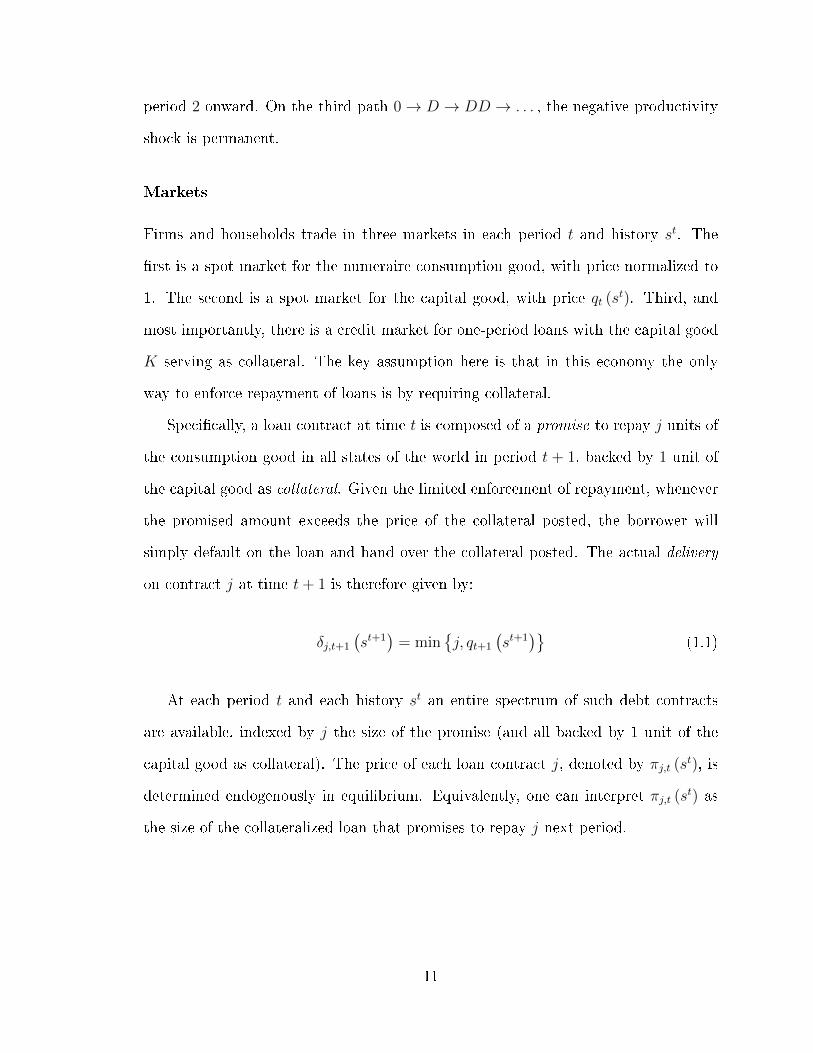
period 2 onward. On the third path 0→ D → DD → . . . , the negative productivity

shock is permanent.

Markets

Firms and households trade in three markets in each period t and history st. The

�rst is a spot market for the numeraire consumption good, with price normalized to

1. The second is a spot market for the capital good, with price qt (st). Third, and

most importantly, there is a credit market for one-period loans with the capital good

K serving as collateral. The key assumption here is that in this economy the only

way to enforce repayment of loans is by requiring collateral.

Speci�cally, a loan contract at time t is composed of a promise to repay j units of

the consumption good in all states of the world in period t + 1, backed by 1 unit of

the capital good as collateral. Given the limited enforcement of repayment, whenever

the promised amount exceeds the price of the collateral posted, the borrower will

simply default on the loan and hand over the collateral posted. The actual delivery

on contract j at time t+ 1 is therefore given by:

δj,t+1

(st+1

)= min

{j, qt+1

(st+1

)}(1.1)

At each period t and each history st an entire spectrum of such debt contracts

are available, indexed by j the size of the promise (and all backed by 1 unit of the

capital good as collateral). The price of each loan contract j, denoted by πj,t (st), is

determined endogenously in equilibrium. Equivalently, one can interpret πj,t (st) as

the size of the collateralized loan that promises to repay j next period.

11

A key feature of this set-up for the credit market is that for each loan j, we can

also compute the promised interest rate:

1 + rj,t(st)

:=j

πj,t (st)(1.2)

and the loan to value (or equivalently 1 minus the haircut imposed on the collateral):

LTVj,t(st)

:=πj,t (st)

qt (st)

=: 1−Haircutj,t(st)

(1.3)

Plotting the loan to value on the x-axis against the promised interest rate on

the y axis for each contract j generates the credit surface in Figure 1.6. The credit

surface is composed of three parts.7 The horizontal segment to the left represents

the risk-free spectrum of the market where the haircut is so high on the collateral

for given promise j ≤ j := minst+1 (qt+1 (st+1)) that the loan is e�ectively risk-free.

I refer to j as the max-min leverage contract, because it is the maximum promise

against one unit of collateral that still minimizes credit risk to the lender. The

increasing function in the middle of the credit surface captures the fact that as

the haircut falls (and the LTV rises), the lender starts to take on more credit risk

and must be compensated through a higher promised interest rate. Lastly, the

credit surface becomes vertical once the maximum loan-to-value is reached. This

cap on loan-to-value arises endogenously because the highest credible promise j :=

maxst+1 (qt+1 (st+1)) is given by the maximum possible valuation of the collateral next

period. I refer to j as the maximum leverage contract. From the de�nition of j and

j it is evident that how much a borrower can promise to repay on their collateralized

debt contract depends on the future price of capital. So any changes in the expected

7This concept of the �Credit Surface� was introduced in Geanakoplos and Zame (2014) andFostel and Geanakoplos (2015). Geanakoplos (2016) discusses the implications of the credit surfacefor monetary policy.

12

price of capital tomorrow can in�uence credit conditions today. Firms' choice of

contracts along the credit surface also determines the credit risk faced by lenders in

equilibrium. The possibility, and the occurrence, of defaults play an essential role in

the model.

Without loss of generality, I show later that the optimal contract for �rms lies on

the increasing segment of the credit surface: j∗ ∈[j, j]. Intuitively, when collateral

is scarce, the max-min leverage contract j is preferable to contracts j < j because

it allows the �rm to borrow more at the same interest rate against the same unit

of collateral. On the other side of the credit surface, any contract j > j will have

the exact same expected delivery as contract j and will thus be priced the same:

πj>j (st) = πj (st). So using the maximum leverage contract j allows the �rm to

borrow the same amount as contracts j > j but with a lower promised interest rate.

Finally, let ϕj,t (st) > 0 denote that the �rm is selling the contract j (i.e. borrowing

an amount equal to |ϕj|πj), and ϕj,t (st) < 0 indicate the �rm is buying the contract

j (i.e. lending |ϕj| πj). The corresponding notation for households is ϕj,t (st).

Agent Optimization

By assumption both the representative �rm and household are price taking and risk

neutral (u (x) = x). The �rm's optimization problem is given by:

max{xt(st),Kt(st),{ϕj,t(st)}}

∞∑t=0

βt∑st∈St

[u(xt(st))

Pr(st|st−1

)](1.4)

subject to:

13

Figure 1.6: Credit Surface - Choice of Leverage

The credit surface plots the loan to value on the x-axis against the promised interest rate on they axis for each collateralized contract j. Contract j := minst+1

(qt+1

(st+1

))promises to repay the

lender an amount equal to the minimum possible value of the collateral next period. Therefore jis the maximum promise that minimizes credit risk to the lender - a max-min leverage contract.Contract j := maxst+1

(qt+1

(st+1

))promises to repay the lender the maximum possible value of the

collateral next period. j is the maximum credible promise the borrower can make, and is thereforethe maximum leverage contract. Due to the scarcity of collateral, �rms will optimal choose a contractin the interval

[j, j]in equilibrium.

14

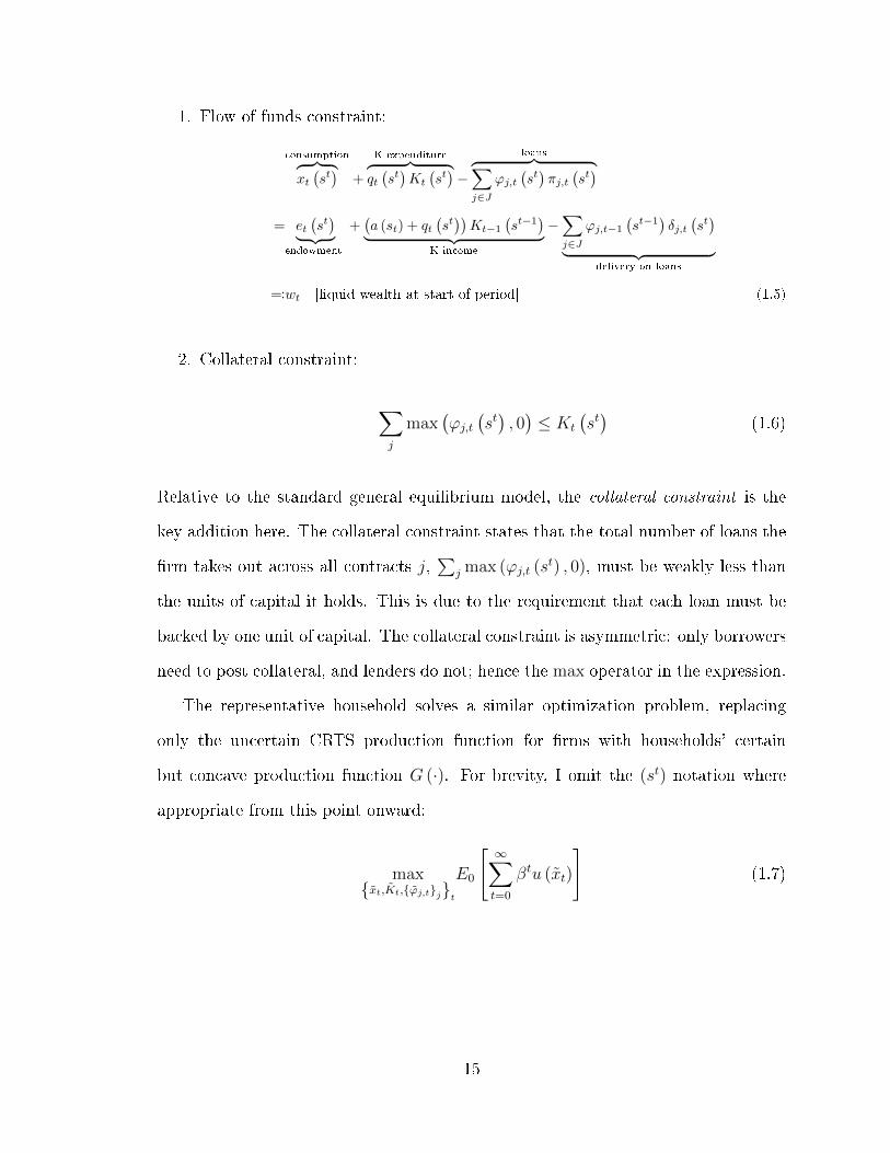
1. Flow of funds constraint:

consumption︷ ︸︸ ︷xt(st)

+

K expenditure︷ ︸︸ ︷qt(st)Kt

(st)−

loans︷ ︸︸ ︷∑j∈J

ϕj,t(st)πj,t

(st)

= et(st)︸ ︷︷ ︸

endowment

+(a (st) + qt

(st))Kt−1

(st−1

)︸ ︷︷ ︸K income

−∑j∈J

ϕj,t−1

(st−1

)δj,t(st)

︸ ︷︷ ︸delivery on loans

=:wt [liquid wealth at start of period] (1.5)

2. Collateral constraint:

∑j

max(ϕj,t

(st), 0)≤ Kt

(st)

(1.6)

Relative to the standard general equilibrium model, the collateral constraint is the

key addition here. The collateral constraint states that the total number of loans the

�rm takes out across all contracts j,∑

j max (ϕj,t (st) , 0), must be weakly less than

the units of capital it holds. This is due to the requirement that each loan must be

backed by one unit of capital. The collateral constraint is asymmetric: only borrowers

need to post collateral, and lenders do not; hence the max operator in the expression.

The representative household solves a similar optimization problem, replacing

only the uncertain CRTS production function for �rms with households' certain

but concave production function G (·). For brevity, I omit the (st) notation where

appropriate from this point onward:

max{xt,Kt,{ϕj,t}j}t

E0

[∞∑t=0

βtu (xt)

](1.7)

15

subject to:

xt + qtKt −∑j∈J

ϕj,tπj,t = et +G(Kt−1

)+ qtKt−1 −

∑j∈J

ϕj,t−1 min {j, qt} =: wt

(1.8)∑j

max (ϕj,t, 0) ≤ Kt (1.9)

Collateral Equilibrium

The solution concept of interest is a collateral equilibrium. Formally, a Collateral

Equilibrium is a vector consisting of the price of capital, contract prices, consumption,

capital holdings and contract trades (q (st) , π (st)) , (x (st) , K (st) , ϕ (st)) ,(x (st) , K (st) , ϕ (st)

)∈(R+ ×RJ

+

)×(R+ ×R+ ×RJ

)×(R+ ×R+ ×RJ

)s.t. at all period t and all history

st:

1. All agents optimize (equations 1.4 to 1.9); and

2. All markets clear:

(a) Consumption good market:

(xt(st)− et

(st))

+(xt(st)− et

(st))

= G(Kt−1

(st−1

))+a (st)Kt−1

(st−1

)(1.10)

(b) Capital good market:

Kt

(st)

+Kt

(st)

= K ≡ 1 (1.11)

(c) Collateralized debt market:

ϕj,t(st)

+ ϕj,t(st)

= 0 ∀j (1.12)

16

First-best Benchmark

Before characterizing the collateral equilibrium of the model, it is useful to establish

the �rst-best outcome as a frame of comparison. In the �rst-best, I assume there is a

central planner who assigns capital between �rms and households in each period and

each history in order to maximize the sum of their discounted utility (suppressing the

(st) notation again for brevity):

max{Kt,Kt}

t≥−1,st∈St

E0

[∑t=0

βt (xt + xt)

]

s.t. xt + xt = et + et +G(Kt−1

)+ atKt−1 ∀t ≥ 0

Kt + Kt = K = 1 ∀t ≥ −1

The �rst-best level of capital holdings therefore equalizes the marginal productiv-

ity of capital between households and �rms:

G′(Kfbt

)= Et [at+1] (1.13)

Kfbt = K − Kfb

t (1.14)

The �rst-best benchmark also coincides with the decentralized solution when we

remove the two main sources of productive ine�ciencies in the collateral equilibrium:

(1) the endogenous collateral constraint which restricts agents' ability to borrow; and

(2) limitations in the �rm's liquid wealth (which arise both exogenously at the start,

and then endogenously in certain histories, e.g. during the downturn at s1 = D).

Speci�cally, if we assume (1) �rms and households are su�ciently well-endowed in

every history to ensure they can always consume in addition to any desired capital

purchases and lending; and (2) there exists a perfect enforcement mechanism for debt

repayments, so promises are always honored and there is no need for posting any

17

collateral; then the equilibrium price of capital qt will adjust to equate the marginal

return of capital between �rms and households: βEt

[G′(Kt

)+ qt+1

]= qt (st) =

βEt [at+1 + qt+1], and it is easy to verify that Kt = Kfbt ∀t ≥ 0.

1.3 Characterizing the Collateral Equilibrium

The �rst-order conditions for both the �rm and household's optimization problems are

reported in Appendix 1.6. I impose assumptions on preferences, production functions

and endowments as follows. These assumptions are fairly weak (with risk neutrality

arguably being the strongest). The assumptions provide analytical tractability and

help restrict attention to equilibria of interest.

Assumptions and household's behavior in equilibrium

Assumption A1 [Risk neutrality]: u′(x) = u

′(x) = 1.

Assumption A2 [Common discounting]: 1 > β = β > 0.

Assumption A3 [Production functions]:

1. 1 > p > aDaU

2. G ∈ C2, with G′(0) = aU > aD = G

′ (K)and G

′′(·) < 0.

Assumption A3.1 imposes an upper bound on the probability of the downstate (1− p).

Assumption A3.2 states that the households are as productive as the �rm in the

Up-state if they hold no capital; but if they hold the entire stock then their marginal

productivity becomes as low as the �rm in the Down-state.

Assumption A4 [Endowments]:

1. K−1 = K and K−1 = 0.

2. e0 = w0 ∈ (0, β2aDKfb0 ] and et (st) = 0 ∀st ∈ St and ∀t ≥ 1.

18

3. et (st) > β1−βaU , ∀t ≥ 0 and ∀st ∈ St.

The �rst part of assumption A4 states that households start period 0 with the entire

stock of capital. The second part restricts the �rms' endowment of consumption good

in period 0 (their starting liquid wealth) and stipulates further that �rms receive no

more exogenous endowments from period 1 onward. These two parts combined imply

that the �rms will borrow from households in order to invest in the capital good. The

third part of assumption A4 ensures that households are su�ciently well endowed to

lend and consume in all periods and histories.

Lastly, I impose a no-bubble condition to rule out an ever increasing price for

capital in equilibrium, whereby any arbitrary price for capital today can be justi�ed

by an su�ciently high expected price tomorrow:

limt→∞

qt(st)<∞ ∀st ∈ St (1.15)

Under assumptions A1-4 and the no-bubble condition, we can characterize the

behavior of the representative household as follows:

Lemma 1. [Household behavior in equilibrium]

1. The household always consumes: xt (st) > 0 ∀t ≥ 0 and ∀st ∈ St.

2. The household never borrows: ϕj,t (st) < 0 ∀t ≥ 0 and ∀st ∈ St.

3. The household is always indi�erent between consuming and purchasing another

marginal unit of capital, so the equilibrium price of capital is given by:

qt = Et

[βu′ (xt+1)

u′ (xt)

(G′(Kt

)+ qt+1

)](1.16)

= Et

[β(G′(Kt

)+ qt+1

)]

19

4. The household is always indi�erent between consuming and lending, so the

equilibrium price of contract j (i.e. the size of the loan granted for a promised

repayment of j next period, collateralized by 1 unit of capital) is given by:

πj,t = Et

[βu′ (xt+1)

u′ (xt)δj,t+1

](1.17)

= Et [βmin {j, qt+1}] ∀j

Proof. Very brie�y, the household always consumes and never borrows because by

assumption they are given very large exogenous endowments in every period and

every history. The price of capital and the price of contract j are both expressed

in the form of standard asset pricing equations (stochastically discounted cash �ows,

from the household's perspective), which can be derived directly from household's �rst

order conditions (Appendix 1.6). More details can be found in Appendix 1.6.

Collaterals Value and the Optimal Choice of Leverage for �rms

For households, who never need to borrow, the capital good is simply a means to

transfer wealth into the next period through production or resale. For �rms however,

the capital good serves as both an investment opportunity and the only means to

secure loans (courtesy of the collateral constraint - equation 1.6). Consequently, from

the �rm's perspective, the price of capital re�ects both its stochastically discounted

cash �ow and its value as collateral.

When the �rm purchases capital on leverage using contract j, the standard asset

pricing equation yields:

qt − πj,t = Et

[βγt+1

γt(at+1 + qt+1 − δj,t+1)

]

20

where the left-hand-side of the expression is the down-payment required, and the

right-hand-side gives the stochastically discounted cash �ow from the transaction,

composed of dividends plus the price next period and minus actual delivery on debt

next period. γt denotes the marginal utility of income of �rms in period t and history

st. Re-arranging this equation illustrates how the price of capital can be decomposed

into its fundamental value and its collateral value to �rms.

Lemma 2. [Collateral Value] When �rms' capital holding is strictly positive Kt > 0

and the collateral constraint is binding, the price of capital can be expressed as:

qt = Et

[βγt+1

γt(at+1 + qt+1)

]+

{πj,t − Et

[βγt+1

γtδj,t+1

]}= Et

[βγt+1

γt(at+1 + qt+1)

]︸ ︷︷ ︸

fundamental value

+

{Et

[βγt+1

γtδj,t+1

]− Et

[βγt+1

γtδj,t+1

]}︸ ︷︷ ︸

collateral value when using contract j

(1.18)

where γt denotes the marginal utility of income of �rms in period t and history st; and

γt = γt+1 = 1 for households. Note that since the �rm does not necessarily consume

in every history, in general γt 6= u′(xt) = 1.

Let λt denote the Lagrangian multiplier for the �rm's collateral constraint at period

t and history st, and γt the multiplier for its budget constraint, then the equilibrium

collateral value can be expressed as:

Collateral Value := maxj

{Et

[(βγt+1

γt− βγt+1

γt

)δj,t+1

], 0

}=λtγt

(1.19)

In other words, collateral value is the dollar value the �rm attaches to a marginal

relaxation of its collateral constraint.

Proof. Both equations can be derived directly from �rm's �rst order conditions (Ap-

pendix 1.6).

21

Equation 1.18 highlights the dual role capital plays for �rms, and equation 1.19

shows that the collateral value is positive whenever the �rm's collateral constraint is

binding (λt > 0). Furthermore, when the collateral constraint is binding, the �rm

will choose the debt contract j that maximizes collateral value. Thus even though an

entire spectrum of contracts j ∈ R+ is priced, potentially only a single contract (if

any) will be actively traded in equilibrium. Lemma 3 below examines how the �rm

chooses the optimal contract j∗.

Lemma 3. [Optimal leverage] Suppose in equilibrium the collateral constraint is

binding (λt > 0), then:

1. Without loss of generality, the �rm will only consider contracts:

j ∈[j, j]

where j := minst+1 (qt (st+1)) is the max-min leverage contract, and j := maxst+1 (qt (st+1))

is the maximum leverage contract.

2. The �rm's optimal choice of debt contract is given by:

j∗ =

j if γt > γUt+1

j if γt < γUt+1[j, j]

if γt = γUt+1

where γUt+1 is the �rm's marginal utility of income in period t+ 1 if the Up-state

is realized (i.e. st+1 = U).

Lemma 3 states that in general the �rm will choose between either the left-hand

or the right-hand side kink of the credit surface (see Figure 1.7). In the knife edge

case where γt = γUt+1, the �rm is indi�erent between all debt contracts j ∈[j, j]. A

formal proof can be found in Appendix 1.6.

22

Figure 1.7: Choosing a point on the credit surface

Due to linear preference, when �rms borrow against capital as collateral, they do so with eitherthe max-min leverage contract j or the maximum leverage contract j. Firms prefer the max-minleverage contract when their marginal utility of income today γt is lower than their marginal utilityof income tomorrow in the Up-state γUt+1. Intuitively, this is because the max-min leverage contractentails a larger downpayment today, but allows the �rm to transfer more resources into the Up-state tomorrow. In contrast, in any ensuing Down-state, �rms default - regardless of whether theyborrowed using the max-min leverage contract or the maximum leverage contract today.

23

To see why the choice between the max-min leverage contract j and the maximum

leverage contract j depends only on the marginal utility of income in the Up-state

tomorrow γUt+1, and not the Down-state γDt+1, note that with buying K using contract

j = qDt+1 the �rm's cash �ow in period t + 1 is given by:

aU + qUt+1 − qDt+1

aD

.

In comparison, if the �rm bought K using contract j = qUt+1 instead, its cash �ow

would be given by

aU

aD

. The net di�erence between the two is

qUt+1 − qDt+1

0

,

an Up-Arrow security that delivers only in the Up-state. Therefore the �rm would

choose the max-min contract j when the marginal utility of income in the Up-state

tomorrow is su�ciently high.

Illustratives Example

Having described households' behavior and the choice of �rms with regard to collat-

eralized debt contracts, we can now proceed to characterize the collateral equilibrium

along the di�erent possible paths of the economy. The main complication that arises

when solving the model is that prices and choices today depend on the expectation

of prices tomorrow. The model is thus solved through backward induction, from

deterministic steady states that can be eventually reached after the uncertainty has

been fully resolved8, back to the uncertain histories in periods t = 0, 1. The path

(0 → D → DU → DUU . . . ), whereby the �rm's productivity su�ers a temporary

negative shock in history D before recovering permanently to aU in period t ≥ 2, is

the most interesting trajectory for our purpose. I illustrate the key features of the

collateral equilibrium with a simple numerical example below, before extending the

key results in the form of general propositions.

Consider an economy characterized by the set of parameters shown in Table

1.1. Restricting attention to the path where �rms su�er a negative, but temporary,

8A full characterization of the deterministic steady states can be found in Appendix 1.6.

24

Table 1.1: Parameters for Illustrative ExampleParameter Value Parameter Value

p 0.75 β 0.8aU 1.5 β 0.8aD 0.75 e0 0.75

G(K)

aUK −(aU−aD

2

)K2 et≥0 6

Note: While assumption A4.2: e0 < β2aDKfb0 , which restricts �rms' starting endowment in period 0,

is useful in the analytical proofs of my Propositions, the assumption is much stricter than necessary.In this illustrative example, I relax this assumption signi�cantly and demonstrate that the keyimplications of the model are robust.

productivity shock (0→ D → DU → DUU . . . ), Figure 1.8 plots the dynamics of the

�rms' capital holding in the collateral equilibrium against the �rst-best benchmark.

In the initial period 0, �rms start with no capital and very limited endowment of the

numeraire consumption good, so they borrow using the maximum leverage contract to

purchase as much capital as they can. Endogenously, the model generates two further

instances of productive ine�ciency along this temporary downturn path. First, �rms

default in historyD, their ability to borrow and leverage collapse and �rms' holding of

capital falls even further. Second, even when the uncertainty has been fully resolved

at history DU and beyond, the recovery to the �rst-best level is gradual. I address

the causes of each of these two distortions in turn.

The Downturn (s1 = D)

During the downturn (history D), �rms experience low productivity. The price of

capital falls because a larger proportion of capital is transferred to households, whose

production function exhibits diminishing returns. Firms would like to hold more

capital in order to produce next period during the potential recovery phase, but

cannot due to a tightening borrowing constraint arising from the reduction in their

liquid wealth and a fall in the borrowing capacity of capital as collateral. Crucially,

even though at both history 0 and D there is a common probability p that aggregate

productivity will be high (aU) next period and (1− p) that it will be low, the situation

25

Figure 1.8: Proportion of capital held by �rms

The representative �rm's capital holding collapses during the downturn (history D) before graduallyrecovering in subsequent periods towards the �rst-best benchmark. Even though by history DU allaggregate productivity uncertainty has been resolved, a full recovery is not achieved immediately.

26

Figure 1.9: Credit Surface during the downturn

Credit conditions deteriorate during the downturn (orange dashed line) relative to normal times(blue solid line). Firms that wish to borrow using the maximum leverage contract face both a higherinterest rate and a higher haircut for each unit of capital posted as collateral.

for �rms at history D is much worse. This is because in history DD the negative

aggregate productivity shock would be permanent. The price of capital at history

DD, qDD, is signi�cantly lower than that in history D. Consequently, each unit of

capital is much more valuable as collateral at history 0 than at history D. Thus

credit conditions deteriorate during the downturn relative to normal times (Figure

1.9). Firms that wish to borrow using the maximum leverage contract face both a

higher interest rate and a higher haircut for each unit of capital posted as collateral.

The collateral constraint faced by �rms and this endogenous fall in the borrowing

capacity of their collateral amplify the adverse aggregate productivity shock to the

real economy, and feed back into even lower capital holding by �rms.

I generalize these �ndings in the two propositions below. In the statement of

these propositions (and corresponding proofs) I adopt a simpli�ed set of notation,

27

combining the time subscript t and the dependence of variables on histories (st) into a

single subscript whenever the context is clear. For instance, let KD := Kt=1 (s1 = D).

Proposition 1. [Productive ine�ciency and leverage during the downturn]

Under assumptions A1 − 4 and given the no-bubble condition (equation 1.15), at

history D:

1. KD < KfbD : �rms hold too little capital relative to the �rst best; and

2.∑

j∈J max {ϕD,j, 0} = KD: the collateral constraint is binding (i.e. �rms pur-

chase capital using leveraged debt contracts).

Proof. Intuitively, at history D credit conditions are so tight and �rms' liquid wealth

are so low that �rms are unable to purchase the �rst-best level of capital even if they

borrow using the maximum leverage contract. Credit conditions tighten at history

D because the negative productivity shock signi�cantly reduces the expected price

of capital in the next period. Speci�cally, if the shock proves to be permanent, the

price of capital in history DD would be signi�cantly lower. The arrival of the bad

news at D therefore endogenously reduces the borrowing capacity of �rms against

each unit of collateral. Moreover, �rms have limited means to transfer their limited

liquid wealth from the initial history 0 to history D. If �rms used leverage during

history 0 to purchase capital, they would default at historyD, hand over the collateral

to lenders and retain only the consumption goods produced. The resulting amount

of liquid wealth is insu�cient to purchase the �rst best level of capital at D given

the prevailing credit conditions. On the other hand, �rms may try to transfer more

resources into history D by purchasing capital without leverage at history 0 (and

thus avoiding default at D).9 But for �rms to have enough liquid wealth at history D

9Another way for �rms to transfer resources into history D is by lending to households at history0. However, since households start with the entire stock of capital and their productivity is concave,it is easy to show that �rms strictly prefer purchasing capital without leverage to lending at history0.

28

to purchase KfbD with this strategy, the price of capital in the downturn qD must be

su�ciently high relative to its initial price q0. In such situations, the household would

also like to purchase more capital in period 0, which would push q0 beyond the level

required for the �rms' strategy to succeed. For the second part of the proposition,

because �rms hold too little capital relative to the �rst-best benchmark at history D,

they are in expectations more productive than households and would like to utilize

leveraged debt contracts to increase their holding of capital. A formal proof can be

found in Appendix 1.6.

Proposition 1 states that �rms would use leveraged debt contracts during the

downturn, but is silent on the optimal choice of contracts j∗D. From corollary 3 we

know that the choice is essentially between the maximum leverage contract jD = qDU

and the max-min (risk-free) leverage contract jD

= qDD. The following proposition

shows that �rms will use maximum leverage when the downturn is �severe�, and

max-min leverage when it is more �moderate�.

Proposition 2. [Optimal leverage during the downturn] Under assumptions

A1−4 and given the no-bubble condition (equation 1.15), at history D ∃KD ∈ (0, KfbD ]

s.t.

j∗D =

jD := qDU if KD < KD

jD

:= qDD if KD > KD{jD, jD

}if KD = KD

(1.20)

Proof. From Lemma 3, we have previously established that �rms prefer the maximum

leverage contract over the max-min leverage contract when their marginal utility of

income today is su�ciently high relative to their marginal utility of income tomor-

row in the Up-State. When �rms start history D with very limited liquid wealth,

households will hold the majority of capital in equilibrium and �rms will hold very

29

little (high KD and low KD). This implies that the equilibrium price of capital will

be very low from the perspective of the �rm, so �rms' marginal utility of income at

history D is very high and they would like to borrow the maximum amount possible

to take advantage of these �re sale prices. In contrast, if �rms have access to more

resources at history D, the price of capital would be higher and �rms may �nd it

optimal to use the max-min leverage contract to transfer more resources into the

Up-state at history DU where the uncertainty surrounding their productivity has

been resolved favorably. Given the linearity in preferences and the continuity of

households' production function G (·), there exists a threshold value of KD whereby

the �rms are indi�erent between the max-min leverage contract and the maximum

leverage contract. A formal proof can be found in Appendix 1.6.

In summary, Proposition 2 shows that when the production distortions in the

downturn is severe (i.e. very low KD) �rms would like to use maximum leverage

contracts to maximize their purchasing power. But when the production distortion

is more moderate (KD closer to KfbD ), then the max-min leverage contract is optimal

instead.

The Recovery (s2 = DU)

In the illustrative example (Figure 1.8) above, in the recovery phase �rms honor the

promise made in history D and repay the loan (jD := qDU) by either selling their

capital holding or equivalently handing over the collateral posted. This leaves �rms

with just the output from production wDU = aUKD with which to rebuild their stock

of capital. Unfortunately, this amount of liquid wealth is insu�cient to purchase the

�rst-best level of capital, even if they use the maximum leverage contract to minimize

the size of the down-payment required. Thus full recovery is not achieved at history

DU even though the uncertainty surrounding aggregate productivity has been fully

resolved. Lemma 4 generalizes this result.

30

Lemma 4. [Gradual Recovery]:

1. If �rms used maximum leverage at s1 = D, then KDU < KfbDU if:

KD < βKfbDU ≡ β

[1−G′−1 (aU)

](1.21)

2. If �rms used max-min leverage at s1 = D, then KDU < KfbDU if:

KD < βKfbDU

[1− β

1− β aDaU

](1.22)

Proof. If �rms used maximum leverage contracts at s1 = D, then their liquid wealth

at history DU is given by wDU,(j∗D=jD) = aUKD. In order to purchase the �rst-best

level of capital KfbDU , the minimum down-payment required in equilibrium is given

by: qDU − πjDU = βG′(KfbDU

)= βaU per unit of capital. So KDU is less than

KfbDU whenever KD < βKfb

DU . If instead �rms used maximum leverage contracts

at s1 = D, then their liquid wealth at history DU is given by wDU,,(j∗D=jD) =

(aU + qDU − qDD)KD, where (qDU − qDD) is bounded above by(

β1−βaU −

β1−βaD

).

Comparing wDU with the minimum down-payment required again yields inequality

1.22.

Recovery from a downturn will typically be gradual because �rms held too little

capital in history D and will need more time to build up su�cient liquid wealth

to purchase the e�cient level of capital at equilibrium prices. Recovery from a

moderate downturn will be faster than that from a severe downturns for two reasons.

First, trivially, �rms retain a higher stock of capital in a moderate downturn (by

de�nition) and this increases their production in history DU . Second, more subtly,

�rms optimally choose a lower level of leverage during moderate downturns (the

max-min leverage contract jD

instead of the maximum leverage contract jD - see

Proposition 2). This more conservative choice of leverage helps �rms transfer a higher

31

level of liquid wealth into the recovery phase, reducing the time required to achieve

the e�cient level of production.

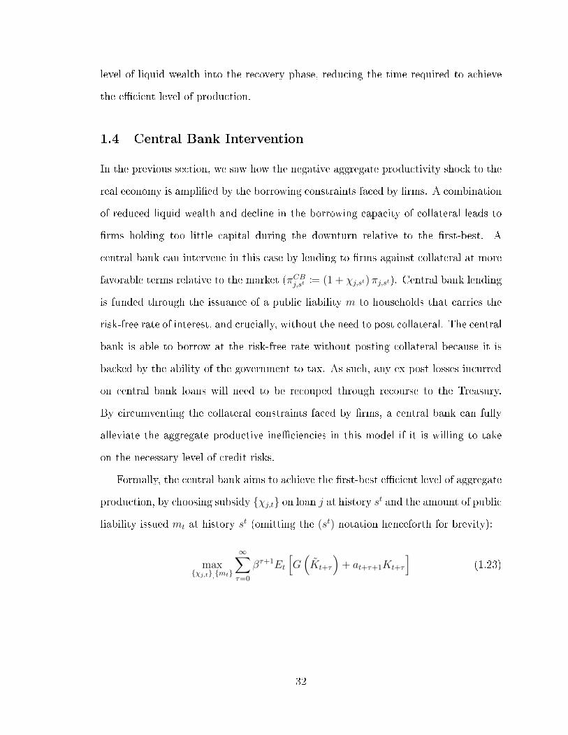
1.4 Central Bank Intervention

In the previous section, we saw how the negative aggregate productivity shock to the

real economy is ampli�ed by the borrowing constraints faced by �rms. A combination

of reduced liquid wealth and decline in the borrowing capacity of collateral leads to

�rms holding too little capital during the downturn relative to the �rst-best. A

central bank can intervene in this case by lending to �rms against collateral at more

favorable terms relative to the market (πCBj,st := (1 + χj,st) πj,st). Central bank lending

is funded through the issuance of a public liability m to households that carries the

risk-free rate of interest, and crucially, without the need to post collateral. The central

bank is able to borrow at the risk-free rate without posting collateral because it is

backed by the ability of the government to tax. As such, any ex post losses incurred

on central bank loans will need to be recouped through recourse to the Treasury.

By circumventing the collateral constraints faced by �rms, a central bank can fully

alleviate the aggregate productive ine�ciencies in this model if it is willing to take

on the necessary level of credit risks.

Formally, the central bank aims to achieve the �rst-best e�cient level of aggregate

production, by choosing subsidy {χj,t} on loan j at history st and the amount of public

liability issued mt at history st (omitting the (st) notation henceforth for brevity):

max{χj,t},{mt}

∞∑τ=0

βτ+1Et

[G(Kt+τ

)+ at+τ+1Kt+τ

](1.23)

32

subject to households' optimization (equations 1.4 - 1.6), �rms' optimization (equa-

tions 1.7 - 1.9) and the public sector budget constraint ∀τ ≥ 0:

1

βmt+τ−1

repayment on outstanding public liability

−∑j

ϕCBj,t+τπCBj,t+τ

new lending (to �rms)

≤ mt+τissuance of new public liability

−∑j

ϕCBj,t+τ−1δj,t+τ

delivery on outstanding loans

+ Tt+τtransfer from/to Treasury

(1.24)

where ϕCBj denotes the number of collateralized debt contract j held by the central

bank, with ϕCBj < 0 indicating the central bank is selling contract j (i.e. lending).

The size of the loan o�ered on contract j: πCBj := (1 + χj) πj depends on the size

of the subsidy o�ered (χj) relative to prevailing market rates. Lastly, T is the lump

sum tax required to balance the budget in every history (representing recourse to

the Treasury when positive and transfer of surplus when negative). The new market

clearing condition for collateralized debt contracts is given by:

ϕCBj,t+τ + ϕj,t+τ + ϕj,t+τ = 0 ∀τ ≥ 0,∀j ∈ J (1.25)

A key point here is that the central bank can intervene both across time t and

across the credit surface. By choosing which segment of the credit surface, or which

speci�c contract j, it is willing to subsidize {χj,t}, the central bank is simultaneously

setting both the interest rate and the haircut it imposes on the collateralized loan to

�rms:

(1 + rj,t) :=j

πCBj,t(1.26)

haircutj,t := 1− LTVj,t = 1−πCBj,tqt

(1.27)

33

The central bank can also choose the timing of the intervention. Since period

0 production is heavily dependent on starting endowments (which are exogenous

parameters in the model), we will instead focus attention on the optimal policy

intervention during the downturn, when credit conditions tighten and �rms' holding

of capital falls endogenously. In the following sections, we will �rst examine the

optimal policy intervention during the downturn (history D) when the central bank's

actions are unanticipated, before turning to the period 0 impact of such policies if

they were anticipated instead.

Unanticipated intervention at history D

From Proposition 2 we see that �rms will choose either the max-min leverage contract

jD

or the maximum leverage contract jD during the downturn depending on the

severity of the recession. Correspondingly, central bank responses can be grouped

into two broad categories: (1) intervene at the risk-free, low LTV end of the credit

surface jD; or (2) intervene at the high LTV end jD.

Proposition 3 states that when the downturn is severe and �rms wish to borrow

using the maximally leveraged loans, then the central bank can bring about the

�rst-best level of capital holding by subsidizing contract jD. In contrast, intervening

at the risk-free end of the credit surface may not be su�cient to achieve the �rst-best

outcome, when the central bank abides by an e�ective-lower-bound on interest rates10

and never lends more than the promised repayment amount (πCBj ≤ j, ∀j).

Proposition 3. [Unanticipated Intervention] Under assumptions A1 − 4 and

given the no-bubble condition (equation 1.15), at history D if j∗D = jD, then:

1. There exists χ∗jD > 0 s.t. πCBjD ≤ jD and KCBD = Kfb

D ; and

10The e�ective-lower-bound here is not a constraint in the strict sense, because the central bankcan always choose to lend at an negative interest rate that is below its cost of funding. But doingso guarantees a loss of public funds on every loan made.

34

2. There may not exist χ∗jD> 0 s.t. πCBj

D≤ j

Dand KCB

D = KfbD .

Proof. Intuitively, when �rms �nd it optimal to use the maximum leverage contract

j∗D = jD during the downturn, they will purchase as much capital as they can with

their available liquid wealth wD. The central bank can increase the amount of capital

the �rms can buy for given wD by subsidizing loans to the �rms and thus e�ectively

reducing the down-payment required on each unit of capital. The intervention will

raise the equilibrium price of capital during the downturn (qCBD > qD) as well as

during any subsequent recovery (qCBDU > qDU), which will a�ect credit conditions in

the private market during the downturn (see Figure 1.10, dashed line). The central

bank can o�set the impact of these price increases on the down-payment required

for �rms by simultaneously reducing the haircuts and the interest rates on high LTV

loans, pushing the credit surface downwards and outwards (Figure 1.10, dotted line).

In fact, when the central bank is willing to intervene at the high LTV segment of

the market, it is always possible to reduce the down-payment faced by �rms such

that they can purchase the �rst-best level of capital for given liquid wealth wD. In

contrast, when the central bank intervenes only at the risk-free segment of the market,

the maximum loan amount it can o�er while ensuring full repayment is given by the

price of capital in history DD, where the �rms are permanently unproductive. In

general, the price of capital at DD, qDD, is so low that the loan amount - even with

the central bank subsidy - is insu�cient to allow �rms to purchase the �rst-best level

of capital. The full proof can be found in Appendix 1.6.

Figure 1.11 plots �rms' capital holding given optimal central bank intervention,

along the path where the productivity shock is temporary, using the same illustrative

parameters as previously. It shows that when the central bank is willing to take on

credit risks, it becomes possible for �rms to hold the socially e�cient level of capital.

35

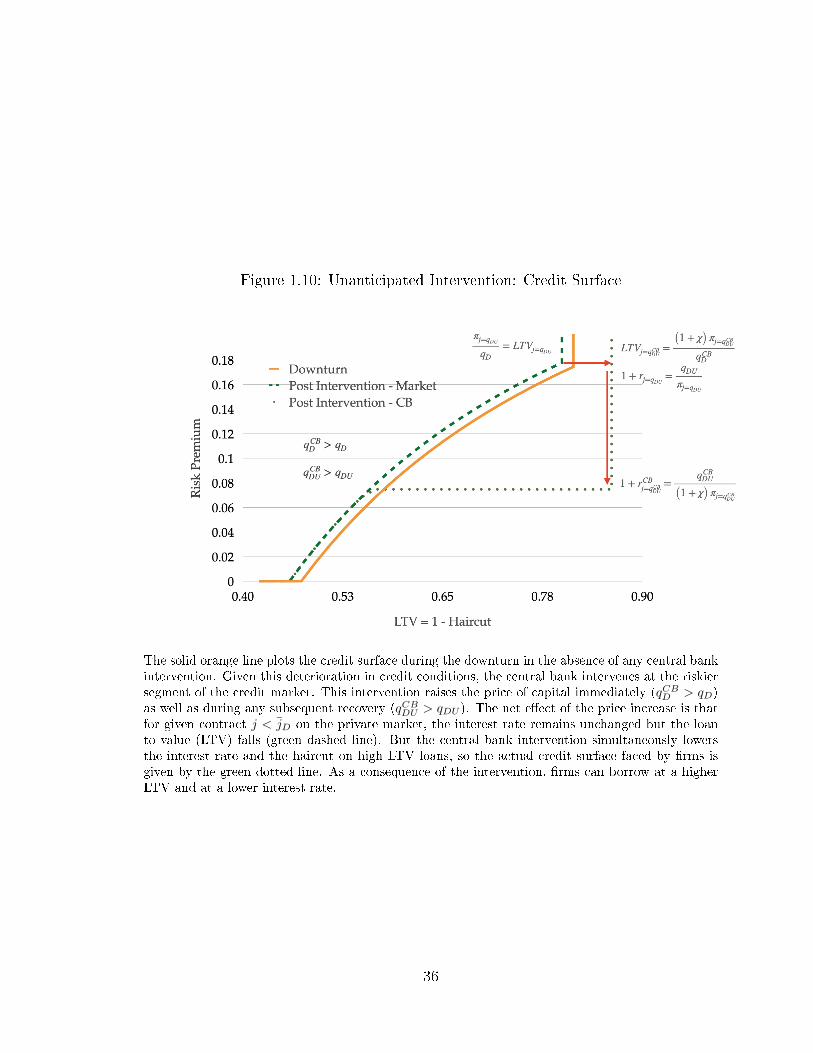
Figure 1.10: Unanticipated Intervention: Credit Surface

The solid orange line plots the credit surface during the downturn in the absence of any central bankintervention. Given this deterioration in credit conditions, the central bank intervenes at the riskiersegment of the credit market. This intervention raises the price of capital immediately (qCBD > qD)as well as during any subsequent recovery (qCBDU > qDU ). The net e�ect of the price increase is thatfor given contract j < jD on the private market, the interest rate remains unchanged but the loanto value (LTV) falls (green dashed line). But the central bank intervention simultaneously lowersthe interest rate and the haircut on high LTV loans, so the actual credit surface faced by �rms isgiven by the green dotted line. As a consequence of the intervention, �rms can borrow at a higherLTV and at a lower interest rate.

36

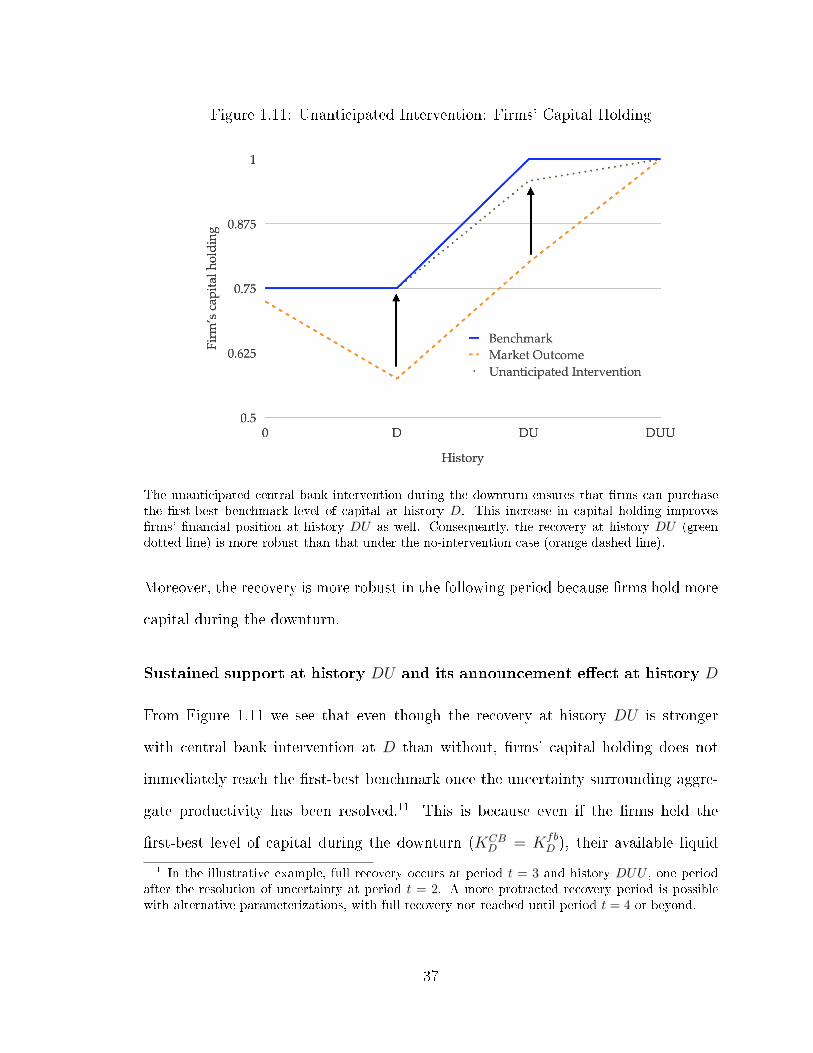
Figure 1.11: Unanticipated Intervention: Firms' Capital Holding

The unanticipated central bank intervention during the downturn ensures that �rms can purchasethe �rst-best benchmark level of capital at history D. This increase in capital holding improves�rms' �nancial position at history DU as well. Consequently, the recovery at history DU (greendotted line) is more robust than that under the no-intervention case (orange dashed line).

Moreover, the recovery is more robust in the following period because �rms hold more

capital during the downturn.

Sustained support at history DU and its announcement e�ect at history D

From Figure 1.11 we see that even though the recovery at history DU is stronger

with central bank intervention at D than without, �rms' capital holding does not

immediately reach the �rst-best benchmark once the uncertainty surrounding aggre-

gate productivity has been resolved.11 This is because even if the �rms held the

�rst-best level of capital during the downturn (KCBD = Kfb

D ), their available liquid

11In the illustrative example, full recovery occurs at period t = 3 and history DUU , one periodafter the resolution of uncertainty at period t = 2. A more protracted recovery period is possiblewith alternative parameterizations, with full recovery not reached until period t = 4 or beyond.

37

wealth during the recovery may not be su�cient, in general, to ramp up production

fully to the new, higher, e�cient level (KfbDU > Kfb

D ).

An immediate implication of the above observation is that it is optimal for the

central bank to continue its credit support during the recovery phase: χ∗jDU=qDUU> 0.

Lemma 5. [Sustained credit support] If KDU < KfbDU , then ∃χ∗jDU=qDUU

> 0 s.t.

πCBjDU ≤ qDUU and KCBDU = Kfb

DU .

Proof. The proof of Lemma 5 is analogous to that for the �rst part of Proposition

3.

A second, more subtle, implication is that whether or not the private sector antic-

ipates continued credit support at history DU can have important �scal implications

for the public sector. Speci�cally, suppose the central bank credibly announces its

commitment to sustained credit support if and only if the resolution of uncertainty

next period is favorable (i.e. at historyDU but not atDD). The anticipation of credit

support during the recovery raises the expected price of capital at DU , which in turn

increases the borrowing capacity of each unit of capital at D. Credit conditions in

the private market ease and capital prices rise immediately at D. The net result is a

reduction in the rate at which central bank loans must be subsidized ( χ falls), but an

overall increase in the total loan amount ((1 + χ) π increases). With or without the

announcement, the central bank still ensures �rms hold the �rst-best level of capital

at D; but with the announcement the larger total loan size means that the return on

public funds in the following period becomes a mean-preserving spread.

Formally, when the central bank makes the announcement, let qAnD denote the

price of capital at history D; qAnDU the price at history DU ; πjD=qAnDUthe price of the

maximum leverage contract on the private credit market atD; and χAnjD=qAnDU

the level of

central bank subsidy required to achieve the �rst-best benchmark at D. Furthermore,

let central bank lending at D be �nanced through the issuance of the risk-free

38

public liability: mAnD =

(1 + χAn

jD=qAnDU

)πjD=qAnDU

. And let any shortfalls/windfalls

in the following period (t = 2) be met through taxation/transfers: ED

[T2|χAnjD

]=[

1β

(1 + χAnj

D=qAnDU

)πjD=qAnDU

]−E

[qAn2

], where E

[qAn2

]is the expected price of capital

next period and is equal to the expected delivery on the maximum leverage contract.

I prove the following proposition:

Proposition 4. [The Announcement E�ect] If �rms used leverage at history 0:

j∗0 ∈[j

0, j0

], and prefer the maximum leverage contract during the downturn j∗D = jD,

then, when the central bank announces conditional credit support at history D, such

that χ∗jDU=qDUU> 0 and χ∗jDD = 0:

1. The optimal rate of subsidy falls,χAnjD

χ∗jD

=πjD=qCB

DU

πjD=qAn

DU

< 1, but the optimal total loan

size increases,(

1 + χAnjD

)πjD=qAnDU

>(

1 + χ∗jD

)πjD=qCBDU

.

2. The return on public funds becomes a mean-preserving spread relative to the no

announcement case: E[T2|χAnjD

]= E

[T2|χ∗jD

], and TDU |χAnjD < TDU |χ∗jD (larger

windfall in the recovery phase) and TDD|χAnjD > TDD|χ∗jD (larger shortfall in the

permanent downturn).

Proof. The intuition of the proof is as follows. A credible announcement of continued

credit support during any subsequent recovery raises the price of capital during

the down-state. Conventionally, one would expect this price increase to improve

the balance sheet position of �rms and reduce the amount of central bank lending

required. However, if �rms used leverage at history 0: j∗0 ∈[j

0, j0

], they would

default in history D and hand over their entire stock of capital to lenders. As a

result, �rms must rebuild their stock of capital from scratch at history D. The

increase in capital prices therefore increases the total amount the central bank must

lend to �rms, even as private market credit conditions improve and the required rate

of subsidy falls. A larger initial loan implies a larger windfall in the recovery phase

but also a larger shortfall in any permanent downturns. Lastly, since with or without

39

the announcement the central bank will ensure the �rms hold the �rst-best level of

capital at history D, the expected cost to taxpayers is unchanged. A formal proof

can be found in Appendix 1.6.

Proposition 4 shows that even though a credible announcement of sustained

credit support in the future can have signi�cant immediate e�ects on asset prices

and credit conditions, the expected return/loss on public funds may stay the same

with or without the announcement. This is a somewhat surprising result. In tra-

ditional Diamond-Dybvig style models with multiple equilibria, a commitment to

�do whatever it takes� can shift the economy to a more virtuous equilibrium and

reduce the initial stimulus required. In my model, having abstracted away from the

asymmetry of information that is central to models of �nancial crises and panics,

we see that a credible announcement of future support provides no additional gains

when responding to big shocks to the real economy. In fact, if the public sector is

instead risk-averse with taxpayer funds, it might prefer to �surprise� the market with

additional stimulus instead of announcing them in advance. The model therefore

suggests that the optimal central bank response might look very di�erent when the

shocks are predominantly hitting the real economy (such as during the COVID-19

crisis) as opposed to the �nancial sector.

Anticipated Intervention

What if the intervention at history D and beyond are anticipated by market partic-

ipants in advance? Conventional wisdom suggests that if agents expect the central

bank to provide credit support during a downturn, they may take on excessive

leverage during normal times, potentially leading to greater productive distortions

and exacerbating the severity of the downturn. There exists however an alternative

narrative. Anticipating low asset prices and central bank credit support during the

40

downturn, �rms may be incentivized to reduce leverage in normal times in order to

exploit more favorable investment opportunities during the downturn.

In the following Proposition, I show that if �rms are using maximum leverage

contracts j∗0 = j0 := qU at history 0, then the anticipation of central bank intervention

at history D will lead to either: (1) �rms continuing to use maximum leverage

contracts at period 0 and hold the same level of capital at history 0; or (2) a jump to

an equilibrium whereby �rms are purchasing capital without leverage at history 0 .

Proposition 5. [Waiting for the downturn] If j∗0 = j0 := qU in the absence

of central bank intervention, and it becomes common knowledge that χ∗jD > 0, then

either:

1. j∗0 = jCB0 := qCBU and K0 = KCB0 ; or

2. ϕCB0,j = 0, ∀j.

where qCBU , KCB0 and ϕCB0,j denote respectively the equilibrium price for capital in

history U , the �rms' optimal capital holding and contract sales at history 0, when

central bank intervention is fully anticipated.

Proof. For the �rst part of the proposition, I show that if �rms continue to �nd it

optimal to use the maximum leverage contract at t = 0, then their capital holding in

equilibrium remains unchanged. This is because when �rms use maximum leverage

contracts, the required down-payment is given by the opportunity cost of production

faced by households (see Corollary 1 and equation 1.41). Therefore K0 = e0q0−πj0

=

e0βG′(K−K0)

and KCB0 = e0

qCB0 −πjCB0

= e0βG′(K−KCB

0 ). And given G

′(·) < 0, we have

K0 = KCB0 . The capital holding of �rms remains unchanged despite the change in

equilibrium prices and credit conditions.

For the second part of the proposition, recall that the payo� to the �rm from

purchasing capital at history 0 without leverage is given by

aU + qU

aD + qD

in the two

41

possible states. Correspondingly the payo� to the �rm from purchasing capital on

leverage is

aU + qU − qD

aD

with the max-min leverage contract, and

aU

aD

with

the maximum leverage contract. We see that the di�erence in payo�s between the

max-min leverage contract and the maximum leverage contract is simply an Up-Arrow

security

qU − qD

0

, which is re�ected in a higher down-payment required with the

max-min leverage contract. Consequently, �rms will only switch from the maximum

leverage contract to the max-min leverage contract when their marginal utility of

income in the up-state is su�ciently higher than their marginal utility of income in

the current period12. The central bank intervention at history D is aimed at reducing

the down-payment required when purchasing capital on leverage during the downturn.

This drives up the �rms' marginal utility of income at D: γCBD > γD, but leaves their

marginal utility of income at U unchanged. Thus the �rm will either continue with

the maximum leverage contract at history 0, or switch to purchasing capital without

leverage. Purchasing capital without leverage generates the highest payo� in the

down-state for each unit of capital, and may become the optimal choice for �rms

when their marginal utility of income at D becomes su�ciently high. When �rms

purchase capital without leverage: ϕCB0,j = 0, ∀j.

A subtle implication of Proposition 5 is that even when �rms continue to use the

maximum leverage contract at period 0 and their holding of capital remain unchanged,

the loan to value on their collateralized debt contract may actually increase due to

the change in equilibrium asset prices. The loan to value on the maximum leverage

contract at history 0 is the ratio between the size of the loan πj0 = β [pqU + (1− p) qD]

and the price of capital q0. The anticipation of central bank interventions increases

both q0 and qD, the former reduces LTV on debt contracts and the latter increases it.

For broad parameterizations, the proportional increase in qD typically outweigh the

12For more details, see Lemma 3

42

increase in q0, so the net e�ect is often an increase in the period 0 leverage of the �rm.

The proposition shows that when the economy is already highly leveraged in normal

times, the anticipation of central bank interventions during any potential downturns

may indeed increase leverage further. However �rms may be borrowing more just

to purchase the same amount of capital, because the price of capital is higher when

central bank interventions are anticipated. Therefore the increase in leverage during

normal times does not always translate directly into greater productive ine�ciencies.

1.5 Concluding Remarks

A salient feature of the �central bank intervention� examined in this paper is the

potential need for recourse to taxpayer funds, when losses are incurred on the loans

extended. In this sense, the intervention is a joint public sector e�ort - similar to the

style of the programs we are seeing during the current pandemic. For instance, in

both the Primary and Secondary Market Corporate Credit Facility, the US Treasury

provides the equity investment in the facility, and the Federal Reserve lends against

the assets held in the facility.

A second point is that although every debt contract is collateralized by a durable

asset in the model, in practice a substantial portion of the underlying bonds/loans

in the credit facilities may not be explicitly secured. Nevertheless, such loans are

still implicitly backed by the value of the tangible assets of the �rm. So a high-LTV

collateralized debt contract in the model simply corresponds to a loan with a higher

degree of credit risk to the lender. The central message of the paper - that central

banks should take on greater credit risk when the downturn is severe - remains un-

changed regardless of whether the loan is contractually collateralized. The analytical

framework presented here highlights the role of defaults and limited enforcement of

repayment in equilibrium outcomes. It can be extended into more general settings

43

where, instead of posting collateral explicitly, promises on debt contracts are backed

by the assets of the �rm.13

Third, the central bank in the model lends directly to �rms that engage in

production, whereas traditionally central banks preferred to lend to �nancial interme-

diaries. Extending the model to encompass a third sector functioning as the �nancial

intermediary is an interesting direction for future research. Nevertheless, current

credit facilities like the Main Street Lending Program in the US demonstrate a policy

shift towards more direct lending to the real economy.

Most importantly, the paper emphasizes that central banks have much more than

just interest rates in their policy toolkit. Collateral requirements (and risk appetites)

are also an important part of the transmission mechanism. Under the Bagehot rule

and as standard practice during normal times, collateral requirements at central banks

are set mechanically to ensure the central bank never takes on signi�cant credit risk.

This leaves the risk-free interest rate as the main policy instrument. In my model -

as in real life - variations in collateral requirements allow central banks to intervene

across the credit surface, and to provide support to riskier borrowers who may be

shut out of the credit markets during a downturn. As such, collateral requirements

in central bank lending should play an integral role in policy discussions.

13In a separate working paper, Du (2020), I analyze the collateral equilibrium in economies withmore than two states of nature when debt contracts can be ordered by seniority and backed by�nancial assets. For instance, with three states of nature, borrowers can issue both senior secureddebt and junior subordinated debt, where the junior subordinated debt is backed by the residualvalue of the �rm after senior creditors are repaid. I show that any equilibrium in this economy isequivalent to another equilibrium where the senior tranche never defaults, and the junior trancheonly defaults in the worst state of the world.

44

References

Adrian, T. and H. Song Shin (2010). Financial intermediaries and monetary

economics. In Handbook of Monetary Economics, Volume 3, pp. 601�650.

Allen, F., E. Carletti, and D. Gale (2009). Interbank market liquidity and central

bank intervention. Journal of Monetary Economics 56 (5), 639�652.

Allen, F. and D. Gale (2000). Financial Contagion. Journal of Political Econ-

omy 108 (1).

Anderson, L. (2020). Hearing to Examine the Main Street Lending Program.

Araújo, A., S. Schommer, and M. Woodford (2015a). Conventional and unconven-

tional monetary policy with endogenous collateral constraints. American Economic

Journal: Macroeconomics 7 (1), 1�43.

Araújo, A., S. Schommer, and M. Woodford (2015b). Conventional and unconven-

tional monetary policy with endogenous collateral constraints. American Economic

Journal: Macroeconomics 7 (1), 1�43.

Auclert, A. (2017). Monetary Policy and the Redistribution Channel. NBER Working

Paper .

Auclert, A. and M. Rognlie (2018). Inequality and Aggregate Demand.

Ayuso, J. and R. Repullo (2004). A model of the open market operations of the

European Central Bank. 113 (January 2003), 883�902.

Bank of England (2014). The Bank of England ' s Sterling Monetary Framework.

(January).

Bank of England (2015). The Bank of England's Sterling Monetary Framework.

45

Bank of England (2017). A summary of the current Bank of England operations in

the sterling money markets 1. (July).

Bank of England (2020a). Bank of England measures to respond to the economic

shock from Covid-19.

Bank of England (2020b). Minutes of the special Monetary Policy Committee meeting

ending on 10 March 2020.

Bech, M. and T. Keister (2017). Liquidity regulation and the implementation of

monetary policy. Journal of Monetary Economics 92, 64�77.

Benigno LUISS, P., E. Roberto Robatto, J. Antonio de Aguirre, M. Gebauer,

L. Infantino, R. Lagos, G. La Spada, M. Magill, F. Mattesini, P. Bolton, M. Quinzii,

J.-C. Rochet, H. Seok Kim, F. Celentano, K. Dempsey, K. Liu, M. Rempel,

and N. Rovo (2018). Private Money Creation, Liquidity Crises, and Government

Interventions *.

Bernanke, B. S. and M. Gertler (1995). Inside the Black Box: The Credit Channel

of Monetary Policy Transmission. Journal of Economic Perspectives No. 5146 (4),

27�48.

Bernanke, B. S., M. Gertler, and S. Gilchrist (1994). The Financial Accelerator and

the Flight to Quality. National Bureau of Economic Research 4789 (July), 1�54.

Bernanke, B. S., M. Gertler, and S. Gilchrist (1999). Chapter 21 The �nancial accel-

erator in a quantitative business cycle framework. In Handbook of Macroeconomics,

Volume 1, pp. 1341�1393.

Bernanke, B. S. and M. Woodford (1997). In�ation Forecasts and Monetary Policy.

BoE (2002). The Framework for the Bank of England's Operations in the Sterling

Money Markets. In Bank of England Quarterly Bulletin, Number June, pp. 15.

46

BoE (2006). The Framework for the Bank of England's Operations in the Sterling

Money Markets. In Bank of England Quarterly Bulletin, Number November.

BoE (2008). The Framework for the Bank of England's Operations in the Sterling

Money Markets. In Bank of England Quarterly Bulletin, Number January.

Borio, C. and H. Zhu (2012). Capital regulation, risk-taking and monetary policy: A

missing link in the transmission mechanism? Journal of Financial Stability 8 (4),

236�251.

Brunetti, C., M. Di Filippo, J. H. Harris, K. Anderson, P. Angelini, B. Buyuksahin,

A. Chaboud, M. Fleming, C. Fur�ne, A. Kirilenko, F. Ravazzolo, M. Robe,

T. Santos, C. Scotti, and C. Vega (2011). E�ects of Central Bank Intervention

on the Interbank Market During the Subprime Crisis. he Review of Financial

Studies 24 (6), 2053�2083.

Brunnermeier, M. K. (2009). Deciphering the Liquidity and Credit Crunch 2007 -

2008. Journal of Economic Perspectives 23 (1), 77�100.

Bruno, V. and H. S. Shin (2015). Capital �ows and the risk-taking channel of

monetary policy. Journal of Monetary Economics 71, 119�132.

Bullard, J. and K. Mitra (2002). Learning about monetary policy rules. Journal of

Monetary Economics 49 (6), 1105�1129.

Caballero, R. J., A. Simsek, M. Rognlie, M. Schneider, L. Summers, J. Ventura,

O. Wang, and N. Zorzi (2017). A RISK-CENTRIC MODEL OF DEMAND

RECESSIONS AND MACROPRUDENTIAL POLICY.

Capponi, A., W. A. Cheng, S. Giglio, and R. Haynes (2017, nov). The Collateral

Rule : An Empirical Analysis of the CDS Market. SSRN Electronic Journal .

47

Chancellor of Exchequer (2020). Letter from Chancellor to Governor. Technical

report.

Churm, R. and A. Radia (2012). The Funding for Lending Scheme. Bank of England

Quarterly Bulletin Q4.

Clarida, R., J. Galí, M. Gertler, R. Clarida, M. Gertler, and M. Gertler (1999). The

Science of Monetary Policy: A New Keynesian Perspective. Journal of Economic

Literature 37 (4), 1661�1707.

Cooper, R. and T. W. Ross (1998). Bank runs: Liquidity costs and investment

distortions. Journal of Monetary Economics 41 (1), 27�38.

Cúrdia, V. and M. Woodford (2016). Credit Frictions and Optimal Monetary Policy.

Journal of Monetary Economics 84, 30�65.

Diamond, D. W. and A. K. Kashyap (2016). Liquidity Requirements, Liquidity

Choice, and Financial Stability. In Handbook of Macroeconomics, Volume 2, pp.

2263�2303.

Du, C. (2020). Multinomial max-min theorem: a generalization of the binomial

no-default theorem.

Dubey, P. and J. D. Geanakoplos (2006, sep). Money and Production, and Liquidity

Trap. International Journal of Economic Theory 2 (1200), 295�317.

Dubey P. and J. Geanakoplos (2003). Inside and outside money, gains to trade, and

IS-LM. Economic Theory 21 (2), 347�397.

England, B. (2013). The Red Book - The Bank of England's Sterling Monetary

Framework. (October).

English, B. and J. N. Liang (2020). Designing the Main Street Lending Program:

Challenges and Options.

48

Evans, G. and S. Hankaphja (2003). Expectations and the Stability Problem for

Optimal Monetary Policies. The Review of Financial Studies 70 (4), 807�824.

Fostel, A. and J. Geanakoplos (2008a). Collateral restrictions and liquidity under-

supply: A simple model. Economic Theory 35 (3), 441�467.

Fostel, A. and J. Geanakoplos (2008b). Leverage cycles and the anxious economy.

American Economic Review 98 (4), 1211�1244.

Fostel, A. and J. Geanakoplos (2012). Tranching, CDS, and asset prices: How

�nancial innovation can cause bubbles and crashes. American Economic Journal:

Macroeconomics 4 (1), 190�225.

Fostel, A. and J. Geanakoplos (2016). Financial innovation, collateral, and invest-

ment. American Economic Journal: Macroeconomics 8 (1), 242�284.

Fostel, A. and J. Geanakoplos (2019). Leverage Cycles and Financial Innovation

Cycles in Collateral Equilibrium. pp. 1�166.

Fostel, A. and J. D. Geanakoplos (2015). Leverage and Default in Binomial

Economies: A Complete Characterization. Econometrica 83 (6), 2191�2229.

Freixas, X., A. Martin, and D. Skeie (2011). Bank liquidity, interbank markets, and

monetary policy. Review of Financial Studies 24 (8), 2656�2692.

Freixas, X., B. Parigi, and J. C. Rochet (2000). Systemic Risk, Interbank Relations

and Liquidity Provision by the Central Bank. Journal of Money, Credit and

Banking 3 (3), 611�638.

Fuerst, T. S. (1992). Liquidity, loanable funds, and real activity. Journal of Monetary

Economics 29 (1), 3�24.

Geanakoplos, J. (1997). Promises Promises. In The economy as an evolving complex

system II.

49

Geanakoplos, J. (2003, aug). Liquidity, Default and Crashes: Endogenous Contracts

in General Equilibrium. Advances in economics and econometrics: theory and

applications: eighth World Congress 170.

Geanakoplos, J. (2010). The Leverage Cycle. NBER Macroeconomics Annual 24 (1),

1�66.

Geanakoplos, J. (2016). The Credit Surface and Monetary Policy. Progress and

Confusion: The State of Macroeconmic Policy .

Geanakoplos, J. and P. Dubey (2010). Credit cards and in�ation.

Geanakoplos, J., I. Karatzas, M. Shubik, and W. D. Sudderth (2014). In�ationary

equilibrium in a stochastic economy with independent agents. Journal of Mathe-

matical Economics 52, 1�11.

Geanakoplos, J. and K. J. Walsh (2017). Ine�cient liquidity provision. Economic

Theory , 1�21.

Geanakoplos, J. and W. R. Zame (2014). Collateral equilibrium, I: A basic framework.

Economic Theory 56 (3), 443�492.

Gertler, M. and P. Karadi (2011). A Model of Unconventional Monetary Policy.

Journal of Monetary Economics 58, 17�34.

Gertler, M. and N. Kiyotaki (2010). Financial intermediation and credit policy in

business cycle analysis. In Handbook of Monetary Economics, Volume 3, pp. 547�

599.

Gilchrist, S., B. Wei, Z. Yue, and E. Zakrajsek (2020). The Fed Takes on Corporate

Credit Risk: An Analysis of the E�cacy of the SMCCF.

Gorton, G. (1988). Banking panics and business cycles. Oxford Economic Pa-

pers 40 (4), 751�781.

50

Gorton, G. and A. Metrick (2010). Haircuts. Technical report.

Gorton, G., A. Metrick, and U. Nber (2012). Securitized banking and the run on

repo. Journal of Financial Economics 104, 425�451.

Gorton, G. and G. Ordoñez (2014). Collateral crises. American Economic

Review 104 (2), 343�378.

Gorton, G. and G. Ordõnez (2019). Fighting Crisis with Secrecy.

Gorton, G. and G. Pennacchi (1990). Financial Intermediaries and Liquidity Creation.

The Journal of Finance 45 (1), 49�71.

Gorton, G. and A. Winton (2003). Financial Intermediation. In Handbook of the

Economics of Finance, Volume 1, pp. 431�552.

Hansen, L. P. and T. J. Sargent (2003). Robust control of forward-looking models.

Journal of Monetary Economics 50 (3), 581�604.

Hanson, S. G., J. C. Stein, A. Sunderam, and E. Zwick (2020). Business Credit

Programs in the Pandemic Era.

He, Z., B. Kelly, and A. Manela (2017, oct). Intermediary asset pricing: New evidence

from many asset classes. Journal of Financial Economics 126 (1), 1�35.

He, Z., A. Krishnamurthy, and K. Milbradt (2016). A model of safe asset

determination.

HM Treasury; and Bank of England (2020). Joint HM Treasury and Bank of England

Covid Commercial Financing Facility ( CCFF ) - Market Notice 18 March 2020.

Holmstrom, B. and J. Tirole (1997a). Financial Intermediation, Loanable Funds, and

The Real Sector. The Quarterly Journal of Economics 112 (3), 663�691.

51

Holmstrom, B. and J. Tirole (1997b). Financial Intermediation, Loanable Funds, and

the Real Sector. The Quarterly Journal of Economics 112 (3), 663�691.

Kiyotaki, N. and J. Moore (1997). Credit Cycles. Journal of political economy 105 (2),

211�248.

Koulischer, F. and D. Struyven (2014, dec). Central bank liquidity provision and

collateral quality. Journal of Banking and Finance 49, 113�130.

Lagos, R. (2010). Asset prices and liquidity in an exchange economy. Journal of

Monetary Economics 57 (8), 913�930.

Mankiw, N. G. and R. Reis (2002). Sticky information versus sticky prices: a proposal

to replace the New Keynesian Phillips curve. Quarterly Journal of Economics 3 (4),

1295�1328.

Martin, A. (2006). Liquidity provision vs. deposit insurance: Preventing bank panics

without moral hazard. Economic Theory 28 (1), 197�211.

Melosi, L. (2016). Signalling E�ects of Monetary Policy. The Review of Economic

Studies , 853�884.

of England, B. (2019). The Bank of England's operations under the funding for

lending scheme - operating procedures. Technical report.

Ottonello, P. and Winberry Thomas (2017). Financial Heterogeneity and the

Investment Channel of Monetary Policy. Working Paper , 1�49.

Poledna, S., S. Thurner, J. D. Farmer, and J. Geanakoplos (2014). Leverage-induced

systemic risk under Basle II and other credit risk policies. Journal of Banking and

Finance 42 (1), 199�212.

52

Schularick, M. and A. M. Taylor (2012). Credit Booms Gone Bust: Monetary

Policy, Leverage Cycles and Financial Crises, 1870-2008. American Economic

Review 102102 (22), 1029�1061.

Shleifer, A. and R. W. Vishny (1992). Liquidation Values and Debt Capacity: A

Market Equilibrium Approach Liquidation Values and Debt Capacity: A Market

Equilibrium Approach. The Journal of Finance 47 (4), 1343�1366.

Sims, C. a. (2011). Rational Inattention and Monetary Economics. Handbook of

Monetary Economics 3 (2007), 155�181.

Simsek, A. (2013). Belief Disagreements and Collateral Constraints. Economet-

rica 81 (1), 1�53.

Tella, S. D. (2018). A Neoclassical Theory of Liquidity Traps.

Tommaso, M. (2008). Optimal Monetary Policy with Collateralized Household Debt

and Borrowing Constraints. Asset Prices and Monetary Policy (NBER).

Winters, B. (2012). Review of the Bank of England's Framework for Providing

Liquidity to the Banking System. Technical Report October.

Woodford, M. (2003). Imperfect Common Knowledge and the E�ects of Monetary

Policy. In Knowledge, Information and Expectations in Modern Macroeconomics:

In Honor of Edmund S.

Woodford, M., S. The, A. Economic, and N. March (2010). Robustly Optimal

Monetary Policy with Near-Rational Expectations. The American Economic

Review 100 (1), 274�303.

53

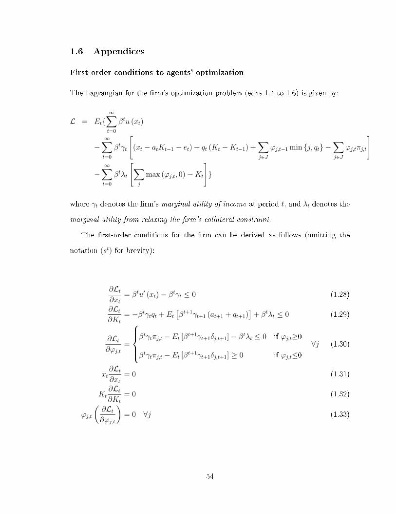
1.6 Appendices

First-order conditions to agents' optimization

The Lagrangian for the �rm's optimization problem (eqns 1.4 to 1.6) is given by:

L = Et{∞∑t=0

βtu (xt)

−∞∑t=0

βtγt

[(xt − atKt−1 − et) + qt (Kt −Kt−1) +

∑j∈J

ϕj,t−1 min {j, qt} −∑j∈J

ϕj,tπj,t

]

−∞∑t=0

βtλt

[∑j

max (ϕj,t, 0)−Kt

]}

where γt denotes the �rm's marginal utility of income at period t, and λt denotes the

marginal utility from relaxing the �rm's collateral constraint.

The �rst-order conditions for the �rm can be derived as follows (omitting the

notation (st) for brevity):

∂Lt∂xt

= βtu′ (xt)− βtγt ≤ 0 (1.28)

∂Lt∂Kt

= −βtγtqt + Et[βt+1γt+1 (at+1 + qt+1)

]+ βtλt ≤ 0 (1.29)

∂Lt∂ϕj,t

=

βtγtπj,t − Et [βt+1γt+1δj,t+1]− βtλt ≤ 0 if ϕj,t≥0

βtγtπj,t − Et [βt+1γt+1δj,t+1] ≥ 0 if ϕj,t≤0∀j (1.30)

xt∂Lt∂xt

= 0 (1.31)

Kt∂Lt∂Kt

= 0 (1.32)

ϕj,t

(∂Lt∂ϕj,t

)= 0 ∀j (1.33)

54

Correspondingly, the �rst-order conditions for the household are given by:

∂Lt∂xt

= βtu′ (xt)− βtγt ≤ 0 (1.34)

∂Lt∂Kt

= −βtγtqt + Et

[βt+1γt+1

(G′(Kt

)+ qt+1

)]+ βtλt ≤ 0 (1.35)

∂Lt∂ϕj,t

=

βtγtπj,t − Et

[βt+1γt+1δj,t+1

]− βtλt ≤ 0 if ϕj,t≥0

βtγtπj,t − Et[βt+1γt+1δj,t+1

]≥ 0 if ϕj,t≤0

∀j (1.36)

xt∂Lt∂xt

= 0 (1.37)

Kt∂Lt∂Kt

= 0 (1.38)

ϕj,t

(∂Lt∂ϕj,t

)= 0 ∀j (1.39)

Household behavior

In this subsection I provide a sketch of the proof for Lemma 1, as well as further

discussions on its implications.

Lemma 1 follows quite naturally from assumptions A1-A4. In particular, assump-

tion A4.3 ensures that households always have su�cient endowments to consume

after any desired capital purchases, current lending and repayment on existing debt

obligations. Households would not borrow from �rms in order purchase capital on

leverage because (1) households are well endowed in every history (A4.3); and (2)

household production exhibits diminishing return to scale (A3.2).

Households are always indi�erent between consumption and holding capital. Sup-

pose not, then households are consuming yet strictly prefer holding capital. By

linearity of preferences, households must be holding the entire stock of capital. But by

assumption G′ (K)

= aD, so the price of capital must be so low that �rms also want

to hold capital, thus violating the market clearing condition for equilibrium. Simi-

larly, if households strictly prefers consumption over holding capital, their marginal

55

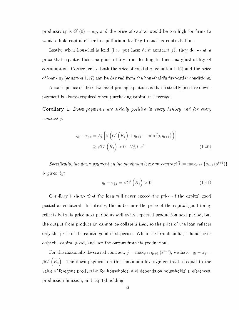
productivity is G′(0) = aU , and the price of capital would be too high for �rms to

want to hold capital either in equilibrium, leading to another contradiction.

Lastly, when households lend (i.e. purchase debt contract j), they do so at a

price that equates their marginal utility from lending to their marginal utility of

consumption. Consequently, both the price of capital q (equation 1.16) and the price

of loans πj (equation 1.17) can be derived from the household's �rst-order conditions.

A consequence of these two asset pricing equations is that a strictly positive down-

payment is always required when purchasing capital on leverage.

Corollary 1. Down-payments are strictly positive in every history and for every

contract j:

qt − πj,t = Et

[β(G′(Kt

)+ qt+1 −min {j, qt+1}

)]≥ βG′

(Kt

)> 0 ∀j, t, st (1.40)

Speci�cally, the down-payment on the maximum leverage contract j := maxst+1 {qt+1 (st+1)}

is given by:

qt − πj,t = βG′(Kt

)> 0 (1.41)

Corollary 1 shows that the loan will never exceed the price of the capital good

posted as collateral. Intuitively, this is because the price of the capital good today

re�ects both its price next period as well as its expected production next period, but

the output from production cannot be collateralized, so the price of the loan re�ects

only the price of the capital good next period. When the �rm defaults, it hands over

only the capital good, and not the output from its production.

For the maximally leveraged contract, j = maxst+1 qt+1 (st+1), we have: qt − πj =

βG′(Kt

). The down-payment on this maximum leverage contract is equal to the

value of foregone production for households, and depends on households' preferences,

production function, and capital holding.

56

Optimal Leverasge for Firms (Proof for Lemma 3)

The �rst part of Lemma 3 states that we can restrict attention to j ∈ J =[j, j].

Recall j := minst+1 (qt (st+1)) is the max-min leverage contract. When the �rm is

borrowing using contract j, it is promising to repay an amount equal to the lowest

possible price of the collateral next period. Since delivery on contract j is given by

δj,t+1 = min{j, qt+1

}= j, the contract is risk-free and will be priced at πj,t = βj with

implied interest rate 1 + rj,t :=j

πj,t= 1

β. Selling any other debt contracts j < j will

also incur the same risk-free interest rate but raise a lower amount of funds at time

t: πj,t = βj < πj,t ∀j < j. Since every contract j must be backed by one unit of

collateral, the �rm will always choose j over any j < j when the collateral constraint

is binding.

Suppose instead the �rm is borrowing using contract j := maxst+1 (qt (st+1)). This

is the maximum leverage contract, because with any promise j > j the �rm will

always default and the promise is no longer credible. Consequently any contract

j > j generates the same expected delivery as j and will be priced identically. It is

therefore possible to restrict attention to j ≤ j without loss of generality.

The second and third part of Lemma 3 state that if the �rm's marginal utility of

income is high today relative to tomorrow in the Up-state, then the �rm will choose

the maximum leverage contract; and conversely the max-min leverage contract if the

inequality is reversed. To see this formally, note that for j ∈ J =[j, j]and λt > 0:

λtγt

= maxj∈J

{Et

[(βγt+1

γt− βγt+1

γt

)δj,t+1

]}

= maxj∈J

{p

(βγUt+1

γt−βγUt+1

γt

)j + (1− p)

(βγDt+1

γt−βγDt+1

γt

)qDt+1

}(1.42)

57

so collateral value is maximized for jt = jt whenβγUt+1

γt>

βγUt+1

γt; and for jt = j

twhen

the inequality is reversed. Setting β = β and γt = γUt+1 = 1 simpli�es the condition

to γt > γUt+1 ⇒ j∗t = jt as required.

Deterministic Steady States

There are two possible deterministic steady states. One where the �rm's productivity

is known to be aU permanently, and another where it is aD permanently. Let's denote

these two steady states by U∞ and D∞ respectively.

In the Up-steady-state U∞, the �rm will consume and hold the entire stock of

capital (as per the �rst-best benchmark). In the absence of uncertainty, there is only

one risk-free collateralized debt contract available to trade (with promised repayment

j = j = qU∞) and �rms are indi�erent between purchasing the capital with and

without leverage. In the following lemma, I summarize the equilibrium outcomes in

U∞ when the �rm purchases capital on leverage.

Lemma 6. [The Up-steady-state] In the deterministic steady state U∞ where a =

aU , prices and allocations in the collateral equilibrium are given by:

1. Capital and contract prices: qU∞ = β1−βaU ; πj=qU∞ = βqU∞

2. Capital holdings: KU∞ = Kfb = G′−1 (aU); KU∞ = K − KU∞

3. Contract trades: ϕj=qU∞ = KU∞ = −ϕj=qU∞

4. Consumption: xU∞ = eU∞ +G(KU∞

)+ βaUKU∞; xU∞ = (1− β) aUKU∞

In the Down-steady-state D∞, the household will end up holding the entire stock

of capital. The �rms that are shown to be permanently unproductive exit the market.

Lemma 7. [The Down-steady-state] In the deterministic steady state D∞ where

a = aD, prices and allocations in the collateral equilibrium are given by:

58

1. Capital and contract prices: qD∞ = β1−βaD; πj=qD∞ = βqD∞

2. Capital holdings: KD∞ = K; KD∞ = 0

3. Contract trades: ϕj=qD∞ = 0 = −ϕj=qD∞

4. Consumption: xD∞ = eD∞ + aD; xD∞ = 0

I omit proofs for Lemma 6 and 7 as they can both be readily derived from the

relevant �rst-order conditions.

It is also clear that neither steady states will be reached immediately upon the res-

olution of uncertainty in the model. Even when the �rm is known to be permanently

productive at time t, (at+τ = aU ∀τ ≥ 0), in general the �rm might not have enough

liquid wealth to purchase KU∞ and consume xU∞ . A period of transition is required

whereby the �rm gradually builds up its liquid wealth and capital stock towards the

steady state. During this transition towards deterministic Up-steady-state U∞, it is

possible to show that the �rm will use leverage in order to accumulate capital faster.

The transition to the Down-steady-state D∞ is straight-forward. Once the �rm is

known to be permanently unproductive at history s2 = DD, the �rm will exit the

market by handing over any collateral, liquidating its remaining capital stock, and

consuming the entirety of its net worth. The deterministic steady state D∞ will then

be reached immediately in the following period.

Proof of proposition 1 [Productive ine�ciency and leverage during the

downturn]

For the �rst part of Proposition 1 I show that �rms will not begin history s1 = D

with enough liquid wealth to purchase the �rst-best benchmark level of capital KfbD

given equilibrium prices for capital and debt contracts.

1. Suppose to the contrary that KD ≥ KfbD , then �rm's liquid wealth at history

D must be high enough to at least purchase KfbD using the maximum leverage

59

debt contract j = qDU (since the maximum leverage contract demands the

lowest down-payment):

wD ≥(qD − πD,j

)KfbD

= βG′(KfbD

)KfbD given corollary 1

= βE [a]KfbD by de�nition of Kfb

D (eqn 1.13)

> βaDKfbD

2. If the �rm used any leverage debt contracts in period 0 (j ∈ J = [qD, qU ]), then

during the downturn it will surrender the collateral posted and retain only the

products of its capital holding, so wD = aDK0. For the �rm to be able to a�ord

KfbD in history D, we must have:

K0 ≥ βKfbD

= βKfb0 by de�nition of Kfb

t (eqn 1.13)

However this level of capital holding in period 0 cannot be achieved given the

�rm's starting endowment even if it used maximum leverage in period 0:

K0 ≤e0(

q0 − π0,j

) =e0

βG′(K0

) given corollary 1

≤ e0

βaDby assumption A3.2

<β2aDK

fb0

βaD= βKfb

0 by assumption A4.2

So we reach a contradiction K0 < βKfb0 ≤ K0.

3. Suppose instead the �rm purchased capital without leverage in period 0. Then

wD = (aD + qD)K0, where K0 is bounded above by K0 ≤ e0q0

<β2aDK

fb0

q0.

60

Consequently for �rm to purchase at least KfbD in history D we need:

(aD + qD)β2aDK

fb0

q0

≥ wD > βaDKfbD

⇔ β (aD + qD)

q0

> 1

but if β(aD+qD)q0

> 1 then the household would also want to purchase more

capital instead of consuming, leading to a contradiction with respect to Lemma

1. Intuitively, for the �rm to transfer enough resources into state D to purchase

KfbD without using leverage in period 0, the price of capital in the downturn qD

must be su�ciently high relative to the initial price q0. But in such situations,

the household would also like to purchase more capital in period 0, which would

push q0 beyond the level required for the �rm.

To prove the second part of Proposition 1, I show that when �rms hold less capi-

tal than under the �rst-best benchmark, they will prefer to purchase capital using

leverage than without leverage.

Lemma 8. If Kt (st) < Kfbt (st), then

∑j∈J(st) max {ϕt,j (st) , 0} = Kt (st), ∀t ≥ 0

and ∀st ∈ St.

Proof. It is su�cient to show that the maximum leverage contract jt is preferable to

purchasing capital without leverage, when Kt < Kfbt . The expected rate of return

from buying capital with contract j at time t is given by:

γt,j :=Et [βγt+1 (at+1)]

qt − βEt [qt+1]

=βEt [γt+1at+1]

βG′(Kt

) by corollary 1

=Et [γt+1at+1]

G′(Kt

)61

The expected rate of return from buying capital without leverage is given by:

γt,no :=Et [βγt+1 (at+1 + qt+1)]

β[G′(Kt

)+ E [qt+1]

]=Et [γt+1at+1] + Et [γt+1qt+1]

G′(Kt

)+ Et [qt+1]

Since ab> a+c

b+d⇔ a

b> c

d∀a, b, c, d > 0, we have γt,j > γt,no if and only if Et[γt+1at+1]

G′(K)>

Et[γt+1qt+1]Et[qt+1]

. Furthermore, since Kt < Kfbt ⇔ Kt > Kfb

t , we know G′(K)< E [at+1]

and Et[γt+1at+1]

G′(K)> Et[γt+1at+1]

E[at+1]≥ Et[γt+1at+1]

Et[at+1]. Therefore a su�cient condition for γt,j >

γt,no is:

Et [γt+1at+1]

Et [at+1]≡pγUt+1aU + (1− p) γDt+1aD

paU + (1− p) aD

≥Et [γt+1qt+1]

Et [qt+1]≡pγUt+1q

Ut+1 + (1− p) γDt+1q

Dt+1

pqUt+1 + (1− p) qDt+1

With a little algebra we can show that the su�cient condition captured in the

inequality above is equivalent to:

aUaD≥qUt+1

qDt+1

Since the price of capital is always given by households' asset pricing equation, it

is bounded above and below by its value in the deterministic Up and Down steady

states respectively qt ∈[

β1−βaD,

β1−βaU

], ∀t ≥ 0,∀st ∈ St. Therefore we have

aUaD≥qUt+1

qDt+1

⇒ γt,j > γt,no

as required.

Lemma 8 concludes the proof for Proposition 1. In summary, during the downturn,

�rms hold too little capital relative to the �rst-best benchmark. Consequently they are

62

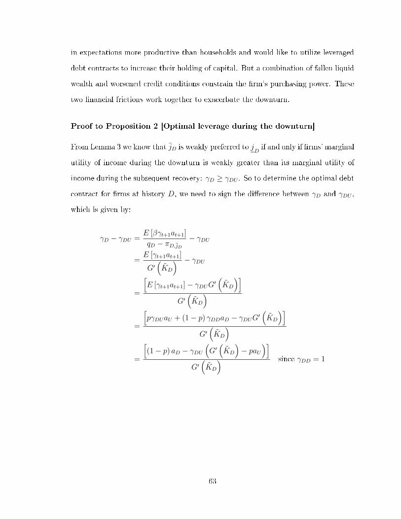
in expectations more productive than households and would like to utilize leveraged

debt contracts to increase their holding of capital. But a combination of fallen liquid

wealth and worsened credit conditions constrain the �rm's purchasing power. These

two �nancial frictions work together to exacerbate the downturn.

Proof to Proposition 2 [Optimal leverage during the downturn]

From Lemma 3 we know that jD is weakly preferred to jDif and only if �rms' marginal

utility of income during the downturn is weakly greater than its marginal utility of

income during the subsequent recovery: γD ≥ γDU . So to determine the optimal debt

contract for �rms at history D, we need to sign the di�erence between γD and γDU ,

which is given by:

γD − γDU =E [βγt+1at+1]

qD − πD,jD− γDU

=E [γt+1at+1]

G′(KD

) − γDU

=

[E [γt+1at+1]− γDUG′

(KD

)]G′(KD

)=

[pγDUaU + (1− p) γDDaD − γDUG′

(KD

)]G′(KD

)=

[(1− p) aD − γDU

(G′(KD

)− paU

)]G′(KD

) since γDD = 1

63

First, when KD = KfbD (and KD = Kfb

D ), we have γD − γDU ≤ 0:

γD − γDU =

[(1− p) aD − γDU

(G′(KfbD

)− paU

)]G′(KD

)≤

[(1− p) aD −

(G′(KfbD

)− paU

)]G′(KD

) since γDU ≥ 1

=[(1− p) aD − (1− p) aD]

G′(KD

) since G′(KfbD

)= E [a]

= 0

Second, when KD = 0 (and KD = 1), we have γD − γDU > 0

γD − γDU =[(1− p) aD − γDU (G′ (1)− paU)]

G′(KD

)=

[(1− p) aD − γDU (aD − paU)]

G′(KD

)> 0 since p ≥ aD

aUby assumption A3.1

Since G ∈ C2, by the intermediate value theorem ∃KD ∈ (0, KfbD ] s.t. γD−γDU = 0

and the �rm is indi�erent between the maximum leverage contract and the max-min

leverage contract. This concludes the proof.

Proof of proposition 3 [Unanticipated Intervention at D]

When �rms �nd it optimal to use the maximum leverage contract j∗D = jD, they will

purchase as much capital as they can with their available liquid wealth wD. So �rms'

capital holding is given by KD = wDqD−πjD=qDU

< KfbD (inequality by Proposition 1).

Suppose the central bank subsidizes the maximum leverage contract jD. This will

allow the �rms to hold a larger stock of capital in equilibrium, and the equilibrium

price for capital will rise both immediately and in any ensuing recovery period: qCBD >

64

qD and qCBDU > qDU . The required level of subsidy to achieve the �rst-best benchmark

level of capital holding by �rms is thus given by:

KfbD =

wD

qCBD −(

1 + χ∗jD=qCBDU

)πjD=qCBDU

=:wD

qCBD − πCBjD=qCBDU

(1.43)

It remains to show that this subsidized loan entails a positive interest rate πCBjD=qCBDU

≤

qCBDU , which follows immediately given KfbD > 0, wD > 0 and qCBDU ≥ qCBD . The

last condition qCBDU ≥ qCBD claims that the price of capital will be (weakly) higher

during the recovery (history DU) than during the downturn (history D). This

is equivalent to showing that �rms will hold a higher proportion of capital in the

recovery: KDU > KfbD . We do this in two steps. First, observe that in history DU the

uncertainty surrounding �rms' productivity has been fully resolved and the economy is

transitioning towards the Up-steady-state. Second, �rms use leveraged debt contracts

along the transition path to build up capital faster14 so KDU = wDUqDU−πj=qDUU

=

aUKfbD

βG′(KDU)≥ aUK

fbD

βaU= 1

βKfbD > Kfb

D as required.

For the second part of the proposition, suppose the central bank subsidizes the

max-min leverage contract jD. The equilibrium price for capital will be (weakly)

higher during the downturn: qCBD≥ qD; and remains unchanged if the productivity

shock turns out to be permanent and the households hold the entire stock of capital:

qCBDD = qDD. The required level of subsidy to achieve the �rst-best benchmark

14Note that all debt contracts along the transition path are riskless because all uncertainty hasalready been resolved.

65

becomes:

KfbD =

wD

qCBD−(

1 + χ∗jD

=qDD

)πj

D=qDD

=:wD

qCBD− πCBj

D=qDD

(1.44)

Consequently, for su�ciently low wD and su�ciently large gap in the price of capital

between periods qCBD− qDD, both of which depend in part on the speci�cations of the

initial endowment for �rms e0 and on the household's production function G (·), the

size of the central bank loan required to achieve the �rst-best outcome may exceed

the promised value of repayment: πCBjD

=qDD> qDD, thus violating the e�ective-lower-

bound condition.

Proof to Proposition 4 [The Announcement E�ect]

When the central bank optimally provides credit support in history DU , χ∗jDU=qDUU>

0, we know that the �rms' capital holding at DU is raised to the �rst-best benchmark

KfbDU . Consequently, the price of capital rises relative to the scenario where the central

bank is only expected to intervene at D: qAnDU > qCBDU . The price of capital at history

DD remains unchanged: qAnDD = qCBDD because the �rms will always default and the

households hold the entire stock of capital at DD. Higher capital prices during the

recovery eases credit conditions in the private market at history D. For the maximum

leverage contract: πjD=qAnDU> πjD=qCBDU

, so the �rms can secure a larger loan against

the same unit of capital. The improved access to credit leads to an immediate increase

in capital prices: qAnD > qCBD . With and without the announcement, the central bank

will set subsidy, χAnD and χCBjD respectively, such that �rms hold the �rst-best level of

66

capital at history D:

qCBD −(1 + χ∗jD

)πjD=qCBDU

=wD

KfbD

= qAnD −(1 + χAnjD

)πjD=qAnDU

⇔ qAnD − qCBD =(1 + χAnjD

)πjD=qAnDU

−(1 + χ∗jD

)πjD=qCBDU

> 0 (1.45)

where wD = aDK0 because the �rm used leverage at history 0.

Since agents' capital holdings are unchanged, from households' asset pricing equa-

tions (see equation 1.41) we know that the net down-payment required on the private

market for maximum leverage contracts also remains unchanged, despite the changes

in the price of capital and the size of the loan:

qCBD − πjD=qCBDU= βG

′(KfbD

)= qAnD − πjD=qAnDU

(1.46)

With a little algebra, combining equations 1.45 and 1.46 above yields:χAnjD

χ∗jD

=πjD=qCB

DU

πjD=qAn

DU

<

1 as required.

To see why the balancing tax transfers become a mean-preserving spread, note

that:

E[T2|χ∗jD

]− E

[T2|χAnjD

]=

{1

β

(1 + χ∗jD

)πjD=qCBDU

− E[qCB2

]}−{

1

β

(1 + χAnjD

)πjD=qFGDU

− E[qAn2

]}=

1

β

{(1 + χ∗jD

)πjD=qCBDU

−(1 + χAnjD

)πjD=qAnDU

}+{E[qAn2 − qCB2

]}=− 1

β

{qAnD − qCBD

}+{E[qAn2 − qCB2

]}=− 1

β

{βE[G′(KfbD

)+ qAn2

]− βE

[G′(KfbD

)+ qCB2

]}+{E[qAn2 − qCB2

]}=0

67

Lastly, identical liquidation value qADDD = qCBDD at history DD but larger public

liability given announcement 1β

(1 + χADjD

)πjD=qANDU

> 1β

(1 + χ∗jD

)πjD=qCBDU

means a

larger shortfall at DD: TDD|χAN > TDD|χ∗jD ; and correspondingly a larger windfall

at DU .

68

2 The Collateral Rule - Theory for the Credit De-

fault Swap Market15

2.1 Introduction

The empirical results in Capponi et al. (2020) demonstrate that extreme tail risk

measures have a higher explanatory power for observed collateral requirements than

the standard Value-at-Risk rule. This �nding lends support to models where the

collateral rule is determined endogenously, like Fostel and Geanakoplos (2015). A

key prediction of Fostel and Geanakoplos (2015) is that in a binomial economy (i.e.

when there are two states of nature only), any collateral equilibrium is equivalent to

one in which there is no default - that is, where collateral covers the most extreme

losses. But linking the empirical results on the CDS market to this model faces two

main limitations: (1) the conclusions only hold if there are two states of nature; and

(2) defaults on CDS obligation, although rare, do arise in practice.

We develop a new model of endogenous collateral that is speci�cally suited for the

CDS market: it features a continuum of states (as opposed to just two), and non-zero

default probability in equilibrium. Trade in this model occurs because of di�erences

in beliefs. The model presented in this paper is a natural adaptation of Simsek

(2013), where belief disagreements are central to asset prices and endogenous margin

requirements. But unlike Simsek (2013) who considers standard debt contracts and

short selling, our model is specialized to an economy where the only contracts available

for trading are state contingent promises (CDSs) backed by risk-free collateral (cash).

Thus the model presented here is not a nested version of Simsek (2013), but an

extension of the framework to the CDS market.

In our model, optimists naturally sell insurance (CDS protection) to pessimists,

and pessimists require that the sellers post collateral (in the form of cash). The

15This is joint work with Agostino Capponi and Stefano Giglio.

69

amount of cash required to collateralize the CDS contract (the collateralization rate)

arises endogenously in the model. we show that what matters for the level of collat-

eralization is not the extent of the disagreement between market participants per se,

but the nature of their disagreement. In particular, when the optimists becomes more

optimistic, the level of collateralization falls; but when the pessimists attach a larger

weight to negative tail events, the level of collateralization rises. In both cases the

level of disagreement between participants widened, but the change in the collateral

requirement went in opposite directions.

Most importantly, the model can generate the high margin requirements and low

default probabilities we observe in the data, when the clearing house (i.e. the pessimist

in the model) places a greater emphasis on extreme tail risks. Moreover, whilst the

collateral requirement that arises in such an equilibrium may be viewed as onerous by

the clearing members (the optimist in the model), it may nevertheless not be enough

to fully prevent default when viewed from the clearinghouse's perspective.

2.2 Model Setup

Consider an economy with two periods t = {0, 1} and two risk-neutral agents: one

optimist and one pessimist. All agents trade in period t = 0 and consume in period

t = 1. Uncertainty is captured by a continuum of states s ∈ S = [smin, smax] realized

in period t = 1, with smin normalized to zero for simplicity. The pessimist, denoted by

i = 0, holds prior beliefs over S given by the distribution F0 and corresponding density

f0. The optimist, denoted by i = 1, has prior beliefs characterized by the distribution

F1 and density f1. The optimist has a higher expectation than the pessimist on the

state in period 1, i.e., E1 [s] > E0 [s]. These prior beliefs are common knowledge for

all agents.

At the start of period t = 0, each agent i = {0, 1} is endowed with ni units of

the numeraire consumption good which can be safely stored without depreciation for

70

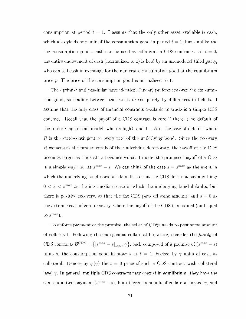
consumption at period t = 1. I assume that the only other asset available is cash,

which also yields one unit of the consumption good in period t = 1, but - unlike the

the consumption good - cash can be used as collateral in CDS contracts. At t = 0,

the entire endowment of cash (normalized to 1) is held by an un-modeled third party,

who can sell cash in exchange for the numeraire consumption good at the equilibrium

price p. The price of the consumption good is normalized to 1.

The optimist and pessimist have identical (linear) preferences over the consump-

tion good, so trading between the two is driven purely by di�erences in beliefs. I

assume that the only class of �nancial contracts available to trade is a simple CDS

contract. Recall that the payo� of a CDS contract is zero if there is no default of

the underlying (in our model, when s high), and 1− R in the case of default, where

R is the state-contingent recovery rate of the underlying bond. Since the recovery

R worsens as the fundamentals of the underlying deteriorate, the payo� of the CDS

becomes larger as the state s becomes worse. I model the promised payo� of a CDS

in a simple way, i.e., as smax − s. We can think of the case s = smax as the event in

which the underlying bond does not default, so that the CDS does not pay anything;

0 < s < smax as the intermediate case in which the underlying bond defaults, but

there is positive recovery, so that the the CDS pays o� some amount; and s = 0 as

the extreme case of zero recovery, where the payo� of the CDS is maximal (and equal

to smax).

To enforce payment of the promise, the seller of CDSs needs to post some amount

of collateral. Following the endogenous collateral literature, consider the family of

CDS contracts BCDS ={

[smax − s]s∈S , γ}, each composed of a promise of (smax − s)

units of the consumption good in state s at t = 1, backed by γ units of cash as

collateral. Denote by q (γ) the t = 0 price of such a CDS contract with collateral

level γ. In general, multiple CDS contracts may coexist in equilibrium: they have the

same promised payment (smax− s), but di�erent amounts of collateral posted γ, and

71

� as a consequence � trade for di�erent prices q(γ). Thus we can index the di�erent

CDS contracts in BCDS by γ.

Since the promised payment on a CDS contract is enforceable only through the

potential of seizing the collateral, the actual delivery on each contract in state s is

given by the minimum of the promised payment and the value of the collateral in

that state: δ (s, γ) := min {smax − s, γ}. In other words, in any state s such that

smax − s > γ, the seller of the CDS contract would default on her promise, and the

buyer would only receive the value of the collateral γ.

Denote by µ+i , µ

−i , respectively, agent i's long and short positions on CDS contracts

(where a long position means that the agent has purchased the corresponding CDS

contract). Let ai ∈ R+ denote agent i's holding of the numeraire consumption good;

and ci ∈ R+ be her cash holdings. Then agent i's budget constraint can be written

as:

ai + pci +

∫γ∈BCDS

q (γ) dµ+i ≤ ni +

∫γ∈BCDS

q (γ) dµ−i , (2.1)

where the left hand side represents the total value of the agent's portfolio, comprised

of her holding of the numeraire good ai, the value of her cash holding pci and her

long-position in CDS contracts∫γ∈BCDS q (γ) dµ+

i . The right hand side represents the

total value of the funding available to the agent, comprising of her endowment of

the consumption good ni and the amount she can raise by shorting CDS contracts,∫γ∈BCDS q (γ) dµ−i . If an agent i has a short position on the CDS contracts, then she

is also subject to the collateral constraint:

∫γ∈BCDS

γdµ−i ≤ ci, (2.2)

which means that agent i must have su�cient cash holdings to satisfy the collateral

requirements for the CDS contracts sold. In contrast, the purchaser of the CDS

contracts (the party who is long) is not subject to any collateral requirements.

72

The optimization problem for each agent i is given by:

max(ai,ci,µ+

i ,µ−i )∈R4

+

ai + ci + Ei

[∫γ

min {smax − s, γ} dµ+i

]− Ei

[∫γ

min {smax − s, γ} dµ−i]

(2.3)

subject to the budget constraint (2.1) and the collateral constraint (2.2).

De�nition 1. A collateral equilibrium is a set of portfolio choices(ai, ci, µ

+i , µ

−i

)i∈{0,1}

and a set of prices (p ∈ R+, q : γ → R+) such that the portfolio choices solve the

optimization problem (2.3) of each agent i ∈ {0, 1}; and the prices are such that

the market for cash clears∑

i∈{0,1} ci = 1, and the CDS markets clear∑

i∈{0,1} µ+i =∑

i∈{0,1} µ−i .

We will show that although the entire family of CDS contracts will be priced, only

one contract will be traded in equilibrium. This result is line with the literature on

collateral equilibrium (Fostel and Geanakoplos (2015); Simsek (2013)). Furthermore,

the collateral level γ of the actively traded CDS contract, and the price of cash p, will

be determined endogenously. The equilibrium level of collateral requirement γ will

depend on the nature of belief di�erences between the optimist and the pessimist.

2.3 Existence and Uniqueness of the Collateral Equilibrium

Following the approach in Simsek (2013), it is possible to show that (under suitable

assumptions over initial endowments and beliefs) the collateral equilibrium exists, is

unique, and is equivalent to a principal-agent equilibrium where the optimist chooses

her cash holdings and the optimal CDS contract to sell, subject to the pessimist's

participation constraint. To this end, we impose the following assumptions on initial

endowments and prior beliefs, that parallel similar assumptions in Simsek (2013):

73

Assumption A1: [Restriction on Initial Endowments]

n1 <E1 [s]

smax(2.4)

and n0 >E0 [smax − s]E1 [smax − s]

− n1 (2.5)

The �rst inequality ensures that the optimist's initial endowment is not large

enough to purchase the entire supply of cash in the economy with her own

resources alone (that is, she will need to raise some more of the numeraire con-

sumption good by selling CDS contracts).16 The second inequality ensures that

the initial endowment of the pessimist (n0) is large enough that the pessimist

will always have some residual consumption after paying for the CDS.17

Since the pessimist is risk neutral, this implies that her expected return on any CDS

contracts purchased must also be equal to 1 in equilibrium. Thus the equilibrium

price of a CDS contract with collateral γ must be given by:

q (γ) = E0 [min (smax − s, γ)] . (2.6)

This pricing equation serves as a convenient characterization of the pessimist's par-

ticipation constraint.

We can now formulate the optimist's problem as choosing the level of cash holdings

c1, and the CDS contract γ to sell, so as to maximize the expected payo�s, subject

to the pessimist's participation constraint of achieving an expected return of 1 on the

16For a more detailed discussion of this, see Appendix 2.7.17More speci�cally, this inequality implies that the sum of the endowments needs to be greater

than the maximum price cash can take in equilibrium (which I will show is bounded from above by(E0[smax−s]E1[smax−s]

)).

74

CDS contract sold:

max(c1,γ)∈R2

+

c1 −c1

γE1 [min {smax − s, γ}] (2.7)

s.t. pc1 = n1 +c1

γE0 [min {smax − s, γ}]

This leads us to de�ne the principal-agent equilibrium as follows:

De�nition 2. A principal-agent equilibrium is a pair of optimist's portfolio choices

(c∗1, γ∗) and price for cash (p∗) such that the optimist's portfolio solves her optimiza-

tion problem (2.7), and the market for cash clears: c∗1 = 1.

In order to show equivalence between the principal-agent equilibrium outlined here

and the collateral equilibrium de�ned previously, further restrictions on the nature of

belief di�erences are required:

Assumption A2: [Restrictions on Prior Beliefs] The probability densities of

the optimist's and the pessimist's beliefs satisfy the monotone likelihood ratio

property:

f1 (s1)

f0 (s1)>f1 (s0)

f0 (s0)for every s1 > s0 (2.8)

Note that this assumption implies: (1) �rst-order stochastic dominance: F1 (s) <

F0 (s),∀s ∈ (smin, smax); (2) monotone hazard rate: f1(s)1−F1(s)

< f0

1−F1(s),∀s ∈

(smin, smax); and (3) f0(s)F0(s)

< f1(s)F1(s)

∀s ∈ (smin, smax) (which in turn implies

ddsF0(s)F1(s)

< 0).

We can then prove the following Proposition:

Proposition 6. [Existence, Uniqueness, and Equivalence of Equilibria] Un-

der Assumptions A1 and A2:

1. There exists a unique principal-agent equilibrium (p∗, (c∗1, γ∗)) s.t. p∗ > 1.

75

2. There exists a collateral general equilibrium,(ai, ci, µ

+i , µ

−i

)i∈{0,1}, whereby the

optimist sells CDS to the pessimist (i.e. µ+1 = µ−0 = 0), and only a single CDS

contract is actively traded (i.e. µ+0 is a measure that puts weight only at one

contract γ ∈ BCDS). This collateral equilibrium is unique in the sense that

the price of cash p and the price of the traded CDS contract q (γ) are uniquely

determined.

3. The collateral equilibrium and the principal-agent equilibrium are equivalent:

p = p∗, c1 = c∗1, γ = γ∗

and q (γ) = E0 [min (smax − s, γ∗)]

The detailed proof is reported in the Appendix. Intuitively, because under assumption

A1 the pessimist will hold a surplus of the consumption good in equilibrium (he has

a larger endowment than what the optimist would want to borrow), he must be

indi�erent between holding the consumption good (with a sure return of 1) and

holding the CDS sold by the optimist. Hence, the optimist e�ectively holds all

the bargaining power when deciding which CDS they should trade, and will only

trade in the contract that maximizes the optimist's expected return. Assumption A2

provides the su�cient conditions for there to exist a unique contract γ∗ that solves

the optimist's principal agent problem.

2.4 Characterizing the Equilibrium

In this section, we show that in equilibrium the optimist will wish to sell CDS contracts

to the pessimist (so as to bet on the events she thinks are more likely). But, to do so,

the optimist must �rst obtain more units of the numeraire good from the pessimist

by selling CDS contracts, in order to purchase the cash required to collateralize the

76

CDS contracts.18 Because cash is the only asset that can be used as collateral, its

equilibrium price will exceed its fundamental value (p > 1), so cash is held exclusively

by the optimist in equilibrium.

To formally characterize the equilibrium, �rst substitute c1 = n1

(p− 1γE0[min{smax−s,γ}])

from the optimist's constraint into his objective function. This reduces the dimension

of the problem by one, and allows us to restrict attention to choosing only the optimal

contract γ. The resulting �rst order condition characterizes the optimal contract

choice for given p:

Proposition 7. Under assumptions A1 and A2, and �xing a price for cash p, the

optimal CDS contract, s, with respect to the optimist's problem (2.7) is given by the

unique solution to:

p = F0 (smax − s) + (1− F0 (smax − s)) E0 [smax − s|s ≥ smax − s]E1 [smax − s|s ≥ smax − s]

=: popt (s) (2.9)

Inverting popt (s) gives the optimal CDS contract s for the optimist, for given price

of cash p. This �rst order condition e�ectively determines how much collateralization

the optimist (seller) chooses for the CDS contract, since the states s ≤ smax−s are the

ones where the optimist is defaulting on the promise of delivering the CDS payment

and is instead relinquishing the collateral. Once the equilibrium price of cash p∗ is

known (see Eq. (2.11) below), we can use Eq. (2.9) to derive the equilibrium level of

collateral γ∗ by setting p∗ = popt (γ∗).

Equation (2.9) also implies that the price of cash is composed of two parts: (a)

the pessimist's assessment of the probability of default on the CDS: (F0 (smax − s)),

multiplied by the pessimist's valuation of cash in the default state (1); plus (b) the

pessimist's assessment of the probability of the no-default state, multiplied by the

value of cash to the optimist in the non-default state (each unit of cash allowed the

18This mechanism is analogous to a mortgage contract, where the borrower is raising funds fromthe lender in order to purchase the collateral (i.e. the house) required to back the mortgage.

77

optimist to borrow 1sE0 [smax − s|s ≥ smax − s] from the pessimist, with an expected

actual delivery of 1sE1 [smax − s|s ≥ smax − s]). Given the di�erences in beliefs, the

optimist expects to deliver less than what the pessimist envisages on the CDS con-

tract: E0[smax−s|s≥smax−s]E1[smax−s|s≥smax−s] ≥ 1. Hence, p ≥ 1, i.e., cash generates collateral value.

Consistent with the �Asymmetric Disciplining of Optimism� result in Simsek (2013),

the pessimist's beliefs are used in assigning weights to the default and non-default

states. The belief of the optimist enters only in determining the value of collateral in

the non-default state.

Further, we show in the proof of Proposition 7 that popt (s) is an increasing function

of s. To see this intuitively, denote the optimist's perceived interest rate on (borrowing

through selling) the CDS contract as

1 + rper1 (s) :=E1 [min {smax − s, s}]E0 [min {smax − s, s}]

(2.10)

Under assumption A2, it can be shown that the perceived interest is decreasing in

s (d(1+rper1 (s))

ds< 0). In other words, given the nature of belief di�erences, o�ering a

CDS contract with higher margin requirements is more attractive for the optimist.

Thus the higher the margins s posted, the greater the discrepancy between expected

deliveries becomes, and the more attractive selling the CDS is to the optimist. Thus,

increasing s increases the collateral value of cash.

To close the model, we impose the market clearing condition for cash. The budget

constraint in equation (2.7) implies that the optimist's demand for cash is given by:

c1 =n1

p− 1sE0 [min {smax − s, s}]

Since the supply of cash is normalized to 1, we have:

p = n1 +1

sE0 [min {smax − s, s}] =: pmc (s) (2.11)

78

We show that pmc (s) is a decreasing function of s,19 with boundary conditions

pmc (smin) > popt (smin) and pmc (smax) < popt (smax). Hence, the unique intersection

between popt (s) and pmc (s) pins down the equilibrium price for cash p∗ and margin

requirement γ∗.

Proposition 8. Under assumptions A1 and A2, there is a unique principal-agent

equilibrium (c∗1, γ∗, p∗) characterized by:

c∗1 = 1

p∗ = pmc (γ∗) = popt (γ∗)

where popt (·) and pmc (·) are respectively de�ned in equations (2.9) and (2.11).

Proof. See appendix.

2.5 Comparative Statics and Illustrative Example

We present a simple numerical example to illustrate the collateral equilibrium and

perform comparative statics, before presenting the more general results as proposi-

tions.

Suppose that the starting endowments of the numeraire consumption good are

n0 = 3 and n1 = 0.5 for the pessimist and the optimist respectively. Let the set of

states and the prior beliefs be given by: S = [0, 1] and

F0 (s) = s12 ∀s ∈ S (2.12)

F1 (s) = s3 ∀s ∈ S (2.13)

19pmc (s) is downward sloping because 1sE0 [min {smax − s, s}] is decreasing in s. Intuitively,

even though a CDS contract with higher margin requirements demands a higher price (i.e.E0 [min {smax − s, s}] is increasing in s), the need to post more margins reduces the number of suchcontracts the optimist can sell with a single unit of cash as collateral. The overall e�ect is that postingmore margins reduces the total amount that the optimist can borrow, 1

sE0 [min {smax − s, s}], andthis reduction in the purchasing power of optimists reduces the market clearing price of cash.

79

Panel A of Figure 2.1 plots the upward sloping cash price schedule {popt (s)}s∈[0,smax]

(equation (2.9)), and the downward sloping cash price schedule {pmc (s)}s∈[0,smax]

schedule (equation (2.11)), the intersection of which characterizes the equilibrium

price of cash p∗ and the equilibrium margin requirement γ∗.

Suppose instead that the optimist becomes less optimistic, such that:

F1 (s) = s32 ∀s ∈ S

Then we can see from equation (2.9) that the decreased optimism of the optimist

shifts the popt (s) schedule downwards and leaves the pmc (s) schedule untouched. The

resulting equilibrium, as illustrated in panel B of Figure 2.1, is comprised of a lower

price for cash p∗ and higher margin requirements γ∗.

We generalize this intuition in the following general proposition:

Proposition 9. [Change in optimist's beliefs] Suppose that the optimist's beliefs

becomes 'less optimistic' in the sense that it changes from F1 to F1, s.t. the monotone

likelihood ratio condition is satis�ed: f1(s1)

f1(s1)> f1(s0)

f1(s0)for every s0, s1 ∈ [smin, smax] and

s1 > s0 . Then the equilibrium level of collateral (γ∗) increases, and the equilibrium

collateral value (p∗) falls. Conversely, when the optimist's beliefs becomes 'more

optimistic' s.t. f1(s1)

f1(s1)< f1(s0)

f1(s0)for every s0, s1 ∈ [smin, smax] and s1 > s0 , then the

equilibrium level of collateral falls and the equilibrium collateral value rises.

Proof. See appendix.

While the changes in the optimist's beliefs lead to unambiguous changes in the

equilibrium, the same is not true for the pessimist's beliefs. Since the pessimist's

beliefs feature in the cash price schedule of both the optimist (i.e, popt) and the

pessimist (i.e., pmc), a given change in the pessimist's beliefs can either increase or

decrease equilibrium collateral levels depending on the initial equilibrium. Intuitively,

when the pessimist becomes more pessimistic, she is willing to pay more for any given

80

CDS contracts (i.e. E0 [min {smax − s, s}] increases). This means that the optimist is

now both: a) able to raise more funding from selling CDS contracts; and b) willing to

pay more for each unit of collateral. The former e�ect shifts up the market clearing

schedule pmc, and the latter e�ect can push up the popt schedule. Therefore, whether

the equilibrium collateral level increases depends on the interaction of these two

e�ects. Moreover, since the popt schedule also depend on the pessimist's evaluation

of the default probability (i.e. F0 (smax − s))20, the e�ect of increased pessimism is

not always monotone along S = [0, 1]. For low levels of collateral s, the protection

o�ered may be deemed insu�cient, so the new popt schedule may be lower than before;

but for high levels of collateral, the new popt schedule might be higher. In short, the

popt schedule may pivot as well as shift in response to a change in pessimist's beliefs,

creating further ambiguity in the direction of the equilibrium collateral level γ∗.

Instead, we show that a su�cient (but not necessary) condition for the equilibrium

collateral level to increase is for the pessimist to become more concerned about the tail

risks (i.e. to place a larger weight on the default states {s ∈ S : γ < smax − s} ) such

that the probability density she attaches to all the non-default states are consistently

lower than before, i.e., f0 (s) < f0 (s) ∀s ∈ [smax − γ∗, smax].

For illustration, consider a change in pessimist's beliefs from F0 (eqn. 2.12) to F0:

F0 (s) = s14 ∀s ∈ S

Then the equilibrium collateral level and collateral value both increase (Panel C of

Figure 2.1). Note that under the speci�c beliefs outlined here, the equilibrium level

of collateral in Panel C is 0.8251, and the optimist believes default will occur with

probability 0.0053. This is consistent with our empirical �nding that extreme tail

risk measures are important in explaining the high collateral levels and low default

20Recall from equation (2.9) the popt is the weighted average of 1 and E0[smax−s|s≥smax−s]E1[smax−s|s≥smax−s]>1, with

weights F0 (smax − s) and (1− F0 (smax − s)) respectively.

81

frequencies observed in practice. We state this result more formally in the following

proposition.

Proposition 10. [Pessimist's concern for tail events]: For any given initial

equilibrium (γ∗, p∗), if the pessimist becomes �more concerned about tail events� in

the sense that her beliefs changes from F0 to F0, such that: f0 (s) < f0 (s) ∀s ∈

[smax − γ∗, smax], then the equilibrium collateral level (γ∗) increases.

Proof. See Appendix.

Finally, note that the key to high collateral requirements in the model is the

nature � rather than the degree � of the belief di�erence between the two agents.

The equilibrium level of collateral increases both when the optimist becomes more

pessimistic (which reduces the extent of the disagreement), and when the pessimist

becomes more concerned about the tail events (which increases the extent of the

disagreement). What the market participant disagree about matters more than how

much they disagree per se.

2.6 Concluding Remarks

We have shown that under suitable assumptions, a unique collateral equilibrium

exists for the trading of CDS contracts between optimists and pessimists. In this

equilibrium, the pessimist buys CDS contracts from the optimist. Since selling a CDS

requires cash as collateral, the optimist needs to secure more cash from the market. In

equilibrium, the price of cash will be higher than the value of the non-collateralizable

numeraire consumption good. This endogenous premium on cash re�ects its value as

collateral.

In the collateral equilibrium, only one CDS contract with a particular level of

collateral γ∗ will be actively traded. Default on the CDS obligations will, in general,

happen with positive probability. The level of collateral γ∗, the price of the CDS

82

contract q(γ∗), and the price of cash p∗ all depend on the belief disagreement between

the optimist and the pessimist. In particular, the higher the disagreement about the

probability of states in which counterparty defaults may occur (i.e. the left tail of the

distribution), the higher the margin requirements γ∗ in equilibrium, and the higher

the CDS price q (γ∗) the buyer is willing to pay.

The methodological framework presented here can thus generalize the key intuition

of Fostel and Geanakoplos (2015), which predicts that observed collateralization levels

might be set extremely conservatively in order to cover extreme losses in tail events.

But unlike Fostel and Geanakoplos (2015), which restricts attention to economies

with two states and the collateral equilibrium without default, the model in this paper

allows for a continuum of states, and a low but strictly positive probability of default.

Furthermore, we show that as the optimist's beliefs become 'less optimistic', or when

the pessimist becomes even more concerned about tail events, the equilibrium level

of collateralization rises, such that from the perspective of the market participants

the probability of default on CDS contracts tend to zero.

The model can therefore explain the particularly high collateral levels (γ∗) and

the low but strictly positive probability of default events that we observe in the

data (Capponi et al. (2020)). Viewed through the lens of this endogenous collateral

framework, the empirical results point to disagreement about the states of the world

in which CDS sellers would default on their obligations to the clearinghouse as the

fundamental reason why collateral levels are set so high.

83

Capponi, A., W. A. Cheng, S. Giglio, and R. Haynes (2020). The Collateral Rule :

Evidence from the Credit Default Swap Market. Working Paper .

Fostel, A. and J. D. Geanakoplos (2015). Leverage and Default in Binomial

Economies: A Complete Characterization. Econometrica 83 (6), 2191�2229.

Simsek, A. (2013). Belief Disagreements and Collateral Constraints. Economet-

rica 81 (1), 1�53.

84

2.7 Appendices

Figure 2.1: Collateral Equilibrium and Comparative Statics

Panel A illustrates the upward-sloping popt (s) schedule (eqn 2.9, blue line) and the downward-sloping pmc (s) schedule(eqn 2.11, red line) , the intersection of which gives the collateral equilibrium (γ∗, p∗). The popt (s) schedule isincreasing in the level of collateralization (s) because the pessimist is willing to pay a higher price for a bettercollateralized CDS, which in turn increases the collateral value of cash (p) for the optimist. The pmc (s) schedule isdecreasing in the level of collateralization (s) because even though each unit of a better collateralized CDS is worthmore, the scarcity of collateral implies that a fewer number of such contracts can be written and the total amount offunding the optimist can raise from the pessimist is lower. Therefore, in order for the market for collateral (i.e. cash)to clear, its equilibrium price (p) must fall as the level of collateralization increases.Panel B illustrates the case where the optimist becomes 'less optimistic': in the sense that her beliefs changes from

F1 (s) to F1 (s) wheref1(s1)

f1(s1)>

f1(s0)

f1(s0)for every s0, s1 ∈

[smin, smax

]and s1 > s0 . When the optimist becomes

more pessimistic, the popt (s) schedule shifts down to popt (s) (yellow dashed line). Intuitively, this is because as theoptimist and pessimist's beliefs converge, trading in CDSs becomes less attractive for both, so the optimist's demandfor cash (the required collateral) falls (weakly) for every level of collateralization. The resulting equilibrium is onewhere the price of cash (its collateral value) is lower and the level of collateralization is higher.Panel C illustrates the case where the pessimist becomes more concerned about the tail risks associated with thedefault states {s ∈ S : s < smax − γ∗}. Speci�cally, the pessimist's beliefs changes from F0 (s) to F0 (s), wheref0 (s) > f0 (s) ∀s ∈ [smax − γ∗, smax] . A greater concern for tail events increases the value of highly collateralizedCDS contracts, and decreases the value of less collateralized contracts, so the collateral value of cash for the optimistis higher only when it is used to back highly collateralized CDS contracts (the popt schedule pivots to popt, yellowupward-sloping dashed line). The total amount of the numeraire good the optimist can raise through selling suchCDS contracts also rises, pushing up the market clearing price for cash (thepmc schedule shifts up to pmc, purpledownward-sloping dashed line). The resulting equilibrium is one where the equilibrium level of collateralization (γ∗)is higher (see Proposition 10). Note that under the speci�c beliefs outlined in the illustrative example section of themain text, the equilibrium level of collateral in Panel C is 0.8251, and the optimist believes default will occur withprobability 0.0053.

85

A. Additional discussion of the assumptions

We discuss here in greater detail some of the assumptions in the model. The �rst

inequality (2.4) states that the optimist's initial endowment is not large enough to

purchase the entire supply of cash by issuing only fully collateralized CDS contracts.

To see this, note that the value of one unit of cash to the optimist when selling

contract γ is given by:

1 +1

γ[E0 [min {smax − s, γ}]− E1 [min {smax − s, γ}]]

The total amount of funding the optimist can raise by selling riskless CDS con-

tracts γ = smax (the contract with the maximum collateral) using 1 unit of collateral

(i.e. cash) is:

1

smaxE0 [min {smax − s, smax}]

We assume that the optimist's endowment is not large enough to �nance the

purchase of cash using riskless CDS contracts:

n1 +1

smaxE0 [min {smax − s, smax}] < 1 +

1

smax[E0 [min {smax − s, smax}]− E1 [min {smax − s, smax}]]

n1 < 1− 1

smaxE1 [min {smax − s, smax}]

= 1− 1

smax[smax − E1 [s]] =

E1 [s]

smax

Since n1 <E1[s]smax≤ 1, this in turn ensures that the optimist cannot simply purchase

the entire stock of cash (normalized to 1) without borrowing from the pessimist.

B. Proof of Proposition 7

Returning to the optimist's problem under the principal-agent formulation (2.7), we

can substitute the pessimist's participation constraint into the objective function to

86

reduce dimension of the choice variable to one:

maxγ∈R+

n1(p− 1

γE0 [min {smax − s, γ}]

) [1− 1

γE1 [min {smax − s, γ}]

](2.14)

⇔ maxγ∈R+

n1RCDS1 (γ)

where we de�ne RCDS1 (γ) as the expected return to the optimist who buys one unit

of cash and uses it to back the sale of the CDS contract:

RCDS1 (γ) :=

1− 1γE1 [min {smax − s, γ}]

p− 1γE0 [min {smax − s, γ}]

=γ − E1 [min {smax − s, γ}]pγ − E0 [min {smax − s, γ}]

(2.15)

(the numerator is the expected t = 1 payo� from purchasing the cash whilst simulta-

neously selling the CDS; the denominator is the down payment required to purchase

the cash).

Note that since Ei [min {smax − s, γ}] ≡ γFi (smax − γ)+

∫ smaxsmax−γ (smax − s) dFi (s),

we have

dEi [min {smax − s, γ}]dγ

= Fi (smax − γ)− γfi (smax − γ)− (−1) (smax − (smax − γ)) fi (s

max − γ)

= Fi (smax − γ)

Therefore the derivative of RCDS1 (γ) with respect to λ can be expressed as:

dRCDS1 (γ)

dγ=

(1− F1 (smax − γ)) (pγ − E0 [min {smax − s, γ}])(pγ − E0 [min {smax − s, γ}])2

− (p− F0 (smax − γ)) (γ − E1 [min {smax − s, γ}])(pγ − E0 [min {smax − s, γ}])2

=1

(pγ − E0 [min {smax − s, γ}])[(1− F1 (smax − γ))− (p− F0 (smax − γ))RCDS

1 (γ)]

87

The �rst order condition for the optimist's problem simpli�es to:

(1− F1 (smax − s)) = (p− F0 (smax − s)) s− E1 [min {smax − s, s}]ps− E0 [min {smax − s, s}]

Re-arranging and simplifying notation (let Fi := Fi (smax − s)) gives:

p =(1− F1)E0 [min {smax − s, s}] + F0E1 [min {smax − s, s}]− sF0

E1 [min {smax − s, s}]− sF1

=(1− F1)

[sF0 +

∫ smaxsmax−s (smax − s) f0 (s) ds

]+ F0

[sF1 +

∫ smaxsmax−s (smax − s) f1 (s) ds

]− sF0[

sF1 +∫ smaxsmax−s (smax − s) f1 (s) ds

]− sF1

= F0 +(1− F1)

∫ smaxsmax−s (smax − s) f0 (s) ds∫ smax

smax−s (smax − s) f1 (s) ds

= F0 +(1− F1) (1− F0)E0 [smax − s|s ≥ smax − s]

(1− F1)E1 [smax − s|s ≥ smax − s]

= F0 (smax − s) + (1− F0 (smax − s)) E0 [smax − s|s ≥ smax − s]E1 [smax − s|s ≥ smax − s]

=: popt (s)

as required.

Lemma 9. The price of cash (i.e. the collateral) is strictly increasing in the optimist's

desired level of collateralization: dpopt(s)ds

> 0 for s ∈ (smin, smax).

Proof. Using the fact that

d

dsEi [s

max − s|s ≥ smax − s]

=d

ds

(1

1− Fi (smax − s)

∫ smax

smax−s(smax − s) f1 (s) ds

)=

(sfi (smax − s)) (1− Fi (smax − s))− fi (smax − s)

∫ smaxsmax−s (smax − s) f1 (s) ds

(1− Fi (smax − s))2

=sfi (s

max − s)− fi (smax − s)Ei [smax − s|s ≥ smax − s]1− Fi (smax − s)

=fi (s

max − s)1− Fi (smax − s)

(s− Ei [smax − s|s ≥ smax − s])

88

Di�erentiating popt (s) (and using short-hands: fi := fi (smax − s), Fi := Fi (s

max − s),

and Ei := Ei [smax − s|s ≥ smax − s]) yields:

dpopt (s)

ds= −f0 +

[f0E0 + (1− F0)

(f0

1−F0(s− E0)

)][E1]−

[f1

1−F1(s− E1)

][(1− F0)E0]

(E1)2

= −f0 +sf0

E1

− sf11− F0

1− F1

E0

(E1)2 + f11− F0

1− F1

E0

E1

= f0

(s

E1

− 1

)+ f1

1− F0

1− F1

E0

E1

(1− s

E1

)=

(s

E1

− 1

)︸ ︷︷ ︸

>0

(f0 − f1

∫ smaxsmax−s (smax − s) f0 (s) ds∫ smaxsmax−s (smax − s) f1 (s) ds

)︸ ︷︷ ︸

>0

where the �rst inequality follows from s > E1 [smax − s|s ≥ smax − s] ∀s ∈ (smin, smax),

and the second inequality holds due to assumption A2:

f0 (smax − s)∫ smax

smax−s(smax − s) f1 (s) ds− f1

∫ smax

smax−s(smax − s) f0 (s) ds

=

∫ smax

smax−s(smax − s) [f0 (smax − s) f1 (s)− f1 (smax − s) f0 (s)] ds

>0 since by A2:f1 (s)

f0 (s)>f1 (smax − s)f0 (smax − s)

∀s > (smax − s)

Lemma 10. The optimist's perceived interest rate on the CDS is strictly decreasing

in the level of collateral s:d(1+rper1 (s))

ds< 0 for s ∈ (smin, smax).

Proof. Recall from equation (2.10) that the perceived interest rate is de�ned as

1 + rper1 (s) := E1[min{smax−s,s}]E0[min{smax−s,s}] . Di�erentiating with respect to s (using the result

dEi[min{smax−s,s}]ds

= Fi (smax − s)) yields:

d (1 + rper1 (s))

ds=F1 (smax − s)E0 [min {smax − s, s}]− F0 (smax − s)E1 [min {smax − s, s}]

(E0 [min {smax − s, s}])2

89

Because the denominator in the above expression is always positive, to show that

d(1+rper1 (s))ds

< 0 it is enough to show that for s ∈ (smin, smax), we have E1[min{smax−s,s}]E0[min{smax−s,s}] >

F1(smax−s)F0(smax−s) . Proceed as follows:

E1 [min {smax − s, s}]E0 [min {smax − s, s}]

=sF1 (smax − s) +

∫ smaxsmax−s (smax − s) f1 (s) ds

sF0 (smax − s) +∫ smaxsmax−s (smax − s) f0 (s) ds

>

F1(smax−s)F0(smax−s) sF0 (smax − s) +

∫ smaxsmax−s (smax − s) f0 (s) F1(s)

F0(s)ds

sF0 (smax − s) +∫ smaxsmax−s (smax − s) dF0 (s)

>

F1(smax−s)F0(smax−s) sF0 (smax − s) + F1(smax−s)

F0(smax−s)

∫ smaxsmax−s (smax − s) f0 (s) ds

sF0 (smax − s) +∫ smaxsmax−s (smax − s) dF0 (s)

=F1 (smax − s)F0 (smax − s)

where the �rst inequality follows from Assumption A2 (f0 (s) F1(s)F0(s)

< f1 (s)), and the

second inequality follows from Assumption A2 ( ddsF0(s)F1(s)

< 0) .

C. Proof of Proposition 8

In the main body, we argued that the principal-agent equilibrium is given by the inter-

section of the optimality condition popt (s) = F0 (smax − s)+(1− F0 (smax − s)) E0[smax−s|s>smax−s]E1[smax−s|s>smax−s]

derived from the optimist's optimization problem, and the market clearing condition

for cash: pmc (s) = n1 + 1sE0 [min {smax − s, s}]. From the proof to Proposition 7, We

have also established that popt (s) is strictly increasing in s over s ∈ (smin, smax). It

remains to show that (i) pmc (s) is strictly decreasing in s over s ∈ (smin, smax); and (ii)

the boundary conditions are such that an intersection exists: pmc (smin) > popt (smax)

and pmc (smax) < popt (smax).

1. Show that pmc (s) is strictly decreasing in s over s ∈ (smin, smax) .

90

Given pmc (s) = n1 + 1sE0 [min {smax − s, s}], di�erentiating with respect to s

yields:

dpmc (s)

ds=F0 (smax − s) s− E0 [min {smax − s, s}]

s2

=sF0 (smax − s)−

(sF0 (smax − s) +

∫ smaxsmax−s sdF0

)s2

= −∫ smaxsmax−s sdF0

s2< 0 ∀s ∈

(smin, smax

)

2. Consider the boundary conditions for pmc (s) and popt (s):

(a) For s = smax, we have:

pmc (smax) = n1 +

(smax − E0 [s]

smax

)<E1 [s]

smax+

(smax − E0 [s]

smax

)by assumption A1

= 1 +E0 [smax − s]− E1 [smax − s]

smax

< 1 +E0 [smax − s]− E1 [smax − s]

E1 [smax − s]

=E0 [smax − s]E1 [smax − s]

= popt (smax) .

(b) For s = smin ≡ 0, using L'Hospital's rule, we have:

lims↓0

pmc (s) = n1 + lims↓0

dds

(E0 [min {smax − s, s}])dds

(s)

= n1 + lims↓0

F0 (smax − s)1

= n1 + 1

91

and

lims↓0

popt (s) = lims↓0

[F0 (smax − s) + (1− F0 (smax − s)) E0 [smax − s|s ≥ smax − s]

E1 [smax − s|s ≥ smax − s]

]= lim

s↓0F0 (smax − s) + lim

s↓0

∫ smaxsmax−s (smax − s) f0 (s) ds

11−F1(smax−s)

∫ smaxsmax−s (smax − s) f1 (s) ds

= 1 + lims↓0

(1− F1 (smax − s)) lims↓0

dds

∫ smaxsmax−s (smax − s) f0 (s) ds

dds

∫ smaxsmax−s (smax − s) f1 (s) ds

= 1 + 0× lims↓0

sf0 (smax − s)sf1 (smax − s)

= 1 + 0× f0 (smax)

f1 (smax)

= 1

so

pmc(smin

)= n1 + 1 > 1 = popt

(smin

)3. Because popt (γ) and pmc (γ) are both continuous functions, by the intermediate

value theorem they intersect at some interior point γ∗ ∈ (smin, smax) and

p∗ ∈ [1, E0[smax−s]E1[smax−s]). Since pmc (s) is strictly decreasing, and popt (s) is strictly

increasing, the intersection is unique.

D. Proof of Proposition 6

The existence of a unique Principal-Agent equilibrium has been shown in the proof of

propositions 7 and 8. In this section we show that a collateral general equilibrium as

de�ned in the main body exists and is equivalent to the principal-agent equilibrium.

1. Step 1: Simplifying observations for solving the collateral general equilibrium:

(a) Without loss of generality, we can show that the equilibrium price of cash

satis�es p ∈[1, 1 + [E1[s]−E0[s]]

smax

). Since cash guarantees a safe return of

1, its equilibrium price will never fall below 1. The optimist attach a

higher value to cash, because by using cash as collateral in selling CDS

92

contracts γ, an optimist also gains the di�erence in the expected delivery

1γ

[E0 [min {smax − s, γ}]− E1 [min {smax − s, γ}]]21. This di�erence in be-

liefs is fully exploited when the CDS is fully collateralized at γ = smax.

So the maximum price an optimist is willing to pay for cash is equal

to: 1 + 1smax

[E0 [min {smax − s, smax}]− E1 [min {smax − s, smax}]] = 1 +

[E1[s]−E0[s]]smax

, at which point the optimist would also weakly prefer to hold

the illiquid asset instead. [E1[s]−E0[s]]smax

can be interpreted as the upper bound

on the equilibrium collateral value for cash. For the rest of the proof, we

restrict attention to the more interesting cases where p is strictly less than

1 + [E1[s]−E0[s]]smax

.

(b) Note that each agent's optimization problem (2.3) is linear in the objective

variables, thus their value functions will take the form vini, where vi

denotes the return on agent i's endowment ni.

(c) Since the agents can always just hold their endowment of the illiquid asset

or buy cash in order to sell the fully collateralized CDS contract γ = smax,

we must have:

vi ≥ max

{1,

1− 1smax

Ei [min {smax − s, smax}]p− 1

smaxE0 [min {smax − s, smax}]

}∀i = {0, 1} (2.16)

In the above expression, 1 represents the rate of return on the illiquid asset;

and(

1− 1smax

Ei[min{smax−s,smax}]p− 1

smaxE0[min{smax−s,smax}]

)represents the expected rate of return on

buying cash to use as collateral in selling the CDS contract γ = smax. For

the latter, the expected payo� in the second period is 1 (from the cash) mi-

nus 1smax

Ei [min {smax − s, smax}] (the expected delivery on the CDS con-

tract γ). The down-payment on this transaction is(p− 1

smaxE0 [min {smax − s, smax}]

),

21Note that even though 1γ [E0 [min {smax − s, γ}]− E1 [min {smax − s, γ}]] is maximized at γ =

smax. This is does not mean the optimist will always want to sell the fully collateralised CDS atany p. The popt (s) curve plots the optimal collateral level s for the optimist at any given price p.

(Derived from the interior solution to maxγ R, where R :=1− 1

γE1[min{smax−s,γ}]p− 1

γE0[min{smax−s,γ}] ).

93

where p is the price paid for the unit of cash, and 1smax

E0 [min {smax − s, smax}]

is the amount raised from selling the CDS to the pessimist who values it

the most.

(d) Summing over the two agents' budget constraints (2.1), and imposing the

market clearing conditions in equilibrium (holdings of CDS contracts must

cancel out and the sum of total cash holdings is normalized to 1) yields:

a0 + a1 + p× 1 = n0 + n1

Recall that by Assumption A1 n0 + n1 > E0[smax−s]E1[smax−s] = 1 + E1[s]−E0[s]

E1[smax−s] >

1 + [E1[s]−E0[s]]smax

, so p ∈ [1, 1 + [E1[s]−E0[s]]smax

] implies that a0 + a1 > 0 (i.e. one

or more agents must hold the illiquid asset in equilibrium).

(e) Since p < 1 + [E1[s]−E0[s]]smax

, we know from equation (2.16) that v1 > 1.

Therefore, the pessimist must be the one holding the illiquid asset in the

collateral equilibrium, which gives us v0 = 1.

(f) Lastly, without loss of generality, CDS contracts with γ > smax will not be

used in equilibrium (such contracts tie down a larger amount of collateral

without a compensating increase in price).

2. Agents' bid and ask prices for CDS contracts:

(a) An agent's bid price is the price that would make her indi�erent between

buying the CDS contract and simply receiving the equilibrium value per

net worth vi , so:

qbid0 (γ) =E0 [min {smax − s, γ}]

v0

= E0 [min {smax − s, γ}]

> qbid1 (γ) =E1 [min {smax − s, γ}]

v1

(2.17)

94

(b) An agent's ask price for the CDS contract γ is the price that would make

the trader indi�erent between taking a negative position in the CDS γ and

simply receiving the equilibrium value vi, so:

v0 =1− 1

γE0 [min {smax − s, γ}]p− 1

γqask0 (γ)

= 1

v1 =1− 1

γE1 [min {smax − s, γ}]p− 1

γqask1 (γ)

> 1 (2.18)

(c) Market clearing for CDS contracts (µ+1 + µ+

0 = µ−1 + µ−0 ) implies:

miniqaski (γ) ≥ q (γ) ≥ max

iqbidi (γ) ∀γ

(Suppose maxi qbidi (γ) > q (γ), then some buyer wants to buy an in�nite

amount, but seller can only sell a �nite amount due to the collateral con-

straint. It also cannot occur that q (γ) > max{

mini qaski (γ) ,maxi q

bidi (γ)

},

so we must have mini qaski (γ) ≥ q (γ))

(d) A CDS contract is traded in positive quantities only if:

qaski (γ) = q (γ) = qbidj (γ) for some {i, j} = {0, 1}

(e) Claim the pessimist's ask prices are always higher than optimist's bid

prices:

qask0 (γ) = γ (p− 1) + E0 [min {smax − s, γ}] from eqn (2.18)

> E0 [min {smax − s, γ}] since p > 1

= qbid0 (γ) > qbid1 (γ) from eqn (2.17)

95

so there are no traded CDS contracts in which the optimist buy and the

pessimist sell.

(f) The equilibrium prices of CDS contracts are therefore:

q (γ) = qbid0 (γ) = qask1 (γ) for each γ with positive trade

q (γ) ∈[maxi q

bid (γ) ,mini qask (γ)

]for each γ

(2.19)

3. Characterize the equilibrium in CDS markets for a given price for cash p ∈

[1, E0[smax−s]E1[smax−s])

� The optimist faces quasi-equilibrium prices for all CDS contracts (even

those that are not positively traded in equilibrium):

q (γ) = qbid0 (γ) = E0 [min {smax − s, γ}] (2.20)

� Given these quasi-equilibrium prices, optimists solve the following opti-

mization problem:

v1n1 = maxc1≥0,µ−1

c1 −∫γ∈BCDS

1

γE1 [min {smax − s, γ}] dµ−1 (2.21)

s.t. pc1 −∫γ∈BCDS

1

γE0 [min {smax − s, γ}] dµ−1 = n1 [budget constraint]

(2.22)∫γ∈BCDS

1

γdµ−1 ≤ c1 [collateral constraint] (2.23)

� Since v1 > 1, the collateral constraint binds in equilibrium. Let λ1 denote

the Lagrangian multiplier for the collateral constraint. v1 will correspond

to the multiplier for the budget constraint

96

� The FOCs for c1 and µ−1 yields:

1 + λ1 = v1p

v11

γE0 [min {smax − s, γ}] ≤ 1

γE1 [min {smax − s, γ}] + λ1 with equality only if γ ∈ supp

(µ−1)

� Combining the FOCs yield:

v1p = 1 + λ1

≥ 1 + v11

γE0 [min {smax − s, γ}]− 1

γE1 [min {smax − s, γ}]

⇒ v1 ≥1− 1

γE1 [min {smax − s, γ}]

p− 1γE0 [min {smax − s, γ}]

=: RCDS1 (γ) with equality only in γ ∈ supp

(µ−1)

� As per the proof of Proposition 7, RCDS1 (γ) has a unique maximum char-

acterized by popt (γ = s). So again the unique collateral-GE is pinned down

by the intersection between popt (s) and the market clearing condition for

cash: pmc (s) = n1 + 1sE0 [min {smax − s, s}], s.t. the equilibrium collateral

level γ and the price of cash p satis�es:

p = popt (γ) = pmc (γ)

4. It follows that the unique general equilibrium is equivalent to the principal-agent

equilibrium.

E. Proof of Proposition 9

We prove the case where the optimist becomes 'more pessimistic'. Let g1 (s) :=

f1(s)1−F1(smax−s) ∀s ∈ [smax − s, smax] , ∀s ∈ [smin, smax) and g1 (s) := f1(s)

1−F1(smax−s) ∀s ∈

[smax−s, smax) . Then by Assumption A2 g (·) and g (·) must also satisfy the monotone

likelihood ratio condition: dds

(f1

f1

)> 0 ∀s ∈ S ⇒ d

ds

(g1

g1

)> 0 ∀s ≥ (smax − s).

97

This in turn implies E1 [s|s > smax − s] < E1 [s|s ∈ smax − s] ∀s ∈ (smin, smax), so the

upward sloping popt curve shifts down when the optimist becomes 'more pessimistic'.

The converse of the proposition follows from the same logic.

F. Proof of Proposition 10

We show that a su�cient (but not necessary) condition for the equilibrium collateral

level to increase is for the pessimist to attach su�ciently larger probability weights

to the default states.

Let F0 (s) and F0 (s) denote the initial and the new beliefs of the pessimist respec-

tively. For brevity, let E0 [x] := EF0[x]; popt (s) := F0 (smax − s)+

(1− F0 (smax − s)

)E0[smax−s|s>smax−s]E1[smax−s|s>smax−s] ;

and pmc (s) := n1 + 1sE0 [min {smax − s, s}]. De�ne, respectively, the initial and the

new equilibrium collateral levels γ∗ and γ∗∗ implicitly as:

popt (γ∗) = pmc (γ∗)

popt (γ∗∗) = pmc (γ∗∗)

Then given pmc is strictly decreasing, popt is strictly increasing, and the two curves

intersects within (smin, smax) (see proofs for Propositions 7 and 8), we have γ∗∗ > γ∗

i�:

pmc (γ∗) > popt (γ∗)

⇔ pmc (γ∗)− pmc (γ∗) > popt (γ∗)− popt (γ∗)

98

With a little bit of algebra, we can show that:

pmc (γ∗)− pmc (γ∗)

=1

γ∗

[E0 [min {smax − s, γ∗}]− E0 [min {smax − s, γ∗}]

]=

1

γ∗

[γ∗F0 +

∫ smax

smax−γ∗(smax − s) f0 (s) ds− γ∗F0 −

∫ smax

smax−γ∗(smax − s) f0 (s) ds

]=(F0 − F0

)+

1

γ∗

[∫ smax

smax−γ∗(smax − s) f0 (s) ds−

∫ smax

smax−γ∗(smax − s) f0 (s) ds

]

and

popt (γ∗)− popt (γ∗)

=F0 +(

1− F0

) E0 [smax − s|s > smax − γ∗]E1 [smax − s|s > smax − γ∗]

· · · −[F0 + (1− F0)

E0 [smax − s|s > smax − γ∗]E1 [smax − s|s > smax − γ∗]

]

=(F0 − F0

)+

[∫ smaxsmax−γ∗ (smax − s) f0 (s) ds−

∫ smaxsmax−γ∗ (smax − s) f0 (s) ds

]E1 [smax − s|s > smax − γ∗]

Taken together, we get:

[pmc (γ∗)− pmc (γ∗)]−[popt (γ∗)− popt (γ∗)

]=

[1

γ∗− 1

E1 [smax − s|s > smax − γ∗]

] [∫ smax

smax−γ∗(smax − s) f0 (s) ds−

∫ smax

smax−γ∗(smax − s) f0 (s) ds

]=

[1

E1 [smax − s|s > smax − γ∗]− 1

γ∗

]︸ ︷︷ ︸

>0

[∫ smax

smax−γ∗(smax − s)

(f0 (s)− f0 (s)

)ds

]

(2.24)

Therefore, whether the collateral requirement in the new equilibrium increases

(γ∗∗ > γ∗) depends on whether the second term∫ smaxsmax−γ (smax − s)

(f0 (s)− f0 (s)

)ds

is positive, for which a su�cient condition is that f0 (s) > f0 (s) ∀s ∈ [smax −

γ∗, smax).

99

3 From Binomial No-Default to Multinomial Max-

Min

3.1 Introduction

The theoretical model of collateral equilibrium presented in Chapter 1 draws from the

analytical framework �rst developed in Geanakoplos (1997). Fostel and Geanakoplos

(2015) went on to provide a complete characterization of the collateral equilibrium

in models with two states of nature in every period (i.e. �binomial models�) with a

�nite number or a continuum of heterogeneous agents, and where debt contracts are

backed by �nancial assets.22 In contrast, the model in Chapter 2 draws from Simsek

(2013), which characterize the collateral equilibrium in models with a continuum of

states, but only two agents. A natural next step is therefore to generalize the insights

of the endogenous leverage framework to models with more than two agents and more

than two states.

The Binomial No-Default Theorem of Fostel and Geanakoplos (2015) states that

�in binomial economies with �nancial assets serving as collateral, any equilibrium is

equivalent in real allocations and prices to another equilibrium in which there is no

default�. In this Chapter, I extend this theorem to economies with more than two

states of nature when debt can be ordered by seniority. For instance, with three

states of nature, borrowers can issue both senior secured debt and junior unsecured

debt. The senior secured debt is explicitly backed by the risky �nancial asset held by

the �rm, whereas the junior unsecured debt is implicitly backed by the residual value

of the �rm after the senior creditors satisfy their claims. The Multinomial Max-Min

theorem I prove states that any equilibrium is equivalent to another equilibrium where

22In Fostel and Geanakoplos (2015), a �nancial asset is de�ned as an asset that �gives no directutility to investors, and pays the same dividends no matter who owns it�. Note that the capital goodK used as collateral in Chapter 1 is not a �nancial asset under this de�nition, due to its di�erentialproductivity under di�erent agents.

100

the senior tranche never defaults, and the junior tranche only defaults in the worst

state of the world.

The Multinomial Max-Min theorem nests the Binomial No-Default theorem when

there are only two states of the nature in every period, and it shows that the analytical

framework in Geanakoplos (1997) can be generalized to models where debt contracts

are not explicitly collateralized, but are instead implicitly backed by the residual value

on the assets of the debtor.

3.2 Set-up

Consider a simple model with two periods t = {1, 2}: with a certain initial period

S1 = {0} and three possible states of nature in the second period S2 = {U,M,D}.

Let there be a single perishable consumption good c and a risky asset Y that pays

dividends dY = (dU , dM , dD) in units of the consumption numeraire in the second

period. Suppose, without loss of generality, dU > dM > dD > 0. Agents h ∈ H derive

utility from their holding of the consumption numeraire ch in every period.

In the initial period, the agents in the model can trade in the risky asset Y ,

and also in simple non-state-contingent debt contracts with a creditor hierarchy

that determines the priority of claims in the event of default or insolvency. At

the top of the creditor hierarchy is senior secured debt that promises to repay

j units of the consumption numeraire in all three states in period 2. Every unit of

senior secured debt sold must be backed by 1 unit of the risky asset Y as collateral.

The agents can trade an entire spectrum of such senior secured debt contracts J =

j

j

j

,

Y = 1

Y −1 = 0

Y −2 = 0

that di�er only in the promised repayment amount j (the

�rst vector), which we will use to index the debt instrument being traded. The second

component of J represents the collateral used to back the contract, which is one unit

101

of Y for all contracts j ∈ J . The terms Y −1 and Y −2 denote any residual claims on

Y and will be de�ned shortly.

If the promised repayment j ever exceed the value of the collateral Y in the second

period, the issuer of the debt will default. Therefore, the actual delivery on the

senior secured debt j is given by:

δ (j) =

min {j, dU}

min {j, dM}

min {j, dD}

= min{j1, dY

}(3.1)

The key observation here is that whenever a senior secured debt j is sold, it creates

a �new� �nancial asset that is given by the residual claim on Y . Let's denote this

�rst-order residual claim by Y−1 (j), which comes with a period 2 payo� vector of

dY−1 (j) = dY − δ (j).

For given senior secured debt j issued against Y , a junior subordinated debt

instrument can also be written that is either contractually or implicitly backed by the

residual claim Y−1 (j). Let the promised repayment on junior subordinated debt be

denoted by k. The spectrum of possible junior subordinated debt instruments is given

by: K (j) =

k

k

k

,

Y = 0

Y −1 = ej

Y −2 = 0

, where ej denotes a 1× (J + 1) vector with

1 on the (j + 1)'th element and zeros elsewhere.23 The actual delivery on junior

subordinated debt (j, k) is given by:

δ−1 (j, k) = min{k1, dY−1 (j)

}(3.2)

23Note that Y = Y−1 (0), so the dimension of ej is J +1 to accommodate the case where there areno senior secured debt issued, and any junior subordinated debt e�ectively becomes senior secureddebt.

102

This junior subordinated debt in turn creates a second-order residual claim

on Y , denoted by Y−2 (j, k), with a period 2 payo� vector of dY−2 (j, k) = dY −

δ (j) − δ−1 (j, k). We can also think of this second-order residual claim as simply

the equity stake in Y . An interesting observation is that a state contingent equity

contract can therefore also be expressed as a collateralized debt contract with non-

state-contingent promise l backed by the second-order residual claim on Y : L (j, k) =

l

l

l

,

Y = 0

Y −1 = 0

Y −2 = ej,k

, where ej,k denotes a (J + 1)× (K + 1) matrix with 1

on the (j + 1, k + 1) element, and zeros elsewhere. The actual delivery on equity

(l, j, k) is given by:

δ−2 (j, k, l) = min{l1, dY−2 (j, k)

}(3.3)

The key point here is that even though the promised repayment amount on equity

contract (l, j, k) is not state-contingent, the actual delivery on the contract is very

much state-contingent due to the changing value of the collateral across states.

In summary, the set of feasible contracts are composed of senior secured debt

J ⊆ R+, junior unsecured debt K (j) ⊆ RJ+ and equity contracts L (j, k) ⊆ RJK

+ .

All contracts are essentially backed by the same unit of the risky asset Y , but the

claims are ordered in a creditors' hierarchy. The contract space is clearly very large.

However, although all contracts will be priced in equilibrium, I will show that we can

restrict attention to a much smaller subset of actively traded contracts in equilibrium

without any loss of generality, a result that I will refer to as the Multinomial Max-Min

Theorem.

Before moving on to the statement of the theorem, it is helpful to �rst de�ne the

max-min contract for each creditor tier (which will be the only actively traded

contracts in the equilibria of interest). First, I will refer to j∗ = dD as the max-min

senior secured debt contract. This is because the promise to repay j∗ = dD will always

103

be honored when it is backed by 1 unit of Y as collateral. So j∗ = dD is the maximum

credible promise that ensures minimum credit risk to lenders (it is essentially risk

free). In a similar sense, I will refer to k∗ (j∗) = dM − dD as the max-min junior

subordinated debt contract. This is because given that a senior secured claim j∗ has

already been issued on the underlying collateral Y , the best junior creditors can hope

for is to be made whole in states other than the worst state D. So k∗ (j∗) = dM − dD

is the maximum promise that can be honored in all states other than D. Lastly,

the max-min equity contract l∗ (j∗, k∗) = dU − dM is worth zero in states M and D,

but pays o� dU − dM in the best state U . This max-min equity contract l∗ (j∗, k∗)

can be equivalently thought of as purchasing the risky asset Y on leverage whilst

simultaneously issuing tiered debt contracts j∗ and k∗ against Y .

As a �nal point on notation, let ϕh (j) > 0, ϕh−1 (j, k) > 0 and ϕh−2 (j, k, l) > 0

denote respectively the number of senior secured contracts j, junior subordinated

contracts (j, k) and equity contracts (j, k, l) sold by agent h. Let π (j), π (j, k),

π (j, k, l) be the price of these respective contracts; and let p denote the price of the

risky asset Y at period 1. We are now ready to state the Multinomial Max-Min

theorem and its relation to the Binomial No-Default Theorem.

3.3 The Multinomial Max-Min Theorem

The Binomial No-Default Theorem of Fostel and Geanakoplos (2015) states that

�in binomial economies with �nancial assets serving as collateral, any equilibrium is

equivalent in real allocations and prices to another equilibrium in which there is no

default�. The Multinomial Max-Min Theorem generalizes this powerful result to the

three states set-up outlined above with tiered collateralized debt contracts.

Theorem 1. [Multinomial Max-Min Theorem]: Suppose that S = {0, U,M,D},

that Y (and its corresponding residuals Y −1, Y −2) are �nancial assets, and that the

max-min debt contracts j∗ = dD ∈ J , k∗ = dM − dD ∈ KJ are available for trade in

104

s1 = 0. Then given any equilibrium((p, {πj}j∈J ,

{πk(j)

}k(j)∈kJ

),(ch, yh, ϕh, ϕh−1

)h∈H

),

we can construct another equilibrium((p, {πj}j∈J ,

{πk(j)

}k(j)∈kJ

),(ch, yh, ϕh, ϕh−1

)h∈H

)with the same asset and contract prices and the same consumption, in which j∗and

k∗ are the only debt contract traded: ϕhk = ϕhj = 0 if j 6= j∗ and k 6= k∗.

Like the Binomial No-Default Theorem, the power of the Multinomial Max-Min

Theorem lies in the observation that even though the agents can trade a very wide

spectrum of debt contracts J and KJ , we can instead restrict attention to the

equilibrium where the only contracts traded are the max-min debt contracts j∗ and

k∗ (j∗), without any loss of generality. However, unlike the Binomial No-Default

Theorem where there is no default in equilibrium, with the three states set-up above

and when junior subordinated debt are issued (i.e. when ϕhk∗ > 0 for some h), defaults

can occur in equilibrium. Such defaults are kept to the �minimal� extent, in the sense

that the buyers of junior subordinated debt k∗ never expected to be paid in state D.

When trading the max-min debt contracts in equilibrium, the senior tranche never

defaults, and the junior tranche only defaults in the worst state of the world.

The proof of the Multinomial Max-Min Theorem mirrors that of the Binomial

No-Default Theorem and proceeds in three steps. First, the Payo� Cone Lemma

shows that the portfolio of assets and contracts that any agent h holds in equilibrium

that delivers payo� vector(whU , w

hM , w

hD

)must lie in the cone positively spanned by the

three max-min contracts j∗, k∗ (j∗) and l∗ (j∗, k∗). Second, the State Pricing Lemma

proves the existence of unique state prices (a, b, c) such that if any agent h holds a

portfolio delivering(whU , w

hM , w

hD

), the portfolio must cost awhU + bwhM + cwhD. Lastly,

I show that for any given equilibrium, it is possible to construct a new equilibrium

that is equivalent in consumption and asset prices, but where the agents trades only

the max-min debt contracts. Details of the formal proof is left to the appendix.

105

3.4 Concluding Remarks

The goal of the Multinomial Max-Min Theorem is to show that the insights of

Fostel and Geanakoplos (2015) are even more general than previously envisaged. The

theorem improves the tractability of the endogenous leverage framework in models

with a continuum of agents and more than two states. The con�nes of simple

non-state-contingent collateralized debt contracts are also not as restrictive as it

might �rst appear. With appropriately de�ned residual claims on the underlying

asset, we can encompass both senior secured and junior unsecured debt using the

same analytical toolkit. One can even characterize the payo�s of a state-contingent

equity instrument as equivalent to that of a suitably collateralized and subordinated

debt contract. I hope the analysis presented here can form an important step in

incorporating the insights of the endogenous leverage framework of Geanakoplos

(1997) into larger DSGE-style macroeconomic models.

106

Fostel, A. and J. D. Geanakoplos (2015). Leverage and Default in Binomial

Economies: A Complete Characterization. Econometrica 83 (6), 2191�2229.

Geanakoplos, J. (1997). Promises Promises. In The economy as an evolving complex

system II.

Simsek, A. (2013). Belief Disagreements and Collateral Constraints. Economet-

rica 81 (1), 1�53.

107

3.5 Appendix - Proof

The proof of the Multinomial Max-Min Theorem proceeds in three steps.

Payo� Cone Lemma

First, I show that any agent h can replicate any payo� vector(whU , w

hM , w

hD

)across

the three states using only the three max-min contracts j∗, k∗ (j∗) and l∗ (j∗, k∗).

Lemma 11. [Payo� Cone Lemma]: The portfolio of assets and contracts that

any agent h holds in equilibrium delivers payo� vector(whU , w

hM , w

hD

)which lies in

the cone positively spanned by the three max-min contracts: (1) the j∗ = dD senior

secured debt contract with actual delivery δ (j∗) = (j∗, j∗, j∗); (2) the k∗ (j∗) = dM−dD

junior subordinated contract with actual delivery δ−1 (j∗, k∗) = (k∗, k∗, 0); and (3) the

l∗ (j∗, k∗) = dU − dM equity contract with actual delivery δ−2 (j∗, k∗, l∗) = (l∗, 0, 0).

Note that the l∗ (j∗, k∗) equity contract is equivalent to an Arrow-U security, with

actual delivery δ−2 (j∗, k∗, l∗) = dY − δ (j∗) − δ−1 (j∗, k∗) that can be obtained by

buying the asset Y while simultaneously selling the max-min debt contracts j∗ and

k∗ (i.e. purchasing Y on leverage by issuing senior secured and junior subordinated

debt against it). Since there are no Arrow-M nor Arrow-D securities available for

purchase, we must have whU ≥ whM ≥ whD in equilibrium, and it is easy to see that all

feasible(whU , w

hM , w

hD

)satisfying this condition can be replicated using only the three

max-min contracts.

State Pricing Lemma

The next step of the proof is to demonstrate the existence of unique state prices at

t = 1 for the delivery of the consumption numeraire in each state at t = 2:

108

Lemma 12. [State Pricing Lemma]: There exist unique state prices a, b, c such

that if any agent h holds a portfolio delivering(whU , w

hM , w

hD

), the portfolio costs awhU+

bwhU + cwhD.

Proof. In three broad stages: (1) Establish that the max-min contracts can be priced

using a unique vector of state prices. (2) Use the payo� cone lemma to establish these

state prices as the upper bound on contract and asset prices. This is because buyer

won't pay more than the state prices because otherwise they can replicate the delivery

using max-min contracts instead at lower costs. (3) Argue that the state prices are

also the lower bound on contract and asset prices, because otherwise for sellers the

cost of obtaining the collateral required to sell the max-min contracts would exceed

the value received.

1. [Unique State Prices] Find state prices for the max-min debt contracts j∗ =

dD, k∗ = dM − dD, l∗ = dU − dM . That is, solving:

πj∗

πk∗

πl∗

=

dD dD dD

dM − dD dM − dD 0

dU − dM 0 0

a

b

c

which gives: a = πl∗

dU−dM; b = πk∗

dM−dD− a; and c =

πj∗

dD− a− b.

� Note that πl∗ = a (dU − dM) is the price of buying the (dU − dM , 0, 0)

Arrow U securities, which equals to buying the asset Y and selling the

max-min contracts j∗ and k∗ (j∗), so p = πj∗+πk∗+πl∗ , and thus the asset

Y itself is also priced using the state prices.

� Note also that the promised interest rate on the junior subordinated debt

is higher than that on the senior secured debt:

k∗

πk∗=

1

a+ b>

1

a+ b+ c=

j∗

πj∗

109

2. [Upper bound on residual assets prices pY−1 (j) and pY−2 (j, k)] We want to

show that the dividends on residual assets, dY−1 (j) = dY − δ (j) and dY−2 (j, k) =

dY−1 − δ−1 (j, k), for Y−1 (j) and Y−2 (j, k) respectively, cannot be priced more

than their valuation under the state prices:

pY−1 (j) ≤

a

b

c

· δ (j)

pY−2 (j, k) ≤

a

b

c

· δ−1 (j, k)

By the payo�-cone lemma, the dividends on the residual assets Y−1 (j) , Y−2 (j, k)

are spanned by the max-min debt contracts, so their price cannot exceed

a

b

c

·

δ0 (j) and

a

b

c

· δ−1 (j, k) respectively. Otherwise buyers can replicate the

same payo� for cheaper using the max-min contracts instead.

3. [Upper bound on πj and πk] Suppose that the senior secured debt contract j

with j 6= j∗ = dD is positively traded in equilibrium, then πj ≤ amin {j, dU}+

bmin {j, dM}+ cmin {j, dD} =

a

b

c

· δ (j). Similarly for k (j) with j 6= j∗ or

k (j∗) 6= k∗ (j∗) = dM − dD, we must have πk(j) ≤ amin {k, dU −min {j, dU}}+

110

bmin {k, dM −min {j, dM}} + cmin {k, dD −min {j, dD}} =

a

b

c

· δ−1 (k, j)

.

This is because by the Payo� Cone Lemma, the delivery of contracts j and k

are both positively spanned by the Arrow U security and the max min contracts

j∗, k∗, all of which are priced by a and b (by the previous step). Thus if πj,

πk were priced higher than the value of its delivery under (a, b, c), the buyer

can achieve the same deliveries by buying a linear combination of the max-min

contracts j∗, k∗, l∗ (where l∗ = dU − dM is equivalent to the Arrow U contract).

We have therefore established an upper bound for πj, πk.

4. [Lower bound on πj] Suppose that a senior secured debt contract j with

j 6= j∗ = dD is positively traded in equilibrium, then we want to show that

πj ≥

a

b

c

· δ (j).

(a) Consider �rst the case j ≤ j∗ = dD. This contract j fully delivers in all

states and is proportional to the delivery under contract j∗. So if its price

were less than jj∗πj∗ = aj+ bj+ cj, then the seller could have sold j

j∗units

of contract j∗ instead (which is feasible because it requires less collateral).

(b) Consider next the case j ∈ (dD, dU ]. In order to sell contract j, the seller

need to purchase the asset Y on leverage, incurring net costs p − πj, and

receiving the residual delivery vector dY−1 (j). By a previous step, we have

established that the price of dY−1 (j) (denoted pY−1 (j)) cannot be higher

than

a

b

c

· dY−1 (j), so for the seller to be willing to sell contract j, we

111

must have:

p− πj ≤

a

b

c

· dY−1 (j)

⇔ πj ≥ p−

a

b

c

· dY−1 (j) =

a

b

c

· dY (j)−

a

b

c

· dY−1 (j)

=

a

b

c

· (dY (j)− dY−1 (j))

=

a

b

c

· δ (j)

112

Similarly, since πk(j) is bounded above by

a

b

c

· δ−1 (j, k), we have:

p− πj − πk(j) ≤

a

b

c

· dY−2 (j, k)

⇔ πj ≥ p− πk(j) −

a

b

c

· dY−2 (j, k)

≥

a

b

c

· dY (j)−

a

b

c

· δ−1 (j, k)−

a

b

c

· dY−2 (j, k)

=

a

b

c

· (dY (j)− δ−1 (j, k)− dY−2 (j, k))

=

a

b

c

· δ (j)

as required. Taken the two previous steps together, we have now estab-

lished πj =

a

b

c

· δ (j).

113

5. [Lower bound on πk]: For k (j) with j 6= j∗ or k (j) 6= k∗ (j∗) = dM − dD, we

want to show that πk(j) ≥

a

b

c

· δ−1 (k, j) .

Following a similar argument to above, but now with πj =

a

b

c

· δ (j), we

must have:

p− πj − πk(j) ≤

a

b

c

· dY−2 (j, k)

⇔ πk(j) ≥ p− πj −

a

b

c

· dY−2 (j, k)

=

a

b

c

· dY (j)−

a

b

c

· δ (j)−

a

b

c

· dY−2 (j, k)

=

a

b

c

· δ−1 (k, j)

As required. We have now established that πk(j) =

a

b

c

· δ−1 (k, j).

114

6. [Lower bound on residual asset prices pY−1 and pY−2]. Given πj =

a

b

c

·

δ (j) and πk(j) =

a

b

c

·δ−1 (j, k), we must have pY−n ≥

a

b

c

·dY−n for n = 1, 2

(otherwise there would be in�nite demand for the asset Y which violates market

clearing).

Construction of the new max-min equilibrium

All that remains is to show that any equilibrium((p, {πj}j∈J ,

{πk(j)

}k(j)∈kJ

),(ch, yh, ϕh, ϕh−1

)h∈H

)with period 2 portfolio payo�s

(whU , w

hM , w

hD

)can be replicated in a new max-min equi-

librium((p, {πj}j∈J ,

{πk(j)

}k(j)∈kJ

),(ch, yh, ϕh, ϕh−1

)h∈H

)where only the max-min

contracts are traded.

1. De�ne:

(whU , w

hM , w

hD

)= dY yh −

∑j

δ (j)ϕh (j)−∑k

δ−1 (k, j)ϕh−1 (k (j))

yh =whU − whM(dU − dM)

ϕh (j∗) = yh − whDdD

ϕh−1 (k∗) = yh −(whM − whD

)(dM − dD)

2. Verify that all agents are optimizing under the new max-min equilibrium:

� It is easy to check that the proposed portfolio(yh, ϕh0 (j∗) , ϕh−1 (k∗)

)also

yields the payo�(whU , w

hM , w

hD

).

115

� By the payo� cone lemma and the state pricing lemma, the portfolio then

must have the same cost.

� Note that since ϕh (j∗) ≤ yh and ϕh−1 (k∗) ≤ yh, this portfolio choice

satis�es the collateral constraints.

� Lastly, since Y is a �nancial asset that yields the same payo� to ev-

ery agent, every agent is optimizing given the new proposed portfolio(yh, ϕh0 (j∗) , ϕh−1 (k∗)

).

3. Verify that markets clears:

� Sum over individuals to get:

∑h

yh

dU

dM

dD

−∑h

ϕh (j∗)

dD

dD

dD

−∑h

ϕh−1 (k∗)

dM − dD

dM − dD

0

=∑h

whU

whM

whD

=∑h

yh

dU

dM

dD

−∑h

∑j

ϕh (j) δ (j)−∑h

∑j

∑k

ϕh−1 (k (j)) δ−1 (k, j)

=∑h

yh

dU

dM

dD

(since∑h

ϕh0 (j) =∑h

ϕh−1 (k (j)) = 0 in the original equilibrium)

116

� Therefore we must have:

∑h

(yh − yh

)

dU

dM

dD

−∑h

ϕh0 (j∗)

dD

dD

dD

−∑h

ϕh−1 (k∗)

dM − dD

dM − dD

0

= 0

� Since the vectors (dU , dM , dD), (dM − dD, dM − dD, 0) and (dD, dD, dD) are

linearly independent, we must have:

∑h

(yh − yh

)= 0

∑h

ϕh0 (j∗) = 0

∑h

ϕh−1 (k∗) = 0

so all markets clear.

This completes the proof to the Multinomial Max-Min Theorem.

117

4 Capital requirements, the safe real interest rate

and the fundamental problem of bank risk taking24

4.1 Introduction

The great �nancial crisis that started in 2007-08 revealed that many banks in many

countries had taken excessive risks. Asymmetry of information between banks and

those that provide them with debt, high leverage and limited liability makes a ten-

dency for banks to take excessive risks more than just an occasional phenomenon

linked to episodes of excessive exuberance, but rather something more fundamental

and persistent. How best to counter this excessive risk taking is a major policy issue

facing governments and their central banks. It has prompted some questioning of

whether it is wise to use monetary policy simply to hit in�ation and real activity

targets, without attention to incentives that low interest rates might give to excessive

risk taking in the banking sector. It has raised a pressing policy issue about the right

level of bank capital requirements. It also raised questions about how the level of

interest rates and limits on bank funding structure (capital requirements) interact

and about which has the greater e�ect on excessive risk taking. These are the issues

we address in this paper.

We develop a model where banks take excessive risks because of asymmetric

information and limited liability. By excessive risks we mean investment risks that

would be rejected by a well-informed, risk-neutral agent who is entitled to the entirety

of the investment payo�. Excessive risk taking by banks arises because banks know

more about the probability of the success of the risky loans extended than do investors

(including households) who provide the debt funding to banks. Acquiring assets with

excessive risks is optimal for banks because they are protected in the down-state by

limited liability. Recognizing this, investors charge a higher interest rate on loans

24Joint work with David Miles.

118

made to banks with lower internal equity (or 'skin-in-the-game'), disincentivising

them from carrying out socially valuable, but privately costly, screening of potential

investments. Thus in the absence of intervention, we have sub-optimally low levels of

screening by banks; and excessive risk taking by those banks that do screen.

There are only imperfect tools available to bank regulators, central banks and

governments to counter this tendency for banks to take too many risks. One tool is

to use capital requirements to force banks to use more equity funding than they would

choose themselves. Another tool is to raise the safe real interest rate to push up the

real cost of debt to banks. Limits on bank leverage o�set incentives to gamble at the

expense of those supplying debt; a higher safe interest rate raises the required return

on bank liabilities, incentivising them to be more selective on the assets they acquire.

We show that capital requirements and the safe real interest rates are (imperfect)

substitutes when used to combat excessive risk taking by banks. Neither policy

instruments are perfect remedies and both incur costs. We illustrate under what

conditions each tool is more e�ective and when both might be used.

There are a number of ways through which a national authority might be able

to in�uence the local safe real interest rate. A government could choose to o�er a

savings vehicle paying a guaranteed real interest rate (and that has been the original

rationale for many governments to issue real, ie in�ation�proof, debt). Central banks

set a nominal interest rate that feeds through to the safe real interest rate given

nominal rigidities. For the remainder of the paper, we refer to attempts by a �scal or

monetary authority to a�ect the safe real interest rate as 'interest rate policy'. The

scope to use such policies may be limited however. With a perfectly integrated global

capital market the safe real rate may be exogenous to any government. In this case

one can interpret the results in this paper in another way, which is about what e�ect

changes in a global real interest rate should have on the appropriate setting of bank

capital requirements. We �nd such e�ects are substantial. Given the large decline in

119

the average real yields on in�ation-proof government bonds in recent decades this set

of results is of signi�cant practical relevance.

There is a growing literature on the impact of capital requirements on bank

lending; there is also a much larger (and older) literature on the e�ects of interest rates

on banks. But there is less research on the interaction of bank capital requirements

with variations in the safe real interest rate in o�setting ine�cient lending - which is

the focus of this paper.

The broad consensus in the existing literature is that stricter capital requirements

can curb excessive risk-taking and lending (see for instance Furlong and Keeley (1989);

and Gersbach and Rochet (2017)); and a tightening of monetary policy could achieve

similar e�ects, albeit potentially at a cost to other macroeconomic considerations

(Farhi and Tirole (2009) and Nicolò et al. (2010)). A separate body of work exists

on the role of bank capital in the transmission of monetary policy (such as Kashyap

and Stein (1994), Kashyap and Stein (2000) and Bolton and Freixas (2006))25.

More recently, Angeloni and Faia (2013) compared the performance of di�erent

Taylor Rules under four banking regimes. They concluded that the optimal mone-

tary policy rule should incorporate some response to �nancial conditions. Angelini

et al. (2014) analyzed the impact of monetary policy and capital requirements on

macroeconomic performance and stability, and discussed the need for cooperative

arrangements between the authorities responsible for each instrument.

Woodford (2012) asks to what extent one might tilt monetary policy away from a

'pure' in�ation targeting stance because of its potential impact on �nancial stability.

He says:

�The real issue, I would argue, should not be one of controlling the possible

mispricing of assets in the marketplace ... but rather one of seeking to

deter extreme levels of leverage and of maturity transformation in the

25See Borio and Zhu (2012) for a survey of this literature

120

�nancial sector. ... Even modest changes in short-term rates can have a

signi�cant e�ect on �rms' incentives to seek high degrees of leverage or

excessively short-term sources of funding. ... Acceptance that monetary

policy deliberations should take account of the consequences of the policy

decision for �nancial stability will require a sustained research e�ort.�

Much of the literature which explores whether monetary policy should play a role

in reducing problems in the �nancial sector assumes that interest rates can be used

to control leverage and that - for reasons not modeled - leverage is sometimes too

high. An exception is Stein (2012) who is precise about the source of market failure

and we follow that route. Not being clear about exactly why �nancial outcomes are

problematic means that policy conclusions are not robust. The fundamental source

of market failure in our model is precisely that which provides the most compelling

rationale for the existence of banks - namely their specialization in collecting and

interpreting information on types of assets whose risks are hard to assess and which

make their �nancing through the issuance of securities in capital markets problematic.

Our paper develops a simple theoretical framework to illustrate the trade-o�s

involved in using interest rate policy and capital requirements to in�uence banks' risk

taking decisions. We analyze what an optimal combination of capital requirements

and interest rate policy might look like for a policy-maker maximizing the aggregate

expected return on investments undertaken. The model we use is an extension of

the framework developed in Bernanke and Gertler (1990), which focused on �nancial

fragility and economic performance. Their model described an economy with two

types of risk-neutral agents: entrepreneurs that have access to risky investment

projects; and households from whom the entrepreneurs must borrow in order to fund

their investment projects. Entrepreneurs must undertake costly screening before they

can �nd out the probability of success of their project, so some with low endowments

(and thus high funding requirements) may choose to forego the lending opportunity

121

even before the screening stage. Those that do undertake screening are incentivized to

take excessive risks. This is because entrepreneurs enjoy limited liability and cannot

credibly reveal their probability of success to their creditors. The extent to which

an individual entrepreneur is prone to excessive risk-taking is also exacerbated by

lower initial endowments. Bernanke and Gertler concluded that the dependence of

aggregate investment on the initial distribution of endowment introduces '�nancial

fragility'. A '�nancially fragile' economy, de�ned as one with a sizeable proportion

of its entrepreneurs operating around the threshold level of endowment between

screening and not screening, may experience a dramatic collapse in investment if

subjected to a negative shock to endowments.

We make a number of changes to the Bernanke and Gertler (1990) model:

1. Banks : We introduce bank intermediation by distinguishing between two types

of Bernanke and Gertler 'entrepreneurs': those that can credibly communicate

the quality of their assets to creditors and access funding directly (we call these

'�rms'); and those that cannot and thus rely on banks. We assume that banks

fund projects where it is hard for individual investors to assess their risks. Banks

e�ectively come to own these projects and �nance them from internal equity

and from debt (and possibly equity) raised from outside investors. We therefore

have two types of corporations that invest: (1) '�rms' which fund risky assets

that are easy to assess and monitor by creditors; and (2) 'banks' which fund

assets that are hard to value and where information is not shared with other

investors.

2. Debt and Equity : We distinguish between two types of funding contracts: banks

in our model can raise funds from households either in the form of debt or in

the form of equity. Debt contracts promise to pay the creditor a �xed sum;

equity contracts promise a share of the return on the risky project (net of any

debt obligations). There may be a non-zero pay-o� for the risky project in the

122

event it fails. Providers of debt have priority claim over this liquidation value

of the risky project.

3. Policy tools : The policy maker has two levers - interest rate policy and regula-

tory capital requirements - with which to ameliorate the e�ects of the asymmetry

of information in the banking sector that combine with limited liability to make

market outcomes ine�cient. Interest rate policy sets the safe rate paid on the

outside option (i.e. a risk-free deposit facility) that is available to all agents.

One could think of this safe rate as paid by the central bank on deposits it

takes, and recouped through taxes set by the �scal authority. Regulatory

capital requirements prohibit banks with internal equity less than the regulatory

minimum from proceeding with the risky lending project, unless they raise the

additional equity from households. Banks for which the capital regulation is

binding will be �nanced by a mixture of debt and external equity.

We �nd that interest rate policy and prudential capital requirements operate as im-

perfect substitutes. A tightening of either instrument can improve 'prudence' (by dis-

incentivising the banks against acquiring excessively risky assets with sub-optimally

low probability of success); but only at the cost of decreased 'participation' (where

decreased 'participation' means that more banks will choose to forego the risky asset

even before they discover its probability of success through costly screening). The

substitutability between the policy instruments, and this trade-o� between 'prudence'

and 'participation', implies that the optimal level of prudential capital requirements

rises as the safe real interest rate falls. We �nd that, across a broad range of

calibrations, using capital requirements is more e�cient as a way to get the level

of risk-taking right in the economy than changing the safe real interest rate. But

there are situations where using both tools is optimal and some where using only the

interest rate is optimal. However in a truly global market the government might be a

price taker, in which case the safe real rate is not a policy variable but an exogenous

123

factor. Our results then illustrate how exogenous variations in that rate should a�ect

the design of capital limits on banks.

The rest of the paper is organized as follows. Section 2 lays out the basic

theoretical model for analyzing bank risk taking decisions. Section 3 calculates

the outcome under the �rst-best scenario. Section 4 characterizes the equilibrium

under asymmetric information. The two policy instruments are introduced in Section

5 where we also describe the main propositions of the model. Section 6 provides

quantitative results from numerical simulations of the model. Section 7 concludes

with a discussion of policy implications.

4.2 The Model

We develop a two-sector, two-period, model at the center of which is the decision of

banks to acquire risky assets. We show conditions under which banks take excessive

risks and how capital requirements and variations in the safe real interest rate can

o�set the extent of such mis-allocation. Banks are intermediaries that screen risky

projects, and then �nance these risky assets by raising funds from households. By

undertaking costly screening, banks receive private information on the value of the

assets they acquire; and by borrowing from households, banks can maximize their

returns through leverage. When a bank's assets drop in value, the bank bene�ts from

limited liability. The information asymmetry in the model give rise to moral hazard

and the Modigliani-Miller theorem does not hold.

Agents: The banking sector and the non-�nancial corporate sector

Banks On the asset side, the banks in our model have access to a risky asset and

a risk-free deposit facility at the central bank.

The risk-free deposit facility remunerates any amount deposited at the risk-free

rate (1 + r). This is a purely real model so we could think of r as a safe real rate

124

o�ered by the central bank and potentially requiring �scal backing to make good on

the promise. One could equally think of the policy rate as being directly chosen by

the �scal authorities who o�er real government debt to households and �nance the

real interest costs by levying taxes.

The risk-free asset is common to all banks while each bank has access to a risky

asset that is unique to them.26 (We will use the terms "risky asset" and "project"

interchangeably). The risky project requires 1 unit of input in the �rst period. In

the second period, it pays out yh > 1 + r when it succeeds (with probability p), and

yl < 1 + r when it fails (with probability (1− p)). The probability of success for each

project, p, is independently and identically distributed between [0, 1] with probability

density function h (p) and cumulative density function H (p).

A key feature of banks is that they can undertake costly screening (�xed cost

C � 1) to discover the realization of p for their own projects in period 1, before

having to commit a full unit of input. We assume that the risky project is not

worthwhile in the absence of screening, so yl + E [p] (yh − yl) < 1 + r.

We allow for a continuum of banks in our model that are heterogeneous in two

dimensions. First, they di�er in the realization of their probability of success (pi)

for their risky projects. Second each bank makes a draw of initial endowment ωi

(i.e. initial bank equity). The p.d.f. and c.d.f. of ω are denoted by f (ω) and F (ω)

respectively, with support [ωlb, ωub], where 0 ≤ ωlb < ωub � 1.

Since ωub � 1, all banks must seek funding from households in order to proceed

with their project. This external funding can take the form of additional equity (ω)

or debt (i.e. deposits from the general public).

Both the distribution of ω and each bank's realization of ωi are publicly observed.

But whilst the ex ante distribution of p is also common knowledge, each bank's

26We do not think of the risky asset as literally being one single asset. Rather we interpret it as aportfolio of assets which pays out yh in a good state, and yl in a bad state. Risky assets di�er onlyin their probability of success p.

125

individual realization of pi is assumed to be private information. We assume p and ω

to be independently distributed.

The assumption that the probability of success of a bank's assets pi is the private

information of the bank is crucial. This captures the idea that banks have assets

(projects) where the information gathered in screening is hard to share and where the

probability of success cannot be credibly announced. Households depositing in banks

know that they don't know much about the quality of the assets.

Firms The second sector in our model is composed of a continuum of �rms. Firms

also have access to both the risk-free deposit facility and the risky asset/project.

But critically, �rms are assumed to be su�ciently transparent that investors know

as much about the chances of success (pi) as the �rms themselves know after screen-

ing. So �rms directly issue securities to investors with no intermediation by banks.

The fraction of ��rms� and �banks� in the population are given by µ and (1− µ)

respectively.

The existence of asymmetry of information in the banking sector, and the lack

of it in the non-�nancial corporate sector, lies at the core of our model and results.

The model captures the idea that banks specialize in acquiring information on the

probabilities of good and bad outcomes for the value of the assets they acquire -

assets where the assessment of outcomes is time consuming and tricky and where

continued monitoring may be required. In many ways that is the fundamental reason

why banks, who largely hold non-marketable assets, exist (see Diamond (1984); and

Gale and Hellwig (1985)).

126

Households Households provide funding to both banks and �rms. For simplicity27,

we do not model the households explicitly and assume they, like all other agents, are

risk-neutral and so demand an expected return of at least (1 + r).

Timing

The model has two periods. The timing in the �rst period is sub-divided into three

stages:

1. In the �rst stage of the �rst period, each �rm and bank draws a realization

of their initial endowments, ωi, from the common distribution for endowments.

Given the realization of ωi, each then decides whether or not to undertake costly

screening to discover the success rate of the risky assets that they can acquire,

pi. Those that do not screen put the entirety of their endowments in the risk-free

facility.

2. In the second stage, those �rms or banks that did screen discover their proba-

bility of success, pi, and decide whether to proceed with the acquisition of risky

assets. When �rms/banks do proceed, they commit the entirety of their initial

endowment 28 and begin to seek external funding

3. In the third stage, those �rms/banks that are proceeding with their projects

decide whether to fund the shortfall through debt, additional equity, or a

combination of the two. Any external equity injections take place before the

�rm/bank seeks debt. By assumption, households can observe the capital of

the �rm/bank (ω + ω, composed of the initial endowment plus any subsequent

27Our framework can be extended to a general equilibrium setting where households maximizeutility across two periods, and the risk-free interest rate on the deposit facility r adjust endogenouslyto clear the market for household funds. Such an extension does not a�ect our key results regardingthe behavior of banks.

28Firms and banks would only proceed with the project if its expected return exceeds the certainreturn from the deposit facility (recall that all agents are assumed to be risk neutral). Therefore,when a project is deemed worthwhile, a �rm or bank would prefer to commit the entirety of theirendowment rather than to place a portion in the safe deposit facility.

127

equity injections). Firms can also credibly communicate their probability of

success pi, whereas banks cannot.

� An equity contract takes the form{ω, ω

ω+ω

}, where ω is the size of the

equity injection, ω is the �rm/bank's own endowment, and ωω+ω

is the

share of net return promised to the external equity providers.

� A debt contract between a household and a bank takes the form {R(ω +

ω, r), (1− ω − ω)}, where ω + ω is the total capital of the bank and (1−

ω− ω) is the amount of debt sought. R(ω+ ω, r) denotes the gross amount

(principal plus interest) that is promised on debt. A bank that funds its

shortfall only through debt sets ω = 0; whereas a bank that uses only

equity sets ω = 1− ω. All intermediate cases are permitted.

� A debt contract between a household and a �rm takes a similar form,

except the terms of the contract is also conditioned on p.

� All �rms and banks have limited liability, so when the project fails the

return to debtors is min {yl, R}.

In the second period, the returns from the risky projects are realized and deposits in

the safe facility mature, contracts are ful�lled (or defaulted).

Mechanics

Since there is no asymmetry of information between households and �rms, their

analysis is relatively straight-forward. Ine�ciencies arise in the relationship between

households and banks.

Two key thresholds drive the mechanics of the model for banks:

1. The threshold level of a banks' initial endowment, ω, at which point it is

indi�erent between screening and simply depositing its endowments in stage

1 to earn the safe rate; and

128

2. The threshold level of the success probability of projects, p, at which point a

bank in stage 2 is indi�erent between proceeding after screening and depositing

at the safe-rate .

The level of bank endowment matters for the screening decision because a lower

initial endowment implies a larger funding gap and higher cost of funding. A bank

with initial endowment (i.e. internal equity) less than ω would �nd that the funding

cost, plus the �xed cost of screening, exceed the expected return from acquiring risky

assets. The endowment threshold ω is de�ned formally in Section 4.3.

The realization of a bank's success probability pi determines whether it proceeds

with the project after screening. A bank with pi < p �nds that it can achieve a

higher expected return by using the risk-free deposit facility, so will forego the lending

opportunity. We de�ne p more formally in Section 4.3.

For the rest of the paper, we will refer to ω as the 'participation threshold'

of a bank and p as the 'prudence threshold' of a bank. ω is described as the

'participation threshold' because banks with initial endowment (or internal equity)

below this level do not 'participate' in acquiring risky assets. p is described as

the 'prudence threshold' because the success rate banks are willing to accept is an

indicator of how prudent they are in handling funds from households. Imprudent

banks will tend to take excessive risks to take advantage of their private information

and limited liability � that is they acquire assets with a probability of success lower

than a fully informed, risk-neutral agent would �nd acceptable.

4.3 The First-Best - the model under perfect information

Under the �rst-best, households can observe a bank's probability of success, pi, as well

as its level of capitalization (ωi + ωi). Therefore there is no information asymmetry,

and no distinction between �rms and banks. Thus for the rest of this section, we will

129

use the ��rms� to encapsulate the behavior of both �rms and banks under perfect

information.

The Prudence Threshold - First-Best Contracts

Working backwards, we start by examining the prudence threshold (at Stage 2 of the

game) for those �rms that have discovered their individual realization of pi through

screening. The prudence threshold, p, is de�ned as the success rate required to make

a �rm indi�erent between undertaking the risky project and simply depositing its

endowments in the risk-free facility.

Speci�cally, for a �rm with initial endowment ωi, and which is looking for ωi in

additional equity and 1 − (ωi + ωi) in debt from households, its prudence threshold

pi = p(ωi + ωi) and the terms of its funding contract are jointly determined by the

following three equations29:

1. The condition where the �rm is indi�erent between the risky asset and the safe

deposit facility:

ω

ω + ω(p (yh −R) + (1− p) max [0, yl −R]) = ω(1 + r); or

p (yh −R) + (1− p) max [0, yl −R] = (ω + ω) (1 + r) (4.1)

where ω is the size of the equity injection from households; ω + ω is the total

capital of the �rm; and ωω+ω

is the share of the return retained by the �rm.

A �rm with capital of ω + ω needs to �nance the remainder of the project

(1−ω− ω) through debt. R(ω+ ω, p) denotes the gross amount (principal plus

interest) that is promised on that debt.

29For brevity, we suppress the i subscript henceforth where possible.

130

2. The condition where the households are receiving, in expectation, their required

return from providing debt funding to a �rm:

pR + (1− p) min [yl, R] = (1− (ω + ω)) (1 + r) (4.2)

3. The condition where for the households providing additional equity to the �rm

their expected return from the capital injection is at least equal to the expected

return on debt/deposits:

ω

ω + ω(p (yh −R) + (1− p) max [0, yl −R]) ≥ ω(1 + r)

or p (yh −R) + (1− p) max [0, yl −R] ≥ (ω + ω) (1 + r) (4.3)

This last condition is always satis�ed given equation 4.1, and the fact that

corporations will only proceed with p ≥ pfb, where pfb is the �rst-best level of

prudence that re�ects risk neutrality of all agents. Speci�cally, pfb is the lowest

level of p that gives an expected return of at least (1 + r).

Proposition 11. When p is common knowledge between all agents, �rms will not

take excessive risks, regardless of the level of their capitalization.

p(ωi + ωi) =(1 + r)− yl

(yh − yl)≡ pfb for ∀ (ωi + ωi) (4.4)

Proof. See Annex. The intuition of the proof is simple. Creditors to the �rm can

perfectly observe the risks the �rm is taking, so they can structure their contracts

such that there are no incentives for the �rm to engage in excessive risk-taking, where

excessive risk taking is de�ned as pi < pfb.

Let ω∗ (p) denote the level of capital (ω + ω) such that yl = R (p, ω∗), so for a �rm

with {p, ω∗ (p)}, we can re-arrange equation 4.2 and 4.1 to give:

131

� ω∗ (p) = ω∗ = 1− yl(1+r)

[so ω∗ is independent of p];

� R (p, ω∗) = R (ω∗) = (1− ω∗) (1 + r) [so R (ω∗) is independent of p]; and

� p (ω∗) = (1+r)−yl(yh−yl)

= pfb

We will refer to any �rm with ω + ω ≥ ω∗ as a 'fully capitalized' �rm, because such

a �rm can pay its debt in full - even in the bad state30.

Proposition 12. After screening in the �rst-best:

1. �rms invest in the risky asset if and only if p ≥ p(ω + ω, r); and

2. 'fully-capitalised' �rms weakly prefer debt funding to equity funding. 'Not-fully-

capitalised' �rms (with ωi + ωi < ω∗) are indi�erent between using all debt, or

using a mixture of debt and additional equity (provided that the additional

equity injection does not make the �rm 'fully-capitalised').

For simplicity, we assume that when �rms are indi�erent between debt and

equity, they will proceed with the project using debt �nance only.

Proof. See Annex. Part (1) follows from the de�nition of p(ω+ ω): �rms with success

probability p < p(ω + ω, r) would receive a higher expected return from the risk-free

facility than the risky asset. Part (2) holds because for 'fully-capitalised' �rms (ω +

ω > ω∗), debt can be obtained at the risk-free rate [see the proof for proposition 11],

but equity comes at the cost of sharing a proportion of the expected return - and

that expected return exceeds the expected return on debt. We know that a �rm will

proceed with the project if and only if the expected return is weakly greater than the

safe-rate of return (from part (1) and equation 4.1). Thus equity is more expensive

than debt for a 'fully-capitalised' �rm. For 'not-fully capitalized' �rms, households

with perfect information set debt contracts as a function of both p and ω. Additional

30These �rms can still 'fail' in the sense that their equity holders may be wiped out in the badstate.

132

equity injections lowers the cost on the bank's entire stock of debt, so equity becomes

just as attractive as debt [the Modigliani-Miller Theorem holds]. We o�er a more

formal proof of this proposition in the Annex.

Corollary 2. In the absence of capital regulations, �rms will not seek external equity

injections when they undertake risky lending.

The Participation Threshold - First Best Case

Having established the 'prudence threshold' of �rms, we continue to work backwards

to �nd �rms' 'participation threshold' - the threshold amount of internal capital

below which screening is not worthwhile. Upon discovering its realization of ωi at

Stage 1 of the game, a �rm decides whether to engage in costly screening. The

'participation threshold' of �rms is de�ned as the level of initial endowment that

equates the expected value of screening (V ) to the �xed cost of screening (C). The

costly screening process can be interpreted as buying an option on the risky asset. In

general, the value of the option will depend on the funding structure of the �rm, in

particular how much additional equity it is trying to attract from households.

Formally, V is given by:

V (ω, ω, r)

≡ Ep

max

0 ,ω

ω + ω

p (yh −R) +

(1− p) max [0, yl −R]

− ω(1 + r)

=ω

ω + ω

∫ 1

p

[p (yh − yl) + yl − (1 + r)]h(p)dp (4.5)

where the last line follows because the debt is provided by households at an

expected return of 1 + r (more detail can be found in the annex).

133

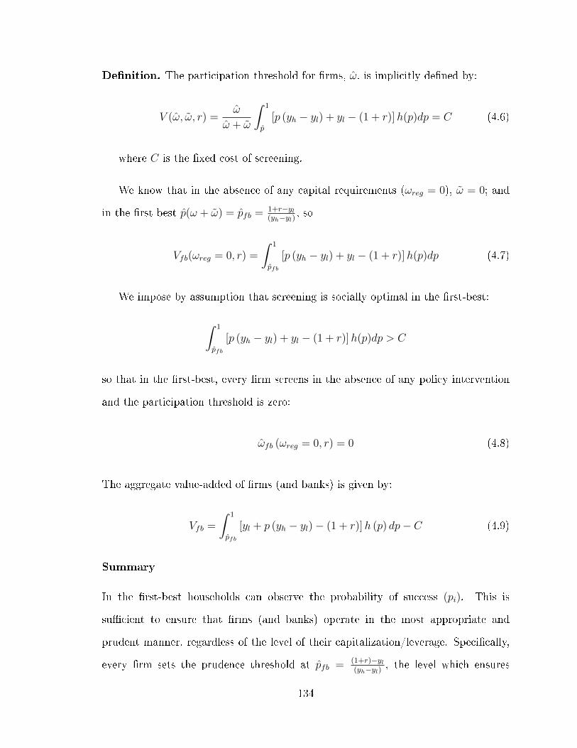
De�nition. The participation threshold for �rms, ω, is implicitly de�ned by:

V (ω, ω, r) =ω

ω + ω

∫ 1

p

[p (yh − yl) + yl − (1 + r)]h(p)dp = C (4.6)

where C is the �xed cost of screening.

We know that in the absence of any capital requirements (ωreg = 0), ω = 0; and

in the �rst-best p(ω + ω) = pfb = 1+r−yl(yh−yl)

, so

Vfb(ωreg = 0, r) =

∫ 1

pfb

[p (yh − yl) + yl − (1 + r)]h(p)dp (4.7)

We impose by assumption that screening is socially optimal in the �rst-best:

∫ 1

pfb

[p (yh − yl) + yl − (1 + r)]h(p)dp > C

so that in the �rst-best, every �rm screens in the absence of any policy intervention

and the participation threshold is zero:

ωfb (ωreg = 0, r) = 0 (4.8)

The aggregate value-added of �rms (and banks) is given by:

Vfb =

∫ 1

pfb

[yl + p (yh − yl)− (1 + r)]h (p) dp− C (4.9)

Summary

In the �rst-best households can observe the probability of success (pi). This is

su�cient to ensure that �rms (and banks) operate in the most appropriate and

prudent manner, regardless of the level of their capitalization/leverage. Speci�cally,

every �rm sets the prudence threshold at pfb = (1+r)−yl(yh−yl)

, the level which ensures

134

that every risky project undertaken after screening is expected to deliver at least

the risk-free return. In addition, with the participation threshold (ω) equal to zero,

all �rms screen so no pro�table lending opportunities are wasted. Leverage and

limited-liability, in the absence of asymmetric information, do not lead to ine�ciencies

and do not necessitate any policy intervention.

4.4 The Model with Asymmetry of Information

Frictions in the model arise because of the interaction between asymmetric informa-

tion, leverage and limited liability. When households cannot observe banks' proba-

bility of success (pi), moral hazard becomes prevalent in the banking sector. This

problem manifests itself in a sub-optimal level of screening for the risky asset; and for

those banks that do screen, a lower level of prudence than ideal in deciding whether

to invest in the risky asset.

Analytically, the structure of the model remains unchanged under asymmetric

information (the majority of the equations are identical). The main distinction is

that for banks p becomes a function of ω, and therefore can no longer be evaluated

outside of the integral over ω. The analysis for �rms is identical to the �rst-best case.

The Prudence Threshold

As with the �rst-best, we start by examining the prudence threshold (at Stage 2 of the

game) for those banks that have discovered their individual realization of pi through

screening. Under asymmetric information, the analogues of equations 4.1-4.4 are:

135

1. The condition that a bank with initial capital ω and additional equity injection

ω is indi�erent between the risky asset and the risk-free asset:

ω

ω + ω{p (yh −R) + (1− p) max [0, yl −R]} = ω(1 + r)

or:

p (yh −R) + (1− p) max [0, yl −R] = (ω + ω) (1 + r) (4.10)

this is identical to equation 4.1.

2. The condition that the households are indi�erent between providing debt and

the risk-free facility:

A (p)R + (1− A (p)) (min [yl, R]) = (1− ω − ω) (1 + r) (4.11)

where A (p) ≡ E[p | p > p] ≡ 11−H(p)

∫ 1

pph (p) dp denotes the conditional

expectation of p given that p ≥ p.

Note that the key di�erence here (relative to equation 4.2) is that instead of

observing the p directly, households now need to form a conditional expectation

of p.

3. The condition that for households providing additional equity to the bank their

expected return from the capital injection is at least equal to the safe rate of

return:

ω

ω + ω{A (p) (yh −R) + (1− A (p)) (max [0, yl −R])} ≥ ω (1 + r)

or:

A (p) (yh −R) + (1− A (p)) (max [0, yl −R]) ≥ (ω + ω) (1 + r) (4.12)

136

This last condition is always satis�ed given equation 4.10 and the fact that

A (p) ≥ p.

Proposition 13. With asymmetric information, banks that are not 'fully capitalized'

will take excessive risks (p < pfb):

1. As before, let ω∗ = ω + ω denote the level of capital such that R (ω∗) = yl, so

ω∗ = 1− yl(1+r)

. We refer to any bank with ωi + ωi ≥ ω∗ as a �fully capitalized"

bank.

2. Banks become more prudent as they increase their capital, up to a cap when

they become fully capitalized.

(a) For ω + ω ≥ ω∗, we have p = (1+r)−yl(yh−yl)

; R = (1− (ω + ω)) (1 + r);

(b) For ω + ω < ω∗, we have ∂p∂ω

= (A(p)−p)(1+r)(yh−R)A(p)+pA′(p)(R−yl)

; and p ≤ (1+r)−yl(yh−yl)

=

pfb.

The function for p (ω + ω) kinks at ω∗, with right-hand derivative given by

∂+p (ω∗) /∂ω = 0 and left-hand derivative given by ∂−p (ω∗) /∂ω = (A(p)−p)(1+r)(yh−R)A(p)+pA′(p)(R−yl)

>

0.

An increase in internal equity has the same marginal impact on prudence as an

increase in external equity. Banks behavior is in�uenced by the quantity of their

equity rather than its source.

Proof. A full proof is in the annex, here we give the intuition. In the �rst part of the

proposition, ω∗ is de�ned as the level of internal capital such that yl = R (ω∗, r), so

ω∗ = 1 − yl(1+r)

follows directly from re-arranging equation 4.11. Banks with capital

above this level can borrow at the risk free rate because the liquidation value of their

risky assets is su�cient to cover the bank's debt obligations (again from re-arranging

equation 4.11 after setting R (ω∗) = yl). The second part of the proposition says

137

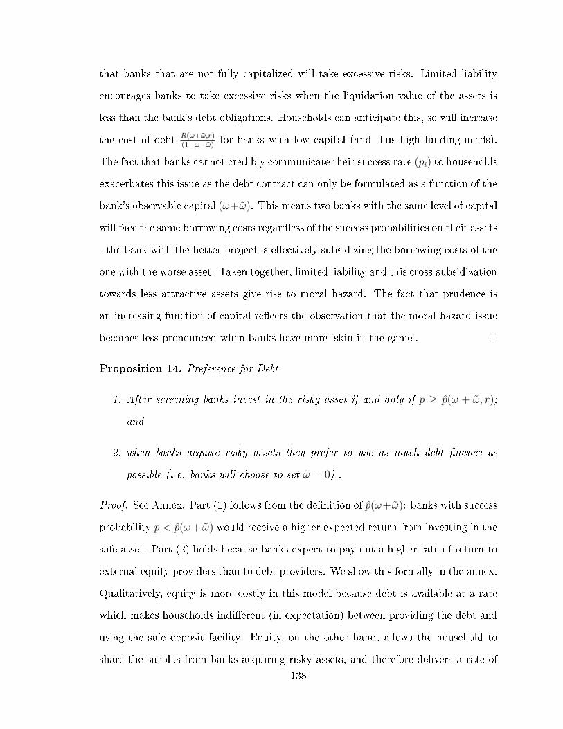
that banks that are not fully capitalized will take excessive risks. Limited liability

encourages banks to take excessive risks when the liquidation value of the assets is

less than the bank's debt obligations. Households can anticipate this, so will increase

the cost of debt R(ω+ω,r)(1−ω−ω)

for banks with low capital (and thus high funding needs).

The fact that banks cannot credibly communicate their success rate (pi) to households

exacerbates this issue as the debt contract can only be formulated as a function of the

bank's observable capital (ω+ω). This means two banks with the same level of capital

will face the same borrowing costs regardless of the success probabilities on their assets

- the bank with the better project is e�ectively subsidizing the borrowing costs of the

one with the worse asset. Taken together, limited liability and this cross-subsidization

towards less attractive assets give rise to moral hazard. The fact that prudence is

an increasing function of capital re�ects the observation that the moral hazard issue

becomes less pronounced when banks have more 'skin in the game'.

Proposition 14. Preference for Debt

1. After screening banks invest in the risky asset if and only if p ≥ p(ω + ω, r);

and

2. when banks acquire risky assets they prefer to use as much debt �nance as

possible (i.e. banks will choose to set ω = 0) .

Proof. See Annex. Part (1) follows from the de�nition of p(ω+ω): banks with success

probability p < p(ω+ ω) would receive a higher expected return from investing in the

safe asset. Part (2) holds because banks expect to pay out a higher rate of return to

external equity providers than to debt providers. We show this formally in the annex.

Qualitatively, equity is more costly in this model because debt is available at a rate

which makes households indi�erent (in expectation) between providing the debt and

using the safe deposit facility. Equity, on the other hand, allows the household to

share the surplus from banks acquiring risky assets, and therefore delivers a rate of

138

return for households that is greater than the risk-free facility. The original owners of

bank equity have the value of their claims diluted by raising new equity from outsiders.

Consequently banks stick with debt in the absence of any policy intervention, because

this is the cheapest way for them to raise funds at the margin.

Corollary 3. In the absence of capital regulations, banks will not seek external equity

injections when they acquire risky assets.

The Participation Threshold

As in the �rst-best case, the value of screening for banks is still given by equation

4.5:

V (ω, ω, r + δr)

≡ Ep

max

0 ,ω

ω + ω

p (yh −R) +

(1− p) max [0, yl −R]

− ω(1 + r)

=ω

ω + ω

∫ 1

p(ω+ω)

[p (yh − yl) + yl − (1 + r)]h(p)dp (4.13)

And the participation threshold ω is still given implicitly by equation 4.6:

ω

ω + ω

∫ 1

p(ω+ω)

[p (yh − yl) + yl − (1 + r)]h(p)dp = C (4.14)

with the only di�erence that p is now a function of ω + ω. Since p (ω + ω) ≤ pfb,

this means that even when ω = 0, the participation threshold under asymmetric

information will in general be a positive number.

Proposition 15. ∂V (ω,ω=0,r)∂ω

> 0 for ω < ω∗

= 0 for ω ≥ ω∗. In the absence of capital regula-

tions (and ω = 0), the expected value of screening is increasing in the bank's initial

139

endowments (up to a cap when the bank becomes fully well capitalized). (see proof in

the annex)

Since we have established through corollary 3 that banks will only use debt funding

in the absence of capital regulations, for now we can restrict attention to the case

where ω = 0.

Summary and Implications

The presence of moral hazard in the model give rise to sub-optimal outcomes com-

pared to the �rst-best scenario. Banks have no incentives to top-up their capital.

Consequently, the hurdle for participation, ω > 0, is too high; and the level of

prudence, p(ω, r) ≤ (1+r)−yl(yh−yl)

= pfb is too low. As a result aggregate value added

of the banking sector is lower than it is in the �rst-best (where we assumed that p

is common knowledge). Banks do not do enough screening (and so will be missing

opportunities that investors would value), but those that do screen will accept some

investments that well-informed, risk-neutral investors would reject.

4.5 Policy Tools and Their Transmission

Interest rate policy and capital regulations can be used to drive outcomes closer to

the �rst-best level in the banking sector. Both policy tools function through their

e�ects on the participation and prudence thresholds.

Interest Rate Policy / Variations in the safe real interest rate

Let us assume that the policy maker (either through its central bank or directly by

o�ering assets to the private sector) can set the risk-free rate of return on the deposit

facility (r) and this a�ects the attractiveness of the risky asset relative to the risk-free

deposit. (We return to the issue of whether the national authority have control over

r below). The central bank remunerates all resources placed in its deposit facilities at

140

the rate r, the servicing cost of which is covered by lump sum taxation of households.

This interest rate (r) is revealed to all agents at the very beginning of the game.

We normalize r = 0 as the neutral interest rate. In the �rst-best scenario, there

is no need for interest rate policy intervention, so r = 0 and the �rst-best level of

prudence becomes:

pfb =1− yl

(yh − yl)(4.15)

The �rst-best level of the participation threshold ωfb (ωreg = 0) = 0 remains the

same as before (see equation 4.8)

Note that the possibility of interest rate policy intervention introduces a wedge

between the socially optimal outcome and what is privately optimal in the absence

of asymmetric information. In particular, the privately optimal level of prudence is

given by

p∗ (r) =1 + r − yl(yh − yl)

(4.16)

which will be di�erent to pfb (the socially optimal level of prudence) for non-zero

r. So using interest rate policy to combat the ine�ciencies of the banking sector will

lead to distortions in the non-bank sector (i.e. the risk-taking behavior of ��rms�).

This makes the relative size of the banking sector to that of the non-�nancial sector

(µ) a factor in assessing the extent to which the authorities should use the in�uence

they may have over r to curb excess risk taking.

The e�ect of interest rate policy on banks' behavior is summarized in the propo-

sition below.

Proposition 16. Interest rate tightening improves 'prudence' at the cost of decreasing

'participation'. Policy loosening achieves the converse:

1. ∂p∂r> 0; and

2. ∂ω∂r> 0

141

Proof. We describe the intuition for the proposition here; formal proof is in the annex.

Interest rate policy tightening improves prudence for all �rms and banks by increasing

the attractiveness of the outside option. A quick way to illustrate the result ∂p∂r> 0

is by appealing to proposition 13: p(ω + ω) ≤ pfb. Recall from equation 4.15: pfb =

1−yl(yh−yl)

; and from Proposition 13: p(ω + ω, r) ≤ 1+r−yl(yh−yl)

= p∗ (r). So by increasing r,

a central bank can increase p∗ (r) and thus push p(ω + ω, r) closer to pfb for all ω.

Interest rate policy tightening decreases the level of participation because it increases

the relative attractiveness of the outside option. Recall that ω (ω, r) is implicitly

de�ned by

V (ω, ω, r) =ω

ω + ω

∫ 1

p(ω+ω,r)

[p (yh − yl) + yl − (1 + r)]h(p)dp = C

Increasing r reduces the value of screening, so for a given �xed cost of screening

C, banks need a higher amount of internal equity to make the screening process

worthwhile.

Prudential Policy

We model capital regulations in the simple form of a leverage ratio restriction. Regu-

lators impose a minimum capital requirement ωreg such that banks with endowments

ωi < ωreg must seek outside equity of at least (ωreg − ωi) or are barred from investing

in the risky asset. We rule out the possibility that the regulator can set a capital

requirement that depends on the riskiness of bank assets by assuming the asset speci�c

chance of success pi remains private bank information.

The capital requirement ωreg is announced as soon as banks �nd out their indi-

vidual realizations of ωi. A strengthening of capital requirements achieves the same

qualitative e�ect as a tightening of interest rate policy on banks' decisions, albeit

through di�erent means. Critically, capital regulations can be imposed on banks

142

alone, without a�ecting the behavior of �rms. This is an important di�erence between

the blunt instrument of interest rate policy (one "that gets in all the cracks") and the

targeted instrument of bank capital requirements.

Proposition 17. Capital regulations improve prudence by forcing some banks to seek

additional equity funding, but do so at the cost of decreased participation:

1. ω = max [0, ωreg − ω]. Only banks that are constrained by the capital regulations

will seek equity injections from households. And when they do, they will only

top-up to the minimum capital standard.

2. ∂p(ω+ω,r)∂ωreg

≥ 0 with strict inequality as long as ω (ω = 0, r) < ωreg < ω∗. Capital

requirement will improve the prudence level of banks for which it binds, so long

as they are not already 'fully capitalized'.

3. ω (ω = ωreg − ω, r) > ω (ω = 0, r) for all ωreg such that ωreg > ω (ω = 0, r). The

participation threshold is higher for banks that require external equity injections

(i.e. banks that falls short of the capital requirement), than for banks that are

not bound by the capital requirement.

4. ∂ω(ωreg−ω,r)∂ωreg

≥ 0 . A tightening of capital standards increases the participation

threshold.

Proof. We give the intuition of the result here, details are in the annex.

1. ω = max [0, ωreg − ω] follows directly from the observation that banks weakly

prefer debt to equity (proposition 14). Consequently, banks for which the

regulations are binding will only top-up their capital to the regulatory minimum,

and seek the remaining funds in the form of debt.

2. ∂p(ω+ω,r)∂ωreg

≥ 0 is a corollary of proposition 13 (∂p(ω+ω,r)∂ω

≥ 0 ) and the previous

observation that ω = max [0, ωreg − ω]. In particular, ∂p(ω+ω,r)∂ωreg

= 0 for banks

143

with ωi > ωreg or ωi ≥ ω∗. Banks with ωi > ωreg obviously will remain

una�ected by a marginal increase in ωreg. Banks with ωi ≥ ω∗ already operate

at the optimal level of prudence, so pushing ωreg above ω∗ does not bring any

further gains in prudence.

3. ω (ωreg − ω, r) > ω (0, r) holds because equity funding is more costly than debt

funding due to the dilution e�ect (proposition 14). Therefore, the value of

screening is lower for banks that are constrained by the capital requirement.

(ωreg is announced in Stage 1, so banks can anticipate capital needs in advance of

screening.) Consequently, the presence of binding capital regulations increases

the participation threshold for a given �xed cost of screening.

4. ∂ω(ωreg−ω,r)∂ωreg

≥ 0 follows from part 1 and 3. Higher capital requirements increase

the size of equity injection required, and thus reduce the value of screening and

increase the threshold for participation.

Summary of Policy Implications

An increase in the risk-free interest rate increases the opportunity cost of funding risky

assets. This pushes up prudence for all banks at all levels of initial endowments /

internal equity. So poorly endowed (or highly leveraged) banks become more prudent,

but �rms which do not su�er asymmetric information will become too cautious31. A

strengthening of bank capital standards forces more banks to seek out more external

equity, inducing them to behave as if they are a better endowed bank.

The two policy instruments will also a�ect participation. Because external equity

is more costly than debt, tougher capital requirements make the break-even level of

initial endowment for banks higher for a given �xed cost of screening. So more banks

31Very well capitalized banks will also become too cautious. But this side e�ect falls away if werestrict the upper support of ω to a value signi�cantly below 1.

144

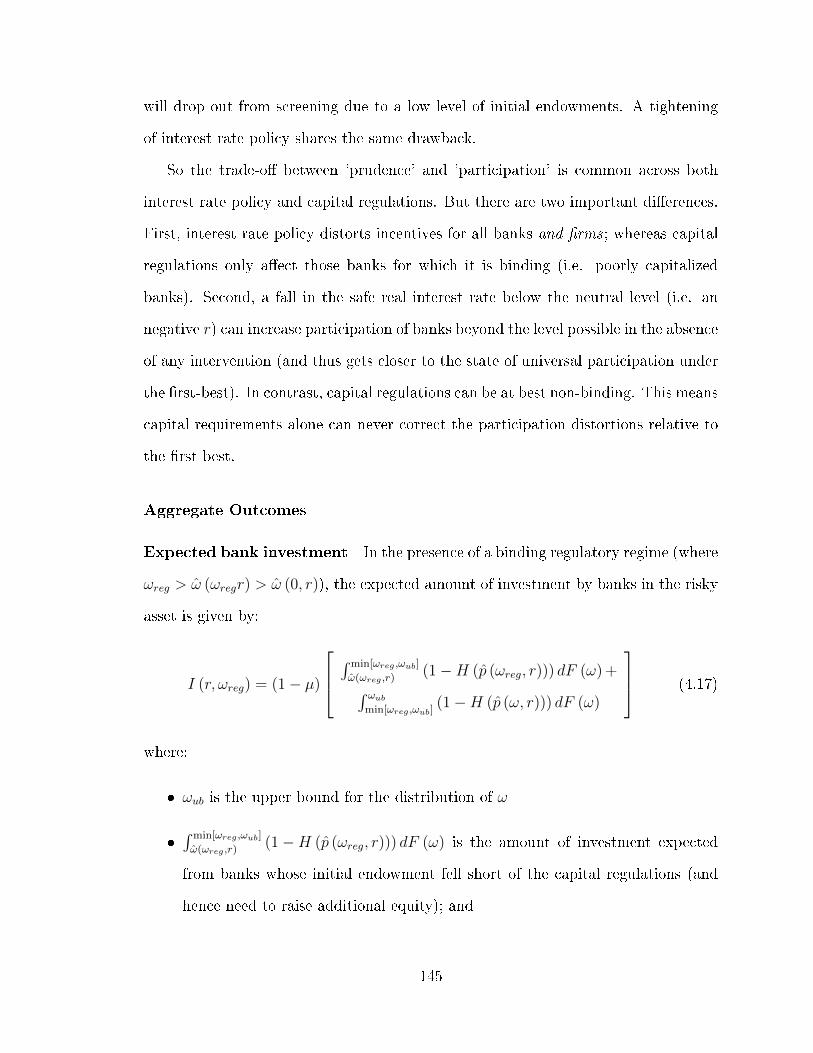
will drop out from screening due to a low level of initial endowments. A tightening

of interest rate policy shares the same drawback.

So the trade-o� between 'prudence' and 'participation' is common across both

interest rate policy and capital regulations. But there are two important di�erences.

First, interest rate policy distorts incentives for all banks and �rms ; whereas capital

regulations only a�ect those banks for which it is binding (i.e. poorly capitalized

banks). Second, a fall in the safe real interest rate below the neutral level (i.e. an

negative r) can increase participation of banks beyond the level possible in the absence

of any intervention (and thus gets closer to the state of universal participation under

the �rst-best). In contrast, capital regulations can be at best non-binding. This means

capital requirements alone can never correct the participation distortions relative to

the �rst best.

Aggregate Outcomes

Expected bank investment In the presence of a binding regulatory regime (where

ωreg > ω (ωregr) > ω (0, r)), the expected amount of investment by banks in the risky

asset is given by:

I (r, ωreg) = (1− µ)

∫ min[ωreg ,ωub]

ω(ωreg ,r)(1−H (p (ωreg, r))) dF (ω) +∫ ωub

min[ωreg ,ωub](1−H (p (ω, r))) dF (ω)

(4.17)

where:

� ωub is the upper bound for the distribution of ω

�∫ min[ωreg ,ωub]

ω(ωreg ,r)(1−H (p (ωreg, r))) dF (ω) is the amount of investment expected

from banks whose initial endowment fell short of the capital regulations (and

hence need to raise additional equity); and

145

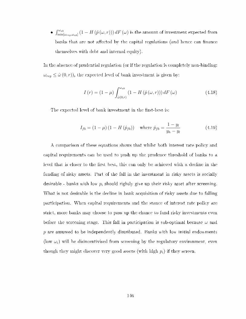
�∫ ωub

min[ωreg ,ωub](1−H (p (ω, r))) dF (ω) is the amount of investment expected from

banks that are not a�ected by the capital regulations (and hence can �nance

themselves with debt and internal equity).

In the absence of prudential regulation (or if the regulation is completely non-binding:

ωreg ≤ ω (0, r)), the expected level of bank investment is given by:

I (r) = (1− µ)

∫ ωub

ω(0,r)

(1−H (p (ω, r))) dF (ω) (4.18)

The expected level of bank investment in the �rst-best is:

Ifb = (1− µ) (1−H (pfb)) where pfb =1− ylyh − yl

(4.19)

A comparison of these equations shows that whilst both interest rate policy and

capital requirements can be used to push up the prudence threshold of banks to a

level that is closer to the �rst best, this can only be achieved with a decline in the

funding of risky assets. Part of the fall in the investment in risky assets is socially

desirable - banks with low pi should rightly give up their risky asset after screening.

What is not desirable is the decline in bank acquisition of risky assets due to falling

participation. When capital requirements and the stance of interest rate policy are

strict, more banks may choose to pass up the chance to fund risky investments even

before the screening stage. This fall in participation is sub-optimal because ω and

p are assumed to be independently distributed. Banks with low initial endowments

(low ωi) will be disincentivised from screening by the regulatory environment, even

though they might discover very good assets (with high pi) if they screen.

146

Expected value added Under a binding regulatory regime, where ωreg > ω (ωregr) >

ω (0, r)), the expected amount of value added from �rms and banks is given by:

V (ωreg, r) = µ

∫ ωub

ω(0,r)

[∫ 1

p∗(r)

[yl + p (yh − yl)− 1] dH (p)− C]dF (ω)

+ (1− µ)

∫ min[ωreg ,ωub]

ω(ωreg ,r)

[∫ 1

p(ω,r)

[yl + p (yh − yl)− 1] dH (p)

]dF (ω)

+ (1− µ)

∫ ωub

min[ωreg ,ωub]

[∫ 1

p(ω,r)

[yl + p (yh − yl)− 1] dH (p)

]dF (ω)

− (1− µ)C

[∫ ωub

ω(ωreg ,r)

dF (ω)

](4.20)

where V (ωreg, r) is composed of:

� The value-added of �rms µ∫ ωubω(0,r)

[∫ 1

p∗(r)[yl + p (yh − yl)− 1] dH (p)− C

]dF (ω),

where p∗ (r) = 1+r−yl(yh−yl)

.

� The value-added of banks that are constrained by the capital requirement:

(1− µ)

∫ min[ωreg ,ωub]

ω(ωreg ,r)

[∫ 1

p(ω,r)

[yl + p (yh − yl)− 1] dH (p)

]dF (ω)

� The value-added of banks that are not constrained by the capital requirement:

(1− µ)

∫ ωub

min[ωreg ,ωub]

[∫ 1

p(ω,r)

[yl + p (yh − yl)− 1] dH (p)

]dF (ω)

� Minus the cost of screening by all banks: (1− µ)C[∫ ωub

ω(ωreg ,r)dF (ω)

]In the absence of capital regulations (or when it is entirely non-binding), the expected

aggregate value-added is given by:

V (r) = µ

∫ ωub

ω(0,r)

[∫ 1

p∗(r)

[yl + p (yh − yl)− 1] dH (p)− C]dF (ω)

+ (1− µ)

∫ ωub

ω(0,r)

[∫ 1

p(ω,r)

[yl + p (yh − yl)− 1] dH (p)− C]dF (ω)

147

Lastly, recall that the aggregate value added in the �rst-best is given by:

Vfb =

∫ 1

pfb

[yl + p (yh − yl)− 1] dH (p)− C (4.21)

where pfb = 1−ylyh−yl

.

In the following section, we treat the expected level of aggregate value added

V (ωreg, r), which is also the weighted average rate of return on all savings invested

in �rms and banks, as the objective function for policymakers32. This allows us to

employ numerical techniques to calculate the optimal setting of interest rate policy

and capital requirements under illustrative parameterizations of the model.

4.6 Numerical Simulations

We use numerical simulations to illustrate the trade-o� between interest rate policy

and capital requirements. The model we have outlined above is necessarily a sig-

ni�cant simpli�cation of the �nancial intermediation process. A precise calibration

of the model is not straight-forward because there are no direct empirical counter-

parts to some of the key parameters of the model, speci�cally the pair of binary

outcomes(yh, yl) for the risky asset. We chose a wide range of parameter combinations

for (yh, yl) which cover high and low risk investment environments. And we rely on

robustness tests to demonstrate that our main qualitative results are sound, namely

that: (1) interest rate policy and capital regulations function as imperfect substitutes;

(2) these policy interventions can trade-o� between 'prudence' and 'participation' of

banks; (3) the level of the optimal capital requirement is sensitive to variations in

the safe real interest rates; and (4) across a wide, plausible, range of calibrations, the

optimum setting of policy is one where the capital requirement plays the main role

in addressing the asymmetric information distortions in the banking sector.

32Using the expected aggregate value added as the objective function makes sense given theassumption of risk neutrality.

148

We allow the binary outcomes for the risky asset (yh, yl) to vary between permis-

sible values in the model33, whilst making some assumptions on the remaining model

parameters. Speci�cally, we assume that the probability of success, p, is uniformly

distributed between [0, 1]; initial endowments ω are uniformly distributed between

[0, 0.1]34; and the cost of screening C is 1%. In our model, µ represents the proportion

of initial endowments in the economy that are available to �rms rather than banks.

We set µ to 0.85, to re�ect the fact that �nancial companies account for roughly 15%

of the capitalization of major stock indices in the US and the UK.

Table 4.1 presents the optimal policy combinations when we allow (yh, yl) to vary.

The range of combinations of yh and yl that we consider runs from very low to very

high risk worlds. A world in which yh is as low as 1.1 and yl as high as 0.8 is one

in which at the �rst best losses on those investments which fail are only 3% of total

investment. But the expected return on investments are also quite low at 5%. At the

other extreme when yh is 1.9 and yl = 0 optimal investment implies that losses from

projects failing are around 24% of total investment, but the expected return is over

45%.

33As part of the theoretical model, we impose two conditions on the permissible levels for (yh, yl):

1. The risky asset must not be so attractive that banks will always proceed without screening:

yl + E [p] (yh − yl) < 1

2. The risky asset must be attractive enough such that all banks will screen in the �rst-best:∫ 1

pfb

[p (yh − yl) + yl − 1]h (p) dp > C

where pfb = 1−yl(yh−yl) .

In the numerical simulation, we also required that the risky asset must be attractive enough such thatat least some banks will screen under asymmetric information when there is no policy intervention:ω (r = 0, ωreg = 0) < ωub. This additional restriction ruled out the combination (yh = 1.1, yl = 0.6)in table 4.1.

34Note that because the prudence threshold of �rms is independent of ω, and that �rms areessentially indi�erent between debt and equity funding, the results of the model is invariant to thedistribution of �rm's initial endowments. So for simplicity, we assume that banks and �rms sharethe same distribution for ω. In the Appendix, we show that when we extend the model to allow fortaxes (that have debt deductions), the distribution of endowments for �rms does matter.

149

In Table 4.1 the �gures in curved brackets for each combination of (yh, yl) are

the optimal interest rate (deviation from the neutral policy setting) and the cap-

ital requirement. The �gure in square brackets is the associated maximal value

added (as per equation 4.20, which is also the weighted average rate of return on

all savings invested in �rms and banks ). The results here shows that, across these

wide-ranging parameterizations, capital regulations are generally the main tool policy

makers should use in addressing banking ine�ciencies. Only in the safest investment

environment (yh = 1.1; yl = 0.8) should interest rate policy be used on its own, and

then the safe real interest rate should be set to 0.5 percentage points above a neutral

level. In most cases capital requirements are substantial - ranging from around 10%

to up to 30%. In the most risky environment (yh = 1.9; yl = 0.9), where incentives

for banks to raise too much debt and invest too much are at their greatest, both

interest rate policy and capital requirements are very tight; the safe real interest rate

is 2.5% above neutral and capital should be 30% of total bank assets.

150

Table 4.1: Optimal Policy Setting across (yh, yl) pairs

In order to examine the trade-o�s between interest rate policy and capital reg-

ulations, and to demonstrate the more detailed implications of the model, we take

a speci�c illustrative parameterization (see Table 4.2) and present the associated

results. We have chosen the pair (yh, yl) = (1.4, 0.5) for this illustrative example. This

combination generates �rst-best outcomes where about 20% of those assets acquired

(after screening) become non-performing (and in this low state, the loss of value is

such that the residual worth of the asset is only one half of the investment). This

scale of risk and of losses is not implausible for loans to �nance corporate activity -

particularly of small businesses that rely on bank intermediation. Given the losses on

sub-prime mortgage lending that was behind the �nancial crisis of 2007-08, this scale

of risk may not be excessive even for lending backed by residential property which

used to be considered relatively safe. Our aim in choosing these values is not however

151

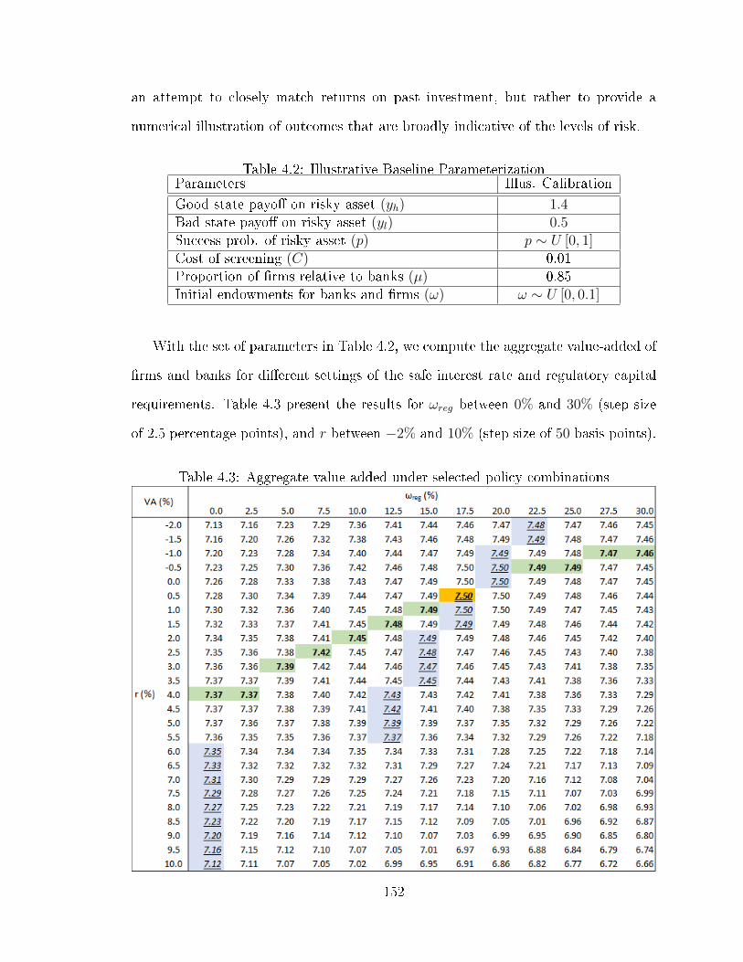
an attempt to closely match returns on past investment, but rather to provide a

numerical illustration of outcomes that are broadly indicative of the levels of risk.

Table 4.2: Illustrative Baseline ParameterizationParameters Illus. Calibration

Good state payo� on risky asset (yh) 1.4Bad state payo� on risky asset (yl) 0.5Success prob. of risky asset (p) p ∼ U [0, 1]Cost of screening (C) 0.01Proportion of �rms relative to banks (µ) 0.85Initial endowments for banks and �rms (ω) ω ∼ U [0, 0.1]

With the set of parameters in Table 4.2, we compute the aggregate value-added of

�rms and banks for di�erent settings of the safe interest rate and regulatory capital

requirements. Table 4.3 present the results for ωreg between 0% and 30% (step size

of 2.5 percentage points), and r between −2% and 10% (step size of 50 basis points).

Table 4.3: Aggregate value added under selected policy combinations

152

Each row in Table 4.3 illustrates how expected aggregate value added changes as

we vary the level of capital requirements, for a given safe real interest rate. This

allows us to trace a path for the optimal capital requirement conditioned on the safe

interest rate (italic, underlined, blue �ll). Table 4.3 thus shows that the optimal

regulatory capital standards strengthens as the safe real interest rate falls.

In particular, under this illustrative calibration, the optimal capital requirement

is 20% when the safe real interest rate is at its neutral stance (r = 0). Even when

the safe real interest rate rises to 5.5% above its neutral level, the optimal capital

requirement is still as high as 12.5%. Given that ω is assumed to be distributed

between 0 and 0.1, this means a leverage ratio that is binding for all banks in the

population. For no capital requirements to be (locally) optimal, the safe real rate of

interest need to rise to 6 percentage points above the neutral rate and beyond.

We could alternatively read Table 4.3 on a column-by-column basis. This would

allow us to trace out a path for the optimal the real safe interest rates for given level

of bank capital requirements (bold, green �ll). We �nd that the optimal stance of

interest rate policy loosens as regulatory capital standard strengthens. Under this

speci�c set of parameters, the globally optimal outcome is achieved when capital

requirement is set to 17.5% and the real safe interest rate is 0.5 percentage points

above the neutral level.

The model also allows us to describe the banks' behavior under each policy

setting (see Table 4.4). Under the globally optimal combination of r = 0.5% and

ωreg = 17.5%, the capital regulation is binding for all banks in the population. The

participation threshold equals 0.023, meaning that 23% of banks would choose not

to screen the risky asset. For banks that do screen, they will invest if and only if the

probability of success exceeds the prudence threshold of 0.41 (the �rst-best level is

0.56). The conditional expectation of success is therefore E [p|p ≥ p (ωreg) = 0.41] ≈

153

0.70, which implies that around 30% of the risky investments made are expected to

underperform. In aggregate about 46% of banks invest in risky assets.

Table 4.4 also shows that across a broad range of measures - including aggregate

value added, investment in the risky asset, and probability of failure - the outcomes

under optimal policy are between �rst-best levels (where there is no asymmetry of

information, no capital requirements and interest rate policy is neutral) and levels

under asymmetry of information but no policy intervention. The table shows that

investment in the risky asset is signi�cantly lower in the �rst-best case and under

optimal policy than compared to the case of no-intervention. Free market outcomes

with asymmetric information generate much too much bank funding of risky assets.

Note that although the banks in our model are heterogeneous at the start (they

take independent draws from the distribution of ω), having a minimum capital re-

quirement that exceeds the upper bound of the ω distribution (i.e. ωreg ≥ ωub)

imposes homogeneity of leverage amongst those banks that do proceed with investing

in the risky asset. All banks that proceed will top-up their equity to the minimum

level required (ω = 17.5% in the optimal case) and fund the remainder through

debt. These banks therefore share a common prudence threshold: p (ωreg) = 0.41. In

contrast, if ωreg was lower than ωub (say ωreg = 5%), then we would observe a cluster

of banks with capital equal to the regulatory minimum, as well as some banks with a

surplus of capital for regulatory purposes (having started with a better endowment).

Since the prudence threshold p is a function of capital ω, banks would no longer

behave in a homogeneous fashion.

An alternative interpretation - the safe rate is set in global capital markets

We have assumed so far that the authorities (possibly through the central bank) can

o�er a safe asset with an o�ered real rate of return that is a choice variable � though

it must accept the �scal implications of that choice. Suppose instead that the safe

154

Table 4.4: Behavior of banks under illustrative baseline parameterization

rate is a price set in a global capital market. We can still use our results to draw

implications for the setting of bank capital requirements. We have shown that the

lower is the safe real interest rate the worse is the problem of excessive risk taking by

banks. An exogenous fall in the safe real rate should be countered by tight capital

requirements.

Table 4.3 illustrates the scale of the e�ects. In recent decades global safe real rates

� proxied by the average yield on in�ation-proof debt issued by developed country

governments � have fallen dramatically, from nearly 4% 30 years ago to close to 0%

today. At a 4% safe real rate Table 4.3 shows the optimal capital requirement is

12.5%; at a 0% safe real rate the optimal capital requirement is 20%. Movements in

real rates appear to have a sizeable e�ect on appropriate capital requirements.

4.7 Concluding Remarks

We �nd that prudential capital requirements and variations in the safe real interest

rate (implemented as part of an interest rate policy) operate as imperfect substitutes

when used to counter excessive risk taking by banks. A tightening of either instru-

ments can improve 'prudence' (by disincentivising banks against investing in risky

assets with low probability of success); but only at the cost of decreased 'participation'

(as more banks will choose to forego the opportunity to acquire a risky asset even

before they discover its probability of success through costly screening).

155

Numerical simulations of our model help to illustrate, and to broadly quantify, the

magnitude of this interaction between the safe real interest rate and capital regulation.

We �nd that the trade-o� between 'prudence' and 'participation' is such that the

optimal level of prudential capital requirements rises as the safe real interest rate falls.

In general the global optimum is one where interest rates should be slightly higher

than a neutral setting and capital requirements should be substantial and binding.

Investment in risky assets is much lower when policy is set optimally. This suggests

how very weak is the argument that regulations on banks should not be so tight

as to materially reduce bank lending. Our �ndings also suggest that the signi�cant

and simultaneous decline in global real interest rates on in�ation proof debt of many

governments in recent years should have prompted a rise in bank capital requirements.

There are several interesting ways one could extend the baseline analytical frame-

work presented here. One of these is to introduce corporate taxation and explore

whether using the tax rate can help o�set a tendency to over-invest in risky assets.

We present one version of this extension in the appendix and discuss preliminary

results.

We assumed here that banking regulators have no more information on the riski-

ness of bank assets than outside investors. If they have some - but less than complete

- information on risks (pi) then risk based capital requirements become feasible. That

could mean that optimal risk weighted bank capital requirements are on average lower

than the leverage ratios we have calculated. It is not clear however that regulators

having very imperfect information on bank risk pi should mean that average leverage

requirements would be very substantially lower. If they are not - so that capital

requirements of 10% or more of bank assets are indeed optimal - then this suggests

that current rules on bank leverage that allow capital to be as low as 3% or so of total

assets may well be far too lax.

156

References

Angelini, P., S. Neri, and F. Panetta (2014, sep). The Interaction between Capital

Requirements and Monetary Policy. Journal of Money, Credit and Banking 46 (6),

1073�1112.

Angeloni, I. and E. Faia (2013). Capital regulation and monetary policy with fragile

banks. Journal of Monetary Economics 60 (3), 311�324.

Bernanke, B. and M. Gertler (1990). Financial Fragility and Economic Performance.

The Quarterly Journal of Economics 105 (1), 87�114.

Bolton, P. and X. Freixas (2006). Corporate �nance and the monetary transmission

mechanism. Review of Financial Studies 19 (3), 829�870.

Borio, C. and H. Zhu (2012). Capital regulation, risk-taking and monetary policy: A

missing link in the transmission mechanism? Journal of Financial Stability 8 (4),

236�251.

Diamond, D. (1984). Financial intermediation and delegated monitoring. Review of

Economic Studies 51 (3), 393�414.

Farhi, E. and J. Tirole (2009). Leverage and the central banker's put. In American

Economic Review, Volume 99, pp. 589�593.

Furlong, F. T. and M. C. Keeley (1989). Capital Regulation and Bank Risk-Taking:

A Note. Journal of Banking and Finance 13 (1977), 883�891.

Gale, D. and M. Hellwig (1985). Incentive-Compatibl Debt The One-Period Problem.

Review of Economic Studies 52 (4), 647�663.

Gersbach, H. and J. C. Rochet (2017). Capital regulation and credit �uctuations.

Journal of Monetary Economics 90, 113�124.

157

Kashyap, A. K. and J. C. Stein (1994). Monetary Policy and Bank Lending, Volume

ISBN. The University of Chicago Press.

Kashyap, A. K. and J. C. Stein (2000). What Do a Million Observations on Banks

Say about the Transmission of Monetary Policy. American Economic Review .

Nicolò, G. D., G. D. Ariccia, L. Laeven, and F. Valencia (2010). Monetary Policy

and Bank Risk Taking. IMF Sta� Position Note.

Stein, J. C. (2012, feb). Monetary policy as �nancial stability regulation. Quarterly

Journal of Economics 127 (1), 57�95.

Woodford, M. (2012, apr). In�ation Targeting and Financial Stability. NBER Working

Paper .

158

4.8 Appendices

A.1 Proof of Proposition 11- No excessive risk-taking under perfect infor-

mation

Consider the case where min [yl, R (p, ω + ω)] = R (p, ω + ω) (the debt obligation is

less than the liquidation value), re-arranging equations 4.1 and 4.2 gives:

R (p, ω + ω | yl > R) = (1− (ω + ω)) (1 + r)

p(ωi + ωi | yl > R) =(1 + r)− yl

(yh − yl)

Consider the case where min [yl, R (p, ω + ω)] = yl (the debt obligation is greater than

the liquidation value): So from equation 4.2 we have pR+(1− p) yl = (1− (ω + ω)) (1 + r),

or

R (p, ω + ω | yl < R) =(1− (ω + ω)) (1 + r)− (1− p) yl

p

SubstituteR (p, ω + ω | yl < R) into equation 4.1 to give p(yh − (1−(ω+ω))(1+r)−(1−p)yl

p

)=

(ω + ω) (1 + r), which simpli�es to

p (ω + ω| yl < R) =(1 + r)− yl

(yh − yl)

Since it is easy to see that R is a decreasing function of (ω + ω), from the de�nition

of ω∗ we can conclude that yl < R whenever ω + ω < ω∗, and yl > R whenever

ω + ω > ω∗. So p ((ω + ω) > ω∗) = p ((ω + ω) < ω∗) = p (ω∗) = (1+r)−yl(yh−yl)

. We de�ne

this �rst-best level of prudence as pfb ≡ (1+r)−yl(yh−yl)

.

A.2 Proof of Proposition 12 - Weak preference for debt in the First-Best

1. Case A: For a �rm with ω ≥ ω∗, and thus yl > R (ω), we show that the �rm

has at least a weak preference for external �nance using debt, through proof by

contradiction:

159

(a) Statement A: suppose that the �rm with ω ≥ ω∗ strictly prefers using some

amount of external equity as opposed to only using debt:

p (yh −R (ω))+(1− p) (yl −R (ω)) < ωω+ω

[p (yh −R (ω + ω)) + (1− p) (yl −R (ω + ω))]

for some ω ∈ [0, 1− ω].

Then this implies:

p (yh − yl) + (yl −R (ω)) < ωω+ω

[p (yh − yl) (yl −R (ω + ω))]

From proposition 11: R (ω + ω) = (1− (ω + ω)) (1 + r), so:

p (yh − yl)+(yl − (1− ω) (1 + r)) < ωω+ω

[p (yh − yl) + (yl − (1− (ω + ω)) (1 + r))]

ω [p (yh − yl) + yl] < −ω (1− (ω + ω)) (1 + r) + (ω + ω) (1− ω) (1 + r)

ω [p (yh − yl) + yl] < [(ω + ω)− ω (ω + ω)− ω + ω (ω + ω)] (1 + r)

p (yh − yl) + yl < (1 + r)

p < (1+r)−ylyh−yl

= pfb. Contradiction - since we know from the de�nition of the

prudence threshold pfb, that �rms will only proceed with lending if p ≥ pfb.

2. Case B: Consider �rms with ω < ω∗, and thus yl < R (ω). As before, we show

weak preference for debt through proof by contradiction.

(a) Statement B1: �rms strictly prefer to use some external equity when the

equity injection means they are still not 'fully capitalized':

p (yh −R (ω)) < ωω+ω

[p (yh −R (ω + ω))] for some ω ∈ [0, ω∗ − ω)

(b) Statement B2: �rms strictly prefer to use some external equity when the

equity injection means they become 'fully capitalized':

p (yh −R (ω)) < ωω+ω

[p (yh −R (ω + ω)) + (1− p) (yl −R (ω + ω))] for some

ω ∈ [ω∗ − ω, 1− ω]

Consider statement B1, which simpli�es to

yh −R (ω) < ωω+ω

[(yh −R (ω + ω))]

160

From equation 4.1 and proposition 11, we have: pfb (yh −R (ω)) = ω (1 + r) =

ωω+ω

[pfb (yh −R (ω + ω))]

So (yh −R (ω)) = ωω+ω

(yh −R (ω + ω)). Contradiction. In fact, the same

proof shows that a 'not-fully-capitalised �rm' would be indi�erent between using

all debt, or using a mixture of debt and additional equity (provided that the

additional equity injection does not make the �rm 'fully-capitalised').

Consider statement B2, which simpli�es to:

p (yh −R (ω)) < ωω+ω

[p (yh − yl) + yl −R (ω + ω)],

where R (ω < ω∗) = (1−ω)(1+r)−(1−p)ylp

, and

R (ω + ω > ω∗) = (1− (ω + ω)) (1 + r).

From equation 4.1 and proposition 11, we have:

pfb (yh −R (ω)) = ω (1 + r) = ωω+ω

[pfb (yh −R (ω + ω)) + (1− pfb) (yl −R (ω + ω))],

so when p = pfb, the statement is false.

For the remainder of the proof we just need to show that the statement is also

false for p > pfb.

The derivative of the LHS of statement B2 w.r.t. p is: (yh −R (ω))− p∂R(ω)∂p

=

(yh −R (ω))− p(−R(ω)

p+ yl

p

)= (yh − yl)

The derivative of the RHS of statement B2 w.r.t. of p is ωω+ω

(yh − yl) <

(yh − yl). The LHS increases faster than the RHS when p increases from pfb.

Therefore p (yh −R (ω)) ≥ ωω+ω

[p (yh − yl) + yl −R (ω + ω)] for any p ≥ pfb.

Contradiction reached.

161

A.3 Proof of Proposition 13 - Prudence Threshold under Asymmetric

Information

Proposition 13.1

The proof for ω∗ = 1− yl(1+r+δr)

follows directly from re-arranging equation 4.11, which

also shows that banks with ωi + ωi = ω∗ can borrow at the risk-free rate 1 + r. For

banks with ωi + ωi > ω∗, their funding shortfall is smaller and thus their gross debt

obligation is lower: R (ωi + ωi) < R (ω∗) = yl (since∂R(ωi+ωi,r)

∂ω< 0, a result we will

show in the proof to part 2 of the proposition below). The rate at which the debt is

provided is still �oored at 1 + r, again from re-arranging equation 4.11.

Proposition 13.2

1. Consider case A where yl ≥ R.

Re-arrange the banks' and the households' indi�erence equations to give: R =

(1− (ω + ω)) (1 + r) and p = (1+r)−yl(yh−yl)

.

Note that under this case: ∂R∂ω

< 0 so we can deduce that yl > R holds whenever

we have (ω + ω) > ω∗.

2. Consider case B where yl ≤ R.

Re-arranging the indi�erence equations gives:

p [yh −R] = (ω + ω) (1+r); and A (p)R+(1− A (p)) yl = (1− (ω + ω)) (1 + r).

Partially di�erentiate both w.r.t. ω, [or ω], and solve the system of linear

equations to give: ∂p∂ω

∂R∂ω

=

(A(p)−p)(1+r)(yh−R)A(p)+pA′(p)(R−yl)

− [A′(p)(R−yl)+(yh−R)](1+r)(yh−R)A(p)+pA′(p)(R−yl)

Since (A (p)− p) > 0 and A′ (p) > 0 unless p = 1 (i.e. the degenerate case where

no banks lend - which we will rule out by parameterization), and yh ≥ R ≥ yl,

162

we can deduce that ∂p∂ω

> 0 and ∂R∂ω

< 0. Also, yl < R whenever we have

(ω + ω) < ω∗.

3. To summarize: whenever (ω + ω) ≥ ω∗, we have p (ω + ω) = (1+r)−yl(yh−yl)

; and

whenever (ω + ω) < ω∗, we have ∂p∂ω

> 0 . Therefore p ≤ (1+r)−yl(yh−yl)

for all

(ω + ω).

A.4 Proof of Proposition 14 - Preference for Debt under Asymmetric

Information.

Part 1 of the proposition follows directly from the de�nition of p(ω + ω, r) as the

'prudence threshold' for banks (see discussion in main body).

For part 2 of the proposition, we show that for any given level of initial endowment

banks weakly prefer to fund the remainder of the project through debt rather than

through any other funding arrangements:

� Case A: consider a bank with ω ≥ ω∗, and thus yl ≥ R, we show that the bank

has a weak preference to top-up the remainder using debt through proof by

contradiction:

Statement A: suppose that the bank with ω ≥ ω∗ strictly prefers using some

amount of external equity as opposed to only using debt:

p (yh −R (ω))+(1− p) (yl −R (ω)) < ωω+ω

(p (yh −R (ω + ω)) + (1− p) (yl −R (ω + ω)))

for some 0 < ω ≤ 1− (ω + ω).

Then this implies yl −R (ω) + p (yh − yl) < ωω+ω

[yl −R (ω + ω) + p (yh − yl)]

Recall from Proposition 13, for ω ≥ ω∗: R (ω) = (1− ω) (1 + r); R (ω + ω) =

(1− (ω + ω)) (1 + r)

So(1− ω

ω+ω

)(yl + p (yh − yl)) < R (ω)− ω

ω+ωR (ω + ω)

ωω+ω

(yl + p (yh − yl)) < (1− ω) (1 + r)− ωω+ω

(1− (ω + ω)) (1 + r)

163

ω (yl + p (yh − yl)) < (ω + ω) (1− ω) (1 + r)− ω (1− (ω + ω)) (1 + r)

ω (yl + p (yh − yl)) < [(ω + ω) (1− ω)− ω (1− (ω + ω))] (1 + r)

ω (yl + p (yh − yl)) < [(ω + ω)− ω (ω + ω)− ω + ω (ω + ω)] (1 + r)

ω (yl + p (yh − yl)) < ω (1 + r)

yl + p (yh − yl) < (1 + r)

p < (1+r)−yl(yh−yl)

But recall from Proposition 1 that for any bank with ω ≥ ω∗, p = (1+r)−yl(yh−yl)

.

Therefore, given banks will proceed with the project if and only if p > p =

(1+r)−yl(yh−yl)

, statement A cannot be true, and the bank will weakly prefer to use

debt for any ω ∈ [0, 1− (ω + ω)]. [For simplicity, we assume that when banks

are indi�erent between debt and equity, they will proceed with the project using

debt �nance].

� Case B: consider a bank with ω < ω∗, and thus yl < R (ω), we show a weak

preference for debt through proof by contradiction:

1. Statement B1: the bank strictly prefers to use some external equity:

p (yh −R (ω)) < ωω+ω

p (yh −R (ω + ω)) for some ω ∈ [0, ω∗ − ω); and

2. Statement B2: the bank strictly prefers to use some external equity:

p (yh −R (ω)) < ωω+ω2

[p (yh −R (ω + ω2)) + (1− p) (yl −R (ω + ω2))] for

some ω2 ∈ [ω∗ − ω, 1− ω]

Consider Statement B1, which simpli�es to yh −R (ω) < ωω+ω

(yh −R (ω + ω)).

Let w = ω+ω denote total capital. Recall from the bank's indi�erence condition

p (w) [yh −R (w)] = w(1 + r); so yh −R (w) = w(1+r)p(w)

So Statement B1 becomes ω(1+r)p(ω)

< ωω+ω

(ω+ω)(1+r)p(ω+ω)

; or p (ω + ω) < p (ω) when

ω + ω < ω∗

164

i.e. a better capitalized bank is less prudent. Contradiction [see Proposition

13].

Consider Statement B2, which simpli�es to:

p (yh −R (ω)) <ω

ω + ω2

[(yl −R (ω + ω2)) + p (yh − yl)]

for some ω2 ∈ [ω∗ − ω, 1− ω], where R (ω + ω2) = (ω + ω2) (1 + r)

But from bank's indi�erence condition we know:

p (ω) [yh −R (ω)] = ω(1+r); and ωω+ω2

((yl −R (ω + ω2)) + p (ω + ω2) (yh − yl)) =

ω(1 + r)

So p (ω) [yh −R (ω)] = ωω+ω2

((yl −R (ω + ω2)) + p (ω + ω2) (yh − yl))

Since ω < ω∗ ≤ ω + ω2 by assumption, we know from proposition 13 that

p (ω) < p (ω + ω2)

Therefore we have p (yh −R (ω)) ≥ ωω+ω2

[(yl −R (ω + ω2)) + p (yh − yl)] for any

p ∈ [p (ω) , p (ω + ω2)]. Contradiction.

For the last part of the proof by contradiction, just need to show that as p

increases, the return from debt �nanced investments increases faster than that

from mixed �nanced investments:

i.e.(yh −R (ω)) ≥ ωω+ω2

(yh − yl).

∂p∂ω

∂R∂ω

=

(A(p)−p)(1+r)(yh−R)A(p)+pA′(p)(R−yl)

− [A′(p)(R−yl)+(yh−R)](1+r)(yh−R)A(p)+pA′(p)(R−yl)

Recall again yh − R (ω) = ω(1+r)

p(ω), and p (ω) < (1+r)−yl

(yh−yl), we have yh − R (ω) >

ω(1 + r) (yh−yl)(1+r)−yl

= ω (yh − yl) (1+r)(1+r)−yl

so to complete the contradiction to statement B2, just need to show ω (yh − yl) (1+r)(1+r)−yl

≥ω

ω+ω2(yh − yl); or (1+r)

(1+r)−yl≥ 1

ω+ω2

Recall ω∗ = 1 − yl(1+r)

= (1+r)−yl(1+r)

, so 1ω∗

= (1+r)(1+r)−yl

. And given ω + ω2 ≥ ω∗, we

have 1ω∗

= (1+r)(1+r)−yl

≥ 1ω+ω2

. QED.

165

A.5 Value of Screening (equation 4.5)

We present the proof for the last line of equation 4.5:

V (ω, ω, r)

≡ Ep

max

0 ,ω

ω + ω

p (yh −R) +

(1− p) max [0, yl −R]

− ω(1 + r)

=ω

ω + ω

∫ 1

p

[p (yh − yl) + yl − (1 + r)]h(p)dp

The last equality follows because household provide debt at the risk-free rate:

1. For fully capitalized banks with ω + ω ≥ ω∗ = 1− yl(1+r)

:

V (ω, ω, r) = Ep

max

0 ,ω

ω + ω

p (yh −R) +

(1− p) (yl −R)

− ω(1 + r)

So from equation 4.10 we have:

V (ω, ω, r) =

∫ 1

p(ω+ω,r)

ω

ω + ω

p (yh −R) +

(1− p) (yl −R)

− ω(1 + r)

h(p)dp

Which can be simpli�ed to:

V (ω, ω, r) = ωω+ω

∫ 1

p[p (yh − yl) + yl −R (ω + ω)− (ω + ω) (1 + r)]h(p)dp

But when ω + ω ≥ ω, we know from proposition 13 that R (ω + ω) = (1 −

(ω + ω)) (1 + r)

So V (ω, ω, r) = ωω+ω

∫ 1

p(ω+ω,r)[p (yh − yl) + yl − (1 + r)]h(p)dp.

2. For banks with ω + ω < ω∗:

166

V (ω, ω, r) = Ep[max

(0 , ω

ω+ωp (yh −R (ω + ω))− ω(1 + r)

)]Which can be simpli�ed again to:

V (ω, ω, r) = ωω+ω

∫ 1

p[p (yh −R (ω + ω, r))− (ω + ω) (1 + r)]h(p)dp

Recall from equation 4.11 A (p)R (ω + ω)+(1− A (p)) yl = (1−ω− ω) (1 + r),

so A (p) (R (ω + ω, r)− yl) + yl = (1− ω − ω) (1 + r).

Substituting in the de�nition of A (.) as the conditional expectation:[1

1−H(p)

∫ 1

pph (p) dp

](R (ω + ω)− yl) + yl = (1− (ω + ω)) (1 + r)

Re-arrange to give:∫ 1

pp (R (ω + ω)− yl)h (p) dp = [(1− (ω + ω)) (1 + r)− yl]

[∫ 1

ph (p) dp

]... because R (.) is not a function of p, and ω and p are independently dis-

tributed.

So∫ 1

ppR (ω + ω)h (p) dp =

∫ 1

p[pyl − yl + (1− ω − ω) (1 + r)]h (p) dp

And V (ω, ω, r) = ωω+ω

∫ 1

p(ω+ω,r)[p (yh − yl) + yl − (1 + r)]h(p)dp Q.E.D.

3. Note that when ω = 0 (i.e. in the absence of capital regulation):

V (ω, 0, r) =∫ 1

p[p (yh − yl) + yl − (1 + r)]h(p)dp.

Note further that when ω = ωreg−ω (i.e. when a bank tops-up to the regulatory

minimum - see proposition 17):

V (ω, ω = ωreg−ω, r) = ωωreg

∫ 1

p(ωreg ,r)[p (yh − yl) + yl − (1 + r)]h(p)dp = ω

ωregV (ω =

ωreg , ω = 0 , r).

So the value of screening for a bank which falls short of the regulatory capital

requirement (ωi < ωreg) is aωiωreg

fraction of the value of screening for a bank

that is just meeting the regulatory requirement:

V (ω, ω = ωreg − ω) =ω

ωregV (ω = ωreg, ω = 0) (4.22)

167

and the participation threshold for a capital constrained bank is given by:

ω (ω = ωreg − ω) =ωregC

V (ω = ωreg, ω = 0)(4.23)

(see de�nition 4.6).

A.6 Proof of Proposition 15 - Participation Threshold

Recall: V (ω, ω, r) = ωω+ω

∫ 1

p[p (yh − yl) + yl − (1 + r)]h(p)dp

Using the Product Rule and the Leibniz Integral Rule35 we get:

∂V (ω, ω)

∂ω=

ω

(ω + ω)2

∫ 1

p

[p (yh − yl) + yl − (1 + r)]h(p)dp

− ω

ω + ω[p (yh − yl) + yl − (1 + r)]h(p)

∂p

∂ω

or ∂V (ω,ω)∂ω

= 1(ω+ω)

ωωV − ω

ω+ω[p (yh − yl) + yl − (1 + r)]h(p) ∂p

∂ω.

Recall ω = max [0, ωreg − ω] (see proposition 17):

� So when ω = 0, ∂V (ω,ω=0,r)∂ω

= − [p (yh − yl) + yl − (1 + r)]h(p) ∂p∂ω≥ 0

where the inequality holds because ∂p∂ω≥ 0 with equality when (ω + ω) ≥ ω∗;

and p (yh − yl) + yl − (1 + r) ≤ 0 with equality when (ω + ω) ≥ ω∗.

� When ω = ωreg − ω, equation 4.22 shows V (ω, ω = ωreg − ω) = ωωreg

V (ω =

ωreg, ω = 0), so ∂V (ω,ω=ωreg−ω)

∂ω= 1

ωregV (ω = ωreg, ω = 0) ≥ 0.

A.7 Proof of Proposition 16 - Transmission of Interest Rate Policy

Proposition 16.1: ∂p∂r> 0

1. For banks with ω + ω ≥ ω∗ , recall that p (ω + ω) = (1+r)−yl(yh−yl)

, so ∂p∂r> 0.

35Leibniz Integral Rule:ddx

∫ y1y0f(x, y)dy =

∫ y1y0fx(x, y)dy+f(x, y1)dy1dx −f(x, y0)dy0dx provided f and fx are both continuous

over a region in the form [x0, x1]× [y0, y1]

168

2. For banks with ω + ω < ω∗ (and thus yl < R (ω + ω)) we have from equation

4.10 and equation 4.11:

p (yh −R (ω + ω)) = (ω + ω) (1 + r); and

A (p)R (ω + ω) + (1− A (p)) yl = (1− ω − ω)(1 + r).

Partially di�erentiate both equations with respect to r, and solving the resulting

system of linear equations to give:

∂p(ω+ω,r)∂r

= A(p)(ω+ω)+p(1−ω−ω)(yh−R)A(p)+pA′(p)(R−yl)

> 0. Q.E.D.

Proposition 16.2: ∂ω/∂r > 0

Recall that w (ω, r) is implicitly de�ned by:

V (ω, ω, r) =ω

ω + ω

∫ 1

p

[p (yh − yl) + yl − (1 + r)]h(p)dp = C

We know also from proposition 15 that ∂V (ω,ω,r)∂ω

> 0 forω+ω<ω∗

= 0 for ω + ω ≥ ω∗. So to

show ∂w∂r

> 0 for w < ω∗36, it would be su�cient to show that ∂V (ω,ω,r)∂r

< 0 for

ω + ω < ω∗ (by the implicit function theorem).

Using the Leibniz Integral Rule we get:

∂V (ω, ω, r)

∂r= − ω

ω + ω[1−H (p)] +

ω

ω + ω[(1 + r)− yl − p (yh − yl)]h (p)

∂p

∂r

So ∂V∂r< 0 for ω + ω < ω∗ i� ∂p

∂r(ω + ω < ω∗) < 1−H(p)

[(1+r)−yl−p(yh−yl)]h(p)37

For ω + ω < ω∗, recall from the �rst part of this proposition that:

∂p∂r

(ω + ω < ω∗) = A(p)(ω+ω)+p(1−ω−ω)(yh−R)A(p)+pA′(p)(R−yl)

36 ∂w∂r for ω + ω ≥ ω∗ is not well de�ned.

37We are looking at cases where ω + ω < ω∗, so [(1 + r + δr)− yl − p (yh − yl)] > 0.

169

Substituting this into the inequality above means we need to show:

A(p)(ω+ω)+p(1−ω−ω)(yh−R)A(p)+pA′(p)(R−yl)

< 1−H(p)[(1+r)−yl−p(yh−yl)]h(p)

Re-arranging equation 4.10 and 4.11 (when ω + ω < ω∗) gives:

yh − R = (ω+ω)(1+r)p

; R = (1−(ω+ω))(1+r)−ylA(p)

+ yl; and (yh − yl) = (ω+ω)(1+r)p

+

(1−(ω+ω))(1+r)−ylA(p)

.

It can also be shown generically that 1−H(p)h(p)

= A(p)−pA′(p)

(to be shown in Annex #

below).

So substituting these results into the inequality above we get:

A(p)(ω+ω)+p(1−ω−ω)

( (ω+ω)(1+r)p )A(p)+pA′(p)

((1−(ω+ω))(1+r)−yl

A(p)

) < 1[(1+r)−yl−p

((ω+ω)(1+r)

p+

(1−(ω+ω))(1+r)−ylA(p)

)] A(p)−pA′(p)

Re-arrange and simplify the RHS to give:

A(p)(ω+ω)+p(1−ω−ω)

( (ω+ω)(1+r)p )A(p)+pA′(p)

((1−(ω+ω))(1+r)−yl

A(p)

) < 1[(1−(ω+ω))(1+r)−yl]

A(p)A′(p)

So:

[A (p) (ω + ω) + p(1− (ω + ω))] [(1− (ω + ω)) (1 + r)− yl] <

(

(ω+ω)(1+r)p

)A (p) A(p)

A′(p)+

p ((1− (ω + ω)) (1 + r)− yl)

... which can be further simpli�ed to:

A (p) (1− (ω + ω)) (1 + r)−A (p) yl−p [(1− (ω + ω)) (1 + r)− yl] < A(p)p

A(p)A′(p)

(1 + r).

Recall from equation 4.11 : (1− (ω + ω)) (1 + r)− yl = A (p) (R− yl) > 0, so for

the above inequality to hold it is su�cient to show that:

A (p) (1− (ω + ω)) (1 + r) < A(p)p

A(p)A′(p)

(1 + r); or (1− (ω + ω)) < 1pA(p)A′(p)

.

For p ∼ U [0, 1], 1pA(p)A′(p)

= (p+1)p

> 1 > (1− (ω + ω)). Therefore, ∂V∂r

< 0 for

ω + ω < ω∗, and ∂w∂r> 0 for w < ω∗. Q.E.D.

170

A.8 Relationship between conditional expectation and probability density

function

Proposition 18. 1−H(p)h(p)

= A(p)−pA′(p)

, where A (p) ≡ 1[1−H(p)]

∫ pubp

ph (p) dp and pub is

the upper bound of the p distribution with pdf h (.) and cdf H (.).

Proof. Let g (p) =∫ph (p) dp, then A (p) = 1

[1−H(p)][g (pub)− g (p)], and

A′ (p) = h(p)

[1−H(p)]2[g (pub)− g (p)] + 1

[1−H(p)]g′ (p) = A (p) h(p)

[1−H(p)]+ 1

[1−H(p)]ph (p)

So A′ (p) = (A (p)− p) h(p)[1−H(p)]

, and 1−H(p)h(p)

= A(p)−pA′(p)

A.9 Proof of Proposition 17

Part 1 and 2 of the proposition are proved in the main text (these are corollaries of

previous propositions). We start with the proof for part 4 of the proposition here,

and use the result ∂ω(ωreg−ω,r)∂ωreg

> 0 to prove part 3 of the proposition.

Proof of Proposition 17.4: ∂ω(ωreg−ω,r)∂ωreg

≥ 0

Given equation 4.23 in Annex 4.8, we have ω (ω = ωreg − ω) = ωregC

V (ω=ωreg ,ω=0), so

∂ω(ω=ωreg−ω,r)∂ωreg

= CV (ω=ωreg ,ω=0)

− ωregC

[V (ω=ωreg ,ω=0)]2∂V (ω=ωreg ,ω=0)

∂ωreg= C

{V (ω=ωreg ,ω=0)−ωreg

∂V (ω=ωreg,ω=0)

∂ωreg

[V (ω=ωreg ,ω=0)]2

}implying that for non-zero C and V (ω = ωreg, ω = 0), ∂ω(ω=ωreg−ω,r)

∂ωreg≥ 0 i�

V (ω = ωreg, ω = 0)− ωreg ∂V (ω=ωreg ,ω=0)

∂ωreg≥ 0.

Recall that V (ω, ω) ≥ 0 by de�nition (V is the value of an option in risky bank

lending), so when ωreg = 0: V (ω = ωreg, ω = 0) − ωreg ∂V (ω=ωreg ,ω=0)

∂ωreg= V (0, 0) ≥ 0.

All that remains is to show V (ω = ωreg, ω = 0)− ωreg ∂V (ω=ωreg ,ω=0)

∂ωregis non-decreasing

for ωreg ∈ [0, 1].

Di�erentiating with respect to ωreg gives:

171

∂{V (ω = ωreg, ω = 0)− ωreg ∂V (ω=ωreg ,ω=0)

∂ωreg

}∂ωreg

=

∂V (ω=ωreg ,ω=0)

∂ωreg+ ...

−∂V (ω=ωreg ,ω=0)

∂ωreg− ωreg ∂

2V (ω=ωreg ,ω=0)

∂ω2reg

= −ωreg

∂2V (ω = ωreg, ω = 0)

∂ω2reg

So we need to show that ∂2V (ω=ωreg ,ω=0)

∂ω2reg

≤ 0.

Recall from the proof to proposition 15 that:

∂V (ω, ω = 0)

∂ω= − [p (yh − yl) + yl − (1 + r)]h(p)

∂p

∂ω

So we have:

∂2V (ω = ωreg, ω = 0)

∂ω2reg

=∂2V (ω, 0)

∂ω2(ω = ωreg)

= −

[∂p(ωreg)

∂ω(yh − yl)

]h(p (ωreg))

∂p(ωreg)

∂ω+

h′(p (ωreg)) [p (ωreg) (yh − yl) + yl − (1 + r)] ∂p(ωreg)

∂ω+

[p (ωreg) (yh − yl) + yl − (1 + r)]h(p (ωreg))∂2p(ωreg)

∂2ω

For uniformly distributed p, h′ (.) = 0. So ∂2p(ωreg)

∂2ω≤ 0 is su�cient for ∂

2V (ω=ωreg ,ω=0)

∂ω2reg

≤

0.38 This in turn implies that∂{V (ω=ωreg ,ω=0)−ωreg

∂V (ω=ωreg,ω=0)

∂ωreg

}∂ωreg

≥ 0 and �nally

∂ω(ωreg−ω,r)∂ωreg

≥ 0.

38Recall for ω + ω < ω∗: ∂p∂ω = (A(p)−p)(1+r)

(yh−R)A(p)+pA′(p)(R−yl) > 0. For uniformly distributed p, we have

h (p) = 1pub−plb , h

′ (p) = 0 and A (p) = 12 (p+ pub).

So ∂p∂ω =

( 12 (p+pub)−p)(1+r)

(yh−R) 12 (p+pub)+p

12 (R−yl)

= (pub−p)(1+r)pub(yh−R)+p(yh−yl) > 0.

∂2p∂ω2 =

− ∂p∂ω (1+r)[pub(yh−R)+p(yh−yl)]−(pub−p)(1+r)[−pub ∂R∂ω+ ∂p

∂ω (yh−yl)][pub(yh−R)+p(yh−yl)]2

≤ 0 since ∂p∂ω > 0 and ∂R

∂ω ≤ 0.

172

Proof of Proposition 17.3: ω (ω = ωreg − ω, r) > ω (ω = 0, r) for all ωreg >

ω (0, r)

From the (implicit) de�nition of ω, we have:

V (ω (0, r) , ω = 0) = C; and

V (ω (ωreg − ω, r) , ω = ωreg − ω) = C.

We also know from equation 4.22: V (ω, ω = ωreg − ω) = ωωreg

V (ω = ωreg, ω = 0)

[i.e. the value of screening for a bank which falls short of the regulatory capital

requirement (ωi < ωreg) is aωiωreg

fraction of the value of screening for a bank that is

just meeting the regulatory requirement].

Taken together, the above equations imply

V (ω (ωreg − ω, r) , ω = ωreg − ω) =ω (ωreg − ω, r)

ωregV (ω = ωreg, ω = 0) = C

and therefore ω (ωreg − ω, r) = ωreg i� ωreg = ω (0, r). In other words, when the

minimum capital requirement is set at the level of participation threshold which

prevails in the absence of the requirement, then the capital requirement has no impact

on participation. We can de�ne a 'binding regulatory regime' as one where ωreg >

min [ω (ωreg − ω, r) , ω (0, r)], because if the capital requirement is less than or equal

to the lower of the two participation thresholds then no banks would be bound by it

should their decide to engage in lending.

The rest of the proof is shown by contradiction:

Suppose ω (ω = ωreg − ω, r) ≤ ω (ω = 0, r) and the regulatory regime is binding

ωreg > min [ω (ωreg − ω, r) , ω (0, r)]. We can then examine the participation thresh-

olds for banks with ωi < ωreg (banks for which the regulatory regime is binding), and

show that a contradiction must arise:

1. First consider regulatory regime (i): ω (ω = 0, r) ≥ ωreg > ω (ω = ωreg − ω, r).

173

Under this regime ωreg > ω (ω = ωreg − ω, r). So for the condition shown at the

start of the proof

V (ω (0, r) , ω = 0) = V (ω (ωreg − ω, r) , ω = ωreg − ω)

=ω (ωreg − ω, r)

ωregV (ω = ωreg, ω = 0)

to hold we need V (ω = ωreg, ω = 0) > V (ω (0, r) , ω = 0), which given ∂V (ω,ω)∂ω

≥

0 (see proof to proposition 15) means ωreg > ω (0, r). Contradiction.

2. Now consider regulatory regime (ii): ωreg > ω (ω = 0, r) ≥ ω (ω = ωreg − ω, r)

We have already shown that ω (ωreg − ω, r) = ωreg i� ωreg = ω (0, r); which

implies ω (ωreg − ω, r) = ω (0, r) when ωreg = ω (0, r). So given ∂ω(ωreg−ω,r)∂ωreg

≥ 0

(Proposition 17.4), when ωreg > ω (0, r), ω (ωreg − ω, r) > ω (0, r). Contradic-

tion.

Therefore ω (ω = ωreg − ω, r) > ω (ω = 0, r) for all ωreg > ω (0, r). Q.E.D.

A.10 The Model with Corporate Taxation

Suppose the government imposes a proportional tax on corporate pro�ts t.

The key equations for �rms (and banks when there is no asymmetric information)

become:

pfirm (yh −R) + (1− pfirm) max [0, yl −R] = (ω + ω) (1 + r) + tpfirm (yh −R− (ω + ω))

(4.24)

pR + (1− p) min [yl, R] = (1− ω − ω) (1 + r) (4.25)

p (yh −R) + (1− p) max [0, yl −R] ≥ (ω + ω) (1 + r) + tp (yh −R− (ω + ω))

(4.26)

174

So for �rms that are not 'fully capitalized', we can show that:

pfirm (r, t) =(1 + r)− yl − t ((1− ω − ω) (1 + r)− yl)

yh − yl − t (yh − yl − (ω + ω))(4.27)

The participation threshold for �rms is given by:

V (ω, ω, r) =

∫ 1

pfirm

[p (yh − yl) + yl − (1 + r)− tp (yh −Rfirm − (ω + ω))]h(p)dp = C

Note that since debt payments are tax deductible in this set-up, the distribution

of �rms' initial endowments now matters for the equilibrium outcome. Modigiliani-

Miller no longer holds.

The key equations for banks under asymmetric information (eqns 4.10, 4.11 and

4.12) become:

p (yh −R) + (1− p) max [0, yl −R] = (ω + ω) (1 + r) + tp (yh −R− (ω + ω))

(4.28)

A (p)R + (1− A (p)) min [yl, R] = (1− ω − ω) (1 + r) (4.29)

A (p) (yh −R) + (1− A (p)) max [0, yl −R] ≥ (ω + ω) (1 + r) + tA (p) (yh −R− (ω + ω))

(4.30)

For banks that are not 'fully-capitalised', we can show that a su�cient condition

for the prudence threshold to be increasing in t is:

A′ (p) <A (p)

p

which is satis�ed when p follows a uniform distribution. It is not di�cult to show

that banks that are not 'fully-capitalised' retains a preference for debt funding.

175

Next, the value of screening for banks is given by:

V (ω, ω) = Ep

max

0,ω

ω + ω

p (yh −R)− tp (yh −R− (ω + ω)) + . . .

(1− p) max [0, yl −R]

− ω (1 + r)

=

∫ 1

p(ω+ω)

ω

ω + ω

p (yh −R)− tp (yh −R− (ω + ω)) + . . .

(1− p) max [0, yl −R]

− ω (1 + r)

h (p) dp

=ω

ω + ω

[∫ 1

p(ω+ω)

(yl + p (yh − yl)− (1 + r)− tp (yh −R− (ω + ω)))h (p) dp

]

where the last equality can be shown by considering the two cases ω ≥ ω∗ and ω < ω∗

separately.

The participation threshold ω is implicitly de�ned by the equation:

ω

ω + ω

[∫ 1

p(ω+ω)

(p (yh − yl) + yl − (1 + r)− tp (yh −R− (ω + ω)))h (p) dp

]= C

where ω = max {0, ωreg − ω}.

Accounting for corporate taxation as an additional dimension of policy does not

a�ect the main results in our baseline model. All three tools: interest rate policy,

capital regulation, and corporation tax operate as imperfect substitutes which trade-

o� prudence and participation. Similar to the interest rate policy, the corporation

tax a�ects both the transparent '�rms' sector and the banking sector indiscriminately

and therefore can lead to ine�ciencies when used to tackle excessive risk taking in

the banking sector. Numerical simulations based on parameterizations in table 4.2

shows that the optimal policy combination now depend on the initial distribution of

endowments for �rms: ωfirm. When leverage is just as high in the transparent �rms

sector as the banking sector: ωfirm ∼ U [0, 0.1], the optimal policy response is to rely

on an (prohibitively) high rate of corporate tax (>0.75) to boost prudence, with a

lower than neutral (i.e. negative) interest rate to o�set the costs in participation. But

176

the level of leverage in the non-�nancial sector of developed economies is generally

very much lower than it is for banks. When we allow for even slightly lower levels

of leverage in the �rm sector, say ωfirm ∼ U [0, 0.2], the optimal policy setting

becomes (r = 0, ωreg = 17.5%, t = 5%). Under more realistic assumptions, ωfirm ∼

U[0, ωubfirm ≥ 0.3

], we revert back to the solution in the main body of the text:

(r = 0.5%, ωreg = 17.5, t = 0). Thus blunt instruments, such as the interest rate,

and particularly the corporate tax rate, are not the ideal tools when dealing with

high leverage and excessive risk taking in the banking sector.

177

ProQuest Number:

INFORMATION TO ALL USERS The quality and completeness of this reproduction is dependent on the quality

and completeness of the copy made available to ProQuest.

Distributed by ProQuest LLC ( ). Copyright of the Dissertation is held by the Author unless otherwise noted.

This work may be used in accordance with the terms of the Creative Commons license or other rights statement, as indicated in the copyright statement or in the metadata

associated with this work. Unless otherwise specified in the copyright statement or the metadata, all rights are reserved by the copyright holder.

This work is protected against unauthorized copying under Title 17, United States Code and other applicable copyright laws.

Microform Edition where available © ProQuest LLC. No reproduction or digitization of the Microform Edition is authorized without permission of ProQuest LLC.

ProQuest LLC 789 East Eisenhower Parkway

P.O. Box 1346 Ann Arbor, MI 48106 - 1346 USA

28321715

2021