How Collateral Affects Small Business

Lending: The Role of Lender Specialization

Manasa Gopal∗

First Draft: Oct 2019

Current Draft: November 19, 2019

Job Market Paper

CLICK HERE FOR LATEST VERSION

Abstract

I study the role of collateral on small business credit access in the aftermath of the 2008financial crisis. I construct a novel, loan-level dataset covering all collateralized smallbusiness lending in Texas from 2002-2016 and link it to the U.S. Census of Establish-ments. Using textual analysis, I quantify whether a lender is specialized in a borrower’scollateral by comparing the collateral pledged by the borrower to the lender’s collateralportfolio. I show that post-2008, lenders reduced credit supply by focusing on borrow-ers that pledged collateral in which the lender specialized. This result holds whencomparing lending to the same borrower from different lenders, and when comparinglending by the same lender to different borrowers. A one standard deviation higherspecialization in collateral increases lending to the same firm by 3.7%. Abstractingfrom general equilibrium effects, if firms switched to lenders with the highest special-ization in their collateral, aggregate lending would increase by 14.8%. Furthermore,firms borrowing from lenders with greater specialization in the borrower’s collateralsee a larger growth in employment after 2008. I identify the lender’s informationaladvantage in the posted collateral to be the mechanism driving lender specialization.Finally, I show that firms with collateral more frequently accepted by lenders in theeconomy find it easier to switch lenders. In sum, my paper shows that borrowing fromspecialized lenders increases access to credit and employment during a financial crisis.

∗New York University, Stern School of Business, mgopal@stern.nyu.edu. I am grateful to Philipp Schnabl(Chair), Anthony Saunders, and Viral Acharya for extensive guidance and support. I would like to thankNicola Cetorelli, Adam Copeland, Abhinav Gupta, Arpit Gupta, Sabrina Howell, Kose John, Theresa Kuch-ler, Simone Lenzu, Andres Liberman, David Lucca, Stephan Luck, Holger Mueller, Cecilia Parlatore, FahadSaleh, Asani Sarkar, Alexi Savov, Johannes Stroebel, James Vickery, Siddharth Vij, Iris Yao, Nicholas Zarra,and seminar participants at the Federal Reserve Bank of New York and NYU Stern for helpful comments.Part of this paper was completed during the Dissertation Internship at the Federal Reserve Bank of NewYork in the summer of 2019. The research in this paper was conducted while the author was a SpecialSworn Status researcher of the U.S. Census Bureau at the Center for Economic Studies. Research resultsand conclusions expressed are those of the author and do not necessarily reflect the views of the CensusBureau. This paper has been screened to ensure that no confidential data are revealed.

1 Introduction

How does collateral affect credit supply to borrowers in a downturn? The answer to this

question is crucial for understanding the heterogeneous effects of credit supply shocks. Col-

lateral plays a central role in small business credit access, with over 88% of small business

loans backed by collateral in 2016.1 If lenders are differentially equipped to evaluate the col-

lateral of a borrower, i.e., lenders have specialization by collateral type, then credit supply

to the borrower may differ based on the lender’s specialization. In this paper, I investigate

the link between lender collateral specialization, borrower-lender matching on collateral, and

small business outcomes in the aftermath of the 2008 financial crisis in the U.S.

To understand why collateral may affect lender behavior, consider the benefits and costs

of collateral. On the one hand, collateral serves to reduce a lender’s exposure to the bor-

rower’s default risk when providing credit. Collateral reduces lender loss by helping screen

observationally identical borrowers, reducing moral hazard, and by allowing the lender to

foreclose on the borrower’s collateral in case of default.2 On the other hand, the use of

collateral is costly for lenders. They incur the cost of monitoring, screening, as well as dis-

posing off collateral.3 Differences in the benefits and costs of collateral may vary by collateral

type and lender, driven by lender’s informational advantages or expertise. These advantages

become consequential in a crisis. As borrower default probabilities increase, the relative

importance of collateral for credit access increases. If lenders have a comparative advantage

(specialization) in evaluating certain categories of collateral and not others, it can affect the

set of firms receiving credit. This, in turn, can have first order effects on real outcomes.

There are two main challenges in understanding how lender collateral specialization af-

fects the allocation of credit. The first challenge is the lack of data on firm-level borrowing

and firm collateral for small businesses in the United States. Studies on the financial crisis

have largely focused on European markets or on large, syndicated loans in the U.S. due to the

1Loans below $1 million. Survey of Terms of Business Lending, Federal Reserve Board. Source - https://www.federalreserve.gov/releases/e2/201612/default.htm

2Collateral can serve as a signaling device reducing adverse selection (Stiglitz and Weiss (1981), Besankoand Thakor (1987a), Besanko and Thakor (1987b), Bester (1985), Bester (1987), and Chan and Thakor(1987)), moral hazard (Boot et al. (1991), Boot and Thakor (1994), and Holmstrom and Tirole (1997)), andby increasing contract enforceability (Albuquerque and Hopenhayn (2004) and Cooley et al. (2004))

3See Leeth and Scott (1989)

1

lack of detailed lending data for small businesses in the U.S. However, small businesses are

the most likely to be affected by credit supply shocks. Nearly all small businesses in the U.S.

are privately held and lack access to public capital markets. With fewer options to substitute

credit, small businesses rely on debt for financing investment and growth. Thus, studies on

large U.S. businesses or in regions with different banking and financial environments may

underestimate the true effect of a financial crisis on the economy.4

I address this challenge by collecting a novel dataset covering all collateralized loans in

Texas between 2002 and 2016. The matched borrower-lender loan data is collected from

public records filed under the Uniform Commercial Code (UCC). I further link the loan-level

data to the U.S. Census of Establishments for borrower outcomes. My paper is one of the

first to create a quasi-credit registry for the U.S. using detailed information on borrower

and lender collateral. As an added advantage, my dataset contains information on non-bank

lenders such as finance companies who constitute nearly half of total small business lending

in the U.S., but are often ignored in the academic literature. My final dataset contains

around 486,000 loans to 93,000 firms from over 600 lenders between 2002 and 2016.

The second challenge in addressing my research question is the non-random matching

between borrowers and lenders. The ideal experiment for understanding the effect of lender

collateral specialization on credit supply would involve tracking credit to identical borrowers

that were randomly matched ex-ante to lenders with varying levels of collateral specialization.

However, it is unlikely in practice that borrowers and lenders match on random. Firms that

borrow from lenders specialized in their collateral may be intrinsically different from firms

that borrow from lenders with low collateral specialization. Any observed changes in lending,

therefore, could be due to differences in borrower credit demand or changes in credit supply

due to firm unobservables. Alternatively, lenders that are more specialized (lending only to

borrowers whose collateral they have expertise in) may respond differentially when credit

supply is constrained when compared to more diversified lenders. The key identification

concern, therefore, is the ability to separate unobservable differences between borrowers and

4Small businesses are independently important, contributing nearly 50% of employment in the econ-omy, and generating 2 out of the 3 net new private sector jobs. Source: Small Business Adminis-tration https://www.sba.gov/sites/default/files/advocacy/Frequently-Asked-Questions-Small-

Business-2018.pdf

2

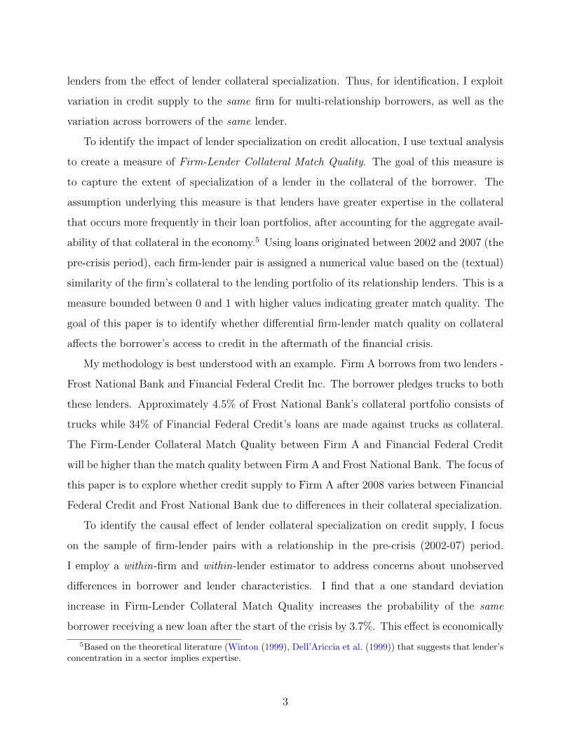
lenders from the effect of lender collateral specialization. Thus, for identification, I exploit

variation in credit supply to the same firm for multi-relationship borrowers, as well as the

variation across borrowers of the same lender.

To identify the impact of lender specialization on credit allocation, I use textual analysis

to create a measure of Firm-Lender Collateral Match Quality. The goal of this measure is

to capture the extent of specialization of a lender in the collateral of the borrower. The

assumption underlying this measure is that lenders have greater expertise in the collateral

that occurs more frequently in their loan portfolios, after accounting for the aggregate avail-

ability of that collateral in the economy.5 Using loans originated between 2002 and 2007 (the

pre-crisis period), each firm-lender pair is assigned a numerical value based on the (textual)

similarity of the firm’s collateral to the lending portfolio of its relationship lenders. This is a

measure bounded between 0 and 1 with higher values indicating greater match quality. The

goal of this paper is to identify whether differential firm-lender match quality on collateral

affects the borrower’s access to credit in the aftermath of the financial crisis.

My methodology is best understood with an example. Firm A borrows from two lenders -

Frost National Bank and Financial Federal Credit Inc. The borrower pledges trucks to both

these lenders. Approximately 4.5% of Frost National Bank’s collateral portfolio consists of

trucks while 34% of Financial Federal Credit’s loans are made against trucks as collateral.

The Firm-Lender Collateral Match Quality between Firm A and Financial Federal Credit

will be higher than the match quality between Firm A and Frost National Bank. The focus of

this paper is to explore whether credit supply to Firm A after 2008 varies between Financial

Federal Credit and Frost National Bank due to differences in their collateral specialization.

To identify the causal effect of lender collateral specialization on credit supply, I focus

on the sample of firm-lender pairs with a relationship in the pre-crisis (2002-07) period.

I employ a within-firm and within-lender estimator to address concerns about unobserved

differences in borrower and lender characteristics. I find that a one standard deviation

increase in Firm-Lender Collateral Match Quality increases the probability of the same

borrower receiving a new loan after the start of the crisis by 3.7%. This effect is economically

5Based on the theoretical literature (Winton (1999), Dell’Ariccia et al. (1999)) that suggests that lender’sconcentration in a sector implies expertise.

3

significant, equivalent to 17.9% of the unconditional probability that a firm gets a loan from

its relationship lender. Under a partial equilibrium counter-factual exercise where borrowers

match to lenders with the highest specialization in their collateral, aggregate lending would

increase by 14.8%.

Next, I evaluate the potential sources of lender advantage driving the specialization

of lenders in the aftermath of the financial crisis. My main focus is on the distinction

between lending advantages that are collateral-specific from those that are industry-specific

or firm-specific. While collateral specialization can be considered one aspect of industry

specialization, I show that the effect of collateral match persists even after the inclusion of

controls for lender specialization in an industry, and by looking across borrowers within the

same lender-industry cell. I find that after controlling for lender specialization in the 6-digit

NAICS industry of the borrower, a one standard deviation in Firm-Lender Collateral Match

Quality increases the probability of receiving a new loan by 3.5%, roughly equal to the 3.7%

increase in lending in the baseline specification.

I also test whether lending advantages are driven by specialization in collateral or firm-

specific knowledge, such as soft information. Thus, I include proxies for borrower-lender

relationship strength as controls in the baseline specification. While these measures may

themselves be correlated to the collateral match between the borrower and the lender (i.e.,

stronger relationship because of expertise in collateral), I show that a one standard deviation

increase in collateral match including relationship strength controls leads to a 2.1% higher

likelihood of getting a new loan compared to 3.7% higher likelihood without the controls.

As an alternate test for soft information, I study how firm-lender collateral match of new

borrowers of the lender compare to its current set of borrowers. For new borrowers, the lender

does not have private, firm-specific information. I show, however, that the new borrowers

are closely related to the lender’s collateral specialization. This provides further support to

my contention that collateral specialization explains lender behavior, rejecting the null that

collateral does not differentially affect credit supply across lenders.

Next, I explore the mechanisms driving lender specialization in collateral. I argue that

lender specialization is driven by informational advantages of the lender6 by eliminating

6Advantages may include ex-ante private asymmetric information about the quality of collateral, or

4

other potential channels for lender specialization. First, I show that lending behavior is not

driven by the type of business the lender is involved in. Traditionally, banks are thought

to do more cash-based lending (evaluate firms based on projected cash flows) while finance

companies tend to lend against collateral values. For some lenders in the sample, specifically

captive finance companies, increasing collateral sales and collateral value may be the primary

motivation for lending. I find that these differences do not explain the observed specialization

patterns.

Second, lenders may concentrate new lending to otherwise distressed borrowers to reduce

the probability of having to recognize loan losses on old loans and thus, reduce charges

against their loss reserves and capital. If the firm-lender collateral match captures the level

of prior lending or commitments of the lender, they may be inclined to continue lending

to borrowers with higher collateral match to prevent losses on their loan portfolio. I show,

however, that low-capitalization banks, who are most likely to have such motives to distort

lending,7 do not behave differently from high-capitalization banks.

Third, an alternate hypothesis for change in lender behavior could be concerns about fire-

sale discounts.8 Lenders may concentrate their lending portfolio, in a crisis, on the types of

collateral least likely to face losses in the event of borrower default. To test whether fire-sale

concerns drive lender behavior, I test how lenders respond to industry distress. In the case

that lender behavior is driven by fire-sales concerns and not collateral specialization, lenders

would be less likely to lend to distressed industries that face greater fire-sale discounts even

if they have greater specialization in the collateral. However, importantly, I show that the

effect of Firm-Lender Collateral Match Quality on lending does not vary by level of industry

distress.

Next, I examine the impact of lender collateral specialization on firm-level access to

credit and real economic activity. For the firm-level results, I create a measure of Firm

Collateral Match as the weighted average of firm-lender collateral match qualities. I show

that greater the aggregate measure of firm match quality, larger the availability of credit to

greater ability to redeploy the collateral ex-post through the presence of existing infrastructure for collateralstorage and disposal, network of potential buyers etc.

7See Caballero et al. (2008)8See Shleifer and Vishny (1992)

5

firms from its relationship lenders. A one standard deviation increases in Firm Collateral

Match leads to 3.2% increase in lending from relationship lenders, equivalent to 10.4% of the

mean probability of a repeat loan to a firm.

Furthermore, I show that firm’s match quality can have real implications affecting firm

employment during the crisis, and the pace of recovery following the financial crisis. A one

standard deviation increase in firm collateral match quality increases the average level of

post-crisis firm employment by 0.83%. This effect is economically large. The average firm

in the sample experiences a 6.6% growth in employment between the pre-crisis and post-

crisis period. Thus, a one standard deviation increase in firm collateral match quality raises

employment by a value equal to 12.5% of the mean growth rate in employment.

The effect of firm’s collateral match quality on employment implies that relationship

lender matching is a significant determinant of firm outcomes. This suggests firms are unable

to completely substitute for drop in lending from relationship lenders. To study the ability

of firms to substitute, I once again focus on borrower collateral. I create a measure of Firm

Similarity by comparing the collateral of the firm to the (weighted) average lender in the

economy. This measure quantifies how commonly accepted the borrower’s collateral is in the

economy. I show that firms with greater overall similarity (i.e. more lenders lending against

the firm’s collateral) are more likely to substitute to a new lender. A one standard deviation

increase in firm similarity increases the probability of borrowing from a new lender by 3.4%.

In summary, this paper provides evidence on the important role of lender specialization

in borrower collateral for firm outcomes in a downturn. I show that within-firm, and within-

lender, a greater level of ex-ante collateral match between borrowers and lenders leads to

increased credit supply in the aftermath of the financial crisis. This increase is due to lender

specialization in collateral driven by informational advantage of the lender. I further show

that quality of collateral match between the borrower and lender can have aggregate impact

on total credit to the firm, as well as firm employment.

The rest of the paper is organized as follows. Section 2 documents how the paper relates to

the extant literature. Section 3 described the data sources and panel construction. Section 4

describes the text analysis techniques used in creating the measure of Firm-Lender Collateral

Match Quality. Section 5 describes the identification strategy and empirical results. Section

6

6 concludes.

2 Related Literature

This paper relates to several strands of the literature. First, my paper relates to the role

of lender specialization in credit allocation. Traditional banking theory argues for diver-

sification across projects (Diamond (1984), Boyd and Prescott (1986)). Here, diversifica-

tion reduces risks associated with idiosyncratic shocks lowering monitoring costs for lenders.

This suggests banks should avoiding concentrating their lending portfolio. However, the

argument relies on banks having equal expertise in all sectors of the economy.9 But, lender

specialization has been shown to be valuable as it helps in information collection (Loutskina

and Strahan (2011), Berger et al. (2017)), increase market valuations (Laeven and Levine

(2007)), allows lenders to extract rents (Petersen and Rajan (1994), Rajan (1992)), and

protects against market competition (Boot and Thakor (2000), Dell’Ariccia and Marquez

(2004), Hauswald and Marquez (2006), Degryse and Ongena (2004)).10

Consequently, in practice, lenders tend to be specialized by type of borrower (Carey et al.

(1998)), or export markets (Paravisini et al. (2018)) among other areas. Liberti et al. (2017)

document the role of lender specialization in collateral. While Liberti et al. (2017) show

that collateral can affect lending decisions of lenders in new markets, I show that the extent

to which borrower’s collateral matters for credit supply changes with lender constraints.

Thus, I add to the literature on lender specialization by documenting the important role of

collateral in lender specialization decisions when lenders are constrained, and the important

real economic consequences of lender specialization on borrowers.

Second, my paper relates to the literature on matching between borrowers and lenders

in the economy. Prior work has shown that borrower-lender matching is influenced by geo-

graphic proximity (Petersen and Rajan (1995), Petersen and Rajan (2002)), bank size (Stein

(2002), Hubbard et al. (2002), Cole et al. (2004)), or bank capital structure (Schwert (2018)).

9Diversification may hurt as monitoring becomes weaker in new sectors (Winton (1999), Acharya et al.(2006), Berger et al. (2010)) or if resource allocation across divisions is inefficient (Rajan et al. (2000)).Furthermore, Fricke and Roukny (2018) show that high leverage can undo the benefits of diversification

10Private information of some lenders may also have externalities on other market players. See for example,Stroebel (2016) or Murfin and Pratt (2019)

7

I extend this literature by documenting matching based on collateral, and studying the con-

sequences of matching for credit and real outcomes. In Schwert (2018), under the assumption

that observed matches are optimal, the paper explores borrower-lender characteristics that

explain the match. Unlike his approach, I estimate the quality of matches between borrowers

and lenders and document the consequences of changes in match quality. I also examine how

borrower-lender matching changes over the business cycle. In this respect, the mechanism is

similar to the one described by Granja et al. (2018) for geographic proximity.

Third, my paper relates to the role of collateral in lending. Collateral is a significant

feature of loan contracts, especially small business loans where over 88% of small business

loans were backed by collateral in 2016.11 On the theoretical side, collateral arises naturally

in settings with asymmetric information.12 The importance of collateral has also been doc-

umented in the empirical literature.13 I add to the literature on the importance of collateral

by showing that the benefits to collateral vary by the type of collateral as well as by lender.

I also focus on the dynamic role of collateral in lending decisions.

Fourth, my paper relates to the literature on the role asset specificity in lending. Start-

ing with seminal work by Shleifer and Vishny (1992), the literature has documented the

important role of asset fire sales and asset redeployability for credit access. The empiri-

cal literature has shown that firms with liquid collateral receive loans with longer maturity

(Benmelech (2008)), lower spreads on loans, higher credit ratings, and higher LTV ratios

(Benmelech and Bergman (2009), Almeida and Campello (2007)), and have a lower cost of

capital (Ortiz-Molina and Phillips (2014)). Asset redeployability has been shown to be an

important determinant of leverage for small businesses (Campello and Giambona (2013),

Giambona et al. (2018)) with special importance during periods of distress (Pulvino (1998),

11Benmelech et al. (2019) document the secular downward trend in secured debt over the past century butdo not focus on small business lending around the financial crisis.

12Collateral can serve as a signaling device reducing adverse selection (Stiglitz and Weiss (1981), Besankoand Thakor (1987a), Besanko and Thakor (1987b), Bester (1985), Bester (1987), and Chan and Thakor(1987)), moral hazard (Boot et al. (1991), Boot and Thakor (1994), and Holmstrom and Tirole (1997)),and by increasing contract enforceability (Albuquerque and Hopenhayn (2004) and Cooley et al. (2004)).Collateral also arises in settings with costly state verification (as in Townsend (1979), Gale and Hellwig(1985), and Williamson (1986)), and to incentivize lender monitoring (Rajan and Winton (1995)).

13For reference, see Berger et al. (2011b), Jimenez and Saurina (2004), Berger and Udell (1995), Johnet al. (2003), Berger and Udell (1990), Brick and Palia (2007), Chakraborty and Hu (2006), Jimenez et al.(2006), Berger et al. (2011a), Berger et al. (2016).

8

Schlingemann et al. (2002), Acharya et al. (2007)).14 Consistent with this literature, I show

using detailed firm-level data, and comparison across industries, that firms with more com-

monly accepted collateral have a easier time substituting credit when faced with a supply

shock. However, I add to this literature by documenting not only the importance of the type

of collateral but the importance of the lender lending against the collateral.

Finally, my paper relates to the literature on credit supply during and in the aftermath

of the financial crisis. The literature argues that changes in credit supply played an impor-

tant role in triggering and amplifying the financial crisis.15 Ivashina and Scharfstein (2010)

document the drop in bank lending to large businesses following the bankruptcy of Lehman

Brothers. Chen et al. (2017), Bord et al. (2018) document specifically the impact of the

financial crisis on small business lending.16 I add to this literature by documenting the het-

erogeneity in treatment across borrowers of the same lender. With detailed information on

borrowers and lenders of small business loans, I document a new channel for the propaga-

tion of credit supply shocks to the economy.17 Furthermore, I contribute to the literature

documenting the real effects of credit supply shocks with detailed information linking small

business lending to employment outcomes.18

3 Data and Summary Statistics

3.1 Data Sources

The insights in this paper come from combining two data sources- UCC filings for information

on firm-lender relationships and the Census of Establishments for firm outcomes.

14Shleifer and Vishny (2010) provide a full review of the fire sales literature. In contrast, Diamond et al.(2019) argue that high asset pledgeability could hurt firms in a downturn. Collateral usefulness also dependson creditor rights (Calomiris et al. (2017), Vig (2013), Campello and Larrain (2015)), and ability to repossessthe asset (Eisfeldt and Rampini (2008), Benmelech and Bergman (2008)). Furthermore, type of collateralpledged varies by firm characteristics (Liberti and Sturgess (2014), Mello and Ruckes (2017)).

15Mian and Sufi (2009), Mian and Sufi (2018) argue that expansion in supply of mortgages was responsiblefor the boom and bust in housing markets, and the subsequent recession.

16Cortes et al. (2018), Acharya et al. (2018a), Covas (2018) argue that post-crisis stress testing of largebanks led to decrease in small business lending.

17Chaney et al. (2012), and Adelino et al. (2015) document the importance of collateral channel using realestate as collateral

18See Bernanke (1983), Peek and Rosengren (2000), Benmelech et al. (2016), Ashcraft (2005), Chodorow-Reich (2013), Greenstone et al. (2014), Bentolila et al. (2017)

9

3.1.1 UCC-1 Filings

My main dataset is sourced from state-level public records filed under the Uniform Com-

mercial Code (UCC). The UCC is the set of laws that guide all commercial transactions

in the U.S., such as sales, leases, and rentals. Article 9 of the UCC states that secured

creditors have the right to make a public filing detailing their claim on borrower assets when

originating a secured loan. In case of borrower default, these filings determine priority in

bankruptcy proceedings. Secured lenders without an active UCC filing are considered un-

secured creditors by law. For this reason, and due to the low cost of making UCC filings

(typically $15-$25 for electronic filings), I believe my sample is representative of the universe

of secured lending.

UCC filings under Article 9 are made to determine security interest in “personal-property”.

Filings are made at the state-level at Secretary of State offices in the state of the borrower.19

Real estate transactions, while governed by the UCC laws, require lenders to make filings

at local county offices responsible for tracking that piece of land.20 Furthermore, properties

with titles, such as automobiles, boats, and airplanes, generally do not require state-level

UCC filings for liens.21 Any other collateral pledged by borrowers must be detailed through

a state-level UCC filing.

One of the biggest strengths of the UCC data is that it allows for the creation of a “quasi”

credit registry for the U.S. including data on loans originated by bank and non-bank lenders

such as finance companies.22 To the best of my knowledge, Edgerton (2012) is the only other

paper that creates a similar registry from UCC filings for the U.S. by focusing on businesses

in California over a six-year period. Murfin and Pratt (2019) use data on equipment financing

sourced from UCC filings to study optimal pricing by captive finance companies. However,

their paper only includes heavy equipment financing of firms in construction and agriculture.

19State of incorporation for registered businesses or headquarters for unincorporated businesses.2063% of loans to small and medium-size businesses are backed by non real-estate collateral - see Calomiris

et al. (2017)21Recent court rulings have opened up debate on the need for UCC-1 filings on titled property.

See for example - https://www.cscglobal.com/blog/court-finds-certificate-of-title-alone-not-sufficient-to-create-security-interest.If the titled property is inventory meant for sale, a UCC filing is required.

22List of largest lenders in the sample available in Appendix A5

10

One shortcoming of the UCC data is that we can only observe the extension of credit. Loan

terms such as loan amount or pricing information are not reported.23

3.1.2 Texas Data

In this paper, I mainly focus on firms operating in Texas. To understand the role of firm-

specific collateral on firm outcomes, I need detailed information on collateral pledged by

firms. While this information is available at individual state offices, a bulk download of

historical data is either unavailable or prohibitively expensive. California and Texas are two

states that allow for the bulk download of UCC filings. However, the California data only

goes back six years from the date of download (see Edgerton (2012) for details).

The Texas Secretary of State website allows for the download of historical data starting

from 1966. However, I restrict my sample to filings made from 2002 onwards. The main

reason for this choice is a July 2001 change to the laws governing where UCC filings are

to be made. Before this date, a UCC filing was required in every state in which a firm

maintained assets. After 2001, the filing location was changed to the state of incorporation

for incorporated businesses or the location of the CEO’s office for unincorporated firms with

multiple offices.24

Thus, the final sample includes six years (2002-07) before the crisis, and a nine year crisis

and recovery period (2008-16) with a total of 995,657 new loan originations in the period.

Collateral Information As described above, UCC filings are made for all non real-estate,

non-titled personal property of borrowers. Figure A3 gives an example of a typical UCC

filing. The filing includes information on the borrower (Best Dedicated LLC located in

Kernersville, North Carolina), the lender (Webster Capital Finance Inc), the date of the

filing (8/12/2014), and a description of the collateral (in this case, trailers) pledged.

There is large variation in the type of collateral pledged for loans, a fact which is going

to be critical for my identification strategy. For example, collateral can vary from very

23Petersen and Rajan (1994) show that, based on a survey of small businesses, availability of credit isaltered on quantities, rather than prices. More recently, DeYoung et al. (2015) show that decrease in creditto SMEs during the crisis was caused not by increased pricing of credit risk but rather by quantity rationing.

24Including data before 2002 might lead to repeat counting of the same loan to a business with multipleoffices.

11

specifically identified assets (as in the example above which identifies assets by their serial

numbers) to blanket liens. Detailed examples are provided in Appendix Section A4.3.

Blanket liens occur commonly in collateral descriptions. A blanket lien is a lien that

gives the lender rights to seize all assets of the borrower in case of default. As such, these

statements contain generic descriptions of the collateral. A typical blanket lien reads as

follows:

“all assets of debtor wherever located and whether now owned or existing or here

after existing or acquired including, but not limited to, the following: all accounts,

accounts receivable, furniture, machinery and equipment, inventory, goods in pro-

cess, goods, contract rights, documents of title, chattel paper, letter of credit rights

and instruments, general intangibles, instruments, documents, all returned goods

and repossessions and replacements thereof, deposit accounts, cash, cash equiva-

lents, investment property, all attachments, accessions, accessories, fittings, in-

creases, tools, parts, repairs, supplies and commingled goods relating to any of the

foregoing and all products, substitutions, renewals, improvements, replacements,

and proceeds of any of the foregoing, and all books, correspondence, credit files,

records, invoices and other papers and documents, tangible or electronic, relating

to the foregoing, and to the extent so related, all rights in, to and under all poli-

cies of insurance, including claims of rights to payments thereunder and proceeds

therefrom, including any credit insurance”

As such, blanket lien descriptions do not provide sufficient information about the exact

assets of the borrower, which is crucial for my measure and identification strategy. Thus, I

remove from the sample loans with blanket lien pledges. My sample retains firms with real

assets where an exact description of the asset is available. Appendix Section A6 includes

additional results comparing firms with blanket liens (or cash-flow pledges) to firms that

pledge real assets.

12

3.1.3 Longitudinal Business Database

For real outcomes at the firm-level, I use information from the U.S. Census Bureau, specif-

ically the Longitudinal Business Database (LBD). The LBD contains annual data (as of

March 12) on establishment level employment, payroll, industry, location, and years of op-

eration for the universe of non-farm employer firms in the U.S.

The LBD is the most comprehensive and accurate source of firm-level employment avail-

able in the U.S. and contains time-invariant establishment identifiers to track changes in

outcomes over time. The database covers both single-establishment and multi-establishment

firms. A firm-level identifier tracks the various establishments operated by a single legal

entity.25

Finally, I aggregate the establishment-level data to the firm-level to track the effects

of credit access on firm employment. The majority of the sample (∼ 92%) is single-

establishment firms. For firms with multiple establishments, I take the firm county (industry)

as the county (industry) with the highest employment share of the firm.

3.2 Matching

To track the relation between firm credit and employment outcomes, I link the loan data

from UCC filings to the LBD. With no common identifiers between the UCC Filings and

the Census data, I use a fuzzy match based on firm names. To improve the accuracy of the

matches, I focus on fuzzy name matching within a ZIP code, i.e., I look for the closest name

match among all firms in the borrower’s ZIP code. I use a combination of bigram string

comparators to aid with the matching.26 Through my matching algorithms, I am able to

match roughly 52% of the total loans. The match rate over time is provided in Figure A1.27

25FIRMIDs are generated from Employer Identification Numbers (EIN) in tax forms. Thus, a firm is a setof establishments under the same tax filing unit. A single large firm may have multiple EIN numbers. Thisis less of a concern for small businesses.

26See COMPGED and SPEDIS functionality in SAS27There are multiple reasons for unmatched firms in the original sample. First, the LBD only contains

employer firms (non-farm payroll employment excluding non-profit organizations). Thus, non-employer firmswith outstanding loans cannot be matched to the LBD. Non-employer firms account for nearly 23 of the28 million establishments in the U.S. In unreported results, I show that the lending results are robust toincluding the entire sample of firms. Second, firms operating under multiple names might generate low matchscores. Third, firms that exit the sample before the start of the financial crisis are dropped. Further detail

13

The final matched sample includes 93,000 non-FIRE firms and roughly 486,000 loans

between 2002 and 2016. Comparison of the full Census data to the matched UCC lending -

Census data is provided in Table A2. On average, the matched sample is larger (70 employees

in matched sample vs. 25 employees in the average firm) and older (13.6 vs 10.6 years in

operation).

In this matched sample, 44,500 firms have at least one loan between 2002 and 2007 (pre-

crisis period). Of these, 23,500 firms have loans with real assets pledged as collateral. These

23,500 firms, therefore, constitute my baseline sample. Summary statistics on the baseline

sample are provided in Panel A of Table 1. The average firm has operated for 12.73 years

as of March 2007, with 14.12 employees in that year.

4 Collateral Match Quality

The goal of this paper is to identify whether differences in level of firm-lender collateral

match affect firm access to credit in the event of a credit supply shock. Specifically, I study

how specialization of a lender in the assets of the firm can affect firm outcomes. In this

section, I formalize what I mean by collateral match and lender specialization and how I

construct these measures.

In principle, I want to estimate the collateral that a lender is specialized in and measure

how a borrower’s collateral compares to the specialization of the lender. My measure relies

on the theoretical literature (Winton (1999), Dell’Ariccia et al. (1999)) that suggests that

lender’s concentration in a sector implies expertise. In these models, because lenders have

more interaction with borrowers in sectors in which they have a greater exposure, they are

better informed about these sectors. Similarly, under my measure, borrowers with collateral

more in line to what the lender traditionally accepts (controlling for aggregate availability

of the collateral in the economy), would imply a better match on collateral.

I create the measure of firm-lender collateral match by examining the textual similar-

ity between the borrower’s collateral and the collateral accepted by the lender. To create

the measure, I translate the text descriptions into a numeric equivalent and compare two

on the data cleaning and matching are provided in Appendix A4.

14

descriptions using the cosine similarity measure. I describe each of these steps in detail

below.

4.1 Text to Numeric Conversion

First, I translate textual descriptions of collateral into a numerical format suitable for analy-

sis. I start by aggregating the collateral description for each loan filing and cleaning collateral

descriptions.28 Next, I create a dictionary of all words in the universe of collateral descrip-

tions. I manually inspect the list to retain words that describe the collateral while removing

extraneous descriptive words.29 To retain loans/firms with real assets, I create a dictionary of

words for all real assets (equipment and machinery) from my sample, and retain descriptions

with just these words. Appendix A5 contains the full list of words.

The words are then transformed into a matrix of features (in my case, collateral types)

using a “bag of words” approach. Each description is represented as a vector where the ith

component takes a value of one if the ith feature is present, and zero if not.30 Vectors are

adjusted by feature weights across documents, i.e., the inverse document frequency (IDF).

The IDF captures how common a given word is in the overall sample of loans. Scaling by

IDF prevents the overweighting of common terms. The idea behind IDF is to provide higher

weights to words with more information. Collateral that occurs rarely provides greater infor-

mation about a lender’s specialization if present in it’s portfolio. In my case, the weighting

controls the aggregate availability of the collateral in the economy.

To understand the importance of weighting in my case, consider the following hypotheti-

cal example. Lender A’s portfolio consists of 10% loans against cattle and 10% loans against

tractors. Overall in the economy, only 1% of loans are made against cattle while 20% of

loans are made against tractors. Without the weighting, the collateral match between a

28I remove punctuation, special characters, extra spaces, and numbers (like serial numbers of equipment)from the description. Furthermore, I remove stop words (most common words that occur in the Englishlanguage).

29For example, common words in collateral description include “proceeds”, “limited”, “including’ whichdo not add additional information about the assets are removed.

30The baseline measure does not include weighting by term frequency (TF), i.e., the number of times aterm appears in a given description. Collateral descriptions very often repeat terms to describe the claimson the same asset. Thus, weighting by TF could lead to over weighting firm assets. I ensure results arequalitatively similar when including the weighting.

15

borrower with tractor to Lender A would be identical to the collateral match between a

borrower with cattle and Lender A. However, the disproportionate share of cattle in Lender

A’s portfolio compared to the economy implies Lender A has greater specialization in cattle

than the average lender in the economy. The weighting captures this effect.

To formalize, for each word w in collateral description c in the universe of collateral

descriptions C, I create

TFIDFcw = TFcw × IDFCw

where TFcw takes the value 1 if the firm has the type of collateral and 0 if it does not,

and

IDFCw = logN

|c ∈ C : w ∈ c|

which is the log of the total number of collateral descriptions scaled by the number of

descriptions where the term w appears

4.2 Cosine Similarity

Next, I use the concept of cosine similarity to calculate the match quality on collateral

between borrowers and lenders. Cosine similarity has been previously used in the finance

literature to measure industry similarities in Hoberg and Phillips (2010) and Hoberg and

Phillips (2016) and to calculate the impact of patents in Kelly et al. (2018). Technically,

with each description represented in the vector space as described above, similarity between

two descriptions can be calculated as the cosine of the angle between the two vectors. This

commonly used measure follows from the Eucledian dot product formula

Similarity = cos(θ) =~A · ~B~‖A‖ ~‖B‖

To create my measure of collateral match between Firm A and Lender B, I compare the

collateral of firm A to the collateral of the average borrower of lender B.

The intuition underlying cosine similarity is the idea that two collateral descriptions are

16

similar if their vectors “point” in the same direction. It is a measure of orientation rather

than magnitude. This is advantageous when comparing collateral descriptions of varying

lengths. Descriptions with the same set of words in the same proportion will have similarity

of one and descriptions with no common words between them will have a similarity of zero.

In this aspect, cosine similarity performs better than standard measures such as Euclidean

distance when high dimensional, sparse matrices are present.

To better understand the intuition, consider a simple example. Think of a universe with

just two types of collateral - cattle and tractors - in equal proportion. In this world, every

firm and lender can be represented in a two-dimensional space.

0 0.5 1 1.5 20

0.5

1

1.5

2

Firm A

Lender B

Lender C

θ1

θ2

Tractor

Cat

tle

A firm with only tractors (Firm A) is on the X-axis. Lenders with both tractors and

cattle can also be represented in the two-dimensional space. Consider two such lenders -

Lender B (with 50% tractor and 50% cattle) and Lender C (25% tractors and 75% cattle).

To measure the match quality (similarity) between a firm and lender, I calculate the cosine

of the angle between the two vectors. The angle between Firm A and Lender B is smaller

than Firm A and Lender C. A smaller angle implies greater “similarity” in collateral, or in

other words, a better match on collateral. In this example, Firm A has a better match to

Lender B (cosine similarity of 0.7071) than it does to Lender C (cosine similarity of 0.3162).

I calculate the match quality at the firm-lender level as the cosine similarity between the

firm and the average borrower of that lender in the sample. Measures are all calculated based

on loans originated in the pre-period (2002-07). To construct the measure, I use information

17

on real assets pledged by the borrower to its relationship lender, and compare that to the

average borrower of its relationship lender.

Statistics on the firm-lender collateral match quality values are provided in Panel B of

Table 1. The average match quality between firms and lenders on collateral for observed

firm-lender pairs is 0.3827 with a standard deviation of 0.3085. The 10th percentile of the

distribution is 0.01649 and 90th percentile is 0.8619.

5 Empirical Methodology and Results

5.1 Empirical Strategy

I study how collateral matching between borrowers and lenders affects credit supply to firms

in the aftermath of the financial crisis. I am interested in understanding whether lenders

treat borrowers differentially based on the collateral available at the firm and the level of

matching between borrowers and lenders on collateral. Broadly speaking, a drop in credit to

firms following the financial crisis could be driven either by lower firm demand, or a decrease

in supply of credit to firms. Under the demand side explanation, firms that received fewer

loans did so because they lowered their demand for credit. Under the supply side argument,

decrease in lending to firms could be driven by the characteristics of the firm, or differences

in firm collateral. I aim to isolate the credit supply channel, specifically the role of collateral,

in determining firm credit access.

To estimate the causal effect of borrower-lender collateral match on credit supply, I follow

a difference-in-difference strategy with continuous treatment intensity. I measure a firm’s

treatment intensity based on the level of matching between a borrower and lender using

collateral pledged by the firm to the lender in loans extended to it in the pre-crisis (2002-07)

period. I then study the effect of the firm’s collateral match to its lenders on credit access

in the downturn.

I first document the role of collateral in observed matching between borrowers and lenders.

I show that the equilibrium distribution of borrower-lender pairs show a much higher col-

lateral match score than would be implied by a random match. Furthermore, there is het-

18

erogeneity in level of matching across borrower-lender pairs. My tests rely on exploiting the

heterogeneity in these match scores.

Given non-random matching between borrowers and lenders, endogeneity concerns due to

self-selection arise. Specifically, I am concerned that borrowers that have better matches to

lenders may be unobservably different from borrowers with weak lender matches. Similarly,

lenders who lend to borrowers with collateral in which the lender has greater expertise may

be different from lenders who make loans to borrowers outside of their specialization.

To address the identification concerns, I focus on differences in lending behavior to bor-

rowers of the same lender, and lenders of the same borrower. That is, I estimate the effect

of matching on collateral within borrowers and within lenders. The aim of the within-firm

regression (see for example Khwaja and Mian (2008), Gan (2007), Schnabl (2012), Jimenez

et al. (2017)) is to control for unobservable differences across firms. Through this approach,

I test the effect of collateral matching independent of inherent differences across borrowers

and lenders. Conditional on having borrowed from a given set of lenders in the pre-crisis

(2002-07) period, I test the post-crisis change in lending to the same firm from lenders with

differential levels of collateral match.

I then try to disentangle other potential channels driving lender behavior. Specifically,

I want to establish two facts. First, I aim to show that differences in lending are driven

by collateral specialization and not other potential lender advantages such as knowledge

about the industry, or firm-specific knowledge. Second, I try to disentangle the channels

driving specialization of lenders. Broadly speaking, lender specialization can be driven by

informational advantages about the collateral, or the lender’s concerns about potential losses

incurred on loans. I argue informational advantages about the collateral push lenders to

specialize in a downturn.

After establishing the importance of collateral matching for lending outcomes at the firm-

lender level, I proceed to test the effect of matching at the firm-level. I study the effect of

credit from pre-existing relationship lenders of the firm. Furthermore, I study the ability of

firms to substitute to new lenders, and the total credit available to the firm. Finally, I focus

on the differences in firm-level employment growth.

Below, I present each of these results in detail.

19

5.2 Firm-Lender Level Results

I start by documenting the importance of collateral match for lending outcomes. First, I

provide evidence for matching between borrowers and lenders based on collateral specializa-

tion of lenders. For this, I plot in Figure 1a two distributions. In the solid line, I plot the

firm-lender collateral match scores for all possible firm-lender pairs. That is, for every firm in

my sample, I create a measure of collateral match to every lender in the sample (irrespective

of whether they actually borrow from them). To create the measure, I use the pre-crisis

(2002-07) collateral pledged by the borrower and compare it to the pre-crisis lending port-

folio of the lender. The solid line, therefore, is the distribution of collateral match scores for

a random firm-lender match. Note that the distribution is highly skewed with most of the

distribution concentrated at near-zero values of collateral match. In the dashed-line, I plot

the same firm-lender collateral match scores for equilibrium observed matches of firm-lender

pairs (firm-lender pairs with a loan in the pre-crisis period). We note that the observed

firm-lender pairs have a greater match on collateral than would be implied by a random

matching. Specifically, nearly half the observed firm-lender pairs are in the right 5% tail

of the distribution of random scores. This provides suggestive evidence that collateral, and

lender specialization in collateral is an important determinant of firm credit.

In this paper, I am interested in how the level of matching between firms and lenders

affects change in lending during a crisis. For this, I focus my analysis on the second big

takeaway from the plot, i.e. the heterogeneity in match scores across observed borrower-

lender pairs. I exploit this heterogeneity to identify distribution of credit across borrowers

in a downturn.

Figure 1b plots the distribution of firms receiving loans in the pre- and post-crisis periods.

In the solid line, the Firm-Lender Collateral Match Quality for the full set of firm-lender

pairs with at least loan in the pre-crisis period is plotted. In the dashed line, I plot the

distribution of scores for the set of firm-lender pairs within that sample that also get a loan

after 2008. Notice that the distribution for firms receiving repeat loans is shifted to the right.

Figure 2 plots lending over time for firm-lender pairs with a relationship between 2002

and 2007. Firm-lender pairs are divided into two groups with above and below median scores

20

on firm-lender match quality score. We see that lending to the two groups grow along similar

paths in the pre-crisis period. After the start of the crisis, however, growth of loans between

the two groups diverge. Firms with closer match to the lender see a smaller drop in lending

during the crisis, and the gap between the two groups persists post-crisis.

However, as described above, this result is prone to endogeneity concerns. Firms that

borrow from lenders that are specialized in their collateral may be inherently different from

borrowers with weak lender matches. Similarly, lenders that lend to borrowers with collateral

they have expertise in may respond differently when constrained from lenders with a diverse

set of borrowers. Thus, I plot two additional figures. In Figure 3a, I split lenders to the same

firm into above and below median match scores. That is, firm-lender pairs are classified as

above or below median within firm. The sample here is restricted to firms with multiple

relationships pre-crisis. As above, lending to the firm from the two groups of lenders grows

on a similar path pre-crisis but diverges after the start of the crisis. Similarly, in Figure

3b, I separate firm-lender pairs into above and below median match quality within the same

lender, i.e. borrowers with high vs. low match to a given lender. Observed lending patterns

are similar with this categorization.

I now turn towards establishing this result more formally through regression analysis.

My main empirical specification is as follows:

Repeat Loanfl = αf + γl + βFirm-Lender Collateral Match Qualityfl + εfl (1)

for every firm f , lender l with a pre-existing relationship in the pre-crisis period. The

outcome variable takes value of 1 if the firm gets a new loan from the same lender in the

post-crisis (2008-16) period. Since all firm-lender pairs have a loan between them ex-ante,

repeat loan captures the change in lending to the firm. The main variable of interest is

the measure of Firm-Lender Collateral Match Quality created based on pre-crisis (2002-07)

loans. The measure captures the similarity between the borrower’s collateral and the lender’s

collateral portfolio. The baseline specification also includes borrower and lender fixed effects

to study the change in lending within the same firm across different lenders, as well as change

in lending across borrowers of the same lender. Standard errors are clustered at the lender

21

level.

Table 2 presents the results of the baseline specification in Equation 1. Column 1 presents

the results for all firm-lender pairs observed in pre-crisis period. A one standard deviation

increase in the match quality to lender increases the probability of a new loan by 2.04%

equivalent to 10.3% of the mean probability of a repeat loan. In column 2, I include controls

for county and industry31 of the borrower to control for differences in demand. The effect

increases to loan probability 2.41% for a one standard deviation increase in match quality.

In Column 3, lender fixed effects are included to control for lender-level variation in spe-

cialization and lender level differences in borrower matching. This increases the probability

of getting a repeat loan by 2.56%. Including lender fixed effects, local county-industry de-

mand, and firm controls in column 4 leaves the effect almost unchanged at a 2.53% increase

in repeat loan probability for a one standard deviation increase in match quality.

In Columns 5-7, I restrict the sample to firms with multi-lending relationships in the pre-

crisis period. Column 5 repeats the results of Column 3 for multi-lender relationship firms.

In this, the effect is slightly larger for this sample with a one standard deviation increase

in collateral match leading to a 3.36% increase in probability of a loan, equivalent to 16.2%

of the unconditional probability of getting a repeat loan. Including firm fixed effects in

Column 6 implies a one standard deviation increase in match quality leads to 3.27% increase

in repeat lending. That is, a one standard deviation increase in match quality between lender

and borrower increases lending to the same firm by 3.27%. Finally, the last column includes

both firm and lender fixed effects. Here, a one standard deviation increase in firm-lender

collateral match quality increases the probability of the firm receiving a loan by 3.7%, or

17.85% of the mean and 9.13% of the standard deviation of the probability of receiving a

repeat loan in the post-crisis (2008-16) period. These effects are large and economically

important to small firms who rely on debt financing. This indicates the important role of

borrower-lender collateral matching on small business lending.

Dynamic Difference-in-Difference

Next, I test for dynamic effects of firm-lender collateral match on lending. Specifically, I

31For multi-establishment firms, county is the assigned based on the region with highest employment sharefor the firm. Industry at 2-digit NAICS level but robust to narrower industry definitions.

22

run the following panel regression:

yflt =αf + γl + δt + βt Firm-Lender Collateral Matchfl × 1t + εflt (2)

where for each firm f , lender l pair with a loan in the pre-crisis period, I test for change

in lending each year t. The dependent variable is an indicator that takes value of one if

the firm-lender pair is observed to have a loan in a given year, scaled by frequency of loans

between the pair in the pre-crisis period. I scale the loans for a measure of percentage

change in lending given the data limitation of only observing the extensive margin of loan

originations. I am interested in how the coefficient on firm-lender collateral match changes

over time.

The dynamic version of the difference-in-difference setting identifies the timing of the

effect of firm-lender collateral match on loan outcomes, and to establish the existence of

parallel pre-trends which is crucial for my identification strategy.

The results are presented in Figure 4. Point coefficients can be found in Column 2 of Table

A6. I note that there are no statistically significant differences in lending across firms with

different levels of firm-lender collateral match in the pre-crisis period, except for a negative

and statistically significant coefficient on firm-lender collateral match in 2007. However,

after the start of the financial crisis (2008-), firms with high quality match are more likely to

get a loan. The effect persists for a number of years before recovering to pre-crisis levels in

2015. The magnitude of the effect is highest in 2008, with a one standard deviation increase

in match leading to an 9.2% increase in lending. Coefficients with varying levels of controls

can be found in Table A6.

5.2.1 Other Specialization Channels

Next, I aim to disentangle whether the observed results are truly driven by expertise in

borrower collateral. Lenders could have borrower-specific advantages beyond expertise in

collateral. Lenders could be specialized in the industry of the borrower, with an informational

advantage over borrowers in certain industries versus others. Lenders could also have firm-

specific knowledge, i.e., they may have borrower-specific information gathered through past

23

relationships with the lender. Such expertise may help them distinguish good borrowers

from bad, and could be the underlying mechanism driving observed lending behavior. I test

for these alternate channels below.

Industry vs. Collateral Specialization

First, I test for lender specialization in the borrower’s industry. Here, I analyze whether the

observed lending patterns are driven by the collateral of the borrower or the industry of the

borrower. Clearly, collateral and industry specialization may overlap. Borrower collateral

is largely driven by the industry in which the firm operates, for example - farmers often

use tractors while restaurants do not. However, oftentimes, collateral could be more broad-

based or more specific than implied by industry definitions. On the one hand, certain types

of collateral are used across multiple industries (e.g. forklifts and trucks). On the other

hand, lenders may specialize in lending only against certain types of collateral even within

an industry. As an example, People’s United Bank’s equipment financing division makes

loans against large service trucks but not against delivery or utility trucks.32

To separate lender specialization in an industry from its collateral specialization, I con-

duct two tests.

Repeat Loanfli = αf + γl × δi + βFirm-Lender Collateral Match Qualityfl + εfl (3)

for firm f , in industry i, borrowing from lender l, I include lender times industry fixed

effects to compare the treatment of borrowers within the same industry and who borrow from

the same lender. The sample is once again firm-lender pairs with a pre-existing relationship

in the pre-crisis period. The outcome variable takes value of 1 if the firm gets a new loan

from the same lender in the post-crisis period.

Panel A of Table 3 presents these results. I present the results with 2-digit and 3-digit

industry cells in Column 2 and 3 of Table 3. We see that including the industry interactions

changes the magnitude of the effect on likelihood of a matched firm getting a repeat loan

from the lender from 3.7% to 4.1% with 2-digit industry fixed effects and to 4.13% with

32https://www.peoples.com/business/equipment-finance/peoples-united-equipment-finance-

corporation/transportation

24

3-digit industry fixed effects. Collateral match, therefore, is still a significant determinant of

credit to borrowers.

While we might be interested in more narrow industry specializations of lender, includ-

ing very narrow industry fixed effects significantly would decrease sample size. Thus, in

alternative tests, I include instead of lender-industry fixed effects, lender concentration by

industry. I calculate lender concentration for narrow industry cells as the share of lending

to that industry in the lender’s portfolio.

Panel B of Table 3 presents these results. I include lender concentration at the 2,4, or

6 digit NAICS level. On including lender shares in industry, the probability of receiving a

repeat loan changes by 3.54% for a one standard deviation increase in firm-lender collateral

match quality across the specifications. That is, industry specialization does not seem to

explain away the observed borrower-lender collateral specialization.

Hard vs. Soft Information

Next, I test for whether lender behavior is driven by firm-specific knowledge. Lenders

may collect firm-specific soft information through lending relationships. Changes in lending

could, therefore, be driven by changes in firm-specific soft information rather than borrower

collateral. To test this, I conduct two tests.

First, I include proxies for relationship strength as controls in my baseline regression. I

create three proxies for strength of relationship - 1) Number of past loans from the lender,

2) share of total borrower lending from the lender, 3) time since the last loan between the

borrower and lender and the start of the crisis. An increase in number of loans from the lender

implies the lender has had greater interaction with the borrower, increasing the potential

soft information the lender has about the borrower. Conversely, if a longer time has passed

since the last loan to the borrower, the lender may have less up-to-date soft information

about the borrower.

While these measures proxy for soft information, they may themselves be correlated with

higher collateral match. For example, lenders may be willing to make a greater number of

loans to borrowers whose collateral they are familiar with. Thus, adding these controls may

bias downward the true effect of the importance of collateral matching. Consequently, the

25

results shown in Table 4 are a conservative estimate for the effect of collateral match quality.

As shown in Table 4, including the controls for relationship lending decreases the mag-

nitude on the coefficient of interest. In Column 1, I repeat the results from the baseline

regression. Here, a one standard deviation increase in firm-lender match quality increases

lending to the borrower by 3.72%. In Column 2, I use share of lending from the relationship

lender as a control for relationship strength. Compared to the baseline regression, the effect

here reduces to 2.29% increased loan likelihood, or 11% increase over the mean loan likeli-

hood. In Column 3, I include a measure of the average annual number of loans between the

borrower and lender in the pre-crisis period. This decreases the effect to 10.1% above the

unconditional mean of repeat loan . In Column 4, I include, as a control, the number of years

since the last loan to the borrower. The effect of match quality in this case is equivalent to

a 14.87% increase over the mean. Finally, I include both the number of loans and time from

the last loan as a control. The final effect is a 2.1% increase in loan likelihood, or 10.1% over

the mean value. Thus, even though the inclusion of these controls reduces the magnitude

of the effect on collateral match quality, lender match is still an economically significant

determinant of firm credit.

For the second test of importance of private firm-specific information, I test the im-

portance of match on collateral for new borrowers of the lender. For firms with no prior-

relationship, the lender does not possess private firm-specific information. As shown in

Figure 5, the observed matches for borrowers with loans in the post-crisis period is signif-

icantly higher than would be implied by a random firm-lender pair match. This provides

evidence for non-random matching between borrowers and lenders on collateral, conditional

on the lender not having any borrower-specific private information. Thus, collateral is an

important determinant of credit.

5.2.2 Mechanisms for Specialization

Next, I try understand the channels driving lender specialization in a downturn. Specif-

ically, lenders could be specializing for multiple reasons. First, lender specialization may

be driven by informational advantage. Lenders could have ex-ante private asymmetric in-

formation about the quality of collateral (ability to identify good collateral from bad), or

26

possess greater ability to redeploy the collateral ex-post (which may include existing infras-

tructure for collateral storage and disposal, network of potential buyers etc.). Informational

advantages may cause a lender to specialize in core collateral when in distress.

Second, lending behavior could be driven by the type of business the lender is involved

in. Traditionally, banks are thought to do more cash-based lending (evaluate firms based on

project cash flows) while finance companies lend against asset values (Carey et al. (1998)).

For some lenders in the sample, for example captive finance companies, collateral sales

and value may be primary motivation for lending. In this case, one could be worried that

concentration of lenders is driven by need to increase parent company sales and collateral

value. Thus, observed behavior of change in lending against collateral could be driven by

differences in underlying businesses.

Third, lenders may concentrate borrowing to prevent the writing down of bad loans, i.e.

distressed firm lending (zombie lending in Caballero et al. (2008)). Distressed banks, i.e.

banks with limited capital reserves and loan loss reserves, may reallocate credit to borrowers

most likely to lead to loan losses if cut-off. If the firm-lender collateral measure captures

the level of prior investment or commitment of the lender, they may be inclined to continue

lending to borrowers with higher match to prevent losses on their portfolio.

Fourth, lenders may be worried about fire sales losses (as in Shleifer and Vishny (1992)).

Lenders may concentrate their lending portfolio, in a crisis, on the types of collateral least

likely to face losses in the event of borrower default. In this case, lenders would concentrate

lending on the most redeployable assets in the economy which, in turn, are likely to be the

most liquid and least prone to fire-sale discounts. If, on average, lenders are more specialized

in assets that are more redeployable, a shift to redeployable collateral would line up with a

shift to collateral the lender is more specialized in.

In this paper, I argue that lender specialization is driven by informational advantage.

While I cannot directly test for the amount of information about collateral available to the

lender, I seek to eliminate the other potential channels described above.

Heterogeneity Across Lenders

First, I test for whether differences in underlying business of the lenders drive observed

27

variation in lending. To test for variation across lenders, I include indicators for lender type

in my baseline specification.

Repeat Loanfl = αf + γl + β1Firm-Lender Collateral Match Qualityfl

+ β2Firm-Lender Collateral Match Qualityfl × Lender Typel + εfl

(4)

Primarily, I test three main theories for specialization. First, I test for whether results

are driven by the subset of lenders in my sample that are only concerned about collateral

values. Lenders such as finance companies who lend primarily against collateral value of

the borrower could be shifting focus in times of distress while traditional lenders such as

banks lend to borrowers based on cash-flow evaluations. If that were the case, borrowers of

finance companies would be affected while banks would not alter behavior based on collateral.

In Column 1 of Table 5, I show that there is no statistically (or economically) significant

difference between banks33 and non-banks in their behavior in times of distress.

Second, my results may be driven by lenders whose primary business is not small business

lending. Specifically, captive finance companies, who are lending arms of manufacturing

companies, may be interested in increasing asset sales and propping up collateral values

to benefit the parent company sales in the goods market. These companies may increase

lending to increase their parent company’s revenue from sales. As these lenders are also on

average more specialized, greater lending from better firm-lender collateral matches could

be driven by increased lending from captive finance companies. I test whether this is case.

However, it is important to note that captive finance companies also have informational

advantage over other lenders in the economy. Specifically, captive finance companies have

greater information about the true quality and resale value of the collateral due to their

close association with the primary goods producer. Thus, difference across captive finance

companies and other lenders could be driven by either channel. I check whether shift in

lending is driven only be lenders whose primary goal is asset sales. In Column 2 of Table 5, I

interact the firm-lender collateral match quality measure by an indicator for captive finance

companies. The effect of increase in collateral match on lending is significantly higher for

captive finance companies. A one standard deviation increase in match quality increases

33Commercial banks, non-bank subsidiaries of bank holding companies, and credit unions.

28

lending by 3.85% for non-captive lenders and 10.18% for captive lenders.

Third, I test for differences driven by large banks. As shown in Chen et al. (2017), the

largest 4 commercial banks34 pulled out of lending to small businesses in the aftermath of

the financial crisis. If large banks are less specialized (more diversified) and pulled out of

small business lending, the average continuing post-crisis firm-lender pair would appear to

be better matched on collateral. I test for this in Column 3 of Table 5. There appears to be

no statistically significant difference across Top4 banks and other lenders in the sample.

Distress Lending

Next, I test for the existence of distressed firm lending. In a downturn, lender decisions

may be driven by bank need to prevent loan losses especially for undercapitalized banks. Such

lenders, to prevent writing down bad loans, may continue making loans to bad borrowers. If

firm-lender collateral match captures the extent of the lender’s exposure to the borrower’s

business, lenders have more to lose by cutting off lending to borrowers they are better

matched to and they may be inclined to continue lending to such borrowers.

To test for presence of distressed lending, I compare lending behavior of banks based

on their financial strength. Theories would indicate that distressed lending should be more

pronounced for lenders who are capital constrained. Under-capitalized banks are more likely

to engage in zombie lending behavior. Thus, I split my banks into above and below median

capitalization based on Tier 1 Capital Ratio of banks as of December 2006. I test for

differences across the two sets of banks through the following specification:

yflt =αfl + δt + β1t Firm-Lender Collateral Matchfl × 1t+

β2t Firm-Lender Collateral Matchfl × 1t × Low Lender Capitall + εfci

(5)

where for each firm f , lender l pair with a loan in the pre-crisis period, I test for change

in lending each year t. The dependent variable is an indicator that takes value of one if

the firm-lender pair is observed to have a loan in a given year, scaled by frequency of loans

between the pair in the pre-crisis period. I scale the loans for a measure of percentage change

in lending given the data limitation of only observing extensive margin of loan originations.

34JPMorgan Chase, Bank of America, Wells FArgo, Citibank after accounting for mergers and acquisitions

29

I am interested in the variation in the coefficient on firm-lender collateral match interacted

with lender capitalization over time. Low Lender Capital takes a value of one if the lender

has below median Tier-1 capital ratio as of December 2006.

Results are shown in Figure 6. I show that there is no statistically significant differences in

specialization across lenders with high and low Tier 1 capital. The point coefficients, though

insignificant, are negative, inconsistent with the distressed lending hypothesis. Coefficients

are presented in Appendix Table A7.

Fire Sales

Finally, I test for whether fire-sale concerns drive lender behavior. Here, the concern is

that lenders shift towards the types of collateral that are least likely to face fire sale discounts

when a borrower defaults (i.e. most common / redeployable collateral). If all lenders have a

lower initial concentration of illiquid collateral in their portfolio, a shift to liquid collateral

will appear to be a shift towards collateral they specialize in.

To test the existence of fire sales, I test differences in lending by industry performance.

Theories of fire-sales indicate that fire-sale discounts are highest when other potential buyers

of the collateral are in distress, and when inside users (buyers in the same industry) are

unable to buy the collateral.35 Therefore, fire sale discounts would be highest for distressed

industries. Thus, if lenders are worried about potential fire sale losses, even a high firm-

lender collateral match would not be sufficient to persuade a lender to lend to the borrower

in a distressed industry. I examine this by analyzing the interaction between the level of

industry distress and borrower-lender collateral matching.

Repeat Loanfli = αf + γl + β1Firm-Lender Collateral Match Qualityfl (6)

+ β2Firm-Lender Collateral Match Qualityfl × Industry Performancei + εfl

for firm f in industry i borrowing from lender l. I measure industry performance as

the weighted average change in employment around the financial crisis for all firms in the

borrower’s industry.36

35See Shleifer and Vishny (1992), Acharya et al. (2007), Shleifer and Vishny (2010) for details36Measured here as change in employment in a three year window around the financial crisis - i.e. change

30

The results are presented in Table 6. Columns 1,2,3 show the effect of firm-lender collat-

eral matches interacted with performance of the industry at the 3-digit, 4-digit, and 6-digit

NAICS level. I show that there is no statistically significant effect of collateral match by

performance of the industry on lending. This result suggests that fire-sale concerns are not

the main driver of lender specialization.

5.2.3 Counter-factual Exercise

I use the results from the within-firm regressions to study the aggregate effects of lender

matching on loan supply. I follow a strategy similar to Chodorow-Reich (2013) and Acharya

et al. (2018b) to estimate the aggregate effect on loan supply. For each borrower-lender pair,

I estimate the counter-factual loan supply if the firm and lender were aligned on collateral.

Specifically, I estimate the additional credit to the firm if the lender had been specialized in

the borrower’s collateral.

I consider the effect of change in matching to a lender under two different conditions.

First, I consider the highest possible firm-lender match score given the collateral the borrower

pledged to the lender. In other words, for every firm-lender pair, I take as given the collateral

pledged by the borrower to the lender. With this collateral, I compute the match scores to

all other lenders in the sample and take the lender with the highest match score as the

best match. Second, I consider improvement in lending under a hypothetical scenario where

specialized lenders exist for all borrowers. That is, I take the highest value, the 95th and 90th

percentile of the firm-lender collateral match score distribution. In this case, I estimate the

increased lending to the borrower under the hypothetical scenario where a lender specialized

to the same extent in the borrower’s collateral is available.

I use a partial equilibrium analysis to determine the aggregate effect. Under the assump-

tion that total lending is the sum of lending to individual firm-lender pairs, I can estimate

the effect as follows:

yfl = yfl + β × [ ˜FLSimbest − FLSimfl] (7)

in average employment between 2005-07 and 2008-10. Results are insensitive to the choice of the time period.Lack of balance sheet information for small businesses prevents the calculation of other industry performancemeasures for this sample.

31

where yfl denotes the fitted value from the regression in Equation 1. ˜FLSimbest is the

counter-factual level of firm-lender similarity on collateral. In the baseline case, this value

is 1 indicating perfect match in collateral between the borrower and lender. FLSimfl is the

observed value of the level of firm-lender collateral similarity. β1 is the estimated coefficient

in Table 2 Column 7.

yfl provides the estimate of loan supply conditional only on change in the level of firm-

lender matching keeping all else equal.

The total lending in this counter-factual case is calculated by summing loan supply over

all firm-lender pairs: ∑yfl (8)

To estimate the gain from the shift in lender matching, I estimate the change in lending

from the counter-factual lender matching scaled by the observed level of lending in the

economy, or

∑[yfl − yfl]yfl

(9)

The results are provided in Table 7. If borrowers changed their match to the most

specialized lenders for their collateral, total lending to multi-relationship firms would increase

by 14.76%. On the other hand, if there existed for each borrower, a lender as specialized in

its collateral as the most specialized lender, the increase would be even higher. A shift in

lender matching from the observed values to a counter-factual with perfect matching to the

lender increases total lending by 42.67%. If the firm-lender pairs were instead at the 95th

percentile of match score, lending would be 31.34% higher. At the lower bound of a match

score at the 90th percentile, aggregate lending would still increase by 21.76%.

5.3 Firm-Level Results

Having established the importance of collateral for credit outcomes at the firm-lender level,

I trace the impact of collateral match quality for firm outcomes. I create a measure of

firm-level collateral match by computing the wighted average of firm-lender collateral match

32

scores. That is,

Firm Collateral Matchf =∑l∈L

Lender Sharefl × Firm-Lender Collateral Matchfl

based on all relationship lenders l of the borrower f .

5.3.1 Lending

For firm credit outcomes, I first test the impact of firm collateral match on credit to firms

from their relationship lenders. In Figure 7a, I plot lending over time to firms with above

and below median match on collateral to their relationship lenders. We see that lending to

the two sets of firms grows along a parallel path before the start of the crisis. After 2008,

firms with better match to their relationship lenders get more credit from them, and this

gap persists in the post crisis period.

To control for differences across borrowers with differential collateral match to their

relationship lenders, I regress firm credit from relationship lenders on the level of Firm

Collateral Match, controlling for observable differences across borrowers

Repeat Loanf = α + βFirm Collateral Matchf +Xf + εf (10)

The results are provided in Panel A of Table 8. Columns 1-3 present the results for

the full sample of firms in the sample. In Column 1, without any firm-level controls, a

one standard deviation increase in firm collateral match increases lending from relationship

lenders by 1.77%. Adding local county and industry fixed effects changes the magnitude of

the effect to 2.05%. Finally, in Column 3, I include controls for firm size (log employment as

of 2007) and age (log firm age as of 2007). This reduces the effect of firm collateral match to

1.55% for a one standard deviation increase in collateral match. This is equivalent to 5.08%

of the mean likelihood of loan from at least one relationship lender.

In Columns 4-6, I focus on the set of firms with multiple pre-crisis lending relationships.

This sample is a direct mapping to the set of firms in my baseline regression in Table 2. For

this sample of firms, a one standard deviation increase in firm collateral match increases total

33

lending from relationship lenders by 3.56%, double the size of the effect on the sample of all

firms. Adding county, industry controls increases magnitude to 4.42%, and with inclusion

of firm size and age controls, the final magnitude of the effect of a one standard deviation

increase in collateral match is 3.19% increase in lending, equivalent to 10.35% of the mean

and 6.91% of the standard deviation of mean probability of repeat lending to a firm.

Finally, To test the ability of firms to substitute, I again focus on the collateral of the

firm. I create a measure of Firm Similarity which compares the collateral of the borrower

to the collateral of the weighted average lender in the sample. This measure is analogous to

the firm-lender collateral match quality created previously. The difference is that instead of

comparing the borrower collateral to its relationship lenders, I now compare it to all lenders

in the sample.

In Panel B of Table 8, I test borrower substitution to new lenders against the measure

of firm similarity.

New Lenderf = α + βFirm Similarityf +Xf + εf (11)

New Lender takes a value of 1 if the firm gets at least one loan after 2008 from a lender

with no pre-crisis relationship.

Column 1 indicates that a one standard deviation increase in firm similarity increases

the probability of shifting to a new lender by 4.36%. When I include county and 2-digit

industry fixed effects, the effect becomes 4.52%. Including controls for firm size and age

reduces the effect to 3.44% but still economically significant, equal to 6.56% of the mean

probability of shifting to a new lender. In Columns 4-6, I present results by including the firm

collateral match to relationship lenders. Better firm collateral match to relationship lenders

reduces the probability of borrowing from a new lender by 1.9% in the strictest specification

in Column 6.

5.3.2 Real Effects

In the previous section, I established that firm collateral match affects lending from rela-

tionship lenders. Next, I study the effect of firm collateral on real outcomes. I focus on firm

34

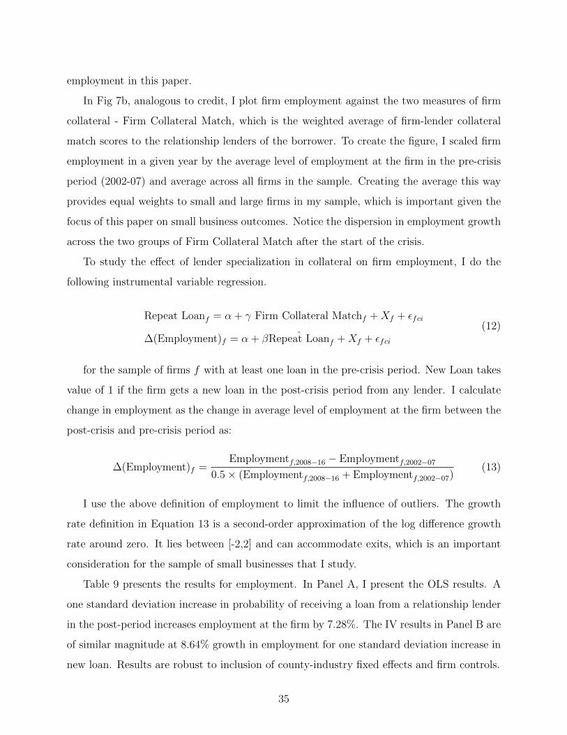
employment in this paper.

In Fig 7b, analogous to credit, I plot firm employment against the two measures of firm

collateral - Firm Collateral Match, which is the weighted average of firm-lender collateral

match scores to the relationship lenders of the borrower. To create the figure, I scaled firm

employment in a given year by the average level of employment at the firm in the pre-crisis

period (2002-07) and average across all firms in the sample. Creating the average this way

provides equal weights to small and large firms in my sample, which is important given the

focus of this paper on small business outcomes. Notice the dispersion in employment growth

across the two groups of Firm Collateral Match after the start of the crisis.

To study the effect of lender specialization in collateral on firm employment, I do the

following instrumental variable regression.

Repeat Loanf = α + γ Firm Collateral Matchf +Xf + εfci

∆(Employment)f = α + β ˆRepeat Loanf +Xf + εfci

(12)

for the sample of firms f with at least one loan in the pre-crisis period. New Loan takes

value of 1 if the firm gets a new loan in the post-crisis period from any lender. I calculate

change in employment as the change in average level of employment at the firm between the

post-crisis and pre-crisis period as:

∆(Employment)f =Employmentf,2008−16 − Employmentf,2002−07

0.5× (Employmentf,2008−16 + Employmentf,2002−07)(13)

I use the above definition of employment to limit the influence of outliers. The growth

rate definition in Equation 13 is a second-order approximation of the log difference growth

rate around zero. It lies between [-2,2] and can accommodate exits, which is an important

consideration for the sample of small businesses that I study.

Table 9 presents the results for employment. In Panel A, I present the OLS results. A

one standard deviation increase in probability of receiving a loan from a relationship lender

in the post-period increases employment at the firm by 7.28%. The IV results in Panel B are

of similar magnitude at 8.64% growth in employment for one standard deviation increase in

new loan. Results are robust to inclusion of county-industry fixed effects and firm controls.

35

5.4 Aggregate Patterns

The time series patterns for the set of borrowers receiving credit can provide more information

on the importance of collateral. In this paper, I argue that the reduction in credit supply

in the aftermath of the financial crisis was associated with a shift towards borrowers with a

greater collateral match to their lenders. However, this analysis does not clarify how lender

behavior varies at other points in time. I shed some light on changing lending behavior over

time through two tests.

In Figure 8a, I plot the average level of firm-lender collateral match score for the set of

firms that receive credit in a give year. The main takeaway from the figure is that in the

pre-crisis boom the average level of firm-lender collateral match is lower (and decreasing

over time) than the average firm-lender similarity of the set of firms who receive credit in the

post-crisis period. After 2007, the firm-lender collateral match is successively increasing till

about 2012 after which it stabilizes. This suggests that the level of firm-collateral matching

required for credit extension is most important in a downturn.

To identify whether this pattern is driven by just changing composition of lenders and

borrowers in the sample, I run the following regression:

Loanflt = αf + γl + δt + βt Firm-Lender Collateral Matchfl × 1t + εflt (14)

for the set of all firms f and lenders l that receive a loan at any point in my sample. Loan

takes a value of 1 if a firm-lender pair is observed with a loan in a given year t. Firm-lender

collateral match is calculated based on the full sample (2002-16) of loans. I control for firm,

lender, and time differences to test the time varying importance of firm-lender collateral

match.

Figure 8b presents the results of the regression in Equation 14. Results are in line with

the aggregate results presented - that is, firm-lender collateral match becomes important

after the start of the financial crisis while the level does not differentially access to credit in

the pre-crisis boom.

36

6 Conclusion

This paper documents the important role of collateral specialization of lenders for credit

supply to borrowers in the aftermath of the financial crisis. Using novel loan-level data

on all collateralized loans in Texas between 2002 and 2016 linked to the U.S. Census of

establishments, I create a new measure of Firm-Lender Collateral Match Quality to quantify

the extent of specialization of a lender in the collateral of the borrower.

By focusing on the set of borrower-lender pairs with pre-existing relationships before the

start of the financial crisis, I show that a firm that was borrowing from lenders with greater

specialization in its collateral is more likely to continue receiving credit after the start of

the crisis. This effect is not driven by differences across firms or lenders but holds within

borrowers of a lender and within lenders of a firm. Lender collateral specialization, in turn,

affects firm-level outcomes such as employment.

On exploring the channels leading to lender specialization, I show that informational

advantages in collateral are the most likely driver of lender specialization in a crisis. Fur-

thermore, collateral specialization is distinct from other lender advantages that may be

industry or firm-specific, such as lender concentration in an industry or the availability of

firm-specific soft information.

The findings in this paper have important implications for heterogeneous effects of credit

supply shocks. I show that the decrease in lending to borrowers of the same lender varies

based on borrower collateral and its “match” to the lender’s specialization by collateral.

These findings also suggest that not all relationships are equally valuable to a borrower in

times of a crisis, and credit substitution may be limited by lender collateral specialization.

37

References

Acharya, V., I. Hasan, and A. Saunders (2006): “Should Banks Be Diversified?

Evidence from Individual Bank Loan Portfolios,” The Journal of Business, 79, 1355–1412.

Acharya, V. V., A. N. Berger, and R. A. Roman (2018a): “Lending Implications of

U.S. Bank Stress tests: Costs or Benefits?” Journal of Financial Intermediation, 34, 58 –

90.

Acharya, V. V., S. T. Bharath, and A. Srinivasan (2007): “Does Industry-Wide Dis-

tress Affect Defaulted Firms? Evidence From Creditor Recoveries,” Journal of Financial

Economics, 85, 787 – 821.

Acharya, V. V., T. Eisert, C. Eufinger, and C. Hirsch (2018b): “Real Effects of

the Sovereign Debt Crisis in Europe: Evidence from Syndicated Loans,” The Review of

Financial Studies, 31, 2855–2896.

Adelino, M., A. Schoar, and F. Severino (2015): “House Prices, Collateral, and

Self-Employment,” Journal of Financial Economics, 117, 288 – 306.

Albuquerque, R. and H. A. Hopenhayn (2004): “Optimal Lending Contracts and

Firm Dynamics,” The Review of Economic Studies, 71, 285–315.

Almeida, H. and M. Campello (2007): “Financial Constraints, Asset Tangibility, and

Corporate Investment,” The Review of Financial Studies, 20, 1429–1460.

Ashcraft, A. B. (2005): “Are Banks Really Special? New Evidence from the FDIC-

Induced Failure of Healthy Banks,” The American Economic Review, 95, 1712–1730.

Benmelech, E. (2008): “Asset Salability and Debt Maturity: Evidence from Nineteenth-

Centure American Railroads,” Review of Financial Studies.

Benmelech, E. and N. Bergman (2008): “Liquidation Values and the Credibility of

Financial Contract Renegotiation: Evidence from U.S. Airlines,” Quarterly Journal of

Economics.

——— (2009): “Collateral Pricing,” Journal of Financial Economics.

Benmelech, E., N. Kumar, and R. Rajan (2019): “The Decline of Secured Debt,”

Working Paper.

Benmelech, E., R. R. Meisenzahl, and R. Ramcharan (2016): “The Real Effects

of Liquidity During the Financial Crisis: Evidence from Automobiles,” The Quarterly

Journal of Economics, 132, 317–365.

Bentolila, S., M. Jansen, and G. Jimenez (2017): “When Credit Dries Up: Job Losses

in the Great Recession,” Journal of the European Economic Association, 16, 650–695.

38

Berger, A., S. Frame, and V. Ioannidou (2011a): “Tests of Ex Ante versus Ex

Post Theories of Collateral Using Private and Public Information,” Journal of Financial

Economics.

Berger, A. N., M. A. Espinosa-Vega, W. S. Frame, and N. H. Miller (2011b):

“Why do Borrowers Pledge Collateral? New Empirical Evidence on the Role of Asym-

metric Information,” Journal of Financial Intermediation, 20, 55 – 70.

Berger, A. N., W. S. Frame, and V. Ioannidou (2016): “Reexamining the Empirical

Relation Between Loan Risk and Collateral: The Roles of Collateral Liquidity and Types,”

Journal of Financial Intermediation, 26, 28 – 46.

Berger, A. N., I. Hasan, and M. Zhou (2010): “The Effects of Focus versus Diver-

sification on Bank Performance: Evidence from Chinese Banks,” Journal of Banking &

Finance, 34, 1417 – 1435, performance Measurement in the Financial Services Sector.

Berger, A. N. and G. F. Udell (1990): “Collateral, Loan Quality and Bank Risk,”

Journal of Monetary Economics, 25, 21 – 42.

——— (1995): “Relationship Lending and Lines of Credit in Small Firm Finance,” The

Journal of Business, 68, 351–381.

Berger, P. G., M. Minnis, and A. Sutherland (2017): “Commercial Lending Con-

centration and Bank Expertise: Evidence from Borrower Financial Statements,” Journal

of Accounting and Economics, 64, 253 – 277.

Bernanke, B. S. (1983): “Nonmonetary Effects of the Financial Crisis in the Propagation

of the Great Depression,” The American Economic Review, 73, 257–276.

Besanko, D. and A. V. Thakor (1987a): “Collateral and Rationing: Sorting Equilibria

in Monopolistic and Competitive Credit Markets,” International Economic Review, 28,

671–689.

——— (1987b): “Competitive Equilibrium in the Credit Market Under Asymmetric Infor-

mation.” Journal of Economic Theory, 42, 167–182.

Bester, H. (1985): “Screening vs. Rationing in Credit Markets with Imperfect Informa-

tion,” The American Economic Review, 75, 850–855.

——— (1987): “The Role of Collateral in Credit Markets with Imperfect Information,”

European Economic Review, 31, 887 – 899, special Issue on Market Competition, Conflict

and Collusion.

Boot, A. W. A. and A. V. Thakor (1994): “Moral Hazard and Secured Lending in an

Infinitely Repeated Credit Market Game,” International Economic Review, 35, 899–920.

39

——— (2000): “Can Relationship Banking Survive Competition?” The Journal of Finance,

55, 679–713.

Boot, A. W. A., A. V. Thakor, and G. F. Udell (1991): “Secured Lending and

Default Risk: Equilibrium Analysis, Policy Implications and Empirical Results,” The

Economic Journal, 101, 458–472.

Bord, V., V. Ivashina, and R. Taliaferro (2018): “Large Banks and Small Firm

Lending,” Working Paper.

Boyd, J. H. and E. C. Prescott (1986): “Financial Intermediary-Coalitions,” Journal

of Economic Theory, 38, 211 – 232.

Brick, I. E. and D. Palia (2007): “Evidence of Jointness in the Terms of Relationship

Lending,” Journal of Financial Intermediation, 16, 452 – 476.

Caballero, R. J., T. Hoshi, and A. K. Kashyap (2008): “Zombie Lending and De-

pressed Restructuring in Japan,” American Economic Review, 98, 1943–77.

Calomiris, C., M. Larrain, J. Liberti, and J. Sturgess (2017): “How Collateral

Laws Shape Lending and Sectoral Activity,” Journal of Financial Economics.

Campello, M. and E. Giambona (2013): “Real Assets and Capital Structure,” The

Journal of Financial and Quantitative Analysis, 48, 1333–1370.

Campello, M. and M. Larrain (2015): “Enlarging the Contracting Space: Collateral

Menus, Access to Credit, and Economic Activity,” The Review of Financial Studies, 29,

349–383.

Carey, M., M. Post, and S. A. Sharpe (1998): “Does Corporate Lending by Banks

and Finance Companies Differ? Evidence on Specialization in Private Debt Contracting,”

The Journal of Finance, 53, 845–878.

Cerqueiro, G., S. Ongena, and K. Roszbach (2016): “Collateralization, Bank Loan

Rates, and Monitoring,” The Journal of Finance, 71, 1295–1322.

——— (2019): “Collateral Damaged? Priority Structure, Credit Supply, and Firm Perfor-

mance,” Journal of Financial Intermediation, 100824.

Chakraborty, A. and C. X. Hu (2006): “Lending Relationships in Line-of-Credit and

Nonline-of-Credit Loans: Evidence from Collateral use in Small Business,” Journal of

Financial Intermediation, 15, 86 – 107.

Chan, Y.-S. and A. V. Thakor (1987): “Collateral and Competitive Equilibria with

Moral Hazard and Private Information,” The Journal of Finance, 42, 345–363.

Chaney, T., D. Sraer, and D. Thesmar (2012): “The Collateral Channel: How Real

40

Estate Shocks Affect Corporate Investment,” American Economic Review, 102, 2381–2409.

Chen, B., S. Hanson, and J. Stein (2017): “The Decline of Big-Bank Lending to Small

Business: Dynamic Impacts on Local Credit and Labor Markets,” Working Paper.

Chodorow-Reich, G. (2013): “The Employment Effects of Credit Market Disruptions:

Firm-level Evidence from the 2008-9 Financial Crisis,” The Quarterly Journal of Eco-

nomics, 129, 1–59.

Cole, R. A., L. G. Goldberg, and L. J. White (2004): “Cookie Cutter vs. Character:

The Micro Structure of Small Business Lending by Large and Small Banks,” The Journal

of Financial and Quantitative Analysis, 39, 227–251.

Cooley, T., R. Marimon, and V. Quadrini (2004): “Aggregate Consequences of Lim-

ited Contract Enforceability,” Journal of Political Economy, 112, 817–847.

Cortes, K., Y. Demyanyk, L. Li, E. Loutskina, and P. Strahan (2018): “Stress

Tests and Small Business Lending,” NBER Working Paper Series.

Covas, F. (2018): “Capital Requirements in Supervisory Stress Tests and Their Adverse

Impact on Small Business Lending,” TCH Working Paper.

Degryse, H. and S. Ongena (2004): “The Impact of Competition on Bank Orientation

and Specialization,” CEPR Discussion Papers 4543.

Dell’Ariccia, G., E. Friedman, and R. Marquez (1999): “Adverse Selection as a

Barrier to Entry in the Banking Industry,” The RAND Journal of Economics, 30, 515–

534.

Dell’Ariccia, G. and R. Marquez (2004): “Information and Bank Credit Allocation,”

Journal of Financial Economics, 72, 185 – 214.

DeYoung, R., A. Gron, G. Torna, and A. Winton (2015): “Risk Overhang and

Loan Portfolio Decisions: Small Business Loan Supply before and during the Financial

Crisis,” The Journal of Finance, 70, 2451–2488.

Diamond, D. W. (1984): “Financial Intermediation and Delegated Monitoring,” The Re-

view of Economic Studies, 51, 393–414.

Diamond, D. W., Y. Hu, and R. G. Rajan (2019): “Pledgeability, Industry Liquidity,

and Financing Cycles,” Journal of Finance.

Donaldson, J. R., D. Gromb, and G. Piacentino (2019): “The Paradox of Pledge-

ability,” Journal of Financial Economics.

Drechsel, T. (2019): “Earnings-Based Borrowing Constraints and Macroeconomic Fluc-

tuations,” Working Paper.

41

Edgerton, J. (2012): “Credit Supply and Business Investment During the Great Recession:

Evidence from Public Records of Equipment Financing,” Working Paper.

Eisfeldt, A. L. and A. A. Rampini (2008): “Leasing, Ability to Repossess, and Debt

Capacity,” The Review of Financial Studies, 22, 1621–1657.

Fricke, D. and T. Roukny (2018): “Generalists and Specialists in the Credit Market,”

Journal of Banking & Finance, 105335.

Gale, D. and M. Hellwig (1985): “Incentive-Compatible Debt Contracts: The One-

Period Problem,” The Review of Economic Studies, 52, 647–663.

Gan, J. (2007): “The Real Effects of Asset Market Bubbles: Loan- and Firm-Level Evidence

of a Lending Channel,” The Review of Financial Studies, 20, 1941–1973.

Giambona, E., A. S. Mello, and T. J. Riddiough (2018): “Real Assets, Collateral

and the Limits of Debt Capacity,” Real Estate Economics, 46, 836–886.

Granja, J., C. Leuz, and R. Rajan (2018): “Going the Extra Mile: Distant Lending

and Credit Cycles,” Working Paper 25196, National Bureau of Economic Research.

Greenstone, M., A. Mas, and H.-L. Nguyen (2014): “Do Credit Market Shocks Affect

the Real Economy? Quasi-Experimental Evidence from the Great Recession and ‘Normal’

Economic Times,” Working Paper.

Hauswald, R. and R. Marquez (2006): “Competition and Strategic Information Acqui-

sition in Credit Markets,” The Review of Financial Studies, 19, 967–1000.

Hoberg, G. and G. Phillips (2010): “Product Market Synergies and Competition in

Mergers and Acquisitions: A Text-Based Analysis,” The Review of Financial Studies, 23,

3773–3811.

——— (2016): “Text-Based Network Industries and Endogenous Product Differentiation,”

Journal of Political Economy, 124, 1423–1465.

Holmstrom, B. and J. Tirole (1997): “Financial Intermediation, Loanable Funds, and

the Real Sector,” The Quarterly Journal of Economics, 112, 663–691.

Hubbard, R., K. Kuttner, and D. Palia (2002): “Are There Bank Effects in Borrowers’

Costs of Funds? Evidence from a Matched Sample of Borrowers and Banks,” The Journal

of Business, 75, 559–581.

Ivashina, V., L. Laeven, and E. Moral-Benito (2019): “Loan Types and the Bank

Lending Channel,” Working Paper.

Ivashina, V. and D. Scharfstein (2010): “Bank Lending During the Financial Crisis of

2008,” Journal of Financial Economics, 97, 319–338.

42

Jimenez, G., S. Ongena, J.-L. Peydro, and J. Saurina (2017): “Macroprudential

Policy, Countercyclical Bank Capital Buffers, and Credit Supply: Evidence from the Span-

ish Dynamic Provisioning Experiments,” Journal of Political Economy, 125, 2126–2177.

Jimenez, G., V. Salas, and J. Saurina (2006): “Determinants of Collateral,” Journal

of Financial Economics, 81, 255 – 281.

Jimenez, G. and J. Saurina (2004): “Collateral, Type of Lender and Relationship Bank-

ing as Determinants of Credit Risk,” Journal of Banking & Finance, 28, 2191 – 2212.

John, K., A. Lynch, and M. Puri (2003): “Credit Ratings, Collateral, and Loan Char-

acteristics: Implications for Yield,” The Journal of Business, 76, 371–409.

Kelly, B. T., D. Papanikolaou, A. Seru, and M. Taddy (2018): “Measuring Tech-

nological Innovation over the Long Run,” Yale ICF Working Paper.

Khwaja, A. I. and A. Mian (2008): “Tracing the Impact of Bank Liquidity Shocks:

Evidence from an Emerging Market,” American Economic Review, 98, 1413–42.

Laeven, L. and R. Levine (2007): “Is there a Diversification Discount in Financial

Conglomerates?” Journal of Financial Economics, 85, 331 – 367, the economics of conflicts

of interest financial institutions.

Leeth, J. D. and J. A. Scott (1989): “The Incidence of Secured Debt: Evidence from

the Small Business Community,” The Journal of Financial and Quantitative Analysis, 24,

379–394.

Lian, C. and Y. Ma (2019): “Anatomy of Corporate Borrowing Constraints,” Working

Paper.

Liberti, J., J. Sturgess, and A. Sutherland (2017): “Information Sharing and Lender

Specialization: Evidence from the U.S. Commercial Lending Market,” Working Paper.

Liberti, J. M. and J. Sturgess (2014): “Uncovering Collateral Constraints,” Working

Paper.

Loutskina, E. and P. E. Strahan (2011): “Informed and Uninformed Investment in

Housing: The Downside of Diversification,” The Review of Financial Studies, 24, 1447–

1480.

Mello, A. S. and M. Ruckes (2017): “Collateral in Corporate Financing,” in Working

Paper.

Mian, A. and A. Sufi (2009): “The Consequences of Mortgage Credit Expansion: Evi-

dence from the US Mortgage Default Crisis,” The Quarterly Journal of Economics, 124,

1449–1496.

43

——— (2018): “Credit Supply and Housing Speculation,” Working Paper.

Murfin, J. and R. Pratt (2019): “Who Finances Durable Goods and Why It Matters:

Captive Finance and the Coase Conjecture,” The Journal of Finance, 74, 755–793.

Ortiz-Molina, H. and G. M. Phillips (2014): “Real Asset Illiquidity and the Cost of

Capital,” Journal of Financial and Quantitative Analysis, 49, 1–32.

Paravisini, D., V. Rappoport, and P. Schnabl (2018): “Specialization in Bank Lend-

ing: Evidence from Exporting Firms,” NBER Working Paper.

Peek, J. and E. S. Rosengren (2000): “Collateral Damage: Effects of the Japanese Bank

Crisis on Real Activity in the United States,” American Economic Review, 90, 30–45.

Petersen, M. A. and R. G. Rajan (1994): “The Benefits of Lending Relationships:

Evidence from Small Business Data,” The Journal of Finance, 49, 3–37.

——— (1995): “The Effect of Credit Market Competition on Lending Relationships,” The

Quarterly Journal of Economics, 110, 407–443.

——— (2002): “Does Distance Still Matter? The Information Revolution in Small Business

Lending,” The Journal of Finance, 57, 2533–2570.

Pulvino, T. C. (1998): “Do Asset Fire Sales Exist? An Empirical Investigation of Com-

mercial Aircraft Transactions,” The Journal of Finance, 53, 939–978.

Rajan, R., H. Servaes, and L. Zingales (2000): “The Cost of Diversity: The Diversi-

fication Discount and Inefficient Investment,” The Journal of Finance, 55, 35–80.

Rajan, R. and A. Winton (1995): “Covenants and Collateral as Incentives to Monitor,”

The Journal of Finance, 50, 1113–1146.

Rajan, R. G. (1992): “Insiders and Outsiders: The Choice between Informed and Arm’s-

Length Debt,” The Journal of Finance, 47, 1367–1400.

Schlingemann, F. P., R. M. Stulz, and R. A. Walkling (2002): “Divestitures and

the Liquidity of the Market for Corporate Assets,” Journal of Financial Economics, 64,

117 – 144.

Schnabl, P. (2012): “The International Transmission of Bank Liquidity Shocks: Evidence

from an Emerging Market,” The Journal of Finance, 67, 897–932.

Schwert, M. (2018): “Bank Capital and Lending Relationships,” The Journal of Finance,

73, 787–830.

Shleifer, A. and R. W. Vishny (1992): “Liquidation Values and Debt Capacity: A

Market Equilibrium Approach,” Journal of Finance.

——— (2010): “Fire Sales in Finance and Macroeconomics,” NBER Working Papers 16642,

44

National Bureau of Economic Research, Inc.

Stein, J. C. (2002): “Information Production and Capital Allocation: Decentralized versus

Hierarchical Firms,” Journal of Finance, LVII, 1891–1921.

Stiglitz, J. and A. Weiss (1981): “Credit Rationing in Markets with Imperfect Infor-

mation,” The.

Stroebel, J. (2016): “Asymmetric Information about Collateral Values,” The Journal of

Finance, 71, 1071–1112.

Townsend, R. M. (1979): “Optimal Contracts and Competitive Markets with Costly State

Verification,” Journal of Economic Theory, 21, 265 – 293.

Vig, V. (2013): “Access to Collateral and Corporate Debt Structure: Evidence from a

Natural Experiment,” The Journal of Finance, 68, 881–928.

Williamson, S. D. (1986): “Costly Monitoring, Financial Intermediation, and Equilibrium

Credit Rationing,” Journal of Monetary Economics, 18, 159 – 179.

Winton, A. (1999): “Don’t Put All Your Eggs in One Basket? Diversification and Spe-

cialization in Lending,” Manuscript, University of Minnesota.

45

Figures

Figure 1: Distribution of Firm-Lender Collateral Match Quality

This figure plots the kernel density for Firm-Lender Collateral Match Quality. Unit of observationis a firm-lender pair. Firm-Lender Collateral Match Quality captures the level of collateral special-ization of the lender in the borrower’s collateral. Values are capped at 5th and 95th percentiles.

(a) Firm-Lender Pre-Crisis Collateral Match

The solid line includes all potential firm-lender pairs based on the total set of borrowers and lendersin Texas. The dashed line plots the firm-lender collateral match scores for equilibrium observedfirm-lender matches with at least one loan between the pair in the pre-crisis (2002-07) period.

(b) Firm-Lender Collateral Match - Pre-Crisis vs. Post-Crisis

The solid line includes all firm-lender pairs in Texas with at least one loan between the borrowerand lender in the pre-crisis (2002-07) period. The dashed line includes all firm-lender pairs with atleast one loan between the borrower and lender in both the pre-crisis (2002-07) and post (2008-16)period

46

Figure 2: Effect of Firm-Lender Collateral Match on Lending

This figure plots new loan originations between 2002 and 2016 to study the effect of borrower-lender collateral match on access to credit around the 2008 financial crisis. The sample consistsof borrower-lender pairs with a lending relationship between 2002-07. On the Y-axis, log of thenumber of loans originated in a given year demeaned by the average pre-crisis (2002-07) log numberof loans is plotted. Borrower-lender pairs are classified into above and below median Firm-LenderCollateral Match Quality. Firm-Lender Collateral Match Quality captures the level of collateralspecialization of the lender in the borrower’s collateral. It is created by comparing the collateralpledged by the borrower to collateral portfolio of the lender based on pre-crisis (2002-07) loans.Higher values of the measure implies the lender has a greater specialziation in the collateral of theborrower.

47

Figure 3: Effect of Firm-Lender Collateral Match on Lending - Within Group

This figure plots new loan originations between 2002 and 2016 to study the effect of borrower-lender collateral match on access to credit around the 2008 financial crisis. The sample consists ofborrower-lender pairs in Texas with a lending relationship between 2002-07. Firm-Lender CollateralMatch Quality captures the level of collateral specialization of the lender in the borrower’s collateral.

(a) Within Firm

Within each firm, lenders with pre-crisis relationship are classified into above and below mediancollateral match quality. The sample is restricted to firms with multiple lending relationships.

(b) Within Lender

Within each lender, firms that borrowed at least once between 2002-07 are categorized into aboveand below median collateral match quality.

48

Figure 4: Time Varying Effect of Firm-Lender Collateral Match on Lending

This figure examines the time-varying effect of borrower-lender collateral match on access to creditaround the 2008 financial crisis. The sample consists of borrower-lender pairs in Texas with alending relationship between 2002-07. Observations are at the firm-lender-year level. Regressionbetas from the following specification are plotted:

yflt =αf + γlt + βt Firm-Lender Collateral Matchfl × 1t + εflt

for firm f , lender l, and year t. The dependent variable is an indicator that takes value of one if thefirm-lender pair is observed to have a loan in a given year, scaled by frequency of loans between thepair in the pre-crisis period. Firm-Lender Collateral Match Quality captures the level of collateralspecialization of the lender in the borrower’s collateral, and is measured based on pre-crisis (2002-07) loans between the borrower and lender. Regression includes firm (αf ) and lender-year (γlt)fixed effects. 1t takes value 1 in year t and is zero otherwise. Standard errors are clustered at thelender level. Point coefficients and 95% confidence intervals are plotted. Coefficients can be foundin column 2 of Table A6.

49

Figure 5: Distribution of Firm-Lender Collateral Match Quality - Post-Crisis Matches

This figure plots the kernel density for Firm-Lender Collateral Match Quality. Firm-Lender Col-lateral Match Quality captures the level of collateral specialization of the lender in the borrower’scollateral, based on pre-crisis (2002-07) loans. Values are capped at 5th and 95th percentiles. Thesolid line includes all potential firm-lender pairs in Texas based on the total set of borrowers andlenders in the sample. The dashed line plots the distribution of scores for firm-lender pairs with amatch in the post-crisis (2008-16) period.

50

Figure 6: Low Bank Capitalization Does Not Explain Lending Change

This figure examines the interaction between lender specialization and bank capitalization on accessto credit around the 2008 financial crisis. The sample consists of borrower-lender pairs in Texas witha lending relationship between 2002-07. Sample is restricted to loans made by banks (commercialbank, nonbank-subsidiary of bank holding company, or a credit union). Regression betas from thefollowing specification are plotted:

yflt =αfl + δt + β1t Firm-Lender Collateral Matchfl × 1t+

β2t Firm-Lender Collateral Matchfl × 1t × Low Capitall + εfci

for firm f , lender l and year t. The dependent variable is an indicator that takes value of one if thefirm-lender pair is observed to have a loan in a given year, scaled by frequency of loans between thepair in the pre-crisis period. Firm-Lender Collateral Match Quality captures the level of collateralspecialization of the lender in the borrower’s collateral, and is measured based on pre-crisis (2002-07) loans between the borrower and lender. Low capital takes value 1 for lenders with below medianTier 1 capital ratio as of December 2006. Regression includes firm-lender (αfl) and time (δt) fixedeffects. 1t takes value 1 in year t and is zero otherwise. Standard errors are clustered at the lenderlevel. Point coefficients and 95% confidence intervals are plotted below. Coefficients can be foundin Column 2 of Table A7.

51

Figure 7: Firm Collateral Match on Firm-Level Outcomes

This figure plots examines the effect of borrower-lender collateral match on firm outcomes aroundthe 2008 financial crisis. Sample includes firms in Texas with at least one loan in the pre-crisis (2002-07) period. Firm Collateral Match is the weighted average of firm-lender collateral match quality.Firm collateral match captures the average level of collateral specialization of relationship lendersof the borrower. Higher values indicate the firm borrows from lenders with greater specializationin the borrower’s collateral.

(a) Lending

Log of the number of loans originated in a given year demeaned by the average pre-crisis (2002-07)log number of loans is plotted.

(b) Firm Employment

Average of scaled firm-level employment is plotted. Scaled Employment is annual firm employmentscaled by pre-crisis (2002-07) level of firm employment.

52

Figure 8: Aggregate Trends

This figure examines the time-varying effect of lender collateral specialization on credit accessaround the 2008 financial crisis. Firm-lender collateral match quality captures the level of collateralspecialization of the lender in borrower’s collateral and is calculated based on all loans in the samplebetween 2002 and 2016.

(a) Average Firm-Lender Collateral Match Quality

This figure plots the average level of Firm-Lender Collateral Match Quality over time for firm-lenderpairs with a loan in the given year.

(b) Dynamic Difference-in-Difference

This figure plots the coefficients from the following regression:

yflt = αfl + δt + βtFirm-Lender Collateral Matchfl + εflt

Dependent variable takes value of one if the firm f gets a loan from lender l in year t and zerootherwise. The sample includes all firm-lender pairs with at least one loan between 2002-16. 2006is the omitted year. Standard errors are clustered at the lender level.

53

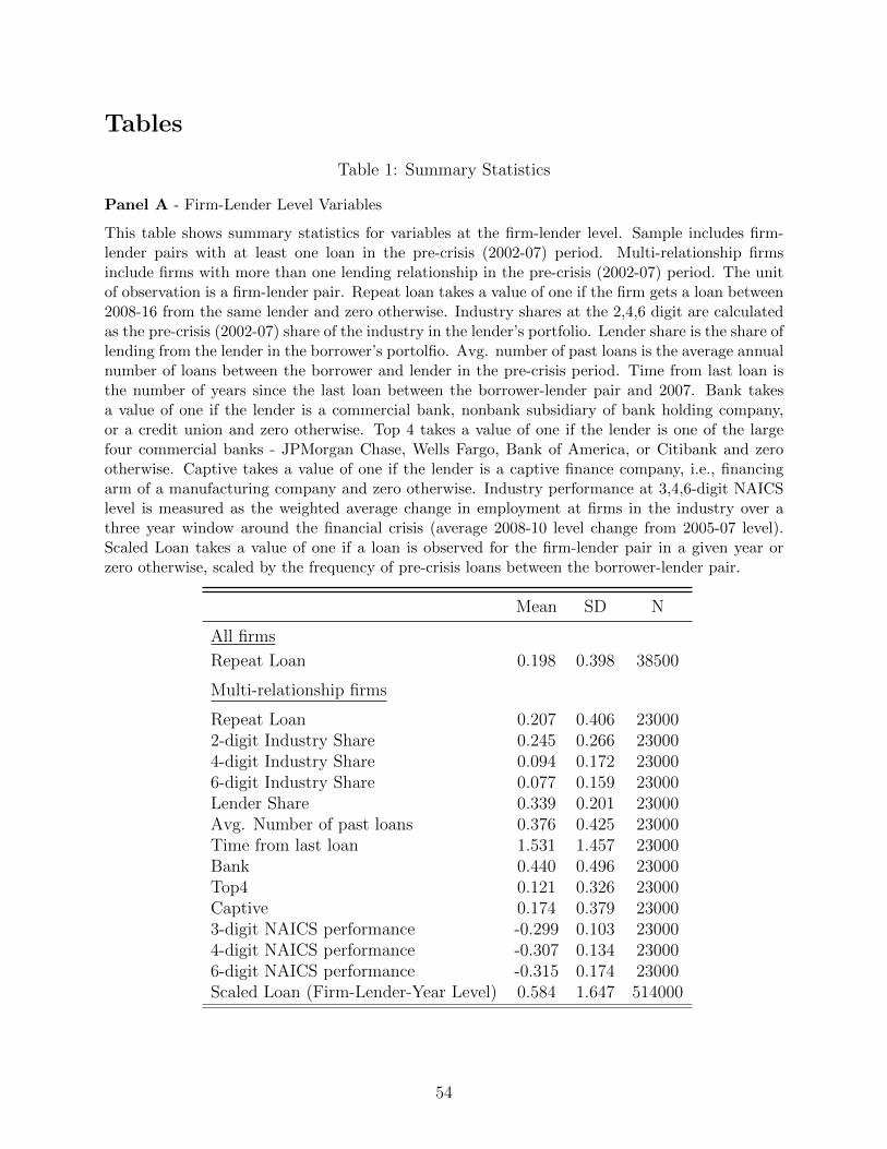
Tables

Table 1: Summary Statistics

Panel A - Firm-Lender Level Variables

This table shows summary statistics for variables at the firm-lender level. Sample includes firm-lender pairs with at least one loan in the pre-crisis (2002-07) period. Multi-relationship firmsinclude firms with more than one lending relationship in the pre-crisis (2002-07) period. The unitof observation is a firm-lender pair. Repeat loan takes a value of one if the firm gets a loan between2008-16 from the same lender and zero otherwise. Industry shares at the 2,4,6 digit are calculatedas the pre-crisis (2002-07) share of the industry in the lender’s portfolio. Lender share is the share oflending from the lender in the borrower’s portolfio. Avg. number of past loans is the average annualnumber of loans between the borrower and lender in the pre-crisis period. Time from last loan isthe number of years since the last loan between the borrower-lender pair and 2007. Bank takesa value of one if the lender is a commercial bank, nonbank subsidiary of bank holding company,or a credit union and zero otherwise. Top 4 takes a value of one if the lender is one of the largefour commercial banks - JPMorgan Chase, Wells Fargo, Bank of America, or Citibank and zerootherwise. Captive takes a value of one if the lender is a captive finance company, i.e., financingarm of a manufacturing company and zero otherwise. Industry performance at 3,4,6-digit NAICSlevel is measured as the weighted average change in employment at firms in the industry over athree year window around the financial crisis (average 2008-10 level change from 2005-07 level).Scaled Loan takes a value of one if a loan is observed for the firm-lender pair in a given year orzero otherwise, scaled by the frequency of pre-crisis loans between the borrower-lender pair.

Mean SD N

All firms

Repeat Loan 0.198 0.398 38500

Multi-relationship firms

Repeat Loan 0.207 0.406 230002-digit Industry Share 0.245 0.266 230004-digit Industry Share 0.094 0.172 230006-digit Industry Share 0.077 0.159 23000Lender Share 0.339 0.201 23000Avg. Number of past loans 0.376 0.425 23000Time from last loan 1.531 1.457 23000Bank 0.440 0.496 23000Top4 0.121 0.326 23000Captive 0.174 0.379 230003-digit NAICS performance -0.299 0.103 230004-digit NAICS performance -0.307 0.134 230006-digit NAICS performance -0.315 0.174 23000Scaled Loan (Firm-Lender-Year Level) 0.584 1.647 514000

54

Table 1: Summary Statistics - Contd.

Panel B - Collateral Measures

This table shows summary statistics for measures of collateral specialization at the firm-lenderlevel. Sample includes firms with at least one loan in the pre-crisis (2002-07) period. Firm-LenderCollateral Match Quality captures the level of lender specialization in borrower collateral. It ismeasured based on a comparison of the firm’s collateral to the lending portfolio of the lender basedon pre-crisis loans (2002-07). Firm Collateral Match is the firm-level weighted average of firm-lender collateral match quality. Firm Similarity captures the specialization of the average lenderin the economy with respect to the borrower’s collateral . It is measured based on comparison ofthe firm’s collateral in the pre-crisis period to the (weighted) average lender. Pseudo-percentilesare the average of observations in a ±1 percentile window around the level of interest.

Firm-Lender Firm FirmCollateral Match Quality Collateral Match Similarity

Mean 0.383 0.382 0.218Standard Deviation 0.309 0.285 0.153Pseudo 10th pct (mean of 9 - 11) 0.016 0.030 0.035Pseudo 25th pct (mean of 24 - 26) 0.094 0.137 0.087Pseudo 75th pct (mean of 74 - 76) 0.605 0.573 0.318Pseudo 90th pct (mean of 89 - 91) 0.862 0.808 0.432

Panel C - Firm-Level Variables

This table shows summary statistics for variables at the firm-level. Sample includes firms with atleast one loan in the pre-crisis (2002-07) period. Repeat loan takes a value of one if firm gets arepeat loan from any of its relationship lenders in the post-crisis period and zero otherwise. NewLoan takes a value of one if firm gets any loan in the post-crisis period, irrespective of whetherthe firm and lender had a pre-crisis relationship and zero otherwise. New Lender takes a value ofone if the firm gets at least one loan from a lender it did not borrow from in the pre-crisis periodand zero otherwise. Firm Age is the log of the number of years the firm has been in operationas of 2007. Firm Size is the log of employment at the firm in 2007. Average employment changeis symmetric growth rate of firm employment between the pre-crisis and post-crisis periods and isbounded between [-2,2]. Scaled Employment is annual firm employment scaled by pre-crisis levelof firm employment.

Mean SD N

Repeat Loan 0.308 0.462 23500New Loan - Total 0.616 0.486 23500New Lender 0.524 0.499 23500Firm Age (2007) 12.73 9.901 23500Firm Size (2007) 2.648 1.513 23500Average Employment Change (2002-07 to 2008-16) 0.066 0.650 23500Average Scaled Employment (Firm-Year Level) 1.098 0.832 303000

55

Tab

le2:

Len

der

Col

late

ral

Sp

ecia

liza

tion

and

Len

din

g

Th

ista

ble

stu

die

sth

eeff

ect

ofb

orr

ower

-len

der

coll

ater

alm

atch

onac

cess

tocr

edit

inth

eaf

term

ath

ofth

e20

08fin

anci

alcr

isis

.T

he

sam

ple

con

sist

sof

borr

ower

-len

der

pair

sin

Tex

asw

ith

ale

nd

ing

rela

tion

ship

bet

wee

n20

02-0

7.T

he

un

itof

obse

rvat

ion

isa

firm

-len

der

pai

r.R

egre

ssio

nsp

ecifi

cati

on

isas

foll

ows:

Rep

eat

Loa

nfl

=αf

+γl+β

Fir

m-L

end

erC

olla

tera

lM

atch

Qu

alit

yfl+ε f

l

for

firm

fan

dle

nd

erl.

Th

ed

epen

den

tva

riab

leta

kes

ava

lue

ofon

eif

the

firm

gets

an

ewlo

anb

etw

een

2008

and

2016

from

the

sam

ele

nd

eran

dze

root

her

wis

e.F

irm

-Len

der

Col

late

ral

Mat

chQ

ual

ity

cap

ture

sth

ele

vel

ofco

llat

eral

spec

iali

zati

onof

the

len

der

inth

eb

orr

ower

’sco

llate

ral.

Itis

crea

ted

by

com

pari

ng

the

coll

ater

alp

led

ged

by

the

bor

row

erto

the

coll

ater

alp

ortf

olio

ofth

ele

nd

erb

ased

onp

re-c

risi

s(2

002-

07)

loan

s.H

igh

erva

lues

of

the

mea

sure

imp

lies

the

len

der

has

agr

eate

rsp

ecia

lzia

tion

inth

eco

llat

eral

ofth

eb

orro

wer

.R

egre

ssio

nin

clu

des

firm

and

len

der

fixed

effec

ts.

Th

efi

rmco

ntr

ols

are

firm

size

mea

sure

dby

emp

loym

ent,

and

firm

age

in20

07.

Sta

nd

ard

erro

rsar

ecl

ust

ered

atle

nd

erle

vel.

Col

um

ns

1-4

incl

ud

eth

efu

llsa

mp

leof

firm

s.C

olu

mn

s5-

7ar

ere

stri

cted

tofi

rms

wit

hm

ult

iple

len

din

gre

lati

onsh

ips.

All

Fir

ms

Mult

i-R

elat

ionsh

ipF

irm

s

(1)

(2)

(3)

(4)

(5)

(6)

(7)

Loa

nL

oan

Loa

nL

oan

Loa

nL

oan

Loa

n

Fir

m-L

ender

Col

late

ral

0.06

6*0.

078*

*0.

083*

*0.

082*

**0.

109*

**0.

106*

**0.

120*

**M

atch

Qual

ity

(0.0

34)

(0.0

31)

(0.0

32)

(0.0

29)

(0.0

21)

(0.0

40)

(0.0

22)

Obse

rvat

ions

3850

038

500

3850

038

500

2300

023

000

2300

0C

ounty

xIn

dust

ryF

EN

YN

YY

NN

Len

der

FE

NN

YY

YN

YF

irm

Con

trol

sN

NN

YY

NN

Fir

mF

EN

NN

NN

YY

R2

0.00

30.

077

0.15

80.

215

0.26

50.

388

0.52

8

56

Table 3: Collateral vs. Industry Specialization

This table examines the impact of lender collateral specialization on credit access in the aftermathof the 2008 financial crisis, after controlling for the lender’s industry specialization. The sampleconsists of borrower-lender pairs in Texas with a lending relationship between 2002-07. The unitof observation is a firm-lender pair. The dependent variable takes a value of one if the firm gets anew loan between 2008 and 2016 from the same lender and zero otherwise. Firm-Lender CollateralMatch Quality captures the level of collateral specialization of the lender in the borrower’s collateral.Industry shares at the 2,4,6 digit are calculated as the pre-crisis (2002-07) share of the industry inthe lender’s portfolio. Standard errors are clustered at lender level.

Panel A - Inclusion of Lender-Industry fixed effects

(1) (2) (3)Loan Loan Loan

Firm-Lender Collateral Match Quality 0.120*** 0.132*** 0.134***(0.022) (0.026) (0.027)

Observations 23000 23000 23000Firm FE Y Y YLender FE Y N NLender x 2-digit NAICS FE N Y NLender x 3-digit NAICS FE N N YR2 0.528 0.643 0.703

Panel B - Inclusion of Lender-Industry Shares

(1) (2) (3)Loan Loan Loan

Firm-Lender Collateral Match Quality 0.115*** 0.114*** 0.114***(0.022) (0.022) (0.022)

2-digit Industry Share 0.118***(0.029)

4-digit Industry Share 0.217***(0.047)

6-digit Industry Share 0.233***(0.045)

Observations 23000 23000 23000Firm FE Y Y YLender FE Y Y YR2 0.529 0.529 0.529

57

Table 4: Collateral Specialization vs. Soft Information

This table examines the impact of lender collateral specialization on credit access in the aftermathof the 2008 financial crisis, after controlling for potential soft information. The sample consists ofborrower-lender pairs in Texas with a lending relationship between 2002-07. The unit of observationis a firm-lender pair. The dependent variable takes a value of one if the firm gets a new loan between2008 and 2016 from the same lender and zero otherwise. Firm-Lender Collateral Match Qualitycaptures the level of collateral specialization of the lender in the borrower’s collateral. Controlsinclude the average annual number of pre-crisis loans between the borrower and lender, the lender’sshare in total lending to the borrower in the pre-crisis period, the number of years between 2007 andthe last pre-crisis (2002-07) loan between the borrower and lender. Standard errors are clusteredat lender level.

(1) (2) (3) (4) (5)Loan Loan Loan Loan Loan

Firm-Lender Collateral 0.120*** 0.074*** 0.068*** 0.100*** 0.068***Match Quality (0.022) (0.018) (0.018) (0.020) (0.017)

Lender Share 0.405*** 0.323***(0.028) (0.027)

Avg. Number of past loans 0.186***(0.011)

Time From Last Loan -0.052*** -0.041***(0.004) (0.004)

Observations 23000 23000 23000 23000 23000Firm FE Y Y Y Y YLender FE Y Y Y Y YR2 0.528 0.542 0.544 0.541 0.549

58

Table 5: Heterogeneous Treatment Effect

This table examines variation across lender types in the impact of collateral specialization on creditaccess in the aftermath of the 2008 financial crisis. The sample consists of borrower-lender pairs inTexas with a lending relationship between 2002-07. The unit of observation is a firm-lender pair.The dependent variable takes a value of one if the firm gets a new loan between 2008 and 2016 fromthe same lender and zero otherwise. Firm-Lender Collateral Match Quality captures the level ofcollateral specialization of the lender in the borrower’s collateral. Bank is an indicator that takesa value of one if the lender is a commercial bank, nonbank-subsidiary of bank holding company, ora credit union. Top4 is an indicator that takes a value of one for the 4 largest commercial banksby size - JP Morgan Chase, Bank of America, Wells Fargo, or Citibank including acquisitions.Captive Finance is an indicator that takes a value of one if the parent company of the lender is amanufacturing company. Standard errors are clustered at lender level.

(1) (2) (3)Loan Loan Loan

Firm-Lender Collateral Match 0.129*** 0.125*** 0.091***(0.030) (0.024) (0.020)

Firm-Lender Collateral Match × Bank -0.022(0.039)

Firm-Lender Collateral Match × Captive Finance 0.205***(0.046)

Firm-Lender Collateral Match × Top4 -0.039(0.051)

Observations 23000 23000 23000Firm FE Y Y YLender FE Y Y YR2 0.528 0.528 0.529

59

Table 6: Fire-Sales Channel

This table examines whether fire-sales concerns drive the effect of collateral specialization on creditaccess in the aftermath of the 2008 financial crisis. The sample consists of borrower-lender pairsin Texas with a lending relationship between 2002-07. The unit of observation is a firm-lenderpair. The dependent variable takes a value of one if the firm gets a new loan between 2008 and2016 from the same lender and zero otherwise. Firm-Lender Collateral Match Quality captures thelevel of collateral specialization of the lender in the borrower’s collateral. Industry performance ismeasured as the weighted average change in employment at firms in the borrower’s industry overa three year window around the financial crisis (average 2008-10 level change from 2005-07 level).Standard errors are clustered at lender level.

(1) (2) (3)Loan Loan Loan

Firm-Lender Collateral Match 0.101** 0.144*** 0.137***(0.040) (0.036) (0.031)

Firm-Lender Collateral Match × -0.066Industry Performance (3-digit NAICS) (0.103)

Firm-Lender Collateral Match × 0.083Industry Performance (4-digit NAICS) (0.080)

Firm-Lender Collateral Match × 0.06Industry Performance (6-digit NAICS) (0.058)

Observations 23000 23000 23000Firm FE Y Y YLender FE Y Y YR2 0.528 0.528 0.528

60

Table 7: Aggregate Effects - Counter-factual Exercise

This table presents the aggregate effect on lending under counterfactual firm-lender matching ex-ercises. Sample is restricted to firm-lender pairs with a loan between 2002-07.Counter-factual excercise calculates change in lending on adjusting firm-lender collateral matchquality from current level to counter-factual levels keeping all else about the firm-lender pair thesame. Results presented as percentage increase in lending over current level of lending.For each firm-lender pair, I take as given the collateral plegded between the pair. Given the collat-eral, I estimate hypothetical collateral match scores to all lenders in the sample. The highest scoreis assigned as the value for Best Available Match for Collateral.Next, I consider improvement in lending under hypothetical scenario where specialized lenders existfor all borrowers. I take the 90th percentile, the 95th percentile, and highest firm-lender collateralmatch score from the full distribution of match scores. Lending to the borrower is estimated underthe hypothetical scenario where a specialzied lender for the borrower’s collateral exists.

Best Available Match for Collateral 14.76%90th percentile of Firm-Lender Collateral Match 21.76%95th percentile of Firm-Lender Collateral Match 31.34%Maximum of Firm-Lender Collateral Match 42.67%

61

Table 8: Firm-Level Results on Lending

This table examines the effect of collateral match on lending at the firm level. Sample is restrictedto firms with a loan between 2002-07. Firm Collateral Match is created as a weighted average offirm-lender collateral match values. Firm-lender collateral match captures the level of collateralspecialization of each of the borrower’s pre-crisis (2002-07) relationship lenders. Firm Similaritycaptures the specialization of the average lender in the economy with respect to the borrower’scollateral. Firm controls are firm size measured by employment, and firm age in 2007. Standarderrors are clustered at the firm level.

Panel A - Relationship Lending

Dependent variable takes a value of one if the firm gets a new loan from any of its relationshiplenders after 2008 and zero otherwise. Columns 1-3 include all firms in the sample. Columns 4-6include firms with multiple lending realtionships pre-crisis (2002-07).

All Firms Multi-Relationship Firms

(1) (2) (3) (4) (5) (6)Loan Loan Loan Loan Loan Loan

Firm Collateral Match 0.062*** 0.072*** 0.055*** 0.125*** 0.155*** 0.112***(0.010) (0.010) (0.010) (0.027) (0.031) (0.031)

Observations 23500 23500 23500 7700 7700 7700County x Industry FE N Y Y N Y YFirm Controls N N Y N N YR2 0.001 0.119 0.147 0.003 0.212 0.229

Panel B - New Lender

Dependent variable takes a value of one if the firm gets a loan after 2008 from a lender with noprevious relationship and zero otherwise.

New Lender

(1) (2) (3) (4) (5) (6)

Firm Similarity 0.285*** 0.295*** 0.225*** 0.311*** 0.326*** 0.263***(0.021) (0.022) (0.022) (0.022) (0.023) (0.023)

Firm Collateral Match -0.047*** -0.054*** -0.067***(0.012) (0.013) (0.012)

Observations 23500 23500 23500 23500 23500 23500County x Industry FE N Y Y N Y YFirm Controls N N Y N N YR2 0.008 0.105 0.151 0.008 0.106 0.152

62

Table 9: Firm-Level Results on Employment

This table examines the effect of collateral match on employment at the firm level. Sample isrestricted to firms with a loan between 2002-07. Average employment change is symmetric growthrate of firm employment between the pre-crisis and post-crisis periods and is bounded between [-2,2]. Firm Collateral Match is created as a weighted average of firm-lender collateral match values.Firm-lender collateral match captures the level of collateral specialization of each of the borrower’spre-crisis (2002-07) relationship lenders. Repeat Loan takes value if firm gets a loan between 2008and 2016 from a lender with a pre-crisis relationship. Firm controls are firm size measured byemployment, and firm age in 2007. Standard errors are clustered at the firm level.

Panel A - OLS

∆(Employment)fci =α+ β1Repeat Loanf + β3Xf + γci + εfci

(1) (2) (3)∆(Emp) ∆(Emp) ∆(Emp)

Repeat Loan 0.183*** 0.188*** 0.193***(0.009) (0.010) (0.009)

Observations 23500 23500 23500County x Industry FE N Y YFirm Controls N N YWeighted N N NR2 0.017 0.101 0.169

Panel B - IV

Repeat Loanf = α+ γFirm-Collateral Matchf +Xf + δci + εfci

∆(Employment)fci = α+ β ˆRepeat Loanf +Xf + δci + εfci

(1) (2) (3)∆(Emp) ∆(Emp) ∆(Emp)

Repeat Loan 0.217*** 0.245*** 0.258**(0.078) (0.097) (0.108)

Observations 23500 23500 23500County x Industry FE N Y YFirm Controls N N YFirst Stage F-stat 332.8 221.8 171.8

63

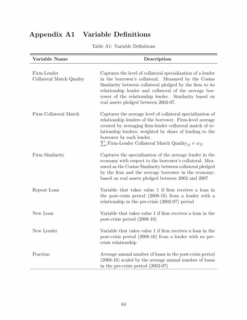
Appendix A1 Variable Definitions

Table A1: Variable Definitions

Variable Name Description

Firm-LenderCollateral Match Quality

Captures the level of collateral specialization of a lenderin the borrower’s collateral. Measured by the CosineSimilarity between collateral pledged by the firm to itsrelationship lender and collateral of the average bor-rower of the relationship lender. Similarity based onreal assets pledged between 2002-07.

Firm Collateral Match Captures the average level of collateral specialization ofrelationship lenders of the borrower. Firm-level averagecreated by averaging firm-lender collateral match of re-lationship lenders; weighted by share of lending to theborrower by each lender.∑

l Firm-Lender Collateral Match Qualityfl × wfl

Firm Similarity Captures the specialization of the average lender in theeconomy with respect to the borrower’s collateral. Mea-sured as the Cosine Similarity between collateral pledgedby the firm and the average borrower in the economy;based on real assets pledged between 2002 and 2007

Repeat Loan Variable that takes value 1 if firm receives a loan inthe post-crisis period (2008-16) from a lender with arelationship in the pre-crisis (2002-07) period

New Loan Variable that takes value 1 if firm receives a loan in thepost-crisis period (2008-16)

New Lender Variable that takes value 1 if firm receives a loan in thepost-crisis period (2008-16) from a lender with no pre-crisis relationship

Fraction Average annual number of loans in the post-crisis period(2008-16) scaled by the average annual number of loansin the pre-crisis period (2002-07)

64

Table A1: Variable Definitions

Variable Name Description

∆(Emp) Average employment change is the symmetric growthrate of firm employment between the pre-crisis(2002-07)and post-crisis (2008-16) periods calculated as,

∆(Emp)f =Avg. Empf,2008−16 − Avg. Empf,2002−07

0.5× (Avg. Empf,2008−16 + Avg. Empf,2002−07)

Scaled Employment Firm employment scaled by the average annual firm em-ployment in the pre-crisis period (2002-07)

Firm County For single-establishment firms - county of operation; formulti-establishment firms - county with highest employ-ment share of the firm

Firm Industry For single-establishment firms - industry of operation;for multi-establishment firms - industry with highest em-ployment share of the firm; 2-digit NAICS in baselinespecification

Firm Size Log(Employment+1) based on 2007 employment of thefirm

Firm Age Log(Firm-Age+1) based on 2007 age of the firm

65

Appendix A2 Additional Figures

Figure A1: Match Rates

Figure plots the number of loans in the full sample of UCC-1 filings and the matched UCC-LBDsample.

66

Figure A2: Regression Betas

Coefficients from the following regression specification are plotted -

Scaled Employmentft = α+ Firm Similarityf × 1t + δt + εft

for firm f , in year t where Scaled Employment is annual firm employment scaled by average pre-crisis level of employment at the firm. Firm Similarity is a measure of collateral match between theborrower and (weighted) average of all lenders in the sample based on pre-crisis (2002-07) collateralplegded by firms. 1t takes value 1 in year t and is zero otherwise. Regression includes time fixedeffects (δt). Regression is weighted by the firm employment in 2007.

67

Appendix A3 Additional Tables

Table A2: Comparison of LBD to Matched Sample

This table compares the firms in the Longitudinal Business Database with an establishment atsome point in Texas to the set of matched UCC-LBD firms. Multi-establishment is a value thattakes one if the firm has more than a signle establishment.

All firms Matched Firms

Firm Employment (2007) 25.03 70.56Mean Payroll 1061 3421Multi-Establishment Firms 0.0524 0.08449Firm Age (2007) 10.66 13.6

No. of Firms 1044000 93000

Table A3: Distribution of Firm Employment

This table provides the distribution of firm employment for the set of UCC firms matched to theLBD

Percentile Value

Pseudo 10th pct (mean of 9 - 11) 2.157Pseudo 25th pct (mean of 24 - 26) 5.107Pseudo 75th pct (mean of 74 - 76) 33.9Pseudo 90th pct (mean of 89 - 91) 92.01

No. of Firms 23500

Table A4: Comparison of Firm Characteristics by Match Quality

This table provides summary statistics and comparison across groups for firms with above medianand below median firm collateral match.

Mean

Below Median Above Median Difference Std. Error

Firm Age 12.47 12.98 -0.5036 0.129Firm Size 2.552 2.744 -0.1923 0.0197Multi-Establishment Firm 0.0798 0.1015 -0.0218 0.0037Multi-Relationship Firm 0.2975 0.3583 -0.0609 0.0061Avg annual number loans (2002-07) 0.6003 0.8005 -0.2003 0.0142Avg annual number loans (2008-16) 0.1153 0.2066 -0.0913 0.0072Exit Rate 0.3692 0.353 0.0162 0.0063

68

Table A5: Largest Lenders in the Sample

This table includes the 40 largest lenders in Texas including the number of loans originated by thelender between 2002 and 2016.

Lender Name No. of Loans

Wells Fargo 38736John Deere 38602JPMorgan Chase 33233Caterpillar 24181US Bancorp 18840GE Capital 15089Dell Financial Services 11876Citibank 11254Bank Of America 9667The Frost National Bank 9664Toyota Motor Credit Corp 8608CNH Capital America 8156Compass Bank 7816TCF National Bank 7766Kubota 7512Plainscapital Bank 6960De Lage Landen 6419Texas Capital Bank 6200Holt Cat 5971Bank Of The West 5827Automotive Finance Corporation 5809Prosperity Bank 5779Amegy Bank 5574Frost Bank 5505Komatsu Financial Limited Partnership 5168First National Bank 5008ISI Commercial Refrigeration 4770First Financial Bank 4535CIT Finance 4368First State Bank 4325Sterling Bank 3982Regions Bank 3886Bank Of Texas 3642Texas State Bank 3516RDO Equipment Co 3346Nextgear Capital Inc 3286The American National Bank Of Texas 3191HPSC Inc 3182Austin Bank Texas 3099City Bank 3055

69

Table A6: Firm-Lender Lending - Dynamic Difference-in-difference

This table studies the effect of borrower-lender collateral match on access to credit in theaftermath of the 2008 financial crisis. The sample consists of borrower-lender pairs in Texas witha lending relationship between 2002-07.

yflt =αf + γl + δt + βt Firm-Lender Collateral Matchfl × 1t + εfci

where firm f , lender l, and year t. The dependent variable is an indicator that takes value of oneif the firm-lender pair is observed to have a loan in a given year, scaled by frequency of loansbetween the pair in the pre-crisis period. Firm-Lender Collateral Match Quality captures the levelof collateral specialization of the lender in the borrower’s collateral. It is created by comparingthe collateral pledged by the borrower to the collateral portfolio of the lender based on pre-crisis(2002-07) loans. Higher values of the measure implies the lender has a greater specialization inthe collateral of the borrower. Standard errors clustered at lender level.

(1) (2) (3) (4)

Loan Loan Loan Loan

Firm-Lender Collateral Match x 2002 -0.108 -0.120*** 0.146 -0.028

(0.076) (0.037) (0.119) (0.041)

Firm-Lender Collateral Match x 2003 -0.119** -0.013 0.136 -0.216***

(0.057) (0.045) (0.103) (0.067)

Firm-Lender Collateral Match x 2004 -0.136*** -0.099* 0.119 -0.162**

(0.049) (0.057) (0.083) (0.065)

Firm-Lender Collateral Match x 2005 -0.080 0.015 0.176** -0.070

(0.051) (0.051) (0.075) (0.064)

Firm-Lender Collateral Match x 2006 0.026 0.012 0.279*** 0.117*

(0.063) (0.052) (0.065) (0.067)

Firm-Lender Collateral Match x 2007 -0.254*** -0.243*** 0.01

(0.067) (0.061) 0 (0.072)

Firm-Lender Collateral Match x 2008 0.350*** 0.298*** 0.604*** 0.223***

(0.051) (0.047) (0.081) (0.064)

Continued on next page

70

Table A6 – Continued from previous page

(1) (2) (3) (4)

Scaled Scaled Scaled Scaled

Loan Loan Loan Loan

Firm-Lender Collateral Match x 2009 0.306*** 0.311*** 0.560*** 0.152***

(0.062) (0.044) (0.103) (0.051)

Firm-Lender Collateral Match x 2010 0.227*** 0.203*** 0.481*** 0.084

(0.064) (0.044) (0.111) (0.054)

Firm-Lender Collateral Match x 2011 0.082 0.089** 0.335*** 0.113**

(0.055) (0.045) (0.077) (0.053)

Firm-Lender Collateral Match x 2012 0.077* 0.051 0.328*** 0.117***

(0.045) (0.046) (0.062) (0.045)

Firm-Lender Collateral Match x 2013 0.135*** 0.102** 0.386*** 0.151***

(0.041) (0.044) (0.072) (0.049)

Firm-Lender Collateral Match x 2014 0.152*** 0.137*** 0.403*** 0.152***

(0.039) (0.044) (0.071) (0.042)

Firm-Lender Collateral Match x 2015 0.077** 0.019 0.327*** 0.097**

(0.034) (0.034) (0.068) (0.049)

Firm-Lender Collateral Match x 2016 0.051 0.029 0.300*** 0.054

(0.035) (0.037) (0.069) (0.055)

Observations 514000 514000 514000 308000

Firm FE Y Y N N

Lender FE Y N N N

Year FE Y N Y Y

Lender x Year FE N Y N N

Firm x Lender FE N N Y Y

R2 0.173 0.276 0.192 0.496

71

Table A7: Distress Lending

This table examines the interaction between lender specialization and bank capitalization onaccess to credit around the 2008 financial crisis. The sample consists of borrower-lender pairs inTexas with a lending relationship between 2002-07. Sample is restricted to loans made by banks(commercial bank, nonbank-subsidiary of bank holding company, or a credit union). Regressiontakes the following form:

yflt =αf + γl + δt + β1t Firm-Lender Collateral Matchfl × 1t+

β2t Firm-Lender Collateral Matchfl × 1t × Low Capitall + εfci

for firm f , lender l and year t. The dependent variable is an indicator that takes value of one ifthe firm-lender pair is observed to have a loan in a given year, scaled by frequency of loansbetween the pair in the pre-crisis period. Firm-Lender Collateral Match Quality captures the levelof collateral specialization of the lender in the borrower’s collateral, and is measured based onpre-crisis (2002-07) loans between the borrower and lender. Low capital takes value 1 for lenderswith below median Tier 1 capital ratio as of December 2006. Regression includes firm, lender, andyear fixed effects. 1t takes value 1 in year t and is zero otherwise.

(1) (2)

Scaled Scaled

Loan Loan

Firm-Lender Collateral Match x 2002 -0.442 -0.374

(0.465) (0.697)

Firm-Lender Collateral Match x 2003 -0.572** -0.505

(0.288) (0.524)

Firm-Lender Collateral Match x 2004 -0.207 -0.137

(0.218) (0.353)

Firm-Lender Collateral Match x 2005 0.041 0.116

(0.253) (0.286)

Firm-Lender Collateral Match x 2006 0.076 0.151

(0.328) (0.178)

Firm-Lender Collateral Match x 2007 -0.077 0

(0.299)

Continued on next page

72

Table A7 – Continued from previous page

(1) (2)

Scaled Scaled

Loan Loan

Firm-Lender Collateral Match x 2008 0.827*** 0.904***

(0.198) (0.280)

Firm-Lender Collateral Match x 2009 0.643** 0.720*

(0.252) (0.409)

Firm-Lender Collateral Match x 2010 0.255 0.333

(0.304) (0.536)

Firm-Lender Collateral Match x 2011 -0.253 -0.177

(0.181) (0.249)

Firm-Lender Collateral Match x 2012 -0.011 0.066

(0.197) (0.246)

Firm-Lender Collateral Match x 2013 0.493** 0.567*

(0.193) (0.322)

Firm-Lender Collateral Match x 2014 0.509*** 0.579*

(0.187) (0.321)

Firm-Lender Collateral Match x 2015 0.093 0.162

(0.124) (0.296)

Firm-Lender Collateral Match x 2016 0.157 0.225

(0.136) (0.302)

Collateral Match x Low Cap x 2002 -0.21 -0.431

(0.238) (0.326)

Continued on next page

73

Table A7 – Continued from previous page

(1) (2)

Scaled Scaled

Loan Loan

Collateral Match x Low Cap x 2003 -0.399*** -0.621**

(0.145) (0.245)

Collateral Match x Low Cap x 2004 -0.039 -0.26

(0.116) (0.176)

Collateral Match x Low Cap x 2005 0.112 -0.106

(0.132) (0.152)

Collateral Match x Low Cap x 2006 0.068 -0.15

(0.164) (0.109)

Collateral Match x Low Cap x 2007 0.217 0

(0.150)

Collateral Match x Low Cap x 2008 0.305** 0.089

(0.121) (0.148)

Collateral Match x Low Cap x 2009 0.103 -0.114

(0.141) (0.200)

Collateral Match x Low Cap x 2010 -0.049 -0.265

(0.162) (0.254)

Collateral Match x Low Cap x 2011 -0.181 -0.398**

(0.133) (0.168)

Collateral Match x Low Cap x 2012 0.030 -0.187

(0.111) (0.135)

Collateral Match x Low Cap x 2013 0.251** 0.032

Continued on next page

74

Table A7 – Continued from previous page

(1) (2)

Scaled Scaled

Loan Loan

(0.109) (0.161)

Collateral Match x Low Cap x 2014 0.273** 0.053

(0.106) (0.160)

Collateral Match x Low Cap x 2015 0.124 -0.096

(0.079) (0.147)

Collateral Match x Low Cap x 2016 0.134 -0.086

(0.085) (0.150)

Observations 242000 242000

Firm FE Y N

Lender FE Y N

Year FE Y Y

Lender x Year FE N N

Firm x Lender FE N Y

R2 0.18 0.189

75

Table A8: Firm-Level Results on Employment

This table examines the effect of collateral match on employment at the firm level. Sample isrestricted to firms with a loan between 2002-07. Average employment change is symmetric growthrate of firm employment between the pre-crisis and post-crisis periods and is bounded between [-2,2].New Loan takes value if firm gets a loan between 2008 and 2016 from any lender. Firm CollateralMatch is created as a weighted average of firm-lender collateral match values. Firm-lender collateralmatch captures the level of collateral specialization of each of the borrower’s pre-crisis (2002-07)relationship lenders. Firm Similarity is a measure of collateral match between the borrower and(weighted) average of all lenders in the sample based on pre-crisis (2002-07) collateral plegded byfirms. Firm controls are firm size measured by employment, and firm age in 2007. Standard errorsare clustered at firm level.

Panel A - OLS

∆(Employment)fci =α+ β1New Loanf + β3Xf + γci + εfci

(1) (2) (3) (4)∆(Emp) ∆(Emp) ∆(Emp) ∆(Emp)

New Loan 0.240*** 0.243*** 0.256*** 0.272***(0.009) (0.009) (0.009) (0.038)

Observations 23500 23500 23500 23500

County x Industry FE N Y Y YFirm Controls N N Y YWeighted N N N YR2 0.032 0.115 0.184 0.358

Panel B - IV

New Loanf = α+ β1Firm-Similarityf + β1Firm-Collateral Matchf +Xf + δci + εfci

∆(Employment)fci = α+ β ˆNew Loanf +Xf + δci + εfci

(1) (2) (3) (4)∆(Emp) ∆(Emp) ∆(Emp) ∆(Emp)

New Loan 0.319*** 0.338*** 0.193** 0.934***(0.072) (0.079) (0.093) (0.267)

Observations 23500 23500 23500 23500

County x Industry FE N Y Y YFirm Controls N N Y YWeighted N N N YFirst Stage F-stat 181.2 152.8 106.8 13.95

76

Table A9: Employment Results - Dynamic Diff-in-diff

This table examines the effect of collateral match on employment at the firm level. Sample isrestricted to firms with a loan between 2002-07. Dependent variable is the employment of thefirm as of March scaled by the average employment of the firm in the pre-crisis period (2002-07).Similarity is measured based on real assets pledged by the firm between 2002 and 2007.Regression is at the firm level.

Scaled Employmentfcit =α+ βtFirm Similarityf × 1t + β2Xf + γcit + εfci

(1) (2) (3)

Scaled Scaled Scaled

Employment Employment Employment

Firm Similarity x 2001 −0.099 −0.149** −0.082

(0.077) (0.073) (0.071)

Firm Similarity x 2002 −0.023 −0.056 −0.027

(0.052) (0.054) (0.052)

Firm Similarity x 2003 −0.038 −0.021 −0.020

(0.053) (0.050) (0.046)

Firm Similarity x 2004 −0.003 0.022 −0.009

(0.057) (0.047) (0.056)

Firm Similarity x 2005 0.083** 0.062 0.111**

(0.039) (0.038) (0.044)

Firm Similarity x 2006 0.040 0.004 0.072

(0.062) (0.072) (0.058)

Firm Similarity x 2007 0.052 0.177** 0.107

(0.087) (0.075) (0.089)

Firm Similarity x 2008 0.233** 0.363*** 0.318***

(0.118) (0.092) (0.086)

Firm Similarity x 2009 0.358*** 0.332*** 0.373***

Continued on next page

77

Table A9 – Continued from previous page

(1) (2) (3)

Scaled Scaled Scaled

Employment Employment Employment

(0.129) (0.106) (0.102)

Firm Similarity x 2010 0.279** 0.259** 0.209

(0.134) (0.125) (0.128)

Firm Similarity x 2011 0.413*** 0.384** 0.404***

(0.144) (0.156) (0.132)

Firm Similarity x 2012 0.411** 0.331** 0.367**

(0.186) (0.153) (0.148)

Firm Similarity x 2013 0.417** 0.179 0.341**

(0.184) (0.180) (0.152)

Firm Similarity x 2014 0.386* 0.309 0.266

(0.200) (0.202) (0.184)

Firm Similarity x 2015 0.326 0.101 0.080

(0.228) (0.225) (0.205)

Firm Similarity x 2016 0.539** 0.217 0.151

(0.213) (0.241) (0.208)

Observations 303000 303000 303000

Year FE Y N N

County x Industry x Year FE N Y N

County x Year Industry x Year FE N N Y

Firm Controls N Y Y

Weighted Y Y Y

R2 0.047 0.372 0.175

78

Appendix A4 Data Appendix

Figure A3: Sample UCC Filing

79

A4.1 Data Construction

Sample Restrictions I start with the universe of secured lending in Texas available from

the Texas Secretary of State Website. This is a sample of 9.3 million loans. First, I restrict

the sample to only new loan originations. This results in a sample of 5.5 million loans.

The sample is then restricted to business loan originations (UCC filings are made for both

individual debtors (consumer loans) as well as for business loans). This leaves a sample of

2.9 million loans. I then drop loans that were originated before 2002 or after 2016, dropping

another 1.2 million observations. Finally, I drop loans without collateral descriptions or

missing lender information. Thus, my final sample before matching to the Census data

contains 995,657 new loan originations between 2002 and 2016.

Data Cleaning The downloaded raw data is based on the text used in the original UCC

filing which is usually unformatted and non-uniform. Therefore, I clean the raw UCC filing

information for uniform borrower and lender name. There is a need to clean lender names

to track the various loans made by the same lender. Borrower names have to be cleaned for

more accurate matching to the Census data.

First, I first remove punctuations and special characters. Then, for lenders with at least

250 loans in the sample, I manually map the various combinations of the names to a common

moniker. Through this process, I obtain clean lender names for 75% of the total sample. For

the remaining loans, I automate the cleaning by removing common trailing patterns (LLC,

Inc, Ltd etc.), expanding abbreviations, and fixing typos in the names to generate common

lender names. For bank holding companies with subsidiaries, I match them under a common

bank name (for example, loans made by Wells Fargo Bank and loans made by Wells Fargo

Leasing as classified as Wells Fargo loans.).

I drop from my sample lending backed by government agencies, such as the Small Business

Administration backed loans, or liens held by government agencies such as the Internal

Revenue Service. I further drop filings made by UCC filing agencies such as Corporation

Service Company (CSC). These services make filings on behalf of their lender customers,

and thus makes it impossible to identify the true loan originator.

Similarly, on the borrower side, I clean debtor names by removing common trailing and

leading patterns. After merging to the Census data, I drop all firms in FIRE industries

(financial, and real estate firms; NAICS code 52 and 53) from the sample. I also drop firms

with 0 employment and payroll from the sample.

80

A4.2 Comparison to Other Data Sources

CRA data The most commonly used data on small business lending is the data collected

under the Community Reinvestment Act (henceforth, CRA data). While there is overlap be-

tween the UCC data and the CRA data, there are also significant differences that I highlight

below.

First, my data covers bank, finance companies, and other nonbank lenders. The CRA

data only covers lending by banks whose assets exceed $1 billion.

Second, my data is collected from UCC filings. Lenders make UCC filings to preserve

priority in bankruptcy. The CRA data is collected under the Community Reinvestment Act.

The CRA data is used to compute a bank’s CRA rating, which is relevant to banks because

it determines whether regulators approve proposed mergers and acquisitions. Hence, banks

have incentives to report lending in certain areas and there is anecdotal evidence that banks

adjust their reported lending according to these incentives.37 Hence, reporting incentives

may affect the quality of the CRA data when used to measure new credit.

Third, the CRA data includes both secured and unsecured credit while UCC filings,

by definition, are only made for secured transactions. This means I do not cover unsecured

credit to businesses. My understanding is that the main source of unsecured credit are credit

cards issued to small businesses.38

Fourth, my data identifies new loan originations. The CRA data reports changes in credit

limits as new lending even if the change does not result in lending. Moreover, the CRA data

counts loan refinancing as new loan originations, while the UCC filings do not. Hence, there

is a concern that the CRA may overstate changes in new lending.

Fifth, my data covers all secured lending irrespective of loan size. The CRA data only

includes commercial and industrial loans (C&I loans) of less than $1 million. The Govern-

ment Accountability Office (GAO) has pointed out that the $1 million cut-off (which has

remained unchanged since 1992) may undercount lending and that the cut-off in loan size

rather than firm size may mismeasure actual lending to small businesses.39

Sixth, the CRA data are collected at different levels of aggregation. The UCC data is at

the loan-level and be matched to lender and firm characteristics. It also contains information

on the underlying collateral. The UCC data, however, does not include information on loan

37See for example, https://www.wsj.com/articles/never-mind-the-ferrari-showroom-bank-

regulators-say-this-a-poor-neighborhood-149510880038For credit lines and business credit cards, the CRA calculates the loan amount as the total credit

limit of the line. As of 2013, there were 28.3 million business cards. Source - The 2013 Federal ReservePayments Study, which can be found at https://www.frbservices.org/assets/news/research/2013-

fed-res-paymt-study-detailed-rpt.pdf39https://www.gao.gov/reports/GAO-18-312/

81

amount. CRA data is collected at the bank-county level and cannot be matched to firm

characteristics and does not contain collateral information.

Taken together, the two datasets appear to be complementary. My data has detailed

information at the firm-level and regarding collateral but misses information on loan amount

and unsecured lending. CRA data includes unsecured lending but cannot be matched at the

firm-level and has no information on collateral and larger loans. The CRA data covers banks,

while the UCC data includes finance companies and other nonbank lenders. Both datasets

may suffer from potential reporting biases. At a minimum, the UCC data provides a way to

assess the validity of the widely used CRA data.

Syndicated loan data Another commonly used data source on business lending comes

from DealScan. DealScan covers syndicated lending to large businesses. The average size

of a syndicated loan in 2016 was $417 million, with 90% of the loans over $10 million.

Syndicated loan borrowers are large with mean annual sales of $9 billion in 2016. While

syndicated lending is covered by the UCC filings, it only constitutes a small fraction of the

number of loans. In 2016, there were about 4,300 syndicated loans made to 2,400 companies.

For comparison, there were 1.25 million loans made to over 790,000 firms in the U.S. in the

universe of UCC data. Syndicated loans account for less than 0.35% of the UCC data.

A4.3 Example Collateral Descriptions

Examples on lien on specific (real) assets

1 john deere 6210 utility tractor s/n l06210 p2220681 john deere 620 loader

s/n w00620 x008907

one (1) 1999 ford model f350 truck vin# 1fdwf36f6xee66983 one (1) 2000 ford

mode l f350 truck vin# 1fdwf36f2yeb69887 one (1) john deere model 550h crawler

dozer s/n t0550hx878428 one (1) ingersoll rand model sd100 roller s/n 160632

one (1) ingersoll rand model sd100f roller s/n 160766 one (1) caterpillar model

416c loader backhoe s/n 4zn21386 one (1) dynaweld lowboy vin#4u181djx7y1038915

one (1) freightliner model fl70 truck vin# 1fv6hlba4tl601168 one (1) terex

model rt230xl 30 ton rough terrain crane s/n 12218 one (1) 1994 freightliner

model fld12064sd tractor truck vin# 1fuyfsyb8rh763880 one (1) komatsu model

br350jg crusher s/n 12 67 one (1) caterpillar model d8r dozer s/n 7xm04399

one (1) caterpillar model 81 5f compactor s/n 1gn00742 one (1) caterpillar

model 140h motor grader s/n 9tn008 74 one (1) ingersoll rand model sd100f

82

compactor s/n 160297 complete with all present and future attachments, acces-

sories, replacement parts, repairs, additions and all proceeds thereof.

1 9 channel dvmr with cd, 250gb hd1 ups battery backup 450va capacity1 jvc low

light digital color camera with auto iris varifocal lens and outdoor housing and

mount

1. 250 acres of irrigated wheat located on section 449, block 1-t, t& no ry. co.

survey, sherman county, texas (”section 449”);2. 114 acres of dry land wheat

located on section 449;3. 2 anhydrous storage tanks located on section 449; and

4. 1 moline irrigation motor and 1 caterpillar motor located on section 449.

one (1) manitex model m22101 hydraulic boom crane s/n 45161 complete

with all present and future attachments, accessories, replacment parts, repairs,

additions and all proceeds thereof.

Examples of blanket liens

all inventory, equipment, accounts (including but not limited to all

health-care -insurance receivables), chattel paper, instruments (in-

cluding but not limited to all promissory notes), letter-of-credit rights,

letters of credit, documents, deposit accounts, investment property,

money, other rights to payment and performance, and general intangibles

(including but not limited to all software and al l payment intangibles); all at-

tachments, accessions, accessories, fittings, increases, tools, parts, repairs, sup-

plies, and commingled goods relating to the foregoing property, and all additions,

replacements of and substitutions for all or any part of the foregoing property;

all insurance refunds relating to the foregoing property; all good will relating to

the foregoing property; all records and data and embedded software relating to the

foregoing property, and all equipment, inventory and software to utilize,

create, maintain and process any such records and data on electronic media;

and all supporting obligations relating to the foregoing property; all whether now

existing or hereafter arising, whether now owned or hereafter acquired or whether

now or hereafter subject to any rights in the foregoing property; and all products

and proceeds (including but not limited to all insurance payments) of or relating

to the foregoing property. including but not limited to all business assets of mdj

floorings, inc. located at 10641 harwin dr. #500, houston, texas 77036; and

wherever located.

83

all of debtor’s accounts, notes, drafts, acceptances, instruments, chattel

paper and general intangibles, and all guaranties and suretyship agreements

relating thereto and all security for the payment or performance thereof, whether

now existing or hereafter arising; all proceeds, monies, income, benefits, collec-

tions and products thereof and thereon and attributable or accruing thereto; all

goods which give rise or may give rise thereto, including, without limitation, all

re turned or repossessed goods and other goods the sale or delivery of which gave

rise or may give rise to any of such accounts, notes, drafts, acceptances,

instruments, chattel paper or general intangibles, including the right of

stoppage in transit, and the products and proceeds thereof; and all rights of debtor,

whether or not earned by performance, under contracts to sell or lease goods or

render services, and all proceeds thereof.

all debtors assets and properties wherever located, including without limitation

all equipment of any kind or nature, all vehicles, vehicle parts and in-

ventory now owned or hereafter acquired, without limitation, purchase money

inventory, the purchase of which was financed or floorplanned by dealer services

corporation for debtor of whatever kind or nature, and all returns, repossessions,

exchanges, substitutions, attachments, additions, accessions, accessories, replace-

ments , and proceeds thereof; all accounts receivable, chattel paper, and

general intangibles now owned or hereafter acquired by debtor together with

the proceeds thereof; all of debtors documents, books and records relating to the

forgoing.

all inventory, chattel paper, accounts, contract rights, equipment,

general intangibles and fixtures; together with following specifically described

property: furniture and machinery; whether any of the foregoing is owned

now or acquired later; all accessions, additions, replacements and substitutions

relating to any of the foregoing; all records of any kind relating to any of the fore-

going; all proceeds relating to any of the foregoing (including insurance, general

intangibles and other account proceeds)

84

Appendix A5 Dictionary of Real Assets

adapter, aircraft, airframe, alarm, ale, alloy, alum, aluminum, amplifier, antenna, apple, ap-

pliance, arrow, art, asphalt, atv, audio, auto, automobile, automotive, avionics, axle, back-

hoe, bailee, ball, band, barrel, basket, battery, beam, bed, beef, bell, belt, beverage, bike,

bin, blade, blast, blaster, blender, blinds, blocks, blower, bluetooth, boat, boiler, bolt, bot-

tle, box, bracket, brakes, brass, bread, bridge, broom, brush, buckets, buggy, bulls, burner,

bus, bush, cab, cabinet, cable, cad, cage, calves, camera, canopy, car, carbon, card, carpet,

carriage, carriers, cars, cart, cartridge, casing, cassette, cattle, cell, cellular, cement, chains,

chair, chamber, charger, chassis, chemical, chiller, chip, chipper, chisel, chrome, chute, cir-

cuit, clamp, cleaner, clothing, coil, coin, compactor, components, compressor, computer,

concrete, condenser, conditioner, condominium, cone, connector, console, container, con-

troller, converter, conveyors, coolant, cooler, copier, cord, cordless, corn, cotton, counters,

coupler, cows, cpu, craft, crane, crawler, crop, crude, crusher, cultivator, cup, cutter, cycle,

cylinder, deck, dental, desk, desktop, diamond, diesel, dig, digger, digital, dishes, dishwash-

ers, disk, dispenser, dock, dodge, dome, door, dozer, drain, drapes, drawers, drill, drilling,

drink, drives, drugs, drum, dryer, duct, dumbbell, electric, electrical, electronic, elevator,

embroidery, encumbrancer, engine, ethernet, excavator, exhaust, exploration, extinguisher,

extraction, extractor, fab, fabric, fans, farm, fax, feed, feeder, fence, fertilizer, fiber, fiber-

glass, film, filters, flatbed, fleet, flex, flight, floor, floppy, fluid, forklift, forks, frame, freezer,

freight, freightliner, fryer, fuel, furance, fuse, gas, gasoline, gator, gauge, gear, generator,

genset, gin, glass, gold, golf, goods, grain, granite, graphic, grill, grinder, gun, hammer,

handpiece, handsets, hardware, harvester, hat, hauler, hay, header, headsets, heater, heat-

ing, highway, hoe, hog, hopper, hose, hustler, hvac, hydraulic, hydro, hydrocarbons, ice,

imagerunner, imaging, incinerators, inkjet, inverter, iron, irrigation, jack, jaws, jet, jewelry,

keyboard, kitchenware, knife, lamb, laminator, lamp, land, laptop, laser, laserjet, latex,

lathe, laundry, lcd, lead, leather, led, lever, lift, lighting, lights, liquid, liquor, livestock,

loader, lock, log, loop, lots, lowboy, lube, macbook, magnet, mast, medicine, merchan-

dise, mercury, metal, meters, microfiche, microfilm, microwave, milk, milling, mineral, min-

ing, mirror, mixer, mobile, modem, modular, monitor, motor, motorgrader, mouse, mower,

mud, needle, network, nylon, oak, oil, oilfield, optical, optiplex, orange, oven, oxygen, pack-

age, pad, paint, paintings, pallet, panel, pencil, peripheral, petroleum, phone, photograph,

pickup, pipes, pivot, plane, plant, planter, plasma, plat, plate, platinum, plow, plumbing,

pneumatic, pool, ports, pot, poultry, print, printer, printing, probing, propane, propeller,

pulse, pump, quad, rack, radio, rafts, rail, railroad, rake, rams, ranch, recorder, refrigerator,

rice, rings, ripper, robot, rock, rod, roll, rollers, roof, rotary, router, rubber, saddle, sand,

85

sander, sapphire, satellite, savings, scale, scanner, scanning, scissor, scraper, screens, screw,

scrubber, seats, seed, sensor, server, sewer, shaft, sheets, shelf, shell, shifter, ship, shipment,

shippers, shipping, shredder, shuttle, signage, silver, sink, skid, skidder, skidsteer, software,

solar, spindle, sprayer, sprinkler, ssd, stabilizer, stacker, stainless, stationary, steam, steel,

steer, stone, stool, storage, store, stoves, strap, stream, stripper, strobe, structures, swap,

sweeper, swing, switchboards, systems, table, tablet, tank, tanker, tape, taps, technology,

telehandler, telephone, telescopic, television, tents, terminal, thermal, thumb, timber, tire,

titan, titles, tooling, tools, tower, track, tractor, trailer, trailmobile, trainer, transformers,

transmission, tray, treadmill, trench, trimble, trimmer, trolley, truck, trucking, trunk, trust,

tube, tubing, tv, ultrasonic, ultrasound, upholstery, vacuum, valve, van, vehicle, ventilating,

vessel, wagon, walls, walnut, ware, warehouse, washer, welding, wheat, wheel, wheeler, whet,

widescreen, wifi, wind, window, wine, wing, wire, wireless, wiring, wood, wrench,

86

Appendix A6 Results on Cash Flow Pledgeability

Up until now, this paper has focused on firms with real assets, while ignoring loans with

blanket lien pledges. In this section, I retain the full sample of loans. As described in Lian and

Ma (2019) and Drechsel (2019), there is a great prevalence of earnings based constraints in

syndicated lending. While small business loans do not generally contain covenants, blanket-

lien claims that provide rights to all firm assets and cash flows serve a similar purpose by

linking borrower cash-flow prospects to borrowing lending constraints.

I split the type of collateral pledged by firms into two categories - loans where the borrower

pledges rights to firm assets (asset pledgeability), and loans wherein the firm pledges the

rights to firm cash flows (cash flow pledgeability). When a firm pledges real assets such

as equipment, machinery, and tools, it gives the lender the right to seize and liquidate the

particular piece of asset in case of default. On the other hand, when a lender places a blanket

lien on all of the firm’s assets and income sources (such as accounts receivables, inventory,

etc.) or firm cash flows (through a lien on deposit accounts), the lender has the right to

every asset of the firm.40 Parallelly, this could be considered a mapping between fixed and

floating liens as in Cerqueiro et al. (2019) and Cerqueiro et al. (2016)

Differences in firm real assets are driven by the line of business of the firm. Business

needs reduce the flexibility in substitution of collateral within real assets. For example,

while uncommon in the economy, tower cranes are required for construction of high-rise

buildings and cannot be substituted for by other types of cranes or machinery. However,

firms can additionally pledge rights to cash flows to compensate for lack of real assets.

The separation of asset and cash flow pledgeability in my case can also be mapped to the

characterization in Diamond et al. (2019).41 They consider two characteristics of collateral -

liquidity (which provides lenders the right to repossess and sell the asset ), and pledgeability

(which provides creditors control rights to the firm). In my case, real assets serve to reduce

lender losses through asset resale while blanket liens and cash-like assets provide the lender

control rights over cash flows generated by the business.

To separate cash flow pledgeability, I consider all loans with blanket liens on firm assets,

as well as loans that independently pledge cash-like assets such as deposit accounts, accounts

receivables, chattel paper, inventory, contract rights, intangibles, claims on tax refunds etc.

Loans are considered to be “real asset” loans if the lien is only on specifically identified assets

including cash flow from proceeds of the asset.

In this section, I disentangle the effect of pledging rights to cash flows (interchangeably,

40As in Ivashina et al. (2019), I do not include inventory and accounts receivables as cash-flow lending41Donaldson et al. (2019) argue cash-flow pledges are required to prevent a dilution of lender claims.

87

blanket liens) on future firm outcomes. Theoretically, the relationship could go in either

direction. Since blanket liens provide rights to all firm assets, it increases creditor control

and potential recovery in case of default. However, given the endogenous nature of the

pledge, safe firms may be less willing to pledge away the rights to all assets. Additionally,

lenders may require riskier firms to pledge greater collateral under the ex-post theories of

collateral. This is, therefore, an empirical question.

To disentangle the mechanism, I run the following OLS regression:

yfci = α + βCash-Pledgef +Xf + δci + εfci (15)

where yfcit is either an indicator variable that takes value of one if the firm f in county

c, industry i gets a loan after 2007 and zero otherwise, or the number of loans to the firm

after 2007 scaled by the number of loans to the firm in the pre-crisis period. The sample is

restricted to firms with at least one loan in the pre-crisis period (2002-07).

Here Cash-Pledge takes a value of zero if the firm pledges real assets when taking out

loans in the pre-period and a value of one if it pledges blanket liens or cash assets in all its

pre-crisis loans. Regression includes firm controls such as size and age as well as controls of

local demand at the county-industry (2-digit NAICS) level.42

Table A10 presents the results of regression specification in Equation 15. The outcome

variable in Columns 1-3 is an indicator for new loan, and Columns 4-6 is fraction of post-

crisis to pre-crisis lending. Panel A provides results for lending from pre-crisis relationship

lenders of the firm. Panel B provides results for total lending to the firm including lending

from new, non-relationship lenders.

Column 1 of Panel A indicates that firms that pledge blanket liens assets are 15.7% less

likely to get a loan from their relationship lenders, compared to an unconditional probability

of getting a new loan that is 23%. In Columns 2 and 3, I include controls to understand

whether lending differences are driven by alternate channels. In Column 2, I include county

and industry fixed effects to control for local demand. This reduces the magnitude of the

coefficient from 15.7% to 13.1%. In Column 3, I further include firm controls for size (firm

employment) and age (time from establishment) as of 2007. Size and age control for observ-

able differences in firm characteristics that may explain differences in outcomes. Including

controls changes the coefficient to 11.2%, still highly economically significant.

In Panel B of Table A10, I study the extent to which firms are able to substitute to new

lenders. While a long literature in banking has shown the importance of lending relationships

for small businesses, if firms are able to substitute for credit drop through substitution to

42Results robust to extending the industry categorization upto 4 digit NAICS industries.

88

new lenders, credit supply shocks should not have real outcomes. To test for firms ability to

substitute, I study total firm lending in Panel B.

Column 1 of Panel B indicates that firms that pledge blanket liens assets are 18%. less

likely to get a loan in the post period while the unconditional probability of getting a new

loan is 53.46%. In Columns 2 and 3, I include controls. In Column 2, I include county

and industry fixed effects to control for local demand. This reduces the magnitude of the

coefficient from 18% to 16.3%. In Column 3, I further include firm controls for size (firm

employment) and age (time from establishment) as of 2007. Including controls changes the

coefficient to 12.7%.

In Table A11, I show that loan outcomes are not driven by differential lender matching. If

firms that pledge blanket liens were more likely to have borrowed from lenders that suffered

during the financial crisis, the difference in firm outcomes could be explained by differences

in lender behavior rather than differences in firm collateral. I show that including lender

controls, and studying the differential effect on firms of the same lender leads to qualitatively

identical results.

For each firm-lender pair, firms that pledge blanket liens to their lender are 7.8% less

likely to get a loan from that lender. Controlling for the lender decreases the effect to 7.5%.

Additional controls for county and industry of borrower as well as firm controls reduces the

magnitude to 5.2%.

Finally, Table A12 presents the within-firm specification for firms that pledge both real

assets and blanket liens. This controls for any association between firm risk and likelihood

of pledging blanket lien. Results in Column 3 of Table A12 suggest that lending to the same

firm from a lender that has been pledged a blanket lien in the pre-crisis period is 3.6% lower.

These results suggest that lenders that did not accept real assets from the borrower pre-crisis

(probably due to lack of specialization in the borrower’s collateral) are least likely to lend to

the borrower after 2008.

89

Table A10: Firm Lending based - Split by Real Assets vs. Blanket Liens

This table includes firms in Texas between 2002 and 2016. Sample is restricted to firms with a loanbetween 2002 and 2007. Dependent variable takes a value of 1 if the firm gets a new loan after 2008(columns 1-3), or the average annual lending to the firm between 2008-16 as a fraction of averagelending between 2002 and 2007 (columns 3-6). Cash-only is a variable that takes value 1 if the firmonly pledges cash-like assets or blanket liens in the pre-crisis period. Regression is at the firm level.

yfci =α+ β1Blanket Liensf + β3Xf + γci + εfci

Firm controls include the firm size measured by employment, and firm age in 2007.

Panel A - Relationship Lending

Loan Fraction

(1) (2) (3) (4) (5) (6)

Cash-Only −0.157*** −0.131*** −0.112*** −0.051*** −0.040*** −0.031***(0.004) (0.004) (0.004) (0.002) (0.002) (0.002)

Observations 44500 44500 44500 44500 44500 44500

County x Industry FE N Y Y N Y YFirm Controls N N Y N N YR2 0.033 0.111 0.131 0.014 0.091 0.104

Panel B - Total Lending

Loan Fraction

(1) (2) (3) (4) (5) (6)

Cash-Only −0.180*** −0.163*** −0.127*** −0.123*** −0.096*** −0.043***(0.005) (0.005) (0.005) (0.007) (0.007) (0.007)

Observations 44500 44500 44500 44500 44500 44500

County x Industry FE N Y Y N Y YFirm Controls N N Y N N YR2 0.031 0.093 0.137 0.008 0.074 0.119

90

Table A11: Firm-Lender Lending - Split by Real Assets vs. Blanket Liens

This table includes firms in Texas between 2002 and 2016. Sample is restricted to firm-lender pairswith a loan between 2002 and 2007. Dependent variable takes a value of 1 if the firm gets a new loanafter 2008 (columns 1-4), or the average annual lending to the firm between 2008-16 as a fractionof average lending between 2002 and 2007 (columns 5-8). Cash-only is a variable that takes value1 if the firm only pledges cash-like assets or blanket liens in the pre-crisis period. Regression is atthe firm-lender level.

yflcit =α+ β1Cash-Onlyf + β3Xf + δl + γcit + εflcit

Firm controls include the firm size measured by employment, and firm age in 2007.

Panel A - New Loan

(1) (2) (3) (4)Loan Loan Loan Loan

Cash-Only −0.078*** −0.075*** −0.065*** −0.052***(0.013) (0.007) (0.007) (0.006)

Observations 74000 74000 74000 74000

Lender FE N Y Y YCounty x Industry FE N N Y YFirm Controls N N N YR2 0.008 0.138 0.174 0.179

Panel B - Fraction of Loans

(1) (2) (3) (4)Fraction Fraction Fraction Fraction

Cash-Only −0.047*** −0.044*** −0.037*** −0.027***(0.009) (0.005) (0.005) (0.004)

Observations 74000 74000 74000 74000

Lender FE N Y Y YCounty x Industry FE N N Y YFirm Controls N N N YR2 0.007 0.130 0.166 0.172

91

Table A12: Real Assets vs. Blanket Liens - Within-Firm

This table includes firms in Texas between 2002 and 2016. Sample is restricted to firm-lenderpairs with a loan between 2002 and 2007, and firms that borrow from multiple lenders. Dependentvariable takes a value of 1 if the firm gets a new loan after 2008. Cash-only is a variable that takesvalue 1 if the firm pledges cash-like assets or blanket liens to the lender in the pre-crisis period.Regression is at the firm-lender level.

(1) (2) (3)Loan Loan Loan

Cash-Only −0.065*** −0.052*** −0.036***(0.016) (0.014) (0.009)

Observations 38500 38500 38500County x Industry FE Y N NFirm Controls Y N NFirm FE N Y YLender FE N N YR2 0.072 0.349 0.501

92