Lending Relationships in the Interbank Market
25
J. Finan. Intermediation 18 (2009) 24–48 Contents lists available at ScienceDirect J. Finan. Intermediation www.elsevier.com/locate/jfi Lending relationships in the interbank market João F. Cocco a , Francisco J. Gomes a,∗ , Nuno C. Martins b a London Business School, Regent’s Park, London NW1 4SA, UK, and CEPR b Universidade Nova de Lisboa and Banco de Portugal, Av. Almirante Reis, 71, 1150-012 Lisboa, Portugal article info abstract Article history: Received 4 March 2007 Available online 14 August 2008 JEL classification: G21 Keywords: Banking Liquidity Bank reserves Monitoring Insurance We use a unique dataset to show that relationships are an important determinant of banks’ ability to access interbank market liquidity. More precisely, we find that: (i) banks with a larger reserve imbalance are more likely to borrow funds from banks with whom they have a relationship, and to pay a lower interest rate than otherwise; (ii) smaller banks and banks with more non- performing loans tend to have limited access to international markets, and rely more on relationships; (iii) relationships are established between banks with less correlated liquidity shocks. These results suggest that relationships allow banks to insure liquidity risk in the presence of market frictions such as transaction and information costs. Our analysis explicitly controls for the endogeneity of bank relationships. © 2008 Elsevier Inc. All rights reserved. 1. Introduction Many interactions between economic agents are of a frequent and repeated nature. In such a setting agents may establish relationships, and equilibrium outcomes may be different from those that arise in an anonymous market. In a recent paper, Carlin et al. (2007) solve a dynamic model of trading based on liquidity needs. They show that cooperation is an equilibrium outcome of the repeated-game model. Cooperation involves refraining from predation and allows the trader who has suffered a liquidity shock (the distressed trader) to transact at more favorable prices. Their model predicts that the level of cooperation is an important determinant of traders’ ability to access funds, and of the amount of liquidity available in the market. Our paper studies the role (if any) of relationships in the process of liquidity provision in the in- terbank market. The importance of interbank markets as distributors of liquidity is well recognized in * Corresponding author. E-mail addresses: [email protected] (J.F. Cocco), [email protected] (F.J. Gomes), [email protected] (N.C. Martins). 1042-9573/$ – see front matter © 2008 Elsevier Inc. All rights reserved. doi:10.1016/j.jfi.2008.06.003
-
Upload
independent -
Category
Documents
-
view
4 -
download
0
Transcript of Lending Relationships in the Interbank Market
J. Finan. Intermediation 18 (2009) 24–48
Contents lists available at ScienceDirect
J. Finan. Intermediation
www.elsevier.com/locate/jfi
Lending relationships in the interbank market
João F. Cocco a, Francisco J. Gomes a,∗, Nuno C. Martins b
a London Business School, Regent’s Park, London NW1 4SA, UK, and CEPRb Universidade Nova de Lisboa and Banco de Portugal, Av. Almirante Reis, 71, 1150-012 Lisboa, Portugal
a r t i c l e i n f o a b s t r a c t
Article history:Received 4 March 2007Available online 14 August 2008
JEL classification:G21
Keywords:BankingLiquidityBank reservesMonitoringInsurance
We use a unique dataset to show that relationships are animportant determinant of banks’ ability to access interbank marketliquidity. More precisely, we find that: (i) banks with a largerreserve imbalance are more likely to borrow funds from bankswith whom they have a relationship, and to pay a lower interestrate than otherwise; (ii) smaller banks and banks with more non-performing loans tend to have limited access to internationalmarkets, and rely more on relationships; (iii) relationships areestablished between banks with less correlated liquidity shocks.These results suggest that relationships allow banks to insureliquidity risk in the presence of market frictions such as transactionand information costs. Our analysis explicitly controls for theendogeneity of bank relationships.
© 2008 Elsevier Inc. All rights reserved.
1. Introduction
Many interactions between economic agents are of a frequent and repeated nature. In such asetting agents may establish relationships, and equilibrium outcomes may be different from thosethat arise in an anonymous market. In a recent paper, Carlin et al. (2007) solve a dynamic modelof trading based on liquidity needs. They show that cooperation is an equilibrium outcome of therepeated-game model. Cooperation involves refraining from predation and allows the trader who hassuffered a liquidity shock (the distressed trader) to transact at more favorable prices. Their modelpredicts that the level of cooperation is an important determinant of traders’ ability to access funds,and of the amount of liquidity available in the market.
Our paper studies the role (if any) of relationships in the process of liquidity provision in the in-terbank market. The importance of interbank markets as distributors of liquidity is well recognized in
* Corresponding author.E-mail addresses: [email protected] (J.F. Cocco), [email protected] (F.J. Gomes), [email protected] (N.C. Martins).
1042-9573/$ – see front matter © 2008 Elsevier Inc. All rights reserved.doi:10.1016/j.jfi.2008.06.003
J.F. Cocco et al. / J. Finan. Intermediation 18 (2009) 24–48 25
the literature. Ho and Saunders (1985) examine a model in which banks’ reserve positions are affectedby stochastic customers’ deposits and withdrawals; interbank trading allows them to meet their re-serve requirements. In Bhattacharya and Gale (1987) interbank market trading also provides insuranceagainst inter-temporal liquidity shocks. Similarly, in Allen and Gale (2000) liquidity shocks arise fromuncertainty in the timing of depositors’ consumption, whereas in Freixas et al. (2000) liquidity riskarises from consumers’ uncertainty about where to consume. A common feature to these models isthat a well functioning interbank market is important for banks’ ability to access liquidity, and as aresult, it is important for firms’ and consumers’ ability to access bank financing, and ultimately forthe efficiency of the financial system.
The interbank market is a natural setting to study the question of whether relationships play a rolein the process of liquidity provision. The interbank market is fragmented in nature. For direct loans,which account for most of the market volume, the loan’s terms are agreed on a one-to-one basisbetween borrower and lender. Other banks do not have access to the same terms. When quotes areposted on screens, they are merely indicative. In addition, there are frequent and repeated interactionsbetween the same banks. This market structure allows relationships to play an important role.1
In order to study this question we use a unique dataset that contains information on all directloans that took place in the Portuguese interbank market between January 1997 and August 2001.The Portuguese market is smaller than the Fed Funds and most Euro area interbank markets, butits market structure is similar to that of these larger markets. Our dataset contains comprehensiveinformation on each loan (date, amount, interest rate, maturity, and identity of lender and borrower).These data allow us to track loans between each and every pair of banks over time, information thatwe use to construct dynamic measures of relationships, based on the intensity of pair-wise lendingactivity. Our data also include daily information on banks’ reserve deposits, and quarterly informationon balance sheet variables such as total assets and non-performing loans. Finally, we also observeall financial flows between banks, other than interbank market loans, which we use to construct ameasure of “other interactions” that take place between them.
Our results support the prediction that bank relationships are an important determinant of theirability to access funds, and of the amount of liquidity available in the market. First, we find thatbanks with a larger imbalance in their reserve deposits are more likely to borrow funds from bankswith whom they have a relationship, and to pay a lower interest rate on these loans than they wouldotherwise. This result supports the prediction of Carlin et al.’s (2007) model that under repeated inter-action, cooperation among banks is an equilibrium outcome that involves refraining from predation,and that allows those with a larger reserve imbalance to transact at more favorable prices.
Second, we find that small banks and banks with a higher proportion of non-performing loanstend to have limited access to international markets, and that they tend to rely more on relationshipswhen borrowing funds in the domestic interbank market. This result is consistent with relationshipsallowing banks to access liquidity in the presence of market frictions, such as transaction and infor-mation costs. It provides support for the assumption of Freixas and Holthausen’s (2005) model thatinformation on foreign banks is coarser that on domestic peers, with whom inter-bank market rela-tionships may have developed over a longer time period. We find evidence that these relationships arelikely to extend beyond the interbank market. More precisely, we show that the relationship measureconstructed using interbank market data is positively correlated with a measure of other relationshipsconstructed using data on other financial flows.
Third, we use the information on each bank’s reserve deposits to construct a measure of liquidityshocks which is equal to the daily change in these deposits. We find that banks with more volatileliquidity shocks are more likely to rely on relationships, and they tend to do so with banks which faceless volatile liquidity shocks. Furthermore, we find that banks establish relationships with those bankswith whom they have a lower correlation of liquidity shocks, which may further enhance the liquidityof the overall market. This is an important finding since Allen and Gale’s (2000) model predicts that
1 The issue of price formation and the properties of prices in centralized versus fragmented markets has been the subject ofmuch research (see for example Wolinsky, 1990 or Biais, 1993).
26 J.F. Cocco et al. / J. Finan. Intermediation 18 (2009) 24–48
the financial system is less fragile when the correlation of liquidity shocks between banks that arerelated is lower.
Overall, our results support the prediction that relationships play an important role in the processof liquidity provision in the interbank market. The potential for these relationships to develop is animportant advantage of bilateral markets relative to anonymous ones. This may help to explain whythe interbank market seems to function well, even in periods of financial crisis (Furfine, 2002). Inaddition, our results provide support for the notion that it is important to take into account off-balance sheet variables (in our case, relationships), when evaluating the ability of banks to cope withliquidity risk.
Our analysis of the interbank market also uncovers a variety of patterns of trade that is consistentwith evidence for the Fed Funds market. We find that large banks tend to be net borrowers, whilesmall banks tend to be net lenders in the market (see Furfine, 1999; Ho and Saunders, 1985, forevidence on the Fed Funds market). We find that, controlling for the degree of lending relationshipand holding the size of the counterparty fixed, larger banks trade at more favorable rates. In addition,borrowers with a higher proportion of non-performing loans tend to pay higher interest rates (Furfine,2001).
On the methodological side, our analysis recognizes that the decision of whether to rely on re-lationships is an endogenous choice. We estimate instrumental variables regressions, in which weexplore the time-series dimension of the panel by using lagged relationship measures as instruments,and a seemingly unrelated regressions system of equations, with the loan characteristics and the re-lationship measures as dependent variables. This allows us to simultaneously study the determinantsof the terms of the loan and of relationships.
Our paper is related to the previously cited literature on the interbank market. There is also aliterature on lending relationships that focuses on bank–firm relationships.2 This literature focuses onlong-term relationships between banks and firms, by which banks acquire inside knowledge aboutfirm characteristics or the project that is being financed. Although somewhat related, it is importantto note that these relationships are of a different nature than the ones that we study in our paper,which are transaction based. Our paper is also related to the papers which show that more regularcustomers tend to receive better allocations or prices when buying shares, both in primary markets(Cornelli and Goldreich, 2005) and secondary markets (Bernhardt et al., 2004). Although related, ourpaper differs from these in that it emphasizes the role of relationships in the process of liquidityprovision. In this respect, our paper is closer to Battalio et al. (2005).
The paper proceeds as follows. Section 2 describes the data, our relationship metrics and reportssummary statistics. Section 3 studies the pricing of interbank loans. Section 4 investigates the deter-minants of relationships. Section 5 presents additional evidence on these determinants, that allows usto be more precise with respect to their nature. Section 6 concludes.
2. The data
2.1. Description
We combine information from three different datasets, which we have obtained from the Por-tuguese Central Bank. The first dataset has information on all direct loans in the Portuguese interbankmarket from January 1997 to August 2001. This market has a similar structure to other interbankmarkets in the Euro area, and to the Fed Funds market. Each loan may be either borrower or lenderinitiated. When a bank wishes to borrow or lend funds, it approaches another bank, identifies itself,and asks for prices, i.e. interest rates, for borrowing and lending funds at a given maturity. It is veryrare that banks asking for quotes are turned down, or simply refused funds. But banks do provide
2 This literature has found evidence that relationships help overcome constraints that arise from monitoring and defaultrisk (Berger and Udell, 1995; Petersen and Rajan, 1995; Slovin et al., 1993), and they allow banks to provide insurance tofirms in the form of interest-rate smoothing (Ongena and Smith, 2000; Berlin and Mester, 1999; Petersen and Rajan, 1995;Berger and Udell, 1992).
J.F. Cocco et al. / J. Finan. Intermediation 18 (2009) 24–48 27
different quotes for different banks that approach them, and it is common practice for them to shoparound for the best rates.
Our dataset is unique in that it comprises all direct loans, and contains information on the loan’sdate, amount, interest rate, and maturity, as well as the identity of the lender and the borrower. Beingable to identify the lender and borrower for each loan, and to observe all loans over a long periodof time, is crucial for our study of lending relationships. Even though interbank loans are privatelynegotiated, they must be reported to the central bank, who is responsible for their settlement, bydebiting and crediting the reserve accounts of borrowers and lenders.
We restrict our analysis to overnight loans, i.e. loans maturing on the next business day. We doso because the interbank market is mainly a market for short-term borrowing and lending of funds:during there sample period there were 44,768 overnight loans accounting for over 75 percent of thetotal amount lent. And the vast majority of the remaining loans are also short term in nature: over thesample period there were only 2145 (303) loans with maturity longer than one month (six months).If we were to include these loans in the analysis together with the overnight loans, and given thatsuch loans are very infrequent, it would be very difficult to calculate a valid benchmark or marketwide interest rate. This is why we have decided to exclude such transactions from the sample, and tofocus the analysis on the overnight loans.
One could question the appropriateness of measuring a long-term economic behavior—relation-ships—with something that is short-term in nature—overnight loans. However, we would like to notethat even though the focus of the analysis are overnight loans, over the sample period there arefrequent and repeated loans between the same banks. One may expect that under such circum-stances relationships may be formed. Furthermore, we will present evidence that relationships basedon overnight loans are part of wider relationship between banks. Finally, even though credit risk forloans of overnight maturity may be small, it is important to note that these are large and uncollater-alized loans, with the average loan amount of roughly twelve million euros. Therefore we expect thateven small differences across banks in credit risk are reflected on the loan interest rate.
The second dataset provides daily information on the balance in the banks’ reserve accounts. Itallows us to study how the banks’ reserve position affects their behavior in the interbank market.
The third dataset contains quarterly information on bank characteristics, including total assets,financial and profitability ratios, and credit risk variables. This dataset also allows us to determinewhether the bank belongs to a banking group, defined in terms of control of the institution. Weexclude loans between banks belonging to the same group, which leaves us with a total of 37,701overnight loans.
2.2. Measuring lending relationships
We measure lending relationships by the intensity of lending activity between banks. More pre-cisely, for every lender (L) and every borrower (B), we compute a lender preference index (LPI), equalto the ratio of total funds that L has lent to B during a given year/quarter, over the total amount offunds that L has lent in the interbank market during that same year/quarter. Thus each time period,t , in our analysis is a year/quarter. Overall there are nineteen time periods during our sample period.3
Let F j→ki denote the amount lent by bank j to bank k on loan i then:
LPIL,B,t =∑
i∈t
F L→Bi /
∑
i∈t
F L→alli (1)
where t denotes time period. This ratio is more likely to be high if L relies on B more than on otherbanks to lend funds in the market.
3 We discuss our choice of time period in detail below. Since our data is from January 1997 until August 2001, there are 18quarters and 2 months. We had the option of dropping the last two months or grouping them into one (smaller) quarter. Wechose the second option so as to increase our sample size.
28 J.F. Cocco et al. / J. Finan. Intermediation 18 (2009) 24–48
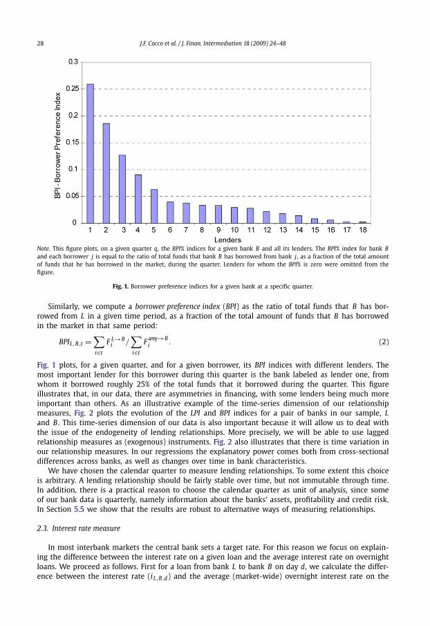
Note. This figure plots, on a given quarter q, the BPI% indices for a given bank B and all its lenders. The BPI% index for bank Band each borrower j is equal to the ratio of total funds that bank B has borrowed from bank j, as a fraction of the total amountof funds that he has borrowed in the market, during the quarter. Lenders for whom the BPI% is zero were omitted from thefigure.
Fig. 1. Borrower preference indices for a given bank at a specific quarter.
Similarly, we compute a borrower preference index (BPI) as the ratio of total funds that B has bor-rowed from L in a given time period, as a fraction of the total amount of funds that B has borrowedin the market in that same period:
BPIL,B,t =∑
i∈t
F L→Bi /
∑
i∈t
F any→Bi . (2)
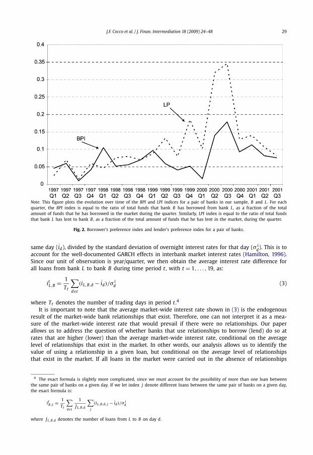
Fig. 1 plots, for a given quarter, and for a given borrower, its BPI indices with different lenders. Themost important lender for this borrower during this quarter is the bank labeled as lender one, fromwhom it borrowed roughly 25% of the total funds that it borrowed during the quarter. This figureillustrates that, in our data, there are asymmetries in financing, with some lenders being much moreimportant than others. As an illustrative example of the time-series dimension of our relationshipmeasures, Fig. 2 plots the evolution of the LPI and BPI indices for a pair of banks in our sample, Land B . This time-series dimension of our data is also important because it will allow us to deal withthe issue of the endogeneity of lending relationships. More precisely, we will be able to use laggedrelationship measures as (exogenous) instruments. Fig. 2 also illustrates that there is time variation inour relationship measures. In our regressions the explanatory power comes both from cross-sectionaldifferences across banks, as well as changes over time in bank characteristics.
We have chosen the calendar quarter to measure lending relationships. To some extent this choiceis arbitrary. A lending relationship should be fairly stable over time, but not immutable through time.In addition, there is a practical reason to choose the calendar quarter as unit of analysis, since someof our bank data is quarterly, namely information about the banks’ assets, profitability and credit risk.In Section 5.5 we show that the results are robust to alternative ways of measuring relationships.
2.3. Interest rate measure
In most interbank markets the central bank sets a target rate. For this reason we focus on explain-ing the difference between the interest rate on a given loan and the average interest rate on overnightloans. We proceed as follows. First for a loan from bank L to bank B on day d, we calculate the differ-ence between the interest rate (iL,B,d) and the average (market-wide) overnight interest rate on the
J.F. Cocco et al. / J. Finan. Intermediation 18 (2009) 24–48 29
Note. This figure plots the evolution over time of the BPI and LPI indices for a pair of banks in our sample, B and L. For eachquarter, the BPI index is equal to the ratio of total funds that bank B has borrowed from bank L, as a fraction of the totalamount of funds that he has borrowed in the market during the quarter. Similarly, LPI index is equal to the ratio of total fundsthat bank L has lent to bank B , as a fraction of the total amount of funds that he has lent in the market, during the quarter.
Fig. 2. Borrower’s preference index and lender’s preference index for a pair of banks.
same day (id), divided by the standard deviation of overnight interest rates for that day (σ id). This is to
account for the well-documented GARCH effects in interbank market interest rates (Hamilton, 1996).Since our unit of observation is year/quarter, we then obtain the average interest rate difference forall loans from bank L to bank B during time period t , with t = 1, . . . ,19, as:
itL,B = 1
Tt
∑
d∈t
(iL,B,d − id)/σid (3)
where Tt denotes the number of trading days in period t .4
It is important to note that the average market-wide interest rate shown in (3) is the endogenousresult of the market-wide bank relationships that exist. Therefore, one can not interpret it as a mea-sure of the market-wide interest rate that would prevail if there were no relationships. Our paperallows us to address the question of whether banks that use relationships to borrow (lend) do so atrates that are higher (lower) than the average market-wide interest rate, conditional on the averagelevel of relationships that exist in the market. In other words, our analysis allows us to identify thevalue of using a relationship in a given loan, but conditional on the average level of relationshipsthat exist in the market. If all loans in the market were carried out in the absence of relationships
4 The exact formula is slightly more complicated, since we must account for the possibility of more than one loan betweenthe same pair of banks on a given day. If we let index j denote different loans between the same pair of banks on a given day,the exact formula is:
itB,L = 1
Tt
∑
d∈t
1
J L,B,d
∑
j
(iL,B,d, j − id)/σ id
where J L,B,d denotes the number of loans from L to B on day d.
30 J.F. Cocco et al. / J. Finan. Intermediation 18 (2009) 24–48
the market-wide interest rate would change and our results are not informative about what wouldhappen.
2.4. Other variables
In this section we describe the variables that we use to explain the interest rate and lending rela-tionships. The first set of variables that we include are bank size (measured by total assets), quarterlyreturn on assets, and the proportion of non-performing loans (NPL). The latter is defined as loans thatare past-due for a period exceeding 90 days, over the total outstanding credit granted by the bank.Several papers have shown that these variables matter for the pricing of Fed Fund loans (Allen andSaunders, 1986; Furfine, 2001, among others). These variables may also constitute important deter-minants of relationships. Several papers in the interbank market literature model agency problemsthat arise from asymmetric information between borrowers and lenders of funds, which monitoringmay help to overcome (Rochet and Tirole, 1996).5 The asymmetries of information may be larger, andmonitoring may be more important when banks are smaller, profitability is lower, or credit risk (asmeasured by the proportion of non-performing loans) is higher. It is conceivable that this monitoringalso takes place outside of the interbank market. After all, banks undertake many kinds of transac-tions with each other, of which interbank overnight loans are just one. In Section 5 we construct ameasure of interactions between banks that take place outside of the interbank market, to explorethis possibility further.
Banks face liquidity risk that arises from the behavior of retail depositors (Ho and Saunders, 1985;Bhattacharya and Gale, 1987; and Freixas et al., 2000). Lending relationships may help banks to insureagainst such liquidity risk. For example, the model of Carlin et al. (2007) predicts that relationshipsallow traders who have suffered a liquidity shock (the distressed traders) to transact at more favorableprices. In order to test this prediction we need to obtain a measure of distress. A natural measure canbe constructed from the fact that banks are required to satisfy minimum reserve requirements. Overa given reserve maintenance period (or settlement period) a given bank’s average reserves must notfall below a given proportion of its short-term liabilities (mostly customer deposits).6
If relationships allow banks which have suffered a liquidity shock to transact at more favorableprices, we would expect that, banks’ who have a higher shortage of funds in their reserve account,would borrow funds from banks with whom they have a relationship, and through this pay a lowerinterest rate than they would otherwise. To investigate this prediction we construct a proxy for eachbank’s reserve requirements, equal to the average of the daily deposits in the bank’s reserve accountover the reserve maintenance period. We then measure surplus deposits for bank i on day d (SDid)as the ratio between the current average level of deposits in the reserve account (since the start ofthe current reserve requirement period) and our proxy for reserve requirements.7 We calculate theaverage value of this variable over each time period, for those days in which the bank intervened inthe interbank market.
To investigate further the extent to which bank relationships provide insurance against liquidityrisk, we construct a measure of such risk. First, we measure liquidity shocks by the daily change inthe bank’s reserve deposits, that is not due to interbank market loans. For each bank and year/quarter,liquidity risk is measured by the standard deviation of liquidity shocks, divided by the bank’s average
5 Broecker (1990), Flannery (1996), and Freixas and Holthausen (2005) also solve models of the interbank market withasymmetric information and credit risk. Freixas and Holthausen (2005) solve such a model in an international setting, whencross-country information is noisy.
6 Campbell (1987), Hamilton (1996), Hartmann et al. (2001), and Spindt and Hoffmeister (1988) have noticed how shortagesof liquidity at the end of the maintenance period often lead to special behavior of overnight rates during those days.
7 The formula for surplus deposits is:
SDid =∑
s∈{m(d): s�d} Depositis/nd∑s∈m(d) Depositis/n
(4)
where m(d) refers to the days in the same reserve maintenance period as day d, and nd and n are the up to d and the totalnumber of days in the maintenance period, respectively.
J.F. Cocco et al. / J. Finan. Intermediation 18 (2009) 24–48 31
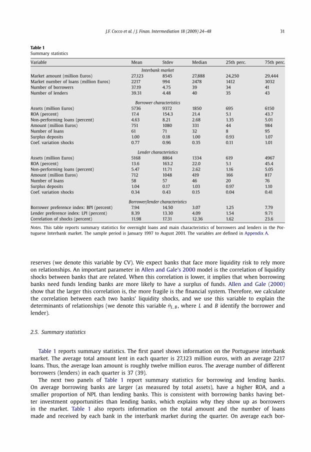
Table 1Summary statistics
Variable Mean Stdev Median 25th perc. 75th perc.
Interbank marketMarket amount (million Euros) 27,123 8545 27,888 24,250 29,444Market number of loans (million Euros) 2217 994 2478 1412 3032Number of borrowers 37.19 4.75 39 34 41Number of lenders 39.31 4.48 40 35 43
Borrower characteristicsAssets (million Euros) 5736 9372 1850 695 6150ROA (percent) 17.4 154.3 21.4 5.1 43.7Non-performing loans (percent) 4.63 8.21 2.68 1.35 5.01Amount (million Euros) 751 1080 331 44 984Number of loans 61 71 32 8 95Surplus deposits 1.00 0.18 1.00 0.93 1.07Coef. variation shocks 0.77 0.96 0.35 0.11 1.01
Lender characteristicsAssets (million Euros) 5168 8864 1334 619 4967ROA (percent) 13.6 163.2 22.0 5.1 45.4Non-performing loans (percent) 5.47 11.71 2.62 1.16 5.05Amount (million Euros) 712 1048 419 166 817Number of loans 58 57 46 20 76Surplus deposits 1.04 0.17 1.03 0.97 1.10Coef. variation shocks 0.34 0.43 0.15 0.04 0.41
Borrower/lender characteristicsBorrower preference index: BPI (percent) 7.94 14.50 3.07 1.25 7.79Lender preference index: LPI (percent) 8.39 13.30 4.09 1.54 9.71Correlation of shocks (percent) 11.98 17.31 12.36 1.62 23.6
Notes. This table reports summary statistics for overnight loans and main characteristics of borrowers and lenders in the Por-tuguese Interbank market. The sample period is January 1997 to August 2001. The variables are defined in Appendix A.
reserves (we denote this variable by CV). We expect banks that face more liquidity risk to rely moreon relationships. An important parameter in Allen and Gale’s 2000 model is the correlation of liquidityshocks between banks that are related. When this correlation is lower, it implies that when borrowingbanks need funds lending banks are more likely to have a surplus of funds. Allen and Gale (2000)show that the larger this correlation is, the more fragile is the financial system. Therefore, we calculatethe correlation between each two banks’ liquidity shocks, and we use this variable to explain thedeterminants of relationships (we denote this variable θL,B , where L and B identify the borrower andlender).
2.5. Summary statistics
Table 1 reports summary statistics. The first panel shows information on the Portuguese interbankmarket. The average total amount lent in each quarter is 27,123 million euros, with an average 2217loans. Thus, the average loan amount is roughly twelve million euros. The average number of differentborrowers (lenders) in each quarter is 37 (39).
The next two panels of Table 1 report summary statistics for borrowing and lending banks.On average borrowing banks are larger (as measured by total assets), have a higher ROA, and asmaller proportion of NPL than lending banks. This is consistent with borrowing banks having bet-ter investment opportunities than lending banks, which explains why they show up as borrowersin the market. Table 1 also reports information on the total amount and the number of loansmade and received by each bank in the interbank market during the quarter. On average each bor-
32 J.F. Cocco et al. / J. Finan. Intermediation 18 (2009) 24–48
rower receives 751 million Euros in 61 loans, while each lender loans out 712 million Euros in 58loans.8
Table 1’s last panel shows summary statistics for the relationship metrics, and for the correlationof shocks. The average BPI is 7.94 percent, and the average LPI is 8.39 percent. These averages aresignificantly higher than the median values (3 and 4 percent respectively), a sign of a skewed distri-bution. That is, banks borrow/lend relatively little from most banks, but large amounts from a few ofthem.
Our interest rate measure is the difference between the loan interest rate and the averageovernight interest rate, so that on average it is zero. But some numbers are helpful for understand-ing interest rate cross-sectional variability in our sample. The standard deviation of interest rates ona given day is on average 8 basis points. Moreover, this is naturally a strongly skewed distribution.While the median standard deviation is 6 basis points, in ten percent of the days the standard devi-ation of interest rates is higher than 18 basis points. We have calculated several summary statisticsthat allow us to understand by how much the interest rate vary across lenders/borrowers. On averagethe interest rate is 43 basis points higher for small than for large borrowers, and it is 39 basis pointshigher for large than for small lenders (small (large) are those banks in the bottom (top) one-third ofthe total assets distribution).9 Interest rates also tend to vary with return on assets: on average theinterest rate is 17 basis points higher for borrowers with a low return on assets (bottom one third)than with a high return on assets (top one third).
3. Pricing of interbank loans
3.1. Baseline regressions
We investigate the determinants of the interest rate on interbank market loans. We do so us-ing a regression analysis. An alternative approach would have been to use a matching methodology,in which we would matched banks according to size and other bank characteristics. The match-ing approach could offer some advantages relative to regression analysis, in that we might have amore appropriate choice for the benchmark interest rate. However, we have decided to use regres-sion analysis since it has several advantages relative to the matching methodology. First, it allowsus to simultaneously establish different benchmarks depending on multiple bank characteristics (e.g.bank size, percentage of non-performing loans, profitability), without significantly decreasing cell size,which would happen if we performed matches along several bank characteristics. Second, it allowsus to estimate the impact of different bank characteristics (size, profitability, etc.) on the loan interestrate, within the context of a single regression.
We first estimate the unconditional correlation between the relationship metrics and the loaninterest rate defined in Section 2.3:
itL,B = α + γ BPIt
L,B + κLPItL,B + βt Dt + ut
L,B (5)
where t indexes time, Dt are time dummies, the subscripts L and B refer to lending and borrowingbank, respectively, and ut
L,B is the residual. Column (i) of Table 2 shows the estimation results. Theseresults appear to suggest that borrowers (lenders) tend to pay (receive) higher (lower) interest rateson loans with banks with whom they have higher relationship indices. We will show that the reasonfor this result is that the decision of whether to rely on lending relationships is endogenous, andcorrelated with bank characteristics that also affect the interest rate on the loan. With this in mindwe include size, ROA and NPL as additional independent variables. The regression that we estimate isthen:
itL,B = α +
∑
j=L,B
[β1 jSizet
j + β2 jROAtj + β3 jNPLt
j
] + γ BPItL,B + κLPIt
L,B + βt Dt + utL,B . (6)
8 The average amount and number of loans for borrowing and lending banks are not exactly equal because there is a differentnumber of borrowing and lending banks in the market.
9 These numbers are very similar to the ones reported by Furfine (2001) for the FED Funds Market.
J.F. Cocco et al. / J. Finan. Intermediation 18 (2009) 24–48 33
Table 2Multivariate model for interest rate
Independent variables (i) (ii) (iii) (iv) (v) (vi) Fixed effects
Borrower characteristicsLog assets −0.098*** −0.103*** −0.086*** −0.096***
(13.43) (12.98) (8.72) (3.96)Market share −2.141*** −0.603***
(9.80) (2.25)ROA 1.194* 1.245* −0.318 −0.032 1.166
(1.84) (1.85) (0.48) (1.65) (0.04)Non-performing loans 0.512*** 0.548*** 0.616*** 0.539*** −0.005
(2.67) (2.72) (3.12) (2.70) (0.02)Surplus deposits −0.117** −0.100* −0.111** −0.259***
(2.21) (1.85) (2.09) (4.19)Coef. variation 0.000 0.000 0.000 −0.001
(0.26) (0.30) (0.04) (0.55)
Lender characteristicsLog assets 0.083*** 0.087*** 0.090*** 0.112***
(15.25) (14.98) (13.02) (4.89)Market share 1.666*** −0.129
(8.29) (0.56)ROA 0.150 0.1333 1.184*** 0.146 −0.304
(0.54) (0.44) (3.69) (0.47) (0.74)Non-performing loans 0.066* 0.089 −0.076 0.089 −0.094
(1.66) (1.45) (1.19) (1.44) (0.78)Surplus deposits 0.063 0.052 0.059 0.059
(1.18) 0.95 (1.11) (0.97)Coef. variation −0.017*** −0.012*** −0.018*** −0.019***
(10.53) (3.89) (9.61) (8.92)
Borrower/lender characteristicsCorrelation of shocks −0.003 −0.003 −0.004 −0.013
(0.06) (0.05) (0.09) (0.26)Borrower pref. index 0.240*** −0.155*** −0.184*** −0.142*** −0.196*** −0.253***
(4.18) (2.71) (2.85) (2.00) (2.83) (3.60)Lender pref. index −0.180*** 0.218*** 0.347*** 0.445*** 0.404*** 0.331***
(3.15) (3.44) (4.78) (5.25) (4.97) (4.44)
Number obs. 7724 7046 6410 6410 6410 6410R2 0.01 0.08 0.08 0.05 0.08 0.11
Notes. The dependent variable is interest rate defined for every pair of lender and borrower as the quarterly average of thedifference between the interest rate on the loans between those two banks and the market interest rate on the same days,divided by the standard deviation of interest rates for the day. The independent variables are defined in Appendix A, and theyinclude time fixed effects. Column (vi) shows the estimation results including bank fixed effects in addition to the time fixedeffects. The sample period is January 1997 to August 2001. Robust t-statistics are shown in parenthesis.
* Significance at the 10% level.** Idem, 5%.
*** Idem, 1%.
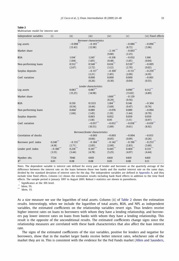
As a size measure we use the logarithm of total assets. Column (ii) of Table 2 shows the estimationresults. Interestingly, when we include the logarithm of total assets, ROA, and NPL as independentvariables, the estimated coefficients on the relationship variables revert sign. Thus lenders receivehigher interest rates on loans to borrowers with whom they have a lending relationship, and borrow-ers pay lower interest rates on loans from banks with whom they have a lending relationship. Thisresult is the opposite of the unconditional results. The estimated coefficients change signs since therelationship measures are correlated with these bank characteristics that also affect the loan interestrate.
The signs of the estimated coefficients of the size variables, positive for lenders and negative forborrowers, show that in the market larger banks receive better interest rates, whichever side of themarket they are in. This is consistent with the evidence for the Fed Funds market (Allen and Saunders,

34 J.F. Cocco et al. / J. Finan. Intermediation 18 (2009) 24–48
1986; Stigum, 1990; Furfine, 2001). The estimated positive coefficient on the ROA of borrowers isintuitive: borrowers with a higher ROA have a more profitable application for the funds, and thus arewilling to pay a higher interest rate for borrowing them. As expected we find that borrowers with ahigher proportion of NPL tend to pay higher interest rates on interbank market loans, a result which isstatistically significant at the one percent level. The estimated coefficients on ROA and NPL of lendersare not statistically significant, at least when we include as independent variables those that captureliquidity risk (column (iii)). The equation that we estimate is now:
itL,B = α +
∑
j=L,B
[β1 jSizet
j + β2 jROAtj + β3 jNPLt
j + β4 jSDtj + β5 jCVt
j
]
+ β6θL,B + γ BPItL,B + κLPIt
L,B + βt Dt + utL,B (7)
where SD denotes surplus deposits, or the net reserve position of borrowers and lenders when theyborrow or lend funds in the market, CV denotes the coefficient of variation of liquidity shocks, andθL,B denotes the correlation of liquidity shocks between lender and borrower of funds.
The results in column (iii) of Table 2 show that borrowers with a lower surplus deposit pay onaverage a higher interest rate on their loans. The magnitude of the coefficient is economically signif-icant: an increase in the shortage of funds from the 25th to the 75th percentile leads to a 13 basispoint increase in the loan interest rate. However, if this change is accompanied by an increase inthe BPI index from the 25th to the 75th percentile, then the increase in the interest rate is only 7basis points. Thus relationships seem to allow borrowers with a larger reserve imbalance to transactat more favorable rates. The estimated coefficient on the surplus deposits of lenders is not statisti-cally significant. What seems to matter for lenders is the volatility of liquidity shocks: the larger thevolatility the lower is the interest rate that lenders receive on interbank market loans. The estimatedcoefficient on θL,B is not significantly different from zero.
In columns (iv) and (v) we investigate why larger banks receive better rates. The fact that borrow-ers’ size matters is intuitive and could be due to better information being available for larger banks,or to larger banks being too-big-to-fail. However, the reason why larger lenders receive better ratesis less clear. A possible explanation may be that larger banks have more bargaining power (Osborneand Rubinstein, 1994). In order to investigate this explanation, we have calculated market shares forborrowers and lenders. Market shares are positively correlated with bank size, as measured by thelogarithm of total assets, with coefficients of correlation equal to 0.59 (0.74) for lenders (borrow-ers). When we include market shares as explanatory variables for the loan interest rate we find thatlenders/borrowers with larger market shares receive better rates (column (iv)). When in column (v)we include both market shares and the logarithm of total assets as independent variables we find thatthe explanatory power of both variables is diminished, reflecting the fact that they are co-linear.
One may be concerned that our results on the impact of the relationship measures on interest ratesare driven by unobserved bank heterogeneity. In order to address this concern, the last column ofTable 2 shows the estimation results when we include bank fixed effects among the set of explanatoryvariables. Comparing these results with those in column (iii) of the same table, two conclusions canbe drawn. First, some of the variables that we use to capture the effects of borrower characteristicson the loan interest rate are no longer significant. This tells us that these variables were previouslysignificant due of cross sectional differences in bank characteristics, which are now captured by thefixed effects. Second, and importantly, we find that the effects of the relationship measures on theloan interest rate are robust to the introduction of bank fixed effects. More precisely, the estimatedcoefficients on the BPI and LPI indices are still negative and positive, respectively, and statisticallysignificant.
It is important to clarify that we do not find that small banks that lend funds in the interbankcharge higher interest rates. In fact, we find exactly the opposite. The estimated positive coefficientson log assets for lender characteristics in the second panel of Table 2 shows that larger (smaller)banks receive a higher (lower) interest rate when lending funds in the market. These results holdacross all specifications. Therefore we find that: (i) small banks are net lenders in the market but,within all lenders, small banks receive lower interest rates than large banks on the funds that theylend; (ii) large banks are net borrowers in the market but, within all borrowers, large banks pay lower
J.F. Cocco et al. / J. Finan. Intermediation 18 (2009) 24–48 35
interest rates than small banks on the funds that they borrow. With respect to lending relationships,the results in Table 2 show that, both smaller and larger banks receive better terms both when bor-rowing and when lending (pay a lower interest rate when borrowing and receive a higher interestrate when lending) when they interact with banks with whom they have high relationship indices.
3.2. Instrumental variables
In order to address the issue of the endogeneity of relationships we estimate Eq. (7) using instru-mental variables (IV). This allows us to identify the causal link between the relationship measures andthe loan interest rate. This is a departure from most of the existing literature on lending relationships,which does not address the endogeneity of those relationships. The validity of the IV approach de-pends crucially on the quality of the instruments used in the first stage regression. Good instrumentsinclude those which are simultaneously pre-determined and highly correlated with the relationshipmetrics. Therefore, we explore the time-series dimension of our data set, and use the lagged relation-ship measures as instruments. Obviously, such instruments are not available in cross sectional data,which is typically used in the existing literature on lending relationships. The quality of these instru-ments can be measured by the R-squared of the first-stage regressions: for the BPI (LPI) measure it isequal to 67% (78%).10
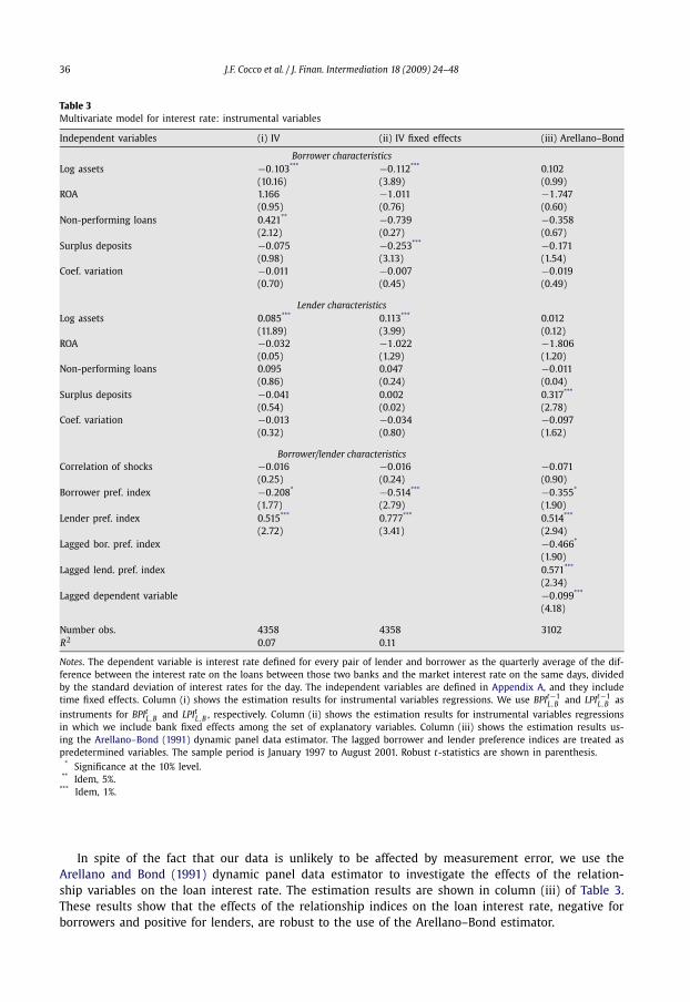
The estimation results for the second stage regressions are shown in the column (i) of Table 3.The t-statistics (reported below the estimated coefficients) have been adjusted for first-stage estima-tion error. We compare the results in column (i) of Table 3 to those in column (iii) of Table 2, inwhich we did not use instruments for the relationship metrics. First, the coefficients on total assetsand non-performing loans remain essentially unchanged. Second, the estimated coefficient on the sur-plus deposit of borrowers is no longer significant, and the estimated coefficient on the coefficient ofvariation of lenders is only significant in (ii). Thus the level of significance of the insurance variablesis reduced once we control for the endogeneity of relationships. This suggests that relationships areimportant because they allow banks to obtain insurance in the interbank market. In the next sectionwe will explicitly study the determinants of lending relationships.
Third, the estimated coefficients on the relationship variables are significant throughout, and havethe same signs. Moreover, the magnitude of the estimated coefficients is either unchanged or evenslightly increased (in absolute value). This result implies that, at least in our dataset, the endogeneityproblem does not affect the inference regarding the causal link between lending relationships andinterest rates. Of course, one should be careful about generalizing this result to other applications,since we have only shown that it holds in our data. Furthermore, and even though the estimatedcoefficients on the relationship metrics are robust to an IV approach, the inference on the coefficientsof some of the insurance variables changes. If these are only control variables, then this is not an issue.However, if one is interested in the economic interpretation of those coefficients, then controlling forendogeneity is important.
In column (ii) of Table 3 we report the results of estimating Eq. (7) using instrumental variables,but including bank fixed effects among the set of explanatory variables. As it was the case in Table 2,we see that the effects of the relationship metrics on the loan interest rate are robust to the inclusionof bank fixed effects.
The use of lagged relationship indices as instruments raises some concerns in the presence of mea-surement error. In that case, even though the true dependent variable and consequently the residualof a hypothetical “true regression” would only be measurable at time t , the observed value of de-pendent variable would have a component that is measurable at time t − 1. This would create serialcorrelation in the regression residual and lead to inconsistent estimators. However, our data is unlikelyto be affected by measurement error in any significant way: we observe the variables directly fromcentral bank data, including the terms of the loan which must be reported separately by borrowerand lender to the central bank, which in turn is responsible for the settlement of the loan.
10 We have also estimated the IV regressions using the first lag of all the explanatory variables in Eq. (7) as instruments in thefirst-state regression. The first stage R2 was almost unaffected, and the second stage results were the same and are thereforenot reported.
36 J.F. Cocco et al. / J. Finan. Intermediation 18 (2009) 24–48
Table 3Multivariate model for interest rate: instrumental variables
Independent variables (i) IV (ii) IV fixed effects (iii) Arellano–Bond
Borrower characteristicsLog assets −0.103*** −0.112*** 0.102
(10.16) (3.89) (0.99)ROA 1.166 −1.011 −1.747
(0.95) (0.76) (0.60)Non-performing loans 0.421** −0.739 −0.358
(2.12) (0.27) (0.67)Surplus deposits −0.075 −0.253*** −0.171
(0.98) (3.13) (1.54)Coef. variation −0.011 −0.007 −0.019
(0.70) (0.45) (0.49)
Lender characteristicsLog assets 0.085*** 0.113*** 0.012
(11.89) (3.99) (0.12)ROA −0.032 −1.022 −1.806
(0.05) (1.29) (1.20)Non-performing loans 0.095 0.047 −0.011
(0.86) (0.24) (0.04)Surplus deposits −0.041 0.002 0.317***
(0.54) (0.02) (2.78)Coef. variation −0.013 −0.034 −0.097
(0.32) (0.80) (1.62)
Borrower/lender characteristicsCorrelation of shocks −0.016 −0.016 −0.071
(0.25) (0.24) (0.90)Borrower pref. index −0.208* −0.514*** −0.355*
(1.77) (2.79) (1.90)Lender pref. index 0.515*** 0.777*** 0.514***
(2.72) (3.41) (2.94)Lagged bor. pref. index −0.466*
(1.90)Lagged lend. pref. index 0.571***
(2.34)Lagged dependent variable −0.099***
(4.18)
Number obs. 4358 4358 3102R2 0.07 0.11
Notes. The dependent variable is interest rate defined for every pair of lender and borrower as the quarterly average of the dif-ference between the interest rate on the loans between those two banks and the market interest rate on the same days, dividedby the standard deviation of interest rates for the day. The independent variables are defined in Appendix A, and they includetime fixed effects. Column (i) shows the estimation results for instrumental variables regressions. We use BPIt−1
L,B and LPIt−1L,B as
instruments for BPItL,B and LPItL,B , respectively. Column (ii) shows the estimation results for instrumental variables regressionsin which we include bank fixed effects among the set of explanatory variables. Column (iii) shows the estimation results us-ing the Arellano–Bond (1991) dynamic panel data estimator. The lagged borrower and lender preference indices are treated aspredetermined variables. The sample period is January 1997 to August 2001. Robust t-statistics are shown in parenthesis.
* Significance at the 10% level.** Idem, 5%.
*** Idem, 1%.
In spite of the fact that our data is unlikely to be affected by measurement error, we use theArellano and Bond (1991) dynamic panel data estimator to investigate the effects of the relation-ship variables on the loan interest rate. The estimation results are shown in column (iii) of Table 3.These results show that the effects of the relationship indices on the loan interest rate, negative forborrowers and positive for lenders, are robust to the use of the Arellano–Bond estimator.
J.F. Cocco et al. / J. Finan. Intermediation 18 (2009) 24–48 37
4. The determinants of lending relationships
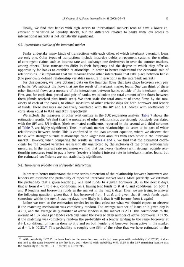
The instrumental variables regressions that we have estimated in the previous section allow usto estimate the effects of lending relationships on the loan interest rate, but they do not explain thedeterminants of lending relationships. In this section we investigate which bank characteristics explainthe decision of whether or not to rely on lending relationships. We do so in a setting in which weallow both the loan amount and interest rate to be correlated with the identity of the borrowingand lending banks (i.e. on whether they have a lending relationship). More precisely, we estimate aseemingly unrelated regressions (SUR) system of equations, with the amount lent, interest rate, andthe relationship measures between lender and borrower (LPI and BPI) as our endogenous dependentvariables. Thus, we estimate simultaneously the following equations:
itL,B = α1 +
∑
j=L,B
[β1
1 jSizetj + β1
2 jROAtj + β1
3 jNPLtj + β1
4 jSDtj + β1
5 jCVtj
]
+ β16 θB,L + βt1 Dt1 + ut
L,B , (8)
BPItL,B = α2 +
∑
j=L,B
[β2
1 jSizetj + β2
2 jROAtj + β2
3 jNPLtj + β2
4 jSDtj + β2
5 jCVtj
]
+ β26 θB,L + βt2 Dt2 + εt
L,B , (9)
LPItL,B = α3 +
∑
j=L,B
[β3
1 jSizetj + β3
2 jROAtj + β3
3 jNPLtj + β3
4 jSDtj + β3
5 jCVtj
]
+ β36 θB,L + βt3 Dt3 + ξ t
L,B , (10)
Ln(
V tL,B
) = α4 +∑
j=L,B
[β4
1 jSizetj + β4
2 jROAtj + β4
3 jNPLtj + β4
4 jSDtj + β4
5 jCVtj
]
+ β46 θB,L + βt4 Dt4 + vt
L,B (11)
where V tL,B is the total amount of funds lent by bank L to bank B during time period t , and Ln
denotes logarithm. We estimate a reduced form system, and therefore allow for contemporaneouscorrelation across the four different innovations (u, ε, ξ and v). We include time dummies in allequations.
4.1. BPI and LPI equations
Table 4 shows the estimation results. The results for the BPI equation are shown in the secondcolumn. In this equation we try to determine which borrower and lender characteristics explain thevariation in BPI indices. In other words, who are the borrowers who have higher relationship indices,and who are the lenders with whom they have those higher indices. For instance, the negative esti-mated coefficient on the logarithm of total assets of borrowers shows that small borrowers rely moreon lending relationships. On the other hand, the estimated positive coefficient on the total assets oflenders in the same equation, implies that small borrowers tend to have large banks as their preferredlenders. These results suggest a dichotomy between large and small banks in the market, an issue thatwe explore further in Section 5.1.
Interestingly, we find that borrowers with higher default risk are more likely to rely on lendingrelationships (the estimated coefficient on NPL in the BPI equation is positive) and to pay higherinterest rates (the estimated coefficient on NPL in the interest rate equation is also positive). Fromthese two results one may reasonably expect that banks which borrow funds from banks with whomthey have a lending relationship pay higher rates. This may seem inconsistent with the result inTable 2 that loan rates tend to be lower for banks borrowing from lenders with whom they havelarge relationship indices.
The key to understanding this apparent inconsistency is to note that in Table 2 we did not findthat unconditionally borrowers with a high default risk and large BPI indices pay lower interest rates.In fact the reverse is true: large values for BPI indices tend to be associated with higher interest

38 J.F. Cocco et al. / J. Finan. Intermediation 18 (2009) 24–48
Table 4SUR model
Independent variables BPI LPI Int. rate Amount
BorrowerLog assets −0.025*** 0.024*** −0.090*** 6.313***
(20.67) (23.14) (13.40) (7.33)ROA 0.088 −0.064 1.207 −178.190
(0.49) (0.42) (1.22) (1.41)Non-performing loans 0.152*** −0.009 0.517*** −34.552*
(5.47) (0.36) (3.32) (1.74)Surplus deposit −0.044*** −0.051*** −0.143** 23.017***
(3.71) (5.05) (2.17) (2.75)Coef. variation 0.011*** −0.000 −0.002 −0.776
(16.03) (0.40) (0.47) (1.63)
LenderLog assets 0.011*** −0.001 0.084*** −5.442***
(10.33) (1.43) (14.37) (7.27)ROA −0.025 −0.064 0.116 −337.062***
(0.23) (0.69) (0.19) (4.40)Non-performing loans 0.003 −0.003 0.087 44.831***
(0.19) (0.18) (0.89) (3.55)Surplus deposit −0.009 −0.001 0.064 −24.495***
(0.77) (0.14) (0.98) (2.92)Coef. variation −0.002** 0.015*** −0.012** −1.423**
(2.20) (18.45) (2.26) (2.14)
Borrower/lenderCorrelation of shocks −0.062*** −0.049*** −0.008 −64.583***
(6.37) (5.85) (0.16) (9.31)
Number obs. 6410 6410 6410 6410R2 0.17 0.19 0.08 0.05
Correlation of residualsBPI 1.000LPI 0.128 1.000Interest rate −0.026 0.049 1.000Amount 0.312 0.438 0.008 1.000
Notes. We estimate a SUR system where the dependent variables are the interest rate, the borrower and lender preferenceindices, and the logarithm of loan volume. The independent variables are defined in Appendix A, and they include time fixedeffects. The sample period is January 1997 to August 2001. Robust t-statistics are shown in parenthesis.
* Significance at the 10% level.** Idem, 5%.
*** Idem, 1%.
rates (column (i) in Table 2). It is only when controlling for the proportion of NPL that the estimatedcoefficient on the BPI index becomes negative (Table 2 column (ii)), but even then it is an order ofmagnitude smaller than the coefficient on the default risk variable. That is: borrowers with a highproportion of NPL pay on average higher interest rates, but the interest rate premium is smaller ifthey borrow funds from a lender with whom they have a high BPI.
Some calculations help to clarify this important point. Consider an increase in the proportion ofNPL from the 25th to the 75th percentile, while everything else remains the same. Using the estimatedcoefficients in the third column of Table 2 we see that the interest rate on the loan increases by 2basis points.11 However, if the increase in the proportion of NPL is accompanied by an increase in theBPI index from the 25th to the 75th percentile, the interest rate only goes up by 0.6 basis points. Ifinstead we consider an increase in the proportion of NPL from the 10th to the 90th percentile the
11 Due to our scaling of the dependent variable we need to multiply this increase by the standard deviation of the interestrate.
J.F. Cocco et al. / J. Finan. Intermediation 18 (2009) 24–48 39
interest rate now goes up by 20 basis points when the BPI index is unchanged, and by 5 basis pointswhen the BPI index also increases from the 10th to the 90th percentile.12
The fact that borrowers with a higher proportion of NPL rely more on relationships suggests banksrelationships may help overcome agency problems. One could reasonably question where does themonitoring associated with such relationships take place. After all, repeated overnight loans are fre-quent, but lenders are only able to observe the extent to which borrowers were able to repay the loan.It is conceivable that the monitoring associated with these relationships also takes place outside ofthe interbank market, as banks undertake many kinds of transactions with each other. In Section 5 weconstruct a measure of bank interactions that take place outside of the interbank market, to explorethis issue further.
Interestingly we also find evidence that relationships allow banks to insure against liquidity risk.More precisely, we find that banks with a larger imbalance in their reserve deposits are more likely toborrow funds from banks with whom they have a relationship (the estimated coefficient on surplusdeposits in the BPI equation is negative). This result supports the prediction of Carlin et al.’s (2007)model that under repeated interaction cooperation among traders is an equilibrium outcome whichinvolves refraining from predation, and that allows distressed traders to access liquidity. In addition,we find that borrowers with more volatile liquidity shocks tend to rely more on lending relationships(the coefficient on CV B is positive), and they tend to do so with lenders that have less volatile liquidityshocks (the estimated coefficient on CV L in the BPI equation is negative). This result lends furthersupport to the idea that relationships allow banks to insure against liquidity risk.
The third column of Table 4 reports the results for the LPI equation. Similarly to the borrowers, wefind that small lenders tend to have larger relationship indices with large borrowers (the estimatedcoefficient on total assets of lenders is negative and on the total assets of borrowers is positive). Inaddition, lenders with more volatile liquidity shocks tend to have higher relationship indices withborrowers that face less volatile liquidity shocks, although the estimated coefficient for borrowers isnot significantly different from zero.
The estimated coefficients on the correlation of liquidity shocks are negative in both the BPI andLPI equations. Banks are more likely to have high relationship indices with banks with whom theirliquidity shocks are less correlated. This is an interesting and important finding since Allen and Gale(2000) show that the financial system is less fragile when the correlation of liquidity shocks betweenbanks that are related is lower. This may further enhance market liquidity.
As a whole, columns two and three of Table 4 show that it is mostly borrower characteristicsthat explain variation in the relationship indices. One might have an a priori expectation that fornon-secure loans such as interbank market loans, borrowers’ characteristics are more important forexplaining the terms of the loan than lenders’ characteristics. Table 4 suggests that this reasoningcarries through when explaining lending relationships.
4.2. Interest rate and loan volume equations
The fourth column of Table 4 shows the results for the interest rate equation. This equation issimilar to that estimated in specification (iii) of Table 2, except that now we do not include the LPIand BPI indices as independent variables, but instead treat them as endogenous when estimatingthe system of equations. The results are similar to those reported in Table 2. In the last column ofTable 4 we report the results for loan volume (the fourth equation in the SUR system). We find thatlarger banks borrow larger amounts. Interestingly, we find that more profitable banks lend less (theestimated coefficients on ROAL is negative). In addition, we find that banks with a higher proportionof non-performing loans lend more and borrow less. The estimated coefficients for ROA and NPL areconsistent with banks that have better investment opportunities borrowing more and lending less.Finally, the estimated coefficients on surplus deposit show that banks which have smaller imbalancestend to rely on larger loans with any particular bank.
12 The full effect of NPL on the interest rate may be even larger because default risk is likely to be correlated with bank size,for which we are also controlling in Table 2.
40 J.F. Cocco et al. / J. Finan. Intermediation 18 (2009) 24–48
At the bottom of Table 4 we report the estimated correlation matrix of residuals in the systemof equations. Larger residuals for the BPI (LPI) equation are associated with lower (higher) interestrates, but these correlations are fairly small. The largest correlations are of amount lent with LPI andBPI, which are equal to 0.44 and 0.31, respectively. This supports the idea that relationships have thegreatest effect on the provision of credit, and not on the price at which banks are able to borrow orlend.
5. Further evidence on the determinants of lending relationships
In this section we provide further evidence on the determinants of lending relationships, thatallows us to be more precise as to their exact nature.13
5.1. Small versus large banks
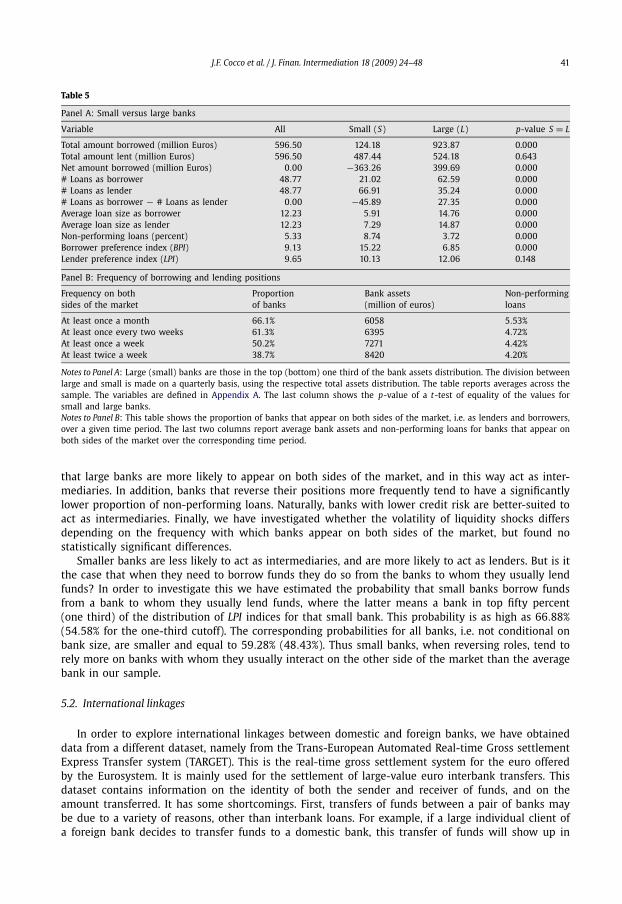
The estimation results in the previous sections show that bank size is an important determinantof interbank market interest rates, and of lending relationships. In this section we explore furtherthe role of bank size in the market structure. In order to do so, and for each time period in oursample, we classify banks into large and small, based on the distribution of bank assets. Large (small)banks are those whose assets are larger (smaller) than percentile 66 (33) of this distribution. We thencompare several variables for small and large banks.
The first two rows of Table 5, Panel A report the average amount borrowed/lent per bank andperiod over the whole sample period. The third row reports the net amount borrowed, which issimply the difference between the first two. The second column shows the results for all banks, i.e.not conditional on bank size, while columns three and four show the results for small and largebanks, respectively. On average, and per period, each bank in our sample has lent/borrowed 596.5million euros. There are significant differences between small and large banks: large banks tend tobe net borrowers, with the average net amount borrowed roughly equal to 400 million euros, whilesmall banks tend to be net lenders, with the average net amount lent equal to 363 million euros.
Interestingly, this pattern of trade, in which large banks tend to be net buyers of liquidity and smallbanks tend to be net sellers, is also a distinctive feature of the U.S. Fed Funds market (Furfine, 1999;Ho and Saunders, 1985).14 It can be rationalized by the model of Ho and Saunders (1985). If largebanks are better able to diversify their risk exposure than small banks, then larger banks will bemore rate sensitive than small banks, and the slopes of the demand functions for interbank funds oflarge banks will be more price-elastic than those of small banks.
Table 5, Panel A reports information on the number of loans and the average loan amount. Large(small) banks tend to transact mostly as borrowers (lenders), reflecting the fact that they tend to benet borrowers (lenders) in the market. Unsurprisingly, the average loan amount for small banks is sig-nificantly lower than the average loan amount for large banks. The last three rows of Table 5, Panel Areport the proportion of non-performing loans, and relationship indices. Small banks tend to have asignificantly higher proportion of non-preforming loans than large banks. Furthermore, they tend tohave significantly higher BPI indices than large banks when borrowing funds. This suggests that smallbanks find it optimal, when borrowing funds, to concentrate their borrowing activity. Interestingly,the same is not true when lending funds, since there are no statistically significant differences in LPIindices between small and large banks.
We have also investigate the likelihood that banks appear on both sides of the market, i.e. aslenders and borrowers, over a given time period. Panel B of Table 5 reports that 66.1% (50.2%) of allbanks have been on average active market participants on both sides of the market at least once amonth (week).
Panel B of Table 5 also reports summary statistics for bank assets and proportion of non-performing loans as a function of how often banks appear on both sides of the market. It shows
13 We would like to thank an anonymous referee for suggestions that have led us to investigate the questions in this section.14 See also Stigum’s (1990) description of the Fed Funds market: “To cultivate correspondents that will sell funds to them,
large banks stand ready to buy whatever sums these banks offer, whether they need all these funds or not.”
J.F. Cocco et al. / J. Finan. Intermediation 18 (2009) 24–48 41
Table 5
Panel A: Small versus large banks
Variable All Small (S) Large (L) p-value S = L
Total amount borrowed (million Euros) 596.50 124.18 923.87 0.000Total amount lent (million Euros) 596.50 487.44 524.18 0.643Net amount borrowed (million Euros) 0.00 −363.26 399.69 0.000# Loans as borrower 48.77 21.02 62.59 0.000# Loans as lender 48.77 66.91 35.24 0.000# Loans as borrower − # Loans as lender 0.00 −45.89 27.35 0.000Average loan size as borrower 12.23 5.91 14.76 0.000Average loan size as lender 12.23 7.29 14.87 0.000Non-performing loans (percent) 5.33 8.74 3.72 0.000Borrower preference index (BPI) 9.13 15.22 6.85 0.000Lender preference index (LPI) 9.65 10.13 12.06 0.148
Panel B: Frequency of borrowing and lending positions
Frequency on bothsides of the market
Proportionof banks
Bank assets(million of euros)
Non-performingloans
At least once a month 66.1% 6058 5.53%At least once every two weeks 61.3% 6395 4.72%At least once a week 50.2% 7271 4.42%At least twice a week 38.7% 8420 4.20%
Notes to Panel A: Large (small) banks are those in the top (bottom) one third of the bank assets distribution. The division betweenlarge and small is made on a quarterly basis, using the respective total assets distribution. The table reports averages across thesample. The variables are defined in Appendix A. The last column shows the p-value of a t-test of equality of the values forsmall and large banks.Notes to Panel B: This table shows the proportion of banks that appear on both sides of the market, i.e. as lenders and borrowers,over a given time period. The last two columns report average bank assets and non-performing loans for banks that appear onboth sides of the market over the corresponding time period.
that large banks are more likely to appear on both sides of the market, and in this way act as inter-mediaries. In addition, banks that reverse their positions more frequently tend to have a significantlylower proportion of non-performing loans. Naturally, banks with lower credit risk are better-suited toact as intermediaries. Finally, we have investigated whether the volatility of liquidity shocks differsdepending on the frequency with which banks appear on both sides of the market, but found nostatistically significant differences.
Smaller banks are less likely to act as intermediaries, and are more likely to act as lenders. But is itthe case that when they need to borrow funds they do so from the banks to whom they usually lendfunds? In order to investigate this we have estimated the probability that small banks borrow fundsfrom a bank to whom they usually lend funds, where the latter means a bank in top fifty percent(one third) of the distribution of LPI indices for that small bank. This probability is as high as 66.88%(54.58% for the one-third cutoff). The corresponding probabilities for all banks, i.e. not conditional onbank size, are smaller and equal to 59.28% (48.43%). Thus small banks, when reversing roles, tend torely more on banks with whom they usually interact on the other side of the market than the averagebank in our sample.
5.2. International linkages
In order to explore international linkages between domestic and foreign banks, we have obtaineddata from a different dataset, namely from the Trans-European Automated Real-time Gross settlementExpress Transfer system (TARGET). This is the real-time gross settlement system for the euro offeredby the Eurosystem. It is mainly used for the settlement of large-value euro interbank transfers. Thisdataset contains information on the identity of both the sender and receiver of funds, and on theamount transferred. It has some shortcomings. First, transfers of funds between a pair of banks maybe due to a variety of reasons, other than interbank loans. For example, if a large individual client ofa foreign bank decides to transfer funds to a domestic bank, this transfer of funds will show up in
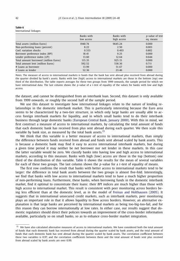
42 J.F. Cocco et al. / J. Finan. Intermediation 18 (2009) 24–48
Table 6International linkages
Banks withlow access
Banks withhigh access
p-value of testeq. means
Total assets (million Euros) 1940.74 9645.24 0.000Non-performing loans (percent) 8.22 2.50 0.003Coef. variation shocks 0.555 0.493 0.802Borrower preference index (BPI) 18.41 9.25 0.000Lender preference index (LPI) 13.60 12.64 0.644Total amount borrowed (million Euros) 115.35 925.15 0.000Total amount lent (million Euros) 592.52 538.36 0.711# Loans as borrower 13.99 51.67 0.000# Loans as lender 52.36 23.46 0.000
Notes. The measure of access to international markets is funds that the bank has sent abroad plus received from abroad duringthe quarter divided by bank’s assets. Banks with low (high) access to international markets are those in the bottom (top) onethird of the distribution. The table reports averages for these two groups from 1999 onwards, the sample period for which wehave international data. The last column shows the p-value of a t-test of equality of the values for banks with low and highaccess.
the dataset, and cannot be distinguished from an interbank loan. Second, this dataset is only availablefrom 1999 onwards, or roughly the second half of the sample period.
We use this dataset to investigate how international linkages relate to the nature of lending re-lationships in the domestic interbank market. This is particularly interesting because the Euro areaseems to be characterized by a two-tier structure, in which only large banks are usually able to ac-cess foreign interbank markets for liquidity, and in which small banks tend to do their interbankbusiness through large domestic banks (European Central Bank, January 2000). With this in mind, wefirst construct a measure of access to international markets, by calculating the total amount of fundsthat each domestic bank has received from plus sent abroad during each quarter. We then scale thisvariable by bank size, as measured by the total bank assets.15
We think that this variable is a better measure of access to international markets, than simplythe difference between funds received from abroad and funds sent abroad scaled by bank assets. Thisis because a domestic bank may find it easy to access international interbank markets, but duringa given time period it may neither be net borrower nor net lender in these markets. In this casethe latter variable would be zero. We classify banks into having low and high access to internationalmarkets, according to this measure. Banks with high (low) access are those in the top (bottom) onethird of the distribution of this variable. Table 6 shows the results for the mean of several variablesfor each of these two groups. The last column shows the p-value for a t-test of equality of means.
The first row confirms the result that banks with better access to international markets tend to belarger: the difference in total bank assets between the two groups is almost five-fold. Interestingly,we find that banks with low access to international markets tend to have a much higher proportionof non-performing loans. Furthermore, these banks, when borrowing funds in the domestic interbankmarket, find it optimal to concentrate their loans: their BPI indices are much higher than those withhigh access to international market. This result is consistent with peer monitoring across borders be-ing less efficient than at the domestic level, as in the model of Freixas and Holthausen (2005). Itsuggests that in international unsecured credit markets, such as interbank markets, peer monitoringplays an important role in that it allows liquidity to flow across borders. However, an alternative ex-planation is that large banks are perceived by international markets as being too-big-too-fail, and forthis reason they can borrow internationally at low rates. In either case, our results suggest that do-mestic regulators should direct their policies towards an improvement of the cross-border informationavailable, particularly so on small banks, so as to enhance cross-border market integration.
15 We have also calculated alternative measures of access to international markets. We have considered both the total amountof funds that each domestic bank has received from abroad during the quarter scaled by bank assets, and the total amount offunds that each domestic bank has sent abroad during the quarter scaled by bank assets. The correlation coefficient betweenthese two variables is 0.97, and the correlation coefficients between them and the total amount of funds sent plus receivedfrom abroad scaled by bank assets are over 0.99.
J.F. Cocco et al. / J. Finan. Intermediation 18 (2009) 24–48 43
Finally, we find that banks with high access to international markets tend to have a lower co-efficient of variation of liquidity shocks, but the difference relative to banks with low access tointernational markets is not statistically significant.
5.3. Interactions outside of the interbank market
Banks undertake many kinds of transactions with each other, of which interbank overnight loansare only one. Other types of transactions include intra-day debits on payment systems, the tradingof contingent claims such as interest rate and exchange rate derivatives in over-the-counter markets,among others. These transactions differ in their frequency and the degree to which they offer anopportunity for banks to establish relationships. In order to better understand the economic role ofrelationships, it is important that we measure these other interactions that take place between banks(the previously defined relationship variables measure interactions in the interbank market).
For this purpose, we have obtained data on the financial flows that take place between each pairof banks. We subtract the flows that are the result of interbank market loans. One can think of theseother financial flows as a measure of the interactions between banks outside of the interbank market.First, and for each time period and pair of banks, we calculate the total amount of the flows betweenthem (funds received plus funds sent). We then scale the total amount of these flows by the totalassets of each of the banks, to obtain measures of other relationships for both borrower and lenderof funds. These measures are positively correlated with the BPI and LPI indices, with coefficients ofcorrelation equal to 0.41 and 0.31, respectively.
We include the measures of other relationships in the SUR regression analysis. Table 7 shows theestimation results. We find that the measures of other relationships are strongly positively correlatedwith the BPI and LPI indices (their estimated coefficients, reported in the second and third columnsof Table 7, are highly significant). Thus, interbank market relationships do seem to be part of widerrelationships between banks. This is confirmed in the loan amount equation, where we observe thatbanks with stronger outside relationships trade larger loan amounts with each other in the interbankmarket. However, when comparing the results in Tables 4 and 7, we find that the estimated coeffi-cients for the control variables are essentially unaffected by the inclusion of the other relationshipsmeasures. In the interest rate regression we find that borrowers (lenders) with stronger outside rela-tionship measures tend to pay a lower (receive a higher) interest rate in interbank market loans, butthe estimated coefficients are not statistically significant.
5.4. Time-series probabilities of repeated interactions
In order to better understand the time-series dimension of the relationship between borrowers andlenders we estimate the probability of repeated interbank market loans. More precisely, we estimatethe probability that a given lender (L) will lend funds to a given borrower (B) in the next k days,that is from d + 1 to d + k, conditional on L having lent funds to B at d, and conditional on both Land B lending and borrowing funds in the market in the next k days. Thus, we are trying to answerthe following question: given that B has borrowed from L at d, and given that B needs funds againsometime within the next k trading days, how likely is it that it will borrow from L again?
Before we turn to the estimation results let us first calculate what we should expect to observeif the matching mechanism was completely random. The average number of loans on a given day is43.31, and the average daily number of active lenders in the market is 23.1. This corresponds to theaverage of 1.87 loans per lender each day. Since the average daily number of active borrowers is 17.95,if the matching was completely random the probability of a lender lending to the same borrower atd + 1, conditional on having done so at d and on both lender and borrower being active in the marketat d + 1, is 10.2%.16 This probability is roughly one fifth of the value that we have estimated in the
16 With probability 1/17.95 the bank lends to the same borrower in its first loan, plus with probability (1–1/17.95) it doesnot lend to the same borrower in the first loan, but it does so with probability 0.87/17.95 in the 0.87 remaining loan, so thatthe probability is 1/17.95 + (1 − 1/17.95) × 0.87/17.95.
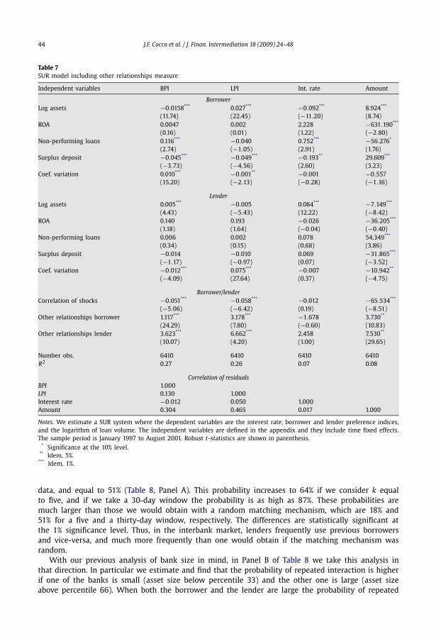
44 J.F. Cocco et al. / J. Finan. Intermediation 18 (2009) 24–48
Table 7SUR model including other relationships measure
Independent variables BPI LPI Int. rate Amount
BorrowerLog assets −0.0158*** 0.027*** −0.092*** 8.924***
(11.74) (22.45) (−11.20) (8.74)ROA 0.0047 0.002 2.228 −631.190***
(0.16) (0.01) (1.22) (−2.80)Non-performing loans 0.116*** −0.040 0.752*** −56.276*
(2.74) (−1.05) (2.91) (1.76)Surplus deposit −0.045*** −0.049*** −0.193** 29.609***
(−3.73) (−4.56) (2.60) (3.23)Coef. variation 0.010*** −0.001** −0.001 −0.557
(15.20) (−2.13) (−0.28) (−1.16)
LenderLog assets 0.005*** −0.005 0.084*** −7.149***
(4.43) (−5.43) (12.22) (−8.42)ROA 0.140 0.193 −0.026 −36.205***
(1.18) (1.64) (−0.04) (−0.40)Non-performing loans 0.006 0.002 0.078 54.349***
(0.34) (0.15) (0.68) (3.86)Surplus deposit −0.014 −0.010 0.069 −31.865***
(−1.17) (−0.97) (0.07) (−3.52)Coef. variation −0.012*** 0.075*** −0.007 −10.942**
(−4.09) (27.64) (0.37) (−4.75)
Borrower/lenderCorrelation of shocks −0.051*** −0.058*** −0.012 −65.534***
(−5.06) (−6.42) (0.19) (−8.51)Other relationships borrower 1.117*** 3.178*** −1.678 3.730**
(24.29) (7.80) (−0.60) (10.83)Other relationships lender 3.623*** 6.662*** 2.458 7.530**
(10.07) (4.20) (1.00) (29.65)
Number obs. 6410 6410 6410 6410R2 0.27 0.26 0.07 0.08
Correlation of residualsBPI 1.000LPI 0.130 1.000Interest rate −0.012 0.050 1.000Amount 0.304 0.465 0.017 1.000
Notes. We estimate a SUR system where the dependent variables are the interest rate, borrower and lender preference indices,and the logarithm of loan volume. The independent variables are defined in the appendix and they include time fixed effects.The sample period is January 1997 to August 2001. Robust t-statistics are shown in parenthesis.
* Significance at the 10% level.** Idem, 5%.
*** Idem, 1%.
data, and equal to 51% (Table 8, Panel A). This probability increases to 64% if we consider k equalto five, and if we take a 30-day window the probability is as high as 87%. These probabilities aremuch larger than those we would obtain with a random matching mechanism, which are 18% and51% for a five and a thirty-day window, respectively. The differences are statistically significant atthe 1% significance level. Thus, in the interbank market, lenders frequently use previous borrowersand vice-versa, and much more frequently than one would obtain if the matching mechanism wasrandom.
With our previous analysis of bank size in mind, in Panel B of Table 8 we take this analysis inthat direction. In particular we estimate and find that the probability of repeated interaction is higherif one of the banks is small (asset size below percentile 33) and the other one is large (asset sizeabove percentile 66). When both the borrower and the lender are large the probability of repeated

J.F. Cocco et al. / J. Finan. Intermediation 18 (2009) 24–48 45
Table 8Probability of repeated interactions assuming random matching and in the data
Panel A: Random matching and in the data for all banks
Number of days Random matching Data p-value: random = data
1 0.102 0.511 0.0003 0.140 0.585 0.0005 0.179 0.643 0.000
10 0.269 0.732 0.00030 0.513 0.865 0.000
Panel B: In the data by bank size
Number of days Large–large (LL) Large–small (LS) Small–small (SS)
1 0.526 0.547 0.333L S** LL**
3 0.591 0.590 0.355SS** SS** LL**, LS**
5 0.653 0.671 0.429LS**, SS*** LL**, SS*** LL***, LS***
10 0.741 0.779 0.447LS***, SS*** LL***, SS*** LL***, LS***
30 0.875 0.904 0.581LS***, SS*** LL***, SS*** LL***, LS***
Notes. This table shows the probability that a given lender (L) will lend funds to a given borrower (B) in the next k days, thatis from d + 1 to d + k, conditional on L having lent funds to B at t , and conditional on both L and B lending and borrowingfunds in the market in the next k trading days. The table shows the results for k = 1,3,5,10,30. Panel A shows the calculatedprobability assuming random matching of lenders and borrowers, and the estimated probabilities in the data. The last columnof Panel A shows the p-value of a test of the equality of the random matching probabilities and the estimated probabilities inthe data. Panel B shows the estimated probabilities in the data by bank size. Large (small) banks are those in the top (bottom)one third of the distribution of total assets. Below the estimated coefficients we report whether the estimated probabilities arestatistically significant across banks of different sizes.** Significance at the 5% level.
*** Idem, 1%.
interaction is lower, and it is lowest when both lender and borrower are small. These estimatedprobabilities suggest that lending relationship are most important when between small and largebanks in the domestic market. In Panel B of Table 8, below the estimated probabilities, we reportwhether these probabilities are statistically different from one another. It is important to note that fork equal to one we do not find that the probability of SS is significantly different than LL or LS becausethere are very few observations for SS and k = 1.
5.5. Robustness checks
We have investigated the robustness of our results to alternative relationship measures. Moreprecisely. We have also constructed lender and borrower preference indices using number of loansinstead of loan amounts. That is the lender preference index was constructed as the number of timesthat L has lent funds to B during time period t , as a fraction of the total number of times that bankL has lent funds in the interbank market during the time period. The results were similar to thebaseline results and are not reported.
We have also used as alternative measures of lending relationships the (absolute) number of dif-ferent banks to which bank L lent funds during time period t , and the number of different banks fromwhich bank B borrowed funds during t . The main difference in terms of the results was that in theinterest rate regression the borrower preference index thus measured is not significant. Thus it seemsthat for borrowers of funds it is important to use as a measure of the strength of the relationship avariable that reflects the (possible) asymmetric nature of the financing.
We have constructed LPI as being equal to the total amount that bank L has lent to bank B as afraction of the total amount that bank L has lent in the interbank market during the period. However,
46 J.F. Cocco et al. / J. Finan. Intermediation 18 (2009) 24–48
during the same period bank L may borrow funds from bank B . We have investigated the robustnessof the results to measures that take into account a two-sided relationship factor, with the borrowerpreference index defined as the total amount bank B borrowed from plus lent to bank L divided bythe total amount of funds that B has borrowed plus lent in the market during period t . The estimationresults for these alternative relationship measures are similar to those we obtained before (and arenot reported).
6. Conclusion and policy implications
Interbank markets play an important role in distributing liquidity across the financial system. Itis in this market that banks obtain insurance against idiosyncratic liquidity shocks arising from thebehavior of retail depositors, by borrowing and lending funds among themselves (as in the models ofHo and Saunders, 1985; Bhattacharya and Gale, 1987; and Freixas et al., 2000). The bilateral natureof the market allows banks to establish relationships. In this paper we have studied the role of bankrelationships in the process of liquidity provision in the interbank market.
We have constructed measures of interbank market relationships, based on the intensity of banks’pair-wise lending activity. We have found that banks with a larger imbalance in their reserve depositsare more likely to borrow funds from banks with whom they have a relationship, and to pay a lowerinterest rate on these loans than they would otherwise. This result supports the prediction of Carlinet al.’s (2007) model that under repeated interaction cooperation among traders is an equilibriumoutcome that involves refraining from predation, and that allows distressed traders, or banks with alarger imbalance in their reserve deposits, to transact at more favorable prices.
We have found evidence that smaller banks and banks with a larger proportion of non-performingloans tend to rely more on lending relationships when borrowing funds in the domestic market. Thisis consistent with relationships allowing banks to access liquidity in the presence of market frictionssuch as transaction and information costs.
In order to be more precise as to the exact nature of lending relationships, we have investigatedthe role of bank size in the market structure. Interestingly, we have documented that large banks tendto be net buyers of liquidity and small banks tend to be net sellers. This pattern of trade is also adistinctive feature of the U.S. Fed Funds market (Furfine, 1999; Ho and Saunders, 1985), and it canbe rationalized by the model of Ho and Saunders (1985). If large banks are better able to diversifytheir risk exposure than small banks, then large banks will be more sensitive to interest rates thansmall banks, and the slopes of the demand functions for interbank funds of large banks will be moreprice-elastic than those of small banks.
We have also investigated how access to international markets affects the nature of lending rela-tionships in the domestic market. We have documented that large domestic banks tend to have betteraccess to international markets. Interestingly, banks with low access to international markets tend tohave a much higher proportion of non-performing loans. Furthermore, these banks, when borrowingin the domestic interbank market, find it optimal to concentrate their loans. This result is consis-tent with peer monitoring across borders being less efficient than at the domestic level, as in themodel of Freixas and Holthausen (2005). It suggests that in international unsecured credit marketssuch as interbank markets, peer monitoring plays an important role in that it allows liquidity to flowacross borders. However, an alternative explanation is that large banks are perceived by internationalmarkets as being too-big-too-fail, and for this reason they can borrow internationally. In either case,our results suggest that domestic regulators should direct their policies towards an improvement ofthe cross-border information available, particularly so on small banks, so as to enhance cross-bordermarket integration.
Acknowledgments
We would like to thank Viral Acharya, Andrea Buraschi, Jennifer Conrad, Francesca Cornelli, De-nis Gromb, Michel Habib, Philipp Hartmann, Narayan Naik, Jose Peydro-Alcayde, Mitchell Petersen,Maximiano Pinheiro, Raghuram Rajan, Rafael Repullo, Henri Servaes, Raman Uppal and seminar par-ticipants at the Bank of England, Banco de Portugal, Cass Business School, European Central Bank,
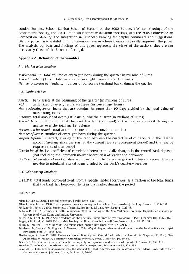
J.F. Cocco et al. / J. Finan. Intermediation 18 (2009) 24–48 47
London Business School, London School of Economics, the 2002 European Winter Meetings of theEconometric Society, the 2004 American Finance Association meetings, and the 2005 Conference onCompetition, Stability, and Integration in European Banking for helpful comments and suggestions.We are particularly grateful to an anonymous referee whose comments greatly improved the paper.The analysis, opinions and findings of this paper represent the views of the authors, they are notnecessarily those of the Banco de Portugal.
Appendix A. Definition of the variables
A.1. Market wide variables
Market amount: total volume of overnight loans during the quarter in millions of EurosMarket number of loans: total number of overnight loans during the quarterNumber of borrowers (lenders): number of borrowing (lending) banks during the quarter
A.2. Bank variables
Assets: bank assets at the beginning of the quarter (in millions of Euros)ROA: annualized quarterly return on assets (in percentage terms)Non-performing loans: loans that are overdue for more than 90 days divided by the total value of
outstanding loansAmount: total amount of overnight loans during the quarter (in millions of Euros)Market share: total amount that the bank has lent (borrowed) in the interbank market during the
quarter over the total market volumeNet amount borrowed: total amount borrowed minus total amount lentNumber of loans: number of overnight loans during the quarterSurplus deposits: quarterly average of the ratio between the current level of deposits in the reserve
account (average since the start of the current reserve requirement period) and the reserverequirements of that period
Correlation of shocks: coefficient of correlation between the daily changes in the central bank deposits(not including the interbank market operations) of lender and borrower
Coefficient of variation of shocks: standard deviation of the daily changes in the bank’s reserve depositsnot due to interbank market loans divided by the bank’s quarterly reserves
A.3. Relationship variables
BPI (LPI): total funds borrowed (lent) from a specific lender (borrower) as a fraction of the total fundsthat the bank has borrowed (lent) in the market during the period
References
Allen, F., Gale, D., 2000. Financial contagion. J. Polit. Econ. 108, 1–33.Allen, L., Saunders, A., 1986. The large–small bank dichotomy in the Federal Funds market. J. Banking Finance 10, 219–230.Arellano, M., Bond, S., 1991. Some tests of specification for panel data. Rev. Econom. Stud. 58.Battalio, R., Ellul, A., Jennings, R., 2005. Reputation effects in trading on the New York Stock exchange. Unpublished manuscript,
University of Notre Dame and Indiana University.Berger, A.N., Udell, G., 1992. Some evidence on the empirical significance of credit rationing. J. Polit. Economy 100, 1047–1077.Berger, A.N., Udell, G., 1995. Relationship lending and lines of credit in small firm finance. J. Bus. 68, 351–381.Berlin, M., Mester, L., 1999. Deposits and relationship lending. Rev. Finan. Stud. 12, 579–607.Bernhardt, D., Dvoracek, V., Hughson, E., Werner, I., 2004. Why do larger orders receive discounts on the London Stock exchange?
Rev. Finan. Stud. 18, 1343–1368.Bhattacharya, S., Gale, D., 1987. Preference shocks, liquidity, and Central Bank policy. In: Barnett, W., Singelton, K. (Eds.), New
Approaches to Monetary Economics. Cambridge University Press, Cambridge, pp. 68–88.Biais, B., 1993. Price formation and equilibrium liquidity in fragmented and centralized markets. J. Finance 48, 157–185.Broecker, T., 1990. Credit-worthiness tests and interbank competition. Econometrica 58, 429–452.Campbell, J., 1987. Money announcements, the demand for bank reserves, and the behavior of the Federal Funds rate within
the statement week. J. Money, Credit, Banking 19, 56–67.
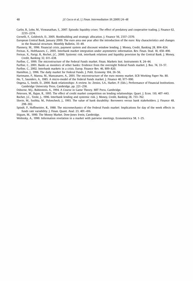
48 J.F. Cocco et al. / J. Finan. Intermediation 18 (2009) 24–48
Carlin, B., Lobo, M., Viswanathan, S., 2007. Episodic liquidity crises: The effect of predatory and cooperative trading. J. Finance 62,2235–2274.
Cornelli, F., Goldreich, D., 2005. Bookbuilding and strategic allocation. J. Finance 56, 2337–2370.European Central Bank, January 2000. The euro area one year after the introduction of the euro: Key characteristics and changes
in the financial structure. Monthly Bulletin, 35–49.Flannery, M., 1996. Financial crisis, payment system and discount window lending. J. Money, Credit, Banking 28, 804–824.Freixas, X., Holthausen, C., 2005. Interbank market integration under asymmetric information. Rev. Finan. Stud. 18, 458–490.Freixas, X., Parigi, B., Rochet, J.C., 2000. Systemic risk, interbank relations and liquidity provision by the Central Bank. J. Money,
Credit, Banking 32, 611–638.Furfine, C., 1999. The microstructure of the Federal Funds market. Finan. Markets Inst. Instruments 8, 24–44.Furfine, C., 2001. Banks as monitors of other banks: Evidence from the overnight Federal Funds market. J. Bus. 74, 33–57.Furfine, C., 2002. Interbank markets in a crisis. Europ. Finance Rev. 46, 809–820.Hamilton, J., 1996. The daily market for Federal Funds. J. Polit. Economy 104, 26–56.Hartmann, P., Manna, M., Manzanares, A., 2001. The microstructure of the euro money market. ECB Working Paper No. 80.Ho, T., Saunders, A., 1985. A micro-model of the Federal Funds market. J. Finance 40, 977–990.Ongena, S., Smith, D., 2000. Bank relationships: A review. In: Zenios, S.A., Harker, P. (Eds.), Performance of Financial Institutions.
Cambridge University Press, Cambridge, pp. 221–258.Osborne, M.J., Rubinstein, A., 1994. A Course in Game Theory. MIT Press, Cambridge.Petersen, M., Rajan, R., 1995. The effect of credit market competition on lending relationships. Quart. J. Econ. 110, 407–443.Rochet, J.C., Tirole, J., 1996. Interbank lending and systemic risk. J. Money, Credit, Banking 28, 733–762.Slovin, M., Sushka, M., Poloncheck, J., 1993. The value of bank durability: Borrowers versus bank stakeholders. J. Finance 48,
298–302.Spindt, P., Hoffmeister, R., 1988. The micromechanics of the Federal Funds market: Implications for day of the week effects in
funds rate variability. J. Finan. Quant. Anal. 23, 401–416.Stigum, M., 1990. The Money Market. Dow-Jones Irwin, Cambridge.Wolinsky, A., 1990. Information revelation in a market with pairwise meetings. Econometrica 58, 1–25.