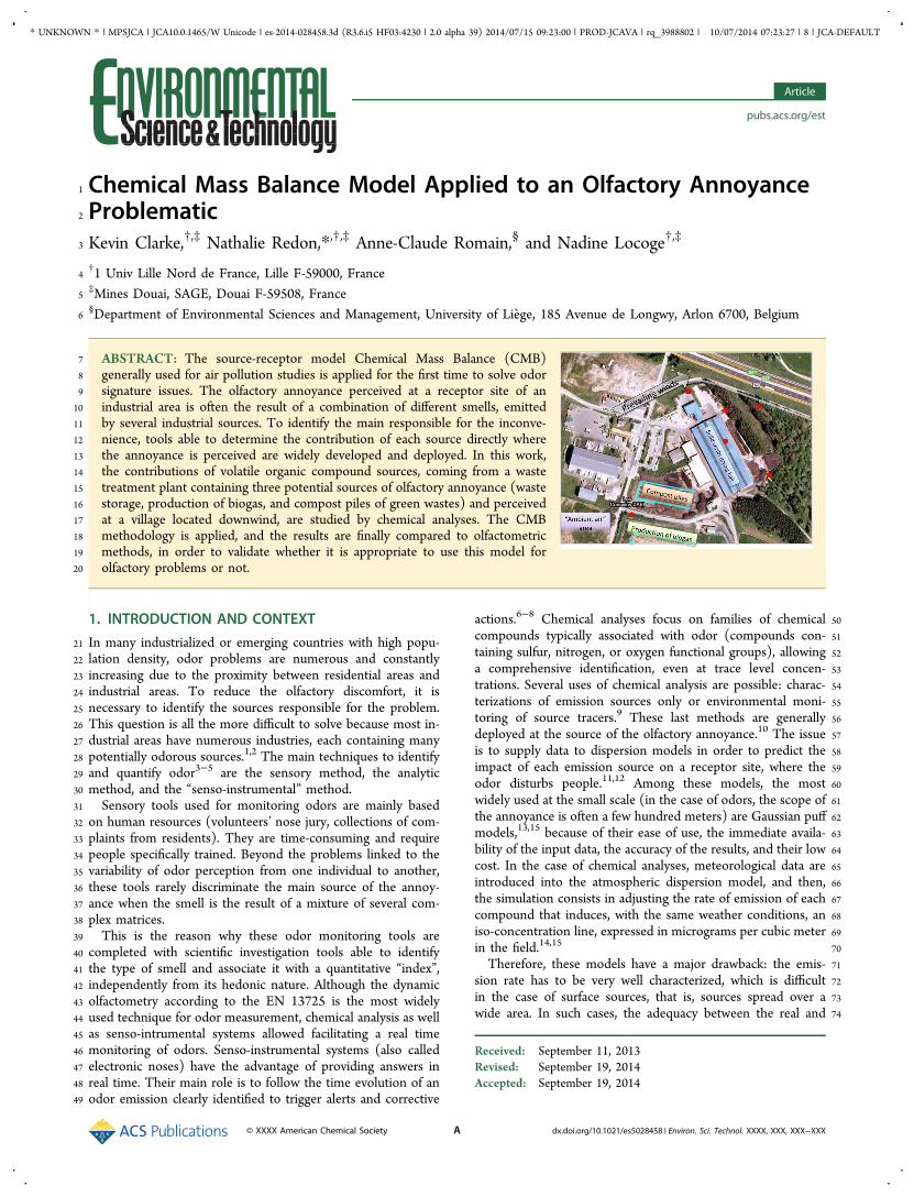
1 Chemical Mass Balance Model Applied to an Olfactory Annoyance2 Problematic3 Kevin Clarke,†,‡ Nathalie Redon,*,†,‡ Anne-Claude Romain,§ and Nadine Locoge†,‡

4†1 Univ Lille Nord de France, Lille F-59000, France

5‡Mines Douai, SAGE, Douai F-59508, France

6§Department of Environmental Sciences and Management, University of Liege, 185 Avenue de Longwy, Arlon 6700, Belgium

7 ABSTRACT: The source-receptor model Chemical Mass Balance (CMB)8 generally used for air pollution studies is applied for the first time to solve odor9 signature issues. The olfactory annoyance perceived at a receptor site of an10 industrial area is often the result of a combination of different smells, emitted11 by several industrial sources. To identify the main responsible for the inconve-12 nience, tools able to determine the contribution of each source directly where13 the annoyance is perceived are widely developed and deployed. In this work,14 the contributions of volatile organic compound sources, coming from a waste15 treatment plant containing three potential sources of olfactory annoyance (waste16 storage, production of biogas, and compost piles of green wastes) and perceived17 at a village located downwind, are studied by chemical analyses. The CMB18 methodology is applied, and the results are finally compared to olfactometric19 methods, in order to validate whether it is appropriate to use this model for20 olfactory problems or not.

1. INTRODUCTION AND CONTEXT

21 In many industrialized or emerging countries with high popu-22 lation density, odor problems are numerous and constantly23 increasing due to the proximity between residential areas and24 industrial areas. To reduce the olfactory discomfort, it is25 necessary to identify the sources responsible for the problem.26 This question is all the more difficult to solve because most in-27 dustrial areas have numerous industries, each containing many28 potentially odorous sources.1,2 The main techniques to identify29 and quantify odor3−5 are the sensory method, the analytic30 method, and the “senso-instrumental” method.31 Sensory tools used for monitoring odors are mainly based32 on human resources (volunteers’ nose jury, collections of com-33 plaints from residents). They are time-consuming and require34 people specifically trained. Beyond the problems linked to the35 variability of odor perception from one individual to another,36 these tools rarely discriminate the main source of the annoy-37 ance when the smell is the result of a mixture of several com-38 plex matrices.39 This is the reason why these odor monitoring tools are40 completed with scientific investigation tools able to identify41 the type of smell and associate it with a quantitative “index”,42 independently from its hedonic nature. Although the dynamic43 olfactometry according to the EN 13725 is the most widely44 used technique for odor measurement, chemical analysis as well45 as senso-intrumental systems allowed facilitating a real time46 monitoring of odors. Senso-instrumental systems (also called47 electronic noses) have the advantage of providing answers in48 real time. Their main role is to follow the time evolution of an49 odor emission clearly identified to trigger alerts and corrective

50actions.6−8 Chemical analyses focus on families of chemical51compounds typically associated with odor (compounds con-52taining sulfur, nitrogen, or oxygen functional groups), allowing53a comprehensive identification, even at trace level concen-54trations. Several uses of chemical analysis are possible: charac-55terizations of emission sources only or environmental moni-56toring of source tracers.9 These last methods are generally57deployed at the source of the olfactory annoyance.10 The issue58is to supply data to dispersion models in order to predict the59impact of each emission source on a receptor site, where the60odor disturbs people.11,12 Among these models, the most61widely used at the small scale (in the case of odors, the scope of62the annoyance is often a few hundred meters) are Gaussian puff63models,13,15 because of their ease of use, the immediate availa-64bility of the input data, the accuracy of the results, and their low65cost. In the case of chemical analyses, meteorological data are66introduced into the atmospheric dispersion model, and then,67the simulation consists in adjusting the rate of emission of each68compound that induces, with the same weather conditions, an69iso-concentration line, expressed in micrograms per cubic meter70in the field.14,15

71Therefore, these models have a major drawback: the emis-72sion rate has to be very well characterized, which is difficult73in the case of surface sources, that is, sources spread over a74wide area. In such cases, the adequacy between the real and

Received: September 11, 2013Revised: September 19, 2014Accepted: September 19, 2014

Article

pubs.acs.org/est

© XXXX American Chemical Society A dx.doi.org/10.1021/es5028458 | Environ. Sci. Technol. XXXX, XXX, XXX−XXX

* UNKNOWN * | MPSJCA | JCA10.0.1465/W Unicode | es-2014-028458.3d (R3.6.i5 HF03:4230 | 2.0 alpha 39) 2014/07/15 09:23:00 | PROD-JCAVA | rq_3988802 | 10/07/2014 07:23:27 | 8 | JCA-DEFAULT

75 perceived olfactory prediction is often bad, with a high un-76 certainty.16

77 Few studies directly focus on geographic area where the78 annoyance is perceived; in this case, the issue is to estimate the79 contributions of each source responsible for the overall olfac-80 tory discomfort at the receptor site. Receptor models have been81 elaborated to solve this problem. These models also use linear82 combinations to determine the contribution of different sources83 on the impacted site but are mainly based on measurements84 done at a receptor site. Scientific literature reports three main85 source-receptor models: the Chemical Mass Balance (CMB),86 the Positive Matrix Factorization (PMF), and the UNMIX; all87 of them share two main common principles: (1) making the88 assumption that the source signatures are still constant from the89 sources location to the receptor site and (2) optimizing the li-90 near combinations of different sources in order to minimize the91 difference between calculated values and experimental values.92 PMF and UNMIX are used when the compositions of the93 sources are totally unknown but calculations take hundreds94 of measurements done on the receptor site.17 This point is a95 major drawback especially for chemical analyses that require96 bulky equipment, complex handling, and manual sampling.18

97 By comparison, CMB is easier to implement, provided that98 sources are clearly defined and quantified. Moreover, it can be99 calculated with only a few dozen measurements on the receptor100 site. In the case of odors, the sources and the receptor sites are101 generally distant from a few hundred meters, up to several kilo-102 meters, so the reactivity and the washing of the volatile organic103 compounds (VOCs) are negligible.19 Furthermore, the sources104 are well known, and their signatures are easy to establish. These105 are the reasons why we chose to use the CMB model for this106 study.107 The CMB model is used and described in many scientific108 publications, especially for the VOC pollution of big cities, for109 example, in Mumbai and Delhi.20 It is also used to study auto-110 motive exhaust gases and use of industrial solvents for example111 in Seoul,21 Columbus,22 and in 20 other urban areas of the112 United States.23 Two other studies using two receptor models113 in parallel (respectively, CMB and PMF and CMB and UNMIX)114 showed minor variations between the results.24,25 Finally, a115 study comparing CMB, PMF, and UNMIX found a good ho-116 mogeneity of the main contributors to the total content of117 VOCs in Beijing.26

118 Thus, source-receptor models are very common in the allo-119 cation of VOCs sources and lead to reliable results, but the120 CMB model was never implemented in specific measurements121 of odor annoyance, which justifies the innovative nature of this122 work.123 A municipal solid waste (MSW) treatment center has been124 selected in order to conduct field measurement campaigns on a125 site representative of a smell annoyance. This site includes three126 different sources of odors, which potentially cause an annoy-127 ance to three villages under prevailing winds. The first objective128 was to establish the chemical profiles for each odor source of129 the emission site to be able to determine the contribution of130 the different odors in air samples collected at the immission131 (also called “receptor site”). These composite samples, that is,132 constituted by several mixed odors, were taken where an annoy-133 ance is perceived. To compare the CMB model predictions134 applied to the chemical analyses, characterizations of the odors135 were done by field olfactometry associated with odor intensity,136 on a scale from 0 to 6, as defined by the German norm VDI137 3940 directly in the field.

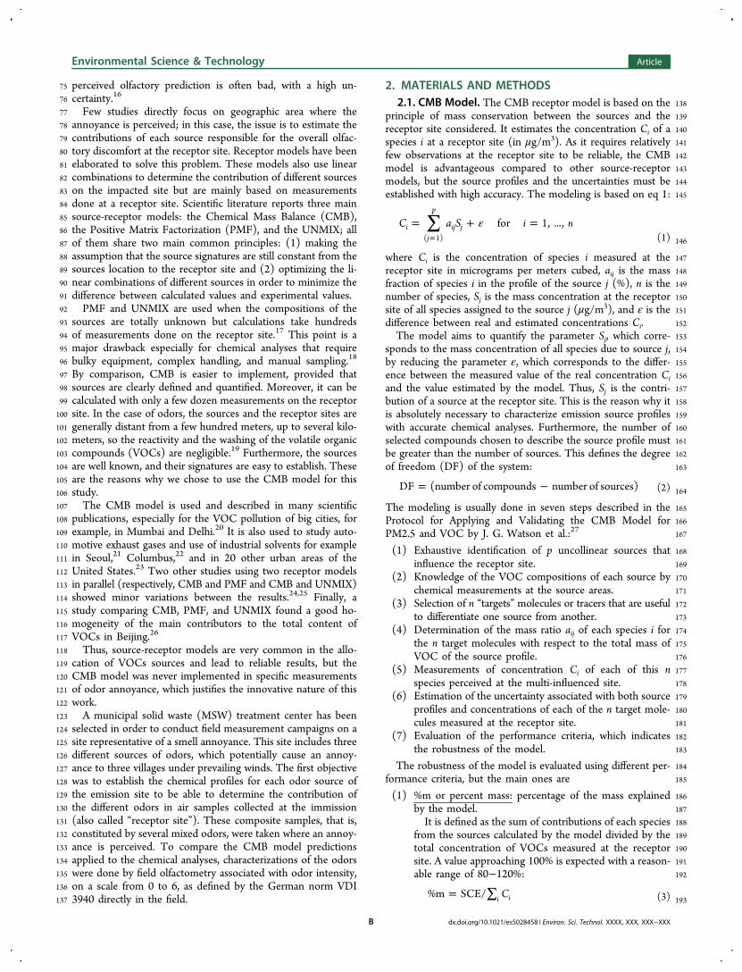
2. MATERIALS AND METHODS1382.1. CMB Model. The CMB receptor model is based on the139principle of mass conservation between the sources and the140receptor site considered. It estimates the concentration Ci of a141species i at a receptor site (in μg/m3). As it requires relatively142few observations at the receptor site to be reliable, the CMB143model is advantageous compared to other source-receptor144models, but the source profiles and the uncertainties must be145established with high accuracy. The modeling is based on eq 1:

∑ ε= + ==

C a S i nfor 1, ...,ij

p

ij j( 1) 146(1)

147where Ci is the concentration of species i measured at the148receptor site in micrograms per meters cubed, aij is the mass149fraction of species i in the profile of the source j (%), n is the150number of species, Sj is the mass concentration at the receptor151site of all species assigned to the source j (μg/m3), and ε is the152difference between real and estimated concentrations Ci.153The model aims to quantify the parameter Sj, which corre-154sponds to the mass concentration of all species due to source j,155by reducing the parameter ε, which corresponds to the differ-156ence between the measured value of the real concentration Ci157and the value estimated by the model. Thus, Sj is the contri-158bution of a source at the receptor site. This is the reason why it159is absolutely necessary to characterize emission source profiles160with accurate chemical analyses. Furthermore, the number of161selected compounds chosen to describe the source profile must162be greater than the number of sources. This defines the degree163of freedom (DF) of the system:

= −DF (number of compounds number of sources) 164(2)

165The modeling is usually done in seven steps described in the166Protocol for Applying and Validating the CMB Model for167PM2.5 and VOC by J. G. Watson et al.:27

168(1) Exhaustive identification of p uncollinear sources that169influence the receptor site.170(2) Knowledge of the VOC compositions of each source by171chemical measurements at the source areas.172(3) Selection of n “targets” molecules or tracers that are useful173to differentiate one source from another.174(4) Determination of the mass ratio aij of each species i for175the n target molecules with respect to the total mass of176VOC of the source profile.177(5) Measurements of concentration Ci of each of this n178species perceived at the multi-influenced site.179(6) Estimation of the uncertainty associated with both source180profiles and concentrations of each of the n target mole-181cules measured at the receptor site.182(7) Evaluation of the performance criteria, which indicates183the robustness of the model.

184The robustness of the model is evaluated using different per-185formance criteria, but the main ones are

186(1) %m or percent mass: percentage of the mass explained187by the model.188It is defined as the sum of contributions of each species189from the sources calculated by the model divided by the190total concentration of VOCs measured at the receptor191site. A value approaching 100% is expected with a reason-192able range of 80−120%:

= ∑ C%m SCE/ i i 193(3)

Environmental Science & Technology Article

dx.doi.org/10.1021/es5028458 | Environ. Sci. Technol. XXXX, XXX, XXX−XXXB

194 where Ci is the measured concentration of species i at the195 receptor site (μg/m3) and SCE is the source contribution196 estimate (μg/m3).197 (2) Tstat: ratio of the total concentration of VOC calculated198 for a source divided by its uncertainty.199 A Tstat greater than 2 indicates a significant contri-200 bution of sources:

=T SCE/std errstat201 (4)

202 where SCE is the source contribution estimate (μg/m3)203 and std err is the standard deviation associated with204 the contribution of a source to the total concentration of205 VOC receptor site (μg/m3).206 (3) R2 coefficient: measure of the variance of the ambient207 concentration explained by the calculated concentration.208 It is defined as the sum of the square of the differences209 between measured and calculated concentrations, divided210 by the sum of the measured concentrations. A low value211 of R2 indicates that the profiles of selected sources did212 not explain the concentrations at the receptor site for the213 selected species. The value of R2 can vary from 0 to 1, but214 a good model is characterized by a R2 greater than 0.8:

= −∑ − ∑ ×

∑R

C F S

C1

( )i i i ij j

i i

22

2215 (5)

216 where Ci is the measured concentration of species i (μg/m3),

217 Fij is the fraction of species i in the source j (in %), and Sj218 is the mass concentration at the receptor site from source219 j (μg/m3).220 (4) χ2 or chi squared: goodness of fit model, defined as the221 sum of the squares of the differences between measured222 and calculated concentrations divided by the sum of the223 variances. A high χ2, beyond 4, means that the uncer-224 tainty associated with the sources profiles is not sufficient225 to explain the difference between measured and calcu-226 lated concentrations:

χσ σ

=∑ − ∑ ×

+ ∑ ××

C F S

S

( )DFi i i ij j

C j j F

22

2 2i j227 (6)

228 where Ci is the measured concentration of species i229 (μg/m3), σ2 is the uncertainty on concentration Ci, Fij is230 the fraction of species i in the source j (in %), Sj is the231 mass concentration at the receptor site from source232 j (μg/m3), and DF is the degree of freedom.

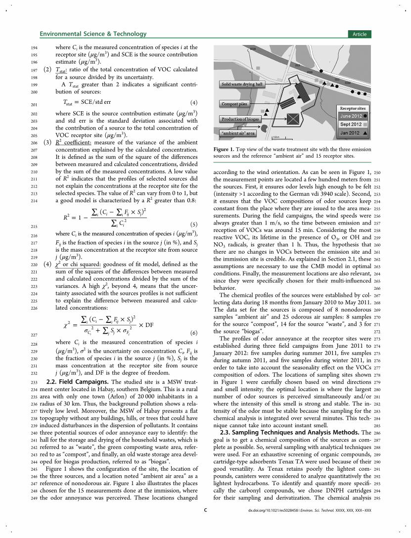
233 2.2. Field Campaigns. The studied site is a MSW treat-234 ment center located in Habay, southern Belgium. This is a rural235 area with only one town (Arlon) of 20 000 inhabitants in a236 radius of 30 km. Thus, the background pollution shows a rela-237 tively low level. Moreover, the MSW of Habay presents a flat238 topography without any buildings, hills, or trees that could have239 induced disturbances in the dispersion of pollutants. It contains240 three potential sources of odor annoyance easy to identify: the241 hall for the storage and drying of the household wastes, which is242 referred to as “waste”, the green composting waste area, refer-243 red to as “compost”, and finally, an old waste storage area devel-244 oped for biogas production, referred to as “biogas”.245 Figure 1 shows the configuration of the site, the location of246 the three sources, and a location noted “ambient air area” as a247 reference of nonodorous air. Figure 1 also illustrates the places248 chosen for the 15 measurements done at the immission, where249 the odor annoyance was perceived. These locations changed

250according to the wind orientation. As can be seen in Figure 1,251the measurement points are located a few hundred meters from252the sources. First, it ensures odor levels high enough to be felt253(intensity >1 according to the German vdi 3940 scale). Second,254it ensures that the VOC compositions of odor sources keep255constant from the place where they are issued to the area mea-256surements. During the field campaigns, the wind speeds were257always greater than 1 m/s, so the time between emission and258reception of VOCs was around 15 min. Considering the most259reactive VOC, its lifetime in the presence of O3, or OH and260NO3 radicals, is greater than 1 h. Thus, the hypothesis that261there are no changes in VOCs between the emission site and262the immission site is credible. As explained in Section 2.1, these263assumptions are necessary to use the CMB model in optimal264conditions. Finally, the measurement locations are also relevant,265since they were specifically chosen for their multi-influenced266behavior.267The chemical profiles of the sources were established by col-268lecting data during 18 months from January 2010 to May 2011.269The data set for the sources is composed of 8 nonodorous270samples “ambient air” and 25 odorous air samples: 8 samples271for the source “compost”, 14 for the source “waste”, and 3 for272the source “biogas”.273The profiles of odor annoyance at the receptor sites were274established during three field campaigns from June 2011 to275January 2012: five samples during summer 2011, five samples276during autumn 2011, and five samples during winter 2011, in277order to take into account the seasonality effect on the VOCs278composition of odors. The locations of sampling sites shown279in Figure 1 were carefully chosen based on wind directions280and smell intensity; the optimal location is where the largest281number of odor sources is perceived simultaneously and/or282where the intensity of this smell is strong and stable. The in-283tensity of the odor must be stable because the sampling for the284chemical analysis is integrated over several minutes. This tech-285nique cannot take into account instant smell.2862.3. Sampling Techniques and Analysis Methods. The287goal is to get a chemical composition of the sources as com-288plete as possible. So, several sampling with analytical techniques289were used. For an exhaustive screening of organic compounds,290cartridge-type adsorbents Tenax TA were used because of their291good versatility. As Tenax retains poorly the lightest com-292pounds, canisters were considered to analyze quantitatively the293lightest hydrocarbons. To identify and quantify more specifi-294cally the carbonyl compounds, we chose DNPH cartridges295for their sampling and derivatization. The chemical analysis

Figure 1. Top view of the waste treatment site with the three emissionsources and the reference “ambient air” and 15 receptor sites.

Environmental Science & Technology Article

dx.doi.org/10.1021/es5028458 | Environ. Sci. Technol. XXXX, XXX, XXX−XXXC

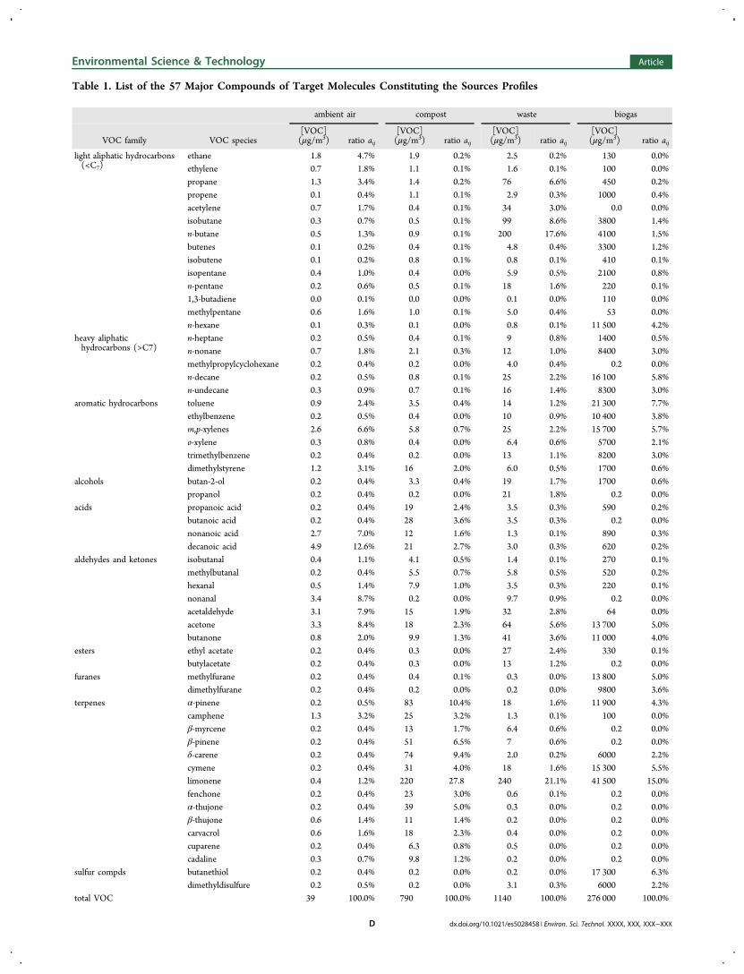
Table 1. List of the 57 Major Compounds of Target Molecules Constituting the Sources Profiles

ambient air compost waste biogas

VOC family VOC species[VOC](μg/m3) ratio aij

[VOC](μg/m3) ratio aij

[VOC](μg/m3) ratio aij

[VOC](μg/m3) ratio aij

light aliphatic hydrocarbons(<C7)

ethane 1.8 4.7% 1.9 0.2% 2.5 0.2% 130 0.0%ethylene 0.7 1.8% 1.1 0.1% 1.6 0.1% 100 0.0%propane 1.3 3.4% 1.4 0.2% 76 6.6% 450 0.2%propene 0.1 0.4% 1.1 0.1% 2.9 0.3% 1000 0.4%acetylene 0.7 1.7% 0.4 0.1% 34 3.0% 0.0 0.0%isobutane 0.3 0.7% 0.5 0.1% 99 8.6% 3800 1.4%n-butane 0.5 1.3% 0.9 0.1% 200 17.6% 4100 1.5%butenes 0.1 0.2% 0.4 0.1% 4.8 0.4% 3300 1.2%isobutene 0.1 0.2% 0.8 0.1% 0.8 0.1% 410 0.1%isopentane 0.4 1.0% 0.4 0.0% 5.9 0.5% 2100 0.8%n-pentane 0.2 0.6% 0.5 0.1% 18 1.6% 220 0.1%1,3-butadiene 0.0 0.1% 0.0 0.0% 0.1 0.0% 110 0.0%methylpentane 0.6 1.6% 1.0 0.1% 5.0 0.4% 53 0.0%n-hexane 0.1 0.3% 0.1 0.0% 0.8 0.1% 11 500 4.2%

heavy aliphatichydrocarbons (>C7)

n-heptane 0.2 0.5% 0.4 0.1% 9 0.8% 1400 0.5%n-nonane 0.7 1.8% 2.1 0.3% 12 1.0% 8400 3.0%methylpropylcyclohexane 0.2 0.4% 0.2 0.0% 4.0 0.4% 0.2 0.0%n-decane 0.2 0.5% 0.8 0.1% 25 2.2% 16 100 5.8%n-undecane 0.3 0.9% 0.7 0.1% 16 1.4% 8300 3.0%

aromatic hydrocarbons toluene 0.9 2.4% 3.5 0.4% 14 1.2% 21 300 7.7%ethylbenzene 0.2 0.5% 0.4 0.0% 10 0.9% 10 400 3.8%m,p-xylenes 2.6 6.6% 5.8 0.7% 25 2.2% 15 700 5.7%o-xylene 0.3 0.8% 0.4 0.0% 6.4 0.6% 5700 2.1%trimethylbenzene 0.2 0.4% 0.2 0.0% 13 1.1% 8200 3.0%dimethylstyrene 1.2 3.1% 16 2.0% 6.0 0.5% 1700 0.6%

alcohols butan-2-ol 0.2 0.4% 3.3 0.4% 19 1.7% 1700 0.6%propanol 0.2 0.4% 0.2 0.0% 21 1.8% 0.2 0.0%

acids propanoic acid 0.2 0.4% 19 2.4% 3.5 0.3% 590 0.2%butanoic acid 0.2 0.4% 28 3.6% 3.5 0.3% 0.2 0.0%nonanoic acid 2.7 7.0% 12 1.6% 1.3 0.1% 890 0.3%decanoic acid 4.9 12.6% 21 2.7% 3.0 0.3% 620 0.2%

aldehydes and ketones isobutanal 0.4 1.1% 4.1 0.5% 1.4 0.1% 270 0.1%methylbutanal 0.2 0.4% 5.5 0.7% 5.8 0.5% 520 0.2%hexanal 0.5 1.4% 7.9 1.0% 3.5 0.3% 220 0.1%nonanal 3.4 8.7% 0.2 0.0% 9.7 0.9% 0.2 0.0%acetaldehyde 3.1 7.9% 15 1.9% 32 2.8% 64 0.0%acetone 3.3 8.4% 18 2.3% 64 5.6% 13 700 5.0%butanone 0.8 2.0% 9.9 1.3% 41 3.6% 11 000 4.0%

esters ethyl acetate 0.2 0.4% 0.3 0.0% 27 2.4% 330 0.1%butylacetate 0.2 0.4% 0.3 0.0% 13 1.2% 0.2 0.0%

furanes methylfurane 0.2 0.4% 0.4 0.1% 0.3 0.0% 13 800 5.0%dimethylfurane 0.2 0.4% 0.2 0.0% 0.2 0.0% 9800 3.6%

terpenes α-pinene 0.2 0.5% 83 10.4% 18 1.6% 11 900 4.3%camphene 1.3 3.2% 25 3.2% 1.3 0.1% 100 0.0%β-myrcene 0.2 0.4% 13 1.7% 6.4 0.6% 0.2 0.0%β-pinene 0.2 0.4% 51 6.5% 7 0.6% 0.2 0.0%δ-carene 0.2 0.4% 74 9.4% 2.0 0.2% 6000 2.2%cymene 0.2 0.4% 31 4.0% 18 1.6% 15 300 5.5%limonene 0.4 1.2% 220 27.8 240 21.1% 41 500 15.0%fenchone 0.2 0.4% 23 3.0% 0.6 0.1% 0.2 0.0%α-thujone 0.2 0.4% 39 5.0% 0.3 0.0% 0.2 0.0%β-thujone 0.6 1.4% 11 1.4% 0.2 0.0% 0.2 0.0%carvacrol 0.6 1.6% 18 2.3% 0.4 0.0% 0.2 0.0%cuparene 0.2 0.4% 6.3 0.8% 0.5 0.0% 0.2 0.0%cadaline 0.3 0.7% 9.8 1.2% 0.2 0.0% 0.2 0.0%

sulfur compds butanethiol 0.2 0.4% 0.2 0.0% 0.2 0.0% 17 300 6.3%dimethyldisulfure 0.2 0.5% 0.2 0.0% 3.1 0.3% 6000 2.2%

total VOC 39 100.0% 790 100.0% 1140 100.0% 276 000 100.0%

Environmental Science & Technology Article

dx.doi.org/10.1021/es5028458 | Environ. Sci. Technol. XXXX, XXX, XXX−XXXD

296 techniques depend on the type of sampling used in the field297 and on the trapped compounds: Tenax cartridges were ana-298 lyzed using a gas chromatography−flame ionization detector/299 mass spectrometry (GC-FID/MS) system (Agilent 6890/5975300 with a 100% PDMS column and a thermodesorber system301 Gerstel). Canisters were analyzed using a GC-FID system302 (Chrompack CP9001 with a Micro Purge & Trap Entech 7100303 and dual columns CP-SIL-5CB and PLOT AL2O3/KCl).304 DNPH cartridges were analyzed using a high-performance liquid305 chromatography system (Waters 2695 with a UV detector at λ =306 365 nm and a reverse-phase column C18).307 To compare the results obtained by chemical analyses and to308 validate the CMB model predictions, simultaneous measure-309 ments of odors by field olfactometry associated with an odor310 intensity, on a scale from 0 to 6, as defined by the German311 norm VDI 3940, were conducted by operators. A value of “0”312 corresponds to an imperceptible odor, and a value of “6” corre-313 sponds to an extremely strong odor. In our case, the odor in-314 tensity was rated from 1 to 3, that is, from very weak to distinct.

3. RESULTS AND DISCUSSION

315 As seen in Section 2.1, to calculate the CMB parameters, the316 second step of the protocol requires establishing of the source317 profiles, and judiciously choosing compounds representative of318 the odor annoyance. During the chemical sources character-319 isations, 291 VOCs were identified and quantified in the sam-320 pled sources. To apply the CMB model, it was not necessary to321 use all of these VOCs, because many compounds present low322 concentrations not detectable at the receptor site (the limit was323 10 μg/m3). Thus, a list of 57 major compounds, characteristic324 of the sources, was established, with concentration levels high325 enough to apply the CMB model in good conditions. These 57326 VOCs represent an average of 77% of the total mass content of327 VOCs in the sample, which indicates a good representativeness328 of the total VOCs depending of the sources. They represent329 between 69% and 95% of the compost source, between 53%330 and 95% of the waste source, and between 61% and 66% of331 the biogas source. The results of all measurement campaigns,332 averaged source by source, are compiled in Table 1.333 The results are consistent with previous studies conducted334 on the same types of waste treatment plants. For example, the335 “compost” source shows a majority of terpenes, followed by336 some aldehydes and ketones. This profile is similar to those337 obtained by Persoons et al.,28 Komilis et al.,29 Staley et al.,30

338 and Kumar et al.31 The chemical composition of the “waste”339 source depends on the maturation and the season, but there is a340 high presence of aromatic hydrocarbons, including a majority of341 BTEX, and oxygenated VOCs, mainly aldehydes, ketones,342 esters, alcohols, dioxolanes, and finally, a minority of aliphatic343 hydrocarbons and chlorinated compounds. In the literature,344 the amount of aromatic hydrocarbons (including BTEX) are345 generally equal or greater than to the quantities of aliphatic346 hydrocarbons,10,32−38 but in all these studies, samples were347 taken by adsorbent cartridges and/or SPME, which is a very348 bad trap for the lighter aliphatic hydrocarbons. Finally, three

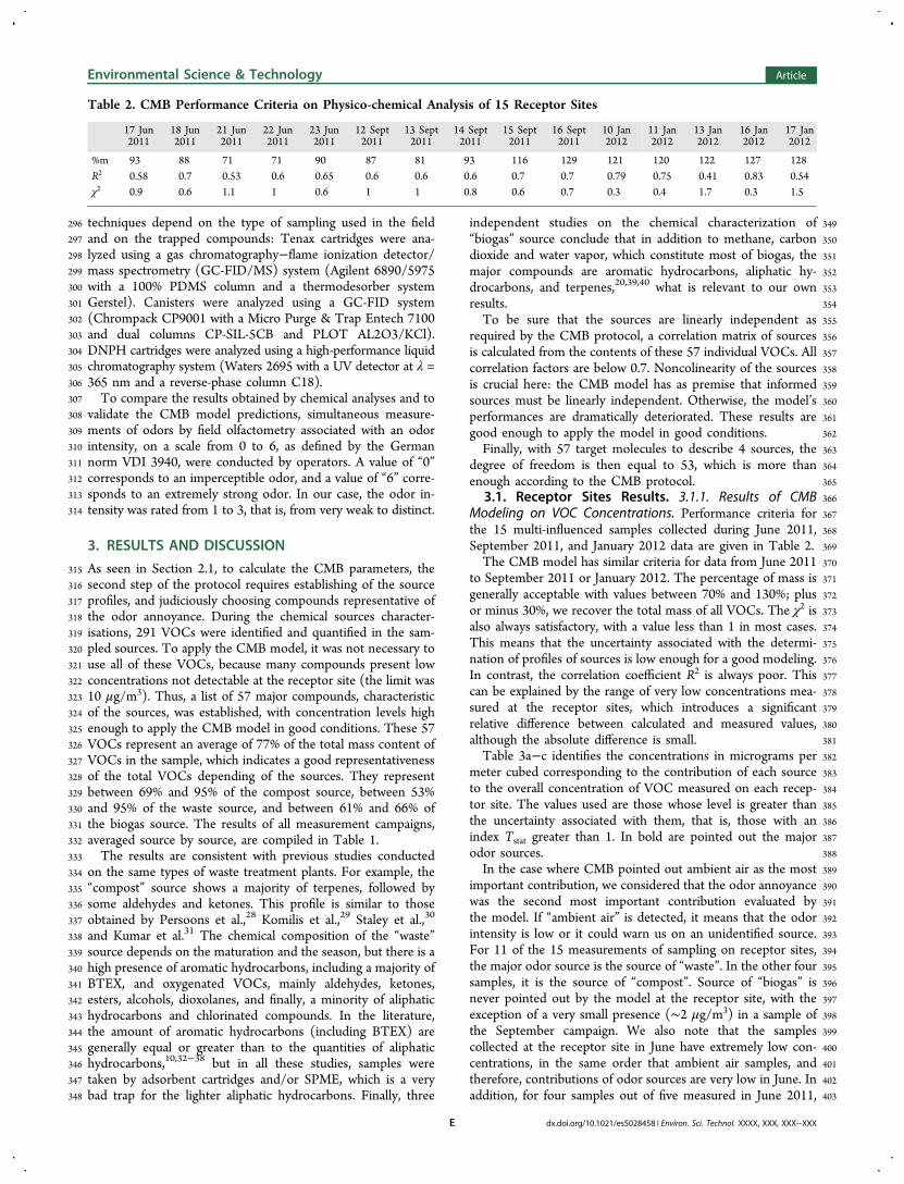
349independent studies on the chemical characterization of350“biogas” source conclude that in addition to methane, carbon351dioxide and water vapor, which constitute most of biogas, the352major compounds are aromatic hydrocarbons, aliphatic hy-353drocarbons, and terpenes,20,39,40 what is relevant to our own354results.355To be sure that the sources are linearly independent as356required by the CMB protocol, a correlation matrix of sources357is calculated from the contents of these 57 individual VOCs. All358correlation factors are below 0.7. Noncolinearity of the sources359is crucial here: the CMB model has as premise that informed360sources must be linearly independent. Otherwise, the model’s361performances are dramatically deteriorated. These results are362good enough to apply the model in good conditions.363Finally, with 57 target molecules to describe 4 sources, the364degree of freedom is then equal to 53, which is more than365enough according to the CMB protocol.3663.1. Receptor Sites Results. 3.1.1. Results of CMB367Modeling on VOC Concentrations. Performance criteria for368the 15 multi-influenced samples collected during June 2011,369September 2011, and January 2012 data are given in Table 2.370The CMB model has similar criteria for data from June 2011371to September 2011 or January 2012. The percentage of mass is372generally acceptable with values between 70% and 130%; plus373or minus 30%, we recover the total mass of all VOCs. The χ2 is374also always satisfactory, with a value less than 1 in most cases.375This means that the uncertainty associated with the determi-376nation of profiles of sources is low enough for a good modeling.377In contrast, the correlation coefficient R2 is always poor. This378can be explained by the range of very low concentrations mea-379sured at the receptor sites, which introduces a significant380relative difference between calculated and measured values,381although the absolute difference is small.382Table 3a−c identifies the concentrations in micrograms per383meter cubed corresponding to the contribution of each source384to the overall concentration of VOC measured on each recep-385tor site. The values used are those whose level is greater than386the uncertainty associated with them, that is, those with an387index Tstat greater than 1. In bold are pointed out the major388odor sources.389In the case where CMB pointed out ambient air as the most390important contribution, we considered that the odor annoyance391was the second most important contribution evaluated by392the model. If “ambient air” is detected, it means that the odor393intensity is low or it could warn us on an unidentified source.394For 11 of the 15 measurements of sampling on receptor sites,395the major odor source is the source of “waste”. In the other four396samples, it is the source of “compost”. Source of “biogas” is397never pointed out by the model at the receptor site, with the398exception of a very small presence (∼2 μg/m3) in a sample of399the September campaign. We also note that the samples400collected at the receptor site in June have extremely low con-401centrations, in the same order that ambient air samples, and402therefore, contributions of odor sources are very low in June. In403addition, for four samples out of five measured in June 2011,

Table 2. CMB Performance Criteria on Physico-chemical Analysis of 15 Receptor Sites

17 Jun2011

18 Jun2011

21 Jun2011

22 Jun2011

23 Jun2011

12 Sept2011

13 Sept2011

14 Sept2011

15 Sept2011

16 Sept2011

10 Jan2012

11 Jan2012

13 Jan2012

16 Jan2012

17 Jan2012

%m 93 88 71 71 90 87 81 93 116 129 121 120 122 127 128R2 0.58 0.7 0.53 0.6 0.65 0.6 0.6 0.6 0.7 0.7 0.79 0.75 0.41 0.83 0.54χ2 0.9 0.6 1.1 1 0.6 1 1 0.8 0.6 0.7 0.3 0.4 1.7 0.3 1.5

Environmental Science & Technology Article

dx.doi.org/10.1021/es5028458 | Environ. Sci. Technol. XXXX, XXX, XXX−XXXE

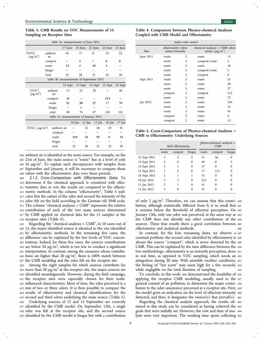
404 ambient air is identified as the main source. For example, on the405 21st of June, the main source is “waste” but at a level of only406 16 μg/m3. To explain such discrepancies with samples from407 September and January, it will be necessary to compare these408 values with the olfactometric data over these periods.409 3.1.2. Cross-Comparison with Olfactometric Data. To410 determine if the chemical approach is consistent with olfac-411 tometric data or not, the results are compared to the olfacto-412 metric methods. In the column “olfactometry”, Table 5 indi-413 cates first the nature of the odor and second the intensity of the414 odor felt on the field according to the German vdi 3940 scale.415 The column “chemical analyses + CMB” represents the relative416 contribution of each of the two main sources determined417 by CMB applied on chemical data for the 15 samples at the418 receptor sites (Table 4).419 Regarding the “chemical analyses + CMB”, in 10 cases out of420 15, the major identified source is identical to the one identified421 by olfactometric methods. In the remaining five cases, the422 difference can be explained by the low levels of VOC concen-423 trations. Indeed, for these five cases, the sources contributions424 are below 20 μg/m3, which is too low to conduct a significant425 interpretation. In contrast, among the measures whose contribu-426 tions are higher than 20 μg/m3, there is 100% match between427 the CMB modeling and the odor felt on the receptor site.428 Among the eight samples for which sources contribute for429 more than 20 μg/m3 at the receptor site, the major sources are430 identified unambiguously. However, during the field campaign,431 the receptor sites were especially chosen for their multi-432 influenced characteristics. Most of time, the odor perceived is a433 mix of two or three odors. It is then possible to compare the434 results of olfactometry and chemical identifications for the435 second and third odors underlying the main source (Table 5).436 Underlying sources of 12 and 15 September are correctly437 identified by the CMB model. On September 13th, a single438 odor was felt at the receptor site, and the second source439 identified by the CMB model is biogas but with a contribution

440of only 2 μg/m3. Therefore, we can assume that this contri-441bution, although statistically different from 0, is so small that442it remains below the threshold of olfactory perception. On443January 13th, only one odor was perceived, in the same way as444the CMB does not identify any other contribution of the445sources. These four results show a good correlation between446olfactometry and analytical methods.447In contrast, for the four remaining dates, we observe a448constant problem: the second odor identified by olfactometry is449always the source “compost”, which is never detected by the450CMB. This can be explained by the time difference between the451two methodology: olfactometry is an instantly perception, done452in real time, as opposed to VOC sampling, which needs an453integration during 30 min. With unstable weather conditions,454the feeling of “hot scent” may seem high for a few seconds,455while negligible on the total duration of sampling.456To conclude, in this work, we demonstrated the feasibility of457applying the receptor CMB modeling, usually used in the458general context of air pollution, to determine the major contri-459butors to the odor annoyance perceived at a receptor site. First,460the model gives an indication on the level of olfactory intensity461detected, and then, it designates the source(s) that prevail(s).462Regarding the chemical analysis approach, the results ob-463tained in this study can be considered as having achieved the464goals that were initially set. However, the cost and time of ana-465lysis were very important. The working time spent collecting

Table 3. CMB Results on VOC Measurements of 15Sampling on Receptor Sites

table 3a: measurements of June 2011

17 June 18 June 21 June 22 June 23 June

[VOC](μg/m3)

ambientair

42 17 8 25 22

compost − 5 7 6 6waste 13 4 16 4 −biogas − − − − −total 55 26 31 35 28table 3b: measurements of September 2011

12 Sept 13 Sept 14 Sept 15 Sept 16 Sept

[VOC](μg/m3)

ambientair

13 22 30 − 46

compost 26 − − 113 −waste 51 50 37 17 76biogas − 2 − − −total 90 74 67 130 121table 3c: measurements of January 2012

10 Jan 11 Jan 13 Jan 16 Jan 17 Jan

[VOC] (μg/m3) ambient air − 31 48 29 41compost − − − − −waste 316 51 91 4 15biogas − − − − −total 55 26 31 35 28

Table 4. Comparison between Physico-chemical AnalysesCoupled with CMB Model and Olfactometry

major odor source

dateolfactometry odorsnature/intensity

chemical analyses + CMB odorsnature (μg/m3)

June 2011 waste 2 waste 13waste 2 compost/waste 5waste 2 waste 16waste 3 compost/waste 5waste 2 compost 6

Sept 2011 waste 3 waste 51waste 2 waste 49waste 3 waste 37compost 3 compost 113waste 2 waste 75

Jan 2012 waste 3 waste 316waste 2 waste 51waste 3 waste 91compost 3 waste 4compost 2 waste 15

Table 5. Cross-Comparison of Physico-chemical Analyses +CMB vs Olfactometry: Underlying Sources

field olfactometryphysicochemical analyses +

CMB

waste compost biogas waste compost biogas

12 Sept 2011 3 2 2 51 26 013 Sept 2011 2 0 0 49 0 214 Sept 2011 3 1 0 37 0 015 Sept 2011 1 3 0 17 113 016 Sept 2011 2 1 1 75 0 010 Jan 2012 3 3 0 312 0 011 Jan 2012 2 1 0 51 0 013 Jan 2012 3 0 0 91 0 0

Environmental Science & Technology Article

dx.doi.org/10.1021/es5028458 | Environ. Sci. Technol. XXXX, XXX, XXX−XXXF

466 data for chemical analysis and to interpret them was much467 greater than the time spent working to collect and interpret468 data for the measure by the e-nose. To make the “chemical” ap-469 proach viable, it is imperative to reduce these costs (expensive470 equipment, time-consuming analyses, etc.). Alternatives to471 chromatographic techniques are recently proposed, including472 for example, the analysis by proton transfer reaction mass473 spectrometry, which despite having a very high initial cost is474 much cheaper on a day-to-day basis, less time-consuming, and475 also allows lower detection limits.41 It is however necessary to476 keep in mind that the methods do not need to be that heavy in477 relatively simple problems, looking for some specific tracer478 compounds sources could provide good results. If the goal is479 to identify the source of an annoyance, the calculation of ratios480 in 16 VOCs is enough to convincingly identify the source of481 “waste” as generally predominant in the olfactory annoyance482 receptor sites.

483 ■ AUTHOR INFORMATION

484 Corresponding Author485 *Phone: +33 (0)3 27.71.24.77; fax: +33 (0)3 27 71 29 14; e-486 mail: nathalie.redon@mines-douai.fr.

487 Notes488 The authors declare no competing financial interest.

489 ■ REFERENCES(1)490 ADEME. Pollutions Olfactives − Origine, Legislation, Analyse,

491 Traitement; Dunod: Paris, 2005.(2)492 Nicolas, J.; Cors, M.; Romain, A.-C.; Delva, J. Identification of

493 odour sources in an industrial park from resident diaries statistics.494 Atmos. Environ. 2010, 44 (13), 1623−1631.

(3)495 Gutierrez, M. C.; Chica, A. F.; Martín, M. A.; Romain, A. C.496 Compost pile monitoring using different approaches: GC−MS, E-nose497 and dynamic olfactometry. Waste Biomass Valorization 2013, 1−11.

(4)498 Romain, A.-C.; Delva, J.; Nicolas, J. Complementary approaches499 to measure environmental odours emitted by landfill areas. Sens.500 Actuators, B 2008, 131 (1), 18−23.

(5)501 Gostelow, P.; Parsons, S. A.; Cobb, J. Development of an odorant502 emission model for sewage treatment works. Water Sci. Technol. 2001,503 44 (9), 181−188.

(6)504 Nicolas, J.; Romain, A.-C. Establishing the limit of detection and505 the resolution limits of odorous sources in the environment for an506 array of metal oxide gas sensors. Sens. Actuators, B 2004, 99, 384−392.

(7)507 Sohn, J. H.; Pioggia, G.; Craig, I. P.; Stuetz, R. M.; Atzeni, M. G.508 Identifying major contributing sources to odour annoyance using a509 non-specific gas sensor array. Biosyst. Eng. 2009, 102 (3), 305−312.

(8)510 Romain, A. C. Monitoring an odour in the environment with an511 electronic nose: Requirements for the signal processing. In Biologically512 Inspired Signal Processing for Chemical Sensing; Gutierrez, A., Marco, S.,513 Eds.; Springer: Berlin, Germany, 2009; Vol. 188, p 210.

(9)514 Kleeberg, K. K.; Liu, Y.; Jans, M.; Schlegelmilch, M.; Streese, J.;515 Stegmann, R. Development of a simple and sensitive method for the516 characterization of odorous waste gas emissions by means of solid-517 phase microextraction (SPME) and GC-MS/olfactometry. Waste518 Manage. 2005, 25 (9), 872−879.

(10)519 Fang, J. J.; Yang, N.; Cen, D. Y.; Shao, L. M.; He, P. J. Odor520 compounds from different sources of landfill: Characterization and521 source identification. Waste Manage. 2012, 32 (7), 1401−1410.

(11)522 Sironi, S.; Capelli, L.; Centola, P.; Del Rosso, R.; Pierucci, S.523 Odour impact assessment by means of dynamic olfactometry,524 dispersion modelling and social participation. Atmos. Environ. 2010,525 44 (3), 354−360.

(12)526 Capelli, L.; Sironi, S.; Del Rosso, R.; Guillot, J.-M. Measuring527 odours in the environment vs. dispersion modelling: A review. Atmos.528 Environ. 2013, 79, 731−7.

(13) 529De Melo, L. H.; Guillot, J. M.; Fanlo, J. L.; Le Cloirec, P.530Dispersion of odorous gases in the atmosphere Part I: Modeling531approaches to the phenomenon. Sci. Total Environ. 2006, 361, 220−532228.

(14) 533Romain, A.-C. 8.3 Landfill of solid waste. In Odour Impact534Assessment Handbook; Belgiorno, V., Ed.; Wiley: Chichester, England,5352013; pp 232−250.

(15) 536Collard, C.; Lebrun, V.; Fays, S.; Salpeteur, V.; Nicolas, J.;537Romain, A.-C. Air survey around MSW landfills in Wallonia: Feedback538of 8 years field measurements, ORBIT 2008, Wageningen, Nether-539lands, Oct 13−15th, 2008.

(16) 540Barneoud, P.; Page, T.; Heroux, M.; Leduc, R.; Guy, C.541Evaluation de l’impact odeur d’un centre de compostage en milieu542urbain a l’aide d’un reseau d’observateurs et comparaison avec des543modeles de dispersion atmospherique. Pollut. Atmos. 2012, 213-214,54483−96.

(17) 545Viana, M.; Kuhlbusch, T. A. J.; Querol, X.; Alastuey, A.;546Harrison, R. M.; Hopke, P. K.; Winiwarter, W.; Vallius, A.; Szidat, S.;547Prevot, A. S. H.; et al. Source apportionment of particulate matter in548Europe: A review of methods and results. J. Aerosol Sci. 2008, 39 (10),549827−849.

(18) 550Badol, C.; Locoge, N.; Galloo, J.-C. Using a source-receptor551approach to characterise VOC behaviour in a French urban area552influenced by industrial emissions: Part II: Source contribution553assessment using the Chemical Mass Balance (CMB) model. Sci.554Total Environ. 2008, 389 (2−3), 429−440.

(19) 555Volatile Organic Compounds in the Atmosphere; Koppmann, R.,556Ed.; Wiley-Blackwell: Hoboken, NJ, 2007.

(20) 557Srivastava, A.; Sengupta, B.; Dutta, S. A. Source apportionment558of ambient VOCs in Delhi City. Sci. Total Environ. 2005, 343 (1−3),559207−220.

(21) 560Na, K.; Pyo Kim, Y. Chemical mass balance receptor model561applied to ambient C2-C9 VOC concentration in Seoul, Korea: Effect562of chemical reaction losses. Atmos. Environ. 2007, 41 (32), 6715−6728.

(22) 563Mukund, R.; Kelly, T. J.; Spicer, C. W. Source attribution of564ambient air toxic and other VOCs in Columbus, Ohio. Atmos. Environ.5651996, 30 (20), 3457−3470.

(23) 566Lee, S.; Liu, W.; Wang, Y.; Russell, A. G.; Edgerton, E. S. Source567apportionment of PM2.5: Comparing PMF and CMB results for four568ambient monitoring sites in the southeastern United States. Atmos.569Environ. 2008, 42 (18), 4126−4137.

(24) 570Wohrnschimmel, H.; Marquez, C.; Mugica, V.; Stahel, W. A.;571Staehelin, J.; Cardenas, B.; Blanco, S. Vertical profiles and receptor572modeling of volatile organic compounds over Southeastern Mexico573City. Atmos. Environ. 2006, 40 (27), 5125−5136.

(25) 574Latella, A.; Stani, G.; Cobelli, L.; Duane, M.; Junninen, H.;575Astorga, C.; Larsen, B. R. Semicontinuous GC analysis and receptor576modelling for source apportionment of ozone precursor hydrocarbons577in Bresso, Milan, 2003. J. Chromatogr. A 2005, 1071 (1−2), 29−39.

(26) 578Song, Y.; Dai, W.; Shao, M.; Liu, Y.; Lu, S.; Kuster, W.; Goldan,579P. Comparison of receptor models for source apportionment of580volatile organic compounds in Beijing, China. Environ. Pollut. 2008,581156 (1), 174−183.

(27) 582Watson J. G. et al. Protocol for Applying and Validating the CMB583Model for PM2.5 and VOC, EPA-451/R-04-001; Environmental584Protection Agency: Washington, DC, 2004.

(28) 585Persoons, R.; Parat, S.; Stoklov, M.; Perdrix, A.; Maitre, A.586Critical working tasks and determinants of exposure to bioaerosols and587MVOC at composting facilities. Int. J. Hyg. Environ. Health 2010, 213588(5), 338−347.

(29) 589Komilis, D. P.; Ham, R. K.; Park, J. K. Emission of volatile590organic compounds during composting of municipal solid wastes.591Water Res. 2004, 38 (7), 1707−1714.

(30) 592Staley, B. F.; Xu, F.; Cowie, S. J.; Barlaz, M. A.; Hater, G. R.593Release of trace organic compounds during the decomposition of594municipal solid waste components. Environ. Sci. Technol. 2006, 40595(19), 5984−5991.

(31) 596Kumar, A.; Alaimo, C. P.; Horowitz, R.; Mitloehner, F. M.;597Kleeman, M. J.; Green, P. G. Volatile organic compound emissions

Environmental Science & Technology Article

dx.doi.org/10.1021/es5028458 | Environ. Sci. Technol. XXXX, XXX, XXX−XXXG

598 from green waste composting: Characterization and ozone formation.599 Atmos. Environ. 2011, 45 (10), 1841−1848.

(32)600 Zou, S. C.; Lee, S. C.; Chan, C. Y.; Ho, K. F.; Wang, X. M.;601 Chan, L. Y.; Zhang, Z. X. Characterization of ambient volatile organic602 compounds at a landfill site in Guangzhou, South China. Chemosphere603 2003, 51, 1015−1022.

(33)604 Davoli, E.; Gangai, M. L.; Morselli, L.; Tonelli, D. Character-605 isation of odorants emissions from landfills by SPME and GC/MS.606 Chemosphere 2003, 51 (5), 357−368.

(34)607 Dincer, F.; Muezzinoglu, A. Chemical characterization of odors608 due to some industrial and urban facilities in Izmir, Turkey. Atmos.609 Environ. 2006b, 40 (22), 4210−4219.

(35)610 Dincer, F.; Odabasi, M.; Muezzinoglu, A. Chemical character-611 ization of odorous gases at a landfill site by gas chromatography-mass612 spectrometry. J. Chromatogr. A 2006a, 1122 (1−2), 222−229.

(36)613 Sadowska-Rociek, A.; Kurdziel, M.; Szczepaniec-Cieciak, E.;614 Riesenmey, C.; Vaillant, H.; Batton-Hubert, M.; Piejko, K. Analysis of615 odorous compounds at municipal landfill sites. Waste Manage. Res.616 2009, 27 (10), 966−975.

(37)617 Gallego, E.; Roca, F. J.; Perales, J. F.; Sanchez, G.; Esplugas, P.618 Characterization and determination of the odorous charge in the619 indoor air of a waste treatment facility through the evaluation of620 volatile organic compounds (VOCs) using TD/GC/MS. Waste621 Manage. 2012, 32 (12), 2469−2481.

(38)622 Ying, D.; Chuanyu, C.; Bin, H.; Yueen, X.; Xuejuan, Z.; Yingxu,623 C.; Weixiang, W. Characterization and control of odorous gases at a624 landfill site: A case study in Hangzhou, China. Waste Manage. 2011, 32625 (2), 317−326.

(39)626 Takuwa, Y.; Matsumoto, T.; Oshita, K.; Takaoka, M.; Morisawa,627 S.; Takeda, N. Characterization of trace constituents in landfill gas and628 a comparison of sites in Asia. J. Mater. Cycles Waste Manage. 2009, 11629 (4), 305−311.

(40)630 Sadowska-Rociek, A.; Kurdziel, M.; Riesenmey, C.; Piejko, K.;631 Vaillant, H.; Batton-Hubert, M.; Szczepaniec-Cieciak. Analysis of632 odorous compounds at municipal landfill sites. Waste Manage. Res.633 2009, 27 (10), 966−975.

(41)634 Biasioli, F.; Gasperi, F.; Odorizzi, G.; Aprea, E.; Mott, D.;635 Marini, F.; Autiero, G.; Rotondo, G.; Mark, T. D. PTR-MS monitoring636 of odour emissions from composting plants. Int. J. Mass Spectrom.637 2004, 239 (2−3), 103−109.

Environmental Science & Technology Article

dx.doi.org/10.1021/es5028458 | Environ. Sci. Technol. XXXX, XXX, XXX−XXXH