Identification and Inference in Nonlinear

Difference-In-Differences Models∗

Susan Athey

Stanford University and NBER

Guido W. Imbens

UC Berkeley and NBER

First Draft: February 2002,

This Draft: April 3, 2005

Abstract

This paper develops a generalization of the widely used Difference-In-Difference (DID)method for evaluating the effects of policy changes. We propose a model that allows thecontrol group and treatment groups to have different average benefits from the treatment.The assumptions of the proposed model are invariant to the scaling of the outcome. Weprovide conditions under which the model is nonparametrically identified and propose anestimator that can be applied using either repeated cross-section or panel data. Our ap-proach provides an estimate of the entire counterfactual distribution of outcomes that wouldhave been experienced by the treatment group in the absence of the treatment, and likewisefor the untreated group in the presence of the treatment. Thus, it enables the evaluation ofpolicy interventions according to criteria such as a mean-variance tradeoff. We also proposemethods for inference, showing that our estimator for the average treatment effect is root-N consistent and asymptotically normal. We consider extensions to allow for covariates,discrete dependent variables, and multiple groups and time periods.

JEL Classification: C14, C20.Keywords: Difference-In-Differences, Identification, Nonlinear Models, Heterogenous Treat-

ment Effects, Nonparametric Estimation∗We are grateful to Alberto Abadie, Joseph Altonji, Don Andrews, Joshua Angrist, David Card, Esther Duflo,

Austan Goolsbee, Jinyong Hahn, Caroline Hoxby, Rosa Matzkin, Costas Meghir, Jim Poterba, Scott Stern, Petra

Todd, Edward Vytlacil, seminar audiences at the University of Arizona, UC Berkeley, the University of Chicago,

University of Miami, Monash University, MIT, Northwestern University, UCLA, USC, Yale University, Stanford

University, the San Francisco Federal Reserve Bank, the Texas Econometrics conference, SITE, NBER, AEA

2003 winter meetings, the 2003 Joint Statistical Meetings, and especially Jack Porter for helpful discussions. We

are indebted to Bruce Meyer, who generously provided us with his data. Four anonymous referees and a co-

editor provided insightful comments. Richard Crump, Derek Gurney, Lu Han, Peyron Law, Matthew Osborne,

Leonardo Rezende, and Paul Riskind provided skillful research assistance. Financial support for this research was

generously provided through NSF grants SES-9983820 (Athey) and SBR-9818644 and SES 0136789 (Imbens).

Electronic correspondence: athey@stanford.edu, http://www.stanford.edu/˜athey/, imbens@econ.berkeley.edu,

http://elsa.berkeley.edu/users/imbens/.

1 Introduction

Difference-In-Differences (DID) methods for estimating the effect of policy interventions havebecome very popular in economics.1 These methods are used in problems with multiple sub-populations – some subject to a policy intervention or treatment and others not – and outcomesthat are measured in each group before and after the policy intervention (though not necessarilyfor the same individuals).2 To account for time trends unrelated to the intervention, the changeexperienced by the group subject to the intervention (referred to as the treatment group) isadjusted by the change experienced by the group not subject to treatment (the control group).Several recent surveys describe other applications and give an overview of the methodology,including Meyer (1995), Angrist and Krueger (2000), and Blundell and MaCurdy (2000).

For settings where repeated cross-sections of individuals are observed in a treatment groupand a control group, before and after the treatment, this paper analyzes nonparametric identi-fication, estimation, and inference for the average effect of the treatment. Our approach differsfrom the standard DID approach in several ways. We allow the effects of both time and thetreatment3 to differ systematically across individuals, as when inequality in the returns to skillincreases over time, or when new medical technology differentially benefits sicker patients. Wepropose an estimator for the entire counterfactual distribution of effects of the treatment onthe treatment group as well as the distribution of effects of the treatment on the control group,where the two distributions may differ from each other in arbitrary ways. We accomodatethe possibility – but do not assume – that the treatment group adopted the policy because itexpected greater benefits than in the control group.4 In contrast, standard DID methods givelittle guidance about what the effect of a policy intervention would be in the (counterfactual)event that it were applied to the control group, except in the extreme case where the effect ofthe policy is constant across individuals.

We develop our approach in several steps. First, we develop a new model that relatesoutcomes to an individual’s group, time, and unobservable characteristics.5 The standard DID

1In other social sciences such methods are also widely used, often under other labels such as the “untreatedcontrol group design with independent pretest and posttest samples” (e.g. Shadish, Cook, and Campbell, 2002).

2Examples include the evaluation of labor market programs (Ashenfelter and Card, 1985; Blundell, Dias,Meghir, and Van Reenen, 2001), civil rights (Heckman and Payner, 1989; Donohue, Heckman, and Todd, 2002),the inflow of immigrants (Card, 1990), the minimum wage (Card and Krueger, 1993), health insurance (Gruberand Madrian, 1994), 401(k) retirement plans (Poterba, Venti, and Wise, 1995), worker’s compensation (Meyer,Viscusi, and Durbin, 1995), tax reform (Eissa and Liebman, 1996; Blundell, Duncan, and Meghir, 1998), 911systems (Athey and Stern, 2002), school construction (Duflo, 2001), information disclosure (Jin and Leslie,2001), World War II internment camps (Chin, 2002), and speed limits (Ashenfelter and Greenstone, 2001). Timevariation is sometimes replaced by another type of variation, as in Borenstein (1991)’s study of airline pricing.

3Treatment effect heterogeneity has been a focus of the general evaluation literature, e.g., Heckman and Robb(1984), Manski (1990), Imbens and Angrist (1994), Dehejia (1997), Lechner (1998), Abadie, Angrist and Imbens(2002), Chernozhukov and Hansen (2001), although it has received less attention in difference-in-differencessettings.

4Besley and Case (2000) discuss this possibility as a concern for standard DID models.5The proposed model is related to models of wage determination proposed in the literature on wage decom-

position where changes in the wage distribution are decomposed into changes in returns to (unobserved) skills

[1]

model is a special case of our model, which we call the “changes-in-changes” model. In thestandard model, the defining feature of time periods and groups is that, for a particular scaling ofthe outcomes, the mean of individual outcomes in the absense of the treatment can vary by groupand by time.6 In contrast, in our model, time periods and groups are treated asymmetrically.The defining feature of a time period is that in the absense of the treatment, within a periodthe outcomes for all individuals are determined by a single, monotone “production function”that maps individual-specific unobservables to outcomes. The defining feature of a group isthat the distribution of individual unobservable characteristics is the same within a group inboth time periods, even though the characteristics of any particular agent can change over time.Groups can differ in arbitrary ways, and in particular, the treatment group might have moreindividuals who experience a high return to the treatment.

Second, we provide conditions under which the model is identified nonparametrically, andwe propose a new estimation strategy based on the identification result. We use the entire“before” and “after” outcome distributions in the control group to nonparametrically estimatethe change over time that occurred in the control group. Assuming that the distribution ofoutcomes in the treatment group would experience the same change in the absence of theintervention, we estimate the counterfactual distribution for the treatment group in the secondperiod. We compare this counterfactual distribution to the actual second-period distributionfor the treatment group, yielding an estimate of the distribution of effects of the interventionfor this group. Thus, we can estimate – without changing the assumptions underlying theestimators – the effect of the intervention on any feature of the distribution. We use a similarapproach to estimate the effect of the treatment on the control group.

A third contribution is to develop the asymptotic properties of our estimator. Estimat-ing the average and quantile treatment effects involves estimating the inverse of an empiricaldistribution function with observations from one group/period, and applying that function toobservations from a second group/period (and averaging it for the average treatment effect).We establish consistency and asymptotic normality of the estimator for the average treatmenteffect and quantile treatment effects. We extend the analysis to incorporate covariates.

In a fourth contribution, we extend the model to allow for discrete outcomes. With discreteoutcomes the standard DID model can lead to predictions outside the allowable range. Theseconcerns have led researchers to consider nonlinear transformations of an additive single index.However, the economic justification for the additivity assumptions required for DID may betenuous in such cases. Because we do not make functional form assumptions, this problem doesnot arise using our approach. However, without additional assumptions, the counterfactualdistribution of outcomes may not be identified when outcomes are discrete. We provide bounds

and changes in relative skill distributions (Juhn, Murphy, and Pierce, 1991; Altonji and Blank, 2000).6We use the term “standard DID model” to refer to a model that assumes that outcomes are additive in a

time effect, a group effect, and an unobservable that is independent of the time and group (e.g., Meyer, 1995;Angrist and Krueger, 2000; Blundell and MaCurdy, 2000). The scale-dependent additivity assumptions of thismodel have been criticized as unduly restrictive from an economic perspective (e.g. Heckman, 1996).

[2]

(in the spirit of Manski (1990, 1995)) on the counterfactual distribution and show that thebounds collapse as the outcomes become “more continuous.” We then discuss two alternativeapproaches for restoring point identification. The first alternative relies on an additional as-sumption about the unobservables. It leads to an estimator that differs from the standard DIDestimator even for the simple binary response model without covariates. The second alternativeis based on covariates that are independent of the unobservable. Such covariates can tightenthe bounds or even restore point identification.

Fifth, we consider an alternative approach to constructing the counterfactual distributionof outcomes in the absence of treatment, the “quantile DID” approach. In the QDID approachwe compute the counterfactual distribution by adding the change over time at the qth quantileof the control group to the qth quantile of the first-period treatment group. Meyer, Viscusi, andDurbin (1995) and Poterba, Venti, and Wise (1995) apply this approach to specific quantiles.We propose a nonlinear model for outcomes that justifies the quantile DID approach for everyquantile simultaneously and thus validates construction of the entire counterfactual distribution.The standard DID model is a special case of this model. Despite the intuitive appeal of thequantile DID approach, we show that the underlying model has several unattractive features.

We also provide extensions to settings with multiple groups and multiple time periods.Some of the results developed in this paper can also be applied outside of the DID setting.

For example, our estimator for the average treatment effect for the treated is closely related toan estimator proposed by Juhn, Murphy, and Pierce (1991) and Altonji and Blank (2000) todecompose the Black-White wage differential into changes in the returns to skills and changesin the relative skill distribution.7 As we discuss below, our asymptotic results apply to theAltonji-Blank estimator, and further, our results about discrete data extend their model.

Within the literature on treatment effects, the results in this paper are most closely relatedto the literature concerning panel data. In contrast, our approach is tailored for the case ofrepeated cross-sections. A few recent papers analyze the theory of DID models, but their focusdiffers from ours. Abadie (2001) and Blundell, Dias, Meghir and Van Reenen (2001) discussadjusting for exogenous covariates using propensity score methods. Donald and Lang (2001)and Bertrand, Duflo and Mullainathan (2001) address problems with standard methods forcomputing standard errors in DID models; their solutions require multiple groups and periodsand rely heavily on linearity and additivity.

Finally, we note that our approach to nonparametric identification relies heavily on an as-sumption that in each time period, the “production function” is monotone in an unobservable.Following Matzkin (1999, 2003) and Altonji and Matzkin (1997, 2001, 2003), a growing lit-erature exploits monotonicity in the analysis of nonparametric identification of nonseparablemodels; we discuss this literature in more detail below.

In supplementary material on the Econometrica website we apply the methods developed7See also the work by Fortin and Lemieux (1999) on the gender gap in wage distributions.

[3]

in this paper to study the effects of disability insurance on injury durations using data previ-ously analyzed by Meyer, Viscusi and Durbin (1995). This application shows that the approachused to estimate the effects of a policy change can lead to results that differ from the standardDID results in terms of magnitude and significance. Thus, the restrictive assumptions requiredfor standard DID methods can have significant policy implications. We also present simula-tions that illustrate the small sample properties of the estimators and highlight the potentialimportance of accounting for the discrete nature of the data.

2 Generalizing the Standard DID Model

The standard model for the DID design is as follows. Individual i belongs to a group, Gi ∈ {0, 1}(where group 1 is the treatment group), and is observed in time period Ti ∈ {0, 1}. Fori = 1, . . . , N , a random sample from the population, individual i’s group identity and timeperiod can be treated as random variables. Letting the outcome be Yi, the data are the triple(Yi, Gi, Ti). Let Y N

i denote the outcome for individual i if that individual does not receive thetreatment, and let Y I

i be the outcome for the same individual if he or she does receive thetreatment. Thus, if Ii is an indicator for the treatment, the realized outcome for individual i is

Yi = Y Ni · (1 − Ii) + Ii · Y I

i .

In the DID setting we consider, Ii = Gi · Ti.In the standard DID model the outcome for individual i in the absence of the intervention

satisfies

Y Ni = α+ β · Ti + η ·Gi + εi. (2.1)

The second coefficient, β, represents the time component. The third coefficient, η, represents agroup-specific, time-invariant component.8 The third term, εi, represents unobservable charac-teristics of the individual. This term is assumed to be independent of the group indicator andhave the same distribution over time, i.e. εi ⊥ (Gi, Ti), and is normalized to have mean zero.The standard DID estimand is

τDID = E[Yi|Gi = 1, Ti = 1] − E[Yi|Gi = 1, Ti = 0] (2.2)

− [E[Yi|Gi = 0, Ti = 1] − E[Yi|Gi = 0, Ti = 0] ] .

In other words, the population average difference over time in the control group (Gi = 0) issubtracted from the population average difference over time in the treatment group (Gi = 1)to remove biases associated with a common time trend unrelated to the intervention.

8In some settings, it is more appropriate to assume a time-invariant individual-specific fixed effect ηi, po-tentially correlated with Gi. See, e.g., Angrist and Krueger (2000). This variation of the standard model doesnot affect the standard DID estimand, and it will be subsumed as a special case of the model we propose. SeeSection 3.4 for more discussion of panel data.

[4]

Note that the full independence assumption εi ⊥ (Gi, Ti) (e.g., Blundell and MaCurdy, 2000)is stronger than necessary for τDID to give the average treatment effect. One can generalizethis framework and allow for general forms of heteroskedasticity by group or time by assumingonly mean-independence (e.g. Abadie (2001)), or zero correlation between εi and (Gi, Ti). Ourproposed model will nest the DID model with independence (which for further reference willbe labeled the standard DID model), but not the DID model with mean-independence.9

The interpretation of the standard DID estimand depends on assumptions about how out-comes are generated in the presence of the intervention. It is often assumed that the treatmenteffect is constant across individuals, so that Y I

i − Y Ni = τ . Combining this restriction with the

standard DID model for the outcome without intervention this leads to a model for the realizedoutcome

Yi = α+ β · Ti + η ·Gi + τ · Ii + εi.

More generally, the effect of the intervention might differ across individuals. Then, the standardDID estimand gives the average effect of the intervention on the treatment group.

We propose to generalize the standard model in several ways. First, we assume that in theabsence of the intervention, the outcomes satisfy

Y Ni = h(Ui, Ti), (2.3)

with h(u, t) increasing in u. The random variable Ui represents the unobservable characteristicsof individual i, and (2.3) incorporates the idea that the outcome of an individual with Ui = u

will be the same in a given time period, irrespective of the group membership. The distributionof Ui is allowed to vary across groups, but not over time within groups, so that Ui ⊥ Ti | Gi.The standard DID model in (2.1) embodies three additional assumptions, namely

Ui = α+ η ·Gi + εi, (additivity) (2.4)

h(u, t) = φ(u+ δ · t), (single index model) (2.5)

for a strictly increasing function φ(·), and

φ(·) is the identity function. (identity transformation) (2.6)

Since the standard DID model assumes εi ⊥ (Gi, Ti), (2.4) plus the standard DID model impliesthat Ui ⊥ Ti | Gi. Hence the proposed model nests the standard DID as a special case. The

9The DID model with mean-independence assumes that, for a given scaling of the outcome, changes acrosssubpopulations in the mean of Yi have a structural interpretation (β and η), and as such are used in predictingthe counterfactual outcome for the second-period treatment group in the absence of the treatment. In contrast,all differences across subpopulations in the other moments of the distribution of Yi are ignored when makingpredictions. In the model we propose, all changes in the distribution of Yi across subpopulations are given astructural interpretation and used for inference. Neither our model, nor the DID model with mean-independence,impose any restrictions on the data.

[5]

mean-independence DID model is not nested; rather, the latter model requires that changesover time in moments of the outcomes other than the mean are not relevant for predicting themean of Y N

i . Note also that in contrast to the standard DID model, our assumptions do notdepend on the scaling of the outcome, for example whether outcomes are measured in levels orlogarithms.10

A natural extension of the standard DID model might have been to maintain assumptions(2.4) and (2.5) but relax (2.6), to allow φ(·) to be an unknown function. Doing so wouldmaintain an additive single index structure within an unknown transformation, so that

Y Ni = φ(α+ η ·Gi + δ · Ti + εi).

However, this specification still imposes substantive restrictions, for example ruling out somemodels with mean and variance shifts both across groups and over time.

In the proposed model, the treatment group’s distribution of unobservables may be differentfrom that of the control group in arbitrary ways. In the absence of treatment, all differencesbetween the two groups arise through differences in the conditional distribution of U givenG. The model further requires that the changes over time in the distribution of each group’soutcome (in the absence of treatment) arise from the fact that h(u, 0) differs from h(u, 1), thatis, the effect of the unobservable on outcomes changes over time. Like the standard model, ourapproach does not rely on tracking individuals over time; each individual has a new draw of Ui,and though the distribution of that draw is assumed not to change over time within groups, wedo not make any assumptions about whether a particular individual has the same realizationUi in each period. Thus, the estimators we derive for our model will be the same whether weobserve a panel of individuals over time or a repeated cross-section. We discuss alternativemodels for panel data in more detail in Section 3.4.

Just as in the standard DID approach, if we only wish to estimate the effect of the interven-tion on the treatment group, no assumptions are required about how the intervention affectsoutcomes. To analyze the counterfactual effect of the intervention on the control group, weassume that in the presence of the intervention,

Y Ii = hI(Ui, Ti)

for some function hI(u, t) that is increasing in u. That is, the effect of the treatment at agiven time is the same for individuals with the same Ui = u, irrespective of the group. Nofurther assumptions are required on the functional form of hI , so the treatment effect, equal tohI(u, 1) − hN (u, 1) for individuals with unobserved component u, can differ across individuals.Because the distribution of the unobserved component U can vary across groups, the averagereturn to the policy intervention can vary across groups as well.

10To be precise, we say that a model is invariant to the scaling of the outcome if, given the validity of themodel for Y , the same assumptions remain valid for any strictly monotone transformation of the outcome.

[6]

3 Identification in Models with Continuous Outcomes

3.1 The Changes-In-Changes Model

This section considers identification of the CIC model. We modify the notation by dropping thesubscript i, and treating (Y,G, T, U) as a vector of random variables. To ease the notationalburden, we define the following random variables:

Y Ngt

d∼ Y N∣∣G = g, T = t, Y I

gtd∼ Y I

∣∣G = g, T = t,

Ygtd∼ Y |G = g, T = t, Ug

d∼ U |G = g.

Recall that Y = Y N · (1 − I) + I · Y I , where I = G · T is an indicator for the treatment. Thecorresponding distribution functions are FY N ,gt, FY I ,gt, FY,gt, and FU,g, with supports YN

gt, YIgt,

Ygt, and Ug respectively.We analyze sets of assumptions that identify the distribution of the counterfactual second

period outcome for the treatment group, that is, sets of assumptions that allow us to express thedistribution FY N ,11 in terms of the joint distribution of the observables (Y,G, T ). In practice,these results allow us to express FY N ,11 in terms of the three estimable conditional outcomedistributions in the other three subpopulations not subject to the intervention FY,00, FY,01, andFY,10. Consider first a model of outcomes in the absence of the intervention.

Assumption 3.1 (Model) The outcome of an individual in the absence of intervention sat-isfies the relationship Y N = h(U, T ).

The next set of assumptions restricts h and the joint distribution of (U,G, T ).

Assumption 3.2 (Strict Monotonicity) The production function h(u, t), where h : U ×{0, 1} → R, is strictly increasing in u for t ∈ {0, 1}.

Assumption 3.3 (Time Invariance Within Groups) U ⊥ T | G.

Assumption 3.4 (Support) U1 ⊆ U0.

Assumptions 3.1-3.3 comprise the changes-in-changes (CIC) model; we will invoke Assump-tion 5.2 selectively for some of the identification results as needed. Assumption 3.1 requiresthat outcomes not depend directly on the group, and further that all relevant unobservablescan be captured in a single index, U . Assumption 3.2 requires that higher unobservables corre-spond to strictly higher outcomes. Such monotonicity arises naturally when the unobservableis interpreted as an individual characteristic such as health or ability although the assumptionof a single index is restrictive. It rules out, for example, the presence of classical measurementerror on the outcome. Strict monotonicity is automatically satisfied in additively separablemodels, but it allows for a rich set of non-additive structures that arise naturally in economic

[7]

models. The distinction between strict and weak monotonicity is innocuous in models wherethe outcomes Ygt are continuous.11 However, in models where there are mass points in thedistribution of Y N

gt , strict monotonicity is unnecessarily restrictive.12 In Section 4, we focusspecifically on discrete outcomes; the results in this section are intended primarily for modelswith continuous outcomes (although they remain valid with discrete outcomes).

Assumption 3.3 requires that the population of agents within a given group does not changeover time. This strong assumption is at the heart of both the DID and CIC approaches. Itrequires that any differences between the groups be stable, so that estimating the trend on onegroup can assist in eliminating the trend in the other group. This assumption allows for generaldependence of the unobserved component on the group indicator. Under this assumption, anychange over time within a group of the variance of outcomes will be attributed to changes overtime in the production function; in contrast, the standard DID model with full independencerules out such changes, and the DID model with mean-independence ignores such changes.

When the outcomes are continuous, the assumptions of the CIC model do not restrict thedata, and thus the model is not testable.

Assumption 5.2 implies that Y10 ⊆ Y00 and YN11 ⊆ Y01; below, we relax this assumption in

a corollary of the identification theorem.Our analysis makes heavy use of inverse distribution functions, which are right-continuous

but not neccessarily strictly increasing. We will use the convention that, for q ∈ [0, 1], and fora random variable Y with support Y,

F−1Y (q) = inf{y ∈ Y : FY (y) ≥ q}. (3.7)

This implies that FY (F−1Y (q)) ≥ q, and F−1

Y (FY (y)) ≤ y with equality for these inequalities atall y for continuous Y , and for discrete Y equality in the second equation at mass points, andat discontinuity points of F−1

Y (q) in the first equation.Identification for the CIC model is established in the following theorem.

Theorem 3.1 (Identification of the CIC Model) Suppose that Assumptions 3.1-5.2hold. Then the distribution of Y N

11 is identified, and

FY N ,11(y) = FY,10(F−1Y,00(FY,01(y))). (3.8)

Proof: By Assumption 3.2, h(u, t) is invertible in u; denote the inverse by h−1(y; t). Considerthe distribution FY N ,gt:

FY N ,gt(y) = Pr(h(U, t) ≤ y|G = g) = Pr(U ≤ h−1(y; t)|G = g)

11To see this, observe that if Ygt is continuous and h is nondecreasing in u, Ygt and Ug must be one-to-one,and so Ug is continuous as well. But then, h must be strictly increasing in u.

12Since Ygt = h(Ug, t), strict monotonicity of h implies that each mass point of Yg0 corresponds to a masspoint of equal size in the distribution of Yg1.

[8]

= Pr(Ug ≤ h−1(y; t)) = FU,g(h−1(y; t)). (3.9)

The preceeding equation is central to the proof. Letting (g, t) = (0, 0) and substituting iny = h(u, 0),

FY,00(h(u, 0)) = FU,0(h−1(h(u, 0); 0)) = FU,0(u).

Then applying F−1Y,00 to each quantity, we have for all u ∈ U0,13

h(u, 0) = F−1Y,00(FU,0(u)). (3.10)

Second, applying (3.9) with (g, t) = (0, 1), and using the fact that h−1(y; 1) ∈U0 for all y ∈Y01,

h−1(y; 1) = F−1U,0(FY,01(y)) (3.11)

for all y ∈Y01. Combining (3.10) and (3.11) yields, for all y ∈Y01,

h(h−1(y; 1), 0) = F−1Y,00(FY,01(y)). (3.12)

Note that h(h−1(y; 1), 0) is the period 0 outcome for an individual with the realization of u thatcorresponds to outcome y in group 0 and period 1. Equation (3.12) shows that this outcomecan be determined from the observable distributions.

Third, apply (3.9) with (g, t) = (1, 0), and substitute y = h(u, 0) to get

FU,1(u) = FY,10(h(u, 0)). (3.13)

Combining (3.12) and (3.13), and substituting into (3.9) with (g, t) = (1, 1), we obtain for ally ∈Y01,

FY N ,11(y) = FU,1(h−1(y; 1)) = FY,10(h(h−1(y; 1), 0)) = FY,10(F−1Y,00(FY,01(y))).

By Assumption 5.2, U1 ⊆ U0, it follows that YN11 ⊆ Y01. Thus, the directly estimable distribu-

tions FY,10, FY,00, and FY,01 determine FY N ,11 for all y ∈YN11. �

Under the assumptions of the CIC model, we can interpret the identification result using atransformation,

kcic(y) = F−1Y,01(FY,00(y)). (3.14)

This transformation gives the second period outcome for an individual with an unobservedcomponent u such that h(u, 0) = y. Then, the distribution of Y N

11 is equal to the distributionof kcic(Y10). This transformation suggests that the average treatment effect can be written as:

τ cic ≡ E[Y I11 − Y N

11 ] = E[Y I11] − E[kcic(Y10)] = E[Y I

11] − E[F−1Y,01(FY,00(Y10))]. (3.15)

13Note that the support restriction is important here, because for u /∈ U0, it is not true thatF−1

Y,00(FY,00(h(u, 0))) = h(u, 0).

[9]

and an estimator for this effect can be constructed using empirical distributions and sampleaverages.

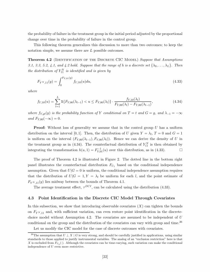
The transformation kcic is illustrated in Figure 1. Start with a value of y, with associatedquantile q in the distribution of Y10, as illustrated in the bottom panel of Figure 1. Then findthe quantile for the same value of y in the distribution of Y00, FY,00(y) = q′. Next, compute thechange in y according to kcic, by finding the value for y at that quantile q′ in the distributionof Y01 to get

∆CIC = F−1Y,01(q

′) − F−1Y,00(q

′) = F−1Y,01(FY,00(y)) − y,

as illustrated in the top panel of Figure I. Finally, compute a counterfactual value of Y N11 equal

to y + ∆cic, so that

kcic(y) = y + ∆cic = F−1Y N ,11

(FY,10(y)) = F−1Y N ,11

(q).

For the standard DID model the equivalent transformation is

kDID(y) = y + E[Y01] − E[Y00].

Consider now the role of the support restriction, Assumption 5.2. Without it, we can onlyestimate the distribution function of Y N

11 on Y01. Outside that range, we have no informationabout the distribution of Y N

11 .

Corollary 3.1 (Identification of the CIC Model Without Support Restrictions)

Suppose that Assumptions 3.1-3.3 hold. Then we can identify the distribution of Y N11 on Y01.

For y ∈ Y01, FY N ,11 is given by (3.8). Outside of Y01, the distribution of Y N11 is not identified.

To see how this result could be used, define

q = miny∈Y00

FY,10(y), q = maxy∈Y00

FY,10(y). (3.16)

Then, for any q ∈ [q, q], we can calculate the effect of the treatment on quantile q of thedistribution of FY,10, according to

τ cicq ≡ F−1

Y I ,11(q) − F−1

Y N ,11(q) = F−1

Y I ,11(q) − F−1

Y,01(FY,00(F−1Y,10(q))). (3.17)

Thus, even without the support assumption (5.2), for all quantiles of Y10 that lie in this range,it is possible to deduce the effect of the treatment. Furthermore, for any bounded functiong(y), it will be possible to put bounds on E[g(Y I

11)− g(Y N11 )], following the approach of Manski

(1990, 1995). When g is the identity function and the supports are bounded, this approachyields bounds on the average treatment effect.

The standard DID approach requires no support assumption to identify the average treat-ment effect. Corollary 3.1 highlights the fact that the standard DID model identifies the average

[10]

treatment effect only through extrapolation: because the average time trend is assumed to bethe same in both groups, we can apply the time trend estimated on the control group to allindividuals in the initial period treatment group, even those who experience outcomes outsidethe support of the initial period control group.

Also, observe that our analysis extends naturally to the case with covariates X; we simplyrequire all assumptions to hold conditional on X. Then, Theorem 3.1 extends to establishidentification of Y N

11 |X. Of course, there is no requirement about how the distribution of Xvaries across subpopulations; thus, we can relax somewhat our assumption that populationcharacteristics are stable over time within a group, if all relevant factors that change over timeare observable.

The CIC model treats groups and time periods asymmetrically. Of course, there is nothingintrinsic about the labels of period and group. In some applications, it might make moresense to reverse the roles of the two, yielding what we refer to as the reverse CIC (CIC-r) model. For example, (CIC-r) applies in a setting where, in each period, each memberof a population is randomly assigned to one of two groups, and these groups have different“production technologies.” The production technology does not change over time in the absenceof the intervention; however, the composition of the population changes over time (e.g., theunderlying health of 60-year-old males participating in a medical study changes year by year),so that the distribution of U varies with time but not across groups. To uncover the averageeffect of the new technology we need to estimate the counterfactual distribution in the secondperiod treatment group, which combines the treatment group production function with thesecond period distribution of unobservables. When the distribution of outcomes is continuous,neither the CIC nor the CIC-r model has testable restrictions, and so the two models cannotbe distinguished. Yet, these approaches yield different estimates. Thus, it will be important inpractice to justify the choice of which dimension is called the group and which is called time.

3.2 The Counterfactual Effect of the Policy for the Untreated Group

Until now, we have only specified a model for an individual’s outcome in the absence of theintervention. No model for the outcome in the presence of the intervention is required to drawinferences about the effect of the policy change on the treatment group, that is, the effect of“the treatment on the treated” (e.g., Heckman and Robb, 1985); we simply need to comparethe actual outcomes in the treated group with the counterfactual. However, more assumptionsare required to analyze the effect of the treatment on the control group.

Consider augmenting the CIC model with an assumption about the treated outcomes. Itseems natural to specify that these outcomes follow a model analogous to that for untreatedoutcomes, so that Y I = hI(U, T ). In words, at a given point in time, the effect of the treatmentis the same across groups for individuals with the same value of the unobservable. However,outcomes can differ across individuals with different unobservables, and no further functional

[11]

form assumptions are imposed about the incremental returns to treatment, hI(u, t) − h(u, t).14

At first, it might appear that finding the counterfactual distribution of Y I01 could be qual-

itatively different than finding the counterfactual distribution of Y N11 , since three out of four

subpopulations did not experience the treatment. However, it turns out that the two problemsare symmetric. Since Y I

01 = hI(U0, 1) and Y00 = h(U0, 0),

Y I01

d∼ hI(h−1(Y00; 0), 1). (3.18)

Since the distribution of U1 does not change with time, for y ∈ supp[Y10],

F−1Y I ,11

(FY,10(y)) = hI(h−1(y; 0), 1). (3.19)

This is just the transformation kcic(y) with the roles of group 0 and group 1 reversed. Followingthis logic, to compute the counterfactual distribution of Y I

01, we simply apply the approachoutlined in Section 3.1, but replace G with 1 −G.15 Summarizing:

Theorem 3.2 (Identification of the Counterfactual Effect of the Policy in the

CIC Model) Suppose that Assumptions 3.1-3.3 hold. In addition, suppose that Y I = hI(U, T ),where hI(u, t) is strictly increasing in u. Then the distribution of Y I

01 is identified on the re-stricted support supp[Y I

11], and is given by

FY I ,01(y) = FY,00(F−1Y,10(FY I ,11(y))). (3.20)

If supp[U0]⊆supp[U1], then supp[Y I01]⊆supp[Y I

11], and FY I ,01 is identified everywhere.

Proof: The proof is analogous to those of Theorem 3.1 and Corollary 3.1. Using (3.19), fory ∈ supp[Y I11],

F−1Y,10(FY I ,11(y)) = h(hI,−1(y; 1), 0).

Using this and (3.18), for y ∈ supp[Y I11],

Pr(hI(h−1(Y00; 0), 1) ≤ y) = Pr(Y00 ≤ F−1Y,10(FY I ,11(y))) = FY,00(F−1

Y,10(FY I ,11(y))).

The statement about supports follows from the definition of the model. �14Although we require monotonicity of h and hI in u, we do not require that the value of the unobserved

component is identical in both regimes, merely that the distribution remains the same (that is, U ⊥ G|T ). Forexample, letting UN and UI denote the unobserved components in the two regimes, we could have a fixed effecttype error structure with UN

i = ε+ νNi , and UI

i = εi + νIi , where the εi is a common component and the νN

i andνI

i are idiosyncratic errors with the same distribution in both regimes.15It might also be interesting to consider the effect that the treatment would have had in the first period.

Our assumption that hI(u, t) can vary with t implies that Y I00 and Y I

10 are not identified, since no informationis available about hI(u, 0). Only if we make a much stronger assumption, such as hI(u, 0) = hI(u, 1) for all u,

can we identify the distribution of Y Ig,0. But that assumption would imply that Y I

00d∼ Y I

01 and Y I10

d∼ Y I11, a fairly

restrictive assumption. Comparably strong assumptions are required to infer the effect of the treatment on thecontrol group in the CIC-r model, since the roles of group and time are reversed in that model.

[12]

Notice that in this model, not only can the policy change take place in a group with differentdistributional characteristics (e.g. “good” or “bad” groups tend to adopt the policy), butfurther, the expected benefit of the policy may vary across groups. Because hI(u, t) − h(u, t)varies with u, if FU,0 is different from FU,1, then the expected incremental benefit to the policydiffers.16 For example, suppose that E[hI(U, 1) − h(U, 1)|G = 1] > E[hI(U, 1) − h(U, 1)|G = 0].Then, if the costs of adopting the policy are the same for each group, we would expect that ifpolicies are chosen optimally, the policy would be more likely to be adopted in group 1. Usingthe method suggested by Theorem 3.2, it is possible to compare the average effect of the policyin group 1 with the counterfactual estimate of the effect of the policy in group 0 and to verifywhether the group with the highest average benefits is indeed the one that adopted the policy.It is also possible to describe the range of adoption costs and distributions over unobservablesfor which the treatment would be cost-effective or not.

In the remainder of the paper, we focus on identification and estimation of the distributionof Y N

11 . However, the results that follow extend in a natural way to Y I01; simply exchange the

labels of the groups 0 and 1 to calculate the negative of the treatment effect for group 0.

3.3 The Quantile DID Model

A third possible approach, distinct from the DID and CIC models, applies DID to each quantilerather than to the mean. We refer to this approach as the “Quantile DID” approach, or QDID.Some of the DID literature has followed this approach for specific quantiles. Poterba, Venti,and Wise (1995) and Meyer, Viscusi, and Durbin (1995) start from equation (2.1) and assumethat the median of Y N conditional on T and G is equal to α + β · T + η · G. Applying thisapproach to each quantile, with the coefficients α, β and η indexed by the quantile, we obtainthe following transformation:

kQDID(y) = y + F−1Y,01(FY,10(y)) − F−1

Y,00(FY,10(y)),

with FY N ,11(y) = Pr(kQDID(Y10) ≤ y). As illustrated in Figure 1, for a fixed y, we determine thequantile q for y in the distribution of Y10, q = FY,10(y). The difference over time in the controlgroup at that quantile, ∆QDID = F−1

Y,01(q) − F−1Y,00(q), is added to y to get the counterfactual

value, so that kQDID(y) = y+∆QDID. In this method, instead of comparing individuals acrossgroups according to their outcomes and accross time according to their quantiles, as in the CICmodel, we compare individuals across both groups and time according to their quantile.

The following model justifies the QDID estimator:

Y N = h(U,G, T ) = hG(U,G) + hT (U, T ). (3.21)

16For example, suppose that the incremental returns to the intervention, hI(u, 1) − h(u, 1), are increasing inu, so that the policy is more effective for high-u individuals. If FU,1(u) ≤ FU,0(u) for all u (i.e. First-OrderStochastic Dominance), then expected returns to adopting the intervention are higher in group 1.

[13]

The additional assumptions of the QDID model are: (i) h(u, g, t) is strictly increasing in u,

and (ii) U⊥(G,T ); thus, the standard DID model is a special case of QDID.17 Under theassumptions of the QDID model, the counterfactual distribution of Y N

11 is equal to that ofkQDID(Y10). Details of the identification proof are in Athey and Imbens (2002), hereafter AI.

Although the estimate of the counterfactual distribution under the QDID model differs fromthat under the DID model, under continuity the means of the two counterfactual distributionsare identical: E[kDID(Y10)] = E[kQDID(Y10)].

The QDID model has several disadvantages relative to the CIC model: (i) additive sepa-rability of h is difficult to justify, and it implies that the assumptions are not invariant to thescaling of y; (ii) the underlying distribution of unobservables must be identical in all subpop-ulations, eliminating an important potential source of intrinsic heterogeneity; (iii) the QDIDmodel places some restrictions on the data.18

3.4 Panel Data versus Repeated Cross-Sections

The discussion so far has avoided distinguishing between panel data and repeated cross-sections.In order to discuss these issues it is convenient to introduce additional notation. For individuali, let Yit be the outcome in period t, for t = 0, 1. We augment the model by allowing theunobserved component to vary with time:

Y Nit = h(Uit, t).

The monotonicity assumption is the same as before: h(u, t) must be increasing in u. We donot place any restrictions on the correlation between Ui0 and Ui1, but we modify Assumption3.3 to require that conditional on Gi, the marginal distribution of Ui0 is equal to the marginaldistribution of Ui1. Formally, Ui0|Gi

d∼ Ui1|Gi. Note that the CIC model (like the standard DIDmodel) does not require that individuals maintain their rank over time, that is, it does notrequire Ui0 = Ui1. Although Ui0 = Ui1 is an interesting special case, in many contexts, perfectcorrelation over time is not reasonable.19 Alternatively one may have Uit = εi+ νit, with νit anidiosyncratic error term with the same distribution in both periods.

The estimator proposed in this paper therefore applies to the panel setting as well as thecross-section setting. In the panel setting it is distinct from the estimand based on the assump-tion unconfoundedness or “selection on observables” (Barnow, Cain, and Goldberger, 1980;

17As with the CIC model, the assumptions of this model are unduly restrictive if outcomes are discrete. Thediscrete version of QDID allows h to be weakly increasing in u; the main substantive restriction implied by theQDID model is that the model should not predict outcomes out of bounds. For details on this case, see Atheyand Imbens (2002).

18Without any restrictions on the distributions of Y00, Y01, and Y10, the transformation kQDID is not necessarilymonotone, as it should be under the assumptions of the QDID model; thus, the model is testable (see AI fordetails).

19If an individual gains experience or just age over time, her unobserved skill or health is likely to change. SeeHeckman, Smith and Clements (1997) for an analysis of various models of the correlation between Ui0 and Ui1.

[14]

Rosenbaum and Rubin, 1983; Heckman and Robb, 1984). Under such an assumption individu-als in the treatment group with an initial period outcome equal to y are matched to individualsin the control group with an identical first period outcome, and their second period outcomesare compared. Formally, let FY01|Y00

(·|·) be the conditional distribution function of Y01 givenY00. Then, for the “selection on observables” model,

FY N ,11(y) = E[FY01|Y00(y|Y10)],

which is in general different from the counterfactual distribution for the CIC model, FY N ,11(y) =FY,10(F−1

Y,00(FY,01(y))). The two models are equivalent if and only if Ui0 ≡ Ui1, that is, if inthe population there is perfect rank correlation between the first and second period unobservedcomponents.

Several other authors have analyzed semi-parametric models with fixed effects in panel datasettings, including Honore (1992), Kyriazidou (1997), and Altonji and Matzkin (1997, 2001).Typically these models have an endogenous regressor that may take on a range of values ineach period. In contrast, in the DID setting only one subpopulation receives the treatment.

3.5 Application to Wage Decompositions

A distinct but related problem to that of estimating the effect of interventions in a difference-in-differences setting is studied in the literature on wage decompositions. In a typical example,researchers compare wage distributions for two groups, e.g., men and women, or Whites andBlacks, at two points in time. Juhn, Murphy, and Pierce (1991) and Altonji and Blank (2000)decompose changes in Black-White wage differentials, after taking out differences in observedcharacteristics, into two effects: (i) the effect due to changes over time in the distribution ofunobserved skills among Blacks, and (ii) the effect due to common changes over time in themarket price of unobserved skills.

In their survey of studies of race and gender in the labor market, Altonji and Blank (2000)formalize a suggestion by Juhn, Murphy and Pierce (1991) to generalize the standard paramet-ric, additive model for this problem to a nonparametric one, using the following assumptions:(i) the distribution of White skills does not change over time, whereas the distribution of Blackskills can change in arbitrary ways; (ii) there is a single, strictly increasing function mappingskills to wages in each period, the market equilibrium pricing function. This pricing functioncan change over time, but is the same for both groups within a time period. Under the Altonji-Blank model, if we let Whites be group W and Blacks be group B, and let Y be the observedwage, then E[YB1] − E[F−1

Y,W1(FY,W0(YB0))] is interpreted as the part of the change in Blacks’average wages due to the change over time in unobserved Black skills. Interestingly, this ex-pression is the same as the expression we derived for τ cic, even though the interpretation isvery different: in our case the distribution of unobserved components remains the same overtime, and the difference is interpreted as the effect of the intervention. This illustrates a closeconnection between the difference-in-differences model and models for wage decompositions.

[15]

Note that to apply an analog of our estimator of the effect of the treatment on the controlgroup in the wage decomposition setting, we would require additional structure to specify whatit would mean for Whites to experience “the same” change over time in their skill distributionthat Blacks did, since the initial skill distributions are different. More generally, the preciserelationship between estimators depends on the primitive assumptions for each model, sincethe CIC, CIC-r, and QDID models all lead to distinct estimators. The appropriateness of theassumptions of the underlying structural models must be justified in each application, for bothtreatment effects and wage decompositions.

Altonji and Blank (2000) do not analyze the asymptotic properties of their estimator. Thus,the asymptotic theory we provide for the CIC estimator is useful for the wage decompositionproblem as well. In addition, as we show below, the model, estimator, and asymptotic theorymust be modified when data are discrete. Discrete wage data is common, since it arises ifwages are measured in intervals or if there are mass points (such as the minimum wage, roundnumbers, or union wages) in the observed wage distribution.

3.6 Relation to Econometric Literature Exploiting Monotonicity

In our approach to non-parametric identification, monotonicity of the production function playsa central role. Here, we build on Matzkin (1999, 2003), who initiated a line of research inves-tigating the role of monotonicity in wide range of models, starting with an analysis of the casewith exogenous regressors. In subsequent work (e.g. Das (2000, 2001), Imbens and Newey(2001), and Chesher (2003)), monotonicity of the relation between the endogenous regressorand the unobserved component plays a crucial role in settings with endogenous regressors. Inall these cases, as in the current paper, monotonicity in unobserved components implies a di-rect one-to-one link between the structural function and the distribution of the unobservables,a link that can be exploited in various ways. All of these papers require strict monotonicity,typically ruling out settings with discrete endogenous regressors other than in trivial cases. Fewresults are available for binary or discrete data,20 because typically (as in this paper) discretedata in combination with weak monotonicity leads to loss of point identification of the usualestimands, e.g., population average effects. In the current paper, we show below that althoughpoint identification is lost, one can still identify bounds on the population average effect of theintervention in the DID setting or regain point identification through additional assumptions.

Consider more specifically the relationship of our paper with the recent innovative work ofAltonji and Matzkin (1997, 2001, 2003) (henceforth AM). In both our study and in AM, thereis a central role for analyzing subpopulations that have the same distribution of unobservables.In our work, we argue that a defining feature of a group in a DID setting should be that thedistribution of unobservables is the same in the group in different time periods. AM focus on

20An exception is Imbens and Angrist (1994), who use a weak monotonicity assumption and obtain results for

the subpopulation of compliers.

[16]

subsets of realizations of a vector of covariates Z, where for all realizations in a particular subset,the distribution of unobservables is the same. In one example, Z incorporates an individual’shistory of experiences, and permutations of that history should not affect the distribution ofunobservables. So, an individual who completed first training program A and then program Bwould have the same unobservables as an individual who completed program B and then A. Ina cross-sectional application, if in a given family, one sibling was a high-school graduate andthe other a college graduate, both siblings would have the same unobservables. In both ourstudy and AM, within a subpopulation (induced by covariates) with a common distribution ofunobservables, after normalizing the distribution of unobservables to be uniform, it is possibleto identify a strictly increasing production function as the inverse of the distribution of out-comes conditional on the covariate. AM focus on estimation and inference for the productionfunction itself, and as such they use an approach based on kernel methods. In contrast, we areinterested in estimating the average difference of the production function for different subpopu-lations. We establish uniform convergence of our implicit estimator of the production function,in order to obtain root-n consistency of our estimator of the average treatment effect for thetreated and control groups as well as for treatment effects at a given quantile. We use theempirical distribution function as an estimator of the distribution function of outcomes in eachsubpopulation, which does not require the choice of smoothing parameters. Furthermore, ourapproach generalizes naturally to the case with discrete outcomes (as we argue, a commonlyencountered case), and our continuous-outcome estimator of the average treatment effect canbe interpreted as a bound on the average treatment effect when outcomes are discrete. Thus,the researcher need not make an a priori choice about whether to use the discrete or continuousmodel since we provide bounds that collapse when outcomes are continuous.

The next section develops the discrete model and analyzes identification.

4 Identification in Models with Discrete Outcomes

With discrete outcomes the baseline CIC model as defined by Assumptions 3.1-3.3 impliesunattractive restrictions. We therefore weaken Assumption 3.2 by allowing for weak rather thanstrict monotonicity. We show that this model is not identified without additional assumptions,and calculate bounds on the counterfactual distribution. We also propose two approaches totighten the bounds or even restore point identification, one using an additional assumption onthe distribution of unobservables, and one based on the presence of exogenous covariates.

However, we note that there are other possible approaches for tightening the bounds. Forexample, one may wish to consider restrictions on how the distribution of the unobserved com-ponents varies across groups, such as stochastic dominance relations or parametric functionalforms. Alternatively one may wish to put more structure on (the changes over time in) the pro-duction functions, or restrict the treatment effect as a function of the unobserved component.We leave these possibilities for future work.

[17]

4.1 Bounds in the Discrete CIC Model

The standard DID model imputes the averge outcome in the second period for the treatedsubpopulation in the absence of the treatment to E[Y N

11 ] = E[Y10]+[E[Y01]−E[Y00]]. With binarydata the imputed average for the second period treatment group outcome is not guaranteed tolie in the interval [0, 1]. For example, suppose E[Y10] = .5, E[Y00] = .8 and E[Y01] = .2. In thecontrol group the probability of success decreases from .8 to .2. However, it is impossible that asimilar percentage point decrease could have occurred in the treated group in the absence of thetreatment, since the implied probability of success would be less than zero.21 The CIC modelis also not very attractive as it severely restricts the joint distribution of the observables.22

We therefore weaken the strict monotonicity condition to:

Assumption 4.1 (Weak Monotonicity) h(u, t) is non-decreasing in u.

This assumption allows, for example, a latent index model h(U, T ) = 1{h(U, T ) > 0}, forsome h strictly increasing in U. With weak instead of strict monotonicity, we no longer obtainpoint identification. Instead, we can derive bounds on the average effect of the treatment inthe spirit of Manski (1990, 1995). To build intuition, consider again an example with binaryoutcomes. Without loss of generality we assume that in the control group U has a uniformdistribution on the interval [0, 1]. Let u0(t) = sup{u : h(u, t) = 0}. The observables relate tothe primitives of the model according to

E[Y Ngt ] = Pr(Ug > u0(t)). (4.22)

In particular, E[Y N11 ] = Pr(U1 > u0(1)). All we know about the distribution of U1 is that

Pr(U1 > u0(0)) = E[Y10]. Suppose that E[Y01] > E[Y00], implying u0(1) < u0(0). Then, thereare two extreme cases for the distribution of U1 conditional on U1 < u0(0). First, all of themass might be concentrated between u0(0) and u0(1). In that case, Pr(U1 > u0(1)) = 1. Second,there might be no mass between u0(0) and u0(1), in which case Pr(U1 > u0(1)) = Pr(U1 >

u0(0)) = E[Y10]. Together, these two cases imply E[Y N11 ] ∈ [E[Y10], 1]. Analogous arguments

yield bounds on E[Y N11 ] when E[Y01] < E[Y00]. When E[Y01] = E[Y00], we conclude that the

production function does not change over time, and so the probability of success does not21 One approach that has been used to deal with this problem (Blundell, Dias, Meghir and Van Reenen, 2001)

is to specify an additive linear model for a latent index,

Y ∗i = α+ β · Ti + η · Gi + τ · Ii + εi,

with the observed outcome equal to an indicator that the latent index is positive, Yi = 1{Y ∗i ≥ 0}. Given a

distributional assumption on εi (e.g., logistic), one can estimate the parameters of the latent index model andderive the implied estimated average effect for the second period treatment group.

22For example, with binary outcomes, strict monotonicity of h(u, t) in u implies that U is binary with h(0, t) = 0and h(1, t) = 1 and thus Pr(Y = U |T = t) = 1, or Pr(Y = U) = 1. Independence of U and T then impliesindependence of Y and T , which is very restrictive.

[18]

change over time within a group either, implying E[Y N11 ] = E[Y10]. Since the average treatment

effect, τ, is defined by τ = E[Y I11] − E[Y N

11 ], it follows that

τ ∈

[E[Y I11] − 1, E[Y I

11] − E[Y10]] if E[Y01] > E[Y00]E[Y I

11] − E[Y10] if E[Y01] = E[Y00][E[Y I

11] − E[Y10], E[Y I11]] if E[Y01] < E[Y00].

In this binary example the sign of the treatment effect is determined if and only if the observedtime trends in the treatment and control groups move in opposite directions.

Now consider the general case, where Y can be mixed discrete and continuous. Our definitionof the inverse distribution function F−1

Y (q) = inf{y ∈ Y|FY (y) ≥ q} implies FY (F−1Y (q)) ≥ q.

It is useful to have an alternative inverse distribution function. Define

F(−1)Y (q) = sup{y ∈ Y ∪ {−∞} : FY (y) ≤ q}, (4.23)

where we use the convention FY (−∞) = 0. For q such that q = FY (y) for some y ∈ Y, the twodefinitions of inverse distribution functions agree and F (−1)

Y (q) = F−1Y (q). For other values of q

FY (F (−1)Y (q)) < q, so that in general, FY

(F

(−1)Y (q)

)≤ q ≤ FY

(F−1Y (q)

).

Theorem 4.1 (Bounds in the Discrete CIC Model) Suppose that Assumptions 3.1, 3.3,5.2, and 4.1 hold. Suppose that U is continuous. Then we can place bounds on the distribution ofY N

11 . For y < inf Y01, FLBY N ,11

(y) = FUBY N ,11

(y) = 0, for y > inf Y01, FLBY N ,11

(y) = FUBY N ,11

(y) = 1,while for y ∈ Y01,

FLBY N ,11(y) = FY,10(F(−1)Y,00 (FY,01(y))), FUBY N ,11(y) = FY,10(F−1

Y,00(FY,01(y))). (4.24)

These bounds are tight.

Proof: By assumption U1 ⊆ U0. Without loss of generality we can normalize U0 to be uniformon [0, 1].23 Then for y ∈ Y0t,

FY,0t(y) = Pr(h(U0, t) ≤ y) = sup{u : h(u, t) = y}. (4.25)

Define

K(y) ≡ sup{y′ ∈ Y00∪{−∞} : FY,00(y′) ≤ FY,01(y)}, (4.26)

K(y) ≡ inf{y′ ∈ Y00 : FY,00(y′) ≥ FY,01(y)}. (4.27)

By our definitions of inverse distribution functions, (3.7) and (4.23), we have

K(y) = F(−1)Y,00 (FY,01(y)), K(y) = F−1

Y,00(FY,01(y)). (4.28)

23To see that there is no loss of generality, observe that given a real-valued random variable U0 with convexsupport, we can construct a nondecreasing function ψ such that FU,0(u) = Pr(ψ(U∗) ≤ u), where U∗

0 is uniformon [0, 1]. Then, h(u, t) = h(ψ(u), t) is nondecreasing in u since h is, and the distribution of Y0t is unchanged.Since U1 ⊆ U0, the distribution of Y1t is unchanged as well.

[19]

Using (4.25) and continuity of U , we can express FY N ,1t(y) as

FY N ,1t(y) = Pr(Y N1t ≤ y) = Pr(h(U1, t) ≤ y) (4.29)

= Pr (U1 ≤ sup{u : h(u, t) = y} ) = Pr(U1 ≤ FY N ,0t(y)

).

Thus, using (4.26), (4.27), and (4.29),

FY,10(K(y)) = Pr (U1 ≤ FY,00(K(y)) ) ≤ Pr (U1 ≤ FY,01(y) ) = FY N ,11(y), (4.30)

FY,10(K(y)) = Pr(U1 ≤ FY,00(K(y))

)≥ Pr (U1 ≤ FY,01(y) ) = FY N ,11(y). (4.31)

Substituting (4.28) into (4.30) and (4.31) yields the desired result.To see that the bounds are tight, consider a given F ≡(FY,00, FY,01, FY,10). Normalizing U0 to

be uniform on [0, 1], for u ∈ [0, 1] define h(u, t) = F−1Y,0t(u). Observe that this is nondecreasing

and left-continuous, and this h and FU,0 are consistent with FY,00 and FY,01. Further, using(4.29), consistency with FY,01 is equivalent to

FU,1(FY,00(y)) = FY,10(y) (4.32)

for all y ∈ Y10. Let FLBU,1 and FUBU,1 be the (pointwise) infimum and supremum of the set ofall probability distributions with support contained in [0, 1] and consistent with (4.32). Then,applying the definitions of K(y) and K(y), for y ∈ Y00

FLBU,1 (FY,01(y)) = inf{q ∈ [0, 1] : q ≥ FY,10(K(y))} = FY,10(K(y)) ≡ FLBY N ,11(y),

FUBU,1 (FY,01(y)) = sup{q ∈ [0, 1] : q ≤ FY,10(K(y))} = FY,10(K(y)) ≡ FUBY N ,11(y).

Thus, there can be no tighter bounds. �

The proof of Theorem 4.1 is illustrated in Figure 2. The top left panel of the figure summa-rizes a hypothetical dataset for an example with four possible outcomes, {λ0, λ1, λ2, λ3}. Thetop right panel of the figure illustrates the production function in each period, as inferred fromthe group 0 data (when U0 is normalized to be uniform), where uk(t) is the value of u at whichh(u, t) jumps up to λk. In the bottom right panel, the diamonds represent the points of thedistribution of U1 that can be inferred from the distribution of Y10. The distribution of of U1

is not identified elsewhere. This panel illustrates the infimum and supremum of the probabilitydistributions that pass through the given points; these are bounds on FU1 . The circles indicatethe highest and lowest possible values of FY N

11(y) = FU1(u

k(t)) for the support points; we willreturn to discuss the dotted line in the next section.

Note that if we simply ignore the fact that the outcome is discrete and use the continuousCIC estimator (3.8) to construct FY N ,11, we will obtain the upper bound FUB

Y N ,11from Theorem

4.1. If we calculate E[Y N11 ] directly from the distribution FUB

Y N ,11,24 we will thus obtain the

24With continuous data, kcic(Y10) has the distribution given in (3.8), and so (3.15) can be used to calculatethe average treatment effect. As we show below, with discrete data, kcic(Y10) has distribution equal to FLB

Y N ,11

rather than FUBY N ,11, and so an estimate based directly on (3.8) yields a different answer than one based on (3.15).

[20]

lower bound for the estimate of E[Y N11 ], which in turn yields the upper bound for the averagetreatment effect, E[Y I

11] − E[Y N11 ]. Clearly, confidence intervals will be misleading in that case.

4.2 Point Identification in the Discrete CIC Model Through the Conditional

Independence Assumption

The following assumption restores point identification in the discrete CIC model.

Assumption 4.2 (Conditional Independence) U ⊥ G | Y, T.

In the continuous CIC model, the level of outcomes can be compared across groups, andthe quantile of outcomes can be compared over time. The role of Assumption 4.2 is to preservethat idea in the discrete model. In other words, to figure out what would have happened toa treated unit in the first period with outcome y, we look at units in the first period controlgroup with the same outcome y. Using weak monotonicity, we can derive the distribution oftheir second period outcomes, and we use that to derive the counterfactual distribution for thesecond period treated in the absence of the intervention. Note that together, Assumptions 4.2and 4.1 are strictly weaker than the strict monotonicity assumption (3.2).25

Consider the consequences of Assumption 4.2 for identification. To provide some intuition,we initially focus on the binary case. Without loss of generality normalize U0 to be uniform on[0, 1], and recall the definition of u0(t) = sup{u : h(u, t) = 0}, so that 1−E[Y Ngt ]=Pr(Ug ≤ u0(t)).Then we have for u ≤ u0(t),

Pr(U1 ≤ u| U1 ≤ u0(t)) = Pr(U1 ≤ u| U1 ≤ u0(t), T = 0, Y = 0)

= Pr(U0 ≤ u| U0 ≤ u0(t)) = Pr(U0 ≤ u| U0 ≤ u0(t), T = 0, Y = 0) =u

u0(t).

Using the preceeding expression together with an analogous expression for Pr(Ug > u| Ug >u0(t)), and the definitions from the model, it is possible to derive the counterfactual E[Y N

11 ]:

E[Y N11 ] =

{ E[Y01]E[Y00]E[Y10] = E[Y01] + E[Y01]

E[Y00] (E[Y10] − E[Y00]) if E[Y01] ≤ E[Y00]

1 − 1−E[Y01]1−E[Y00] (1 − E[Y10]) = E[Y01] +

1−E[Y01]1−E[Y00] (E[Y10] − E[Y00]) if E[Y01] > E[Y00]

Notice that this formula always yields a prediction between 0 and 1. When the time trend inthe control group is negative, the counterfactual is the probability of successes in the treatmentgroup initial period, adjusted by the proportional change over time in the probability of successin the control group. When the time trend is positive, the counterfactual probability of failure is

25If h(u, t) is strictly increasing in u, then one can write U = h−1(T, Y ), so that conditional on T and Y therandom variable U is degenerate and hence independent of G. If the outcomes are continuously distributed, theAssumption 4.2 is automatically satisfied. In that case flat areas of the function h(u, t) are ruled out as theywould induce discreteness of Y , and hence U must be continuous and the correspondence between Y and U mustbe one-to-one.

[21]

the probability of failure in the treatment group in the initial period adjusted by the proportionalchange over time in the probability of failure in the control group.

This following theorem generalizes this discussion to more than two outcomes; to keep thenotation simple, we assume there are L possible outcomes.

Theorem 4.2 (Identification of the Discrete CIC Model) Suppose that Assumptions3.1, 3.3, 5.2, 4.1, and 4.2 hold. Suppose that the range of h is a discrete set {λ0, . . . , λL}. Thenthe distribution of Y N

11 is identified and is given by

FY N ,11(y) =∫ FY,01(y)

0fU,10(u)du, (4.33)

where

fU,10(u) =L∑

l=1

1{FY,00(λl−1) < u ≤ FY,00(λl)} ·fY,10(λl)

FY,00(λl) − FY,00(λl−1), (4.34)

where fY,gt(y) is the probability function of Y conditional on T = t and G = g, and λ−1 = −∞and FY,00(−∞) = 0.

Proof: Without loss of generality we assume that in the control group U has a uniformdistribution on the interval [0, 1]. Then, the distribution of U given Y = λl, T = 0 and G = 1is uniform on the interval (FY,00(λl−1), FY,00(λl)). Hence we can derive the density of U inthe treatment group as in (4.34). The counterfactual distribution of Y N

11 is then obtained byintegrating the transformation h(u, 1) = F−1

Y,01(u) over this distribution, as in (4.33). �

The proof of Theorem 4.2 is illustrated in Figure 2. The dotted line in the bottom rightpanel illustrates the counterfactual distribution FU1 based on the conditional independenceassumption. Given that U |G = 0 is uniform, the conditional independence assumption requiresthat the distribution of U |G = 1, Y = λl be uniform for each l, and the point estimate ofFY N ,11(y) lies midway between the bounds of Theorem 4.1.

The average treatment effect, τDCI , can be calculated using the distribution (4.33).

4.3 Point Identification in the Discrete CIC Model Through Covariates

In this subsection, we show that introducing observable covariates (X) can tighten the boundson FY N ,11 and, with sufficient variation, can even restore point identification in the discrete-choice model without Assumption 4.2. The covariates are assumed to be independent of Uconditional on the group and the distribution of the covariates can vary with group and time.26

Let us modify the CIC model for the case of discrete outcomes with covariates.26The assumption that U ⊥ X | G is very strong, and should be carefully justified in applications, using similar

standards to those applied to justify instrumental variables. The analog of an “exclusion restriction” here is thatX is excluded from FUg (·). Although the covariates can be time-varying, such variation can make the conditionalindependence of U even more restrictive.

[22]

Assumption 4.3 (Discrete Model with Covariates) The outcome of an individual inthe absence of intervention satisfies the relationship

Y N = h(U, T,X).

Assumption 4.4 (Weak monotonicity) h(u, t, x) is nondecreasing in u for t = 0, 1 and forall x ∈ X.

Assumption 4.5 (Covariate Independence) U ⊥ X | G.

We refer to the model defined by Assumptions 4.3-4.5, together with time invariance (As-sumption 3.3), as the Discrete CIC Model with Covariates. Note that Assumption 4.5 allowsthe distribution of X to vary with group and time. Let X be the support of X, with Xgt thesupport of X|G = g, T = t. We maintain the assumption that these supports are compact.

To see why variation in X aids in identification, suppose that the range of h is a discreteset {λ0, . . . , λL}, and define

uk(t, x) = sup{u′ : h(u′, t, x) ≤ λk}.

Recall that FY,10|X(·|x) reveals the value of FU,1(u) for u ∈ {u0(t, x), .., uL(t, x)}, as illustratedin Figure 2. Variation in X allows us to learn the value of FU,1(u) for more values of u.

More formally, for each (x, y), define K(y;x) and L(y;x) by

(K(y;x),L(y;x)) = arg sup(x′,y′)∈X00×(Y00∪{−∞}):FY,00(y′|x′)≤FY,01(y|x)

FY,00(y′|x′);

(K(y;x), L(y;x)) = arg inf(x′,y′)∈X00×Y00:

FY,00(y′|x′)≥FY,01(y|x)

FY,00(y′|x′).

If either of these is set-valued, take any selection from the set of solutions.The following result places bounds on the counterfactual distribution of Y N

11 .

Theorem 4.3 (Bounds in the Discrete CIC Model With Covariates) Suppose thatAssumptions 4.3-4.5 and Assumption 3.3 hold. Suppose that U is continuous and X0t = X1t

for t ∈ {0, 1}. Then we can place the following bounds on the distribution of Y N11 :

FLBY N ,11|X(y|x) = FY |X,10(K(y;x) | L(y;x)), FUBY N ,11|X(y|x) = FY |X,10(K(y;x) | L(y;x)).

Proof: As in the proof of Theorem 4.1, without loss of generality normalize U0 to be uniformon [0, 1]. By continuity of U , we can express FY N ,1t(y) as

FY N ,1t|X(y|x) = Pr(Y N1t ≤ y|X = x) = Pr(h(U1, t, x) ≤ y) (4.35)

= Pr (U1 ≤ sup{u : h(u, t, x) = y} ) = Pr(U1 ≤ FY N ,0t|X(y|x)

).

[23]

Thus, using definitions and (4.35),

FY,10|X(K(y;x) | L(y;x)) = Pr(U1 ≤ FY,00|X(K(y;x)|L(y;x))

)

≤ Pr(U1 ≤ FY,01|X(y|x)

)= FY N ,11|X(y|x),

FY,10|X(K(y;x) | L(y;x)) = Pr(U1 ≤ FY,00|X(K(y;x)|L(y;x))

)

≥ Pr(U1 ≤ FY,01|X(y|x)

)= FY N ,11(y|x).

�When there is no variation in X, the bounds are equivalent to those given in Theorem 4.1.

When there is sufficient variation in X, the bounds collapse and point identification can berestored.

Theorem 4.4 (Identification of the Discrete CIC Model with Covariates) Supposethat Assumptions 4.3-4.5 and Assumption 3.3 hold. Suppose that U is continuous and X0t = X1t

for t ∈ {0, 1}. Normalize U0 to be uniform on [0, 1]. Define

St(y) = {u : ∃x ∈ X0t s.t. u = FY,0t|X(y|x)}. (4.36)

Assume that for all y ∈ Y01, S1(y) ⊆ ∪y∈Y00S0(y). Then the distribution of Y N11 |X is identified.

Proof: For each x ∈ X01 and each y ∈ Y01, let (ψ(y;x), χ(y;x)) be a selection from the set ofpairs (y′, x′) ∈ {Y00,X00} that satisfy FY,00|X(y′|x′) = FY,01|X(y|x). Since S1(y) ⊆ ∪y∈Y00S0(y),there exists such a y′ and x′. Then, uψ

k(x)(0, χk(x)) = uk(1, x). Then,

FY N |X,11(y|x) = FU,1(FY,01|X(y|x)) = FU,1(FY,00|X(ψ(y;x)|χ(y;x))) = FY |X,10(ψ(y;x)|χ(y;x)).

�

5 Inference

In this section we consider inference for the continuous and discrete CIC models.

5.1 Inference in the Continuous CIC Model

In order to guarantee that τ cic = E[Y11] − E[F−1Y,01(FY,00(Y10))], in this subsection we maintain

Assumptions 3.1-5.1 (alternatively, we could simply redefine τ cic according to the latter expres-sion, since those assumptions are not directly used in the analysis of inference.) We make thefollowing assumptions regarding the sampling process.

Assumption 5.1 (Data Generating Process)

(i) Conditional on Ti = t and Gi = g, Yi is a random draw from the subpopulation with Gi = g

[24]

during period t.(ii) αgt ≡ Pr(Ti = t,Gi = g) > 0 for all t, g ∈ {0, 1}.(iii) The four random variables Ygt are continuous with densities that are continuously differ-entiable, bounded, and bounded away from zero with support Ygt that is a compact subset of R.

Assumption 5.2 (Support Condition)

Y10 ⊂ Y00.

We have four random samples, one from each group/period. Let the observations from groupg and time period t be denoted by Ygt,i, for i = 1, . . . , Ngt. We use the empirical distributionas an estimator for the distribution function:

FY,gt(y) =1Ngt

Ngt∑

i=1

1{Ygt,i ≤ y}. (5.37)

As an estimator for the inverse of the distribution function we use

F−1Y,gt(q) = min{y : FY,gt(y) ≥ q}, (5.38)

for 0 < q ≤ 1 and F−1Y,gt(0) = y

gt, where y

gtis the lower bound on the support of Ygt. As an

estimator of τ cic = E[Y11] − E[F−1Y,01(FY,00(Y10))] we use

τ cic =1N11

N11∑

i=1

Y11,i −1N10

N10∑

i=1

F−1Y,01(FY,00(Y10,i)). (5.39)

First, define

p(y, z) =1

fY,01(F−1Y,01(FY,00(z)))

· (1{y ≤ z} − FY,00(z)) ,

q(y, z) =1

fY,01(F−1Y,01(FY,00(z)))

· (1{FY,01(y) ≤ FY,00(z)} − FY,00(z)) ,

r(y) = F−1Y,01(FY,00(y)) − E

[F−1Y,01(FY,00(Y11))

].

s(y) = y − E[Y11].

Also define the two U -statistics

µp =1

N00 ·N10

N00∑

i=1

N10∑

j=1

p(Y00,i, Y10,j), and µq = − 1N01 ·N10

N01∑

i=1

N10∑

j=1

q(Y01,i, Y10,j),

and the two averages

µr = − 1N10

N10∑

i=1

r(Y10,i), and µs =1N11

N11∑

i=1

s(Y11,i).

[25]

Because µp is a two-sample U -statistic it can be approximated by the sum of two averages:

µp =1N00

N00∑

i=1

E[p(Y00,i, Y10)|Y00,i] +1N10

N10∑

i=1

E[p(Y00, Y10,j)|Y10,j ] + op(N−1/2).

Since E[p(Y00, Y10,j)|Y10,j ] = 0, it follows that µp = µp + op(N−1/2), with

µp =1N00

N00∑

i=1

E[p(Y00,i, Y10)|Y00,i].

Similarly µq = µq + op(N−1/2), with

µq =1N01

N01∑

i=1

E[q(Y01,i, Y10)|Y01,i].

Finally, define the normalized variances of the µ’s:

V p = N00 · Var(µp), V q = N01 · Var(µq),

V r = N10 · Var(µr), and V s = N11 · Var(µs).

Theorem 5.1 (Consistency and Asymptotic Normality) Suppose Assumptions 5.1 and5.2 hold. Then:(i) τ cic − τ cic = Op

(N−1/2

),

and (ii)√N

(τ cic − τ cic

) d−→ N (0, V p/α00 + V q/α01 + V r/α10 + V s/α11) .

The variance of the CIC estimator, τ cic, can be equal to the variance of the standardDID estimator, τdid, in some special cases, such as when the following conditions hold: (i)Assumption 5.1 holds, (ii) Y00

d∼ Y10, and (iii) there exists a ∈ R such that, for each g,

Y Ng0

d∼ Y Ng1 + a. More generally, the variance of τ cic can be larger or smaller than the variance

of τdid.27

To estimate the asymptotic variance we replace expectations with sample averages, usingempirical distribution functions and their inverses for distribution functions and their inverses,and by using any uniformly consistent nonparametric estimator for the density functions. Tobe specific, let Ygt be the support of Ygt, and let Ygt be the midpoint of the support, Ygt =

27To see this, suppose that Y00 has mean zero, unit variance, and compact support, and that Y00d∼ Y10. Now

suppose that Y Ng1

d∼ σ·Yg0 for some σ > 0, and thus Y Ng1 has mean zero and variance σ2 for each g. The assumptions

of the both the CIC model and the mean-independence DID model are satisfied, and the probability limits of τdidand τ cic are identical and equal to E[Y11] − E[Y10] − [E[Y01] − E[Y00]]. If N00 and N01 are much larger than N10

and N11, the variance of the standard DID estimator is essentially equal to V ar(Y11) + V ar(Y10). The varianceof the CIC estimator is in this case approximately equal to V ar(Y11) + V ar(k(Y10)) = V ar(Y11) +σ2 · V ar(Y10).Hence with σ2 < 1 the CIC estimator is more efficient, and with σ2 > 1 the standard DID estimator is moreefficient.

[26]

(max Ygt − min Ygt)/2. Then we can use the following estimator for fY,gt(y):28

fY,gt =

(FY,gt(y +N−1/3) − FY,gt(y)

)/N−1/3 if y ≤ Ygt,(

FY,gt(y) − FY,gt(y −N−1/3))/N−1/3 if y > Ygt.

Given these definitions, we propose the following consistent estimator for the asymptotic vari-ance, where we let g00, g01, and g10 be the empirical counterparts of g00, g01, and g10, with F

and F−1 substituted for F and F−1, and sample averages replacing expectations. Then define

V p =1N00

N00∑

i=1

1N10

N10∑

j=1

g00(Y00,i, Y10,j)

2

, V q =1N01

N01∑

i=1

1N10

N10∑

j=1

g01(Y01,i, Y10,j)

2

,

V r =1N10

N10∑

i=1

g10(Y10,i) −

1N10

N10∑

j=1

g10(Y10,j)

2

, V s =1N11

N11∑

i=1

Y11,i −

1N11

N11∑

j=1

Y11,j

2

,

and let αgt = 1N

∑Ni=1 1{Gi = g, Ti = t}.

Theorem 5.2 (Consistent Estimation of the Variance) Suppose Assumption 5.1 holdsand Y10 ⊆ Y00. Then: αgt

p→ αgt for all g, t, V p p→ V p, V q p→ V q, V r p→ V r, V s p→ V s, andtherefore

V p/α00 + V q/α01 + V r/α10 + V s/α11p−→ V p/α00 + V q/α01 + V r/α10 + V s/α11,

Proof: See Appendix. �For the quantile case we derive the large sample properties of the estimator τ cic

q = F−1Y,11(q)−

F−1Y N ,11

(q) for τ cicq (as given in 3.17) and F−1

Y N ,11is defined by empirical distributions and inverses

as described above. To establish its asymptotic properties it is useful to define the quantileequivalent of the functions p(·), q(·), r(·) and s(·), denoted by pq(·), qq(·), rq(·) and sq(·):

pq(y) =1

fY,01(F−1Y,01(FY,00(F

−1Y,10(q)))

(1{y ≤ F−1

Y,10(q)} − FY,00(F−1Y,10(q))

),

qq(y) =1

fY,01(F−1Y,01(FY,00(F

−1Y,10(q)))

(1{FY,01(y) ≤ FY,00(F−1

Y,10(q))} − FY,00(F−1Y,10(q))

),

rq(y) =fY,00((F−1

Y,10(q))

fY,01(F−1Y,01(FY,00(F

−1Y,10(q)))fY,10(F

−1Y,10(q))

(1{FY,11(y) ≤ q} − q) ,

and

sq(y) = y − E[Y11].

Define also the corresponding variances: V pq = E

[pq(Ygt)2

], V q

q = E[qq(Ygt)2

], V r

q = E[rq(Ygt)2

],

and V sq = E

[sq(Ygt)2

].

28Other estimators for fY,gt(y) can be used as long as they are uniformly consistent, including at the boundaryof the support.

[27]

Theorem 5.3 (Consistency and Asymptotic Normality of Quantile CIC Estima-

tor) Suppose Assumption 5.1 holds. Then, defining q and q as in (3.16), for all q ∈ (q, q),(i) τ cic

qp−→ τ cic

q ,

(ii)√N(τ cic

q − τ cicq ) d−→ N

(0, V p

q /α00 + V qq /α01 + V r

q /α10 + V sq /α11

).

Proof: See Appendix. �The variance of the quantile estimators can be estimated analogously to that for the esti-

mator of the average treatment effect. We may also wish to test the null hypothesis that thetreatment has no effect by comparing the distributions of the second period outcome for thetreatment group with and without the treatment – that is, FY I ,11(y) and FY N ,11(y), or first orsecond order stochastic dominance relations (e.g., Abadie, 2002). One approach for testing theequality hypothesis is to estimate τ cic

q for a number of quantiles and jointly test their equality.For example, one may wish to estimate the three quartiles or the nine deciles and test whetherthey are the same in both distributions. In AI, we provide details about carrying out such atest, showing that a X 2 test can be used. More generally, it may be possible to construct aKolmogorov-Smirnov or Cramer-Von Mises test on the entire distribution. Such tests could beused to test the assumptions underlying the model if more than two time periods are available.

With covariates one can estimate the average treatment effect for each value of the covariatesby applying the estimator discussed in Theorem 5.1 and taking the average over the distributionof the covariates. When the covariates take on many values this procedure may be infeasible, andone may wish to smooth over different values of the covariates. One approach is to estimate thedistribution of each Ygt conditional on covariates X nonparametrically (using kernel regressionor series estimation) and then again average the average treatment effect at each X over theappropriate distribution of the covariates.

As an alternative, consider a more parametric approach to adjusting for covariates. Suppose

h(u, t, x) = h(u, t) + x′β and hI(u, t, x) = hI(u, t) + x′β

with U independent of (T,X) given G.29 Because, in this model, the effect of the interventiondoes not vary with X, the average treatment effect is still given by τ cic. To derive an estimatorfor τ cic, we proceed as follows. First, β can be estimated consistently using linear regressionof outcomes on X and the four group-time dummy variables (without an intercept). We canthen apply the CIC estimator to the residuals from an ordinary least squares regression withthe effects of the dummy variables added back in. To be specific, let D be the four-dimensionalvector ((1 − T )(1 −G), T (1 −G), (1 − T )G,TG)′. In the first stage, we estimate the regression

Yi = D′iδ +X ′

iβ + εi.

29A natural extension would consider a model of the form h(u, t) +m(x); the function m could be estimatedusing nonparametric regression techniques, such as series expansion or kernel regression. Alternatively one couldallow the coefficients β to depend on the group and or time. The latter extension would be straightforward giventhe results in AI.

[28]

Then construct the residuals with the group/time effects added back in:

Yi = Yi −X ′iβ = D′

iδ + εi.

Finally, apply the CIC estimator to the empirical distributions of the augmented residuals Yi.In AI we show that the covariance-adjusted estimator of τ cic is consistent and asymptoticallynormal, and we calculate the asymptotic variance.

5.2 Inference in the Discrete CIC Model

In this subsection we discuss inference for the discrete CIC model. If one is willing to make theconditional independence assumption 4.2, the model is a fully parametric, smooth model, andinference becomes standard. We therefore focus on the discrete case without Assumption 4.2.We maintain Assumptions 3.1, 3.3, 5.2, and 4.1 (as in the continuous case, these assumptionsare used only to ensure derive expressions for τLB and τUB , and in particular they are not useddirectly in the analysis of inference). We make one additional assumption.

Assumption 5.3 (Absence of Ties) Y is a finite set, and for all y, y′ ∈ Y,

FY,01(y) 6= FY,00(y′).

For example, if Y = {0, 1}, this assumption requires Pr(Y01 = 0) 6= Pr(Y00 = 0) andPr(Y01 = 0),Pr(Y00 = 0) ∈ (0, 1). When ties of this sort are not ruled out, the bounds on thedistribution function do not converge to their theoretical values as the sample size increases.30

Define

F Y,00(y) = Pr(Y00 < y),

k(y) = F−1Y,01(F Y,00(y)), and k(y) = F−1

Y,01(FY,00(y)),

with estimated counterparts

F Y,00(y) =1N00

N00∑

i=1

1{Y00,i < y},

k(y) = F−1Y,01(F Y,00(y)), and k(y) = F−1

Y,01(FY,00(y)).

The functions k(y) and k(y) can be interpreted as the bounds on the transformation k(y)defined for the continuous case in (3.14). Note that k(y) ≡ kcic(y). In the Appendix (LemmaA.10), we show that k(Y10)

d∼ FUBY N ,11

and k(Y10)d∼ FLB

Y N ,11. The bounds on τ are then

τLB = E[Y11] − E[k(Y10)], and τUB = E[Y11] − E[k(Y10)],30An analoguous situation arises in estimating the median of a binary random variable Z with Pr(Z = 1) = p.

If p 6= 1/2, the sample median will converge to the true median (equal to 1{p ≥ 1/2}), but if p = 1/2, then inlarge samples the estimated median will be equal to 1 with probability 1/2 and equal to 0 with probability 1/2.

[29]

with the corresponding estimators

τLB =1N11

N11∑

i=1

Y11,i −1N10

N10∑

i=1

k(Y10,i), and τUB =1N11

N11∑

i=1

Y11,i −1N10

N10∑

i=1

k(Y10,i).

Theorem 5.4 (Asymptotic Distribution for Bounds) Suppose Assumption 5.3 holds.Then:

√N(τUB − τUB) d−→ N (0, V s/α11 + V r/α10),

and√N(τLB − τLB) d−→ N (0, V s/α11 + V

s/α10),

where V s = Var(k(Y10)) and V s = Var(k(Y10)).

Proof: See Appendix. �Note the difference between the asymptotic variances for the bounds and the variance for the

continuous CIC estimator. In the discrete case, the estimation error from the transformationsk(·) and k(·) (and thus the uncertainty in the sample of Y00 and Y01) does not affect the varianceof the estimates for the lower and upper bounds. This is because the estimators for k(·) andk(·) converge to their probability limits faster than

√N.31

5.3 Inference With Panel Data

In this section we modify the results to allow for panel data instead of repeated cross-sections.As the formal proofs are similar to those in the repeated cross-section case we present theresults without proofs. Consider first the continuous case. We make the following assumptionsregarding the sampling process.

Assumption 5.4 (Data Generating Process)

(i) Conditional on Gi = g, the pair (Yi0, Yi1) is a random draw from the subpopulation withGi = g during periods 0 and 1.(ii) αg ≡ Pr(Gi = g) > 0 for g ∈ {0, 1}.(iii) The four random variables Ygt are continuous with densities bounded and bounded awayfrom zero with support Ygt that is a compact subset of R.

We have now have two random samples, one from each group, with sample sizes. N0 andN1 respectively, and N = N0 +N1. (In terms of the previous notation, N0 = N00 = N01, andN1 = N10 = N11. For each individual we observe Yi0 and Yi1. This induces some correlationbetween components of the estimator. The following theorem formalizes the changes in theasymptotic distribution.

31Again a similar situation arises when estimating the median of a discrete distribution. Suppose Z is binarywith Pr(Z = 1) = p. The median is m = 1{p ≥ 1/2}, and the estimator is m = 1{FZ(0) < 1/2}. If p 6= 1/2,then

√N(m−m) → 0.

[30]

Theorem 5.5 (Consistency and Asymptotic Normality) Suppose Assumption 5.4 holds.Then:(i) τ cic p−→ τ cic,

(ii)√N

(τ cic − τ cic

) d−→ N (0, V p/α0 + V q/α0 + Cpq/α0 + V r/α1 + V s/α1 + Crs/α1) ,

where V p, V q, V r and V s are as before, and

Cpq = E [E[p(Y00, Y10)|Y00] · E[q(Y01, Y10)|Y01]] , and Crs = E [(r(Y10) · s(Y11)]] .

The variances V p, V q, V r, and V s can be estimated as before. For Cpq and Crs we use thefollowing estimators:

Cpq =1N0

N0∑

i=1

1N1

N10∑

j=1

p(Y00,i, Y10,j)

·

1N1

N1∑

j=1

q(Y01,i, Y10,j)

,

and

Crs =1N0

N0∑

i=1

r(Y10,i) · s(Y11,i).

Theorem 5.6 (Consistent Estimation of the Variance with Panel Data) SupposeAssumption 5.4 holds and Y10 ⊆ Y00. Then: Cpq

p−→ Cpq and Crsp−→ Crs.

Now consider the discrete model.

Theorem 5.7 (Asymptotic Distribution for Bounds) Suppose Assumptions 5.3 and 5.4(i) and (ii) hold. Then:

√N(τUB − τUB) d−→ N (0, V s/α1 + V r/α1 + Crs/α1),

and

√N(τLB − τLB) d−→ N (0, V s/α1 + V

r/α10 + C

rs/α1),

where V r = Var(k(Y r)), V r = Var(k(Y r)), Crs = Covar(k(Y10), Y11), and Crs = Covar(k(Y10), Y11).

6 Multiple Groups and Multiple Time Periods: Identification,

Estimation and Testing

So far we have focused on the simplest setting for DID methods, namely the two group, twotime-period case (from hereon, the 2 × 2 case). In many applications, however, researchershave data from multiple groups and multiple time periods with different groups receiving thetreatment at different times. In this section we discuss the extension of our proposed methods

[31]

to these cases.32 We provide large sample results based on a fixed number of groups and timeperiods. We generalize the assumptions of the CIC model by applying them to all pairs ofgroups and pairs of time periods. An important feature of the generalized model is that theestimands of interest, e.g., the average or quantile effect of the treatment, will differ by groupand time period. One reason is that an intrinsic property of our model is that the productionfunction h(u, t) is not restricted as a function of time. Hence even holding fixed the group(the distribution of the unobserved component U), and even if the production function undertreatment hI(u, t) does not vary over time, the average effect of the treatment may vary bytime period. Similarly, because the groups differ in their distribution of unobservables, theywill differ in the average or quantile effects of the intervention.33 Initially we therefore focus onestimation of the average treatment effects separately by group and time period.

To estimate the average effect of the intervention for group g in time period t we require acontrol group g′ and a baseline time period t′ < t such that the control group g′ is not exposedto the treatment in either of the time periods t and t′ and the treatment group g is not exposedto the treatment in the initial time period t′. Under the assumptions of the CIC model, anypair (g′, t′) that satisfies these conditions will estimate the same average treatment effect. Moreefficient estimators can be obtained by combining estimators from different control groups andbaseline time periods.

The different control groups and different baseline time periods can also be used to testthe maintained assumptions of the CIC model. For example, such tests can be used to assessthe presence of additive group/period effects. The presence of multiple groups and/or multipletime periods has previously been exploited to construct confidence intervals that are robust tothe presence of additive random group/period effects (e.g., Bertrand, Duflo, and Mullainathan,2004; Donald and Lang, 2004). Those results rely critically on the linearity of the estimators toensure that the presence of such effects does not introduce any bias. As a result, in the currentsetting the presence of additive group/period effects would in general lead to bias. Moreover,outside of fully parametric models with distributional assumptions, inference in such settingsrequires large numbers of groups and/or periods even in the linear case.

6.1 Identification in the Multiple Group and Multiple Time-period Case

As before, let G and T be the set of group and time indices, where now G = {1, 2, . . . , NG} andT = {1, 2, . . . , NT }. Let I be the set of pairs (t, g) such that units in period t and group g receivethe treatment, with the cardinality of this set equal to NI .34 For unit i the group indicator is

32To avoid repetition we focus in this section mainly on the average effects of the intervention for the continuous

case for the group that received the treatment in the case of repeated cross-sections. We can deal with quantile

effects, discrete outcomes, effects for the control group and panel data in the same way as in the 2 × 2 case.33This issue of differential effects by group arose already in the discussion of the average effect of the treatment

on the treated versus the average effect of the treatment on the control group.34In the 2 × 2 case G = {0, 1}, T = {0, 1}, and I = {(1, 1)} with NI = 1.

[32]

Gi ∈ G and the time indicator is Ti ∈ T . Let Ii be a binary indicator for the treatment received,so that Ii = 1 if (Ti, Gi) ∈ I. We assume that no group receives the treatment in the initialperiod: (1, g) /∈ I. In addition we assume that after receiving the treatment, a group continuesreceiving the treatment in all remaining periods, so that if t, t + 1 ∈ T and (t, g) ∈ I, then(t + 1, g) ∈ I. Let FY,g,t(y) be the distribution function of the outcome in group g and timeperiod t, and let αg,t be the population proportions of each subsample, for g ∈ G and t ∈ T .As before, Y N = h(U, t) is the production function in the absence of the intervention.

For each “target” pair (g, t) ∈ I define the average effect of the intervention:

τ cicg,t = E[Y I

g,t − Y Ng,t] = E[Y Ig,t] − E[h(U, t)|G = g].

This average treatment effect potentially differs by target group/period (g, t) because we restrictneither the distribution of Y I by group and time, nor the production function h(u, t) beyondmonotonicity in the unobserved component.

In the 2×2 case there was a single control group and a single baseline time period. Here τ cicg,t

can be estimated in a number of different ways, using a range of control groups and baselinetime periods. Formally, we can use any control group g0 6= g in time period t0 < t as long as(g0, t0), (g0, t), (g, t0) /∈ I. It is therefore useful to introduction a separate notation for theseobjects. For each (g, t) defining the target group g and time period t and each control groupand baseline time period (g0, t0) define

κg0,g,t0,t = E[Yg,t] − E[F−1Y,g0,t

(FY,g0,t0(Yg,t0))].

As before, the identification question concerns conditions under which E[F−1Y,g0,t

(FY,g0,t0(Yg,t0))]

=

E[Y Ng,t], implying κg0,g,t0,t = τ cic

g,t . Here we present a generalization of Theorem 3.1. For ease ofexposition we strengthen the support assumption, although this can be relaxed as in the 2 × 2case.

Assumption 6.1 (Support in the Multiple Groups and Multiple Time-periods Case)

The support of U |G = g, denoted by Ug, is the same for all g ∈ G.

Theorem 6.1 (Identification in the Multiple Group and Time-period Case)

Suppose Assumption 3.1-3.3 and 6.1 hold. Then for any (g1, t1) with (g1, t1) ∈ I such that thereis a pair (g0, t0) satisfying (g0, t0), (g0, t1), (g1, t0) /∈ I the distribution of Y N

g1,t1 is identified, andfor any such (g0, t0):

FY N ,g1,t1(y) = FY,g1,t0(F−1Y,g0,t0

(FY,g0,t1(y))). (6.40)

The proof of Theorem 6.1 is similar to that of Theorem 3.1 and is omitted.The implication of this theorem is that for all control groups and baseline time periods

(g0, t0) that satisfy the conditions in Theorem 6.1, we have τ cicg1,t1 = κg0,g1,t0,t1 .

[33]

6.2 Inference in the Multiple Group and Multiple Time-period Case

The focus of this section is estimation of and inference for τ cicg,t . As a first step we consider

inference for κg0,g1,t0,t1 . For each quadruple (g0, g1, t0, t1) we can estimate the correspondingκg0,g1,t0,t1 as

κg0,g1,t0,t1 =1

Ng1,t1

Ng1,t1∑

i=1

Yg1,t1,i −1

Ng1,t0

Ng1,t0∑

i=1

F−1Y,g0,t1

(FY,g0,t0(Yg1,t0,i)). (6.41)

By Theorem 6.1, if t0 < t1, (g1, t1) ∈ I and (g0, t0), (g0, t1), (g1, t0) /∈ I it follows thatκg0,g1,t0,t1 = τ cic

g1,t1 . Hence we have potentially many consistent estimators for each τ cicg,t . Here we

first analyze the properties of each κg0,g1,t0,t1 as an estimator for κg0,g1,t0,t1 , and then considercombining the different estimators into a single estimator τg,t for τg,t.

For inference concerning κg0,g1,t0,t1 we exploit the asymptotic linearity of the estimatorsκg0,g1,t0,t1 . In order to do so it is useful to index the previously defined functions p(·), q(·), r(·)and s(·) by groups and time periods. First, define35

pg0,g1,t0,t1(y, z) =1

fY,g0,t1(F−1Y,g0,t1

(FY,g0,t0(z)))· (1{y ≤ z} − FY,g0,t0(z)) ,

qg0,g1,t0,t1(y, z) =1

fY,g0,t1(F−1Y,g0,t1

(FY,g0,t0(z)))· (1{FY,g0,t1(y) ≤ FY,g0,t0(z)} − FY,g0,t0(z)) ,

rg0,g1,t0,t1(y) = F−1Y,g0,t1

(FY,g0,t0(y)), and sg0,g1,t0,t1(y) = y.

Also define the four averages

µpg0,g1,t0,g1 =1

Ng0,t0

Ng0,t0∑

i=1

E[pg0,g1,t0,t1(Yg0,t0,i, Yg1,t0)|Yg0,t0,i],

µqg0,g1,t0,g1 = − 1Ng0,t1

Ng0,t1∑

i=1

E[qg0,g1,t0,t1(Yg0,t1,i, Yg1,t0)|Yg0,t1,i],

µrg0,g1,t0,g1 = − 1Ng1,t0

Ng1,t0∑

i=1

rg0,g1,t0,t1(Yg1,t0,i),

µsg0,g1,t0,g1 =1

Ng1,t1

Ng1,t1∑

i=1

sg0,g1,t0,t1(Yg1,t1,i).

Define the normalized variances of the µ’s:

V pg0,g1,t0,t1

= Ng0,t0 · Var(µpg0,g1,t0,g1), , V qg0,g1,t0,t1

= Ng0,t1 · Var(µqg0,g1,t0,g1),

35The function sg0,g1,t0,t1(y) is indexed by g0, g1, t0, and t1 only to make it comparable to the others, it does

not actually depend on group or time.

[34]

V rg0,g1,t0,t1 = Ng1,t0 · Var(µrg0,g1,t0,g1) and V s

g0,g1,t0,t1 = Ng1,t1 · Var(µsg0,g1,t0,g1).

Finally, define

κg0,g1,t0,t1 = κg0,g1,t0,t1 + µpg0,g1,t0,g1 + µqg0,g1,t0,g1 + µrg0,g1,t0,g1 + µsg0,g1,t0,g1 .

For convenience we strengthen the support condition compared to Assumption 5.2.

Assumption 6.2 (Support Condition with Multiple Groups and Multiple Time

Periods)For each t ∈ T there is a Yt ⊂ R such that if (g, t) /∈ I, then Ygt = Yt.

The last assumption requires that for a given time period the support of Yg,t is identical for allgroups that do not receive the treatment.36 This assumption avoids the type of complicationswith the support we have discussed in the 2 × 2 case in Corollary 3.1, and can be weakenedanalogous to the 2 × 2 case at the expense of additional notation.

Lemma 6.1 (Asymptotic Linearity) Suppose Assumption 5.1 and 6.2 hold. Then κg0,g1,t0,t1is asymptotically linear: κg0,g1,t0,t1 = κg0,g1,t0,t1 + op(N−1/2).

The proof of Lemma 6.1 follows directly from that of Theorem 5.1.The implication of this lemma is that the normalized asymptotic variance of κcic

g0,g1,t0,t1 isequal to the normalized variance of κcic

g0,g1,t0,t1 , which is equal to

N ·Var (κg0,g1,t0,t1) =1

αg0,t0·V pg0,g1,t0,t1 +

1αg0,t1

·V qg0,g1,t0,t1 +

1αg1,t0

·V rg0,g1,t0,t1 +

1αg1,t1

·V sg0,g1,t0,t1 .

In addition to the variance, we also need the normalized large sample covariance betweenκg0,g1,t0,t1 and κg′0,g′1,t′0,t′1 . We give the expressions for the case with repeated cross-sections.The case with panel data is similar. There are 25 cases (including the case with g0 = g′0,g1 = g′1, t0 = t′0, and t1 = t′1 where the covariance is equal to the variance). For example, ifg0 = g′0, g1 = g′1, t0 = t′0, and t1 6= t′1, then the normalized covariance is

N · Cov(κcicg0,g1,t0,t1 , κ

cicg′0,g

′1,t

′0,t

′1

)= N · Cov

(κcicg0,g1,t0,t1 , κ

cicg0,g1,t0,t′1

)

= N · E[µpg0,g1,t0,t1 · µ

pg0,g1,t0,t′1

]+N · E

[µrg0,g1,t0,t1 · µ

rg0,g1,t0,t′1

].

The details of the full set of 25 cases is given in the Appendix.Let J be the set of quadruples (g0, g1, t0, t1) such that (g0, t0), (g0, t1), (g1, t0) /∈ I and

(g1, t1) ∈ I, and letNJ be the cardinality of this set. Stack all κg0,g1,t0,t1 such that (g0, g1, t0, t1) ∈J into theNJ -dimensional vector κJ , and similarly stack the κg0,g1,t0,t1 into theNJ -dimensionalvector κJ . Let VJ be the asymptotic covariance matrix of

√N · κJ .

Theorem 6.2 Suppose Assumptions 5.1 and 6.2 hold. Then√N(κJ − κJ ) d−→ N (0, VJ ).

36Note that Assumptions 3.1-3.3 and 6.1 combined imply that Assumption 6.2 holds.

[35]

Proof: See AppendixNext, we wish to combine the different estimates of τ cic

g,t . In order to do so efficiently we needto estimate the covariance matrix of the estimators κg0,g1,t0,t1 , VJ . As shown in the appendix,all the covariance terms involve expectations of products of the functions E[pg0,g1,t0,t1(y, Yg1,t0)],E[qg0,g1,t0,t1(y, Yg1,t0)], rg0,g1,t0,t1(y) and sg0,g1,t0,t1(y), evaluated over the distribution of Yg,t.These expectations can be estimated by averaging over the sample. Let the resulting estimatorfor VJ be denoted by VJ . The following Lemma, implied by Theorem 5.2, states its consistency.

Lemma 6.2 Suppose Assumption 5.1 holds. Then VJp−→ VJ .

It is important to note that the covariance matrix VJ is not necessarily of full rank.37 Inthat case we denote the (Moore-Penrose) generalized inverse of the matrix VJ by V (−)

J .We wish to combine the estimators for κg0,g1,t0,t1 into estimators for τ cic

g,t . Let τ cicI denote

the vector of length NI consisting of all τ cicg,t stacked. In addition, let A denote the NJ × NI

matrix of zero/one indicators such that κJ = A · τ cicI . Specifically, if under the assumptions of

Theorem 6.1 the jth element of κJ is equal to the ith element of τ cicI , then then (i, j)th element

of A is equal to one. Then we estimate τ cicI as

τ cicI =

(A′V

(−)J A

)−1 (A′V

(−)J κcic

J

).

Theorem 6.3 Suppose Assumptions 3.1-3.3, 5.1 and 6.1 hold. Then√N · (τ cic

I − τ cicI ) d−→ N (0, (A′V

(−)J A)−1).

Proof: A linear combination of a jointly normal random vector is normally distributed. Themean and variance then follow directly from those for κJ . �

In some cases we may wish to combine these estimates further. For example, suppose wemay wish to estimate a single effect for a particular group, combining estimates for all periodsin which this group was exposed to the intervention. Alternatively, we may be interested inestimating a single effect for each time period, combining all estimates from groups exposedto the intervention during that period. We may even wish to combine estimates for differentgroups and periods into a single average estimate of the effect of the intervention. In generalwe can consider estimands of the form τ cic

Λ = Λ′τ cicI , where Λ is a NI × L matrix of weights.

37To see how this may arise, consider a simple example with four groups (G = {1, 2, 3, 4}) and two time periods

(T = {1, 2}). Suppose only the last two groups (groups 3 and 4) receive the treatment in the second period, so

that (3, 2), (4, 2) ∈ I and all other combinations of (g, t) /∈ I. There are two treatment effects, τ cic3,2 and τ cic

4,2, and

four comparisons that estimate these two treatment effects, κ1,3,1,2 and κ2,3,1,2 which are both equal to τ cic3,2 and

κ1,4,1,2 and κ2,4,1,2 which are both equal to τ cic4,2. Suppose also that FY,g,t(y) = y for all g, t. In that case simple

calculations show E[pg0,g1,t0,t1(y, Yg1,t0)] = E[qg0,g1,t0,t1(y, Yg1,t0)] = rg0,g1,t0,t1(y) = sg0,g1,t0,t1(y) = y − 1/2, so

that κ1,3,1,2 = Y3,2 − Y3,1 − Y1,2 − Y1,1, κ1,4,1,2 = Y4,2 − Y4,1 − Y1,2 − Y1,1, κ2,3,1,2 = Y3,2 − Y3,1 − Y2,2 − Y2,1, and

κ2,4,1,2 = Y4,2 − Y4,1 − Y2,2 − Y2,1. Then κ2,4,1,2 − κ2,3,1,2 − κ1,4,1,2 + κ1,3,1,2 = 0, which shows that the covariance

matrix of the four estimators is asymptotically singular. In general the covariance matrix will have full rank, but

we we need to allow for special cases such as these.

[36]

If we are interested in a single average L = 1, but more generally we may be interested in avector of effects, e.g., one for each group or each time period. The weights may be choosen toreflect relative sample sizes, or depend on the variances of the τ cic

I . The natural estimator forτ cicΛ is τ cic

Λ = Λτ cicI . For fixed Λ it satisfies

√N · (τ cic

Λ − τ cicΛ ) d−→ N (0,Λ′(A′V

(−)J A)−1Λ).

As an example, suppose one wishes to estimate a single average effect, so Λ is a NI -vectorand (with some abuse of notation) τ cic

Λ =∑

(g,t)∈I Λg,t · τ cicg,t . One natural choice is to weight

by the sample sizes of the group/time-periods, so Λg,t = Ng,t/∑

(g,t)∈I Ng,t. Alternatively one

can weight using the variances, leading to Λ = (ι′A′IV

(−)J Aι)−1ι′A′V

(−)J A. This latter choice is

particularly appropriate under the (strong) assumption that the treatment effect does not varyby group or time period, although the above large sample results do not require this.

6.3 Testing

In addition to combining the vector of estimators to obtain a more efficient estimator for τ cic,we can also use it to test the assumptions of the CIC model. Under the maintained assumptionsall estimates of the form κg0,g1,t0,t1 will estimate τ cic

g1,t1 . If the model is mis-specified the separateestimators may converge to different limiting values. We can implement this test as follows.

Theorem 6.4 Suppose that Assumptions 3.1-3.3, 5.1 and 6.1 hold. Then

N · (κJ −A · τ cicI )′V (−)

J (κJ −A · τ cicI ) d−→ X 2(rank(VJ ) −NI).

Proof: By joint normality of κJ and the definition of τ cicI it follows that κJ −A · τ cic

I is jointlynormal with mean zero and covariance matrix with rank rank(VJ ) −NI . �

This test will have power against a number of violations of the assumptions. In particularit will have power against violations of the assumption that the unobserved component isindependent of the time period conditional on the group, or U ⊥ T |G. One form such violationscould take are through additive random group-time effects. In additive linear DID models suchrandom group-time effects do not introduce bias, although for inference the researcher relieseither on distributional assumptions or on asymptotics based on large numbers of groups ortime periods (e.g., Bertrand, Duflo and Mullainathan, 2003; Donald and Lang, 2003). Inthe current setting the presence of such effects can introduce bias because of the nonadditityand nonlinearity of h(u, t). There appears to be no simple adjustment to remove this bias.Fortunately, the presence of such effects is testable using Theorem 6.4.

We may wish to further test equality of τ cicg,t for different g and t. Such tests can be based on

the same approach as used in Theorem 6.4. As an example, consider testing the null hypothesisthat τ cic

g,t = τ cic for all (g, t) ∈ I. In that case we first estimate τ cic as τ cic = Λτ cicI with

Λ = ι′A′IV

(−)J Aι)−1ι′A′V

(−)J A. Then the test statistic is N ·(τ cic

I − τ cic ·ι)′A′IV

(−)J A(τ cic

I − τ cic ·ι).In large samples, N ·(τ cic

I −τ cic·ι)′A′IV

(−)J A(τ cic

I −τ cic·ι) d−→ X 2(NI−1) under the null hypothesisof τ cic

g,t = τ cic for all groups and time periods.

[37]

7 Conclusion

In this paper, we develop a new approach to differences-in-differences models that highlightsthe role of changes in entire distribution functions over time. Using our methods, it is possibleto evaluate a range of economic questions suggested by policy analysis, such as questions aboutmean-variance tradeoffs or which parts of the distribution benefit most from a policy, whilemaintaining a single, internally consistent economic model of outcomes.

The model we focus on, the “changes-in-changes” model, has several advantages. It isconsiderably more general than the standard DID model. Its assumptions are invariant tomonotone transformations of the outcome. It allows the distribution of unobservables to varyacross groups in arbitrary ways. For example, it allows that the distribution of outcomes inthe absence of the policy intervention would change over time in both mean and variance. Ourmethod could evaluate the effects of a policy intervention on the mean and variance of thetreatment group’s distribution relative to the underlying time trend in these moments.

An application presented in the working paper version of this paper (Athey and Imbens,2002) illustrates that the approach used to estimate the effects of a policy change can leadto results that differ from one another, in magnitude, significance, and even in sign. Thus,the restrictive assumptions required for standard DID methods can have significant policyimplications. Even when one applies the more general classes of models proposed in this paper,however, it will be important to justify such assumptions carefully.

A number of issues concerning DID methods have been debated in the literature. Onecommon concern (e.g., Besley and Case, 2000) is that the effects identified by DID may not berepresentative if the policy change occurred in a jurisdiction that derives unusual benefits fromthe policy change. That is, the treatment group may differ from the control group not just interms of the distribution of outcomes in the absence of the treatment but also in the effects ofthe treatment. Our approach allows for both of these types of differences across groups becausewe allow the effect of the treatment to vary by unobservable characteristics of an individual, andthe distribution of those unobservables varies across groups. So long as there are no differencesacross groups in the underlying treatment and non-treatment “production functions” that mapunobservables to outcomes at a point in time, our approach can provide consistent estimates ofthe effect of the policy on both the treatment and control group.

[38]

Appendix A

Before presenting a proof of Theorem 5.1 we give a couple of preliminary results. These results will beused in constructing an asymptotically linear representation of τcic. The technical issues involve checkingthat the asymptotic linearization of F−1

Y,01(FY,00(z)) is uniform in z at the appropriate rate, since τcic

involves the average (1/N10)∑

i F−1Y,01(FY,00(Y10,i)). This in turn will hinge on an asymptotically linear

representation of F−1Y,gt(q) that is uniform in q ∈ [0, 1] at the appropriate rate (Lemma A.5). The key

result uses a result by Stute (1982), restated here as Lemma A.3, that bounds the supremum of thedifference in empirical distributions functions evaluated at points close together.For (g, t) ∈ {(0, 0), (0, 1), (1, 0)}, let Ygt,1, . . . , Ygt,Ngt be iid with common density fY,gt(y). We maintainthe following assumptions.

Assumption 7.1 (Distribution of Ygt)

(i) The support of Ygt is equal to Ygt = [ygt

, ygt].

(ii) The density fY,gt(y) is bounded and bounded away from zero by fgt and fgt

respectively.(iii) The density fY,gt(y) is continuously differentiable on Ygt.

Let N = N00+N01+N10, and let Ngt/N → αgt, with αgt positive. Hence any term that is Op(N−δgt ) is also

Op(N−δ), and similarly terms that are op(N−δgt ) are op(N−δ). For notational convenience we drop in the

following discussion the subscript gt when the results are valid for Ygt for all (g, t) ∈ {(0, 0), (0, 1), (1, 0)}.As an estimator for the distribution function we use the empirical distribution function:

FY (y) =1N

N∑

i=1

1{Yj ≤ y} = FY (y) +1N

N∑

i=1

(1{Yi ≤ y} − FY (y)) ,

and as an estimator of its inverse we use

F−1Y (q) = Y([N ·q]) = min{y ∈ R : FY (y) ≥ q}, (A.1)

for q ∈ (0, 1], where Y(k) is the kth order statistic of Y1, . . . , YN , [a] is the smallest integer greater thanor equal to a, and F−1

Y (0) = y. Note that F−1Y (q) is defined for q ∈ [0, 1] and that

q ≤ FY (F−1Y (q)) < q + 1/N, (A.2)

with FY (F−1Y (q)) = q if q = j/N for some integer j ∈ {0, 1, . . . , N}. Also

y − maxi

(Y(i) − Y(i−1)) < F−1Y (FY (y)) ≤ y,

where Y(0) = y, with F−1Y (FY (y)) = y at all sample values.

First we state a general result regarding the uniform convergence of the empirical distribution function.

Lemma A.1 For any δ < 1/2,

supy∈Y

N δ · |FY (y) − FY (y)| p→ 0.

Proof: Billingsley (1968) and Shorack and Wellner (1986) show that with X1, X2, . . . iid and uniform on[0, 1], sup0≤x≤1 N1/2 · |FX (x)−x| = Op(1). Hence for all δ < 1/2, we have sup0≤x≤1 N δ · |FX (x)−x| p→ 0.

[39]

Consider the one-to-one transformation, from X to Y, Y = F−1Y (X) so that the distribution function for

Y is FY (y). Then:

supy∈Y

N δ · |FY (y) − FY (y)| = sup0≤x≤1

N δ · |FY (F−1Y (x)) − FY (F−1

Y (x))| = sup0≤x≤1

N δ · |FX (x) − x| p→ 0,

because FX (x) = (1/N)∑

1{FY (Yi) ≤ x} = (1/N)∑

1{Yi ≤ F−1Y (x)} = FY (F−1

Y (x)). �Next, we show uniform convergence of the inverse of the empirical distribution at the same rate:

Lemma A.2 For any δ < 1/2,

supq∈[0,1]

N δ · |F−1Y (q) − F−1

Y (q)| p→ 0.

This result follows from a more general result given below (Lemma A.5).Next we state a result concerning uniform convergence of the difference between the difference of theempirical distribution function and its population counterpart and the same difference at a nearby point.The following lemma is for uniform distributions on [0, 1].

Lemma A.3 (Stute, 1982) Let

ω(a) = sup0≤y≤1,0≤x≤a,0≤x+y≤1

N1/2 ·∣∣∣FY (y + x) − FY (x) − (FY (y + x) − FY (y))

∣∣∣ .

Suppose that (i) aN → 0, (ii) N · aN → ∞, (iii) log(1/aN)/ log log N → ∞, and (iv) log(1/aN )/(N ·aN ) → 0. Then:

limN→∞

ω(aN)√2aN log(1/aN)

= 1 w.p.1.

Proof: See Stute (1982), Theorem 0.2, or Shorack and Wellner (1986), Chapter 14.2, Theorem 1.Using the same argument as in Lemma A.1, one can show that the rate at which ω(a) converges tozero as a function of a does not change if one relaxes the uniform distribution assumption to allow fora distribution with compact support and continuous density bounded and bounded away from zero. Westate this result without proof.

Lemma A.4 (Uniform Convergence) Suppose Assumption 8.1 holds. Then, for 0 < η < 3/4, and0 < δ < 1/2, δ > 2η − 1, and 2δ > η,

supy,x≤N−δ

Nη ·∣∣∣FY (y + x) − FY (y) − x · fY (y)

∣∣∣ p−→ 0.

(Here we only take the supremum over y and x such that y ∈ Y and y + x ∈ Y.)Next we state a result regarding asymptotic linearity of quantile estimators, and a rate on the error ofthis approximation.

Lemma A.5 For all 0 < η < 3/4,

supq

Nη ·∣∣∣∣F

−1Y (q) − F−1

Y (q) +1

fY (F−1Y (q))

(FY (F−1

Y (q)) − q)∣∣∣∣

p→ 0.

[40]

Proof: By the triangle inequality,

supq

Nη ·∣∣∣∣F−1

Y (q) − F−1Y (q) +

1fY (F−1

Y (q))

(FY (F−1

Y (q)) − q)∣∣∣∣ (A.3)

≤ supq

Nη ·

∣∣∣∣∣F−1Y (q) − F−1

Y (FY (F−1Y (q))) +

1fY (F−1

Y (q))(FY (F−1

Y (q)) − FY (F−1Y (q)))

∣∣∣∣∣ (A.4)

+ supq

Nη ·

∣∣∣∣∣1

fY (F−1Y (q))

(FY (F−1Y (q)) − q) − 1

fY (F−1Y (q))

(FY (F−1Y (q)) − FY (F−1

Y (q)))

∣∣∣∣∣ (A.5)

+ supq

Nη ·∣∣∣F−1

Y (FY (F−1Y (q))) − F−1

Y (q)∣∣∣ (A.6)

First, consider (A.4):

supq

Nη ·

∣∣∣∣∣F−1Y (q) − F−1

Y (FY (F−1Y (q))) +

1fY (F−1

Y (q))(FY (F−1

Y (q)) − FY (F−1Y (q)))

∣∣∣∣∣

≤ supy

Nη ·∣∣∣∣y − F−1

Y (FY (y)) +1

fY (y)(FY (y) − FY (y))

∣∣∣∣

Expanding F−1Y (FY (y)) around FY (y) we have, for some y in the support of Y ,

F−1Y (FY (y)) = y +

1fY (F−1

Y (FY (y)))(FY (y) − FY (y)) − 1

fY (y)3∂fY

∂y(y)(FY (y) − FY (y))2.

By Lemma A.1 we have that for all δ < 1/2, N δ · supy |FY (y) − FY (y)| p−→ 0, and implying that forη < 1 we have Nη · supy |FY (y) − FY (y)|2 p−→ 0. This in combination with that fact that both thederivative of density is bounded and the density is bounded away from zero, we have

supy

Nη · |F−1Y (FY (y)) − y − 1

fY (y)(FY (y) − FY (y))| = sup

yNη

∣∣∣∣∂ ln fY

∂y(y)(FY (y) − Fy(y))2

∣∣∣∣p−→ 0,

which proves that (A.4) converges to zero in probability.Second, consider (A.5). By the triangle inequality,

supq

Nη ·

∣∣∣∣∣1

fY (F−1Y (q))

(FY (F−1Y (q)) − q) − 1

fY (F−1Y (q))

(FY (F−1Y (q)) − FY (F−1

Y (q)))

∣∣∣∣∣

≤ supq

Nη ·

∣∣∣∣∣1

fY (F−1Y (q))

(FY (F−1Y (q)) − q) − 1

fY (F−1Y (q))

(FY (F−1Y (q)) − q)

∣∣∣∣∣

+ supq

Nη ·

∣∣∣∣∣1

fY (F−1Y (q))

(FY (F−1Y (q)) − q) − 1

fY (F−1Y (q))

(FY (F−1Y (q)) − FY (F−1

Y (q)))

∣∣∣∣∣

≤ supq

Nη/2 ·

∣∣∣∣∣1

fY (F−1Y (q))

− 1fY (F−1

Y (q))

∣∣∣∣∣ · supq

Nη/2 ·∣∣∣(FY (F−1

Y (q)) − q)∣∣∣ (A.7)

+1f

supq

Nη ·∣∣∣(FY (F−1

Y (q)) − q) − (FY (F−1Y (q)) − FY (F−1

Y (q)))∣∣∣ . (A.8)

[41]

Since supy Nη/2|F−1Y (q)−F−1

Y (q)| converges to zero by Lemma A.2, it follows that supy Nη/2|1/fY (F−1Y (q))−

1/fY (F−1Y (q))| converges to zero. By Lemma A.1 supq Nη/2|FY (F−1

Y (q))−q| ≤ supy Nη/2|FY (y)−FY (y)|converges to zero. Hence (A.7) converges to zero. Next, consider (A.8). By the triangle inequality

supq

Nη ·∣∣∣(FY (F−1

Y (q)) − q) − (FY (F−1Y (q)) − FY (F−1

Y (q)))∣∣∣

≤ supq

Nη ·∣∣∣FY (F−1

Y (q)) − FY (F−1Y (FY (F−1

Y (q))))∣∣∣ (A.9)

+ supq

Nη ·∣∣∣FY (F−1

Y (q)) − q∣∣∣ (A.10)

+ supq

Nη ·∣∣∣(FY (F−1

Y (FY (F−1Y (q)))) − FY (F−1

Y (q))) − (FY (F−1Y (q)) − FY (F−1

Y (q)))∣∣∣ . (A.11)

The second term, (A.10), converges to zero because of (A.2). For (A.9):

supq

Nη ·∣∣∣FY (F−1

Y (q)) − FY (F−1Y (FY (F−1

Y (q))))∣∣∣ ≤ sup

qNη ·

∣∣∣FY (F−1Y (q)) − FY (F−1

Y (q + 1/N))∣∣∣

≤ supq

Nη ·∣∣∣FY (F−1

Y (q)) − FY (F−1Y (q) + 1/(fN)))

∣∣∣

≤ supq

Nη ·∣∣∣FY (F−1

Y (q)) − FY (F−1Y (q) + 1/(fN))) −

(FY (F−1

Y (q)) − FY (F−1Y (q) + 1/(fN)))

)∣∣∣

+ supq

Nη ·∣∣FY (F−1

Y (q)) − FY (F−1Y (q) + 1/(fN)))

∣∣

≤ supy

Nη ·∣∣∣FY (y) − FY (y + 1/(fN))) −

(FY (y) − FY (y + 1/(fN)))

)∣∣∣ (A.12)

+ supq

Nη ·∣∣FY (y) − FY (y + 1/(fN)))

∣∣ (A.13)

The first term (A.12) converges to zero using the same argument as in (??). The second term (A.12)converges because

∣∣FY (y) − FY (y + 1/(fN)))∣∣ ≤ f/(fN). This demonstrates that (A.9) converges to

zero.For (A.11), note that

supq

Nη ·∣∣∣(FY (F−1

Y (FY (F−1Y (q)))) − FY (F−1

Y (q))) − (FY (F−1Y (q)) − FY (F−1

Y (q)))∣∣∣

≤ supy

Nη ·∣∣∣FY (F−1

Y (FY (y))) − FY (y) −(FY (y) − FY (y)

)∣∣∣ . (A.14)

Note that we can write the expression inside the absolute value signs as∣∣∣FY (y + x) − FY (y) − (FY (y + x) − FY (y))

∣∣∣ ,

for x = F−1Y FY (y)− y. The probability that (A.14) exceeds ε can be bounded by sum of the conditional

probability that it exceeds ε conditional on supy N δ|FY (y) − FY (y)| ≤ 1/f and the probability thatsupy N δ|FY (y) − FY (y)| > 1/f . By choosing δ = η/2 and N sufficiently large we can make the secondprobability arbitrarily small by Lemma A.1, and by (??) we can choose N sufficiently large that thefirst probability is arbitrarily small. Thus (A.11) converges to zero. Combined with the convergence of(A.9) and (A.10) this implies that (A.8) converges to zero. This in turn combined with the convergenceof (A.7) implies that (A.5) converges to zero.Third, consider (A.6). Because |FY (F−1

Y (q)) − q| < 1/N for all q, this term converges to zero uniformlyin q. Hence all three terms (A.4)-(A.6) converge to zero, and therefore (A.3) converges to zero. �

[42]

Lemma A.6 (Consistency and Asymptotic Linearity) Suppose Assumption 7.1 holds. Then:(i):

1N10

N10∑

i=1

F−1Y,01(FY,00(Y10,i))

p−→ E[F−1Y,01(FY,00(Y10))],

and (ii):

1N10

N10∑

i=1

F−1Y,01(FY,00(Y10,i)) − E[F−1

Y,01(FY,00(Y10))] − µp − µq − µr = op

(N−1/2

).

Proof: (i) Because FY,00(z) converges to FY,00(z) uniformly in z, and F−1Y,01(q) converges to F−1

Y,01(q)uniformly in q, it follows that F−1

Y,01(FY,00(z)) converges to F−1Y,01(FY,00(z)) uniformly in z. Hence

1N10

∑N10i=1 F−1

Y,01(FY,00(Y10,i)) converges to 1N10

∑N10i=1 F−1

Y,01(FY,00(Y10,i)) which by a law of large numbersconverges to E[F−1

Y,01(FY,00(Y10))], which proves the first statement.(ii) The first step is to show that

N1/2

(1

N10

N10∑

i=1

F−1Y,01(FY,00(Y10,i)) −

1N10

N10∑

i=1

F−1Y,01(FY,00(Y10,i)) − µq

)p→ 0. (A.15)

To see this, note that

N1/2

∣∣∣∣∣1

N10

N10∑

i=1

F−1Y,01(FY,00(Y10,i)) −

1N10

N10∑

i=1

F−1Y,01(FY,00(Y10,i)) − µq

∣∣∣∣∣

≤ N1/2

∣∣∣∣∣1

N10

N10∑

i=1

F−1Y,01(FY,00(Y10,i)) −

1N10

N10∑

i=1

F−1Y,01(FY,00(Y10,i)) (A.16)

− 1N10

1N01

N10∑

i=1

N01∑

j=1

1fY,01(F−1

Y,01(FY,00(Y10,j)))

(1{FY,01(Y01,j) ≤ FY,00(Y10,i)} − FY,00(Y10,i)

)∣∣∣∣∣∣

+N1/2

∣∣∣∣∣∣1

N10

1N01

N10∑

i=1

N01∑

j=1

1fY,01(F−1

Y,01(FY,00(Y10,j)))

(1{FY,01(Y01,j) ≤ FY,00(Y10,i)} − FY,00(Y10,i)

)− µq

∣∣∣∣∣∣.

The first term in (A.16) can be bounded by

N1/2 supq

∣∣∣∣∣∣F−1

Y,01(q) − F−1Y,01(q) −

1N01

N01∑

j=1

1fY,01(F−1

Y,01(q))(1{FY,01(Y01,j) ≤ q} − q)

∣∣∣∣∣∣

= N1/2 supq

∣∣∣∣∣F−1Y,01(q) − F−1

Y,01(q) −1

fY,01(F−1Y,01(q))

(FY,01(F−1

Y,01(q)) − q)∣∣∣∣∣

which converges to zero in probability by Lemma A.5. The convergence of the second term in (A.16)follows by an argument similar to that of the convergence of (A.5).Second,

N1/2

(1

N10

N10∑

i=1

F−1Y,01(FY,00(Y10,i)) −

1N10

N10∑

i=1

F−1Y,01(FY,00(Y10,i)) − µp

)

[43]

≤ N1/2 supy

∣∣∣∣∣F−1Y,01(FY,00(y)) − F−1

Y,01(FY,00(y)) − 1fY,01(F−1

Y,01(FY,00(y)))1

N00

N00∑

i=1

(1{Y00,i < y} − FY,00(y))

∣∣∣∣∣ .

Convergence of this expression to zero is by Lemma A.1, which implies that N1/2 supy |FY (y)−FY (y)|2

converges to zero. Hence

1N10

N10∑

i=1

F−1Y,01(FY,00(Y10,i)) = µq + µp + µr

+

(1

N10

N10∑

i=1

F−1Y,01(FY,00(Y10,i)) −

1N10

N10∑

i=1

F−1Y,01(FY,00(Y10,i)) − µq

)(A.17)

+

(1

N10

N10∑

i=1

F−1Y,01(FY,00(Y10,i)) −

1N10

N10∑

i=1

F−1Y,01(FY,00(Y10,i)) − µp

)(A.18)

The last two terms, (A.17), and (A.17) are op(N−1/2), implying the second result in the Lemma. �

Lemma A.7 (Asymptotic Normality) Suppose Assumption 7.1 holds. Then:

√N

(1

N10

N10∑

i=1

F−1Y,01(FY,00(Y10,i)) − E[F−1

Y,01(FY,00(Y10))]

)d−→ N (0, V p/α00 + V q/α01 + V r/α10).

Proof: Because of Lemma A.6 it is sufficient to show that√

N (µp + µq + µr) d−→ N (0, V p/α00 + V q/α01 + V r/α10),

Consider the three components separately. µr is a sample average so that√

N · µrd−→ N (0, V r/α10)

by a central limit theorem. µp is a two-sample U -statistic. By standard results on U -statistics, andboundedness of p(y, z) it follows that

µp − 1N00

N00∑

i=1

p1(Y00,i) −1

N10

N10∑

i=1

p2(Y10,i) = op

(N−1/2

).

Since p2(z) = E[p(Y00, z)] = 0, it follows that

µ00 −1

N00

N00∑

i=1

p1(Y00,i) = op

(N−1/2

).

This implies that µp and µr are asymptotically independent, and also√

N · µp d−→ N (0, V p/α00). Thesame argument shows that

√N · µq d−→ N (0, V q/α01), and implies asymptotic independence of µp, µq ,

and µr. �Proof of Theorem 5.1: Apply Lemmas A.6 and A.7. That gives us the asymptotic distribution of∑

F−1Y,01(FY,00(Y10i))/N10. We are interested in the large sample behavior of

∑Y11i/N11−

∑F−1

Y,01(FY,00(Y10i))/N10,which leads to the extra variance term V11, with the normalizations by N = N00 + N01 + N10 + N11. �Before proving Theorem 5.2 we state without proof two preliminary lemmas.

Lemma A.8 Suppose that for h1, h1 : Y1p→ R, and h2, h2 : Y2

p→ R, supy∈Y1

∣∣∣h1(y) − h1(y)∣∣∣ p−→ 0,

supy∈Y2

∣∣∣h2(y) − h2(y)∣∣∣ −→ 0, supy∈Y1

|h1(y)| < h1 < ∞, and supy∈Y2|h2(y)| < h2 < ∞. Then

supy1∈Y1,y2∈Y2

∣∣∣h1(y1)h2(y2) − h1(y1)h2(y2)∣∣∣ −→ 0.

[44]

Lemma A.9 Suppose that for h1, h1 : Y1 → Y2 ⊂ R, h2 : Y2 → R, supy∈Y1

∣∣∣h1(y) − h1(y)∣∣∣ p−→ 0, and

suppose that h2(y) is continuously differentiable with its derivative bounded in absolute value by h′2 < ∞.

Then (i):

supy∈Y1

∣∣∣h2(h1(y)) − h2(h1(y))∣∣∣ p−→ 0. (A.19)

If also for h2 : Y2 → R, we have supy∈Y2

∣∣∣h2(y) − h2(y)∣∣∣ p−→ 0, then (ii):

supy∈Y1

∣∣∣h2(h1(y)) − h2(h1(y))∣∣∣ p−→ 0. (A.20)

Proof of Theorem 5.2: Let f = infy,g,t fY,gt(y), f = supy,g,t fY,gt(y), and let f ′ = supy,g,t∂fY,gt

∂y (y).Also let p = supy00,y10

p(y00, y10), q = supy01,y10q(y01, y10), r = supy10

r(y10), and let C = max(p, q, r).By assumption f > 0, f < ∞, f ′ < ∞, and C < ∞.It suffices to show αgt

p−→ αgt for all g, t = 0, 1 and V p p−→ V p, V q p−→ V q, V r p−→ V r and V s p−→ V s.Consistency of αgt and V s is immediate. Next consider consistency of V p. The proof is broken upinto three steps: the first step is to prove uniformly consistency of fY,00(y), the second step is to proveuniformly consistency of p(y00, y10), and the third step is consistency of V p given uniform consistencyof p(y00, y10).For uniform consistency of fY,00(y) first note that for all 0 < δ < 1/2 we have by Lemmas A.1 and A.2

supy∈Ygt

N δgt · |FY,gt(y) − FY,gt(y)| p→ 0, and sup

q∈[0,1]

N δgt · |F−1

Y,gt(q) − F−1Y,gt(q)|

p→ 0.

Now consider first the case with y < Ygt:

supy<Ygt

∣∣∣fY,gt(y) − fY,gt(y)∣∣∣ = sup

y<Ygt

∣∣∣∣∣FY,gt(y + N−1/3) − FY,gt(y)

N−1/3− fY,gt(y)

∣∣∣∣∣

≤ supy<Ygt

∣∣∣∣∣FY,gt(y + N−1/3) − FY,gt(y)

N−1/3− FY,gt(y + N−1/3) − FY,gt(y)

N−1/3

∣∣∣∣∣

+ supy<Ygt

∣∣∣∣FY,gt(y + N−1/3) − FY,gt(y)

N−1/3− fY,gt(y)

∣∣∣∣

≤ supy<Ygt

∣∣∣∣∣FY,gt(y + N−1/3) − FY,gt(y + N−1/3)

N−1/3− FY,gt(y) − FY,gt(y)

N−1/3

∣∣∣∣∣+ N−1/3

∣∣∣∣∂fY,gt

∂y(y)∣∣∣∣

≤ 2N1/3 supy∈Ygt

∣∣∣FY,gt(y) − FY,gt(y)∣∣∣+ N−1/3 sup

y∈Ygt

∣∣∣∣∂fY,gt

∂y(y)∣∣∣∣

p−→ 0,

where y is some value in the support Ygt. The same argument shows that

supy≥Ygt

∣∣∣fY,gt(y) − fY,gt(y)∣∣∣ p−→ 0,

which, combined with the earlier part, shows that

supy∈Ygt

∣∣∣fY,gt(y) − fY,gt(y)∣∣∣ p−→ 0.

[45]

The second step is to show uniform consistency of p(y00, y10). By boundedness of the derivative ofF−1

Y,01(q), uniform convergence of F−1Y,01(q) and FY,00(y), Lemma A.9(ii) implies uniform convergence

of F−1Y,01(FY,00(y)) to F−1

Y,01(FY,00(y)). This in turn, combined with uniform convergence of fY,01(y)and another application of Lemma A.9(ii) implies uniform convergence of fY,01(F−1

Y,01(FY,00(y10))) tofY,01(F−1

Y,01(FY,00(y10))). Applying Lemma A.9(i), using the fact that fY,01(y) is bounded away fromzero, implies uniform convergence of 1/fY,01(F−1

Y,01(FY,00(y10))) to 1/fY,01(F−1Y,01(FY,00(y10))). Finally,

using Lemma A.8 then gives uniform convergence of p(y00, y10) to p(y00, y10), completing the secondstep of the proof.The third step is to show consistency of V p given uniform convergence of p(y00, y10). For any ε > 0,let η = min(

√ε/2, ε/(4C)). Then for N large enough so that supy00,y10

|p(y00, y10) − p(y00, y10)| < η, itfollows that

supy00

∣∣∣∣∣∣1

N10

N10∑

j=1

p(y00, Y10,j)) −1

N10

N10∑

j=1

p(y00, Y10,j))

∣∣∣∣∣∣≤ sup

y00

1N10

N10∑

j=1

|p(y00, Y10,j)) − p(y00, Y10,j))| < η,

and thus, using A2 − B2 = (A − B)2 + 2B(A − B),

supy00

∣∣∣∣∣∣∣

1

N10

N10∑

j=1

p(y00, Y10,j))

2

−

1

N10

N10∑

j=1

p(y00, Y10,j))

2∣∣∣∣∣∣∣< η2 + 2Cη ≤ ε.

Hence∣∣∣∣∣∣∣

1N00

N00∑

i=1

1

N10

N10∑

j=1

p(Y00,i, Y10,j)

2

− 1N00

N00∑

i=1

1

N10

N10∑

j=1

p(Y00,i, Y10,j)

2∣∣∣∣∣∣∣≤ ε.

Thus it remains to prove that

V p − 1N00

N00∑

i=1

1

N10

N10∑

j=1

p(Y00,i, Y10,j)

2

p−→ 0,

By boundedness of p(y00, y10) it follows that 1N10

∑N10j=1 p(y, Y10,j) − E[p(y, Y10)]

p−→ 0, uniformly in y.Hence

1N00

N00∑

i=1

1

N10

N10∑

j=1

p(Y00,i, Y10,j)

2

− 1N00

N00∑

i=1

[E[p(Y00,i, Y10)|Y00,i]]2 p−→ 0,

Finally, by a law of large numbers

1N00

N00∑

i=1

[E[p(Y00,i, Y10)|Y00,i]]2 − V p p−→ 0,

which completes the proof of consistency of V p.Consistency of V q and V r follows the same pattern first establishing uniform consistency of q(y01, y10)and r(y) followed by using a law of large numbers, and the proofs are therefore omitted. �Proof of Theorem 5.3: We will prove that

τcicq =

1N00

N00∑

i=1

pq(Y00,i) +1

N01

N01∑

i=1

qq(Y01,i) +1

N10

N10∑

i=1

rq(Y10,i) +1

N11

N11∑

i=1

sq(Y11,i) + op(N−1/2),

[46]

and thus has an asymptotically linear representation. Then the result follows directly from the fact that1

N00

∑N00i=1 pq(Y00,i), 1

N01

∑N01i=1 qq(Y01,i), 1

N10

∑N10i=1 rq(Y10,i), and 1

N11

∑N11i=1 sq(Y11,i) all have expectation

zero, variances equal to V pq , V q

q , V rq , and V s

q respectively and zero covariances. To prove this assertionis sufficient to show that

F−1Y,01(FY,00(F−1

Y,10(q))) = F−1Y,01(FY,00(F−1

Y,10(q)))

+1

N00

N00∑

i=1

pq(Y00,i) +1

N01

N01∑

i=1

qq(Y01,i) +1

N10

N10∑

i=1

rq(Y10,i) + op(N−1/2).

This can be shown by direct extension of the arguments in Lemma A.5. �Next we establish an alternative representation of the bounds on the distribution function, as well as ananalytic representation of bounds on the average treatment effect.

Lemma A.10 (Bounds on Average Treatment Effects) Suppose Assumptions 3.1, 3.3, 5.2, 4.1,4.3, and 5.3 hold. Suppose that the support of Y is a finite set. Then:(i) F LB

Y N ,11(y) = Pr(k(Y10) ≤ y) and F UBY N ,11(y) = Pr(k(Y10) ≤ y), and

(ii) the average treatment effect, τ , satisfies

τ ∈[E[Y I

11

]− E

[F−1

Y,01(FY,00(Y10))], E

[Y I

11

]− E

[F−1

Y,01(F Y,00(Y10))]]

.

Proof: Let Y00 = {λ1, . . . , λL} and Y01 = {γ1, . . . , γM} be the support of Y00 and Y01 respectively.38

By Assumption 5.2 the supports of Y10 and Y N11 are subsets of these.

Fix y. Let l(y) = max{l = 1, . . . , L : k(λl) ≤ y}. Consider two cases: (i) l(y) < L, and (ii) l(y) = L.Start with case (i). Then, k(λl(y)+1) > y. Also, since k(y) is non-decreasing in y,

F UBY N ,11(y) ≡ Pr(k(Y10) ≤ y) = Pr(Y10 ≤ λl(y)) = FY,10(λl(y)).

Define γ(y) ≡ k(λl(y)), and γ′(y) ≡ k(λl(y)+1) so that γ(y) ≤ y < γ′(y). Also define for j ∈ {1, .., L}, qj =FY00(λj) and note that by definition of F Y,00, F Y,00(λj) = qj−1. Define p(y) ≡ FY,01(y). Because y ≥k(λl(y)) = F−1

Y,01(F Y,00(λl(y))) (the inequality follows from the definition of l(y), and the equality followsfrom the definition of k(y)), applying the nondecreasing function FY,01(·) to both sides of the inequalityyields p(y) = FY,01(y) ≥ FY,01(F−1

Y,01(F Y,00(λl(y)))). By the definition of the inverse distribution functionFY (F−1

Y (q)) ≥ q, so that p(y) ≥ F Y,00(λl(y)) = ql(y)−1. Since l(y) < L, Assumption 5.3 rules out equalityof FY,01(γm) and FY,00(λj), and therefore p(y) > ql(y)−1. Also, F−1

Y,01(p(y)) = F−1Y,01(FY,01(y)) ≤ y <

γ′(y), and substituting in definitions, γ′(y) = F−1Y,01(F Y,00(λl(y)+1)) = F−1

Y,01(ql(y)). Putting the lattertwo conclusions together, we conclude that F−1

Y,01(p(y)) < F−1Y,01(ql(y)), which implies p(y) < ql(y). Since

we have now established ql(y)−1 < p(y) < ql(y), it follows by the definition of the inverse function thatF−1

Y,00(p(y)) = λl(y). Hence

F UBY N11

(y) = FY,10(F−1Y,00(FY,01(y))) = FY,10(F−1

Y,00(p(y))) = FY,10(λl(y)) = F UBY N11

(y).

This proves the first part of the Lemma for the upper bound for case (i).In case (ii), k(λL) ≤ y, implying that F UB

Y N ,11(y) ≡ Pr(k(Y10) ≤ y) = Pr(Y10 ≤ λL) = 1. Applying thesame argument as before one can show that p(y) ≡ FY,01(y) ≥ F Y,00(λL), implying F−1

Y,00(p(y)) = λL,and hence F UB

Y N ,11(y) = FY,10(λL) = 1 = F UBY N ,11(y).

38These supports can be the same.

[47]

The result for the lower bound follows the same pattern and is omitted here. The second part ofthe Lemma follows since we have established that k(Y10) has distribution F UB

Y N ,11(·) and k(Y10) hasdistribution F LB

Y N ,11(·). �Before proving Theorem 5.4 we need some definitions and a preliminary result. Define

F Y,00(y) =1

N00

N00∑

i=1

1{Y00,i < y}, k(y) = F−101 (F 00(y)), and k(y) = F−1

01 (F00(y)).

Lemma A.11 For all l = 1, . . . , L,√

N(k(λl) − k(λl))p→ 0 and

√N(k(λl) − k(λl))

p→ 0.

Proof: Define ν = minl,m:min(l,m)<L |F00(λl) − F01(λm)| . By assumption 5.3 and the finite supportassumption, ν > 0. By uniform convergence of the empirical distribution function there is for all ε > 0an Nε,ν such that for N ≥ Nε,ν we have

Pr

(sup

y

∣∣∣F00(y) − F00(y)∣∣∣ > ν/3

)< ε/4, and Pr

(sup

y

∣∣∣F01(y) − F01(y)∣∣∣ > ν/3

)< ε/4.

and

Pr

(sup

y

∣∣∣F 00(y) − F 00(y)∣∣∣ > ν/3

)< ε/4, and Pr

(sup

y

∣∣∣F 01(y) − F 01(y)∣∣∣ > ν/3

)< ε/4.

Now consider the case where

supy

∣∣∣F00(y) − F00(y)∣∣∣ ≤ ν/3, sup

y

∣∣∣F01(y) − F01(y)∣∣∣ ≤ ν/3,

supy

∣∣∣F 00(y) − F 00(y)∣∣∣ ≤ ν/3, and sup

y

∣∣∣F 01(y) − F 01(y)∣∣∣ ≤ ν/3. (A.21)

By the above argument the probability of (A.21) is larger than 1 − ε for N ≥ Nε,ν . Hence it can bemade arbitrarily close to one by choosing N large enough.Let λm = F−1

01 (q00,l). By Assumption 5.3 it follows that F01(λm−1) < q00,l = F00(λl) < F01(λm),with F01(λm) − q00,l > ν and q00,l − F01(λm−1) > ν by the definition of ν. Conditional on (A.21) wetherefore have F01(λm−1) < F00(λl) < F01(λm). This implies F−1

01 (F00(λl)) = λm = F−101 (F00(λl)), and

thus k(λl) = k(λl). Hence, for any η, ε > 0, for N > Nε,ν , we have

Pr(∣∣∣√

N(k(λl) − k(λl))∣∣∣ > η

)≤ 1 − Pr

(∣∣∣√

N(k(λl) − k(λl))∣∣∣ = 0

)≤ 1 − (1 − ε) = ε,

which can be choosen arbitrarily small. The same argument applies to√

N(k(λl − k(λl)), and it istherefore omitted. �Proof of Theorem 5.4: We only prove the first assertion. The second follows the same argument.

√N(τUB − τUB) =

1√α11N11

·N11∑

i=1

(Y11,i − E[Y11]) −1√

α10N10

·N10∑

i=1

(k(Y10,i) − E[k(Y10)]

)

=1√

α11N11

·N11∑

i=1

(Y11,i − E[Y11])−1√

α10N10

·N10∑

i=1

(k(Y10,i) − E[k(Y10)])+1√

α10N10

·N10∑

i=1

(k(Y10,i) − k(Y10)

).

[48]

By a central limit theorem, and independence of Y11 and ¯k(Y10) we have

1√α11N11

·N11∑

i=1

(Y11,i − E[Y11])−1√

α10N10

·N10∑

i=1

(k(Y10,i) − E[k(Y10)])d−→ N (0, V s/α11 + V r/α10).

Hence all we need to prove is that 1√α10N10

·∑N10

i=1

(k(Y10,i) − k(Y10)

)p−→ 0. This expression can be

bounded in absolute value by√

N · maxl=1,...,L

∣∣∣k(λl) − k(λl)∣∣∣ . Since

√N ·

∣∣∣k(λl) − k(λl)∣∣∣ converges to

zero for each l by Lemma A.11, this converges to zero. �.Proof of Theorem 6.2: The result in Corollary 6.1 implies that it is sufficient to show that

√N(κJ −

κJ ) d−→ N (0, VJ ). To show joint normality, we need to show that for any arbitrary linear combinationsof the

√N ·(κg0,g1,t0,t1−κg0,g1,t0,t1) are normally distributed. This follows from the asymptotic normality

and independence of the µpg,t, µq

g,t, µrg,t, and µs

g,t, combined with their independence across groups andtime periods. �

Appendix B

Here we list for all combinations of (g0, g1, t0, t1) and (g′0, g′1, t

′0, t

′1) the covariance of

√Nκg0,g1,t0,t1 and

√Nκg′

0,g′1,t′0,t′1

.

Note that t1 > t0 and t′1 > t′0. To avoid duplication we also only consider the cases with g1 > g0 and g′1 > g′0.

1. g0 = g′0, g1 = g′1, t0 = t′0, and t1 = t′1:

C = N · E[(µp

g0,g1,t0,t1)2

]+N · E

[(µq

g0,g1,t0,t1)2

]+N · E

[(µr

g0,g1,t0,t1)2]+N · E

[(µs

g0,g1,t0,t1)2].

2. g0 = g′0, g1 = g′1, t0 = t′0, and t1 6= t′1: C = N · E[µp

g0,g1,t0,t1(Yg0,t0) · µp

g0,g1,t0,t′1(Yg0,t0)

]/αg0,t0 +N ·

E[µr

g0,g1,t0,t1 · µrg0,g1,t0,t′1

].

3. g0 = g′0, g1 = g′1, t0 6= t′0, and t1 = t′1: C = N ·E[µq

g0,g1,t0,t1· µq

g0,g1,t′0,t1

]+N ·E

[µs

g0,g1,t0,t1 · µsg0,g1,t′0,t1

].

4. g0 = g′0, g1 = g′1, t0 6= t′0, t1 6= t′1, and t′0 = t1: C = N · E[µq

g0,g1,t0,t1· µp

g0,g1,t1,t′1

]+ N ·

E[µs

g0,g1,t0,t1 · µrg0,g1,t1,t′1

].

5. g0 = g′0, g1 = g′1, t0 6= t′0, t1 6= t′1, and t0 = t′1: C = N · E[µp

g0,g1,t0,t1· µq

g0,g1,t′0,t0

]+ N ·

E[µr

g0,g1,t0,t1 · µsg0,g1,t′0,t0

].

6. g0 = g′0, g1 6= g′1, t0 = t′0, and t1 = t′1: C = N ·E[µp

g0,g1,t0,t1· µp

g0,g′1,t0,t1

]+N ·E

[µq

g0,g1,t0,t1· µq

g0,g′1,t0,t1

].

7. g0 = g′0, g1 6= g′1, t0 = t′0, and t1 6= t′1: C = N · E[µp

g0,g1,t0,t1· µp

g0,g′1,t0,t′1

].

8. g0 = g′0, g1 6= g′1, t0 6= t′0, and t1 = t′1: C = N · E[µq

g0,g1,t0,t1· µq

g0,g′1,t′0,t1

].

9. g0 = g′0, g1 6= g′1, t0 6= t′0, t1 6= t′1, and t′0 = t1: C = N · E[µq

g0,g1,t0,t1· µp

g0,g′1,t1,t′1

].

10. g0 = g′0, g1 6= g′1, t0 6= t′0, t1 6= t′1, and t0 = t′1: C = N · E[µp

g0,g1,t0,t1· µq

g0,g′1,t′0,t0

].

11. g0 6= g′0, g1 = g′1, t0 = t′0, and t1 = t′1: C = N ·E[µr

g0,g1,t0,t1 · µrg′0,g1,t0,t1

]+N ·E

[µs

g0,g1,t0,t1 · µsg′0,g1,t0,t1

].

12. g0 6= g′0, g1 = g′1, t0 = t′0, and t1 6= t′1: C = N · E[µr

g0,g1,t0,t1 · µrg′0,g1,t0,t′1

].

13. g0 6= g′0, g1 = g′1, t0 6= t′0, and t1 = t′1: C = N · E[µs

g0,g1,t0,t1 · µsg′0,g1,t′0,t1

].

14. g0 6= g′0, g1 = g′1, t0 6= t′0, t1 6= t′1, and t′0 = t1: C = N · E[µs

g0,g1,t0,t1 · µrg′0,g1,t1,t′1

].

15. g0 6= g′0, g1 = g′1, t0 6= t′0, t1 6= t′1, and t0 = t′1: C = N · E[µr

g0,g1,t0,t1 · µsg′0,g1,t′0,t0

].

16. g0 6= g′0, g1 6= g′1, g′0 = g1, t0 = t′0, and t1 = t′1: C = N · E

[µr

g0,g1,t0,t1 · µp

g1,g′1,t0,t1

]+ N ·

E[µs

g0,g1,t0,t1 · µqg1,g′

1,t0,t1

].

[49]

17. g0 6= g′0, g1 6= g′1, g′0 = g1, t0 = t′0, and t1 6= t′1: C = N · E

[µr

g0,g1,t0,t1 · µp

g1,g′1,t0,t′1

].

18. g0 6= g′0, g1 6= g′1, g′0 = g1, t0 6= t′0, and t1 = t′1: C = N · E

[µs

g0,g1,t0,t1 · µq

g1,g1,t′0,t1

].

19. g0 6= g′0, g1 6= g′1, g′0 = g1, t0 6= t′0, t1 6= t′1, and t′0 = t1: C = N · E

[µs

g0,g1,t0,t1 · µp

g1,g′1,t1,t′1

].

20. g0 6= g′0, g1 6= g′1, g′0 = g1, t0 6= t′0, t1 6= t′1, and t0 = t′1: C = N · E

[µr

g0,g1,t0,t1(·µq

g1,g′1,t′0,t0

].

21. g0 6= g′0, g1 6= g′1, g0 = g′1, t0 = t′0, and t1 = t′1: C = N · E[µp

g0,g1,t0,t1· µs

g′0,g0,t0,t1

]+ N ·

E[µq

g0,g1,t0,t1· µr

g′0,g0,t0,t1

].

22. g0 6= g′0, g1 6= g′1, g0 = g′1, t0 = t′0, and t1 6= t′1: C = N · E[µp

g0,g1,t0,t1· µs

g′0,g0,t0,t′1

].

23. g0 6= g′0, g1 6= g′1, g0 = g′1, t0 6= t′0, and t1 = t′1: C = N · E[µq

g0,g1,t0,t1· µr

g′0,g0,t′0,t1

].

24. g0 6= g′0, g1 6= g′1, g0 = g′1, t0 6= t′0, t1 6= t′1, and t′0 = t1: C = N · E[µq

g0,g1,t0,t1· µr

g′0,g0,t1,t′1

].

25. g0 6= g′0, g1 6= g′1, g0 = g′1, t0 6= t′0, t1 6= t′1, and t0 = t′1: C = N · E[µp

g0,g1,t0,t1· µs

g′0,g0,t′0,t0

].

26. g0 6= g′0, g1 6= g′1, g0 6= g′1, and g′0 6= g1: C = 0.

[50]

REFERENCES

Abadie, Alberto, (2001): “Semiparametric Difference-in-Differences Estimators,” unpublished manuscript, Kennedy

School of Government.

Abadie, Alberto, (2002): “Bootstrap Tests for Distributional Treatment Effects in Instrumental Variable Mod-

els,” Journal of the American Statistical Association, 97: 284-292.

Abadie, Alberto, Joshua Angrist and Guido Imbens, (2002): “Instrumental Variables Estimates of the Effect

of Training on the Quantiles of Trainee Earnings,” Econometrica, Vol. 70, No. 1, 91-117.

Altonji, J., and R. Blank, (2000): “Race and Gender in the Labor Market,” Handbook of Labor Economics, O.

Ashenfelter and D. Card, eds. North Holland: Elsevier, 2000, pp 3143-3259.

Altonji, J., and R. Matzkin, (1997, revised 2001): “Panel Data Estimators for Nonseparable Models with

Endogenous Regressors,” Department of Economics, Northwestern University.

Altonji, J., and R. Matzkin, (2003): “Cross-section and Panel Data Estimators for Nonseparable Models with

Endogenous Regressors,” Department of Economics, Northwestern University.

Angrist, Joshua, and Alan Krueger, (2000): “Empirical Strategies in Labor Economics,” Handbook of Labor

Economics, O. Ashenfelter and D. Card, eds. North Holland: Elsevier, 2000, pp 1277-1366.

Ashenfelter, O., and D. Card, (1985), “Using the Longitudinal Structure of Earnings to Estimate the Effect of

Training Programs,” Review of Economics and Statistics, v67, n4, 648-660.

Ashenfelter, O., and M. Greenstone, (2001): “Using the Mandated Speed Limits to Measure the Value of a

Statistical Life,” unpublished manuscript, Princeton University.

Athey, S. and G. Imbens, (2002), “Identification and Inference in Nonlinear Difference-In-Differences Models,”

NBER Technical Working Paper No. t0280.

Athey, S., and S. Stern, (2002), “The Impact of Information Technology on Emergency Health Care Outcomes,”

RAND Journal of Economics.

Barnow, B.S., G.G. Cain and A.S. Goldberger, (1980), “Issues in the Analysis of Selectivity Bias,” in Evaluation

Studies, vol. 5, ed. by E. Stromsdorfer and G. Farkas. San Francisco: Sage.

Bertrand, M., E. Duflo, and S. Mullainathan, (2001): “How Much Should We Trust Differences-in-Differences

Estimates?” Working Paper, MIT.

Besley, T., and A. Case, (2000), “Unnatural Experiments? Estimating the Incidence of Endogenous Policies,”

Economic Journal v110, n467 (November): F672-94.

Blundell, R., A. Duncan and C. Meghir, (1998), “Estimating Labour Supply Responses Using Tax Policy

Reforms,” Econometrica, 6 (4), 827-861.

Blundell, Richard, and Thomas MaCurdy, (2000): “Labor Supply,” Handbook of Labor Economics, O. Ashen-

felter and D. Card, eds., North Holland: Elsevier, 2000, 1559-1695.

Blundell, Richard, Monica Costa Dias, Costas Meghir, and John Van Reenen, (2001), “Evaluating the Employ-

ment Impact of a Mandatory Job Search Assistance Program,” Working paper WP01/20, Institute for

Fiscal Studies, 7 Ridgmount Street, London, WC1E 7AE, United Kingdom.

Borenstein, S., (1991): “The Dominant-Firm Advantage in Multiproduct Industries: Evidence from the U.S.

Airlines,” Quarterly Journal of Economics v106, n4 (November 1991): 1237-66

Card, D., (1990): “The Impact of the Muriel Boatlift on the Miami Labor Market,” Industrial and Labor

Relations Review, 43, 245-257.

Card, D., and A. Krueger, (1993): “Minimum Wages and Employment: A Case Study of the Fast-food Industry

in New Jersey and Pennsylvania,” American Economic Review, 84 (4), 772-784.

[51]

Chay, K., and D. Lee, (2000), “Changes in the Relative Wages in the 1980s: Returns to Observed and Unob-

served Skills and Black-White Wage Differentials,” Journal of Econometrics, Vol. 99, 1-38.

Chernozhukov, V., and C. Hansen, (2004): “An IV Model of Quantile Treatment Effects,” forthcoming, Econo-

metrica.

Chesher, A. (2003), “Identification in Nonseparable Models,” Econometrica, Vol 71, No 5, 1405-1441.

Chin, A. (2002) “Long-run Labor Market Effects of the Japanese-American Internment During World-War II,”

Department of Economics, University of Houston.

Das, M. (2000): “Nonparametric Instrumental Variable Estimation with Discrete Endogenous Regressors,”

Working Paper, Department of Economics, Columbia University.

Das, M. (2001): “Monotone Comparative Statics and the Estimation of Behavioral Parameters,” Working

Paper, Department of Economics, Columbia University.

Dehejia, Rajeev, (1997) “A Decision-theoretic Approach to Program Evaluation”, Chapter 2, Ph.D. Disserta-

tion, Department of Economics, Harvard University.

Dehejia, R., and S. Wahba, (1999) “Causal Effects in Non-Experimental Studies: Re-Evaluating the Evaluation

of Training Programs,” Journal of the American Statistical Assocation 94, 1053-1062.

Donald, Stephen and Kevin Lang, (2001): “Inference with Difference in Differences and Other Panel Data,”

unpublished manuscript, Boston University.

Donohue, J., J. Heckman, and P. Todd (2002): “The Schooling of Southern Blacks: The Roles of Legal Activism

and Private Philanthropy, 1910-1960,” Quarterly Journal of Economics, CXVII (1): 225-268.

Duflo, E., (2001), “Schooling and Labor Market Consequences of School Construction in Indonesia: Evidence

from an Unusual Policy Experiment,” American Economic Review, 91, 4, 795-813.

Eissa, Nada, and Jeffrey Liebman, (1996): “Labor Supply Response to the Earned Income Tax Credit,” Quar-

terly Journal of Economics, v111, n2 (May): 605-37.

Fortin, N, and T. Lemieux, (1999): “Rank Regressions, Wage Distributions and the Gender Gap,” Journal of

Human Resources, 33(3), 611-643.

Gruber, J., and B. Madrian, (1994): “Limited Insurance Portability and Job Mobility: The Effects of Public

Policy on Job–Lock,” Industrial and Labor Relations Review,48 (1), 86-102.

Hahn, J., (1998), “On the Role of the Propensity Score in Efficient Semiparametric Estimation of Average

Treatment Effects,” Econometrica 66 (2), 315-331.

Heckman, J. (1996): “Discussion,” in Empirical Foundations of Household Taxation, M. Feldstein and J.

Poterba, eds. Chicago: University of Chicago Press.

Heckman, J. and R. Robb, (1985), ”Alternative Methods for Evaluating the Impact of Interventions,” in

J. Heckman and B. Singer, eds., Longitudinal Analysis of Labor Market Data, New York: Cambridge

University Press.

Heckman, James J., and Brook S. Payner, (1989): “Determining the Impact of Federal Antidiscrimination

Policy on the Economic Status of Blacks: A Study of South Carolina,” American Economic Review v79,

n1: 138-77.

Heckman, J., H. Ichimura, and P. Todd, (1998), “Matching As An Econometric Evaluations Estimator,” Review

of Economic Studies 65, 261-294.

Hirano, K., G. Imbens, and G. Ridder, (2000), “Efficient Estimation of Average Treatment Effects Using the

Estimated Propensity Score,” NBER Working Paper.

Honore, B., (1992), “Trimmed LAD and Least Squares Estimation of Truncated and Censored Regression

Models with Fixed Effects,” Econometrica, Vol. 63, pp. 533-565.

[52]

Imbens, G., and J. Angrist (1994), “Identification and Estimation of Local Average Treatment Effects,” Econo-

metrica, Vol. 62 (2), 467-475.

Imbens, G., and W. Newey (2001), “Identification and Estimation of Triangular Simultaneous Equations Models

Without Additivity,” mimeo, department of economics, UC Berkeley and MIT.

Imbens, G. W., and C. F. Manski (2004): “Confidence Intervals for Partially Identified Parameters,” forthcom-

ing. Econometrica.

Jin, G., and P. Leslie, (2001): “The Effects of Disclosure Regulation: Evidence from Restaurants,” unpublished

manuscript, UCLA.

Juhn, C., K. Murphy, and B. Pierce, (1991),: “Accounting for the Slowdown in Black-White Wage Convergence,”

in M. Kosters, eds., Workers and Their Wages, Washington, D.C.: The AEI Press, pages 107-143.

Juhn, C., K. Murphy, and B. Pierce, (1993): “Wage Inequality and the Rise in Returns to Skill,” Journal of

Political Economy, v101, n3: 410-442.

Krueger, Alan, (1999): “Experimental Estimates of Education Production Functions,” Quarterly Journal of

Economics 114 (2), May, 497-532.

Kyriazidou, E., (1997): “Estimation of A Panel Data Sample Selection Model,” Econometrica, Vol. 65, No 6,

pp. 1335-1364.

Lechner, Michael, (1998), “Earnings and Employment Effects of Continuous Off-the-job Training in East Ger-

many After Unification,” Journal of Business and Economic Statistics.

Manski, Charles, (1990): “Non–parametric Bounds on Treatment Effects”, American Economic Review, Papers

and Proceedings, Vol 80, 319–323.

Manski, C. (1995): Identification Problems in the Social Sciences, Harvard University Press, Cambridge, MA.

Marrufo, G. (2001): “The Incidence of Social Security Regulation: Evidence from the Reform in Mexico,”

Mimeo, University of Chicago.

Matzkin, R. (1999), “Nonparametric Estimation of Nonadditive Random Functions”, Department of Economics,

Northwestern University.

Matzkin, R. (2003), “Nonparametric Estimation of Nonadditive Random Functions”, Econometrica, Vol 71.

Meyer, B, (1995), “Natural and Quasi-experiments in Economics,” Journal of Business and Economic Statistics,

13 (2), 151-161.

Meyer, B., K. Viscusi and D. Durbin (1995), “Workers’ Compensation and Injury Duration: Evidence from a

Natural Experiment,” American Economic Review, Vol. 85, No. 3, 322-340.

Moffitt, R., and M Wilhelm, (2000) “Taxation and the Labor Supply Decisions of the Affluent,” in Does Atlas

Shrug? Economic Consequences of Taxing the Rich, Joel Slemrod (ed), Russell Sage Foundation and

Harvard University Press.

Moulton, Brent R., (1990): “An Illustration of a Pitfall in Estimating the Effects of Aggregate Variables on

Micro Unit,” Review of Economics and Statistics, v72, n2 (May 1990): 334-38.

Poterba, J., S. Venti, and D. Wise, (1995), “Do 401(k) contributions crowd out other personal saving?” Journal

of Public Economics, 58, 1-32.

Rosenbaum, P., and D. Rubin, (1983), ”The central role of the propensity score in observational studies for

causal effects”, Biometrika, 70 (1), 41–55.

Shadish, William, Thomas Cook, and Donald Campbell, (2002), Experimental and Quasi-Experimental Designs

for Generalized Causal Inference, Houghton Mifflin Company, Boston, Massachusetts.

Shorack, G., and J. Wellner, (1986), Empirical Processes with Applications to Statistics, Wiley, New York, NY.

Stute, W. (1982), “The Oscillation Behavior of Empirical Processes,” Annals of Probability, 10, 86-107.

Van Der Vaart, A. (1998), Asymptotic Statistics, Cambridge University Press, Cambridge, UK.

[53]

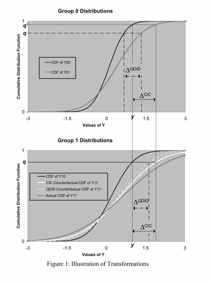
Group 0 Distributions

0

1

-3 -1.5 0 1.5 3Values of Y

Cum

ulat

ive

Dis

trib

utio

n Fu

nctio

n

CDF of Y00

CDF of Y01

y

qq'

Group 1 Distributions

0

1

-3 -1.5 0 1.5 3Values of Y

Cum

ulat

ive

Dis

trib

utio

n Fu

nctio

n

CDF of Y10

CIC Counterfactual CDF of Y11

QDID Counterfactual CDF of Y11

Actual CDF of Y11

y

q

∆QDID

∆CIC

∆CIC

∆QDID

Figure 1: Illustration of Transformations

Figu

re 2

: Bou

nds a

nd th

e C

ondi

tiona

l Ind

epen

denc

e A

ssum

ptio

n in

the

Dis

cret

e M

odel

Dat

a

11

1λ 3

.9.8

.7λ 2

.5.6

.4λ 1

.3.2

.1λ 0

F Y,01

F Y,01

F Y,00

λ

λ 0λ 1λ 2λ 3

h(u,

0)h(u,

1)

u0

1

1

u0

1

1

u0

1

F U,0

(u)

norm

aliz

ed to

Uni

form

[0,1

]

Val

ues o

f FU,1

(u)

infe

rred

from

F Y,10(y)

To p

in d

own u k

(t), j

ump

poin

ts o

f

h(u,t),

not

eF Y,0t(λ

k)=F U

,g(uk (t

))=u

k (t).

Upp

er b

ound

Low

er b

ound

Con

ditio

nal i

ndep

ende

nce

assu

mpt

ion