IApioneer v. 3.0.3 Software User's Manual
89
IApioneer v. 3.0.3 Software User’s Manual Powered by the GeoSPHERIC™ v3.0 Common Code Foundation
-
Upload
khangminh22 -
Category
Documents
-
view
2 -
download
0
Transcript of IApioneer v. 3.0.3 Software User's Manual

IApioneer v. 3.0.3 Software User’s Manual
Powered by the GeoSPHERIC™ v3.0 Common Code Foundation

IApioneer v. 3.0.3 Software User’s Manual – February 2015 [IAVO-TD-1009] Page i
CONTENTS
1 Getting Started ...................................................................................................................................... 1
1.1 UI Conventions .............................................................................................................................. 1
1.2 Installation and Licensing .............................................................................................................. 1
1.3 How to Contact Us ........................................................................................................................ 2
1.4 Site Administration for Settings .................................................................................................... 2
1.5 User Interface (UI) ......................................................................................................................... 4
1.5.1 Elements of the UI................................................................................................................. 4
1.5.2 The Backstage ....................................................................................................................... 5
2 Loading and Viewing Data..................................................................................................................... 7
2.1 Loading Data Into the Session ....................................................................................................... 7
2.1.1 Data Discovery ...................................................................................................................... 7
2.2 Viewing Raster Data ...................................................................................................................... 8
2.2.1 Exploring Raster Data ............................................................................................................ 9
2.2.2 The Home Tab Visualization Tools ........................................................................................ 9
2.2.3 Auxiliary Viewers ................................................................................................................. 10
2.3 Viewing Vector, Tie Point, and Annotation Layers ..................................................................... 11
3 Data Management .............................................................................................................................. 12
3.1 Session Management .................................................................................................................. 12
3.2 Raster Image Properties .............................................................................................................. 12
4 Setting Up Camera Sensor Models ..................................................................................................... 13
4.1 Spatial Reference Systems .......................................................................................................... 13
4.1.1 Configuring Spatial Reference Systems .............................................................................. 13
4.2 Frame Camera Sensor Model Configuration .............................................................................. 14
4.2.1 Scanned Film Affine Parameters From Fiducials ................................................................. 15
4.2.2 Digital Affine from Sensor Information ............................................................................... 18
4.2.3 Batch Frame Camera Setup ................................................................................................ 19
4.3 RPC Sensor Model Configuration ................................................................................................ 22
4.4 Orthographic Sensor Model Configuration ................................................................................. 23

IApioneer v. 3.0.3 Software User’s Manual – February 2015 [IAVO-TD-1009] Page ii
5 Customizing the View ......................................................................................................................... 24
5.1 Customizing the Viewer Display.................................................................................................. 24
5.1.1 Histogram Adjustment ........................................................................................................ 24
5.1.2 Brightness, Contrast, and Filters ......................................................................................... 25
5.1.3 Image Overview .................................................................................................................. 25
5.1.4 North Arrow, Zoom Indicator, and Grid Lines ..................................................................... 25
5.1.5 Cursor Information .............................................................................................................. 26
5.2 User Settings ............................................................................................................................... 26
5.2.1 Geolocation Formats ........................................................................................................... 27
5.2.2 Measurement ...................................................................................................................... 29
5.2.3 Data Discovery Directories .................................................................................................. 30
5.2.4 Terrain ................................................................................................................................. 30
5.2.5 Pixel Cursor ......................................................................................................................... 32
5.2.6 Display ................................................................................................................................. 33
5.2.7 Grid Lines ............................................................................................................................ 34
5.2.8 ROI ....................................................................................................................................... 35
6 Exporting Your Data ............................................................................................................................ 36
6.1 Crop, Resample, and Reproject Raster Data ............................................................................... 36
6.2 Raster Data Type Conversion ...................................................................................................... 38
6.3 Export Raster Data ...................................................................................................................... 38
6.4 Region of Interest and Image Chipping From Viewers ............................................................... 39
6.4.1 Region of Interest ................................................................................................................ 39
6.4.2 Image Chipping ................................................................................................................... 39
6.4.3 Screen Capture .................................................................................................................... 40
6.5 Exporting Vector Data ................................................................................................................. 40
6.5.1 Exporting multiple vector files as a single KMZ .................................................................. 41
7 IApioneer Analysis ............................................................................................................................... 42
7.1 What is IApioneer Analysis? ........................................................................................................ 42
7.2 Annotation Layer Management .................................................................................................. 42
7.2.1 Creating an Annotation Layer ............................................................................................. 42

IApioneer v. 3.0.3 Software User’s Manual – February 2015 [IAVO-TD-1009] Page iii
7.2.2 Saving Annotation Layers .................................................................................................... 43
7.2.3 Loading Annotation Layers into the Session ....................................................................... 43
7.3 Editing an Annotation Layer ........................................................................................................ 43
7.3.1 Annotation Visibility and Setting the Active Layer.............................................................. 43
7.3.2 Adding Shapes and Clipart .................................................................................................. 44
7.3.3 Adding Linear and Angular Mensuration Annotations ....................................................... 46
7.3.4 Editing Annotations ............................................................................................................. 46
7.3.5 Editing the Text in a Text Box .............................................................................................. 47
7.3.6 Viewing and Editing Annotation Properties ........................................................................ 47
7.4 IApioneer Analysis User Settings ................................................................................................ 48
7.4.1 Footprints ............................................................................................................................ 49
7.4.2 Mensuration Tools .............................................................................................................. 50
8 FeatureXTract ...................................................................................................................................... 57
8.1 What is FeatureXTract? ............................................................................................................... 57
8.2 Vector Layer Management ......................................................................................................... 57
8.2.1 Creating a Vector Layer ....................................................................................................... 57
8.2.2 Saving Vector Layers ........................................................................................................... 58
8.2.3 Loading Vector Layers into the Session .............................................................................. 59
8.3 Editing a Vector Layer ................................................................................................................. 59
8.3.1 Vector Layer Visibility and Setting the Active Layer ........................................................... 59
8.3.2 Creation Tools ..................................................................................................................... 60
8.3.3 Manipulation Tools ............................................................................................................. 61
8.3.4 Detailing Tools ..................................................................................................................... 62
8.4 Building a Simple Model ............................................................................................................. 63
8.5 Building More Complex Models .................................................................................................. 66
8.5.1 Using the Loft Tool to Create Conics ................................................................................... 66
8.5.2 Using the Snapping Tool for Complex Geometry ................................................................ 67
8.5.3 Using Boolean Geometry to Combine Shapes .................................................................... 68
8.5.4 Using Parameterized Structures ......................................................................................... 69
8.6 Using the 3D Viewer.................................................................................................................... 75

IApioneer v. 3.0.3 Software User’s Manual – February 2015 [IAVO-TD-1009] Page iv
8.6.1 3D Viewer Navigation ......................................................................................................... 77
8.6.2 Real-time Visualization........................................................................................................ 77
8.7 Combining it All Together ........................................................................................................... 78
Index............................................................................................................................................................ 81

IApioneer v. 3.0.3 Software User’s Manual – February 2015 [IAVO-TD-1009] Page 1
1 GETTING STARTED
1.1 UI CONVENTIONS The UI Conventions used in this document are meant to convey visually the information from the UI to
the manual. The following conventions are used is this manual:
Button (both dialog and ribbon): [OK]
Dialog label: Parameters
Context menu item: “Send to Viewer”
Tab label: File
1.2 INSTALLATION AND LICENSING Installation of the IApioneer software is very simple. Standard installer packages are available for MS
Windows. Double click on the installer to launch the installation wizard, and follow the steps.
Minimum System Requirements
Windows XP SP2, Vista, or Windows 7 (32- or 64-bit)
4 GB RAM
Core 2 Duo processor
7200 RPM hard drives
250MB Disk Space
OpenGL 2.1 supported graphics card*
Two-Button Mouse with a scroll wheel
Recommended System Requirements
Windows 7 (64-bit)
8 GB RAM
Core i5 processor
7200 RPM hard drives
1GB Disk Space
Graphics Card: NVIDIA graphics card
Two-Button Mouse with a scroll wheel
* GPU acceleration for some processes not supported on all graphics architectures

IApioneer v. 3.0.3 Software User’s Manual – February 2015 [IAVO-TD-1009] Page 2
1.3 HOW TO CONTACT US Software support is available from IAVO Research and Scientific to assist with software technical issues.
Before you contact us, please have the following information ready:
Company Name
Customer Number
Email Address
Product name and version
Computer O/S version
Error message, if any
Steps necessary to re-create the issue
By e-mail:
By phone:
Direct: 919-433-2400
Toll Free: 888-860-4286
For more information, see http://iapioneer.com/support.html.
1.4 SITE ADMINISTRATION FOR SETTINGS IApioneer provides a tool to configure the default settings for all users on a single computer. The
IApioneer Administrative Setup tool allows a site administrator to set the default settings for a given
machine, and even lock/unlock certain fields to prevent users from overriding the site specific settings.
To run the Site Administrative Setup tool , click on the Windows button, then go to the IApioneer
software group. Under IApioneer, choose to run Administrative Setup.
Upon launch, the settings dialog will be displayed with the same layout and fields as the User Settings
dialog within IApioneer (see User Settings). Each field or group of fields can be set by the site
administrator, and then locked. Once locked (Figure 1), the user cannot override the field value with
their own custom appearance. If not locked, the user is free to specify their own settings for those
fields. All of the User Settings for the main IApioneer application and any add-on modules can be
configured in this manner.
If more than one system at a site needs to have the same default site parameters specified, it is
recommended that the site settings are configured on one system, then the settings file is copied to

IApioneer v. 3.0.3 Software User’s Manual – February 2015 [IAVO-TD-1009] Page 3
each of the other systems. That file can be found in the C:\ProgramData\IAVO Research and
Scientific\GeoSPHERIC directory as the Preferences.dat file.
Figure 1. The Site Administrative Setup tool, showing some locked parameters and some unlocked ones.

IApioneer v. 3.0.3 Software User’s Manual – February 2015 [IAVO-TD-1009] Page 4
1.5 USER INTERFACE (UI)
1.5.1 ELEMENTS OF THE UI Figure 2 shows the components of the user interface.
Figure 2. Components of the user interface, shown with the demo dataset loaded.
1. The Ribbon – The tabs of the Ribbon organize capabilities by module, allowing the user to
interact with the data in a logical manner. The Home tab contains all of the camera and image
viewing tools, including; zoom, rotation, brightness, contrast, and histogram adjustments. Each
of these is applied to the active viewer only. In addition to the Home tab, each licensed
processing module may add one or more tabs to the Ribbon.
2. Left Viewer – One of the two primary viewers used to interact with the data. Images can be sent
to the Left Viewer from the Image Gallery. Data layers (vectors, tie points, and annotations) can
be displayed from the Layer Manager.

IApioneer v. 3.0.3 Software User’s Manual – February 2015 [IAVO-TD-1009] Page 5
3. Right Viewer – One of the two primary viewers used to interact with the data. Images can be
sent to the Right Viewer from the Image Gallery. Data layers (vectors, tie points, and
annotations) can be displayed from the Layer Manager.
4. Image Gallery –Thumbnails of the raster data loaded in the current session are displayed here.
Images can be added to the Left or Right Viewers by right-clicking on the thumbnail in the Image
Gallery and selecting “Send to Left Viewer” or “Send to Right Viewer”.
5. Layer Manager – Vector, tie point, and annotation layers loaded in the current session are listed
here. Each has a checkbox to indicate whether or not it is displayed in the viewers, and a radio
button to select the actively editable layer.
1.5.2 THE BACKSTAGE Data loading and system parameters are accessed through the Backstage (Figure 3), which can be
brought up by clicking on the File tab in the Ribbon. Here, you can load/remove data, save/open
sessions, and access the Help and Settings for the application.
Figure 3. The Backstage, shown with the demo dataset loaded.

IApioneer v. 3.0.3 Software User’s Manual – February 2015 [IAVO-TD-1009] Page 6
The Session section of the Backstage lists all of the data currently loaded in the session. It also has the
ability to create new data layers (vectors, tie points, and annotations). The data are organized by
category: Images, DEMs, Vectors, Tie Points, and Annotations. DEMs are a special form of raster image,
where the pixel value corresponds to an elevation.
IApioneer v. 3.0.3 Software User’s Manual – February 2015 [IAVO-TD-1009] Page 7
2 LOADING AND VIEWING DATA You can load a number of different types of data into IApioneer, including: satellite imagery, aerial
imagery (scanned film and digital images), orthographic images, Digital Elevation Models (DEMs), 2D and
3D vectors, tie points, and annotations.
2.1 LOADING DATA INTO THE SESSION To load data, go to the Backstage and select [Load Data]. Navigate to where your data is located and
select the data that you wish to load into the session.
As the data is ingested, it will be added to the data items in the Session section of the Backstage. Raster
data without pyramids (reduced resolutions, R-sets, etc.) will have the pyramids automatically
generated for optimal viewing quality. Until the pyramids have been generated, you will have minimal
functionality for those images. Raster images with no pyramids generated will have a warning icon
overlaid on the image icon in the Session data section.
Note: Large datasets may take some time to load, especially large vector sets. Be patient, as these will
appear in the Session shortly.
Alternatively, from the Windows Explorer, you can select one or more supported data types and drag
them into an IApioneer viewer. If only a single image is selected, that image will be loaded into the
current session, and displayed in the viewer that it was dragged into. If only a single data layer is
selected (e.g., feature store, annotation layer, etc.) then that data layer file is loaded into the current
session and made the active data layer for editing. If more than one file (raster or data layer) is selected,
all supported files will be loaded into the current session.
2.1.1 DATA DISCOVERY Instead of directly loading data into the Session, you can use the Data Discovery mechanism to trawl
your local and remote data archives for data that meets your production criteria. To use Data Discovery
in your workflow, you must first specify the data repositories you wish to use. You can do this in the
Data Discovery section of the IApioneer settings (see Data Discovery Directories).
Once the data repositories have been identified, 3D FeatureXtract will crawl the directory structures,
building a list of files and metadata for use in the Data Discovery process. This may take anywhere from
a few seconds to a few minutes, depending on how many files are in the repository.
Go to the Backstage and select [Data Discovery] to launch the Data Discovery tool. Figure Z shows the
Data Discovery tool with nearly 4000 files in the repository. From here you can search by location, date,
number of bands, sampling resolution, and obliquity angle. The results are categorized by type of data,
and then by subtype.

IApioneer v. 3.0.3 Software User’s Manual – February 2015 [IAVO-TD-1009] Page 8
Figure 4. Data Discovery within a defined repository.
Once the desired filters have been placed, use the checkboxes next to the found items to select data to
load into the current Session. Entire categories can be selected at once by checking the box next to the
category name. Single items can be added or removed from the list by checking/unchecking the
appropriate box. Once all the data has been identified, press [Load] to ingest the selected data into the
current Session.
2.2 VIEWING RASTER DATA Once the data has been loaded into the current session, it can be sent to the viewers for visualization
and exploitation. Raster Data, once loaded, appear in the Image Gallery as a set of thumbnails (Figure 2,
area 4). Other geospatial data (vectors, tie points, and annotations) appear in the Layer Manager
(Figure 2, area 5).

IApioneer v. 3.0.3 Software User’s Manual – February 2015 [IAVO-TD-1009] Page 9
2.2.1 EXPLORING RASTER DATA Raster data can be loaded into the viewers by right-clicking on the thumbnail of the data in the Image
Gallery and selecting “Send to Left Viewer” or “Send to Right Viewer”. The image will be loaded into the
chosen Viewer and a small arrow will appear in the bottom corner of the image thumbnail in the Image
Gallery to indicate which Viewer the image is loaded in.
You can pan the image by clicking and dragging with the center mouse button (the scroll wheel on many
mice). Free zooming can be performed by using the scroll wheel of your mouse. Click into the desired
Viewer to make it active, the roll the mouse wheel forward (away from you) to zoom out, and backward
(toward you) to zoom in. The zoom is centered on the viewer, allowing you to keep the region of
interest centered at all times, no matter where the mouse cursor is.
If you have no third mouse button or scroll wheel, you can pan by holding down both the left and right
mouse buttons simultaneously and dragging. Zooming can be performed using the fixed zoom intervals
in the Home tab of the Ribbon.
The divider between the Left and Right Viewers can be moved by clicking and dragging anywhere on the
divider.
2.2.2 THE HOME TAB VISUALIZATION TOOLS The Home tab (Figure 5) contains a number of visualization tools useful for interacting with the loaded
data.
The Display group contains tools for determining how the imagery is displayed, including options for
Histogram adjustment, Brightness/Contrast, and Filters for removing noise and enhancing structure.
There are also a number of overlays for context awareness, including display of the North arrow,
geospatial grid lines, zoom ratio, overviews, and working regions. For more information on these
overlays, see Customizing the Viewer Display.
Figure 5. The Home tab contains visualization tools for data exploration.
The Camera group contains tools for manipulating the position of the camera, including the zoom tools,
jump to location, viewer linking, and movement modes. [Camera Lock] is used to geographically link the
viewers so that movement (pan and zoom) in one corresponds to movement in the other. The camera
movement mode can be selected as either [Pan Mode] (default) or [Roam Mode]. In the roaming
mode, movement is accomplished by holding down the middle mouse button and dragging in the
direction that you want the image to move.

IApioneer v. 3.0.3 Software User’s Manual – February 2015 [IAVO-TD-1009] Page 10
The Rotation group contains the tools to allow you to rotate the current view. Free rotation can be
performed by selecting [Compass] and using the slider to set the desired orientation. There are also a
few pre-determined rotation angles. [Image Up] orients the image such that the columns of the image
are aligned with the columns of the viewer. [North Up] orients the image in the viewer so that the
direction to North – as determined by the spatial reference system – is aligned with the columns of the
viewer. [Z Up] orients the image so that vertical changes in elevation (such as the vertical lines of tall
buildings) are aligned with the columns of the viewer. There are also quick rotate buttons to quickly
rotate 90 degrees in either direction, or 180 degrees.
The Source DEM allows the user to specify the DEM used for viewer-related processing, including
Camera Lock and a number of exploitation and analysis tools. The drop down allows the user to select
any currently loaded DEM to use as the base DEM. Alternatively, the No DEM Selection option uses the
default low-resolution DEM included with the software.
2.2.2.1 JUMP TO LOCATION
The [Jump to Location] button in the Camera group on the Home tab provides the mechanism for you
to center the active viewer on a specific geospatial or pixel location. For geospatial coordinates, the
coordinate templates for string input are controlled by the Display Format designated in the Geolocation
Formats settings (see Geolocation Formats). If the Elevation parameter is left blank, then IApioneer uses
a DEM elevation lookup for the Jump To Location operation. Once valid locations have been entered,
press [OK] to center the active viewer on the provided location.
Figure 6. The Jump to Location dialog lets you center on a specific point.
2.2.3 AUXILIARY VIEWERS If you need more than two images for context awareness during processing, you can launch an image
into an auxiliary image viewer by right clicking on the image thumbnail in the Image Gallery and
selecting “Open in New Viewer” . A new image viewer will be launched with the selected image loaded.
The auxiliary viewers are image viewers only. They do not contain other data layers and cannot be used
for processing or production with any of the IApioneer modules.

IApioneer v. 3.0.3 Software User’s Manual – February 2015 [IAVO-TD-1009] Page 11
2.3 VIEWING VECTOR, TIE POINT, AND ANNOTATION LAYERS Data layers are types of data that can be overlaid on top of imagery to provide additional exploitation
capabilities. Some IApioneer modules allow the creation and editing of data layers. Clicking on [Layer
Manager] in the Data Layers group on the Home tab expands the Data Layer Manager if it is not
currently displayed, and hides the Data Layer Manager if it is already visible (Figure 7). You can also click
on the button of the divider between the Left Viewer and the Data Layer Manager to show/hide the
Data Layer Manager. The Data Layer Manager can be resized by clicking and dragging on the divider.
Each data item in the Data Layer Manager has both a checkbox and a radio button beside it. The
checkboxes indicate whether or not the data item is visible in the viewers. The radio box indicates
which data item is currently being edited. Any number of data layers can be visible at once, but only
one data layer can be edited at a time.
Note: To quickly hide all off the data layers, select [Hide All] in the Data Layers group on the Home tab.
Figure 7. The UI showing the Data Layer Manager.

IApioneer v. 3.0.3 Software User’s Manual – February 2015 [IAVO-TD-1009] Page 12
3 DATA MANAGEMENT
3.1 SESSION MANAGEMENT The data loaded in the application is considered a Session. IApioneer-based modules work on one
Session at a time. IApioneer can save the state of your workspace for later processing using the [Save
Session] or [Save Session As] functionality in the Backstage, accessed from the File tab. The saved
Session (*.xpj file) contains the references for the currently loaded data items, allowing for quick
recovery of a previous set of data.
Archived Sessions can be retrieved by selecting [Open Session] and navigating to the desired Session
file. Alternatively, double-clicking on a *.xpj file in the Windows Explorer will open IApioneer (if it is not
already open) and load the selected session file.
Clicking on [Close Session] closes out the current Session, prompting you to save individual data items
that have pending changes. Once pending changes to individual items have been saved, you will be
prompted to save the current Session before all items are removed and a new Session is created.
3.2 RASTER IMAGE PROPERTIES To view or edit the properties of a raster image, go to the Session section on the Backstage, right click on
the image that you wish to modify, and select “Properties”. The Properties dialog has four tabs:
General – This tab contains information about the image itself, including basics such as file size,
type, image dimensions, number of bands, and the type of image (Image or DEM). It also has
indicators as to whether or not the image has embedded metadata for spatial referencing
information, affine transforms, or RPC sensor models. Finally, it contains an estimate of the
image GSD and its geospatial bounding box.
Metadata – This tab contains metadata tags embedded in image formats such as NITF.
Band Info – This tab provides information about the number of bands in the image, each band’s
format, and a histogram estimate per band.
Sensor Model – This tab is where the user is able to view or set the sensor model information
used for the photogrammetric calculations with each of the software processing modules.
There are three sensor model formats supported: frame camera, RPC, and orthographic.
Note: You can specify that an orthographic image is a DEM from the General Properties tab. Click on
the Image Type button to change an orthographic image from a raster Image to a DEM.
IApioneer v. 3.0.3 Software User’s Manual – February 2015 [IAVO-TD-1009] Page 13
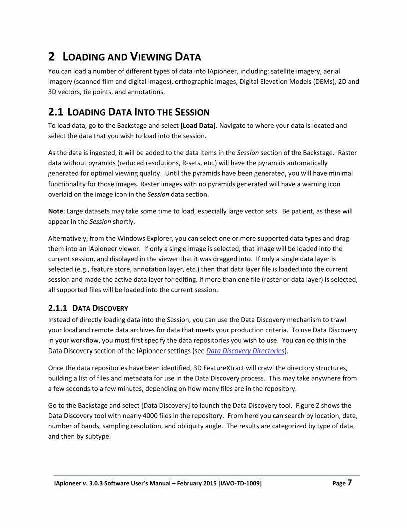
4 SETTING UP CAMERA SENSOR MODELS Most geospatial raster data have inherent metadata, which incorporates both the spatial referencing
system that the data was acquired in, as well as the sensor model defining the projective nature of the
image data. IApioneer supports three sensor model formats: frame camera (scanned film and digital
back), RPC, and orthographic. Any image data loaded without embedded sensor model information will
default to a unitary orthographic sensor model.
To set/modify the sensor model for a raster image, go to the Session section of the Backstage and right-
click on the image. Select “Properties”, and navigate to the Sensor Model tab of the Properties dialog.
4.1 SPATIAL REFERENCE SYSTEMS A Spatial Reference System (SRS) is a coordinate-based system (local or global) that is used to locate
geospatial data points. A SRS consists of a Projection and a Datum.
A Projection transforms the earth’s 3D surface into a flat (2D) representation at either a local or global
level. There are a number of projections in current use, but most are based on a conical, cylindrical, or
azimuthal model.
A Datum is a mathematical construct approximating the earth’s surface, allowing measurements to be
made along the surface. The most commonly used Datums are ellipsoidal, or geoidal in nature. The
ellipsoidal model approximates the surface as a 3D ellipsoid, as defined by a set of mathematical
parameters. An example would be the WGS84 ellipsoid. A geoidal model uses a network of physical or
derived measurements to define the 3D surface. An example would be the EGM96 model.
If you look at the same point using two different projections or datums, the geospatial coordinates of
that point will differ. Be sure to use the correct SRS parameters for your data to ensure accurate
processing.
4.1.1 CONFIGURING SPATIAL REFERENCE SYSTEMS All sensor models contain a Spatial Reference System that defines the map projection of the data. For
some data (e.g., RPC sensor models), the spatial reference system is an intrinsic one, whereas it needs to
be explicitly assigned for other data. For all raster data sensor models, the specification of the spatial
reference system follows the same process. Once the Sensor Type has been specified, select [Change]
beside the Spatial Reference System identifier to configure the data’s spatial reference system.
Figure 8 shows the Spatial Referencing dialog. Here you can set the Projection, Datum, Linear and
Angular Units, and the map projection Zone (as required). Currently, there are a limited number of
spatial reference systems that can be manually set in the application, though we ingest thousands of
spatial reference systems through Well Known Text (WKT) strings.

IApioneer v. 3.0.3 Software User’s Manual – February 2015 [IAVO-TD-1009] Page 14
Figure 8. The Spatial Referencing configuration dialog.
Currently, the software supports the following manually selectable projections: Latitude/Longitude,
UTM, and State Plane. Specifying either the UTM or State Plane projections also requires you to specify
the appropriate Zone. The geospatial Datums supported by the application are: WGS84, WGS72,
NAD83, and NAD27. The Linear and Angular unit options determine how the sensor model parameters
are interpreted. To specify a custom spatial reference system, choose that option from the Projection
drop-down, then copy a valid PROJCS WKT string into the text box at the bottom of the dialog.
4.2 FRAME CAMERA SENSOR MODEL CONFIGURATION The Frame Camera sensor model consists of two primary sets of parameters, defining the interior
orientation (IO) and exterior orientation (EO) parameters of the sensor as the image was acquired
(Figure 9). For the internal parameters, the user must have knowledge of the camera’s focal length and
focal offset, and the internal affine representation of the sensor. If using a scanned film image, you will
need to also have the sensor’s fiducial locations. These are typically found in a camera calibration
report. Digital back images do not have fiducials, and their affine parameters are easily computed from
the image dimensions and knowledge of either the sensor size, or the pixel size on the sensor. In
addition, radial distortion parameters can be provided. Exterior orientation parameters define the
camera’s position and orientation at the time of acquisition, and are often provided in a text file
containing the EO parameters of all the images acquired during a single flight/project. Each of the
parameters for the Frame Camera sensor model can be manually entered by the user.

IApioneer v. 3.0.3 Software User’s Manual – February 2015 [IAVO-TD-1009] Page 15
Figure 9. Frame camera sensor model configuration.
Once both the IO and EO parameters of the sensor have been set, press [OK] to apply the new sensor
model. In the Backstage, an asterisk will appear beside the dataset’s name, indicating that the metadata
has changed. The metadata must be saved for the changes to persist after the session has been closed
out or the data has been removed from the current session.
4.2.1 SCANNED FILM AFFINE PARAMETERS FROM FIDUCIALS Much of the imagery taken prior to 2005 was acquired on film and then digitized by means of a scanner.
The affine parameters are therefore irregular. The affine parameters can be computed from the sensor
fiducial parameters and their measured locations on the image. Selecting [Use Fiducials] launches the
Fiducial Selection workflow. This workflow walks you through the process of setting up the fiducial
detection for the image.
The first stage of the Fiducial Selection workflow (Figure 10) is where you set the sensor coordinates of
the fiducials, and the orientation of the film on the scanner. The sensor fiducial locations are typically
found in a camera calibration report, such as that seen in Figure 11. Select the radio button for the
number of fiducials you were given in your calibration information, and enter the coordinates. If you
have a camera file (*.CAM) containing the fiducial information, you can load those values from that file.
Note: The 4 Fiducials configuration option works for either “corners” or “cross” configurations – fiducials
lying on the corners or the sides of the sensor, respectively.

IApioneer v. 3.0.3 Software User’s Manual – February 2015 [IAVO-TD-1009] Page 16
Use the rotation arrows to change the orientation of the displayed image so that it appears “image up”
in the display. While doing so, you can use the scroll wheel to zoom in and out, and the left mouse
button to pan around to help you set the orientation. Once the fiducial coordinates and the scanner
orientation has been set, click [Next] to proceed to the second stage.
Figure 10. The first stage of the Fiducial Selection workflow, where you set the sensor’s fiducial coordinates.

IApioneer v. 3.0.3 Software User’s Manual – February 2015 [IAVO-TD-1009] Page 17
Figure 11. Scanned in portion of a camera calibration report showing the principal point and fiducial locations.
In between the first and second stages of the workflow, an auto-detection process is run to identify the
locations of the fiducials in the image. The second stage (Figure 12) shows you the result of the auto-
detection process on all the fiducials specified in the first stage. If there are fiducials that were not
correctly aligned with the image locations, you can manually edit their positions.
Click on the thumbnail corresponding to the fiducial you wish to edit. The sub-image will expand to give
you a large canvas on which to locate the fiducial. Click and drag the image to align with the fiducial
mark. You can zoom in and out to better find the precise location of the center of the fiducial marker on
the image. Click [Done] to finalize the position. Repeat the process for any fiducials that need
refinement.
If you get too far off track, or wish to start over, click [Auto Detect] to re-run the auto-detection
process. Once the fiducial marks have been aligned, press [Finish] to compute and assign the affine
parameters.

IApioneer v. 3.0.3 Software User’s Manual – February 2015 [IAVO-TD-1009] Page 18
Figure 12. The second stage of the Fiducial Selection workflow, where you can confirm the fiducial alignment.
4.2.2 DIGITAL AFFINE FROM SENSOR INFORMATION Images taken with a digital back (modern imagery) have no fiducials. Instead, the affine is regular and
can be computed directly from the sensor information; knowing either the sensor size or the size of a
pixel is sufficient.
Click [Digital Frame] to launch the Digital Frame Affine Calculation dialog. Select the radio button for
the parameter that you know, either Pixel Dimensions or Sensor Dimensions. Enter the Width and
Height for those parameters and select [OK] to set the digital affine.

IApioneer v. 3.0.3 Software User’s Manual – February 2015 [IAVO-TD-1009] Page 19
Figure 13. The Digital Frame Affine Calculation dialog with pixels of size 12μm x 12μm.
4.2.3 BATCH FRAME CAMERA SETUP Aerial imagery is often acquired in large batches, either from a set of flight lines or from some other
pre-specified flight path. Manually editing each of the sensor models for these images would be quite a
chore. You can configure the sensor models for an entire batch of aerial imagery using the [Batch Aerial
Workflow] option from the Backstage.
The Batch Aerial Workflow will walk you through each of the steps for configuring the sensors models
for a handful of images up to thousands at one time. You simply follow the steps to set the fields for
your cameras: internal parameters, external parameters, and data pairing parameters.
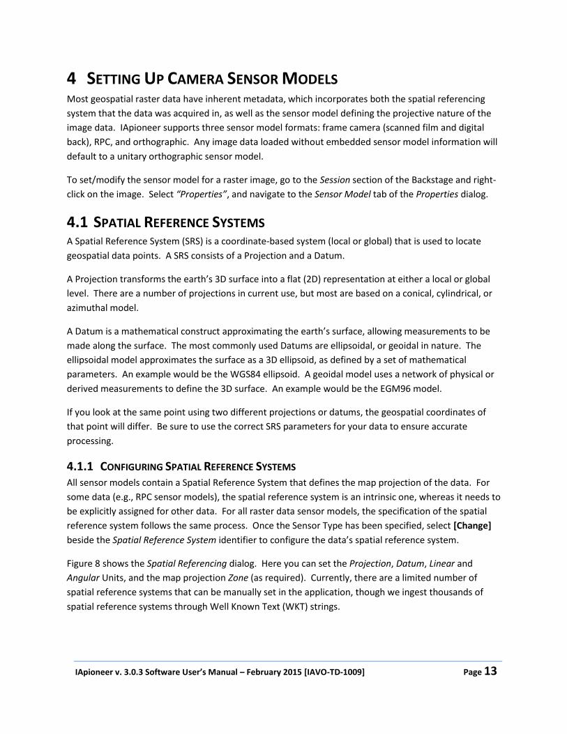
The first stage of the Batch Aerial Workflow involves providing the IO parameters of the cameras. This
includes the focal lengths, focal offsets, distortion parameters, and internal affine information. This
information is provided with the camera calibration reports received with your data. Make sure to
choose the appropriate Sensor Affine model. If you have images with fiducials, choose the Standard
option. For fully digital cameras, choose the Digital option. Figure 14 shows the first stage with the
parameters for our test data entered. Once the IO information is correct, press [Next] to continue.
IApioneer v. 3.0.3 Software User’s Manual – February 2015 [IAVO-TD-1009] Page 20
Figure 14. First stage of the Batch Aerial Workflow, where you provide IO parameters.
The second stage of the Batch Aerial Workflow is where you specify the exterior orientation parameters.
These include the spatial reference system, the text file and containing the EO parameters, and the
format of the text file. Figure 15 shows the second stage, with appropriate values for our test data.
Once the information is correct, press [Next] to continue.
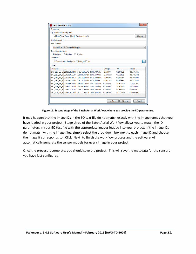
IApioneer v. 3.0.3 Software User’s Manual – February 2015 [IAVO-TD-1009] Page 21
Figure 15. Second stage of the Batch Aerial Workflow, where you provide the EO parameters.
It may happen that the Image IDs in the EO text file do not match exactly with the image names that you
have loaded in your project. Stage three of the Batch Aerial Workflow allows you to match the ID
parameters in your EO text file with the appropriate images loaded into your project. If the Image IDs
do not match with the image files, simply select the drop down box next to each Image ID and choose
the image it corresponds to. Click [Next] to finish the workflow process and the software will
automatically generate the sensor models for every image in your project.
Once the process is complete, you should save the project. This will save the metadata for the sensors
you have just configured.

IApioneer v. 3.0.3 Software User’s Manual – February 2015 [IAVO-TD-1009] Page 22
Figure 16. Third stage of the Batch Aerial Workflow, where you match loaded images with their Image IDs.
4.3 RPC SENSOR MODEL CONFIGURATION Satellite imagery is typically delivered with its rigorous camera model information hidden behind a
generic replacement sensor model in the form of RPCs. RPC data are usually either embedded in the
image file itself as metadata, or supplied via a secondary metadata file. This information can be read
from the external file, either by loading an IKONOS metadata file, or a standard RPC00B file (as seen in
Figure 17).
Figure 17. RPC sensor model configuration.

IApioneer v. 3.0.3 Software User’s Manual – February 2015 [IAVO-TD-1009] Page 23
Once the RPC parameters have been set, press [OK] to apply the new sensor model. In the Backstage,
an asterisk will appear beside the dataset’s name, indicating that the metadata has changed. The
metadata must be saved for the changes to persist after the session has been closed out or the data has
been removed from the current session.
4.4 ORTHOGRAPHIC SENSOR MODEL CONFIGURATION Orthographic images (orthos) have been processed to remove perspective from the raster data so that
each pixel falls on a point of a georeferenced grid. An orthographic sensor model is defined by the
geographic coordinates of its Upper Left Corner and the Post Spacing in both the X (horizontal) and Y
(vertical) directions (Figure 18). For most ortho images, the data has been processed so that traversing
along a row of pixels corresponds to stepping along the X direction in the spatial reference system only,
and traversing along the columns corresponds to stepping along the Y direction of the spatial reference
system only. However, it is possible that movement along either row or column can correspond to
stepping both in the X and Y directions, geospatially. This is referred to as a non-aligned ortho image.
Figure 18. Orthographic sensor model configuration.
Once the ortho parameters have been set, press [OK] to apply the new sensor model. In the Backstage,
an asterisk will appear beside the dataset’s name, indicating that the metadata has changed. The
metadata must be saved for the changes to persist after the session has been closed out or the data has
been removed from the current session.

IApioneer v. 3.0.3 Software User’s Manual – February 2015 [IAVO-TD-1009] Page 24
5 CUSTOMIZING THE VIEW
5.1 CUSTOMIZING THE VIEWER DISPLAY The Display group in the Home tab contains a number of tools useful for adjusting how the selected
image is displayed, as well as contextual overlays that can provide a better overview for exploitation.
5.1.1 HISTOGRAM ADJUSTMENT Selecting [Histogram] launches the Color Curves dialog (Figure 19). In this dialog, you can affect a color
transform on individual channels, or all channels simultaneously, of the image in the active viewer.
Output values from the color transform are scaled between 0 (black) and 1 (white). A number of Presets
are available for quick color transformations, including:
Piecewise Custom – Allows you to manually set the Input and Output values for the curve. These
can be set by manually clicking on a curve endpoint and dragging it to the desired position, or by
manually entering the values in the text boxes below the curves.
Linear Min/Max – Sets the minimum image value to an output value of 0, and the maximum
image value to a value of 1.
Linear 2% - Uses the histogram to scale the output between the 2nd percentile and 98th
percentile of the image values.
Equalization – Transforms the input image histogram into a uniform distribution.
Gaussian – Transforms the input image histogram into a normal distribution.
Figure 19. Color Curves dialog showing a Gaussian transformation.

IApioneer v. 3.0.3 Software User’s Manual – February 2015 [IAVO-TD-1009] Page 25
As you are making changes to the color curves, the image in the active viewer will adjust according to
your changes. Selecting [OK] will fix those adjustments in place, while [Cancel] will revert to the last
saved color curves.
5.1.2 BRIGHTNESS, CONTRAST, AND FILTERS Use the [Brightness] and [Contrast] options to adjust the overall brightness and contrast of the image in
the active viewer. Clicking on one of the above options will open a gallery of preset choices, as well as a
manual slider option at the bottom of the list. As changes are made, the active image will adjust
accordingly to provide a preview of the changes.
Use [Filter] to choose sharpening, smoothing, and haze reduction filters. These filters are applied to the
displayed data only, and can be used to quickly enhance the active image. There are five options for
quick filters:
Low Pass – This smoothing filter performs a low pass convolution on the data in the active
image. It uses a 5x5 smoothing kernel with normalized weights.
Gaussian Low Pass - This smoothing filter performs a low pass convolution on the data in the
active image. It uses a 5x5 smoothing kernel with Gaussian weights. It provides less smoothing
distortion than the Low Pass filter.
High Pass – This sharpening filter performs a high pass convolution on the data in the active
image. It uses a 5x5 convolution kernel with normalized weights.
Gaussian High Pass – This sharpening filter performs a high pass convolution on the data in the
active image. It uses a 5x5 convolution kernel with Gaussian weights. It provides less sharpening
distortion than the Low Pass filter.
Haze Reduction – This combination of smoothing and sharpening filters provides local contrast
enhancement and the removal of aerosol-like distortions in the image.
5.1.3 IMAGE OVERVIEW [Image Overview] launches a small dialog with a thumbnail of the active image and a vector graphic that
shows the current displayed bounds of the active image.
5.1.4 NORTH ARROW, ZOOM INDICATOR, AND GRID LINES The [North Arrow] option turns on/off a graphic depicting the direction to North in the current viewer.
Use [Grid Lines] to turn on/off a map-coordinate grid overlay on the active image. The map grid display
parameters can be set in the Settings (see

IApioneer v. 3.0.3 Software User’s Manual – February 2015 [IAVO-TD-1009] Page 26
Grid Lines).
The [Zoom Ratio] button turns on/off the zoom indicator for the active viewer.
5.1.5 CURSOR INFORMATION [Cursor Information] in the Image group on the Home tab launches a dialog (Figure 20) showing the
image (pixel) coordinates of the cursor, in addition to its projected map coordinates. The projection
coordinates are relayed based on the projection and display string formats specified in the Geolocation
Formats settings. Images that are chipped from larger sources have two sets of cursor location info;
one for the chipped cursor location, and one for where that pixel would lie in the full image.
Figure 20. Cursor Information dialog showing both full and chipped image pixel locations.
5.2 USER SETTINGS To change the default settings for a variety of display and measurement operations within the UI, click
on [Settings] in the Backstage. The Settings dialog (Figure 21) allows you to specify how the UI displays
certain types of information, including: measurement units, cursor information, display colors, fonts,
and other graphics. Unless locked by a Site Administrator (see Site Administration for Settings), the user
settings can be changed to suit the customization desires of each individual user on a given system.

IApioneer v. 3.0.3 Software User’s Manual – February 2015 [IAVO-TD-1009] Page 27
Figure 21. The Settings dialog.
To change a setting, click on the setting type on the left tree and edit the parameters in the right hand
side of the dialog. Changes made to the preferences are saved on a per-user basis, allowing all users of
a system to configure the look and feel of the software as they see fit.
5.2.1 GEOLOCATION FORMATS The Geolocation Formats settings control how map information is displayed and entered (Figure 22).
The Display Format controls how map coordinates are relayed to you in areas such as the Cursor
Information dialog. The Display Format settings consist of a map projection, a string format, the vertical
datum used for reporting elevation, and the units to measure elevation.
Projection Type – Specifies the map projection used. Can be Native, Geographic, or UTM.
o Native – The underlying projection of the source data
o Geographic – Latitude/Longitude
o UTM – UTM zone is defined by projection from the center of the source data’s bounds
Geographic String Format – Specifies the display string format as a decimal combination of
degrees (DD), minutes (MM), and seconds(SS). Only used if the Projection Type is Geographic.
Vertical Datum – Specifies the datum used to display elevation values. Can be Ellipsoid(WGS84)
or MSL (EGM96). Value supersedes the datum used in the data’s SRS (for display purposes
only).
o Ellipsoid (WGS84) – Uses the WGS84 ellipsoid for reporting elevation values.

IApioneer v. 3.0.3 Software User’s Manual – February 2015 [IAVO-TD-1009] Page 28
o MSL (EGM96) – Uses the EGM96 geoid for reporting elevation values.
Vertical Units – Specifies the linear units used to report elevation values.
Input Format provides the template for user-derived information, such as that provided in the Jump to
Location dialog. The input format consists of a map projection and string format.
Projection Type – Specifies the map projection used. Can be Native, Geographic, or UTM.
o Native – The underlying projection of the source data
o Geographic – Latitude/Longitude
o UTM – UTM zone is defined by projection from the center of the source data’s bounds
Geographic String Format – Specifies the display string format as a decimal combination of
degrees (DD), minutes (MM), and seconds(SS). Only used if the Projection Type is Geographic.
Figure 22. Changing the geolocation format settings.

IApioneer v. 3.0.3 Software User’s Manual – February 2015 [IAVO-TD-1009] Page 29
5.2.2 MEASUREMENT The Measurement settings control how all measurements are displayed to you throughout the
application (Figure 23). The measurement units can be specified for Length, Area, and Angles.
Figure 23. Changing the Measurement settings.

IApioneer v. 3.0.3 Software User’s Manual – February 2015 [IAVO-TD-1009] Page 30
5.2.3 DATA DISCOVERY DIRECTORIES The Data Discovery settings is where you can configure the locations of the source data to use with the
Data Discovery Tool (see Data Discovery).
Figure 24. Changing the Data Discovery settings.
5.2.4 TERRAIN The Terrain settings is where you can configure the application to look for DTED files to use as DEM
sources (Figure 25). You can specify locations for DTED0, DTED1, or DTED2 DEM files. Use the up and
down arrows to set the priority for the elevation files.

IApioneer v. 3.0.3 Software User’s Manual – February 2015 [IAVO-TD-1009] Page 31
Figure 25. Changing the Terrain settings.

IApioneer v. 3.0.3 Software User’s Manual – February 2015 [IAVO-TD-1009] Page 32
5.2.5 PIXEL CURSOR Use the Pixel Cursor properties to specify the look of the measurement cursor (Figure 26). The cursor
has an Inner Color and an Outer Color, as well as a Size – Small, Medium, or Large.
Note: For best visibility of the cursor, set the Inner Color and Outer Color to be highly contrasting.
Figure 26. Changing the Pixel Cursor settings.

IApioneer v. 3.0.3 Software User’s Manual – February 2015 [IAVO-TD-1009] Page 33
5.2.6 DISPLAY Use the Display settings to configure default parameters for the viewers (Figure 27). Currently, the only
configurable parameter is the Image Orientation, which can be set to one of the primary rotation angles
in the Home tab.
Image Up orients the image such that the columns of the image are aligned with the columns of
the viewer.
North Up orients the image in the viewer so that the direction to North – as determined by the
spatial reference system – is aligned with the columns of the viewer.
Z Up orients the image so that vertical changes in elevation (such as the vertical lines of tall
buildings) are aligned with the columns of the viewer.
Figure 27. Changing the Display settings.
IApioneer v. 3.0.3 Software User’s Manual – February 2015 [IAVO-TD-1009] Page 34
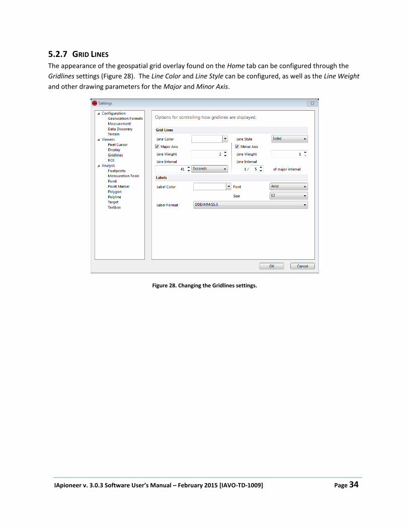
5.2.7 GRID LINES The appearance of the geospatial grid overlay found on the Home tab can be configured through the
Gridlines settings (Figure 28). The Line Color and Line Style can be configured, as well as the Line Weight
and other drawing parameters for the Major and Minor Axis.
Figure 28. Changing the Gridlines settings.

IApioneer v. 3.0.3 Software User’s Manual – February 2015 [IAVO-TD-1009] Page 35
5.2.8 ROI The ROI settings can be used to change the default appearance of the region of interest, as accessed
through the Home tab (Figure 29). You can specify the Line Color, Line Weight, and Line Style here.
Figure 29. Changing the ROI settings.

IApioneer v. 3.0.3 Software User’s Manual – February 2015 [IAVO-TD-1009] Page 36
6 EXPORTING YOUR DATA IApioneer is capable of exporting a number of data types for easy ingestion into other utilities. Both
raster data and vector data can be exported, for a variety of product delivery types.
6.1 CROP, RESAMPLE, AND REPROJECT RASTER DATA The primary mechanism for exporting raster data is the Crop, Resample, and Reproject dialog (Figure
30). This dialog is accessed from the Backstage by right-clicking on the raster image that you wish to
export and selecting the “Crop, Resample, and Reproject” option.
The Crop, Resample, and Reproject dialog allows the user to chip a sub-image from the original raster
data. The bounds of the chipping process can be set to pixel values, either by click-dragging a
highlighted rectangle in the image thumbnail, or by specifying the pixel locations in the dialog itself.
Alternatively, the user can crop the image based on geospatial coordinates by selecting [Use Geospatial
Coordinates]. From that dialog (Figure 31), the user can specify the Spatial Reference System used as
the base map projection, and the bounding coordinates of the sub-image.
A third option is to define the sub-image boundaries from another geospatial data item, by clicking
[From Other Data]. The Geospatial Data Selection dialog allows the user to select another data item as
the basis for the chip boundaries, as well as a buffer around that data, if desired.
Checking the Resample box allows you to specify the nominal GSD (spatial resolution) of the output
image. Here you can specify the Resolution and Linear Units.
You can change the output spatial reference system for Orthographic sensor models only by selecting
the Reproject checkbox and setting the output spatial reference system. This changes the base map
projection for the output sub-image
Once the chipping parameters have been specified, selecting the Filename and output format for the
sub-image is the final step. Pressing [OK] kicks off the chipping process. When complete, the generated
sub-image will be added to the current session.

IApioneer v. 3.0.3 Software User’s Manual – February 2015 [IAVO-TD-1009] Page 37
Figure 30. The Crop, Resample, and Reproject dialog allows you to export sub-images.
Figure 31. Select chip boundaries from geospatial coordinates.
Figure 32. Select chip boundaries from another data item.

IApioneer v. 3.0.3 Software User’s Manual – February 2015 [IAVO-TD-1009] Page 38
6.2 RASTER DATA TYPE CONVERSION Raster data can be converted from one data type (float, int, etc.) to another. This is accomplished by
right-clicking on the raster data item in the Session section of the Backstage and choosing “Data
Conversion”. Data conversion allows you to convert raster data from one Data Type (Byte, Short,
Unsigned Short, Int, Unsigned Int, Float, Double) to another, as seen in Figure 33. This is a batch process,
meaning that multiple images can be processed at a time by selecting them in the Backstage and
launching the dialog on the group. The user selects the output Data Type and File Format from the
dropdown boxes, the output filename – or output directory plus suffix for multiple images – and kicks
off the conversion process by selecting [Run]. Once the process is complete, the generated items will be
added to the current session.
Figure 33. The Data Conversion dialog allows the user to convert from one data type to another.
6.3 EXPORT RASTER DATA Rich-clicking on a single (or multiple) raster item(s) in the Backstage and selecting the “Export” option
will launch the Export Images dialog (Figure 34). Here, you can export the selected images as they are,
changing only the File Format, as desired. This is another batch operation dialog, where multiple images
can be processed at a time by selecting them in the Backstage and launching the dialog on the group.
The user selects the output File Format from the dropdown boxes, the Output Filename – or Output
Path plus Suffix for multiple images – and kicks off the conversion process by selecting [Run]. Exporting
imagery is typically only used to convert file formats for use in other applications, but the user can
choose to add the generated items to the current session by selecting the Add Results to Project
checkbox.
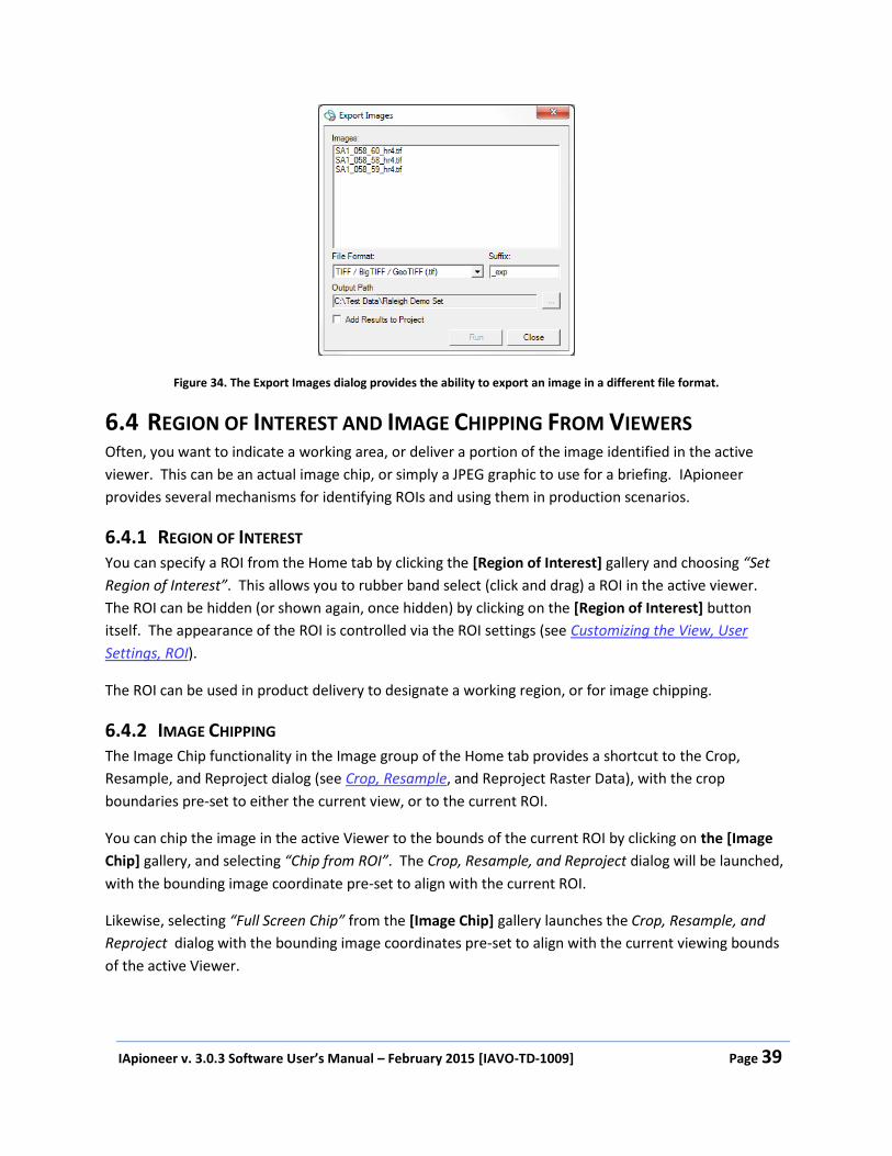
IApioneer v. 3.0.3 Software User’s Manual – February 2015 [IAVO-TD-1009] Page 39
Figure 34. The Export Images dialog provides the ability to export an image in a different file format.
6.4 REGION OF INTEREST AND IMAGE CHIPPING FROM VIEWERS Often, you want to indicate a working area, or deliver a portion of the image identified in the active
viewer. This can be an actual image chip, or simply a JPEG graphic to use for a briefing. IApioneer
provides several mechanisms for identifying ROIs and using them in production scenarios.
6.4.1 REGION OF INTEREST You can specify a ROI from the Home tab by clicking the [Region of Interest] gallery and choosing “Set
Region of Interest”. This allows you to rubber band select (click and drag) a ROI in the active viewer.
The ROI can be hidden (or shown again, once hidden) by clicking on the [Region of Interest] button
itself. The appearance of the ROI is controlled via the ROI settings (see Customizing the View, User
Settings, ROI).
The ROI can be used in product delivery to designate a working region, or for image chipping.
6.4.2 IMAGE CHIPPING The Image Chip functionality in the Image group of the Home tab provides a shortcut to the Crop,
Resample, and Reproject dialog (see Crop, Resample, and Reproject Raster Data), with the crop
boundaries pre-set to either the current view, or to the current ROI.
You can chip the image in the active Viewer to the bounds of the current ROI by clicking on the [Image
Chip] gallery, and selecting “Chip from ROI”. The Crop, Resample, and Reproject dialog will be launched,
with the bounding image coordinate pre-set to align with the current ROI.
Likewise, selecting “Full Screen Chip” from the [Image Chip] gallery launches the Crop, Resample, and
Reproject dialog with the bounding image coordinates pre-set to align with the current viewing bounds
of the active Viewer.

IApioneer v. 3.0.3 Software User’s Manual – February 2015 [IAVO-TD-1009] Page 40
6.4.3 SCREEN CAPTURE You can save the active Viewer (and its contents) by selecting the [Screen Capture] option in the Image
group of the Home tab. The screen capture mechanism stores all of the visible information in the active
Viewer for ingestion into other products, such as a PowerPoint briefing.
The “Save Screen to File” option from the gallery copies the active viewer’s contents to a flat image file,
such as a JPG, PNG, BMP, or similar.
“Save Screen to PowerPoint” copies the active viewer’s contents to the clipboard, and then opens a new
PowerPoint presentation, pasting the viewer’s contents into the new presentation. This mechanism
requires Microsoft PowerPoint 2007 or newer to be installed on the system.
“Copy Screen to Clipboard” sends the contents of the active viewer to the system clipboard, where it can
be pasted into other applications for product generation.
The “Copy ROI to Clipboard” option copies only the contents of the active ROI to the system clipboard.
6.5 EXPORTING VECTOR DATA Vector data can be exported in a variety of formats for archival and ingestion into other data processing
packages. Go to the Backstage and right-click on the vector data item you wish to export. Choose the
“Export” option to launch the vector Export dialog.
The Export dialog allows the user to export the selected vector file, with options for output format,
projection, texturing, and more (Figure 35). The Output Format parameter includes the most common
geospatial 2D and 3D file formats, including:
GeoVector (IAVO proprietary)
ESRI Shapefile
Presagis OpenFlight
Collada
KML/KMZ
Wavefront OBJ
PLY
XYZ point set
Common Data Base (CDB)
The Reproject Data checkbox is used to convert the vector file’s spatial reference system from the
original to one of your choosing. Click [Change] to specify the output spatial reference system.
Output formats that include texture information can have automatic texturing applied to the data by
checking the Include Textures checkbox. With that option checked, click [Change] to specify which

IApioneer v. 3.0.3 Software User’s Manual – February 2015 [IAVO-TD-1009] Page 41
images will be used to automatically texture the data. The automatic texturing process takes into
account camera look angle, spatial resolution, and occlusions to identify the best texture patches for
every polygon in the dataset.
Complete the operation by selecting the Output Filename and pressing [Export].
Figure 35. The Vector Export dialog allows the user to export 2D and 3D vector data in a variety of formats.
6.5.1 EXPORTING MULTIPLE VECTOR FILES AS A SINGLE KMZ Often, 3D site models are developed in parts by multiple members of a modeling team. These parts are
typically stored in separate files for editing and display, but need to be exported into a single file for
distribution. Multiple 3D vector models can be exported into a single KMZ file by selecting two or more
vectors in the backstage, then right-clicking and following the export process for KMZ files detailed
above.

IApioneer v. 3.0.3 Software User’s Manual – February 2015 [IAVO-TD-1009] Page 42
7 IAPIONEER ANALYSIS
7.1 WHAT IS IAPIONEER ANALYSIS? IApioneer Analysis is a module of the IApioneer family of geospatial processing applications. It is used
for imagery exploration, exploitation, analysis, and annotation. Specifically, the Analysis module is
focused on product annotation and delivery, allowing the user to generate annotated products that can
be delivered in the form of PowerPoint briefings, chipped datasets, and other single-layer export
process. These annotation overlays can be saved and distributed as viewable layers to anyone with
IApioneer.
IApioneer Analysis offers the capability to:
Annotate imagery with text boxes, point markers, and simple geometry
Measure length, area, and azimuth values with a few mouse clicks
Capture screenshots of annotated products
Save annotations for future use and distribution to other IApioneer users
Use intuitive drawing mechanisms to develop sophisticated products
7.2 ANNOTATION LAYER MANAGEMENT Annotation Layers are individual documents within IApioneer, and are listed in the Session section of the
Backstage, under the Annotations heading. From the Backstage, Annotation Layers can be created,
saved, and loaded. New Annotation Layers can also be created directly from the Home tab of the
ribbon, or from the Data Layer Manager.
When working with Annotation Layer data, use the Data Layer Manager to specify the active Annotation
Layer for editing and viewing.
7.2.1 CREATING AN ANNOTATION LAYER Click [Add Annotation Layer] in the Session section of the Backstage to create a new annotation layer.
The new Annotation Layer will be added to the session as an Unnamed Annotation Document, ready for
editing or saving. To change the Annotation Layer’s name, save it (see Saving Vector Layers). The new
filename will become the Annotation Layer’s display name.
Alternatively, Annotation Layers can be created directly from the Home tab of the Ribbon. Click on the
[Add Layer] dropdown and choose the Add Annotation Layer option. The same mechanism is in place in
the Layer Manager.
Whichever method is used to create an annotation layer, the new layer is set as the active layer for
immediate editing.

IApioneer v. 3.0.3 Software User’s Manual – February 2015 [IAVO-TD-1009] Page 43
7.2.2 SAVING ANNOTATION LAYERS Right click on an Annotation Layer in the Backstage and choose “Save Data” or “Save Data As” to save
the Annotation Layer for future processing. The file will be saved in a *.gad format, which is an XML-
based IAVO internal file format.
Save Data – Allows you to store the Annotation Layer. If there is no file currently associated
(i.e., a new Annotation Layer) you will be prompted to provide a filename. That filename will
become the name of the Annotation Layer.
Save Data As – To prevent you from overwriting the original document, the Save Data As
command stores the current Annotation Layer in a new document.
7.2.3 LOADING ANNOTATION LAYERS INTO THE SESSION Ingestion of Annotation Layers is the same as ingestion of raster data (or any other data type). Use the
[Load Data] option in the Backstage, and point the file dialog to the annotation data file(s) you wish to
load.
7.3 EDITING AN ANNOTATION LAYER With IApioneer, you can edit Annotation Layers, as well as create and view them. Although annotations
are typically drawn on a reference image, they are anchored geospatially, and thus can propagate across
multiple images. It is important to note that unless the data is perfectly registered, annotations drawn
on one reference image may be slightly off (visibly) when overlaid on any other image.
7.3.1 ANNOTATION VISIBILITY AND SETTING THE ACTIVE LAYER The first step in editing an Annotation Layer is the set it as both visible, and the active layer for editing,
using the Layer Manager. Figure 36 shows the IApioneer module with the Data Layer Manager visible
and a single Annotation Layer ready for editing. Clicking on [Layer Manager] in the Data Layers group
on the Home tab expands the Data Layer Manager if it is not currently displayed, and hides the Data
Layer Manager if it is already visible. You can also click on the button of the divider between the Left
Viewer and the Data Layer Manager to show/hide the Data Layer Manager. The Data Layer Manager
can be resized by clicking and dragging on the divider.
Each Annotation Layer in the Layer Manager has a checkbox and a radio button to the right of its name.
The checkbox indicates visibility – checked means that the layer is visible in the Viewers. The radio
button indicates the active (editable) layer. Module tabs appear in the ribbon, based on the type of the
active layer. When the active layer is an Annotation Layer, the Analysis module tab appears in the
Ribbon.

IApioneer v. 3.0.3 Software User’s Manual – February 2015 [IAVO-TD-1009] Page 44
Figure 36. IApioneer Analysis module with an Annotation Layer loaded.
7.3.2 ADDING SHAPES AND CLIPART The Analysis tab contains two groups of tools for annotations and measurements. The Insert group
allows you to insert single shapes and MIL-STD-2525B clip art. The types of shapes supported i include
basic shapes – points, lines, and polygons – as well as complex items such as text boxes, point markers,
and target rings. Initial parameters for the appearance of the annotation objects are pulled from the
defaults settings (see IApioneer Analysis User Settings IApioneer Analysis User Settings).
The drawing objects in the IApioneer Analysis toolset are modal in nature. Once the drawing object
mode has been selected (e.g., Polygon), new objects can be repeatedly drawn by holding the CTRL
button and left clicking to start the new object. The object can then be drawn as detailed below.
Polygon – Select “Polygon” from the [Polygon] drop down. Click on the image in the location of the first
point of the polygon. Continue clicking to set the vertices of the polygon. The last selected point will
always be attached to the first point, closing the polygon. Once the last vertex has been placed, right-
click to finish drawing.

IApioneer v. 3.0.3 Software User’s Manual – February 2015 [IAVO-TD-1009] Page 45
Rectangle – Select “Rectangle” from the [Polygon] drop down. Click on the image in the location of the
upper left corner of the rectangle and drag the cursor to define the rectangle. Release the left mouse
button to finalize the shape.
Ellipse – Select [Ellipse]. Click on the image in the location of the upper left corner of the ellipse’s
bounding box and drag the cursor to define the ellipse. Release the left mouse button to finalize the
shape.
Point – Select [Point]. Click on the image in the location of the point to draw the shape.
Polyline – Select [Line]. Click on the image in the location of the first point of the polyline. Continue
clicking to set the vertices of the polyline. Once the last vertex has been placed, right-click to finish
drawing.
Text Box – Select [Text Box]. Click on the image in the location of the center point of the text box. A
text box will be placed in the image and the text highlighted for easy text entry. Click outside of the text
box to finalize the annotation.
Point Marker – Select [Point Marker]. Click on the image in the location of the point marker to draw
the shape. A small circle will be drawn, indicating the location of the point. In addition, a text box will
be drawn attached to the point, indicating the geospatial coordinates of the point marker.
Targeting Circle – Select [Targeting Circle]. Click on the image in the location of the point to draw the
shape. A set of target rings will be drawn around the selected point, along with a text box indicating the
geospatial coordinates of the center of the target rings.
North Arrow – Select [North Arrow]. Click on the image in the location of the point to draw the shape.
Unlike other clip art-style graphics, which maintain their orientation with respect to the viewer as the
image is rotated – the North Arrow graphic always indicates the direction of True North for images with
the appropriate support data.
Clip Art – Clip art can be added as graphic annotations to the image through the use of the Clip Art
dialog. Click on [ClipArt] to launch the dialog. (Note: Currently, IApioneer only supports the Warfighting
symbols from the MIL-STD 2525B graphics objects.)
To place a graphics object from the library of images, navigate the tree structure to find the desired
graphic. As the tree is navigated, the contents of the library folders are previewed in the graphic pane
to the right. When the desired graphic has been found, click on the preview icon in the right pane and
drag the icon into the image viewer. Release the left mouse button to drop the graphic into the viewer,
centered at the point of release.

IApioneer v. 3.0.3 Software User’s Manual – February 2015 [IAVO-TD-1009] Page 46
Note: The Clip Art dialog is a persistent dialog, that defers to the primary application for window
placement. If you click on the Clip Art button and the dialog does not launch, check to see if it is open
“behind” the application.
7.3.3 ADDING LINEAR AND ANGULAR MENSURATION ANNOTATIONS The Inspect/Measure group of the IApioneer tab provides tools for linear and angular measurement.
Initial parameters for the appearance of the annotation objects are pulled from the defaults settings
(see IApioneer Analysis User Settings).
Separation Angle – Click [Separation Angle] to begin measuring an angle in the image. Begin by clicking
on an endpoint of the angle. Then, click the pivot vertex of the angle, and finish by clicking on the other
angle endpoint. As the cursor moves to the final position, the angle measurement between the first line
segment and the one joining the pivot point to the cursor is continually displayed, allowing the user to
view a number of angle measurements before finally selecting the last point.
Length – Click [Length] to begin measuring a length in the image. Begin by clicking on the starting point
of the line segment and finish by clicking on the endpoint. As the cursor moves to the final position, the
length measurement is continually displayed, along with the change in elevation, allowing the user to
view a number of length measurements before finally selecting the last point.
7.3.4 EDITING ANNOTATIONS IApioneer provides a limited capability to edit annotations once they have been initially drawn. Most of
the annotation objects can be moved by clicking anywhere on the annotation and dragging it to its new
location. The exceptions are Point Markers and Target Circles, which only allow their text boxes to be
moved.
To edit the vertices of a polygon, once placed, right click on the selected polygon and choose “Edit
Points”. Click and drag a highlighted vertex to move it. When the editing is complete, double click
outside of the selection to finalize the new geometry.
It is possible to subdivide any convex polygon with four sides (convex quadrilateral), into regularly
sampled subregions by right-clicking on the polygon and choosing “Subdivide”. The Subdivide Polygon
dialog allows you to specify the number of Rows and Columns of the subdivision, dynamically updating
the annotation in the Viewer to provide immediate feedback on the final appearance. Pressing [Apply]
deletes the original annotation and replaces it with the subdivisions, each as a separate annotation
object. The subdivision annotations’ properties are copied from the parent annotation.

IApioneer v. 3.0.3 Software User’s Manual – February 2015 [IAVO-TD-1009] Page 47
Figure 37. Polygon annotation subdivision.
7.3.5 EDITING THE TEXT IN A TEXT BOX Double click inside any text box annotation (or the text box of a complex annotation object) to edit the
text. Type the new text, including carriage returns, and click outside the text box to finalize the changes.
7.3.6 VIEWING AND EDITING ANNOTATION PROPERTIES Each annotation object has a set of properties that contain appearance parameters for its geometry and
textboxes, as well as mensuration information. Some annotations may contain one, two, or even all
three of these sets of parameters. Default parameters for each of these parameters are pulled from the
Settings, but you can change these properties for individual annotations. These properties can be
accessed by right-clicking on the annotation and choosing the “Properties” option.

IApioneer v. 3.0.3 Software User’s Manual – February 2015 [IAVO-TD-1009] Page 48
7.3.6.1 MENSURATION PROPERTIES
The Details tab in the Annotation Properties dialog gives you metrics about the selected annotation.
These include Area, Perimeter, and Centroid information. The units used for reporting here are drawn
from the Measurement default settings. Figure 38 shows an example of the mensuration properties for
a polygon annotation.
Figure 38. The Mensuration properties of a polygon annotation.
7.4 IAPIONEER ANALYSIS USER SETTINGS To change the default settings for the annotation objects in IApioneer, click on [Settings] in the
Backstage. The Analysis group in the Settings dialog is where the defaults for each of the annotation
objects reside.
To change a setting, click on the setting type on the left tree and edit the parameters in the right hand
side of the dialog. Unless locked by a Site Administrator (see Site Administration for Settings), the user
settings can be changed to suit the customization desires of each individual user on a given system.

IApioneer v. 3.0.3 Software User’s Manual – February 2015 [IAVO-TD-1009] Page 49
7.4.1 FOOTPRINTS The Footprints settings control how DPPDB footprints are displayed in the viewer (Figure 39). You can
specify the Line Color, Line Style, and Line Weight for both the Controlled Footprint and the Uncontrolled
Footprint of a DPPDB segment.
Figure 39. Changing the Footprints settings.

IApioneer v. 3.0.3 Software User’s Manual – February 2015 [IAVO-TD-1009] Page 50
7.4.2 MENSURATION TOOLS The Mensuration Tools settings control how mensuration annotations appear (Figure 40). You can
specify the default look and feel of the mensuration tools by specifying the Font parameters and Effects,
as well as the Foreground and Background colors for the text. You can also specify the Line Properties of
the mensuration vector components.
Figure 40. Changing the Mensuration Tools settings.

IApioneer v. 3.0.3 Software User’s Manual – February 2015 [IAVO-TD-1009] Page 51
7.4.3 Point
The Point settings control how point annotations appear (Figure 41). You can specify the default Color,
Weight, and Style for the Point annotation.
Figure 41. Changing the Point annotation settings.

IApioneer v. 3.0.3 Software User’s Manual – February 2015 [IAVO-TD-1009] Page 52
7.4.4 Point Marker
The Point Marker settings control how the point vector appears (Figure 42) for the point marker
annotation. You can specify the default Color, Weight, and Style for the marker annotation. You can also
specify the Font parameters and Effects, as well as the Foreground and Background colors for the text.
Figure 42. Changing the Point Marker annotation settings.
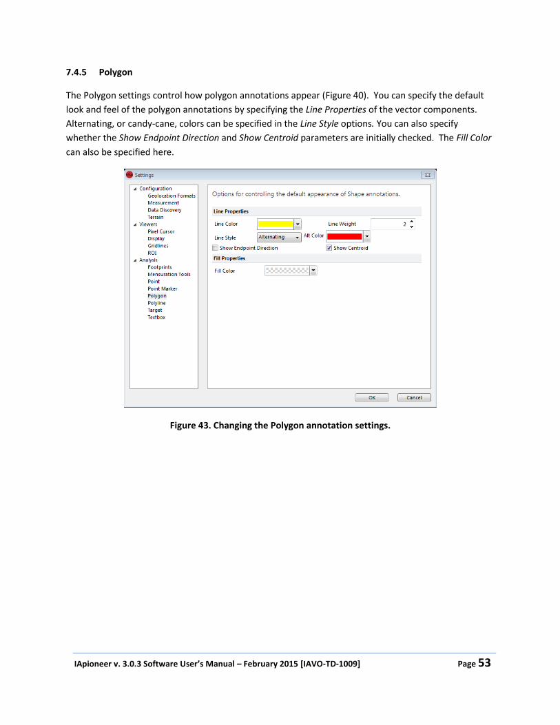
IApioneer v. 3.0.3 Software User’s Manual – February 2015 [IAVO-TD-1009] Page 53
7.4.5 Polygon
The Polygon settings control how polygon annotations appear (Figure 40). You can specify the default
look and feel of the polygon annotations by specifying the Line Properties of the vector components.
Alternating, or candy-cane, colors can be specified in the Line Style options. You can also specify
whether the Show Endpoint Direction and Show Centroid parameters are initially checked. The Fill Color
can also be specified here.
Figure 43. Changing the Polygon annotation settings.

IApioneer v. 3.0.3 Software User’s Manual – February 2015 [IAVO-TD-1009] Page 54
7.4.6 Polyline
The Polyline settings control how polygon annotations appear (Figure 44). You can specify the default
look and feel of the polyline annotations by specifying the Line Properties of the vector components.
You can also specify whether Show Endpoint Direction is initially checked.
Figure 44. Changing the Polyline annotation settings.

IApioneer v. 3.0.3 Software User’s Manual – February 2015 [IAVO-TD-1009] Page 55
7.4.7 Target
The Target settings control how target circle annotations are initially constructed (Figure 45). You can
specify the Marker Color for the annotation object delineating the center of the target annotation.
Here, you can also specify parameters for the default rings, including the Damage Ring Units, and the
initial Radius and Colors for the ring annotations. You can also specify the Font parameters and Effects,
as well as the Foreground and Background colors for the text.
Figure 45. Changing the Target annotation settings.

IApioneer v. 3.0.3 Software User’s Manual – February 2015 [IAVO-TD-1009] Page 56
7.4.8 Textbox
The Textbox settings (Figure 46) control the Font, Effects, and Color parameters for both standalone
textbox annotations, as well as textboxes that appear as a component in complex annotations (e.g.,
point markers, target rings). The Line Properties are used for both the textbox border, as well as any
necessary callout lines for complex annotations.
Figure 46. Changing the Textbox annotation settings.
IApioneer v. 3.0.3 Software User’s Manual – February 2015 [IAVO-TD-1009] Page 57
8 FEATUREXTRACT
8.1 WHAT IS FEATUREXTRACT? FeatureXTract is a module of the IApioneer family of geospatial processing tools. It is used for 2D and
3D modeling and feature extraction, with simplified tools for identifying features in overlapping 2D
images and modeling them in 3D space. All you need is two or more overlapping images, with support
data, to easily extract points, edges, and polygons to create accurate 3D scenes of roads, buildings, and
more.
FeatureXTract offers the capability to:
• Perform geospatially accurate 3D modeling from overlapping satellite and aerial imagery
• Streamline the feature extraction process through draw and match technology
• Rapidly extract 3D buildings and roads
• Export feature layers for use in GIS applications
• Export textured features to Presagis, Google Earth for use in visual simulation applications or
editing
• Automatically texture map the extracted scenes
8.2 VECTOR LAYER MANAGEMENT Vector Layers are individual documents within FeatureXTract, and are listed in the Session section of the
Backstage, under the Vectors heading. From the Backstage, Vector Layers can be created, saved, and
loaded.
When working with Vector Layer data, use the Data Layer Manager to specify the active Vector Layer for
editing and viewing.
8.2.1 CREATING A VECTOR LAYER Click [Add Vector Layer] in the Session section of the Backstage to create a new vector layer. The new
Vector Layer will be added to the session as an Unnamed Feature Set document, ready for editing or
saving. To change the Vector Layer’s name, save it (see Saving Vector Layers). The new filename will
become the Vector Layer’s display name.
Alternatively, Vector Layers can be created directly from the Home tab of the Ribbon. Click on the [Add
Layer] dropdown and choose the Add Vector Layer option. The same mechanism is in place in the Layer
Manager.
Whichever method is used to create a vector layer, the new layer is set as the active layer for immediate
editing.

IApioneer v. 3.0.3 Software User’s Manual – February 2015 [IAVO-TD-1009] Page 58
8.2.2 SAVING VECTOR LAYERS Right click on a Vector Layer in the Backstage and choose “Save Data” or “Save Data As” to save the
Vector Layer for future processing. The file will be saved in a *.gvf format, which is a binary IAVO
internal file format.
Save Data – Allows you to store the Vector Layer. If there is no file currently associated (i.e., a
new Vector Layer) you will be prompted to provide a filename. That filename will become the
name of the Vector Layer.
Save Data As – To prevent you from overwriting the original document, the Save Data As
command stores the current Vector Layer in a new document.
Export – Allows you to save the data in a number of different file formats.
8.2.2.1 VECTOR DATA EXPORT
Choosing “Export” launches the Export dialog (Figure 47), where you can specify the Output Format.
Depending on the format chosen, you may be able to Reproject Data, Include Textures, or Center the
Data at the Origin.
Figure 47. The vector data Export dialog allows you to save your vector data in a number of common output formats.
Reproject Data allows you to transform the vertices of the selected vector dataset from one spatial
reference system to another.
For output formats that support texturing, checking the Include Textures checkbox allows you to specify
the textures used for automatic texturing of the data. Click [Change] beside the Include Textures listing
to specify the textures used for the automated texturing process. In the GeoData Selection dialog, select
the images to use for texturing and hit [OK]. When the export process is run, each polygon in the vector
data set will be textured with the “best” texture segment pulled from the selected images, based on a
number of criteria including: best camera angle, highest resolution, and minimal occlusions.

IApioneer v. 3.0.3 Software User’s Manual – February 2015 [IAVO-TD-1009] Page 59
Choose the Center Data at Origin option for those file formats that are designed to be used with data
centered about the origin (0,0,0).
Once your options have been set, provide an Output Filename, and click [Export] to run the export
process. This process can be lengthy for large datasets with textures.
8.2.3 LOADING VECTOR LAYERS INTO THE SESSION Ingestion of Vector Layers is the same as ingestion of raster data (or any other data type). Use the [Load
Data] option in the Backstage, and point the file dialog to the vector data file(s) you wish to load.
8.3 EDITING A VECTOR LAYER With FeatureXTract, you can edit Vector Layers, as well as create and view them. It is important to note
that unless the data is well registered, features extracted between one pair of images may not align
exactly with another pair.
Whether you are extracting planar features from orthographic images, or 3D features from overlapping
imagery, FeatureXTract depends on the underlying elevation source. There are three primary elevations
sources that FeatureXTract draws from. In order (least priority to highest) they are: the low resolution
DEM provided with the FeatureXTract install, user-provided DTED, and a user-specified DEM. The best
choice, if you have it available, is to load a high resolution DEM into the application, and specify it as the
working Source DEM in the Home tab of the Ribbon. Alternatively, in the Settings section of the
Backstage, you can specify a directory location for local or network DTED data. Finally, if no other
source of elevation can be found, FeatureXTract is deployed with a low resolution elevation model of
the earth.
The command actions Copy (CRTL-C), Paste (CTRL-V), and Undo (CTRL-Z) are available during the vector
editing process.
8.3.1 VECTOR LAYER VISIBILITY AND SETTING THE ACTIVE LAYER The first step in editing a Vector Layer is to set it as both visible and as the active layer for editing, using
the Layer Manager. Figure 48 shows the FeatureXTract module with the Data Layer Manager visible and
a single Vector Layer ready for editing. Clicking on [Layer Manager] in the Data Layers group on the
Home tab expands the Data Layer Manager if it is not currently displayed, and hides the Data Layer
Manager if it is already visible. You can also click on the button of the divider between the Left Viewer
and the Data Layer Manager to show/hide the Data Layer Manager. The Data Layer Manager can be
resized by clicking and dragging on the divider.
Each Vector Layer in the Layer Manager has a checkbox and a radio button to the right of its name. The
checkbox indicates visibility – checked means that the layer is visible in the Viewers. The radio button
indicates the active (editable) layer. Module tabs appear in the ribbon, based on the type of the active
layer. When the active layer is a Vector Layer, the FeatureXTract module tab appears in the Ribbon.

IApioneer v. 3.0.3 Software User’s Manual – February 2015 [IAVO-TD-1009] Page 60
You can have any number of data layers loaded and visible, but only one data layer can be edited
(active) at a time.
Figure 48. FeatureXTract module with a vector layer loaded and ready for editing.
8.3.2 CREATION TOOLS The FeatureXTract Creation group contains the basic geometries used to extract complex 2D and 3D
features from the imagery. The types of geometries supported include: polygons, points, polylines, and
circles. The creation tools are modal, meaning that one creation mode is active at all times. This allows
you to quickly draw many items of the same geometry without having to return to the Ribbon.
For all geometries, except points, the drawing process is similar. Begin by holding the CRTL key and left-
clicking to set the initial point. Release the CTRL key and continue to left click each vertex of the
geometry you are modeling. When you have placed the last point, right-click to finalize the shape.
Note: Mis-click a point? You can use the Backspace key to remove the last vertex you placed. Or, if you
wish to start completely over, use the ESC key.

IApioneer v. 3.0.3 Software User’s Manual – February 2015 [IAVO-TD-1009] Page 61
Polygon – There are two types of polygons that are available from the Polygon gallery: Polygon, and
Box. A Box is a special form of Polygon where all the sides of the geometry are parallel or perpendicular
to the first drawn segment. Alternatively, you can hold down the CTRL key while drawing a standard
Polygon and force the newest line segment to be perpendicular to the last drawn line segment. All
Polygons are closed shapes, where the last vertex placed is always connected back to the first placed
vertex.
Ellipse – There are two types of ellipses available from the Ellipse gallery: Ellipse, and Circle. An Ellipse
is drawn by placing 5 points anywhere on its perimeter. A Circle is drawn by placing three points
anywhere on its perimeter.
Point – To draw a Point, CTRL-click to place the point in the image.
Line – The Line object can be used to draw single line segments, or joined segments as a polyline.
Don’t want to hit CTRL to start every geometry?
Instead of starting every new geometry with a CTRL-click, you can use the mouse to initiate a new
geometry. Simply click on the geometry type in the Ribbon and then begin clicking your vertices.
8.3.3 MANIPULATION TOOLS The FeatureXTract Manipulation group contains the tools necessary to convert the drawn geometries to
accurate 3D shapes by visibly aligning the geometries in the images. Making 3D models is simply a
matter of drawing the shapes in one image, and then visibly aligning them in another. The available
manipulation actions are: epipolar, z-axis, freehand, and rotation. Like the Creation tools, the
Manipulation tools are modal, with one Manipulation mode active at all times.
Move Epipolar – Clicking and dragging objects when the Epipolar movement mode is active restricts
movement to the epipolar line defined by the relationship between the sensor models of the images in
the Left and Right Viewers. This is the primary manipulation mode used to model in 3D between two
images. By drawing the geometry in one Viewer and moving it along the epipolar line in the other
Viewer until it aligns with the imagery, you can accurately place the geometry in 3D space.
Move Z-Axis – Clicking and dragging objects when the Z-Axis movement mode is active restricts
movement to the local z-axis, as defined by the data’s spatial reference system.
Move Freehand – Clicking and dragging objects while the Freehand movement mode is active restricts
the movement to the local X-Y plane (keeping the z values constant), as defined by the data’s spatial
reference system.
Rotate – Clicking and dragging objects while the Rotate mode is active rotates the selected objects
around the local z-axis.

IApioneer v. 3.0.3 Software User’s Manual – February 2015 [IAVO-TD-1009] Page 62
8.3.4 DETAILING TOOLS The FeatureXTract Detailing group contains tools to add 3D details to existing geometries. The available
detailing actions are: polygon extrusion, feature lofting, roof building, and reversing the selected face
normal. Unlike the Creation and Manipulation tools, the Detailing tools are single-use operations that
act on a selected object or group of objects.
Extrude Polygon(s) – Extrudes the selected polygon(s) to the underlying elevation source (3D model,
user-specified DEM, DTED, or embedded DEM).
Planar Extrusion – All points in the polygon are extruded to the same elevation value, the
lowest point of extrusion.
Extrude by Point – Each point is extruded separately, with each lying on the first intersected
surface.
Loft Feature – Loft a selected polygon to a point, or another polygon of the same topology (number of
sides). Use the Loft action to generate any conic form, such as: cone (circle to point), pyramid (polygon
to point), truncated cone (circle to circle), or truncated pyramid (polygon to polygon). Combine lofting
with Rotation and Freehand movement to add twist and skew to your conics.
Reverse Face – Sometimes in the creation process, your face normals may be reversed from how you
intended to draw them. Use this tool to reverse the directions of the selected faces.
Mesh Convert – Provides conversion from a set of polygons to a Mesh object, or from a Mesh object to
a set of polygons. The parameterized structures in the Roof and Structures gallery and the Model
Library both use Mesh objects.
Split Edge –Splits the selected edge by adding a new vertex in the center of the line segment.
Combine Shapes – Provides the ability to create complex shapes by adding or subtracting simple shapes
from each other.
Union – Combines any number of 2D shapes into a single 2D shape.
Subtraction – Subtracts one shape from a another.
Roofs and Structures – This gallery contains a set of parameterized structures, each based on an
underlying feature type.

IApioneer v. 3.0.3 Software User’s Manual – February 2015 [IAVO-TD-1009] Page 63
8.4 BUILDING A SIMPLE MODEL Let’s start by constructing a simple 3D model of a rectilinear building with a simple superstructure. First,
create a new vector layer and then make it the active layer for editing (see Creating a Vector Layer and
Vector Layer Visibility and Setting the Active Layer). Next, load overlapping imagery into the Left and
Right Viewers. Navigate to a simple rectangular building, such as that seen in Figure 49.
On the FeatureXTract tab, select the Creation mode as Polygon. Draw the outline of the roof (the
gutterline) in the Left Viewer by CTRL-clicking the first point, and then clicking on each vertex of the
gutterline. Once the last point has been placed, right-click to finalize the shape. In the Right Viewer, the
shape will be projected, based on the elevation drawn from the elevation source specified – DTED or a
Source DEM, if you specified that in the Settings or from the Source DEM on the Home tab; the default
elevation model, if not.
Set the Manipulation mode to Move Epipolar. In the Right Viewer, click on the polygon and drag it along
the epipolar line until the shape aligns with the building’s gutterline in the Right Viewer (Figure 49).
Once the shapes are aligned in both images, the polygon has been accurately located in 3D space.
Next, click [Extrude Polygon(s)] in the Detailing group. The selected polygon will be extruded to the
underlying elevation source to provide a 3D structure.

IApioneer v. 3.0.3 Software User’s Manual – February 2015 [IAVO-TD-1009] Page 64
Figure 49. Set the 3D location of the polygon by visually aligning it in both images.
To add the superstructure, repeat the process above, outlining the perimeter of the superstructure.
When the superstructure is extruded, the base of the structure is lying on the terrain. However, we
want the base to lie on top of the building, not on the terrain. Set the Manipulation mode to Move Z-
Axis. Click on the base of the extruded superstructure. Because there are multiple overlapping polygons
at the location where the cursor was clicked, the Select Feature dialog (Figure 50) will appear. All the
features lying beneath the cursor appear in the selection dialog, in order of elevation – the lowest
elevation sources are on the bottom of the list, with features having the highest elevation on the top of
the list. Selecting a feature in the list highlights the feature in the Viewers. Press [OK] to select the
feature. Once the bottom feature has been selected, click and drag inside the feature to raise the
elevation until it is aligned with the bottom of the superstructure in the image, as seen in Figure 51.
Note: Multiple features can be selected by holding Shift and repeatedly launching the Select Features
dialog.

IApioneer v. 3.0.3 Software User’s Manual – February 2015 [IAVO-TD-1009] Page 65
Figure 50. The feature selection dialog.
Figure 51. 3D building model with superstructure.

IApioneer v. 3.0.3 Software User’s Manual – February 2015 [IAVO-TD-1009] Page 66
8.5 BUILDING MORE COMPLEX MODELS Using the same principles as Constructive Solid Geometry (CSG), where complex solids are built using
binary operations on simpler primitives, you can build complex 3D site models in FeatureXTract using a
combination of simple tools. For example, a water tank could be represented by a cylindrical body and
conical top. We can model a water tower by combining the cylinder and cone, along with the stanchions
and supporting elements.
8.5.1 USING THE LOFT TOOL TO CREATE CONICS Cones, pyramids, and the truncated forms of these shapes can be easily created using the Loft Feature
tool in the Detailing group of the FeatureXTract tab. This allows us to rapidly create common geometry
that would be difficult to create by hand.
For example, the cone of the building in Figure 52 was created by drawing a circle on the top of the
superstructure, followed by a point to represent the tower tip, and moving the shapes along the
epipolar lines to set the 3D locations. Then, drag-select the two shapes and press [Loft Feature].
FeatureXTract will automatically connect the vertices of the base polygon (circle) to the point to form
the cone. This same process can be performed with any base polygon to form a polygonal pyramid.
Figure 52. Loft a circle to a point to create a cone.
Many roof types are in the form of truncated pyramids. For example, see the main roof of the building
in Figure 53. Create the polygons representing the lower and upper roof lines, and move the shapes

IApioneer v. 3.0.3 Software User’s Manual – February 2015 [IAVO-TD-1009] Page 67
along the epipolar lines to set their 3D locations. Select both shapes and press [Loft Feature] to form
the truncated pyramid roof.
Figure 53. Loft a polygon to another polygon to create a truncated pyramid.
8.5.2 USING THE SNAPPING TOOL FOR COMPLEX GEOMETRY The roof shape in Figure 53 can be also be generated using the snapping tool. The snapping tool (SHIFT)
allows you to connect new geometry to existing vertices, and is one of the primary mechanisms used for
complex geometry creation. To begin, start as in the previous example, by drawing the upper and lower
rooflines and using the epipolar manipulation to set their 3D locations.
Next, hold both CTRL and SHIFT and move the mouse cursor to the lower left corner of the lower (larger)
roof polygon. The CTRL button is used to initiate the drawing process, while the SHIFT button signals the
snapping mechanism. When the mouse cursor is near – within 5 pixels – an existing vertex, the cursor
will “snap” to the vertex location. Clicking while “snapped” sets the new drawing point to the existing
point, thereby locking the new geometry and the old geometry together. Release the CTRL key, and
move to the lower left corner of the upper (smaller) polygon. When the cursor is moved more than 5
pixels from the existing vertex, it will move freely, until moved within 5 pixels of another vertex. Click on
the new vertex while snapped to set the second point. Continue around the roof section to the upper
left corner of the upper roof polygon, and then to the upper left corner of the lower polygon. When the
last point has been placed, right-click to finalize the shape. You can repeat this process for each of the
four roof segments, as seen in Figure 54.

IApioneer v. 3.0.3 Software User’s Manual – February 2015 [IAVO-TD-1009] Page 68
Figure 54. Using the snapping tool to build a roof structure by sections.
Hint: Preserve your outward-facing normal by placing vertices in a counter-clockwise (right hand rule)
order
8.5.3 USING BOOLEAN GEOMETRY TO COMBINE SHAPES The concept of Boolean geometry abounds in manmade structures, and support the basic premise of 3D
FeatureXtract – that you can model complex shapes using combinations of simple structures. For
modeling purposes, we define this concept in the Combine Shapes tools.
Figure 55 shows the process of creating a pill shape by combining a quadrilateral with a pair of circles
using the Union operator from the [Combine Shapes] gallery. The Union operator uses the Boolean
formula A + B + C + … to combine any number of simple 2D shapes into a single polygon.
Figure 55. Combining multiple shapes using Boolean geometry.
Figure 56 shows the process of subtraction, where one shape is removed from another, using the
Subtraction operator from the [Combine Shapes] gallery.. This reflects the space carving approach of

IApioneer v. 3.0.3 Software User’s Manual – February 2015 [IAVO-TD-1009] Page 69
reducing simple geometries to form more complex ones. The Subtraction operator uses the Boolean
operation A – B to remove one 2D shape from another. There is a limitation that disallows any resulting
geometry with a hole in it.
Figure 56. Using Boolean subtraction to carve complex shapes.
8.5.4 USING PARAMETERIZED STRUCTURES There are a number of parameterized structures you can use as a shortcut to geometry creation. 3D
FeatureXtract has the capability to build gable, saltbox, hipped, pyramid, parapet, gambrel, mansard,
cylindrical vault, pitched vault, and dome type roofs from base polygons. All of these are built upon base
polygons. Walls can be built from a base polyline.
The output of a parameterized structure dialog is a Mesh object. This is a single object whose vertices
cannot be individually edited, unless it is converted to a set of polygons using the [Mesh Convert]
process. The parameters for the Mesh object are stored with it, allowing you to edit them after
creation. To edit the parameters once the Mesh object has been created, select the Mesh and then
select the appropriate parameterized structure from the gallery. The dialog will be populated with the
current parameters, which you can then edit.
8.5.4.1 CREATING GABLED AND HIPPED ROOF VARIANTS
Figure 57 shows how to create a pitched roof from a rectangular roof gutterline by selecting the base
rectangle and choosing “Hipped Roof” from the parameterized structures gallery in the Detailing group.
Set the Roof Axis to match the orientation of the pitched roof ridgeline. Then, set the Height parameter
to adjust the height of the roof until the preview geometry aligns with the roof geometry in the imagery
(as seen in Figure 57). Use the Ridgeline Offset to account for any offset of the axis from the center line.

IApioneer v. 3.0.3 Software User’s Manual – February 2015 [IAVO-TD-1009] Page 70
If your pitched roof has vertical ends – also known as a gabled roof – you are done. However, if all sides
of your pitched roof slope downward, you have a hipped roof, as is the one in Figure 57. Creating the
hips in 3D FeatureXtract is straightforward. If both hips appear to be the same, use the Lock Hip Values
checkbox. Adjust the Left and Right Hip values until the preview geometry aligns with the imagery.
Press [OK] to finalize the geometry.
Figure 57. Creating a hipped roof from a base polygon.
8.5.4.2 CREATING PARAPET ROOFS
Figure 58 shows how to create a parapet roof from a roof gutterline by selecting the base polygon and
choosing “Parapet Roof” from the parameterized structures gallery in the Detailing group. Set the
Width to match the observed width of the parapet. Then, set the Depth parameter to adjust the height
of the parapet. Press [OK] to finalize the geometry.

IApioneer v. 3.0.3 Software User’s Manual – February 2015 [IAVO-TD-1009] Page 71
Figure 58. Creating a parapet roof from a base polygon.
8.5.4.3 CREATING GAMBREL AND MANSARD ROOFS
Mansard and Gambrel roofs have multiple pitch slopes, leading to a common centerline. 3D
FeatureXtract has quick access to each of these through the parameterized structures library. Figure 59
shows how to create a mansard roof from a rectangular roof gutterline by selecting the base rectangle
and choosing “Mansard Roof” from the parameterized structures gallery in the Detailing group. Set the
Roof Axis to match the orientation of the pitched roof ridgeline. Then, set the Peak Height parameter
to adjust the height of the roof until the preview geometry aligns with the roof geometry in the imagery.
Set the Ridge Length to match the ridgeline geometry in the image. The Curb Offset and Height
parameters describe the falloff of the second slope. Press [OK] to finalize the geometry.

IApioneer v. 3.0.3 Software User’s Manual – February 2015 [IAVO-TD-1009] Page 72
Figure 59. Creating a mansard roof from a base polygon.
8.5.4.4 CREATING VAULTED ROOFS
3D FeatureXtract has two different parameterized vaults for quickly adding these structures to your
scene. The barrel vault (barracks, Quonset) is essentially a half-cylinder laying on its side. A pointed
vault lofts the structure to a peak. Both vault roof types are constructed in a similar fashion.
Creating a barrel vault (barracks, Quonset) roof from a base polygon follows a similar process to that of
the pitched roof creation (Figure 60). Select the base polygon, and then choose “Barrel Vault” from the
parameterized structures gallery in the Detailing group. Set the Roof Axis to match the orientation of
the pitched roof ridgeline. Then, set the # Slices parameter to match the amount of geometry
refinement you wish to have in the final geometry. More slices means a smoother roof, but also more
geometry to manipulate and texture. Once the number of slices has been set, use the Height parameter
to adjust the height of the roof until the preview geometry aligns with the roof geometry in the imagery.
Press [OK] to finalize the geometry.

IApioneer v. 3.0.3 Software User’s Manual – February 2015 [IAVO-TD-1009] Page 73
Figure 60. Creating a cylindrical roof from a base polygon.
8.5.4.5 CREATING DOMES
You can easily create a dome from a circular feature by using the “Dome” option from the from the
parameterized structures gallery in the Detailing group. Set the # Layers parameter to specify the
geometry refinement desired. Then, set the Height parameter to match the preview geometry to the
imagery. Press [OK] to finalize the geometry.

IApioneer v. 3.0.3 Software User’s Manual – February 2015 [IAVO-TD-1009] Page 74
Figure 61. Creating a dome from a circle base.
8.5.4.6 CREATING WALLS AND FENCES
Walls and fences can be created from a line feature by using the “Wall” option from the from the
parameterized structures gallery in the Detailing group, as seen in Figure 62. Set the Height parameter
to match the preview geometry to the imagery. Press [OK] to finalize the geometry. Then, set the width
to match the width of the wall. Side To Build From describes the side of the measured line to use to
build out the wall. Side A and Side B reflect the “left” and “right” sides of the line, while Split builds the
wall using the measured line as a centerline for the wall. Fence uses the measured line as a centerline,
and sets the Width to 0. Once the parameters have been set, press [OK] to finalize the geometry.

IApioneer v. 3.0.3 Software User’s Manual – February 2015 [IAVO-TD-1009] Page 75
Figure 62. Creating a wall from a line base.
8.6 USING THE 3D VIEWER The 3D Viewer is a useful tool for examining your created FeatureXTract output, and for performing
Quality Assurance on the fly. To launch the 3D Viewer, click on [Show 3D Viewer] in the Home tab of the
Ribbon. The 3D Viewer is launched as a new viewer, and has its own controls. The 3D Viewer displays
the active Vector Layer (Figure 63). Each time a new vector layer is loaded into the 3D Viewer, it is
displayed from above.

IApioneer v. 3.0.3 Software User’s Manual – February 2015 [IAVO-TD-1009] Page 76
Figure 63. The 3D Viewer, viewing a vector layer from above.

IApioneer v. 3.0.3 Software User’s Manual – February 2015 [IAVO-TD-1009] Page 77
8.6.1 3D VIEWER NAVIGATION The 3D Viewer navigation controls are similar to those of most flight simulators.
Note: If you get lost in the navigation, and set the camera to a viewpoint where you cannot find the 3D
scene you are editing, use the [View Extents] option in the Home tab of the 3D Viewer Ribbon to reset
to the default overhead view.
Zooming In and Out – Zoom into the current scene by rolling the scroll wheel up (away from you). Zoom
out of the current scene by rolling the scroll wheel down (toward you).
Looking Around – Click and drag with the left mouse button to grab a point in the scene and move it.
The 3D point that was clicked on tracks the mouse cursor as it moves.
Camera Rotation – Click and drag with the right mouse button to rotate the camera about the current
viewpoint.
Fixed Elevation Panning – Click and drag with the center mouse button (or scroll wheel) to pan the
camera around the scene at a fixed elevation and camera angle.
Flythrough – Hold down the left and right mouse buttons simultaneously to move forward along the
current look angle. Move the mouse to change the look angle and fly direction. Moving the mouse
forward (away from you) causes the camera to look down, and moving it backward (toward you) causes
the camera to look up. While flying, holding the SHIFT key speeds up the movement by 500%.
8.6.2 REAL-TIME VISUALIZATION With the 3D Viewer active, you can visualize your 3D geometry creation and editing in real-time,
providing a valuable resource for accurate and timely modeling, as well as in-process Quality Assurance.
Figure 64 shows the 3D Viewer as ne geometry is being created. The top cylinder is resting on the
bottom one, and there is no air gap, as evidenced by inspection in the 3D Viewer.

IApioneer v. 3.0.3 Software User’s Manual – February 2015 [IAVO-TD-1009] Page 78
Figure 64. Using the 3D Viewer to visualize geometry creation in real-time.
8.7 COMBINING IT ALL TOGETHER Combining these concepts together, it is simple to create large-scale 3D site models from overlapping
imagery. Figure 65 shows a compilation of hundreds of structure models covering the entire downtown
Durham, NC area, all modeled in FeatureXTract. You can export the final model into a number of
formats, including textured KML (KMZ), as seen in Figure 66 (see Vector Data Export).
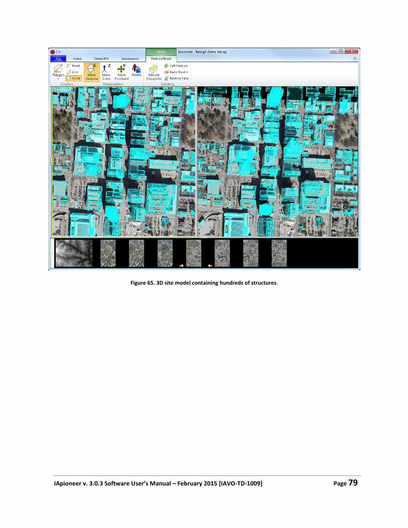
IApioneer v. 3.0.3 Software User’s Manual – February 2015 [IAVO-TD-1009] Page 79
Figure 65. 3D site model containing hundreds of structures.

IApioneer v. 3.0.3 Software User’s Manual – February 2015 [IAVO-TD-1009] Page 80
Figure 66. Exported textured KMZ site model shown in Google Earth.

IApioneer v. 3.0.3 Software User’s Manual – February 2015 [IAVO-TD-1009] Page 81
INDEX 3
3D, 57, 59, 63
3D viewer, 75
flythrough, 77
navigation, 77
panning, 77
rotation, 77
zoom, 77
A
active layer, 43, 59
Add Annotation Layer, 42
Add Vector Layer, 57
affine, 14
annotations, 42
annotation layers, 42, 43
creating, 42
editing, 43, 46
layer management, 42
loading, 43
properties, 47
save, 43
save as, 43
automatic texturing, 40
Auxiliary Viewer, 10
B
Backstage, 5, 42, 57
Session, 6
Band Info, 12
Brightness, 9, 25
C
Camera group, 9
Camera Lock, 9
Chip from ROI, 39
clip art, 44, 45
Color Curves, 24
color transformations, 24
Combine Shapes, 62, 68
subtraction, 62, 68
union, 62, 68
Compass, 10
Contact Us, 2
By e-mail, 2
By phone, 2
Contrast, 9, 25
copy, 59
Creation group, 60
Crop, 36, 39
Crop, Resample, and Reproject, 36, 39
geospatial coordinates, 36
geospatial data, 36
Reproject, 36
Resample, 36
Cursor Information, 26
D
Data Discovery, 7, 30
Data Layer Manager, 11, 43, 59
Data Layers group, 11, 43, 59
Datum, 13
DEM, 6, 59
Detailing group, 62, 63, 69, 70, 71, 72, 73, 74
Digital Affine, 18
Display, 33
Display Format, 27
Display group, 9, 24
DTED, 59, 63
E
EGM96, 13, 28
elevation source, 59, 63
ellipse, 45
epipolar line, 63
Export Data, 36
Crop, Resample, and Reproject, 36
Export Raster Data, 38
Image Chipping, 39
Type Conversion, 38
vector data, 40
exterior orientation (EO), 14
Extrude Polygon, 62, 63
by point, 62
planar, 62
IApioneer v. 3.0.3 Software User’s Manual – February 2015 [IAVO-TD-1009] Page 82
F
feature extraction, 57
FeatureXTract, 57, 59, 63, 66
fiducials, 14, 15
Filters, 9, 25
Gaussian High Pass, 25
Gaussian Low Pass, 25
Haze Reduction, 25
High Pass, 25
Low Pass, 25
focal length, 14
focal offset, 14
Footprints, 49
frame camera, 13
configuration, 14
Digital Affine, 18
Full Screen Chip, 39
G
Geolocation Formats, 10, 27
grid lines, 9, 25
Grid Lines, 34
gutterline, 63
H
Hide All, 11
Histogram, 9
Histogram Adjustment, 24
Home Tab, 9, 11, 43, 59
I
IApioneer, 42, 43
Image Chipping, 39
Image Gallery, 5
Image group, 26
image overview, 9
Image Overview, 25
Image Up, 10, 33
Input Format, 28
Insert group, 44
Inspect/Measure group, 46
Installation, 1
interior orientation (IO), 14
J
jump to location, 9, 10
K
KML, 78
KMZ, 78
L
Layer Manager, 5, 11, 43, 59
Left Viewer, 4
length, 46
Load Data, 7
Loft Feature, 62, 66
M
Manipulation group, 61
Manipulation mode, 61, 63, 64
Measurement, 29
mensuration, 46
settings, 50
Mensuration Properties, 48
Mensuration Tools, 50
Mesh Convert, 62
Metadata, 12, 15
MIL-STD-2525B, 44
Move Epipolar, 61, 63
Move Freehand, 61
Move Z-Axis, 61, 64
N
New Viewer. See Auxilliary Viewer
north arrow, 45
North arrow, 9, 25
North Up, 10, 33
O
ortho. See orthographic
orthographic, 13, 23
Sensor Model Configuration, 23
P
pan, 9

IApioneer v. 3.0.3 Software User’s Manual – February 2015 [IAVO-TD-1009] Page 83
Pan Mode, 9
parameterized structures. See Roofs and Structures
Parameterized Structures, 69
barrel vault, 72
dome, 73
fence, 74
gabled, 69
gambrel, 71
hipped, 69
mansard, 71
parapet, 70
pointed vault, 72
saltbox, 69
wall, 74
paste, 59
Pixel Cursor, 32
point, 45, 51
settings, 51
point marker, 45, 46, 52
settings, 52
polygon, 44, 48, 53
edit vertices, 46
settings, 53
subdivide, 46
polyline, 45, 54
settings, 54
Projection, 13
pyramids, 7
R
radial distortion, 14
RASTER DATA, 8
chipping, 39
Exploring, 9
Export, 36
Properties, 12
rectangle, 45
reduced resolutions. See pyramids
Region of Interest, 35, 39
Region Of Interest, 9
Reproject, 36, 39
Resample, 36, 39
Reverse Face, 62
Ribbon, 4
File tab, 5
Right Viewer, 5
Roam Mode, 9
roof shapes
gabled, 70
hipped, 70
Roofs and Structures, 62
Rotate, 61
rotation, 10
Rotation group, 10
RPC, 13
Configuration, 22
R-sets. See pyramids
S
Scanned Film, 15
Screen Capture, 40
ROI, 40
to Clipboard, 40
to File, 40
to PowerPoint, 40
Sensor Model, 12
frame camera, 13
Frame Camera Sensor Model Configuration, 14
orthographic, 13
Orthographic Sensor Model Configuration, 23
RPC, 13
RPC Sensor Model Configuration, 22
Setting Up Camera Sensor Models, 13
separation angle, 46
Session, 6, 7, 12
Session Management, 12
Close Session, 12
Open Session, 12
Save Session, 12
Save Session As, 12
Settings. See User Settings
shapes, 44
Site Administration, 2
snapping tool, 67
SHIFT, 67
Source DEM, 10, 59, 63
Spatial Reference Systems, 13
Configuring, 13
Spatial Referencing dialog, 13
Split Edge, 62
SRS. See Spatial Reference System
Subdivide Polygon, 46

IApioneer v. 3.0.3 Software User’s Manual – February 2015 [IAVO-TD-1009] Page 84
T
Target, 55
target circles, 45, 46
settings, 55
Terrain, 30
text box, 45
textbox, 56
settings, 56
Textbox
editing, 47
Type Conversion, 38
U
UI Conventions, 1
undo, 59
User Interface (UI), 4
Elements of the UI, 4
User Settings, 26, 48
Data Discovery, 30
Display, 33
Footprints, 49
Geolocation Formats, 27
Grid Lines, 34
Measurement, 29
Mensuration Tools, 50
Pixel Cursor, 32
Point, 51
Point Marker, 52
Polygon, 53
Polyline, 54
Region of Interest, 35
Target, 55
Terrain, 30
Textbox, 56
V
vector data
export, 40
vector layers, 57
vectors
circle, 61
cones, 66
creating, 57, 63
creation, 60
editing, 59
ellipse, 61
exporting, 58
finalize, 63
layer management, 57
line, 61
loading, 59
point, 61
polygon, 61
pyramids, 66
renaiming, 58
save, 58
save as, 58
selection, 64
vector layers, 57, 59
Viewer
Auxilliary, 10
divider, 9
Send to Left Viewer, 9
Send to Right Viewer, 9
Visibility, 43, 59, 63
W
WGS84, 13, 27
Z
Z Up, 10, 33
zoom, 9
zoom indicator, 26