Surfer User's Guide - Golden Software
1452
-
Upload
khangminh22 -
Category
Documents
-
view
0 -
download
0
Transcript of Surfer User's Guide - Golden Software


Surfer® Registration Information
Your Surfer product key is located in the download instructions email and inyour account at MyAccount.GoldenSoftware.com.
Register your Surfer product key online at www.GoldenSoftware.com. Thisinformation will not be redistributed.
Registration entitles you to free technical support, download access in youraccount, and updates from Golden Software.
For future reference, write your product key on the line below:
____________________________________________________
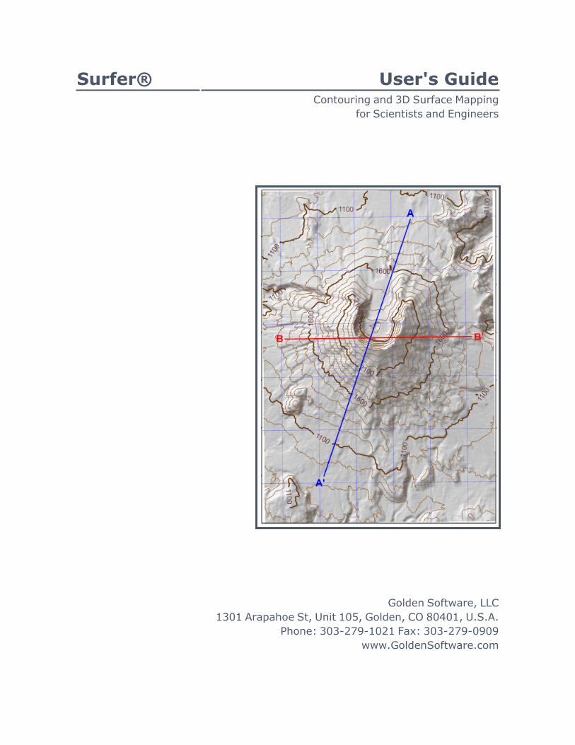
Surfer® User's GuideContouring and 3D Surface Mapping
for Scientists and Engineers
Golden Software, LLC1301 Arapahoe St, Unit 105, Golden, CO 80401, U.S.A.
Phone: 303-279-1021 Fax: 303-279-0909www.GoldenSoftware.com

COPYRIGHT NOTICE
Copyright Golden Software, LLC
The Surfer® program is furnished under a license agreement. The Surfer soft-ware, quick start guide, and user's guide may be used or copied only in accord-ance with the terms of the agreement. It is against the law to copy the software,quick start guide, or user's guide on any medium except as specifically allowed inthe license agreement. Contents are subject to change without notice.
Surfer is a registered trademark of Golden Software, LLC. All other trademarksare the property of their respective owners.
September 2021

ContentsChapter 1 - Introduction 17Introduction to Surfer 17Three-Minute Tour 20Create a Grid from XYZ Data 23Surfer Flow Chart of Data and Maps 27Using Scripter For Automation 27Surfer User Interface 28Ribbon 30Quick Access Toolbar 33Tabbed Documents 35Changing the Layout 36Contents 38Properties 45Status Bar 48Progress 49Menu and Tab Commands 50Worksheets 52Grid Editor 53File Types 57Gridding Overview 58Map Types 59Map Wizard 64Introduction to Map Layers 71Coordinate Systems 76Map Coordinate System Overview 77File Menu Commands 78Home Tab Commands 96Welcome to Surfer Help 98Welcome to Surfer Dialog 100Technical Support 102Register Product Key 103What's New in Surfer? 103
Chapter 2 - Tutorial 111Tutorial 111Getting Started 112Creating a Map 112Changing Map Properties 114Viewing a Map in 3D 116Saving and Exporting 117
Chapter 3 - Data Files and the Worksheet 121Data Files 121Data File Formats 124
- v -

Date/Time Formatting 125Working with Date/Time Values 127Date Time Formats 128Opening a Worksheet Window 133Worksheet Window 134Row and Column Label Bars 135Active Cell 135Active Cell Location Box 136Active Cell Edit Box 137Select Entire Worksheet 138Working with Worksheet Data 138Selecting Cells 142Selecting Cells with the Keyboard 143Selecting Cells with the Mouse 144Selecting a Column or Row Dividing Line 145Hiding Columns or Rows 146Displaying Hidden Columns or Rows 147Worksheet Error Codes and Special Numeric Values 148Worksheet Specifications 148Worksheet Commands 149
Chapter 4 - Creating Grid Files 203Grid Files 203A Gridding Example 203Grid Data 205Introduction to Gridding Methods 239General Gridding Recommendations 240Choosing Methods Based on the Number of XYZ Data Points 241Gridding Method Comparison 242Exact and Smoothing Interpolators 246Weighted Averaging 247Kriging 248Kriging 252Minimum Curvature 258Modified Shepard's Method 262Natural Neighbor 264Nearest Neighbor 267Polynomial Regression 268Radial Basis Function 270Triangulation with Linear Interpolation 273Moving Average 275Data Metrics 277Local Polynomial 285Grid from Server 288Grid from Contours 289Grid Function 296Producing a Grid File from a Regular Array of XYZ Data 298
- vi -

Surfer User's Guide
Chapter 5 - Introduction to Variograms 299Variogram Overview 299Kriging and Variograms 301Variogram Grid 302Variogram Model 304New Variogram 305New Variogram Dataset Properties 307New Variogram General Properties 309Variogram Properties 310Variogram Experimental Properties 311Estimator Type 314Smoothing a Variogram with Lag Width 316Variogram Model Properties 317Anisotropy 319AutoFit 323Variogram Model Graphics 325Variogram Statistics Properties 329Variogram Plot Properties 330Info Properties 333Default Linear Variogram 338Nugget Effect 339Export Variogram 341Using Variogram Results in Kriging 341Suggested Reading - Variograms 341Variogram Tutorial 342
Chapter 6 - Grid Editor 365Grid Editor 365Node Labels - Grid Editor 369Node Symbols - Grid Editor 371Contours - Grid Editor 372Contour Levels - Grid Editor 375Color Fill - Grid Editor 377Select - Grid Editor 379Brush 379Warp 383Smooth 386Push Down 389Pull Up 392Eraser 395Eyedropper 399Zoom In - Grid Editor 400Zoom Out - Grid Editor 400Grid Info 401Update Layer 401Open Grid 403Save Grid As 409
- vii -
Chapter 7 - Grid Operations 413Grids Tab Commands 413Assign NoData 414Grid Filter 423Grid Convert 433Grid Spline Smooth 434Assign Coordinate System - Grid 439Grid Project 440Grid Calculus 443Volumes and Areas 465Grid Math 480Grid Transform 485Grid Slice 490Residuals 496Point Sample 499Contour Volume and Area 501Isopach Map 503Grid Mosaic 505Grid Extract 510Grid Info 513Filtering Grid Files 515Grid Operations References 515
Chapter 8 - Base Maps 517Base Map 517Base Map from Data 521View Data 524Base Map from Server 524Empty Base Map 525Export Drawn Objects in Map Units 525Placing Boundaries on Other Maps 527Changing Properties in a Base Map 528Base (vector) Layer General Properties 530Symbology 533Base (raster) Layer General Properties 554Base Map Labels Properties 558
Chapter 9 - Contour Maps 563Contour Map 563Drawing Contours 565Contour Map General Properties 566Contour Map Levels Properties 568Contour Map Advanced Levels Properties 575Contour Lines 583Adding Color Fill between Contours 596Labels - Contour 604Hachures 610
- viii -

Surfer User's Guide
Masking Portions of a Contour Map with a Base Map 613Smoothing Contours 614
Chapter 10 - Post and Classed Post Maps 617Post Map 617Post Layer General Properties 619Post Layer Symbol Properties 623Proportional Scaling 626Classed Post Map 629Classed Post Layer General Properties 631Classed Post Layer Classes Properties 636Labels Properties 644Edit Post Labels 651Data Files Used for Posting 652Updating Post Map and Classed Post Map Data Files 654Symbol Specifications in the Data File 654
Chapter 11 - 3D Surface Maps 6573D Surface 6573D Surface Group General Properties 6603D Surface Layer Mesh Properties 663Lighting Properties 6663D Surface Layer Overlays Properties 669
Chapter 12 - 3D Wireframe Maps 6713D Wireframe 6713D Wireframe Layer General Properties 6733D Wireframe Layer Z Levels Properties 6763D Wireframe Layer Color Zones Properties 678Line Spectrum Dialog 681Wireframe Level Files 681Color Filled Wireframe 682Specifying the Lines to Draw on a Wireframe 683Adding Color Zones to a 3D Wireframe 684Line Property Precedence 685Wireframe Base 686Smoothing a Wireframe 686Wireframe NoData Regions 687
Chapter 13 - Relief Maps 689Color Relief Layer General Properties 689Reflectance Shading Methods 695
Chapter 14 - Grid Values Maps 697Grid Values Map 697Grid Values Layer General Properties 699
- ix -

Grid Values Layer Symbols Properties 702Grid Values Layer Labels Properties 703
Chapter 15 - Watershed Maps 707Watershed 707Watershed Layer General Properties 710
Chapter 16 - Vector Maps 7171-Grid Vector Map 7171-Grid Vector Map Data Properties 7192-Grid Vector Map 7202-Grid Vector Map Data Properties 723Cartesian Data 725Polar Data 726Vector Map Symbol Properties 726Vector Map Scaling Properties 729Clipping Symbols on Vector Maps 732
Chapter 17 - Point Cloud Maps 733Point Cloud Map 733Import Points Dialog 735Select Bounds Dialog 741Point Cloud Layer General Properties 742Point Cloud Tab Commands 744
Chapter 18 - Viewshed Layers 761Viewshed 761Viewshed Layer General Properties 763
Chapter 19 - Peaks and Depressions Maps 769Peaks and Depressions Map 769Peaks and Depressions Layer General Properties 772Peaks and Depressions Layer Depressions Properties 774Peaks and Depressions Layer Peaks Properties 777Peaks and Depressions Report 781
Chapter 20 - Drillhole Maps 783Drillhole Map 783Drillhole Manager 793Drillhole Properties 794
Chapter 21 - Downloading Layers from a Server 807Base Map from Server 807Grid from Server 807Download Online Maps or Grids 808Map Source Dialogs 819
- x -

Surfer User's Guide
Chapter 22 - Map Properties 825Introduction to Common Map Properties 825Map Properties 826View Properties 827Scale Properties 831Using Different Scaling in the X and Y Dimensions 835Using Scaling to Minimize Distortion on Latitude/Longitude Maps 836Limits Properties 838Setting Map Limits 842Frame Properties 843Reload Data 844
Chapter 23 - Map Features 847Add to Map 847Layer Properties 847Scale Bar 848Legend 849Graticule 862Profile 868Map Axes 874
Chapter 24 - 3D View 8933D View Window 8933D View Properties 8983D Drillhole Properties 9213D View Commands 926
Chapter 25 - Map Tools 935Map Tools Tab Commands 935Set Limits 936Trackball 940Measure 942Overlay Maps 947Combining Maps 949Stack Maps 951Creating Several Maps in the Same Plot Window 952Aligning Several Maps on the Same Page 953Masking with Background 953Extract Grid or Data from Map 954
Chapter 26 - Layer Tools 957Digitize 957Creating a Blanking File with the Digitize Command 959Break Apart Layer 960Delete Map Layer (Break Apart Overlay) 961Assigning Coordinates to a Base (raster) Layer 961
- xi -

Georeference Image 963Attribute Table 978Query Objects 983Track Cursor 986Export Contours 989
Chapter 27 - Coordinate Systems 993Coordinate Systems 993Map Coordinate System Overview 993Source Coordinate System Properties 994Target Coordinate System Properties 996Displaying Data with Different Coordinate Systems in a Single Map 998Coordinate System Notes 999Coordinate System Frequently Asked Questions 999Assign Coordinate System 1001What is a Map Projection? 1011Predefined Coordinate Systems 1021Supported Projections 1023Golden Software Reference Files 1064Latitude and Longitude Coordinates 1064Latitude and Longitude in Decimal Degrees 1066How to Convert from NAD27 to NAD83 Using NTv2 1066Projection References 1068
Chapter 28 - Creating and Editing Features 1069Features Tab Commands 1069Text 1070Text Editor 1071Polyline 1086Polygon 1087Point 1088Spline Polyline 1089Range Ring 1091Range Ring General Properties 1092Rectangle 1094Rounded Rectangle 1095Ellipse 1096Create a North Arrow 1096Editing Objects 1100Undo 1127Redo 1128Paste 1128Paste Special - Plot Document 1130Copy 1131Cut 1131Delete 1131
- xii -

Surfer User's Guide
Chapter 29 - Common Properties 1133Text and Font Properties 1133Fill Properties 1137Line Properties 1148Symbol Properties 1158Label Properties 1161Metafile Properties 1166Image General Properties 1167Introduction to Color Spectrums 1170Color Palette 1187Colors Dialog 1188Color List 1190Info Properties 1195
Chapter 30 - Selecting and Arranging Objects 1203Selecting Objects 1203Select Tool 1204Block Select 1205Select All 1205Deselect All 1205Invert Selection 1206Transform 1206Rename Object 1207Layout Tab Commands 1208Positioning and Sizing Objects 1209Resize Objects 1210Lock Position 1211Bring to Front 1211Bring Forward 1212Send to Back 1213Send Backward 1213Size Objects 1214Align Objects 1215Distribute Horizontally 1216Distribute Vertically 1217Align to Margins 1218Free Rotate 1219Rotate 1220Group 1220Ungroup 1221
Chapter 31 - Changing the View 1223View Tab Commands 1223Fit to Window 1223Page 1224Zoom In 1224Zoom Out 1225
- xiii -

Zoom Selected 1226Zoom Realtime 1226Zoom Rectangle 1227Actual Size 1227Full Screen 1227Pan 1228Redraw 1228Auto Redraw 1229Rulers 1229Drawing Grid 1229New Window 1229Cascade 1230Arrange Icons 1230Tile Horizontal 1230Tile Vertical 1230Reset Windows 1230
Chapter 32 - Importing, Exporting, and Printing 1231Import 1231Export 1236Page Setup 1247Header & Footer Dialog 1249Print - Plot 1250Page Setup - Worksheet 1253Print - Worksheet 1259
Chapter 33 - Options, Defaults, and Customizations 1261Options 1261Default Settings 1277Customize 1286
Chapter 34 - Automating Surfer 1297Introduction to Scripter 1297Scripter Windows 1298Working with Scripts 1300Scripter BASIC Language 1301Visual BASIC Compatibility 1301Using Scripter For Automation 1303Using Scripter Help 1303Suggested Reading - Scripter 1304Writing Scripts 1304Running Scripts 1305Running Scripts from the Command Line 1306Debugging Scripts 1307Program Statements 1311Line Continuation 1311Comments 1311
- xiv -

Surfer User's Guide
Double Quotes and Text 1312Operators 1312Flow Control 1312Optional Arguments and Named Arguments 1313Named and Positional Arguments 1314Subroutines and Functions 1314Specifying Cell Coordinates 1317Code, Class, and Object Modules 1320Type Library References 1323The Object Browser 1324Variables 1325Object Variables 1327Array Variables 1327User-Defined Types 1328Global Variables 1328Coordinate Arrays 1328Getting User Input 1329Creating Dialogs 1330UserDialog Example 1330Surfer Object Model 1332Overview of Surfer Objects 1334A Brief Introduction to the Major Surfer Objects 1334Derived Objects 1339Using Collection Objects 1340Parent and Application Properties 1342PlotWindow, WksWindow, and GridWindow Objects 1342Using Surfer Objects 1342Object List 1343Object Hierarchy 1346Improve Automation Performance 1347Automation Examples 1347Creating and Printing a Contour Map 1348Opening, Saving, and Closing Documents 1349Creating a Variogram with Scripter 1350Overlaying Maps with Automation 1352Modifying Axes 1353
Appendix A - Mathematical Functions 1355Mathematical Functions 1355
Appendix B - Math Text Instructions 1365Math Text Instruction Syntax 1365
Index 1371
- xv -


Chapter 1 - Introduction
Introduction to SurferWelcome to Surfer, a powerful contouring, gridding, and surface mapping pack-age for scientists, engineers, educators, or anyone who needs to generate mapsquickly and easily. Producing publication quality maps has never been quicker oreasier. Adding multiple map layers and objects, customizing the map display,and annotating with text creates attractive and informative maps. Virtually allaspects of your maps can be customized to produce the exact presentation youwant.
Surfer is a grid-based mapping program that interpolates irregularly spacedXYZ data into a regularly spaced grid. Grids may also be imported from othersources, such as the United States Geological Survey (USGS). The grid is used toproduce different types of maps including contour, color relief, and 3D surfacemaps among others. Many gridding and mapping options are available allowingyou to produce the map that best represents your data.
An extensive suite of gridding methods is available in Surfer. The variety of avail-able methods provides different interpretations of your data, and allows you tochoose the most appropriate method for your needs. In addition, data metricsallow you to map statistical information about your gridded data. Surface area,projected planar area, and volumetric calculations can be performed quickly inSurfer. Cross-sectional profiles can also be computed and exported.
The grid files can be edited, combined, filtered, sliced, queried, and math-ematically transformed. For example, grids can be sliced to create cross-sec-tional profiles, or the Grids | Calculate | Isopach command can be used tocreate an isopach map from two grid files. Grids can be edited with an intuitiveuser interface in the grid editor.
ScripterThe Scripter TM program, included with Surfer, is useful for creating, editing,and running script files. A script is a text file containing a series of instructions forexecution when the script is run that automates Surfer procedures. By writingand running script files, simple mundane tasks or complex system integrationtasks can be performed precisely and repetitively without direct interaction.Surfer also supports ActiveX Automation using any compatible client, such asVisual BASIC. These two automation capabilities allow Surfer to be used as adata visualization and map generation post-processor for any scientific modelingsystem.
New FeaturesThe new features in Surfer are summarized:
- 17 -
Chapter 1 - Introduction
l Online at www.GoldenSoftware.com/products/surfer.com
l Online at theWhat's New in Surfer Knowledge Base article
Who Uses Surfer?People from many different disciplines use Surfer. Since 1984, over 100,000 sci-entists and engineers worldwide have discovered Surfer's power and simplicity.Surfer's outstanding gridding and contouring capabilities have made Surfer thesoftware of choice for working with XYZ data. Over the years, Surfer users haveincluded hydrologists, engineers, geologists, archeologists, oceanographers, bio-logists, foresters, geophysicists, medical researchers, climatologists, educators,students, and more! Anyone wanting to visualize their XYZ data with striking clar-ity and accuracy will benefit from Surfer's powerful features!
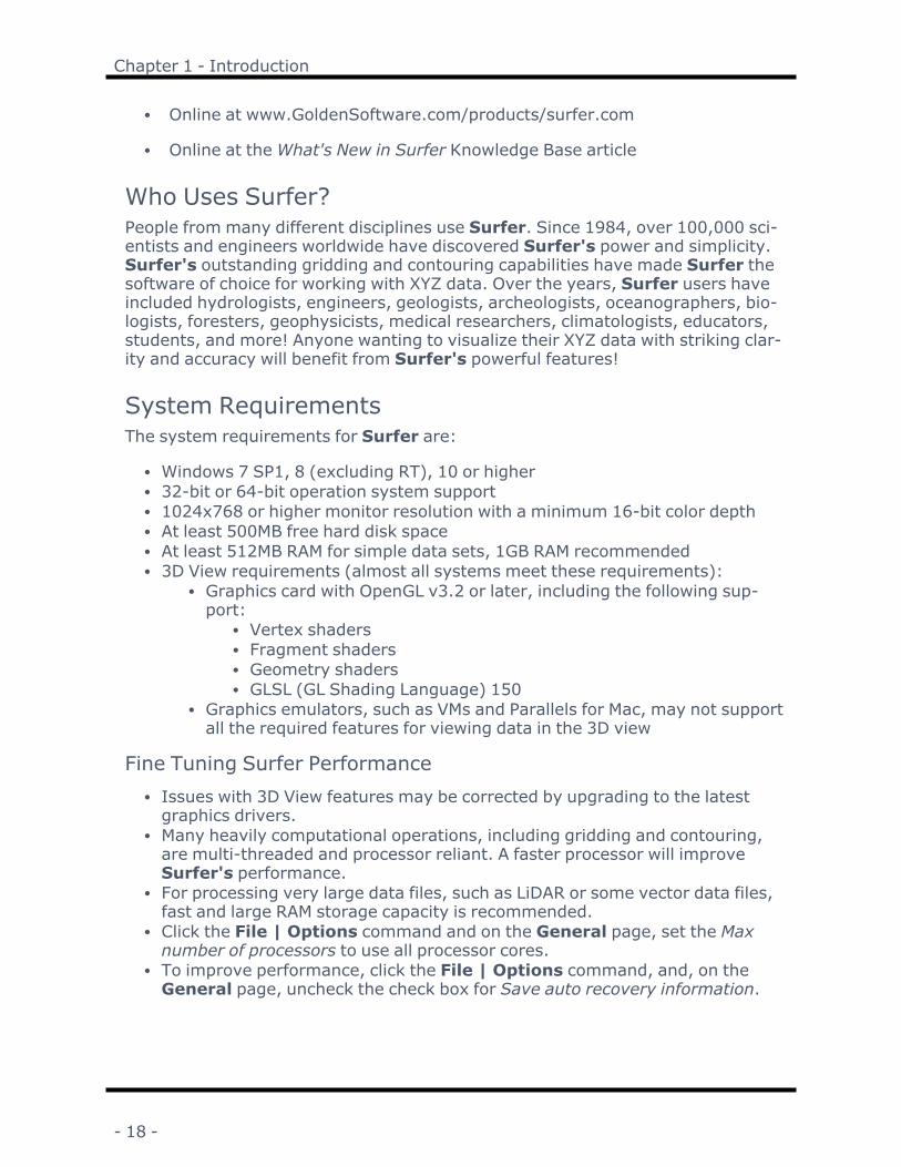
System RequirementsThe system requirements for Surfer are:
l Windows 7 SP1, 8 (excluding RT), 10 or higherl 32-bit or 64-bit operation system supportl 1024x768 or higher monitor resolution with a minimum 16-bit color depthl At least 500MB free hard disk spacel At least 512MB RAM for simple data sets, 1GB RAM recommendedl 3D View requirements (almost all systems meet these requirements):
l Graphics card with OpenGL v3.2 or later, including the following sup-port:
l Vertex shadersl Fragment shadersl Geometry shadersl GLSL (GL Shading Language) 150
l Graphics emulators, such as VMs and Parallels for Mac, may not supportall the required features for viewing data in the 3D view
Fine Tuning Surfer Performancel Issues with 3D View features may be corrected by upgrading to the latestgraphics drivers.
l Many heavily computational operations, including gridding and contouring,are multi-threaded and processor reliant. A faster processor will improveSurfer's performance.
l For processing very large data files, such as LiDAR or some vector data files,fast and large RAM storage capacity is recommended.
l Click the File | Options command and on the General page, set the Maxnumber of processors to use all processor cores.
l To improve performance, click the File | Options command, and, on theGeneral page, uncheck the check box for Save auto recovery information.
- 18 -

Surfer User's Guide
Installation DirectionsGolden Software recommends installing only the latest version of Surfer.
Installing Surfer requires Administrator rights. Either an administrator accountcan be used to install Surfer or the administrator's credentials can be enteredbefore installation while logged in to a standard user account. If you wish to usea Surfer single-user license, the product key must be activated while logged into the account under which Surfer will be used. For this reason, we recommendlogging into Windows under the account for the Surfer user, and entering thenecessary administrator credentials when prompted. Golden Software does notrecommend installing the current version of Surfer in the same location as anyprevious versions of Surfer.
To install Surfer from a download:
l Log into Windows under the account for the individual who is licensed to useSurfer.
l Download Surfer according to the emailed directions you received.l Double-click on the downloaded file to begin the installation process.l Once the installation is complete, run Surfer.l License Surfer by activating a single-user license product key or connectingto a license server.
Updating SurferTo update your version of Surfer, open the Surfer program and choose the File| Online | Check for Update command. This will launch the Internet Updateprogram which will check Golden Software's servers for any updates. If there isan update for your version of Surfer, you will be prompted to download andinstall the update.
You can also email your registered Surfer product key [email protected] and request to download the full productupdate. See the Check for Update topic in the help for additional information.
Uninstalling SurferTo uninstall Surfer, follow the directions below for your specific operating sys-tem.
Windows 7To uninstall Surfer go to the Windows Control Panel and click the Uninstall a pro-gram link. Select Surfer from the list of installed applications. Click the Uninstallbutton to uninstall Surfer.
- 19 -

Chapter 1 - Introduction
Windows 8From the Start screen, right-click the Surfer tile and click the Uninstall button atthe bottom of the screen. Alternatively, right-click anywhere on the Start screenand click All apps at the bottom of the screen. Right-click the Surfer tile and clickUninstall at the bottom of the screen.
Windows 10Select Settings in the Start menu. In Settings, select System | Apps & fea-tures. Select Surfer and then click Uninstall. To uninstall Surfer from the Win-dows Control Panel, click Programs | Programs and Features. Select Surferand click Uninstall.
Surfer Trial FunctionalityThe Surfer trial is a fully functioning time-limited trial. This means that com-mands work exactly as in the full program for the duration of the trial. The trialhas no further restrictions on use. The trial can be installed on any computer thatmeets the system requirements. The trial version can be licensed by activating aproduct key or connecting to a license server.
Three-Minute TourWe have included several sample files with Surfer so that you can quickly seethe variety of Surfer's capabilities. Only a few files are discussed here, andthese examples do not include all of Surfer's many map types and features. TheContents window is a good source of information as to what is included in eachSurfer file. The different types of maps that can be created is found in the pro-gram help in the Map Types topic.
- 20 -

Surfer User's Guide
Surfer, a powerful contouring, gridding, and surface mapping pack-age, produces publication quality maps. Virtually all aspects of yourmaps can be customized to produce the exact presentation you
want.
To access the example files from your computer:1. Open Surfer.2. Click the File | Open command.3. In the Open dialog, navigate to the Surfer Samples folder located in C:\Pro-
gram Files\Golden Software\Surfer\Samples by default.4. Select the sample .SRF file of interest and click Open. The sample file is now
displayed. Repeat as necessary to see the files of interest.
- 21 -

Chapter 1 - Introduction
Examples of Surfer CapabilitiesView Data in 2D and 3DThe 3DView.SRF sample file includescontour and color relief layers, as wellas a base (vector) layer that is usedfor a 3D view fly-through.
To view the 3D and fly-through, openthe 3DView.SRF file and select themap in the Contents window. Next,clickMap Tools | View | 3D Viewto open a 3D view. Click 3D View |Fly-Through | Play to view theexample fly-through.
Present Scientific ResearchThe Classed Post.SRF sample file dis-plays two maps. The left map is a con-tour map with a classed post maplayer displaying the location of thesample of copper in parts per millionand assay results over a study area.The right map is a classed post mapthat displays the drill hole assay res-ults by comparing the depth from sur-face to the Easting. A classed postmap legend has been added to eachmap.
- 22 -

Surfer User's Guide
Display Complex Spatial DataThe Profile.SRF file contains a mapwith two base map layers, a contourlayer, and a shaded relief layer. Thebase maps were created with theMapTools | Add to Map | Profile com-mand. At the bottom of the page, theA and B profile lines are displayed,showing two elevation profiles acrossthe Mount St. Helens map.
Layer Multiple Types of DataThe BaseSymbology (PieChart).SRFsample file was created from one postlayer and two base layers. The postlayer displays circular symbols rel-atively sized according to populationcount in various cities throughout Flor-ida. The base layer depicts populationin all the counties in Florida usingUnclassed Colors symbology. The Piesbase layer uses Pie Chart symbologyto depict the proportion of women tomen in each county.
Create a Grid from XYZ DataThe most common application of Surfer is to create a grid-based map from anXYZ data file. An XYZ data file has X data, Y data, and Z data delimited into sep-arate columns (for example, longitude, latitude, and elevation). The Grid Data
- 23 -

Chapter 1 - Introduction
command uses an XYZ data file to produce a grid file. The grid file is then used bymost of the Home | New Map commands to produce maps. Post maps, basemaps, point cloud, and drillhole maps do not use grid files.
The general steps to progress from an XYZ data set to a finished grid-based mapare as follows:
1. Create an XYZ data file. This file can be created in a Surfer worksheet win-dow or outside of Surfer (using an ASCII text editor or Microsoft Excel, forexample).
Start with irregular XYZ data in threecolumns.
2. To display the data points, click the Home | New Map | Post command.
A post map displays the original XYZ data locations.
- 24 -

Surfer User's Guide
3. Create a grid file .GRD from the XYZ data file using the Home | Grid Data| Grid Data command.
Gridding interpolates a Z value at the intersection of each row and column in the grid file.This fills the holes in the data. Here the rows and columns are represented by grid lines.
4. To create a map, select the map type from the Home | New Map com-mands. Select the grid file from step three. New grid-based maps that canbe created include contour, 3D surface, 3D wireframe, color relief, peaksand depressions, 1-grid or 2-grid vector, watershed, and grid values maps.
- 25 -

Chapter 1 - Introduction
The post map layer shows the original data points. The contour map layer shows the gridbased contour map.
5. Click on the map to display the map properties in the Properties windowwhere you can customize the map to fit your needs.
The contour map layer is filled with a gradational colorfill.
- 26 -

Surfer User's Guide
6. Click the File | Save command to save the project as a Surfer .SRF filewhich contains all the information needed to recreate the map.
Surfer Flow Chart of Data and MapsThis flow chart illustrates the relationship between XYZ data files, grid files, vec-tor files, image files, and various maps. This example displays only one of thegrid based maps, a contour map.
This flow chart illustrates the relationship between different data files and different maptypes.
Using Scripter For AutomationTasks can be automated in Surfer using Golden Software's Scripter program orany ActiveX Automation-compatible client, such as Visual BASIC. A script is atext file containing a series of instructions for execution when the script is run.Scripter can be used to perform almost any task in Surfer. Scripts are useful forautomating repetitive tasks and consolidating a sequence of steps. Scripter isinstalled in the same location as Surfer. Refer to the Surfer Automation topic inthe help for more information about Scripter. We have included severalexample scripts so that you can quickly see some of Scripter's capabilities.
To run a sample script file:
1. Open Scripter by navigating to the installation folder, C:\ProgramFiles\Golden Software\Surfer\Scripter. If you are running a 32-bit versionof Surfer on a 64-bit version of Windows, navigate to C:\Program Files(x86)\Golden Software\Surfer\Scripter. Right-click on the Scripter.exeapplication file and select Run as administrator.
2. Choose the File | Open command.
- 27 -

Chapter 1 - Introduction
3. Select a sample script .BAS file. These are located in the C:\ProgramFiles\Golden Software\Surfer\Samples\Scripts folder or, if you are runninga 32-bit version of Surfer on a 64-bit version of Windows, the C:\ProgramFiles (x86)\Golden Software\Surfer\Samples\Scripts folder.
4. Click the Script | Run command and the script is executed. Most samplescripts open Surfer and display a map in the plot window.
Surfer User InterfaceSurfer contains four document window types: the plot document, worksheetdocument, 3D view, and grid editor. Maps are created and displayed in the plotdocument and 3D view. The worksheet document displays, edits, transforms,and saves data in a tabular format. The grid editor displays and edits Z values forthe grid with various editing tools.
This is the Surfer plot window with the Contents and Properties windows onthe left and the worksheet and grid editor tabs on the top of the horizontal ruler.
- 28 -

Surfer User's Guide
Surfer LayoutThe following table summarizes the function of each component of the Surferlayout.
ComponentName
Component Function
Title Bar The title bar lists the program name plus the saved Surfer.SRF file name (if any). An asterisk after the file name indic-ates the file has been modified.
Quick AccessToolbar
All window types in Surfer include the quick access toolbarto the left of the title bar. The quick access toolbar containsbuttons for many common commands. The quick access tool-bar can be customized to add or remove buttons with theCustomize Ribbon command.
Ribbon The ribbon includes all of the commands in Surfer. Com-mands are grouped under the File menu and various tabs.Some commands and tabs are only available in specificviews. For example, the Features | Insert | Polyline com-mand is only available in the plot window. The ribbon com-mands can be modified and rearranged with the CustomizeRibbon command. On the upper right side of the ribbon is aflag icon that will display badges when there are user-spe-cific notifications to be read.
Tabbed Docu-ments
The plot, 3D view, worksheet, and grid editor windows aredisplayed as tabbed documents. The tabs may be reorderedby clicking and dragging. When more than one window isopen, tabs appear at the top of the document, allowing youto click on a tab to switch to a different window. When a doc-ument contains unsaved changes, an asterisk (*) appearsnext to its tabbed name.
Contents The Contents window contains a hierarchical list of all theobjects in a Surfer plot document, grid editor, or 3D view win-dow displayed in a tree view. The objects can be selected,added, arranged, or edited. Changes made in the Contentswindow are reflected in the plot document, grid editor, or 3Dview and vice versa. The Contents window is initiallydocked at the left side of the window.
Properties The Properties window contains all of the properties for theselected object or objects. Changes made in the Propertieswindow are reflected in the plot document, grid editor, or 3Dview. The properties in the Properties window are groupedby page. The Properties window is initially docked belowthe Contents window.
- 29 -

Chapter 1 - Introduction
Status Bar The status bar displays information about the current com-mand or activity in Surfer. The status bar is divided into fivesections. The sections display basic plot commands anddescriptions, the name of the selected object, the cursormap coordinates and units, the cursor page coordinates, andthe dimensions of the selected object.
Opening WindowsSelecting the File | Open command opens grid files and data files as maps. TheFile | New | Plot command creates a new plot window. The File | New |Worksheet command creates a new worksheet window. TheMap Tools |View | 3D View command opens a 3D view of the selected map. The Grids |Editor | Grid Editor command opens a grid in the grid editor.
RibbonThe ribbon is the strip of buttons and icons located above the manager and viewwindows. The ribbon replaces the menus and toolbars found in earlier versions ofSurfer. The ribbon is designed to help you quickly find the commands that youneed to complete a task.
Above the ribbon are a number of tabs, such as Home, Features, andMapTools. Clicking or scrolling to a tab displays the commands located in this sec-tion of the ribbon. The tabs have commands that are organized into a group. Forinstance, all the commands for adding drawn objects are on the Features tab inthe Insert group.
The Ribbon is displayed with the Data tab selected.
Minimizing the RibbonThe ribbon can be minimized to take up less space on the screen. To minimizethe ribbon, right-click on the ribbon and selectMinimize the Ribbon or clickthe button in the top right portion of the Surfer window. When displayed in aminimized mode, only the tabs at the top of the screen are visible. To see thecommands on each tab, click the tab name. After selecting a command, the rib-bon automatically minimizes again. Double-click any tab name to quickly min-imize or maximize the ribbon.
- 30 -

Surfer User's Guide
The Ribbon displayed with theMinimize the Ribbon option selected. Clicking any tab namedisplays the ribbon.
Customizing the RibbonThe ribbon is customizable in Surfer. To customize the commands in the ribbon,right-click on the ribbon and select Customize the Ribbon.
In the Customize Ribbon dialog, you can add new tabs, add groups, hide exist-ing tabs or custom groups, and add commands to any custom group. You canalso rearrange the tabs into an order that fits your needs better.
To customize the commands in the Customize Ribbon dialog, right-click on theribbon and select Customize the Ribbon. In the Customize Ribbon dialog,use the following options.
Tab optionsl To add a custom tab, set the Customize the Ribbon section to All Tabs. Clickin the list on the right side of the dialog where the custom tab should be loc-ated and click the New Tab button.
l To delete custom tab, right-click on the tab name in the list on the rightside of the dialog and select Delete.
l To rename a default or custom tab, click on the tab name in the list on theright side of the dialog. Click the Rename button. Type the new name andpress OK to make the change.
l To hide a default or custom tab, uncheck the box next to the tab name onthe right side of the dialog. Only checked tabs will be displayed.
l To change the order of default or custom tabs, click on the tab name thatshould be moved in the list on the right side of the dialog. Click the up anddown arrow buttons on the far right side of the dialog to move the selectedtab up or down. Default tabs must remain in their major group.
- 31 -

Chapter 1 - Introduction
Group optionsl To add a custom group to a default or custom tab, click on the next to thetab name. Click in the list of group names where the new group should belocated and click the New Group button.
l To delete a default or custom group on any tab, right-click on the groupname in the list on the right side of the dialog and select Delete.
l To rename a default or custom group on any tab, click on the group namein the list on the right side of the dialog. Click the Rename button. Type thenew name and click OK to make the change.
l To change the order of default or custom groups on any tab, click on thegroup name that should be moved in the list on the right side of the dialog.Click the up and down arrow buttons on the far right side of the dialog tomove the selected group up or down in the list.
l To replace a default group with a custom group, right-click on the defaultgroup name and select Delete. Click the New Group button. Add thedesired commands to the new group that you want displayed. Rename thenew group, if desired.
Command optionsCommands can only be added to or deleted from custom groups. Commands canonly be rearranged or renamed in custom groups. If you wish to edit the com-mands in default group, the default group should be hidden and a new customgroup should be created with the same commands.
l To add a command to a custom group, set the Choose commands from: listto All Tabs so that all commands are listed on the left side of the dialog.Select the desired command that should be added. On the right side of thedialog, click the next to the custom group name. Click on the desired pos-ition in the list of commands. If no commands exist in the group yet, clickon the group name. Click the Add>> button and the command is added tothe custom group.
l To delete a command from a custom group, right-click on the commandname in the list on the right side of the dialog and select Delete. Only com-mands from custom groups can be deleted.
l To rename a command in a custom group, click on the command name inthe list on the right side of the dialog. Click the Rename button. Type thenew name and click OK to make the change. Only commands in customgroups can be renamed.
- 32 -

Surfer User's Guide
l To change the order of commands in a custom group, click on the com-mand name that should be moved in the list on the right side of the dialog.Click the up and down arrow buttons on the far right side of the dialog tomove the selected command up or down in the list.
Reset the RibbonTo reset all customizations on the ribbon, click the Reset button at the bottom ofthe Customize Ribbon dialog.
Command and Help SearchThe ribbon also includes a command search to the right of the last tab (View,Data, or Grid Editor depending on document type). Begin typing a commandname to search for commands. Click on a command in the search results to usethe command. Press ENTER to quickly use the top search result command. Forexample type post into the command search bar and the Home | New Map |Post command group,Map Tools | Add to Map | Layer command group, andMap Tools | Edit Layer | Post Labels commands are displayed in the searchresults. You can also click the Search help file at the bottom of the results list tosearch the help file for the search term.
The command search will return commands from all ribbon tabs. No more thanfive commands are displayed in the results list. A command may be disabled inthe results list if the command is not applicable to the current document or selec-tion.
Quick Access ToolbarThe quick access toolbar is at the top of the Surfer window. This toolbar has fre-quently used commands and can be customized by the user. The commands inthe quick access toolbar are the same regardless of the type of window displayedin Surfer .
The Quick Access Toolbar is dis-played at the top of the Surfer win-
dow.
Customizing the Quick Access ToolbarThe quick access toolbar is a customizable toolbar. One method that can be usedto add commands to the quick access toolbar is to right-click on the command inthe ribbon and click Add to Quick Access Toolbar. The command is auto-matically added to the end of the toolbar.
- 33 -

Chapter 1 - Introduction
To customize the commands on the quick access toolbar, right-click on the quickaccess toolbar or ribbon and select Customize Quick Access Toolbar.
In the Quick Access Toolbar dialog,
1. To add a command, select the command from the list on the left that youwant to add. Click the Add>> button and the command is added to the liston the right.
2. To add a separator between commands, set the Choose commands from toMain on the left side of the dialog. Select <Separator> and click Add>> .Move the separator to the desired position.
3. To delete a command, select the command from the list on the right. Clickthe <<Remove button and the command is removed from the list on theright.
4. To rearrange commands or move separators, click on the command or sep-arator name from the list on the right that you want to move. Click the upand down arrow buttons on the far right to move the command up or downthe list. Commands are shown in the exact order that they are displayed inthe Quick Access Toolbar.
5. To reset the Quick Access Toolbar to the default display, click the Reset but-ton below the list on the right side of the dialog.
6. Click OK and all changes are made.
Displaying the Quick Access Toolbar Below the RibbonTo display the quick access toolbar below the ribbon, right-click on the quickaccess toolbar or ribbon and click Show Quick Access Toolbar Below theRibbon. This setting is useful if you have added many commands to the quickaccess toolbar. More commands display, by default, when the quick access tool-bar is below the ribbon. When combined with the minimized ribbon appearance,this can give single click access to all your most used commands and maximizethe viewing area for the plot.
Customize the Quick Access Toolbar to display all the commands you frequently use. Then,display the Quick Access Toolbar below the ribbon bar. When the ribbon bar is minimized, itappears that all of your commands are in a single toolbar, ready to create exactly what you
want with a single click.
- 34 -

Surfer User's Guide
Tabbed DocumentsThe plot, 3D view, worksheet, and grid node editor windows are displayed astabbed documents. When more than one window is open, tabs appear at the topof the screen, allowing you to click on a tab to switch to that window.
Selecting and Closing WindowsTo select a tab to view, click the tab name. To close a tab, right-click and selectClose or click the X next to the tab name. If unsaved changes are present in thedocument, you will be prompted to save the changes before the file is closed.
Change Order of TabsWhen viewing in tabbed document mode, the tabs may be dragged to reorderthem. Left-click on a tab, hold the left mouse button, drag to a new location, andrelease the mouse button to move the tab to a new location.
To move to the next tab, you can use the Next command. Alternatively, pressCTRL + F6 to move to the next tab.
The and buttons on the sides of the tabs are used to scroll the tabs shouldthere be more tabs than can fit along the top of the window.
Unsaved ChangesWhen a document contains unsaved changes, an asterisk (*) appears next to itstabbed name. The asterisk disappears once the unsaved changes have beensaved.
The Plot1 tab has unsaved changes, indicated by the (*) asterisk. The Sheet1 and Sheet2 tabsdo not have unsaved changes.
Tab StyleThe style of the tab can be changed in File | Options | User Interface. Select anew tab style from the MDI tab style list.
No TabsTabs can be turned off in Options dialog User Interface page. Select None fromthe MDI tab style list.
- 35 -

Chapter 1 - Introduction
Changing the LayoutThe plot, worksheet, grid editor, 3D view window, Properties window, and Con-tents window are in a docked view by default. However, they can be displayedas floating windows. The visibility, size, and position of each item may bechanged.
VisibilityUse the View | Show/Hide commands to toggle the display of the rulers, draw-ing grid, status bar, Contents window, and Properties window. Alternatively,click the or buttons in the Contents and Properties windows to auto-hideor close the windows.
Right-click the ribbon or quick access toolbar to minimize the ribbon, move thequick access toolbar above or below the ribbon, and customize the ribbon orquick access toolbar.
Auto-Hiding the Contents or Properties WindowsClick the button to auto-hide a docked Contents or Properties window. Thewindow slides to the side of the Surfermain window and a tab appears with thewindow name.
The Con-tents
appears as atab on theside of thewindow.
Position the mouse pointer over the tab to view the window. Move your mouseaway from the window and the window "hides" again. Click inside the window toanchor it at its current position. Click in another window to release the anchorand hide the window. Click the button to return the window to a docked pos-ition.
- 36 -

Surfer User's Guide
SizeDrag the sides of the application window, Contents window, Properties win-dow, or document window to change its size. If a window is docked, its left andright bounds are indicated by a cursor, and its upper and lower bounds areindicated by a cursor. Click and drag the cursor to change the size.
PositionTo change the position of a docked window, click the title bar and drag it to a newlocation. To dock the Contents or Properties windows, use the docking mech-anism. Double-click the window's title bar to toggle between floating and dockedmodes. Left-click the title bar of a window and drag it to a new location whileholding the left mouse button. The docking mechanism displays with arrow indic-ators as you move the window.
The docking mechanismmakes it easy to position theContents and Properties win-
dows.When the cursor touches one of the docking indicators in the docking mech-anism, a blue rectangle shows the window docking position. Release the leftmouse button to allow the window to be docked in the specified location.
- 37 -
Chapter 1 - Introduction
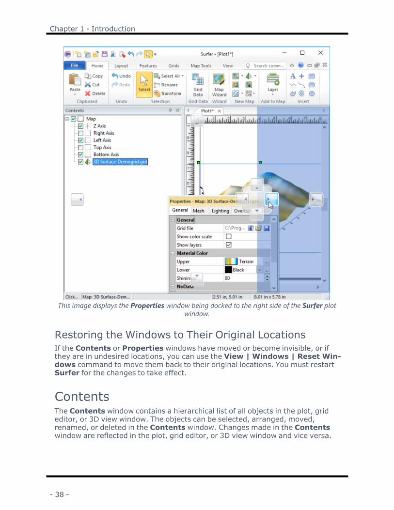
This image displays the Properties window being docked to the right side of the Surfer plotwindow.
Restoring the Windows to Their Original LocationsIf the Contents or Properties windows have moved or become invisible, or ifthey are in undesired locations, you can use the View | Windows | Reset Win-dows command to move them back to their original locations. You must restartSurfer for the changes to take effect.
ContentsThe Contents window contains a hierarchical list of all objects in the plot, grideditor, or 3D view window. The objects can be selected, arranged, moved,renamed, or deleted in the Contents window. Changes made in the Contentswindow are reflected in the plot, grid editor, or 3D view window and vice versa.
- 38 -

Surfer User's Guide
The Contents window displays the struc-ture of all the objects in the plot window.
Displaying or Hiding the Contents WindowThe Contents window is opened and closed with the View | Show/Hide | Con-tents command. Clear the Contents check box to hide the Contents window.Check the Contents check box to display the Contents window. Alternatively,you can click on the button in the title bar of the Contents window to closethe window. You can also right-click on the Contents window title bar and clickHide. To activate the Contents window, click inside the Contents window orpress ALT+F11 on the keyboard.
Auto Hide the Contents WindowYou can increase the plot document space by minimizing the Contents windowwith the Auto Hide feature. To hide the manager, click on the button in theupper right corner of the Contents window. The window hides on the left, top, orright side of the plot window as a small tab labeled Contents.
To view the contents of the Contents window while in tab view, place the cursordirectly over the tab. Click in the window to keep it open for use. Click outsidethe window to return it to the hidden position. Click on the button to return itto the normal display mode. Alternatively, right-click the Contents window titlebar and select Auto Hide. You can also drag the sides the Contents window tochange the size of the window.
- 39 -

Chapter 1 - Introduction
Changing the Contents Window Location - Floating vs.DockingThe Contents window can be docked on the edge of the Surfer window orfloated as a dialog. The Contents window is displayed in a docked view bydefault. The manager can also be detached to display as a floating window.Double-click on the Contents window title bar to toggle between floating anddocked modes. Alternatively, right-click the Contents window title bar andselect Floating, Docking, Auto Hide, or Hide.
To change the position of the docked Contents window, left-click the title bar ofthe manager and drag it to a new location while holding the left mouse button.The docking mechanism displays with arrow indicators as you move the window.When the cursor touches one of the docking indicators in the docking mech-anism, a blue rectangle shows the window docking position. Release the leftmouse button to allow the manager to be docked in the specified location.
The docking mech-anism displays withdocking indicators.
Object TreeIf an object contains sub-objects, a or is located to the left of the objectname. Click on the or button to expand or collapse the list. For example, amap object normally contains at least one map layer (e.g. Contours) and fouraxes. The Map object may contain many other objects. To expand the Map tree,click on the control. You can also select the item, and press the PLUS key onthe numeric keypad or press the RIGHT ARROW key on your keyboard. To col-lapse a branch of the tree, click on the control. You can also select the item,and press the MINUS key on the numeric keypad or press the LEFT ARROW key.The expansion state of sub-objects in the Contents window is retained in theSurfer file .SRF. Use the Expand new Contents window items option in theOptions dialog to control the expansion state of new objects in Contents win-dow.
- 40 -

Surfer User's Guide
The + sign to left of the Group indicates itis collapsed. The - sign to the left of the
Map indicates it is expanded.
Selecting ObjectsTo select an item in the Contents window, click on the item or press the arrowkeys, and the object text is highlighted. The selection handles in the plot changeto indicate the selected item. If you select an object in the plot window, its nameis selected in the Contents window as well. More than one nested object can beselected at a time.
To select multiple objects at the same level in the tree, hold down the CTRL keyand click on each object. To select multiple contiguous objects at the same levelin the tree, select the first object, and then hold down the SHIFT key and click onthe last object.
Click on a layer or a group in the Contents window and an orange left-handarrow with a small pushpin appears. Clicking on the pin either pins or unpins
the layer or group for editing. When a layer or group is pinned, only objectswithin the pinned layer or group can be selected. This feature is useful for select-ing objects in the plot window.
The Group and 3DMap objects were
clicked while holdingCTRL.
The Group and 3DMap objects were
clicked while holdingSHIFT.
- 41 -

Chapter 1 - Introduction
Arranging ObjectsTo change the display order of the objects with the mouse, select an object anddrag it to a new position in the list above or below an object at the same level inthe tree. The pointer changes to a black arrow if the object can be moved to thecursor location, or a red circle with a diagonal line if the object cannot be movedto the indicated location. Alternatively, select an object and use the Bring toFront, Send to Back, Bring Forward, and Send Backward commands.These commands can be accessed in the Layout | Arrange command group orby right-clicking on an object in the Contents window.
Moving FeaturesFeatures such as points, polylines, and polygons can be moved between base(vector) layers and the plot document. TheMove/Copy to Layer command canbe used to move or copy features. Features can also be moved in the Contentswindow. To move a feature to another base (vector) layer, select the feature anddrag it to a new position within another base (vector) layer. To move a feature tothe plot document, select the feature and drag it to a new position above,between, or below the top-level objects in the Contents window.
Editing Features in GroupsFeatures such as points, polylines, and polygons can be added, edited, andremoved from composite objects such as groups and base (vector) layers. A spe-cial edit mode is enabled to do so. Edit mode is started and stopped auto-matically by the application. Ensure that edit mode is not enabled before usingthe Export command either by clearing the selection or selecting a non-com-posite object.
An orange arrow and italic text indic-ates edit mode is enabled.
- 42 -

Surfer User's Guide
Object VisibilityEach object in the Contents window includes an icon indicating the type ofobject and a text label for the object. All objects also have a check box that indic-ates if the object is visible. A indicates the object is visible. A indicates theobject is not visible. Click on the check box to change the visibility state of theobject. Invisible objects do not appear in the plot window and do not appear onprinted output. The visibility check box also controls the visibility for all of itssub-objects. For example, if a Map object is made invisible then the axes and lay-ers within the Map will also be hidden. Note that if a surface is made invisible,any overlays also become invisible. Select multiple objects to toggle the visibilityfor multiple objects at one time.
A check mark indicates the object is vis-ible. In this example, the grid values layer
is not visible.
Locked ObjectsObjects and layers can be locked to prevent changes to their size and positionwith the Lock Position command. When an object or layer is locked, a smalllock icon appears in the lower-right corner of the visibility check box. When amap, group, or base layer object is locked, all of its sub-objects are auto-matically locked.
- 43 -

Chapter 1 - Introduction
The lock icon indicates the object is locked.In this example a polygon and base map
layer are locked.
Opening Object PropertiesTo display the properties for an object, click once on the object in the Contentswindow or in the plot window. The properties are displayed in the Properties win-dow. To display a context menu of available actions for an object, right-click onthat object. When the Properties window is hidden or closed, double-clicking onan object in the Contents window opens the Properties window with the prop-erties for the selected object displayed. The map properties control the map'sView, Scale, Limits, Frame, and Coordinate System. Each map layer has specificproperties that controls the options for the specific map type. Each map axis alsohas properties.
Renaming ObjectsTo edit an object’s text ID, select the object in the Contents window and thenclick again on the selected item (two slow clicks) to edit the text ID associatedwith an object. Allow enough time between the two clicks so it is not interpretedas a double-click. Enter the new name into the box. Alternatively, right-click onan object name and select Rename Object, select the object and click theRename command, or select the object and press F2 on the keyboard. Enter anID in the Rename Object dialog and click OK.
Deleting ObjectsTo delete an object, select the object and press the DELETE key. To move a maplayer from one map to a new map, click on the map layer and click theMapTools | Layer Tools | Break Apart command. Or right-click on the map layer
- 44 -

Surfer User's Guide
and select Break Apart Layer. Select multiple objects and press DELETE todelete multiple objects at one time.
Scroll the Contents WindowIf the list of objects in the Contents window is long, you can use the scroll bar onthe side of the Contents window to scroll down to an object. Alternatively, youcan use the mouse scroll wheel to scroll down. To scroll down using the mouse,click once in the Contents window to select the window. Roll the mouse wheelbackward to scroll lower in the Contents window. Roll the mouse wheel forwardto scroll higher in the Contents window.
PropertiesThe Properties window allows you to edit the properties of a selected object,such as a contour map or axis. The Properties window contains a list of all prop-erties for the selected object. The Properties window can be left open so thatthe properties of the selected object are always visible.
To display the properties for an object, click once on the object in the Contentswindow or in the plot window. The properties are displayed in the Propertieswindow. When the Properties window is hidden or closed, double-clicking on anobject in the Contents window opens the Properties window with the prop-erties for the selected object displayed. To activate the Properties window, clickinside the Properties window or press ALT+ENTER on the keyboard.
For information on a specific feature or property that is shown in the Propertieswindow, refer to the help page for that Properties window page. For instance, ifyou are interested in determining how to set the Fill colors for a contour map orhow to save data for a post map, refer to the contour map Levels topic or postmap General topic in the program help, respectively.
Opening and Closing the Properties WindowThe Properties window is opened and closed with the View | Show/Hide |Properties command. Clear the Properties check box to close the Propertieswindow. Check the Properties check box to open the Contents window. Altern-atively, you can click on the button in the title bar of the Properties windowto close the window. You can also right-click on the Properties window title barand click Hide . To activate the Properties window, click inside the Propertieswindow or press ALT+ENTER on the keyboard.
Auto Hide the Properties WindowYou can increase the plot document space by minimizing the Properties windowwith the Auto Hide feature. To hide the Properties window, click on the but-ton in the upper right corner of the Properties window.
- 45 -

Chapter 1 - Introduction
Click on the autohide button to display the Prop-erties window as a tab.
The window hides on the left, top, or right side of the plot window as a small tablabeled Properties.
The Properties tabview.
To view the contents of the Properties window while in tab view, place thecursor directly over the tab. Click in the window to keep it open for use. Click out-side the window to return it to the hidden position. Click on the button toreturn it to the docked display mode. Alternatively, right-click the Propertiestitle bar and click Auto Hide . You can also drag the sides of the Properties win-dow to change the size of the window.
Changing the Properties Window Location - Floating vs.DockingThe Properties window can be docked on the edge of the Surfer window orfloated as a dialog. The Properties window is displayed in a docked view bydefault. The window can also be detached to display as a floating window.Double-click on the Properties window title bar to toggle between floating anddocked modes. Alternatively, right-click the Properties window title bar andselect Floating, Docking, Auto Hide, or Hide.
- 46 -
Surfer User's Guide
To change the position of the docked Properties window, left-click the title barof the window and drag it to a new location while holding the left mouse button.The docking mechanism displays with arrow indicators as you move the window.When the cursor touches one of the docking indicators in the docking mech-anism, a blue rectangle shows the window docking position. Release the leftmouse button to allow the manager to be docked in the specified location.
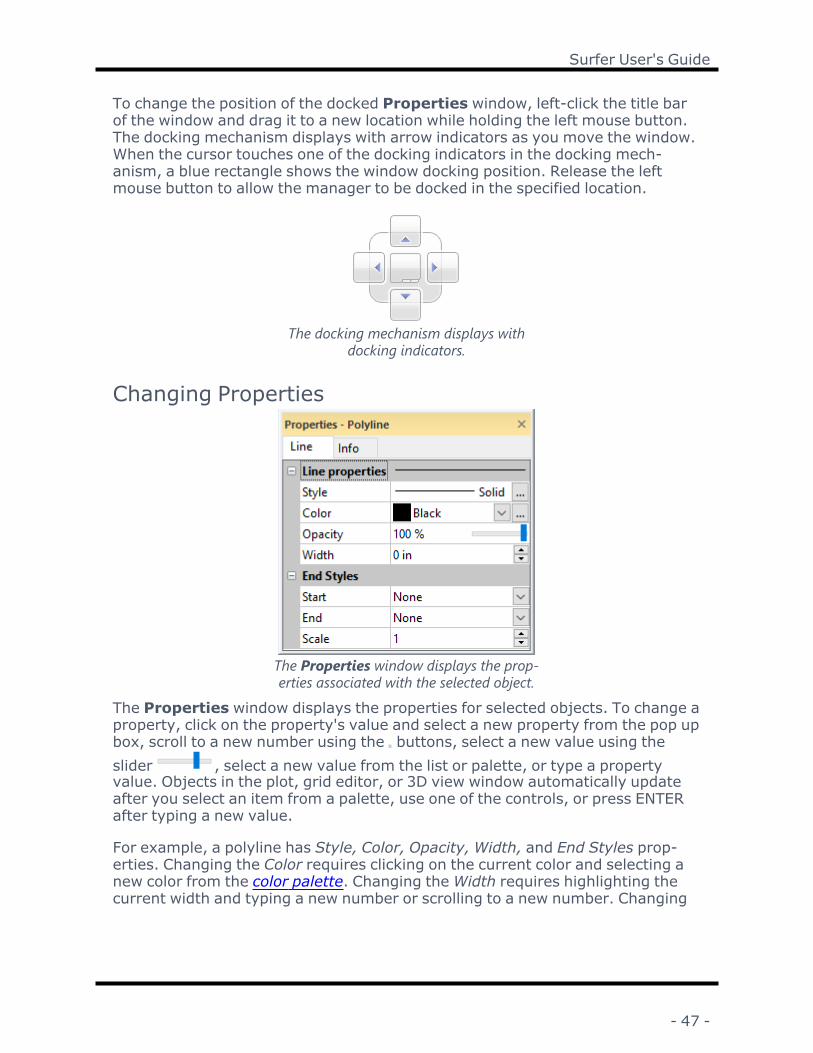
The docking mechanism displays withdocking indicators.
Changing Properties
The Properties window displays the prop-erties associated with the selected object.
The Properties window displays the properties for selected objects. To change aproperty, click on the property's value and select a new property from the pop upbox, scroll to a new number using the buttons, select a new value using theslider , select a new value from the list or palette, or type a propertyvalue. Objects in the plot, grid editor, or 3D view window automatically updateafter you select an item from a palette, use one of the controls, or press ENTERafter typing a new value.
For example, a polyline has Style, Color, Opacity, Width, and End Styles prop-erties. Changing the Color requires clicking on the current color and selecting anew color from the color palette. Changing theWidth requires highlighting thecurrent width and typing a new number or scrolling to a new number. Changing
- 47 -

Chapter 1 - Introduction
the Opacity requires highlighting the current value and typing a new number orclicking on the slider bar and dragging it to a new value.
You can modify more than one object at a time. Only shared properties can bechanged are when multiple objects are selected. For example, you can click on apolyline in the Contents window. Hold the CTRL key and click on a polygon. Youcan then change the line properties of both objects at the same time. Fill prop-erties, which are available if only a polygon is selected, are not available as thepolyline does not have fill properties.
Some properties are dependent on your other selections. For example, there is aPattern Offset section on the Fill page. This section is only available when animage fill type is selected as the Pattern.
Expand and Collapse FeaturesFeatures with multiple options appear with a or to the left of the name. Toexpand a group, click on the icon. To collapse the group, click on the icon.For example, the expanded Filled Contours section in the Levels page containsthree options, Fill contours, Fill colors, and Color scale.
Keyboard CommandsTo activate the Properties window, press ALT+ENTER on the keyboard. Whenworking with the Properties window, the up and down arrow keys move up anddown in the Properties window list. The TAB key activates the highlighted prop-erty. The right arrow key expands collapsed sections, e.g., Filled Contours, andthe left arrow collapses the section.
Property DefaultsUse the File | Options command to change the default settings. Default set-tings for rulers, drawing grid, line, fill, text, symbol, label format, and advancedsettings that control each map type can be set from the Options dialog.
Property Information AreaIf the Show property info area is checked on the Options dialog User Interfacepage, a short help statement for each selected command is presented in theProperties window.
Status BarThe status bar is located at the bottom of the Surfer window. The status bar dis-plays information about the current command or activity in Surfer. Click theView | Show/Hide | Status Bar check box to show or hide the status bar.
- 48 -

Surfer User's Guide
A check mark next to Status Bar indicates that the status bar is displayed. Clearthe Status Bar check box to hide the status bar.
Status Bar SectionsThe status bar is divided into five sections. The left section displays informationabout the selected command or item in the Properties window. The second sec-tion shows the selected object name or the number of objects/points in the selec-tion. The middle section shows the cursor coordinates in map units, if the cursoris placed above a map. The fourth section shows the cursor coordinates in pageunits of inches or centimeters. The right section displays the dimensions of theselected object. In the worksheet, the status bar displays tool tips.
The status bar has five sections of information.
Grid Editor Status Bar SectionsWhen viewing a grid in the grid editor, the first three sections of the status bardisplay a description for the selected property in the Properties window, the act-ive grid node grid coordinates, and the map coordinates of the cursor location.
The status bar displays different information when viewing a grid in the grid editor.
Adjust Section WidthThe status bar section widths can be adjusted to display additional text. If "..." isdisplayed at the end of the text, additional text can be displayed. To change thewidth, place the cursor over a section division. When the cursor changes to a ,left-click and drag the divider left or right to a new location.
A portion of the status bar. The "..." in the left section indicates there is additionaltext.
A portion of the status bar after making the left section larger.
ProgressThe Progress dialog indicates the progress of a procedure, such as gridding.The percent of completion and time remaining will be displayed. Click Cancel tostop the current process.
- 49 -

Chapter 1 - Introduction
The progress of a procedure is shown in the Progress dia-log.
When the program does not know how much time is required to complete a task,the Indeterminatemode is displayed in the Progress dialog. This indicates thatthe program is actively completing the task, with an unknown time of com-pletion. The program is not frozen.
The Progress dialog does not display a percentage or timeestimate in Indeterminate mode.
Menu and Tab CommandsThe ribbon contains the commands that allow you to add, edit, and control theobjects on the plot, worksheet, grid editor, or 3D view window page.
Plot Document CommandsWhen viewing a plot document, the main ribbon tab commands are available:
File Open and save files, import or export data, print, and setoptions and defaults
Home Contains common editing, selection, feature, grid, and mapcommands
Layout Set the page display and arrange or position maps andobjects in the plot document
- 50 -
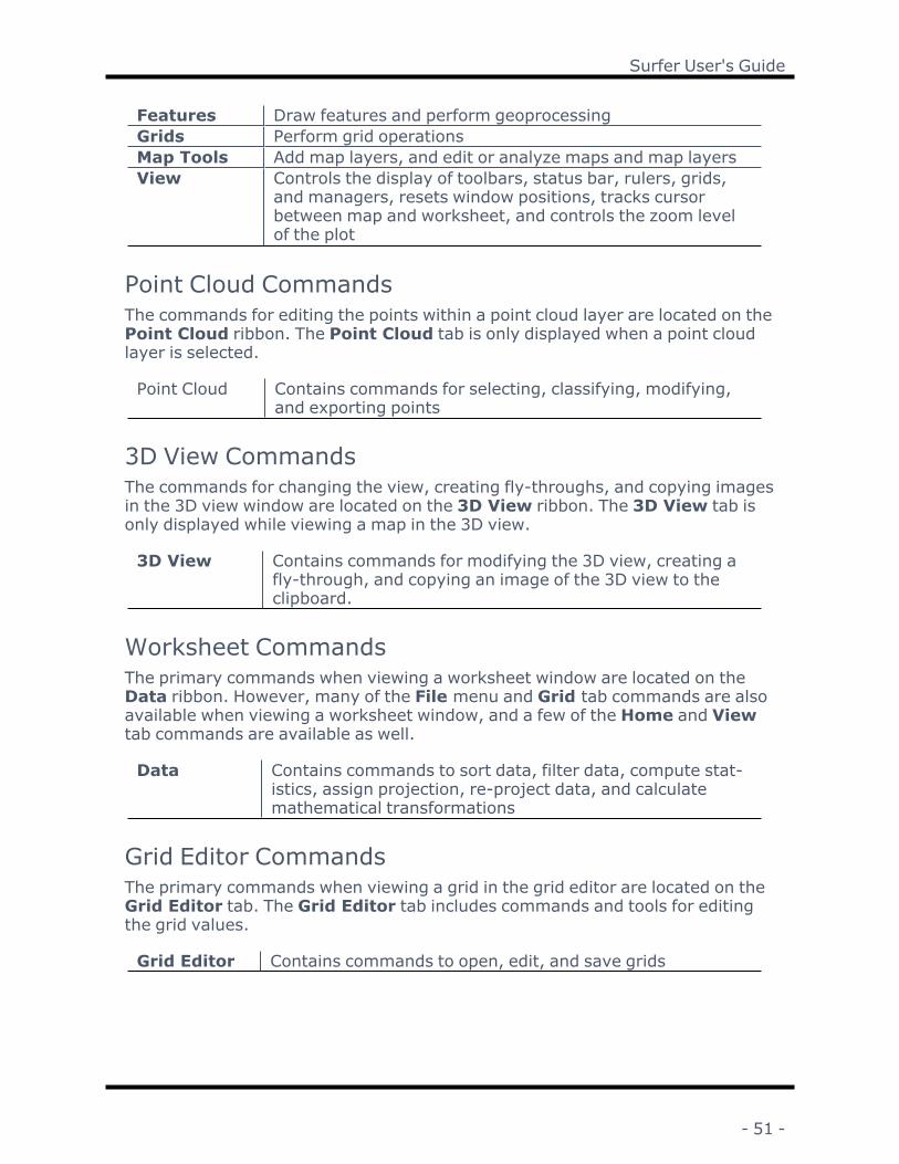
Surfer User's Guide
Features Draw features and perform geoprocessingGrids Perform grid operationsMap Tools Add map layers, and edit or analyze maps and map layersView Controls the display of toolbars, status bar, rulers, grids,
and managers, resets window positions, tracks cursorbetween map and worksheet, and controls the zoom levelof the plot
Point Cloud CommandsThe commands for editing the points within a point cloud layer are located on thePoint Cloud ribbon. The Point Cloud tab is only displayed when a point cloudlayer is selected.
Point Cloud Contains commands for selecting, classifying, modifying,and exporting points
3D View CommandsThe commands for changing the view, creating fly-throughs, and copying imagesin the 3D view window are located on the 3D View ribbon. The 3D View tab isonly displayed while viewing a map in the 3D view.
3D View Contains commands for modifying the 3D view, creating afly-through, and copying an image of the 3D view to theclipboard.
Worksheet CommandsThe primary commands when viewing a worksheet window are located on theData ribbon. However, many of the File menu and Grid tab commands are alsoavailable when viewing a worksheet window, and a few of the Home and Viewtab commands are available as well.
Data Contains commands to sort data, filter data, compute stat-istics, assign projection, re-project data, and calculatemathematical transformations
Grid Editor CommandsThe primary commands when viewing a grid in the grid editor are located on theGrid Editor tab. The Grid Editor tab includes commands and tools for editingthe grid values.
Grid Editor Contains commands to open, edit, and save grids
- 51 -

Chapter 1 - Introduction
The Application/Document Control Menu commands control the size andposition of the application window or the document window.
WorksheetsWorksheet windows are a view of the data file and are designed to display, edit,enter, and save data. The worksheet windows have several useful and powerfulediting, transformation, and statistical operations available. In addition, acoordinate system can be assigned to the data file. Several import and exportoptions are available for opening data files from other spreadsheet programs.The components of the worksheet window are displayed below.
Worksheet CommandsThe worksheet commands include commands on the following tabs:
File Open and save files, import or export data, print, and set optionsand defaults
Home Contains clipboard and undo commandsGrids Perform grid operationsView Controls the display of status bar and windows and resets window
positionsData Edit, find, format data in the worksheet. Manipulate, transform,
and perform calculations with worksheet data. Assign or projectcoordinates. Track the cursor between the plot, worksheet, andgrid windows.
Not all of the File, Home, Grids, and View commands are available in the work-sheet view.
The Application/Document Control menu commands control the size and positionof the application window or the document window.
Tab ViewThe plot, worksheet, and grid node editor windows are displayed as tabbed doc-uments. When more than one window is open, tabs appear at the top of the doc-ument, allowing you to click on a tab to switch to a different window. The tabsmay be dragged to reorder them. When a document contains unsaved changes,an asterisk (*) appears next to its tabbed name. The asterisk is removed oncethe changes have been saved.
Worksheet WindowThe image below displays the parts of the worksheet document.
- 52 -

Surfer User's Guide
This is the Surfer worksheet document with the Contents and Properties windows inauto hide mode on the left, and the plot document and worksheet tabs at the top of
the worksheet.
Grid Editor
The File | Open, Grids | Editor | Grid Editor command, the button, andtheMap Tools | Edit Layer | Grid commands open the grid editor as a newdocument.
l
The Grids | Editor | Grid Editor command and the button open a gridfile with the Open Grid dialog.
l TheMap Tools | Edit Layer | Grid command opens the grid file from theselected map layer in the plot document. You can also edit the grid for a maplayer by right-clicking on the map layer and clicking Edit Grid. This com-mand enables the Update Layer command in the grid editor. TheMapTools | Edit Layer | Grid command is not available for 1-grid vector and 2-grid vector layers.
- 53 -

Chapter 1 - Introduction
The grid editor contains various methods for editing the grid Z values. Editing thegrid Z values will change the appearance of any grid-based maps. For example,the grid editor can be used to edit contours on a contour map or change the sur-face in a 3D surface map.
Each grid node is indicated with a black "+" in the grid editor window by default.Each NoData grid node is indicated with a blue "x" by default. The active node ishighlighted with a red diamond. To move between grid nodes, press the arrowkeys, or click a node with the Select tool active to make it the active node. Thegrid editor also includes contours, node labels, and a color fill. The grid appear-ance is controlled by the items in the Contents window and the properties dis-played in the Properties window. Note the Undo command does not undochanges in the Properties window in the grid editor.
Images in the Grid EditorThe grid editor also allows you to open an image file and save as a grid file.
A grid requires a single floating point value at each grid node. Images contain col-ors which are three separate values (Red, Green, Blue) at each pixel.
Color ImageColor image formats are converted to a single floating point value by calculatingthe intensity of each color value using the intensity equation:
I = A(.30R + .59G + .11B)
where I = intensity, R,G,B,A are the red, green, blue, and normalized alpha val-ues.
For example, a pixel from a color image with Red=255, Green=0, and Blue=0would be mapped to a grid node with the value of:
I = .30*255 + .59*0 + .11*0 = 77
Grayscale ImageGrayscale images are imported directly. Grayscale images have a single colorvalue and do not need to use the intensity equation. Surfer does not normalizethe grayscale value. The value is used exactly as specified in the image.
For example, consider a grayscale image with a pixel that contains a value of 55.The grid node value would be set to 55.
Grid Editor WindowThe following image and table explain the purpose of the grid editor window com-ponents.
- 54 -

Surfer User's Guide
This is the Surfer grid editor with the Contents and Properties windows on the left and grideditor window on the right.
ComponentName
Component Definition
Ribbon The ribbon contains the Grid Editor commands.Contents Toggle the display of the Node Labels, Node Symbols, Con-
tours, and Color Fill with the Contents window.Properties Edit Node Labels, Node Symbols, Contours, and Color Fill dis-
play properties in the Properties window.Tabbed Docu-ments
Plot windows, worksheet windows, and grid editor windowsare displayed as tabbed documents.
Tool Options The tool options bar contains the Z value box, Brush size,Density, and/or Pressure depending on the selected toolmode.
- 55 -

Chapter 1 - Introduction
Active Node The node that is currently selected. The active node is high-lighted with a red diamond.
Grid Node Each grid node is indicated with a black "+" in the grid editorwindow by default. NoData nodes are indicated with a blue"x".
Status Bar The status bar includes information about the selected prop-erty, active node grid coordinates, and cursor map coordin-ates.
Grid Editor CommandsThe Grid Editor ribbon tab includes the following commands:
Select Select a grid node to edit the grid Z values one node at a timeBrush Apply a specific Z value to one or more nodesWarp Drag grid values from one region into anotherSmooth Apply weighted averaging to grid nodesPush Down Decrease grid node valuesPull Up Increase grid node valuesEraser Assign the NoData value to grid nodesEyedropper Acquire a grid node value by clicking on the gridUndo Undo the last operationRedo Redo the last undone operationFit to Win-dow
Fits the entire grid in the grid editor window
Zoom In Increase the grid editor window magnificationZoom Out Decrease the grid editor window magnificationZoom Rect-angle
Zoom in to an area of interest
Grid Info Display information about the grid in a report windowTrackCursor
Track cursor location across plot, worksheet, and grid editorwindows for maps, data files, and grids.
UpdateLayer
Updates the associated map layer with the edited grid
Using the Grid EditorThe grid editor can be used on existing map layers or on grid files without firstcreating a map.
To edit a map layer's grid:1. Select the map layer created from a grid file to edit in the plot document Con-tents window. Only the grid for this map layer will be edited even when mul-tiple layers, such as contour or color relief, use the same grid file.
- 56 -

Surfer User's Guide
2. ClickMap Tools | Edit Layer | Grid in the plot window. The grid file isopened and is represented by a filled contour map. The location of each gridnode in the file is marked with a black "+". NoData nodes are marked with ablue "x".
3. Use the Grid Editor | Tools commands to make the desired adjustments tothe grid.
4. When you are done editing the grid, click the Grid Editor | Options |Update Layer command to update the map layer in the plot document withyour grid.
5. Click the plot document tab to view the changes to the map layer. If you wishto revert the changes to the map layer, click the Undo command while view-ing the plot window. If you are satisfied with the changes to the map layer,you may wish to save the edited grid to a file.
6. If you wish to save your edits to a file, click File | Save As to create a newgrid file. Click File | Save to overwrite the existing grid file. It is necessary tosave your edits to a file with Save or Save As if you wish to update all layersin your map to use the edited grid.
7. To close the grid editor window, click the File | Close command or click the Xin the grid editor document tab. To view an existing window and keep the grideditor window open, click on another document tab.
To edit a grid file:1. Click the Grids | Editor | Grid Editor command and select the grid file in
the Open Grid dialog. Alternatively, click the File | Open command andselect a grid file in the Open dialog. The grid file is opened and is representedby a filled contour map. The location of each grid node in the file is markedwith a black "+". NoData nodes are marked with a blue "x".
2. Use the Grid Editor | Tools commands to make the desired adjustments tothe grid.
3. When you are done editing the grid, click File | Save As to create a new gridfile. Click File | Save to overwrite the existing grid file. It is necessary tosave your edited grid to a file with Save or Save As if you wish to create maplayers with the grid.
4. To close the grid editor window, click the File | Close command or click the Xin the grid editor document tab. To view an existing window and keep the grideditor window open, click on another document tab.
File TypesSurfer uses four basic file types: data, grid, base map, and Surfer .SRF files.
Data FilesVarious types of data files are used to produce grid files, point cloud maps, anddrillhole maps or to post data points on a map. These files are generally referredto as XYZ data files or data files throughout the help. Data can be read from
- 57 -

Chapter 1 - Introduction
various file types. Most data files contain numeric XY location coordinates andoptional Z values. The Z values contain the variable to be modeled, such as elev-ation, concentration, rainfall, or similar types of values.
XYZ data files contain raw data that Surfer interprets to produce a grid file. Tocreate a grid file, you must start with an XYZ data file. XYZ data files are organ-ized in column and row format. Surfer requires the X, Y, and Z data to be in threeseparate columns.
Grid FilesGrid files, also known as raster files, produce several different types of grid-based maps, are used to perform grid calculations, and to carry out grid oper-ations. Grid files are a regularly spaced rectangular array of Z values in columnsand rows. Grid files can be created in Surfer using the Home | Grid Data |Grid Data command or can be imported from a wide variety of sources such asWCS servers or other applications.
Base Map FilesBase map files contain XY location data such as aerial photography, state bound-aries, rivers, or point locations. Base map files can be used to create layers over-laid on other map types, or to specify the limits for assigning NoData values,faults, breaklines, or slice calculations. Base map files can be created from awide variety of vector and image formats. Base map files may be referred to asvector data files, raster data files, and images or image files in the help, depend-ing on the type of data in the base map file.
Surfer FilesSurfer .SRF files preserve all the objects and object settings contained in a plotwindow. These files are called Surfer .SRF files throughout the documentation.Surfer can open .SRF files from previous versions as far back as Surfer 7.Surfer can save files to previous .SRF formats for sharing with other users. Forexample, the Surfer 15 Document .SRF file type can be opened in Surfer 15, butdoes not contain features that are in later Surfer versions. Beginning with ver-sion 16, the Surfer Plot (*.srf) file type is backwards compatible with all Surferversions 16 and newer.
Gridding OverviewA grid, also known as a raster in other software products, is a rectangular regioncomprised of evenly spaced rows and columns. The intersection of a row andcolumn is called a grid node. Rows contain grid nodes with the same Y coordin-ate. Columns contain grid nodes with the same X coordinate. Contour, colorrelief, grid values, peaks and depressions, vector, viewshed, watershed, 3D sur-face, 3D wireframe map layers all require grids in Surfer.
- 58 -

Surfer User's Guide
What is Gridding?Gridding is the process of taking irregularly or regularly spaced XYZ data and gen-erating a regularly spaced grid of Z values at each grid node by interpolating orextrapolating the data values. In addition to gridding data, Surfer can also use avariety of other grid files directly. For a list of these, refer to the File FormatChart in the online Help.
Gridding MethodsGridding the data produces a regularly spaced, rectangular array of grid nodes,with a calculated Z value at each node, from regularly or irregularly spaced XYZdata. The term "irregularly spaced" means that the distance between data pointsvaries in the X or Y direction, or both. Irregularly spaced data often has manyholes where data are missing. Gridding calculates the Z values for grid nodeswhere data exists, and can also calculate the Z values for grid nodes in the holeswhere no data exists, by extrapolating or interpolating the Z values in the data.The gridding method determines the mathematical algorithms used to computethe Z value at each grid node. Each method results in a different representationof your data. It is advantageous to test each method with a typical data set todetermine the gridding method that provides you with the most satisfying inter-pretation of your data.
When your XYZ data is regularly spaced, meaning the distance between datapoints does not change in the X and Y directions, you may produce a grid file thatuses the Z values directly and does not interpolate values for the grid nodes. Seethe Producing a grid file from a regular array of XYZ data help topic for moreinformation.
General Gridding OptionsEach gridding method has its own set of gridding options. Some of the optionsare the same or similar for the different gridding methods, while other optionsare specific to particular gridding methods. Some options that are available tomultiple gridding methods include: Search, Anisotropy, Breaklines, and Faults.
Map TypesSeveral different map types can be created, modified, and displayed withSurfer. These map types include base, contour, post, classed post, 3D surface,3D wireframe, color relief, grid values, drillhole, peaks and depressions, pointcloud, watershed, viewshed, 1-grid vector, and 2-grid vector maps. A briefdescription and example of each map is listed below.
- 59 -

Chapter 1 - Introduction
This is a base map of Michigan withcounty polygons. One of the individual
polygons has fill.
Base MapBase maps display boundaries on a map andcan contain polygons, polylines, 3D poly-gons, 3D polylines, 3D polymesh objects,points, text, images, or metafiles. Basemaps can be overlaid with other map layersto provide details such as roads, buildings,streams, city locations, areas of no data,and so on. Base maps can be produced fromvector files, images, and data files. Indi-vidual base map objects can be edited,moved, reshaped, or deleted. Symbologycan be added to a base map to com-municate statistical information about themap features. Empty base maps can be cre-ated and used for drawing objects on othermaps. Raster (image) and vector base mapscan be downloaded from online WMS, OSM,and WFS mapping servers.
This is a contour map consisting of con-tour lines representing elevation.
Contour MapContour maps are two-dimensional rep-resentations of three-dimensional data. Con-tours define lines of equal Z values acrossthe map extents. The shape of the surface isshown by the contour lines. Contour mapscan display the contour lines and colors orpatterns between the contour lines. Con-tours can be linearly or logarithmicallyspaced, or a custom spacing can be setbetween each set of lines.
The post map layer has black symbols.The classed post map layer has red
Post MapPost maps and classed post maps show datalocations on a map. You can customize thesymbols and text associated with each datalocation on the map. Each location can havemultiple labels. Classed post maps allowyou to specify classes and change symbolproperties for each class. Classes can besaved and loaded for future maps.
- 60 -

Surfer User's Guide
circles and blue squares. Only a sampleof the data set is displayed in the
classed post map.
This is a 3D surface map of the Tel-luride, Colorado USGS SDTS grid file.
3D Surface Map3D surface maps are color three-dimen-sional representations of a grid file. The col-ors, lighting, overlays, and mesh can bealtered on a surface. Multiple 3D surfacemaps can be layered to create a block dia-gram.
This is a 3D wireframe map with a cus-tom rotation (47° ), tilt (49° ), and field
of view (112° ).
3D Wireframe Map3D wireframe maps are three-dimensionalrepresentations of a grid file. Wireframesare created by connecting Z values alonglines of constant X and Y.
This is a color relief map of theHelens2.grd sample file.
Color Relief MapColor relief maps are raster images basedon grid files. Color relief maps assign colorsbased on Z values from a grid file. NoDataregions on the color relief map are shown asa separate color or as a transparent fill.Pixels can be interpolated to create asmooth image. Hill shading or reflectanceshading can be applied to the color reliefmap to enhance its depth and appearance.
- 61 -

Chapter 1 - Introduction
The grid values layer posts symbols,labels, and/or lines along grid rows and
columns at a specified density.
Grid Values MapGrid values maps show symbols labels atgrid node locations across the map. Thedensity of the labels and symbols is con-trolled in the X and Y directions inde-pendently. Symbol color can vary by valueacross a colormap, and symbols and labelscan be displayed for only a specific range ofvalues. Grid lines can be added to the map.
This is a watershed map of a USGSSDTS grid file.
Watershed MapWatershed maps display the direction thatwater flows across the grid. The watershedmap breaks the grid into drainage basinsand streams. Colors can be assigned to thebasins and line properties can be associatedwith the streams. In addition, depressionscan be removed by filling the depression.
This is a 1-grid vector map of Coloradoelevations.
Vector Map1-grid and 2-grid vector maps display dir-ection and magnitude data using indi-vidually oriented arrows. At any grid nodeon the map, the arrow points in the downhilldirection of the steepest descent and thearrow length is proportional to the slopemagnitude. Vector maps can be createdusing information in one grid file (i.e. anumerically computed gradient) or two dif-ferent grid files (i.e. each grid giving a com-ponent of the vectors).
- 62 -

Surfer User's Guide
This is a point cloud of the Golden, COarea from USGS Elevation Source Data
Point Cloud MapPoint cloud maps display LAS/LAZ data aspoints at XY locations. LAS/LAZ data can becombined from multiple files and filteredwith various criteria when creating a pointcloud map. Color is assigned to the pointsby elevation, intensity, return number, orclassification. Surfer includes commands formodifying, classifying, and exporting pointsin a point cloud layer. A grid can be createdfrom the point cloud layer. Point cloud lay-ers are displayed in the 3D View as three-dimensional points.
This is a viewshed layer overlaid on acontour map.
Viewshed LayerViewshed layers highlight the regions of amap that are visible (or invisible) from atransmitter location. The transmitter,receiver, and obstruction height above thesurface can be specified. The viewshed ana-lysis radius and angle can also be specified.Viewsheds can be added to any 2D gridbased map. A viewshed can also be addedto a 3D surface map that is displayed withno tilt (90 degrees) and in the orthographicview.
The legend for this peaks anddepressions map of the CraterLake area explains the shaded
areas and markings.
Peaks and Depressions MapVolumes of surface water and ground waterare informed by topographic data, Karsttopography, and geographic data, which arecaptured in Surfer grid files and mapped inpeaks and depression maps. Boundariescan be drawn around peaks where waterflows from and depressions which capturewater to create unique areas for statisticalanalysis.
- 63 -

Chapter 1 - Introduction
This is a 3D view of a drillholelayer
Drillhole MapA drillhole map can be created from collars,survey, intervals, and point data. The 2Ddrillhole layer shows the location, deviation,and path of each hole, core, or well. The drill-hole map can also be viewed in 3D. Separ-ate symbols can be defined to create alegend of the drillholes by hole id or anyother attribute in the data.
Map Wizard
Click the Home | Wizard | Map Wizard command or the button to createa map with the Map Wizard. TheMap Wizard steps through the map creationprocess from raw data to a map with one or more layers. If necessary, data isgridded to create a grid-based map layers.
TheMap Wizard consists of two or three pages, depending on the input datatype. Click the following links for more information on each of the wizard pages.
1. Select Your Data - Select the data, boundary, or grid file you wish to use tocreate your map.
2. Select Your Map Type - Select one or more map layer types and decide to cre-ate a new map or place the new layers in an existing map.
3. Select Gridding Parameters - Create a grid file if you selected a data file and agrid-based layer in the first two steps.
A map is created, or layers are added to a map, in the plot window after pro-ceeding through theMap Wizard.
Map Wizard - Select Your DataClick the Home | Wizard | Map Wizard command to open theMap Wizard.The first page is the Select Your Data page. Here you select the data, grid,boundary, or image file you wish to use to create your map. Once you have selec-ted your data source, click Next to proceed to the Select Your Map Type page.
- 64 -

Surfer User's Guide
Specify the data file and coordinate columns or grid file you wish to use to create a map.
Select FileSelect your data, grid, vector, or image file in the Select File list. The Select Filelist includes a list of Recent files, Sample files, Project files, or files in a folder youselect with Browse. To change the Select File list, click the current selection atthe top of the list and select Recent files , Sample files, Project files, or Browse.
Recent FilesWhen Recent files is selected in the Select File list, the most recently opened filesare displayed in the Select File list. By default the number of files in the Recentfiles list is 10. Change the number of files in the Recent files list in the Options dia-log User Interface page.
Sample FilesWhen Sample files is selected in the Select File list, the sample files included withSurfer are displayed in the Select File list.
- 65 -

Chapter 1 - Introduction
Project FilesWhen Project files is selected in the Select File list, the files located in the userdefined project folder are displayed in the Select File list. The Project folderoption can be set in the Options dialog on the General page or in the Welcome toSurfer dialog.
BrowseClick Browse near the Select File list to open a file with the Open dialog. After youselect a file in the Open dialog, the file preview is loaded in the Select YourData page and the folder contents are visible in the Select Files list.
Data PreviewThe Data Preview section contains a preview of the selected file. Check the Showpreview check box to see a preview of the selected data, grid, or boundary file.When a file is selected in the Select File list, the file is loaded and a preview is dis-played. The Surfer status bar displays the loading progress for large data files.
l Data files are displayed in a table.
l Grid files are displayed as a color relief map.
l Boundary files are displayed as a base map.
Clear the Show preview check box to hide the preview.
Select Data ColumnsWhen a data file is selected in the Select File list, the Select Data Columns sec-tion is displayed. Specify the columns that contain the X, Y, and Z data in theSelect Data Columns table. The Coordinate column indicates the row for the X, Y,and Z selections. The Column column includes the column letter and, if a headerrow is present, the column header. To change a selection, click the column youwish to changed and select the desired column from the list.
Next and CancelClick Next to proceed to the Select Your Map Type page. Click Cancel to close theMap Wizard without creating a map.
Map Wizard - Select Your Map TypeClick the Home | Wizard | Map Wizard command to open theMap Wizard.The second page is the Select Your Map Type page. Here you select the layertypes you would like to create in your map and whether to create a new map oradd the layers to an existing map. Click Next to proceed to the Select GriddingParameters or click Finish to create your map. Which button is displayed dependson your selections in the Select Your Data and Select Your Map Type pages.
- 66 -

Surfer User's Guide
Specify the layer types you wish to create and select whether to create a new map or add thelayer(s) to an existing map.
Add Layer ToThe Add layer to option determines if the new map layer or layers will be addedto a new map or an existing map. A new map is created by default. Select [NewMap] to create a new map in the plot document. Alternatively, click the Add layerto field and select an existing map from the list to add the layers to an existingmap.
Map TypesSelect the desired layer types by clicking the map type. A check mark indicates amap layer will be included. Click on a selected layer type to clear the check box.A lock indicates the map type is not compatible with the source file selected onthe Select Your Data page.
l Data files can be used to create any of the map layer types: Base, Contour,Post, Classed Post, Color Relief, 3D Surface, 3D Wireframe, Watershed, 1-Grid Vector, and Grid Values.
- 67 -

Chapter 1 - Introduction
l Grid files can be used to create the grid-based map layers: Contour, ColorRelief, 3D Surface, 3D Wireframe, Watershed, 1-Grid Vector, and Grid Val-ues.
l Boundary files can only be used to create a Base map. Try the Home |New Map | Base command to quickly create base maps without theMapWizard.
The 3D wireframe layer type cannot be overlaid with a 3D surface or color relieflayer. When a new selection cannot overlay with a previous selection, the pre-vious selection is cleared.
Creating Grid Based Maps from Data FilesWhen a data file is selected on the Select Your Data page and a grid-based layeris selected on the Select Your Map Type page, a grid must be created beforecreating the map. The Finish button changes to Next. Click Next to proceed tothe Select Gridding Parameters page and create the grid.
When the data source is a grid file or boundary file, the map can be created byclicking Finish.
DescriptionThe Description section includes a brief explanation of the map type, as well aswhich data types are used to create the layer type and any conflicts with otherlayer types.
Back, Finish, Next, or CancelClick Back to return to the Select Your Data page if you wish to change the datasource. Click Finish to create your map. When gridding is necessary, click Next toproceed to the Select Gridding Parameters page. Click Cancel to close theMapWizard without creating a map.
Map Wizard - Select Gridding ParametersClick the Home | Wizard | Map Wizard command to open theMap Wizard.The third page is the Select Gridding Parameters page. Here you specify thegridding parameters for creating the grid for the grid-based layer or layers. Onceyou have specified the gridding parameters, click Finish to create your grid fileand map.
- 68 -

Surfer User's Guide
Specify gridding parameters for creating a grid from the source data file.
Simple Gridding ParametersSelect Simple gridding parameters to quickly generate a grid with the defaultgridding options. When Simple gridding parameters is selected, specify the Grid-ding method and output grid geometry.
Gridding MethodSurfer has several different gridding methods. These gridding methods definethe way in which the XYZ data are interpolated when producing a grid file.Change the Gridding method by clicking the current selection and selecting thedesired method from the list. Refer to the gridding methods for more informationon the options.
Output Grid GeometryThe Output Grid Geometry section defines the grid limits and grid density. TheOutput Grid Geometry section also controls whether grid nodes outside the dataare automatically assigned the NoData value. See the Grid Data topic for a gridgeometry example.
- 69 -

Chapter 1 - Introduction
Copy GeometryThe Copy geometry from option copies the grid geometry from an existing maplayer or grid file. This option is useful when creating grids that will become over-laid map layers, processed with the Grid Math command, or used to calculate avolume between two surfaces. TheMath and Volume commands require theinput grids to have the same geometry.
To copy the geometry from an existing layer, select the layer in the Copy geo-metry from list. To copy the geometry from a grid file, click Browse and selectthe file in the Open Grid dialog. Select <None> to return the Output Grid Geo-metry options to their default values and to manually edit the grid geometry.
Minimum and Maximum X and Y Coordinate (Grid Limits)Grid limits are the minimum and maximum X and Y coordinates for the grid.Surfer computes the minimum and maximum X and Y values from the XYZ datafile. These values are used as the default minimum and maximum coordinatesfor the grid.
Grid limits define the X and Y extent of contour maps, color relief maps, vectormaps, 3D wireframes, and 3D surfaces created from grid files. When creating agrid file, you can set the grid limits to the X and Y extents you want to use foryour map. Once a grid file is created, you cannot produce a grid-based map lar-ger than the extent of the grid file. If you find you need larger grid limits, youmust regrid the data. You can, however, read in a subset of the grid file to pro-duce a map smaller than the extent of the grid file.
When either the X, Y, or Z value is in a date/time format, the date/time valuesare converted and stored in the grid as numbers.
Spacing and # of Nodes (Grid Density)Grid density is usually defined by the number of columns and rows in the grid,and is a measure of the number of grid nodes in the grid. The # of Nodes in the XDirection is the number of grid columns, and the # of Nodes in the Y Direction isthe number of grid rows. The direction (X Direction or Y Direction) that coversthe greater extent (the greater number of data units) is assigned 100 grid nodesby default. The number of grid nodes in the other direction is computed so thatthe grid nodes Spacing in the two directions are as close to one another as pos-sible.
By defining the grid limits and the number of rows and columns, the Spacing val-ues are automatically determined as the distance in data units between adjacentrows and adjacent columns.
Assign NoData Outside Convex HullCheck the box next to the Assign NoData outside convex hull of data to auto-matically assign the NoData value to the grid nodes outside the convex hull of
- 70 -

Surfer User's Guide
the data. Leave the box unchecked to extrapolate the data to the minimum andmaximum grid limits, regardless of whether data exists in these areas.
Output Grid FileChoose a path and file name for the grid file in the Output grid file option. You
can type a path and file name, or click the button to browse to a new pathand enter a file name in the Save Grid As dialog.
Advanced Gridding ParametersSelect Advanced gridding parameters for full control over the gridding method,advanced options, and grid geometry. After selecting Advanced gridding para-meters, click the Advanced Gridding Parameters button to set the griddingoptions in the Grid Data dialog. See the Grid Data topic for more information onthe advanced gridding parameters.
Back, Finish, or CancelClick Back to return to the Select Your Map Type page. Click Finish to create themap or add the layers to the existing map. Click Cancel to close the dialogwithout creating a map.
Introduction to Map LayersA map layer is a single map type contained in a larger map object. The map layermay be a contour layer, a post layer, a base layer, or any other layer type thatSurfer can create. The larger map object contains all of the individual map lay-ers and axes used to create the entire map. Map layers can be created as sep-arate maps or added to a single map object.
It is possible to combine several maps created from related data to create onemap object with multiple map layers. You can add any combination and numberof contour, base, post, color relief, grid values, point cloud, vector, watershed,viewshed, or 3D surface layers to a single map. However, a map can contain onlyone 3D wireframe layer.
There are multiple ways to overlay map layers in Surfer. If you have multiplemaps and wish to move only one layer, you can drag a map layer from one mapobject to another map object in the Contents window. If you wish to combine allthe layers from multiple maps, you can select all of the maps and use theMapTools | Map Tools | Overlay Maps command. This moves all of the map lay-ers to a single map object. If you have already created a map and need to addmap layers to it, you can select the map and use one of the Home | Add toMap | Layer commands to add a map layer to the existing map. Grid-basedmap layers can be changed to other layer types by selecting the object in theContents window and using theMap Tools | Layer Tools | Convert Layercommand.
- 71 -

Chapter 1 - Introduction
This one map object contains four map layers. There is a baselayer, watershed layer, contour layer, and a color relief layer.
Using Map LayersWhen you use map layers, the layers use a single set of X, Y, and Z axes and themaps are positioned according to the map object coordinate system. If two ormore maps use the same limits, they will overlay on top of one another. If mapscover adjacent areas, adding a map layer places them in the correct position rel-ative to one another and creates a single set of axes that span the entire range.Layered maps become a single object and are moved and scaled as a singleentity.
Consider a contour map and a base map that displays the outline of a lake on thecontour map. The limits of the base map are the X, Y extents of the lake and arenot the same as the contour map limits. If you create both the base map and thecontour map in a single plot window as separate maps by using the Home |New Map commands for both maps, they do not overlay correctly because themaps have different scaling. In addition, each map uses a different set of X, Yaxes. The two maps can be overlaid to correctly position the lake on the contourmap by dragging the base map layer to the other map object that has the con-tour layer. The result will be a map object with a base map layer and contourmap layer. Alternatively, if you create the contour map and then added a basemap layer with the Home | Add to Map | Layer | Base command, the twomaps are automatically scaled and combined into a single map using a single setof axes. The lake is correctly positioned on the contour map.
Sharing Data Between LayersSurfer maintains a list of files currently being used along with the data that isshared from those files among the various layers. Grids, images and data filesare recognized as being open in the background, thus making opening and usingfile information quicker. The Open dialogs for grids, images, and data files will
- 72 -

Surfer User's Guide
have their respective Open Grid, Open images, Open worksheet field that showsthe list of open files that can be shared.
Shared FilesSurfer tracks the files being used by maintaining a list of opened files for newmaps and the files used in saved maps. The file(s) used to build maps are shownin a compiled list in the Open Grids field of the Open Grid dialog. The only excep-tion is that vector data between base layers will not be shown.
Layers and 3D WireframesWhen you layer a contour, post, or base map on a 3D wireframe, the maps aredraped over the wireframe. The wireframe is drawn in the usual fashion but thebase, vector, or contour maps are "molded" over the top of the wireframe lines.Hidden lines are not removed from maps layered on wireframes. For example,contour lines are not hidden when the contour map lies over a wireframe.
Layers and 3D SurfacesWhen you layer maps on top of 3D surface maps, hidden lines are removed andthe maps are "molded" on the surface. Surface maps and images, vector files,and even other surface maps can be overlaid onto a single map object. The Over-lays page in the surface properties dialog contains options for handling color inthese cases.
Layer ExceptionsTheMap Tools | Add to Map | Layer commands add a map layer to the selec-ted map. Most combinations of map types can be layered. The exceptions arecombining a 3D wireframe and 3D surface map, adding a raster map layer orpoint cloud to a wireframe, and adding multiple wireframe layers. Raster mapsinclude color relief maps, surfaces, and base maps containing an image. Theoptions under the Add command change to fit the existing map. For example, ifa 3D wireframe map is selected, theMap Tools | Add to Map | Layer | 3DSurface command is grayed out.
Method 1: Adding a Map Layer to an Existing Map Frame1. Create a new map with a Home | New Map command. For example, you
can choose Home | New Map | Contour to create a contour map.2. Select the map and click theMap Tools | Add to Map | Layer command to
add a map layer. Select the map layer type to add to your existing map. Forexample, select the contour map and use theMap Tools | Add to Map |Post to add a post map layer to the contour map.
- 73 -

Chapter 1 - Introduction
3. The maps are combined in the correct position based on their coordinates andlimits. For example, in the Contents window, you will see one map objectwith a contour map layer and a post map layer.
Method 2: Overlaying Two Existing Maps1. Create a new map with a Home | New Map command. For example, you
can choose Home | New Map | Contour to create a contour map.2. Create a second map with the Home | New Map command. You could cre-
ate a post map with the Home | New Map | Post | Post command.3. Note that each map has an independent set of axes.4. Click Home | Selection | Select All to select both the contour and post
maps.5. ClickMap Tools | Map Tools | Overlay Maps. The two maps are com-
bined onto a single map object with a single set of axes. The empty mapobject is automatically deleted.
This method works well when you have multiple map layers that you want tocombine.
Method 3: Combining Two Existing Maps in the ContentsWindowIf two maps already exist, you can move (or overlay) a map layer from one mapframe into the other map frame by dragging and dropping in the Contents win-dow.
1. Create a new map with a Home | New Map command. For example, youcan choose Home | New Map | Contour to create a contour map.
2. Create a second map with the Home | New Map command. You could cre-ate a post map with the Home | New Map | Post | Post command.
3. Note that each map has an independent set of axes.4. Select the post map layer in the Contents window and drag it to the contour
map object. To do this, left-click and hold the left mouse button while youdrag the map layer to a new map frame. When the cursor changes to a hori-zontal arrow, release the left mouse button and the map layer is added to thecontour map's map frame. The post map will now be overlaid on the contourmap. An empty map frame may remain after removing the last map layerfrom the map object, depending on your options.
5. If an empty map frame exists, select the empty map frame and press DELETEon the keyboard to remove the empty map frame. The end result is a singlemap object with two map layers: a post map layer and a contour map layer.Additional map layers can be added with theMap Tools | Add to Map com-mands.
- 74 -

Surfer User's Guide
The contour map layer and the post map layer are displayed in separate mapobjects in the Contents window and the plot window.
First left-click and select the post map layer (left), then drag the post map layer to the othermap object. When the cursor is a horizontal arrow (middle), release the mouse button to drop
the map layer in the new location (right).
The result of this method is one Map object with two map layers.
Layer Map LimitsIf a map layer is added to a map frame and the map layer exceeds the currentmap limits, a Surfer warning message will be displayed allowing you to adjustthe map limits to include all layers. Select Yes to adjust the map to include all lay-ers. Select No to leave the current map limits.
- 75 -
Chapter 1 - Introduction
Editing a Map LayerTo edit individual layers in a multi-layer map, select the map layer (i.e.Contours) in the plot window or Contents window and use the Properties win-dow to edit the properties. Make the desired changes in the map layer prop-erties, and the map layer is redrawn with the specified changes.
Hiding a Map LayerAfter adding map layers, it is possible to hide one or more of the layers. To tem-porarily hide a map layer, uncheck the visibility box next to the map layer name(i.e. Contours) in the Contents window. The map is redrawn without the selectedoverlay. To make the overlay visible again, recheck the visibility box. Note that ifa surface is made invisible, the overlays are also made invisible.
Removing a Map LayerSelect the map layer and use the Break Apart Layer command to remove a maplayer from a map object. Alternatively, right-click on the map layer and selectBreak Apart Layer.
Deleting a Map LayerTo delete a map layer from a map frame, select the map layer in the Contentswindow and press the DELETE key on the keyboard. Alternatively, you can selectthe map layer and use the Home | Clipboard | Delete command, or right-clickthe map layer and select Delete.
Coordinate SystemsA coordinate system is method of defining how a file's point locations display ona map. Different types of coordinate systems exist that control how the coordin-ates are shown on the map. In Surfer, a map can be unreferenced in localcoordinates, referenced to a geographic latitude and longitude coordinate sys-tem, or referenced to a known projection and datum. Each data set, grid, maplayer, and the map frame can have an associated coordinate system. All coordin-ate systems for individual layers are converted “on the fly” to the map’s targetcoordinate system. This allows maps with different coordinate systems to be eas-ily combined in Surfer.
A local coordinate system generally is considered unreferenced. A local systemhas a location that begins numbering at an arbitrary location and incrementsnumbers equidistant in the X and Y directions from this location. This is fre-quently referred to as a Cartesian coordinate system. The distance units can bespecified for an unreferenced local system in the Assign Coordinate Systemdialog.
- 76 -

Surfer User's Guide
A Geographic coordinate system uses a spherical surface to define locations onthe earth. Geographic coordinate systems are commonly called unprojectedlat/long. Surfer has several predefined geographic coordinate systems avail-able. Each system has a different datum. The same latitude and longitude valuewill plot in different locations depending on the datum.
A Projected coordinate system consists of a projection and a datum. Each pro-jection distorts some portion of the map, based on the ellipsoid and datum spe-cified. Coordinates can be lat/long, meters, feet, or other units. Differentprojections cause different types of distortion. It is recommended that you donot use projected coordinate systems if you do not need to convert betweencoordinate systems or if all your data are in the same coordinate system.
Map Coordinate System OverviewIn Surfer, data, grids, map layers, and maps can have an associated coordinatesystem. All coordinate systems defined by the data, grids, and map layers areconverted "on the fly" to the map's target coordinate system. This allows mapswith different coordinate systems to be easily combined in Surfer.
The standard procedure for creating maps in a specific coordinate system is asfollows:
1. Create the map by clicking on the appropriate Home | New Map command.2. In the Open Grid(s) dialog, select the file to open and click Open.3. In the Contents window, click on the map layer to select it.4. In the Properties window, click on the Coordinate System page.5. If the Coordinate system is not correct, click the Set button next to Coordin-
ate System. The Assign Coordinate System dialog opens. This is the initialcoordinate system for the map layer, i.e. the coordinate system for thesource data. Select the correct coordinate system in the dialog. When fin-ished making changes, click OK.
6. To change the target coordinate system for the map, click on the Map objectin the Contents window. In the Properties window, click on the Coordin-ate System tab. This is the coordinate system in which you want the map todisplay.
7. Click on the Change button next to Coordinate System to set the desired tar-get coordinate system. When finished, click OK.
8. All of the map layers are converted on the fly to the target coordinate system.The entire map is now displayed in the desired coordinate system.
Surfer does not require a map coordinate system be defined. Maps can be cre-ated from unreferenced data, grid, and map layers. As long as all map layershave the same X and Y ranges, coordinate systems do not need to be specified.If you do not specify a source coordinate system for each map layer, it is highlyrecommended that you do not change the target coordinate system. Changes tothe target coordinate system for the map can cause the unreferenced map layersto appear incorrectly or to not appear.
- 77 -

Chapter 1 - Introduction
3D surface maps and wireframe maps cannot be converted to a new coordinatesystem.
File Menu CommandsThe Filemenu in the plot document has the following commands:
New Creates a new plot window or new worksheet windowOpen Opens a file in a plot documentOpen inWorksheet
Opens a data file in a worksheet
Close Closes the active documentClose All Closes all open documentsSave Saves the active documentSave As Saves the active document window to a new file name or loc-
ationImport Imports vector or graphics filesExport Exports vector or graphics filesReload MapData
Reloads external data used to generate maps
ReloadLayer Data
Reloads only external data used to generate the selected layer
PageSetup
Set the page options for the plot, or set the page and printingoptions for the worksheet
Print Prints the active plot document or worksheetOptions Set Surfer options and default properties in the plot windowDefaults Set advanced default settingsCustomizeRibbon
Customize the ribbon, quick access toolbar, and keyboardcommands
Online Check for Update or open the Golden Software Home Page,Surfer Product Page, or Frequently Asked Questions
Feedback Send a Problem Report, Suggestion, or Information RequestRecentDocuments
Open a recent plot, worksheet, or grid file
LicenseInfo
Activate a product key, connect to a license server, or viewlicense information
AboutSurfer
View version information, system information, and contactinformation
Exit Closes Surfer
- 78 -

Surfer User's Guide
New PlotYou can create a new plot document or worksheet with the File | New command
or click the button. Click the File | New | Plot command, or click the but-ton in the Quick Access Toolbar, to create a new plot document. Maps are cre-ated in a plot document.
New WorksheetYou can create a new plot document or worksheet with the File | New com-mand. The worksheet document is used to manage data. Click the File | New |
Worksheet command, or click the button in the Quick Access Toolbar, to cre-ate a new worksheet window.
OpenThe File | Open command opens a file as a map into a new plot window. Youcan also click on the button on the Quick Access Toolbar, or press CTRL + Oon the keyboard to open files.
Grid files open grid-based maps versus data files which open data-based maps.The default for grid files is set to the Color Relief Map whereas for data files thedefault is the Post Map. The default map types for grid files and data files can bechanged by the user by clicking on the File | Options command and navigating tothe General page.
Other file formats open as specific map types:
l Surfer .SRF files open in a new plot window.l Image files open as Base maps.l LAS files open as a point cloud layer map.l Vector files open as Base (vector) layer maps.
Instead of opening data files as maps, they may be opened as worksheets byclicking on the File | Open in Worksheet command. In the Open dialog, the filetypes shown are limited to Common Data Files (*...).
Open DialogClick the File | Open command in the plot document, worksheet document, orgrid node editor to open the Open dialog. Hold down the CTRL key while clickingon files to select multiple files, or hold down the SHIFT key to select adjacentfiles. Then click Open and the maps will open in a single plot window.
- 79 -

Chapter 1 - Introduction
Select the file to open in the Open dialog.Look InThe Look in field shows the current directory. Click the down arrow to see the dir-ectory structure and click on the folders to change directories.
Creating New Folders and Changing the ViewThe buttons to the right of the Look in field allow you to create new folders andchange the view of the file list.
File ListThe file list displays files in the current directory. The current directory is listed inthe Look in field. The Files of type field controls the display of the file list. Forexample, if Golden Software Data (*.DAT) is listed in the Files of type field only[*.DAT] files appear in the files list.
Specify a File NameThe File name field shows the name of the selected file, or type a path and filename into the box to open a file.
Specify a File TypeThe Files of type field shows the file format to be opened. To change the fileformat, click the down arrow and select the file type from the list. All Files (*.*)display all files in a directory.
- 80 -

Surfer User's Guide
The Common Document Files (*...) format type is selected when clicking the File| Open command. This displays all the common file formats in the navigationpane. If a different format type is selected, Surfer will remember the settinguntil the end of the current session. When Surfer is restarted, the default formattype will be used.
The Common Data Files (*...) format type is selected when clicking the File |Open in Worksheet command.
To see all files in the directory, choose All Files (*.*) from the Files of type list.Double-click on a file to open it or single click the file and then click the Open but-ton. The All Files shows all of the file formats even if the file type is not appro-priate for the action chosen (i.e. displaying a data file when creating a grid basedmap that requires a grid file).
Import DatabaseClick the Database button in the Open dialog to open the Data Link Propertiesdialog and import a database.
Data Link PropertiesYou can open database files in Surfer by clicking Database in the Open and OpenData dialogs or Load Database in the Import Data dialog. The Data Link Prop-erties dialog will open. Imported databases appear in a new worksheet window.Once the worksheet is saved, the link to the database is removed.
The data linking provides a method to link virtually any database supported byMicrosoft via an OLE DB Provider, ODBC, or some other supported format.Because the data link provides access to many types of databases that vary bycomputer, and since this link is provided by Microsoft, only general information isprovided here. Click Help in the Data Link Properties dialog to accessMicrosoft's help file for this dialog. If you need additional information on specificconnection information, contact your network administrator.
ODBC DriversNote that ODBC drivers are installed by the database program, not by Surfer. Ifa database program is not installed on the computer, a driver may still be able tobe located to import the data from the database. For example, the MicrosoftAccess database engine can be downloaded from Microsoft's website.
Data Link Properties DialogData linking is used to define links to many types of databases. The Data LinkProperties dialog is accessed by clicking the Database button in the Open orOpen Data dialogs or the Load Database button in the Import Data dialogs.The Open dialog appears when you use the File | Open command. The ImportData dialog appears when you use the worksheet File | Import command. TheOpen Data dialog appears when you use the Grid Data, New Variogram, ClassedPost Map, or Post Map command.
- 81 -
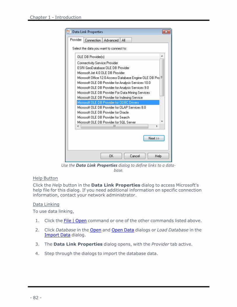
Chapter 1 - Introduction
Use the Data Link Properties dialog to define links to a data-base.
Help ButtonClick the Help button in the Data Link Properties dialog to access Microsoft'shelp file for this dialog. If you need additional information on specific connectioninformation, contact your network administrator.
Data LinkingTo use data linking,
1. Click the File | Open command or one of the other commands listed above.
2. Click Database in the Open and Open Data dialogs or Load Database in theImport Data dialog.
3. The Data Link Properties dialog opens, with the Provider tab active.
4. Step through the dialogs to import the database data.
- 82 -

Surfer User's Guide
Provider TabUse the Provider tab to select the appropriate OLE DB provider for the type ofdata you want to access. Not all applications allow you to specify a provider ormodify the current selection; this tab is displayed only if your application allowsthe OLE DB provider selection to be edited. You can save a data link with theapplication itself or as a separate file. For more information about creating a datalink, refer to the Microsoft help.
Option DescriptionOLE DBProvider(s)
Lists all OLE DB providers detected on your computer. For moreinformation about providers, see "Microsoft OLE DB ProvidersOverview" in the MDAC SDK.
Next Opens the Connection tab for the selected OLE DB provider.
Note You can navigate directly to the Connection tab by double-clicking thedesired provider. For more information about Data Links, see the Data Link APIReference.
Click Next or click the Connection tab to specify how to connect to ODBC data.
Connection TabThis Connection tab is provider-specific and displays only the connection prop-erties that are required by the Microsoft OLE DB Provider for ODBC.
Option DescriptionUse datasourcename
Select from the list, or type the ODBC data source name(DSN) you want to access. You can add more sources throughthe ODBC Data Source Administrator. Refresh the list by click-ing Refresh.
Use con-nectionstring
Allows you to type or build an ODBC connection string insteadof using an existing DSN.
Build Opens the Select Data Source dialog box. Once you select adata source the connection string in that data source willappear in the Connection tab of the Data Link Properties dia-log.
If you select a File DSN, the resulting ODBC connection stringis not based on a DSN. The ODBC connection string is per-sisted in the data link (.udl) file and does not rely on the selec-ted file DSN.
If you select a Machine DSN, the resulting ODBC connectionstring is based on a DSN. The ODBC connection string ref-erences the selected machine DSN. If a user on a different sys-tem attempts to access the data link (.udl) file, the user mustalso have the machine DSN installed.
- 83 -

Chapter 1 - Introduction
User name Type the User ID to use for authentication when you log on tothe data source.
Password Type the password to use for authentication when you log onto the data source.
Blank pass-word
Enables the specified provider to return a blank password inthe connection string.
Allow sav-ing pass-word
Allows the password to be saved with the connection string.Whether the password is included in the connection stringdepends on the functionality of the calling application.
Note If saved, the password is returned and saved unmaskedand unencrypted.
Enter theinitial cata-log to use
Type in the name of the catalog (or database), or select fromthe drop-down list.
Test Con-nection
Click to attempt a connection to the specified data source. Ifthe connection fails, ensure that the settings are correct. Forexample, spelling errors and case sensitivity can cause failedconnections.
Note: For more Data Link connection information, see the Data Link API Refer-ence.
Advanced TabUse the Advanced tab to view and set other initialization properties for yourdata.
The Advanced tab of the Data Link Properties dialog box is provider-specificand displays only the initialization properties required by the selected OLE DBprovider. For more information about advanced initialization properties, see thedocumentation provided with each specific OLE DB provider.
The following table describes most initialization options.
Option Description
- 84 -

Surfer User's Guide
Impersonationlevel
The level of impersonation that the server is allowed to usewhen impersonating the client. This property applies onlyto network connections other than Remote Procedure Call(RPC) connections; these impersonation levels are similarto those provided by RPCs. The values of this property cor-respond directly to the levels of impersonation that can bespecified for authenticated RPC connections, but can beapplied to connections other than authenticated RPCs.Select from the following levels:
l Anonymous—The client is anonymous to the server.The server process cannot obtain identificationinformation about the client and cannot impersonatethe client.
l Delegate—The process can impersonate the client'ssecurity context while acting on behalf of the client.The server process can also make outgoing calls toother servers while acting on behalf of the client.
l Identify—The server can obtain the client's identity.The server can impersonate the client for Access Con-trol List (ACL) checking but cannot access systemobjects as the client.
l Impersonate—The server process can impersonatethe client's security context while acting on behalf ofthe client. This information is obtained when the con-nection is established, not on every call.
- 85 -

Chapter 1 - Introduction
Protectionlevel
The level of data protection sent between client andserver. This property applies only to network connectionsother than RPC connections; these protection levels aresimilar to those provided by RPCs. The values of this prop-erty correspond directly to the levels of protection that canbe specified for authenticated RPC connections, but can beapplied to connections other than authenticated RPCs.Select from the following levels:
l Call—Authenticates the source of the data at thebeginning of each request from the client to theserver.
l Connect—Authenticates only when the client estab-lishes the connection with the server.
l None—Performs no authentication of data sent to theserver.
l Pkt—Authenticates that all data received is from theclient.
l Pkt Integrity—Authenticates that all data received isfrom the client and that it has not been changed intransit.
l Pkt Privacy—Authenticates that all data received isfrom the client, that it has not been changed intransit, and protects the privacy of the data byencrypting it.
Connecttimeout
Specifies the amount of time (in seconds) that the OLE DBprovider waits for initialization to complete. If initializationtimes out, an error is returned and the connection is notcreated.
- 86 -

Surfer User's Guide
Access per-missions
Select one or more of the following permissions:
l Read - Read only.
l ReadWrite - Read and write.
l Share Deny None - Neither read nor write accesscan be denied to others.
l Share Deny Read - Prevents others from opening inread mode.
l Share Deny Write - Prevents others from openingin write mode.
l Share Exclusive - Prevents others from opening inread/write mode.
l Write - Write only.
Note For more Data Link initialization information, see the Data Link API Refer-ence.
All TabUse the All tab to view and edit all OLE DB initialization properties available foryour OLE DB provider. Properties can vary depending on the OLE DB provideryou are using. For more information about the initialization properties, refer tothe documentation provided with each specific OLE DB provider.
Option DescriptionInitialization prop-erties list
Lists all properties and their current values.
Edit Value Opens the Edit Property Value dialog box for the selec-ted property.
Note: You can open the Edit Property Value dialog box by double-clicking thedesired property. For more Data Link initialization information, see the Data LinkAPI Reference.
CloseClicking the File | Close command or the button, right-clicking on a doc-ument tab and selecting Close, or clicking the X next to the tab name closes theactive window. If you have not saved the current changes, you are prompted tosave changes before the window closes.
- 87 -

Chapter 1 - Introduction
Specify if you would like changes saved in the Surferdialog.
YesClick Yes to save changes and then close the window. If the file has not been pre-viously saved the Save As dialog appears.
NoClick No to close the document without saving changes.
CancelClick Cancel to return to the active document window.
Close AllClick the File | Close All command or the button to close all plot, worksheet,and grid documents in Surfer without exiting the application. You are promptedto save or discard any changes in each document before the window closes.
Click the application control close button or File | Exit to close all documents andexit Surfer.
Specify if you would like changes saved in the Surferdialog.
- 88 -
Surfer User's Guide
YesClick Yes to save changes and then close the window. If the file has not been pre-viously saved the Save As dialog appears.
NoClick No to close the document without saving changes.
CancelClick Cancel to return to the active document window.
SaveThe File | Save command writes information to disk using the current file name
and type. You can also click the button on the quick access toolbar to save afile. If the file has not yet been saved, the Save As dialog is displayed so you cangive the file a name and select the file type. If you would like to save an existingfile to a new file name or change the file type, choose File | Save As instead ofFile | Save.
In the plot document, the Save command saves information in the Surfer .SRFfile format that is not recognized by other applications. When you want to useSurfer information in other applications, you can use the File | Export commandto create files in several useful formats.
Use Caution when Saving Excel Files!A file can be saved in an Excel format from Surfer, but only one worksheet canbe saved. Surfer does not allow for saving multiple worksheets in a single Exceldocument. If a multi-worksheet Excel document is opened and saved as an .XLSfile from Surfer, be aware that only the single worksheet will be saved in the doc-ument. All the unused worksheets will be lost. In this case, a warning message isissued.
File Names, Formats, and File ExtensionsWhen a worksheet file is saved, the file format can be specified by typing theappropriate extension on the file name. If the needed file is an ASCII DAT file,type a file name such as MYDATA.DAT. The .DAT extension tells the worksheet tosave the file as an ASCII DAT file.
If the extension is not included in the file name the format is determined by theSave as type field. For example, if the name MYDATA is typed into the file namefield and theSave as typefield is set toExcel Spreadsheet (*.XLS), the file issaved as
- 89 -

Chapter 1 - Introduction
The file can be saved with any extension by enclosing the file name in doublequotes. The file is saved with the name and extension typed in the file name box,but it is saved in the format specified in the Save as type field. For example, typethe name (with quotes) "MYDATA.ABC in the file name box. If theSave astypefield is set toComma Separated Variables (*., the file is saved as
Surfer FilesSurfer .SRF files preserve all the objects and object settings contained in a plotwindow. These files are called Surfer .SRF files throughout the documentation.Surfer can open .SRF files from previous versions as far back as Surfer 7.Surfer can save files to previous .SRF formats for sharing with other users. Forexample, the Surfer 15 Document .SRF file type can be opened in Surfer 15, butdoes not contain features that are in later Surfer versions. Beginning with ver-sion 16, the Surfer Plot (*.srf) file type is backwards compatible with all Surferversions 16 and newer.
Save AsThe File | Save As command or the button saves a new document or savesa modified document with a new file name. The File | Save As command in theplot document and worksheet document opens the Save As dialog. The File |Save As command in the grid editor opens the Save Grid As dialog.
Save As DialogThe Save As dialog is displayed when saving a document with the File | SaveAs command.
- 90 -

Surfer User's Guide
Specify the save location, file name, and file type in the Save As dialog. This graphic maylook different, depending on the operating system.
Save InThe Save In field shows the current directory. Click the down arrow to see the dir-ectory structure and click on the folders to change directories.
Button ShortcutsThe buttons to the right of the Save in field allow you to create new folders andchange the view of the file list.
File ListThe File list displays the files using the extension specified in the Save as typebox. A file can be overwritten by selecting it from the file list.
File NameThe File name box displays the name of the selected file, or type in the path andfile name of the file to be saved.
Save As TypeSelect the file format in the Save as type list.
- 91 -
Chapter 1 - Introduction
File TypesThe available file types to save as or export depend on the location from you areexporting.
l Save Surfer files .SRF in the Plot Document with File | Save As. Surfer Plot(*.srf) files created in Surfer can be opened in 16 and later versions. TheSurfer Plot (*.srf) file type will be backward compatible with every Surfer ver-sion back to Surfer 16 as new versions are released. It is only necessary tosave back to a specific file version if you wish to open the file in Surfer 15 orolder versions.
l Save version-specific backward compatible Surfer files for versions prior toSurfer 16 by selecting Surfer 11 Plot (*.srf), Surfer 12 Plot (*.srf), Surfer 13Plot (*.srf), Surfer 14 Plot (*.srf), and Surfer 15 Plot (*.srf) files can beopened in previous versions of Surfer. For example Surfer 11 Plot (*.srf)files can be opened by Surfer 11 and newer versions. New features areremoved from the file when saving in a previous Surfer version format.
l Save BLN, BNA, CSV, DAT, TXT, SLK, XLS, XLSX files in the Worksheet Docu-ment with File | Save As.
File Names, Formats, and File ExtensionsWhen a worksheet file is saved, the file format can be specified by typing theappropriate extension on the file name. If the needed file is an ASCII DAT file,type a file name such as MYDATA.DAT. The .DAT extension tells the worksheet tosave the file as an ASCII DAT file.
If the extension is not included in the file name the format is determined by theSave as type field. For example, if the name MYDATA is typed into the file namefield and theSave as typefield is set toExcel Spreadsheet (*.XLS), the file issaved as
The file can be saved with any extension by enclosing the file name in doublequotes. The file is saved with the name and extension typed in the file name box,but it is saved in the format specified in the Save as type field. For example, typethe name (with quotes) "MYDATA.ABC in the file name box. If theSave astypefield is set toComma Separated Variables (*., the file is saved as
Use Caution when Saving Excel Files!A file can be saved in an Excel format from Surfer, but only one worksheet canbe saved. Surfer does not allow for saving multiple worksheets in a single Exceldocument. If a multi-worksheet Excel document is opened and saved as an .XLSfile from Surfer, be aware that only the single worksheet will be saved in the doc-ument. If the existing file is overwritten all the unused worksheets will be lost. Inthis case, a warning message is issued.
- 92 -

Surfer User's Guide
Check for UpdateClick the File | Online | Check for Update command or the button to checkfor the most recent version of Surfer. If there is an update available, you can fol-low the directions to download and install the free update. An update containsminor changes to the program. Normally new features are added in updates. Seethe Golden Software website version information page for a list of changes.Surfer can be updated to the latest minor version regardless of maintenancestatus.
Before using this command, make sure your computer is connected to the inter-net. Follow the directions in the dialog to complete the update if an update isavailable. If you have any difficulties with the update, please contact technicalsupport.
Automatic UpdateSurfer automatically checks for available updates and notifications are presen-ted through the application. This preference can be adjusted at any time usingthe File | Options command. The user can prompt Surfer manually to check forupdates from the File | Options command.
Check for Internet Updatel Click the File | Online | Check for Update command, the InternetUpdate dialog appears. If you are running in Windows 7 as a user, a dialogappears asking for Administrator permissions. Click the Allow button.
l Click the Next button to proceed. Surfer will attempt to connect to theGolden Software server and check if an update exists for your version ofthe product.
l If no update exists and/or you are already running the latest version, a dia-log will appear letting you know there are no updates for your current ver-sion of Surfer. Click the OK button and the Internet Update dialog willclose.
l If an update is available, the dialog will inform you about the specifics ofthe update. Click Next to download the update file. A progress gauge dis-plays. If you choose not to download the update at this time, click Cancel .It is highly advised that updates be installed when available as updates con-tain corrections to known issues in the software.
l When the download is complete, the Install Updates dialog will appear.
l Save any changes to your work and exit the Surfer program by clicking theFile | Exit command. Click Install to proceed with the update.
- 93 -

Chapter 1 - Introduction
l After the update is installed successfully, you can open Surfer and con-tinue working.
UpgradeIf your maintenance license is active, you can upgrade to the next major version(e.g. Surfer 20 to Surfer 21) by clicking the File | Online | Check for Updatecommand. If your maintenance has expired and you'd like to renew your main-tenance, contact Golden Software.
About SurferUse the File | About Surfer command or click the button to see detailedinformation about Surfer such as: version number, copyright date, serial num-ber, system information, and Golden Software, LLC contact information.
About DialogUse the File | About Surfer command to open the About dialog.
Find your Surfer version number in the About dialog.
- 94 -

Surfer User's Guide
Surfer VersionThe version of Surfer you are currently using is listed in the About dialog. Usethe File | Online | Check for Update command to ensure you are running themost recent version of Surfer. Updates (e.g. Surfer 15.0 to Surfer 15.1) arefree.
Company Contact InformationThe Golden Software mailing address, sales phone number, and technical sup-port phone number are listed in the About dialog. You can also use the File |Feedback commands to contact technical support.
Golden Software WebsiteClick the link to open the Golden Software website in a new internet browser win-dow.
System InfoClick the System Info button to open the System File Information dialog.Detailed file information ( Name, Version, Date, Size ) is available for files In Dir-ectory, In Memory, or for All system files. You can view the system file inform-ation, or copy the information by clicking Copy to Clipboard button.
Recent DocumentsUse the numbers and file names listed on the right side of the Filemenu to openthe most recently used files. You can type a number that corresponds with thedocument or click on the document name to open it.
- 95 -

Chapter 1 - Introduction
Click on any of the document names listed in the Recent Documentslist to open that file.
You can pin documents to the Recent Documents list. Pinned files will be movedto the top of the Recent Documents list and will not be removed as new files areadded to the list.
To pin a file, click the gray pin to the right of the file name. The pin is dis-played as , and the file is pinned to the top of the Recent Documents list.
To unpin a file from the Recent Documents list, click the blue pin to the rightof the file name. The pin is displayed as , and the file is unpinned.
ExitUse the File | Exit command or click the button to close Surfer. Ifchanges have been made to any open documents there will be a prompt to savethe changes.
Home Tab CommandsThe ribbon Home tab contains the following commands:
- 96 -

Surfer User's Guide
Paste Insert clipboard contents into the documentPaste Special Insert clipboard contents into the plot document or work-
sheet with formatting optionsCopy Copy the selected object to the clipboardCut Cut the selected object to the clipboardDelete Delete the selected objectsDuplicate Duplicate the selected objectCopy Format Copy the selected object's format to the clipboardPaste Format Paste the previously copied format to the selected objectMove/Copy toLayer
Move or copy the selected object to another base (vec-tor) layer or the plot document
Undo Undo the last actionRedo Redo the previously undone actionPrevious View Reverses the last operation that changed the view in the
plot windowSelect Changes the cursor to the select toolSelect All Select all objects in the documentDeselect All Deselect all selected objectsBlock Select Select objects within a rectangleInvert Reverse the selectionRename Change the name of the selected objectTransform Moves, scales, rotates objects, or clears transformsGrid Data Create a grid from irregularly spaced XYZ dataMap Wizard Creates a map with one or more layers from a boundary,
data, or grid fileBase Create a new base map from a boundary file, data file, or
server or create a new empty base mapContour Create a new contour mapPost Create a new post map or classed post map3D Surface Create a new surface or wireframeColor Relief Create a new color relief mapSpeciality Create a new grid values, watershed, 1-grid vector, 2-
grid vector, point cloud or peaks and depressions mapLayer Add a base, base from server, base from data, empty
base, contour, post, classed post, surface, wireframe,color relief, grid values, watershed, viewshed, 1-grid vec-tor, 2-grid vector, or point cloud layer to the selectedmap frame
Graphic Imports a foreign file format such as an image or vectorgraphics
Text Creates a text blockPolyline Create a polylinePolygon Creates a polygonPoint Creates a pointSpline Polyline Creates a spline polyline
- 97 -

Chapter 1 - Introduction
Range Ring Creates a range ringRectangle Creates a rectangle or squareRounded Rect-angle
Creates a rectangle with rounded corners
Ellipse Creates an ellipse or circleHelp Open the help file.KnowledgeBase
Open the Knowledge Base in the default browser.
Welcome to Surfer HelpThere are several ways to obtain help in Surfer:
Getting HelpWithin Surfer, the help file is opened by clicking the Home | Help | Help com-
mand or the Help button in the upper right corner of the ribbon. You can alsoquickly search the Help by typing a term in the Search commands and Helpbox above the ribbon and clicking Search help file in the results. Alternatively,press F1 at any time to open the Help.
Context-Sensitive HelpTo obtain context-sensitive help about dialogs or highlighted commands:
l Find the function of commands by hovering the cursor over the command andpress Fn and F1.
l Click the button, the Help button, or press F1 in dialogs to open thehelp topic pertaining to that dialog.
l Press SHIFT + F1 on your keyboard, then click a command or screen regionto view information regarding that item.
Internet Help ResourcesThere are several Internet help resources:
l Use the File | Feedback commands to send an Information Request,Problem Report, or Suggestion by email.
l Use the File | Online commands to access additional help, including theGolden Software home page, Surfer product page, and Frequently AskedQuestion (FAQ's) page.
l Search goldensoftware.com/products/surfer to find upcoming webinars, readthe Golden Software Blog, and download the latest Surfer Quick Start Guideand User Guide.
- 98 -

Surfer User's Guide
l From support.goldensoftware.com download new versions of Surfer, accessSurfer Knowledge Base articles and recordings of webinars and trainingvideos, and with active maintenance submit a request for support.
l The web help can be viewed by navigating to surferhelp.goldensoftware.com.
Complete the Surfer TutorialThe Surfer tutorial is a great way to get started in Surfer. Tutorial lessons onethrough six will teach you the basics of creating and editing a map. There arealso additional optional advanced tutorial lessons available. If you are using thedemo version of Surfer, you will not be able to complete some of the tutorialsteps that require saving or exporting. The demo version is a fully functionalread-only version of the program. When this is a factor it is noted in the text andyou are directed to proceed to the next step that can be accomplished with thedemo.
Automation HelpThe Surfer Automation help book in the table of contents is designed to help youwork with Scripter. Each object, method, and property has a help topic inSurfer. Use the object hierarchy to determine how to access each object. Also,each method and property contains some sample code lines with the command.To find out how a particular method or property is accessed click the object namein the Used by list. In some cases you may need to change some words to workwith the particular object if the sample was not specifically written for the object.Sample scripts are also available in the Samples folder (C:\Program Files\GoldenSoftware\Surfer\Samples\Scripts) to help get you started.
A Note about the DocumentationThe Surfer documentation includes the online help and the quick start guide.Use the Help | Contents command in the program to access the detailed onlinehelp. Information about each command and feature in Surfer is included in theonline help. In the event the information cannot be located in the online help,other sources of Surfer help include our FAQs, knowledge base, and contactingour technical support.
Various font styles are used throughout the Surfer documentation. Bold textindicates menu commands, dialog names, and page names. Italic text indicatesitems within a dialog such as group names, options, and field names. Forexample, the Save As dialog contains a Save as type list. Bold and italic textoccasionally may be used for emphasis.
In addition, menu commands appear as File | Open. This means, "click on theFilemenu at the top of the document, then click on the Open command withinthe Filemenu list." The first word is always the menu name, followed by the com-mands within the menu list.
- 99 -

Chapter 1 - Introduction
Welcome to Surfer DialogTheWelcome to Surfer dialog is displayed when you first start Surfer. TheWelcome to Surfer dialog provides immediate access to the File | New | Plot,File | New | Worksheet, Map Wizard and Grid Data | Grid Data commands;sample files, recent files, and project files; and the tutorial. TheWelcome toSurfer dialog also displays a tip about using Surfer. Resize theWelcome toSurfer dialog by clicking and dragging any side or corner of the dialog.
TheWelcome to Surfer dialog helps you get started quickly in Surfer.
New PlotClick the New Plot button to start Surfer with a new plot open in the plotwindow.
New WorksheetClick the New Worksheet button to start Surfer with a new worksheet open inthe worksheet window.
Map WizardClick Map Wizard to create a new plot and get straight to creating your map withthe Map Wizard.
- 100 -

Surfer User's Guide
Grid DataClick the Grid Data button to start Surfer with the Grid Data dialog Select Datapage.
Open Files and File PreviewThe Files section of theWelcome to Surfer dialog displays Surfer SRF files inone of three categories. Click the current selection in the Files Type list, andselect Recent Files, Sample Files, or Project Files to change which files are dis-played in the Files section. The Files Type selection is remembered the next timeSurfer is started.
Click a file name to see a preview image in theWelcome to Surfer dialog. Thepreview is only available for Surfer 13 and newer .SRF files. Click on another fileor press the UP ARROW or DOWN ARROW keys to change the file selection. Oncea file is selected, the Open button is enabled. Click the Open button to startSurfer with the selected file open in the plot window. Alternatively, double-clickon a file name to start Surfer with the selected file open in the plot window.
If the file you wish to open is not in the Recent Files , Sample Files , or ProjectFiles list, select Browse in the Files Type list. Next, select the file to open in theOpen dialog.
Recent FilesWhen Recent Files is selected in the Files Type list, the most recently openedSurfer files are displayed in the Files list. By default the number of files in theRecent Files list is 10. Change the number of files in the Recent Files list in theOptions dialog User Interface page.
Sample FilesWhen Sample Files is selected in the Files Type list, the sample files included withSurfer are displayed in the Files list.
Project FilesWhen Project Files is selected in the Files Type list, the Surfer files located in theuser defined project folder are displayed in the Files list. Change the projectfolder by clicking the Set Project Folder button and selecting the appropriatefolder in the Select Folder dialog. Alternatively, the Project folder option can beset in the Options dialog on the General page. However, if the project folder isset in the Options dialog, Surfermust be closed and reopened for the changesto take effect.
BrowseSelect Browse in the Files Type list to open a file with the Open dialog.
- 101 -

Chapter 1 - Introduction
TipThe Tip is a useful statement regarding a Surfer command or process.
OpenClick the Open button to start Surfer with the selected file in the Files list in theplot window. The Open button is enabled when a file is selected in the Files list.
Set Project FolderChange the project folder by clicking the Set Project Folder button and selectingthe appropriate folder in the Select Folder dialog. The Files Type selection ischanged to Project Files after changing the project folder. If you click Cancel inthe Select Folder dialog, the Files Type selection is not changed.
TutorialsClick the Tutorials button to open the online help Tutorial Introduction help topic.The tutorial is a useful starting place for users who are new to Surfer.
Hiding the Welcome to Surfer DialogUncheck the Show this dialog at start up check box to start Surfer without dis-playing theWelcome to Surfer dialog in the future. TheWelcome to Surferdialog can be enabled or disabled by checking or unchecking the Show welcomescreen at startup check box in the Options dialog on the User Interface page.
CloseClick the Close button, the button, or press ESC to close theWelcome toSurfer dialog and start Surfer with a new plot in the plot window.
Technical SupportGolden Software’s technical support is free to registered users of Golden Soft-ware products. Our technical support staff is trained to help you find answers toyour questions quickly and accurately. We are happy to answer all of your ques-tions about any of our products, both before and after your purchase. We alsowelcome suggestions for improvements to our software and encourage you tocontact us with any ideas you may have for adding new features and capabilitiesto our programs.
When contacting us with your question please have the following informationavailable:
- 102 -

Surfer User's Guide
l Your Surfer product keyl Your Surfer version number, found in File | About Surferl The operating system you are using (Windows 7, 8, 10 or higher)l The steps taken to produce your probleml The exact wording of the first error message that appears (if any)
If you cannot find the answer to your question in online help, the quick startguide, or on our web page FAQs or Knowledge Base, please do not hesitate tocontact us:
Phone: 303-279-1021
Fax: 303-279-0909
Email: [email protected]
Web: www.goldensoftware.com
Mail: Golden Software, LLC; 1301 Arapahoe St; Unit 105; Golden, CO 80401,USA
Register Product KeyPlease remember to register your software by filling out the registration formonline. Registering your product key entitles you to free technical support,announcements, and training resources. Our database is confidential, andGolden Software will not share or sell your contact information.
To register your product key,
1. Navigate to http://myaccount.goldensoftware.com.2. Log in to your account.3. Click Register Software.4. Fill out the registration form.5. Click Submit Registration.
Your product key is located in your email download instructions. Please take aminute to register your copy of Surfer with us.
What's New in Surfer?There are a ton of awesome new features in the latest release of Surfer! Wefocused on increasing processing speed, optimizing workflows to maximize yourefficiency, and we included a lot of exciting new features. Help topics for thesenew features can be found in the help contained in the Surfer application, in thePDF user guide you can download from your account portal, or online.
- 103 -

Chapter 1 - Introduction
There are also several new, exciting features in the latest release of SurferBeta. We focused on making it easier to create great looking maps by addingsome visual enhancements and some time saving improvements. You can nowdigitize in 3D, save a TIFF image as a grid, and get instant grid information. Thetop new beta features are listed below. Full help topics for these new featurescan be found in the help contained in the Surfer Beta application. A more com-plete list of the new features can be found in the Surfer Beta Version Historypage.
What's New in Surfer2D/3D Drillholes
l A powerful new visualization tool, Surfer easily imports drillhole data to gen-erate a 2D drillhole layer that shows the location, deviation, and path of eachhole, core, or well. Users can view the path in a 2D map view and then visu-alize the drillhole in true 3D along with its data content (e.g. contaminant con-centration, mineralization concentration, assay results, geophysicalproperties, etc.) Drillhole paths, data points and intervals can be displayedand colorized by data values.
Alpha Shape Boundary Creationl Create a tight polygon boundary around data points in post, classed post andbase layers or directly from any data file, even in concave areas. Control howtight the polygon is shrink-wrapped to the data limits. Use the polygon bound-ary for assigning NoData or delineating coverage area.
Easy Isopach Calculationl Surfer accurately measures the true stratigraphic thickness of a unit or layerregardless of its orientation. This is especially useful in measuring under-ground geologic horizons that have been tilted at an angle away from hori-zontal.
Fast Grid Math and Grid Volume Calculationsl Grid Math enables users to perform mathematical calculations using one ormore grid files. Similarly, Grid Volume can determine the volume between anupper and lower grid surface. These calculations were always possible inSurfer but only between grid files with the exact same geometry – a rarity.Surfer now allows users to perform these calculations with grids of differentsizes and different X and Y value extents.
Other new features in Surfer Beta include,
l Geoprocessing: Alpha shape (concave hull to create tight boundary arounddata points)
l Geoprocessing: Convex Hull
- 104 -

Surfer User's Guide
l Grid Data and Grid from Contours: Alpha shape (tighter blanking to databoundary than convex hull)
l Grid Math/Volume with grids with different sizes (# rows and cols)l Grid Math: apply math to XY values, not row column locationl Grid: create/calculate Isopach grid and map
What's New in Surfer BetaImproved 3D Surface Maps
l New methods have been added to show the base on surface maps. You cannow select three different Z value settings to define how the base is shown.Previously, the 3D surface map base filled the sides of the map under the sur-face layer from the surface down to the map minimum Z value. Now you canselect to show the base from the surface down to the minimum Z value in themap, to the minimum Z value in the selected grid, or to a Z value that youspecify.
Digitize in 3Dl Before this new beta release, you could digitize your XY coordinates in 2Dmaps. Many of you use this feature to create blanking data. You can now per-form the same type of digitization of data in the 3D view using the new 3DView | Tools | 3D Digitize command. 3D digitization collects XY and Zcoordinates. Although you can use this new feature in a variety of functions,one function could be to obtain the XYZ coordinates of specific locations,which could be points on a surface or subsurface points.
l This new feature works well with our new drillhole map. For example, you candigitize specific locations on each drillhole (e.g. the top of a unit or strati-graphic layer using your drillhole data). You can then go back to the 2D plotview, grid the digitized XYZ data, and create a contour map from the digitizeddata. Then, you can add that contour map to the 3D view as a surface dis-played with the drillholes.
- 105 -

Chapter 1 - Introduction
3D Digitize
New Frames for Color Scale Bars and Map Scale Barsl We have added two important enhancements to the visual appeal and aes-thetics of maps that you need to present to clients or peers. You can now addand customize a frame around color scale bars and map scale bars. You canset the margin between the frame and text in the scale bars and you candefine its fill and line properties.
More Help with Color Scale Barsl We know that many of you often build maps that have several layers andthus have several color scale bars. A new enhancement in Surfer Betamakes it easy for you to know which layer a color scale bar belongs to. Inthe Contents window, click on one of the color scales to show the layer itbelongs to. The name of the layer will show in the Linked layer property inthe General property tab.
Manage Warning Messages and Warning Default Behaviorl Because of Surfer’s flexibility, the application helps prevent some changesto maps that you may not be aware would occur without the warning. Forexample Surfer has a warning when increasing the limits of the map orwhen changing a map would make it larger than the printed page. Thesewarnings give you the option of cancelling out of the change or accepting
- 106 -

Surfer User's Guide
the change and continuing. Because some of you perform routine tasksthat trigger these types of warnings, we have made several of these warn-ings optional. You can use the File | Options command to open theOptions dialog and define the options to suppress these warnings. Two ofthe warnings also let you define default behavior.
Manage Warning Messages
Save a Grid as a GEOTiffl You can now save a grid as a GEOTiff instead of just as an image TIFF.These files can be used as a grid data file. You could always export a grid asan image TIF, but our new features allows you to save a grid as a GeoTIFFso that the Z values are saved as actual Z values instead of as colors in animage. This feature is found in the Save Grid As dialog’s new TIFF Imageas Grid option. You can select this option from all of the tools and com-mands you regularly use with grid files: Grid Data, Function, Filter, Con-vert, Spline Smooth, Calculus, etc. Saving a TIFF as a grid also works inSurfer automation.
Save Grid as TIFF
- 107 -

Chapter 1 - Introduction
Enhancements to the Map Wizardl TheMap Wizard has some new wizardry! We have added point cloud andpeaks and depressions maps to this wizard. These enhancements work thesame way as creating other maps in theMap Wizard. Simply select theHome | Wizard | Map Wizard command and then select your data file.Note that if you select a LiDAR data file, you are prompted to select to use itas either point cloud or data points data.
Grid Info
Quick access to Grid Infol We created a quicker way to access grid information by expanding a grid’sInfo properties page and adding an Info properties page to the GridEditor. These new Info pages contain detailed information about a grid’sgeometry, statistical, and file information. The Info properties tab is aquick way to see information for any grid in the plot window or the activegrid in the Grid Editor. Simply click on a grid layer and select the Info prop-erties page. At the bottom of the Info page for grid layers, click the Copybutton to copy and then paste this information into another application.
- 108 -

Surfer User's Guide
This grid information, and more, is also available from the Grids | GridInfo command or the Grid Editor | Options | Grid Info command fromthe Grid Editor.
Grid Info
- 109 -


Chapter 2 - Tutorial
TutorialThe tutorial is designed to introduce basic Surfer features and should take lessthan an hour to complete. After you have completed the tutorial, you will havethe skills needed to create maps in Surfer using your own data. The tutorial can
be accessed in the program by clicking the button and navigating to theTutorial book or by clicking Tutorials in theWelcome to Surfer dialog.
If you find you still have questions after you have completed the tutorial, youshould consider reviewing the material in Surfer's extensive in-program help.The help is also available on the web. Golden Software's website contains a know-ledge base of questions and answers and training videos. Usually, the answers toyour questions are found in one of these locations. However, if you find you stillhave questions, do not hesitate to contact Golden Software’s technical supportteam. We are happy to answer your questions before they become problems.
Tutorial OverviewThe following is an overview of lessons included in the tutorial.
StartingSurfer
Open Surfer and a new plot window
Creating aMap
Create a map with multiple layers
Changing MapProperties
Change the map coordinate system and scaling and adjustthe appearance of the map layers
Viewing Mapsin 3D
View the map in the 3D view and show 3D vector contours
Saving andExporting
Export the map in various file formats and save the project
A Note about the DocumentationVarious font styles are used throughout the Surfer quick start guide and onlinehelp. Bold text indicates commands, dialog names, tab names, and pagenames. Italic text indicates items within a dialog or the Contents or Propertieswindows such as section names, options, and field names. For example, theSave As dialog contains a Save as type list. Bold and italic text may occasionallybe used for emphasis.
- 111 -

Chapter 2 - Tutorial
Also, commands appear as Home | New Map | Contour. This means, "click orscroll to the Home tab at the top of the plot window, then click on the Contourcommand within the New Map command group." The first word is always themenu or ribbon tab name, followed by the command group, and finally the com-mand name within the menu list or on the ribbon.
Sample File LocationThe sample files used in the tutorial lessons are located in the Surfer Samplesfolder. The Samples folder is located by default at C:\Program Files\Golden Soft-ware\Surfer\Samples. Note, if you are running the 32-bit version of Surfer on a64-bit version of Windows, the Samples folder is located at C:\Program Files(x86)\Golden Software\Surfer\Samples, by default.
Getting StartedOpen Surfer by:
l double-clicking the Surfer icon in the desktop, orl selecting Surfer in the Start menu, orl searching for Surfer in the Task Bar search field.
TheWelcome to Surfer dialog is displayed each time you start Surfer. To pre-pare for the tutorial, click New Plot to create a new plot in the plot window. Theplot window is the main component of the Surfer user interface.
If you opened Surfer before starting the tutorial, click File | New | Plot Docu-ment to open a new plot document if you don't already have an empty plot doc-ument.
Each plot document is a new Surfer project and is saved to its own SRF file. Mul-tiple plot windows can be open at once. In Surfer, data is imported while cre-ating new maps and features. In the next lesson we'll start with creating a map.
Creating a MapFirst, we'll create a map with multiple layers. A map frame or map object is aframe with four axes and a coordinate system. Data is visualized in one or morelayers that have been added to the map frame. Maps are created by selecting alayer type and choosing the data, grid, image, or vector file. This action adds anew map with a single layer to the plot window.
Add a contour map to the empty plot.
1. Click the Home | New Map | Contour command.2. In the Open Grid(s) dialog, navigate to the sample files folder (C:\Program
Files\Golden Software\Surfer\Samples by default).
- 112 -

Surfer User's Guide
3. Select the Diablo.grd grid file.4. Click Open.
The Diablo.grd sample file is a grid file with the topography of the southern faceof Mt. Diablo in California. Most maps in Surfer use grids for input data.However, we'll add two more layers that use different data files to the mapframe. Next, add a post layer.
1. Select the Map frame in the Contents window or click the map in the plot win-dow.
2. Click the Home | Add to Map | Layer | Post command.3. Select the Diablo Example.dat sample data file.4. Click Open.
The Diablo Example.dat sample file is a tabular data file with XYZ coordinates forvarious points in the Mt. Diablo region. Many different data file types are sup-ported, and the most common are CSV and XLSX files. Finally, we'll add animage as a base raster layer.
1. Select the Map frame in the Contents window or click the map in the plot win-dow.
2. Click the Home | Add to Map | Layer | Base command.3. Select the Diablo_Sat.tif sample image file.4. Click Open.5. Click OK in the TIFF Import Options dialog to accept the default options.6. Click Yes in the Surfer Warning dialog to automatically extend the map lim-
its to include the entire image.
Images are usually imported into Surfer for use as base maps. However, theHome | Insert | Graphic command can be used to add images directly into theplot window without creating a map.
- 113 -

Chapter 2 - Tutorial
Multiple map layers are added to the map.
It is difficult to see the contours and post map symbols with the image base map.Next we will change the map properties to improve its appearance.
Changing Map PropertiesThere are primarily two ways to change how the map looks: by changing thesource data or by changing the properties. You can change the data you use tocreate the map layers by creating and editing grids with the Grids ribbon com-mands or by creating and editing features with the Features ribbon commands.
- 114 -

Surfer User's Guide
You can change how maps appear with the map and layer properties. In thistutorial, we will focus on changing properties.
Surfer automatically converts source data from different coordinate systemsinto the coordinate system specified by the Map frame. In this case,
l Diablo.grd (contour layer) uses State Plane 1927 California III (meters),l Diablo Example.dat (post layer) uses NAD27 UTM Zone 10N,l and Diablo_Sat.tif (base raster layer) uses WGS1984.
We'll change themap target coordinate system to WGS1984.
1. The target coordinate system is part of the Map frame. Select the Map framein the Contents window. For this action, it is not recommended to click in theplot window to select the Map frame.
2. Click the Coordinate System tab in the Properties window.3. Click Change in the Coordinate system field.4. Use the search bar at the top of the Assign Coordinate System dialog to
locate theWorld Geodetic System 1984 coordinate system in the structuredlist. SelectWorld Geodetic System 1984.
5. Click OK.
Next, because WGS1984 is a geographic (unprojected) coordinate system wewill adjust the scaling to reduce distortion in the map.
1. Click the Scale tab in the Properties window.2. Clear the Proportional XY scaling option.3. Set the Length (page units) in the X Scale section to 6in (15.2cm) if it is not
already.4. Set the Length (page units) in the Y Scale section to 7.6in (19.3cm).
Now the map frame has been modified. Next we will modify the map layers toimprove contrast between the contours, post symbols, and base map image.
1. Select the Contours-Diablo.grd layer in the Contents window.2. Click the Levels tab in the Properties window.3. In the Major Contours | Line properties section,
1. Set the line Color property to White2. Set the lineWidth property to 0.02 in (0.05cm).
4. In the Minor Contours | Line properties section, set the line Color property toWhite.
5. Select the Post-Diablo Example.dat layer in the Contents window.6. Click the Symbol tab in the Properties window.7. In the Symbol | Symbol properties section, set the Symbol property to the
filled diamond (Number 6) and Fill color property to Cyan.
Tip: Click the Home | Undo | Undo command or press CTRL+Z on the key-board to reverse the last operation performed. Click the Home | Undo | Redocommand or press CTRL+Y on the keyboard to reverse the last Undo command.
- 115 -

Chapter 2 - Tutorial
We have completed the basics of creating a map and changing some properties.Next we'll see the map in the 3D view.
Viewing a Map in 3DThe 3D view window can help provide context and understanding when look-ing at complex information. You can pan, tilt, and zoom the view, create fly-throughs, "walk" around surfaces, and export images and 3D PDF models. Sur-faces are created from grid-based layers in the map; vector objects are createdfrom contours, post layers, vector base layers, and drillhole layers; 3D pointclouds are created from point cloud layers. All layers from the plot window can beoverlaid on each surface.
1. Select the Map frame in the Contents window.2. Click theMap Tools | View | 3D View command.
We can change properties in the 3D view window in the same manner as the lastlesson.
1. Select the Environment in the Contents window.2. Click the General tab in the Properties window.3. Set the Vertical exaggeration to 3e-05.4. Select the Surfaces in the Contents window.5. In the Properties window, set the Surface quality to 100 by using the slider
or by typing 100. The lower the surface quality the more likely it is vectorobjects can appear to intersect the surface, even in places they should not. Ifyour PC's performance becomes slow, reduce the Surface quality until accept-able speeds are restored.
6. Select the Diablo.grd surface in the Contents window.7. In the Textures to Display section of the Properties window, clear the Con-
tours-Diablo.grd option.8. Check the box next to Contours-Diablo.grd in the Contents window to dis-
play 3D vector contour lines.
- 116 -

Surfer User's Guide
Use the 3D view to explore for meaning in your data.The Properties window includes many options to change the appearance inboth the plot window and 3D view. Next, we will export the map.
Saving and ExportingSurfer is not usually the final stop for the maps users create. Most users incor-porate the visualizations into reports and use the contours, features, and othercomponents in other programs. Since we are already in the 3D view window,we'll start with exporting an image from the 3D view.
1. Click the 3D View | Tools | Export Image command.2. In the Export Image dialog, set the Save as type to PNG.3. Specify a location and name for the image file, e.g. your Documents folder.
The Samples folder will be displayed by default, but most users cannot saveto the Samples folder.
4. Click Save.5. Review the export options in the Export Options dialog, and click OK.
- 117 -

Chapter 2 - Tutorial
Use tabs to navigate between plot windows, 3D view windows, worksheets, andgrid editor windows.
Next we'll export a .KML file. Surfer supports many export formats for movingdata in to and out of other programs.
1. Switch back to the plot window by clicking the Plot1:1 tab.2. Click the File | Export command.3. Set the Save as type to KML.4. Specify a path and file name for the KML file.5. Click Save.6. Review the options in the Export Options dialog and click OK.
Now you have a .PNG image and a .KML file with the tutorial map for use in othermediums.
- 118 -

Surfer User's Guide
The completed tutorial map includes three overlaid layers with visible contour linesand post symbols.
This concludes the tutorial. If you wish, save the tutorial map by clicking the File| Save command. Feel free to experiment with the tutorial map. We also recom-mend you review the Surfer sample files. Check out the in-program help, theonline KB articles, or contact support if you need more information.
- 119 -


Chapter 3 - Data Files and theWorksheet
Data FilesData files contain the raw information used to create a grid file, perform residualcalculations, or produce post maps. Each record in a data file occupies a singlerow and is comprised of at least two values (X, Y) for post maps and at leastthree values for gridding (X, Y, Z). The X, Y, and Z values are each placed in sep-arate columns. The X and Y coordinates define the position of the point on themap, and the Z value defines the value assigned to the specific X, Y location.Common examples of X, Y coordinates include longitude and latitude, eastingand northing, or UTM (Universal Transverse Mercator) coordinates. The Z datamight be topographic elevation, water depth, chemical concentration, tem-perature, or any other quantity amenable to mapping.
Data files can be created in the Surfer worksheet, a text editor, or any programthat can produce files in one of the supported file formats. Regardless of the pro-gram used to create your data files, you must save the file on disk prior to per-forming any Surfer operation requiring a data file, including the griddingoperation. Surfer reads data only from a data file in one of the recognizedformats.
It is not necessary to open a data file in the worksheet in order to use the datafile for a command (e.g. Grid | Data). If you want to view or alter the data in adata file, you can use the File | Open in Worksheet command to gain access tothe worksheet data.
Surfer requires the use of decimal degree values when using Latitude and Lon-gitude data.
XYZ Data FilesXYZ data files contain the raw data Surfer interprets to produce a grid file.Before you create a grid file in Surfer, you must create an XYZ data file. XYZdata files must be organized in column and row format. By default, Surferexpects the X data to be contained in column A, the Y data in column B, and theZ data in column C. However, the data can be placed in any order in any column.
Portions of two simple data files are shown below. The order of the data in thefile is not important. These examples contain descriptive headers in Row 1 ofeach column. Such information is helpful but not required by Surfer to create agrid file. When text appears in Row 1 of a column, this text appears in list boxesin various Surfer dialogs as column titles. If a number resides in Row 1, it is not
- 121 -

Chapter 3 - Data Files and the Worksheet
incorporated into the dialogs, and instead, the column heading (such as columnB) is displayed.
This is a simple XYZ data file.
This is another example of an XYZ data file with header information in row 1 of each columnin the data file.
Missing EntriesRows with non-numeric entries (empty cells or text) in any of the X, Y, or Zcolumns are excluded when performing various tasks, including gridding or trans-forming data in the worksheet. If there is no Z information for a particular XY loc-ation, you can leave the Z cell blank for that row. In the example shown here,there are two data records without Z values. These records are not consideredduring the gridding operation.
Blank Z column cells are ignored when gridding a datafile.
- 122 -

Surfer User's Guide
Multiple Columns of Information for Additional MapsData files can contain up to one billion columns. Since you can specify thecolumns to be gridded, your X, Y, and Z values can occupy any three columns.This allows you to have columns containing other information particular to eachpoint. The data file can contain several Z columns, so you can produce severalcontour maps using the same XY coordinates. For example, you might have con-centrations of different contaminants at each sample location. All the con-taminant concentration data can be placed in the same data file.
This is an example of an XYZ data file containing several columns of Z data. You could usethis file to create several different grid files, where each uses the same XY coordinates, but dif-
ferent Z data.
Additional Information in Data FilesData files may contain information in addition to the X, Y, and Z values. Forexample, when posting data with the Home | New Map | Post command, addi-tional columns can be used to specify the symbol, the rotation angle, the symbolcolor, labels, etc. The following is an example of such a data file. Columns A, B,and C contain the X, Y, and Z data used to produce a contour map of depth to thewater table. Columns D, E, and F contain information used to create an over-laying post map.
A data file used to create a post map or a classed post map can contain several columns ofdata. Each column can have a different effect on the posted data points.
- 123 -

Chapter 3 - Data Files and the Worksheet
Data as Numbers or TextWorksheet data are in one of two forms: numbers or text. Grid file creation, stat-istics, post maps, and other operations require data as numbers. Text data (evenif it contains numeric digits) can be used for labels in Surfer, but it cannot beused to create grids or in any operation requiring numbers.
Numbers can consist of digits (0 - 9), decimal points ( . ), the letters "e," "d," "E,"or "D" (indicating an exponent), and the plus (+) or minus (-) sign. If you typeany characters other than these when entering a number (or type any of the spe-cial characters more than once), Surfer automatically converts the cell entry totext. For example, if your longitude data appears as 104.5 W in a worksheet cell,it is interpreted as text and cannot be used to grid data. To successfully read thisdata, use the -104.5 format to indicate a location 104.5 degrees west of theprime meridian. If a number has if formatted as text and should be formatted asa number, highlight the cell or group of cells to select them and click the Text toNumber command.
You can also convert numeric data to text by typing a single quotation mark ( ' )in front of the number. Surfer does not place the single quotation in the work-sheet cell, however the single quotation is visible in the Active Cell Edit Box.
By default, numeric data is right justified in a cell, and text is left justified. Cellentries, whether numeric or text, can be justified by specifying the desired align-ment using the options on the Alignment page of the Format Cells dialog. Usethe Text to Number command to remove text formatting.
Notice that column B is left aligned. This means the numbers are formatted as text. When acell is highlighted, an apostrophe appears in the active cell edit box, also indicating that the
number is formatted as text.
Data File FormatsSurfer can import and export data in several data file formats. A variety of com-mands in the plot document, worksheet document, and grid node editor can beused to import and export data. The commands are summarized below:
- 124 -

Surfer User's Guide
Import Data File Formatsl Data | Edit | Merge in the worksheet document
l File | Open in Worksheet in the plot, worksheet, or grid editor
Export Data File Formatsl File | Export in the plot document
l File | Save As in the plot document
l Grids | Edit | Convert in the plot document
l File | Save As in the grid editor
l File | Save As in the worksheet document
Date/Time FormattingIn addition to numbers and text, dates and times are format types in Surfer.Dates and times can be used to create a grid, as axis and plot labels, and to setaxis limits.
Using Date/Time FormattingTo use dates and times in Surfer, the data need to be formatted as dates andtimes. One way to format data in Surfer is to use the worksheet. The worksheetcan be accessed with the File | New | Worksheet or File | Open command. High-light the column containing dates and times and select Data | Format | FormatCells to set the column as date/time in the worksheet. On the Number tab,select Date/time as the Type. Next, type the appropriate Date/Time formatoption, or click the button and select or create a date/time format in theDate/Time Format Builder dialog.
Once the formatting is set to date/time, you can use the date/time informationjust as you would use numbers in Surfer:
l you can create a post map of the data using date/time values
l you can set the map limits using date/time values
l you can grid date/time values
Date/time information can also be used as labels anywhere in the map layer oras axis tick labels.
- 125 -

Chapter 3 - Data Files and the Worksheet
Date/Time formats are made of combinations of year, month, day, hours,minutes, seconds, BC/AD or BCE/CE designation,and AM/PM designation. Yearsare shown as yy or yyyy. Months are shown as M, MM, MMM, MMMM, or MMMMM.Days are shown as d, dd, ddd, or dddd. Hours are shown as h, hh, H, HH, or [h].Minutes are shown as m, mm, or [mm]. Seconds are shown as ss, ss.0, ss.00,ss.000, ss.0000, or [ss]. AM/PM designation is shown as tt or TT. BC/AD des-ignation is shown as gg or GG. BCE/CE designation is shown as g, G, ggg, orGGG. See the Date Time Formats help topic for examples of date/time formats.
Date/Time Formatting Tipsl In the worksheet, save data files containing date/time formatting as Excelfiles to preserve the date time formatting as seen in the worksheet.
l You can save date/time-formatted data files as ASCII files (.DAT, .CSV,.TXT, .BNA, or BLN). Sometimes this is necessary if you exceed the Excelrow or column limits. When opening the file in Surfer's worksheet, you canmake the serial numbers appear as dates by using Data | Format |Format Cells.
l If you have formatted the data as date/time in another spreadsheet pro-gram such as Excel, the data are formatted as date/time in Surfer.
l Whenever possible, enter and display dates and times in one of the manycalendar formats, e.g., "6/14/2009” or “14-June-2009”, and let the soft-ware handle converting to/from internal numeric representations.
l When the recognized format is ambiguous (i.e. 10/7/12), the month, day,and year order is determined by the Windows locale. In some countries,this will be recognized as M/d/yy, in others as d/M/yy, and in others asYY/M/d. It is important to use non-ambiguous date/time formats when theWindows locale may change.
l The year 0 is defined, according to the ISO 8601:2004 standard.
l If dates/times occur before 1/1/0000, use the BC or BCE suffix after thedate. So, Alexander III of Macedon's birthday would be listed as 20-July-356 BCE in the worksheet. Using AD or CE is not necessary and the work-sheet will automatically remove these in dates after 1/1/0000.
l When a two digit year is input in the worksheet (00 to 99), it means theyear in the current century. For instance, inputting 11/4/13, indicates thatthe year is 2013, not 0013. In order to have the year 0013, the full fourdigits (0013) must be input for the date. So, the date would be input as11/4/0013 CE for November 4, 0013 CE or 11/4/0013 BCE for November 4,0013 BCE.
- 126 -

Surfer User's Guide
Working with Date/Time ValuesDate/time values can be displayed as labels on axes, map layers, and used in set-ting limits on maps. Below are some methods available to work with date/timeformats.
Formatting Data as Date/TimeTo format cells in the worksheet as date/time, open the worksheet and select allof the cells that should be date/time format. Click the Data | Format | FormatCells command. In the Format Cells dialog, select Date/time as the Type andtype the date/time format string into the Date/Time format field. Click OK andthe selected cell is formatted as date/time. Alternatively, click the button tocreate the date/time format in the Date/Time Format Builder dialog. Save to aformat, such as an Excel file, that accepts date/time formats to retain the date/-time format.
Gridding Date/Time ValuesAny worksheet column containing numbers, dates, or times can be used for grid-ding. When using date/time formats for any of the Data Columns, the values arestored in the grid as numbers, not in date/time format. To display date/timeformats on the map, select the appropriate map part (axis, map layer, or map)and set the date/time label format.
Formatting Axes to Display Date/TimeAny axis can be changed to display dates or times for axis labels. To display dateor time labels, click on the axis to select it. In the Properties window, click onthe General tab. In the Labels section in the Label Format section, change theType to Date/time. Then, set the Date/Time format to the desired label formats.
Formatting Contour Maps to Display Date/Time LabelsAny contour map label can be changed to display dates or times for axis labels.To display date or time labels, click on the contour map layer to select it. In theProperties window, click on the Levels tab.
For simple or logarithmic level methods: In the Labels section in the LabelFormat section, change the Type to Date/time. Then, set the Date/Time Formatto the desired label formats.
For advanced level methods: Click the Edit Levels button next to the Contourlevels command. In the Levels for Map dialog, click the Label button. Click theFormat button to open the Label Format dialog. Change the Type to Date/Time.Then, set the Date/Time Format to the desired label formats. Click OK in all dia-logs and the labels update.
- 127 -
Chapter 3 - Data Files and the Worksheet
Formatting Post or Classed Post Maps to DisplayDate/Time LabelsAny post map or classed post map label can be changed to display dates or timesfor axis labels. To display date or time labels, click on the post map layer orclassed post map layer to select it. In the Properties window, click on the Labelstab. In the Label Set 1 section, set theWorksheet column to the column that con-tains the date/time values. In the Label Format section, change the Type toDate/time. Then, set the Date/Time Format to the desired label formats.
Setting Map Limits with Date/TimeWhen using date/time formats for any of the axis labels, the minimum and max-imum on the Limits tab are entered in date/time format. To change the map lim-its, click on the Map object to select it. In the Properties window, click on theLimits tab. Highlight the existing date/time value in any of the xMin, xMax, yMin,or yMax boxes and enter the minimum or maximum date/time value. Forinstance, 02/02/2014 12:00:00 AM can be entered into the xMin option. Themap limits must be entered in M/d/yyyy hh:mm:ss TT format.
Grid ResidualsThe Grids | Calculate | Residuals command takes an existing grid and an X,Y,Zcolumn from a data file and computes the residuals at the locations specified inthe data file. The residual value is written to a new column in the worksheet. Ifthe input Z values in the worksheet are in date/time format, then the residualsare the difference between the Z grid value and the input date/time Z value. Thisis not a date/time format, but is rather the difference between the times, sig-nifying a time duration. The units are days.
Date Time FormatsDate and time formats can be set from the worksheet, from labels, and fromaxes. In addition, date and time formats can be used for data columns when cre-ating post maps or when gridding data. Date and time options are case sensitive.
When dates are parsed during input/import, the month and day of week namesmust match those of the local language as set in the Windows Control Panel, oth-erwise the entry will not be recognized as a valid date and will be treated as atext string.
Date/Time formats are made of combinations of locale, year, month, day, hours,minutes, seconds, BC/AD or BCE/CE designation, and AM/PM designation. Yearsare shown as yy or yyyy. Months are shown as M, MM, MMM, MMMM, or MMMMM.Days are shown as d, dd, ddd, or dddd. Hours are shown as h, hh, H, HH, or [h].Minutes are shown as m, mm, or [mm]. Seconds are shown as ss, ss.0, ss.00,ss.000, ss.0000, or [ss]. AM/PM designation is shown as tt or TT. BC/AD
- 128 -

Surfer User's Guide
designation is shown as gg or GG. BCE/CE designation is shown as g, G, ggg orGGG.
To add new date/time designations, use any combination of the following codes:
d 9 Single digit day, excluding leading zerodd 09 Double digit day, including leading zeroddd Wed Shortened day of week namedddd Wednesday Full day of week nameM 7 Single digit month, excluding leading zeroMM 07 Double digit month, including leading zeroMMM Jul Shortened month nameMMMM July Full month nameMMMMM J First letter of month nameyy 98 Two digit yearyyyy 1998 Full yearg Before Common Era designator - Includes space
and bce or nothing if ce, lower casegg ad BC/AD designator - Includes space and bc or ad,
lower caseggg ce Before Common Era designator - Includes space
and bce or ce, lower caseG Before Common Era designator - Includes space
and BCE or nothing if CE, upper caseGG AD BC/AD designator - Includes space and BC or AD,
upper caseGGG CE Before Common Era designator - Includes space
and BCE or CE, upper caseh 6 Single digit hours - 1-12, excluding leading zerohh 06 Double digit hours - 01-12, including leading zeroH 18 Hours - 0-23 military, excluding leading zeroHH 18 Hours - 00-23 military, including leading zero[h] 1003914 Hours portion of total time, excludes leading zerosm 45 Minutes - 0-60, excluding leading zeromm 45 Minutes - 00 to 60, including leading zero[mm] 45 Minutes portion of total time, includes leading
zerosss 44 Seconds - 0-60, rounded to the nearest secondss.0 44.1 Seconds - 0-60, rounded to the nearest tenth of a
secondss.00 44.12 Seconds - 0-60, rounded to the nearest hundredth
of a secondss.000 44.123 Seconds - 0-60, rounded to the nearest mil-
lisecondss.0000 44.12345 Seconds - 0-60, maximum precision
- 129 -

Chapter 3 - Data Files and the Worksheet
[ss] 44 Seconds portion of total time, includes leadingzeros
tt pm am or pm designator, lower caseTT PM AM or PM designator, upper case\ escape character - output next character verbatim'...' output ALL characters between single quotes ver-
batim, including escape character[$-xxxx] [$-409] xxxx is an up to four hex digit representation of a
locale ID
Custom Date/Time Examplemm/dd/yyh:mm:sstt
Month double digits, Day double digits, Yeardouble digits, Hour in standard format, Minutes,Seconds and AM/PM designation
04/14/096:45:44PM
When dates are parsed during input/import, the month and day of week namesmust match those of the local language as set in the Windows Control Panel, oth-erwise the entry will not be recognized as a valid date and will be treated as atext string.
When the recognized format is ambiguous (i.e. 10/7/12), the month, day, andyear order is determined by the Windows locale. In some countries, this will berecognized as M/d/yy, in others as d/M/yy, and in others as YY/M/d. It is import-ant to use non-ambiguous date/time formats when the Windows locale maychange.
The tables below show many examples of date/time format strings.
Date FormatsAll rows below use the date September 7, 1998 for the Example.
Date/TimeCode
Example Description
(None) Date not displayedM/d/yy 9/7/98 Single digit month and day, two digit year,
separated with /MM/dd/yy 09/07/98 Double digit month, day, and year, separated
with /M/d/yyyy 9/7/1998 Single digit month and day, full year, sep-
arated with /MMM dd,yyyy
Sep 07,1998
Shortened month name, double digit day, fullyear, separated with spaces and comma
MMMM dd,yyyy
September07, 1998
Full month name, double digit day, full year,separated with spaces and comma
- 130 -

Surfer User's Guide
MMMM-d-yyyy
September-7-1998
Full month name, single digit day, full year,separated with -
d MMMMyyyy
7 Septem-ber 1998
Single digit day, full month name, full year,separated with spaces
d-MMM-yy 7-Sep-98 Single digit day, shortened month name, twodigit year, separated with -
dd-MMM-yy 07-Sep-98 Double digit day, shortened month name, twodigit year, separated with -
d-MMM-yyyy
7-Sep-1998 Single digit day, shortened month name, fullyear, separated with -
d-MMM 7-Sep Single digit day, shortened month name, sep-arated with -
MMM-yy Sep-98 Shortened month name, two digit year, sep-arated with -
MMM-yyyy Sep-1998 Shortened month name, full year, separatedwith -
MMMM-yy September-98
Full month name, two digit year, separatedwith -
MMMM-yyyy September-1998
Full month name, full year, separated with -
MM-dd-yy 09-07-98 Double digit month and day, two digit year,separated with -
yyyy 1998 Full yearyyyy gg 1998 ad Full year with lowercase bc/ad designationyyyy GGG 1998 CE Full year with uppercase BCE/CE designationyy 98 Two digit yearMMMMM S First letter of month nameMMMM September Full month nameMMM Sep Shortened month nameMM 09 Double digit monthM 9 Single digit monthMMMMM-yy S-98 First letter of month name, two digit year, sep-
arated with -MMM-d Sep-7 Shortened month name, single digit day, sep-
arated with -M/d 9/7 Single digit month and day, separated with /dddd Monday Full day of week nameddd Mon Shortened day of week namedd 07 Double digit dayd 7 Single digit dayd/M/yy 7/9/98 Single digit day and month, two digit year,
separated with /d.M.yy 7.9.98 Single digit day and month, two digit year,
separated with .
- 131 -

Chapter 3 - Data Files and the Worksheet
dd/MM/yy 07/09/98 Double digit day and month, two digit year,separated with /
dd/MM/yyyy 07/09/1998 Double digit day and month, full year, sep-arated with /
yy/MM/dd 98/09/07 Two digit year, double digit month and day,separated with /
yyyy-MM-dd 1998-09-07 Full year, double digit month and day, sep-arated with -
Time FormatsAll rows below use the time 2:45:44.12 PM for the Example.
Date/TimeCode
Example Description
(None) Time not displayedh:mm tt 2:45 PM Hour in 0-12 (standard format), two digit
Minutes 00 to 60, then a space and AM orPM
h:mm 14:45 Hour in 0-23 (military time), two digitMinutes 00 to 60
hh:mm 14:45 Two digit Hour 00-23 (military time), twodigit Minutes 00 to 60
h:mm:ss tt 2:45:44 PM Hour in 0-12 (standard format), two digitMinutes 00 to 60
h:mm:ss 14:45:44 Hour in 0-23 (military time), two digitMinutes 00 to 60, two digit Seconds 00 to60
hh:mm:ss 14:45:44 Two digit Hour 00-23 (military time), twodigit Minutes 00 to 60, two digit Seconds00 to 60
m:ss 45:44 Single digit Minutes 0 to 60, two digitSeconds 00 to 60
mm:ss 45:44 Two digit Minutes 00 to 60, two digitSeconds 00 to 60
m:ss.0 45:44.1 Single digit Minutes 0 to 60, two digitSeconds 00 to 60, fractional seconds roun-ded to the nearest tenth of a second
mm:ss.0 45:44.1 Two digit Minutes 00 to 60, two digitSeconds 00 to 60, fractional seconds roun-ded to the nearest tenth of a second
h:mm:ss.000 14:45:44.12 Hour in 0-23 (military time), two digitMinutes 00 to 60, two digit Seconds, 00 to60, fractional seconds with full precision
- 132 -

Surfer User's Guide
m:ss.000 45:44.12 Single digit Minutes 0 to 60, two digitSeconds 00 to 60, fractional seconds withfull precision
mm:ss.000 45:44.12 Two digit Minutes 00 to 60, two digitSeconds 00 to 60, fractional seconds withfull precision
[h]:mm:ss 865094:45:44 Total hours (day value plus hour value),two digit Minutes 00 to 60, two digitSeconds 00 to 60.
Example Explanation: Date value 865080= September 7, 1998
Hour value = 14, added to 865080 =865094
Opening a Worksheet WindowYou can view, enter, or modify data in the worksheet document.
To open a blank worksheet window:l Click the File | New | Worksheet command in the plot document, grideditor, or worksheet document.
l Click the button in the toolbar.
l Press the CTRL + W keyboard command.
To view worksheet data:l Click the File | Open in Worksheet command in the plot document, gridnode editor, or worksheet document, click on a data file and click Open. Toopen multiple data files in separate windows, hold down the CTRL key whileclicking on files to select multiple files, or hold down the SHIFT key to selectadjacent files.
l Click Data | Edit | Open Data command in a worksheet document. In theOpen dialog, select a data file and click OK.
l
Click the button on the Data tab Ribbon. In the Open dialog, select adata file.
l Select the Data | Edit | Merge command in the worksheet and then select adata file.
- 133 -

Chapter 3 - Data Files and the Worksheet
l If there is an open worksheet window, return to it at any time by clickingthe desired worksheet tab.
To enter and modify worksheet data:See Working with Worksheet Data for more information.
Worksheet WindowTo enter data in a worksheet, click the File | Open command to open an exist-ing data file or click the File | New | Worksheet command to create a blankworksheet. The components of the worksheet window are discussed below.
The components of a worksheet window shown above are described in thetable below.
Component FunctionColumn Letters The letter that identifies a column of the worksheet.Row Numbers The number that identifies a row of the worksheet.Active Cell The cell highlighted with a bold outline. The active
cell receives data input (numeric values or textstrings) from the keyboard. Only one cell is activeat a time.
Active Cell Location The location of the active cell, specified by columnletter and row number.
Active Cell Edit Box The box displaying the data or text contained in theactive cell. Data typed into an empty cell appears inboth the edit box and the active cell.
Worksheet Name The name of the data file displayed in the work-sheet or the worksheet number prior to saving.
Select Entire Work-sheet Button
The button used to select all cells in the worksheet.Located in the top left corner of the worksheet.
- 134 -

Surfer User's Guide
Row and Column Label BarsThe worksheet cells are located by column label bars (A, B, C…) or row label bars(1,2,3…). Click the label to select entire rows or columns, to change row height,to change column width, or to hide or unhide rows and columns. To select mul-tiple rows or columns, drag the mouse over several adjacent labels.
The column and row label bars are highlighted in this example.
Active CellThe active cell is displayed with a heavy border surrounding the cell. The con-tents of this cell are displayed in the cell edit box. You can enter or edit data inthe active cell. To edit existing data, activate the desired cell and press the F2key or highlight the information in the cell edit box.
- 135 -

Chapter 3 - Data Files and the Worksheet
Special Key Functions when editing the active cell include the following:
KeyboardCommand
Action
ESC ESC cancels edit mode and restores the original con-tents of the active cell.
ENTER ENTER stores the contents of the cell edit box and thenmoves the active cell down one cell.
CTRL+ENTER CTRL+ENTER completes the entry and keeps the cur-rent cell active.
ARROWS (leftand right)
Left and right ARROWS move within the cell's text if theF2 key has been pressed. Otherwise, these keys storethe contents of the cell edit box and then move the act-ive cell to the left or right.
ARROWS (upand down)
Up and down ARROWS store the contents of the celledit box in the active cell and move the active cellabove or below.
DELETE DELETE deletes the character to the right of the cursorif the F2 key has been pressed. Otherwise, pressing thedelete key deletes the entire contents of the cell.
BACKSPACE BACKSPACE deletes the character to the left of thecursor if the F2 key has been pressed. Otherwise, press-ing the backspace key deletes the entire contents ofthe cell.
PAGE UP andPAGE DOWN
PAGE UP and PAGE DOWN store the contents of the celledit box in the active cell and move one page up ordown.
TAB andSHIFT+TAB
TAB and SHIFT+TAB store the contents of the cell editbox in the active cell and move the active cell to theright or left.
Active Cell Location BoxThe active cell location box shows the location of the active cell in the worksheet.Letters are the column labels and numbers are the row labels.
This example shows the active cell as cell C5. The name of the active cell "C5" is listed in theactive cell location box in the upper left portion of the worksheet.
- 136 -

Surfer User's Guide
Active Cell Edit BoxThe cell edit box is located at the top of the worksheet window just above thecolumn letter bar. The cell edit box shows the contents of the active cell and isused for editing cells. Use the cell edit box to see the contents of a worksheet cellwhen the column is too narrow to display all of the cell contents.
To begin editing the selected cell, press the F2 key. Alternatively, highlight thecontents of the cell edit box to edit the cell. To overwrite the current cell con-tents, simply begin typing without pressing F2. If the mouse is clicked on a newcell, the new cell becomes the active cell.
Right-click in the active cell edit box to access the following commands in the con-text menu:
Right to leftReadingorder
Toggles right to left reading order on or off.
ShowUnicode con-trol char-acters
Toggles the display of Unicode control characters on or off.
InsertUnicode con-trol character
Select a Unicode control character from the list, and it isinserted in the active cell edit box at the cursor location.
Open/CloseIME
When a user types a phonetic representation of a word, theIME displays a candidate list on the screen. The user canselect the intended word or phrase from among several dif-ferent possible representations in the candidate list, and theuser's selection then replaces the phonetic representation inthe document. This command toggles the IME on or off.
Reconversion IME reconversion allows users who are typing in Japaneseto convert back and forth between the phonetic spelling of aword (using the standard Western keyboard) and the Japan-ese character that represents the word.
Special Key Functions when Editing the Active Cell:
KeyboardCommand
Action
ESC ESC cancels edit mode and restores the original contents ofthe active cell.
ENTER ENTER stores the contents of the cell edit box and thenmoves the active cell down one cell.
CTRL+ENTER CTRL+ENTER completes the entry and keeps the currentcell active.
- 137 -

Chapter 3 - Data Files and the Worksheet
ARROWS (leftand right)
Left and right ARROWS move within the cell's text if the F2key has been pressed. Otherwise, these keys store the con-tents of the cell edit box and then move the active cell to theleft or right.
ARROWS (upand down)
Up and down ARROWS store the contents of the cell edit boxin the active cell and move the active cell above or below.
DELETE DELETE deletes the character to the right of the cursor if theF2 key has been pressed. Otherwise, pressing the deletekey deletes the entire contents of the cell.
BACKSPACE BACKSPACE deletes the character to the left of the cursor ifthe F2 key has been pressed. Otherwise, pressing the back-space key deletes the entire contents of the cell.
PAGE UP andPAGE DOWN
PAGE UP and PAGE DOWN store the contents of the cell editbox in the active cell and move one page up or down.
TAB andSHIFT+TAB
TAB and SHIFT+TAB store the contents of the cell edit boxin the active cell and move the active cell to the right or left.
Select Entire WorksheetClicking on the small box above the row labels and to the left of the columnlabels selects the entire worksheet.
The Select Entire Worksheet button is located to the left of column A and above row1.
Working with Worksheet DataThere are three ways to enter data into the worksheet. Data are entered into theworksheet by using the File | Open in Worksheet command and opening a datafile, by typing data directly into the worksheet, or by copying the data fromanother application and pasting it into the worksheet. Use the Data menu com-mands to sort the data, filter the data, view statistics, transform the data using
- 138 -

Surfer User's Guide
mathematical functions, assign default columns for coordinate data, assign acoordinate system to the data, and project coordinates.
There are two basic modes in the worksheet. Normal mode is when the activecell can be moved throughout the worksheet, and edit mode allows the contentsof a single cell to be edited in the active cell edit box. Only one mode may be act-ive at a given time. ESC, ENTER, or clicking on another cell can be used to exitedit mode and return to normal mode.
Entering Data Into a CellEdit the contents of a cell by making it the active cell. The active cell is positionedby clicking on a cell with the mouse, by using the ARROW keys, PAGE UP, PAGEDOWN, TAB, HOME, END, and SHIFT+TAB. Press the F2 key or highlight the con-tents of the cell edit box to edit the contents of the cell.
To enter new data and delete the old, position the active cell and begin typing.Edit mode is entered automatically and the old data is deleted. Pressing theENTER, Up or Down ARROWS, TAB, SHIFT+TAB, PAGE UP, or PAGE DOWN keyscauses the edit changes to be recorded permanently in the cell. After pressing F2or highlighting the cell edit box use the HOME, END, BACKSPACE, DEL, andARROW keys to edit the cell. Pressing ESC while editing a cell cancels thechanges and restores the original data.
Moving the Active CellYou can designate any worksheet cell as the active cell by left-clicking on it withthe mouse. The active cell can also be repositioned by using keyboard com-mands. The active cell is the cell with a thick border drawn around it.
Keyboard Com-mand
Action
ARROW keys(Up, Down,Left, Right)
The ARROWS move the active cell to an adjacent cell.
PAGE UP/PAGEDOWN
Press the PAGE UP or PAGE DOWN to move the active cellup or down by the number of rows visible in the window.
HOME Press HOME to move the active cell to the first occupiedcell in the current column. Press HOME again to move theactive cell to the top row in the current column.
END Press END to move the active cell to the last occupied rowin the current column. Press END again to move the activecell to the bottom row of the worksheet.
ENTER Press ENTER to move the active cell down one row andend "edit mode."
TAB Press TAB to move the active cell right one column andend "edit mode."
- 139 -

Chapter 3 - Data Files and the Worksheet
SHIFT +ENTER
Press SHIFT+ENTER to move the active cell up one rowand end "edit mode."
SHIFT + TAB Press SHIFT+TAB to move the active cell left one columnand end "edit mode."
CTRL+HOME Press CTRL+HOME to move the active cell to the top cell ofthe left most column in the worksheet (A1).
CTRL+END Press CTRL+END to move the active cell to the bottomoccupied row of the last occupied column in the work-sheet.
CTRL+LEFTARROW
The CTRL+LEFT ARROW behavior depends on the positionof the active cell. If the active cell is to the right of the lastoccupied column in the current row, it moves the activecell to the last occupied column in the current row. If theactive cell is in or to the left of the last occupied column inthe current row, but to the right of the first occupiedcolumn in the current row, it moves the active cell to thefirst occupied column in the current row. Otherwise,
CTRL+RIGHTARROW
The CTRL+RIGHT ARROW behavior depends on the pos-ition of the active cell. If the active cell is to the left of thefirst occupied column in the current row, it moves the act-ive cell to the first occupied column in the current row. Ifthe active cell is in or to the right of the first occupiedcolumn in the current row, but to the left of the last occu-pied column in the current row, it moves the active cell tothe last occupied column. Otherwise,
CTRL+UPARROW
The CTRL+UP ARROW behavior depends on the position ofthe active cell. If the active cell is below the bottom occu-pied row in the current column, it moves the active cell tothe bottom occupied row in the current column. If the act-ive cell is below the top occupied row in the currentcolumn, but in or above the bottom occupied row in thecurrent column, it moves the active cell to the top occu-pied row in the current column. Otherwise,
CTRL+DOWNARROW
The CTRL+DOWN ARROW behavior depends on the pos-ition of the active cell. If the active cell is above the topoccupied row in the current column, it moves the activecell to the top occupied row in the current column. If theactive cell is above the bottom occupied row in the currentcolumn, but below the top occupied row in the currentcolumn, it moves the active cell to the bottom occupiedrow in the current column. Otherwise,
ENTER, TAB,SHIFT+ENTER,andSHIFT+TAB
If a block of cells is selected, the ENTER, TAB,SHIFT+ENTER, and SHIFT+TAB keys move the active cellwithin a group of selected cells without canceling the selec-tion.
- 140 -

Surfer User's Guide
Moving the Active Cell Within SelectionsThe ENTER, TAB, SHIFT+ENTER, and SHIFT+TAB keys move the active cellwithin a group of selected cells without canceling the selection.
Pasting DataIf data are copied to the clipboard from another software application, the con-tents of the clipboard can be pasted into the worksheet. If the source applicationis Microsoft Excel, some formatting information is retained. When pasting datainto the worksheet, select a cell and use Home | Clipboard | Paste (CTRL+V).Any data to the right or below the active cell is overwritten, so be sure to locatethe active cell carefully. When data are copied to the clipboard, special format-ting information is also copied. The Home | Clipboard | Paste | Paste Special com-mand determines the format in which the contents are pasted into theworksheet.
Opening Data FilesWhen you create a grid file or use another command that requires data, you donot need to open the data into the worksheet first. However, the worksheet isavailable if you would like to view or edit your data. The File | Open in Worksheetcommand loads a data file into a new worksheet.
If the worksheet already contains data, additional data can be imported into theworksheet using the Data | Edit | Merge command. The contents of the new fileare merged into the worksheet at the active cell so it is imperative that the cellbe positioned at the edge of the existing data. Any cells in the existing worksheetthat lie to the right and below the active cell will be overwritten with the contentsof the merging file.
Multiple files can be opened at one time into the same worksheet with Data |Edit | Merge using the SHIFT or CONTROL keyboard keys while selecting files inthe Import Data dialog.
Worksheet Input ModesThe worksheet has several special input modes that tracks the mouse position:
l Drag-Select Mode - for selecting cells with the mouse
l Drag-Row-Height Mode - for adjusting row heights with the mouse
l Drag-Column-Width Mode - for adjusting column widths with the mouse
Pressing the ESC key before releasing the mouse button cancels the mouse-tracking mode.
- 141 -

Chapter 3 - Data Files and the Worksheet
Selecting CellsThe keyboard and the mouse may be used to select cells. Selected cells are indic-ated by reverse video (white background becomes black, etc.). Hidden cells areselected if their columns or rows are within a selected block of cells. Single cells,a rectangular block of cells, one or more rows, one or more columns, or theentire worksheet can be selected.
Selecting CellsCells may be selected to:
l perform editing and clipboard functions,
l perform a transform function,
l sort the selected cells,
l compute statistics for selected cells, or to
l set column properties for several columns via the column width, rowheight, and cell format commands.
There are several ways to select cells:
l Clicking on the small box above the row labels and to the left of the columnlabel bar selects the entire worksheet.
l To deselect all selected cells, click the left mouse button anywhere withinthe worksheet, or move the active cell with an ARROW key. Alternatively,the PAGE UP, PAGE DOWN, HOME, and END keys may also be used todeselect the cells.
l To rapidly select a large block, first select one corner of the block, and thenuse the scroll bars to scroll to the opposite corner. Hold down the SHIFT keyand click on the cell at the opposite corner. The PAGE UP, PAGE DOWN,HOME, and END keys may also be used, but the SHIFT key must be helddown while these keys are pressed. The SHIFT key is not needed whileusing the scroll bars.
l To select all cells in a column or row, click the column letter or row number.To select several adjacent columns or rows, press and hold the left mousebutton and drag the pointer on the column letters or row numbers. Todeselect a single row or column from a multiple row or column selection,hold CTRL and click the row or column label.
l While holding down the CTRL key, the active cell may be repositioned forselecting a new, discontinuous block.
- 142 -

Surfer User's Guide
l The CTRL key is used to select multiple blocks and the SHIFT key is used toresize the last selected block. Details and exceptions are given in separatehelp sections for selecting with the mouse and selecting with the keyboard.
l If entire rows or columns are selected by clicking on the headers, someoperations, such as statistics, can take a long time. Rather than clicking onthe headers, only select the cells containing data.
l Clicking and holding the left mouse button while dragging the mouse in theworksheet selects a block. Similarly, using the SHIFT key plus the ARROWkeys selects a block.
l The keys used with SHIFT for selecting cells are the ARROW keys, PAGE UP,PAGE DOWN, HOME, and END. TAB and SHIFT+TAB cannot be used.
l While holding down the SHIFT key, the last selected block may be resized.Use the SHIFT key and the mouse or the SHIFT key and ARROW keys.
l The active cell is at one corner (or edge) of a selected block and must firstbe positioned before selecting multiple cells.
l The last block cannot be resized if the active cell has been moved.
Selecting Cells with the KeyboardThe keyboard may be used to select cells. Selected cells are indicated by reversevideo (white background becomes black, etc.).
To Select ProcessSingle cells Click in the cell to select it, or use the arrow keys to select a
cell. The selected cell will have a thick outline around it.A rect-angularblock ofcells
Move the active cell to one corner of the block. While holdingdown the SHIFT key, use the movement keys to position theopposite corner of the block. The movement keys include theARROW keys, PAGE UP, PAGE DOWN, HOME, and END, butnot TAB and SHIFT+TAB. When the block has been sized,release the SHIFT key. To resize the block, see the instruc-tions below.
Severaladjacentrows
Select the first or last row. Then, while holding down theSHIFT key, use the vertical movement keys. These include upARROW, down ARROW, page up, page down, HOME, and END.
Severaladjacentcolumns
Select the first or last column. Then, while holding down theSHIFT key, use the right and left ARROW keys.
- 143 -

Chapter 3 - Data Files and the Worksheet
Resize the Last Selected BlockTo resize the last selected block, hold down the SHIFT key while using the move-ment keys (as appropriate to the type of block). The last block cannot be resizedif the active cell has been moved.
Deselect All Selected CellsTo deselect all selected cells, left-click anywhere within the worksheet or movethe active cell with an ARROW key or other movement key.
Selecting Cells with the MouseThe mouse may be used to select cells. Selected cells are indicated by reversevideo (white background becomes black, etc.).
To Select ProcessSingle cells Click the left mouse button on the cell. The cell will have a
thick outline around it.A rect-angularblock ofcells
Move the active cell to one corner of the block. Click and holdthe left mouse button, and drag it to the opposite corner ofthe block. Then release the mouse button.
An entirerow
Click the mouse on the row label.
Severaladjacentrows
Click and hold the mouse on the first row label and drag it tothe last row. Make sure the cursor is a normal arrow cursornot the double arrow cursor used for selecting column dividinglines. To deselect a single row from a multiple row selection,hold CTRL and click the row label.
An entirecolumn
Click the mouse on the column label.
Severaladjacentcolumns
Click and hold the mouse on the first column label and drag itto the last column. Make sure the cursor is a normal arrowcursor not the double arrow cursor used for selecting columndividing lines. To deselect a column from a multiple columnselection, hold CTRL and click the column label.
The entireworksheet
Click on the small box above the row labels and to the left ofthe column label bar.
The worksheet will scroll automatically if the mouse is dragged past the visiblelimits of the worksheet.
Select Additional BlocksTo select additional blocks, hold down the CTRL key while clicking.
- 144 -

Surfer User's Guide
Resize the Last Selected BlockTo resize the last selected block, hold down the SHIFT key while clicking and hold-ing the left mouse button. Then, drag the edge of the last selected block to thenew position. The last block cannot be resized if the active cell has been moved.
Deselect All Selected CellsTo deselect all selected cells, left-click anywhere within the worksheet or movethe active cell with an arrow key or other movement key.
Selecting a Column or Row Dividing LineThe column or row dividing lines are the lines between the column letter labelsand row number labels along the borders of the worksheet. These lines dividethe columns or rows. When selecting a dividing line, the cursor must be withinappoximately a characther's width of the dividing line and it must be on the labelbar.
Change the column width or row height by dragging the dividing line. Rows orcolumns can be hidden or unhidden by using the mouse. The Data | Format |Column Width or Data | Format | Row Height commands can also be used to setcolumn widths or row heights.
Move the cursor to the label bar near the dividing line until the cursor changes toa between columns, and a between rows. The cursor must be withinapproximately a character's width of the dividing line and it must be on the labelbar. Click and hold the left mouse button and drag the dividing line.
- 145 -
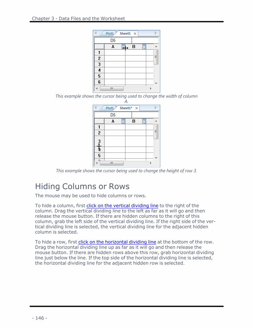
Chapter 3 - Data Files and the Worksheet
This example shows the cursor being used to change the width of columnA.
This example shows the cursor being used to change the height of row 3.
Hiding Columns or RowsThe mouse may be used to hide columns or rows.
To hide a column, first click on the vertical dividing line to the right of thecolumn. Drag the vertical dividing line to the left as far as it will go and thenrelease the mouse button. If there are hidden columns to the right of thiscolumn, grab the left side of the vertical dividing line. If the right side of the ver-tical dividing line is selected, the vertical dividing line for the adjacent hiddencolumn is selected.
To hide a row, first click on the horizontal dividing line at the bottom of the row.Drag the horizontal dividing line up as far as it will go and then release themouse button. If there are hidden rows above this row, grab horizontal dividingline just below the line. If the top side of the horizontal dividing line is selected,the horizontal dividing line for the adjacent hidden row is selected.
- 146 -

Surfer User's Guide
With the Format MenuColumns and rows can also be hidden with the Data | Format | Column Widthand Data | Format | Row Height commands. Select the columns or rows to hide,click the Data | Format | Column Width or Data | Format | Row Heightcommand, and then set the Column Width or Row Height to zero.
Displaying Hidden Columns or RowsThe mouse may be used to display hidden columns or rows.
To display a hidden column, first click on the vertical dividing line at the right ofthe hidden column and then drag the vertical dividing line to the new position. Ifseveral adjacent columns are hidden, only the far right column is displayed afterdragging the dividing line. If the cursor is to the left of the vertical dividing linewhen the line is selected, then the selected vertical dividing line is for the visiblecolumn to the left and not for the hidden column.
To display a hidden row, first click on the horizontal dividing line below the hid-den row and then drag the horizontal dividing line to the new position. If severaladjacent rows are hidden, only the bottom row is displayed after dragging thedividing line. If the cursor is above the horizontal dividing line when the line isselected, then the horizontal dividing line will be for the visible row above the hid-den rows, and not for the hidden rows.
ExampleIf columns B, C, and D are hidden and columns A and E are visible, then one ver-tical dividing line appears between columns A and
This example shows the vertical line being dragged to display hidden columnD.
- 147 -

Chapter 3 - Data Files and the Worksheet
With the Format MenuHidden columns and rows can also be displayed with the Data | Format | ColumnWidth and Data | Format | Row Height commands. To display hidden rows orcolumns, select the columns or rows on both sides of the hidden columns orrows, click the Data | Format | Column Width or Data | Format | RowHeight command, and then set the Column Width or Row Height to a numbergreater than zero.
Worksheet Error Codes and Special NumericValuesThere are a few different error codes and special numeric values that can appearin a worksheet cell depending on the type and nature of the data that appears.
Codes Explanation######### number will not fit in the column - the column must be
wider for the number to be shown#N/A value cannot be computed (for example, not enough data
to calculate a statistic)#DIV/0! an attempt to divide-by-zero was made in performing a cal-
culation#ERROR a value could not be computed (for example, square root
of a negative number)#OVERFLOW the value is too large for the worksheet (largest absolute
value is about 1.797E+308)1.#INF the value is too large for the worksheet (i.e., "infinite"
value)1.#IND numeric value is indefinite (usually the result of per-
forming a calculation with an infinite value or attemptingto divide by zero)
Worksheet SpecificationsThe following technical specifications for the worksheet include the number ofcells allowed in the worksheet and the nature of the numbers allowed in the work-sheet.
l Maximum number of rows in a worksheet: 1 billion
l Maximum number of columns in a worksheet: 1 billion
l Maximum numeric precision: 15 digits (Counting the digits before and afterthe decimal place)
- 148 -

Surfer User's Guide
l Maximum numeric resolution: 2.22E-16 (The smallest detectable dif-ference between two numbers)
l Maximum absolute value: 1.79769E+308 (The largest value that can berepresented)
l Minimum absolute value: 2.22507E-308 (The smallest value that is dif-ferent from zero)
l Double precision floating-point numbers can only represent approximately15 significant decimal digits.
l Approximate memory requirements for unformatted numeric data: 10.5bytes per cell + 24 bytes per column
Example 110,000 rows of numbers in 3 columns
30,000 cells x 10.5 bytes/cell = 315,000 bytes (308 Kbytes)
3 columns x 24 bytes/column = 72 bytes
TOTAL MEMORY NEEDED (in addition to memory needed to run the program):308 Kbytes
Example 23 rows of numbers in 10,000 columns
30,000 cells x 10.5 bytes/cell = 315,000 bytes (308 Kbytes)
10,000 columns x 24 bytes/column = 240,000 bytes (234 Kbytes)
TOTAL MEMORY NEEDED (in addition to memory needed to run the program):542 Kbytes
Worksheet CommandsThe following commands can be used to create and modify data in the work-sheet.
- 149 -

Chapter 3 - Data Files and the Worksheet
Paste
Click the Home | Clipboard | Paste command or the button, or pressCTRL+V on the keyboard to paste the clipboard contents into the current doc-ument. The objects to be pasted must first be placed in the clipboard using theCut or Copy commands of Surfer or some other application. The clipboard con-tents remain on the clipboard until something new is cut or copied to the clip-board.
WorksheetIn the worksheet, the upper left corner of the pasted data is placed in the activecell. Any cells in the existing worksheet that lie to the right of and below the act-ive cell will be overwritten with the contents of the pasted data. The followingrules are used to paste into the worksheet:
l Only the TAB character is recognized as a column separator. Spaces, com-mas, semi-colons, etc. are included in a text cell.
l The RETURN character is recognized as the row separator.
l Numbers paste as number values. The period can always be used as adecimal separator, and the system locale determines any other decimal sep-arator. For example if the system locale uses a comma as the decimal sep-arator, then both 123.456 and 123,456 are pasted as the number 123,456.
l Mixed text and numbers paste as text.
l Dates and/or times will paste as date values in a wide variety of date/timeformats. Ambiguous dates are determined by the system locale setting. Ifdates are not pasted correctly, consider using Paste Special and the Localesettings in the Data Import Options dialog.
Pasting a single cell's contents across multiple cellsA single cell's contents can be pasted into multiple cells by coping the cell, select-ing a block of cells, and using the Paste command. Each cell in the selection ispopulated with the clipboard contents when this operation is performed. If morethan one cell is copied, then the copied cells are only pasted once.
The multiple paste operation will not be performed for an entire row, entirecolumn, or across multiple selections. When an entire row or column is selected,only the first cell in the row or column will receive the pasted content. If youattempt to paste in multiple selections an error message will be displayed.
- 150 -

Surfer User's Guide
PlotIn the plot window, the clipboard contents are pasted in the center of the win-dow. The pasted contents are automatically selected, and can be dragged to anew location. Alternatively, change the position or size of the selected objectwith the Position/Size group.
Paste Special - WorksheetWhen data are copied to the clipboard, special formatting information is alsocopied. The Paste Special dialog determines the format in which the contentsare pasted into the worksheet. The Paste Special command can also be used toremove text formatting.
Paste Special DialogClick the Home | Clipboard | Paste | Paste Special command in the work-sheet to open the Paste Special dialog.
Select a paste special format in the Paste Specialdialog. This example shows options after copyingSurfer worksheet data and using paste special.
The clipboard formats displayed may vary depending the original location of theinformation being copied. For example, data copied from the Surfer worksheetmay yield different options than data copied from Excel.
Biff8 [Excel Spreadsheet]The Biff8 [Excel Spreadsheet] format is a Microsoft Excel Binary Interchange FileFormat (BIFF) version 8.
Biff5 [Excel Spreadsheet]The Biff5 [Excel Spreadsheet] format is a Microsoft Excel Binary Interchange FileFormat (BIFF) version 5.
- 151 -

Chapter 3 - Data Files and the Worksheet
Biff4 [Excel Spreadsheet]The Biff4 [Excel Spreadsheet] format is a Microsoft Excel Binary Interchange FileFormat (BIFF) version 4.
Biff3 [Excel Spreadsheet]The Biff3 [Excel Spreadsheet] format is a Microsoft Excel Binary Interchange FileFormat (BIFF) version 3.
Biff [Excel Spreadsheet]The Biff [Excel Spreadsheet] format is a Microsoft Excel Binary Interchange FileFormat (BIFF).
Sylk [Microsoft SYLK]The Sylk [Microsoft SYLK] format is a symbolic link Microsoft file format typicallyused to exchange data between applications, specifically spreadsheets. The Sylkfile format is composed of only displayable ANSI characters, allowing it to be eas-ily created and processed by other applications, such as databases.
Unicode Text [Clipboard Text]The Unicode Text [Clipboard Text] format is unformatted text.
Text [Clipboard Text]The Text [Clipboard Text] format is unformatted text.
Show Import OptionsWhen Unicode Text [Clipboard Text] or Text [Clipboard Text] is selected, theShow Import Options option is available. Check the box to open the Data ImportOptions dialog before importing the data. The Data Import Options dialog isuseful when pasting data with comma, period, semicolon, or other column delim-iters; fixed-width column data; ambiguous date/time formatted data; and datafrom different locales.
Data Import OptionsIf a file is in an ASCII text format with an unrecognized file extension, the DataImport Options dialog appears when opening the file. Choose the Delimitersused in the file (Tab, Comma, Semicolon, Space, or Other), and the Text Qual-ifiers used in the file (Double Quote or Single Quote).
Data Import Options DialogThe Data Import Options dialog may appear when importing tabular data fromdelimited text files (i.e. .DAT, .CSV, .TXT). These file formats are assumed tohave one record per line in which each record contains a fixed number of numericdata fields.
- 152 -
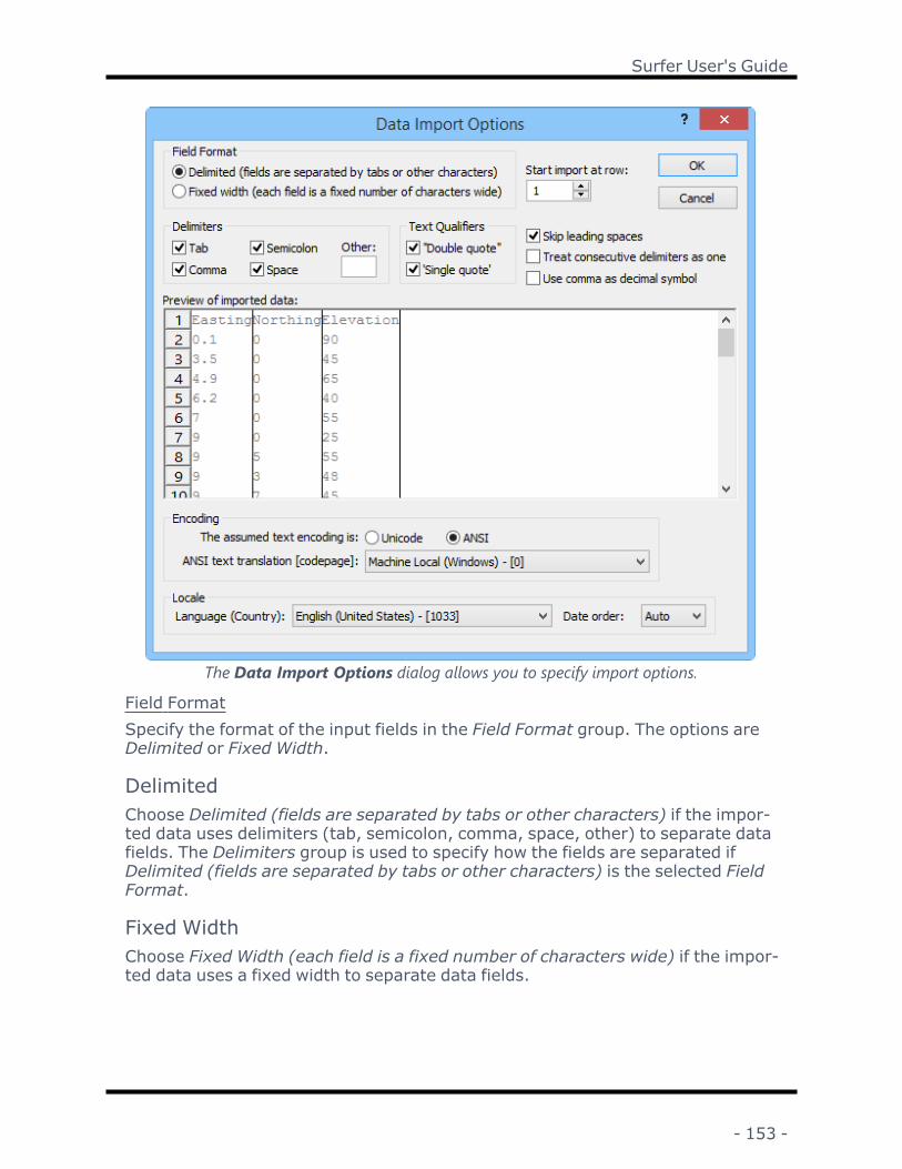
Surfer User's Guide
The Data Import Options dialog allows you to specify import options.
Field FormatSpecify the format of the input fields in the Field Format group. The options areDelimited or Fixed Width.
DelimitedChoose Delimited (fields are separated by tabs or other characters) if the impor-ted data uses delimiters (tab, semicolon, comma, space, other) to separate datafields. The Delimiters group is used to specify how the fields are separated ifDelimited (fields are separated by tabs or other characters) is the selected FieldFormat.
Fixed WidthChoose Fixed Width (each field is a fixed number of characters wide) if the impor-ted data uses a fixed width to separate data fields.
- 153 -

Chapter 3 - Data Files and the Worksheet
Start Import at RowSpecify the row number at which to start the data import in the Start import atrow box. To change the first row to import, highlight the existing value and typea new value or click the buttons to increase or decrease the value. Forexample, a value of one will start the data import at row one. A value of five willstart the data import at row five and ignore the data in rows one through four.
DelimitersChoose the desired delimiters to be used during the import process by checkingthe box next to Tab, Comma, Semicolon, or Space. You may also enter a customdelimiter in the Other box. More than one delimiter may be checked.
Text QualifiersCheck the box next to Double Quote or Single Quote in the Text Qualifiers groupto indicate the correct qualifier to identify text values in the data file. Everythingbetween the selected characters will be interpreted as a single value, and anydelimiter characters between text qualifiers are ignored and treated as part ofthe text.
Double QuoteCheck the box next to "Double Quote" to specify that everything between thosemarks should be interpreted as a single value, and any delimiter charactersbetween any two quote characters are not treated as a delimiter.
For example, if Space is chosen as the delimiter and Double Quote is chosen asthe text qualifier, the string "Aspen Park" is treated as a single data value due tothe double quotes surrounding it, and the space delimiter between the words istreated as part of the value.
Single QuoteCheck the box next to 'Single Quote' to specify that everything between thosemarks should be interpreted as a single value, and any delimiter charactersbetween any two quote characters are not treated as a delimiter.
For example, if Space is chosen as the delimiter and Single Quote is chosen asthe text qualifier, the string 'Aspen Park' is treated as a single data value due tothe single quotes surrounding it, and the space delimiter between the words istreated as part of the value.
Skip Leading SpacesCheck the box next to Skip leading spaces to tell the software to ignore spacesthat appear before initial text.
- 154 -
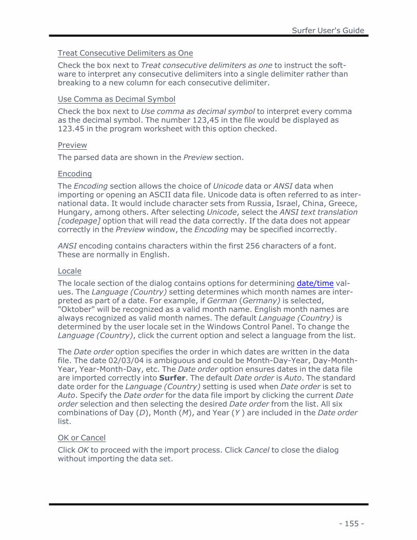
Surfer User's Guide
Treat Consecutive Delimiters as OneCheck the box next to Treat consecutive delimiters as one to instruct the soft-ware to interpret any consecutive delimiters into a single delimiter rather thanbreaking to a new column for each consecutive delimiter.
Use Comma as Decimal SymbolCheck the box next to Use comma as decimal symbol to interpret every commaas the decimal symbol. The number 123,45 in the file would be displayed as123.45 in the program worksheet with this option checked.
PreviewThe parsed data are shown in the Preview section.
EncodingThe Encoding section allows the choice of Unicode data or ANSI data whenimporting or opening an ASCII data file. Unicode data is often referred to as inter-national data. It would include character sets from Russia, Israel, China, Greece,Hungary, among others. After selecting Unicode, select the ANSI text translation[codepage] option that will read the data correctly. If the data does not appearcorrectly in the Preview window, the Encodingmay be specified incorrectly.
ANSI encoding contains characters within the first 256 characters of a font.These are normally in English.
LocaleThe locale section of the dialog contains options for determining date/time val-ues. The Language (Country) setting determines which month names are inter-preted as part of a date. For example, if German (Germany) is selected,"Oktober" will be recognized as a valid month name. English month names arealways recognized as valid month names. The default Language (Country) isdetermined by the user locale set in the Windows Control Panel. To change theLanguage (Country), click the current option and select a language from the list.
The Date order option specifies the order in which dates are written in the datafile. The date 02/03/04 is ambiguous and could be Month-Day-Year, Day-Month-Year, Year-Month-Day, etc. The Date order option ensures dates in the data fileare imported correctly into Surfer. The default Date order is Auto. The standarddate order for the Language (Country) setting is used when Date order is set toAuto. Specify the Date order for the data file import by clicking the current Dateorder selection and then selecting the desired Date order from the list. All sixcombinations of Day (D), Month (M), and Year (Y ) are included in the Date orderlist.
OK or CancelClick OK to proceed with the import process. Click Cancel to close the dialogwithout importing the data set.
- 155 -

Chapter 3 - Data Files and the Worksheet
Copy
Click the Home | Clipboard | Copy command or the button, or pressCTRL+C on the keyboard to copy the selected objects to the clipboard. The ori-ginal objects remain in the window. Use this command to duplicate objects in adifferent location in the same window, or copy the objects into a different win-dow or application. The copied objects can later be pasted with the Paste orPaste Special commands.
Only one set of data may be placed in the clipboard at a time. The next Cut orCopy command replaces the contents of the clipboard.
CutClick the Home | Clipboard | Cut command or the button, or press CTRL+Xon the keyboard to move the selected objects to the clipboard. This deletes theselected objects from the file after copying them to the clipboard. Cut objectscan later be pasted with the Paste or Paste Special commands.
Only one set of data may be placed in the clipboard at a time. The next Cut orCopy command replaces the contents of the clipboard.
Data Tab CommandsThe Data tab contains commands for editing the cell and worksheet, finding andreplacing cell contents, formatting the cells, manipulating data, and assigning orprojecting coordinate systems. The Data tab is only available when viewing aworksheet.
The worksheet ribbon Data tab has the following commands:
Open Data Open data file in a new worksheetClear Remove the selected cellsMerge Combines a worksheet file with the existing worksheetInsert Displace selected cells and insert new cells into the work-
sheetDelete Delete selected worksheet cells and move rows or columnsFind Find a particular word or phrase in the worksheetFind Next Find the next occurrence of the word or phraseReplace Replace the word or phrase with alternate textFormat Cells Sets the numeric format, alignment, and background color
for the selected cellsColumnWidth
Sets column widths for selected cells
Row Height Sets row height for selected cellsTransform Applies a mathematical transform to columns
- 156 -

Surfer User's Guide
Sort Sorts selected cellsSpatial Filter Spatially filters X, Y and optional Z coordinatesStatistics Computes statistics on selected cellsText to Num-ber
Convert the text in selected cells to numbers
Transpose Convert columns to rows and rows to columnsAssign XYZColumns
Specifies the default columns for X, Y, and Z coordinate data
AssignCoordinateSystem
Specifies the existing coordinate system
New Pro-jectedCoordinates
Specifies the columns containing the source X, Y coordinatesand target X, Y columns for a new coordinate system
DMS to DD Convert DMS latitudes and longitudes to decimal degreesTrack Cursor Track cursor location across plot, worksheet, and grid editor
windows for a maps, data files, and grids.
Clear - Worksheet
Click the Data | Edit | Clear command or the button, or press the DELETEkey on the keyboard, to remove data from selected worksheet cells. The cellsbecome empty when the data are removed. To shift the data from unselectedcells into the selected cell locations, use the Delete command instead.
Merge - Worksheet DocumentThe Data | Edit | Merge command in the worksheet loads the contents of adata file into the existing worksheet. Select a file to import into the existing file inthe Import Data dialog. The contents of the new file are merged into the work-sheet at the active cell so be sure to position the cell at the edge of the existingdata. Any cells in the existing worksheet that lie to the right of and below the act-ive cell are overwritten with the contents of the merging file.
Import Data Dialog
Click the Data | Edit | Merge command or the button to open the ImportData dialog.
- 157 -

Chapter 3 - Data Files and the Worksheet
Specify files to import into the Surfer worksheet using the Import Data dialog.Look InThe Look in field shows the current directory. Click the down arrow to see the dir-ectory structure and click on the folders to change directories.
Creating New Folders and Changing the ViewThe buttons to the right of the Look in field allow you to create new folders andchange the view of the file list.
File ListThe File list displays files in the current directory. The current directory is listedin the Look in field. The Files of type field controls the display of the file list. Forexample, if DAT Data (*.dat) is listed in the Files of type field only *.DAT filesappear in the files list.
Specify a File NameThe File name field shows the name of the selected file. Alternatively, type a pathand file name into the box to open a file.
Files of TypeThe Files of type field controls the display of the file list. For example, if DAT Data(*.dat) is listed in the Files of type field only *.DAT files appear in the files list.
The All Recognized Types (*...) format type is selected by default. This displaysall the common file formats in the navigation pane. If a different format type isselected, Surfer will remember the setting until the end of the current session.When Surfer is restarted, the default format type will be used.
- 158 -

Surfer User's Guide
To see all files in the directory, choose All Files (*.*) from the Files of type list.Double-click on a file to open it or single-click the file and then click the Open but-ton. The All Files (*.*) option shows all of the file formats in the current dir-ectory, even if the file type is not appropriate for the action chosen. For example,a .GRD file may be displayed, even though a .GRD file cannot be imported intothe worksheet.
Select a file type from the Files of type list. The following formats are supported:
l ACCDB Microsoft Access .ACCDB
l BLN Golden Software Blanking .BLN
l BNA Atlas Boundary .BNA
l CSV Comma Separated Variables .CSV
l DAT Data .DAT
l DBF Database .DBF
l DXF AutoCAD Drawing Data .DXF
l LAS LiDAR Data .LAS
l MDB Microsoft Access 97-2003 Database .MDB
l SEG-P1 Data Exchange Format .SEG
l P1 Data Exchange Format .SP1
l SLK Sylk Spreadsheet .SLK
l TXT Text Data .TXT
l XLS Excel Spreadsheet .XLS
l XLSX Excel 2007 Spreadsheet .XLSX
l XLSM Excel 2007 Spreadsheet .XLSM
Load DatabaseClick the Load Database button in the Import Data dialog to open the Data LinkProperties dialog and import a database.
Show Options If They Are AvailableIf Show options if they are available is checked, then opening .TXT files or ASCIItext files with unsupported file extensions will bring up the Data Import Optionsdialog where you can specify the import options. The Data Import Options dia-log can be used to import data from different locales correctly, for example when
- 159 -

Chapter 3 - Data Files and the Worksheet
the data uses ambiguous or different date order or when the data uses differentdecimal and column delimiters than the local PC.
Insert - WorksheetThe Data | Edit | Insert command inserts a single blank cell or a block of blankcells in the worksheet. Select cells in the area in which you wish to insert cellsand then click Data | Edit | Insert, or right-click and select Insert from the con-text menu. The Insert dialog appears. Specify how you want the original dis-placed contents moved when the blank cells are inserted.
Click the Data | Edit | Insert command or the button, or press CTRL+R onthe keyboard, to open the Insert dialog.
When using Insert, you can shift cells tothe right or down to make room for the
new cells.
Shift Cells Right or Shift Cells DownClick the Shift Cells Down or Shift Cells Right option to insert blank cells and dis-place the original contents either down or to the right.
Entire Row or Entire ColumnClick the Entire Row or Entire Column option to insert an entire row or column inthe area that contains highlighted cells.
Delete - WorksheetThe Data | Edit | Delete command deletes the selected worksheet cells andshifts cells up or to the left to fill in the gap. After selecting Data | Edit |Delete, the Delete dialog appears. Specify the desired behavior of the cells andclick the OK button. The selected cells are deleted and the contents of cells belowor to the right are moved to fill the deleted block.
Click the Data | Edit | Delete command or the button, or press CTRL+D onthe keyboard, to open the Delete dialog.
- 160 -

Surfer User's Guide
When using Data | Edit | Delete, you canshift cells to the left or up to fill in the gap.
Shift Cells Left or Shift Cells UpClick the Shift Cells Up or Shift Cells Left option to specify if cells will be shifted tothe left or up to fill in the gap after deleting the selected cells.
Delete Entire Row or Entire ColumnClick Entire Row or Entire Column to delete the entire row or column that con-tains highlighted cells.
Leave Deleted Cells EmptyTo leave the selected cells empty when the data are removed, use the Clear com-mand, press the DEL key, or use the Cut command.
FindThe Find and Replace dialog displays when the Data | Find | Find or Data |Find | Replace commands are selected. The Find and Replace dialog is usedto locate and replace specific numbers or text in the worksheet.
The Data | Find | Find Next command is used to find the next instance of aparticular number, word, or phrase in the worksheet. If the Data | Find | Findcommand was not used initially, the Find and Replace dialog opens so that youcan define your search criteria.
Find Page
Clicking the Data | Find | Find command or the button, pressing CTRL+F onthe keyboard, or clicking the F3 key on the keyboard opens the Find page of theFind and Replace dialog.
- 161 -

Chapter 3 - Data Files and the Worksheet
Search for and replace specific text in the worksheet with theFind and Replace dialog.
FindTo find objects, type the text you want to search for in the Find field. Click thearrow at the right to select from a list of the most recently used text strings. Theasterisk (*) and question mark (?) wildcards can be used in the Find box. Clickthe arrow at the right to select from a list of the most recently used criteria.
l A question mark ? finds a single character in the specified location. Forexample, 200? finds 2009, 2008, 200a, etc.
l An asterisk * finds any number of characters at the specified location. Forexample, *01 finds 601, 1201, cd01, etc.
InNext to In, choose the parameters of the search from the list. Choices includeThe column where active cell is, The row where active cell is, and The entire lim-its.
l Select The column where the active cell is to search only the column (e.g.column B) of the active cell (e.g. cell B2) for the information listed in the Findfield.
l Select The row where active cell is to search only the row (e.g. row _2) of theactive cell (e.g. cell B2) for the information listed in the Find field.
l Select The entire limits to search the entire worksheet for the information lis-ted in the Find field.
Search OrderThe Search order controls the direction of the search: down through columns byselecting By column or to the right across rows by selecting By row.
- 162 -

Surfer User's Guide
In this example, cell A2 is selected. If the Find cri-teria is "9", and By column is the search order, cellA4 is found first. If By row is the search order, cell
C2 is found first.Match CaseIf you have case sensitive characters in the Find text string, check the Matchcase check box. Selecting Match case distinguishes between uppercase andlowercase characters. For example, a search for "Elevation" with the Match caseoption selected will not find entries for "elevation", but will find entries for "Elev-ation".
Deselect All FirstCheck the Deselect all first box to deselect all selected cells before performingthe search. All previously selected cells will be deselected prior to the searchwhen the Deselect all first check box is checked. If the Deselect all first box iscleared, the results of a previous search will remain highlighted when performingthe next search.
MethodChoose the search Method from the list to determine how the search is per-formed. The examples assume "Golden, CO" is in the Find field.
l Select Cell matches target exactly to require that the exact criteria in theSearch box is present in a cell before it is selected. For example, only cellsthat have exactly "Golden, CO" will be selected.
l Select Cell contains target phrase to require that the phrase in the Searchbox is present in a cell before it is selected. For example, cells that has"Golden CO", "Golden Company", or "Golden Colorado" will be selected.
l Select Cell contains all of the target words to require that all of the Search cri-teria words are present in a cell before it is selected. For example, cells thathave "Golden" and "CO" somewhere in the cell (i.e. "Golden is the best city inColorado" will be selected).
l Select Cell contains any of the target words to require that any of the Searchcriteria words are present in a cell before it is selected. For example, cellsthat have "Golden is a city" or "CO is a state" will be selected.
- 163 -

Chapter 3 - Data Files and the Worksheet
Find All ButtonClick the Find All button to find all occurrences of the Find criteria in the work-sheet. All of the cells that contain the Find criteria will be highlighted.
Find Next ButtonClick the Find Next button to find the next occurrence of the characters specifiedin the Find box. This allows you to meet the criteria one at a time. The nextinstance of the Find criteria will be highlighted.
Close ButtonClick the Close button to exit the Find and Replace dialog.
Find NextClicking the Data | Find | Find Next command or the button or pressing theF3 key on the keyboard finds the next instance of a particular number, word, orphrase in the worksheet. Each cell matching the search parameters remainsselected. If the Data | Find | Find command was not used initially, the Findand Replace dialog opens so that you can define your search criteria.
ReplaceThe Find and Replace dialog displays when the Data | Find | Find or Data |Find | Replace commands are selected. The Find and Replace dialog is usedto search and replace specific numbers or text in the worksheet.
Replace Page
Clicking the Data | Find | Replace command or the button or pressingCTRL+H on the keyboard opens the Replace page of the Find and Replace dia-log. The Replace page has all of the Find page fields, with the addition of theReplace with field. The Replace page Method field has only two options.
- 164 -

Surfer User's Guide
Use the Find and Replace dialog to replace numbers ortext in the worksheet.
Replace WithType the text you want to replace in the Find box. To delete the characters in theFind box from your worksheet, leave the Replace with box blank. Click the arrowat the right to select from a list of the most recently searched items.
MethodChoose the search Method from the list to determine how the search is per-formed. The examples assume "Golden, CO" is in the Find field.
l Select Cell matches target exactly to require that the exact criteria in theSearch box is present in a cell before it is selected. For example, only cellsthat have exactly "Golden, CO" will be selected.
l Select Cell contains target phrase to require that the phrase in the Searchbox is present in a cell before it is selected. For example, cells that has"Golden CO", "Golden Company", or "Golden Colorado" will be selected.
Replace ButtonClick the Replace button to replace the selected occurrence of the criteria in theFind box with the criteria in the Replace with box, find the next occurrence of thecriteria in the Find box, and then stop. If you want to automatically replace alloccurrences of the search criteria in the worksheet, click the Replace All button.
Replace All ButtonClick the Replace All button to replace all occurrences of the Find criteria in yourdocument with the Replace with criteria. If you want to review and selectivelyreplace each occurrence, click the Replace button.
- 165 -

Chapter 3 - Data Files and the Worksheet
Format CellsCell numbers, alignment, or background color can be formatted through theFormat Cells dialog. To format a cell, select the cells to be formatted (seeSelecting Worksheet Cells), and click the Data | Format | Format Cells com-mand or the button. The Format Cells dialog opens.
The Format Cells dialog has three pages: Number, Alignment, and Back-ground.
Number PageUse the Number page to change the numeric data display in the worksheet.
Alignment PageUse the Alignment page to set the cell alignment.
Background PageUse the Background page to set cell background color.
Text StringNumber formatting has no effect on a numeric text string (numbers entered astext). A number with an apostrophe in front of it ('8123) is a text string. The apo-strophe only shows in the active cell edit box. For example, an ASCII data filemight contain the digits "8123" (digits surrounded by quotes), '8123 (digits pre-ceded with an apostrophe), numbers with letters, or numbers with symbols (i.e.a blackslash "\"). These "numbers" are read as text and not as a number. TheTransform command can be used to perform a mathematical function, such asATOI(X), to convert a text string to an integer value. Alternatively, the cell canbe converted to numbers with the Text to Number command.
Preserving Cell FormatThe only formats that preserve cell-formatting information are Excel or SYLKSLK. ASCII file formats (.CSV, .TXT, .DAT, .BNA, .BLN) do not preserve fileformat information.
Format Cells - NumberCell numbers, alignment, or background color can be formatted through theFormat Cells dialog. To format a cell, select the cells to be formatted (seeSelecting Worksheet Cells), and then click the Data | Format | Format Cellscommand. Use the Number page to change the numeric data display in theworksheet. Number formatting has no effect on a numeric text string (numbersentered as text). For example, an ASCII data file might contain the numbers"8123" (numbers surrounded by quotes) which are read as text and not as anumber. The Transform command can be used to perform a mathematical func-
- 166 -

Surfer User's Guide
tion, such as ATOI(X), to convert a text string to an integer value. Alternatively,the cell can be converted to numbers with the Text to Number command.
Select the number format options on the Number pageof the Format Cells dialog.
TypeThe Type section contains the numeric format for the selected cells. Availableoptions are General, Fixed, Exponential, Currency, Percent, and Date/Time. Clickon the desired option.
l General displays numbers as fixed or exponential, whichever is shorter.l Fixed displays numbers as d.ddd. The number to the left of the decimal canvary. Set the number to the right of the decimal in theDecimal Digitsbox.
l Exponential displays numbers as d.ddde+dd. Set the number of digits to theright of the decimal in the Decimal Digits box.
l Currency displays fixed numbers with a currency symbol such as the dollarsign ($).
l Percent displays numeric values (such as 0.13) as percentages with a percentsymbol suffix (13%).
l Date/Time formats the cells as date and/or time. Select Date/Time and thentype or select the Date/Time format.
Decimal DigitsThe Decimal Digits controls the number of digits to the right of the decimal whenthe Type is set to Fixed, Exponential, Currency, or Percent. To change theDecimal Digits, highlight the existing value and type a new value. Alternatively,click the to increase or decrease the value.
- 167 -

Chapter 3 - Data Files and the Worksheet
Thousands SeparatorThe Thousands separator option controls whether a comma appears in the num-ber, indicating thousands. When checked, a comma appears every three digits tothe left of the decimal point. When unchecked, the number appears without thecomma. Do not type a comma when entering data as this causes the number tobe read as text.
SampleThe Sample box displays the current number format.
Date/Time FormatWhen the Type is set to Date/Time, the Date/Time format option becomes avail-able. Type the desired format into the Date/Time format field, or click the but-ton to insert a date/time format with the Date/Time Format Builder dialog.Available formats are made of combinations of day, month, year, AD/BC orCE/BCE designation, hours, minutes, seconds, and AM/PM designation. Days areshown as d or dd. Months are shown as M, MM, MMM, MMMM, or MMMMM. Yearsare shown as yy or yyyy. Hours are shown as h or hh. Minutes are shown as m ormm. Seconds are shown as ss. Sub-seconds are displayed as ss.0 or ss.000.AM/PM designation are shown as tt or TT. BC/AD designation is shown as gg orGG. BCE/CE designation is shown as g, ggg, G, or GGG. Total elapsed time isshown as [h]. After clicking on the Date/Time format, the Sample updates toshow a value in the selected format.
OK or CancelClick OK to make the change to the cell format. Click Cancel to return to the work-sheet without making the change.
Format Cells - AlignmentCell numbers, alignment, or background color can be formatted through theFormat Cells dialog. To format a cell, select the cells to be formatted (seeSelecting Worksheet Cells), and then click the Data | Format | Format Cellscommand. Use the Alignment page to align the cell in one of four ways. Bydefault, imported ASCII files automatically align numbers to the right and text tothe left.
- 168 -

Surfer User's Guide
Select the alignment options on the Alignment page ofthe Format Cells dialog.
GeneralGeneral aligns text on the left side of the cell and numbers on the right side ofthe cell.
LeftLeft aligns text and numbers with the left side of the cell.
CenterCenter aligns text and numbers with the center of the cell.
RightRight aligns text and numbers with the right side of the cell.
Format Cells - BackgroundCell numbers, alignment, or background color can be formatted through theFormat Cells dialog. To format a cell, select the cells to be formatted (seeSelecting Worksheet Cells), and then click the Data | Format | Format Cellscommand. You can set cell background color on the Background page. Save theworksheet in Excel format to save background color in the file.
- 169 -

Chapter 3 - Data Files and the Worksheet
Select the cell background color the Background page ofthe Format Cells dialog.
NoneClick the None button to remove any previously assigned background colors.
Color PaletteSelect a cell background color from the color palette.
SampleA sample of the color is displayed in the Sample box.
Column WidthYou can change the column width of selected cells by clicking the Data |Format | Column Width command or by the or by using the mouse to resizethe column. The Excel XLS or SYLK SLK file format must be used to save thecolumn width in the file since ASCII file formats (.CSV, .TXT, .DAT, .BNA, .BLN)do not preserve file format information.
Column Width DialogTo set column widths or to hide columns, select either the entire column or indi-vidual cells within the columns (see Selecting Worksheet Cells), and then clickthe Data | Format | Column Width command. Enter the width for the selec-ted column or cells into the Column Width dialog. Columns can range from zeroto 512 characters wide. The value zero (0) hides the column.
- 170 -

Surfer User's Guide
Change the column width by selectingcolumns, clicking Column Width, andthen entering a number into the Column
Width dialog.
Changing Column Widths with the MouseColumn width can also be changed using the mouse. When the cursor is movedto the line that defines the right boundary of the column header, the cursorchanges to a . Press and hold the left mouse button and move the cursor tothe left or right to change the width of the column. You can double-click thecolumn line to automatically set the column width. When automatically settingthe column width, the column narrows or widens to the smallest size necessaryto completely display the data and column name.
Hide a Column with the MouseYou can hide a column by moving the cursor to the left until the next dividing lineis reached.
Display Hidden Columns with the MouseTo display hidden columns, press and hold the left mouse button at the rightedge of the hidden column and move the cursor to the right to widen the column.
Row HeightYou can change the Row Height of selected cells by clicking the Data | Format| Row Height command or the button or by using the mouse to size the row.The Excel XLS or SYLK SLK file format must be used to save the row height andnumeric format information with the file since ASCII file formats (.CSV, .TXT,.DAT, .BNA, .BLN) do not preserve file format information.
Row Height DialogTo set the row height or hide rows, select either the entire row or individual cellswithin the rows (see Selecting Worksheet Cells), and click the Data | Format |Row Height command. Enter the height for the selected row or cells in the RowHeight dialog. Rows can range from zero to 512 points in height. A value of zero(0) hides the row.
- 171 -

Chapter 3 - Data Files and the Worksheet
Change the row height by selecting rows,clicking Data | Format | Row Height ,and then entering a number into the Row
Height dialog.
Changing Row Heights with the MouseRow height can also be changed using the mouse. When the cursor is moved tothe line that defines the lower boundary of the row header, the cursor changes toa line with two arrows . Press and hold the left mouse button and move thecursor up or down to change the height of the row.
Hide a Row with the MouseYou can hide a row by moving the cursor up until the next dividing line isreached.
Display Hidden Row with the MouseTo display hidden rows, press and hold the left mouse button at the bottom ofthe hidden row and move the cursor down to stretch the row height.
Transform - Worksheet
Click the Data | Data | Transform command or the button to open theTransform dialog, where you can apply mathematical transformations to thecolumns, rows, or cells. Valid math operators include addition (+), subtraction(-), multiplication (*), and division (/) as well as a large library of built-in math-ematical functions. Parentheses should be used to override precedence or for cla-rification.
- 172 -

Surfer User's Guide
Use the Transform dialog to apply math func-tions to data. The dialog options update toreflect the option selected for Transform with
field.
Transform WithSelect the type of transform from the Transform with list. Column variables(e.g., C = A + B) applies the transform equation to the specified rows in theTransform equation column. Row variables (i.e., _3 = _1 + _2) applies the trans-form equation to the specified columns in the Transform equation row. Cell vari-ables (i.e., C3 = A1 + B2) applies the transform equation only to the cellspecified in the Transform equation.
Transform EquationType the formula into the Transform equation box. Formulas consist of a des-tination column, row, or cell on the left side of the equation and a mathematicalmanipulation on the right side of the equation. Use the column label letters, rownumbers, or cell locations on both sides of the equation. Click the down arrow touse previously entered equations. For columns, a sample equation may be C = A+ B. For rows, a sample equation is _4=_1+_2. For cells, a sample equationwould look like C2=A1+B1-C1.
If the transform method is by column, the range functions (sum, avg, std, row-min and rowmax) take column indices only, i.e., sum(A...C). If transformmethod is by variable rows, the range functions take row indices only, i.e., sum(_1..._3). If transform method is by variable cells, the range functions are notsupported.
- 173 -

Chapter 3 - Data Files and the Worksheet
The last ten functions are stored in the Transform equation field. After ten func-tions are included in the list, the oldest function is replaced when a new functionis added. The Transform equations are stored between sessions. To use a storedfunction, click the in the Transform equation box and select a function from thelist. Note that the First row and Last row or First col and Last col values are notsaved with the stored Transform equations.
First and Last Columns and RowsWhen calculating transformations on columns, enter the First row and the Lastrow to limit the calculation to the specified rows. When calculating trans-formations on rows, enter the First col and Last col to limit the calculation to thespecified columns. When calculating transformations on cells, the First row, Lastrow, First col, and Last col options are not available.
By default, these are set to the first row and last row (or first column and lastcolumn) with text or numbers entered into a cell for the entire worksheet.
Relative Cell ReferencesSelect the Relative cell references option to apply the Transform equation to mul-tiple cells. The Relative cell references option is only available when Transformwith is set to Cell variables (e.g., C3 = A1 + B2). The Transform equation is onlyapplied relatively by incrementing the row numbers. The columns do not changewhen Relative cell references is selected.
The Relative cell references option appliesthe Transform equation to multiple rows.
- 174 -

Surfer User's Guide
Specify the number of rows to which the Transform equation is applied in theNumber of rows field. Note this value is not the row number. By default the Num-ber of rows value is the total number of rows in the worksheet.
Empty CellsThe Empty cells option controls how empty cells are treated in the calculations offormulas. Available options are Blank the result, Are treated as the number zero(0), and Are treated as empty text (""). The default option is Blank the result,which results in the formula not being calculated for any row that contains ablank cell in any of transform equation rows or columns.
l Setting the Empty cells option to Blank the result results in a blank cell for thetransform when the cells on the right side of the equation are empty.
l Setting the Empty cells option to Are treated as the number zero (0) resultsin the transform creating a number when all of the cells on the right side ofthe equation are empty or numeric. When the right side of the equation com-bines text and blank cells, the equation is blank.
l Setting the Empty cells option to Are treated as empty text ("") results in thetransform creating a text string when all of the cells on the right side of theequation are empty or text. When the right side of the equation combinesnumeric and blank cells, the equation is blank.
Text CellsThe Text cells option controls how text cells are treated in the calculations of for-mulas. Available options are Blank the result, Are treated as text, Are convertedto numbers (if possible), and Are treated as the number zero (0). The defaultoption is Blank the result, which results in the formula not being calculated forany row that contains a text cell in any of transform equation rows or columns.
l Setting the Text cells option to Blank the result results in a blank cell for thetransform when any of the cells on the right side of the equation contain textstrings (including numbers formatted as text).
l Setting the Text cells option to Are treated as text results in the transform cre-ating a text string when all of the cells on the right side of the equation aretext (or treated as text). If a mix of text cells and numbers or empty cells(that are not treated as text) are in the cells on the right side of the equation,the transform results in a blank cell. This option allows text strings to be con-catenated.
l Setting the Text cells option to Are converted to numbers (if possible) resultsin the transform creating a number when all of the cells on the right side ofthe equation are numeric or treated as numbers. Any cells with numbersformatted as text are treated as the number. For example, the text string '05would be treated as the number 5 if this option is selected.
l Setting the Text cells option to Are treated as the number zero (0) results inthe transform creating a number when all of the cells on the right side of theequation are numeric or treated as numbers. Any cells with text are replacedwith the value zero for the transform. For example, if you are using the
- 175 -

Chapter 3 - Data Files and the Worksheet
equation C=A+B and A has Colorado and B has 45, the value in cell C will be45.
Number CellsThe Number cells option controls how numeric cells are treated in the cal-culations of formulas. Available options are Blank the result, Are treated asnumeric values, Are converted to text, and Are treated as empty text (""). Thedefault option is Are treated as numeric values, which results in the formulabeing calculated for any row that contains numbers in any of transform equationrows or columns.
l Setting the Number cells option to Blank the result results in a blank cell forthe transform when any of the cells on the right side of the equation containnumbers. This option is useful when you only want to combine text cells orblank cells.
l Setting the Number cells option to Are treated as numeric values results inthe transform creating a number when all of the cells on the right side of theequation are number (or treated as numbers). If a mix of text cells and num-bers or empty cells (that are not treated as numbers) are in the cells on theright side of the equation, the transform results in a blank cell.
l Setting the Number cells option to Are converted to text results in the trans-form creating a text string when all of the cells on the right side of the equa-tion are text or treated as text. Any cells with numbers are treated as the textstring of the number. For example, number 5 is in the cell, so the text stringwould appear as '5 if this option is selected.
l Setting the Number cells option to Are treated as empty text ("") results inthe transform creating a text string when all of the cells on the right side ofthe equation are text or treated as text. Any cells with numbers are replacedwith "" for the transform. For example, if you are using the equation C=A+Band A has Colorado and B has 45, the value in cell C will be Colorado.
Combining Text, Numbers, and Empty CellsMany possible combinations of the Empty cells, Text cells, and Number cells existto allow combining these different types of cells in a Transform equation . If thetransform result is not what you expect, check the settings for these options andadjust if necessary.
FunctionsClick the Functions >> button to display a list of predefined mathematical func-tions. Click the Functions << button again to hide the list of predefined math-ematical functions.
To use a function, place the cursor in the location to add a function, select a func-tion from the list, click the Insert button, and then replace the X in the functionwith a column letter (A); underscore and row number (_1); or cell location (A1).Also, be sure to use proper mathematical operators (+_*/) between the function
- 176 -

Surfer User's Guide
and the rest of the equation. The definition of the function is listed below theFunction name list when a function is selected.
The IF function is not included in the Functions list. See the Mathematical Func-tions topic for the syntax of the IF function.
InsertWhen the Functions are expanded, the Insert button is visible. Click the Insertbutton to add a function to the Transform equation box. In the Transform equa-tion box, manually change the variable (i.e. X or Y) in the listed functions to acolumn letter, row number (_1), or cell location.
ExamplesAn example of a column formula is C = A + B. Columns A and B are added andinserted into column C with this equation. The formula adds the contents of Aand B in each row and places the results in column C for that row.
An example of a row formula is _4=_1+_2. Rows 1 and 2 are added and insertedinto row 4 with this equation. The formula adds the contents of the 1 and 2 ineach column listed between the First col and Last col values and places the res-ults in row 4 for that column.
An example of a cell formula is C2=A1+B1-C1. The value in C1 is subtractedfrom the sum of the values in cells A1 and B1. The result is inserted into cell C2with this equation.
Example FunctionsThis example shows how to use the built in functions. Consider, for example, tak-ing the cosine of data in column C. Column D is the first empty column, so we willuse column D as the destination column.
1. Click the Data | Data | Transform command to open the Transform dia-log. You do not need to highlight any columns before selecting Transform.
2. In the Transform equation box, type "D = " without the quotes.3. Click the Functions button.4. Double-click on the function name COS(X) in the Function name group.
Alternatively, you could select a Function name and click the Insert button.5. COS(X) is automatically placed in the equation as "D = COS(X)" without the
quotes.6. Replace the X in the function with the column letter containing the data to be
transformed (column C). The equation will be "D = COS(C)" without thequotes.
7. Change the First row and Last row if you wish.8. Make sure that Empty cells and Text cells are set to Blank the result to only
calculate values with numbers.9. Click OK to create a new data column with column C's data transformed with
the cosine.
- 177 -

Chapter 3 - Data Files and the Worksheet
Sort - WorksheetThe Data | Data | Sort command arranges data according to rank in user-spe-cified sort columns. Sorting rank is based on numbers, ASCII characters, andpunctuation. Sort numeric data, text, or mixed columns. Sorting specificationsare made in the Sort dialog.
Selecting Cells to SortSorting is performed only on the selected columns (see Selecting Cells). If onlyone column is selected, only that column is sorted. To keep records (rows ofdata) together, select all columns containing data even if only one column is sor-ted.
Sort DialogClick the Data | Data | Sort command or the button in the worksheet toopen the Sort dialog.
Click the Data | Data | Sort command to sort data onmultiple columns.
Sort OrderThe Sort First By option defines the primary column on which the rows are sor-ted. The positions of the sorted rows are determined by the Ascending or Des-cending rank in the Sort First By column.
Secondary SortWhen two or more rows have identical entries in the Sort First By column, theSort Next By column can further organize the data set. Duplicates in the SortFirst By Column are then sorted according to the rank in the Sort Next Bycolumn.
- 178 -

Surfer User's Guide
Final SortThe Sort Last By column can be used when the Sort Next By column containsduplicates.
Ascending or Descending SortThe sort order in an Ascending sort is based on the ASCII table. Numeric valuesare placed first, followed in order by cells starting with a space character, com-mon punctuation, numeric text (numbers entered as text), uppercase letters,less common punctuation, lower case letters, uncommon punctuation, and blankcells. Descending order is the opposite of ascending order although blank cellsare still listed last.
0 1 2 3 4 5 6 7 8 9space ! " # $ % & ' ( )* + , - . / "0" "1" "2" "3""4" "5" "6" "7" "8" "9" : ; < => ? @ A B C D E F GH I J K L M N O P QR S T U V W X Y Z [\ ] ^ _ ` a b c d ef g h i j k l m n op q r s t u v w x yz { | } ~ blank
This ASCII table shows the sort order in the worksheet.Ignore CaseBecause sorting is based on an ASCII table, upper and lowercase letters aretreated differently. For example, "A" is sorted separately from "a." If the lettersare to be treated as the same during the sort, check the Ignore case option.When this check box is activated, "A" is considered identical to "a" in the sortingrank.
Labels in First RowThe data set may contain text identifying the data in the column (header inform-ation) in Row 1. In this case, click the Labels in first row option to exclude thelabel row from the sort process.
Spatial FilterThe Data | Data | Spatial Filter command can be used to spatially filter the X,Y and Z coordinates. This can be useful when pre-filtering data before creating apost map, variogram, or grid file and saving the data for use in other programs inthe future. The spatial filter can be used to allow duplicate removal and arbitraryexclusion with a mathematical expression. Spatial filter specifications are madein the Spatial Filter dialog.
- 179 -

Chapter 3 - Data Files and the Worksheet
Spatial Filter DialogClick the Data | Data | Spatial Filter command or the button in the work-sheet to open the Spatial Filter dialog.
Specify custom options to spatially filter data in the Spatial Filter dialog.Input ColumnsThe Input Columns section indicates the original X, Y and Z columns. Select theInput Columns in the X, Y, and Z lists. Click the arrow button to see the list. TheZ column is optional and can be set to None if the operation is for 2D (X, Y)coordinates only. If the Z Input Columns is set to None, the Z Output Columns isnot available.
Output ColumnsThe Output Columns section indicates the location where the filtered results ofthe X, Y and Z columns are written. Select the Output Columns in the X, Y, and Zlists. Click the arrow button to see the list. If the Z Input Columns is set to None ,the Z Output Columns is not available.
Filtered results are written to the original row and new worksheet columns as spe-cified in the Output Columns group. New data are added to the bottom of theworksheet to ensure that the source and target points stay aligned on the samerow.
Duplicate DataThe Duplicate Data section contains methods for defining and handling duplicatedata points. Duplicate data are two or more data points having nearly identical X,Y coordinates (Z values may vary for these X, Y coordinates). Select the action
- 180 -

Surfer User's Guide
for duplicate data in the To Keep list. Enter the X Tolerance and Y Tolerance. If apoint is deleted (due to duplication or exclusion), the output cell is left blank.
To KeepDuplicates are determined by moving from the lowest X value to the highest Xvalue. A datum only belongs to one set of duplicates. The To Keep options spe-cify which duplicate data points to keep and which to delete in each set of duplic-ate points. Specify All, None, First, Last, Minimum X, Maximum X, Median X,Minimum Y, Maximum Y, Median Y, Minimum Z, Maximum Z, Median Z, Sum,Average, Midrange, or Random from the To Keep list.
All Do not delete any duplicates.None Eliminate all of the duplicates.First Keep the first point, as defined by the order in the data file,
from each set of duplicates.Last Keep the last point, as defined by the order in the data file, from
each set of duplicates.MinimumX
Keep the point with the minimum X coordinate.
MaximumX
Keep the point with the maximum X coordinate.
Median X Keep the point with the median X coordinate.MinimumY
Keep the point with the minimum Y coordinate.
MaximumY
Keep the point with the maximum Y coordinate.
Median Y Keep the point with the median Y coordinate.MinimumZ
Keep the point with the minimum Z value.
MaximumZ
Keep the point with the maximum Z value.
Median Z Keep the point with the median Z value.Sum Create an artificial datum at the centroid of the duplicate points
with a Z value equal to the sum of the duplicate set's Z values.Average Create an artificial datum at the centroid of the duplicate points
with a Z value equal to the average of the duplicate set's Z val-ues.
Midrange Create an artificial datum at the centroid of the duplicate pointswith a Z value equal to the midrange of the duplicate obser-vations' Z values halfway between the minimum Z and the max-imum Z.
Random Keep a single randomly selected representative point.
X and Y ToleranceIn addition to the To Keep options there are X Tolerance and Y Tolerance options.For example, two points, A and B are duplicates if:
- 181 -

Chapter 3 - Data Files and the Worksheet
Using this definition, it is possible for points A and B to be "duplicates," for pointB and C to be "duplicates," but for A and C to not be "duplicates."
Data Exclusion FilterThe Data Exclusion Filter allows a Boolean expression to specify how to excludedata. The Data Exclusion Filter can be used with any column in the worksheetthat contains numbers. Columns in the worksheet that contain text or columnsthat are empty will not be excluded by the Data Exclusion Filter.
To use one of the X, Y, or Z columns, use X, Y, or Z in the Data Exclusion Filter .To use another column from the worksheet, use _A, _B, _C, etc. The underscoreis required when specifying a worksheet column.
For example:
X=-999 orY=-999 orZ=-999
Excludes any data with a -999 value in either the X, Y, or Zcolumns.
X<10 orX>20 orY<10 orY>20
Excludes all data except for points in the range 10 to 20 forboth the X and Y directions.
Z < 0.0 Excludes any triplet with Z value less than 0.0._A > 10 Excludes any row in the worksheet that contains a value
greater than 10 in column A.Z < 0 AND _D= -999
Excludes any triplet with Z value less than 0.0 and whoserow in the worksheet contains a value in column D equal to -999.
Boolean expressions, used by Grids | New Grid | Function, Grids | Calculate |Math, Grid | Data, and Grid | Variogram, include:
l logical operators (AND, OR, XOR, NOT)l comparison operators (=, <>, <, >, <=, >=)l the IF function - for example IF(condition,
The words AND, OR, XOR, NOT, and IF are reserved keywords and may not beused as variable names.
To use a stored function, click the next to the current function. This will dis-play the ten most recent functions used. The functions are stored in the registry,so the equations are stored between Surfer sessions. You can also start typingthe function in the function box. If the function is in the ten function history, theentire function will auto-complete.
- 182 -

Surfer User's Guide
For example, consider the case of ignoring data outside of a grid. The originalgrid X Maximum is 50, but the grid X Maximum is reset to 40. To limit the searchto data with X values less than 40, use the Data Exclusion Filter by entering X >40 into the Data Exclusion Filter text box. This tells Surfer to exclude all datawith X values greater than 40.
Consider a second case where data contains a numerical identifier in column D.When the value in this column is equal to -999, the data point is considered inac-curate and should not be used when gridding. To grid only those data wherecolumn D is not equal to -999, exclude column D with the Data Exclusion Filterby entering _D = -999 into the Data Exclusion Filter text box. This excludes allrows of data where column D contains the value -999.
Statistics - WorksheetThe Data | Data | Statistics command calculates statistical values for a groupof selected numeric cells (see Selecting Cells). Select an entire column or a con-tinuous group of cells in a column to use the Statistics command. If a rect-angular block of rows and columns are selected, the Statistics commandcalculates the statistics for each column separately. A warning message appearsif a group of cells cannot be used with the Statistics command. Non-numericcell entries (empty cells or text) are ignored in statistics calculations.
Statistics DialogUse the Data | Data | Statistics command or the button in the worksheet toopen the Statistics dialog.
- 183 -

Chapter 3 - Data Files and the Worksheet
Click in the box adjacent to the statistics name to computethe statistics for the selected columns.
Select Items to ComputeClick in the check boxes next to the statistics options to calculate the statisticsfor the selected data:
l First input row reports the first row number in the selection. If the Labels infirst row option is checked, the First input row is the second row in the selec-tion.
l Last input row reports the last row number containing data in the column.l Number of values indicates the number of numeric cells in the column.l Number of missing values indicates the number of non-numeric cells in theselection. If columns are selected by clicking the column letters, the numberof missing values includes blank values up to the last used row in the work-sheet, which may be different than the last used row in the selected column.If cells are selected by highlighting specific cells, then only the blank cellswithin the selection are counted.
l Sum is the sum of all numeric cells in the column.l Minimum indicates the minimum value in the column.l Maximum indicates the maximum value in the column.l Range indicates the range of the numeric values in the column (Maximum –Minimum).
- 184 -

Surfer User's Guide
l Mean is the arithmetic average of the data values. It is the sum of the datavalues divided by the number of data values.
l Median is the middle value among the data values. Half of the data values arelarger than the median and half are smaller than the median. When there arean even number of data values the median is the average of the two middlevalues.
l Mode is the value that appears most often in a data set. If the data set con-tains multiple modes, the modes will be displayed separated by a comma.#N/A will be displayed if no mode exists for the data set, i.e. there is an equalnumber of each data value.
l First quartile (25thpercentile) is the value such that one-fourth of the data val-ues are smaller than the quartile and three-fourths of the data values are lar-ger than the first quartile.
l Third quartile (75thpercentile) is the value such that three-fourths of the datavalues are smaller than the quartile and one-fourth of the data values are lar-ger than the third quartile.
l Standard error of the meanl 95% confidence interval for the meanl 99% confidence interval for the meanl Variancel Average deviationl Standard deviationl Coefficient of variationl Coefficient of skewnessl Coefficient of kurtosisl Kolmogorov-Smirnov goodness of fit for normal distributionl Critical value of K-S statistic at 90% significance levell Critical value of K-S statistic at 95% significance levell Critical value of K-S statistic at 99% significance level
Data GroupThe Data group is used to select Sample or Population statistics. Select Sampleor Population statistics, depending on whether the data represent a statisticalsample or the complete set of all possible members of a population.
The Labels in first row option is also specified in the Data group. Check the Labelsin first row box if the first row of the selection contains descriptive labels. If thisbox is checked the label appears at the top of the statistics report for eachcolumn.
Results GroupThe Results group is used to show the statistics report in a window or copy theresults to a new location of the worksheet. Select Show in a window to write thestatistics results to a Statistics Results dialog. The results in this dialog can becopied to the clipboard to paste to other locations.
- 185 -

Chapter 3 - Data Files and the Worksheet
Select Copy to worksheet to write the statics report to a new location in the work-sheet. Use the Starting in cell box to specify the cell for the upper left corner ofthe statistics report. If the destination cells contain data, a warning is displayedthat data will be overwritten. Click OK to overwrite the data, or click Cancel to seta new Starting in cell location.
Data Range to Include GroupThe Data range to include contains options to limit the values where the statisticsare calculated. Available options are Use all values, Use values inside the range,Use values outside the range, and Use all values except.
Use all valuesWhen the Data range to include is set to Use all values, all of the values in thehighlighted section are used to calculate the statistics.
Use values inside the rangeWhen the Data range to include is set to Use values inside the range, the Min-imum >= and Maximum <= options are available. Type in the data values thatbracket the range of values where the statistics should be calculated. Forinstance, if the Minimum >= is set to 15 and the Maximum <= is set to 65, onlydata points between (and including) 15 and 65 are used for calculating the stat-istics.
Only the values that are inside the range are includedin the calculated statistics.
Use values outside the rangeWhen the Data range to include is set to Use values outside the range, the Min-imum < and Maximum > options are available. Type in the data values thatbracket the range of values where the statistics should be calculated. Forinstance, if the Minimum < is set to 15 and the Maximum > is set to 65, only datapoints below 15 or greater than 65 (and excluding 15 and 65) are used for cal-culating the statistics.
Only the values that are outside the range are includedin the calculated statistics.
- 186 -

Surfer User's Guide
Use all values exceptWhen the Data range to include is set to Use all values except, the Value and Tol-erance options are available. Type in the data value that should be excluded inthe Value box. The Tolerance value gives a range on either side of the Value.Everything in the range Value-Tolerance to Value+Tolerance is excluded fromthe statistics calculation. For instance, if the Value is set to -999 and the Tol-erance is set to 10, all values between -1009 and -989 are excluded from thestatistics. This means that all values less than -1009 and greater than -989 areincluded in the statistics calculations.
Only the values that are outside the range Value-Tol-erance to Value+Tolerance are included in the cal-
culated statistics.The Use all values except option can be used to ignore NoData values. Forexample, the NoData value for the Concentration.grd sample grid file is theSurfer default NoData value, 1.70141E+38. Two methods exist for ignoring theNoData value. One method is to enter the NoData Value displayed in the Grid |Info report exactly into the Value field of the Statistics dialog. Using Con-centration.grd as an example, 1.70141E+38 would be entered into the Valuefield. Another method is to enter an approximation of the NoData value and a tol-erance that will include the actual NoData value while excluding the desired data.Using this method with the previous example, 1.70E+38 is entered into theValue field and 1E+37 is entered into the Tolerance field. Both of these methodsresult in the Statistics command returning results for the non-NoData valuesonly.
Statistics Results DialogThe Statistics Results dialog is displayed when the Show in a window option isselected in the Results section of the Statistics dialog.
- 187 -

Chapter 3 - Data Files and the Worksheet
The Statistics Results dialog displays the results fromthe Statistics command.
Click Copy to copy the results to the clipboard. The results can be pasted inanother program. If you wish to paste the results into a Surfer worksheet, closethe Statistics Results dialog first.
Click Close to close the Statistics Results dialog.
95% and 99% Confidence Interval for the MeanIf CI is the value of the confidence interval reported by the worksheet, the rangeof values between the sample mean minus
95% Confidence Interval for the Mean
99% Confidence Interval for the Mean
where
tv,a=the value of the Student’s
SE = the standard error of the mean
Average DeviationThe average deviation is the average of the difference between the absolute val-ues of data points and the mean.
- 188 -
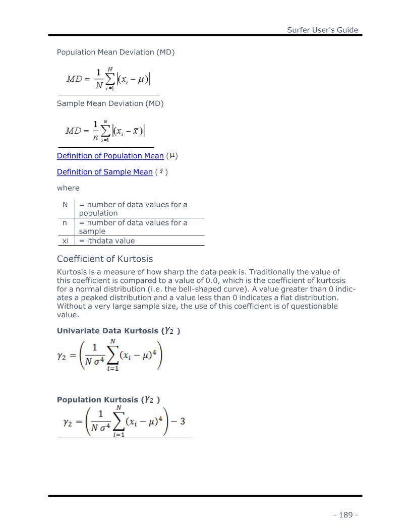
Surfer User's Guide
Population Mean Deviation (MD)
Sample Mean Deviation (MD)
Definition of Population Mean ( )
Definition of Sample Mean ( )
where
N = number of data values for apopulation
n = number of data values for asample
xi = ithdata value
Coefficient of KurtosisKurtosis is a measure of how sharp the data peak is. Traditionally the value ofthis coefficient is compared to a value of 0.0, which is the coefficient of kurtosisfor a normal distribution (i.e. the bell-shaped curve). A value greater than 0 indic-ates a peaked distribution and a value less than 0 indicates a flat distribution.Without a very large sample size, the use of this coefficient is of questionablevalue.
Univariate Data Kurtosis ( )
Population Kurtosis ( )
- 189 -

Chapter 3 - Data Files and the Worksheet
Sample Kurtosis ( )
(adapted from King and Julstrom, 1982)
where
= Population Standard Deviations = Sample Standard Deviation
= Population Mean= Sample Mean
N = number of data values for apopulation
n = number of data values for asample
xi = ithdata value
Coefficient of SkewnessSkew is a measure of asymmetry in the distribution. A positive skew indicates alonger tail to the right, while a negative skew indicates a longer tail to the left. Aperfectly symmetric distribution, like the normal distribution, has a skew equalto 0. For small data sets this measure is unreliable.
Population Skew ( )
Sample Skew ( )
- 190 -

Surfer User's Guide
(adapted from King and Julstrom, 1982 and Hildebrand, 1986)
where
= Population Standard Deviations = Sample Standard Deviation
= Population Mean= Sample Mean
N = number of data values for apopulation
n = number of data values for asample
xi = ithdata value
Coefficient of VariationThe coefficient of variation is the standard deviation divided by the mean. Theworksheet reports the quotient: it does not convert the value to a percentage.The coefficient of variation is a dimensionless measure of variation. This statisticis not defined for the case of a zero mean and this measure is only useful whendealing with strictly positive data.
Population Coefficient of Variation (V)
Sample Coefficient of Variation (V)
where
= Population Standard Devi-ation
s = Sample Standard Deviation
- 191 -

Chapter 3 - Data Files and the Worksheet
= Population Mean= Sample Mean
Critical Value of K-S Statistic at 90%, 95%, and 99% SignificanceLevelThe critical value of K-S statistic at 90%, 95%, or 99% significance level areindicators of normal distributions. For example, if a sample collected from a pop-ulation has a normal frequency distribution, the K-S statistic for that sample isless than the critical value 90, 95, or 99 percent of the time. If the K-S statistic islarger than the critical value, the hypothesis that the underlying population is dis-tributed normally with a mean of and a standard deviation of s should be rejec-ted.
Kolmogorov-Smirnov Goodness of Fit for Normal DistributionThe Kolmogorov-Smirnov statistic is the largest difference between an expectedcumulative probability distribution and an observed frequency distribution. Theexpected distribution used here is the normal probability distribution with meanand variance equal to the mean and variance of the sample data. The observedfrequency distribution is a stepped function that increases by 1/n with each step,where n is the number of values in the data set.
For example, suppose that there are five values in a data set. The observed fre-quency distribution is 0 to the left of the first data point. At the first data pointthe observed distribution function jumps to 0.2 (since there are five data values,the size of the step at each value is one divided by five). At each successive datavalue the observed frequency distribution jumps by 0.2.
The K-S statistic is calculated as the largest difference (in absolute value)between the normal cumulative probability function and the observed frequencydistribution, as shown below. Note that at each step it's necessary to computethe difference between bottom of the step and the normal curve and alsobetween the top of the step and the normal curve.
- 192 -

Surfer User's Guide
MeanThe mean is the arithmetic average of the data values. It is the sum of the datavalues divided by the number of data values.
Population Mean ( )
Sample Mean ( )
where
N = number of data values for apopulation
n = number of data values for asample
xi = ithdata value
- 193 -
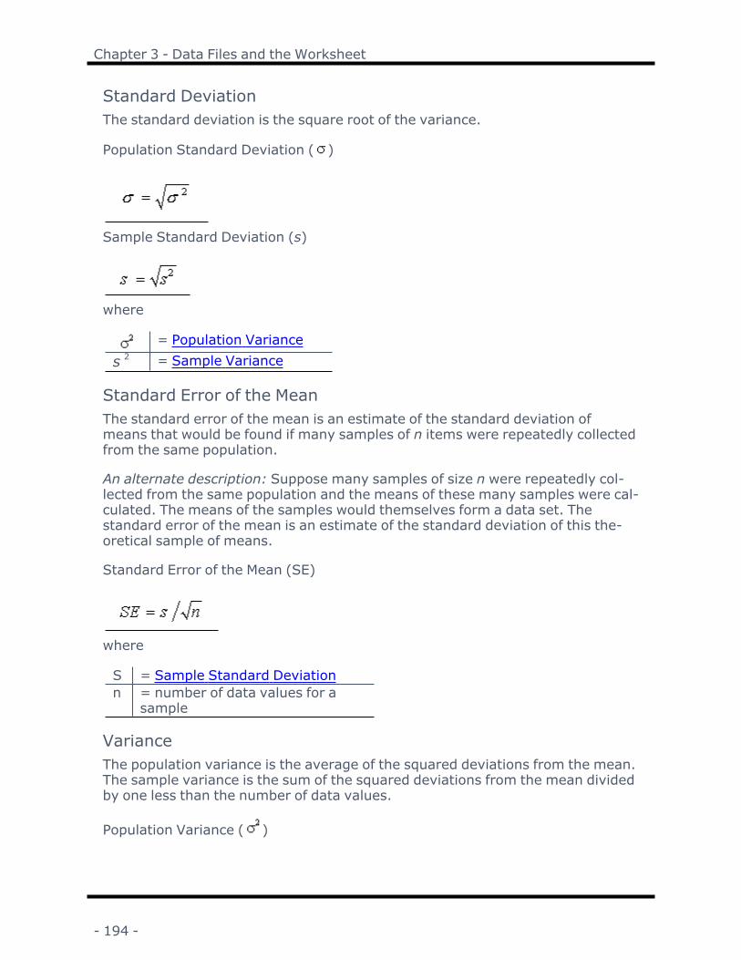
Chapter 3 - Data Files and the Worksheet
Standard DeviationThe standard deviation is the square root of the variance.
Population Standard Deviation ( )
Sample Standard Deviation (s)
where
= Population Variances 2 = Sample Variance
Standard Error of the MeanThe standard error of the mean is an estimate of the standard deviation ofmeans that would be found if many samples of n items were repeatedly collectedfrom the same population.
An alternate description: Suppose many samples of size n were repeatedly col-lected from the same population and the means of these many samples were cal-culated. The means of the samples would themselves form a data set. Thestandard error of the mean is an estimate of the standard deviation of this the-oretical sample of means.
Standard Error of the Mean (SE)
where
S = Sample Standard Deviationn = number of data values for a
sample
VarianceThe population variance is the average of the squared deviations from the mean.The sample variance is the sum of the squared deviations from the mean dividedby one less than the number of data values.
Population Variance ( )
- 194 -

Surfer User's Guide
Sample Variance (S 2)
where
= Population Mean= Sample Mean
N = number of data values for apopulation
n = number of data values for asample
xi = ithdata value
Statistics ReferencesClark, P. and F. Evans. (1954) Distance to nearest neighbor as a measure of spa-tial relationships in populations. Ecology, 35:445–453.
Cressie, N. A. C. (1991) Statistics for Spatial Data. New York: John Wiley & Sons,Inc.
Gilbert, Richard O. (1987)Statistical Methods For Environmental Pollution Mon-itoring. New York: Van Nostrand Reinhold.
Hildebrand, David K. (1986) Statistical Thinking for Behavioral Scientists.Duxbury Press.
King, Ronald S. and Bryant Julstrom. (1982) Applied Statistics Using the Com-puter. Sherman Oaks, California: Alfred Publishing Company.
Press, William H. et al. (1992) Numerical Recipes in C: The Art of Scientific Com-puting. New York: Cambridge University Press.
Montgomery, D. C. and G. C. Runger. (1994) Applied Statistics and Probabilityfor Engineers. New York: John Wiley & Sons, Inc.
Ryan, T. (1997) Modern Regression Methods. New York: John Wiley Sons, Inc.
Sheskin, D.J. (2000) Handbook of Parametric and Nonparametric Statistical Pro-cedures, Second Edition. Boca Raton, Florida: Chapman & Hall/CRC.
- 195 -
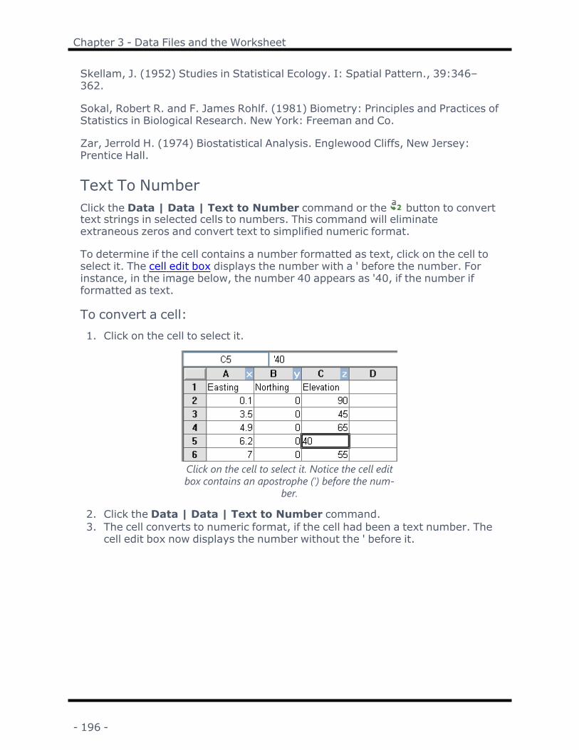
Chapter 3 - Data Files and the Worksheet
Skellam, J. (1952) Studies in Statistical Ecology. I: Spatial Pattern., 39:346–362.
Sokal, Robert R. and F. James Rohlf. (1981) Biometry: Principles and Practices ofStatistics in Biological Research. New York: Freeman and Co.
Zar, Jerrold H. (1974) Biostatistical Analysis. Englewood Cliffs, New Jersey:Prentice Hall.
Text To NumberClick the Data | Data | Text to Number command or the button to converttext strings in selected cells to numbers. This command will eliminateextraneous zeros and convert text to simplified numeric format.
To determine if the cell contains a number formatted as text, click on the cell toselect it. The cell edit box displays the number with a ' before the number. Forinstance, in the image below, the number 40 appears as '40, if the number ifformatted as text.
To convert a cell:1. Click on the cell to select it.
Click on the cell to select it. Notice the cell editbox contains an apostrophe (') before the num-
ber.
2. Click the Data | Data | Text to Number command.3. The cell converts to numeric format, if the cell had been a text number. The
cell edit box now displays the number without the ' before it.
- 196 -

Surfer User's Guide
The cell now shows the number right alignedand the cell edit box does not contain an apo-
strophe (') before the number.
TransposeThe Data | Data | Transpose command rearranges data from columns to rowsor from rows to columns. To quickly switch the layout of your data, highlight thedata that should be flipped. Click the Data | Data | Transpose command orthe button and the columns become rows and the rows become columns.
For example, consider the following data:
Categories A, B, and C are displayed with each category ina row.
Highlight the rows 1-4. Click the Data | Data | Transpose command and thedata appears in columns:
Categories A, B, and C are now displayed witheach category in a separate column.
Assign XYZ Columns - WorksheetThe Data | Data | Assign XYZ Columns command allows you to specify the X,Y, and Z columns containing your coordinate data.
- 197 -

Chapter 3 - Data Files and the Worksheet
The assigned columns are used as the default X, Y, and Z columns for commandsthat require column input, such as the Grids | New Grid | Grid Data andHome | New Map | Post commands. The track cursor command requires thatthe X, Y, and Z columns be specified properly in order to display the currentcoordinates when a point is clicked in another window.
Indicators in the worksheet column headers display the current columns. Whenthe coordinates are changed in the Assign XYZ Columns dialog, the X, Y, and Zindicators move to the specified columns. If there is no actual data in the userassigned columns, Surfer will assign columns that contain data to the coordin-ate columns.
Indicators in the worksheet column headersdisplay the X, Y, and Z columns specified in
the Assign XYZ Columns dialog.
The Assign XYZ Columns Dialog
The Data | Data | Assign XYZ Columns command or the button opens theAssign XYZ Columns dialog.
Use the Assign XYZ Columns dialog to specifythe worksheet columns where the X, Y, and Z val-
ues are located.X (Easting) ColumnSelect a worksheet column from the X (Easting) column list.
- 198 -

Surfer User's Guide
Y (Northing) ColumnSelect a worksheet column from the Y (Northing) column list.
Z (Elevation) ColumnSelect a worksheet column from the Z (Elevation) column list.
Click OK to save the assigned X, Y, and Z columns. The X, Y, and Z indicators willmove to the assigned columns. Click Cancel to cancel the change in the columndefinitions. The default columns are used.
Assign Coordinate System - WorksheetThe Data | Coordinate System | Assign Coordinate System command or
the button links a data file to a specific coordinate system. Once the coordin-ate system is defined for the data file, a Golden Software Georeference .GSR2file is created. This file contains all the relevant projection information thatSurfer needs to load the data in the proper projection.
When a .GRD file is created using the Grids | New Grid | Grid Data command, the.GSR2 file for the data is read. The projection information can be saved with thegrid file using the Spatial References options. It is recommended to check the GSReference (Version 2) file if you intend to use the grid file in Surfer, as the GSR2retains all of the information needed. The grid has the same coordinate systemas the original data file, but the .GSR2 is required to define the coordinate sys-tem. When a map is created from either the data file or the .GRD file, the .GSR2file is read and the map layer automatically has the correct coordinate system.
New Projected Coordinates - WorksheetThe Data | Coordinate System | New Projected Coordinates commandspecifies a Source Coordinate System and projects the X and Y coordinate datato a new Target Coordinate System. The input Source Columns and output Tar-get Columns allow you to either overwrite the original coordinate columns, orwrite the new coordinates to new columns in the worksheet. For example, thiscommand can be useful if you have coordinate data in latitude and longitude andneed to project the coordinates to UTM.
New Projected Coordinates DialogThe Data | Coordinate System | New Projected Coordinates command orthe button in the worksheet opens the New Projected Coordinates dialog.
- 199 -

Chapter 3 - Data Files and the Worksheet
Change coordinates in the New Projected Coordinates dialog.Source ColumnsSpecify the columns containing the X and Y coordinates in the Source Columns Xand Y. Click the arrow to see a list of the data columns in your worksheet. TheSource Columns contain the X and Y values in the existing coordinate system.
Source Coordinate System
Assign the Source Coordinate System by clicking the button to open theAssign Coordinate System dialog. The Source Coordinate System is the systemthat your X, Y coordinate data are currently using.
Target ColumnsSpecify the X and Y destination columns in the Target Columns X and Y. The pro-jected output coordinates will be located in the target columns specified. Clickthe arrow to see a list of the data columns in your worksheet.
Target Coordinate System
Assign the Target Coordinate System by clicking the button to open theAssign Coordinate System dialog. The Target Coordinate System is the newcoordinate system that you want to use to project your X, Y coordinate data.
OK and CancelClick OK to write the new projected X and Y coordinates to the Target Columns.Click Cancel to close the New Projected Coordinates dialog without makingany changes to the worksheet.
DMS to DDClick the Data | Coordinate System | DMS to DD command or the buttonto convert DMS longitude and latitude values to decimal degrees. The DMS to
- 200 -

Surfer User's Guide
DD command converts two source columns of data and writes the new values intwo target columns.
DMS to DD DialogThe DMS to DD dialog is opened when the DMS to DD command is clicked. Spe-cify the source and target columns and the source DMS format in the DMS toDD dialog.
Specify the source and target columns and the DMS format.Source ColumnsThe Source Columns group contains the Longitude and Latitude columns and theDMS Format.
Longitude and LatitudeSelect the column containing DMS longitude values in the Longitude field. Selectthe column containing DMS latitude values in the Latitude field. Click the currentselection to change the column. The Longitude and Latitude column lists onlyinclude columns with data. Latitude column values must be between -90 and 90degrees.
DMS FormatSelect the source data format in the DMS Format field. Click the current selectionand select the desired format from the list. DMS source data must be formattedin one of the following data formats, and all of the source data must use thesame format:
l DDD MM SS.SSS - DMS separated - this format includes degrees, minutes,and seconds separated by spaces. Optionally, this format can include sym-bols and a hemisphere indicator, e.g 105° 6' 32.5" W.
- 201 -

Chapter 3 - Data Files and the Worksheet
l DDD MM.MMM - DM separated - this format includes degrees and minutesseparated by a space. Optionally, this format can include symbols and a hemi-sphere indicator, e.g. 105° 6.54167' W.
l DDMMSS.SSS - DMS packed - this format includes degrees, minutes, andseconds without any spaces. The minutes and seconds values must includetwo digits. Optionally, this format can include a hemisphere indicator, e.g.1050632.5 W.
l DDMM.MMM - DM packed - this format includes degrees and minutes withoutany spaces. The minutes value must include two digits. Optionally, thisformat can include a hemisphere indicator, e.g. 10506.54167 W
l DD.DDD H - Degrees w/ hemisphere - this format is decimal degrees with ahemisphere indicator, e.g. 105.109 W
Target ColumnsThe Target Columns group contains the Longitude and Latitude columns. Selectthe column where the converted longitude values should be created in the Lon-gitude field. Select the column where the converted latitude values should be cre-ated in the Latitude field. Click the current selection to change the column. Selectthe same columns as the Source Columns if you wish to overwrite the sourcedata. The default Longitude and Latitude columns are the first empty columns inthe worksheet.
OK and CancelClick OK to create the decimal degrees longitude and latitude columns. ClickCancel to close the DMS to DD dialog without converting the values to decimaldegrees.
- 202 -

Chapter 4 - Creating Grid Files
Grid FilesContour maps, color relief maps, vector maps, watershed maps, 3D surfaces,and 3D wireframes all require grids for their creation in Surfer. A grid is a reg-ular, rectangular array of values. The Home | Grid Data | Grid Data commandprovides you with several methods for generating a Surfer .GRD grid file fromyour XYZ data. In addition to the grid files that Surfer creates, it can also readmany common grid file formats directly. A grid with all NoData nodes cannot besaved.
A Gridding ExampleConsider the scenario of producing a contour map of water table depth given welldata collected over a region. The well locations are not regularly spaced over thearea of interest. If you provide Surfer with the locations of the wells (the XYcoordinates) and the depth to the water table (the Z value) in the form of an XYZdata file, Surfer can produce a grid file from the original data and a grid-basedmap from the gridded data. The following series of figures show the normal pro-gression from a data file, to a grid file, to a contour map.
1. In a worksheet window, define well locations (X and Y coordinates) andwater table depth (Z value) at each location in an XYZ data file.
This is the XYZ data file that defines the well locations and water table depth at each loc-ation.
2. In the plot window, click the Home | New Map | Post command. Selectthe data file created in step 1and click Open to create a post map displayingthe data locations with Z value labels. This step is to show the irregularlyspaced data across the map.
- 203 -

Chapter 4 - Creating Grid Files
This is a post map displaying the data locations. The well locations are irregularly spacedover the map in this example. There are many "holes" where no data exists.
3. Click the Grids | New Grid | Grid Data command to create a regularlyspaced grid .GRD file from the irregularly spaced XYZ data file. Use thedefault values in the Grid Data dialog and click OK to create the .GRD file.
Gridding interpolates a Z value at the intersection of each row and column in the grid file,thereby filling holes in the data. Here the rows and columns are represented by grid lines
drawn across the map.
- 204 -

Surfer User's Guide
4. Click once on the post map to select it. Click the Home | Add to Map |Layer | Contour command to add a contour map of the grid file to thepost map of the data file.
The irregularly spaced data points are used to interpolate grid node values. These inter-polated values are written to a grid file. The grid file is used to produce the contour map. This
figure shows the filled contour map, the posted data points, and the layout of the grid.
Grid DataGrid files are necessary in Surfer to create grid-based maps types. Data files aretypically randomly spaced files, and this data must be converted into an evenlyspaced grid before using many of Surfer's features. Grid files are produced from
XYZ data using the Home | Grid Data | Grid Data, the button, or theGrids | New Grid | Grid Data command. With this command, you can specifythe parameters for the particular gridding method and the extents of the grid.The gridding methods define the way in which the XYZ data are interpolatedwhen producing a grid file.
Data files should be arranged with all X data in one column, all Y data in anothercolumn, and all Z data in a third column. Each data column can be any column inthe data file and in any order. The columns are selected in the Select Datapage.
When creating a grid file you can usually accept all of the default gridding para-meters and generate a grid file that represents your data well. Under most cir-cumstances, the recommended gridding method is kriging with the default linear
- 205 -
Chapter 4 - Creating Grid Files
variogram. This is the selected default gridding method because it gives good res-ults for most XYZ data sets.
There are several gridding parameters you can set when producing a grid file.Refer to the gridding method for more information on specific parameters. Mostgridding methods require at least three non-collinear data points. The InverseDistance, Nearest Neighbor, Moving Average, and Data Metricsmethods requireat least three data points, collinear or not. Some methods require more datapoints. For example, a higher-order polynomial fit needs more than three datapoints; there must be at least as many data as there are degrees of freedom.When the Z Transform is set to Log, save as log or Log, save as linear, at leastthree data points must contain Z values that are non-negative and non-zero.Click the Grids | New Grid | Grid Data or Home | Grid Data | Grid Datacommand to choose the data to be used in the gridding process.
Grid Data DialogClick the Grids | New Grid | Grid Data or Home | Grid Data | Grid Datacommand to display the Grid Data dialog. The Grid Data dialog includes mul-tiple pages:
l Select Datal Variograml Optionsl Cross Validationl Output
Open Data DialogThe Open Data dialog is used by some plot window grid commands (i.e. GridData).
- 206 -

Surfer User's Guide
Select a data file in the Open Data dialog.
Look InThe Look in field shows the current directory. Click the down arrow to see the dir-ectory structure and click on the folders to change directories.
Creating New Folders and Changing the ViewThe buttons to the right of the Look in field allow you to create new folders andchange the view of the file list.
File ListThe File list displays files in the current directory. The current directory is listedin the Look in field. The Files of type field controls the display of the file list. Forexample, if DAT Data (*.dat) is listed in the Files of type field only *.DAT filesappear in the files list.
- 207 -

Chapter 4 - Creating Grid Files
Open WorksheetsSurfer tracks the files being used by maintaining a list of opened files for newmaps and the files used in saved maps. The file(s) used to build maps are shownin a compiled list in the Open Worksheets field.
Specify a File NameThe File name field shows the name of the selected file. Alternatively, type a pathand file name into the box to open a file.
Files of TypeThe Files of type field controls the display of the file list. For example, if DAT Data(*.dat) is listed in the Files of type field only *.DAT files appear in the files list.
The All Recognized Types (*...) format type is selected by default. This displaysall the common file formats in the navigation pane. If a different format type isselected, Surfer will remember the setting until the end of the current session.When Surfer is restarted, the default format type will be used.
To see all files in the directory, choose All Files (*.*) from the Files of type list.Double-click on a file to open it or single-click the file and then click the Open but-ton. The All Files (*.*) option shows all of the file formats in the current dir-ectory, even if the file type is not appropriate for the action chosen. For example,a GRD file may be displayed, even though a GRD file cannot be imported into theworksheet.
Select a file type from the Files of type list. The following formats are supported:
l ACCDB Access Database (*.accdb)l BLN Golden Software Blanking .BLNl BNA Atlas Boundary .BNAl CSV Comma Separated Variables .CSVl DAT Data .DATl DBF Database .DBFl DXF AutoCAD Drawing Data (*.dxf)l LAS LiDAR Data (*.las)l MDB Microsoft Access .MDBl SEG-P1 Data Exchange Format (*.seg)l P1 Data Exchange Format (*.sp1)l SLK Sylk Spreadsheet .SLKl TXT Text Data .TXTl XLS Excel Spreadsheet .XLSl XLSX Excel 2007 Spreadsheet .XLSXl XLSM Excel 2007 Spreadsheet .XLSMl ACCDB Access Database (*.accdb)l BLN Golden Software Blanking .BLNl BNA Atlas Boundary .BNA
- 208 -

Surfer User's Guide
l CSV Comma Separated Variables .CSVl DAT Data .DATl DBF Database .DBFl DXF AutoCAD Drawing Data (*.dxf)l LAS LiDAR Data (*.las)l MDB Microsoft Access .MDBl SEG-P1 Data Exchange Format (*.seg)l P1 Data Exchange Format (*.sp1)l SLK Sylk Spreadsheet .SLKl TXT Text Data .TXTl XLS Excel Spreadsheet .XLSl XLSX Excel 2007 Spreadsheet .XLSXl XLSM Excel 2007 Spreadsheet .XLSM
Open WorksheetsThe Open worksheets group displays worksheets that are currently open to beselected. If a worksheet is selected from the Open worksheets group that hasassigned XYZ coordinates, the following dialogs (i.e. Grid Data dialog) will havethe X, Y, and Z columns populated to match the assigned XYZ coordinates.
Surfer tracks the files being used by maintaining a list of opened files for newmaps and the files used in saved maps. The file(s) used in existing maps areshown in a compiled list in the Open worksheets field of the Open Data dialog.
Load DatabaseClick the Database button in the Open Data dialog to open the Data Link Prop-erties dialog and import a database.
Cross ValidationGenerally, cross validation can be considered an objective method of assessingthe quality of a gridding method, or to compare the relative quality of two ormore candidate gridding methods. In Surfer, cross validation can be used withall gridding methods. While cross validation can be used to select a griddingmethod, the results can also be used to assess the spatial variation in griddingquality and to guide data sampling. Cross validation is always performed on thelinear Z values, not the transformed Z values.
A generalized discussion of cross validation is given here. Refer to one of themany geostatistics books for more information. In the listed references below,much of the discussion concerns kriging, but the generalized discussion appliesto all of the gridding methods in Surfer.
- 209 -

Chapter 4 - Creating Grid Files
Cross Validation ProcessGiven the known values at N observation locations in the original data set, crossvalidation allows you to assess the relative quality of the grid by computing andinvestigating the gridding errors. In Surfer, these errors are calculated byremoving the first observation from the data set, and using the remaining dataand the specified algorithm to interpolate a value at the first observation loc-ation. Using the known observation value at this location, the interpolation erroris computed as:
error = interpolated value − observed value
Then, the first observation is put back into the data set and the second obser-vation is removed from the data set. Using the remaining data (including the firstobservation), and the specified algorithm, a value is interpolated at the secondobservation location. Using the known observation value at this location, theinterpolation error is computed as before.
The second observation is put back into the data set and the process is continuedin this fashion for the third, fourth, fifth observations, etc., all the way throughup to and including observation N, the last observation in the data file. This pro-cess generates N interpolation errors. Various statistics computed for the errorscan be used as a quantitative, objective measure of quality for the griddingmethod.
Thus, cross validation involves four steps:
1. Select a gridding method, along with all of the defining parameters.
2. For each observation location, interpolate the value using the neighboringdata, but not the observation itself.
3. Compute the resulting interpolation errors.
4. Assess the quality of the selected gridding method using various summarystatistics of the errors.
Grid Data - Cross ValidationThe Cross Validation page is displayed after the Options page in the Grid Datadialog.
- 210 -

Surfer User's Guide
Evaluate gridding methods with cross validation.Number of Random Points to ValidateFor large and very large data sets the cross validation process of sweepingthrough each and every observation point can take a great deal of time and com-putational effort. A quicker alternative is to carry-out the cross validation pro-cedure at a random subset of the observation locations.
Number of random points to validate allows you to specify the number of crossvalidation points. By default, this value is equal to the total number of obser-vations. For large and very large data sets this values should be 1,000 or more toensure a relatively stable set of error statistics. Note, the entire data set is usedthrough-out the cross validation process, not just the random subset. The ran-dom subset merely identifies the locations at which cross validation errors arecomputed. Also, note that the random subset is determined without replace-ment, using a random number generator that is randomly initialized for everyexecution; thus, the random subset may be different every time cross validationis run.
- 211 -

Chapter 4 - Creating Grid Files
Points FilterSet the X, Y, and Z direction values for Minimum and Maximum in the Point Filtersection. This restricts the cross validation to a subarea of the data extent. Datafalling outside of these limits may be used during the interpolation, but they arenot used as cross validation points. The limits in Z direction are useful to excludecross validation at known anomalous observation locations.
Exclude Data WithinOften observations come in relatively homogeneous clusters. In these cir-cumstances, the standard cross validation approach may not generate useful res-ults as the interpolated values are merely the values of the close-by adjacentobservations. To counter this potential problem, the X tolerance and Y tolerancefields define a centered rectangular buffer zone around each of the observationsat which cross validation is carried out. This buffer zone is two times the X tol-erance in the X direction, and two times the Y tolerance in the Y direction. Anyobservations falling within a validation point’s buffer zone are not used in theinterpolation of that validation point. When these values are zero, all points inthe validation limits are used.
Cross Validation ReportClick Report to generate a cross validation report.
Cross Validation Results FileClick Save to save a cross validation results file. The results are presented in anASCII data file, which can be used as a gridding data file. The first line in the filecontains column titles. Each subsequent line is associated with a validation point.There are seven numeric values per line. The first three values are the X, Y, andZ values from the original data file of each validation point. The fourth column,titled ID is the line number from the original data file of the validation point. Thenext two columns are the estimated and residual values. The nData column con-tains the total number of original data points.
Statistics NoteUnder most interesting statistical models, the cross validation errors are not stat-istically independent: the estimate at one observation location uses much of thesame information as the estimate at a neighboring observation location. As such,standard hypothesis testing and test of statistical significance are not valid. A dis-cussion of this point can be found in the cross validation reference, Kitanidis(1997).
Cross Validation ReferencesThe following references include extensive discussion of the theory and applic-ation of cross validation. Isaaks and Srivastava [1989], Kitanidis [1997], Olea[1999], and Chiles and Delfiner [1999] focus on cross validation with kriging, butthe general discussion applies to all of the supported gridding methods inSurfer.
- 212 -

Surfer User's Guide
Chiles, J. P. and P. Delfiner. (1999)Geostatistics: Modeling Spatial Uncertainty.John Wiley and Sons, New York, 695 pp.
Isaaks, E. H. and R. M. Srivastava. (1989) Applied Geostatistics. OxfordUniversity Press, Inc., New York, 561 pp.
Kitanidis, P. K. (1997)Introduction to Geostatistics: Applications inCambridgeUniversity Press, Cambridge, 249 pp.
Olea, R. (1999) Geostatistics for Engineers and Earth Scientists. Kluwer Aca-demic Publishers, Boston, 303 pp.
What's Next?Click Next or Skip to End to proceed to the Output page. Click Finish to create thegrid file.
ReportsSurfer can generate several types of detailed grid reports. This table provides asnapshot of the types of information produced for each report type. Descriptionsof the report sections are below the table.
If you make changes to the data selection (i.e. changing a data column or chan-ging the data filtering method) generate a new report by repeating one of theprocesses listed with the report type.
InformationProduced Report Types and How to Access Them
Cross Val-idationReport
Data Stat-isticsReport
Grid Con-tour
Vol/AreaReport
GriddingReport
Grid Inform-ation Report
VariogramDataReport
ClickReport inthe CrossValidationdialog
Click theStatisticsbutton inthe GridData dialog
Click theGrids | Cal-culate |ContourVol/Areacommand
Check theGrid ReportOption onthe GridData dia-log
Click theGrids | Info| Grid Infocommand; orclick Options| Grid Info inthe GridEditor
In the Vari-ogram Prop-erties clickthe DisplayStatistics but-ton on theStatisticspage andthen clickReport
Data Counts,includesFiltered and atValidationPoints
X X X X
- 213 -

Chapter 4 - Creating Grid Files
Filtering,includes Break-line, Duplicate,Exclusion
X X
Grid Inform-ation, includesGrid Geometry
X X
Gridding Rules X XInter-VariableCorrelation,Rank Cor-relation andCovariance
X X X X
Output Grid XPrincipal Com-ponent Ana-lysis
X X
Polygon Usedfor Statistics X
Regression,includesPlanar:Z=AX+BY+Cand Residual:R=AX+BY +C
X X X
Statistics, suchas Univariate,Nearest Neigh-bor, and Cross-Validation
X X X X X
Variogram Grid XVolume andArea X
Z Transform,includes Gridand Data
X
Information Contained in Each Report SectionEach section of the report contains information about the grid, data, or vari-ogram.
Time StampTime of report Date and time the report was created in
Mon Oct 14 10:43:13 2013
formatElapsed time to cre-ate grid
Seconds required when gridding. Only included in theGridding Report.
- 214 -

Surfer User's Guide
Data SourceSource Data FileName
path and file name of the data used in gridding
X Column X data columnY Column Y data columnZ Column Z data columnDetrending variogram data detrending method selected on the
General page in the New Variogram dialog. Onlyincluded in the Variogram Grid Report.
Data Counts and Filtered Data CountsActive Data number of data after applying filtersOriginal Data number of original data points (excludes breakline
data)Excluded Data number of data excluded by the Data Exclusion Filter
- the excluded data are listed in the Exclusion Fil-tering section
Deleted Duplicates number of duplicates deleted by the Duplicate Datafilter - the deleted duplicates are listed in the Duplic-ate Filtering section
Retained Duplicates number of duplicates retained by the Duplicate Datafilter (this statistic is not computed if the duplicaterule is ALL) - the retained duplicates are listed in theDuplicate Filtering section including any artificial data
Artificial Data number of artificial data created by the Sum, Aver-age, and Midrange Duplicate Data filters
Superseded Data Superseded data are number of data eliminated bybreaklines in the Data Statistics Report and the Grid-ding Report. Breakline data always supersede pointdata. If point data are on, or in the immediate vicinityof, breakline data the point data are eliminated.
Data Counts at Validation PointsThe Data Counts at Validation Points section is only included in the Cross Val-idation Report.
Active Results locations at which the cross validation interpolationwas successfully carried out
- 215 -

Chapter 4 - Creating Grid Files
NoData Results The NoData results are the locations at which crossvalidation interpolation was attempted, but was notsuccessful. For example, the natural neighbor grid-ding algorithm can only interpolate at locationswithin the convex hull of the active data. As such, anobservation that lies on the convex hull of the ori-ginal, complete, data set will lie outside of the convexhull of the active data when that observation is thecross validation point. Cross validation is not possibleusing the natural neighbor algorithm at such a point,so it is assigned the NoData value.
Attempted Results reports the number of locations at which cross val-idation interpolation was attempted
Requested Results contains the original number of random data
Z Data TransformIncludes the transformation method (if any) applied to the Z values. Lists thedata that was unable to be transformed in a table.
The rest of the report information is calculated using the active data, includingany artificial data generated by duplicate filtering. Excluded, deleted, or super-seded data are not included in the following calculations.
Exclusion FilteringExclusion FilterString
shows the Data Exclusion Filterstring
Excluded Data number of data excluded by the Data Exclusion Filter-
Excluded Data Table the excluded data are listed in a table. The ID is equalto the line number in the original data file. This list is100 data rows long by default.
Duplicate FilteringDuplicate Points toKeep
To Keep filter used
X Duplicate Tol-erance
maximum X spacing of points to be considered aduplicate
Y Duplicate Tol-erance
maximum Y spacing of points to be considered aduplicate
Deleted Duplicates number of duplicates deleted by the Duplicate Datafilter - the deleted duplicates are listed in the Duplic-ate Filtering section
- 216 -

Surfer User's Guide
Retained Duplicates number of duplicates retained by the Duplicate Datafilter (this statistic is not computed if the duplicaterule is ALL) - the retained duplicates are listed in theDuplicate Filtering section including any artificialdata
Artificial Data number of artificial data created by the Sum, Aver-age, and Midrange Duplicate Data filters
Duplicate DataTable
the duplicate data table lists all of the duplicatepoints with X, Y, Z, ID, and Status. The ID is equal tothe line number in the original data file. When thestatus is artificial, no ID is given since this data doesnot come from the original data file. The Status(Retained, Deleted, or Artificial) reports how theduplicate was handled. This list is 100 data rows longby default.
Breakline FilteringWhen breaklines are used, data that is within the X Tolerance and Y Tolerance,as set in the Filter dialog, of the breakline are deleted due to breakline datasuperseding original data.
Anisotropy Angle the anisotropy angle reported for the default vari-ogram
Anisotropy Ratio the anisotropy ratio reported for the default vari-ogram
X Tolerance maximum X spacing of points to be considered aduplicate
Y Tolerance maximum Y spacing of points to be considered aduplicate
Superseded Data Superseded data are number of data eliminated bybreaklines in the Data Statistics Report and the Grid-ding Report. Breakline data always supersede pointdata. If point data are on, or in the immediate vicinityof, breakline data the point data are eliminated.
Breakline DataTable
the breakline data table lists all of the supersededdata points with X, Y, Z, ID, and Status. The ID isequal to the line number in the original data file. TheStatus (Retained, Deleted, or Artificial) reports howthe duplicate was handled. This list is 100 data rowslong by default.
Inter-Variable CorrelationThe Inter-Variable Correlation table shows the correlation between the X, Y, andZ variables. The Cross Validation Report also contains Estimated Z and ResidualZ columns and rows. The correlations are computed with
- 217 -

Chapter 4 - Creating Grid Files
The correlation is positive when both variables increase or decrease together.The correlation is negative when one variable increases while the other variabledecreases. A correlation of zero shows that there is no linear relationshipbetween the variables.
Inter-Variable CovarianceThe Inter-Variance Covariance table shows the covariance between the X, Y, andZ variables. The covariances are computed with
The covariance is positive if, on average, the variables are both above the mean.The covariance is negative if one variable is above the mean and the other vari-able is below the mean.
Inter-Variable Rank CorrelationThe Inter-Variance Rank Correlation table shows the rank correlation betweenthe X, Y, and Z variables. The data is ordered and then assigned a rank valuefrom 1 to the count of values. Rank values range from -1 to +1. The correlationis positive when both variables increase or decrease together. The correlation isnegative when one variable increases while the other variable decreases. A cor-relation of zero shows that there is no linear relationship between the variables.
Univariate StatisticsThis group of statistics shows information for X, Y, and Z data. These statistics donot include breakline data.
Count total number of points1%-tile 1 percent of the values are smaller than this number
and 99 percent of the values are larger5%-tile 5 percent of the values are smaller than this number
and 95 percent of the values are larger10%-tile 10 percent of the values are smaller than this num-
ber and 90 percent of the values are larger25%-tile lower quartile; 25 percent of the values are smaller
than this number and 75 percent of the values are lar-ger
50%-tile middle data value, 50 percent of the data values arelarger than this number and 50 percent of the dataare smaller than this number
75%-tile upper quartile; 75 percent of the values are smallerthan this number and 25 percent of the values are lar-ger than this number
- 218 -

Surfer User's Guide
90%-tile 90 percent of the values are smaller than this num-ber and 10 percent of the values are larger
95%-tile 95 percent of the values are smaller than this num-ber and 5 percent of the values are larger
99%-tile 99 percent of the values are smaller than this num-ber and 1 percent of the values are larger
Minimum minimum valueMaximum maximum valueMean arithmetic average of the data
Median middle data value, 50 percent of the data values arelarger than this number and 50 percent of the dataare smaller than this number
Geometric Mean geometric mean of the dataHarmonic Mean harmonic mean of the dataRoot Mean Square square root of the mean squareTrim Mean (10%) Trim Mean is the mean without the upper five percent
and lower five percent of the data, therefore,extreme value influence is removed. If there arefewer than 20 data points, the minimum and max-imum data points are removed instead of the upperand lower five percent.
Interquartile Mean interquartile mean, or midmean, is a truncated meanusing only the data in the second and third quantiles(all data beween the 25%%-tile and 75%%-tile)
Midrange the value halfway between the minimum and max-imum values
Midrange = (Minimum + Maximum ) / 2Winsorized Mean Winsorized mean is a truncated mean. This method
replaces the extreme highs and lows values with amore central value. This mean is less sensitive to out-liers.
TriMean the trimean, or Tukey's trimean, is a measure of prob-ability distribution location. This is equivalent to thethe sum of (quartile 1, 2 times the quartile 2, andquartile 3) divided by four.
Variance
Standard Deviation square root of the variance
- 219 -

Chapter 4 - Creating Grid Files
Interquartile Range separation distance between the 25%-tile and 75%-tile
this shows the spread of the middle 50 percent of thedata, similar to standard deviation, though this stat-istic is unaffected by the tails of the distribution
Range separation between the minimum and maximumvalue
Range = Maximum - MinimumMean Difference the mean or average of the absolute difference of two
random variables X and Y.Median Abs. Devi-ation
Median Absolute Deviation is the median value of thesorted absolute deviations. It is calculated by
1. computing the data's median value
2. subtracting the median value from each data value
3. taking the absolute value of the difference
4. sorting the values
5. calculating the median of the valuesAverage Abs Devi-ation
Average Absolute Deviation is the average value ofthe sorted absolute deviations. It is calculated by
1. computing the data's average mean value
2. subtracting the mean value from each data value
3. taking the absolute value of the difference
4. calculating the average valueQuartile Dispersion Measures dispersion of the data using: (Quartile 3 -
Quartile 1)/(Quartile 3 + Quartile 1)Relative Mean Dif-ference
The mean difference of the entire data set divided bythe sample mean of the data set
Standard Error The standard error of the mean is the standard devi-ation of those sample means over all possiblesamples drawn from the population. This is cal-culated by dividing the standard deviation by thesquare root of the number of samples.
Coef. of Variation The Coefficient of Variation is calculated by dividingthe standard deviation by the mean. If a "-1" is repor-ted, the coefficient of variation could not be com-puted. The coefficient of variation is computed onlyfor the Z values.
- 220 -

Surfer User's Guide
Skewness The Coefficient of Skewness is calculated by
If a "-1" is reported, the coefficient of skewness couldnot be computed. The coefficient of skewness is com-puted only for the Z values.
Kurtosis The Coefficient of Kurtosis is calculated by
Sum the sum of all X, Y, or Z valuesSum Absolute the absolute value of the sum of all X, Y, or Z valuesSum Squares the sum of all squared X, Y, or Z valuesMean Square
Planar RegressionPlanar regression is an ordinary least-squares fit where Z=AX+BY+C.
l The Parameter Values are the A, B, and C values.
l The Standard Error is the estimated standard deviation of the parameters.
l The Inter-Parameter Correlations are the correlation between A, B, and Ccoefficients.
l The ANOVA Table shows regression statistics on the planar fit where df arethe degrees of freedom and F is the ratio of the mean squares.
l The Coefficient of Multiple Determination (R2) is calculated with
For the Cross Validation Report, the planar regression is the residual regressionat the validation points.
Nearest Neighbor StatisticsThe nearest neighbor statistics represent aspects of the data values and of thedata locations. The nearest neighbor to a data point uses a simple separation dis-tance without taking anisotropy into account. If two or more points tie as the
- 221 -

Chapter 4 - Creating Grid Files
nearest neighbor, the tied data points are sorted on X, then Y, then Z, and thenID. The smallest value is selected as the nearest neighbor.
The Separation column shows the separation distances between the observationand its nearest neighbor. The |Delta Z| column shows the absolute values of thedifferences between the observation Z value and the nearest neighbor Z value.
The statistics are the same as the Univariate Statistics (see above).
The Nearest Neighbor Statistics also includes the Complete Spatial Randomnesssection. The Complete Spatial Randomness statistics measure how random loc-ations are in space. Surfer does not correct for edge effects so the statistics maybe biased.
Lamda is the average spatial density
Clark and Evans
where
= average spatial density
Si= separation distance between the observation andthe nearest neighbor
The distribution of this statistic is normal, with amean equal to one and a variance of
See Clark and Evans (1954) and Cressie (1991) formore information.
- 222 -

Surfer User's Guide
Skellam
where
= average spatial density
Si= separation distance between the observation andthe nearest neighbor
The distribution is Chi-Squared with 2N degrees offreedom. See Skellam (1952) and Cressie (1991) formore information.
Principal Component AnalysisPrincipal component analysis (PCA) is a mathematical procedure that uses ortho-gonal transformation to convert a set of observations of possibly correlated vari-ables into a set of values of linearly uncorrelated variables called principalcomponents. The number of principal components is less than or equal to thenumber of original variables. The principal components are calculated for the X,Y, and Z values. A value is also reported for each principal component.
Variogram GridMax Lag Distance Max Lag Distance set on the General page in the
New Variogram dialogAngular Divisions number of Angular Divisions set on the General page
in the New Variogram dialogRadial Divisions number of Radial Divisions set on the General page in
the New Variogram dialog
Output GridGrid File Name name of the output grid fileGrid Size number of rows and columns in the gridTotal Nodes number of columns times the number of rowsFilled Nodes number of grid nodes containing interpolated valuesNoData Nodes number of grid nodes containing the NoData valueNoData Value reports the Z value associated with NoData nodesX Minimum minimum X grid line value specified in the Output
Grid Geometry group in the Grid Data dialogX Maximum maximum X grid line value specified in the Output
Grid Geometry group in the Grid Data dialogX Spacing X spacing set in the Grid Data dialogY Minimum Minimum Y grid line value specified in the Output
Grid Geometry group in the Grid Data dialogY Maximum Maximum Y grid line value specified in the Output
Grid Geometry group in the Grid Data dialog
- 223 -

Chapter 4 - Creating Grid Files
Y Spacing Y spacing set in the Grid Data dialog
Grid InformationGrid File Name name of the output grid fileGrid Size number of rows and columns in the gridTotal Nodes number of columns times the number of rowsFilled Nodes number of grid nodes containing interpolated valuesNoData Nodes number of grid nodes containing the NoData valueNoData Value reports the Z value associated with NoData nodes
Grid GeometryX Minimum minimum X grid line value specified in the Output
Grid Geometry group in the Grid Data dialogX Maximum maximum X grid line value specified in the Output
Grid Geometry group in the Grid Data dialogX Spacing X spacing set in the Grid Data dialogY Minimum Minimum Y grid line value specified in the Output
Grid Geometry group in the Grid Data dialogY Maximum Maximum Y grid line value specified in the Output
Grid Geometry group in the Grid Data dialogY Spacing Y spacing set in the Grid Data dialog
Polygon used for statisticsSide Whether statistics were calculated for values Inside
or Outside the polygon(s)Polygons Number of polygons used for calculating statisticsNumber of points Total number of vertices among the polygon(s)
Gridding RulesThis section displays the gridding method used, as well as the option settings foreach gridding method.
Univariate Grid StatisticsThe Univariate Grid Statistics are the same as those reported in the UnivariateStatistics and Nearest Neighbor Statistics sections.
Univariate Cross-Validation StatisticsThe Univariate Cross Validation Statistics section are the same as those reportedin the Univariate Statistics. It also contains an additional column of data, calledData Used. This column shows the number of data points used in the calculation.
- 224 -

Surfer User's Guide
Volumes and AreasVolume and area calculations are based on the Simple level method for contourline properties. Minimum and maximum contours along with the contour intervalmust be specified. Surface area and planar area calculations are made above,below, and between contours. Contour volume calculations are made above,below, and between contours.
SearchSearch options control which data points are considered by the gridding oper-ation when interpolating grid nodes. To access the search options, if availablewith the gridding method, click the Advanced Options button in the Grid Data dia-log. If searching is available with the selected gridding method, a Search Neigh-borhood section appears in the Grid Data Advanced Options dialog. If searchoptions are not available for a gridding method this means that all the datapoints from the data file must be used when calculating the grid.
Search RulesSearch rules define the number of points included in interpolating a grid nodevalue. Clear the None (Use all data) option to enable the search rules edit con-trols. Search rules limit the number of data points to include in the interpolationat each grid node. Search rules work in concert with the Search Ellipse. TheSearch Ellipse specifies the size of the local neighborhood in which to look fordata, and the search rules specify the number of points to actually considerwithin the neighborhood.
If the number of data points defined by the Min data in ALL sectors is not foundwithin the Search Ellipse distance, the NoData value is assigned at the grid node.NoData values indicate that insufficient data existed to satisfy the search criteriaat that particular location. Grid nodes assigned the NoData value truncate con-tour lines on contour maps, and produce low flat regions on wireframes.
Search NeighborhoodTo access the search options, if available with the gridding method, click theAdvanced Options button in the Grid Data dialog and expand the Search Neigh-borhood section of the Grid Data Advanced Options dialog.
- 225 -

Chapter 4 - Creating Grid Files
Specify the search options for the selected gridding method in the Search Neighborhoodsection.
No SearchThe None (use all data) option tells Surfer to use all data when interpolatingeach grid node. Clear the None (use all data) box to activate the search duringthe gridding process. If the search is enabled, the following search options canbe specified.
Number of Sectors to SearchThe Number of sectors to search option divides the search area into smaller sec-tions to which you can apply the following three search rules. You can specify upto 32 search sectors.
Maximum Number of Data to Use from ALL SectorsThe Max data to use from ALL sectors value limits the total number of pointsused when interpolating a grid node.
- 226 -

Surfer User's Guide
Maximum Number of Data to Use from EACH SectorThe Max data to use from EACH sector value specifies the maximum number ofpoints to be used from each sector. Data points beyond the nearest points in asector are ignored even if the data points in another sector are farther from thegrid node being calculated.
Minimum Number of Data in All SectorsThe Min data in ALL sectors (set to NoData if fewer) value assures that the spe-cified number of points are encountered when interpolating a grid node. If theminimum number of points is not found, the NoData value is assigned at the gridnode.
Assign NoData to Node if More Than This Many Sectors are EmptyAssign NoData if more than this many sectors are empty assures that if moreempty sectors than the specified value are encountered, the NoData value isassigned at the grid node.
Search EllipseSearch ellipses are specified by defining the ellipse radii and the angle for theellipse.
Radius 1 and 2Radius 1 and Radius 2 are positive values indicating the distance in data units.The Radius 1 and Radius 2 values are the length that is searched in the directionindicated by the Angle. For all gridding methods except Nearest Neighbor andModified Shepard's Method, the default values are calculated by taking half thedistance of the diagonal.
AngleAngle is the inclination between the positive X axis and the ellipse axis asso-ciated with Radius 1. This can be any value between -360 and +360 degrees.
No SearchThe search options tell Surfer how to find data points during the calculation ofgrid node values. The No Search (use all of the data) option tells Surfer to useall data when interpolating each grid node. Uncheck the No Search box to activ-ate the search during the gridding process.
For small data sets (up to 250 points) the No Search option is usually the mostappropriate. This type of search increases gridding speed. No Search uses alldata points in the calculation of every grid node. The distance weighting factorsare still applied. Therefore, although a point far removed from the grid node isstill used when calculating the grid node value, it carries relatively little weightcompared to data points close to the grid node.
- 227 -

Chapter 4 - Creating Grid Files
When data points are evenly distributed over the map area, the No Search optionis adequate. When observations are heavily clustered within the map area, afour-sector or eight-sector search is recommended. These types of searches arealso appropriate when you have data collected on widely spaced traverses. Aone-sector search might attempt to estimate grid nodes using data points from asingle direction. This might generate unrealistic slopes between traverses, andunrealistic polygonal shaped plateaus across the map area. Four- or eight- sec-tor searches should eliminate or reduce this effect. Up to 32 sectors can be spe-cified.
Some gridding methods construct an internal matrix based on the number ofsearch points (such as Kriging and Radial Basis Function). This matrix can con-sume a large amount of memory if too many search points are used. For thesemethods, the default cut off for using all data (No Search) versus searching is250 data points. If there are more than 250 points, Surfer defaults to per-forming a search. If there are 250 or fewer data points, Surfer selects the NoSearch (use all of the data) option by default. The absolute maximum number ofdata points that can be used with the No Search (use all of the data) option withthese methods is 10,000. If you have more than 10,000 points the No Search(use all of the data) option is disabled.
This is an example of a four-sector search. The three nearest points in each quadrant areincluded during gridding in this example.
Search EllipseThe Search Ellipse defines the local neighborhood of points to consider wheninterpolating each grid node. This defines the distance in data units from the gridnode that Surfer looks to find data points when calculating grid nodes. Datapoints outside the search ellipse are not considered during grid node inter-polation.
Elliptical searches do not impart extra weight to data points in the various dir-ections, but do search farther along one ellipse axis. The default Search Ellipse iscircular; meaning that Surfer looks the same distance in all directions.
- 228 -

Surfer User's Guide
Search ellipses are specified by defining the ellipse radii and the angle for theellipse.
Radius 1 and 2Radius 1 and Radius 2 are positive values indicating the distance in data units.The Radius 1 and Radius 2 values are the length that is searched in the directionindicated by the Angle. For all gridding methods except Nearest Neighbor andModified Shepard's Method, the default values are calculated by taking half thedistance of the diagonal.
AngleAngle is the inclination between the positive X axis and the ellipse axis asso-ciated with Radius 1. This can be any value between -360 and +360 degrees.
The search ellipse angle is the angle between the positive X axis and the ellipse axis asso-ciated with Radius 1.
Radius 1 = 2
Radius 2 = 1
Angle = 0
is the same ellipse as
Radius 1 = 1
Radius 2 = 2
Angle = 90
NoData ValuesNoData values indicate that insufficient data existed to generate a grid nodevalue at that particular location based on the specified search rules. Forexample, if you inadvertently set your search ellipse size to be smaller than halfthe distance between your data points, a significant number of grid nodes may
- 229 -

Chapter 4 - Creating Grid Files
be assigned the NoData value in the grid file. Grid nodes assigned the NoDatavalue cause truncation of contour lines within contour maps, and flat regions onwireframes. Also, NoData values are assigned outside of the convex hull of thedata for non-extrapolating gridding methods, like Triangulation with Linear Inter-polation and Natural Neighbor and when the Assign NoData outside convex hullof data box is checked in the Grid Data dialog.
When a search ellipse is set too small, the NoData value is assigned to the grid nodes wherenot enough data were found within the search ellipse. This can result in an incomplete con-tour map, with truncation of contour lines, or a wireframe or surface map with pronounced
discontinuities.
Anisotropy (Optional)Although not required, in most cases it works well to set the search ellipse ratioand direction to coincide with the anisotropy ratio and direction. For more inform-ation on anisotropy, see Anisotropy.
AnisotropyNatural phenomena are created by physical processes. Often these physical pro-cesses have preferred orientations. For example, at the mouth of a river thecoarse material settles out fastest, while the finer material takes longer to settle.Thus, the closer one is to the shoreline the coarser the sediments while the fur-ther from the shoreline the finer the sediments. When interpolating at a point, anobservation 100 meters away but in a direction parallel to the shoreline is morelikely to be similar to the value at the interpolation point than is an equidistantobservation in a direction perpendicular to the shoreline. Anisotropy takes thesetrends in the data into account during the gridding process.
Usually, points closer to the grid node are given more weight than points fartherfrom the grid node. If, as in the example above, the points in one direction havemore similarity than points in another direction, it is advantageous to give pointsin a specific direction more weight in determining the value of a grid node. Therelative weighting is defined by the anisotropy ratio. The underlying physical pro-cess producing the data as well as the sample spacing of the data are importantin the decision of whether or not to reset the default anisotropy settings.
- 230 -

Surfer User's Guide
Anisotropy is also useful when data sets use fundamentally different units in theX and Y dimensions. See below for examples.
Detailed discussions of anisotropy and Kriging as well as anisotropy equationsare given in the variogram help topics.
The Anisotropy options are displayed in the Options page of the Grid Data dia-log when a gridding method that supports anisotropy is selected..
Set the anisotropy options in the Grid DataOptions dialog.
RatioThe Ratio is the maximum range divided by the minimum range. An anisotropyratio less than two is considered mild, while an anisotropy ratio greater than fouris considered severe. Typically, when the anisotropy ratio is greater than threethe effect is clearly visible on grid-based maps.
Unless there is a good reason to use an anisotropy ratio, you should accept thedefault value of 1.0.
AngleThe Angle is the preferred orientation (direction) of the major axis in degrees. 0degrees is defined as east-west orientation. 90 degrees is defined as north-southorientation. Angles rotate counterclockwise.
EllipseIn the most general case, anisotropy can be visualized as an ellipse. The ellipseis specified by the lengths of its two orthogonal axes and by an orientation angle.In Surfer, the lengths of the axes are called Radius 1 and Radius 2. The ori-entation angle is defined as the counterclockwise angle between the positive Xaxis and Radius 1. Since the ellipse is defined in this manner, an ellipse can bedefined with more than one set of parameters.
For example,
Radius 1 = 2
Radius 2 = 1
Angle = 0
is the same ellipse as
Radius 1 = 1
- 231 -

Chapter 4 - Creating Grid Files
Radius 2 = 2
Angle = 90
The anisotropy angle is the angle between the positive X axis and the ellipse axis associatedwith Radius 1.
For most of the gridding methods in Surfer, the relative lengths of the axes aremore important than the actual length of the axes. The relative lengths areexpressed as a Ratio in the Anisotropy section. The ratio is defined as Radius 1divided by Radius 2. Using the examples above, the ratios are 2 and 0.5. Theratio of 2 indicates that Radius 1 is twice as long as Radius 2. The Angle is thecounterclockwise angle between the positive X axis and Radius 1. This meansthat:
Ratio = 2
Angle = 0
is the same ellipse as
Ratio = 0.5
Angle = 90
The small picture in the Anisotropy group displays a graphic of the ellipse to helpdescribe the ellipse.
Example 1: Plotting a Flood Profile Along a RiverFor an example when data sets use fundamentally different units in the X and Ydirections, consider plotting a flood profile along a river. The X coordinates arelocations, measured in miles along the river channel. The Y coordinates are time,measured in days. The Z values are river depth as a function of location andtime. Clearly in this case, the X and Y coordinates would not be plotted on a com-mon scale, because one is distance and the other is time. One unit of X does not
- 232 -
Surfer User's Guide
equal one unit of Y. While the resulting map can be displayed with changes inscaling, it may be necessary to apply anisotropy as well.
Example 2: Isotherm Map of Average Daily TemperatureAnother example of when anisotropy might be employed is an isotherm map(contour map) of average daily temperature over the upper Midwest. Althoughthe X and Y coordinates (easting and northing) are measured using the sameunits, along the east-west lines (X lines) the temperature tends to be very sim-ilar. Along north-south lines (Y lines) the temperature tends to change morequickly (getting colder as you head north). When gridding the data, it would beadvantageous to give more weight to data along the east-west axis than alongthe north-south axis. When interpolating a grid node, observations that lie in aneast-west direction are given greater weight than observations lying an equi-valent distance in the north-south direction.
Example 3: Oceanographic Survey to Determine WaterTemperature at Varying DepthsA final example where an anisotropy ratio is appropriate is an oceanographic sur-vey to determine water temperature at varying depths. Assume the data are col-lected every 1000 meters along a survey line, and temperatures are taken everyten meters in depth at each sample location. With this type of data set in mind,consider the problem of creating a grid file. When computing the weights toassign to the data points, closer data points get greater weights than pointsfarther away. A temperature at 10 meters in depth at one location is similar to asample at 10 meters in depth at another location, although the sample locationsare thousands of meters apart. Temperatures might vary greatly with depth, butnot as much between sample locations.
- 233 -

Chapter 4 - Creating Grid Files
In the oceanographic survey described here, the contour lines clusteraround the data points when an anisotropy ratio is not employed. In thelower contour map, an anisotropy ratio results in contour lines that are a
more accurate representation of the data.
Breaklines and FaultsBreaklines and faults are a means to show discontinuities in the surface. Selectgridding methods support breaklines and/or faults. Breaklines and faults aredefined with Golden Software Blanking .BLN files.
If your grid is not dense enough, the breakline or fault will not show very well inthe map. If you cannot see any indication of the breakline or fault (i.e. contoursdo not bend properly), regrid the data with a denser grid.
To include the breakline or fault as a line on your map, select the map and usethe Home | Add to Map | Layer | Base. If the grid file used to create a con-tour map contains a fault, the contour properties General page has a Fault Linesection, so you do not need to use a base map to show faults on contour maps.
- 234 -

Surfer User's Guide
The map on the left is created from demogrid.dat using default gridding settings. The centermap is created with two fault lines. The right map is created with breaklines.
Using Breaklines and Faults when GriddingTo reach the Breaklines and Faults page, click the Advanced Options button inthe Grid Data dialog, then expand the Breaklines and/or Faults section in theGrid Data Advanced Options dialog. The Breaklines and Faults page con-tains two fields for entering the file names of the faults and breaklines to usewhen gridding. If faults are not available with the selected gridding method, onlybreaklines are available. The page is then named Breaklines.
l Click the button next to File Containing Breaklines to select the blank-ing file .BLN containing the breaklines. In the Open dialog, specify theblanking file and click Open. The blanking file will be displayed in the FileContaining Breaklines. The number of traces and the number of total ver-tices are displayed under the file name. Click the Clear button to deletethe file name to exclude the breaklines from the gridding process. Break-lines must contain 3 columns: X, Y, and Z. If the Z column is missing, the.BLN file cannot be used as a breakline.
l Click the button next to File Containing Fault Traces to select theblanking file .BLN containing the fault traces. In the Open dialog, specifythe blanking file and click Open. The blanking file will be displayed in theFile Containing Fault Traces. The number of traces and the number oftotal vertices are displayed under the file name. Click the Clear button todelete the file name to exclude the fault traces from the gridding pro-cess.
FaultsFaults are used to show discontinuity when gridding, similar to breaklines. A faultis a two-dimensional boundary file defining a line acting as a barrier to inform-ation flow when gridding. When gridding a data set, data on one side of a fault isnot directly used when calculating grid node values on the other side of the fault.
If the fault line is a closed polygon, the gridding algorithm will grid the data onthe side of the polygon where the data are located. If the fault line is not a closedpolygon, the gridding algorithm can search around the end of the fault to see a
- 235 -

Chapter 4 - Creating Grid Files
point on the other side of the fault, but this longer distance reduces the weight ofthe point in interpolating the grid node value. If a point lies directly on the faultline, random round-off error determines which side of the fault captures thepoint.
The following gridding methods support faults:
l Inverse Distance to a Powerl Minimum Curvaturel Nearest Neighborl Data Metrics
You can create a blanking file to define a fault in the Surfer worksheet or anytext editor. Enter a header containing the number of vertices in the breakline, fol-lowed by the X, Y coordinates of each vertex, one per line.
Faults consume memory and increase gridding time in proportion to the squareof the number of fault segments. In addition, they may cause some griddingmethods to fail. With Minimum Curvature, the failure is due to lack of con-vergence. The only grid file format that retains fault information is the SurferGRD grid file. If you use another grid file format, the faulting information is lost.If the grid is modified, the fault is removed.
Fault ExampleAn example of a fault .BLN format is:
A fault is defined by X and Y values in a .BLN file.
Using Faults when GriddingThe faults options are displayed in the Faults section of the Grid Data dialogOptions page when the selected interpolation method supports faults.
The Faults section is displayed when an interpolation method supportsfaults.
- 236 -

Surfer User's Guide
Click the button next to File containing fault traces to select the blanking fileBLN containing the fault traces. In the Open dialog, specify the blanking file andclick Open. The blanking file will be displayed in the File containing fault tracesfield. The number of traces and the number of total vertices are displayed underthe file name. Delete the file name to exclude the fault traces from the inter-polation process. Note that .TXT files can be used to define faults, but the datamust be formatted similarly to the .BLN format.
BreaklinesBreaklines are used when gridding to show discontinuity in the grid. A breaklineis a three-dimensional boundary file that defines a line with X, Y, and Z values ateach vertex. When the gridding algorithm sees a breakline, it calculates the Zvalue of the nearest point along the breakline, and uses that value in com-bination with nearby data points to calculate the grid node value. Surfer uses lin-ear interpolation to determine the values between breakline vertices whengridding. Unlike faults, breaklines are not barriers to information flow, and thegridding algorithm can cross the breakline to use a point on the other side of thebreakline. If a point lies on the breakline, the value of the breakline takes pre-cedence over the point. Breakline applications include defining streamlines,ridges, and other breaks in the slope.
The gridding algorithm search uses a single Z value at the closestpoint along the line. The search can cross the breakline to search
for data.Gridding algorithm searches use the specified anisotropy ratio when determiningthe distance to the breakline. The use of complex breaklines or a large number ofbreaklines slows the gridding process significantly. Breaklines cannot cross other
- 237 -

Chapter 4 - Creating Grid Files
breaklines or faults. Breaklines are not allowed with the No Search (use all of thedata) search method for any gridding method.
The following gridding methods support breaklines:
l Inverse Distance to a Powerl Krigingl Minimum Curvaturel Nearest Neighborl Radial Basis Functionl Moving Averagel Data Metricsl Local Polynomial
Breakline ExampleAn example of a breakline .BLN format is:
A breakline file contains X, Y, and Z values in the .BLN file.
Using Breaklines when GriddingThe breaklines options are displayed in the Breaklines section of the Grid Datadialog Options page when the selected interpolation method supports break-lines.
The Breaklines section is displayed when an interpolationmethod supports breaklines.
Click the button in the File containing breaklines field to select the blankingfile BLN containing the breaklines. In the Open dialog, specify the blanking fileand click Open. The blanking file will be displayed in the File containing break-lines field. The number of traces and the number of total vertices are displayedunder the file name. Delete the file name to exclude the breaklines from the inter-polation process. Breaklines must contain 3 columns: X, Y, and Z. If the Zcolumn is missing, the .BLN file cannot be used as a breakline. Note that .TXTfiles can be used to define breaklines, but the data must be formatted similarly tothe .BLN format.
- 238 -

Surfer User's Guide
View DataThe View Data button in the Grid Data and Base from XY Data dialogs displays apreview of the data file in the View Data dialog. Use the View Datadialogto besure you are selecting the correct X, Y, and Z data columns in the Grid Data orBase from XY Data dialog.
The View Data dialog displays a preview of the data file.
Introduction to Gridding MethodsGrid method parameters control the interpolation procedures. When you createa grid file, you can usually accept the default gridding method and produce anacceptable map. The differences between gridding methods are in the math-ematical algorithms used to compute the weights during grid node interpolation.Each method results in a different representation of your data. It is advant-ageous to test each method with a typical data set to determine the griddingmethod that provides you with the most satisfying interpretation of your data.
Because Surfermaps are created from gridded data, the original data are notnecessarily honored in the grid file. When you post the original data points on acontour map, some of the contour lines might be positioned "wrong" relative tothe original data. This happens because the locations of the contour lines aredetermined solely by the interpolated grid node values and not directly by the ori-ginal data. Some methods are better than others in preserving your data, andsometimes some experimentation (i.e. increasing grid density) is necessarybefore you can determine the best method for your data.
The gridding method is selected in the Grid Data dialog. The Grid Data dialog isaccessed through the Grids | New Grid | Grid Data command.
Gridding methods include:
- 239 -

Chapter 4 - Creating Grid Files
l Krigingl Cokrigingl Inverse Distance to a Powerl Minimum Curvaturel Modified Shepard's Methodl Natural Neighborl Nearest Neighborl Polynomial Regressionl Radial Basis Functionl Triangulation with Linear Interpolationl Moving Averagel Data Metricsl Local Polynomial
The General Gridding Recommendations give a quick overview of each griddingmethod with some advantages and disadvantages of each.
General Gridding RecommendationsThe following list gives you a quick overview of each gridding method and someadvantages and disadvantages in selecting one method over another.
Some gridding methods, such as Natural Neighbor, do not generate grid nodevalues outside the data by default. To make any gridding method not generategrid node values outside the data, check the Assign NoData outside convex hullof data option. Any grid nodes outside the data boundary are automaticallyassigned the NoData value.
l Inverse Distance to a Power is fast but has the tendency to generate "bull's-eye patterns of concentric contours around the data points.Inverse Distanceto a Powerdoes not extrapolate Z values beyond the range of data.
l Kriging is one of the more flexible methods and is useful for gridding almostany type of data set. With most data sets, Kriging with the default linear vari-ogram is quite effective. In general, we would most often recommend thismethod. Kriging is the default gridding method because it generates a goodmap for most data sets. For larger data sets, Kriging can be rather slow. Kri-ging can extrapolate grid values beyond your data's Z range.
l Cokriging is a geostatistical gridding method that uses a densely sampledsecond correlated variable to improve the estimation of a primary variablewith the kriging algorithm.
l Minimum Curvature generates smooth surfaces and is fast for most data setsbut it can create high magnitude artifacts in areas of no data. The internal ten-sion and boundary tension allow you control over the amount of smoothing.Minimum Curvature can extrapolate values beyond your data's Z range.
l Natural Neighbor generates good contours from data sets containing densedata in some areas and sparse data in other areas. It does not generate data
- 240 -
Surfer User's Guide
in areas without data. Natural Neighbor does not extrapolate Z grid valuesbeyond the range of data.
l Nearest Neighbor is useful for converting regularly spaced (or almost reg-ularly spaced) XYZ data files to grid files. When your observations lie on anearly complete grid with few missing holes, this method is useful for filling inthe holes, or creating a grid file with the NoData value assigned to those loc-ations where no data are present. Nearest Neighbor does not extrapolate Zgrid values beyond the range of data.
l Polynomial Regression processes the data so that underlying large-scaletrends and patterns are shown. This is used for trend surface analysis. Poly-nomial Regression is very fast for any amount of data, but local details in thedata are lost in the generated grid. This method can extrapolate grid valuesbeyond your data's Z range.
l Radial Basis Function is quite flexible. It compares to Kriging since it gen-erates the best overall interpretations of most data sets. This method pro-duces a result quite similar to Kriging.
l Modified Shepard's Method is similar to Inverse Distance to a Power but doesnot tend to generate "bull's eye" patterns, especially when a smoothingfactor is used. Modified Shepard's Method can extrapolate values beyondyour data's Z range.
l Triangulation with Linear Interpolation is fast. When you use small data sets,Triangulation with Linear Interpolation generates distinct triangular facesbetween data points. Triangulation with Linear Interpolation does not extra-polate Z values beyond the range of data.
l Moving Average is most applicable to large and very large data sets (e.g. >1,000 observations). Moving Average extracts intermediate-scale trends andvariations from large, noisy data sets, and it is fast even for very large datasets. This gridding method is a reasonable alternative to Nearest Neighbor forgenerating grids from large, regularly spaced data sets.
l Data Metrics is used to create grids of information about the data.l Local Polynomial is most applicable to data sets that are locally smooth (i.e.relatively smooth surfaces within the search neighborhoods). The com-putational speed of the method is not significantly affected by the size of thedata set.
Choosing Methods Based on the Number ofXYZ Data PointsThe size of your input data set should be considered when selecting a griddingmethod. For example, some gridding methods interpret small data sets moreeffectively than others do. Surfer requires a minimum of three X, Y, and Z pointsto perform the gridding process.
- 241 -

Chapter 4 - Creating Grid Files
l Ten or fewer points are not enough to define more than a general trend inyour data. Triangulation with Linear Interpolation and Moving Average arenot effective with few points. As with most data sets, Kriging and RadialBasis Function methods will produce the best representation of your data inthis situation. If you want only to define the trend of the data, you can usePolynomial Regression. With 10 or fewer points, gridding is extremely fast,so you might want to try the different methods to determine the mosteffective method for your data.
l With small data sets (<250 observations), Kriging with the default linearvariogram, or Radial Basis Function with themultiquadric function producegood representations of most data sets.
l With moderate-sized data sets (from 250 to 1000 observations), Tri-angulation with Linear Interpolation is fast and creates a good rep-resentation of your data. Although Kriging or Radial Basis Functiongenerate the grids more slowly, they also produce good data rep-resentations.
l For large data sets (>1000 observations), both Minimum Curvature and Tri-angulation with Linear Interpolation are quite fast, and both produce goodrepresentations. As with most other data sets, Kriging or Radial Basis Func-tion probably produce the best maps but are quite a bit slower.
l Using Kriging or Radial Basis Function with large data sets does not resultin significantly different gridding times. For example, if your data file con-tains 3,000 or 30,000 data points, the gridding time with Kriging and RadialBasis Function is not significantly different. Either data set (i.e. 3,000 or30,000 data points) might take a considerable amount of time to grid, butthe two gridding methods (i.e. Kriging and Radial Basis Function) will takeapproximately the same amount of time.
Gridding Method ComparisonIt is recommended that you try each of the different gridding methods, acceptingthe defaults, in much the same fashion as you have seen here. This gives you away to determine the best gridding method to use with the same data set.
In this example, we will use the Demogrid.dat file located in the Samples folder.Each image shows the contour and post map combination created from thedefault settings for each of the various gridding methods.
- 242 -

Surfer User's Guide
- 243 -
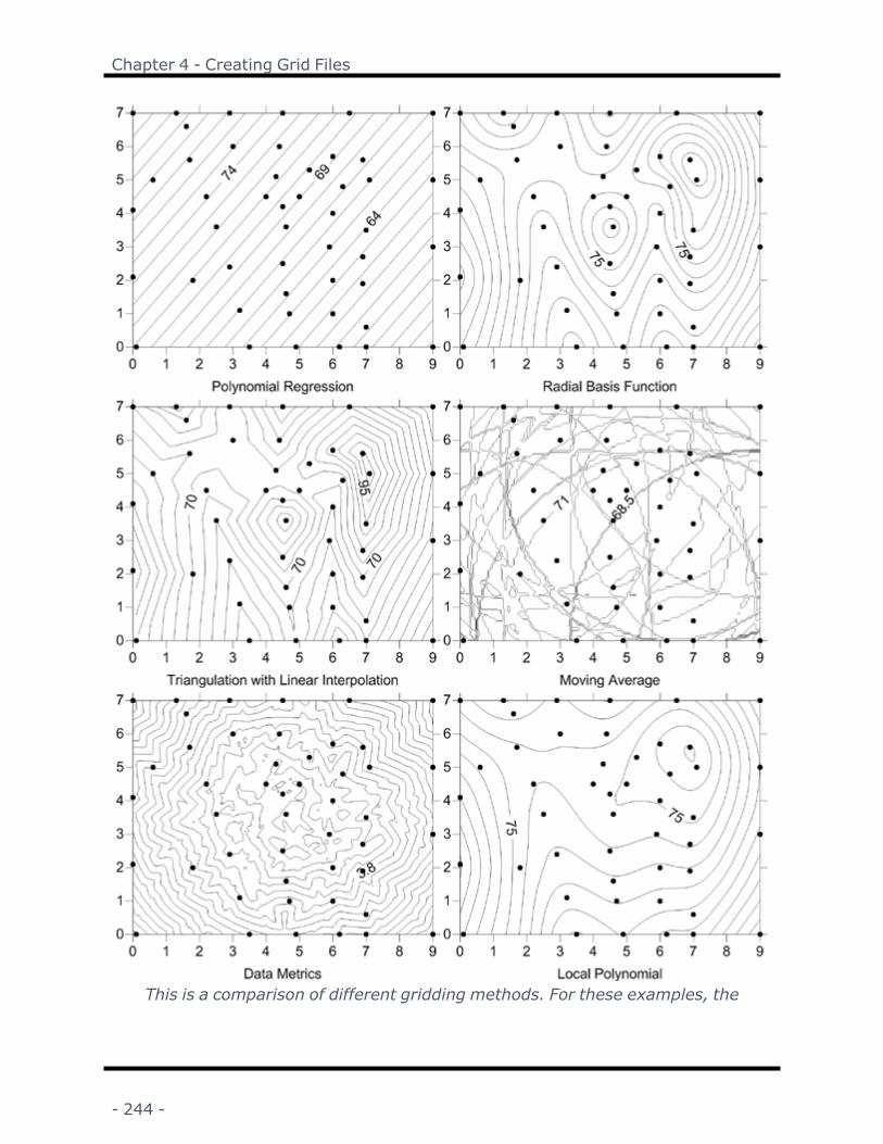
Chapter 4 - Creating Grid Files
This is a comparison of different gridding methods. For these examples, the
- 244 -

Surfer User's Guide
sample file, Demogrid.dat, was used. All the defaults for the various methods wereaccepted. This data set contains 47 data points, irregularly spaced over the extent
of the map. The data point locations are displayed as a post map layer.
Achieving Different Results with Different GriddingMethods:Using the same data set from the Demogrid.dat file and applying different grid-ding methods produces maps that emphasize different patterns.
Smooth AppearanceKriging, Minimum Curvature, Natural Neighbor, and Radial Basis Function all pro-duced acceptable contour maps with smooth appearance.
Bulls Eye PatternInverse Distance to a Power and Modified Shepard's Method both tended to gen-erate "bull's eye" patterns.
Triangular FacetsWith Triangulation with Linear Interpolation, there are too few data points to gen-erate an acceptable map, and this explains the triangular facets apparent on thecontour map.
BlockyNearest Neighbor shows as a "blocky" map because the data set is not regularlyspaced and therefore a poor candidate for this method.
Tilted PlanePolynomial Regression shows the trend of the surface, represented as a tiltedplane.
DiscontinuitiesDue to the small number of data in Demogrid.dat, the Moving Averagemethod isnot applicable. The results of using this method with an inadequate data set areshown as discontinuities are created as data are captured and discarded by themoving search neighborhoods.
Median DistanceData Metrics can show many different types of information about the data andabout the gridding process, depending on which metric is selected. This exampleshows the median distance between each grid node and the original 47 datapoints.
- 245 -

Chapter 4 - Creating Grid Files
Smooth Local VariationLocal Polynomialmodels smooth local variation in the data set.
Exact and Smoothing InterpolatorsGridding methods included with Surfer are divided into two general categories:exact interpolators and smoothing interpolators. Some exact interpolators canincorporate a smoothing factor that causes them to become smoothing inter-polators.
Exact InterpolatorsExact interpolators honor data points exactly when the point coincides with thegrid node being interpolated. In other words, a coincident point carries a weightof essentially 1.0 and all other data points carry a weight of essentially zero.Even when using exact interpolators, it is possible that the grid file does nothonor specific data points if the data points do not exactly coincide with the gridnodes. Refer to Weighted Averaging for more information on weights assignedduring interpolation.
To increase the likelihood that your data are honored, you can increase the num-ber of grid nodes in the X and Y direction. This increases the chance that gridnodes coincide with data points, thereby increasing the chance that the data val-ues are applied directly to the grid file.
The following methods are exact interpolators:
l Inverse Distance to a Power when you do not specify a smoothing factor
l Kriging when you do not specify a nugget effect
l Nearest Neighbor under all circumstances
l Radial Basis Function when you do not specify an R2 value
l Modified Shepard's Method when you do not specify a smoothing factor
l Triangulation with Linear Interpolation
l Natural Neighbor
Smoothing InterpolatorsSmoothing interpolators or smoothing factors can be employed during griddingwhen you do not have strict confidence in the repeatability of your data meas-urements. This type of interpolation reduces the effects of small-scale variabilitybetween neighboring data points. Smoothing interpolators do not assign weights
- 246 -

Surfer User's Guide
of 1.0 to any single point, even when a point is exactly coincident with the gridnode. When smoothing is used, weighting factors are assigned so the map issmoother. In the extreme case, all data points are given equal weight and thesurface becomes a horizontal plane at the average for all data in the data file.
The following methods are smoothing interpolators:
l Inverse Distance to a Power when you specify a smoothing factor
l Kriging when you specify an error nugget effect
l Polynomial Regression
l Radial Basis Function when you specify an R2 value
l Modified Shepard's Method when you specify a smoothing factor
l Local Polynomial
l Moving Average
Weighted AveragingThe gridding methods in Surfer use weighted average interpolation algorithms.This means that, with all other factors being equal, the closer a point is to a gridnode, the more weight it carries in determining the Z value at that grid node. Thedifference between gridding methods is how the weighting factors are computedand applied to data points during grid node interpolation.
To understand how weighted averages are applied, consider the equation shownhere.
Given N data values:
the interpolated value at any grid node (for example, ) can be computed as theweighted average of the data values:
where
Gj = interpolated grid node value at node j;N = number of points used to interpolate at each node;Zi Z value at the ithpoint
- 247 -

Chapter 4 - Creating Grid Files
wij weight associated with the ithdata value when com-puting
KrigingKriging is a geostatistical gridding method that has proven useful and popular inmany fields. This method produces visually appealing maps from irregularlyspaced data. Kriging attempts to express trends suggested in your data, so that,for example, high points might be connected along a ridge rather than isolatedby bull's-eye type contours.
Kriging is a very flexible gridding method. You can accept the Kriging defaults toproduce an accurate grid of your data, or Kriging can be custom-fit to a data setby specifying the appropriate variogram model. Within Surfer, Kriging can beeither an exact or a smoothing interpolator depending on the user-specified para-meters. It incorporates anisotropy and underlying trends in an efficient and nat-ural manner.
Kriging Options DialogIn the Grid Data dialog, specify Kriging as the Gridding Method and click the Nextbutton to open the Grid Data Kriging Options dialog.
- 248 -

Surfer User's Guide
Specify the variogram parameters, Kriging standard deviations file, Kriging type, and drifttype in the Grid Data Kriging Options dialog.
Kriging TypeChoose Point or Block Kriging from the Kriging Type list box.
Surfer includes two Kriging types: Point Kriging and Block Kriging. A detailed dis-cussion of the two methods can be found in Isaaks and Srivastava (1989,Chapters 12 and 13).1 Ordinary (no drift) and Universal Kriging (linear or quad-ratic drift) algorithms can be applied to both Kriging types.
Both Point Kriging and Block Kriging generate an interpolated grid. Point Krigingestimates the values of the points at the grid nodes. Block Kriging estimates theaverage value of the rectangular blocks centered on the grid nodes. The blocksare the size and shape of a grid cell. Since Block Kriging is estimating the aver-age value of a block, it generates smoother contours (block averaging smooths).Furthermore, since Block Kriging is not estimating the value at a point, Block Kri-ging is not a perfect interpolator. That is even if an observation falls exactly on a
- 249 -

Chapter 4 - Creating Grid Files
grid node, the Block Kriging estimate for that node does not exactly reproducethe observed value.
When a Kriging standard deviation grid is generated with Block Kriging, the gen-erated grid contains the Block Kriging standard deviations and not the Point Kri-ging standard deviations.
The numerical integration required for point-to-block variogram calculationsnecessary for Block Kriging are carried out using a 3x3, two-dimensional Gaus-sian-Quadrature. In particular, Surfer uses Section 25.4.62 of Aramowitz andStegun (1972).2
Note that Point Kriging is the default method.
The crosses indicate a block ofgrid nodes and the diamonds
indicate data points.In the diagram above, if we were to interpolate the center grid node with PointKriging, the data point closest to the center grid node would have the greatestweight in determining the value of the grid node. If we were to interpolate thecenter grid node with Block Kriging, all three data points within the block of gridnodes are averaged to interpolate the grid node value.
Drift TypeSelect a Linear or Quadratic drift type. Drift type None is Ordinary Kriging, whileLinear or Quadratic drift type is Universal Kriging.
If you use the Get Variogram command to apply a variogram model, be sure toset the Drift Type option to the same value as you used in the General page forDetrend when creating the variogram.
Output Grid of Kriging Standard DeviationsClick the button to enter a file name into the Standard deviations grid field toproduce an estimation standard deviation grid. If this box is empty, then theestimation standard deviation grid is not created. Click the button to removethe destination path from the Standard deviations grid field.
- 250 -

Surfer User's Guide
The Kriging standard deviation grid output option greatly slows the Kriging pro-cess. This is contrary to what you may expect since the Kriging variances are usu-ally a by-product of the Kriging calculations. However, Surfer uses a highlyoptimized algorithm for calculating the node values. When the variances arerequested, a more traditional method must be used, which takes much longer.
There are several cases where a standard deviation grid is incorrect or mean-ingless. If the variogram model is not truly representative of the data, the stand-ard deviation grid is not helpful to your data analysis. Also, the Kriging standarddeviation grid generated when using a variogram model estimated with theStandardized Variogram estimator or the Autocorrelation estimator is not cor-rect. These two variogram estimators generate dimensionless variograms, sothe Kriging standard deviation grids are incorrectly scaled. Similarly, while thedefault linear variogram model will generate useful contour plots of the data, theassociated Kriging standard deviation grid is incorrectly scaled and should not beused. The default linear model slope is one, and since the Kriging standard devi-ation grid is a function of slope, the resulting grid is meaningless.
The Kriging standard deviation grid cannot be created when the None (use alldata) option in the Search section is selected.
Kriging with External DriftLoad a grid in the External drift grid field to perform Kriging with external driftinterpolation. Click the button and select the external drift grid file in theOpen Grid dialog. Click the button to remove the file from the External driftgrid field.
Kriging with external drift uses a grid of a correlated variable to refine the inter-polation of grid values. The External drift grid is sampled at the grid nodes duringinterpolation. The External drift grid should be strongly correlated with and pre-dictive of the variable of interest. Kriging with external drift extends the cov-ariance matrix with the values of auxiliary predictors. Otherwise, Kriging withexternal drift is similar to ordinary Kriging.
The External drift gridmust have larger areal extents than the input data set andthe Output grid geometry in the Grid Data dialog. Any interpolated grid node thatdoes not include a sample from the External drift grid will be assigned theNoData value.
Search NeighborhoodThe options in the Search Neighborhood section specify search rules. Searchoptions control which data points are considered by the gridding operation wheninterpolating grid nodes.
BreaklinesThe Breaklines section is used to add breaklines to the gridding process. Faultsare not supported with Kriging.
- 251 -

Chapter 4 - Creating Grid Files
1Isaaks, E. H., and Srivastava, R. M. (1989), An Introduction to Applied Geo-statistics, Oxford University Press, New York, 561 pp.
2Abramowitz, M., and Stegun, I. (1972), Handbook of Mathematical Functions,Dover Publications, New York.
Inverse Distance to a Power MathThe equation used for Inverse Distance to a Power is:
where:
hij is the effective separation distance between grid node "j" and theneighboring point "i."is the interpolated value for grid node "j";
Zi are the neighboring points;dij is the distance between the grid node "j" and the neighboring point "i";
is the weighting power (the Power parameter); and
is the Smoothing parameter.
KrigingKriging is a geostatistical gridding method that has proven useful and popular inmany fields. This method produces visually appealing maps from irregularlyspaced data. Kriging attempts to express trends suggested in your data, so that,for example, high points might be connected along a ridge rather than isolatedby bull's-eye type contours.
Kriging is a very flexible gridding method. You can accept the Kriging defaults toproduce an accurate grid of your data, or Kriging can be custom-fit to a data setby specifying the appropriate variogram model. Within Surfer, Kriging can beeither an exact or a smoothing interpolator depending on the user-specified para-meters. It incorporates anisotropy and underlying trends in an efficient and nat-ural manner.
- 252 -

Surfer User's Guide
Kriging Options DialogIn the Grid Data dialog, specify Kriging as the Gridding Method and click the Nextbutton to open the Grid Data Kriging Options dialog.
Specify the variogram parameters, Kriging standard deviations file, Kriging type, and drifttype in the Grid Data Kriging Options dialog.
Kriging TypeChoose Point or Block Kriging from the Kriging Type list box.
Surfer includes two Kriging types: Point Kriging and Block Kriging. A detailed dis-cussion of the two methods can be found in Isaaks and Srivastava (1989,Chapters 12 and 13).1 Ordinary (no drift) and Universal Kriging (linear or quad-ratic drift) algorithms can be applied to both Kriging types.
Both Point Kriging and Block Kriging generate an interpolated grid. Point Krigingestimates the values of the points at the grid nodes. Block Kriging estimates theaverage value of the rectangular blocks centered on the grid nodes. The blocks
- 253 -

Chapter 4 - Creating Grid Files
are the size and shape of a grid cell. Since Block Kriging is estimating the aver-age value of a block, it generates smoother contours (block averaging smooths).Furthermore, since Block Kriging is not estimating the value at a point, Block Kri-ging is not a perfect interpolator. That is even if an observation falls exactly on agrid node, the Block Kriging estimate for that node does not exactly reproducethe observed value.
When a Kriging standard deviation grid is generated with Block Kriging, the gen-erated grid contains the Block Kriging standard deviations and not the Point Kri-ging standard deviations.
The numerical integration required for point-to-block variogram calculationsnecessary for Block Kriging are carried out using a 3x3, two-dimensional Gaus-sian-Quadrature. In particular, Surfer uses Section 25.4.62 of Aramowitz andStegun (1972).2
Note that Point Kriging is the default method.
The crosses indicate a block ofgrid nodes and the diamonds
indicate data points.In the diagram above, if we were to interpolate the center grid node with PointKriging, the data point closest to the center grid node would have the greatestweight in determining the value of the grid node. If we were to interpolate thecenter grid node with Block Kriging, all three data points within the block of gridnodes are averaged to interpolate the grid node value.
Drift TypeSelect a Linear or Quadratic drift type. Drift type None is Ordinary Kriging, whileLinear or Quadratic drift type is Universal Kriging.
If you use the Get Variogram command to apply a variogram model, be sure toset the Drift Type option to the same value as you used in the General page forDetrend when creating the variogram.
- 254 -

Surfer User's Guide
Output Grid of Kriging Standard DeviationsClick the button to enter a file name into the Standard deviations grid field toproduce an estimation standard deviation grid. If this box is empty, then theestimation standard deviation grid is not created. Click the button to removethe destination path from the Standard deviations grid field.
The Kriging standard deviation grid output option greatly slows the Kriging pro-cess. This is contrary to what you may expect since the Kriging variances are usu-ally a by-product of the Kriging calculations. However, Surfer uses a highlyoptimized algorithm for calculating the node values. When the variances arerequested, a more traditional method must be used, which takes much longer.
There are several cases where a standard deviation grid is incorrect or mean-ingless. If the variogram model is not truly representative of the data, the stand-ard deviation grid is not helpful to your data analysis. Also, the Kriging standarddeviation grid generated when using a variogram model estimated with theStandardized Variogram estimator or the Autocorrelation estimator is not cor-rect. These two variogram estimators generate dimensionless variograms, sothe Kriging standard deviation grids are incorrectly scaled. Similarly, while thedefault linear variogram model will generate useful contour plots of the data, theassociated Kriging standard deviation grid is incorrectly scaled and should not beused. The default linear model slope is one, and since the Kriging standard devi-ation grid is a function of slope, the resulting grid is meaningless.
The Kriging standard deviation grid cannot be created when the None (use alldata) option in the Search section is selected.
Kriging with External DriftLoad a grid in the External drift grid field to perform Kriging with external driftinterpolation. Click the button and select the external drift grid file in theOpen Grid dialog. Click the button to remove the file from the External driftgrid field.
Kriging with external drift uses a grid of a correlated variable to refine the inter-polation of grid values. The External drift grid is sampled at the grid nodes duringinterpolation. The External drift grid should be strongly correlated with and pre-dictive of the variable of interest. Kriging with external drift extends the cov-ariance matrix with the values of auxiliary predictors. Otherwise, Kriging withexternal drift is similar to ordinary Kriging.
The External drift gridmust have larger areal extents than the input data set andthe Output grid geometry in the Grid Data dialog. Any interpolated grid node thatdoes not include a sample from the External drift grid will be assigned theNoData value.
- 255 -

Chapter 4 - Creating Grid Files
Search NeighborhoodThe options in the Search Neighborhood section specify search rules. Searchoptions control which data points are considered by the gridding operation wheninterpolating grid nodes.
BreaklinesThe Breaklines section is used to add breaklines to the gridding process. Faultsare not supported with Kriging.
1Isaaks, E. H., and Srivastava, R. M. (1989), An Introduction to Applied Geo-statistics, Oxford University Press, New York, 561 pp.
2Abramowitz, M., and Stegun, I. (1972), Handbook of Mathematical Functions,Dover Publications, New York.
Variogram ComponentsClick the Add button in the Grid Data Kriging Options dialog (accessed throughthe Advanced Options button in Grids | New Grid | Grid Data when Kriging is theselected gridding method) to open the Variogram Components dialog. If youhave not modeled the variogram or if you do not understand variograms, leavethe variogram set at the original defaults (linear variogram; slope=1, aniso-tropy=1,0; no nugget effect).
The Variogram Components Dialog
Customize the Variogram Components in theVariogram Components dialog, if necessary.
- 256 -

Surfer User's Guide
Variogram Model ListChoose from the Exponential, Gaussian, Linear, Logarithmic, Nugget Effect,Power, Quadratic, Rational Quadratic, Spherical,Wave (Hole Effect), Cubic, orPentasphericalmodels.
Model OptionsDepending on which model is selected, the options below the model list changes.Set the Scale (vertical scale) and Length (horizontal range) for Exponential,Gaussian, Logarithmic, Quadratic, Rational Quadratic, Spherical,Wave (HoleEffect), Cubic, or Pentasphericalmodels. In addition to the Scale and Length, setthe Power for the Powermodel. Set the Slope for the Linearmodel. When theNugget Effect is selected set the Error Variance and Micro Variance.
Anisotropy Ratio and AngleThe Anisotropy Ratio and Angle can be set for all models except the NuggetEffect.
Kriging ReferencesFor a detailed derivation and discussion of Kriging see Cressie (1991) or Journeland Huijbregts (1978). Journel (1989) is, in particular, a concise presentation ofgeostatistics (and Kriging). Isaaks and Srivastava (1989) offer a clear intro-duction to the topic, though it does not cover some of the more advanced details.
For those who need to see computer code to really understand an algorithm,Deutsch and Journel (1992) includes a complete, well-written, and well-doc-umented source code library of geostatistics computer programs (in FORTRAN).Finally, a well-researched account of the history and origins of Kriging can befound in Cressie (1990).
Abramowitz, M., and Stegun, I. (1972), Handbook of Mathematical Functions,Dover Publications, New York.
Cressie, N. A. C. (1990), "The Origins of Kriging", Mathematical Geology, v. 22,p. 239-252.
Cressie, N. A. C. (1991), Statistics for Spatial Data, John Wiley and Sons, Inc.,New York, 900 pp.
Deutsch, C. V., and Journel, A. G. (1992), GSLIB - Geostatistical SoftwareLibrary and User's Guide, Oxford University Press, New York, 338 pp.
Isaaks, E. H., and Srivastava, R. M. (1989), An Introduction to Applied Geo-statistics, Oxford University Press, New York, 561 pp.
Journel, A. G., and Huijbregts, C. (1978), Mining Geostatistics, Academic Press,600 pp.
- 257 -

Chapter 4 - Creating Grid Files
Journel, A. G. (1989), Fundamentals of Geostatistics in Five Lessons, AmericanGeophysical Union, Washington D.C.
Minimum CurvatureMinimum Curvature is widely used in the earth sciences. The interpolated sur-face generated by Minimum Curvature is analogous to a thin, linearly elasticplate passing through each of the data values with a minimum amount of bend-ing. Minimum Curvature generates the smoothest possible surface while attempt-ing to honor your data as closely as possible. Minimum Curvature is not an exactinterpolator, however. This means that your data are not always honoredexactly.
Minimum Curvature produces a grid by repeatedly applying an equation over thegrid in an attempt to smooth the grid. Each pass over the grid is counted as oneiteration. The grid node values are recalculated until successive changes in thevalues are less than the Maximum Residuals value, or the maximum number ofiterations is reached (Maximum Iteration field).
Minimum Curvature Options DialogIn the Grid Data dialog, specify Minimum Curvature as the Gridding Method andclick the Next button to open the Grid Data Minimum Curvature Options dia-log.
- 258 -

Surfer User's Guide
Click the Advanced Options button in the Grid Data Minimum Curvature Options dialogto set the minimum curvature options.
Maximum ResidualThe Maximum Residual parameter has the same units as the data, and an appro-priate value is approximately 10% of the data precision. If data values are meas-ured to the nearest 1.0 units, the Maximum Residual value should be set at 0.1.The iterations continue until the maximum grid node correction for the entire iter-ation is less than the Maximum Residual value. The default Maximum Residualvalue is given by:
Default Max Residual = 0.001 (Zmax - Zmin)
Maximum IterationThe Maximum Iteration parameter should be set at one to two times the numberof grid nodes generated in the grid file. For example, when generating a 50 by 50grid using Minimum Curvature, the Maximum Iteration value should be setbetween 2,500 and 5,000.
- 259 -

Chapter 4 - Creating Grid Files
Relaxation FactorThe Minimum Curvature gridding algorithm solves the specified partial dif-ferential equation using a successive over-relaxation algorithm. The interior isupdated using a "chessboard" strategy, as discussed in Press, et al. (1988, p.868). The only difference is that the biharmonic equation must have nine dif-ferent "colors," rather than just black and white.
The Relaxation Factor is as described in Press et al. (1988). In general, the Relax-ation Factor should not be altered. The default value (1.0) is a good genericvalue. Roughly, the higher the Relaxation Factor (closer to two) the faster theMinimum Curvature algorithm converges, but the more likely it will not convergeat all. The lower the Relaxation Factor (closer to zero) the more likely the Min-imum Curvature algorithm will converge, but the algorithm is slower. Theoptimal Relaxation Factor is derived through trial and error.
Internal and Boundary TensionQualitatively, the Minimum Curvature gridding algorithm is attempting to fit apiece of sheet metal through all of the observations without putting any creasesor kinks in the surface. Between the fixed observation points, the sheet bows abit.
The Internal Tension is used to control the amount of this bowing on the interior:the higher the tension, the less the bowing. For example, a high tension makesareas between observations look like facets of a gemstone.
The Boundary Tension controls the amount of bowing on the edges. The range ofvalues for Internal Tension and Boundary Tension are 0 to 1.
By default, the Internal Tension and the Boundary Tension are set to 0.
AnisotropySet anisotropy settings if needed. For more information about anisotropyoptions, see Anisotropy.
Breaklines and FaultsSpecify a breakline and/or fault. For more information, see Breaklines andFaults.
Minimum Curvature MathThe Surfer code fully implements the concepts of tension as described anddetailed in Smith and Wessel (1990). Also, as recommended by Smith and Wes-sel, this routine first fits a simple planar model using least squares regression:
- 260 -

Surfer User's Guide
Thus, there are four steps to generate the final grid using the minimumcurvature method.
1. The least squares regression model is fit to the data.
2. The values of the planar regression model at the data locations are sub-tracted from the data values; this yields a set of residual data values.
3. The minimum curvature algorithm is used to interpolate the residuals atthe grid nodes.
4. The values of the planar regression model at the grid nodes are added tothe interpolated residuals, yielding a final interpolated surface.
Unlike Smith and Wessel (1990), the fixed nodes are defined as the average ofthe neighboring observed values. That is, consider a rectangle the size andshape of a grid cell. The neighborhood of a grid node is defined by this rectanglecentered on the grid node. If there are any observed data within the neigh-borhood of a grid node, the value of that grid node is fixed equal to the arith-metic average of contained data.
The Minimum Curvature algorithm generates the surface that interpolates theavailable data and solves the modified biharmonic differential equation with ten-sion:
There are three sets of associated boundary conditions:
On the edges:
On the edges:
At the corners:
where:
is the Laplacian operator
is the boundary normal
is the internal tension
is the boundary tension
- 261 -

Chapter 4 - Creating Grid Files
ConvergenceAs mentioned in Briggs (1974), and strongly recommended in Smith and Wessel(1990), Surfer uses a "multiple lattice strategy." It starts with a coarse grid andthen incrementally refines the grid until the final density is achieved.
The relaxation approach is a local smoothing process and, consequently, short-wavelength components of Z are found quickly. On the other hand, the relax-ation process does not propagate the effects of the data constraints to longerwavelengths efficiently.
As recommended by Briggs (1974) and Smith and Wessel (1990), this routinedetermines convergence by comparing the largest magnitude nodal change inone iteration to the specified tolerance (Maximum Residual).
The status of the algorithm is reflected on the status line. For example: pass 2 of4, iteration 360 (0.1234 > 0.08)
This says that there are four levels of grids considered (the fourth is the finalgrid), and the algorithm is currently working on the second. The algorithm is cur-rently on iteration 360. If the iteration number exceeds the Maximum Iterationsparameter, the algorithm terminates without generating the grid and provides afailure-to-converge warning. The numbers in the parentheses are the currentlargest residual and the largest allowed residual. The largest allowed residualequals the Maximum Residual parameter on the final pass.
The Minimum Curvaturemethod requires at least four data points.
Minimum Curvature ReferencesBriggs, I. C. (1974), Machine Contouring Using Minimum Curvature, Geophysics,v. 39, n. 1, p. 39-48.
Press, W.H., , Numerical Recipes in C , Cambridge University Press.
Smith, W. H.
Modified Shepard's MethodModified Shepard's Method uses an inverse distance weighted least squaresmethod. As such, Modified Shepard's Method is similar to the Inverse Distance toa Power interpolator, but the use of local least squares eliminates or reduces the"bull's-eye" appearance of the generated contours. Modified Shepard's Methodcan be either an exact or a smoothing interpolator.
The Surfer algorithm implements Franke and Nielson's (1980) Modified Quad-ratic Shepard's Method with a full sector search as described in Renka (1988).(Surfer 6 was based upon Franke and Nielson, not Renka.)
- 262 -

Surfer User's Guide
Modified Shepard's Method Options DialogIn the Grid Data dialog, specify Modified Shepard's Method as the GriddingMethod and click the Advanced Options button to open the Grid Data ModifiedShepard's Method Options dialog.
Set the options, including search, and smoothing factor, in the Grid Data Modified Shep-ard's Method Options dialog.
Smoothing FactorYou can assign a smoothing parameter to the gridding operation. The SmoothingFactor parameter allows Modified Shepard's Method to operate as a smoothinginterpolator. Greater smoothing occurs as you increase the value of the smooth-ing parameter. In general, values between zero and one are most reasonable.
- 263 -

Chapter 4 - Creating Grid Files
Quadratic NeighborsThe Modified Shepard's Method starts by computing a local least squares fit of aquadratic surface around each observation. The Quadratic Neighbors parameterspecifies the size of the local neighborhood by specifying the number of localneighbors. The local neighborhood is a circle of sufficient radius to includeexactly this many neighbors. The default value follows the recommendation ofRenka (1988).
Weighting NeighborsThe interpolated values are generated using a distance-weighted average of thepreviously computed quadratic fits associated with neighboring observations.TheWeighting Neighbors parameter specifies the size of the local neighborhoodby specifying the number of local neighbors. The local neighborhood is a circle ofsufficient radius to include exactly this many neighbors. The default value followsthe recommendation of Renka (1988).
SearchYou can set Search parameters in this dialog. For more information about searchoptions, see Search.
ReferencesFranke, R., and Nielson, G. (1980), 'Smooth Interpolation of Large Sets ofScattered Data', International Journal for Numerical Methods in Engineering, v.15, p. 1691-1704.
Renka, R. J. (1988), 'Algorithm 660: QSHEP2D: Quadratic Shepard Method forBivariate Interpolation of Scattered Data', ACM Transactions on MathematicalSoftware, v. 14, No. 2, p. 139-148.
Shepard, D. (1968), A two dimensional interpolation function for irregularlyspaced data, Proc. 23rd Nat., p. 517-523.
Natural NeighborThe Natural Neighbor gridding method interpolates grid values by weightingneighboring data points based on proportionate areas. Consider a set ofThiessen polygons (the dual of a Delaunay triangulation). If a new point (target)were added to the data set, these Thiessen polygons would be modified. In fact,some of the polygons would shrink in size, while none would increase in size. Thearea associated with the target's Thiessen polygon that was taken from an exist-ing polygon is called the "borrowed area." The Natural Neighbor interpolationalgorithm uses a weighted average of the neighboring observations, where theweights are proportional to the "borrowed area."
- 264 -

Surfer User's Guide
The Natural Neighbormethod assigns the NoData value at and beyond the con-vex hull of the data locations (i.e. the outline of the Thiessen polygons).
The map on the left shows contours generated by the inverse dis-tance to a power method. The map on the right shows contoursgenerated by the natural neighbor method. Contours are not
extrapolated beyond the boundary of the Thiessen polygons withthe natural neighbor gridding method.
Natural Neighbor Advanced Options DialogIn the Grid Data dialog, specify Natural Neighbor as the Gridding Method andclick the Advanced Options button to open the Natural Neighbor AdvancedOptions dialog.
- 265 -

Chapter 4 - Creating Grid Files
Set the anisotropy options and save Delaunay triangles in the Grid Data Natural NeighborOptions dialog.
Save TrianglesCheck the Save Triangles To box to export the Delaunay triangulation. The res-ulting file can be loaded as a base map and combined with other maps (i.e. con-tour maps, 3D surface maps, etc.).
Click the button to open the Export Triangles dialog. Specify a Save In loc-ation, File Name, and Save as type. The Delaunay triangle export formatsinclude: .BLN, .BNA, .EMF, .GSB, .MIF, .PDF (Vector), and .WMF. Click the Savebutton to return to the Grid Data Advanced Options dialog.
AnisotropyFor more information about anisotropy options see Anisotropy.
- 266 -

Surfer User's Guide
ReferencesThe main reference for this method is Sibson (1981), however, also refer to Sib-son (1980) and Watson (1994). Watson (1994) discusses the Natural Neighborgridding technique in some detail, although Surfer does not use any of Watson'ssource code.
Sibson, R. (1980), 'A Vector Identity for the Dirichlet Tesselation', Math. Proc.Cambridge Phil. Soc., v. 87, p. 151-155.
Sibson, R. (1981), 'A Brief Description of Natural Neighbor Interpolation', Inter-preting Multivariate Data, V. Barnett editor, John Wiley and Sons, New York, p.21-36.
Watson, Dave (1994), Nngridr - An Implementation of Natural Neighbor Inter-polation, David Watson, P.O. Box 734, Clarement, WA 6010, Australia.
Nearest NeighborThe Nearest Neighbor gridding method assigns the value of the nearest point toeach grid node. This method is useful when data are already evenly spaced, butneed to be converted to a Surfer grid file. Alternatively, in cases where the dataare nearly on a grid with only a few missing values, this method is effective forfilling in the holes in the data.
Sometimes with nearly complete grids of data, there are areas of missing datathat you want to exclude from the grid file. In this case, you can set the SearchEllipse to a value so the areas of no data are assigned the NoData value in thegrid file. By setting the search ellipse radii to values less than the distancebetween data values in your file, the NoData value is assigned at all grid nodeswhere data values do not exist.
When you use the Nearest Neighbormethod to convert regularly spaced XYZdata to a grid file, you can set the grid spacing equal to the spacing between datapoints in the file. Refer toProducing a Grid File from a Regular Array of XYZ Datafor the procedure of converting regularly spaced XYZ data into a Surfer grid file.
Nearest Neighbor Options DialogIn the Grid Data dialog, specify Nearest Neighbor as the Gridding Method andclick the Next button to open the Grid Data Nearest Neighbor Options dia-log.
- 267 -

Chapter 4 - Creating Grid Files
Set the search parameters page in the Grid Data Nearest Neighbor Options dialog.
Search NeighborhoodSpecify search rules. For more information about search rules, see Search.
Breaklines and FaultsSpecify a breakline and/or fault. For more information, see Breaklines andFaults.
Polynomial RegressionPolynomial Regression is used to define large-scale trends and patterns in yourdata. Polynomial Regression is not really an interpolator because it does notattempt to predict unknown Z values. There are several options you can use todefine the type of trend surface.
- 268 -

Surfer User's Guide
If you would like a report of the coefficients used in the calculation of the surface,make sure to select the Grid Report check box in the Grid Data dialog.
Polynomial Regression Advanced Options DialogIn the Grid Data dialog, specify Polynomial Regression as the Gridding Methodand click the Next button to open the Grid Data Polynomial RegressionOptions dialog.
Specify the Surface Definition and Parameters in the Grid Data Polynomial RegressionOptions dialog.
Surface DefinitionYou can select the type of polynomial regression to apply to your data from theSurface Definition group. As you select the different types of polynomials, a gen-eric polynomial form of the equation is presented in the dialog, and the values inthe Parameters group change to reflect the selection. The available choices are:
- 269 -
Chapter 4 - Creating Grid Files
l Simple planar surfacel Bi-linear saddlel Quadratic surfacel Cubic surfacel User defined polynomial
ParametersThe Parameters group allows you to specify the maximum powers for the X and Ycomponent in the polynomial equation. As you change the Parameters values,the options are changed in the Surface Definition group to reflect the definedparameters.
l The Max X Order specifies the maximum power for the X component in thepolynomial equation.
l The Max Y Order specifies the maximum power for the Y component in thepolynomial equation.
l The Max Total Order specifies the maximum sum of the Max X Order and MaxY Order powers. All of the combinations of the X and Y components areincluded in the polynomial equation as long as the sum of the two powersdoes not exceed the Max Total Order value.
ReferenceDraper, N., and Smith, H. (1981), Applied Regression Analysis, second edition,Wiley-Interscience, 709 pp.
Radial Basis FunctionRadial Basis Function interpolation is a diverse group of data interpolation meth-ods. In terms of the ability to fit your data and to produce a smooth surface, theMultiquadricmethod is considered by many to be the best. All of the Radial BasisFunctionmethods are exact interpolators, so they attempt to honor your data.You can introduce a shaping factor to all the methods in an attempt to produce asmoother surface. Regardless of the R2 value, the Radial Basis Function is anexact interpolator.
Radial Basis Function Options DialogIn the Grid Data dialog, specify Radial Basis Function as the Gridding Method andclick the Next button to open the Grid Data Radial Basis Function Optionsdialog.
- 270 -

Surfer User's Guide
Set the type of Basis Function and Anisotropy in the Grid Data Radial Basis FunctionOptions dialog.
Basis FunctionSpecify the function type from the Basis Function list. The basis kernel functionsare analogous to variograms in Kriging. The basis kernel functions define theoptimal set of weights to apply to the data points when interpolating a grid node.The available basis kernel functions are listed in the Basis Function list in theGrid Data Radial Basis Function Options dialog.
Type EquationInverse Multiquadric
Multilog
Multiquadric
- 271 -

Chapter 4 - Creating Grid Files
Natural Cubic Spline
Thin Plate Spline
where:
h = the anisotropically rescaled, relative dis-tance from the point to the node
R2
= the shaping factor specified by the user
R2 ParameterThe default value for R2 in the Radial Basis Function gridding algorithm is cal-culated as follows:
(length of diagonal of the data extent)2 / (25 * number of data points)
Search NeighborhoodSpecify search rules. For more information about search rules, see Search.
AnisotropySet anisotropy settings if needed. For more information about anisotropyoptions, see Anisotropy.
BreaklinesThe Breaklines section is used to add breaklines to the gridding process. Faultsare not supported with Radial Basis Function.
ReferencesA concise and readable introduction to Radial Basis Function interpolation can befound in Carlson and Foley (1991a). Given the clarity of presentation and thenumerous examples, Hardy (1990) provides an excellent overview of themethod, although this paper focuses exclusively on the special case of mul-tiquadrics.
Carlson, R.E., and Foley, T.A. (1991a), Radial Basis Interpolation Methods onTrack Data, Lawrence Livermore National Laboratory, UCRL-JC-1074238.
Carlson, R. E., and Foley, T. A. (1991b), The Parameter R2 in Multiquadric Inter-polation, Computers Math. Applic, v. 21, n. 9, p. 29-42.
Franke, R. (1982), Scattered Data Interpolation: Test of Some Methods, Mathem-atics of Computations, v. 33, n. 157, p. 181-200.
- 272 -

Surfer User's Guide
Hardy, R. L. (1990), Theory and Applications of the Multiquadric-BiHarmonicMethod, Computers Math. Applic, v. 19, n. 8/9, p. 163-208.
Powell, M.J.D. (1990), The Theory of Radial Basis Function Approximation in1990, University of Cambridge Numerical Analysis Reports, DAMTP 1990/NA11.
Triangulation with Linear InterpolationThe Triangulation with Linear Interpolationmethod in Surfer uses the optimalDelaunay triangulation. The algorithm creates triangles by drawing linesbetween data points. The original points are connected in such a way that no tri-angle edges are intersected by other triangles. The result is a patchwork of tri-angular faces over the extent of the grid. This method is an exact interpolator.
Each triangle defines a plane over the grid nodes lying within the triangle, withthe tilt and elevation of the triangle determined by the three original data pointsdefining the triangle. All grid nodes within a given triangle are defined by the tri-angular surface. Because the original data are used to define the triangles, thedata are honored very closely.
Triangulation with Linear Interpolation works best when your data are evenly dis-tributed over the grid area. Data sets that contain sparse areas result in distincttriangular facets on the map.
Triangulation with Linear Interpolation Options DialogIn the Grid Data dialog, specify Triangulation with Linear Interpolation as theGridding Method and click the Next button to open the Grid Data Tri-angulation with Linear Interpolation Options dialog.
- 273 -

Chapter 4 - Creating Grid Files
Set the anisotropy options and save Delaunay triangles in the Grid Data Triangulationwith Linear Interpolation Options dialog.
Save TrianglesCheck the Save Triangles To box to export the Delaunay triangles to a file. Theresulting file can be loaded as a base map and combined with other maps (i.e.contour maps, 3D surface maps, etc.).
Click the button to open the Export Triangles dialog. Specify a Save In loc-ation, File name, and Save as type. The Delaunay triangle export formatsinclude: .BLN, .BNA, .EMF, .GSB, .MIF, .PDF (Vector), and .WMF. Click the Savebutton to return to the Grid Data Triangulation with Linear InterpolationOptions dialog.
AnisotropyFor more information about anisotropy options see Anisotropy.
- 274 -

Surfer User's Guide
ReferencesThe Surfer implementation of Triangulation with Linear Interpolation is basedupon three papers. Lee and Schachter (1980) present a complete discussion of(Delaunay) triangulation, including the details of two algorithms and the under-lying mathematical proofs. Lawson (1977) is equally informative. The algorithmpresented in Guibas and Stolfi (1985) form the basis for the Surfer imple-mentation.
Guibas, L., and J. Stolfi (1985), 'Primitives for the Manipulation of General Sub-divisions and the Computation of Voronoi Diagrams', ACM Transactions on Graph-ics, v. 4, n. 2, p. 74-123.
Lawson, C. L. (1977), 'Software for C1 surface interpolation', Mathematical Soft-ware III, J. Rice ( ed.), Academic Press, New York, p. 161-193.
Lee, D. T., and Schachter, B. J. (1980), 'Two Algorithms for Constructing aDelaunay Triangulation', International Journal of Computer and InformationSciences, v. 9, n. 3, p. 219-242.
Moving AverageThe Moving Average gridding method assigns values to grid nodes by averagingthe data within the grid node's search ellipse.
Moving Average Tipsl The moving average gridding method can incorporate breakline data.
l The moving average gridding method is not recommended for generatingmaps from small and moderate-sized data sets. It is, however, a useful toolfor characterizing and investigating large and very large spatial data sets.
Moving Average Options DialogIn the Grid Data dialog, specify Moving Average as the Gridding Method and clickthe Next button to open the Grid Data Moving Average Options dialog.
- 275 -

Chapter 4 - Creating Grid Files
Set the NoData options and the search ellipse in the Grid Data Moving Average Optionsdialog.
Minimum Number of DataTheMinimum number of data (node is set to NoData if fewer) value setsthe specified number of points when interpolating a grid node. If the minimumnumber of points is not found, the NoData value is assigned to the gride node.
Search NeighborhoodSpecify search rules. For more information about search rules, see Search.
BreaklinesThe Breaklines section is used to add breaklines to the gridding process. Faultsare not supported with Moving Average.
- 276 -

Surfer User's Guide
Data MetricsThe collection of data metrics gridding methods creates grids of informationabout the data on a node-by-node basis. The data metrics gridding methods arenot, in general, weighted average interpolators of the Z values. For example, youcan obtain information such as:
l The number of data points used to interpolate each grid node. If the num-ber of data points used are fairly equal at each grid node, then the qualityof the grid at each grid node can be interpreted.
l The standard deviation, variance, coefficient of variation, and median abso-lute deviation of the data at each grid node. These are measures of the vari-ability in space of the grid, and are important information for statisticalanalysis.
l The distance to the nearest data point. For example, if the XY values of adata set are sampling locations, use the Distance to Nearest data metric todetermine locations for new sampling locations. A contour map of the dis-tance to the nearest data point, quantifies where higher sampling densitymay be desired.
Data Metrics Options DialogIn the Grid Data dialog, specify Data Metrics as the Gridding Method and click theNext button to open the Grid Data - Data Metrics - Options dialog.
- 277 -
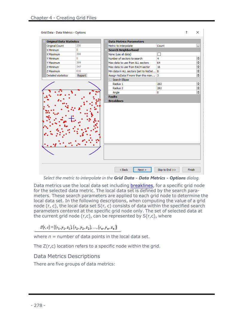
Chapter 4 - Creating Grid Files
Select the metric to interpolate in the Grid Data - Data Metrics - Options dialog.Data metrics use the local data set including breaklines, for a specific grid nodefor the selected data metric. The local data set is defined by the search para-meters. These search parameters are applied to each grid node to determine thelocal data set. In the following descriptions, when computing the value of a gridnode (r, c), the local data set S(r, c) consists of data within the specified searchparameters centered at the specific grid node only. The set of selected data atthe current grid node (r,c), can be represented by S(r,c), where
where n = number of data points in the local data set.
The Z(r,c) location refers to a specific node within the grid.
Data Metrics DescriptionsThere are five groups of data metrics:
- 278 -

Surfer User's Guide
l Z Order Statistics
l Z Moment Statistics
l Other Z Statistics
l Data Location Statistics
l Terrain Statistics
Planar GridsData metrics is used to provide information about your data. After information isobtained from data metrics, it is likely you will grid the data again using one ofthe other gridding methods. When using data metrics, you will usually want touse the same output grid geometry, search, breakline, and fault parameters aswhen you grid the data using another gridding method.
When using some data metrics, a horizontal planar or sloping planar grid is gen-erated. This is usually a result of the selected search method. For example, con-sider using Demogrid.dat and the Count data metric. The Count data metricdetermines the number of data points used in determining the grid node value.Since Demogrid.dat contains 47 data points, No search (use all of the data) is thedefault search method. Using No search (use all of the data)means for each cal-culated grid node, all 47 points are used in determining the grid node value. Theresulting data metric grid is horizontal planar because all grid nodes have a Zvalue of 47. The grid report shows both the Z minimum and the Z maximum as47.
Other data metrics can yield similar results. For example, if the search radius islarge enough to include all of the data using Terrain Statistics, the moving aver-age is computed with such a large search radius that the resulting grid will be aplanar surface at the data average. When interpreting data metrics results, keepthe gridding parameters and the data metrics calculation approach in mind.
Search NeighborhoodSpecify search rules. For more information about search rules, see Search.
Breaklines and FaultsSpecify a breakline and/or fault. For more information, see Breaklines andFaults.
Data Metrics Z Order StatisticsThere are five groups of data metrics: Z Order Statistics, Z Moment Statistics,Other Z Statistics, Data Location Statistics, and Terrain Statistics.
- 279 -

Chapter 4 - Creating Grid Files
The data at a grid node within the search parameters are sorted for the Z orderstatistics.
where . Square brackets indicate ordered Z values.
Data Metric Definition EquationMinimum each nodal value is the min-
imum Z value of data selectedby the specified sector searchcentered at that node
Lower Quart-ile
each nodal value is the 25th per-centile Z value of data selectedby the specified sector searchcentered at that node
Median each nodal value is the medianZ value of data selected by thespecified sector search centeredat that node
Upper Quart-ile
each nodal value is the 75th per-centile Z value of data selectedby the specified sector searchcentered at that node
Maximum each nodal value is the max-imum Z value of data selectedby the specified sector searchcentered at that node
Range each nodal value is the dif-ference between the maximumZ value and the minimum Zvalue for the data selected bythe specified sector searchcentered at that node
Midrange each nodal value is the averageof the maximum Z value andthe minimum Z value, for thedata selected by the specifiedsector search centered at thatnode
- 280 -

Surfer User's Guide
InterquartileRange
The Interquartile Range datametric generates a grid forwhich each nodal value is thedifference between the 75th per-centile Z value and the 25th per-centile Z value, for the dataselected by the specified sectorsearch centered at that node.This data metric shows the spa-tial variation of variability of thedata, but it focuses on themiddle fifty percent of the dataonly. Thus, it is insensitive tovariations in the tails of thelocal distributions
Data Metrics Z Moment StatisticsThere are five groups of data metrics: Z Order Statistics, Z Moment Statistics,Other Z Statistics, Data Location Statistics, and Terrain Statistics. The Z MomentStatistics calculate information about the values at the nodes.
DataMetric
Definition Equation
Mean each nodal value is the arithmeticaverage of the data selected by thespecified sector search centered atthat node
StandardDeviation
each nodal value is the standarddeviation of the data selected by thespecified sector search centered atthat node
where is the mean ofthe selected data
Variance each nodal value is the variance ofthe data selected by the specifiedsector search centered at that node
where is the mean ofthe selected data
- 281 -

Chapter 4 - Creating Grid Files
Coef. ofVariation
The Coef. of Variation data metricgenerates an output grid for whicheach nodal value is the local stand-ard deviation divided by the localmean of the data selected by the spe-cified sector search centered at thatnode. Note that this measure is use-less for data whose local mean val-ues are close to zero; this includesdata that changes sign within thedomain of interest.
Data Metrics Other Z StatisticsThere are five groups of data metrics: Z Order Statistics, Z Moment Statistics,Other Z Statistics, Data Location Statistics, and Terrain Statistics. The Other ZStatistics calculate additional information about the values at the nodes.
DataMetric
Definition Equation
Sum The Sum data metric generates an out-put grid for which each nodal value isthe sum of the Z values of the data selec-ted by the specified sector searchcentered at that node.
M.A.D. The Median Absolute Deviation (M.A.D.)data metric generates an output grid forwhich each nodal value is the medianabsolute deviation of the data selectedby the specified sector search centeredat that node.
R.M.S. The Root Mean Square (R.M.S.) datametric generates an output grid forwhich each nodal value is the root meansquare of the data selected by the spe-cified sector search centered at thatnode.
Data Metrics Data Location StatisticsThere are five groups of data metrics: Z Order Statistics, Z Moment Statistics,Other Z Statistics, Data Location Statistics, and Terrain Statistics. The Data Loca-tion Statistics calculate information about the points around each of the nodes.
- 282 -
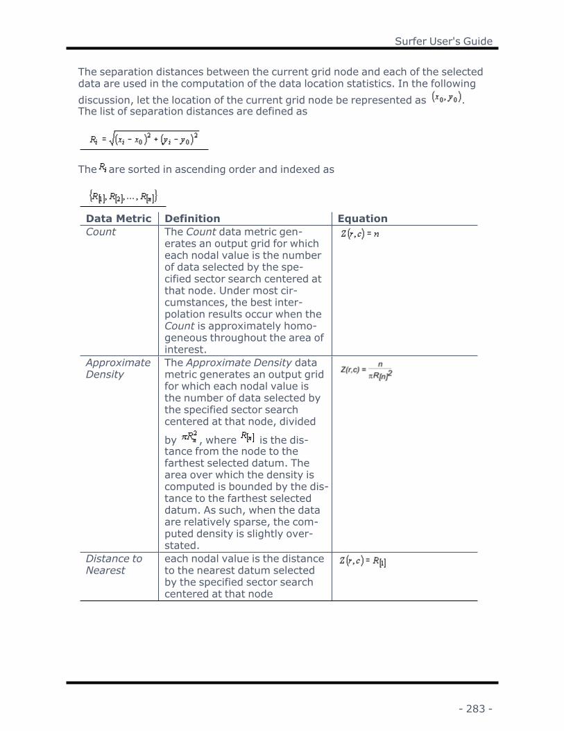
Surfer User's Guide
The separation distances between the current grid node and each of the selecteddata are used in the computation of the data location statistics. In the followingdiscussion, let the location of the current grid node be represented as .The list of separation distances are defined as
The are sorted in ascending order and indexed as
Data Metric Definition EquationCount The Count data metric gen-
erates an output grid for whicheach nodal value is the numberof data selected by the spe-cified sector search centered atthat node. Under most cir-cumstances, the best inter-polation results occur when theCount is approximately homo-geneous throughout the area ofinterest.
ApproximateDensity
The Approximate Density datametric generates an output gridfor which each nodal value isthe number of data selected bythe specified sector searchcentered at that node, divided
by , where is the dis-tance from the node to thefarthest selected datum. Thearea over which the density iscomputed is bounded by the dis-tance to the farthest selecteddatum. As such, when the dataare relatively sparse, the com-puted density is slightly over-stated.
Distance toNearest
each nodal value is the distanceto the nearest datum selectedby the specified sector searchcentered at that node
- 283 -

Chapter 4 - Creating Grid Files
Distance toFarthest
each nodal value is the distanceto the farthest datum selectedby the specified sector searchcentered at that node
MedianDistance
each nodal value is the medianseparation distance betweenthe node and all of the dataselected by the specified sectorsearch centered at that node
AverageDistance
each nodal value is the averageseparation distance betweenthe node and all of the dataselected by the specified sectorsearch centered at that node
OffsetDistance
each nodal value is the distancebetween the node and thecentroid of all of the data selec-ted by the specified sectorsearch centered at that node
Terrain StatisticsThere are five groups of data metrics: Z Order Statistics, Z Moment Statistics,Other Z Statistics, Data Location Statistics, and Terrain Statistics. The TerrainStatistics calculate information about the slope and aspect of the grid aroundeach node.
Terrain statistics are all based upon a locally fitted planar surface. For each gridnode, the specified sector search is performed. Then, using ordinary leastsquares, the following equation is fitted to the selected data:
Least squares fitting is carried out using the data coordinates and it ignoresfaults. A sector search and the subsequent least squares fit are carried out foreach grid node.
These data metrics are similar to Grids | Calculate | Calculus terrain modeling,however, data metrics work on a local subset of the data rather than the grid.
DataMetric
Definition Equation
- 284 -
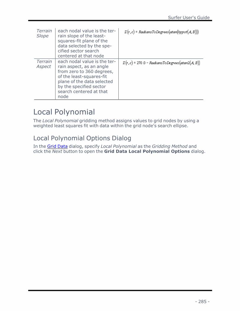
Surfer User's Guide
TerrainSlope
each nodal value is the ter-rain slope of the least-squares-fit plane of thedata selected by the spe-cified sector searchcentered at that node
TerrainAspect
each nodal value is the ter-rain aspect, as an anglefrom zero to 360 degrees,of the least-squares-fitplane of the data selectedby the specified sectorsearch centered at thatnode
Local PolynomialThe Local Polynomial gridding method assigns values to grid nodes by using aweighted least squares fit with data within the grid node's search ellipse.
Local Polynomial Options DialogIn the Grid Data dialog, specify Local Polynomial as the Gridding Method andclick the Next button to open the Grid Data Local Polynomial Options dialog.
- 285 -

Chapter 4 - Creating Grid Files
Choose a Power and Polynomial Order in the Grid Data Local Polynomial Options dialog.
PowerSet the Power to a number between 0 and 20. The Power parameter is used toassign the power for the weighted least square function, see Local PolynomialMath. This allows data closer to the grid node to have more impact on the valueof the grid node than data farther away. This parameter is similar to the InverseDistance to a Power gridding method.
Polynomial OrderSelect a Polynomial Order, 1, 2, or 3.
1: F(X,Y) = a +bX + cY
2: F(X,Y) = a +bX + cY + dXY + eX2 + fX2
3: F(X,Y) = a +bX + cY + dXY + eX2 + fX2 +gX2Y + hXY2 + iX3 + iY3
- 286 -

Surfer User's Guide
Search NeighborhoodSpecify search rules. For more information about search rules, see Search.
BreaklinesThe Breaklines section is used to add breaklines to the gridding process. Faultsare not supported with Local Polynomial.
Local Polynomial MathFor each grid node, the neighboring data are identified by the user-specified sec-tor search. Using only these identified data, a local polynomial is fit usingweighted least squares, and the grid node value is set equal to this value. Localpolynomials can be order 1, 2, or 3.
The form of these polynomials are:
Order 1
Order 2
Order 3
The weighted least squares function weights data closer to the grid node higherand data further away lower. The weighting function depends on the searchellipse, the power, and the specific data geometry. The actual calculations for theweights are somewhat involved. Define TXX,
where
is the angle of the search ellipse
is search radius 1
is search radius 2
Define AXX,
- 287 -

Chapter 4 - Creating Grid Files
Note that these values (AXX,
Next, consider a datum at location (Xi,
then
and finally,
where Wiis the weight for datum i andpis the specified power.
Let the collection of neighboring data be enumerated as
The local least squares parameters are computed by minimizing the weightedsum of the squared residuals:
Grid from Server
Click the Grids | New Grid | Grid from Server command or the buttonto download data from an online web mapping server and create a new grid file.Clicking the Grid from Server command opens the Download Online Grids dia-log.
The Download Online Grids dialog can also be accessed from the Open Griddialog by clicking Download. The downloaded grid will be used to create a grid-based map layer or in the following grid command dialog, depending on whichcommand was used to open the Open Grid dialog.
- 288 -

Surfer User's Guide
When using the Download Online Grids dialog, a server with appropriate datamust be selected. Surfer currently supports four types of servers, web mappingserver (WMS), Open Street Map server (OSM), web coverage server (WCS), andweb feature server (WFS). WMS, OSM, WCS, and WFS servers provide differenttypes data.
l When selecting a WMS or OSM server, an image is downloaded to be used asa grid file. There are no Z values associated with the image. When the imageis used as a grid file, a value between 0 and 1 is assigned to each pixel in theimage based on the color of that pixel. WMS and OSM servers are generallyused to create base maps with the Home | New Map | Base | Base fromServer command.
l When selecting a WCS server, data values are downloaded to be used as agrid file.
l When selecting a WFS server, vector data is downloaded with points, poly-lines, and/or polygons representing features. WFS servers cannot be usedwith the Grid from Server command.
Grid from ContoursClick the Grids | New Grid | Grid from Contours command or the buttonto create a grid file from contour lines. The contour lines can be loaded as a baselayer or the vector file containing the contour lines can be used to generate a gridfile. The Grid from Contours command uses the contour line polyline, polygon,3D polyline and 3D polygon vertices and height attribute (commonly ZLEVEL) tocreate a grid. The Grid from Contours command algorithm interpolates gridnode values as a linear combination of the two nearest contour values. The GridContours dialog is opened when the Grids | New Grid | Grid from Contourscommand is clicked.
Grid Contours DialogThe Grid Contours dialog contains the input vector file or layer, input fault fileor layer, gridding options, and output grid file settings.
- 289 -

Chapter 4 - Creating Grid Files
Create grid files from contour lines with the Grid Contours dialog.
Contour SourceThe Contour Source is the vector data file, base layer, or contour layer con-taining the contour lines from which to generate a grid. There are two methodsfor specifying the Contour Source:
l Select a map layer from the Contour Source list by clicking the current selec-tion and then clicking the desired layer. Base layers are only included in theContour Source list if the objects in the layer contain one or more numericattribute fields.
l Specify a vector data file as the Contour Source by clicking Browse. The Opendialog is displayed. Navigate to the desired vector file and click Open. An
- 290 -

Surfer User's Guide
Import Options dialog may be displayed depending on the vector fileformat.
Once a Contour Source is selected, the Select Field dialog is displayed. Specifywhich attribute field contains elevation information in the Select Field dialog.For 3D polylines and 3D polygons, select [None] and check Use Z coordinate for3D geometry to use the Z coordinates rather than the attributes. If an attributefield and Use Z coordinate for 3D geometry are both selected, the Z coordinatewill take precedence. To exclude all 2D objects, select [None].
The layer name or file path and name is displayed in the Contour Source fieldwhen a Contour Source has been loaded. The number of contours, number of ver-tices, and elevation field selection are displayed below the Contour Source.
Fault SourceThe Fault Source is the vector data file or base layer containing any faults toinclude in the grid generation. Select a base layer from the Fault Source list byclicking the current selection and then clicking the desired layer. Specify a vectordata file as the Fault Source by clicking Browse. The Open dialog is displayed.Navigate to the desired vector file and click Open. An Import Options dialogmay be displayed depending on the vector file format.
The layer name or file path and name is displayed in the Fault Source field whena Fault Source has been loaded. The number of faults and number of vertices isdisplayed below the Fault Source.
Supported FormatsThe following file formats are supported in the Contour Source and Fault Sourcefields:
BLN Golden Software BlankingBNA Atlas BoundaryDDF SDTS TVPDXF AutoCAD DrawingE00 Esri ArcInfo Export FormatGSB Golden Software BoundaryGSI Golden Software InterchangeMIF MapInfo Interchange FormatSHP Esri Shapefile
Output Grid GeometryThe Output Grid Geometry section defines the grid limits and grid density.
Copy GeometryThe Copy geometry from option copies the grid geometry from an existing maplayer or grid file. This option is useful when creating grids that will become over-laid map layers, processed with the Grid Math command, or used to calculate a
- 291 -

Chapter 4 - Creating Grid Files
volume between two surfaces. TheMath and Volume commands require theinput grids to have the same geometry.
To copy the geometry from an existing layer, select the layer in the Copy geo-metry from list. To copy the geometry from a grid file, click Browse and selectthe file in the Open Grid dialog. Select <None> to return the Output Grid Geo-metry options to their default values and to manually edit the grid geometry.
Minimum and Maximum X and Y Coordinate (Grid Limits)Grid limits are the minimum and maximum X and Y coordinates for the grid.Surfer computes the minimum and maximum X and Y values from the ContourSource layer or data file. These values are used as the default minimum and max-imum coordinates for the grid.
Grid limits define the X and Y extent of contour maps, color relief maps, vectormaps, 3D wireframes, and 3D surfaces created from grid files. When creating agrid file, you can set the grid limits to the X and Y extents you want to use foryour map. Once a grid file is created, you cannot produce a grid-based map lar-ger than the extent of the grid file. If you find you need larger grid limits, youmust regrid the data. You can, however, read in a subset of the grid file to pro-duce a map smaller than the extent of the grid file.
When either the X, Y, or Z value is in a date/time format, the date/time valuesare converted and stored in the grid as numbers.
Spacing and # of Nodes (Grid Density)Grid density is usually defined by the number of columns and rows in the grid,and is a measure of the number of grid nodes in the grid. The # of Nodes in the XDirection is the number of grid columns, and the # of Nodes in the Y Direction isthe number of grid rows. The direction (X Direction or Y Direction) that coversthe greater extent (the greater number of data units) is assigned 500 grid nodesby default. The number of grid nodes in the other direction is computed so thatthe grid nodes Spacing in the two directions are as close to one another as pos-sible.
By defining the grid limits and the number of rows and columns, the Spacing val-ues are automatically determined as the distance in data units between adjacentrows and adjacent columns.
You can also increase or decrease the grid density by using the Grids | Edit |Spline Smooth, Grids | Resize | Extract, or Grids | Resize | Mosaic commandsafter a grid is created. See the Grid Data topic for information on memoryrequirements for large and/or dense grids and a grid geometry example.
OptionsThe Options section of the Grid Contours dialog contains options for assigningthe NoData value outside the convex hull of the data or outside of the alpha
- 292 -

Surfer User's Guide
value, control over extrapolation in peaks and basins, contour closing, and con-tour cleanup.
Assign NoData
Convex HullSelect Convex hull from the Assign NoData outside of list to assign the NoDatavalue to the grid nodes outside the convex hull of the data. The convex hull of adata set is the smallest convex polygon containing all the data. The convex hullcan be thought of as a rubber band that encompasses all data points. The rubberband only touches the outside points. Areas inside the convex hull without dataare still gridded. See the Grid Data topic for an example of assigning NoData out-side the convex hull of the data.
If Convex hull is selected from the Assign NoData outside of list, the Grid Con-tours dialog displays the Inflate convex hull by box. Enter a value to expand orcontract the convex hull. When set to zero, the boundary connects the outsidedata points exactly. When set to a positive value, the area assigned the NoDatavalue is moved outside the convex hull boundary by the number of map units spe-cified. When set to a negative value, the area assigned the NoData value ismoved inside the convex hull boundary by the number of map units specified.Values are in horizontal (X) map units. If the value is set to a large positivevalue, the grid values may extend all the way to the minimum and maximum Xand Y limits of the grid, essentially overriding the Assign NoData outside convexhull of data option. If the value is set to a large negative value, the entire gridmay be assigned the NoData value, resulting in no grid file being created.
Alpha ShapeSelect Alpha shape from the Assign NoData outside of list to assign the NoDatavalue to the grid nodes outside the alpha value of the data. Select Alpha shapeinstead of Convex hull to have a tighter boundary, especially if a boundary couldform concave areas. If Alpha shape is selected from the Assign NoData outside oflist, the Grid Contours dialog displays the Alpha value box. Enter a value todefine the radius of the circles that are created by the edges of the triangulationof the points. Larger alpha values create a more convex boundary and smalleralpha numbers create a tighter, concave boundary. If too low or too high of analpha value was entered, a message will appear stating that the grid could not beassigned NoData because of the alpha value. For more information on alphashapes or to determine an appropriate alpha value, see the Alpha Shape helptopic.
Extrapolation FactorThe Extrapolation factor controls the rate of change in the Z for grid node valueswith only one bounding contour. These grid nodes are usually located near peaksand basins. The slope between the nearest two contour lines is multiplied by theExtrapolation factor to perform linear extrapolation. Type the desired factor inthe Extrapolation factor field.
- 293 -

Chapter 4 - Creating Grid Files
The Extrapolation factormust be greater than or equal to zero, and the defaultExtrapolation factor is one. An Extrapolation factor of zero generates a grid withflat peaks and basins. An Extrapolation factor less than one will lessen the rate ofchange in Z with distance from the nearest contour and generate lower peaksand shallower basins. An Extrapolation factor greater than one will increase therate of change in Z with distance from the nearest contour and generate higherpeaks and deeper basins.
Close Open ContoursCheck the Close open contours check box to automatically close any contourlines with ends within the specified Ends within tolerance. Contours will not beclosed if the added section intersects any existing contours. Contours will alsonot be closed if the ends are further apart than the Ends within distance.
The Close open contours option is enabled by default. This improves thealgorithm performance near the edges of the map and for any open contours inthe map interior. The default Ends within distance is 1% of the diagonal distanceof the grid. Specify an Ends within distance in horizontal (X) map units by typingthe value in the Ends within field.
Clear the Close open contours check box to generate the grid from the contourlines in the layer or vector file without closing open contours. The Ends withinfield is not available when Close open contours is not checked.
Partial Contour CleanupCheck the Partial contour cleanup check box to improve performance aroundopen contours that terminate in the interior of the map, especially near theedges of the map or when the contour lines indicate faulting. However for someinput layers or files, the Partial contour cleanup option will decrease performancein the resulting grid. By default the Partial contour cleanup check box is notchecked.
The Partial contour cleanup option changes the algorithm to ignore "invisible"contour lines when calculating grid node values. First, the algorithm determinesthe nearest contour levels. Next, the algorithm determines if any of the levelsare blocked from view by nearer levels. If this is the case, the occluded contourlevels are ignored and the algorithm treats the grid node value as a boundedpoint (see the Extrapolation factor section).
Output GridChoose a path and file name for the grid file in the Output Grid group. You can
type a path and file name, or click the button to browse to a new path andenter a file name in the Save Grid As dialog.
- 294 -

Surfer User's Guide
Add New Map or LayerCheck Add grid as layer to to add the created grid to a new or existing map.Select [New Map] in the Add grid as layer to field to create a new map. Click thecurrent selection and select an existing map to add a new layer to the map.Select the layer type by clicking the current selection in the New layer type fieldand selecting the desired layer type from the list.
Notes: If you are saving the grid file in the DEM grid format, clear the Add grid aslayer check box and add the map or layer with a Home | New Map or Home |Add to Map | Layer command. When exporting to a BLN or DXF file, the Zcoordinates for 3D polylines are not exported.
Reference for Grid from ContoursSee Koshel, S. M., Algorithm for Topologically Correct Gridding of Contour Data,Department of Cartography and Geoinformatics, Faculty of Geography, Lomono-sov Moscow State University, for more information regarding the griddingalgorithm.
Select Field DialogThe Select Field dialog specifies which attribute value contains elevation inform-ation for the contour lines in the map layer or vector data file.
Specify which field contains elevation informationin the Select Field dialog.
For 2D polylines and polygons, click the current attribute in the Select the fieldcontaining the contour elevations field and select the desired attribute from thelist.
With 3D polylines and 3D polygons, check the Use Z coordinate for 3D geometrycheck box to use the Z coordinate, or unclick the Use Z coordinate for 3D geo-metry and select the attribute to use from Select the field containing the contourelevations.
To ignore 2D objects when both 2D objects and 3D objects are present, setSelect the field containing the contour elevations to [None].
- 295 -

Chapter 4 - Creating Grid Files
If both Use Z coordinate for 3D geometry is checked and an attribute is selected,3D objects will use the Z coordinate and the 2D objects will use the attribute. For3D objects, the Z coordinate always takes precedent.
Click OK when you have selected the desired field.
Click Cancel to return to the Grid Contours dialog without selecting the elevationfield. If you click Cancel the map layer or vector file will not be loaded.
Grid FunctionThe Grids | New Grid | Function command creates a grid file from a user-defined two variable equation of the form Z = f(X,Y). The density of the gen-erated grid is a function of the Minimum, Maximum, and Increment values forboth X and Y. The Grids | New Grid | Function command can use any of themathematical functions. Grids created as functions can be plotted in the sameway as grids created using the Grid Data command.
Grid Function DialogClick the Grids | New Grid | Function command or the button to open theGrid Function dialog.
Set the mathematical function, the minimum and maximum X and Yvalues, and the function increment values in the Grid Function dia-
log.
- 296 -

Surfer User's Guide
Enter a FunctionEnter the function of interest into the Enter a function of the form Z = f (X,Y)box. The function calculation is repeated for each Z value to be written to thegrid file. The number of grid nodes in the output grid and, therefore, the numberof calculations to be performed, is based on the Minimum, Maximum and Incre-ment values specified.
To use a stored function, click the next to the current function. This will dis-play the ten most recent functions used. The functions are stored in the registry,so the equations are stored between Surfer sessions. You can also start typingthe function in the function box. If the function is in the ten function history, theentire function will auto-complete.
Minimum X and YIn the Minimum X and Y boxes, specify the beginning values used in the specifiedfunction. The first grid node, defined by these boxes, is calculated based onthese values. These values also specify the lower X and Y limits in the grid file.
Maximum X and YIn the Maximum X and Y boxes, specify upper values to be applied to the func-tion and the upper X and Y limits for the grid.
Increment X and YIn the Increment boxes, specify the amount to step in the X and Y directions foreach grid line. This is similar to the grid Spacing setting in the Grid Data dialog.
Output GridType a file path and file name, including the file type extension, in the Output
Grid field, or click the button and specify the path and file name for the gridfile in the Save Grid As dialog.
Add New Map or LayerCheck the Add grid as layer to check box to automatically add the created grid toa new or existing map. Select [New Map] in the Add grid as layer to field to cre-ate a new map. Click the current selection and select an existing map to add anew layer to the map. Select the layer type by clicking the current selection inthe New layer type field and selecting the desired layer type from the list.
Note: If you are saving the grid file in the DEM grid format, clear the Add grid aslayer check box and add the map or layer with a Home | New Map or Home |Add to Map | Layer command.
- 297 -

Chapter 4 - Creating Grid Files
Producing a Grid File from a Regular Array ofXYZ DataWhen your XYZ data are collected or generated on regular intervals it is possibleto produce a grid file that uses your values directly and does not interpolate thevalues for the grid nodes. You can use the Grid Data command to create a gridfile in the correct format.
When you have a complete array of XYZ data (or a nearly complete set of datawith only a few "holes"), you can use the Nearest Neighbor gridding method toconvert your data directly to a grid file. The Nearest Neighbormethod does notinterpolate data but merely picks the closest point and assigns that value to thegrid node.
To use the Home | Grid Data | Grid Data command to produce a .GRD gridfile from regularly spaced data:
1. Create an XYZ data .DAT file from your data.
2. Select the Home | Grid Data | Grid Data command.
3. Specify the name of the XYZ data file in the Open dialog and click Open.
4. In the Grid Data dialog, select the Nearest Neighbor gridding method fromthe Gridding Method list. During gridding, the nearest Z value from thedata file is assigned to the grid node.
5. Set the Spacing values in the Output Grid Geometry group to match thespacing of your data in the X and Y directions. This assures that the gridnodes coincide with your data. For example, if your data are separated by100 meters over the extent of your map, enter 100 for the X Direction andY Direction boxes.
6. Click OK in the Grid Data dialog and the grid file is created.
You can also produce grid files directly from an evenly spaced array of Z values.When your Z values are organized correctly in an ASCII file, you can use the filedirectly as a TXT Formatted Text Grid file. Alternatively, add some header inform-ation identifying the data as a grid file, specify the limits of the data, and thensave the file. The ASCII grid file format is given in Surfer 6 Text Grid Format.
- 298 -

Chapter 5 - Introduction to Variograms
Variogram OverviewSurfer includes an extensive variogram modeling subsystem. This capabilitywas added to Surfer as an integrated data analysis tool. The primary purpose ofthe variogram modeling subsystem is to assist you in selecting an appropriatevariogram model when gridding with the kriging algorithm. Variogram modelingmay also be used to quantitatively assess the spatial continuity of data evenwhen the kriging algorithm is not applied.
Surfer's variogram modeling feature is intended for experienced variogramusers who need to learn Surfer's variogram modeling features. The novice vari-ogram user may find the following four authors helpful: Cressie (1991), Isaaksand Srivastava (1989), Kitanidis (1997), and Pannatier (1996). Please refer toSuggested Reading for full references for each of the previous books. If you donot understand variograms or if you are unsure about which model to apply, useSurfer's default linear variogram with the kriging algorithm.
Variogram modeling is not an easy or straightforward task. The development ofan appropriate variogram model for a data set requires the understanding andapplication of advanced statistical concepts and tools: this is the science of vari-ogram modeling. In addition, the development of an appropriate variogrammodel for a data set requires knowledge of the tricks, traps, pitfalls, and approx-imations inherent in fitting a theoretical model to real world data: this is the artof variogram modeling. Skill with the science and the art are both necessary forsuccess.
The development of an appropriate variogram model requires numerous correctdecisions. These decisions can only be properly addressed with an intimate know-ledge of the data at hand, and a competent understanding of the data genesis(i.e. the underlying processes from which the data are drawn). The cardinal rulewhen modeling variograms is know your data.
VariogramThe variogram is a measure of how quickly things change on the average. Theunderlying principle is that, on the average, two observations closer together aremore similar than two observations farther apart. Because the underlying pro-cesses of the data often have preferred orientations, values may change morequickly in one direction than another. As such, the variogram is a function of dir-ection.
The variogram is a three dimensional function. There are two independent vari-ables (the direction θ, the separation distance h) and one dependent variable(the variogram value g(q,h)). When the variogram is specified for Kriging we
- 299 -

Chapter 5 - Introduction to Variograms
give the sill, range, and nugget, but we also specify the anisotropy information.The variogram grid is the way this information is organized inside the program.
The variogram (XY plot) is a radial slice (like a piece of pie) from the variogramgrid, which can be thought of as a "funnel shaped" surface. This is necessarybecause it is difficult to draw the three-dimensional surface, let alone try to fit athree dimensional function (model) to it. By taking slices, it is possible to drawand work with the directional experimental variogram in a familiar form - an XYplot.
Remember that a particular directional experimental variogram is associatedwith a direction. The ultimate variogram model must be applicable to all dir-ections. When fitting the model, the user starts with numerous slices, but mustultimately mentally integrate the slices into a final 3D model.
This is a variogram using the defaultparameters and the sample data file
VARIO1.DAT.Variogram Components
Kriging and Variograms
Variogram Grid
Variogram Properties
Experimental Page
Model Page
Statistics Page
Plot Page
- 300 -

Surfer User's Guide
Kriging and VariogramsThe kriging algorithm incorporates four essential details:
1. When computing the interpolation weights, the algorithm considers the spa-cing between the point to be interpolated and the data locations. Thealgorithm considers the inter-data spacings as well. This allows for declus-tering.
2. When computing the interpolation weights, the algorithm considers theinherent length scale of the data. For example, the topography in Kansasvaries much more slowly in space than does the topography in central Col-orado. Consider two observed elevations separated by five miles. In Kan-sas it would be reasonable to assume a linear variation between these twoobservations, while in the Colorado Rockies such an assumed linear vari-ation would be unrealistic. The algorithm adjusts the interpolation weightsaccordingly.
3. When computing the interpolation weights, the algorithm considers theinherent trustworthiness of the data. If the data measurements are exceed-ingly precise and accurate, the interpolated surface goes through each andevery observed value. If the data measurements are suspect, the inter-polated surface may not go through an observed value, especially if a par-ticular value is in stark disagreement with neighboring observed values.This is an issue of data repeatability.
4. Natural phenomena are created by physical processes. Often these phys-ical processes have preferred orientations. For example, at the mouth of ariver the coarse material settles out fastest, while the finer material takeslonger to settle. Thus, the closer one is to the shoreline the coarser the sed-iments, while the further from the shoreline the finer the sediments. Whencomputing the interpolation weights, the algorithm incorporates this nat-ural anisotropy.When interpolating at a point, an observation 100 metersaway but in a direction parallel to the shoreline is more likely to be similarto the value at the interpolation point than is an equidistant observation ina direction perpendicular to the shoreline.
Items two, three, and four all incorporate something about the underlying pro-cess from which the observations were taken. The length scale, data repeat-ability, and anisotropy are not a function of the data locations. These enter intothe Kriging algorithm via the variogram. The length scale is given by the vari-ogram range (or slope), the data repeatability is specified by the nugget effect,and the anisotropy is given by the anisotropy.
- 301 -

Chapter 5 - Introduction to Variograms
Variogram GridSurfer uses a variogram grid as a fundamental internal data representation, inlieu of a pair comparison file. The pair comparison file can be extremely large formoderately sized data sets. For example, 5000 observations create N(N-1)/2pairs (12,497,500). Each pair requires 16 bytes of information for a pair com-parison file, so a 5000-observation pair comparison file would take approx-imately 191 megabytes of memory to merely hold the pair comparisoninformation. The time to read and search through this large file makes thisapproach impractical for many Surfer users.
Computational speed and storage are gained by using the variogram gridapproach. Once the variogram grid is built, any experimental variogram can becomputed instantaneously. This is independent of the number of observations.However, the ability to carry out on-the-fly editing of variograms on a pair-by-pair basis is lost by using the variogram grid approach in Surfer.
Unlike the grids used elsewhere in Surfer, which are rectangular grids, vari-ogram grids are polar grids. Polar grids cannot be viewed in Surfer, and are onlyused within the context of variogram computation. The first coordinate in a vari-ogram grid is associated with the polar angle, and the second coordinate is asso-ciated with the radial distance out from the origin.
Consider the following variogram grid:
Polar variogram grid for three pairs (A, B, andC) of observation points, showing separation
angles and separation distances.There are eight angular divisions: {0°, 45°, 90°, 135°, 180°, 225°, 270°, 315°}and four radial divisions: {100, 200, 300, 400}. Thus, there are 32 individualcells in this variogram grid. Users familiar with VarioWin® will notice similaritiesbetween Surfer's variogram grid and the "variogram surface" in VarioWin® 2.2.In Surfer, only the upper half of the grid is used. See the General Page for amore detailed explanation.
- 302 -

Surfer User's Guide
Consider the following three observation locations: {(50,50), (100, 200), and(500,100)}. There are three observations, so there are 3*(3-1)/2 = 3 pairs. Thepairs are:
A (50,50), (100,200)
B (50,50), (500,100)
C (100,200), (500,100)
Each pair is placed in a particular cell of the variogram grid based upon the sep-aration distance and separation angle between the two observation locations.
The separation distance is:
The separation angle is:
Using the above equations, the separation angle for the first pair of observations{(50,50), (100,200)} is 71.57 degrees and the separation distance is 158.11.This pair is placed in the cell bounded by the 100 circle on the inside, the 200circle on the outside, the 45° line in the clockwise direction, and the 90° line inthe counterclockwise direction. The location of this pair in the variogram grid isshown on the previous page as point A.
PairSeparationAngle
SeparationDistance
A 71.57 158.11B 6.34 452.77C -14.04 412.31
The separation angle and separation distance foreach pair are calculated using the previous equations.
Since the separation distance of pairs B and C are greater than the radius of thelargest circle (400), these pairs fall outside of the variogram grid. Pairs B and Care not included in the variogram grid and therefore, not included in the vari-ogram. Using the above equations, every pair is placed into one of the variogramgrid cells or it is discarded if the separation distance is too large.
For a large data set there could be millions of pairs (or more) and the associatedpair comparison file would be very large. On the other hand, with the variogramgrid in the example above there are only 32 grid cells regardless of the numberof pairs contained in a particular grid cell. Herein lies the computational saving ofthe variogram grid approach. It is not necessary that every pair is stored in a
- 303 -

Chapter 5 - Introduction to Variograms
variogram grid cell; each variogram grid cell stores only a small set of summarystatistics which represent all of the pairs contained within that cell.
Variogram ModelThe variogram model mathematically specifies the spatial variability of the dataset and the resulting grid file. The interpolation weights, which are applied todata points during the grid node calculations, are direct functions of the vari-ogram model.
A variogram model demonstrating the variogram parameters.
Nugget EffectThe Nugget Effect quantifies the sampling and assaying errors and the shortscale variability (i.e. spatial variation occurring at distance closer than thesample spacing).
Partial SillThe Partial sill (C) is the vertical scale for the structured component of the vari-ogram. Each component of a variogram model has its own scale.
- 304 -

Surfer User's Guide
SillThe Sill is the total vertical scale of the variogram (Nugget Effect + Sum of allcomponent Scales). Linear, Logarithmic, and Power variogram models do nothave a sill.
RangeThe Range (Length) is the horizontal range of the variogram. (Some variogrammodels do not have a range parameter; e.g., the linear model has a slopeinstead.)
VarianceThe Variance is the mean squared deviation of each value from the mean value.Variance is indicated by the dashed horizontal line in the diagram shown above.
where: N is the number of data
PairsPairs represents the average variogram value for the group of pairs separated bya specified distance (lag width). The number adjacent to the square symbolsindicates the number of pairs within each lag distance.
Model CurveModel Curve shows the shape of the variogram model.
Experimental CurveExperimental Curve displays the groups of variogram pairs on a plot of sep-aration distance versus the estimated variogram.
For more information on the nugget effect, scale, and length settings, seetheModel Page.
New VariogramClick the Grids | New Grid | Variogram | New Variogram command to cre-ate a new variogram from a data file in the plot window. When you create a new
- 305 -

Chapter 5 - Introduction to Variograms
variogram, the New Variogram dialog is displayed after the data file is selec-ted.
The New Variogram dialog contains options for setting up the variogram gridused for the variogram. Once the variogram is created, the variogram prop-erties, such as the variogram model used, are set through the Variogram Prop-erties located in the Properties window. Once the variogram grid is created, it isused for the duration of the variogram modeling effort. See Variogram Grid formore information on variogram grids.
New Variogram DialogClick the Grids | New Grid | Variogram | New Variogram command or thebutton from the plot window to open the Open Data dialog. Select a data file
and click Open to open the New Variogram dialog.
Specify options for a new variogram in the New Variogram dialog.
Dataset PageSelect data for a new variogram on the Dataset page.
General PageDefine the variogram grid on the General page.
- 306 -

Surfer User's Guide
Creating a VariogramThe following directions contain the general steps to create a variogram.Decisions about the various options should be made based on knowledge of thedata and based on knowledge of variograms. As such, specific modeling recom-mendations can not be made.
1. Click Grids | New Grid | Variogram | New Variogram .2. Select a data file in the Open Data dialog and click Open.3. Set the data columns to use on the Data page in the New Variogram dialog.4. Select the variogram grid settings on the General page.5. Click OK to create the variogram.6. Once the variogram has been created, click once on the variogram to select
it. The Properties window allows you to select a variogram options, includinga variogram model other than the default linear model.
New Variogram Dataset PropertiesThe New Variogram dialog is used to create a new variogram. Click Grids | NewGrid | Variogram | New Variogram and select a data file to open the New Vari-ogram dialog.
Dataset PageThe Dataset page defines the input data in the data file.
The Data page in the New Variogram dialog is used to set the data columns, fil-ter duplicate data, and to view data statistics.
- 307 -

Chapter 5 - Introduction to Variograms
Input Data FileThe Input Data File is the data file from which the variogram is created. ClickBrowse to select a new data file in the Open Data dialog.
Data ColumnsYou can specify the columns for the X data, the Y data, and the Z data in the DataColumns group. Surfer defaults to X: column A, Y: column B, and Z: column C.Your data can be in any three columns, however. Click the down arrow on eachbox and select the appropriate column for each variable.
Duplicate DataYou can choose the type of duplicate data to use in the variogram gridding pro-cess from the To Keep list. The X Tolerance and Y Tolerance boxes set the dis-tance, in data units, that define whether or not the data are duplicates. If thedata do not share identical coordinates, but you would like close-by points to beconsidered duplicates, use this setting.
Data Exclusion FilterTo set up rules for excluding data when gridding, use the Data Exclusion Filter.The Data Exclusion Filter can exclude data based on X, Y, or Z values or by a num-ber in another column in the worksheet.
To use a stored function, click the next to the current function. This will dis-play the ten most recent functions used. The functions are stored in the registry,so the equations are stored between Surfer sessions. You can also start typingthe function in the function box. If the function is in the ten function history, theentire function will auto-complete.
Trend RemovalThe Trend Removal list contains three options for detrending the data before cre-ating a variogram. The Trend Removal options carry out a simple polynomialleast squares regression of the data and computes the variogram grid for the res-ulting residuals only. See Section 6.12 in Kitanidis (1997) for a more detailed dis-cussion of detrending data.
l None should be used most of the time.
l Linear detrending should be used when the Kriging algorithm is appliedwith a linear drift.
l Quadratic detrending should be used when the Kriging algorithm is appliedwith a quadratic drift.
Creating a variogram with Linear or Quadratic detrending does not automaticallychange the Kriging Variogram options in the Grid Data dialog. You must manu-
- 308 -

Surfer User's Guide
ally import the variogram model by clicking Get Variogram to create a grid withthe Kriging algorithm.
StatisticsClick Statistics to display statistics about the data in the Statistics window.
New Variogram General PropertiesThe New Variogram dialog is used to create a new variogram. Click Grids | NewGrid | Variogram |New Variogram and select a data file to open the New Vari-ogram dialog.
General PageUse the New Variogram command to open the New Variogram dialog. The Gen-eral page is used to define the variogram grid.
You can set the variogram grid properties on the General page in the New Vari-ogram dialog.
Variogram GridThe Variogram Grid group contains the maximum lag distance, angular divisions,and the radial divisions settings for the variogram grid, as pictured on the rightside of the group.
- 309 -

Chapter 5 - Introduction to Variograms
The picture to the right of the edit controls depicts the specified variogram grid.However, to make the picture legible, the number of concentric circles drawn isequal to the number of radial divisions divided by ten. The number of radialspokes drawn is equal to the number of angular divisions divided by ten.
Max Lag DistanceMax Lag Distance specifies the largest separation distance contained in the vari-ogram grid. Any pairs separated by more than the maximum lag distance are notincluded in the variogram grid. The default value of the Max Lag Distance is onethird the diagonal extent of the data rounded down at the second significant fig-ure (i.e. 1.2345 becomes 1.2).
Angular DivisionsThe Angular Divisions specify the number of angular divisions: i.e. the number ofspaces between "spokes" in the variogram grid. 0° is located on the positive Xaxis, not the positive Y axis (azimuth). The angular divisions only go from 0° to180°, and not all the way back around to 360°. If a vector were drawn from thefirst point in the pair to the second point in the pair, the arrow symbol wouldpoint to one direction in the polar grid. In Surfer, the first point is the point withthe smaller Y value and the second point is the point with the larger Y value. Assuch, the lower half of the variogram grid is empty and unnecessary. The exper-imental variogram for any direction between 180° and 360° can be computedfrom the upper half of the grid using the inherent symmetry of the variogram.The default value of 180 makes each variogram grid cell span 1° of arc.
Radial DivisionsThe Radial Divisions specify the number of concentric circles in the variogramgrid. The default value is 100. Keep in mind that increasing the number of Angu-lar Divisions and Radial Divisions increases the amount of memory required tostore the grid. See The Variogram Grid for more information on memory require-ments.
Generate ReportClick in the Generate Report check box to create a report of the data, includingstatistics. For more information about the contents of the report, see Reports.
Variogram PropertiesOnce the variogram grid has been created through the with Grids | New Grid |Variogram | New Variogram, the properties of the variogram can be changed inthe Properties window. To change the features of an existing variogram clickonce on the variogram in either the Contents window or in the plot window toselect it. The properties are displayed in the Properties window.
- 310 -

Surfer User's Guide
Variogram PropertiesThe variogram properties contains five pages: Experimental, Model, Stat-istics, Plot, and Info.
Experimental PageThe Experimental page contains parameters for the experimental variogramsuch as lag direction, estimator type, maximum lag distance, number of lags, lagwidth, and vertical scale.
Model PageThe Model page allows you to set a specific variogram model and its parameterssuch as variogram components, error variance, micro variance, automatic vari-ogram fitting, and anisotropy.
Statistics PageThe Statistics page shows histograms and scatter plots of the data, as well asproviding statistics on the data.
Plot PageMost of the visual characteristics of the variogram display are controlled throughthe Plot page.
Info PageInformation on attributes and the ability to copy attribute data are available onthe Info page.
Variogram Experimental PropertiesThe Experimental page in the Properties window contains parameters for theexperimental variogram such as the lag direction, estimator type, maximum lagdistance, number of lags, lag width, and vertical scale.
- 311 -

Chapter 5 - Introduction to Variograms
The Experimental page in the Properties windowcontains the parameters for the experimental vari-ogram. The diagram in the Lag Direction sectionshows the direction and size of the angular window
of the current variogram.
Estimator TypeSurfer contains four estimating options when create a variogram: thevariogram, standardized variogram, autocovariance, and autocorrelation. Whenin doubt use the default classical variogram. When cokriging, the cross vari-ogram, Var1-Var2, estimator is Covariance.
Maximum Lag DistanceThe Max lag distance specifies the extent of the separation distance axis(abscissa or X axis). This value should never be larger than the Max Lag Distancespecified in the New Variogram dialog. Pairs with separation values beyond theNew Variogram Max lag distance have been eliminated from the variogramalready. The Max lag distance specified when creating the variogram grid (NewVariogram) limits the maximum separation distance that you can look (withoutrecreating a new variogram grid). The Max lag distance specified in the
- 312 -

Surfer User's Guide
variogram properties dialog limits the maximum separation distance youwilllook. The Max lag distance specified in the Experimental page in the variogramproperties dialog is often less than the Max lag distance specified when creatingthe variogram grid. Select a value >0.
Number of LagsThe Number of lags specifies how many experimental variogram points are com-puted and plotted. The default Number of Lags is 25. Select a value >=1.
Lag Width/Lag Size and Auto Lag WidthWhen the Auto lag width box is checked, the Lag width is automatically set equalto the Max lag distance divided by the Number of lags. For example, if the Maxlag distance is 100, and the Number of lags is five, the Lag width would be set to100 / 5 = 20. In this case, the first plotted point would summarize all pairs withseparation distances greater than or equal to zero and less than 20. The secondplotted point would summarize all pairs with separation distances greater than orequal to 20 and less than 40, etc. Lag intervals are 0 to 20, 20 to 40, ..., 80 to100; they do not overlap. You can use Lag Width to smooth a variogram.
Vertical Scale and Auto Vertical ScaleThe Vertical scale specifies the extent of the variogram axis (ordinate or Y axis).If the Auto vertical scale box is checked, the vertical scale is determined on thefly so that the entire variogram fits on the plot. When the Auto vertical scale boxis checked the vertical scale is recomputed every time the variogram is redrawn.As you step around with the Step CCW or Step CW buttons, the vertical scalechanges with each step.
When the Auto vertical scale box is not checked, the Vertical scale is held con-stant at the specified value. When using the Step CCW and Step CW buttons torotate the lag direction, it is advisable to uncheck the Auto vertical scale box toavoid having the vertical scale change for every plot. This allows for easier visualcomparison between plots.
Lag DirectionThe Lag Direction section controls the direction from which the variogram isviewed.
DirectionThe Direction specifies the focal direction when computing the experimental vari-ogram. In keeping with the standard notation used in geostatistics, this directionis given using a mathematical convention: 0° is along the positive X axis, and 90°is along the positive Y axis. The direction is not given as an azimuth.
- 313 -

Chapter 5 - Introduction to Variograms
ToleranceThe direction Tolerance specifies the size of the angular window for the exper-imental variogram. The angular window is:
Direction - Tolerance < Angle < Direction + Tolerance
thus, the width of the entire angular window is twice the Tolerance. Select a Tol-erance value between 0 and 90.
For example, the default Tolerance of 90° captures all directions (omni-dir-ectional variogram). The diagrammatic representation of the current angular win-dow appears in theLag Directiongroup.
Step Amount and Step DirectionWhen building a complete model of a variogram, it is necessary to review thevariogram and the model in many directions. Surfer allows you to step throughas many directions as desired in an animated fashion. Since Surfer uses a vari-ogram grid approach it can compute and replot directional variograms almostinstantaneously. The Step amount specifies the increment in the lag Directioneach time the Step or Step buttons are clicked. When the Step CW button isclicked, the lag Direction is decremented by the Step amount and the variogramplot is automatically updated. When the Step CCW button is clicked, the lag Dir-ection is incremented by the Step amount and the variogram plot is auto-matically updated.
Estimator TypeThere are a number of different formulae for estimating the variogram. Eachmethod has different strengths, weaknesses, and proponents. Surfer containsfour estimating options: the variogram, standardized variogram,autocovariance, and autocorrelation. When in doubt use the default classical vari-ogram.
An observation is an (X, Y, Z) triple. A pair of observations contains two suchtriples. Consider the set of N pairs of observations that go into the calculation ofa single plotted point on an experimental variogram. These N pairs are orderedpairs; the two observations are not randomly ordered within a pair. The firstobservation in the pair is the point with the smaller Y value and the second obser-vation is the point with the larger Y value. The first observation is called the"head" (denoted by an "h"), and the second observation is called the "tail"(denoted by a "t).
Let
be the observed value of the head observation of the ithpair, and
- 314 -

Surfer User's Guide
be the observed value of the tail observation of the ithpair.
The required sums over the set of all N pairs are denoted:
The average and variance for all of the observed head values are:
Similarly, the average and variance for all of the observed tail values are:
Then define the following two intermediate quantities:
VariogramThe "classical variogram" estimator is:
(seePannatier, 1996, p. 38).
Standardized VariogramThe standardized variogram estimator is:
- 315 -

Chapter 5 - Introduction to Variograms
(seePannatier, 1996, p. 39).
AutocovarianceThe autocovariance estimator is:
(seePannatier, 1996, p. 41).
AutocorrelationThe autocorrelation estimator is:
(see Pannatier, 1996, p. 42).
Smoothing a Variogram with Lag WidthOn the variogram properties Experimental page, when the associated Autocheck box is not checked, the Lag Width may be independently specified. In thiscase, the Lag Width is not a function of the Max lag distance and the Number ofLags. This flexibility allows for overlapping lag intervals and, therefore, asmoothed experimental variogram.
For example, consider the case where the Max lag distance is 100, the Number ofLags is five, and the Lag Width is 40. The resulting lag intervals would be 0 to 40,10 to 50, 30 to 70, 50 to 90, and 60 to 100. Notice these intervals overlap. Over-lapping lag intervals causes a moving average type smoothing of the exper-imental variogram. Often, it is easier to select an appropriate model for suchsmoothed experimental variograms.
In either case, the formulae for determining the intervals are given by the fol-lowing pseudo-code fragment.
for(lag = 0; lag Number of Lags; ++lag ){ center = Max Lag Distance / Number of Lags * (lag+0.5);from = max( center - ( Lag Width / 2.0 ), 0.0 );to = min( center + ( Lag Width / 2.0 ), Max Lag Distance );}
- 316 -

Surfer User's Guide
Variogram Model PropertiesTheModel page in the Properties window allows you to set a specific variogrammodel and its parameters. Computing an experimental variogram from yourdata is the only certain way to determine which variogram model you should use.There are lengthy chapters in many geostatistics textbooks discussing the toolsand techniques necessary to generate a variogram (e.g. Isaaks and Srivastava,1989).
Options such as the variogram model are set on theModel page.
Surfer allows for a general nested variogram model. There are no limits on thenumber of models that can be nested in Surfer. Because of this, there are hun-dreds of possible combinations of variogram models.
Current ComponentClick the item next to Current component to select a different variogram com-ponent to edit. A list appears containing all of the components defined for the cur-rent variogram. When you select a component, the properties of that componentare shown in the Parameters section.
Add ComponentsClick the Add button to open the Add Component dialog and add a variogramcomponent. There are twelve common variogram functions: Nugget Effect,Spherical, Exponential, Linear, Gaussian,Wave (Hole-Effect), Quadratic,Rational Quadratic, Logarithmic, Power, Cubic, and Pentaspherical. Each of thecomponents allow for independent specification of the anisotropy, except for thenugget effect.
- 317 -

Chapter 5 - Introduction to Variograms
Remove ComponentsSelect a Variogram Component and click the Remove button to remove a vari-ogram component.
Partial Sill (C)With the exception of the Linear, Logarithmic, and Power variogram models(which do not have a sill), the Partial sill parameters (denoted by C in the vari-ogram equations) define the sill for the variogram components you select. Thus,the sill of the variogram model equals the Nugget Effect plus the sum of the com-ponent’s Partial sill (C) parameters. In many situations, the variogram model sillis approximately equal to the variance of the observed data (see Barnes, 1991).
Range (A)The Range (A) parameters define how rapidly the variogram components changewith increasing separation distance. The Range (A) parameter for a variogramcomponent is used to scale the physical separation distance. For the Sphericaland Quadratic variogram functions, the Range (A) parameter is also known asthe variogram range. In an isotropic setting, the relative separation distance, h,is computed by the following equation:
where
is the separation vector (in map coordinates), and
A is the component’s Range parameter.
The anisotropically rescaled relative separation distance for the variogram equa-tions is computed by the following matrix equation
where
is the separation vector (in map coordinates),
A is the component’s Range parameter.
is the anisotropy Angle, and
- 318 -

Surfer User's Guide
is the anisotropy Ratio.
With a Linear variogram model, the slope is given by the Partial sill divided bythe Radius. By allowing an anisotropic radius, it is possible to specify an aniso-tropic linear variogram slope. The slope of the linear variogram makes no dif-ference in the kriging algorithm if the nugget effect is zero.
AnisotropyNatural phenomena are created by physical processes. Often these physical pro-cesses have preferred orientations. For example, at the mouth of a river thecoarse material settles out fastest, while the finer material takes longer to settle.Thus, the closer one is to the shoreline the coarser the sediments while the fur-ther from the shoreline the finer the sediments. When interpolating at a point, anobservation 100 meters away but in a direction parallel to the shoreline is morelikely to be similar to the value at the interpolation point than is an equidistantobservation in a direction perpendicular to the shoreline. Anisotropy takes thesetrends in the data into account during the gridding process.
Usually, points closer to the grid node are given more weight than points fartherfrom the grid node. If, as in the example above, the points in one direction havemore similarity than points in another direction, it is advantageous to give pointsin a specific direction more weight in determining the value of a grid node. Therelative weighting is defined by the anisotropy ratio. The underlying physical pro-cess producing the data as well as the sample spacing of the data are importantin the decision of whether or not to reset the default anisotropy settings. Aniso-tropy is also useful when data sets use fundamentally different units in the X andY dimensions. See below for examples.
Detailed discussions of anisotropy and Kriging as well as anisotropy equationsare given in the variogram help topics.
The Anisotropy options are displayed in the Options page of the Grid Data dia-log when a gridding method that supports anisotropy is selected..
Set the anisotropy options in the Grid DataOptions dialog.
RatioThe Ratio is the maximum range divided by the minimum range. An anisotropyratio less than two is considered mild, while an anisotropy ratio greater than fouris considered severe. Typically, when the anisotropy ratio is greater than threethe effect is clearly visible on grid-based maps.
- 319 -

Chapter 5 - Introduction to Variograms
Unless there is a good reason to use an anisotropy ratio, you should accept thedefault value of 1.0.
AngleThe Angle is the preferred orientation (direction) of the major axis in degrees. 0degrees is defined as east-west orientation. 90 degrees is defined as north-southorientation. Angles rotate counterclockwise.
EllipseIn the most general case, anisotropy can be visualized as an ellipse. The ellipseis specified by the lengths of its two orthogonal axes and by an orientation angle.In Surfer, the lengths of the axes are called Radius 1 and Radius 2. The ori-entation angle is defined as the counterclockwise angle between the positive Xaxis and Radius 1. Since the ellipse is defined in this manner, an ellipse can bedefined with more than one set of parameters.
For example,
Radius 1 = 2
Radius 2 = 1
Angle = 0
is the same ellipse as
Radius 1 = 1
Radius 2 = 2
Angle = 90
The anisotropy angle is the angle between the positive X axis and the ellipse axis associatedwith Radius 1.
- 320 -

Surfer User's Guide
For most of the gridding methods in Surfer, the relative lengths of the axes aremore important than the actual length of the axes. The relative lengths areexpressed as a Ratio in the Anisotropy section. The ratio is defined as Radius 1divided by Radius 2. Using the examples above, the ratios are 2 and 0.5. Theratio of 2 indicates that Radius 1 is twice as long as Radius 2. The Angle is thecounterclockwise angle between the positive X axis and Radius 1. This meansthat:
Ratio = 2
Angle = 0
is the same ellipse as
Ratio = 0.5
Angle = 90
The small picture in the Anisotropy group displays a graphic of the ellipse to helpdescribe the ellipse.
Example 1: Plotting a Flood Profile Along a RiverFor an example when data sets use fundamentally different units in the X and Ydirections, consider plotting a flood profile along a river. The X coordinates arelocations, measured in miles along the river channel. The Y coordinates are time,measured in days. The Z values are river depth as a function of location andtime. Clearly in this case, the X and Y coordinates would not be plotted on a com-mon scale, because one is distance and the other is time. One unit of X does notequal one unit of Y. While the resulting map can be displayed with changes inscaling, it may be necessary to apply anisotropy as well.
Example 2: Isotherm Map of Average DailyTemperatureAnother example of when anisotropy might be employed is an isotherm map(contour map) of average daily temperature over the upper Midwest. Althoughthe X and Y coordinates (easting and northing) are measured using the sameunits, along the east-west lines (X lines) the temperature tends to be very sim-ilar. Along north-south lines (Y lines) the temperature tends to change morequickly (getting colder as you head north). When gridding the data, it would beadvantageous to give more weight to data along the east-west axis than alongthe north-south axis. When interpolating a grid node, observations that lie in aneast-west direction are given greater weight than observations lying an equi-valent distance in the north-south direction.
- 321 -

Chapter 5 - Introduction to Variograms
Example 3: Oceanographic Survey to Determine WaterTemperature at Varying DepthsA final example where an anisotropy ratio is appropriate is an oceanographic sur-vey to determine water temperature at varying depths. Assume the data are col-lected every 1000 meters along a survey line, and temperatures are taken everyten meters in depth at each sample location. With this type of data set in mind,consider the problem of creating a grid file. When computing the weights toassign to the data points, closer data points get greater weights than pointsfarther away. A temperature at 10 meters in depth at one location is similar to asample at 10 meters in depth at another location, although the sample locationsare thousands of meters apart. Temperatures might vary greatly with depth, butnot as much between sample locations.
In the oceanographic survey described here, the contour lines clusteraround the data points when an anisotropy ratio is not employed. In thelower contour map, an anisotropy ratio results in contour lines that are a
more accurate representation of the data.
- 322 -

Surfer User's Guide
AutoFitAutoFit takes a user-specified variogram model and an initial set of parameters,and attempts to find a better set of parameter values. For example, if you haveselected a spherical variogram model with a nugget effect, the AutoFit tool canbe used to determine the "best" fitting anisotropy parameters.
The AutoFit button on the Model page in the variogram properties and the Vari-ogram page in the Grid Data dialog opens the Automatic Variogram Fittingdialog. Please note that the AutoFit tool is meant to hone and polish a set of userspecified parameters. AutoFit does not select the appropriate modelform. It should not be used as an exploratory tool in the search for an appro-priate model. It merely fits the parameters once you select a reasonablemodel.
The underlying fitting algorithm is a simple implementation of Powell's SearchMethod. This search does not involve the use of derivatives. This means thereare no gradient calculations. One iteration of this algorithm includes a line searchalong each of the individual parameter directions, and then a line search alongthe accumulated direction moved during this iteration. There is some useful dis-cussion of this method in Press et al.(1988, Section 10.1). However, this routinedoes not attempt to build a set of conjugate directions.
While the fitting algorithm is working, the current iteration number and the cur-rent value of the objective function are printed on the status bar. The fitalgorithm can take some time to work.
The Automatic Variogram Fitting dialog is opened by clickingthe AutoFit button on theModel page of the Variogram Prop-erties dialog. The AutoFit feature does not select an appropriatemodel. Before using AutoFit, select reasonable model parameters
and then use AutoFit to fine tune the model.
- 323 -

Chapter 5 - Introduction to Variograms
Fit CriterionThere are two fit criteria available in AutoFit, Least Squares and Least AbsoluteValue. An important consideration is that both of these criteria work by fitting themodel to the variogram grid in all directions at once and not to the current dir-ectional variogram plot shown on the screen.
The Least Squares criterion is an implementation of the simple weighted leastsquares method discussed in Cressie (1991, Section 2.6.2). See Zimmermanand Zimmerman (1991) for a rather detailed comparison among various meth-ods. The Least Squaresmethod minimizes the sum of the square of the error,and the Least Absolute Valuemethod minimizes the sum of the absolute value ofthe errors.
The Defaultmethod uses the default linear variogram. Default calculates a slopeand nugget effect similar to the default linear variogram as first displayed withNew Variogram.
Maximum IterationsThe maximum number of iterations specifies a termination criterion for AutoFit.After this number of iterations the search stops, though the iterations also ter-minate if a target precision is met. One iteration includes a line search for each ofthe free parameters, plus a line search in the direction of the accumulatedchange.
One feature of AutoFit is that the search can be stopped and restarted multipletimes. Therefore, you could run the search for a few iterations, see what is hap-pening, and then try a few more iterations. You can terminate the search by click-ing on the ESC button on your keyboard and selecting the Abort button in thedialog that appears. If you stop AutoFit, the best set of parameters so far issaved.
Target Precision (%)The target precision is also a termination criterion for the search with AutoFit.The target precision specifies a maximum relative change in the objective func-tion during one iteration. If the change in the objective function is less than thespecified amount, the search is terminated. If the change in the objective func-tion is greater than the specified amount, the search is continued for another iter-ation (assuming that the maximum number of iterations has not been reached).The actual formula is
Maximum DistanceAutoFit attempts to fit the model to the data contained in the variogram grid. Theextent of the variogram grid is given by the Max Lag Distance parameter spe-cified when the variogram grid is created with the New Variogram dialog. Often,
- 324 -

Surfer User's Guide
the Max Lag Distance specified when the variogram grid is created is greaterthan the maximum lag distance that a user is interested in working with while fit-ting. (Remember that the variogram grid is created before you start modeling).
The Maximum Distance parameter limits the extent of the search. The fittingalgorithm ignores any pairs separated by more than the Maximum Distance,even if they are included in the variogram grid.
Parameter Fit LimitsTheParameter Fit Limitsdefine the range of values over which the fittingalgorithm searches with AutoFit. TheParameter Fit Limitsallow the user a greatdeal of control in applying the fitting algorithm. For example, if you specifytheMaximumequal to theMinimum,the fitting algorithm does not adjust the spe-cified parameter.
Although the fit algorithm attempts to fit parameters with a large range betweenthe Maximum and the Minimum, you will have greater success with the fittingalgorithm if the limits are as tight as you can make them. Use a "reasonablevalue" approach in specifying the limits.
MinimumThe Minimum is the lower bound on the fitted parameter value. No value lowerthan this is considered by the fitting algorithm.
InitialThe Initial option is the guess for the parameter value. Since the objective func-tion is non-linear, the final fitted values can be sensitive to the starting point.The objective function (fit criterion) may have numerous local minima which aredistinct from the global minima.
MaximumThe Maximum is the upper bound on the fitted parameter value. No valuegreater than this is considered by the fitting algorithm.
Variogram Model GraphicsWhen in doubt, you should use the Linear variogram model with the defaultScale (C) and Length (A) parameters.
In the Variogram Properties in the Properties window, click on the Model tab.Click the Add button to open the Add Component dialog. Select one of the vari-ogram model components and click the OK button.
- 325 -

Chapter 5 - Introduction to Variograms
Select a variogram model component in the Add Component dia-log.
Variogram Model ComponentsThe variogram model components available in Surfer are:
- 326 -

Surfer User's Guide
- 327 -

Chapter 5 - Introduction to Variograms
- 328 -
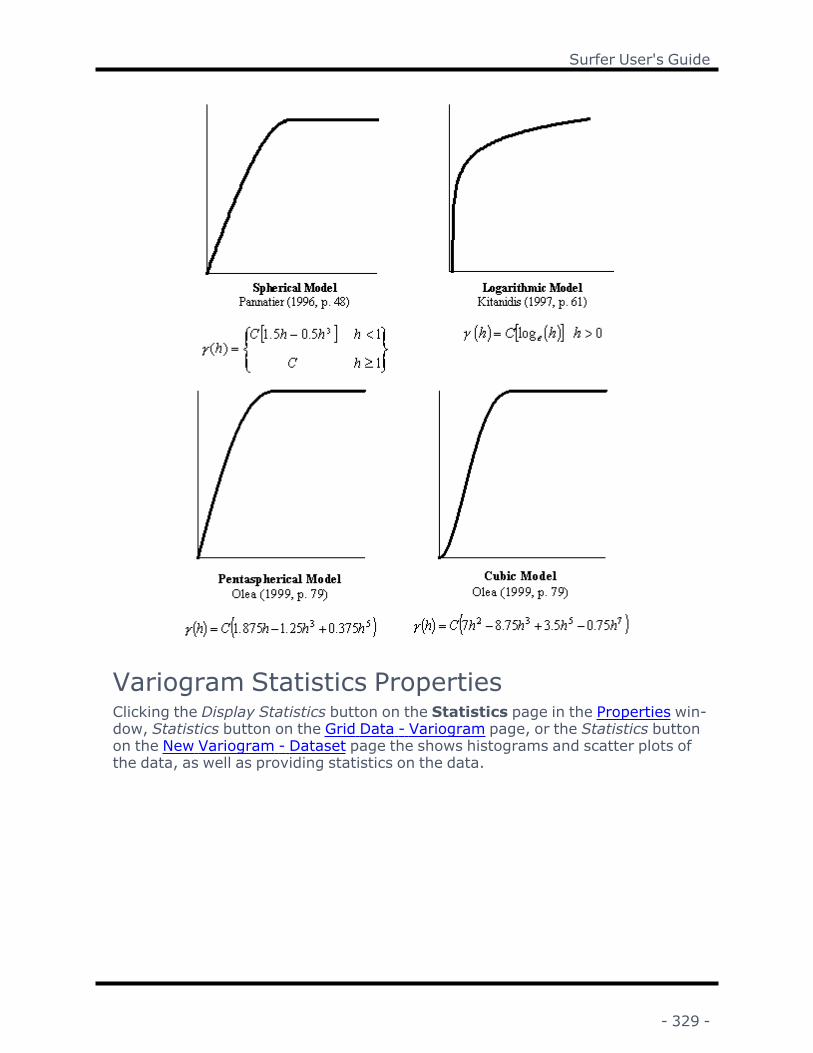
Surfer User's Guide
Variogram Statistics PropertiesClicking the Display Statistics button on the Statistics page in the Properties win-dow, Statistics button on the Grid Data - Variogram page, or the Statistics buttonon the New Variogram - Dataset page the shows histograms and scatter plots ofthe data, as well as providing statistics on the data.
- 329 -

Chapter 5 - Introduction to Variograms
In the Statistics dialog, you can show an X, Y, or Z histogram,view statistics, or generate a variogram report.
Graph X, Y, Z Histogram or XY ScatterThe X, Y, Z Histogram options show the distribution of the X, Y, and Z datarespectively. The histogram is shown to the right of the options. The XY Scatteroption shows the distribution of the data as a simple scatter diagram.
ReportClick the Report button to open the statistics and variogram information in areport window. The statistics can be printed if they are opened in the report win-dow.
StatisticsYou can use the scroll bar on the right of the statistics box to view the statistics.
Variogram Plot PropertiesMost of the visual characteristics of the variogram display are controlled thoughthe Plot page.
- 330 -

Surfer User's Guide
Control the display of the variogram graph on thePlot page of the variogram properties in the Prop-
erties window.
TitleYou can change the title and title font in the Title section. Click next to Title andtype in the desired title text.
Titles can contain multiple lines. To create a multiple line title, click the button.The Text Editor appears. Type the text in the dialog. To add a new line of text,press the ENTER key on the keyboard. To change the properties of the text, high-light the text and change the desired property. When finished, click OK. You arereturned to the Properties window.
To edit all of the text properties for the entire title at once, click the next toFont Properties. You can then set any desired font settings, including font, size,and text color.
- 331 -

Chapter 5 - Introduction to Variograms
SymbolsTo display symbols, check the Enable box in the Symbols section.
To change the symbol properties, click the next to Symbol Properties. You canchange any desired symbol properties, including the symbol type, size, andcolor.
EstimateTo display the curve showing the actual data, check the Enable box in the Estim-ate section.
To change the line properties, click the next to Line Properties. You can changeany desired line properties, including the line style, width, and color.
ModelTo display the model line, check the Enable box in the Model section.
To change the line properties, click the next to Line Properties. You can changeany desired line properties, including the line style, width, and color.
VarianceTo display the variance line, check the Enable box in the Variance section.
To change the line properties, click the next to Line Properties. You can changeany desired line properties, including the line style, width, and color.
SubtitleTo display the subtitle, check the box next to Enable in the Subtitle section. Thesubtitle lists the direction and tolerance of the variogram being displayed.
To edit the text properties, click the next to Font Properties. You can then setany desired font settings, including font, size, and text color.
PairsTo display the number of pairs for each point on the variogram, check the boxnext to Enable in the Pairs section.
To edit the text properties, click the next to Font Properties. You can then setany desired font settings, including font, size, and text color.
- 332 -

Surfer User's Guide
Info PropertiesThe Info properties page contains information about the selected object. Infoproperties are available with drawn objects, such as polylines, polygons, points,grouped objects, images, and metafiles, with map objects, axes, and maplayers, such as contours or base layers. The information displayed is dependenton the type of object.
The Info page is located in the Properties window for the selected object. Asingle object must be selected to display the Info page.
The Info page displays information for the selec-ted object.
Geometry SectionThe Geometry section includes properties that specify the Coordinate systemfor calculating the geometry values and display the perimeter, length, position,or area of the selected object. Click on the next to Geometry to open the sec-tion. This section is only available for polylines, polygons, symbols, rectangles,rounded rectangles, ellipses, or spline polylines.
- 333 -

Chapter 5 - Introduction to Variograms
Select the units for the units for the Perimeter, Area, Length, or Position valuesby clicking the value and selecting the desired units from the list. The selectedunits are moved to the top of the list, otherwise the units are displayed alpha-betically.
Coordinate SystemSpecify a coordinate system from the Coordinate system list to be used for theinformation displayed for the object.
l Page uses the page coordinate system (inches or centimeters depending onthe setting in the Options dialog General page).
l Local uses the units from the layer in which the geometry was originally spe-cified. For example, if the geometry was loaded from a file, this is the originalfile units. If the geometry was created interactively, this is an internal coordin-ate system with 0.0 in the center of the page (in inches).
l Map displays information in map units if the geometry is part of a map. If theobject is not part of a map, this option is not available.
The default Coordinate system property is Map for map objects and Page forobjects outside a map. Changes to the Coordinate system selection are appliedto all objects. For example, if the property is changed to Local for one object, theLocal information will be displayed for the next selected object. If the selectedCoordinate system is a geographic coordinate system, i.e. uses sphericalcoordinates, some geometry information cannot be displayed.
Total Number of VerticesThe Total number of vertices displays how many vertices are used in the selectedobject. The Reshape command can be used to see the vertex locations for poly-gons and polylines.
Number of Sub-PolygonsIf the object contains a complex polygon, the Number of sub-polygons (rings) dis-plays how many polygons are included in the complex polygon. For example, thesample file ca2010.gsb has polygons of California counties. Some of the countiesare complex polygons (i.e. Santa Barbara) that include sub-polygon islands.
Number of CurvesThe Number of curves is displayed for a spline polyline. The Number of curves isthe number of inflection points along the spline polyline. This is one less than thetotal number of vertices.
Perimeter/LengthDepending on the object selected, either Perimeter or Length will be displayed.
l The Perimeter displays the calculated perimeter of the selected closed object(i.e. polygon).
- 334 -

Surfer User's Guide
l The Length displays the calculated length of the selected open object (i.e.polyline). The units displayed are dependent on what is selected for theCoordinate system.
The Perimeter or Length is not displayed in spherical coordinates (i.e. degreesfor Unprojected Lat/Long coordinate systems). If your map is in a geographiccoordinate system, change the Target Coordinate System to a projected coordin-ate system to view the Perimeter or Length. Then specify Map in the Coordinatesystem field on the Info page.
AreaThe Area displays the calculated area of the selected object. The units displayedare dependent on what is selected for the Coordinate system.
The Area is not displayed in spherical coordinates (i.e. degrees squared forUnprojected Lat/Long coordinate systems). If your map is in a geographiccoordinate system, change the Target Coordinate System to a projected coordin-ate system to view the Area. Then specify Map in the Coordinate system list onthe Info page.
Add Geometry AttributesClick the Add Geometry Attributes command to add the geometry values dis-played above to the object's attributes. If you wish to add the geometry attrib-utes to all objects in the base layer, use the Attribute Table.
Info SectionThe Info section allows you to view the Type, Description, Number of records,size in bytes, Objects in group and image information for the selected object.Click on the next to Info to open the section. This section is available for text,images, metafiles, grouped objects, and point cloud layers.
TypeThe Type displays the type of metafile being displayed.
DescriptionThe Description displays any information about the metafile.
Number of RecordsThe Number of records displays the number of objects in the metafile.
Pixel FormatThe Pixel format option displays the type of image imported, including the num-ber of bits per pixel included in the image.
- 335 -

Chapter 5 - Introduction to Variograms
Size in BytesThe Size in bytes or the Size (bytes) option displays the file size of the image ormetafile in bytes.
Size in PixelsThe Size (pixels) option displays the number of pixels in the image.
Image SourceThe Image source displays the name of the file imported for an image.
Number of PointsThe Number of points displays the number of points in the point cloud layer.
ExtentsThe xMin, xMax , yMin , yMax, Zmin, and Zmax values display the extents of thepoint cloud layer.
Attributes SectionThe Attributes section contains any information that is available about the selec-ted object. To open the Attributes section, click the next to Attributes.
Attributes can be image properties, such as TIFF_Compression, or can be inform-ation about a specific object that was imported from a file, such as a .DEM, .DXF,or .SHP file. Each object (such as polylines in a base map) can have its own attrib-ute information. The Attributes can also contain user generated information.
Adding AttributesTo add an attribute to the Attribute Table,
1. Click on the object to select it.2. In the Properties window, click on the Info page.3. Open the Attributes section by clicking the next to Attributes.4. Click on the Add button next to Add new attribute.5. Type the new attribute name, such as Surveyor's Name, in the Attribute
name field of the New Attribute Name dialog.6. Click OK in the New Attribute Name dialog. The new attribute is added to
the object displayed on the Info page.7. Click in the value column next to the new attribute name. Type the desired
description, such as Thomas Denver.8. Now the new attribute and its value has been added to the object.
To rename or remove an attribute, use the Attribute Table.
- 336 -
Surfer User's Guide
Edit AttributesEdit attribute values by typing the new value into the field next to the attributename in the Properties window. Edit values for multiple attributes in a baselayer with the Attribute Table.
Options SectionThe Options section contains the option to copy the attribute data for a selectedobject. To open the Options section, click the next to Options.
Copy AttributesClick the Copy button next to Copy to clipboard to copy all of the information onthe Info page for the selected object to the clipboard. The text can be pastedinto Surfer or any other program using the Paste command. All information onthe Info page is copied, including the information in the Geometry and Info sec-tions. If the Copy button is not available, no attribute information is available forthe selected item.
Exporting AttributesAttribute information is exported for polygons, polylines, and points to fileformats that support metadata. The file type will determine how many attributesare exported. Refer to the specific file type pages for specific information.
Displaying AttributesAttributes can be added to base maps as labels. Click on the Basemap layerobject in the Contents window to select the base layer. In the Properties win-dow, click on the Labels tab to turn label display on. Any attribute can be used asa label for polylines, polygons, or symbols on a base map layer.
Information Displayed for ObjectsAll objects display an Attributes and Options section. The information in the Geo-metry section changes depending on the object selected.
PolylineThe Info properties for Polylines displays the Coordinate system, Number of ver-tices, and Length.
PolygonThe Info properties for Polygons displays the Coordinate system, Total numberof vertices, Number of sub-polygons (rings), Perimeter, and Area.
- 337 -

Chapter 5 - Introduction to Variograms
PointThe Info properties for Symbols displays the Coordinate system and Position inX and Y units.
RectangleThe Info properties for Rectangles displays the Coordinate system, Perimeterand Area.
Rounded RectangleThe Info properties for Rounded Rectangles displays the Coordinate system,Perimeter and Area.
EllipseThe Info properties for Ellipses displays the Coordinate system, Perimeter andArea.
Spline PolylineThe Info properties for Spline Polylines displays the Coordinate system, Numberof curves and Length.
Range RingThe Info properties for Range Rings displays the Coordinate system, Perimeter,and Area. Note that when Number of rings is greater than one, the Perimeterand Area values are for the largest ring.
Group ObjectsThe Info page for Group Properties displays the number of Objects in group.Each group object can be selected in the Contents window to display the objectinfo.
MetafileThe Info properties for Metafiles displays the Type of metafile, Description, Num-ber of records, and Size in bytes.
ImageThe Info properties for Images displays the Pixel format, Size (pixels), Size(bytes), and Image source.
Default Linear VariogramThe default linear variogram takes the form
- 338 -

Surfer User's Guide
where is the unknown nugget effect, and is the unknown slope. We needtwo defining equations to solve for these two unknown parameters.
According to theory, the expected value of the sample variance is the averagevalue of the variogram between all possible pairs of sample locations (Barnes,1991); this yields one equation. The second equation is generated by equatingthe experimental sample variogram for nearest neighbors to the modeled vari-ogram. Thus, we can write
where
= average distance to the nearest neighbor
= average inter-sample separation distance
= one half the averaged squared difference between nearest neighbors
= sample variance
By solving the two equations for the two unknown parameters, and checking forunreasonable values, we get the final formulae used in Surfer:
Nugget EffectThe Nugget Effect is used when there are potential errors in the collection of yourdata. The nugget effect is implied from the variogram you generate of your data.Specifying a nugget effect causes Kriging to become more of a smoothing inter-polator, implying less confidence in individual data points versus the overalltrend of the data. The higher the Nugget Effect, the smoother the resulting grid.The units of the nugget effect are the units of the observations squared.
The nugget effect is made up of two components:
Nugget Effect = Error Variance + Micro Variance.
- 339 -

Chapter 5 - Introduction to Variograms
Error VarianceThe Error Variance is a measure of the direct repeatability of the data meas-urements. If you took an observation at one point, would the second meas-urement at that exact point be exactly the same as the first measurement? TheError Variance values take these variances in measurement into account. A non-zero Error Variancemeans that a particular observed value is not necessarily theexact value of the location. Consequently, Kriging tends to smooth the surface: itis not a perfect interpolator.
Micro VarianceThe Micro Variance is a measure of variation that occurs at separation distancesof less than the typical nearest neighbor sample spacing. For example, considera nested variogram where both of the models are spherical. The range of one ofthe structures is 100 meters while the range of the second structure is fivemeters. If our closest sample spacing were 10 meters, we would not be able tosee the second structure (five meter structure). The Micro Variance box allowsyou to specify the variance of the small-scale structure. If you do not know themicro variance, leave the setting at 0.0.
This is the nugget effect model.
ReferenceSurfer's implementation of the Nugget Effect follows the recommendation ofCressie (1991, Section 3.2.1), and this reference should be consulted for a morerigorous presentation of the nugget effect and its partitioning.
- 340 -

Surfer User's Guide
Export VariogramYou can use Grids | New Grid | Variogram | Export Variogram to exportthe XY coordinates of the symbols representing the pairs for each lag distance.
To Export a Variogram:1. Create a variogram using the New Variogram command.2. Click once on the variogram to select it.3. Click the Grids | New Grid | Variogram | Export Variogram command
or the button. In the Save As dialog, set the File name and location. ClickSave and the file is created.
The resulting file is an ASCII text file [.DAT] with the X coordinates (separationdistance) in column A, the Y coordinates (variogram - g(
Using Variogram Results in KrigingOnce you have completed the variogram, you can use the results of the vari-ogram model when gridding the data with the Kriging gridding option.
To use model results:
1. Make sure the variogram is displayed in the plot window. If you switch to anew plot window, the variogram results cannot be used.
2. Select Grids | New Grid | Grid Data.
3. In the Open Data dialog, choose the data file to be modeled and clickOpen.
4. In the Grid Data dialog, select Kriging for the gridding method.
5. Click the Next button twice to open the Grid Data Kriging Options dialog.
6. Click the Get Variogram button to use the variogram model open in the plotwindow. If more than one variogram exists in the document, a dialog is dis-played prompting you for the variogram to use.
Suggested Reading - VariogramsAlfaro, M. (1980), The Random Coin Method: Solution of the Problem of the Sim-ulation of a Random Function in the Plane,Mathematical Geology, v. 12, n. 1, p.25-32.
Barnes, R. (1991), The Variogram Sill and the Sample Variance, MathematicalGeology. v. 23, n. 4, p. 673-678.
- 341 -

Chapter 5 - Introduction to Variograms
Barnes, R. Variogram Tutorial. http://www.goldensoft-ware.com/variogramTutorial.pdf
Cressie, Noel (1991), Statistics for Spatial Data , John Wiley and Sons, NewYork, 900 pp., ISBN 0-471-84336-9.
Isaaks, Edward and Mohan Srivastava (1989), An Introduction to Applied Geo-statistics , Oxford University Press, New York, 561 pp., ISBN 0-19-505013-4.
Kitanidis, Peter (1997), Introduction to Geostatistics - Applications in Hydro-geology , Cambridge University Press, New York, 249 pp., ISBN 0-521-58747-6.
Olea, R.A., 1999, Geostatistics for Engineers and Earth Scientists, Kluwer Aca-demic Publishers, Boston, 303 pp. ISBN 0-7923-8523-3.
Pannatier, Yvan (1996), VarioWin - Software for Spatial Data Analysis in 2D ,Springer-Verlag, New York, 91 pp., ISBN 0-387-94579-9.
Press, W.H., , Numerical Recipes in C , Cambridge University Press.
Zimmerman, D. L., and Technometrics , v. 33, n. 1, p. 77-91.
Variogram TutorialSurfer's variogram modeling feature is intended for experienced variogramusers who need to learn Surfer's variogram modeling features.
The novice variogram user may find the following four authors helpful: Cressie(1991), Isaaks and Srivastava (1989), Kitanidis (1997), and Pannatier (1996). Atutorial for use with Surfer's variogram modeling is also available. Please referto Suggested Reading for full references for each of the previous books.
If you do not understand variograms or if you are unsure about which model toapply, use Surfer's default linear variogram with the kriging algorithm. The fol-lowing tutorial is intended for those who have a basic knowledge of variogramsand need assistance with using Surfer's variogram feature.
Variogram IntroductionThe variogram characterizes the spatial continuity or roughness of a data set.Ordinary one-dimensional statistics for two data sets may be nearly identical,but the spatial continuity may be quite different. Refer to What Does a VariogramRepresent? for a partial justification of the variogram.
Variogram analysis consists of the experimental variogram calculated from thedata and the variogram model fitted to the data. The experimental variogram iscalculated by averaging one-half the difference squared of the z-values over allpairs of observations with the specified separation distance and direction. It is
- 342 -
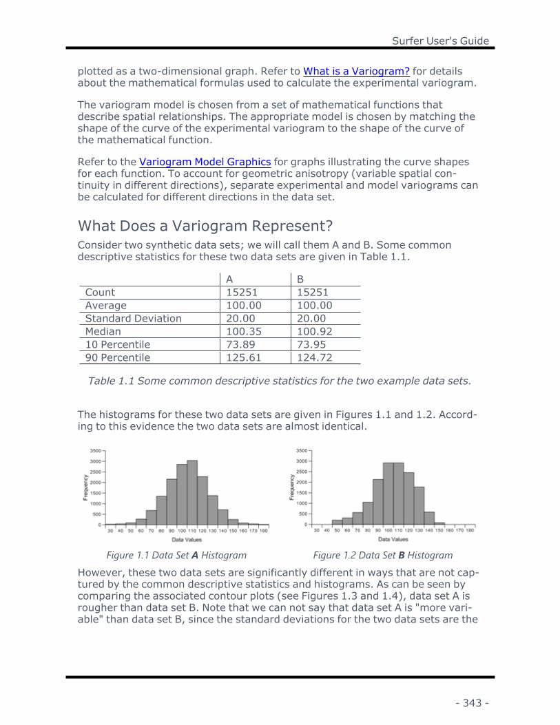
Surfer User's Guide
plotted as a two-dimensional graph. Refer to What is a Variogram? for detailsabout the mathematical formulas used to calculate the experimental variogram.
The variogram model is chosen from a set of mathematical functions thatdescribe spatial relationships. The appropriate model is chosen by matching theshape of the curve of the experimental variogram to the shape of the curve ofthe mathematical function.
Refer to the Variogram Model Graphics for graphs illustrating the curve shapesfor each function. To account for geometric anisotropy (variable spatial con-tinuity in different directions), separate experimental and model variograms canbe calculated for different directions in the data set.
What Does a Variogram Represent?Consider two synthetic data sets; we will call them A and B. Some commondescriptive statistics for these two data sets are given in Table 1.1.
A BCount 15251 15251Average 100.00 100.00Standard Deviation 20.00 20.00Median 100.35 100.9210 Percentile 73.89 73.9590 Percentile 125.61 124.72
Table 1.1 Some common descriptive statistics for the two example data sets.
The histograms for these two data sets are given in Figures 1.1 and 1.2. Accord-ing to this evidence the two data sets are almost identical.
Figure 1.1 Data Set A Histogram Figure 1.2 Data Set B HistogramHowever, these two data sets are significantly different in ways that are not cap-tured by the common descriptive statistics and histograms. As can be seen bycomparing the associated contour plots (see Figures 1.3 and 1.4), data set A isrougher than data set B. Note that we can not say that data set A is "more vari-able" than data set B, since the standard deviations for the two data sets are the
- 343 -

Chapter 5 - Introduction to Variograms
same, as are the magnitudes of highs and lows. The visually apparent differencebetween these two data sets is one of texture and not variability.
Figure 1.3 Data Set A Contour Plot Figure 1.4 Data Set B Contour PlotIn particular, data set A changes more rapidly in space than does data set B. Thecontinuous high zones (red patches) and continuous low zones (blue patches)are, on the average, smaller for data set A than for data set B. Such differencescan have a significant impact on sample design, site characterization, and spatialprediction in general.
It is not surprising that the common descriptive statistics and the histograms failto identify, let alone quantify, the textural difference between these two exampledata sets. Common descriptive statistics and histograms do not incorporate thespatial locations of data into their defining computations.
The variogram is a quantitative descriptive statistic that can be graphically rep-resented in a manner which characterizes the spatial continuity (i.e. roughness)of a data set. The variograms for these two data sets are shown in Figures 1.5and 1.6. The difference in the initial slope of the curves is apparent.
Figure 1.5 Data Set A Variogram andModel
Figure 1.6 Data Set B Variogram andModel
- 344 -
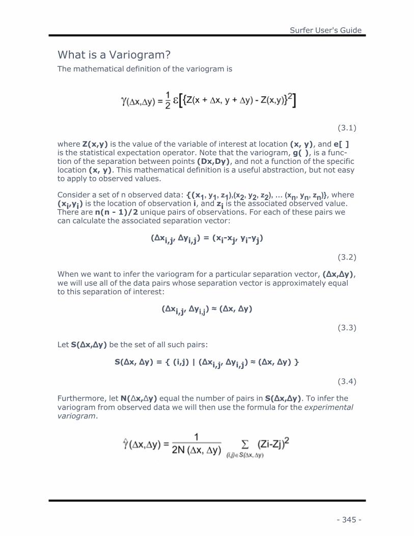
Surfer User's Guide
What is a Variogram?The mathematical definition of the variogram is
(3.1)
where Z(x,y) is the value of the variable of interest at location (x, y), and e[ ]is the statistical expectation operator. Note that the variogram, g( ), is a func-tion of the separation between points (Dx,Dy), and not a function of the specificlocation (x, y). This mathematical definition is a useful abstraction, but not easyto apply to observed values.
Consider a set of n observed data: {(x1, y1, z1),(x2, y2, z2), … (xn, yn, zn)}, where(xi,yi) is the location of observation i, and zi is the associated observed value.There are n(n - 1)/2 unique pairs of observations. For each of these pairs wecan calculate the associated separation vector:
(∆xi,j, ∆yi,j) = (xi-xj, yi-yj)
(3.2)
When we want to infer the variogram for a particular separation vector, (∆x,∆y),we will use all of the data pairs whose separation vector is approximately equalto this separation of interest:
(∆xi,j, ∆yi,j) ≈ (∆x, ∆y)
(3.3)
Let S(∆x,∆y) be the set of all such pairs:
S(∆x, ∆y) = { (i,j) | (∆xi,j, ∆yi,j) ≈ (∆x, ∆y) }
(3.4)
Furthermore, let N(∆x,∆y) equal the number of pairs in S(∆x,∆y). To infer thevariogram from observed data we will then use the formula for the experimentalvariogram.
- 345 -

Chapter 5 - Introduction to Variograms
(3.5)
That is, the experimental variogram for a particular separation vector of interestis calculated by averaging one-half the difference squared of the z-values overall pairs of observations separated by approximately that vector.
Variogram Tutorial - Variogram GridIf there are n observed data, there are n(n - 1)/2 unique pairs of observations.Thus, even a data set of moderate size generates a large number of pairs. Forexample, if n = 500, n(n - 1)/2 = 124,745 pairs. The manipulation of such alarge number of pairs can be time consuming, even for a fast computer. Surferpre-computes all of the pairs and stores the necessary sums and differences inthe variogram grid. Note: a variogram grid is not the same format as a grid usedin creating a map.
To create a new variogram, choose the Grid | Variogram | New Variogrammenu command, specify the data file name in the Open dialog box, and clickOpen. Specify the X, Y, and Z columns, Duplicate Data settings, Data ExclusionFilter (if any), and review the data Statistics.
Figure 4.1 Choose the Grid | Variogram | New Variogram menu to display the Data tabof the New Variogram dialog box.
Click the General tab to view the Variogram Grid and Detrending options. TheMax Lag Distance is the maximum separation distance to be considered duringvariogram modeling. By default, this is approximately one-third the diagonal
- 346 -

Surfer User's Guide
extent of the observed data. The Angular Divisions of 180 and the Radial Divi-sions of 100 are adequate for almost any setting.
The Detrend options offer advanced data handling options for universal kriging.Typically, the appropriate option is Do not detrend the data. However, if youknow that a strong trend exists in the data, you may want to consider Lineardetrending. Click the Generate Report option to create a list of the Data Filter Set-tings and Data Statistics.
Figure 4.2 Click the General tab in the New Variogram dialog box to display the VariogramGrid , Detrend , and Generate Report options.
Without changing any of the settings, click OK. Figure 4.3 is displayed.
- 347 -

Chapter 5 - Introduction to Variograms
Figure 4.3 Resulting variogram with default variogram settings usingExampleDataSetC.xls.
The black line with the dots is the omni-directional experimental variogram,while the blue line is a first pass (albeit a poor one) at a fitted variogram model.
Modeling the Omni-Directional VariogramBy default, this first plot is the omni-directional variogram (the directional tol-erance is 90 degrees). Choose the model type, the sill, and the nugget effectbased upon the omni-directional variogram.
5.1 Selecting the variogram model typeThere are infinitely many possible variogram models. Surfer allows for the con-struction of thousands of different variogram models by selecting combinationsof the ten available component types. When combined with a nugget effect, oneof three models is adequate for most data sets: the linear, the exponential, andthe spherical models. Examples of these three models are shown in Figure 5.1.
- 348 -

Surfer User's Guide
Figure 5.1 Variogram ModelsIf the experimental variogram never levels out, then the linear model is usuallyappropriate. If the experimental variogram levels out, but is "curvy" all the wayup, then the exponential model should be considered. If the experimental vari-ogram starts out straight, then bends over sharply and levels out, the sphericalmodel is a good first choice.
For the data in ExampleDataSetC.xls, a spherical model appears appropriate,though one could also try an exponential model. Click on the variogram plot andselect theModel tab in the Properties window.
Figure 5.2 TheModel tab of the Variogram prop-erties in the Properties window.
To see the current model, click on the Nugget Effect next to Current component.You can see that there is also a Linear component to the default model. Next toComponents, click the Remove button twice to remove the inappropriate defaultmodel. Then click the Add button. In the Add Component dialog, select theSphericalmodel and click OK.
5.2 Selecting the variogram model scale and length parametersWe must now set the Scale and the Length (A) parameters using an iterativeapproach (i.e. guess and check). The Scale is the height on the y-axis at whichthe variogram levels off. By simply looking at the plot, a value between 400 and
- 349 -

Chapter 5 - Introduction to Variograms
450 seems reasonable: enter 425. TheLength (A) for a spherical model is the lagdistance at which the variogram levels off. Again, from the plot a value between30 and 40 seems reasonable: enter 35. The new candidate variogram model isautomatically drawn.
This is not a bad first guess, but upon examination of the redrawn curve, itappears that the Length (A) is a little bit too long since the model (blue line) liesto the right of the experimental variogram plot (black line and dots). Reset theLength (A) to 30. This is still a little bit too long. Try 29 for theLength (A) This is agood fit for a variogram.
Figure 5.3 Variogram model with initial assumptions Left: Scale = 425, Length (A) = 35. Right:Scale =425. Length (A) = 29.
5.3 Selecting the variogram nugget effectIf the experimental variogram appears to have a non-zero intercept on the ver-tical axis, then the model may need a nugget effect component. The variance ofDelta Z in the Nearest Neighbor Statistics section of the Variogram Grid Reportoffers a quantitative upper bound for the nugget effect in most circumstances.
- 350 -

Surfer User's Guide
Figure 5.4 Linear Variogram model with nugget effect for data set Demog-rid.dat.
In Surfer the nugget effect is partitioned into two sub-components: the errorvariance and themicro variance. Both of these sub-components are non-negative,and the sum of these two sub-components should equal the apparentnon-zero intercept.
The error variancemeasures the reproducibility of observations. This includesboth sampling and assaying (analytical) errors. The error variance is best selec-ted by computing the variance of differences between duplicate samples.
Themicro variance is a substitute for the unknown variogram at separation dis-tances of less than the typical sample spacing. This is best selected by taking thedifference between the apparent non-zero intercept of the experimental vari-ogram and the error variance.
The model for our example appears to intersect the vertical axis at 0, so we willnot apply a nugget effect.
Modeling the Variogram AnisotropyOften, the experimental variogram shows different length scales in different dir-ections. This is called geometric anisotropy. For a linear variogram model thiswould appear as a different slope in different directions, while a spherical modelmanifests geometric anisotropy as different apparent Length (A) parameters indifferent directions.
To investigate the variogram anisotropy click on the variogram. In the Prop-erties window, click on the Experimental tab. The omni-directional exper-imental variogram averages the behavior over all directions. To look in particulardirections open the Lag Direction section and change the Direction and the Tol-erance parameters. Start by setting the Tolerance to 30 degrees. Notice how the
- 351 -

Chapter 5 - Introduction to Variograms
small circular diagram shows the blue sector centered at 0 degrees (east in thismodel), with an angular tolerance (plus or minus) of 30 degrees.
Figure 6.1 Set the Tolerance to 30 on the Exper-imental tab of the Variogram properties in the
Properties window.To quickly sweep through all directions press the Step CCW button. Press it onceand the plot is now set for a direction of 30 degrees. Press it again and you haveselected 60 degrees. Press it again and again and again and notice how the smallcircular diagram helps you keep track of the current direction.
Sweep through all directions a few times. Notice how the scaling of the verticalaxis changes. To fix the vertical scale of the plot, in the General section, set theVertical Scale to 515.
Figure 6.2 Directional variogram plots with Tolerance set to 30°. From left to right: Direction= 0°, 30°, 60°, 90°, 120°, 150°.
- 352 -

Surfer User's Guide
Change the Step Amount to 15 degrees and sweep through all directions acouple of times. It appears that for directions between 90 and 180 degrees theomni-directional model is consistently to the right of the ascending portion of theexperimental variogram. Conversely, the omni-directional model is consistentlyto the left of the ascending portion of the experimental variogram for directionsbetween 0 and 90 degrees. This is a clear indication of geometric anisotropy.
By pressing the Step CCW button move to the direction at which the apparentlength and scale of the experimental variogram is maximized: say, 30 degrees.Click on theModel tab and change the Length (A) parameter to better fit this dir-ectional variogram. 40 is too long, 30 is too short, and 37 appears to fit quitewell. Change the Anisotropy Angle to 30 degrees. .
Click on the Experimental tab and change the Direction to 120 degrees (this isorthogonal to the direction of maximum length, 120 = 30 + 90). Click on theModel tab. Change only the Anisotropy Ratio to fit the variogram model to thecurrent directional experimental variogram. As you change the setting, themodel will automatically update the plot. A Anisotropy Ratio value of 1.6 appearsto be a good fit.
Figure 6.3 Change the variogram model prop-erties to add anisotropy.
To get a final visual verification of your model, take it for a "spin". Click on theExperimental tab and repeatedly click the Step CCW button. Notice how thevariogram model mimics the changing shape of the experimental variogram. Youcan fine tune the model parameters to better match the model to the exper-imental variogram, but do not over-model: one or two significant digits is all thatyou can hope for.
- 353 -

Chapter 5 - Introduction to Variograms
Figure 6.4 Directional variograms with anisotropy settings. Left: Direction = 30°, Right: Dir-ection = 120° Anisotropy Ratio = 1.6, Angle = 30°.
Click the AutoFit button on theModel tab to fine-tune the model after choosingappropriate initial parameters. Click OK to accept the defaults, and AutoFitreturns an Anisotropy Ratio of 1.741 and Anisotropy Angle of 38.57°.
Figure 6.5 Directional Variogram plots with Anisotropy Ratio = 1.75 and Anisotropy Angle= 38.49°. From left to right: Direction = 0°, 30°, 60°, 90°, 120°, 150°.
Variogram Modeling Rules of ThumbThe following rules of thumb are general tips for variogram modeling:
l Know your data! Before calculating the experimental variogram, calculateregular non-spatial statistics. Use the Variogram Report to display the dataminimum, maximum, median, mean, standard deviation, variance, andskewness. Create a post map or classed post map in Surfer to display scat-ter plots. Use Grapher to create histograms and cumulative frequencyplots.
l Do not over model. The simplest model that reproduces the important fea-tures of the experimental variogram is the best model.
- 354 -

Surfer User's Guide
l When in doubt, use the default variogram model for gridding. A simple lin-ear variogram model usually generates an acceptable grid; this is espe-cially true for initial data analysis. Remember, however, that the krigingstandard deviation grid generated using the default variogram is mean-ingless.
l Unless there is a clear, unambiguous, physical justification, do not use ananisotropy ratio of greater than 3 to 1. If the experimental variogramappears to support an anisotropy of greater than 3 to 1, and there is nounambiguous, physical justification for such a severe anisotropy, theremay be a trend in the data. Consider detrending the data before carryingout your variogram analysis.
l Try the model and see how the resulting grid looks in a contour map. If youhave competing candidate variogram models, generate a grid and contourmap from each. If there are no significant differences, choose the simplestvariogram model.
l The range of the variogram is often close to the average size of physicalanomalies in the spatial fluctuation of the Z values. In the absence of a reli-able experiment variogram, this rule of thumb may be used to postulate avariogram range.
l An experimental variogram that fluctuates around a constant value is notan ill-behaved variogram. It is an indication that the Z values are uncor-related at the scale of the typical sample spacing. In such a situation a con-tour map, regardless of the gridding method used, is an unreliablerepresentation of the data, and more data at closer sample spacing areneeded for detailed local characterization.
l If the following three conditions are met, then the sample variance is a reas-onable approximation for the variogram sill:
1. The data are evenly distributed across the area of interest, as dis-played in a post map.
2. There is no significant trend in the data across the area of interest.
3. The dimension of the area of interest is more than three times theeffective variogram range.
Variogram Frequently Asked QuestionsQ. What is a variogram?A. A variogram is a statistically-based, quantitative, description of a surface'sroughness. A variogram is a function of a separation vector: this includes bothdistance and direction, or a ∆x and a ∆y. The variogram function yields the aver-
- 355 -

Chapter 5 - Introduction to Variograms
age dissimilarity between points separated by the specified vector (dissimilarityis measured by the squared difference in the Z-values).
Q. What is the difference between a variogram and a semi-variogram?A. The difference is simply a factor of 2. The variogram was originally defined as
where 2γ( ) was given the name variogram. The function of practical interest wasγ( ) which was given the name semi-variogram since it is one-half the variogramfunction. Since only the function γ( ) is used in kriging, the prefix semi- is reg-ularly dropped, and the function γ( ) is interchangeably called the variogram andthe semi-variogram in the geostatistical literature.
Q. What are the units of the variogram plot?A. Let (X, Y) represent the location of an observation, and let Z represent theassociated observed value. The abscissa (lag distance axis) has the same unitsas X and Y. The ordinate (variogram axis) has the units equal to the units of Zsquared (like the variance of Z). For
example, let
l X represent the distance east of a benchmark measured in [m],
l Y represent the distance north of a benchmark also measured in [m], and
l Z represent rainfall intensity measured in [cm/hr].
The abscissa subsequently has units of [m], and the ordinate has units of[(cm/hr)2].
Q. Why can't I specify the sill in the variogram parameters? How isthe scale related to the sill?A. The sill is the value of the ordinate at which the variogram levels off. A vari-ogram model may be comprised of multiple components (e.g. a spherical com-ponent plus a nugget effect). While the individual components may be said tohave a sill, such usage often leads to confusion between the sill of the overallmodel and the various sills of the individual components. A further source of con-fusion is that some components, and therefore models including such com-ponents, do not have a sill (e.g. the linear model).
- 356 -

Surfer User's Guide
To reduce confusion, the word sill was used to describe the leveling-off of theentire model, and not of the individual components. When discussing the lev-eling-off of an individual component, we use the term scale.
Q. What does the variogram direction do? Why does the variogramchange when I change the direction?A. This behavior is called anisotropy. The variogram measures dissimilarity as afunction of separation distance and direction. In many physical settings it is pos-sible for the variable of interest to change more rapidly in one direction than inanother. For example, the distribution of grain size changes more rapidly in a dir-ection perpendicular to the shoreline than it does parallel to the shoreline. Sim-ilarly, in an arid climate the prevalence of certain species of plants changes morerapidly as one moves in a direction perpendicular to a river than it does as onemoves along the river.; i.e. different behavior in different directions. The dir-ection parameter allows you to investigate the variogram in different directions.Thus, you can identify and quantify the anisotropy.
Q. Are the various variogram directions used when gridding withSurfer?A. Yes. The variogram anisotropy is explicitly entered when specifying the vari-ogram for gridding with the kriging algorithm.
Q. Does Surfer have a multi-directional gridding algorithm so thatmore than just the anisotropy can be changed (different sills indifferent directions)?A. The variogram model contains the necessary information to describe the beha-vior of the variogram in all directions. The spherical model, for example, is a fun-nel-like surface. The variogram plot on which a single line is drawn to representthe variogram model is a vertical slice through the variogram model.
The anisotropy ratio and angle describe the ratio of the Lengths (A) in differentdirections (geometric anisotropy). Sometimes the apparent sill of the exper-imental variogram differs in different directions (zonal anisotropy). For example,an experimental variogram appears to be well described by a spherical modelwith a Length (A) of 100 meters. It levels off (sill) at 2.0 in the East/West dir-ection (Angle = 0 degrees), while it levels off at 3.0 in the North/South direction(Angle = 90 degrees). Surfer can reproduce such behavior using a nested model.Make the first component an isotropic spherical model with a length of 100 and ascale of 2. Make the second component be an anisotropic model with length 100,ratio1000, direction 90, and scale of 1. Adding the two components results in acompound model with a sill of 2 in the East/West direction and a sill of 3 in theNorth/South direction.
- 357 -

Chapter 5 - Introduction to Variograms
Q. Why are some of the cells blank when exporting variogramdata?A. A cell is blank when there are no data pairs separated by the specified lag dis-tance interval and angular tolerance represented by the cell.
Q. How do I perform kriging cross-validation, jack-knifing (leave-out-one modeling), and such.A. The Grids | New Grid | Grid Data command in Surfer offers an extensiveset of cross-validation tools. The Cross Validation Report (using the Kriging grid-ding method) offers numerous quantitative measures that can be used as a good-ness-of-fit statistic for the variogram. We recommend three particular statisticsas the most consistently useful: the median absolute deviation of the cross val-idation residuals, the standard deviation of the cross validation residuals, andthe rank correlation between the measurements and the estimates.
Q. How do I plot the 3D variogram surface?A. This option is not available in Surfer.
Q. Does Surfer calculate S2 (variance of the data) and how do wefind this value in the program outputs?A. Surfer uses the formula for calculating the sample variance in the exper-imental variogram. This value is reported in the Statistics tab of the VariogramProperties and in the Variogram Report.
Q. Why doesn't the grid change when using a linear variogram withdifferent slope values?A. This occurs if there is no nugget effect. Changing the slope of a linear vari-ogram is equivalent to changing only the scale of the observation locations;thus, the ratio of the variogram values between any two pairs of points isunchanged by changing the slope. It is important to note, however, that the kri-ging variance is sensitive to the slope even if the interpolation weights and inter-polated value are not.
Q. How can I get information on the distance between data points?A. Plot your data as a post map (see the Home | New Map | Post command).Surfer reports some useful quantitative statistics in the Variogram Report and atthe bottom of the table on the Statistics tab of the variogram properties. Forexample, the Nearest Neighbor (NN) values for the ExampleDataSetC.xls are:
l Avg. distance to nearest neighbor: 2.90403
l Min. distance to nearest neighbor: 1
- 358 -

Surfer User's Guide
l Max. distance to nearest neighbor: 9.48683
l Gamma for nearest neighbors: 64.735
In addition, the Grids | New Grid | Grid Datamenu with the Data Metrics grid-ding method offers an extensive suite of tools for characterizing the data geo-metry. This includes a neighborhood count, data density, distance to the nearestneighbor, etc.
Q. When using an exponential variogram model for kriging, is theinput parameter Length (A) the correlation length (i.e. the lengthat which the variogram value reaches 63 percent of the sill) or thepractical range (i.e. the length at which the variogram valuereaches 95 percent of the sill)?A. Different geostatistical software packages use various definitions for thelength parameter of an exponential model. Surfer defines the Length (A) para-meter, as the correlation length. Graphically, the correlation length correspondsto the lag distance at which the tangent line to the curve at lag distance zerointersects the sill of the exponential model. The exponential model achievesabout 63 percent of the sill at Lag Distance (A). At a lag distance of 3A the expo-nential model reaches about 95 percent of the sill.
Q. When applying the Gaussian model, I seem to be getting amismatch between what I see on the plot of the variogram and thelength reported by the software after AutoFit has finished. Thelength at which the sill is reached seems to be much larger than thevalue reported under the Model tab when AutoFit has finished.A. As with the exponential model, different geostatistical software packages usevarious definitions for the Length (A) parameter of a Gaussian model. Surferdefines the Length (A) parameter as the correlation length. Graphically, the cor-relation length corresponds to the lag distance of the inflection point of thecurve. The Gaussian model achieves about 63 percent of the sill at Lag Distance(A). At a lag distance of 3A the Gaussian model reaches about 99.99 percent ofthe sill.
Q. Is there a function in the variogram procedure in the new Surferthat can actually tell me the exact nugget, length, and scale?A. To view the nugget, length, and scale, choose the Grid | Variogram | NewVariogram command. Specify the data file, click the Open button, and click OKto use the defaults. Click on the variogram graph and the variogram propertiesare listed in the Properties window on theModel tab. The Nugget Error andMicro Variance are listed for the nugget and the default linear model Slope andAnisotropy parameters are listed for the linear component. Other componentshave other options, such as Scale or Length (A) listed.
- 359 -

Chapter 5 - Introduction to Variograms
Q. I tried to fit a spherical variogram using AutoFit and all thestandard settings. The fit is poor. Could you explain how Surferdoes the fitting? How can I make an appropriate fit using thespherical function?A. The AutoFit function requires reasonable initial parameters to arrive at a goodfit. Examine the plot of the experimental variogram and estimate the Length (A)and Scale visually. If it is difficult to estimate the scale from your data set, usethe Z variance listed in the Variogram Report and on the Statistics tab of thevariogram properties.
Q. I set the Lag Width to a particular value. Why aren't the pointson the variogram plotted at multiples of this value?A. The Lag Width defines the midpoint of a range plus or minus half the lagwidth. The point is plotted at the average separation distance for all points withinthat range.
Q. How can I get a list of the average separation distances?A. Export the variogram to a data file. This file includes the average lags, half theaverage variance, and the number of pairs in the range.
Q. Is it possible to create a grid file from two juxtaposed areas onwhich different variogram models are applied? The areas havespatially contrasted morphologies.A. If the areas are defined by rectangles, you may be able to grid each area witha separate model, convert the grid to XYZ data files, import the data files in theworksheet and regrid using the Nearest Neighbor method to prevent furtherinterpolation.
Q. How is the drift used within the kriging algorithm? Should themodeling be done on transformed data (data minus drift) or onnon-transformed data? Kriging with prior removal of the trend isdifferent than Universal Kriging.A. We recommend calculating the variogram model of the detrended data priorto applying drift during kriging, after Kitanidis, 1997, p. 143, section 6.12.
- 360 -

Surfer User's Guide
Q. I haven't found any procedure in Surfer that can help me to tellHOW well the theoretical variogram models are fitted to theexperimental data in my variogram. I understand that I can useAutoFit but I would like a quantitative number that measures thegoodness-of-fit.A. The best measure of "how well" the theoretical model fits the data is to try itout and see. Grid the data with the selected variogram model. Create a contourmap and overlay a post map of the data file. Judge the quality of the model byexamining the contour map. The Cross Validation Report (using the Kriging grid-ding method) offers numerous quantitative measures that can be used as a good-ness-of-fit statistic for the variogram. We recommend three particular statisticsas the most consistently useful: the median absolute deviation of the cross val-idation residuals, the standard deviation of the cross validation residuals, andthe rank correlation between the measurements and the estimates.
Q. Can Surfer import a variogram model from Variowin, GeoEAS,GSLIB, or other software?A. Surfer does not have this feature. Submit a request to [email protected] with the name of the software you would like tosupport.
Q. I've read somewhere that the scale should not exceed thevariance. Is this true? For the data set ExampleDatSetC.xls, thevariance of Z is 405.371, but you recommend a scale of 425.A. Under a reasonable and commonly applicable set of assumptions, the sill ofthe variogram should be equal to the variance of the underlying population; how-ever, the sample variance is often an inappropriate measure of the populationvariance (the standard formula for estimating the variance assumes inde-pendent data, which is invalid in most geological settings). Thus, a rule like "thescale should not exceed the variance" is not a useful generalization. The criticalresult is
This result states that the expected value of the sample variance, S 2, is equal tothe average value of the variogram between all n 2 pairs of sample values. If then sample values are evenly distributed over an areal extent many times largerthan the range of the variogram, then there will be significantly more pairs atlong separation distances and fewer pairs at short separation distances. Thus,the average value of the variogram between all pairs will be the average of many
- 361 -

Chapter 5 - Introduction to Variograms
values equal to the sill and a few values less than the sill. In this case, thesample variance is a reasonable first estimate for the variogram sill.
Geostatistical ReferencesArmstrong, M. [ed.], 1989, Geostatistics, volumes 1 and 2, Kluwer AcademicPublishers, 1027 pp.
Armstrong, M., 1997, Basic Linear Geostatistics, Springer-Verlag, New York,ISBN: 3540618457, 220 pp.
Baafi, E. Y., 1997, Geostatistics Wollongong ’96 – Quantitative Geology and Geo-statistics, Kluwer Academic Publishers, ISBN: 0792302044, 1333 pp.
Bras, R., and Rodriguez-Iturbe, R., 1985, Random Functions and Hydrology,Addison-Wesley, 559 pp.
Chiles, J., and Delfiner, P., 1999, Geostatistics: Modeling Spatial Uncertainty,John Wiley and Sons, New York, ISBN: 0471083151, 695 pp.
Christakos, G., 2001, Modern Spatiotemporal Geostatistics, Oxford UniversityPress; ISBN: 0195138953, 312 pp.
Clark, I., 1979, Practical Geostatistics, Applied Science Publishers, 129 pp.
Clark, I., and W. V. Harper, 2000, Practical Geostatistics 2000, Ecosse NorthAmerica, LLC; ISBN: 0970331703, 442 pp.
Cressie, N., 1991, Statistics for Spatial Data, John Wiley and Sons, New York,900 pp.
David, M., 1977, Geostatistical Ore Reserve Estimation, 2nd edition, Elsevier,364 pp.
David, M., 1988, Handbook of Applied Advanced Geostatistical Ore ReserveEstimation, Elsevier, 216 pp.
Davis, J., 1973, Statistics and Data Analysis in Geology, Wiley, 550 pp.
deMarsily, G., 1986, Quantitative Hydrogeology, Academic Press, 440 pp.
Deutsch, Clayton, V., Journel, Andre G., 1992, GSLIB - Geostatistical SoftwareLibrary and User's Guide, Oxford University Press, New York, 338 pp.
Draper, N., and Smith, H., 1981, Applied Regression Analysis, second edition,Wiley-Interscience, 709 pp.
Dubrule, O. 1998, Geostatistics in Petroleum Geology, American Association ofPetroleum Geologists; ISBN: 0891811877.
- 362 -

Surfer User's Guide
Gelhar, L. W., 1993, Stochastic Subsurface Hydrology, Prentice Hall, EnglewoodCliffs, New Jersey, 390 pp.
Geostatistics, 1980, McGraw-Hill, 168 pp.
Gilbert, R.O., 1987, Statistical Methods for Environmental Pollution Monitoring,Van Nostrand Reihold Company, 320 pp.
Gomez-Hernandez, J., A. Soares, and R. Froidevaux [eds.], Geoenv II -- Geo-statistics for Environmental Applications, Kluwer Academic Publishers, 562 pp.
Goovaerts, P. 1997, Geostatistics for Natural Resources Evaluation, OxfordUniversity Press, New York, 483 pp.
Guarascio, M., David, M., and Huijbregts, C. [eds.], 1976, Advanced Geo-statistics in the Mineral Industry, Reidel, 491 pp.
Gy, P., 1979, Sampling of Particulate Materials, Elsevier, 431 pp.
Houlding, S. W., 2000, Practical Geostatistics - Modeling and Spatial Analysis,Springer-Verlag,New York, 160 pp.
Hohn, M. E., 1998, Geostatistics and Petroleum Geology, 2nd edition, KluwerAcademic Publishers; ISBN: 041275780X, 238 pp.
Isaaks, E. H., and Srivastava, R. M., 1989, An Introduction to Applied Geo-statistics, Oxford University Press, New York, 561 pp.
Johnson, M. E., 1987, Multivariate Statistical Simulation, John Wiley and Sons,New York, 230 pp.
Journel, A.G., and Huijbregts, C., 1978, Mining Geostatistics, Academic Press,600 pp.
Journel, A.G., 1988, Geostatistics for the Environmetal Sciences, EPA ProjectReport, Project No. CR 811893, EPA/EMSL, Las Vegas, Nevada.
Journel, A.G., 1989, Fundamentals of Geostatistics in Five Lessons, AmericanGeophysical Union, Washington D.C.
Kitanidis, P. K., 1997, Introduction to Geostatistics: Applications in Hydro-geology, ISBN 0-521-58747-6.
Koch, G., and Link, R., 1971, Statistical Analysis of Geological Data, volumes Iand II, Wiley, 375 pp. now available through Dover reprints.
Krige, D., 1978, Lognormal DeWijsian Geostatistics for Ore Evaluation, SouthAfrican I.M.M., 55 pp.
- 363 -

Chapter 5 - Introduction to Variograms
Knudsen, H.P, 1988, A Short Course on Geostatistical Ore Reserve Estimation,Division of Mining and Minerals Engineering, Montana Tech.
Manoukian, E.B., 1986, Modern Concepts and Theorems of Mathematical Stat-istics, Springer-Verlag, 156 pp.
Matheron, G., 1965, Les Variables Regionalisees et leur Estimation, Editions Mas-son, Paris.
Matheron, G., and Armstrong, M. [eds.], 1987, Geostatistical Case Studies,Reidel, 248 pp.
Monestiez, P., D. Allard, R. Froidevaux [eds.], 2001, Geoenv III -- Geostatisticsfor Environmental Applications, Kluwer Academic Publishers, ISBN:0792371070, 555 pp.
Olea, R., 1999, Geostatistics for Engineers and Earth Scientists, Kluwer Aca-demic Publishers, Boston, MA, 303 pp.
Pannatier, Y., 1996, VARIOWIN: Software for Spatial Data Analysis in 2D,Springer-Verlag, New York, 91 pp.
Rendu, J., 1978, An Introduction to Geostatistical Methods of Mineral Evaluation,South African I.M.M., 100pp.
Ripley, B., 1981, Spatial Statistics, John Wiley and Sons, New York, 252 pp.
Rouhani, S., and M. Srivastava, 1997, Geostatistics for Environmental and Geo-technical Applcations, ASTM Special Technical Publication 1283, American Soci-ety for Testing and Materials, ISBN: 0803124147.
Rivoirard, J., J. Simmonds, K. G. Foote, P. Fernandes, and N. Bez [eds.], Geo-statistics for Estimating Fish Abundance, Blackwell Science Inc; ISBN:0632054441, 206 pp.
Soares, A. [ed.], 1992, Geostatistics Troia '92, volumes 1 and 2, Reidel, 1088pp.
Soares, A., Gomez-Hernandez, J., and R. Froidevaux [eds.], Geoenv I -- Geo-statistics for Environmental Applications, Kluwer Academic Publishers, ISBN:0792345908, 516 pp.
Thompson, S. K., 1992, Sampling, John Wiley and Sons, New York, 343 pp.
Verly, G., David, M., Journel, A.G., and Marachel, A. [eds.], 1984, Geostatisticsfor Natural Resources Characterization, volumes 1 and 2, Reidel, 1092 pp.
Webster, R. and M. A. Oliver, 2001, Geostatistics for Environmental Scientists,John Wiley and Sons, Ltd., Chichester, England, 271 pp.
- 364 -

Chapter 6 - Grid Editor
Grid Editor
The File | Open, Grids | Editor | Grid Editor command, the button, andtheMap Tools | Edit Layer | Grid commands open the grid editor as a newdocument.
l
The Grids | Editor | Grid Editor command and the button open a gridfile with the Open Grid dialog.
l TheMap Tools | Edit Layer | Grid command opens the grid file from theselected map layer in the plot document. You can also edit the grid for a maplayer by right-clicking on the map layer and clicking Edit Grid. This com-mand enables the Update Layer command in the grid editor. TheMapTools | Edit Layer | Grid command is not available for 1-grid vector and 2-grid vector layers.
The grid editor contains various methods for editing the grid Z values. Editing thegrid Z values will change the appearance of any grid-based maps. For example,the grid editor can be used to edit contours on a contour map or change the sur-face in a 3D surface map.
Each grid node is indicated with a black "+" in the grid editor window by default.Each NoData grid node is indicated with a blue "x" by default. The active node ishighlighted with a red diamond. To move between grid nodes, press the arrowkeys, or click a node with the Select tool active to make it the active node. Thegrid editor also includes contours, node labels, and a color fill. The grid appear-ance is controlled by the items in the Contents window and the properties dis-played in the Properties window. Note the Undo command does not undochanges in the Properties window in the grid editor.
Images in the Grid EditorThe grid editor also allows you to open an image file and save as a grid file.
A grid requires a single floating point value at each grid node. Images contain col-ors which are three separate values (Red, Green, Blue) at each pixel.
Color ImageColor image formats are converted to a single floating point value by calculatingthe intensity of each color value using the intensity equation:
I = A(.30R + .59G + .11B)
- 365 -

Chapter 6 - Grid Editor
where I = intensity, R,G,B,A are the red, green, blue, and normalized alpha val-ues.
For example, a pixel from a color image with Red=255, Green=0, and Blue=0would be mapped to a grid node with the value of:
I = .30*255 + .59*0 + .11*0 = 77
Grayscale ImageGrayscale images are imported directly. Grayscale images have a single colorvalue and do not need to use the intensity equation. Surfer does not normalizethe grayscale value. The value is used exactly as specified in the image.
For example, consider a grayscale image with a pixel that contains a value of 55.The grid node value would be set to 55.
Grid Editor WindowThe following image and table explain the purpose of the grid editor window com-ponents.
- 366 -

Surfer User's Guide
This is the Surfer grid editor with the Contents and Properties windows on the left and grideditor window on the right.
ComponentName
Component Definition
Ribbon The ribbon contains the Grid Editor commands.Contents Toggle the display of the Node Labels, Node Symbols, Con-
tours, and Color Fill with the Contents window.Properties Edit Node Labels, Node Symbols, Contours, and Color Fill dis-
play properties in the Properties window.Tabbed Docu-ments
Plot windows, worksheet windows, and grid editor windowsare displayed as tabbed documents.
Tool Options The tool options bar contains the Z value box, Brush size,Density, and/or Pressure depending on the selected toolmode.
- 367 -

Chapter 6 - Grid Editor
Active Node The node that is currently selected. The active node is high-lighted with a red diamond.
Grid Node Each grid node is indicated with a black "+" in the grid editorwindow by default. NoData nodes are indicated with a blue"x".
Status Bar The status bar includes information about the selected prop-erty, active node grid coordinates, and cursor map coordin-ates.
Grid Editor CommandsThe Grid Editor ribbon tab includes the following commands:
Select Select a grid node to edit the grid Z values one node at a timeBrush Apply a specific Z value to one or more nodesWarp Drag grid values from one region into anotherSmooth Apply weighted averaging to grid nodesPush Down Decrease grid node valuesPull Up Increase grid node valuesEraser Assign the NoData value to grid nodesEyedropper Acquire a grid node value by clicking on the gridUndo Undo the last operationRedo Redo the last undone operationFit to Win-dow
Fits the entire grid in the grid editor window
Zoom In Increase the grid editor window magnificationZoom Out Decrease the grid editor window magnificationZoom Rect-angle
Zoom in to an area of interest
Grid Info Display information about the grid in a report windowTrackCursor
Track cursor location across plot, worksheet, and grid editorwindows for maps, data files, and grids.
UpdateLayer
Updates the associated map layer with the edited grid
Using the Grid EditorThe grid editor can be used on existing map layers or on grid files without firstcreating a map.
To edit a map layer's grid:1. Select the map layer created from a grid file to edit in the plot document Con-tents window. Only the grid for this map layer will be edited even when mul-tiple layers, such as contour or color relief, use the same grid file.
- 368 -

Surfer User's Guide
2. ClickMap Tools | Edit Layer | Grid in the plot window. The grid file isopened and is represented by a filled contour map. The location of each gridnode in the file is marked with a black "+". NoData nodes are marked with ablue "x".
3. Use the Grid Editor | Tools commands to make the desired adjustments tothe grid.
4. When you are done editing the grid, click the Grid Editor | Options |Update Layer command to update the map layer in the plot document withyour grid.
5. Click the plot document tab to view the changes to the map layer. If you wishto revert the changes to the map layer, click the Undo command while view-ing the plot window. If you are satisfied with the changes to the map layer,you may wish to save the edited grid to a file.
6. If you wish to save your edits to a file, click File | Save As to create a newgrid file. Click File | Save to overwrite the existing grid file. It is necessary tosave your edits to a file with Save or Save As if you wish to update all layersin your map to use the edited grid.
7. To close the grid editor window, click the File | Close command or click the Xin the grid editor document tab. To view an existing window and keep the grideditor window open, click on another document tab.
To edit a grid file:1. Click the Grids | Editor | Grid Editor command and select the grid file in
the Open Grid dialog. Alternatively, click the File | Open command andselect a grid file in the Open dialog. The grid file is opened and is representedby a filled contour map. The location of each grid node in the file is markedwith a black "+". NoData nodes are marked with a blue "x".
2. Use the Grid Editor | Tools commands to make the desired adjustments tothe grid.
3. When you are done editing the grid, click File | Save As to create a new gridfile. Click File | Save to overwrite the existing grid file. It is necessary tosave your edited grid to a file with Save or Save As if you wish to create maplayers with the grid.
4. To close the grid editor window, click the File | Close command or click the Xin the grid editor document tab. To view an existing window and keep the grideditor window open, click on another document tab.
Node Labels - Grid EditorThe Node Labels object in the grid editor Contents window contains the grideditor node label properties. Click the Node Labels object to change the gridnode label properties in the Properties window.
The visibility check box next to the Node Labels object is used to turn on or offthe node label display in the grid editor window. When the check box is checked,a number appears below each grid node when zoomed in a sufficient amount.
- 369 -

Chapter 6 - Grid Editor
When the zoom or density is such that the labels would be too close together, nolabels appear. NoData node labels appear as "n/a".
This image displays grid nodes, grid labels, and contourlines for a grid file.
Grid Node Labels PropertiesThe Labels page is displayed in the Properties window when the Node Labelsobject is selected. Edit the label opacity, font properties, and format in the Prop-erties window.
Edit label properties in the Propertieswindow.
OpacityChange the Opacity of the labels by entering a value from 0% (completely trans-parent) to 100% (completely opaque). To change the opacity, highlight the exist-ing value and type a new value. Press ENTER on the keyboard to make thechange. Or, click and drag the to change the opacity percentage.
- 370 -

Surfer User's Guide
Font PropertiesClick the next to Font Properties to display the Font Properties section. Thefont properties are applied to all grid node labels.
Label FormatClick the next to Label Format to display the Label Format section. The numericformat is applied to all grid node labels.
Node Symbols - Grid EditorThe Node Symbols object in the grid editor Contents window contains the grideditor symbol properties. Click the Node Symbols object to change the grid nodesymbol properties in the Properties window.
The visibility check box next to the Node Symbols object is used to turn on or offthe symbol display in the grid editor window. When the check box is checked, ablack "+" appears at the location of each grid node. NoData nodes appear with ablue "x" at each grid node location. When the command is not checked, the sym-bols are not displayed, but you can still edit the grid. Some node markers are notdisplayed if the zoom or density is such that they are too close together.Although not all of the markers are shown, the active node indicator still "snaps"to each grid node as the arrow keys and mouse are used.
This image displays grid node symbols, labels,contour lines, and a color fill for a grid file.
Grid Node Symbol PropertiesThe Symbols page is displayed in the Properties window when the Node Sym-bols object is selected. Edit the symbol opacity in the Properties window.
- 371 -

Chapter 6 - Grid Editor
Edit symbol opacity in the Propertieswindow.
OpacityChange the Opacity of the grid node symbols by entering a value from 0% (com-pletely transparent) to 100% (completely opaque). To change the opacity, high-light the existing value and type a new value. Press ENTER on the keyboard tomake the change. Or, click and drag the to change the opacity per-centage.
Contours - Grid EditorThe Contours object in the grid editor Contents window contains the grid editorcontour level and line properties. Click the Contours object to change the contourproperties in the Properties window.
The visibility check box next to the Contours object is used to turn on or off thecontour lines in the grid editor window. When the check box is checked, contourlines are displayed on the grid in the grid editor. When the command is notchecked, the contour lines are not displayed.
This image displays grid node symbols, labels, contourlines, and a color fill for a grid file.
- 372 -

Surfer User's Guide
Grid Contour PropertiesThe Contours page is displayed in the Properties window when the Contoursobject is selected. Edit the contour opacity, level method and properties, and lineproperties in the Properties window.
Edit contour properties in the Propertieswindow.
OpacityChange the Opacity of the labels by entering a value from 0% (completely trans-parent) to 100% (completely opaque). To change the opacity, highlight the exist-ing value and type a new value. Press ENTER on the keyboard to make thechange. Or, click and drag the to change the opacity percentage.
Data RangeThe Data range displays the Z minimum and maximum values read from the gridfile.
Level MethodThe Level method determines which options are available for setting the grideditor contour level properties. Available options are Simple, Logarithmic, andAdvanced. Simple allows basic options to be set. These are discussed below. Log-arithmic uses a log(10) interval to display the contours. These are also discussedbelow. Advanced allows individual lines to have z-level and line properties setindividually. These options are explained on the Contour Levels - Grid Editor
- 373 -

Chapter 6 - Grid Editor
topic. To set the Level method, click on the existing method and select thedesired method from the list.
Minimum ContourSet the Minimum contour to the value of the first contour line you want displayedin the grid editor. To set a new value, highlight the existing value and type thenew value. Press ENTER on the keyboard or click another command in the Prop-erties window for the value to be applied. Values are in map Z units. When theLevel method is set to Logarithmic , the Minimum contour value must be greaterthan 0.
Maximum ContourSet the Maximum contour to the value of the last contour line you want displayedin the grid editor. To set a new value, highlight the existing value and type thenew value. Press ENTER on the keyboard or click another command in the Prop-erties window for the value to be applied. Values are in map Z units.
Contour IntervalThe Contour interval option is available when the Level method is set to Simple .The Contour interval defines the spacing units between adjacent contour lines.This will affect how many contours appear in the grid editor and how close thosecontours are to one another. To set a new value, highlight the existing value andtype the new value. Press ENTER on the keyboard or click another command inthe Properties window for the value to be applied. Values are in map Z units.
Surfer uses the Contour interval , the Minimum contour value, and the Max-imum contour value to determine how many contour lines are created on themap. Surfer will issue a warning message if the number of contour linesincreases above 5000. Click OK in the warning message and alter the Contourinterval , the Minimum contour value, or the Maximum contour value so that thetotal number of lines is less than 5000.
Default LevelsThe Default levels option is available when the Level method is set to Simple. Ifthe Minimum contour, Maximum contour, or Contour interval has changed, youcan return to the Surfer default values by clicking the button next toDefault levels. Surfer returns the Minimum contour, Maximum contour, and Con-tour interval to reasonable values.
Major Contour EveryThe Major contour every option is available when the Level method is set toSimple. The Major contour every option sets the frequency for how often a majorcontour line appears on the map. Major contour lines and minor contour lines canhave different line properties. By default, the first line is the Minimum contour.The Major contour every value tells the program how many contour lines to skip
- 374 -
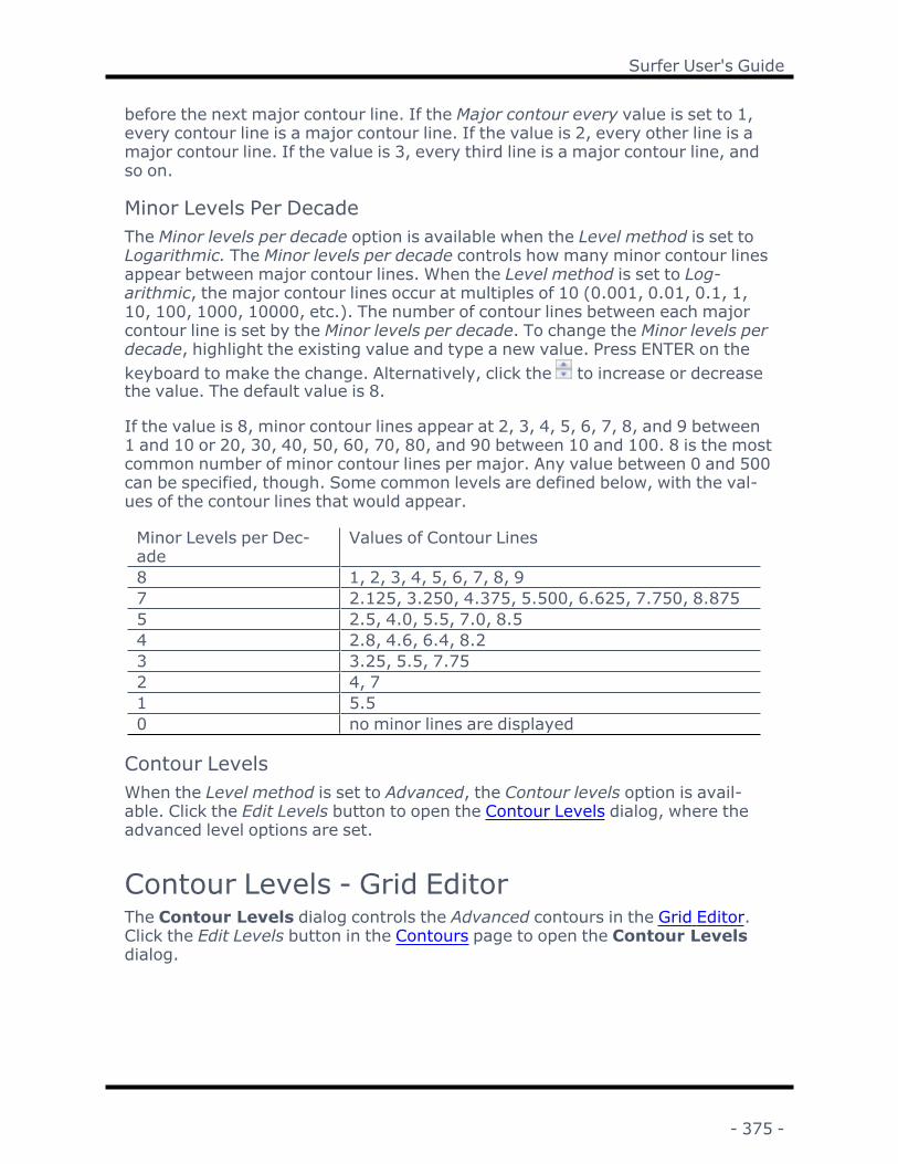
Surfer User's Guide
before the next major contour line. If the Major contour every value is set to 1,every contour line is a major contour line. If the value is 2, every other line is amajor contour line. If the value is 3, every third line is a major contour line, andso on.
Minor Levels Per DecadeThe Minor levels per decade option is available when the Level method is set toLogarithmic. The Minor levels per decade controls how many minor contour linesappear between major contour lines. When the Level method is set to Log-arithmic, the major contour lines occur at multiples of 10 (0.001, 0.01, 0.1, 1,10, 100, 1000, 10000, etc.). The number of contour lines between each majorcontour line is set by the Minor levels per decade. To change the Minor levels perdecade, highlight the existing value and type a new value. Press ENTER on thekeyboard to make the change. Alternatively, click the to increase or decreasethe value. The default value is 8.
If the value is 8, minor contour lines appear at 2, 3, 4, 5, 6, 7, 8, and 9 between1 and 10 or 20, 30, 40, 50, 60, 70, 80, and 90 between 10 and 100. 8 is the mostcommon number of minor contour lines per major. Any value between 0 and 500can be specified, though. Some common levels are defined below, with the val-ues of the contour lines that would appear.
Minor Levels per Dec-ade
Values of Contour Lines
8 1, 2, 3, 4, 5, 6, 7, 8, 97 2.125, 3.250, 4.375, 5.500, 6.625, 7.750, 8.8755 2.5, 4.0, 5.5, 7.0, 8.54 2.8, 4.6, 6.4, 8.23 3.25, 5.5, 7.752 4, 71 5.50 no minor lines are displayed
Contour LevelsWhen the Level method is set to Advanced, the Contour levels option is avail-able. Click the Edit Levels button to open the Contour Levels dialog, where theadvanced level options are set.
Contour Levels - Grid EditorThe Contour Levels dialog controls the Advanced contours in the Grid Editor.Click the Edit Levels button in the Contours page to open the Contour Levelsdialog.
- 375 -

Chapter 6 - Grid Editor
The Contour Levels dialog controls the display of thecontour map in the grid editor window.
Levels GroupThe Levels group lists the contour levels and colors of contour lines used in thegrid editor window.
LevelsClick the Level button to display the Contour Levels dialog. The Contour Levelsdialog controls the minimum and maximum contour levels as well as the contourinterval to use between levels.
LineThe Line button displays the Line Spectrum dialog that controls the colors andwidths of the minimum and maximum contour lines. Surfer automatically pro-duces a gradational spectrum of colors between the minimum and maximum col-ors.
AddThe Add button adds a contour line halfway between selected contour level andthe next lower contour. If the minimum contour level is selected, the added con-tour level is the same as the minimum level.
DeleteThe Delete button removes the selected contour from the list of contours.
LoadThe Load button allows you to select an existing level file [.LVL] containing con-tour level information. All grid files using the level file must have comparable Zdata ranges, otherwise contour lines will not appear on the map.
- 376 -

Surfer User's Guide
SaveThe Save button allows you to save the current contour level and line propertyinformation to a level file .LVL.
Color Fill - Grid EditorThe Color Fill object in the grid editor Contents window contains the grid editorcolor fill properties. Click the Color Fill object to change the grid node colors inthe Properties window.
The visibility check box next to the Color Fill object is used to turn on or off thecolor fill display in the grid editor window. When the check box is checked, thegrid editor displays a color relief map. When the command is not checked, thelabels, nodes, and contours are displayed on a white background.
This image displays grid node symbols, labels, contourlines, and a color fill for a grid file.
Grid Node Color Fill PropertiesThe Color Fill page is displayed in the Properties window when the Color Fillobject is selected. Edit the fill opacity, color map, and interpolation option in theProperties window.
- 377 -

Chapter 6 - Grid Editor
Edit color fill properties in the Propertieswindow.
OpacityChange the Opacity of the color fill by entering a value from 0% (completelytransparent) to 100% (completely opaque). To change the opacity, highlight theexisting value and type a new value. Press ENTER on the keyboard to make thechange. Or, click and drag the to change the opacity percentage.
Fill ColorsThe Fill colors property controls which color map is used to fill the grid editor win-dow. To use a predefined colormap, click the current selection and select acolormap from the list. The default Fill colors is Terrain. To edit a colormap or cre-ate a custom colormap, click the button to open the Colormap Editor.
Interpolate ColorsThe Interpolate colors check box activates color smoothing on the map. Whenchecked, Interpolate colors uses bilinear interpolation to calculate colors on themap. Bilinear interpolation makes the color gradations smoother, but it canslightly slow the on-screen drawing of the grid editor.
When a dense grid (a grid with relatively large numbers of rows and columns) isused, little difference is seen between the final display whether the Interpolatecolors option is checked or not. For dense grids, on-screen drawing time can bereduced when the Interpolate colors option is unchecked.
When a coarse grid (a grid with relatively few rows and columns) is used and theInterpolate colors option is not checked, all pixels within a single grid square areassigned the same color. This creates a grid-square map, and can result in ancolor fill with a very blocky appearance. For coarse grids, therefore, a smootherappearance results when the Interpolate colors check box is checked.
Note there is a difference between a grid node and a grid cell. The non-inter-polated color fill maps each grid node to a pixel, which is expanded to a block ofpixels to make the map the correct size. The interpolated color fill positions agrid node at the four corners and then interpolates all the interior pixels.
- 378 -

Surfer User's Guide
Select - Grid EditorClick the Grid Editor | Tools | Select command or the button to select indi-vidual grid nodes in the grid editor. The cursor changes to a crosshair whenSelectmode is active. The active grid nodes is indicated by a red diamond. Theactive grid node's grid coordinates are displayed in the status bar. Press ESCwhen in a different tool mode, such as Eraser, to quickly return to select mode.
Select a different grid node by clicking the node with the Select tool or pressingthe ARROW keys.
Z Value BoxThe Z value box in the tool options bar at the top of the grid editor window dis-plays the Z value for the active grid node. Type a new value in the Z value boxand press ENTER to change the grid node value. The Label, Node, Contours, andColor FIll display updates in the grid editor once you press ENTER or select a dif-ferent grid node. Press ESC while editing a value in the Z value box to cancel thechange.
BrushThe Grid Editor | Tools | Brush command or the button in the grid editorassigns the specified Z value in the Z value box to the grid nodes within thebrush. Click the Grid Editor | Tools | Brush command to start brush mode.The cursor changes to a crosshair with a circle to visually indicate the Brush size. The Brush command button is highlighted in yellow to indicate brush mode
as well.
Click to apply the value in the Z value box to grid nodes within the circle. Clickand drag to continuously apply the Z value as the cursor moves across the grid.The grid Nodes, Labels, Color Fill, and Contours update automatically as you usethe Brush command.
Press ESC or click another Grid Editor | Tools command to end Brushmode.
Tool OptionsThe Brush size and Z value box controls how the Brush tool changes the gridvales.
Brush SizeThe Brush size tool option controls the diameter of the tool. The Brush size spe-cifies the diameter in number of grid cells in the X direction. The Brush size set-ting is located in the tools options bar at the top of the grid editor window. Thereare three methods for changing the Brush size:
- 379 -

Chapter 6 - Grid Editor
l Click in the Brush size field and type the desired Brush size.l Click the buttons to increment the Brush size by one. Click and hold the but-tons to quickly scroll the Brush size value up or down.
l Press the [ key to decrease the Brush size. Press the ] key to increase theBrush size. Press and hold the [ or ] key to quickly decrease or increase theBrush size. The [ and ] keys increment the Brush size by 1 at Brush size val-ues less than 10. The increment increases to 5 at a Brush size greater than10 and less than 50. The increment increases to 10 at a Brush size greaterthan 50 and less than 100. The increment size continues to increase as theBrush size increases.
The cursor circle increases or decreases size with the Brush size setting andzoom level. The Brush size setting is saved and persistent across multiple grideditor windows.
A Brush size of 1 makes the dia-meter of the brush equal to thehorizontal spacing of one grid
cell.
A Brush size of 3 makes the dia-meter of the brush equal to thehorizontal spacing of three grid
cells.
Z Value BoxThe Z value box in the tool options bar at the top of the grid editor window dis-plays the Z value you wish to apply to the grid nodes. Type a new value in the Zvalue box and press ENTER to change the Brush Zvalue. By default the Z valuebox uses the grid Z value from the most recently selected grid node.
Press and hold the "i" key to temporarily change to the Eyedropper tool modewhile using the Brush tool. The cursor changes to an eyedropper . While hold-ing the "i" key, click in the grid to quickly change the value in the Z value box tothe grid Z value nearest the location you click. Release the "i" key to return toBrushmode.
UndoEach click is registered as one operation in the Undo levels list. For example, ifyou set the Brush size to 1 and click once on five individual grid nodes, you mustuse the Undo command five times to undo all the changes. However, if you click
- 380 -

Surfer User's Guide
and drag once across all five grid nodes, you must only use the Undo commandonce to undo all the changes.
Brush Grid Values ExampleThe following example will demonstrate editing the Demogrid.grd sample filewith the Brush tool:
In this example, we will assume the gridding algorithm smoothed over a featurewe wish to represent in the grid near node (29,6) in grid coordinates.
We will add a depression near the active grid node.
1. Click the Grid Editor | Tools | Brush command.2. Set the Brush size to 1 by typing 1 in the Brush size field.3. Set the Z value to 73 by typing 73 in the Z value box.4. Click near the grid node at (29,6) and drag one row down and one column
left.
- 381 -

Chapter 6 - Grid Editor
The Brush applied the Z value (73) to three grid nodes.We've now added the feature back to the grid. Now we wish to smooth the grid inthe area we edited.
1. Click the Grid Editor | Tools | Smooth command.2. Set the Brush size to 5 by typing 5 in the Brush size field.3. Click near the grid node at (29,6). The grid is smoothed within the brush
region.4. Click twice more near the grid node at (29,6).
- 382 -

Surfer User's Guide
The edited area was then smoothed with the Smooth tool.Now the depression feature has been added back to the grid and the surface hasbeen smoothed to give a natural appearance.
WarpThe Grid Editor | Tools | Warp command in the grid editor enables theWarptool mode. Use theWarp tool mode to drag grid values and "sculpt" the grid.Click the Grid Editor | Tools | Warp command or the button to start warpmode. The cursor changes to a crosshair with a circle to visually indicate the
Brush size . TheWarp command button is highlighted in yellow to indicatewarp mode as well.
Click and drag to pull grid values in the direction that you drag the cursor. Thegrid Nodes, Labels, Color Fill, and Contours update automatically as you use theWarp command.
Press ESC or click another Grid Editor | Tools command to endWarpmode.
NoData Nodes and WarpWhen dragging from a region with data into a NoData region, the NoData valuesare replaced by values from neighboring nodes. TheWarp tool can be used toremove NoData regions from the grid. However, NoData values are not draggedout from NoData regions by the warp tool. If you wish to assign the NoData valueto nodes, use the Eraser.
- 383 -
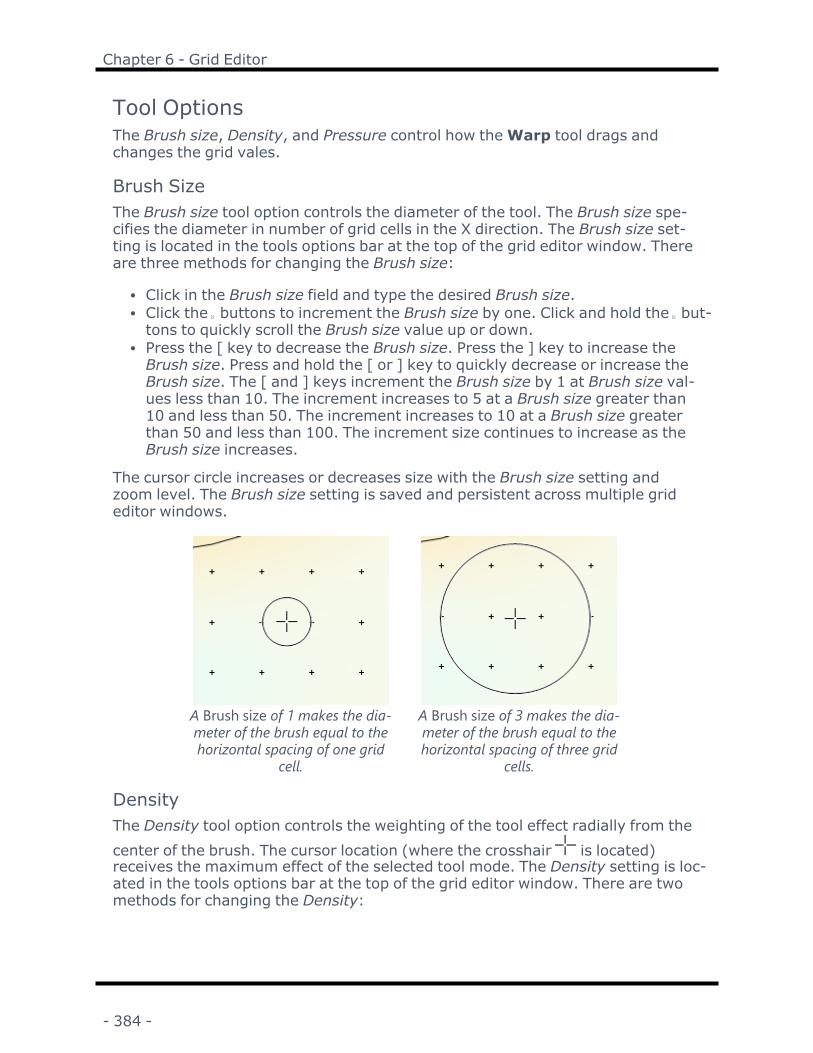
Chapter 6 - Grid Editor
Tool OptionsThe Brush size, Density, and Pressure control how theWarp tool drags andchanges the grid vales.
Brush SizeThe Brush size tool option controls the diameter of the tool. The Brush size spe-cifies the diameter in number of grid cells in the X direction. The Brush size set-ting is located in the tools options bar at the top of the grid editor window. Thereare three methods for changing the Brush size:
l Click in the Brush size field and type the desired Brush size.l Click the buttons to increment the Brush size by one. Click and hold the but-tons to quickly scroll the Brush size value up or down.
l Press the [ key to decrease the Brush size. Press the ] key to increase theBrush size. Press and hold the [ or ] key to quickly decrease or increase theBrush size. The [ and ] keys increment the Brush size by 1 at Brush size val-ues less than 10. The increment increases to 5 at a Brush size greater than10 and less than 50. The increment increases to 10 at a Brush size greaterthan 50 and less than 100. The increment size continues to increase as theBrush size increases.
The cursor circle increases or decreases size with the Brush size setting andzoom level. The Brush size setting is saved and persistent across multiple grideditor windows.
A Brush size of 1 makes the dia-meter of the brush equal to thehorizontal spacing of one grid
cell.
A Brush size of 3 makes the dia-meter of the brush equal to thehorizontal spacing of three grid
cells.
DensityThe Density tool option controls the weighting of the tool effect radially from the
center of the brush. The cursor location (where the crosshair is located)receives the maximum effect of the selected tool mode. The Density setting is loc-ated in the tools options bar at the top of the grid editor window. There are twomethods for changing the Density:
- 384 -

Surfer User's Guide
l Click in the Density field and type the desired Density.l Click the buttons to increment the Density by one. Click and hold the but-tons to quickly scroll the Density value up or down.
The Density setting can be any value between 1 and 100. A Density setting of 1has maximum "feathering" or blending between the center of the brush and val-ues just outside the brush. A Density setting of 100 applies the tool mode effectto all nodes within the brush equally. The Density setting is saved and persistentacross multiple grid editor windows. The default Density setting is 25.
These line plots show how Density affects the weighting of the tool modeeffect
(y-axis) as distance from the center of the brush increases (x-axis)
- 385 -

Chapter 6 - Grid Editor
PressureThe Pressure tool option controls the speed at which tool effects are applied asthe brush moves. The Pressure setting is located in the tools options bar at thetop of the grid editor window. There are two methods for changing the Pressure:
l Click in the Pressure field and type the desired Pressure.l Click the buttons to increment the Pressure by one. Click and hold the but-tons to quickly scroll the Pressure value up or down.
The Pressure setting can be any value between 1 and 100. A Pressure setting of1 applies the tool effect the minimum amount with each click or drag. A Pressuresetting of 100 applies the tool effect the maximum amount with each click ordrag. The Pressure setting is saved and persistent across multiple grid editor win-dows. The default Pressure setting is 25.
SmoothThe Grid Editor | Tools | Smooth command in the grid editor smooths gridnode values within the brush with a moving 3x3 average filter. Click the GridEditor | Tools | Smooth command or the button to enable Smoothmode.The cursor changes to a crosshair with a circle to visually indicate the Brush size. The Smooth command button is highlighted in yellow to indicate smooth
mode as well.
Click to smooth values within the brush circle. Click and drag to continuouslysmooth grid values as the cursor moves across the grid. The grid Nodes, Labels,Color Fill, and Contours update automatically as you use the Smooth command.
Press ESC or click another Grid Editor | Tools command to end Smoothmode.
Tool OptionsThe Brush size, Density, and Pressure control how the Smooth tool smooths thegrid vales.
Brush SizeThe Brush size tool option controls the diameter of the tool. The Brush size spe-cifies the diameter in number of grid cells in the X direction. The Brush size set-ting is located in the tools options bar at the top of the grid editor window. Thereare three methods for changing the Brush size:
l Click in the Brush size field and type the desired Brush size.l Click the buttons to increment the Brush size by one. Click and hold the but-tons to quickly scroll the Brush size value up or down.
l Press the [ key to decrease the Brush size. Press the ] key to increase theBrush size. Press and hold the [ or ] key to quickly decrease or increase the
- 386 -

Surfer User's Guide
Brush size. The [ and ] keys increment the Brush size by 1 at Brush size val-ues less than 10. The increment increases to 5 at a Brush size greater than10 and less than 50. The increment increases to 10 at a Brush size greaterthan 50 and less than 100. The increment size continues to increase as theBrush size increases.
The cursor circle increases or decreases size with the Brush size setting andzoom level. The Brush size setting is saved and persistent across multiple grideditor windows.
A Brush size of 1 makes the dia-meter of the brush equal to thehorizontal spacing of one grid
cell.
A Brush size of 3 makes the dia-meter of the brush equal to thehorizontal spacing of three grid
cells.
DensityThe Density tool option controls the weighting of the tool effect radially from the
center of the brush. The cursor location (where the crosshair is located)receives the maximum effect of the selected tool mode. The Density setting is loc-ated in the tools options bar at the top of the grid editor window. There are twomethods for changing the Density:
l Click in the Density field and type the desired Density.l Click the buttons to increment the Density by one. Click and hold the but-tons to quickly scroll the Density value up or down.
The Density setting can be any value between 1 and 100. A Density setting of 1has maximum "feathering" or blending between the center of the brush and val-ues just outside the brush. A Density setting of 100 applies the tool mode effectto all nodes within the brush equally. The Density setting is saved and persistentacross multiple grid editor windows. The default Density setting is 25.
- 387 -

Chapter 6 - Grid Editor
These line plots show how Density affects the weighting of the tool modeeffect
(y-axis) as distance from the center of the brush increases (x-axis)
PressureThe Pressure tool option controls the speed at which tool effects are applied asthe brush moves. The Pressure setting is located in the tools options bar at thetop of the grid editor window. There are two methods for changing the Pressure:
l Click in the Pressure field and type the desired Pressure.l Click the buttons to increment the Pressure by one. Click and hold the but-tons to quickly scroll the Pressure value up or down.
- 388 -

Surfer User's Guide
The Pressure setting can be any value between 1 and 100. A Pressure setting of1 applies the tool effect the minimum amount with each click or drag. A Pressuresetting of 100 applies the tool effect the maximum amount with each click ordrag. The Pressure setting is saved and persistent across multiple grid editor win-dows. The default Pressure setting is 25.
UndoEach click is registered as one operation in the Undo levels list. For example, ifyou set the Brush size to 1 and click once on five individual grid nodes, you mustuse the Undo command five times to undo all the changes. However, if you clickand drag once across all five grid nodes, you must only use the Undo commandonce to undo all the changes.
Push DownThe Grid Editor | Tools | Push Down command in the grid editor decreasesgrid node values within the brush. Click the Grid Editor | Tools | Push Downcommand or the button to enable Push Down mode. The cursor changes to acrosshair with a circle to visually indicate the Brush size . The Push Downcommand button is highlighted in yellow to indicate Push Downmode as well.
Click once to decrease values within the brush circle. Click and drag to con-tinuously decrease grid values as the cursor moves across the grid. The gridNodes, Labels, Color Fill, and Contours update automatically as you use thePush Down command.
Press ESC or click another Grid Editor | Tools command to end Push Downmode.
Tool OptionsThe Brush size controls the area around the cursor that is affected by the PushDown tool. The Density controls how the Push Down tool decreases the gridvales in the brush area. The Pressure controls how much the grid values areaffected.
Brush SizeThe Brush size tool option controls the diameter of the tool. The Brush size spe-cifies the diameter in number of grid cells in the X direction. The Brush size set-ting is located in the tools options bar at the top of the grid editor window. Thereare three methods for changing the Brush size:
l Click in the Brush size field and type the desired Brush size.l Click the buttons to increment the Brush size by one. Click and hold the but-tons to quickly scroll the Brush size value up or down.
- 389 -

Chapter 6 - Grid Editor
l Press the [ key to decrease the Brush size. Press the ] key to increase theBrush size. Press and hold the [ or ] key to quickly decrease or increase theBrush size. The [ and ] keys increment the Brush size by 1 at Brush size val-ues less than 10. The increment increases to 5 at a Brush size greater than10 and less than 50. The increment increases to 10 at a Brush size greaterthan 50 and less than 100. The increment size continues to increase as theBrush size increases.
The cursor circle increases or decreases size with the Brush size setting andzoom level. The Brush size setting is saved and persistent across multiple grideditor windows.
A Brush size of 1 makes the dia-meter of the brush equal to thehorizontal spacing of one grid
cell.
A Brush size of 3 makes the dia-meter of the brush equal to thehorizontal spacing of three grid
cells.
DensityThe Density tool option controls the weighting of the tool effect radially from the
center of the brush. The cursor location (where the crosshair is located)receives the maximum effect of the selected tool mode. The Density setting is loc-ated in the tools options bar at the top of the grid editor window. There are twomethods for changing the Density:
l Click in the Density field and type the desired Density.l Click the buttons to increment the Density by one. Click and hold the but-tons to quickly scroll the Density value up or down.
The Density setting can be any value between 1 and 100. A Density setting of 1has maximum "feathering" or blending between the center of the brush and val-ues just outside the brush. A Density setting of 100 applies the tool mode effectto all nodes within the brush equally. The Density setting is saved and persistentacross multiple grid editor windows. The default Density setting is 25.
- 390 -
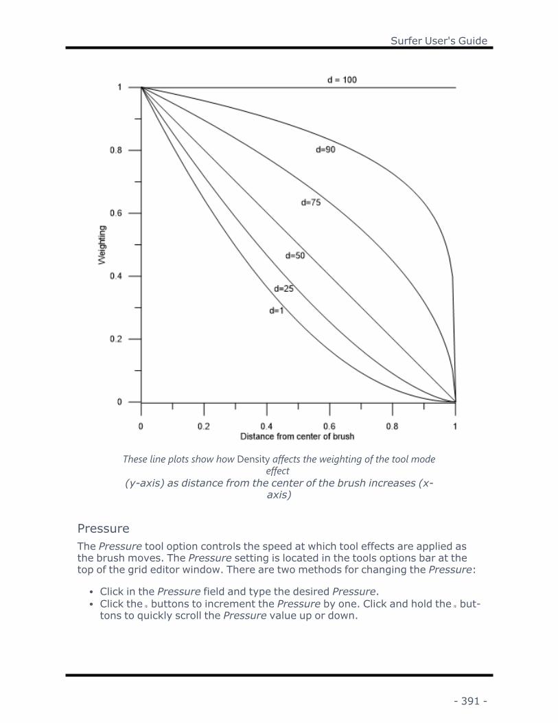
Surfer User's Guide
These line plots show how Density affects the weighting of the tool modeeffect
(y-axis) as distance from the center of the brush increases (x-axis)
PressureThe Pressure tool option controls the speed at which tool effects are applied asthe brush moves. The Pressure setting is located in the tools options bar at thetop of the grid editor window. There are two methods for changing the Pressure:
l Click in the Pressure field and type the desired Pressure.l Click the buttons to increment the Pressure by one. Click and hold the but-tons to quickly scroll the Pressure value up or down.
- 391 -

Chapter 6 - Grid Editor
The Pressure setting can be any value between 1 and 100. A Pressure setting of1 applies the tool effect the minimum amount with each click or drag. A Pressuresetting of 100 applies the tool effect the maximum amount with each click ordrag. The Pressure setting is saved and persistent across multiple grid editor win-dows. The default Pressure setting is 25.
The Push Down tool decreases the Z value by 1% of the Z-range of the grid atthe cursor location when Pressure is 100. When the grid is planar, the PushDown tool decreases the Z value by 1% of the diagonal distance of the grid atthe cursor location when Pressure is 100. The Pressure changes this amount pro-portionally. For example when the Pressure is 50, the amount the grid changesunder the cursor location is 0.5% of the grid Z range (0.01 x 0.5 = 0.005)
UndoEach click is registered as one operation in the Undo levels list. For example, ifyou set the Brush size to 1 and click once on five individual grid nodes, you mustuse the Undo command five times to undo all the changes. However, if you clickand drag once across all five grid nodes, you must only use the Undo commandonce to undo all the changes.
Pull UpThe Grid Editor | Tools | Pull Up command in the grid editor increases gridnode values within the brush area. Click the Grid Editor | Tools | Pull Up com-mand or the button to enable Pull Up mode. The cursor changes to acrosshair with a circle to visually indicate the Brush size . The Pull Up com-mand button is highlighted in yellow to indicate Pull Upmode as well.
Click once to increase values within the brush circle. Click and drag to con-tinuously increase grid values as the cursor moves across the grid. The gridNodes, Labels, Color Fill, and Contours update automatically as you use the PullUp command.
Press ESC or click another Grid Editor | Tools command to end Pull Upmode.
Tool OptionsThe Brush size controls the area around the cursor that is affected by the PullUp tool. The Density controls how the Pull Up tool increases the grid vales in thebrush area. The Pressure controls how much the grid values are affected.
Brush SizeThe Brush size tool option controls the diameter of the tool. The Brush size spe-cifies the diameter in number of grid cells in the X direction. The Brush size set-ting is located in the tools options bar at the top of the grid editor window. Thereare three methods for changing the Brush size:
- 392 -

Surfer User's Guide
l Click in the Brush size field and type the desired Brush size.l Click the buttons to increment the Brush size by one. Click and hold the but-tons to quickly scroll the Brush size value up or down.
l Press the [ key to decrease the Brush size. Press the ] key to increase theBrush size. Press and hold the [ or ] key to quickly decrease or increase theBrush size. The [ and ] keys increment the Brush size by 1 at Brush size val-ues less than 10. The increment increases to 5 at a Brush size greater than10 and less than 50. The increment increases to 10 at a Brush size greaterthan 50 and less than 100. The increment size continues to increase as theBrush size increases.
The cursor circle increases or decreases size with the Brush size setting andzoom level. The Brush size setting is saved and persistent across multiple grideditor windows.
A Brush size of 1 makes the dia-meter of the brush equal to thehorizontal spacing of one grid
cell.
A Brush size of 3 makes the dia-meter of the brush equal to thehorizontal spacing of three grid
cells.
DensityThe Density tool option controls the weighting of the tool effect radially from the
center of the brush. The cursor location (where the crosshair is located)receives the maximum effect of the selected tool mode. The Density setting is loc-ated in the tools options bar at the top of the grid editor window. There are twomethods for changing the Density:
l Click in the Density field and type the desired Density.l Click the buttons to increment the Density by one. Click and hold the but-tons to quickly scroll the Density value up or down.
The Density setting can be any value between 1 and 100. A Density setting of 1has maximum "feathering" or blending between the center of the brush and val-ues just outside the brush. A Density setting of 100 applies the tool mode effectto all nodes within the brush equally. The Density setting is saved and persistentacross multiple grid editor windows. The default Density setting is 25.
- 393 -

Chapter 6 - Grid Editor
These line plots show how Density affects the weighting of the tool modeeffect
(y-axis) as distance from the center of the brush increases (x-axis)
PressureThe Pressure tool option controls the speed at which tool effects are applied asthe brush moves. The Pressure setting is located in the tools options bar at thetop of the grid editor window. There are two methods for changing the Pressure:
l Click in the Pressure field and type the desired Pressure.l Click the buttons to increment the Pressure by one. Click and hold the but-tons to quickly scroll the Pressure value up or down.
- 394 -

Surfer User's Guide
The Pressure setting can be any value between 1 and 100. A Pressure setting of1 applies the tool effect the minimum amount with each click or drag. A Pressuresetting of 100 applies the tool effect the maximum amount with each click ordrag. The Pressure setting is saved and persistent across multiple grid editor win-dows. The default Pressure setting is 25.
The Pull Up tool increases the Z value by 1% of the Z-range of the grid at thecursor location when Pressure is 100. When the grid is planar, the Pull Up toolincreases the Z value by 1% of the diagonal distance of the grid at the cursor loc-ation when Pressure is 100. The Pressure changes this amount proportionally.For example when the Pressure is 50, the amount the grid changes under thecursor location is 0.5% of the grid Z range (0.01 x 0.5 = 0.005)
UndoEach click is registered as one operation in the Undo levels list. For example, ifyou set the Brush size to 1 and click once on five individual grid nodes, you mustuse the Undo command five times to undo all the changes. However, if you clickand drag once across all five grid nodes, you must only use the Undo commandonce to undo all the changes.
EraserThe Grid Editor | Tools | Eraser command in the grid editor assigns theNoData value (1.70141e+038) to the grid nodes within the brush. Click the GridEditor | Tools | Eraser command or the button to start eraser mode. Thecursor changes to a crosshair with a circle to visually indicate the eraser Brush
size . The Eraser command button is highlighted in yellow to indicate erasermode as well.
Click to erase values within the circle. Click and drag to continuously erase gridvalues as the cursor moves across the grid. The grid Nodes, Labels, Color Fill,and Contours update automatically as you use the Erase command.
Press ESC or click another Grid Editor | Tools command to end Erasermode.
Brush SizeThe Brush size tool option controls the diameter of the tool. The Brush size spe-cifies the diameter in number of grid cells in the X direction. The Brush size set-ting is located in the tools options bar at the top of the grid editor window. Thereare three methods for changing the Brush size:
l Click in the Brush size field and type the desired Brush size.l Click the buttons to increment the Brush size by one. Click and hold the but-tons to quickly scroll the Brush size value up or down.
l Press the [ key to decrease the Brush size. Press the ] key to increase theBrush size. Press and hold the [ or ] key to quickly decrease or increase the
- 395 -

Chapter 6 - Grid Editor
Brush size. The [ and ] keys increment the Brush size by 1 at Brush size val-ues less than 10. The increment increases to 5 at a Brush size greater than10 and less than 50. The increment increases to 10 at a Brush size greaterthan 50 and less than 100. The increment size continues to increase as theBrush size increases.
The cursor circle increases or decreases size with the Brush size setting andzoom level. The Brush size setting is saved and persistent across multiple grideditor windows.
A Brush size of 1 makes the dia-meter of the brush equal to thehorizontal spacing of one grid
cell.
A Brush size of 3 makes the dia-meter of the brush equal to thehorizontal spacing of three grid
cells.
UndoEach click is registered as one operation in the Undo levels list. For example, ifyou set the Brush size to 1 and click once on five individual grid nodes, you mustuse the Undo command five times to undo all the changes. However, if you clickand drag once across all five grid nodes, you must only use the Undo commandonce to undo all the changes.
Erasing Grid Values ExampleThe following example will demonstrate using the Erase command to assign theNoData value to a 20x20 node section of the Demogrid.grd sample file grid withthe Erase command,
1. Click the Grid Editor | Tools | Eraser command.
2. Set the Brush size to 20 by typing 20 in the Brush size field.
3. Click once in the grid near node (9,9). This is approximately (1.6,1.6) inmap coordinates. The cursor map coordinates are displayed in the statusbar.
- 396 -

Surfer User's Guide
Many nodes can be erased in a single click when the Brush size islarge.
4. Press and hold the [ key to reduce the Brush size to 5.
5. Click and drag around the NoData region to create a rectangle.
- 397 -

Chapter 6 - Grid Editor
Click and drag with Erase to create any shape NoData region.
6. A Brush size of 5 is too large to easily erase the final node. Change theBrush size to 1.
7. Click the node at (19,19) in grid coordinates to create the 20x20 nodeNoData rectangle.
- 398 -

Surfer User's Guide
Erasing single nodes is easier when the brush size is small.
EyedropperClick the Grid Editor | Tools | Eyedropper command or the button to pullgrid Z values by clicking in the grid. The cursor changes to an eyedropperwhen the Eyedropper command is clicked. The Grid Editor | Tools | Eyed-ropper command button is highlighted in yellow to indicate eyedropper toolmode.
Click on the grid with the eyedropper to place the nearest grid node's Z valuein the Z value box .
Press ESC or click another Grid Editor | Tools command to end Eyedroppermode.
Z Value BoxThe Z value box in the tool options bar at the top of the grid editor window dis-plays the Z value from the nearest grid node when you click the grid.
- 399 -

Chapter 6 - Grid Editor
Eyedropper and Select ToolAfter pressing ESC or clicking the Grid Editor | Tools | Select command, the gridnode nearest your most recent click is made the active grid node.
Eyedropper and Brush ToolYou can use the Eyedropper tool to set the Z value box value for the Brush toolwith two different methods:
l Click the Grid Editor | Tools | Eyedropper command, and click on the desiredgrid node to place its value in the Z value box. Next, click the Grid Editor |Tools | Brush command.
l After clicking Grid Editor | Tools | Brush to enable brush tool mode, pressand hold the "i" key to temporarily enable Eyedroppermode. While holdingthe "i" key, click on the desired grid node to place its value in the Z value box. Release the "i" key to return to Brush tool mode.
Zoom In - Grid EditorClick the Grid Editor | View | Zoom In command or the button to imme-diately increase the magnification of the grid editor.
Zoom with A Wheel MouseYou can use a wheel mouse to zoom realtime and pan in the plot window or grideditor. Rotate the wheel forward to zoom in, or rotate the wheel backward tozoom out. Hold down the wheel button straight down, and the cursor will turn toa closed hand. When the cursor is a , drag the mouse to pan the plot window.Be sure to click straight down with the scroll wheel. The zoom is changed so thatthe cursor location remains on the screen.
Zoom with the KeyboardYou can use keyboard commands to zoom in and out of the plot window. Thedefault commands are CTRL+EQUAL SIGN (=) to zoom in, and CTRL+HYPHEN(-) to zoom out.
Zoom Out - Grid EditorClick the Grid Editor | View | Zoom Out command or the button to imme-diately decrease the magnification of the grid editor window.
- 400 -

Surfer User's Guide
Zoom with A Wheel MouseYou can use a wheel mouse to zoom realtime and pan in the plot window or gridnode editor. Rotate the wheel forward to zoom in, or rotate the wheel backwardto zoom out. Hold down the wheel button straight down, and the cursor will turnto a closed hand. When the cursor is a , drag the mouse to pan the plot win-dow. Be sure to click straight down with the scroll wheel. The zoom is changed sothat the cursor location remains on the screen.
Zoom with the KeyboardYou can use keyboard commands to zoom in and out of the plot window. Thedefault commands are CTRL+EQUAL SIGN (=) to zoom in, and CTRL+HYPHEN(-) to zoom out.
Grid Info
The Grid Editor | Options | Grid Info command or the button in the GridEditor displays the file name, grid size in rows x columns, and grid X, Y, and Zminimums and maximums. If the grid file contains more than 40 million nodes,you are asked if you wish to create a detailed report or a quick report. Click Yesin the message to create a detailed grid report, or click No to create a shorterquick grid report. This is the same basic information as displayed in the plot win-dow with the Grids | Info | Grid Info command.
The Open Grid dialog also displays the Grid Info of the selected grid. The OpenGrid dialog displays the following Grid Info: Name, Format, Size, xMax, yMax,zMax, xMin, yMin, and zMin.
Update Layer
Click the Grid Editor | Options | Update Layer command or the buttonto update the map layer from which the grid was opened. The grid must byopened by selecting the map layer and clicking theMap Tools | Edit Layer |Grid command or right-clicking the map layer and clicking Edit Grid in the con-text menu to use the Update Layer command. The Update Layer command isdisabled when viewing a grid opened with the File | Open or Grids | Editor | GridEditor command.
To edit a map layer,
1. Select the map layer you wish to edit in the plot document Contents window.2. ClickMap Tools | Edit Layer | Grid in the plot window.3. Use the Grid Editor | Tools commands to make the desired adjustments to
the grid.
- 401 -

Chapter 6 - Grid Editor
4. When you are done editing the grid, click the Grid Editor | Options |Update Layer command to update the map layer in the plot document withyour grid.
5. If you wish to save your edits to a file, click File | Save As to create a new gridfile. Click File | Save to overwrite the existing grid file. It is necessary to saveyour edits to a file with Save or Save As if you wish to update all layers inyour map to use the edited grid.
6. To close the grid editor window, click the File | Close command or click the Xin the grid editor document tab. To view an existing window and keep the grideditor window open, click on another document tab.
After clicking the Update Layer command, view the map layer by clicking thedocument tab for the plot window that contains the original map layer. Noticethat only the map layer that was selected in step 1 was changed. The UpdateLayer command does not overwrite the grid file used to create the map layer.The Update Layer command does not save a new grid file. The Update Layercommand only changes the grid for the original map layer.
Undo Update LayerThe Update Layer command changes the map layer in the plot document.Therefore to undo the Update Layer command, click the document tab for theplot window that contains the original map layer. Next click the Home | Undo |Undo command or press CTRL+Z. The map layer will return to the uneditedstate. The grid in the grid editor can be reapplied to the map layer by clickingHome | Undo | Redo in the plot document or Grid Editor | Options | UpdateLayer in the grid editor.
If you did not overwrite the original grid file, you can also revert back to the ori-ginal grid by clicking File | Reload Map Data.
You can discard the edited grid by closing the grid editor. Click No in the Surferdialog when asked to save the grid.
Saving the Edited GridWhen you have finished making changes to the grid you can overwrite the ori-ginal grid file or save a new grid file. You must save the grid file to use the editedgrid in other map layers. To overwrite the original file, click the File | Save com-mand in the grid editor. To save the edited grid to a new file, click the File | SaveAs command in the grid editor.
If you closed the grid editor without saving changes, but you decide later youwish to save the grid, click the layer that was updated with the Update Layercommand. Next, clickMap Tools | Edit Layer | Grid to open the grid in thegrid editor. The edited grid will be opened in the grid editor and you can over-write the original grid file or create a new grid file.
- 402 -

Surfer User's Guide
Updating All Map LayersOnly the originally selected map layer is updated when you click the Grid Editor| Options | Update Layer command, even when multiple map layers use thesame grid file in the plot document. You must save the grid to a file to use thegrid in new or existing map layers.
To update the other map layers after overwriting the original grid with the File |Save command,
1. Return to the plot document by clicking the document tab for the plot win-dow.
2. Click the File | Reload Map Data command.
All map layers that were created from the same grid as the one that was editedare automatically updated to the new grid.
To update the other map layers after creating a new grid file,
1. Return to the plot document by clicking the document tab for the plot win-dow.
2. Click one of the map layers that is still using the original grid file in the Con-tents window.
3. Click the General tab in the Properties window.4. Click the button in the Grid file property field.5. Locate and click the new grid file in the Open Grid dialog.6. Click Open in the Open Grid dialog.7. Repeat steps 2 through 6 for each map layer you wish to update.
All the maps layers that were created from the same grid as the one that wasedited are now updated to the new grid.
Open GridContour maps, color relief maps, vector maps, watershed maps, 3D wireframes,3D surfaces, grid values maps, and viewsheds all require grids for their gen-eration in Surfer. A grid is a regular, rectangular array of values. The Home |Grid Data | Grid Data command provides you with several methods for gen-erating a grid file from your XYZ data. In addition to the grid files that Surfer cre-ates, it can also import many common grid files directly. The Gridmenu containsmany commands for grid operations. A grid with all NoData nodes cannot besaved.
The Open Grid dialog is used to open one or more grid files when creating newgrid-based maps or layers or when using a grid command (i.e. Grids | Edit |Convert). When multiple files are selected, one map is created for each inputfile.
- 403 -
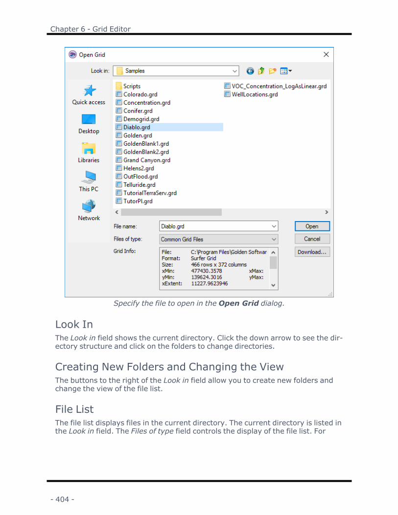
Chapter 6 - Grid Editor
Specify the file to open in the Open Grid dialog.
Look InThe Look in field shows the current directory. Click the down arrow to see the dir-ectory structure and click on the folders to change directories.
Creating New Folders and Changing the ViewThe buttons to the right of the Look in field allow you to create new folders andchange the view of the file list.
File ListThe file list displays files in the current directory. The current directory is listed inthe Look in field. The Files of type field controls the display of the file list. For
- 404 -

Surfer User's Guide
example, if Golden Software Data (*.DAT) is listed in the Files of type field only*.DAT files appear in the files list.
Double-click on a file to open it or single-click the file and then click the Open but-ton. To open more than one file, select the files you wish to use by holding CTRLwhile clicking, and then click Open. When adding grid-based maps, each file isadded as a separate map.
Specify a File NameThe File name field shows the name of the selected file, or type a path and filename into the box to open a file.
Specify a File TypeThe Files of type field shows the file format to be opened. To change the fileformat, click the down arrow and select the file type from the list. All Files (*.*)display all files in a directory.
The Common Document Files (*...) format type is selected by default. This dis-plays all the common file formats in the navigation pane. If a different formattype is selected, Surfer will remember the setting until the end of the currentsession. When Surfer is restarted, the default format type will be used.
To see all files in the directory, choose All Files (*.*) from the Files of type list.Double-click on a file to open it or single click the file and then click the Open but-ton. The All Files (*.*) option shows all of the file formats in the current dir-ectory, even if the file type is not appropriate for the action chosen. For example,a .BLN file may be displayed, even though a .BLN file cannot be used to create agrid base map.
Open FilesSurfer tracks the files being used by maintaining a list of opened files for newmaps and the files used in saved maps. The file(s) used in existing maps areshown in a compiled list in the Open Grids field of the Open Grid(s) dialog.
Grid InfoThe selected grid file information is listed in the Grid Info section. The specific loc-ation, name, format, size, xMin, xMax, yMin, yMax, zMin, and zMax values aredisplayed. Use the scroll bar to the right if necessary to see all of the information.Use the grip at the lower right corner of the dialog to expand the size of the dia-log if the grid information is cut off on the right.
- 405 -

Chapter 6 - Grid Editor
Download Online GridsClick the Download button to open the Download Online Grids dialog. Use theDownload Online Grids dialog to retrieve a grid file from a WMS server.
File Typesl ADF Arc/Info Binary Gridl AM Amira Meshl AN? ACR-NEMA Medical Imagel ASC Arc/Info ASCII Gridl ASI Amira Stacked Imagesl BIL/BIP/BSQ Banded Gridl BMP Windows Bitmapl CPS-3 Grid Formatl DICOM3 Medical Imagel DDF SDTS DEMl DEM USGS DEMl DTD DTEDl E00 ASCII Grid Formatl ECW ERMapperl ERS ER Mapper Grid Formatl FLD AVS Fieldl FLT Esri Float Grid Formatl GIF Imagel GLOBE DEMl GRD Surfer Gridl GRD Geosoft Binary Gridl GXF Grid eXchange Formatl HDF Hierarchical Data Formatl HDR GTOPO-30l IMG Analyze 7.5 Medical Imagel IMG Idrisi Raster Formatl INFO Leica Confocal Raw Slicesl JPG Compressed Bitmapl LAT Iris Explorerl PNG Portable Network Graphicsl PNM/PPM/PGM/PBM Imagel RAW Raw Binary Gridl RGB SGI-RGB Imagel SID LizardTech MrSID Imagel STK Metamorphl SUN Sun Raster Imagel TAR SDTS DEMl TAR.GZ SDTS DEMl TGA Targa (TrueVision)
- 406 -

Surfer User's Guide
l TGZ SDTS DEMl TIF Tagged Imagel VTK Visualization Toolkitl X AVS X-Imagel ZIP SDTS DEMl ZMap Plus Grid Format
File Types
ADF Arc/Info Binary Grid
AM Amira Mesh
AN? ACR-NEMA Medical Image
ASC Arc/Info ASCII Grid
ASI Amira Stacked Images
BIL/BIP/BSQ Banded Grid
BMP Windows Bitmap
CPS-3 Grid Format
DICOM3 Medical Image
DDF SDTS DEM
DEM USGS DEM
DTD DTED
E00 ASCII Grid Format
ECW ERMapper
ERS ER Mapper Grid Format
FLD AVS Field
FLT Esri Float Grid Format
GIF Image
GLOBE DEM
GRD Surfer Grid
GRD Geosoft Binary Grid
GXF Grid eXchange Format
- 407 -

Chapter 6 - Grid Editor
HDF Hierarchical Data Format
HDR GTOPO-30
IMG Analyze 7.5 Medical Image
IMG Idrisi Raster Format
INFO Leica Confocal Raw Slices
JPG Compressed Bitmap
LAT Iris Explorer
PNG Portable Network Graphics
PNM/PPM/PGM/PBM Image
RAW Raw Binary Grid
RGB SGI-RGB Image
SID LizardTech MrSID Image
STK Metamorph
SUN Sun Raster Image
TAR SDTS DEM
TAR.GZ SDTS DEM
TGA Targa (TrueVision)
TGZ SDTS DEM
TIF Tagged Image
VTK Visualization Toolkit
X AVS X-Image
ZIP SDTS DEM
ZMap Plus Grid Format
Open GridsSurfer tracks the files being used by maintaining a list of opened grids for newmaps and the grids used in saved maps. The grids(s) used to build maps are
- 408 -

Surfer User's Guide
shown in a compiled list in the Open Grids field of the Open Grid dialog. The onlyexception is that vector data between base layers will not be shown.
Save Grid AsThe Save Grid As dialog allows you to specify a location and grid type to save agrid file.
Save Grid As DialogUse the File | Save As command in the grid node editor or one of the Gridmenu commands in the plot document to open the Save Grid As dialog.
Specify the save location, file name, and file type in the Save Grid As dialog. This graphicmay look different in another operating system.
Save InThe Save in field shows the current directory. Click the down arrow to see the dir-ectory structure and click on the folders to change directories.
Creating New Folders and Changing the ViewThe buttons to the right of the Look in field allow you to create new folders andchange the view of the file list.
- 409 -
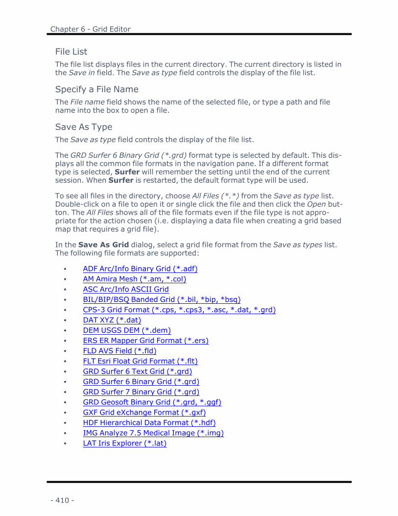
Chapter 6 - Grid Editor
File ListThe file list displays files in the current directory. The current directory is listed inthe Save in field. The Save as type field controls the display of the file list.
Specify a File NameThe File name field shows the name of the selected file, or type a path and filename into the box to open a file.
Save As TypeThe Save as type field controls the display of the file list.
The GRD Surfer 6 Binary Grid (*.grd) format type is selected by default. This dis-plays all the common file formats in the navigation pane. If a different formattype is selected, Surfer will remember the setting until the end of the currentsession. When Surfer is restarted, the default format type will be used.
To see all files in the directory, choose All Files (*.*) from the Save as type list.Double-click on a file to open it or single click the file and then click the Open but-ton. The All Files shows all of the file formats even if the file type is not appro-priate for the action chosen (i.e. displaying a data file when creating a grid basedmap that requires a grid file).
In the Save As Grid dialog, select a grid file format from the Save as types list.The following file formats are supported:
l ADF Arc/Info Binary Grid (*.adf)l AM Amira Mesh (*.am, *.col)l ASC Arc/Info ASCII Gridl BIL/BIP/BSQ Banded Grid (*.bil, *bip, *bsq)l CPS-3 Grid Format (*.cps, *.cps3, *.asc, *.dat, *.grd)l DAT XYZ (*.dat)l DEM USGS DEM (*.dem)l ERS ER Mapper Grid Format (*.ers)l FLD AVS Field (*.fld)l FLT Esri Float Grid Format (*.flt)l GRD Surfer 6 Text Grid (*.grd)l GRD Surfer 6 Binary Grid (*.grd)l GRD Surfer 7 Binary Grid (*.grd)l GRD Geosoft Binary Grid (*.grd, *.ggf)l GXF Grid eXchange Format (*.gxf)l HDF Hierarchical Data Format (*.hdf)l IMG Analyze 7.5 Medical Image (*.img)l LAT Iris Explorer (*.lat)
- 410 -

Surfer User's Guide
l netCDF Network Common Data Format (*.nc)l RAW Binary Grid (*.raw, *.bin)l STL 3D Mesh (*.stl)l VTK Visualization Toolkit (*.vtk)l Z-Map Plus Grid Format (*.asc, *.dat, *.grd, *.xyz, *.zmap, *.zyc, *.zy-
cor)
Some Save As Grid dialog Save as type lists may differ slightly, depending onthe command that invoked the dialog.
- 411 -


Chapter 7 - Grid Operations
Grids Tab CommandsThere are many ways to manipulate grid files in Surfer. The Grids ribbon con-tains commands used to assign the NoData value, convert, create, extract, filter,mosaic, slice, smooth, and transform grid files. In addition, volume calculations,variogram generation, calculus operations, cross section creation, and residualcalculations can be performed using the commands on the Grids ribbon. Click onthe Grids tab to access the commands on the ribbon.
Data Create a grid from irregularly spaced XYZ dataGrid fromServer
Create a grid from downloaded DEM data
Grid from Con-tours
Create a grid from contour lines
Function Create a grid from a user-specified functionVariogram Create a new variogram and export a variogramAssign NoData Assign NoData to grid nodes inside or outside a boundaryFilter Filter an existing grid by applying a moving matrix filterConvert Convert between various grid formatsSpline Smooth Smooth an existing grid using cubic splinesAssign Coordin-ate System
Assign the coordinate system of a grid file and save theinformation to an external file
Project Create a grid in a different coordinate systemCalculus Perform calculus operations on an existing grid fileVolume Compute the volume under or over a grid surfaceMath Provide grid-to-grid and grid-to-constant math oper-
ationsTransform Scale, offset, mirror, or rotate an existing grid fileSlice Compute a cross section of data through a grid surfaceResiduals Compute the difference between XYZ data and a grid sur-
facePoint Sample Compute the Z value at specified XY locations on the grid
surfaceContour Volumeand Area
Compute the volume and area above, below, andbetween contour lines
Isopach Create an isopach or isochore mapMosaic Combine a series of compatible input grids into a single
output gridExtract Extract a subset of a grid from an existing grid fileGrid Editor Change the values of nodes in a grid or edit the grid with
various toolsGrid Info Display information about the grid
- 413 -

Chapter 7 - Grid Operations
Assign NoDataThe Grids | Edit | Assign NoData command is used to remove grid node datafrom a grid in areas not supported by original data or in areas where you do notwant to display contours on a map. The Assign NoData command assigns theNoData value (1.70141e+038) to specified groups of grid nodes in a grid file.Grids used with Assign NoData contain the same number of grid nodes and thesame grid limits as the original grid file. The grid nodes in the new grid areidentical to the values in the original grid except in those locations where theNoData values are assigned.
NoData polygon boundaries are defined in a vector file or in a base layer. Theblanking file format can be used and is a special ASCII format file containing theX, Y coordinates defining the NoData polygon boundary. Blanking *.BLN files canbe made in the Surfer worksheet. Blanking *.BLN files can also be created withthe Digitize command. The NoData values can be assigned to areas inside or out-side the polygon or 3D polygon boundary. Regions can be assigned the NoDatavalue using the Eraser command in the Grid Editor window.
Nearly any feature type can be used when specifying boundaries with a baselayer: polygon, range ring, rectangle, rounded rectangle, or ellipse. A polyline orspline polyline can also be used, but unexpected behavior may occur if the line isopen. The most common feature for defining NoData polgyon and 3D polygonboundaries is the polygon or 3D polygon. The features must be in a base layer tobe used with the Assign NoData command. Features in paper space cannot beused. Create new features in an empty base layer if you wish to assign NoDatavalues with features created in Surfer.
To automatically assign the NoData value to areas outside the original data, clickthe Grids | New Grid | Grid Data command. In the Grid Data dialog, check theAssign NoData outside convex hull of data. Any grid nodes outside the boundarycreated by connecting the original data is automatically assigned the NoDatavalue.
In Surfer 14 and prior versions, the Assign NoData command was referred toas Grid Blank.
Assign NoData to Grid DialogThe Assign NoData to Grid dialog is displayed by clicking the Grids | Edit |
Assign NoData command or the button. Specify the input grid layer or file,vector file or layer, output grid file, and optional output map layer in the AssignNoData to Grid dialog.
- 414 -

Surfer User's Guide
Assign the NoData value to regions of a grid file or map layer with theAssign NoData to Grid dialog.
Input GridSpecify the source map layer or grid file in the Input Grid section. Click the cur-rent selection and select a map layer from the list. Only map layers created fromgrid files are included in the Input Grid list. Click Browse to load a grid file withthe Open Grid dialog.
Polygon BoundarySpecify the region or regions to be assigned the NoData value and whether ornot to use only selected objects in the NoData Polygon Boundary section. Selecteither a map layer or vector file in the NoData Polygon Boundary section:
l Click the current selection and select a base layer from the list. Only baselayers that contain at least one polygon, polyline, 3D polygon or 3D polylinewill be included in the list. The base layer must use the same sourcecoordinate system as the grid.
l Click Browse to load a vector file with the Open dialog. The file must use thesame coordinate system as the grid.
The number of polygons and 3D polygons and vertices is displayed below theNoData polygon boundary once a file or map layer has been selected. If theboundaries have blanking flags or BLN_Flag attributes, the total number ofinside and outside flags is displayed.
- 415 -

Chapter 7 - Grid Operations
Polyline BoundariesPolylines and 3D polylines can be used for NoData polygon boundaries. The poly-lines in the base layer or vector file will be treated as polygons and 3D polylinestreated as 3D polygons while assigning NoData values. The Assign NoData com-mand is not recommended with open polylines as unexpected results may occur.Before clicking Grids | Edit | Assign NoData, consider converting the objectto another type better suited to the operation you wish to perform with one ofthe Change To commands, and edit features with the Reshape command.
If the layer you wish to use contains both polygons and polylines, but you onlywish to use some or all of the polygons, select the objects you wish to use beforeclicking Grids | Edit | Assign NoData and select the Selected objects onlyoption. If the file you wish to use contains both polylines and polygons, first loadthe file as a base layer, and then use the Assign NoData command with theSelected objects only option.
Inside, Outside, or MixedSelect Inside to assign the NoData value to the region inside the NoData poly-gon/3D polygon boundary or boundaries. Select Outside to assign the NoDatavalue to the region outside the NoData polygon/3D polygon boundary or bound-aries. Select Mixed to use the blanking flag or BLN_Flag attribute values from thefile or layer. The Mixed option is only available when the layer or file containsboth blanking flags or BLN_Flag attributes: assign NoData inside (1) and assignNoData outside (0). If all blanking flags or BLN_Flag attributes are the same, theNoData Inside or NoData Outside option is selected automatically, and the Mixedoption is not available.
Selected Objects OnlySelect the Selected objects only option to use only the selected objects in thebase layer to assign NoData values to the grid. When the Selected objects onlybox is checked, the Loaded polygonsandvertices values are updated. Select abase layer in the NoData Polygon Boundary field to use the Selected objects onlyoption. The Selected objects only option is not available when the NoData Poly-gon Boundary is a vector file. The polygon or polygons must be selected beforeclicking the Grids | Edit | Assign NoData command.
Supported Vector FormatsThe following file formats can be used to assign NoData values to a grid:
BLN Golden Software Blanking GSI Golden Software Interchange
BNA Atlas BoundaryKML Google Earth Keyhole Markup Lan-guage
DDF SDTS TVP MIF MapInfo Interchange FormatDLG USGS Digital Line Graph PLT Golden Software PlotCallDXF AutoCAD Drawing PLY Stanford PolygonE00 Esri AcrInfo Export Format SHP Esri ShapefileEMF Windows Enhanced Metafile STL Stereo Lithograph
- 416 -

Surfer User's Guide
GML Geo Markup Language WMF Windows MetafileGSB Golden Software Boundary
Output Grid
In the Output Grid group click the button to open the Save Grid As dialog.Specify a path or file name for the grid file to be created and click Save. A varietyof output grid file types can be specified. Alternatively, type a file path andname, including the file type extension, in the Output Grid field.
Add New Map or LayerCheck the Add grid as layer to check box to automatically add the created grid toa new or existing map. Select [New Map] in the Add grid as layer to field to cre-ate a new map. Click the current selection and select an existing map to add anew layer to the map. Select the layer type by clicking the current selection inthe New layer type field and selecting the desired layer type from the list.
Note: If you are saving the grid file in the DEM grid format, clear the Add grid aslayer check box and add the map or layer with a Home | New Map or Home |Add to Map | Layer command.
Assign NoData ExampleIn this example, some of the nodes in the Demogrid.grd sample file will beassigned the NoData value with the Demorect.bln sample file.
1. Click the Home | New Map | Contour command.2. In the Open Grid dialog, select the Demogrid.grd sample file and click Open.3. Click on the contour map in the plot window.4. Click the Home | Add to Map | Layer | Base command.5. In the Import dialog, select the DemoRect.bln sample file and click Open .6. In the plot window, click the Grids | Edit | Assign NoData command.7. In the Assign NoData to Grid dialog, click <None> in the Input Grid field
and select Contours-Demogrid.grd from the list.8. Click <None> in the NoData Polygon Boundary field and select Base-
DemoRect.bln from the list.9. Click the button next to NoData Outside.10. Specify a file name and path in the Output Grid field.11. Verify the Add grid as layer to check box is checked.12. Verify [New Map] is displayed in the Add grid as layer to field.13. Click the current selection in the New layer type field and select Contour.14. Click OK in the Assign NoData to Grid dialog.
A new grid is created and saved to the file name specified in step 10. A new con-tour map is created and displayed in the plot window.
- 417 -

Chapter 7 - Grid Operations
Before Assign NoData: After Assign NoData:
The Blanking *.BLN file isdisplayed as a base maplayer on the contour map.
This is a contour map cre-ated from the new grid
file.If the edges of the NoData region are jagged, the original grid file can be recre-ated with a higher grid density (i.e. more rows and columns). Use the moredense grid file and follow the steps to assign the NoData values to the grid fileagain. Assigning NoData values marks areas of a grid or map as "no data" areas.In NoData areas of a grid:
l Contours are not drawn.l A separate fill color can be assigned to NoData regions/missing data in con-tour maps and color relief maps.
l 3D wireframe maps display a flat surface at the minimum Z value in the gridfile.
l Volumes are not calculated and areas are calculated separately.l Grids | Calculate | Math operations produce a NoData node if one of the gridscontains a NoData node at a given location, unless a Remap to is selected forthe grid.
- 418 -

Surfer User's Guide
Example 2
The left map shows an unfilled contour map with a base map layerdisplaying the circular NoData polygon boundary. Contour lines aretruncated within one grid cell width of the boundary. The right mapshows a filled contour map with a forward slash fill pattern assigned
to NoData areas.
NoData regions appear as low flat regions on a 3D wireframe. Thiswireframe is produced from the same grid file used to produce the
contour maps in the example above .
Assigning NoData to Areas within a GridThere are several ways to assign the NoData value to areas within a grid.
Starting with a data file, the Grids | New Grid | Grid Data command assignsthe NoData value to grid nodes:
l where the search criteria are not satisfied.l outside the convex boundary of the data set if the triangulation or naturalneighbor gridding methods are used.
l outside the convex boundary of the data set with any gridding method if theAssign NoData grid outside convex hull of data option is checked.
l within an area delineated by a fault polygon if there are no data values withinthat area.
Starting with a grid file, nodes are assigned NoData if:
l the Grids | Edit | Assign NoData command is used to assign NoData val-ues to the area inside or outside a boundary defined by a blanking file or base
- 419 -

Chapter 7 - Grid Operations
layer.l the Eraser tool is used to assign NoData values to grid nodes in the grideditor.
l the Grids | Edit | Filter is used to assign NoData values to filtered grid nodes.
Assign NoData and .GSR2 FilesWhen the input .GRD file for a Grids | Edit | Assign NoData command has adefined .GSR2 file with coordinate system information, this information is usedfor the output .GRD file. The .BLN file must be in the same coordinate system asthe input .GRD file, otherwise the file is not assigned the NoData value. TheExport Options dialog appears with the option to save the coordinate systeminformation. It is recommended to check the GS Reference (Version 2) file ifyou intend to use the grid file in Surfer, as the GSR2 retains all of the informationneeded. The grid has the same coordinate system as the original file, but the.GSR2 is required to define the coordinate system.
Golden Software Blanking .BLN File DescriptionSurfer imports and exports Golden Software Blanking Files .BLN.
Golden Software Blanking File .BLN is an ASCII format file used to store geo-graphic information including polygons, polylines, and points. Spatial inform-ation is only concerned with the location of objects in space (i.e., theircoordinates) and not with their attributes (i.e. line or fill style, marker symbolused, text labels, etc.). Even though the primary use of GS Blanking files is toindicate regions of a grid file to be assigned the NoData value, they can also beused for simple boundaries and decorative illustrations.
File FormatThe general format of the file is:
length,flag "Pname 1"x1,y1x2,y2...xn,ynlength,flag "Pname 2"x1,y1x2,y2...xn,yn
LengthThe length value is an integer which indicates the number of X, Y coordinatepairs that follow.
- 420 -

Surfer User's Guide
FlagThe flag value is 1 if the region inside areas is to be assigned the NoData valueand 0 if the region outside areas is to be assigned the NoData value.
PnamePname is optional and is the name of a primary ID to be associated with theobject. The primary ID is used to link the object to external data.
X, Y CoordinatesFollowing lines contain the actual X, Y coordinate pairs that make up the object.These can be integers or real numbers, and are stored 1 pair per line.
Type of ObjectThe type of object is determined as follows:
l If the type/length field is 1, the object is considered a point. One coordinatepair follows.
l If the type/length field is greater than 1 and the first and last coordinatepairs are equal, the object is considered a simple closed polygon. Other-wise, the object is considered a polyline.
AttributesThe first ID attribute for all polyline, polygon, and symbol objects are auto-matically exported to all .BLN files. For contour maps, the elevation is exportedas the "STD_ID1" attribute for all polylines in the contour map. If a differentattribute other than the first listed attribute for objects is desired, rename thedesired attribute to "STD_ID1". This named attribute will be used instead of thefirst attribute listed on the Info tab. The color, size, symbol shape, width, andother properties are not exported.
Multiple Polygons and PolylinesThe sequence may be repeated any number of times within the same file todefine multiple polygons and polylines.
Blanking FlagThe blanking flag parameter is used to determine whether the NoData value isassigned inside (1) or outside (0) the polygon. The XY coordinates used in theblanking file are in the same units used for the XY coordinates in the grid file.When creating a .BLN with the Digitize command, the default blanking flag is a 1.If you need to assign NoData values outside the polygon, click Options |NoData Inside Region in the Digitized Coordinates window to clear theNoData Inside Region option.
With breaklines and faults, the blanking flag is not needed and can be left empty.
- 421 -

Chapter 7 - Grid Operations
Optional Z CoordinateA Z coordinate may be specified after the X and Y coordinates when using a .BLNfile for breaklines. The Z value is required for breaklines. Faults do not require aZ coordinate.
ExamplesThis example shows a simple .BLN file, with a single polygon:
5 01 11 34 34 11 1
This example shows a single complex polygon .BLN file, with an island. Note the48,99 coordinate pair starts the first polygon (line 2), closes the first polygon(line 8), and closes the entire complex polygon (line 14). The 40,70 coordinatepair starts (line 9) and closes (line 13) the sub-object within the complex poly-gon. Each sub-object in a complex polygon is followed by the first polygoncoordinate pair:
13 048 9952 2057 1956 829 027 7148 9940 7050 6048 5534 4040 7048 99
The following example defines two breaklines for input into the gridding module:
2, 13.0, 4.5, 1.00.5, 4.5, 2.03, 14.5, 0.0, 1.18.5, 0.0, 1.28.5, 1.5, 1.4
- 422 -

Surfer User's Guide
The following example defines one fault for input into the gridding module:
2, 11.5, 1.07.5, 8.5
Loading a BLNUse the File | Open or the Open Data dialog (i.e. Home | New Map | Base,Home | New Map | Post) to load a .BLN file.
Saving a BLNUse File | Export to save a BLN file from the plot window. BLN files are also cre-ated via the Digitize command and various grid operations.
Import Options DialogNo import options dialog is displayed.
Import Automation OptionsNo import options are available.
Grid FilterThe Grids | Edit | Filter command applies methods of digital image analysis togrids. This includes a broad suite of smoothing (low-pass) filters, as well as con-trast enhancement filters, edge enhancement filters, edge detection filters, gen-eral high-pass filters, etc. Surfer also includes the capability for user-defined,general linear filters.
The NeighborhoodWhen filtering a grid, each node of the output grid is computed as a function ofthe corresponding node, and its neighbors, in the input grid. The concept of theneighborhood is used in grid filtering. The neighborhood of an output grid node isa rectangular sub-array of nodes in the input grid that is centered on the cor-responding input grid node. A neighborhood has a non-zero width, and a non-zero height. Since the neighborhood is centered on a node, the width and heightmust both be odd numbers. For example, if the width and the height of the neigh-borhood are both three, the neighborhood of the output grid node at (21, 35) isthe following rectangular sub-array of input grid nodes:
(20, 36) (21, 36) (22, 36)(20, 35) (21, 35) (22, 35)(20, 34) (21, 34) (22, 34)
- 423 -

Chapter 7 - Grid Operations
If the height of the neighborhood is represented by S and the width of the neigh-borhood is represented by T, then the number of nodes in the neighborhoodequals S ×. Furthermore, the nodes in the neighborhood can be enumerated as:
where is the largest integer less than or equal to A.
The box in the lower-right part of the dialog displays the neighborhood size,based on the number of Rows and Cols, along with the weights for each gridnode in the neighborhood. Each element of the matrix is used to weight the gridnode that lies “below” it. The products are then summed, normalized, andassigned to the value below the center node. The filter is then “moved” to thenext node and the process is repeated until all nodes have been processed.
Grid Filter Dialog
Click the Grids | Edit | Filter command or the button to open the Grid Fil-ter dialog.
Specify filtering options in the Grid Filter dialog.
- 424 -

Surfer User's Guide
Filter CategoriesThere are two main categories of filters: Linear Convolution Filters and NonlinearFilters. Both of these general types are real space filtering methods.
Input GridSpecify the source map layer or grid file in the Input Grid section. Click the cur-rent selection and select a map layer from the list. Only map layers created fromgrid files are included in the Input Grid list. Click Browse to load a grid file withthe Open Grid dialog.
Edge EffectsThere are two settings for edge effects, how to calculate the Edge of Grid nodesand how to calculate neighborhoods with NoData Nodes.
Filter SizeFilter Size is available with user-defined linear convolution filters and some non-linear filters. You can use Filter Size to determine the size of the neighborhood.
Number of PassesSet the number of times the filter is applied with the Number of Passes box.
Output GridDigital filtering computes each node of the output grid as a function of the cor-responding node, and its neighbors, of the input grid. Choose a path and filename for the grid in the Output Grid section. Type a file path and file name,
including the file type extension, in the Output Grid field, or click the buttonand specify the path and file name for the grid file in the Save Grid As dialog.
Add New Map or LayerCheck the Add grid as layer to check box to automatically add the created grid toa new or existing map. Select [New Map] in the Add grid as layer to field to cre-ate a new map. Click the current selection and select an existing map to add anew layer to the map. Select the layer type by clicking the current selection inthe New layer type field and selecting the desired layer type from the list.
Note: If you are saving the grid file in the DEM grid format, clear the Add grid aslayer check box and add the map or layer with a Home | New Map or Home |Add to Map | Layer command.
Grid Filter and .GSR2 FilesWhen the input .GRD file for a Grids | Edit | Filter command has a defined.GSR2 file with coordinate system information, this information is used for theoutput .GRD file. The Export Options dialog appears with the option to save the
- 425 -

Chapter 7 - Grid Operations
coordinate system information. It is recommended to check the GS Reference(Version 2) file if you intend to use the grid file in Surfer, as the GSR2 retains allof the information needed. The grid has the same coordinate system as the ori-ginal file, but the .GSR2 is required to define the coordinate system auto-matically.
Linear Convolution FiltersAll linear convolution filters compute weighted averages of the neighboring inputgrid nodes. The only differences between the various linear convolution filtersare the size and shape of the neighborhood, and the specific weights used. Con-sider the computation of the output grid value at row r and column
whereW(i, are the weights defined for the specified filter. The output grid nodevalue is then
User Defined FiltersThere are two types of user defined filters, Low-pass Filters and General User-defined. With these filters, you can specify the height and width of the filterneighborhood.
Low-pass FiltersA low-pass filter removes the high frequency noise with the resulting outputbeing a smoother grid. There are four user-defined low-pass filters. Each ofthese four filters allows you to specify the size of the neighborhood. The widthand height of the filter neighborhood must both be positive, odd numbers. Letthe neighborhood height be S and width be T,
- 426 -

Surfer User's Guide
MovingAverage(mxn)
In the Moving Average (mxn) filter the weights are all equal toone.
DistanceWeight-ing(mxn)
With the Distance Weighting (mxn) filter the weights fall-off withincreased distance. The distance weighting function is
where p is the specified Power. The higher the power the morerapidly the weights fall-off with distance. The resulting iso-weight contour lines are concentric rectangles.
InverseDistance(mxn)
With the Inverse Distance (mxn) filter, the weights fall-off withincreased distance. With a neighborhood height S and width T,the distance weighting function is
where WCis the specifiedCentral Weightandpis thePower. Thehigher the powerp, the more rapidly the weights fall-off with dis-tance. The resulting
GaussianLow-pass(mxn)
With the Gaussian Low-pass (mxn) filter, the weights fall-offwith increased distance. With a neighborhood height S and widthT, the distance weighting function is
where is the Alpha value (positive). This weight function takesthe form of half the common bell-shaped curve. The Alpha para-meter controls how quickly the weights fall-off with distance.The resulting iso-weight contour lines are concentric ellipses.The lower the Alpha value, the more weight neighborhood pointshave on the grid value and the slower the weight drops off. Con-versely, the higher the Alpha value, the more weight the centerpoint has on the grid value and the faster the weight of the otherpoints drops off.
- 427 -

Chapter 7 - Grid Operations
General User-defined FilterTheGeneralUser-Defined(MXN)
The General User-defined (mxn) linear filter allows you to specifythe height and width of the filter neighborhood and any com-bination of weights. The box in the lower-right part of the dialogdisplays the neighborhood size, based on the number of Rows andCols, along with the weights for each grid node in the neigh-borhood. Click in a cell in the box to change the node's weight.
The grid matrix can be selected and copied using CTRL+C and pas-ted into the user-defined matrix. This allows a pre-defined matrixto be used as a base and then be modified.
Predefined FiltersThe predefined filters section is a large collection of 3×3 filters defined in the gridfilter references.
Low-PassFilters
Low-pass Filters are also known as smoothing or blurring fil-ters. These filters remove the high frequency variation.
High-PassFilters
High-pass Filters are also known as sharpening or crispening fil-ters. They have the opposite effect of blurring. They tend toremove the background variation and emphasize the localdetails.
Order 1DerivativeFilters
Order 1 Derivative Filters are used to find horizontal and ver-tical edges.
Order 2DerivativeFilters
Order 2 Derivative Filters are another set of edge enhance-ment filters.
Shift andDifferenceFilters
Shift and Difference Filters are the two simplest horizontal andvertical differential operators.
GradientDirectionalFilters
Gradient Directional Filters compute and return the directionalderivatives in each of the eight compass directions.
EmbossingFilters
Embossing Filters identify and enhance edges aligned in one ofthe eight compass directions.
Nonlinear FiltersThe Nonlinear Filters are not weighted averages of the neighboring input grid val-ues; however, they are simple functions of the neighboring input grid values.
Order Statistics FiltersMinimum(mxn)
The output grid node value equals the minimum of the neigh-boring values.
- 428 -

Surfer User's Guide
LowerQuartile(mxn)
The output grid node value equals the twenty-five percentileof the neighboring values.
Median(mxn)
The output grid node value equals the fifty percentile of theneighboring values.
UpperQuartile(mxn)
The output grid node value equals the seventy-five percentileof the neighboring values.
Maximum(mxn)
The output grid node value equals the maximum of the neigh-boring values.
Range(mxn)
The output grid node value equals the maximum minus theminimum of the neighboring values.
Moment Statistics FiltersStandardDeviation(mxn)
The output grid node value equals the standard deviation of theneighboring values. The standard deviation is the square root ofthe variance.
Variance(mxn)
The output grid node value equals the variance of the neigh-boring values. The computation involves three steps. First,count the number of non-NoData (i.e. non-blank) input gridnode values in the neighborhood. With a neighborhood height Sand width T, compute
Second calculate the local average, ,
Third, compute the local variance as
Coef. ofVariation(mxn)
The output grid node value equals the coefficient of variation ofthe neighboring values. The coefficient of variation is the stand-ard deviation divided by the average.
If the average (the denominator) is too small, then the coef-ficient of variation is arbitrarily set equal to 0.
- 429 -

Chapter 7 - Grid Operations
Other Nonlinear FiltersMedian Dif-ference(mxn)
For each output grid node, (r, c), identify the set of non-NoData(non-blank), neighboring input grid node values. Compute themedian of these neighboring values. Let B represent thismedian value. Then the output grid node value is set equal to
The effect of this filter is to emphasize outliers in the grid.ThresholdAveraging(mxn)
For each output grid node, (r, c), identify the set of non-NoData(non-blank), neighboring input grid node values. Compute theaverage of these neighboring values, excluding the value of thecorresponding input grid node. Let A represent this averagevalue. Then the output grid node value is set equal to
where Threshold is the specified value. The effect of this filter isto eliminate outliers in the grid.
Compass Gradient FiltersCompass gradient filters find edges in the eight different compass orientations(east, northeast, north, northwest, west, southwest, south, and southeast).First, eight different linear convolution filters designed to detect edges in each ofthe eight directions is applied. The output grid node value is the maximum abso-lute value resulting from these eight convolutions. The Prewitt (3X3), Kirsch(3X3), Robinson 3-level (3X3), and Robinson 5-level (3X3) are four of the morecommon edge detection convolution filters in the literature. For details see Crane(1997, p.88-90).
Edge of GridWhen computing the Grids | Edit | Filter values of the output nodes near theedge of the grid, the specified neighborhood may extend outside the range of thegrid. This presents an issue because the output grid nodes are then functions ofnon-existent input grid nodes. There are three general ways of dealing with thisissue: assign the NoData value to the output grid nodes near the edge, modifythe defining function near the edge, or generate artificial input grid nodes bey-ond the edge upon which the defining function operates. The following methodsfor handling the edge are as follows:
- 430 -

Surfer User's Guide
Assign NoDataAny grid node, for which its neighborhood overlaps one or more edge, isassigned the NoData value. For example, if the neighborhood size is 3×3 thenevery application of the filter assigns the NoData value to one line of nodes oneach edge. Every application of the filter shrinks the active grid by two rows andtwo columns: one row on the top, one row on the bottom, one column on the leftedge, and one column on the right edge. Similarly, a 5×5 filter neighborhoodAssigns the NoData value to four rows and four columns every application.
IgnoreIgnore is the default setting. In this case, the filter function is modified by trun-cating the neighborhood at the edge of the grid. For example, in the Neigh-borhood section, even though the general neighborhood is specified to be 3×3,the effective neighborhood of node (21, 0), on the left edge of the grid, is only3×2:
(22, 0) (22, 1)
(21, 0) (21, 1)
(20, 0) (20, 1)
This approach to handling the edges applies an essentially different function nearthe edges than in the middle of the grid. This can cause unexpected, visuallyapparent, artifacts in some extreme cases.
ReplicateThe edge grid node value is copied. For a grid with M rows and
where
MirrorThe grid node value pattern at the edge is mirrored. For a grid with M rows and
where
- 431 -

Chapter 7 - Grid Operations
Cyclic WrapThe grid is wrapped in two dimensions. If you go off the grid on the right edge,you come back on the left; if you go off on the top you come back on the bottom,etc. For a grid with M rows and
where
FillFill the edge with a specified constant. A common value for the fill is the arith-metic average of the grid.
where A is the user-specified constant. Enter a number into the Value box to theright when using this option.
NoData Nodes - Grid FilterThere are several ways to handle NoData nodes in a neighborhood in filtering. (Ifall nodes in a neighborhood contain the NoData value, the output node is alsoassigned NoData.) NoData nodes must be exactly equal to the NoData value.
ExpandExpand the NoData regions. If the neighborhood of an output grid node containsa NoData node in the input grid, then the output node is assigned the NoDatavalue. Like assigning NoData on the edge, this approach leads to NoData areasthat grow with every application of the filter.
- 432 -

Surfer User's Guide
LeaveLeave the NoData regions. This is the default setting. Every output grid node isassigned the NoData value for which the corresponding input grid node isNoData. When the corresponding input grid node contains a value, but a neigh-boring grid node contains NoData, modify the filter to ignore the NoData node;essentially, remove the NoData node from the neighborhood. For example, if thefilter called for computing the median value in the neighborhood, the NoData val-ues would not be considered when determining the median. This keeps theNoData areas constant, but can cause internal artifacts for some filter types.
IgnoreIgnore the NoData nodes by filtering across them. The NoData nodes areremoved from the neighborhood. For example, if the filter called for computingthe median value in the neighborhood, the NoData values would not be con-sidered when determining the median. This option is similar to Leave, however,this option does not assign NoData to the output grid nodes corresponding toNoData input grid nodes. This is essentially a simultaneous filtering and inter-polation. Every application of the filter would see a shrinking of the NoDataregions, since the only NoData output grid nodes are those with neighborhoodsof only NoData values.
FillFill NoData grid nodes with a user-specified constant prior to filtering. Whenusing this option, enter the Fill value into the Value field.
Grid Filter ReferencesCrane, R. (1997) A Simplified Approach to Image Processing: Classical andModern Techniques in C, Prentice Hall PTR, Upper Saddle River, NJ, 317 pp.ISBN: 0-13-226416-1.
Pitas, I. (2000)Digital Image Processing Algorithms and Applications, John Wileyand Sons, New York, 419 pp. ISBN: 0-471-37739-2.
Wiggin, Ender (2001) Elementary Digital Filtering, http://www.game-dev.net/reference/articles/article1068.asp, (09/20/2001).
Grid ConvertThe Grids | Edit | Convert command converts a grid file to another gridformat, or an ASCII XYZ data file format.
- 433 -

Chapter 7 - Grid Operations
To convert a grid:
1. Click the Grids | Edit | Convert command or the button.2. In the Open Grid dialog, select a grid file and click Open.3. In the Save Grid As dialog, enter a file name in the File name box.4. Select a file format from the Save as type list. Refer to the Save Grid As page
for a list of available formats.5. Click the Save button to create the new file.
Grid Convert and .GSR2 FilesWhen the input .GRD file for a Grids | Edit | Convert command has a defined.GSR2 file with coordinate system information, this information is used for theoutput file. The Export Options dialog appears with the option to save thecoordinate system information. It is recommended to check the GS Reference(Version 2) file if you intend to use the grid file in Surfer, as the GSR2 retains allof the information needed. The grid has the same coordinate system as the ori-ginal file, but the .GSR2 is required to define the coordinate system.
Grid Spline SmoothThe Grids | Edit | Spline Smooth command uses cubic spline interpolation tocompute new grid nodes. The interpolation simulates a drafting technique wherea flexible strip (a spline) is used to draw a smooth curve between data points.Spline smoothing does not extrapolate beyond the edge of the original grid file.The original grid limits are used to define the grid limits for the smoothed grid.Spline smoothing does not retain faulting information.
A spline is really nothing more than the graphs of a set of contiguous (end-pointadjacent) cubic polynomials with the same slopes at their endpoints. Cubic splinesmoothing may increase the maximum Z value and decrease the minimum Zvalue from the input grid.
There are two ways to perform spline smoothing; by expanding the grid or byrecalculating the grid.
Expanding a GridWhen a grid is expanded, the original grid nodes are preserved in the smoothedgrid, and new grid nodes are added between existing grid nodes. The number ofadded grid nodes is defined in the Spline Smooth dialog by the Number Nodesto Insert boxes.
Original Grid:
o o o o o
- 434 -
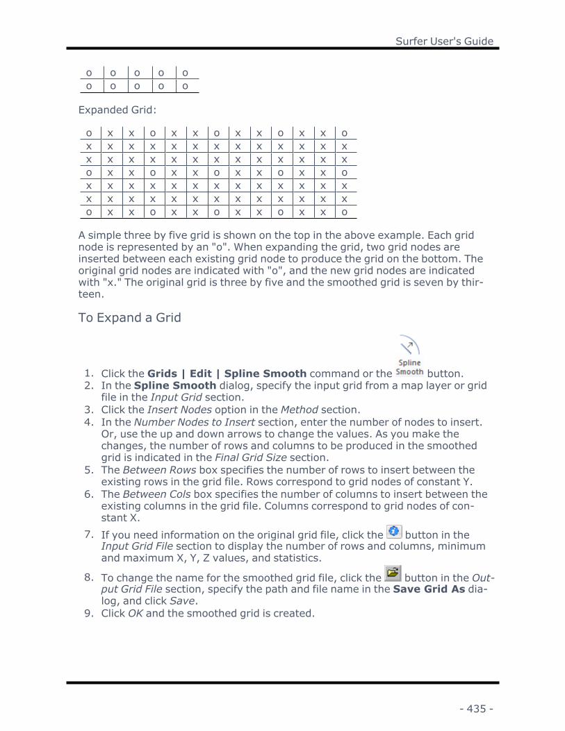
Surfer User's Guide
o o o o oo o o o o
Expanded Grid:
o x x o x x o x x o x x ox x x x x x x x x x x x xx x x x x x x x x x x x xo x x o x x o x x o x x ox x x x x x x x x x x x xx x x x x x x x x x x x xo x x o x x o x x o x x o
A simple three by five grid is shown on the top in the above example. Each gridnode is represented by an "o". When expanding the grid, two grid nodes areinserted between each existing grid node to produce the grid on the bottom. Theoriginal grid nodes are indicated with "o", and the new grid nodes are indicatedwith "x." The original grid is three by five and the smoothed grid is seven by thir-teen.
To Expand a Grid
1. Click the Grids | Edit | Spline Smooth command or the button.2. In the Spline Smooth dialog, specify the input grid from a map layer or grid
file in the Input Grid section.3. Click the Insert Nodes option in the Method section.4. In the Number Nodes to Insert section, enter the number of nodes to insert.
Or, use the up and down arrows to change the values. As you make thechanges, the number of rows and columns to be produced in the smoothedgrid is indicated in the Final Grid Size section.
5. The Between Rows box specifies the number of rows to insert between theexisting rows in the grid file. Rows correspond to grid nodes of constant Y.
6. The Between Cols box specifies the number of columns to insert between theexisting columns in the grid file. Columns correspond to grid nodes of con-stant X.
7. If you need information on the original grid file, click the button in theInput Grid File section to display the number of rows and columns, minimumand maximum X, Y, Z values, and statistics.
8. To change the name for the smoothed grid file, click the button in the Out-put Grid File section, specify the path and file name in the Save Grid As dia-log, and click Save.
9. Click OK and the smoothed grid is created.
- 435 -

Chapter 7 - Grid Operations
Recalculating a GridWhen a grid file is recalculated, the number of rows and columns are increasedor decreased relative to the original grid. The original grid values are lost unlesstheir locations correspond exactly with the grid nodes in the output grid. Thesmoothed grid file will still be an accurate representation of the original data. Forexample, you might have a 75 x 75 grid and need a 100 x 100 grid to performgrid math with another grid. You can recalculate the grid to have exactly thenumber of rows and columns needed.
To Recalculate a grid:1. Click the Grids | Edit | Spline Smooth command.2. In the Spline Smooth dialog, specify the input grid from a map layer or grid
file in the Input Grid section.3. Click the Recalc Grid option in the Method section.4. In the Final Grid Size section, specify the number of rows and columns to pro-
duce in the smoothed grid. You can increase or decrease the number of rowsand columns in the grid file. Enter the desired value, or use the up and downarrows on your keyboard to change the values for the number of rows andcolumns to be produced in the smoothed grid.
l The # Rows box specifies the number of rows for the smoothed grid file.l The # Cols box specifies the number of columns for the smoothed gridfile.
5. If you need information on the original grid file, click the button in theInput Grid File section to display the number of rows and columns, minimumand maximum X, Y, Z values, and statistics.
6. To change the name for the smoothed grid file, click the button in the Out-put Grid File group, specify the path and file name in the Save Grid As dia-log, and click Save.
7. Click OK and the smoothed grid is created.
Reduce Grid File DensitySpline smoothing can be used to reduce grid file density. If a dense grid is cre-ated, producing a map from this grid might take a considerable amount of time.The less dense grid can be used to produce the contour map or 3D wireframe inless time. USGS GTopo30 files are quite dense and it is necessary to thin themout before attempting to plot a map of the grid.
Fill in a Sparse GridOne of the purposes of spline smoothing is to fill in a sparse grid. A map pro-duced from a sparse grid may have an angular appearance. For example, splinesmoothing can be used to increase a 10 x 10 grid (a sparse grid) to a 50 x 50grid. Denser grids produce smoother maps.
- 436 -

Surfer User's Guide
Increasing the grid density using spline smoothing increasesthe roundness or smoothness of the contours and the surface
appearance.
The Spline Smooth DialogClick the Grids | Edit | Spline Smooth command to open the Spline Smoothdialog.
To expand a grid, choose the Insert Nodes option in the Spline Smooth dia-log. When recalculating a grid, choose the Recalc Grid option in the Spline
Smooth dialog.
- 437 -

Chapter 7 - Grid Operations
Input GridSpecify the source map layer or grid file in the Input Grid section. Click the cur-rent selection and select a map layer from the list. Only map layers created fromgrid files are included in the Input Grid list. Click Browse to load a grid file withthe Open Grid dialog.
Insert NodesChoose the Insert Nodes option in the Method section to activate the NumberNodes to Insert section.
Number of Nodes to InsertChoose the Insert Nodes option in the Method section to activate the NumberNodes to Insert section. Enter the number of nodes to insert, or use the up anddown arrows to change the values. As you make the changes, the number ofrows and columns to be produced in the smoothed grid is indicated in the FinalGrid Size section.
Insert Nodes Between RowsThe Between Rows box specifies the number of rows to insert between the exist-ing rows in the grid file. Rows correspond to grid nodes of constant Y.
Insert Nodes Between ColumnsThe Between Cols box specifies the number of columns to insert between theexisting columns in the grid file. Columns correspond to grid nodes of constant X.
Recalculate GridChoose the Recalc Grid option in the Method section to activate the Final GridSize section. This group specifies the number of rows and columns to produce inthe smoothed grid. You can increase or decrease the number of rows andcolumns in the grid file.
Final Grid SizeChoose the Recalc Grid option in the Method section to activate the Final GridSize section. This group specifies the number of rows and columns to produce inthe smoothed grid. You can increase or decrease the number of rows andcolumns in the grid file. Enter the # Rows and/or # Cols, or use the up and downarrows to change the values.
# RowsThe # Rows box specifies the number of rows for the smoothed grid file. Enterthe desired value, or use the up and down arrows to change the values for thenumber of rows to be produced in the smoothed grid.
- 438 -

Surfer User's Guide
# ColumnsThe # Cols box specifies the number of columns for the smoothed grid file. Enterthe desired value, or use the up and down arrows to change the values for thenumber of columns to be produced in the smoothed grid.
Output GridType a file path and file name, including the file type extension, in the Output
Grid field, or click the button and specify the path and file name for the gridfile in the Save Grid As dialog.
Add New Map or LayerCheck the Add grid as layer to check box to automatically add the created grid toa new or existing map. Select [New Map] in the Add grid as layer to field to cre-ate a new map. Click the current selection and select an existing map to add anew layer to the map. Select the layer type by clicking the current selection inthe New layer type field and selecting the desired layer type from the list.
Note: If you are saving the grid file in the DEM grid format, clear the Add grid aslayer check box and add the map or layer with a Home | New Map or Home |Add to Map | Layer command.
Grid Spline Smooth and .GSR2 FilesWhen the input .GRD file for a Grids | Edit | Spline Smooth command has adefined .GSR2 file with coordinate system information, this information is usedfor the output .GRD file. The Export Options dialog appears with the option tosave the coordinate system information. It is recommended to check the GSReference (Version 2) file if you intend to use the grid file in Surfer, as the GSR2retains all of the information needed. The grid has the same coordinate systemas the original grid file, but the new .GSR2 is required to define the coordinatesystem.
Assign Coordinate System - Grid
The Grids | Edit | Assign Coordinate System command or the buttonlinks a grid file to a specific coordinate system. Once the coordinate system isdefined for the grid file, a Golden Software Georeference .GSR2 file is created.This file contains all the relevant projection information that Surfer needs toload the grid in the proper projection.
Use the Data | Coordinate System | Assign Coordinate System command to linka data file to a .GSR2 file. When a .GRD file is created using the Grids | New Grid| Grid Data command, the .GSR2 file for the data is read. The projection inform-ation can be saved with the grid file using the Spatial References options. It isrecommended to check the GS Reference (Version 2) file if you intend to use the
- 439 -

Chapter 7 - Grid Operations
grid file in Surfer, as the GSR2 retains all of the information needed. The gridhas the same coordinate system as the original data file, but the .GSR2 isrequired to define the coordinate system. When a map is created from either thedata file or the .GRD file, the .GSR2 file is read and the map layer automaticallyhas the correct coordinate system.
If the data file did not have an assigned coordinate system, or the grid file wasprovided directly from another source, the Grids | Edit | Assign CoordinateSystem can be used to link the grid with a .GSR2 file.
When any grid operation is performed on the referenced grid file, the ExportOptions dialog appears with the option to create a new .GSR2 file for the newoutput grid. For instance, if you use the Grids | Edit | Filter command andsmooth the grid, the output smoothed grid will contain a .GSR2 file with thesame coordinate system information as the original grid. When a map is createdfrom the smoothed grid file, the .GSR2 file is read and the map layer auto-matically has the correct coordinate system. For commands that use multiplefiles, such as Grids | Edit | Assign NoData or Grids | Resize | Mosaic, all filesshould be in the same reference system, otherwise unexpected results mayoccur. The .GSR2 file in these cases is assigned by the first .GRD file specified.
Grid Project
Click the Grids | Edit | Project command or the button to create a newgrid in a different coordinate system from a grid in an existing map layer or a gridfile. The Project command creates a grid in the desired coordinate system andthen resamples the original grid to populate the new grid with Z values. You cancontrol the output grid coordinate system, geometry, and resampling method.Click the Grids | Edit | Project command to open the Grid Project dialog.
Grid Project DialogThe Grid Project dialog contains the options for creating the projected grid file.
- 440 -

Surfer User's Guide
Specify the coordinate system, grid geometry, and resamplemethod in the Grid Project dialog.
Input GridSpecify the source map layer or grid file in the Input Grid section. Click the cur-rent selection and select a map layer from the list. Only map layers created fromgrid files are included in the Input Grid list. Click Browse to load a grid file withthe Open Grid dialog. Click and drag the corner of the Grid Project dialog to res-ize the dialog if the entire Input Grid path and file name is not visible.
The input grid file coordinate system will be displayed below the Input Grid Filefield. The coordinate system will be updated automatically if the map layer is ref-erenced or if the grid file includes a georeference file, such as GSR2. Define theInput Grid coordinate system by clicking Set and defining the coordinate systemin the Assign Coordinate System dialog.
Output GridSpecify a path, name, and file format for the projected grid in the Output Gridsection. Type a file path and file name, including the file type extension, in the
Output Grid field, or click the button and specify the path and file name forthe grid file in the Save Grid As dialog.
Click and drag the corner of the Grid Project dialog to resize the dialog if theentire Output Grid path and file name is not visible.
- 441 -

Chapter 7 - Grid Operations
Specify the desired coordinate system for the projected grid by clicking Set anddefining the coordinate system in the Assign Coordinate System dialog.
Resize Output GridBy default the Resize output grid check box is not checked. The output grid willbe the same size as the input grid. The number of rows and columns will be adjus-ted if necessary to maintain the same or nearly the same grid spacing as theinput grid file. The # Rows and # Cols display the number of rows and columns inthe output grid. When Resize output grid is not checked, the # Rows and # Colsvalues are informational and cannot be changed.
Check the Resize output grid check box to specify the number of rows andcolumns in the output grid. Type a number in the # Rows field or click the but-tons to select the number of rows. Type a number in the # Cols field or click thebuttons to select the number of columns.
ResampleThe Resamplemethod determines how the Z values for the output grid are cal-culated. Define the resampling method by selecting a method in the Resamplelist. The output grid values can be resampled with the Nearest Neighbor,Bilinear, or Cubic Convolutionmethod.
Nearest NeighborThe Nearest Neighbormethod applies the closest grid node value on the originalgrid to the grid node value in the new projected grid. When the original grid andthe new grid differ in size, more than one original node may be applied to thenew grid and some original grid cells may not be applied to the new grid. TheNearest Neighbormethod is the fastest resampling method, though it can resultin distorted output.
Bilinear InterpolationThe Bilinear Interpolationmethod uses a weighted average of four nodes in theoriginal grid and applies this to the projected grid node value. The projected gridis smoothed compared to the original grid.
Cubic ConvolutionThe Cubic Convolutionmethod uses a weighted average of 16 nodes in the ori-ginal grid and applies this to the new grid node value. The projected grid issmoother than the original grid. This method is best for continuous data. This isthe slowest resampling method, but it results in a sharper grid than the BilinearInterpolation or the Nearest Neighbormethods.
OK and CancelClick OK to create the projected grid. Click Cancel to close the Grid Project dia-log without creating a grid.
- 442 -

Surfer User's Guide
Grid Calculus
Click the Grids | Calculate | Calculus command or the button to accesstools to interpret your grid files. Grid calculus can help you define and quantifycharacteristics in the grid file that might not be obvious by looking at a contouror 3D wireframe of the grid.
The Grids | Calculate | Calculus command creates a new grid file of the gen-erated data. Generated grid files use the same dimensions as the original gridfile but might use different ranges of data depending on the type of output.
When a numerical derivative is needed, central difference formulae are used inthe calculus computations in Surfer. Because a central difference approach isused, values on both sides of the location for which the derivative is computedare required. This leads to NoData values along the edges of the derivative grids,otherwise known as an edge effect.
Surfer uses "compass-based" grid notation to indicate the neighboring gridnodes used for many of the Grid Calculus operations, as illustrated below:
Using this grid notation, we can write the difference equation approximations forthe necessary derivatives at location Z as follows:
- 443 -

Chapter 7 - Grid Operations
The Grid Calculus DialogClick the Grids | Calculate | Calculus command to open the Grid Calculusdialog.
- 444 -

Surfer User's Guide
The Grid Calculus dialog provides four sections of commands to interpret yourgrid file.
The Grid Calculus dialog is divided into four sections:
l Directional Derivatives,l Terrain Modeling,l Differential and Integral Operators, andl Fourier and Spectral Analysis.
Input GridSpecify the source map layer or grid file in the Input Grid section. Click the cur-rent selection and select a map layer from the list. Only map layers created fromgrid files are included in the Input Grid list. Click Browse to load a grid file withthe Open Grid dialog.
Output GridType a file path and file name, including the file type extension, in the Output
Grid field, or click the button and specify the path and file name for the gridfile in the Save Grid As dialog.
- 445 -

Chapter 7 - Grid Operations
Add New Map or LayerCheck the Add grid as layer to check box to automatically add the created grid toa new or existing map. Select [New Map] in the Add grid as layer to field to cre-ate a new map. Click the current selection and select an existing map to add anew layer to the map. Select the layer type by clicking the current selection inthe New layer type field and selecting the desired layer type from the list.
Note: If you are saving the grid file in the DEM grid format, clear the Add grid aslayer check box and add the map or layer with a Home | New Map or Home |Add to Map | Layer command.
Using Grid CalculusTo create a grid using Grid | Calculus :
1. Click the Grids | Calculate | Calculus command.2. Select the grid map layer or grid file in the Input Grid section.3. Expand the calculus type you wish to use by clicking on the next to the type
name.4. Select a calculus operation (e.g. terrain slope).5. If available, set the options for the operation.
6. Click the button to set the Output Grid path and file name.7. Click OK and the new grid file is created.
Grid Calculus and .GSR2 FilesWhen the input .GRD file for a Grids | Calculate | Calculus command has adefined .GSR2 file with coordinate system information, this information is usedfor the output .GRD file. The Export Options dialog appears with the option tosave the coordinate system information. It is recommended to check the GSReference (Version 2) file if you intend to use the grid file in Surfer, as the GSR2retains all of the information needed. The grid has the same coordinate systemas the original file, but the .GSR2 is required to define the coordinate system.
Directional DerivativesThe Grids | Calculate | Calculus directional derivatives provide you with inform-ation about the slope, or rate of change of slope, of the gridded surface in a spe-cified direction. Because this takes a specified direction into account, this slope,or rate of change in slope, might not be the steepest slope at a given point. Forexample, if the specified direction is due East, but the gradient is due North, thedirectional derivative slope is zero at that point. In the specified direction, thereis no slope at that point, although there is a slope to the North.
Directional derivatives are different from the values given in Terrain Modelingwhere the direction of the slope is defined as the gradient, or the direction ofsteepest ascent at a given point (i.e., straight uphill at that point). In the above
- 446 -

Surfer User's Guide
example, the terrain model would report the slope in the north direction at thatpoint. The two methods would report different values at that particular point onthe grid.
Let Z be defined as a function of X and Y in a domain that includes point P. Atwhat rate does Z change if we move from point P in a specified direction? In theX axis direction, the rate of change for Z is , and the rate of change in the Yaxis direction for Z is .
Definition - The Directional Derivative (Schwartz, 1974)
Let f(x,
,
such that the line segment PQ lies in D, and let
.
Then
is the directional derivative of f(x,y) at P in the direction of
There are three directional derivative options available: First Derivative, SecondDerivative, and Curvature. You can specify the angular direction for the oper-ation.
First Derivative
Second Derivative
Curvature
Directional Derivative ExampleThis example is based on the Demogrid.grd file included with Surfer, althoughthe limits of the grid have been extended to 10 units in both the X and Y dimen-sions. The map shows the contours and the direction chosen for the Grids | Cal-culate | Calculus directional derivative operations. A profile line is alsoincluded on the map. The graphs included are based on Grids | Calculate | Slicecommand data collected along the profile lines. Each operation was performed,and the Slice command was applied to the resultant grid files. The results areshown in the graphs that were produced in Golden Software, LLC's Grapher™ .A comparison of the map and the graphs gives a good visual analysis of the res-ults of the directional derivative operations.
- 447 -
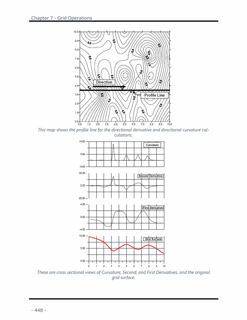
Chapter 7 - Grid Operations
This map shows the profile line for the directional derivative and directional curvature cal-culations.
These are cross sectional views of Curvature, Second, and First Derivatives, and the originalgrid surface.
- 448 -

Surfer User's Guide
First DerivativeThe Grids | Calculate | Calculus directional derivative, First Derivative, calculatesthe slope of the surface along a given direction. First derivative grid files producecontour maps that show isolines of constant slope along lines of fixed direction.At a particular grid node location, if the slope is uphill, the slope is positive; and ifdownhill, the slope is negative. Slope is reported as rise over run and canapproach negative or positive infinity as the slope approaches vertical in thedown or up direction.
The directional first derivative is exactly as in the definition (Schwartz, 1974).Instead of a known function "Z(X,Y)" for which we can compute the necessarylimits, Surfer uses a grid file, so directional derivative is approximated using dif-ference equations.
The original grid file is displayed as a contour map with thin contour lines. The first derivativemap is overlaid on the contour map with negative values (downhill in the +x direction) ingray, positive values (uphill in the + x direction) in white, and the zero contour shown as a
bold black line.The directional derivative at a point is equal to the dot product between the gradi-ent vector and a unit vector in the direction of interest:
- 449 -

Chapter 7 - Grid Operations
where a is the user specified angle (see Schwartz, 1974, p. 785, or Tuma, 1979,p. 89). Using compass-based grid notation, the equation takes the followingform:
Second DerivativeThe Grids | Calculate | Calculus directional derivative, Second Derivative, cal-culates the rate of change of slope along a given direction. Second derivativegrid files produce contour maps that show isolines of constant rate of change ofslope across the surface. If the slope is uphill, the rate of change is positive anddownhill is negative.
Contour map of original grid file is overlaid on second derivative map. Areas of greatestchange in slope in the X direction occur on ridges (light gray) and valleys (dark gray).
- 450 -

Surfer User's Guide
The directional second derivative is the directional derivative of the first dir-ectional derivative:
The compass-based grid notation difference equation used in Surfer takes theform:
CurvatureThe Grids | Calculate | Calculus directional derivative, Curvature, is a measure ofthe rate of change of the inclination angle of tangential planes on a profile linedefined by the surface along a specified direction. Curvature is reported as theabsolute value of the rate of change and is, therefore, a positive number.Curvature is similar to the Second Derivative.
The directional curvature is the absolute value of the rate of change, in a spe-cified direction, of the inclination angle of the tangent plane.
- 451 -

Chapter 7 - Grid Operations
The contour map of the original grid file is overlaid with a filled directional curvature map.The maximum curvature in the X direction (as indicated by the darker gray contour fill)
occurs at valleys and ridges.The mathematical formula for the directional curvature of a surface f(x,
(see Schwartz, 1974, p. 592).
Terrain ModelingThe Grids | Calculate | Calculus terrain modeling option provides additional toolsto analyze the surface geometry of a grid file. Results are based on the gradientdirection (direction of steepest slope) and not a predefined direction as with Dir-ectional Derivatives. For each grid node location on a surface, Surfer determinesthe magnitude and direction of the steepest slope.
There are five terrain modeling operations:
- 452 -

Surfer User's Guide
l Terrain Slope
l Terrain Aspect
l Profile Curvature
l Plan Curvature
l Tangential Curvature
ThresholdWhen you choose the Terrain Aspect, Profile Curvature, Plan Curvature, or Tan-gential Curvature options, you can also specify a Threshold value. In areaswhere the steepest slope approaches zero (where the surface is nearly hori-zontal), the gradient direction is somewhat difficult to ascertain (i.e., the defin-itions "downhill" and "uphill" are rather arbitrary). In these cases, it is preferableto classify the surface as flat. The Threshold value is the minimum value for theslope for which the aspect and curvature values are computed. In locationswhere the Threshold value is not met, the grid node value in the output grid isset to NoData. The Threshold value is, by default, set to a very small value.
Terrain SlopeThe Grids | Calculate | Calculus terrain model, Terrain Slope, calculates the slopeat any grid node on the surface. Terrain Slope is reported in degrees from zero(horizontal) to 90 (vertical). For a particular point on the surface, the TerrainSlope is based on the direction of steepest descent or ascent at that point (Ter-rain Aspect). This means that across the surface, the gradient direction canchange. Grid files of the Terrain Slope can produce contour maps that showisolines of constant steepest slope. This operation is similar to the way the FirstDirectional Derivative defines the slope at any point on the surface but is morepowerful in that it automatically defines the gradient direction at each point onthe map.
- 453 -

Chapter 7 - Grid Operations
In this example, a contour map of the original DEM is overlaid with a terrain aspect map.South-facing slopes (between SE or 135° and SW or 215° ) are indicated with gray fills. Graylines on north facing slopes are contour fills drawn where the aspect varies between 0 degrees
(north) and 359 degrees (1 degree west of north).The slope, S, at a point P is the magnitude of the gradient at that point. From thedefinition of the gradient:
Using the compass-based grid notation difference equation yields:
The terrain slope is represented as a slope angle ST in degrees in keeping withthe terrain modeling literature, such as Moore et al. (1993):
Terrain AspectThe Grids | Calculate | Calculus terrain model, Terrain Aspect, calculates thedownhill direction of the steepest slope (i.e. dip direction) at each grid node. It isthe direction that is perpendicular to the contour lines on the surface, and is
- 454 -

Surfer User's Guide
exactly opposite the gradient direction. Terrain Aspect values are reported in azi-muth, where 0 degrees points due North, and 90 degrees points due East.
A contour map of the original DEM is layered with a terrain aspect map. South facing slopes(between SE or 135° and SW or 215° ) are indicated with gray fills. Gray lines on north facingslopes are contour fills drawn where the aspect varies between 0 degrees (north) and 359
degrees (1 degree west of north).In keeping with the terrain modeling literature, i.e. Moore et al. (1993), Surferrepresents the terrain aspect, AT, as an azimuth (in degrees, not radians):
The compass-based grid notation version of this equation is:
Profile CurvatureThe Grids | Calculate | Calculus terrain model, Profile Curvature, determines thedownhill or uphill rate of change in slope in the gradient direction (opposite ofslope aspect direction) at each grid node. Grid files of Profile Curvature producecontour maps that show isolines of constant rate of change of steepest slopeacross the surface. This operation is comparable to the Second Directional Deriv-ative but is more powerful because it automatically determines the downhill dir-ection at each point on the surface, and then determines the rate of change ofslope along that direction at that point. Negative values are convex upward and
- 455 -

Chapter 7 - Grid Operations
indicate accelerated flow of water over the surface. Positive values are concaveupward and indicate slowed flow over the surface.
Profile Curvature measures the curvature of the surface in the direction of gradient. Negativecurvature, shown with a gray fill, indicates a convex upward surface and accelerated water
flow.The profile curvature KPis given by:
where
Plan CurvatureThe Grids | Calculate | Calculus terrain model, Plan Curvature, reflects the rateof change of the Terrain Aspect angle measured in the horizontal plane, and is ameasure of the curvature of contours. Negative values indicate divergent waterflow over the surface, and positive values indicate convergent flow.
- 456 -

Surfer User's Guide
Plan Curvature calculates the curvature of the surface in the horizontal plane, or thecurvature of the contour. Negative curvature, shown with a gray fill, indicates areas of diver-
gent flow.The plan curvature KHis given by:
where
Tangential CurvatureThe Grids | Calculate | Calculus terrain model,Tangential Curvature, measurescurvature in relation to a vertical plane perpendicular to the gradient direction,or tangential to the contour. The negative and positive areas are the same as forPlan Curvature, but the curvature values are different. Tangential Curvature isrelated to the Plan Curvature KHby the sine of the slope:
- 457 -
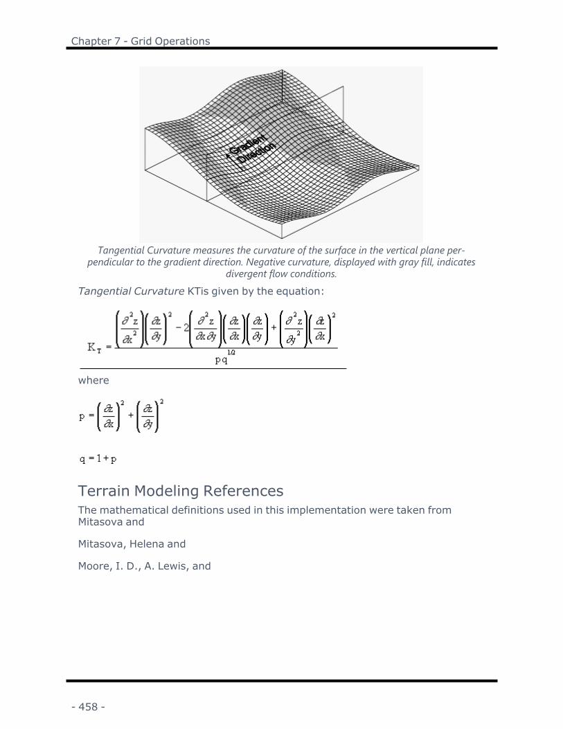
Chapter 7 - Grid Operations
Tangential Curvature measures the curvature of the surface in the vertical plane per-pendicular to the gradient direction. Negative curvature, displayed with gray fill, indicates
divergent flow conditions.Tangential Curvature KTis given by the equation:
where
Terrain Modeling ReferencesThe mathematical definitions used in this implementation were taken fromMitasova and
Mitasova, Helena and
Moore, I. D., A. Lewis, and
- 458 -

Surfer User's Guide
Differential and Integral OperatorsThe Grids | Calculate | CalculusDifferential and Integral Operators include theGradient Operator, the Laplacian Operator, the Biharmonic Operator, and Integ-rated Volume.
Select differential and integral operators from the list on the left side of the Grid Calculusdialog. There are no options for Differential & Integral Operators.
Gradient Operator
Laplacian Operator
Biharmonic Operator
Integrated Volume
Gradient OperatorThe Grids | Calculate | Calculus differential and integral operator, Gradient Oper-ator, generates a grid of steepest slopes (i.e. the magnitude of the gradient) atany point on the surface. This is similar to the Terrain Slope operation, but theGradient Operator is reported as a number (rise over run) rather than indegrees, and the direction is opposite that of the slope. The Gradient Operator iszero for a horizontal surface, and approaches infinity as the slope approachesvertical.
The definition of the gradient yields the following equation:
- 459 -

Chapter 7 - Grid Operations
Using the compass based grid notation yields the equation used in Surfer:
Laplacian OperatorThe Grids | Calculate | Calculus differential and integral operator, Laplacian Oper-ator, provides a measure of discharge or recharge on a surface. In grid files gen-erated with the Laplacian Operator recharge areas are positive and dischargeareas are negative.
Groundwater, heat, and electrical charge are three examples of conservativephysical quantities whose local flow rate is proportional to the local gradient. The
Laplacian operator, , is the mathematical tool that quantifies the net flowinto (Laplacian > 0, or areas of recharge) or out of (Laplacian < 0, areas of dis-charge) a local control volume in such physical situations. The Laplacian operatoris defined in multivariable calculus by.
The Surfer implementation of the Laplacian Operator generates a grid using astandard five-point central difference formula.
Biharmonic OperatorBending of thin plates and shells, viscous flow in porous media, and stress func-tions in linear elasticity are three examples of physical quantities that can bemathematically described using the Grids | Calculate | Calculus differential and
integral operator,Biharmonic Operator. The Biharmonic Operator, , isdefined in multivariable calculus by
This is comparable to applying the Laplacian Operator twice.
- 460 -

Surfer User's Guide
Integrated VolumeThe Grids | Calculate | Calculus differential and integral operator, IntegratedVolume, gives the accumulated volume over the grid from the southwest to thenortheast corner, or over a subgrid from southwest to northeast. This methodcan calculate volumes over
Mathematically, the integrated volume is defined by
Consider a surface defined over a rectangular region extending from X min to Xmax and Y min to Y max:
V(x,
The Integrated Volume option enables easy computation of volumes under rect-angular subgrids. For example, the volume under the shaded area in the figurebelow is simply V(xr,
The integral of the bilinear form over the grid cell is the average value of the fourcorners times the area of the grid cell. Therefore, the underlying formula is
Fourier and Spectral AnalysisThe correlogram and periodogram are used in a variety of fields, including hydro-logy, agriculture, forestry, meteorology, ecology, and sociology.
- 461 -

Chapter 7 - Grid Operations
ExampleSee, for example, Ripley (1981, Chapter 5), and Bras and Rodriguez-Iturbe(1985, Chapter 6). The correlogram assesses spatial patterns and spatial cor-relation, while the periodogram identifies periodicities in the data.
CorrelogramThe Grids | Calculate | Calculus Fourier and spectral analysis, Grid Correlogram,assesses spatial patterns and spatial correlation of a grid. Correlograms indicatehow well grid values correlate across the grid. They indicate underlying trends inthe grid and give a measure of the anisotropy of the grid.
Correlograms are symmetric; Z(x,
A contour map of a DEM is shown on the left and the grid correlogram is shown on the right.The heavy line illustrates the approximate directions of anistropy on both maps.
Given gridded data z(u,v), where {u = 0, ..., NX-1} and {v = 0, ..., NY-1} thegrid auto-covariance,
where the summation is over u and v such that
and is the arithmetic average of the grid values:
Note that the grid auto-covariance function is itself a grid.
The grid auto-covariance is the two-dimensional lattice equivalent of the timeseries auto-covariance function. It is comparable to the two-dimensional vari-ogram; under the appropriate assumptions of statistical stationarity, there is aone-to-one relationship between the grid auto-covariance function and the
- 462 -
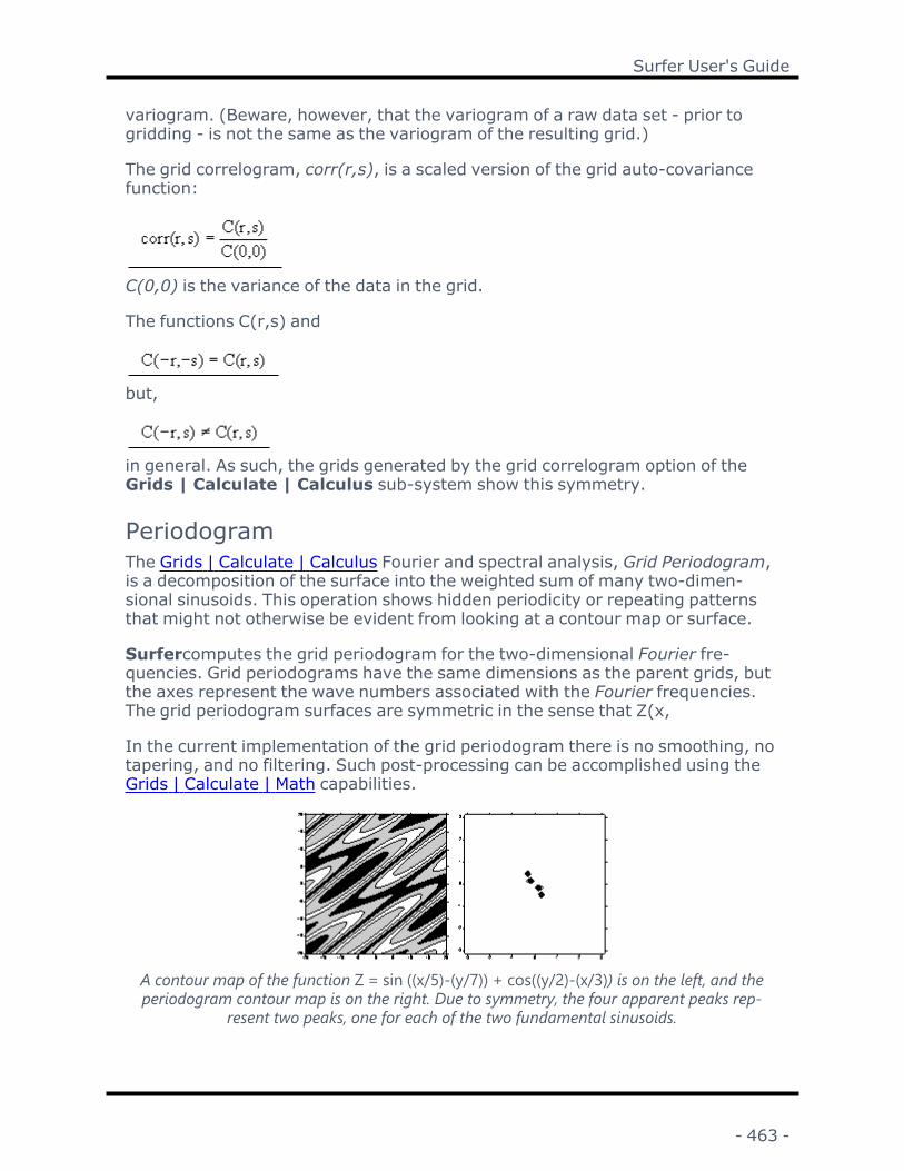
Surfer User's Guide
variogram. (Beware, however, that the variogram of a raw data set - prior togridding - is not the same as the variogram of the resulting grid.)
The grid correlogram, corr(r,s), is a scaled version of the grid auto-covariancefunction:
C(0,0) is the variance of the data in the grid.
The functions C(r,s) and
but,
in general. As such, the grids generated by the grid correlogram option of theGrids | Calculate | Calculus sub-system show this symmetry.
PeriodogramThe Grids | Calculate | Calculus Fourier and spectral analysis, Grid Periodogram,is a decomposition of the surface into the weighted sum of many two-dimen-sional sinusoids. This operation shows hidden periodicity or repeating patternsthat might not otherwise be evident from looking at a contour map or surface.
Surfercomputes the grid periodogram for the two-dimensional Fourier fre-quencies. Grid periodograms have the same dimensions as the parent grids, butthe axes represent the wave numbers associated with the Fourier frequencies.The grid periodogram surfaces are symmetric in the sense that Z(x,
In the current implementation of the grid periodogram there is no smoothing, notapering, and no filtering. Such post-processing can be accomplished using theGrids | Calculate | Math capabilities.
A contour map of the function Z = sin ((x/5)-(y/7)) + cos((y/2)-(x/3)) is on the left, and theperiodogram contour map is on the right. Due to symmetry, the four apparent peaks rep-
resent two peaks, one for each of the two fundamental sinusoids.
- 463 -

Chapter 7 - Grid Operations
Given gridded data z(u,v), where {u = 0, ..., NX-1} and {v = 0, ..., NY-1} thegrid periodogram,
where .
The value of I(l,) is the weight or strength of the sinusoid with a two dimensionalfrequency of (,).
Breaking this calculation into the component real and imaginary parts yields:
Then
where
Surfer does not compute the grid periodogram, I(l,), for all possible frequencies(l,m) in this range. Rather, it computes the grid periodogram for the two-dimen-sionalFourier frequencies.
A two-dimensional frequency is a Fourier frequency if λ is an integer multiple of, and µ is an integer multiple of . In Surfer we consider the specific
frequencies:
- 464 -

Surfer User's Guide
The indices (j, k) are called the wave number of the associated frequency (l,m).Surfer follows the engineering convention (rather than the mathematicians' con-vention) of plotting the grid periodogram as a function of the wave numbersrather than as a function of the frequency:
wave number = 2π / wavelength (e.g. radians/meter)
The maximum wave number is the Nyquist frequency =p/
Volumes and AreasThe Grids | Calculate | Volume command is used to compute net volumes,cut and fill volumes, planar areas, and surface areas. The computation resultsare displayed in the grid volume report. The results can be saved as an ASCIItext file, in Rich Text Format, or can be pasted into the clipboard.
Volume calculations are performed on solids defined by an upper and lower sur-face or 3D polygons. The upper and lower surfaces are defined by a grid file or aplane of constant Z level. The upper surface does not have to be above the lowersurface at all points; the upper surface may dip below the lower surfaces in somelocations. NoData regions on either the upper or the lower surface are excludedfrom consideration during the volume calculations.
If the upper and lower surface grid files do not have the same number of rowsand columns or the same XY limits, the selected master file determines the geo-metry for the volume calculations. Surfer matches the input grids by their XYcoordinates and performs the calculations on the overlapping nodes.
Volume results are provided in cubic units based on the units of the input gridfile.
Volume Accuracy ExampleVolume calculations are generated for each grid cell. In areas where the surfaceis tilted at the top or bottom of a grid cell, Surfer approximates the volume ofthe prism at the top or bottom of the grid cell column. For very coarse grids, theprisms can contain a significant volume. Volume calculations become more accur-ate as the density of the grid is increased because the relative size of the prismsis reduced compared to the size of the associated column. Grids with significant"noise" or with highly irregular surfaces are poor candidates for volume cal-culations.
- 465 -

Chapter 7 - Grid Operations
This grid has a highly irregular surface and is a poor candidate for volume calculations.
These two grids are based on the same data but created at different grid densities. The gridon the right is a better candidate for obtaining accurate volume information because it is a
much more smooth and dense grid.
To Calculate Volumes and AreasUse the Grids | Calculate | Volume command to calculate net volumes, cutand fill volumes, planar areas, surface areas, and 3D polygon volumes.
1. Click the Grids | Calculate | Volume command or the button.2. Specify the Upper Surface and Lower Surface parameters, or for 3D polygon
volumes specify a file in Upper Surface and a file for Polygon Boundary. Seethe Grid Volume Dialog section below for instructions on PolygonBoundary.
l The Grid File option is used to specify a grid to use as the upper or lowersurface. Specify the source map layer or grid file in the Grid File section.Click the current selection and select a map layer from the list. Onlymap layers created from grid files are included in the Grid File list. ClickBrowse to load a grid file with the Open Grid dialog.
l The Constant option is used to specify the level of the planar surface touse as the upper or lower surface. Specify the level of the planar surfaceby entering the value into the Z = box. The specified value is in Z dataunits.
- 466 -

Surfer User's Guide
3. In the Options section Align grids using list, select Node position if the upperand lower grid files have the same number of rows and columns or selectXY coordinates if they do not. If XY coordinates was selected, also select avalue from the Master grid (for geometry) list. Select either the upper orlower grid file to be the base geometry for the calculation.
4. If the X, Y, and Z units are different, the resulting volume calculations aremeaningless. If, for example, your XY values are in meters but your Z valuesare in feet, the volume results are square meters times feet, rather thancubic units. In the Options section, Z Scale Factor can be used to adjust forthis problem. In this example, setting the Z Scale Factor to 0.3048 (numberof meters in a foot) results in cubic meters for volume calculations. You willneed to know the conversion factor to use this field.
5. Click OK in the Grid Volume dialog and the results are displayed in a report.6. Click File | Save As to save the report, or you can copy the information to
the clipboard and paste it into another application.
Use the Grids | Calculate | Volume command to calculate net volumes, cutand fill volumes, planar areas, and surface areas.
Grid Volume DialogClick the Grids | Calculate | Volume command to open the Grid Volume dia-log.
- 467 -

Chapter 7 - Grid Operations
Specify grid volume options in the Grid Volume dialog.
Upper Surface and Lower SurfaceSpecify the upper surface in the Upper Surface section, and specify the lower sur-face in the Lower Surface section. The surfaces can be grid files or constantplanar surfaces.
Grid FileThe Grid File option is used to specify a grid to use as the upper or lower surface.Specify the source map layer or grid file in the Grid File section. Click the currentselection and select a map layer from the list. Only map layers created from gridfiles are included in the Grid File list. Map layers will be displayed from all openplot documents. Click Browse to load a grid file with the Open Grid dialog.
Constant ZThe Constant option is used to specify the level of the planar surface to use asthe upper or lower surface. Specify the level of the planar surface by entering thevalue into the Z = box. The specified value is in Z data units.
- 468 -

Surfer User's Guide
Align GridsIf the input grid files have the same number of rows and columns, select theNode position value from the Align grids using list. The volume calculation will beperformed in equivalent grid nodes, regardless of the X and Y values. If the inputgrid files do not have the same number of rows and columns, select theXY coordinates value from the Align grids using list to match the input grid fileson X and Y values.
If Align grids using is set to XY coordinates and all grids are referenced but in adifferent coordinate system, the calculation uses the master grid's coordinatesystem. If an input grid files is not referenced but another grid file is referenced,Surfer displays a warning about mixing referenced and unreferenced grid files.Selecting Yes continues with the volume calculation, but none of the other gridswill be projected to the master grid's coordinate system. If the grids are in thesame coordinate system, selecting Yes will perform the calculation as expected.However, if a grid is not referenced and not in the same coordinate system,select No at the warning to cancel the calculation and return to the Grid Volumedialog. Select different grid files with referenced or matching coordinate systemsor use the Grids | Edit | Assign Coordinate System to change the coordinatesystem of one or more of the grid files.
Master GridFrom the Master grid (for geometry) list, select Upper Surface or Lower Surfaceas the master grid to use for the base geometry for the volume calculation.
Z Scale FactorIf the X, Y, and Z units are different, the resulting volume calculations are mean-ingless. If, for example, your X, Y values are in meters but your Z values are infeet, the volume results are square meters times feet, rather than cubic units. ZScale Factor can be used to adjust for this problem. In this example, setting theZ Scale Factor to 0.3048 (number of meters in a foot) results in cubic meters forvolume calculations. You will need to know the conversion factor to use this field.
A grid with X, Y, and Z units in feet, the units for the results are: Net Volume =(feet * feet * feet) or ft3.
Polygon BoundaryCalculate the volume inside or outside a specific region by specifying a PolygonBoundarymap layer or vector file. Specify the source map layer or vector file inthe Polygon Boundary section. Click the current selection and select a base layerfrom the list. Base layers will be displayed from all open documents. ClickBrowse to load a vector file with the Open dialog. When the base layer or vectorfile includes more than one polygon/3D polygon, the volume is calculated insideor outside all of the polygons/3D polygons in the layer or file. The number of poly-gons and number of vertices in the base layer or vector file is displayed belowthe Polygon Boundary field.
- 469 -

Chapter 7 - Grid Operations
The following vector file types are supported in the Polygon Boundary field:
BLN Golden SoftwareBlanking
GSB Golden SoftwareBoundary
BNA Atlas Boundary GSI Golden Software Inter-change
DDF SDTS TVP KML Google EarthDLG USGS Digital LineGraph
MIF MapInfo InterchangeFormat
DXF AutoCAD Drawing SHP Esri ShapefileE00 Esri ArcInfo ExportFormat
WMF Windows Metafile
EMF Windows EnhancedMetafile
Volume Inside or Volume OutsideClick Volume Inside to calculate the volume inside of the polygon(s) or 3D poly-gon(s) in the base layer or vector file. Click Volume Outside to calculate thevolume outside of the polygon(s) or 3D polygon(s) in the base layer or vectorfile.
Selected Objects OnlyCheck the Selected objects only check box to use only the selected objects in thebase layer to calculate volumes. The Loaded polygons and vertices values areupdated when the Selected objects only box is checked. Select a base layer inthe Polygon Boundary field to use the Selected objects only option. The Selectedobjects only option is not available when the Polygon Boundary is a vector file.The polygon or polygons must be selected before clicking the Grids | Calculate| Volume command.
Combine All PolygonsSelect Combine all polygons to add all the statistics for the total number of poly-gons. If there is only one polygon in the map, the box is checked by default andCombine all polygons is not active. When Combine all polygons is unchecked, thereport presents statistics for each individual polygon.
Grid ReportClick OK in the Grid Volume dialog and the results are displayed in the GridVolume Report. Use File | Save As to save the report, or you can copy theinformation to the clipboard and paste it into another application.
Introduction to Volumes and AreasThe procedures described here are used to provide more information about thedata contained in grid files. The topics discussed include volumes and areas.
- 470 -

Surfer User's Guide
The Grids | Calculate | Volume command calculates the volume and areas for thesurfaces defined by grid files or a grid file and a horizontal plane. The Grids |Calculate | Volume computations contain the following information:
l Net volume between two grid filesl Net volume between a grid file and a horizontal planel Cut and fill volumesl Surface area of a grid file above and below a specified levell Planar area of a grid above and below a specified levell volumes inside and outside of 3D polygons.
Grid Volume ReportWhen Grids | Calculate | Volume computations are performed, the results are dis-played in the Grid Volume Report.
The volume computations in the Grid Volume Report dialog include the fol-lowing:
Upper Surface and Lower SurfaceThese sections display the parameters that define the upper and lower surfaces.
Polygon BoundaryThe Polygon Boundary section displays information about any polygon bound-aries used in the volume calculation. The File Name shows the file path and namefor the base layer or vector file used to specify the boundary or boundaries. TheNumber of Polygons value indicates the number of polygons used from the baselayer or vector file. The Volume describes whether volume is calculated inside oroutside the polygon boundaries.
VolumesThe volume is calculated by three methods: Extended Trapezoidal Rule, Exten-ded Simpson's Rule, and Extended Simpson's 3/8 Rule. The reported volume isthe sum of the Positive Volume (Cut) and Negative Volume (Fill). The Z ScaleFactor is also reported in this section.
The Positive Volume (Cut) is the volume of material in those places where theupper surface is above the lower surface. The Negative Volume (Fill) is thevolume of material in those places where the upper surface is below the lowersurface. The Cut Minus Fill is the difference between the cut and fill volumes. SeeCut and Fill Volumes for more information on cut and fill.
AreasThe Areas section reports both planar areas and surface areas. The PositivePlanar Area represents the planar area where the upper surface is above thelower surface. The Negative Planar Area represents the planar area where the
- 471 -

Chapter 7 - Grid Operations
upper surface is below the lower surface. The NoData Planar Area is the sum ofthe areas over the NoData regions on both the upper and lower surfaces. TheTotal Planar Area represents the planar area for the entire grid.
The Positive Surface Area represents the area of the surface where the upper sur-face is above the lower surface. The Negative Surface Area represents the areaof the surface where the upper surface is below the lower surface. Where two sur-faces coincide exactly, the area of coincidence is reported as part of the PositivePlanar Area.
Net VolumeThe volume calculation determines the net volume between the upper and lowersurface. The net volume is reported in the Volumes section of the Grid VolumeReport. See Cut and Fill Volumes for more information on the upper and lowersurface.
To visualize net volume, consider a construction site where the topography mustbe graded to a flat surface prior to the beginning of construction. The upper sur-face represents the current topography, and the lower surface represents thefinal graded site elevations. In some places, cut must be made into the currenttopography to remove earth to the level of the final site. In other areas, earthmay be needed to fill in areas where the current topography is below the elev-ation of the final site. The net volume is the difference between all cuts and allfills. If the volume is positive, earth needs to be removed from the site to achievethe final level. If the volume is negative, earth needs to be hauled into the site toachieve the final planned grade for the site.
Three methods are used to determine volumes. Surfer approximates the neces-sary one-dimensional integrals using three classical numerical integrationalgorithms: Extended Trapezoidal Rule, Extended Simpson's Rule, and ExtendedSimpson's 3/8 Rule; see Press et al., 1988, Section [4.1]. The difference in thevolume calculations by the three different methods measures the accuracy of thevolume calculations. If the three volume calculations are reasonably closetogether, the true volume is close to these values. If the three values differ some-what, a new denser grid file should be used before performing the volume cal-culations again. The net volume can be reported as the average of the threevalues.
Press, W.H., Flannery, B.P., Teukolsky, S.A., and Vetterling, W.T.(1988), Numerical Recipes in C, Cambridge University Press.
Mathematically, the volume under a function is defined by a double integ-ral:
- 472 -

Surfer User's Guide
In Surfer, this is computed by first integrating over X (the columns) to get theareas under the individual rows, and then integrating over Y (the rows) to getthe final volume. This approach is explained in detail in Press, et al., 1988, Sec-tion [4.6].
UnitsWhen the X, Y, and Z units are the same, volume results are given in cubic units.A common situation is a grid with X, Y in latitude and longitude and Z in meters.The grid should be converted to X, Y in meters to create useful results in(meter)3. Use the Project command to project the grid to a different coordinatesystem. Alternatively if the source data is available, you can first project the Xand Y columns in a worksheet. Next create a new grid with the projected X and Yvalues.
Example 1A grid with X, Y, and Z units in feet, the units for the results are (feet)3.
Net Volume = (feet * feet * feet)
Example 2A grid with X, Y, and Z units in meters, the units for the results are (meter)3.
Net Volume = (meter * meter * meter)
Cut and Fill VolumesThe Cut & Fill Volumes section of the Grid Volume Report displays the PositiveVolume (Cut) and the Negative Volume (Fill). The cut portion is the volumebetween the upper and lower surface when the upper surface is above the lowersurface. The fill portion is the volume between the upper and lower surfaceswhen the upper surface is below the lower surface.
Calculating Cut and Fill VolumesThe Cut & Fill Volumes section uses a different calculation technique than thethree methods used to define the volume, Extended Trapezoidal Rule, ExtendedSimpson's Rule, and Extended Simpson's 3/8 Rule. For determining cut and fillvolumes, first the lower surface grid values are subtracted from the upper sur-face grid values. This normalizes the Z values where positive values indicate theupper surface is above the lower surface and negative values indicate the uppersurface is below the lower surface.
Next each grid cell is split into two triangles. For example the grid cell defined bythe first row and first column of the grid file would be split into the following tri-angles in grid coordinates (row, column): one triangle is Z(0,0), Z(1,0), and Z(0,1) while the other is Z(1,0), Z(0,1), and Z(1,1).
- 473 -

Chapter 7 - Grid Operations
The grid cell is split into two triangles.The triangles are compared to a horizontal plane at Z=0. This generates tri-angular prisms between the calculated surface and the horizontal plane. Someprisms are completely above the horizontal plane. These prisms occur where allthree Z values for the upper surface are greater than the values for the lower sur-face. This leads to a positive volume or cut. Some prisms are completely belowthe horizontal plane. These prisms occur where all three Z values for the uppersurface are less than the values for the lower surface. This leads to a negativevolume or fill. Finally some prisms intersect the horizontal plane. This leads toone prism with a quadrilateral base and one prism with a triangular base, whereone prism is a positive (cut) volume and one is a negative (fill) volume. The quad-rilateral prism is between two points on the same side of the Z=0 plane. The tri-angular prism is opposite the quadrilateral prism.
Prisms are created from the net grid values and the horizontal planar surface at Z=0. The redprisms above are positive (cut) volumes. The blue prisms are negative (fill) volumes.
Finally, the volumes are calculated for all the positive (cut) prisms and summed,and the volumes are calculated for all the negative (fill) prisms and summed. Fin-ally, the net volume is the difference between the cut and fill volumes.
- 474 -

Surfer User's Guide
NoData regions on either the upper or lower surface are excluded from con-sideration during the cut and fill calculations.
Net VolumeThe net volume is the positive, or cut, volume minus the negative, or fill,volume. To visualize net volume, consider a construction site where the topo-graphy must be graded to a flat surface prior to the beginning of construction.The upper surface represents the current topography, and the lower surface rep-resents the final graded site elevations. In some places, cut must be made intothe current topography to remove earth to the level of the final site. In otherareas, earth may be needed to fill in areas where the current topography isbelow the elevation of the final site. The net volume is the difference between allcuts and all fills. If the volume is positive, earth needs to be removed from thesite to achieve the final level. If the volume is negative, earth needs to be hauledinto the site to achieve the final planned grade for the site.
Cross-section showing the relation between the upper and lower surfaces, and the cut and fillvolumes. The lower surface is defined by Z=75.
ExampleYou can determine the volume of a pond for which you have generated a grid file.You can define the grid file of the pond bottom as the upper surface, and use aplane set at the level of the surface of the pond as the lower surface. The volumeof the pond is the Negative Volume (Fill) in the Cut & Fill Volumes section of theGrid Volume Report.
Extended Trapezoidal RuleThe pattern of the coefficients is {1,2,2,2,...,2,2,1}:
- 475 -

Chapter 7 - Grid Operations
where:
is the grid column spacing
is the grid row spacing
is the grid node value in row i and column j.
Extended Simpson's RuleThe pattern of the coefficients is {1,4,2,4,2,4,2,...,4,2,1}:
where:
is the grid column spacing
is the grid row spacing
is the grid node value in row i and column j.
Extended Simpson's 3/8 RuleThe pattern of the coefficients is {1,3,3,2,3,3,2,...,3,3,2,1}:
where:
is the grid column spacing
is the grid row spacing
is the grid node value in row i and column j.
- 476 -

Surfer User's Guide
Planar Area CalculationsPlanar area is computed by projecting the cut and fill portions of the surface ontoa plane and calculating the area of the projection.
Positive Planar AreaPositive Planar Area represents the projection of the cut (map areas where theupper surface is above the lower surface) onto a horizontal plane.
Negative Planar AreaNegative Planar Area represents the projection of the fill (map areas where theupper surface is below the lower surface) onto a horizontal plane.
This is a contour map showing the relation between positive and negative planar area on amap. The lower surface is defined by a plane where Z = 75.
Surface Area CalculationsThe surface area is the actual area of the surface. Positive Surface Area cor-responds to the area of the surface where the upper surface is above the lowersurface. Negative Surface Area corresponds to the area of the surface where theupper surface is below the lower surface.
ExampleAs an example, consider a grid file representing the bottom of a pond, with thewater level at a Z value of zero. If the grid representing the pond bottom isdefined as the upper surface and Z = 0 is defined as the lower surface, you can
- 477 -

Chapter 7 - Grid Operations
determine the surface area of the bottom of the pond. Suppose you want to drainthe pond and line it with plastic. You need to know the area of the plastic neces-sary to line the pond bottom. In this case, the negative surface area representsthe surface of the pond bottom. This would tell us precisely the amount of plasticnecessary to line the pond bottom.
The green line displays the negative surface area of the pond. This value determines theamount of plastic needed to line the pond bottom in the example.
Calculating the Volume between Two SurfacesA common problem solved with a volume calculation is determining the volumeof material between two grid files. For example, you might have drill hole datathat provides the elevation of the top and bottom of a coal seam, and you wantto determine the volume of coal present in the seam. The elevation of the topand bottom of the coal seam defines the upper and lower surfaces, respectively.In this case, the lower surface would be entirely below the upper surface.
To find the volume between two surfaces:
1. Create grid files of the upper and lower surfaces. In the example here, thegrid files would define the elevation of the top and bottom of the coal seam.Both grids must use the same dimensions and the same number of rowsand columns.
2. Choose the Grids | Calculate | Volume command and select the upper sur-face grid file in the Open Grid dialog and then click the Open button.
3. In the Grid Volume dialog, the Grid File option button should be selectedin the Upper Surface group.
- 478 -

Surfer User's Guide
4. In the Lower Surface group, click the Grid File option button and click thebutton.
5. In the Open Grid dialog, select the lower surface grid file and click theOpen button.
6. In the Grid Volume dialog, verify that the correct grid files are specifiedfor the upper and lower surfaces and click OK. The Grid Volume Report isgenerated. The volume between the surfaces is reported as the PositiveVolume (Cut), which, in this case, is the same as the Volume calculation.
7. To save the volume information, use the File | Save As command in thereport window and specify a name and file extension. Click OK and theinformation is saved.
Calculating the Volume of a Grid with NoData ValuesSurfer can be used to calculate the volume between two grid surfaces orbetween a grid surface and a horizontal plane. The accuracy of the volume cal-culation increases as the number of grid nodes in the grid file increases. Whenone of the grid surfaces contains NoData values, or the area of interest is a sub-set of the entire grid, additional error is introduced. This error can be minimizedby specifying more grid nodes during the gridding operation.
Consider the way Surfer calculates the volume of a cube that is 1 foot x 1 foot x1 foot. Surfer cannot generate a surface that is a perfect cube since each XYcoordinate can only have a single Z value. A diagonal line is drawn from the topsurface to the lower with a width of one grid unit. Using a grid with a one-footgrid line spacing, the resulting surface looks like a pyramid with the top choppedoff.
A cube with a coarse grid. Volume error is increased.
A cube with a finer grid. Volume error is reduced.
- 479 -

Chapter 7 - Grid Operations
Calculating the Volume of a LakeTo illustrate the capability of using the Grids | Calculate | Volume command, con-sider the application of calculating the volume of water within a lake. This applic-ation requires that a grid file be created which defines the lake bottom. The othersurface is defined as a horizontal planar surface that defines the water surface ofthe lake.
To calculate the volume of a lake:
1. Create the grid file for the lake. If the lake bottom is defined as the depth ofthe water, use negative Z values so that the lake appears as a basin ratherthan a hill. It is also recommended that data points be added beyond thelimits of the lake shore so that the surface is above the level of the lake inthose areas.
2. Select the Grids | Calculate | Volume command.
3. Specify the grid file for the lake in the Open Grid dialog and click Open .
4. In the Grid Volume dialog, click the Grid File option in the Lower Surfacegroup.
5. In the Upper Surface group, click the Constant option. Enter the value forthe lake surface into the Z = box. For example, if you are using depth inyour grid file as a negative value, the Z = value for your horizontal (lake)surface should be zero.
6. Click OK and the volume and area calculations are reported. The volume ofthe lake is reported as the Positive Volume.
7. To save the information, use the File | Save As command in the GridVolume Report window and specify a name and file extension.
Grid MathThe Grids | Calculate | Math command creates a new grid file that transformsthe Z values of a single grid file or combines Z values from multiple grid files. Theoutput grid file is based on a mathematical function of the form f(A, B, C, D),where A, B, C, D represent input grid files.
A defined math function can be performed by node position on correspondingnodes with the same row and column coordinates from the input grid files. Theresult of the calculation is placed at the same coordinates in the output grid file.For example, the function log10(A) creates an output grid file with the log-arithmic base 10 values for each of the grid nodes in Grid A.
- 480 -

Surfer User's Guide
A math function can also be performed on grid files that do not have the samenumber of rows and columns. Surfer matches the grid files' X and Y values andthen performs calculations on those overlapping values. If needed, input gridsare projected to the master grid's coordinate system and then resampled to themaster grid's geometry.
By default, if a node contains the NoData value in any input grid, it is assignedthe NoData value in the output grid. However, you can change the NoData Hand-ling for each grid so that NoData nodes are assigned a value. The output grid filewill then have a value when the input grid contains the NoData value.
Grid Math DialogClick the Grids | Calculate | Math command to open the Grid Math dialog.
Specify grid files and define a math function in the Grid Math dialog.
Input GridThe Input Grid column displays the selected grid files. The X and Y limits and gridsize of these files define the output grid. Place the mouse over any grid file toreveal the full path and file name for the grid.
VariableBy default, Surfer defines each grid with a Variable name letter. The first grid isA, the second grid is B, and so on. To change the Variable name for a grid, clickin the Variable name box next to the current Variable name. Delete the existingtext and type a new name. The variable name is case insensitive, so G1B is the
- 481 -

Chapter 7 - Grid Operations
same as g1b. Variable names must start with an underscore (_) or letter and canonly contain alphanumeric characters.
NoData HandlingThe NoData Handling option specifies the value to use for any NoData nodes inthe grid. If a NoData node is found in the grid, the NoData output option assignsthe NoData value to the output grid file for the same node. If the NoData Hand-ling is changed to Remap to, the NoData node in the input grid is changed to thevalue in the Remap Value column. To change the NoData Handling option, clickon the current option and select the desired option from the list.
If Align grids using is set to XY coordinates and NoData Handling is set to NoDataoutput, all nodes outside the overlapping area will be assigned NoData. To keepthe original values of the master grid in areas where there is no data overlap, setNoData Handling to Remap to, and then set the Remap Value to a value thatdoes not affect the math function (e.g., 0 for addition or subtraction).
Remap ValueWhen the NoData Handling is set to Remap to, the Remap Value box becomesavailable. Highlight the existing value and type in a new value to change theRemap to value. This sets every NoData node in the input grid to this new RemapValue. Each grid file can contain a different Remap Value.
Add GridsClick the Add Grids button to open the Open Grid(s) dialog. To perform an oper-ation on a single grid, select only one grid file. To perform an operation on mul-tiple grids, select multiple grid files using the CTRL and SHIFT keys. You canselect any number of grid files at once. When all grids are selected, click theOpen button. The grid file names are displayed in the Input Grid list.
Remove GridTo remove a grid from the Input Grid list, click once on the grid to select it. Clickthe Remove Grid button. The selected grid is removed from the list.
Grid InfoClick the Grid Info button to display the number of grid rows, number of gridcolumns, X, Y, Z minimums and maximums, and statistics for the selected grid.If the grid file is large, click OK in the message box that appears to create adetailed grid report or click Cancel to create a shorter, less detailed grid report.
Align GridsIf the input grid files have the same number of rows and columns, select theNode position value from the Align grids using list. The math function will be per-formed in equivalent grid nodes, regardless of the X and Y values. If the inputgrid files do not have the same number of rows and columns, select the
- 482 -

Surfer User's Guide
XY coordinates value from the Align grids using list to match the input grid fileson X and Y values.
If Align grids using is set to XY coordinates and all grids are referenced but in adifferent coordinate system, the resulting grid file uses the master grid's coordin-ate system. If an input grid files is not referenced but another grid file is ref-erenced, Surfer displays a warning about mixing referenced and unreferencedgrid files. Selecting Yes continues with the math function operation, but none ofthe other grids will be projected to the master grid's coordinate system. If thegrids are in the same coordinate system, selecting Yes will perform the math asexpected. However, if a grid is not referenced and not in the same coordinate sys-tem, select No at the warning to cancel the math function operation and returnto the Grid Math dialog. Select different grid files with referenced or matchingcoordinate systems or use the Grids | Edit | Assign Coordinate System tochange the coordinate system of one or more of the grid files.
Master GridFrom the Master grid (for geometry) list, select the master grid to use as thebase geometry for the new grid produced by the math function.
Enter a Function of the Form f(A,B, ...)In the Enter a function of the form f(A,B, ...) where A, B, ... are the variables inthe list above box, enter a function which describes the output grid file. The Vari-able names are used in the equation. By default, variable names are A, B, C, D,etc. These refer to the input grid files. To perform a calculation on grid file A only,you can leave any reference to additional grid files out of the specified function.
Mathematical functions and operators can be used in the Enter a function of theform f(A,B...) where A, B... are the variables in the list above field. For example,to add the Z values from two grids A and B, type A + B . Or for example to createan output grid where the values are the greater value from two grids A and B,type IF(B>A,B,A).
To use a stored function, click the next to the current function. This will dis-play the ten most recent functions used. The functions are stored in the registry,so the equations are stored between Surfer sessions. You can also start typingthe function in the function box. If the function is in the function history, theentire function will auto-complete.
Output GridType a file path and file name, including the file type extension, in the Output
Grid field, or click the button and specify the path and file name for the gridfile in the Save Grid As dialog.
- 483 -

Chapter 7 - Grid Operations
Add New Map or LayerCheck the Add grid as layer to check box to automatically add the created grid toa new or existing map. Select [New Map] in the Add grid as layer to field to cre-ate a new map. Click the current selection and select an existing map to add anew layer to the map. Select the layer type by clicking the current selection inthe New layer type field and selecting the desired layer type from the list.
Note: If you are saving the grid file in the DEM grid format, clear the Add grid aslayer check box and add the map or layer with a Home | New Map or Home |Add to Map | Layer command.
To Use the Math Command
1. Click the Grids | Calculate | Math command or the button.2. In the Grid Math dialog, click the Add Grids button. Select any number of
grid files and click Open.3. In the Align grids using list, select what type of grid alignment to use.
4. In the Output Grid section, click the button to specify a different path orfile name for the grid file to be created.
5. In the Enter a function of the form f(A,B, ...) where A, B, ... are the variablesin the list above. box, enter a function that represents the output grid file,and where A and B refer to the input grid files.
6. Click OK to create the new grid file.
Grid Math and .GSR2 FilesWhen the input .GRD file for a Grid | Math command has a defined .GSR2 filewith coordinate system information, the information in the first input .GRD file isused for the output .GRD file. The Export Options dialog appears with the optionto save the coordinate system information. It is recommended to check the GSReference (Version 2) file if you intend to use the grid file in Surfer, as the GSR2retains all of the information needed. The grid has the same coordinate systemas the original file, but the .GSR2 is required to define the coordinate system.
Using the Grid Math Command to Eliminate NegativeValues from a Grid FileNote: This method is no longer necessary for grid files created in Surfer. Toeliminate negative values while creating a grid file with the Grid | Data com-mand, set the Minimum value to the Data min or a Custom value (such as 0) inthe Grid Z Limits section of the Grid Data dialog.
Some gridding methods (i.e. Kriging, Radial Basis Function, Minimum Curvature,and Modified Shepard's Method) extrapolate beyond the Z range of the data,which can create inappropriate negative values for parameters like
- 484 -

Surfer User's Guide
concentration, thickness, and magnitude. The Grids | Calculate | Math commandcan set negative values equal to zero with the formulamax(A,0).
To set negative values equal to zero:
1. Click the Grid | Math command.2. In the Grid Math dialog, click the Add Grids button. Select the grid file con-
taining the unwanted negative values and click Open. This grid file appearsin Input Grid column.
3. Select an output grid file name in the Output Grid File section by clicking on
the button.4. In the Enter a function of the form f(A,B,...) where A, B, ... are the vari-
ables in the list above. box, entermax(a,0). This tells the program toreturn whichever is greater, the value in the grid or zero.
5. Click OK and the new grid without negative values is created.
Grid TransformThe Grids | Calculate | Transform command contains several options thatmodify the X and Y map coordinates of grid nodes within the grid file. It does notalter the Z values. The Transform options are used to shift, scale, rotate, or mir-ror grid nodes within a grid file.
The Grid Transform DialogClick the Grids | Calculate | Transform command or the button to openthe Grid Transform dialog.
Specify grid transform options in the Grid Transform dialog.
- 485 -

Chapter 7 - Grid Operations
Input GridSpecify the source map layer or grid file in the Input Grid section. Click the cur-rent selection and select a map layer from the list. Only map layers created fromgrid files are included in the Input Grid list. Click Browse to load a grid file withthe Open Grid dialog.
OperationThe Operation list controls the transformation type. Click on the box or drop-down arrow and select an option from the list.
Off-set
The Offset option adds or subtracts a number from the X and Ydimensions. Specify the Offset option from the Operation list, andspecify the amount of the offset in the X Offset and Y Offset boxes inpositive or negative units. For example, if the input grid ranges areX: 1 to 9 and Y: 2 to 8, and the offsets are 10.0 for both the X Offsetand Y Offset, then the output grid ranges will be X: 11 to 19 and Y:12 to 18.
Scale The Scale option multiplies the X and Y ranges by a factor. Specifythe Scale option from the Operation list, and specify the scalingfactors in the X Scale and Y Scale boxes displayed in the GridTransform dialog. The scaling origin is the lower left corner of thegrid, so only the xMax and yMax values are changed. For example,if the input grid ranges are X: 1 to 9 and Y: 2 to 8 and the X Scaleand Y Scale factors are both 3.0, then the output grid ranges will beX: 1 to 25 (((9 - 1) x 3.0) + 1) and Y: 2 to 20 (((8 - 2) x 3.0) + 2).
- 486 -

Surfer User's Guide
Rotat-e
The Rotate option rotates a grid in multiples of 90 degrees (0, 90,180, 270, …). Select the Rotate option in the Operation list, and spe-cify the rotation angle in the Angle box. The origin of the mapremains in the lower left, and the axes continue to increase in thesame direction, with the X axis increasing to the right, and the Yaxis increasing upwards.
The Rotate option rotates the grid in multiples of 90 degrees without changingthe XY origin.
- 487 -

Chapter 7 - Grid Operations
Mir-ror X
The Mirror X option creates a new grid file with the order of the gridnodes reversed in the X direction. The output grid file uses the sameminimum and maximum X and Y coordinates as the input grid file.The origin of the grid remains in the lower left corner, with X increas-ing to the right and Y increasing upward. The Y order remainsunchanged.
The Mirror X option creates a mirror image of the grid file with the X orderreversed.
- 488 -

Surfer User's Guide
Mir-ror Y
The Mirror Y option creates a new grid file with the order of the gridnodes reversed in the Y direction. The output grid file uses the sameminimum and maximum X and Y coordinates as the input grid file.The origin of the grid remains in the lower left corner, with X increas-ing to the right and Y increasing upward. The X order remainsunchanged.
The Mirror Y option creates a mirror image of the grid file with the Y orderreversed.
- 489 -

Chapter 7 - Grid Operations
Output GridType a file path and file name, including the file type extension, in the Output
Grid field, or click the button and specify the path and file name for the gridfile in the Save Grid As dialog.
Add New Map or LayerCheck the Add grid as layer to check box to automatically add the created grid toa new or existing map. Select [New Map] in the Add grid as layer to field to cre-ate a new map. Click the current selection and select an existing map to add anew layer to the map. Select the layer type by clicking the current selection inthe New layer type field and selecting the desired layer type from the list.
Note: If you are saving the grid file in the DEM grid format, clear the Add grid aslayer check box and add the map or layer with a Home | New Map or Home |Add to Map | Layer command.
To Transform a Grid File
1. Click the Grids | Calculate | Transform command or the button.2. In the Open Grid dialog, select a grid file to transform and click Open.3. In the Grid Transform dialog, choose an Operation and any associated
options.
4. Click the button to display the Save Grid As dialog.5. In the Save as type list, select the format for the output file. nter the path
and File name for the transformed grid. Click Save to return to the GridTransform dialog.
6. Click OK to create the transformed file.
Grid Transform and .GSR2 FilesWhen the input .GRD file for a Grid | Transform command has a defined .GSR2file with coordinate system information, this information is used for the output.GRD file. The Export Options dialog appears with the option to save the coordin-ate system information. It is recommended to check the GS Reference (Version2) file if you intend to use the grid file in Surfer, as the GSR2 retains all of theinformation needed. The grid has the same coordinate system as the original file,but the .GSR2 is required to define the coordinate system.
Grid SliceThe Grids | Calculate | Slice command or the button produces cross sec-tional data for 2D and 3D objects. The cross section is generated by taking a ver-tical slice through a gridded surface along a boundary line. Surface traces on across section are sometimes referred to as profile lines.
- 490 -

Surfer User's Guide
Another method to create a slice from the data is to use the Map Tools | Add toMap | Profile command. The profile automatically creates a graph showing accu-mulated distance and elevation. The Grids | Calculate | Slice command pro-duces a data file that can show the same object, but contains additional data aswell.
The surface is based on a grid file and the boundary line is based on the inform-ation in a vector file or base map. The boundary line can be defined by a polylinein a base map or by one of the following file formats:
BLN Golden Software Blank-ing
GSB Golden Software Bound-ary
BNA Atlas Boundary GSI Golden Software Inter-change
DDF SDTS TVP KML Google EarthDLG USGS Digital LineGraph
MIF MapInfo InterchangeFormat
DXF AutoCAD Drawing PLT Golden Software PlotcallE00 Esri AcrInfo Export PLY Stanford PolygonEMF Windows EnhancedMetafile
SHP Esri Shapefile
GML Geo. Markup Lan-guage
STL Stereolithograph
GPX GPS Exchange Format WMF Windows Metafile
At each point where the boundary linecrosses a grid line, a cross section data
point is generated.
The Grid Slice DialogClick the Grids | Calculate | Slice command or the button. The Grid Slicedialog opens.
- 491 -

Chapter 7 - Grid Operations
The Grid Slice dialog allows you to specify the resulting .BLN and/or .DAT file nameand location.
Input GridSpecify the source map layer or grid file in the Input Grid section. Click the cur-rent selection and select a map layer from the list. Only map layers created fromgrid files are included in the Input Grid list. Click Browse to load a grid file withthe Open Grid dialog.
Slice LineSpecify the file or base layer with the slice line in the Slice Line section. Loadeither a map layer or vector file in the Slice Line section:
l Click the current selection and select a base layer from the list. Only base lay-ers that contain at least one polyline or polygon will be included in the list.The base layer must use the same source coordinate system as the grid.
l Click Browse to load a vector file with the Open dialog. The file must use thesame coordinate system as the grid.
Once a file or map layer has been selected the number of lines and vertices is dis-played below the slice line selection.
Output BLN FileA Blanking BLN file may be produced with the slicing operation by selecting theOutput to BLN file option. Type a path and filename for the Output BLN, or set
- 492 -

Surfer User's Guide
the path and filename in the Save As dialog by clicking the button next toOutput BLN. The blanking file contains three columns of data:
ColumnA:
Accumulated horizontal distance along the boundaryline. This distance is accumulated even if the boundarylines go outside the grid region. The distance is reset tozero for each new boundary in the blanking file.
ColumnB:
Z value at the boundary line and grid line (row orcolumn) intersection.
ColumnC:
Boundary number, used when more than one boundaryline is contained in the file. Each new boundary line inthe blanking file is assigned a different number.
The output BLN file can be used to display a profile in Surfer as a base map. TheProfile command generates a profile with more display options. However, it maybe faster to generate a profile from the Output BLN when the surface tracealready exists in a vector file format and has many vertices. To create a profilefrom the Output BLN file,
1. After creating the BLN file with the Slice command, click the Home | NewMap | Base command
2. Select the output BLN file in the Import dialog.3. Click Open and the profile is created as a base map. The X axis corresponds
to accumulated distance along the trace, and the Y axis corresponds to grid Zvalues along the trace.
4. Select the Map object for the output BLN base map.5. On the Properties window Scale page, clear the Proportional XY scaling
check box.6. On the Properties window Scale page, adjust the X Scale and Y Scale section
Length (page units) property values until the profile scaling is displayed asdesired.
Output DAT FileCross section data can be written to an ASCII data .DAT file during the Sliceoperation by selecting the Output to .DAT file option. Type a path and filenamefor the Output DAT, or set the path and filename in the Save As dialog by click-
ing the button next to Output DAT. The ASCII data file consists of fivecolumns of data. When the profile is written to the ASCII file, a new row of data isgenerated for each point where the boundary line intersects the grid lines in thedata file. The output data file can be used to plot the profile in a graphing applic-ation, such as Grapher. The columns in the data file are arranged as follows:
ColumnA:
X coordinate of the boundary line and grid line (row orcolumn) intersection.
ColumnB:
Y coordinate of the boundary line and grid line (row orcolumn) intersection.
- 493 -

Chapter 7 - Grid Operations
ColumnC:
Z value at the boundary line and grid line (row orcolumn) intersection.
ColumnD:
Accumulated horizontal distance along the boundaryline. This distance is accumulated even if the boundarylines go outside the grid region. The distance is reset tozero for each new boundary in the blanking file.
ColumnE:
Boundary number, used when more than one boundaryline is contained in the file. Each new boundary line inthe blanking file is assigned a different number.
Set Values Outside Grid ToThe Set values outside grid to option assigns a special Z value to points that liebeyond the grid limits when the check box is active. If this option is not activ-ated, points outside the grid limit are not included in the output data file. Thedefault value is equal to the following equation:
Set NoData Values ToThe Set NoData values to option assigns a special Z value to points that lie insideNoData regions when the check box is selected. If the check box is cleared,points inside the NoData areas are not included in the output data file.
OK or CancelClick OK and a data file (and a blanking file, if specified) is created. Click Cancelto exit the dialog without creating the data.
To Create a Data File Containing Cross Section Data1. Click the Grids | Calculate | Slice command.2. In the Open Grid dialog, select a grid file and click Open.3. In the Open dialog, select the blanking file to use when producing the profile
data and then click Open.4. If desired, enter a name for the Output BLN in the Grid Slice dialog by click-
ing the button to open the Save As dialog.
5. Specify the name for the Output DAT by clicking the button to open theSave As dialog.
6. Click OK and a data file (and a blanking file, if specified) is created.
- 494 -

Surfer User's Guide
You can display the profile line across the contour map. This is the profile line used to pro-duce the following cross section.
This is the cross section taken from the profile line on the map. The cross section was createdas a base map using the Output BLN.
Plotting Cross SectionsTo display the location of the slice for the cross section on a map, use the Home |New Map | Base command and create a base map from the slice line vector fileused for the cross section.
Profile Line Projected onto the X-Z PlaneIn Surfer use the Home | New Map | Post command to plot the actual crosssection projected onto a specific plane. To plot the cross section, column C, the Zvalue, is plotted as the Y coordinate. Plotting column A as the X coordinate andcolumn C as the Y coordinate produces a profile line projected onto the X-Zplane.
- 495 -
Chapter 7 - Grid Operations
Profile Line Projected onto the Y-Z PlaneIn Surfer use the Home | New Map | Post command to plot the actual crosssection projected onto a specific plane. To plot the cross section, column C, the Zvalue, is plotted as the Y coordinate. Using column B as the X coordinate andcolumn C as the Y coordinate produces a profile line projected onto the Y-Zplane.
Profile Line Showing True Accumulated DistanceUse the Output BLN to create a profile with the Home | New Map | Base com-mand. The Output BLN produces a profile line that shows true accumulated dis-tance along the boundary line.
Alternatively, to create a profile from the Output DAT data file, in Surfer use theHome | New Map | Post command to plot the actual cross section projectedonto a specific plane. To plot the cross section, column C, the Z value, is plottedas the Y coordinate. Using column D as the X coordinate and column C as the Ycoordinate produces a profile line that shows the true accumulated distancealong the boundary line.
To create more elaborate cross sections, we recommend Golden Software’sGrapher program.
ResidualsThe Grids | Calculate | Residuals command computes the vertical differencebetween the Z value in the data file and the interpolated Z value on a gridded sur-face. It gives a quantitative measure of how well the grid file agrees with the ori-ginal data.
A residual is the difference between the Z value of a point in a data file and theinterpolated Z value at the same XY location on a gridded surface. Residual val-ues are reported as either positive or negative values. If the Z value in the datafile is greater than the Z value derived from the gridded surface, the residualvalue is positive. A negative residual value indicates that the Z value from thedata file is less than the interpolated Z value at that point. If the grid file is con-tains the NoData value at the data point, the residual value is left blank in theworksheet. Surfer uses a bilinear interpolation method to calculate Z values atpoints that do not coincide with grid nodes.
The formula used to compute a residual value is:
where:
= the residual value
- 496 -
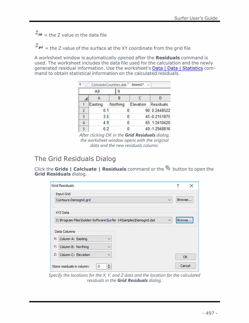
Surfer User's Guide
= the Z value in the data file
= the Z value of the surface at the XY coordinate from the grid file
A worksheet window is automatically opened after the Residuals command isused. The worksheet includes the data file used for the calculation and the newlygenerated residual information. Use the worksheet's Data | Data | Statistics com-mand to obtain statistical information on the calculated residuals.
After clicking OK in the Grid Residuals dialog,the worksheet window opens with the original
data and the new residuals column.
The Grid Residuals DialogClick the Grids | Calcluate | Residuals command or the button to open theGrid Residuals dialog.
Specify the locations for the X, Y, and Z data and the location for the calculatedresiduals in the Grid Residuals dialog.
- 497 -

Chapter 7 - Grid Operations
Input GridSpecify the source map layer or grid file in the Input Grid section. Click the cur-rent selection and select a map layer from the list. Only map layers created fromgrid files are included in the Input Grid list. Click Browse to load a grid file withthe Open Grid dialog.
XYZ DataSpecify the data file in the XYZ Data section. Click the current selection andselect a map layer from the list. Only post and classed post layers are displayedin the XYZ Data list. Click Browse to load the data file with the Open Data dialog.
Data ColumnsSpecify the location for the X, Y, and Z coordinates from the data file in the DataColumns section.
Store Residuals in ColumnIn the Store residuals in column box, enter the column where you would like theresiduals stored. By default, Surfer selects the first empty column in the datafile.
To Calculate Residuals1. Click the Grids | Calculate | Residuals command or the button.2. In the Open Grid dialog, select the grid file to be used for the residual cal-
culation and then click Open.3. In the Open dialog, select the data file to be compared to the grid file, and
then click Open.4. In the Grid Residuals dialog, specify the location for the X, Y, and Z coordin-
ates in the Data Columns section.5. In the Store residuals in column box, enter the column where you would like
the residuals stored. By default, Surfer selects the first empty column in thedata file.
6. Click OK and the worksheet window opens. The worksheet window displaysthe data file as it was specified in the Grid Residuals dialog with the addi-tional column for the residual data.
Calculating the Agreement between a Grid and theOriginal Data FileAfter performing the Grids | Calculate | Residuals command:
- 498 -

Surfer User's Guide
1. In the worksheet, click the column letter for the column containing theresidual values to select the entire column. To get the statistics for just aportion of the residual values, select only those particular values.
2. Choose the Data | Data | Statistics command. Specify the desired para-meters to be reported.
3. If Show in a window is selected, the Statistics Results window is displayedwith the statistical information on the residual data. If the Copy to work-sheet option is selected, the residual results are placed directly into the spe-cified columns of the worksheet.
Point SampleThe Grids | Calculate | Point Sample command computes the interpolated Zvalue on a gridded surface at given XY locations. XY locations from a data file areused to sample the grid. Bilinear interpolation is used to calculate the Z value atthe XY location from the nearest four grid nodes. If a Z value cannot be cal-culated due to NoData nodes or if the XY location is beyond the extent of thegrid, the cell is left blank in the output worksheet.
A worksheet window is automatically opened after the Point Sample commandis used. The worksheet includes the data file used for the calculation and thenewly generated point sample information. Use the worksheet's Data | Data |Statistics command to obtain statistical information on the calculated Z values.
After clicking OK in the Point Sample dialog, theworksheet window opens with the original data and
the new Grid Value column.
The Point Sample DialogClick the Grids | Calculate | Point Sample command or the button to openthe Point Sample dialog.
- 499 -
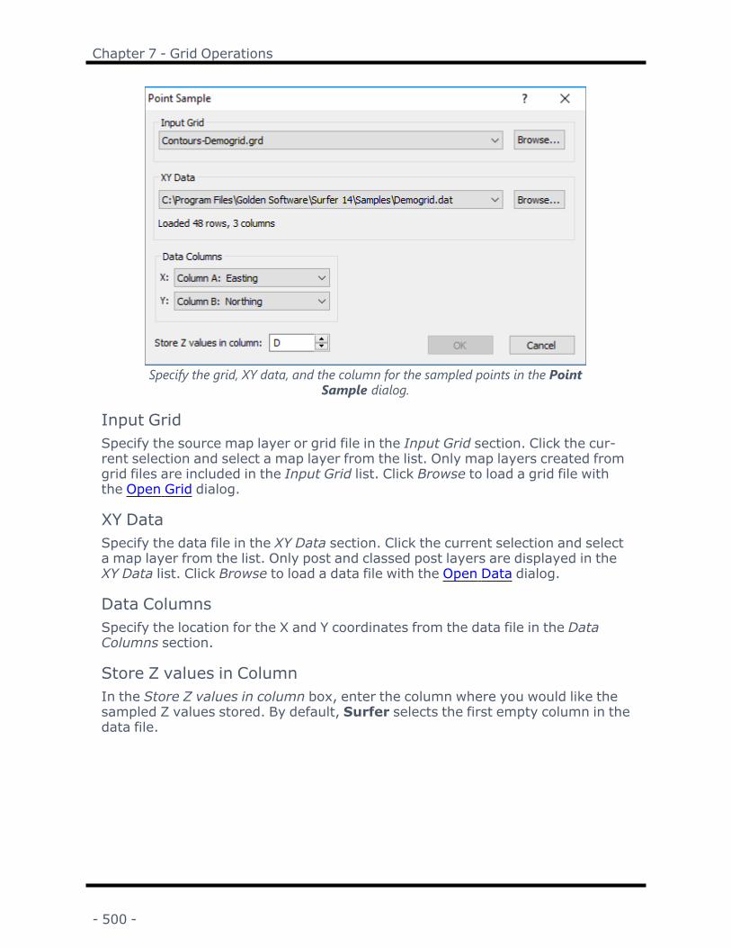
Chapter 7 - Grid Operations
Specify the grid, XY data, and the column for the sampled points in the PointSample dialog.
Input GridSpecify the source map layer or grid file in the Input Grid section. Click the cur-rent selection and select a map layer from the list. Only map layers created fromgrid files are included in the Input Grid list. Click Browse to load a grid file withthe Open Grid dialog.
XY DataSpecify the data file in the XY Data section. Click the current selection and selecta map layer from the list. Only post and classed post layers are displayed in theXY Data list. Click Browse to load a data file with the Open Data dialog.
Data ColumnsSpecify the location for the X and Y coordinates from the data file in the DataColumns section.
Store Z values in ColumnIn the Store Z values in column box, enter the column where you would like thesampled Z values stored. By default, Surfer selects the first empty column in thedata file.
- 500 -

Surfer User's Guide
Calculating the Z Value of the Surface at a PointThe Grids | Calculate | Point Sample command samples Z values from a grid atany point. To perform the operation, create a data file with X and Y coordinatesfor the points you'd like to sample and click the Grids | Calculate | PointSample command.
ExampleConsider a grid file that ranges from zero to 10 in the X and Y dimensions, andyou want to determine the value of the surface at the points (1,3) and (4,2) onthe surface.
1. Open a new worksheet window with File | New | Worksheet.
2. In column A, type the X coordinates for the points you wish to find the Zvalue, e.g. type 1 in Row 1 and 4 in Row 2. In column B, type in the Ycoordinate, e.g. type 3 in Row 1 and 2 in Row 2. Add as many points as youwant into the data file by entering the coordinates for each point into a dif-ferent row in the data file.
3. Use the File | Save As command and enter a name for the data file, forexample PointSample.dat. Click Save and the XYZ data file is created.
4. Click the Point Sample command.
5. Specify the Input Grid, XY Data, and Data Columns in the Point Sampledialog.
6. Click OK and a worksheet is opened with the Z values from the points youentered.
Contour Volume and AreaThe Grids | Calculate | Contour Vol/Area command computes the volumeand area above contour lines, below contour lines, and between contour lines oncontour maps. Two contour lines must be defined to calculate the area andvolume, otherwise the result is n/a. The computation results are displayed in thegrid contour vol/area report. The volume and area results can be saved as anASCII text file, in Rich Text Format, or can be copied onto the clipboard.
Area results are provided in square units and volume results are provided incubic units based on the units of the input grid file.
Calculating Volumes and AreasClick the Grids | Calculate | Contour Vol/Area command or the button toopen the Contour Volume and Area dialog.
- 501 -

Chapter 7 - Grid Operations
Specify the minimum and maximum contour lines andcontour interval for the sampled contour lines in the
Contour Volume and Area dialog.
Input GridSpecify the source map layer or grid file in Input Grid. Click the current selectionand select a map layer from the list. Only map layers created from grid files areincluded in the Input Grid list. Click Browse to load a grid file with the Open Griddialog.
The defaults for Minimum Contour, Maximum Contour, and Contour Interval areset on the Levels page in the Properties window for the contour layer.
Minimum ContourSet the Minimum contour to the value of the first contour line to be included inthe calculation. To set a new value, highlight the existing value and type the newvalue. Press ENTER on the keyboard.
Maximum ContourSet the Maximum contour to the value of the last contour line you want to beincluded in the calculation. To set a new value, highlight the existing value andtype the new value. Press ENTER on the keyboard.
Contour IntervalThe difference between two contour lines is defined as the Contour Interval. TheSimple level method is always used to define the spacing between adjacent con-tours when calculating the volume and area, even if another level method hasbeen set for the contour layer in the plot.
Grid Contour Vol/Area ReportClick OK in the Contour Volume and Area dialog and the results are displayedin the Grid Contour Vol/Area Report. Use File | Save As to save the report, oryou can copy the information to the clipboard and paste it into another applic-ation.
- 502 -

Surfer User's Guide
Isopach MapThe Grids | Calculate | Isopach command can be used to generate an isopachor isochore grid and map to show thickness between two surfaces. An isopachmap is also referred to as a True Stratigraphic Thickness (TST) map. This type ofmap represents the true thickness of a stratigraphic unit. An isochore map, alsoknown as a True Vertical Thickness (TVT) map, shows the vertical thickness of aunit, which is the thickness from the upper surface straight down to the lower sur-face. If the unit was horizontal, this would be the same as TST, but if units have adip or incline, the vertical thickness is different from the stratigraphic thickness.The following image illustrates this difference:
Isopach and isochore thickness measurement example.
1. Isopach (TST) measures the actual thickness between two surfaces.2. Isochore (TVT) measures from a point on the upper surface to a point on
the lower surface, which may not be the actual thickness. This is what theGrids | Calculate | Math command calculates when you subtract onegrid file from another.
Note: Before creating an isopach map, make sure the XY and Z data in your gridfile are the same unit of measure (e.g. meters, feet, etc...). If they are not thesame units, then you must convert or project them to the same units. Isochoremaps can be created from data in different units.
To convert or project a grid file to the same units for isopach maps:
l If the grid data is based on longitude and latitude, use the Grids |Edit | Project command to project the grid in a coordinate sys-tem in units that match the Z units. For example, if the Z units aremeters, an appropriate coordinate system could be one of the UTMsystems.
- 503 -

Chapter 7 - Grid Operations
l If the map uses different linear units for XY, and Z (e.g. X and Yare in feet and Z is in meters), use the Grids | Calculate | Mathcommand to convert the Z units to match the X and Y units, or usethe Grids | Calculate | Project command to convert the X and Yunits to match the Z units.
Follow these steps to create an isopach or isochore map, for example to generatea contour map representing the thickness of a coal seam using drillhole data thatprovides the elevation of the upper surface and lower surface of the coal seam.
1. Create grid files of the upper and lower surfaces (for example, grid files thatdefine the elevation of the top and bottom of a coal seam). Both grids mustuse the same XY ranges and have the same number of rows and columns.
2. Select the Grids | Calculate | Isopach command.
Grid Isopach dialog
3. In the Grid Isopach dialog, click the Browse button next to Upper Surface.In the Open Grid dialog, select the grid file for the upper surface and clickOpen or click the Download button to download a grid file.
4. Click the Browse button next to Lower Surface. In the Open Grid dialog,select the grid file for the lower surface and click Open or click the Downloadbutton to download a grid file.
5. Based on the type of map that you want, click Isopach or Isochore from theCalculation Type section.
6. Click the button in the Output Grid section, enter the name for the thick-ness grid file in the Save Grid As dialog, and click Save.
- 504 -

Surfer User's Guide
7. Check the Add grid as layer to check box to display the grid or leaveunchecked to just create the grid file listed in Output Grid.
8. Select the layer type for the new grid from the New layer type list.9. Click OK to generate the selected grid.
Grid MosaicThe Grids | Resize | Mosaic command combines two or more input grids of thesame coordinate system into a single output grid. For example, if you have fourUSGS SDTS Raster Profiles (.DEMs), you can easily combine them into one gridwith Grids | Resize | Mosaic.
Grid Mosaic DialogClick the Grids | Resize | Mosaic command or the button, specify the gridfile to mosaic in the Open Grid(s) dialog, and click Open to display the GridMosaic dialog.
- 505 -
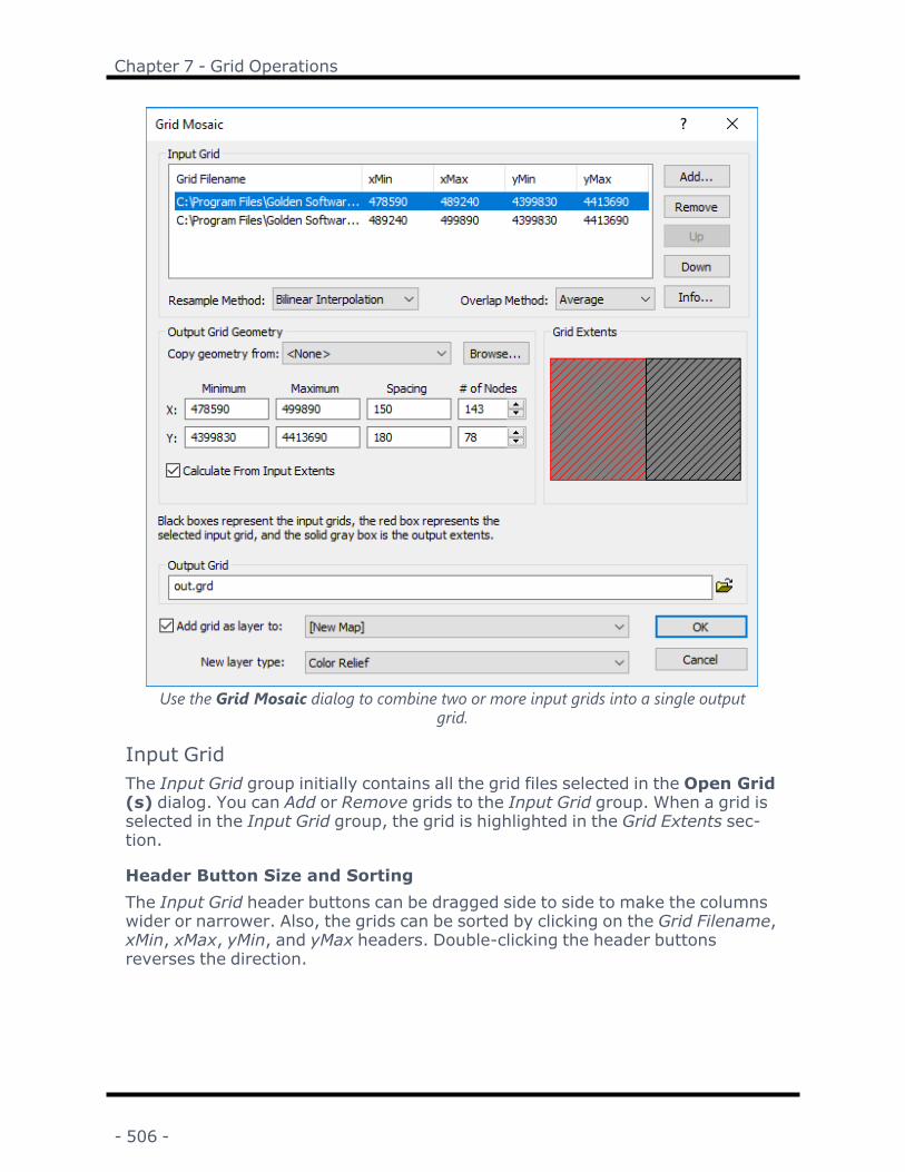
Chapter 7 - Grid Operations
Use the Grid Mosaic dialog to combine two or more input grids into a single outputgrid.
Input GridThe Input Grid group initially contains all the grid files selected in the Open Grid(s) dialog. You can Add or Remove grids to the Input Grid group. When a grid isselected in the Input Grid group, the grid is highlighted in the Grid Extents sec-tion.
Header Button Size and SortingThe Input Grid header buttons can be dragged side to side to make the columnswider or narrower. Also, the grids can be sorted by clicking on the Grid Filename,xMin, xMax, yMin, and yMax headers. Double-clicking the header buttonsreverses the direction.
- 506 -

Surfer User's Guide
AddClick the Add button to open the Open Grid(s) dialog and add additional gridsto the mosaic. Added grids will be listed in the Input Grid Files section. All gridsmust be in the same coordinate system. For example, this means that 30 meterDEM files must be in the same UTM zone.
RemoveSelect a grid and click the Remove button to remove a grid from the mosaic. Onegrid can be removed at a time.
Up and Down ButtonsAlternatively, the grids can be moved around the list by highlighting a grid name(click on it) and then clicking the Up and Down buttons.
InfoClick the Info button to obtain information about the selected grid, including thegrid file name and statistics. If the grid file is large, click OK in the message boxthat appears to create a detailed grid report or click Cancel to create a shorter,less detailed grid report.
Resample MethodsThere are three Resample Methods from which to choose: Bilinear Interpolation,Nearest Neighbor, and Cubic Convolution.
Overlap MethodWhen grids overlap, choose an Overlap Method to determine the value of thegrid node in the new grid: Average, First, Last, Minimum, Maximum, or Sum. TheFirst and Last are the first and last grids listed in the Input Grid Files section.
Output Grid GeometryOutput Grid Geometry defines the grid limits and grid density. Grid limits are theminimum and maximum X and Y coordinates of all grid files. The default grid Spa-cing is set to the minimum spacing of the input grids. The # of Nodes in the X dir-ection is the number of grid columns, and the # of Nodes in the Y direction is thenumber of grid rows. Increasing the grid extents will not increase the grid as theresampling methods do not extrapolate beyond the extents of the original grid.
Copy GeometryThe Copy geometry from option copies the grid geometry from an existing maplayer or grid file. This option is useful when creating grids that will become over-laid map layers, processed with the Grid Math command, or used to calculate avolume between two surfaces. TheMath and Volume commands require theinput grids to have the same geometry.
- 507 -

Chapter 7 - Grid Operations
To copy the geometry from an existing layer, select the layer in the Copy geo-metry from list. To copy the geometry from a grid file, click Browse and selectthe file in the Open Grid dialog. Select <None> to return the Output Grid Geo-metry options to their default values and to manually edit the grid geometry.
Calculate From Input ExtentsCheck the Calculate From Input Extents box to return the grid to its original sizebased on the input grids' minimum and maximum.
Grid ExtentsThe Grid Extents group graphically displays the Input Grid files. Each grid that isadded to the Input Grid files group is displayed in the Grid Extents group. Blackboxes represent input grids. Red boxes represent the selected input grid. Thesolid gray box represents the output extents. The input grid boxes can be clickedwith the mouse to graphically select the grid in the Grid Extents group. Altern-atively, select a grid file in the Input Grid files group to select a grid box.
Output GridChoose a path and file name for the grid in the Output Grid section. You can type
a path and file name, or click the button to browse to a new path and enter afile name in the Save Grid As dialog.
Add New Map or LayerCheck the Add grid as layer to check box to automatically add the created grid toa new or existing map. Select [New Map] in the Add grid as layer to field to cre-ate a new map. Click the current selection and select an existing map to add anew layer to the map. Select the layer type by clicking the current selection inthe New layer type field and selecting the desired layer type from the list.
Note: If you are saving the grid file in the DEM grid format, clear the Add grid aslayer check box and add the map or layer with a Home | New Map or Home |Add to Map | Layer command.
To Combine (Mosaic) Grids1. Click the Grids | Resize | Mosaic command or the button.2. Select the files you would like to combine in the Open Grid(s) dialog. If the
grid files are in the same folder, use the CTRL and SHIFT keys while clickingon the file names to make multiple selections. If the files are not in the samefolder, you will have the opportunity to select more files later. Click Open
3. In the Grid Mosaic dialog, choose the desired Resample method and Over-lap method. You can also set the Output Grid Geometry .
4. Name the new grid in the Output Grid box by typing a path and file name or
using the button to browse to a new path.5. Click OK and the new grid is created.
- 508 -

Surfer User's Guide
Mosaic Tipsl When a NoData node overlaps a node with a value, the NoData node isignored.
l The default output grid spacing is set to the minimum spacing of the inputgrids.
l By specifying First for the Overlap Method, a second overlapping grid can beused to fill in NoData values in the first grid.
l Some grid files, such as USGS DEM files, are not seamless. Occasionally, agrid node is missing along an edge. Sometimes, the reported corner pointsfor adjacent files are slightly different, which causes the neat lines betweengrids to be slightly off, which causes some edge nodes to be excluded fromboth grids. This shows up as a NoData node along the seam.
l It is possible to resample a single grid with Grids | Resize | Mosaic by spe-cifying a single grid and changing the grid spacing.
Grid Mosaic and .GSR2 FilesWhen the input .GRD file for a Grids | Resize | Mosaic command has a defined.GSR2 file with coordinate system information, the information from the firstinput .GRD file is used for the output .GRD file. All .GRD files should be in thesame coordinate system. The Export Options dialog appears with the option tosave the coordinate system information. It is recommended to check the GSReference (Version 2) file if you intend to use the grid file in Surfer, as the GSR2retains all of the information needed. The grid has the same coordinate systemas the original file, but the .GSR2 is required to define the coordinate system.
Resample MethodsWhen using Grids | Resize | Mosaic, Surfer uses resampling methods to assigndata values in the new grid. For each grid node location in the output grid (X, Y)the Z value is located in the set of input grids. The Z value is computed accordingto the specified resample method.
Note that all resample methods are exact interpolators - that is, if the X, Y loc-ation falls exactly on a grid node, the grid node’s Z value is returned. If morethan one grid can supply a Z value at the specified X, Y position, they are com-bined according to the specified Overlap Method.
The resampling methods do not extrapolate outside the grid limits. This meansthat NoData nodes may be inserted between adjacent input grids if the inputgrids to not each include the common boundary.
Nearest NeighborThe Nearest Neighbormethod applies the closest grid node value on the originalgrid to the grid node value in the new grid. When the original grid and the new
- 509 -

Chapter 7 - Grid Operations
grid differ in size, more than one original node may be applied to the new gridand some original grid cells may not be applied to the new grid.
The Nearest Neighbormethod is the fastest resampling method, though it canresult in distorted output if the original grid and new grid differ in size.
Bilinear InterpolationThe Bilinear Interpolationmethod uses a weighted average of four nodes in theoriginal grid and applies this to the new grid node. The new grid is smoothed com-pared to the original grid.
Cubic ConvolutionThe Cubic Convolutionmethod uses a weighted average of 16 nodes in the ori-ginal grid and applies this to the new grid. The new grid is smoother than the ori-ginal grid. This method is best for continuous data. This is the slowestresampling method, but it results in a sharper grid than the Bilinear Interpolationor the Nearest Neighbormethods.
Grid ExtractThe Grids | Resize | Extract command creates a subset of an existing grid file.Grid files consist of rows and columns (lines of constant Y and X value) con-taining Z values. When you extract information from a grid file, you can specifythe starting and ending rows and columns to extract. For example, you can cre-ate a new grid file that consists of only the center portion of an existing grid byspecifying the middle columns and rows from the original grid.
Consider a grid file that has 100 rows and 100 columns. You might want to cre-ate a grid that contains the information from row 25 to row 75 and column 25 tocolumn 75. In this example, specify 25 as the first row and first column to extractand 75 as the last row and last column to extract. The grid file you create in thiscase would consist of 51 rows and 51 columns of data (from 25 to 75 rows andcolumns, inclusive).
Subsets can also be based on every nth row or column read from the input gridfile, reducing the density of the grid. In this case, you specify a step factor thatskips rows and columns when reading information from the original grid file.
Extract Grid DialogClick the Grids | Resize | Extract command or the button to open the OpenGrid dialog. Select a grid file and click Open to open the Extract Grid dialog.
- 510 -
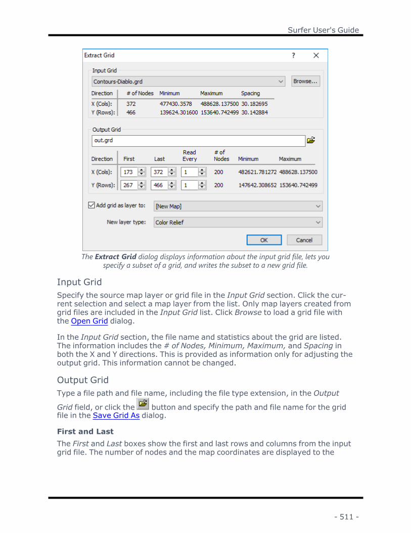
Surfer User's Guide
The Extract Grid dialog displays information about the input grid file, lets youspecify a subset of a grid, and writes the subset to a new grid file.
Input GridSpecify the source map layer or grid file in the Input Grid section. Click the cur-rent selection and select a map layer from the list. Only map layers created fromgrid files are included in the Input Grid list. Click Browse to load a grid file withthe Open Grid dialog.
In the Input Grid section, the file name and statistics about the grid are listed.The information includes the # of Nodes, Minimum, Maximum, and Spacing inboth the X and Y directions. This is provided as information only for adjusting theoutput grid. This information cannot be changed.
Output GridType a file path and file name, including the file type extension, in the Output
Grid field, or click the button and specify the path and file name for the gridfile in the Save Grid As dialog.
First and LastThe First and Last boxes show the first and last rows and columns from the inputgrid file. The number of nodes and the map coordinates are displayed to the
- 511 -

Chapter 7 - Grid Operations
right. As you change the First and Last values, the number of nodes and mapcoordinates change accordingly.
Read EveryThe Read Every boxes specify a skip factor to "thin out" a grid. A value of onereads every row or column within the selected limit. A value of two reads everyother row or column, and so on.
Add New Map or LayerCheck the Add grid as layer to check box to automatically add the created grid toa new or existing map. Select [New Map] in the Add grid as layer to field to cre-ate a new map. Click the current selection and select an existing map to add anew layer to the map. Select the layer type by clicking the current selection inthe New layer type field and selecting the desired layer type from the list.
Note: If you are saving the grid file in the DEM grid format, clear the Add grid aslayer check box and add the map or layer with a Home | New Map or Home |Add to Map | Layer command.
Extracting a Subset of an Existing Grid File1. Click the Grids | Resize | Extract command or the button.2. In the Open Grid dialog, select the grid file from which you want to extract a
subset and click Open.3. In the Extract Grid dialog, specify the First, Last, and Read Every values in
the Rows (Y) and Cols (X) boxes.
4. Click the button to display the Save Grid As dialog.5. In the Save as type list, select the format for the output file. Specify the path
and file name for the file to be created, and click Save .6. In the Extract Grid dialog, click OK and the grid is created with the subset of
grid information from the original grid file.
Grid Extract and .GSR2 FilesWhen the input .GRD file for a Grids | Resize | Extract command has a defined.GSR2 file with coordinate system information, this information is used for theoutput .GRD file. The Export Options dialog appears with the option to save thecoordinate system information. It is recommended to check the GS Reference(Version 2) file if you intend to use the grid file in Surfer, as the GSR2 retains allof the information needed. The grid has the same coordinate system as the ori-ginal file, but the .GSR2 is required to define the coordinate system.
- 512 -

Surfer User's Guide
Grid Info
The Grids | Info | Grid Info command or the button in the plot windowallow you to select a .GRD file and display the file name, grid size in rows xcolumns, and grid X, Y, and Z minimums and maximums. If the grid file containsmore than 40 million nodes, you are asked if you wish to create a detailed reportor a quick report. Click Yes in the message to create a detailed grid report, orclick No to create a shorter quick grid report. This is the same basic informationas displayed in the Grid Editor window with the Grid Editor | Options | Grid Infocommand.
The Open Grid dialog also displays the Grid Info of the selected grid. The OpenGrid dialog displays the following Grid Info: Name, Format, Size, xMax, yMax,zMax, xMin, yMin, and zMin.
Grid Info DialogThe Grid Info dialog is displayed after clicking the Grid Info command or the
button.
Select the grid for calculating grid statistics.
Input GridSpecify the source map layer or grid file in the Input Grid section. Click the cur-rent selection and select a map layer from the list. Only map layers created fromgrid files are included in the Input Grid list. Click Browse to load a grid file withthe Open Grid dialog.
- 513 -
Chapter 7 - Grid Operations
Polygon BoundarySpecify the region or regions from which to calculate the statistics in the PolygonBoundary section. Select either a map layer or vector file in the Polygon Bound-ary section:
l Click the current selection and select a base layer from the list. Only base lay-ers that contain at least one polygon or polyline will be included in the list.The base layer must use the same source coordinate system as the grid.
l Click Browse to load a vector file with the Open dialog. The file must use thesame coordinate system as the grid.
The number of polygons and vertices is displayed below the Polygon boundaryonce a file or map layer has been selected. If the boundaries have blanking flagsor BLN_Flag attributes, the total number of inside and outside flags is displayed.
Polyline BoundariesPolylines can be used for polygon boundaries. The polylines in the base layer orvector file will be treated as polygons while assigning regions for calculating stat-istics. The Grid Info command is not recommended with open polylines, unex-pected results my occur. Consider converting polylines to polygons with thePolyline to Polygon command and editing features with the Reshape command.
If the layer you wish to use contains both polygons and polylines, but you onlywish to use some or all of the polygons, select the objects you wish to use beforeclicking Grids | Info | Grid Info and select the Selected objects only option. Ifthe file you wish to use contains both polylines and polygons, first load the file asa base layer, and then use the Grid Info command with the Selected objectsonly option.
Inside, Outside, or MixedSelect Inside to use the region inside the polygon boundary or boundaries to cal-culate statistics. Select Outside to use the region outside the polygon boundaryor boundaries. Select Mixed to use the blanking flag or BLN_Flag attribute valuesfrom the file or layer. The Mixed option is only available when the layer or file con-tains both blanking flags or BLN_Flag attributes: assign NoData inside (1) andassign NoData outside (0). If all blanking flags or BLN_Flag attributes are thesame, the Inside or Outside option is selected automatically, and the Mixedoption is not available.
Selected Objects OnlySelect the Selected objects only option to use only the selected objects in thebase layer to calculate statistics. When the Selected objects only box is checked,the Loaded polygons and vertices values are updated. Select a base layer in thePolygon Boundary field to use the Selected objects only option. The Selectedobjects only option is not available when the Polygon Boundary is a vector file.The polygon or polygons must be selected before clicking the Grids | Info |Grid Info command.
- 514 -

Surfer User's Guide
Combine All PolygonsCombine all polygons is checked by default and the statistics will be calculatedfor the total of all the polygons. When Combine all polygons is unchecked, thereport presents statistics for each polygon.
Filtering Grid FilesSurfer contains filtering commands which operate on grid files, or on contours ina contour map. These commands round out angular contours, eliminate noise ina map, or change the density of a grid.
These are the smoothing methods available in Surfer:
l Filter contains predefined filtering options and also allows you to defineyour own filtering schemes.
l Spline Smooth is best for eliminating angular contours or surfaces; thisoperation fills in a sparse grid. For example, a 10 x 10 grid might result invery angular contours on a contour map produced from the grid. By increas-ing the grid density using the Grids | Edit | Spline Smooth command,the 10 x 10 grid can be expanded to a 50 x 50 grid. The 50 x 50 grid pro-duces a much smoother appearing contour map than the 10 x 10 grid.
l The Smooth tool in the Grid Editor smooths the grid with a 3x3 averagingfilter.
l Contour Smoothing smooths contour lines of a contour map by smoothingthe grid file or changing the contour map properties.
Filter Data Before GriddingTo filter your data before gridding, use the data filters in Grids | New Grid | GridData.
Grid Operations ReferencesAkai, Terrence J., (1994), Applied Numerical Methods for Engineers, John Wileyand Sons, Inc., New York, 410 pp.
Bras, R. L., and I. Rodriguez-Iturbe, (1985), Random Functions and Hydrology,Addison-Wesley, Reading, Massachusetts, 559 pp.
Mitasova, Helena and Jaroslav Hofierka, (1993), Interpolation by RegularizedSpline with Tension: II. Application to Terrain Modeling and Surface GeometryAnalysis, Mathematical Geology, v. 25, no. 6, p. 657-669.
- 515 -

Chapter 7 - Grid Operations
Moore, I. D., R. B. Grayson, and A. R. Ladson, (1991), Digital Terrain Modeling:A Review of Hydrological, Geomorphological and Biological Applications, Hydro.Proc., v. 5, no. 1, p. 3-30.
Moore, I. D., A. Lewis, and J. C. Gallant, (1993), Terrain properties: EstimationMethods and Scale Effects, Modeling Change in Environmental Systems, A.J.Jakeman et al. editors, John Wiley and Sons, New York.
Press, William H., Saul A. Teukolsky, William T. Vetterling, and Brian P. Flannery,(1992), Numerical Recipes in C: The Art of Scientific Computing, Second Edition,Cambridge University Press, New York, 994 pp.
Ripley, B. D., (1981), Spatial Statistics, John Wiley and Sons, New York, 252 pp.
Schwartz, Abraham, (1974), Calculus and Analytic Geometry, 3rd edition, Holt,Rinehart, and Winston, New York, 1140 pp.
Tuma, Jan J., (1979), Engineering Mathematics Handbook, 2nd edition, McGraw-Hill Book Company, New York, 394 pp.
- 516 -

Chapter 8 - Base Maps
Base MapBase maps display geographic and political information such as roads, streams,lakes, or state and county boundaries. Base maps can be combined with anyother map type in Surfer. A vector base map or raster base map is automaticallycreated based on the input data.
This map shows multiple base layers, depictingroads, waterways, and a USGS urban area satellite
image for Golden, Colorado, USA.
Base (vector) LayersBase (vector) layers are created when a vector data file is used to create a basemap. Vector files draw objects at precise X, Y locations on a map and can containpoints, polygons, polylines, and text.
SymbologyVector base maps can also include symbology. Symbology uses symbols or col-ors to display statistical information about the features in the base layer. Sym-bology applies line, fill, and/or symbol properties to features in the base layerdepending on an attribute value. The symbology can be included in a legend. Thetype of symbology and the symbols' appearance are controlled in the Sym-bology dialog. Click Edit Symbology in the Base (vector) layer Properties
- 517 -

Chapter 8 - Base Maps
window General page to open the Symbology dialog. These are the symbologytypes in Surfer:
l Unique Values - Line, fill, and/or symbol properties are specified for uniquevalues in the attribute field.
l Unclassed Colors - Colors from a color spectrum are applied to the featuresby numeric attribute value.
l Unclassed Symbols - Symbols are added for each polygon feature and scaledproportionally by numeric attribute value, or point features are scaled bynumeric attribute value. Unclassed Symbols symbology is not applied to poly-lines.
l Classed Colors - Colors are applied to the features by classifying numericattribute values.
l Classed Symbols - Symbols are added for each polygon feature and classifiedby a numeric attribute value, or point features are classified by a numericattribute value. Classed Symbols symbology is not applied to polylines.
l Pie Chart - Attributes in the base layer are added as Pie Chart symbols withclassified pie slices.
Editing FeaturesSome base maps consist of multiple objects (i.e. polygons, polylines, text, etc.).The sub-objects can be selected individually in the Contents window and editedin the Properties window. The expansion state of sub-objects in the Contentswindow is retained in the Surfer .SRF file. Use the Expand new Contents windowitems option in the Options dialog to control the expansion state of new objectsin Contents window.
Moving FeaturesFeatures such as points, polylines, and polygons can be moved between base(vector) layers and other base (vector) layers the plot document. TheMove/Copy to Layer command can be used to move or copy features. Featurescan also be moved in the Contents window. To move a feature to another base(vector) layer, select the feature and drag it to a new position within anotherbase (vector) layer. To move a feature to the plot document, select the featureand drag it to a new position above, between, or below the top-level objects inthe Contents window.
Base Layers with Vector and Raster DataWhen importing a file that includes both vector and raster data, such as withsome DXF or GSI files, a base (vector) layer is created. In this case, the imageproperties are controlled by clicking the Image object in the Contents window.
- 518 -

Surfer User's Guide
Base (raster) LayersBase (raster) layers are created when an image file is used to create a base map.An image file is a raster data file where the cell values correspond to pixel color.Rasters files where the cell values describe other information, such as elevation,are used to create grid-based maps. Some images files are georeferenced,where the image includes real world coordinates. Base (raster) layers can begeoreferenced in Surfer.
Georeferencing is necessary to place unreferenced images in the correct relativeposition in the coordinate system. Occasionally you may need to adjust a geor-eferenced image. Georeference an image by selecting the base (raster) layerand clickingMap Tools | Layer Tools | Georeference Image. You can alsoright-click the base layer in the Contents window or plot window and click Geor-eference Image in the context menu. Finally, you can georeference a base (ras-ter) layer by clicking Georeference image in the General page for the base(raster) layer. The image must be at least 2x2 pixels to be georeferenced.
If you need to add vector features to a map with a base (raster) layer, add anempty base layer to the map.
Creating Base MapsThere are four commands for creating new base maps:
l The Home | New Map | Base command or the button create base mapsfrom existing vector or image files. Use the base map properties in the Prop-erties window to set the base map line, fill, symbol, font, and opacity prop-erties. With some images, you can also reassign the base map coordinates.You can also set the base map coordinate system.
l The Home | New Map | Base | Base from Data command or the but-ton create a base map from a data file. A data file containing XY data is usedto create points in the base layer. Other data in the data file is added to thepoints as attribute data.
l The Home | New Map | Base | Base from Server command or thebutton allows you to download an image or vector data as a base map froman online web mapping server.
l The Home | New Map | Base | Empty Basemap command or the but-ton create an empty base map with the intention of creating new geometrywithin the empty base map limits.
For example, the following steps are used to create a new base map from anexisting file:
1. Click the Home | New Map | Base command, click the Home | New Map| Base | Base from Data command, click the Home | New Map | Base |Base from Server command, or click the Home | New Map | Base |Empty Basemap command.
- 519 -

Chapter 8 - Base Maps
2. Depending on which command was used, a dialog is respectively displayed.l For the Base command, the Import dialog is displayed with a list of filesin all the format types that can be imported. Select a file in the list andclick the Open button. Sometimes an Import Options dialog for thefile type is displayed. Make any changes to the import options and clickOK.
l For the Base from Data command, the Base from XY Data dialog is dis-played. Specify the rows to include and set the X and Y data columns.Click OK to create a base layer.
l For the Base from Server command, the Download Online Maps dia-log is displayed. Select or add the server and layer, specify the area todownload and resolution, and click OK to download the server basemap.
l For the Empty Basemap command, the Base Map Limits dialog is dis-played. Set the Minimum and Maximum X and Y values and click OK. Anew empty base map is created.
The map is automatically created with reasonable defaults. Base maps arenamed with the name of the file from which the base map was created, such asBase(vector)-CentralCalifornia.gsi. New empty base maps are named Base.Base maps from servers are named with the map server name, such as Base(ras-ter)-Orthoimagery/USGS_EDC_Ortho_NAIP or Base(vector)-Interstate. In addi-tion, the image downloaded with the base map from server adds attributeinformation, including the server name and layer title.
Adding Base LayersSelect one of the four Add to Map base layer commands to add a base layer to anexisting map:
l The Home | Add to Map | Layer | Base command adds a base map layerto the selected map.
l The Home | Add to Map | Layer | Base from Data command adds abase map layer from an XY data file to the selected map.
l The Home | Add to Map | Layer | Base from Server command allowsyou to add an image base map from an online web mapping server. Whenadding a base map layer from a server to an existing map with a definedcoordinate system, the Specify Latitude/Longitude extents option is auto-matically selected. The boxes are filled in with the map limits of the currentmap.
l The Home | Add to Map | Layer | Empty Base command allows you toadd an empty base map layer to an existing map.
Editing an Existing Base MapTo change the features of a base map, click once on the base map to select it.The properties are displayed in the Properties window.
- 520 -

Surfer User's Guide
Base (vector) Layer PropertiesThe vector base layer properties contains the following pages:
GeneralLabelsLayerCoordinate SystemInfoIndividual objects in the vector base layer may have other pages, such as Line,Fill, or Text. Each object also has a Info page.
Base (raster) Layer PropertiesThe raster base layer properties contains the following pages:
GeneralLayerCoordinate SystemInfo
Map PropertiesThe map properties contain the following pages:
ViewScaleLimitsFrameCoordinate SystemInfo
Base Map from DataClick the Home | New Map | Base from Data command or the button tocreate a new base map from an XY data file. Click the Home | Add to Map |Layer | Base from Data orMap Tools | Add to Map | Layer | Base fromData to add a base layer from an XY data file to an existing map. Each XY datapoint in the file is represented by a point object in the base map. Any othercolumn data is added as attributes to the points in the base layer. If the data fileincludes a header row, the headers will be used for attribute names. The data filemust contain at least two rows and two columns of data to create a base map.
The points in the base map can be edited, queried, and geoprocessed with theFeatures tab commands.
To create a base map from XY data,
- 521 -

Chapter 8 - Base Maps
1. Click the Home | New Map | Base | Base from Data command.2. Select the data file in the Open Data dialog and click Open.3. The Base from XY Data dialog is displayed.4. Specify the rows you wish to include in the base layer and which columns con-
tain the X and Y coordinates.5. Click OK.
Base from Data Layer vs Post LayerThe Base from Data, post, and classed post layer types use XY data files to cre-ate map layers. Post and classed post layers are a single object, and thereforepost and classed post maps use less memory and are faster to render. Post orclassed post maps should be used for large data files. Post and classed postmaps have more control over labels and can be included in legends. Base layersinclude each point as an object. These point objects can be edited and queriedafter creating the base layer. The points in the base layer also retain attributeinformation, and therefore a symbology can be applied to the base layer.
Base from XY Data DialogThe Base from XY Data dialog is displayed when creating a base layer. Specifythe rows you wish to include in the base layer and which columns contain the Xand Y coordinates in the Base from XY Data dialog.
Specify data rows and columns in the Base from XY Data dialog.
Data RowsThe Data Rows group controls which rows from the data file are included in thebase layer.
- 522 -

Surfer User's Guide
FirstSpecify the first row you wish to include in the base layer in the First field. Typethe row number in the First field or click the buttons to change the value.
LastSpecify the last row you wish to include in the base layer in the Last field. Typethe row number in the Last field or click the buttons to change the value.
FrequencySpecify the number of rows included between the first and last row in the Fre-quency field. Use the Frequency field to reduce the number of points createdfrom large data files. A Frequency of 1 includes every row. A Frequency of 2includes every second row after the First row. A Frequency of 3 includes everythird row, 4 includes every fourth row, etc. The First row is always included.
For example the Demogrid.dat sample data file includes a header row and 47rows of XYZ Data. When First is set to 1, Last is set to 48, and Frequency is set to2, rows 1, 3, 5, 7, ...47 are included in the base map. For Demogrid.dat row 1 isexcluded because it is a header and contains text data. When First is set to 2,Last is set to 48, and Frequency is set to 2, rows 2, 4, 6, ...48 are included in thebase map.
AllCheck the All check box to include all data in the data file in the base map. TheFirst value will change to 1, the Last value will change to the last row containingdata, and the Frequency will change to 1 when the All check box is clicked.
Data ColumnsThe Data Columns group controls which columns are used for the X and Ycoordinates when creating the base layer.
X and Y CoordinatesSpecify the column containing X coordinates in the X field. Click the current selec-tion and click the desired column in the list to change the value. Only columnscontaining data will be included in the X list. Specify the column containing Ycoordinates in the Y field. Click the current selection and click the desired columnin the list to change the value. Only columns containing data will be included inthe Y list. If the data file contains a header row, the column names will beincluded next to the column letter.
View DataClick View Data to view the data file in a read-only worksheet window. This win-dow is useful if you need to see the data before determining the X and Y columnsor what you want to use for First, Last, and Frequency values.
- 523 -

Chapter 8 - Base Maps
View DataThe View Data button in the Grid Data and Base from XY Data dialogs displays apreview of the data file in the View Data dialog. Use the View Datadialogto besure you are selecting the correct X, Y, and Z data columns in the Grid Data orBase from XY Data dialog.
The View Data dialog displays a preview of the data file.
Base Map from ServerClick the Home | New Map | Base | Base from Server command or thebutton, the Home | Add to Map | Layer | Base from Servercommand, ortheMap Tools | Add to Map | Layer | Base from Server command to down-load a base map from an online web server. Clicking one of the preceding com-mands opens the Download Online Maps dialog. Use the Download OnlineMaps dialog to select the server, map extents, and image resolution.
When using the Download Online Maps dialog, a server with appropriate datamust be selected. Surfer currently supports four types of servers, web mappingservice (WMS), Open Street Map (OSM), web coverage service (WCS), and webfeature service (WFS). WMS, OSM, WCS, and WFS servers provide differenttypes data.
l When selecting a WMS or OSM server, an image is downloaded to be used asa base (raster) layer.
l When selecting a WCS server, data values are downloaded to be used as agrid file. WCS servers cannot be used with the Base from Server command.Use the Grid from Server command or the Download button in the Open Griddialog instead.
- 524 -

Surfer User's Guide
l When selecting a WFS server, vector data is downloaded with points, poly-lines, and/or polygons representing features in a base (vector) layer.
Empty Base MapThe Home | New Map | Base | Empty Basemap command or the buttoncreate an empty base map. An empty base map is often created with the inten-tion of creating new geometry within the base map limits. The Home | Add toMap | Layer | Empty Basemap command adds an empty base map layer toan existing map. When an empty base layer is added to an existing map, thebase layer is created with the same coordinate system as the map frame.
Base Map Limits DialogThe Home | New Map | Base | Empty Basemap command opens the BaseMap Limits dialog.
Use the Base Map Limits dialog to specifyMinimum and Maximum values.
Minimum and Maximum X and YEnter the limits of the new empty base map in the Minimum and Maximum boxesfor the X and Y coordinates. This specifies the initial limits of the new base map,but may be overridden on the map Limits page later if needed.
Export Drawn Objects in Map UnitsTo export drawn objects in map units, you can either draw them on a base layerand export that layer or you can turn off the visiblity of the map and export thedrawn objects in map units. To move or scale drawn objects with the map, youcan either add draw them on a base layer, export the objects and import them asa new base layer, or copy/paste them into a base layer.
To draw objects on a base layer:
- 525 -

Chapter 8 - Base Maps
1. Select your existing map and click Home | Add to Map | Layer | EmptyBase.
2. Click the Features tab and select the item you want to draw (text, poly-lines, polygons, symbols, etc).
3. Draw the objects over the map. Create as many objects as you wish.
4. If you want a separate base map file with these objects, hide the originalmap layer and all the axes in the Contents window (clear their visibilitycheck boxes), and click File | Export to export the new base layer anddrawn objects to a new file (e.g. BLN or DXF).
If the objects are already drawn on top of the map, and you just want to exportthem in map units, you can turn off the visiblity of the map and export theobjects. To do this:
1. Clear the map layer visibility check box in the Contents window, so it isinvisible. Hide any other objects, so only the objects you want to export arevisible.
2. Click File | Export.
3. Give the file a name, choose the export format and click Save.
4. In the Export Options dialog, select Map as the Scaling source. The FileRectangle coordinates should update with map units.
5. Click OK the file is exported. You can turn on the visibility of the map.
If the objects are already drawn on top of the map, and you want to add them tobe part of the map to be moved and scaled with the map, you can either exportthe objects (as above) and then add them as a new base layer to the map. Or,you can create a new base layer and then copy and paste them into it. If youcopy and paste them, any formatting of the objects (e.g. fill color, fill pattern)will be retained. To do this:
1. Select the drawn objects to be added and click Home | Clipboard | Copy.
2. Select the map and click Home | Add to Map | Layer | Empty Base.
3. Click Home | Clipboard | Paste. The objects are pasted in the baselayer.
4. Select the pasted objects and move them so that they are directly over theoriginal objects. To move them, you can click and drag, arrow keys on thekeyboard or type the object locations into the X: and Y: fields in the Pos-ition/Size Toolbar.
- 526 -

Surfer User's Guide
5. You can delete the original objects if you wish, or hide them by clearingtheir visibility check boxes in the Contents window.
6. If you want a separate base map file with these objects, hide the originalmap layer and all the axes in the Contents window, select the map andclick File | Export. In the Export dialog, check Selected objects only, andexport the base layer with the drawn objects to a new file (e.g. BLN orDXF).
Placing Boundaries on Other MapsBase maps can be used to place boundary features on any type of map. To placeboundary lines on a map, add a base map layer to the existing map with theMapTools | Add to Map | Layer | Base command.
CoordinatesIn Surfer, you can use map layers with different coordinate systems by settingthe source coordinate system for each map separately. Surfer displays the mapin the target coordinate system by changing the view of the individual maps. Forexample, consider a contour map based on latitude/longitude coordinates. Tooverlay a boundary map on the contour map, the boundary map must cover thesame general range as the contour map. But, the coordinate system can be anycoordinate system for this location. For example, the CoordinateSystems.srfsample file includes three layers with two different source coordinate systems.
Limits and ScaleWhen you overlay maps, if the new map limits exceed that of the current maplimits, Surfer gives you the option to adjust the map limits to include all layers.
To add a boundary base map to another map:
1. Create a map with the Home | New Map command. The grid file shoulduse limits that cover the same general extent as the boundary base map.
2. Select the map and click theMap Tools | Add to Map | Layer | Basecommand to add a base map layer.
3. In the Import dialog, select your boundary file and click the Open button.
4. Set any file import properties, if required, and click OK.
5. To clip the map to specific limits, click on the Map object in the Contentswindow.
- 527 -

Chapter 8 - Base Maps
6. Open the Limits page in the Properties window, or use the Map Tools | MapTools | Set Limits command.
7. If necessary, set the scale on the Scale page.
The map automatically redraws to the new limits and size.
Changing Properties in a Base MapProperties can be assigned to base map polylines, polygons, text, symbols, orimages. Any properties you assign are applied to all the objects in the base map.The only properties that can be changed in images are the coordinates.
Change All ObjectsTo change the properties of all objects in a base map:
1. Click on the Basemap layer in the Contents window.
2. On the General page in the Properties window, click the button next tothe type of property you want to change (i.e. Line Properties, Fill Prop-erties, Font Properties, or Symbol Properties). If the option is not present,the base map does not contain any objects of that type. For example, if thebase map does not contain any polygons, the Fill Properties option is notavailable.
3. Specify the properties you want to assign to the objects in the base map.
The base map is automatically redrawn. The specified properties are applied toall the polyline, polygon, text, or symbols in the base map.
- 528 -

Surfer User's Guide
Select the Base map layer to change properties for all of theobjects.
Change One ObjectTo change the properties of an individual object in a base map:
1. Click the object within the base map layer (i.e. Polygon, Polyline, etc.) inthe Contents window.
- 529 -

Chapter 8 - Base Maps
2. Make changes to the properties available for that object on the appropriatepage (i.e. Line page, Fill page, etc.) in the Properties window.
The property change is automatically shown for the individual object.
Select the sub-object to change individual properties.
Changing Multiple ObjectsTo change the properties of multiple objects in a base map:
1. Click the Basemap layer in the Contents window.2. Use the SHIFT or CTRL key to select multiple sub-objects of the base map
layer.3. The shared properties are displayed in the Properties window. Make
changes as needed. The objects will automatically update to reflect the newproperties.
Base (vector) Layer General PropertiesThe General page in the base map properties contains options for setting fea-ture properties. The properties can be applied based on attribute values, or prop-erties can be the same for all objects within the layer.
The base map properties General page contains the following options:
- 530 -

Surfer User's Guide
The General page specifies the Input file, Sym-bology, and shared properties.
Input FileThe Input File lists the current file used in the base map.
Change File
Click the button to display the Import dialog. This allows you to select a newfile or an updated version of the current file used to create the base map. If thefile exceeds the current map limits, you will be prompted to adjust the map lim-its.
A vector file must be selected when changing the Input file for a base (vector)layer. An error message will be displayed if a raster file is selected in the Importdialog. If you wish to add an image to the map, select the Home | Add to Map| Layer | Base command instead.
Coordinate System NoteRegardless of the file selected with either the File | Reload Map Data com-
mand or by clicking the button in the Properties window, the coordinate sys-tem for the original map layer is used after updating the file. If this is not thecorrect coordinate system, click on the map layer to select it. In the Propertieswindow, click on the Coordinate System tab and set the coordinate system tothe appropriate new system.
Save File
The button displays the Export dialog. Type a File name and change the Saveas type to the desired file format. Click Save. For some file types, a file type spe-cific Export Options dialog appears. The Export Options dialog Spatial
- 531 -
Chapter 8 - Base Maps
References and Scaling pages are available when saving a base layer. Check thedesired file formats. It is recommended that GS Reference (Version 2) file optionbe checked to generate a .GSR2 file. Set any export options and click OK to savethe file.
Attribute for Object NameThe Attribute for object name shows the attribute field from the Attribute Table.The default is None. The names shown in the Contents window for the objects inthe base layer correspond with their attribute value from the attribute field selec-ted. Objects without attribute values are named according to their object type,e.g. Polygon. All objects are named according to their object type when None isselected. Changes made to the object's attribute value in the attribute table willbe shown in the object's name in the Contents window when the attribute fieldis selected. Changing an object name in the Contents window using RenameObject does not change the object's attribute value.
Reset Object NamesTo reset all custom object names, click the Reset button to return the objectnames to their attribute values.
SymbologySymbology uses symbols or colors to display statistical information about the fea-tures in the base layer. Symbology applies line, fill, and/or symbol properties tofeatures in the base layer depending on an attribute value. The type of sym-bology and the layer's appearance are controlled in the Symbology dialog. ClickEdit Symbology in the Base (vector) layer Properties window General page toopen the Symbology dialog. These are the symbology types in Surfer:
l Unique Values - Line, fill, and/or symbol properties are specified for uniquevalues in the attribute field.
l Unclassed Colors - Colors from a color spectrum are applied to the featuresby numeric attribute value.
l Unclassed Symbols - Symbols are added for each polygon feature and scaledproportionally by numeric attribute value, or point features are scaled bynumeric attribute value. Unclassed Symbols symbology is not applied to poly-lines.
l Classed Colors - Colors are applied to the features by classifying numericattribute values.
l Classed Symbols - Symbols are added for each polygon feature and classifiedby a numeric attribute value, or point features are classified by a numericattribute value. Classed Symbols symbology is not applied to polylines.
l Pie Chart - Attributes in the base layer are added as Pie Chart symbols withclassified pie slices.
- 532 -
Surfer User's Guide
None can also be selected. When symbology is not used, the properties are con-trolled for all features in the Properties section of the General page for the baselayer or controlled for individual features in the Line, Fill and/or Symbol Prop-erties window pages.
PropertiesThe Properties section controls the properties for all objects in the base layerwhen no symbology is applied. When Symbology is applied to the objects, theProperties section controls the properties for any object not included in the sym-bology and for properties of the objects that are not determined by the Sym-bology settings. For example, when Unclassed Colors is used for polygonfeatures the polygon fill properties are controlled by the symbology and the poly-gon line properties are controlled in the Properties section.
The Properties section is separated by property type:
l Click the next to Line Properties to adjust the line properties for all objectsin the base layer.
l Click the next to Fill Properties to adjust the fill properties for all objects inthe base layer.
l Click the next to Font Properties to adjust the font properties for all objectsin the base layer.
l Click the next to Symbol Properties to adjust the symbol properties for allobjects in the base layer.
l Click the next to Shadow Properties to adjust the shadow properties for allobjects in the base layer.
If no object exists in the base layer that uses a particular property type, thatproperty type is not displayed.
SymbologyVector base maps can include symbology. Symbology applies line, fill, and/orsymbol properties to features in the base layer depending on an attribute value.The symbology can be included in a legend. The type of symbology and thelayer's appearance are controlled in the Symbology dialog. Click Edit Sym-bology in the Base (vector) layer Properties window General page to open theSymbology dialog. The symbology types in Surfer are:
l Unique Values - Line, fill, and/or symbol properties are specified for uniquevalues in the attribute field.
l Unclassed Colors - Colors from a color spectrum are applied to the featuresby numeric attribute value.
l Unclassed Symbols - Symbols are added for each polygon feature and scaledproportionally by numeric attribute value, or point features are scaled bynumeric attribute value. Unclassed Symbols symbology is not applied to poly-lines.
- 533 -

Chapter 8 - Base Maps
l Classed Colors - Colors are applied to the features by classifying numericattribute values.
l Classed Symbols - Symbols are added for each polygon feature and classifiedby a numeric attribute value, or point features are classified by a numericattribute value. Classed Symbols symbology is not applied to polylines.
l Pie Chart - Attributes in the base layer are added as Pie Chart symbols withclassified pie slices.
Adding Symbology to a Base LayerA symbology can be added to a base (vector) layer by clicking Edit Symbology inthe Properties window General page. Select the symbology type, specify theattribute field for the symbology, and then specify the various line, fill, and/orsymbol properties for the symbology in the Symbology dialog. Click OK or Applyto apply the symbology to the base layer.
To apply symbology, the features in the base (vector) layer must have at leastone attribute field. Any of the five symbology types can be applied to an attributefield that contains numeric data. Unique Values symbology can be applied to textor numeric data. Add or edit attribute data in the base layer with the AttributeTable.
The following example uses the NV2010_Population.gsb sample file to create abase map with a symbology:
1. Create the base map by clicking Home | New Map | Base.2. Select the NV2010_Population.gsb sample file in the Import dialog. The
sample files are located at C:\Program Files\Golden Soft-ware\Surfer\Samples by default.
3. Click Open in the Import dialog. The base (vector) map is created.4. Click Base(vector)-NV2010_Population.gsb in the Contents window to select
the base layer.5. Click General in the Properties window to view the General page.6. Click Edit Symbology in the Symbology field of the Properties window Gen-eral page. The Symbology dialog opens.
7. Click Classed Symbols on the left side of the Symbology dialog to displaythe Classed Symbols page.
8. If Population was not automatically selected in the Attribute field, click thecurrent selection and select Population from the Attribute field list in the Gen-eral properties section.
9. In the Classes properties section, select Natural breaks from the Classmethod list.
10. Click the button to reduce the Class counts to 4.11. In the Symbol properties section, select Square root from the Scaling method
list.12. Click the next to Symbol properties to expand the symbol properties.13. Change the symbol by selecting the filled circle (Symbol 12) in the Symbol
property list.
- 534 -
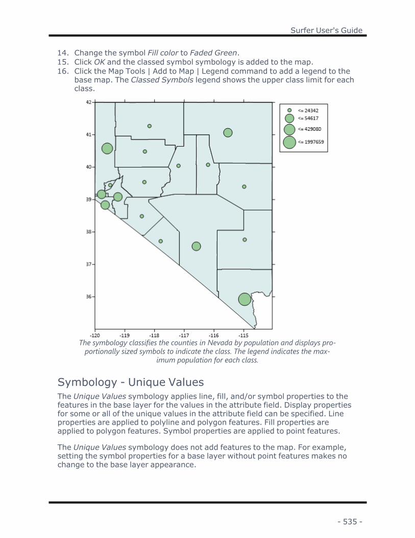
Surfer User's Guide
14. Change the symbol Fill color to Faded Green.15. Click OK and the classed symbol symbology is added to the map.16. Click the Map Tools | Add to Map | Legend command to add a legend to the
base map. The Classed Symbols legend shows the upper class limit for eachclass.
The symbology classifies the counties in Nevada by population and displays pro-portionally sized symbols to indicate the class. The legend indicates the max-
imum population for each class.
Symbology - Unique ValuesThe Unique Values symbology applies line, fill, and/or symbol properties to thefeatures in the base layer for the values in the attribute field. Display propertiesfor some or all of the unique values in the attribute field can be specified. Lineproperties are applied to polyline and polygon features. Fill properties areapplied to polygon features. Symbol properties are applied to point features.
The Unique Values symbology does not add features to the map. For example,setting the symbol properties for a base layer without point features makes nochange to the base layer appearance.
- 535 -

Chapter 8 - Base Maps
Select Unique Values to specify properties for unique values in the Attribute field.
Attribute FieldThe Attribute field specifies which attribute is used to define the features' prop-erties in the base layer. Select the desired attribute from the Attribute field list.When the Attribute field value is changed, the values in the Values List areremoved.
The first attribute for the objects in the layer is the default selection in the Attrib-ute field when a symbology is selected for the first time. The Attribute field valueis not changed when Unique Values is selected and a symbology is already inuse.
Sort MethodThe Sort Method specifies the sort order for the unique values in the Symbologyand Add Unique Values dialogs and the legend. The Sort Method automaticallyupdates when an Attribute field is selected. If the first ten values in the selectedAttribute field are numeric, then the Sort Method becomes Numeric. Otherwise,the Sort Method is set to Text.
Select Text to sort the unique values alphabetically from A to Z. Select Numberto sort the unique values from low to high. Select None to use the same order asthe features in the Contents window in the Symbology dialog and to sort the val-ues alphabetically in the Add Unique Values dialog.
Show Missing ValuesSelect the Show missing values option to include any features that do not havean attribute value equal to one of the values in the Values list in the map. Whenthe Show missing values option is checked, features that are not represented bya value in the Values list are displayed, and their properties are controlled by the
- 536 -
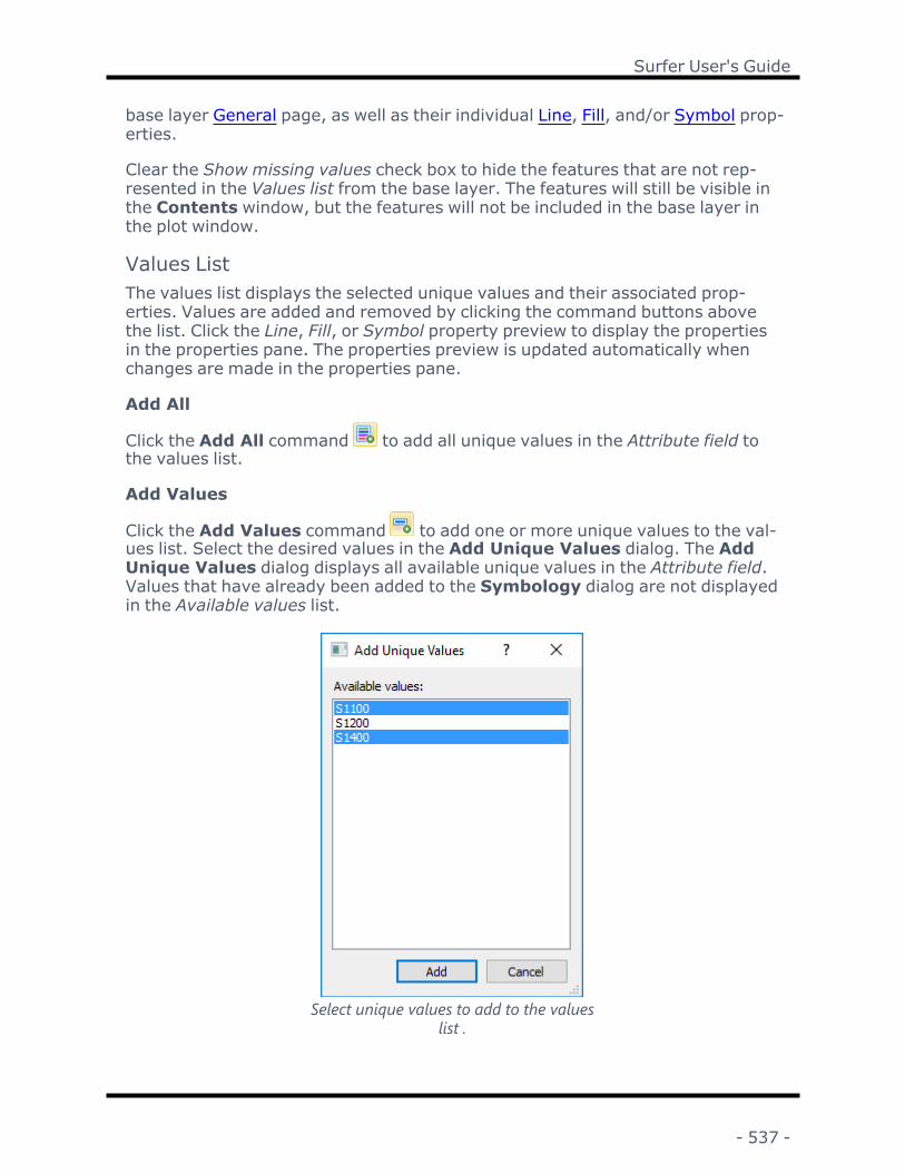
Surfer User's Guide
base layer General page, as well as their individual Line, Fill, and/or Symbol prop-erties.
Clear the Show missing values check box to hide the features that are not rep-resented in the Values list from the base layer. The features will still be visible inthe Contents window, but the features will not be included in the base layer inthe plot window.
Values ListThe values list displays the selected unique values and their associated prop-erties. Values are added and removed by clicking the command buttons abovethe list. Click the Line, Fill, or Symbol property preview to display the propertiesin the properties pane. The properties preview is updated automatically whenchanges are made in the properties pane.
Add All
Click the Add All command to add all unique values in the Attribute field tothe values list.
Add Values
Click the Add Values command to add one or more unique values to the val-ues list. Select the desired values in the Add Unique Values dialog. The AddUnique Values dialog displays all available unique values in the Attribute field.Values that have already been added to the Symbology dialog are not displayedin the Available values list.
Select unique values to add to the valueslist .
- 537 -

Chapter 8 - Base Maps
Click a value to select the value. Hold CTRL to select multiple values. Click avalue, hold SHIFT, and click a second value to select a contiguous group of val-ues. When you have selected the desired unique values, click Add to add the val-ues to the values list in the Symbology dialog. Click Cancel to close the AddUnique Values dialog without adding any values to the list.
Remove All
Click the Remove All command to remove all unique values from the valueslist.
Remove
Click the Remove command to remove the selected value from the list.
Color Scheme
Click the Color Scheme command to apply a color scheme to the line, fill,and/or symbol properties in the unique values list in the Color Scheme dialog.
Select color scheme properties to change the color properties for every unique value in theSymbology dialog.
- 538 -

Surfer User's Guide
Select the Color method to apply a scheme to the unique values' line, fill, symbolline, and/or symbol fill properties. The Line properties, Fill properties, Symbolline properties, and Symbol fill properties are all applied independently.
l Select As Is to make no changes to the current colors for the unique values.As Is is selected by default each time the Color Scheme dialog is opened.
l Select Random to apply random colors to the unique values.l Select Fixed to apply a single Color and Opacity to all unique values.l Select Colormap to apply a colormap to the unique values properties. Thecolormap is applied in the order the unique values appear in the Symbologydialog.
Save and Load Values
Click the Save Values command to save the unique values and their prop-erties to a Symbology Unique Values File (*.ssuv) in the Save As dialog. TheSave Values command is only available after at least one value has been addedto the current table.
Click the Load Values command to load unique values with their propertiesfrom a Symbology Unique Values File (*.ssuv) in the Open dialog. Values fromthe file are added to the Unique Values table. If the file includes a value that isalready listed in the Unique Values table, the properties of the existing value aremaintained and the loaded value is ignored.
Line, Fill, and Symbol PropertiesThe line, fill, and symbol properties for the selected value are displayed on theright side of the Symbology dialog. No properties are displayed when no valueis selected.
l To edit the line properties for a value, click the line preview in the row for thevalue. The line properties are applied to any polylines and/or polygons withthis value in the Attribute field.
l To edit the fill properties for a value, click the fill preview in the row for thevalue. The fill properties are applied to any polygons with this value in theAttribute field.
l To edit the symbol properties for a value, click the symbol preview in the rowfor the value. The symbol properties are applied to any points with this valuein the Attribute field.
OK, Cancel, and ApplyClick OK to save your changes, close the Symbology dialog, and update thebase layer symbology. Click Cancel to close the Symbology dialog without mak-ing changes to the base layer symbology. Click Apply to apply your changes tothe base layer while keeping the Symbology dialog open.
- 539 -

Chapter 8 - Base Maps
Symbology - Unclassed ColorsThe Unclassed Colors symbology applies line, fill, or symbol fill color to the fea-tures in the base layer. The color is specified by the attribute value and thecolormap. When used with normalized data, population per area for example,the Unclassed Colors symbology creates a choropleth map.
l The attribute value and colormap determine the line color for polyline fea-tures.
l The attribute value and colormap determine the fill color for polygon fea-tures. Polygon line color is set on the base layer General page.
l The attribute value and colormap determine symbol fill color for point fea-tures. Point symbol line color is set on the base layer General page.
Select Unclassed Colors to map a color spectrum to the features by attribute value.
Attribute FieldThe Attribute field specifies which attribute is used to define the features' prop-erties in the base layer. Select the desired attribute from the Attribute field list.Only attributes with numeric values are displayed in the Attribute field list whenthe Unclassed colors symbology is selected.
The first numeric attribute for the objects in the layer is the default selection inthe Attribute field when a symbology is selected for the first time. When a baselayer symbology using a numeric attribute is already applied, the Attribute fieldvalue is not changed when Unclassed Colors is selected. The Attribute fieldchanges to the first numeric attribute for the objects in the layer when UnclassedColors is selected and the base layer is using a text attribute for the current sym-bology.
- 540 -

Surfer User's Guide
Show Missing ValuesSelect the Show missing values option to include any features that do not havean attribute value for the selected Attribute field in the layer. When the Showmissing values option is checked, features that do not have an Attribute fieldvalue are displayed, and their properties are controlled by the base layer Generalpage, as well as their individual Line, Fill, and/or Symbol properties.
Clear the Show missing values check box to hide the features that do not havean Attribute field value from the base layer. The features will still be visible in theContents window, but the features will not be included in the base layer in theplot window.
ColormapThe Colormap is the color spectrum that is assigned to the features in the baselayer. Select a predefined colormap from the Colormap list. Click the tomodify or create a colormap in the Colormap Editor.
Beyond selecting the colors for the color spectrum, the Colormap Editor is usedto apply linear or logarithmic scaling, use attribute value minimum and max-imum or fixed values, and apply transparency to colors in the colormap. Colorspectrums can be saved and/or loaded with the Colormap Editor.
OK, Cancel, and ApplyClick OK to save your changes, close the Symbology dialog, and update thebase layer symbology. Click Cancel to close the Symbology dialog without mak-ing changes to the base layer symbology. Click Apply to apply your changes tothe base layer while keeping the Symbology dialog open.
Symbology - Unclassed SymbolsThe Unclassed Symbols symbology adds proportionally scaled symbols to themap. The proportional symbol map is useful for indicating the relative differencein a value between areas.
When the Unclassed Symbols symbology is applied to polygon features, symbolsare created in addition to the polygon features. When the Unclassed Symbolssymbology is applied to point features, the point feature symbol properties arecontrolled by the symbology. Unclassed Symbols symbology is not applied topolyline features.
- 541 -

Chapter 8 - Base Maps
Select Unclassed Symbols to add proportionally scaled symbols to the map.
GeneralThe General section includes the Attribute field and Show missing values prop-erties.
Attribute FieldThe Attribute field specifies which attribute is used to scale the symbols. Selectthe desired attribute from the Attribute field list. Only attributes with numeric val-ues are displayed in the Attribute field list when the Unclassed symbols sym-bology is selected.
The first numeric attribute for the objects in the layer is the default selection inthe Attribute field when a symbology is selected for the first time. When a baselayer symbology using a numeric attribute is already applied, the Attribute fieldvalue is not changed when Unclassed Symbols is selected. The Attribute fieldchanges to the first numeric attribute for the objects in the layer when UnclassedSymbols is selected and the base layer is currently using a text attribute for thecurrent symbology.
Show Missing ValuesSelect the Show missing values option to include any features that do not havean attribute value for the selected Attribute field in the layer. When the Showmissing values option is checked, features that do not have an Attribute field
- 542 -

Surfer User's Guide
value are displayed, and their properties are controlled by the base layer Generalpage, as well as their individual Line, Fill, and/or Symbol properties.
Clear the Show missing values check box to hide the features that do not havean Attribute field value from the base layer. The features will still be visible in theContents window, but the features will not be included in the base layer in theplot window.
SymbolThe properties in the Symbol section control the appearance of the symbols,including the Symbol and Symbol set.
Symbol SizeThe Symbol Size section includes properties for scaling the symbols.
Minimum and Maximum SizeSpecify the smallest and largest symbol sizes in the Minimum size and Maximumsize fields. The feature with the minimum attribute value is created with the Min-imum size. The feature with the maximum attribute value is created with theMaximum size. The remaining features' symbols are scaled proportionallybetween the Minimum size and Maximum size by the Scaling method.
Scaling MethodThe Scaling method specifies which scaling type is used to determine symbolsizes between the minimum and maximum. Select Linear or Square root fromthe Scaling method list. The interpolation equations for the scaling methods areas follows:
Linear:SquareRoot:
Square root scaling is commonly used with solid symbols to offset the fact thatthe area increases as a function of the symbol height squared. Square root scal-ing is essentially making the area of the symbol proportional to the Z value,rather than making the size of the symbol proportional to the Z value.
Symbol Fill and Line ColorsThe Symbol Fill Color section specifies the symbol fill color method and color. TheSymbol Line Color section specifies the symbol line color method and color. Sym-bol fill and line colors are set separately.
Color MethodThe Color method property sets whether the symbols use a single color or thesymbols are colored by their attribute value. Select Fixed to use a single color forall symbols. Select Colormap to color the symbols by their attribute values.
- 543 -

Chapter 8 - Base Maps
ColorSpecify the symbol color when the Color method is Fixed in the Color field. Selecta color from the color palette.
OpacitySpecify the symbol opacity when the Color method is Fixed in the Opacity field.Select a value between 100% (completely opaque) to 0% (completely trans-parent).
ColormapSelect a predefined colormap in the Colormap field when the Color method isColormap . Create a custom colormap in the Colormap Editor by clicking thebutton.
OK, Cancel, and ApplyClick OK to save your changes, close the Symbology dialog, and update thebase layer symbology. Click Cancel to close the Symbology dialog without mak-ing changes to the base layer symbology. Click Apply to apply your changes tothe base layer while keeping the Symbology dialog open.
Symbology - Classed ColorsThe Classed Colors symbology applies line, fill, or symbol fill color to the featuresin the base layer by class. The features in the base layer are classified by theselected attribute. The colors for each class can be assigned one at a time or acolormap can be used to assign graduated colors across the classes. When usedwith normalized data, population per area for example, the Classed Colors sym-bology creates a choropleth map.
l The class color is applied to the line color for polyline features.
l The class color is applied to the fill color for polygon features. Polygon linecolor is set on the base layer General page.
l The class color is applied to symbol fill color for point features. Point symbolline color is set on the base layer General page.
- 544 -

Surfer User's Guide
Select Classed Colors to color features by a classified attribute value.
PropertiesThe Properties pane includes the properties for selecting the attribute and defin-ing the classes. The Properties pane is in the middle of the Symbology dialog.
Attribute FieldThe Attribute field specifies which attribute is used to classify the features in thebase layer. Select the desired attribute from the Attribute field list. Only attrib-utes with numeric values are displayed in the Attribute field list when the Classedcolors symbology is selected.
The first numeric attribute for the objects in the layer is the default selection inthe Attribute field when a symbology is selected for the first time. When a baselayer symbology using a numeric attribute is already applied, the Attribute fieldvalue is not changed when Classed Colors is selected. The Attribute field changesto the first numeric attribute for the objects in the layer when Classed Colors isselected and the base layer is currently using a text attribute for the current sym-bology.
Show Missing ValuesSelect the Show missing values option to include any features that do not havean attribute value for the selected Attribute field in the layer. When the Showmissing values option is checked, features that do not have an Attribute fieldvalue are displayed, and their properties are controlled by the base layer Generalpage, as well as their individual Line, Fill, and/or Symbol properties.
- 545 -

Chapter 8 - Base Maps
Clear the Show missing values check box to hide the features that do not havean Attribute field value from the base layer. The features will still be visible in theContents window, but the features will not be included in the base layer in theplot window.
Features that have an Attribute field value outside the class limits are controlledby the Show all others option. When Show all others is cleared, features with anAttribute field value outside the class limits are treated the same as missing val-ues. When Show all others is selected, features with an Attribute field value out-side the class limits are controlled by the All others class properties.
Class MethodThe Class method specifies the method used to calculate the limits of theclasses. There are five options available: Equal number, Equal interval, Naturalbreaks , Standard deviation , and User defined. To change the Class method,click on the current option and select the desired option from the list.
l Equal number assigns the class ranges such that approximately equal num-bers of features are included in each class. Normally in this case, the inter-val of each class is different.
l Equal interval assigns the class ranges so the interval between the min-imum and maximum values are equal for each class. Normally in this case,a different number of features is assigned to each class.
l Natural breaks uses the Fisher-Jenks algorithm to calculate the ideal nat-ural breaks in the data. Typically these natural breaks are ideal beginningsand endings for data classes. The algorithm is based on Fisher's statementthat any optimal classification of data consists of the sum of optimal classesof subsets of the data. To learn more about Jenks' natural breaks data clas-sification method, please refer to Slocum, Terry A. Thematic Cartographyand Visualization. New Jersey: Prentice-Hall, 1999.
l Standard deviation generates data classes based on the standard deviationof the data.
l User Defined allows you to set the >=Minimum value and the <Maximumvalue for each class individually. This allows you to specify your own rangesfor the classes. Ranges defined in this way do not have to be contiguous. Tochange the >=Minimum or <Maximum value, double-click the values in theclass list.
Class CountsThe Class counts value specifies the number of classes there will be on the map.When the Class count value is changed, the classes are automatically updated toreflect the change. To change the number of classes, click the button toincrease or decrease Class count or highlight the existing number and type in anew value from 1 to 1000 classes.
- 546 -

Surfer User's Guide
Show All OthersSelect the Show all others option to include a color for features where the attrib-ute value does not fall within an existing class. Clear the Show all others checkbox to remove the All others class.
Features that do not have an Attribute field value are controlled by the Showmissing values option. When Show all others is not selected, features where theAttribute field value is outside the class limits are treated the same as missingvalues.
Reverse Color OrderClick Reverse in the Reverse color order field to reverse the colors in the Classeslist.
Load/Save ClassesClick Load to load an existing Symbology Color Class (*.colorclass) file. ClickSave to save the current classes to a Symbology Color Class (*.colorclass) file.The class limits, names, and colors are saved in the Symbology Color Class(*.colorclass) file.
Colormap for ClassSelect the Colormap for class option to apply the Colormap color spectrum colorsto the classes. Changing the color of any class in the Classes list automaticallyclears the Colormap for class check box.
ColormapThe Colormap is the color spectrum that is assigned to the classes. Select a pre-defined colormap from the Colormap list. Click the to modify or create acolormap in the Colormap Editor.
The Colormap property applies colors to the classes based on class number, notthe data value. Therefore the Data section of the Colormap Editor does nothave any effect on the class colors by default. We recommend you do not changethe Data properties in the Colormap Editor. The first class is always assignedthe minimum value color, and the last class is always assigned the maximumvalue color. Remaining classes are distributed equally across the colormap. TheData properties may change the class colors when Logarithmic scaling is used:The first class is always assigned the minimum value color, and the last class isalways assigned the maximum value color. The remaining classes are distributedlogarithmically across the colormap.
ClassesThe Classes list displays the class color (Color), upper limit (<= Upper Value),proportion (%), count (Count), and class name (Name) for the classes. TheClasses listis on the right side of the Symbology dialog.
- 547 -

Chapter 8 - Base Maps
Changing the Class ColorThe Color column displays the colors for the classes. Click the color preview inthe Color column to change the color for the class. The Color Properties dialogis displayed.
Specify the class Color and Opacity in the Color Properties dia-log.
Specify the class color by selecting a predefined color from the color palette inthe Color field, or click to select a color in the Colors dialog. Set the class opa-city by clicking and dragging the slider or typing a value between 0 and100 in the Opacity field. An Opacity of 100% is completely opaque. An Opacity of0% is completely transparent.
Changing the Class LimitsThe <= Upper Value column displays the upper limit for each class. The firstclass in the Classes list has no lower limit. Subsequent classes use the prior classupper limit for a class minimum. For example, in the image above Class 2includes values greater than 28160 (Class 1's upper limit) and less than or equalto 159064.
The class limits are automatically calculated when the Class method is Equalnumber, Equal interval, Natural breaks, or Standard deviation. The class limitsmust be individually defined when the Class method is User defined. Changing aclass <= Upper Value automatically updates the Class method to User defined.
Type the desired class maximum in the <= Upper Value column to change theupper limit for a class. The proportion and count statistics are automaticallyupdated when the <= Upper Value is changed.
Statistical Information about the Features in Each ClassThe Classes list displays summary statistics for each class. The% and Countcolumns display statistical information about the class. The% column indicatesthe percentage of features in the particular class. The Count column indicates
- 548 -

Surfer User's Guide
the number of features included in each class. These values cannot be directlyedited and are for informational purposes only.
Changing the Class NameThe Name column displays the class names. Specify a class name in the Classeslist to display class names in a legend. By default, classes are named Class 1,Class 2, etc. Type a name in the Name column to change the class name.
OK, Cancel, and ApplyClick OK to save your changes, close the Symbology dialog, and update thebase layer symbology. Click Cancel to close the Symbology dialog without mak-ing changes to the base layer symbology. Click Apply to apply your changes tothe base layer while keeping the Symbology dialog open.
Symbology - Classed SymbolsThe Classed Symbols symbology adds proportionally sized symbols to the fea-tures by class. The features in the base layer are classified by the selected attrib-ute. The symbols for each class can be assigned individually or graduatedsymbols can be assigned across the classes.
When the Classed Symbols symbology is applied to polygon features, symbolsare created in addition to the polygon features. When the Classed Symbols sym-bology is applied to point features, the point feature symbol properties are con-trolled by the symbology. Classed Symbols symbology is not applied to polylinefeatures.
- 549 -

Chapter 8 - Base Maps
Select Classed Symbols to add symbols to the map by a classified attribute value.
PropertiesThe Properties pane includes the properties for selecting the attribute and defin-ing the classes. The Properties pane is in the middle of the Symbology dialog.
Attribute FieldThe Attribute field specifies which attribute is used to classify the features in thebase layer. Select the desired attribute from the Attribute field list. Only attrib-utes with numeric values are displayed in the Attribute field list when the Classedcolors symbology is selected.
The first numeric attribute for the objects in the layer is the default selection inthe Attribute field when a symbology is selected for the first time. When a baselayer symbology using a numeric attribute is already applied, the Attribute fieldvalue is not changed when Classed Symbols is selected. The Attribute fieldchanges to the first numeric attribute for the objects in the layer when ClassedSymbols is selected and the base layer is currently using a text attribute for thecurrent symbology.
- 550 -

Surfer User's Guide
Show Missing ValuesSelect the Show missing values option to include any features that do not havean attribute value for the selected Attribute field in the layer. When the Showmissing values option is checked, features that do not have an Attribute fieldvalue are displayed, and their properties are controlled by the base layer Generalpage, as well as their individual Line, Fill, and/or Symbol properties.
Clear the Show missing values check box to hide the features that do not havean Attribute field value from the base layer. The features will still be visible in theContents window, but the features will not be included in the base layer in theplot window.
Features that have an Attribute field value outside the class limits are controlledby the Show all others option. When Show all others is cleared, features with anAttribute field value outside the class limits are treated the same as missing val-ues. When Show all others is selected, features with an Attribute field value out-side the class limits are controlled by the All others class properties.
Class MethodThe Class method specifies the method used to calculate the limits of theclasses. There are five options available: Equal number, Equal interval, Naturalbreaks, Standard deviation, and User defined. To change the Class method, clickon the current option and select the desired option from the list.
l Equal number assigns the class ranges such that approximately equal num-bers of features are included in each class. Normally in this case, the inter-val of each class is different.
l Equal interval assigns the class ranges so the interval between the min-imum and maximum values are equal for each class. Normally in this case,a different number of features is assigned to each class.
l Natural breaks uses the Fisher-Jenks algorithm to calculate the ideal nat-ural breaks in the data. Typically these natural breaks are ideal beginningsand endings for data classes. The algorithm is based on Fisher's statementthat any optimal classification of data consists of the sum of optimal classesof subsets of the data. To learn more about Jenks' natural breaks data clas-sification method, please refer to Slocum, Terry A. Thematic Cartographyand Visualization. New Jersey: Prentice-Hall, 1999.
l Standard deviation generates data classes based on the standard deviationof the data.
l User Defined allows you to set the >=Minimum value and the <Maximumvalue for each class individually. This allows you to specify your own rangesfor the classes. Ranges defined in this way do not have to be contiguous. Tochange the >=Minimum or <Maximum value, double-click the values in theclass list.
- 551 -

Chapter 8 - Base Maps
Class CountsThe Class counts value specifies the number of classes there will be on the map.When the Class count value is changed, the classes are automatically updated toreflect the change. To change the number of classes, click the button toincrease or decrease Class count or highlight the existing number and type in anew value from 1 to 1000 classes.
Show All OthersSelect the Show all others option to include a symbol for features where theattribute value does not fall within an existing class. Clear the Show all otherscheck box to remove the All others class.
Features that do not have an Attribute field value are controlled by the Showmissing values option. When Show all others is not selected, features where theAttribute field value is outside the class limits are treated the same as missingvalues.
Reverse Symbol OrderSelect the Reverse symbol order option to reverse the symbols in the Classeslist. When the Reverse symbol order option is selected, the class with the smal-lest <= Upper Value is sized by the Maximum size and the class with the largest<= Upper Value is sized by the Minimum size. Clear the Reverse symbol ordercheck box to return the symbols to the original order and scaling.
Load/Save ClassesClick Load to load an existing Symbology Symbol Class (*.symbolclass) file. ClickSave to save the current classes to a Symbology Symbol Class (*.symbolclass)file . The class limits, names, symbol set, symbol fill and line colors, symbolindexes, and symbol sizes are saved in the Symbology Symbol Class (*.sym-bolclass) file.
Symbol SizeSpecify the smallest and largest symbol sizes in the Minimum size and Maximumsize fields. By default, the class with the smallest <= Upper Value is created withthe Minimum size. The class with the largest <= Upper Value is created with theMaximum size. The remaining features' symbols are scaled proportionallybetween the Minimum size and Maximum size by the Scaling method. Select theReverse symbol order option to reverse the symbol sizing.
Scaling MethodThe Scaling method specifies which scaling type is used to determine symbolsizes between the minimum and maximum. Select Linear or Square root fromthe Scaling method list. The interpolation equations for the scaling methods areas follows:
Linear:
- 552 -
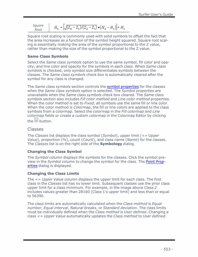
Surfer User's Guide
SquareRoot:
Square root scaling is commonly used with solid symbols to offset the fact thatthe area increases as a function of the symbol height squared. Square root scal-ing is essentially making the area of the symbol proportional to the Z value,rather than making the size of the symbol proportional to the Z value.
Same Class SymbolsSelect the Same class symbols option to use the same symbol, fill color and opa-city, and line color and opacity for the symbols in each class. When Same classsymbols is checked, only symbol size differentiates symbols between theclasses. The Same class symbols check box is automatically cleared after thesymbol for any class is changed.
The Same class symbols section controls the symbol properties for the classeswhen the Same class symbols option is selected. The Symbol properties areunavailable when the Same class symbols check box cleared. The Same classsymbols section also includes Fill color method and Line color method properties.When the color method is set to Fixed, all symbols use the same fill or line color.When the color method is Colormap, the fill or line colors are applied to the classsymbols from a colormap. Select the colormap in the Fill colormap and Linecolormap fields or create a custom colormap in the Colormap Editor by clickingthe button.
ClassesThe Classes list displays the class symbol (Symbol), upper limit (<= UpperValue), proportion (%), count (Count), and class name (Name) for the classes.The Classes list is on the right side of the Symbology dialog.
Changing the Class SymbolThe Symbol column displays the symbols for the classes. Click the symbol pre-view in the Symbol column to change the symbol for the class. The Point Prop-erties dialog is displayed.
Changing the Class LimitsThe <= Upper Value column displays the upper limit for each class. The firstclass in the Classes list has no lower limit. Subsequent classes use the prior classupper limit for a class minimum. For example, in the image above Class 2includes values greater than 28160 (Class 1's upper limit) and less than or equalto 56390.
The class limits are automatically calculated when the Class method is Equalnumber, Equal interval, Natural breaks, or Standard deviation. The class limitsmust be individually defined when the Class method is User defined. Changing aclass <= Upper Value automatically updates the Class method to User defined.
- 553 -

Chapter 8 - Base Maps
Type the desired class maximum in the <= Upper Value column to change theupper limit for a class. The proportion and count statistics are automaticallyupdated when the <= Upper Value is changed.
Statistical Information about the Features in Each ClassThe Classes list displays summary statistics for each class. The% and Countcolumns display statistical information about the class. The% column indicatesthe percentage of features in the particular class. The Count column indicatesthe number of features included in each class. These values cannot be directlyedited and are for informational purposes only.
Changing the Class NameThe Name column displays the class names. Specify a class name in the Classeslist to display class names in a legend. By default, classes are named Class 1,Class 2, etc. Type a name in the Name column to change the class name.
OK, Cancel, and ApplyClick OK to save your changes, close the Symbology dialog, and update thebase layer symbology. Click Cancel to close the Symbology dialog without mak-ing changes to the base layer symbology. Click Apply to apply your changes tothe base layer while keeping the Symbology dialog open.
Base (raster) Layer General PropertiesImage files can be loaded into Surfer as a base (raster) layer with the Home |New Map | Base or Home | Add to Map | Layer | Base command. Click onthe Base (raster) Layer object in the Contents window to open the base layerproperties in the Properties window. If you wish to import the image without cre-ating a map layer, use the Home | Insert | Graphic command instead.
- 554 -

Surfer User's Guide
The General page controls the image appear-ance and Spatial Extents.
Input FileThe Input File lists the current file used in the base map.
Change File
Click the button to display the Import dialog. This allows you to select a newfile or an updated version of the current file used to create the base map. If thefile exceeds the current map limits, you will be prompted to adjust the map lim-its.
A raster file must be selected when changing the Input file for a base (raster)layer. An error message will be displayed if a vector file is selected in the Importdialog. If you wish to add a base (vector) layer to the map, select the Home |Add to Map | Layer | Base command instead.
Coordinate System NoteRegardless of the file selected with either the File | Reload Map Data com-
mand or by clicking the button in the Properties window, the coordinate sys-tem for the original map layer is used after updating the file. If this is not thecorrect coordinate system, click on the map layer to select it. In the Propertieswindow, click on the Coordinate System tab and set the coordinate system tothe appropriate new system.
- 555 -

Chapter 8 - Base Maps
Save File
The button displays the Export dialog. Type a File name and change the Saveas type to the desired file format. Click Save. For some file types, a file type spe-cific Export Options dialog appears. The Export Options dialog Spatial Refer-ences and Scaling pages are available when saving a base layer. Check thedesired file formats. It is recommend that GS Reference (Version 2) file option bechecked to generate a .GSR2 file. Set any export options and click OK to save thefile.
The georeference information is not saved for the image when exporting fromthe Properties window General page. To export the image in the map coordin-ate system, click the File | Export command and select Selected objects onlyoption in the Export dialog.
Image PropertiesThe properties in the Image Properties section on the General page transformthe image appearance: Opacity , Contrast , Brightness , Saturation , and Hue.These image transformations are applied to the display of the image or baselayer, not to the image file. However, the image transformations are saved to theexported file when exporting the image or map.
OpacityChange the Opacity of an image by entering a value from 0% (completely trans-parent) to 100% (completely opaque) or dragging the to change theopacity percentage.
ContrastContrast is the difference in luminance or color of the objects in the image. Lightand dark objects appear to stand out from one another when contrast is high.The difference in luminance between objects is difficult to see when contrast islow. The Contrast value is relative in Surfer. The original image is given a Con-trast value of 0. Positive values increase the image contrast. Negative valuesdecrease the image contrast. Type a value between -100 and 100 in the Contrastfield or click and drag the to adjust the image contrast.
BrightnessBrightness is the perception of emitted or reflected light. Brightness can also beconsidered the average of the Red, Green, and Blue values for the pixels in theimage. As brightness increases objects become lighter until they begin to "washout" or turn white. Objects in the image get darker until they become black asbrightness decreases. The Brightness value is relative in Surfer. The originalimage is given a Brightness value of 0. Positive values increase the image bright-ness. Negative values decrease the image brightness. Type a value between -
- 556 -

Surfer User's Guide
100 and 100 in the Brightness field or click and drag the to adjust theimage brightness.
SaturationSaturation is a combination of light intensity and distribution across differentwavelengths. High saturation relates to vivid, bright colors, i.e. high intensityacross a narrow wavelength band or even single wavelength. This can also beconsidered very pure color. Low saturation leads to muted or gray colors, i.e. lowintensity across a wide band of wavelengths. No saturation transforms the imageto grayscale. The Saturation value is relative in Surfer. The original image isgiven a Saturation value of 0. Positive values increase the image saturation. Neg-ative values decrease the image saturation. Type a value between -100 and 100in the Saturation field or click and drag the to adjust the image sat-uration.
HueHue describes the colors in the image. The Hue property shifts the colors in theimage around the color wheel. The Hue value is relative in Surfer. The originalimage is given a Hue value of 0. Positive values shift the colors in the red toorange, then yellow, green, blue and finally magenta direction. Negative valuesshift colors in the opposite direction, from red to magenta then blue, green, yel-low and finally orange. Type a value between -180 and 180 in the Hue field orclick and drag the to adjust the image hue.
ResetClick Reset to return the image to its original appearance. This sets Opacity to100% and Contrast, Brightness, Saturation, and Hue to 0.
GeoreferenceClick Georeference Image in the Georeference field to apply control points to theimage and reference it to your map's coordinate system. Clicking GeoreferenceImage opens the Georeference Image window. The Georeference Image com-mand is only available when the image is a base (raster) layer. The image mustbe at least 2x2 pixels to be georeferenced.
Spatial ExtentsThe Left, Right, Bottom, and Top values in the Spatial Extents group displays thecurrent extents of the image. These values are read-only. Click the GeorefenceImage button to change the spatial extents.
- 557 -

Chapter 8 - Base Maps
Base Map Labels PropertiesAfter assigning attributes to polylines, polygons, and symbols, attribute labelscan be added. The attribute, position, and font properties can also be specifiedon the Labels page in the base map properties. Attributes for rectangles, roun-ded rectangles, and ellipses do not appear as labels. To add labels from attrib-utes to a base map, click once on the base map layer to select it. In theProperties window, click on the Labels tab.
Change base map label properties on the Labels page inthe Properties window.
- 558 -

Surfer User's Guide
Labels PropertiesThe properties in the Labels section control the content, position, and appear-ance of the base (vector) layer labels.
Label SourceThe Label source determines whether or not labels are displayed and whichattribute should be displayed. To change the Label source, click on the existingoption and select the desired option from the list. Available options are [None],[Template], and then a list of all attribute names in the file. To display no labels,set the Label source to [None] . To display a single attribute, select the attributename from the list. To display multiple attribute names or an attribute name andadditional text, select [Template] . Then, set the Template option to the desiredtext and attributes.
TemplateThe Template option allows multiple attributes or attributes and text to be dis-played for the label. Attribute names must be listed exactly as they appear in theLabel source list. Attribute names must have square brackets around them, suchas [Attribute Name] in order to be recognized. Attribute names are case sens-itive, so there is a difference between [name] and [Name]. Any number of attrib-utes may be added to the Template section.
The square brackets are mandatory. Math text options (such as \up50 ) mustappear outside of the square brackets. If the font or font properties are changedfor the attribute, highlight the entire text including the square brackets beforechanging the properties in the Text Editor.
Click the button to open the Text Editor where multiple lines of text can becreated. Attribute names must appear in the Text Editor with square bracketsaround the name.
PositionThe Position controls the offset of the label from the object center. To change theposition, click on the existing position and select the new position in the list. Spe-cify Center, Left, Right, Above, Below, or User defined. User defined allows youto specify the exact offset (in page units) in the X offset and Y offset boxes. Theposted labels are all placed in the same position relative to the associated object.Positive values in the X offset shift the label position toward the positive direction(to the right for normal axes, to the left for reversed axes). Negative values inthe X offset shift the label position toward the negative direction (to the left fornormal axes, to the right for reversed axes). Positive values in the Y offset shiftthe label position toward the positive direction (upward for normal axes, down-ward for reversed axes). Negative values in the Y offset shift the label positiontoward the negative direction (downward for normal axes, upward for reversedaxes). The X offset and Y offset values are numbers between -4 and +4 inches (-10.16 and +10.16 centimeters). To change the X offset and Y offset values,
- 559 -

Chapter 8 - Base Maps
highlight the existing value and type a new value or click the buttons toincrease or decrease the offset.
Angle (degrees)The Angle (degrees) box specifies the angle in degrees to rotate the labels. Pos-itive angles rotate the labels counterclockwise. To change the Angle (degrees),highlight the existing angle value. Type a new value or click and drag the
to the desired angle position.
FontClick the next to Font Properties to display the Font Properties section. Thefont properties are applied to all labels.
FormatClick the next to Label Format to display the Label Format section. The labelformat properties are applied to all labels. If the values in the Label source attrib-ute are not numeric, the label will be displayed as unformatted text.
ExamplesThe following examples demonstrate adding labels to base layer objects.
Attribute LabelsCreate a base map from a .SHP file. When the .SHP file is loaded, the attributesare also imported. To label all of the polygons with the Primary ID:
1. Click on the Base object in the Contents window to select it.2. In the Properties window, click on the Labels tab.3. Change the Label source to Primary ID. The Primary ID will appear next to all
polylines, polygons, and symbols in the .SHP file.
Template LabelsCreate a base map from a file that contains attributes. After the file is loaded, theattributes appear for each of the individual polylines, polygons, and symbols. Tocreate complex labels for each object:
1. Click on the Base object in the Contents window to select it.2. In the Properties window, click on the Labels tab.3. Change the Label source to [Template].4. Next to Template, type the desired attribute names, surrounded by square
brackets. For instance, if you wanted to display the name of a property andthe owner's name, your Templatemay look like:
[Name] - [Owner]
- 560 -

Surfer User's Guide
5. To create multiple lines, click the button.6. In the Text Editor, type the attribute names, surrounded by square brackets.
Add any additional text. To add a new line, press ENTER on the keyboard. Youmight have:
Property Name and Owner: [Name] - [Owner]
Surveyor Name: [Surveyor]
7. When all edits are complete, click OK to close the Text Editor. The labelsappear on the screen.
The label appears in the desired location, substitutingthe attribute value for the attribute names in square
brackets.
- 561 -


Chapter 9 - Contour Maps
Contour MapThe Home | New Map | Contour command creates a contour map from a gridfile. A contour map is a two-dimensional representation of three-dimensionaldata. The first two dimensions are the X and Y coordinates. The third dimension(Z) is represented by lines of equal value. The relative spacing of the contourlines indicate the relative slope of the surface. The area between two contourlines contains only grid nodes having Z values within the limits defined by thetwo enclosing contours. The difference between two contour lines is defined asthe contour interval.
The Home | Add to Map | Layer | Contour , the button, orMap Tools |Add to Map | Layer | Contour command adds a contour map layer to theselected map.
This example contour map shows filled color contours and acolor scale bar.
- 563 -

Chapter 9 - Contour Maps
Creating a Contour MapTo create a new contour map:
1. Click Home | New Map | Contour command.2. Select a grid file in the Open Grid dialog. Click Open.
The map is automatically created with reasonable defaults.
Editing an Existing Contour MapTo change the features of the contour map, click once on the contour map in theContents window or plot window. When the contour map is selected, the contourmap properties are displayed in the Properties window.
Click on the Contours map layerto select it.
Contour Layer PropertiesThe contour layer properties contains the following pages:
GeneralLevelsLayerCoordinate SystemInfo
Map PropertiesThe map properties contains the following pages:
ViewScaleLimitsFrameCoordinate SystemInfo
- 564 -

Surfer User's Guide
Drawing ContoursWhen you create a contour map, the grid file is read into the plot window as aninternal array of X, Y, and Z grid nodes. The grid nodes consist of rows andcolumns of Z values. The rows contain grid nodes with the same Y coordinate,and the columns contain grid nodes with the same X coordinate. Grid filecolumns and rows are sometimes referred to as X grid lines and Y grid lines,respectively. The intersection of a row and column is defined as a grid node. Gridfiles define the X, Y location of each grid node over the extent of the map, andthe interpolated Z value at each node.
The path of a contour line (Z = 50) through a grid isdefined by interpolating between grid nodes. This
example shows the straight-line segments that definethe contour line. The dots are added to show the ends
of each line segment.When Surfer creates a contour map, the contour lines are drawn as a series ofstraight line segments between adjacent grid lines. The point where a contourline intersects a grid line is determined by interpolation between Z values at adja-cent grid nodes.
The grid limits define the extent of contour maps. Once a grid file is created youcannot produce a contour map larger than the extent of the grid file. However,you can use the Limits page to specify a subset of the grid used to create the con-tour map.
- 565 -

Chapter 9 - Contour Maps
Contour Map General PropertiesThe contour map properties General page controls the Grid file, Smoothing,Fault line properties, and Blanked Regions for a contour map. To open the Gen-eral page, click on a contour map to select it. In the Properties window, click onthe General tab.
Change contour map properties in the Propertieswindow on the General page.
Input Grid FileThe Grid file lists the current grid file used in the contour map. The path and filename are the location of the grid file when the map was created or the grid filewas most recently changed.
Grid Information
The button displays information about the grid file used to produce the maplayer. The information includes the grid size, the minimum and maximum X, Y, Zvalues contained in the grid file, and statistics. If the grid file contains more than40 million nodes, you are asked if you wish to create a detailed report or a quickreport. Click Yes in the message to create a detailed grid report, or click No to cre-ate a shorter quick grid report.
Change FileThe button displays the Open Grid dialog. This allows you to select a newgrid file, or an updated version of the grid file used to create the contour map.Select a grid file and click Open. If the Z range for the new grid is outside the oldcontour levels, you will be prompted to continue the operation. If you click-Cancel, the grid file is not replaced. If you clickOK, the grid file is replaced, butno contour lines are drawn. You can update the contour levels being displayed ontheLevelstab.
- 566 -
Surfer User's Guide
If the new grid exceeds the current map limits, another warning will appear ask-ing you to adjust the map limits. If you click Yes, the limits are automaticallyadjusted to fit the new grid. If you click No, the limits are not automatically adjus-ted. The map may not be displayed. To change the map limits, click on the Mapobject in the Contents window and the Limits tab in the Properties window.
You may also see a warning message that the current map scale may result in anun-viewable map. Clicking OK allows the map scale to automatically be adjusted.
Coordinate System NoteRegardless of the file selected with either the File | Reload Map Data com-mand or by clicking the button in the Properties window, the coordinate sys-tem for the original map layer is used after updating the file. If this is not thecorrect coordinate system, click on the map layer to select it. In the Propertieswindow, click on the Coordinate System tab and set the coordinate system tothe appropriate new system.
Save File
The button displays the Save Grid As dialog. Type a File name and changethe Save as type to the desired grid file format. Click Save. If a coordinate sys-tem has been defined on the Coordinate System tab in the Properties window,an Export Options dialog appears. Check the desired file formats. It is recom-mend that GS Reference (Version 2) file option be checked to generate a .GSR2file. Click OK and the file is saved.
SmoothingThe Smoothing option allows you to smooth the contours displayed on the map.Click on the existing value (None, by default) and select a new smoothing valuefrom the list. If smoothing is enabled, contour lines may cross. The Smoothingoption in the contour map properties applies a constrained spline smoothingalgorithm to interpolate additional contour vertices. Each line is separately cal-culated, thus the lines can cross if too much smoothing is applied.
A better method to smooth contours is to regrid the data using the Grids | NewGrid | Grid Data command, use the Grids | Edit | Spline Smooth or Grids | Resize| Mosaic commands to create a new grid with smaller grid node spacing. SeeSmoothing Contours for more information on smoothing.
Fault LineIf your grid file contains faulting information, you can set the fault line color,style, opacity, and thickness of the fault line drawn on the contour map by click-ing on the next to Fault line and changing the appropriate line propertyoptions.
- 567 -

Chapter 9 - Contour Maps
NoData RegionsThe NoData Regions section allows you to choose fill and line color properties forareas containing nodes assigned the NoData value.
Click on the next to Fill Properties to set fill properties for NoData areas, or toload a custom fill pattern. If no colors appear after setting these options, click onthe Levels tab and check the box next to the Fill contours option.
Click on the next to Line Properties to set the line properties that outline theNoData area.
Contour Map Levels PropertiesThe contour map properties Levels page controls the display of contours, con-tour labels, and color fill on the contour map. The levels can be set using asimple, logarithmic, equal area, or advanced method. All methods are describedbelow. The advanced option is useful when more control over individual contourline properties is desired.
Display Simple, Logarithmic, or Equal Area OptionsTo use the simple options, click on the contour map to select it. In the Propertieswindow, click on the Levels tab. Change the Level method to Simple. To use log-arithmic options, change the Level method to Logarithmic.
Switching Between Level MethodsWhen switching the Level method to Advanced, all current Simple, Logarithmic,or Equal area options are initially shown in the Levels for Map dialog. However,when switching the Level method from Advanced to Simple, Logarithmic, orEqual area it is likely that some level customizations will be lost.
Some settings require the Level method be set to Advanced. For example, if youwish to load a .LVL file, you must use the Advanced setting.
- 568 -

Surfer User's Guide
Adjust the contour map contour line properties on theLevels page in the Properties window.
Data RangeThe Data range displays the Z minimum and maximum values read from the gridfile.
- 569 -

Chapter 9 - Contour Maps
GeneralThe General section controls the method used to create the contour lines, theminimum contour value, maximum contour value, contour interval, how manyminor contours are in a major contour interval, and the display of the color scalebar.
Level MethodThe Level method determines which options are available for setting the contourmap contour line properties. Available options are Simple, Logarithmic, Equalarea, and Advanced. Simple allows basic options to be set. Logarithmic uses alog(10) interval to display the contours. Equal area separates the map intoapproximately equal area bins and creates contour lines at the bin boundaries.Advanced allows individual lines to have labels, hachures, fill, and line propertiesset individually. Advanced options are explained on the Contour Map AdvancedLevels Dialog page. To set the Level method, click on the existing method andselect the desired method from the list.
When the Level method is set to Logarithmic, the colormap for the filled contoursautomatically changes to use a logarithmic scaling, as well.
Minimum ContourSet the Minimum contour to the value of the first contour line you want displayedon the contour map. To set a new value, highlight the existing value and type thenew value. Press ENTER on the keyboard or click another command in the Prop-erties window for the value to be accepted. Values are in map Z units. When theLevel method is set to Logarithmic , the Minimum contour value must be greaterthan 0.
Maximum ContourSet the Maximum contour to the value of the last contour line you want displayedon the contour map. To set a new value, highlight the existing value and type thenew value. Press ENTER on the keyboard or click another command in the Prop-erties window for the value to be accepted. Values are in map Z units.
Contour IntervalThe Contour interval option is available when the Level method is set to Simple .The Contour interval defines the spacing units between adjacent contour lines.This will affect how many contours appear on the contour map and how closethose contours are to one another. To set a new value, highlight the existingvalue and type the new value. Press ENTER on the keyboard or click another com-mand in the Properties window for the value to be accepted. Values are in mapZ units.
- 570 -

Surfer User's Guide
Surfer uses the Contour interval, theMinimum contour value, and theMax-imum contour value to determine how many contour lines are created on themap. Surfer will issue a warning message if the number of contour linesincreases above 5000. Click OK in the warning message and alter the Contourinterval, theMinimum contour value, or theMaximum contour value sothat the total number of lines is less than 5000.
Default LevelsThe Default levels option is available when the Level method is set to Simple. Ifthe Minimum contour, Maximum contour, or Contour interval has changed, youcan return to the Surfer default values by clicking the button next toDefault levels. Surfer returns the Minimum contour, Maximum contour, and Con-tour interval to reasonable values. This is similar to clicking the Use Defaults but-ton on the Contour Levels dialog when using the advanced Level method.
Number of ContoursThe Number of contours property is available when the Level method is set toEqual area. The Number of contours property defines how many contour lines,and therefore equal area intervals, are displayed on the map. The number ofintervals is equal to Number of contours plus one. In the rare case the grid hasfewer unique values than necessary for the specified Number of contours, thenumber of contours on the map may be less than the Number of contours value.
Area per IntervalThe Area per interval property is a read-only value that indicates the approx-imate area in each interval. Surfer calculates Area per interval by the area of thegrid multiplied by the ratio of non-NoData to total grid nodes divided by numberof levels plus one. The actual area of each interval will likely be very near, butnot exactly equal, the Area per interval value. As the Number of contoursincreases, the Area per interval decreases. The Area per interval value is in layerunits.
Major Contour EveryThe Major contour every option is available when the Level method is set toSimple or Equal area. The Major contour every option sets the frequency for howoften a major contour line appears on the map. Major contour lines and minorcontour lines can have different line properties. By default, the first line is theMinimum contour. The Major contour every value tells the program how manycontour lines to skip before the next major contour line. If the Major contourevery value is set to 1, every contour line is a major contour line. If the value is2, every other line is a major contour line. If the value is 3, every third line is amajor contour line, and so on.
- 571 -

Chapter 9 - Contour Maps
Minor Levels Per DecadeThe Minor levels per decade option is available when the Level method is set toLogarithmic. The Minor levels per decade controls how many minor contour linesappear between major contour lines. When the Level method is set to Log-arithmic, the major contour lines occur at multiples of 10 (0.001, 0.01, 0.1, 1,10, 100, 1000, 10000, etc.). The number of contour lines between each majorcontour line is set by the Minor levels per decade. To change the Minor levels perdecade, highlight the existing value and type a new value. Press ENTER on thekeyboard to make the change. Alternatively, click the to increase or decreasethe value. The default value is 8.
If the value is 8, minor contour lines appear at 2, 3, 4, 5, 6, 7, 8, and 9 between1 and 10 or 20, 30, 40, 50, 60, 70, 80, and 90 between 10 and 100. 8 is the mostcommon number of minor contour lines per major. Any value between 0 and 500can be specified, though. Some common levels are defined below, with the val-ues of the contour lines that would appear.
Minor Levels per Decade Values of Contour Lines8 1, 2, 3, 4, 5, 6, 7, 8, 97 2.125, 3.250, 4.375, 5.500, 6.625, 7.750,
8.8755 2.5, 4.0, 5.5, 7.0, 8.54 2.8, 4.6, 6.4, 8.23 3.25, 5.5, 7.752 4, 71 5.50 no minor lines are displayed
Contour LevelsWhen the Level method is set to Advanced, the Contour levels option is avail-able. Click the Edit Levels button to open the Levels for Map dialog, where theadvanced level options are set.
Color ScaleCheck the box next to the Color scale option to display a color scale bar object.The color scale bar will be displayed in the plot window and the Contents win-dow. The color scale bar can show the line properties for the contour lines, andthe color scale bar shows the fill colors for a filled contour map. See color scalebar for more information on the color scale properties.
Filled ContoursThe Filled Contours section controls the display of color fill between the contourlines.
- 572 -

Surfer User's Guide
Fill ContoursCheck the box next to Fill contours to fill the space between each contour linewith color. See Adding Color Fill between Contours for more information on filledcontours.
Fill ColorsThe Fill colors option defines the colormap used to fill the contour map. To fill con-tours, check the box next to the Fill contours option. Then, change the color byclicking the existing color bar next to Fill colors. Select the new colormap fromthe list. If the desired color map is not listed, click the button to the right of thecolor. The Colormap Editor appears. Make any changes and click OK to see thechange on the map. If the Level method is set to Advanced, the colors are set inthe Levels for Map dialog.
When changing the Level method to Logarithmic , the colormap scaling is auto-matically changed to logarithmic. When changing the Level method to Equal area, the colormap is not changed. However, when using Equal area level method,consider using the Equalize option in the Stretch field of the Colormap Editor.
Major ContoursClick on the next to Major Contours to set the line properties for the major con-tour lines. You can also turn label display on or off.
Line PropertiesClick on the next to Line Properties to set the major contour line properties.Line Style, Color, Opacity , andWidth can be set.
Show LabelsCheck the box next to the Show labels option to display contour labels alongmajor contour lines. When checked, all major contour lines contain labels. Whenunchecked, no major contour lines contain labels. If you want to set label vis-ibility on an individual contour line basis, set the Level method to Advanced anduse the options in the Levels page. Label font and format are controlled in theLabels section.
Minor ContoursClick on the next to Minor Contours to set the line properties for the minor con-tour lines. You can also turn label display on or off.
Line PropertiesClick on the next to Line Properties to set the minor contour line properties.Line Style, Color, Opacity, andWidth can be set. By default, the minor lines use a30% Black (light gray) color.
- 573 -

Chapter 9 - Contour Maps
Show LabelsCheck the box next to the Show labels option to display contour labels alongminor contour lines. When checked, all minor contour lines contain labels. Whenunchecked, no minor contour lines contain labels. If you want to set label vis-ibility on an individual contour line basis, set the Level method to Advanced anduse the options in the Levels dialog. Label font and format are controlled in theLabels section.
LabelsClick on the next to Labels to set the major and minor contour label properties.Font properties, label format, and label properties can be changed.
Font PropertiesClick on the next to Font Properties to set the text properties for the contourline labels.
Label FormatClick on the next to Label Format to set the label format for the contour labels.
When the Type is set to Date/time, if Invalid date text is displayed instead of theactual date/time format, the value for the label is outside the defined date/timerange.
Label OrientationThe Orient labels uphill check box displays the labels so they are always orienteduphill. If this box is checked, the "tops" of the labels point uphill. If this option isunchecked, the labels always are oriented right-side up on the page.
Curve LabelsThe Curve labels option creates contour labels that curve along the path of thecontour lines. Select the Curve labels option to curve the contour labels. Clearthe Curve labels option to create straight contour labels, regardless of contourline curvature.
Curve ToleranceCurve Tolerance specifies the maximum amount of contour curvature allowedwhen placing labels on contour lines. Curve tolerance is calculated by dividingthe actual distance along the contour line by the straight-line distance betweenthe end points of the contour label. Highly curved lines might not be labeled auto-matically. You can increase the curve tolerance value to allow labels on highlycurved contour lines, although contour labels might be hard to read. The defaultCurve Tolerance value of 1.015 should be acceptable in most cases.
- 574 -

Surfer User's Guide
Label to Label DistanceLabel to Label Distance specifies the minimum distance (in inches or cen-timeters) between labels along the contour line. Surfer searches for the nextsuitable location for a label after moving the minimum distance specified by theLabel to Label Distance. The next label is not drawn until a segment of the neces-sary length, within the curve tolerance limits, is found. As the Label to LabelDistance is increased, fewer labels are drawn on the contours.
Label to Edge DistanceLabel to Edge Distance specifies the minimum distance (in inches or cen-timeters) from the label to the edge of the map. This feature controls label place-ment so labels do not overwrite the map borders or axes.
Contour Map Advanced Levels PropertiesThe contour map properties Levels page controls the display of contours, con-tour labels, and color fill on the contour map. The levels can be set using asimple, logarithmic, or equal area method, which uses the same options for allmajor and minor contour lines. Or, an advanced option can be set that allowsmore control over individual contour line properties.
Display Advanced OptionsTo use the advanced options, click on the contour map to select it. In the Prop-erties window, click on the Levels tab. Change the Level method to Advanced. Toopen the advanced Levels for Map dialog, click the Edit Levels button next toContour levels.
The Levels page in the contour map Levels for Map dialog controls the displayof contours, contour labels, color fill, and hachures on the contour map. The con-tour level list shows the contour levels to be displayed on the map. Contour levelparameters can be set as a group or individually.
Switching Between Level MethodsWhen switching the Level method to Advanced, all current Simple, Logarithmic,or Equal area options are initially shown in the Levels for Map dialog. However,when switching the Level method from Advanced to Simple, Logarithmic, orEqual area it is likely that some level customizations will be lost.
Some settings require the Level method be set to Advanced. For example, if youwish to load a .LVL file, you must use the Advanced setting.
- 575 -

Chapter 9 - Contour Maps
Change the Level method to Advanced to control indi-vidual contour lines.
Levels for Map DialogControl advanced settings for the Level, Line, Fill, Label, and Hach properties ofthe contour map in the Levels for Map dialog. Properties can be adjusted for allcontours at once (by clicking on the column buttons), or for individual contours(by double-clicking on the specific contour level). Click the Edit Levels button inthe Contour levels field to edit the advanced levels.
- 576 -

Surfer User's Guide
The Levels for Map dialog appears when the Level method is set to Advanced.This allows increased control for displaying the contour map levels.
Level Parameters For All LevelsTo apply level parameters to all defined levels, click the Level, Line, Fill, Label, orHach buttons at the top of the contour level list. For example, to define the con-tour range and the interval between contours, click the Level button and specifythese parameters in the Contour Levels dialog.
Clicking the Level, Line, Fill, Label, and Hach buttons allow you toapply parameters to multiple levels at once.
Level Parameters For One LevelTo set parameters for a specific contour level, double-click any of the elements inthe list. For example, to change one contour level line's properties, double-clickon the specific line to open the line properties. Make any changes and click OK.To edit one contour level's value, double-click on the individual Level to open theZ Level dialog, enter a new value, and click OK.
To change the display of an individual level label or hachure, double-click on theYes or No value for that level. The option will change.
- 577 -

Chapter 9 - Contour Maps
Load and SaveThe Load and Save buttons allow you to load and save .LVL level files containingcontour level settings. If you want to retain contour map settings such as con-tour intervals, contour labels, line color, and color fill you can save the setting ina level .LVL file. Once you have modified the settings click the Save button on theLevels page in the Levels for Map dialog. Level files can only be used withmaps of similar Z ranges.
If you want to save only the color definitions, you can do this by clicking the Fillbutton. In the dialog that appears, click the color bar next to Foreground Color.In the Colormap Editor that appears, click the Save button to save the color defin-itions as a .CLR file. The .CLR file can be used with any Z range, because only therelative locations of the colors are saved.
Add and DeleteUse the Add and Delete buttons to add or delete specific contour levels.
Editing Advanced Contour Options1. Click on a contour map to select it.2. In the Properties window, click on the Levels page.3. Change the Level method to Advanced.4. To open the advanced levels dialog, click the Edit Levels button next to Con-
tour levels.5. Click on an existing contour level value to select it.6. Click the Add button to add a contour level with a value halfway between the
selected level and the next lower level. Adding levels creates irregularlyspaced contours.
7. Click the Delete button to remove the selected level from the list.8. To modify an existing level, double-click the level value. Enter a new value for
the contour level in the Z Level dialog. Click OK and the contour level list isupdated.
9. When you are finished changing the contour levels, click OK and the map isdisplayed with your changes.
10. To add color to the contours, check the box next to Fill contours in the Prop-erties window on the Levels page.
Specifying Contour LevelsThe Contour Levels dialog is used to assign regularly spaced contour levels orcolor zones (i.e. 3D wireframe). For example, assume the smallest Z value isdefined as 50, the largest Z value is 100, and the interval between contours orzones is 10. In this case, contour lines or color zones are drawn at Z levels of 50,60, 70, 80, 90, and 100. If the range of grid Z values goes beyond the definedminimum and maximum contour levels, the contours or color zones outside thelevels are not drawn.
- 578 -

Surfer User's Guide
You can manually change the Z value of any single contour level by double-click-ing on the level value on the Levels page in the Levels for Map dialog when theLevel method is set to Advanced.
Contour Levels DialogClick the Level button in the Levels for Map dialog to open the Contour Levelsdialog.
Customize contour levels in the ContourLevels dialog.
Data LimitsThe actual Data Limits of the grid file are listed for reference. These values can-not be changed.
Minimum, Maximum, Interval Contour ValuesEnter values for the Minimum and Maximum contours, and the Interval valuethat defines the spacing in Z units between adjacent contour lines.
Surfer uses the Interval, the Minimum contour value, and the Maximum contourvalue to determine how many contour lines are created on the map. Surfer willissue a warning message if the number of contour lines increases above 5000.Click OK in the warning message and alter the Interval, the Minimum contourvalue, or the Maximum contour value so that the total number of lines is lessthan 5000.
Use DefaultsThe Use Defaults button can be used to calculate a reasonable set of parametersbased on the range of Z values within the grid.
OK and Cancel buttonsClick OK and the contour level list is updated with the selections made in the Con-tourgroup. Click Cancelto close the dialog with making any changes.
- 579 -

Chapter 9 - Contour Maps
To Create Contour Levels at Regular IntervalsThe easiest way to create regular contour intervals is to use the simple levelmethod:
1. Click on a contour map to select it.2. In the Properties window, click on the Levels tab.3. Set the Level method to Simple.4. Set the values for the Minimum contour and Maximum contour.5. Set the Contour interval value that defines the spacing in Z units between
adjacent contour lines.
Regularly spaced contours are automatically created.
Using advanced options allows the possibility of controlling additional featuresfor each contour line separately. Use these steps for advanced contour lines:
1. Click on a contour map to select it.2. In the Properties window, click on the Levels tab.3. Set the Level method to Advanced.4. Click the Edit Levelsbutton next toContour levelsto open the advanced
optionsLevels for Mapdialog.5. To assign evenly spaced contour levels, click the Level button and the Con-tour Levels dialog is displayed.
6. Set the values for the Minimum and Maximum contours.7. Set the Interval value that defines the spacing in Z units between adjacent
contour lines.8. The Use Defaults button can be used to calculate a reasonable set of para-
meters based on the range of Z values within the grid.9. Click OK and the contour level list is updated.10. Click OK in the dialog to update the map.
Z LevelIndividual contour levels can be adjusted by double-clicking on an individualLevel in the Levels column of the Levels for Map dialog when the Level methodis set to Advanced.
- 580 -

Surfer User's Guide
Double-click a contour level to open the Z Level dialog. This example showsthe 65 level contour being adjusted.
New ValueEnter a new value into the Enter a new value box, and click OK to add the newvalue to the dialog.
Change individual contour lineswith theZ Level dialog.
Level Files - ContourFor contour maps, .LVL level files contain information about contour levels,including the line properties, color fill, label frequency, and hachure information.The level file contains all the information contained on the Levels page in theadvanced contour map Levels for Map dialog. After defining custom contourlevels and colors on a map, you can save the level and color information in alevel file. A level file can be recalled for any other contour map or 3D wireframe.Not all of the information in a level file can be used in a 3D wireframe. If you usea level file created in the contour map properties dialog in a wireframe, the colorfill, contour label, and hachure information are ignored.
- 581 -

Chapter 9 - Contour Maps
Creating Level FilesThe easiest way to create a level file is from the advanced contour map prop-erties or 3D wireframe properties dialogs. You can also create a level file in theworksheet or in an ASCII editor, using the .LVL file format.
To create a .LVL level file containing contour level information in the advancedcontour map level properties:
1. Click once on a contour map to select it. The contour map properties will beshown in the Properties window.
2. Click on the Levels tab. Change the Level method to Advanced.
3. Click the Edit Levels button next to Contour levels. The Levels for Map dia-log opens.
4. Change any of the contour parameters, including the contour levels, lineproperties, fill properties, contour labels, and hachure information.
5. After changing the settings, click Save.
6. In the Save As dialog, type the name of the level file and click the Save but-ton. The level file is saved with a .LVL extension.
7. Click OK to close the dialog.
Using Level FilesTo use an existing .LVL file with any contour map:
1. Click once on a contour map to select it. The contour map properties will beshown in the Properties window.
2. Click on the Levels tab. Change the Level method to Advanced.
3. Click the Edit Levels button next to Contour levels. The Levels for Map dia-log opens.
4. Click Load.
5. Select the .LVL file and click Open.
6. Click OK and the contour map updates.
Note, all contour maps using the level file must have comparable Z data ranges,otherwise contour lines and fill will not appear on the map.
- 582 -

Surfer User's Guide
Creating Level Files in the WorksheetYou can create simple level files in the Surfer worksheet or an ASCII editor. Theminimum amount of information a level file contains is the elevation data tellingSurfer which contour lines to place on a contour map. For more information onthe level file format, see thelevel file format.
Creating Level Files from the Worksheet1. Enter level values into column A.
2. Add any other information you wish to include for the levels (i.e. line color)according to the level file format.
3. After entering the level information, click File | Save As.
4. In the File name field, enter the level file name and .LVL extension enclosedin quotes ( "colors.lvl" ).
5. Choose DAT Data (*.dat) from the Save as type field and click Save.
6. In the Data Export Options dialog, choose Space as the Delimiter andDouble Quote as the Text Qualifier. Choosing any other delimiter in theData Export Options dialog results in an invalid level file since the filemust be space delimited.
7. Click OK to create the level file.
Contour LinesThe following sections describe the various methods for adjusting the contourline appearance.
Line PropertiesUse the Line page in the Properties window to change line properties for selectedlines in the document. You can set default line properties in the Options dialogDefaults page by clicking on Line.
Most line properties are edited in the Properties window in a Line Properties sec-tion. When changing line properties for a selected object, the Line Properties sec-tion will appear in a different location in the Properties window, depending onthe type of object selected.
Occasionally, objects will open a Line Properties dialog to access the line prop-erties.
- 583 -

Chapter 9 - Contour Maps
Specify individual line properties in theProperties window in a Line Properties sec-
tion.
SampleThe sample of the line is displayed next to Line Properties. The sample shows theline style, color, opacity, and width options.
If the Line Properties section is closed, click the next to Line Properties to openthe section.
StyleClick the line next Style to open the line style palette. Click on a style to use it forthe selected line. The line style sample updates to show the new selection. Clickon the button at the right of the line style to open the Custom Line dialog,where you can specify a custom line style.
Complex line styles can be selected for most object types. Wireframe map layersand surface mesh lines do not support complex line styles. When a complex linestyle is selected, the lineWidth automatically increased to 0.03125 inches(0.079 cm). Most complex line styles require lines with theWidth set to some-thing larger than 0.03125 inches to fully distinguish the line style.
ColorClick the color next to Color to open the color palette. Click on a color to use it forthe selected line. The color box and the sample line update to show the newselection. Click on the button at the right of the color sample to open the Col-ors dialog, where you can specify a custom color.
- 584 -

Surfer User's Guide
OpacityThe Opacity is the amount of transparency of the line. This is a value from 0%(completely transparent) to 100% (completely opaque). To change the value,highlight the existing value and type a new value. Press ENTER on the keyboardor click anywhere else in the Properties window to make the change. Altern-atively, click and drag the to change the opacity percentage.
WidthTheWidth controls the thickness of the line in page units. The value can be zeroto 0.5 inches (1.27 cm) wide. A width of zero is one pixel wide. To change theWidth, highlight the existing number and type a new value. Press ENTER on thekeyboard to make the change. Alternatively, click the buttons to increase ordecrease the width.
End StylesThe End Styles section is unique to polylines. The ends of the polylines can havearrowheads on them as defined in the End Styles section. To open the End Stylessection, click the next to End Styles.
The Start style is placed at the first vertex of the polyline. The End style is placedat the last vertex of the polyline. To change the Start or End style, click on thecurrent option and select the desired option from the list.
The Scale determines the scale factor of the arrowhead. To change the size, high-light the existing value and type a new value. Press ENTER on the keyboard tomake the change. Alternatively, click the buttons to increase or decrease thevalues. A value of 1 makes the arrow the default size.
Line Properties DialogUse the Line Properties dialog to change line properties for selected lines in thedocument. You can set default line properties in the Options dialog Defaultspage by clicking on the Line option.
Most line properties are edited in the Properties window in a Line Properties sec-tion. When changing line properties for a selected object, the Line Properties sec-tion will appear in a different location in the Properties window, depending onthe type of object selected.
Some objects use a Line Properties dialog. This dialog is accessed differently,depending on the type of object selected. For example, with the Level methodset to Advanced for a contour map, the Line Properties dialog appears when youdouble-click on an individual line in the Levels for Map dialog.
- 585 -

Chapter 9 - Contour Maps
Specify individual line properties in the Line Properties dia-log.
StyleClick the button next Style to open the line style palette. Click on a style to use itfor the selected line. The line style sample updates to show the new selection.Click on the Custom button at the bottom of the line style palette to specify a cus-tom line style.
Complex line styles can be selected for most object types. Wireframe map layersand surface mesh lines do not support complex line styles. When a complex linestyle is selected, the lineWidth automatically increased to 0.03125 inches(0.079 cm). Most complex line styles require lines with theWidth set to some-thing larger than 0.03125 inches to fully distinguish the line style.
ColorClick the button next to Color to open the color palette. Click on a color to use itfor the selected line. The color box and the sample line update to show the newselection. Click on the Custom button at the bottom of the color palette to choosea custom color.
Width
Change the lineWidth by typing a new number into the box or by using thebuttons to the right of the box to increase or decrease the value. The line widthcan be 0 to 0.5 inches (1.27 cm) wide. A width of zero is one pixel wide.
OpacityThe Opacity is the amount of transparency of the line. This is a value from 0%(completely transparent) to 100% (completely opaque). To change the value,highlight the existing value and type a new value, use the buttons to the rightof the box to increase or decrease the value, or click and drag the tochange the opacity percentage.
- 586 -

Surfer User's Guide
SampleThe sample of the line is displayed in the Sample section. The sample shows theline style, color, opacity, and width options.
Line DialogThe Line dialog contains methods to assign line styles, colors, widths to specificline levels when advanced levels are used to create a contour map. Refer to thecontour level settings for simple contour maps.
Click the Line button on the Levels page of the Levels for Map dialog to open theLine dialog.
Specify line properties for multiple contour lines in theLinedialog.
PropertiesIn the Properties group, select Uniform to apply the same line properties to alllines. Select Gradational to apply a color spectrum to the lines.
Affected LevelsThe Affected Levels group is used to set line color on a frequency basis.
- 587 -

Chapter 9 - Contour Maps
You can set the frequency of the line properties in theAffected Levels group. This example has an index contour
of a thicker width every fifth contour line.StyleClick the button next Style to open the line style palette. Click on a style to use itfor the lines. The line style sample updates to show the new selection. Click onthe Custom button at the bottom of the line style palette to specify a custom linestyle.
ColorIf you have Uniform selected, clicking the Color button opens the color palette.Click on a color to use it for the selected line. The color box and the sample lineupdate to show the new selection. Click on the Custom button at the bottom ofthe color palette to choose a custom color.
If you have Gradational selected, clicking the Color button opens the ColormapEditor. Set the properties in the Colormap Editor and click OK to return to theLine dialog.
OpacityThe Opacity is the amount of transparency of the lines. This is a value from 0%(completely transparent) to 100% (completely opaque). To change the value,highlight the existing value and type a new value, use the buttons to the rightof the box to increase or decrease the value, or click and drag the tochange the opacity percentage.
- 588 -

Surfer User's Guide
Line WidthIf you have Uniform selected, change the Line width by typing a new number intothe box or by using the buttons to the right of the box to increase or decreasethe value. The line width can be zero to 0.5 inches (1.27 cm) wide. A width ofzero is one pixel wide.
If you have Gradational selected, enter a Min width and Max width value to cre-ate a gradational line width for the contour map. The line width can be zero to0.5 inches (1.27 cm) wide. A width of zero is one pixel wide. To set the Min widthor Max width, type a new number into the box or use the buttons to the rightof the box to increase or decrease the value. The line width can be zero to 0.5inches (1.27 cm) wide. A width of zero is one pixel wide.
This is a contour map using gradational line widths.
- 589 -

Chapter 9 - Contour Maps
This is a contour map using gradational line colors.
Assigning Gradational Line PropertiesGradational line properties on a contour map can be done with the advanced con-tour level method. To create gradational lines,
1. Click on an existing contour map to select it.2. In the Properties window, click on the Levels tab.3. Change the Level method to Advanced.4. Click the Edit Levels button next to Contour levels to open the advanced
levels dialog.5. Click the Line button to display the Line dialog.6. In the Line dialog, select Gradational contour lines.7. Click the line Style button to assign a specific style to all of the contour lines.8. Click the Color button to assign a color spectrum to the contour lines.9. To assign varying line thickness, enter numbers into the Min width and Max
width edit boxes. These line widths are applied to the minimum and max-imum contour levels respectively. All intermediate line widths are inter-polated proportionally.
10. If the Skip box in the Affected Levels section is set to a number other thanzero, the contour lines are not all assigned the colors or widths set in the Linedialog.
11. Click OK in the Line dialog to return to the advanced levels dialog. The selec-ted line colors and widths are shown under Line. Be aware that some videocards and monitors are not capable of generating smooth gradations fromone color to another, so the line spectrum might consist of ranges of onecolor, resulting in "color zones" rather than a smooth line color spectrum.
12. Click OK in the Levels for Map dialog and the contour map is drawn with thespecified color and width contour lines.
- 590 -

Surfer User's Guide
Assigning the Same Line Properties to all Contour LevelsThe easiest way to assign the same line properties to all contour levels is to usethe simple levels method:
1. Click on an existing contour map to select it.2. In the Properties window, click on the Levels tab.3. Change the Level method to Simple.4. Set the Major contour every value to one. This means that all contour lines
are major contour lines.5. Open the Line Properties section under Major Contours. Set the Style, Color,
Width, and Opacity.
If you have customizations on individual levels, you can still set the same lineproperties from the advanced levels dialog. To assign the same line properties toall contour levels:
1. Click on an existing contour map to select it.2. In the Properties window, click on the Levels tab.3. Change the Level method to Advanced.4. Click the Edit Levels button next to Contour levels to open the advanced
levels dialog.5. Click the Line button to display the Line dialog.6. In the Line dialog, choose Uniform contour lines.7. Click the Style and Color buttons to open the line style and color palettes.
Select the style and color to use for all of the contour lines. To eliminate thecontour lines from the contour map, set the line style to "Invisible."
8. Enter a number into the Line width box to set the line width. A Line width of0.00 is one pixel wide.
9. Set the First value to 1. This is the first contour line that will have the prop-erties applied.
10. Set the Set to 1. This tells the program to set only one line.11. Set the Skip to 0. The zero tells the program to skip no lines. This means all
lines will have the same properties.12. Click OK to return to the Levels for Map dialog.13. Click OK in the advanced levels dialog to create a contour map with the same
line properties for all contours on the map.
Setting Line Properties on a Frequency BasisIf the contour map should have a two different line types at a regular interval,the easiest way to create this interval would be to use the simple contour levelsmethod. To set line properties on a frequency basis with simple contour levels,you need to set a major and minor contour level:
1. Click on an existing contour map to select it.2. In the Properties window, click on the Levels tab.3. Change the Level method to Simple.
- 591 -

Chapter 9 - Contour Maps
4. Change the Major contour every value to the desired frequency for major con-tour lines. Setting this value to one means every contour line is a major con-tour line. Setting this value to two means every other value is a majorcontour line. Setting this value to three means every third line is a major con-tour line, and so on.
5. Open the Line Properties section under Major Contours. Set the Style, Color,Width, and Opacity.
6. Open the Line Properties section under Minor Contours. Set the Style, Color,Width, and Opacity. This will set the line properties for all non-major contourlines.
If you have additional properties to change for an individual level, you can setline properties on a frequency basis using the advanced contour levels method.To set line properties for advanced contour levels:
1. Click on an existing contour map to select it.2. In the Properties window, click on the Levels tab.3. Change the Level method to Advanced.4. Click the Edit Levels button next to Contour levels to open the advanced
levels dialog.5. Click the Line button to display the Line dialog.6. Set the Style, Color, Width, and select Uniform or Gradational for the line.7. Set the First value to the first contour line position that will have the prop-
erties applied.8. Set the Set value to the number of contour lines to apply this property.9. Set the Skip value to the number of contour lines to not apply this property.10. Click OK to return to the Levels for Map dialog.11. Click OK in the Levels for Map dialog to create a contour map with the same
line properties for all contours on the map.
Affected LevelsThe Affected Levels settings are used to modify the contour levels on a frequencybasis. These settings can be found by clicking the Line button on the Levels pagein the contour map advanced levels dialog. The First, Set, and Skip fields allowyou to specify which contour levels are modified.
FirstThe First field indicates the first contour level affected by the change. The num-ber refers to the contour level position in the list (starting with 1) and not theactual contour value.
SetThe Set field indicates the number of levels to apply the changes.
SkipThe Skip field indicates the number of contour levels to skip when assigning thespecified properties.
- 592 -

Surfer User's Guide
Apply Multiple Sets of Affected LevelsYou can set the Affected Levels as many times as you want before leaving the dia-log. For example:
1. In the Line dialog, enter First=one,Set=one,Skip=four and click theOKbut-ton. This applies the properties to the first contour level, skip four levels, setthe next level, and so on.
2. In the Line dialog, enter First =two, Set =four, Skip =one and then click theOK button. This applies the new properties starting at the second level. Fourconsecutive levels are modified, one is skipped, four are modified, one isskipped, etc. This combination of Affected Levels applies one set of propertiesto one group of levels and another set of properties to a second group oflevels. Combinations of settings for line properties are limitless.
Levels First =1
Set = 1
Skip =4
First =2
Set = 4
Skip =1
0 Yes No10 No Yes20 No Yes30 No Yes40 No Yes50 Yes No60 No Yes70 No Yes80 No Yes90 No Yes100 Yes No
Assigning Line Properties to Specific Contour LevelsTo assign line properties to specific contour levels, you must use the advancedcontour levels method.
1. Click on an existing contour map to select it.2. In the Properties window, click on the Levels tab.3. Change the Level method to Advanced.4. Click the Edit Levels button next to Contour levels to open the Levels forMap dialog.
5. Double-click the line sample for the contour line you want to modify.
- 593 -

Chapter 9 - Contour Maps
In this example, the line sample for the 14 Level is selected.
6. The Line Properties dialog is displayed, allowing you to select the line style,color, width, and opacity.
7. Click OK in the Line Properties dialog and repeat the procedure for anyother contour lines you want to change.
8. When you are done, click OK and the map is drawn with the specified lineproperties.
Index (Major) ContoursIndex contours are lines of different colors, styles, or widths that appear at a reg-ular frequency. With simple and logarithmic contour levels, this is called MajorContours. You can create index contours in several ways: use Major Contourswith the simple contour levels. With advanced contour levels, you can set indi-vidual contour line properties, or use the Affected Levels group in the Line dialogto automatically assign the index contours.
This is an example of a map with redindex contours.
- 594 -
Surfer User's Guide
To set index line properties with simple contour levels, you need to set a majorand minor contour level:
1. Click on an existing contour map to select it.2. In the Properties window, click on the Levels tab.3. Change the Level method to Simple.4. Change the Major contour every value to the desired frequency for major con-
tour lines. This is the interval for the index contours. To have a red index lineevery fifth line, set this value to 5.
5. Open the Line Properties section under Major Contours. This is the index con-tour properties. Set the Color to Red.
6. Open the Line Properties section under Minor Contours. This will set the lineproperties for all non-major contour lines. Set the Color to Blue.
To set index line properties with logarithmic contour levels, you need to set thenumber of minor levels per decade:
1. Click on an existing contour map to select it.2. In the Properties window, click on the Levels tab.3. Change the Level method to Logarithmic.4. Change the Minor levels per decade value to the desired frequency for minor
contour lines.5. Open the Line Properties section under Major Contours. This is the index con-
tour properties. Set the Color to Red. When using the logarithmic contourlevel method, the decades are automatically defined to be multiples of 10(0.001, 0.01, 0.1, 1, 10, 100, 1000, etc).
6. Open the Line Properties section under Minor Contours. This will set the lineproperties for all non-major contour lines. Set the Color to Blue.
To create index contours with advanced contour levels, you can use the affectedlevels options:
1. Click on an existing contour map to select it.2. In the Properties window, click on the Levels tab.3. Change the Level method to Advanced.4. Click the Edit Levels button next to Contour levels to open the advancedLevels for Map dialog.
5. Click the Line button to display the Line dialog.6. Click the line Color button and change the color to red.7. Set the index contour line properties in the Affected Levels group in the Line
dialog.8. In the Affected Levels group, set First to one, Set to one, and Skip to four.
This means, starting with the first contour level, set one contour level to red,skip four contour levels, and then set the fifth contour level to red, skip fourmore levels, etc.
9. Click OK.10. Next, set the line style and color used on the intermediate levels. Click the
Line button on the Levels page.
- 595 -

Chapter 9 - Contour Maps
11. Click the line Color button and change the line color to blue.12. In the Affected Levels group, set First to two, Set to four, and Skip to one.
This means, starting with the second contour level (the first level is a redindex contour) change the line color to blue for the next four contour levels,skip one contour level, set the next four contour levels to blue, etc.
13. Click OK in the Line dialog to return to the contour map properties dialog.The first contour level line appears as red, the next four are blue, followed byone red line, etc.
14. Click OK in the contour map properties dialog to draw the map with the spe-cified contour lines.
The Affected Levels group contains First, Set, and Skip fields. This group allowsyou to apply the selected line properties to a repeating series of levels. Forexample, use the Affected Levels options to create four blue contour lines, onered contour line, followed by four blue contour lines, etc. The Affected Levelsgroup exists in the Line, Fill, Labels, and Hachures dialogs.
Adding Color Fill between ContoursSurfer allows you to fill the areas between contour lines with color fill. The colorfill can gradationally change from the minimum to maximum contours, or spe-cific fill properties can be assigned to individual contour levels.
Gradational colors are assigned in the Properties window for predefined colorspectrums. Or, gradational colors can be defined in the Colormap Editor. Forexample, if the color red is assigned to the minimum value, and the color blue tothe maximum value, the resulting color spectrum gradually changes from red toblue.
Individual fill colors for specific contour levels can be assigned from theadvanced contour levels dialog by double-clicking the fill sample for a contourvalue on the contour map advanced levels dialog. There is no gradational changefor fill patterns.
Fill Properties - ContoursContour maps can be filled using a simple or logarithmic contour level method oran advanced contour level method.
Use the Fill colors option in the Properties window to change the fill color prop-erties for a simple level contour map.
1. Click on the contour map to select it.
2. In the Properties window, open the Levels tab.
3. Set the Level method to Simple or Logarithmic.
4. Check the box next to Fill contours.
- 596 -

Surfer User's Guide
5. Click the color bar next to Fill colors. Select the desired predefinedcolormap.
6. If a different colormap is desired, click the button to the right of the cur-rent color bar. The Colormap Editor appears, where you can make any cus-tomizations.
Fill DialogWith an advanced level contour map, the Fill dialog will open, allowing you to setadditional properties. To open the Fill dialog:
1. Click on the contour map to select it.
2. In the Properties window, open the Levels tab.
3. Check the box next to Fill contours.
4. Set the Level method to Advanced.
5. Click the Edit Levels button next to Contour levels.
6. In the advanced contour Levels for Map dialog, click the Fill button. The Filldialog opens.
Specify methods to assign fill patterns and colors in the Fill dia-log.
Fill PatternChange the Fill Pattern by selecting a pattern from the pattern palette. Open thepattern palette by clicking the fill pattern button. Any pattern, including solidfilled patterns, can be transparent by setting the Opacity in the Colormap Editor.
- 597 -

Chapter 9 - Contour Maps
Foreground ColorForeground Color is the color of the pattern lines or pixels. With the Fill Patternset to Solid, the Foreground Color is the solid color. Click on the ForegroundColor button to open the Colormap Editor. Foreground color Opacity can be con-trolled in the Colormap Editor.
Background ColorBackground Color is the color behind the pattern. All raster (pixel) patterns musthave a background color. Click on the Background Color button to open theColormap Editor. Background color Opacity can be controlled in the ColormapEditor.
Affected LevelsThe Affected Levels settings are used to modify the contour levels on a frequencybasis. The First, Set, and Skip fields allow you to specify which contour levels aremodified.
FirstThe First field indicates the first contour level affected by the change. The num-ber refers to the contour level position in the list (starting with 1) and not theactual contour value.
SetThe Set field indicates the number of levels to apply the changes.
SkipThe Skip field indicates the number of contour levels to skip when assigning thespecified properties.
Assigning Color Fill Based on a Fill SpectrumThe Levels page properties can be used to apply a color fill to the contour layerlevels.
To assign color fill based on a fill spectrum for a simple level contour map, usethe Fill Colors option:
1. Click on the contour map to select it.2. In the Properties window, open the Levels tab.3. Set the Level method to Simple.4. Check the box next to Fill contours.5. Click the color bar next to Fill colors. Select the desired predefined colormap.6. If a different colormap is desired, click the button to the right of the selec-
ted colormap. The Colormap Editor appears, where you can make any cus-tomizations.
- 598 -

Surfer User's Guide
To assign color fill based on a fill spectrum for a logarithmic level contour map,use the Fill Colors option:
1. Click on the contour map to select it.2. In the Properties window, open the Levels tab.3. Set the Level method to Logarithmic.4. Check the box next to Fill contours.5. Click the color bar next to Fill colors. Select the desired predefined colormap.6. Click the button to the right of the selected colormap. The Colormap Editor
appears, where you can make any customizations. Check the box next to Log-arithmic scaling, if it is not already checked.
To assign color fill based on a fill spectrum for an advanced level contour map:
1. Click on the contour map to select it.2. In the Properties window, open the Levels tab.3. Check the box next to Fill contours.4. Set the Level method to Advanced.5. Click the Edit Levels button next to Contour levels.6. Click the Fill button to display the Fill dialog.7. Click the Fill Pattern button to display the pattern palette. The fill pattern is
constant for all levels.8. Click the Foreground Color or Background Color buttons to open the
Colormap Editor. The foreground color is used for the pattern. The back-ground color is used for areas behind the pattern. The Background Mode canbe set to Opaque or Transparent with stock Windows patterns (except Solid).With image fills, the background is always set to Opaque.
9. Click OK in the Fill dialog to return to the Levels for Map dialog. The spe-cified fill properties are displayed under the Fill button.
10. Click OK and the contour map is drawn with colors filling the areas betweenthe contour lines.
Assigning Color Fill to Specific Contour LevelsTo assign color fill to specific contour levels, you need to use the advanced con-tour level method.
1. Click on the contour map to select it.
2. In the Properties window, open the Levels tab.
3. Set the Level method to Advanced.
4. Check the box next to Fill contours .
5. Click the Edit Levels button next to Contour levels.
6. Double-click the fill sample for the contour level you want to modify.
- 599 -

Chapter 9 - Contour Maps
7. Select the fill properties from the Fill Properties dialog.
8. Click OK in the Fill Properties dialog and repeat the procedure for all ofthe contour levels you want to change.
9. Click OK and the contour map is drawn with colors filling the areas betweenthe contour lines.
Creating a Filled Contour Map Containing NoData AreasWhen a filled contour map contains regions with NoData values, the NoData areahas a default color assigned to it. You can select the fill for the NoData areas aswell as the line surrounding the NoData areas on the General page in the contourmap properties. NoData areas are typically created with the Grids | Edit | AssignNoData command. NoData areas can also be created due to insufficient data dur-ing the gridding process.
To assign fill and line properties to NoData areas:
1. Click on the contour map to select it.
2. In the Properties window, click on the Levels tab.
3. Check the box next to Fill contours.
4. Click on the General tab.
5. In the NoData Regions section, click the next to Fill Properties. Choosethe Pattern, Foreground Color, Foreground Opacity, Background Color, andBackground Opacity for the NoData areas. Use the Load From if you wantthe Pattern to use an image on your computer.
6. Click the next to Line Properties. Choose the line Style, Color, Opacity,andWidth for the line surrounding NoData areas.
The contour map automatically updates to show the NoData area properties.
Displaying a Filled Contour Map without Contour LinesTo create a filled contour map without contour lines using a simple or logarithmiclevel contour map,
1. Click on the contour map to select it.
2. In the Properties window, click on the Levels tab.
3. Set the Level method to SimpleorLogarithmic.
4. Check the box next to Fill contours.
- 600 -

Surfer User's Guide
5. In the Major Contours section,
1. Click the next to Line Properties.
2. Set the Style to Invisible.
3. Uncheck the box next to Show labels.
6. In the Minor Contours section,
1. Click the next to Line Properties.
2. Set the Style to Invisible.
3. Uncheck the box next to Show labels.
To create a filled contour map without contour lines using an advanced level con-tour map,
1. Click on the contour map to select it.
2. In the Properties window, click on the Levels tab.
3. Set the Level method to Advanced.
4. Check the box next to Fill contours.
5. Click the Edit Levels button next to Contour levels.
6. Click the Line button to open the Line dialog.
7. In the Line dialog, click the line Style palette and choose the Invisible linestyle.
8. In the Affected Levels group, set First to one, Set to one, and Skip to zero.
9. Click OK in the Line dialog to return to the Levels for Map dialog.
10. Click OK in the Levels for Map dialog, and the filled contour map is dis-played without contour lines.
- 601 -

Chapter 9 - Contour Maps
This contour map (Demogrid.grd) has invisible contourlines.
Setting Fill Properties on a Frequency BasisIf the contour map should have a two different fill types at a regular interval, theeasiest way to create this interval would be to use the advanced contour levelsmethod. To set fill properties for advanced contour levels:
1. Click on an existing contour map to select it.
2. In the Properties window, click on the Levels tab.
3. Change the Level method to Advanced.
4. Click the Edit Levels button next to Contour levels to open the advancedlevels dialog.
5. Click the Fill button to display the Fill dialog.
6. Set the Fill Pattern, Foreground Color, Background Color, and BackgroundMode for the fill.
7. Set the First value to the first contour fill position that will have the prop-erties applied.
8. Set the Set value to the number of contour intervals to apply this property.
9. Set the Skip value to the number of contour intervals to not apply this prop-erty.
10. Click OK to return to the Levels for Map dialog.
- 602 -

Surfer User's Guide
11. Click OK in the Levels for Map dialog to create a contour map with thesame fill properties for all contours on the map.
Fill DialogClick the Fill button on the Levels page in the contour map properties dialog toopen the Fill dialog.
The First, Set, and Skip fields in the Fill dialog specifywhich contour levels are modified.
Affected LevelsThe Affected Levels settings are used to modify the contour levels on a frequencybasis. These settings can be found by clicking the Fill button on the Levels pagein the contour map advanced levels dialog. The First, Set, and Skip fields allowyou to specify which contour levels are modified.
FirstThe First field indicates the first contour level affected by the change. The num-ber refers to the contour level position in the list (starting with 1) and not theactual contour value.
SetThe Set field indicates the number of levels to apply the changes.
SkipThe Skip field indicates the number of contour levels to skip when assigning thespecified properties.
The Affected Levels settings are used to modify the contour levels on a frequencybasis. To use Affected Levels with fills
1. Click on the contour map to select it.
2. In the Properties window, click on the Levels tab.
- 603 -

Chapter 9 - Contour Maps
3. Set the Level method to Advanced.
4. Click the Edit Levels button next to Contour levels.
5. Click the Fill button.
6. Set the First contour level to apply the properties to, the number of levelsto be set, and the number of levels to skip.
7. You can set the Affected Levels as many times as you want before leavingthe dialog. For example, entering First=one,
Levels First =1
Set =1
Skip =4
First= 2
Set =4
Skip= 1
0 Yes No10 No Yes20 No Yes30 No Yes40 No Yes50 Yes No60 No Yes70 No Yes80 No Yes90 No Yes100 Yes No This is an example of a map
using multiple fill styles.
Labels - ContourContour labels indicate the value of the contour line. Labels are regularly spacedalong the contour line subject to curvature restrictions. Contour labels can useany text properties and numeric format, but all contour labels in a given mapmust use the same properties.
Contour labels are controlled from the contour map properties. Labels can be con-trolled when using simple, logarithmic, or advanced level contour maps. To showlabels when using simple or logarithmic contour maps,
1. Click on the contour map to select it.
2. In the Properties window, open the Levels tab.
- 604 -

Surfer User's Guide
3. Set the Level method to SimpleorLogarithmic.
4. Check the box next to Show labels in the Major Contours section to showlabels along the major contour lines.
5. Check the box next to Show labels in the Minor Contours section to showlabels along the minor contour lines.
6. Click the next to Labels to set the properties for the labels.
To show labels on advanced contour level maps,
1. Click on the contour map to select it.
2. In the Properties window, click on the Levels tab.
3. Set the Level method to Advanced.
4. Click the Edit Levels button next to Contour levels.
5. To turn the display of individual labels on or off, double-click on the wordYes or No. In the Label column, the labeled contour levels are indicated bythe word Yes.
6. To change properties for all labels, click the Label button. The Labels dia-log is displayed.
7. Make any changes and clickOKin both dialogs. The change is shown on themap.
Labels DialogClick the Label button to open the Labels dialog.
Customize label spacing in theLabelsdialog.
- 605 -

Chapter 9 - Contour Maps
Label SpacingThe Label Spacing group controls where labels are placed on the contour lines.
Curve ToleranceCurve Tolerance specifies the maximum amount of contour curvature allowedwhen placing labels on contour lines. Curve tolerance is calculated by dividingthe actual distance along the contour line by the straight-line distance betweenthe end points of the contour label. Highly curved lines might not be labeled auto-matically. You can increase the curve tolerance value to allow labels on highlycurved contour lines, although contour labels might be hard to read. The defaultCurve Tolerance value of 1.015 should be acceptable in most cases.
Label to Label DistanceLabel to Label Distance specifies the minimum distance (in inches or cen-timeters) between labels along the contour line. Surfer searches for the nextsuitable location for a label after moving the minimum distance specified by theLabel to Label Distance. The next label is not drawn until a segment of the neces-sary length, within the curve tolerance limits, is found. As the Label to LabelDistance is increased, fewer labels are drawn on the contours.
Label to Edge DistanceLabel to Edge Distance specifies the minimum distance (in inches or cen-timeters) from the label to the edge of the map. This feature controls label place-ment so labels do not overwrite the map borders or axes.
Affected Levels - Label FrequencyThe Affected Levels settings are used to modify the contour levels on a frequencybasis. The First, Set, and Skip fields allow you to specify which contour levels aremodified.
FirstThe First field indicates the first contour level affected by the change. The num-ber refers to the contour level position in the list (starting with 1) and not theactual contour value.
SetThe Set field indicates the number of levels to apply the changes.
SkipThe Skip field indicates the number of contour levels to skip when assigning thespecified properties.
- 606 -
Surfer User's Guide
Label OrientationThe Orient Labels Uphill check box displays the labels so they are always ori-ented uphill. If this box is checked, the "tops" of the labels point uphill. If thisoption is unchecked, the labels always are oriented right-side up on the page.
Font PropertiesClick the Font button to display the Font Properties dialog. Choose the font,points, style, color, and opacity to use for the contour labels in this dialog.
Label FormatClick the Format button to display the Label Format dialog. This dialog allows youto specify the numeric format to use for the contour labels (i.e. number ofdecimal places).
When the Type is set to Date/time, if Invalid date text is displayed instead of theactual date/time format, the value for the label is outside the defined date/timerange.
Edit Contour LabelsContour labels can be interactively moved, added, and deleted. To enter contourlabel edit mode, select a contour map by clicking on it in the plot window or byclicking on it in the Contents window. Next, click theMap Tools | Edit Layer |Contour Labels command or the button. Alternatively, right-click on theselected map and select Edit Contour Labels. Each contour label is displayed witha rectangular outline.
Move Individual Contour LabelTo move a label, select it with the mouse or keyboard and drag it to a new loc-ation. To drag with the mouse, hold down the left mouse button and move thecursor to a new location. To drag with the keyboard, position the cursor on top ofthe label, hold down the SPACEBAR, and press the ARROW keys.
Cancel and Undo Label MovementTo cancel label movement and to return the label to its original position, pressthe ESC key before releasing the left mouse button or SPACEBAR.
Use the Undo command to undo a label move, label deletion, or label insert.
Add a Contour LabelTo insert a contour label, hold down the CTRL key and left-click with the mouseon a contour line. A label is not added if the contour is too small or too curved fora label to fit.
- 607 -

Chapter 9 - Contour Maps
Delete a Contour LabelTo delete a label, click once on the label and press the DELETE key.
Move Around the Plot Window in Edit modeIf you are zoomed in on the contours, use the scroll bars to move to off windowlocations. Alternatively, click and hold the scroll button of a wheel mouse to panthe plot window.
Exit the Edit modeTo leave contour label edit mode, press the ESC key or click theMap Tools |Edit Layer | Contour Labels command again.
Reset Contour Labels to Default PositionsIf you make any changes to the contour map, changes to the contour labels aredeleted. Surfer displays a warning message that the custom labels will be lost inthis case.
Setting Label Properties on a Frequency BasisIf the contour map should have a two labels on a frequency basis, the easiestway to create this interval would be to use the simple contour levels method. Toset label frequency with simple contour levels, you need to set a major andminor contour level:
1. Click on an existing contour map to select it.
2. In the Properties window, click on the Levels tab.
3. Change the Level method to Simple.
4. Change the Major contour every value to the desired frequency for majorcontour labels. Setting this value to one means every contour line is amajor contour line. Setting this value to two means every other value is amajor contour line. Setting this value to three means every third line is amajor contour line, and so on. Only the major contour lines will be labeled.
5. Open the Line Properties section under Major Contours. Check the Showlabels box.
6. Open the Line Properties section under Minor Contours. Uncheck the Showlabels box.
If you have additional properties to change for an individual level, you can setlabel properties on a frequency basis using the advanced contour levels method.To set label properties using advanced contour levels:
- 608 -

Surfer User's Guide
1. Click on an existing contour map to select it.
2. In the Properties window, click on the Levels tab.
3. Change the Level method to Advanced.
4. Click the Edit Levels button next to Contour levels to open the advancedLevels for Map dialog.
5. Click on the Label button to open the Labels dialog.
6. Set the First contour level affected by the setting, the Set number indic-ating the number of levels to set with the specified properties, and the Skipnumber indicating the number of levels to skip assigning the specified prop-erties.
Labels can only have one set of Affected Levels. If the Affected Levels are set asecond time, they override the changes made by the first.
Levels First =1
Set = 1
Skip =4
6000 Yes6100 No6200 No6300 No6400 No6500 Yes6600 No6700 No6800 No6900 No7000 Yes
Removing All LabelsTo avoid displaying contour labels on the contour map when the Level method isset to Simple:
1. Click on the contour map to select it.
2. In the Properties window, click on the Levels tab.
- 609 -

Chapter 9 - Contour Maps
3. In the Major Contours section, uncheck the Show labels box. All majorlabels are now removed from the contour map.
4. In the Minor Contours section, uncheck the Show labels box. All minorlabels are now removed from the contour map.
To avoid displaying contour labels on the contour map when the Level method isset to Advanced, follow these steps:
1. Click on the contour map to select it.
2. In the Properties window, click on the Levels tab.
3. Set the Level method to Advanced.
4. Click the Edit Levels button next to Contour levels.
5. Click the Label button.
6. In the Affected Levels section of the Labels dialog, change the First to 1,the Set to 0, and the Skip to 0. Click OK in the Labels dialog to return tothe contour map Levels for Map dialog.
7. Click OK in the contour map Levels for Map dialog to remove all labels.
HachuresHachures are small tick marks placed along contour lines to indicate the directionof slope. In Surfer, hachures can either point upslope or downslope.
To display hachures on a contour map:
1. Click on the contour map to select it.
2. In the Properties window, click on the Levels tab.
3. Set the Level method to Advanced.
4. Click the Edit Levels button next to Contour levels.
5. Click the Hach button to open the Hachures dialog. Set any properties.This controls the hachures for the entire map. Click OK.
6. In the Hach column, the hachured contour levels are indicated by the wordYes. Contours not hachured are indicated with the word No. To control thedisplay of hachures for a particular level, double-click the words Yes or No.
7. Click OK in the dialog to make the changes on the map.
- 610 -

Surfer User's Guide
If you do not want to display hachures on any contour lines, specify a Set valueof zero in the Hachures dialog.
Hachures DialogClick the Hach column button to open the Labels dialog.
Use the Hachures dialog to customize hachure set-tings.
Hachure LengthUse the Length box to control the length of the hachures. Hachure length can begreater than zero and up to one inch. To change the length, highlight the existingvalue and type a new value or click the buttons to increase or decrease thevalue.
Hachure DirectionThe Direction box controls whether hachures point in an upward or downward dir-ection. For example, to point hachures towards contours of lower value, choosethe Downhill option. To change the Direction, click on the existing option andselect the desired option from the list.
Hachure Closed Contours OnlyIf theHachure Closed Contours Only check box is checked, then only closed con-tour lines use hachures. If a contour line intersects the border of the map, hach-ures are not displayed on that contour line. If the Direction is set to Uphill, onlypeaks are hachured. If the Direction is set to Downhill, only depressions are hach-ured. If the Hachure Closed Contours Only option is not checked, then all con-tours are hachured relative to the Affected Levels.
Affected LevelsThe Affected Levels group controls which levels are hachured. For more inform-ation on the use of First, Set, and Skip see Setting Hachures on a FrequencyBasis.
- 611 -

Chapter 9 - Contour Maps
These are two examples showing different hachuring parameters. The map on the left dis-plays hachures on the uphill side of contours on closed contours only. The map on the rightdisplays hachures on both open and closed contours, and the hachures are placed on the
downhill side of the contours.
Setting Hachures on a Frequency BasisThe Affected Levels settings are used to modify the contour levels on a frequencybasis. These settings can be found by clicking the Hach button on the Levelspage in the contour map properties dialog. The First, Set, and Skip fields allowyou to specify which contour levels are modified.
l The First field indicates the first contour level affected by the change. Thenumber refers to the contour level position in the list (starting with one)and not the actual contour value.
l The Set field indicates the number of levels to apply the changes to.
l The Skip field indicates the number of contour levels to skip when assigningthe specified properties.
To use Affected Levels with hachures:
1. To display hachures on a contour map:
2. Click on the contour map to select it.
3. In the Properties window, click on the Levels tab.
4. Set the Level method to Advanced.
5. Click the Edit Levels button next to Contour levels.
6. Click the Hach button to open the Hachures dialog.
- 612 -
Surfer User's Guide
7. Set the First contour level affected by the setting, the Set number indic-ating the number of levels to set with the specified properties, and the Skipnumber indicating the number of levels to skip assigning the specified prop-erties.
8. Click OK.
9. Click OK in the dialog to make the changes on the map.
Hachures can only have one set of Affected Levels. If the Affected Levels are seta second time, they override the changes made by the first.
ExampleAs an example, consider a map displaying contour lines every ten feet from 50 to100. Within the Hachures dialog, if you specify 1 (corresponding to the first con-tour line in the levels list) as the First hachured contour line, and a Skip value ofone, then hachures appear on the contour lines at 50, 70, and 90 (every secondcontour line on the map).
Masking Portions of a Contour Map with a BaseMapTo mask areas of a contour map, you can overlay a base map or filled shape onthe contour map. The base map must contain polygons that can be filled with pat-terns or colors that obscure the underlying contour map.
To overlay a masking base map:
1. Create a contour map of your grid file by clicking the Home | New Map |Contour command.
2. Select the contour map.
3. Click the Map Tools | Add to Map | Layer | Base command and select a vec-tor base map. This will add a base map layer to your contour map and cre-ate a single multi-layer map. Note: The base map must contain polygons(areas).
4. Right-click on the base map in the Contents window and select OrderObjects | Move to Front. The base map moves to the top of the list.
5. When the base map is selected, the base map properties appear in the Prop-erties window. Click on the General tab.
6. Click the next to Fill Properties to specify the fill properties to apply to theboundaries from the base map. The map is automatically updated to showthe boundaries that mask the underlying contour lines.
- 613 -

Chapter 9 - Contour Maps
To add an empty base map and use the drawing tools:
1. Create a contour map of your grid file by clicking the Home | New Map |Contour command.
2. Select the contour map. Click the Map Tools | Add to Map | Layer | EmptyBase command. This will add an empty base map on top of the contourlayer.
3. Click the Home | Insert | Polygon command to draw a polygon over the con-tour map. You could use any of the Drawmenu commands. By drawingobjects inside an empty base map, the drawn objects become map objects.
4. When the base map is selected, the base map properties are displayed inthe Properties window. Click on the General tab.
5. Click the next to Fill Properties to specify the fill properties to apply to theboundaries from the base map. The map is automatically updated to showthe boundaries that mask the underlying contour lines.
To assign the NoData value to regions of grid-based maps:
1. Create a grid file using the Grids | New Grid | Grid Data command.
2. Create a .BLN file. The .BLN file should have identical first and last points.This closes the polygon.
3. Click the Grids | Edit | Assign NoData command.
1. Select the .GRD file created in step 1 as the Input Grid.
2. Select the .BLN file created in step 2 as the NoData Polygon Bound-ary.
3. Type a File name and click OK. A new .GRD file is created.
4. Create a contour map using the Home | New Map | Contour command. TheNoData portion will not appear on the map.
Smoothing ContoursContour smoothness controls the angularity, or roundness, of the contour lines.Smoothness in a contour map can be controlled in several ways:
l By using Grids | New Grid | Grid Data to produce a denser grid file fromyour original data. As a rule, contour maps made from high-density gridsare visibly smoother than contour maps made from low-density grid files.For example, a 10 X 10 grid file (10 rows and 10 columns) results in more
- 614 -

Surfer User's Guide
angular contours than a 50 X 50 grid file.
l By using the Grids | Edit | Spline Smooth command to insert additionalrows and columns into an existing grid file.
l By using the Smooth tool in the Grid Editor.
l By using the Grids | Resize | Mosaic command to resample an existing gridfile.
l By changing the Smoothing option in the contour map general properties.If smoothing is enabled, contour lines may cross. The Smoothing option inthe contour map properties applies a constrained spline smoothingalgorithm to interpolate additional contour vertices. Each line is separatelycalculated, thus the lines can cross if too much smoothing is applied.
l By using Grids | New Grid | Grid Data to change the gridding method orgridding method parameters. Some methods produce smoother grids thanothers, and some have smoothing parameters that can be utilized duringgridding. See Creating Grid Files for more information on gridding.
If you perform the smoothing by creating a new grid, click on the contour map toselect it. In the Properties window, click on the General tab. Click the buttonnext to Grid file to replace the old grid in the contour map. Use the Grid Editor |Options | Update Layer command to update the grid in the contour map if youperform the smoothing with the grid editor.
- 615 -


Chapter 10 - Post and Classed PostMaps
Post MapPost maps indicate X, Y locations with symbols and labels. Post maps display afixed or proportionally sized symbol at each data location. Posting data points ona map can be useful for determining the spatial distribution and density of yourdata, as well as placing data or text information at specific locations on the map.You can specify the symbol type, size, color, and angle for the data points. Asso-ciated data values or text strings may be placed next to the posted point. Thesize, angle, color, and typeface for the label can also be specified. Multiplecolumns can be displayed as labels around each symbol.
This post map shows varied symbols and labels. A contour map is over-laid.
Post maps can be used to show the spatial distribution of the original data whenoverlaid on a grid-based map, such as a contour map. This is often an excellentmeans of presenting a qualitative measure for the accuracy of the contour lineson the map.
- 617 -

Chapter 10 - Post and Classed Post Maps
The limits of a post map are based on the limits of the X and Y coordinates con-tained within the associated data file. These limits can be changed if necessary.
Data FilesPost maps are created from data files containing X and Y coordinates. Thesecoordinates are used to determine the locations for symbols on the post map.The data files can contain additional information to size the symbols, determinethe symbol angle, set the symbol color, or post text associated with the point loc-ation. To create a post map, you must first create a data file in the formatdescribed in the Data Files Used for Posting topic.
Creating a Post MapTo create a post map:
1. Click the Home | New Map | Post command or the button.2. Select a data file in the Open Data dialog and click Open.
The map is automatically created with reasonable defaults.
If the post map does not have any symbols in it, the map may not have the cor-rect worksheet columns specified or may have text instead of numerical valuesin the worksheet columns. To determine if this is the case, click on the post mapto select it. In the Properties window, click on the General tab. Open theWork-sheet Columns section, if necessary. Adjust the X coordinates and Y coordinatescolumns. If the columns are specified correctly, check the data file to verify thatthe columns contain numeric data. If the data columns are correct, the post maplimits may be incorrect, preventing the data from being displayed. Click on theMap in the Contents window to select it. Check the values on the Limits tab.
Editing an Existing Post MapTo change the features of the post map, open the post map properties by clickingon the post map in the plot window or clicking on the post map name in the Con-tents window. The properties are displayed in the Properties window.
Adding a Map LayerWhen post maps are created, they are independent of other maps in the plot win-dow. For example, creating a post map while a contour map is present in the plotwindow yields two separate maps, each with its own set of axes and scaling para-meters. To create a single map with the post map data points on the contourmap, select both maps by clicking the Home | Selection | Select All command.Overlay the maps using the Overlay Maps command.
- 618 -

Surfer User's Guide
Alternatively, you can add the post map directly to the existing contour map bycreating the post map using the Home | Add to Map | Layer | Post orMapTools | Add to Map | Layer | Post command. This automatically adds thepost map to the contour map axes.
Another alternative, is to create both maps using the Home | New Map com-mands. Then, select one map and drag the map layer to the other map object.This is equivalent to using the Overlay Maps command to overlay maps. Forexample, create a contour map with the Home | New Map | Contour com-mand. Create the post map using the Home | New Map | Post command. Thiscreates two separate maps. Click on the post map, hold down the left mouse but-ton, and drag the post map into the contour map. A single map with two map lay-ers, using one set of axes and scaling parameters is created.
You can combine any number of post maps with any other map.
Post Layer PropertiesThe post layer properties contains the following pages:
GeneralSymbolLabelsLayerCoordinate SystemInfo
Map PropertiesThe map properties contains the following pages:
ViewScaleLimitsFrameCoordinate SystemInfo
Post Layer General PropertiesTo edit a post map, click once on the post map to select it. In the Properties win-dow, click on the General tab. The post map properties General page containsthe following options:
- 619 -

Chapter 10 - Post and Classed Post Maps
Change post map properties in the Properties win-dow on the General page.
Data FileThe Data file displays the current file used in the post map. If the entire file nameis not shown, place the mouse over the file name. A small window will appearwith the full path and name displayed.
Change FileClick the button to display the Open Data dialog. This allows a new orupdated data file to be specified for the post map. Select the new data file andclick Open to reference the new file.
Coordinate System NoteRegardless of the file selected with either the File | Reload Map Data com-mand or by clicking the button in the Properties window, the coordinate sys-tem for the original map layer is used after updating the file. If this is not thecorrect coordinate system, click on the map layer to select it. In the Propertieswindow, click on the Coordinate System tab and set the coordinate system tothe appropriate new system.
Save File
Click the button to display the Save As dialog. This allows the data file usedfor the post map to be saved to a new name. Set the File name, Save as type,and click Save. If a coordinate system has been defined on the Coordinate
- 620 -

Surfer User's Guide
System tab in the Properties window, the Export Options dialog appears. Checkthe desired file formats. It is recommend that GS Reference (Version 2) fileoption be checked to generate a .GSR2 file. Click OK and the file is saved.
Worksheet ColumnsTheWorksheet Columns section specifies the columns to be used from the datafile.
X and Y Coordinate ColumnsSet X coordinates and Y coordinates to the columns containing the X and Ycoordinates, respectively. If an empty cell is encountered in either of thesecolumns, the corresponding point is excluded from the map. To change thecolumn, click on the existing column name and select the new column from thelist.
Worksheet RowsTheWorksheet Rows section specifies the rows to be used from the data file.
First RowSet the First row to the first row in the worksheet for which you want a postedsymbol to be displayed. The default value is 1, which will start at the firstnumeric row of data in the worksheet. To change the first row, highlight the exist-ing row number and type a new row number. Alteratively, click the to increaseor decrease the first row value.
Last RowSet the Last row to the last row in the worksheet for which you want a postedsymbol to be displayed. The default is the last row of data in the worksheet. Tochange the last row, highlight the existing value and type a new value. Alter-atively, click the to increase or decrease the last row value.
To return to showing all of the rows in the worksheet, check the All box. If theFirst row is set to 1 and the Last row is set to All, all of the rows of data in theworksheet will be used.
FrequencyUse the Frequency setting to control how often data points are posted. A fre-quency of 1 posts every point. A frequency of 2 posts every other point, 3 postsevery third, etc. This is often used to reduce the number of displayed data pointsto avoid symbols overwriting each other.
- 621 -

Chapter 10 - Post and Classed Post Maps
Exclusion FilterThe Exclusion Filter allows a Boolean expression to specify how to exclude data.The Exclusion Filter can be used with any column in the worksheet that containsnumbers. Columns in the worksheet that contain text or columns that are emptywill not be excluded by the Exclusion Filter.
To use one of the X, Y, or Z columns, use X, Y, or Z in the Exclusion Filter . To useanother column from the worksheet, use _A, _B, _C, etc. The underscore isrequired when specifying a worksheet column.
For example:
X=-999 orY=-999 orZ=-999
Excludes any data with a -999 value in either the X, Y, or Zcolumns.
X<10 orX>20 orY<10 orY>20
Excludes all data except for points in the range 10 to 20 forboth the X and Y directions.
Z < 0.0 Excludes any triplet with Z value less than 0.0._A > 10 Excludes any row in the worksheet that contains a value
greater than 10 in column A.Z < 0 AND _D= -999
Excludes any triplet with Z value less than 0.0 and whoserow in the worksheet contains a value in column D equal to -999.
Boolean expressions, used by Grids | New Grid | Function, Grids | Calculate |Math, Grid | Data, and Grid | Variogram, include:
l logical operators (AND, OR, XOR, NOT)l comparison operators (=, <>, <, >, <=, >=)l the IF function - for example IF(condition,
The words AND, OR, XOR, NOT, and IF are reserved keywords and may not beused as variable names.
To use a stored function, click the next to the current function. This will dis-play the ten most recent functions used. The functions are stored in the registry,so the equations are stored between Surfer sessions. You can also start typingthe function in the function box. If the function is in the ten function history, theentire function will auto-complete.
For example, consider the case of ignoring data outside of a grid. The originalgrid X Maximum is 50, but the grid X Maximum is reset to 40. To limit the searchto data with X values less than 40, use the Exclusion Filter by entering X > 40into the Exclusion Filter text box. This tells Surfer to exclude all data with X val-ues greater than 40.
- 622 -

Surfer User's Guide
Consider a second case where data contains a numerical identifier in column D.When the value in this column is equal to -999, the data point is considered inac-curate and should not be used when gridding. To grid only those data wherecolumn D is not equal to -999, exclude column D with the Exclusion Filter byentering _D = -999 into the Exclusion Filter text box. This excludes all rows ofdata where column D contains the value -999.
Connection LineThe Connection Line section controls the line that connects points in the postmap.
Connect PointsCheck the box next to Connect points to connect all points in the post map layerwith a line. Uncheck the box to remove the line from the post map layer. Whenthe Connect points box is checked, points are connected in the order the pointsappear in the worksheet.
The line is drawn below the points. With open symbols, this can cause the line toappear inside the symbol. If the line should not be drawn through the symbol,use a closed symbol with the Fill color set to white instead of the open symbol.
Line PropertiesClick on the next to Line Properties to set the connecting line properties. TheStyle, Color, Opacity , andWidth can be set.
Post Layer Symbol PropertiesTo edit a post map, click once on the post map to select it. In the Properties win-dow, click on the Symbol tab. The post map properties Symbol page containsthe following options:
- 623 -

Chapter 10 - Post and Classed Post Maps
Change post map symbol properties in the Prop-erties window on the Symbol page.
SymbolThe Symbol section contains the Symbol column and default symbol properties.
Symbol ColumnThe Symbol column command specifies an optional column containing symbolinformation. See Symbol Specifications in the Data File for more information. Tochange the symbol column, click on the existing column name (or None) andselect the column that contains the symbol information.
Symbol PropertiesThe Symbol Properties section is used to specify the symbol set and symbol(unless a Symbol column or Color column is used). Click the next to SymbolProperties to open the section. From here, you can change the Symbol index,Symbol Set, Fill color, Fill opacity, Line color, and Line opacity.
If no symbol should be displayed, set the Symbol size to 0 inches or set the Fillopacity and Line opacity for the symbol to 0%.
Symbol AngleThe Symbol Angle section contains options for setting the Angle column and thedefault angle for all symbols.
- 624 -

Surfer User's Guide
Angle ColumnThe Angle column command specifies an optional column containing an angle torotate each symbol. To change the angle column, click on the existing columnname (or None) and select the column that contains the angle information. Pos-itive values rotate the symbol counterclockwise the specified number of degreesup to +360. Negative values rotate the symbol clockwise the specified number ofdegrees down to -360. If an empty cell is encountered, the Default angle(degrees) is used for that point.
Default Angle (degrees)The Default angle (degrees) specifies the angle in degrees to apply to all the sym-bols on the map (unless an Angle column is used). Positive angles of up to +360degrees rotate the symbol in a counterclockwise fashion. To change the Defaultangle (degrees), highlight the existing angle value and type a new value or clickand drag the to the desired value.
Symbol SizeThe Symbol Size section controls the symbol size in two ways: fixed or pro-portional.
Fixed SizeChange the Sizing method to Fixed size to use the same size symbols throughoutthe map. To set a new symbol size, click on the existing number next to Symbolsize. Type in a new value, or use the to change the Symbol size value. Select avalue between 0 and 4 inches (0 and 10.16 cm). The fixed size is either in or cm,depending on whether Inches or Centimeters is selected for the Page units onthe General page of the Options dialog.
If no symbol should be displayed, set the Symbol size to 0 inches or set the Fillopacity and Line opacity for the symbol to 0%.
ProportionalChange the Sizing method to Proportional to use different sized symbols on themap. Click the Scaling button next to Proportional to open the Proportional Scal-ing dialog. Use the scaling information in the Proportional Scaling dialog tosize all symbols proportionally based on a data column.
Symbol ColorThe Symbol Color section allows the symbol color to be determined from acolumn in two ways: using a color name or mapping a worksheet value to a colorusing a colormap.
- 625 -

Chapter 10 - Post and Classed Post Maps
Color ColumnThe Color column command specifies an optional column containing either avalue or color name used to change the color of each symbol. To change thecolor column, click on the existing column name (or None) and select the columnthat contains the color information. To not use a color column, select None fromthe list.
Color MethodThe Color method command controls the type of data that specifies the symbolcolor. Available options are Explicit color names and Numeric via colormap. Tochange the method, click on the existing option and select the desired optionfrom the list.
When the Color method option is set to Explicit color names, the selected Colorcolumn should contain color names, RGB (red green blue) or RGBA (red greenblue alpha) values. If using color names, refer to the names in any color box for alist of names. If using RGB or RGBA color values, the worksheet should contain asingle column with data in the format Rxxx Gxxx Bxxx or Rxxx Gxxx Bxxx Axxxwhere the xxx is any value between 0 and 255. If a color name or value is miss-ing for any row, the default post map symbol property is used.
When the Color method is set to Numeric via colormap, the Color column shouldcontain numeric values. The values are mapped to a colormap using the Symbolcolors option.
Symbol ColorsThe Symbol colors option is only available when the Color method is set toNumeric via colormap. The Symbol colors option defines the colormap used tomap the values in the Color column to a color if the Color method is set toNumeric via colormap. To change the colormap used, click on the existing colorbar next to Symbol colors. Select the new colormap from the list. If the desiredcolor map is not listed, click the button to the right of the color. The ColormapEditor appears. Make any changes and click OK to see the change on the map.
Proportional ScalingThe Symbol Size group on the Symbol page of the post map properties allowsyou to specify the symbol Sizing method in two ways: fixed or proportional.Fixed size uses the same size symbols throughout the map. Set the Sizingmethod to Fixed size and set the Symbol size in page units. Change the Sizingmethod to Proportional to use symbols that are scaled relative to a data column.
- 626 -

Surfer User's Guide
These post maps display the same data. The map on the left shows a fixed symbol size. Themap in the middle shows proportional symbols with the Scaling Method set to Linear. Themap on the right shows proportional symbols with the Scaling Method set to Square Root.
Proportional Scaling DialogTo open the Proportional Scaling dialog, click on the post map to select it. Inthe Properties window, click on the Symbol tab. Change the Sizing method toProportional to use proportional scaling. Click the Scaling button next to Pro-portional to open the Proportional Scaling dialog. The Proportional optionsizes all symbols proportionally, based on scaling information in the Pro-portional Scaling dialog. By default, the scaling is based on the data in thethird worksheet column. This column usually contains the Z values. If you wantto scale your symbols based on data in a different column, click the Scaling but-ton to display the Proportional Scaling dialog. Select the desired column in theWorksheet Column Containing Height list.
The Proportional Scaling dialog is opened by clicking on the Scaling button in the SymbolSize section of the Symbol page in the Properties window.
Symbol HeightFor proportional scaling, Surfer uses two Symbol Height to Data Value pairs todefine the scaling equations. These pairs define the symbol size at two differentdata values, usually the minimum and maximum values in the height column. Allother values are scaled proportionally. Assume the first symbol height is definedas H1 and is associated with the minimum Z value in the data file (Z1). Similarly,the maximum symbol height is defined as H2 and is associated with the max-imum Z value in the data file (Z2). Then Hnis the symbol height for a symbol withthe proportional value
- 627 -

Chapter 10 - Post and Classed Post Maps
Linear Scaling MethodIf the Scaling Method is set to Linear, a standard linear interpolation is used:
Square Root Scaling MethodIf the Scaling Method is set to Square Root, a standard square root interpolationequation is used:
Square root scaling is commonly used with solid symbols to offset the fact thatthe area increases as a function of the symbol height squared. Square root scal-ing is essentially making the area of the symbol proportional to the Z value,rather than making the size of the symbol proportional to the Z value.
This graph shows the height versus Z value relationship for linear proportional symbols andsquare root proportional symbols.
Enter the values you wish to use for H1, H2, Z1, and Z2 into the Symbol Heightand Data Value fields, respectively.
Use Data LimitsCheck the Use Data Limits option to use the minimum and maximum data valuesin the specified height column for Z1, and Z2.
- 628 -

Surfer User's Guide
Classed Post MapClassed post maps indicate XY locations with symbols and labels and require Zvalues in addition to the XY coordinates. Classed post maps group the data intodiscrete classes (bins). The data points are displayed using the symbol assignedto the class. Classed post maps can also include a legend.
The limits of a classed post map are based on the limits of the X and Y coordin-ates contained within the associated data file. These limits can be changed ifnecessary.
This classed post map displays colored symbols and labels. Thelegend to the right adds information about how the symbols are
classed.
Data FilesClassed post maps are created from data files containing X and Y coordinates.The X and Y coordinates are used to determine the locations for symbols on thepost map. A third worksheet column of numbers is used to separate the pointsinto different classes. The data files can contain additional information to posttext associated with the point location. To create a classed post map you mustfirst create a data file in the format described in the Data Files Used for Postingtopic.
Creating a New Classed Post MapTo create a classed post map:
1. Click the Home | New Map | Classed Post command or the button.2. Select a data file in the Open Data dialog and click Open.
- 629 -

Chapter 10 - Post and Classed Post Maps
The map is automatically created with reasonable defaults.
If the classed post map does not have any symbols in it, the map may not havethe correct worksheet columns specified or may have text instead of numericalvalues in the worksheet columns. To determine if this is the case, click on theclassed post map to select it. In the Properties window, click on the General tab.Open theWorksheet Columns section, if necessary. Adjust the X coordinates andY coordinates columns. If the columns are specified correctly, check the data fileto verify that the columns contain numeric data. If the data columns are correct,the class post map limits may be incorrect, preventing the data from being dis-played. Click on the Map in the Contents window to select it. Check the values onthe Limits tab.
Editing an Existing Classed Post MapTo change the features of the classed post map, click once on the classed postmap in either the plot window or the Contents window. The properties are dis-played in the Properties window.
Loading and Saving Classed Post Map Class .CLS FilesSurfer has the ability to load or save a classed post map's color and symbol classdefinitions. To load an existing class file, click on the post map to select it. In theProperties window, click on the Classes tab. Click the Edit Classes button toopen the dialog where you can set the class properties. Click the Load button toimport the information from an existing class file. To save the information to anew .CLS class file, click the Save button.
Adding a Map LayerWhen classed post maps are created, they are independent of other maps in theplot window. For example, creating a classed post map while a contour map ispresent in the plot window yields two separate maps, each with its own set ofaxes and scaling parameters. To create a single map with the classed post mapdata points on the contour map, select both maps by clicking the Select All com-mand. Overlay the maps using theMap Tools | Map Tools | Overlay Mapscommand.
Alternatively, you can add the classed post map directly to the existing contourmap by creating the classed post map using the Home | Add to Map | Layer |Classed Post orMap Tools | Add to Map | Layer | Classed Post command.This automatically adds the classed post map to the contour map axes.
Another alternative, is to create both maps using the Home | New Map com-mands. Then, select one map and drag the map layer to the other map object.This is equivalent to using the Overlay Maps command to overlay maps. Forexample, create a contour map with the Home | New Map | Contour com-mand. Create the classed post map using the Home | New Map | Post |
- 630 -
Surfer User's Guide
Classed Post command. This creates two separate maps. Click on the classedpost map, hold down the left mouse button, and drag the classed post map intothe contour map. A single map with two map layers, using one set of axes andscaling parameters is created.
You can combine any number of classed post maps with any other map.
Classed Post Layer PropertiesThe classed post layer properties contains the following pages:
GeneralLabelsClassesLayerCoordinate SystemInfo
Map PropertiesThe map properties contains the following pages:
ViewScaleLimitsFrameCoordinate SystemInfo
Classed Post Layer General PropertiesTo edit a classed post map, click once on the classed post map to select it. In theProperties window, click on the General tab. The classed post map propertiesGeneral page contains the following options:
- 631 -

Chapter 10 - Post and Classed Post Maps
Change classed post map properties in the Prop-erties window on the General page.
Data FilenameThe Data Filename section specifies the data file to use and allows the file to besaved or changed. Click the next to Data Filename to open the Data Filenamesection.
Data FileThe Data file displays the current file used in the classed post map. If the entirefile name is not shown, place the mouse over the file name. A small window willappear with the full path and name displayed.
Change File
Click the button to display the Open Data dialog. This allows a new orupdated data file to be specified for the classed post map. Select the new datafile and click Open to reference the new file.
- 632 -

Surfer User's Guide
Coordinate System NoteRegardless of the file selected with either the File | Reload Map Data com-
mand or by clicking the button in the Properties window, the coordinate sys-tem for the original map layer is used after updating the file. If this is not thecorrect coordinate system, click on the map layer to select it. In the Propertieswindow, click on the Coordinate System tab and set the coordinate system tothe appropriate new system.
Save File
Click the button to display the Save As dialog. This allows the data file usedfor the classed post map to be saved to a new name. Set the File name, Save astype, and click Save to save the file. If a coordinate system has been defined onthe Coordinate System tab in the Properties window, the Export Options dialogappears. Check the desired file formats. It is recommend that GS Reference (Ver-sion 2) file option be checked to generate a .GSR2 file. Click OK and the file issaved.
Worksheet ColumnsTheWorksheet Columns section specifies the columns to be used from the datafile. Click the next toWorksheet Columns to open theWorksheet Columns sec-tion and set the columns for the classed post map layer.
X and Y CoordinatesSet X coordinates and Y coordinates to the columns containing the X and Ycoordinates respectively. The X and Y columns are used to place the points onthe map. If an empty cell is encountered in either of these columns, the cor-responding point is excluded from the map. To change a column, click on theexisting column name and select the desired column from the list.
Z CoordinatesSet the Z coordinates column to the column containing the values that will beused to determine the classes. If an empty cell is encountered in the Z column,the corresponding point is excluded from the map. To change a column, click onthe existing column name and select the desired column from the list.
Worksheet RowsTheWorksheet Rows section specifies the rows to be used from the data file.Click the next toWorksheet Rows to open theWorksheet Rows section and setthe rows and frequency for the classed post map layer.
- 633 -

Chapter 10 - Post and Classed Post Maps
First RowSet the First row to the first row in the worksheet for which you want a postedsymbol to be displayed. The default value is 1, which will start at the firstnumeric row of data in the worksheet. To change the First row, highlight theexisting value and type a new value. Press ENTER on the keyboard or click any-where else in the Properties window to make the change. Alternatively, clickthe button to increase or decrease the First row.
Last RowSet the Last row to the last row in the worksheet for which you want a postedsymbol to be displayed. The default is the last row of data in the worksheet. Tochange the last row, highlight the existing value and type a new value. To returnto showing all of the rows in the worksheet, check the All box. If the First row isset to 1 and the Last row is set to All , all of the rows of data in the worksheet willbe used. To change the Last row , highlight the existing value and type a newvalue. Press ENTER on the keyboard or click anywhere else in the Propertieswindow to make the change. Alternatively, click the button to increase ordecrease the Last row.
FrequencyUse the Frequency setting to control how often data points are posted. A fre-quency of 1 posts every point. A frequency of 2 posts every other point, 3 postsevery third, etc. This is often used to reduce the number of displayed data pointsto avoid symbols overwriting each other. To change the number of points, high-light the existing value and type a new value. Press ENTER on the keyboard orclick anywhere else in the Properties window to make the change. Altern-atively, click the button to increase or decrease the Frequency.
Exclusion FilterThe Exclusion Filter allows a Boolean expression to specify how to exclude data.The Exclusion Filter can be used with any column in the worksheet that containsnumbers. Columns in the worksheet that contain text or columns that are emptywill not be excluded by the Exclusion Filter.
To use one of the X, Y, or Z columns, use X, Y, or Z in the Exclusion Filter . To useanother column from the worksheet, use _A, _B, _C, etc. The underscore isrequired when specifying a worksheet column.
For example:
X=-999 orY=-999 orZ=-999
Excludes any data with a -999 value in either the X, Y, or Zcolumns.
- 634 -

Surfer User's Guide
X<10 orX>20 orY<10 orY>20
Excludes all data except for points in the range 10 to 20 forboth the X and Y directions.
Z < 0.0 Excludes any triplet with Z value less than 0.0._A > 10 Excludes any row in the worksheet that contains a value
greater than 10 in column A.Z < 0 AND _D= -999
Excludes any triplet with Z value less than 0.0 and whoserow in the worksheet contains a value in column D equal to -999.
Boolean expressions, used by Grids | New Grid | Function, Grids | Calculate |Math, Grid | Data, and Grid | Variogram, include:
l logical operators (AND, OR, XOR, NOT)l comparison operators (=, <>, <, >, <=, >=)l the IF function - for example IF(condition,
The words AND, OR, XOR, NOT, and IF are reserved keywords and may not beused as variable names.
To use a stored function, click the next to the current function. This will dis-play the ten most recent functions used. The functions are stored in the registry,so the equations are stored between Surfer sessions. You can also start typingthe function in the function box. If the function is in the ten function history, theentire function will auto-complete.
For example, consider the case of ignoring data outside of a grid. The originalgrid X Maximum is 50, but the grid X Maximum is reset to 40. To limit the searchto data with X values less than 40, use the Exclusion Filter by entering X > 40into the Exclusion Filter text box. This tells Surfer to exclude all data with X val-ues greater than 40.
Consider a second case where data contains a numerical identifier in column D.When the value in this column is equal to -999, the data point is considered inac-curate and should not be used when gridding. To grid only those data wherecolumn D is not equal to -999, exclude column D with the Exclusion Filter byentering _D = -999 into the Exclusion Filter text box. This excludes all rows ofdata where column D contains the value -999.
GeneralThe General section controls the default angle and the legend display. Click thenext to General to open the General section and set the default angle and legenddisplay for the classed post map layer.
- 635 -

Chapter 10 - Post and Classed Post Maps
Symbol AngleThe Default angle (degrees) specifies the angle to apply to all the symbols on themap. Positive angles of up to +360 degrees rotate the symbol in a coun-terclockwise fashion. To change the symbol rotation, highlight the existing anglevalue and type a new value or click and drag the until the symbols arerotated to the desired amount.
Connection LineThe Connection Line section controls the line that connects points in the postmap. Click the next to Connection Line to open the Connection Line section andline properties for the connecting line for the classed post map layer.
Connect PointsCheck the box next to Connect points to connect all points in the post map layerwith a line. Uncheck the box to remove the line from the post map layer. Whenthe Connect points box is checked, points are connected in the order the pointsappear in the worksheet.
The line is drawn below the points. With open symbols, this can cause the line toappear inside the symbol. If the line should not be drawn through the symbol,use a closed symbol with the Fill color set to white instead of the open symbol.Symbols are set on the Classes tab.
Line PropertiesClick the next to Line Properties to set the connecting line properties. TheStyle, Color, Opacity , andWidth can be set.
Classed Post Layer Classes PropertiesThe classed post mapClasses page allows you to open the dialog to set classedpost map classes. To edit classed post map classes, click once on the classedpost map to select it. In the Properties window, click on the Classes tab. Clickthe Edit Classes button.
The Classes page provides access to theClasses for Map dialog.
- 636 -

Surfer User's Guide
In the Classes for Map dialog, define the classes used to group the data values.Each class is represented by a unique symbol in the classed post map.
The classed post Classes for Map dialog allows you to define classesthat group data values. Hover over any portion of the dialog for addi-
tional information.
Binning MethodThe Binning method specifies the method used to calculate the limits of theclasses. There are three options available: Equal Number, Equal Intervals, andUser Defined. To change the Binning method, click on the existing option andselect the desired option from the list.
l Equal Number assigns the class ranges such that approximately equal num-bers of points are included in each class. Normally in this case, the intervalof each class is different.
l Equal Intervals assigns the class ranges so the interval between the >=Minimum value and the <Maximum value is equal for each class. Normallyin this case, a different number of points is assigned to each class.
l User Defined allows you to set the >=Minimum value and the <Maximumvalue for each class individually. This allows you to specify your own rangesfor the classes. To change the >=Minimum or <Maximum value, double-click the values in the class list.
- 637 -

Chapter 10 - Post and Classed Post Maps
Number of ClassesThe Number of classes value is used to indicate how many classes or groupingsthere will be on the map. When you change the Number of classes value, theclass list box is automatically updated to reflect the change. Surfer allows thecreation of up to 200 classes. To change the number of classes, click the but-ton to increase or decrease the number of classes or highlight the existing num-ber and type in a new value from 1 to 200 classes.
Insert ClassWhen the Binning method is set to User Defined, the Insert Class option is avail-able. To add a new class, click anywhere in the class list on the row where thenew bin should be created. Click the Insert Class button or right-click on theselected row and select Insert Class. The new class is added. The new class auto-matically has the >=Minimum and <Maximum values set to the selected row'sminimum value. When a new bin is created, it automatically uses the symbolproperties and size for the previously selected bin.
For example: Suppose you have three bins 0-1, 1-2, and 2-3 and you want to cre-ate a new bin with values between 0.5 and 1, you would click anywhere on thesecond bin's (1-2) row. The new class will be set with 1 for the >=Minimum and<Maximum values. Double-click on the >=Minimum value. In the Class Limitdialog, type 0.5 and click OK. The new bin will be updated to show 0.5 to 1. Thenew class will use the same symbol as the 1-2 class.
Delete ClassWhen the Binning method is set to User Defined, the Delete Class option is avail-able. Click on the class that should be deleted and click the Delete Class buttonor right-click on the selected row and select Delete Class . The class is removedfrom the bin list.
Changing the Class NameSpecify a class name in the Classes for Map dialog to display class names in alegend. By default, classes are named Class 1, Class 2, etc. Double-click a classname in the name column to change the name. Type the desired class name inthe pop-up dialog.
Changing the Bin Limits for a Each ClassThe class list box displays summary statistics and allows you to specify the prop-erties for each class. Available columns are: >=Minimum, <Maximum, %,Count, Symbol, and Size. The >=Minimum and <Maximum control the limits ofthe class.
- 638 -

Surfer User's Guide
The >= Minimum list specifies the lower limit for each class of data. The min-imum value is included in the bin. The <Maximum list specifies the upper limit foreach class of data. The maximum value is not included in the bin. Double-click onany number in the >=Minimum or <Maximum column, or right-click on a rowand select Minimum or Maximum to open the Class Limit dialog. Change thevalue for the selected class and click OK in the dialog to make the change. Binlimits are adjacent. The <Maximum value for the previous bin is automaticallyset to the >=Minimum value of the following bin. When one value changes, theother automatically updates.
Note, when using date/time formats for the bin minimum and maximum, the>=Minimum and the <Maximummust always be in numbers, not in date/timeformat.
Statistical Information about the Points in Each ClassThe class list box displays summary statistics and allows you to specify the prop-erties for each class. Available columns are: >=Minimum, <Maximum, %,Count, Symbol, and Size. The% and Count columns display statistical inform-ation about the class. The% column indicates the percentage of data points inthe particular class. The Count column indicates the number of points included ineach class. These values cannot be directly edited and are for informational pur-poses only.
Changing an Individual Class SymbolThe Symbol column displays the symbol used for each class. To change a symbolor symbol property used for a particular class, double-click the class symbol orright-click and select Symbol Properties . Make changes in the Symbol Propertiesdialog. To change the symbols for all classes, click the Symbol button at the topof the column.
Changing an Individual Class SizeThe Size column specifies the size of the symbol. To change the size of a symbolfor a particular class, double-click the Size value in the class row or right-clickand select Symbol Properties. Change the value in the Symbol Properties dia-log. To change the symbol size for all classes, click the Size button at the top ofthe column.
Changing All Class Symbols at the Same TimeClick the Symbol button to set the properties for all symbols at the same time.The Class Symbol Properties dialog opens. Change the properties in the dialog toset all symbols to the same (uniform) properties or to assign different propertiesaccording to a gradational colormap. The symbol set, symbol, fill color, and linecolor can be changed for all classes at the same time.
- 639 -
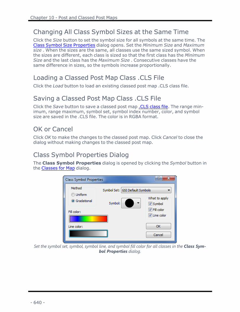
Chapter 10 - Post and Classed Post Maps
Changing All Class Symbol Sizes at the Same TimeClick the Size button to set the symbol size for all symbols at the same time. TheClass Symbol Size Properties dialog opens. Set the Minimum Size and Maximumsize . When the sizes are the same, all classes use the same sized symbol. Whenthe sizes are different, each class is sized so that the first class has the MinimumSize and the last class has the Maximum Size . Consecutive classes have thesame difference in sizes, so the symbols increase proportionally.
Loading a Classed Post Map Class .CLS FileClick the Load button to load an existing classed post map .CLS class file.
Saving a Classed Post Map Class .CLS FileClick the Save button to save a classed post map .CLS class file. The range min-imum, range maximum, symbol set, symbol index number, color, and symbolsize are saved in the .CLS file. The color is in RGBA format.
OK or CancelClick OK to make the changes to the classed post map. Click Cancel to close thedialog without making changes to the classed post map.
Class Symbol Properties DialogThe Class Symbol Properties dialog is opened by clicking the Symbol button inthe Classes for Map dialog.
Set the symbol set, symbol, symbol line, and symbol fill color for all classes in the Class Sym-bol Properties dialog.
- 640 -

Surfer User's Guide
MethodThe Method is the method used to set the symbol line and fill colors. Availableoptions are Uniform and Gradational. Setting the Method to Uniformmakes allclasses use the same line color or fill color for the symbols. Setting the Method toGradational allows each class to have a different line or fill color for the symbolsbased on a colormap.
Symbol SetSelect the Symbol Set from the list. The Symbol Set can be any TrueType fontinstalled on your system. To change the Symbol Set, click on the existing fontname. Select the new font from the list. The same Symbol Set is used for allclasses.
SymbolChoose the Symbol by clicking the existing symbol and selecting a new symbolfrom the symbol palette. The same Symbol is used for all classes.
Fill Color and OpacityWhen the Method is set to Uniform, the Fill color and opacity section is available.The Fill color is the inside color of a solid symbol. When changed, all classes willuse the same fill color for the symbols. Change the Fill color of the symbol byselecting a new color from the color palette. Create new colors by clicking theCustom button at the bottom of the color palette. Change the Fill opacity of thesymbol by highlighting the existing value and typing a new value, by clicking theto increase or decrease the opacity, or by clicking and dragging the to
change the opacity percentage. Percentages range from 0% (completely trans-parent) to 100% (completely opaque).
When the Method is set to Gradational, the Fill color section is available. The Fillcolor is the inside color of a solid symbol. When changed, symbol fill color foreach class will be based on a colormap. Click the color scale bar to change thecolormap.
Line Color and OpacityWhen the Method is set to Uniform, the Fill color and opacity section is available.The Line color is the outside edge color of the symbol. When changed, all classeswill use the same line color for the symbols. Change the Line color of the symbolby selecting a new color from the color palette. Create new colors by clicking theCustom button at the bottom of the color palette. Change the Line opacity of thesymbol by highlighting the existing value and typing a new value, by clicking theto increase or decrease the opacity, or by clicking and dragging the to
change the opacity percentage. Percentages range from 0% (completely trans-parent) to 100% (completely opaque).
- 641 -

Chapter 10 - Post and Classed Post Maps
When the Method is set to Gradational, the Line color section is available. TheLine color is the outside edge color of the symbol. When changed, symbol linecolor for each class will be based on a colormap. Click the color scale bar tochange the colormap.
What to ApplyAfter setting the Symbol Set, Symbol, Method, Fill color, and Line color, checkthe boxes in theWhat to apply section to apply the selected changes. Availableoptions are Symbol, Fill color, and Line color. When the box is checked, the prop-erties from the Class Symbol Properties dialog for the checked box areapplied to all classes in the classed post map. When the box is not checked, theproperties from the Class Symbol Properties dialog are not applied.
Setting the Same Symbol for All ClassesTo set the same symbol for all classes, click the Symbol button in the Classes forMap dialog. In the Class Symbol Properties dialog, click on the Symbol Setand select the desired font. Click on the Symbol and select the desired symbol.Check the box next to Symbol in theWhat to apply section and click OK. Allclasses are changed to use the selected symbol.
Setting the Same Symbol Line or Fill Properties for All ClassesTo set the same symbol fill properties for all classes, click the Symbol button inthe Classes for Map dialog. In the Class Symbol Properties dialog, set theMethod to Uniform. Click on the Fill color and opacity color box and select thedesired color from the list. Change the Fill opacity, as desired. Check the boxnext to Fill color in theWhat to apply section and click OK. All classes arechanged to use the selected symbol fill color.
To set the same symbol line properties for all classes, click the Symbol button inthe Classes for Map dialog. In the Class Symbol Properties dialog, set theMethod to Uniform. Click on the Line color and opacity color box and select thedesired color from the list. Change the Line opacity, as desired. Check the boxnext to Line color in theWhat to apply section and click OK. All classes arechanged to use the selected symbol line color.
Setting Gradational Symbol Line or Fill Properties for All ClassesTo set gradational symbol fill properties for all classes, click the Symbol button inthe Classes for Map dialog. In the Class Symbol Properties dialog, set theMethod to Gradational. Click on the Fill color button. In the Colormap Editor,set the colormap, scaling, and opacity. Click OK. Check the box next to Fill colorin theWhat to apply section and click OK. All classes are changed to use thecolormap to determine the symbol fill color.
To set gradational symbol line properties for all classes, click the Symbol buttonin the Classes for Map dialog. In the Class Symbol Properties dialog, set theMethod to Gradational. Click on the Line color button. In the Colormap Editor,
- 642 -

Surfer User's Guide
set the colormap, scaling, and opacity. Click OK. Check the box next to Line colorin theWhat to apply section and click OK. All classes are changed to use thecolormap to determine the symbol line color.
OK or CancelClick OK to make the changes to the class symbol properties. Click Cancel toclose the dialog without making changes.
Dialog PersistenceDue to the nature of the settings allowed in the Class Symbol Properties dia-log, only the last set of dialog settings are recalled after closing and reopeningthe dialog. The settings in the Class Symbol Properties dialog are intended tobe additive, adding new line, fill, or symbol properties to the existing class prop-erties. Therefore, not all previous settings are displayed when opening the dia-log.
Class Symbol Size Properties DialogThe Class Symbol Size Properties dialog is opened by clicking the Size buttonin the Classes for Map dialog.
Set the minimum and maximum class symbol size in the Class Symbol Size Properties dia-log.
Minimum SizeThe Minimum size is the smallest size to use for all classes. The Minimum size isused for the first class. To change the value, highlight the existing value and typethe new value. Alternatively, click the to increase or decrease the value. Sizesrange from zero to 4 inches (0 to 10.16 centimeters).
Maximum SizeThe Maximum size is the smallest size to use for all classes. The Maximum size isused for the last class. To change the value, highlight the existing value and typethe new value. Alternatively, click the to increase or decrease the value. Sizesrange from zero to 4 inches (0 to 10.16 centimeters).
- 643 -

Chapter 10 - Post and Classed Post Maps
Same Symbol Size for All ClassesSetting the Minimum size and the Maximum size to the same value results in allclasses having symbols that are the same size.
Incrementing Symbol Size for All ClassesSetting the Minimum size and Maximum size to different values results in allclasses having symbols that increment symbol sizes by a fixed amount. Todetermine the incrementing amount, subtract the Minimum size from the Max-imum size and divide by the Number of classes.
OK or CancelClick OK to make the changes to the symbol sizes for all classes. Click Cancel toclose the dialog without making changes.
Labels PropertiesWhen posting data points on a post map or classed post map, you can associatetext from the worksheet with each posted symbol. The position, font, andnumeric format can also be specified on the Labels page in the post propertiesand classed post properties.
To add labels to a post map or classed post map, click once on the post map toselect it. In the Properties window, click on the Labels tab.
- 644 -

Surfer User's Guide
Change post map or classed post map label prop-erties on the Labels page in the Properties window.
Label SetsThe Label Sets section controls which label is being controlled by the Label Set #section. Multiple labels can be displayed by changing the Label Sets settings.Click the next to Label Sets to open the Label Sets section.
Label SetThe Label set displays the name of the label that is currently being changed.Click on the set name (Set 1, for instance) to select a different set name from thelist. If only Set 1 is displayed in the list, only a single label set is currently cre-ated. All of the Label Set # properties apply to only the selected Label set.
Add Label SetThe Add label set option allows new labels to be added. Click the Add button tocreate a new Label set. The Label set option automatically changes to the newset. If this is the second label to be added, a Set 2 is added to the Label set list. Ifthis is the third label to be added, a Set 3 is added to the Label set list, and so on.
- 645 -

Chapter 10 - Post and Classed Post Maps
Remove Label SetThe Remove label set option deletes a label from the Label set list. To delete alabel, first set the Label set to the label that should be deleted. Then, click theRemove button next to Remove label set to delete the label. All properties of thelabel set are removed.
Label Set #The Label Set # section controls the worksheet column, position, angle, font,and label properties for the selected Label set . Before making any changes inthis section, change the Label set option to the desired label. The Label Set #changes to display the name of the Label set . For instance, if Label set is set toSet 3 , the Label Set # section name changes to Label Set 3.
Worksheet ColumnSelect the worksheet column containing the values or text from which you wishthe Label set to display near the posted points in theWorksheet column list. Clickon the existing worksheet column or None to change to a new worksheetcolumn. Labels may be the original data values for the data points, or may beother identifying text such as well names or sample numbers. Labels can usemath text instructions to define custom character formatting. Different work-sheet columns can be selected for each Label set.
Position Relative to SymbolThe Position relative to symbol controls the offset of the selected label from thesymbol center. To change the position, first change the Label set to the desiredlabel. Then, click on the existing position in the Position relative to symbol optionand select the new position from the list. Available options are Center, Left,Right, Above, Below, and User defined. User defined allows you to specify theexact offset (in page units) in the X offset and Y offset boxes. The posted labelsare all placed in the same position relative to the associated symbol.
Positive offset values move the labels in the positive axis direction. For reversedaxes, this means that the label is moved in the opposite direction of the Positionrelative to symbol specified. For instance, if the bottom axis is reversed, settingthe Position relative to symbol to Left will move the label to the right of the sym-bol (in the negative direction). Setting the Position relative to symbol to Userdefined and setting the X offset to 0.25 inches will move the label 0.25 inches inthe negative axis direction.
X Offset and Y OffsetWhen the Position relative to symbol option is set to User defined, the X offsetand Y offset options are available. The X offset controls the location of the labelin the left-right direction. Positive values in the X offset shift the label positiontoward the positive direction (to the right of the symbol for normal axes, to theleft for reversed axes). Negative values in the X offset shift the label position
- 646 -

Surfer User's Guide
toward the negative direction (to the left of the symbol for normal axes, to theright for reversed axes). A value of zero places the label directly in the center ofthe symbol.
The Y offset controls the placement of the label in the up-down direction. Positivevalues in the Y offset shift the label position toward the positive direction(upward for normal axes, downward for reversed axes). Negative values in the Yoffset shift the label position toward the negative direction (downward for normalaxes, upward for reversed axes). A value of zero places the label directly in thecenter of the symbol.
The X offset and Y offset values are numbers between -4 and +4 inches (-10.16and +10.16 centimeters). To change the value, highlight the existing value andtype a new value. Alternatively, click the to increase or decrease the value.
Angle (degrees)The Angle (degrees) box specifies the angle in degrees to rotate the selectedlabel set. Positive angles rotate the labels counterclockwise. To change the Angle(degrees), highlight the existing angle value. Type a new value or click and dragthe to the desired angle position.
FontClick the next to Font Properties to display the Font Properties section. Thefont properties are applied to all labels in this label set. Different label sets cancontain different font properties.
FormatClick the next to Label Format to display the Label Format section. The numericformat is applied to all numbers read from the specified label column in this labelset. Different label sets can contain different label formatting.
When the Type is set to Date/time, if Invalid date text is displayed instead of theactual date/time format, the value for the label is outside the defined date/timerange.
GeneralThe General section controls the label plane for all label sets. In addition, all labelsets can be set to use the symbol fill color for the label font color.
Label PlaneThe Label plane list specifies the coordinate plane that contains the label. Tochange the Label plane, click on the existing plane and choose the new planefrom the list. Available options are X-Y plane and Screen. If X-Y plane is selected,labels are oriented parallel to the X-Y plane of the map. As the map is tilted in3D, the labels tilt as well. This can make it hard to read the labels at shallow tilt
- 647 -

Chapter 10 - Post and Classed Post Maps
angles since the labels are viewed on edge. In this case, it may be better to ori-ent the labels in the Screen plane. Screen oriented labels are always displayedperpendicular to the viewer’s line of sight, no matter how the map is tilted orrotated. All labels from all label sets use the same Label plane.
Use Symbol Fill ColorThe Use symbol fill color option controls whether the color of the symbol is usedfor all label sets. When the Use symbol fill color option is checked, all label setsfor a point use the symbol color for the text color instead of the Font Propertiessection Foreground color option. When the symbol color changes, the label colorautomatically changes, as well. When the Use symbol fill color option isunchecked, the Font Properties section Foreground color option controls thelabel color. Each label set can then be a separate color.
Leader LinesThe Leader Lines section is used when the post map or classed post map haslabels that are offset in the Z direction or when a label is moved to a new loc-ation. The leader line is drawn from the symbol center to the new label location.
Enable for Dragged LabelsCheck the Enable for dragged labels option to display leader lines when labelsare manually dragged to a new location with the Edit Post Labels command. Theleader line will display a line from the original label location to the dragged loc-ation.
- 648 -

Surfer User's Guide
This map has a contour map layer and a post map layer. Thepost points are labeled. The labels have been moved with theEdit Post Labels command. Leader lines go from the data
point to the posted label.
3D LengthThe 3D length defines the distance above the map that the points are postedwhen the post map is tilted at a value other than 90 degrees. The 3D length boxspecifies how long the label lines are and how far above the wireframe or tiltedpost map the labels are drawn. 3D Leader Lines are not drawn on post maps over-laid on a 3D surface map. The 3D length is a value between 0 and 10 inches (0and 25.4 centimeters). To change the length, highlight the existing value andtype a new value. Press ENTER on the keyboard or click anywhere else in theProperties window to make the change. Alternatively, click the buttons toincrease or decrease the line length.
- 649 -

Chapter 10 - Post and Classed Post Maps
This map has a 3D wireframe layer and a post map layer. The post points are labeled andhave 3D leader lines from the data point to the post label.
Leader Line PropertiesClick the next to Line Properties displays the Line Properties options, allowingyou to specify the line Style, Color, Opacity, andWidth for leader lines.
Creating a Post Map with Multiple LabelsPost maps and classed post maps can have multiple labels from differentcolumns displayed on the map. To create a single map with multiple labels:
1. Click the Home | New Map | Post command to create a new post map.
2. Select the data file in the Open Data dialog and click Open.
3. Click on the Post layer to select it in the Contents window.
4. In the Properties window, click on the Labels tab.
5. With the Label set as Set 1,
- 650 -

Surfer User's Guide
1. In the Label Set 1 section, set theWorksheet column for the firstlabel.
2. Change the Position relative to symbol to the desired position.
3. Set any Font Properties or Label Format options.
6. Click the Add button next to the Add label set option.
7. With the Label set as Set 2,
1. In the Label Set 2 section, set theWorksheet column for the secondlabel.
2. Change the Position relative to symbol to the desired position.
3. Set any Font Properties or Label Format options.
Edit Post LabelsPost map and classed post map labels can be moved interactively so that labelsdo not overlap or so that labels appear in a more desirable location. To movelabels, a post map or classed post map must have theWorksheet column on theLabels page set to a column other than None to use theMap Tools | Edit Layer| Layer Labels command.
Enter Edit Post Labels ModeTo enter the post map label edit mode, click on a post map or classed post mapin the plot window or Contents window. Once the post map is selected, click theMap Tools | Edit Layer | Layer Labels command or the button. Altern-atively, right-click on the selected map and click Edit Labels or the button.
The cursor will change to a to indicate you are now in post label editingmode. The post map labels can now be individually moved.
Move Individual Post LabelsTo move a label, enter the Edit Post Labelsmode. Click once on the label youwish to move. Once the label is selected, hold down the left mouse button anddrag the label to a new location. When the label is in the desired location, releasethe mouse button.
Labels can also be moved using the keyboard. To click on a label using the key-board, hold down the ARROW keys until the cursor is above the label. Press andhold the SPACEBAR to select the label. Press the ARROW keys to move the labelto a new location. When the label is in the desired location, release theSPACEBAR.
- 651 -
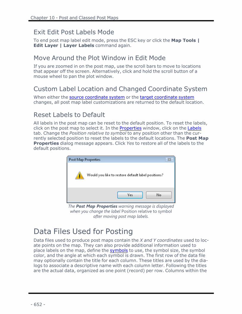
Chapter 10 - Post and Classed Post Maps
Exit Edit Post Labels ModeTo end post map label edit mode, press the ESC key or click theMap Tools |Edit Layer | Layer Labels command again.
Move Around the Plot Window in Edit ModeIf you are zoomed in on the post map, use the scroll bars to move to locationsthat appear off the screen. Alternatively, click and hold the scroll button of amouse wheel to pan the plot window.
Custom Label Location and Changed Coordinate SystemWhen either the source coordinate system or the target coordinate systemchanges, all post map label customizations are returned to the default location.
Reset Labels to DefaultAll labels in the post map can be reset to the default position. To reset the labels,click on the post map to select it. In the Properties window, click on the Labelstab. Change the Position relative to symbol to any position other than the cur-rently selected position to reset the labels to the default locations. The Post MapProperties dialog message appears. Click Yes to restore all of the labels to thedefault positions.
The Post Map Properties warning message is displayedwhen you change the label Position relative to symbol
after moving post map labels.
Data Files Used for PostingData files used to produce post maps contain the X and Y coordinates used to loc-ate points on the map. They can also provide additional information used toplace labels on the map, define the symbols to use, the symbol size, the symbolcolor, and the angle at which each symbol is drawn. The first row of the data filemay optionally contain the title for each column. These titles are used by the dia-logs to associate a descriptive name with each column letter. Following the titlesare the actual data, organized as one point (record) per row. Columns within the
- 652 -

Surfer User's Guide
data file contain various properties for the point such as its X coordinate, Ycoordinate, Z value, etc. The data must contain, at a minimum, the X and Ycoordinates. Incomplete or blank records in the X and Y coordinate columns arenot plotted on the map.
Data files used for post maps and classed post maps can contain slightly dif-ferent information. Both types of files must contain X, Y coordinates used to loc-ate the points on the map. In addition, data files for classed post maps shouldcontain a column with data values used to determine the class for each point. If athird data column is not available for the Z coordinates for a classed post map,the first data column is used.
XY Coordinates in the Data FileThe X and Y coordinates define the symbol locations and the extents of the postmap. These coordinates can be in any columns in the data file, but Surferassumes X is in column A and Y is in column B by default.
Z Values in the Data FileZ values in the data values, such as elevation or concentration, are associatedwith each X,Y location. This is typically the same column that was used when cre-ating a grid file. Z values can be used to proportionally scale the posted symbols.You can define the minimum and maximum symbol size, and all points are scaledin proportion to these sizes. See Specifying Scaled Symbols for more inform-ation. Z values can also be used to assign colors to symbols. A colormap isdefined based on the Z values and the symbols change color according to thecolormap.
For classed post maps, the Z value is used to determine which class or bin willcontain the data. Classes are based on specified data ranges, and each class isassigned a unique symbol. Classes can be saved and loaded for future use.
A common application for post maps and classed post maps is as overlays on con-tour maps. While the Z values used to scale the posted symbols in a post map, orto define the classes in a class post map, may be the same Z values used to gen-erate the contour map, this is not required. For example, the posted symbolscould be used to indicate rock type, while the contours show ore grade.
Data Labels in the Data FileData labels are text strings or numbers associated with each point on a postmap. Labels may be the original data values for the data points, or may be otheridentifying text such as well names or sample numbers. Labels can use math textinstructions to define custom character formatting.
- 653 -

Chapter 10 - Post and Classed Post Maps
Updating Post Map and Classed Post Map DataFilesA copy of the data file is created and embedded within the post map at the timethe post map is created. This means any subsequent changes made to the datafile are not reflected in the post map. To incorporate changes made to a data fileinto its associated post map, the data file must be reassigned to the map.
To automatically updated a post or classed post map:1. Select the map to be updated.
2. Use the File | Reload Map Data command. All map layers on the selectedmap are reloaded. This can change your map properties (i.e. base map con-taining an image).
To manually update a post or classed post map:1. Select the map to be updated.
2. Click once on the post map or classed post map in the Contents window toselect it.
3. In the Properties window, click on the General tab.
4. Click on the button next to Data file.
5. Select the updated data file and click Open.
The map automatically redraws with the updated data.
Symbol Specifications in the Data FilePost map data files can contain a column defining which symbol set and symbolindex to use for each posted point. This information can be specified in one ofthree ways:
Form DescriptionSymbolSet:Index This form allows both the symbol set and the symbol
index to be specified. SymbolSet specifies the facename of the desired symbol set. The colon charactermust appear between the symbol set and the index. Ifthe specified face name is invalid, the default symbolset specified in the post map properties is used instead.
- 654 -

Surfer User's Guide
Index If a single integer is specified, it is interpreted as a sym-bol index for the current symbol set. The current symbolset is the last specified symbol set or the default symbolset specified in the post map properties on the Generaltab.
<Empty> If the cell is empty, the last specified symbol set anddefault symbol index is used.
This is a sample data file containing the symbol set and index, symbol color, and symbolangle for symbols on a post map.
Symbol IndexThe symbol index is the symbol or font number as it appears in the Symbol Prop-erties. This is the 0-based offset of the symbol within the symbol set. To use thesymbol index in a data column, use the value displayed in the Symbol Prop-erties. This value is the ASCII code minus 32. For example, the ASCII code forthe Arial font lowercase "a" is 97. The index value displayed in the symbol prop-erties and used in the symbol column is 65.
When saving your plot to a Surfer13 or older .SRF file, i.e. Surfer 13 Document(*.srf), Surfer 12 Document (*.srf), or Surfer 11 Document (*.srf), the symbolindex is automatically updated in the internal data to display the correct symbolin the previous Surfer version, i.e. 32 is added to the index value from the cur-rent Surfer version. Before version 14, Surfer required the use of the ASCIIcode (index + 32) in the data file. After opening the .SRF file in a previous ver-sion of Surfer, this automatically updated data file can be saved by clicking thebutton in the Data file field in the post layer General properties.
When opening a Surfer .SRF file from a previous Surfer version, the symbolindex is automatically updated in the internal data to display the correct symbolin the post layer, i.e. 32 is subtracted from the worksheet value from the pre-vious version. Previous Surfer versions required the use of the ASCII code(index + 32) in the data file. This automatically updated data file can be saved inthe current Surfer version by clicking the button in the Data file field in the postlayer General properties.
- 655 -
Chapter 10 - Post and Classed Post Maps
You can use the Window’s character map utility to determine the ASCII code forfont symbols and subtract 32 to determine the index value. Though it is gen-erally faster to obtain the index value from the Symbol Properties. Note thatthe character map utility displays ASCII codes in hexadecimal.
If anything about the symbol specified in the data file is incorrect or missing,then the default symbol is used.
Symbol Angle Values from the Data FileThe angle (in degrees) for the posted symbol can be specified in the data file fornon-classed post maps. Positive angles rotate the symbols in a counterclockwisedirection. On classed post maps, all symbols are drawn at the same orientation,which is specified within the classed post map properties dialog.
Symbol Color from the Data FileThe posted symbol color can be specified in the data file for non-classed postmaps. Color names, as shown above, RGB or RGBA color values (red, green,blue, alpha values) can be used or a value in the Color column can be mapped toa colormap.
- 656 -

Chapter 11 - 3D Surface Maps
3D SurfaceThe Home | New Map | 3D Surface command can be used to create a three-dimensional shaded rendering from a grid file. You can also click the Home |New Map | 3D Surface | 3D Surface command to create a 3D surface. Theheight of the surface corresponds to the Z value of the associated grid node.Denser grids show greater detail on the surface.
Color can be used to show Z values on surfaces. The colors are blended to form asmooth gradation. Once the color is selected, the lighting can be adjusted, chan-ging the appearance of the map.
This 3D surface map is displayed with customcolors and no axes. Customize your map to dis-
play exactly the map you want.
Creating a 3D SurfaceTo create a 3D surface:
1. Click on the Home | New Map | 3D Surface command or the button.2. Select a grid file in the Open Grid dialog and click Open.
The map is automatically created with reasonable defaults.
Editing an Existing 3D SurfaceTo change the features of the 3D surface map, click once on the surface map inthe plot window or in the Contents window to select it. The properties are dis-played in the Properties window.
- 657 -

Chapter 11 - 3D Surface Maps
Adding a Map LayerWhen surface maps are created, they are independent of other maps in the plotwindow. For example, creating a surface map while a contour map is present inthe plot window yields two separate maps, each with its own set of axes and scal-ing parameters. To create a single map with the contour map on the surfacemap, select both maps by clicking the Home | Selection | Select All command.Overlay the maps using the Overlay Maps command.
Alternatively, you can add the contour map directly to the existing surface mapby creating the contour map using the Home | Add to Map | Layer | Contouror Map Tools | Add to Map | Layer | Contour command. This automaticallyadds the contour layer to the existing surface map axes.
Another alternative, is to create both maps using the Home | New Map com-mands. Then, select one map and drag the map layer to the other map object.This is equivalent to using the Overlay Maps command to overlay maps. Forexample, create a contour map with the Home | New Map | Contour com-mand. Create the surface map using the Home | New Map | 3D Surface com-mand. This creates two separate maps. Click on the contour map, hold down theleft mouse button, and drag the contour map into the surface map. A single mapwith two map layers, using one set of axes and scaling parameters is created.
Surface maps can be layered with images, vector files, and other 3D surfaces.You can overlay other map types, with the exception of 3D wireframes, on a sur-face. 3D surface maps can be created independently of other maps, or can becombined with other maps in map layers. Surfaces can be scaled, limited(clipped), or moved in the same way as other types of maps.
If there are map layers on a 3D surface, and the surface is made invisiblethrough the Contents window, the layers will not be visible.
Overlaying Coincident 3D SurfacesMultiple coincident 3D surfaces can be overlaid. The bases can be displayed bychecking Show base on the Properties window General page to create a blockdiagram. Control which base color is displayed by arranging the 3D surface lay-ers in the Contents window. The 3D surface layer that is to be drawn first shouldbe placed at the bottom of the Map object in the Contents window. The 3D sur-face that should be drawn last should be placed highest in the Map object. Varythe base fill colors to represent different layers in the block diagram.
- 658 -

Surfer User's Guide
This is an example of multiple overlaid 3D surface layers with differentcolor bases.
3D Surface Tipsl Image base maps, i.e. base (raster) layers, can be added to surface maps ifboth maps contain the same coordinate ranges. You may need to change theimage coordinates so the maps use the same coordinates.
l Two or more 3D surface maps can be overlaid with one another. This is usefulif you want to join two adjacent surface maps. Alternatively, you can useGrids | Resize | Mosaic to create one grid.
l Surface maps do not have a source coordinate system. All maps that are over-laid onto a surface map must have the same coordinates.
3D Surface Layer PropertiesThe surface properties contains the following pages:
GeneralMeshLightingOverlaysInfo
Map PropertiesThe map properties contains the following pages:
ViewScaleLimitsFrameInfo
- 659 -

Chapter 11 - 3D Surface Maps
3D Surface Group General PropertiesTo edit a 3D surface map, click once on the surface map to select it. The prop-erties for the surface map are displayed in the Properties window. The 3D sur-face properties General page contains the following options:
Change 3D surface map properties in the Prop-erties window on the General page.
Input Grid FileThe Grid file displays the path and file name for the grid file used for the map. Ifthe entire file name is not shown, place the mouse over the file name. A smallwindow will appear with the full path and name displayed.
Grid Information
The button displays information about the grid file used to produce the maplayer. The information includes the grid size, the minimum and maximum X, Y, Zvalues contained in the grid file, and statistics. If the grid file contains more than40 million nodes, you are asked if you wish to create a detailed report or a quickreport. Click Yes in the message to create a detailed grid report, or click No to cre-ate a shorter quick grid report.
- 660 -

Surfer User's Guide
Change File
Click the button to display the Open Grid dialog. This allows a new orupdated grid file to be specified for the surface map. Select the new grid file andclick Open to reference the new file. When the grid file is changed, the map limitsare reset but the data limits are not recalculated.
If the Z range for the new grid is outside the old Z range, the full color spectrummay not be used. Click the button next to the Upper option in the MaterialColor section. In the Colormap Editor, check the Use data limits box to use thefull color spectrum. Click OK and the map is updated.
Save File
Click the button to display the Save Grid As dialog. This allows the grid fileused for the surface map to be saved to a new name. Set the File name, Save astype, and click Save to save the file.
Color ScaleYou can check the Show color scale option to display a color scale bar adjacent tothe map. The color scale bar indicates the colors assigned to the Z levels on themap and the associated Z level values are displayed as labels on the color scalebar. If the colormap is set to a logarithmic scale, the color scale bar will auto-matically display logarithmic scaling.
LayersCheck the Show layers box to show the overlay layers on the surface. Forexample, add a post map layer to a surface. Check the Show layers box to makethe post map visible. Multiple layers can be combined into a single compositemap, and this allows the overlays to be displayed on an individual basis. Theappearance of the overlay layers is controlled on the Overlays page.
Material ColorThe Material Color section shows the spectrum of colors used to color the upperand lower sides of the surface. The light angle and colors also affect the appear-ance of the surfaces.
UpperThe Upper color controls the main color spectrum of the surface map. To changethe upper surface colors, click on the color next to Upper. Select any newcolormap from the list. If the desired colormap is not displayed, click the but-ton next to the selected colormap. The Colormap Editor opens, allowing you tospecify additional color options. To set the colormap to use a logarithmic scale,click the button to the right of the selected colormap. Check the Logarithmic
- 661 -

Chapter 11 - 3D Surface Maps
scaling option and click OK. The color map is automatically updated to show log-arithmic scaling.
When overlaying map layers on a surface, especially image base layers, the lay-ers will be brighter if you change the Upper material color to a completely whitecolormap:
1. Click the button next to Upper.2. In the Colormap Editor, change the Presets to Grayscale.3. Click the lower limit (left) anchor node.4. Change the Color to white.5. Click OK in the Colormap Editor.
LowerThe Lower button controls the single color of the bottom of the surface. Unlessthe bottom of the surface is at a sufficient angle to the light source, there will beinsufficient reflection to see it. Also, as you increase the ambient light (colorscloser to white) the lower surface color becomes more visible because ambientlight is everywhere and directionless. To change the Lower surface color, click onthe current color next to Lower. Click on the new color in the list. To use a cus-tom color or set additional color options, click the button next to the selectedcolor. The Colors dialog opens, allowing you to set additional options.
ShininessShininess controls the size of the specular reflections. As the shininess per-centage increases, the reflections become more focused. Select a value between0 and 100. To change the value, highlight the existing Shininess percentagevalue and type a new value or use the up and down arrow buttons to scroll to anew value.
NoData NodesThe NoData section defines how nodes assigned the NoData value are handled inthe surface map. Set the Method to Don't draw or Remap to.
l If Don't draw is selected, the NoData areas are not drawn on the map andappear as small transparent gaps in the surface.
l If Remap to is selected, type the new Z value into the Remap value optionbelow. The Remap value is in Z coordinate units. Make sure the new value iswithin the range of Z values in the current map. The default Remap value isthe grid Z minimum.
- 662 -

Surfer User's Guide
BaseCheck the Show base box to fill the base from the edge of the surface to the axislines. This creates the look of a filled solid. The Show base option is useful whencreating block diagrams. Control which base color is visible in the block diagramby arranging the 3D surface layers in the Contents window. The bottom-mostlayer in the map should be the bottom layer in the Contents window, and thetop-most layer in the map should be the top layer in the Contents window.
Base Line PropertiesClick the button to view the Line Properties for the base line. The line prop-erties for the 3D surface map base line are different than line properties for otherobjects.
l Click the current line Style and select None or Solid to hide or display thebase line.
l To change the base line color , click the current selection next to Color andselect a new color from the color palette. Alternatively, click the buttonand select or create a color in the Colors dialog.
l Change the base line width by typing a value in page units into theWidthfield. Alternatively you can adjust the line with by clicking the buttons.
Base Fill PropertiesClick the button to view the Fill Properties for the base line. The fill propertiesfor the 3D surface map base fill are different than fill properties for other objects.
l Click the current fill Style and select None, Solid, or Lit to change the fill stylefor the 3D surface base. Solid shows the base with a uniform fill, and the fill isnot affected by the 3D surface lighting. Lit applies the 3D surface lighting tothe base.
l To change the base fill color , click the current selection next to Color andselect a new color from the color palette. Alternatively, click the buttonand select or create a color in the Colors dialog.
3D Surface Layer Mesh PropertiesTo edit a 3D surface map, click once on the surface map to select it. The prop-erties for the surface map are displayed in the Properties window. The 3D sur-faceMesh page is used to add mesh lines to the surface of the map. Mesh linescan be used to simulate a wireframe.
- 663 -
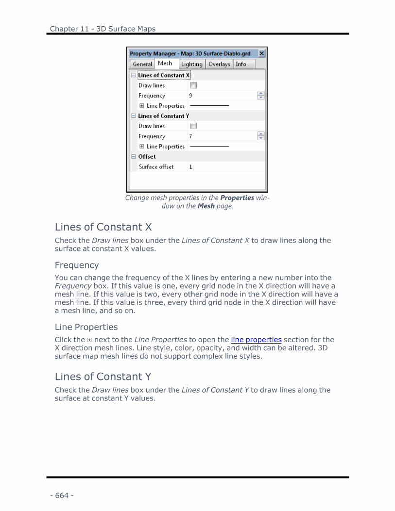
Chapter 11 - 3D Surface Maps
Change mesh properties in the Properties win-dow on theMesh page.
Lines of Constant XCheck the Draw lines box under the Lines of Constant X to draw lines along thesurface at constant X values.
FrequencyYou can change the frequency of the X lines by entering a new number into theFrequency box. If this value is one, every grid node in the X direction will have amesh line. If this value is two, every other grid node in the X direction will have amesh line. If this value is three, every third grid node in the X direction will havea mesh line, and so on.
Line PropertiesClick the next to the Line Properties to open the line properties section for theX direction mesh lines. Line style, color, opacity, and width can be altered. 3Dsurface map mesh lines do not support complex line styles.
Lines of Constant YCheck the Draw lines box under the Lines of Constant Y to draw lines along thesurface at constant Y values.
- 664 -

Surfer User's Guide
FrequencyYou can change the frequency of the Y lines by entering a new number into theFrequency box. If this value is one, every grid node in the Y direction will have amesh line. If this value is two, every other grid node in the Y direction will have amesh line. If this value is three, every third grid node in the Y direction will havea mesh line, and so on.
Line PropertiesClick the next to the Line Properties to open the line properties section for theY direction mesh lines. Line style, color, opacity, and width can be altered. 3Dsurface map mesh lines do not support complex line styles.
Surface OffsetIf you overlay two or more 3D surface maps, the mesh lines may appear dashedor broken. Experiment with the Surface offset values to change the distancebetween where the surface and mesh lines are drawn. The value is not asso-ciated with map units, instead it is offset by a factor. It is recommended thatsmall changes be made to the Surface offset when trying to make the lines moreclear.
Mesh Tipsl The default line frequency is one line in each direction.l The mesh offset value o is calculated by:
o = (m)(factor)+r
where,
m = maximum depth slope of the polygon
factor = user-specified value in Surface offset, values typically range from0.0 to 5.0
r = the smallest value guaranteed to produce a resolvable difference in win-dow coordinate depth values (a constant)
To Draw Mesh Lines1. Click on the surface map to select it.2. In the Properties window, click on theMesh tab.3. Check the Draw lines boxes in the Lines of Constant X and Lines of Constant Y
sections.4. Change the Line Properties for the X and Y lines.5. You can change the frequency of the lines by entering a new number into the
Frequency boxes.
- 665 -

Chapter 11 - 3D Surface Maps
6. If you overlay two or more surface maps, the mesh lines may appear dashedor broken. Experiment with the Surface offset values to change the distanceabove the surface that the mesh is drawn.
Lighting PropertiesTo edit a 3D surface map, click once on the surface map to select it. The prop-erties for the surface map are displayed in the Properties window. To edit theLighting in the 3D View, click Environment in the Contents window. Changesmade to the environment lighting will be automatically applied to the lighting ofpoint vector data in the 3D view. The 3D view window lighting properties are dis-played in the Properties window.
The Lighting page controls the lighting for the entire multi-layer map. Thisincludes the surface, any overlays that may have been combined with the sur-face, and point vector data in 3D. The light source is fixed relative to the surface,so if the surface is rotated, the light rotates with it.
Hill and Reflectance Shading in the 3D ViewThe 3D view lighting is turned off when the map in the 3D view contains a hillshaded or reflectance shaded color relief layer. This is because the map isalready shaded by hill shading or reflectance. The cumulative effect of both light-ing systems would result in very dark regions of the map in the 3D view.
To use the 3D view Lighting properties instead of the color relief hill or reflect-ance shading, the Terrain representation option on the color relief layer Generalpage must be set to Color only.
Lighting PropertiesThe following properties control the lighting appearance of the 3D surface map inthe plot window or the lighting of the map in the 3D view.
- 666 -

Surfer User's Guide
Change lighting properties in the Properties windowon the Lighting page.
LightingThere are three lighting options. Click on the current lighting option next toModel. In the list, select the desired lighting option.
l None disables all lighting effects. The color shown is from the surface mater-ial color only.
l Smooth splits each grid cell is into two triangular polygons. Gouraud shadingis used to interpolate colors within the triangles from the three vertices ofeach triangle. This results in smooth transitions across the triangles and theentire grid, but it is slightly slower than flat shading.
l Flat uses a single vertex (grid node) to define the shaded color for the entirepolygon. Note that each grid cell is divided into two triangular polygons. Thisresults in a faceted look since each triangle is only filled with a single color.
Light PositionThe Light Position section specifies the orientation of the light source. The lightsource can be thought of as the sun shining on a topographic surface.
The Horizontal (degrees) box defines the direction for the light source in the hori-zontal plane. Zero degrees corresponds to the light source shining from due easttoward the west. Positive angles rotate the light source counterclockwise. Forexample, a specified horizontal angle of 90 degrees places the light source northof the unrotated surface. 180 degrees places the light source west of the unro-tated surface and shining east. 270 degrees places the light source south of theunrotated surface and shining north. The default horizontal angle is set at 135degrees, or NW. To change the Horizontal (degrees), highlight the existing anglevalue. Type a new value or click and drag the to the desired angle pos-ition.
- 667 -

Chapter 11 - 3D Surface Maps
The Vertical (degrees) box rotates the light source in the vertical plane. A ver-tical angle of zero degrees places the light source at the horizon and shining hori-zontally. An angle of 90 degrees places the light source directly overhead andshining down onto the map. 180 degrees places the light source at the oppositehorizon and shining horizontally. 270 degrees places the light source directlybelow the map and shining up. The default vertical angle is 45 degrees. As thevertical angle approaches zero, shadows lengthen and the overall display shiftsto the colors at the left end of the color spectrum. To change the Vertical(degrees), highlight the existing angle value. Type a new value or click and dragthe to the desired angle position.
Light ColorsThere are three different types of light color, Ambient, Diffuse, and Specular.Note that these colors are used to represent reflectivity. White is 100% reflectiveand reflects the material color unaltered to the viewer. Black is 0% reflective,and causes all material color to be absorbed. Our perception of color is based onreflected and absorbed light. For example, a leaf appears green because itabsorbs all colors in the light spectrum EXCEPT green. Since only green is reflec-ted to your eye, the leaf appears green.
Surfer uses a pure white light source. The light "strikes" the surface and some ofthe light is absorbed based on the color of the surface material at the point thelight ray struck it. Some light is reflected to the viewer according to the type oflight (Ambient, Diffuse, and Specular), and the reflectivity color associated witheach type of light specified in the Light Colors section.
l Ambient refers to light that has been scattered so evenly by the environmentthat its direction is impossible to determine. Increasing the ambient light com-ponent brightens the scene without casting shadows. The default Ambientcolor is 90% black which means that the ambient light contribution is fairlysmall.
l Diffuse refers to light coming from a particular direction and is brighter ifaimed directly down on a surface than barely glancing off the surface. Whendiffuse light hits the surface, it is scattered uniformly in all directions so thatit appears equally bright no matter where the eye is located. Increasing dif-fuse light intensifies shadow effects. The default Diffuse color is white, whichis the maximum amount of reflectivity.
l Specular refers to light coming from a particular direction, and tends tobounce off the surface in a preferred direction. A shiny surface such as metalhas a high specular component, while a surface like carpet has almost nospecular component. Increasing the percentage of specular light results instrong shadow effects and more pronounced "shiny" or glare spots. Thedefault Specular color is 90% black.
In general, these reflectivity colors should be specified as shades of gray in orderto evenly reflect the surface material color components. However, special effectsare possible by specifying non-gray colors for the reflectivity. For example,assume the Ambient reflectivity is set to pure red, and the Diffuse and Specular
- 668 -

Surfer User's Guide
components are set to pure black. The Diffuse and Specular components areessentially disabled by setting their reflectivity color to black. The only light thatis reflected to the viewer is red ambient light. Portions of the surface that lack ared component in the material color will appear black, since only red light isreflected to the viewer.
Object LightingThe 3D Symbols property is selected by default to enable the lighting to illu-minate and cast shadows on point vector data as it does on the surface displayedin the 3D View window. When this property is cleared, shadows on 3D symbolsremain static. The Symbol method for 3D vector point data must be set to Sym-bols and the symbol style either Shaded Circle, Sphere or Cube. The lightingModelmust be either Smooth or Flat.
3D Surface Layer Overlays PropertiesTo edit a 3D surface map, click once on the surface map to select it. The prop-erties for the surface map are displayed in the Properties window. The 3D sur-face Overlays page contains options to control how overlay layers are combinedwith the surface plot. Overlay layers are converted into an image known as a tex-ture map. This texture map is applied to the surface by stretching it and shrink-ing it as necessary. Note that this stretching applies to all graphics in theoverlays, including text. If the text is positioned over a steep portion of the sur-face, it can be stretched quite a bit, resulting in significant distortion. The usualsolution to this is to view the surface from a higher angle to minimize stretchingalong the Z axis.
Change overlay properties in the Properties windowon the Overlays page.
Resampling MethodWhen the texture map is stretched, the colors in the original overlay must be res-ampled to a new size and position. The Resampling method specifies how the tex-ture map is is resampled. To change the Resampling method, click on the currentmethod. In the list, select the desired method. The options are Linear andNearest. Linear uses bilinear interpolation to combine the four surroundingpixels. Bilinear interpolation results in higher quality, but is usually slower.Nearest uses the nearest pixel in the source image.
- 669 -

Chapter 11 - 3D Surface Maps
ResolutionThe Resolution refers to the resolution (in pixels) of the overlaid texture map onthe surface map. High-resolution texture maps result in more detail, but line andtext features become thinner and may eventually fade or break up. If linesappear too thin, you should change the Resolution to a smaller value. The defaultvalue of Automatic allows Surfer to automatically determine what the best res-olution should be. Options are 64, 128. 256, 512, 1024, 2048, or 4096.
The maximum allowed value is determined by the video driver. This means thatsurface maps with overlays may appear differently on computers that do nothave the same video driver resolution.
Color ModulationColor modulation refers to the method used to combine the texture map and sur-face material colors. You can Use surface color only, Use overlay color only, oryou can Blend overlay and surface colors. When set to Use surface color only,any other overlays will not be shown in the map. The surface map color isdefined by the Upper colormap on the General page. When Use overlay coloronly is selected, the surface map color does not appear. The color is defined byany maps that are overlaid onto the surface. When Blend overlay and surface col-ors is selected, the surface map color and the overlaid maps are combined toform a new color. To change the Color modulation , click on the current option.In the list that appears, select the new option. The map will automaticallyupdate.
Map Layer VisibilityIf there are map layers on a 3D surface, and the surface is made invisiblethrough the Contents window, the layers will not be visible.
- 670 -

Chapter 12 - 3D Wireframe Maps
3D WireframeWireframes are three-dimensional representations of a grid file. Wireframes arecreated by connecting Z values along lines of constant X and Y. Each XY inter-section occurs at a grid node and the height of the wireframe is proportional tothe Z value assigned to that node. The number of columns and rows in the gridfile determines the number of X and Y lines drawn on the wireframe.
This wireframe displays gradationally colored lines that showelevation. The intersections of the lines occur at grid nodes.
Wireframes can display any combination of X lines, Y lines, or Z contour lines. Onthe wireframe, X lines correspond to the columns in the grid file and Y lines cor-respond to rows in the grid file.
The grid limits define the extent of the wireframe. When creating a grid file, setthe grid limits to the desired limits for the wireframe. The wireframe cannot belarger or smaller than the extent of the grid file. Use the Grids | Resize | Extractor Grids | Resize | Mosaic commands to produce a subset or to thin a grid file.Use Grid | Spline Smooth to increase the density of a grid file in order to add addi-tional X and Y lines to the wireframe. Use the Grid | Data command to create anew grid file with different limits.
Creating a 3D Wireframe1. Click on the Home | New Map | 3D Surface | 3D Wireframe command
or the button.2. Select a grid file in the Open Grid dialog and click Open.
The map is automatically created with reasonable defaults.
- 671 -
Chapter 12 - 3D Wireframe Maps
Editing an Existing 3D WireframeTo change the features of the 3D wireframe map, click once on the wireframemap in the plot window or in the Contents window to select it. The properties aredisplayed in the Properties window.
Adding a Map LayerWhen wireframe maps are created, they are independent of other maps in theplot window. For example, creating a wireframe map while a contour map ispresent in the plot window yields two separate maps, each with its own set ofaxes and scaling parameters. To create a single map with the contour map onthe wireframe map, select both maps by clicking the Home | Selection | SelectAll command. Overlay the maps using the Overlay Maps command.
Alternatively, you can add the contour map directly to the existing wireframemap by creating the contour map using the Home | Add to Map | Layer | Con-tour command. This automatically adds the contour map to the existing wire-frame map axes.
Another alternative is to create both maps using the Home | New Map com-mands. Then, select one map and drag the map layer to the other map object.This is equivalent to using the Overlay Maps command to overlay maps. Forexample, create a contour map with the Home | New Map | Contour com-mand. Create the wireframe map using the Home | New Map | 3D Surface |Wireframe command. This creates two separate maps. Click on the contourmap, hold down the left mouse button, and drag the contour map into the wire-frame map. A single map with two map layers, using one set of axes and scalingparameters is created.
Wireframes cannot be overlaid with other wireframes, point cloud layers, or onraster-based maps such as 3D surfaces, color relief maps, and base (raster) lay-ers.. Wireframes can be overlaid with contour maps and other map types.
Wireframe Layer PropertiesThe wireframe properties contains the following pages:
GeneralZ LevelsColor ZonesLayerInfo
Map PropertiesThe map properties dialog contains the following pages:
View
- 672 -

Surfer User's Guide
ScaleFrameInfo
3D Wireframe Layer General PropertiesTo edit a 3D wireframe, click once on the wireframe map to select it. The prop-erties for the wireframe map are displayed in the Properties window. The 3D wire-frame properties General page contains the following options:
Change 3D wireframe map properties in the Propertieswindow on the General page.
Input Grid FileThe Grid file displays the path and file name for the grid file used for the map. Ifthe entire file name is not shown, place the mouse over the file name. A smallwindow will appear with the full path and name displayed.
- 673 -

Chapter 12 - 3D Wireframe Maps
Grid Information
The button displays information about the grid file used to produce the maplayer. The information includes the grid size, the minimum and maximum X, Y, Zvalues contained in the grid file, and statistics. If the grid file contains more than40 million nodes, you are asked if you wish to create a detailed report or a quickreport. Click Yes in the message to create a detailed grid report, or click No to cre-ate a shorter quick grid report.
Change File
Click the button to display the Open Grid dialog. This allows a new orupdated grid file to be specified for the wireframe map. Select the new grid fileand click Open to reference the new file. When the grid file is changed, the maplimits are reset but the data limits are not recalculated.
Save File
Click the button to display the Save Grid As dialog. This allows the grid fileused for the wireframe map to be saved to a new name. Set the File name, Saveas type, and click Save to save the file.
Show Upper SurfaceCheck the Show upper surface box to display only the top portion of the surface.If the Remove hidden lines box is checked, only those portions of the upper sur-face not obscured by other portions of the surface are drawn.
Show Lower SurfaceCheck the Show lower surface box to display only the bottom of the surface. Ifthe Remove hidden lines box is checked, only those portions where the bottom ofthe wireframe is not obscured by other portions of the surface are drawn. A basecannot be displayed when viewing the lower surface.
Remove Hidden LinesCheck the Remove hidden lines box to remove the display of X and Y lines behindother lines on the surface. When hidden lines are not removed, the wireframehas a transparent appearance.
BorderThe Border option controls the display of the border line around the outside ofthe wireframe, at the intersection of the wireframe with the sides of the base. Tochange the border display, click on the existing option next to Border . Select thenew option in the list. Options are to display the border on the Front Only, on AllSides, or on None of the sides. The border line is not visible on wireframes
- 674 -

Surfer User's Guide
displaying both X and Y lines. The border line color is set in the Plot Lines of Con-stant section.
Plot Lines of ConstantThe Plot Lines of Constant section allows you to specify the lines to be used whendisplaying the wireframe. Any combination of X, Y, and Z lines may be used. Theproperties on the Z Levels tab and Color Zones tab are only applied if the PlotLines of Constant boxes are checked for the appropriate X, Y, or Z lines.
X LinesCheck the box next to X to display lines of constant X value on the wireframe.
Line PropertiesClick the next to the Line Properties to open the line properties section for theX direction lines. Line Style, Color, Opacity, andWidth can be altered. 3D wire-frames do not support complex line styles.
Y LinesCheck the box next to Y to display lines of constant Y value on the wireframe.
Line PropertiesClick the next to the Line Properties to open the line properties section for theY direction lines. Line Style, Color, Opacity, andWidth can be altered. 3D wire-frames do not support complex line styles.
Z LinesCheck the box next to Z to display lines of constant Z value on the wireframe.
Line PropertiesClick the next to the Line Properties to open the line properties section for theZ direction lines. Line Style, Color, Opacity, andWidth can be altered. 3D wire-frames do not support complex line styles.
BaseThe Base section controls the display of a base on the wireframe. The base is thearea "underneath" the wireframe. The bottom of the base can be drawn at any Zlevel relative to the surface.
Show BaseCheck the Show base box to display the base. The base on a wireframe is thelines connecting the wireframe to the corners of the axes.
- 675 -

Chapter 12 - 3D Wireframe Maps
Show Vertical LinesAdd X and Y lines to the base by checking the Show vertical lines box.
ElevationYou can adjust the elevation of the base in the Elevation box. To change the elev-ation, highlight the existing value and type a new one.
Line PropertiesClick the next to the Line Properties to open the line properties section for thebase lines. Line Style, Color, Opacity, andWidth can be altered. 3D wireframesdo not support complex line styles.
3D Wireframe Layer Z Levels PropertiesTo edit a 3D wireframe, click once on the wireframe map to select it. The prop-erties for the wireframe map are displayed in the Properties window.
In the Properties window, click the Edit Levels button toopen the dialog and set theZ Levelsoptions for a wire-
frame.In the Properties window, click on the Z Levels tab. Then, click the Edit Levelsbutton to open the Z Levels dialog. The 3D wireframe Z Levels dialog controlsthe display of lines of constant Z. When displaying the Z lines on a 3D wireframe,use the options on the Z Levels dialog to control which levels of Z lines to dis-play. You can specify the Z contour levels and the line properties for the indi-vidual Z lines on this page. For the Z Levels options to appear, the box next to Zin the Plot Lines of Constant section on the General tab must be checked.
- 676 -

Surfer User's Guide
Change the Z level properties in the Z Levels dialog.
LevelEvenly spaced Z levels are assigned by clicking the Level button. This displaysthe Contour Levels dialog. Set the Minimum, Maximum, and Interval and clickOK.
Level Value For One LevelTo set a specific contour level, double-click the level value in the list that youwish to change. The Z Value dialog opens. Enter a new value, and click OK. Thismethod creates unequal intervals between wireframe Z level lines.
LineClick the Line button to open the Line Spectrum dialog and create gradationalline color.
Level Line Property For One LevelTo set a specific contour level line property, double-click the sample line next tothe level value you wish to change. The Line Properties dialog opens. Makechanges to the line properties and click OK. Line Style, Color, Opacity, andWidthcan be altered. 3D wireframes do not support complex line styles.
AddClick the Add button to add a level. The added level is placed between the cur-rently selected level and the level above the currently selected level with a valuethat is halfway between the two level values.
- 677 -

Chapter 12 - 3D Wireframe Maps
DeleteHighlight a level and then click the Delete button to remove a level.
LoadClick the Load button to load a level file. Level files can be created manually, orwith wireframe or contour maps. When the level file contains additional options,like labels and hachures, the selected level line properties affect the Z contourson the 3D wireframe and do not display contour labels or hachures.
SaveClick the Save button to save a level file.
Editing Z Levels Zones1. Click on the wireframe map to select it.2. In the Properties window, click on the General tab.3. In the Plot Lines of Constant section, check the box next to Z.4. Click on the Z Levels tab.5. Click the Edit Levels button next to Z levels.6. In the Z Levels dialog, change the desired level and line properties.7. Click OK and the 3D wireframe is updated.
3D Wireframe Layer Color Zones PropertiesTo edit a 3D wireframe, click once on the wireframe map to select it. The prop-erties for the wireframe map are displayed in the Properties window.
Click on the Color Zones tab to edit the properties.In the Properties window, click on the Color Zones tab. Then, click on the EditLevels button to open the 3D wireframe Color Zones dialog. The Color Zonesdialog controls the color to apply to lines of constant X, Y, and Z based on Z val-ues in the grid file. For the Color Zones options to appear, the same box next toX, Y, or Z in the Plot Lines of Constant section on the General tab must also bechecked.
- 678 -

Surfer User's Guide
Change the color zone properties in the Color Zones dialog.
LevelEvenly spaced Z levels are assigned by clicking the Level button. This displaysthe Contour Levels dialog. Set the Minimum, Maximum, and Interval and clickOK.
Level Value For One LevelTo set a specific contour level, double-click the level value in the list that youwish to change. The Z Value dialog opens. Enter a new value, and click OK. Thismethod creates unequal intervals between wireframe Z level lines.
LineClick the Line button to open the Line Spectrum dialog and create gradationalline color.
Level Line Property For One LevelTo set a specific contour level line property, double-click the sample line next tothe level value you wish to change. The Line Properties dialog opens. Makechanges to the line properties and click OK. Line Style, Color, Opacity, andWidthcan be altered. 3D wireframes do not support complex line styles.
AddClick the Add button to add a level. The added level is placed between the cur-rently selected level and the level above the currently selected level with a valuethat is halfway between the two level values.
- 679 -

Chapter 12 - 3D Wireframe Maps
DeleteHighlight a level and then click the Delete button to remove a level.
LoadClick the Load button to load a level file. Level files can be created manually, orwith wireframe or contour maps. When the level file contains additional options,like labels and hachures, the selected level line properties affect the Z contourson the 3D wireframe and do not display contour labels or hachures.
SaveClick the Save button to save a level file.
Apply Zones to Lines of Constant X, Y, and ZThe Apply zones to lines of constant allows the selection of which type of linesyou want the color zones applied. Check the boxes next to X, Y, and Z to applythe colors to lines of constant X, Y, or Z.
Note that the same boxes must be checked on the General tab in the Plot Lines ofConstant section for the color zone changes to appear on the map.
Color Scale BarA color scale bar can be displayed on the map by checking the box next to theColor Scale option on this page.
Editing Color Zones1. Click once on the wireframe to select it.2. In the Properties window, click on the General tab.3. In the Plot Lines of Constant section, check the box next to X, Y, or Z . The
box must be checked on this tab for the color zone line properties to have anaffect.
4. In the Properties window, click on the Color Zones tab.5. Click the Edit Levels button next to Color zones.6. In the Color Zones dialog, change the desired line and level properties.7. Check the X, Y, or Z boxes to apply the color zone to that type of constant
line.8. Click OK and the wireframe is updated.
- 680 -

Surfer User's Guide
Line Spectrum DialogClick the Line button in the 3D wireframe dialog Color Zones or Z Levels page, orclick the Line button in the grid node editor Contour Levels dialog to open theLine Spectrum dialog and create gradational line color.
Specify the line properties in the Line Spectrum dia-log.
Minimum and Maximum Line PropertiesClick the Minimum Line Properties and Maximum Line Properties buttons to spe-cify the line style, color, and width for the minimum and maximum levels. Whenyou click the Minimum Line Properties or Maximum Line Properties button, theLine Properties dialog is displayed. The minimum line property is assigned to thelowest contour level and the maximum line property is assigned to the highestcontour level. Surfer automatically assigns gradational line colors or widthsbetween the minimum and maximum levels.
If you choose different line styles for the minimum and maximum contours,there is no gradational change in line styles. The lower half of the contour linesuse the style assigned for the minimum and the upper half of the contour linesuse the style assigned for the maximum.
Invisible LineIf you do not want to display contour lines for a plot you can assign an invisibleline style for both the minimum and maximum lines from the Line Spectrumdialog.
Wireframe Level FilesFor 3D wireframes, .LVL level files contain information for the Z level line prop-erties and for the color zone line properties. After defining custom level and lineproperties on the Z Levels page or the Color Zones page, save the level and colorinformation in a level file. This level file can be recalled for any other 3D wire-frame or contour maps.
- 681 -

Chapter 12 - 3D Wireframe Maps
Level files created from the wireframe properties dialog contain only informationfor the Z level line properties. Color fill, contour label, or hachure information isnot written to the level file if the level file is created from the wireframe.However, a level file created from the advanced contour map level properties dia-log may contain such additional information. A level file created from the wire-frame properties dialog can be used for a contour map and vice versa. Anyadditional information not used is ignored.
Creating Level FilesTo create a .LVL level file containing level and line property information from thewireframe properties:
1. Click once on a wireframe map to select it. The wireframe map properties willbe shown in the Properties window.
2. Click on the Z Levels tab or the Color Zones tab.3. Click the Edit Levels button. The Properties dialog opens.4. Change any of the parameters, including the contour levels or line properties.5. After changing the settings, click Save.6. In the Save As dialog, type the name of the level file and click the Save but-
ton. The level file is saved with a .LVL extension.7. Click OK to close the dialog. The wireframe map updates.
Using Level FilesTo use an existing .LVL file with any wireframe map:
1. Click once on a wireframe map to select it. The wireframe map properties willbe shown in the Properties window.
2. Click on the Z Levels tab or the Color Zones tab.3. Click the Edit Levels button. The Properties dialog opens.4. Click Load.5. Select the .LVL file and click Open.6. Click OK to close the dialog. The wireframe map updates.
Note, all wireframe maps using the level file must have comparable Z dataranges, otherwise lines will not appear on the map.
Color Filled WireframeWireframes do not allow you to create filled contours, but you can create a 3Dwireframe and add a filled contour map layer. This allows you to create a filledcontour wireframe. Usually, 3D surface maps are better for creating this type ofmap.
To create a filled contour map and overlay on a 3D wireframe map:
- 682 -

Surfer User's Guide
1. Create a 3D wireframe map with the Home | New Map | 3D Surface |Wireframe command.
2. Select the grid file and click Open.
3. Click once on the wireframe map to select it.
4. Click the Home | Add to Map | Layer | Contour command.
5. Select the grid file and click Open.
6. Click once on the contour map in the Contents window to select it.
7. In the Properties window, click on the Levels page.
8. Check the box next to the Fill contours option.
9. Set any additional parameters for the contour map. The map will auto-matically update to display the changes.
10. The result is a filled contour map draped over the 3D wireframe map. Sinceno hidden line removal is performed on the contour map, it may be neces-sary to adjust the tilt so all areas are visible. Select the Map Tools | View |Trackball command or right-click on the map and select Trackball. Set thedesired orientation parameters for the 3D wireframe. Press the ESC key onyour keyboard and the wireframe is redrawn at the orientation you specify.
11. Alternatively, you can adjust the tilt, field of view, rotation, and projectionvalues on the View page of the map properties.
Specifying the Lines to Draw on a WireframeAny combination of X, Y, and Z lines can be displayed on wireframe maps. Whenusing X and Y lines to represent the surface, a mesh appears on top of the sur-face. When using the Z lines, an elevated contour map is drawn.
To specify which lines to draw on the 3D wireframe:
1. Click once on the wireframe map to select it.2. In the Properties window, click on the General tab.3. In the Plot Lines of Constant section, check the appropriate boxes to display
any combination of X, Y, and Z lines on the wireframe.4. When displaying the Z lines on a wireframe, use the options on the Z Levels
page to control which levels of Z lines to display. Specify the Z contour levelsand the line properties for the individual Z lines on this page. The selectedlevels affect the Z contours on the wireframe and do not display contourlabels or hachures.
- 683 -

Chapter 12 - 3D Wireframe Maps
5. Note: To display contour labels or hachures on a wireframe, add a contourmap layer. Select the wireframe map and use the Home | Add to Map |Layer | Contour.
6. Set any other desired options on the General page.7. The wireframe is displayed with the line types you have chosen.
Adding Color Zones to a 3D WireframeYou can change the line colors of any 3D wireframe by applying color zones. Inthis example, we will change color zones gradationally and individually.
To add a color zone to a 3D wireframe:
1. Click on the wireframe layer to select it.
2. In the Properties window, click on the General tab.
3. In the Plot Lines of Constant section, check the box next to X and Y.Whichever line you want to have the color zone applied to must be checkedin this section.
4. Click the Color Zones tab.
5. Click the Edit Levels button next to Color zones .
6. Click the Line button to display the Line Spectrum dialog.
7. Click the Minimum Line Properties button to open the Line Properties dia-log. From here, you can select the line Color, Style,Width, or Opacity.
8. Click the Color button and select Blue from the list.
9. Click OK to return to the Line Spectrum dialog.
10. Click the Maximum Line Properties button and change the line color to Redusing the steps above.
11. Click OK in the Line Spectrum dialog to return to the Color Zones page.
12. Check the Apply Zones to Lines of Constant X and Y boxes.
13. Click OK and the wireframe is displayed with gradational X and Y lines vary-ing colors by the Z variable.
To change the properties of an individual Z value:
1. Click on the wireframe, and the 3D wireframe properties are displayed inthe Properties window.
- 684 -

Surfer User's Guide
2. Click the Color Zones tab.
3. Click the Edit Levels button next to Color zones.
4. Double-click the line sample for the contour level at Z = 70.
5. You can select the line color, style, width, or opacity for the selected line inthe Line Properties dialog. In theWidth box, click the up arrow andchange the width value to 0.030 in.
6. Click OK in the Line Properties dialog and the Color Zones page isupdated to reflect the change.
7. Click OK in the 3D wireframe Properties dialog and the map is redrawn.The color zone at Z = 70 is drawn with a thicker line, and is emphasized onthe map.
Line Property PrecedenceWireframe line properties can be assigned on three different pages in the Prop-erties window depending on the effect you are trying to achieve.
1. Color Zones page2. Z Levels page3. General page
The highest precedence is applied to line properties assigned on the ColorZones page. When the Apply zones to lines of constant check boxes on theColor Zones page are enabled, those properties take precedence over anyother assigned line properties.
Line properties assigned in the Plot Lines of Constant section on the Generalpage have the same precedence as the line properties assigned on the Z Levelspage. If the options on the Color Zones page are not used, the next highest pre-cedence are selections on the General page or Z Levels page, whichever ischanged last. The Z Levels page colors are only used on Z lines.
Line PropertiesLine properties for wireframes are controlled from the wireframe properties inthe Properties window. The X and Y line properties specified in the Plot Lines ofConstant section on the General page are applied over the entire surfacewithout regard to the relative level of the surface.
To assign X and Y line properties so that they change over the vertical range ofthe surface, set the line properties on the Color Zones page. Color zone lineproperties vary based on Z values in the grid file.
- 685 -

Chapter 12 - 3D Wireframe Maps
Use the Line Properties in the Plot Lines of Constant section on the General pageto apply the same line properties to all lines of constant Z without regard to level.To apply Z line properties that vary according to elevation, use the options in theZ Levels or Color Zones pages.
Wireframe BaseA 3D wireframe base is the area below the wireframe. The bottom of the basecan extend to any Z level. The sides of the base can be highlighted with verticallines that are extensions of the X and Y lines.
To change the base parameters:
1. Click on the wireframe map to select it.2. In the Properties window, click on the General tab.3. Check the Show base box to display the base lines.4. To display vertical base lines, check the Show vertical lines box. Vertical lines
are drawn on the face between the base and the surface border. The verticallines represent the X and Y grid lines extended from the border of the surfaceto the base.
5. To specify base height, enter the value into the Elevation box. The value is inZ data units. The smaller the number entered in the Elevation box, thefarther the base begins from the bottom of the wireframe surface, creating athicker base.
6. Specify the line properties for the base in the Line Properties section.7. The wireframe is drawn with the specified base parameters.
Smoothing a WireframeThe smoothness of a 3D wireframe map is a function of the density and topo-graphy of the grid. For example, a 10 by 10 grid file (ten rows and ten columns)appears much more angular than a 50 by 50 grid file created from the samedata. To smooth the wireframe map, you need to increase the number of rowsand columns in the grid file.
You can increase the number of grid rows or columns in one of two ways. Onemethod is to create a new grid file with more grid nodes in the X and Y directionsin the Grid Data dialog.
Alternatively, use the Grids | Edit | Spline Smooth command to insert additionalrows and columns into an existing grid file. Also, the Grids | Edit | Filter com-mand can be used to increase the smoothness of the map.
- 686 -

Surfer User's Guide
Wireframe NoData RegionsNoData regions of a grid file are represented by low flat areas on a 3D wireframemap. The level of the NoData region is set to the minimum Z value for the gridfile or the Elevation value on the General page, whichever is greater. Forexample, consider a grid file that ranges from 0 to 100 in the Z dimension. Whena wireframe is created, any NoData region appears as a large flat area at the Z=0 value, and the Elevation property value also equals 0. If the Elevation propertyis changed to -15, the NoData region remains and Z=0. If the Elevation value isincreased to 10, the NoData region is a low flat area at Z=10.
Digital Elevation Models (DEM) may have some NoData regions along the edgesof the surface. The DEM polygon contained within a 7.5-minute quadrangle con-sists of profiles that do not always have the same number of data points becauseof the variable angle between the UTM coordinate system and true north. Theresult is a regular, stair-stepped arrangement of the data points along the edgesof the map that can translate to grid nodes assigned the NoData value along theedges of grid files produced in Surfer.
- 687 -


Chapter 13 - Relief Maps
Color Relief Layer General PropertiesTo edit a color relief layer, click once on the color relief layer to select it. The prop-erties for the color relief layer are displayed in the Properties window. The colorrelief properties General page contains the following options:
The color relief layer properties General page con-trols the layer color, color scale bar, hill shading, pixel
interpolation, and missing data.
Input Grid FileThe Grid file displays the path and file name for the grid file used for the map. Ifthe entire file name is not shown, place the mouse over the file name. A smallwindow will appear with the full path and name displayed.
- 689 -

Chapter 13 - Relief Maps
Grid Information
The button displays information about the grid file used to produce the maplayer. The information includes the grid size, the minimum and maximum X, Y, Zvalues contained in the grid file, and statistics. If the grid file contains more than40 million nodes, you are asked if you wish to create a detailed report or a quickreport. Click Yes in the message to create a detailed grid report, or click No to cre-ate a shorter quick grid report.
Change FileClick the button to display the Open Grid dialog. This allows a new orupdated grid file to be specified for the color relief map. Select the new grid fileand click Open to reference the new file.
Coordinate System NoteRegardless of the file selected with either the File | Reload Map Data com-mand or by clicking the button in the Properties window, the coordinate sys-tem for the original map layer is used after updating the file. If this is not thecorrect coordinate system, click on the map layer to select it. In the Propertieswindow, click on the Coordinate System tab and set the coordinate system tothe appropriate new system.
Save File
Click the button to display the Save Grid As dialog. This allows the grid fileused for the color relief map to be saved to a new name. Set the File name, Saveas type, and click Save to save the file. If a coordinate system has been definedon the Coordinate System tab in the Properties window, an Export Optionsdialog appears. Check the desired file formats. It is recommend that GS Refer-ence (Version 2) file option be checked to generate a .GSR2 file. Click OK and thefile is saved.
Terrain RepresentationThe Terrain Representation property specifies if the color relief layer visu-alization is enhanced by hill shading or reflectance or if only colors are displayed.Select Color only to color the layer by the Z value and colormap only. Select Hillshaded to apply hill shading to the map. Select Reflectance to apply reflectanceshading to the map.
Hill shading is a method of representing relief by depicting shadows cast by apoint light source. Select the Hill shaded to apply hill shading to the color reliefmap. For hill shading a color relief map with a GrayScale colormap, it is recom-mended you change the lower color of the colormap to a slightly lighter black(e.g. 80% Black). The Hill Shading Parameters are displayed when the Hillshaded option is selected.
- 690 -

Surfer User's Guide
Reflectance uses colors to indicate the local orientation of the surface relative toa user-defined light source direction. Surfer determines the orientation of eachgrid cell and calculates reflectance of a point light source on the grid surface. Thelight source can be thought of as the sun shining on a topographic surface. Por-tions of the surface that face away from the light source reflects less light towardthe viewer, and thus appear darker. The colors on a reflectance shaded colorrelief map are based on the reflectance from the grid surface. Reflectance valuesrange from zero to one. A reflectance value of zero means that no light is reflec-ted toward the viewer. A reflectance value of one means that all incident light isreflected toward the viewer. The Reflectance Parameters are displayed when theReflectance option is selected.
Hill shading and Reflectance replaces the 3D View Lighting properties. To use the3D view lighting properties when viewing the map in the 3D view, set the Terrainrepresentation to Color only.
ColorsThe Colors option defines the colormap used to fill the color relief map. Thecolormap can use a linear or logarithmic scale. Change the color by clicking theexisting color bar next to Colors. Select the new colormap from the list. If thedesired color map is not listed, click the button to the right of the selectedcolormap. The Colormap Editor appears. Make any changes and click OK to seethe change on the map. To set the colormap to use a logarithmic scale, click thebutton to the right of the selected colormap. Check the Logarithmic scaling
option and click OK. The color map is automatically updated to show logarithmicscaling.
Interpolate PixelsThe Interpolate pixels check box activates color smoothing on the map. Whenchecked, Interpolate pixels uses bilinear interpolation to calculate colors on themap. Bilinear interpolation makes the color gradations smoother, but it canslightly slow the on-screen drawing of the color relief map.
When a dense grid (a grid with relatively large numbers of rows and columns) isused, little difference is seen between the final color relief maps whether theInterpolate pixels option is checked or not. For dense grids, on-screen drawingtime can be reduced when the Interpolate pixels option is unchecked.
When a coarse grid (a grid with relatively few rows and columns) is used and theInterpolate pixels option is not checked, all pixels within a single grid square areassigned the same color. This creates a grid-square map, and can result in acolor relief map with a very blocky appearance. For coarse grids, therefore, asmoother appearance results when the Interpolate pixels check box is checked.
- 691 -

Chapter 13 - Relief Maps
The non-interpolated color relief map maps each grid node to a pixel, i.e. a gridcell, which is expanded to a block of pixels to make the map the correct size. Theinterpolated color relief map assigns colors to the pixel or pixels at a grid nodeand then interpolates the colors for the pixels between the grid nodes.
Image Size (Pixels)The Image size (pixels) property determines the number of pixels along thelongest side of the color relief map. The number of pixels along the shorter sideof the map is calculated from the Image size (pixels) and aspect ratio of the inputgrid file. The default Image size (pixels) value is 1000. Click the buttons toincrease or decrease the Image size (pixels) by 100.
Increase the Image size (pixels) value to smooth the appearance of the colorrelief layer. Decrease the Image size (pixels) value to speed up the color relieflayer rendering time. The Image size (pixels) property can be any integer valuebetween 2 and 32767. Use caution when increasing the Image size (pixels) valueto very large numbers. Large values can significantly increase the time to renderthe color relief layer.
Show Color ScaleThe Show color scale option permits the display of a color scale bar adjacent tothe map. The color scale bar indicates the colors assigned to the Z levels on themap, and the associated Z level values are displayed as labels on the color scalebar. When the Show color scale box is checked, the color scale bar is displayed.If the colormap is set to a logarithmic scale, the color scale bar will automaticallydisplay logarithmic scaling.
Hill Shading ParametersThe Hill Shading Parameters are displayed when the Hill shaded option is selec-ted.
Horizontal Light AngleThe Horizontal light angle (degrees) box defines the direction for the light sourcein the horizontal plane. Zero degrees corresponds to the light source shiningfrom due east toward the west. Positive angles rotate the light source coun-terclockwise. For example, a specified horizontal angle of 90 degrees places thelight source north of the unrotated surface. 180 degrees places the light sourcewest of the unrotated surface and shining east. 270 degrees places the lightsource south of the unrotated surface and shining north. The default horizontalangle is set at 135 degrees, or NW. To change the Horizontal light angle(degrees), highlight the existing angle value. Type a new value or click and dragthe to the desired angle position. The Horizontal light angle (degrees)option is disabled when the Enable hill shading box is not checked.
- 692 -

Surfer User's Guide
Vertical Light AngleThe Vertical light angle (degrees) box rotates the light source in the verticalplane. A vertical angle of zero degrees places the light source at the horizon andshining horizontally. An angle of 90 degrees places the light source directly over-head and shining down onto the map. The default vertical angle is 45 degrees. Asthe vertical angle approaches zero, shadows lengthen. To change the Verticallight angle (degrees), highlight the existing angle value. Type a new value orclick and drag the to the desired angle position. The Vertical light angle(degrees) option is disabled when the Enable hill shading box is not checked.
Z Scale FactorThe Z scale factor box allows you to specify the Z scale to use for the surface. Asyou increase the Z scale factor, the surface becomes more exaggerated ver-tically. Increasing the factor enhances the shading effect, and can be useful forbringing out more detail, especially on relatively flat surfaces. The default Z scalefactor scales the Z coordinates to 1/4th the XY diagonal of the input grid. The Zscale factor option is disabled when the Enable hill shading box is not checked.The Z scale factormust be greater than 0. If a value less than or equal to 0 isentered into the Z scale factor box, the value will be automatically set to approx-imately 1.192 x 10⁻⁷.
Ambient Light IntensityThe Ambient light intensity property controls the overall brightness of the sur-face. The Ambient light intensity is a value between 0 and 1. To change the Ambi-ent light intensity, highlight the existing angle value. Type a new value or clickand drag the to the desired angle position. The Ambient light intensityoption is disabled when the Enable hill shading box is not checked.
Reflectance ParametersThe Reflectance Parameters are displayed when the Reflectance option is selec-ted.
Reflectance MethodThe Reflectance method specifies the algorithm used to compute the reflectedlight at each grid cell. The Reflectance method determines how the colors are dis-tributed in relation to the slopes and slope directions (aspect) over the extent ofthe map.
- 693 -

Chapter 13 - Relief Maps
Horizontal Light AngleThe Horizontal (degrees) box defines the direction for the light source in the hori-zontal plane. Zero degrees corresponds to the light source shining from due easttoward the west. Positive angles rotate the light source counterclockwise. Forexample, a specified horizontal angle of 90 degrees places the light source northof the unrotated surface. 180 degrees places the light source west of the unro-tated surface and shining east. 270 degrees places the light source south of theunrotated surface and shining north. The default horizontal angle is set at 135degrees, or NW. To change the Horizontal (degrees), highlight the existing anglevalue. Type a new value or click and drag the to the desired angle pos-ition.
Vertical Light AngleThe Vertical (degrees) box rotates the light source in the vertical plane. A ver-tical angle of zero degrees places the light source at the horizon and shining hori-zontally. An angle of 90 degrees places the light source directly overhead andshining down onto the map. 180 degrees places the light source at the oppositehorizon and shining horizontally. 270 degrees places the light source directlybelow the map and shining up. The default vertical angle is 45 degrees. As thevertical angle approaches zero, shadows lengthen and the overall display shiftsto the colors at the left end of the color spectrum. To change the Vertical(degrees), highlight the existing angle value. Type a new value or click and dragthe to the desired angle position.
Z Scale FactorThe Z scale factor box allows you to specify the Z scale to use for the surface. Asyou increase the Z scale factor, the surface becomes more exaggerated ver-tically. Increasing the factor enhances the shading effect, and can be useful forbringing out more detail, especially on relatively flat surfaces. The default Z scalefactor scales the Z coordinates to 1/10th the XY diagonal of the input grid. The Zscale factormust be greater than 0. If a value less than or equal to 0 is enteredinto the Z scale factor box, the value will be automatically set to approximately1.192 x 10-7.
NoDataThe NoData section sets the color for grid nodes that have been assigned theNoData value.
NoData ColorTo select a different NoData region color, click on the existing color to the rightColor and click on the desired color from the palette. Click the button to theright of the selected color to define new colors in the Colors dialog.
- 694 -

Surfer User's Guide
NoData OpacityTo change the Opacity of the NoData regions, enter a value from 0% (completelytransparent) to 100% (completely opaque) by highlighting the existing valueand typing a new value or by dragging the to change the opacity per-centage.
Reflectance Shading MethodsThere are four reflectance methods available for color relief layers using Reflect-ance for the Terrain representation. To set the Reflectance method, click on thecolor relief layer to select it. In the Properties window, click on the General tab.Change the Terrain representation to Reflectance and change the Reflectancemethod to the desired method, described below.
SimpleSimple is the fastest of the shading methods, but produces a rather crude image.With Simple, the Horizontal (azimuth) and Vertical (zenith) values are fixed at135 and 45 degrees, respectively, and cannot be changed.
Peucker’s ApproximationPeucker’s approximation uses a piecewise linear approximation. This methodgives somewhat better results than the Simplemethod, but redrawing the maptakes slightly longer. With Peucker’s approximation, the Horizontal (azimuth)and Vertical (zenith) values are fixed at 135 and 45 degrees, respectively, andcannot be changed.
Lambertian ReflectionLambertian reflection assumes an ideal surface that reflects all the light thatstrikes it and the surface appears equally bright from all viewing directions. TheLight Position Angles section allows the Horizontal (angle) and Vertical (angle)values to be specified with this option. This is the default Reflectance method.
Lommel-Seeliger LawThe Lommel-Seeliger lawmethod is based on an analysis of light scattering froma surface. This method is a compromise between an ideal diffuser and a real sur-face. With some surfaces, this may actually give better results than the Lam-bertian reflectionmethod. The Light Position Angles section allows the Horizontal(angle) and Vertical (angle) values to be specified with this option.
- 695 -


Chapter 14 - Grid Values Maps
Grid Values MapThe Home | New Map | Specialty | Grid Values command creates a grid val-ues map. A grid values map indicates the location and values of the grid nodeswith symbols and labels. Posting grid values on a map can be useful for visu-alizing the density of the grid, as well as for verifying the plausibility of your grid-ded data. The frequency of the plotted grid nodes can be controlled in the X andY directions independently. The grid values can also be displayed for only a spe-cific range of values. You can specify the symbol type, size, color, and angle forthe grid nodes. Associated data values may be placed next to the posted point.The size, angle, color, and typeface for the label can also be specified. Grid linescan also be plotted to help you visualize the grid density.
The Home | Add to Map | Layer | Grid Values orMap Tools | Add to Map| Layer | Grid Values command adds a grid values map layer to the selectedmap.
The grid values map displays grid node location and values for all or a sub-set of the grid nodes. In this example every fourth grid node value and loc-ation is displayed in the X and Y directions. The grid values layer is overlaid
with a filled contour layer.
Creating a Grid Values MapTo create a new grid values map:
- 697 -

Chapter 14 - Grid Values Maps
1. Click Home | New Map | Specialty | Grid Values.
2. Select a grid file in the Open Grid dialog. Click Open.
The map is automatically created with symbols and labels displayed across themap. The X and Y frequencies are automatically set to display approximately tenrows and columns of grid nodes.
Editing an Existing Grid Values MapTo change the features of the grid values map, click once on the grid values layerin the Contents window or plot window. When the grid values layer is selected,the grid values properties are displayed in the Properties window.
Click on the Grid Valuesmaplayer to select it.
Grid Values Layer PropertiesThe Properties window for a grid values layer contains the following pages:
General
Symbols
Labels
Layer
Coordinate System
Info
Map PropertiesThe map properties contains the following pages:
View
Scale
- 698 -

Surfer User's Guide
Limits
Frame
Coordinate System
Info
Grid Values Layer General PropertiesThe General page for a grid values layer controls the display of symbols, labels,and lines, as well as the grid values density and constraints.
Specify general display options on the Generalpage of the Properties window.
GeneralThe General section of the General page includes options for the layer grid fileand display of symbols and labels.
Input Grid FileThe Grid file lists the current grid file used in the contour map. The path and filename are the location of the grid file when the map was created or the grid filewas most recently changed.
Grid Information
The button displays information about the grid file used to produce the maplayer. The information includes the grid size, the minimum and maximum X, Y, Zvalues contained in the grid file, and statistics. If the grid file contains more than
- 699 -

Chapter 14 - Grid Values Maps
40 million nodes, you are asked if you wish to create a detailed report or a quickreport. Click Yes in the message to create a detailed grid report, or click No to cre-ate a shorter quick grid report.
Change File
The button displays the Open Grid dialog. This allows you to select a newgrid file, or an updated version of the grid file used to create the grid values map.Select a grid file and click Open.
If the new grid exceeds the current map limits, another warning will appear ask-ing you to adjust the map limits. If you click Yes, the limits are automaticallyadjusted to fit the new grid. If you click No, the limits are not automatically adjus-ted. The map may not be displayed. To change the map limits, click on the Mapobject in the Contents window and the Limits tab in the Properties window.
You may also see a warning message that the current map scale may result in anun-viewable map. Clicking OK allows the map scale to automatically be adjusted.
Coordinate System NoteRegardless of the file selected with either the File | Reload Map Data com-
mand or by clicking the button in the Properties window, the coordinate sys-tem for the original map layer is used after updating the file. If this is not thecorrect coordinate system, click on the map layer to select it. In the Propertieswindow, click on the Coordinate System tab and set the coordinate system tothe appropriate new system.
Save File
The button displays the Save Grid As dialog. Type a File name and changethe Save as type to the desired grid file format. Click Save. If a coordinate sys-tem has been defined on the Coordinate System tab in the Properties window,an Export Options dialog appears. Check the desired file formats. It is recom-mend that GS Reference (Version 2) file option be checked to generate a .GSR2file. Click OK and the file is saved.
Show SymbolsSymbols are displayed at grid node locations when the Show symbols check boxis checked. Symbols are displayed by default. Clear the Show symbols check boxto hide the symbols. The frequency of the symbols is controlled by the propertiesin the Density section.
Show LabelsGrid node value labels are displayed relative to the grid node locations when theShow labels check box is checked. Labels are displayed below the symbols bydefault. When symbols are not displayed, labels are positioned relative to the
- 700 -

Surfer User's Guide
grid node location. Clear the Show labels check box to hide the labels. The fre-quency of the labels is controlled by the properties in the Density section.
Grid LinesThe Grid Lines section of the General page contains options for the display ofgrid lines and their properties.
Show Grid LinesCheck the Show grid lines check box to display grid lines for grid rows andcolumns. Clear the Show grid lines check box to hide the grid lines. The fre-quency of the grid lines is controlled by the properties in the Density section.
Line PropertiesThe Line properties control the display of the grid lines. See the Line Propertiestopic for more information on editing line properties.
DensityThe Density section of the General page contains options for the density of thesymbol, label, and/or line display.
X FrequencyThe X frequency value specifies the frequency of drawn symbols, labels, and/orlines in the X direction. An X frequency value of 1 displays every grid nodecolumn. A frequency of 2 displays every other grid node column, 3 displays everythird column, etc. The default value is the value in which approximately ten gridcolumns are visible across the map. Type a value in the X frequency field or clickthe buttons to change the density of the symbols, labels, and/or lines in the Xdirection.
Y FrequencyThe Y frequency value specifies the frequency of drawn symbols, labels, and/orlines in the Y direction. A Y frequency value of 1 displays every grid node row. Afrequency of 2 displays every other grid node row, 3 displays every third row,etc. The default value is the value in which approximately ten grid rows are vis-ible across the map. Type a value in the Y frequency field or click the buttons tochange the density of the symbols, labels, and/or lines in the Y direction.
ConstraintsThe Constraints section of the General page controls the minimum and max-imum values for grid nodes displayed on the map.
- 701 -

Chapter 14 - Grid Values Maps
Minimum Node ValueThe Minimum node value sets the smallest grid node value that will have a sym-bol and/or label displayed on the grid values map. By default the Minimum nodevalue is -1e+39, i.e. -1 x 1039. Only grid nodes with a value greater than orequal to the Minimum node value will be displayed.
Maximum Node ValueThe Maximum node value sets the largest grid node value that will have a sym-bol and/or label displayed on the grid values map. By default the Maximum nodevalue is 1e+39, i.e. 1 x 1039. Only grid nodes with a value less than or equal tothe Maximum node value will be displayed.
Grid Values Layer Symbols PropertiesThe Symbols page controls the appearance of symbols in a grid values layer.Symbols are displayed by checking the Show symbols check box on the Generalpage.
Specify symbol display options on the Symbolspage of the Properties window.
Symbol PropertiesThe Symbol properties section controls the appearance of grid node symbols inthe map. See the Symbol Properties topic for more information on changing sym-bol properties.
- 702 -

Surfer User's Guide
AngleThe Angle (degrees) property sets the rotation of the symbols in the grid valueslayer. Type a value in degrees in the Angle (degrees) field between 0 and 360 orclick and drag the slider to select a value. Symbols rotate coun-terclockwise as the Angle (degrees) increases.
Color MethodThe symbols in a grid values layer can all be the same color or be varied by gridnode value. When the Color method is set to Fixed, the symbols are all the samecolor and all of the properties in the Symbol properties section applies to the sym-bols.
Set the Color method to Colormap to apply the colors from a colormap to thesymbols based on grid node value. When the Color method is set to Colormap,the Fill color, Fill opacity, Line color, and Line opacity properties in the Symbolproperties section are ignored. Symbols use the same line and fill color and opa-city, which is determined by the grid node value and colormap.
ColorsThe Colors property is enabled when the Color method is set to Colormap. Clickthe current colormap and select a predefined colormap from the list or create acustom colormap in the Colormap Editor by clicking the button in the Colorsfield.
Show NoData NodesCheck the Show NoData nodes check box to display symbols at grid nodesassigned the NoData value. NoData nodes will not have a symbol by default.Clear the Show NoData nodes check box to hide symbols at NoData grid nodes.
Grid Values Layer Labels PropertiesThe Labels page controls the appearance of labels in a grid values layer. Labelsare displayed by checking the Show labels check box on the General page.
- 703 -

Chapter 14 - Grid Values Maps
Specify label display options on the Labels pageof the Properties window.
Position Relative to SymbolSelect the relative position for labels in the Position relative to symbol field. Clickthe current selection and select Center, Left, Right, Above, Below, or Customfrom the Position relative to symbol list. If you select Custom, the X offset and Yoffset properties are displayed.
X OffsetThe X offset positions the labels relative to the symbol position in the X direction(left and right). Positive X offset values move the labels to the right. Negative Xoffset values move the labels to the left. Type a value in page units between -4.0and 4.0 inches (-10.16 to 10.16 centimeters) to set the X offset, or click the but-ton to change the X offset .
Y OffsetThe Y offset positions the labels relative to the symbol position in the Y direction(up and down). Positive Y offset values move the labels up. Negative Y offset val-ues move the labels down. Type a value in page units between -4.0 and 4.0inches (-10.16 to 10.16 centimeters) to set the Y offset, or click the button tochange the Y offset.
AngleThe Angle (degrees) property sets the rotation of the labels in the grid valueslayer. Type a value in degrees in the Angle (degrees) field between 0 and 360 orclick and drag the slider to select a value. Labels rotate counterclockwiseas the Angle (degrees) increases.
- 704 -

Surfer User's Guide
Label NoData NodesCheck the Label NoData nodes check box to display labels at grid nodes with theNoData value. NoData nodes will not have a label by default. Clear the LabelNoData nodes check box to hide labels at NoData nodes. "N/A" is displayed forlabels at NoData grid nodes.
Font PropertiesThe Font properties section controls the font for grid node labels in the map. Seethe Text and Font Properties topic for more information on changing font prop-erties.
Label FormatThe Label format section controls the format of the grid node labels in the map.See the Label Formats topic for more information on changing label format prop-erties
- 705 -


Chapter 15 - Watershed Maps
WatershedThe Home | New Map | Specialty | Watershed command or the buttoncan be used to create a watershed map from a grid file. The Home | Add toMap | Layer | Watershed orMap Tools | Add to Map | Layer | Water-shed command adds a watershed map layer to the selected map.
A watershed is defined as the region draining into a stream, stream system, orbody of water. A watershed map reads the data from a grid file and splits the gridup into basin, or catchment, areas. Basin areas are areas that drain water to thestream. Stream paths are calculated based on the amount of flow into the gridnode from all surrounding grid nodes. This shows the path water will take acrossthe grid. Stream lines mark the low points on the map. Depressions are areas ofinternal drainage, such as a sink. Depressions can be forced to overfill so thatwater continues to move across the surface. Depression areas can be exported.Pour points are the outlets of the stream systems and are calculated at all drain-age intersections and where the drainage leaves the edge of the grid. The pourpoints can be generated automatically or selected from a file. Surfer uses theeight-direction pour point algorithm to calculate the flow direction at each gridnode. Custom methods are used to calculate the flow direction through flat areasand for filling depressions.
- 707 -

Chapter 15 - Watershed Maps
This example map shows a watershed with severalbasins and streams. A relief layer is overlaid.
Creating a WatershedTo create a watershed:
1. Click the Home | New Map | Specialty | Watershed command.2. Select a grid file in the Open Grid dialog and click Open.
The map is automatically created with reasonable defaults.
Editing an Existing WatershedTo change the features of the watershed map layer, click once on the watershedmap layer in the plot window or in the Contents window to select it. The prop-erties are displayed in the Properties window.
- 708 -

Surfer User's Guide
Click on theWatershed layer toselect it.
Adding a Map LayerWhen watershed maps are created, they are independent of other maps in theplot window. For example, creating a watershed map while a contour map ispresent in the plot window yields two separate maps, each with its own set ofaxes and scaling parameters. To create a single map with the contour map onthe watershed map, select both maps by clicking the Home | Selection | SelectAll command. Overlay the maps using the Overlay Maps command.
Alternatively, you can add the contour map directly to the existing watershedmap by creating the contour map using the Home | Add to Map | Layer | Con-tour command. This automatically adds the contour map to the existing water-shed map axes.
Another alternative, is to create both maps using the Home | New Map com-mands. Then, select one map and drag the map layer to the other map object.This is equivalent to using the Overlay Maps command to overlay maps. Forexample, create a contour map with the Home | New Map | Contour com-mand. Create the watershed map using the Home | New Map | Specialty |Watershed command. This creates two separate maps. Click on the contourlayer, hold down the left mouse button, and drag the contour map into the water-shed map. A single map with two map layers, using one set of axes and scalingparameters is created.
Any number of peaks and depressions maps can be combined with any othermap layers.
Watershed PropertiesThe peaks and depressions properties contains the following pages:
GeneralLayerCoordinate SystemInfo
- 709 -

Chapter 15 - Watershed Maps
Map PropertiesThe map properties contains the following pages:
ViewScaleLimitsFrameCoordinate SystemInfo
Watershed ReferencesMany of the parameters for the watershed map are technical in origin, and adetailed development is beyond the scope of this document. For additionalinformation, see the following resources:
O'Callaghan JF, Mark DM. (1984) “The Extraction of Drainage Networks fromDigital Elevation Data.” Computer vision, Graphics and Image Processing, Vol.28, 323-344.
Wang, L. & H. Liu (2006) “An Efficient Method for Identifying and Filling SurfaceDepressions in Digital Elevation Models for Hydrologic Analysis and Modelling.”International Journal of Geographical Information Science, Vol. 20, No. 2: 193-213.
Garbrecht, J. and Martz, L.W. (1997) “The assignment of drainage direction overflat surfaces in raster digital elevation models.” Journal of Hydrology, Vol. 193,204-213.
Welsh, D. J. A.; Powell, M. B. (1967), "An upper bound for the chromatic numberof a graph and its application to timetabling problems." The Computer Journal,Vol. 10 (1): 85–86.
Jenson S. K. and J. O. Domingue. 1988. "Extracting Topographic Structure fromDigital Elevation Data for Geographic Information System Analysis." Pho-togrammetric Engineering and Remote Sensing, Vol. 54 (11): 1593-1600.
Pierre Soille, Jurgen Vogt, and Roberto Colombo, 2003, "Carving and adaptivedrainage enforcement of grid digital elevation models."Water ResourcesResearch, Vol. 39, NO. 12, 1366.
Watershed Layer General PropertiesTo edit a watershed map, click once on the watershed map layer to select it. Theproperties for the watershed layer are displayed in the Properties window. Thewatershed properties General page contains the following options:
- 710 -

Surfer User's Guide
Change watershed layer properties in theProperties window on the General page.
Input Grid FileThe Grid file displays the path and file name for the grid file used for the map. Ifthe entire file name is not shown, place the mouse over the file name. A smallwindow will appear with the full path and name displayed.
Grid Information
The button displays information about the grid file used to produce the maplayer. The information includes the grid size, the minimum and maximum X, Y, Zvalues contained in the grid file, and statistics. If the grid file contains more than40 million nodes, you are asked if you wish to create a detailed report or a quickreport. Click Yes in the message to create a detailed grid report, or click No to cre-ate a shorter quick grid report.
Change File
Click the button to display the Open Grid dialog. This allows a new orupdated grid file to be specified for the watershed map. Select the new grid fileand click Open to reference the new file.
If the new grid exceeds the current map limits, a warning will appear asking youto adjust the map limits. If you click Yes, the limits are automatically adjusted tofit the new grid. If you click No, the limits are not automatically adjusted. The
- 711 -

Chapter 15 - Watershed Maps
map may not be displayed. To change the map limits, click on the Map object inthe Contents window and the Limits tab in the Properties window.
You may also see a warning message that the current map scale may result in anun-viewable map. Clicking OK allows the map scale to automatically be adjusted.
Coordinate System NoteRegardless of the file selected with either the File | Reload Map Data com-
mand or by clicking the button in the Properties window, the coordinate sys-tem for the original map layer is used after updating the file. If this is not thecorrect coordinate system, click on the map layer to select it. In the Propertieswindow, click on the Coordinate System tab and set the coordinate system tothe appropriate new system.
Save File
Click the button to display the Save Grid As dialog. This allows the grid fileused for the watershed map to be saved to a new name. Set the File name, Saveas type, and click Save to save the file. If a coordinate system has been definedon the Coordinate System tab in the Properties window, the Export Options dia-log appears. Check the desired file formats. It is recommend that GS Reference(Version 2) file option be checked to generate a .GSR2 file. Click OK and the fileis saved.
DepressionsThe Depressions section contains the option to fill the depressions and save thedata created by the filled depressions to a grid file. Depressions are areas ofinternal drainage. The only way water can leave a depression is by checking theFill depressions (pits) option. Click the next to Depressions to set the filloptions and export a grid file that contains the depressions.
Fill DepressionsCheck the box next to the Fill depressions (pits) option to fill all depressions inthe grid. Depressions cause the flow of water to terminate. Checking this optioncauses the flow from all grid cells to exit the edge of the grid, allowing no trappedwater areas. Unchecking this option allows areas to become internal sinks andallows the flow to terminate in these sinks. This may or may not be appropriate,depending on the topography of the grid. Changing this option does affect theresulting basin boundaries.
When the Fill depressions (pits) box is checked or unchecked, the Threshold(cells) value is re-evaluated. If the Threshold (cells) value is greater than theminimum flow and smaller than the maximum flow, the Threshold (cells) doesnot change. If the new value is outside the range, the Threshold (cells) valuechanges to be within the new range of flow. This can create a different number ofbasins by simply unchecking and checking the Fill depressions (pits) box.
- 712 -

Surfer User's Guide
Filled GridClick the Save to File button next to Filled grid to save the depressions to a gridfile. The resulting grid file has the Z value in depressions changed to match thelowest Z value of surrounding grid nodes. This makes the surface flat in thesedepression areas. The Save to File button is disabled when Fill depressions (pits)is unchecked.
Stream OptionsStreams show the path water will take across the grid. Stream paths are cal-culated based on the amount of flow into the grid node from all surrounding gridnodes. Streams start when the number of upstream grid cells draining into a gridcell exceeds the specified Threshold (cells) value. Click the next to StreamOptions to set the threshold and line properties for streams.
Show StreamsCheck the box next to Show streams to show the drainages with flow valuesgreater than or equal to the Threshold (cells) value. Set the line properties forthe streams in the Line Properties section.
Threshold (cells)The Threshold (cells) value is the number of upstream cells that are flowing intothe grid cell that are required to create a stream line. Higher values create lessstreams and basins. Lower values create more streams and basins.
Line PropertiesClick the next to Line Properties to set the stream line properties, includingstyle, color, opacity, and width.
Basin OptionsBasin areas are areas that drain water to the stream. You can set the basin col-ors and the pour point source in the Basin Options section by clicking the nextto Basin Options to open the section.
Basin ColorsThe Basin colors option controls the colors used for creating the watershed basinareas. To change the colors, click on the color bar next to Basin colors. Selectone of the predefined colormaps from the list. To create custom colors, click onthe button to the right of the selected colormap to open the Colormap Editor.
Surferapplies a custom algorithm to determine how many colors are needed sothat no adjacent basins have the same color. This algorithm usually determinesthat between three and six colors are necessary. Once the number of colors isdetermined, the selected colormap is sampled to choose the colors. The
- 713 -

Chapter 15 - Watershed Maps
colormap ranges in value from 0 to 1. The first color is picked at a value of 0 onthe left side of the colormap. The second color is picked 1/10th to the right onthe colormap at a value of 0.1. The third color is picked at a value of 0.2, thefourth at 0.3, and so on. With most colormaps, this provides a smooth transitionof colors for the basins in the watershed map.
ExampleConsider this watershed map and the Rainbowcolormap.
The watershed is filled with four colors, ranging from a purple togreen.
Because the watershed requires four colors, the colors at 1/10th increments (atvalues 0.0, 0.1, 0.2, and 0.3) are selected to fill the basins. These correspond tothe light purple, blue-purple, blue, and blue-green colors.
The colors at values of 0, 0.1, 0.2, and 0.3 are used forthe watershed map above.
If additional colors were needed, the green color at value 0.4, the yellow-greencolor at 0.5, the yellow color at 0.6, and the yellow-orange color at 0.7 would beused.
Because it is rare that more than six colors will ever be needed, the colors on theright side of the colormap are rarely used. If you want dramatically different col-ors for the watershed basins, you should vary the colors on the left side of thecolormap. For instance, if the four colors for the map above should be purple,green, yellow, and red, the blue and orange nodes should be removed. The
- 714 -

Surfer User's Guide
green and yellow nodes should be moved to the left, aligning with the 0.1 and0.2 values. A new node should be added at a value of 0.3 with the color red. Todetermine the value a node is at, click on the node in the Colormap Editor. TheValue is displayed at the top of the dialog.
Setting a variety of colors on the left side of thecolormap will result in more differentiation in the
watershed basin colors.
Line PropertiesClick the next to Line Properties to set the basin boundary line properties,including style, color, opacity, and width.
Pour Point SourcePour points are the outlets of the stream systems and are calculated at all drain-age intersections and where the drainage leaves the edge of the grid. The pourpoints can be generated automatically or selected from a file. Surfer uses theeight-direction pour point algorithm to calculate the flow direction at each gridnode.
To change the Pour point source, click on the current option and select thedesired option from the list. Available options are None, Stream intersections,and File. When set to None, the basins are not drawn or filled on the map. Onlythe streams appear. When set to Stream intersections, pour points are com-puted at the intersection of all tributary streams. When set to File, a .BLN file isimported that defines the locations where pour points should be located. Theeasiest way to create this file is to click on the map and click the Digitize com-mand. Click on the map at the desired locations. Save the points to a .BLN fileand load the file in the Pour point file option.
Too Many Pour PointsThe maximum number of pour points is 65535. If you exceed the maximum num-ber of pour points a "Too many pour points" or "Too many control points" errorwill be displayed. If the error occurs while Pour point source is set to Streamintersections , increase the Threshold (cells) value. If Pour point source is set toFile , do not load a file with more than 65535 points.
Pour Point FileThe Pour point file is used to define the pour points when the Pour point source isset to File. This .BLN file should contain point locations that are within the water-
- 715 -
Chapter 15 - Watershed Maps
shed map grid limits. To select the file, click on the button to the right of Pourpoint source. In the Open dialog, select the .BLN file and click Open.
Snap Pour PointsThe Snap pour points option is used when the Pour point source is set to File. Acommon problem with using digitized points to define the pour points is locatingthe point slightly off the desired location, such as on the side of a hill. Checkingthis option moves the points in the Pour point file to if any of the eight neigh-boring grid node cells have a higher flow value. This allows more flow and betterdelineation of the basins.
- 716 -

Chapter 16 - Vector Maps
1-Grid Vector MapVector map information, direction and magnitude, can be derived from one grid.The arrow symbol points in the "downhill" direction and the length of the arrowdepends on the magnitude, or steepness, of the slope. A vector is drawn at eachgrid node unless some nodes are skipped by changing the Frequency setting onthe Symbol page in the vector map properties.
For example, consider a grid containing elevation information. If water werepoured over the surface, the direction arrows would point in the direction waterflows - from high elevation to low elevation. Magnitude is indicated by arrowlength. In the water flow example, the steeper slopes would have longer arrows.
This vector map is overlaid on a filled contour map.Longer arrows indicate areas of steeper slope.
Creating a 1-Grid Vector MapTo create a 1-grid vector map:
- 717 -
Chapter 16 - Vector Maps
1. Click the Home | New Map | Specialty | 1-Grid Vector command or thebutton.
2. Select a grid file in the Open Grid dialog and click Open.
The map is automatically created with reasonable defaults.
Editing a 1-Grid Vector MapTo change the features of the vector map, click once on the vector map in theplot window or in the Contents window to select it. The properties are displayedin the Properties window.
Adding a Map LayerWhen vector maps are created, they are independent of other maps in the plotwindow. For example, creating a vector map while a contour map is present inthe plot window yields two separate maps, each with its own set of axes and scal-ing parameters. To create a single map with the vector map on the contour map,select both maps by clicking the Select All command. Overlay the maps using theMap Tools | Map Tools | Overlay Maps command.
Alternatively, you can add the vector map directly to the existing contour map bycreating the vector map using the Home | Add to Map | Layer | 1-GridVector command. This automatically adds the vector map to the contour mapaxes.
Another alternative, is to create both maps using the Home | New Map com-mands. Then, select one map and drag the map layer to the other map object.This is equivalent to using the Overlay Maps command to overlay maps. Forexample, create a contour map with the Home | New Map | Contour com-mand. Create the vector map using the Home | New Map | Specialty | 1-Grid Vector command. This creates two separate maps. Click on the vectormap, hold down the left mouse button, and drag the vector map into the contourmap. A single map with two map layers, using one set of axes and scaling para-meters is created.
Any number of vector maps can be combined with any other map layers.
1-Grid Vector Map Properties1-grid vector map layers contain the following property pages:
DataSymbolScalingLayerCoordinate SystemInfo
- 718 -

Surfer User's Guide
Map PropertiesThe map properties contains the following pages:
ViewScaleLimitsFrameCoordinate SystemInfo
1-Grid Vector Map Data PropertiesTo edit a 1-grid vector map, click once on the vector map to select it. The prop-erties for the vector map are displayed in the Properties window. The vector mapData page contains the following options:
Specify the input grid file on the Data page for a 1-Grid vector map.
Input Grid FileThe Grid file displays the path and file name for the grid file used for the map. Ifthe entire file name is not shown, place the mouse over the file name. A smallwindow will appear with the full path and name displayed.
Grid Information
The button displays information about the grid file used to produce the maplayer. The information includes the grid size, the minimum and maximum X, Y, Zvalues contained in the grid file, and statistics. If the grid file contains more than40 million nodes, you are asked if you wish to create a detailed report or a quickreport. Click Yes in the message to create a detailed grid report, or click No to cre-ate a shorter quick grid report.
- 719 -

Chapter 16 - Vector Maps
Change FileClick the button to display the Open Grid dialog. This allows a new orupdated grid file to be specified for the 1-grid vector map. Select the new grid fileand click Open to reference the new file.
Coordinate System NoteRegardless of the file selected with either the File | Reload Map Data com-
mand or by clicking the button in the Properties window, the coordinate sys-tem for the original map layer is used after updating the file. If this is not thecorrect coordinate system, click on the map layer to select it. In the Propertieswindow, click on the Coordinate System tab and set the coordinate system tothe appropriate new system.
Save File
Click the button to display the Save Grid As dialog. This allows the grid fileused for the 1-grid vector map to be saved to a new name. Set the File name,Save as type, and click Save to save the file. If a coordinate system has beendefined on the Coordinate System tab in the Properties window, the ExportOptions dialog appears. Check the desired file formats. It is recommend that GSReference (Version 2) file option be checked to generate a .GSR2 file. Click OKand the file is saved.
2-Grid Vector Map2-grid vector maps use two separate grid files to determine the vector directionand magnitude. The grids can contain Cartesian or polar data. With Cartesiandata, one grid consists of X component data and the other grid consists of Y com-ponent data. With polar data, one grid consists of angle information and theother grid contains length information.
- 720 -

Surfer User's Guide
This map shows two Cartesian grid files. The blue vectors are Xcomponent grid values. The red vectors are Y component gridvalues. The black is the vector that Surfer plots when the two
grids are specified when creating a 2-grid Cartesian vector map.
Creating a 2-Grid Vector MapTo create a 2-grid vector map:
1. Use the Home | New Map | Specialty | 2-Grid Vector command or the
button.2. Select the first grid file in the Open Grid dialog. This is the X component or
Angle component grid file. Click Open.3. Select the second grid file in the Open Grid dialog. This is the Y component
or the Length component grid file. Click Open.
The map is automatically created with reasonable defaults.
Editing an Existing 2-Grid Vector MapTo change the features of the 2-grid vector map, click once on the 2-grid vectormap in the plot window or the Contents window. The properties are displayed inthe Properties window.
- 721 -

Chapter 16 - Vector Maps
Adding a Map LayerWhen vector maps are created, they are independent of other maps in the plotwindow. For example, creating a vector map while a contour map is present inthe plot window yields two separate maps, each with its own set of axes and scal-ing parameters. To create a single map with the vector map on the contour map,select both maps by clicking the Select All command. Overlay the maps using theMap Tools | Map Tools | Overlay Maps command.
Alternatively, you can add the vector map directly to the existing contour map bycreating the vector map using the Home | Add to Map | Layer | 2-GridVector command. This automatically adds the vector map to the contour mapaxes.
Another alternative, is to create both maps using the Home | New Map com-mands. Then, select one map and drag the map layer to the other map object.This is equivalent to using the Overlay Maps command to overlay maps. Forexample, create a contour map with the Home | New Map | Contour com-mand. Create the vector map using the Home | New Map | Specialty | 2-Grid Vector command. This creates two separate maps. Click on the vectormap, hold down the left mouse button, and drag the vector map into the contourmap. A single map with two map layers, using one set of axes and scaling para-meters is created.
Any number of vector maps can be combined with any other map layers.
2-Grid Vector Map PropertiesThe 2-grid vector map layer properties contains the following pages:
DataSymbolScalingLayerCoordinate SystemInfo
Map PropertiesThe map properties contains the following pages:
ViewScaleLimitsFrameCoordinate SystemInfo
- 722 -

Surfer User's Guide
2-Grid Vector Map Data PropertiesTo edit a 2-grid vector map, click once on the vector map to select it. The prop-erties for the vector map are displayed in the Properties window. The vector mapData page contains the following options:
Specify the Coordinate System, Angle, Units, and twogrid files on the Data page for a 2-grid polar vector
map.
Specify the X component and Y componenton the Data page for a 2-grid Cartesian vector map.
Input Grid FilesThe Input Grid section displays the path and file name for the grid files used forthe map. If the entire file name is not shown, place the mouse over the filename. A small window will appear with the full path and name displayed.
For a Polar (angle, length) 2-grid vector map, the grids contain Angle componentand Length component grids. The Angle component grid contains directioninformation. The vector at each grid node will be pointed in the direction of the
- 723 -

Chapter 16 - Vector Maps
Angle component. The Length component grid contains the length of the vector.The vector at each grid node will be as long as the value in the Length com-ponent.
For a Cartesian (X, Y) 2-grid vector map, the grids contain X component and Ycomponent grids. The X component grid contains the length of the vector in theX direction. The Y component grid contains the length of the vector in the Y dir-ection. The direction of each vector will be found by adding the two grid files. Themagnitude is found using the Pythagorean theorem.
Grid Information
The button displays information about the grid file used to produce the maplayer. The information includes the grid size, the minimum and maximum X, Y, Zvalues contained in the grid file, and statistics. If the grid file contains more than40 million nodes, you are asked if you wish to create a detailed report or a quickreport. Click Yes in the message to create a detailed grid report, or click No to cre-ate a shorter quick grid report.
Change FileClick the button to display the Open Grid dialog. This allows a new orupdated grid file to be specified for the 2-grid vector map. Select the new grid fileand click Open to reference the new file.
Coordinate System NoteRegardless of the file selected with either the File | Reload Map Data com-
mand or by clicking the button in the Properties window, the coordinate sys-tem for the original map layer is used after updating the file. If this is not thecorrect coordinate system, click on the map layer to select it. In the Propertieswindow, click on the Coordinate System tab and set the coordinate system tothe appropriate new system.
Save File
Click the button to display the Save Grid As dialog. This allows the grid fileused for the 2-grid vector map to be saved to a new name. Set the File name,Save as type, and click Save to save the file. If a coordinate system has beendefined on the Coordinate System tab in the Properties window, the ExportOptions dialog appears. Check the desired file formats. It is recommend that GSReference (Version 2) file option be checked to generate a .GSR2 file. Click OKand the file is saved.
- 724 -

Surfer User's Guide
Coordinate SystemCartesian (X, Y) or Polar (Angle, Length) can be used in a two-grid vector map.To change the type of 2-grid vector map, click on the existing Coordinate Systemand select the desired coordinate system from the list. The Cartesian (X, Y)coordinate system requires one grid file with X magnitude components and thesecond grid file with Y magnitude components. The Polar (Angle, Length) coordin-ate option requires one grid with angle (direction) information and the secondgrid with length (magnitude) direction for the vectors. The Length ComponentGrid File cannot contain negative values.
AngleWhen working with polar coordinates, set the location of the zero value to thenorth or east in the Angle option. Setting Angle to 0=north, increases CW, cre-ates a polar system with increasing angles as shown in the left image below. Set-ting Angle to 0=eash, increases CCW, creates a polar system with increasingangles as shown in the right image below.
This image shows the two coordinate Angle orientations.In the image on the left, zero = North. Numbers increaseclockwise. In the image on the right, zero = East. Numbers
increase counter-clockwise.
Angle UnitsWhen working with polar coordinates,you can set the type of angle units used inthe grid file. Set the Angle units to either Degrees or Radians . This is the unit ofthe data in the Angle component grid.
Cartesian Data2-grid vector maps created with Cartesian data require that one grid contains Xcomponent data and a Y component data grid. The data from the two grids arecombined to produce vector direction and magnitude. The components can be ineither negative or positive space. The direction and magnitude of the resultingvectors are determined from the two grids as shown in the following example.
- 725 -

Chapter 16 - Vector Maps
ExampleThe lower right corner's X component is 3.5 and the Y component is 3.5. To sim-plify the math, the origin of both are zero. The direction of the resulting vector isfound by adding the two vectors together:
The magnitude of the vector is:
Polar Data2-grid vector maps created with polar data require that one grid contains angle(direction) data and the other contains length (magnitude) data.
Negative Data and Polar GridsMagnitude values cannot be negative. If you have chosen a gridding techniquethat displays trends in the data, such as Kriging, you may end up with negativevalues in your grid even if the original data are all positive.
When creating a grid, you can use the Grid Z Limits section of the Grid Data dia-log to limit the grid Z values to a specific range. Set the Minimum option to Cus-tom and the value to 0 to ensure negative values are not created in the gird. TheGrid Z Limits options can be used with any Gridding Method.
Alternatively, regridding the magnitude data and decreasing the grid spacing isone way to make the grid honor the data better. If you regrid the magnitudedata you must also regrid the angle data using the same output grid geometry. Ifyou do not want to change the output grid geometry of the grids or if decreasingthe grid nodes is not completely eliminating the negative data, then you can useGrid | Math to set all negative values equal to zero. Another alternative is to usea gridding method that does not trend the data as much (Triangulation with Lin-ear Interpolation or Natural Neighbor).
Vector Map Symbol PropertiesTo edit a 1-grid vector map or 2-grid vector map, click once on the vector map toselect it. The properties for the vector map are displayed in the Properties win-dow. The vector map Symbol page contains the following options for the vectorsymbol drawn at each grid node:
- 726 -

Surfer User's Guide
Change vector symbol properties in the Properties win-dow on the Symbol page.
StyleThe Style list contains several symbols to use to display the vectors. To changethe symbol Style , click on the existing style. A list appears. Click on a new sym-bol from the list and the map automatically updates to show the new symbol.
FrequencyThe X frequency and Y frequency settings control the number of symbols dis-played on the vector map. If the frequency is set to one, every symbol is dis-played on the vector map. If the frequency is set to two, every other symbol isdisplayed. If the frequency is set to three, every third symbol is displayed on thevector map, and so on. The symbols are located at grid nodes. So, skipping sym-bols skips vectors at the specified number of grid nodes in the X or Y direction. Ifthere are too many symbols on the vector map, increase the X frequency and Yfrequency numbers until the map becomes legible. To change the frequency,highlight the existing value and type a new number. Press ENTER on the key-board or click anywhere else in the Properties window to make the change.Alternatively, click the buttons to increase or decrease the frequency.
Line PropertiesClick on the next to Line Properties to open the line properties section. The LineProperties control the line on the outside of a filled symbol. If the Scaling method
- 727 -

Chapter 16 - Vector Maps
is set to By magnitude or By grid file , the Line Properties indicated in this sectionare not used.
Fill PropertiesClick on the next to Fill Properties to open the fill properties section. The FillProperties control the color and patter of the area inside a filled symbol. If theScaling method is set to By magnitude or By grid file, the Fill Properties indicatedin this section are not used.
Color ScalingThe Color Scaling section contains options for gradationally coloring the symbols.
Scaling MethodThe Scaling method determines how to gradationally color the vector map sym-bols. To change the Scaling method, click on the current method. A list appears.Select the desired method and the map is updated.
l When the Scaling method is set to Disabled, the Line Properties and FillProperties specified in the Symbol Properties section are used to color thevector symbols.
l When the Scaling method is set to By magnitude, the vectors are grad-ationally colored, by the length of the vector.
l When the Scaling method is set to By grid file, the vectors are gradationallycolored by the value in another grid file. The grid file must contain the sameoutput grid geometry as the vector map grid files. This means the numberof rows and columns and the grid range must be the same for all grids. Thevectors are colored according to the corresponding Z value in the color gridfile.
Vector ColorsThe Vector colors option defines the colormap used to fill the vector map symbolwhen Scaling method is set to either By magnitude or By grid file. Change thecolor by clicking the existing color bar next to Vector colors. Select the newcolormap from the list. If the desired color map is not listed, click the button tothe right of the selected colormap. The Colormap Editor appears. Make anychanges and click OK to see the change on the map. The range for the colors isalso set from the Colormap Editor. To set the colormap to use a logarithmicscale, click the button to the right of the selected colormap. Check the Log-arithmic scaling option and click OK. The color map is automatically updated toshow logarithmic scaling.
- 728 -

Surfer User's Guide
Grid FileThe Grid file displays the path and file name for the grid file used to color the vec-tor symbols when the Scaling method is set to By grid file. If the entire file nameis not shown, place the mouse over the file name. A small window will appearwith the full path and name displayed.
Grid Information
The button displays information about the grid file used to produce the maplayer. The information includes the grid size, the minimum and maximum X, Y, Zvalues contained in the grid file, and statistics. If the grid file contains more than40 million nodes, you are asked if you wish to create a detailed report or a quickreport. Click Yes in the message to create a detailed grid report, or click No to cre-ate a shorter quick grid report.
Change File
Click the button to display the Open Grid dialog. This allows a new orupdated grid file to be specified for the vector symbol colors. Select the new gridfile and click Open to reference the new file. If a new unreferenced file is selec-ted, select the appropriate coordinate system in the Assign Coordinate Sys-tem dialog and click OK.
Save File
Click the button to display the Save Grid As dialog. This allows the grid fileused to be saved to a new name. Set the File name, Save as type, and click Saveto save the file.
Show Color ScaleThe Show color scale option permits the display of a color scale bar adjacent tothe map. The color scale bar indicates the colors assigned to the vector symbolson the map, and the associated Z level values are displayed as labels on the colorscale bar. When the Show color scale box is checked, the color scale bar is dis-played. If the colormap is set to a logarithmic scale, the color scale bar will auto-matically display logarithmic scaling.
Vector Map Scaling PropertiesTo edit a 1-grid vector map or 2-grid vector map, click once on the vector map toselect it. The properties for the vector map are displayed in the Properties win-dow. The Scaling page contains placement and sizing options for vector sym-bols. Each symbol is located at a grid node.
- 729 -

Chapter 16 - Vector Maps
Change vector scaling properties in the Prop-erties window on the Scaling page.
Symbol OriginThe symbol is located on the grid node with the Symbol origin options. To changethe Symbol origin, click on the existing option and select a new option from thelist. The symbol can be placed at the Tail, at the Center, or at the Head. At theTail, places the end of the vector symbol on the grid node. At the Head , placesthe tip of the arrow symbol at the grid node. At the Center places the center ofthe vector at the grid node.
Scaling MethodThere are three ways to scale vectors listed in the Scaling method option. Youcan scale the symbols between the minimum and maximum data values linearly,logarithmically, or by square root. Linear scaling provides a better visual rep-resentation of symbols that, for the most part, are scaled in one dimension (suchas arrows with varying shaft length). When scaling the arrows in two dimensions(symbol width and shaft length), Square root or Logarithmic scaling displays thearrows more effectively. To change the Scaling method , click the current option.A list is displayed. Click on the new option and the map automatically updates.
- 730 -

Surfer User's Guide
Reverse Vector OrientationThe direction the arrowhead points can be reversed by checking the Reverse vec-tor orientation check box. By default, vectors point in the "downhill" direction.Checking the Reverse vector orientation points the vectors in the "uphill" dir-ection.
Vector Magnitude (data)Set the Minimum and Maximum data values for the vectors in the Magnitude(data) section. Check the Use data limits box to set the vector minimum andmaximum to the grid minimum and maximum values. Setting a new Minimumand Maximum is useful in displaying a series of maps in which you would like allof the vectors to be scaled the same even though the data minimum and max-imum may differ.
To set the Minimum or Maximum value, highlight the existing value and type anew value. Values are in Z magnitude units.
Shaft LengthSet the range of the arrow shaft length in the Shaft Length section. The ShaftLength is the length of the arrow symbol from the tip of the tail to the tip of thearrow head. The Minimum value is the smallest shaft length displayed in the mapat the Minimum value specified by the Magnitude (data) section. The Maximumvalue is the longest shaft length displayed in the map at the Maximum value spe-cified by the Magnitude (data) section. Enter a new value into the boxes tochange the length. Values are in page units. Values can be between 0 and 10inches (0 and 25.4 centimeters).
Head LengthSet the range of the head length in the Head Length section. The Head Length isthe length of the arrow head portion of the arrow symbol. The Minimum value isthe smallest arrow head displayed in the map at the Minimum value specified bythe Magnitude (data) section. The Maximum value is the longest arrow head dis-played in the map at the Maximum value specified by the Magnitude (data) sec-tion. Enter a new value into the boxes to change the length. Values are in pageunits. Values can be between 0 and 10 inches (0 and 25.4 centimeters). If theHead Length values match the Shaft Length values, the arrow heads will be theentire length of the vector map symbol.
Symbol WidthSet the range of the symbol width in the Symbol Width section. The SymbolWidth is the width of the arrow head portion of the arrow symbol at the widestpoint. The Minimum value is the smallest arrow head displayed in the map at theMinimum value specified by the Magnitude (data) section. The Maximum value is
- 731 -

Chapter 16 - Vector Maps
the longest arrow head displayed in the map at the Maximum value specified bythe Magnitude (data) section. Enter a new value into the boxes to change thelength. Values are in page units. Values can be between 0 and 5 inches (0 and12.7 centimeters).
Clipping Symbols on Vector MapsIn a 1-grid vector map or a 2-grid vector map, any symbols at the edge of themap are truncated at the map limits. This results in a partial vector being drawnwhen the vector extends beyond the map limits. If a partial vector is drawn, buta full vector is desired, a change in the map limits is required. Follow these stepsto change the map limits:
1. Create a vector map using the Home | New Map | Specialty | 1-GridVector Map or Home | New Map | Specialty | 2-Grid Vector Mapcommand.
2. Click on the map in the Contents window or plot window to select it.
3. Click on the Limits page in the Properties window.
4. If a partial vector is displayed at the bottom or left of the map, decrease thevalues in the xMin and yMin boxes to display the entire vector.
5. If a partial vector is displayed at the top or right of the map, increase thevalue in the xMax and yMax boxes to display the entire vector.
- 732 -

Chapter 17 - Point Cloud Maps
Point Cloud MapPoint cloud maps display LiDAR data as points at XY locations. Color is assignedto the points by elevation, intensity, return number, or classification. The pointcloud layer includes commands for modifying, classifying, and exporting points.Point cloud layers are displayed in the 3D View as three-dimensional points.LiDAR data can be combined from multiple files and filtered with various criteriawhen creating a point cloud map. The point cloud layer requires one or moreLAS/LAZ LiDAR data files to be selected for the input files.
This example shows a point cloud layer in the plot window (left) and 3D view (right). Thecolormap is applied by elevation.
Creating a Point Cloud MapTo create a point cloud map:
1. Click the Home | New Map | Specialty | Point Cloud command or thebutton.
2. Select one or more LiDAR files in the Open dialog and click Open.3. Add or remove files, set the coordinate system, and apply filters to the points
in the Import Points dialog, if desired, and click OK.
The map is automatically created with reasonable defaults. The point cloud layername includes the input file name in the Contents window, e.g. Point Cloud -myData.las . If the point cloud layer consists of multiple input files, a "+" isappended to the layer name, e.g. Point Cloud - myData.las+ .
- 733 -

Chapter 17 - Point Cloud Maps
Editing an Existing Point Cloud MapTo change the features of the point cloud map, open the point cloud map prop-erties by clicking on the point cloud map in the plot window or clicking on thepoint cloud layer name in the Contents window. The properties are displayed inthe Properties window.
To classify, modify, or export points or grids, open the Point Cloud ribbon tab byclicking the point cloud map in the plot window or clicking the point cloud layername in the Contents window. The Point Cloud tab is added to the ribbon andautomatically selected.
Adding a Map LayerWhen point cloud maps are created, they are independent of other maps in theplot window. For example, creating a point cloud map while a contour map ispresent in the plot window yields two separate maps, each with its own set ofaxes and scaling parameters. To create a single map with the point cloud mapdata points on the contour map, select both maps by clicking the Home | Selec-tion | Select All command. Overlay the maps using the Overlay Maps command.
Alternatively, you can add the point cloud map directly to the existing contourmap by creating the point cloud map using the Home | Add to Map | Layer |Point Cloud command. This automatically adds the point cloud map to the con-tour map axes.
Another alternative, is to create both maps using the Home | New Map com-mands. Then, select one map and drag the map layer to the other map object.This is equivalent to using the Overlay Maps command to overlay maps. Forexample, create a contour map with the Home | New Map | Contour com-mand. Create the point cloud map using the Home | New Map | Specialty |Point Cloud command. This creates two separate maps. Click on the point cloudlayer in the Contents window, hold down the left mouse button, and drag thepoint cloud layer into the contour map. A single map with two map layers, usingone set of axes and scaling parameters is created.
Point cloud maps cannot be added as a map layer to 3D wireframe maps, but apoint cloud map can be added to any other map layer, including 3D surfacemaps.
Saving a Point Cloud MapSurfer embeds most grid and vector data in the Surfer SRF file. However,Surfer does not embed the point cloud data in the SRF file. Surfer saves a pathto the source data, the Import Points options, and point cloud layer settings.When sharing an SRF file with a point cloud layer with another user, provide theuser with the LAS source data files. Consider storing LAS source data in a net-work location if you often share SRF files with point cloud layers.
- 734 -

Surfer User's Guide
When opening an SRF file that includes a point cloud layer, Surfer first checksthe saved file path to locate the data. If the data is not found in the same pathwith the same name, Surfer then checks paths relative to the SRF file locationfor the LAS source data. If the source data is still not found, the Import Pointsdialog is displayed with missing data files highlighted. Click Update File Path inthe Import Points dialog to locate the missing source data files.
When opening an SRF file with a point cloud layer, the point cloud data loadingprogress is displayed in place of the layer until the source data has finished load-ing. You can begin working on your map while the point cloud data loads.
Point Cloud Layer PropertiesThe point cloud layer properties contains the following pages:
GeneralLayerCoordinate SystemInfo
Map PropertiesThe map properties contains the following pages:
ViewScaleLimitsFrameCoordinate SystemInfo
Import Points DialogThe Import Points dialog specifies the input LAS/LAZ files, the source file elev-ation units, the layer source coordinate system, and various data filters for theinput data. The Import Points dialog is displayed when creating a point cloudlayer or when changing the Sources for the layer in the General page.
The Import Points dialog is also displayed when opening an SRF file and one ormore LAS source data files were not found. Missing files are highlighted in redand include the error message, "Unable to open file <filename>." Click UpdateFile Path to update the path to the missing data files, or click to remove themissing files from the Files list.
- 735 -

Chapter 17 - Point Cloud Maps
Select the source data and point filtering for the point cloud layer in the Import Points dia-log.
FilesThe Files section lists the source data files. The Files section includes commandsfor adding and removing source files, specifying the data elevation units, and set-ting the output layer coordinate system.
File ListThe File list displays the source LAS/LAZ files, the number of points in the file,the file XYZ extents, and the file coordinate system. Click the to expand the filedetails in the file list. Click the to collapse the file details in the file list. When asource file is collapsed, only the file name and number of points are displayed.
- 736 -
Surfer User's Guide
Source files with errors will be highlighted in red. The error description is dis-played below the file name when there is a source file error. Errors must beresolved before the OK button is enabled and the point cloud layer can be cre-ated.
File ExtentsThe spatial extents of the source data is displayed below the file name. Theextents include the X Min, X Max, Y Min, Y Max, Z Min, and Z Max.
Source Coordinate SystemThe Source Coordinate System is displayed below the file spatial extents. Thesource data files can have different coordinate systems. All coordinates will beconverted to the Target Coordinate System.
The Source Coordinate System will be set automatically if the coordinate systeminformation is available in the data file. If the Source Coordinate System is incor-rect, click Set to specify the source data coordinate system.
When the Source Coordinate System is unknown for one or more files, the Set allunreferenced option is available. Click Set all unreferenced to specify the samecoordinate system for all source files that are currently unreferenced.
Source Elevation UnitsThe Source Elevation Units are displayed below the Source Coordinate System.The source data files can have different elevation units. All elevation units will beconverted to the Target Elevation Units.
The Source Elevation Unitsmay be determined automatically if the information isavailable in the source file. Click Set to change the elevation units to the appro-priate units if the Source Elevation Units is incorrect.
When one or more source file Elevation Units are Unknown, the Set all unknownoption is available. Click Set all unknown to specify the same Elevation Units forall source files that currently have their Elevation Units set to Unknown.
Remove Files
Click the to the right of the points count to remove a file from the File list.
Add FilesClick Add files to add new files to the File List with the Open dialog. More thanone file from the same directory can be selected. Only LiDAR data files can beselected for creating a point cloud layer.
- 737 -

Chapter 17 - Point Cloud Maps
Target Coordinate SystemThe Target Coordinate System is the coordinate system to which all the sourcefile coordinates are transformed. This becomes the point cloud layer sourcecoordinate system when the point cloud layer is created.
Target Elevation UnitsSelect the Target Elevation Units from the Target Elevation Units list. The sourceelevation values will be converted to the corresponding value in the Target Elev-ation Units in the point cloud layer.
Point FilterThe points in the input files can be filtered by various criteria in the Point Filtersection.
Boundary FilterThe Points within bounds filter limits the imported points by XY extents. Selectthe Points within bounds check box to apply the Points within bounds filter. ClickSelect to set the bounds in the Select Bounds dialog. The minimum and max-imum XY values and their coordinate system are displayed below Points withinbounds.
Elevation/Z FilterThe Elevation / Z filter limits the imported points to a specific elevation/Z valuerange. Select the Elevation / Z check box to apply the Elevation / Z filter. Specifythe minimum Z value to be imported in the Min field. Specify the maximum Zvalue to be imported in the Max field.
Select the units for the Min and Max values from the Units list. The Source Elev-ation Unitsmust be specified in the Files list to use the Elevation / Z Units . If anyinput file has Source Elevation Units set to Unknown , then the Elevation / ZUnitsmust also be set to Unknown . When set to Unknown , the Z values are com-pared directly to the Min and Max values without any unit conversions.
Sample FilterThe Sample 1 point out of every filter limits the imported points to every nthpoint. Select the Sample 1 point out of every check box to apply the sample fil-ter. For example to import every other point, type 2 in the Sample 1 point out ofevery field. Type 10 to import every tenth point. Click the buttons to increase ordecrease the value, or type a value directly in the Sample 1 point out of everyfield.
- 738 -

Surfer User's Guide
Source ID FilterThe point source ID value indicates the file from which the point originated. Thepoint source ID is a value from 0 to 16384 inclusive. Select the Source ID checkbox to apply a source ID filter to the data. Type the desired source ID number inthe Source ID field to limit the import to points with the specified point source ID.
Reject Inconsistent RecordsThe Reject inconsistent records filter removes all invalid or inconsistent datafrom import. Select the Reject inconsistent records check box to reject invalid orinconsistent data.
Scan Direction FlagThe scan direction flag indicates whether the point was located on a forward scansweep or backward scan sweep. The Scan Direction Flag filter limits the importedpoints to forward scan sweep data, backwards scan sweep data, or both. Clickthe Scan Direction Flag check box to change the filter state.
A check mark indicates only forward scan sweep points are imported. Acleared check box indicates only backwards scan sweep points are imported. Ablack square indicates no scan direction filtering is applied. No Scan DirectionFlag filter is applied by default.
Edge of Flight FlagThe edge of flight flag indicates whether the point is located at the farthest reachof the scanner during the sweep. The Edge of Flight Flag filter limits the importedpoints to points with the edge of flight flag, points without the edge of flight flag,or both. Click the Edge of Flight Flag check box to change the filter state.
A check mark indicates only points with an edge of flight flag are imported. Acleared check box indicates only points without an edge of flight flag are impor-ted. A black square indicates no edge of flight filtering is applied. No Edge ofFlight Flag filter is applied by default.
Synthetic PointThe synthetic point flag indicates the point was created by a means other thanLiDAR collection, such as a point created via interpolation in post-processing soft-ware or digitized from a photogrammetric stereo model. The Synthetic Point fil-ter limits the imported points to points with the synthetic point flag, pointswithout the synthetic point flag, or both. Click the Synthetic Point check box tochange the filter state.
A check mark indicates only points with a synthetic point flag are imported. Acleared check box indicates only points without a synthetic point flag areimported. A black square indicates no synthetic point filtering is applied. NoSynthetic Point filter is applied by default.
- 739 -

Chapter 17 - Point Cloud Maps
Key PointThe key point flag indicates the point is considered a model key point and shouldnot be removed. The Key Point filter limits the imported points to points with thekey point flag, points without the key point flag, or both. Click the Key Pointcheck box to change the filter state.
A check mark indicates only points with a key point flag are imported. Acleared check box indicates only points without a key point flag are imported.A black square indicates no key point filtering is applied. No Key Point filter isapplied by default.
Withheld PointThe withheld point flag indicates the point is considered suspect or redundantand should not be included in processing. TheWithheld Point filter limits theimported points to points with the withheld point flag, points without the with-held point flag, or both. Click theWithheld Point check box to change the filterstate.
A check mark indicates only points with a withheld point flag are imported. Acleared check box indicates only points without a withheld point flag are impor-ted. A black square indicates no withheld point filtering is applied. NoWithheldPoint filter is applied by default.
Classification FilterThe Classification filter limits the imported points to only the selected classes.Select the Classification check box to import all classes. Clear the Classificationcheck box to clear all the classes. Select individual classes for import by selectingthe check boxes next to the desired classes.
Return Type FilterThe Return type filter limits the imported points to only the specified returntypes. The return types are defined by the return number and number of returnsfrom the pulse. For example, Single selects all points with a return number of 1and a number of returns of 1. The following table defines the Return typeoptions.
Option DefinitionUnknown The return number is unknownFirst Return Number = 1Second Return Number = 2Third Return Number = 3Last Return Number = Number of ReturnsSingle Return Number = Number of Returns = 1 (e.g. 1st of 1)First ofMany
Return Number < Number of Returns AND Return Number = 1(e.g. 1st of 3)
- 740 -

Surfer User's Guide
Secondof Many
Return Number < Number of Returns AND Return Number = 2(e.g. 2nd of 4)
Third ofMany
Return Number < Number of Returns AND Return Number = 3(e.g. 3rd of 4)
Last ofMany
Return Number = Number of Returns AND Return Number > 1(e.g. 2nd of 2, 3rd of 3, etc.)
Select the Return type check box to import all return types. Clear the Returntype check box to clear all the return types. Select individual return types forimport by selecting the check boxes next to the desired return type.
Select Bounds DialogThe Select Bounds dialog is displayed when defining the boundary filter in theImport Points dialog or the boundary criteria in the Select by Criteria dialog. Thedata filtering or selecting bounds can be specified in the Import Points TargetCoordinate System or in latitude and longitude degrees.
Filter the data by XY extents with the Select Bounds dia-log.
- 741 -
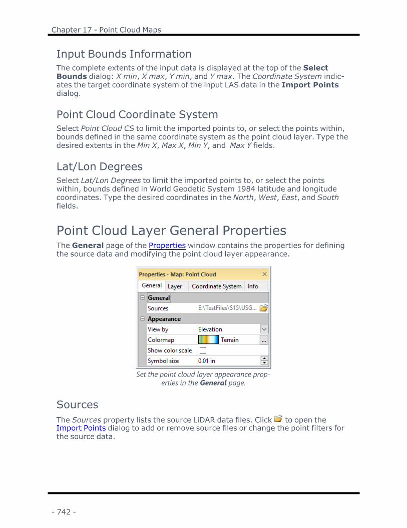
Chapter 17 - Point Cloud Maps
Input Bounds InformationThe complete extents of the input data is displayed at the top of the SelectBounds dialog: X min, X max, Y min, and Y max. The Coordinate System indic-ates the target coordinate system of the input LAS data in the Import Pointsdialog.
Point Cloud Coordinate SystemSelect Point Cloud CS to limit the imported points to, or select the points within,bounds defined in the same coordinate system as the point cloud layer. Type thedesired extents in the Min X, Max X, Min Y, and Max Y fields.
Lat/Lon DegreesSelect Lat/Lon Degrees to limit the imported points to, or select the pointswithin, bounds defined in World Geodetic System 1984 latitude and longitudecoordinates. Type the desired coordinates in the North,West, East, and Southfields.
Point Cloud Layer General PropertiesThe General page of the Properties window contains the properties for definingthe source data and modifying the point cloud layer appearance.
Set the point cloud layer appearance prop-erties in the General page.
SourcesThe Sources property lists the source LiDAR data files. Click to open theImport Points dialog to add or remove source files or change the point filters forthe source data.
- 742 -

Surfer User's Guide
AppearanceThe Appearance section includes properties for modifying the point cloud layerappearance in the plot window and 3D view.
View ByThe View by property specifies whether the Colormap is applied to the points byElevation, Intensity, Return number, or Classification.
l Elevation applies point color by elevation value. The default colormap is Ter-rain.
l Intensity applies point color by intensity value. The default colormap isGrayScale.
l Return number applies point color by return number. The default colormap isGrayScale.
l Classification applies point color by classification value. A custom colormap isused by default. See the LAS LiDAR Binary File Description for a list of classesand colors.
Click the current selection and select the desired option from the list to changethe View by property.
ColormapThe Colormap property specifies the colormap for the four View by options. EachView by option, Elevation, Intensity, Return number, and Classification uses aseparate colormap. The previous Colormap settings are maintained when switch-ing to a new View by option. To change the colormap for the current View byselection, click the current colormap and select a predefined colormap from thelist. To modify the colormap, create a custom colormap, or change the data tocolor mapping, click in the Colormap field to open the Colormap Editor.
Show Color ScaleThe Show color scale option displays a color scale bar adjacent to the map. Thecolor scale bar indicates the colors assigned to the levels on the map, and theassociated values are displayed as labels on the color scale bar. When the Showcolor scale box is checked, the color scale bar is displayed. If the colormap is setto a logarithmic scale, the color scale bar will automatically display logarithmicscaling.
The Show color scale option is not available when View by is set to Classification.When Show color scale is selected and the View by property is changed to Clas-sification , the color scale is removed. Change the View by property to Elevation ,Intensity , or Return number to enable the Show color scale property.
- 743 -

Chapter 17 - Point Cloud Maps
Symbol SizeThe Symbol size property specifies the diameter of the points in the layer in pageunits. Type a value between 0 and 0.25 in (0 and 0.635 cm) in the Symbol sizefield to change the size of the point cloud points. Alternatively, click the toincrease or decrease the point Symbol size . When the Symbol size is set to 0,the point symbols will be one pixel in size.
Point Cloud Tab CommandsWhen a point cloud layer is selected, the contextual Point Cloud ribbon tab isavailable and automatically selected. The Point Cloud tab contains commandsfor selecting, classifying, removing, and exporting points in the point cloud.
Criteria Select points by various criteria: XY bounds, Z value, clas-sification, return type, every nth, etc.
Rectangle Select points by drawing a rectanglePolygon Select points by drawing a polygonDeselect All Deselect all pointsReclassify Change the classification for selected pointsRemove Clas-sifications
Remove the classification for select points
Crop to Selec-tion
Remove all non-selected points from the layer
Remove Selec-ted Points
Remove all selected points from the layer
Create Grid Create a grid file from the point cloud layerExportLAS/LAZ
Export the point cloud layer to an LAS or LAZ file
Point Cloud Tab CommandsWhen a point cloud layer is selected, the contextual Point Cloud ribbon tab isavailable and automatically selected. The Point Cloud tab contains commandsfor selecting, classifying, removing, and exporting points in the point cloud.
Criteria Select points by various criteria: XY bounds, Z value, clas-sification, return type, every nth, etc.
Rectangle Select points by drawing a rectanglePolygon Select points by drawing a polygonDeselect All Deselect all pointsReclassify Change the classification for selected pointsRemove Clas-sifications
Remove the classification for select points
Crop to Selec-tion
Remove all non-selected points from the layer
- 744 -

Surfer User's Guide
Remove Selec-ted Points
Remove all selected points from the layer
Create Grid Create a grid file from the point cloud layerExportLAS/LAZ
Export the point cloud layer to an LAS or LAZ file
Selecting PointsPoints in the point cloud layer can be reclassified, removed, and/or exported.First the points must be selected. The Point Cloud ribbon tab includes three com-mands for selecting points in the point cloud layer: Criteria, Rectangle, and Poly-gon. When one or more points is selected the selected point(s) are surroundedby a blue dashed line. Regions of the map with no selected points are faded, andthe region that includes the selected points is highlighted.
The Polygon command was used to select points in the trapezoidalregion in the center of the map.
Once you have selected the desired points, use the Reclassify, Remove Clas-sifications, Crop to Selection, or Remove Selected Points commands to modifythe layer. To export the selected points, use the Export LAS/LAZ command andselect the Selected points only option in the Export Point Cloud dialog.
Click the Deselect All command to deselect all points. The dashed blue line isremoved, and the layer returns to its normal appearance.
- 745 -

Chapter 17 - Point Cloud Maps
The map returns to its normal appearance when no points are selec-ted.
Criteria SelectThe Point Cloud | Point Selection | Criteria command selects points in thepoint cloud layer based on spatial, random sampling, flag, classification, orreturn type criteria. Click the Point Cloud | Point Selection | Criteria com-
mand or the button to select points based on specific criteria. Specify thedesired criteria in the Select by Criteria dialog, and then click OK to select thepoints in the point cloud layer that meet the criteria.
There are two indications of the point selection in the Surfer window.
l The number of selected points is displayed in the status bar.l If the selected points fall within a specific region of the map, the selectedpoints are highlighted, and the non-selected points are faded out. Note thatwith criteria select, the highlighted region may include points that are notselected due to the various selection criteria. If the selected points cover theextent of the map, no region will appear faded out.
Select by Criteria DialogThe Select by Criteria dialog contains spatial, classification, return type, andflag criteria for selecting points in the point cloud layer.
- 746 -

Surfer User's Guide
Select points by criteria with the Select by Criteria dialog.Boundary CriteriaThe Points within bounds criteria selects the points by XY extents. Select thePoints within bounds check box to apply the Points within bounds criteria. ClickSelect to set the bounds in the Select Bounds dialog. The minimum and max-imum XY values and their coordinate system are displayed below Points withinbounds.
Elevation/Z CriteriaThe Elevation / Z criteria selects the points within a specific elevation/Z valuerange. Select the Elevation / Z check box to apply the Elevation / Z criteria. Spe-cify the minimum Z value to be selected in the Min field. Specify the maximum Zvalue to be selected in the Max field. Select the units for the Min and Max valuesfrom the Units list.
Sample CriteriaThe Sample 1 point out of every criteria selects the every nth point. Select theSample 1 point out of every check box to apply the sample criteria. For exampleto select every other point, type 2 in the Sample 1 point out of every field. Type10 to select every tenth point. Click the buttons to increase or decrease thevalue, or type a value directly in the Sample 1 point out of every field.
- 747 -

Chapter 17 - Point Cloud Maps
Source ID CriteriaThe point source ID value indicates the file from which the point originated. Thepoint source ID is a value from 0 to 16384 inclusive. Select the Source ID checkbox to apply a source ID criteria to the data. Type the desired source ID numberin the Source ID field to select the points with the specified point source ID.
Reject Inconsistent RecordsThe Reject inconsistent records filter removes all invalid or inconsistent datafrom the selection. Select the Reject inconsistent records check box to rejectinvalid or inconsistent data.
Scan Direction FlagThe scan direction flag indicates whether the point was located on a forward scansweep or backward scan sweep. The Scan Direction Flag criteria selects forwardscan sweep data, backwards scan sweep data, or both. Click the Scan DirectionFlag check box to change the criteria state.
A check mark indicates only forward scan sweep points are selected. A clearedcheck box indicates only backwards scan sweep points are selected. A blacksquare indicates no scan direction criteria is applied. No Scan Direction Flag cri-teria is applied by default.
Edge of Flight FlagThe edge of flight flag indicates whether the point is located at the farthest reachof the scanner during the sweep. The Edge of Flight Flag criteria selects thepoints with the edge of flight flag, points without the edge of flight flag, or both.Click the Edge of Flight Flag check box to change the criteria state.
A check mark indicates only points with an edge of flight flag are selected. Acleared check box indicates only points without an edge of flight flag are selec-ted. A black square indicates no edge of flight criteria is applied. No Edge ofFlight Flag criteria is applied by default.
Synthetic PointThe synthetic point flag indicates the point was created by a means other thanLiDAR collection, such as a point created via interpolation in post-processing soft-ware or digitized from a photogrammetric stereo model. The Synthetic Point cri-teria selects points with the synthetic point flag, points without the syntheticpoint flag, or both. Click the Synthetic Point check box to change the criteriastate.
A check mark indicates only points with a synthetic point flag are selected. Acleared check box indicates only points without a synthetic point flag are selec-ted. A black square indicates no synthetic point criteria is applied. No Syn-thetic Point criteria is applied by default.
- 748 -

Surfer User's Guide
Key PointThe key point flag indicates the point is considered a model key point and shouldnot be removed. The Key Point criteria selects points with the key point flag,points without the key point flag, or both. Click the Key Point check box tochange the criteria state.
A check mark indicates only points with a key point flag are selected. A clearedcheck box indicates only points without a key point flag are selected. A blacksquare indicates no key point criteria is applied. No Key Point criteria is appliedby default.
Withheld PointThe withheld point flag indicates the point is considered suspect or redundantand should not be included in processing. TheWithheld Point criteria selectspoints with the withheld point flag, points without the withheld point flag, orboth. Click theWithheld Point check box to change the criteria state.
A check mark indicates only points with a withheld point flag are selected. Acleared check box indicates only points without a withheld point flag are selec-ted. A black square indicates no withheld point criteria is applied. NoWithheldPoint criteria is applied by default.
Classification FilterThe Classification filter selects points within the selected classes. Select the Clas-sification check box to select all classes. Clear the Classification check box toclear all the classes. Select individual classes for selection by selecting the checkboxes next to the desired classes.
Return Type FilterThe Return type filter selects points within the specified return types. Select theReturn type check box to select all return types. Clear the Return type check boxto clear all the return types. Select individual return types for selection by select-ing the check boxes next to the desired return type.
Rectangle SelectClick the Point Cloud | Point Selection | Rectangle command or the but-ton to select points in the point cloud layer by drawing a rectangle. The cursor
changes to a cross hair when the Rectangle command is selected.
1. Click the Point Cloud | Point Selection | Rectangle command.2. Click and drag in the map to draw a rectangle around the points you wish to
select.3. Release the left mouse button to finish drawing the rectangle. The points
within the rectangle are selected.
- 749 -

Chapter 17 - Point Cloud Maps
The selected points are indicated by the highlighted area andblue dashed line.
Drawing Tipsl Hold down the CTRL key while dragging the mouse to draw a square ratherthan a rectangle.
l Hold down the SHIFT key while dragging the mouse to draw a rectangle fromthe center point rather than from corner to corner.
l Hold down the SHIFT and CTRL keys while dragging the mouse to draw thesquare from the center point rather than from corner to corner.
l The number of selected points is indicated in the status bar.
Polygon SelectClick the Point Cloud | Point Selection | Polygon command or the buttonto select points in the point cloud layer by drawing a polygon. The cursor
changes to a cross hair when the Polygon command is selected.
1. Click the Point Cloud | Point Selection | Polygon command.2. Click in the map to add a vertex to the polygon.3. Continue adding vertices around the points you wish to select.4. Double-click the last vertex or press the ENTER key to finish drawing the poly-
gon. The points within the polygon are selected.
- 750 -

Surfer User's Guide
The selected points are indicated by the highlighted areaand blue dashed line.
Drawing Tipsl Click points on the page to draw a polygon, or click and hold the left mousebutton and drag the cursor to draw a continuous stream of points.
l Click the right mouse button to remove the last drawn point. This can be donerepeatedly.
l If the CTRL key is pressed while clicking points, the points are constrained to45-degree angles.
l Double-click the left mouse button or press the ENTER key to close the poly-gon.
l To cancel drawing a polygon, press the ESC key before closing the polygon.l The number of selected points is indicated in the status bar.
Deselect All PointsClick the Point Cloud | Point Selection | Deselect All command to deselectall points in the point cloud layer. When the points in the point cloud layer aredeselected, the blue dashed line indicating the selected points bounding box isremoved.
- 751 -

Chapter 17 - Point Cloud Maps
ReclassifyThe Point Cloud | Classify | Reclassify field displays the classification of theselected points. When the selected points include more than one classificationvalue, no classification is displayed in the Reclassify field.
To reclassify the selected points, select the desired classification from theReclassify list. The reclassify list includes the following classifications:
l Never Classifiedl Unclassifiedl Groundl Low Vegetationl Medium Vegetationl High Vegetationl Buildingl Low Point Noisel Mass Pointl Waterl Railroadl Road Surface
Remove ClassificationsClick the Point Cloud | Classify | Remove Classifications command or the
button to remove the classifications from the selected points.
Crop to SelectionClick the Point Cloud | Modify | Crop to Selection command or the buttonto crop the point cloud layer to the selected points. The Crop to Selection com-mand removes points from the layer that are outside the rectangular extents ofthe selected points. For example if you create a selection with the Polygon com-mand, the crop area will be the smallest rectangle that completely surrounds theselection polygon.
To crop the layer to the selected points:1. Select points using the Criteria, Rectangle, or Polygon commands.
- 752 -

Surfer User's Guide
Select the points you wish to keep when using the Crop toSelection command.
2. Click the Point Cloud | Modify | Crop to Selection command. All pointsthat are not selected are removed from the map. The map extents are notchanged.
- 753 -

Chapter 17 - Point Cloud Maps
Crop to Selection removes all points outside the extents of the selec-tion.
3. If desired, change the map limits and scale in the Properties window or withthe Set Limits command.
You may wish to change the map limits and scale after usingthe Crop to Selection command.
- 754 -

Surfer User's Guide
Remove Selected PointsClick the Point Cloud | Modify | Remove Selected Points command or the
button to remove the selected points from the layer.
Grid Point CloudClick Point Cloud | Features | Create Grid or the button to create a gridfile from the point cloud layer. The Grid Point Cloud dialog is displayed whenthe Create Grid command is clicked.
The Create Grid command uses a binning algorithm to create a grid file fromthe point cloud data. Each grid node is at the center of a grid cell, and all pointswithin the cell are aggregated by the selected Aggregation method to computethe grid node value. The binning algorithm does not extrapolate beyond the con-vex hull of the data, and any grid nodes with no points within their cell areassigned the NoData value.
If you wish to create a grid with one of the gridding methods, export the pointcloud layer to an LAS/LAZ file and use the newly created file with the Grid Datacommand.
Grid Point Cloud DialogThe Grid Point Cloud dialog is displayed when the Point Cloud | Features |Create Grid command is clicked. Specify the data field, aggregation method,output grid geometry and file name in the Grid Point Cloud dialog.
Create a grid file from a point cloud layer with Grid Point Cloud .
- 755 -

Chapter 17 - Point Cloud Maps
Data Field to GridA grid can be created from the elevation, intensity, return number, or clas-sification value. Select the field Elevation, Intensity, Return number, or Clas-sification in the Data field to grid list.
Aggregation MethodThe Aggregation method specifies how the grid node values are calculated fromthe points in the grid cell.
l Average assigns the average value of the points within the cell.
l Minimum assigns the minimum value from the points within the cell.
l Maximum assigns the maximum value from the points within the cell.
l Nearest assigns the value from the point nearest the grid node.
l IDW assigns the inverse distance squared weighted average value of thepoints within the cell.
Select the desired method from the Aggregation method list.
Data StatisticsThe data statistics section shows the number of points and the spatial extents ofthe point cloud layer.
Output Grid GeometryThe Output Grid Geometry section defines the grid limits and grid density. Bydefault, the Output Grid Geometry settings are spaced to include an average often points per grid node cell.
Minimum and Maximum X and Y Coordinate (Grid Limits)Grid limits are the minimum and maximum X and Y coordinates for the grid.Surfer computes the minimum and maximum X and Y values from the pointcloud layer. These values are used as the default minimum and maximumcoordinates for the grid.
Grid limits define the X and Y extent of contour maps, color relief maps, 3D sur-faces, etc. created from grid files. When creating a grid file, you can set the gridlimits to the X and Y extents you want to use for your map. Once a grid file is cre-ated, you cannot produce a grid-based map larger than the extent of the gridfile. If you find you need larger grid limits, you must regrid the data. You can,however, read in a subset of the grid file to produce a map smaller than theextent of the grid file.
- 756 -
Surfer User's Guide
Spacing and # of Nodes (Grid Density)Grid density is usually defined by the number of columns and rows in the grid,and is a measure of the number of grid nodes in the grid. The # of Nodes in the XDirection is the number of grid columns, and the # of Nodes in the Y Direction isthe number of grid rows. By defining the grid limits and the number of rows andcolumns, the Spacing values are automatically determined as the distance indata units between adjacent rows and adjacent columns.
Output GridChoose a path and file name for the grid file in the Output Grid section. You cantype a path and file name, or click the button to browse to a new path andenter a file name in the Save Grid As dialog. By default the grid file name isbased on the first file in the point cloud metadata.
Add Grid as LayerCheck the Add grid as layer to check box to automatically add the created grid toa new or existing map. Select [New Map] in the Add grid as layer to field to cre-ate a new map. Click the current selection and select an existing map to add anew layer to the map. Select the layer type by clicking the current selection inthe New layer type field and selecting the desired layer type from the list.
Export LAS/LAZClick Point Cloud | Features | Export LAS/LAZ or the button to exportthe points in the point cloud layer to an uncompressed LAS or compressed LAZLiDAR Binary file.
Export Point Cloud DialogThe Export Point Cloud dialog is displayed when the Point Cloud | Features| Export LAS/LAZ command is clicked. Specify the output file path and name,format, and tiling options in the Export Point Cloud dialog.
- 757 -

Chapter 17 - Point Cloud Maps
Set the export options in the Export Point Cloud dialog.OutputChoose a path and file name for the LiDAR file in the Output section. You cantype a path and file name, or click the button to browse to a new path andenter a file name in the Export Points to File dialog. By default the file name isbased on the first file in the point cloud metadata.
OptionsSelect the Format and whether to export only selected points in the Options sec-tion.
FormatSelect LAS (Uncompressed LAS File) or LAZ (Compressed LAZ File) in the Formatlist to export an LAS or LAZ file.
Selected Points OnlySelect the Selected points only option to export only selected points in theLAS/LAZ file. Clear the Selected points only check box to export all points in thepoint cloud layer to the LAS/LAZ file.
TilingThe Tiling section controls the data tiling options. Tiling is used to limit the size ofthe exported files. For example, an 11.7 million point layer may be exported to a
- 758 -

Surfer User's Guide
single 313MB LAS file, or split into nine tiles with file sizes varying between 28and 45MB.
Export TilesSelect the Export tiles option to export the point cloud layer as multiple indexedfiles to reduce file size. The number of tiles is the product of the Rows andColumns values. For example, selecting three (3) rows by three (3) columnsleads to nine (9) tiles.
RowsSpecify the number of Rows for tiling the point cloud layer. Type the desired num-ber in the Rows field or click the to change the value. More Rowsmeans a largernumber of smaller files. Fewer Rows leads to a smaller number of larger files.
ColumnsSpecify the number of Columns for tiling the point cloud layer. Type the desirednumber in the Columns field or click the to change the value. More Columnsleads to a larger number of smaller files. Fewer Rows leads to a smaller numberof larger files.
Tile IndexingThe tile file names can be indexed in one of three ways:
l Append row then column number - the row number is appended first andthen the column number is appended to the end of the file name in the Out-put field.
l Append column then row number - the column number is appended first andthen the row number is appended to the end of the file name in the Outputfield.
l Sequential numbering (Row-major order) - the tile in the first row and firstcolumn is numbered 0, and then the tiles are numbered in row-major order.
- 759 -

Chapter 17 - Point Cloud Maps
The table above demonstrates the indexing for the tile file names.
ExampleThe Example shows an example of the tile file names for the first three tiles inrow 0.
- 760 -

Chapter 18 - Viewshed Layers
ViewshedThe Home | Add to Map | Layer | Viewshed, the button, orMap Tools |Add to Map | Layer | Viewshed command adds a viewshed analysis layer to amap. The viewshed analysis indicates which grid cells are visible from anobserver's, or transmitter's, location. Since the viewshed requires a grid and atransmitter location, the viewshed analysis must be added to a map object thatalready contains a 2D grid layer, i.e. contour, color relief, 1-grid vector, 2-gridvector, or watershed map. The current map layer provides a visual reference forplacing the transmitter location.
In this viewshed example, areas that are vis-ible from the transmitter location are indic-ated with the partially transparent black fill.
Add a Viewshed Layer1. Click the map object or map layer to which the viewshed will be added in the
Contents.2. Click the Home | Add to Map | Layer | Viewshed orMap Tools | Add toMap | Layer | Viewshed command. The cursor changes to a cross-hair .
- 761 -
Chapter 18 - Viewshed Layers
3. Click the desired transmitter location on the current map. Use the currentmap layer and the cursor location coordinates in the status bar to aid in trans-mitter location placement. The transmitter location can be refined or changedin the Properties window once the viewshed is created.
Viewsheds and 3D Surface MapsViewsheds can only be added to maps that are not tilted and in the orthographicprojection. To temporarily change a 3D Surface map to this orientation,
1. Click on the Map object in the Contents window.2. In the Properties window, click on the View tab.3. Change the Projection to Orthographic.4. Click and drag the Tilt (degrees) to 90.5. Then, click the Home | Add to Map | Layer | Viewshed command.
Once the viewshed is located on the map, the Projection and Tilt (degrees) canbe changed back to their previous values. Viewsheds cannot be added to 3DWireframe maps.
Viewshed PropertiesOnce created, a viewshed can be modified with the properties in the Propertieswindow. Click on the viewshed layer in the Contents window to view its prop-erties in the Properties window. The viewshed properties contain the followingpages:
GeneralLayerCoordinate SystemInfo
Map PropertiesThe map properties contains the following pages:
ViewScaleLimitsFrameCoordinate SystemInfo
- 762 -

Surfer User's Guide
Viewshed Layer General PropertiesTo edit a viewshed layer, click once on the viewshed layer to select it. The prop-erties for the viewshed layer are displayed in the Properties window. Theviewshed layer properties General page contains the following options:
Edit the viewshed properties on the General page of theProperties window.
Input Grid FileThe Grid file lists the current grid file used in the viewshed layer. The path andfile name are the location of the grid file when the viewshed layer was created orthe grid file was most recently changed.
Change File
The button displays the Open Grid dialog. This allows you to select a newgrid file, or an updated version of the grid file used to create the map. Select agrid file and click Open.
- 763 -

Chapter 18 - Viewshed Layers
If the new grid exceeds the current map limits, another warning will appear ask-ing you to adjust the map limits. If you click Yes, the limits are automaticallyadjusted to fit the new grid. If you click No, the limits are not automatically adjus-ted. The map may not be displayed. To change the map limits, click on the Mapobject in the Contents window and the Limits tab in the Properties window.
You may also see a warning message that the current map scale may result in anun-viewable map. Clicking OK allows the map scale to automatically be adjusted.
Coordinate System NoteRegardless of the file selected with either the File | Reload Map Data com-
mand or by clicking the button in the Properties window, the coordinate sys-tem for the original map layer is used after updating the file. If this is not thecorrect coordinate system, click on the map layer to select it. In the Propertieswindow, click on the Coordinate System tab and set the coordinate system tothe appropriate new system.
Save File
The button displays the Save Grid As dialog. Type a File name and changethe Save as type to the desired grid file format. Click Save. If a coordinate sys-tem has been defined on the Coordinate System tab in the Properties window,an Export Options dialog appears. Check the desired file formats. It is recom-mend that GS Reference (Version 2) file option be checked to generate a .GSR2file. Click OK and the file is saved.
Sampling DistanceThe viewshed is calculated by casting a ray from the transmitter position to eachgrid node. Starting at the transmitter position, a point is sampled at each Samp-ling distance along the ray and visibility is determined. Small Sampling distancevalues increase the viewshed accuracy, but increase the time to create theviewshed. Generally the viewshed calculation is performed very quickly, but ifnecessary the Sampling distance can be increased to reduce the time to createthe viewshed. The default Sampling distance value is one-half the length of agrid node diagonal.
Click the current value in the Sampling distance field, and type a new value intothe field to change the Sampling distance. The sampling distance is in the lineardistance units specified by the source coordinate system.
ShowThe Show property specifies whether the visible or invisible regions of the layerare highlighted. When Visible areas is selected, regions that are visible from thetransmitter location are displayed with the viewshed line and fill properties.When Invisible areas is selected, regions that are not visible from the transmitter
- 764 -

Surfer User's Guide
are displayed with the viewshed line and fill properties. Click the current selec-tion in the Show field, and select Visible areas or Invisible areas from the list tochange the Show property.
Line PropertiesThe line properties for the polygons created by the viewshed analysis are editedin the Line properties section of the General page. See the Line Properties helptopic for more information on changing line properties.
Fill PropertiesThe fill properties for the polygons created by the viewshed analysis are edited inthe Fill properties section of the General page. See the Fill Properties help topicfor more information on changing fill properties.
Transmitter SymbolThe transmitter location is represented on the viewshed layer by a symbol.Change the Transmitter symbol properties in the Transmitter symbol section ofthe General page. See the Symbol Properties help topic for more information onchanging symbol properties.
Transmitter PositionThe transmitter position is first specified when creating the viewshed. The trans-mitter position can be changed by changing the values in the X and Y coordinatesfields. The X and Y coordinates are specified in reference to the source coordin-ate system. Change the X or Y coordinate by clicking on the current value andtyping a new value into the field.
View Radius and AngleThe viewshed view Radius property limits the viewshed to a specified distancefrom the transmitter location. The viewshed is limited radially by the Start angleand Sweep angle properties.
RadiusBy default the Radius is equal to the diagonal of the grid extents, so the entiregrid is included in the viewshed analysis. Change the viewshed Radius by clickingthe current value in the Radius field and typing a new value. The viewshed radiusis in the linear distance units specified by the source coordinate system.
- 765 -

Chapter 18 - Viewshed Layers
Start AngleThe Start angle specifies the starting direction for the viewshed analysis. TheStart angle can be from 0 to 360 degrees, where 0 or 360 degrees is East, 90degrees is North, 180 degrees is West, and 270 degrees is South. Change theStart angle by typing a value into the field or clicking and dragging thebar.
Sweep AngleThe Sweep angle controls which portion of the map is included in the viewshedanalysis. The viewshed analysis is begins at the Start angle and continues radi-ally for the number of degrees specified by the Sweep angle. The Sweep anglecan vary from -360 to 360 degrees. Positive values sweep in a counter-clockwisedirection, and negative values sweep in a clockwise direction. For example, witha Start angle of 0 degrees and a Sweep angle of 90 degrees, the viewshed ana-lysis is performed for grid nodes to the east and continues counter-clockwiseuntil it reaches the grid nodes north of the transmitter location.
Change the Sweep angle value by typing a new value into the field or clickingand dragging the bar.
Height Above SurfaceThe height of the transmitter, receiver, and obstructions can be adjusted in theHeight Above Surface section of the General page. The viewshed is calculatedby casting a ray from the transmitter position to each grid node. If any of thesample points along the ray occlude the reciever, the node is determined to beinvisible. The relative heights of the transmitter and receiver affect the slope ofthe ray. The obstruction height affects the height of the sample points. In thisway, each height has an effect on what is and is not included in the viewshed ana-lysis results. The heights are specified in the same units as the grid Z level.
TransmitterThe Transmitter height is the height of the observation point above the surfaceat the transmitter position. Often, but not always, a taller observation point gen-erates a larger viewshed. The default value for the Transmitter height is 0.3% ofthe Z range of the grid ((Zmax-Zmin) * 0.003). Viewshed calculations are verysensitive to minute undulations in the surface, so it is not recommended that theTransmitter height is set to 0. Change the Transmitter height by clicking on thecurrent value and typing a new value into the field.
ReceiverThe Receiver height is the height above the surface that is evaluated at each gridnode. The default value is 0. This means grid cells are visible when the surface isvisible from the transmitter. This value can be increased to represent structures,for example a 150-foot tall power line or a ten-meter tall building. Change the
- 766 -

Surfer User's Guide
Receiver height by clicking on the current value and typing a new value into thefield.
Obstructions/vegetationThe Obstructions/vegetation height is added to the surface between the trans-mitter and receiver during viewshed calculations. The transmitter and receiverheights change the slope of the line of sight. The Obstructions/vegetation heightaffects the likelihood of a sample point obstructing the line of sight, renderingthe receiver grid node invisible in the viewshed analysis. As implied, the Obstruc-tions/vegetation height is used to simulate vegetation, buildings, or any otherobstructions between the transmitter and the receivers. The default value is 0.Change the Obstructions/vegetation height by clicking on the current value andtyping a new value into the field.
- 767 -


Chapter 19 - Peaks and DepressionsMaps
Peaks and Depressions MapThe Home | New Map | Specialty | Peaks and Depressions command canbe used to create a peaks and depressions map from a grid file. The Home |Add to Map | Layer | Peaks and Depressions orMap Tools | Add to Map| Layer | Peaks and Depressions command adds a peaks and depressionsmap layer to the selected map.
A peaks and depressions map creates polygons around peaks and depressions ina grid file. The polygons represent the first or last closed polygon around anarea, where drainage flows away from it (peak) or into it (depression). Peaksand depression areas can be labeled, hachured, the minimum and maximumpoints can be located with a symbol, and a report can be generated with stat-istical information about each peak and depression (e.g. length, width,height/depth, volume, orientation, etc).
Peaks and depressions maps are useful for modeling water moving over land-masses and landscapes characterized by caves, sinkholes, fissures, and under-ground streams.
For example, the availability of surface water and groundwater changes overtime depending on precipitation, water runoff, evaporation, seepage, and dis-charge. Determining the current and future water availability also depends onthe geology and geography of the catchment area or the building site and waterdemand. Volumes of surface water and ground water are informed by topo-graphic data, Karst topography, and geographic data, which are captured inSurfer grid files and mapped in peaks and depression maps. Boundaries can bedrawn around peaks where water flows from and depressions which capturewater to create unique areas for statistical analysis. Sinkholes and hills can bespecifically selected and analyzed. The boundary areas can be saved for lateranalysis when geographic or topographic data changes.
The following example peaks and depressions map is from Peak-sAndDepressions.srf, which you can find in the Surfer sample files (C:\ProgramFiles\Golden Software\Surfer\Samples).
- 769 -

Chapter 19 - Peaks and Depressions Maps
Peak areas of Crater Lake are in the default red color and the depression area is inthe default blue. Hachures indicate the direction of the slope from the contour linein the depression area. The highest point is labeled with a triangle and its elev-ation in feet, while the lowest point is marked with a blue circle and labeled with
its elevation.
Creating Peaks and DepressionsTo create a peaks and depressions map:
1. Click the Home | New Map | Specialty | Peaks and Depressions com-mand.
2. Select a grid file in the Open Grid dialog and click Open.
The map is automatically created with reasonable defaults.
- 770 -

Surfer User's Guide
Editing a Peaks and Depressions MapTo change the features of the peaks and depressions map, click once on thepeaks and depressions map layer in the plot window or in the Contents windowto select it. The properties are displayed in the Properties window.
Adding a Map LayerWhen peaks and depressions maps are created, they are independent of othermaps in the plot window. For example, creating a peaks and depressions mapwhile a contour map is present in the plot window yields two separate maps,each with its own set of axes and scaling parameters. To create a single mapwith the contour map on the peaks and depressions map, select both maps byclicking the Home | Selection | Select All command. Overlay the maps using theMap Tools | Map Tools | Overlay Maps command.
Alternatively, you can add the contour map directly to the existing peaks anddepressions map by creating the contour map using the Home | Add to Map |Layer | Contour command. This automatically adds the contour map to theexisting peaks and depressions map axes.
Another alternative is to create both maps using the Home | New Map com-mands. Then, select one map and drag the map layer to the other map object.This is equivalent to using the Overlay Maps command to overlay maps. Forexample, create a contour map with the Home | New Map | Contour com-mand. Create the peaks and depressions map using the Home | New Map |Specialty | Peaks and Depressions command. This creates two separatemaps. Click on the contour layer, hold down the left mouse button, and drag thecontour map into the peaks and depressions map. A single map with two map lay-ers, using one set of axes and scaling parameters is created.
Any number of peaks and depressions maps can be combined with any othermap layers.
Peaks and Depressions Layer PropertiesThe peaks and depressions map properties contains the following pages:
GeneralPeaksDepressionsLayerCoordinate SystemInfo
Map PropertiesThe map properties contains the following pages:
- 771 -

Chapter 19 - Peaks and Depressions Maps
ViewScaleLimitsFrameCoordinate SystemInfo
Peaks and Depressions Layer GeneralPropertiesTo edit a peaks and depressions map, click once on map layer to select it. Theproperties for the peaks and depressions map are displayed in the Properties win-dow. The peaks and depressions properties General page contains the followingoptions:
Change peaks and depressions layer properties in theProperties window on the General page.
Grid FileThe Grid file displays the path and file name for the grid file used for the map. Ifthe entire file name is not shown, place the mouse over the file name. A smallwindow will appear with the full path and name displayed.
Grid Information
The button displays information about the grid file used to produce the maplayer. The information includes the grid size, the minimum and maximum X, Y, Zvalues contained in the grid file, and statistics. If the grid file contains more than40 million nodes, you are asked if you wish to create a detailed report or a quickreport. Click Yes in the message to create a detailed grid report, or click No to cre-ate a shorter quick grid report.
- 772 -

Surfer User's Guide
Change File
Click the button to display the Open Grid dialog. This allows a new orupdated grid file to be specified for the peaks and depressions map. Select thenew grid file and click Open to reference the new file.
If the new grid exceeds the current map limits, a warning will appear asking youto adjust the map limits. If you click Yes, the limits are automatically adjusted tofit the new grid. If you click No, the limits are not automatically adjusted. Themap may not be displayed. To change the map limits, click on the Map object inthe Contents window and the Limits tab in the Properties window.
You may also see a warning message that the current map scale may result in anun-viewable map. Clicking OK allows the map scale to automatically be adjusted.
Coordinate System NoteRegardless of the file selected with either the File | Reload Map Data com-
mand or by clicking the button in the Properties window, the coordinate sys-tem for the original map layer is used after updating the file. If this is not thecorrect coordinate system, click on the map layer to select it. In the Propertieswindow, click on the Coordinate System tab and set the coordinate system tothe appropriate new system.
Save File
Click the button to display the Save Grid As dialog. This allows the grid fileused for the peaks and depressions map to be saved to a new name. Set the Filename, Save as type, and click Save to save the file. If a coordinate system hasbeen defined on the Coordinate System tab in the Properties window, theExport Options dialog appears. Check the desired file formats. It is recommendthat GS Reference (Version 2) file option be checked to generate a .GSR2 file.Click OK and the file is saved.
Display DataDisplay either All local highs/lows or the Maximum high/Minimum low.
ReportClick Create Report to run a report of statistics of the peak and depression areas.Statistics are only included for peaks and or depressions displayed on the map.In the Peaks and Depressions Report Options dialog enter the appropriatenumber if the Z dimension is in different units than the X and Y dimensions. Thedefault is 1. The statistics can be saved or printed when opened in the report win-dow.
- 773 -

Chapter 19 - Peaks and Depressions Maps
Peaks and Depressions Layer DepressionsPropertiesTo edit the depressions in a peaks and depressions map click on the grid file inthe Contents window to access the Depressions page in the Properties window.The Depressions page contains the following options:
Change the properties of depressions in theProperties window on the Depressions
page.
VisibilityCheck the Show depressions box to show depressions on the map.
- 774 -

Surfer User's Guide
Line PropertiesUse the Line Properties sections in the Properties window to change line prop-erties for selected lines in the document. You can set default line properties inthe Options dialog Defaults page by clicking on Line.
StyleClick the line next Style to open the line style palette. Click on a style to use it forthe selected line. The line style sample updates to show the new selection. Clickon the button at the right of the line style to open the Custom Line dialog,where you can specify a custom line style.
Complex line styles can be selected for most object types. Wireframe map layersand surface mesh lines do not support complex line styles. When a complex linestyle is selected, the lineWidth automatically increased to 0.03125 inches(0.079 cm). Most complex line styles require lines with theWidth set to some-thing larger than 0.03125 inches to fully distinguish the line style.
ColorClick the color next to Color to open the color palette. Click on a color to use it forthe selected line. The color box and the sample line update to show the newselection. Click on the button at the right of the color sample to open the Col-ors dialog, where you can specify a custom color.
OpacityThe Opacity is the amount of transparency of the line. This is a value from 0%(completely transparent) to 100% (completely opaque). To change the value,highlight the existing value and type a new value. Press ENTER on the keyboardor click anywhere else in the Properties window to make the change. Altern-atively, click and drag the to change the opacity percentage.
WidthTheWidth controls the thickness of the line in page units. The value can be zeroto 0.5 inches (1.27 cm) wide. A width of zero is one pixel wide. To change theWidth, highlight the existing number and type a new value. Press ENTER on thekeyboard to make the change. Alternatively, click the buttons to increase ordecrease the width.
Fill PropertiesMost fill properties are edited in the Properties window in a Fill Properties section.When changing fill properties for a selected object, the Fill Properties section willappear in a different location in the Properties window, depending on the typeof object selected.
- 775 -

Chapter 19 - Peaks and Depressions Maps
Fill PatternChange the Pattern by selecting a pattern from the fill pattern palette. Open thepattern palette by clicking the pattern button. Click on a new pattern in the list toselect it.
Foreground ColorForeground color is the color of the pattern lines or pixels. Select a new color byclicking on the color in the color palette. Only the foreground color can be appliedto solid colors. The foreground colors can be applied to any stock hatch patternor grayscale image pattern. They cannot be applied to the None pattern or non-grayscale image patterns. Click the button at the right of the color sample toopen the Colors dialog, where you can specify a custom color.
Foreground OpacityThe Foreground opacity is the amount of transparency of the fill. This is a valuefrom 0% (completely transparent) to 100% (completely opaque). To change thevalue, highlight the existing value and type a new value. Press ENTER on the key-board or click anywhere else in the Properties window to make the change.Alternatively, click and drag the to change the opacity percentage. Opa-city is disabled if it does not apply to the current pattern. Note that for true colorimage fill patterns the Foreground opacity applies to the image in its entirety.
Load a Fill Pattern FileTo load a fill pattern from a raster image file, click the File or Clipboard button inthe Load from field. The Clipboard button is only active when there is an imageon the clipboard suitable to use for a fill pattern. If you select File, an Import dia-log will appear. Click on the image file and click Open to load the image as the fillpattern.
MinimumThe Minimum section includes properties for displaying symbols at the depres-sions.
Show MarkerCheck the Show marker box to mark the minimum point in the depressions orpolygon(s).
Symbol PropertiesExpand Symbol properties to change or set symbol properties.
Show LabelCheck the Show label box to display labels.
- 776 -

Surfer User's Guide
PositionThe Position controls the offset of the selected label. To change the position,select the new position from the list. Available options are Center, Left, Right,Above, Below, and User defined. User defined allows you to specify the exact off-set (in page units) in the X offset and Y offset boxes.
FormatClick the next to Label format to display the Label Format section. The numericformat is applied to all numbers read from the specified label column in this labelset.
Font PropertiesClick the next to Font properties to display the Font Properties section. Thefont properties are applied to all labels in this label set.
HachuresCheck the Show Hachures box to display hachures in the areas of the depres-sions. Change the direction of all the hachures to either Downhill or Uphill toindicate the direction of slope.
Peaks and Depressions Layer Peaks PropertiesTo edit the peaks in a peaks and depressions map click on the grid file in the Con-tents window to access the Peaks page in the Properties window. The Peakspage contains the following options:
- 777 -

Chapter 19 - Peaks and Depressions Maps
Change the properties of peaks in theProperties window on the Peaks page.
VisibilityCheck the Show peaks box to show peaks on the map.
Line PropertiesUse the Line Properties sections in the Properties window to change line prop-erties for selected lines in the document. You can set default line properties inthe Options dialog Defaults page by clicking on Line.
- 778 -
Surfer User's Guide
ColorClick the color next to Color to open the color palette. Click on a color to use it forthe selected line. The color box and the sample line update to show the newselection. Click on the button at the right of the color sample to open the Col-ors dialog, where you can specify a custom color.
The default color for peaks is red.
OpacityThe Opacity is the amount of transparency of the line. This is a value from 0%(completely transparent) to 100% (completely opaque). To change the value,highlight the existing value and type a new value. Press ENTER on the keyboardor click anywhere else in the Properties window to make the change. Altern-atively, click and drag the to change the opacity percentage.
StyleClick the line next Style to open the line style palette. Click on a style to use it forthe selected line. The line style sample updates to show the new selection. Clickon the button at the right of the line style to open the Custom Line dialog,where you can specify a custom line style.
Complex line styles can be selected for most object types. Wireframe map layersand surface mesh lines do not support complex line styles. When a complex linestyle is selected, the lineWidth automatically increased to 0.03125 inches(0.079 cm). Most complex line styles require lines with theWidth set to some-thing larger than 0.03125 inches to fully distinguish the line style.
WidthTheWidth controls the thickness of the line in page units. The value can be zeroto 0.5 inches (1.27 cm) wide. A width of zero is one pixel wide. To change theWidth, highlight the existing number and type a new value. Press ENTER on thekeyboard to make the change. Alternatively, click the buttons to increase ordecrease the width.
Fill PropertiesMost fill properties are edited in the Properties window in a Fill Properties section.When changing fill properties for a selected object, the Fill Properties section willappear in a different location in the Properties window, depending on the typeof object selected.
- 779 -

Chapter 19 - Peaks and Depressions Maps
Fill PatternChange the Pattern by selecting a pattern from the fill pattern palette. Open thepattern palette by clicking the pattern button. Click on a new pattern in the list toselect it.
Foreground ColorForeground color is the color of the pattern lines or pixels. Select a new color byclicking on the color in the color palette. Only the foreground color can be appliedto solid colors. The foreground colors can be applied to any stock hatch patternor grayscale image pattern. They cannot be applied to the None pattern or non-grayscale image patterns. Click the button at the right of the color sample toopen the Colors dialog, where you can specify a custom color.
Foreground OpacityThe Foreground opacity is the amount of transparency of the fill. This is a valuefrom 0% (completely transparent) to 100% (completely opaque). To change thevalue, highlight the existing value and type a new value. Press ENTER on the key-board or click anywhere else in the Properties window to make the change.Alternatively, click and drag the to change the opacity percentage. Opa-city is disabled if it does not apply to the current pattern. Note that for true colorimage fill patterns the Foreground opacity applies to the image in its entirety.
Load a Fill Pattern FileTo load a fill pattern from a raster image file, click the File or Clipboard button inthe Load from field. The Clipboard button is only active when there is an imageon the clipboard suitable to use for a fill pattern. If you select File, an Import dia-log will appear. Click on the image file and click Open to load the image as the fillpattern.
MaximumThe Maximum section includes properties for displaying symbols at the peaks.
Show MarkerCheck the Show marker box to mark the maximum point in the peaks or polygon(s).
Symbol PropertiesExpand Symbol properties to change or set symbol properties.
Show LabelCheck the Show label box to display labels.
- 780 -

Surfer User's Guide
PositionThe Position controls the offset of the selected label. To change the position,select the new position from the list. Available options are Center, Left, Right,Above, Below, and User defined. User defined allows you to specify the exact off-set (in page units) in the X offset and Y offset boxes.
FormatClick the next to Label format to display the Label Format section. The numericformat is applied to all numbers read from the specified label column in this labelset.
Font PropertiesClick the next to Font properties to display the Font Properties section. Thefont properties are applied to all labels in this label set.
HachuresCheck the Show Hachures box to display hachures in the areas of the peaks.Change the direction of all the hachures to either Downhill or Uphill to indicatethe direction of slope.
Peaks and Depressions ReportThe Peaks and Depressions Report is created by clicking the Generate Report but-ton on the General page of the Peaks and Depressions Properties page. It con-tains the Time Stamp, Data Source, and separate sections with the statistics forPeaks, Depressions, and Individual Peaks. Save or print the report from the Filemenu commands. See below for the information contained in each section of thereport.
Time StampThe date and time the report was created.
Data SourceThe Grid file name provides the path and file name of the data used in gridding.
Peaks and Depressions SectionsThe peaks section and depressions section each provide statistics for the total ofall the peaks and/or depressions as long as Show peaks/depressions is checkedrespectively on the Peaks page or Depressions page in the Properties window.
This list of statistics is calculated for Height (Peaks) and Depth (Depressions),Length,Width, Planar Area, and volume. Three methods are used to determinevolumes. Surfer approximates the necessary one-dimensional integrals using
- 781 -
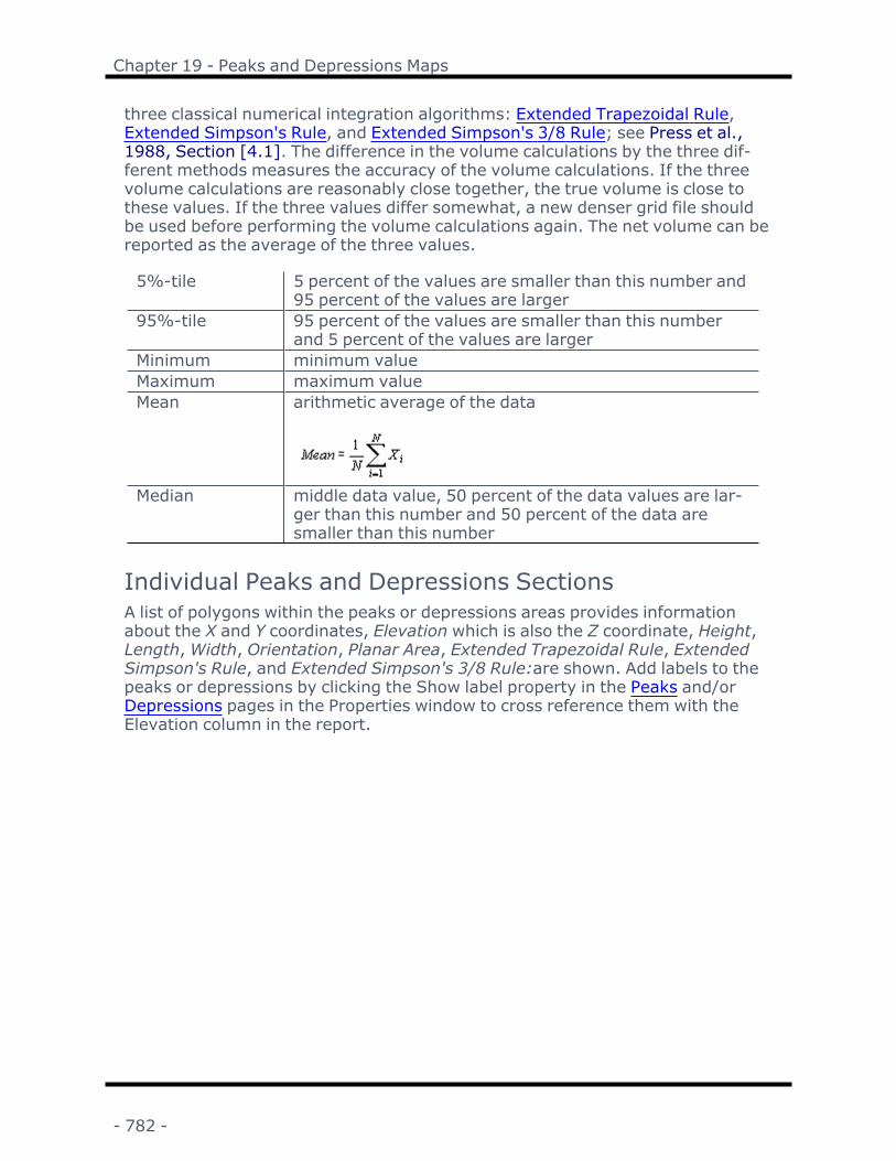
Chapter 19 - Peaks and Depressions Maps
three classical numerical integration algorithms: Extended Trapezoidal Rule,Extended Simpson's Rule, and Extended Simpson's 3/8 Rule; see Press et al.,1988, Section [4.1]. The difference in the volume calculations by the three dif-ferent methods measures the accuracy of the volume calculations. If the threevolume calculations are reasonably close together, the true volume is close tothese values. If the three values differ somewhat, a new denser grid file shouldbe used before performing the volume calculations again. The net volume can bereported as the average of the three values.
5%-tile 5 percent of the values are smaller than this number and95 percent of the values are larger
95%-tile 95 percent of the values are smaller than this numberand 5 percent of the values are larger
Minimum minimum valueMaximum maximum valueMean arithmetic average of the data
Median middle data value, 50 percent of the data values are lar-ger than this number and 50 percent of the data aresmaller than this number
Individual Peaks and Depressions SectionsA list of polygons within the peaks or depressions areas provides informationabout the X and Y coordinates, Elevation which is also the Z coordinate, Height,Length,Width, Orientation, Planar Area, Extended Trapezoidal Rule, ExtendedSimpson's Rule, and Extended Simpson's 3/8 Rule:are shown. Add labels to thepeaks or depressions by clicking the Show label property in the Peaks and/orDepressions pages in the Properties window to cross reference them with theElevation column in the report.
- 782 -

Chapter 20 - Drillhole Maps
Drillhole MapSurfer allows you to create 2D maps and 3D models of the path and shape of drill-holes, boreholes, shafts, wells, and tunnels to help you build models of thoseobjects. All of these types of data can be displayed as lines and symbols on a 2Dmap or as shaped 3D cylinders in a 3D model. Using interval data, Surfer canalso display a 3D segmented view with a color scale. For example, if your datacontains contaminant or deviation data, you can model those aspects in 3D in dif-ferent colors and shapes along the path of the drillhole, well, or borehole. Youcan create labels using values in your data files. To help visualize and sharethese maps and 3D models, export 2D and 3D images to other applications oruse the Surfer plot window or the 3D view window to dynamically view the bore-hole, drillhole, or well paths.
This help topic uses sample drillhole data to walk you through the process ofdefining both 2D and 3D drillhole maps. You can add drillholes to a new map orto an existing map. Use the Home | New Map | Specialty | Drillhole com-mand to create a new map with a drillhole layer or use the Home | Add to Map| Layer | Drillhole orMap Tools | Add to Map | Layer | Drillhole com-mand to add a drillhole layer to an existing map.
After creating a drillhole layer, you can view it in 3D, Add a Drillhole Layer, define2D properties, and define 3D properties.
This help topic contains the following main sections:Drillhole Data RequirementsCreate a Drillhole MapAdd a Drillhole LayerTips and Hints
Drillhole Data RequirementsThe data to create a drillhole map include required collars data, and optional sur-vey, interval and point data. In addition to drillhole depth and path data, otherdata considerations include having supporting values in the point and intervaldata to map different aspects of your drillhole, borehole, or well (for example,various mineral concentrations). Our sample data include information aboutTiO2 and MnO, which are shown in the example images in the 3D drillhole helptopic. The following sections define the types of data that Surfer needs to createa drillhole layer and the types of data that Surfer can use to enhance the3D modeling of drillholes and boreholes.
- 783 -

Chapter 20 - Drillhole Maps
Note: The data below are examples (from C:\Program Files\Golden Soft-ware\Surfer\Samples\SampleDrillholeData.xlsx), your data column names mayvary. The drillhole or borehole identifier (listed as ID or Hole Id in the examples)is a required column for any imported data table so that Surfer can link allrelated data to the same drillhole or borehole.
Collars DataCollars data should have information about the drillhole or borehole, such asHole ID (name), East (X) coordinate, North (Y) coordinate, elevation, startingdepth, ending depth, azimuth, and inclination. The Hole ID, East (X), and North(Y) coordinate fields are required for this table type. Inclination and azimuthdata can be used to calculate true vertical depth for deviated paths. This tablecan have multiple rows, but Hole IDs must be unique. A collars table is requiredunless you import a LAS (log-ascii) file as interval and point data.
Example Collars Data
ID Easting Northing ElevationMW-1 595299 3968125 2145MW-2 595203 3968210 2145MW-3 595176 3968113 2145
Example Collars Data DefinitionsHole ID Contains the borehole or drillhole identifier. Required
EastingContains the X value, easting, longitude, or other horizontal locationvalue of the borehole or drillhole. Required
NorthingContains the Y value, northing, latitude, or other vertical locationvalue of the borehole or drillhole. Required
Elevation Contains the Z value or elevation of the borehole or drillhole. Optional
StartingDepth
Contains the starting Z value for the borehole or drillhole in depth orelevation units. Keep in mind that starting depth is not the same aselevation. Optional
Ending DepthContains the ending Z value for the borehole or drillhole in depth orelevation units. Optional
Inclination
The angle the borehole or drillhole is oriented, in degrees. Inclinationvaries from 0 to 180. 0 indicates vertical pointing down, 90 indicateshorizontal, and 180 indicates vertical pointing up. When recorded in acollars table, the azimuth and inclination apply to the entire boreholeor drillhole length. Negative and positive inclination values aretreated the same for depth calculations. A negative inclinationchanges the direction (azimuth) to the opposite of the similar positiveinclination. For example, the azimuth value of 90 and inclination of 45describes the same orientation as the azimuth value of 270 and inclin-ation of -45 degrees. Both combinations describe an eastward dir-ection at 45 degrees down from the horizontal plane. Optional
Azimuth The compass orientation of the borehole or drillhole. Azimuth is in Optional
- 784 -

Surfer User's Guide
degrees and varies from 0 (true vertical north) to 360. When recordedin a collars table, the azimuth and inclination apply to the entire bore-hole or drillhole length.
Survey DataOptional survey data should have information about the orientation of the drill-hole, such as Hole ID, depth, azimuth, and inclination. This table can have mul-tiple rows with the same Hole IDs.
Example Survey Data
ID MD Azimuth InclinationMW-1 0 370 44.62MW-1 20 370 44.89MW-2 0 315 45.44
Example Survey Data DefinitionsHole ID Contains the borehole or drillhole ID. RequiredDepth Contains the depth or elevation for the recorded deviation. Required
Inclination
The angle the borehole or drillhole is oriented in degrees. Inclination var-ies from 0 to 180. 0 indicates vertical pointing down, 90 indicates hori-zontal, and 180 indicates vertical pointing up. When recorded in a surveytable, the azimuth and inclination apply from the depth to the next recor-ded depth. Required
Azimuth
The compass orientation of the borehole's or drillhole's deviation. Azi-muth is in degrees and varies from 0 (true vertical north) to 360. Whenrecorded in a survey table, the azimuth and inclination (or dip) applyfrom the depth to the next recorded depth. Required
Intervals DataOptional interval data should have actual down hole information in one or moredata files (e.g., XLSX, DAT, and CSV) or LAS files. LAS files import both the down-hole data and the collars information. Interval data can have multiple rows withthe same Hole IDs.
Example Intervals Data
ID From To TiO2 MnOMW-1 10 30 2.903 0.302MW-1 20 40 2.915 0.299MW-1 40 60 2.83 0.282
Example Intervals Data DefinitionsHole ID Contains the borehole or drillhole ID associated with the interval. RequiredFrom Contains the top depth or elevation of the recorded parameter. Required
- 785 -

Chapter 20 - Drillhole Maps
To Contains the bottom depth or elevation of the recorded parameter. Required
Parameter(s)
One or more columns that contain information, such as contamination,chemical concentration, etc. The parameter value is recorded across atthe interval. Optional
Points DataOptional point data should have actual down hole information in one or moredata files (e.g., XLSX, DAT, and CSV) or LAS files. LAS files import both the down-hole data and the collars information. All variable information relates to that spe-cific depth. Points data can have multiple rows with the same Hole IDs.
Example Points Data
ID Depth TiO2 MnOMW-1 10 2.903 0.302MW-1 30 2.915 0.299MW-1 50 2.83 0.282
Example Points Data Definitions
Hole IDContains the borehole or drillhole ID associated withthe depth. Required
DepthContains the depth or elevation of the recorded para-meter. Required
Parameter(s)
One or more columns that contain information, such ascontamination, chemical concentration, etc. The para-meter value is recorded at the depth. Optional
Create a Drillhole Map1. In a new plot window click the Home | New Map| Specialty | Drillhole
command. A Drillhole Data Import dialog appears.
- 786 -

Surfer User's Guide
Example Drillhole Data Import data selectiondialog using SampleDrillholeData.xls
2. In the Drillhole Data Import dialog, click the Browse and Add buttons toselect each of the drillhole data files (collar and optional survey, interval,and point data), and then click Next to open the next Drillhole DataImport dialog. A Drillhole Data Import dialog will appear for each datafile selected to be imported. The top section contains a table of the selecteddata source (Source Fields) and the bottom section contains the mappingof that data source to the table structure (Table Fields) that Surfer will useto create the drillhole map.
- 787 -

Chapter 20 - Drillhole Maps
Example Drillhole Data Import dialog for col-lars data using SampleDrillholeData.xls
3. To import collars or survey data from a Drillhole Data Import dialog:
Note: If both the collars and survey table have azimuth and inclinationdata, Surfer will use the survey table data. If neither the collars nor the sur-vey data has azimuth or inclination data, then Surfer will assume that thehole is vertical.
a. In the Table Fields section, assign a Source field to each Name field.Rows marked with a are required. If a source field is not assigned toa predefined, non-required table field, the table field can be left empty(<None>) and have no values imported.
b. Use the Units fields to define the units for source data. If Units aredefined in the source field, the value will automatically be added to theselected table field. If needed, data conversion will occur for the selec-ted unit of the table field. The select units will also show in the DrillholeManager.
c. Click the button next to any additional data in the Source Fields sec-tion to import that data or click the Add All Fields button to add all data.For any additional rows that were added to the Table Fields section,
- 788 -

Surfer User's Guide
click the button to not import that data. Any data not listed in theTable Fields will not be imported.
d. After associating the Name to the Source data and defining any Units,click Next to display the next data import dialog.
4. If interval or point data were selected to be imported, a Drillhole DataImport dialog appears for every data source. If the imported data are inter-val data, click Interval (From/To) Data. If the imported data are point data,click Point (Depth) Data. Interval data usually has rows with Hole ID, From,and To, and point data will have Depth data.
Example interval data Drillhole Data Importdialog.
a. In the Table Fields section, assign a Source field to each Name field.Rows marked with a are required. If a source field is not assigned toa predefined, non-required table field, the table field can be left empty(<None>) and have no values imported.
b. Click the button next to any additional data in the Source Fields sec-tion to import the data or click the Add All Fields button to add all data.
- 789 -

Chapter 20 - Drillhole Maps
For any additional rows that were added to the Table Fields section,click the button to not import that data.
c. After associating the Name to the Source data and defining any Units,click Next. If additional imported data need to be defined, another Drill-hole Data Import will appear.
5. If one or more LAS files were selected to import, each LAS file will importdata into the Collars and Points tabs in the Drillhole Data Import dialogfor LAS files. The Collars tab is similar to the collars table Drillhole DataImport dialog described above and takes data from the well informationblock and the parameter information block in the LAS file. The Points tabtakes data from the curve information block in the LAS file.
Example Points tab for LAS data import in theDrillhole Data Import dialog
a. In the Table Fields section, assign a Source field to each Name field.Rows marked with a are required.
b. If all LAS files have the same data format, check the Apply to all LASfiles in this set check box to apply this data import definition to all LASfiles selected to be imported.
c. Click the button next to any additional data in the Source Fields sec-tion to import that data or click the Add All Fields button to add all data.For any additional rows that were added to the Table Fields section,click the button to not import that data.
- 790 -
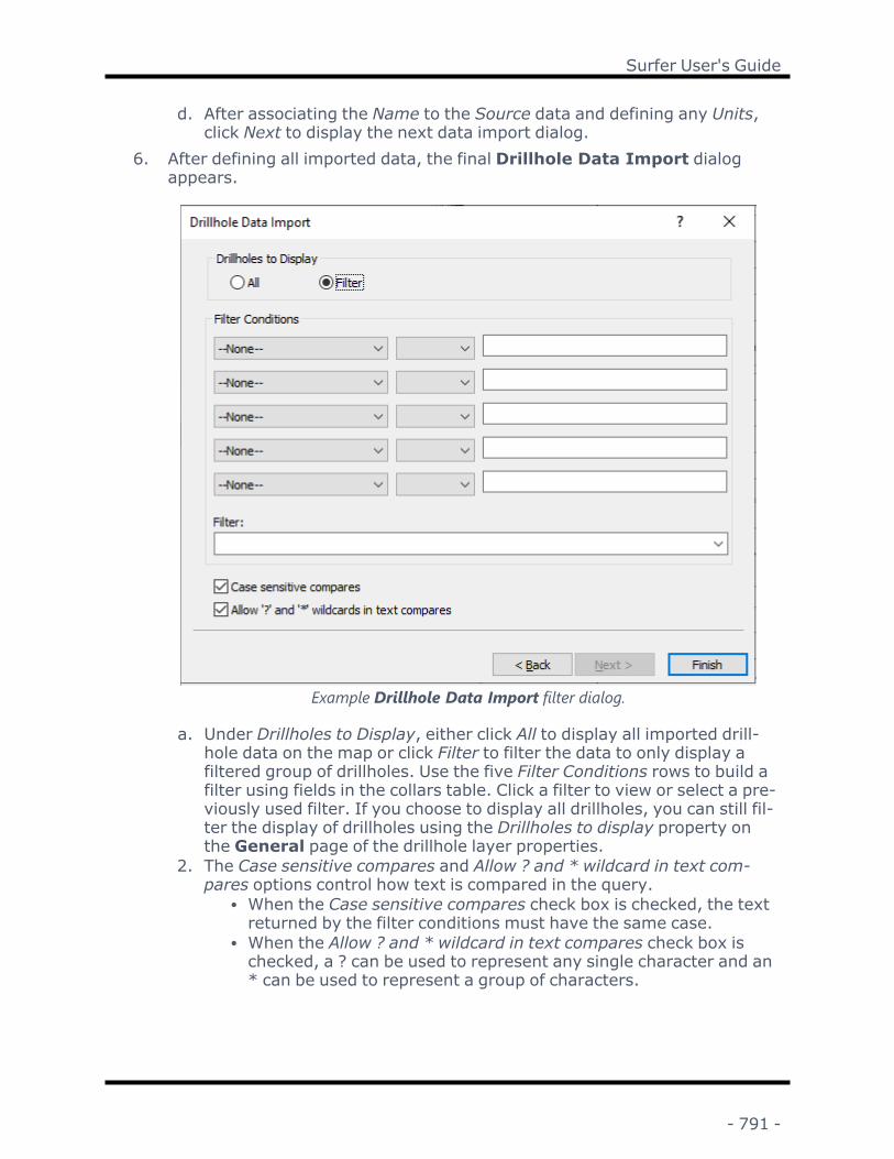
Surfer User's Guide
d. After associating the Name to the Source data and defining any Units,click Next to display the next data import dialog.
6. After defining all imported data, the final Drillhole Data Import dialogappears.
Example Drillhole Data Import filter dialog.
a. Under Drillholes to Display, either click All to display all imported drill-hole data on the map or click Filter to filter the data to only display afiltered group of drillholes. Use the five Filter Conditions rows to build afilter using fields in the collars table. Click a filter to view or select a pre-viously used filter. If you choose to display all drillholes, you can still fil-ter the display of drillholes using the Drillholes to display property onthe General page of the drillhole layer properties.
2. The Case sensitive compares and Allow ? and * wildcard in text com-pares options control how text is compared in the query.
l When the Case sensitive compares check box is checked, the textreturned by the filter conditions must have the same case.
l When the Allow ? and * wildcard in text compares check box ischecked, a ? can be used to represent any single character and an* can be used to represent a group of characters.
- 791 -

Chapter 20 - Drillhole Maps
c. After defining any needed filters, click the Finish button to create anddisplay the drillhole map.
7. After creating a drillhole map, view a 3D Drillhole Properties, define drill-hole properties, Add a Drillhole Layer, or use the Drillhole Manager to man-age imported data.
Add a Drillhole LayerTo add a drillhole layer to an existing map:
1. Select the map and click Home | Layer | Add to Map | Drillhole or rightclick over the map layer and select Add to Map | Drillhole.
2. If drillhole data has already been imported into the plot document, then theNew Drillhole Layer dialog appears.a. If you have new drillhole data you want to display in the new layer, click
the Add New Data button to display the Drillhole Data Import dialog.Follow the steps above in the Create a Drillhole Map section, beginningwith Step 2.
b. If you want to use the same drillhole data to create the new layer, per-haps using different filter conditions, select the desired settings underDrillholes to Display and Filter Conditions and click OK.
3. If drillhole data has not already been imported into the plot document, thenfollow the steps above in the Create a Drillhole Map section, beginning withStep 2.
Note: When adding new drillhole data, you may receive a warning about adjust-ing map limits to include all data. If you select to adjust the map limits, and thendecide to not include the new data, you can readjust the map limits to the ori-ginal data (see the Limits Properties help topic).
Tips and HintsYou can create a 3D model of vertical drillholes or boreholes using just collarsdata, if your collars data include ending depth values. The example below showsthe first four columns of the collar data in the sample data file, with added enddepth values (shown in blue). During the data import of the collars data, asso-ciate the collars table End Depth field with the end depth values in your collarsdata. You can also associate the collars Start Depth field to start depth values inyour data. If you don't have or don't associate start depth data, Surfer will use astart depth of 0.
Example collars data with added EndDepth values:ID Easting Northing Elevation EndDepthMW-1 595299 3968125 2145 690MW-2 595203 3968210 2145 670MW-3 595176 3968113 2145 500
- 792 -

Surfer User's Guide
Drillhole ManagerThe Drillhole Manager lets you view and manage imported drillhole or bore-hole data. To open the Drillhole Manager, select the Drillhole layer in the Con-tents window, and in the Properties window, click the View button on theGeneral page. Alternatively, you can right click the Drillhole layer in the Con-tents window and click Open Drillhole Manager or clickMap Tools | LayerTools| Open Drillhole Manager.
Example Drillhole Manager using SampleDrillholeData.xlsx
View and Edit DataClick the Collars, Surveys, Points, and Intervals tabs to view the importeddata. Data can be edited in any of these tables, except in the Hole ID or Sourcefields. The changes will be saved in the Drillhole Manager, but the changes willnot be saved to the source data files. The Sources table contains a list of datafiles imported into the Drillhole Manager and the date the data was lastupdated. This table cannot be edited.
Import and Reload DataTo import new data into the Drillhole Manager, click the button. Select thisoption to add additional drillholes that have not yet been imported. Follow thesame steps used to import the initial data.
To reload all of the data files imported into the Drillhole Manager, click thebutton.
To reload one or more existing data sources, select the Sources tab, select oneor more data sources, and then select the button to reload only the selectedsources. This is a good option to select when only one or a few data files haveupdated data, so all files do not have to be reloaded.
- 793 -

Chapter 20 - Drillhole Maps
Tips and HintsThe Drillhole Manager can also be used to help locate a specific drillhole. Whena row is selected in the Drillhole Manager, the drillhole for that Hole ID is selec-ted in the Contents window and in the plot window. This is useful when workingin the Drillhole Manager and you want to change individual drillhole attributes,such as its symbol.
For example, when the Drillhole Manager is open, click one of the Hole IDs(Hole ID MW-2 is selected in our sample data example below). The selected HoleID will be selected on the map and in the Contents window, and its propertieswill be displayed in the Properties window. In the Properties window, click onthe Symbol page, if that page is not already active. If you check the Overridelayer check box in the Hole Top Symbol section, you can define a new symbolfor the selected drillhole. When you select another Hole ID in the Drillhole Man-ager, that drillhole will be selected on the map and its properties displayed in theProperties window.
Example Drillhole Manager showing a selected Hole ID and its symbol properties
Drillhole PropertiesA drillhole layer's properties can be modified in properties pages. Properties canalso be modified for an individual drillhole (see Individual Drillhole Properties)and for the 3D view (see 3D Drillhole Properties). To define drillhole layer prop-erties, click on the drillhole layer in the Contents window.
This help topic contains three main sections:Drillhole PropertiesIndividual Drillhole PropertiesLegend Properties
- 794 -

Surfer User's Guide
General PageThe General page of the Properties window contains the properties for view-ing, reloading, and filtering drillhole data.
Drillhole layer General Properties
View DataSelect the View button to open the Drillhole Manager that allows you to man-age imported drillhole data. See the Drillhole Manager help topic for more inform-ation.
Drillholes to DisplayUse the Drillholes to display property to filter the drillhole data. If a filter wasdefined during the initial data import, that filter condition will be listed in the Drill-holes to display property in the General page. If no filter was defined, All will belisted in the Drillholes to display property.
This filter is an inclusion filter to define the drillholes you want to display on themap. To create or edit a drillhole filter:
1. Click the button to the right of the Drillholes to display property. The Fil-ter Drillholes dialog will appear.
- 795 -

Chapter 20 - Drillhole Maps
Example Filter Drillholes dialog
2. Under Drillholes to Display, click the Filter option to filter the imported drill-hole data. Use the five Filter Conditions rows to build the Filter using fields inthe collars table or type the filter directly into the Filter box. Click a filter rowto select a previously used query.
3. The Case sensitive compares and Allow ? and * wildcard in text comparesoptions control how text is compared in the filter query.
l When the Case sensitive compares check box is checked, the textreturned by the filter conditions must have the same case.
l When the Allow ? and * wildcard in text compares check box is checked,a ? can be used to represent any single character and an * can be usedto represent a group of characters.
4. After defining a filter, click the OK button to refresh the drillhole layer withonly the drillholes that match the filter conditions.
Data SourcesThe Data sources property lists the data files that have been imported. You canalso view the imported file list in the Drillhole Manager.
- 796 -

Surfer User's Guide
Symbol PageThe Symbol page for a drillhole layer has two sections: Hole Top Symbol andHole Bottom Symbol. Hole Top Symbol defines the symbol properties for the loc-ation of the top of each drillhole, and Hole Bottom Symbol defines the symbolproperties for the location at the bottom of each drillhole. If the drillhole is ver-tical, the location of the top of the hole and bottom of the hole will be at the sameXY position, but they will have a different Z position. If inclination and azimuthdata were imported, then the X, Y and Z positions are different.
Hole Top SymbolThe Hole Top Symbol defines the symbol properties for the top of the drillhole,using the East (X) and North (Y) location values imported into the collars table.The symbol properties can define a fixed symbol or different symbols using col-lars data.
Example drillholes symbols properties
Symbol MethodTo define fixed symbols so that all symbols are the same, select Fixed from theSymbol method list. See Symbol Properties for more information on setting com-mon symbol properties. To define symbols that are specific to selected collarsdata, select by By collar from the Symbol method list, and then click the EditSymbology button. The Drillhole Symbols dialog will appear.
Drillhole SymbologyThe Drillhole Symbols dialog has two main sections: the section on the left dis-plays the values of specific collars data to which the symbols will be applied, andthe section on the right contains the properties that define those symbols.
- 797 -

Chapter 20 - Drillhole Maps
Example Drillhole Symbols dialog
Follow these steps to create drillhole symbols.
1. To use an existing drillhole symbols definition, click the button, locate asaved drillhole symbols file, and click Open.
2. To define a new set of drillhole symbols:a. Select a value from the Collars field list to use as the hole top symbol
and then use one of the buttons below to select specific collars values.l Click the button to add all values from the selected collars data.l Click the button to display a pick list of collars data.l Click the button to remove all collars data that were added tothe collars values.
l Click one or more values from the collars values and click thebutton to remove the selected rows.
b. After the collars values are set, click one or more of the collar data val-ues and use the Symbols properties section to define the symbols forthose values. See Symbol Properties for more information on settingcommon symbol properties. After defining one or more symbols, youcan click the Apply button to view the changes on the map.
c. After defining symbols for all collar data values, click the button tosave the symbol definition to a file.
d. After saving changes to a file, click the OK button to close the dialog.
- 798 -

Surfer User's Guide
Hole Bottom SymbolCheck the Show symbol check box in the Hole Bottom Symbol section to dis-play a symbol at the XY location of the bottom of each drillhole. See Symbol Prop-erties for more information on setting common symbol properties.
Line PageCheck the Show deviation path check box to show the drillhole path defined inthe survey data. If you did not import survey data, but you did import azi-muth/inclination collars data, the path will be a straight line. See Line Propertiesfor information on setting the other line properties.
Label PageUse the Label Sets properties to label the drillholes on the map using any field inthe collars data. You can label the drillholes using one or multiple collars fields bycreating one or multiple label sets. For information on common label properties,such as Font and Label Format, see the Label Properties help topic.
Example Label page properties
Label SetsThe Label Sets section controls which label is being controlled by the Label Set #section. Multiple labels can be displayed by changing the Label Sets settings.Click the next to Label Sets to open the Label Sets section.
- 799 -

Chapter 20 - Drillhole Maps
Note: If only one label needs to be customized (e.g., moved to a different pos-ition), click on the specific drillhole in the Contents window. See the IndividualDrillhole Label Page section below for more information.
Label SetThe Label set displays the name of the label that is currently being changed.Click on the set name (Set 1, for instance) to select a different set name from thelist. If only Set 1 is displayed in the list, only a single label set is currently cre-ated. All of the Label Set # properties apply to only the selected Label set.
Add Label SetThe Add label set option allows new labels to be added. Click the Add button tocreate a new Label set. The Label set option automatically changes to the newset. If this is the second label to be added, a Set 2 is added to the Label set list. Ifthis is the third label to be added, a Set 3 is added to the Label set list, and so on.
Remove Label SetThe Remove label set option deletes a label from the Label set list. To delete alabel, first set the Label set to the label that should be deleted. Then, click theRemove button next to Remove label set to delete the label. All properties of thelabel set are removed.
Label Set #The Label Set # section controls the worksheet column, position, angle, font,and label properties for the selected Label set . Before making any changes inthis section, change the Label set option to the desired label. The Label Set #changes to display the name of the Label set . For instance, if Label set is set toSet 3 , the Label Set # section name changes to Label Set 3.
Label ValueFrom the Label Value list, select the collars column containing the values or textyou wish the Label set to display near the drillholes. Labels may be the originaldata values for the drillholes, or may be other identifying text such as well namesor sample numbers.
Position Relative to Drillhole StartThe Position relative to drillhole start controls the offset of the selected labelfrom the symbol center. To change the position, first change the Label set to thedesired label. Then, click on the existing position in the Position relative to drill-hole start option and select the new position from the list. Available options areCenter, Left, Right, Above, Below, and User defined. User defined allows you tospecify the exact offset (in page units) in the X offset and Y offset boxes. Thelabels are all placed in the same position relative to the associated symbol.
- 800 -

Surfer User's Guide
Positive offset values move the labels in the positive axis direction. For reversedaxes, this means that the label is moved in the opposite direction of the Positionrelative to symbol specified. For instance, if the bottom axis is reversed, settingthe Position relative to symbol to Left will move the label to the right of the sym-bol (in the negative direction). Setting the Position relative to symbol to Userdefined and setting the X offset to 0.25 inches will move the label 0.25 inches inthe negative axis direction.
X Offset and Y OffsetWhen the Position relative to symbol option is set to User defined, the X offsetand Y offset options are available. The X offset controls the location of the labelin the left-right direction. Positive values in the X offset shift the label positiontoward the positive direction (to the right of the symbol for normal axes, to theleft for reversed axes). Negative values in the X offset shift the label positiontoward the negative direction (to the left of the symbol for normal axes, to theright for reversed axes). A value of zero places the label directly in the center ofthe symbol.
The Y offset controls the placement of the label in the up-down direction. Positivevalues in the Y offset shift the label position toward the positive direction(upward for normal axes, downward for reversed axes). Negative values in the Yoffset shift the label position toward the negative direction (downward for normalaxes, upward for reversed axes). A value of zero places the label directly in thecenter of the symbol. The X offset and Y offset values are numbers between -4and +4 inches (-10.16 and +10.16 centimeters).
Angle (degrees)The Angle (degrees) box specifies the angle in degrees to rotate the selectedlabel set. Positive angles rotate the labels counterclockwise. To change the Angle(degrees), highlight the existing angle value. Type a new value or click and dragthe to the desired angle position.
FontClick the next to Font Properties to display the Font Properties section. Thefont properties are applied to all labels in this label set. Different label sets cancontain different font properties.
FormatClick the next to Label Format to display the Label Format section. The numericformat is applied to all numbers read from the specified label column in this labelset. Different label sets can contain different label formatting.
When the Type is set to Date/time, if Invalid date text is displayed instead of theactual date/time format, the value for the label is outside the defined date/timerange.
- 801 -

Chapter 20 - Drillhole Maps
Layer PageUse the Opacity slider to define the opacity of the drillholes.
Coordinate System PageSee Assign Coordinate System for coordinate system information.
Info PageSee Info Properties for general information on info pages and on how to defineattributes.
Individual Drillhole PropertiesIn the Contents window, expand a drillhole layer to show each of its drillholes.Check or uncheck the check box next to one of the drillholes to show or not showthat drillhole. Select one of the drillholes to define its properties. Individual drill-holes have five Properties pages.
Note: Some of the check boxes in the individual drillhole property pages havethree settings instead of just checked and unchecked.
l A filled check box means that the individual drillhole object property alwaysmatches the drillhole layer property. Changes made to the drillhole layerproperty are applied to each individual drillhole.
l Checked and unchecked check boxes mean that the property settings foran individual drillhole are applied and override any setting in the drillholelayer properties.
Individual Drillhole Symbol PageThe individual drillhole Symbol page for hole top and hole bottom symbols is sim-ilar to the drillhole layer symbol properties. The individual Symbol page has anOverride layer check box for the hole top symbol and the hole bottom symbol.When checked, this box overrides the drillhole layer symbol properties. If anOverride layer box is not checked, then only the drillhole layer symbol propertiesare displayed. The Show symbol check box in the Hole Bottom Symbol sectionhas three settings: a filled check box uses the drillhole layer properties; checkedshows the symbol and overrides the drillhole layer properties; and uncheckeddoes not show the symbol and overrides the drillhole layer properties.
Individual Drillhole Line PageThe individual drillhole Line page is similar to the drillhole layer line properties.The individual Line page has an Override layer check box that overrides the drill-hole layer line properties. If this box is not checked, then only the drillhole layerline properties are displayed. The Show deviation path check box has three set-tings: a filled check box uses the drillhole layer properties; checked shows the
- 802 -

Surfer User's Guide
deviation path and overrides the drillhole layer properties; and unchecked doesnot show the path and overrides the drillhole layer properties.
Individual Drillhole Label PageLabel sets are added in the drillhole layer properties and cannot be added orchanged for individual drillholes. The label position, font and format for an indi-vidual drillhole can be changed. The individual drillholes Label page has threecheck boxes (Override Position, Override Font, and Override Format) that over-ride the drillhole layer label properties. A filled check box uses the drillhole layerproperties; checked applies the property to the individual drillhole and overridesthe drillhole layer properties; and unchecked does not apply the property andoverrides the drillhole layer properties.
See the Label Sets section above for more information on label sets and theshared drillhole layer and individual drillhole label properties. See the Font Prop-erties and Label Format help topics for information on common label properties.
Example Individual Drillhole LabelsThe following image is an example of two label sets. Set 1 and Set 2 create labelsfrom drillhole collar data: Hole ID (in blue) and StartDepth (in black). The indi-vidual drillhole, "MW-6", is shown with its Override Position box checked, so aUser defined Position relative to drillhole start property could be applied tochange the Set 2 StartDepth X offset value to move the label to a more readableposition.
Example drillhole labeling with two collars data
- 803 -

Chapter 20 - Drillhole Maps
fields
Individual Drillhole Coordinates PageThis page shows the X, Y and TVD (True Vertical Depth) coordinates for the spe-cific drillhole. The X and Y values are from the collars data. The TVD is calculatedfrom the azimuth and inclination data (either in a collars or survey data), alongwith either the start and end depths (collars data) or the measured depth data(survey data ). If there is no depth data, then Surfer uses the depth data avail-able in the points or interval data.
Note: When drillholes are deviated, the true vertical depth can be calculated bySurfer. Several calculation methods exist, and each method creates a math-ematical approximation of the true X, Y, and Z value along the drillhole path.Surfer uses the tangential method for calculating true vertical depth from meas-ured depth. This method is probably the simplest method for computing true ver-tical depth. It uses only the inclination and direction measured at the lower endof the borehole or drillhole. The drillhole path is assumed to be a straight linethroughout the course. This method has historically been used more than anyother, but can be the least accurate. Drillholes calculated with the tangentialmethod can appear too shallow and the lateral displacement along the drillholecan be too large. The error is minimized if short intervals are used betweenpoints.
Individual Drillhole Info PageThis page contains information about the selected drillhole that can also becopied to the clipboard. All the fields from the collars data are displayed herewith the values for the selected drillhole. If needed, an attribute can be created.
Legend PropertiesIf the drillhole layer Symbol property for Symbol method in the Hole Top Sym-bol section is set to By collar, you can add a legend to a drillhole layer. Click theMap Tools | Add to Map | Legend command to add a legend and then clickthe Legend object in the Contents window to display legend properties. Most ofthese properties, such as the General and Info properties, are similar tolegends in other maps (see the Legend help topic).
- 804 -

Surfer User's Guide
Example drillhole Legend Layers Page prop-erties
Drillhole Layers Legend PropertiesThe Drillhole Layer section of the Layers page is unique to drillholes.
l Check Show default to add the symbol displayed for drillholes that were notadded to the symbology table in the drillhole properties.
l In the Default name field, enter a name to use to name those drillholes.l Enter a value in the Sample spacing field to define the spacing between thelines in the legend.
New Drillhole Layer or Map
- 805 -


Chapter 21 - Downloading Layers froma Server
Base Map from ServerClick the Home | New Map | Base | Base from Server command or thebutton, the Home | Add to Map | Layer | Base from Servercommand, ortheMap Tools | Add to Map | Layer | Base from Server command to down-load a base map from an online web server. Clicking one of the preceding com-mands opens the Download Online Maps dialog. Use the Download OnlineMaps dialog to select the server, map extents, and image resolution.
When using the Download Online Maps dialog, a server with appropriate datamust be selected. Surfer currently supports four types of servers, web mappingservice (WMS), Open Street Map (OSM), web coverage service (WCS), and webfeature service (WFS). WMS, OSM, WCS, and WFS servers provide differenttypes data.
l When selecting a WMS or OSM server, an image is downloaded to be used asa base (raster) layer.
l When selecting a WCS server, data values are downloaded to be used as agrid file. WCS servers cannot be used with the Base from Server command.Use the Grid from Server command or the Download button in the Open Griddialog instead.
l When selecting a WFS server, vector data is downloaded with points, poly-lines, and/or polygons representing features in a base (vector) layer.
Grid from Server
Click the Grids | New Grid | Grid from Server command or the buttonto download data from an online web mapping server and create a new grid file.Clicking the Grid from Server command opens the Download Online Grids dia-log.
The Download Online Grids dialog can also be accessed from the Open Griddialog by clicking Download. The downloaded grid will be used to create a grid-based map layer or in the following grid command dialog, depending on whichcommand was used to open the Open Grid dialog.
When using the Download Online Grids dialog, a server with appropriate datamust be selected. Surfer currently supports four types of servers, web mappingserver (WMS), Open Street Map server (OSM), web coverage server (WCS), and
- 807 -

Chapter 21 - Downloading Layers from a Server
web feature server (WFS). WMS, OSM, WCS, and WFS servers provide differenttypes data.
l When selecting a WMS or OSM server, an image is downloaded to be used asa grid file. There are no Z values associated with the image. When the imageis used as a grid file, a value between 0 and 1 is assigned to each pixel in theimage based on the color of that pixel. WMS and OSM servers are generallyused to create base maps with the Home | New Map | Base | Base fromServer command.
l When selecting a WCS server, data values are downloaded to be used as agrid file.
l When selecting a WFS server, vector data is downloaded with points, poly-lines, and/or polygons representing features. WFS servers cannot be usedwith the Grid from Server command.
Download Online Maps or GridsThe Download Online Maps and Download Online Grids dialogs are used inthe same manner to download data from online servers when creating a map.The Download Online Maps dialog is displayed when creating a base map.The Download Online Grids dialog is displayed when creating a grid-basedmap. The difference between the two dialogs is very minor and is discussed inthe Select Image Resolution to Download section below.
Click the Home | New Map | Base from Server command orMap Tools |Add to Map | Layer | Base from Server command to open the DownloadOnline Maps dialog.
Click the Grids | New Grid | Grid from Server or the Download button in theOpen Grid dialog to open the Download Online Grids dialog.
This dialog contains a server list and download options for downloading datafrom a web mapping service (WMS), Open Street Map (OSM), web coverage ser-vice (WCS), or web features service (WFS). Data can be downloaded from any ofthe predefined servers:
l Download images from the predefined WMS servers in the US Imagery orWorldwide Imagery categories. Use these images to create a base map.Images can be used to create a grid-based map, but the grid values will bean arbitrary color index on a scale from 0 to 1. In almost all cases WMSservers should not be used for grid-based maps.
l Download images from the predefined OSM servers in the OpenStreetMapsImagery category. Use these images to create a base map. Images can beused to create a grid-based map, but the grid values will be an arbitrarycolor index on a scale from 0 to 1. In almost all cases OSM servers shouldnot be used for grid-based maps.
- 808 -

Surfer User's Guide
l Download vector data from the predefined WFS servers in the US VectorData orWorldwide Vector Data categories. Use the vector data to create abase map. WFS servers cannot be used to create a grid-based map. Surfercan download data from WFS protocol 1.0.0, 1.1.0, and 2.0.0 servers.
l Download grids from the predefined WCS server. Use the grid data to cre-ate a grid-based map. WCS servers cannot be used to create a base map.
New categories and servers can be added to the list.
The Download Online Maps and Download Online Grids dialogs can accessservers that require a proxy server connection. Surfer uses the proxy server set-tings set in the Windows Internet Options, accessed via the Windows ControlPanel.
- 809 -

Chapter 21 - Downloading Layers from a Server
Select or add the server, specify extents and resolution, and download layers in the Down-load Online Maps dialog.
Data SourceThe Select Data Source list contains servers and layers, separated in categories,from which map data or images can be downloaded. The categories are USImagery, Worldwide Imagery, OpenStreetMaps Imagery, US Vector Data,
- 810 -

Surfer User's Guide
Worldwide Vector Data, and Favorites. These categories include sample servers.In the Select Data Source section, click the arrow to expand a category orserver. The arrow turns black when a section is opened. Click the black arrowto collapse the category or server.
Adding New CategoriesRight-click on an existing category or in the white space of the Select DataSource list and click Add New Category to add a user-defined category to theSelect Data Source list. After clicking Add New Category, the a new category iscreated at the bottom of the list. The category can be renamed immediately afteradding the category. If desired, type in a new name for the category. Then pressENTER or click elsewhere in the Select Data Source list to finish creating the cat-egory.
Server and Layer InformationTo see additional options for a specific server, right-click on the server in theSelect Data Source section, such as the NASA Terra Modis server.
Right-click on the server name to see the URL for the server and information about theserver's layers.
Click Info to view data source and layer information for the selected server. Theinformation is presented in the View Map Source dialog. The View Map Sourcedialog also displays layer information such as the minimum scale, height orwidth, layer name and title. None of the options are editable.
The layer list from the data source is cached on the local hard drive. This reducesthe load time for the Select Data Source list. Update the layer information byright-clicking on the data source and selecting Reload in the context menu.
To copy the server and layer name, right-click on the layer name and selectCopy to Clipboard. You can then paste the text to any text editor, word pro-cessing program, or to the window. The pasted information includes the name ofthe server, the server location, the layer title and layer name selected.
- 811 -

Chapter 21 - Downloading Layers from a Server
Arranging the Data Source ListCategories can be rearranged by clicking and dragging the category name aboveor below other categories. Layers and servers can be rearranged within a cat-egory in the same method. Layers can also be dragged and dropped into a dif-ferent category.
Favorites SectionTo add any layer to the Favorites section, right-click on the layer name andselect Add Favorite. Only the selected layer is added to the favorites. Other lay-ers from the same server are not added automatically.
To add a new server to the Favorites section, right-click on the Favorites cat-egory and select Add Map Source. Use the Add Map Source dialog to add thedata source. To copy any existing server to the Favorites category, click and dragthe server to the Favorites folder.
To remove a server or layer from the Favorites section, right-click on the serveror layer name in the Favorites section and click Delete. Click Yes in the dialog toremove the server or layer from the Favorites. Click No in the dialog to keep theserver or layer in the Favorites. Removing the server or layer from the Favoritessection does not remove the server or layer from any other section.
Adding New Data SourcesTo add new data sources to the list, right-click on the a category in the SelectData Source section. Click Add Map Source to open the Add Map Source dialog.Set the Name, Type, and URL to the new web service. Click Validate and the webserver will be tested. If the test is successful, click OK and the new web service isadded to the Select Data Source list. If the test is not successful, verify the URLand Type are correct.
All custom data sources are saved to an XML file, allowing multiple Golden Soft-ware programs to use the custom definitions. Servers that have been added inprevious Surfer versions or in other Golden Software programs will be auto-matically added to the server list. The XML file is located at C:\User-s\<username>\AppData\Roaming\Golden Software\Shared\Geode.xml. The filecan be copied from one computer to another to share custom data sourcesbetween multiple computers and users.
When sharing the Geode.xml file between a previous version of Surfer and thecurrent version, the Data source list may include servers with unsupported pro-tocols for the previous Surfer version. If this happens, the unsupported serverwill be displayed in the Data Source list. However, the server name will be dis-abled in the list, and you will not be able to download data from the server.
- 812 -

Surfer User's Guide
Editing Data SourcesTo edit the data source for any user-defined server, right-click on the servername and click Edit. The Edit Map Source dialog updates the web server Name,Type, and URL. This may be useful if the location for the server changes or if thename listed in the Download Online Maps dialog should be changed. The EditMap Source dialog also displays information about the server and layers. Pre-defined servers cannot be edited.
To view information about the server, right-click on the server name and clickInfo. The View Map Source dialog opens and displays the server and layerinformation. The Name, Type, and URL cannot be edited in the View MapSource dialog.
Deleting Data SourcesTo delete a user-defined server from the Select Data Source list, right-click onthe server name and click Delete. In the Delete Data Source dialog, click Yesto delete the server. Click No to keep the server in the Select Data Source list.Predefined servers cannot be deleted.
Select Area to DownloadThe Select Area to Download section controls the areal extent of the image beingdownloaded. Available options are Entire data source extents, Within <dis-tance> <units> of Longitude <Lon> Latitude <Lat>, or Specify Lat-itude/Longitude extents. Click on the desired option to select it.
Select the extents of the map to download in the Select Area to Download sec-tion.
The Entire data source extents reads all of the data on the specified server. All ofthe data is downloaded in the single image. With servers that cover large areas,this option is not recommended because even at high resolutions, very littledetail will appear on the downloaded map.
TheWithin <distance> <units> of Longitude <Lon> Latitude <Lat> optionallows a single longitude and latitude value to be entered. A square area is down-loaded based on the distance value and the units option. The square is centered
- 813 -

Chapter 21 - Downloading Layers from a Server
on the value entered for the Longitude and Latitude. To use this option, entervalid values in each box.
l The first box sets the width and height of the square area. For instance, 25can be input.
l The second option (units) can be set to either Kilometers or Miles. Click onthe existing option to select the desired option.
l The third option is the central Longitude value. In the example below, the cen-ter point of the downloaded image will be -105.220139. Longitude valuesmust be between -180 and +180. Negative values are western hemispherelongitudes. Positive values are eastern hemisphere longitudes.
l The last option is the central Latitude value. In the example below, the centerpoint of the downloaded image will be 39.753304. Latitude values must bebetween -90 and +90. Negative values are entered for the southern hemi-sphere. Positive values are entered for the northern hemisphere.
The downloaded area will be 25 miles wide and 25 miles tall. The image will be centered onthe longitude and latitude location of -105.220139, 39.753304.
The Specify Latitude/Longitude extents option allows a rectangular area to beinput in latitude and longitude coordinates. When adding a base map layer to anexisting map with a defined coordinate system, this option is automatically selec-ted. The boxes are filled in with the map limits of the current map. After selectingthis option,
l Type in the western-most edge for the downloaded map in longitude degreescoordinates in theWest box. Longitude values must be between -180 and+180. Negative values are western hemisphere longitudes. Positive valuesare eastern hemisphere longitudes.
l Type in the eastern-most edge for the downloaded map in longitude degreescoordinates in the East box. Longitude values must be between -180 and+180. Negative values are western hemisphere longitudes. Positive valuesare eastern hemisphere longitudes.
l Type in the northern-most edge for the downloaded map in latitude degreescoordinates in the North box. Latitude values must be between -90 and +90.Negative values are entered for the southern hemisphere. Positive values areentered for the northern hemisphere.
l Type in the southern-most edge for the downloaded map in latitude degreescoordinates in the South box. Latitude values must be between -90 and +90.Negative values are entered for the southern hemisphere. Positive values areentered for the northern hemisphere.
- 814 -

Surfer User's Guide
The downloaded area will cover from -105.5 to -105degrees longitude and 39.25 to 40.75 degrees lat-
itude.
Select Image/Grid Resolution to DownloadThe Select Image Resolution to Download section controls the quality of theimage being downloaded. This section is called Select Grid Resolution to Down-load in the Download Online Grids dialog. Drag the slider to the right toincrease the image resolution. Click a point on the slider bar and the slider willjump to that resolution. The farther to the right the slider is located, the betterthe resolution and the larger the image. Clicking on one of the lines on the leftside of the slider will normally download a map of sufficient quality that is smallerin size. The larger the file size, the longer the image will take to process and themore memory the program will use to manipulate the image. If N/A is displayedor no size information is displayed, the image cannot be downloaded at therequested resolution. Change the resolution by moving the slider to select a dif-ferent size image.
The selected WMS server may have an original data source resolution (forexample, 1 meter/pixel) for its imagery. You may be able to select an image res-olution higher or lower than this original data source resolution. Increasing theimage resolution here cannot give you better image detail over the original datasource. By requesting a higher resolution than the original data source, theimage is simply larger in size and in the number of pixels. The server returns therequested image in the requested size. Some servers provide resolution inform-ation, and if so, this information and be found in the View Map Source dialog. Ifthe server does not provide resolution information, consider checking the serverprovider's documentation.
OSM servers may have more than one layer available. When this is the case,increasing the Image Resolution to Downloadmay download a more detailedimage. For example with the Carto Light predefined server, using the defaultImage Resolution to Download will download the image as displayed in the pre-view, and increasing the resolution will download an image that includes moregeographic names and more detailed streets. Just as with the WMS servers,eventually increasing the Image Resolution to Download will exceed the originaldata source resolution for the most detailed layer, and this will result in down-loading larger images with no appreciable difference.
WFS servers provide vector data. When a WFS server is selected the SelectImage Resolution to Download slider is disabled.
- 815 -

Chapter 21 - Downloading Layers from a Server
If a WCS server only provides only one resolution, such as the SRTM Global 90m(GMU) predefined server, the Select Grid Resolution to Download slider is dis-abled.
In some instances a may be displayed next to the image size estimate. Thisoccurs when the selected resolution is outside the recommended scale for thesever. Hover the cursor over the to display information about the warning. Gen-erally this warning is removed by increasing the Image Resolution to Downloadby moving the slider to the right or reducing the Area to Download selection.
Set the image quality by dragging the slider to the right or left.
Image PreviewThe Preview section displays a picture of the area to be downloaded. The Previewsection uses low resolution previews. The final output image quality is controlledby the Select Image Resolution to Download. Some servers use scale-dependentrendering. If a preview is not displayed but no errors are visible in the DataSource or Preview sections, then try zooming in and/or out until you find the cor-rect scale for the server.
l For OSM and WMS servers, the Preview section contains a low resolutionpreview of the image.
l For WCS servers, the Preview section shows a coverage footprint over aworld map.
l For WFS servers, the Preview section shows a coverage footprint over aworld map. The preview can also include vector data for the selected areato download. The preview is not displayed automatically for vector datafrom WFS servers, because all vector data must be downloaded first. Thedata download and rendering may take a few seconds or up to a fewminutes depending on the size of the area to download and the WFS server.Set the Select Area to Download before enabling the vector data preview.
The vector data preview must be enabled manually by clicking the but-ton. If you preview the vector data and make no changes to the area todownload extents, it will not be necessary to download the data again whenclicking OK. If the preview is taking longer than you would like to wait, clickthe Cancel button in the lower right portion of the dialog, next to the pre-view status bar.
- 816 -

Surfer User's Guide
The Preview window displays the area to download, buttons to zoom in/out, pan, orchange the download area, a map scale, and the coordinates of map cursor.
l
Click the buttons on the left side of the image preview to zoom in or outon the area. Changing the zoom level does not affect the area to download.The area to download is indicated in the Preview section by a yellow out-line.
l Click the button on the left side of the image preview to zoom to theselected area extents. Changing the zoom level does not affect the area todownload. The area to download is indicated in the Preview section by a yel-low outline.
l Click the button on the left side of the image preview to quickly movethe image in the Preview section. The cursor changes to , indicating panmode. Click and hold the left mouse button down and drag the image tochange the view; the cursor changes to to indicate the left mouse buttonis held. Changing the view does not affect the area to download. The areato download is indicated in the Preview section by a yellow outline.
l Click the button on the left side of the image preview to change the
extents of the image that is downloaded. The cursor changes to , indic-ating draw mode. Click and hold the left mouse button down and drag themouse over the area to download. The zoom extents update and the yellowbox coincides with the area drawn. The Select Area to Download alsoupdates. Only the portion of the image highlighted by the yellow box willdownload.
- 817 -

Chapter 21 - Downloading Layers from a Server
l Click the button to download the vector preview for the selected area todownload. Additionally, the vector data preview may be simplified in the
Download Online Maps dialog. The icon is displayed if preview sim-plification has occurred. Even if the preview is simplified, all vector data willbe added to the map layer when clicking OK.
l If the server or selected layer returns an warning, a and/or is displayedin the Preview section. Hover the cursor over the warning icon to view moreinformation about the warning.
OK, Cancel and HelpOnce all of the options are set, click OK to download the image, grid, or vectordata. Click Cancel to cancel the download and return to the Surfer plot window.Click Help to open the help file. A progress bar is displayed showing downloadprogress and number of bytes (kB, MB, or GB) downloaded.
Clicking OK in the Download Online Maps dialog downloads the map layer andcreates a new base map or adds a base layer to the select map frame. ClickingOK in the Download Online Grids dialog opens the Save Grid As dialog or cre-ates a new grid based layer.
If the OK button is not available, the layer is not selected. Go back to the SelectData Source section and select a specific layer, not a server name.
Server ResponsivenessNote: Download speeds will vary, depending on the server selected. Some serv-ers may become unresponsive. These data sources are on external serverswhich are out of Golden Software's control. If one server is unresponsive or slowto download, you may wish to select a different server.
Naming ConventionBase maps from servers are named with the map server name, such as Base-USGS_EROS_Ortho_NAIP. In addition, the image downloaded with the base mapfrom server adds attribute information, including the server name and layer title.
Grid-based maps created by clicking Download in the Open Grid dialog arenamed with the map type and server name, for example Contours-NED Con-tiguous U.S. 1 3W arc second elevation data.
Changing the Window and Section SizesThe Download Online Maps and Download Online Grids dialogs can be res-ized by clicking and dragging a side or corner, as with normal windows. Theimage preview and Select Data Source sections can also be enlarged or reduced
- 818 -

Surfer User's Guide
by clicking and dragging the double horizontal bars between the sections of thedialog.
Map Source DialogsThe following map source dialogs are accessed via the Download Online Mapsor Download Online Grids dialog. The map source dialogs add, edit, and showinformation for source servers.
Add Map Source DialogRight-click on an existing category in the Download Online Maps dialog, and thenclick Add Map Source to open the Add Map Source dialog. This dialog adds newweb servers to the list in the Download Online Maps dialog.
The Add Map Source dialog adds a new server to the selected category. Notice the Validatebutton is disabled. The Validate button is enabled once a URL is added to the Add Map
Source dialog.
Edit Map Source DialogRight-click on a user-added map source in the Download Online Maps dialog, andthen click Edit to open the Edit Map Source dialog. This dialog is the same asthe Add Map Source dialog, but includes the server information for the selected
- 819 -

Chapter 21 - Downloading Layers from a Server
map source. Use the Edit Map Source dialog to edit the map source Name andURL.
The Edit Map Source dialog allows you to change the Name and/or URL for the selectedserver. The Edit Map Source dialog validates the server immediately once the dialog is
opened. The Edit Map Source dialog also displays server and layer information for the selec-ted server.
View Map Source DialogRight-click on an pre-existing server in the Download Online Maps dialog, andthen click Info in the context menu to open the View Map Source dialog. Thisdialog shows server and layer information. Editing the server name and URL isdisabled in the View Map Source dialog.
Dialog ControlsThe following section describes the purpose and use of the components in theView Map Source, Edit Map Source, and Add Map Source dialogs.
- 820 -

Surfer User's Guide
NameIn the Name section, type the name of the server. This is the name that is listedin the Download Online Maps dialog, so the name can be as descriptive asdesired.
TypeSelect the Type from the list. Available types areWCS: Web Coverage Service,WFS Web Feature Service,WMS: Web Map Service, or OSM: Open Street Maps.Surfer can download vector data from WFS protocol 1.0.0, 1.1.0, and 2.0.0 serv-ers.
URLIn the URL section, type the full internet location of the web service. The addressmust contain the http:// or https:// before the location. Sites with https:// orsites that redirect to SSL servers are supported.
Open Street Map URLsOSM Open Street Map server URLs can be defined for multiple tiles by using vari-ables in the URL:
l Use ${s[i-j]} where i and j are the tile letters or numbers you wish toinclude in the data source, for example http://${s[1-5]}.toolserv-er.org/tiles/hikebike/${z}/${x}/${y}.png specifies five tile servers for theHike & Bike data source.
l Use ${s[a,b]} where values a, b are the comma-separated tile letters ornumbers you wish to include in the data source, for example http://${s[a,b,c]}.tile.openstreetmap.org/${z}/${x}/${y}.png specifies the threetile servers for the OSM Mapnik data source.
Example OSM URLs are displayed in the Add Map Source dialog when OSM:Open Street Maps is selected in the Type field. Also, when copying and pastingan OSM URLs from a web browser, the %7B and %7D characters will be auto-matically converted to { and }.
Use Specific Protocol VersionWhen contacting a server, Surfer allows the server to pick which protocol isused. Occasionally, a server will select a protocol that does not work well or doesnot work at all. Try specifying the protocol in the Use specific protocol version listif you are having issues with a specific WCS or WFS server. Protocol 1.0.0 isoften the most reliable.
Surfer supports WCS protocols 2.0.1, 2.0.0, 1.1.3, 1.1.2, 1.1.1, 1.1.0, and1.0.0. Surfer supports WFS protocols 1.0.0, 1.1.0, and 2.0.0.
- 821 -
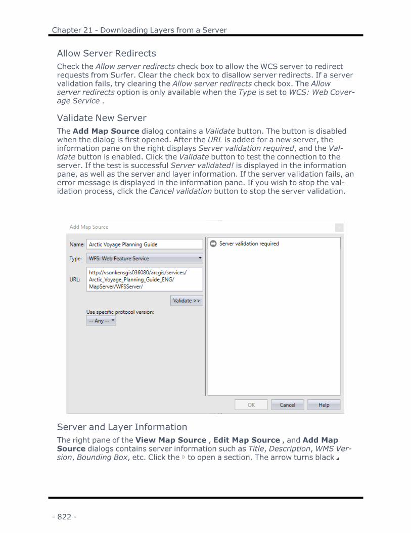
Chapter 21 - Downloading Layers from a Server
Allow Server RedirectsCheck the Allow server redirects check box to allow the WCS server to redirectrequests from Surfer. Clear the check box to disallow server redirects. If a servervalidation fails, try clearing the Allow server redirects check box. The Allowserver redirects option is only available when the Type is set toWCS: Web Cover-age Service .
Validate New ServerThe Add Map Source dialog contains a Validate button. The button is disabledwhen the dialog is first opened. After the URL is added for a new server, theinformation pane on the right displays Server validation required, and the Val-idate button is enabled. Click the Validate button to test the connection to theserver. If the test is successful Server validated! is displayed in the informationpane, as well as the server and layer information. If the server validation fails, anerror message is displayed in the information pane. If you wish to stop the val-idation process, click the Cancel validation button to stop the server validation.
Server and Layer InformationThe right pane of the View Map Source , Edit Map Source , and Add MapSource dialogs contains server information such as Title, Description,WMS Ver-sion, Bounding Box, etc. Click the to open a section. The arrow turns black
- 822 -

Surfer User's Guide
when a section is opened. Different servers will return different information.When a data source contains more than one layer, the layer information is listedfor each layer. Click the to open a layer section. The layer information includesitems such as Description , Bounding Box, Supported CRS, etc.
Cancel or FinishClick Cancel or the button to return to the Download Online Maps dialog,without making any changes. Click OK in the View Map Source to return to theDownload Online Maps dialog, making any changes to the Name, Type, orURL in the dialog. Click OK in the Add Map Source dialog to return to the Down-load Online Maps dialog, and the data source is added to the Select DataSource list.
HelpClick Help to open the online help file with information about the open dialog.
- 823 -


Chapter 22 - Map Properties
Introduction to Common Map PropertiesMap properties common to all layers are located in the Properties window whenthe Map object is selected in the Contents window. These properties include theview, scale, limits, frame, and coordinate system. If there are multiple map lay-ers in a map frame, the changes made on the View, Scale, Limits, Frame, andCoordinate System pages apply to all layers. The attributes and options on theInfo page apply only the map. Each layer can have separate attributes.
ViewMaps can be displayed at any orientation using the View page. The Projection,Rotation, Tilt, and Field of view of a map are changed on the View page.
ScaleMap scale controls the size of a map on the printed page. This is accomplished bydefining a correspondence between length on the map (in map units) and lengthon the printed page (in page units). For example, one mile on the map cor-responds to one inch on the page. The map scale is set using the Scale page. Themap scale for the X axis and the map scale for the Y axis can be set in unison(proportionally), or they can be set independently. On 3D wireframes and 3D sur-faces, the map scale for the Z axis can also be set.
LimitsMap limits are defined as the X and Y extents of the map. When a map is first cre-ated, the map limits are set to the minimum and maximum X and Y coordinatevalues in the grid file, base map, or data file used to create the map. You canaccept these as the limits for the map, or you can specify custom limits using theLimits page. Custom limits are useful when plotting only a portion of a map.
FrameIn addition to adding color to maps, a background can be added behind the map.The Frame page sets the background fill properties and the border line prop-erties for a map. The map background limits coincide with the axis limits on acontour, base, post, and vector maps. On 3D wireframes, the map backgroundrefers to the bottom plane of the base. On 3D surfaces, the background color isblended with the surface.
- 825 -

Chapter 22 - Map Properties
Coordinate SystemThe map coordinate system is the target coordinate system for the map. Acoordinate system has a defined projection and datum. If some map layers areusing a different coordinate system, the layer is converted to the map coordinatesystem. The map's Coordinate System is the new coordinate system that youwant to use to project your X, Y coordinate data. 3D surface maps and wireframemaps do not have a coordinate system associated with them. When the mapCoordinate System changes, these maps do not change.
InfoThe Info page provides additional information about the map. Comments can beadded, deleted, and edited to clarify information contained in the map.
Map PropertiesProperties common to all layers in a map are displayed in the Properties windowwhen the Map object is selected. Specific properties of a map layer are controlledby the specific map layer properties.
The properties of one or more maps can be opened by selecting the Map object(s) in the Contents window or by clicking on the Map object in the plot window.
Click on the Mapobject to open themap properties.
Click on the Con-tours object toopen the contourlayer properties.
TheMap Properties control the View, Scale, Limits, Frame, Coordinate System,and Info of Surfermap frames.
- 826 -

Surfer User's Guide
Specify the View, Scale, Limits, Frame, Coordinate Sys-tem, and Info in the Properties window when a map
is selected.
View PropertiesMaps can be displayed at any orientation using the map properties, View tab.The projection, rotation, tilt, and field of view of a map are changed on this page.
View PageThe View page is located in the Properties window. To open the map properties,click on the Map object in the Contents window.
Control the orientation of the map or maps on theView page.
Multiple MapsWhen you have more than one map on the page, the View settings are appliedto all selected maps. For example, this command is useful if you have a contourmap and 3D wireframe based on the same grid file and displayed in the sameplot window. You can select the map object for both the contour map and 3D
- 827 -

Chapter 22 - Map Properties
wireframe. In the Properties window, click on the View tab to change the set-tings for both maps at one time.
ProjectionThe Projection group sets the type of projection for the selected maps. Per-spective projections more closely simulate reality, but Orthographic projectionsmaintain parallel lines and allow accurate measurements to be taken from thedrawing.
Perspective ProjectionThe Perspective projection creates a visual effect whereby the size of the surfacevaries with the distance from the observer. When a Perspective projection isused, you can change the Field of View value to increase or decrease the per-spective effect.
Orthographic ProjectionThe Orthographic projection creates a plot with a projection of the surface onto aplane, oriented perpendicular to the line of sight between the observer and thesurface.
RotationThe Rotation (degrees) value controls the rotation of the map about the center.As the Rotation (degrees) value increases, the map rotates in a counterclockwisedirection.
To change the Rotation (degrees), click in the box next to Rotation (degrees).Highlight the existing value and type a new value. Values are always displayedwith three digits after the decimal. Press ENTER on the keyboard after typing anew value to show the value on the map. Alternatively, click and drag the
to a new value. Values must range between zero and 360.000.
TiltTilt refers to the orientation of the Z axis in the map display. A zero degree tiltmeans the Z axis lies in the plane of the page or screen. As the angle of tiltincreases, the Z axis tilts toward the viewer. A 90.000 degree tilt means the XYplane lies in the plane of the page or screen and is orthogonal to the viewing dir-ection. The default tilt is 30.000 degrees for 3D wireframes and 3D surfaces, and90.000 degrees for all other map types. When you tilt three dimensional maps(i.e. 3D surface) to 90.000 degrees, the surface relief is no longer visible.
To change the Tilt (degrees), click in the box next to Tilt (degrees). Highlight theexisting value and type a new value. Values are always displayed with threedigits after the decimal. Press ENTER on the keyboard after typing a new value toshow the value on the map. Alternatively, click and drag the to a newvalue. Values must range between zero and 90.000.
- 828 -

Surfer User's Guide
Maps can be displayed at any rotation angle and at any tilt anglefrom zero to 90 degrees. When more than one map is selected, the
view parameters are applied to all selected maps.
Field of ViewThe Field of View controls the perspective effect of the Perspective projectionoption. The perspective effect is the visual effect of the map changing size rel-ative to the distance from the observer. A small Field of View shows the map inperspective as the if the observer was far from the viewpoint, making the per-spective more pronounced. A large Field of View shows the map in perspective asif the observer was very close to the viewpoint. The Field of View angle is formedby the left edge of the bounding box, the viewpoint, and the right edge of thebounding box. The image below illustrates the bounding sphere wedged into theviewing cross section.
- 829 -

Chapter 22 - Map Properties
The field of view cross section shows the position of the eye (E), thecenter of the surface (C), the distance from the eye to the point (d),and the radius of the bounding sphere around the surface plot (r).
With an Orthographic projection the Field of View values have no effect. Notethat the Field of View parameter does not influence the map scale.
To change the Field of view, click in the box next to Field of view. Highlight theexisting value and type a new value. Values are always displayed with threedigits after the decimal. Press ENTER on the keyboard after typing a new value toshow the value on the map. Alternatively, click and drag the to a newvalue. Values must range between one and 160.000.
3D ViewClick 3D View to view the map in a new 3D view window. You can also create anew 3D view by selecting the map and clickingMap Tools | View | 3D View.The map must include at least one grid-based layer or point cloud map to createa 3D view.
Example of Tilt, Rotation, and Projection Parameters
This is the same wireframe displayed at the same rotation angle but different tilt angles:10, 30, and 45 degrees.
- 830 -

Surfer User's Guide
This is the same wireframe displayed at the same tilt angle but different rotation angles.
This is the same wireframe using different projection parameters. The map on the left uses anOrthographic projection. The map in the middle uses a Perspective projection with a Field ofView value of 20 degrees. The map on the right uses a Perspective projection with a Field of
View value of 75 degrees.
Scale PropertiesThe scale controls the size of a map or profile on the printed page. This is accom-plished by defining a correspondence between lengths on the map (in map units)and lengths on the printed page (in page units). The map scale is specified usingthe Scale page in the Properties window. The scale for the X axis and the scalefor the Y axis can be set in unison (proportionally), or they can be set inde-pendently. On three-dimensional maps (i.e. wireframes and surface maps), thescale for the Z axis can also be set.
Axes are part of the map on which they are drawn. Therefore, when the scale isredefined, the axes are modified accordingly. Because Surfer calculates reas-onable tick spacing based on the map lengths and map limits, redefining thescales can result in different tick spacing along the axis.
Default ScaleBy default, map scales are defined proportionally in the X and Y dimensions, withthe longest side measuring six inches on the printed page. For example, considera map extending 60 map units in the X dimension and 40 map units in the Ydimension. Since the extent in the X dimension is longer than the extent in the Ydimension, the map is drawn six inches wide. The resulting scale is 10 map unitsper inch. The scale in the Y dimension is also 10 map units per inch, so the map isdrawn four inches in height.
- 831 -

Chapter 22 - Map Properties
This map scale was customized. The Ydimension covers a greater extentthan the X dimension in this map. Bydefault, the Y axis would be six inchesin length, and the X axis is pro-
portionally shorter.
- 832 -

Surfer User's Guide
These are two 3D wireframe maps of the same grid, each using adifferent Z scale. The Z scale is exaggerated in the top view. Use
the Scale page to change the length of the Z axis.On three-dimensional maps the default scale in the Z dimension is defined suchthat the vertical extent of the map is one-fourth the maximum horizontal extent.
The default scales are a function of the map limits. Map limits are determined bythe file used to create the map, or they can be defined using Limits page.
Scale PageThe Scale page is located in the map properties.
- 833 -

Chapter 22 - Map Properties
Specify the relative X, Y, and Z map scaling onthe Scale page in the Properties window.
Proportional XY ScalingThe Proportional XY scaling check box ensures that the X and Y dimensions arescaled equally. When the box is checked, a change in either the X or Y dimensionis reflected in the other dimension by a proportional amount. To scale the axesindependently, uncheck the box.
Sizing a map with its selection handles rescales the map internally. To return tothe proper scale, use the Home | Selection | Transform command to clear thetransform, and then use the Scale page to scale the map.
When Proportional XY scaling is checked, the Scaling ratio (1:N) option is avail-able. The Scaling ratio (1:N) property is hidden when Proportional XY scaling isnot checked.
Scaling RatioSpecify the X and Y map scale representative fraction by typing the desired valuein the Scaling ratio (1:N) property field. The Proportional XY scaling check boxmust be checked to scale maps with by representative fraction. Press ENTER orclick a different property to update the scaling values. Changing the Scaling ratio(1:N) automatically updates the X Scale and Y Scale sections Map units per in(cm) and Length (page units) property values.
The representative fraction scaling method shows the map scale as a ratio of dis-tance on the map (1) to distance on the ground (N). For example, a rep-resentative fraction of 1:100000 means one centimeter on the map represents100,000cm on the ground (1000m or 1km). Similarly on a 1:100000 scale map,
- 834 -

Surfer User's Guide
1 inch on the map represents 100,000 inches on the ground (8333.3ft or 1.578miles).
When perspective, tilt, and rotation are applied to a map view, the ratio ishonored for the center of the map in the X direction. The ratio may not be validfor other regions of the map, depending on the View page settings.
X, Y, and Z ScaleThe X Scale, Y Scale, and Z Scale sections specify the scale along the indicatedaxis. Each axis can be scaled independently by clearing the Proportional XY scal-ing check box. When the Proportional XY scaling box is checked, any changesmade to the scale in the X or Y dimension is automatically reflected in the otherdimension. Z scaling is always independent of the X and Y scaling. Similarly, anychange in the X or Y scale values automatically updates the Scaling ratio (1:N)value when Proportional XY scaling is checked.
Map Units Per In. (cm.)The Map units per in. (cm.) option sets the number of map units per page unit inthe associated dimension. For example, to draw a map at a scale of 1000 mapunits per inch, type the value 1000 into the box. The Length (page units) value isautomatically updated to reflect the change. For example, if the map is 8000units in the dimension you are setting, the map is 8 inches long in that dimen-sion.
LengthThe Length (page units) option sets the length of the map in the X, Y, or Z dimen-sion. When the Length (page units) value is changed, the Map units per In. (cm.)box is automatically updated to reflect the change.
Using Different Scaling in the X and YDimensionsUnder some conditions, different map units are used for the X and Y dimensions.
Consider a contour map of soil temperature as a function of depth and time.Depth is measured in feet, while time is measured in days. Clearly, one day isnot equivalent to one foot. The two axes must be scaled differently because twodifferent types of units are used for the two axes. Depth data might be collectedevery half foot from zero to four feet in depth, and the time data might be col-lected every day over a 30-day period. The depth axis extends four units and thetime axis extends 30 units. Default scaling would produce a map six inches longin the time dimension by 0.8 inches high in the depth dimension. To create asquare map, you must clear the Proportional XY scaling box on the Scale pageand then set the map scaling so 30 units in the time dimension is equal to fourunits in the depth dimension. The map is then plotted at six inches by six inches.
- 835 -

Chapter 22 - Map Properties
Using Scaling to Minimize Distortion onLatitude/Longitude MapsWhen you display maps based on latitude and longitude coordinates extendingover a large region, they might appear somewhat distorted. This occurs becauseone degree of latitude is not equivalent to one degree of longitude. For example,consider a base map of the state of California (ca2010.gsb).
This shows the map of California before and after scaling. The map on the right is scaled upin the Y dimension so the map does not appear compressed.
As an approximation, the distance covered by one degree of latitude at theequator is equal to the distance covered by one degree of latitude at the poles,and is approximately 69 miles. This distance between degrees of latituderemains nearly constant over the globe, although it does vary slightly becausethe earth is not a perfect sphere. However, the distance between a degree of lon-gitude decreases from the equator to the poles. For any latitudinal position, youcan determine the length, in miles, between degrees of longitude based on theformula:
Distance covered by 1° of longitude (in miles) = cosine (latitude) x 69.172.
This equation assumes a Clark 1866 reference ellipsoid.
This table illustrates the change as you move from the equator to the poles.
LatitudeDistance Covered by OneDegree of Longitude
0°(equator)
69.172 miles
30° 59.904 miles60° 34.586 miles90°(poles) 0 miles
- 836 -
Surfer User's Guide
Substitutions for units other than miles:
l For kilometers, you can substitute the number 111.321 for 69.172 in theformula above.
l For meters, you can substitute the number 111,321 for 69.172 in the for-mula above.
l For feet, you can substitute the number 365,228 for 69.172 in the for-mula above.
So, how can you put this information to use? Remember that you are plottingdegrees of latitude and longitude, but what you really want to show on the mapare the correct distances. You must scale the longitude values correctly for thecorrect distances to be represented on the map. The scaling factor to apply formaps is based on the cosine of the latitude for the area you are working on.
To determine the scaling factors:
1. Determine the latitude for the parallel through the center of the map, andobtain the cosine for this latitude value. The center parallel in ca2010.gsb isapproximately 37.27 degrees. The cosine of 37.27 degrees is 0.80.
2. Click on the Map in the Contents window to select it. The map propertiesare displayed in the Properties window.
3. Click the Scale tab to set the X direction for the map. You can set either theLength (page units) value or the Map units per in. (cm.) value. The X ScaleMap units is 1.72 inches in this example.
4. Uncheck the Proportional XY scaling box.
5. Multiply the X Scale Map units value by the cosine of the latitude, and enterthis number into the Y Scale Map units field. 1.72 (X Scale Map units) X0.80 (cosine of latitude) = 1.38 (Y Scale Map units). Enter 1.38 into theMap units per in. box under Y Scale.
The map is automatically updated.
ExampleConsider a map of the state of Montana. When you plot the map on a one to onescale, the map appears stretched in the east-west direction. To understand thisproblem, consider that for Montana the latitude ranges from 44.36° to 49°. Thelatitude for the center of the map is determined from this to be 46.68°. Thecosine of 46.68° is 0.686. The distance covered by one degree of longitude atthis latitude is only 0.686 times the distance covered by one degree of latitude.To reduce the distortion on this map, you must correct for this difference.
- 837 -

Chapter 22 - Map Properties
Let's say you are plotting the map at an X scale of 1" = 2 map units (longitude).For the map to be scaled appropriately, you would plot the Y scale at 1" = 1.372map units (latitude, 2 x 0.686 = 1.372). This effectively stretches the map in thelatitude (N-S) direction. Now the map distances are nearly the same in the lon-gitude and latitude directions.
When the map is scaled so 1° of longitude equals 1° of latitude, map distances are distorted.Notice that the graticules form squares (equal spacing).
When you apply scaling factors, map distances are represented more accurately. The rect-angular spacing of graticule lines indicate the difference in scaling.
Limits PropertiesThe Limits page in the map properties lets you define the X and Y minimum andmaximum map coordinates (specified as xMin, xMax, yMin, and yMax values).The Limits page is unavailable if there is a 3D wireframe layer in a multi-layermap.
When a map is created, the limits are automatically defined by the coordinate val-ues contained in the file used to create the map. The limits of the selected mapcan be adjusted on the Limits page of the map properties or interactively withthe Set Limits command.
- 838 -

Surfer User's Guide
The map limits of the map are set to the default limits as defined by the basemap. The limits of a smaller area of interest are indicated with the dashed rect-
angle.
The map limits of the map have been adjusted to the limits of thearea of interest.
Limits and 3D WireframesMap limits cannot be defined for 3D wireframes; this constraint includes com-posite maps containing 3D wireframe layers. These maps are limited to theextent of the grid file used to create the wireframe. To change the limits of a gridfile for a wireframe, use Grids | Resize | Extract or create a new grid file with newlimits. Alternatively, use a 3D surface map with mesh lines to simulate a wire-frame map.
- 839 -

Chapter 22 - Map Properties
Limits and Axis ScalingWhen you change map limits, axes that use automatic scaling are redefined to fitthe new limits of the map. If you do not use automatic scaling for the axes, theaxes are drawn over the same range as the original map and will not match themap using the new limits.
The map limits have been reset on this map. The Left Axis andTop Axis use automatic scaling and match the new map limits.The Right Axis and Bottom Axis do not use automatic scaling,
and reflect the original limits of the map.
Limits and Map ScaleWhen new map limits are defined for a map, the map scale is not changed. Forexample, if the map uses a scaling of 1 inch = 1000 meters, the new map usesthis same scale. This can result in maps much smaller or larger than the originalmap. In this case, click on the map and set the new scale on the Scale page.
Limits and Post MapsLimits can be set on post maps or maps containing a post map layer. When a pos-ted point lies outside the map limits, the posted symbol and the label are clippedfrom the map. When a posted point is at or inside the map limits, the entire sym-bol and posted label are printed, even if the symbol and label extend beyond thelimits of the map.
- 840 -

Surfer User's Guide
Limits and Reversed AxesWhen an axis is reversed on the Scaling tab, the limits do not change. The xMinvalue must still be less than the xMax value. The reverse axis option onlychanges the display of the axes and map layers, not the actual limits.
Limits, Scale, and Adding Map LayersWhen a new map layer is added to an existing map or a modified map layerexceeds the current map limits, a message appears prompting you to adjust themap limits to include all the layers. Select Yes to adjust the map limits. Select Noto preserve the current map limits.
Limits PageThe Limits page is located in the map properties.
Specify the map limits in the Properties windowon the Limits page.
Limits XY Min and MaxSet custom xMin, xMax, yMin, and yMaxmap limits in the Spatial Extents group.
Map limits can be set larger or smaller than the limits of the current map. Forexample, if you have a map that ranges from zero to 100 in the X dimension, butyou only want to display the map from 25 to 50 in the X dimension, use 25 and50 as the new minimum and maximum values on the Limits page.
When using date/time formats for any of the axis labels, the minimum and max-imum on the Limits tab are entered in date/time format. To change the value,highlight the existing value and enter the minimum or maximum date/timevalue. For instance, 02/02/2014 12:00:00 AM can be entered into the xMinoption.
- 841 -

Chapter 22 - Map Properties
This example shows a map with xMinand xMax values in date/time format.
Use Data LimitsThe Use data limits check box resets the map limits to the limits of the grid file,base map, or post map data file limits.
Setting Map LimitsTwo methods exist for setting map limits. Map limits can be set in the plot win-dow with the Set Limits command. The limits can be entered as values in theProperties window Limits page.
To set map limits on the Limits page:
1. Click once on the map object to select it.
2. The map properties appear in the Properties window.
3. On the Limits page, specify the X and Y minimum and maximum values forthe map by entering the values into the xMin, xMax, yMin, and yMax boxes.The Use data limits check box resets the map limits to the limits of the gridfile, base map, or posting data file limits.
4. The map is redrawn with the new limits. If the axes use automatic scaling,they are also redrawn to fit the new map limits.
Change map limits on the Limits page in the Properties win-dow.
- 842 -

Surfer User's Guide
Frame PropertiesThe map properties Frame page sets the map border line properties and thebackground fill properties for the selected map. The map background limits coin-cide with the axis limits on contour, base, post, 3D surface, and vector maps.
Map backgrounds lie underneath all other objects on the map. This means thatthe background can be obscured by other map features. For example, when youcreate color filled contour maps, the fill between contours obscures the map back-ground wherever a solid or image pattern is used for the contour fill. Similarly,the outline of the map background can be obscured by the map axes.
This is a contour map displaying green filled con-tours. The remainder of the contours are 0%
opaque, allowing the light blue background to beseen. A heavy dark blue map border has also been
added to the map.
Frame PropertiesThe Frame page is located in the Properties window when a Map object is selec-ted.
- 843 -

Chapter 22 - Map Properties
Specify the map border and background properties in the Prop-erties window on the Frame page.
Line PropertiesClick the next to Line Properties to open the Line Properties section and cus-tomize the map border.
Fill PropertiesClick the next to Fill Properties button to open the Fill Properties section andcustomize the map background.
Reload DataYou can reload external map data for all maps in the currently loaded Surfer filewith the File | Reload Map Data command or the button. For only the selec-ted layer use the File | Reload Layer Data command or the button.
Surfer caches all data used by all maps within the .SRF file including the datapoints used in a post map and the grids used in grid based maps.
If the original data file or grid file is changed and unsaved, the modified file willnot be used when the .SRF file is reopened. Use the File | Reload Map Datacommand to update data or grid file information from the saved version of thefiles.
Unable to LocateIf the data are not found a dialog with the name of the map layer is displayed.Click the Yes button to manually find the missing data file. Click the No button toskip the map layer and choose not to update the file that cannot be located.
- 844 -

Surfer User's Guide
This example shows data file used for a post layer that is not found when reloading the mapdata.
Updating a Single Map LayerMap data can be reloaded for individual map layers by clicking the File | ReloadLayer Data command or by clicking the button in the Properties windowand re-selecting the data file.
Coordinate System NoteRegardless of the file selected with either the File | Reload Map Data com-mand or by clicking the button in the Properties window, the coordinate sys-tem for the original map layer is used after updating the file. If this is not thecorrect coordinate system, click on the map layer to select it. In the Propertieswindow, click on the Coordinate System tab and set the coordinate system tothe appropriate new system.
- 845 -


Chapter 23 - Map Features
Add to MapTheMap Tools | Add to Map command group contains commands for addingmap layers, additional left, right, top, bottom, or Z axes, a scale bar, a viewshed,a graticule, or a profile to the existing map. Alternatively, right-click on an exist-ing map and click Add to Map to add a map layer, axis, scale bar, or profile.
Map LayersAdd a Base Layer from Server, Base Layer, Empty Base Layer, Contour Layer,Post Layer, Classed Post Layer, Color Relief Layer, Grid Values Layer, 1-GridVector Layer (aspect and gradient are calculated), 2-Grid Vector Layer (X, Y ordirection, magnitude), Watershed Layer,Point Cloud layer, Viewshed layer, 3DWireframe Layer, 3D Surface Layer, Left Axis, Right Axis, Top Axis, Bottom Axis,Z Axis, Scale Bar, or Profile to the selected map.
Layers that cannot be added to the selected map are grayed out. For example, a3D wireframe map layer cannot be added to a 3D surface map.
Layers can be dragged between maps in the Contents window. Layers can becombined with the Overlay Maps command to create a single Map object.
Select multiple files to add multiple layers to the map. One layer is added foreach selected file. Multiple files cannot be selected when adding 2-Grid Vectorlayers.
Map LimitsAdding a new layer to an existing map will not change custom scaling or map lim-its, with the exception of 3D wireframe and 3D surface maps. Adding a 3D wire-frame or 3D surface to an existing map will change custom scaling or map limits.
If a map layer is added to a map frame and the map layer exceeds the currentmap limits, a Surfer warning dialog will be displayed allowing you to adjust themap limits to include all layers. Select Yes to adjust the map to include all layers.Select No to leave the current map limits.
Layer PropertiesThe Layer page in the Properties window for a base, post, classed post, grid val-ues, contour, color relief, vector, peaks and depressions, point cloud, watershed,3D wireframe, viewshed, or graticule controls the opacity of the entire maplayer. Surface maps do not have a Layer page.
- 847 -

Chapter 23 - Map Features
Adjust the Opacity of the entire layer on the Layer page. Thisexample shows the Layer page of a contour map in the Prop-
erties window.
OpacityChange the opacity of the entire layer by entering an Opacity value from 0%(completely transparent) to 100% (completely opaque). To change the opacity,highlight the existing number and type a new number. Press ENTER on the key-board or click on another item in the Properties window for the value to beaccepted. Alternatively, click and drag the to change the opacity per-centage.
3D surface maps do not have the ability to change the opacity for the entire map.
Scale BarTheMap Tools | Add to Map | Scale command or the button places ascale bar on the map. Alternatively, right-click on an existing map and selectAdd to Map | Scale Bar to add a scale bar. Scale bars are divided into equallyspaced cycles. Any number of cycles between one and 100 can be used. Eachcycle is labeled based on map units.
To place a scale bar on a map:
1. Select the map and click theMap Tools | Add to Map | Scale command.2. The scale bar is automatically placed below the bottom axis.3. To make changes to the scale bar, click once on it to select it. The properties
are displayed in the Properties window.
Scale Bar PropertiesThe scale bar properties are displayed in the following pages:
GeneralLabelsInfo
- 848 -

Surfer User's Guide
Legend
Click theMap Tools | Add to Map | Legend command or the button toadd a legend to the plot. The legend can include any number of post, classedpost, 1-grid vector, 2-grid vector, and base symbology layers from any of themaps in the plot. However once a layer is included in a legend, it cannot beadded to any other legends. The total number of legends is limited to the totalnumber of post, vector, and base layers in the plot, i.e. each layer can have itsown legend. Once all of the post, classed post, 1-grid vector, 2-grid vector, andbase layers are represented in a legend, theMap Tools | Add to Map |Legend command button is disabled. Every layer that is not already included ina legend is added automatically when a new legend is created. Use the Layers inLegend section of the Properties window Layers page to control which layers areincluded in the legend.
Base Symbology LegendsWhen a base layer includes a symbology, a legend can be displayed for the baselayer. Unique values legends can include the value, fill, line, and symbolsamples, and the legend order is determined by the order in the Symbology dia-log. Unclassed colors legends can include fill value and fill samples. Unclassedsymbols legends can include value and symbol samples. Classed colors legendscan include the upper limit value, class name, and fill samples. Classed symbolslegends can include the upper limit value, class name, and symbol samples. Piechart symbols can be relatively sized and can include slice colors with labels.
Drillhole Layer LegendsWhen a drillhole layer Symbol property for Symbol method in the Hole TopSymbol section is set to By collar, a legend can be added to a drillhole layer. Thelegend will display the hole top symbol and the hole id from the collars data. SeeDrillhole Map for more information.
Post Layer LegendsLegends can be displayed for post layers and classed post layers. The post layerlegend displays symbols representing the symbol size when proportional sizing isspecified. The post layer legend displays symbols representing the symbol colorwhen a color column is specified and the Color method is Numeric via colormap.When both proportional sizing and the Numeric via colormap color method isused, the symbols representing size and color are displayed separately with"Color" and "Size" headers. When neither proportional sizing nor a Numeric viacolormap color method is applied to the post layer, a single symbol is displayed.The classed post layer legend displays a symbol for each class and optionalinformation about the class.
- 849 -
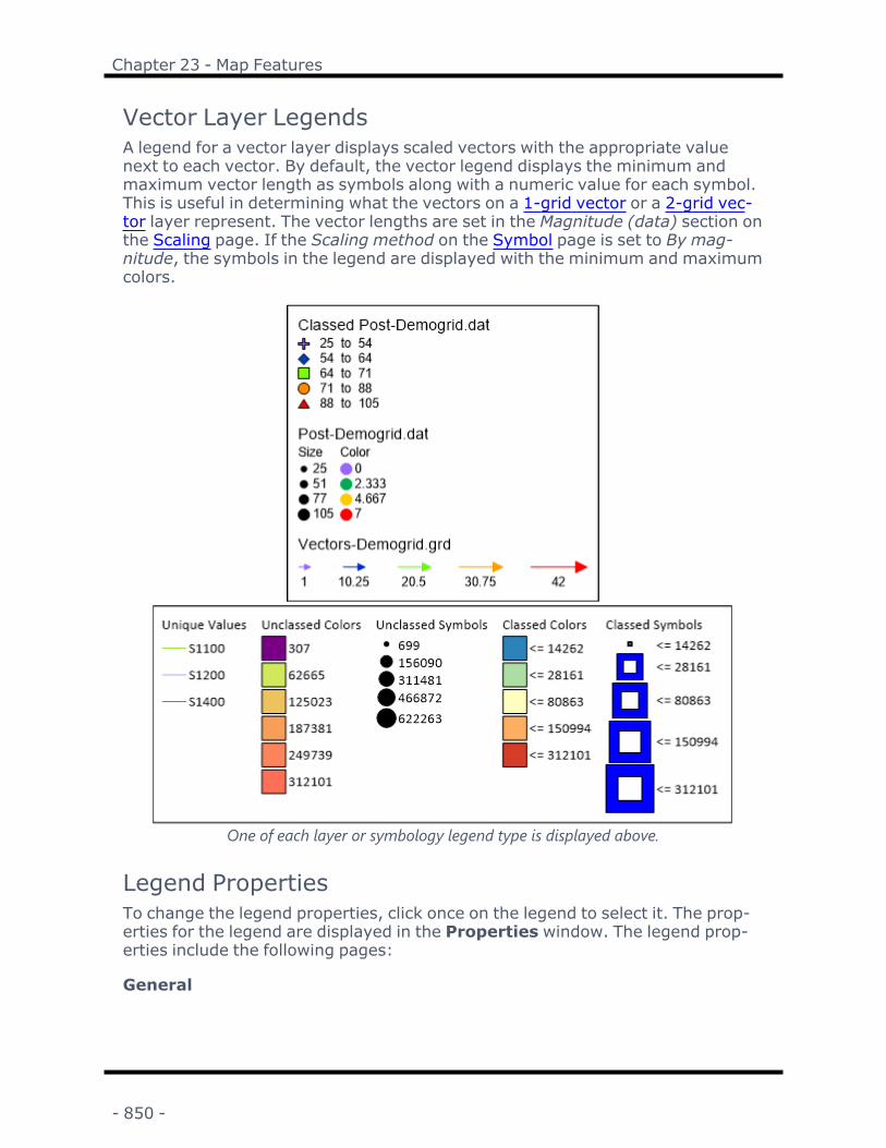
Chapter 23 - Map Features
Vector Layer LegendsA legend for a vector layer displays scaled vectors with the appropriate valuenext to each vector. By default, the vector legend displays the minimum andmaximum vector length as symbols along with a numeric value for each symbol.This is useful in determining what the vectors on a 1-grid vector or a 2-grid vec-tor layer represent. The vector lengths are set in the Magnitude (data) section onthe Scaling page. If the Scaling method on the Symbol page is set to By mag-nitude, the symbols in the legend are displayed with the minimum and maximumcolors.
One of each layer or symbology legend type is displayed above.
Legend PropertiesTo change the legend properties, click once on the legend to select it. The prop-erties for the legend are displayed in the Properties window. The legend prop-erties include the following pages:
General
- 850 -

Surfer User's Guide
LayersInfo
General PropertiesThe General page of the legend properties includes frame and title properties.
Set the frame and title properties in the Generalpage.
FrameThe Frame section specifies the properties to use for the border around thelegend.
TypeThe Type list specifies the type of border to use for the legend. You can selectNone, Square, or Rounded for the frame type. Setting this value to None showsno border around the box. Fill properties cannot be applied to the legend framewhen the Type is set to None. Setting the Type to Rectangle creates a rectangleat the edge of the legend at the Margin distance. Setting Type to Rounded cre-ates a rounded rectangle at the edge of the legend at the Margin distance.
MarginMargin specifies the distance between the edge of theframe and the text or sym-bols within the legend. To set the Margin distance, highlight the existing valueand type in the new value. Press ENTER on the keyboard or click anywhere elsein the Properties window to make the change. Alternatively, click the buttonsto increase or decrease the margin. Values are in inches or centimeters determ-ined by the page units.
LineClick the next to Line Properties to open the Line Properties section. Set thethe Style , Color, Opacity , andWidth of the line to use for the legend frame.
- 851 -
Chapter 23 - Map Features
FillClick the next to Fill Properties to open the Fill Properties section. Set the Pat-tern, Color, and other fill properties to use for the foreground and background ofthe legend area.
TitleThe Title section adds a title for the legend.
Title TextClick in the box next to Title text and type the title for the legend. The title mayinclude math text instructions. Type the title exactly as you want the text toappear in the legend.
Titles can contain multiple lines. To create a multiple line title, click the button.The Text Editor appears. Type the text in the dialog. To add a new line of text,press the ENTER key on the keyboard. To change the properties of the text, high-light the text and change the desired property. When finished, click OK. You arereturned to the plot window.
Title FontClick the next to Font Properties to open the Font Properties section. Set thefont properties to use for the legend title here. The legend title and legend classfont properties may be set separately.
Legend Layers PropertiesThe Layers page in the Properties window controls which layers are included inthe legend and the appearance of the legend.
- 852 -

Surfer User's Guide
The Layers page controls which layers are included in the legend and the legend sampleappearance. The image on the left displays the Layers page for a post layer legend while the
image on the right displays the vector layer legend.
GeneralThe General section contains options for the display of layer names in thelegend.
Show Layer NameCheck the Show layer name check box to display layer names above the layers'samples in the legend. Clear the Show layer name check box to display onlysamples in the legend.
Layer SpacingThe Layer spacing property sets the spacing between the layers in the legend inpage units.
Font PropertiesExpand the Font properties to control the font properties for the layer names inthe legend. All of the layer names use the same font properties.
- 853 -

Chapter 23 - Map Features
Layers in LegendThe Layers in Legend section controls which layers are included in the legend,the legend layout, the order of the layers in the legend, and which layer'ssamples are being edited in the Layer section below.
Layer to EditThe Layer to edit selection determines which layer is moved by the Layer pos-ition property and which layer's properties are displayed in the Layer section.Click the current selection in the Layer to edit field and select the layer you wishto edit from the list. The list includes all of the layers in the legend.
Edit Layer ListClick Edit list in the Edit layer list field to add and remove layers in the legendwith the Layers for Legend dialog. The Layers for Legend dialog can also beused to rearrange the layers in the legend.
Layer LayoutChange the overall layout of the legend by selecting Vertical or Horizontal in theLayer layout property field. The Layer layout property is only available when thelegend contains two or more layers. Select Vertical to display layers arranged topto bottom. Select Horizontal to display layers arranged left to right. The Layer lay-out selection controls the buttons in the Layer position field.
Layer PositionThe Layer position field changes the position of the Layer to edit selection. WhenLayer layout is set to Vertical, click Move Up to move the layer up one position inthe legend, and click Move Down to move the layer down one position in thelegend. When Layer layout is set to Horizontal, click Move Left to move the layerone position to the left in the legend, and click the Move Right button to movethe layer one position to the right in the legend. You can also rearrange the lay-ers in the Layers for Legend dialog.
Layer SectionThe Layer section contains the properties for the appearance of the samples forthe Layer to edit selection. The Layer section name includes the layer type andlayer name formatted as <Type> Layer - <Layer Name>, for example Post Layer- Post-Drillholes_Collars.xlsx!Sheet1 . The properties in the layer section dependon the layer type: post, classed post, 1-grid vector, 2-grid vector, or base.
Post, Classed Post, and Base Symbology PropertiesThe following properties are available when a post, classed post, or base layer isselected in the Layer to edit field.
- 854 -

Surfer User's Guide
Variable LayoutThe Variable layout property controls the display of the size and color sampleswhen both are displayed on the legend for a post layer. Proportional sizing mustbe used on the post layer, and a color column must be used with the Numeric viacolormap color method to display both size and color samples in the legend. Setthe Variable layout property to Horizontal to display the size and color samplesside by side. Set the Variable layout property to Vertical to display the sizesamples above the color samples.
The Variable layout property is only available for the post layer legend.
Number of SamplesSet the number of samples for legend with the Number of samples property. TheNumber of samples controls both the size and color samples sections in the postlayer legend. Type the desired number of samples in the Number of samples fieldor click the to change the value.
The Number of samples property is available for post layer, unclassed colorssymbology, and unclassed symbols symbology legends.
TemplateThe Template box customizes the format of the legend items. The specified tem-plate is applied to each class or sample in the legend. Normal text and math textinstructions can be included within the template, in addition to the following spe-cial legend template directives:
Dir-ective Post
Classe-d Post
Uniqu-e Val-ues
Unclass-ed Col-ors
Unclass-ed Sym-bols
Classe-d Col-ors
Classe-d Sym-bols
PieChart
\fill fillsamp-le
colorsample
colorsamp-le
colorsamp-le
\line linesamp-le
\lower lowerclasslimit
\name classname
classname
classname
\sym-bol
sym-bolsamp-le
sym-bolsamp-le
sym-bolsamp-le
symbolsample
sym-bolsamp-le
\up-per
upperclasslimit
- 855 -
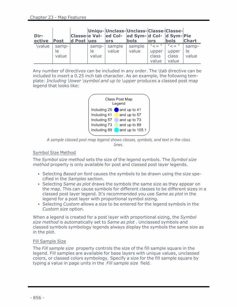
Chapter 23 - Map Features
Dir-ective Post
Classe-d Post
Uniqu-e Val-ues
Unclass-ed Col-ors
Unclass-ed Sym-bols
Classe-d Col-ors
Classe-d Sym-bols
PieChart
\value samp-levalue
samp-levalue
samplevalue
samplevalue
"<= "upperclassvalue
"<= "upperclassvalue
samp-levalue
Any number of directives can be included in any order. The \tab directive can beincluded to insert a 0.25 inch tab character. As an example, the following tem-plate: Including \lower \symbol and up to \upper produces a classed post maplegend that looks like:
A sample classed post map legend shows classes, symbols, and text in the classlines.
Symbol Size MethodThe Symbol size method sets the size of the legend symbols. The Symbol sizemethod property is only available for post and classed post layer legends.
l Selecting Based on font causes the symbols to be drawn using the size spe-cified in the Samples section.
l Selecting Same as plot draws the symbols the same size as they appear onthe map. This can cause symbols for different classes to be different sizes in aclassed post layer legend. It's recommended you use Same as plot in thelegend for a post layer with proportional symbol sizing.
l Selecting Custom allows a size to be entered for the legend symbols in theCustom size option.
When a legend is created for a post layer with proportional sizing, the Symbolsize method is automatically set to Same as plot . Unclassed symbols andclassed symbols symbology legends always display the symbols the same size asin the plot.
Fill Sample SizeThe Fill sample size property controls the size of the fill sample square in thelegend. Fill samples are available for base layers with unique values, unclassedcolors, or classed colors symbology. Specify a size for the fill sample square bytyping a value in page units in the Fill sample size field.
- 856 -

Surfer User's Guide
Sample SpacingThe Sample spacing property controls the spacing between samples. The Samplespacing can be set independently for each layer in the legend. Type a value inpage units in the Sample spacing field to specify the space between legendsamples.
1-Grid Vector and 2-Grid Vector PropertiesThe following properties are available when a 1-grid vector or 2-grid vector layeris selected in the Layer to edit field.
MagnitudesIf you would like to display different vector lengths in the legend, enter the newlengths in the Magnitudes box. The new vectors are scaled relative to the scalingset on the Scaling page in the vector map properties. You can display more thantwo vectors in the legend by entering a string of numbers separated by commasor spaces into the Magnitudes box. For example, 0.5, 10, 25, 50 would show foursymbols in the vector legend.
Use LimitsIf the Use limits box is checked, only two vectors are displayed in the vectorlength legend. These are the Minimum and Maximum values set on the Scalingpage in the Magnitude (data) section. When checked, the Magnitudes propertyand legend will update to show the new values when the Magnitude (data)changes.
Magnitude LayoutThe Magnitude layout options align the symbols vertically or horizontally in thelegend. To change the Magnitude layout, click on the current option. Selecteither Vertical or Horizontal in the list.
SamplesThe Samples section contains the options for the sample order within layers, andthe sample font and label format properties.
Sample OrderThe Sample order property specifies whether the samples are listed in ascendingorder (from smallest to largest) or descending order (from largest to smallest).Click the current selection and select Ascend or Descend from the list. TheSample order applies to the samples in all layers in the legend.
Font PropertiesControl the sample font properties in the Font properties section. The font prop-erties apply to the samples in all layers in the legend.
- 857 -

Chapter 23 - Map Features
Label FormatControl the sample label format in the Label Format section. The label formatproperties apply to the samples in all layers in the legend.
Layers for Legend DialogClick the Edit list button in the Properties window Layers page to add, remove,and move map layers in the legend.
Add, remove, and move layers in the Layers for Legend dialog.
Available LayersThe layers that can be added to the legend are listed in the Available layers list.The Available layers list includes any layer that is not in a legend and the layersin the selected legend. One or more layers must be selected to add a layer to thelegend. Select a layer by clicking on the layer name. Select multiple layers byholding CTRL while clicking on the layer names. Select a group of layers by click-ing the first layer, holding SHIFT, and clicking the last layer. The first, last, andall layers between are selected. Deselect a layer by selecting another layer, or byholding CTRL and clicking the selected layer.
Add layers to the legend by selecting the desired layer or layers. Next click toadd the selected layer(s) to the Selected layers list. The added layers are addedto the end of the Selected layers list.
- 858 -

Surfer User's Guide
Selected LayersThe Selected layers list shows the layers that are included in the legend and theorder in which they are displayed. Layers can be removed from the Selected lay-ers list, and layers can be rearranged within the Selected layers list.
One or more layers must be selected to remove or move the layers in the legend.Select a layer by clicking on the layer name. Select multiple layers by holdingCTRL while clicking on the layer names. Select a group of layers by clicking thefirst layer, holding SHIFT, and clicking the last layer. The first, last, and all layersbetween are selected. Deselect a layer by selecting another layer, or by holdingCTRL and clicking the selected layer.
Removing LayersRemove layers from the legend by selecting the desired layer or layers. Next
click to remove the selected layer(s) from the Selected layers list.
Rearranging LayersRearrange layers in the in the legend by selecting the desired layer or layers.Next click and drag the selected layer(s) to a new position in the list. While drag-ging the selection, the position to which the layers will be moved is indicated by ared line with red arrows at the ends. Release the left mouse button to move thelayers.
The Post, Classed Post, and Vectors layers will be moved between the Unclassed Symbols andClassed Colors layers when the left mouse button is released.
OK and CancelClick OK to apply the changes to the legend. Click Cancel to close the Layers forLegend dialog without making any changes to the legend.
- 859 -

Chapter 23 - Map Features
Color Scale Bar - Vector, Color Relief, 3D Surface, andPoint Cloud MapsA color scale bar is a legend that shows the fill assigned to vector symbols on a 1-grid vector map or a 2-grid vector map, or the colors used in a color relief map,3D surface map, or point cloud map. Color scale bars can be added to 2D and 3Dmaps, but have slightly different options. Color scale bars for contour and wire-frame map layers are similar, but have slightly different options.
Click on the color scale bar to open the color scale properties in the Propertieswindow.
Color Scale Bar VisibilityThe color scale bar display can be turned on or off in the Contents window bychecking or clearing the box to the left of the color scale bar name.
Adding a Color Scale BarTo add a color scale bar to a vector map:
1. Click on the vector layer to select it.2. In the Properties window, click on the Symbol tab.3. Specify the fill properties to use for the vectors in the Color Scaling section.4. Check the Show color scale box to activate the color scale bar.
To add a color scale bar to a color relief, surface, or point cloud map:
1. Click on the color relief, surface, or point cloud layer to select it.2. In the Properties window, click on the General tab.3. Check the Show color scale box to activate the color scale bar.
Removing a Color Scale BarA color scale bar can be removed by clicking on the color scale bar and pressingthe DELETE key on the keyboard. Alternatively, you can clear the Show colorscale box in the layer properties.
Using a Logarithmic Scale on a Color Scale BarThe color scale bar reflects the scaling of the colormap. To set the colormap touse a logarithmic scale for a vector map:
1. Click on the vector map layer to select it.2. In the Properties window, click on the Symbol tab.3. Click the next to Color Scaling to open the Color Scaling section.4. Set the Scaling method to By magnitude or By grid file.5. Click the next to the Vector colors colormap.6. Check the Logarithmic scaling option and click OK.7. The color scale bar is automatically updated to show logarithmic scaling.
- 860 -
Surfer User's Guide
To set the colormap to use a logarithmic scale for a color relief, surface, or pointcloud map:
1. Click on the color relief, surface, or point cloud layer to select it.2. In the Properties window, click on the General tab.3. Click the next to the Colors colormap for a color relief map layer. Click the
next to the Upper colormap for a 3D surface map layer. Click the next toColormap for a point cloud layer.
4. Check the Logarithmic scaling option and click OK.5. The color scale bar is automatically updated to show logarithmic scaling.
Editing a Color Scale BarTo modify a color scale bar, click on the color scale bar to select it. The propertiesare listed in the Properties window.
GeneralLabelsLineInfo
Color Scale Bar - Contour and 3D WireframeA color scale bar is a legend that shows the line color, line style, fill color, and fillpattern assigned to each contour level on a contour map, or the colors assignedto levels in a 3D wireframe. Click on the color scale bar to open the color scaleproperties in the Properties window. Color scale bars for vector, color relief, and3D surface map layers are similar, but have slightly different options.
Color Scale Bar VisibilityThe color scale bar display can be turned on or off in the Contents window bychecking or unchecking the box to the left of the color scale bar name.
Adding a Color Scale BarTo add a color scale bar to a contour map:
1. Click on a contour map to select it.2. In the Properties window, click on the Levels tab.3. Check the Color scale box to display the color scale bar.4. Check the Fill contours box to fill the contours with color, if desired.
To add a color scale bar to a 3D wireframe:
1. Click on a wireframe map to select it.2. In the Properties window, click on the Color Zones tab.3. Click the Edit Levels button next to Color zones.
- 861 -

Chapter 23 - Map Features
4. In the Properties dialog, check one or more of the Apply zones to lines ofconstant boxes.
5. Check the Color Scale box.
6. Click OK in the dialog to draw the wireframe with a color scale bar.
Removing a Color Scale BarA color scale bar can be removed by clicking on the scale bar and pressing theDELETE key on your keyboard. Alternatively, you can clear the Color Scale checkbox in the Properties window or the Properties dialog.
Color Scale Bar PropertiesTo modify a color scale bar, click on the color scale bar to select it. The propertiesare listed in the Properties window.
GeneralLabelsLineInfo
Graticule
Clicking theMap Tools | Add to Map | Graticule command or the buttonadds a graticule to an existing map. A graticule is a network of lines representingthe Earth's parallels of latitude and meridians of longitude. A graticule representslines of latitude and longitude. A map grid represents lines in other units. TheMap Tools | Add to Map | Graticule command creates either a graticule ormap grid. An existing map or one of its child objects must be selected to enabletheMap Tools | Add to Map | Graticule command.
The graticule Units, Origin, Spacing, and Label Format are updated automaticallywhen changing the map target coordinate system.
- 862 -

Surfer User's Guide
A graticule has been added to this contour map to indicate lat/long coordin-ates in addition to the coordinate system values displayed on the left and bot-
tom axes.
To add a graticule to a map:1. In the Contents window or plot window, click on the map to which the gratic-
ule should be added.2. Click theMap Tools | Add to Map | Graticule command. Alternatively,
right-click the map and select Add | Graticulein the context menu.3. A graticule is added to the map. Select the graticule in the Contents window
or plot window to view its properties in the Properties window.
Graticule PropertiesThe graticule properties are edited in the Properties window. The Propertieswindow contains General, Labels, Layer, and Info pages.
General PageThe General page of the Properties window contains options for the graticuleunits, line style, and spacing.
- 863 -

Chapter 23 - Map Features
The General page of the Properties window con-trols graticule display options.
Graticule UnitsThe Units property specifies the units for the graticule. The options in the Unitslist are dependent on the map coordinate system. If the map is projected, theavailable options include Degrees (Lat/Long) , Millimeters, Centimeters, Meters,Kilometers, Inches, Feet, Survey Feet, Yards, and Miles. If the map uses a knownphysical unit, the linear units in the preceding list are available. If the map has adatum, Degrees (Lat/Long) and Unknown map units are available. If the map isunreferenced, only Unknown map units is available. Click the current selectionand select a new unit from the Units list to change the graticule units.
Graticule StyleThe Style property specifies if Lines or Crosses are displayed to indicate thegraticule. Click the current selection and select None, Lines,or Crosses from thelist to change the graticule style. The Cross size property is enabled when theStyle is set to Crosses. Change the Cross size by typing a value in page units intothe Cross size field or clicking the buttons.
Graticule Line PropertiesThe Line Properties section controls the display for graticule Lines or Crosses.See the Line Properties help topic for more information on editing line properties.By default, the graticule is created with a Baby Blue line color and 39% opacity.
- 864 -

Surfer User's Guide
Graticule Line Origin and SpacingGraticule lines are drawn at a specified latitude and longitude and equally spacedfrom the origin. The Longitude ( X ) Spacing section controls the placement andspacing of longitude graticule lines. The Latitude ( Y ) Spacing section controlsthe placement and spacing of latitude graticule lines.
The Origin property determines the alignment point for the graticule lines. Spe-cify the Origin by typing a value in the Units specified in the Properties win-dowinto Origin field. The Origin also controls which lines are labeled when theLabel Frequency property on the Labels page is a value other than 1. The gratic-ule line at the origin is always labeled.
The Spacing property specifies the distance between the graticule lines. Set thegraticule Spacing by typing a value in the Units specified in the Properties win-dow into the Spacing field. The minimum Spacing value is arbitrarily limited sothat a maximum of 10000 graticule lines are drawn.
Labels Page - GraticuleThe Labels page in the Properties window controls the display options and labelformats for graticule labels.
- 865 -
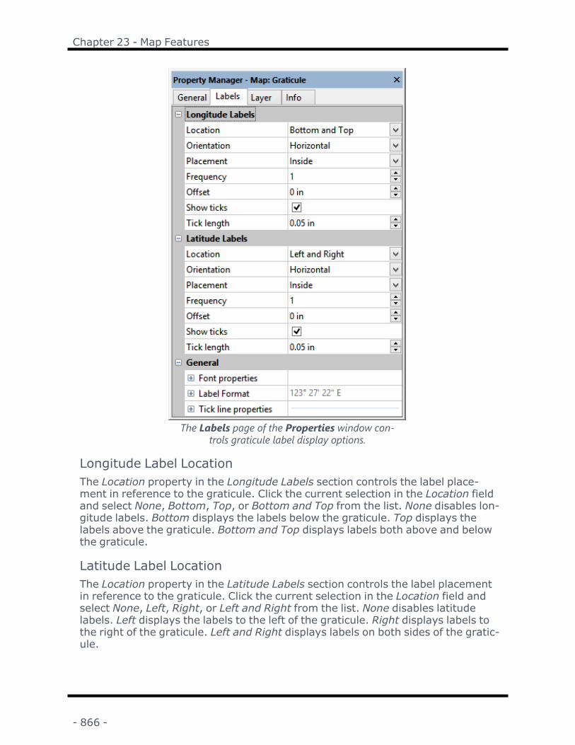
Chapter 23 - Map Features
The Labels page of the Properties window con-trols graticule label display options.
Longitude Label LocationThe Location property in the Longitude Labels section controls the label place-ment in reference to the graticule. Click the current selection in the Location fieldand select None, Bottom, Top, or Bottom and Top from the list. None disables lon-gitude labels. Bottom displays the labels below the graticule. Top displays thelabels above the graticule. Bottom and Top displays labels both above and belowthe graticule.
Latitude Label LocationThe Location property in the Latitude Labels section controls the label placementin reference to the graticule. Click the current selection in the Location field andselect None, Left, Right, or Left and Right from the list. None disables latitudelabels. Left displays the labels to the left of the graticule. Right displays labels tothe right of the graticule. Left and Right displays labels on both sides of the gratic-ule.
- 866 -

Surfer User's Guide
Label OrientationThe Orientation property specifies the label orientation. Click the current selec-tion in the Orientation field and select Horizontal, Vertical, Along line, or Normalto line from the list. Horizontal displays the labels horizontally. Vertical displaysthe labels vertically. Along line displays the labels parallel to the graticule lines.Normal to line displays the labels perpendicular to the graticule lines.
The image on the left shows the labels oriented parallel to the graticule lines when the Alongline option is selected for the Orientation property. The image on the right shows the labels
oriented perpendicular to the graticule lines with the Normal to line option selected.
Label PlacementThe Placementproperty specifies the label placement in reference to the mapframe. Click the current selection in the Orientation field and select Outside orInside from the list. Outside displays the labels outside the map limits. Inside dis-plays the labels inside the map limits.
3D Surfaces are limited to the extents of the map, so the Placementmust beInside for the graticule labels to be visible on a 3D Surface map.
Label FrequencyThe Frequency property specifies for which graticule lines labels are displayed.The labels are displayed at every nth graticule line, starting from the origin. AFrequency value of 1 displays labels at every graticule line, 2 displays labels atevery other line, 3 displays labels at every third line, etc. A label is always dis-played at the origin value, unless None is selected in the Location field. Type avalue of 1 or greater into the Frequency field, or adjust the value by clicking thebuttons.
- 867 -
Chapter 23 - Map Features
Label OffsetThe Offset property specifies the label distance from either the map frame or tickmarks. The Offset is the distance from the map frame when ticks marks are notdisplayed. The Offset is the distance from the end of the tick marks when Showticks is checked. Type a value in page units into the Offset field or click the but-tons to adjust the Offset. Increasing the offset moves the labels away from themap or ticks and in the direction of the Placement property. When Placement isset to Outside, increasing the Offsetmoves the labels away from the map. WhenPlacement is set to Inside, increasing the Offsetmoves the labels into the map.
Tick MarksThe Show ticks property controls the display of label tick marks. When Showticks is checked, label ticks are displayed in the direction specified by the Place-ment property. Label ticks are not displayed when Show ticks is unchecked. Clickthe Show ticks check box to check or uncheck the box.
Tick LengthThe Tick length property specifies the length of the tick marks from the mapedge. The Tick length property is enabled when Show ticks is checked. Type avalue in page units or click the buttons to change the Tick length value.
Label FontThe Font Properties section of the Labels page controls the label font properties.See the Font Properties help topic for more information on changing font prop-erties.
Label FormatThe Label Format section of the Labels page controls the label format prop-erties. See the Label Formats help topic for more information on changing formatproperties.
Tick Line PropertiesThe Tick Line Properties section of the Labels page controls the tick mark lineproperties. See the Line Properties help topic for more information on changingline properties.
ProfileTheMap Tools | Add to Map | Profile command allows the user to digitize aline on the map. A profile, or cross section, is created automatically from the lineand a base map layer added to the existing map. Alternatively, right-click on an
existing map and click Add to Map | Profile or the button to add a profile.
- 868 -

Surfer User's Guide
Profiles display distance traveled from the first point to the last on the X Axis andelevation on the Y Axis.
Adding a ProfileTo add a profile by drawing a new polyline on a map:
1. Select the map or map layer and click theMap Tools | Add to Map | Pro-file command. The cursor changes to .
2. Draw a line by clicking in the locations where the profile should be located.See the Polyline topic for more information on drawing lines.
3. Double-click the last point or press ENTER on the keyboard to end the draw-ing mode.
The profile is automatically placed below the bottom axis and the profile line isadded as a new base map layer. The base map layer is named Base - Profile 1.The Base - Profile 1 will automatically assign the coordinate system from the Mapcoordinate system. The profile is named Profile 1. The 1 increments for both theprofile name and the base layer name for each additional profile added to themap.
To add a profile using an existing polyline:
1. Select the polyline you wish to use for the profile. The polyline must be in abase layer in a map that also includes a grid-based layer.
2. Click theMap Tools | Add to Map | Profile command or right-click thepolyline and select Add Profile.
The profile is automatically placed below the bottom axis. The profile numberincrements for each additional profile added to the map.
Editing a ProfileTo make changes to the profile, click once on the profile in the Contents windowor in the plot window to select it. The properties are displayed in the Propertieswindow.
Reshaping the Profile LineProfile lines can be altered with the reshape command. To edit the path of a pro-file, click on the Polyline object in the Base - Profile layer in the map to select it.Click the Features | Edit Features | Reshape command. You can then moveexisting points on the line by clicking and dragging the point to the desired loc-ation. Add new points to the line by holding down the CTRL key on the keyboardand clicking on the desired location. Delete points by clicking on the point andpressing the DELETE key on the keyboard. Press ESC on the keyboard when alledits are complete. The profile graph updates as the points are moved.
- 869 -

Chapter 23 - Map Features
Moving the Profile LineIf a profile line needs to be moved on the map, click the Polyline object and moveit to the desired location. The profile graph updates after the line is moved.
Resizing the ProfileProfiles can be resized by clicking on the Profile object in the Contents window.In the Properties window, click on the Scale tab. The Length of either axis canbe changed.
Saving the Profile Line CoordinatesTo save the coordinates of the profile line, click on the Base - Profile layer in themap to select it. In the Properties window, click on the General tab. Click the
button next to the Input file option. Type a File name and click Save. Click OKin the options dialog and the .BLN file is created. The .BLN file can be used forother base maps or opened in the worksheet.
Saving the Profile DataTo save the elevations and distances along the profile, click the Profile object toselect it. In the Properties window, click on the Plot tab. Click the Save to Filebutton to save the information to a .DAT file.
Profiles with Multiple Map LayersWhen multiple map layers are overlaid, a profile is created for each unique gridin the map. For example two profiles are created for a map that has three layerscreated from two grid files, i.e. a profile is created for each grid. Hide the displayof individual profiles with the properties on the Plot page in the Properties win-dow. Profiles are always created using the Map coordinate system.
When a new layer is added to a map with a profile, the new layer is automaticallyadded to the profile.
Profiles and Vector LayersProfiles are not created for vector layers. This is because the vector magnitudesare usually of a significantly different scale than the Z values in the grid file, andprofiles of widely different scales cannot be reasonably plotted on the same setof axes. If you wish to create a profile of slope, gradient, or magnitude valuesfrom a vector layer, use the following process:
1. Use Grid Calculus Terrain Slope or Gradient Operator to create a grid ofslope or gradient values if you are using a 1-grid vector layer. Use Grid Mathwith the function sqrt(A^2 + B^2)to create a grid of magnitudes if you areusing a 2-grid vector layer with Cartesian coordinates. Use the magnitude
- 870 -

Surfer User's Guide
grid directly in step 2 if you are using a 2-grid vector layer with polar coordin-ates.
2. Use Grid Slice to slice the slope, gradient, or magnitude grid created in step 1along the profile trace. The trace line can be a loaded from a file, an existingbase (vector) layer, or drawn in an empty base map. Create an Output BLNfile in the Grid Slice dialog.
3. Create a base map from the Output BLN file. This is the profile of the slope,gradient, or magnitude along the profile trace. You will likely need to adjustthe profile scale.
Profiles and 3D MapsProfiles can only be added to maps that are not tilted and in the orthographic pro-jection. To temporarily change a map to this orientation:
1. Click on the Map object in the Contents window.2. In the Properties window, click on the View tab. Change the Projection to
Orthographic.3. Click and drag the Tilt (degrees) to 90.4. Then, click theMap Tools | Add to Map | Profile command.
Once the profile is located on the map, the Projection and Tilt (degrees) prop-erties can be changed back to their previous values.
Profile Plot PropertiesClick theMap Tools | Add to Map | Profile command or right-click on a mapand click the Add to Map | Profile to add a profile to an existing map.
Profile PropertiesYou have flexibility over the display and color of the profile. The Plot page con-trols the profile title and display order, line, and fill properties for the profile linesin the profile plot.
- 871 -

Chapter 23 - Map Features
The profile properties are set in the Properties win-dow.
General SectionThe General section of the Plot page includes the title properties and Export pro-file data command.
TitleProfile titles can use any text properties including math text formatting instruc-tions. Type the profile title exactly as you want it to appear on the Title line.
Titles can contain multiple lines. To create a multiple line title, click the button.The Text Editor appears. Type the text in the dialog. To add a new line of text,press the ENTER key on the keyboard. To change the properties of the text, high-light the text and change the desired property. When finished, click OK. You arereturned to the Properties window.
Font PropertiesTo edit all of the text properties for the entire title at once, click the next toFont properties. You can then set any desired font settings, including font, size,and text color.
NoData MethodThe NoData method property controls how NoData areas in the map are dis-played in the profile. Available options are Skip, Minimum, and Custom Value.When the NoData method is set to Skip, the areas where NoData values areencountered are not displayed on the profile. When set to Minimum, the areaswhere NoData values are located are displayed with the minimum Elevationvalue of the profile. When set to Custom Value, the Custom value option
- 872 -

Surfer User's Guide
becomes available. Type a value into the Custom value field, and the NoDataareas are drawn in the profile with an elevation equal to the Custom value.
Export Profile DataClick the Save to File button in the Export profile data field to save the profileelevation and distance data. In the Save As dialog, type a File name and click theSave button. A .DAT file is created.
The .DAT file contains one column of distance data and one or more columns ofelevation data. The first column, Column A when opened in the worksheet,includes the accumulated distance along the profile line. The remaining columnsinclude the elevation data for each profile in the profile plot. The DAT file alsoincludes a header row with "Distance" in the first column and the profile name inthe remaining columns.
Profiles SectionThe Profiles section includes the display state, display order, and line and fillproperties for each of the profiles in the profile plot.
Current ProfileSelect the profile you wish to edit in the Current profile field. The selected profileis indicated in the profile plot with blue circles along the profile. Click the currentselection and select the desired profile from the list. All profiles in the profile plotare included in the Current profile list. Profiles use the name of their cor-responding grid file, when available. When a grid file name is not available, pro-files use their corresponding layer name.
The Current profile list also indicates the order of the profiles in the plot. The pro-file at the back of the plot is listed first. The profile at the front of the plot is listedlast.
Show ProfileCheck the Show profile check box to display the Current profile in the profileplot. Clear the Show profile check box to hide the Current profile from the plot.
Display OrderControl the display order Current profile with the Display order property. ClickForward to move the Current profile forward one position in the plot. Click Back-ward to move the Current profile backward in position in the plot. When the pro-file plot contains only one profile, the Forward and Backward buttons aredisabled.
Line PropertiesSpecify the line properties for the Current profile by clicking on the next to LineProperties and setting the desired option. The line style, color, opacity, and widthcan be set.
- 873 -

Chapter 23 - Map Features
Fill PropertiesSpecify the fill properties for the Current profile by clicking on the next to FillProperties and setting the desired option. The fill pattern, color, and opacity canbe set. The fill goes from the profile line to the X Axis. You may wish to use semi-transparent fill or no fill when profile lines intersect.
Map AxesFour axes are automatically created for each map in Surfer . Axes are named bytheir relative positions on the map and are called the Left Axis, Right Axis, TopAxis, and Bottom Axis. The Left Axis and Right Axis are Y axes, and the Top Axisand Bottom Axis are X axes. 3D wireframe and 3D surface maps also have asingle Z Axis. Variograms and profiles have two axes with the default names of XAxis and Y Axis.
By default, axis limits match the X, Y limits of the grid file, boundary file, or datafile used to create the map. When a map is first created, the Left Axis and Bot-tom Axis display major ticks and tick labels, and the Top Axis and Right Axis dis-play only major ticks. The tick spacing is automatically scaled so a reasonablenumber of ticks are drawn along each axis. Tick scaling and label format para-meters can be independently specified for the axes on the map. By default, axesstart with the lowest value at the bottom of Y axes and increase up and the low-est value at the left side of X axes and increase to the right. Axes can be reversedso that the small value is at the top of the Y axis or at the right side of the X axis.Axes can show numbers or date/time values.
- 874 -

Surfer User's Guide
This is a contour map with the four axeslabeled with their default names.
This 3D surface map contains a Z axis in addition to the Xand Y axes. 3D wireframe maps also contain a Z axis.
Editing AxesTo edit an axis, click on the axis to select it. The axis properties are listed in theProperties window on the General, Ticks, Scaling, Grid Lines, and Info tabs.
- 875 -

Chapter 23 - Map Features
Axis VisibilityWhen the map, variogram, or profile is created, the axes are displayed auto-matically. You can turn off the display of any or all of the axes on the map byenabling the visibility of the axis with the Contents window. Click the check boxadjacent to the axis name to turn on or off the axis. On a 3D wireframe or 3D sur-face, only the Left Axis, Bottom Axis, and Z Axis are initially visible.
Axis PositionIndividual axes cannot be moved with the mouse, but you can position axes rel-ative to the map layers on the Scaling page in the axis properties. Open the axisproperties by clicking on the axis name in the Contents window.
TicksMap axes can display both major and minor ticks. Major ticks can display ticklabels. Minor ticks are displayed at regular intervals between major ticks, and donot have associated tick labels. When tick labels are displayed, all major ticksalong the axis are represented with a label. The display of tick marks is con-trolled from the Ticks page in the axis properties. The spacing of the major ticksalong the axis is controlled from the Scaling page in the axis properties. Majortick labels are controlled by the Labels group on the General page in the axisproperties.
On this axis, four minor ticks are included with every major tick.
Selecting an AxisClick an axis in the Contents window or plot window to select it. When selectingin the plot window, place the pointer on the tick marks or tick labels when click-ing. Hollow blue circle handles appear at each end of the axis. Because the axesare part of the map on which they are drawn, the eight solid green squarehandles appear around the entire map. In addition, the name of the axis is dis-played in the middle left side of the status bar. For example, if you select the bot-tom axis of a contour map, the text in the status bar appears as "Map: BottomAxis." The axis is also highlighted in the Contents window. The properties forthe axis are shown in the Properties window.
- 876 -
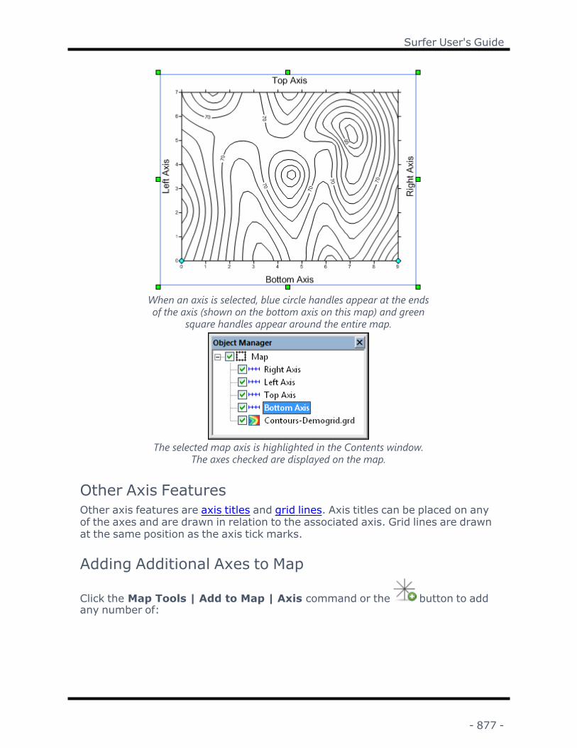
Surfer User's Guide
When an axis is selected, blue circle handles appear at the endsof the axis (shown on the bottom axis on this map) and green
square handles appear around the entire map.
The selected map axis is highlighted in the Contents window.The axes checked are displayed on the map.
Other Axis FeaturesOther axis features are axis titles and grid lines. Axis titles can be placed on anyof the axes and are drawn in relation to the associated axis. Grid lines are drawnat the same position as the axis tick marks.
Adding Additional Axes to Map
Click the Map Tools | Add to Map | Axis command or the button to addany number of:
- 877 -

Chapter 23 - Map Features
l Left Axesl Right Axes ,l Top Axes ,l Bottom Axes , orl Z Axes ,
to your current map. Alternatively, right-click on an existing map and click Addto Map to add a map layer, axis, or scale bar.
Click on the axis to display the axis properties in the Properties window. Theposition of the axis is changed by changing the Crosses At value on the Scalingpage.
Axis General PropertiesAdd an axis title, change axis line properties, display labels, or change the axisplane to make an axis more informative and customized. These items are set onthe General page for axis properties. To display the axis properties, click onceon the axis. The properties are displayed in the Properties window.
General PageThe General page controls the display of axis titles, axis lines, tick labels, andthe plane of the axis.
Specify the axis title and line settings in the Prop-erties window on the General page.
AxisThe Axis section controls the axis line properties and the plane of the axis.
- 878 -

Surfer User's Guide
Line PropertiesClick the button next to Line Properties to display the Line Properties options.Choose the line Style, Color,Width, and Opacity for the selected axis.
Axis PlaneThe Axis Plane option specifies the plane in which the tick marks and labels aredrawn. For maps with a 90-degree tilt, axis tick marks and labels must appear inthe XY plane to be seen. TheXYoption draws the tick marks and labels in theplane defined by the X and Y axes. For planar view maps (the default orientationfor base, contour, post, etc. maps), use this setting.
The XZ option draws the tick labels in the plane defined by the X and Z axes. TheYZ option draws the tick labels in the plane defined by the Y and Z axes. Theseoptions are used only when the tilt for the map is less than 90 degrees.
Axis tick labels can be drawn in different axis planes and can berotated to make reading easier. In this example, the bottom axisis on the XZ Axis Plane and the right axis is on the XY Axis Plane.
TitleAxis titles can use any text properties including math text formatting instruc-tions. Type the axis title exactly as you want it to appear on the Title text line.
Titles can contain multiple lines. To create a multiple line title, click the button.The Text Editor appears. Type the text in the dialog. To add a new line of text,press the ENTER key on the keyboard. To change the properties of the text, high-light the text and change the desired property. When finished, click OK. You arereturned to the Properties window.
- 879 -

Chapter 23 - Map Features
Offset along AxisThe Offset along axis box controls the placement of the title along the axis. Pos-itive offset values move the axis title in the positive direction along the axis. Theoffset values are set in page units.
Offset from AxisThe Offset from axis box controls the placement of the title towards or away fromthe axis. Positive offset values move the axis title away from the axis. The offsetvalues are set in page units.
Angle (degrees)The Angle (degrees) box controls the angle at which the title is drawn. Positiveangles rotate the title in a counterclockwise direction. Values must be between 0and 360. To change the Angle (degrees), highlight the existing value and type anew number. Or, click and drag the bar to the desired location. The textmoves in the plot window as the slider moves.
Font PropertiesClick the button next to Font Properties to specify the text properties for theaxis title.
Axis Ticks PropertiesAxes can display both major and minor ticks. When a map is created, the displayof major ticks is on by default. Major ticks display tick labels along the axis.Minor ticks on an axis are not represented with a tick label, and are not drawn onan axis by default. Minor ticks are defined as the number of minor ticks to bedrawn between adjacent major ticks.
Axis PlaneThe Axis plane option specifies the plane in which the tick marks and labels aredrawn. The Axis plane property is located on the General page. For maps with a90-degree tilt, axis tick marks and labels must appear in the XY plane to be seen.The XY option draws the tick labels in the plane defined by the X and Y axes. Forplanar view maps (the default orientation for base maps, contour maps and postmaps), use this setting. The XZ option draws the tick labels in the plane definedby the X and Z axes. The YZ option draws the tick labels in the plane defined bythe Y and Z axes. These options are used only when the tilt for the map is lessthan 90 degrees.
Ticks PageThe Ticks page controls the display of major and minor ticks, the position, andlength of ticks.
- 880 -

Surfer User's Guide
Specify the axis tick properties in the Properties win-dow on the Ticks page.
Major TicksThe Major Ticks section controls the display of the major tick marks. Click thenext to Major Ticks to open the Major Ticks section.
StyleClick the Style option to display a list. In the list, select the desired tick mark loc-ation. Options are Outside, Inside, or Cross the selected axis. If you do not wantto show ticks, select None from the list.
LengthThe Length box controls the length of the major tick marks. The tick lengths arein page units.
Minor TicksThe Minor Ticks section controls the display of the minor tick marks. Click thenext to Minor Ticks to open the Minor Ticks section.
StyleClick the Style option to display a list. In the list, select the desired tick mark loc-ation. Options are Outside, Inside, or Cross the selected axis. If you do not wantto show minor ticks, select None from the list.
LengthThe Length box controls the length of the minor tick marks. The tick lengths arein page units.
Minor Ticks Per MajorTo specify the number of minor ticks to draw between adjacent major ticks,enter the number into the Minor ticks per major box. This should be one less
- 881 -

Chapter 23 - Map Features
than the number of minor divisions you want to appear between adjacent majorticks. Specify a value between 0 and 100.
For example, if you want the minor ticks to indicate 10 divisions, the Minor ticksper major value should be set to 9.
Axis Legend PropertiesTick labels are the numbers or text that appear at major tick mark locations. Ticklabels indicate the axis values in data units. The Labels page includes propertiesto set the axes label position, format, and font. To display the axis properties,click once on the axis. The properties are displayed in the Properties window.
Axis PlaneThe Axis plane option specifies the plane in which the tick marks and labels aredrawn. The Axis plane property is located on the General page. For maps with a90-degree tilt, axis tick marks and labels must appear in the XY plane to be seen.The XY option draws the tick labels in the plane defined by the X and Y axes. Forplanar view maps (the default orientation for base maps, contour maps and postmaps), use this setting. The XZ option draws the tick labels in the plane definedby the X and Z axes. The YZ option draws the tick labels in the plane defined bythe Y and Z axes. These options are used only when the tilt for the map is lessthan 90 degrees.
Labels PageThe Labels page controls the display of tick labels.
Specify the axis tick label settings in the Prop-erties window on the Labels page.
ShowThe Show check box controls the display of tick labels. When the Show box ischecked, major ticks on the selected axis are displayed with a label.
- 882 -

Surfer User's Guide
Angle (degrees)The Angle (degrees) box specifies the angle at which the tick labels are drawn.Positive angles rotate each axis tick label in a counterclockwise direction. Valuesmust be between 0 and 360. To change the Angle (degrees), highlight the exist-ing value and type a new number. Or, click and drag the bar to thedesired location. The text moves in the plot window as the slider moves.
Offset From AxisThe Offset from axis box controls how far away the tick labels are drawn from thetick marks. Positive offset values move the axis title away from the axis. The off-set values are set in page units.
Label FormatClick the button next to Label Format to display the Label Format options. Thissets the numeric format used for the tick labels. Labels can be formatted withFixed, Exponential, Compact, Date/time, or DMS (Lat/Long) numeric formats.See the Label Formats help topic for more information on the label format typesand options.
Font PropertiesClick the button next to Font Properties to display the text properties for theaxis tick labels. The Font, Size (points), Foreground color, Foreground opacity,Background color, Background opacity, Bold, Italic, Strikeout, and Underlineoptions are available.
Axis Scaling PropertiesAxis scaling controls the axis limits, the major tick starting and ending values,and the position of the axis relative to the other axes in the map. To set axis scal-ing, click on the axis to select it. Click on the Scaling page in the Properties win-dow.
Axis scaling is different from setting the map scale. When axis scaling is set, theaxis limits are defined but does not rescale the map. Axes that use different lim-its than the map are still drawn at the same scale as the map. Because of this, itis possible to have axes shorter or longer than the map. To change the mapscale, click on the Map object and click the Scale tab in the Properties window.
- 883 -

Chapter 23 - Map Features
In this example, the Bottom Axis and Left Axis are offset fromthe map, and the limits of the axes are set differently than the
map limits.
Scaling PageThe Scaling page for an axis in the Properties window controls the axis scalingproperties.
Specify the axis scaling in the Properties windowon the Scaling page.
- 884 -

Surfer User's Guide
Automatic ScalingThe Automatic check box uses the limits of the map as the limits for the axes anduses a reasonable tick mark spacing along the axis. When any parameters arechanged on the axis properties Scaling page, the Automatic check box is auto-matically unchecked. After making any changes, you can return to the automaticsettings by checking the Automatic box.
Axis MinimumThe Axis minimum box specifies the minimum axis value. To change the min-imum value, highlight the existing value and type a new value. Press ENTER onthe keyboard to make the change.
When using date/time formats for the axis labels, enter the minimum date/timeaxis value. For instance, 02/02/2014 12:00:00 AM can be entered into the Axisminimum option.
Axis MaximumThe Axis maximum box specifies the maximum axis value. To change the max-imum value, highlight the existing value and type a new value. Press ENTER onthe keyboard to make the change.
When using date/time formats for the axis labels, enter the maximum date/timeaxis value. For instance, 10/31/2014 12:00:00 AM can be entered into the Axismaximum option.
Major IntervalThe Major interval box contains the value of the spacing, in data units, betweenmajor ticks along the selected axis. The major tick marks occur at values
Tick = First major tick + n* Major interval n =0, 1, ..., N
where N is the largest integer such that Tick ≤ Last major tick. Thus, a tick markis placed at the value of the Last major tick only if the interval (Last major tick -First major tick) is evenly divisible by Major interval. To change the interval, high-light the existing value and type a new value. Press ENTER on the keyboard tomake the change.
When using the date/time formats for the axis labels, click on the existing timescale (Years, Weeks, Days, Hours, Minutes, or Seconds) and select the desiredtime scale to select how often the labels are drawn. Then, highlight the existingvalue and type a new value to set how many of the desired time scales shouldoccur before the next tick. Alternatively, click the to increase or decrease thevalue. For instance, setting the Major interval to 3 Years displays a tick at theFirst major tick location. The second tick will occur 3 years after the first.
When date/time axis labels are displayed, the Majorinterval is set in date/time units.
- 885 -

Chapter 23 - Map Features
First Major TickThe First major tick box contains the major tick mark minimum value. This valueis expressed in data units. The First major tick does not need to be the same asthe Axis minimum but it cannot be less than the Axis minimum. To change theFirst major tick value, highlight the existing value and type a new value. PressENTER on the keyboard to make the change.
When using date/time formats for the axis labels, enter the first major date/timeaxis tick mark value. For instance, 02/02/2014 12:00:00 AM can be entered intothe First major tick option.
Last Major TickThe Last major tick box contains the maximum allowed major tick mark value.This value is expressed in data units. The Last major tick does not need to be thesame as the Axis maximum but it cannot be greater than the Axis maximum. Tochange the Last major tick value, highlight the existing value and type a newvalue. Press ENTER on the keyboard to make the change.
When using date/time formats for the axis labels, enter the last major date/timeaxis tick mark value. For instance, 10/31/2014 12:00:00 AM can be entered intothe Last major tick option.
Axis PositionAxes are a part of the map on which they are placed. By default, axes are drawnat the edge of a map or surface. Map axes are placed in relation to the other axeson the map.
A contour map has two Y axes: the Left Axis and Right Axis. The placement of theY axes are relative to the data units along the X axes (the Top Axis and BottomAxis) on the map. By default, the left Y axis crosses the X axes at the minimum Xaxis value.
Cross Y Axis AtThe Cross Y axis at box is only displayed when an X or Z axis is selected. This spe-cifies the position of the X or Z axis along the Y axis. The value is entered in Ydata units. To change the value, highlight the existing value and type a newvalue. Press ENTER on the keyboard to make the change.
When using date/time formats for the axis labels, the Cross X axis at, Cross Yaxis at, and Cross Z axis atmust always be in numbers, not in date/time format.
Cross Z Axis AtThe Cross Z axis at box specifies the position of the X or Y axis relative to the Zaxis on a 3D wireframe or surface map. The value is entered in Z data units. Tochange the value, highlight the existing value and type a new value. PressENTER on the keyboard to make the change. By default, the X and Y axes aredrawn at the elevation of the base defined for the wireframe or surface map. For
- 886 -

Surfer User's Guide
example, if the base for the wireframe is set to be 25, the X and Y axes cross theZ axis at an elevation of 25.
When using date/time formats for the axis labels, the Cross X axis at, Cross Yaxis at, and Cross Z axis atmust always be in numbers, not in date/time format.
Cross X Axis AtThe Cross X axis at box is only displayed when an Y or Z axis is selected. This spe-cifies the position of the Y or Z axis along the X axis. The value is entered in Xdata units. To change the value, highlight the existing value and type a newvalue. Press ENTER on the keyboard to make the change.
When using date/time formats for the axis labels, the Cross X axis at, Cross Yaxis at, and Cross Z axis atmust always be in numbers, not in date/time format.
Axis DirectionTo make an axis descending, check the box next to Reverse axis. Map layers areautomatically updated when the axis is reversed. When the axis is normal (theReverse axis box is unchecked), the axis minimum value is on the left side for anX axis and on the bottom for a Y axis. When reversed, the axis minimum is loc-ated on the right side for an X axis and the top for a Y axis. When one X axis isreversed (i.e. Bottom Axis), all X axes on the map are automatically reversed.When one Y axis is reversed (i.e. Right Axis), all Y axes on the map are auto-matically reversed.
Z axes and variogram axes cannot be reversed.
The two maps both display contours and classed post data from the same files. The map onthe right has the Reverse axis option checked for the Bottom Axis . All map properties are
reversed.
- 887 -

Chapter 23 - Map Features
Setting the Axis ScaleAxis limits are specified in map coordinates, profile, or variogram units. Axis lim-its do not need to coincide with the map limits. Use these steps to change theaxis scale:
1. Click on an axis to select it. The Properties window automatically showsthe properties for the axis.
2. Click on the Scaling tab.
3. You can set any of the parameters listed below.
1. The Automatic box uses the limits of the map as the limits for theaxes and uses a reasonable tick mark spacing along the axis. Whenany parameters are changed in the axis properties, the Automatic boxis automatically unchecked. After making any changes, you canreturn to the automatic settings by checking the Automatic box.
2. The Axis minimum box specifies the minimum axis limit.
3. The Axis maximum box specifies the maximum axis limit.
The axis is automatically updated with the new axis scale settings as the valuesare changed.
Edit Major Tick Spacing on an AxisOn the Scaling page in the axis properties there are three options that controlthe spacing of major ticks along the selected axis: the First major tick, Lastmajor tick, and Major interval boxes.
To edit major ticks on an axis:
1. Click once on the axis to select it.
2. In the Properties window, click the Scaling tab.
3. You can specify the position for the first and last major ticks, and the spa-cing in data units between each major tick along the axis.
4. The First major tick box contains the value of the minimum major tickmark. This value is expressed in data units. The First major tick does nothave to be the same as the axis minimum but it cannot be less than theaxis minimum.
5. The Last major tick box contains the value of the maximum allowed majortick. This value is expressed in data units. The Last major tick does nothave to be the same as the axis maximum but it cannot be greater than the
- 888 -

Surfer User's Guide
axis maximum.
6. The Major interval box contains the value of the spacing, in data units,between major ticks along the selected axis. The major tick marks occur atvalues,
Tick = First Major Tick + n * Major Interval n=0,1,...,N
where N is the largest integer such that Tick <= Last Major Tick. Thus, atick mark is placed at the value of the Last major tick only if the interval(Last Major Tick - First Major Tick) is evenly divisible by Major interval.
7. The axis is redrawn with the selected tick parameters.
By setting the First major tick, Last major tick and Major interval values, you can control theposition of major ticks along the axis.
Axis Grid Line PropertiesGrid lines are a mesh over the top of the map. Along an axis, grid lines can ori-ginate from the major ticks, minor ticks, or both. The major and minor grid linescan use different line properties. When grid lines are added to 3D wireframe or3D surface maps, the lines are drawn on the plane defined by the base of themap.
Grid lines are drawn over the extent of the map. For example, if you draw gridlines for an X axis (the Bottom Axis), the grid lines are drawn parallel to the Yaxis (Left Axis) over the entire map. If your X axis is offset from the Y axis, thegrid lines are not drawn beginning at the end of the X axis, but beginning at theminimum Y value on the map.
- 889 -

Chapter 23 - Map Features
Specify the tick spacing to use for the grid lines on the Scaling page. The ticks donot need to be displayed for the grid lines to be drawn.
Grid lines originate from the tick marks. Different line prop-erties can be used for the major and minor grid lines. In thisexample, major grid lines are solid and minor grid lines are
dotted.
Grid Lines PageThe Grid Lines page controls the visibility and properties of major and minorgrid lines.
Specify the axis grid line properties in the Prop-erties window on the Grid Lines page.
- 890 -

Surfer User's Guide
Major Grid LinesIf you want grid lines to extend from the major ticks, check the Show box in theMajor Grid Lines section. Click the next to Line Properties to open the line prop-erties section for the Major Grid Lines. Change the Style, Color, Opacity, andWidth for the major grid lines.
Minor Grid LinesIf you want grid lines to extend from the minor ticks, check the Show box in theMinor Grid Lines section. Click the next to Line Properties to open the line prop-erties section for the Minor Grid Lines. Change the Style, Color, Opacity, andWidth for the minor grid lines.
To Draw a Grid Covering the Map1. Click on an axis to select it. The axis properties are automatically displayed
in the Properties window.
2. Specify the tick spacing to use for the grid lines on the Scaling page. Theticks do not need to be displayed for the grid lines to be drawn.
3. Click the Grid Lines tab.
4. If you want grid lines to extend from the major ticks, check the Show box inthe Major Grid Lines section.
5. Change the options under Line Properties for the Major Grid Lines. You canchange the Style, Color, Opacity, andWidth for the major grid lines.
The grid lines are drawn on the map as you make changes in the Properties win-dow.
- 891 -


Chapter 24 - 3D View
3D View WindowThe 3D view window displays a map in a three-dimensional view space. Theinput grids from grid-based layers are rendered as surfaces in the 3D view. Base(vector and raster), post, and classed post layers are overlaid on the surfaces astextures. Point data in base (vector) layers from data, post, and class post layersare also displayed in 3D. If the base (vector) layers have 3D polylines, 3D poly-gons or a 3D polymesh in them, then those 3D objects will display in true 3D inthe 3D view. The visualizations from the grid-based maps are also overlaid onthe surface. For example, contour lines or color relief layers will be overlaid onthe surfaces. Point cloud layers are rendered as a 3D point cloud. Contour linesmay be rendered as 3D polyline objects. However, contours are displayed asoverlays on a surface and not as 3D polylines by default. If the base (vector) lay-ers have 3D polylines, 3D polygons or a 3D polymesh in them, then those 3Dobjects will display in true 3D in the 3D view.
The 3D view window only displays layers that are visible in the map in the plotwindow. Show or hide surfaces, textures, and vector data in the 3D view byselecting or clearing the visibility check boxes in the 3D view Contents window.Completely remove a surface, texture, vector data, axis, or color scale from the3D view by switching to the plot window and turning the visibility off for the asso-ciated map layer.
Click theMap Tools | View | 3D View command or the button or the 3DView button in the Map frame View properties page to open a 3D view window ofthe selected map. A new 3D view is created for the selected map. A 3D view canalso be created by right-clicking a map or map layer and clicking 3D View in thecontext menu. To create a 3D view, the map must include at least one grid-based layer or base from data, post, classed post or point cloud layer or a base(vector) layer with a 3D object. The document tab includes the file name andview number. For example, when a 3D view is created for a map in the Plot1 plotwindow, the plot window tab name is Plot1:1 and the 3D view window tab nameis Plot1:2.
- 893 -

Chapter 24 - 3D View
The 3D view displays the map in a three-dimensional space. This map includes contour, colorrelief, post, base, and point cloud layers.
3D View CommandsThe 3D View ribbon tab contains commands for modifying the view and creatingvideos and images in the 3D view window.
Fit to Window Zoom to fit the entire map in the 3D view windowZoom In Zoom in on the center of the 3D view windowZoom Out Zoom out from the center of the 3D view windowRealtime Zoom by clicking and dragging the mousePan Pan the 3D view windowTrackball Rotate the 3D view windowWalk Walk along the surface in the 3D view windowGo to Home Move the 3D view to the home positionSet Home Set the 3D view home positionCreate/Edit Create or edit a fly-throughPlay Play the fly-throughRecord Create a video with the current fly-through settingsCopy to Clip-board
Copy an image of the 3D view window to the clipboard
Export Image Export the current view in the 3D view window as animage
Export 3D Export the map in the 3D view window to a 3D PDF model
- 894 -

Surfer User's Guide
ContentsThe Contents window contains the Environment and the surface and vectorobjects in the 3D view. Surfaces are generated from the grids in the map, andVectors are generated from the point cloud and contour layers in the map. Selectthe objects in the Contents window to change the properties of the 3D view andthe map in the 3D view. A check mark next to the layer name indicates the layeris displayed in the 3D view. Clear the check box next to a layer to hide the layerin the 3D view.
The Contents window includes the surfaces,vectors, axes, and color scales in the 3D
View.
EnvironmentThe Environment object in the Contents window contains the properties for the3D view. Select the Environment to modify the 3D view background, verticalexaggeration, water level, camera, and lighting. The Environment object hasthree Properties pages:
GeneralCameraLighting
- 895 -

Chapter 24 - 3D View
The Lighting properties have no effect on the 3D view when a hill shaded orreflectance shaded color relief layer is present in the map. Turn off hill shadingand reflectance shading for the color relief layer(s) to use the EnvironmentLight-ing properties.
Surfaces GroupThe Surfaces group in the Contents window contains the surfaces in the 3Dview. A surface is created for each grid in the map. The Surface group includesproperties for controlling the rendering quality of all the surfaces in the 3D viewand their overlay textures. The Surfaces group has one Properties page, Gen-eral.
Individual SurfacesEach surface in the 3D view can have overlays from the map. The available over-lay textures are listed under the General page in the Properties window foreach surface. Available textures include the grid-based map visualizations, e.g.contours and color relief, as well as any base or post layers in the map. Indi-vidual overlays can be hidden or displayed on each surface by selecting the sur-face you wish to edit in the Contents window, and then selecting or clearing thevisibility check boxes next to the overlay layer names in the Textures to displaysection of the General page.
By default, each surface shows the texture from any map layer that uses thesame grid file as the surface, and the textures from any base or post layers. Usethe General page to hide or display textures.
The overlay textures do not have any 3D view properties. To change the appear-ance of the overlays, modify their properties in the plot window. Switch to theplot window by clicking the plot window document tab.
Vector Data GroupThe Vector Data group in the Contents window contains the 3D vector objects inthe 3D view, i.e. point cloud layers and 3D polyline contours. There are no VectorData group properties.
ContoursContours are created for contour layers in the map. By default, the contour layeris displayed as a texture overlay on the surface. Vector contour lines are hiddenby default. Select the check box next to the contours vector object in the Con-tents window to display the contours. Change the properties of the contours onthe General page of the Properties window. Leave the contours the same asthose assigned in the 2D plot by selecting Same as plot for Color Method. Or,select Fixed to change the contours to have the same color and width in the 3Dview.
- 896 -

Surfer User's Guide
Vector Data3D point vector data is displayed for post and classed post layers in the map. 3Dpoint, polygon, and polyline vector data is displayed for base (vector) layers inthe map. The post, classed and post layers have one Properties page, General;and the base(vector) layer has two Properties pages, General and Z coordinate.
Point CloudsSelect the individual point cloud layers within the Vector Data group to changethe Point size for the point clouds. The point cloud layers have one Propertiespage, General. The number of points in the point cloud is limited by the 3D Viewmaximum number of points in the Options dialog Rendering page.
Drillhole Group3D drillhole layers are created for drillhole layers in the map. The Drillhole grouphas no properties. See the 3D Drillhole Properties topic for Points, Intervals,Path, and Label properties for 3D drillhole layers.
Axes GroupThree axes are automatically created for a map in the 3D view in Surfer. TheAxes group in the Contents window contains the X, Y, and Z axes for the 3Dmap. All the axes are displayed by default. Clear an axis to remove it from the 3Dmap. Each axis has four Properties pages. Click on the axis in the Contents win-dow to change its properties in the Properties window:
GeneralTicksLabelsScaling
Color Scales GroupThe Color Scales group in the Contents window contains color scales in the 3Dview. A color scale is created for 2D layers that have a colormap. The ColorScales group adds or hides a color scale on the plot. The color scales can includeany number of post, classed post, 1-grid vector, 2-rid vector, contour, pointcloud and base colormaps from any of the maps in the plot. The total number ofcolor scales is limited to the total number of layers that have their own colorscales. The Color Scales group has one Properties page, Color Scales.
Individual Color ScalesEach color scale in the 3D view can have overlays from the map. The availableoverlay color scale for each 2D layer are listed under the Color Scales page in theProperties window. Select the color scale you wish to display on the 3D view.Clear the color scale to remove it from the 3D view. Color scales that are dis-played may be edited by selecting the color scale in the Contents window. Colorscales have four Properties pages:
General
- 897 -

Chapter 24 - 3D View
TitleLabelsFrameColor scales will not export to a 3D file but will export to images and be copied tothe clipboard.
3D View PropertiesThe following sections describe the properties for the 3D view window and thevarious objects in the 3D view.
3D View Environment General PropertiesThe Environment page contains the 3D view window background, vertical exag-geration, antialiasing and water properties. Select the Environment object in the3D view Contents window to modify the 3D view and 3D symbol properties.
Set the 3D view background and water prop-erties in the General page.
Background modeThe Background mode property specifies the background style. Select Color touse a solid color for the 3D view window background. Select Skybox to use a sky-box for the 3D view background. A skybox is a scene that creates the illusion ofthree-dimensional distant surroundings. The skybox is also useful for keepingtrack of the camera orientation when rotating the view.
- 898 -

Surfer User's Guide
Background ColorWhen Background mode is set to Color, the Background color property is dis-played. Select the desired Background color from the color palette or click tocreate a custom color in the Colors dialog.
SkyboxWhen Background mode is set to Skybox, the Skybox property is displayed.Selected the desired Skybox from the list. Select (none) to use the previous solidcolor background.
AntialiasingThe Antialiasing property is selected by default to enable multisampling anti-aliasing. Copy-to-clipboard and export-to-image functions also employ themultisampled framebuffer when Antialiasing is selected. Older versions of Surferand computers which do not have modern graphics cards will not show theAntialiasing property.
Vertical ExaggerationThe Vertical exaggeration property is a unitless scale factor for Z coordinates inthe 3D view. The Vertical exaggeration scales the Z direction to maintain a pro-portional appearance in the 3D view when Z values are in different units than theXY coordinates or when the XY extents and Z values are in significantly differentranges. The default Vertical exaggeration scales the maximum Z extent to one-fourth the maximum X or Y range.
Increase the Vertical exaggeration to accentuate the differences in the surface Zvalues. Decrease the Vertical exaggeration to flatten the appearance of theobjects in the 3D view. The slider can be used to decrease the Verticalexaggeration to one-tenth of the default value, and the slider can beused to increase the Vertical exaggeration to ten times the default value. To spe-cify a Vertical exaggeration value outside this range, type the desired value dir-ectly in the Vertical exaggeration field.
The Vertical exaggeration is originally calculated based on the X, Y, and Zextents of data loaded into the 3D view when it is created. The Vertical exag-geration is recalculated when the extents of the visible data changes due to chan-ging visibility for surfaces or vector data in the Contents window.
WaterSelect theWater property to display a water level plane on the 3D view. CleartheWater property to remove the water level plane from the 3D view. A waterlevel plane is an XY plane that extends across the extents of the map in the 3Dview.
- 899 -

Chapter 24 - 3D View
Water LevelTheWater level property sets the Z value, or elevation, for the water level planein the 3D view window. Type the desiredWater level in the field or click and dragthe to change theWater level.
Water ColorTheWater color property sets the color of the water level plane. Select thedesiredWater color from the color palette or click to create a custom color inthe Colors dialog.
Water OpacityTheWater opacity property sets the opacity of the water level plane. A value of0% is completely transparent. A value of 100% is completely opaque. Type avalue between 0 - 100 in theWater opacity field or click and drag the toadjust the water level plane opacity.
Semi-Transparent Water Level and 3D Surface LayersSemi-transparent water levels require certain settings. When applying aWateropacity less than 100% to a 3D view, the following properties should be used:
1. Make sure Show surface background is selected on the surface General page.2. Clear any 3D surface layer texture check boxes on the surface General page.3. The surface should include at least one other layer texture.
If these options are not used, the water level opacity may be inconsistent. Notethat this requires the 3D surface layer texture to be removed. Use a color relieflayer instead of a 3D surface layer to maintain a colormap on the surface with asemi-transparent water level in the 3D view.
3D View Environment Camera PropertiesThe Camera page contains the camera field of view, location, and aim propertiesfor the 3D view window.
- 900 -

Surfer User's Guide
Set the camera FOV, position, and target in theCamera page.
Field of ViewThe Field of View controls the perspective effect of the 3D view window. The per-spective effect is the visual effect of the map changing size relative to the dis-tance from the observer. The Field of View angle is the angle between the leftedge of the 3D view window, the viewpoint, and the right edge of the 3D viewwindow. A large Field of view increases the perspective effect, while a small Fieldof view decreases it. Type a value in the Field of view property field to change theField of view, or change the Field of view by clicking and dragging the slider
.
PositionThe Position section includes the camera position properties: X position, Y pos-ition, and Z position. The Position properties update automatically as the camerais moved with the Pan, Trackball, Zoom, or Walk commands. You can also typecoordinates into the X position, Y position, and Z position fields to move the cam-era.
TargetThe Target section includes the camera aim properties: X target, Y target, and Ztarget. The Target properties update automatically as the camera is moved withthe Pan, Trackball, Zoom, or Walk commands. The X target, Y target, and Z tar-get values are the coordinates of the point at which the camera is pointing. TheTarget values also describe the point about which the view rotates when theTrackball command is used.
- 901 -

Chapter 24 - 3D View
It is recommended that the camera position is saved with Set Home before modi-fying the Target properties. The Go to Home command can then be used toreturn the camera to the default state.
Lighting PropertiesTo edit a 3D surface map, click once on the surface map to select it. The prop-erties for the surface map are displayed in the Properties window. To edit theLighting in the 3D View, click Environment in the Contents window. Changesmade to the environment lighting will be automatically applied to the lighting ofpoint vector data in the 3D view. The 3D view window lighting properties are dis-played in the Properties window.
The Lighting page controls the lighting for the entire multi-layer map. Thisincludes the surface, any overlays that may have been combined with the sur-face, and point vector data in 3D. The light source is fixed relative to the surface,so if the surface is rotated, the light rotates with it.
Hill and Reflectance Shading in the 3D ViewThe 3D view lighting is turned off when the map in the 3D view contains a hillshaded or reflectance shaded color relief layer. This is because the map isalready shaded by hill shading or reflectance. The cumulative effect of both light-ing systems would result in very dark regions of the map in the 3D view.
To use the 3D view Lighting properties instead of the color relief hill or reflect-ance shading, the Terrain representation option on the color relief layer Generalpage must be set to Color only.
Lighting PropertiesThe following properties control the lighting appearance of the 3D surface map inthe plot window or the lighting of the map in the 3D view.
- 902 -

Surfer User's Guide
Change lighting properties in the Properties windowon the Lighting page.
LightingThere are three lighting options. Click on the current lighting option next toModel. In the list, select the desired lighting option.
l None disables all lighting effects. The color shown is from the surface mater-ial color only.
l Smooth splits each grid cell is into two triangular polygons. Gouraud shadingis used to interpolate colors within the triangles from the three vertices ofeach triangle. This results in smooth transitions across the triangles and theentire grid, but it is slightly slower than flat shading.
l Flat uses a single vertex (grid node) to define the shaded color for the entirepolygon. Note that each grid cell is divided into two triangular polygons. Thisresults in a faceted look since each triangle is only filled with a single color.
Light PositionThe Light Position section specifies the orientation of the light source. The lightsource can be thought of as the sun shining on a topographic surface.
The Horizontal (degrees) box defines the direction for the light source in the hori-zontal plane. Zero degrees corresponds to the light source shining from due easttoward the west. Positive angles rotate the light source counterclockwise. Forexample, a specified horizontal angle of 90 degrees places the light source northof the unrotated surface. 180 degrees places the light source west of the unro-tated surface and shining east. 270 degrees places the light source south of theunrotated surface and shining north. The default horizontal angle is set at 135degrees, or NW. To change the Horizontal (degrees), highlight the existing anglevalue. Type a new value or click and drag the to the desired angle pos-ition.
- 903 -

Chapter 24 - 3D View
The Vertical (degrees) box rotates the light source in the vertical plane. A ver-tical angle of zero degrees places the light source at the horizon and shining hori-zontally. An angle of 90 degrees places the light source directly overhead andshining down onto the map. 180 degrees places the light source at the oppositehorizon and shining horizontally. 270 degrees places the light source directlybelow the map and shining up. The default vertical angle is 45 degrees. As thevertical angle approaches zero, shadows lengthen and the overall display shiftsto the colors at the left end of the color spectrum. To change the Vertical(degrees), highlight the existing angle value. Type a new value or click and dragthe to the desired angle position.
Light ColorsThere are three different types of light color, Ambient, Diffuse, and Specular.Note that these colors are used to represent reflectivity. White is 100% reflectiveand reflects the material color unaltered to the viewer. Black is 0% reflective,and causes all material color to be absorbed. Our perception of color is based onreflected and absorbed light. For example, a leaf appears green because itabsorbs all colors in the light spectrum EXCEPT green. Since only green is reflec-ted to your eye, the leaf appears green.
Surfer uses a pure white light source. The light "strikes" the surface and some ofthe light is absorbed based on the color of the surface material at the point thelight ray struck it. Some light is reflected to the viewer according to the type oflight (Ambient, Diffuse, and Specular), and the reflectivity color associated witheach type of light specified in the Light Colors section.
l Ambient refers to light that has been scattered so evenly by the environmentthat its direction is impossible to determine. Increasing the ambient light com-ponent brightens the scene without casting shadows. The default Ambientcolor is 90% black which means that the ambient light contribution is fairlysmall.
l Diffuse refers to light coming from a particular direction and is brighter ifaimed directly down on a surface than barely glancing off the surface. Whendiffuse light hits the surface, it is scattered uniformly in all directions so thatit appears equally bright no matter where the eye is located. Increasing dif-fuse light intensifies shadow effects. The default Diffuse color is white, whichis the maximum amount of reflectivity.
l Specular refers to light coming from a particular direction, and tends tobounce off the surface in a preferred direction. A shiny surface such as metalhas a high specular component, while a surface like carpet has almost nospecular component. Increasing the percentage of specular light results instrong shadow effects and more pronounced "shiny" or glare spots. Thedefault Specular color is 90% black.
In general, these reflectivity colors should be specified as shades of gray in orderto evenly reflect the surface material color components. However, special effectsare possible by specifying non-gray colors for the reflectivity. For example,assume the Ambient reflectivity is set to pure red, and the Diffuse and Specular
- 904 -

Surfer User's Guide
components are set to pure black. The Diffuse and Specular components areessentially disabled by setting their reflectivity color to black. The only light thatis reflected to the viewer is red ambient light. Portions of the surface that lack ared component in the material color will appear black, since only red light isreflected to the viewer.
Object LightingThe 3D Symbols property is selected by default to enable the lighting to illu-minate and cast shadows on point vector data as it does on the surface displayedin the 3D View window. When this property is cleared, shadows on 3D symbolsremain static. The Symbol method for 3D vector point data must be set to Sym-bols and the symbol style either Shaded Circle, Sphere or Cube. The lightingModelmust be either Smooth or Flat.
Surfaces Group General PropertiesThe General page contains the surface and texture resolution properties for allsurfaces in the 3D view. Select the Surfaces group in the 3D view Contents win-dow to modify the resolution of the surfaces and textures. Increase the surfaceand texture resolution to improve the appearance of the map. Decrease the sur-face and texture resolution to increase the drawing speed in the 3D view.
Set the surface and texture appearance in theGeneral page.
Surface ResolutionThe Surface quality property in the Surface Resolution section controls the qual-ity of the surfaces in the 3D view. As the Surface quality is increased, more ver-tices are included in the surfaces in the 3D view. When Surface quality is set to100, the surface is displayed at the full grid resolution. When the Surface qualityis 50, half as many vertices in the X and Y directions are used to display the sur-face, i.e. the number of vertices is one-fourth the number of grid nodes. WhenSurface quality is set to 0, the minimum resolution is used to display the surface.
- 905 -

Chapter 24 - 3D View
When the Surface quality is less than 100, overlaid texture contour lines mayappear to vary in elevation on the surface. If your computer is capable of ren-dering the surface at full resolution, a Surface quality of 100 is recommendedwhen the surface in the 3D view includes a contour layer texture overlay.
Texture ResolutionThe Texture Resolution properties control the appearance of the surface overlaytextures. The Texture width is the number of pixels used to render the textureoverlays in the X direction. The Texture height is the number of pixels used torender the texture overlays in the Y direction.
The Texture width and Texture height can be specified independently to accountfor different surfaces. For surfaces that are generally square, the Texture widthand Texture height should be set to the same value. For surfaces that are rect-angular, i.e. one side is significantly longer than the other, the texture appear-ance may be improved by increasing the resolution along the long side of thesurface.
By default the Texture width and Texture height are set to automatic. When bothTexture width and Texture height are set to Automatic, the surface resolutionalong the longer direction is set to 1024 and the surface resolution along theshorter side is set based on the ratio between the surface width and height. Forexample, a square surface will have 1024 pixels along the width and height whilea long and skinny surface may only use 256 pixels along the shorter direction.When only one of the Texture width or Texture height values are set to Auto-matic, the Automatic value varies based on the specified value and the ratiobetween the surface width and height.
To change the Texture width or Texture height, select the desired resolutionfrom the list. Select Automatic, 256, 512, 1024, 2048, 4096, 8192, or 16384pixels.
Shading ResolutionThe Shading Resolution properties control the amount and quality of the surfaceshading. The Shading detail specifies the amount of surface shading detail. The Zscale factor increases or decreases shading.
The Shading detail has three levels of shading quality:
l High increases the level of detail in the surface shading. High looks best formost surfaces, but consider lowering the level if your video card memory islimited.
l Medium is similar to the shading by the color relief layer, where some shad-ing information is visible at every grid node.
l Low is best for computers with little memory or when displaying low res-olution grids in the 3D view.
- 906 -

Surfer User's Guide
The Z scale factor property sets the Z scale to use for the surface. As youincrease the Z scale factor, the surface becomes more exaggerated vertically.Increasing the factor enhances the shading effect, and can be useful for bringingout more detail, especially on relatively flat surfaces.
3D View Color Scales GroupThe Color Scales page in the Properties window contains the group of colorscale bars for 3D layers. Colormap(s) created in 2D layers are converted to colorscale bars in the 3D View. Select the Color Scales group in the 3D view Contentswindow to show the layers that have color scale bars in the Properties window.Click the button to open the map type section on the Color Scales page toselect the color scale to display adjacent to the map.
When the Color Scales group is selected in theContents window, the color scale bars for eachlayer are displayed in the Properties window.
3D View Color Scale General PropertiesThe General page contains the properties of the individual color scale in the 3Dview. Click once on the individual color scale in the Color Scale group in the 3Dview Contents window to change the position of the color scale on the 3D map.
- 907 -

Chapter 24 - 3D View
Change the position of the color scale in the3D View on the General page in the Prop-
erties window.OrientationThe Orientation section controls whether the color scale bar is set to Vertical orHorizontal.
X and Y PositionUse the X position and Y position to set the X, Y position on the page for the colorscale. To change the location, highlight the existing value and type the desiredvalue. Or click the buttons to increase or decrease the position.
Length and WidthUse the Length andWidth controls to set the length and width of the color scale.To change the size, highlight the existing value and type the desired value. Or,click the buttons to increase or decrease the size.
3D View Color Scale Labels PropertiesThe Labels page for the 3D view color scale sets the number of labels that areincluded on the color scale, their appearance and format. Labels are created inthe colormap editor of the 2D map. Click once on the map in the Color Scalegroup in the 3D view Contents window to select it.
- 908 -
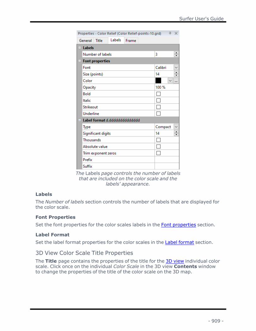
Surfer User's Guide
The Labels page controls the number of labelsthat are included on the color scale and the
labels' appearance.
LabelsThe Number of labels section controls the number of labels that are displayed forthe color scale.
Font PropertiesSet the font properties for the color scales labels in the Font properties section.
Label FormatSet the label format properties for the color scales in the Label format section.
3D View Color Scale Title PropertiesThe Title page contains the properties of the title for the 3D view individual colorscale. Click once on the individual Color Scale in the 3D view Contents windowto change the properties of the title of the color scale on the 3D map.
- 909 -

Chapter 24 - 3D View
Edit the properties of the color scale title on theTitle page of the Properties window.
Title TextThe Title Text section adds a title for the color scale. Click in the box next to TitleText and type the title exactly as you want the text to appear above the colorscale.
Font PropertiesSet the font properties for the color scale labels in the Font properties section.
3D View Color Scale Frame PropertiesThe Frames page for the 3D view color scale specifies the properties to use forthe border and the foreground area around the color scale.
- 910 -

Surfer User's Guide
Edit the properties of the color scale frame onthe Frame page of the Properties window.
FrameThe Frame section specifies the Type and Margin for the border around the colorscale.
TypeThe Type list specifies the type of border to use for the color scale. You can selectNone, Rectangle, or Rounded Rectangle for the frame type. Setting this value toNone shows no border around the box. Fill properties cannot be applied to thelegend frame when the Type is set to None. Setting the Type to Rectangle cre-ates a rectangle at the edge of the color scale at the Margin distance. SettingType to Rounded Rectangle creates a rounded rectangle at the edge of the colorscale at the Margin distance.
MarginMargin specifies the distance between the edge of the frame and the text or sym-bols within the legend. To set the Margin distance, highlight the existing valueand type in the new value. Press ENTER on the keyboard or click anywhere elsein the Properties window to make the change. Alternatively, click the buttons toincrease or decrease the margin.
Line PropertiesClick the next to Line Properties to open the Line Properties section. Set theStyle , Color, Opacity, andWidth of the line to use for the color scale frame.
- 911 -
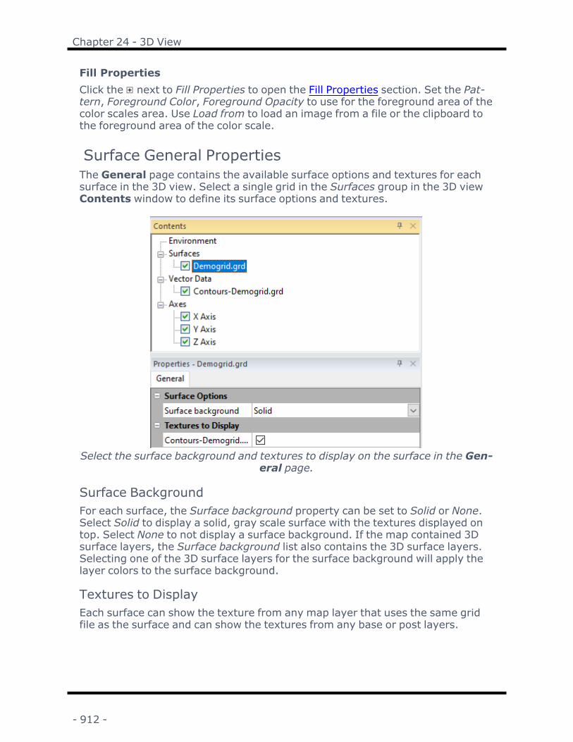
Chapter 24 - 3D View
Fill PropertiesClick the next to Fill Properties to open the Fill Properties section. Set the Pat-tern, Foreground Color, Foreground Opacity to use for the foreground area of thecolor scales area. Use Load from to load an image from a file or the clipboard tothe foreground area of the color scale.
Surface General PropertiesThe General page contains the available surface options and textures for eachsurface in the 3D view. Select a single grid in the Surfaces group in the 3D viewContents window to define its surface options and textures.
Select the surface background and textures to display on the surface in the Gen-eral page.
Surface BackgroundFor each surface, the Surface background property can be set to Solid or None.Select Solid to display a solid, gray scale surface with the textures displayed ontop. Select None to not display a surface background. If the map contained 3Dsurface layers, the Surface background list also contains the 3D surface layers.Selecting one of the 3D surface layers for the surface background will apply thelayer colors to the surface background.
Textures to DisplayEach surface can show the texture from any map layer that uses the same gridfile as the surface and can show the textures from any base or post layers.
- 912 -

Surfer User's Guide
The textures from the layers in the map are overlaid on the surface are listed inthe Textures to display section of the General page. Select the check box nextto the textures you wish to display on the surface. Clear the check box next tothe texture name to remove the texture from the surface.
The associated layer must be visible in the 2D plot window for the texture to beincluded in the Textures to display list.
Point Cloud General PropertyThe General page contains the properties for the point cloud in the 3D view win-dow. Select a point cloud in the Vector Data group in the 3D view Contents win-dow to modify the point cloud properties. The number of points in the point cloudis limited by the 3D View maximum number of points in the Options dialog Ren-dering page.
Set the point cloud point size in the Generalproperties page.
Point SizeThe Point size property sets the size of the point cloud points. Click and drag theslider to the left to decrease the Point size value, or drag the slider
to the right to increase the Point size value. The Point size property setsthe points to a constant-pixel diameter. However, the number of pixels for thePoint size values depends on your PC video card.
Vector Data General PropertiesThe General page contains the properties for the point vector data. 3D point vec-tor data is displayed for post and classed post layers and for base (vector) layersthat include point features. Select a Post, Classed Post, or Base layer in theVector Data group in the 3D view window to edit the point vector data properties.
- 913 -

Chapter 24 - 3D View
Select the appearance of the 3D rendering.
GeneralThe General section includes the properties for defining points and symbols.
Point DensityThe Point density property specifies the number of displayed points. Select avalue from the Density list to plot between 1% and 100% of points: 100% (allpoints), 50% (every other point), 33% (every 3rd point), 25% (every 4th point),20% (every 5th point), 10% (every 10th point), 5% (every 20th point), or 1%(every 100th point).
RenderingThe Rendering section includes properties that specify the style of the symbols.
Symbol MethodThe Symbol method property defines the style of the point vector data symbols.Select Symbols in the Symbol method list to display the points as circles,squares, spheres, or cubes. Select Same as plot to display the points with thesame symbol style as found the in map in the plot window.
- 914 -

Surfer User's Guide
SymbolThe Symbol property specifies the symbol style when the Symbol method prop-erty is set to Symbols. Select Circle, Square, Cube, Shaded circle, or Spherefrom the list. The Circle, Square, and Shaded circle are two dimensional symbols,and the Cube and Sphere are three dimensional. If you have a large quantity ofpoints, a Shaded circlemight be a better option than the Sphere if you need toreduce rendering time and cannot reduce the point density.
Sphere DetailIf Sphere is the selected Symbol, use Sphere detail to set the level of smooth-ness of the rendered spheres. Possible values range from 1 to 10, with a defaultof 6. When Lighting is set to Smooth, higher Sphere detail values rendersmoothly rounded spheres. When Lighting is set to Flat, higher values rendersmaller facets than lower values. Lower Sphere detail values render more quicklythan higher values. Other ways to reduce rendering time is to select a lower Fre-quency value or choose a 2D symbol, such as a Square, Circle, or Shaded circle.
Symbol SizeThe Symbol Size section includes properties for setting the symbol size based onthe plot, to a fixed value, or by proportional scaling.
Sizing MethodThe Sizing method specifies the point vector data symbol size. Select the desiredSizing method from the list:
l Same as plot uses the same size symbols as the symbols in the map in theplot window.
l Fixed size uses the same size symbols throughout the 3D view. The Size prop-erty is available when the Sizing method is set to Fixed.
l Proportional uses different sized symbols for the point vector data based on adata value. The Size column, Minimum size, and Maximum size properties areavailable when the Sizing method is set to Proportional. The Proportionaloption uses linear scaling between the data minimum and maximum. Formore scaling options, use the proportional scaling options in 2D map layersand set the Sizing method to Same as plot.
SizeThe Size property is available when the Sizing method is set to Fixed. The Sizeproperty sets the size of the fixed symbols. Click and drag the slider tothe left to decrease the Size value, or drag the slider to the right toincrease the Size value.
Size ColumnSelect the data column or attribute for scaling the symbol sizes in the Sizecolumn. The Size column list includes data columns for post and classed post lay-ers. The Size column list includes attributes from the base layer with numeric or
- 915 -

Chapter 24 - 3D View
mixed data. Attributes that include only text data are not included in the Sizecolumn list.
If a mixed data column is selected, point vector data with text data will not be dis-played.
Minimum SizeSpecify the size of the symbol that corresponds to the smallest data value in theMinimum size property. Set the Minimum size to a value between 0.00 and 1.00.
Maximum SizeSpecify the size of the symbol that corresponds to the largest data value in theMaximum size property. Set the Maximum size to a value between 0.00 and1.00.
Symbol ColorThe Symbol Color section includes properties for coloring the symbols based onthe plot, to a specific fixed color, or by a colormap.
Color MethodThe Color method property specifies the symbol color for the point vector data:
l Same as plot uses the same symbol color(s) as the symbols in the map in theplot window.
l Fixed uses the same symbol fill color throughout. The Color property is avail-able when the Color method is set to Fixed.
l By colormap assigns colors to the symbols based on a data value andcolormap. The Color column and Colormap properties are available when theColor method is set to By colormap. If the post, classed post, or base (vector)layer already assigns colors by a colormap, you may wish to set the Colormethod to Same as plot.
ColorThe Color property specifies the symbol color when the Color method is set toFixed. Select a fill color for the scatter plot by clicking the current Color andselecting the desired color in the color palette. Click the button to define a cus-tom color in the Colors dialog.
Color ColumnSelect the data column or attribute for the colormap in the Color column field.The Color column list includes data columns for post and classed post layers. TheColor column list includes attributes from the base layer with numeric or mixeddata. Attributes that include only text data are not included in the Color columnlist.
- 916 -

Surfer User's Guide
ColormapThe Colormap is the color spectrum that is mapped to the Color column data val-ues. Select a predefined colormap from the Colormap list, or click the tomodify or create a colormap in the Colormap Editor.
NoDataThe NoData section includes properties for specifying the size or color of pointswhere the Size column and/or Color column do not include data. Specify theNoData symbol size in the Size field. Specify the NoData symbol color in theColor field.
Z Coordinate Page - 3D View Base(vector) LayerThe Z coordinate page in the Properties window contains the attributes for theZ values for 3D polylines and 3D polygons. Select the Z coordinates for the base(vector) layer in the Z coordinates field. The Z coordinates list includes datacolumns for base(vector) layers. The Z coordinates list includes attributes fromthe base layer with numeric data. Attributes that include only text data are notincluded in the Z coordinates list.
Select [None] to remove all 3D polyline and 3D polygon objects from the 3DView Window that have do not have any Z values.
Select the Z coordinates for the base(vec-tor) layer on the Z coordinate page in the
Properties window.
3D View Axis Ticks PropertiesThe Ticks page for the 3D view axis objects includes options for axis tick andgrid line spacing and appearance. The Ticks page properties can be reset todefault values on the Scaling page.
- 917 -

Chapter 24 - 3D View
Set the tick and grid line properties in the Tickspage.
TicksSet the tick size and spacing options in the Ticks section.
Tick Min and Tick MaxSpecify the range over which tick mark and grid lines are displayed in the Tickmin and Tick max property fields. Set the Tick min and Tick max values to thedesired value in map units.
Perpendicular grid lines are drawn to the Tick max for an axis. For example, theTick max property for an X axis controls which grid lines are drawn for the X axisand the grid line length for the Y axis and Z axis grid lines.
Major Interval and Minor Ticks Per MajorSpecify the tick spacing in the Major interval field. Major ticks and major gridlines are drawn at the Tick min and then at every Major interval between the Tickmin and Tick max. Minor tick marks and minor grid lines are controlled by theMinor ticks per major property. Specify the number of minor ticks and minor gridlines between the major ticks in the Minor ticks per major field. For example,with a Major interval of 50 units, a Minor ticks per major value of 4 places minortick marks at 10, 20, 30, and 40 unit increments between the major ticks.
Tick LengthThe Tick length property sets the length of the major tick marks. Set the Ticklength to a value between 0 and 1. Set the Tick length to 0 to hide the tickmarks. The minor tick mark length automatically adjusts to half the major tickmark length
- 918 -

Surfer User's Guide
Tick WidthThe Tick width property sets the width of the tick marks. Set the Tick width to avalue between 0 and 1. Both major and minor tick marks are controlled by theTick width property.
Grid LinesThe Grid lines section includes the appearance properties for the grid lines.
Show Major Grid Lines and Show Minor Grid LinesSelect the Show major grid lines property to display grid lines at the major tickmarks. Select the Show minor grid lines property to display grid lines at theminor tick marks. Clear the check boxes to remove the grid lines.
ColorSelect the axis color in the Color field. Select a color from the color palette orclick to set a custom color in the Colors dialog.
WidthThe Width property sets the grid line width. Set the Width property to a valuebetween 0 and 1.
3D View Axis Labels PropertiesThe Labels page for the 3D view axis objects includes options for axis labelappearance and position.
Set the label properties in the General page.
ShowSelect Show to display labels at the end of the major tick marks.
Label AngleThe Label angle property sets the rotation of the labels in the axis plane. Set theLabel angle to a value between 0 and 360 degrees.
- 919 -

Chapter 24 - 3D View
Label OffsetThe Label offset property sets the distance between the labels and the major tickmarks. Set the Label offset to a value between -1 and 1. Positive values movethe labels away from the map region. Negative values move the labels into themap region. A value of 0 places the labels at the end of the major tick marks.
Font PropertiesSet the font properties for the axis labels in the Font properties section. Note thelabel font Size property is in relative units rather than points (pt). The label incre-ment is automatically updated as the label font size changes to ensure labels donot overlap, i.e. fewer labels are drawn as the label font size is increased.
Label FormatSet the label format properties for the axis labels in the Label format section.
3D View Axis Scaling PropertiesThe Scaling page for the 3D view axis objects includes the axis limits and pos-ition properties.
Set the axis limits and position properties in theScaling page.
ScalingThe Scaling section includes axis limits properties and an option to reset the scal-ing to default values.
AutomaticSelect Automatic to set the axis limits, axis position, and the Ticks properties totheir default values. The Automatic property is automatically cleared after chan-ging any of the related properties.
- 920 -

Surfer User's Guide
Axis Minimum and Axis MaximumThe Axis minimum and Axis maximum properties control the axis length. Set theAxis minimum and Axis maximum to the desired value in map units.
Axis PositionThe Axis Position section includes two of the Cross X axis at:, Cross Y axis at:,and Cross Z axis at: properties for specifying the axis position. Which propertiesare displayed depends on which axis is selected. Specify a value in map units tomove the selected axis in the plane with the other axis. For example when an Xaxis is selected, the Cross Y axis at: property moves the X axis in the XY planeand the Cross Z axis at: property moves the axis in the XZ plane.
3D Drillhole PropertiesAfter a Drillhole Map is created, view the drillholes, wells, or boreholes in the 3Dview by right clicking the drillhole layer and clicking 3D View, by selecting themap and clickingMap Tools | View | 3D View, or by clicking the 3D View but-ton in the Map frame View Page page properties.
To define 3D drillhole properties, click the drillhole layer in the Contents windowin the 3D view. The 3D drillhole Properties window appears.
This help topic has the following main sections that describe the 3D drillhole prop-erties.Points PageIntervals PagePath PageLabel PageDrillhole Color Scales
Points PageIf points data were imported in the 2D map, these data can be displayed as pointsymbols in the 3D model. In the example below, the sample data has values inthe TiO2 column in the points data (see C:\Program Files\Golden Soft-ware\Surfer\Samples\SampleDrillholeData.xlsx).
- 921 -

Chapter 24 - 3D View
Show PointsTo display points, click the Show points check box in the Points page in theProperties window.
Example 3D Drillhole Points properties usingthe TiO2 field in the sample points data
FieldSelect the field to display as the point value from the Field list. Only fields impor-ted from the points data in the Drillhole Manager can be selected.
FrequencySet the Frequency of point symbols to display. For example, 50% displays half ofthe points.
SymbolSelect the symbol to use for the points from the Symbol list: Circle, Square,Cube, Shaded circle, or Sphere. The Circle, Square, and Shaded circle are twodimensional symbols, and the Cube and Sphere are three dimensional. If youhave a large quantity of points, a Shaded circlemight be a better option than theSphere if you need to reduce rendering time and cannot reduce the point dens-ity.
Sizing MethodSelect either Fixed or By data for a Sizing method.
l Fixed creates point symbols that are the same specified size. After selectingFixed, use the Size property to define the point size.
l By data sizes point symbols using data in the Field property. After selectingBy data, use the Minimum Size and Maximum Size properties to set the sizerange.
Color MethodSelect either Fixed or By data for the Color method.
- 922 -

Surfer User's Guide
l Fixedmakes all symbols the same specified color. After selecting Fixed,select a color for the point symbols by clicking the current color and selectingthe desired color in the color palette, or by clicking the button to define acustom color in the Colors dialog. See the Colors Dialog help topic for moreinformation.
l By data uses the data in the Field property to apply a color scale to the pointdata. After selecting By data, select a color scale for the symbols by clickingthe current color scale and selecting a new one, or by clicking the button tomodify or create a colormap in the Colormap Editor.
Intervals PageIf interval data were imported in the Drillhole Manager in the 2D map, thesedata can be displayed in colored intervals in the 3D model. In the examplebelow, the sample data has values in the TiO2 column in the interval data (seeC:\Program Files\Golden Software\Surfer\Samples\SampleDrillholeData.xlsx).
Show IntervalsCheck the Show intervals check box to display the intervals.
Example 3D Drillhole Intervals propertiesusing the TiO2 field in the sample intervals
data
FieldSelect the field to display as the interval value from the Field list. Only fieldsimported from the interval data in the Drillhole Manager can be selected.
Sizing MethodSelect either Fixed or By data for a Sizing method for the width of the tube. Thesize (radius of the path cylinder) is 0-100, where the units are proportional to themap’s x-axis range.
l Fixedmakes all intervals the same specified size. After selecting Fixed, definea size in the Size control.
- 923 -

Chapter 24 - 3D View
l By data uses the data in the Field property. After selecting By data, use theMinimum Size and Maximum Size properties to set the size range.
Color MethodSelect either Fixed or By data for the Color method.
l Fixedmakes all symbols the same specified color. After selecting Fixed,select a color for the symbols by clicking the current color and selecting thedesired color in the color palette, or by clicking the button to define a cus-tom color in the Colors dialog. See the Colors Dialog help topic for moreinformation.
l By data uses the data in the Field property to apply a color scale to the inter-val data. After selecting By data, select a color scale for the symbols by click-ing the current color scale and selecting a new one, or by clicking thebutton to modify or create a colormap in the Colormap Editor.
Path PageThese properties define the path of the drillhole using the depth, azimuth, andinclination values specified in the collars and survey tables.
Show PathsCheck the Show paths check box to display the path of the drillholes. Drillholepaths can still be displayed, even if point and interval data are not imported.
Example 3D Drillhole Path properties showingpaths
ColorSelect the Color of the path. Click the current color and select the desired color inthe color palette or click the button to define a custom color in the Colors dia-log. See the Colors Dialog help topic for more information.
- 924 -

Surfer User's Guide
SizeSet the Size of the path. The path is the radius of the path cylinder in a 0-100scaling, where the units are proportional to the map’s x-axis range.
Label PageThe Label page for the 3D view drillhole layer includes options for drillhole labelappearance and position.
Show LabelsCheck the Show labels check box to display labels using a field from the importedcollars table.
Example 3D Drillhole Label properties showinglabels
FieldSelect the field to display as the label from the Field list. Only fields importedfrom the collars data in the Drillhole Manager can be selected.
PositionIn the Position list select a Default, Left, Center, or Right position of the label rel-ative to the drillhole. Use the X offset, Y offset, and Z offset boxes to enter a spe-cific, user-defined position.
FontUse the Font properties to define the font of the label. See the Text and FontProperties help topic for more information.
- 925 -

Chapter 24 - 3D View
Label FormatUse the Label format properties to define the format of the labels in the map.See the Label Properties help topic for more information.
Leader LinesWhen a value is entered for the X, Y, or Z offset, check the Leader lines checkbox to display leader lines that connect the label to the top of the drillhole. If theLeader lines check box is checked, properties appear to define theWidth andColor of the leader lines.
Drillhole Color ScalesClick the Color Scales object in the Contents window to display the Prop-erties for the color scales. Color scales are available for drillhole points and inter-vals when the drillhole layer uses By data for the point or interval Color method.When checked, the selected color scale will be displayed. When unchecked, thecolor scale will not be displayed. See the 3D View Color Scales Group help topicfor more information.
3D View CommandsThe following sections describe the commands in the 3D view window.
Walk
Click the 3D View | View | Walk command or the button to enter walkmode. TheWalk camera position and orientation is saved when you walk modeand restored when you reenter walk mode. While in walk mode, the keyboardand mouse are used to walk along the surface in the 3D view window. The 3Dview window must contain at least one surface to enter walk mode.
Walk Mouse ControlsClick and drag in the 3D view window to move and rotate the view.
l Drag the mouse up to move forward, or towards where the view is pointed.l Drag the mouse down to move backward, or away from where the view ispointed.
l Drag the mouse right to rotate to the right, or clockwise.l Drag the mouse left to rotate to the left, or counterclockwise.l Roll the mouse wheel forward to increase the elevation of the camera.l Click and drag down with the mouse wheel or middle-mouse button toincrease the elevation of the camera.
l Roll the mouse wheel backward to decrease the elevation of the camera.l Click and drag up with the mouse wheel or middle-mouse button to decreasethe elevation of the camera.
- 926 -

Surfer User's Guide
Walk Keyboard ControlsPress the ARROW or WASD keys to move and rotate the view. Use SHIFT andCTRL to change the camera elevation.
l Press UP ARROW or W to move forward, or towards where the view is poin-ted.
l Press DOWN ARROW or S to move backward, or away from where the view ispointed.
l Press RIGHT ARROW or D to rotate to the right, or clockwise.l Press LEFT ARROW or A to rotate to the left, or counterclockwise.l Press SHIFT to increase the camera elevation.l Press CTRL to decrease the camera elevation.
Walk with Multiple SurfacesThe 3D View | View | Walk command may be used with a 3D view thatincludes more than one surface. When the surfaces are contiguous, you maywalk from one surface to another while in walk mode.
It is not recommended to use theWalk command in a 3D view with two or moresurfaces that occupy the same XY extents but have significantly different Z val-ues. When this is the case, the camera elevation follows the highest surface(largest Z values).
Go to Home
Click the 3D View | Home | Go to Home command or the button to resetthe camera position, rotation, and zoom to the last saved home position.
The home position is set with the 3D View | Home | Set Home command. Aftersetting the view to the desired rotation, zoom, and position, click the 3D View |Home | Set Home command to save this position.
The home position is only saved while the plot window is open. The 3D view canbe opened and closed, and the home position will be remembered. However, thehome position is forgotten when the plot window is closed.
Set Home
Click the 3D View | Home | Set Home command or the button to storethe current camera rotation, zoom, and position to the home position. The newhome position is stored for each 3D view individually. The home position is onlysaved while the plot window is open. The 3D view can be opened and closed, andthe home position will be remembered. However, the home position is forgottenwhen the plot window is closed. The next time the plot is opened in the plot win-dow and 3D view window, the Surfer default view position is used.
- 927 -

Chapter 24 - 3D View
To set the home position,
1. Use the Pan, Trackball, and zoom commands, or the Camera properties, toset the view to the desired rotation, zoom, and position.
2. Click the 3D View | Home | Set Home command to save this position.
Only one home position may be saved at any time. Click the Set Home com-mand to overwrite the previous home position.
The home position is not set by default. The Set Home command must be usedbefore the Go to Home command can be used to change the camera position.
Create/Edit Fly-Through
Click the 3D View | Fly-Through | Create/Edit command or the buttonto create or edit a fly-through. A fly-through moves the camera along a path spe-cified by the vertices of a vector object. The Flight Path Editor is displayedwhen the 3D View | Fly-Through | Create/Edit command is clicked.
Fly-throughs can be played from the 3D view or recorded and saved as an AVIfile once a fly-through has been created.
A flight path is defined by key frames. A key frame is a rendering of the 3D viewat a specific time with a specific camera position and aim. The camera positionand aim are interpolated between the key frames to generate the remainingframes for the fly-through animation. The key frame positions are listed in theKey Frame list in the Flight Path Editor.
Flight Path EditorThe Flight Path Editor defines the path, camera aim, duration, and quality forthe flight path.
- 928 -

Surfer User's Guide
Create or edit the flight path in the Flight Path Editor.Input Vector PathDefine the vector feature for the flight path in the Input Vector Path section.Select a vector feature from a layer in the map from the Input Vector Path list.The features are listed by layer name and feature name, separated by a colon.For example, in the image above FlightPath is the base (vector) layer name andPolyline is the feature name. The Key Frame list is updated after a vector featureis selected.
Click Browse to load a vector flight path from a file. If the file includes more thanone feature, only the first feature will be used to define the Input Vector Path.
Key Frame ListThe Key Frame list displays the Index, Time, camera position, and camera aimfor the key frames in the flight path.
- 929 -

Chapter 24 - 3D View
l The Index value shows the order of the key frames.l The key frame Time is determined by the Duration and the distance betweenkey frames.
l The key frame camera X and Y positions are specified by the Input VectorPath feature's vertices.
l The camera's Z position is defined by the properties in the Position group.l The key frame camera Heading and Pitch are defined by the properties in theCamera Aim group.
PositionThe Position group controls the Z position of the camera for the key frames. TheElevation Source determines whether the Z position is relative to the surface oran absolute elevation.
Select Relative to Surface to specify an elevation for the key frame Z positionsabove or below the surface in the Elevation field. Negative values position thecamera below the surface, and positive values position the camera above the sur-face. The Key Frame list is updated when a value is typed in the Elevation field.
Select Absolute Height to set a single Z position for all key frames in the Elev-ation field. Type the Z position for the key frames in the Elevation field.
Camera AimThe Camera Aim group controls the camera aim for the key frames. Three Cam-era Aim options are available: Along Path, Constant Direction, Constant Point.The Camera Aim options control the Heading and Pitch for the key frames.
Heading is the direction the camera is pointing, and it is greater than or equal to0 and less than 360 degrees. A heading of 0 degrees is pointing parallel to theincreasing y-axis direction, i.e. North. Heading increases as the direction rotatesclockwise. A heading of 90 degrees is parallel to the increasing x-axis direction,i.e. East.
Pitch is the rotation of the camera about its lateral axis. In other words, it is ameasure of how much the camera is pointing up or down. The Pitch value mustbe greater than -90 degrees and less than 90 degrees. A Pitch of 0 degrees islooking directly ahead. A positive pitch value has the camera pointed up, and anegative pitch value has the camera pointed down.
Along PathSelect Along Path to orient the camera along the flight path at each key frame.
Constant DirectionSelect Constant Direction (degrees) to set a single Heading and Pitch for all keyframes.
- 930 -

Surfer User's Guide
Constant PointSelect Constant Point to specify a target X, Y, and Z position for the camera aim.The key frame Heading and Pitch values will be updated where the camera isaimed at the target position at each key frame. Type the desired target coordin-ates in the X, Y, and Z fields.
AnimationThe Animation group controls the fly-through Duration, Frames per second, andQuality.
DurationThe Duration (seconds) option defines the length of the fly-through in seconds.The camera moves at a constant velocity along the flight path. The Duration(seconds) value and flight path distance defines the time between each keyframe. The flight Duration (seconds) value must be greater than or equal to 1.
Frames per SecondThe Frames per second option specifies the number of frames generated persecond in the fly-through. A large Frames per second value generates asmoother fly-through, but it also requires more processing time and generates alarger AVI file. With small Frames per second values, the fly-through will appearchoppy, but it will also process faster and generate a smaller file. The Frames persecond value must be greater than or equal to 2.
Preview and Save ChangesClick Preview to view a preview of the fly-through with the current Flight PathEditor settings. Once the preview is complete, the Flight Path Editor is dis-played again. Click OK to save the changes to the fly-through. Click Cancel toclose the Flight Path Editor without saving any changes.
The Play and Record commands are enabled after the fly-through is created.
Play Fly-Through
Click 3D View | Fly-Through | Play or the button to play the current fly-through. A fly-through must be created by clicking the 3D View | Fly-Through |Create/Edit command before the Play command is available.
Once a fly-through has been created, click 3D View | Fly-Through | Play toview the fly-through, click 3D View | Fly-Through | Record to record the fly-through, or click 3D View | Fly-Through | Create/Edit to modify the fly-through.
- 931 -

Chapter 24 - 3D View
Record Fly-Through
Click 3D View | Fly-Through | Record or the button to play and recordthe current fly-through. A fly-through must be created by clicking the 3D View |Fly-Through | Create/Edit command before the Record command is available.
Once a fly-through has been created, click 3D View | Fly-Through | Recordto view the fly-through. Specify a file name and path in the Save As dialog andclick Save to record the fly-through. The Record command creates an AVI videofile of the fly-through.
Click 3D View | Fly-Through | Play to play the fly-through or click 3D View |Fly-Through | Create/Edit to modify the fly-through.
Copy to Clipboard
Click the 3D View | Tools | Copy to Clipboard command or the buttonto copy an image of the current view in the 3D view window to the clipboard. Thesize of the copied image is the same as it appears in the current 3D view window.Paste the image in a Surfer plot window with the Paste command. The imagecan also be pasted in another application with that application's Paste commandor usually by pressing CTRL+V.
Changing the Image SizeControl the size of the copied image by changing the size of the Surfer applic-ation window or the 3D view window.
The following steps describe one method to reduce the size of the image:
1. Click the View | Windows | Cascade command.2. Resize the 3D view window to the desired size.3. Click the 3D View | Tools | Copy to Clipboard command.4. Paste the image in the desired Surfer plot window or other application.5. Maximize the 3D view window to return Surfer to the tabbed document view.
The following steps describe one method to maximize the size of the image:
1. Maximize the Surfer application window.2. Hide the Contents and Properties windows.3. Minimize the ribbon.4. Click the 3D View | Tools | Copy to Clipboard command.5. Paste the image in the desired Surfer plot window or other application.6. Return Surfer to the desired layout by showing the Contents and Prop-erties windows, changing the application window size, and restoring the rib-bon. You can also clear all application customizations if desired by clicking theView | Windows | Reset Windows command.
- 932 -

Surfer User's Guide
3D View Export Image
Click the 3D View | Tools | Export Image command or the button toexport the current view in the 3D view window to an image. The Export Imagedialog is displayed. Only image file formats are available in the Export Imagedialog Save as type list:
l BMP Windows Bitmapl EPS Encapsulated Postscriptl GIF Imagel JPG JPEG Compressed Bitmapl JPEG-2000 Bitmapl PNG Portable Network Graphicsl PNM Imagel RGB SGI-RGB Imagel SUN Sun Raster Imagel TGA Targa Truevisionl TIF Tagged Imagel X AVS X-Image
The default size of the image is set to the current size of the 3D view window, butthe exported image size can be changed in the Export Options dialog Size andColor page. The PNG and TIF export file formats support background trans-parency, i.e. the image will be exported without a background or skybox. Asalways, this option requires a 32-bit RGBA color depth and must be selected inthe Export Options dialog.
3D View Export 3D
Click the 3D View | Tools | Export 3D command or the button to exportthe current view in the 3D view window to a 3D image. The Export 3D dialog isdisplayed. 3D PDF and WRL VRML 3D Vector Model file formats are available inthe Export 3D dialog Save as type list. Specify export options in the Vector PDFOptions or VRML Export pages of the Export Options dialog. The grid surfacequality may be specified in the Quality page of the Export Options dialog. Thegrid surface quality directly affects the image quality and file size of the export.
- 933 -


Chapter 25 - Map Tools
Map Tools Tab CommandsTheMap Tools tab in the plot document has the following commands:
Layer Adds a Base, Base from Server, Basefrom Data, Empty Base, Contour, Post,Classed Post, 3D Surface, 3DWireframe, Color Relief, Grid Values,Watershed, Viewshed, 1-Grid Vector, or2-Grid Vector layer to the selected map
Scale Adds a scale bar to the selected mapLegend Adds a legend to the plotGraticule Adds a graticule or grid lines to the selec-
ted mapProfile Adds a profile to the selected mapAxis Adds a top or bottom (X), left or right
(Y), or Z axis to the selected mapTrackball Rotates and zooms the selected map in
3D3D View View the selected map in a new 3D view
windowSet Limits Set the map limits by drawing a rect-
angleMeasure Measure distance and area on the selec-
ted mapOverlay Maps Combine selected maps to use the same
map propertiesStack Maps Aligns two or more selected mapsConvert Layer Changes one grid-based layer type to
anotherDigitize Displays the coordinates of the selected
map in map units and collects datapoints from the map
Break Apart Removes a map layer from the selectedmulti-layer map
Georeference Image Georeference or warp an image in abase layer
Open Attribute Table Opens the Attribute Table for the objectsin the selected layer
Open Drillhole Manager Open the Drillhole Manager to man-age or view drillhole data
- 935 -

Chapter 25 - Map Tools
Track Cursor Track cursor location across plot, work-sheet, and grid editor windows for amaps, data files, and grids
Query Objects Selects objects returned from a spe-cified query
Join Attributes Import a data file to add attributes tothe existing attribute table
Export Contours Export contours as lines in a DXF, SHP,or TXT file
Grid Opens the selected layer's grid in theGrid Editor
Data Opens the data for a selected layer in aworksheet window
Contour Labels Edits individual contour labels of theselected map
Layer Labels Edits individual post map labels of theselected map
Set Limits
Click theMap Tools | Map Tools | Set Limits command or the button tointeractively set the map limits. When Set Limits is enabled, the map limits canbe adjusted by clicking and dragging the sides or corners of the map limits rect-angle or by drawing a new rectangle. A map, layer, or object within the map orlayer must be selected before clicking the Set Limits command.
The plot window appearance changes when the Set Limits command is clicked.The areas outside the map limits are shaded. Regions of the plot window withinthe map limits are displayed normally. The map limits are represented by a bluerectangle with yellow selection handles. Additionally, theMap Tools | MapTools | Set Limits command button is highlighted when Set Limits is active.
Set Limits TipsThe following keyboard and mouse actions control the Set Limits commandmode.
l Click and drag the yellow selection handles to move the map limits.l Press and hold CTRL, then click and drag to draw a rectangle to specify the
map limits. The cursor will change to a crosshair to indicate draw mode.l Double-click in the plot window or press ENTER to update the map with newmap limits and exit Set Limitsmode. Alternatively, right-click in the plot win-dow and click Save to update the map and exit Set Limitsmode.
- 936 -

Surfer User's Guide
l Press ESC to exit Set Limitsmode without making any changes to the map.Alternatively, right-click in the plot window and click Cancel to exit Set Lim-itsmode without making changes.
l Use the mouse wheel or scroll bars to zoom and pan the plot window.l The Undo command will undo changes to the map limits after you pressENTER or double-click the plot window. However, using the Undo commandwhile Set Limits is activated will undo actions made prior to activating SetLimitsmode. If you wish to make changes to the map limits while still in SetLimitsmode, click and drag the selection handles or press CTRL and draw anew rectangle.
l The Set Limits command cannot be used with 3D surfaces or wireframes.l The Set Limits command cannot be used with rotated, tilted, or shearedmaps. Most maps have no rotation, tilt, or shear by default. If the Set Limitscommand is unavailable, set the Rotation to 0 and the Tilt to 90 on the Mapframe View page and set the Shear to 0 with the Home | Selection | Trans-form command
ExampleIn the following example, the map limits will be set by clicking and dragging theselection handles and by drawing a rectangle. The example map includes a colorrelief layer, a base (raster) layer, and a base (vector) layer. The vector baselayer extents are significantly larger than the extents for the other layers. We willset the map limits to a region within the image base layer extents.
The map limits cover the entire dataextents.
- 937 -

Chapter 25 - Map Tools
1. Click the map in the plot window to select it.2. Click theMap Tools | Map Tools | Set Limits command. The Set Limits
mode is activated.
The map limits are represented by the blue rect-angle.
3. Press and hold the CTRL key.4. Click and drag in the plot window to draw the new map limits.
The new rectangle was drawn around the image base layer.
- 938 -
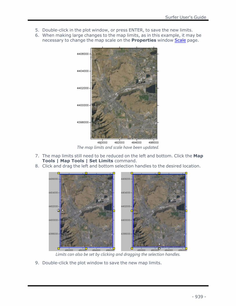
Surfer User's Guide
5. Double-click in the plot window, or press ENTER, to save the new limits.6. When making large changes to the map limits, as in this example, it may be
necessary to change the map scale on the Properties window Scale page.
The map limits and scale have been updated.
7. The map limits still need to be reduced on the left and bottom. Click theMapTools | Map Tools | Set Limits command.
8. Click and drag the left and bottom selection handles to the desired location.
Limits can also be set by clicking and dragging the selection handles.
9. Double-click the plot window to save the new map limits.
- 939 -

Chapter 25 - Map Tools
The map limits are now in the desired loc-ation.
Now the map limits have been updated.
TrackballTheMap Tools | View | Trackball command rotates, tilts, and changes thefield of view in the plot window. The 3D View | View | Trackball commandalso rotates and tilts the view in the 3D view.
Trackball in the Plot Window
Click theMap Tools | View | Trackball command or the button or right-click on the map and click Trackball to rotate, tilt, and change the field of viewof a selected map in the plot window. The cursor will change to a , indicatingyou are in trackball mode. TheMap Tools | View | Trackball command is sim-ilar to using the properties in the map View tab in the Properties window.
Tilt and RotationIn trackball mode, left-click in the map's bounding box. While holding down theleft mouse button, drag the mouse up and down to change tilt, and drag themouse left or right to change rotation. The rotation and tilt values are shown inthe status bar when the left mouse button is held down.
Field of ViewIn trackball mode, when you right-click in the map's bounding box, dragging upincreases the field of view and changes the Projection to Perspective. Draggingdown while right-clicking decreases the field of view, and the Projection changes
- 940 -

Surfer User's Guide
to Orthographic if the field of view is decreased to 1°. The field of view value isshown in the status bar when the right mouse button is held down.
Exit Trackball ModePress the ESC key on your keyboard to exit trackball mode. Alternatively, clicktheMap Tools | View | Trackball command again or select another commandmode, such as select, draw, or reshape.
To modify the map orientation with Trackball:
1. Select one map.2. Click theMap Tools | View | Trackball command, or right-click on the
map and click Trackball.3. Left-click in map's bounding box. While holding down the left mouse button,
drag the mouse up and down to change tilt, and drag the mouse left or rightto change rotation. The rotation and tilt values are shown in status bar.
4. Right-click in the map's bounding box. While holding down the right mousebutton, drag the mouse up to increase the field of view and changes the Pro-jection to Perspective. Drag the mouse down while right-clicking to decreasethe field of view, and change the Projection to Orthographic if the field of viewis decreased to 1°. The field of view value is shown in status bar.
5. Press the ESC key on the keyboard to end trackball mode.
Trackball in the 3D ViewClick the 3D View | View | Trackball command to rotate and tilt the field ofview of the 3D view window. The cursor will change to a , indicating you are intrackball mode. The 3D view can also be changed by adjusting the values in theEnvironment properties Camera page.
Trackball mode is the default mode for the 3D view window. Press ESC while inanother tool mode to return to the trackball mode. While in trackball mode in the3D view, pan the view by clicking and dragging with the middle mouse button.
Tilt and RotationIn trackball mode, left-click in the 3D view window. While holding down the leftmouse button, drag the mouse to change the tilt and rotation. How the view istilted and rotated is determined by the location you first click and the directionyou drag. For example, clicking near the left side of the 3D view window anddragging the mouse up tilts the left side of the map up and right side down.While clicking near the center of the view and dragging the mouse up tilts thefront of the map up and the back of the map down.
- 941 -

Chapter 25 - Map Tools
Measure
Click theMap Tools | Map Tools | Measure command or the button orright-click and selectMeasure to calculate the distance and area of a high-lighted section of a map. After clicking the command, click on the screen aroundthe edge of the line or area you wish to measure. The Segment length, Totallength, Total perimeter, and Enclosed area are displayed in theMeasure dialogin map units. Double-click or press ENTER on the keyboard to finish the currentmeasurement. The dialog will stay open until you click the button in the topright of the dialog or click on the dialog and press ESC on the keyboard.
Units are in map units. Use the Options command to change the units. Thelength and area are calculated only using the X and Y coordinates (planar lengthand area). The Z values are not used to calculate the length or area of the meas-ured polyline or polygon. When using latitude and longitude, the lengths andareas are calculated using a Cartesian coordinate system, not using a great circleor the curvature of the earth.
The area and length are displayed in theMeasure dialog.
Drawing PointsClick the left mouse button to add points to the measuring object. If the CTRLkey is pressed while clicking points, the points are constrained to 45-degreeangles. Double-click the left mouse button or press ENTER on the keyboard toend adding points to the measuring object. Press ESC to exit measure mode.Points can be added inside or outside of the selected map layer and the mapframe.
Removing PointsRight-click to remove the last drawn point. This can be done repeatedly.
- 942 -

Surfer User's Guide
Panning and ZoomingClick and drag the scroll bars to move the view up or down while in measuremode. Alternatively, hold down the wheel button straight down, and the cursorwill turn to a closed hand. When the cursor is a , drag the mouse to pan theplot window. Be sure to click straight down with the scroll wheel.
You can use a wheel mouse to zoom in and out while in measure mode. Rotatethe wheel forward to zoom in, or rotate the wheel backward to zoom out.
3D Maps, Tilt, and PerspectiveA 2D non-tilted, non-perspective must be selected. If a 3D surface map layer or3D wireframe map layer is included, theMeasure command will be unavailable.Select the 3D surface map layer or 3D wireframe map layer and press DELETE onthe keyboard or click the Break Apart command.
When all 3D maps have been removed, click on the Map in the Contents windowto select it. Click on the View tab in the Properties window. Set the Projection toOrthographic and the Tilt (degrees) to 90.
MeasurementsTheMeasure dialog displays four measurements derived from the drawn poly-gon or polyline:
l The Segment length is the length of the last segment drawn. To indicate anew segment, click the left mouse button. The Segment length starts againat zero and increases in any direction as the mouse is moved.
l The Total length is the length of all of the individual line segments. Each Seg-ment length is a positive value and added together. This is the sum length ofall cyan colored lines.
l The Total perimeter is similar to the Total length, except it includes the lastunfinished segment that would return the digitized area to the original point.In the diagram below, this is the light black line.
l The Enclosed area is the area of the shaded region being displayed. If a poly-gon intersects itself, the area from all sub-polygons will be added together.
- 943 -

Chapter 25 - Map Tools
The cyan lines are included in theTotal length. The Total perimeterincludes all cyan lines and the blackline. The Enclosed area is rep-
resented by the area filled by bluehorizontal lines.
Copying MeasurementsTo copy the information from theMeasure dialog, right-click in the dialog andselect Select All. Right-click again and select Copy . The information can then bepasted into the plot window or another program.
Measure OptionsClick the Optionsmenu in theMeasure dialog to modify how the meas-urements are displayed and to save or export the measurement geometry.
Numeric FormatThe numeric format for the length and area values can be changed by clickingthe Options | Numeric Format command. The Label Format dialog opens. Setthe desired format and click OK and the formats in theMeasure dialog update.
UnitsThe units displayed in theMeasure dialog are in Map units. By default, the Mapunits are controlled by the Coordinate System tab in the Properties window forthe Map object. To change the units, click the Options | Units command in theMeasure dialog. In the Units dialog, select the appropriate Linear Units andArea Units. Click OK to return to theMeasure dialog.
- 944 -

Surfer User's Guide
Select the Linear Units and Area Units forthe measurements.
The Linear Units are used for the Segment length, Total length, and Total peri-meter. The Area Units are used for the Enclosed area.
Note that the units cannot be changed if the map is not referenced or if the Mapcoordinate system is set to display latitude and longitude. Set the layer sourcecoordinate system and the map target coordinate system and the units can bechanged.
The default Linear Units and Area Units can be changed with themtDistUnit andmtAreaUnitDefault Settings. The following table lists the default setting value forthe various options.
LinearUnits
mtDistUnitValue
Area Units mtAreaUnitValue
Millimeters 0 Square millimeters 0Centimeters 1 Square centimeters 1Meters 2 Square meters 2Kilometers 3 Square kilometers 3Inches 4 Square inches 4Feet 5 Square feet 5Survey feet 6 Square survey feet 6Yards 7 Square yards 7Miles 8 Square miles 8Nauticalmiles
9 Square nauticalmiles
9
Chains 10 Square chains 10Rods 11 Square rods 11Links 12 Square links 12Fathoms 13 Square fathoms 13
Hectares 14Acres 15
- 945 -

Chapter 25 - Map Tools
Save Geometry to Base LayerClick Options | Save Geometry to Base Layer in theMeasure dialog to addthe polyline or polygon used for measurement to a new or existing base layer.After clicking Save Geometry to Base Layer the Destination Layer dialog isdisplayed.
Select or create a destination layer for themeasure geometry.
By default, measurement geometries are saved to the Measure base layer. If theMeasure base layer does not exist, one will be created. Click the to select alayer from the list if you wish to add the geometry to an existing base layer. Typea layer name in the Destination Layer dialog to create a new base layer for themeasurement geometry.
Export GeometryClick Options | Export Geometry in theMeasure dialog to export the meas-urement geometry to a vector file. After clicking the Export Geometry com-mand, the Export dialog is displayed. Note that only vector file types will bedisplayed in the Save as type list.
Other Methods to View Area and LengthOther methods of displaying length and area are to digitize an object and createa base map from the object or add an empty base map to an existing map anddraw the objects in the base map. Both of these methods are described below.The perimeter and area are displayed on the Info page in the Properties win-dow when the object is selected.
DigitizeTo digitize an object, click on an existing map layer and click the Digitize com-mand. Click on the screen in the desired locations. The coordinates appear in theDigitized Coordinates window. Save the coordinates to a .BLN file by clickingthe File | Save As command in the window. A new base map can be created byclicking the Home | New Map | Base command or the Home | Add to Map |Layer | Base command, if an existing map is selected. Once the base layerexists, click on any object in the base layer to see the length and area inform-ation on the Info tab in the Properties window.
- 946 -

Surfer User's Guide
Drawing Objects on an Existing MapTo draw objects on an existing map, click on the map to select it. Click the Home| Add to Map | Layer | Empty Base command to add an empty base maplayer to the map. Click on the Base object in the Contents window to select thenew empty base layer. Use the Features tab commands to add polylines, splinepolylines, polygons, rectangles, rounded rectangles, or ellipses to the base maplayer. Click on any object in the base layer to see the length and area informationon the Info tab in the Properties window.
Overlay MapsIt is possible to combine several maps by overlaying the maps. You can overlayany combination of contour, base, post, color relief, vector, or surface maps.Overlays can contain only one wireframe, however. When you overlay maps, theoverlays use a single set of X, Y, and Z axes and the maps are positioned accord-ing to the Map coordinate system. If two or more maps use the same limits, theywill overlay on top of one another. If maps cover adjacent areas, overlayingmaps places them in the correct position relative to one another and creates asingle set of axes that span the entire range. Overlaid maps become a singleobject and are moved and scaled as a single entity.
Consider a contour map and a base map that displays the outline of a lake on thecontour map. The limits of the base map are the XY extents of the lake and arenot the same as the contour map limits. If you create both the base map and thecontour map in a single plot window, they do not overlay correctly because bydefault the maps are scaled differently. In addition, each map uses a differentset of XY axes. If you select both maps and then click theMap Tools | Map
Tools | Overlay Maps command or the button, the contour map and thebase map are rescaled and combined into a single map using a single set of axes.The lake is now correctly positioned on the contour map.
Overlays and WireframesWhen you overlay contour, post, or base maps on a wireframe, the maps aredraped over the wireframe. The wireframe is drawn in the usual fashion but thebase, vector, or contour maps are "molded" over the top of the wireframe lines.Hidden lines are not removed from maps overlaid on wireframes. For example,contour lines are not hidden when the contour map lies over a wireframe.
Overlays and SurfacesWhen you overlay maps on top of surface maps, hidden lines are removed andthe maps are "molded" on the surface. Surface maps and images, vector files,and even other surface maps can be overlaid. The Overlays tab in the surfacemap properties contains options for handling color in these cases.
- 947 -

Chapter 25 - Map Tools
Overlay ExceptionsTheMap Tools | Map Tools | Overlay Maps command overlays all selectedmaps. Most combinations of map types can be overlaid. The exceptions are com-bining wireframes and surfaces, overlaying raster maps or point clouds with wire-frames, and overlaying multiple wireframes. Raster maps include color reliefmaps, surfaces, and base maps containing an image.
Overlaying MapsMap layers from different map objects can be overlaid with the Overlay Mapscommand or with the Contents window. Click and drag map layers into othermap objects to overlay maps with the Contents window. To overlay maps withtheMap Tools | Map Tools | Overlay Maps command:
1. Create the maps in a single plot window by choosing the Home | New Mapcommands. When maps are first drawn in the plot window, they may or maynot overlay directly, and each map is an independent object with its own setof axes.
2. Select the maps you want to combine. When selecting multiple objects youcan:a. Hold down the SHIFT key and click each map layer to be combined in
the plot window.b. Hold down the CTRL key and click each map to be combined in the Con-tents window.
c. Click Home | Selection | Select All or press CTRL+A on the keyboardto select all the maps in the plot window.
d. Click Home | Selection | Select All | Block Select to surround themaps to be combined.
3. ChooseMap Tools | Map Tools | Overlay Maps to combine all the selec-ted maps. The maps are combined in the correct position based on theircoordinates and limits.
Editing OverlaysTo edit individual overlays in a composite map, click on the desired map layer inthe Contents window. Make the changes in the Properties window. The maplayer is automatically updated with the changes.
Hiding OverlaysAfter combining maps, it is possible to hide one or more of the overlays. To tem-porarily hide a map, uncheck the visibility box next to the map layer name in theContents window. The map is redrawn without the selected overlay. To makethe overlay visible again, recheck the visibility box. Note that if a surface is madeinvisible, the overlays are also made invisible.
- 948 -

Surfer User's Guide
Deleting OverlaysTo permanently remove an overlay from a map, select the map layer and pressthe DELETE key on the keyboard.
Combining MapsOverlay maps in Surfer by dragging the map layer to a new map frame in theContents window, by using theMap | Add command, or by using the Map Tools| Map Tools | Overlay Maps command. To combine two maps by dragging in theContents window,
1. Start with two separate map objects. In this example, there is a post mapand a contour map. Note that each map has an independent set of axes.
The contour map layer and the post map layer are displayed in separate map objects in theContents window and the plot window.
2. Select the post map layer in the Contents window and drag it to the con-tour map object. To do this, left-click and hold the left mouse button whileyou drag the map layer to a new map frame. When the cursor changes to ahorizontal arrow, release the left mouse button and the map layer is addedto the new map frame. The post map will now be overlaid on the contourmap.
- 949 -

Chapter 25 - Map Tools
First left-click and select the post map layer (left), then drag the post map layer to the othermap object. When the cursor is a horizontal arrow (middle), release the mouse button to drop
the map layer in the new location (right).
3. An empty map frame may remain after removing the last map layer fromthe map object, depending on your options. If an empty map frame exists,select the empty map frame and press DELETE on the keyboard to removethe empty map frame. The end result is a single map object with two maplayers; a post map layer and a contour map layer. Additional map layerscan be added with the Add to Map commands.
The result of this method is one Map object with two map layers.
Overlaying Maps on an Existing Map FrameMaps can be overlaid on an existing map frame. Select the existing map and usetheMap | Add command to overlay a new map on the selected map. See Intro-duction to Map Layers.
Removing a Map OverlaySelect the map layer and use the Break Apart Layer command to remove a maplayer from a map object. Alternatively, right-click on the map layer and selectBreak Apart Layer.
- 950 -

Surfer User's Guide
Deleting a Map LayerTo delete a map layer from a map frame, select the map layer in the Contentswindow and press the DELETE key on the keyboard. Alternatively, you can selectthe map layer and use the Home | Clipboard | Delete command, or right-click themap layer and select Delete.
Overlaying Two Existing MapsIf two maps already exist, you can move (or overlay) a map layer from one mapframe into the other map frame by dragging and dropping in the Contents win-dow or by selecting both maps with Home | Selection | Select All and over-laying the maps with theMap Tools | Map Tools | Overlay Maps command.
Deleting Empty Map LayersWhen the last map layer has been removed from a map, there is an option toautomatically delete the existing map frame and axes. Click File | Options andclick on the General page. Check the Delete empty maps option. Click OK. Whenthe last map layer is moved from a map frame, the map frame and axes are auto-matically deleted. When this option is not checked, empty map frames and axesremain after the last map layer is moved. By default, this option is checked sothat empty map objects are automatically deleted.
Stack MapsTheMap Tools | Map Tools | Stack Maps command aligns individual mapshorizontally so that their coordinates align on the page. The Stack Maps com-mand was designed to stack maps using similar coordinates on each map. Thiscommand is useful for keeping two or more maps separated on the page. Thevertical position of individual maps on the page is not changed by this command.
When usingMap Tools | Map Tools | Stack Maps the same View should beused for each map. This ensures that points on the stacked maps are alignedproperly. The View parameters are applied to all selected maps. Stacking mapswith perspective projections can be problematic since the Z axis is not vertical onthe page. It is better to use the orthographic projection when stacking maps withdifferent Z ranges.
The relative vertical placement of maps on the page defines how far apart themaps are after they are stacked. Before using the Stack Maps command, pos-ition the maps in the approximate location on the page where you want eachmap to be drawn. The Stack Maps command only moves maps horizontally onthe page, not up or down.
The Stacked Maps.SRF sample file displays a contour map stacked on a 3D sur-face map.
- 951 -

Chapter 25 - Map Tools
Stacking a Contour Map over a 3D Surface MapYou can produce a plot of a contour map over a 3D surface map usingMapTools | Map Tools | Stack Maps. Usually a contour map is stacked over a 3Dsurface of the same grid file, but you can also stack different grid files one overanother. If different grid files are used for stacking, the X and Y coordinates forboth the grid files should be similar.
To stack a contour map over a 3D surface map:
1. Create a 3D surface and a contour map with the Home | New Map com-mand.
2. Select both maps with the Home | Selection | Select All command.3. With both maps selected, the map properties appears in the Properties win-
dow.4. Click the View tab.5. Set Projection to Orthographic.6. Set the Rotation (degrees) and Tilt (degrees) to the desired values by drag-
ging the . As you drag the slider next to the Rotation (degrees) andTilt (degrees) commands, the maps automatically update.
7. Position the surface and contour maps vertically on the page where you wantthem to appear. For example, you might move the surface to the bottom halfof the page, and move the contour map to the top half of the page.
8. Select both the surface and the contour map with the Home | Selection |Select All command and click theMap Tools | Map Tools | Stack Maps
command or the button. The X and Y coordinates of the two maps arealigned horizontally on the page.
9. To show vertical lines connecting the maps, use Home | Insert | Polyline todraw the lines at the corners of the map.
Creating Several Maps in the Same PlotWindowWhen you create several maps in one plot window, the default map size often res-ults in overlapping maps even after they are carefully placed on the page.
To create several maps in the same plot window:
1. In an empty plot window, create a map using the commands available intheMapmenu.
2. If the default scaling is not satisfactory, use the map properties Scale pageto adjust the map size.
- 952 -

Surfer User's Guide
3. Select each map and drag it to the position on the page where you want itto appear, or enter a specific X and Y location in the Position/Size toolbar.
4. Repeat the previous steps as many times as needed.
Aligning Several Maps on the Same PageSurfer provides several ways to align maps on the same page.
l Use the mouse to manually drag the maps on the page. Use the arrow keyson the keyboard to nudge the map. This method is rather imprecise, butprovides complete control over the map position.
l Use Map Tools | Map Tools | Stack Maps to align maps placed one abovethe other on the page. Maps are moved horizontally on the page so theircoordinate systems and origins are aligned. Both maps must be selected toactivate the Stack Maps command.
l Use Layout | Arrange | Align to align selected objects relative to the bound-ing box surrounding the objects. The objects may be aligned both verticallyand horizontally. Map alignment done in this way is based on the map’sbounding box and not on the coordinate system for the maps. The bound-ing box for a map is indicated by the selection handles.
l Use the Rulers and Grid page in the File | Options command to select theSnap to Ruler option. When the Snap to Ruler option is on, the upper leftcorner of the object’s bounding box is snapped to the nearest ruler divisionwhen the object is moved.
l Use the X and Y fields in the Position/Size toolbar to enter the same Xand/or Y locations for multiple maps as needed to create the desired align-ment.
Masking with BackgroundPolygons can also obscure the background of a base map. For example, considerthe sample map of California. The fill properties for the counties (sub-polygons)on the base map are set to solid white, and the map background uses a graybackground.
To create a map with a masked background:
1. Create a base map containing polygons. Use the Home | New Map |Base command and select the sample file ca2010.gsb. Alternatively, thereare many boundary files available for download on the Golden Softwarewebsite.
- 953 -

Chapter 25 - Map Tools
2. Click on the Map object in the Contents window to open the map propertiesin the Properties window.
3. Click the Frame tab.
4. Click the next to Fill Properties to open the fill properties section.
5. Set the Pattern to Solid.
6. Set the Foreground Color to 30% Black. The entire map is drawn with alight gray color.
7. Click on the Base object in the Contents window to open the base prop-erties in the Properties window.
8. On the General page, click the next to Fill Properties to open the fill prop-erties section.
9. Set the Pattern to Solid.
10. Set the Foreground Color toWhite. The map is now drawn with whitecounties on a gray background.
11. The fill properties of individual counties can also be adjusted if needed. Todo so, click on a Polygon in the Base object. The properties listed in theProperties window are for that individual county.
Extract Grid or Data from MapSurfer has the ability to extract a .GRD file from a grid based map or a data filefrom a post map. This is useful if you have lost the original .GRD or data file usedto create a Surfermap and want to alter the grid or data to update the map.
To extract a grid from a grid based map:
1. Click once on the map layer in either the plot window or the Contents win-dow to select the map layer.
2. With the map layer selected, click in the Properties window on the Generaltab.
3. Next to Grid file, click the button.
4. In the Save Grid As dialog, type in a File name. Set the Save as type tothe desired grid format. Click Save.
5. The grid is saved to the specified location.
To extract a data file from a post or classed post map:
- 954 -

Surfer User's Guide
1. Click once on the post or classed post map layer in either the plot windowor the Contents window to select the map layer.
2. With the map layer selected, click in the Properties window on the Gen-eral tab.
3. Next to Data file, click the button.
4. In the Save As dialog, type in a File name. Set the Save as type to thedesired worksheet format. Click Save.
5. The data file is saved to the specified location.
- 955 -


Chapter 26 - Layer Tools
DigitizeTheMap Tools | Layer Tools | Digitize command allows you to write mapcoordinates to a data file. As you move the pointer across the selected map, theX, Y, and Z map coordinates for the current mouse position are shown in thestatus bar. Left-click on a map to write digitized points to the Digitized Coordin-ates dialog.
To use the Digitize command, you must select a horizontal planar map. Toensure that your map is horizontal planar, click on the Map object in the Con-tents window. Click on the View tab in the Properties window. Change the Tilt(degrees) to 90.
Digitized Coordinates Window
Click theMap Tools | Layer Tools | Digitize command or the button orright-click on a map and select Digitize to enter into digitize mode. Left-click ona map, and the Digitized Coordinates window is displayed.
The digitized X, Y, and Z values are written to the Digit-ized Coordinates window.
The coordinates for the clicked point are written to the Digitized Coordinateswindow. Each time the map is clicked, a small, temporary red symbol is drawnon the map, and the map coordinates for the current mouse position are writtento the Digitized Coordinates window. In this way, you can digitize boundariesfrom maps and easily create blanking files from the digitized information. Youcan also create a blanking file withMap Tools | Layer Tools | Digitize.
The Digitized Coordinates window stays open until it is closed by clicking thebutton in the top right corner of the Digitized Coordinates window. This
allows convenient editing of the data and allows digitizing to start and stop mul-tiple times and be recorded in the same window.
- 957 -

Chapter 26 - Layer Tools
Menu CommandsThe Digitized Coordinates window has three menus: File, Edit, and Options.
FileThe Filemenu allows you to save or open an Data .DAT data file or Golden Soft-ware Blanking .BLN file.
EditThe Editmenu command allows for common editing, such as undo, redo, cut,copy, paste, delete, find, replace, and select all. These commands work in muchthe same way as the commands in the Home and Data tabs for a worksheet.
OptionsThe Optionsmenu allows the user to set the numeric format with the Options |Coordinate Format command. This opens the Label Format dialog, where thenumeric format can be set. The period is always used as the decimal separator.No prefix, suffix, or thousands comma can be displayed in the DigitizedCoordinates window.
The Optionsmenu also allows the user to specify whether the Z value isincluded when digitizing a grid based map. Click the Options | Include Zcoordinate command. The points you digitize after selecting this command willhave a Z value when digitizing a grid based map. When digitizing other maps,such as base maps, or when you are digitizing outside the gridded area, the Zvalue is not included.
When multiple grid based maps are overlaid, the Z value is determined by theTrack map coordinates of option in the Options dialog. When this option is set toTopmost map/layer, the map layer that is above all others in the Contents win-dow is used for the Z value. When the Track map coordinates of option is set toSelected map/layer, the digitized Z value is determined by the current map layerthat is selected in the Contents window. If the Track map coordinates of optionis set to Selected map/layer and you select a different map layer while digitizing,the Z value will come from the newly selected map layer for new digitized points.
The Optionsmenu also determines if the digitized blanking file assigns theNoData value inside or outside the defined points. By default, the Options |NoData Inside Region option is checked. When saving the digitized coordin-ates, a 1 is written to the BLN file blanking flag, and the area inside polygons isassigned the NoData value. Click the NoData Inside Region option to changethe setting. When NoData Inside Region is unchecked, a 0 is written to theBLN file blanking flag, and the region outside polygons is assigned the NoDatavalue. By default, this setting is remembered during each Surfer session.
Digitizing Information from a MapTo digitize information from a map, follow these steps:
- 958 -

Surfer User's Guide
1. Create a map in the plot window and select the map. You can select an over-lay, although the overlay cannot contain a wireframe or surface, or be tiltedat an angle other than 90 degrees.
2. Click theMap Tools | Layer Tools | Digitize command or right-click andselect Digitize. The cursor becomes a cross hair to indicate digitize mode.
3. As you move the cross hair cursor within the plot window, the map coordin-ates for the position are displayed in the status bar. If the map is a grid basedmap, like a contour map, the Z values are also displayed in the status bar.
The status bar displays the X, Y, and Z coordinates before you click on the map.
4. Click the left mouse button in the plot window to write the current coordin-ates to the Digitized Coordinates window. Continue adding points in thismanner. Digitized points appear as temporary small red plus-signs on themap.
5. When you are finished using the Digitize command, click on any tool buttonor command, or press the ESC key on the keyboard.
6. To save the data in the Digitized Coordinates window, click the File |Save As command in the window. You are prompted to save the data asBlanking Files (*.bln) or Data Files (*.dat). Type a File name and click Save tosave the data. Click Cancel to not save the data and return to the DigitizedCoordinates window.
7. Click the button in the top right corner of the window to close the Digit-ized Coordinates dialog. The dialog will stay open until closed in this man-ner.
Coordinate System InformationIf the map that you are digitizing from is referenced with a coordinate system onthe Coordinate System page, the digitized .BLN or data file automatically cre-ates a .GSR2 file. The points digitized and the .GSR2 file contains the map's tar-get coordinate system information. This is the map's coordinate system, not themap layer's coordinate system.
If you want to digitize information in a map layer's source coordinate system,you will need to change the map's target Coordinate System information tomatch the map layer's coordinate system.
Creating a Blanking File with the DigitizeCommandOne of the uses of the Digitize command is to create a Golden Software Blanking.BLN file. When creating a blanking file in this manner the header information isadded to the file automatically. The file automatically assigns the NoData inside
- 959 -

Chapter 26 - Layer Tools
(1) flag to the polygon. If you wish to assign the NoData outside flag (0) to thepolygon, click Options | NoData Inside Region in the Digitized Coordin-ates window to clear the NoData Inside Region option.
To create a blanking file with the Digitize command:
1. Create a map in the plot window.
2. Click once on the map layer to select it. This can be a map layer in an over-lay, although the map cannot contain a 3D surface or 3D wireframe, or betilted at any angle other than 90 degrees.
3. Click theMap Tools | Layer Tools | Digitize command or right-click onthe map and select Digitize. The cursor becomes a cross hair.
4. Click the left mouse button in the plot window to write the current coordin-ates to the Digitized Coordinates window. Continue adding points in thismanner. Digitized points appear as temporary small red plus-signs on themap.
5. If you wish to create multiple polylines, click in the Digitized Coordinateswindow. Manually insert a blank line between the coordinates that make upeach polyline. Each group of contiguous coordinates will form a separatepolyline in the blanking file.
6. If you wish to create a closed polygon, ensure the first and last coordinateare identical. You may need to copy the first line and paste it as the lastline.
7. When you are finished defining the polyline(s) or polygon(s), select theFile| Save Ascommand in theDigitized Coordinateswindow. Save the file usinga .BLN extension.
8. Press ESC on the keyboard or choose any toolbar button to exit digitizemode.
9. Click the button in the Digitized Coordinates window to close the win-dow.
Break Apart LayerTheMap Tools | Layer Tools | Break Apart Layer command breaks apart alayer from the map. Select the map layer in the Contents window and click theMap Tools | Layer Tools | Break Apart Layer command or the button tocreate a separate map object containing the selected map layer. Alternatively,right-click on the map layer in the Contents window and click Break ApartLayer.
The Break Apart Layer command is only active if a map layer is selected.
- 960 -

Surfer User's Guide
Delete Map Layer (Break Apart Overlay)To delete a map layer (overlay) from a composite map, select the map layer inthe Contents window and press the DELETE key on your keyboard. Altern-atively, select the map in the Contents window, right-click and select Delete.
Assigning Coordinates to a Base (raster) LayerWhen you import a georeferenced image as a base map, the image will be loc-ated according to its referenced coordinates. If your image is not georeferenced,you can assign coordinates to the image. You can redefine image coordinateswhen the image is part of a base layer, i.e. the image must be added using theHome | New Map | Base or Home | Add to Map | Layer | Base command (notthe Home | Insert | Graphic command). By default, image files that are not geor-eferenced are assigned a coordinate system that corresponds to the rows andcolumns of the raster image. Under most circumstances the pixel coordinates orpage coordinates do not match the coordinate systems used on other types ofmaps. In order to overlay this base map with other maps, you will need toredefine the coordinates for the image. After the image coordinates areredefined, the image base maps can be used in overlays with other types ofmaps. The image coordinate options are grayed unless the base map consists ofa single image.
To change the base map image coordinates:
1. Click the Home | New Map | Base command. The Import dialog opens.
2. Select the image to create the base map.
3. Click Open.
4. In the Contents window, click on the base layer object to open the baselayer properties in the Properties window.
- 961 -

Chapter 26 - Layer Tools
Click on the Base(raster) object to open the base map properties in the Properties window.
5. You may wish to specify the coordinate system for the base layer under thefollowing conditions:
l You know the coordinate system you will be using to georeference thebase layer, AND
l You plan to overlay the base layer with layers in different coordinatesystems, OR
l You plan to transform the map to a different coordinate system,
If so, set the source coordinate system on the Coordinate System tab of theProperties window. Otherwise, leave the coordinate system set to Unrefer-enced local system.
- 962 -

Surfer User's Guide
6. Click theMap Tools | Layer Tools | Georeference Image command.The Georeference Image window is displayed.
7. Add control points to the image, specify the control point target coordin-ates, specify the warp method, and update the map with the Geor-eference Image window.
8. Verify the map looks correct in the Surfer window. Add, remove, or changecontrol points or change the warp method if the map does not appear cor-rect.
9. When you are satisfied with the georeferenced image, close the Geor-eference Image window.
The image is updated using the new coordinates.
Remarksl When first georeferencing an image, or when making large changes to ageoreferenced image, it is likely you will have to adjust the Map object'sLimits and Scale to see the image.
1. Click on the Map object in the Contents window.
2. Click on the Limits tab. Check the Use data limits box.
3. Click on the Scale tab. Change the scale properties, if necessary.
l Image files load as base maps in pixel coordinates unless the image is ref-erenced.
l If you did not set the source coordinate system before georeferencing theimage, you may wish to set the coordinate system. Set the base layer'scoordinate system on the Coordinate System tab.
Georeference ImageAn image is often used for a base map. Georeferencing is necessary to placeunreferenced images in the correct relative position in the coordinate systemwhen overlaying multiple map layers. Occasionally you may need to adjust analready georeferenced image. Georeference an image by selecting the base (ras-ter) layer and clicking theMap Tools | Layer Tools | Georeference Imagecommand or the button. You can also right-click the base layer in the Con-tents window or plot window and click Georeference Image in the contextmenu. Finally, you can georeference an image by clicking Georeference Image inthe Properties window General page for the base (raster) layer.
- 963 -

Chapter 26 - Layer Tools
Images must be in a base layer to be georeferenced, and the image must be atleast 2x2 pixels to be georeferenced. Images are georeferenced with the Geor-eference Image window. Use the Home | New Map | Base or Home | Add toMap | Layer | Base command to import an image as a base layer. The Geor-eference Image command cannot be used with images imported with File |Insert | Graphic.
Georeference Image WindowThe Georeference Image window is opened by clickingMap Tools | LayerTools | Georeference Image, right-clicking the base layer or image object inthe Contents window and clicking Georeference Image, or clicking Geor-eference Image in the Properties window General page for the base (raster)layer.
Calibrate the image and set the warping method in the GeoreferenceImage window.
- 964 -

Surfer User's Guide
The Georeference Image window is a separate window from the Surfer applic-ation. You can move back and forth between the windows to verify your changesare correct and to test different warping methods. You can also minimize, max-imize, restore, move, and resize the Georeference Image window.
When the Georeference Image window is minimized, the title bar is moved tothe lower left corner of your screen. You can click the Restore orMaximize but-ton to restore the window. Alternatively, click theMap Tools | Layer Tools |Georeference Image command or Georeference image button in the Prop-erties window to restore the window.
The Georeference Image window displays the image name in the title bar. TheGeoreference Image window has four menus with various commands and acommand toolbar. The window has two panes: a viewer pane that displays theimage and control points, and a table that hold georeferencing information aboutthe control points. Click and drag the dividing line between the table and viewerto adjust the relative sizes within the window. The entire window can also be res-ized by clicking and dragging a side or corner. A status bar is displayed at the bot-tom of the Georeference Image window.
Menu Commands and ToolbarThe Georeference Image window has four menus: File, Edit, View, and Tool.The Filemenu commands are used to apply changes to the map and save orload control points. The Editmenu commands edit the control points and setsthe warp method. The Viewmenu commands change the view in the view pane.The Toolmenu commands change the tool mode for the mouse and cursor.
File Menu CommandsUpdateMap
Applies the image georeferencing to the map inthe Surfer window.
CTRL+ U
LoadPoints
Appends control points from a GeoreferenceGEOREF file to the control points table.
CTRL+ L
SavePoints
Saves the control points to a GEOREF file. CTRL+ S
Close Closes the Georeference Image window.
Edit Menu CommandsUndo Undoes the previous action in the Georeference
Image window.CTRL+ Z
Redo Redoes the previously undone action. CTRL+ Y
Delete Deletes the selected control point or points. DELSelect All Selects all control points. CTRL
+ A
- 965 -

Chapter 26 - Layer Tools
DeselectAll
Deselects all control points.
Set WarpMethod
Sets the warp method
Add Con-trolPoints AtCorners
Adds control points to the four corners of theimage. Appends the control points to the end ofthe control points table.
View Menu CommandsImage Adjust the view to fit the entire image in the view
pane.Zoom In Changes cursor to zoom in mode.
Zoom Out Changes cursor to zoom out mode.
Zoom Selec-ted
Zooms in to the selected point or points
Pan Changes the cursor to pan mode.
Antialiasing Use automatic mode, or turn antialiasing on or off.
Tool Menu CommandsSelectMode
Changes the cursor to select mode.
Add Mode Changes the cursor to add point mode.
DeleteMode
Changes the cursor to delete point mode.
View PaneThe view pane displays the source image and control points. The view pane isdynamically linked to the control points table. Selecting, adding, changing, orremoving a control point in the view pane automatically selects, adds, changes,or removes the control point in the control point table. Use the Viewmenu com-mands, toolbar buttons, or mouse wheel to change the view in the view pane.
AntaliasingBy default, the View | Antialiasing | Automatic option is active. Whenzoomed out, antialiasing is enabled to smooth lines in the image. When youzoom in to the point at which one pixel in the image is 10x10 pixels or larger onthe screen, antialiasing is turned off to provide a sharper picture.
However, if you wish to keep antialiasing on or off regardless of zoom level, clickthe View | Antialiasing | On or View | Antialiasing | Off command.
- 966 -

Surfer User's Guide
Control Point TableThe control point table contains information about the source and target coordin-ates for the control points. At least three control points are required to warp theimage. Most warp methods require at least four control points, but there is nolimit to the number of control points you can add. At least six columns are dis-played in the control point table. Each row represents a single control point. Thecontrol point table is dynamically linked to the view pane. Changes made in thecontrol point table are automatically reflected in the view pane. Any missing val-ues or values that result in errors are highlighted in yellow in the control pointtable.
Enter the control point information in the control point table.
l The ID column contains the ID number for the control point. The ID helps youassociate rows with points in the view pane.
l The Source X and Source Y columns contain the pixel location of the controlpoints on the image. The 0,0 point is located at the lower left corner of theimage. The maximum values are determined by the number of pixels in theimage. The maximum point is located at the upper right corner of the image.
l The Target X and Target Y columns contain the desired coordinates of the con-trol points. The Target X and Target Y columns are displayed when the baselayer is assigned an unreferenced local coordinate system. Type the coordin-ate values for the control point in the Target X and Target Y fields.
l The Longitude and Latitude columns contain the desired coordinates of thecontrol points. The Longitude and Latitude columns are displayed when thebase layer is assigned a geographic or projected coordinate system. Type thecoordinate values in degrees for the control point in the Longitude and Lat-itude fields. The values in the Projected X and Projected Y columns are auto-matically updated when you make a change to the values in the Longitude orLatitude column.
l The Projected X and Projected Y columns contain the desired coordinates ofthe control points. The Projected X and Projected Y columns are displayedwhen the base layer is assigned a projected coordinate system. Type thecoordinate values in the coordinate system's units for the control point in theProjected X and Projected Y fields. The values in the Longitude and Latitudecolumns are automatically updated when you make a change to the values inthe Projected X or Projected Y column.
l The Errorcolumn displays the RMS error value for each calibration pointbetween the source image and referenced image.
- 967 -

Chapter 26 - Layer Tools
Click a cell to select it. Begin typing to replace the selected cell's contents.Double-click on a cell to enter cell edit mode and edit the current cell contents.When you are finished replacing or editing the cell's contents, press enter, clickon another cell, or navigate to another cell with the ARROW keys.
Status BarThe status bar is displayed at the bottom of the Georeference Image window.The status bar includes three to five sections depending on the base layer'ssource coordinate system, from left to right:
l A tool tip for the current tool or the command over which the cursor is hov-ering.
l The selected warp method. No warp method is displayed if Edit | Set WarpMethod | Automatic is selected.
l The cursor location in pixel units for all images.l The cursor location in longitude and latitude units for images with a geo-graphic source coordinate system.
l The cursor location in the coordinate system's units for images with a pro-jected source coordinate system.
You may need to resize the Georeference Image window and/or the status barsections to see all the status bar sections. Individual sections of the status barcan also be resized by clicking and dragging the separators.
Adding, Removing, Modifying, and Saving the ControlPointsControl points are added, removed, and modified with the various commands,actions with the mouse, and/or key strokes. The Georeference Image windowmust contain at least three control points to warp the image.
Adding a New Control PointThere are three methods for adding control points to the image. All three meth-ods add one or more points to the end of the control points table. Existing pointsare not replaced.
l Click the Tool | Add Mode command or button to add points to theimage with the mouse. The cursor changes to a crosshair to indicate you arein add mode. Click on the image and a control point is created. Zoom in withthe mouse wheel or Zoom In command to precisely place control points.
l Click the Edit | Add Control Points At Corners command or button toadd a control point at each corner of the image. Note that aerial photographsmay have distortion around the edges, and therefore using control pointsthat are not on the edges may generate a more accurate calibration.
- 968 -

Surfer User's Guide
However, this depends on if or to what extent there is distortion along theedges and the extents of the image coverage.
l Click the File | Load Points command or button to add control pointsfrom a GEOREF file.
Selecting Control Points
Click the Tool | Select Mode command or button or press ESC to enableselect mode. Click a control point to select it. Click and drag in the view pane toblock select one or more control points. Click the Edit | Select All command orpress CTRL + A to select all control points. Selected points are represented bygreen symbols and text, while deselected points are represented by red symbolsand text. When points are selected in the view pane, the rows with the points arehighlighted in the control point table.
Select a control point by clicking anywhere in the control point's row in the table.Select multiple control points by holding CTRL while clicking in different rows.Select a contiguous group of points by clicking the first row you'd like to select,holding SHIFT, and clicking the last row you'd like to select. The two rows youclicked and all rows between are selected.
Moving Control PointsControl points can be moved in the view pane or with the control point table:
l Select one or more control points to move the point or points to a different loc-ation on the image. Once you have selected the point you wish to move, clickand drag the point to the desired location. All selected points will move thesame direction and distance from their original starting location if you havemore than one point selected. The Source X and Source Y values in the con-trol point table update automatically for the moved point or points.
l Type a new value in the Source X and/or Source Y column to move a controlpoint. The control point moves in the view pane automatically to reflect thenew Source X and Source Y values.
Deleting Control PointsControl points can be deleted by clicking the control point when delete mode is
active. Click Tool | Delete Mode or the button to activate delete mode.
Alternatively, select one more control points with any of the methods listed inthe Selecting Control Points section of this topic. Next click the Edit | Deletecommand or press DEL to remove the control point or points. The point or pointsare removed from the control point table and view pane.
- 969 -

Chapter 26 - Layer Tools
Saving Calibration Points
Click the File | Save Points command or button to save the calibrationpoints to a GEOREF file. The GEOREF file can be used with the image source fileto quickly georeference the image in other Surfer projects. Alternatively you canexport the georeferenced image to a file type that includes georeference inform-ation, such as GeoTIFF.
Warp MethodThe warp method determines how the image is warped to the control points.Available options are: Affine Polynomial, First Order Polynomial, Second OrderPolynomial, Third Order Polynomial, Thin Plate Spline, Natural Cubic Spline, Mar-cov Spline, Exponential Spline, Rational Quadratic Spline, and Inverse DistanceSquared.
Click the Edit | Set Warp Method command and click the desired method fromthe list to change the warp method. If too few points exist for a warp method,the method is disabled in the Edit | Set Warp Methodmenu. The number ofrequired control points is displayed before the warp method name. Affine Poly-nomial requires at least three control points. Second Order Polynomial requiresat least six control points. Third Order Polynomial requires at least ten controlpoints. All other methods require at least four control points. Refer to each spe-cific warp method topic for the transformation information and an image demon-strating the warp.
Automatic Warp MethodThe Edit | Set Warp Method | Automatic option is checked by default. Thedefault option is determined by the number of control points when the Automaticoption is active. When there are three or more control points, the default methodis Affine Polynomial.
Turn off automatic warp method selection by clicking the Edit | Set WarpMethod | Automatic command to remove the check mark. The status bar willdisplay Unknown and the File | Update Map command will be unavailable if theselected warp method requires more control points.
Applying the Georeferencing to the MapClick the File | Update Map command or button to update the map with theimage georeferencing. Click on the main Surfer window to view the map andverify the base layer image is satisfactory. When first georeferencing an image,or when making large changes to a georeferenced image, it is likely you will haveto adjust the Map object's Limits and Scale to see the image. If the image is notsatisfactory, you can change, add, or remove control points or change the warpmethod. Once the base layer image looks correct, you can close the Geor-ference Image window by clicking the File | Close command or button.
- 970 -

Surfer User's Guide
If you click the Close command with unapplied changes to the control points, aSurfer dialog is displayed.
Click Yes to apply your recent changes to the map and close the GeoreferenceImage window. Click No to close the Georeference Image window withoutapplying the changes. Click Cancel to return to the Georeference Image win-dow.
Undoing Changes to the MapIf you wish to revert the changes to the map after clicking the File | UpdateMap command, the changes must be undone with the plot window Undo com-mand. The action is added to the plot window undo list, because the change hap-pens in the plot window rather than the Georeference Image window. Afterclicking the Undo command in the plot window, the map will revert back to itsprevious state. The control points and image in the Georeference Image win-dow will not be changed.
Spatial TransformationsYou can georeference an image with one of several spatial transformation meth-ods, called warp methods. Image warping involves the process of mappingsource coordinates to destination coordinates. This process requires that severalpoints with known coordinates are located in the image. These points are knownas control points. With these known points and the selected warp method,Surfermaps the control points to the desired coordinates. The points cannot fallinto a straight line.
The spatial transformation methods correct for translation, rotation, and dif-ferential scaling. Spatial transformation is analogous to stretching and pinning arubber sheet. The sheet is pinned down in various locations (control points) andis consequently stretched and contracted between these points. Spatial trans-formations can stretch the project in several different directions at one time.Therefore, it is beneficial to define more control points where distortion isgreatest.
- 971 -

Chapter 26 - Layer Tools
Spatial Transformation MethodsA generalized discussion of the spatial transformation methods is included in thishelp file. For mathematical details, refer to one of the references. A graphicalillustration of each method is included. Keep in mind that the results dependupon the mapping from the source control points to the destination controlpoints and the spatial transformation selected. In this case, the graphics areexaggerated for detail.
If a selected spatial transformation method is incompatible with the number ofcontrol points, Surfer replaces the method with the best method available. Ifyou are unsure of which method to use, select Affine Polynomial.
Affine Polynomial
First Order Polynomial
Second Order Polynomial
Third Order Polynomial
Thin Plate Spline
Natural Cubic Spline
Marcov Spline
Exponential Spline
Rational Quadratic Spline
Inverse Distance Squared
Affine PolynomialThe most common transformation is Affine Polynomial. Affine transformationsare a subset of bilinear transformations. Bilinear transformations account forrotation, shift, and differential scaling in X and Y. The X and Y axis orthogonalitymay change, but parallel lines remain parallel. Affine polynomial transformationsof a plane change squares into parallelograms and change circles into ellipses ofthe same shape and orientation. The affine polynomial transformation resultsmay not be as good as when using a higher order polynomial.
The minimum number of control points required for this transformation is three,though four are required to calculate an RMS value.
The general form for affine transformations is:
- 972 -

Surfer User's Guide
This is called the six parameter affine polynomial transform.
The left graphic is the file before using the affine polynomial transformation. The rightgraphic is the file after an affine polynomial transformation. Note that lines remain parallel.
First Order PolynomialThe First Order Polynomial transformation preserves equally spaced points alonga line but does not preserve diagonal lines. The equation is of the form:
The minimum number of control points required for this transformation is four.
The left graphic is the file before using the first order polynomial transformation. The rightgraphic is the file after using a first order polynomial transformation. Note that lines are no
longer parallel.
Second Order PolynomialThe minimum number of control points required for the Second Order Polynomialtransformation is six. The equation is of the form:
- 973 -

Chapter 26 - Layer Tools
The left graphic is the file before using the second order polynomial trans-formation. The right graphic is the file after using second order polynomial trans-
formation.
Third Order PolynomialThe minimum number of control points required for the Third Order Polynomialtransformation is ten. The equation is of the form:
The left graphic is the file before using the third order polynomial transformation. The rightgraphic is the file after using third order polynomial transformation.
Thin Plate SplineRadial basis functions include the Thin Plate Spline, Natural Cubic Spline, MarcovSpline, Exponential Spline, and Rational Quadratic Spline. These methods arebest for correcting local distortions. RMS values are not reported when usingradial basis function methods as these methods are perfect interpolators at thecontrol points.
The minimum number of control points required for the Thin Plate Spline trans-formation is four. The equation is of the form:
- 974 -

Surfer User's Guide
The left graphic is the file before using the thin plate spline transformation. The right graphicis the file after using a thin plate spline transformation.
Natural Cubic SplineRadial basis functions include the Thin Plate Spline, Natural Cubic Spline, MarcovSpline, Exponential Spline, and Rational Quadratic Spline. These methods arebest for correcting local distortions. RMS values are not reported when usingradial basis function methods as these methods are perfect interpolators at thecontrol points.
The minimum number of control points required for the Natural Cubic Splinetransformation is four. The equation is of the form:
The left graphic is the file before using the natural cubic spline transformation. The rightgraphic is the file after using a natural cubic spline transformation.
Marcov SplineRadial basis functions include the Thin Plate Spline, Natural Cubic Spline, MarcovSpline, Exponential Spline, and Rational Quadratic Spline. These methods arebest for correcting local distortions. RMS values are not reported when usingradial basis function methods as these methods are perfect interpolators at thecontrol points.
The minimum number of control points required for the Marcov Spline trans-formation is four. The equation is of the form:
- 975 -

Chapter 26 - Layer Tools
The left graphic is the file before using the Marcov spline transformation. The right graphic isthe file after using a Marcov spline transformation.
Exponential SplineRadial basis functions include the Thin Plate Spline, Natural Cubic Spline, MarcovSpline, Exponential Spline, and Rational Quadratic Spline. These methods arebest for correcting local distortions. RMS values are not reported when usingradial basis function methods as these methods are perfect interpolators at thecontrol points.
The minimum number of control points required for the Exponential Spline trans-formation is four. The equation is of the form:
The left graphic is the file before using the exponential spline transformation. The rightgraphic is the file after using an exponential spline transformation.
Rational Quadratic SplineRadial basis functions include the Thin Plate Spline, Natural Cubic Spline, MarcovSpline, Exponential Spline, and Rational Quadratic Spline. These methods arebest for correcting local distortions. RMS values are not reported when usingradial basis function methods as these methods are perfect interpolators at thecontrol points.
The minimum number of control points required for the Rational Quadratic Splinetransformation is four. The equation is of the form:
- 976 -

Surfer User's Guide
The left graphic is the file before using the rational quadratic spline transformation. The rightgraphic is the file after using a rational quadratic spline transformation.
Inverse Distance SquaredThe Inverse Distance Squaredmethod is an inverse distance to a power method.The minimum number of control points required for this transformation is four. ARMS value is not reported for this method because this method is a perfect inter-polator at the control points. The equation is of the form:
The left graphic is the file before using the inverse distance squared transformation. The rightgraphic is the file after using an inverse distance squared transformation.
Spatial Transformation Methods ReferencesChalermwat, Prachya, High Performance Automatic Image Registration forRemote Sensing, http://science.gmu.edu/~prachya/thesis/#_Toc467903485,July 30, 2001.
Crane, Randy (1996), A Simplified Approach to Image Processing: Classic andModern Techniques in C, Prentice Hall, 336 pp.
- 977 -

Chapter 26 - Layer Tools
Fogel, David N., Image Rectification with Radial Basis Functions: Application toRS/GIS Data Integration, http://www.ncgia.ucsb.edu/conf/SANTA_FE_CD-ROM/sf_papers/fogel_david/santafe.html, July 30, 2001.
Gong, Peng, Remote Sensing and Image Analysis, 4.4 Georeferencing (Geo-metric Correction), http://www.cnr.berke-ley.edu/~gong/textbook/chapter4/html/sect44.htm, July 30, 2001.
Gong, Peng, Remote Sensing and Image Analysis, 4.5 Image Resampling,http://www.cnr.berkeley.edu/~gong/textbook/chapter4/html/sect45.htm, July30, 2001.
Glynn, Earl F., Image Processing, http://www.e-fg2.com/Lab/Library/ImageProcessing/Algorithms.htm#ImageRegistration, July30, 2001.
Wolberg, George, (1990) Digital Image Warping, IEEE Computer Society PressMonograph, 340 pp.
Attribute TableThe Attribute Table contains all the attributes for all the objects in a baselayer. Use the attribute table to add, rename, or remove the attributes, ormetadata, associated with the objects in a base map. The attribute table can alsobe used to edit attribute values for multiple objects without selecting the objectsin the Properties window.
Opening the Attribute TableA base layer or one of the objects in a base layer must be selected to open theattribute table.
To open the attribute table, click theMap Tools | Layer Tools | Open Attrib-ute Table command or the button. Alternatively, right-click the base layer,or one of its child objects, and click Open Attribute Table in the context menu.When one of the objects in a base layer is selected before opening the attributetable, the attribute table is opened with the selected object highlighted.
The attribute table can be kept open as long as desired. It is unnecessary toclose the attribute table to continue using Surfer. An attribute table can be openfor each base layer in the document, but only one attribute table can be open fora each base layer.
Automatic UpdatingChanges made in the attribute table are immediately displayed in the Prop-erties window Info page. Changing the attribute value in the Info page auto-matically updates the attribute table. Changes and selections made in the
- 978 -

Surfer User's Guide
Contents window are immediately displayed in the attribute table. Adding ordeleting objects in the Contents window or plot window is reflected in the attrib-ute table.
However, adding, renaming, and deleting attributes in the Info page is notreflected in the attribute table. Close and reopen the attribute table to see thechanges made to attribute fields in the Info page.
Attribute and Object OrderThe attribute table includes each object in the base layer and the attributes foreach object. The objects are listed by row in the same order as in the Contentswindow. As mentioned above, changing the object order in the Contents win-dow will automatically update the object order in the attribute table. Click on thecolumn header once to sort the column in ascending order and twice in des-cending order.
Selected Object IndicationWhen an object is selected in the Contents window or plot window, the activeobject is highlighted by a sky blue background in the attribute table. When a cellis clicked in the attribute table, the associated object is selected in the windowand plot window.
Undo and RedoClick the Home | Undo | Undo command, button, or press CTRL+Z to undothe last action in the attribute table. Click the command, button, or pressCTRL+Y to redo the last action in the attribute table.
Selecting CellsSelect a single cell by clicking once on the cell. Select multiple cells by clickingand dragging from one cell to another. Select non-adjacent cells by holding CTRLand clicking once on the cell. The selected cells are indicated with a blue back-ground and white text.
Attribute Table DialogThe attribute table consists of object rows, the Id column, and attribute fields.For each object and attribute, a cell displays the attribute value for the object.
- 979 -

Chapter 26 - Layer Tools
Edit or add attributes and attribute values for each object in the Attribute Table dia-log.
Add Attribute Field
Click the button in the top left section of the dialog to add a new attributefield. The attribute field is also added to the Info page for all objects in the baselayer. Clicking the button opens the New Attribute Name dialog. Type the newattribute name in the Attribute name field and click OK. A new attribute field canalso be added by right-clicking on any node and selecting Add Field from the con-text menu.
Delete Attribute Field
Click the attribute field title or any node within the field, then click the buttonin the top left section of the dialog to delete the attribute field. The attribute fieldis also removed from the Info page for all objects in the base layer. Altern-atively, delete an attribute field by right-clicking any node within the field andselecting from the context menu.
Rename Attribute FieldClick the attribute field title or any node within the field, then click the button inthe top left section of the dialog to rename the attribute field. Clicking the but-ton opens the New Attribute Name dialog. Type the new attribute name in thefield and click OK. The attribute field is also renamed in the Info page for all
- 980 -

Surfer User's Guide
objects in the base layer. Alternatively, rename an attribute field by right-click-ing any node within the field and selecting Rename field from the context menu.
Copying and Pasting in the Attribute TableAttribute values can be copied from the attribute table and pasted into Surfer oranother program. Copy the selected cells by pressing CTRL+C. The Home | Clip-board | Copy command copies the selected object(s) in the plot window. Themust be selected and the keyboard command must be used to copy values in theattribute table.
Text can be pasted into a single cell by clicking the button or pressingCTRL+V. The Home | Clipboard | Paste command pastes the clipboard con-tents in the plot window, not the attribute table.
Click the button or press CTRL+S to save the attributes to a data file in theSave As dialog.
Add Geometry Attributes
Click the button to add geometry attributes to the attribute table. Select theunits and which geometry attributes are added to the attribute table in the AddGeometry Attributes dialog.
Calculate Attributes
Click the button to modify an existing attribute or create a new attribute withmathematical functions and existing attribute values in the Calculate Attributesdialog.
Join Attributes
Click the button to add attributes to the existing attribute table. As long as asingle attribute is in common between the existing layer of attributes and thenew file, Surfer will import all the columns from the new file. Select the file toimport and attributes from the file in the Join Attributes dialog.
Query Objects
Click the button to Query Objects to select, deselect, move, copy, or exportsobjects that satisfy a user-defined query. Queries are performed on the objectsin a single base layer.
Find and Replace
Click the button to find and replace text in the attribute table. The attributetable version of the Find and Replace dialog is displayed.
- 981 -

Chapter 26 - Layer Tools
Id ColumnThe Id field displays the object name. The object name is edited with theRename Object command. When an object is renamed, the object name isupdated in the Id column of the attribute table. When objects are rearranged inthe Contents window, the object order is updated in the attribute table. Objectnames cannot be edited in the attribute table.
Attribute FieldsClick once on a cell and type a value to change the attribute value for the object.Press ENTER to update the attribute value. Press one of the ARROW keys toupdate the attribute value and move the active cell selection to another cell.
Double-click on a cell to enter cell edit mode. While in cell edit mode the ARROWkeys move the insertion point. The insertion point is where the next charactersfrom the keyboard will appear. Type the desired value and press ENTER tochange the attribute value. While in cell edit mode, you can paste text into thecell by pressing CTRL+V.
ZLEVELSurfer automatically links ZLEVEL attribute values and the Z coordinate valuesfor Point features. Changing either the Z coordinate value or ZLEVEL attributevalue for a point will automatically update the other value. If a Z coordinate isadded to a point, a ZLEVEL attribute will be created for that point. However, theZ coordinate value for 3D Polyline and 3D Polygon vertices is not linked to theZLEVEL attribute, as each vertex can have its own Z coordinate value.
New Attribute Name DialogThe New Attribute Name dialog is opened after the Add button is clicked in theAttributes section of Properties window Info Page or the button in the Attrib-ute Table.
Enter the new attribute name in the New Attribute Name dialog.
Attribute NameType the name for the new attribute in the Attribute name field.
- 982 -

Surfer User's Guide
Attribute TypeSpecify the data type for the attribute in the Attribute type field. Select Text orNumeric.
OK or CancelClick OK and the new attribute is added to the object. Click Cancel and the NewAttribute Name dialog is closed without adding a new attribute.
Query ObjectsTheMap Tools | Layer Tools | Query Objects command selects, deselects,moves, copies, or exports objects that satisfy a user-defined query. Queries areperformed on the objects in a single base layer.
Click theMap Tools | Layer Tools | Query Objects command or the but-ton or right-click the base layer and click Query Objects to open the Query dia-log and perform a query.
Query DialogClick the Query Objects command to create a query in the Query dialog.Create the query by selecting object types and specifying conditions using thecontrols in the dialog or by typing a query into the Query field. The controls andthe Query field are synchronized, so control selections are reflected in the Queryfield. When possible, changes in the Query field are reflected in the controls. Thecontrols and options are discussed in detail below.
Create a query with the Query dialog by selecting object types and applying conditionsor by typing a query into the Query field. Select options for text comparisons and the
desired Operation for the objects returned by the query.
- 983 -

Chapter 26 - Layer Tools
Object TypesSpecify the objects to query in the Select objects of type list. If you wish to queryall object types, do not make any selections in the Select objects of type list.Click the check box next to an object type to add the object type to the Queryfield. When selecting multiple object types, the objects are combined with "or"and enclosed in parenthesis. The Select objects by type list contains the objectsin the selected base layer. The base layer can contain one or more of the fol-lowing object types: Point, Polyline, Polygon, Spline Polyline , Rectangle, Roun-ded Rectangle, Ellipse, Text, Metafile, and Image. Any number and combinationof object types can be selected.
Control ClausesEach of the five lines in the where all of the following conditions are met sectionis an independent control clause. Use the control clauses to further refine theobject selection returned by the Query Objects command. Each clause consistsof a Field, Operator, and Value from left to right. Specify a control clause by mak-ing a selection in the Field and Operator lists and typing a value into the Valuefield. By default multiple clauses are combined with the "and" logical operator.You can manually change the AND operator to another logical operator, such asOR, by typing into the Query field.
The Field list contains items and attributes that can be queried, and it includes:Type, ID, Length, Area, VertexCount, RingCount, and all attributes in the Attrib-ute Table. Length is the length of a polyline or perimeter of a polygon. Select --None-- to clear the Operator and Value fields, and remove the clause from thequery. The selection is added to the Query field when it is clicked in theField list.
The Operator compares the values returned by the Field selection and the spe-cified Value. Choose equals (=), does not equal (!=), less than (<), less than orequal to (<=), greater than (>), or greater than or equal to (>=) from the Oper-ator list. The selected Operator is added to the Query field.
The Value is the user-specified number or text to used in the query constraints.Mathematical Functions can also be used in the Value field. Numbers and texttyped in the Value field are added to the Query field. Text is added with doublequotes, so enclosing text with quotes in the Value field is not necessary.
Specify up to five constraints for the query using the control clauses. If morethan five constraints are needed, or if more complex comparisons need to be per-formed, generate the query by typing directly into the Query field.
Query FieldThe Query field contains the query used to return objects and perform the spe-cified Operation. Click the arrow to view or select one of the last ten queries.Typing a query updates the Select objects of type and where all of the followingconditions are met selections, when available. Complex queries and queries
- 984 -

Surfer User's Guide
requiring more than 5 constraints must be created by typing in the Query field.Also, AND operators generated by the control clauses can be changed manuallyin the Query field. Mathematical Functions can be used in queries. The followinglist explains the syntax rules for queries:
l Text must be enclosed in double quotes. For example, type="Ellipse" orID="Denver"
l User-defined attributes must be enclosed in square brackets. For example,[dip]=60
l The application-defined attributes Type, ID, Length, Area, VertexCount, andRingCount are not enclosed in square brackets.
Query OptionsThe Case sensitive compares and Allow ? and * wildcard in text comparesoptions control how text is compared in the query.
l When the Case sensitive compares check box is checked, the text returnedby the Field selection and the specified text in the Value field must have thesame case.
l When the Allow ? and * wildcard in text compares check box is checked, a ?can be used to represent any single character and an * can be used to rep-resent a group of characters.
OperationSelect the desired action for the objects returned by the query in the Operationlist.
l Create a new selection selects only the objects returned by the query.l Add to current selection adds the objects returned by the query to the cur-rently selected objects.
l Remove from current selection removes the returned objects from the cur-rent selection.
l Select from current selection selects the objects returned by the query thatare part of the current selection. Objects not included in the current selectionwill not be selected with Select from current selection, even if the objects out-side the current selection satisfy the query.
l Copy to new layer copies the objects returned by the query to a new emptybase layer. A warning is displayed and no layer is created if no objects arereturned by the query.
l Move to new layermoves the objects returned by the query to a new emptybase layer. A warning is displayed and no layer is created if no objects arereturned by the query.
l Export to file exports the objects returned by the query to a new file. Specifythe path, file name, and file type in the Export Query Results dialog. A warn-ing is displayed and no file is created if no objects are returned by the query.To maintain the spatial references for the objects, change the Scaling sourceto the map in the Export Options dialog Scaling page when saving the file.
- 985 -

Chapter 26 - Layer Tools
OK and Cancel ButtonsClick OK to perform the query. Click Cancel to close the Query dialog withoutperforming the query.
Track CursorCursor tracking provides connections between the worksheet, plot windows, andgrid node editor windows. Tracking occurs between multiple maps in the plot win-dow. Links are graphical connections that connect what you see on a map to thesame location on another map, and to the original data in the worksheet or gridin the grid node editor. This can be useful for finding bad data points, and forshowing the same point on multiple maps that have the same X and Y datarange.
Track Cursor in the Plot DocumentTheMap Tools | Layer Tools | Track Cursor command allows you to enableor disable the cursor tracking between multiple maps. Tracking is done on thecurrent map frame's coordinate system. Left-click a map to see the location ofthe cursor click on additional maps. The cursor tracking is updated with everyleft-click.
This command can also be used to link map layers to the worksheet or grid. Clicka location in the plot window, and the tracking cursor will be displayed in thesame location in the plot window and grid editor. The closest point in the work-sheet will be highlighted.
3D surface and 3D wireframe maps cannot be used as the source map for cursortracking. A 3D map can be rotated to a birds eye view (field of view = 45° , rota-tion = 45° , tilt = 90° ) to see the tracked cursor in the correct location.
Example in the Plot
1. Click the Home | New Map | Contour command or the button.2. In the Open Grid dialog, select the Demogrid.grd sample file (located in the
Samples folder), and click Open. The contour map is created.3. Click the Home | New Map | Color Relief command.4. In the Open Grid dialog, select the Demogrid.grd sample file (located in the
Samples folder), and click Open. The color relief map is created.5. Click on the color relief map and drag it to the right to arrange the maps to be
side by side.
6. Click theMap Tools | Layer Tools | Track Cursor command or the but-ton to enable cursor tracking. A check mark next to Track Cursor indicatescursor tracking is on.
7. With the track cursor command enabled, left-clicking on one map will displaythe tracking cursor on the other map in the appropriate location.
- 986 -

Surfer User's Guide
8. To disable cursor tracking, click theMap Tools | Layer Tools | TrackCursor command.
The contour map (left) and color relief map (right) were both created with the sample file,Demogrid.grd. With the track cursor command on, clicking on one map, displays the track-
ing cursor on the other map in the appropriate location.
Track Cursor in the Worksheet DocumentThe Data | Tools | Track Cursor command allows you to enable or disable thecursor tracking between worksheet data, maps in the plot window and grids inthe grid node editor. Select cells in the worksheet to position the tracking cursoron the map or grid. Alternatively, in the plot window or grid node editor, click ona location that contains the same XY range as the data file. The closest data pointto the click will be highlighted in the worksheet.
Cursor tracking must be enabled, and the worksheet containing the selected rowmust have the X and Y data in the current X and Y columns. By default this iscolumn A for the X coordinates, and column B for the Y coordinates. If your X andY post map data columns are not in the default columns, click the Assign XYZColumns command to assign new columns.
The coordinates in the worksheet row must be included within the map extentsfor the cursor to appear in the plot window.
Example in the Worksheet1. Using the example from above, select the contour map.2. Click the File | Open command to open the Demogrid.dat file. The data file
is displayed in the worksheet.3. Click the Data | Data | Assign XYZ Columns command to ensure the X
and Y coordinate columns are specified correctly. Make changes if necessary.4. Click the Data | Tools | Track Cursor command to enable cursor tracking.5. Click on a cell in the worksheet. The tracking cursor will move to the selected
location on the maps in the plot window. Use the tabs to toggle between theplot and worksheet.
- 987 -

Chapter 26 - Layer Tools
6. Alternatively, click on the map in the plot window and the closest data pointwill be highlighted in the worksheet.
In the plot, click neara post point.
In the worksheet, thenearest post point is
highlighted.
Track Cursor in the Grid EditorThe Grid Editor | Options | Track Cursor command allows you to enable ordisable the cursor tracking between worksheet data, maps in the plot windowand grids in the grid editor. Click in the grid editor to position the tracking cursor.When clicking in the grid editor, the nearest grid node will also be selected. Thetracking cursor is displayed in the same XY location on the map, and the closestpoint in the worksheet is highlighted. Click in the plot window or worksheet, andthe tracking cursor will be displayed at the same XY location in the grid editor.However when clicking in the plot window or worksheet, the selected node willnot change.
Example in the Grid Editor1. Using the example from above, select the contour layer.2. Click theMap Tools | Edit Layer | Grid command.3. Click the Grid Editor | Options | Track Cursor command to enable cursor
tracking.4. Click on the grid in the grid editor. The tracking cursor will move to the selec-
ted location in the grid editor and plot window. The nearest grid node will beselected if the Select tool is active. Use the tabs to toggle between the plotand grid editor.
5. Next, click on the map in the plot window. The tracking cursor will move tothe new selected location. Use the tabs to toggle between the plot and grideditor. Click the tracking cursor in the grid editor if you wish to select thenearest grid node.
- 988 -

Surfer User's Guide
Click in the mapin the plot win-
dow.
In the grid node editor,the tracking cursor
moves, but the selectednode remains the same.
Export ContoursTo retain the Z information for contour lines for use in other mapping programs,click theMap Tools | Layer Tools | Export Contours command or the but-ton. The Export Contours command exports the currently selected contourmap as an AutoCAD .DXF, 2D Esri .SHP, 3D Esri .SHP, or a .TXT text format.
Surfer prompts to save the coordinate system and projection information, if oneis specified for the map. The Export Options dialog appears with the option tosave the coordinate system information. It is recommended to check the GSReference (Version 2) file if you intend to use the grid file in Surfer, as the GSR2retains all of the information needed. The grid has the same coordinate systemas the original data file, but the .GSR2 is required to define the coordinate sys-tem.
Export vs Export ContoursThe File | Export command can be used to export Z information to an attributefield for BLN, BNA, DXF, GSB, GSI, KML, KMZ, MIF, and SHP files. The Exportcommand can also export 2D or 3D BLN, DXF, SHP, or XYZ Points files. However,the Export command will also export any other visible items in the map, includ-ing contour labels. The Export Contours command automatically removes thecontour labels from the output and closes the gaps where the labels were, andthe Export Contours command only exports the contours lines, regardless ofwhich items are visible in the map.
- 989 -

Chapter 26 - Layer Tools
Export File TypesThe following file types are available for export when using the Export Con-tours command.
AutoCAD DXFThe contours are saved as elevated polylines. The POLYLINE entities in the DXFhave X and Y coordinates for each vertex, and the Z coordinate is stored as anattribute for the lines. The polylines are clipped to the map limits and scaled tothe current map scale. Axes, labels, contour fills, line properties (width, style,and color), etc. are not exported. The contours are not affected by 2D page trans-formations or rotations. The coordinates in the AutoCAD .DXF file are saved with64-bit floating-point precision.
Use the File | Export command with theWrite LWPOLYLINE entities even when3D data is available export option cleared to export the contours as POLYLINEentities with the Z values written for each vertex. Use the File | Export com-mand with theWrite LWPOLYLINE entities even when 3D data is available exportoption checked to export the contours as LWPOLYLINE entities with the Z valuesas an attribute for each line.
2D SHPThe 2D .SHP exports a shape 2D polyline type where each vertex along the linecomprises an X and Y coordinate. The Z coordinate for each vertex is stored inthe associated .DBF file.
3D SHPThe 3D .SHP exports a shape polyline Z type where each vertex along the linecomprises an X, Y, and Z coordinate. The Z coordinate for each vertex is alsostored in the associated .DBF file.
Text FormatThe text format .TXT exports each contour line as a series of X, Y, Z points. Eachpoint is on a separate line in the .TXT file. This file type is similar to the DAT orCSV XYZ Points file type.
To export 3D contour lines1. Create a contour map by clicking the Home | New Map | Contour com-
mand. Select the .GRD file and click Open.2. Select the contour map by clicking on Contours in the Contents window. It
does not matter if the contour map is overlaid with other maps as long asonly the contour map is selected.
3. ClickMap Tools | Layer Tools | Export Contours to display the Save Asdialog. Enter the File name, specify the Save as type, and click Save. The file
- 990 -

Surfer User's Guide
is exported with the specified extension. The selected file format and a .GSR2and a .PRJ file are created.
If you would like to export the contours as part of a complete map, choose one ofthe export options in File | Export.
- 991 -


Chapter 27 - Coordinate Systems
Coordinate SystemsA coordinate system is method of defining how a file's point locations display ona map. Different types of coordinate systems exist that control how the coordin-ates are shown on the map. In Surfer, a map can be unreferenced in localcoordinates, referenced to a geographic latitude and longitude coordinate sys-tem, or referenced to a known projection and datum. Each data set, grid, maplayer, and the map frame can have an associated coordinate system. All coordin-ate systems for individual layers are converted “on the fly” to the map’s targetcoordinate system. This allows maps with different coordinate systems to be eas-ily combined in Surfer.
A local coordinate system generally is considered unreferenced. A local systemhas a location that begins numbering at an arbitrary location and incrementsnumbers equidistant in the X and Y directions from this location. This is fre-quently referred to as a Cartesian coordinate system. The distance units can bespecified for an unreferenced local system in the Assign Coordinate Systemdialog.
A Geographic coordinate system uses a spherical surface to define locations onthe earth. Geographic coordinate systems are commonly called unprojectedlat/long. Surfer has several predefined geographic coordinate systems avail-able. Each system has a different datum. The same latitude and longitude valuewill plot in different locations depending on the datum.
A Projected coordinate system consists of a projection and a datum. Each pro-jection distorts some portion of the map, based on the ellipsoid and datum spe-cified. Coordinates can be lat/long, meters, feet, or other units. Differentprojections cause different types of distortion. It is recommended that you donot use projected coordinate systems if you do not need to convert betweencoordinate systems or if all your data are in the same coordinate system.
Map Coordinate System OverviewIn Surfer, data, grids, map layers, and maps can have an associated coordinatesystem. All coordinate systems defined by the data, grids, and map layers areconverted "on the fly" to the map's target coordinate system. This allows mapswith different coordinate systems to be easily combined in Surfer.
The standard procedure for creating maps in a specific coordinate system is asfollows:
1. Create the map by clicking on the appropriate Home | New Map command.2. In the Open Grid(s) dialog, select the file to open and click Open.
- 993 -

Chapter 27 - Coordinate Systems
3. In the Contents window, click on the map layer to select it.4. In the Properties window, click on the Coordinate System page.5. If the Coordinate system is not correct, click the Set button next to Coordin-
ate System. The Assign Coordinate System dialog opens. This is the initialcoordinate system for the map layer, i.e. the coordinate system for thesource data. Select the correct coordinate system in the dialog. When fin-ished making changes, click OK.
6. To change the target coordinate system for the map, click on the Map objectin the Contents window. In the Properties window, click on the Coordin-ate System tab. This is the coordinate system in which you want the map todisplay.
7. Click on the Change button next to Coordinate System to set the desired tar-get coordinate system. When finished, click OK.
8. All of the map layers are converted on the fly to the target coordinate system.The entire map is now displayed in the desired coordinate system.
Surfer does not require a map coordinate system be defined. Maps can be cre-ated from unreferenced data, grid, and map layers. As long as all map layershave the same X and Y ranges, coordinate systems do not need to be specified.If you do not specify a source coordinate system for each map layer, it is highlyrecommended that you do not change the target coordinate system. Changes tothe target coordinate system for the map can cause the unreferenced map layersto appear incorrectly or to not appear.
3D surface maps and wireframe maps cannot be converted to a new coordinatesystem.
Source Coordinate System PropertiesMaps can be created from data, grids, or base map files in any coordinate sys-tem. The Source Coordinate System is the coordinate system for the originaldata, grid, or base map used to create a map layer. Each map layer can ref-erence a different projection and datum. If some map layers are using a differentsource coordinate system than what you want the map to display, the map layeris converted to the map's Target Coordinate System.
3D surface maps and wireframe maps do not have an associated coordinate sys-tem and cannot be converted to a different coordinate system. When a layer witha coordinate system is overlaid onto either a surface or wireframe map, thelayer's coordinate system is removed and the layers are displayed in Cartesiancoordinates.
When a surface map or wireframe map is created first, the Map object and Sur-face layer or the Map object andWireframe layer are set to an unreferencedcoordinate system. Any map layers subsequently added to the Mapmust be inthe same units as the surface or wireframe layer.
- 994 -

Surfer User's Guide
When a surface layer or wireframe layer is added to an existing map, the targetcoordinate system of the existing map must first be set to the same coordinatesystem as the surface or wireframe map to be added. To determine the coordin-ate system for the surface or wireframe layer, you may need to create a contourmap from the grid file, first. Match the Map coordinate system to this grid file.Then, add the surface map or wireframe map.
When a vector map coordinate system is changed, only the location of the vec-tors changes. The components of the grids, including the direction of the vectors,are not projected. It is assumed that the grid components are in the map coordin-ate system units.
The target coordinate system can be applied to the source coordinate system forall unreferenced map layers. The Assign to unreferenced layers operation is loc-ated in the Coordinate System page of the Map object properties. Forexample, you may have overlaid map layers all created from the same unrefer-enced local system with specific units. You can create a new local coordinate sys-tem to define the units for the map, and apply the new system to the map'starget coordinate system. Next use Assign to unreferenced layers to assign thecustom local coordinate system (the map's target coordinate system) to thesource coordinate system for all the map layers simultaneously.
The Coordinate System PageThe Coordinate System page is located in the Properties window when a maplayer object is selected.
Specify the map layer coordinate system on theCoordinate System page.
- 995 -

Chapter 27 - Coordinate Systems
Coordinate SystemClick the Set button next to Coordinate system to open the Assign CoordinateSystem dialog. This dialog lets you set the source coordinate system. This is thecoordinate system for the original data, grid, or base map.
Target Coordinate System PropertiesMaps can be displayed in any coordinate system. The map is displayed in thecoordinate system defined as the Target Coordinate System. When a map layeruses a different Source Coordinate System than the map's Target CoordinateSystem, the map layer is converted to the map's Target Coordinate System.
3D surface layers and wireframe layers do not have a coordinate system asso-ciated with them and cannot be converted to a different coordinate system. Forthis reason, there is not a Coordinate System tab in the Properties windowfor the surface layer, the wireframe layer, the Map object, or any other maplayer when either a surface layer or wireframe layer exists in the Map.
When a surface map or wireframe map is created, the Map object and Surfacelayer or the Map object andWireframe layer are set to an unreferenced coordin-ate system. Any map layers subsequently added to the Mapmust be in the sameunits as the surface layer.
When a surface layer or wireframe layer is added to an existing map, the coordin-ate system of the existing map must first be set to the same coordinate systemas the surface or wireframe map to be added. To determine the coordinate sys-tem for the surface or wireframe layer, you may need to create a contour mapfrom the grid file, first. Match the Map coordinate system to this grid file. Then,add the surface map or wireframe map.
Coordinate System PageThe Coordinate System page is located in the Properties window when a Mapobject is selected.
- 996 -

Surfer User's Guide
Specify the map coordinate system on theCoordinate System page.
Coordinate SystemClick the Change button next to Coordinate system to open the Assign Coordin-ate System dialog. This dialog lets you set the desired target coordinate system.This is the coordinate system in which you want the map to be displayed.
Assign to Unreferenced LayersClick the Assign Now button in the Assign to unreferenced layers field to applythe map target coordinate system to the source coordinate system for all maplayers with an unreferenced coordinate system. The Assign to unreferenced lay-ers operation only changes the source coordinate system for current map layers.If more map layers are added with unreferenced coordinate systems, then the
- 997 -
Chapter 27 - Coordinate Systems
Assign Now button must be clicked again to apply the target coordinate systemto the new map layers.
Displaying Data with Different CoordinateSystems in a Single MapSurfer allows you to display map layers from any coordinate system in a singlemap. To do so, you need to assign the coordinate system for each map layer.Then, change the desired target coordinate system for the map.
The standard procedure for creating maps in a specific coordinate system are:
1. Create the map by clicking on the appropriate Home | New Map com-mand.
2. Click on the map layer to select it. In the Properties window, click on theCoordinate System tab.
3. If the Coordinate System is not correct, click the Set button next to Coordin-ate System . The Assign Coordinate System dialog opens.
4. Make any changes in the dialog. This is the existing coordinate system forthe map layer. When finished making changes, click OK.
5. Add the second map layer to the map using the appropriateMap Tools |Add to Map | Layer command.
6. After the second map layer appears, click once on it to select it. In the Prop-erties window, click on the Coordinate System tab.
7. If the Coordinate System is not correct, click the Set button next to Coordin-ate System . The Assign Coordinate System dialog opens.
8. Make any changes in the dialog. This is the existing coordinate system forthe second map layer. This coordinate system can be different from thefirst map layer and has no effect on the first map layer. When finished mak-ing changes, click OK.
9. To change the coordinate system for the map, click on the Map object. Inthe Properties window, click on the Coordinate System tab.
10. If the Coordinate System is not correct, click on the Change button next toCoordinate System to set the desired target coordinate system. When fin-ished, click OK.
11. The entire map is now displayed in the desired target coordinate system.
- 998 -

Surfer User's Guide
Coordinate System NotesCurrently, imported metafiles do not change coordinates. When the coordinatesystem changes from the source coordinate system, the metafile is removedfrom the map view. When the coordinate system changes back to the metafile'scoordinate system, the metafile reappears. To have metafile coordinate systemchanged, the metafile needs to be broken apart. To do this, click once on themetafile to select it. Click the Features | Group | Ungroup command. Themetafile becomes a collection of lines, text, polygons, and images.
3D surface layers and wireframe layers do not have a coordinate system asso-ciated with them and cannot be converted to a different coordinate system. Forthis reason, there is not a Coordinate System tab in the Properties windowfor the surface layer, the wireframe layer, the Map object, or any other maplayer when either a surface layer or wireframe layer exists in the Map.
When a surface map or wireframe map is created, the Map object and Surfacelayer or the Map object andWireframe layer are set to an unreferenced coordin-ate system. Any map layers subsequently added to the Mapmust be in the sameunits as the surface layer.
When a surface layer or wireframe layer is added to an existing map, the coordin-ate system of the existing map must first be set to the same coordinate systemas the surface or wireframe map to be added. To determine the coordinate sys-tem for the surface or wireframe layer, you may need to create a contour mapfrom the grid file, first. Match the Map coordinate system to this grid file. Then,add the surface map or wireframe map.
Text is stretched slightly in the horizontal and vertical directions (before rota-tion) so that the text will occupy the same overall space as it did before beinggeotransformed. This can cause the individual characters to be spaced slightlycloser together or further apart than the characters appeared before the coordin-ate system conversion. The text is still in the correct geographic location as itappeared before the transformation.
Coordinate System Frequently AskedQuestionsQ: Do I need to specify a coordinate system for every map layer inSurfer?A: You do not need to specify a coordinate system for your map layers in Surferif you are not going to be converting between different coordinate systems or dis-playing maps from different coordinate systems. If all your map layers are in thesame system, you do not need to specify the coordinate system.
- 999 -

Chapter 27 - Coordinate Systems
However if all map layers are in the same coordinate system and you wish to spe-cify the coordinate system, the map's Target Coordinate System can be appliedto the layers' Source Coordinate Systems simultaneously with the Assign nowbutton in the Properties window.
Q: Why would I want to set the coordinate system for a map?A: If your data, grids, and base maps are in different coordinate systems, youwill want to set the coordinate system for each map layer and the entire map. Ifyou want to change the projection of your data, grid, or base map, you will wantto set the coordinate system.
Q: Is there an easy way to define the coordinate system for mymap and all layers at once?A: Yes, but only when the unreferenced map layers all use the same coordinatesystem. If applicable, define the Source Coordinate System for any layers thatdo not share the same coordinate system as the other layers. Next verify thatthe Source Coordinate System is set to Unreferenced local system for the layersthat you wish to set to the same coordinate system. Finally, set the TargetCoordinate System for the map to the coordinate system shared by the unrefer-enced layers, and then click the Assign now button in the Properties window.
Q: How do I set the coordinate system for a data file?A: Set the data file coordinate system using the worksheet's Data | CoordinateSystem | Assign Coordinate System command. The spatial reference informationis saved in an external GSR2 file.
Q: How do I set the coordinate system for a grid?A: Set the grid file coordinate system using the Grids | Edit | Assign CoordinateSystem command. The spatial reference information is saved in an externalGSR2 file.
Q: If my data file has a coordinate system defined, do I need todefine a different coordinate system for the grid?A: If the grid was created from the data file after the coordinate system wasdefined, you do not need to define a coordinate system for your grid separately.Surfer automatically carries the coordinate system definition from the data tothe grid and to any maps created from the data or grid.
Q: My map disappears after defining a coordinate system! Nowwhat can I do?A: Most likely, the map layer that disappeared did not have a defined coordinatesystem. In the Contents window, click on the map layer that has disappeared.In the Properties window, click on the Coordinate System tab. Click the Setbutton and define the map layer's coordinate system. Click OK. The map should
- 1000 -

Surfer User's Guide
now appear correctly. See the Source Coordinate System page for more inform-ation.
Q: My axes do not show the correct coordinates. How can I makethem show the coordinates I want?A: If the map axes are showing incorrect coordinates, you may need to changeyour Target Coordinate System. Click on the Map object in the Contents win-dow. In the Properties window, click on the Coordinate System tab. Click theChange button to define the map's target coordinate system. After making thechange, click OK. The map axes will now appear in the desired coordinates.
Q: When I import a map from another program, does it import theprojection information?A: If the map contained a reference file, Surfer will automatically read the ref-erence file and apply any information it finds to the map layer.
Q: When I change the target coordinate system, my map limitschange.Surfer retains the map size, but the limits change when the target coordinatesystem changes.
Q: I need additional information about coordinate systems. Do youhave any references that can help?A: A good starting place is the references on the Projection References page.Many other good resources are available either online or in printed doc-umentation.
Assign Coordinate SystemThe Assign Coordinate System dialog is accessed from several locations.Often it is opened by clicking the Set button in the layer Coordinate SystemProperties page or the Change button in the map Coordinate System Prop-erties page. It links a file, map layer, or map to a specific coordinate system.Once a coordinate system is defined for a file, a Golden Software Georeference.GSR2 file is created. This file contains all the relevant coordinate system inform-ation that Surfer needs to load the file in the proper coordinate system in thefuture.
When a .GSR2 file is created for a data file, it is read when creating grids or mapsfrom the data file. The resulting grid or map layer has the same coordinate sys-tem as the original data file. The projection information can be saved with thegrid file using the Spatial References options. It is recommended to check the GSReference (Version 2) file if you intend to use the grid file in Surfer, as the GSR2retains all of the information needed.
- 1001 -

Chapter 27 - Coordinate Systems
Assign Coordinate System DialogAssign a coordinate system to a map, layer, or file in the Assign CoordinateSystem dialog.
Assign a projection to your file or map layer in the Assign Coordinate Systemdialog.
Search for Coordinate SystemsSurfer has over 2500 coordinate systems in the Assign Coordinate Systemdialog. To search for a specific coordinate system type a partial name, completename, or EPSG code into the Search for text or EPSG code field. Next click thebutton or press ENTER to search for the coordinate system. The number ofreturned search results will be displayed below the search bar. The search res-ults will replace the full coordinate system list. Navigate through the search
- 1002 -

Surfer User's Guide
results by clicking the button to expand the categories in the Assign Coordin-ate System dialog. Click the button to clear the search results and display allof the coordinate systems in the Assign Coordinate System dialog.
When searching in the Assign Coordinate System dialog, the search stringmust exactly match a portion of the desired coordinate system name or EPSGcode. However, the search string does not need to be the complete name orEPSG code. For example, searching for System 1984 will return theWorld Geo-detic System 1984 coordinate system, but searching forWorld 1984 returns noresults.
Projection CategoriesClick the button to expand the options in the Assign Coordinate System dia-log. Click the button to collapse the options.
Local SystemExpand Local System to select the Unreferenced local system, which contains aProjection of None, a Datum of None, and aWarp of None. For example, you mayhave a data set with an arbitrary coordinate system (i.e. not real world X, Ycoordinates). You would assign this data to a Local System , if a coordinate sys-tem is necessary.
PredefinedExpand the Predefined section by clicking the + button. The Predefined sectionincludes all coordinate systems that have been predefined for Surfer.
Geographic (lat/lon)Expand Geographic (lat/lon) to select a Latitude/Longitude coordinate systemand datum that fits your needs. Detailed information about each projection is lis-ted at the bottom of the dialog when the system is selected. If your data are cur-rently in a form of lat/lon, you would want to select one of the options inGeographic (lat/lon).
Projected SystemsExpand Projected Systems to select a predefined Polar/Arctic/Antarctic, Region-al/National, State Plane, UTM, orWorld coordinate system. Detailed informationabout each projection is listed to the right when the datum is selected.
TemplatesExpand the Templates section to select a predefined template. Click the desiredtemplate and press the Modify button to change the properties. Once modified,the new coordinate system is added to the Custom section.
- 1003 -
Chapter 27 - Coordinate Systems
FavoritesSelect a coordinate system and click the Add to Favorites button to add a coordin-ate system to your Favorites list. Alternatively, right-click on a selected coordin-ate system and choose Add to Favorites from the menu. Select a coordinatesystem and click the Remove from Favorites button to remove a coordinate sys-tem from your Favorites list. By default, no favorite coordinate systems are spe-cified. It is recommended that systems that you use frequently and Customsystems that you intend to use more than once be added to the Favorites sectionfor ease of navigation.
CustomExpand Custom to see the custom coordinate system you have defined for thecurrent file. Custom systems can be defined by clicking the New button. Bydefault, no custom coordinate systems are specified. Custom coordinate systemsare only listed in the dialog when the file using the custom coordinate system isopen.
If a Custom coordinate system is defined and intended to be used more thanonce, it is highly recommended that the system be added to the Favorites sec-tion by clicking the Add to Favorites button.
New Local Coordinate SystemThe linear units and offsets can be specified for local coordinate systems. Clickthe New Local System button to open the Define Unreferenced Coordinate Sys-tem dialog and define a custom local unreferenced coordinate system. Altern-atively, click the Modify button while Unreferenced local system is selected in theSelect coordinate system list to open the Define Unreferenced CoordinateSystem dialog.
New Geographic Coordinate SystemClick the New Geographic System button to open the Define Coordinate Systemdialog and define a custom projection and datum. Alternatively, right-click on anexisting coordinate system and choose New Geographic System to create a newprojection based off the selected projection. The new custom projection anddatum will be listed in the Custom section with the name you defined.
Modify Coordinate SystemSelect any coordinate system from the Select a coordinate system list. Click theModify button to open the Define Coordinate System or Define UnreferencedCoordinate System dialog. Alternatively, right-click on the coordinate systemand choose Modify from the menu. Modify any properties and click OK. The mod-ified coordinate system is added to the Custom list.
- 1004 -

Surfer User's Guide
If the Modify button is unavailable, make sure that a specific coordinate systemis selected. If a category of systems, such as Predefined or Geographic (lat/lon)is selected, the Modify button is unavailable.
Add to FavoritesClick the Add to Favorites button to add a projection to your Favorites list. Altern-atively, right-click on a coordinate system and choose Add to Favorites. This isvery useful if you frequently use the same projection, such as World GeodeticSystem 1984. This is also useful for Custom systems that will be used on mul-tiple project files. Adding the projection to the Favorites list makes selecting theprojection easier in the future.
If the Add to Favorites button is unavailable, make sure that a specific coordinatesystem is selected. If a category of systems, such as Predefined or Geographic(lat/lon) is selected, the Add to Favorites button is unavailable.
Remove from FavoritesSelect a coordinate system in the Favorites list and click the Remove from Favor-ites button to delete the system. Alternatively, right-click on a coordinate systemin the Favorites section and choose Remove. The coordinate system is removedfrom the Favorites section.
If the Remove from Favorites button is unavailable, make sure that a specificcoordinate system is selected in the Favorites list. If a category of systems, suchas Predefined or Geographic (lat/lon) is selected or if a coordinate system isselected in a category other than Favorites, the Remove from Favorites button isunavailable.
Load from FileClick Load from File to load a coordinate system from a spatial reference file withthe Open dialog. The following file types are supported for import:
l Golden Software Reference .GSR2l Golden Software Reference .GSRl Esri Projection .PRJl Well Known Text .WKTl Esri Auxiliary .AUX.XML
Save to FileClick Save to File to save a predefined or custom coordinate system to a spatialreference file with the Save As dialog. The following file types are supported forexport:
- 1005 -

Chapter 27 - Coordinate Systems
l Golden Software Reference .GSR2l Esri Projection .PRJl Well Known Text .WKTl Esri Auxiliary .AUX.XML
Example 1: Select a Predefined Coordinate System (i.e. UTM)1. In the Assign Coordinate System dialog, click the button to the left of
Predefined.2. Click the button to the left of Projected Systems.3. Click the button to the left of UTM.4. Click the button to the left ofWGS84.5. SelectWGS84 UTM zone 13N.6. Click OK . The projection for this data is now set to WGS84 UTM zone 13N.
Example 2: Create and Select a Custom Coordinate System (i.e.Lambert Conformal Conic)1. In the Assign Coordinate System dialog, click the New button to open theDefine Coordinate System dialog.
2. Change the Name to Lambert Conformal Conic Custom.3. From the Projection list, select Lambert Conformal Conic.4. Make any necessary changes to the Parameter or Values in the Projection sec-
tion.5. Make any necessary changes to the Datum section.6. Click OK and the Lambert Conformal Conic Custom projection is added to the
Custom section.7. Click the custom projection and click OK to apply the projection to the data.
Example 3: Saving a Custom Coordinate System1. In the Assign Coordinate System dialog, click the button to the left of
Custom.2. Select the coordinate system in the Custom section and click the Add to Favor-
ites button.3. Click the button to the left of Favorites to open the Favorites section. The
custom projection is saved here.4. Click OK to close the dialog.
Define Coordinate SystemClick the New Geographic System or Modify buttons in the Assign Coordinate Sys-tem dialog to open the Define Coordinate System dialog. The DefineCoordinate System dialog allows you to create a Custom coordinate system.Select a Projection, enter the projection Parameters, and specify a Datum. ClickOK and the new coordinate system will be added to the Assign Coordinate Sys-tem dialog Custom list for future use.
- 1006 -
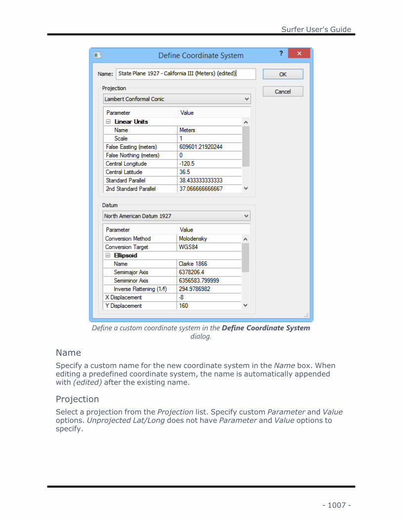
Surfer User's Guide
Define a custom coordinate system in the Define Coordinate Systemdialog.
NameSpecify a custom name for the new coordinate system in the Name box. Whenediting a predefined coordinate system, the name is automatically appendedwith (edited) after the existing name.
ProjectionSelect a projection from the Projection list. Specify custom Parameter and Valueoptions. Unprojected Lat/Long does not have Parameter and Value options tospecify.
- 1007 -

Chapter 27 - Coordinate Systems
The projection options include: Unprojected Lat/Long, Albers Equal Area Conic,Azimuthal Equidistant, Bonne, Cassini, Eckert IV, Eckert VI, Equidistant Conic,Equidistant Cylindrical, Gnomonic, Hotine Oblique Mercator, Lambert AzimuthalEqual Area, Lambert Conformal Conic, Mercator, Miller Cylindrical, Mollweide,Oblique Mercator, Orthographic, Polyconic, Robinson, Robinson-Sterling, Sinus-oidal, Stereographic, Transverse Mercator, Universal Transverse Mercator(UTM), and Van Der Grinten.
DatumSelect a datum from the Datum list. Specify custom Parameter and Value optionsto fit your needs.
OK or CancelClick OK to create your new custom coordinate system. The coordinate systemwill be listed in the Custom section of the Assign Coordinate System dialog forthis file. If you want to save the custom coordinate system for future use, addthe custom coordinate system to the Favorites section. Click Cancel to return tothe Assign Coordinate System dialog without creating a custom coordinate sys-tem.
Example 1: Defining a Custom Coordinate System1. In the Assign Coordinate System dialog, click the New Geographic Sys-
tem button to open the Define Coordinate System dialog.
2. Change the Name to Lambert Conformal Conic Custom.
3. From the Projection list, select Lambert Conformal Conic.
4. Make any necessary changes to the Parameter or Values.
5. Make any necessary changes to the Datum section.
6. Click OK and the Lambert Conformal Conic Custom projection is added tothe Custom section.
7. In the Assign Coordinate System dialog, select the custom projectionand click OK.
Example 2: Saving a Custom Coordinate System1. In the Assign Coordinate System dialog, click the button to the left of
Custom.
2. Select the coordinate system in the Custom section and click the Add toFavorites button.
- 1008 -

Surfer User's Guide
3. Click the button to the left of Favorites to open the Favorites section. Thecustom projection is saved here.
4. Click OK to close the dialog.
Define Unreferenced Coordinate SystemClick the New Local System button, or Modify button with a local coordinate sys-tem selected, in the Assign Coordinate System dialog to open the DefineUnreferenced Coordinate System dialog. The Define UnreferencedCoordinate System dialog creates a Custom coordinate system. Specify the lin-ear units for the unreferenced coordinate system. Click OK and the new coordin-ate system will be added to the Assign Coordinate System dialog Custom listfor future use.
Define a custom local coordinate system in the Define UnreferencedCoordinate System dialog.
NameSpecify a custom name for the new coordinate system in the Name box. Whenediting a predefined coordinate system, the name is automatically appendedwith (edited) after the existing name.
Linear UnitsSpecify the units for the new coordinate system in the Name field. Click the cur-rent selection and select the desired units from the list.
Alternatively, specify custom units by typing the number of units per meter inthe Units per meter box. For example, to use the uncommon unit UK Metric Foot(defined as 300mm), type 3.33333333 into the Units per meter field.
OffsetApply an offset by typing a value in the X Offset or Y Offset fields.
OK or CancelClick OK to create your new custom coordinate system. The coordinate systemwill be listed in the Custom section of the Assign Coordinate System dialog forthis file. If you want to save the custom coordinate system for future use, addthe custom coordinate system to the Favorites section. Click Cancel to return tothe Assign Coordinate System dialog without creating a custom coordinatesystem.
- 1009 -

Chapter 27 - Coordinate Systems
Example 1: Defining Units for an Unreferenced Coordinate System1. In the Assign Coordinate System dialog, click the New Local System but-
ton to open the Define Unreferenced Coordinate System dialog.
2. Change the Name to Local Meters (no offset).
3. From the Name list in the Linear Units section, select Meters.
4. Click OK and the Local Meters (no offset) coordinate system is added to theCustom section.
5. In the Assign Coordinate System dialog, select the custom projectionand click OK.
Example 2: Saving a Custom Coordinate System1. In the Assign Coordinate System dialog, click the button to the left of
Custom.
2. Select the coordinate system in the Custom section and click the Add toFavorites button.
3. Click the button to the left of Favorites to open the Favorites section. Thecustom projection is saved here.
4. Click OK to close the dialog.
Assign Coordinate System - WorksheetThe Data | Coordinate System | Assign Coordinate System command or
the button links a data file to a specific coordinate system. Once the coordin-ate system is defined for the data file, a Golden Software Georeference .GSR2file is created. This file contains all the relevant projection information thatSurfer needs to load the data in the proper projection.
When a .GRD file is created using the Grids | New Grid | Grid Data command, the.GSR2 file for the data is read. The projection information can be saved with thegrid file using the Spatial References options. It is recommended to check the GSReference (Version 2) file if you intend to use the grid file in Surfer, as the GSR2retains all of the information needed. The grid has the same coordinate systemas the original data file, but the .GSR2 is required to define the coordinate sys-tem. When a map is created from either the data file or the .GRD file, the .GSR2file is read and the map layer automatically has the correct coordinate system.
- 1010 -

Surfer User's Guide
Assign Coordinate System - Grid
The Grids | Edit | Assign Coordinate System command or the buttonlinks a grid file to a specific coordinate system. Once the coordinate system isdefined for the grid file, a Golden Software Georeference .GSR2 file is created.This file contains all the relevant projection information that Surfer needs toload the grid in the proper projection.
Use the Data | Coordinate System | Assign Coordinate System command to linka data file to a .GSR2 file. When a .GRD file is created using the Grids | New Grid| Grid Data command, the .GSR2 file for the data is read. The projection inform-ation can be saved with the grid file using the Spatial References options. It isrecommended to check the GS Reference (Version 2) file if you intend to use thegrid file in Surfer, as the GSR2 retains all of the information needed. The gridhas the same coordinate system as the original data file, but the .GSR2 isrequired to define the coordinate system. When a map is created from either thedata file or the .GRD file, the .GSR2 file is read and the map layer automaticallyhas the correct coordinate system.
If the data file did not have an assigned coordinate system, or the grid file wasprovided directly from another source, the Grids | Edit | Assign CoordinateSystem can be used to link the grid with a .GSR2 file.
When any grid operation is performed on the referenced grid file, the ExportOptions dialog appears with the option to create a new .GSR2 file for the newoutput grid. For instance, if you use the Grids | Edit | Filter command andsmooth the grid, the output smoothed grid will contain a .GSR2 file with thesame coordinate system information as the original grid. When a map is createdfrom the smoothed grid file, the .GSR2 file is read and the map layer auto-matically has the correct coordinate system. For commands that use multiplefiles, such as Grids | Edit | Assign NoData or Grids | Resize | Mosaic, all filesshould be in the same reference system, otherwise unexpected results mayoccur. The .GSR2 file in these cases is assigned by the first .GRD file specified.
What is a Map Projection?Maps are usually seen in a flat, two-dimensional medium such as a drawing onpaper or an image on a computer screen. Since the surface of the Earth iscurved, or three-dimensional, the visual elements on the surface must somehowbe transformed from three dimensions to two in order to display a map of theEarth's surface. Projections are a mathematical process by which the visual ele-ments are transformed from three dimensions to two.
One of the simplest forms of projection is analogous to shining a light through atranslucent globe onto a piece of paper and tracing the outlines. Other forms ofprojection may involve dozens of complex mathematical equations. Since notwo-dimensional representation of a three-dimensional surface can be accurate
- 1011 -

Chapter 27 - Coordinate Systems
in every regard, a variety of different projections have been developed to suit dif-ferent purposes. Some projections are accurate in terms of area but not in scale,some are accurate in terms of scale but not in shape, and so on. The selection ofan appropriate projection for a map depends on which characteristics of a mapare most important or most desirable for a given project or audience.
Surfer supports several of the projections that are most often used in moderncartography and related fields. The Surfer worksheet allows you to load dataand define the projection using the Data | Coordinate System | Assign Coordin-ate System command. You can then convert the data to another coordinate sys-tem using the Data | Coordinate System | New Projected Coordinates commandto project the data in another projection, ellipsoid, or datum. Surfer's plot win-dow allows you to assign a coordinate system to a grid file using the Grids | Edit |Assign Coordinate System command. You can also load maps, assign mapcoordinate systems using the Source Coordinate System for each map layer, andconvert the entire map to another system using the Target Coordinate System.
There are many excellent textbooks and publications on this subject, and we donot attempt to explain projections in full detail here. If you need or want moreinformation, you might consider reading the references that provide good intro-ductory discussions of map projections.
EllipsoidsFor maps of the Earth where accuracy is not of particular concern, we can safelyassume that the Earth is perfectly spherical in shape. For small-scale maps, thedifference between a sphere and ellipsoid is not detectable on the map.
However, the Earth is actually somewhat ellipsoidal (or egg-shaped), approx-imately 1/300th wider than it is tall, assuming a vertical orientation with respectto the axis of rotation. This shape needs to be taken into account to produce lar-ger scale maps of any significant accuracy.
This is an example of an ellipsoid (dashed blue line) superimposed on a sphere (solid blackline).
- 1012 -

Surfer User's Guide
While an ellipsoid is a closer approximation of the Earth's shape than a sphere,the Earth's surface is not entirely uniform in curvature, so any ellipsoidal rep-resentation of the Earth is still only an approximation. This being the case, car-tographers have historically used a number of slightly different ellipsoidalrepresentations in attempts to produce more accurate maps of different regionsof the Earth.
Ellipsoids are defined by the ellipse being used and by the amount of rotation ofthe ellipse. An ellipse has two axes. The longer axis is the Semimajor Axis. Theshorter axis is the Semiminor Axis. Rotating the ellipse around the semiminoraxis creates the ellipsoid.
The diagram shows the semimajor and semiminor axes on anellipse.
In Surfer, the ellipsoid can be defined by the Semimajor Axis and the SemiminorAxis or by the Semimajor Axis and the Inverse Flattening (1/f) value. The flat-tening value ranges from zero to 1, so the Inverse Flattening (1/f) value must belarger than 1. The flattening value is determined by:
f = (Semimajor Axis - Semiminor Axis)/Semimajor Axis
In the Assign Coordinate System dialog, click the New button to define a newcoordinate system. In the Define Coordinate System dialog, the Datum groupallows you to specify parameters for the datum. The Ellipsoid can be customizedin terms of Name, Semimajor Axis, Semiminor Axis, and Inverse Flattening(1/f). The Semimajor Axis, Semiminor Axis, and Inverse Flattening ratio shouldbe set in meters. If you do not understand ellipsoids and datum definitions, it isrecommended you use the defaults. For more information on these subjects, seethe projection references.
DatumsSince coordinates on the Earth's surface can be recorded under widely varyingassumptions about the shape and size of the Earth and the locations of the polesand prime meridian, cartographers have developed a standard for identifying theframe of reference for a coordinate system. This standard is called the datum.Because the frames of reference differ, a coordinate recorded in one datum usu-
- 1013 -

Chapter 27 - Coordinate Systems
ally has slightly different latitude and longitude values from the same point recor-ded in any other datum.
Some datums are designed to provide a marginally accurate representation ofcoordinates spanning the entire Earth, while other datums are designed toprovide more accurate results in a particular region at the expense of lesseraccuracy in other parts of the world. For example, the South American Datum of1969 (SA69) is tailored to provide good results for maps of the South Americancontinent and surrounding areas, but, as a consequence, provides poor resultsfor the rest of the world.
When combining data from multiple sources into a single map, it is importantthat all of the coordinate systems being combined specify the projection anddatum accurately. Since each datum has slightly different latitude and longitudevalues for the same coordinates, mixing coordinates from multiple datumstogether without fully defining the datum introduces inaccuracies into the map.Surfer will automatically convert different source coordinate systems from dif-ferent datums to the target coordinate system.
A datum conversion can be used to convert coordinates from one datum toanother using the Data | Coordinate System | New Projected Coordinatescommand. Click the ... next to the Target Coordinate System to open the AssignCoordinate System dialog. Click New to define a new projection and datum.The Define Coordinate System dialog has the Conversion Method and Ellipsoidparameters necessary to allow you to define a coordinate system with a customdatum.
Several different Conversion Methodsmay be used for converting coordinatesfrom one datum to another:
Molodensky The Molodenskymethod is the most widely used method ofdatum conversion. It adjusts latitude and longitude coordin-ates by taking into account the displacement between twodatum's ellipsoids on all three axes. It does not take intoaccount any rotational differences between the two ellipsoids.
Bursa-Wolfe
The Bursa-Wolfemethod is similar to the Molodenskymethod, but in some instances it produces more accurate res-ults because it takes into account both displacement and rota-tional differences between two ellipsoids. Surfer supports theBursa-Wolfemethod for conversions from the WGS84 datumto the following datums: World Geodetic System 1972,DHDN-1, DHDN, Australian Geodetic 1984, ANS84, MRT -Everest Modified, Switzerland - CH1903, NTF France - ParisMeridian, and Pulkovo 1942 - Hungary.
Surfer supports the NTv2 datum conversion method. NTv2 is the Canadian gov-ernment's officially sanctioned method of converting Canadian map data fromthe old NAD27 datum to the NAD83 datum. NTv2 is based on a hierarchical data-base of interpolation grids of different resolutions for different regions of the
- 1014 -
Surfer User's Guide
country. NTv2 datum conversions cannot be performed unless an NTv2 grid shiftfile is installed in the same folder/directory as the Surfer program. Visit NaturalResources Canada's Geodetic Reference Systems page on the web for moreinformation about this datum and obtaining an NTv2 grid shift file. See theGolden SoftwareHow to convert from NAD27 to NAD83 using NTv2 help topicfor detailed steps on using the NTv2 datum conversion.
Surfer supports conversions for over 200 different predefined datums.
Custom Datum DefinitionClick the New button in the Assign Coordinate System dialog to open the DefineCoordinate System dialog. Use the Datum group to define a custom datum andspecify the exact datum parameters and values.
DatumThe Datum list contains predefined datums. Select a datum to populate the Para-meter and Value columns. Customize the parameters and values as needed.
Conversion MethodThe Conversion Method controls the method of datum conversion and the con-version parameters. The conversion methods include Molodensky, Bursa-Wolfe,and None.
l The Molodenskymethod is the most widely used method of datum con-version. It adjusts latitude and longitude coordinates by taking into accountthe displacement between two datum's ellipsoids on all three axes. It doesnot take into account any rotational differences between the two ellipsoids.
l The Bursa-Wolfemethod is similar to the Molodenskymethod, but in someinstances it produces more accurate results because it takes into accountboth displacement and rotational differences between two ellipsoids.
l Choose None if the predefined methods do not suite your purpose. If youselect <custom> from the Ellipsoid Name list, you can specify your ownellipsoid model parameters.
Conversion Parameter and ValuesYou can edit the conversion parameter and values directly by selecting the valueyou want to edit and typing a new value over it. Parameters vary depending onthe selected Conversion Method.
- 1015 -

Chapter 27 - Coordinate Systems
EllipsoidThe Ellipsoid group contains options for defining the ellipsoid. Use these settingsto define the ellipsoid model that best approximates the curvature of the Earth'sshape in the map region. If you do not understand ellipsoids and datum defin-itions, it is recommended you use the defaults.
l The Name list contains a collection of ellipsoid models that cartographershave historically used in attempts to produce more accurate maps of dif-ferent regions of the Earth. The Name list also contains the option to createa <custom> ellipsoid.
l The Semimajor Axis box can be edited to define the major axis.
l The Semiminor Axis box can be edited to define the minor axis.
l The Inverse Flattening (1/f) can be edited to define the flattening ratio.
l The X Displacement, Y Displacement, and Z Displacement are the axis dis-placements in meters.
Prime MeridianThe Prime Meridian section contains options for defining the prime meridianName and Prime Meridian Shift. A meridian is a line of constant longitude run-ning north-south on a map. The zero meridian or prime meridian is used as a ref-erence line from which longitude east and west is measured. The prime meridianpasses through Greenwich, England. The Prime Meridian Shift is the shift fromthe prime meridian, typically 0 degrees, in decimal degrees.
Understanding Local DatumsTo understand how local datum transforms affect data, you need to understandthe ellipsoid, the spheroid, and how both relate to the datum. The spheroid is thea perfect circular object, located at mean sea level. This is constant everywhere.Because of local variations in the gravitational field, the shape actually has localvariations.
The image from Verhoogan, shows the variation in the geoid, ellipsoid, and actual topo-graphic surface.
- 1016 -

Surfer User's Guide
The ellipsoid is used to approximate the global differences. But additional dif-ferences exist because of the actual topographic surface. Local datums were cre-ated to locally account for these differences. The datum includes the ellipsoid,the prime meridian shift, and any offsets in the X or Y direction. Because localdatums align the ellipsoid with a particular location on the earth's surface, localdatums are not suitable for use outside the designed area.
In the Define Coordinate System dialog, you can choose how datums are con-verted from one datum to another. This is the Conversion Method. TheMolodenskymethod is the most widely used method of datum conversion. Itadjusts latitude and longitude coordinates by taking into account the dis-placement between two datum's ellipsoids on all three axes. It does not take intoaccount any rotational differences between the two ellipsoids. The Bursa-Wolfemethod is similar to the Molodenskymethod, but in some instances it producesmore accurate results because it takes into account both displacement and rota-tional differences between two ellipsoids. Surfer supports the Bursa-Wolfemethod for conversions from the WGS84 datum to the following datums: WorldGeodetic System 1972, DHDN-1, DHDN, Australian Geodetic 1984, ANS84, MRT- Everest Modified, Switzerland - CH1903, NTF France - Paris Meridian, andPulkovo 1942 - Hungary.
Changing the datum incorrectly can cause maps to appear wrong or not appearat all. It is advised that changing the datum be done with caution and a basicunderstanding of the local datums is advised.
Types of ProjectionsMost forms of projection operate by projecting Earth coordinates onto a geo-metric shape that can be easily flattened to a two-dimensional image. This math-ematical transformation is commonly referred to as a map projection. A mapprojection systematically projects locations from the surface of the spheroid torepresent positions on the geometric shape.
Three geometric shapes are frequently used:
Type ofShape
How it works Characteristicsof Projection
Examples ofProjection
- 1017 -

Chapter 27 - Coordinate Systems
Cylinder Earth coordinates may beprojected onto a cylinder.The cylinder is cut length-wise and unrolled to makea two-dimensional map.This type of projection iscalled a cylindrical pro-jection.
l Lines of lon-gitude areparallel toeach other.
l Lines of lat-itude are par-allel to eachother.
l Lines of lon-gitude are atright anglesto lines of lat-itude.
l Regionsnear theequator orselectedstandard par-allels areminimallydistorted.
l Regionsnear thepoles arehighly dis-torted.
Cassini,EquidistantCylindrical,HotineOblique Mer-cator, Mer-cator, MillerCylindrical,New ZealandMap Grid,Oblique Mer-cator, Trans-verseMercator, andUniversalTransverseMercator
Cone Earth coordinates may beprojected onto a cone. Thepoint of the cone is usuallydirectly above the pole andthe sides of the cone passthrough the globe at twouser-defined latitudes,called the Standard Par-allels. At the standard par-allels, there is no differencebetween the east-west andnorth-south scales. Thecone is cut from tip to baseand unrolled to make atwo-dimensional map. Thistype of projection is calleda conic projection.
l Lines oflatitudeform con-centricarcs.
l Lines oflongitudearestraightand radi-ate out-ward fromthe tip ofthe ima-ginarycone.
Albers EqualArea,EquidistantConic, Lam-bert Con-formal Conic,Polyconic, andBonne
- 1018 -

Surfer User's Guide
Plane Earth coordinates may beprojected directly onto aflat plane. This type of pro-jection is called an azi-muthal projection.Projections of this type arerecommended for maps ofpolar regions because cyl-indrical and conic pro-jections generally eitherhave severe distortion inpolar regions or are unableto project coordinates inpolar regions.
l The sideof theEarth thatis facingaway fromthe centerof the pro-jection isnot vis-ible.
AzimuthalEquidistant,Gnomonic,Orthographic,Stereographic, and LambertAzimuthalEqual Area
Other Projections in this categoryare pseudocylindrical,pseudoconic, or based onsome other mathematicalprojection or mathematicaltables.
Eckert IV, Eck-ert VI, Moll-weide,Robinson,Robinson-Sterling,Sinusoidal,State Plane*,UnprojectedLat/Long, andVan der Grin-ten
* The State Plane Coordinate System uses Transverse Mercator, Lambert Con-formal Conic, or the Hotline Oblique Mercator projection.
Characteristics of ProjectionsSome projections are imbued with characteristics that tell us if certain types ofmeasurements (e.g. measurements of distance, area, etc.) are accurate on theprojected map. Some of these characteristics include the following:
Type ofProjection
Characteristic of Pro-jection
Drawbacks Example Pro-jections
- 1019 -

Chapter 27 - Coordinate Systems
Equal Area A equal area projection iswhen the area of anygiven part of the map ispreserved. This meansthat the any object thatcovers the same area onthe Earth as any otherpart of the map will bethe same size.
For example, if a one inchdiameter circle on themap covers a 100 milediameter circle on theEarth's surface, then weknow that a one inch dia-meter circle anywhereelse on the map is knownto cover another 100 milediameter circle on theEarth.
In maps of smallerregions, shapes may notbe obviously distorted.
In order for aprojection to beequal area, how-ever, con-sistency in theshapes, scales,and/or anglesacross the mapmust be sac-rificed.
Meridians andparallels maynot intersect atright angles.
Albers EqualArea, Bonne,Eckert IV, Eck-ert VI, Lam-bertAzimuthalEqual Area,Mollweide,and Sinus-oidal
Conformal A conformal projectionpreserves local shapes.This means that when thelocal angles for points onthe map are representedaccurately. This meansthat the angles betweenany given point and anynearby points are accur-ate, but are not neces-sarily accurate for widelyseparated points on themap.
A side effect is that con-formal projections pre-serve the preciseperpendicular inter-sections between par-allels and meridians onthe map. When mappingsmaller areas, relativeshape is preserved.
In order for aprojection to beconformal, how-ever, con-sistency in thesurface areas,shapes, and/orscales across themap must be sac-rificed. An areaenclosed by aseries of arcsmay be greatlydistorted.
HotineOblique Mer-cator, Lam-bertConformalConic, Mer-cator, ObliqueMercator,State PlaneCoordinateSystem,TransverseMercator, andUniversalTransverseMercator
- 1020 -

Surfer User's Guide
Equidistant A equidistant projectionis when the scalebetween at least one spe-cific origin point on themap with respect toevery other point on themap is represented accur-ately.
In order for aprojection to beequidistant, how-ever, con-sistency in thesurface areas,shapes, and/orangles acrossthe map must besacrificed.
AzimuthalEquidistant,EquidistantCylindrical,EquidistantConic, andCassini
Azimuthal A azimuthal projection iswhen the direction of (orangle to) all points on themap are accurate withrespect to the centerpoint of the projection.
In order for aprojection to beazimuthal,areas, shapes,and angles maybe sacrificed atareas not closeto the center ofthe map.
AzimuthalEquidistant,Gnomonic,Lambert Azi-muthal EqualArea, Ortho-graphic, andStereographic
Other Some projections try tominimize the effects of alldistortions and as a resultdo not minimize any onedistortion in particular.
Polyconic,Robinson andRobinson-Sterling,UnprojectedLat/Long, andVan der Grin-ten
In addition to the characteristics described above, some projections have highlyspecialized characteristics that may be useful in certain applications. Forexample, on maps made with a Mercator projection, all lines of constant dir-ection (rhumb lines) are known to be straight, thereby making such maps verydesirable as navigational charts.
Predefined Coordinate SystemsThe following sections describe the various predefined coordinate systems.
Geographic (lat/long) Coordinate SystemsIn the Assign Coordinate System dialog, the Geographic (lat/long) category con-tains unprojected latitude and longitude coordinate systems. Coordinates arealways in latitude and longitude. Each coordinate system has a different datum.Datums are defined for specific regions. Properties for each coordinate systemand datum are listed in the dialog by clicking on the desired system.
- 1021 -

Chapter 27 - Coordinate Systems
Polar/Arctic/Antarctic Projection SystemsIn the Assign Coordinate System dialog, the coordinate systems under Pre-defined are separated into different categories.
The Polar/Arctic/Antarctic category contains different projections that can beused near the north and south poles. Several different projections fit into this cat-egory: Lambert Conformal Conic, Orthographic, and Stereographic. Coordinatesare always in latitude and longitude. The difference between the projections arein the definition of the false easting, northing, central longitude, central latitude,standard parallel or datum. Projections are defined for specific regions. Prop-erties for each coordinate system and datum are listed in the dialog by clickingon the desired system.
Regional/National Projection SystemsIn the Assign Coordinate System dialog, the coordinate systems under Pre-defined are separated into different categories.
The Regional/National category contains different projections that can be usedfor specific regions or countries of the world. Several different projections fit intothis category: Albers Equal Area Conic, Azimuthal Equidistant, Cassini,Gnomonic, Hotine Oblique Mercator, Lambert Azimuthal Equal Area, LambertConformal Conic, Mercator, New Zealand Map Grid, Polyconic, Stereographic,Transverse Mercator, and UTM. Coordinates are in latitude and longitude, feet,meters, or occasionally other units. The difference between the projections are inthe definition of the false easting, northing, central longitude, central latitude,standard parallel or datum. Projections are defined for specific countries or spe-cific regions. Properties for each coordinate system and datum are listed in thedialog by clicking on the desired system.
State Plane Coordinate SystemsIn the Assign Coordinate System dialog, the coordinate systems under Pre-defined are separated into different categories.
The State Plane category contains both 1927 and 1983 systems. Coordinates arein either feet or meters. The difference between the 1927 and 1983 systems arein the definition of the false easting, northing, central longitude, central latitude,standard parallel or datum. Settings are defined for specific regions of individualstates. Properties for each coordinate system and datum are listed in the dialogby clicking on the desired system.
UTM Coordinate SystemsIn the Assign Coordinate System dialog, the coordinate systems under Pre-defined are separated into different categories.
- 1022 -

Surfer User's Guide
The UTM category contains different systems separated by country, region, ortype. Coordinates are in meters. The difference between the systems are in thedefinition of the false easting, northing, central longitude, central latitude, stand-ard parallel or datum. Settings are defined for specific regions or individual coun-tries. Properties for each coordinate system and datum are listed in the dialog byclicking on the desired system.
World Projection SystemsIn the Assign Coordinate System dialog, the coordinate systems under Pre-defined are separated into different categories.
TheWorld category contains different projections that can be used to display themap in a particular way. Several different projections fit into this category:Bonne, Eckert IV, Eckert VI, EPSG 3395 – Mercator, EPSG 3785 – Popular Visu-alisation CRS / Mercator, Equidistant Conic , Equidistant Cylindrical, Miller, Moll-weide, Orthographic Western Hemisphere, Robinson and Robinson-Sterling,Sinusoidal, and Van Der Grinten. Coordinates are in latitude and longitude. Thedifference between the projections are in the definition of the false easting, north-ing, central longitude, central latitude, standard parallel or datum. Projectionscan be used for multiple countries or specific regions, depending on the pro-jection type. Properties for each coordinate system and datum are listed in thedialog by clicking on the desired system.
TemplatesIn the Assign Coordinate System dialog, the coordinate systems under Pre-defined are separated into different categories.
The Templates section is an easy way to modify one of the predefined systemswithout needing to find the system in one of the other Predefined lists. To modifya coordinate system, click on the desired template coordinate system and clickthe Modify button.
Supported ProjectionsThe following projections are supported in Surfer.
Albers Equal Area Conic Projection
- 1023 -
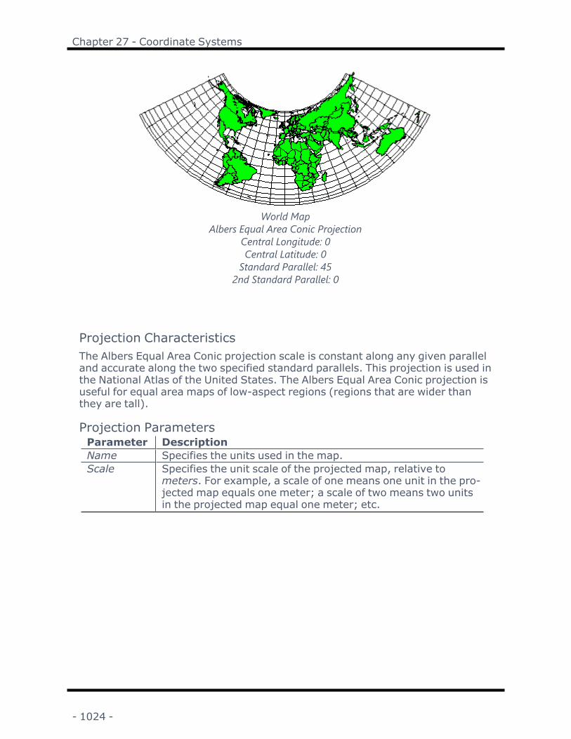
Chapter 27 - Coordinate Systems
World MapAlbers Equal Area Conic Projection
Central Longitude: 0Central Latitude: 0Standard Parallel: 452nd Standard Parallel: 0
Projection CharacteristicsThe Albers Equal Area Conic projection scale is constant along any given paralleland accurate along the two specified standard parallels. This projection is used inthe National Atlas of the United States. The Albers Equal Area Conic projection isuseful for equal area maps of low-aspect regions (regions that are wider thanthey are tall).
Projection ParametersParameter DescriptionName Specifies the units used in the map.Scale Specifies the unit scale of the projected map, relative to
meters. For example, a scale of one means one unit in the pro-jected map equals one meter; a scale of two means two unitsin the projected map equal one meter; etc.
- 1024 -

Surfer User's Guide
False East-ing
Specifies the false easting, or horizontal offset, of the pro-jected coordinates, in meters. False Eastings and False Nor-things are added to the underlying "projected" coordinates asa way to arbitrarily offset their internal XY coordinates afterthe projection. Unless you have a reason for using these off-set values, do not use them. These values do not affect thelatitude/longitude coordinates for the map, only the internalcoordinates used to plot the map on the screen. If you useFalse Easting and False Northing offsets for a map, any sub-sequent boundaries you append to the map must also usethese same offsets if you want the imported boundaries to bedrawn in the correct relative position to the existing bound-aries.
False Nor-thing
Specifies the false northing, or vertical offset, of the projectedcoordinates, in meters. See above.
Central Lon-gitude
Specifies the central longitude of the projection in degrees.The Central Longitude value typically should be defined as thelongitudinal center of the map you are going to produce. Forexample, the value -95.5 represents the geographic center ofthe United States, so the map of the U.S. is drawn upright.
Central Lat-itude
Specifies the central latitude of the projection in degrees. TheCentral Latitude value should be defined as the latitudinal cen-ter of the map you are going to produce. This value is only sig-nificant when you define False Easting and False Northingvalues.
StandardParallel
Specifies the latitude of the first of two standard parallels, indegrees. The standard parallels typically are defined atapproximately one-sixth of the distance inside the north andsouth limits of the map. For example, if your map latituderanges from 30° to 36°, you could place your Standard Par-allels at 31° and 35°. There are alternative methods fordetermining the best position of the standard parallels. Pleasesee Snyder for more information.
2nd Stand-ard Parallel
Specifies the latitude of the second of two standard parallels,in degrees. See above.
- 1025 -

Chapter 27 - Coordinate Systems
Azimuthal Equidistant Projection
World MapAzimuthal Equidistant Projection
Standard Parallel: 0Central Longitude: 0
Projection CharacteristicsThe Azimuthal Equidistant projection is a planar projection. Directions and scaleare true from the center point of the map. Shapes are true at the center of themap, but are distorted the further you move from the center. When using a polarview of this projection, all meridians are straight lines. When using an equatorialview, the central longitude and equator are straight lines, otherwise, only thecentral longitude is a straight line. This projection is typically used in polar hemi-spheric maps.
Projection ParametersParameter DescriptionName Specifies the units used in the map.Scale Specifies the unit scale of the projected map, relative to
meters. For example, a scale of one means one unit in the pro-jected map equals one meter; a scale of two means two unitsin the projected map equal one meter; etc.
- 1026 -

Surfer User's Guide
False East-ing
Specifies the false easting, or horizontal offset, of the pro-jected coordinates, in meters. False Eastings and False Nor-things are added to the underlying "projected" coordinates asa way to arbitrarily offset their internal XY coordinates afterthe projection. Unless you have a reason for using these off-set values, do not use them. These values do not affect thelatitude/longitude coordinates for the map, only the internalcoordinates used to plot the map on the screen. If you useFalse Easting and False Northing offsets for a map, any sub-sequent boundaries you append to the map must also usethese same offsets if you want the imported boundaries to bedrawn in the correct relative position to the existing bound-aries.
False Nor-thing
Specifies the false northing, or vertical offset, of the projectedcoordinates, in meters. See above.
Central Lon-gitude
Specifies the central longitude of the projection in degrees.The Central Longitude value typically should be defined as thelongitudinal center of the map you are going to produce.
StandardParallel
Specifies the central latitude of the projection in degrees. TheStandard Parallel value typically should be defined as the lat-itudinal center of the map you are going to produce.
Bonne Projection
North America MapBonne Projection
Central Longitude: -100Standard Parallel: 40
Projection CharacteristicsThe Bonne projection is a pseudo-conical, equal area projection. The scale is con-stant along any given parallel, and accurate along the specified standard par-
- 1027 -

Chapter 27 - Coordinate Systems
allels. The Bonne projection is distortion-free along the central longitude and theparallels. This projection is used for continental and topographic mapping.
Projection ParametersParameter DescriptionName Specifies the units used in the map.Scale Specifies the unit scale of the projected map, relative to
meters. For example, a scale of one means one unit in the pro-jected map equals one meter; a scale of two means two unitsin the projected map equal one meter; etc.
False East-ing
Specifies the false easting, or horizontal offset, of the pro-jected coordinates, in meters. False Eastings and False Nor-things are added to the underlying "projected" coordinates asa way to arbitrarily offset their internal XY coordinates afterthe projection. Unless you have a reason for using these off-set values, do not use them. These values do not affect thelatitude/longitude coordinates for the map, only the internalcoordinates used to plot the map on the screen. If you useFalse Easting and False Northing offsets for a map, any sub-sequent boundaries you append to the map must also usethese same offsets if you want the imported boundaries to bedrawn in the correct relative position to the existing bound-aries.
False Nor-thing
Specifies the false northing, or vertical offset, of the projectedcoordinates, in meters. See above.
Central Lon-gitude
Specifies the central longitude of the projection in degrees.The Central Longitude value typically should be defined as thelongitudinal center of the map you are going to produce.
StandardParallel
Specifies the central latitude of the projection in degrees. TheStandard Parallel value typically should be defined as the lat-itudinal center of the map you are going to produce.
- 1028 -

Surfer User's Guide
Cassini Projection
Map of North AmericaCassini Projection
Central Longitude = -100Central Latitude = 40
Projection CharacteristicsThe Cassini projection is a cylindrical projection. The scale is accurate along thecentral longitude and along latitude lines perpendicular to the central longitude.This projection is useful for high-aspect regions (regions taller than they arewide).
Projection ParametersParameter DescriptionName Specifies the units used in the map.Scale Specifies the unit scale of the projected map, relative to
meters. For example, a scale of one means one unit in the pro-jected map equals one meter; a scale of two means two unitsin the projected map equal one meter; etc.
False East-ing
Specifies the false easting, or horizontal offset, of the pro-jected coordinates, in meters. False Eastings and False Nor-things are added to the underlying "projected" coordinates asa way to arbitrarily offset their internal XY coordinates afterthe projection. Unless you have a reason for using these off-set values, do not use them. These values do not affect thelatitude/longitude coordinates for the map, only the internalcoordinates used to plot the map on the screen. If you useFalse Easting and False Northing offsets for a map, any sub-sequent boundaries you append to the map must also usethese same offsets if you want the imported boundaries to bedrawn in the correct relative position to the existing bound-aries.
- 1029 -

Chapter 27 - Coordinate Systems
False Nor-thing
Specifies the false northing, or vertical offset, of the projectedcoordinates, in meters. See above.
Central Lat-itude
Specifies the central latitude of the projection in degrees. TheCentral Latitude value typically should be defined as the lat-itudinal center of the map you are going to produce.
Central Lon-gitude
Specifies the central longitude of the projection in degrees.The Central Longitude value typically should be defined as thelongitudinal center of the map you are going to produce.
Eckert IV Projection
World MapEckert IV ProjectionCentral Longitude: 0
Projection CharacteristicsThe scale is constant along any given parallel and accurate along the parallels40°30' north and south in the Eckert IV projection. This is a pseudo-cylindrical,equal area projection with the central longitude half the length of the equator.The poles are represented by lines half the distance of the equator as well. Themeridians are semi-ellipses. Eckert IV is designed to produce aesthetically pleas-ing world maps.
Projection ParametersParameter DescriptionName Specifies the units used in the map.Scale Specifies the unit scale of the projected map, relative to
meters. For example, a scale of one means one unit in the pro-jected map equals one meter; a scale of two means two unitsin the projected map equal one meter; etc.
- 1030 -

Surfer User's Guide
False East-ing
Specifies the false easting, or horizontal offset, of the pro-jected coordinates, in meters. False Eastings and False Nor-things are added to the underlying "projected" coordinates asa way to arbitrarily offset their internal XY coordinates afterthe projection. Unless you have a reason for using these off-set values, do not use them. These values do not affect thelatitude/longitude coordinates for the map, only the internalcoordinates used to plot the map on the screen. If you useFalse Easting and False Northing offsets for a map, any sub-sequent boundaries you append to the map must also usethese same offsets if you want the imported boundaries to bedrawn in the correct relative position to the existing bound-aries.
False Nor-thing
Specifies the false northing, or vertical offset, of the projectedcoordinates, in meters. See above.
Central Lon-gitude
Specifies the central longitude of the projection in degrees.The Central Longitude value typically should be defined as thelongitudinal center of the map you are going to produce.
Eckert VI Projection
World MapEckert VI ProjectionCentral Longitude: 0
Projection CharacteristicsThe scale is constant along any given parallel, and accurate along the parallels49°16' north and south in the Eckert VI projection. This is a pseudo-cylindrical,equal area projection with the central longitude half the length of the equator.The poles are represented by lines half the distance of the equator as well. Themeridians are sinusoidal. The Eckert VI projection is useful for world maps.
Projection ParametersParameter Description
- 1031 -

Chapter 27 - Coordinate Systems
Name Specifies the units used in the map.Scale Specifies the unit scale of the projected map, relative to
meters. For example, a scale of one means one unit in the pro-jected map equals one meter; a scale of two means two unitsin the projected map equal one meter; etc.
False East-ing
Specifies the false easting, or horizontal offset, of the pro-jected coordinates, in meters. False Eastings and False Nor-things are added to the underlying "projected" coordinates asa way to arbitrarily offset their internal XY coordinates afterthe projection. Unless you have a reason for using these off-set values, do not use them. These values do not affect thelatitude/longitude coordinates for the map, only the internalcoordinates used to plot the map on the screen. If you useFalse Easting and False Northing offsets for a map, any sub-sequent boundaries you append to the map must also usethese same offsets if you want the imported boundaries to bedrawn in the correct relative position to the existing bound-aries.
False Nor-thing
Specifies the false northing, or vertical offset, of the projectedcoordinates, in meters. See above.
Central Lon-gitude
Specifies the central longitude of the projection in degrees.The Central Longitude value typically should be defined as thelongitudinal center of the map you are going to produce.
Equidistant Conic Projection
World MapEquidistant Conic Projection
Central Longitude: 0Central Latitude: 0Standard Parallel: 452nd Standard Parallel: 0
Projection CharacteristicsThere is no distortion in scale, shape, or area along the standard parallels in anEquidistant Conic projection. Scale is true along all longitudes and along thestandard parallels. Direction is locally true along the standard parallels. This
- 1032 -

Surfer User's Guide
projection is useful for maps of low-aspect regions (regions that are wider thanthey are tall).
Projection ParametersParameter DescriptionName Specifies the units used in the map.Scale Specifies the unit scale of the projected map, relative to
meters. For example, a scale of one means one unit in the pro-jected map equals one meter; a scale of two means two unitsin the projected map equal one meter; etc.
False East-ing
Specifies the false easting, or horizontal offset, of the pro-jected coordinates, in meters. False Eastings and False Nor-things are added to the underlying "projected" coordinates asa way to arbitrarily offset their internal XY coordinates afterthe projection. Unless you have a reason for using these off-set values, do not use them. These values do not affect thelatitude/longitude coordinates for the map, only the internalcoordinates used to plot the map on the screen. If you useFalse Easting and False Northing offsets for a map, any sub-sequent boundaries you append to the map must also usethese same offsets if you want the imported boundaries to bedrawn in the correct relative position to the existing bound-aries.
False Nor-thing
Specifies the false northing, or vertical offset, of the projectedcoordinates, in meters. See above.
Central Lon-gitude
Specifies the central longitude of the projection in degrees.The Central Longitude value typically should be defined as thelongitudinal center of the map you are going to produce. Forexample, the value -95.5 represents the geographic center ofthe United States, so the map of the U.S. is drawn upright.
Central Lat-itude
Specifies the central latitude of the projection in degrees. TheCentral Latitude value should be defined as the latitudinal cen-ter of the map you are going to produce. This value is only sig-nificant when you define False Easting and False Northingvalues.
StandardParallel
Specifies the latitude of the first of two standard parallels, indegrees. The standard parallels typically are defined atapproximately one-sixth of the distance inside the north andsouth limits of the map. For example, if your map latituderanges from 30° to 36°, you could place your Standard Par-allels at 31° and 35°. There are alternative methods fordetermining the best position of the standard parallels. Pleasesee Snyder for more information.
2nd Stand-ard Parallel
Specifies the latitude of the second of two standard parallels,in degrees. See above.
Equidistant Cylindrical Projection
- 1033 -
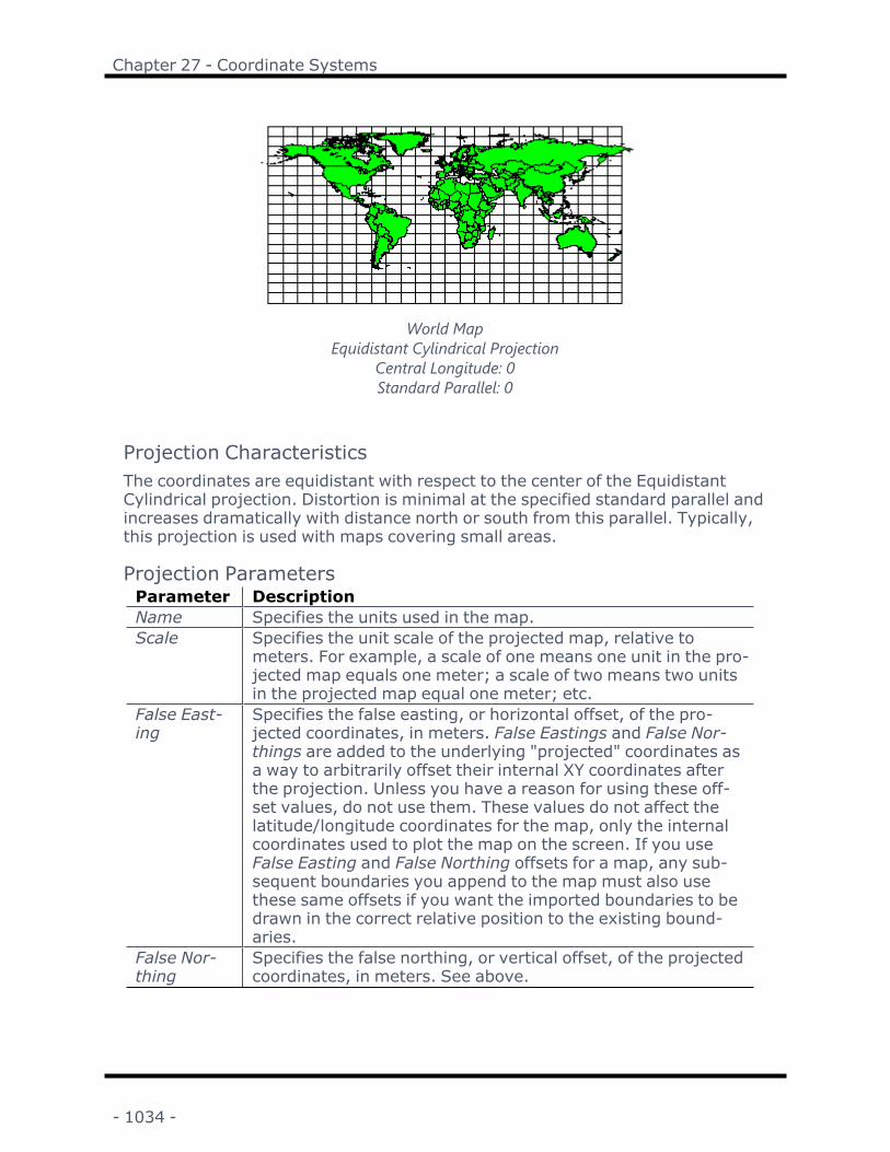
Chapter 27 - Coordinate Systems
World MapEquidistant Cylindrical Projection
Central Longitude: 0Standard Parallel: 0
Projection CharacteristicsThe coordinates are equidistant with respect to the center of the EquidistantCylindrical projection. Distortion is minimal at the specified standard parallel andincreases dramatically with distance north or south from this parallel. Typically,this projection is used with maps covering small areas.
Projection ParametersParameter DescriptionName Specifies the units used in the map.Scale Specifies the unit scale of the projected map, relative to
meters. For example, a scale of one means one unit in the pro-jected map equals one meter; a scale of two means two unitsin the projected map equal one meter; etc.
False East-ing
Specifies the false easting, or horizontal offset, of the pro-jected coordinates, in meters. False Eastings and False Nor-things are added to the underlying "projected" coordinates asa way to arbitrarily offset their internal XY coordinates afterthe projection. Unless you have a reason for using these off-set values, do not use them. These values do not affect thelatitude/longitude coordinates for the map, only the internalcoordinates used to plot the map on the screen. If you useFalse Easting and False Northing offsets for a map, any sub-sequent boundaries you append to the map must also usethese same offsets if you want the imported boundaries to bedrawn in the correct relative position to the existing bound-aries.
False Nor-thing
Specifies the false northing, or vertical offset, of the projectedcoordinates, in meters. See above.
- 1034 -

Surfer User's Guide
Central Lon-gitude
Specifies the central longitude of the projection in degrees.The Central Longitude value typically should be defined as thelongitudinal center of the map you are going to produce. Thisvalue is only significant when you define False Easting andFalse Northing values, and has no apparent effect on themap.
StandardParallel
Specifies the central latitude of the projection in degrees. TheStandard Parallel value typically should be defined as the lat-itudinal center of the map you are going to produce.
Geographic Coordinate System
World MapUnprojected Lat/Long
Projection CharacteristicsThis is a simplistic cylindrical projection. If the coordinates in a Surfermap layerare stored in a geographic coordinate system (also known as UnprojectedLat/Long or latitude/longitude), the map is displayed on the screen by simplytreating the longitudes as horizontal offsets and the latitudes as vertical offsets.
When plotting latitude/longitude coordinates, Surfer constructs the map coordin-ate system by first determining the latitude for the center of the map. Then theappropriate scale is determined for the east-west (longitude) relative to thenorth-south (latitude) dimension of the map. See latitude/longitude and UsingScaling to Minimize Distortion on Latitude/Longitude Maps for more informationon relative scaling of latitude versus longitude.
The features of a geographic coordinate system (Unprojected Lat/Long) mapare:
l Meridians (lines of constant longitude) are equally spaced and are drawnperpendicular to the parallels.
- 1035 -

Chapter 27 - Coordinate Systems
l Parallels (lines of constant latitude) are equally spaced over the entiremap and are drawn perpendicular to the meridians. The further yourmap area is from the equator, the further apart the parallels are spaced.
l The spacing between meridians is different than the spacing between par-allels except when the equator is at the north-south center of the map.
l At the center of the map, the scale is accurate in both the north-southand east-west direction.
l Scale is accurate in the north-south direction over the extent of the map.l East-west scale increases towards the poles, and decreases towards the
equator.
There are no parameters for this coordinate system.
Gnomonic Projection
AntarcticaGnomonic ProjectionFalse Easting: 0False Northing: 0
Central Longitude: 19.0Standard Parallel: 2.4
Projection CharacteristicsThe Gnomonic projection is an azimuthal projection. It is represented as a planetangent to the globe. At this point of tangency, which is called the standard par-allel, all major characteristics are retained. When you move away from the stand-ard parallel in any direction the map is not conformal, not equal-area, anddistances are not true to scale. Only areas of less than a hemisphere can beshown and distortion increases noticeably as you move further from the stand-ard parallel.
- 1036 -

Surfer User's Guide
Projection ParametersParameter DescriptionName Specifies the units used in the map.Scale Specifies the unit scale of the projected map, relative to
meters. For example, a scale of one means one unit in the pro-jected map equals one meter; a scale of two means two unitsin the projected map equal one meter; etc.
False East-ing
Specifies the false easting, or horizontal offset, of the pro-jected coordinates, in meters. False Eastings and False Nor-things are added to the underlying "projected" coordinates asa way to arbitrarily offset their internal XY coordinates afterthe projection. Unless you have a reason for using these off-set values, do not use them. These values do not affect thelatitude/longitude coordinates for the map, only the internalcoordinates used to plot the map on the screen. If you useFalse Easting and False Northing offsets for a map, any sub-sequent boundaries you append to the map must also usethese same offsets if you want the imported boundaries to bedrawn in the correct relative position to the existing bound-aries.
False Nor-thing
Specifies the false northing, or vertical offset, of the projectedcoordinates, in meters. See above.
Central Lon-gitude
Specifies the central longitude of the projection in degrees.The Central Longitude value typically should be defined as thelongitudinal center of the map you are going to produce. Thisvalue is only significant when you define False Easting andFalse Northing values, and has no apparent effect on themap.
StandardParallel
Specifies the central latitude of the projection in degrees. TheStandard Parallel value typically should be defined as the lat-itudinal center of the map you are going to produce.
- 1037 -

Chapter 27 - Coordinate Systems
Hotine Oblique Mercator Projection
Alaska PanhandleHotine Oblique Mercator Pro-
jectionScale = 1
False Easting = 818676.73440112False Northing =575097.68887519
Central Scale Factor = .9999Azimuth (Alpha) = -36.8698976
Central Latitude = 571st Meridian = -133.6667Rotate U/V to X/Y = True
Offset by U = True
Projection CharacteristicsThe Hotine Oblique Mercator projection is a cylindrical, conformal projection. Thescale is accurate along the chosen central line by the longitude/latitude settingsbelow. This projection is useful for oblique areas (areas that do not follow lines oflatitude and longitude), such as the Alaska panhandle because the central linedoes not have to follow a line of constant longitude. This projection is typicallyused with areas that are state or province sized and it is not suitable for maps ofthe world. There are two forms of the Hotine projection equation. The HotineOblique Mercator projection is defined by a point and an azimuth that defines aline (Alternate B, Snyder).
Projection ParametersParameter DescriptionName Specifies the units used in the map.Scale Specifies the unit scale of the projected map, relative to
meters. For example, a scale of one means one unit in the pro-jected map equals one meter; a scale of two means two unitsin the projected map equal one meter; etc.
- 1038 -

Surfer User's Guide
False East-ing
Specifies the false easting, or horizontal offset, of the pro-jected coordinates, in meters. False Eastings and False Nor-things are added to the underlying "projected" coordinates asa way to arbitrarily offset their internal XY coordinates afterthe projection. Unless you have a reason for using these off-set values, do not use them. These values do not affect thelatitude/longitude coordinates for the map, only the internalcoordinates used to plot the map on the screen. If you useFalse Easting and False Northing offsets for a map, any sub-sequent boundaries you append to the map must also usethese same offsets if you want the imported boundaries to bedrawn in the correct relative position to the existing bound-aries.
False Nor-thing
Specifies the false northing, or vertical offset, of the projectedcoordinates, in meters. See above.
CentralScale Factor(KO)
Specifies the central scaling factor for the projection. Thisvalue is often set to 1.0, but may be set to another value forspecific applications.
Azimuth(Alpha)
The angle in degrees in which to rotate the central line. Zerois north, and rotation is clockwise. Value must be greaterthan -360 and less than +360. Value cannot equal 0, 360, or -360. Value cannot equal 90, 270, -90, or -270 if Offset by U isset to False.
Central Lat-itude
Specifies the central latitude of the projection in degrees. TheCentral Latitude value typically should be defined as the lat-itudinal center of the map you are going to produce, andshould typically be defined as the center of the map.
1st Meridian Defines one end of the X extent for the central line.Rotate U/Vto X/Y
u,v are unrectified coordinates that follow the central line ofthe projection. x,y are rectified rectangular coordinates.When True, u,v are rotated to x,y. See Snyder page 70.
Offset by U When True, u coordinates are offset to remove the Us centercomponent, to normalize the origin of the u axis. This is typ-ically required for State Plane coordinate systems that usethe Hotine Oblique Mercator projection method.
- 1039 -
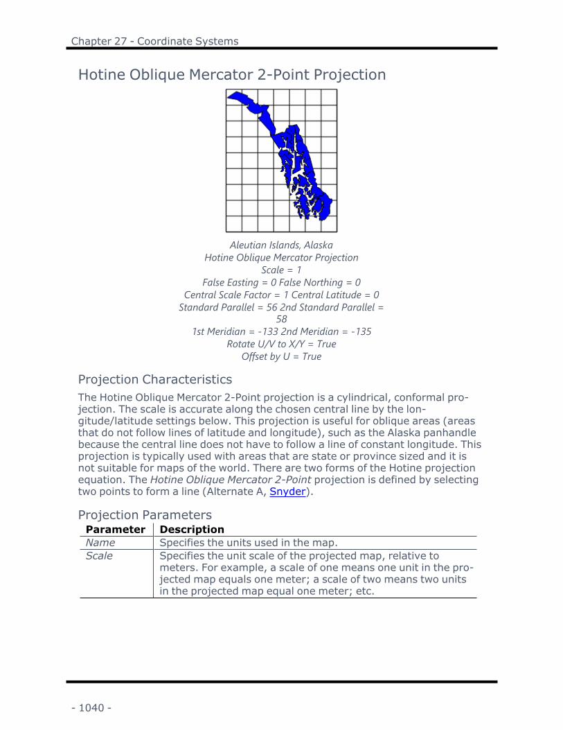
Chapter 27 - Coordinate Systems
Hotine Oblique Mercator 2-Point Projection
Aleutian Islands, AlaskaHotine Oblique Mercator Projection
Scale = 1False Easting = 0 False Northing = 0
Central Scale Factor = 1 Central Latitude = 0Standard Parallel = 56 2nd Standard Parallel =
581st Meridian = -133 2nd Meridian = -135
Rotate U/V to X/Y = TrueOffset by U = True
Projection CharacteristicsThe Hotine Oblique Mercator 2-Point projection is a cylindrical, conformal pro-jection. The scale is accurate along the chosen central line by the lon-gitude/latitude settings below. This projection is useful for oblique areas (areasthat do not follow lines of latitude and longitude), such as the Alaska panhandlebecause the central line does not have to follow a line of constant longitude. Thisprojection is typically used with areas that are state or province sized and it isnot suitable for maps of the world. There are two forms of the Hotine projectionequation. The Hotine Oblique Mercator 2-Point projection is defined by selectingtwo points to form a line (Alternate A, Snyder).
Projection ParametersParameter DescriptionName Specifies the units used in the map.Scale Specifies the unit scale of the projected map, relative to
meters. For example, a scale of one means one unit in the pro-jected map equals one meter; a scale of two means two unitsin the projected map equal one meter; etc.
- 1040 -

Surfer User's Guide
False East-ing
Specifies the false easting, or horizontal offset, of the pro-jected coordinates, in meters. False Eastings and False Nor-things are added to the underlying "projected" coordinates asa way to arbitrarily offset their internal XY coordinates afterthe projection. Unless you have a reason for using these off-set values, do not use them. These values do not affect thelatitude/longitude coordinates for the map, only the internalcoordinates used to plot the map on the screen. If you useFalse Easting and False Northing offsets for a map, any sub-sequent boundaries you append to the map must also usethese same offsets if you want the imported boundaries to bedrawn in the correct relative position to the existing bound-aries.
False Nor-thing
Specifies the false northing, or vertical offset, of the projectedcoordinates, in meters. See above.
CentralScale Factor(KO)
Specifies the central scaling factor for the projection. Thisvalue is often set to 1.0, but may be set to another value forspecific applications.
Central Lat-itude
Specifies the central latitude of the projection in degrees. TheCentral Latitude value typically should be defined as the lat-itudinal center of the map you are going to produce, andshould typically be defined as the center of the map.
StandardParallel
Defines one end of the Y extent for the central line.
1st Meridian Defines one end of the X extent for the central line.2nd Stand-ard Parallel
Defines the other end of the Y extent for the central line.
2ndMeridian
Defines the other end of the X extent for the central line.
Rotate U/Vto X/Y
u,v are unrectified coordinates that follow the central line ofthe projection. x,y are rectified rectangular coordinates.When True, u,v are rotated to x,y. See Snyder page 70.
Offset by U When True, u coordinates are offset to remove the Us centercomponent, to normalize the origin of the u axis. This is typ-ically required for State Plane coordinate systems that usethe Hotine Oblique Mercator projection method.
- 1041 -

Chapter 27 - Coordinate Systems
Lambert Azimuthal Equal Area Projection
World MapLambert Azimuthal Equal Area Pro-
jectionCentral Longitude: -90Standard Parallel: 45
Projection CharacteristicsScale on a Lambert Azimuthal Equal Area projected map is accurate only fromthe center to any other point on the map. Distortion is minimal near the centerand increases with distance from the center. This projection is useful for con-tinents, polar regions (hemispheres), or smaller regions. The Lambert AzimuthalEqual Area projection is not generally used for world maps due to extreme dis-tortion outside the center of the map.
Projection ParametersParameter DescriptionName Specifies the units used in the map.Scale Specifies the unit scale of the projected map, relative to
meters. For example, a scale of one means one unit in the pro-jected map equals one meter; a scale of two means two unitsin the projected map equal one meter; etc.
- 1042 -

Surfer User's Guide
False East-ing
Specifies the false easting, or horizontal offset, of the pro-jected coordinates, in meters. False Eastings and False Nor-things are added to the underlying "projected" coordinates asa way to arbitrarily offset their internal XY coordinates afterthe projection. Unless you have a reason for using these off-set values, do not use them. These values do not affect thelatitude/longitude coordinates for the map, only the internalcoordinates used to plot the map on the screen. If you useFalse Easting and False Northing offsets for a map, any sub-sequent boundaries you append to the map must also usethese same offsets if you want the imported boundaries to bedrawn in the correct relative position to the existing bound-aries.
False Nor-thing
Specifies the false northing, or vertical offset, of the projectedcoordinates, in meters. See above.
Central Lon-gitude
Specifies the central longitude of the projection in degrees.The Central Longitude value typically should be defined as thelongitudinal center of the map you are going to produce.
StandardParallel
Specifies the central latitude of the projection in degrees. TheStandard Parallel value typically should be defined as the lat-itudinal center of the map you are going to produce.
Lambert Conformal Conic Projection
World MapLambert Conformal Conic Projection
Central Longitude: 0Central Latitude: 0Standard Parallel: 452nd Standard Parallel: 0
- 1043 -

Chapter 27 - Coordinate Systems
Projection CharacteristicsIn a Lambert Conformal Conic projection, scale is constant along any given par-allel and accurate along the specified standard parallels. Scale is the same in alldirections at any given point. This projection is useful for equal area maps of low-aspect regions (regions that are wider than they are tall). The pole is a point inthe hemisphere containing the standard parallels and the graticules stretch toinfinity in the other hemisphere. The Lambert Conformal Conic projection is usedfor many of the zones in the State Plane Coordinate System.
Projection ParametersParameter DescriptionName Specifies the units used in the map.Scale Specifies the unit scale of the projected map, relative to
meters. For example, a scale of one means one unit in the pro-jected map equals one meter; a scale of two means two unitsin the projected map equal one meter; etc.
False East-ing
Specifies the false easting, or horizontal offset, of the pro-jected coordinates, in meters. False Eastings and False Nor-things are added to the underlying "projected" coordinates asa way to arbitrarily offset their internal XY coordinates afterthe projection. Unless you have a reason for using these off-set values, do not use them. These values do not affect thelatitude/longitude coordinates for the map, only the internalcoordinates used to plot the map on the screen. If you useFalse Easting and False Northing offsets for a map, any sub-sequent boundaries you append to the map must also usethese same offsets if you want the imported boundaries to bedrawn in the correct relative position to the existing bound-aries.
False Nor-thing
Specifies the false northing, or vertical offset, of the projectedcoordinates, in meters. See above.
Central Lon-gitude
Specifies the central longitude of the projection in degrees.The Central Longitude value typically should be defined as thelongitudinal center of the map you are going to produce. Forexample, the value -95.5 represents the geographic center ofthe United States, so the map of the U.S. is drawn upright.
Central Lat-itude
Specifies the central latitude of the projection in degrees. TheCentral Latitude value should be defined as the latitudinal cen-ter of the map you are going to produce. This value is only sig-nificant when you define False Easting and False Northingvalues.
- 1044 -

Surfer User's Guide
StandardParallel
Specifies the latitude of the first of two standard parallels, indegrees. The Standard Parallels typically are defined atapproximately one-sixth of the distance inside the north andsouth limits of the map. For example, if your map latituderanges from 30° to 36°, you could place your Standard Par-allels at 31° and 35°. There are alternative methods fordetermining the best position of the standard parallels. Pleasesee Snyder for more information.
2nd Stand-ard Parallel
Specifies the latitude of the second of two standard parallels,in degrees. See above.
Mercator Projection
World MapMercator ProjectionCentral Longitude: 0Central Latitude: 0
Projection CharacteristicsThe Mercator projection is a cylindrical projection and it is conformal. In a Mer-cator projection, scale is constant along any given parallel and accurate alongthe specified center latitude. Scale is the same in all directions near any givenpoint. Distortion is minimal near the center parallel, but becomes extremetoward the poles. All lines of constant direction (rhumb lines) are known to bestraight, thereby making this projection very desirable for producing nav-igational charts. A limitation of this projection is that coordinates at or near thepoles cannot be projected due to constraints of the mathematical formulas used.
Projection ParametersParameter DescriptionName Specifies the units used in the map.
- 1045 -

Chapter 27 - Coordinate Systems
Scale Specifies the unit scale of the projected map, relative tometers. For example, a scale of one means one unit in the pro-jected map equals one meter; a scale of two means two unitsin the projected map equal one meter; etc.
False East-ing
Specifies the false easting, or horizontal offset, of the pro-jected coordinates, in meters. False Eastings and False Nor-things are added to the underlying "projected" coordinates asa way to arbitrarily offset their internal XY coordinates afterthe projection. Unless you have a reason for using these off-set values, do not use them. These values do not affect thelatitude/longitude coordinates for the map, only the internalcoordinates used to plot the map on the screen. If you useFalse Easting and False Northing offsets for a map, any sub-sequent boundaries you append to the map must also usethese same offsets if you want the imported boundaries to bedrawn in the correct relative position to the existing bound-aries.
False Nor-thing
Specifies the false northing, or vertical offset, of the projectedcoordinates, in meters. See above.
Central Lon-gitude
Specifies the central longitude of the projection in degrees.The Central Longitude value typically should be defined as thelongitudinal center of the map you are going to produce.
Central Lat-itude
Specifies the central latitude of the projection in degrees. TheCentral Latitude value typically should be defined as the lat-itudinal center of the map you are going to produce.
Miller Cylindrical Projection
World MapMiller Cylindrical Projection
Central Longitude: 0
- 1046 -

Surfer User's Guide
Projection CharacteristicsScale is constant along any given parallel and accurate along the equator in aMiller Cylindrical projection. Scale is the same in all directions near any givenpoint. Miller Cylindrical projection maps use variable latitudinal scale as a way tominimize distortion as you move north or south from the equator. The methodeffectively corrects for the relative distances covered by one degree of longituderelative to one degree of latitude as you move away from the equator. Distortionis minimal near the equator, but becomes extreme toward the poles. MillerCylindrical maps do not represent relative land areas accurately, but do approx-imate the relative shapes of individual land areas. Miller Cylindrical projectionmaps are useful for displaying the entire world.
Projection ParametersParameter DescriptionName Specifies the units used in the map.Scale Specifies the unit scale of the projected map, relative to
meters. For example, a scale of one means one unit in the pro-jected map equals one meter; a scale of two means two unitsin the projected map equal one meter; etc.
False East-ing
Specifies the false easting, or horizontal offset, of the pro-jected coordinates, in meters. False Eastings and False Nor-things are added to the underlying "projected" coordinates asa way to arbitrarily offset their internal XY coordinates afterthe projection. Unless you have a reason for using these off-set values, do not use them. These values do not affect thelatitude/longitude coordinates for the map, only the internalcoordinates used to plot the map on the screen. If you useFalse Easting and False Northing offsets for a map, any sub-sequent boundaries you append to the map must also usethese same offsets if you want the imported boundaries to bedrawn in the correct relative position to the existing bound-aries.
False Nor-thing
Specifies the false northing, or vertical offset, of the projectedcoordinates, in meters. See above.
Central Lon-gitude
Specifies the central longitude of the projection in degrees.This value should be defined as the longitudinal center of themap you are going to produce. This value is only significantwhen you define False Easting and False Northing values andit has no apparent effect on the map.
- 1047 -

Chapter 27 - Coordinate Systems
Mollweide Projection
World MapMollweide ProjectionCentral Longitude: 0
Projection CharacteristicsThe Mollweide projection is a pseudo-cylindrical, equal area projection. Scale isconstant along any given parallel, and true along 40°44' north and south. Thecentral longitude is half the length of the equator. This projection was designedto produce aesthetically pleasing world maps.
Projection ParametersParameter DescriptionName Specifies the units used in the map.Scale Specifies the unit scale of the projected map, relative to
meters. For example, a scale of one means one unit in the pro-jected map equals one meter; a scale of two means two unitsin the projected map equal one meter; etc.
False East-ing
Specifies the false easting, or horizontal offset, of the pro-jected coordinates, in meters. False Eastings and False Nor-things are added to the underlying "projected" coordinates asa way to arbitrarily offset their internal XY coordinates afterthe projection. Unless you have a reason for using these off-set values, do not use them. These values do not affect thelatitude/longitude coordinates for the map, only the internalcoordinates used to plot the map on the screen. If you useFalse Easting and False Northing offsets for a map, any sub-sequent boundaries you append to the map must also usethese same offsets if you want the imported boundaries to bedrawn in the correct relative position to the existing bound-aries.
- 1048 -

Surfer User's Guide
False Nor-thing
Specifies the false northing, or vertical offset, of the projectedcoordinates, in meters. See above.
Central Lon-gitude
Specifies the central longitude of the projection in degrees.The Central Longitude value typically should be defined as thelongitudinal center of the map you are going to produce.
New Zealand Map Grid
New ZealandNew Zealand Map Grid Pro-
jectionFalse Easting: 2510000False Northing: 6023150
Scale = 1
Projection CharacteristicsThe New Zealand Map Grid projection is a modified cylindrical projection and isconformal. It is a sixth-order conformal modification of the Mercator projectionusing the International spheroid. Scale is constant along any given parallel and ishighly accurate for New Zealand. Scale is the same in all directions near anygiven point. Distortion is minimal near 173° East, 41° South, and becomes moredistorted the further from this location. This projection should only be used forlarge-scale maps of New Zealand and is not useful outside of New Zealand.
Projection ParametersParameter DescriptionName Specifies the units used in the map.Scale Specifies the unit scale of the projected map, relative to
meters. For example, a scale of one means one unit in the pro-jected map equals one meter; a scale of two means two unitsin the projected map equal one meter; etc.
- 1049 -

Chapter 27 - Coordinate Systems
False East-ing
Specifies the false easting, or horizontal offset, of the pro-jected coordinates, in meters. False Eastings and False Nor-things are added to the underlying "projected" coordinates asa way to arbitrarily offset their internal XY coordinates afterthe projection. Unless you have a reason for using these off-set values, do not change them. These values do not affectthe latitude/longitude coordinates for the map, only theinternal coordinates used to plot the map on the screen. Ifyou use False Easting and False Northing offsets for a map,any subsequent boundaries you append to the map must alsouse these same offsets if you want the imported boundariesto be drawn in the correct relative position to the existingboundaries.
False Nor-thing
Specifies the false northing, or vertical offset, of the projectedcoordinates, in meters. See above.
Oblique Mercator Projection
State of AlaskaOblique Mercator Projection
Scale = 1Central Scale Factor (KO) = 11st Meridian = -132.27Standard Parallel = 55.952nd Meridian = -177.22
2nd Standard Parallel = 52.45
Projection CharacteristicsThe Oblique Mercator projection is a cylindrical, conformal projection. The scaleis accurate along the chosen central line by the longitude and latitude settingsbelow (1st Point and 2nd Point). This projection is used for oblique areas whichare areas that do not follow lines of latitude and longitude, such as the Alaskapanhandle. This projection is usually used with areas that are state or provincesized. This projection is not suitable for maps of the world.
- 1050 -

Surfer User's Guide
Projection ParametersParameter DescriptionName Specifies the units used in the map.Scale Specifies the unit scale of the projected map, relative to
meters. For example, a scale of one means one unit in the pro-jected map equals one meter; a scale of two means two unitsin the projected map equal one meter; etc.
False East-ing
Specifies the false easting, or horizontal offset, of the pro-jected coordinates, in meters. False Eastings and False Nor-things are added to the underlying "projected" coordinates asa way to arbitrarily offset their internal XY coordinates afterthe projection. Unless you have a reason for using these off-set values, do not use them. These values do not affect thelatitude/longitude coordinates for the map, only the internalcoordinates used to plot the map on the screen. If you useFalse Easting and False Northing offsets for a map, any sub-sequent boundaries you append to the map must also usethese same offsets if you want the imported boundaries to bedrawn in the correct relative position to the existing bound-aries.
False Nor-thing
Specifies the false northing, or vertical offset, of the projectedcoordinates, in meters. See above.
1st Meridian Defines one end of the X extent for the central line.StandardParallel
Defines one end of the Y extent for the central line.
2ndMeridian
Defines the other end of the X extent for the central line.
2nd Stand-ard Parallel
Defines the other end of the Y extent for the central line.
CentralScale Factor(KO)
Specifies the central scaling factor for the projection. Thisvalue is often set to 1.0, but may be set to another value forspecific applications.
- 1051 -

Chapter 27 - Coordinate Systems
Orthographic Projection
World MapOrthographic ProjectionCentral Longitude: -90Central Latitude: 45
Projection CharacteristicsThe Orthographic projection is an azimuthal projection. In an Orthographic pro-jection, scale is accurate at the center and along any circle circumscribed aroundthe center. Distortion is nil at the center, and increasingly extreme with increas-ing distance from the center. This projection is useful for "view of globe" or "viewfrom space" pictures of the Earth. A limitation of this projection is that the hemi-sphere facing away from the center of the projection is not visible. Objects nearthe edge of the visible hemisphere may be clipped.
Projection ParametersParameter DescriptionName Specifies the units used in the map.Scale Specifies the unit scale of the projected map, relative to
meters. For example, a scale of one means one unit in the pro-jected map equals one meter; a scale of two means two unitsin the projected map equal one meter; etc.
- 1052 -

Surfer User's Guide
False East-ing
Specifies the false easting, or horizontal offset, of the pro-jected coordinates, in meters. False Eastings and False Nor-things are added to the underlying "projected" coordinates asa way to arbitrarily offset their internal XY coordinates afterthe projection. Unless you have a reason for using these off-set values, do not use them. These values do not affect thelatitude/longitude coordinates for the map, only the internalcoordinates used to plot the map on the screen. If you useFalse Easting and False Northing offsets for a map, any sub-sequent boundaries you append to the map must also usethese same offsets if you want the imported boundaries to bedrawn in the correct relative position to the existing bound-aries.
False Nor-thing
Specifies the false northing, or vertical offset, of the projectedcoordinates, in meters. See above.
Central Lon-gitude
Specifies the central longitude of the projection in degrees.The Central Longitude value typically should be defined as thelongitudinal center of the map you are going to produce.
Central Lat-itude
Specifies the central latitude of the projection in degrees. TheCentral Latitude value typically should be defined as the lat-itudinal center of the map you are going to produce.
Polyconic Projection
World MapPolyconic ProjectionCentral Longitude: 0Central Latitude: 0
- 1053 -

Chapter 27 - Coordinate Systems
Projection CharacteristicsThe Polyconic projection is useful for maps of continental or smaller regions. Gen-erally, this projection is not used for world maps due to extreme distortion at anysignificant distance from the center of the projection. Only the central meridianis distortion-free. Notice in the sample map shown above that Africa is relativelyundistorted, but the rest of the world is barely recognizable. Scale is true alongthe central longitude and along each parallel.
Projection ParametersParameter DescriptionName Specifies the units used in the map.Scale Specifies the unit scale of the projected map, relative to
meters. For example, a scale of one means one unit in the pro-jected map equals one meter; a scale of two means two unitsin the projected map equal one meter; etc.
False East-ing
Specifies the false easting, or horizontal offset, of the pro-jected coordinates, in meters. False Eastings and False Nor-things are added to the underlying "projected" coordinates asa way to arbitrarily offset their internal XY coordinates afterthe projection. Unless you have a reason for using these off-set values, do not use them. These values do not affect thelatitude/longitude coordinates for the map, only the internalcoordinates used to plot the map on the screen. If you useFalse Easting and False Northing offsets for a map, any sub-sequent boundaries you append to the map must also usethese same offsets if you want the imported boundaries to bedrawn in the correct relative position to the existing bound-aries.
False Nor-thing
Specifies the false northing, or vertical offset, of the projectedcoordinates, in meters. See above.
Central Lon-gitude
Specifies the central longitude of the projection in degrees.The Central Longitude value typically should be defined as thelongitudinal center of the map you are going to produce.
Central Lat-itude
Specifies the central latitude of the projection in degrees. TheCentral Latitude value typically should be defined as the lat-itudinal center of the map you are going to produce.
- 1054 -

Surfer User's Guide
Robinson and Robinson-Sterling Projections
World MapRobinson-Sterling Projection
Central Longitude: 0
Projection CharacteristicsThese projections are pseudo-cylindrical. Scale and area are always distorted bythe Robinson and Robinson-Sterling projections. These projections are designedto produce aesthetically pleasing world maps.
The Robinson and Robinson-Sterling projections produce visually similar results,but use two entirely different mathematical processes. As a result, the numericvalues of the projected coordinates produced by these two methods are slightlydifferent. For most applications, these differences are not significant.
Projection ParametersParameter DescriptionName Specifies the units used in the map.Scale Specifies the unit scale of the projected map, relative to
meters. For example, a scale of one means one unit in the pro-jected map equals one meter; a scale of two means two unitsin the projected map equal one meter; etc.
- 1055 -

Chapter 27 - Coordinate Systems
False East-ing
Specifies the false easting, or horizontal offset, of the pro-jected coordinates, in meters. False Eastings and False Nor-things are added to the underlying "projected" coordinates asa way to arbitrarily offset their internal XY coordinates afterthe projection. Unless you have a reason for using these off-set values, do not use them. These values do not affect thelatitude/longitude coordinates for the map, only the internalcoordinates used to plot the map on the screen. If you useFalse Easting and False Northing offsets for a map, any sub-sequent boundaries you append to the map must also usethese same offsets if you want the imported boundaries to bedrawn in the correct relative position to the existing bound-aries.
False Nor-thing
Specifies the false northing, or vertical offset, of the projectedcoordinates, in meters. See above.
Central Lon-gitude
Specifies the central longitude of the projection in degrees.The Central Longitude value typically should be defined as thelongitudinal center of the map you are going to produce. Thisoption is only available for the Robinson-Sterling projection.
Sinusoidal Projection
World MapSinusoidal ProjectionCentral Longitude: 0
Projection CharacteristicsThe Sinusoidal projection is a pseudo-cylindrical, equal area projection. Scale isaccurate along any given parallel and along the specified central longitude. Thisprojection is useful for continental or world maps, particularly for high-aspectregions (regions taller than they are wide). To get good results with the Sinus-oidal projection, the map must have coordinates between +/-180 degrees lon-gitude and +/- 90 degrees latitude.
- 1056 -

Surfer User's Guide
Projection ParametersParameter DescriptionName Specifies the units used in the map.Scale Specifies the unit scale of the projected map, relative to
meters. For example, a scale of one means one unit in the pro-jected map equals one meter; a scale of two means two unitsin the projected map equal one meter; etc.
False East-ing
Specifies the false easting, or horizontal offset, of the pro-jected coordinates, in meters. False Eastings and False Nor-things are added to the underlying "projected" coordinates asa way to arbitrarily offset their internal XY coordinates afterthe projection. Unless you have a reason for using these off-set values, do not use them. These values do not affect thelatitude/longitude coordinates for the map, only the internalcoordinates used to plot the map on the screen. If you useFalse Easting and False Northing offsets for a map, any sub-sequent boundaries you append to the map must also usethese same offsets if you want the imported boundaries to bedrawn in the correct relative position to the existing bound-aries.
False Nor-thing
Specifies the false northing, or vertical offset, of the projectedcoordinates, in meters. See above.
Central Lon-gitude
Specifies the central longitude of the projection in degrees.The Central Longitude value typically should be defined as thelongitudinal center of the map you are going to produce.
State Plane Coordinate System Projections
State of OregonState Plane Coordinate System of 1983Projection for Oregon North Zone
- 1057 -
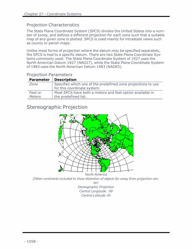
Chapter 27 - Coordinate Systems
Projection CharacteristicsThe State Plane Coordinate System (SPCS) divides the United States into a num-ber of zones, and defines a different projection for each zone such that a suitablemap of any given zone is plotted. SPCS is used mainly for intrastate views suchas county or parish maps.
Unlike most forms of projection where the datum may be specified separately,the SPCS is tied to a specific datum. There are two State Plane Coordinate Sys-tems commonly used. The State Plane Coordinate System of 1927 uses theNorth American Datum 1927 (NAD27), while the State Plane Coordinate Systemof 1983 uses the North American Datum 1983 (NAD83).
Projection ParametersParameter DescriptionZone Specifies which one of the predefined zone projections to use
for this coordinate system.Feet orMeters
Most SPCS have both a meters and feet option available inthe predefined list.
Stereographic Projection
North America(Other continents included to show distortion of objects far away from projection cen-
ter)Stereographic ProjectionCentral Longitude: -90Central Latitude: 45
- 1058 -

Surfer User's Guide
Projection CharacteristicsThe Stereographic projection is an azimuthal, conformal projection. In a Ste-reographic projection, scale is constant along any circle circumscribed aroundthe center of the projection. Distortion is minimal at the center and becomesextreme with distance from the center. Generally, this projection is not used forregions larger than a continent or a hemisphere due to distortion effects. The Ste-reographic projection is often used for maps of the poles.
Projection ParametersParameter DescriptionName Specifies the units used in the map.Scale Specifies the unit scale of the projected map, relative to
meters. For example, a scale of one means one unit in the pro-jected map equals one meter; a scale of two means two unitsin the projected map equal one meter; etc.
False East-ing
Specifies the false easting, or horizontal offset, of the pro-jected coordinates, in meters. False Eastings and False Nor-things are added to the underlying "projected" coordinates asa way to arbitrarily offset their internal XY coordinates afterthe projection. Unless you have a reason for using these off-set values, do not use them. These values do not affect thelatitude/longitude coordinates for the map, only the internalcoordinates used to plot the map on the screen. If you useFalse Easting and False Northing offsets for a map, any sub-sequent boundaries you append to the map must also usethese same offsets if you want the imported boundaries to bedrawn in the correct relative position to the existing bound-aries.
False Nor-thing
Specifies the false northing, or vertical offset, of the projectedcoordinates, in meters. See above.
CentralScale Factor(KO)
Specifies the central scaling factor for the projection. Thisvalue is often set to 1.0, but may be set to another value forspecific applications.
Central Lon-gitude
Specifies the central longitude of the projection in degrees.The Central Longitude value typically should be defined as thelongitudinal center of the map you are going to produce.
Central Lat-itude
Specifies the central latitude of the projection in degrees. TheCentral Latitude value typically should be defined as the lat-itudinal center of the map you are going to produce.
- 1059 -

Chapter 27 - Coordinate Systems
Transverse Mercator Projection
State of OregonTransverse Mercator Projection
Central Latitude: 41.75Central Longitude: -120.5
Projection CharacteristicsThe Transverse Mercator projection is also known as the Gauss-Kruger pro-jection or the Gauss Conformal projection. This projection is cylindrical and con-formal. In this projection, scale is constant along any straight line that is parallelto the specified central meridian. Scale increases with distance from the centralmeridian. Distortion is minimal near the center of the projection and increasesdramatically with distance from the center. Distortion is considerable when pro-jecting coordinates that fall within a few degrees of the poles. This projection isuseful primarily for mapping small regions no more than a few degrees across,particularly high-aspect regions (regions taller than they are wide). A limitationof this projection is that coordinates at or near the poles cannot be projected. Anadditional limitation is that regions larger than a quadrant (e.g. having greaterthan 90 degrees extent either vertically or horizontally) result in portions of theprojected image folding over each other due to constraints of the mathematicalformulas used. The projection is best used with areas that are no greater than 30degrees wide or tall, and preferably with areas that are much smaller.
Projection ParametersParameter DescriptionName Specifies the units used in the map.Scale Specifies the unit scale of the projected map, relative to
meters. For example, a scale of one means one unit in the pro-jected map equals one meter; a scale of two means two unitsin the projected map equal one meter; etc.
- 1060 -
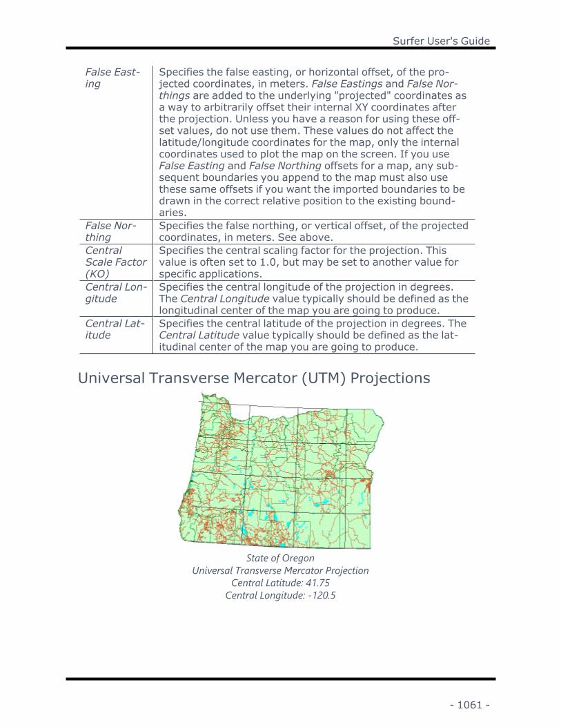
Surfer User's Guide
False East-ing
Specifies the false easting, or horizontal offset, of the pro-jected coordinates, in meters. False Eastings and False Nor-things are added to the underlying "projected" coordinates asa way to arbitrarily offset their internal XY coordinates afterthe projection. Unless you have a reason for using these off-set values, do not use them. These values do not affect thelatitude/longitude coordinates for the map, only the internalcoordinates used to plot the map on the screen. If you useFalse Easting and False Northing offsets for a map, any sub-sequent boundaries you append to the map must also usethese same offsets if you want the imported boundaries to bedrawn in the correct relative position to the existing bound-aries.
False Nor-thing
Specifies the false northing, or vertical offset, of the projectedcoordinates, in meters. See above.
CentralScale Factor(KO)
Specifies the central scaling factor for the projection. Thisvalue is often set to 1.0, but may be set to another value forspecific applications.
Central Lon-gitude
Specifies the central longitude of the projection in degrees.The Central Longitude value typically should be defined as thelongitudinal center of the map you are going to produce.
Central Lat-itude
Specifies the central latitude of the projection in degrees. TheCentral Latitude value typically should be defined as the lat-itudinal center of the map you are going to produce.
Universal Transverse Mercator (UTM) Projections
State of OregonUniversal Transverse Mercator Projection
Central Latitude: 41.75Central Longitude: -120.5
- 1061 -

Chapter 27 - Coordinate Systems
Projection CharacteristicsThe Universal Transverse Mercator system, commonly known as UTM, dividesthe Earth into sixty discrete zones, each representing a vertical slice of the globespanning six degrees of longitude. A Transverse Mercator projection is applied toeach zone with the central meridian of the projection at the center of the givenzone and the central latitude of the projection at the equator. This coordinate sys-tem is the basis for many standardized regional maps, such as tract or neigh-borhood maps by the US Census Bureau and topographic quadrangles by the USGeological Survey. UTM is not generally used for coordinates outside the rangeof -80 to +84 degrees latitude due to the distortion inherent in Transverse Mer-cator projections near the poles.
Projection ParametersParameter DescriptionName Specifies the units used in the map.Scale Specifies the unit scale of the projected map, relative to
meters. For example, a scale of one means one unit in the pro-jected map equals one meter; a scale of two means two unitsin the projected map equal one meter; etc.
CentralScale Factor(KO)
Specifies the central scaling factor for the projection. Thisvalue is often set to 1.0, but may be set to another value forspecific applications.
Central Lon-gitude
Specifies the central longitude of the projection in degrees.The Central Longitude value typically should be defined asthe longitudinal center of the map you are going to produce.For example, the value -95.5 represents the geographic cen-ter of the United States, so the map of the U.S. is drawnupright.
Central Lat-itude
Specifies the central latitude of the projection in degrees. TheCentral Latitude value should be defined as the latitudinal cen-ter of the map you are going to produce.
Projectionin SouthernHemisphere
Choose True if your map is in the southern hemisphere.Choose False if your map is in the northern hemisphere.
Van der Grinten Projection
- 1062 -

Surfer User's Guide
World MapVan der Grinten Pro-
jectionCentral Longitude: 0
Projection CharacteristicsThis projection is typically used for maps of the world and the scale is accuratealong the equator. This projection was used by the National Geographic for worldmaps. The central longitude and the equator are straight lines and the poles aregreatly distorted.
To get good results with the Van der Grinten projection, the map must havecoordinates between +/-180 degrees longitude and +/- 90 degrees latitude.Surfer does not wrap around +/-180 degrees longitude. The example map isusing world-proj.gsb as the base map. If you are using world-scale maps, thecentral longitude generally cannot be set far from 0 degrees since there is nowrap around in Surfer.
Projection ParametersParameter DescriptionName Specifies the units used in the map.Scale Specifies the unit scale of the projected map, relative to
meters. For example, a scale of one means one unit in the pro-jected map equals one meter; a scale of two means two unitsin the projected map equal one meter; etc.
False East-ing
Specifies the false easting, or horizontal offset, of the pro-jected coordinates, in meters. False Eastings and False Nor-things are added to the underlying "projected" coordinates asa way to arbitrarily offset their internal XY coordinates afterthe projection. Unless you have a reason for using these off-set values, do not use them. These values do not affect thelatitude/longitude coordinates for the map, only the internalcoordinates used to plot the map on the screen. If you useFalse Easting and False Northing offsets for a map, any sub-sequent boundaries you append to the map must also usethese same offsets if you want the imported boundaries to bedrawn in the correct relative position to the existing bound-aries.
False Nor-thing
Specifies the false northing, or vertical offset, of the projectedcoordinates, in meters. See above.
- 1063 -

Chapter 27 - Coordinate Systems
Central Lon-gitude
Specifies the central longitude of the projection in degrees.The Central Longitude value typically should be defined as thelongitudinal center of the map you are going to produce.
Golden Software Reference FilesIf you have looked in a folder that contains data, boundary files, or grid files cre-ated by Surfer, you may have noticed files with a .GSR2 extension in the folder.These Golden Software Reference files are created when you save a projectedfile from Surfer. For example, if you create a data file and use the Data |Coordinate System | Assign Coordinate System command, when you save thedata file, you will see both the filename.dat and filename.dat.gsr2 in the dir-ectory.
The Golden Software Reference files contain the projection settings used to pro-ject the data in Surfer. Projection, datum, and georeference information arestored in the .GSR2 file. When you create a map from data or a grid that has anassociated .GSR2 file into Surfer, the projection information is used when dis-playing the map. If the Golden Software Reference file is deleted, the boundarycan be imported but it will not be projected properly.
Surfer .SRF file format retains all of the information in a map, including pro-jection information.
Latitude and Longitude CoordinatesIn Surfer , worksheet data can be projected using a projection. The projecteddata can then be used to create a grid file and a grid based map.
Latitude and longitude are spherical coordinates used to locate a point on theearth. Many maps do not need to take the curvature of the earth into account.For maps covering relatively small land areas, such as a state or small group ofstates, the earth can be assumed to be flat. In these cases, the lat-itude/longitude coordinates can be plotted on a Cartesian coordinate system.Maps plotted in this way must use different scaling in the two dimensions to min-imize distortion on the map.
Surferonly plots latitude and longitude coordinates in decimal degrees. You cansee DMS to DD for information on converting DMS to decimal degrees withSurfer and Latitude and Longitude Coordinates in Decimal Degrees for inform-ation on converting degrees-minutes-seconds to decimal degrees manually.
- 1064 -

Surfer User's Guide
Parallels define lines of constant latitude. Meridians define lines of constant longitude. ThisAlbers projected map makes use of graticule lines to indicate the relationship.
LatitudeLatitude is the Y coordinate and defines north-south global position measuredfrom the equator. Lines of constant latitude are called parallels because theydefine a series of rings parallel to the equator. Parallels run east-west, but definenorth-south position on the globe. Parallels are designated in degrees from 0° atthe Equator to 90° at the poles. Surfer uses the convention that parallels arepositive north of the equator (north latitudes), and negative south of the equator(south latitudes). Designations such as 45° indicate a position 45 degrees northof the equator, while -65° indicates a position 65 degrees south of the equator.At any position on the globe, the distance covered by a degree of latituderemains nearly constant.
LongitudeLongitude is the X coordinate and indicates east-west position on the globe.Lines of constant longitude are called meridians. Meridians lie at right angles tothe parallels and are half-circles drawn from the North Pole to the South Pole.One meridian is designated as the prime meridian. The prime meridian most com-monly in use in the United States runs through Greenwich, England, althoughthere are several other prime meridians in use throughout the world. Longitudeis measured 180° east and 180 degrees west from the prime meridian. InSurfer, longitude is positive east (east longitude) of the prime meridian, andnegative west of the prime meridian (west longitude). A designation such as -105° is used to indicate a location 105 degrees west of the prime meridian.Meridians converge at the poles so the distance covered by one degree of lon-gitude decreases as you move north or south from the equator.
- 1065 -

Chapter 27 - Coordinate Systems
Latitude and Longitude in Decimal DegreesLatitude and Longitude coordinates are often presented in degrees, minutes, andsecond, such as 39°25'30" (39 degrees, 25 minutes, 30 seconds). However,Surfer can only plot values in decimal degrees. So, for example, 39°25'30" isreferred to as 39.425 in Surfer.
Converting from degrees, minutes, and seconds is easy. There are 60 minutes inone degree and 3600 seconds in one degree. To convert minutes and seconds todecimal degrees, divide minutes by 60, divide seconds by 3600, and then addthe results to obtain the decimal equivalent.
Convert columns of DMS values with the DMS to DD command.
Conversion Equation:
Decimal Degrees = Degrees + (Minutes / 60) + (Seconds / 3600)
ExampleConsider the latitude value 39°25'30". This value needs to be converted todecimal degree in order to use it in Surfer.
To convert 39°25'30" to decimal degrees:
1. First, convert minutes (25') and seconds (30") to their degree equivalentsand add the results.
25'/60 = 0.4167
30"/3600 = 0.0083
0.4167 + 0.0083 = 0.425
2. Then, add this number to the number of degrees.
39 + 0.425 = 39.425
3. The final result is the decimal degree value.
39°25'30" = 39.425°
How to Convert from NAD27 to NAD83 UsingNTv2NTv2 is the Canadian government's officially sanctioned method of convertingCanadian map data from the old NAD27 datum to the NAD83 datum. If you areconverting from Lat/Long WGS84 (or any coordinate system with a datum other
- 1066 -

Surfer User's Guide
than NAD27) to NAD83, you will not need to use NTv2. If you are converting datawith a datum of NAD83 back to NAD27, you will not need to use NTv2. Again,this is only a method of converting data from the NAD27 datum to the NAD83datum.
To perform the conversion, you need an additional grid shift file in the Surferinstallation directory. Golden Software cannot supply this file, but you can down-load it from the Natural Resources Canada website.
To convert NAD27 to NAD83 using NTv2, the first step is to download the con-version file.
1. Download the ZIP file from the Natural Resources Canada webpage. Youcan find more information about this NTv2 grid shift file from their site.
2. Extract the file NTV2_0.GSB to the Surfer installation directory (by defaultthis is C:\Program Files\Golden Software\Surfer).
Now you can use the NAD 1927 - Canada (NTV2) datum as the source coordinatesystem in Surfer when converting to another system with the NAD83 datum. Forexample:
1. Select a map layer in the Contents window (i.e. Contours).
2. In the Properties window, click the Coordinate System tab and click theSet button.
3. Select the coordinate system for the layer (i.e. Predefined | UTM | NorthAmerica | North America NAD27 UTM zone 12N)
4. Click Modify.
5. Change the datum to NAD 1927 – Canada (NTV2).
6. Click OK, then OK again. The souce coordinate system is specified to usethe NTv2 datum transformation.
7. To convert the map to NAD83, select Map in the Contents window.
8. In the Properties window, click the Coordinate System tab and click theChange button.
9. Select the NAD83 coordinate system you want the map to be displayed in(i.e. Predefined | UTM | North America | North America NAD83 UTM zone12N).
10. Click OK and the map is converted.
- 1067 -
Chapter 27 - Coordinate Systems
Projection ReferencesDent, Borden D., Cartography, Thematic Map Design, Wm. C. Brown Publishers,Dubuque, 1990.
Greenhood, David, Mapping, The University of Chicago Press, Chicago, 1964, pp.113-171.
Robinson, A.H., et al., Elements of Cartography, Fifth Edition, John Wiley & Sons,New York, 1984, pp. 75-105.
Snyder, John P., Map Projections - A Working Manual, U.S. Geological Survey Pro-fessional Paper 1395, Washington D.C., Department of the Interior, 1987.
Verhoogan, John, Francis., J. Turner, Lionel E. Weiss, Clyde Wahrhaftig, WilliamS. Fyfe, The Earth: An Introduction To Physical Geology, Holt, Rinehart and Win-ston, Inc., New York, 1970.
Coordinate Systems Overview, http://www.-colorado.edu/geography/gcraft/notes/coordsys/coordsys_f.html, July 2, 2001.
Map Projection Overview, http://www.-colorado.edu/geography/gcraft/notes/mapproj/mapproj_f.html, July 2, 2001.
Map Projection Home Page, http://www.geography.hunter.cuny.edu/mp/, June16, 2004.
Datums, Ellipsoids, Grids, and Grid Reference Systems, Defense MappingAgency Technical Manual 8358.1, August 2, 2004.
Matching the Map Projection to the Need, http://www.gis.psu.edu/projection/,June 16, 2004.
- 1068 -

Chapter 28 - Creating and EditingFeatures
Features Tab CommandsThe Features tab in the plot document has the following commands:
Text Creates a text blockPolyline Create a polylinePolygon Creates a polygonPoint Creates a pointSplinePolyline
Creates a spline polyline
Range Ring Creates a range ringRectangle Creates a rectangle or squareRoundedRectangle
Creates a rectangle with rounded corners
Ellipse Creates an ellipse or circleGroup Combine objects into a groupUngroup Split grouped objectsChange Convert selected objects to other object types: Points to
Polyline, Points to 3D Polyline, Polyline to Polygon, Polylineto Points, Polyline to 3D Polyline Polygon to Polyline, Poly-gon to 3D Polygon
Reshape Moves, adds, or deletes points in the selected polyline, poly-gon, or spline polyline
Thin Simplify polylines and polygons by removing additionalpoints
Smooth Smooth polylines and polygons by adding additional pointsCrop Crop an image or raster base layerConnectPolylines
Connect two or more polylines
BreakPolyline
Break a polyline at a specific point
Break atIntersections
Break polylines at intersections with polylines and polygons
Alpha Shape Creates a polygon boundary around a set of three or moreselected data points
Union of Poly-gons
Create a new polygon by combining polygons
IntersectPolygons
Create a new polygon from intersecting regions of selectedpolygons
- 1069 -

Chapter 28 - Creating and Editing Features
Difference ofPolygons
Create new polygons from the difference between selectedpolygons
Buffer Creates a polygon at a specified distance around or withinselected objects
IntersectionPoints
Creates points at intersections of two or more polyline orpolygon objects
Triangulation Creates a Delaunay triangulationThiessenPolygons
Creates Thiessen (Voroni) polygons
Split Split complex polygons into multiple single ring polygonsCombine Combine multiple polygons into a single complex polygon
Text
Click the Home | Insert | Textcommand, the button, or the Features |Insert | Text command to create text in the plot document. The typeface, size,style, alignment, opacity, and color can be set for individual characters in a textblocks.
Drawing TextTo create text:
1. Click the Home | Insert | Text command.2. The cursor changes to a cross hair. Left-click in the plot window where you
want text to appear.3. Enter text into the Text Editor dialog.4. Highlight the text to be changed and set the properties by clicking the appro-
priate button or option in the Text Editor dialog. The math text instructionsare not used in this dialog.
5. Click OK to return to the plot window.6. Press the ESC key or click another toolbar button to end draw mode.
The text appears inside a movable, sizable text box. Click on the box and drag itto move the box to the desired location.
Editing Text PropertiesThe text can be edited in the Text Editor. To edit existing text content, double-click on the text to open the Text Editor, or you can edit text content in theProperties window:
1. Click on the text object in the plot window or the Contents window to select it.2. In the Properties window, the text and font properties can be edited.
- 1070 -

Surfer User's Guide
3. To change the font properties, click on the next to Font Properties. Setany font properties for all of the text in the text block.
4. To change the text, click on the next to Text Properties. Click in the boxnext to Text to edit the text. For a single line of text, highlight the charactersand type the desired text. Math text instructions can be added directly to theText line in the Properties window.
5. To include multiple lines of text or to edit individual characters in the textblock, click the button. Edit the text in the Text Editor .
6. When all changes have been made in the Text Editor , click OK to view thechanges in the plot window.
Text PropertiesThe Font, Size, Color, Opacity, and Style can be set for text blocks in the TextEditor dialog when typing text. These options can be set in the Properties win-dow in the Font Properties section after the text is drawn. The Properties windowalso includes the Drop Shadow and Info pages.
Default PropertiesSet the default font properties with the File | Options command. In the DefaultProperties section, click on Font to set the default font and text properties.
Text EditorYou can access the Text Editor by creating new text or by editing existing text.Type the desired text into the text editor, add templates and symbols, date/timestamps, and apply unique formatting. Add tabs in the Text Editor by pressingCTRL + TAB. When you click OK, the text in the text editor is parsed to math textinstructions and the Text field is updated in the Properties window Text page.
Type or edit text in the Text Editor.
- 1071 -

Chapter 28 - Creating and Editing Features
Text AppearanceThe top row of tools and buttons change the appearance of currently selectedtext. Additionally, subsequent text will appear with the selected options.
l Select a typeface from the list in the upper left corner of the dialog.l Set the size (in points) of the typeface in the box to the right of the typefacelist.
l Click the colored button to the right of the size box to display the color paletteand change the text color. Click the Custom button at the bottom of the colorpalette to use a custom color.
l Several styles (including bold , italic , underline , and strikethrough ) canbe applied to the text. Note that some typefaces, such as Symbol, do not sup-port bold or italicized text.
l You can left justify , center , or right justify the text in the bounding box.These options only make a difference with multiple lines of text.
Superscripts and SubscriptsWhen working with superscripts and subscripts, you can type the character, high-light it, and then click the superscript or subscript buttons. Alternatively, youcan click the superscript or subscript button and then type the characters. Clickthe superscript or subscript button a second time to return to the normal sizefont and placement.
After clicking the or button, the superscript or subscript will be sized relativeto the text immediately preceding it until the Text Editor is closed. Superscriptsand subscripts are 60% the size of normal text by default. To maintain the rel-ative sizing, select both the normal text and the superscript or subscript andthen change the font size. For example, if 'x2' is typed in 10pt font and the '2' issuperscripted, the font size for the '2' will be 6pt font, x2. Next if x2 is selectedand font size is increased to 15pt, the superscript will be size 9pt font, x2. Oncethe Text Editor is closed, the superscripts and/or subscripts must be sized inde-pendently in the Text Editor. However, the Size (points) field in the Text Prop-erties window page can be used to relatively increase the size of the normal,superscripted, and subscripted text all at same time.
If the default superscript or subscript placement is not sufficient, you can high-light the text and enter a number in the character position box to raise orlower text from the midpoint of the existing line. You can also change the char-acter position by clicking the buttons. Click the reset button to reset the high-lighted character's position to the default position.
You can click in any field in a template and use the boxes below Sub Position tomodify the position of the field in a template. The values are offsets from themain character's zero position and are in pixels. How far each value moves thetemplate field is determined in part by the font size. Positive values move thefield to the right and up.
- 1072 -

Surfer User's Guide
Editing ToolsText can be edited using the following tools:
l You can cut , copy , or paste selected text, or paste objects from the clip-board into the Text Editor.
l Click the Insert Symbol button to open the Symbol Properties dialog andadd a symbol to the text block.
l Click the Insert Date/Time button to open the Date/Time Format Builder dia-log and enter a date and/or time format. The current date and/or time will beupdated and displayed in the project every time the Surfer project isredrawn.
l Click Insert Template button to open the Template Library dialog and enterequations based on a template.
l You can undo and redo actions.
l You can magnify text in the Text Editor by entering a new number in theZoom box. By default, the text is zoomed to a reasonable level.
l You can adjust the opacity of the selected text by entering a new number inthe Opacity box. Enter a value between zero (no opacity, full transparency)and 100% (full opacity, no transparency).
Sub PositionYou can click in any field in a template and use the boxes belowSub Position to modify the position of the field in a template.The values are offsets from the main character's zero positionand are in pixels. How far each value moves the template fieldis determined in part by the font size. Positive values move thefield to the right and up. The Sub Position values are only avail-able when editing text in a template field.
BackgroundClick the Background button to open the Background Color dialog to set thebackground fill properties for the text object. To edit the background fill for textthat already exists, change the Background and Background Opacity options inthe Properties window on the Text tab.
Set the background color and opacity in the Back-ground Colordialog.
- 1073 -

Chapter 28 - Creating and Editing Features
Text Box AlignmentA reference point is the point clicked on in the view window after clicking theFeatures | Insert | Text command. The text box is horizontally and verticallyaligned relative to the reference point. The default position is that the referencepoint is at the upper left corner of the bounding box (left, top).
l Right horizontally aligns the text box so that the reference point is to the rightof the text box.
l Left horizontally aligns the text box so that the reference point is to the left ofthe text box.
l Center horizontally centers the text box on the reference point.l Bottom vertically aligns the text box so that the reference point is below thetext box.
l Top vertically aligns the text box so that the reference point is above the textbox.
l Baseline vertically aligns the text box so that the reference point is located atthe base of the text. The baseline is the imaginary line along which charactersare positioned as they are drawn. Descenders on characters are drawn belowthe baseline.
To edit the alignment for text that already exists, change the Horizontal Align-ment and Vertical Alignment options in the Properties window on the Text tab.
Resize the Text EditorTo make the Text Editor larger or smaller, click and drag on the lower leftcorner of the dialog. When the dialog is the desired size, release the mouse but-ton.
OK or CancelClick the OK button to save your changes and close the Text Editor. Click theCancel button to exit the Text Editor without saving your changes.
Symbol Properties DialogThe Symbol Properties dialog can be used to insert symbols from any font intoa text block in the Text Editor or change for selected objects in the text template.
You can set default symbol properties through the Options command. In theOptions dialog, scroll down to the Symbol section to access these defaults.Changes made in the Options dialog affect all subsequent documents. Customsymbols can be created using a third party TrueType font editing software.
- 1074 -

Surfer User's Guide
Specify a Symbol Set and Symbol in the Symbol Prop-erties dialog.
Symbol SetThe Symbol Set displays all the fonts installed on the computer. Click on the sym-bol set name and then you can choose a new font from the list.
SymbolClick on the displayed symbol to choose a Symbol from the symbol palette. Thenumber of the selected symbol is indicated in the title bar above the palette andadjacent to the symbol in the Properties window. Add 32 to the value to use thesymbol in a script or when using a Symbol column with a post map.
The symbol index is the symbol or glyph number as it appears in the title barabove the palette and adjacent to the symbol in the Properties window.
Text Editor Template LibraryYou can use text templates from the Template Library to add equation formatsinto the Text Editor.
Template Library DialogClick the button in the Text Editor dialog to open the Template Library dia-log.
- 1075 -

Chapter 28 - Creating and Editing Features
Use the Template Library to insert templates that can be used to input equa-tions into the Text Editor .
Up/DownUse the up and down buttons at the left side of the screen to reposition a selec-ted template in the library.
NewClick the New button to create a new template. The Symbol Properties dialogopens. Select a base symbol, click OK, and the Create\Edit Template dialogappears.
EditClick the Edit button to edit the selected template in the Create\Edit Templatedialog.
CopyClick the Copy button to duplicate the selected template. The copied template isautomatically pasted at the end of the template library.
DeleteClick the Delete button to delete a template.
ImportClick the Import button to use a different Golden Software template library file[.LBT].
- 1076 -

Surfer User's Guide
InsertClick the Insert button to insert a template into the Text Editor.
CloseClick the Close button to close the template library without inserting a templateinto the Text Editor.
ExampleFor example, to use the Template Library to create an image of the square rootof a number:
1. Click the Home | Insert | Text command.2. Click on the view window where you want the text to be displayed.3. In the Text Editor dialog, click the button.
4. In the Template Library dialog, select the template and click theInsert button.
5. In the Text Editor, the template is inserted as . Enter the numeric value,
for example the number nine, and click OK to display the in the view win-dow.
Text Editor Test TemplateClick Test in the Create/Edit Template dialog to see what the final template willlook like without the string and line symbols.
The Test Template dialog displays the final tem-plate.
- 1077 -

Chapter 28 - Creating and Editing Features
Text Editor Create/Edit TemplateTo add custom templates to the Text Editor template library, click the New but-ton in the Template Library dialog. To edit an existing template, select the tem-plate and click the Edit button.
If you are creating a new template select a symbol and click the OK buttonbefore the Create/Edit Template dialog opens.
Use the Create/Edit Template dialog to create new templates oredit existing templates from the template library.
Arrow ButtonsClick the arrow buttons on the left and top sides of the dialog to position a stringor a line. The numbers at the edge of the arrow buttons show the string location.
Add StringClick the Add String button to add a text string box. Text string boxes in the tem-plates allow numbers or letters to be entered into the template in the TextEditor.
Add LineClick the Add Line button to add a line to the template.
FontSelect a text string (#) and click the Font button to open the Text Propertiesdialog and set the properties of the text string.
- 1078 -

Surfer User's Guide
Set the properties of the text string in the Text Properties dia-log.
DeleteSelect a text string or a line, and then click the Delete button to remove it fromthe template.
String AlignmentOnce a text string is created (#), you can set the String Alignment of the enteredtext. Text is entered after the template has been inserted into the text editor.Refer to the Text Box Alignment section of the Text Editor topic for more inform-ation on alignment.
Line AlignmentYou can set the Line Alignment to extend to the right, left, top, or bottom of themarker by selecting a line and clicking one of the Line Alignment buttons. Theline length depends on the bounding box size.
Use the Line Alignment buttons todetermine how lines are drawn.
Main SymbolClick the Main Symbol button open the Symbol Properties dialog and change themain symbol appearing in the template.
To delete the main symbol, click the Main Symbol button to open the SymbolProperties dialog. Choose an empty symbol box, such as symbol number zero.
- 1079 -

Chapter 28 - Creating and Editing Features
TestClick the Test button to open the Test Template dialog and see how the templatewill appear in the Text Editor.
1. Use the Symbol Setmenu to select a set of symbols or text.
2. Highlight the desired symbol and click OK. The Create/Edit Template dia-log opens.
3. Use the following instructions with the Create/Edit Template dialog.
Text PropertiesIn the Create/Edit Template dialog, click the Font button to open the Text Prop-erties dialog. Set the font attributes for the string.
The Text Properties dialog allows you to set the text attributesfor the template text string.
Text Editor Template Editor ExampleWhen entering complex equations in a text box, it is sometimes necessary to cre-ate one or more templates to create the equation. When the templates are cre-ated they can be inserted into the text box. Templates can be imbedded withinother templates. The following example contains two templates: a square roottemplate and a division template.
Example 1 - Square Root TemplateThis example creates a square root template that will be used in the secondexample.
- 1080 -
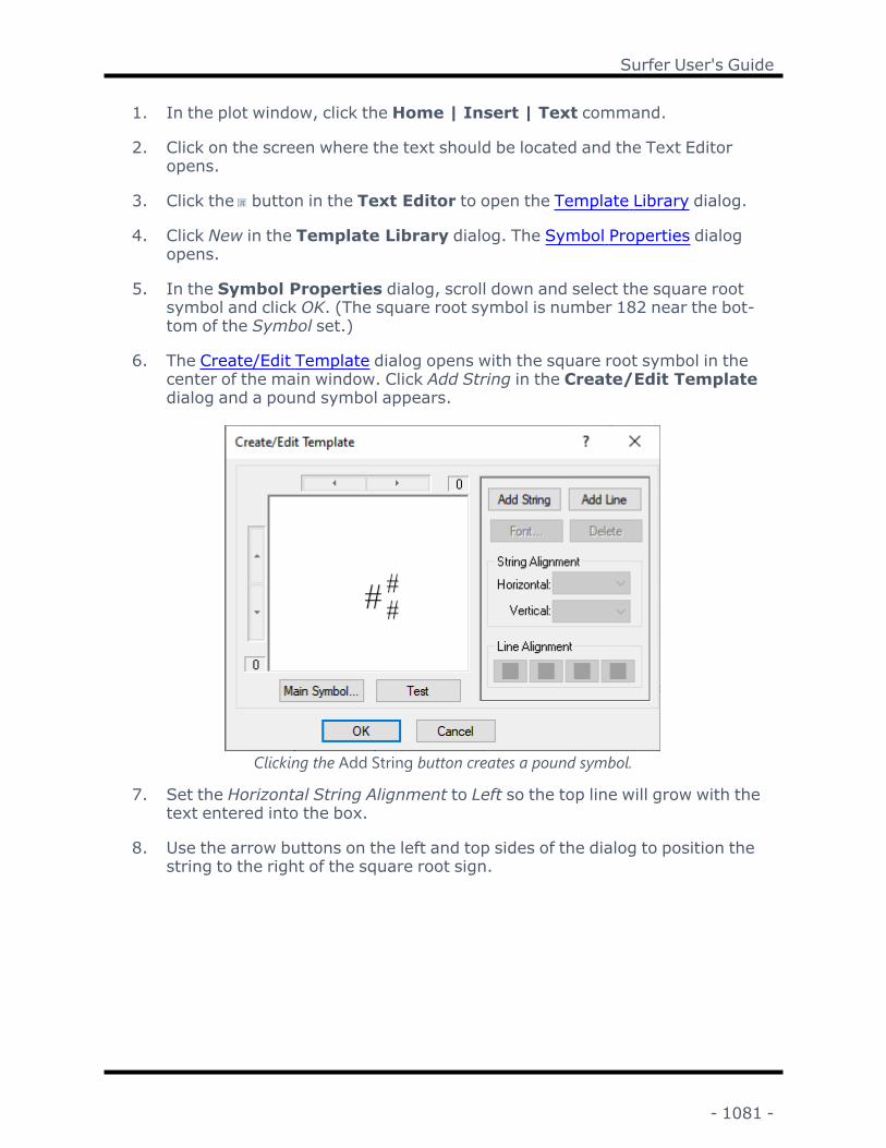
Surfer User's Guide
1. In the plot window, click the Home | Insert | Text command.
2. Click on the screen where the text should be located and the Text Editoropens.
3. Click the button in the Text Editor to open the Template Library dialog.
4. Click New in the Template Library dialog. The Symbol Properties dialogopens.
5. In the Symbol Properties dialog, scroll down and select the square rootsymbol and click OK. (The square root symbol is number 182 near the bot-tom of the Symbol set.)
6. The Create/Edit Template dialog opens with the square root symbol in thecenter of the main window. Click Add String in the Create/Edit Templatedialog and a pound symbol appears.
Clicking the Add String button creates a pound symbol.
7. Set the Horizontal String Alignment to Left so the top line will grow with thetext entered into the box.
8. Use the arrow buttons on the left and top sides of the dialog to position thestring to the right of the square root sign.
- 1081 -

Chapter 28 - Creating and Editing Features
Use the up/down and left/right arrows to move the pound sign to the right of the square rootsymbol.
9. Click Add Line.
10. Click Extend Right in the Line Alignment group box.
11. Use the up/down and left/right arrow buttons to position the line above thestring and to the upper right side of the square root sign.
Position the line so it is next to the square root sym-bol.
12. Click Test to view the final template. Click Close in the Test Template dia-log.
13. Click OK to add this template to the template library. Leave the TemplateLibrary dialog open for the next example.
- 1082 -

Surfer User's Guide
Example 2 - Division TemplateThis example uses the square root template created in the first example.
1. Click New in the Template Library dialog.
2. In the Symbol Properties dialog, Select empty symbol for the main sym-bol and click OK . The empty symbol is the first symbol ( number zero) inthe Symbol set.
3. Click Add Line in the Create/Edit Template dialog.
4. Click Extend Right in the Line Alignment group box.
5. Click Add String .
6. Use the up/down and left/right arrow buttons to position the string abovethe line, and to the right of the line symbol.
7. Click Add String again.
8. Use the up/down and left/right arrow buttons to position the second stringbelow and to the right of the line symbol.
The two string symbols appear to the upper right and lower right of the line sym-bol.
9. Click Test to view the template. Click Close in the Test Template dialog.
10. Click OK to add this template to the template library. Leave the TemplateLibrary dialog open for the next example.
- 1083 -

Chapter 28 - Creating and Editing Features
Using Multiple TemplatesOnce these templates have been created, they can be inserted into the TextEditor. Templates can be inserted into other templates.
To create the dividing/square root equation:
1. If the template library is not open, in the Text Editor click the button toopen the Template Library.
2. Highlight the new square root template in the Template Library, and clickInsert.
3. You will be asked to save the changes in the template library. Click Yes. Thesquare root symbol appears in the Text Editor.
4. You may want to make the symbol larger. Adjust the Zoom of the imagewith the zoom up arrow.
5. Click inside the text box underneath the square root sign.
6. Click to open the Template Library.
7. Click the newly created division template in the Template Library andclick Insert.
8. The division template is inserted under the square root sign.
9. Click in the numerator box and type the letter X.
10. Click in the denominator box and type the number 2.
Once the text is entered into the templates the substrings (added lines or addedsymbols) can be moved around. For example, the top line on the square rootsymbol may not quite touch the square root. Select the line by clicking just to theleft of the line where the pound sign (#) would be in theCreate/Edit Tem-platedialog. Use theSub Positionboxes in theText Editorto move the line around.
Date/Time Format Builder DialogIn the Text Editor dialog, click the button to open the Date/Time FormatBuilder dialog. From the worksheet, click the button in the Format Cells dia-log Number page. The Date/Time Format Builderdialog is also accessed byclicking the button in the Date/Time Format field in the Label Properties sec-tion of the Properties window when the label format Type is Date/time. Whenthe Date/Time Format Builder is used to insert date/time math text instruc-tion with the Text Editor, the date/time will update every time the projectupdates.
- 1084 -
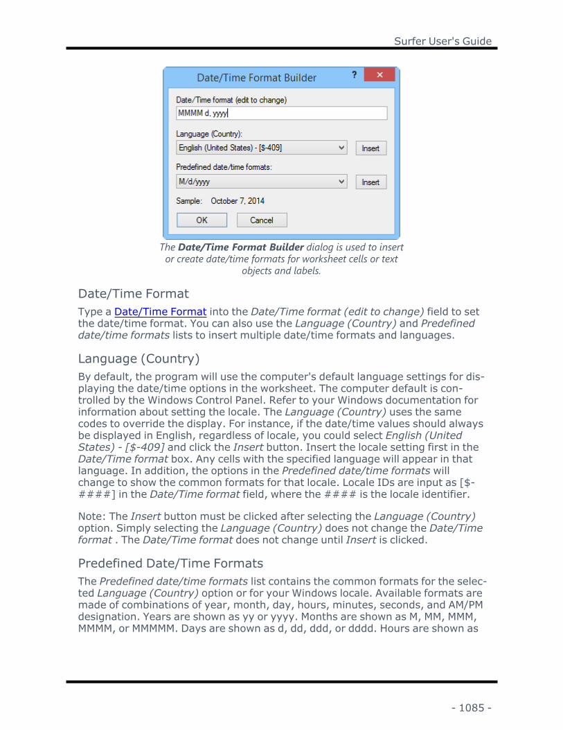
Surfer User's Guide
The Date/Time Format Builder dialog is used to insertor create date/time formats for worksheet cells or text
objects and labels.
Date/Time FormatType a Date/Time Format into the Date/Time format (edit to change) field to setthe date/time format. You can also use the Language (Country) and Predefineddate/time formats lists to insert multiple date/time formats and languages.
Language (Country)By default, the program will use the computer's default language settings for dis-playing the date/time options in the worksheet. The computer default is con-trolled by the Windows Control Panel. Refer to your Windows documentation forinformation about setting the locale. The Language (Country) uses the samecodes to override the display. For instance, if the date/time values should alwaysbe displayed in English, regardless of locale, you could select English (UnitedStates) - [$-409] and click the Insert button. Insert the locale setting first in theDate/Time format box. Any cells with the specified language will appear in thatlanguage. In addition, the options in the Predefined date/time formats willchange to show the common formats for that locale. Locale IDs are input as [$-####] in the Date/Time format field, where the #### is the locale identifier.
Note: The Insert button must be clicked after selecting the Language (Country)option. Simply selecting the Language (Country) does not change the Date/Timeformat . The Date/Time format does not change until Insert is clicked.
Predefined Date/Time FormatsThe Predefined date/time formats list contains the common formats for the selec-ted Language (Country) option or for your Windows locale. Available formats aremade of combinations of year, month, day, hours, minutes, seconds, and AM/PMdesignation. Years are shown as yy or yyyy. Months are shown as M, MM, MMM,MMMM, or MMMMM. Days are shown as d, dd, ddd, or dddd. Hours are shown as
- 1085 -

Chapter 28 - Creating and Editing Features
h, hh, H, HH, or [h]. Minutes are shown as m, mm, or [mm]. Seconds are shownas ss, ss.0, ss.00, ss.000, ss.0000, or [ss]. AM/PM designation is shown as tt orTT. BC/AD designation is shown as gg or GG. BCE/CE designation is shown as g,G, ggg, or GGG. Refer to formats for information about each specific option.
Note: The Insert button must be clicked after selecting the Predefined date/timeformats option. Simply selecting the Predefined date/time formats does notchange the Date/Time format. The Date/Time format does not change untilInsert is clicked.
SampleThe Sample text updates to show a sample of the current entry in the Date/Timeformat (edit to change) field.
PolylineA polyline is a collection of one or more connected line segments. Click the
Home | Insert | Polylinecommand, the button, or the Features |Insert | Polyline command to draw a polyline. Polylines can be converted to 3Dpolylines with the addition of Z coordinates to vertices.
To draw a polyline:1. Click the Home | Insert | Polyline command to begin drawing a polyline.2. The cursor changes to a cross hair cursor to indicate drawing mode.3. Move the cursor over the location for the start of the polyline and click the left
mouse button.4. Move the cursor to the next position along the line and click again.5. Continue this procedure until you click at the final point for the line. Press the
ENTER key.6. To end drawing mode, click on another tool button or press the ESC key on
your keyboard.
Drawing Tipsl Click the endpoints of the line to draw a straight line, or click several points tocreate an irregularly shaped line.
l Click the right mouse button to remove the last drawn point. This can be donerepeatedly.
l Click and hold the left mouse button to create a continuous stream of points.l If the CTRL key is pressed while clicking points, the points are constrained to45-degree angles.
l Hold the SHIFT key to snap the next vertex to the nearest vertex on anotherpolyline or polygon.
l Double-click the left mouse button or press the ENTER key to end the line.
- 1086 -

Surfer User's Guide
l To cancel drawing the line, press the ESC key before ending the line.l Edit the shape of the line using Reshape.l Edit the line style and color by clicking on the line in the plot window or in theContents window.
l Set default line properties with the File | Options command. On the DefaultProperties page, click the Line button to set the default line properties.
Polyline PropertiesPolyline properties are edited in the Properties window. Click on the polyline inthe Contents window or plot window to select it. The properties automaticallyappear in the Properties window:
LineDrop ShadowCoordinatesInfo
PolygonClick the Home | Insert | Polygon command, the button, or theFeatures | Insert | Polygon command to draw an irregularly shaped area.Polygons must have at least three vertices (points). Polygons can be convertedto 3D polygons with the addition of Z coordinates to vertices.
To draw a polygon:1. Click the Home | Insert | Polygon command to begin drawing a polygon.2. The cursor changes to a cross hair cursor to indicate drawing mode.3. Move the cursor over the location for the start of the polygon and click the left
mouse button.4. Move the cursor to the next position along the line and click again.5. Continue this procedure until you click the final point. Then press the ENTER
key.
The first and last points are automatically connected and the new polygon isdrawn. To end draw polygon mode, click on another toolbar button or press theESC key on your keyboard.
Drawing Tipsl Click points on the page to draw a polygon, or click and hold the left mousebutton and drag the cursor to draw a continuous stream of points.
l Click the right mouse button to remove the last drawn point. This can be donerepeatedly.
- 1087 -

Chapter 28 - Creating and Editing Features
l If the CTRL key is pressed while clicking points, the points are constrained to45-degree angles.
l Hold the SHIFT key to snap the next vertex to the nearest vertex on anotherpolyline or polygon.
l Double-click the left mouse button or press the ENTER key to close the poly-gon.
l To cancel drawing a polygon, press the ESC key before closing the polygon.l Edit the polygon shape by using Features | Edit Features | Reshape.l Edit polygons by clicking on the polygon in the plot window or in the Contentswindow.
l Set default line and fill properties with the File | Options command. On theDefault Properties page, click the Line or Fill button to set the default line orfill properties.
Polygon PropertiesTo edit a polygon, click once on the polygon to select it. In the Properties win-dow, the properties are listed. The polygon properties contain the followingpages:
FillLineDrop ShadowCoordinatesInfo
PointPoints are markers that use symbols to indicate 2D or 3D point positions. AnyTrueType font can be used as a symbol, including several custom fonts providedwith Surfer. You can use the Home | Insert | Point , the button, or theFeatures | Insert | Point command to place symbols in the plot document.
The Symbol Set, Size, Fill color, Fill opacity, and Symbol can be customized inthe Symbol Properties section of the Properties window.
To draw a point:1. Click the Home | Insert | Point command.2. The cursor changes to a cross hair cursor to indicate drawing mode.3. Click on a location in the plot window to create a point.4. Press the ESC key or click another tool button to end drawing mode.
- 1088 -

Surfer User's Guide
Drawing Tipsl Edit a symbol style, color, and size by clicking on the point in the plot windowor in the Contents window.
l Set default symbol properties with the File | Options command. On theDefault Properties page, click the Symbol button to set the default symbolproperties.
Symbol PropertiesSymbol properties are edited in the Properties window. Click on the symbol inthe Contents window or plot window to select it. The properties automaticallyappear in the Properties window.
SymbolDrop ShadowCoordinatesInfo
Spline PolylineA spline polyline is a smooth, flowing polyline with no sharp or distinct angles.
Click the Home | Insert | Spline Polyline, the button, or the Features |Insert | Spline Polyline command to draw a spline polyline. You can changethe line style, color, opacity, width, and end styles for the spline polyline display.
To draw a Spline Polyline1. Click the Home | Insert | Spline Polyline command to enter drawing
mode.2. Move the cross hair pointer over the location for the start of the spline poly-
line and click the left mouse button.3. Move the mouse to the next position along the line and click again. Generate
the spline polyline by clicking on the anchor points during the polyline cre-ation. The anchor points identify a change in the spline polyline's shape anddirection. Notice that the spline polyline shape is visible and that you canchange the curvature of the line by moving the mouse in different directions.
4. Continue clicking on the anchor points until you click the last point.5. Press the ENTER key on the keyboard or double-click the left mouse button to
end drawing mode. The new spline polyline is drawn.6. Press the ESC key on the keyboard or click the button to exit drawing mode.
To edit a Spline Polyline1. Select the spline polyline in the Contents window or the plot window by click-
ing on it.
- 1089 -

Chapter 28 - Creating and Editing Features
2. Click the Features | Edit Features | Reshape command to enter editingmode.
3. Anchor points appear as white boxes on the spline polyline. Click on ananchor point to select it.
4. For anchor points that are the first or last point on the spline polyline, two con-trol points will be active. The control point that is located at the exact anchorpoint controls the position of the anchor point. Click and drag the green con-trol point to a new location to move the line. The control point that is con-nected by a line to the anchor point controls the degree of curvature of theline. Click and drag the green control point to make the line more or lesscurvy. The closer the control point is to the line, the straighter the line will be.
The end anchor point is being edited. The top green control pointcontrols the curvature of the spline polyline. The bottom green con-
trol point controls the location of the anchor point.
5. For anchor points that are not the first or last point on the spline polyline,three control points will be active for each anchor point. The three controlpoints are connected by a light blue line. The middle control point determinesthe location of the anchor point. The two outer control points determine thecurvature of the line. Click the outer control points and drag to a new locationto make the line more or less curvy. The line connecting the control pointswill always be tangent to the anchor point on the spline polyline. The shorterthe connecting line, the sharper the angle at the anchor point. The longer theconnecting line, the smoother the curve at the anchor point.
A middle anchor point is being edited. The left and rightgreen control points control the curvature of the spline poly-line. The center green control point determines the location
of the anchor point.
- 1090 -

Surfer User's Guide
Drawing Tipsl Click points on the page to draw a spline polyline.l If the CTRL key is pressed while clicking points, the points are constrained to45-degree angles.
l Right-click to remove the last drawn point. Repeated clicking of the rightmouse button removes all points in reverse order.
l Double-click the left mouse button or press the ENTER key to end drawingmode.
l Press the ESC key to cancel drawing the spline polyline before ending theline.
l Use the Features | Edit Features | Reshape command to change thespline polyline's shape.
l Edit the spline polyline properties in the Properties window.l Change the properties for a group of selected spline polylines in the Prop-erties window.
l Use the Options command Default Properties page to set the default lineproperties for the spline polyline.
Spline Polyline PropertiesThe spline polyline properties includes the following pages:
LineDrop ShadowInfo
Range RingClick the Home | Insert | Range Ring, the button, or the Features |Insert | Range Ring command to draw a range ring or set of rings around apoint. By default a symbol is displayed at the center of the range rings. A rangering with multiple rings is drawn as concentric circles with the largest ring on thebottom and the smallest ring on the top. Therefore range ring fill opacities areadditive. Multiple rings can be used with a semi-transparent fill to create a bulls-eye effect.
To draw a range ring:1. Click the Home | Insert | Range Ring or Features | Insert | RangeRing command.
2. The cursor changes to a cross hair cursor to indicate drawing mode.3. Click on a location in the plot window to create a point and range ring. The
center of the range ring is drawn at the clicked location.4. Press the ESC key or click another tool button to end drawing mode.
- 1091 -

Chapter 28 - Creating and Editing Features
Drawing Tipsl Edit the range ring properties by clicking on the range ring in the plot windowor in the Contents window.
l The point in the center of the range ring uses the default symbol properties.Set default symbol properties with the File | Options command. On theDefault Properties page, click Symbol on the left side of the dialog to set thedefault symbol properties.
l The range ring uses the default line and fill properties. Set default line and fillproperties with the File | Options command. On the Default Propertiespage, click Line on the left side of the dialog to set the default line propertiesor Fill on the left side of the dialog to set the default fill properties.
Range Ring PropertiesRange ring properties are edited in the Properties window. Click on the rangering in the Contents window or plot window to select it. The properties auto-matically appear in the Properties window.
GeneralFill Note: All rings use the same fill properties when Number of rings on the Gen-eral page is greater than 1. If you wish to use different fill properties for therings, consider creating a buffer around a point.Line Note: All rings use the same line properties when Number of rings on theGeneral page is greater than 1. If you wish to use different line properties forthe rings, consider creating a buffer around a point.SymbolDrop ShadowInfo
Range Ring General PropertiesThe General page in the Properties window controls the general appearanceoptions for a range ring. To edit the properties for a range ring, click a range ringin the plot window or Contents window.
Edit the general range ring properties on the Gen-eral page of the Properties window.
- 1092 -

Surfer User's Guide
Number of RingsThe Number of rings property sets the number of range rings drawn extendingfrom the center point. One ring is created by default. Change the number ofrange rings by typing a value between 1-100 in the Number of rings field or click-ing the buttons. Range rings are drawn as concentric stacked circles with a sym-bol in the center. Each additional range ring increases in size by the Radiusvalue. For example, the first ring has a radius of r, the second ring has a radius of2r, the third ring has a radius of 3r, etc.
RadiusThe Radius property specifies the size of the range ring or rings. The first rangering has the radius specified by the Radius property. When the Number of ringsvalue is greater than 1, range rings are drawn as concentric stacked circles witha symbol in the center. Each additional range ring increases in size by the Radiusvalue. For example, the first ring has a radius of r, the second ring has a radius of2r, the third ring has a radius of 3r, etc.
The Radius value is in page units (inches or centimeters) when the range ring isdrawn in the plot document. The value is followed by in. or cm. to indicate thecurrent page units setting. The radius value is in map units when the range ringis drawn in a base layer or empty base layer. The property name is displayed asRadius (in map units) when the range ring is in a base layer.
Show CenterThe Show center property determines if a symbol indicates the center of therange ring. The Show center check box is checked by default. Clear the Show cen-ter check box to hide the symbol in the center of the range ring. Check the Showcenter check box to display a symbol at the center of the range ring.
Rings as SquaresThe Rings as squares property changes the display from rings to boxes, i.e. fromcircles to squares. The range rings are displayed as circles by default. Check theRings as squares check box to display the range rings as concentric squares.When Rings as squares is checked, the Radius property indicates one half of thesquare side length. This is also the minimum center to edge distance. Thismeans the area is increased when checking the Rings as squares check box.
If you wish to show rings as squares where the square covers less area than thecircle, i.e. center to vertex distance is equal to the original circle's radius, changethe Radius value to your original value divided by the square root of two,1.414214.
- 1093 -

Chapter 28 - Creating and Editing Features
RectangleYou can use the Home | Insert | Rectangle command, the button, or theFeatures | Insert | Rectangle command to create a rectangle or square in theplot document. The feature is created as a polygon and the object ID is set toRectangle.
To draw a rectangle:1. Click the Home | Insert | Rectangle command. The cursor changes into a
cross hair to indicate drawing mode.2. Press and hold the left mouse button at one corner of the rectangle.3. Drag the mouse to the opposite corner of the rectangle. The size of the rect-
angle appears in the status bar as it is drawn. You can draw a rectangle outfrom the center rather than corner to corner by holding down the SHIFT key.
4. Release the left mouse button when the rectangle is the preferred size andshape.
5. Press the ESC key or click another tool button to end draw mode.
To draw a square:l Hold down the CTRL key while dragging the mouse to draw a square ratherthan a rectangle.
l Hold down the SHIFT and CTRL keys while dragging the mouse to draw thesquare from a center point rather than from end to end.
Drawing Tipsl Edit the rectangle or square properties by clicking on it in the plot window orin the Contents window.
l Set default line and fill properties with the File | Options command. On theDefault Properties page, click the Line or Fill button to set the default line orfill properties.
Rectangle PropertiesRectangle properties are edited in the Properties window. Click on the rectangleto select it. The rectangle properties contain the following pages:
FillLineDrop ShadowCoordinatesInfo
- 1094 -

Surfer User's Guide
Rounded RectangleYou can use the Home | Insert | Rounded Rectangle command, the but-ton, or the Features | Insert | Rounded Rectangle command to create arounded rectangle or square in the plot document. The feature is created as apolygon and the object ID is set to Rectangle.
To draw a rounded rectangle:1. Click the Home | Insert | Rounded Rectangle command.2. The cursor changes to a cross hair to indicate drawing mode.3. Press and hold the left mouse button at one corner of the rounded rectangle.4. Drag the mouse to the opposite corner of the rounded rectangle. The size of
the rounded rectangle appears in the status bar as it is drawn.5. Release the left mouse button when the rounded rectangle is the preferred
size and shape.6. Press the ESC key or click another tool button to end draw mode.
Drawing Tipsl Hold down the CTRL key while dragging the mouse to draw a rounded squarerather than a rounded rectangle.
l Hold down the SHIFT key while dragging the mouse to draw the rounded rect-angle out from the center rather than from the corner.
l Hold down the SHIFT and CTRL keys while dragging from end to end.l Edit the rounded rectangle or square properties by clicking on it in the plotwindow or in the Contents window.
l Set default line and fill properties with the File | Options command. On theDefault Properties page, click the Line or Fill button to set the default line orfill properties.
Rounded Rectangle PropertiesRounded rectangle properties are edited in the Properties window. Click on therounded rectangle to select it. The rounded rectangle properties contain the fol-lowing pages:
FillLineDrop ShadowCoordinatesInfo
- 1095 -

Chapter 28 - Creating and Editing Features
EllipseYou can use the Home | Insert | Ellipse command, the button, or theFeatures | Insert | Ellipse command to create an ellipse or circle in the plotdocument. The feature is created as a polygon and the object ID is set to Ellipse.
To draw an ellipse:1. Click the Home | Insert | Ellipse command.2. The cursor changes to a cross hair to indicate drawing mode.3. Press and hold the left mouse button at one corner of the bounding box of the
ellipse.4. Drag the mouse to the opposite corner of the ellipse. The size of the ellipse’s
bounding box appears in the status bar as it is drawn.5. Release the left mouse button when the ellipse is the preferred size and
shape.6. Press the ESC key to end draw mode.
Drawing Tipsl Hold down the CTRL key while dragging the mouse to draw a circle ratherthan an ellipse.
l Hold down the SHIFT and CTRL keys while dragging the mouse to draw thecircle from a center point rather than from end to end.
l Edit the ellipse or circle properties by clicking on the object in the plot windowor in the Contents window.
l Set default line and fill properties with the File | Options command. On theDefault Properties page, click the Line or Fill button to set the default line orfill properties.
Ellipse PropertiesEllipse properties are edited in the Properties window. Click on the ellipse toselect it. The ellipse properties contain the following pages:
FillLineDrop ShadowCoordinates
Create a North ArrowA North arrow can be added to a map multiple ways. By drawing a symbol, thenorth arrow is a page object and cannot be layered with a map. By creating apost map or base map symbol, the map can be layered with other maps.
- 1096 -

Surfer User's Guide
To Draw a North Arrow SymbolThis method allows you to draw a North arrow as a page object.
1. Create a new point object using the Home | Insert | Point command.
2. Left-click on the plot window where you want the north arrow to be dis-played. The default symbol is drawn. Press the ESC key to exit the drawmode.
3. After the point is drawn, click once on the point to select it. The symbolproperties are shown in the Properties window.
4. Change the Symbol Set to either GSI Default Symbols or GSI North Arrows.
5. Select a North arrow Symbol (i.e. GSI Default Symbols Number 64 - 71, orGSI North Arrows Number 1 - 25).
6. Change the Size to make your north arrow larger to fit your needs. Changethe Fill color , Line color, Fill opacity , and Line opacity to fit your needs.The north arrow is displayed with the specified properties.
7. You can rotate the North arrow to the desired angle to make sure it lines upcorrectly with the North orientation. Select the symbol and use the Layout| Layout | Arrange | Free Rotate | Rotate command.
8. In the Rotate dialog, enter a value in the Counterclockwise rotation inDegrees box. Click OK. The North arrow is rotated the specified angle.
This North arrow isrotated to 25 degrees. TheGSI North Arrows symbolset Number 9 is used.
To Add a North Arrow as a Post MapThis method allows you to specify exact X, Y map coordinates to display a Northarrow.
- 1097 -

Chapter 28 - Creating and Editing Features
1. Create a data file in the worksheet with the X, Y map coordinates whereyou want the North arrow to appear on the map. You can get the coordin-ates manually from your map, or by right-clicking on the map and selectingthe Digitize option.
2. Click the Home | New Map | Post command, specify the .DAT file name,and click Open to display a new post map with default symbol at thecoordinate location specified in the data file.
3. Click on the post map to select it. The properties are displayed in the Prop-erties window.
4. On the Symbol page, open the Symbol section. Open the Symbol Prop-erties section. Change any of the symbol properties.
5. Change the Symbol Set to either GSI Default Symbols or GSI North Arrows.
6. Select a North arrow Symbol (i.e. GSI Default Symbols Number 64 - 71, orGSI North Arrows Number 1 - 25).
7. Change the Fill color, Line color,Fill opacity, and Line opacity to fit yourneeds. The north arrow is displayed with the specified properties.
8. In the Symbol Size section, set the Sizing method to Fixed size and changethe Symbol size to make your north arrow larger to fit your needs.
9. You can rotate the North arrow to the desired angle to make sure it lines upcorrectly with the North orientation. In the Symbol Angle section, changethe Default angle (degrees) until the north arrow is aligned correctly.
10. Overlay the north arrow post map with other maps if desired.
- 1098 -

Surfer User's Guide
This North arrow is a post map layer on a base map of California. The GSI North Arrows sym-bol set Number 6 is used. The map is rotated to -20 degrees.
To Add a North Arrow as a Base MapYou can draw a North arrow symbol that will be included in the base map coordin-ates. The North arrow symbol will be a part of the base map and able to belayered and scaled.
1. Create a base map with the Home | New Map | Base | EmptyBasemap command.
2. Create a new point object using the Home | Insert | Point command.
3. Left-click in the base map boundaries where you want the north arrow tobe displayed. The default symbol is drawn. Press the ESC key to exit thedraw mode.
4. After the point is drawn, click on the symbol to open the symbol propertiesin the Properties window.
5. Change the Symbol Set to either GSI Default Symbols or GSI North Arrows.
- 1099 -

Chapter 28 - Creating and Editing Features
6. Select a North arrow Symbol (i.e. GSI Default Symbols Number 64 - 71, orGSI North Arrows Number 1 - 25).
7. Change the Size to make your north arrow larger to fit your needs. Changethe Fill color, Line color,Fill opacity, and Line opacity to fit your needs. Thenorth arrow is displayed with the specified properties.
8. If needed, rotate the North arrow to the desired angle to make sure it linesup correctly with the North orientation. Select the symbol and use the Lay-out | Arrange | Free Rotate | Rotate command.
The base map polygons are filled in gray. The basemap background is blue.
Editing ObjectsThe following sections describe commands for editing drawn objects and fea-tures in base map layers.
Polyline to PolygonClick the Features | Change | Change To | Polyline to Polygon commandor right-click on a polyline and click Polyline to Polygon to convert one or moreselected polylines or spline polylines into polygons. Each selected polyline is con-verted to a new separate polygon. To close the polygon, the first point and lastpoint in the polyline are connected with a new line.
- 1100 -

Surfer User's Guide
The new polygon uses the default fill properties and retains the line propertiesfrom the polyline. If the object name has not been changed from the defaultPolyline, the object is renamed Polygon. If the object name had been altered, thecustom object name is retained.
Spline Polyline to PolygonOne way to get a smoothed polygon in Surfer is to create a spline polyline withthe Features | Insert | Spline Polyline command. Click on the screen to cre-ate the polyline. Make sure that the last point is near the first point. Press ESC onthe keyboard to end drawing mode. Click on the spline polyline to select it. Clickthe Features | Change | Change To | Polyline to Polygon command. Thespline polyline is converted to a smooth polygon with enough nodes in the poly-gon to mimic the spline polyline appearance.
Polygon to PolylineClick the Features | Change | Change To | Polygon to Polyline commandor right-click on a polygon and click Polygon to Polyline to convert one ormore selected polygons into polylines. Each selected polygon is converted to anew separate polyline.
The new polyline retains the line properties from the polygon. If the object namehas not been changed from the default Polygon, the object is renamed Polyline.If the object name had been altered, the custom object name is retained.
Polyline to PointsThe Features | Change | Change To | Polyline to Points command con-verts a polyline or spline polyline into points. Each vertex in the polyline is con-verted to a point when the Polyline to Points command is used.
The new points use the polyline's color and opacity Line properties to set theSymbolFill color, Fill opacity, Line color, and Line opacity properties. The remain-ing symbol properties are set by the default symbol properties. If the objectname has not been changed from the default Polyline, the resulting point objectsare renamed Point. If the object name had been altered, the custom name isretained. The attributes from the polyline are also applied to the new points.
Points to PolylineThe Features | Change | Change To | Points to Polyline command con-verts two or more points to a polyline object. The points become vertices in asingle polyline ordered by attribute or draw order in the Contents window.
The new polyline uses the color and opacity from the Symbol Line color and Lineopacity properties. The remaining line properties are the default line properties.If the object name has not been changed from the default Point, the object isrenamed Polyline. If the object name had been altered, the custom name is from
- 1101 -

Chapter 28 - Creating and Editing Features
the last point is retained. The attributes from the last point are also applied tothe new polyline.
Points to Polyline DialogThe Points to Polyline dialog is displayed when the Features | Change |Change To | Points to Polyline command is clicked. The Points to Polylinedialog specifies the sort criteria for connecting the points to create a polyline.
Set the vertex sort order in the Points toPolyline dialog.
Connect Points BySelect List order or Sorted attribute values in the Connect points by list.
l List order uses the draw order of the points to form the polyline. The draworder is indicated by the order in the Contents window from bottom to top.
l Sorted attribute values uses the values from the specified Attribute columnto sort the points.
AttributeThe Attribute list is enabled when Sorted attribute values is selected in the Con-nect points by option. The Attribute list displays all attributes listed in the Infopage or Attribute Table. Select the attribute you wish to use for sorting thepoints by clicking the current option and selecting an attribute from the list.
When all of the selected points attribute values are numbers, the points areordered by attribute value numerically from smallest to largest. The selectedpoints are sorted alphabetically by attribute value when the attribute values arestrings or mixed strings and numbers.
OK and CancelClick OK to convert the points to a polyline. Click Cancel to close the dialogwithout converting the points.
Note about Base MapsIf objects should be edited in a base map, click on the object in the Base layer toselect it. Click the Features | Group | Start Editing command to enter editingmode. Then, click the Features | Change Type | Points to Polyline com-
- 1102 -

Surfer User's Guide
mand. The points are changed to a polyline. Click the Features | Group | StopEditing to end object editing mode in the base map.
Reshape
Click the Features | Edit Features | Reshape command or the button tomove, add, and delete vertices within a selected polyline, polygon, 3D polyline,3D polygon, or spline polyline. Objects such as metafiles, composites, basemaps, polygons, polylines, 3D polylines and 3D polygons can be edited withReshape.
Entering Reshape ModeClick the Features | Edit Features | Reshape command to enter the reshapemode. Alternatively, you can right-click on the object and click Reshape. Afterselecting Reshape, the cursor will change to to indicate reshape mode. Whenyou select an object that can be reshaped (a polyline, spline polyline, or poly-gon), all the vertices in the selected object are shown with hollow squares.Reshape mode is persistent and you can reshape multiple items until you exit thereshape mode. After you reshape an object, select another object to reshape, orexit reshape mode.
Exiting Reshape ModeTo exit reshape mode, press the ESC key on the keyboard. Alternatively, selectanother command mode.
Select Verticesl Left-click on a vertex to select it. The selected vertex is indicated by a solidgreen square.
l To select the first vertex, press the HOME key. To select the last vertex, pressthe END key.
l To shift the selected vertices forward by one position, press the TAB key. Toshift the selected vertices backward by one position, hold the SHIFT key andpress the TAB key.
l To select multiple vertices, hold down the SHIFT key and left-click additionalvertices or left-click and drag the cursor to make a rectangular block selec-tion. Vertices can be added or removed from the block selected vertices byholding down the SHIFT key.
l Hovering the mouse over an unselected vertex will display a grey highlightaround the vertex indicating it may be selected or dragged.
l The cursor will change to a when it is over a vertex to indicate the vertexmay be selected or dragged.
l If you have multiple polyline or polygon objects in the plot window, you canedit multiple objects while in the reshape mode. Vertices can only be editedfor the selected object.
- 1103 -

Chapter 28 - Creating and Editing Features
Move Vertices
Once a vertex or vertices are selected and the cursor display is a , hold theleft mouse button and drag the vertex to a new location. Release the left mousebutton to place the vertex in the new location.
Enter reshapemode and select a
vertex.
Drag the vertex to a new location. Theoriginal line is displayed in addition tothe new line that will connect to the new
vertex position.
Release the mousebutton and the ver-
tex is moved.
Alternatively, place the cursor over the vertex, hold the SPACEBAR, and use theARROW keys on the keyboard to move the vertex to a new location.
Deselect Verticesl A selected vertex can be deselected by holding down the SHIFT key and left-clicking the vertex.
l All vertices can be deselected by clicking in an unused space.l Pressing ESC while dragging will cancel the drag. Pressing ESC while NOTdragging will exit the reshape tool.
l Each individual edit can be undone using the Undo command.
Add Vertices
To enter insert mode, hold down the CTRL key. The cursor will change to . Left-click anywhere in the plot window, or on the existing object and a new node willbe added at the closest point on the existing object.
Remove VerticesSelect a vertex or multiple vertices with one of the methods outlined above.Press DELETE to remove the selected vertex/vertices, and the next vertex in theobject is selected. You can hold DELETE to remove contiguous vertices as theselection moves throughout the object. Degenerate polylines (one-point poly-lines) and degenerate polygons (one- or two-point polygons) can be created byremoving vertices. The objected can be deleted by removing all of the vertices.However, spline polylines are deleted when there are fewer than two knot ver-tices.
- 1104 -

Surfer User's Guide
Status BarWhen the reshape tool is active, the status bar updates with current position inworld coordinates and map coordinates (if available).
To edit a polyline, polygon, 3D polyline or 3D polygon1. Select the object.2. Click the Features | Edit Features | Reshape command.3. The arrow pointer turns into an arrowhead pointer and all the vertices appear
as small hollow squares.4. To move a vertex, left-click on the vertex with the mouse and drag it to a new
location. To add a vertex, hold down the CTRL key and click the area on thepolygon or polyline. To delete a vertex, select it and then press the DELETEkey.
5. After reshaping the object, press the ESC key to exit edit mode.
To edit a spline polyline1. Select the spline polyline in the Contents window or the plot window by click-
ing on it.2. Click the Features | Edit Features | Reshape command to enter editing
mode.3. Anchor points appear as white boxes on the spline polyline. Click on an
anchor point to select it.4. For anchor points that are the first or last point on the spline polyline, two con-
trol points will be active. The control point that is located at the exact anchorpoint controls the position of the anchor point. Click and drag the green con-trol point to a new location to move the line. The control point that is con-nected by a line to the anchor point controls the degree of curvature of theline. Click and drag the green control point to make the line more or lesscurvy. The closer the control point is to the line, the straighter the line will be.
The end anchor point is being edited. The top greencontrol point controls the curvature of the spline poly-line. The bottom green control point controls the loc-
ation of the anchor point.
5. For anchor points that are not the first or last point on the spline polyline,three control points will be active for each anchor point. The three control
- 1105 -
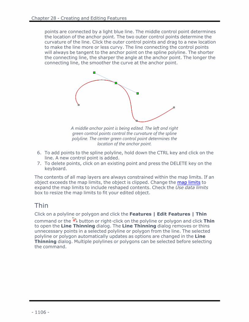
Chapter 28 - Creating and Editing Features
points are connected by a light blue line. The middle control point determinesthe location of the anchor point. The two outer control points determine thecurvature of the line. Click the outer control points and drag to a new locationto make the line more or less curvy. The line connecting the control pointswill always be tangent to the anchor point on the spline polyline. The shorterthe connecting line, the sharper the angle at the anchor point. The longer theconnecting line, the smoother the curve at the anchor point.
A middle anchor point is being edited. The left and rightgreen control points control the curvature of the splinepolyline. The center green control point determines the
location of the anchor point.
6. To add points to the spline polyline, hold down the CTRL key and click on theline. A new control point is added.
7. To delete points, click on an existing point and press the DELETE key on thekeyboard.
The contents of all map layers are always constrained within the map limits. If anobject exceeds the map limits, the object is clipped. Change the map limits toexpand the map limits to include reshaped contents. Check the Use data limitsbox to resize the map limits to fit your edited object.
ThinClick on a polyline or polygon and click the Features | Edit Features | Thincommand or the button or right-click on the polyline or polygon and click Thinto open the Line Thinning dialog. The Line Thinning dialog removes or thinsunnecessary points in a selected polyline or polygon from the line. The selectedpolyline or polygon automatically updates as options are changed in the LineThinning dialog. Multiple polylines or polygons can be selected before selectingthe command.
- 1106 -

Surfer User's Guide
Line Thinning DialogThe Line Thinning dialog controls the simplification method and properties forthinning polylines and polygons.
Set the options in the Line Thinning dialog to removepoints from a selected polyline or polygon.
Simplification MethodThe Simplification method controls how the points are selected to be removedfrom the polyline or polygon. Available options are Keep every nth vertex, Vertexaveraging, and Deviation distance. To select the method, click on the existingoption and select the desired method from the list. Depending on the selectedSimplification method, a Keep every, Average every, or Deviation Distanceoption will appear.
Keep Every nth VertexThe Keep every nth vertex option keeps every nth vertex point from the polylineor polygon, and then reconnects the polyline segments with only the new points.The value of "n" is entered into the Keep every field. For example, if the Keepevery is set to 3, the first point is kept, the next two vertices are removed, theforth point is kept, and so on.
Set the Keep every value based on the number of points to remove. To changethe Keep every value, highlight the current value and type a new value. Altern-atively, click the to increase or decrease the value.
The original polyline is on the left. The polyline after a Keep every of 3 wasapplied is shown on the right.
- 1107 -

Chapter 28 - Creating and Editing Features
Vertex AveragingThe Vertex averaging option preserves the first and last point in a polyline, butaverages the vertices along the polyline based on the number set in the Averageevery field. For example, a polyline that has 10 vertices when averaged using arate of 3 yields a polyline with 6 vertices. The new vertices are located based onthe averaged locations of the previous surrounding vertices.
Set the Average every value based on the number of points to average to createnew points in the polyline. To change the Average every value, highlight the cur-rent value and type a new value. Alternatively, click the to increase ordecrease the value.
The original polyline is on the left. The polyline after an Average every value of 3was applied is shown on the right.
Deviation DistanceThe Deviation distance option controls how many points are removed by the thin-ning process. Points closer than the Deviation distance from the general trend ofthe polyline are removed. A value of 0 removes any duplicate or collinear points.A value of .1 removes all points that are .1 coordinates or closer to the generaltrend of the polyline. The larger the Deviation distance, the more points areremoved from the polyline. The Deviation distance is based on the DouglasPeucker algorithm.
Set the Deviation Distance to the distance away from the general trend line toremove points. To change the Deviation Distance value, highlight the existingvalue and type a new value. The Deviation Distance is in the local units for theobjects. Therefore, if multiple objects are selected, the objects should all use thesame local units.
The original polyline is on the left. The polyline after applying a Deviation dis-tance of 0.50 is shown on the right.
- 1108 -

Surfer User's Guide
OK or CancelClick OK to make simplify the lines and return to the plot window. Click Cancel toreturn to the plot window without simplifying the lines. The lines retain their ori-ginal shape.
PreviewAs the Simplification method and applicable options are changed in the LineThinning dialog, the selected objects update automatically in the plot window.This is a preview, and the changes are not saved unless OK is clicked in the LineThinning dialog.
ReferencesDouglas, David H and Peucker, Thomas K., Algorithms for the Reduction of theNumber of Points Required to Represent a Digitized Line or its Caricature, TheCanadian Cartographer, Vol 10, No 2, p 112-122.
SmoothClick on a polyline or polygon and click the Features | Edit Features |Smooth command or the button or right-click on the polyline or polygon andclick Smooth to open the Line Smoothing dialog. The Line Smoothing dialogadds points to a selected polyline or polygon to smooth the line. Smoothingremoves or lessens jagged sections in polylines. The selected polyline or polygonautomatically updates as options are changed in the Line Smoothing dialog.Multiple polylines or polygons can be selected before selecting the command.
The Features | Edit Features | Smooth command is a good way to create aspline polygon. Create the polygon using the Polygon command. Then, click theFeatures | Edit Features | Smooth command to add additional pointsbetween the drawn points on the polygon. A smooth polygon is created.
Line Smoothing DialogThe Line Smoothing dialog controls the number of points and tension whensmoothing polylines or polygons.
Set the options in the Line Smoothing dialog to addpoints and control the tension for smoothing a selected
polyline or polygon.
- 1109 -

Chapter 28 - Creating and Editing Features
Number of Points to AddSmoothing produces a uniform polyline that passes through all of the datapoints, regardless of the spacing of the data points or the tension factor appliedto the smoothing. Set the Number of points to insert between existing pointsvalue to the desired number of points to add between existing point. If set to 3, 3points are added between existing points. For example when Number of points toinsert between existing points is 3 and a line contains 10 points initially, thesmoothed line will contain 37 points. To change the Number of points to insertbetween existing points value, highlight the existing value and type a new value.Alternatively, click the to increase or decrease the value.
TensionThe Tension can range from 0 to 100%. Higher tension factors result instraighter polylines between the data points and lower tension factors result inmore curvature. To change the Tension value, highlight the existing value andtype a new value. Alternatively, click the to increase or decrease the value.
OK or CancelClick OK to make the lines smoother and return to the plot window. Click Cancelto return to the plot window without smoothing the lines. The lines retain theiroriginal shape.
PreviewAs the line smoothing options are changed in the Line Smoothing dialog, theselected objects update automatically in the plot window. This is a preview, andthe changes are not saved unless OK is clicked in the Line Smoothing dialog.
ReferencesFor additional information on the spline smoothing method, refer to either ofthese resources.
l Renka, R. J. Interpolatory tension splines with automatic selection of tensionfactors.SIAM J. Sci. Stat. Comput. 8 (1987), pp. 393-415.
l Renka, Robert J. TSPACK: Tension Spline Curve Fitting Package. 05/27/91
Connect PolylinesClick the Features | Edit Polylines | Connect Polylines command or thebutton or right-click on the selection and click Connect Polylines to connect selec-ted polylines and spline polylines. The polylines are connected at the closest end-points on each line. For the command to be available, two or more polylines, 3Dpolylines or spline polylines must be selected. 3D polylines cannot be connectedto polylines or spline polylines.
- 1110 -

Surfer User's Guide
The new polyline or 3D polyline retains the line properties from the polyline atthe bottom of the Contents window. If the object name has not been changedfrom the default Polyline, the object is renamed Polyline. If the object name hadbeen altered, the custom object name from the bottom polyline is retained.
Break PolylineClick the Features | Edit Polylines | Break Polyline command or the but-ton or right-click a polyline or 3D polyline and click Break Polyline to break theselected polyline, 3D polyline or spline polyline into multiple polylines. The cursor
changes to to indicate break mode. Click on the polyline, 3D polyline orspline polyline in the location where the line should be broken. For the commandto be available, a single polyline, 3D polyline, or spline polyline must be selected.Spline polylines are converted to regular polylines after being broken apart. 3Dpolylines continue as 3D polylines.
The new polylines retain the line properties from the original polyline. If theobject name has not been changed from the default Polyline, 3D Polyline, orSpline Polyline, the new objects are named Polyline. If the object name had beenaltered, the custom object name from the original polyline is retained for bothnew polylines.
Break Polyline at IntersectionsThe Features | Edit Polylines | Break at Intersections command breaks aselected polyline, spline polyline, or combination of polylines and spline polylinesat every intersection with another object, such as polygons, polylines, splinepolylines, rectangles, rounded rectangles, and ellipses. The original line prop-erties are applied to the created polylines. Only the polylines or spline polylinesto be broken at intersections need to be selected. After a polyline is broken, mul-tiple polyline objects are created based on the boundary intersections with theoriginal polyline. When a spline polyline is broken, the resulting lines are con-verted to polylines.
To break a polyline:1. Select only the polyline that should be broken at its intersections with other
objects. It is not necessary to select the intersecting objects.2. Click the Features | Edit Polylines | Break at Intersections command
or the button. Alternatively, right-click on the selected polyline, and clickBreak at Intersections in the context menu.
- 1111 -

Chapter 28 - Creating and Editing Features
In this example, the polyline in the image on the left is broken into three polylines in theimage on the right since the polyline crosses the polygon twice. The line color was changed to
show the three created polylines.
Alpha ShapeThe Features | New Features | Alpha Shape command creates a polygonboundary around a set of three or more selected data points in a base layer or abase layer created from a data file. The resulting polygon is an alpha shape,which is a subset type of Delaunay triangulation. Holes will be created within thealpha shape where there is no data. Edges of the alpha shape are trimmed so aclosed boundary is formed that conforms to the number of the alpha value.
Alpha shapes can be cre-ated from drawn pointfeatures or pointswithin a base layer.
The alpha value determinesthe radius of the alphacircles. The edges are
drawn based on DelaunayTriangulation.
The edges are trimmed sothe boundary of the alphashape is complete. Wherethere is no data, a hole is
drawn.
- 1112 -

Surfer User's Guide
Creating an Alpha ShapeThe following steps describe how to create an alpha shape.
1. Click the Features | New Features | Alpha Shape command or thebutton to display the Alpha Shape dialog.
Alpha Shape creates a polygon based on thealpha value.
2. In the Alpha Shape dialog, select a Create from value. Depending on theCreate from value selected, the Alpha Shape dialog will add or removeoptions.a. If the selected Create from value is All points in a data file, click the
Browse button to select and add a data file to the Input list. Use the XColumn and Y Column lists to select the XY data from the selected inputfile. Click the View Data button for a quick view of the data file.
b. If the selected Create from value is All points on a layer, select the layerfrom the Input list.
c. If the selected Create from value is Selected points only, Input will begrayed out.
3. Select the desired Alpha value. The Alpha value defines the radius of thecircles that are created by the edges of the triangulation of the points. Theunits are in the units of the layer.
l The alpha shape depends on both data density and the alpha value. Thealpha shape, despite the alpha value, will not extend past the points.
- 1113 -

Chapter 28 - Creating and Editing Features
l Larger alpha values create a more convex boundary and smaller alphanumbers create a tighter, concave boundary.
l With small alpha values, the alpha radii can pass through the data set,and the alpha shape can form several smaller shapes.
l When working in latitude and longitude, use alpha values greater than 0and less than 10.
l When working in meters, use alpha values of 10 or greater.l If the selected alpha value is too small or too large, during its previewcalculations, the Alpha Shape dialog will show a message to try a dif-ferent alpha value.
4. Select the desired Destination layer. The values in this list depend on thevalue selected in the Create from list.
l If All points on layer is selected from the Create from list, and the inputlayer is a post or classed post map, the values in the Destination Layerlist will be New Layer and New Map. New Layer will add the alpha shapeto the same map as the input layer, and New Map will create a new mapthat includes the alpha shape. If all All points on layer is selected fromthe Create from list, and the input layer is a base map, the values in theDestination Layer list will be New Layer, New Map, and the name of theinput layer. New Layer will add the shape to a new layer, New Map willcreate a new map that includes the alpha shape, and selecting the inputlayer will add the shape to that layer.
l If All points in data file is selected from the Create from list from anempty plot window, the only Destination Layer value will be New Map. IfAll points in data file is selected from the Create from list with an exist-ing map in the plot window, and New Layer is selected from the Destin-ation Layer list, the layer will be added to the bottom map in theContents window.
l If Selected points only is selected from the Create from list, all threeDestination layer values will be available. New Layer will add the shapeto the same layer as the input layer, New Map will create a new mapthat includes the alpha shape, and selecting the input layer will add theshape to that layer.
5. After defining the alpha shape, click the Preview button to generate a previewof the alpha shape and display the number of Boundaries created. The num-ber of boundaries created is dependent on the Alpha value. Preview cal-culations may display a message about adjusting the alpha value.
6. After previewing the alpha shape, either reconfigure the alpha shape settingsor click OK to close the Alpha Shape dialog and add the shape to the selec-ted layer.
- 1114 -

Surfer User's Guide
Example with alpha = .01 and alpha = .1
ReferencesGardiner, James, Julia Behnsen and Charlotte A. Brassey, Alpha shapes: determ-ining 3D shape complexity across morphologically diverse structures, BMC Evolu-tionary Biology, 18, Article number: 184, 2018.
Edelsbrunner, Herbert, and Ernst P Mucke, Three-dimensional Alpha Shapes,University of Illinois at Urbana-Champaign, https://arx-iv.org/pdf/math/9410208.pdf.
Union PolygonsThe Features | New Features | Union of Polygons command automaticallycreates a new polygon by combining multiple objects. This command can beused with any combination of existing polygons, rectangles, rounded rectangles,and/or ellipses. The original objects are retained or removed based on the Keeporiginal objects selection in the Union Polygons dialog.
Selections including objects that do not touch or intersect result in a complexpolygon, similar to the Combine Island/Lakes command when combining islands.
Sometimes selections made up of many contiguous objects, for example statesor provinces in a country, have objects that do not completely touch or intersect.If objects do not touch or intersect along the entire border, the Union Polygonscommand results in a complex polygon with small lakes. To remove the lakes,use the Split Islands/Lakes command, and then delete the interior polygons.Alternatively, use the Reshape command to delete the vertices for the lakes.
To use the Union Polygons command
1. Select all the objects that you wish to combine into a single polygon.2. Click the Features | New Features | Union of Polygons command or the
button.
- 1115 -

Chapter 28 - Creating and Editing Features
3. Select whether or not to keep the original objects in the Union Polygons dia-log.
4. Click OK in the Union Polygons dialog, and the selected objects are com-bined into a single polygon. The new polygon is selected when the process iscompleted.
With Union Polygons, you do not have to preserve the original objects. In thisexample, four new polygons are based on groups of counties. When creatingthe example on the left, Keep original objects was not checked. Keep original
objects was checked when creating the example on the right.
Difference between Combine Islands/Lakes and Union PolygonsThis command differs from the Combine Islands/Lakes command. With theUnion Polygons command, a new polygon is created from the selected objects.With Combine Islands/Lakes, the selection is combined into a single complexpolygon. The original objects become islands and lakes, and a new polygon is notcreated.
l Contiguous objects are part of the created polygon with the Union Polygonscommand. With the Combine Islands/Lakes command, contiguousobjects are separate islands in a single complex polygon.
l Intersecting areas of the selected objects are treated as part of the new poly-gon when the Union Polygons command is used. When the CombineIslands/Lakes command is used, intersecting portions of the selection aretreated as lakes, or holes, in the complex polygon.
l The Combine Islands/Lakes and Union Polygons commands behave sim-ilarly only when objects in the selection do NOT touch or intersect. However,the Combine Islands/Lakes command combines the selection into a com-plex polygon. The Union Polygons command creates a new complex poly-gon, and the original objects can be removed or kept.
For example, if you want to indicate an outer boundary with a heavy line and pre-serve the inner boundaries with thinner lines as in the example above, you canaccomplish this with the Union Polygons command, not with the CombineIslands/Lakes command.
- 1116 -
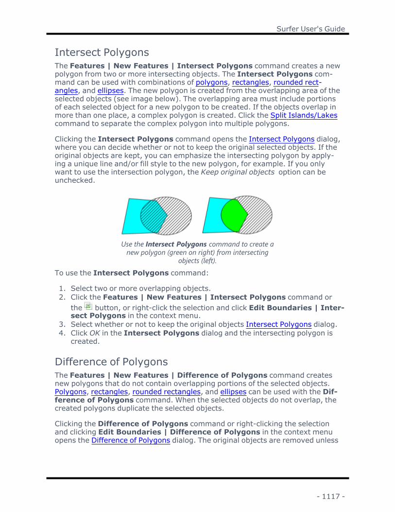
Surfer User's Guide
Intersect PolygonsThe Features | New Features | Intersect Polygons command creates a newpolygon from two or more intersecting objects. The Intersect Polygons com-mand can be used with combinations of polygons, rectangles, rounded rect-angles, and ellipses. The new polygon is created from the overlapping area of theselected objects (see image below). The overlapping area must include portionsof each selected object for a new polygon to be created. If the objects overlap inmore than one place, a complex polygon is created. Click the Split Islands/Lakescommand to separate the complex polygon into multiple polygons.
Clicking the Intersect Polygons command opens the Intersect Polygons dialog,where you can decide whether or not to keep the original selected objects. If theoriginal objects are kept, you can emphasize the intersecting polygon by apply-ing a unique line and/or fill style to the new polygon, for example. If you onlywant to use the intersection polygon, the Keep original objects option can beunchecked.
Use the Intersect Polygons command to create anew polygon (green on right) from intersecting
objects (left).To use the Intersect Polygons command:
1. Select two or more overlapping objects.2. Click the Features | New Features | Intersect Polygons command or
the button, or right-click the selection and click Edit Boundaries | Inter-sect Polygons in the context menu.
3. Select whether or not to keep the original objects Intersect Polygons dialog.4. Click OK in the Intersect Polygons dialog and the intersecting polygon is
created.
Difference of PolygonsThe Features | New Features | Difference of Polygons command createsnew polygons that do not contain overlapping portions of the selected objects.Polygons, rectangles, rounded rectangles, and ellipses can be used with the Dif-ference of Polygons command. When the selected objects do not overlap, thecreated polygons duplicate the selected objects.
Clicking the Difference of Polygons command or right-clicking the selectionand clicking Edit Boundaries | Difference of Polygons in the context menuopens the Difference of Polygons dialog. The original objects are removed unless
- 1117 -

Chapter 28 - Creating and Editing Features
the Keep original objects option is checked in the Difference of Polygons dia-log. When the Keep original objects option is checked, the new polygons are cre-ated without overlapping areas, and the original objects remain unchanged.
These two polygons areselected.
After Difference of Poly-gons, two new polygons arecreated without the inter-
secting area.
Creating a Difference of Polygons:To create a difference of polygons:
1. Select two or more polygons.2. Click the Features | New Features | Difference of Polygons command
or the button, or right-click the polygons and click Edit Boundaries | Dif-ference of Polygons in the context menu.
3. Select whether to keep the original objects in the Difference of Polygons dia-log.
4. Click OK in the Difference of Polygons dialog to create new polygonswithout the overlapped areas.
You may wish to keep the original objects if the overlapping areas need to be rep-resented by a polygon. For example, using the Difference of Polygons com-mand with Keep original objects checked, then using the Intersect Polygonscommand with Keep original objects unchecked results in separate polygons rep-resenting overlapping and non-overlapping portions of the original objects.
Difference of Polygons, Union Polygons, and IntersectPolygons DialogsThe Difference of Polygons dialog is displayed after clicking the Difference ofPolygons command. The Union Polygons dialog is displayed after clicking theUnion Polygons command. The Intersect Polygons dialog is displayed afterclicking the Intersect Polygons command.
Keep or discard original objects with the Difference of Polygons , Union Polygons , andIntersect Polygons dialogs.
- 1118 -

Surfer User's Guide
Keep Original ObjectsWhen Keep original objects is checked, a new polygon is created while leavingthe original selected objects unchanged. The new polygon is created, and the ori-ginal objects are deleted when Keep original objects is unchecked.
BufferThe Features | New Features | Buffer command creates a polygon around orwithin an object or group of objects at a specified distance. Any number or com-bination of points, polylines, spline polylines, polygons, rectangles, rounded rect-angles, and ellipses can be selected before clicking the Buffer command. Apolygon will be created around each selected object.
If Combine overlapping buffer polygons is checked in the Buffer dialog, thenewly created buffer polygons are combined as with the Union Polygons com-mand. For detailed explanation of the combination operation, see the Differencebetween Combine Islands/Lakes and Union Polygons section of the Union Poly-gons help page. The following images provide a visual example of the differencebetween using the Buffer command with and without the Combine overlappingbuffer polygons option checked.
The Combine overlapping buffer polygonsoption was not checked in this example.Notice the overlapping region between theyellow and blue buffer polygons. Three newpolygons were added to the plot window and
Contents window.
The Combine overlapping buffer polygonsoption was checked for this example. Noticethe buffer polygons created from the yellowand blue polygons have been combined.Here the buffer polygons are a single com-plex object consisting of two sub-polygons.Only one polygon was added to the Con-
tents window.
Creating a buffer polygon1. Select the object around which to create a buffer polygon by clicking the
object in the plot window or Contents window.2. Click the Features | New Features | Buffer command or the button.3. Specify the Number of buffers and Buffer distance and select whether to Com-
bine overlapping buffer polygons in the Buffer dialog.4. Click OK, and the buffer polygon is created.
- 1119 -

Chapter 28 - Creating and Editing Features
Buffer DialogThe options for the Buffer command are located in the Buffer dialog. Open theBuffer dialog by selecting one or more objects and clicking the Features | NewFeatures | Buffer command.
The number of buffers and buffer distance is specified in theBuffer dialog.
Number of BuffersSpecify the number of buffers you wish to create around each object in the Num-ber of buffers field. Type a number into the field or click the buttons to changethe value. The first buffer is created at the Buffer distance from the object, andsubsequent buffer polygons are created at the Buffer distance from the previousbuffer polygon.
Buffer DistanceSpecify the distance to draw the buffer polygon from the selected object or groupof objects in the Buffer distance field. Positive distances expand the buffer poly-gon. Negative distances contract the buffer polygon. A buffer polygon with a neg-ative Buffer distance is not created for points or polylines.
The Buffer distance is specified in the source coordinate system distance units,e.g. degrees, feet, meters, or miles. For objects that are not part of a base layer,the Buffer distance is in page units (inches or centimeters).
Combining Buffer PolygonsClick the Combine overlapping buffer polygons check box to combine the bufferpolygons after they are created. Overlapping buffer polygons will combine toform a single polygon. When the buffer polygons do not overlap, the buffer poly-gons are combined into a single complex polygon.
- 1120 -

Surfer User's Guide
The buffer polygons are combined as with the Union Polygons command. Fordetailed explanation of the combination operation, see the Difference betweenCombine Islands/Lakes and Union Polygons section of the Union Polygons helppage.
Create Intersection PointsClick the Features | New Features | Intersection Points command to cre-ate a point at each place selected objects intersect with one another. Points arecreated at all object intersections, and the original objects remain unmodified.The Intersection Points command can be used with any combination of poly-lines, spline polylines, polygons, rectangles, rounded rectangles, and ellipses.
Intersection Points creates points at each place selected objects intersect.
Creating Intersection PointsTo create points at intersections:
1. Select two or more intersecting objects.2. Click the Features | New Features | Intersection Points command or
the button.3. Points are created at every intersection.
TriangulationThe Features | New Features | Triangulation command performs aDelaunay triangulation on the selected points. A Delaunay triangulation for a setof points is a triangulation such that no point is within any triangle. The trianglescan be polylines or polygons. None of the triangles are intersected by other tri-angles.
- 1121 -

Chapter 28 - Creating and Editing Features
A triangulation diagram can be created from drawn point features or pointswithin a base layer.
Triangulation creates triangles from selected points.
Creating a Triangulation DiagramThe following steps describe how to create a triangulation diagram:
1. Select three or more points from which to create the diagram.2. Click the Features | New Features | Triangulation command or the
button.3. Select the desired options in the Triangulation dialog.4. Click OK in the Triangulation dialog.
Triangulation DialogThe Triangulation dialog is displayed after clicking the Features | NewFeatures | Triangulation command.
- 1122 -

Surfer User's Guide
Select the output feature type, output layer, andwhether or not to keep the original points in the
Triangulation dialog.Output Feature TypeThe triangulation diagram can consist of polygons or polylines. Select Polygon orPolyline in the Output feature type list.
Output LayerThe Output layer option specifies the layer where the triangulation polygons orpolylines will be created when the selected points are in a base layer. The Outputlayer list includes the base layers in the map, as well as the option to create a thetriangulation in a new base layer. Select [New Base Layer] to create the tri-angulation in a new layer. When a new base layer is created, the base layer isassigned the same coordinate system as the map frame. Select a base layer toadd the triangulation to an existing layer. The Output layer option is not avail-able when the selected points are not in a base layer.
Keep Original ObjectsSelect Keep original points to create the triangulation while leaving the originalpoints unchanged. Clear the Keep original points check box to remove the pointsafter the triangulation is created.
Thiessen PolygonsThe Features | New Features | Thiessen Polygons command creates poly-gons from selected points. The diagram can consist of polygons or polylines. In aThiessen polygon diagram, also known as a Voronoi diagram, a region is drawnaround each point so that for each point every position in the region around thatpoint is closer to that point than to any of the other points.
Thiessen polygons can be created from drawn point features or points within abase layer.
- 1123 -

Chapter 28 - Creating and Editing Features
Thiessen Polygons creates a Thiessen polygon diagram fromselected points.
Creating a Thiessen Polygon DiagramThe following steps describe how to create a Thiessen polygon (Voronoi) dia-gram:
1. Select three or more points from which to create the diagram.2. Click the Features | New Features | Thiessen Polygons command or the
button.3. Select the desired options in the Thiessen Polygons dialog.4. Click OK in the Thiessen Polygons dialog.
Thiessen Polygons DialogThe Thiessen Polygons dialog is displayed after clicking the Features | NewFeatures | Thiessen Polygons command.
Select the output feature type, output layer, andwhether or not to keep the original points in the
Thiessen Polygons dialog.
- 1124 -

Surfer User's Guide
Output Feature TypeThe Thiessen polygons diagram can consist of polygons or polylines. Select Poly-gon or Polyline in the Output feature type list. When Polygon is selected, anyinput point attributes are assigned to the resultant Thiessen polygons.
Output LayerThe Output layer option specifies the layer where the Thiessen polygons or poly-lines will be created when the selected points are in a base layer. The Outputlayer list includes the base layers in the map, as well as the option to create a theThiessen polygons in a new base layer. Select [New Base Layer] to create theThiessen polygons in a new layer. When a new base layer is created, the baselayer is assigned the same coordinate system as the map frame. Select a baselayer to add the Thiessen polygons to an existing layer. The Output layer optionis not available when the selected points are not in a base layer.
Keep Original ObjectsSelect Keep original points to create the Thiessen polygons while leaving the ori-ginal points unchanged. Clear the Keep original points check box to remove thepoints after the Thiessen polygons are created.
SplitClick the Features | New Features | Split command or right-click on a selec-ted polygon and click Split Islands/Lakes to break a single complex polygoninto multiple polygons. A new polygon is created for each of the polygons con-tained in the complex polygon.
The new polygons use the line and fill properties from the original complex poly-gon. The object name is also retained from the original complex polygon.
Complex polygons can contain polygons that are touching, intersecting, com-pletely separate, or contained completely within other polygons. Each individualpolygon in the group is called an island. An example of islands that can form acomplex area is the Hawaiian islands. When a polygon is completely containedinside another polygon, a lake is formed. Lakes are the holes in a complex poly-gon. When the islands and lakes are split, each island and lake becomes a newpolygon.
Note about Base MapsIf objects should be edited in a base map, click on the object in the Base layer toselect it. Click the Features | Group | Start Editing command to enter editingmode. Select the polygon to be split. Then, click the Features | Islands/Lakes| Split command. The new polygons are created from the single complex poly-gon. Click the Features | Group | Stop Editing to end object editing mode inthe base map.
- 1125 -

Chapter 28 - Creating and Editing Features
Splitting a Complex Polygon into Multiple Polygons1. Click on a complex polygon in the Contents window. The polygon can be
imported with the Home | Insert | Graphic command or can be createdby combining multiple polygons into a single complex polygon using theCombine command.
Click on the complex polygon in the Contents window or inthe plot window.
2. Click the Features | New Features | Split command or the button.Multiple polygons are created from the single complex polygon. Both poly-gons maintain the properties of the original polygon.
The polygon is split into multiple polygons. Each polygon can be indi-vidually selected and edited.
Combine Islands/LakesClick the Features | New Features | Combine command or right-click on mul-tiple selected polygons and click Edit Boundaries | Combine Islands/Lakesto combine multiple polygons into a single complex polygon. A new complex poly-gon containing all of the selected polygons is created.
The new polygon uses the line and fill properties from the lowest selected poly-gon in the Contents window. The object name is also retained from the lowestselected polygon in the Contents window.
Complex polygons can be created from polygons that are touching, polygonsthat are completely separate, or polygons that are contained completely withinother polygons. Each individual polygon in the group is called an island. Anexample of islands that can form a complex area is the Hawaiian islands. When a
- 1126 -

Surfer User's Guide
polygon is completely contained inside another polygon, a lake is formed. Lakesare the holes in a complex polygon.
Combining Multiple Drawn Polygons1. Click the Polygon command.2. On the plot window, click several points. Double-click the last point to close
the polygon.3. Repeat step 2 a few more times so that several polygons are created.4. Press ESC on the keyboard to end drawing mode.5. In the Contents window, click on the first polygon that you want to combine.6. Hold down the CTRL key on the keyboard.7. In the Contents window, click on the each additional polygon that you want
to combine.
In this example, the top and bottom polygons are selected in theContents window and in the plot window.
8. Click the Features | New Features | Combinecommand or the but-ton. A single polygon is created from the selected polygons. Both polygonshave the properties of the bottom-most polygon in the Contents window.
The two polygons become a single complex polygon.
UndoClick the Home | Undo | Undo command the button or press CTRL+Z onthe keyboard to reverse the last operation performed. If the last operation can-not be reversed, the Undo command is grayed. After you close a file, the undo
- 1127 -

Chapter 28 - Creating and Editing Features
operations are cleared, so you cannot undo any operations performed before thefile was closed. After you have undone an operation, the Redo commandbecomes available, allowing you to reverse the last completed Undo command.
Hover the cursor over the Undo command to see the last action. For example,after drawing a polyline the Undo command tooltip displays Undo Creation .
Zoom and pan operations are not included in the undo list. Consider using a viewcommand or keyboard command to quickly move to a different view.
Grid EditorClick the Grid Editor | Undo | Undo command or press CTRL+Z to reverse thelast operation performed when in the grid editor view. Undo operations are onlyperformed on ribbon commands in the Grid Editor . Property changes in theGrid Editor cannot be undone with the Undo command.
Undo LevelsUp to 100 undo levels can be set though Options dialog General page. If theUndo command is not available, check the Undo levels . If the value is set tozero, undo will not be available.
RedoClick the Home | Undo | Redo command or the button, or press CTRL+Y onthe keyboard to reverse the last Undo command.
After you have used the Home | Undo | Undo command, the Redo commandindicates the operation that you have undone. Hover the cursor over the Redocommand to see the last undone action. For example, after deleting an objectand then clicking Undo , the Redo command tooltip displays Redo Deletion .
Grid EditorClick the Grid Editor | Undo | Redo command or press CTRL+Y to reverse thelast operation performed when in the grid editor view.
Paste
Click the Home | Clipboard | Paste command or the button, or pressCTRL+V on the keyboard to paste the clipboard contents into the current doc-ument. The objects to be pasted must first be placed in the clipboard using theCut or Copy commands of Surfer or some other application. The clipboard con-
- 1128 -

Surfer User's Guide
tents remain on the clipboard until something new is cut or copied to the clip-board.
WorksheetIn the worksheet, the upper left corner of the pasted data is placed in the activecell. Any cells in the existing worksheet that lie to the right of and below the act-ive cell will be overwritten with the contents of the pasted data. The followingrules are used to paste into the worksheet:
l Only the TAB character is recognized as a column separator. Spaces, com-mas, semi-colons, etc. are included in a text cell.
l The RETURN character is recognized as the row separator.
l Numbers paste as number values. The period can always be used as adecimal separator, and the system locale determines any other decimal sep-arator. For example if the system locale uses a comma as the decimal sep-arator, then both 123.456 and 123,456 are pasted as the number 123,456.
l Mixed text and numbers paste as text.
l Dates and/or times will paste as date values in a wide variety of date/timeformats. Ambiguous dates are determined by the system locale setting. Ifdates are not pasted correctly, consider using Paste Special and the Localesettings in the Data Import Options dialog.
Pasting a single cell's contents across multiple cellsA single cell's contents can be pasted into multiple cells by coping the cell, select-ing a block of cells, and using the Paste command. Each cell in the selection ispopulated with the clipboard contents when this operation is performed. If morethan one cell is copied, then the copied cells are only pasted once.
The multiple paste operation will not be performed for an entire row, entirecolumn, or across multiple selections. When an entire row or column is selected,only the first cell in the row or column will receive the pasted content. If youattempt to paste in multiple selections an error message will be displayed.
PlotIn the plot window, the clipboard contents are pasted in the center of the win-dow. The pasted contents are automatically selected, and can be dragged to anew location. Alternatively, change the position or size of the selected objectwith the Position/Size group.
- 1129 -

Chapter 28 - Creating and Editing Features
Paste Special - Plot DocumentThe Home | Clipboard | Paste | Paste Special command pastes objectsfrom the clipboard into a plot window. With the Home | Clipboard | Paste |Paste Special command, you have the option of specifying the format to usewhen pasting the object into .
Clipboard Formats DialogUse the Paste Special command to open the Clipboard Formats dialog andselect one of the clipboard formats.
Select a paste special format in the Clip-board Formats dialog.
GS_Surfer2The GS_Surfer2 format lets you cut or copy an entire map or drawing to the clip-board. It is stored in the clipboard as a native object. You can paste this map ordrawing into another plot window in . The map is identical to the original and is acomplete map that can be edited. This is an easy way to place several completedrawings on a single page.
Enhanced Metafile and PictureThe Enhanced Metafile and Picture formats are Windows metafile formats, whichstore objects as a series of Windows drawing commands. Metafiles can be res-ized without distorting the image. These formats are supported by most Win-dows applications.
Break Apart MetafilesWhen you select an Enhanced Metafile or Picture format, you can check theBreak Apart Metafiles box at the bottom of the Clipboard Formats dialog. Thisoption converts the metafile into a series of native objects and groups them as asingle group object. Group objects can be broken apart using the Features |Group | Ungroup command.
- 1130 -
Surfer User's Guide
For example, you could paste a contour map in the picture format, and check theBreak Apart Metafiles check box. In this case, the contour map is pasted as agroup of polylines and text. You can then break apart the group object andmodify the individual polylines (such as the contour lines).
Device Independent BitmapThe Device Independent Bitmap format stores objects as images. Bitmap imagesare difficult to resize without distorting the image, and their colors are limited.This format is relatively common, and is supported by most other Windowsapplications.
TextThe Text format is used to import text. Imported text can contain any number oflines and uses the default text properties. If you want to paste both text andother objects, and retain the text, you must copy and paste the text separatelyfrom the other objects.
Copy
Click the Home | Clipboard | Copy command or the button, or pressCTRL+C on the keyboard to copy the selected objects to the clipboard. The ori-ginal objects remain in the window. Use this command to duplicate objects in adifferent location in the same window, or copy the objects into a different win-dow or application. The copied objects can later be pasted with the Paste orPaste Special commands.
Only one set of data may be placed in the clipboard at a time. The next Cut orCopy command replaces the contents of the clipboard.
CutClick the Home | Clipboard | Cut command or the button, or press CTRL+Xon the keyboard to move the selected objects to the clipboard. This deletes theselected objects from the file after copying them to the clipboard. Cut objectscan later be pasted with the Paste or Paste Special commands.
Only one set of data may be placed in the clipboard at a time. The next Cut orCopy command replaces the contents of the clipboard.
DeleteThe Home | Clipboard | Delete command or the button removes an objectfrom the document. An object can sometimes be restored with the Undo com-mand.
- 1131 -

Chapter 28 - Creating and Editing Features
To delete an object, select the object in the plot window or Contents window andpress the DELETE key or click the Delete command.
- 1132 -

Chapter 29 - Common Properties
Text and Font PropertiesClick the Home | Insert | Text command to create new text. The Text Editor isused to initially create text. After the text is created, the text and font propertiesare displayed in the Properties window. Use the following options to change thetext and font properties.
Edit text in the Text Properties section and font properties in the Font Properties section ofthe Properties window.
Text PropertiesThe text can be edited in the Properties window or in the Text Editor. Click thenext to Text properties to open the Text properties section. You can set the textthat appears by highlighting the existing text next to Text and typing the desiredtext for simple text strings.
For complex text or multiple lines of text, click the button to open the TextEditor. Enter text, edit text properties for individual characters, and add tem-plates, symbols and timestamps with the Text Editor. The text you enter intothe Text Editor is converted into math text instructions and written in the Text
- 1133 -

Chapter 29 - Common Properties
field. You can also type math text instructions directly into the Text field, ifdesired.
Font PropertiesText properties for the entire text block can be edited in the Properties windowin the Font Properties section. Some options may not be available for all text,depending on the type of object selected. For example, when editing axis labels,the Alignment options are not available.
The changes made in the Font Properties section are considered the baseline textproperties and are applied to each line of a text block. Changes made here over-ride "normal" font options in the Text Editor. To have all text the same, click thebutton. Highlight all the text and set all the properties in the Text Editor , as
desired. Then, the changes in the Font Properties section will apply to all text inthe text object.
For example, suppose you type in the following in the Text Editor. After typingthe text, you have highlighted the first line and made the color red and the fontCambria.
After clicking OK in the Text Editor, the following appears in the Text Propertiessection of the Properties window.
The two lines of text appear in the plot window as:
- 1134 -

Surfer User's Guide
Now, in the Properties window in the Font Properties section, set the Font to"Times New Roman", the Foreground Color to Blue, and check the boxes next toBold and Italic. Because the first line contains a font name and color, the fontand color will not change for this line. But, the red text will be bold and italic. Thetext now appears as:
If the second line of text should remain without any text embellishments, suchas bold or italics, in the Properties window, click before the word Date and adda \plainmath text option. This does not control the font name and color, so theywill still change. The Properties window would now appear as:
And, the text would appear in the plot window as:
FontThe Font is the font that is used for the text. To change the Font, click on the cur-rent font name. Select the desired font name from the Font list. Click the arrowbutton or select a font and use the ARROW keys on the keyboard to scrollthrough the Font list. The selected font is displayed in the Text Editor. The fontfiles that are installed on your computer are displayed in the Font list. Surfersupports true type fonts. All text in a text block uses the same Font, unless amath text operation is applied or unless the font for some of the text has beenspecifically edited in the Text Editor.
Size (points)Set the text size in the Size (points) field. Highlight the existing value and type anew value. Press ENTER on the keyboard to make the change. Or, click the but-tons to increase or decrease the size. A Size (points) value between zero and 720can be specified.
- 1135 -

Chapter 29 - Common Properties
Foreground and Background ColorChange the Foreground color and Background color of the text by selecting anew color from the color palette. The Foreground color controls the color of thetext. The Background color controls the area behind the text. Create new colorsby clicking the button to the right of the color name.
Foreground and Background OpacityChange the Foreground opacity and Background opacity of the text by entering avalue from 0% (completely transparent) to 100% (completely opaque). Tochange the opacity, highlight the existing value and type a new value. PressENTER on the keyboard to make the change. Or, click and drag the tochange the opacity percentage.
StyleCheck the boxes next to Bold, Italic, Strikeout, or Underline to apply a style tothe text. Note that some typefaces, such as Symbol, do not support bold oritalicized text.
l Bold will increase the thickness of the text (i.e. example).
l Italic will create obliqueslanted, sloped text (i.e. example).
l Strikeout will add a horizontal line through the center of the text (i.e.example).
l Underline will add a horizontal line under the text (i.e. example).
AlignmentThe Alignment controls the location of the text relative to the reference point. Areference point is the point clicked in the plot window when the crosshair cursoris placing the text on the screen. The text box is horizontally and verticallyaligned relative to the reference point. The default position is that the referencepoint is at the upper left corner of the bounding box (left, top).
l Left horizontally aligns the text box so that the reference point is to the leftof the text box.
l Center horizontally centers the text box on the reference point.
l Right horizontally aligns the text box so that the reference point is to theright of the text box.
l Top vertically aligns the text box so that the reference point is above thetext box.
- 1136 -

Surfer User's Guide
l Baseline vertically aligns the text box so that the reference point is locatedat the base of the text. The baseline is the imaginary line along which char-acters are positioned as they are drawn. Descenders on characters aredrawn below the baseline.
l Bottom vertically aligns the text box so that the reference point is belowthe text box.
l Center vertically centers the text box on the reference point.
Default SettingsSet default text properties through File | Options. In the Default Properties sec-tion, click Font to specify default properties.
Font Properties DialogWhen changing the advanced label font property settings for a contour map, aFont Properties dialog will appear. The options are the same as describedabove in the Properties window. In addition, the Font Properties dialog has aSample section where the font can be previewed.
Set the font properties for contour labels and grid node editor labels in the Font Propertiesdialog.
Fill PropertiesUse the Fill Properties to change fill properties for selected objects in the doc-ument. You can set default line properties through File | Options | Defaults byclicking on Fill.
- 1137 -

Chapter 29 - Common Properties
Most fill properties are edited in the Properties window in a Fill Properties section.When changing fill properties for a selected object, the Fill Properties section willappear in a different location in the Properties window, depending on the typeof object selected.
Occasionally, objects will open a Fill Properties dialog to access the fill properties.
Edit the Fill Properties for a selected object in theProperties window.
SampleThe sample shown next to the Fill Properties line shows the selected pattern, fore-ground color, and background color.
Fill PatternChange the Pattern by selecting a pattern from the fill pattern palette. Open thepattern palette by clicking the pattern button. Click on a new pattern in the list toselect it.
Foreground ColorForeground color is the color of the pattern lines or pixels. Select a new color byclicking on the color in the color palette. Only the foreground color can be appliedto solid colors. The foreground colors can be applied to any stock hatch pattern
- 1138 -

Surfer User's Guide
or grayscale image pattern. They cannot be applied to the None pattern or non-grayscale image patterns. Click the button at the right of the color sample toopen the Colors dialog, where you can specify a custom color.
Foreground OpacityThe Foreground opacity is the amount of transparency of the fill. This is a valuefrom 0% (completely transparent) to 100% (completely opaque). To change thevalue, highlight the existing value and type a new value. Press ENTER on the key-board or click anywhere else in the Properties window to make the change.Alternatively, click and drag the to change the opacity percentage. Opa-city is disabled if it does not apply to the current pattern. Note that for true colorimage fill patterns the Foreground opacity applies to the image in its entirety.
Background ColorBackground color is the color behind the pattern. All patterns must have a back-ground color. If you do not wish to see the background color, change the Back-ground opacity to 0%. Click on the button at the right of the color sample toopen the Colors dialog, where you can specify a custom color.
Background OpacityChange the Background opacity by entering a value from 0% (completely trans-parent) to 100% (completely opaque) or dragging the slider to changethe opacity percentage. Opacity is disabled if it does not apply to the current pat-tern.
StretchCheck the Stretch option to stretch image fills to completely fill the geometry. IfStretch is not selected, the image will be repeated to fill the geometry.
Load a Fill Pattern FileTo load a fill pattern from a raster image file, click the File or Clipboard button inthe Load from field. The Clipboard button is only active when there is an imageon the clipboard suitable to use for a fill pattern. If you select File, an Import dia-log will appear. Click on the image file and click Open to load the image as the fillpattern.
Pattern OffsetThe Pattern Offset can be changed for image patterns. The offset controls the loc-ation of the pattern within the geometry. Change the X and Y values separatelyto move the image in the desired direction.
- 1139 -

Chapter 29 - Common Properties
Pattern ScaleThe Pattern Scale can be changed for image patterns. The scale controls thedensity of the pattern. In the Properties window, check the Proportional box toconnect the X and Y scale values.
When the scale is proportional, the current aspect ratio is maintained. Changingthe X or Y scale will cause the other scale to be adjusted proportionally to main-tain the aspect ratio at the time the scale was set to proportional.
Fill Properties DialogUse the Fill Properties dialog to change fill properties for selected objects in thedocument. You can set default line properties through File | Options | Defaults byclicking on Fill.
Most fill properties are edited in the Properties window in a Fill Properties section.When changing fill properties for a selected object, the Fill Properties section willappear in a different location in the Properties window, depending on the typeof object selected.
Occasionally, objects will open a Fill Properties dialog to access the fill prop-erties. This dialog is accessed differently depending on the type of object cre-ated.
Specify fill properties in the Fill Properties dialog.
Fill PatternChange the Fill Pattern by selecting a pattern from the fill pattern palette. Openthe pattern palette by clicking the pattern button. Click on a new pattern in thelist to select it.
- 1140 -

Surfer User's Guide
Load a Fill Pattern FileTo load a fill pattern from a raster image file, click the File or Clipboard buttonnext to Load from. The Clipboard button is only active when there is an image onthe clipboard suitable to use for a fill pattern. If you select File, an Import dialogwill appear. Click on the image file and click Open to load the image as the fill pat-tern.
Foreground ColorForeground color is the color of the pattern lines or pixels. Select a new color byclicking on the color in the color palette. Only the foreground color can be appliedto solid colors. The foreground colors can be applied to any stock hatch patternor grayscale image pattern. They cannot be applied to the None pattern or non-grayscale image patterns. To create a custom color, click on the Custom buttonat the bottom of the palette. This opens the Colors dialog.
Foreground OpacityChange the Foreground Opacity by entering a value from 0% (completely trans-parent) to 100% (completely opaque), using the arrow buttons to the right ofthe box, or dragging the slider to change the opacity percentage. Opacity is dis-abled if it does not apply to the current pattern. Note that for true color image fillpatterns the Foreground Opacity applies to the image in its entirety.
Background ColorBackground color is the color behind the pattern. All patterns must have a back-ground color. If you do not wish to see the background color, change the Back-ground Opacity to 0%. To create a custom color, click on the Custom button atthe bottom of the palette. This opens the Colors dialog.
Background OpacityChange the Background Opacity by entering a value from 0% (completely trans-parent) to 100% (completely opaque), using the arrow buttons to the right ofthe box, or dragging the slider to change the opacity percentage. Opacity is dis-abled if it does not apply to the current pattern.
OffsetThe Offset can be changed for image patterns. The offset controls the location ofthe pattern within the geometry. Change the X and Y values separately to movethe image in the desired direction.
ScaleThe Scale can be changed for image patterns. The scale controls the density ofthe pattern. Click on the button to connect or disconnect the X and Y scale forproportional or non-proportional scaling.
- 1141 -

Chapter 29 - Common Properties
When the scale is proportional, the current aspect ratio is maintained. Changingthe X or Y scale will cause the other scale to be adjusted proportionally to main-tain the aspect ratio at the time the scale was set to proportional.
StretchCheck the Stretch option to stretch image fills to completely fill the geometry. IfStretch is not selected, the image will be repeated to fill the geometry.
SampleThe Sample box shows the selected pattern, foreground color, and backgroundcolor.
Fill PaletteThe fill pattern palette is opened by clicking on the fill pattern in the Fill Prop-erties section.
l The pattern name and type appears at the top of the palette.l Select a pattern by clicking on it.l Hold the cursor over a pattern to display a tool tip of the pattern name.l Use the scroll bar to see all of the available fill patterns.
Select a fill pattern from the fill patternpalette.
Fill PatternsThere are 315 predefined fill patterns. There are stock patterns and high res-olution image fill patterns. Stock and image patterns can have a transparentbackground. Only image patterns can be scaled and offset in the Fill Properties.
Select a pattern from the fill palette.
- 1142 -

Surfer User's Guide
Stock Windows PatternsNone
Solid
Horizontal
Vertical
Forward Slash
Backward Slash
Crosshatch
Diagonal Cross
5 Percent
10 Percent
20 Percent
25 Percent
30 Percent
40 Percent
50 Percent
60 Percent
70 Percent
75 Percent
80 Percent
90 Percent
Light Downward Diagonal
Light Upward Diagonal
Dark Downward Diagonal
Dark Upward Diagonal
Wide Downward Diagonal
Wide Upward Diagonal
Light Verticle
Light Horizontal
Narrow Vertical
Narrow Hortizontal
Dark Vertical
Dark Horizontal
Dashed Downward Diagonal
Dashed Upward Diagonal
Dashed Horizontal
Dashed Vertical
Small Confetti
Large Confetti
ZigZag
Wave
Diagonal Brick
Horizontal Brick
Weave
Plaid
Divot
Dotted Grid
Dotted Diamond
Shingle
Trellis
Spheres
Small Grid
Small Checkerboard
Checkerboard
Outlined Diamond
Solid Diamond
- 1143 -

Chapter 29 - Common Properties
Image Patterns
- 1144 -

Surfer User's Guide
6.25% Black
12.5% Black
25.0% Black
50.0% Black
75.0% Black
87.5% Black
Sand
Swamp
Forest
Orchard
Water
Limestone
Tilted Limestone
Dolomite
Dolomite2
Shale
Granite
Igneous
Schist
Gravel
Iron
Spheres
Solid Dash
Thatch
Andesite 1
Andesite 2
Inorganic silt 4
USGS 207
USGS 214
USGS 215
USGS 216
USGS 217
USGS 218
USGS 219
USGS 226
USGS 228
USGS 229
USGS 230
USGS 231
Intrusive igneous 1
Intrusive igneous 2
Intrusive igneous 3
Intrusive igneous 4
Basalt
Basalt 3
Basalt 4
Greenschist
Greenschist 2
Diorite
Granodiorite
Granodiorite 2
Granodiorite 3
Chalk
Limestone USGS
Clastic limestone
Fossiliferous limestone
Nodular bedded lime-stone
Limestone w/ sac-charoidal
Crossbedded limestone
Cherty crossbedded lime-stone
Cherty clastic limestone
Oolitic limestone
Sandy limestone
Silty limestone
Argillaceous shaley lime-stone
Cherty limestone 1
Cherty limestone 2
Dolomitic limestone
Dolomite USGS
Crossbedded dolomite
Oolitic dolomite
Sandy dolomite
Silty dolomite
Argillaceous dolomite
Cherty dolomite
Bedded chert 1
- 1145 -

Chapter 29 - Common Properties
Andesite 3
Basalt 1
Basalt 2
Conglomerate
Dolomite
Fish Fossil
Gneiss 1
Gneiss 2
Granite1
Granite 2
Gravel
Limestone - Fossil 1
Limestone - Fossil 2
Limestone - Oolitic
Limestone - Stomatolitic
Limetsone
Mudstone
Quartzite
Rhyolite
Rocks
Sand 1
Sand 2
Sandstone 1
Sandstone 2
Schist
Slate
Hornfels
Hornfels 2
Carbonatite
Kimberlite
Dendrites
Calc-silicate
Oolite
Med unconsolidated sed-iment
Fine unconsolidated sed-iment
Jointed/Fractured rock
Gneiss USGS 2
Gneiss USGS
Clastic dike
Glacial-1
Glacial-2
Rhyolite USGS
Rhyolite USGS 2
Dacite
Salt 1
Salt 2
Volcanic A
Volcanic B
Bedded tilted sandstone
Sandy gravel
Volcanic tuff
Bedded chert 2
Fossiliferous beddedchert
Fossiliferous rock
Diatomaceous rock
Subgraywacke
Crosbedded sub-graywacke
Ripple-bedded gray-wacke
Peat
Bony coal
Underclay
Flint clay
Bentonite
Glaconite
Limonite
Siderite
Phosphatic rock
Gypsum
Salt 3
Interbedded sandstone
Interbedded sandstone2
Ripple-bedded sand-stone
Interbedded shale
Interbedded shale 2
- 1146 -

Surfer User's Guide
Stones
White Marble
BIF
Black Marble
Gneiss 3
Granite 3
Granite 4
Granite 5
Green Marble
Orbicular Granite
Oxidized Zone
Pahoehoe
Pink Marble
Pumice
Ruby Zoisite
Scoria
Zebra Dolomite
Sand and Gravel
Coarse sand
Well graded coarse sand
Coarse, medium-gradedsand
Coarse, well-gradedsand
Coarse, well-gradedsand 2
Fine, well-graded sand
Rhyolitic tuff
Algal mats
Lignite
Fine, poorly-gradedsand 2
claystone
Marsh
Periglacial-1
Periglacial-2
Periglacial-3
Periglacial-4
Periglacial-5
Gravel or conglomerate1
Gravel or conglomerate2
Crosbedded gravel
Till or diamicton
Breccia 1
Breccia 2
Massive sand
Bedded sand
Crossbedded sand
Crossbedded sand 2
Ripple-bedded sand
Argillaceous sandstone
Calcareous sandstone
Interbedded shale 3
Interbedded calcareousshale
Interbedded silty lime-stone
Interbedded limestone 1
Interbedded limestone 2
Interbedded limestone 3
Interbedded limestone 4
Metamorphism
Quartzite USGS
Slate USGS
Schistonse
Schist USGS
Contorted schist
Schist and gneiss
Gneiss
Contorted gneiss
Soapstone
Tuffaceous rock
Crystal tuff
Devitrified tuff
Volcanic breccia and tuff
Volcanic breccia
Zeolitic rock
Basaltic flows
Banded igneous rock
- 1147 -

Chapter 29 - Common Properties
Fine, poorly-graded sand
Medium, poorly-gradedsand
Coarse, crossbeddedsand
Medium, poorly-gradedsand 2
Loose, medium-gradedgravel
Medium graded sand
Coarse crossbeddedgravel
Medium, well-sortedsand
Inorganic silt 1
Inorganic silt 2
Inorganic silt 3
Dolomitic sandstone
Loess
Silty shale
Calcareous siltstone
Dolomitic siltstone
Silty shale 2
Clay shale
Cherty shale
Dolomitic shale
Calcareous shale ormarl
Carbonaceous shale
Oil shale
Granite 2 USGS
Igneous rock 1
Igneous rock 2
Igneous rock 3
Igneous rock 4
Igneous rock 5
Igneous rock 6
Igneous rock 7
Igneous rock 8
Pophyritic rock 1
Porphyritic rock 2
Vitrophyre
Quartz
Ore
Line PropertiesUse the Line page in the Properties window to change line properties for selectedlines in the document. You can set default line properties in the Options dialogDefaults page by clicking on Line.
Most line properties are edited in the Properties window in a Line Properties sec-tion. When changing line properties for a selected object, the Line Properties sec-tion will appear in a different location in the Properties window, depending onthe type of object selected.
Occasionally, objects will open a Line Properties dialog to access the line prop-erties.
- 1148 -

Surfer User's Guide
Specify individual line properties in theProperties window in a Line Properties sec-
tion.
SampleThe sample of the line is displayed next to Line Properties. The sample shows theline style, color, opacity, and width options.
If the Line Properties section is closed, click the next to Line Properties to openthe section.
StyleClick the line next Style to open the line style palette. Click on a style to use it forthe selected line. The line style sample updates to show the new selection. Clickon the button at the right of the line style to open the Custom Line dialog,where you can specify a custom line style.
Complex line styles can be selected for most object types. Wireframe map layersand surface mesh lines do not support complex line styles. When a complex linestyle is selected, the lineWidth automatically increased to 0.03125 inches(0.079 cm). Most complex line styles require lines with theWidth set to some-thing larger than 0.03125 inches to fully distinguish the line style.
ColorClick the color next to Color to open the color palette. Click on a color to use it forthe selected line. The color box and the sample line update to show the newselection. Click on the button at the right of the color sample to open the Col-ors dialog, where you can specify a custom color.
- 1149 -
Chapter 29 - Common Properties
OpacityThe Opacity is the amount of transparency of the line. This is a value from 0%(completely transparent) to 100% (completely opaque). To change the value,highlight the existing value and type a new value. Press ENTER on the keyboardor click anywhere else in the Properties window to make the change. Altern-atively, click and drag the to change the opacity percentage.
WidthTheWidth controls the thickness of the line in page units. The value can be zeroto 0.5 inches (1.27 cm) wide. A width of zero is one pixel wide. To change theWidth, highlight the existing number and type a new value. Press ENTER on thekeyboard to make the change. Alternatively, click the buttons to increase ordecrease the width.
End StylesThe End Styles section is unique to polylines. The ends of the polylines can havearrowheads on them as defined in the End Styles section. To open the End Stylessection, click the next to End Styles.
The Start style is placed at the first vertex of the polyline. The End style is placedat the last vertex of the polyline. To change the Start or End style, click on thecurrent option and select the desired option from the list.
The Scale determines the scale factor of the arrowhead. To change the size, high-light the existing value and type a new value. Press ENTER on the keyboard tomake the change. Alternatively, click the buttons to increase or decrease thevalues. A value of 1 makes the arrow the default size.
Custom Line StyleClick the button to the right of the line style in the Properties window to createnew line styles. You can add line styles to the palette, remove line styles fromthe palette, or replace existing line styles in the palette.
Custom Line Dialog
Click the button to the right of the line style to open the Custom Line dialog.
- 1150 -

Surfer User's Guide
Use the Custom Line dialog to create custom line styles.Enter Dashes and SpacesThe Enter dashes and spaces box determines the pattern of the custom line.
As an example, refer to the custom dash line style shown above. A pattern of0.5, 0.25 will create a line with .5 inch dashes and .25 inch gaps. The patternrepeats the dash pattern and is displayed in the Sample box.
SampleThe Sample box shows the new line style.
Line Properties DialogUse the Line Properties dialog to change line properties for selected lines in thedocument. You can set default line properties in the Options dialog Defaultspage by clicking on the Line option.
Most line properties are edited in the Properties window in a Line Properties sec-tion. When changing line properties for a selected object, the Line Properties sec-tion will appear in a different location in the Properties window, depending onthe type of object selected.
Some objects use a Line Properties dialog. This dialog is accessed differently,depending on the type of object selected. For example, with the Level methodset to Advanced for a contour map, the Line Properties dialog appears when youdouble-click on an individual line in the Levels for Map dialog.
- 1151 -

Chapter 29 - Common Properties
Specify individual line properties in the Line Properties dia-log.
StyleClick the button next Style to open the line style palette. Click on a style to use itfor the selected line. The line style sample updates to show the new selection.Click on the Custom button at the bottom of the line style palette to specify a cus-tom line style.
Complex line styles can be selected for most object types. Wireframe map layersand surface mesh lines do not support complex line styles. When a complex linestyle is selected, the lineWidth automatically increased to 0.03125 inches(0.079 cm). Most complex line styles require lines with theWidth set to some-thing larger than 0.03125 inches to fully distinguish the line style.
ColorClick the button next to Color to open the color palette. Click on a color to use itfor the selected line. The color box and the sample line update to show the newselection. Click on the Custom button at the bottom of the color palette to choosea custom color.
Width
Change the lineWidth by typing a new number into the box or by using thebuttons to the right of the box to increase or decrease the value. The line widthcan be 0 to 0.5 inches (1.27 cm) wide. A width of zero is one pixel wide.
OpacityThe Opacity is the amount of transparency of the line. This is a value from 0%(completely transparent) to 100% (completely opaque). To change the value,highlight the existing value and type a new value, use the buttons to the rightof the box to increase or decrease the value, or click and drag the tochange the opacity percentage.
- 1152 -

Surfer User's Guide
SampleThe sample of the line is displayed in the Sample section. The sample shows theline style, color, opacity, and width options.
Line PaletteThe line palette is opened by clicking the arrow to the right of the line sample.
l The name of the line appears at the top of the palette.l Select a line from the palette by clicking on a line.l Create a custom line style by clicking the button to the right of the
selected line style.
Select a predefined or custom color from the linepalette.
Line StylesSelect a line style from the line palette.
Line StylesInvisibleSolid.1 in. Dash.2 in. Dash.3 in. Dash.4 in. Dash.5 in. DashDash DotDash Dot DotDash Dot DotDash Dash DotDash Dash DotDash Dash Dot
- 1153 -

Chapter 29 - Common Properties
Complex Line StylesSolid - Hollow squaresSolid - Hollow half squares, rightSolid - TicksSolid - Half ticks, alternatingSolid - Double ticksSolid - Double half ticks, alternatingSolid - Half ticks, rightSolid - Double half ticks, rightSolid - CirclesSolid - Squares 1Solid - Squares 2Solid - Half squares, leftSolid - Half squares, rightSolid - DiamondsSolid - TrianglesSolid - Half ovalsSolid - DashesSolid - Arrow, leftSolid - Back arrow, leftSolid thin - Half ticks, rightDouble solidDouble solid - Ticks 1Double solid - Ticks 2Double solid - Double half ticks, rightDouble solid - Interior ticksDouble solid - CirclesDouble solid - SquaresDouble solid - DiamondsDouble solid - TrianglesDouble solid - DashesDouble solid, thinDouble solid, thin - TicksDouble solid, thin - Interior ticksTriple solidTriple solid - Interior ticks
Triple solid, thinLong dash - TicksLong dash - Double ticksLong dash - PlusesDouble long dashMedium dash - Half ticks, alternating
- 1154 -

Surfer User's Guide
Medium dash - Half ticks, rightMedium dash - Half ticks, leftMedium dash - Double half ticks, rightMedium dash - Double half ticks, leftMedium dash - Double half ticks, alternatingMedium dash - CirclesMedium dash - DiamondsMedium dash - TrianglesMedium dash - OvalsMedium dash - SquaresLong barbellMedium barbellNo line - TicksNo line - ChevronsNo line - Chevrons, reversedNo line - CirclesNo line - TrianglesNo line - DiamondsNo line - SquaresMedium dash, wideShort dash, wideDash/dot, wideDash/dot/dot, wideScallopWaveSquare waveWavy dashDouble wavy dashWavy dash, queriedWarm frontCold frontStationary frontOccluded frontFault - Approximately located, queriedFault - Inferred, queriedFault - Concealed, queriedFault - Upthrown/DownthrownStrike-slip fault, left-lateral offset - CertainStrike-slip fault, right-lateral offset - CertainThrust fault, 1st generation - CertainThrust fault, 1st generation - Approximatelylocated
- 1155 -

Chapter 29 - Common Properties
Thrust fault, 1st generation - Approximatelylocated, queriedThrust fault, 1st generation - InferredThrust fault, 1st generation - Inferred, quer-iedThrust fault, 1st generation - ConcealedThrust fault, 1st generation - Concealed, quer-iedThrust fault, 2nd generation - CertainThrust fault, 2nd generation - ApproximatelylocatedThrust fault, 2nd generation - Approximatelylocated, queriedThrust fault, 2nd generation - InferredThrust fault, 2nd generation - Inferred, quer-iedThrust fault, 2nd generation - ConcealedThrust fault, 2nd generation - Concealed, quer-iedDetachment fault, type 1, 1st generation - Cer-tainDetachment fault, type 1, 1st generation -Approximately locatedDetachment fault, type 1, 1st generation -Approximately located, queriedDetachment fault, type 1, 1st generation -InferredDetachment fault, type 1, 1st generation -Inferred, queriedDetachment fault, type 1, 1st generation -ConcealedDetachment fault, type 1, 1st generation -Concealed, queriedAnticline - CertainAnticline - Approximately locatedAnticline - Approximately located, queriedAnticline - InferredAnticline - Inferred, queriedAnticline - ConcealedAnticline - Concealed, queried
Overturned anticline - CertainOverturned anticline - Approximately locatedOverturned anticline - Approximately located,queried
- 1156 -

Surfer User's Guide
Overturned anticline - InferredOverturned anticline - Inferred, queriedOverturned anticline - ConcealedOverturned anticline - Concealed, queriedInverted anticline - CertainInverted anticline - Approximately locatedInverted anticline - Approximately located,queriedInverted anticline - InferredInverted anticline - Inferred, queriedInverted anticline - ConcealedInverted anticline - Concealed, queriedSyncline - CertainSyncline - Approximately locatedSyncline - Approximately located, queriedSyncline - InferredSyncline - Inferred, queriedSyncline - ConcealedSyncline - Concealed, queriedOverturned syncline - CertainOverturned syncline - Approximately locatedOverturned syncline - Approximately located,queriedOverturned syncline - InferredOverturned syncline - Inferred, queriedOverturned syncline - ConcealedOverturned syncline - Concealed, queriedInverted syncline - CertainInverted syncline - Approximately locatedInverted syncline - Approximately located,queriedInverted syncline - InferredInverted syncline - Inferred, queriedInverted syncline - ConcealedInverted syncline - Concealed, queriedDipping Bed - CertainDipping Bed - Approximately locatedDipping Bed - Approximately located, queriedDipping Bed - InferredDipping Bed - Inferred, queriedDipping Bed - ConcealedDipping Bed - Concealed, queriedOverturned Bed - Certain
- 1157 -

Chapter 29 - Common Properties
Symbol PropertiesUse the Symbol Properties in the Properties window to change or set symbolproperties. You can set default symbol properties in the Options dialog in theDefault Properties section by clicking on Symbol.
Symbol PropertiesMost symbol properties are edited in the Properties window in a Symbol Prop-erties section. When changing symbol properties for a selected object, the Sym-bol Properties section will appear in a different location in the Propertieswindow, depending on the type of object selected.
Occasionally, objects will open a Symbol Properties dialog to access the symbolproperties.
Specify symbol properties in the Properties window.
SymbolChoose the Symbol by clicking the existing symbol and selecting a new symbolfrom the symbol palette. The index number of the selected symbol is indicated inthe title bar above the palette. This number is useful when automating the applic-ation with Scripter or when using a symbol column with a post map.
The symbol index is the symbol or glyph number as it appears next to the Sym-bol option. This is the 0-based offset of the symbol within the symbol set. Tomake the symbol the same as its ASCII code, add 32 to the value. You can alsouse the Window’s Character Map to determine the ASCII code for font symbols.
- 1158 -

Surfer User's Guide
Symbol SetSelect the Symbol set from the list. The Symbol set can be any TrueType fontinstalled on your system. To change the Symbol set, click on the existing fontname. Select the new font from the list.
SizeChange the Size of the symbol by highlighting the existing value and typing anew number into the box. Alternatively, click the buttons to increase ordecrease the symbol size. Symbols can be from 0 to 4 inches (0 to 10.160 cen-timeters) in size. Sizes are reported in page units.
Fill ColorThe Fill color is the inside color of a solid symbol. Change the Fill color of the sym-bol by selecting a new color from the color palette. Create new colors by clickingthe button to the right of the selected color.
Fill OpacityChange the Fill opacity of the symbol by highlighting the existing value and typ-ing a new value or by clicking and dragging the to change the opacitypercentage. Percentages range from 0% (completely transparent) to 100%(completely opaque).
Line ColorThe Line color is the outside edge color of the symbol. Change the Line color ofthe symbol by selecting a new color from the color palette. Create new colors byclicking the button to the right of the selected color.
Line OpacityChange the Line opacity of the symbol by highlighting the existing value and typ-ing a new value or by clicking and dragging the to change the opacitypercentage. Percentages range from 0% (completely transparent) to 100%(completely opaque).
Custom SymbolsCustom symbols can be created using a third party TrueType font editing soft-ware.
- 1159 -

Chapter 29 - Common Properties
Info PageThe Info page in the Symbol Properties dialog displays the Position and anyattributes associated with the point.
Point Properties DialogUse the Point Properties in the Properties window to change or set symbolproperties. You can set default symbol properties in the Options dialog in theDefault Properties section by clicking on Symbol.
Most symbol properties are edited in the Properties window in a Symbol Prop-erties or section. When changing symbol properties for a selected object, theSymbol Properties section will appear in a different location in the Propertieswindow, depending on the type of object selected.
Occasionally, objects will open a Point Properties dialog to access the symbolproperties.
Specify symbol properties in Point Properties dialog.
Symbol SetSelect the Symbol Set from the list.
SymbolChoose the Symbol from the symbol palette. The index number of the selectedsymbol is indicated in the title bar above the palette. This number is useful whenautomating the application with Scripter or when using a Symbol column with apost map.
- 1160 -

Surfer User's Guide
The symbol index is the symbol or glyph number as it appears next to the Sym-bol option. This is the 0-based offset of the symbol within the symbol set. Tomake the symbol the same as its ASCII code, add 32 to the value. You can alsouse the Window’s Character Map to determine the ASCII code for font symbols.
Fill Color and OpacityThe Fill color is the inside color of a solid symbol. Change the Fill color of the sym-bol by selecting a new color from the color palette. Create new colors by clickingCustom at the bottom of the color list.
Change the Fill opacity of the symbol by highlighting the existing value and typ-ing a new value or by clicking and dragging the to change the opacitypercentage. Percentages range from 0% (completely transparent) to 100%(completely opaque).
Line Color and OpacityThe Line color is the outside edge color of the symbol. Change the Line color ofthe symbol by selecting a new color from the color palette. Create new colors byclicking Custom at the bottom of the color list.
Change the Line opacity of the symbol by highlighting the existing value and typ-ing a new value or by clicking and dragging the to change the opacitypercentage. Percentages range from 0% (completely transparent) to 100%(completely opaque).
SizeChange the Size of the symbol by typing a new number into the box. The Sizeproperty is not displayed when the Point Properties dialog is opened from theSymbology dialog.
Custom SymbolsCustom symbols can be created using a third party TrueType font editing soft-ware.
Info PageThe Info page in the Point Properties dialog displays the Position in terms of X,Y.
Label PropertiesThe label format used by various objects may be modified using the LabelFormat section in the Properties window or the Label Format dialog. The labeltype, length, prefix, and suffixmay be set using the label format options.
- 1161 -

Chapter 29 - Common Properties
The Label Format section in the Properties window is typically accessed by click-ing the Labels tab and opening the Label Format section. The dialog is displayedfor a contour map that uses the Advanced Levels options. The options in both theProperties window and the dialog work in the same manner.
The Label Format section for a post mapallows customizing the format for post map
labels.
- 1162 -

Surfer User's Guide
Contour maps with Advanced label options display in theLabel Format dialog.
TypeThe Type option changes how numbers are displayed.
Setting Type to Fixed displays numbers as dd.dd. The numbers to the right of thedecimal are set in theDecimal digitsbox. For example, if the numeric format is settoFixedwith three digits after the decimal point, the number 1998 displays as1998.000.
The Exponential option displays numbers as d.ddE+dd. The first d represents asingle digit before the decimal. The dd after the decimal represents one or moredigits, and the number of digits displayed here is controlled by theDecimal digit-sproperty.The +dd represents a sign and at least two digits for the exponent. Atleast two digits are displayed unless theTrim exponent zerosoption is selec-ted.For example, if the numeric format is set toExponentialwith twoDecimaldigits, then 1998 displays as 1.99E+03.
The Compact option displays the labels in either fixed or exponential fashion,whichever requires fewer digits. Enter the number of digits to display in the Sig-nificant digits box. For example, if the numeric format is set to Compact with twototal digits, the year 1998 displays as 1.9E+03.
The Date/time option displays the labels as a combination of date and timeformats. When the Type is set to Date/Time, the Date/Time Format optionbecomes available. Type a date/time format string in the Date/Time Format fieldto set the date/time format. Alternatively click the button to create the formatin the Date/Time Format Builder dialog.
- 1163 -
Chapter 29 - Common Properties
The DMS (Lat/long) option displays the labels in Degrees, Minutes, Secondsformat. The properties in the Label Format section change to DMS (Lat/long) spe-cific properties when the Typeis set to DMS (Lat/long).
The Text option displays the labels as unformatted text. The Text option is avail-able for base map labels.
Decimal DigitsThe numbers to the right of the decimal are set in the Decimal digits box whenType is set to either Fixed, Exponential , or DMS (Lat/long) labels. When the Typeis DMS (Lat/long) , the Decimal digits property is only displayed for applicable DMSFormat selections.
Significant DigitsThe number of significant digits is set in the Significant digits box when Type isset to Compact labels. Significant digits include numbers before and after thedecimal. Scientific notation is used when the number of digits before the decimalexceeds the number of significant digits. For example when Significant digits is3, the value 1001 is displayed as 1e+03 and the value 1005 is displayed as1.01e+03.
ThousandsIf the Thousands box is checked, a comma appears every three digits to the leftof the decimal point.
Absolute ValueCheck the Absolute value check box to display the absolute value of the num-bers. Negative numbers are displayed without negative signs.
Trim Exponent ZerosCheck the Trim exponent zeros box to remove leading zeros in exponential num-bers. For example, 1.9E+03 becomes 1.9E+3 if the Trim exponent zeros box ischecked.
Date/Time FormatWhen the Type is set to Date/time, the Date/Time Format option becomes avail-able. Type the desired date format into the Date/Time Format field, or click thebutton to open the Date/Time Format Builder dialog to select and edit pre-
defined date/time formats.
- 1164 -

Surfer User's Guide
DMS FormatThe DMS format property specifies the format of Degrees, Minutes, Seconds dis-play. Click the current DMS format and select the desired format from the list tochange the DMS style.
The following examples use the longitude -105.2250°.
DMS Format Sampleddmmss E 105 13 30 Wddmmss e 105 13 30 wddmmss.ss E 105 13 30.0 Wddmmss.ss e 105 13 30.0 wddmm.mm E 105 13.5 Wddmm.mm e 105 13.5 wd.dd -105.2d.dd E 105.2 Wd.dd e 105.2 w
Use SymbolsWhen the Use symbols check box is checked, the degrees symbol, °, follows thedegrees, the minutes symbol, ', follows the minutes, and the seconds symbol, ",follows the seconds. The symbols are disabled when the Use symbols check boxis unchecked.
Embed SpaceCheck the Embed space check box to add spaces after each of the DMS symbolsand before the hemisphere suffix. There are no spaces between the symbols andnumbers and no space between the hemisphere suffix and final symbol/numberwhen Embed space is unchecked.
Suppress Leading ZerosCheck the Suppress leading zeros check box to remove leading zeros from theDegrees, Minutes, and Seconds values. When Suppress leading zeros isunchecked, the degrees value will always display three digits, and the minutesand seconds values will always two digits before the decimal.
Suppress Trailing ZerosCheck the Suppress trailing zeros check box to remove trailing zeros after thedecimal point. When Suppress trailing zeros is unchecked, the number ofdecimal digits specified by the Decimal digits property will always be displayed.
- 1165 -

Chapter 29 - Common Properties
PrefixYou can add a text string before each label using the Prefix box. For example, a"$" could be used as a prefix. Type the text exactly as you want it to appear inthe Prefix box.
SuffixYou can add a text string after each label using the Suffix field. For example, aunit of measure " ppm" could be used as a suffix. Type the text exactly as youwant it to appear.
Metafile PropertiesA metafile is a collection of Windows graphic commands that create text andimages. Metafiles are usually transferred through the clipboard or by file. Meta-files can be imported with the Home | Insert | Graphic command. Metafilescan also be used to create a base map with the Home | New Map | Base com-mand.
The Properties window has information and opa-city control for a metafile.
General PageThe General page controls the metafile opacity. Change the Opacity of the meta-file by entering a value from 0% (completely transparent) to 100% (completelyopaque) or dragging the slider to change the opacity percentage.
- 1166 -

Surfer User's Guide
Info PageThe Info page for a metafile displays the type of metafile, description, number ofrecords, and size in bytes.
Image General PropertiesImage files can be loaded into Surfer with the Home | Insert | Graphic com-mand. Click on the Image object in the Contents window to open the image prop-erties in the Properties window. If you wish to use the image in a base (raster)layer, and georeference the image, use the Home | New Map | Base or Home |Add to Map | Layer | Base command instead.
The General page controls the image appear-ance and shows the Spatial Extents.
Image PropertiesThe first five properties on the General page transform the image appearance:Opacity, Contrast, Brightness, Saturation, and Hue. These image trans-formations are applied to the display of the image or base layer, not to the imagefile. However, the image transformations are saved to the exported file whenexporting the image or map.
- 1167 -
Chapter 29 - Common Properties
OpacityChange the Opacity of an image by entering a value from 0% (completely trans-parent) to 100% (completely opaque) or dragging the to change theopacity percentage.
ContrastContrast is the difference in luminance or color of the objects in the image. Lightand dark objects appear to stand out from one another when contrast is high.The difference in luminance between objects is difficult to see when contrast islow. The Contrast value is relative in Surfer. The original image is given a Con-trast value of 0. Positive values increase the image contrast. Negative valuesdecrease the image contrast. Type a value between -100 and 100 in the Contrastfield or click and drag the to adjust the image contrast.
BrightnessBrightness is the perception of emitted or reflected light. Brightness can also beconsidered the average of the Red, Green, and Blue values for the pixels in theimage. As brightness increases objects become lighter until they begin to "washout" or turn white. Objects in the image get darker until they become black asbrightness decreases. The Brightness value is relative in Surfer. The originalimage is given a Brightness value of 0. Positive values increase the image bright-ness. Negative values decrease the image brightness. Type a value between -100 and 100 in the Brightness field or click and drag the to adjust theimage brightness.
SaturationSaturation is a combination of light intensity and distribution across differentwavelengths. High saturation relates to vivid, bright colors, i.e. high intensityacross a narrow wavelength band or even single wavelength. This can also beconsidered very pure color. Low saturation leads to muted or gray colors, i.e. lowintensity across a wide band of wavelengths. No saturation transforms the imageto grayscale. The Saturation value is relative in Surfer. The original image isgiven a Saturation value of 0. Positive values increase the image saturation. Neg-ative values decrease the image saturation. Type a value between -100 and 100in the Saturation field or click and drag the to adjust the image sat-uration.
HueHue describes the colors in the image. The Hue property shifts the colors in theimage around the color wheel. The Hue value is relative in Surfer. The originalimage is given a Hue value of 0. Positive values shift the colors in the red toorange, then yellow, green, blue and finally magenta direction. Negative valuesshift colors in the opposite direction, from red to magenta then blue, green, yel-
- 1168 -
Surfer User's Guide
low and finally orange. Type a value between -180 and 180 in the Hue field orclick and drag the to adjust the image hue.
ResetClick Reset to return the image to its original appearance. This sets Opacity to100% and Contrast, Brightness, Saturation, and Hue to 0.
TransparencyThe Transparency section includes properties for defining a color to make trans-parent in the image.
Use Alpha ChannelSelect Use alpha channel to use the fourth channel of data as alpha for trans-parency. This setting is independent of Set transparent color and Opacity on theLayer page.
Set Transparent ColorSelect Set transparent color to specify a color to make transparent in the image.This can be useful when the image includes a background or some other solidcolor element you wish to remove from the display.
Transparent ColorSpecify the color to make transparent in the Transparent color field. Select acolor from the color palette or click to set a custom color in the Colors dialog.
ToleranceSpecify a tolerance to include colors near the Transparent color to also maketransparent. Select a tolerance between 0 - 255. A Tolerance of 0 means thecolor in the image must match the Transparent color exactly. As Toleranceincreases, more colors are included.
Click Reset to return the image to its original appearance. This sets Opacity to100% and Contrast, Brightness, Saturation, and Hue to 0.
Spatial ExtentsThe Left, Right, Bottom, and Top values in the Spatial Extents group displays thecurrent extents of the image. These values are read-only. Click the Georefenceimage button to change the spatial extents.
- 1169 -
Chapter 29 - Common Properties
GeoreferenceWhen an image is included in a base (vector) layer, the Georeference property isavailable. Click Georeference image in the Georeference field to apply controlpoints to the image and reference it to your map's coordinate system. ClickingGeoreference image opens the Georeference Image window. The image must beat least 2x2 pixels to be georeferenced.
The Georeference Image command is only available in the image propertieswhen the image is part of a base (vector) layer. An image is only part of a base(vector) layer when the base map was created from a file format that includesboth vector and raster data. A base (raster) layer is created when creating abase map from an image file, and the image properties are found in the Generalpage for the base (raster) layer.
Introduction to Color SpectrumsColor fill can be added to several map types and objects in Surfer. Contour mapscan be line drawings or they can have color fill. The vector symbols on a vectormap can be colored. You can choose a preset color spectrum for color reliefmaps, contour maps, and 3D surface maps or you can create and save your owncolor spectrum.
Colors are assigned through the Fill, Fill Properties, or Colormap properties,depending on the type of object. Color spectrums can be saved for future use ascolor spectrum files .CLR or as level files .LVL.
- 1170 -

Surfer User's Guide
Color spectrums, such as the variation of Rainbow.CLRused in the color relief map above, can be saved for future
use in other maps.
Opening the Colormap EditorThe Colormap Editor is opened slightly differently for each map type.
Contour MapsContour maps have two different ways of setting the contour fill color, dependingon if you are using the simple, logarithmic, or advanced Level Method.
To set the contour map fill color:
1. Click on the contour map to select it.2. In the Properties window, click on the Levels tab.3. Check the Fill contours option. This fills the contours with the default color
scheme.4. If the Level method is set to Simple or Logarithmic:
a. Click the color bar next to Fill colors and select a new color scale.b. To open the Colormap Editor, click the button to the right of the
color.5. If the Level method is set to Advanced:
a. Click the Edit Levels button next to Contour levels.b. Click the Fill button.
- 1171 -

Chapter 29 - Common Properties
c. In the Fill dialog, click the Foreground Color button. The ColormapEditor opens.
Contour map lines also use the Colormap Editor if the gradational line coloroption is selected. To set the gradational line option and set the line color:
1. Click on the contour map to select it.2. In the Properties window, click the Levels tab.3. Set the Level method to Advanced.4. Click the Edit Levels button next to Contour levels.5. In the dialog, click the Line button.6. In the Line dialog, select Gradational.7. Click the Color button. The Colormap Editor opens.
Color Relief MapsTo open the Colormap Editor for a color relief map,
1. Click on the color relief map to select it.2. In the Properties window, click on the General tab.3. Open the General section and click the Colors button to select a new
colormap from the list.4. To open the Colormap Editor, click the button to the right of the
colormap.
Vector MapsIn a vector map, the symbols can use a colormap to gradationally color the vec-tor symbols. To set the gradational symbol option:
1. Click on the vector map to select it.2. In the Properties window, click the Symbol page.3. Open the Color Scaling section.4. Change the Scaling method to either By magnitude or By grid file.5. Click the color bar next to Vector colors and select a new color scale.6. To open the Colormap Editor, click the button to the right of the
colormap.
3D Surface MapsTo open the Colormap Editor for a surface map,
1. Click on the surface map to select it.2. In the Properties window, click on the General tab.3. Open the Material Color section.4. Click the color bar next to Upper to select a new color scale.5. To open the Colormap Editor, click the button to the right of the
colormap.
- 1172 -
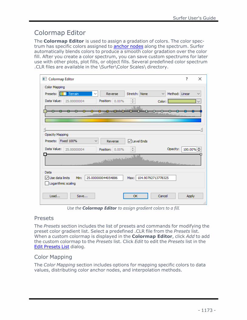
Surfer User's Guide
Colormap EditorThe Colormap Editor is used to assign a gradation of colors. The color spec-trum has specific colors assigned to anchor nodes along the spectrum. Surferautomatically blends colors to produce a smooth color gradation over the colorfill. After you create a color spectrum, you can save custom spectrums for lateruse with other plots, plot fills, or object fills. Several predefined color spectrum.CLR files are available in the \Surfer\Color Scales\ directory.
Use the Colormap Editor to assign gradient colors to a fill.
PresetsThe Presets section includes the list of presets and commands for modifying thepreset color gradient list. Select a predefined .CLR file from the Presets list.When a custom colormap is displayed in the Colormap Editor, click Add to addthe custom colormap to the Presets list. Click Edit to edit the Presets list in theEdit Presets List dialog.
Color MappingThe Color Mapping section includes options for mapping specific colors to datavalues, distributing color anchor nodes, and interpolation methods.
- 1173 -

Chapter 29 - Common Properties
ReverseThe Reverse button flips the order of colors in the colormap so that colors cur-rently associated with low data values will be mapped to high values and colorscurrently associated with high values will be mapped to low values. The samplecolormap updates to show the new color order.
StretchThe Stretch field includes options to distribute colors (anchor nodes) across thecolormap based on data values.
l By default, the Stretch is set to None. When None is selected, each anchornode can be positioned independently.
l Select Evenly Distribute to evenly distribute the anchor nodes between thedata minimum and maximum. The nodes are automatically redistributedevenly when nodes are added or removed or when the data Min or Max ischanged.
l Select Equalize to distribute the nodes to improve the contrast in the mapvia histogram equalization. The nodes are distributed so that each his-togram "bin" between nodes contain an equal number of data points. Thenodes are automatically redistributed evenly when nodes are added orremoved. The Equalize option is not available when a histogram is not dis-played, e.g. for watershed maps.
The Stretch option must be set to None before anchor nodes can be manuallypositioned.
Interpolation MethodThe Method option determines which interpolation method is used to specify thecolors between anchor nodes.
l Linear interpolation uses weighted averages to interpolate colors betweennodes. This linear interpolation between each color node results in agradual transition and smooth appearance.
l Reverse interpolation uses weighted averages to interpolate colorsbetween nodes like the Linear interpolation. However, the colors arereversed between nodes. This reverse linear interpolation between eachcolor node results in a segmented appearance.
l Cosine interpolation uses 180 degree segments of the cosine wave. Therate of change of the color is faster than the Linear interpolation. This inter-polation results in a smooth appearance.
l Flat Start applies the color from the left node to the area between nodes.This interpolation results in a sharp transition between colors.
- 1174 -

Surfer User's Guide
l Flat Middle applies the color from the midpoint linear interpolation betweenthe left and right nodes to the area between nodes. This interpolation res-ults in a sharp transition between colors.
l Flat End applies the color from the right node to the area between nodes.This interpolation results in a sharp transition between colors.
l HSL CW interpolates the colors between nodes from the Hue-Saturation-Luminosity color wheel in a clockwise direction.
l HSL CCW interpolates the colors between nodes from the Hue-Saturation-Luminosity color wheel in a counterclockwise direction.
l HSL Shortest interpolates the colors between nodes from the shortest dis-tance (clockwise or counterclockwise)on the Hue-Saturation-Luminositycolor wheel between each node pair.
l HSL Longest interpolates the colors between nodes from the longest dis-tance (clockwise or counterclockwise)on the Hue-Saturation-Luminositycolor wheel between each node pair.
Data Value and PositionThe Data Value displays the data value of the selected node. The Position fielddisplays the node's relative position in the colormap where the colormap min-imum Position is 0% and the maximum is 100%. The selected node may beaccurately repositioned by entering a new value in the Data Value or percentagein the Position field. The first and last nodes cannot be changed and this controlis disabled when an end node is selected. To change the first and last nodes,change the Min and Max values in the Data section.
The Data Value option applies to any map divided into classes, such as mapswith classed symbols or classed colors. To determine the color in the colormapassociated with each class, the following rules are used:
l The first class uses the Minimum value color. This is the node on the far leftside of the colormap.
l Subtract the Minimum from the Maximum value and divide by the Numberof classes. This is the separation value. Add the separation value to the Min-imum value. This will be the value color associated with the next class.
l Add the separation value to the previous value. This is the value color asso-ciated with the next class.
l Repeat adding the separation value to the previous value until only the lastclass remains. The last class uses the Maximum value color. This is thenode on the far right side of the colormap.
- 1175 -

Chapter 29 - Common Properties
l Surfer automatically interprets the colormap to determine the color valueassociated with each class. Any number of nodes can exist on thecolormap. The nodes and the Value in the colormap are not associated withthe classes.
ColorClick the Color box to specify the color of the currently selected anchor node. Thecolor palette opens.
Data HistogramA data histogram is displayed in both the Color Mapping and Opacity Mappingsections. The histogram consists of equal width bins between the data minimumand data maximum. The number of bins is the number of data points or 256,whichever is fewer.
l For most grid-based maps, the grid Z values are used to create the his-togram.
l For base map symbology, the selected Attribute field data is used to createthe histogram.
l For vector maps with magnitude scaling, the vector magnitude data is usedto create the histogram. The magnitude will be calculated in the case of 1-grid vector and Cartesian 2-grid vector maps. The magnitude is used fromthe magnitude grid directly in the case of a polar 2-grid vector map. For vec-tor maps with grid scaling, the Z values from the selected grid are used tocreate the histogram.
l For point cloud maps, the data selected in the View by property is used tocreate the histogram.
When the Logarithmic scaling option is selected in the Data section, the his-togram bins are calculated from the log of the data values. This ensures the his-togram remains aligned with the colormap when Logarithmic scaling is selected.This scales the X axis (bins).
You can also logarithmically scale the Y axis (frequency) values. This option isuseful when only a few bins contain most of the data values. Logarithmic scalingthe Y axis will show more detail in the histogram. To apply logarithmic scaling tothe Y axis, right-click either of the data histograms and select LogarithmicScale in the context menu. To return to linear scaling on the Y axis, right-clickeither of the data histograms and select Linear Scale.
In the Color Mapping section, the colormap anchor nodes are displayed abovethe data histogram. An anchor node's horizontal position corresponds to its DataValue and Position.
- 1176 -

Surfer User's Guide
Colormap ExampleThe sample of the generated colormap is display directly below the histogramand anchor nodes.
Anchor NodesAnchor nodes are displayed directly above the data histogram. Anchor nodes spe-cify a color and position in the Color Mapping section. Anchor nodes specify anopacity and position in the Opacity Mapping section.
You can add additional anchor nodes at any position along the colormap. To cre-ate a new anchor node, double-click on the data histogram where you want thenew node added. In the Color Mapping section, the new anchor is automaticallyassigned a Color based on the previous colormap, and the Data Value is assignedbased on where you clicked. In the Opacity Mapping section the new anchor isassigned the Opacity and Data Value corresponding to the exact location youclicked. You can add as many anchor nodes as you want. This lets you blend col-ors and opacities in many different ways on the colormap.
Left-click on an anchor node and press the DELETE key on the keyboard to deletea node. The first (far left) and last (far right) anchor nodes cannot be deleted.
Scroll ControlThe scroll control appears as a horizontal bar with end handles. Drag a handleleft or right to zoom the colormap and histogram in or out. Drag the center sec-tion to scroll the visible portion left or right. Double-click the center section toreturn it to the fully visible state. The scroll control changes the view of both theColor Mapping and Opacity Mapping sections.
Use the scroll control to zoom the colormap in or out.
Opacity MappingThe Opacity Mapping section contains the opacity mapping controls. These con-trols specify how a range of data values are mapped to opacity in the final out-put. Note that opacity is the opposite of transparency (0.0 is completelytransparent, 1.0 is completely opaque).
PresetsThe options in the Presets list may be used to preset the opacity settings whichcan then be modified as desired.
l Fixed 100% sets the entire data range to a fixed opacity of 100% (fullyopaque).
l Fixed 20% sets the entire range of data to a fixed opacity of 20%.
- 1177 -

Chapter 29 - Common Properties
l Ramp 0 to 100% sets the data Min value to an opacity of 0% and the dataMax value to an opacity of 100%. The opacity increases linearly from 0% to100% throughout the data range.
l Ramp 0 to 20% sets the data Min value to an opacity of 0% and the dataMax value to an opacity of 20%. The opacity increases linearly from 0% to20% throughout the data range.
l Middle Ramp sets the lowest (fourth) quartile to 0% opacity, followed by alinear ramp over the third and second quartiles, followed by a fixed opacityof 100% for the greatest (first) quartile.
l Custom is displayed automatically when a node is selected, created,removed, or the Opacity value or Data Value options are adjusted.
Data ValueThe Data Value displays the data value of the selected node. The Position fielddisplays the node's relative position in the colormap where the colormap min-imum Position is 0% and the maximum is 100%. The selected node may beaccurately repositioned by entering a new value in the Data Value or percentagein the Position field. The first and last nodes cannot be changed and this controlis disabled when an end node is selected. To change the first and last nodes,change the Min and Max values in the Data section.
Level EndsCheck the Level Ends box to level the first and last segments of the opacitygraph. When the nodes at one end of a level segment are dragged up or down,the other end is also dragged.
OpacitySpecify the opacity for the selected node in the Opacity field. The Opacity valueranges from 0.00% (completely transparent) to 100.00% (completely opaque).To change the opacity, click on one of the nodes. Then, highlight the existingvalue and type a new value or click the button to increase or decrease the opa-city for the selected node.
Data HistogramThe Opacity Mapping section includes a data histogram. See the Color Mappingsection above for the histogram description. Opacity anchor nodes are displayedon the data histogram. An anchor node's vertical position corresponds to its Opa-city. An anchor node's horizontal position corresponds to its Data Value and Pos-ition.
DataThe Data section contains options for setting the minimum and maximum datavalues and scaling to use in the colormap.
- 1178 -

Surfer User's Guide
Use Data LimitsCheck the Use data limits check box to use the data minimum and maximum val-ues. This option is not available for classed post maps.
Colormap Data Minimum and MaximumIf you would prefer to set the colormap minimum and maximum values, enterthe new numbers into the Min and Max boxes. This is useful when you are map-ping different data sets in a similar range and would like to have the same datavalues represented by the same colors in each map. If a data value within themap falls outside this range, it is assigned the minimum or maximum color,whichever is closest.
The minimum and maximum values cannot be set for the classed post map. Forthe classed post map, the far left Min node is always the median value for thefirst class. The far right Max node is always the median value for the last class.This cannot be changed.
Logarithmic ScalingCheck the box next to the Logarithmic scaling to set the intervals between thenodes to a log(10) scale. The Min and Max values are the same. The nodesbetween the minimum and maximum and the color definitions adjust to fit thelog(10) scale. On a log(10) scale, there is as much distance on the colormapsample between 1 and 10 as between 10 and 100 or 100 and 1000. In theexample below, the nodes are displayed at 0.1, 1, 10, 100, and 1000. To use aregular linear scale on the colormap, clear the box next to Logarithmic scaling.
The associated color scalebar is shown with the majorlog intervals displayed.
- 1179 -

Chapter 29 - Common Properties
Loading a ColormapThe Load button opens an existing colormap .CLR file. When you click the Loadbutton, the Open dialog is displayed with a list of colormap files. Click the fileyou want to use and click Open. The colormap is updated to show the colormapfile settings.
Colormap files can be used with maps of varying Z ranges since the anchornodes are stored as percentages rather than as data values. To use the exactsame colors in the exact same data locations when the Z ranges vary slightly,override the default data limits and assign custom values in the Data to ColorMapping group.
Saving a ColormapClick the Save button in the Colormap Editor to create a colormap .CLR filebased on the current colormap settings. When you click the Save button, theSave As dialog is displayed. Type the File name for the colormap file and clickSave. The file is saved for use with other files.
Anchor NodesThe color spectrum is defined by anchor nodes at user-defined points along acolor spectrum in the Colormap Editor. Colors and opacities are automaticallyblended between adjacent anchors. Anchor nodes are represented by a sliderbutton along a line on the Color Mapping and Opacity Mapping data histograms.
Anchor Node ValueThe data value for the node is displayed in the Data Value box. Except for thefirst and last nodes, any node can be assigned to a specific value by typing a newnumber into the Data Value box. The first and last node data values are con-trolled by the Min and Max in the Data section.
Add Anchor NodeYou can add additional anchor nodes at any position along the colormap. To cre-ate a new anchor node, double-click on the data histogram where you want thenew node added. In the Color Mapping section, the new anchor is assigned aColor and Data Value based on where you clicked. In the Opacity Mapping sec-tion, the new anchor is assigned an Opacity and Data Value corresponding to theexact location you clicked. You can add as many anchor nodes as you want. Thislets you blend colors and opacities in many different ways on the colormap.
Delete Anchor NodeLeft-click on an anchor node and press the DELETE key on the keyboard to deletea node. The first (far left) and last (far right) anchor nodes cannot be deleted.
Positioning a Color Anchor NodeTo position an anchor node:
- 1180 -

Surfer User's Guide
1. Move the mouse cursor over the slider button.2. Click and hold the left mouse button.3. Drag the slider button to the desired position and release the left mouse but-
ton. As you move the slider button left or right, the data value is indicated inthe Data Value box. Alternatively, you can set the anchor to a specific datavalue by entering a number into the Data Value box. Note that the beginningand ending anchors cannot be moved or deleted.
4. Specify the Min and Max values in the Data section to change the range, andtherefore, the position of the starting and ending nodes.
Selecting a Color for an AnchorTo select a color to associate with the anchor node in the Color Mapping section:
1. Click on the anchor you wish to modify.2. Click on the desired color in the Color palette. The color spectrum is updated
to indicate the change.
Alternatively, use a preset .CLR color file by selecting one of the options from thePresets list or click the Load button to load a custom .CLR file.
Positioning an Opacity Anchor NodeTo position an anchor node:
1. Move the mouse cursor over the slider button.2. Click and hold the left mouse button.3. Drag the slider button to the desired position and release the left mouse but-
ton. As you move the slider button left or right, the data value is indicated inthe Data Value box. Alternatively, you can set the anchor to a specific datavalue by entering a number into the Data Value box. As you move the sliderbutton up or down, the Opacity value is increased or decreased. Altern-atively, you can set the anchor to a specific value by typing a number in theOpacity box. Note that the beginning and ending anchors cannot be moved ordeleted.
4. Specify the Min and Max values in the Data section to change the range, andtherefore, the position of the starting and ending nodes.
Select an Opacity for an AnchorTo select an opacity to associate with the anchor node in the Opacity Mappingsection:
1. Click on the anchor you wish to modify.2. Type the desired value in the Opacity field. The color spectrum is updated to
indicate the change.
Alternatively, click and drag the anchor node up or down, use a preset .CLR colorfile by selecting one of the options from the Presets list, or click the Load buttonto load a custom .CLR file.
- 1181 -

Chapter 29 - Common Properties
Using Color Spectrums in Map SeriesSometimes it is necessary to use the same range of colors on different maps. Bydefault, color spectrums are assigned to the minimum and maximum data valuesfor a given data set. If the maps have different data ranges, the colors will notmap to the same data values and it will be difficult to compare the maps. In thiscase, you may want to override the default data limits and assign custom valuesin the Colormap EditorData group.
ExampleThe following example contains steps on how to create maps in a series that con-tain the same color spectrums although the data minimums and maximums dif-fer. The example color relief maps show the same gridded area at three differentpoints in time. To accurately compare the maps, the color spectrum needs to bethe same through time even when the range of values fluctuates between grids.
Know Your DataThe first step in producing maps with the same color series is to know your data.Find the minimum and maximum data values for all of your data sets before youbegin. This will help you to decide the minimum and maximum values to use inthe color spectrum for the series of maps. In this example, the maximum Z valueis +251 in one of the grids, and the minimum Z value is -261 in another grid. Thelargest and smallest Z values do not appear in the same grid.
The three maps shown above all use the same color spectrum range, even though the gridminimums and maximums differ.
The three maps above show the same phenomena over a period of time. The gridranges are not the same, but since the maps are to be compared, the colors needto map to the same data values for all maps. Using the same color spectrum.CLR file and changing the minimum and maximum spectrum data values allowsyou to quickly compare the maps visually. The color scale bar to the right is usedfor all three maps. The map on the left contains a dark black area because it hassome extreme negative values, but it does not have any pure white because itdoes not have extreme positive values. The map on the right is opposite, it
- 1182 -

Surfer User's Guide
contains extreme positive values so there is an area of pure white, but the neg-ative values are not extreme so there is no pure black. The map in the centerdoes not contain extremes in either direction so it is mostly red. Note that thesemaps have "stair step" edges due to NoData regions in the corners. A smallergrid spacing or interpolating the pixels would smooth the edges.
Creating a Color Spectrum FileAfter you know the series minimum and maximum and have decided on a spec-trum minimum and maximum, you can create a color spectrum .CLR file to usewith all the data. In this example, -275 is the minimum and +275 is the max-imum.
To create a color spectrum .CLR file:
1. Create a map using the Home | New Map | Color Relief command. Acolor relief map is used throughout this example, though you can use con-tour maps or any other map type that uses a colormap in this procedure.
2. Select one of the sample .GRD files and click Open.
3. Click once on the color relief layer to select it.
4. In the Properties window, click on the General tab.
5. In the General section, click the button next to the currently selectedcolormap displayed in the Colors option to open the Colormap Editor.
6. In the Data section, change the Minimum to -275 and the Maximum to+275.
7. In the color spectrum bar, left-click in the middle of the color spectrum toadd an anchor node. While the node is still selected, change the Value to -200 or slide the node to the -200 position (watch the numbers in the Valuebox). The minimum color (at -275) is black. Select black for the -200 nodeas well.
8. Repeat step 6 to add nodes at zero (gray) and +200 (white).
9. Click the Save button to save the color spectrum .CLR file.
10. In the Save As dialog, type a File name and click Save.
11. Click OK to make the color change to existing map.
Using the Color Spectrum File in Other MapsAfter you have created the color spectrum file as above, you can use it in theremainder of the maps in a series. To use a color spectrum file in another map:
- 1183 -

Chapter 29 - Common Properties
1. Create the map by clicking the Home | New Map | Color Relief com-mand.
2. In this example, a new color relief map is created with the next grid file.Select the next grid file and click Open.
3. Click once the color relief layer to select it.
4. In the Properties window, click on the General tab.
5. In the General section, click the button next to the currently selectedcolormap displayed in the Colors option.
6. Click the Load button in the Colormap Editor and open the color spectrum.CLR file you just created.
7. In the Data group, set the Minimum and Maximum to the pre-determinedvalues. In this example, the minimum is set to -275 and the maximum to+275.
8. Click OKto make the color change to this map.
9. Repeat this process for the rest of the maps in the series.
Level Files.LVL Level files contain information needed to set the contour interval and basicline and fill information for contour and wireframe maps. Label and hachuresinformation is also retained in the .LVL file. .LVL files can be created from the con-tour map, wireframe map, or in the worksheet.
Level files can be used in contour maps, 3D wireframe maps, and the grid editor.
Level Files - ContourFor contour maps, .LVL level files contain information about contour levels,including the line properties, color fill, label frequency, and hachure information.The level file contains all the information contained on the Levels page in theadvanced contour map Levels for Map dialog. After defining custom contourlevels and colors on a map, you can save the level and color information in alevel file. A level file can be recalled for any other contour map or 3D wireframe.
- 1184 -

Surfer User's Guide
Not all of the information in a level file can be used in a 3D wireframe. If you usea level file created in the contour map properties dialog in a wireframe, the colorfill, contour label, and hachure information are ignored.
Creating Level FilesThe easiest way to create a level file is from the advanced contour map prop-erties or 3D wireframe properties dialogs. You can also create a level file in theworksheet or in an ASCII editor, using the .LVL file format.
To create a .LVL level file containing contour level information in the advancedcontour map level properties:
1. Click once on a contour map to select it. The contour map properties will beshown in the Properties window.
2. Click on the Levels tab. Change the Level method to Advanced.
3. Click the Edit Levels button next to Contour levels. The Levels for Map dia-log opens.
4. Change any of the contour parameters, including the contour levels, lineproperties, fill properties, contour labels, and hachure information.
5. After changing the settings, click Save.
6. In the Save As dialog, type the name of the level file and click the Save but-ton. The level file is saved with a .LVL extension.
7. Click OK to close the dialog.
Using Level FilesTo use an existing .LVL file with any contour map:
1. Click once on a contour map to select it. The contour map properties will beshown in the Properties window.
2. Click on the Levels tab. Change the Level method to Advanced.
3. Click the Edit Levels button next to Contour levels. The Levels for Map dia-log opens.
4. Click Load.
5. Select the .LVL file and click Open.
6. Click OK and the contour map updates.
Note, all contour maps using the level file must have comparable Z data ranges,otherwise contour lines and fill will not appear on the map.
- 1185 -

Chapter 29 - Common Properties
Wireframe Level FilesFor 3D wireframes, .LVL level files contain information for the Z level line prop-erties and for the color zone line properties. After defining custom level and lineproperties on the Z Levels page or the Color Zones page, save the level and colorinformation in a level file. This level file can be recalled for any other 3D wire-frame or contour maps.
Level files created from the wireframe properties dialog contain only informationfor the Z level line properties. Color fill, contour label, or hachure information isnot written to the level file if the level file is created from the wireframe.However, a level file created from the advanced contour map level properties dia-log may contain such additional information. A level file created from the wire-frame properties dialog can be used for a contour map and vice versa. Anyadditional information not used is ignored.
Creating Level FilesTo create a .LVL level file containing level and line property information from thewireframe properties:
1. Click once on a wireframe map to select it. The wireframe map properties willbe shown in the Properties window.
2. Click on the Z Levels tab or the Color Zones tab.3. Click the Edit Levels button. The Properties dialog opens.4. Change any of the parameters, including the contour levels or line properties.5. After changing the settings, click Save.6. In the Save As dialog, type the name of the level file and click the Save but-
ton. The level file is saved with a .LVL extension.7. Click OK to close the dialog. The wireframe map updates.
Using Level FilesTo use an existing .LVL file with any wireframe map:
1. Click once on a wireframe map to select it. The wireframe map properties willbe shown in the Properties window.
2. Click on the Z Levels tab or the Color Zones tab.3. Click the Edit Levels button. The Properties dialog opens.4. Click Load.5. Select the .LVL file and click Open.6. Click OK to close the dialog. The wireframe map updates.
Note, all wireframe maps using the level file must have comparable Z dataranges, otherwise lines will not appear on the map.
Creating Level Files in the WorksheetYou can create simple level files in the Surfer worksheet or an ASCII editor. Theminimum amount of information a level file contains is the elevation data telling
- 1186 -

Surfer User's Guide
Surfer which contour lines to place on a contour map. For more information onthe level file format, see thelevel file format.
Creating Level Files from the Worksheet
1. Enter level values into column A.
2. Add any other information you wish to include for the levels (i.e. line color)according to the level file format.
3. After entering the level information, click File | Save As.
4. In the File name field, enter the level file name and .LVL extension enclosedin quotes ( "colors.lvl" ).
5. Choose DAT Data (*.dat) from the Save as type field and click Save.
6. In the Data Export Options dialog, choose Space as the Delimiter andDouble Quote as the Text Qualifier. Choosing any other delimiter in theData Export Options dialog results in an invalid level file since the filemust be space delimited.
7. Click OK to create the level file.
Color PaletteThe color palette is opened by clicking on an existing color button in the Colorslist.
l The name of the color appears at the top of the palette.l Select a color from the palette by clicking on a color.l Create a custom color by clicking the button to the right of the selec-
ted color.
Select a predefined or custom color from the colorpalette.
- 1187 -

Chapter 29 - Common Properties
Colors DialogClick the button to the right of any color in the Properties window to open theColors dialog. Use the Colors dialog to load standard colors or create customcolors. There is a Custom button at the bottom of all palettes.
Standard PageThe standard colors appear on the Standard page in a standard palette spec-trum.
ColorsClick a color in the standard palette spectrum.
NewA preview of the selected color appears under New on the right side of the dialog.Click the OK button to accept the new color. The Colors dialog closes.
SelectClick the Select button to color match to any color on the screen. The cursorchanges to an eyedropper. Move the cursor around the screen and the colorunder New changes accordingly. Click the mouse when you find the color youwant, and that color appears under new. Click the OK button to accept the newcolor. The Colors dialog closes.
- 1188 -

Surfer User's Guide
Use the Colors dialog to load standard colors or create custom col-ors.
Custom PageYou can create custom colors on the Custom page. New colors are created bymixing red, green, and blue.
ColorsClick anywhere in the color spectrum to choose a new color, or enter new valuesin the Hue, Sat, Lum, Red, Green, and Blue boxes. You can drag the slider nextto the color spectrum to adjust the new color's intensity.
NewA preview of the new color appears under New on the right side of the dialog.Click OK to accept the new color. The Colors dialog closes.
SelectClick Select to color match to any color on the screen. The cursor changes to aneyedropper. Move the cursor around the screen and the color under Newchanges accordingly. Click the mouse when you find the color you want, and thatcolor appears under New. Click OK to accept the new color. The Color dialogcloses.
- 1189 -

Chapter 29 - Common Properties
Use the Colors dialog to load standard colors or create custom col-ors.
CancelWhile in the Colors dialog, click Cancel to close the dialog without making anycolor changes.
Color ListColors can be referenced by RGB or RGBA values for advanced options. The syn-tax is Rxxx Gyyy Bzzz Aaaa where xxx, yyy, and zzz and aaa specify a red,green, blue color and transparency component respectively. Each color com-ponent can range from 0 to 255.
Automation does not require color names because there are explicit enu-merations for the colors. Refer to srfColor values or wksColor values for a list ofcolor enumerations. Also, refer to the specific automation topic for specifying col-ors in automation.
Select a color from the color palette.
ExampleR0 G0 B0 All components are 0, resulting in blackR0 G255 B0 Pure green
- 1190 -

Surfer User's Guide
R255 G255B255
All components are at full intensity, resulting in white
- 1191 -

Chapter 29 - Common Properties
Color Names
- 1192 -

Surfer User's Guide
Black=0 0 0 255
90% Black=25 25 25255
80% Black=51 51 51255
70% Black=77 77 77255
60% Black=102 102102 255
50% Black=128 128128 255
40% Black=153 153153 255
30% Black=179 179179 255
20% Black=204 204204 255
10% Black=230 230230 255
White=255 255 255 255
Blue=0 0 255 255
Cyan=0 255 255 255
Green=0 255 0 255
Yellow=255 255 0 255
Red=255 0 0 255
Magenta=255 0 255 255
Purple=153 0 204 255
Orange=255 102 0 255
Pink=255 153 204 255
Dark Brown=102 51 51255
Moss Green=51 102102 255
Dark Green=0 51 51255
Forest Green=0 102 51255
Grass Green=0 153 51255
Wild Willow=181 20497 255
Kentucky Green=51153 102 255
Light Green=51 204102 255
Spring Green=51 20451 255
Turquoise=102 255204 255
Sea Green=51 204 153255
Faded Green=153 204153 255
Ghost Green=204 255204 255
Mint Green=153 255153 255
Army Green=102 153102 255
Avocado Green=102153 51 255
Martian Green=153204 51 255
Dull Green=153 204102 255
Walnut=102 51 0 255
Ruby Red=153 0 0 255
Brick Red=204 51 0255
Tropical Pink=255 102102 255
Soft Pink=255 153 153255
Faded Pink=255 204204 255
Dark Red=128 0 0 255
Crimson=153 51 102255
Regal Red=204 51 102255
Deep Rose=204 51153 255
Neon Red=255 0 102255
Deep Pink=255 102153 255
Hot Pink=255 51 153255
Dusty Rose=204 102153 255
Plum=102 0 102 255
Deep Violet=153 0 153255
Light Violet=255 153255 255
Violet=204 102 204255
- 1193 -
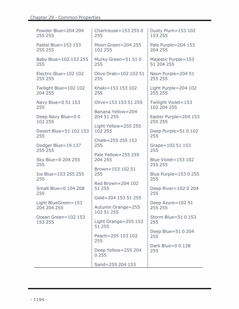
Chapter 29 - Common Properties
Powder Blue=204 204255 255
Pastel Blue=153 153255 255
Baby Blue=102 153 255255
Electric Blue=102 102255 255
Twilight Blue=102 102204 255
Navy Blue=0 51 153255
Deep Navy Blue=0 0102 255
Desert Blue=51 102 153255
Dodger Blue=19 137255 255
Sky Blue=0 204 255255
Ice Blue=153 255 255255
Smalt Blue=0 104 208255
Light BlueGreen=153204 204 255
Ocean Green=102 153153 255
Chartreuse=153 255 0255
Moon Green=204 255102 255
Murky Green=51 51 0255
Olive Drab=102 102 51255
Khaki=153 153 102255
Olive=153 153 51 255
Banana Yellow=204204 51 255
Light Yellow=255 255102 255
Chalk=255 255 153255
Pale Yellow=255 255204 255
Brown=153 102 51255
Red Brown=204 10251 255
Gold=204 153 51 255
Autumn Orange=255102 51 255
Light Orange=255 15351 255
Peach=255 153 102255
Deep Yellow=255 2040 255
Sand=255 204 153
Dusty Plum=153 102153 255
Pale Purple=204 153204 255
Majestic Purple=15351 204 255
Neon Purple=204 51255 255
Light Purple=204 102255 255
Twilight Violet=153102 204 255
Easter Purple=204 153255 255
Deep Purple=51 0 102255
Grape=102 51 153255
Blue Violet=153 102255 255
Blue Purple=153 0 255255
Deep River=102 0 204255
Deep Azure=102 51255 255
Storm Blue=51 0 153255
Deep Blue=51 0 204255
Dark Blue=0 0 128255
- 1194 -

Surfer User's Guide
255
Info PropertiesThe Info properties page contains information about the selected object. Infoproperties are available with drawn objects, such as polylines, polygons, points,grouped objects, images, and metafiles, with map objects, axes, and maplayers, such as contours or base layers. The information displayed is dependenton the type of object.
The Info page is located in the Properties window for the selected object. Asingle object must be selected to display the Info page.
The Info page displays information for the selec-ted object.
Geometry SectionThe Geometry section includes properties that specify the Coordinate systemfor calculating the geometry values and display the perimeter, length, position,or area of the selected object. Click on the next to Geometry to open the sec-
- 1195 -

Chapter 29 - Common Properties
tion. This section is only available for polylines, polygons, symbols, rectangles,rounded rectangles, ellipses, or spline polylines.
Select the units for the units for the Perimeter, Area, Length, or Position valuesby clicking the value and selecting the desired units from the list. The selectedunits are moved to the top of the list, otherwise the units are displayed alpha-betically.
Coordinate SystemSpecify a coordinate system from the Coordinate system list to be used for theinformation displayed for the object.
l Page uses the page coordinate system (inches or centimeters depending onthe setting in the Options dialog General page).
l Local uses the units from the layer in which the geometry was originally spe-cified. For example, if the geometry was loaded from a file, this is the originalfile units. If the geometry was created interactively, this is an internal coordin-ate system with 0.0 in the center of the page (in inches).
l Map displays information in map units if the geometry is part of a map. If theobject is not part of a map, this option is not available.
The default Coordinate system property is Map for map objects and Page forobjects outside a map. Changes to the Coordinate system selection are appliedto all objects. For example, if the property is changed to Local for one object, theLocal information will be displayed for the next selected object. If the selectedCoordinate system is a geographic coordinate system, i.e. uses sphericalcoordinates, some geometry information cannot be displayed.
Total Number of VerticesThe Total number of vertices displays how many vertices are used in the selectedobject. The Reshape command can be used to see the vertex locations for poly-gons and polylines.
Number of Sub-PolygonsIf the object contains a complex polygon, the Number of sub-polygons (rings) dis-plays how many polygons are included in the complex polygon. For example, thesample file ca2010.gsb has polygons of California counties. Some of the countiesare complex polygons (i.e. Santa Barbara) that include sub-polygon islands.
Number of CurvesThe Number of curves is displayed for a spline polyline. The Number of curves isthe number of inflection points along the spline polyline. This is one less than thetotal number of vertices.
Perimeter/LengthDepending on the object selected, either Perimeter or Length will be displayed.
- 1196 -

Surfer User's Guide
l The Perimeter displays the calculated perimeter of the selected closed object(i.e. polygon).
l The Length displays the calculated length of the selected open object (i.e.polyline). The units displayed are dependent on what is selected for theCoordinate system.
The Perimeter or Length is not displayed in spherical coordinates (i.e. degreesfor Unprojected Lat/Long coordinate systems). If your map is in a geographiccoordinate system, change the Target Coordinate System to a projected coordin-ate system to view the Perimeter or Length. Then specify Map in the Coordinatesystem field on the Info page.
AreaThe Area displays the calculated area of the selected object. The units displayedare dependent on what is selected for the Coordinate system.
The Area is not displayed in spherical coordinates (i.e. degrees squared forUnprojected Lat/Long coordinate systems). If your map is in a geographiccoordinate system, change the Target Coordinate System to a projected coordin-ate system to view the Area. Then specify Map in the Coordinate system list onthe Info page.
Add Geometry AttributesClick the Add Geometry Attributes command to add the geometry values dis-played above to the object's attributes. If you wish to add the geometry attrib-utes to all objects in the base layer, use the Attribute Table.
Info SectionThe Info section allows you to view the Type, Description, Number of records,size in bytes, Objects in group and image information for the selected object.Click on the next to Info to open the section. This section is available for text,images, metafiles, grouped objects, and point cloud layers.
TypeThe Type displays the type of metafile being displayed.
DescriptionThe Description displays any information about the metafile.
Number of RecordsThe Number of records displays the number of objects in the metafile.
- 1197 -

Chapter 29 - Common Properties
Pixel FormatThe Pixel format option displays the type of image imported, including the num-ber of bits per pixel included in the image.
Size in BytesThe Size in bytes or the Size (bytes) option displays the file size of the image ormetafile in bytes.
Size in PixelsThe Size (pixels) option displays the number of pixels in the image.
Image SourceThe Image source displays the name of the file imported for an image.
Number of PointsThe Number of points displays the number of points in the point cloud layer.
ExtentsThe xMin, xMax , yMin , yMax, Zmin, and Zmax values display the extents of thepoint cloud layer.
Attributes SectionThe Attributes section contains any information that is available about the selec-ted object. To open the Attributes section, click the next to Attributes.
Attributes can be image properties, such as TIFF_Compression, or can be inform-ation about a specific object that was imported from a file, such as a .DEM, .DXF,or .SHP file. Each object (such as polylines in a base map) can have its own attrib-ute information. The Attributes can also contain user generated information.
Adding AttributesTo add an attribute to the Attribute Table,
1. Click on the object to select it.2. In the Properties window, click on the Info page.3. Open the Attributes section by clicking the next to Attributes.4. Click on the Add button next to Add new attribute.5. Type the new attribute name, such as Surveyor's Name, in the Attribute
name field of the New Attribute Name dialog.6. Click OK in the New Attribute Name dialog. The new attribute is added to
the object displayed on the Info page.7. Click in the value column next to the new attribute name. Type the desired
- 1198 -
Surfer User's Guide
description, such as Thomas Denver.8. Now the new attribute and its value has been added to the object.
To rename or remove an attribute, use the Attribute Table.
Edit AttributesEdit attribute values by typing the new value into the field next to the attributename in the Properties window. Edit values for multiple attributes in a baselayer with the Attribute Table.
Options SectionThe Options section contains the option to copy the attribute data for a selectedobject. To open the Options section, click the next to Options.
Copy AttributesClick the Copy button next to Copy to clipboard to copy all of the information onthe Info page for the selected object to the clipboard. The text can be pastedinto Surfer or any other program using the Paste command. All information onthe Info page is copied, including the information in the Geometry and Info sec-tions. If the Copy button is not available, no attribute information is available forthe selected item.
Exporting AttributesAttribute information is exported for polygons, polylines, and points to fileformats that support metadata. The file type will determine how many attributesare exported. Refer to the specific file type pages for specific information.
Displaying AttributesAttributes can be added to base maps as labels. Click on the Basemap layerobject in the Contents window to select the base layer. In the Properties win-dow, click on the Labels tab to turn label display on. Any attribute can be used asa label for polylines, polygons, or symbols on a base map layer.
Information Displayed for ObjectsAll objects display an Attributes and Options section. The information in the Geo-metry section changes depending on the object selected.
PolylineThe Info properties for Polylines displays the Coordinate system, Number of ver-tices, and Length.
- 1199 -

Chapter 29 - Common Properties
PolygonThe Info properties for Polygons displays the Coordinate system, Total numberof vertices, Number of sub-polygons (rings), Perimeter, and Area.
PointThe Info properties for Symbols displays the Coordinate system and Position inX and Y units.
RectangleThe Info properties for Rectangles displays the Coordinate system, Perimeterand Area.
Rounded RectangleThe Info properties for Rounded Rectangles displays the Coordinate system,Perimeter and Area.
EllipseThe Info properties for Ellipses displays the Coordinate system, Perimeter andArea.
Spline PolylineThe Info properties for Spline Polylines displays the Coordinate system, Numberof curves and Length.
Range RingThe Info properties for Range Rings displays the Coordinate system, Perimeter,and Area. Note that when Number of rings is greater than one, the Perimeterand Area values are for the largest ring.
Group ObjectsThe Info page for Group Properties displays the number of Objects in group.Each group object can be selected in the Contents window to display the objectinfo.
MetafileThe Info properties for Metafiles displays the Type of metafile, Description, Num-ber of records, and Size in bytes.
ImageThe Info properties for Images displays the Pixel format, Size (pixels), Size(bytes), and Image source.
- 1200 -

Surfer User's Guide
New Attribute Name DialogThe New Attribute Name dialog is opened after the Add button is clicked in theAttributes section of Properties window Info Page or the button in the Attrib-ute Table.
Enter the new attribute name in the New Attribute Name dialog.
Attribute NameType the name for the new attribute in the Attribute name field.
Attribute TypeSpecify the data type for the attribute in the Attribute type field. Select Text orNumeric.
OK or CancelClick OK and the new attribute is added to the object. Click Cancel and the NewAttribute Name dialog is closed without adding a new attribute.
- 1201 -

Chapter 30 - Selecting and ArrangingObjects
Selecting ObjectsThere are several ways to select objects in Surfer. An object is selected if thereis a bounding box with selection handles surrounding the object. The name of theselected object appears in the status bar. You can set some selection options inFile | Options.
Editing base layers and groups is done by pinning them. Objects within groupscan be individually or selected in groups once the pin at the higher level in thehierarchy has been established.
Selecting Objects from the Contents Windowl Objects may be selected using the Contents window. To display the Con-tents window, use the View | Show/Hide | Contents command. Oncethe list is displayed, click on the layer or group you wish to select. To theright of the layer or group a button with a left arrow with a broken pinwill appear and the group or layer is selected in the plot window. Click onthe pin to toggle it to the pinned position . Objects contained within thehierarchy that is pinned may be edited without affecting objects in othergroups or layers. Objects outside the hierarchy that is pinned cannot beedited. The object's properties are displayed in the Properties window.
l Hold down the CTRL key while clicking on objects to select multiple objectsin the Contents window, or hold down the SHIFT key to select adjacentobjects.
Selecting Objects from the Plot WindowSeveral procedures are available to select objects in a plot window:
l After the list of objects is displayed and the layer or group has been pinnedin the contents window, objects within that hierarchy can be selected in
the plot window.
l To select a single object in the plot window, move the cursor over the objectusing the mouse or the arrow keys. When the cursor is over the desiredobject, click the left mouse button or press the SPACEBAR on the keyboard.Eight rectangular selection handles appear, indicating that the object is selec-ted.
- 1203 -

Chapter 30 - Selecting and Arranging Objects
l If an object other than the one you want is selected, hold down the CTRLkey and continue clicking with the mouse or SPACEBAR until the desiredobject is selected. Any objects that were previously selected becomedeselected. (The bounding boxes for the objects are overlapping.)
l To select two or more objects in the plot window, hold down the SHIFT keywhile making your selections. This retains previously selected objects andincludes the newly selected objects. You can hold down both the CTRL andSHIFT keys to select several overlapping objects in the plot window.
l The block select allows you to select one or more objects contained in auser-defined rectangle. Press and hold the left mouse button on an emptyportion of the plot window. Drag the mouse to form a rectangle around thegroup of objects you wish to select. Alternatively, you can use the arrowkeys to position the cursor on an empty portion of the plot window, pressand hold the SPACEBAR, and move the cursor with the ARROW keys. If theRectangle must fully surround check box is activated in the Options dialogSelection page, then only objects fully surrounded by the selection rect-angle are selected. If the check box is not activated, then all objects withany portion of their bounding boxes within the block select rectangle areselected.
l The Home | Selection | Select All command is used to select all the objectsin the plot window. Pressing the CTRL+A keys performs the same com-mand.
l The Home | Selection | Select All | Invert command selects all unselectedobjects and deselects all selected objects. This command is useful for select-ing a large number of objects and leaving a few isolated objects unselected.Select the objects you do not want to select and use the Invert Selectioncommand.
l The TAB key can be used to cycle through all objects, selecting each one ata time.
When you select a nested object, the main object is also selected. For example, ifyou select the contours map layer, the map object is also selected. Only one nes-ted object can be selected at a time. For example, it is not currently possible toselect two axes at once.
Select Tool
Click the Home | Selection | Select command or the button to click withthe mouse on objects to select them. When the cursor is in any other tool mode,for example draw or reshape, you can also return to select mode by pressingESC.
- 1204 -

Surfer User's Guide
Block SelectBlock select items by dragging a rectangle around them. To avoid accidentallymoving an object when selecting objects, use the Home | Selection | SelectAll | Block Select command or the button. If an object is properly selected abounding box will surround the object. The block select options are set in Selec-tion page of the Options dialog.
You can use the block select feature by:
l Clicking the Home | Selection | Select All | Block Select command anddragging a rectangle around the objects to select.
l Use the mouse to drag a block selection.
To select an object with block select:
1. Click the Home | Selection | Select All | Block Select command.2. Left-click outside one corner of the object.3. Hold the left mouse button down.4. Drag the mouse to the opposite corner of the object and release the mouse
button.
There are many ways to select objects in Surfer. Two of the most commoninclude the following:
l Select one object in the plot window and hold the SHIFT key, and select addi-tional objects to add to the block selection.
l Select one object in the Contents window, hold the CTRL key, and select addi-tional objects to add to the block selection. Hold SHIFT while selecting objectsin the Contents window to select a contiguous group of objects. Selectgroups or layers and pin them in order to edit the objects in their hier-archy.
Select All
Use the Home | Selection | Select All command or the button , or pressCTRL+A on the keyboard to select all objects in the document. A bounding boxsurrounds all selected objects.
Deselect AllUse the Home | Selection | Select All | Deselect All command or the but-ton, or press CTRL+SHIFT+A on the keyboard, to deselect all selected objects.This command is useful when zoomed in on objects. Alternatively, you candeselect objects by clicking in the white space.
- 1205 -

Chapter 30 - Selecting and Arranging Objects
Invert SelectionThe Home | Selection | Select All | Invert command or the buttonreverses the selected and deselected objects. All previously selected objectsbecome deselected. All previously deselected objects become selected. A bound-ing box surrounds all selected objects.
TransformWhen you select and drag an object, or resize it via the sizing handles, you aretransforming the object. The Align Objects, Rotate, and Free Rotate commandsalso transform the selected object. The accumulated effects of all trans-formations applied to an object are recorded as a set of page transformationparameters.
Transform DialogThe Home | Selection | Transform command or the button open theTransform dialog. This dialog allows you to read, set, and reset the six pagetransformation parameters associated with the selected object. These six para-meters allow for four distinct transformations: scale, shear, rotation, and offset.The coordinate origin for these transformations is the center of the page. Thus,in the untransformed state, the center of an object coincides with the center ofthe printed page.
Use the Transform dialog to change the trans-form parameters for the selected object.
X OffsetThe X Offset specifies the horizontal translation (in page units). A positive X Off-set shifts the object to the right, a negative X Offset shifts the object to the left.
- 1206 -

Surfer User's Guide
Y OffsetThe Y Offset specifies the vertical translation (in page units). A positive Y Offsetshifts the object up, a negative Y Offset shifts the object down.
X ScaleThe X Scale parameter modifies the width of the object. A value of 2.0 doublesthe width, a value of 0.5 cuts the width in half, while a value of 1.0 leaves thewidth unchanged.
Y ScaleThe Y Scale parameter modifies the height of the object. A value of 2.0 doublesthe height, a value of 0.5 cuts the height in half, while a value of 1.0 leaves theheight unchanged.
RotationThe Rotation specifies a counterclockwise rotation about the origin. The rotationangle is given in degrees.
ShearThe Shear changes the X coordinate as the Y coordinate changes. For example, ashear of 1.0 shifts the X coordinate 1 inch to the right for every inch along the Yaxis.
Identity (Clear Transform)When you check the Identity (Clear Transform) box, the transformation is resetback to the identity; that is, the selected object is untransformed.
The order in which the transformations are applied makes a difference (thesetransformations are not commutative). The four transformations are applied inthe following order: scale, shear, rotation, and translation.
ReferencesFoley, James D. and Andries van Dam (1990),Computer Graphics: Principles andPractice, Addison-Wesley, Reading, MA, 1174 pp.
Hearn, D. and M.P. Baker (1997),Computer Graphics C, 2nd edition, PrenticeHall, Upper Saddle River, NJ, 652 pp., ISBN 0-13-530924-7.
Rename ObjectThe Home | Selection | Rename command lets you assign a name to any typeof object, including maps and map axes. After selecting a single object, click theHome | Selection | Rename command or the button to display the
- 1207 -
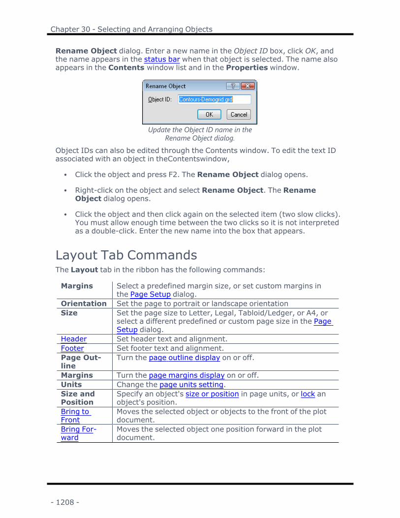
Chapter 30 - Selecting and Arranging Objects
Rename Object dialog. Enter a new name in the Object ID box, click OK, andthe name appears in the status bar when that object is selected. The name alsoappears in the Contents window list and in the Properties window.
Update the Object ID name in theRename Object dialog.
Object IDs can also be edited through the Contents window. To edit the text IDassociated with an object in theContentswindow,
l Click the object and press F2. The Rename Object dialog opens.
l Right-click on the object and select Rename Object. The RenameObject dialog opens.
l Click the object and then click again on the selected item (two slow clicks).You must allow enough time between the two clicks so it is not interpretedas a double-click. Enter the new name into the box that appears.
Layout Tab CommandsThe Layout tab in the ribbon has the following commands:
Margins Select a predefined margin size, or set custom margins inthe Page Setup dialog.
Orientation Set the page to portrait or landscape orientationSize Set the page size to Letter, Legal, Tabloid/Ledger, or A4, or
select a different predefined or custom page size in the PageSetup dialog.
Header Set header text and alignment.Footer Set footer text and alignment.Page Out-line
Turn the page outline display on or off.
Margins Turn the page margins display on or off.Units Change the page units setting.Size andPosition
Specify an object's size or position in page units, or lock anobject's position.
Bring toFront
Moves the selected object or objects to the front of the plotdocument.
Bring For-ward
Moves the selected object one position forward in the plotdocument.
- 1208 -

Surfer User's Guide
Send to Back Moves the selected object or objects to the back of the plotdocument.
Send Back-ward
Moves the selected object one position backward in the plotdocument.
Size Both Size one or more objects to a reference object'sWidth,Height, or Both.
Align Aligns objects to the left, center, right, top, middle, or bot-tom. Distributes objects horizontally or vertically with equalspacing (or overlap). Align or distribute to the bounding boxor page margins.
Free Rotate Rotates an object with the mouseRotate Rotates an object by specific degrees
Positioning and Sizing ObjectsThe Size and Position groups on the Layout tab contain options to position andsize objects. Objects can also be positioned and resized using the mouse and key-board. Objects can also be repositioned by dragging them to a new location withthe mouse or with the keyboard.
Change the size or position ofany object in the Size or Pos-ition group on the Layout tab.
Horizontal and Vertical PositionUse the horizontal position (X) and the vertical position (Y) to set the X, Y pos-ition on the page for most objects. To change the location, highlight the existingvalue and type the desired value. Or, click the buttons to increase or decreasethe position. Press ENTER on the keyboard to make the change.
The X, Y location of the cursor is displayed in the status bar. This can be a goodsource of reference.
Width and HeightUse theW and H controls to set the width and height of the selected object. Tochange the size, highlight the existing value and type the desired value. Or, clickthe buttons to increase or decrease the size. Press ENTER on the keyboard tomake the change.
- 1209 -

Chapter 30 - Selecting and Arranging Objects
Stretching a map with the Layout | Size | W and Layout | Size | H fields doesNOT maintain the internal scale of the map. Use the Scale page in the Prop-erties window to change the map size. Fix the internal scale of a stretched mapby selecting the map and using the Identity (Clear transforms) option in theTransform command.
Resize ObjectsYou can resize objects graphically with the mouse or keyboard. Selected objectsappear with selection handles at the corners and sides of the bounding box forthe object. The size of a selected object is displayed in the status bar. The cursorchanges to a two-headed arrow when it is moved over one of the selectionhandles. Resize a single selected object or several selected objects using the fol-lowing methods. You can resize a single selected object or several selectedobjects using the selection handles. Side selection handles will move with thezoom level. The selection handles will always be visible along the side of thebounding box regardless of the zoom location or view.
l To drag a handle with the mouse, move the cursor over the handle andthen press and hold the left mouse button. Move the cursor to a new pos-ition. Release the left mouse button and the object is resized.
l To drag a handle with the keyboard, move the cursor over the handle,press and hold the SPACEBAR, and use the ARROW keys to move thecursor to a new position. Release the SPACEBAR and the object is resized.
l Drag one of the four corner handles to size the object proportionally.
l Drag one of the side handles to stretch or compress the object in one dimen-sion only.
l Press and hold the ALT key while dragging a corner handle with the mouseto free size an object.
l To resize a map, use the map properties Scale page to size the map.STRETCHING THE MAP DOES NOT PRESERVE THE INTERNAL MAP SCALE.Use Transform to undo the effects of stretching a map.
l Use theW and H fields in the Position and Size groups on the Layout tab tochange the width and height of an object.
l Use the Layout | Arrange | Size Both command to size one or more objectsto a reference object's width and/or height.
To return an object to the original size, select the object. Click Home | Selection |Transform and check the Identity (Clear Transforms) check box . The object isreturned to the original size and location.
- 1210 -

Surfer User's Guide
Lock PositionTo lock an object’s position, click on the object to select it. Click the Layout |Position | Lock command or right-click on the object and select LockPosition. When an object is locked it cannot be moved either through the Pos-ition group or by dragging it with the mouse. Objects that are locked can be res-ized, edited, and rotated.
Repeat the above instructions to unlock a locked object. Locked objects and lay-ers are indicated in the Contents window with a small lock icon.
The lock icon indicates the Map object is locked in the exampleabove.
Locked Map LayersWhen a map layer is locked, only the objects in that layer cannot be moved. Ifthe map or any portion of the map is selected and moved, the locked layer willalso be moved. To prevent map layers from moving on the page, lock the Mapobject.
Locked Objects in a Base LayerWhen objects in a base layer are individually locked, that object cannot bemoved individually. To move the object, unlock the object and move the objectto the desired position. The entire base layer and map object can be movedwhen a sub-object is locked. The sub-object stays in the same relative locationas the objects in the base layer or map.
Bring to FrontThe Layout | Arrange | Bring to Front command or the button moves theselected object or objects to the front of the plot document. The object willappear on top of the other objects. Alternatively, right-click the object and selectOrder Objects | Move to Front.
- 1211 -

Chapter 30 - Selecting and Arranging Objects
Objects can also be moved by dragging them to a new position in the Contentswindow.
The default keyboard shortcut for the Layout | Arrange | Bring to Front com-mand is SHIFT + PAGE UP. The keyboard shortcuts can be customized with theCustomize command.
Example
In the left drawing, the red square is located behind all of the other objects. UseBring to Front to move the square to the front layer so that it appears in frontof all the other objects (right drawing). The Bring Forward command moves thesquare forward one layer at a time.
Bring ForwardThe Layout | Arrange | Bring to Front | Bring Forward command or themoves the selected objects forward one position. Alternatively, right-click theobject and select Order Objects | Bring Forward.
Objects can also be moved by dragging them to a new position in the Contentswindow.
The default keyboard shortcut for the Layout | Arrange | Bring to Front |Bring Forward command is CTRL + PAGE UP. The keyboard shortcuts can becustomized with the Customize command.
Example
In the left drawing, the red square is located behind all the other objects. UseBring Forward to move the square forward one layer so that it appearsbetween the circle and the triangle (middle drawing). Clicking Bring Forwardagain places the square on top of the other objects (right drawing). Bring toFront places the square on top of the other objects.
- 1212 -

Surfer User's Guide
Send to BackThe Layout | Arrange | Send to Back command or the button move theselected object or objects to the back of the plot document. The object willappear behind the other objects. Alternatively, right-click the object and selectOrder Objects | Move to Back.
Objects can also be moved by dragging them to a new position in the Contentswindow.
The default keyboard shortcut for the Layout | Arrange | Send to Back com-mand is SHIFT + PAGE DOWN. The keyboard shortcuts can be customized withthe Customize command.
Example
In the left drawing, the red square is located in front of all the other objects. UseSend to Back to move the square to the back layer so that it appears behind allof the other objects (right drawing). Send Backward moves the square backwardone layer at a time.
Send BackwardThe Layout | Arrange | Send to Back | Send Backward command or thebutton move the selected object backward one position. Alternatively, right-clickthe object and select Order Objects | Move Backward.
Objects can also be moved by dragging them to a new position in the Contentswindow.
The default keyboard shortcut for the Layout | Arrange | Send to Back |Send Backward command is CTRL + PAGE DOWN. The keyboard shortcuts canbe customized with the Customize command.
Example
- 1213 -

Chapter 30 - Selecting and Arranging Objects
In the left drawing, the red square is located in front of all the other objects. UseSend Backward to move the square back one layer so that it appears betweenthe circle and the triangle (middle drawing). Clicking Send Backward againplaces the square on behind all of the other objects (right drawing). Send to Backplaces the square on behind the other objects.
Size ObjectsClick one of the Layout | Arrange | Size Both commands or the button tosize one or more objects to a reference object's width, height, or both. At leasttwo objects must be selected to use the Layout | Arrange | Size Both com-mands. The reference object's size does not change. All other objects are sizedequally to the reference object. The reference object is the highest selectedobject in the Contents window, i.e. the front object in the plot window.
WidthClick Layout | Arrange | Size Both | Width or the button to set the widthoff all selected objects equal to the width of the reference object.
HeightClick Layout | Arrange | Size Both | Height or the button to set theheight of all selected objects equal to the height of the reference object
BothClick Layout | Arrange | Size Both to set both the width and height of allselected objects equal to the width and height of the reference object.
Changing the Reference ObjectThe quickest way to make sure you have the correct reference object is to selectthe object you wish to use as the reference object and click the Layout | Arrange| Bring to Front | Bring to Front command. The object is moved to the top of theContents window and front of the plot window. It will be the reference objectwhen the Size commands are used with any other objects. However, you maynot wish to have your reference object at the front of the plot window. When thisis the case, click and drag the desired reference object in the Contents windowabove the objects you wish to re-size. You can also use the Layout | Arrange |Bring to Front | Bring Forward command to move an object forward one place ata time.
- 1214 -

Surfer User's Guide
Align ObjectsThe Layout |Arrange | Aligncommands are used to align selected objects rel-ative to the bounding box surrounding the selected objects. The objects can bealigned both vertically and horizontally. Objects can also be distributed hori-zontally or distributed vertically. Enable the Align to Margins option to alignobjects to the page margins rather than the bounding box.
Two or more objects must be selected to enable the Align commands whenAlign to Margins is not active. One or more objects must be selected to enablethe Align commands when Align to Margins is active.
Align LeftLeft aligns all selected objects along the left side of the bounding box whenAlign to Margins is not checked. Left aligns the selected object or objects tothe left margin when Align to Margins is checked.
Align CenterCenter centers all selected objects between the left and right sides of thebounding box when Align to Margins is not checked. Center aligns the selec-ted object or objects to the center of the page (between the left and right mar-gins) when Align to Margins is checked.
Align RightRight aligns all selected objects along the right side of the bounding boxwhen Align to Margins is not checked. Right aligns the selected object orobjects to the right margin when Align to Margins is checked.
Align TopTop aligns all selected objects along the top of the bounding box when Alignto Margins is not checked. Top aligns the selected object or objects to the topmargin when Align to Margins is checked.
Align MiddleMiddle centers all selected objects between the top and bottom sides of thebounding box when Align to Margins is not checked.Middle aligns the selec-ted object or objects to the middle of the page (between the top and bottom mar-gins) when Align to Margins is checked.
- 1215 -

Chapter 30 - Selecting and Arranging Objects
Align BottomBottom aligns all selected objects at the bottom of the bounding box whenAlign to Margins is not checked. Bottom aligns the selected object or objectsto the bottom margin when Align to Margins is checked.
Distribute HorizontallyClick the Layout |Arrange | Align | Distribute Horizontally command orthe button to distribute three or more objects from left to right with equal spa-cing in their bounding box. The interior object or objects are aligned horizontallybetween the outermost objects. This means the bounding box size does notchange, and the left and right objects do not move, while the objects arearranged. Three or more objects must be selected to enable the Layout |Arrange | Align | Distribute Horizontally command when Align to Margins isnot active. If the objects must overlap to fit inside the bounding box, the objectsare distributed with equal overlap. You can also right-click the selection and clickAlign Objects | Distribute Horizontally in the context menu to distribute theobjects.
Distribute with Align to MarginsClick the Distribute Horizontally command when Align to Margins is active todistribute two or more objects from left to right with equal spacing between thepage margins. All objects are aligned horizontally between the page margins.This means the bounding box size may change, and the left and right objectsmay move, while the objects are arranged. Two or more objects must be selec-ted to enable the Layout | Arrange | Align | Distribute Horizontally com-mand when Align to Margins is active. If the objects must overlap to fit inside thepage margins, the objects are distributed with equal overlap.
ExampleThe following steps demonstrate how to distribute objects horizontally:
1. Move the outside objects to the desired locations.2. Select the objects that are to be distributed, including the furthest left and fur-
thest right objects.3. Click the Layout | Arrange | Align | Distribute Horizontally command.
The interior objects are arranged between the outer most objects with equal spa-cing.
- 1216 -

Surfer User's Guide
Five objects are unevenly spaced.The circles are moved to the desiredlocations. The Layout |Arrange |Align | Middle command was used
to align the objects in a row.
All five objects are selec-ted before the Dis-tributeHorizontallycommand is used.
The Layout | Arrange |Align | Distribute Hori-zontally command is
clicked and the objects arenow equally spaced from
left to right.
Distribute VerticallyClick the Layout | Arrange | Align | Distribute Vertically command or thebutton to distribute three or more objects from top to bottom with equal spa-
cing. The interior object or objects are aligned vertically between the outermostobjects. This means the bounding box size does not change, and the top and bot-tom objects do not move, while the objects are arranged. Three or more objectsmust be selected to enable the Layout | Arrange | Align | Distribute Ver-tically command. If the objects must overlap to fit inside the bounding box, theobjects are distributed with equal overlap. You can also right-click the selectionand click Align Objects | Distribute Vertically in the context menu to dis-tribute the objects.
Distribute with Align to MarginsClick the Distribute Vertically command when Align to Margins is active to dis-tribute two or more objects from top to bottom with equal spacing between thepage margins. All objects are aligned vertically between the page margins. Thismeans the bounding box size may change, and the top and bottom objects maymove, while the objects are arranged. Two or more objects must be selected toenable the Layout | Arrange | Align | Distribute Vertically command whenAlign to Margins is active. If the objects must overlap to fit inside the page mar-gins, the objects are distributed with equal overlap.
ExampleThe following steps demonstrate how to distribute objects vertically:
1. Move the outside objects to the desired locations.2. Select the objects that are to be distributed, including the top and bottom
objects.3. Click the Layout | Arrange | Align | Distribute Vertically command.
The interior objects are arranged between the outer most objects with equal spa-cing.
- 1217 -

Chapter 30 - Selecting and Arranging Objects
Five objects are unevenly spaced.The circles are moved to thedesired locations. The Layout |Arrange | Align | Center com-mand was used to align the
objects in a column.
All five objects areselected before the
DistributeVerticallycommand is used.
The Layout | Arrange | Align| Distribute Vertically com-mand is clicked and the objectsare now equally spaced from
top to bottom.
Align to MarginsThe Align to Margins option determines whether objects are aligned and/or dis-tributed relative to the bounding box or relative to the page margins. Click theLayout | Align | Align to Margins command or the button to turn the Alignto Marginsmode on or off. When Align to Margins is turned on, the Align com-mands are enabled when one or more objects is selected and the Distribute Hori-zontally and Distribute Vertically commands are enabled when two or moreobjects are selected.
When Align to Margins is turned off, two or more objects must be selected toenable the Align Objects commands, and three or more objects must be selec-ted to enable the Distribute Horizontally and Distribute Vertically com-mands. The Align to Margins command icon is highlighted when Align toMargins is enabled.
The default Align to Margins state is not checked. The Align to Marginsoption applies to all documents and windows open in Surfer in a single session.The setting is not persistent between Surfer sessions, i.e. if you close andreopen Surfer, Align to Margins will be turned off.
Align to Margins ExampleWhen Align to Margins is enabled, the selected objects are individually alignedrelative to the page when one of the Align Objects commands is clicked.
- 1218 -

Surfer User's Guide
The four rectangles were selected and Layout | Arrange | Align | Top was clicked whileAlign to Margins was checked. The four rectangles are aligned along the top margin.
When Align to Margins is disabled, the selected objects are individually alignedrelative to the bounding box when one of the Align Objects commands isclicked.
The four rectangles were selected and Layout |Arrange | Align | Top was clicked whileAlign toMargins was not checked. The four rectangles are aligned along the top of the ori-
ginal bounding box.
You can group the objects with the Group command to maintain the objects' pos-itions relative to one another while aligning the group relative to the marginswhen Align to Margins is checked.
The four rectangles were grouped with Features | Group | Group. Next the group was selec-ted and Layout | Arrange | Align | Top was clicked while Align to Margins was checked.
The top of the group is aligned along the top margin.
Free RotateYou can use the Layout | Arrange | Free Rotate command or the button torotate an object with the mouse. Select the object then click the Layout |Arrange | Free Rotate command. The pointer will change to show next to itto indicate that the program is in rotate mode. To rotate an object, click on thescreen, hold the left mouse button, and move the mouse. As the object is rotatedthe degrees of rotation are indicated in the status bar and the object's outline isdisplayed in the rotated view with a dashed line. To fix the position of the rotatedobject, release the mouse button.
- 1219 -

Chapter 30 - Selecting and Arranging Objects
Clear RotationTo clear rotation, use Home | Selection | Transform.
Exit Rotate ModePress the ESC on your keyboard or click the Select command to exit rotate mode.
RotateUse the Layout | Arrange | Free Rotate | Rotate command or the buttonto rotate an object by a specified number of degrees. After selecting the com-mand, type the number of degrees to rotate the object into the Rotate dialog.Positive numbers rotate the object in a counterclockwise direction and negativenumbers rotate the object in a clockwise direction.
Specify the degree of Counterclockwiserotation in the Rotate dialog.
To clear rotation, use Home | Selection | Transform.
GroupThe Features | Group | Group command or the button is used to group sev-eral independent objects into one Group object. Alternatively, select multipleobjects and then right-click and select Group. Grouped objects can be a com-bination of several types of objects and they can be moved or resized as a singleobject.
- 1220 -

Surfer User's Guide
Group objects to toggle visibility or arrangemultiple objects quickly and easily.
Objects must be on the same level in the Contents window and, if applicable,under the same group or layer to be grouped. For example, top-level objectssuch as features, legends, and map frames can be grouped. Similarly, featureswithin a single base layer can be grouped. If multiple objects can be selected,then the objects can be grouped. However, map layers cannot be grouped, andobjects in different base layers or groups cannot be grouped.
Editing Grouped ObjectsAfter objects are grouped together, the group is displayed in the Contents win-dow as a Group object and sub-objects. Sub-objects can be edited, re-arranged,or deleted in the Contents window. Click on any of the sub-objects in the Con-tents window to display and change the properties for that object in the Prop-erties window. A sub-object may also be deleted.
A group object can be transformed with the Home | Selection | Transformcommand.
UngroupThe Features | Group |Ungroup command or the button is used to sep-arate objects that have been previously combined into a group object using theFeatures | Group | Group command.
- 1221 -

Chapter 30 - Selecting and Arranging Objects
A grouped object can also be ungrouped in the Contents window by right-clickingon the Group object and clicking Ungroup.
The Features | Group | Ungroup command can also be used on some impor-ted files: Golden Software Boundary .GSB, Atlas Boundary .BNA, USGS .DLG,.LGO, .LGS, AutoCAD .DXF, Golden Software Blanking .BLN, Metafiles, and somepasted objects.
- 1222 -

Chapter 31 - Changing the View
View Tab CommandsThe View tab in the plot document has the following commands:
Fit to Win-dow
Zooms to show all of the objects on screen
Page Zooms to fit the full page on screenZoom Zooms in, out, on selected objects, realtime, with rectangles,
actual size, to full screen, or previous viewPan Scrolls the window by "grabbing" the contents and dragging
themHyperlink View hyperlinks in the base layer attributes with the cursorRedraw Refreshes the image on screenAutoRedraw
Turns the automatic display of redraw on or off
Rulers Shows or hide the rulersGrid Shows or hide the drawing gridStatus Bar Shows or hides the status barContents Shows or hides the Contents windowProperties Shows or hides the Properties windowNew Win-dow
Opens a duplicate window of the active document
Cascade Arranges the windows so they overlapArrangeIcons
Arranges icons at the bottom of the application window
Tile Hori-zontal
Arranges windows horizontally so there are no overlapping tiles
Tile Ver-tical
Arranges windows vertically so there are no overlapping tiles
Reset Win-dows
Resets window display to the default layout
Fit to WindowClick the View | Zoom | Fit to Window command in the plot window or the
button, click the Grid Editor | View | Fit to Window command in thegrid editor, click the 3D View | View | Fit to Window command in the 3Dview, or press CTRL+D on the keyboard to adjust the zoom so all objects fill theplot, grid editor, or 3D view window.
- 1223 -

Chapter 31 - Changing the View
PageClick the View | Zoom | Page command or the button or press CTRL + G tosee extents of the page. The page outline is visible if the Show page rectangleoption is checked in the Options dialog User Interface page.
Zoom InThe View | Zoom | In command increases the magnification of the image inthe plot window. The command scrolls the window to keep the point of interestcentered. The 3D View | View | Zoom In command increases the mag-nification of the image in the 3D view. Click to zoom in toward the center of the3D view window.
Zoom In - PlotThe View | Zoom | In command increases the magnification of the image inthe plot window. The command scrolls the window to keep the point of interestcentered.
Enter Zoom In Mode
To enter zoom in mode, click the View | Zoom | In command or the buttonin the plot window. The cursor will change to a to indicate zoom in mode.Left-click the area on which to center the magnified image.
Exit Zoom In ModePress the ESC key or click on another tool command, such as zoom, draw, orreshape, to end zoom in mode.
Zoom with A Wheel MouseYou can use a wheel mouse to zoom realtime and pan in the plot window or gridnode editor. Rotate the wheel forward to zoom in, or rotate the wheel backwardto zoom out. Hold down the wheel button straight down, and the cursor will turnto a closed hand. When the cursor is a , drag the mouse to pan the plot win-dow. Be sure to click straight down with the scroll wheel. The zoom is changed sothat the cursor location remains on the screen.
Zoom with the KeyboardYou can use keyboard commands to zoom in and out of the plot window. Thedefault commands are CTRL + EQUAL SIGN (=) to zoom in, and CTRL + HYPHEN(-) to zoom out.
- 1224 -

Surfer User's Guide
Zoom In - 3D ViewClick the 3D View | View | Zoom In command to change the cursor to zoom-in mode. Click the 3D view window to zoom in to the center of the 3D view win-dow. Press ESC to return the cursor to Trackball mode, or click another 3D View| View command. The 3D view can also be changed by adjusting the values inthe Environment properties Camera page.
You can use a wheel mouse to zoom realtime in the 3D view window. Rotate thewheel forward to zoom in, or rotate the wheel backward to zoom out.
Zoom OutThe View | Zoom | Out command decreases the magnification of the image inthe plot window. The 3D View | View | Zoom Out command decreases themagnification of the 3D view window.
Zoom Out - PlotThe View | Zoom | Out command decreases the magnification of the image inthe plot window. The command scrolls the window to keep the point of interestcentered.
Enter Zoom Out Mode
To enter zoom out mode, select the View | Zoom | Out command or thebutton in the plot window. The cursor will change to a to indicate zoom outmode. Left-click the area on which to center the magnified image.
Exit Zoom Out ModePress the ESC key or click on another tool command to end zoom out mode.
Zoom with A Wheel MouseYou can use a wheel mouse to zoom realtime and pan in the plot window or gridnode editor. Rotate the wheel forward to zoom in, or rotate the wheel backwardto zoom out. Hold down the wheel button straight down, and the cursor will turnto a closed hand. When the cursor is a , drag the mouse to pan the plot win-dow. Be sure to click straight down with the scroll wheel. The zoom is changed sothat the cursor location remains on the screen.
Zoom with the KeyboardYou can use keyboard commands to zoom in and out of the plot window. Thedefault commands are CTRL+EQUAL SIGN(=) to zoom in and CTRL+HYPHEN (-)to zoom out.
- 1225 -

Chapter 31 - Changing the View
Zoom Out - 3D ViewClick the 3D View | View | Zoom Out command to change the cursor tozoom-out mode. Click the 3D view window to zoom out from the center of the 3Dview window. Press ESC to return the cursor to Trackball mode, or click another3D View | View command. The 3D view can also be changed by adjusting thevalues in the Environment properties Camera page.
You can use a wheel mouse to zoom realtime in the 3D view window. Rotate thewheel forward to zoom in, or rotate the wheel backward to zoom out.
Zoom SelectedThe View | Zoom | Selected command magnifies selected objects to the max-imum size possible in the plot window.
Select an object in the plot window or Contents window and click the View |Zoom | Selected command or the button to fit the view around the selectedobject.
Zoom with the KeyboardYou can use keyboard commands to zoom to the selected object in plot window.The default keyboard command for the View | Zoom | Selected command isCTRL+L.
Zoom RealtimeThe Realtime command zooms in and out as the left mouse button is held downand the mouse is dragged up and down in the plot or 3D view window. The 3Dview can also be changed by adjusting the values in the Environment propertiesCamera page.
Enter Zoom Realtime ModeTo enter zoom realtime mode, click the View | Zoom | Realtime command orthe button. The cursor will change to a to indicate that you are in zoomrealtime mode. Hold down the left mouse button and then drag up or down in thewindow to zoom in or out. As you drag the mouse up, the screen is zoomed in. Asyou drag the mouse down, the screen is zoomed out.
Exit Zoom ModeClick another tool or press the ESC key to end zoom mode.
- 1226 -

Surfer User's Guide
Zoom Realtime With A Wheel MouseYou can use a wheel mouse to zoom realtime in the plot window, 3D view win-dow, and grid editor. You can use a wheel mouse to pan in the plot window andgrid node editor. Rotate the wheel forward to zoom in, or rotate the wheel back-ward to zoom out. Hold down the wheel button straight down, and the cursor willturn to a closed hand. When the cursor is a , drag the mouse to pan the plotwindow. Be sure to click straight down with the scroll wheel. The zoom ischanged so that the cursor location remains on the screen.
Zoom RectangleThe Rectangle command allows magnification by drawing a rectangle aroundthe area of interest in the plot window or grid editor.
Enter Zoom Rectangle ModeSelect the View | Zoom | Rectangle command or the button in the plot win-dow or the Grid Editor | View | Zoom Rectangle command in the grid editor
to enter zoom rectangle mode. The cursor will change to a to indicate thatyou are in zoom rectangle mode. Hold down the left mouse button and drag thedotted zoom rectangle around the area of interest to magnify it. When the leftmouse button is released, the plot window will zoom to the selected area.
Exit Zoom ModeClick another tool button or press the ESC key to end zoom mode.
Zoom with the KeyboardYou can use keyboard commands to zoom to a rectangle in plot window. Thedefault keyboard command for the Rectangle command is CTRL+R.
Actual SizeThe View | Zoom | Actual Size command or the button scales the drawingto the approximate size it will be when printed. The size is usually scaled upslightly on the display to allow an adequate size for displaying text.
Full ScreenClick the View | Zoom | Full Screen command or the button to scale theselected object to fit the monitor. The ribbon are not accessible when viewing atFull Screen.
- 1227 -

Chapter 31 - Changing the View
Exit Full Screen ModePress the ESC key to return to the Surfer window. Alternatively, left-click any-where on the screen.
PanThe Pan command moves your location in the plot window, 3D view window, orgrid node editor while retaining the current level of magnification. The 3D viewcan also be changed by adjusting the values in the Environment properties Cam-era page.
Enter Pan Mode
Click the View | Pan | Pan command or the button in the plot window, 3DView | View | Pan command in the 3D view, or use the mouse wheel in thegrid editor to pan the current view.
To pan the current view:
1. Click the Pan command.2. Click on a portion of the current view.3. Hold the left mouse button down while dragging the view to a new position.
Exit Pan ModeClick on another toolbar button or press the ESC key to end pan mode.
Pan With A Wheel MouseYou can use a wheel mouse to zoom realtime in the plot window, 3D view win-dow, and grid editor. You can use a wheel mouse to pan in the plot window, gridnode editor, and 3D view. Rotate the wheel forward to zoom in, or rotate thewheel backward to zoom out. Hold down the wheel button straight down, and thecursor will turn to a closed hand. When the cursor is a , drag the mouse to panthe plot window, grid node window, or 3D view. Be sure to click straight downwith the scroll wheel. The zoom is changed so that the cursor location remains onthe screen.
RedrawClick the View | Redraw | Redraw command or the button or press the F5key on the keyboard to redraw the window.
- 1228 -

Surfer User's Guide
Auto RedrawAuto Redraw is used to automatically redraw the image each time the windowcontents or view is changed. Auto Redraw is on by default, and this is indicatedby a check mark beside the command. Click View | Redraw | Auto Redraw orthe button to toggle the command on and off. If Auto Redraw is disabled useRedraw or press the F5 key on the keyboard to redraw the image.
RulersClick the View | Show/Hide | Rulers command or the button to togglebetween showing and hiding the rulers on the top and left sides of the main plotwindow. When the Rulers command button is depressed, the rulers are shown.Surfer will remember your preference to have the ruler on or off when the pro-gram restarts.
You can also right-click on a ruler and click Ruler and Grid Settings to openthe Options dialog Rulers and Grid page.
Drawing GridClick the View | Show/Hide | Grid command or the button or right-click onthe plot window and click Drawing Grid to toggle between showing and hiding agrid which is superimposed over the plot window. The Grid command button isdepressed to indicate that the grid is displayed. Surfer will remember your pref-erence to have the drawing grid on or off when the program restarts.
The drawing grid is a series of evenly spaced dots, similar to graph paper, whichis used to help align objects in the plot window.
You can control the number of grid divisions in a page unit by clicking File |Options and clicking on the Rulers and Grid page.
New WindowClick the View | Windows | New Window command or the button to cre-ate a duplicate window. You can display different views or different parts of thesame document simultaneously by using New Window. Objects can be editedin either window and the changes appear in both windows.
- 1229 -

Chapter 31 - Changing the View
CascadeClick the View | Windows | Cascade command or the button to arrangemultiple document windows in an overlapped fashion. Each window is offset asmall amount from the previous window. Individual windows can be sized bydragging the window borders.
Arrange IconsClick the View | Windows | Arrange Icons command or the button toarrange the icons for minimized windows at the bottom of the main window. If amaximized window exists, then some or all of the icons may be located under-neath the window.
Tile HorizontalClick the View | Windows | Tile Horizontal command or the button toarrange multiple document windows in a non-overlapped fashion such that thewindows are oriented one above the other.
Tile VerticalClick the View | Windows | Tile Vertical command or the button toarrange multiple windows in a non-overlapped fashion side by side.
Reset WindowsClick the View | Windows | Reset Windows command or the button tochange the display of the program. This command resets the Contents and Prop-erties windows back to the default size and position. It also resets all ribbon,quick access toolbar, and keyboard command customizations back to thedefaults. This command is especially useful if your windows or managers becomehidden by mistake.
You must restart Surfer in order for this command to take effect. Click Yes in thedialog, close the program, and reopen Surfer. The windows, ribbon, and quickaccess toolbar are now in the default conditions.
- 1230 -

Chapter 32 - Importing, Exporting,and Printing
ImportThe Home | Insert | Graphic, the Home | New Map | Base, and the Home| Add to Map | Layer | Base commands in the plot window open the Importdialog.
Select files to import using the Import dialog.
Look InThe Look in field shows the current directory. Click the down arrow to see the dir-ectory structure. Click on the folders to change directories.
- 1231 -

Chapter 32 - Importing, Exporting, and Printing
Creating New Folders and Changing the ViewThe buttons to the right of the Look in field allow you to create new folders andchange the view of the file list.
File ListThe file list displays files in the current directory. The current directory is listed inthe Look in field. The Files of type field controls the display of the file list. Forexample, if Golden Software Boundary (*.GSB) is listed in the Files of type fieldonly .GSB files appear in the files list. To see all files in the directory, choose AllFiles (*.*) from the Files of type list.
Double-click on a file to open it or single-click the file and then click the Open but-ton. To import more than one file, select the files you wish to import by holdingCTRL while clicking, and then click Open. When adding images with Home| Insert | Graphic, each file is added as an image a group. When adding basemaps with Home | New Map | Base, each file is added as a separate map.
File NameThe File name field shows the name of the selected file. Also, a path and filename can be typed into the box to open a file.
Open FilesSurfer tracks the files being used by maintaining a list of opened files for newmaps and the files used in saved maps. The file(s) used in existing maps areshown in a compiled list in the Open images field of the Import dialog.
Files of TypeThe Files of type field shows the file format to be opened. To change the fileformat, click the down arrow and select the file type from the list.
The Common Graphic Files (*...) format type is selected by default. This displaysall the file formats that can be imported with Home | Insert | Graphic in thenavigation pane. If a different format type is selected, Surfer will remember thesetting until the end of the current session. When Surfer is restarted, the defaultformat type will be used.
To see all files in the directory, choose All Files (*.*) from the Files of type list.Double-click on a file to open it or single-click the file and then click the Open but-ton. The All Files (*.*) option shows all of the file formats in the current dir-ectory, even if the file type is not appropriate for the action chosen.
- 1232 -

Surfer User's Guide
Import Format TypesThe Home | Insert | Graphic command in the plot document opens theImport dialog. In the Import dialog, select one of the following formats toimport objects into the plot.
l 000 IHO S-57 Navigation Chart (*.000)l AN? ACR-NEMA Medical Image (*.an1, *.an2)l BLN Golden Software Blanking (*.bln)l BMP Windows Bitmap (*.bmp)l BNA Atlas Boundary (*.bna)l DICOm3 Medical Image (*.dic, *.dcm)l DDF SDTS TVP (*.ddf, *.tar, *.tar.gz, *.zip, *.tgz)l DGN MicroStation Design v7 (*.dgn)l DLG USGS Digital Line Graph (*.dlg, *.lgo, *.lgs)l DXF AutoCAD Drawing (*.dxf)l E00 Esri ArcInfo Export Format (*.e00)l ECW ERMapper (*.ecw)l EMF Windows Enhanced Metafile (*.emf)l GEOJSON JSON Data Interchange (*.geojson, *.json)l GIF Image (*.gif)l GML Geograpy Markup Language (*.gml)l GPX GPS Exchange Format (*.gpx)l GSB Golden Software Boundary (*.gsb)l GSI Golden Software Interchange (*.gsi)l JPG Compressed BItmap (*.jpg, *.jpeg)l JPEG-2000 Bitmap (*.jp2, *.j2k, *.jpc, *.jpt, *.jpeg2000, *.j2000)l KML Google Earth Keyhole Markup File Description (*.kml, *.kmz)l MIF MapInfo Interchange Format (*.mif)l PDF Adobe PDF (Vector or Raster) (*.pdf)l PLT Golden Software PlotCall (*.plt)l PLY Stanford PLY (*.ply)l PNG Portable Network Graphics (*.png)l PNM/PPM/PGM/PBM Image (*.pnm, *.ppm, *.pgn, *.pbm)l RGB SGI-RGB Image (*.rgb, *.rgba, *.bw)l RT Tiger/LINE (*.rt)l SEG-P1 Exchange Format (*.sp1, *.seg)l SHP Esri Shapefile (*.shp)l SID LizardTech MrSID Image (*.sid)l SUN Sun Raster Image (*.ras, *.sun)l TAB MapInfo Table (Vector) (*.tab)l TGA Targa (TrueVision) (*.tga)l TIF Tagged Image (*.tif, *.tiff)l VCT Idrisi Binary Vector (*.vct)l VTK Visualization Toolkit (*.vtk)
- 1233 -

Chapter 32 - Importing, Exporting, and Printing
l WMF Windows Metafile (*.wmf)l X AVS X-Image (*.x, *.ximg)
Open ImagesSurfer tracks the files being used by maintaining a list of opened images for newmaps and the images used in saved maps. The images(s) used to build maps canbe opened from the compiled list in the Open Grids field of the Open Grid dialog.The only exception is that vector data between base layers will not be shown.
Import Format TypesThe Home | Insert | Graphic command in the plot document opens theImport dialog. In the Import dialog, select one of the following formats toimport objects into the plot.
l 000 IHO S-57 Navigation Chart (*.000)l AN? ACR-NEMA Medical Image (*.an1, *.an2)l BLN Golden Software Blanking (*.bln)l BMP Windows Bitmap (*.bmp)l BNA Atlas Boundary (*.bna)l DICOm3 Medical Image (*.dic, *.dcm)l DDF SDTS TVP (*.ddf, *.tar, *.tar.gz, *.zip, *.tgz)l DGN MicroStation Design v7 (*.dgn)l DLG USGS Digital Line Graph (*.dlg, *.lgo, *.lgs)l DXF AutoCAD Drawing (*.dxf)l E00 Esri ArcInfo Export Format (*.e00)l ECW ERMapper (*.ecw)l EMF Windows Enhanced Metafile (*.emf)l GEOJSON JSON Data Interchange (*.geojson, *.json)l GIF Image (*.gif)l GML Geograpy Markup Language (*.gml)l GPX GPS Exchange Format (*.gpx)l GSB Golden Software Boundary (*.gsb)l GSI Golden Software Interchange (*.gsi)l JPG Compressed BItmap (*.jpg, *.jpeg)l JPEG-2000 Bitmap (*.jp2, *.j2k, *.jpc, *.jpt, *.jpeg2000, *.j2000)l Images are typically imported into Surfer as a base map by clicking theHome | New Map | Base command.
l KML Google Earth Keyhole Markup File Description (*.kml, *.kmz)l MIF MapInfo Interchange Format (*.mif)l PDF Adobe PDF (Vector or Raster) (*.pdf)l PLT Golden Software PlotCall (*.plt)l PLY Stanford PLY (*.ply)l PNG Portable Network Graphics (*.png)l PNM/PPM/PGM/PBM Image (*.pnm, *.ppm, *.pgn, *.pbm)
- 1234 -

Surfer User's Guide
l RGB SGI-RGB Image (*.rgb, *.rgba, *.bw)l RT Tiger/LINE (*.rt)l SEG-P1 Exchange Format (*.sp1, *.seg)l SHP Esri Shapefile (*.shp)l SID LizardTech MrSID Image (*.sid)l SUN Sun Raster Image (*.ras, *.sun)l TAB MapInfo Table (Vector) (*.tab)l TGA Targa (TrueVision) (*.tga)l TIF Tagged Image (*.tif, *.tiff)l VCT Idrisi Binary Vector (*.vct)l VTK Visualization Toolkit (*.vtk)l WMF Windows Metafile (*.wmf)l X AVS X-Image (*.x, *.ximg)
Remarksl To open Golden Software Blanking .BLN and Atlas Boundary .BNA files in theworksheet use File | Open in Worksheet rather than Home | Insert| Graphic.
l Images are typically imported into Surfer as a base map by clicking theHome | New Map | Base command.
l Where applicable, Surfer automatically imports all available attribute inform-ation.
Import File TypesThe File Types dialog opens when a file is imported and the file type is not recog-nized.
The Select Format dialog appears when an unsupported or unknown file type is selec-ted.
- 1235 -

Chapter 32 - Importing, Exporting, and Printing
Select a File TypeIf a file format is not recognized, select a supported file type from the Select afile type list in the File Types dialog. If the file type is not in the list, and if thefile is not an ASCII text file, you will not be able to use the file directly. Save thefile in another program as a different format.
ExportThe File | Export command saves files as graphic files to use in other programs.
Click the File | Export command, or the button on the quick access toolbar,to open the Export dialog. The File | Export command is disabled if there areno objects in the document.
Ensure that edit mode is not enabled before using the Export command eitherby clearing the selection or selecting the object(s) you wish to export.
Attribute InformationWhere applicable, the export filter exports attribute information for lines, poly-gons, and symbols. With contour maps, the File | Export command can be usedto export Z information to an attribute field for BLN, BNA, CSV, DAT, GSB, GSI,KML, KMZ, MIF, and SHP files.
Export DialogClick the File | Export command to open the Export dialog.
- 1236 -

Surfer User's Guide
Specify the save location, file name, and file type in the Export dialog.
Save InThe Save in field shows the current directory. Click the down arrow to see the dir-ectory structure and click on the folders to change directories. The buttons to theright of the Save in field allow you to create new folders and change the view ofthe file list.
File ListThe file list displays the files using the extension specified in the Save as typebox. A file can be overwritten by selecting it from the file list.
File NameThe File name box displays the name of the selected file, or type in the path andfile name of the file to be exported.
Save As TypeThe Save as type list box specifies the format of the file to be exported.
- 1237 -

Chapter 32 - Importing, Exporting, and Printing
Selected Objects OnlyCheck the Selected objects only box to export selected objects rather than theentire plot.
Show Options DialogCheck the Show options dialog option to display the Export Options dialog for theselected Save as type. If the Show options dialog option is selected when theSave button is clicked, the Export Options dialog appears. The Scaling pageand Size and Color page of the Export Options dialog is uniform. Additionalpages in the Export Options dialog may be available dependent on the exportformat type.
Current View OnlyCheck the Current view only check box to export only the portion of the plot doc-ument that is currently visible in the plot window. This option is useful if you wishto export only one portion of a plot, map, or surface. Zoom in to the region youwish to export before clicking the Export command. You can also resize theapplication window or plot window to fine tune the extent of the exported region.You can use the Selected objects only option to include only selected objects inthe current view. Clear the Current view only check box to export the plot doc-ument's contents.
File NameExport files typing a name into the File name box and then selecting the file typein the Save as type list. For example, typing MYPLOT in the File name box andchoosing Tagged Image (TIFF) from the Save as type list results in MYPLOT.tif.
Export Options Dialog - Scaling PageMany of the file formats have a Scaling page in the Export Options dialog.
- 1238 -

Surfer User's Guide
Specify scaling options on the Scaling page of the Export Options dialog.
Scaling SourceScaling information can be retrieved from multiple sources: Paper space (pageunits), all map frame names in the Surfer file, any coordinate system for eachimage in the Surfer file, and Saved settings. To select the appropriate map, clickon the existing map name and select the desired map from the list. All objectsare exported with the coordinates from the Scaling source.
Surfer provides potentially useful scaling info whenever possible. If a single Mapis selected in the plot window, the map coordinate system is used for the Coordin-ate System. If a single image is selected in the plot window, the coordinate sys-tem for the image is used for the Coordinate System. If more than one Mapobject is selected, the Coordinate System is set to Paper space (page units). Thiscan be changed to any of the Map coordinate systems in the list and all objectswill be exported to this coordinate system.
If the application detects an unrotated 3-dimensional map object that is viewedfrom directly overhead (i.e., it is really a 2-D map object) and that map object isthe only object being exported, it retrieves the (X,Y) data extents from the mapand makes those the Scaling source. Otherwise, the application sets the Scalingsource to Paper space (page units) so the coordinates will be the same as the doc-ument page units.
Paper SpacePaper space (page units) sets both the Source Rectangle and File Rectangle topage units.
- 1239 -

Chapter 32 - Importing, Exporting, and Printing
Map CoordinatesSelecting anymap or image from the Scaling source will load scaling info cal-culated by the application for the selected map or image.
Saved SettingsSaved settings will reload previously saved values.
RectangleRectangle scaling is accomplished by specifying the corner points of a rectangle(in page units for the Source Rectangle) in the application document and thecorner points of a rectangle (in Scaling sourcemap units for File Rectangle). Thedocument coordinates will be offset and/or scaled so the corner points of the doc-ument rectangle will have the desired coordinates.
The Page Rectangle lists two points on the page in the page coordinates. The FileRectangle lists the same two points on the page in the Scaling source coordin-ates.
Save Scaling InfoCheck the box next to the Save scaling info option to save the scaling inform-ation to be stored for future use.
DefaultsClick the Restore Defaults button to set all options to default conditions. The scal-ing rectangles will, in turn, be reloaded with values from the default scalingsource.
Export Options Dialog - Spatial References PageSome applications associate spatial reference information (such as projection,datum, and georeference parameters) with files, to link the file to a specificregion of the Earth’s surface. If the map that you are exporting has a coordinatesystem defined, the Spatial References tab will appear in the Export Optionsdialog.
- 1240 -

Surfer User's Guide
The Spatial References page allows you to choose how tosave the projection, datum, and georeference information .
Coordinate SystemNext to Coordinate System, select the appropriate coordinate system to usewhen exporting the file. Available options are Paper space (page units), all mapframe names in the Surfer file, and any coordinate system for each image in theSurfer file. To select the appropriate map, click on the existing map name andselect the desired map from the list. All objects are exported in the selectedCoordinate System.
If a single Map is selected in the plot window, the map coordinate system is usedfor the Coordinate System. If a single image is selected in the plot window, thecoordinate system for the image is used for the Coordinate System. If more thanone Map object is selected, the Coordinate System is set to Paper space (pageunits). This can be changed to any of the Map coordinate systems in the list andall objects will be exported to this coordinate system.
- 1241 -

Chapter 32 - Importing, Exporting, and Printing
To export only some of the objects to the desired coordinate system, select theobjects first and check the Export selected objects only option on the Export dia-log.
The Coordinate System option is not available for all file formats. With most vec-tor formats (DXF, SHP, etc.), the Coordinate System option is on the Scaling tab.
Reference File FormatMost bitmap file storage formats don’t have a way to store the spatial referenceinformation in the same file as the bitmap image. For these formats, the onlyway the spatial reference information can be saved is in a separate file. If theselected Coordinate System supports georeferencing information, the appro-priate reference file options will be enabled. If the selected Coordinate Systemhas a warp, only the reference file formats that support warp will be enabled.
Internal File Format (if Possible)If the export format can internally store the georeference information, check thisbox. The spatial reference information will be stored (along with the image) inthe selected format. One format that stores the coordinate reference is a TIF file,a vendor-independent format that can be imported into a variety of geographicsoftware packages.
Blue Marble .RSF FileBlue Marble Geographics supports a text-based format for storing georeferenceinformation in a separate file. Various Blue Marble programs will import theinformation in this file when importing the bitmap file.
Esri World fileEnvironmental Sciences Research Institute (Esri) supports a text-based formatfor storing georeference information in a separate file. Various Esri programs willimport the information in this file when importing the bitmap file. The first andthird characters of the image file’s suffix, plus a final "w", are used for the worldfile suffix. Therefore, "mytown.tif" will have a world file called "mytown.tfw"; for"redlands.bmp", it will be "redlands.bpw".
Esri .PRJ FileEnvironmental Sciences Research Institute (Esri) supports a text-based formatfor storing georeference information in a separate file. Various Esri programs willimport the information in this file when importing vector files, such as .SHP files.
GS Reference (Version 1) FileGolden Software supports a text-based format for storing spatial referenceinformation in a separate file. Projection, datum and georeference informationcan be stored in this format. The file will be created having the same name as theexported bitmap, with the suffix ".GSR" appended. The .GSR file is an olderformat Golden Software reference file.
- 1242 -

Surfer User's Guide
GS Reference (Version 2) FileGolden Software's .GSR2 file is a newer georeference file format that includesspatial reference information in a separate file. Projection, datum and geor-eference information can be stored in this format. The file will be created havingthe same name as the exported file, with the suffix ".GSR2" appended.
Esri .AUX.XML FileEnvironmental Sciences Research Institute (Esri) supports an xml-based formatfor storing georeference information in a separate file. Various Esri programs willimport the information in this file when importing grid files, such as Surfer .GRDfiles.
MapInfo TAB FileMapInfo TAB files are text tables. A TAB file can include various types of inform-ation, including vector graphic information. A TAB file can be used as an externalreference file for an image. Select the MapInfo TAB file option to include aMapInfo TAB reference file.
Export Options Dialog - Size and Color PageAll image export formats have a Size and Color page in the Export Optionsdialog.
- 1243 -

Chapter 32 - Importing, Exporting, and Printing
The Size and Color page of the Export Options dialog con-trols options for image export.
Pixel DimensionsChoose theWidth and Height pixel settings for the image. The Pixel Dimensionsindicate the number of pixels that are in the exported image. The larger the num-ber of pixels, the larger the output image will be.
Document SizeThe Inches displays the current selected image size in inches. The image size isupdated when the Pixel Dimensions are adjusted. The size in inches is determ-ined by dividing the number of Pixel Dimensions by the Pixels per inch and round-ing to the hundredths.
When the Pixels dimensions have not been changed, the Inches is approximatelyequal to the size of the objects being exported. To determine this size, click onceon the object to select it or select all objects that are being exported. The statusbar will list the size of the selected objects.
- 1244 -

Surfer User's Guide
Pixels Per InchChoose the Pixels per inch to increase or decrease the resolution of the imagebeing exported. If you choose to change the number of Pixels per inch, theWidthand Height in the Image Dimensions changes accordingly. The Pixels per inchcontrol how fine a resolution the output image will have. The larger the numberof Dots per inch, the larger the Pixel Dimensions will be.
The Pixels per inch is set to 72 for all GIF images and cannot be changed. GIFimages are always 72 DPI, by definition. For higher quality images, it is sug-gested that PNG, TIF, or BMP be used instead of GIF.
ExampleFor example, a base map is selected. The status bar reports that the size of themap is 6.32 in x 3.82 in.
The status bar shows the size of the objects being exported.
When this map is exported, the Size and Color tab shows the Inches as 6.32 by3.82.
The size is approximately equal to the page size of the objects being expor-ted.
- 1245 -

Chapter 32 - Importing, Exporting, and Printing
Maintain Aspect RatioCheck the Maintain aspect ratio box if you want the image to maintain an equalhorizontal and vertical resolution. When unchecked, the output image mayappear stretched in one of the directions.
Maintain Pixel DimensionsCheck the Maintain pixel dimensions box to export the image at the selectedWidth and Height , but with a different number of Pixels per inch . This results inthe same number of pixels, but a different Document Size .
Color FormatThe Color Format gives you the option to output your image with Color depth.The greater the color depth, the more faithfully the image will represent the col-ors assigned to objects in your document. Different output formats support dif-ferent color depths. Some output formats support 256 colors only, while othersalso support True Color (16 million colors).
Select one of the options from the Color Depth list. The options are: 8-bit gray-scale, 16-bit grayscale, 32-bit grayscale, 1-bit color indexed, 4-bit color indexed,8-bit color indexed, 24-bit true color, or 32-bit true color with alpha.
For example, Windows .BMP format supportsmonochrome, 16 colors, 256 colorsand True Color. Greater color depth will yield a better-looking image, but at theexpense of requiring more memory and disk space to hold the image.
Reduction MethodIf you select a color indexed Color Depth, you can choose a Reduction method.Select one of the options from the Reduction method list. The options are:Ordered Dither, Diffuse Dither, Popularity, MedianCut555, or MedianCut888.
If a Color depth of 256 or fewer colors is selected, you may specify the type ofDithering and the type of Quantization that is used to reduce the application'simage to the selected number of colors.
Dithering determines how similar colors are distributed among clusters of pixelsin the reduced image. Possible selections are Diffuse which uses a pseudo-ran-dom pattern, Ordered which uses a repeating pattern, or None which disablesdithering.
Quantization determines how the colors for the exported image are selectedfrom the palette of 16 million possible colors. Possible selections are Popularitywhich uses the most frequently occurring colors in the image, and Median whichselects colors based on the 'median cut' method that tries to select the mosteven distribution of colors over the range of colors that appear in the image. TheMedianmethod can use either 5, 6, or 8 bits of sample data for each of the threecolor planes in the image, and the corresponding selections are 5:5:5 Median,6:6:6 Median, and 8:8:8 Median. Larger sample sizes require more memory to
- 1246 -
Surfer User's Guide
perform the conversion for export, so the smallest sample size that produces anacceptable image is recommended.
DefaultsClick the Defaults button to return the export options to the default selections.
TransparencyChecking the transparency options on the PNG Options tab, the GIF Options tab,or the TIF Options tab can result in an error message when exporting if the Colordepth option or Reduction method does not allow transparency. Click OK on theerror and change the Color depth to 4-bit, 8-bit, or 32-bit for PNG or TIF images.For either PNG or GIF images, change the Reduction method to MedianCut555,MedianCut888, or Popularity.
Transparent TIFF images in 4-bit and 8-bit modes use TIFF tag number 42113(a.k.a. GDAL_NODATA) which is not yet widely supported by other applications.In applications that don't support this tag, the images appear with an opaquebackground (no transparency). If the application shows an opaque backgroundwhere a transparent background should appear, re-export the file with 32-bitcolor depth. Most programs support transparent TIF files with 32-bit colors.
Page SetupThe File | Page Setup command in the plot window formats the document forprinting. This includes paper size, orientation, margins, and a header and footer.
Page Setup DialogThere are multiple ways to open the Page Setup dialog:
l Click the File | Page Setup command or the buttonl Right-click on the plot window and click Page Setupl Click the Layout | Page Setup | Margins | Custom command or thebutton.
l Click the Layout | Page Setup | Size | More Sizes command.
- 1247 -

Chapter 32 - Importing, Exporting, and Printing
Set page setup preferences in the Page Setup dia-log.
Paper SizeThe Paper Size options control the size of the paper. Click the down arrow next tothe Paper Size to select different paper dimensions. Surfer has several pre-defined page sizes, including Letter, Tabloid/Ledger, Legal, Executive, A0, A1,A2, A3, A4, A5, B0, B1, B2, B3, B4, and B5. For custom paper sizes, select Cus-tom from the list and change the paper size in theWidth and Height boxes.
Select the Letter (8.5"x11"), Legal (8.5"x14"), Tabloid/Ledger (17"x11"), orA4 (210mm x 297mm) paper size by clicking the Layout | Page Setup | Sizecommand.
OrientationThe Orientation group controls whether the page is set to Portrait or Landscapemode. Select Portrait to have a vertical page. Select Landscape to have a hori-zontal page.
MarginsUse the Margins group to set the page margins for all sides of the printed page.The default Margins are 0.25 inches (6.35 mm). Set the Left, Right, Top, and Bot-tom values in inches to any limits the printer will allow. Change the margins byentering new numbers into the Left, Right, Top, and Bottom boxes, or use thearrow buttons to scroll to new numbers.
Select Normal, Narrow,Moderate, orWidemargins by clicking the Layout |Page Setup | Margins command. Narrow is the default selection. Normalmargins are 0.5 inches.Moderatemargins are 0.5 inches at the Top and Bottomand 0.75 inches at the Left and Right.Widemargins are 0.5 inches at the Topand Bottom and 1.0 inches at the Left and Right.
- 1248 -
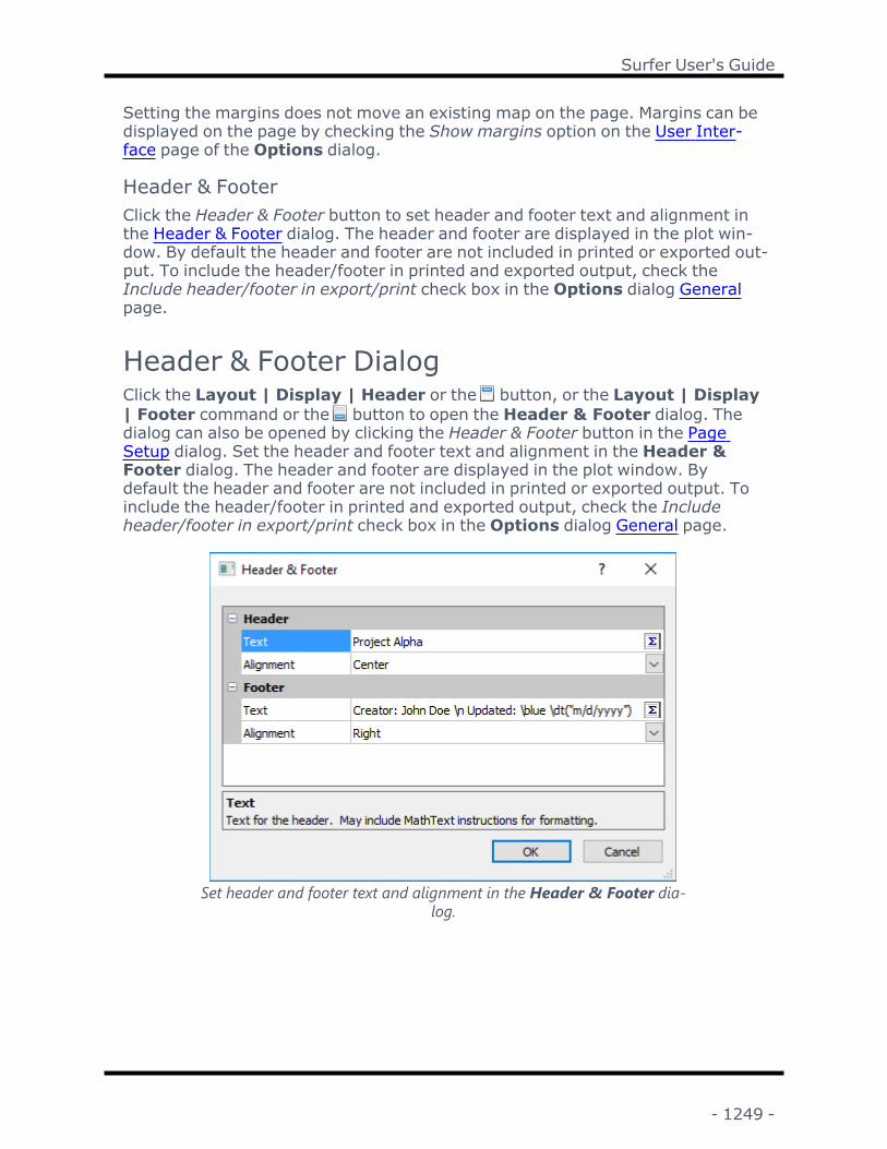
Surfer User's Guide
Setting the margins does not move an existing map on the page. Margins can bedisplayed on the page by checking the Show margins option on the User Inter-face page of the Options dialog.
Header & FooterClick the Header & Footer button to set header and footer text and alignment inthe Header & Footer dialog. The header and footer are displayed in the plot win-dow. By default the header and footer are not included in printed or exported out-put. To include the header/footer in printed and exported output, check theInclude header/footer in export/print check box in the Options dialog Generalpage.
Header & Footer DialogClick the Layout | Display | Header or the button, or the Layout | Display| Footer command or the button to open the Header & Footer dialog. Thedialog can also be opened by clicking the Header & Footer button in the PageSetup dialog. Set the header and footer text and alignment in the Header &Footer dialog. The header and footer are displayed in the plot window. Bydefault the header and footer are not included in printed or exported output. Toinclude the header/footer in printed and exported output, check the Includeheader/footer in export/print check box in the Options dialog General page.
Set header and footer text and alignment in the Header & Footer dia-log.
- 1249 -

Chapter 32 - Importing, Exporting, and Printing
Header and Footer SectionsThe Header section and Footer section each contain fields for the Text and Align-ment. Set the header properties in the Header section. Set the footer propertiesin the Footer section.
TextType the desired header or footer text in the Text field. Click the button to openthe Text Editor to insert math text instructions. You can also type math textinstructions directly into the Text field without opening the Text Editor.
Linked text can be added to headers and footers by typing the linked text vari-ables in the Text field or in the Text Editor. Note that linked text is only sup-ported in the headers and footers.
l Type <<filename>> to display the full name and path for the file, forexample "C:\Users\My Name\Documents\My File.srf"
l Type <<path>> to display the file path, for example "C:\Users\MyName\Documents"
l Type <<title>> to display the file name and extension, for example "MyFile.srf"
l Type <<date/time>> to display the current date and/or time, where date/-time is any date/time format. The date and time update automatically eachtime the plot is changed or opened. For example, type <<ddd dd MMM YYYYHH:mm:ss>> to display the current date/time formatted asWed 16 Nov2016 14:59:24.
AlignmentSet the header or footer text alignment relative to the page in the Alignmentfield. Click the current option and select Left, Center, or Right from the list. Usethe Text Editor to set the text justification to the left, center, or right.
Print - PlotClick the File | Print command or the button in the plot window to print the act-ive document.
Print DialogThe File | Print command in the plot window opens the Print dialog.
- 1250 -

Surfer User's Guide
Set your printer preferences in the Print dialog.
PrinterThe Printer section contains options to specify the printer. The printer Status,Type, Where, and Comments are listed below the printer Name.
NameThe default system printer is listed in the Name field. If more than one printer isinstalled on the computer, use the down arrow to the right of the name field toselect a different printer.
PropertiesClick the Properties button to specify a printer and the printer properties. Forinformation on specific printer settings, see the owner's manual for the printer.
Print MethodThe Print Method options control how the document is printed on the page.
- 1251 -

Chapter 32 - Importing, Exporting, and Printing
l Truncate clips objects that extend past the margins.
l Fit to Page reduces the size of the plot so that it fits within the specified mar-gins. Margins are set and displayed or hidden with the Layout tab com-mands.
l Tile breaks the drawing into page size pieces and generates multiple pagesof output.
l View prints the current view in the plot window.
Print RangeThe Print range options control how the worksheet pages are printed. All printsall the pages that contain data. Selection prints the selected worksheet cells.
CopiesSpecify the number of copies to print in the Number of copies box. If two or morecopies of multiple page documents are printed, check the Collate box to separatethe copies into packets. Note that some printers do not allow multiple copies.
CollateCheck the Collate check box to collate the pages when printing multiple copies.Clear the Collate check box to repeat duplicates in the print order. For exampleassume two copies of a three-page document. When Collate is selected, the printorder is p1, p2, p3, p1, p2, p3. When Collate is not selected, the print order is p1,p2, p2, p3, p3.
OverlapEach page overlaps adjacent pages by the amount specified in the Horizontal andVertical overlap fields. These options are only available when the Print Method isset to Tile . The Overlap is the amount of the map that is printed on both pages.
ScaleScale is used when the Print Method is set to Truncate or Tile to reduce orincrease the overall size of the drawing. A scale of 100% is actual size, 200% istwice as large, and 50% is half as large.
OK and CancelClick OK to start the print. Click Cancel to close the Print dialog without printingthe plot document.
- 1252 -

Surfer User's Guide
Page Setup - WorksheetBefore printing the worksheet, the page format of the worksheet can be set byclicking File | Page Setup or the button. The Page Setup dialog controlsitems such as printing headers and footers, centering the data on the page, show-ing grid lines, etc. There are three pages in the Page Setup dialog: Page,Mar-gins, and Options. There is a Printer button at the bottom of the dialog thatallows you to set the default printer regardless of which page is selected.
The worksheet Page Setup dialog has three pages:
Page Set page size and scaling.Margins Set page margins, header and footer positions, and centering.Options Set grid lines, page order, and content of headers and footers.
Page Setup (Worksheet) - PageClick on the Page tab in the Page Setup dialog to set page size and scaling.Click the File | Page Setup command in the worksheet to open the Page Setupdialog.
- 1253 -

Chapter 32 - Importing, Exporting, and Printing
Change page setup properties in the Page Setup dialog Pagepage.
PaperUse the Paper section to choose the paper Size and Source for the active printer.
SizeClick the down arrow next to the paper Size to change the size of the paper. Thepaper size options available for your printer are listed in the list.
SourceIf your printer has multiple print trays, choose the paper Source by clicking thedown arrow.
OrientationThe Orientation section controls whether the page is set to Portrait or Landscapemode. Select Portrait to have a vertical page. Select Landscape to have a hori-zontal page.
- 1254 -

Surfer User's Guide
ScalingThe Scaling section controls the printed size of the worksheet. There are twooptions with Scaling: Adjust to and Fit to .
Adjust ToThe Adjust to ___ % full size option sets the percent of full size that the work-sheet will print. The arrow buttons are used to scroll up or down from 100% (fullsize), or values can be typed into the box. The Adjust to ___ % full size setting isindependent of the Fit to option.
Fit ToThe amount of data in the worksheet determines how many pages are requiredto print the worksheet. The Fit to __ page(s) across by __ option tells the pro-gram to print the worksheet at 100% scale or less. This option does not auto-matically scale the printed worksheet greater than 100%. This option is mostuseful when the worksheet is large and the number of printed pages needs to belimited.
PrinterThe active printer can be changed by clicking the Printer button at the bottom ofthe Page Setup dialog.
Page Setup (Worksheet) - MarginsUse theMargins page in the Page Setup dialog to set page margins, headerand footer positions, and centering. Click the File | Page Setup command in theworksheet to open the Page Setup dialog.
- 1255 -

Chapter 32 - Importing, Exporting, and Printing
Change page margin properties on the Page Setup dialogMarginspage.
MarginsUse the Margins (inches) group to set the page margins for all sides of the prin-ted page. Set the Left, Right, Top, and Bottom values in inches to any limits theprinter will allow. The margins are for the worksheet printout and are inde-pendent of the settings used for Headers or Footers.
Center on PageThe Center on Page group options automatically center the printout Horizontally,Vertically, or both. If neither option is selected, the worksheet prints in the upperleft corner of the page.
From Edge (inches)Headers and Footers are the only items that print outside of the margins. TheFrom Edge (inches) group options controls how far the Header or Footer is prin-ted from the edge of the page. If these values are greater than the Top or Bot-tommargins, it is possible that the worksheet data can print over the header or
- 1256 -

Surfer User's Guide
footer. The text that is printed for the header and footer is controlled on theOptions page.
PrinterThe active printer can be changed by clicking the Printer button at the bottom ofthe Page Setup dialog.
Page Setup (Worksheet) - OptionsUse the Options page in the worksheet Page Setup dialog to set grid lines,page order, and content of the header and footer. Click the File | Page Setup com-mand in the worksheet to open the Page Setup dialog. Click on the Options tabat the top of the dialog.
Change page option properties in the Page Setup dialog Options page.
PrintThe Print section controls how the worksheet information is printed.
GridlinesCheck the Gridlines option to draw grid lines separating each column and row.
- 1257 -

Chapter 32 - Importing, Exporting, and Printing
Row and Column HeadersCheck the Row and column headers option to print the column letters and rownumbers of the worksheet.
Black and WhiteIf cells contain color backgrounds (set from the Data | Format | Format Cells com-mand), check the Black and white option to print the worksheet in only black andwhite.
Page OrderThe Page Order section controls the order in which multiple pages are printed.The Across and then down option prints from left to right first, and then movesdown and prints left to right again. The Down and then across option prints theworksheet from top to bottom first, and then moves to the right and prints top tobottom again.
Header/FooterThe Header/Footer group controls the type of information included in the work-sheet data print out. The plot window does not have header/footer options. TheHeader appears at the top of the page, and the Footer appears at the bottom ofthe page. The header and footer are spaced from the edge of the page based onthe From Edge option o, the Margins page. Descriptive text can be typed in theHeader and Footer boxes, or click the arrows to the right of the boxes and clickthe items in the list.
Automatic header/footer codes:
l File Name ( <F ) prints the name of the active file. The drive and path are notincluded.
l Page Number ( <P> ) prints the page number for each page. When severalpages are printed, the order of printing is controlled from the Page Order sec-tion.
l Total Page Count ( <C> ) prints the total number of pages that are requiredto print out the worksheet with the specified scaling parameters.
l Current Date ( <D> ) prints the current date.l Current Time ( <T ) prints the current time.l Left/Center/Right Separator (<&> ) separates the header and footer text soit is spread out across the page. Too many separators can actually push textoff the page. If this happens, remove the <&> separator, and use spacesinstead.
PrinterThe active printer can be changed by clicking the Printer button at the bottom ofthe worksheet Page Setup dialog.
- 1258 -

Surfer User's Guide
ExamplesFor a six page document, <&><&>Page <P> of <C> would print (on the rightside of the first page):
Page 1 of 6
Enter Joe Smith<&><FD to print out a name, file name, and date:
Joe Smith COLORADO.DAT 01/05/10
To print centered text use the "&" operator one time, such as <&><F.
FILENAME.DAT
Print - WorksheetClick the File | Print command or the button to print the contents of the work-sheet to the active printer or to a .PRN file. To control the display of data on theprinted page, refer to the File | Page Setup command. While the worksheet isspooling, a dialog indicates that printing is progressing.
The File | Print command in the worksheet opens the Print dialog.
Use the Print dialog to specify the printing options.
PrinterThe Printer section contains options to specify the printer.
- 1259 -

Chapter 32 - Importing, Exporting, and Printing
l The default system printer is listed in the Name field. If more than oneprinter is installed on the computer, use the down arrow to the right of theprinter name to select a different printer.
l The printer Status, Type, Where, and Comment are listed below the printerName.
l Click the Properties button to set printer specific properties. For informationon specific printer settings, see the owner's manual for the printer.
l The Print to file check box allows you to print the data to a .PRN file. .PRN filesare ASCII text files. When this option is checked, click OK in the Print dialogafter setting other printing options. The Print to File dialog will open. Entera path and file name in the Print to File dialog, and click Save .
Print RangeThe Print range options control how the worksheet pages are printed.
l All prints all the pages that contain data.l Pages prints the pages specified. Enter the starting page in the from box.Enter the ending page in the to box.
l Selection prints the selected worksheet cells.
Number of CopiesSpecify the number of copies to print in the Number of copies box. If two or morecopies of multiple page documents are printed, check the Collate box to separatethe copies into packets. Note that some printers do not allow multiple copies.
CollateCheck the Collate box to collate the pages when multiple page documents areprinted two or more times.
OK or CancelClick OK to start the print. Click Cancel to abort the print and return to the work-sheet window.
- 1260 -

Chapter 33 - Options, Defaults, andCustomizations
OptionsThe default settings of Surfer and advanced options are customized by clicking
the File | Options command or the button. By adjusting the settings in theOptions dialog, you can customize Surfer to suit your individual preferencesand work habits. The settings are automatically saved and restored wheneverSurfer is restarted. Changes made in the Options dialog affect all subsequentdocuments.
The Options dialog contains the following pages:
General Set the basic window features such as what type of map will beopened with grid and data files, file open/save paths, sig-nificant digits, and undo levels.
Updates Allow Surfer to automatically check for updates.User Inter-face
Set the interface and tab style, help in the Properties window,and the startup splash screen.
Selection Set the selection handle size and tolerance size for selectingobjects.
Rendering Set antialiasing properties.Printing Controls printer page size settings.Rulersand Grid
Control the display of the rulers and grid.
DefaultProperties
Set line, fill, symbol, font, and label format default attributes.
Advanced default options are available for most menu commands by clicking theFile | Defaults command.
Options - GeneralSet defaults (e.g. open/save paths and undo levels) on the General page in theOptions dialog.
Options Dialog
Click the File | Options command or the button to open the Options dialog.Click on the General option on the left side of the dialog to open the Generalpage.
- 1261 -

Chapter 33 - Options, Defaults, and Customizations
Customize General options in the Options dialog.Project FolderEnter a path into the Project folder box to set the default path for opening andsaving files. Alternatively, click the button to browse for a path. This optionsets the initial directory displayed in all the open, import, save as, and export dia-logs. Surfermust be closed and reopened for the Project folder change to takeeffect. This option can also be set with the Set Project Folder button in the Wel-come to Surfer dialog. If the Project folder is set in theWelcome to Surfer dia-log, it is not necessary to restart Surfer.
To set the Project folder to the Windows default path, delete the current path andleave the option blank. Click OK , and the default Windows path will be used forthe Project folder.
Temporary PathEnter a path into the Temporary path box to set the default path for temporaryfiles. Alternatively, click the button to browse for a path. To set this to thedefault path, delete the current path and leave the option blank. After OK isclicked, the default Windows path will be written to the Temporary path.
Undo LevelsSet the number of commands to undo in the Undo levels box. The maximumnumber of Undo levels is 100. Once the maximum number of actions has beenperformed, the oldest action is dropped off the list as new actions are added.Undo can consume significant amounts of memory, so this option should
- 1262 -

Surfer User's Guide
probably be left between 3 and 10 if memory is at a premium. Set the undolevels to 0 to disable Undo completely. Use the to increase or decrease thenumber of undo levels or highlight the existing value and type a new valuebetween zero and 100.
Maximum Number of Processors to UseThe Max number of processors to use option sets the maximum number of pro-cessors Surfer can concurrently use during multi-threaded operations. The min-imum value is 1 and the maximum value is the number of physical processors onthe PC. The Max number of processors to use is set to the maximum value bydefault. Reduce the Max number of processors to use value if you wish to reservesome of your PC's processing power for other applications during processor-intensive processes, such as gridding.
Image Threshold (MB)The Image threshold (MB) option controls the number of megabytes that can beused before switching images to disk-based images. This option can be set to avalue between 0 and 16384. If an imported image is larger than the imagethreshold, it will be stored in a tiled bitmap format which uses minimal internalmemory but can result in some performance degradation. Increase this value ifyour computer has a lot of internal RAM. Lower this value if you are experiencingvery sluggish performance, "Out of memory" errors, or crashes when using largeimages. Any images already imported must be re-imported to change theirinternal storage format. Use the to increase or decrease the number of mega-bytes used or highlight the existing value and type a new value between zeroand 16384.
Backup Files Before SavingIf Backup files before saving is checked, a backup copy of an existing file is cre-ated before saving the document. The backup copy is saved with a .BAK exten-sion. If an identically named backup file already exists, it will be overwritten.
Save Auto Recovery InformationSelect the Save auto recovery information option to periodically save changes toa temporary file that is automatically restored if Surfer closes unexpectedly.Large files may take a moment to save and can result in periodic slowdownswhile using Surfer with this option enabled.
Auto Recover Save IntervalSpecify the number of minutes between auto-recovery saves in the Auto recoversave interval option. The interval can be a number between 1 and 30 minutes.
Delete Empty MapsCheck the Delete empty maps option to delete empty map frames after com-bining the map layers with other maps. When this option is not checked, the
- 1263 -

Chapter 33 - Options, Defaults, and Customizations
empty map object and axes are still drawn after the map layers are moved. Bydefault, Surfer checks this box so that empty maps are automatically deleted.
Track Map CoordinatesThe Track map coordinates of option controls which map is used to display theXYZ coordinates and units in the status bar and which map is used when theTrack Cursor option is enabled. The options are Topmost map/layer or Selectedmap/layer. When the Topmost map/layer is chosen, the coordinates and unitsbeing shown in the status bar and by theMap Tools | Layer Tools | TrackCursor command or the button are those for the top layer of the map at thetop of the Contents window. When Selected map/layer is chosen, the coordin-ates and units being shown are those for the selected map or layer.
Prompt For Missing Coordinate SystemThe Prompt for missing coordinate system option controls whether Surferprompts for a coordinate system if an unreferenced data file, grid, or base map isloaded. Check this option to enable the prompt for a coordinate system. Uncheckthis option to disable the dialog prompt when loading data, grids, and base mapsthat are unreferenced.
Regardless of whether the Prompt for missing coordinate system is checked ornot, loading a file with the File | Reload Map Data command or by clicking thebutton in the Properties window for the map layer will not prompt for the
coordinate system. The coordinate system for the original map layer is usedafter updating the file. If this is not the correct coordinate system, click on themap layer to select it. In the Properties window, click on the Coordinate Sys-tem tab and set the coordinate system to the appropriate new system.
Page UnitsPage Units are the units used to measure distances on the printed page. SetPage Units to Inches or Centimeters. The location of the cursor on the page is lis-ted in page units in the status bar. The page units are displayed on the Rulers.
Track UsageCheck the box next to Track usage to allow Surfer to send anonymous usagedata to Golden Software. Sending usage data will help improve Surfer to meetour users' needs. This property does not have a default setting; it's initial settingis determined based on your selection to opt-in or opt-out of the Customer Exper-ience Improvement Program during the Surfer install process. Surfermust berestarted for this setting to be applied. A message is displayed reminding you torestart Surfer after changing this setting.
Include Header/Footer in Export and PrintCheck the Include header/footer in export/print check box to include the head-er/footer when printing or exporting the plot window. By default the header andfooter are not included in printed and exported output. Clear the Include
- 1264 -

Surfer User's Guide
header/footer in export print check box to only display the header/footer in theplot window.
On Grid File OpenThe On Grid File Open option controls the map type that is opened in the plot win-dow when a grid file is selected by clicking the File | Open command. Thedefault is set to the Color Relief Map. Click the to see the list of seven differentmap types and click on the map type to change the default and then click OK.
On Data File OpenThe On Data File Open option controls what file type opens when a data file isselected by clicking the File | Open command. Either one of three map typesopens in a plot window or a worksheet editor is opened. The default is set to thePost Map and can be changed by clicking the drop down arrow . Click on a filetype and then click OK.
Options - UpdatesSet automatic update preferences on the Updates page in the Options dialog.
Options DialogClick the File | Options command to open the Options dialog. Click on Updateson the left side of the dialog to open the Updates page.
Customize the Updates options in the Options dialog.
- 1265 -

Chapter 33 - Options, Defaults, and Customizations
Show Announcement NotificationsCheck the Show announcement notifications to allow Golden Software to auto-matically check for program and company announcements. This could includeinformation about a new product release, tips for use of Golden Software pro-grams, special offers, or an update to the program.
Show Update NotificationsCheck Show update notifications to allow Golden Software to automaticallycheck for program updates. The program will link to the Golden Software serverto see if any program updates are available. Program updates include fixes toerrors or problems that are found in the program. It is recommended that youkeep this box checked so that your version of Surfer is always up to date.
Show License NotificationsCheck Show license notifications to display messages regarding the status ofyour software licenses. For example, you might see a message notifying you thatyour software maintenance is about to expire or if a trial version you are using isabout to expire.
Show Registration NotificationsCheck Show registration notifications to display messages about registering yoursoftware product key. You may want to register the software under your nameso you can manage the product license and receive important information andupdates. See Register Product Key.
Check For Updates
Click the next to the Check for updates command to check for pro-gram updates. Before using this command, make sure your computer is con-nected to the Internet. Follow the directions in the Internet Update dialog tocomplete the update if an update is available.
Options - User InterfaceSet the user interface environment on the User Interface page in the Optionsdialog.
The Options Dialog
Click the File | Options command or the button to open the Options dialog.Click on the User Interface option on the left side of the dialog to open the UserInterface page.
- 1266 -

Surfer User's Guide
Customize the User Interface options in the Options dialog.Recent FilesThe Recent files option controls the number of recently used files listed near thebottom of the Filemenu. The default value is 10. This option can be set to avalue between 0 and 16. To change the number of files, click the to increase ordecrease the value or highlight the value and type a new number.
Map Coordinate FormatSet the format for the map coordinates section of the status bar in the Mapcoordinate format section. The status bar displays the cursor location coordin-ates of the tracked map or layer. Select which map or layer is tracked in theOptions dialog General page. Click the to the left of Map coordinate format toexpand the format options. The Linear coordinates section controls the coordin-ate format when displaying linear units in the status bar, i.e. when tracking thecursor location on a projected or unreferenced map/layer. The Spherical coordin-ates (degrees) section controls the coordinate format when displaying sphericalunits in the status bar, i.e. when tracking the cursor location on an unprojectedlatitude/longitude map or layer. The format options for both the Linear coordin-ates and Spherical coordinates (degrees) are the standard label format prop-erties. Using DMS (Lat/long) is NOT recommended for the Linear coordinatesselection.
- 1267 -

Chapter 33 - Options, Defaults, and Customizations
Show Splash Screen at StartupCheck the box next to Show splash screen at startup to allow Surfer to displaythe Surfer splash screen and copyright notice while the program is loading.Uncheck this box to disable the splash screen display.
Show Welcome Screen at StartupCheck the box next to Show welcome screen at startup to show the Welcome toSurfer dialog when Surfer starts. Uncheck this box to disable theWelcome toSurfer dialog.
Show Page RectangleCheck the box next to the Show page rectangle option to turn on the display ofthe paper representation in the plot window. Uncheck this box to turn off the dis-play of the paper representation. The page size is set by clicking the File | PageSetup command.
Show MarginsCheck the box next to the Show margins option to turn on the display of the pagemargin in the plot window. Uncheck this box to turn off the display of the pagemargin. Margins are set by clicking the File | Page Setup command.
Show Property Information AreaCheck the box next to the Show property info area option to display a short helpstatement for each selected command in the Properties window. Uncheck thisbox to turn off the help area in the Properties window.
Always Show Drop Arrows in Properties WindowCheck the box next to Always show drop arrows in Properties window to displaydrop arrows for all combo-box properties in the Properties window. When thisoption is active, fields containing lists can be easily differentiated from fields con-taining text or value input boxes. When the Always show drop arrows in Prop-erties window option is unchecked the drop arrow is only visible when theproperty is selected. Turn this option off when the Properties window is narrow,and more of the properties' text will be shown.
Expand New Contents Window ItemsCheck the box next to the Expand new Contents window items option to force theContents window to expand all new object hierarchies in the tree control. If thisoption is turned off, the objects contain a button. Click the to manuallyexpand additional levels.
Paste in User-picked PositionCheck the box next to Paste in user-picked position to manually position objectswith the cursor when using the Paste command. When the Paste in user-pickedposition check box is checked, a shaded bounding box is displayed around the
- 1268 -

Surfer User's Guide
cursor after Paste is used. Click in the desired location to paste the object orobjects.
Clear the Paste in user-picked position check box to automatically paste objectsin the center of the plot window. This is the default behavior.
User Interface StyleSpecify the interface style in the User interface style list. Available options areWindows XP, Office XP, Office 2000, Office 2003, Visual Studio 2005, Visual Stu-dio 2008, Visual Studio 2010, Office 2010 Black, Office 2010 Blue , and Office2010 Silver. The worksheet window colors are dark when Office 2010 Black isselected, blue when Office 2010 Blue is selected, and silver when any other Userinterface style is selected. The default style is Visual Studio 2008.
MDI Tab StyleSpecify the tabbed document view style in the MDI tab style list. The options areNone, 3D, One Note, and Visual Studio 2005. The plot window, worksheet win-dow, and grid node editor window have a tab appearance when multiple windowsare open when the MDI tab style is set to any option other than None. Thedefault style is Visual Studio 2005.
Notifications for Creating a Grid FileThere are three notification options you can choose from in theWhen grid is com-pleted list: Do Nothing, Play a Sound, or Display a Message Box. This action isperformed after most gridding operations to inform you that the operation hascompleted.
Decimal SeparatorThe Decimal separator controls which character is used to separate the wholenumber portion from the decimal portion in a number. To change the Decimalseparator, click on the existing option and select the desired option from the list.Available options are: System default, Period, and Comma. The default is to usethe System default. System default defers treatment of decimal separators toWindows. The Period option displays a period (.) to separate the numbers beforeand after the decimal. The Comma option display a decimal comma (,) to sep-arate the numbers before and after the decimal. When this option is changed, allmaps that are opened will display the selected character for the decimal sep-arator.
When using System default, the setting is controlled by Windows. To set the Win-dows local, in the Windows Control Panel, under Region and Language, set theFormat. In locale's where the period is the separator, it will be used in Surfer. Inlocale's where the comma is the separator, it will be used in Surfer. All .SRF fileswill use the format specified by Windows. This means that older .SRF files mayappear differently depending on the format. Some changes may be in axislabels.
- 1269 -

Chapter 33 - Options, Defaults, and Customizations
The Decimal separator setting is mainly used to import data files from differentlocales correctly in your instance of Surfer. For example, a CSV file uses theperiod (.) for the decimal separator and a comma (,) for the data delimiter in theEnglish locale. However a CSV file uses the comma (,) for the decimal separatorand a semicolon (;) for the data delimiter in the German locale. You can correctlyimport data files from other locales by updating your Decimal separator setting.This means it is not necessary to update your Windows locale to import and opendata files from other locales.
Options - SelectionSet the options for how objects are selected on the Selection page in theOptions dialog.
The Options DialogClick the File | Options command to open the Options dialog. Click on theSelection option on the left side of the dialog to open the Selection page.
Customize the Selection options in the Options dialog.Rectangle Must Fully SurroundThe Rectangle must fully surround option controls how the block select featurefunctions. If the box is checked, the block select rectangle must be drawn com-pletely around the object to select it. If any portion of the object extends beyondthe block select rectangle, the object is not selected. If this option is unchecked,the block select rectangle only needs to partially intersect an object to select it.
- 1270 -

Surfer User's Guide
Handle SizeThe Handle size in pixels option controls the width and height in pixels of theselection handles that appear around selected objects. The handle size settingrange is from zero to 25 pixels. A setting of 25 will create large size selectionhandles. A setting of zero will create no selection handles. The default setting is ahandle size of six pixels. The handle size scales with zoom. Click the toincrease or decrease the value or highlight the existing value and type a newnumber to change the size.
ToleranceThe Tolerance option controls how far away the cursor can be from an objectwhen clicking to select the object. The tolerance setting range is from zero to 25pixels. When the tolerance size is zero, the cursor must be directly on the objectto select it. The tolerance size does not affect the size of the bounding box, itonly controls the distance the cursor can be from the object to select it. Thedefault tolerance setting is three pixels. The tolerance scales with zoom. Clickthe to increase or decrease the value or highlight the existing value and type anew number to change the tolerance.
Options - RenderingSet the antialias options on the Rendering page in the Options dialog.
The Options DialogClick the File | Options command to open the Options dialog. Click on the Ren-dering option on the left side of the dialog to open the Rendering page.
- 1271 -

Chapter 33 - Options, Defaults, and Customizations
Set the Rendering options in the Options dialog.Antialiased LinesCheck the box next to Antialias lines to allow redraw to diminish jagged edgesand create a smooth appearance for all lines in the plot window. Uncheck thisbox to disable the smoothing and make lines crisper.
Antialiased TextCheck the box next to Antialias text to allow redraw to diminish jagged edgesand create a smooth appearance for all text and symbols in the plot window.Uncheck this box to disable the smoothing and make text and symbols crisper.
Enable OpenGL Hardware AccelerationCheck the box next to Enable OpenGL hardware acceleration to use the OpenGLdriver included with your video card in the 2D plot view. If you experience any dif-ficulties when creating 3D surface maps or see errors or crashes when displayingthe 3D surface map, uncheck the box. Surfer must be restarted after making thischange. This option does not affect the display or rendering in the 3D view.
3D View Maximum Number of PointsLarge point cloud layers can use a lot of resources to render in the 3D view. Thenumber of points displayed in the 3D view is limited by the 3D View maximumnumber of points option. If Surfer is hanging or slow to respond when viewing apoint cloud in the 3D view, reduce the 3D View maximum number of pointsoption. The default is 4 million (4M) points. Select 1M, 2M, 4M, 8M, 12M, or 16Mfrom the list. Any open 3D view windows must be closed and reopened after
- 1272 -

Surfer User's Guide
changing the 3D View maximum number of points value in the Options dialog toapply the change.
Options - PrintingSet printing page size defaults (i.e. warning of invalid page sizes and controllingthe page size based on the selected printer) on the Printing page in the Optionsdialog.
The Options DialogClick the File | Options command to open the Options dialog. Click on the Print-ing option on the left side of the dialog to open the Printing page.
Customize Printing options in the Options dialog.Warn on TruncateTheWarn on truncate option controls if a warning message appears when print-ing if objects are outside the page margin. By default this option is checked.When the box is checked, if the map or any drawn objects are outside the pagemargins, a warning message appears. Click OK on the warning and reset thepage margins or page size using the File | Page Setup command. When theWarnon truncate option is unchecked, if the map or any drawn objects are located out-side the page margins, no warning message appears. The print is truncated tothe page margins.
- 1273 -

Chapter 33 - Options, Defaults, and Customizations
Set Paper Size on PrinterThe Set paper size on printer option controls the page sizes available for printing.By default, this option is unchecked. When unchecked, the paper size on thePage Setup dialog is not automatically sent to the printer. The printer papersize will need to be set separately in the File | Print dialog. When the Set papersize on printer option is checked, Surfer automatically uses the paper size set inthe Page Setup dialog for the printer paper size. If the Page Setup dialog spe-cifies a page size that is not supported by the printer, no page size is transferredto the printer and the page size must still be specified in the Print dialog.
Options - Rulers and GridSet ruler and grid properties on the Rulers and Grid page in the Options dialog.Rulers appear along the top and left edge of the plot window, and are used to pos-ition and align objects. Rulers use the current page units. To change the Pageunits, click on the General page.
The Options DialogClick the File | Options command to open the Options dialog. Click on theRulers and Grid option on the left side of the dialog to open the Rulers and Gridpage.
Specify Rulers and Grid options in the Options dialog.
- 1274 -

Surfer User's Guide
Snap to RulerSnap to ruler causes the cursor to snap to the ruler divisions as objects aredrawn or moved. This allows objects to be easily aligned with the ruler divisionmarks. Check this box to snap the cursor to the ruler divisions. Uncheck this boxto disable the automatic snapping.
Show PositionWhen the Show position option is checked, the current cursor position is dis-played on the rulers. As the cursor is moved, the position indicator moves withinthe rulers to show the exact page position of the cursor. Uncheck this box to dis-able the cursor position in the rulers.
Ruler Divisions Per Page UnitThe Ruler divisions per page unit option controls the number of divisions perpage unit on the ruler. Select a value between 1and 99. To change the value,highlight the existing value and type a new number or click the to increase ordecrease the number of divisions. The number of divisions are in page units. Setthe page units on the General page of the Options dialog.
Grid Divisions Per Page UnitThe Grid divisions per page unit option controls the number of divisions per pageunit on the grid. Select a value between 1 and 99. To change the value, highlightthe existing value and type a new number or click the to increase or decreasethe number of divisions. The number of divisions are in page units. Set the pageunits on the General page of the Options dialog.
Options - Default PropertiesUse the Default Properties pages in the Options dialog to specify the defaultline, fill, symbol, font, and label properties used when creating new objects.
The Options DialogClick the File | Options command to open the Options dialog. Click on theLine, Fill, Symbol, Font, or Label link under the Default Properties option on theleft side of the dialog to open the appropriate default setting page.
- 1275 -
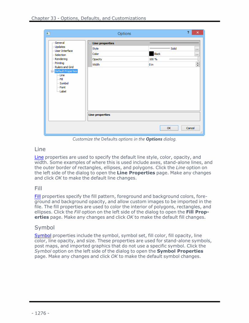
Chapter 33 - Options, Defaults, and Customizations
Customize the Defaults options in the Options dialog.
LineLine properties are used to specify the default line style, color, opacity, andwidth. Some examples of where this is used include axes, stand-alone lines, andthe outer border of rectangles, ellipses, and polygons. Click the Line option onthe left side of the dialog to open the Line Properties page. Make any changesand click OK to make the default line changes.
FillFill properties specify the fill pattern, foreground and background colors, fore-ground and background opacity, and allow custom images to be imported in thefile. The fill properties are used to color the interior of polygons, rectangles, andellipses. Click the Fill option on the left side of the dialog to open the Fill Prop-erties page. Make any changes and click OK to make the default fill changes.
SymbolSymbol properties include the symbol, symbol set, fill color, fill opacity, linecolor, line opacity, and size. These properties are used for stand-alone symbols,post maps, and imported graphics that do not use a specific symbol. Click theSymbol option on the left side of the dialog to open the Symbol Propertiespage. Make any changes and click OK to make the default symbol changes.
- 1276 -

Surfer User's Guide
FontFont properties specify the default face, style, size, color, opacity, and text align-ment. Some examples of where this is used include stand-alone text, axis labels,post map labels, and contour labels. Click the Font option on the left side of thedialog to open the Font Properties page. Make any changes and click OK tomake the default font changes.
Label FormatLabel format properties specify numeric display for labels. The label type, prefix,suffix, number of significant digits, thousands symbol, and absolute value maybe set. Click the Label Format option on the left side of the dialog to open theLabel Format page. Make any changes and click OK to make the default labelchanges.
Default SettingsThe File | Defaults command or the button opens the Defaults dialog. TheDefaults dialog controls most of the default settings used in commands forSurfer. These settings are saved in a .SET setting file, and are reloadedwhenever Surfer is started. Using the hierarchical list in the Defaults dialog,you can customize each default setting independently. This is an advanced fea-ture, and the settings should not be changed indiscriminately. Minimal errorchecking is performed, and it is possible to specify values completely inap-propriate for some data sets. Some inappropriate values may cause maps toappear incorrectly.
Changing Defaults in the DialogAn easy way to make changes to default settings is to set the Setting value toInternal Default and set the Setting Persistence to All sessions. Click OK in theDefaults dialog. Then, open the dialog or command that should be changed.Make any changes in the dialog or command and click OK. You can confirm thechange by clicking the File | Defaults command again and selecting the desiredsetting. The Setting value should now show the options from the dialog.
You must click OK in the dialog that uses the setting for the setting to beupdated. If you Cancel the dialog, the changes are not recorded in the settingfile.
Defaults DialogClick the File | Defaults command to open the Defaults dialog.
- 1277 -

Chapter 33 - Options, Defaults, and Customizations
Customize the Advanced options in the Options dialog.
Current Setting FileThe Current Setting File is the file Surfer is currently using to extract thedefaults. Any changes made to the defaults in the various dialogs are saved inthe current setting file when Surfer is shut down. By default, Surfer uses a filenamed SURFER.SET. This file is located by default in the C:\Users\<username>\AppData\Roaming\Golden Software\Surfer\ directory. It is also possible
to specify a different setting file by clicking the button.
Settings (organized by dialog)The Settings (organized by dialog) list displays the default settings organizedhierarchically by dialog. To change a setting, click the button next to the dialogyou wish to modify. Individual settings can be highlighted by clicking on them orby using the ARROW keys on the keyboard. As each individual setting is high-lighted, a brief description appears in the text box at the bottom of the dialog.
Setting ValueEnter the new value of the default setting in the Setting value control. This con-trol changes depending on the type of setting highlighted in the Settings (organ-ized by dialog) list. Numeric values are entered into a box. Settings with a
- 1278 -

Surfer User's Guide
discrete number of choices are displayed in a list. The values entered in this con-trol are not checked for errors, so be sure to specify an appropriate value for thehighlighted setting.
All settings have a value called Internal Default. Changing the Setting value toInternal Default allows Surfer to determine the best value for the current set-ting. If the Setting value control is an edit box, you can specify the InternalDefault value by deleting the contents of the box so it is empty.
Several default settings require the value to be specified in a particular format.The type of format required is determined from the comments at the bottom ofthe Defaults dialog. See the Formats for Attribute Values topic for a list of thesespecial values.
Setting PersistenceThe Setting persistence option specifies how the setting is updated when theuser changes the setting during normal operation. The options are:
Alwaysreset
Do not update the default setting when it is changed in a dialog.Every time the dialog is invoked, the setting is reset to the valuein the setting file.
Currentsessiononly
This option saves changes made to the setting within the dialogduring the current session only. The settings are not written tothe setting file and are not used the next time Surfer is started.
All ses-sions
This option saves the changes made to the setting within the dia-log during the current session, and writes the changes to the set-ting file to be used the next time Surfer is started.
Using Custom Setting FilesSET files allow custom settings to be saved and reused in Surfer each time theprogram is opened.
Creating a Custom .SET FileTo create a custom setting file:
1. Make a backup of the default SURFER.SET file. The SURFER.SET file is loc-ated in the User's AppData directory. This is C:\Users\<User Name>\Ap-pData\Roaming\Golden Software\Surfer by default.
2. Rename the new copy, keeping the .SET extension.3. Click the File | Defaults command.
4. Click the button next to the Current Setting File.5. Select the new .SET file and click Open.6. Modify the setting you wish to change.7. Save the changes to the file by clicking OK in the Options dialog.
- 1279 -

Chapter 33 - Options, Defaults, and Customizations
Using the Custom .SET FileAfter the preferences are set, you can rename the set file, keeping the .SETextension. Multiple .SET files can exist on the same computer. Each setting filecan use a different set of defaults. You can manually change the setting file
Surfer uses by clicking File | Defaults. Click the button next to the CurrentSetting File field to select a different .SET file.
Alternatively, to use a different setting file with Surfer, start Surfer with the/SET switch on the command line. To do this, click the Windows Start buttonand select Run. Then, enter the following information:
"Path to Surfer.exe" /SET "Path to new .SET file"
An example may look like:
"c:\Program Files\Golden Software\Surfer\Surfer.exe" /SET "C:\Documents andSettings\<User Name>\Application Data\Golden Software\Surfer\custom.set"
To make this entire process easier, you can create a new shortcut on the desktopand specify the /SET switch in the Target: field of the shortcut properties dialog.See your Windows documentation for details on how to create shortcuts. To cre-ate a new shortcut:
1. Right-click on the Windows Desktop and choose New | Shortcut.
2. Type in the "Path to Surfer.exe" /SET "Path to new .SET file" in the box.
3. Click Next.
4. Type a name for the shortcut, such as Surfer.exe SET name.
5. Click Finish and the icon is created.
Using Old .SET FilesYou can also use old Surfer setting files. When using older Surfer setting files,the hierarchy displayed in the File | Defaults dialog is only a single level due tolack of nesting information in the old format.
Be sure you copy the [.SET] file in the correct place for it to be used, C:\Users\(username)\AppData\Roaming\Golden Software\Surfer.
Formats for Attribute ValuesSeveral settings use specially formatted values to specify all the required inform-ation when using Default Settings. When specifying the values for these settings,you must include all the parameters as discussed below.
- 1280 -

Surfer User's Guide
Minimal error checking is performed, and it is possible to specify values com-pletely inappropriate for some data sets. Some inappropriate Setting valuesmaycause maps to appear incorrectly.
ColorsColors are specified by name as they appear in the dialog color palettes, by RxxxGyyy Bzzz values, or by Rxxx Gyyy Bzzz Aaaa values. For detailed syntax inform-ation and an example, see color property syntax.
Line PropertiesLines are specified by the line color, name, and width. For detailed syntax inform-ation and an example, see line property syntax.
Fill PropertiesFills are specified by color, pattern, and additional options. For detailed syntaxinformation and an example, see fill property syntax.
Font PropertiesFonts are specified by font name, size, color, and style. For detailed syntaxinformation and an example, see font property syntax.
Symbol PropertiesSymbols are specified by symbol number, symbol set, color, size, and opacity.For detailed syntax information and an example, see symbol property syntax.
Numeric Label PropertiesThe numeric label is specified by prefix, suffix, font properties, and numeric prop-erties. For detailed syntax information and an example, see numeric label prop-erty syntax.
Color SyntaxColors are specified by name as they appear in the color palettes. The namesmust be enclosed in double quotes. For example, "Ocean Green."
Alternatively, a color is specified using the special syntax:
"Rxxx Gyyy Bzzz"
or
"Rxxx Gyyy Bzzz Aaaa"
- 1281 -

Chapter 33 - Options, Defaults, and Customizations
where xxx, yyy, and zzz specify a red, green, and blue color component and aaaspecifies the opacity value, respectively. Each component can range from 0 to255.
Example"R0 G0 B0" All components are 0, resulting in black"R0 G255B0"
Pure green
"R255 G255B255"
All components are at full intensity, resulting in brightwhite.
"R255 G255B255 A45"
All components are at full intensity, resulting in brightwhite. Opacity is set to 18%.
Line Property SyntaxIn Default Settings, line properties are specified using the syntax:
"Color" "Style" Width
Parameter DescriptionColor The line color name. See Color List for details.Style The style of the line as it appears in the dialog line style
palette. The name must be enclosed in double quotes.Width The width of the line in thousandths of an inch (mils). This
should not be enclosed in quotes.
Example"R0 G255 B50" ".1 in. Dash" 10
Fill Property SyntaxIn Default Settings, fill properties are specified using the syntax:
"version "fgColor" "bgColor" "Pattern" offset scale angle coverage"
Parameter Descriptionversion Defines the version of the fill property. Must be 1.fgColor The RGBA color value for the foreground color. See Colors for
details.bgColor The background color name. See Colors for details.Pattern The fill pattern name as it appears in the dialog fill pattern
palette. The name must be enclosed in double quotes.offset The offset value has an X and Y component. The offset con-
trols the location of the image pattern within the geometry.scale The scale value has an X and Y component. The scale controls
the density of the image pattern.angle The angle value determines the rotation of the pattern. This
should always be 0.
- 1282 -

Surfer User's Guide
coverage The coverage value determines whether an image isstretched or tiled. 0 = tiled, 1 = stretched.
Note that all items are enclosed in quote marks.
ExampleThis example shows a fill property with the following options:
version = 1
fgColor = "R0 G0 B255 A99" indicating a slightly transparent blue
bgColor = "R0 G0 B255 A255" indicating a slightly transparent red
Pattern = "Gneiss 1", an image of a cut gneiss
Offset = 1 and 10, indicating 1 in the X direction and 10 in the Y direction
Scale = 0.9 and 0.8, indicating 0.9 in the X direction and 0.8 in the Y direction
Angle = 0
Coverage = 1, indicating that the pattern is to be stretched.
"1 "R0 G0 B255 A99" "R255 G0 B0 A38" "Gneiss 1" 1 10 0.9 0.8 0 1"
Font Property SyntaxIn Default Settings, font properties are specified using the syntax:
"FaceName" "Color" Style Size
Parameter DescriptionFaceName The font face name as it appears in the Font Properties sec-
tion in the Properties window. The name must be enclosedin double quotes.
Color The font color name. See Color List for details.
- 1283 -

Chapter 33 - Options, Defaults, and Customizations
Style Add the following values to get the style you want:
None = 0
Bold = 16
Italics = 32
Strikethrough = 64
Underline = 128
The style is entered as a number, and is not enclosed indouble quotes.
Size The size of the text in points. This is entered as a number andis not enclosed in double quotes.
Example"Calibri" "Black" 0 6
Symbol Property SyntaxIn Default Settings, symbol properties are specified using the syntax:
""SymSet" "FillColor" "LineColor" BitFlags Index Size"
Parameter DescriptionSymSet SymSet is the symbol set or face name as it appears in the
Symbol Properties. The name must be enclosed in doublequotes.
Fill Color Fill color is the RGBA color for the interior of the symbol. SeeColor List for details.
Line Color Line color is the RGBA color for the line around the symbol.See Color List for details.
Bit Flags Bit flags is no longer used and is only included for backwardcompatibility. In older versions of Surfer, the Bit Flags wasused to indicate whether the symbol Line Color was used. Inthe current version the value should be set to 0.
Index Index is the 0-based index of the symbol to use as it appearsin the Symbol Properties dialog. This is entered as a number,and does not use double quotes.
Size Size is the size of the symbol page units (inches or cen-timeters). This is entered as a number.
Note that all items are enclosed in quote marks.
ExampleThis example shows a symbol with the following properties:
- 1284 -

Surfer User's Guide
SymSet = "GSI Default Symbols"
Fill Color = "R255 G0 B0 A50" indicating a slightly transparent red
Line Color = "R0 G0 B255 A255" indicating a fully opaque blue
Bit Flags = 0
Index = 10
Size = 0.5 inches (or centimeters)
""GSI Default Symbols" "R255 G0 B0 A50" "R0 G0 B255 A255" 0 10 0.5"
Numeric Label Property SyntaxIn Default Settings, numeric label properties are specified using the syntax:
Version Type Digits Style DateFormat TimeFormat "Prefix" "Suffix"
Parameter DescriptionVersion Version is the version of the label format. This should be set
to 5.Type Type is the numeric format. This is entered as a number, and
is not enclosed in double quotes.
0 = Fixed
1 = Exponential
2 = Compact
4 = Date/TimeDigits Digits refers to the number of decimal digits after the decimal
place in the label. This value can range from 0 to 15. This isentered as a number, and is not enclosed in double quotes.
Style Label style is entered as a number, and is not enclosed indouble quotes.
0 = None (no styles)
1 = Thousands (separate thousands with a comma)
2 = Absolute Value (show numbers as absolute values)
3 = Thousands and Absolute Value (use thousands and abso-lute values)
- 1285 -

Chapter 33 - Options, Defaults, and Customizations
DateFormat The date format is entered as a number and is not enclosed indouble quotes. The number values are listed on thewksDateFmtType Values page. Select the desired format anduse the Value from this page in the label property syntax. Forexample, a value of 2 would set the format to DATEFMT_M_D_YY, which would display the format as 9/7/98.
TimeFormat The time format is entered as a number and is not enclosed indouble quotes. The number values are listed on thewksTimeFmtType Values page. Select the desired format anduse the Value from this page in the label property syntax. Forexample, a value of 2 would set the format to TIMEFMT_H_MM_AMPM, which would display the format as 1:03 PM.
Prefix The Prefix text is text that appears at the beginning of everylabel. This must be enclosed in double quotes.
Suffix The Suffix text is text that appears at the end of every label.This must be enclosed in double quotes.
Example0 8 0 "Pre" "Post"
CustomizeCustomize the Surfer ribbon, Quick Access Toolbar, and keyboard shortcuts byclicking File | Customize Ribbon or the button or by right-clicking on theribbon and selecting Customize the Ribbon. Customize the ribbon by clickingCustomize Ribbon on the left side of the dialog. Customize the Quick Access Tool-bar by clicking Quick Access Toolbar on the left side of the dialog. Customize thekeyboard commands by clicking Customize at the bottom of the dialog next toKeyboard shortcuts.
- 1286 -

Surfer User's Guide
The Customize dialog lets you create keyboard shortcuts for common actions and changethe appearance of the ribbon and Quick Access Toolbar.
Customizing the RibbonThe ribbon is customizable in Surfer. To customize the commands in the ribbon,right-click on the ribbon and select Customize the Ribbon.
In the Customize dialog, you can add new tabs, add groups, hide existing tabsor custom groups, and add commands to any custom group. You can alsorearrange the tabs into an order that fits your needs better.
To customize the commands in the Customize dialog, right-click on the ribbonand select Customize the Ribbon. In the Customize Ribbon dialog, use thefollowing options.
Tab options:l To add a custom tab, set the Customize the Ribbon section to All Tabs. Clickin the list on the right side of the dialog where the custom tab should be loc-ated and click the New Tab button.
l To delete custom tab, right-click on the tab name in the list on the rightside of the dialog and select Delete.
- 1287 -

Chapter 33 - Options, Defaults, and Customizations
l To rename a default or custom tab, click on the tab name in the list on theright side of the dialog. Click the Rename button. Type the new name andpress OK to make the change.
l To hide a default or custom tab, uncheck the box next to the tab name onthe right side of the dialog. Only checked tabs will be displayed.
l To change the order of default or custom tabs, click on the tab name thatshould be moved in the list on the right side of the dialog. Click the up anddown arrow buttons on the far right side of the dialog to move the selectedtab up or down. Default tabs must remain in their major group.
Group options:l To add a custom group to a default or custom tab, click on the next to thetab name. Click in the list of group names where the new group should belocated and click the New Group button.
l To delete a default or custom group on any tab, right-click on the groupname in the list on the right side of the dialog and select Delete.
l To rename a default or custom group on any tab, click on the group namein the list on the right side of the dialog. Click the Rename button. Type thenew name and click OK to make the change.
l To change the order of default or custom groups on any tab, click on thegroup name that should be moved in the list on the right side of the dialog.Click the up and down arrow buttons on the far right side of the dialog tomove the selected group up or down in the list.
l To replace a default group with a custom group, right-click on the defaultgroup name and select Delete. Click the New Group button. Add thedesired commands to the new group that you want displayed. Rename thenew group, if desired.
Command options:Commands can only be added to or deleted from custom groups. Commands canonly be rearranged or renamed in custom groups. If you wish to edit commandsin default groups, the default group should be hidden and a new custom groupshould be created with the same commands.
l To add a command to a custom group, set the Choose commands from list:to All Tabs so that all commands are listed on the left side of the dialog.Select the desired command that should be added. On the right side of thedialog, click the next to the custom group name. Click on the desired pos-ition in the list of commands. If no commands exist in the group yet, clickon the group name. Click the Add>> button and the command is added to
- 1288 -

Surfer User's Guide
the custom group.
l To delete a command from a custom group, right-click on the commandname in the list on the right side of the dialog and select Delete. Only com-mands from custom groups can be deleted.
l To rename a command in a custom group, click on the command name inthe list on the right side of the dialog. Click the Rename button. Type thenew name and click OK to make the change. Only commands in customgroups can be renamed.
l To change the order of commands in a custom group, click on the com-mand name that should be moved in the list on the right side of the dialog.Click the up and down arrow buttons on the far right side of the dialog tomove the selected command up or down in the list.
Reset the RibbonTo reset all customizations on the ribbon, click the Reset button at the bottom ofthe Customize Ribbon dialog.
Customizing the Quick Access ToolbarThe Quick Access Toolbar is a customizable toolbar. One method that can beused to add commands to the Quick Access Toolbar is to right-click on the com-mand in the ribbon and choose Add to Quick Access Toolbar. The commandis automatically added to the end of the toolbar.
To customize the commands on the Quick Access Toolbar, right-click on theQuick Access Toolbar or ribbon and select Customize Quick Access Toolbar.
In the Customize dialog,
1. To add a command, select the command from the list on the left that youwant to add. Click the Add>> button and the command is added to the liston the right.
2. To add a separator between commands, select <Separator> and clickAdd>>. Move the separator to the desired position.
3. To delete a command, select the command from the list on the right. Clickthe <<Remove button and the command is removed from the list on theright.
4. To rearrange commands or move separators, click on the command or sep-arator name from the list on the right that you want to move. Click the upand down arrow buttons on the far right to move the command up or downthe list. Commands are shown in the exact order that they are displayed in
- 1289 -

Chapter 33 - Options, Defaults, and Customizations
the Quick Access Toolbar.
5. To reset the Quick Access Toolbar to the default display, click the Reset but-ton below the list on the right side of the dialog.
6. Click OK and all changes are made.
Keyboard ShortuctsClick the Customize button next to Keyboard shortcuts to add, remove, orchange the keyboard shortcuts in Surfer. The Customize Keyboard dialog is dis-played.
Keyboard CommandsKeyboard commands can be used to increase efficiency and precision in theSurfer environment.
Plot WindowYou can use the keyboard to move the pointer within the plot window, to selectobjects, and to move objects.
l The ARROW keys move the pointer within the plot window.
l Pressing the SPACEBAR is equivalent to clicking the left mouse button.
l Press CTRL+TAB to change the active page in a dialog.
Menu CommandsThe keyboard can be used to access the menu commands.
l Hold down the ALT key and pressing an underlined letter in the menu bar.
l When the menu is displayed you can access a command by pressing theunderlined letter in the command.
DialogsThe keyboard can be used to move around in a dialog.
l The TAB key moves between the options in the dialog. As you use the TABkey to move through the dialog, the options are highlighted as theybecome active.
l The SPACEBAR is used to simulate mouse clicks, allowing you to togglecheck boxes or press buttons that provide you with access to other dialogsor close the current dialog.
- 1290 -

Surfer User's Guide
l Use the underlined hot keys by holding down the ALT key and typing the let-ter. This moves you immediately to the desired option.
Customize Keyboard CommandsTo customize keyboard commands use the File | Customize command.
Default Keyboard CommandsUse these keyboard commands.
GeneralCTRL+F4 Close the plot windowALT+SPACE Display the application control menuALT+HYPHEN Display the plot window control menuCTRL+F6 Next document windowCTRL+SHIFT+F6 Previous document windowCTRL+TAB Switch between Surfer windowsF10 or ALT Activate the menu barCTRL+ESC Display the Windows start menuALT+TAB Switch to the last active applicationALT+ENTER Activate the Properties windowALT+F11 Activate the Contents window
HelpF1 Open help for the currently selected command or dialogSHIFT+F1 Click on a command or dialog to open the detailed help topicSHIFT+F10 Opens the context-menu for the selected object(s)
FileCTRL+N Open a New plot windowCTRL + W Open a New worksheetCTRL+O Open a fileCTRL+S Save a Surfer .SRF fileCTRL+I Import a file into the current Surfer windowCTRL+E Export the current Surfer windowCTRL+P Print the drawing in the current plot windowALT+F4 Close Surfer
EditCTRL+A Select all objects in the current plot windowCTRL+X or Cut the selected objects to the clipboardCTRL+C or Copy the selected objects to the clipboardCTRL+V or Paste the clipboard contents into the plot windowCTRL+Y Redo the previous Undo command
- 1291 -

Chapter 33 - Options, Defaults, and Customizations
CTRL+Z or Undo the last commandDELETE Delete the selected objectsCTRL+SHIFT+A Deselect All objects in the current plot windowF2 Rename the selected object
Plot WindowUse these plot window commands.
Order ObjectsSHIFT+PAGE UP Move selected to frontSHIFT+PAGE DOWN Move selected object to backCTRL+PAGE UP Move selected object forwardCTRL+PAGE DOWN Move selected object backward
ViewF5 Redraw the screenCTRL + D Fit to windowCTRL + G PageCTRL + R Zoom to RectangleCTRL + L Zoom to SelectedCTRL + + Zoom InCTRL + - Zoom OutF11 Zoom Full Screen
Digitize Coordinates DialogCTRL+O Open a fileCTRL+S Save as a .BLN or .DAT fileCTRL+A Save the file as a new .BLN or .DAT fileCTRL+Z or Undo the last commandCTRL+Y Redo the last undoCTRL+X Cut the selected text to the clipboardCTRL+C or Copy the selected text to the clipboardCTRL+V or Paste the clipboard contents into the digitizer windowDELETE Delete the selected textCTRL+F FindCTRL+H Replace
Grid Editor WindowCTRL+N Open a new plot windowCTRL+W Opens a new worksheet windowCTRL+O Open a grid fileCTRL+S Save the edited grid fileF5 Redraw the screen
- 1292 -

Surfer User's Guide
CTRL+B Assign NoData to the selected nodeARROW Move to the next node in the direction of the arrow
Worksheet WindowARROW KEYS Move to adjacent cellF2 Edit active cellDELETE Clears contents of marked cellsEND When data are in the column: Go to the last row con-
taining data.
When data are not in the column: Go to the end ofthe document.
ENTER Preserve the typed contents in the cellHOME When data are in the column: Go to the first row
with data.
When data are not in the column: Go to the begin-ning of the document.
PAGE UP Scroll the worksheet up one screenPAGE DOWN Scroll the worksheet down one screenCTRL + HOME Go to cell A1CTRL + Z orALT+BACKSPACE
Undo the last command
CTRL + Y Redo the previous Undo commandCTRL + X orSHIFT+DEL
Cut the selected objects to the clipboard
CTRL + C or CTRL +INSERT
Copy the selected objects to the clipboard
CTRL+V or Paste the clipboard contents into the plot windowDELETE Clears contents of the currently selected cellCTRL + R Opens the Insert dialogCTRL + D Opens the Delete dialogCTRL + F Opens the Find and Replace dialog, Find pageF3 Find next commandCTRL + H Find and Replace dialog, Replace page
Customize KeyboardUse the Customize Keyboard dialog to assign keyboard shortcuts to com-mands. To open the Customize Keyboard dialog click the Customize buttonnext to Keyboard shortcuts in the Customize dialog.
- 1293 -

Chapter 33 - Options, Defaults, and Customizations
Use the Customize Keyboard dialog to customize keyboard shortcuts.
Category, Commands, and DescriptionMenu and Tab titles (File, Home, etc.) are listed in the Category field. When a cat-egory is selected, the Commands list displays the current commands within thecategory. Also, when a command is selected, an explanation of the commandappears in the Description section at the bottom of the dialog.
You can also list all commands by selecting All Commands at the bottom of theCategories list.
Accelerator Menu ApplicationYou can choose to assign the accelerator (keyboard shortcut) to the Surfer,Worksheet, or Defaultmenus in the Set Accelerator for list.
Current Shortcut KeysWhen a command is selected in the Commands list, the accelerator keys are lis-ted in the CurrentKeys list. The Current Keys list only displays accelerators forthe current group of menus selected in the Set Accelerator for list.
- 1294 -
Surfer User's Guide
Press New Shortcut KeyTo create a shortcut, select a command, place the cursor in the Press new short-cut key field, type the shortcut on your keyboard, and then click Assign. If ashortcut is already assigned to a command a message appears below the Pressnew shortcut key field and the Assign button is disabled.
Removing ShortcutsTo remove a shortcut, select the shortcut in the Current Keys list and clickRemove.
Resetting ShortcutsTo reset all shortcuts to the defaults, click Reset All.
- 1295 -


Chapter 34 - Automating Surfer
Introduction to ScripterGolden Software ScripterTMis a program for developing and running scripts.Sur-feroperations can be controlled automatically by scripts. A script is a text file con-taining a series of instructions carried out by a script interpreter program whenthe script is run. Instructions are written in a Visual BASIC-like programming lan-guage.
You can do practically everything with a script that you can do manually with themouse or from your keyboard. Scripts are useful for automating repetitive tasks,consolidating a complicated sequence of steps, or acting as a "front end" to helpnovice users access Surfer's capabilities without having to become familiar withSurfer. In addition, scripts can integrate the features of several programs. Forexample, you could, with a single script, open a data file in Microsoft Excel, trans-fer the data to Surfer, create a map, and copy the map to Microsoft Word.
Scripter offers many features to help you write, edit, and debug scripts. Its fea-tures include language syntax coloring, a list of the procedures defined in thescript, an object browser for examining procedures available in external objects,a visual dialog editor, break points, single-step execution (including options tostep over and to step out of procedures), a watch window for displaying the val-ues of script variables, and others. The Surfer Automation object model is dis-played with the Surfer Object Hierarchy tree.
As an example, suppose you are monitoring groundwater levels in an area. Eachweek you collect XYZ data, create a contour map from this data, print the map,and save it in a Surfer file [.SRF]. The example scripts provide examples thatautomate these tasks. The sample script asks for the XYZ data file, creates a gridfile, produces a contour map, prints the map, and saves it in a file. A personusing the "front-end" script would not have to know anything about Surfer inorder to create a contour map from the raw water level data.
Golden Software recommends that Windows 7 users run the program as admin-istrator for best results.
Start the Scripter ProgramTo start the Scripter program, select it from the Windows Start menu. Scripteris installed in the same program group as Surfer. If Scripter is not present inthe Windows Start menu, installation of Scriptermay have been skipped whenSurfer was installed. You can install Scripter from the Surfer download instruc-tions. If you need new download instructions, contact technical support.
Scripter will open whichever version of Surfer was opened last.
- 1297 -

Chapter 34 - Automating Surfer
This is a script in the main window of the Golden Software Scripter program.
Scripter WindowsWhen Scripter is first started, you are presented with a text editor window con-taining the lines Sub Main, followed by a blank line, and then End Sub. This isthe code editor window where you type script instructions and where the con-tents of script files are displayed.
The code window acts as a text editor, similar to the Windows Notepad program,with a few enhancements to facilitate script writing:
l After you press the ENTER key, tabs or spaces are automatically inserted atthe beginning of the next line to maintain the same indentation level as theprevious line.
l Key words and symbols of the BASIC language are displayed in different col-ors. You can use the View | Colors command to modify the colors used todisplay the various elements of the programming language.
l A light horizontal divider line is automatically drawn between sections ofyour script. The divider lines help you to locate the start of subroutine andfunction definitions.
Above the code editor window is a bar containing the Object and Proc (pro-cedure) lists. Selecting items from these lists moves the various sections of yourscript file into view. The object and procedure lists are useful when your scriptfile becomes large.
- 1298 -

Surfer User's Guide
Above the object and procedure lists, you may see a blank window area with atab on top that reads Immediate. If this window is not visible, select the View |Always Split command to make it appear. The immediate window is used toexecute one-line instructions immediately. When you type an instruction intothis window and press the ENTER key, Scripter carries out the instruction.
In addition to being a scratch area for evaluating language statements, theimmediate window shows debugging information. The output from theDebug.Print statement and the value of variables selected with the Debug |Quick Watch command are printed in the immediate window. While a script pro-gram is running,Watch, Stack, and Loaded tabs are added at the top of theimmediate window area. Click these tabs for information that may be useful fordebugging. See Debugging Scripts for more information on the immediate,watch, stack, and loaded windows.
Along the left edge of the code window are code sheet tabs. When you selecteither the File | New command or the File | Open command, Scripter createsa new code sheet and inserts a new sheet tab. Each tab corresponds to one ofthe code sheets. Clicking once on a tab makes that sheet the current sheet.Double-clicking a tab closes the sheet.
Between the sheet tabs and the code window is an area called the "break bar."When a script is paused, a yellow arrow in the break bar shows which line is nextto execute. The break bar also shows which lines have break points. Set a breakpoint by clicking on the break bar. A red dot appears in the break bar, and theadjacent line in the code window is highlighted. When a line marked as a breakpoint is about to be executed, Scripter pauses program execution. To clear abreak point, click on the red dot in the break bar. See Debugging Scripts formore information on break points.
A status bar along the bottom of the Scripter window shows information aboutthe current state of the program. The View | Show/Hide | Status Bar com-mand hides or reveals the status bar. Before running a script, make sure that thestatus bar is visible because messages about typographical and syntax errors aredisplayed in the status bar.
- 1299 -

Chapter 34 - Automating Surfer
This Scripter application window is shown while execution of a script ispaused.
Working with ScriptsTo create a new script, select the File | New command. A blank script sheet iscreated. You can start typing script instructions into this sheet. If you edit morethan one sheet at a time, click the sheet tabs to switch between them or selectthe Sheet | 1, Sheet | 2, etc. menu commands. You can edit up to nine codesheets at the same time.
New ModulesTo create a custom ActiveX object, select File | New Module, and choose eitherObject Module or Class Module (choosing Code Module is the same as theFile | New command).
Existing Scripts and ModulesTo open an existing script, select the File | Open command. To open a scriptyou opened recently, click its name at the bottom of the Filemenu. To openother modules used by your script, select the Sheet | Open Uses command.Golden Software provides examples to help get you started.
- 1300 -

Surfer User's Guide
Saving ScriptsOnce a script is complete, save the script by using the File | Save or File |Save As commands. If a script has not been changed since the last save, theSave command is grayed out.
Closing ScriptsTo close the active script, use File | Close, use Sheet | Close, or double-clickthe sheet tab of the sheet. Close all open scripts with Sheet | Close All.
Scripter BASIC LanguageThe online help describes the major elements of the Scripter BASIC pro-gramming language, but it does not explain the concepts of writing computer pro-grams. Many good books on the subject of programming with BASIC (Beginner’sAll-purpose Symbolic Instruction Code) have been written. If you are not mod-erately familiar with writing computer programs, we suggest that you refer toone of the books listed in the Suggested Reading topic.
Scripts are text files that contain a sequence of instructions to be carried out bythe Scripter program. Each instruction specifies a task such as defining a vari-able or displaying a message on the screen. When the Scripter program pro-cesses the script, the instructions are carried out one at a time, from top tobottom.
Execution of a script begins with the first statement of the subroutine calledMain. All scripts must therefore include the Sub Main and End Sub statements.Execution proceeds line-by-line until the end of the Main procedure, until an Endstatement is executed, or until an error occurs.
Visual BASIC CompatibilityThe Scripter BASIC programming language is compatible with the Visual BASICfor Applications language (VBA). Scripts that run inScripterwill work in a
Some statements available in VBA are not supported inScripterBASIC:
l The VBA Collection object
l The VBA Clipboard object
l GoSub
l On...GoSub
l On...Goto
- 1301 -

Chapter 34 - Automating Surfer
l GoSub…Return
l Multiple statements on one line (separated by ":")
l All Financial functions
l Resume at current line
l Erl
l Option Compare
l Conditional compilation
l With Events
l LinkExecute
l LinkPoke
l LinkRequest
l LinkSend
l Line numbers
l LoadPicture
Conversely, some features of the Scripter BASIC language are not supported byVBA. Do not use the following features if you want to transfer your scripts fromScripter into VBA:
l Clipboard function
l CallersLine
l User dialogs
l PortInt
l MacroRunThis
l MacroDir
l Wait instruction
l MacroRun
l DDEExecute
l DDEPoke
- 1302 -

Surfer User's Guide
l DDERequest
l DDEInitiate
l DDETerminateAll
l DDETerminate
Using Scripter For AutomationTasks can be automated in Surfer using Golden Software's Scripter program orany ActiveX Automation-compatible client, such as Visual BASIC. A script is atext file containing a series of instructions for execution when the script is run.Scripter can be used to perform almost any task in Surfer. Scripts are useful forautomating repetitive tasks and consolidating a sequence of steps. Scripter isinstalled in the same location as Surfer. Refer to the Surfer Automation topic inthe help for more information about Scripter. We have included severalexample scripts so that you can quickly see some of Scripter's capabilities.
To run a sample script file:
1. Open Scripter by navigating to the installation folder, C:\ProgramFiles\Golden Software\Surfer\Scripter. If you are running a 32-bit versionof Surfer on a 64-bit version of Windows, navigate to C:\Program Files(x86)\Golden Software\Surfer\Scripter. Right-click on the Scripter.exeapplication file and select Run as administrator.
2. Choose the File | Open command.
3. Select a sample script .BAS file. These are located in the C:\ProgramFiles\Golden Software\Surfer\Samples\Scripts folder or, if you are runninga 32-bit version of Surfer on a 64-bit version of Windows, the C:\ProgramFiles (x86)\Golden Software\Surfer\Samples\Scripts folder.
4. Click the Script | Run command and the script is executed. Most samplescripts open Surfer and display a map in the plot window.
Using Scripter HelpFor more information on Scripter program menu commands, select the Help |Contents command in Scripter. Press the F1 key for more information aboutthe Scripter windows or the active dialog. The Help | Surfer AutomationHelp command shows all Surfer-specific methods and properties.
The online help, shown when you select the Help | BASIC Language Help com-mand (or press SHIFT + F1), explains all of the BASIC language statements andfunctions. Each help topic describes the purpose of a statement, and shows thesyntax (the order of keywords and other symbols) to use when writing an
- 1303 -

Chapter 34 - Automating Surfer
instruction. The syntax examples in the online help use a shorthand method toexplain the possible variations in usage:
Sub,End,True
Words with the initial letter capitalized indicate language-spe-cific keywords.
name Lower-case words with a dotted underline are placeholdersfor information you supply.
[param] Items inside square brackets are optional. These may be omit-ted from the statement.
{Until |While}
Items between curly braces, and separated by a vertical barare lists of options. You must use one of the items in the list.
[Private|Public]
Items between square braces, and separated by a verticalbar are lists of optional choices. You may use one of the itemsin the list, or none of them.
... An ellipsis mark indicates that the preceding item in the syn-tax example is repeated. Repeated items are usually optionaland separated by commas.
; , . ( )
Other symbols must be typed as shown in the syntaxexample, with the exception of the underscore "_" character.
_ The underscore is used to show that a sample line has beensplit.
Suggested Reading - ScripterFor additional help in learning how to program or for more information about theVisual BASIC for Applications (VBA) language (which is nearly identical totheScripterBASIC language) we recommend the following books:
Harris, Matthew (1997), Teach Yourself Visual BASIC 5 for Applications in 21Days, Third Edition, SAMS Publishing, Indianapolis, IN, 1248 pp.
Lomax, Paul (1998),,
Wang, Wallace (1998), Visual BASIC 6.0 for Windows for Dummies, IDG BooksWorldwide, Foster City, CA, 477 pp.
Writing ScriptsTo create a script, you must type the script text into the Scripter code window,or edit an existing script. When you want to create a new script that is specific foryour circumstances, you will most likely start with an empty Scripter windowand type the entire script. If you want to perform a routine task such as creatinga grid file or a contour map, you can probably open an existing script file and editthe file to meet you specific needs. Surfer comes with several sample scriptsthat you can modify as desired.
- 1304 -
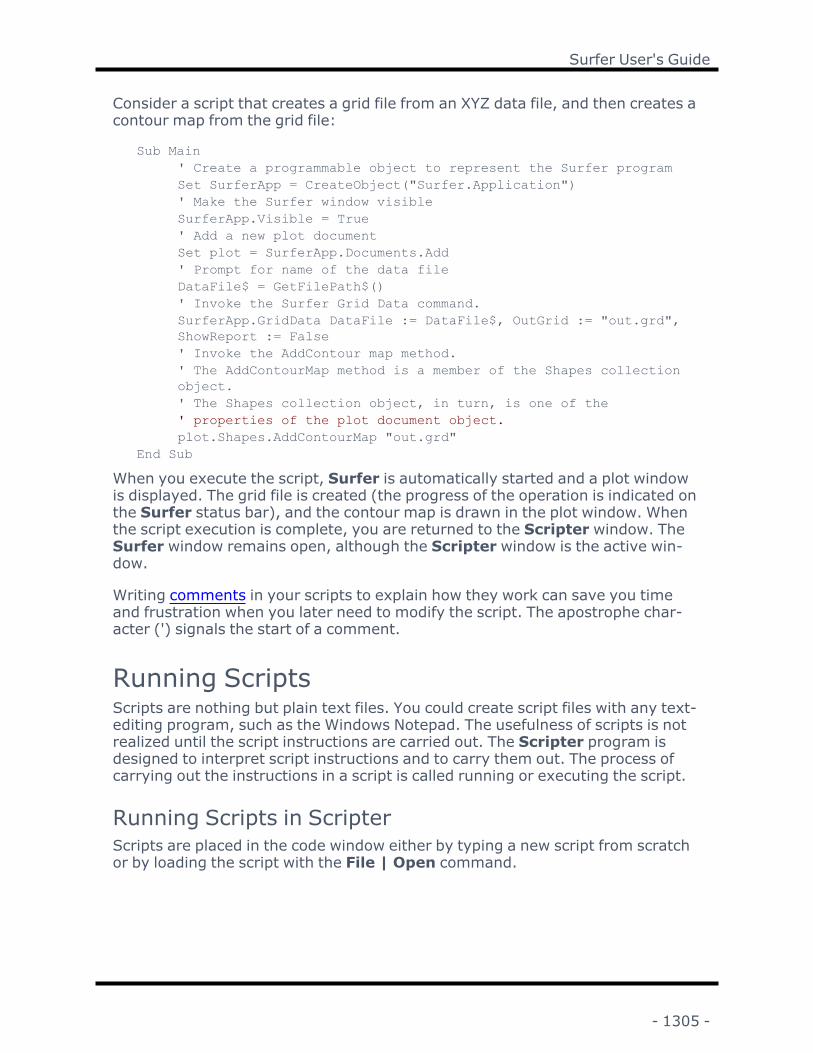
Surfer User's Guide
Consider a script that creates a grid file from an XYZ data file, and then creates acontour map from the grid file:
Sub Main' Create a programmable object to represent the Surfer programSet SurferApp = CreateObject("Surfer.Application")' Make the Surfer window visibleSurferApp.Visible = True' Add a new plot documentSet plot = SurferApp.Documents.Add' Prompt for name of the data fileDataFile$ = GetFilePath$()' Invoke the Surfer Grid Data command.SurferApp.GridData DataFile := DataFile$, OutGrid := "out.grd",ShowReport := False' Invoke the AddContour map method.' The AddContourMap method is a member of the Shapes collectionobject.' The Shapes collection object, in turn, is one of the' properties of the plot document object.plot.Shapes.AddContourMap "out.grd"
End Sub
When you execute the script, Surfer is automatically started and a plot windowis displayed. The grid file is created (the progress of the operation is indicated onthe Surfer status bar), and the contour map is drawn in the plot window. Whenthe script execution is complete, you are returned to the Scripter window. TheSurfer window remains open, although the Scripter window is the active win-dow.
Writing comments in your scripts to explain how they work can save you timeand frustration when you later need to modify the script. The apostrophe char-acter (') signals the start of a comment.
Running ScriptsScripts are nothing but plain text files. You could create script files with any text-editing program, such as the Windows Notepad. The usefulness of scripts is notrealized until the script instructions are carried out. The Scripter program isdesigned to interpret script instructions and to carry them out. The process ofcarrying out the instructions in a script is called running or executing the script.
Running Scripts in ScripterScripts are placed in the code window either by typing a new script from scratchor by loading the script with the File | Open command.
- 1305 -

Chapter 34 - Automating Surfer
To run the script in the Scripter code window, select the Script | Run com-
mand, press the F5 key, or click the button. Scripter examines the scriptinstructions, and, if all the instructions are recognized, it begins to perform eachinstruction in turn.
More often than not, however, a newly typed script will not work correctly thefirst time it is run. Even simple typographical errors will cause the script to fail.For information on finding and fixing errors in scripts, see the Debugging Scripts.
Select the Script | End command or click the button to stop executing ascript. This may be necessary when you want to edit a script after a run-timeerror occurs, or when you accidentally start a script and you want to cancel theexecution.
Running Scripts from the Command LineYou can run scripts from a command prompt without having to manually loadand execute the script in Scripter. The same commands that you would type ata command prompt may also be entered as the "target" for a shortcut in order tolink a shortcut button to a script. Enter the following to run a script from the com-mand line or to link a shortcut to particular script file:
<Scripter path> -x filename.bas
where <Scripter path> represents the path to the Scripter program file. (forexample, "C:\Program Files\Golden Software\Surfer\Scripter.exe"), and file-name.bas represents the name of the script to run. The space between the –xand the file name is required. This command opens the Scripter window, loadsthe specified script file, and runs the specified script. When the script terminates- either successfully or unsuccessfully - the Scripter window closes.
To load a script file but not execute it, the following command can be used:
<Scripter path> filename.bas
This opens the Scripter window and automatically loads the specified script file.The Scripter window remains open.
Passing a Command Line Argument to the ScriptA single command line argument can be passed to a script. The command lineargument can be any text that is used in the script. For example, a file name canbe passed and used to create a map. Enter the following to run a script with acommand line argument:
<Scripter path> -x filename.bas command
- 1306 -

Surfer User's Guide
where command represents the commands that should be passed to the script.Access the command line argument from the script using the Command$ option.For example, if the script name is variable.bas and it can be run with any gridfile, you could use:
"c:\program files\golden software\Surfer\scripter.exe" -x "c:\tem-p\variable.bas" "c:\temp\sample.grd"
Do not quote the arguments in the command. To use the data in the script, use:
'Return the argument to the Immediate windowDebug.Print Command$
'Create a contour map from the gridPlot1.Shapes.AddContourMap(GridFileName:=Command$)
Debugging ScriptsBugs are errors in a script that keep it from performing as intended. Debuggingis the process of locating and fixing these errors. The most common bugs aretypographical errors in scripts or malformed instructions. Scripter detects thesetypes of errors immediately when you try to run a script. The program beeps,highlights the line containing the error in red (or whatever color has been setwith View | Colors command), and displays an error message on the statusbar.
Viewing ErrorsBefore running a script, verify that the View | Show/Hide | Status Bar com-mand is enabled, otherwise you will not see the error message. To resolve theerrors that Scripter immediately detects, you usually must interpret the errormessage and correct the indicated problem. Typical errors are typing mistakes,unbalanced parentheses, misuse of a BASIC language instruction, or failure todeclare variables in a DIM statement (if you use the OPTION EXPLICIT state-ment). If you do not see an obvious problem, refer to the online BASIC languagehelp to make sure you are using the right syntax.
Run-Time ErrorsScripts which encounter errors midway through script execution may be fixedmuch the same way as syntax errors. The error message should guide youractions. Some run-time errors cannot be detected until they are executed, suchas when you try to open a file that does not exist. In these cases, you need tocheck for error conditions in your scripts. For example, use the DIR function tomake sure a file exists before trying to open it. Alternatively, you can use the ON
- 1307 -
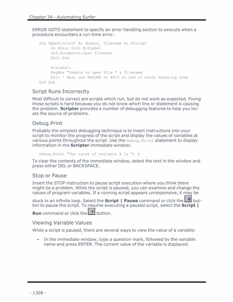
Chapter 34 - Automating Surfer
ERROR GOTO statement to specify an error handling section to execute when aprocedure encounters a run-time error:
Sub OpenFile(srf As Object, filename As String)On Error Goto ErrLabelsrf.Documents.Open filenameExit Sub
ErrLabel:MsgBox "Unable to open file " & filenameExit ' Must use RESUME or EXIT at end of error handling code
End Sub
Script Runs IncorrectlyMost difficult to correct are scripts which run, but do not work as expected. Fixingthese scripts is hard because you do not know which line or statement is causingthe problem. Scripter provides a number of debugging features to help you loc-ate the source of problems.
Debug.PrintProbably the simplest debugging technique is to insert instructions into yourscript to monitor the progress of the script and display the values of variables atvarious points throughout the script. Use the Debug.Print statement to displayinformation in the Scripter immediate window:
Debug.Print "The value of variable X is "; X
To clear the contents of the immediate window, select the text in the window andpress either DEL or BACKSPACE.
Stop or PauseInsert the STOP instruction to pause script execution where you think theremight be a problem. While the script is paused, you can examine and change thevalues of program variables. If a running script appears unresponsive, it may be
stuck in an infinite loop. Select the Script | Pause command or click the but-ton to pause the script. To resume executing a paused script, select the Script |
Run command or click the button.
Viewing Variable ValuesWhile a script is paused, there are several ways to view the value of a variable:
l In the immediate window, type a question mark, followed by the variablename and press ENTER. The current value of the variable is displayed.
- 1308 -

Surfer User's Guide
l In the code window, place the cursor on the variable name you want toexamine (that is, click on the variable name in the code window). Press
SHIFT+F9, select the Debug | Quick Watch command, or click thebutton on the toolbar. The current value of the variable is displayed in theimmediate window.
l To continuously monitor a variable’s value, click on the variable name inthe code window, and press CTRL+F9 or select the Debug | Add Watchcommand. Alternatively, type the variable name in the watch window andpress ENTER. The variable name and its value are displayed in the watchwindow. Every time script execution pauses, the variable value is auto-matically updated. To clear a variable from the watch window, highlight theline showing the variable value and press the DEL or BACKSPACE key.
Changing Variable ValuesTo change the value of a variable, type an assignment expression in the imme-diate window and press ENTER. For example, type "A=5" (without quotes) andpress ENTER to assign a new value to the variable named "A."
StepA powerful debugging technique is to watch Scripter execute your script oneline at a time. This lets you check the effect of each instruction and verify thatthe script is doing what you expect. While stepping through a script, you canexamine and change the values of script variables. Select the Script | Run com-
mand or click the button to resume script execution at full speed after step-ping through script instructions.
l To execute your script one line at a time press the F8 key, or select theDebug | Step Into command. The first line of the script is executed (or, ifthe script was paused, the next highlighted line is executed). The next lineis highlighted and a yellow arrow appears to the left of the next line. Toexecute the highlighted instruction, press F8 again.
l If a statement calls a subroutine or function that is defined within yourscript, the highlight will move into the called procedure. To keep from tra-cing execution into a called procedure, press SHIFT+F8 or select theDebug | Step Over command. This executes the whole subroutine or func-tion in a single step.
l If you accidentally step into a procedure, press CTRL+F8 or select theDebug | Step Out command. This executes all remaining instructions in aprocedure, and returns the highlight to the instruction that called the pro-cedure.
- 1309 -

Chapter 34 - Automating Surfer
l If you do not see the next highlighted instruction, select the Debug |Show Next Statement command to scroll the highlighted line into view.
l Sometimes you may want to skip the execution of some instructions or youmay want to execute the same instructions several times without restartingthe script. To change the next instruction line, click on the line you want toexecute next and select the Debug | Set Next Statement command.
BreakpointWatching Scripter execute every line of the script may be too time consuming.In this case, a breakpoint pauses the script where you think there might be aproblem. A breakpoint is a line of code that you mark. When Scripter encoun-ters a line marked as a breakpoint, it pauses the script just as if it had executed aSTOP instruction. Breakpoints are more convenient than STOP instructionsbecause they may be set and cleared while a script is paused, whereas STOPinstructions may be changed only after a script has ended.
l To set a breakpoint, click in the break bar area next to the line you want tomark. The break bar is the area to the left of the code window, between thesheet tabs and the code window. Alternatively, click on the line you want tomark, and press F9 or select the Debug | Toggle Break command. Theline becomes highlighted in red, and a round marker appears in the breakbar area.
l To clear a breakpoint, click on the round marker, or move the cursor to themarked line and press F9 or select the Debug | Toggle Break commandagain. You can clear all breakpoints by pressing SHIFT+CTRL+F9 or select-ing the Debug | Clear All Breaks command.
A quick alternative to setting a breakpoint is the Debug | Step To Cursor com-mand. This command has the same effect as setting a breakpoint on the currentline, running the script, and then clearing the breakpoint after script executionhas paused on the current line.
TraceTo check flow of execution through your script without having to watch each lineof the script being executed, try using the TRACE function. To activate the tracefunction type "Trace" (without the quotes) in the immediate window and pressENTER. Trace On is displayed in the immediate window. As the script is run, thelocation of every instruction being executed is printed in the immediate window.After the script finishes, the trace function is automatically disabled.
StackIf you nest procedure calls (that is, one procedure calls another procedure, whichcalls yet another procedure, and so forth), the stack window may be useful.When a script is paused, the stack window lists the procedures that have beencalled, and the order in which they were called. For instance, if the Main
- 1310 -

Surfer User's Guide
procedure calls procedure "A" which in turn calls procedure "B," the stack win-dow displays three lines, one for each of the called procedures. Clicking on a linein the stack window moves the corresponding procedure into view in the codewindow.
Module FilesClick the loaded window tab in the immediate window area to see which modulefiles are currently being interpreted by Scripter. The loaded files include the cur-rent script file and any modules it includes with the '#Uses statement.
Program StatementsStatements are individual instructions to Scripter that carry out a specific oper-ation. Statements are case insensitive and are typically written one to a line. Toenter two or more statements on the same line, separate the statements withcolons. For example:
a = 5 : b = 5 * a
Scripter BASIC requires flow control statements (IF, WHILE, DO, etc.) anddeclaration statements (DIM, PUBLIC, TYPE, SUB, etc) to be placed on a line bythemselves.
Line ContinuationTo break a line into two lines in Scripter, use a space followed by an underscore" _". You must include the space for the continuation to work properly in thescript. A backslash continuation " \ " from earlier versions of Scripter is not sup-ported. Comments are not allowed after the continuation character.
ExampleSurferApp.GridData("C:\Program Files\GoldenExclusionFilter:=x4, xMin:=4, Algorithm:=srfKriging,
CommentsWriting comments in your scripts to explain how they work can save you timeand frustration when you later need to modify the script. The apostrophe char-acter ( ' ) signals the start of a comment. Scripter ignores all text following theapostrophe up to the end of the line. Comments can be placed on their own line,or they may be placed at the end of a line. For example:
SurferApp.GridData "demogrid.dat" ' This creates a grid file fromdemogrid.dat
In addition, you can use the REM statement to add a remark in the script.However, REM statements can only be used at the beginning of a line.
- 1311 -

Chapter 34 - Automating Surfer
Double Quotes and TextIn Scripter, text strings must be enclosed in double quotes. File names, forexample, must be surrounded by double quotes. If quotes are missing, the textmay be mistaken for a variable name.
Debug.Print "This text string is printed in Scripter's immediate win-dow"
OperatorsOperators are symbols that direct a script to perform basic calculations, such asaddition, exponentiation, string concatenation, number comparison, and others.The language supports several arithmetic, comparison, and logical operators. InScripter, select Help | BASIC Language Help command and search for "Oper-ators" to see a complete list.
Flow ControlWhen you run a script, execution starts with the Sub Main statement and con-tinues line-by-line until the End Sub statement at the end of the main procedureor until an End statement is encountered. SEveral flow control statements allowyou to change this line-by-line progression according to conditions encounteredby your script. The Scripter BASIC language includes a variety of looping andbranching statements that is typical for modern programming languages. Theflow control statements include the following (see the online BASIC languagehelp for details on the syntax of these statements):
IF...END IFIF...END IF executes a statement only if a condition is true.
IF...ELSE...END IFThe alternate of IF...END IF form executes one statement if a condition is trueand a different statement if the condition is false.
SELECT CASE...END SELECTSELECT CASE...END SELECT branches to one of several statements. This com-pares the value of an expression to several test values and executes the state-ments associated with the test value that matches the expression value.
- 1312 -

Surfer User's Guide
DO...LOOPDO...LOOP is the basic looping statement. This statement loops either while acondition is true or until a condition becomes true and tests the condition eitherat the top of the loop or at the bottom of the loop.
This and all other loop structures may be stopped before the test condition hasbeen met by placing an Exit statement in the body of the loop.
WHILE...WENDWHILE...WEND loops while a condition is true and tests the condition at the top ofthe loop.
FOR...NEXTFOR...NEXT loops a number of times and increments (or decrements) an indexvariable each time through the loop.
FOR EACH...NEXTFOR EACH...NEXT iterates through all the elements in a collection object.Several Surfer automation objects are collection objects. The For...Each state-ment is a convenient way to process each element of a collection.
For example, the following code fragment closes all the documents in the SurferDocuments collection object:
'Assume that several documents are already open and that "SurferApp"' is the name of a variable which refers to the Surfer ApplicationobjectDim documents, doc As ObjectSet documents = SurferApp.DocumentsFor Each doc In documents
doc.CloseNext
Optional Arguments and Named ArgumentsMany procedures, especially the methods provided by Surfer Automationobjects, accept a large number of arguments. Some of the arguments arerequired. Every required argument must be supplied or the script will fail to run.Some arguments are optional. Optional arguments may be omitted and the pro-cedure will assume a default value for the missing arguments.
For example, the PlotDocument object’s "PrintOut" method accepts up to sevenarguments, all of which are optional:
- 1313 -

Chapter 34 - Automating Surfer
plot.PrintOut(Method, SelectionOnly, NumCopies, Collate, _xOverlap, yOverlap, Scale )
Since the arguments are optional, you can skip all or some of them when callingthe procedure. To print three copies at fifty-percent scale, for example, youwould supply just the NumCopies, and Scale argument values. These argumentsmust be listed in the correct position, separated by commas, as shown below:
Set SurferApp = CreateObject("Surfer.Application")Set plot = SurferApp.Documents.Addplot.PrintOut , , 3, , , , 50
Although only two of the seven argument values are supplied in this example,the appropriate number of commas must be used to mark the positions of themissing arguments. Since inserting the right number of commas can be trouble-some, you can supply the arguments by name rather than by position. Namedarguments are specified by the argument name followed by a colon and an equalsign (":="), followed by the argument value:
Set SurferApp = CreateObject("Surfer.Application")Set plot = SurferApp.Documents.Addplot.PrintOut Scale := 50, NumCopies := 3
Named arguments may be listed in any order without regard to the order theyappear in the procedure's definition.
Named and Positional ArgumentsIn Scripter, named arguments must have a colon plus equal sign ( := ), not justan equal sign as in earlier versions of Scripter. The arguments can be named oryou can use positional statements separated by commas. The following twoexamples show the same line written with the two different methods.
Named arguments:
SurferApp.GridData(SurferApp.Path+"\Samples\Demogrid.dat", _ExclusionFilter:="x<4", xMin:=4, Algorithm:=srfKriging, DupMeth-od:=srfDupFirst)
Positional arguments:
SurferApp.GridData(SurferApp.Path+"\Samples\Demogrid.dat", _,,,"x<4",srfDupFirst,,,,,4,,,,srfKriging)
Subroutines and FunctionsWriting a long or complicated script may be easier to manage if you divide thescript into smaller pieces called procedures. A procedure is a separate sequenceof instructions that you can call from multiple places within your script. The
- 1314 -

Surfer User's Guide
BASIC language provides many predefined procedures for performing frequentlyneeded tasks, and, in fact, the methods provided by the Surfer automationobjects are themselves procedures.
When you call a procedure, the instructions in the procedure are executed. Whenthe procedure finishes its task, it returns control to the instruction that called theprocedure. The Scripter BASIC language distinguishes two types of procedures:functions and subroutines. Functions return a value, whereas subroutines donot.
Subroutines and functions may accept one or more values, called arguments.Arguments are passed to a procedure by listing them after the procedure name.If there is more than one argument, the arguments must be separated by com-mas. For example:
x = Cos (0) 'Returns the cosine of the argument (returns 1)a$ = Left("AgAuPb",2) ' Returns the left-most characters (returns"Ag")Wait 5 ' Waits for 5 seconds
Cos, Left, and Wait are procedures built-in to the BASIC language. Cos andLeft are functions which return values to the caller. Wait is a subroutine, and,by definition, it does not return a value. The Wait subroutine waits for the num-ber of seconds specified by its argument (5 seconds in this example) beforereturning control to the calling location.
The arguments passed to a function must be enclosed in parentheses if the func-tion's return value is used. If the function's return value is not used, the argu-ments may be listed without enclosing them in parentheses. Arguments passedto a subroutine are never enclosed in parentheses.
Writing SubroutinesTo define subroutines within a script, use the Sub statement. Subroutine andfunction definitions cannot be nested within other procedures. That is, the Substatement must appear after the End Sub statement of any preceding subroutinedefinitions. The syntax for a subroutine definition is:
Sub name ( arguments )statements
End Sub
Where name represents the name you want to give the subroutine, argumentsrepresents a list of arguments names and types, and statements represents theinstructions that comprise the body of the subroutine. There is no limit to thenumber of instructions you can include between the Sub and the End Sub lines.Consider the definition of a Main procedure and another subroutine:
Sub MainMultipleBeep 25 ' call the MultipleBeep subroutine
End Sub
- 1315 -

Chapter 34 - Automating Surfer
Sub MultipleBeep (count As Integer)For i = 1 To count
BeepWait 0.5 ' Wait one-half second between beeps
NextEnd Sub
Each time the MultipleBeep procedure is called, the instructions between itsSub and End Sub statements are executed.
If the subroutine accepts arguments, the arguments are defined following thesubroutine name using a format similar to the Dim statement. The argumentdefinition list must be enclosed in parentheses, and argument definitions are sep-arated by commas if there is more than one. When a subroutine is called, thevariables listed in the argument list are automatically assigned the values passedin from the calling procedure.
Writing FunctionsFunctions are defined using the Function statement much the same as sub-routines are defined with the Sub statement. Like subroutines, function defin-itions cannot be nested within other procedures. Unlike subrouties, functions canreturn a value to the calling procedure. The syntax of a function definition is:
Function name ( arguments ) As typestatments
End Function
Where name is the function name you want to use, arguments is a list of argu-ments names and types, type is the type of the value returned by the function,and statements represents the instructions in the body of the function. Toreturn a value from a function, assign a value to a variable with the same nameas the function itself. For example:
Function hypotenuse (a As Double, b As Double) As Doublec = a * a + b * b ' The built-in Sqr function computes the squareroothypotenuse = Sqr (c) ' Set the function's return value
End Function
You define the list of arguments accepted by a function the same way as youdefine the arguments accepted by subroutines.
Built-in Functions and Procedures
Numerous useful functions and subroutines are built into the Scripter BASIC lan-guage. These routines can help you perform some of the most commonlyrequired programming tasks. Functions for processing strings, performing math-ematical calculations, error handling, working with disk files, and many othersare available.
- 1316 -

Surfer User's Guide
If you are not already familiar with the Visual BASIC for Applications pro-gramming language, it will be worth your time to review the list of available sub-routines. This list is found by selecting Help | BASIC Language Help inScripter.
Next: Using Surfer Objects
Specifying Cell CoordinatesCell ranges can be specified in various ways for theWksDocument Cells andRange methods:
[1] Cells("A1") is a one argument single cell
[2] Cells("A1:C5") is a one argument range of cells
[3] Cells("A:E) is a one argument range of whole-columns
[4] Cells("1:5") is a one argument range of whole-rows
[5] Cells(Range object) is a one argument range of cells
[6] Cells(1,"A") -or- Cells(1,1) is a two argument single cell
[7] Cells("A1","C5") is a two argument range of cells
[8] Cells(1,"A",5,"C") -or- Cells(1,1,5,3) is a four argument range of cells
Column ranges can be specified in various ways for theWksDocument Columnsmethod:
[1] Columns(1,5) or ("A","E) is a two argument range of columns
[2] Columns(A:
[3] Columns("A1:E1") is a one argument range of columns [the row coordinatesare ignored]
[4] Columns(Range object) is a one argument range of columns [the row coordin-ates are ignored]
[5] Columns("A5") is a one argument single column [the row coordinate isignored]
[6] Columns(1) is a one argument single column
Row ranges can be specified in various ways for theWksDocument Rowsmethod:
[1] Rows(1,5) is a two argument range of rows
- 1317 -

Chapter 34 - Automating Surfer
[2] Rows("1:5") is a one argument range of rows
[3] Rows("A5:A10") is a one argument range of rows [the column coordinatesare ignored]
[4] Rows(Range object) is a one argument range of rows [the column coordin-ates are ignored]
[5] Rows("A5") is a one argument single row [the column coordinate is ignored]
[6] Rows(1) is a one argument single row
Also, the Cells, Columns, and Rows methods work slightly differently wheninvoked on aWksRange object than when invoked on aWksDocument object.When invoked on aWksRange object, the coordinates are relative to the upper-left corner of the range. For example, Range.Cells(A1) refers to whatever theupper-left corner of the Range happens to be, like so:
Set Wks = Surfer.Documents.Add(srfDocWks)Set RangeObject1 = Wks.Cells(C5:E10)' RangeObject2 now contains the cell "C5"Set RangeObject2 = RangeObject1.Cells("A1")
' RangeObject3 now contains the cell "C5"Set RangeObject3 = RangeObject1.Cells(1,1)
' RangeObject4 now contains the cell "D6"Set RangeObject4 = RangeObject1.Cells(2,2)
In addition, you can use a single numeric argument in the Range.Cells() methodto sequentially access each cell in the range, like so:
' Note: RangeObject1 equals C5:E10Set RangeObject5 = RangeObject1.Cells(1) ; cell "C5"Set RangeObject6 = RangeObject1.Cells(2) ; cell "D5"Set RangeObject7 = RangeObject1.Cells(3) ; cell "E5"' There are three cells in the first row of RangeObject1.' Cell #4 is in the second row…Set RangeObject8 = RangeObject1.Cells(4) ; cell "C6"Set RangeObject9 = RangeObject1.Cells(5) ; cell "D6"Set RangeObject10 = RangeObject1.Cells(6) ; cell "E6"' Cell #7 is in the third row…Set RangeObject11 = RangeObject1.Cells(7) ; cell "C7"
There are some special cases when theWksRange objects’ Cells, Columns, andRows methods are called. The behavior for these special cases is explained inthese notes:
WksRange.Cells() Method:
[1] Coordinates are relative to the top, left of the current (base) range
- 1318 -

Surfer User's Guide
[2] The returned range can extend beyond the original range
[3] Rows are limited to the original range if a whole-column sub-range is spe-cified
[4] Columns are limited to the original range if a whole-row sub-range is spe-cified
[5] Cells are indexed across and then down
Examples:
Item Base Range Specified Sub-Range
Range Returned
[1] Wks.Range(B10:C20).
Cells("A1") "B10"
[2] Wks.Range(B10:C20).
Cells("A1:C30") "B10:D39"
[3] Wks.Range(B10:C20).
Cells("A:C") "B10:D20"
[4] Wks.Range("B10:C20").
Cells("1:5") "B10:C14"
[5] Wks.Range("B10:C20").
Cells(n) n=1 "B10", n=2 "C10", n=3"B11", etc.
WksRange.Rows Method
Columns are limited to the original range (the same as if a whole-row sub-rangewere supplied to the Range.Cells method).
Example:
Base Range Specified Sub-Range
Rangereturned
Wks.Range("B10:C20").
Rows("1:5") "B10:C14"
WksRange.Columns Method
Rows are limited to the original range (the same as if a whole-column sub-rangewere supplied to the Range.Cells method)
Example:
Base Range Specified Sub-Range
Rangereturned
Wks.Range("B10:C20").
Columns("A:C") "B10:D20"
- 1319 -

Chapter 34 - Automating Surfer
Code, Class, and Object ModulesIf you create very large scripts, or frequently reuse the same subroutines in sev-eral different scripts, you may want to split your script code into more than onefile. Each script file is called a module.
A script an call subroutines and functions defined in other modules. In addition toprocedures, global variables, type definitions, and enumeration definitions maybe shared among modules. Just as procedures make long scripts easier to man-age and debug, modules make large script projects easier to manage.
Module TypesThe File | New Module command in Scripter adds new code sheets to theworkspace. Each sheet is stored in a separate file. When routines in one codesheet are used by other sheets, the code sheets are called modules. Scriptersupports three types of modules:
l Code modules are used for stand-alone scripts and for storing libraries ofuseful procedures that can be called from other modules. The scriptsdescribed in this chapter are code modules, which contain a Main sub-routine. Code modules without a Main subroutine cannot be run, but theroutines contained in them can be shared by other scripts. Code modulesare stored in files with a [.BAS] extension.
l Class modules are used to define objects that you can use in other mod-ules. A class module defines the properties and methods that the objectsupports. Other modules access the object's properties and methods usingthe same syntax that is used to access Surfer automation objects. UnlikeSurfer objects, new instances of the object defined in a class module arecreated using the NEW keyword. Class modules are stored in files with a[.CLS] extension.
l Object modules are identical to class modules, except that when a scriptuses the object defined in an object module, one instance of the object isautomatically created. Additional instances of an object defined in anobject module can be created with the NEW keyword. Object modules arestored in files with an [.OBM] extension.
The '#Uses LineBefore using the procedures and objects defined in another module, a scriptmust indicate the name of the file containing the procedure or object definitions.You must place a '#Uses statement at the beginning of a script, before any pro-cedure definitions, to instruct Scripter to load all modules used by the script. Forexample:
'#Uses "c:\utils.bas"'#Uses "test.cls"
- 1320 -

Surfer User's Guide
Sub Main' use the procedures and object defined in UTILS.BAS and TEST.CLSEnd Sub
Scripter does not permit cyclic '#Uses statements. That is, if module A usesmodule B, module B cannot use procedures from module A.
Private and Public DefinitionsBy default, all subroutines, functions, and user-defined types (including enu-meration definitions) may be accessed from other modules. To prevent othermodules from accessing procedures or user-defined types precede the definitionwith the Private keyword:
Private Sub MyBeepBeep : BeepEnd Sub
In contrast to procedures, the global variables defined at the top of one moduleare not available to other modules unless they are declared using a Public state-ment. When used for variable declarations, the Public statement has the samesyntax as the Dim statement:
Public universal_data As String
The names of all definitions, even private ones, are visible in other modules. Toavoid errors due to name conflicts you must avoid using the same procedure,type, and variable names in more than one module. A common technique foravoiding name conflicts is to append a prefix to the names of global variablesand procedures. For example, if you write a module of text-processing functions,you might prefix each function name with txt (e.g., txtFunction1).
Module PropertiesTo set the name by which other modules refer to an object defined in a class orobject module, select the Edit | Properties command. The Edit Class ModuleProperties dialog appears. Type the name that you want other scripts to usewhen referring to the object defined in the module. The instancing options con-trol how other applications access the object defined in the module, but theseoptions are not relevant to scripts executed within Scripter. Code modules donot have module properties.
When an object module is used in a script, one instance of the object defined inthe module is automatically created. The name of the object that is automaticallycreated is the name specified in the Edit Object Module Properties dialog.
- 1321 -

Chapter 34 - Automating Surfer
When working with an object module or class module, open the Edit Object Module Prop-erties or Edit Class Module Properties dialog with Edit | Properties .
Defining Object Properties and MethodsClass and object modules define the properties and methods of objects. Todefine the methods for an object, simply define public subroutines and functions.All the public procedures in a class or object module are methods that users ofthe object can call.
The properties of an object typically correspond to private global variablesdefined in the module. To allow users of the object to access the variable values,you provide "property get" and "property set" procedures. Use the PropertyGet statement to define a function that returns the value of a property. Use theProperty Let statement (or the Property Set statement if the property is anobject reference) to define a subroutine that changes the value of a property.
Two special subroutines are called when an object is first created and just beforeit is finally destroyed. In a class module, these subroutines are called "Class_Ini-tialize" and "Class_Terminate." In an object module, these subroutines arecalled "Object_Initialize" and "Object_Terminate." These subroutines do not takeany arguments.
Example: Defining an Object in a Class ModuleThe following class module demonstrates how to define an object. The sample&<<![endif]-->defines a property named Radius and a method named Draw.
' Declare a private global variable for storing the property called"Radius"Dim cirRadius As Double
' Define the initialization subroutinePrivate Sub Class_InitializecirRadius = 99End Sub
' Define the termination subroutinePrivate Sub Class_TerminateEnd Sub
' Define the "property get" function to retrieve the Radius property
- 1322 -

Surfer User's Guide
Property Get Radius() As DoubleRadius = cirRadiusEnd Property
' Define the "property let" procedure to change the Radius valueProperty Let Radius(val As Double)cirRadius = valEnd Property
Sub Draw' Method performs some action hereEnd Sub
Scripts that use the class module would access the object as follows (assumingthe module is stored in the file CIRCLE.CLS and that the object name entered inthe Edit Object Module Properties dialog is MyCircleObject )
'#Uses "circle.cls"Sub MainDim x As New MyCircleObjectx.Radius = 7 ' sets the value of the Radius propertyx.Draw ' calls the Draw methodDebug.Print x.Radius ' prints 7 in the immediate windowEnd Sub
Type Library ReferencesMany application programs expose their services with objects. These objectsmay be used in your scripts, just as the Surfer automation objects are used.Before you can use another application's objects, you must add a reference theapplication's type library. A type library is a file that describes the objects, prop-erties, and methods provided by an application. The Surfer type library is auto-matically referenced.
To add a type library reference to the current script module:
1. Select the Edit | References command to open the References dialog.
2. Click on the check box next to the type library whose objects you want touse in your script.
3. Click on the up and down arrows to adjust the relative priority of thechecked references. If two libraries describe items with the same name,the item described in the higher-listed library is used by your script.
4. Click the OK button when finished adding type library references to yourscript.
- 1323 -

Chapter 34 - Automating Surfer
The Object BrowserThe ActiveX Automation Members dialog shows the methods and propertiesof the objects available to your script. This dialog provides a quick way to checkthe names of objects or to determine the argument list for a method.
Choose the Debug | Browse command to open the ActiveX AutomationMembers dialog.
Use the Debug | Browse command in Scripter to open the ActiveX Automation Membersdialog.
LibraryThe Library list shows object libraries available for use in the current script.These are the same libraries checked in the References dialog. See the TypeLibrary References for information about adding type library references in yourscript.
Data TypeThe Data Type list shows objects available in the type library selected from theLibrary list.
Methods/PropertiesThe Methods/Properties list shows methods and properties available from theobject selected in the Data Type list.
- 1324 -

Surfer User's Guide
Browser Path Edit BoxThe text box along the top of the dialog demonstrates the usage of the selectedmethod or property. Click the Paste button to insert this sample into the codewindow.
Browser Info AreaInformation about the item selected in the Methods/Properties list is shownalong the right half of the dialog. The top line shows the selected item's type(function, property, or property get) and its name. The second line, labeled Res-ult, shows the type of value returned by the method or property. The third line,labeled Dispatch ID, shows a value that uniquely identifies a property of method(this value is not used in scripts).
Follow ResultIf a method or property returns a reference to another object in the type library,the Result label is replaced by a button labeled Follow Value. Click the FollowValue button to see the definition of the object returned by the method or prop-erty. After clicking the Follow Value button, the Back button is enabled. Click theBack button to return to the definition you were previously viewing.
Help StringThe Help String group shows a short description of the item selected in the Meth-ods/Properties list. Click the ? button to view the help file associated with thetype library. Not all type libraries have help files available.
Browser Parameter ListIf the item selected in the Methods/Properties list is a method that accepts para-meters, a Parameters list shows the names and types of all parameters used bythe method.
CloseClick the Close button to dismiss the object browser dialog.
VariablesIn Scripter, a variable is a symbolic name for a value. A variable name startswith a letter and may contain digits. Variable names cannot be the same as areserved word. Because the Scripter code window displays variable names inblack and reserved words in color, you can see when you have selected a vari-able name that conflicts with a reserved word.
- 1325 -

Chapter 34 - Automating Surfer
Variables may be one of several types. The type of a variable determines whatkind of data it may contain. See the following table for the possible variabletypes. In addition to the built-in data types, the Scripter language supportsuser-defined compound data types, user-defined enumeration types, and user-defined objects (defined in object modules and class modules).
The type of a variable is declared in a DIM statement. The syntax of a DIM state-ment is:
Dim varname As type
where varname is the name of the variable being declared and type is the vari-able's data type. Variables not declared in a DIM statement are a variant type,unless the variable name ends with one of the type-definition characters. If avariable name ends with one of the special type-definition characters, listedbelow, its type is recognized based on this character.
Type Type-DefinitionCharacter
Description of Type
Integer % A 16-bit integer valuePortInt ? (Portable Integer) A 16- or 32-bit
integer valueLong & A 32-bit integer valueSingle ! A 32-bit floating-point valueDouble # A 64-bit floating-point valueCurrency @ A 64-bit fixed-point valueString $ A text string of any lengthByte (none) An 8-bit unsigned integer valueBoolean (none) A true or false valueDate (none) A 64-bit floating-point valueObject (none) A reference to an ActiveX objectVariant (none) Capable of holding any type of value
Using the DIM statement to declare the variable type is optional. Variables can beused without first being declared in a DIM statement, but this practice is notrecommended for any script longer than a few dozen lines. To enforce this policy,an OPTION EXPLICIT statement should be placed at the top of long scripts. TheOPTION EXPLICIT statement makes it an error to use any variable without firstdeclaring it. Using this option lets you find typographical errors in variable namesbefore a script is run. Without this option, typographical errors in variable namesare usually detected only when the script fails to produce the expected results.
Next: Object Variables
- 1326 -

Surfer User's Guide
Object VariablesIn Scripter, object variables contain references to ActiveX objects. Creating theprogram Application object is an example of declaring an object variable:
Dim SurferApp As ObjectSet SurferApp = CreateObject("Surfer.Application")
In this example, a DIM statement declares that the variable named SurferAppholds a reference to an object. The built-in CreateObject function returns a ref-erence to a Surfer Application object, and the SET statement assigns this objectreference to the SurferApp variable. Unlike variables of other types, which canbe assigned new values simply with an equal sign ( = ), object variables must beassigned values with a SET statement.
Next: Array Variables
Array VariablesArray variables store a list or table of values. A single variable name refers to theentire collection, and individual values are distinguished by their numeric indices(their "subscripts"). The maximum number of values that can be stored in anarray must be defined by a DIM statement. The elements of an array areaccessed by using the variable name followed by a left parenthesis, the index ofan array element, and a right parenthesis.
Dim month (11) As Stringmonth (0) = "January"month (1) = "February"...month (11) = "December"
Array subscripts begin with zero, unless an Option Base statement is used atthe start of a script. Notice that in the previous example an array whose max-imum subscript value is 11 actually has room for twelve elements because thesubscripts start with zero.
The Dim statement can reserve only a constant number of elements for an array.If the maximum number of elements cannot be known in advance, a dynamicarraymay be used. A dynamic array is an array whose number of elements canbe changed while a script is running. The Redim statement changes the max-imum number of values that can be stored in a dynamic array. Refer to Help |BASIC Language Help in Scripter for mor information on Dim and Redim.
Next: User-Defined Types
- 1327 -

Chapter 34 - Automating Surfer
User-Defined TypesA collection of related variables can be grouped together under one name. TheTYPE statement defines the elements of a user-defined type.
Type measurementjulianday As Integerlevel As Double
End Type
The TYPE definitions must appear at the top of a script file, before any sub-routines. The TYPE…END TYPE statement defines a new type; it does not create avariable of that type. Variables of the user-defined type must be declared in aDIM statement. The elements of a user-defined type variable are accessed byusing the variable name followed by a period and the element name:
Dim m As measurementm.julianday = 192m.level = 12.3Debug.Print m.julianday ' prints 192 in the Immediate windowDebug.Print m.level ' prints 12.3 in the Immediate window
Next: Global Variables
Global VariablesIn Scripter, variables declared in the body of a subroutine or function are avail-able only within that procedure. If you want to share the same variable through-out a script file, then you can define it at the top of the file, before any subroutinedefinitions. Variables declared at the top of the file are available to all sub-routines in the file; hence, they are called "global" variables.
The PUBLIC keyword may be substituted for the DIM keyword to allow a globalvariable to be used in other modules. For more information on modules, seeCode, Class, and Object Modules.
Coordinate ArraysCoordinates are passed to and from Surfer as arrays of doubles with alternatingX and Y coordinates.
For example, the triangle specified by the coordinates (x1,y1), (x2,y2), (x3,y3)would be passed in an array with the elements arranged like so:x1,y1,x2,y2,x3,y3. Surfer is flexible about the dimension of the array so long asthe X and Y coordinates are contiguous (no empty elements) and alternating. Touse arrays in Surfer from within VB:
1. Singly dimensioned array:
Dim coordinates(1 to 6) As Double
- 1328 -

Surfer User's Guide
coordinates(1)=x1coordinates(2)=y1coordinates(3)=x2coordinates(4)=y2coordinates(5)=x3coordinates(6)=y3
2. Doubly dimensioned array:
Dim Points(1 To 2,1 To NumPoints) As DoublePoints(1,1) = x1: Points(2,1) = y1Points(1,2) = x2: Points(2,2) = y2Points(1,3) = x3: Points(2,3) = y3
The first dimension is used for the X and Y coordinate, the second dimensionrefers to the vertex index.
3. You can use the Array statement for initialization, and then copy the resultsto a double array:
coordinates = Array(x1,y1,x2,y2,x3,y3)dim Points(1 to 6) As DoubleFor i=1 to 6Points(i) =Next
Getting User InputThe Scripter language provides several predefined functions for prompting thescript user for information. The GetFilePath function displays a standard Win-dows file open dialog. This allows the script user to select a file. The name of theselected file is returned by the function. The InputBox function allows the user toenter an arbitrary line of text. This function returns the line of text entered.
UserText$ = InputBox(Enter something here:) 'show promptDebug.Print UserText$ 'show line in Immediate window
This is a simple example of the InputBox function. The text entered in the box is returned tothe script.
- 1329 -

Chapter 34 - Automating Surfer
In addition to these simple input routines, Scripter supports user-defined dia-logs. You can design your own dialogs and process their input in any manner youchoose.
Creating DialogsScripter contains a dialog editor that you can use to design customized dialogs.Select Edit | UserDialog Editor to visually design a dialog. You can control thesize and placement of the components of the dialog, as well as customize thetext included in the dialog.
l Dialog Function: The dialog function is the name of a special function thatis called when various events happen in a dialog. Define a dialog function tocontrol the behavior of a dialog and to retrieve its input.
l Field Name: The field name is the name used to refer to a component.
l Caption:The caption is the text displayed within a component.
l Quoted:When not quoted, the caption property gives the name of variablethat contains the text to display for the caption. When quoted, the captionproperty is the literal text to display.
l Array of Items: The array of items is the name of a string array variablethat contains the strings to display in a list. The array variable must be ini-tialized before the dialog is invoked.
l Type: The type is the behavior of some components varies depending onwhich option is selected. Refer to the online help for descriptions of theavailable component types.
l Option Group:For option buttons, the field name is used to refer to agroup of option buttons. Only one option button within a group may bechecked.
l Comment: A comment is the text to insert in the dialog definition block.
UserDialog ExampleThe following function demonstrates how to define, display, and extract the val-ues entered in a user dialog.
Function MyInputBox As String' Define the dialog template. This definition' is inserted by the UserDialog editor.Begin Dialog UserDialog 250,112,"Caption"
TextBox 10,14,230,28,.Text1CheckBox 20,49,160,14,Check Box,.Check1OKButton 20,77,90,21
- 1330 -
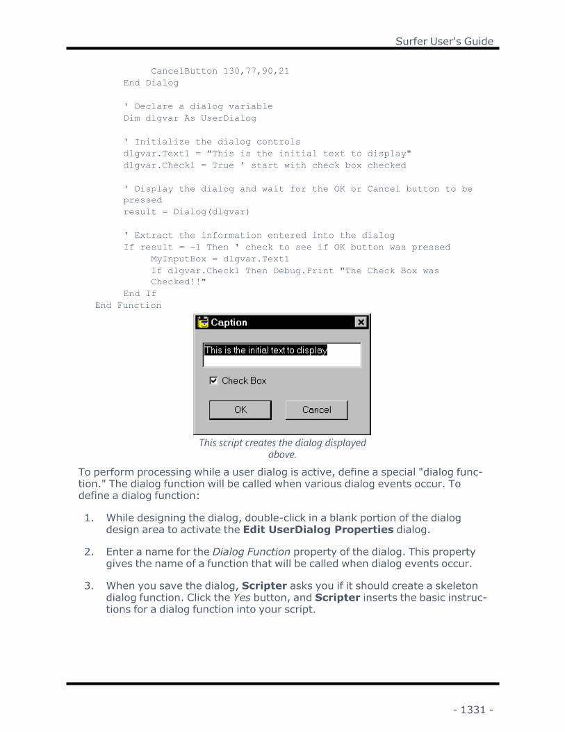
Surfer User's Guide
CancelButton 130,77,90,21End Dialog
' Declare a dialog variableDim dlgvar As UserDialog
' Initialize the dialog controlsdlgvar.Text1 = "This is the initial text to display"dlgvar.Check1 = True ' start with check box checked
' Display the dialog and wait for the OK or Cancel button to bepressedresult = Dialog(dlgvar)
' Extract the information entered into the dialogIf result = -1 Then ' check to see if OK button was pressed
MyInputBox = dlgvar.Text1If dlgvar.Check1 Then Debug.Print "The Check Box wasChecked!!"
End IfEnd Function
This script creates the dialog displayedabove.
To perform processing while a user dialog is active, define a special "dialog func-tion." The dialog function will be called when various dialog events occur. Todefine a dialog function:
1. While designing the dialog, double-click in a blank portion of the dialogdesign area to activate the Edit UserDialog Properties dialog.
2. Enter a name for the Dialog Function property of the dialog. This propertygives the name of a function that will be called when dialog events occur.
3. When you save the dialog, Scripter asks you if it should create a skeletondialog function. Click the Yes button, and Scripter inserts the basic instruc-tions for a dialog function into your script.
- 1331 -

Chapter 34 - Automating Surfer
Refer to the DialogFunc help topic in theHelp | BASIC Language Helpfor moreinformation about how to process dialog events in a dialog function.
Surfer Object ModelSurfer provides ActiveX Automation objects which allow scripts to control prac-tically every feature of Surfer. These objects can be accessed from Scripter orfrom any Automation-enabled environment, such as Visual BASIC, WindowsScripting Host, or Excel.
Accessing SurferThe means of accessing Surfer Automation objects varies depending on thescripting tool and language being used. With the Golden Software Scripter pro-gram and other applications compatible with Visual Basic, the CreateObjectfunction creates a Surfer Application object:
Set x = CreateObject("Surfer.Application")
In this sample, a variable named "x" is assigned the value returned by theVBCreateObject function. The CreateObject function finds the name Surfer-.Application in the system registry, automatically activates Surfer, and returns areference to the SurferApplication object. For an introduction to the Scripter pro-gramming language, see the Scripter BASIC Language help.
After creating an Application object, you can access other Surfer objects throughthe properties and methods of the Application object. Surfer supplies nearly 60different kinds of ActiveX Automation objects. These objects are organized in ahierarchy, with the Application object at the root. This object hierarchy is knownas an object model.
Methods and PropertiesObjects have attributes associated with them. The Grid object, for example, hasan attribute called "xMin" which represents the minimum X coordinate of thegrid. An object’s properties, also known as its properties, may be examined andchanged by scripts. Some properties may be examined, but may not bechanged. These are called read-only properties.
In addition to having properties, many Automation objects perform services. AGrid object, for example, will perform the "SaveFile" service when a scriptinstructs it to do so. The services that an object performs are called itsmethods. Methods often require parameters to control how their services are performed.The Grid object’s "SaveFile" method, for example, accepts two parameters: a filename and a file format code.
- 1332 -

Surfer User's Guide
The way you access Surfer Automation objects’ properties and methods variesdepending on the programming language you use. In the Golden SoftwareScripter language, properties and methods are accessed by typing the name ofan object variable, followed by a period, and the name of the property ormethod:
Set x = CreateObject("Surfer.Application")x.Visible = True
This sample creates an Application object and sets the Application object's "Vis-ible" property to the special "True" value predefined by the Scripter language.
You can find all the properties and methods which are available for each of theAutomation objects, as well as a description of the objects themselves, in theonline help. To view the online help, select either the Help | Automation Helpcommand from the Surfermenu, or the Help | Surfer Automation Help com-mand in Scripter. The ActiveX Automation Members dialog also shows youthe available objects, properties, and methods. To view this dialog, select theDebug | Browse command in Scripter.
CollectionsSeveral non-visible objects, called collection objects, are used to organize theobject hierarchy. Collection objects are containers for groups of other, related,objects. For example, the Overlays collection contains the objects in a compositemap. An Overlays collection object could contain a BaseLayer object,Wireframeobject, and a PostLayer object if these three objects were overlaid together.
All collection objects, regardless of what the collection contains, can be pro-cessed using similar techniques. Thus, you retrieve an object from a collection ofmaps (an Overlays collection) the same way you retrieve an object from a col-lection of axes (an Axes collection). Collection objects also provide methods tocreate new objects.
Object Model ChartThe object model chart shows you which objects provide access to other objectsin the hierarchy. Although the Application object is at the top of the hierarchy,not all objects are directly accessible from the Application object. To accessmany objects you must traverse from the Application object through one ormore layers of sub-objects. People often refer to "drilling" or "boring" throughthe object hierarchy to describe this traversal through several objects to obtainan object you want to use.
To "drill through" the object hierarchy you must know which properties and meth-ods of an object provide access to the next level of objects. Overview of SurferObjects, discusses the most commonly used objects and the properties andmethods which provide access to other objects in the hierarchy.
- 1333 -

Chapter 34 - Automating Surfer
Every object represents a specific part of Surfer. For example, the Wireframeobject represents a wireframe, and the Axis object represents a map axis. Someobjects do not represent a visible entity, but organize other objects into groups.The Shapes object, for example, provides the means to create new maps andnew drawing primitives (rectangles, symbols, polygons, etc.), but the Shapesobject itself is never visible.
Overview of Surfer ObjectsLearning to use the Surfer Automation objects in a script may appear daunting atfirst. Most tasks, however, can be accomplished using just a few Surfer objects.Once you become familiar with these primary objects and learn how to "drillthrough" the object hierarchy, you will be able to access most of Surfer's fea-tures from your scripts.
The online help is the complete reference for all of the Surfer Automationobjects, their properties, and their methods. The object model chart shouldserve as your guide for navigating through the object hierarchy. Use the Help |Automation Help command in Surfer, or the Help | Surfer Automation Helpin Scripter to see the online help reference.
This section shows how to access the Surfer Automation objects using theScripter BASIC language. If you are not familiar with computer programming,you may benefit from a programming tutorial. See the Suggested Reading topicfor recommendations. Refer to the online helpWriting Scripts topic for moreinformation about Scripter BASIC.
A Brief Introduction to the Major SurferObjectsThe following will introduce some of the most important Surfer automationobjects. This is by no means comprehensive. Please see Objects, Properties, andMethods for a complete list.
Application ObjectThe Application object represents the Surfer program. All navigation throughthe Surfer object model begins with the Application object. The Applicationobject is a single instance of Surfer and it is the root of all objects in Surfer.External programs will typically create an instance of the Application object dur-ing initialization. In VB this is done using the function as in:
Set SurferApp = CreateObject("Surfer.Application")
The CreateObject function activates a new instance of Surfer, and returns a ref-erence to the Application object to your script. If Surfer is already running, and
- 1334 -

Surfer User's Guide
you do not want to start a new instance of Surfer, use the VB GetObject functioninstead of CreateObject:
Dim SurferApp As ObjectSet SurferApp = GetObject(,"Surfer.Application")
The GetObject function obtains the Application object from the currently run-ning instance of Surfer. If Surfer is not already running, the function will fail. Callthe Application object’s Quit method to close Surfer from a script.
When Surfer is started by a script, its main window is initially hidden. To makethe Surfer window visible, you must set the Application object’s Visible prop-erty to True:
Set SurferApp = GetObject(,"Surfer.Application")SurferApp.Visible = True
Most of the gridding-related operations are methods of the Application object.Use the GridData, GridFunction, GridMath, GridFilter, GridSplineSmooth,GridAssignNoData, GridConvert, GridVolume, GridSlice, GridTransform, GridEx-tract, and GridCalculus methods to create new grids and perform computationswith grids.
Other methods and properties of the Application object let you move and resizethe Surfer window, adjust the main window state (maximized, minimized, hid-den), change the window caption, and modify preference settings.
The Application object provides two important collections that allow access tothe next level of objects in the hierarchy. Use theDocumentsproperty to obtain areference to the Documents collection object, and use the Windows property toobtain a reference to theWindows collection object. The Documents andWin-dows collection objects provide access to the other objects in the object hier-archy. You can access the currently active document and window objects withthe Application object’s ActiveDocument and ActiveWindow properties.
Set the ScreenUpdating property to False to disable screen updating and makeyour scripts execute more quickly. Turning off screen updating can greatlyincrease the performance of Automation when you want to perform a number ofactions that cause screen redraws.
See Application Object for additional information.
Documents CollectionThe Documents collection contains all open documents. The Documents col-lection provides the means to access plot and worksheet documents. Use theAdd method to create new plot or worksheet documents. Surfer provides thepre-defined values srfDocPlot and srfDocWks for specifying the type of documentto create:
Set srf = CreateObject("Surfer.Application")
- 1335 -

Chapter 34 - Automating Surfer
srf.Documents.Add srfDocPlot ' Create a new, blank plot documentsrf.Documents.Add srfDocWks ' Create a new, blank worksheet document
The Add method returns a reference to the Document object that was created.New grid documents are not created with the Documents collection Add method.You can create grid files by calling the Application object’s grid-related objects.
Use the Open method to open existing plot, worksheet, and grid files. The Openmethod returns a reference to the opened document.
Use the Item method to retrieve a reference to an open plot or worksheet doc-ument object. When iterating through a collection of documents, the documentType and Index properties can be used to determine the type and position of thedocument within the collection.
See Documents Collection for additional information.
Windows CollectionTheWindows collection provides access to all windows within Surfer. TheWin-dows collection returned by the Application object contains all the windows inthe application, including the plot window, the worksheet window, and the grideditor views. To create newWindow objects, call a Document object’s NewWin-dow method.
See Windows Collection for additional information.
PlotDocument ObjectA PlotDocument object corresponds to an SRF file. PlotDocument objects arecreated by the Documents.Add or Documents.Open methods of the Applicationobject. All drawing objects within the document are stored in the Shapes col-lection. All selected objects are part of the Selection collection.
The PlotDocument provides access to all the drawing and map objects. Usemethods and properties in the PlotDocument object to save Surfer files [.SRF],to import and export files, to print, and to change the default line, fill, font, andsymbol for a plot.
Use the Shapes, Selection, and Window properties to access the collectionobjects having the same names. These collection objects provide access to thenext layer of objects in the object hierarchy. Use the Shapes collection object tocreate new drawing and map objects.
See PlotDocument Object for additional information.
- 1336 -

Surfer User's Guide
WksDocument ObjectTheWksDocument object represents a worksheet document. WksDocumentobjects are created by the Documents.Add or Documents.Open methods. Cellswithin a worksheet are accessed through the Cells, Rows, and Columns methods.The active cell and current selection are accessed through a WksWindow object.You can perform a mathematical transformation on worksheet cells and mergefiles together with the WksDocument object. The WksRange object can beaccessed using the Cells, Rows, Columns, and UsedRange properties.
See WksDocument Object for additional information.
PlotWindow, WksWindow, and GridWindow ObjectsIt is important to distinguish between windows and documents. Documentobjects represent a file on disk containing the actual data to be represented. Win-dows are used to view that data. There can be multiple windows viewing thesame document at once.
The Window object encapsulates all the methods and properties associated witha Surfer window. Methods exist to open, close, move and size the window.
When a document is closed, all windows viewing that document are closed aswell. The reverse relationship exists as well. When the last window viewing a doc-ument is closed the document is closed.
See PlotWindow, WksWindow, and GridWindow Objects for additional inform-ation.
Shapes CollectionWithin Automation, graphic drawing and map objects are called Shapes. TheShapes collection contains all of the drawing and map objects in a document.This object is also used to create new shapes and add them to the collection.Methods exist to enumerate all the shapes in the collection, add objects to theSelection collection, and create new drawing and map shapes.
One of the most common uses of the Shapes collection is to create new shapes.There is a unique method to create each type of shape. For example, to create acontour map use the AddContourMap method, as in:
Sub Main
Set SurferApp = CreateObject("Surfer.Application")SurferApp.Visible = True
'Create a new, empty plot documentSet Doc = SurferApp.Documents.Add srfDocPlot
'Get the Shapes collection
- 1337 -

Chapter 34 - Automating Surfer
Set Shapes = Doc.Shapes
'Create the contour mapSet MapFrame = Shapes.AddContourMap(Demogrid.grd)
End Sub
See Shapes Collection for additional information.
Selection CollectionThe Selection collection contains all the properties and methods associated withthe collection of selected shapes. The Selection collection defines methods thatoperate on one or more selected shapes. Most commands within Surfer thatrequire selected objects are part of the Selection collection.
To select a particular shape, set the shape’s Selected property to True. When aShape object is selected, it is added to the Selection collection. When it isdeselected, it is removed from the Selection collection. Note that the shape isneither created nor destroyed by selection operations. It is merely added orremoved from the Selection collection.
The Selection collection allows all selected shapes to be enumerated, and con-tains most methods that operate on multiple objects. This includes moving andsizing one or more shapes; cut, copy, and paste; and overlaying and stackingmultiple maps.
See Selection Collection for additional information.
MapFrame ObjectYou create new maps using the Add<map type>Map methods of the Shapes col-lection (AddVectorBaseMap, AddReliefMap, AddContourMap, and so forth).These methods return a reference to a MapFrame object - not, as you mightexpect, a reference to the object of the specific map type that was created. TheMapFrame object contains the coordinate system, axes, and all properties com-mon to the maps contained within it. TheMapFrame defines the coordinate sys-tem and axes for one or more overlays.
You add layers to an existingMapFrame object with the Add<map type>Layermethods (such as AddContourLayer). These methods return a reference to thespecific map layer that has been created.
When a new map object is created, usually theMapFrame object is returnedrather than the contained overlay. For example, Shapes.AddContourMap returnsthe containingMapFrame object rather than the contour map overlay. Toaccess the overlay within theMapFrame, use the Overlays collection as in:
Set MapFrame = Shapes.AddContourMap(demogrid.grd)Set ContourMap = MapFrame.Overlays(1)
- 1338 -

Surfer User's Guide
Use the Overlays property of theMapFrame to obtain the Overlays collectionobject. The Overlays collection contains all the individual map objects asso-ciated with a map frame. When a new map frame is created, the Overlays col-lection contains just one map item. To obtain a reference to a newly createdmap, access the first item of the collection:
Sub Main
Set SurferApp = CreateObject("Surfer.Application")SurferApp.Visible = True
'Create a blank plotSet plot = SurferApp.Documents.Add srfDocPlot
'Add a new contour map. This will return a MapFrame objectSet mapframe = plot.Shapes.AddContourMap demogrid.grd
'Get a ContourMap object from the MapFrameSet contourmap = mapframe.Overlays(1)
End Sub
Use theMapFrame object to set map limits, adjust the three-dimensional view,adjust the scale, and change the size of the map. Access the Axes collection withtheMapFrame object’s Axes property. Use the Axes collection object to obtainthe individual Axis objects associated with a map. Access the ScaleBars col-lection through theMapFrame object’s ScaleBars property. Use the ScaleBarscollection to add scale bars to a map and to access the ScaleBar objects asso-ciated with a map.
See MapFrame Object for additional information.
Derived ObjectsSeveral objects shown in the object list share common features. For example,the PlotDocument object and WksDocument object each provide SaveAs, Activ-ate, and Close methods. These common features are inherited from a pre-decessor Document object.
Derived objects inherit all the properties and methods of the predecessor object.In the online reference, the help topic for derived objects shows just the prop-erties and methods unique to the object. The predecessor object is accessedthrough the Derived from link. Remember that all the properties and methods ofa predecessor object are available as well. Derived objects and their predecessorobjects include:
- 1339 -

Chapter 34 - Automating Surfer
Document ObjectThe Document object is a predecessor of the PlotDocument and WksDocumentobjects.
Window ObjectThe Window object is a predecessor of the PlotWindow, WksWindow, andGridWindow objects.
Shape ObjectThe Shape object is a predecessor of all objects which can be moved and resized.These include the MapFrame, Variogram, Composite, all of the basic drawingobjects (Rectangle, Ellipse, Symbol, Text, Polyline, Polygon, and RangeRing),various map component objects (Axis, ScaleBar, Profile, VectorLegend andPostLegend), and the predecessor objects listed below (Layer, Legend, and Col-orScale objects).
Layer ObjectThe Layer object is a predecessor of all the map layer objects (ClassedPostLayer,ContourLayer, ColorReliefLayer, PostLayer, RasterBaseLayer, ReliefLayer, Vect-orBaseLayer, VectorLayer, ViewshedLayer, and WatershedLayer) and the Gratic-ule object.
Legend ObjectThe Legend object is a predecessor of the VectorLegend and PostLegend objects.
ColorScale ObjectThe ColorScale object is a predecessor of the ContinuousColorScale and Dis-creteColorScale objects.
Using Collection ObjectsSurfer groups most objects in collections. Although these collections contain dif-ferent types of data, they can be processed using similar techniques.
Count PropertyAll collection objects have a read-only property named Count which gives thenumber of objects in the collection.
- 1340 -

Surfer User's Guide
Item MethodEvery collection also has a method called Item which retrieves one of the objectscontained in the collection. The Item method accepts a single argument spe-cifying either an index number or (for most collections) the name of the object toretrieve. An index number is a value between 1 and the value returned from thecollection’s "Count" property. The name used to identify items in a collection var-ies:
l In a Documents collection, the individual Document objects are identifiedby the file name (or the caption, if the document has not been saved in afile yet).
l In a Windows collection, individual Window objects are identified by the win-dow caption.
l In collections containing objects derived from the Shape object (Shapes,Selection, Axes, ScaleBars, and Overlays collection objects), the individualShape objects are identified by the object ID assigned to the object.
l In the Levels collection, individual Level objects may be retrieved by theirindex number only. The Level objects cannot be retrieved by name.
A shorthand syntax for retrieving items from a collection is to enclose the indexor name of the desired object in parentheses immediately following the name ofa collection object (similar to accessing an element in an array). Thus, the fol-lowing two instructions have the same effect:
' Assume "docs" is a variable holding a reference to the Documents col-lectiondocs.Item(1) ' retrieves the first object in the collectiondocs(1) ' shorthand, retrieves the first object in the collection
Objects contained in collections are typically derived from a base object. Whenyou use the Item method to retrieve an object from a collection, the methodreturns a reference to the base object. To determine the actual type of thereturned object, most base objects contain a Type method. For example, theWin-dows collection may contain PlotWindow,WksWindow, or GridWindow objects.When you retrieve a window from theWindows collection, a reference to a gen-ericWindow object is returned. Use the Window.Typeproperty to determine ifthe returned object is a PlotWindow, WksWindow, or GridWindowobject.
Add MethodMany collections have one or more Add methods for creating new items andadding them to the collection. For example, to add a rectangle to the Shapes col-lection, you would use the AddRectangle method:
Shapes.AddRectangle 2, 2, 4, 4
- 1341 -

Chapter 34 - Automating Surfer
Close and Delete MethodsThe objects contained by collections are automatically removed when the con-tained object is deleted or closed. For example, call a Document object’s Closemethod to close a document or call the Shape object’s Delete method to removeany Shape-derived object.
Parent and Application PropertiesEvery Automation object provides a Parent and an Application property. TheApplication property returns a reference to the top-level Application object. Thisis a convenient way to access the Application object, particularly when passingAutomation objects as arguments to subroutine and function calls.
The Parent property returns a reference to the collection object that an object iscontained in, or the controlling object. If an object is not contained by a col-lection object, the Parent property typically returns a reference to the Applicationobject.
PlotWindow, WksWindow, and GridWindowObjectsIt is important to distinguish between windows and documents. Documentobjects represent a file on disk containing the actual data to be represented. Win-dows are used to view that data. There can be multiple windows viewing thesame document at once.
The Window object encapsulates all the methods and properties associated witha Surfer window. Methods exist to open, close, move and size the window.
When a document is closed, all windows viewing that document are closed aswell. The reverse relationship exists as well. When the last window viewing a doc-ument is closed the document is closed.
Using Surfer ObjectsTo access Surfer commands from your script you must create a Surfer Applic-ation object. To create an Application object, call the CreateObject function withSurfer.Application as the argument. The Application object is the root of anobject hierarchy. Access all other Surfer Automation objects though the prop-erties and methods of the Application object.
Every object has properties and methods associated with it. Properties are val-ues describing the state of an object.Methods are actions an object can per-form. Access properties and methods by typing the name of an object variable,followed by a period, followed by the property or method name.
- 1342 -

Surfer User's Guide
You can use object properties as you would use variables: assign values to prop-erties, branch based on the value of a property, or use the value of a property incalculations. You call an object’s methods as you would call subroutines and func-tions. Use the return values from methods the same as you would use return val-ues from functions.
When you "drill through" the object hierarchy, you can store references to inter-mediate objects in variables, or you can string together long sequences of objectreferences. For example, you can set the default font for a plot document in asingle line:
' Assume "SurferApp" is a variable holding a reference to the Applic-ation objectSurferApp.Documents.Item(1).DefaultFont.Bold = True
Alternatively, you can store each intermediate object in variables as you traversethe object hierarchy:
' Assume "SurferApp" is a variable holding a reference to the Applic-ation objectSet docs = SurferApp.DocumentsSet plot = docs.Item(1)Set font = plot.DefaultFontfont.Bold = True
The second form - storing intermediate objects - is more efficient if you are per-forming several actions with the same object. A third alternative is to use theWITH…END WITH statement:
' Assume "SurferApp" is a variable holding a reference to the Applic-ation objectWith SurferApp.Documents.Item(1).DefaultFont.Bold = True.Size = 12.Color = SurferAppColorBananaYellowEnd With
Object ListThe following table provides a list of all the Surfer automation objects. The tablealso provides the interfaces that are dispatched when writing a late-bindingscript for Surfer.
The interfaces from which the current interfaces have been extended areincluded in the table, if applicable. If you are writing an early binding script andwould like to use the properties and methods available in the latest version, besure to dispatch the current interface.
- 1343 -

Chapter 34 - Automating Surfer
The current interfaces include all of the properties and methods available inSurfer. The properties and methods specific to the former interfaces can befound in the older application help files.
Object Interface (current) Interface(former)
Application IApplication5 IApplication4Axes IAxesAxis IAxis2 IAxisClassedPostLayer IClassedPostlayer2 IClassedPostLay-
er,IClassedPostMa-p
ColorMap IColorMap2 IColorMapColorNode IColorNodeColorNodes IColorNodesColorReliefLayer IColorReliefLayer2 ICo-
lorReliefLayer,IImageLayer,IImageMap
ColorRGBA IColorRGBAColorScale IColorScaleComposite IComposite2 ICompositeContinuousColorScale IContinuousColorScaleContourLayer IContourLayer IContourMapDiscreteColorScale IDiscreteColorScaleDocument IDocumentDocuments IDocumentsEllipse IEllipseFillFormat IFillFormatFontFormat IFontFormatGLFillFormat IGLFillFormatGraticule IGraticuleGrid IGrid3 IGrid2GridMathInput IGridMathInputGridStatistics IGridStatisticsGridWindow IGridWindowImageLayer IImageLayer2LabelFormat ILabelFormat3 ILabelFormat2Layer ILayerLegend ILegendLegendLayers ILegendLayersLevel ILevelLevels ILevelsLineFormat ILineFormat
- 1344 -

Surfer User's Guide
MapFrame IMapFrame3 IMapFrame2MarkerFormat IMarkerFormatOverlays IOverlaysPageSetup IPageSetupPlotDocument IPlotDocument3 IPlotDocument2PlotWindow IPlotWindowPolygon IPolygonPolygon3D IPolygon3DPolyline IPolyline2 IPolylinePolyline3D IPolyline3DPostLayer IPostLayer2 IPostLayer,
IPostMapPostLegend IPostLegend2 IPostLegendProfile IProfileProfiles IProfilesRangeRing IRangeRingRasterBaseLayer IRasterBaseLayer2 IRasterBaseLayerRectangle IRectangleReliefLayer IReliefLayerRuler IRulerScaleBar IScaleBar3 IScaleBar2,
IScaleBarScaleBars IScaleBarsSelection ISelection3 ISelection2,
ISelectionShape IShapeShapes IShapes7 IShapes6,
IShapes5,IShapes4,IShapes3,IShapes2,IShapes
Surface ISurfaceSymbol ISymbolSym-bologyClassedColorsBin
ISym-bologyClassedColorsBin
Sym-bologyClassedColorsBins
ISym-bologyClassedColorsBins
Sym-bologyClassedSymbolsBin
ISym-bologyClassedSymbolsBin
Sym-bologyClassedSymbolsBins
ISym-bologyClassedSymbolsBin
Text ITextTopLegend ITopLegend
- 1345 -

Chapter 34 - Automating Surfer
VarioComponent IVarioComponentVariogram IVariogramVectorBaseLayer IVectorBaseLayer2 IVectorBaseLayerVectorLayer IVectorLayer IVectorMapVectorLegend IVectorLegend2 IVectorLegendViewshedLayer IViewshedLayerWatershedLayer IWatershedLayer2 IWatershedLayerWindow IWindowWindows IWindowsWireframe IWireframeWksCellFormat IWksCellFormatWksDocument IWksDocumentWksPageSetup IWksPageSetupWksRange IWksRangeWksStatistics IWksStatisticsWksWindow IWksWindowWksWindows IWindowsWireframe IWireframeWksCellFormat IWksCellFormatWksDocument IWksDocumentWksPageSetup IWksPageSetupWksRange IWksRangeWksStatistics IWksStatisticsWksWindow IWksWindow
Object HierarchyThe following image shows the Surfer automation object model. To access a par-ticular object you must traverse the object hierarchy using the methods andproperties provided by the objects. This chart shows objects that provide accessto other objects. Collection objects are containers for groups of related objects.Non-container objects represent a specific part of Surfer.
- 1346 -

Surfer User's Guide
Improve Automation PerformanceTurning off screen updating can greatly increase the performance of Automationwhen you want to perform a number of actions that cause screen redraws. Youcan achieve this efficiency by setting ScreenUpdating to false, performing therepetitive operations, and then turning ScreenUpdating back on. WhenScreenUpdating is turned back on, all windows will be redrawn in the new state.
Automation ExamplesIn addition to the examples found in the Table of Contents Examples book withinthe Surfer Automation book, there are many more examples for your use.
- 1347 -

Chapter 34 - Automating Surfer
l The SCRIPTS folder in the Surfer directory contains sample [.BAS] files touse in Scripter. By default, the SCRIPTS folder is located at: C:\ProgramFiles\Golden Software\Surfer\Samples\Scripts.
l In addition, each object, method, and property contains an example in theAutomation help. The methods and properties contain only a few lines forthe example.
l Click on the Used By link for an example on how to tunnel through the hier-archy to the method or property.
l Some methods and properties contain a link showing a full example of theobject.
l Sample scripts are available for download at the Where Can I Find SurferScript Examples article in the Surfer support Knowledge Base.
Creating and Printing a Contour MapThis example automates the process of creating a contour map to visualizechanges in groundwater levels. The script prompts the user for a data file, cre-ates a grid from the file, creates a contour map, prints the map, and saves themap in a Surfer file [.SRF].
Sub Main'Declare object and string variables used in the scriptDim SurferApp, Plot, ContourMapFrame,ContourLayerAs ObjectDim InFile, GridFile,
'Create the Surfer Application object and assign it to the "SurferApp"variableSet SurferApp = CreateObject("Surfer.Application")SurferApp.Visible = True 'Make Surfer visible
'Prompt the user for the name of the data file to process.InFile = GetFilePath("","DAT;TXT;CSV;XLS",CurDir(), Select data file,0)If InFile = "" Then End 'Can't continue: no file was selected
'Get file name without the extension (for example, "week5.txt" becomes"week5")BaseName = InFileExtStart = InStrRev(InFile,.)If ExtStart 1 Then
'Create a grid from the specified data file using the KrigingalgorithmGridFile = BaseName + .
- 1348 -

Surfer User's Guide
SurferApp.GridData DataFile:=InFile, Algorithm:=srfKriging, _DupMethod:=srfDupNone, ShowReport:=False, OutGrid:=GridFile
'Create a plot document in Surfer and assign it to the variable named"Plot"Set Plot = SurferApp.Documents.Add(srfDocPlot)
'Create a contour map. Assign the map frame to the "ContourMapFramevariableSet ContourMapFrame =
'Assign the contour map properties to the variable named "Con-tourLayer"Set ContourLayer = ContourMapFrame.Overlays(1)
ContourLayer.FillContours = True 'Fill the contour map levelsPlot.PrintOut 'Print the page on the default printerPlot.SaveAs(BaseName + ".srf") 'Save the map
End Sub
Opening, Saving, and Closing DocumentsThe Documents collection provides access to the Surfer file commands. Use theDocument object’s "Open" method to open an existing plot, worksheet, or gridfile. Use the Add method to create a blank plot or worksheet. The SaveAllmethod saves all open documents, and the CloseAll method closes all open doc-uments. To save or close an individual document, use the Document object’sSave, SaveAs, and Close methods.
Sub Main
Set SurferApp = CreateObject("Surfer.Application")SurferApp.Visible = True
' Create a blank plotSurferApp.Documents.Add srfDocPlot
' Create a blank worksheetSurferApp.Documents.Add SurferAppDocWks
' Open an existing plotfilename$ = GetFilePath(,SRF)if filename$ ThenSurferApp.Documents.Open filename$End If
' Open the sheet named "Sheet1" from an Excel filefilename$ = GetFilePath(,XLS)
- 1349 -

Chapter 34 - Automating Surfer
If filename$ ThenSurferApp.Documents.Open filename$, Sheet=Sheet1End If
' Close the active documentSurferApp.ActiveDocument.Close
' Save the active document using its current nameIf Not SurferApp.ActiveDocument.Saved ThenSurferApp.ActiveDocument.SaveEnd If
' Save the document whose window caption is "Plot1"SurferApp.Documents("Plot1").SaveAs "MyDocument
' Close all documentsSurferApp.Documents.CloseAll
End Sub
Creating a Variogram with ScripterThe Variogram object represents a variogram. A Variogram object is a type ofShape object. Create a new Variogram using the Shapes collection’s AddVari-ogram method. The AddVariogram method returns a reference to a Variogramobject. Use the properties and methods of the Variogram object to access inform-ation about the computed variogram and to modify the options.
A VarioComponent object represent one component of a variogram model. Whenyou use the Kriging algorithm to create a grid file, you can specify the variogrammodel to use by passing an array of VarioComponent objects to the Applicationobject’s GridData method. Create a VarioComponent by calling the Applicationobject’s NewVarioComponent method. Use the Variogram object’s Model prop-erty to obtain the array of VarioComponent objects used by a variogram.
The following subroutine creates a Variogram object, and then creates a grid fileusing the computed variogram components.
Sub GridWithComputedVariogram(plot As Object,' Create a variogram.Set v = plot.Shapes.AddVariogram (
' Create a grid using the computed variogramplot.Application.GridData DataFile:=datafile, Algorithm := Surfer-AppKriging, _KrigVariogram := v.Model, ShowReport := False, OutGrid := grid
' Delete the variogramv.Delete
- 1350 -

Surfer User's Guide
End Sub
The next subroutine creates two VarioComponent objects and creates a gridbased on these variogram components.
Sub GridWithStaticVariogram(plot As Object, datafile As String, gridAs String)' Get the Application objectSet SurferApp = plot.Application
'Create two VarioComponent objects and store them in an arrayDim components(1 To 2) As ObjectSet components(1) = SurferApp.NewVarioComponent(Surfer-AppVarNugget,1.0,2.0,3.0)Set components(2) = SurferApp.NewVarioComponent(Surfer-AppVarLinear,1.0,2.7,1.5)
'Create a grid using the two variogram componentsSurferApp.GridData DataFile:=datafile, Algorithm := SurferAppKriging,_KrigVariogram := components, ShowReport := False, OutGrid := gridEnd Sub
Finally, the following Main procedure demonstrates how you might use the pre-ceding subroutines:
Sub Main' Start Surfer, set the default directory, and create a plot documentSet SurferApp = CreateObject("Surfer.Application")SurferApp.Visible = TrueSurferApp.DefaultFilePath = SurferApp.Path + "\samples"Set plot = SurferApp.Documents.Add(srfDocPlot)
' Create a grid using a pre-determined variogram modelGridWithStaticVariogram plot, "demogrid.dat, VarioDemo1
' Create a grid using a computed variogram modelGridWithComputedVariogram plot, "demogrid.dat, VarioDemo2
' Create contour maps to compare the two gridsplot.Shapes.AddContourMap "VarioDemo1"plot.Shapes.AddContourMap "VarioDemo2"
End Sub
- 1351 -

Chapter 34 - Automating Surfer
Overlaying Maps with AutomationThe overlay map script is compatible with Surfer 8 and below. In Surfer 9 useadd map layers. In Surfer 10 and above, use one of the add map layers meth-ods (such as AddVectorBaseLayer) or use the OverlayMaps method.
To overlay maps in a script, you must first select the select the map orMapFrame objects to be overlain, and then call the Selection collection’s Over-layMaps method. The following subroutine demonstrates how to overlay maps:
Sub OverlayMapsExample(mapframe1 As Object, mapframe2 As Object)' Retrieve the parent PlotDocument objectSet plot = mapframe1.Parent
' Clear all selections and then select the two MapFrame objectsplot.Selection.DeselectAllmapframe1.Selected = Truemapframe2.Selected = True
' Overlay the selected mapsplot.Selection.OverlayMapsEnd Sub
The subroutine would be used like this:
Sub Main' Start Surfer and create a blank plot documentSet SurferApp = CreateObject("Surfer.Application")SurferApp.Visible = TrueSet plot = SurferApp.Documents.Add(srfDocPlot)
' Create a contour map and a vector mapgridfile$ = SurferApp.Path + \samples\demogrid.grdSet map1 = plot.Shapes.AddContourMap(gridfile$)Set map2 = Plot.Shapes.AddVectorMap(gridfile$)
' Call the example subroutine to overlay the mapsOverlayMapsExample map1, map2
End Sub
Stacking maps is similar to overlaying them. Call the Selection collection’sStackMaps method rather than the OverlayMaps method.
- 1352 -

Surfer User's Guide
Modifying AxesAxis settings may be changed using the Axis object. You access Axis objectsthrough the Axes collection object, which in turn is accessed through aMapFrame object. The following example does not use subroutines, but youcould write the script with subroutines instead.
Sub Main' Start Surfer and create a blank plot documentSet SurferApp = CreateObject("Surfer.Application")SurferApp.Visible = TrueSet plot = SurferApp.Documents.Add(srfDocPlot)
' Create a contour mapgridfile$ = SurferApp.Path + \samples\demogrid.grdSet mapframe = plot.Shapes.AddContourMap(gridfile$)
' Turn off screen redrawing to speed up this procedureold_update_setting =mapframe.Application.ScreenUpdating = False
' Adjust the left and bottom axesFor Each axis In mapframe.AxesIf axis.AxisType = SurferAppATLeft OrWith axis.MajorTickType = SurferAppTickCross.MinorTickType = SurferAppTickIn.MinorTickLength = 0.1.MinorTicksPerMajor = 9.ShowMajorGridLines = True.AxisLine.Width= 0.03End WithEnd IfNext
' Restore the previous screen settingmapframe.Application.ScreenUpdating =End Sub
- 1353 -


Appendix A - Mathematical Functions
Mathematical FunctionsMathematical Functions are used to modify data with the grid Function, Math,Grid Data, and Variogram commands in the plot window, and with the Transformcommand in the worksheet window.
Data TypesThe expression evaluator supports 32-bit signed integer numbers, double-pre-cision floating-point numbers, a boolean value, a text string of 0 to 256 char-acters, and time stamp values.
Variable NamesVariable names must begin with a column letter (i.e. A), row number (i.e. _1), orcell location (i.e. A2), which may be followed by other letters, numbers, or under-scores (_), up to a maximum of 256 characters per variable name.
The variable names are not case sensitive. For example, sum(a..z), sum(A..z),and sum(A..Z) all refer to the same variable.
PrecedenceThe mathematical expression can consist of constants, variables (such ascolumn letters), or functions (outlined below). The formulas follow standard pre-cedence rules. Spaces are used in the equation for clarity.
Formulas are specified using standard precedence rules. Operators, in order ofdecreasing precedence, are:
( ) parentheses- minus (or negative sign)* / multiplication and division+ - addition and subtraction
The expression evaluator treats operators with the following precedence:
1. !, NOT, ~
2. ^
3. *, /, %
4. +, -
- 1355 -

Appendix A - Mathematical Functions
5. <<, >>
6. <, >, <=, >=
7. ==,!=,<>
8. &
9. XOR
10. |
11. &&, AND
12. ||, OR
13. ?:
14. IF
Operators of equal precedence are evaluated from left to right within the equa-tion. Parentheses are used to override precedence, and expressions with the par-entheses are performed first.
The following built-in functions are supported.
Trigonometric FunctionsAll trigonometric functions are carried out in radians. If the data are in degrees,use the d2r(x) conversion function (in the Miscellaneous Functions sectionbelow) to convert degree data to radians and then use the trigonometric func-tions.
sin(x) sine of angle xcos(x) cosine of angle xtan(x) tangent of angle x, the value of x must not be an odd multiple of
/2asin(x) Arcsine in the range - /2 to /2, x must be between -1 and 1acos(x) Arccosine in the range 0 to , x must be between -1 and 1atan(x) Arctangent in the range - /2 to /2atan2(y,x)
Arctangent of y/x in the range - to
- 1356 -

Surfer User's Guide
Bessel Functionsj0(x)
j1(x)
jn(n,x)
Bessel functions of the first kind at x of orders 0, 1, and n, respect-ively
y0(x)
y1(x)
yn(n,x)
Return the Bessel functions of the second kind at x, of orders 0, 1,and n, respectively. For y0, y1, and yn, the value of x must not benegative.
Exponential Functionsexp(x) exponential function of x (e to the x)sinh(x) hyperbolic sine of angle xcosh(x) hyperbolic cosine of angle xtanh(x) hyperbolic tangent of angle xln(x) natural logarithm (base e) of x, x must be positivelog10(x) base 10 logarithm of x, x must be positivepow(x,y) x raised to the yth power
Error conditions result if:
x is zero and y is negative or zero,
x is negative and y is not an integer,
an overflow results.x^y x raised to the yth power, see above
Miscellaneous Functionsmin(x,y)
smaller of x and y
max(x,y)
larger of x and y
randn(x,y)
an approximately normally (Gaussian) distributed real random num-ber with mean x and standard deviation y
randu(x)
a uniformly distributed real random number with mean of x fromthe interval [0,x]
row() returns the row number
- 1357 -

Appendix A - Mathematical Functions
ceil(x)
next whole number greater than or equal to x
floor(x)
next whole number less than or equal to x
pi() returns the value of Pi. To limit to a specific number of digits, useRound(Pi(),y) where Y is the number of digits after the decimalpoint
round(x, y)
X rounded to a the nearest number with Y digits after the decimalpoint
sqrt(x)
square root of x, x must not be negative
fabs(x)
absolute value of x
fmod(x,y)
floating point remainder of x/y, if y is zero, fmod returns zero
d2r(x)
convert angle x from degrees to radians. Example: sin(d2r(30))computes the sine of 30 degrees. Sin(30) computes the sine of 30radians
r2d(x)
convert angle x from radians to degrees
sign(x)
evaluate the sign of a number, returns -1 for x < 0, 0 for x = 0, and1 for x>0
Statistical Functions of Intervalssum(a..z) calculates the sum of a range of columns in a rowsum(_1.._5)
calculates the sum of a range of rows in a column
avg(a..z) calculates the average of a range of columns in a rowavg(_1.._5)
calculates the average of a range of rows in a column
std(a..z) calculates the (population) standard deviation of a range ofcolumns in a row
std(_1.._5) calculates the population standard deviation of a range ofrows in a column
rowmin(a..z)
finds the minimum value of a range of columns in a row
rowmin(_1.._5)
finds the minimum value of a range of rows in a column
rowmax(a..z)
finds the maximum value of a range of columns in a row
rowmax(_1.._5)
finds the maximum value of a range of rows in a column
l The Statistical Functions of Intervals functions operate row-wise on an inter-val of columns or column-wise on an interval of rows.
- 1358 -

Surfer User's Guide
l The Statistical Functions of Intervals do not operate on cells. The equation B1= avg(A1..A6) will result in only the average of row 1, not the average of thespecified cells.
l For example, SUM(A..Z) computes the sum of the twenty-six columns A, B,C, ..., Z. It does this for each row separately.
l Replace 'a..z' by any valid interval of columns or rows, such as W..AC or _4.._612. There must be exactly two periods between the column or row labels.The labels may be given in reverse order, such as SUM(Z..A).
l The Statistical Functions of Intervals functions can only be used in the work-sheet. These functions cannot be used in Grid Math.
String Comparisonatof(x) convert a string x to floating-point valueatoi(x) convert a string x to an integer valueftoa(x,y) convert a floating-point number x to a string with y digits after
the decimal pointstrlen(x) length of string x in charactersstrcmp(x,y)
compare string x with y and return 1 if x>y, -1 if x<y, or 0 if x=y
stricmp(x,y)
compare string x with y without regard to the case of any lettersin the strings
strncmp(x,y,z)
compare the first z characters of string x with y
strnicmp(x,y,z)
compare the first z characters of string x with y without regard tothe case of any letters in the strings
String comparison functions work with strings, not numbers. Any rows orcolumns containing numbers result in blanks. In each of the string comparisonfunctions, 1 is returned if string x is greater than string y, -1 is returned if stringx is less than string y, and 0 if string x = string y. In the three-parameter com-parison functions, the third parameter, z, specifies the number of characters tocompare. For example, a z value of 3 compares the x and y strings' first threecharacters and ignores any characters after the third.
The comparisons are based on the standard ASCII table:
1. numeric values (disregarded in string comparisons as mentioned above)
2. cells starting with a space character
3. common punctuation
4. numeric text (numbers entered as text)
5. less common punctuation
6. uppercase letters
- 1359 -

Appendix A - Mathematical Functions
7. even less common punctuation
8. lower case letters
9. uncommon punctuation
10. blank cells (disregarded in string comparisons)
This is the ASCII table order. The table is read left to right, top to bottom. Items appearingtoward the upper left corner are less than the items appearing toward the lower left corner.
Example of a String ComparisonThe following example shows a comparison of two strings in rows 1 and 2 withthe results displayed in row 4. STRCMP returns a 1 if row 1 is greater than row 2;-1 if row 1 is less than row 2, and 0 if row 1 is equal to row 2.
- 1360 -

Surfer User's Guide
This equation compares the strings in rows 1 and 2 and places the results in row 4.
This table includes results of the string comparisons based on the ASCII table. Cells con-taining numbers and blanks are ignored.
Boolean ExpressionsBoolean expressions include:
l Logical Operators (and, or, xor, not),
l Comparison Operators (=, <>, <, >, <=, >=),
l the IF Function - IF(condition,
The words AND, OR, XOR, NOT, and IF are reserved keywords and may not beused as variable names.
Logical Operators (and, or, xor, not)SYMBOL NAME DESCRIPTIONAND AND The result is true if both operands are true.&& AND The result is true if both operands are true.
- 1361 -

Appendix A - Mathematical Functions
! Logical NOT Inverts the boolean value. True becomes false,false becomes true.
NOT Logical NOT Inverts the boolean value. True becomes false,false becomes true.
& AND The result is true if both operands are true.| OR The result is true if either of the two operands is
trueXOR Exclusive-
OR (XOR)The result is true if both operands differ.
|| OR The result is true if either of the two operands istrue.
OR OR The result is true if either of the two operands istrue.
Comparison Operators (=, <>, <, >, <=, >=)SYMBOL NAME DESCRIPTION~ Bitwise NOT Inverts the bits in an integer* Multiply Multiplies the two operands/ Divide Divides the first operand by the second% Remainder Integer remainder of the first operand divided
by the second.+ Add Adds the two operands- Subtract Subtracts the second operand from the first<< Shift Left Shifts the operand to the left>> Shift Right Shifts the operand to the right< Less Than In the example, A1 < B1, the result is true if
A1 is less than B1.<= Less Than or
Equal ToResult is true if the ordinal value of p1 is lessthan or equal to p2
> Greater Than Result is true if the ordinal value of p1 isgreater than p2
>= Greater Thanor Equal To
Result is true if the ordinal value of p1 isgreater than or equal to p2
== Equal To Result is true if the operands have identicalvalues
!= Not Equal To Result is true if the operands do not haveidentical values
<> Not Equal To Result is true if the operands do not haveidentical values
IF Function - IF(condition,SYMBOL NAME EXAMPLE DESCRIPTION
- 1362 -

Surfer User's Guide
IF ConditionalEvaluation
IF(p1,p2,p3)
IF(condition,true_value,false_value)
i.e. If p1 is true, the result will bep2. If p1 is false, the result will bep3.
IF ConditionalEvaluation
p1?p2:p3 condition?true_value:false_value
i.e. If p1 is true, the result will bep2. If p1 is false, the result will bep3.
ExamplesThe following are examples of mathematical function syntax used in Surfer.With Grids | New Grid | Function and Grids | Calculate | Math use X,Y,and Z for the variables. If you use Data | Data | Transform in the worksheet,replace X,Y, and Z with column letters (A), row numbers (remember the under-score, _1 is row 1), or cell locations (A1).
Equation Mathematical Function Syntaxx^2 or pow(x,2)ln(x)
log10(x)
(1-exp(-X))(1-exp(-X*X))1-(sin(x)/x)
x^2/(1+x^2)
(2 * X) - X^2( x^2+ y^2)*(sin(8*atan(x*y)))
- 1363 -


Appendix B - Math Text Instructions
Math Text Instruction SyntaxThe math text instruction set offers advanced formatting of text in the Surferplot window. Math text instructions can be used to change the typeface, size,color, weight, and style of text on a character-by-character basis. Greek lettersand mathematical symbols can be written in the plot window using math textinstructions. The math text instructions also allow for the detailed placement ofcharacters and symbols; thus, superscripts, subscripts, and the superposition ofcharacters are possible. The worksheet cells used as post labels in a post plot cancontain math text instructions. In general, the clipboard can be used to cut andpaste math text instructions.
All text within the plot window can be controlled by math text instructions. Forexample, an axis label, title, or text block can include math text instructions inthe text string in the Properties window. In the Properties window, add themath text instructions below directly in the Title text, Prefix, Suffix, or Textoption. Do not open the Text Editor as text in the Text Editor cannot use mathtext instructions. To use different text properties in the Text Editor , highlightthe text to change and click the appropriate button or command in the dialog.
Unless otherwise indicated, all math text instructions begin with a backslash("\"), and end with a single space. For example, the instruction "\up50" shifts thebaseline of the text up 50 percent of the current text height. All characters fromthe beginning backslash through the ending single space are interpreted asinstructions by the math text interpreter, and are not included in the resultinglabel.
Each line in a text block starts with the default text properties such as typeface,size, color, and style. (Note that some typefaces, such as Symbol, do not supportbold or italicized text.) A line of text within a text block uses the current prop-erties until a math text instruction is encountered. All text following an instruc-tion is modified according to the instruction. For example, if the typeface ischanged in the middle of a text string, the text following the instruction will usethe new typeface until the end of the line of text is reached, or until anotherinstruction affecting the typeface is encountered.
Encapsulate Math Text InstructionMath text instructions can also be encapsulated so they are not carried out overan entire line. A left curly brace ("{") instructs the math text system to remem-ber all of the text properties in effect at that point. A right curly brace ("}")restores the properties to what they were at the matching left curly brace. Thisallows the insertion of special text in the middle of an otherwise uniform textblock. The only instructions this does not apply to are text baseline instructions
- 1365 -

Appendix B - Math Text Instructions
\dnX and \upX), and the position instructions (\rpX and \spX). Curly braces canbe nested.
To incorporate a backslash, right curly brace, or left curly brace as a text char-acter in a text block, precede them with a backslash when entering the textstring. For example, "\\" produces "\", and "\{" produces "{".
Percentage InstructionsInstructions based on a percentage, such as font size, are cumulative. Thismeans that a second percentage change within a text block is interpreted as apercentage of the first percentage change. For example, if the font is scaled by50%, and later in the same text block the font is scaled by 50% again, the fontsize after the second percentage would be 25% of the original font size.
Note: Instruction names are case insensitive (\fs50, \FS50, \Fs50 or \fS50 areall valid).
Note: The \sp and \rp instructions only refer to positions on the same line.
Instructions that Change Typefaces, Sizes, and StylesMath TextInstruction
Result
\b All text after the \b command is bold.\f"X" Change to the typeface named X. These are the names listed
in the Face list box in the Text dialog in the plot window.Typeface names are case sensitive. Enclose the face name indouble quotes. If the typeface is not found, a generic sticktypeface is used in place of the unfound typeface.
\fsX Change font size to X% of current font size. For example, avalue of 200 for X increases the font size by two, and a valueof 50 for X decreases the font size by one-half.
\i All text after the \i instruction is italicized.\plain This sets the text to "plain" text with normal weight, no ital-
ics, no underlining, and no strikethrough.\strike Strikethrough the text.\ul All text after the \ul instruction is underlined.
Instructions that Change Text ColorThe following instructions are provided to make it easy to set basic text colors:
Math Text Instruction Result\black Sets the text color to black.\blue Sets the text color to blue.\green Sets the text color to green.\cyan Sets the text color to cyan.
- 1366 -

Surfer User's Guide
\red Sets the text color to red.\magenta Sets the text color to magenta.\yellow Sets the text color to yellow.\white Sets the text color to white.\gray Sets the text color to gray.
The following instructions allow the text color to be set to an arbitrary RGBA(Red,Green,Blue, Alpha) value:
Math TextInstruction
Result
\rgbrX Sets the amount of red in an RGBA text color (X=0 to 255).\rgbgX Sets the amount of green in an RGBA text color (X=0 to
255).\rgbbX Sets the amount of blue in an RGBA text color (X=0 to 255).\rgbaX Sets the alpha value in the RGBA text color (X=0 to 255).\color(r,g,b,a)
Sets the amount or red, green, blue, and alpha value in theRGBA text color. r, g, b, and a are all a value between 0 and255.
Instructions that Change Text PositionMath TextInstruction
Result
\dnX Moves text baseline down X% of current font size (sub-script). This instruction produces subscripts or returns thebaseline to the original position following a \upX instruction.If a font size (\fsX) instruction follows the \dnX instruction,any subsequent \dnX or \upX instructions are relative to thechanged font size.
\n Creates a new line in the text block. This works similar to acarriage return - line feed combination. This should be usedinstead of the \dnX to create a new line of text.
\rpX Restores the current position to position #X (X = 1 to 20).This instruction is used in conjunction with the \spX instruc-tion. Any text following this instruction begins at the positiondefined with the \spX instruction. If the \rpX instruction isused without first setting a position with the \spX instruction,the position for the text is returned to the stating position forthe text block.
- 1367 -

Appendix B - Math Text Instructions
\spX Saves the current position as position #X (X = 1 to 20). Theposition is the up, down, left, and right areas within the textblock. When the \spX instruction is used, the current locationwithin the text block is assigned a position number. Returnto this position using the \rpX instruction. Specify the pos-ition number assigned with the \spX instruction when usingthe \rpX instruction. These instructions are most useful whenplacing both superscript and subscripts after the same char-acter.
\upX Moves the text baseline up X% of current font size (super-script). This instruction is used to produce superscripts or toreturn the baseline to the original position following a \dnXinstruction. If a font size (\fsX) instruction follows the \spXinstruction, any subsequent \upX or \dnX instructions are rel-ative to the changed font size.
Instructions Used to Insert Special Characters or Dateand TimeMath TextInstruction
Result
\aX Insert an ANSI character with code given by X (0 to 255).Generally, this instruction is needed for characters withANSI numbers beyond the normal limits of the keyboard.For example, use the ANSI character code to include anintegral sign in a text string. By determining the characterset, followed by the \aX command to specify the correctcharacter number. For example, an integral sign is locatedat ANSI position 242 in a symbol set called Symbol. Type\f"Symbol" \a242 for the integral to appear in the textblock.
The Character Map program is an accessory program in theWindows installations. Use the Character Map to displayeach of the available character sets with the ANSI code.The ANSI code is displayed in the right half of the CharacterMap status bar when a character is selected.
\date Inserts the current date. Be sure to follow this instructionwith a space, even if no other text follows the date. Thedate is updated every time the text is redrawn.
\time Inserts the current time. Be sure to follow this instructionwith a space, even if no other text follows the time. Thetime is updated every time the text is redrawn.
\dt("format")
Inserts the current date and/or time as indicated by a cus-tom format string. Be sure to follow this instruction with aspace, even if no other text follows the closing parenthesis.The date and or time is updated every time the text isredrawn.
- 1368 -

Surfer User's Guide
Examples of Math Text InstructionsDue to page size limitations, some of these examples contain multiple lines ofmath text instructions. These examples must be entered on one line for the textto be displayed correctly.
Math Text Instruction ResultCO\dn50 2 CO2x\up50 2 x2\sp1 {\fs200 \f"Symbol" \a229 \sp2 }{\rp1\dn90 \fs75 i=1\rp1 \up220 n}\rp2 \up25X\dn50 {\fs75 i}\up50 Y\dn50 {\fs75 i}\up50= S{\dn50 {\fs75 XY}\up50 }{\i Avogadro} Constant = 6.022 x 10{\up50{\fs75 23}\dn50 }
Avogadro Constant =6.022 x 10²³
{\f"Symbol" \a209 }{\up50 {\fs50 2}\dn50 }{\f"Symbol" \a102 } = {\f"Symbol" \a182 }{\up50 {\fs50 2}\dn50 }{\f"Symbol" \a102 }/{\f"Symbol" \a182 }x{\up50 {\fs50 2}\dn50 }+ {\f"Symbol" \a182 }{\up50 {\fs50 2}\dn50}{\f"Symbol" \a102 }/{\f"Symbol" \a182 }y{\up50 {\fs50 2}\dn50 }{\fs200 N}\sp1 \up100 \fs75 5 \rp1 \dn50 1
sin{\up50 {\fs50 2}\dn50 }(X) + cos{\up50{\fs50 2}\dn50 }(X) = 1104\f"Symbol" \a176 \f"Arial" 37'
a\dn25 {\fs75 c} \n ___ \n b\dn25 {\fs75 c}
{\f"Symbol" d}\up50 {\fs75 234}\dn50 U
- 1369 -


Surfer User's Guide
Index#
# of lines 205
1
1-grid vector maps 717
2
2-grid vector maps 720
3
3D boreholes 9213D drillholes 9213D DXF 12363D label lines 6443D SHP 12363D surface 657, 660, 663, 666, 669, 860, 893, 9023D view points 12713D wireframe 671, 681-682, 1186
9
95% and 99% confidence interval for the mean 18895%confidence interval for the mean 18899% confidence interval for the mean 188
A
a brief introduction to the major Surfer automation objects 1334a gridding example 203a note about the documentation 99, 111about Surfer 94absolute value 149, 1164, 1358accessing objects 1332accessing Surfer 1332accidentally move 1211accumulated horizontal distance 494across then down 1257
- 1371 -

Index
active 215active cell 52, 134-137active cell edit box 134active cell location 134active cell location box 136ActiveX automation members 1332ActiveX automation objects 1332actual size 1227Add 947add a color scale bar to a 3D wireframe 861add a color scale bar to a filled contour map 861add a map background color 843add a map layer 847, 947add attribute information 333, 1195add axis 874add base layer 517add component 325add contour labels 607add contour levels 578add cross section 868add datadrillholes 792
add data source 819add grids 505add image base map 517add information about the map 333, 1195add layer 847add levels 575, 578add map 847, 947add map source 819add metadata information 333, 1195add method 1341add profile 868add scale bar 848
- 1372 -

Surfer User's Guide
add section 868add sever 819add slice 868add symbols to text 1365add text 1070add to map 847adding a color scale bar 860-861adding a map layer 947adding an overlay 947adding color fill between contours 596adding color zones to a 3D wireframe 684additional information in data files 123ADF 433adjacent maps 71adjust to 1255advanced contour levels 575advanced level method 575advanced levels 575advanced options 248, 253, 258, 263, 265, 267, 269-270, 273, 275, 285,
1261, 1277advanced settings 1261, 1277, 1282affected levels 587, 592, 595, 598, 603, 606, 609, 612albers 199, 1010, 1023albers conic 1023albers equal area 1023Align 1215, 1218align grids 480align maps 951, 953align objects 1215aligning several maps on the same page 953alignment 166, 168, 1074, 1134all data search 227all files 80, 159all recognized types 158
- 1373 -

Index
all sessions 1277Alpha 1169alpha value 293always reset 1279always split 1299AM 434ambient 668, 904anchor nodes 1180and 1355angle 229, 626, 655, 880angle (direction) data 726angle column 624, 654angle component grid file 719angular divisions 223, 309anisotropy 230, 301, 319ANOVA 221ANSI character 1368antarctic 1022antialias lines 1271antialias redraw 1271antialias text 1272apostrophe 1311Application Object 1332, 1342Application Property 1342apply a gradient to class symbols 640approximate density 277arctic 1022area 333, 465, 470-471, 477, 942, 1195area reshape 1103area to download 813area to line 1101arithmetic average 193arrange icons 1230arrange lock 1211
- 1374 -

Surfer User's Guide
arrange lock position 1211arrange maps 951arrange menu commands 1206, 1208, 1211-1213, 1215, 1219-1221arrange objects 38array variables 1327arrays 1328artificial data 215ascending 178ASCII 1236ASCII boundary files 517ascii import 152ASCII table 179assign columns 198assign coordinate 439, 1011assign coordinate system 199, 439, 1001, 1008, 1010-1011, 1022-1023assign projection 199, 1001, 1006, 1010assign xyz columns 197assigning attributes 978assigning color fill based on a fill spectrum 598assigning color fill to specific contour levels 599assigning contour labels to specific levels 604assigning coordinates to an image base map 961assigning fill and line properties to blanked areas 600assigning gradational line properties 590assigning line properties to specific contour levels 593assigning metadata 978assigning the same line properties to all contour levels 591asterisk 29Atlas BNA 124attribute 335, 978, 1197attribute editor 978attribute query 983attribute search 983auto hide 39
- 1375 -

Index
auto redraw 1229AutoCAD DXF export 1236AutoCAD DXF import 517, 530, 1231autocorrelation 251, 255autocorrelation estimator 316autocovariance estimator 316AutoFit 323automatic grid slice 868automatic scaling 689, 885automatic variogram fitting dialog box 323automatically check for updates 1266automating Surfer 1297automation 1346automation example 1347-1350, 1352-1353automation examples 1347automation help 1297, 1333-1334available date formats 128available date time formats 128available time formats 128average 193average data value 213average deviation 188average distance 277average every 1107axes 874Axes Collection 1332, 1340, 1353axis 874, 897axis attributes 878axis date/time labels 878axis direction 887axis labels 878axis limits 883axis maximum 885axis minimum 885
- 1376 -

Surfer User's Guide
Axis Object 1332, 1353axis plane 878axis position 876, 886axis properties 878, 880, 883, 889axis scaling 883axis ticks 874axis visibility 876azimuthal 1026azimuthal equidistant 1026azimuthal projection 1026
B
back 1213backcolor 1282background 843background cell 169background color 166, 598-599, 1073, 1138background map color 843background mode 596backup files before saving 1263backward 1213BAS 1348base 674, 686base layer 517base map 517, 521, 527, 530, 808base map from data 521base map from server 818base map general page 530base map properties 519, 528, 530, 558base object 1341base parameters 686BASIC 1301basin 707, 712basin boundary 707basin color 713
- 1377 -

Index
basin map 707basis kernel functions 271Bessel functions 1357between cols 438between rows 438bezier 1089BIFF 5 151BIFF 8 151biharmonic operator 459-460BIL 433bilinear 669bilinear interpolation 505, 510BIN 433binning method 637bins 638BIP 433bitmap (image) 1130, 1231, 1236bitmap (image) coordinates 961bitmap (image) export 1236bitmap (image) import 517, 530, 1231bitmap (image) pattern 1142bitmap (image) properties general page 1167black and white 1258blank 395, 414, 420, 430blank cells 175blank grid outside convex hull 205blank grid outside convex hull of data 205blank grid outside data 205blank inside 414, 959blank inside data 205blank node 395blank node when searching 225blank outside 414, 959blank outside convex hull 205
- 1378 -

Surfer User's Guide
blank outside data 205blank value 395, 480blanked areas 414blanked grids and volume 479blanked nodes 423, 432, 660blanked planar area 471blanked regions 566, 600, 687, 689blanking a grid file 414blanking file 124, 235, 494, 957, 959blanking file format 420blanking flag 421blanking with search ellipse 228blend overlay and surface colors 669BLN 124, 234, 414, 420, 491, 517, 958-959block diagram 663block kriging 248, 252block select 1205BMP 517, 1233-1234BNA 124, 1236bold 1072, 1135Bold Property 1365bonne 1027bonne projection 1027boolean 1326boolean expressions 1361border 674, 843boreholes 783boreholes, 3D 921boundary 517, 521boundary around data 205boundary maps 517boundary number 493boundary tension 260break a line 1111, 1311
- 1379 -

Index
break apart 960, 1221break apart complex polygon 1125break apart islands 1125break apart islands/lakes 1125break apart lakes 1125break apart layer 960break apart overlay 960break at intersections 1111break line 1111break polyline 1111breakline example 237breakline format 237breaklines 234, 237, 421breaklines and faults 234breakpoint 1310brush 379brush grid 381BSQ 433buffer 1119buffer polygon 1119buffer zone 1119built-in functions and procedures 1316button appearance 1286button persistence 1261byte 1326
C
calculate area 942calculate contour levels by logarithm 568calculate distance 942calculate perimeter 942calculate volumes and areas 465calculating the agreement between a grid and the original data file 498calculating the volume between two surfaces 478calculating the volume of a blanked grid 479
- 1380 -

Surfer User's Guide
calculating the volume of a lake 480calculating the Z value of a surface at a point 501calculation 156, 174calculus 443, 446, 452-457, 459, 462can't find coordinate system 1006cancel 49cannot display script 1297cartesian data 719, 725cascade windows 1230cassini 1029cassini projection 1029catchment area 707catchment basin 707cell alignment 168cell background 169cell edit box 135, 137cell format 156, 166cell number format 166cell numeric format 166cell properties 166, 168-169cells 124center 1072center on page 1256centimeters 1264central difference 689change all symbols at once 640change blank value 480change data file 619, 631, 654change default columns for XYZ data 197change grid 660change grid file 566, 689change ID 1207change image coordinates 961change individual contour level 580
- 1381 -
Index
change points 1101, 1103change polygon shape 1101, 1103change polyline shape 1100-1101, 1103change projection in worksheet 199change the page setup 1247change the view 827change units 1261changing base map properties 528changing contour levels 575changing properties in a base map 528changing the grid node editor 36changing the layout 36changing the managers 36changing the map limits 732changing the menu bar 36changing the object manager location 38changing the plot window 36changing the toolbars 36changing the worksheet 36channel system 707character map 1368characteristics of projections 1019check for update 93, 1266choosing gridding methods 239-241, 246choosing methods based on the number of XYZ data points 241circle 1096class list box 638class scatter color file format 629class symbol fill color 640class symbol gradient 640class symbol properties 640class symbol set all symbols the same 640class symbol set all symbols to a color range 640class symbol size dialog 643
- 1382 -

Surfer User's Guide
class symbol size properties 643class symbol size range 643class symbol uniform 640classed post layer 631classed post legend 852classed post map 629, 631, 636, 644, 654classed post map legends 849classes page 636classical variogram estimator 314clear 157clear selected cells 157clear transform 1207click tolerance 1270clip map 838clip symbols at map limits 726, 732clipboard 151clipping symbols on vector maps 732close 87, 1349close method 1340close polylines 1100close script 1300closing the object manager 38CLP export 1236CLP import 517, 530, 1231CLR 563, 726, 1170, 1173, 1181CLS 640Code, Class, and Object Modules 1320coefficient of kurtosis 189coefficient of skewness 190, 221coefficient of variation 191, 220, 277coefficient of variation filter 428COL 433collate 1260collection objects 1333, 1340
- 1383 -

Index
collections 1333color 1072, 1187-1188, 1190, 1282-1284color column 624color fill 596, 598-599, 682color filled contours 596, 598-599color filled wireframe 682color list 1190color method 626color modulation 670color names 1190color on wireframe maps 684color palette 1187color relief map 690color scale 661, 689, 729, 860-861color scale bar 860-861color scale bar visibility 860-861color scaling 728color selection 1187color spectrum 1170, 1180color spectrums 1182color syntax 1281color zones 684color zones page 678, 685colors 690, 1188, 1281colors dialog 1188column 145-148, 170column formats 156, 170column labels 135column letters 134column width 135, 145, 170columns to rows 197combine 947combine boundaries 1110, 1115, 1126combine curves 1110
- 1384 -

Surfer User's Guide
combine grids 505combine islands 1126combine islands/lakes 1126combine lakes 1126combine lines 1110combine maps 71, 947combine multiple polygons 1126combine multiple polylines 1110combine polygons 1115, 1126combine polylines 1110combining maps 71, 948-949combining maps when exporting 1240command line 1306comments 1311common document files 81common graphic files 1232common map properties 825comparison of gridding methods 240comparison operators 1362compass gradient filters 430compassed-based grid notation 443compatibility 89compatibility with Visual BASIC 1301complex polygon 1126complex polygon to multiple polygons 1125composite object 1220-1221compute statistics 183compute transform 172concatenate 175conformal 1043conjoin polygons 1126connect curves 1110connect lines 1110connect multiple polylines 1110
- 1385 -

Index
connect points 623connect points in a post map 619connect polylines 1110connection line 623contact us 94, 102contour export 1236contour fill 596, 598-599, 602contour interval 570, 575, 578contour label color 604contour labels 604, 607-608contour layer 564contour level 580contour levels 375, 571, 575, 578, 591, 593contour levels dialog 579contour line properties 590-591, 593-594, 600contour lines 578, 587, 1236contour map 563, 565-566, 861, 1348contour map colors 563contour map properties 563, 566, 575contour map properties dialog 563, 566, 575, 847contour smoothing 515, 614contour values 604Contours 501controlling label spacing 604convergence 262convert 433convert boundary to polyline 1101convert polygon to polyline 1101convert polygons 1101convert polyline to polygon 1100convert polylines 1100-1101converting to decimal degree 1066convex hull 293coordinate 996
- 1386 -

Surfer User's Guide
coordinate arrays 1328coordinate system 76-77, 199, 993-994, 996, 998-999, 1001, 1006, 1010coordinate system faq 999coordinate system for export 1240coordinate systems 1022coordinates 199, 527, 961coordinates in images 961copies 1260copy 156, 1131copy attribute 337, 1199copy metadata 333, 1195copy server and layer name 808cores 1261correlogram 462cos 1356count 279Count Property 1340cover contours 613create a custom toolbar 1286create a data file with digitize 957create a grid file from an XYZ data file 205create a grid report 213create a north arrow 1096create colors 1188create complex polygon 1126create contour levels at regular intervals 580create custom line style 1151create donuts 1126create grid 64create grid from contour map 289create grid from contours 289create islands 1126create islands/lakes 1126create lakes 1126
- 1387 -

Index
create layer 64create map 64create multiple lines from one 1111create multiple lines of text 1071create multiple polygons from one 1125create multiple polylines from one 1111create template (text) 1074CreateObject 1332creating a 1-Grid vector map 717creating a 2-Grid vector map 721creating a 3D surface 657creating a 3D wireframe 671creating a base map 517creating a blanking file with the digitize command 959creating a color spectrum file 1183creating a contour map 564creating a cross section 490creating a filled contour map and overlay on a wireframe 682creating a filled contour map containing blanked areas 600creating a grid file 205creating a level file containing contour level information 581, 1184creating a new classed post map 629creating a new contour map 563creating a new post map 617creating a new wireframe map 671creating a variogram 307creating a vector length legend 849creating anchor nodes 1180creating dialogs with Scripter 1330creating grid files 205creating index contours 594creating level files in the worksheet 583, 1186creating post maps 617, 629creating several maps in the same plot window 952
- 1388 -

Surfer User's Guide
criteria select 983critical value of K-S statistic at 90%, 95%, and 99% significance level 192crop 414, 838crop map 838cross section 490, 495, 868, 871cross validate 209cross validation references 212cross X axis at 887cross Y axis at 886cross Z axis at 886CSV 124cubic convolution 507, 510cubic model 317, 325currency 166, 1326currency format 166current command 48current date 1258current map extents 808current session only 1279current time 1258current version 93cursor tracking 986curvature 447, 451, 455curve 1090curve tolerance 606custom button appearance 1286custom colors 1188custom contour label positions 607custom coordinate system 199, 1010custom datum 1016custom datum definition 1015custom keyboard commands 1290custom labels 608, 651custom line style 1150
- 1389 -

Index
custom toolbars 33, 1286customize 1286, 1293customize commands 1286customize keyboard commands 1293customize menu 1286customize options 1261, 1286customize toolbars 1286customizing post map classes 636cut 156, 471, 473, 868, 1131cut and fill volume 466, 473, 501cut and fill volumes 471cyclic 432
D
DAT 152, 433, 490DAT Files 124data 121, 138, 205, 307data as numbers or text 124data command 205data file 27, 124, 652, 654data file base map 521data file formats 124data files 57, 121data files used for posting 652data import options 152data labels in the data file 653data layer information 819data link 81data location statistics 277, 282data menu commands 156, 179, 199, 1010data metric 282, 284data metric other z statistics 282data metric terrain 284data metrics 239, 277, 279, 281-282data metrics data location 282
- 1390 -

Surfer User's Guide
data metrics z moment 281data metrics z order 279data orientation 230, 319data page 307, 719data repeatability 301, 339data set size 241data sort 178data statistics 183data transform 177data used 224database 81database linking 986date 1071, 1084, 1326date format 166, 1084, 1161date formats 130date time 127date time format 1161date time formats 128date values 127date/time 127, 167date/time format 1084, 1163datum 1016datums 1006, 1013, 1015DCX export 1236DCX import 517, 530, 1231Debug.Print 1308debugging scripts 1307decimal degrees 1066decimal digits 166, 1163default angle post map 623default attributes 1271, 1275default columns for XYZ data 197default gridding method 205, 239default linear variogram 338
- 1391 -

Index
default map scale 831default path 1262default settings 1257, 1261, 1271, 1274, 1277, 1279default symbol 1276defaults 1270-1271, 1274, 1277, 1279-1280, 1282-1285define coordinate system 1006deflate convex hull by 205degree units 719degrees 1356degrees minutes seconds 200, 1066, 1161Delaunay 1112Delaunay triangulation 266, 273, 1121delete 160, 1131delete anchor nodes 1180delete contour label 607delete contour levels 578delete levels 575delete map in overlay 71delete metadata 333, 1195delete method 1342delete selected cells 160deleted duplicates 215delimiter 152DEM 58, 433, 565, 687demo 17density 277depressions 712derivatives 446derived objects 1339descending 178descending axis 883description for metafile 333, 1195deselect all 1205destination column 173
- 1392 -

Surfer User's Guide
detrend 309detrending method 215deviation distance 1107device independent bitmap 1131dialog defaults 1277, 1279-1280, 1282-1285dialog editor 1330difference between Z value and grid 496difference of polygons 1117difference polygons 1117different coordinate systems 998different projections 998differential and integral operations 443, 459differential and integral operators 443, 459diffuse 668, 904digital elevation model [.DEM] 58digital filter 425digital filtering 426, 428digitize 957, 959digits 1285dim 1326direction axis 883directional derivatives 443, 446, 449, 451display area 333, 942, 1195display attribute on base map 558display contour labels on a regular interval 604display distance 942display grid node labels 369display hidden columns 135, 145, 147, 171display hidden rows 135, 145, 148display labels 369display labels on grid nodes 369display perimeter 942displaying a filled contour map without contour lines 600displaying date/time on maps 127
- 1393 -

Index
displaying dates on maps 127displaying different coordinate system 998displaying different projections 998displaying hidden columns or rows 147displaying times on maps 127distance 277, 311, 942distance scale 848distance to farthest 277distance to nearest 277distance weighting filter 426distortion 836DLG import 517, 530, 1231dms 200, 1164dms format 1164dms to dd 200dock object manager 38dock toolbars 1286docking mechanism 40Document Object 1340, 1342documentation 99Documents Collection 1341, 1349don't draw blanked nodes 660double 1326down then across 1257downhill hachures 610download 808download base map 808download data 808download maps 808download online maps 808download worldwide data 808downloads 93drag an object 1206drag and drop map layer 71, 949
- 1394 -

Surfer User's Guide
drag labels 607drag toolbars 1286drainage 707drainage boundary 707drainage map 707drainage network map 707drape maps on wireframes 71draw contours 53, 365draw limits 936draw lines of constant 663draw map limits 936draw menu 1069-1070, 1086-1088, 1094-1096draw menu commands 1069draw mesh lines on a 3D surface 663draw polyline 1086draw text 1071drawing 1069drawing contours 565drawing grid 1229drawing tips 1086-1087, 1089, 1094-1096drawing toolbar 1069drift type 309drillhole layer 783, 786drillholes3D points properties 9213D properties 921add data 792layer 783map 783
duplicate data 180duplicate window 1229DXF 989dynamic linking 986
E
eckert 1030-1031
- 1395 -

Index
eckert IV 1030eckert VI 1031edge effect 443edge of grid 425, 430edit attribute 337, 1199edit contour 54, 365edit contour labels 607edit contours 54, 365edit grid 53, 365edit grid value 53, 365edit labels 607, 651edit legend properties 849edit major tick spacing on an axis 888edit map source 819edit maps in an overlay 71edit menu 45, 150, 156, 161, 164, 1127-1128, 1130-1131, 1205-1207edit menu commands 96edit metadata 333, 1195edit overlay 71edit polygon 1103edit polyline 1103edit post labels 651edit properties 45edit server 819edit surface 53, 365edit template (text) 1074edit text 1071editing a color scale bar 861editing an existing 1-Grid vector map 717editing an existing 2-Grid vector map 721editing an existing 3D surface 657editing an existing base map 520editing an existing classed post map 630editing an existing contour map 564
- 1396 -

Surfer User's Guide
editing an existing post map 618editing an existing surface 657editing an existing wireframe 671editing axes 875editing cell contents 137editing color zones 680editing contour label positions 607editing metadata 978editing the data files in the worksheet 96, 142editing the vector length legend 849editing the worksheet 156editing variogram properties 310editing worksheet cells 52, 135, 137editing z levels zones 678elevation 686elevation at a point 496, 501elevation export 1236elevation profile 868ellipse 228, 1096ellipsoids 1012email 102empty base map 525empty cells 175enable labels 369enable labels on grid node editor 369end 1306end sub 1301enhanced metafile 1130enter serial number 78entering data 52, 135, 137, 139entering data into a cell 139entire data source extents 813equal area 1042equal intervals 637
- 1397 -

Index
equal number 637equation template 1071equations 173equations in text blocks 1365equidistant 1032-1033equidistant conic 1032equidistant cylindrical 1033eraser 395error strings and special numeric values 148error variance 339ERS 434estimate 212estimator type 311, 314evenly spaced data 298exact and smoothing interpolators 246exact interpolators 246examples 203, 302, 478, 480, 498, 501, 591, 594, 602, 608, 612, 725, 1347,
1363, 1369examples - Scripter 1330, 1347-1350, 1352-1353Excel files 89, 92, 151exclude data within this distance 212excluded 215exit 96expand 432expand a grid 435expand object manager 1261experimental curve 305experimental page 311explicit color names 626exponent zeros 1163exponential format 166, 1161exponential functions 1357exponential model 317, 325export 1236, 1238, 1240, 1243
- 1398 -

Surfer User's Guide
export 3D contour lines 1236export contour lines 989, 1236export drawing objects in map units 1240export map and non map objects 1240export multiple maps 1240export options - scaling page 1238export options dialog 1238, 1243export profile data 873export scaling 1238export variogram 341exporting a variogram 341extended Simpson's 3/8 rule 476extended Simpson's rule 476extended trapezoidal rule 475extract 510extract data 954extract grid 510, 954extract subset of grid 510extract Z value 501eyedropper 399, 1188
F
FaceName 1283faq coordinate system 999faq projection 999fault line properties 566faults 234-235, 421faults and breaklines 235fax 102field of view 827, 940file export 1236file formats 124file import 157, 517, 530, 1231file list 80, 95, 158, 1261file list (window menu) 95
- 1399 -

Index
file menu 79, 81, 87, 89-90, 95-96, 844, 1231, 1236, 1247, 1250file menu - grid node editor 53, 365file menu commands 78file name 90, 1258file names, formats, and file extensions 89, 92file preferences 1261, 1274file type not recognized 1235file types 57, 157, 203fill 45, 471, 473, 596, 598-599, 602, 1137, 1140fill and line properties 660fill blanks 432fill contours 596fill defaults 1275fill depressions 712fill dialog 597, 1140fill edge 430fill in a sparse grid 436fill palette 1142fill pattern 597, 599, 1142fill pattern defaults 1282fill pattern names 1142fill pits 710fill polyline 1100fill properties 596, 600, 843, 1137, 1140fill properties dialog 596fill property syntax 1282fill spectrum 598filled contours 566filled wireframe 682filter 423filter data 180filter size 425filtering grids 515filters 423, 426, 428
- 1400 -

Surfer User's Guide
final grid size 438find 161, 164find and replace 161, 164find attribute 983find next 161, 164find objects 983find the Z value at a known X and Y coordinate 501finding the volume between two surfaces 478first 592, 602, 609, 612first derivative 447, 449first major tick 885fit criterion 324fit to 1255fit to page 1252fit to window 1223fixed format 166, 1161fixed symbol size 627flat areas on wireframes 687FLD 433flip 197flip axis direction 883flip columns and rows 197flip map 883flip rows and columns 197flow control 1312flow map 710FLT 433font 1072font defaults 1275, 1283font properties 1133font property syntax 1283footer 1249, 1257forecolor 1282foreground color 598-599, 1138
- 1401 -

Index
format 644format builder 1084format cells 166, 168-169format column width 170format date time 128format dates 128format menu commands 156format row height 171format time 128formats for attribute values 1280formatting the data 156formulas 173, 1355forward 1212fourier and spectral analysis 443, 461-463fourier frequency 463frame 843, 851free rotate 1219frequency 591, 602, 608, 621, 633, 664, 727from edge 1256front 1211full screen 1227function 296function types 270functions 172, 1314, 1343, 1355
G
gauss-kruger projection 1060gauss conformal projection 1060gaussian low-pass filter 426gaussian model 317, 325GCS 1035general - preferences 1261general base map 530general gridding options 59, 225, 230, 234, 319general gridding recommendations 240
- 1402 -

Surfer User's Guide
general number format 166general page 309, 530, 566, 619, 631, 660, 673, 689, 878, 1167, 1261general user-defined filter 428generate report 213geode 812geographic coordinate system 1021, 1035geologic profile 868geologic sections 868geometric forms of projections 1017geoprocessing menu commands 1119georeference 963, 1064georeference an image base map 961georeference image 963geostatistical reference 362get variogram 341GetFilePath 1329getting help 98getting started guide 103getting user input 1329GIF export 1236GIF import 517, 530, 1231global variables 1328gnomonic 1036gnomonic projection 1036golden software blanking file description 420golden software blanking import options dialog 420golden software reference 1064goodness of fit statistic 192gouraud 667, 903gradational class symbol size 643gradational lines 587gradient operator 459graticule 862GRD 203, 205, 434
- 1403 -

Index
greek characters 1365grid (drawing) 1229, 1274grid a data set 203grid assign coordinate system 439, 1011grid blank 395, 414grid calculus 443, 452-457, 459, 461-462, 515grid calculus references 515grid contours 289grid convert 409, 433grid coordinate 439, 1011grid data 205grid divisions 1275grid done notification 1261grid editor 53, 365grid erase 395grid extents 205, 507grid extract 510grid feature classes 289grid files 57, 203, 205, 298grid filter 423, 428, 432-433, 515grid filter references 433grid from base layer 289grid from contours 289grid from server 288, 807-808grid from vector 289grid function 296grid info 401, 405, 423, 434, 443, 465, 482, 485, 505, 513, 566, 660, 673,
689, 719grid line geometry 505grid lines 205, 889grid math 480, 484grid menu 53, 205, 296, 305, 341, 365, 413-414, 423, 430, 432-434, 443,
465, 480, 485, 490, 496, 505, 510grid menu commands 413grid mosaic 505
- 1404 -

Surfer User's Guide
grid node 54, 365grid node editor 53, 365, 371-372, 375, 395, 401, 1127grid node editor commands 50grid node editor enable labels 369grid node editor labels 369grid node editor show labels 369grid node labels 370Grid Object 1332grid operations references 515grid periodogram 463grid point sample 499grid project 440grid residuals 497grid slice 490grid spline smooth 434grid stats 513grid toolbar 413grid transform 485grid utilities 413grid values layer 697grid values map 697grid variogram 305grid vector data 289grid volume 467grid volume report 465, 471gridded data 298gridding 58, 205, 239gridding a function 296gridding example 203gridding faults 235gridding method comparison 242gridding methods 205, 239-242, 246, 248, 252, 258, 262, 264, 267-268, 270,
273, 275, 277, 285gridding overview 58
- 1405 -

Index
gridding parameters 205gridding with breaklines 234gridding with faults 234gridlines 1257GridWindow 1341GridWindow Object 1342group 1220GS ASCII 433GS Binary 433GS_Surfer2 1130gsr 1064gsr2 1064GXF 433
H
hach column 610hach list 610hachure direction 611hachures 610, 612handle size 1271handle size in pixels 1271HDF 433head length 731header 1249, 1257height 1210help 98, 111help menu 78, 93-94, 1293help menu commands 78hidden columns 146-147, 171hidden lines 73hidden rows 146-147, 172hide a map in an overlay 71hide object manager 38hiding columns 135, 145-146, 170hiding rows 135, 145-146, 171
- 1406 -

Surfer User's Guide
hierarchy 1332, 1346histogram 329hole-effect model 317, 325honoring data 239, 246horizontal alignment 1074horizontal distance 493horizontal light position 666, 689, 902horizontally align maps 951hotine 1038, 1040hotine oblique mercator 1038hotine projection 1040hotkeys 1290, 1293how contours are created 565how to use Surfer 27hue 1189
I
icon size 1286ID 1208identity 1207if function 1361ignore 431, 433image 961, 1130, 1167, 1243image base map 961image coordinates 961image fill patterns 1142image map 689image resolution to download 815image size 333, 1195image source 336, 1198imagery 808IMG 433immediate 1299import 157, 518, 531, 1231import (worksheet) 157
- 1407 -

Index
import database 81import file 157import file types 1235importing a base map 517, 530improve automation performance 1347in 1224increase down 883increase left 883indeterminate mode 48index 1284index contours 591, 594index number 654inflate convex hull by 293info 98, 333, 401, 507, 1195information about objects 333, 1195initial 323input grid file 566, 660InputBox 1329insert 160insert cells 160insert grid nodes 434insert points on line 1109inserting levels 578inset 1119integer 1326integral and differential operators 459integrated volume 459, 461interactive profile 868internal tension 260internet 98internet maps 808internet update 93, 1265interpolate pixels 691interpolation 246-247
- 1408 -

Surfer User's Guide
interquartile range 277intersect polygons 1117intersection 1111, 1117, 1121intersection points 1121interval 577-578introduction to automation 1297introduction to color spectrums 1170introduction to common map properties 825introduction to grid files 203introduction to grid operations 413introduction to gridding methods 239introduction to level files 1184introduction to map axes 874introduction to map layers 71introduction to map projections 1011introduction to options 1261introduction to Scripter 1297introduction to Surfer 17introduction to Surfer data 121, 138introduction to the major Surfer Automation objects 1334introduction to the worksheet window 52introduction to variograms 299introduction to volumes and areas 470inverse distance 252inverse distance filter 426inverse distance to a power 239-240, 246invert selection 1206invisible contour lines 602invisible regions 761islands 1126islands/lakes 1126isochore map 503isopach map 503italic 1072, 1135
- 1409 -

Index
italic text 1071italicize 1365Item 1341item method 1341
J
join curves 1110join lines 1110join polylines 1110JPG export 1236JPG import 517, 530, 1231justify 1072
K
keep every nth vertex 1107keep every other point in polyline 1106keep object position 1211keyboard commands 1290, 1293keyboard map 1290, 1293kirsch filter 428Kolmogorov-Smirnov goodness of fit statistic 192kriging 240, 242, 246, 248, 252, 309kriging advanced options 248, 253kriging and variograms 301kriging options 248, 252kriging references 248, 252, 257kriging standard deviations 250, 254kriging type 249, 253KSCriticalValue90 Property 192KSCriticalValue95 Property 192KSCriticalValue99 Property 192KSStatistic Property 192kurtosis 189
L
label angle 644
- 1410 -

Surfer User's Guide
label color 604label format 647, 1084, 1161label grid nodes 369label orientation 607label plane 647label position 607, 646, 651label properties 608label property defaults 1285label set 645label source 559label spacing 605label template 558label to edge distance 606label to label distance 606labels 558, 604, 644labels from multiple columns 644labels grid node editor 369labels page 644lag direction 311lag width 311, 316lakes 1126lambert 1042-1043lambert azimuthal 1042lambert conformal conic 199, 1010, 1043lambert equal area 1042lambertian reflection 695landscape 1248, 1254Laplacian operator 459-460large data set 242large icons 1286last major tick 885LAT 433lat/long 1035latitude 1035
- 1411 -

Index
latitude/longitude 199, 836, 1010, 1064layer 64, 71, 847layer information 820layers 950least absolute value 324least squares 324leave 433left justify 1072legend 729, 849, 852, 860-861legend entries 852legend layer 852Legend Object 1340length 305, 317, 333, 831, 1195length (magnitude) data 726length component grid file 719length scale 301length units 1261level buttons 575level files 375, 578, 581, 583, 681, 1184, 1186level list 575levels 568, 575, 578, 590Levels Collection 1340levels page 575library 1075light color 668, 904light position angles 666, 689, 902lighted 660lighting 666, 902limits 527, 732, 838, 883line 331, 583, 585, 587, 1086, 1148, 1151line and fill properties 843line connections 1110line continuation 1311line defaults 1275
- 1412 -

Surfer User's Guide
line dialog 587line format 585, 1151line of profile 868line of sight 868line palette 1153line properties 583, 590-591, 593-594, 685, 844, 1087, 1148, 1150line property defaults 1282line property precedence 685line property syntax 1282line reshape 1103line simplification 1106line smoothing 1106, 1109line spacing 205line spectrum dialog 681line style names 1153line styles 584, 775, 779, 1149-1150, 1153line thinning 1106line to area 1100line width 583, 1148linear 669linear convolution filters 426linear detrending 309linear drift type 309linear symbol scaling 626linear variogram 338linear variogram model 317, 325linearly scaled vectors 729link post maps with the worksheet 986list of math text instructions 1365ln 1357load base map 517, 530load database 81load levels 575loaded 1299
- 1413 -

Index
loading a classed post map class file 636loading a level file in a 3D wireframe map 681, 1186local datum 1016local polynomial 239, 285local polynomial math 287lock object 1211lock position 1211log10 1357logarithmic 568logarithmic contours 568logarithmic model 317, 325logarithmic scaled vectors 729lommel-seeliger law 695long 1326longitude 1035low-pass filters 426lower color 660lower quartile 218, 277lower surface 465, 478, 674lum 1189LVL 575, 581, 583, 681, 1184, 1186-1187
M
M.A.D. 277magnify 1226magnitude 731mail 102main 50major interval 885major Surfer automation objects 1334major ticks 880, 888map 64map add 847map axes 874map coordinate system 77, 993, 995
- 1414 -

Surfer User's Guide
map coordinates 439, 1011map digitize 957, 959map frame 843map grid 862map layer 71, 847map layers 71, 950map legend 849map limits 839, 936map menu 525, 651, 935map menu commands 517, 563, 617, 629, 651, 657, 671, 717, 720, 847,
935, 960map overlay 71, 950map projections 1012map properties 825-827, 838, 843map rectangle 936map scale 831, 835-836, 840map scale bar 848map servers 808map stack maps 951map toolbar 935map trackball 940map types 59, 517, 563, 617, 629, 658, 672, 717, 720map units 831, 996map wizard 64MapFrame Object 1346, 1352-1353mapping date/time values 127mapping dates 127mapping time values 127margins 1208, 1247, 1255mask 414, 613masking portions of a contour map with a base map 613masking with background 953master grid 480material color 661
- 1415 -

Index
math 156, 172, 480, 1355math functions 1355math text editor 1071math text instruction examples 1365math text instruction syntax 1365mathematical functions 1355max lag distance 223, 310, 312, 325maximum 279, 324, 885maximum absolute value 149maximum bin value 636maximum columns 148maximum contour 570maximum data value 213maximum distance 324maximum iterations 324maximum lag distance 213, 311maximum number of data to use from each sector 227maximum rows 148mean 193, 279mean average deviation 277measure 942measure distance 942measure map 942median 219, 277, 782median difference filter 428median distance 277memory requirements 149menu bar 30menu commands 50mercator 199, 1010, 1045, 1050mercator projection 1045Merge 157merge files (worksheet) 157merge grids 505
- 1416 -

Surfer User's Guide
mesh 663metadata 337, 978, 1199metafile 1130, 1166metafile description 333, 1195metafile export 1236metafile import 517, 530, 1231metafile properties 1166metafile size 333, 1195metafile type 333, 1195methods 1332, 1342metric 1261metric system 1261metric units 1261metrics 277micro variance 339midpoint difference 689midrange 215, 277miller 1046miller cylindrical 1046minimum 279, 325, 885minimum absolute value 149minimum bin value 636minimum contour 570minimum curvature 239-241, 258, 260, 262minimum curvature math 260minimum data value 213minimum number of data in all sectors 227minimum number of data to use from each sector 225minimum number of points 307minor ticks 880minor ticks per major 881mirror 431mirror X 488mirror Y 489
- 1417 -

Index
missing data 689, 871missing entries 122mode 1282model 317model curve 305model line 332modified shepard's method 239, 241, 246, 262modify a color scale bar 862modify individual contour levels 578modifying axes 1353modifying the worksheet and data files 166, 170-171, 178mollweide 1048mollweide projection 1048moment statistics filters 429mosaic 505most recently used list 95move backward 1213move contour labels 607move forward 1212move object 1211move points 1103move to back 1213move to front 1211moving average 239, 275moving average filter 426moving individual post map labels 644, 651moving the active cell 139multiline text 1071multilog 271multiple columns of information for additional maps 123multiple labels 645multiple lines text 1071multiple polygons in one 1126multiple select 983
- 1418 -

Surfer User's Guide
multiquadratic 270
N
NAIP data 808name 1207name an object 1207named and positional arguments 1314named arguments 1313-1314national elevation database 288, 807-808national projection 1022natural cubic spline 272natural neighbor 239-240, 246, 264ndata 212nearest 669nearest neighbor 239, 241, 246, 267, 298, 669nearest neighbor resampling 505, 509negative data and polar grids 726negative planar area 471, 477negative surface area 472, 477negative values 726negative values in grid 484negative volume 471, 473neighborhood 423nested variogram model 317net volume 472new 79new contour map 564new coordinate system 199, 1006, 1010new module 1300new plot 79new post map 617new projected coordinates 199, 440new script 1300new value 581new variogram 305, 307, 309
- 1419 -

Index
new variogram properties 307, 309new view 1229new window 1229new worksheet 79new zealand map grid 1049newsletter 98no labels 604no search 227nonlinear filters 428normal distribution 192north arrow 1096not 1355note about the documentation 99, 111notifications 1265nugget effect 304, 317, 338-339number format 166number of classes 638number of curves 334, 1196number of lags 311number of lines 205number of passes 425number of random points to validate 211number of records 335, 1197number of sub-polygons 334, 1196number of vertices 334, 1196numeric cells 176numeric format worksheet 166numeric label property syntax 1285numeric limits 148numeric precision 148numeric resolution 149numeric via colormap 626nzmg 1049
- 1420 -

Surfer User's Guide
O
object 1326, 1340object dimensions 48object hierarchy 1334, 1342, 1346object ID 1208object list 1343object list - graphic 1346object manager 28, 38, 1261object manager tree 38object model 1332, 1334, 1346object model chart 1333, 1346object name 49object properties 45, 826object variables 1327object visibility 43objects 1334, 1339objects in group 335, 1197oblique mercator 1050offset 486, 880, 1139offset along axis 880offset distance 277offset from axis 880one-grid vector map 717online help 111online map servers 808online maps 808online tutorial 111opacity 584, 695, 776, 780, 847, 860-861, 1136, 1139, 1149, 1159, 1166-
1167open 79, 157, 403, 1231open data dialog 206open document 79open file 689open grid 403
- 1421 -

Index
open script 1301opening a worksheet window 133opening data files 141opening surfer 112opening the colormap dialog 1171opening the object manager 38opening windows 30Opening, Saving, and Closing Documents 1349operators 1312optional arguments 1313options 1257, 1261, 1265-1266, 1270-1271, 1274-1275, 1277, 1287options menu - grid node editor 53, 365options printing 1273or 1355order layer 1211-1213order objects 1211-1213order of transformations 1206order statistics filters 428orient labels uphill 604orientation 230, 319, 1208, 1247, 1254original 215orthographic 1052orthographic projection 1052other z statistic 282other Z statistics 279out 1225output grid file 205overlap method 507overlay 71, 618, 847, 947, 949, 998overlay a masking base map 613overlay adjacent maps 71overlay maps 64, 71, 527, 618, 630, 658, 672, 947, 949overlay resolution 669overlay visibility 669
- 1422 -

Surfer User's Guide
overlaying maps 71, 950overlaying maps in Scripter 1352overlaying two or more maps 71, 949OverlayMaps 1352Overlays Collection 1332, 1340overlays page 669overview of Surfer objects 1334
P
page 1224, 1253page layout 1247page layout (worksheet) 1253page margins 1218, 1248, 1255page number 1258page order 1257page outline 1266page rectangle 1268page setup 1247, 1253page setup (worksheet) 1253, 1255, 1257page size 1208, 1248, 1253page transform parameters 1206page units 1208, 1264pair comparison files 302pairs 305, 332palette 1142, 1187pan realtime 1228paper 1247, 1254parameter fit limits 325parent and application properties 1342Parent Property 1342parts of the worksheet 134paste 150-151, 1128, 1130paste special 150-151, 1128, 1130pasting data 141path of travel 707
- 1423 -

Index
pattern 599, 1142, 1282pause script 1308PCF 302PCT export 1236PCT import 517, 530, 1231PCX export 1236PCX import 517, 530, 1231pentaspherical model 317, 325percent format 166percentage 167perimeter 333, 942, 1195periodogram 463perspective 828peucker's approximation 695phone 103picture 1130pixel format 335, 1198place hachures on a contour map 610placing boundaries on other maps 527plan curvature 453, 456planar area 466, 477, 501planar area calculations 477planar grids 279plane 878plot 330plot cross sections 495plot document 79plot document commands 50plot lines of constant 675, 683PlotCall Import 517, 530, 1231plotting cross sections 495PlotWindow 1341PlotWindow Object 1342PLT import 517, 530, 1231
- 1424 -

Surfer User's Guide
PNG export 1236PNG import 517, 530, 1231point 1088point cloud 733, 735point cloud density 1271point cloud points 1271point kriging 248, 252point sample 499pointer coordinates 48points 1135drillholes 921
points to polyline 1101polar 1022polar data 719, 726poly polygons 1125-1126polyconic 1053polyconic projection 1053polygon 1087polygon reshape 1103polygon to polyline 1101polyline 1086polyline connections 1110polyline reshape 1103polyline smoothing 1109polyline to points 1101polyline to polygon 1100polynomial 285polynomial regression 239, 241, 246, 268population coefficient of variation (v) 191population kurtosis 189population mean 193population mean deviation (md) 189population skew 190population standard deviation 194
- 1425 -

Index
population variance 194portInt 1326portrait 1248, 1254position 883, 1180, 1209position object 1211position relative to symbol 646position/size 953, 1208, 1210position/size toolbar 1208positional arguments 1313-1314positive planar area 471, 477positive surface area 472, 477positive volume 471, 473post grid values 697post labels 651post layer 619, 631post legend 852post map 495, 617, 619, 627, 629, 644, 654post map angle column 654post map connect points 619post map labels 644, 651post map rows 619post map symbol 624post map symbol column 654post map symbol properties 624post map worksheet 619post map worksheet columns 619post map worksheet rows 619posting data points 617pour source 710Powell's search method 323power models 317, 325pre-filter 179precedence 685precision 148
- 1426 -

Surfer User's Guide
predefined coordinate system 199, 1010preferences 1261, 1271, 1274prefix 1161, 1285pregridded data 298preserve data values 239prevent moving objects 1211Prewitt filter 428print 1250, 1259print contour map 1348print method 1251print range 1260print setup (worksheet) 1253print to file 1260printer 1248, 1251printing options 1273printing patterns 1261printing the worksheet 1259prisms 465PRN 1259processors 1263producing a grid file from a regular array of XYZ data 298profile 490, 868, 871profile curvature 453, 455profile data 872program statements 1311progress of task 48project coordinates 199, 440, 1010projection 77, 199, 994, 1001, 1006, 1010, 1019, 1068projection faq 999projection reference 1068projection type 1023, 1026-1027, 1029-1033, 1035, 1036, 1038, 1040,
1042-1043, 1045-1046, 1048, 1050, 1052-1053, 1055-1058, 1060-1062projections 77, 993, 999, 1011properties 45, 166, 826, 1332, 1342
- 1427 -

Index
properties of multiple selections 45property manager 45proportional 625proportional scaling 626proportional symbol 623proportional symbol size 626proportional XY scaling 834-835pull up 392push down 389
Q
quadratic detrending 309quadratic drift type 309quadratic model 317, 325quadratic neighbors 264quartile 218, 277query 983query attributes 978, 983query objects 983query string 983quick watch 1299
R
r-squared 270R.M.S. 277R2 270radial basis function 239-240, 242, 246, 270radial divisions 223, 309radian units 719radians 1356radius 1 229, 231, 320radius 2 231, 320range 215, 277range ring 1091ratio 230, 319
- 1428 -

Surfer User's Guide
rational quadratic model 317, 325RAW 433read every 512realtime 1226recalc grid 437recalculating a grid 436recent files 1261recently used list 95rectangle 1094, 1227rectangle must fully surround 1270redo 1128redraw 1228reduce grid file density 436reference vectors 849references 195, 209, 258, 262, 264, 267-268, 272, 275, 339, 341, 433, 458,
471, 515, 689, 1207, 1304reflectance 695regional projection 1022register serial number 103registration card 103regular contour intervals 578regularly spaced data 298Relative 174relaxation factor 260relief parameters 689reload map data 844remap blank value 480remap blanked nodes 660remove duplicate data 179remove hidden lines 674remove jagged line edges 1109remove map from overlay 71remove negative values from grid 484removing a color scale bar 860, 862
- 1429 -

Index
removing all contour labels 609rename 1207replace 161, 164replicate 431report 213, 310, 330, 471report document 213reports 213resample grid 423, 505resample method 669resample methods 509reset window 1230reshape 1103reshape area 1103reshape line 1103reshape polygon 1103reshape polyline 1103residuals 209, 496, 498, 501resize map 831, 1206resize objects 1206, 1210resolution 149retain tool mode 1261retained duplicates 215retrieving items 1341reverse axis 887reverse map 883reverse order 849reverse vector orientation 731RGB 1188, 1190, 1367ridge lines 707right justify 1072river system 707robinson 1055robinson-sterling 1055Robinson 3-level filter 428
- 1430 -

Surfer User's Guide
Robinson 5-level filter 428robinson projection 1055robinson sterling projection 1055root mean square 277rotate 485, 940, 1219-1220rotate worksheet 197rotation 827, 1206rounded rectangle 1095row 145-148, 171row and column headers 1258row and column label bars 135row formats 171row height 145, 171row labels 135row numbers 134rows to columns 197ruler 1264ruler divisions 1275rulers 1229, 1264, 1274rulers and grid 1274run 1305-1306running scripts 1305-1306running scripts from the command line 1306running surfer 112
S
sample coefficient of variation (v) 191sample kurtosis 190sample mean 193sample mean deviation (md) 189sample skew 190sample standard deviation 194sample variance 194sat 1189save 89, 1349
- 1431 -

Index
save as 90save classes 636save data 954save grid 954save grid as 409save levels 575save profile data 871save script 1300saving a classed post map class file 636saving a data file 89-90saving a level file in a 3D wireframe map 681, 1186scale 304, 485, 527, 776, 780, 831, 835-836, 840, 848, 883, 1138scale (C) 318scale bar 848, 860-861scale factor 467scale legend 849scale vectors 730scale with lat/long maps 836ScaleBars Collection 1340scaled symbols 626scaling 883scaling method 627, 730scaling page 1238scaling proportional symbols 623scaling tab 729, 883scattered data interpolation dialog 205, 307screen layout 28script examples 1348script failure 1307Scripter 1297, 1301, 1304-1306, 1312, 1325, 1329-1332scripter BASIC language 1301Scripter examples 1347Scripter windows 1298scripts 1300
- 1432 -

Surfer User's Guide
SDTS import 517, 530, 1231search 225search by attributes 983search ellipse 228, 275search for objects 983search rules 225search type 227search with gridding 225second derivative 447, 450sections 868segment length 943select 138, 142, 1205-1206select all 1205select area to download 813select by attributes 983select data source 810select entire worksheet 138select entire worksheet button 134select image resolution to download 815select tool 1204select validation points within these limits 212selected 1226selecting a column or row dividing line 145selecting an axis 876selecting an object with block select 1205selecting cells 135, 138, 142-144selecting objects 41, 1203Selection Collection 1340, 1352selection options 1270selection settings 1270selection tolerance 1270separate islands 1125separate islands/lakes 1125separate lakes 1125
- 1433 -

Index
separation angle 302separation distance 302separator 1258serial number 94, 103, 112server information dialog 819set 591, 602, 608, 612set all classes to use proportional sized symbols 643set all classes to use the same size symbol 643set all symbols to the same properties 640set all symbols to the same size 643set blank value 423, 480set dialog defaults 1277set drawing defaults 1275SET file 1277, 1279set general defaults 1261set labels to date/time 1161set limits 936set map limits 936set page units 1261set paper size on printer 1274set ruler and grid defaults 1274setting attributes 978setting axis scaling 883setting column options 156setting file 1261, 1277, 1279setting fill properties on a frequency basis 602setting hachures on a frequency basis 612setting label properties on a frequency basis 608setting line properties on a frequency basis 591setting map limits 842setting the 3D surface base properties 660setup 1253shaded relief map 689, 695shading method 689
- 1434 -

Surfer User's Guide
shading methods 695shadow cursor capability 986shaft length 730Shape Object 1332, 1340, 1350Shapes Collection 1340shear 1206Shepard's method 241, 262shininess 662shortcuts 1293show 878show base 663, 675, 686show color scale 661, 692, 729show contours 372show grid 1229show grid node editor labels 369show grid node labels 369show labels 369show legend 849show lower surface 674show margins 1247, 1268show nodes 371show page rectangle 1224show rulers 1229show scale legend 729, 849show splash screen at startup 1268show streams 713show upper surface 674show vertical lines 676, 686SHP 517, 1236SHP export 1236SHP import 517, 530, 1231significant digits 1164sill 305simple level method 568
- 1435 -

Index
simple levels 568simple shading method 689, 695simplification method 1107simplify lines 1106Simpson's 3/8 rule 471, 476Simpson's rule 471, 476sin 1355single 1326single-use tool mode 1261sinusoidal 1056sinusoidal projection 1056size 831, 1072, 1135, 1209, 1214, 1247, 1283-1284size and color page 1243sizing method 625skew 190skewness 221skip 592, 602, 609, 612skip missing data 871slice 490, 495, 871slider button 1180SLK Files 124slope 305, 339, 452-453, 455, 459slope of surface 450small data set 242smooth 386, 1109smooth grid 386smooth lighting 666, 902smooth line 1089, 1106, 1109smooth polyline 1109smoothing 566smoothing a grid file 515smoothing a variogram with lag width 316smoothing contours 614smoothing grids 434, 515
- 1436 -

Surfer User's Guide
smoothing interpolator 339smoothing interpolators 246smoothing wireframes 686snap position 1274snap to ruler 1275soft crop 838sort 178sort data 178source 336, 1198source coordinate system 77, 994spacing 301sparse grid 436spatial 1240spatial coordinate system 1240spatial filter 179spatial reference 1240SPCS 1022specify background properties for a map 843specifying cell coordinates 1317specifying contour levels 578specifying kriging advanced options 248, 252specifying local polynomial advanced options 285specifying minimum curvature advanced options 258specifying modified shepard's method advanced options 262specifying moving average advanced options 275specifying natural neighbor advanced options 264specifying nearest neighbor advanced options 267specifying radial basis function advanced options 270specifying regression advanced options 268specifying the lines to draw on a wireframe 683specifying traingulation with linear interpolation advanced options 273specular 668, 904spherical model 317, 325splash screen 1268
- 1437 -
Index
spline 1089spline polygon 1109spline polyline 1089spline smooth 434, 515, 615, 1110split complex polygon 1125split complex poylgon 1125split islands 1125split islands/lakes 1125split lakes 1125split line 1111split polyline 1111square 1094square root 1358square root of the variance 194square root scaled vectors 729square root symbol scaling 626SRF 57, 89SRF file compatibility 57, 89stack 1299, 1310stack maps 951stacking a contour map over a wireframe 951standard colors 1188standard deviation 194, 219, 277, 1357standard deviation filter 428standard deviation grid 250, 255standard error of the mean 194standardized variogram 248, 252standardized variogram estimator 315starting surfer 112state plane 199, 1010, 1022, 1057state plane coordinates 1057statements 1311statistical functions 1358statistics 157, 183, 307, 513
- 1438 -

Surfer User's Guide
statistics note 212statistics page 213, 329statistics references 195statistics results 185status bar 48step 1309step amount 314step CCW 313step CW 313step direction 314stereographic 1058stereographic projection 1058stock pattern 1142stop script 1307stream intersection 715stream map 707stream path 707streams 713stretch 1206strikeout 1136strikethrough 1072, 1366string 1326style 1136, 1282-1283, 1285sub-polygons 334, 1125-1126, 1196sub main 1301sub position 1072subroutines 1314, 1343subroutines and functions 1314subscript 1072, 1365subset 838subset of grid 512subtitle 332suffix 1161, 1285suggested reading 341, 689, 1304
- 1439 -

Index
sum 277, 1355superscript 1072, 1365support 102surface 465, 657, 660, 663, 666, 669, 860, 902surface area 467, 477surface area calculations 477surface offset 665surface profile 868surface properties 659Surfer 7 [.GRD] 433Surfer automation help 1333-1334Surfer automation object model 1346Surfer automation objects 1332surfer help 98Surfer object model 1332surfer tutorial 112Surfer user interface 28Surfer.ini settings 1277switch 197switch columns and rows 197switch rows and columns 197symbol 1088, 1158, 1160, 1365symbol angle 626, 636, 655symbol angle values from the data file 656symbol column 624, 655symbol defaults 1275, 1284symbol frequency 631symbol height 627symbol index 654symbol number 654, 1158symbol origin 730symbol page 726symbol properties 1158, 1160symbol properties dialog 1160
- 1440 -

Surfer User's Guide
symbol property syntax 1284symbol set 654, 1158symbol size 626, 849symbol size post map 623symbol specifications in the data file 654symbol style 726symbol tab 726symbol width 730symbology legend 855symbols 332, 1365symbols from data file 654symset 1284syntax 1281-1285, 1365system file information 95system info 95system requirements 18
T
tabbed document 29, 35, 52, 55, 367, 1269tabbed view 28, 35, 1266tabbed windows 28, 35, 1266tabs 35tan 1355tangential curvature 453, 457target coordinate system 77, 994target precision 324task progress 48tech support 102technical support 102template 849, 1071template (text) 1071template coordinate systems 1023template label 560template library (text) 1074-1075template projections 1023
- 1441 -

Index
templates 1023tension factor 1110terminate flow 710terrain aspect 277, 453-454terrain modeling 443, 452, 454-458terrain modeling references 458terrain slope 277, 453terrain statistics 284test template (text) 1077text 151, 1070-1071, 1131, 1133text alignment 1071text and font properties 1133text cells 175text editor 1071, 1074-1075, 1077, 1080text editor template library 1075text multiple lines 1071text properties 1071, 1133text strings 1161, 1312text template 1071text template editor example 1080text to number 196texture map 669TGA export 1236TGA import 517, 530, 1231the cross validation dialog 210the cross validation process 210The Object Browser 1324the variogram 299the variogram grid 302Thiessen 264, 1123Thiessen polygon 1123thin 1106thin plate spline 272thin polyline 1106
- 1442 -

Surfer User's Guide
thousands separator 166threshold 453, 712threshold averaging filter 428tick length 881tick spacing 883ticks 874, 880, 888tile 1252tile horizontal 1230tile vertical 1230tilt 827, 940time 125, 1071, 1084time date format 1161time format 168, 1084, 1163time formats 128time values 127tips on selecting cells 142title 851, 878to back 1213to draw a grid over the map 889to front 1211tolerance 314, 1271tool persistence 1261toolbar positions 1286toolbars 28, 30, 33tools menu 50, 78, 1257, 1286tools menu commands 78, 1257tools options 1261, 1265-1266, 1271, 1273-1275, 1277tooltips 50, 1286topological profile 868total number of vertices 334, 1196total page count 1257total planar area 472total volume 465trace 871, 1310
- 1443 -

Index
track cursor 986trackball 940training videos 98transform 156, 172, 485, 1206, 1355transform grid 485transform references 1206transforming data in the worksheet 172transparency 585, 689, 775-776, 779-780, 847, 860-861, 1133, 1139, 1150,
1158transpose 197transverse mercator 199, 1010, 1060transverse mercator projection 1060trapezoidal rule 471, 475treat as blank 172treat as number 172treat as text 172triangulation 264, 1121triangulation with linear interpolation 239, 241, 246, 273trigonometric functions 1356trim 414trim exponent zeros 1164true type fonts 1135truncate 1252tutorial 111tutorial introduction 111tutorial overview 111two-grid vector maps 720TXT 151, 1236TXT files 124type 1285, 1340Type Library References 1323type of metafile 333, 1195types of projections 1017
- 1444 -

Surfer User's Guide
U
u.s. data 808unblank node 1127uncombine maps 960underline 1072, 1136understanding how to use Surfer 27undo 1073, 1127, 1261undo levels 1261ungroup 1221unhiding columns 170-171unhiding rows 171uniform class symbol 640uniform lines 587uninstalling Surfer 19union of polygons 1115union polygons 1115units 230, 319, 473, 476, 1264universal transverse mercator 1061universal transverse mercator coordinate system 1022universal transverse mercator projection 1061unprojected lat/long 1021, 1035unprojected latitude/longitude 1035update 93, 1265update a post or classed post map 654update layer 401, 963update statistics 213updating Surfer 93upgrade 94uphill hachures 610upper and lower surface 472upper color 660upper quartile 218, 277upper surface 465, 478, 674us data 808
- 1445 -

Index
use affected levels with hachures 612use all of the data 227use caution when saving excel files 92use data limits 729, 842use different scaling in the X and Y dimensions 835use grid math to eliminate negative values from a grid file 484use limits 849use overlay color only 670use scaling to minimize distortion on latitude/longitude maps 836use surface color only 669use the digitize command 957use the keyboard to simulate mouse operations 1290user-defined types 1328user defined 637user defined filters 426user input 1329user interface 28, 1266user interface style 1269UserDialog editor 1329-1330UserDialog example 1330USGS file import 517, 530, 1231using a symbol column for post map symbols 654using an angle column for post map symbols 654using breaklines and faults when gridding 234using color spectrums in map series 1182using custom setting files 1279using grid math to eliminate negative values from a grid file 484using scaling to minimize distortion on latitude/longitude maps 836using Scripter 27, 1303using scripter help 1303using surfer 23using the color spectrum file in other maps 1183using the online tutorial 111using the tutorial with the demo version 111
- 1446 -

Surfer User's Guide
using variogram results in kriging 341utm 199, 1010, 1022, 1061
V
validation point 211valley boundary 707valley map 707van der grinten 1062van der grinten projection 1062variables 1307, 1325, 1327-1328variance 194, 277, 305variance filter 428variance line 332variant 1326variation 191VarioComponent Object 1351variogram 301, 305, 341-343, 345-346, 348, 351, 354-355variogram add component 325variogram anisotropy 351variogram autofit 323variogram components 256, 300-302, 318variogram data page 307variogram FAQ 355variogram functions 318variogram grid 302, 309, 346variogram introduction 342variogram model 304, 317, 330, 348, 351, 354, 356variogram model graphics 325Variogram Object 1350variogram overview 299variogram properties 310, 312, 317, 323, 329, 331variogram reference 362variogram report 213variogram tutorial 342-343, 345-346, 348, 351, 354-355vector example 725
- 1447 -

Index
vector legend 857vector legend dialog box 849vector length legend 849vector map 717, 719-720, 726, 729version 94vertex 1103vertex averaging 1107vertical alignment 1074vertical light position 666, 689, 902vertical scale 311vertices 334, 1103, 1196videos 99view 827view data source 819view full screen 1227view map source 820view menu 38, 48, 986, 1223-1229view menu - grid node editor 53, 365view menu commands 1223view page 1224view toolbar 1223view variables 1307view worksheet data 133view zoom selected 1226viewshed 761, 763viewshed analysis 761, 765viewshed layer 761, 763viewshed properties 763Visible Property 1332visible regions 761vista 17, 1297visual aid 1286Visual BASIC 1301volume 459, 465, 470-471, 473
- 1448 -

Surfer User's Guide
volume accuracy 465volume between two surfaces 478volume of a lake 480volume of blanked grid 479volume reference 471volumes and areas 465Voronoi 1123Voronoi diagram 1123VTK 433
W
W** files 124warn on truncate 1273warp 383, 964warp grid 383warp image 963watershed 707, 710watershed layer 707watershed map 707wave model 317, 325wave number 463web map servers 808web mapping servers 808web maps 808web servers 808website URL 819weighted average interpolation 247weighted averaging 246-247weighting neighbors 264welcome to Surfer help 98well holes, 3D 921wells, 3D 921wheel mouse 1227-1228width 1282wildcards 162
- 1449 -

Index
window menu 1223, 1229-1230window menu commands 1223Window Object 1340, 1342window types 28windows 28, 1298Windows Collection 1340windows patterns 1143wireframe 671, 673, 676, 678, 681-683, 685-687, 861, 1186wireframe base 686wireframe blanking 687wireframe line property precedence 685wireframe lines 587, 683Wireframe Object 1332wireframe properties 672wksWindow 1341wksWindow object 1342WMF export 1236WMF import 517, 530, 1231WMS 808working with date/time values 127working with dates 127working with scripts 1300working with times 127working with worksheet data 138worksheet 52, 79, 138, 156worksheet background 169worksheet cells 166worksheet columns 621, 633worksheet commands 51-52, 156, 161, 199, 1010worksheet data 138worksheet document 52worksheet equations 172worksheet error codes and special numeric values 148worksheet label column 644
- 1450 -

Surfer User's Guide
worksheet labels 644worksheet limits 148worksheet memory requirements 148worksheet name 134worksheet numeric format 166worksheet rows 621worksheet size 148worksheet specifications 148worksheet statistics 183worksheet technical specifications 148worksheet transform 172worksheet transpose 197worksheet view menu 1223worksheet window 52, 133-134, 138world coordinate systems 1023world projection 1023worldwide data 808writing functions 1316writing scripts 1304writing subroutines 1315
X
X axis 874X component data 725X component grid 725X component grid file 719X coordinate 490X offset 1206X scale 834, 1207XLS 124, 151xor 1356XY coordinates in a data file 652XY symbols 617XYZ columns 197XYZ data file 121
- 1451 -

Index
Y
Y axis 874Y component data 725Y component grid 725Y component grid file 719Y coordinate 493Y offset 1207Y scale 834, 1207
Z
Z axis 874, 897Z direction 209Z level dialog 578, 580Z levels 676Z Levels 685z moment 281Z moment statistics 277Z order statistics 279Z scale 833Z scale factor 467, 693Z value 493Z value at a point 496Z value of grid at a point 501Z values in the data file 653zoom 400, 1224-1227zoom actual 1227zoom full screen 1227zoom in 400, 1224zoom out 400, 1225zoom page 1224zoom realtime 1226zoom rectangle 1227zoom selected 1226
- 1452 -