I. Fast calculation of limit cycles in dynamic catalysis - ChemRxiv
37
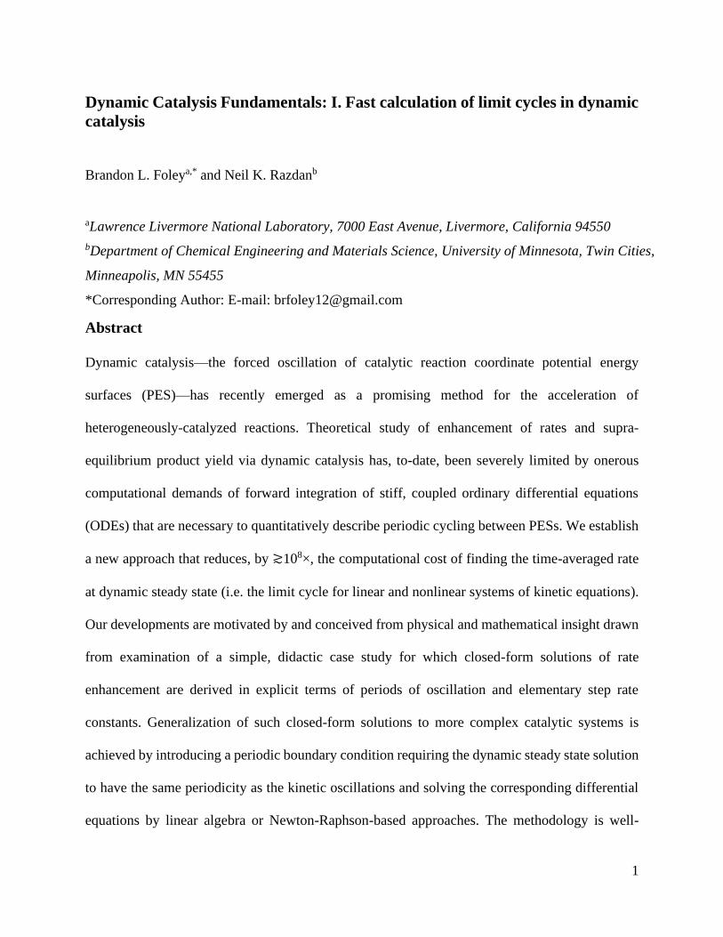
1 Dynamic Catalysis Fundamentals: I. Fast calculation of limit cycles in dynamic catalysis Brandon L. Foley a,* and Neil K. Razdan b a Lawrence Livermore National Laboratory, 7000 East Avenue, Livermore, California 94550 b Department of Chemical Engineering and Materials Science, University of Minnesota, Twin Cities, Minneapolis, MN 55455 *Corresponding Author: E-mail: [email protected] Abstract Dynamic catalysis—the forced oscillation of catalytic reaction coordinate potential energy surfaces (PES)—has recently emerged as a promising method for the acceleration of heterogeneously-catalyzed reactions. Theoretical study of enhancement of rates and supra- equilibrium product yield via dynamic catalysis has, to-date, been severely limited by onerous computational demands of forward integration of stiff, coupled ordinary differential equations (ODEs) that are necessary to quantitatively describe periodic cycling between PESs. We establish a new approach that reduces, by ≳10 8 ×, the computational cost of finding the time-averaged rate at dynamic steady state (i.e. the limit cycle for linear and nonlinear systems of kinetic equations). Our developments are motivated by and conceived from physical and mathematical insight drawn from examination of a simple, didactic case study for which closed-form solutions of rate enhancement are derived in explicit terms of periods of oscillation and elementary step rate constants. Generalization of such closed-form solutions to more complex catalytic systems is achieved by introducing a periodic boundary condition requiring the dynamic steady state solution to have the same periodicity as the kinetic oscillations and solving the corresponding differential equations by linear algebra or Newton-Raphson-based approaches. The methodology is well-
-
Upload
khangminh22 -
Category
Documents
-
view
3 -
download
0
Transcript of I. Fast calculation of limit cycles in dynamic catalysis - ChemRxiv
1
Dynamic Catalysis Fundamentals: I. Fast calculation of limit cycles in dynamic
catalysis
Brandon L. Foleya,* and Neil K. Razdanb
aLawrence Livermore National Laboratory, 7000 East Avenue, Livermore, California 94550
bDepartment of Chemical Engineering and Materials Science, University of Minnesota, Twin Cities,
Minneapolis, MN 55455
*Corresponding Author: E-mail: [email protected]
Abstract
Dynamic catalysis—the forced oscillation of catalytic reaction coordinate potential energy
surfaces (PES)—has recently emerged as a promising method for the acceleration of
heterogeneously-catalyzed reactions. Theoretical study of enhancement of rates and supra-
equilibrium product yield via dynamic catalysis has, to-date, been severely limited by onerous
computational demands of forward integration of stiff, coupled ordinary differential equations
(ODEs) that are necessary to quantitatively describe periodic cycling between PESs. We establish
a new approach that reduces, by ≳108×, the computational cost of finding the time-averaged rate
at dynamic steady state (i.e. the limit cycle for linear and nonlinear systems of kinetic equations).
Our developments are motivated by and conceived from physical and mathematical insight drawn
from examination of a simple, didactic case study for which closed-form solutions of rate
enhancement are derived in explicit terms of periods of oscillation and elementary step rate
constants. Generalization of such closed-form solutions to more complex catalytic systems is
achieved by introducing a periodic boundary condition requiring the dynamic steady state solution
to have the same periodicity as the kinetic oscillations and solving the corresponding differential
equations by linear algebra or Newton-Raphson-based approaches. The methodology is well-
2
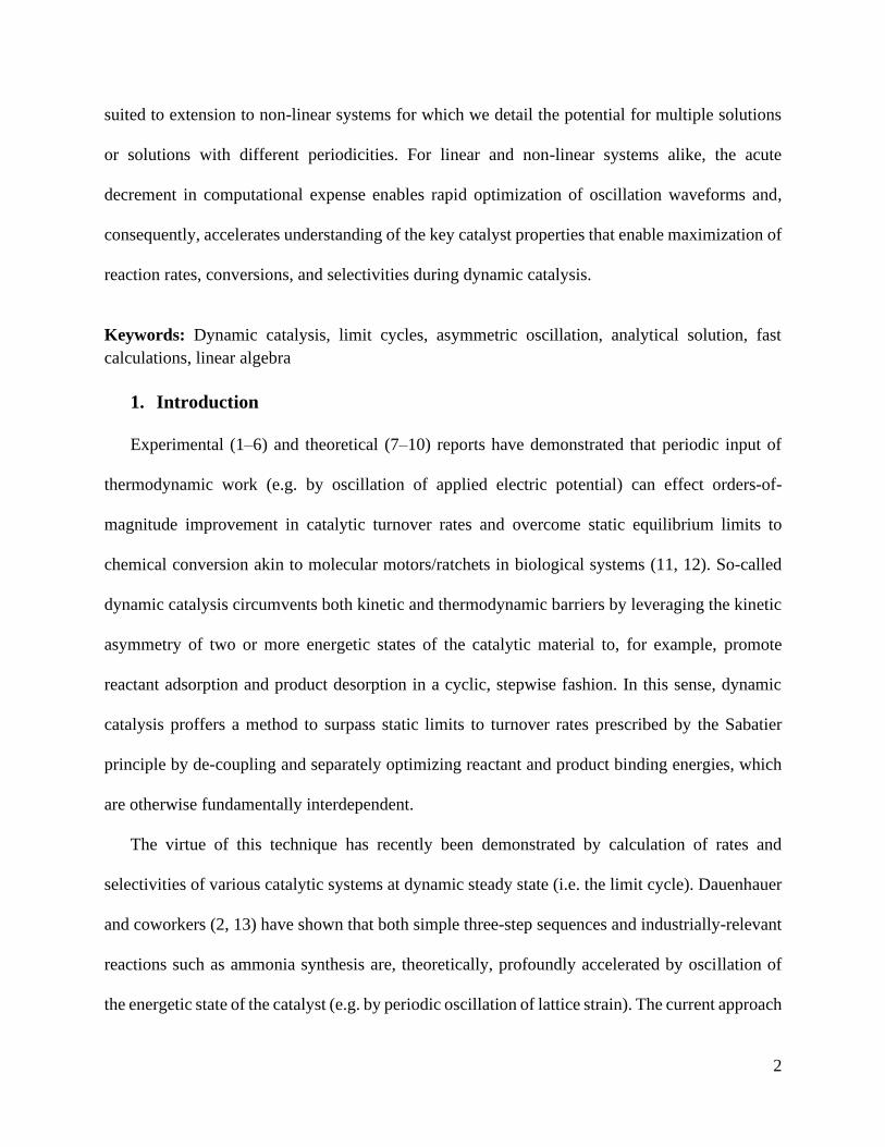
suited to extension to non-linear systems for which we detail the potential for multiple solutions
or solutions with different periodicities. For linear and non-linear systems alike, the acute
decrement in computational expense enables rapid optimization of oscillation waveforms and,
consequently, accelerates understanding of the key catalyst properties that enable maximization of
reaction rates, conversions, and selectivities during dynamic catalysis.
Keywords: Dynamic catalysis, limit cycles, asymmetric oscillation, analytical solution, fast
calculations, linear algebra
1. Introduction
Experimental (1–6) and theoretical (7–10) reports have demonstrated that periodic input of
thermodynamic work (e.g. by oscillation of applied electric potential) can effect orders-of-
magnitude improvement in catalytic turnover rates and overcome static equilibrium limits to
chemical conversion akin to molecular motors/ratchets in biological systems (11, 12). So-called
dynamic catalysis circumvents both kinetic and thermodynamic barriers by leveraging the kinetic
asymmetry of two or more energetic states of the catalytic material to, for example, promote
reactant adsorption and product desorption in a cyclic, stepwise fashion. In this sense, dynamic
catalysis proffers a method to surpass static limits to turnover rates prescribed by the Sabatier
principle by de-coupling and separately optimizing reactant and product binding energies, which
are otherwise fundamentally interdependent.
The virtue of this technique has recently been demonstrated by calculation of rates and
selectivities of various catalytic systems at dynamic steady state (i.e. the limit cycle). Dauenhauer
and coworkers (2, 13) have shown that both simple three-step sequences and industrially-relevant
reactions such as ammonia synthesis are, theoretically, profoundly accelerated by oscillation of
the energetic state of the catalyst (e.g. by periodic oscillation of lattice strain). The current approach
3
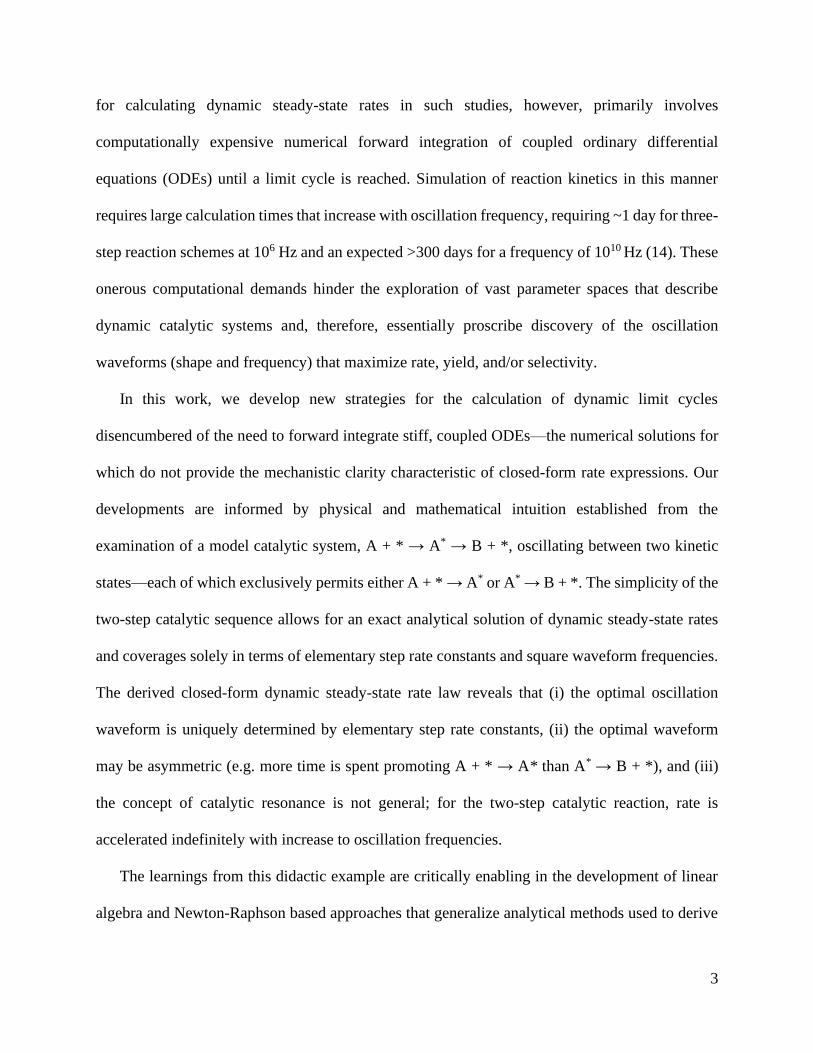
for calculating dynamic steady-state rates in such studies, however, primarily involves
computationally expensive numerical forward integration of coupled ordinary differential
equations (ODEs) until a limit cycle is reached. Simulation of reaction kinetics in this manner
requires large calculation times that increase with oscillation frequency, requiring ~1 day for three-
step reaction schemes at 106 Hz and an expected >300 days for a frequency of 1010 Hz (14). These
onerous computational demands hinder the exploration of vast parameter spaces that describe
dynamic catalytic systems and, therefore, essentially proscribe discovery of the oscillation
waveforms (shape and frequency) that maximize rate, yield, and/or selectivity.
In this work, we develop new strategies for the calculation of dynamic limit cycles
disencumbered of the need to forward integrate stiff, coupled ODEs—the numerical solutions for
which do not provide the mechanistic clarity characteristic of closed-form rate expressions. Our
developments are informed by physical and mathematical intuition established from the
examination of a model catalytic system, A + * → A* → B + *, oscillating between two kinetic
states—each of which exclusively permits either A + * → A* or A* → B + *. The simplicity of the
two-step catalytic sequence allows for an exact analytical solution of dynamic steady-state rates
and coverages solely in terms of elementary step rate constants and square waveform frequencies.
The derived closed-form dynamic steady-state rate law reveals that (i) the optimal oscillation
waveform is uniquely determined by elementary step rate constants, (ii) the optimal waveform
may be asymmetric (e.g. more time is spent promoting A + * → A* than A* → B + *), and (iii)
the concept of catalytic resonance is not general; for the two-step catalytic reaction, rate is
accelerated indefinitely with increase to oscillation frequencies.
The learnings from this didactic example are critically enabling in the development of linear
algebra and Newton-Raphson based approaches that generalize analytical methods used to derive
4
closed-form solutions and, in doing so, calculate the limit cycle for three-step reactions in
milliseconds to seconds, ≳108× faster than previous methods (14). The expedience of the
developed mathematical and algorithmic methods enables facile discovery of dynamic catalysis
conditions that optimize both (i) the magnitude of oscillation of, for example, A* binding energy
and (ii) the wavelength/duration of the oscillation in each energetic state. Linear algebra methods
reveal that previously observed resonance regimes are defined by eigenvalues of the matrices that
describe governing reaction ODEs; these eigenvalues formalize the concept of
characteristic/resonance time scales of catalysis and, like in the two-step example, are relatable, in
closed-form, to elementary step rate constants.
Complex reaction sequences proceeding via non-linear elementary steps (e.g. bimolecular
surface reaction) are not fully describable by matrix algebra methods and, therefore, we instead
recast the description of non-linear systems as an optimization problem solved by Newton-
Raphson-based approaches. Formulation of non-linear catalytic reactions in the framework of
mathematical optimization enables calculation and physical characterization of non-unique steady
states that we surmise are intrinsic to non-linear reactions and therefore may hinder dynamic
control of industrially-relevant reactions.
2. Methods
All functions and scripts are written in Octave GNU and Matlab ® 2020a. The code available to
download for free from https:\\www.github.com/foley352/dynamic. Computational times are
measured using the “tic” and “toc” functions.

5
3. Results and Discussion
3.1. Finding analytical solutions for limit cycles in dynamic catalysis
We begin our discussion by considering the simplest kinetic system suitable for rate
enhancement under dynamic catalysis conditions (Scheme 1), for which we will derive an
analytical solution for the time-averaged rate at dynamic steady state. In Scheme 1, there are two
reaction steps in series: the adsorption of A and the desorptive conversion of A* to B. We consider
the case where there is a square-wave oscillation between two kinetic states, j. Each kinetic state
represents a different state of the catalyst (e.g., strain, electric potential) and has a different set of
elementary step rate constants 𝑘𝑖[𝑗]
, for state j and elementary step i. During dynamic catalysis, the
catalytic state, or potential energy surface (PES), oscillates with a wavelength 𝜆 (or frequency 𝑓 =
1/𝜆). In this example, the rate constants are 𝑘𝑖 = 𝑘𝑖[1]
for time 𝛿𝑡[1] = 𝜆/2 followed by 𝑘𝑖 = 𝑘𝑖[2]
for time 𝛿𝑡[2] = 𝜆/2, as illustrated in Figure 1a. This oscillation repeats indefinitely.
Without oscillation, the static steady-state rate, 𝑟SS, for the reaction network in Scheme 1
is 𝑟SS = 𝑘1𝑘2𝑎A/(𝑘1𝑎𝐴 + 𝑘2), which is zero for kinetic states 1 and 2. Dynamic catalysis enables
the coupling of these kinetic states to give a nonzero reaction rate, by first operating at kinetic state
1 to accumulate A* on the surface and then switching to kinetic state 2 to convert A* to B. Figure
1b illustrates the oscillatory response of A* coverage caused by the periodic switch between
kinetic states 1 and 2 (Figure 1a).
6
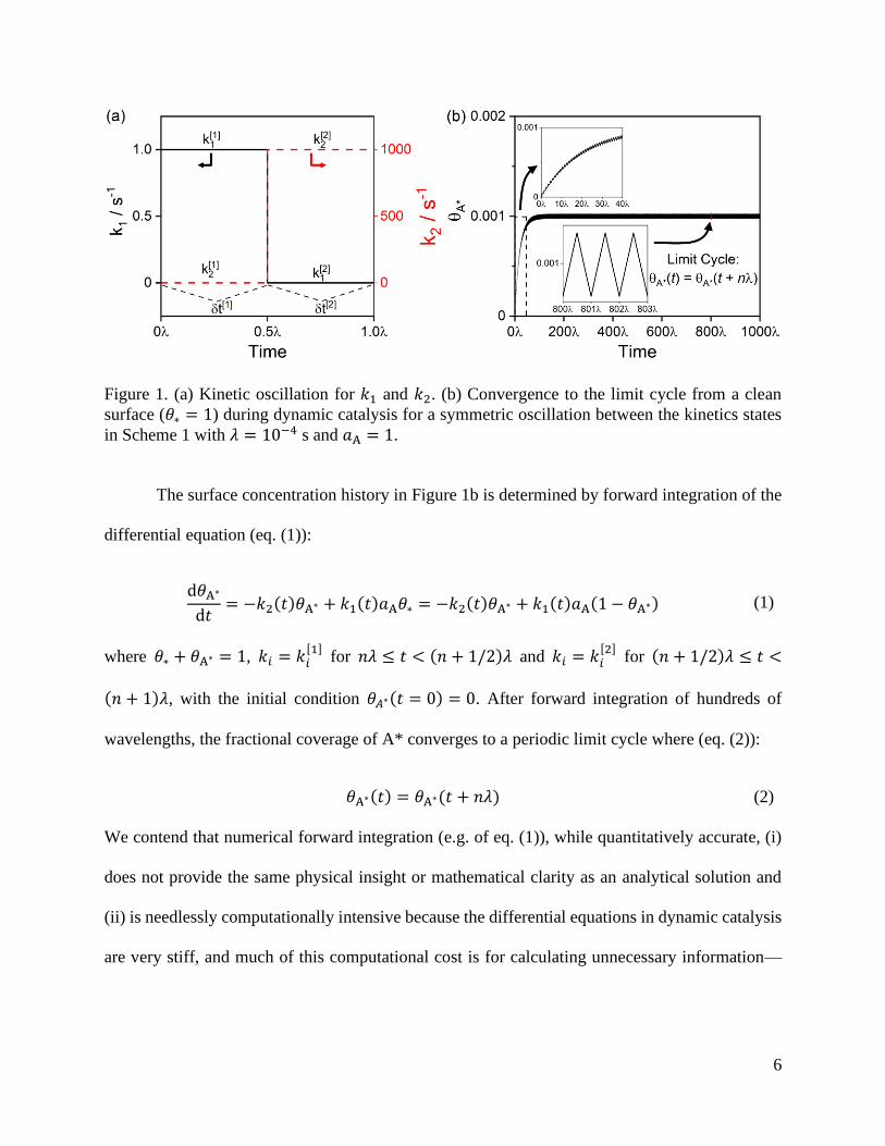
Figure 1. (a) Kinetic oscillation for 𝑘1 and 𝑘2. (b) Convergence to the limit cycle from a clean
surface (𝜃∗ = 1) during dynamic catalysis for a symmetric oscillation between the kinetics states
in Scheme 1 with 𝜆 = 10−4 s and 𝑎A = 1.
The surface concentration history in Figure 1b is determined by forward integration of the
differential equation (eq. (1)):
d𝜃A∗
d𝑡= −𝑘2(𝑡)𝜃A∗ + 𝑘1(𝑡)𝑎A𝜃∗ = −𝑘2(𝑡)𝜃A∗ + 𝑘1(𝑡)𝑎A(1 − 𝜃A∗) (1)
where 𝜃∗ + 𝜃A∗ = 1, 𝑘𝑖 = 𝑘𝑖[1]
for 𝑛𝜆 ≤ 𝑡 < (𝑛 + 1/2)𝜆 and 𝑘𝑖 = 𝑘𝑖[2]
for (𝑛 + 1/2)𝜆 ≤ 𝑡 <
(𝑛 + 1)𝜆, with the initial condition 𝜃𝐴∗(𝑡 = 0) = 0. After forward integration of hundreds of
wavelengths, the fractional coverage of A* converges to a periodic limit cycle where (eq. (2)):
𝜃A∗(𝑡) = 𝜃A∗(𝑡 + 𝑛𝜆) (2)
We contend that numerical forward integration (e.g. of eq. (1)), while quantitatively accurate, (i)
does not provide the same physical insight or mathematical clarity as an analytical solution and
(ii) is needlessly computationally intensive because the differential equations in dynamic catalysis
are very stiff, and much of this computational cost is for calculating unnecessary information—
7
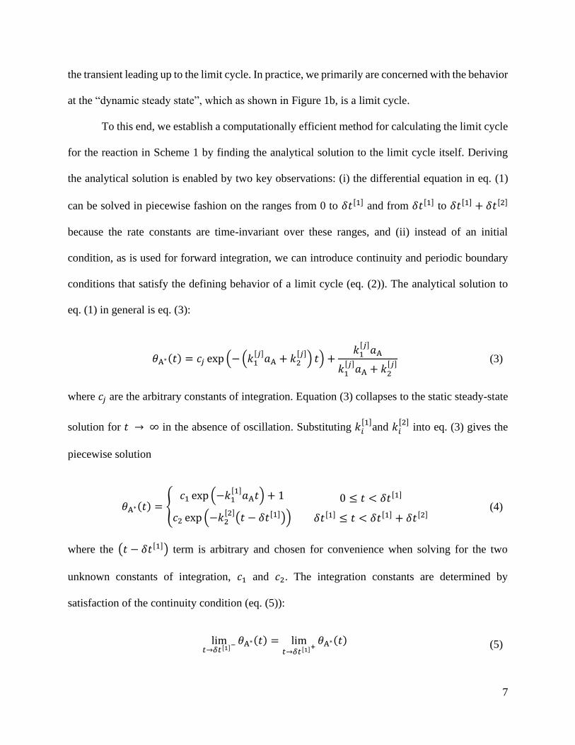
the transient leading up to the limit cycle. In practice, we primarily are concerned with the behavior
at the “dynamic steady state”, which as shown in Figure 1b, is a limit cycle.
To this end, we establish a computationally efficient method for calculating the limit cycle
for the reaction in Scheme 1 by finding the analytical solution to the limit cycle itself. Deriving
the analytical solution is enabled by two key observations: (i) the differential equation in eq. (1)
can be solved in piecewise fashion on the ranges from 0 to 𝛿𝑡[1] and from 𝛿𝑡[1] to 𝛿𝑡[1] + 𝛿𝑡[2]
because the rate constants are time-invariant over these ranges, and (ii) instead of an initial
condition, as is used for forward integration, we can introduce continuity and periodic boundary
conditions that satisfy the defining behavior of a limit cycle (eq. (2)). The analytical solution to
eq. (1) in general is eq. (3):
𝜃A∗(𝑡) = 𝑐𝑗 exp (−(𝑘1[𝑗]
𝑎A + 𝑘2[𝑗]
) 𝑡) +𝑘1
[𝑗]𝑎A
𝑘1[𝑗]
𝑎A + 𝑘2[𝑗]
(3)
where 𝑐𝑗 are the arbitrary constants of integration. Equation (3) collapses to the static steady-state
solution for 𝑡 → ∞ in the absence of oscillation. Substituting 𝑘𝑖[1]
and 𝑘𝑖[2]
into eq. (3) gives the
piecewise solution
𝜃A∗(𝑡) = {𝑐1 exp (−𝑘1
[1]𝑎A𝑡) + 1
𝑐2 exp (−𝑘2[2]
(𝑡 − 𝛿𝑡[1]))
0 ≤ 𝑡 < 𝛿𝑡[1]
𝛿𝑡[1] ≤ 𝑡 < 𝛿𝑡[1] + 𝛿𝑡[2] (4)
where the (𝑡 − 𝛿𝑡[1]) term is arbitrary and chosen for convenience when solving for the two
unknown constants of integration, 𝑐1 and 𝑐2. The integration constants are determined by
satisfaction of the continuity condition (eq. (5)):
lim𝑡→𝛿𝑡[1]−
𝜃A∗(𝑡) = lim𝑡→𝛿𝑡[1]+
𝜃A∗(𝑡) (5)
8
𝑐1 exp (−𝑘1[1]
𝑎A𝛿𝑡[1]) + 1 = 𝑐2
and the periodic boundary conditions (eq. (6)):
𝜃A∗(0) = 𝜃A∗(𝛿𝑡[1] + 𝛿𝑡[2])
𝑐1 + 1 = 𝑐2 exp (−𝑘2[2]
𝛿𝑡[2])
(6)
which ensure coverages are equal on either side of the switch from kinetic state 1 to 2 and from
kinetic state 2 to 1. The solution to the continuity and periodic boundary conditions gives (eq. (7)):
𝑐1 =1 − exp (−𝑘2
[2]𝛿𝑡[2])
exp (−𝑘1[1]
𝑎A𝛿𝑡[1] − 𝑘2[2]
𝛿𝑡[2]) − 1
𝑐2 =exp (−𝑘1
[1]𝑎A𝛿𝑡[1]) − 1
exp (−𝑘1[1]
𝑎A𝛿𝑡[1] − 𝑘2[2]
𝛿𝑡[2]) − 1
(7)
Thus, we now have an analytical solution for 𝜃A∗(𝑡) after substitution of eq. (7) into eq. (4). The
time-averaged rate during the limit cycle is defined as (eq. (8)):
⟨𝑟⟩ =∫ 𝑟(𝑡) d𝑡
𝜆
0
∫ d𝑡𝜆
0
=∫ 𝑘2
[1]𝜃A∗ d𝑡
𝛿𝑡[1]
0+ ∫ 𝑘2
[2]𝜃A∗ d𝑡
𝛿𝑡[1]+𝛿𝑡[2]
𝛿𝑡[1]
𝛿𝑡[1] + 𝛿𝑡[2]
⟨𝑟⟩ =(1 − exp (−𝑘1
[1]𝑎A𝛿𝑡[1])) (1 − exp (−𝑘2
[2]𝛿𝑡[2]))
(𝛿𝑡[1] + 𝛿𝑡[2]) (1 − exp (−𝑘1[1]
𝑎A𝛿𝑡[1] − 𝑘2[2]
𝛿𝑡[2]))
(8)
which, as expected, is a mathematically symmetric function (i.e. interchange of terms
corresponding to states 1 and 2 gives an identical equation). The functional form of eq. (8)
demonstrates that, unlike previously reported dynamic catalysis case studies, there is no effect of
9
“catalytic resonance” (Figure 2a). The only condition relevant to rate enhancement for this system
is whether the oscillation is sufficiently fast, such that 𝑘1[1]
𝑎A𝛿𝑡[1] ≪ 1 and 𝑘2[2]
𝛿𝑡[2] ≪ 1. At these
conditions, the surface coverage is approximately constant because the oscillation frequency is
much faster than the time required for the surface coverages to change. We term this state the
“quasi-static surface condition”, at which eq. (8) simplifies to eq. (9):
⟨𝑟⟩ ≈𝑘1
[1]𝑎A𝛿𝑡[1]𝑘2
[2]𝛿𝑡[2]
(𝛿𝑡[1] + 𝛿𝑡[2]) (𝑘1[1]
𝑎A𝛿𝑡[1] + 𝑘2[2]
𝛿𝑡[2])=
𝑘1[1]
𝑎A𝑘2[2]
(𝛿𝑡[2]
𝛿𝑡[1])
(1 +𝛿𝑡[2]
𝛿𝑡[1])(𝑘1[1]
𝑎A + 𝑘2[2]
(𝛿𝑡[2]
𝛿𝑡[1]))
(9)
At quasi-static surface conditions, the rate of the reaction in Scheme 1 depends solely on the ratio
𝛿𝑡[2]/𝛿𝑡[1], with time-averaged rates shown in Figure 2b.
Scheme 1. Simplest dynamic catalysis reaction network.
A + ∗ → A∗
𝑘1[1]
= 1 s−1
𝑘1[2]
= 0 s−1
A∗ → B +∗
𝑘2[1]
= 0 s−1
𝑘2[2]
= 1000 s−1
Overall: A ⇒ B
10
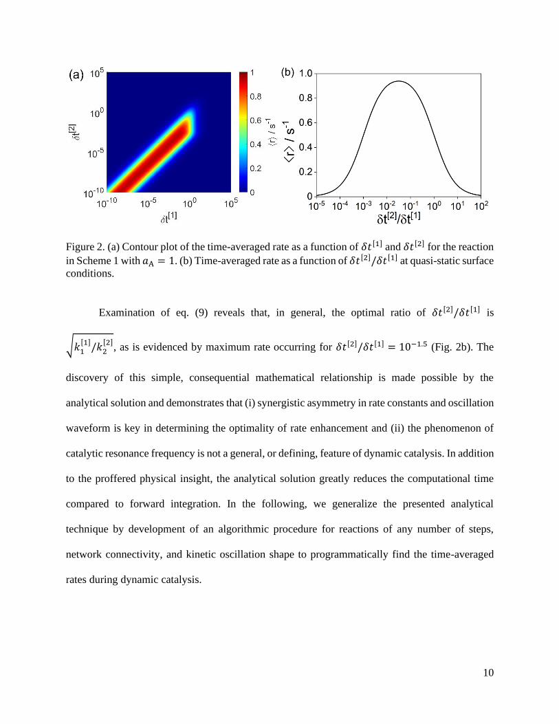
Figure 2. (a) Contour plot of the time-averaged rate as a function of 𝛿𝑡[1] and 𝛿𝑡[2] for the reaction
in Scheme 1 with 𝑎A = 1. (b) Time-averaged rate as a function of 𝛿𝑡[2]/𝛿𝑡[1] at quasi-static surface
conditions.
Examination of eq. (9) reveals that, in general, the optimal ratio of 𝛿𝑡[2]/𝛿𝑡[1] is
√𝑘1[1]
/𝑘2[2]
, as is evidenced by maximum rate occurring for 𝛿𝑡[2]/𝛿𝑡[1] = 10−1.5 (Fig. 2b). The
discovery of this simple, consequential mathematical relationship is made possible by the
analytical solution and demonstrates that (i) synergistic asymmetry in rate constants and oscillation
waveform is key in determining the optimality of rate enhancement and (ii) the phenomenon of
catalytic resonance frequency is not a general, or defining, feature of dynamic catalysis. In addition
to the proffered physical insight, the analytical solution greatly reduces the computational time
compared to forward integration. In the following, we generalize the presented analytical
technique by development of an algorithmic procedure for reactions of any number of steps,
network connectivity, and kinetic oscillation shape to programmatically find the time-averaged
rates during dynamic catalysis.
11
3.2. A programmatic method for solving for dynamic catalysis limit cycles for linear
reaction schemes
In reaction schemes that do not involve the reaction between two species with time-
dependent concentrations, the coupled differential equations that describe the dynamics of
fractional coverages are written in matrix form as (eq. (10)):
d
d𝑡𝜽 = 𝑨(𝑡)𝜽 (10)
where 𝜽 is a vector of all surface species (including vacant sites) and 𝑨 is a time-dependent matrix
that is a function of rate constants and chemical activities of reactants and products, which are the
coefficients that multiply the fractional coverages in each differential equation. Equation (10)
closely resembles a system of coupled first-order ordinary differential equations, with two
exceptions: (1) the coefficient matrix 𝑨 is a function of time and (2) at any time, 𝑨 is a singular
(non-invertible) matrix because the fractional coverages are not linearly independent. To resolve
the second issue, we must eliminate one of the fractional coverages by substituting 𝜃𝑗∗ = 1 −
∑ 𝜃𝑚∗𝑚∗≠𝑗∗ , which is equivalent to the following procedure: (1) remove the jth row of 𝑨 and 𝜽, (2)
remove the jth column of 𝑨 and rename it as a column vector 𝒃, and (3) subtract 𝒃 from each
column of 𝑨. The new matrix, 𝑨′, has one less row and column than 𝑨 and is no longer singular.
The new form of the coupled differential equations is (eq. (11)):
d
d𝑡𝜽′ = 𝑨′(𝑡)𝜽′ + 𝒃(𝑡) (11)
where 𝜽′ is 𝜽 with the jth row removed. Next, it is necessary to eliminate the time-dependence of
𝑨′ and 𝒃. This is accomplished by discretizing continuous waves into square waves with n steps.
At the limit of 𝑛 → ∞, the n-stepped square wave converges to the continuous wave, as illustrated
in Figure 3. On each of the flat terraces of the n-stepped square wave, the rate constants are not
12
functions of time, and only change at the locations of the step discontinuities. Thus, for an n-
stepped square wave, equation (11) can be rewritten as n equations:
d
d𝑡𝜽[𝑗] = 𝑨[𝑗]𝜽[𝑗] + 𝒃[𝑗] ∀ 𝑡 ∈ [𝑡[𝑗−1], 𝑡[𝑗]] (12)
where the superscript [𝑗] refers to the jth step of the n-stepped square wave, and the primes (“ ′ ”)
have been dropped for clarity. There is one eq. (12) for each step of the square wave, and each
equation is valid from the end of the previous step (𝑡[𝑗−1]) to the end of the present step (𝑡[𝑗]). The
utility of formulating dynamic catalytic systems in terms of eq. (12) is that the coefficient matrix
𝑨[𝑗] and the vector 𝒃[𝑗] are not functions of time, and thus eq. (12) is in the form of a differential
equation that is easily solved with linear algebra. The general solution to eq. (12) is of the form
(eq. (13)):
𝜃𝑚∗[𝑗](𝑡) = 𝑝𝑚∗
[𝑗]+ ∑𝑐𝑠
[𝑗]𝑣𝑠𝑚∗
[𝑗]exp (𝜆𝑠
[𝑗](𝑡 − 𝑡[𝑗−1]))
𝑠=1
∀ 𝑡 ∈ [𝑡[𝑗−1], 𝑡[𝑗]] (13)
where 𝜃𝑚∗[𝑗]
is the row of vector 𝜽[𝑗] corresponding to species 𝑚∗, 𝒑[𝑗] is the particular solution
vector for the jth step, 𝑐𝑠
[𝑗] is the sth constant of integration in the jth step, and 𝒗𝒔
[𝑗] is the sth
eigenvector of 𝑨[𝑗] with the corresponding eigenvalue 𝜆𝑠[𝑗]
. Subtraction of 𝑡[𝑗−1] from 𝑡 in the
exponential of eq. (13) is arbitrary and chosen for convenience such that the exponentials all equal
unity at 𝑡 = 𝑡[𝑗−1]. The solution presented in eq. (13) assumes no repeat eigenvalues of 𝑨[𝑗] and
includes the particular solution to 𝑑
𝑑𝑡𝜽[𝑗] = 𝟎, found by eq. (14):
𝒑[𝑗] = −(𝑨[𝑗])−1
𝒃[𝑗] (14)
The only remaining unknowns in eq. (13) are the integration constants 𝑐𝑠[𝑗]
, which are found by
satisfying the boundary conditions analogously to the two-step reaction in Scheme 1. For a system
13
with n steps in the square wave and m surface species, there are 𝑛 × (𝑚 − 1) boundary conditions
(e.g. for the reaction in Scheme 2, the number of boundary conditions is 2 × (2 – 1) = 2).
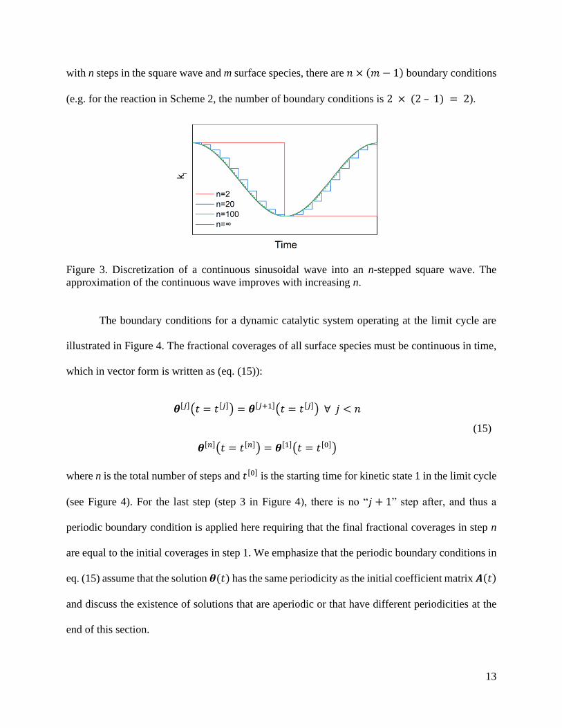
Figure 3. Discretization of a continuous sinusoidal wave into an n-stepped square wave. The
approximation of the continuous wave improves with increasing n.
The boundary conditions for a dynamic catalytic system operating at the limit cycle are
illustrated in Figure 4. The fractional coverages of all surface species must be continuous in time,
which in vector form is written as (eq. (15)):
𝜽[𝑗](𝑡 = 𝑡[𝑗]) = 𝜽[𝑗+1](𝑡 = 𝑡[𝑗]) ∀ 𝑗 < 𝑛
𝜽[𝑛](𝑡 = 𝑡[𝑛]) = 𝜽[1](𝑡 = 𝑡[0])
(15)
where n is the total number of steps and 𝑡[0] is the starting time for kinetic state 1 in the limit cycle
(see Figure 4). For the last step (step 3 in Figure 4), there is no “𝑗 + 1” step after, and thus a
periodic boundary condition is applied here requiring that the final fractional coverages in step n
are equal to the initial coverages in step 1. We emphasize that the periodic boundary conditions in
eq. (15) assume that the solution 𝜽(𝑡) has the same periodicity as the initial coefficient matrix 𝑨(𝑡)
and discuss the existence of solutions that are aperiodic or that have different periodicities at the
end of this section.
14
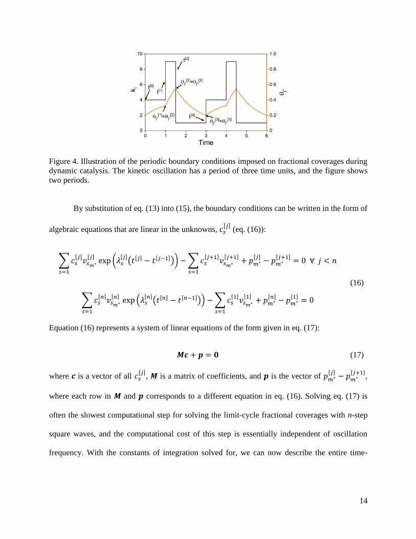
Figure 4. Illustration of the periodic boundary conditions imposed on fractional coverages during
dynamic catalysis. The kinetic oscillation has a period of three time units, and the figure shows
two periods.
By substitution of eq. (13) into (15), the boundary conditions can be written in the form of
algebraic equations that are linear in the unknowns, 𝑐𝑠[𝑗]
(eq. (16)):
∑𝑐𝑠[𝑗]
𝑣𝑠𝑚∗
[𝑗]exp (𝜆𝑠
[𝑗](𝑡[𝑗] − 𝑡[𝑗−1]))
𝑠=1
− ∑𝑐𝑠[𝑗+1]
𝑣𝑠𝑚∗
[𝑗+1]
𝑠=1
+ 𝑝𝑚∗[𝑗]
− 𝑝𝑚∗[𝑗+1]
= 0 ∀ 𝑗 < 𝑛
∑𝑐𝑠[𝑛]
𝑣𝑠𝑚∗
[𝑛]exp (𝜆𝑠
[𝑛](𝑡[𝑛] − 𝑡[𝑛−1]))
𝑠=1
− ∑𝑐𝑠[1]
𝑣𝑠𝑚∗
[1]
𝑠=1
+ 𝑝𝑚∗[𝑛]
− 𝑝𝑚∗[1]
= 0
(16)
Equation (16) represents a system of linear equations of the form given in eq. (17):
𝑴𝒄 + 𝒑 = 𝟎 (17)
where 𝒄 is a vector of all 𝑐𝑠[𝑗]
, 𝑴 is a matrix of coefficients, and 𝒑 is the vector of 𝑝𝑚∗[𝑗]
− 𝑝𝑚∗[𝑗+1]
,
where each row in 𝑴 and 𝒑 corresponds to a different equation in eq. (16). Solving eq. (17) is
often the slowest computational step for solving the limit-cycle fractional coverages with n-step
square waves, and the computational cost of this step is essentially independent of oscillation
frequency. With the constants of integration solved for, we can now describe the entire time-
15
dependence of each species during the limit cycle. The time-averaged rates are found by analytical
integration of the rate as a function of time (eq. (18)):
⟨𝑟⟩ =∫ 𝑟(𝑡) d𝑡
𝜆
0
𝜆 (18)
Ardagh et al. (14) investigated the kinetics of the reaction in Scheme 2 with dynamic
kinetics where the binding energy of surface species B* is oscillated, and this binding energy
correlates linearly with the (i) transition state energy for the A* to B* reaction and (ii) the binding
energy of A* via Brønsted-Evans-Polanyi relations. The relationship between the binding energies
is given by (eq. (19)):
BEA = (BEB − (1 − 𝛾)𝛿 − Δ𝐻ovr)/𝛾 (19)
where Δ𝐻ovr is the heat of the overall reaction, and BEA and BEB are the enthalpy change of
sorption of species A and B, respectively (e.g. BEA = 𝐻A + 𝐻∗ − 𝐻A∗). The definition in eq. (19)
is such that at BEA = 𝛿, the surface reaction becomes isothermic (𝐻A∗ = 𝐻B∗), and the change in
binding energy of A and B are related by 𝛾ΔBEA = ΔBEB. In this work, we reproduce a previously
published example where 𝛾 = 0.5, 𝛿 = 1.4 eV, Δ𝐻ovr = 0 eV, and the binding energy BEB is
oscillated from 0.1 to 1.03 eV. The activation energy of the surface reaction is (eq. (20)):
𝐸a,sr = 𝛼Δ𝐻sr + 𝛽 (20)
where Δ𝐻sr is the enthalpy change of the surface reaction (A* to B*), and in this example 𝛼 = 0.6
and 𝛽 = 102 kJ/mol. Following the methodology described above, we reproduce the simulation
reported by Ardagh et al. (14) for a square wave (n = 2) oscillation in Figure 5a, with excellent
agreement between most data points. The discrepancy for frequencies 10-2-10-4 Hz may be because
Ardagh et al. (14) simulated a continuous stirred tank reactor where the chemical activities of the
16
reactants and products are not fixed in time and the yields may vary slightly from simulation to
simulation. Here, no assumption on a reactor configuration is made and rates are reported for fixed
activities of reactants and products. A final difference between the simulation here and the
simulation from Ardagh et al. (14) is that we capped the value of 𝑘−1 to 1025 s-1, whereas the value
from the simulation by Ardagh et al. (14) reached 1029 s-1. We capped this value because poor
scaling of matrices 𝑨[𝑗] or 𝑴 can cause them to be singular within the numerical precision of
Matlab. We also note that the rate constant 𝑘−1 >> 1013 s-1 is nonphysical and occurs because the
desorption of A* was given a negative activation energy at some conditions. This has no impact
on the theoretical insights of the simulations, and we expect allowing the BEP trends to continue
to artificial, or non-physical, regimes is preferred to capping rate constants if one aims to develop
theoretical insights regarding the general consequences of BEP relationships in dynamic catalysis.
Observed dynamic catalysis behavior, even for artificial rate constants, may be edifying and
relevant for some different, more physically realistic choice of 𝛽, 𝛿, and reference state. We do not
believe that adjusting 𝑘−1 had a significant impact on the comparison of our results to Ardagh et
al. (14).
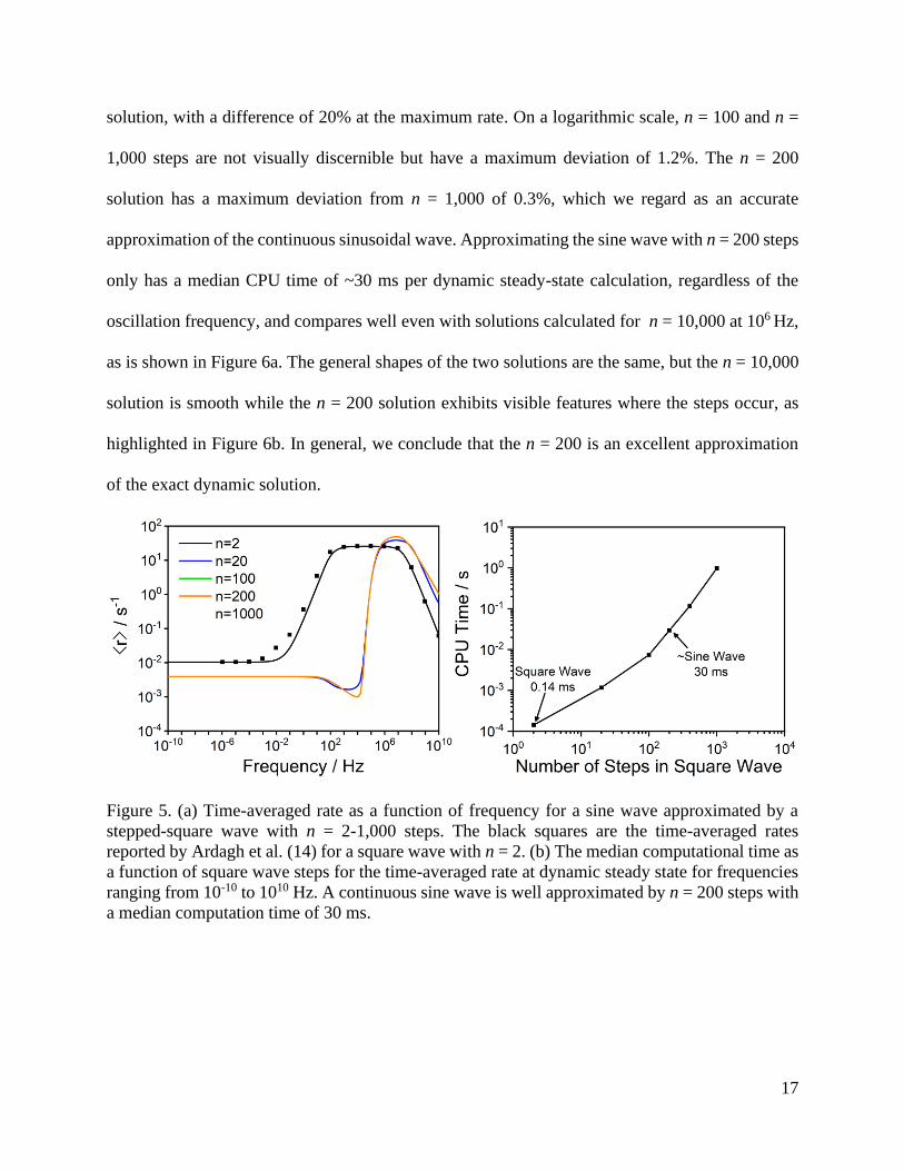
Figure 5b shows the computational time per dynamic steady-state calculation as a function
of the number of steps in the square wave. For the n = 2 square wave, each limit cycle takes on
average 0.14 ms to calculate, regardless of the oscillation frequency. This is more than 8 orders of
magnitude faster than the high frequency calculations reported by Ardagh et al. (14) using
numerical forward integration. Figure 5 also shows the average rate at dynamic steady-state when
oscillating binding energies as a sinusoidal wave approximated by an n-stepped square wave with
varying frequencies. For n = 20 steps, the CPU time is ~1 ms per dynamic steady-state calculation
and the average rate as a function of frequency already closely resembles the n = 1,000 steps
17
solution, with a difference of 20% at the maximum rate. On a logarithmic scale, n = 100 and n =
1,000 steps are not visually discernible but have a maximum deviation of 1.2%. The n = 200
solution has a maximum deviation from n = 1,000 of 0.3%, which we regard as an accurate
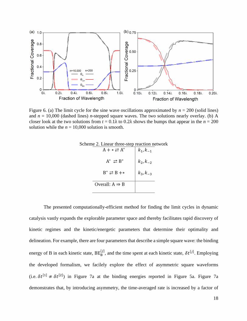
approximation of the continuous sinusoidal wave. Approximating the sine wave with n = 200 steps
only has a median CPU time of ~30 ms per dynamic steady-state calculation, regardless of the
oscillation frequency, and compares well even with solutions calculated for n = 10,000 at 106 Hz,
as is shown in Figure 6a. The general shapes of the two solutions are the same, but the n = 10,000
solution is smooth while the n = 200 solution exhibits visible features where the steps occur, as
highlighted in Figure 6b. In general, we conclude that the n = 200 is an excellent approximation
of the exact dynamic solution.
Figure 5. (a) Time-averaged rate as a function of frequency for a sine wave approximated by a
stepped-square wave with n = 2-1,000 steps. The black squares are the time-averaged rates
reported by Ardagh et al. (14) for a square wave with n = 2. (b) The median computational time as
a function of square wave steps for the time-averaged rate at dynamic steady state for frequencies
ranging from 10-10 to 1010 Hz. A continuous sine wave is well approximated by n = 200 steps with
a median computation time of 30 ms.
18
Figure 6. (a) The limit cycle for the sine wave oscillations approximated by n = 200 (solid lines)
and n = 10,000 (dashed lines) n-stepped square waves. The two solutions nearly overlay. (b) A
closer look at the two solutions from t = 0.1λ to 0.2λ shows the bumps that appear in the n = 200
solution while the n = 10,000 solution is smooth.
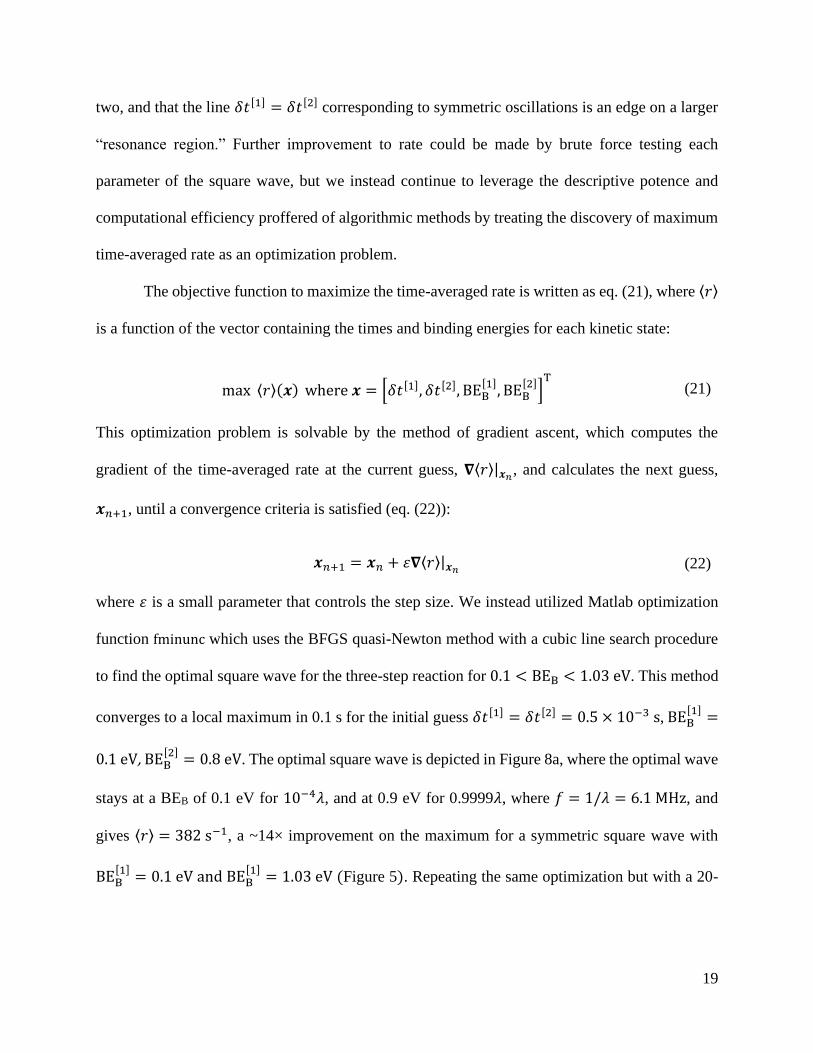
Scheme 2. Linear three-step reaction network
A + ∗ ⇄ A∗ 𝑘1, 𝑘−1
A∗ ⇄ B∗ 𝑘2, 𝑘−2
B∗ ⇄ B +∗ 𝑘3, 𝑘−3
Overall: A ⇒ B
The presented computationally-efficient method for finding the limit cycles in dynamic
catalysis vastly expands the explorable parameter space and thereby facilitates rapid discovery of
kinetic regimes and the kinetic/energetic parameters that determine their optimality and
delineation. For example, there are four parameters that describe a simple square wave: the binding
energy of B in each kinetic state, BEB[𝑗]
, and the time spent at each kinetic state, 𝛿𝑡[𝑗]. Employing
the developed formalism, we facilely explore the effect of asymmetric square waveforms
(i.e. 𝛿𝑡[1] ≠ 𝛿𝑡[2]) in Figure 7a at the binding energies reported in Figure 5a. Figure 7a
demonstrates that, by introducing asymmetry, the time-averaged rate is increased by a factor of
19
two, and that the line 𝛿𝑡[1] = 𝛿𝑡[2] corresponding to symmetric oscillations is an edge on a larger
“resonance region.” Further improvement to rate could be made by brute force testing each
parameter of the square wave, but we instead continue to leverage the descriptive potence and
computational efficiency proffered of algorithmic methods by treating the discovery of maximum
time-averaged rate as an optimization problem.
The objective function to maximize the time-averaged rate is written as eq. (21), where ⟨𝑟⟩
is a function of the vector containing the times and binding energies for each kinetic state:
max ⟨𝑟⟩(𝒙) where 𝒙 = [𝛿𝑡[1], 𝛿𝑡[2], BEB[1]
, BEB[2]
]T
(21)
This optimization problem is solvable by the method of gradient ascent, which computes the
gradient of the time-averaged rate at the current guess, 𝛁⟨𝑟⟩|𝒙𝑛, and calculates the next guess,
𝒙𝑛+1, until a convergence criteria is satisfied (eq. (22)):
𝒙𝑛+1 = 𝒙𝑛 + 휀𝛁⟨𝑟⟩|𝒙𝑛 (22)
where 휀 is a small parameter that controls the step size. We instead utilized Matlab optimization
function fminunc which uses the BFGS quasi-Newton method with a cubic line search procedure
to find the optimal square wave for the three-step reaction for 0.1 < BEB < 1.03 eV. This method
converges to a local maximum in 0.1 s for the initial guess 𝛿𝑡[1] = 𝛿𝑡[2] = 0.5 × 10⁻³ s, BEB[1]
=
0.1 eV, BEB[2]
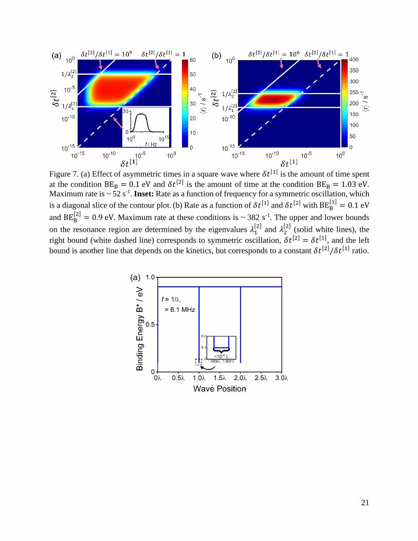
= 0.8 eV. The optimal square wave is depicted in Figure 8a, where the optimal wave
stays at a BEB of 0.1 eV for 10−4𝜆, and at 0.9 eV for 0.9999𝜆, where 𝑓 = 1/𝜆 = 6.1 MHz, and
gives ⟨𝑟⟩ = 382 s−1, a ~14× improvement on the maximum for a symmetric square wave with
BEB[1]
= 0.1 eV and BEB[1]
= 1.03 eV (Figure 5). Repeating the same optimization but with a 20-
20
step square wave gives the same solution, suggesting that this asymmetric two-stepped square
wave is near the global optimum for these kinetics and constraints.
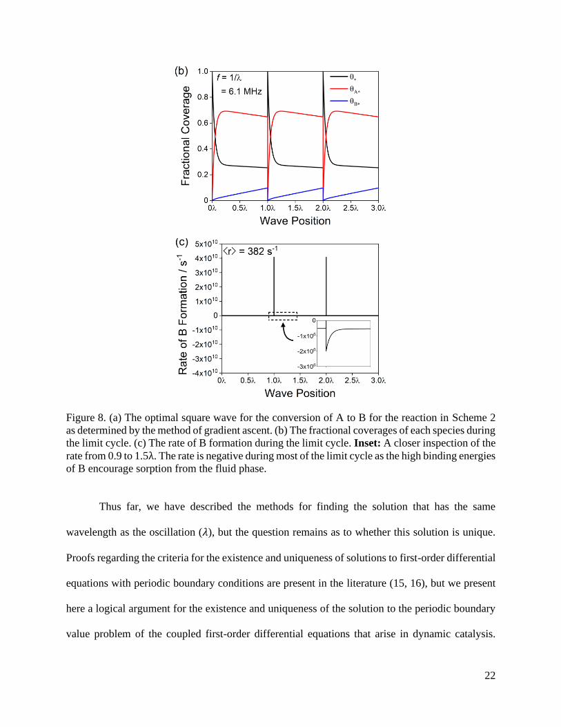
The fractional coverages of each species during the algorithmically optimized limit cycle
is shown in Figure 8b, and the instantaneous rates are shown in Figure 8c. In the optimal square
wave, the binding energy of B is decreased momentarily to rapidly remove all A* and B*,
emptying the surface. The next state of the square wave has a high binding energy of B to
accumulate A* on the surface and convert the A* to B*. During this phase, the rate of B formation
is negative as B adsorbs on the catalyst surface from the fluid phase. The negative rate of B
formation in the second state is compensated by asymmetry in the square wave which maximizes
the time-averaged reaction rate by ensuring time is not needlessly spent during either the
accumulation or recovery of surface-bound intermediates—which, for this particular system,
corresponds to 104× more time spent in the accumulation phase. The critical importance of such
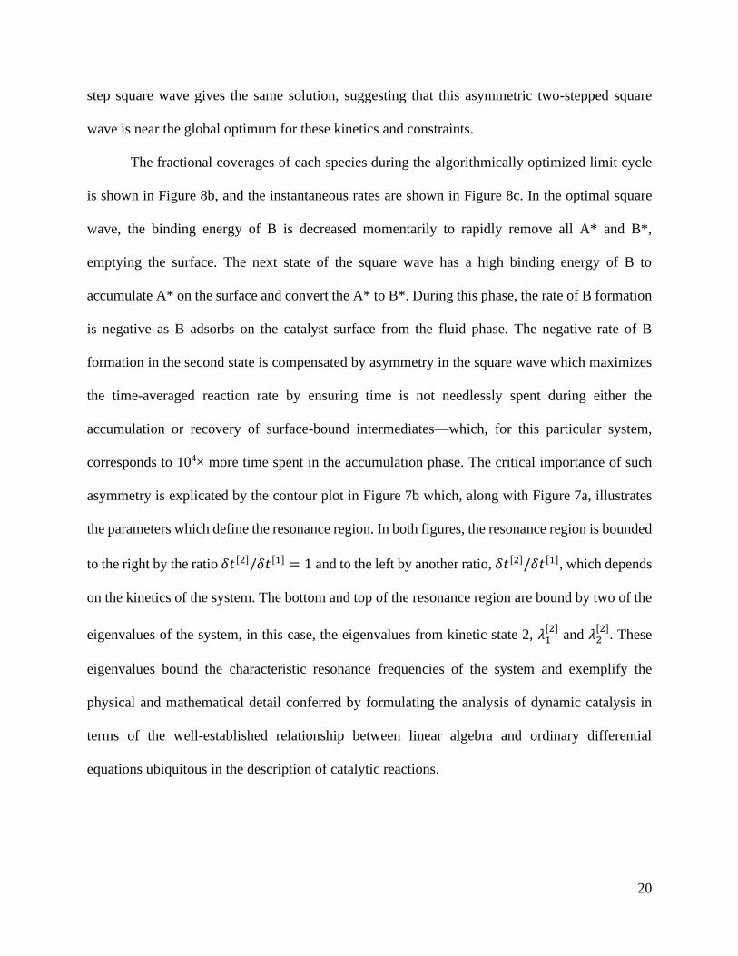
asymmetry is explicated by the contour plot in Figure 7b which, along with Figure 7a, illustrates
the parameters which define the resonance region. In both figures, the resonance region is bounded
to the right by the ratio 𝛿𝑡[2]/𝛿𝑡[1] = 1 and to the left by another ratio, 𝛿𝑡[2]/𝛿𝑡[1], which depends
on the kinetics of the system. The bottom and top of the resonance region are bound by two of the
eigenvalues of the system, in this case, the eigenvalues from kinetic state 2, 𝜆1[2]
and 𝜆2[2]
. These
eigenvalues bound the characteristic resonance frequencies of the system and exemplify the
physical and mathematical detail conferred by formulating the analysis of dynamic catalysis in
terms of the well-established relationship between linear algebra and ordinary differential
equations ubiquitous in the description of catalytic reactions.
21
Figure 7. (a) Effect of asymmetric times in a square wave where 𝛿𝑡[1] is the amount of time spent
at the condition BEB = 0.1 eV and 𝛿𝑡[2] is the amount of time at the condition BEB = 1.03 eV.
Maximum rate is ~ 52 s-1. Inset: Rate as a function of frequency for a symmetric oscillation, which
is a diagonal slice of the contour plot. (b) Rate as a function of 𝛿𝑡[1] and 𝛿𝑡[2] with BEB[1]
= 0.1 eV
and BEB[2]
= 0.9 eV. Maximum rate at these conditions is ~ 382 s-1. The upper and lower bounds
on the resonance region are determined by the eigenvalues 𝜆1[2]
and 𝜆2[2]
(solid white lines), the
right bound (white dashed line) corresponds to symmetric oscillation, 𝛿𝑡[2] = 𝛿𝑡[1], and the left
bound is another line that depends on the kinetics, but corresponds to a constant 𝛿𝑡[2]/𝛿𝑡[1] ratio.
22
Figure 8. (a) The optimal square wave for the conversion of A to B for the reaction in Scheme 2
as determined by the method of gradient ascent. (b) The fractional coverages of each species during
the limit cycle. (c) The rate of B formation during the limit cycle. Inset: A closer inspection of the
rate from 0.9 to 1.5λ. The rate is negative during most of the limit cycle as the high binding energies
of B encourage sorption from the fluid phase.
Thus far, we have described the methods for finding the solution that has the same
wavelength as the oscillation (𝜆), but the question remains as to whether this solution is unique.
Proofs regarding the criteria for the existence and uniqueness of solutions to first-order differential
equations with periodic boundary conditions are present in the literature (15, 16), but we present
here a logical argument for the existence and uniqueness of the solution to the periodic boundary
value problem of the coupled first-order differential equations that arise in dynamic catalysis.
23
Equation (12) is a linear coupled ordinary differential equation and has a unique solution for the
initial value problem 𝜽(𝑡 = 𝑡0) = 𝜽𝟎 by the Picard–Lindelöf theorem (17, 18). Thus, if any
function is discretized into an infinite-stepped square wave, there exists one unique solution to
each step of the square wave for a given initial value. Now, there must be only one initial value
that satisfies the periodic boundary problem criteria 𝜽(𝑡 = 0) = 𝜽(𝑡 = 𝜆) since eqs. (16) and (17)
represent a specified system of linear algebraic equations which has only one solution. Because
each initial value problem gives a unique solution, and there exists only one initial value vector
that satisfies the periodic boundary condition, we conclude that there exists one unique solution to
this system of differential equations.
If instead we searched for a solution with a periodicity 𝑛𝜆, then the periodic boundary
condition becomes 𝜽(𝑡 = 0) = 𝜽(𝑡 = 𝑛𝜆), for which following the same argument as above, there
must exist only one unique solution. Further, we know that the solution 𝜽(𝑡) with periodicity 𝜆
also satisfies the boundary conditions for any periodicity 𝑛𝜆, and thus the only periodic solution
for linear systems will be those that have the same periodicity as the kinetic oscillation. Proving
that aperiodic solutions to this system of equations do not exist is beyond the scope of this work,
but this would require the existence of an initial condition 𝜽(𝑡 = 𝑡0) = 𝜽𝟎 such that
lim𝑛→∞
𝜽(𝑡 = 𝑛𝜆) ≠ 𝜽(𝑡 = (𝑛 + 1)𝜆), which does not seem possible for this linear system of
equations.
The method described above can be employed to find the limit cycles for any dynamic
kinetic system where no reactions occur between species that change in time. However, in non-
differential reactors, the activities of fluid-phase species may be transient, and many important
reactions involve the reaction between two surface species, and thus require an alternative method
to find the dynamic steady states. Further, as the arguments of the existence of unique periodic
24
solutions above required the system of differential equations to be linear, nonlinear differential
equations may allow for the possibility of multiple dynamic steady-state solutions, as discussed
hereinafter.
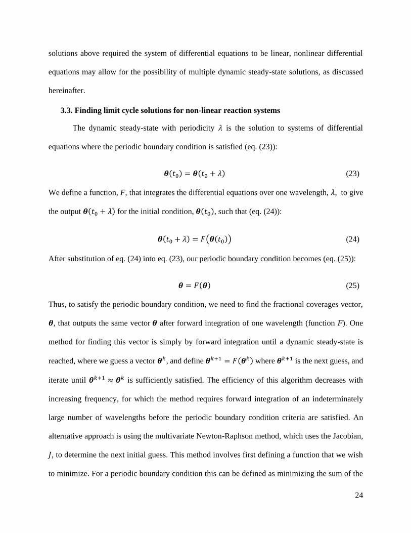
3.3. Finding limit cycle solutions for non-linear reaction systems
The dynamic steady-state with periodicity 𝜆 is the solution to systems of differential
equations where the periodic boundary condition is satisfied (eq. (23)):
𝜽(𝑡0) = 𝜽(𝑡0 + 𝜆) (23)
We define a function, F, that integrates the differential equations over one wavelength, 𝜆, to give
the output 𝜽(𝑡0 + 𝜆) for the initial condition, 𝜽(𝑡0), such that (eq. (24)):
𝜽(𝑡0 + 𝜆) = 𝐹(𝜽(𝑡0)) (24)
After substitution of eq. (24) into eq. (23), our periodic boundary condition becomes (eq. (25)):
𝜽 = 𝐹(𝜽) (25)
Thus, to satisfy the periodic boundary condition, we need to find the fractional coverages vector,
𝜽, that outputs the same vector 𝜽 after forward integration of one wavelength (function F). One
method for finding this vector is simply by forward integration until a dynamic steady-state is
reached, where we guess a vector 𝜽𝑘, and define 𝜽𝑘+1 = 𝐹(𝜽𝑘) where 𝜽𝑘+1 is the next guess, and
iterate until 𝜽𝑘+1 ≈ 𝜽𝑘 is sufficiently satisfied. The efficiency of this algorithm decreases with
increasing frequency, for which the method requires forward integration of an indeterminately
large number of wavelengths before the periodic boundary condition criteria are satisfied. An
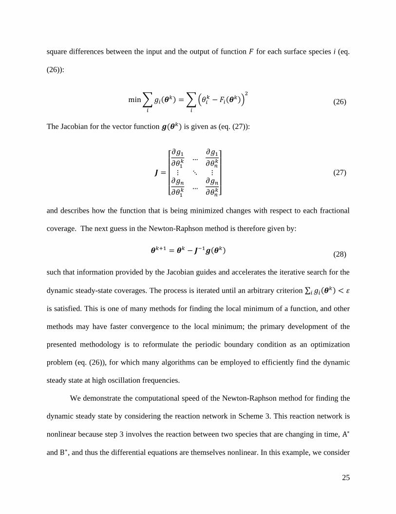
alternative approach is using the multivariate Newton-Raphson method, which uses the Jacobian,
𝐽, to determine the next initial guess. This method involves first defining a function that we wish
to minimize. For a periodic boundary condition this can be defined as minimizing the sum of the
25
square differences between the input and the output of function 𝐹 for each surface species i (eq.
(26)):
min∑𝑔𝑖(𝜽𝑘)
𝑖
= ∑(𝜃𝑖𝑘 − 𝐹𝑖(𝜽
𝑘))2
𝑖
(26)
The Jacobian for the vector function 𝒈(𝜽𝑘) is given as (eq. (27)):
𝑱 =
[ 𝜕𝑔1
𝜕𝜃1𝑘 …
𝜕𝑔1
𝜕𝜃𝑛𝑘
⋮ ⋱ ⋮𝜕𝑔𝑛
𝜕𝜃1𝑘 …
𝜕𝑔𝑛
𝜕𝜃𝑛𝑘]
(27)
and describes how the function that is being minimized changes with respect to each fractional
coverage. The next guess in the Newton-Raphson method is therefore given by:
𝜽𝑘+1 = 𝜽𝑘 − 𝑱−1𝒈(𝜽𝑘) (28)
such that information provided by the Jacobian guides and accelerates the iterative search for the
dynamic steady-state coverages. The process is iterated until an arbitrary criterion ∑ 𝑔𝑖(𝜽𝑘)𝑖 < 휀
is satisfied. This is one of many methods for finding the local minimum of a function, and other
methods may have faster convergence to the local minimum; the primary development of the
presented methodology is to reformulate the periodic boundary condition as an optimization
problem (eq. (26)), for which many algorithms can be employed to efficiently find the dynamic
steady state at high oscillation frequencies.
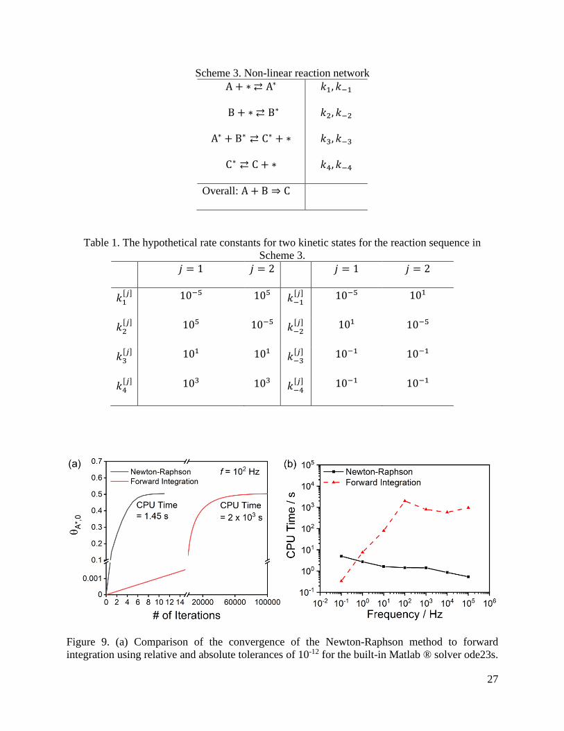
We demonstrate the computational speed of the Newton-Raphson method for finding the
dynamic steady state by considering the reaction network in Scheme 3. This reaction network is
nonlinear because step 3 involves the reaction between two species that are changing in time, A∗
and B∗, and thus the differential equations are themselves nonlinear. In this example, we consider
26
the oscillation of rate constants as simple square waves between two states 𝑗 = 1 and 𝑗 = 2, with
rate constants for each state given in Table 1. The difference between the two kinetic states lies in
the affinity of the catalyst to adsorb A and B, where kinetic state 1 adsorbs B and ejects A∗ off the
surface, while kinetic state 2 does the opposite.
The convergence of the Newton-Raphson and forward integration methods to the limit
cycles are compared in Figure 9 for a frequency f = 102 Hz. The Newton-Raphson method
converges to the fractional coverage of A* at the periodic boundary of the limit cycle, 𝜃A∗,0, in 11
iteration steps and 1.45 seconds. Forward integration requires more than 100,000 iterations to
reach the same value and takes over 2,000 seconds. The computation times of the two methods are
compared across decades of oscillation frequency in Figure 9b. At low frequencies, forward
integrations will converge to limit cycles in as little as one oscillation, and thus can be faster than
the Newton-Raphson method, which requires the numerical calculation of the Jacobian and may
take smaller steps in the low frequency regime. At increasing frequencies, the Newton-Raphson
method becomes faster because each integration is over a shorter length of time, while the forward
integration method generally becomes slower because more oscillations are required before
converging to the limit cycle. The decrease in computation time for the forward integration method
at 102 Hz is a consequence of changing chemical dynamics, which decreases the total time required
before converging to a limit cycle.
27
Scheme 3. Non-linear reaction network
A + ∗ ⇄ A∗ 𝑘1, 𝑘−1
B + ∗ ⇄ B∗ 𝑘2, 𝑘−2
A∗ + B∗ ⇄ C∗ + ∗ 𝑘3, 𝑘−3
C∗ ⇄ C + ∗ 𝑘4, 𝑘−4
Overall: A + B ⇒ C
Table 1. The hypothetical rate constants for two kinetic states for the reaction sequence in
Scheme 3.
𝑗 = 1 𝑗 = 2 𝑗 = 1 𝑗 = 2
𝑘1[𝑗]
10−5 105 𝑘−1[𝑗]
10−5 101
𝑘2[𝑗]
105 10−5 𝑘−2[𝑗]
101 10−5
𝑘3[𝑗]
101 101 𝑘−3[𝑗]
10−1 10−1
𝑘4[𝑗]
103 103 𝑘−4[𝑗]
10−1 10−1
Figure 9. (a) Comparison of the convergence of the Newton-Raphson method to forward
integration using relative and absolute tolerances of 10-12 for the built-in Matlab ® solver ode23s.
28
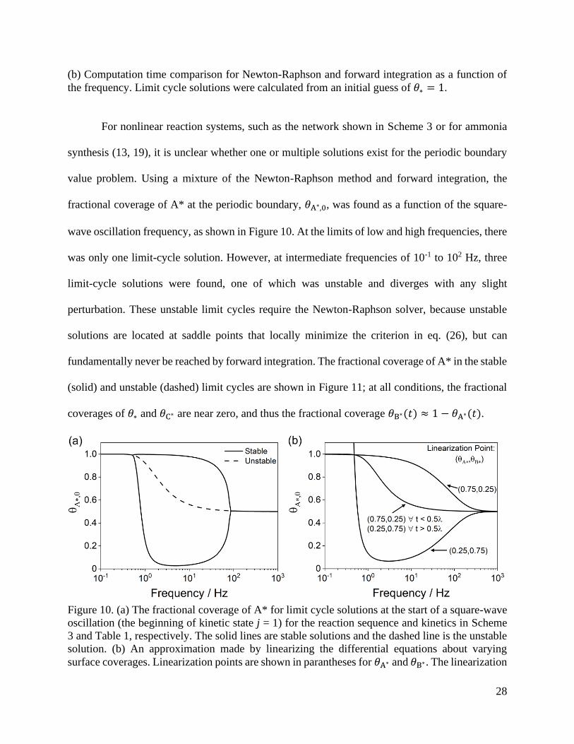
(b) Computation time comparison for Newton-Raphson and forward integration as a function of
the frequency. Limit cycle solutions were calculated from an initial guess of 𝜃∗ = 1.
For nonlinear reaction systems, such as the network shown in Scheme 3 or for ammonia
synthesis (13, 19), it is unclear whether one or multiple solutions exist for the periodic boundary
value problem. Using a mixture of the Newton-Raphson method and forward integration, the
fractional coverage of A* at the periodic boundary, 𝜃A∗,0, was found as a function of the square-
wave oscillation frequency, as shown in Figure 10. At the limits of low and high frequencies, there
was only one limit-cycle solution. However, at intermediate frequencies of 10-1 to 102 Hz, three
limit-cycle solutions were found, one of which was unstable and diverges with any slight
perturbation. These unstable limit cycles require the Newton-Raphson solver, because unstable
solutions are located at saddle points that locally minimize the criterion in eq. (26), but can
fundamentally never be reached by forward integration. The fractional coverage of A* in the stable
(solid) and unstable (dashed) limit cycles are shown in Figure 11; at all conditions, the fractional
coverages of 𝜃∗ and 𝜃C∗ are near zero, and thus the fractional coverage 𝜃B∗(𝑡) ≈ 1 − 𝜃A∗(𝑡).
Figure 10. (a) The fractional coverage of A* for limit cycle solutions at the start of a square-wave
oscillation (the beginning of kinetic state j = 1) for the reaction sequence and kinetics in Scheme
3 and Table 1, respectively. The solid lines are stable solutions and the dashed line is the unstable
solution. (b) An approximation made by linearizing the differential equations about varying
surface coverages. Linearization points are shown in parantheses for 𝜃A∗ and 𝜃B∗. The linearization
29
points for 𝜃∗ and 𝜃C∗ were both zero. The middle curve used a different linearization point for each
kinetic state.
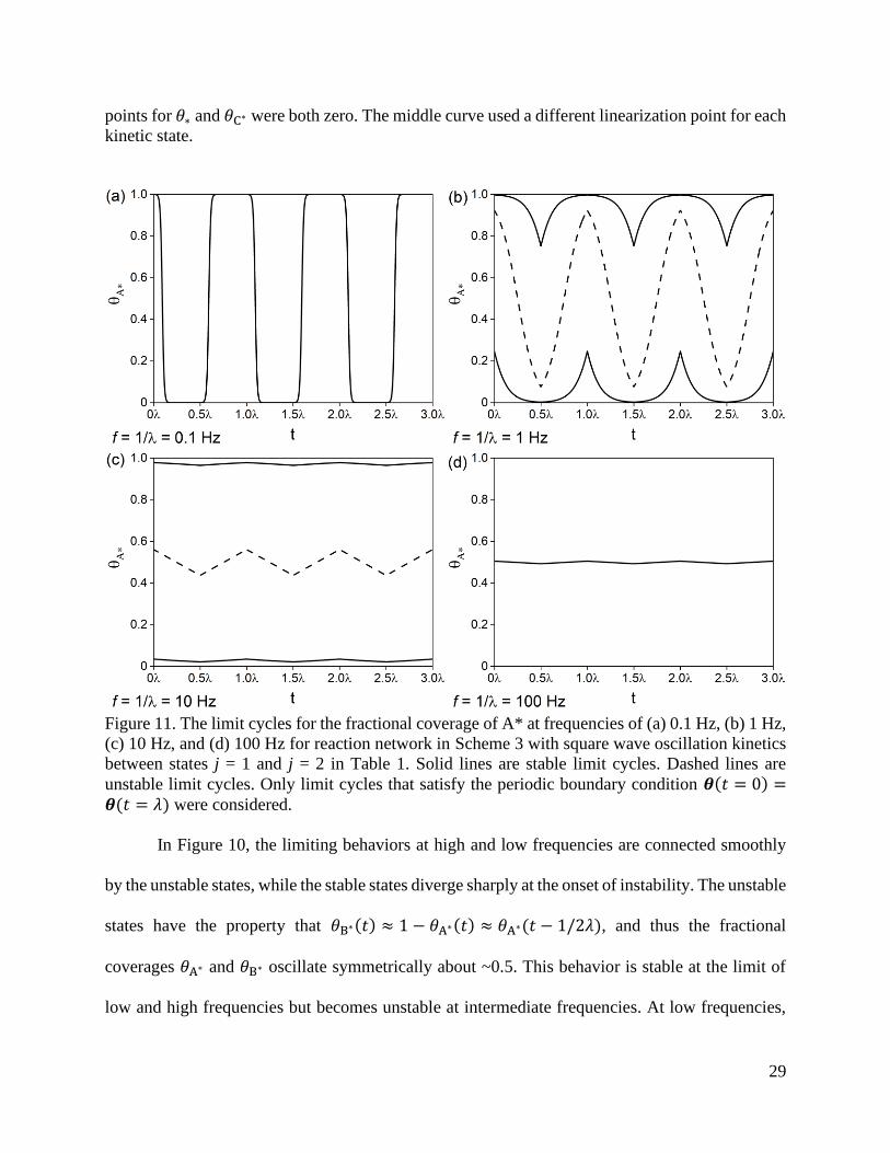
Figure 11. The limit cycles for the fractional coverage of A* at frequencies of (a) 0.1 Hz, (b) 1 Hz,
(c) 10 Hz, and (d) 100 Hz for reaction network in Scheme 3 with square wave oscillation kinetics
between states j = 1 and j = 2 in Table 1. Solid lines are stable limit cycles. Dashed lines are
unstable limit cycles. Only limit cycles that satisfy the periodic boundary condition 𝜽(𝑡 = 0) =𝜽(𝑡 = 𝜆) were considered.
In Figure 10, the limiting behaviors at high and low frequencies are connected smoothly
by the unstable states, while the stable states diverge sharply at the onset of instability. The unstable
states have the property that 𝜃B∗(𝑡) ≈ 1 − 𝜃A∗(𝑡) ≈ 𝜃A∗(𝑡 − 1/2𝜆), and thus the fractional
coverages 𝜃A∗ and 𝜃B∗ oscillate symmetrically about ~0.5. This behavior is stable at the limit of
low and high frequencies but becomes unstable at intermediate frequencies. At low frequencies,
30
the oscillation frequency is sufficiently small that the catalyst surface essentially reaches static
steady-state in each oscillation, reaching the bounds of 𝜃A∗ ≈ 0 and 𝜃A∗ ≈ 1 (Figure 11a). As the
frequency increases, the fractional coverages no longer proceed via a sequence of steady states,
and the stable solutions diverge at the expense of an unstable limit cycle. At sufficiently large
frequencies, the stable solutions separate from the bounds at 𝜃A∗ ≈ 0 and 𝜃A∗ ≈ 1 and ultimately
converge at the quasi-static surface coverage 𝜃A∗(𝑡) ≈ 0.5..
The Newton-Raphson method for finding the limit cycle of nonlinear periodic differential
equations can be much faster than forward integration (Figure 9), but is significantly slower than
the linear algebra method employed for linear reaction schemes. One method for accelerating the
integration of nonlinear differential equations is by Taylor linearization, where the differential
equations are linearized by the formula (eq. (29)):
d𝑥
d𝑡= 𝐹(𝑥, 𝑦) ≈ 𝐹(𝑥0, 𝑦0) +
𝜕𝐹
𝜕𝑥|𝑥0,𝑦0
(𝑥 − 𝑥0) +𝜕𝐹
𝜕𝑦|𝑥0,𝑦0
(𝑦 − 𝑦0) (29)
where, for example, 𝐹 is a function of two variables 𝑥 and 𝑦 and is linearized about some point
(𝑥0, 𝑦0). Linearizing the differential equation for each reaction intermediate in this way, we obtain
a set of linear equations that are analytically solved following eqs. (10)-(17). Doing so decreases
the computation time by several orders of magnitude, but will only give one solution, despite the
actual differential equations having two stable and one unstable limit cycle. Furthermore, the
solution is sensitive to the choice in linearization point, as shown by approximate 𝜃A∗,0 obtained
by linearizing the differential equations for the nonlinear reaction in Scheme 3 with kinetics in
Table 1. Choices in linearization points were informed by the true solutions depicted in Figure 11.
The linearization approximates the true solutions, but further work is necessary to understand the
conditions at which multiple steady states may arise and how to choose reasonable linearization
points a priori.
31
The existence of multiple limit cycles may be problematic in practical application. First,
for the reaction in Scheme 2, the stable solutions give surfaces that are much less evenly distributed
between A∗ and B∗, and thus will have lower rates than the unstable solution. Second, any
perturbations in the system may result in jumping from one limit cycle to another, causing
unpredictable changes in reaction rate, heat generation, optimal feed composition, and outlet
composition—leading to many system controls issues (20). In practice, regimes of multiple steady
states are typically best avoided. In general, for nonlinear reaction systems, we cannot determine
the number of possible limit cycles during dynamic catalysis, nor is it clear at what frequencies
these multiple limit cycles will arise, though they are likely related to the time scales for kinetic
processes (e.g., quasi-equilibrium of reaction or quasi-steady-state of species). This problem has
many similarities to Hilbert’s sixteenth problem, as yet unsolved, which concerns the number of
limit cycles that exist for a coupled system of two variables with time-independent polynomial
differential equations (21). We can also make no justifiable comment on when solutions with
different periodicities or aperiodic, chaotic solutions generally exist under dynamic catalysis
conditions; however, we contend that, at the limit of low and high frequencies, there will always
be one unique limit cycle solution if the reaction network gives only one static steady-state
solution, as we discuss next.
At the low frequency limit, if the reaction network allows for only one steady-state solution
under static kinetics, as determined by chemical reaction network theory (22), then there exists
only one limit cycle during dynamic kinetics. This conclusion is arrived at by recognizing that for
sufficiently low frequencies, sufficient time is spent in each kinetic state such that, for most of the
time spent in each state, rates and surface coverages are time-invariant. Thus, at the low frequency
limit, the fractional coverages of the surface can be approximated as 𝜃𝑗∗(𝑡) ≈ 𝜃𝑗∗,SS(𝑡), where
32
𝜃𝑗∗,SS(𝑡) is the steady-state fractional coverage for species 𝑗∗ for the kinetics at time 𝑡. In this sense,
the reaction simply proceeds via a series of static steady states. Therefore, if the reaction network
allows for only one steady-state solution during static catalysis, then at each time 𝑡 there is only
one 𝜃𝑗∗,SS(𝑡)—ensuring that there is only one limit cycle during dynamic catalysis.
The unique limit cycle in the high frequency limit is defined, not by a series of steady states
at each condition, but a single quasi-static steady state maintained continuously and repeating each
oscillation. In a quasi-static steady state, the oscillation frequency is sufficiently large such that
the fractional coverages of species are essentially constant (𝜃𝑗∗(𝑡) ≈ 𝜃𝑗∗). Therefore, the time-
averaged rate for each elementary step 𝑟𝑖 is a product of the elementary step rate constant, 𝑘𝑖(𝑡),
multiplied by a function of time-invariant fractional coverages 𝐹(𝜃𝑗∗(𝑡)), which is a product of
the fractional coverages of species involved in elementary step i in accordance with mass-action
constitutive equations (eq. (30)):
⟨𝑟𝑖⟩ =∫ 𝑘𝑖(𝑡)𝐹 (𝜃𝑗∗(𝑡)) d𝑡
1/𝑓
0
∫ d𝑡1/𝑓
0
lim𝑓→∞
≈ 𝐹(𝜃𝑗∗)∫ 𝑘𝑖(𝑡) d𝑡
1/𝑓
0
∫ d𝑡1/𝑓
0
= ⟨𝑘𝑖⟩ 𝐹(𝜃𝑗∗) (30)
Thus, the equations for the time-averaged rates of each elementary step are identical to the
equations for static catalysis, with the exception that the rate constants are now time-averaged. The
systems of equations that describe the reaction kinetics for a given reaction network under static
kinetics and quasi-static surface coverages during dynamic kinetics are structurally identical.
Therefore, the number of steady-state solutions for a reaction network during static kinetics must
be the equal to the number of limit cycles during dynamic catalysis at the high frequency limit,
and the differential equations for fractional coverages are entirely analogous to a static steady-state
system (eq. (31)):
33
d𝜃∗
d𝑡≈ ⟨𝑘−1⟩𝜃A∗ − ⟨𝑘1⟩𝑎A𝜃∗ + ⟨𝑘−2⟩𝜃B∗ − ⟨𝑘2⟩𝑎B𝜃∗ + ⟨𝑘3⟩𝜃A∗𝜃B∗ − ⟨𝑘−3⟩𝜃C∗𝜃∗
+ ⟨𝑘4⟩𝜃C∗ − ⟨𝑘−4⟩𝑎C𝜃∗
d𝜃A∗
d𝑡≈ −⟨𝑘−1⟩𝜃A∗ + ⟨𝑘1⟩𝑎A𝜃∗ − ⟨𝑘3⟩𝜃A∗𝜃B∗ + ⟨𝑘−3⟩𝜃C∗𝜃∗
d𝜃B∗
d𝑡≈ −⟨𝑘−2⟩𝜃B∗ + ⟨𝑘2⟩𝑎B𝜃∗ − ⟨𝑘3⟩𝜃A∗𝜃B∗ + ⟨𝑘−3⟩𝜃C∗𝜃∗
d𝜃C∗
d𝑡≈ ⟨𝑘3⟩𝜃A∗𝜃B∗ − ⟨𝑘−3⟩𝜃C∗𝜃∗ − ⟨𝑘4⟩𝜃C∗ + ⟨𝑘−4⟩𝑎C𝜃∗
(31)
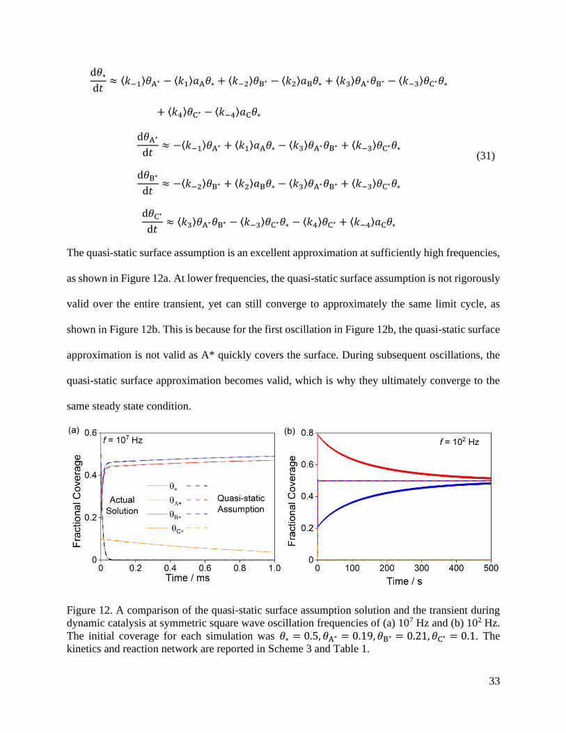
The quasi-static surface assumption is an excellent approximation at sufficiently high frequencies,
as shown in Figure 12a. At lower frequencies, the quasi-static surface assumption is not rigorously
valid over the entire transient, yet can still converge to approximately the same limit cycle, as
shown in Figure 12b. This is because for the first oscillation in Figure 12b, the quasi-static surface
approximation is not valid as A* quickly covers the surface. During subsequent oscillations, the
quasi-static surface approximation becomes valid, which is why they ultimately converge to the
same steady state condition.
Figure 12. A comparison of the quasi-static surface assumption solution and the transient during
dynamic catalysis at symmetric square wave oscillation frequencies of (a) 107 Hz and (b) 102 Hz.
The initial coverage for each simulation was 𝜃∗ = 0.5, 𝜃A∗ = 0.19, 𝜃B∗ = 0.21, 𝜃C∗ = 0.1. The
kinetics and reaction network are reported in Scheme 3 and Table 1.
34
The quasi-static surface assumption reveals that apparent rate constants of elementary steps
can be favorably altered by time-averaging the rate constants of two different kinetic states when
the kinetic oscillation frequency is sufficiently large. This confirms that, while resonance certainly
can be a factor for enhancing the rate (Figure 7), it is not a necessary pre-condition for enhanced
rate, selectivity, or conversion during dynamic catalysis. Instead, as recognized by Astumian and
coworkers (7, 8, 23) the fundamental prerequisite for rate enhancement by dynamic catalysis is
kinetic asymmetry between the energetic states through which the catalyst is cycled. Rate
enhancement by time-averaging of rate constants at quasi-static surface conditions and by
resonance represent two different mechanisms by which dynamic catalysis can enhance rates,
selectivities, and conversions. Understanding under which conditions one mechanism is favored
is a topic that warrants further research.
4. Conclusion
We establish methods significantly faster than numerical forward integration for finding
the limit cycles and time-averaged rates for dynamic catalytic systems. These methods calculate
the limit cycles for kinetic oscillations of any shape with computation times that are essentially
independent of oscillation frequency and enable facile discovery of the optimal kinetic waveform
that maximizes the time-averaged reaction rate using optimization methods. The approach for
linear systems, where no time-dependent species react with each other, uses linear algebra to
analytically solve for the limit cycles. For nonlinear systems, the coupled ODEs and corresponding
periodic boundary conditions are recast as criteria in an optimization problem solved by a Newton-
Raphson approach. For linear systems, it is shown that there exists only one periodic limit cycle,
but for nonlinear systems, multiple limit cycles exist. Generally, if the reaction network allows for
35
only one steady-state solution under static kinetic conditions, only one limit cycle exists under
dynamic conditions in the limit of low oscillation frequency, for which the reaction proceeds via
a series of steady states, and in the limit of high oscillation frequency, for which the reaction is
maintained at a single quasi-static state. For intermediate oscillation frequencies, no such
simplifying conditions exist, and multiple nonlinear solutions are expected.
Under sufficiently fast kinetic oscillations, the activities of species are “quasi-static” in
comparison to the frequency of kinetic oscillations, and thus the reaction network behaves
identically to a static reaction network with rate constants that are equal to the time-averaged rate
constants of the kinetic waveforms. These conditions are rapidly simulated by forward integration
regardless of whether the reaction network is linear. Analysis of reaction networks under quasi-
static conditions reveal that resonance is not always a necessary condition to observe enhanced
kinetics during dynamic catalysis; rather, the principal requirement for rate enhancement is
asymmetry of the kinetic states sampled by the oscillation waveform.
Acknowledgements
This work was performed in part under the auspices of the U.S. Department of Energy by Lawrence
Livermore National Laboratory under Contract DE-AC52-07NA27344.
Supporting Information
Matlab code is downloadable for free from https:\\www.github.com/foley352/dynamic.
Notes
The authors declare no competing financial interest.
36
References
1. J. Qi, et al., Dynamic Control of Elementary Step Energetics via Pulsed Illumination
Enhances Photocatalysis on Metal Nanoparticles. ACS Energy Lett. 5, 3518–3525 (2020).
2. M. Shetty, et al., The Catalytic Mechanics of Dynamic Surfaces: Stimulating Methods for
Promoting Catalytic Resonance. ACS Catal. 10, 12666–12695 (2020).
3. D. A. Gonzalez-Casamachin, J. Rivera De la Rosa, C. J. Lucio–Ortiz, L. Sandoval-Rangel,
C. D. García, Partial oxidation of 5‑hydroxymethylfurfural to 2,5-furandicarboxylic acid
using O2 and a photocatalyst of a composite of ZnO/PPy under visible-light:
Electrochemical characterization and kinetic analysis. Chem. Eng. J. 393, 124699 (2020).
4. F. Sordello, F. Pellegrino, M. Prozzi, C. Minero, V. Maurino, Controlled Periodic
Illumination Enhances Hydrogen Production by over 50% on Pt/TiO2. ACS Catal. 11, 6484–
6488 (2020).
5. J. Gopeesingh, et al., Resonance-Promoted Formic Acid Oxidation via Dynamic
Electrocatalytic Modulation. ACS Catal. 10, 9932–9942 (2020).
6. C. Cheng, et al., An artificial molecular pump. Nat. Nanotechnol. 10, 547–553 (2015).
7. R. D. Astumian, et al., Non-equilibrium kinetics and trajectory thermodynamics of synthetic
molecular pumps. Mater. Chem. Front 4, 1304 (2020).
8. R. D. Astumian, Kinetic asymmetry allows macromolecular catalysts to drive an
information ratchet. Nat. Commun. 10, 3837 (2019).
9. M. A. Ardagh, O. A. Abdelrahman, P. J. Dauenhauer, Principles of Dynamic Heterogeneous
Catalysis: Surface Resonance and Turnover Frequency Response. ACS Catal. 9, 6929–6937
(2019).
10. R. D. Astumian, B. Robertson, Imposed Oscillations of Kinetic Barriers Can Cause an
Enzyme To Drive a Chemical Reaction Away from Equilibrium. J. Am. Chem. Soc. 115
(1993).
11. R. D. Astumian, I. Derényi, Fluctuation driven transport and models of molecular motors
and pumps. Eur. Biophys. J. 27, 474–489 (1998).
12. D. S. Liu, R. D. Astumian, T. Y. Tsong, Activation of Na+ and K+ pumping modes of
(Na,K)-ATPase by an oscillating electric field. J. Biol. Chem. 265, 7260–7267 (1990).
13. G. R. Wittreich, S. Liu, P. J. Dauenhauer, D. G. Vlachos, Catalytic Resonance of Ammonia
Synthesis by Dynamic Ruthenium Crystal Strain. ChemRxiv (2021).
37
14. M. A. Ardagh, T. Birol, Q. Zhang, O. A. Abdelrahman, P. J. Dauenhauer, Catalytic
resonance theory: superVolcanoes, catalytic molecular pumps, and oscillatory steady state.
Catal. Sci. Technol. 9, 5058 (2019).
15. C. C. Tisdell, Existence of solutions to first-order periodic boundary value problems. J.
Math. Anal. Appl. 323, 1325–1332 (2006).
16. S. Boussandel, Existence and uniqueness of periodic solutions for gradient systems in finite
dimensional spaces. Acta Math. Sci. 36, 233–243 (2016).
17. E. A. Coddington, N. Levinson, Theory of Ordinary Differential Equations (McGraw-Hill,
1955).
18. D. M. Marquis, E. Guillaume, A. Camillo, T. Rogaume, F. Richard, Existence and
uniqueness of solutions of a differential equation system modeling the thermal
decomposition of polymer materials. Combust. Flame 160, 818–829 (2013).
19. Á. Logadóttir, J. K. Nørskov, Ammonia synthesis over a Ru(0001) surface studied by
density functional calculations. J. Catal. 220, 273–279 (2003).
20. O. Levenspiel, Chemical Reaction Engineering, 3rd Ed. (John Wiley & Sons, 1999).
21. D. Hilbert, Mathematical problems. Bull. Am. Math. Soc. 8, 437–479 (1902).
22. M. Feinberg, Chemical reaction network structure and the stability of complex isothermal
reactors—I. The deficiency zero and deficiency one theorems. Chem. Eng. Sci. 42, 2229–
2268 (1987).
23. R. D. Astumian, P. B. Chock, T. Y. Tsong, Y.-D. Chen, H. V. Westerhofft, Can free energy
be transduced from electric noise? Proc. Natl. Acad. Sci. 84, 434–438 (1987).