HYDROLOGICAL IMPACTS OF CLIMATE CHANGE ON INFLOWSTO PERTH, AUSTRALIA

JASON EVANS 1� and SERGEI SCHREIDER 2

1Centre for Resource and Environmental Studies, Australian National University, Australia2Integrated Catchment Assessment and Management Centre, Australian National University,

Australia

Abstract. The effects of climate change due to increasing atmospheric CO2 on the major tributariesto the Swan River (Perth, Western Australia) have been investigated. The climate scenarios are basedon results from General Circulation Models (GCMs) and 1000 year time series are produced usinga stochastic weather generator. The hydrological implications of these scenarios are then examinedusing a conceptual rainfall-runoff model, CMD-IHACRES, to model the response of six catchments,which combine to represent almost 90% of the total flow entering the upper Swan River, and hencethe Perth city urban area. The changes in streamflow varies considerably between catchments, ex-hibiting a strong dependence on the physical attributes of the catchment in question. The increase inthe magnitudes of rare flood events despite significant decreases in mean streamflow levels found insome catchments emphasizes the importance of estimating changes in the nature of the precipitation(variance, length of storm and interstorm periods), along with changes in the mean, in climate changescenarios.

1. Introduction

1.1. BACKGROUND

It is likely that the industrially induced increase of greenhouse gases in the at-mosphere could lead to changes of the Earth’s climate. One of the most importantaspects of global change science is an estimation of possible impacts of these cli-matic changes to the world water availability. This is particularly important for anywork aimed at supporting the sustainable management and long-term planning ofwater resources. It is especially important in Australia where the supply of waterresources is a major constraint for further development of large urban areas.

Most hydrologically-focused climate change impact studies assess changes inwater availability as well as extreme events, particularly floods. These studies aregenerally performed in order to answer questions about the future water supply tolarge urban or intensive agricultural areas and, hence, are focused on major watersupply catchments. This study undertakes a comprehensive analysis of climatechange impacts on the hydrological regime of streams entering the Perth City

� Correspondence address: Center for Earth Observation, Department of Geology and Geo-physics, Yale University, New Haven, CT, U.S.A., 06520-8109. E-mail: jason.evans@yale.edu

Climatic Change 55: 361–393, 2002.© 2002 Kluwer Academic Publishers. Printed in the Netherlands.

362 JASON EVANS AND SERGEI SCHREIDER

area, Western Australia. The analysis is focused on the flooding regime and itsimplications for the city’s urban storm water system, and therefore does not lookexplicitly at the water supply for urban consumption.

The problem of streamflow response to climate variation is stated in Nemecand Schaake (1982). A detailed overview of climate models employed for climateimpacts assessment is outside the scope of the present paper, but relevant referencescan be found in Houghton et al. (1990, 1992), Leavesley (1994), Pittock (1988,1993), Tucker (1988), and Whetton et al. (1994).

Climate impacts assessment for Australian catchments have also been imple-mented in some previous research works. Close (1988) modeled nine rivers of theMurray-Darling Drainage Division and estimated the possible climate impact onits water resources using the Murray-Darling Basin Commission empirical model.Nathan et al. (1988) applied a deterministic, conceptual rainfall-runoff model, HY-DROLOG, to study the climate impact on runoff in the Myponga Weir catchmentin Southern Australia and Moogerah Dam in Queensland. Whetton et al. (1993)investigated implications of climate change on floods and droughts in Australia.Chiew et al. (1995) followed the above approach using the Modified HYDROLOGmodel in order to model 28 benchmark catchments in Australia and estimate theclimate impact on their streamflow. Schreider et al. (1997) analyzed the climateimpacts on the water availability and extreme events such as floods and droughtsin four Basins of the Murray-Darling Drainage Division (Goulburn, Ovens, Kiewaand Upper Murray). Climate change impacts on urban flooding in three Australianurban catchments were analyzed in Schreider et al. (1999).

We begin this paper with a short review of various climate change impact analy-sis methods followed by a justification of our model selection. Section 2 providesa description of the rainfall-runoff model used, an investigation into the validityof using temperature as a surrogate for potential evaporation and a short demon-stration of the climate invariance of its parameters. A description of the study siteis provided in Section 3. Section 4 outlines the modeling methodology used, theresults of which are presented in Section 5. A brief discussion of the implicationsof these results can be seen in Section 6.

1.2. METHODS OF CLIMATIC CHANGE IMPACTS ANALYSIS AND ASSUMPTIONS

Where it may be generally accepted that the increasing concentrations of green-house gases in the atmosphere are causing climate change, there still existsconsiderable uncertainty in the magnitude, timing and spatial distribution of thischange. Results from climate change impact studies, such as this one, depend crit-ically on the climate change scenarios used. Several methods for creating climatescenarios exist, which cover a considerable range of complexity, cost and timedemand.

One of the simplest approaches is to use scenarios based on changes to longterm seasonal mean values of climate descriptors (as determined for example

HYDROLOGICAL IMPACTS OF CLIMATE CHANGE ON INFLOWS TO PERTH, AUSTRALIA 363

by GCM runs) to transform present-day climatic time series. This approach hasbeen used in previous studies (Feddema, 1999; Mehrotra, 1999; Schreider et al.,1997), but has several limitations. Primarily, this approach takes no account of anychanges in the variability of the relevant climate descriptors.

The direct use of GCMs as the basis for creating climate scenarios has theadvantage of estimating changes in climate due to increased greenhouse gases for alarge number of climate variables in a physically consistent manner. These climatevariables are consistent with each other within a region and around the world.A major disadvantage of using GCMs is that, although they accurately representglobal climate, they are often inaccurate when simulating current regional climate.To overcome this regional inaccuracy the use of regional (limited area) climatemodels (Giorgi et al., 1994; McGregor and Walsh, 1993) or stochastic downscalingof relevant meteorological variables (Bates et al., 1998; Hughes, 1993; Hughes andGuttorp, 1994) has been promoted in several studies. Both of these methods sharethe disadvantage of being costly and time demanding. The use of regional climatemodels depends intimately on the GCM-supplied boundary conditions, and so maynot correct for errors, while the stochastic downscaling technique assumes thatsynoptic scale relationships are constant over time.

Another approach, used here, utilizes a stochastic weather generator to createextended time series for various climate descriptors (Bates et al., 1993; Charles etal., 1993; Semenov and Barrow, 1997). These stochastic weather models, fitted tocurrent climatic time series, can be adapted to the generation of synthetic seriesfor future climate using the method presented by Wilks (1992). Adjustments to themodel parameters are made in a manner consistent with the changes in monthlystatistics derived from comparisons of GCM runs for control and doubled CO2

conditions. In this study we have used the output statistics of the CSIRO9 GCM(McGregor et al., 1993) to look at a 2 × CO2 future climate scenario. When com-pared with other GCM results, this model is among the models predicting the mostsevere changes, hence we have also included a scenario that embodies about halfof the 2 × CO2 predicted change which we will refer to as 1.5 × CO2. Thesescenarios are consistent with the broad range of global warming projections basedon increased atmospheric concentrations of greenhouse gases. They are physicallyplausible and estimate daily precipitation and mean temperature, which are thenused to drive the hydrological model. By using a 1000 year long daily time seriesit is expected that the potential range of climate variability under each of the CO2

scenarios, would be captured.Other implicit assumptions involve the role of vegetation in the climate system.

Here we have assumed that the overall vegetation response for a given precip-itation and temperature input will remain similar over the next century whilegreenhouse gas concentrations increase. However, the vegetation cover and/or itsevapotranspiration response may change with future changes in climatic patternsof temperature, precipitation, solar radiation, as well as fertilization and stomatalresistance effects related to increases in carbon dioxide. It is worth noting that most

364 JASON EVANS AND SERGEI SCHREIDER

GCMs currently use a static model of the land surface where surface characteristicssuch as roughness length, albedo, soil and vegetation parameters are specified at thestart of a run and do not change regardless of any prolonged change in the predictedclimate.

Several studies have investigated the impact of climate on vegetation structure(Busby, 1988; Monserud et al., 1993). They imply some movement of vegetationtypes, in particular the shrinking of boreal zones and the increasing elevation ofthe tree line in alpine regions. Since our study area doesn’t contain any boreal typevegetation, and the period over which the above increases in CO2 are expected tooccur (about 70 years) is too short for forests to grow over considerable areas, wewould not expect any significant natural migration of vegetation types. Of course,vegetation structure in a region can change quite rapidly and radically due to directhuman intervention. Here we have assumed that any change in land managementpractices will be minor enough to have no significant impact.

Studies have investigated the biological response of some plants to increasedCO2 in the atmosphere, an introductory overview of which can be found in Kris-tiansen (1993). While this response varies between species a few general points canbe made. There are changes in stomatal conductance associated with higher CO2

levels, which lead to reduced water exchange per unit leaf area. The higher levelsof CO2 also lead to enhanced leaf growth. These two effects can, depending onspecies, offset each other in terms of total evapotranspiration response (Lins et al.,1997). Until further knowledge becomes available it seems reasonable to assumethat the net effect of these changes on a vegetation stand, which contains manyspecies, will be within the measurement and model error. Thus the assumption thatthe overall vegetation response will remain similar to that over recent history forthe time covered by this study seems quite plausible.

1.3. MODEL SELECTION

The stochastic weather generator used in this study is based on the WGEN gener-ator described by Richardson and Wright (1984). Its modified form and adaptionto the generation of synthetic climatic series can be found in Bates et al. (1994).WGEN simulates daily precipitation occurrence and amount, maximum and min-imum temperature, and solar radiation. Precipitation occurrence is described by atwo state (wet or dry), first-order Markov chain wherein the transition probabilitiesfor a given location are allowed to vary through an annual cycle. Precipitationamounts on wet days (rainfall greater than 0.3 mm) have their variation charac-terized using a gamma distribution. Standardized temperature and solar radiationcomponents are represented as a first-order, trivariate autoregressive process condi-tioned upon whether the day is wet or dry. WGEN produces stochastic realizationsof the variables above maintaining the statistical relationships established fromobservation.

HYDROLOGICAL IMPACTS OF CLIMATE CHANGE ON INFLOWS TO PERTH, AUSTRALIA 365

Wheater et al. (1993) described three types of rainfall-runoff models whichcould be used for predicting the stream discharge effects of climatic variations:metric, physically-based and conceptual. Metric models are based primarily onobservations and seek to characterise system response from these data. Physically-based models use a more classical mathematical-physics formulation of componentprocesses, based on continuum mechanics, and numerical solution techniques tosolve the relevant equations. Conceptual type models vary considerably in com-plexity but are always based on a representation of internal storages and the fluxesbetween them which are associated with particular hydrological components andprocesses.

Metric models contain too little process description to be used to make pre-dictions on independent periods not used for model calibration, hence have littleapplicability for simulating future climate impacts. Physically based models re-quire large computation and data resources. They also have the disadvantage ofcontaining large numbers of parameters, which introduces serious ambiguity in theidentification of the parameter values. The catchments chosen for considerationhere have been instrumented for a relatively long period, meaning that streamflow,precipitation and temperature data are available for decades in the majority of gaug-ing sites in these regions. Thus, conceptual lumped rainfall-runoff models seem tobe the most suitable type of model for the streamflow analysis required in the regionselected and for the particular purposes of this study. The model CMD-IHACRESfalls within this class of models. The number of parameters (five or seven) to befitted is small compared with other conceptual models, yet its performance hasbeen impressive across a range of hydroclimatologies.

In the present study the CMD-IHACRES rainfall-runoff model (Evans andJakeman, 1998), which is based on the IHACRES model (Jakeman and Horn-berger, 1993; Jakeman et al., 1990), was employed for predicting the future climateimpacts on streamflow. It is a hybrid metric-conceptual model based on the Instan-taneous Unit Hydrograph (IUH) technique. The method represents total streamflowresponse as a linear convolution of the IUH with rainfall excess or effective rainfall,which is in turn a non-linear function of measured rainfall and temperature. Theevaporative losses from the catchment are dealt with through a Catchment MoistureDeficit (CMD) accounting scheme.

One advantage of the CMD-IHACRES model is that its parameters reflect theaverage, lumped properties of the catchment considered. This provides the abilityto predict spatially averaged streamflow response. Therefore, the CMD-IHACRESapplication is suitable even in circumstances which lack spatially distributedcatchment input. Being structurally simpler than physically-based models, theconceptual models can easily utilize records of hydrological data for calibration.

Perhaps the most significant argument for the use of conceptual hydrologicalmodel CMD-IHACRES in the present work is that the model parameters reflectthe geomorphological and vegetation characteristics of the catchment consideredand are little affected by regional climate conditions (Jakeman et al., 1993; Post and

366 JASON EVANS AND SERGEI SCHREIDER

Jakeman, 1996). A demonstration of this parameter climate invariance is given inSection 2.1. CMD-IHACRES parameter values can therefore be established underpresent climatic conditions and then used without reference to the observed stream-flow data. This type of model can be used for streamflow prediction for estimatedfuture climatic conditions, assuming that the catchment properties considered(landscape, vegetation, building and road structure for the urban catchments) willnot change considerably.

2. Rainfall-Runoff Model Description

The CMD-IHACRES module structure consists of a non-linear loss module, whichconverts observed rainfall to effective rainfall or rainfall excess, and a linearstreamflow routing module, which extends the concept from unit hydrograph the-ory that the relationship between rainfall excess and total streamflow (not just quickflow) is conservative and linear.

The linear module allows any configuration of stores in parallel or series. Fromthe application of CMD-IHACRES to many catchments it has been found that thebest configuration is generally two stores in parallel, except in semi-arid regions orfor ephemeral streams, where often one store is sufficient (Ye et al., 1997). In thetwo-store configuration, at time step k, quickflow, x(q)k , and slowflow, x(s)k , combineadditively to yield streamflow (discharge), qk:

qk = x(q)

k + x(s)k (1)

with

x(q)

k = −αqx(q)k−1 + βqUk (2)

x(s)k = −αsx(s)k−1 + βsUk , (3)

where Uk is the effective rainfall. The parameters αq and αs can be expressed astime constants for the quick and slow flow stores, respectively:

τq = −�/ ln(−αq) (4)

τs = −�/ ln(−αs) , (5)

where � is the time step (daily here).Parameters expressing the relative volumes of quick and slow flow can also be

calculated:

Vq = 1 − Vs = βq

1 + αq= 1 − βs

1 + αs. (6)

In catchments which are modeled with only one store only Equations (2) and (4)are relevant.

HYDROLOGICAL IMPACTS OF CLIMATE CHANGE ON INFLOWS TO PERTH, AUSTRALIA 367

The CMD-IHACRES loss module accounts for antecedent soil moisture con-ditions and evapotranspiration (ET) losses. This module is a water balance-basedcatchment moisture store accounting scheme that uses rainfall and temperature asinputs and provides ET and rainfall excess as outputs. The catchment moisture storeaccounting scheme calculates Catchment Moisture Deficit at time step k, CMDk,according to

CMDk = CMDk−1 − Pk + Ek +Dk , (7)

where P is the precipitation, E is the ET loss and D is the drainage. CMD iszero when the catchment is saturated and increases as the catchment becomesprogressively drier. Equation (7) is simply the lumped water balance continuityequation for a catchment.

Effective rainfall is calculated from

U ={

Dk CMDk ≥ 0Dk − CMDk CMDk < 0

(8)

ET and Drainage are calculated using the equations below

Dk =

−c2

c1CMDk + c2 CMDk < c1

0 CMDk ≥ c1

(9)

Ek = c3Tk exp(−c4CMDk) , (10)

where c1, c2, c3 and c4 are non-negative constants, and T is the air temperature. In(10) temperature is assumed to be a proportional surrogate to potential evaporation(PE) which is attenuated according to the antecedent soil moisture conditions interms of the CMD. It has been assumed in (9) that drainage is dependent only onthe soil moisture conditions. The presence of the drainage equation allows water toescape to stream even when a moisture deficit exists within the catchment.

To measure the performance of the model estimate of streamflow, qi , two per-formance statistics are used: the bias (B) and the Nash-Sutcliffe efficiency (NSE)(Nash and Sutcliffe, 1970). These are defined as

B = 1

n

n∑i=1

(qi − qi ) (11)

NSE = 1 − α2e /α

2q , (12)

where α2e and α2

q are the variance of the model residuals (qi − qi ) and of theobserved streamflow respectively. Good model fit is indicated by a bias close tozero and NSE close to one.

368 JASON EVANS AND SERGEI SCHREIDER

2.1. TEMPERATURE AS A SURROGATE FOR PE

PE is the evaporation rate that would be achieved if the catchment surface was wet(i.e., the catchment is saturated). In the current model terminology this occurs whenthe CMD is zero, a condition which is met rarely in the current study area. Whenlooking at the future hydrological impacts it is the evaporative losses which needto be modeled, in this study they are modeled as being proportional to temperature.There are several reasons for this use of this assumption.

Since precipitation and temperature are the two most commonly available me-teorological variables, limiting the methods data requirements allows it to be usedin relatively data sparse areas. Climate model based future scenarios generally donot include estimated changes in PE and the stochastic weather generator usednaturally produces temperature as an output, not PE. This use of temperature in(10) allows the direct application of the output of the stochastic weather genera-tor without the added complication involved in preparing scenarios for potentialevaporation change which is itself fraught with uncertainty.

There currently exist a multitude of methods for calculating PE, and thesemethods have the potential to produce different results. While it is not clear whichmethods are better than others, there are several which display a proportionalitywith temperature. Empirically derived methods such as the Blaney-Criddle For-mula and the Hargreaves method (Jensen, 1990) for example. One of the mostwidely accepted formulations of PE was first proposed by Penman (1948).

E = �

�+ γQne + γ

�+ γEA , (13)

where Qne is the available energy flux density divided by the latent heat of vapor-ization (Le), � = (de∗/dT ) is the slope of the saturation water vapor pressurecurve e∗ = e∗(T ) and is given by (7), γ is the psychrometric constant (whichactually varies with temperature and pressure) is given by

γ = cpp

0.622Le

,

where cp is the specific heat capacity for constant pressure and p is the pressure.Also EA, a drying power of the air, is defined by

EA = f (u)(e∗a − ea) ,

where ea is the mean vapor pressure in the air, Ta is the air temperature, e∗a = e∗(Ta)

the corresponding saturation vapor pressure and u is the mean wind speed.From a practical point of view, (13) requires measurements of vapor pressure

deficit, wind speed, temperature, atmospheric pressure and the net incident radia-tion. Clearly the data required to use this formulation to produce a future climatechange scenario for PE are simply unavailable. To facilitate the use of this equation

HYDROLOGICAL IMPACTS OF CLIMATE CHANGE ON INFLOWS TO PERTH, AUSTRALIA 369

outside experimental areas, Linacre (1992, p. 105) used several substitutions andsimplifications to rewrite (13) as

PE = [0.015 + 4 × 10−4T + 10−6z

] [480(T + 0.006z)

84 − A− 40 + 2.3u(T − Td)

], (14)

where z and A are the elevation and latitude of the location of interest, and Td isthe dewpoint temperature. Taking our area of interest to be at sea level and at 34◦latitude, (14) becomes

PE = [0.015 + 4 × 10−4T ][9.6T − 40 + 2.3u(T − Td)] . (15)

For temperatures around 20 ◦C and low wind speeds the term involving mean windspeed in (15) would be negligibly small compared to 9.6T and hence it can beignored collapsing (15) further to

PE = [0.015 + 4 × 10−4T ][9.6T − 40] . (16)

The climate change scenarios used in this study differ by approximately 5 ◦C, tak-ing typical values for T in two of the scenarios, say T = 20 ◦C and T = 25 ◦C,the first bracketed term in (16) gives values of 0.023 and 0.025 respectively. Thatis, over the estimated climatic change this term is essentially a constant and to firstorder we see that

PE ∝ T .

Hence using a proportionality to temperature can provide a reasonable, firstorder, approximation for PE. It has been shown that using this surrogacy to estimatePE on time scales of a few days provides results at least as good as using morecomplicated forms of potential evaporation such as that given by Priestley andTaylor (1972) or Penman (1956) (Evans et al., 1999).

2.2. CLIMATE INVARIANCE OF RAINFALL-RUNOFF MODEL PARAMETERS

The Jamieson River (stream gauging station 405218), in the Goulburn River Basin,was selected as an example of a catchment with no significant land use changes.The catchment is dominated by state protected forest, where logging is negligi-bly small because this area is mostly covered by unproductive mixed tree species(DNRE, 1998). The mean annual rainfall in lower part of the catchment at theJamieson Post Office is 1250 mm. However, the climatology of this catchment ischaracterized by a considerable difference in precipitation levels between its drierlower part, and headwaters located in an alpine region with 1500–1800 mm ofannual precipitation.

Table I shows the calibration results for the Jamieson River catchment for years1972, 1978 and 1985. These calibration results were obtained using precipitation

370 JASON EVANS AND SERGEI SCHREIDER

Table I

Calibration results for the Jamieson River catchment

Model Starting date c1 c2 c3 c4 Model Model Mean Mean

number efficiency bias precip. temp.

(NSE) (m3/s) (mm) (◦C)

1 1 January 1972 35 3 0.28 0.01 0.856 0.57 920 13.4

2 1 January 1978 35 3 0.28 0.01 0.906 0.30 1330 13.6

3 1 January 1985 35 4 0.28 0.01 0.829 –0.28 1190 13.3

data recorded for the meteorological station at Jamieson PO (83017) and temper-ature from the Lake Eildon meteorological station (88023). Fits to the observedstreamflow are shown in Figure 1.

An important justification that the Jamieson River catchment has not been sub-ject to considerable land use change over the period of study is that simulationruns over the whole period of observation (∼20 years) provide a similarly highNash-Sutcliffe efficiency: 0.753, 0.791 and 0.744 for these three models respec-tively. This test fails for areas with extensive land use change, where the modelparameters can be expected to vary dramatically because of changes in the physicalcharacteristics of the catchment considered. Another important result of streamflowmodelling in this catchment is that the parameters of the non-linear module are verysimilar from one calibration period to another despite the difference in the climaticcondition during these periods (Table I).

These climatic conditions are quite different for the periods of 1972, 1978 and1985 with annual precipitation varying by ±20%. While this change in precip-itation covers the potential range due to climate change the demonstrated rangeof annual temperature falls well short of what could be expected under enhancedgreenhouse gas conditions. Unfortunately the large change in mean annual tem-peratures expected due to climate change fall well outside that present in historicalrecords thus precluding a comprehensive test. However, under the limitations of thehistorical record, the modelling exercise in the Jamieson catchment demonstratesthat the CMD-IHACRES model parameters have little climatic dependence, andhence justifies the applicability of this model for streamflow assessment underfuture climatic change impacts.

3. Site Description

A schematic of the study area, along with catchment boundaries and gauging sites,is given in Figure 2. All the catchments studied drain into the Swan River, whichsubsequently flows through the city of Perth itself. The area is dominated by winter

HYDROLOGICAL IMPACTS OF CLIMATE CHANGE ON INFLOWS TO PERTH, AUSTRALIA 371

Figure 1. Calibration results for the Jamieson River catchment.

372 JASON EVANS AND SERGEI SCHREIDER

rainfall, and the streams are ephemeral in nature. Some Descriptors of the stud-ied catchments are given in Table II. Clearly the Avon River catchment coversan extremely large area and extends much further from the coast than the othercatchments. The majority of the inland parts of this catchment do not contributeflow to the Avon River itself except during large flow events. During ‘normal’conditions a series of inland lakes store the streamflow from the eastern part of thecatchment.

4. Modeling

Using streamflow data provided for each of the streamflow gauges shown inTable II, and rainfall data from Belmont, CMD-IHACRES was calibrated and theresults are shown in Table III. Rainfall from just one station was used since it wasthe station for which the stochastic weather generator was run, producing 1000years of climate data under 1 × CO2, 1.5 × CO2 and 2 × CO2 conditions. Themethodology used to stochastically generate synthetic series for future climates isdescribed in Bates (1993,; 1994) and Charles (1993). The altered climate scenarioswere derived from the CSIRO9 Mark 1 GCM runs (circa 1992) which used a slabocean configuration. The changes in mean temperature and precipitation given bythis scenario are increases of just under 5 ◦C and just over 10% respectively.

More recent scenarios constructed using coupled GCMs suggest that the slabmodel above has overestimated the potential climate change. For this reason, wehave included a ‘1.5 × CO2’ scenario. This scenario was derived by interpolatingthe stochastic weather generator parameters to produce around half the climatechange estimated by the slab model.

Rainfall records from one rainfall station are unlikely to capture the actualrainfall over a catchment, especially if the rainfall station lies outside the catch-ment boundary and/or the catchment is large. This reliance on a single rainfallstation would be expected to cause significant problems in reproducing the currentstreamflow regime using a rainfall-runoff model. This problem is not as severeas it may seem for two reasons: first, the model appears to be robust enough toperform well even with just one rainfall station (see Table III); and secondly, weare concerned with the changes that occur rather than the accuracy with which wecan reproduce current streamflows. We analyze changes in the average recurrenceintervals (ARI) of flood events up to an ARI of 1000 years by using the simulationsfrom the stochastic weather generator.

The Avon River presents a particular challenge since it is extremely large inareal extent. It extends well beyond the coastal region for which rainfall data hasbeen provided, and it contains several lakes within the catchment boundaries. Itdoes however, represent a significant proportion of the total volume of streamflowreaching the Swan River and hence is important for any urban flooding study ofPerth. The Helena River presents a unique challenge in terms of streamflow pre-

HYDROLOGICAL IMPACTS OF CLIMATE CHANGE ON INFLOWS TO PERTH, AUSTRALIA 373

Figure 2. Schematic of study area.

374 JASON EVANS AND SERGEI SCHREIDER

Tabl

eII

Des

crip

tion

ofca

tchm

ents

used

inth

isst

udy

Cat

chm

ent

Des

crip

tion

Are

a(k

m2)

Lan

dus

esS

trea

mfl

owda

ta

Avo

nR

iver

Term

inat

edat

Bev

erly

asno

tmuc

hIn

clud

ing

abov

eG

oing

upth

eA

von

ther

eis

30–4

0km

6160

11

stre

amfl

owab

ove

that

poin

t(1)

.N

orth

amof

fore

st,t

hen

item

erge

son

toth

e

Dra

ins

the

whe

atbe

ltar

eaan

dth

encu

tsw

heat

belt

.Low

inte

nsit

ygr

azin

g

thro

ugh

the

esca

rpm

ent

120,

000

km2

and

crop

ping

(1)

Bro

ckm

anR

iver

No

sign

ifica

ntw

ater

extr

acti

ons.

1512

km2

(1)

Som

efo

rest

,the

nsh

eep

graz

ing

(1).

6160

19

Nor

th-E

asto

fth

est

udy

area

.

OU

TF

LO

WS

toth

isri

ver

(whi

chth

en

join

sth

eA

von

outs

ide

the

stud

yar

ea)

Woo

rool

oB

rook

No

sign

ifica

ntw

ater

extr

acti

ons

525

km2

(1)

Past

ure,

fore

st,m

ixed

farm

ing

(1)

6160

01

Sus

anna

hB

rook

No

sign

ifica

ntw

ater

extr

acti

ons

25km

2(1

)Pa

stur

e,fo

rest

,not

muc

hcr

oppi

ng(1

)61

6040

Jane

Bro

okN

osi

gnifi

cant

wat

erex

trac

tion

s73

km2

(1)

Urb

an,p

astu

re,n

otm

uch

crop

ping

6161

78

Hel

ena

Riv

erFo

rms

low

erbo

unda

ryof

stud

yar

ea.

1600

km2

(1)

Urb

an,f

ores

t,pa

stur

ebe

low

6161

89

Hea

vily

regu

late

dby

Mun

dari

ngW

eir

Mun

dari

ngW

eir;

mos

tly

fore

st

abov

eth

ew

eir

HYDROLOGICAL IMPACTS OF CLIMATE CHANGE ON INFLOWS TO PERTH, AUSTRALIA 375

Tabl

eII

I

Cal

ibra

tion

resu

lts

Cat

chm

ent

Per

iod

NS

EB

Lin

ear

mod

ule

Mod

elpa

ram

eter

s

cum

ecs/

dst

ruct

ure

c 1c 2

c 3c 4

τ qτ s

Vs

Avo

n1/

1/76

–31/

12/7

90.

711.

901

stor

e10

10.

630.

127.

6

Riv

er

Bro

ckm

an1/

1/84

–31/

12/8

70.

740.

001

stor

e18

10.

680.

1024

.1

Riv

er

Woo

rool

o1/

1/79

–31/

12/8

20.

740.

002

stor

esin

para

llel

137

0.46

0.03

1.3

35.9

0.77

Bro

ok

Sus

anna

h1/

1/82

–31/

12/8

50.

78–0

.01

2st

ores

inpa

rall

el13

80.

360.

041.

034

.60.

72

Bro

ok

Jane

1/1/

80–3

1/12

/83

0.78

–0.0

22

stor

esin

para

llel

2313

0.32

0.02

1.2

39.3

0.70

Bro

ok

Hel

ena

1/1/

78–3

1/12

/81

0.67

0.07

1st

ore

251

0.37

0.07

1.6

Riv

er

376 JASON EVANS AND SERGEI SCHREIDER

diction since it is heavily regulated by Mundaring Weir. The weir is a moderatelylarge water supply reservoir that infrequently overflows.

Streamflow entering the Perth urban area from the studied catchments repre-sents some 90% of the total flow of the Swan River. As such, this is a fairlycomprehensive study of the likely impacts on the urban flooding regime for Perth.

4.1. RAINFALL-RUNOFF MODEL CALIBRATIONS

Each of the six catchments was calibrated over a four year period of the historicalrecord. The calibration results can be seen in Table III and Figure 3. The AvonRiver, Brockman River and Helena River were all modeled with a one store linearmodule structure, while the rest used two stores in parallel. The one store structurereflects the lack of an identifiable base flow component in the data, and reduces thenumber of model parameters from seven to five.

Figure 3 shows the modeled streamflow and the observed streamflow for eachof the six catchments calibration periods. In general, the modeled flow agrees quitewell with the observed, even with the problems associated with the use of a singlerainfall station. Note that in Figure 3a the modeled flow is generally underestimatedwhen compared with the observed flow. This is quantified in Table III where theAvon River has significant bias. This bias of 1.90 cumecs per day, while largecompared to the other catchments modeled, is still only a small fraction of the totalflow from the Avon River. Figure 3 shows the Avon River producing around tentimes as much streamflow as the other catchments.

Helena River is strongly regulated by Mundaring Weir, since the model fails tocapture most of the small releases from the weir. It does get the timing of the largereleases correct though their magnitude may be understated. This error is not ofparamount importance since the bulk of the study is focused on the comparativeperformance under different CO2 conditions rather than absolute values.

Results of the validation of the model on independent periods for each catch-ment are presented in Table IV. The performance of the models in terms of theNSE is not as good as during the calibration period, particularly for the Avon Rivercatchment. Much of this decrease in performance can be explained by the changingland uses occurring in the catchments (the model assumes static land use) as wellas the use of only one rainfall station as discussed previously, which is particularlyimportant for the Avon River catchment. Clearly the model performance suggeststhat a reasonably high level of uncertainty is associated with the streamflow pre-dictions and as such caution must be taken when interpreting the results in anyoperational sense.

Figure 4 shows how evapotranspiration changes with CMD given a unit temper-ature for each of the six catchments. The differences between these relationshipscan be explained principally in terms of vegetation and its distribution within thecatchment, as well as catchment size. Two of the largest catchments, the Avon andBrockman Rivers, produce very little ET once the CMD has reached 50–60 mm

HYDROLOGICAL IMPACTS OF CLIMATE CHANGE ON INFLOWS TO PERTH, AUSTRALIA 377

Figure 3a.

378 JASON EVANS AND SERGEI SCHREIDER

Figure 3b.

Figure 3. Observed and modeled streamflow for the calibration period for the: (a) Avon River;(b) Brockman River; (c) Wooroolo Brook; (d) Susannah Brook; (e) Jane Brook; and (f) Helena River.

HYDROLOGICAL IMPACTS OF CLIMATE CHANGE ON INFLOWS TO PERTH, AUSTRALIA 379

Table IV

Validation results

Catchment Period NSE Bias

cumecs/d

Avon River 1/1/80–31/12/83 0.44 –0.22

Brockman River 1/1/77–31/12/80 0.61 –0.11

Wooroolo Brook 1/1/83–31/12/84 0.58 0.32

Susannah Brook 1/1/88–31/12/91 0.64 –0.01

Jane Brook 1/1/84–31/12/85 0.64 –0.06

Helena River 1/1/83–31/12/86 0.52 0.16

Figure 4. Variation in ET with Catchment Moisture Deficit given a unit temperature input.

while for low CMD they display a high gradient and high saturation ET. This isfairly typical of catchments dominated by farming with forest remaining along thehighest parts of the catchment. It has been well established that forests transpire at asignificantly greater rate than grasslands (Holmes and Sinclair, 1986). In Figure 4,the forest dominates the ET at first but since the forest only exists in the catchmenthighlands it is the first area to dry out, subsequently the lowland grassed areas beginto be the dominant ET source and a sharp fall occurs in the total ET.

The three smaller catchments display a similar but less pronounced change inET. This is to be expected in these smaller catchments, since the horizontal gradientin soil moisture would be considerably less than in the large catchments, makingthe transition from forest dominated ET to grassland dominated ET less severe. The

380 JASON EVANS AND SERGEI SCHREIDER

ET for Jane Brook displays the smallest gradient for low catchment moisture; thisis due to the relatively uniform land cover in the catchment as shown in Table II. Inparticular there is no forest present and hence no transition from forest dominatedto grass dominated ET. In fact the ET displays an almost linear fall with increasingCMD.

As it was stated above, the Helena River streamflow is strongly affected bythe presence of Mundaring Weir. Despite being a large catchment with forestdominated uplands and crop dominated lowlands the catchment displays a muchsmaller gradient difference between high and low CMD than is seen in the Avon orBrockman. This can be largely attributed to the presence of the reservoir above theweir which evaporates water at a fairly consistent rate regardless of the CMD.

5. Results

The models given in Table III were then used, in conjunction with the sup-plied 1000 year precipitation and temperature records, to produce 1000 years ofstreamflow data under 1 × CO2, 1.5 × CO2 and 2 × CO2 conditions.

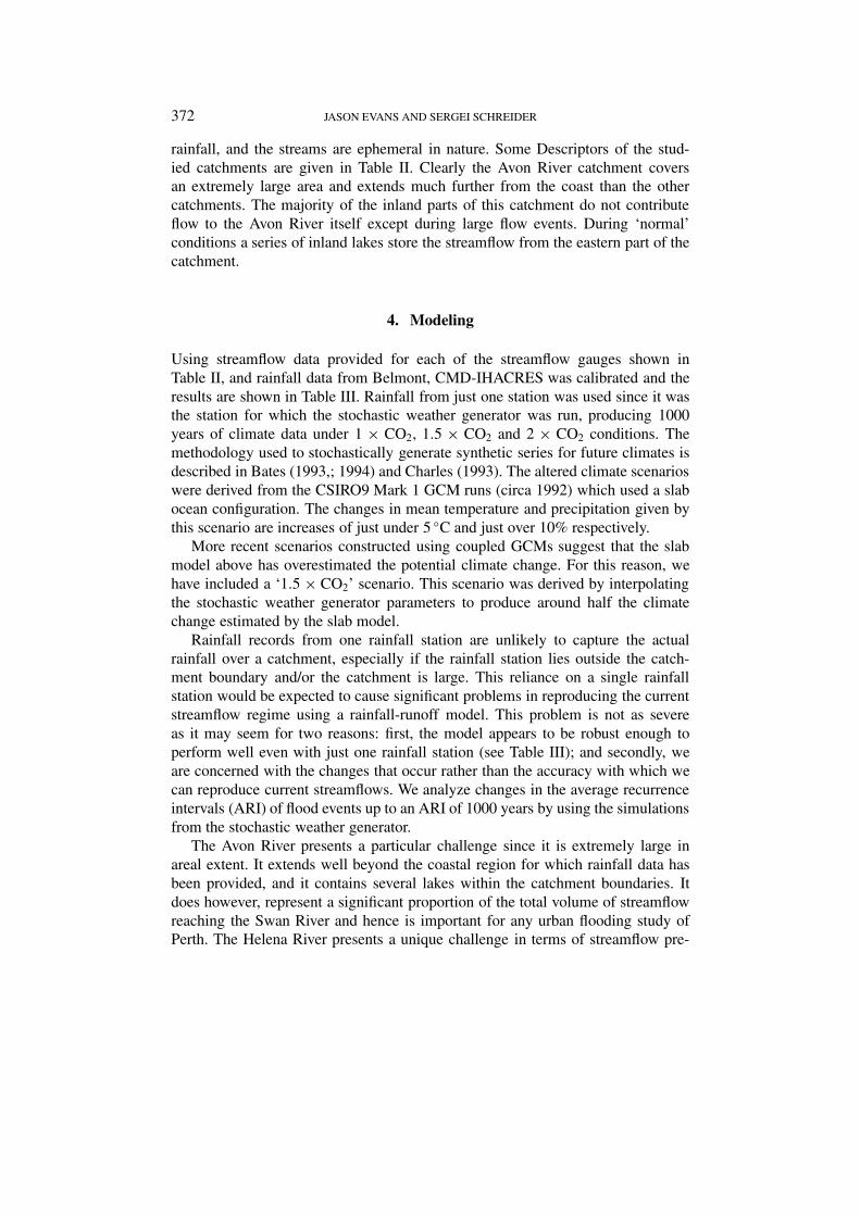
Figures 5 and 6 display properties of the temperature and precipitation timeseries under different CO2 conditions. Clearly seen in Figure 5 is a fairly uniformincrease in temperature with increasing CO2. In isolation, this increase in tempera-ture would be expected to lead to an increase in evaporation, and hence a decreasein streamflow. Figure 6a shows a slight increase in precipitation with increasingCO2 across the broad range of precipitation occurrence. Figure 6b shows significantincreases in the precipitation of the few largest events, i.e., events with very largeARIs. In isolation, this change in precipitation would be expected to have littleeffect on the streamflow except for the few largest events when significant increasesin streamflow could be expected.

Figure 7 shows flow duration curves for each catchment under the three CO2

scenarios. In general, the potential impacts outlined above have occurred, with flowdecreasing as CO2 increases. The 1.5 × CO2 scenario streamflow is consistentlylower then present streamflow conditions, while the 2 × CO2 scenario streamflowcommonly produces even less streamflow. Deviations from this general outcomeoccur in Wooroolo Brook where Figure 7c shows an increase in some of the lowestflows with increasing CO2.

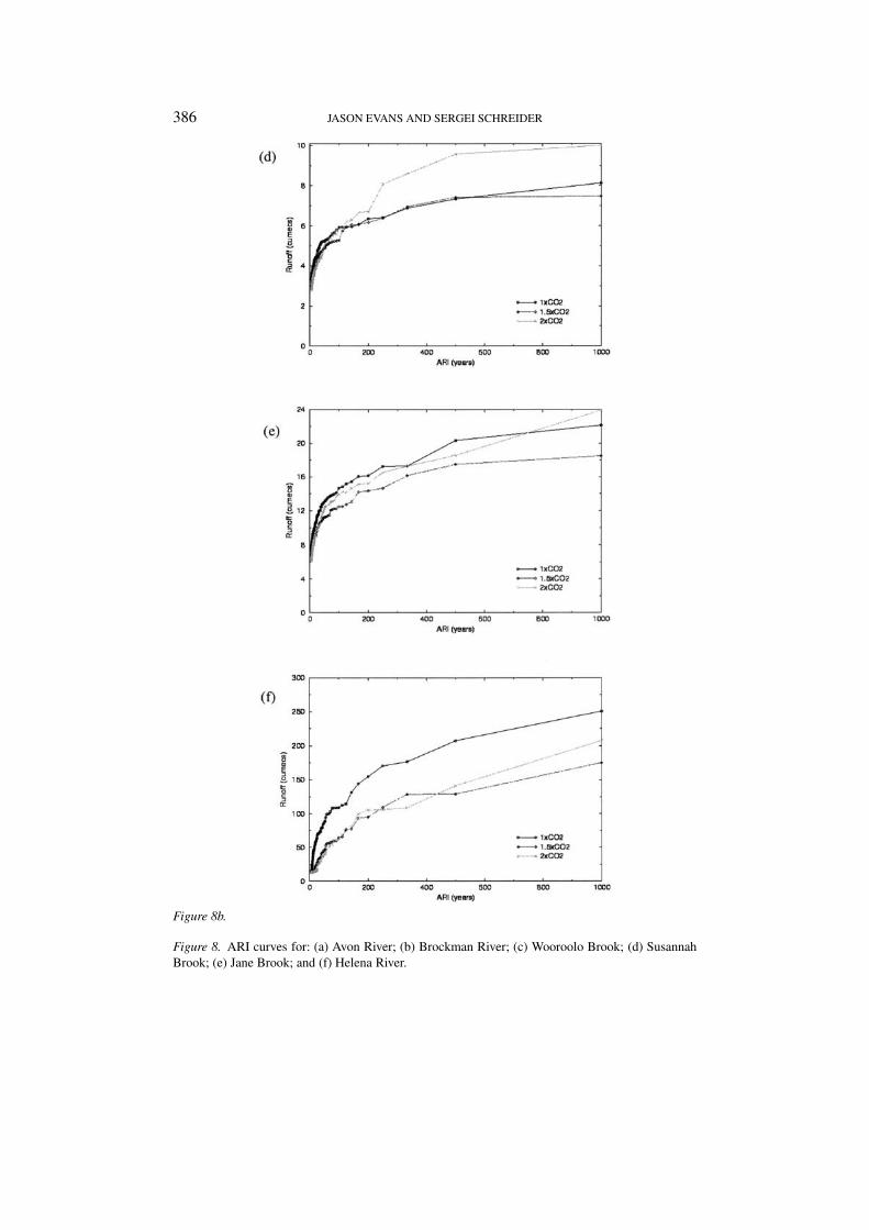
In Figure 8 are shown ARI curves for all six catchments starting with eventspossessing an ARI of five years. For these most common events (i.e., smallestARI) the trend seen in Figure 7 is borne out with the 1.5 × CO2 scenario pro-ducing smaller flood events than under present day conditions while the 2 × CO2

scenario floods are smaller again. The high ARI events demonstrate significantlymore variation among the catchments. The magnitude of the rarest flood eventsunder 1.5 × CO2 conditions is generally below those under 2 × CO2 conditionsand almost always lower than present day conditions. For the Avon, Brockman and

HYDROLOGICAL IMPACTS OF CLIMATE CHANGE ON INFLOWS TO PERTH, AUSTRALIA 381

Figure 5. Temperature duration curves for 1 × CO2, 1.5 × CO2 and 2 × CO2 conditions.

Helena Rivers, flood events under 2 × CO2 are always smaller than those underpresent day conditions. Wooroolo Brook and Jane Brook have only the rarest floodevents under 2×CO2 conditions being greater than those under current conditions,while Susannah Brook has larger flood events under 2 × CO2 conditions for ARIsgreater than 113 years. Figure 9 presents the ARI curves for the total flow enteringthe Swan River from these tributaries.

6. Discussion and Conclusions

Under the 1.5×CO2 and 2×CO2 scenarios, the mean streamflow entering the SwanRiver from these tributaries decreases by approximately 12% and 24% respectively.This outcome may be typical of relatively dry areas where current catchment mois-ture is rarely high enough to allow evaporation at the potential rate. Under globallywarmed conditions any increase in precipitation will allow evaporation to reachthis potential rate more often. It should also be noted that an increase in potentialevaporation is associated with global warming. To account for this increase in evap-orative demand precipitation would have to increase substantially. In the currentstudy the mean precipitation does not increase by a substantial enough factor andmean streamflow levels decrease.

However, when investigating the flood regime it is the outliers rather than themeans that are of interest. How much water from a single large precipitation eventis converted to streamflow depends to a large extent on what the antecedent mois-ture conditions in the catchment are. These antecedent conditions are affected byvarious catchment characteristics such as soil type and depth, and vegetation, which

382 JASON EVANS AND SERGEI SCHREIDER

Figure 6. Precipitation under 1×CO2, 1.5×CO2 and 2×CO2 conditions. (a) Precipitation durationcurve; (b) average recurrence interval.

determine the movement of water through the catchment as well as the evaporativelosses. Figure 8 provides the most insight into the changing flood regime with in-creasing CO2 levels in the atmosphere. It demonstrates the influence of catchmentcharacteristics on the streamflow response changes with a significantly differentresponse to global warming for each catchment.

It is of interest to note that the change in extreme events is often larger in the1.5×CO2 scenario than the 2×CO2 and in the cases of Wooroolo Brook, Susannah

HYDROLOGICAL IMPACTS OF CLIMATE CHANGE ON INFLOWS TO PERTH, AUSTRALIA 383

Figure 7a.

384 JASON EVANS AND SERGEI SCHREIDER

Figure 7b.

Figure 7. Flow duration curves the three CO2 scenarios: (a) Avon River; (b) Brockman River;(c) Wooroolo Brook; (d) Susannah Brook; (e) Jane Brook; and (f) Helena River.

HYDROLOGICAL IMPACTS OF CLIMATE CHANGE ON INFLOWS TO PERTH, AUSTRALIA 385

Figure 8a.

386 JASON EVANS AND SERGEI SCHREIDER

Figure 8b.

Figure 8. ARI curves for: (a) Avon River; (b) Brockman River; (c) Wooroolo Brook; (d) SusannahBrook; (e) Jane Brook; and (f) Helena River.

HYDROLOGICAL IMPACTS OF CLIMATE CHANGE ON INFLOWS TO PERTH, AUSTRALIA 387

Figure 9. Average recurrence interval for flood events in the upper Swan River.

Brook and Jane Brook the change in these extreme events can even differ in signbetween the two scenarios. To elucidate the causes of this difference in model re-sponse, closer examination of these extreme events was conducted and will here bediscussed with particular attention on the largest events at Jane Brook and HelenaRiver as presented in Figure 10. These events display characteristics which broadlyappear for the extreme events in all of the catchments and are indicative of the twomodel responses mentioned above.

Figure 10 shows the 6 days leading up to and 3 days following the event inquestion for all three scenarios. We note that given similar precipitation inputsfor the two catchments results in significantly different peak runoff outputs fromthe catchments. The order of largest to smallest runoff peaks in Jane Brook is the2 × CO2 scenario, 1 × CO2 scenario and 1.5 × CO2 scenario, while for the HelenaRiver the order is 1 × CO2, 2 × CO2 and 1.5 × CO2. This difference in runoffresponse can be attributed to the difference in catchment physical characteristics asembodied in the parameters of CMD-IHACRES.

The precipitation which causes the largest runoff event for each scenariodemonstrates significantly different characteristics and it should be noted that thisprecipitation event is not the largest precipitation event for any of the scenarios.For the 1 × CO2 scenario precipitation falls for several days increasing towards thepeak precipitation which is only around half that of the peak 2×CO2 precipitation.The 2 × CO2 scenario on the other hand, has almost no precipitation falling otherthen the peak which is relatively huge. The 1.5 × CO2 scenario precipitation falls

388 JASON EVANS AND SERGEI SCHREIDER

Figure 10. Precipitation, runoff and catchment moisture deficit (CMD) for the largest runoff event inJane Brook and Helena River.

somewhere in between the other scenarios. This is fairly typical of these climatechange scenarios which have increases in both the peak precipitation amounts andalso the length of the interstorm/dry down periods (i.e., variability) with increasingCO2.

The interplay between the precipitation and the antecedent catchment moistureconditions, as embodied in the CMD, then determines the height of the runoffpeak. For the 1 × CO2 scenario precipitation in the days preceding the peak bringthe catchment to saturation (CMD = 0) thus allowing the precipitation that fell thatday (minus any ET) to contribute directly to the runoff. For the 1.5 × CO2 scenariothe catchment is not quite saturated thus some of the precipitation that falls is usedto saturate the catchment before the rest contributes to runoff. Hence despite havingsimilar amounts of precipitation fall the 1.5×CO2 scenario produces a smaller peak

HYDROLOGICAL IMPACTS OF CLIMATE CHANGE ON INFLOWS TO PERTH, AUSTRALIA 389

than the 1×CO2 scenario. The 2×CO2 scenario has little to no precipitation prior tothe actual event, thus just prior to the event the CMD is significantly higher than inthe previous cases and a substantial proportion of the precipitation that falls must beused to bring the catchment to saturation before contributing directly to the runoff.In Jane Brook less than a quarter of the incident precipitation is required to bringthe catchment to saturation, resulting in a runoff peak above that of the 1 × CO2

scenario. For the Helena River almost half the precipitation is required to bringthe catchment to saturation, resulting in a runoff peak below that of the 1 × CO2

scenario but above the 1.5 × CO2 scenario. This difference in catchment responsedemonstrates the complex interplay between precipitation, catchment moisture andrunoff.

It should be emphasized that these extreme runoff events are associated with achange in the nature of the precipitation events as CO2 increases. Under 1 × CO2

conditions several days of moderate to large precipitation in a row are required toproduce extreme flood conditions. Under 2 × CO2 conditions, the most extremeflood events are driven by isolated but massive precipitation events. Under 1.5 ×CO2 conditions the consistency of precipitation required to produce extreme floodsunder 1 × CO2 conditions is much less evident and individual precipitation eventsdo not reach the massive levels of those under 2×CO2 conditions. Thus, in general,the 1.5 × CO2 conditions produce smaller extreme flood events than either of theother scenarios. This suggests that, assuming the climate changes as the climatemodels predict, the study area would likely see a decrease in the magnitude ofextreme floods followed by an increase. Of course, since changes in the level ofCO2 explored here are likely to be reached within a century these changes to floodevents with high ARI could be considered a mute point.

Of particular interest then is the importance not just of estimating the changes inpeak precipitation amounts but changes in the distributions of these events, in thelength of both storm (consecutive days with precipitation) and interstorm periods(dry down). Accurate predictions of the changes in the nature of precipitation (notjust the amounts) are vital before any confidence can be placed in estimates ofchanges in the flooding regime.

The two increased CO2 scenarios, while not encapsulating the full range ofglobal climate model estimates, provide some measure of the uncertainty in theglobal warming prediction. When combined with the uncertainties associated withthe hydrological modeling and vegetation response to increased CO2 in the at-mosphere, these types of studies can provide little more than an indication of apossible range of potential future flooding regimes. As found by Lins et al. (1997)these uncertainties preclude the use of such forecasts operationally.

More recent scenarios have been constructed using GCMs coupled to dynamicocean models (circa 1996). Some doubts about the reliability of scenarios from thecoupled models currently exist (Whetton et al., 1996). These include the observedlatitudinal gradient of warming in the southern hemisphere (IPCC, 1996), whichis more like that in the slab ocean GCMs, and the simulated rainfall decreases in

390 JASON EVANS AND SERGEI SCHREIDER

summer over Australia, given by the coupled models, which are contrary to theobserved small increases this century. In a comparison of the simulation results offive coupled models, Whetton et al. (1996) found that half the models simulated adecrease in total precipitation during summer and all-but-one simulated a decreasein total precipitation during winter for our study area. The implications of thesechanges to the results of a study such as this could be profound. One would expectthat the general decrease in runoff with increasing CO2 seen in Figure 7 would befurther exacerbated and probably accompanied by a decrease in the peaks of theextreme events. However without further information concerning the change in thenature of the precipitation, rather than simply the total, it is difficult to estimatewhat change to the flooding regime these coupled simulations would imply. In aregion such as this, where much of the area of interest could be considered semi-arid, the implications of a general decrease in the precipitation and runoff wouldlikely be a much more sever problem for the ecology and management of the areathan any likely change in the flooding regime.

It is of interest to note however, that despite the prediction of a significantreduction in the mean streamflow it is still possible to obtain increases in themagnitudes of floods at the 100 year ARI level (Figure 8d), which is the levelfocused on by urban storm water planning in Australia (ACT government, 1994).Thus, in order for future global warming scenarios to provide useful informationfor water resource management it may be vital to include estimates of the changein variance of the precipitation along with changes in the mean. It also serves toemphasis the need for a reduction in the uncertainty associated with the globalwarming predictions before much confidence can be placed in long term waterresource planning.

Acknowledgements

This work has been implemented within a CSIRO Land and Water project headedby Dr. Sue Cuddy. Authors thank Dr. Christopher Zoppou and Dr. ChengchaoXu who kindly provided us streamflow data and catchment information. We arealso grateful to Dr. Steven Charles and Dr. Neil Viney for providing the 1000-yearprecipitation and temperature simulations for the 1×CO2, 1.5×CO2 and 2×CO2

conditions at the Belmont meteorological station. Last, but not least, we wouldlike to thank Bob Oglesby and the reviewers for their helpful comments on thiswork. Special thanks to the Centre for Resource and Environmental Studies at theAustralian National University who supported the first author during this study.

References

ACT government: 1994, Urban Stormwater. Edition 1: Standard Engineering Practices, AustralianCapital Territory Government, Woden, Australia, ISBN 0644332743.

HYDROLOGICAL IMPACTS OF CLIMATE CHANGE ON INFLOWS TO PERTH, AUSTRALIA 391

Bates, B. C., Charles, S. P., and Fleming, P. M.: 1993, ‘Simulation of Daily Climatic Series for theAssessment of Climate Change Impacts on Water Resources’, in Kuo, C. Y. (ed.), EngineeringHydrology. Amer. Soc. Civ. Eng., New York, pp. 67–72.

Bates, B. C., Charles, S. P., and Hughes, J. P.: 1998, ‘Stochastic Downscaling of Numerical ClimateModel Simulations’, Environ. Model. Software 13, 325–331.

Busby, J. R.: 1988, ‘Potential Impacts of Climate Change on Australia’s Flora and Fauna’, inPearman, G. I. (ed.), Greenhouse: Planning for Climate Change, E. J. Brill, New York,pp. 387–398.

Charles, S. P., Fleming, P. M., and Bates, B. C.: 1993, ‘Problems of Simulation of Daily Precipitationand Other Input Time Series for Hydrological Climate Change Models’, Hydrology and WaterResources Symposium, Institute of Engineers, Australia, pp. 469–477.

Chiew, F. H. S., Whetton, P. H., McMahon, T. A., and Pittock, A. B.: 1995, ‘Simulation of theImpact of Climate Change on Runoff and Soil Moisture in Australian Catchments’, J. Hydrol.167, 121–147.

Close, A. F.: 1988, ‘Potential Impact of Greenhouse Effect on the Water Resources of the RiverMurray’, in Pearman, G. I. (ed.), Greenhouse: Planning for Climate Change, E. J. Brill, NewYork, pp. 312–323.

DNRE: 1998, North East Victoria: Comprehensive Regional Assessment, Department of NaturalResources and Environment, Victoria.

Evans, J. P. and Jakeman, A. J.: 1998, ‘Development of a Simple, Catchment-Scale, Rainfall-Evapotranspiration-Runoff Model’, Environ. Model. Software 13, 385–393.

Evans, J. P., Oglesby, R. J., and Jakeman, A. J.: 1999, ‘A New Method Improving the Simulationof Streamflow in Climate Models’, in Oxley, L., Scrimgeour, F., and Jakeman, A. J. (eds.),International Congress on Modelling and Simulation, MODSIM99, University of Waikato, NewZealand, pp. 611–616.

Feddema, J. J.: 1999, ‘Future African Water Resources: Interactions between Soil Degradation andGlobal Warming’, Clim. Change 42, 561–596.

Giorgi, F., Brodeur, C. S., and Bates, G. T.: 1994, ‘Regional Climate Change Scenarios over theUnited States Produced with a Nested Regional Climate Model’, J. Climate 7, 375–399.

Holmes, J. W. and Sinclair, J. A.: 1986, ‘Water Yield from Some Afforested Catchments in Victoria’,in Hydrology and Water Resources Symposium, Griffith University, Brisbane, pp. 214–218.

Houghton, J. T., Callander, B. A., and Varney, S. K. (eds.): 1992, Climate Change 1992. The Supple-mentary Report to the IPCC Scientific Assessment, Cambridge University Press, Cambridge.

Houghton, J. T., Jenkins, G. J., and Ephraums, J. J. (eds.): 1990, Climate Change, the IPCC ScientificAssessment, Cambridge University Press, Cambridge.

Hughes, J. P.: 1993, A Class of Stochastic Models for Relating Synoptic Atmospheric Patterns toLocal Hydrologic Phenomena, Ph.D. Thesis, Univ. Washington, Seattle.

Hughes, J. P. and Guttorp, P.: 1994, ‘A Class of Stochastic Models for Relating Synoptic AtmosphericPatterns to Regional Hydrologic Phenomena’, Water Resour. Res. 30, 1535–1546.

IPCC: 1996, Houghton, J. T., Filho, L. G. M., Callander, B. A., Harris, N., Kattenberg, A., andMaskell, K. (eds.), Climate Change 1995. The Science of Climate Change, IntergovernmentalPanel on Climate Change, Cambridge, p. 572.

Jakeman, A. J. et al.: 1993, ‘Assessing Uncertainties in Hydrological Response to Climate at LargeScale’, in Wilkinson, W. B. (ed.), Macroscale Modelling of the Hydrosphere, IAHS, Yokohama,pp. 37–47.

Jakeman, A. J. and Hornberger, G. M.: 1993, ‘How Much Complexity is Warranted in a Rainfall-Runoff Model?’, Water Resour. Res. 29, 2637–2649.

Jakeman, A. J., Littlewood, I. G., and Whitehead, P. G.: 1990, ‘Computation of the InstantaneousUnit Hydrograph and Identifiable Component Flows with Application to Two Small UplandCatchments’, J. Hydrol. 117, 275–300.

392 JASON EVANS AND SERGEI SCHREIDER

Jensen, M. E., Burman, R. D., and Allen, R. G.: 1990, ‘Evapotranspiration and Irrigation WaterRequirements’, in ASCE Manual on Engineering Practice, ASCE, New York, p. 332.

Kristiansen, G.: 1993, Biological Effects of Climate Change. An Introduction to the Field and Surveyof Current Research, Center for International Climate and Energy Research (CICERO), GlobalChange and Terrestrial Ecosystems (GCTE), International Geosphere-Biosphere Programme(IGBP), Oslo.

Leavesley, G. H.: 1994, ‘Modelling the Effects of Climate Change on Water Resources – a Review’,Clim. Change 28, 159–177.

Linacre, E.: 1992, Climate, Data and Resources. A Reference and Guide, Routledge, London, p. 366.Lins, H. F., Wolock, D. M. and McCabe, G. J.: 1997, ‘Scale and Modeling Issues in Water Resources

Planning’, Clim. Change 37, 63–88.McGregor, J. L., Gordon, H. B., Watterson, I. G., Rotstayn, M. R., and Rotstayn, L. D.: 1993, ‘The

CSIRO 9-Level Atmospheric General Circulation Model. 25’, CSIRO Division of AtmosphericResearch, Melbourne.

McGregor, J. L. and Walsh, K.: 1993, ‘Nested Simulations of Perpetual January Climate over theAustralian Region’, J. Geograph. Res. 98, 23,283–23,290.

Mehrotra, R.: 1999, ‘Sensitivity of Runoff, Soil Moisture and Reservoir Design to Climate Changein Central Indian River Basins’, Clim. Change 42, 725–757.

Monserud, R. A., Tchebakova, N. M., and Leeemans, R.: 1993, ‘Global Vegetation Change Predictedby the Modified Budyko Model’, Clim. Change 25, 59–83.

Nash, J. E. and Sutcliffe, J. V.: 1970, ‘River Flow Forecasting through Conceptual Models, Part I –A Discussion of Principles’, J Hydrol. 10, 282–290.

Nathan, J. E., McMahon, T. A., and Finlayson, B. A.: 1988, ‘The Impact of the Greenhouse Effecton Catchment Hydrology and Storage-Yield Relationships in Both Winter and Summer RainfallZones’, in Pearman, G. I. (ed.), Greenhouse: Planning for Climate Change, E. J. Brill, New York,pp. 273–295.

Nemec, J. and Schaake, J.: 1982, ‘Sensitivity of Water Resource Systems to Climate Variation’, J.Hydrol. Sci. 27, 327–343.

Penman, H. L.: 1948, ‘Natural Evaporation from Open Water, Bare Soil and Grass’, Proc. Roy. Soc.London A193, 116–140.

Pittock, A. B.: 1988, ‘Actual and Anticipated Changes in Australia’s Climate’, in Pearman, G. I.(ed.), Greenhouse: Planning for Climate Change, E. J. Brill, New York, pp. 35–51.

Pittock, A. B.: 1993, ‘Climate Scenario Development’, in Jakeman, A. J., Beck, M. B., and McAleer,M. J. (eds.), Modelling Change in Environmental Systems, John Wiley and Sons, Chichester,pp. 481–504.

Post, D. A. and Jakeman, A. J.: 1996, ‘Relationships between Catchment Attributes and HydrologicalResponse Characteristics in Small Australian Mountain Ash Catchments’, Hydrol. Proc. 10, 877–892.

Richardson, C. W. and Wright, D. A.: 1984, ‘WGEN: A Model for Generating Daily WeatherVariables’, ARS-8, U.S. Dept. of Agriculture, Agricultural Res. Service.

Schreider, S. Y., Jakeman, A. J., Whetton, P. H., and Pittock, A. B.: 1997, ‘Estimation of ClimateImpact on Water Availability and Extreme Events for Snow-Free and Snow-Affected Catchmentsof the Murray-Darling Basin’, Aust. J. Water Resour. 2, 35–46.

Schreider, S. Y., Smith, D. I., and Jakeman, A. J.: 2000, ‘Climate Change Impact on Urban Flooding’,Clim. Change 47, 91–115.

Semenov, M. A. and Barrow, E. M.: 1997, ‘Use of a Stochastic Weather Generator in theDevelopment of Climate Change Scenarios’, Clim. Change 35, pp. 397–414.

Tucker, G. B.: 1988, ‘Climate Modelling: How Does It Work?’, in Pearman, G. I. (ed.), Greenhouse:Planning for Climate Change, E. J. Brill, New York, pp. 22–34.

HYDROLOGICAL IMPACTS OF CLIMATE CHANGE ON INFLOWS TO PERTH, AUSTRALIA 393

Wheater, H. S., Jakeman, A. J., and Beven, K. J.: 1993, ‘Progress and Directions in Rainfall-RunoffModelling’, in Jakeman, A. J., Beck, M. B., and McAleer, M. J. (eds.), Modelling Change inEnvironmental Systems, John Wiley and Sons Ltd., p. 584.

Whetton, P. H., Fowler, A. M., Haylock, M. R., and Pittock, A. B.: 1993, ‘Implications of ClimateChange due to the Enhanced Greenhouse Effect on Floods and Droughts in Australia’, Clim.Change 25, 289–317.

Whetton, P. H., Rayner, P. J., Pittock, A. B., and Haylock, M. R.: 1994, ‘An Assessment of PossibleClimate Change in the Australian Region Based on an Intercomparison of General CirculationModel Results’, J. Climate 7, 441–463.

Wilks, D. S.: 1992, ‘Adapting Stochastic Weather Generation Algorithms for Climate ChangeStudies’, Clim. Change 22, 67–84.

Ye, W., Bates, B. C., Viney, N. R., Sivapalan, M., and Jakeman, A. J.: 1997, ‘Performance ofConceptual Rainfall-Runoff Models in Low-Yielding Catchments’, Water Resour. Res. 33,153–166.

(Received 12 May 2000; in revised form 30 January 2002)