Hs

Fa

b

a

ARRAA

KHMWS

1

a(Tptrpwi12ttt

a

P

0h

Ecological Engineering 49 (2012) 233– 243

Contents lists available at SciVerse ScienceDirect

Ecological Engineering

j ourna l ho me page: www.elsev ier .com/ locate /eco leng

ydraulic performance assessment of passive coal mine water treatmentystems in the UK

.M. Kusina,b,∗, A.P. Jarvisa, C.J. Gandya

Hydrogeochemical Engineering Research and Outreach Group, School of Civil Engineering and Geosciences, Newcastle University, NE1 7RU, UKDepartment of Environmental Sciences, Universiti Putra Malaysia, 43400 Serdang, Malaysia

r t i c l e i n f o

rticle history:eceived 24 February 2012eceived in revised form 6 July 2012ccepted 10 August 2012vailable online 3 September 2012

eywords:ydraulicine water

a b s t r a c t

Hydraulic performance assessment of passive treatment systems has been conducted for UK’s CoalAuthority mine water treatment systems. The study aims to improve the understanding of the hydraulicfactors that govern contaminant behaviour, such that future design of treatment systems is able to opti-mise treatment efficiency and make performance more predictable, and improve performance over thelong-term. Assessment of the hydraulic behaviour (i.e. residence time and flow pattern) of the treat-ment systems was accomplished by means of tracer tests. The tracer tests were undertaken at eight UKCoal Authority mine water treatment systems (lagoons and wetlands) within Northern England (mainstudy areas) and part of southern Scotland. A modelling approach using a tanks-in-series (TIS) model

etlandettlement lagoon

was adopted to precisely analyse and characterise the residence time distributions (RTDs), in an effort toaccount for the different flow patterns across the treatment systems. Generally, lagoon RTDs are charac-terised by a greater flow dispersion compared to wetlands (i.e. higher dispersion number, D and lowernumber of TIS, n). Consequently, the hydraulic efficiency, e� for lagoons is much lower than wetlands(mean of 0.20 for lagoons compared to 0.66 for wetlands). Implications for design and maintenance ofmine water treatment systems are discussed.

kaaekofiatbameast

. Introduction

Hydraulic performance in passive treatment systems is oftenssociated with the hydraulic residence time within the systeme.g. Martinez and Wise, 2003; Lin et al., 2003; Kjellin et al., 2007).he time a fraction of water spends in a system may reflect theatterns of water movement across the system and the degree ofreatment received of polluted waters (Thackston et al., 1987). Theelative importance of residence time as a measure of hydraulicerformance of passive treatment systems, in particular withinetland-type treatment systems, has been discussed in many stud-

es (e.g. Thackston et al., 1987; Kadlec, 1994; Werner and Kadlec,996; Martinez and Wise, 2003; Persson et al., 1999; Goulet et al.,001). However, detailed investigations on the actual residenceime to reflect the hydraulic performance of the treatment sys-ems have not been widely explored in the application of passive

reatment of coal mine water in the UK.

Current design practice for aerobic wetlands treating net-lkaline mine waters in UK applications are based on the zero-order

∗ Corresponding author at: Department of Environmental Sciences, Universitiutra Malaysia, 43400 Serdang, Malaysia. Tel.: +60 389468596.

E-mail addresses: diella@env.upm.edu.my, alidaxia@yahoo.com (F.M. Kusin).

flwpica2i

925-8574/$ – see front matter © 2012 Elsevier B.V. All rights reserved.ttp://dx.doi.org/10.1016/j.ecoleng.2012.08.008

© 2012 Elsevier B.V. All rights reserved.

inetics for pollutant removal i.e. the commonly used area-djusted removal as recommended by Hedin et al. (1994). Lagoonsre designed to allow nominal 48 h of retention time. A knowl-dge that iron removal under aerobic conditions follows first-orderinetics model for pollutant removal has been the basis for a rec-mmended alternative method for the design of such systems (e.g.rst-order removal model by Tarutis et al., 1999). Both of thesepproaches are based on the plug-flow assumption, which is nothe case in real systems. An increasing knowledge of the hydraulicehaviour (e.g. flow pattern across a treatment system) requires

better understanding of the hydraulic factors relating to treat-ent system performance. Such an assessment has not been widely

xplored in UK mine water treatment systems. The extent to whichctual systems deviate from an ideal flow pattern is the subject oftudy here. Such an investigation is particularly of interest to bet-er understand the impacts of the residence time (and hence theow pattern) have on the hydraulic performance of the system,hich potentially has an effect on pollutant removal. This is com-ounded by first-order removal kinetics of some contaminants e.g.

ron; removal is not only dependent on the chemical factors i.e.

oncentration, pH, dissolved oxygen but also the time it takes tottenuate the pollutant (e.g. Jarvis and Younger, 2001; Goulet et al.,001). Understanding the actual flow pattern rather than assum-

ng plug-flow, which is rarely the case in actual systems is a key

2 l Engin

owfim0srao

whnoombcottWfYetfs

2

2

watwiaIsmUarfs

2

2

adBpWtbwiie

wdtflw

ApotibfieuwpttVmTti

2

iahEtinwaudSMpw2abams

2

tisRt(sR

34 F.M. Kusin et al. / Ecologica

bjective of this investigation. This is somewhat related to recentork by Sapsford and Watson (2011), in which a pH-dependentrst-order removal rate constant have been developed for typicaline water conditions in the UK, and are found to be in the range of

.04 d−1 (pH 6)–372 d−1 (pH 8) for first-order oxidation rate con-tant, and 12.5 d−1 for first-order sedimentation rate constant. Thisetention time-based approach seems to be appropriate for it takesccount of the chemical characteristics of mine water and is basedn the first-order kinetics for iron removal.

Certainly, the primary pollutant of concern in UK coal mineater discharges is iron. Settlement lagoons and aerobic wetlandsave been regarded as ‘proven technology’ for passive treatment ofet-alkaline, ferruginous mine waters within the UK applicationsf passive treatment (PIRAMID Consortium, 2003). However, onef the limitations of the current design practice for these passiveine water treatment systems are that hydraulic factors are not

eing accounted for in the design of such systems. This has signifi-antly led to limited understanding of the hydraulic characteristicsf the treatment systems which, together with the knowledge ofhe geochemical processes governing pollutant removal, are cen-ral in the assessment of the overall treatment system performance.

ith regard to the variation in current treatment systems per-ormance i.e. iron removal (e.g. Jarvis and Younger, 1999, 2001;ounger, 2000; Younger et al., 2004; Kruse et al., 2007; Johnstont al., 2007) and hydraulic residence time (e.g. Kruse et al., 2009),his study aims to investigate the hydraulic factors influencing per-ormance of passive mine water treatment systems, specifically inettlement lagoons and aerobic wetlands.

. Materials and methods

.1. Site description

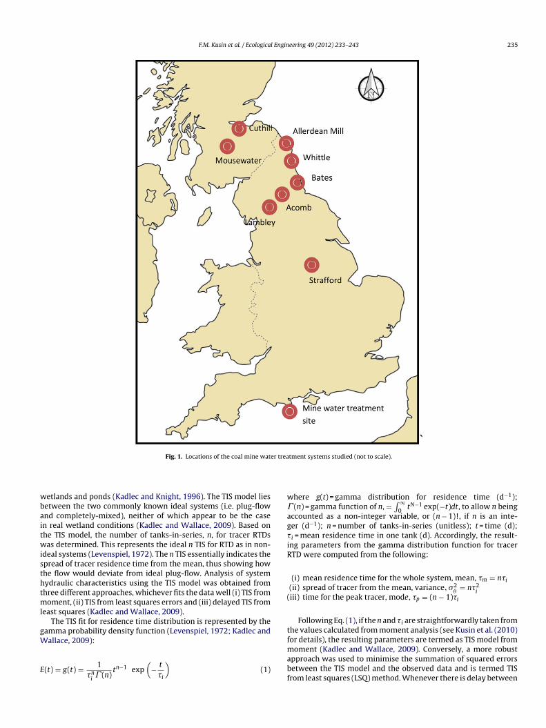
The study was undertaken at eight UK Coal Authority mineater treatment systems within Northern England (main study

reas) and part of southern Scotland, which consist of mine waterreatment wetlands and settlement lagoons (Fig. 1). The systemsere designed to treat net-alkaline (i.e. alkalinity > acidity), ferrug-

nous mine water with design flow capacity ranging between 10nd 88 L/s and influent iron concentration from 6 mg/L to 60 mg/L.rrespective of lagoon or wetland, these include a range of relativelymall to very large systems, of between 600 and 11,400 m2 treat-ent area. In typical applications of passive treatment within theK coal mine water treatment systems, settlement lagoon serves a pre-treatment unit preceded by an aeration cascade, aimed atemoving about 50% iron by means of hydrolysis and settlement oferric hydroxides, prior to final polishing in wetland system (or aeries of wetlands) (Younger et al., 2002).

.2. Field sampling and measurements

.2.1. Tracer test implementationThe hydraulic factors influencing treatment performance were

ssessed by means of conducting tracer tests to experimentallyetermine the actual residence time within the treatment systems.ackground tracer concentrations were pre-determined from sam-les taken prior to the tracer experiments (Lin et al., 2003;olkersdorfer et al., 2005) so that any changes due to tracer addi-

ion could be detected and that the actual mass recovered coulde precisely determined. The method employed for the tracer test

as the slug tracer injection, where a known amount of tracer was

njected into the inlet of the treatment system and complete mix-ng with the flow was assumed (Kilpatrick and Cobb, 1985). Tonsure maximum mixing, the tracers were dissolved with the mine

mmWi

eering 49 (2012) 233– 243

ater and were poured directly into the turbulent zone at the inletischarge point. Throughout the full series of tracer experimentshree types of tracer have been employed; sodium bromide, Na-uorescein and sodium chloride. Dual-tracer tests were conductedhenever possible for verifying the results (Kusin et al., 2009).

Samples of mine water were automatically collected byquamatic Auto Cell P2 Autosamplers equipped with 24 × 1 Lolyethylene bottlers at specific time intervals (estimated basedn the system nominal residence time). The tracer test typicallyakes between 24 and 72 h, depending on the system nominal res-dence time. On-site measurement for bromide was not available,ut other tracers i.e. Na-fluorescein and NaCl were measured in theeld. Outlet autosamplers were installed for capturing the recov-red bromide tracer. The bromide was analysed in the laboratorysing a calibrated Dionex 100 Ion Chromatograph. Na-fluoresceinas continuously measured in the field using a calibrated Sea-oint fluorimeter (detection limit 0.2 �g/L) which was set up toake the concentration readings at 5 min intervals. Alternatively,he Na-fluorescein was also analysed in the laboratory using aarian Cary Eclipse Fluorescence Spectrometer whenever on-siteeasurement was not possible and/or for verifying the results.

he sodium chloride tracer was measured as electrical conduc-ivity which was recorded using an Eijelkamp CTD Diver at 5 minntervals.

.3. Flow measurements

The flow rates during the tracer tests were continuously mon-tored at the outlet of the systems using an Eijelkamp CTD Divernd a BaroDiver for atmospheric pressure correction. The watereads were ascertained using water levels data recorded by theijelkamp CTD Diver. The BaroDiver semi-continuously measuredhe water and atmospheric pressure, temperature and conductiv-ty at a point behind the 90◦ V-notch weir where the water wasot disturbed by the sharp notch. Velocity–area method was usedhenever other methods were not possible e.g. in an open channel

t the inlet of treatment system. The water depth was measuredsing a graduated pole and a flow impeller was set at 0.6 of theepth measured downstream from the surface (Brassington, 2007;haw et al., 2011). The velocity was measured using a Valeportodel 801 Electromagnetic Flow Meter suspended in the water

ointing in an upstream direction. Measured flow rates ware takenithin 5–10% precision (PIRAMID Consortium, 2003; Brassington,

007). For precision, timely data of the measured flow rates werescertained (i.e. 5, 10 and 15 min intervals) and are used to compareetween dynamic (timely data) and average flow using momentnalysis. This enables precise measurement and analysis to beade as a means for demonstrating that the flow rates were con-

istent throughout the duration of the tracer tests.

.3.1. Tracer flow-pattern modellingA modelling approach was adopted as a means for comparing

he actual tracer residence time distribution (RTD) responses dur-ng the tracer tests with the expected theoretical response, to assessystem performance under current design. Modelling of the tracerTD curves was applied to determine the main RTD characteris-ics (i.e. mean residence time, variance (spread of tracer) and modepeak of tracer)) which will then lead to determination of treatmentystem performance metrics i.e. system volumetric efficiency (ev),TD efficiency (eRTD) and the overall hydraulic efficiency (e�).

The tracer RTDs were modelled based on a tanks-in-series (TIS)

odel, which is believed to represent a good approximation ofost wetland conditions and/or systems similar to it (Kadlec andallace, 2009). The model is simple and can be used with any kinet-

cs (Levenspiel, 1972), and is a widely applied tool for treatment

F.M. Kusin et al. / Ecological Engineering 49 (2012) 233– 243 235

r trea

wbaitwisthtml

gW

E

w�ag�iR

(

tf

Fig. 1. Locations of the coal mine wate

etlands and ponds (Kadlec and Knight, 1996). The TIS model liesetween the two commonly known ideal systems (i.e. plug-flownd completely-mixed), neither of which appear to be the casen real wetland conditions (Kadlec and Wallace, 2009). Based onhe TIS model, the number of tanks-in-series, n, for tracer RTDsas determined. This represents the ideal n TIS for RTD as in non-

deal systems (Levenspiel, 1972). The n TIS essentially indicates thepread of tracer residence time from the mean, thus showing howhe flow would deviate from ideal plug-flow. Analysis of systemydraulic characteristics using the TIS model was obtained fromhree different approaches, whichever fits the data well (i) TIS from

oment, (ii) TIS from least squares errors and (iii) delayed TIS fromeast squares (Kadlec and Wallace, 2009).

The TIS fit for residence time distribution is represented by theamma probability density function (Levenspiel, 1972; Kadlec andallace, 2009):

(t) = g(t) = 1�n

i� (n)

tn−1 exp(

− t

�i

)(1)

mabf

tment systems studied (not to scale).

here g(t) = gamma distribution for residence time (d−1); (n) = gamma function of n, =

∫ ∞0

tN−1 exp(−t)dt, to allow n beingccounted as a non-integer variable, or (n − 1)!, if n is an inte-er (d−1); n = number of tanks-in-series (unitless); t = time (d);i = mean residence time in one tank (d). Accordingly, the result-ng parameters from the gamma distribution function for tracerTD were computed from the following:

(i) mean residence time for the whole system, mean, �m = n�i

(ii) spread of tracer from the mean, variance, �2�

= n�2i

iii) time for the peak tracer, mode, �p = (n − 1)�i

Following Eq. (1), if the n and �i are straightforwardly taken fromhe values calculated from moment analysis (see Kusin et al. (2010)or details), the resulting parameters are termed as TIS model from

oment (Kadlec and Wallace, 2009). Conversely, a more robustpproach was used to minimise the summation of squared errorsetween the TIS model and the observed data and is termed TISrom least squares (LSQ) method. Whenever there is delay between

2 l Engin

tLa

g

w

pmtoa(

�

w

mfco

e

wtuas�t(

�

wN((wti

3

3

3

ftbaintaicardhtrr(sqmmwmtmec

mohbpfeaR

TS

36 F.M. Kusin et al. / Ecologica

racer injection and first tracer detection, delayed TIS model fromSQ was used (Kadlec et al., 1993; Chazarenc et al., 2003; Kadlecnd Wallace, 2009).

(t) = 1�i(n − 1)!

(t − tD

�i

)n−1exp

(− t − tD

�i

)(2)

here tD = delay time (d); �i = tracer residence time in one tank (d).Results from a TIS model can in fact be compared to those of a

lug-flow with dispersion (PFD) model (another commonly appliedodel for tracer flow studies). According to the PFD model, sys-

em dispersion number, D, for systems with relatively large extentf dispersion (D > 0.01), was calculated according to the appropri-te boundary conditions as follows (i.e. for closed-closed systemLevenspiel, 1999)):

2� = 2D − 2D2(1 − e−1/D) (3)

here �2�

= system dimensionless variance = �2/t2m (unitless).

Hydraulic efficiency (e�) for the treatment systems was deter-ined using Eq. (4) (after Persson et al., 1999), reflecting both the

ractions of water involved in the flow-through and the mixingharacteristics of water movement characterised by the behaviourf system dispersion.

� = eveRTD (4)

here ev = (tm/tan) = (Veff/V); tm = actual mean residence time (d);an = actual nominal residence time (d); Veff = system effective vol-me; (m3) V = system nominal volume (m3); Q = flow rate (m3/d),nd eRTD = residence time distribution efficiency = (1 − �2

�); �2

�=

ystem dimensionless variance (unitless). Note that the term (1 −2�

) is an equivalent form of (1−1/n) (Kadlec and Wallace, 2009). Inhe case of a TIS system, the �an was determined as the followingKadlec and Wallace, 2009):

an = �in

(1N

∑N

j=1

(1

1 − (˛j/N)

))(5)

here ̨ = water loss fraction, ̨ = 1 − R = 1 − Qo/Qi (dimensionless); = total number of tanks; j = tank number counter i.e. j = 1, 2, . . ., N

unitless). Computation of this actual nominal residence time (Eq.5)) gives the advantages of accurately determine the fraction of

ater involved in the treatment as it takes account of the flow pat-

ern during tracer test, in addition to effect of flow changes betweennlet and outlet.

sft0

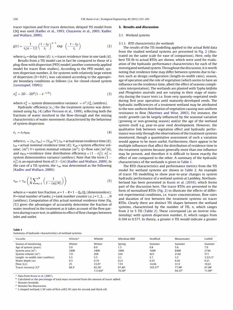
able 1ummary of hydraulic characteristics of wetland systems.

Variable Whittlea Whittle A

Season of monitoring Winter Winter SAge of system (years) 5.0 8.0 1System area (m2) 2400 2400 1System volume (m3) 721 458 2Length- to-width ratio (unitless) 5.5 5.5 2Water depth (m) 0.3 0.19 0Flow (L/s) 25 23.07 7Tracer recovery (%)b 60.3c 82.56c 6

113.64d 7

a Data from Kruse et al. (2007).b Calculated as the percentage of total mass recovered from the amount of tracer addedc Denotes bromide.d Denotes Na-fluorescein.e L-shaped wetland, L:W ratio of first cell/L:W ratio for second and third cell.

eering 49 (2012) 233– 243

. Results and discussion

.1. Wetland systems

.1.1. RTD characteristics for wetlandsThe results of the TIS modelling applied to the actual field data

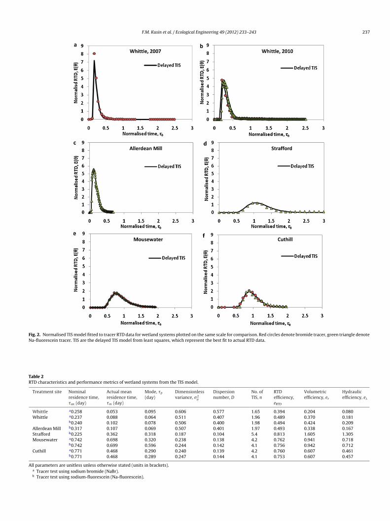
rom the studied wetland systems are presented in Fig. 2 (illus-rated on the same scale for ease of comparison). Here, only theest TIS fit to actual RTDs are shown, which were used for evalu-tion of the hydraulic performance characteristics for each of thenvestigated wetland system. Throughout the discussion, it is worthoting that residence time may differ between systems due to fac-ors such as design configuration (length-to-width ratio), season,ge of operation and the role of vegetation (which seems to have annfluence on the residence time, albeit the effect of seasons compli-ates interpretation). The wetlands are planted with Typha latifoliand Phragmites australis and are varying in their stage of matu-ity during the tracer tests i.e. from very sparsely-vegetated reedsuring first year operation until maturely-developed reeds. Theydraulic inefficiencies of a treatment wetland may be attributedo the non-uniform distribution of vegetation causing non-uniformesistance to flow (Martinez and Wise, 2003). For instance, theeeds’ growth can be largely influenced by the seasonal variationgrowing or non-growing season) and/or the age of the wetlandystem itself e.g. year-to-year reed development. However, theualitative link between vegetation effect and hydraulic perfor-ance was only through the observations of the treatment systemsonitored, though a quantitative assessment of such a variationould appear to be more useful. Furthermore, there appear to beultiple influences that affect the distribution of residence time in

he treatment systems because generally more than one influenceay be present, and therefore it is difficult to know exactly the

ffect of one compared to the other. A summary of the hydraulicharacteristics of the wetlands is given in Table 1.

The RTD characteristics and performance metrics from the TISodel for wetland systems are shown in Table 2. An example

f tracer TIS modelling to show year-to-year changes in systemydraulic performance of a wetland system at Lambley, Northum-erland has been presented in Kusin et al. (2010), which formsart of the discussion here. The tracer RTDs are presented in theorm of normalised RTDs (Fig. 2) to illustrate the effects of differ-nt experimental conditions, i.e. tracer concentrations, flow ratesnd duration of test between the treatment systems on tracerTDs. Clearly there are distinct TIS shapes between the wetland

ystems, characterised by the number of TIS, n, which rangesrom 2 to 5 TIS (Table 2). These correspond (as an inverse rela-ionship) with system dispersion number, D, which ranges from.104 to 0.577. In theory, a greater n TIS would indicate a greater

llerdean Mill Strafford Mousewater Cuthill

pring Summer Summer Summer.5 0.8 5.8 7.0066 1690 8400 274424 423 2142 571.1 5.7 3.5 3.5/5.3e

.21 0.25 0.26 0.21

.91 14.04 31.9 10.617.40c 103.57d 77.98c 67.98c

6.58d 94.33d 71.99d

.

F.M. Kusin et al. / Ecological Engineering 49 (2012) 233– 243 237

Fig. 2. Normalised TIS model fitted to tracer RTD data for wetland systems plotted on the same scale for comparison. Red circles denote bromide tracer, green triangle denoteNa-fluorescein tracer. TIS are the delayed TIS model from least squares, which represent the best fit to actual RTD data.

Table 2RTD characteristics and performance metrics of wetland systems from the TIS model.

Treatment site Nominalresidence time,�an (day)

Actual meanresidence time,�m (day)

Mode, �p

(day)Dimensionlessvariance, �2

�

Dispersionnumber, D

No. ofTIS, n

RTDefficiency,eRTD

Volumetricefficiency, ev

Hydraulicefficiency, e�

Whittle a0.258 0.053 0.095 0.606 0.577 1.65 0.394 0.204 0.080Whittle a0.237 0.088 0.064 0.511 0.407 1.96 0.489 0.370 0.181

b0.240 0.102 0.078 0.506 0.400 1.98 0.494 0.424 0.209Allerdean Mill b0.317 0.107 0.069 0.507 0.401 1.97 0.493 0.338 0.167Strafford b0.225 0.362 0.318 0.187 0.104 5.4 0.813 1.605 1.305Mousewater a0.742 0.698 0.320 0.238 0.138 4.2 0.762 0.941 0.718

b0.742 0.699 0.596 0.244 0.142 4.1 0.756 0.942 0.712Cuthill a0.771 0.468 0.290 0.240 0.139 4.2 0.760 0.607 0.461

b0.771 0.468 0.289 0.247 0.144 4.1 0.753 0.607 0.457

All parameters are unitless unless otherwise stated (units in brackets).a Tracer test using sodium bromide (NaBr).b Tracer test using sodium-fluorescein (Na-fluorescein).

238 F.M. Kusin et al. / Ecological Engin

Tab

le

3Su

mm

ary

of

hyd

rau

lic

char

acte

rist

ics

of

lago

on

syst

ems.

Var

iabl

eA

com

ba

East

Aco

mba

Wes

tA

com

bEa

stA

com

bW

est

Wh

ittl

eaW

hit

tle

Bat

esri

ght

L1B

ates

righ

t

L2B

ates

left

L1B

ates

left

L2St

raff

ord

All

erd

ean

Mil

lM

ouse

wat

er

Cu

thil

l

Seas

on

of

mon

itor

ing

Win

ter

Win

ter

Win

ter

Sum

mer

Win

ter

Spri

ng

Sum

mer

Sum

mer

Sum

mer

Sum

mer

Sum

mer

Spri

ng

Sum

mer

Sum

mer

Age

of

syst

em

(yea

rs)

55

77

58

5.8

5.8

5.8

5.8

0.8

1.5

5.8

7.1

Syst

em

area

(m2)

375

375

375

375

900

900

2850

2850

2850

2850

850

883

3036

726

Syst

em

volu

me

(m3)

1050

1050

1050

1050

1305

1305

6242

6242

6242

6242

2040

1325

6527

1089

Len

gth

-to-

wid

th

rati

o(u

nit

less

)1.

51.

51.

51.

53.

03.

02.

02.

02.

02.

04.

54.

71.

23.

2

Wat

er

dep

th

(m)

2.8

2.8

2.8

2.8

1.65

1.65

2.2

2.2

2.2

2.2

2.4

1.6

2.2

2.0

Flow

(L/s

)6.

255.

86.

256.

525

2578

.69

78.6

958

.55

58.5

514

.04

9.67

36.7

210

.72

Trac

er

reco

very

(%)b

82.1

4c82

.14c

61.7

5c77

.74c

82.0

5c95

.97c

130.

62d

155.

24d

69.1

9d65

.78d

69.6

9d76

.58d

84.7

2c67

.66c

119.

29d

76.0

0d77

.68d

aD

ata

from

Kru

se

et

al. (

2007

).b

Cal

cula

ted

as

the

per

cen

tage

of

tota

l mas

s

reco

vere

d

from

the

amou

nt

of

trac

er

add

ed.

cD

enot

es

brom

ide.

dD

enot

es

Na-

flu

ores

cein

.

apip

shwnemttaTapRowNyech

palflPSpwfltl

3

tpeepsItei0dSra(sptarrftw

eering 49 (2012) 233– 243

mount of complete-mixing, and the more it approximates an ideallug-flow system (Persson et al., 1999). Therefore there should

deally be a small degree of dispersion resulted from this flowattern.

Individual assessment of the wetland systems using n and Dhowed that the Whittle wetland (during 2007 tracer test) had theighest dispersion number, D of 0.577 (corresponding to n = 1.7),hile the Strafford wetland indicated the lowest system dispersionumber of 0.104 (corresponding to n = 5.4). The poor flow mixingffect and variation from the ideal flow pattern at Whittle wetlanday be attributable to the apparent short-circuiting across the sys-

em following its fifth year operation. Field observation showedhat the wetland is a mature system with well-established reedsnd a substantial build up of dead plant material (Kruse et al., 2007).his can lead to the development of channels through the wetland,nd thus a rapid transit of flow across the system, but also there isortion of water that remained in the system longer (i.e. the longTD tail). In contrast, the Strafford system is only in its first yearperation, with notably very sparse reed growth, but the flow wasell-distributed within the system (i.e. a low dispersion number).ote that this is in contrast to Lambley wetland during its firstear operation, during which the flow was very dispersed (Kusint al., 2010). Thus, it appears that whilst reeds may result in short-ircuiting, neither are they necessarily essential to ensuring goodydraulic performance.

The greater flow mixing effect seen at Strafford wetland wasresumably due to the presence of deep zones and islands createds planting blocks near the inlet and in the middle of the wet-and system. This results in a greater mixing and redistribution ofow, and hence a more well-distributed flow across the system.ersson (2000), in a simulation of surface flow wetland shapes of acandinavian stormwater treatment wetland, found that an islandlaced in front of the inlet improves the hydraulic performanceith respect to effective volume and degree of mixing. Thus, theow in the Strafford wetland was found to be much less dispersedhan that of Whittle wetland, despite having a fairly similar systemength to width ratio.

.1.2. Hydraulic performance metrics for wetland systemsThe different TIS shapes resulted in the mean residence time for

he wetlands ranging from 0.05 to 0.7 days. However, direct com-arison of these mean residence times will not necessarily implyfficiency of the systems e.g. longer residence time does not nec-ssarily mean an efficient system, because such a system wouldrobably have a long nominal residence time (i.e. due to largeystem volume or a relatively low flow per treatment volume).nstead, an appropriate measure to compare between these sys-em residence times is by assessing the metric of system volumetricfficiency, ev which is a measure of mean relative to nominal res-dence time. Generally, the wetland systems have a range of ev of.204–1.605. Again, the lowest was found in the Whittle wetlanduring the 2007 tracer test, whilst the longest was found in thetrafford wetland in the 2009 tracer test. These, apparently cor-espond with the systems dispersion characteristics i.e. the n TISnd D, as discussed earlier. The high ev in the Strafford wetlandmean residence time 60% higher than nominal residence time)hows that the wetland system was capable of retaining a largeroportion of water volume during flow passage through the sys-em, whilst enhancing a more distributed flow across the systemnd thus encourage a long water travel time. Sherman et al. (2009)eported a mean residence time of 50% greater than the nominal

esidence time in a free water surface wetland treating effluentrom a mine’s wastewater treatment plant in Australia. However,he reason of this larger mean relative to nominal residence timeas not reported.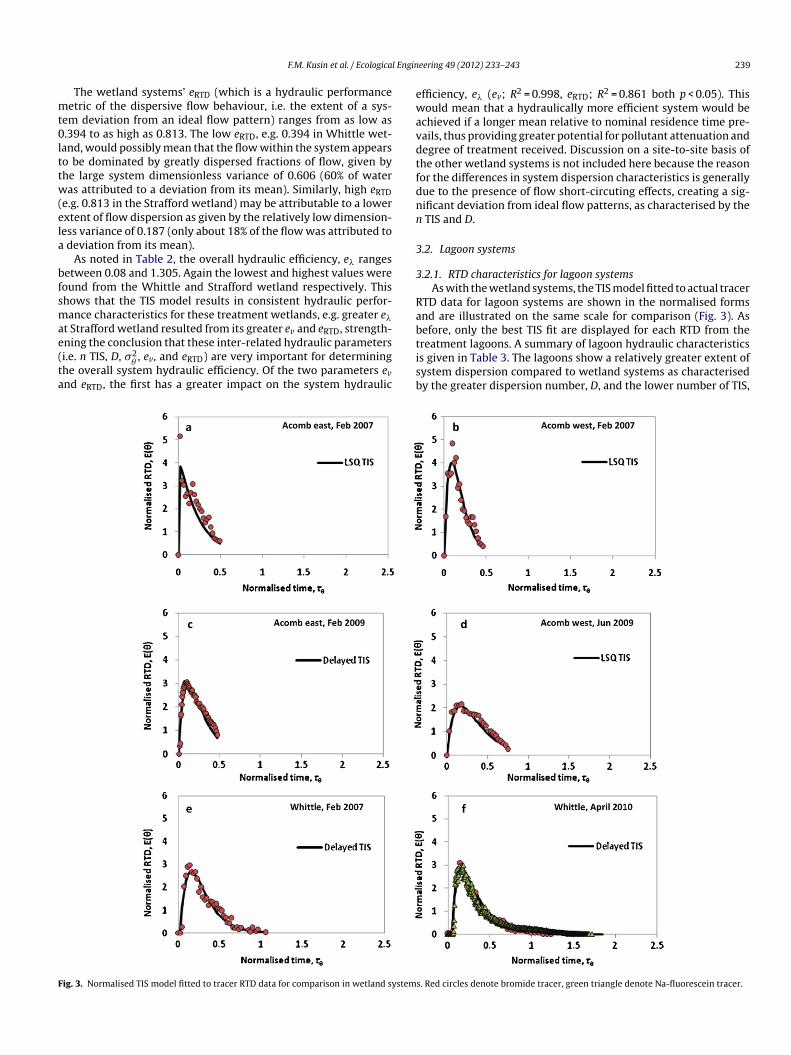

Engin

mt0lttw(ela

bfsmae(ta

ewavdtfdnn

3

3

Rab

F

F.M. Kusin et al. / Ecological

The wetland systems’ eRTD (which is a hydraulic performanceetric of the dispersive flow behaviour, i.e. the extent of a sys-

em deviation from an ideal flow pattern) ranges from as low as.394 to as high as 0.813. The low eRTD, e.g. 0.394 in Whittle wet-

and, would possibly mean that the flow within the system appearso be dominated by greatly dispersed fractions of flow, given byhe large system dimensionless variance of 0.606 (60% of wateras attributed to a deviation from its mean). Similarly, high eRTD

e.g. 0.813 in the Strafford wetland) may be attributable to a lowerxtent of flow dispersion as given by the relatively low dimension-ess variance of 0.187 (only about 18% of the flow was attributed to

deviation from its mean).As noted in Table 2, the overall hydraulic efficiency, e� ranges

etween 0.08 and 1.305. Again the lowest and highest values wereound from the Whittle and Strafford wetland respectively. Thishows that the TIS model results in consistent hydraulic perfor-ance characteristics for these treatment wetlands, e.g. greater e�

t Strafford wetland resulted from its greater ev and eRTD, strength-

ning the conclusion that these inter-related hydraulic parametersi.e. n TIS, D, �2

�, ev, and eRTD) are very important for determining

he overall system hydraulic efficiency. Of the two parameters evnd eRTD, the first has a greater impact on the system hydraulic

tisb

ig. 3. Normalised TIS model fitted to tracer RTD data for comparison in wetland system

eering 49 (2012) 233– 243 239

fficiency, e� (ev; R2 = 0.998, eRTD; R2 = 0.861 both p < 0.05). Thisould mean that a hydraulically more efficient system would be

chieved if a longer mean relative to nominal residence time pre-ails, thus providing greater potential for pollutant attenuation andegree of treatment received. Discussion on a site-to-site basis ofhe other wetland systems is not included here because the reasonor the differences in system dispersion characteristics is generallyue to the presence of flow short-circuting effects, creating a sig-ificant deviation from ideal flow patterns, as characterised by the

TIS and D.

.2. Lagoon systems

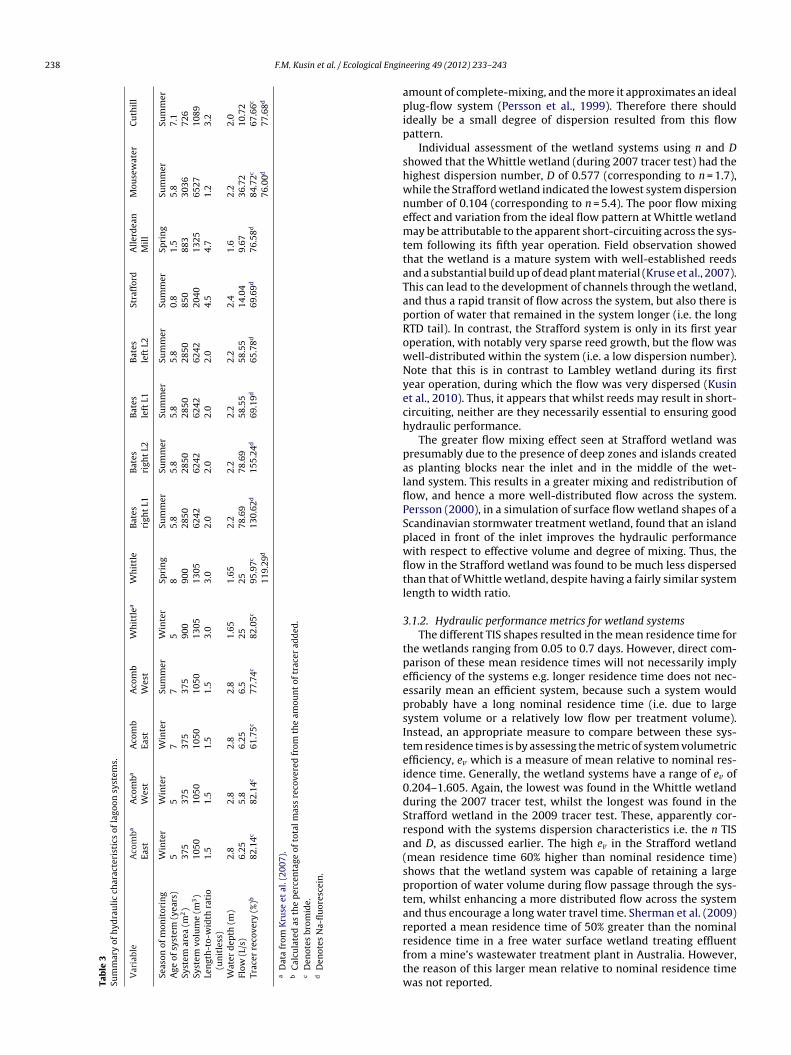
.2.1. RTD characteristics for lagoon systemsAs with the wetland systems, the TIS model fitted to actual tracer

TD data for lagoon systems are shown in the normalised formsnd are illustrated on the same scale for comparison (Fig. 3). Asefore, only the best TIS fit are displayed for each RTD from the

reatment lagoons. A summary of lagoon hydraulic characteristicss given in Table 3. The lagoons show a relatively greater extent ofystem dispersion compared to wetland systems as characterisedy the greater dispersion number, D, and the lower number of TIS,

s. Red circles denote bromide tracer, green triangle denote Na-fluorescein tracer.

240 F.M. Kusin et al. / Ecological Engineering 49 (2012) 233– 243

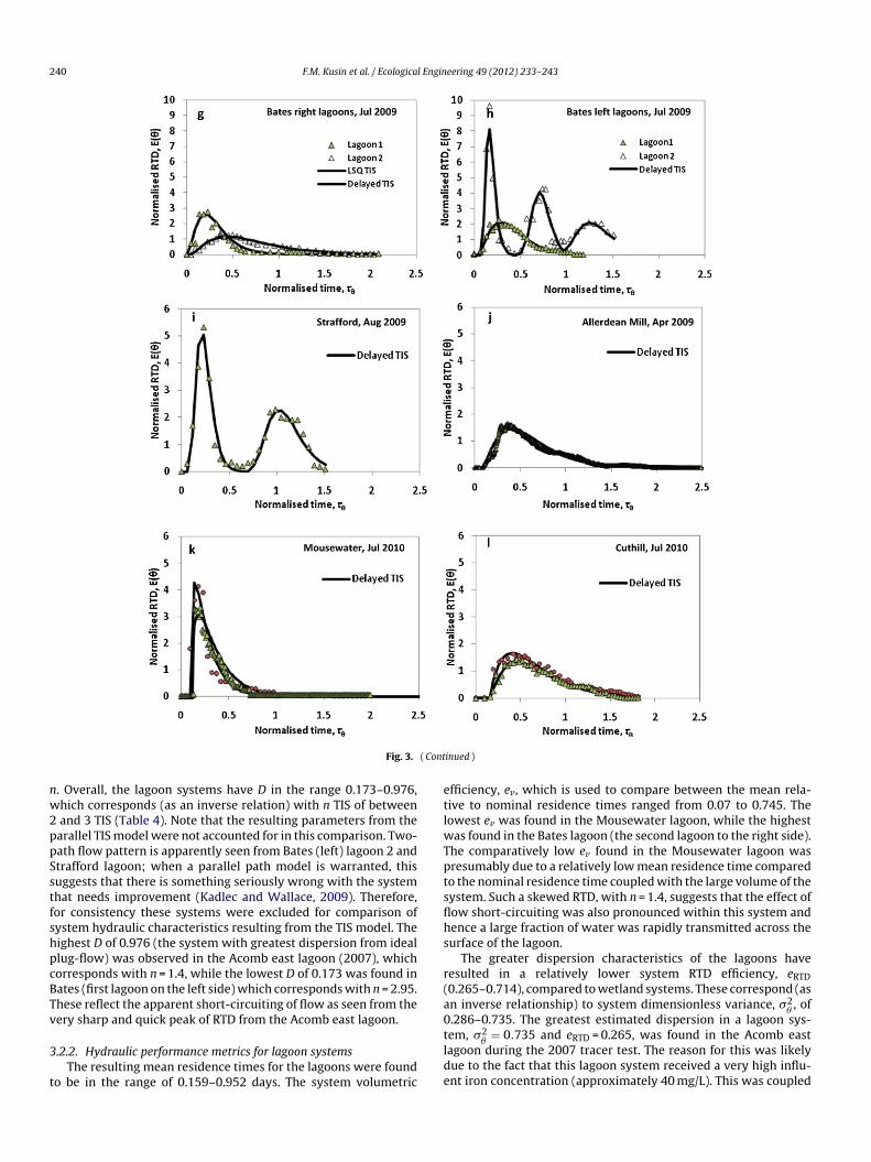
( Cont

nw2ppSstfshpcBTv

3

t

etlwTptsflhs

r(a0

Fig. 3.

. Overall, the lagoon systems have D in the range 0.173–0.976,hich corresponds (as an inverse relation) with n TIS of between

and 3 TIS (Table 4). Note that the resulting parameters from thearallel TIS model were not accounted for in this comparison. Two-ath flow pattern is apparently seen from Bates (left) lagoon 2 andtrafford lagoon; when a parallel path model is warranted, thisuggests that there is something seriously wrong with the systemhat needs improvement (Kadlec and Wallace, 2009). Therefore,or consistency these systems were excluded for comparison ofystem hydraulic characteristics resulting from the TIS model. Theighest D of 0.976 (the system with greatest dispersion from ideallug-flow) was observed in the Acomb east lagoon (2007), whichorresponds with n = 1.4, while the lowest D of 0.173 was found inates (first lagoon on the left side) which corresponds with n = 2.95.hese reflect the apparent short-circuiting of flow as seen from theery sharp and quick peak of RTD from the Acomb east lagoon.

.2.2. Hydraulic performance metrics for lagoon systemsThe resulting mean residence times for the lagoons were found

o be in the range of 0.159–0.952 days. The system volumetric

tlde

inued )

fficiency, ev, which is used to compare between the mean rela-ive to nominal residence times ranged from 0.07 to 0.745. Theowest ev was found in the Mousewater lagoon, while the highest

as found in the Bates lagoon (the second lagoon to the right side).he comparatively low ev found in the Mousewater lagoon wasresumably due to a relatively low mean residence time comparedo the nominal residence time coupled with the large volume of theystem. Such a skewed RTD, with n = 1.4, suggests that the effect ofow short-circuiting was also pronounced within this system andence a large fraction of water was rapidly transmitted across theurface of the lagoon.

The greater dispersion characteristics of the lagoons haveesulted in a relatively lower system RTD efficiency, eRTD0.265–0.714), compared to wetland systems. These correspond (asn inverse relationship) to system dimensionless variance, �2

�, of

.286–0.735. The greatest estimated dispersion in a lagoon sys-

em, �2

�= 0.735 and eRTD = 0.265, was found in the Acomb east

agoon during the 2007 tracer test. The reason for this was likelyue to the fact that this lagoon system received a very high influ-nt iron concentration (approximately 40 mg/L). This was coupled

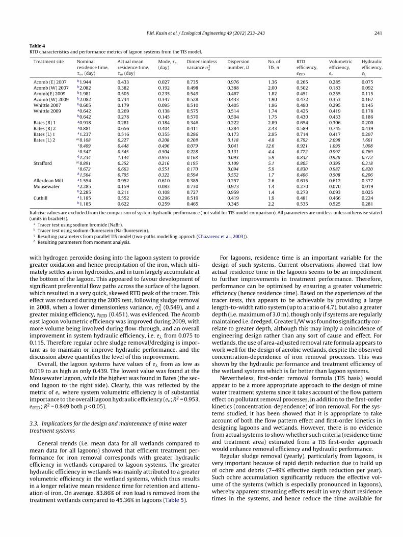
F.M. Kusin et al. / Ecological Engineering 49 (2012) 233– 243 241

Table 4RTD characteristics and performance metrics of lagoon systems from the TIS model.

Treatment site Nominalresidence time,�an (day)

Actual meanresidence time,�m (day)

Mode, �p

(day)Dimensionlessvariance �2

�

Dispersionnumber, D

No. ofTIS, n

RTDefficiency,eRTD

Volumetricefficiency,ev

Hydraulicefficiency,e�

Acomb (E) 2007 b1.944 0.433 0.027 0.735 0.976 1.36 0.265 0.285 0.075Acomb (W) 2007 b2.082 0.382 0.192 0.498 0.388 2.00 0.502 0.183 0.092Acomb(E) 2009 b1.981 0.505 0.235 0.549 0.467 1.82 0.451 0.255 0.115Acomb (W) 2009 b2.082 0.734 0.347 0.528 0.433 1.90 0.472 0.353 0.167Whittle 2007 b0.605 0.179 0.095 0.510 0.405 1.96 0.490 0.295 0.145Whittle 2009 a0.642 0.269 0.138 0.575 0.514 1.74 0.425 0.419 0.178

b0.642 0.278 0.145 0.570 0.504 1.75 0.430 0.433 0.186Bates (R) 1 a0.918 0.281 0.184 0.346 0.222 2.89 0.654 0.306 0.200Bates (R) 2 a0.881 0.656 0.404 0.411 0.284 2.43 0.589 0.745 0.439Bates (L) 1 a1.237 0.516 0.355 0.286 0.173 2.95 0.714 0.417 0.297Bates (L) 2 ac0.108 0.227 0.208 0.208 0.118 4.8 0.792 2.098 1.661

c0.409 0.448 0.496 0.079 0.041 12.6 0.921 1.095 1.008c0.547 0.545 0.504 0.228 0.131 4.4 0.772 0.997 0.769d1.234 1.144 0.953 0.168 0.093 5.9 0.832 0.928 0.772

Strafford ac0.891 0.352 0.216 0.195 0.109 5.1 0.805 0.395 0.318c0.672 0.663 0.551 0.170 0.094 5.9 0.830 0.987 0.820d1.564 0.795 0.322 0.594 0.552 1.7 0.406 0.508 0.206

Allerdean Mill a1.554 0.952 0.610 0.385 0.257 2.6 0.615 0.612 0.377Mousewater a2.285 0.159 0.083 0.730 0.973 1.4 0.270 0.070 0.019

b2.285 0.211 0.108 0.727 0.959 1.4 0.273 0.093 0.025Cuthill a1.185 0.552 0.296 0.519 0.419 1.9 0.481 0.466 0.224

b1.185 0.622 0.259 0.465 0.345 2.2 0.535 0.525 0.281

Italicise values are excluded from the comparison of system hydraulic performance (not valid for TIS model comparison). All parameters are unitless unless otherwise stated(units in brackets).

a Tracer test using sodium bromide (NaBr).

hazar

wgmtsweigemi0td

0Momie

3t

mfehviat

datpetldmrewwcst

awektadfaw

vo

b Tracer test using sodium-fluorescein (Na-fluorescein).c Resulting parameters from parallel TIS model (two-paths modelling approch (Cd Resulting parameters from moment analysis.

ith hydrogen peroxide dosing into the lagoon system to providereater oxidation and hence precipitation of the iron, which ulti-ately settles as iron hydroxides, and in turn largely accumulate at

he bottom of the lagoon. This appeared to favour development ofignificant preferential flow paths across the surface of the lagoon,hich resulted in a very quick, skewed RTD peak of the tracer. This

ffect was reduced during the 2009 test, following sludge removaln 2008, when a lower dimensionless variance, �2

�(0.549), and a

reater mixing efficiency, eRTD (0.451), was evidenced. The Acombast lagoon volumetric efficiency was improved during 2009, withore volume being involved during flow-through, and an overall

mprovement in system hydraulic efficiency, i.e. e� from 0.075 to.115. Therefore regular ochre sludge removal/dredging is impor-ant as to maintain or improve hydraulic performance, and theiscussion above quantifies the level of this improvement.

Overall, the lagoon systems have values of e� from as low as.019 to as high as only 0.439. The lowest value was found at theousewater lagoon, while the highest was found in Bates (the sec-

nd lagoon to the right side). Clearly, this was reflected by theetric of ev where system volumetric efficiency is of substantial

mportance to the overall lagoon hydraulic efficiency (ev; R2 = 0.953,RTD; R2 = 0.849 both p < 0.05).

.3. Implications for the design and maintenance of mine waterreatment systems

General trends (i.e. mean data for all wetlands compared toean data for all lagoons) showed that efficient treatment per-

ormance for iron removal corresponds with greater hydraulicfficiency in wetlands compared to lagoon systems. The greaterydraulic efficiency in wetlands was mainly attributed to a greater

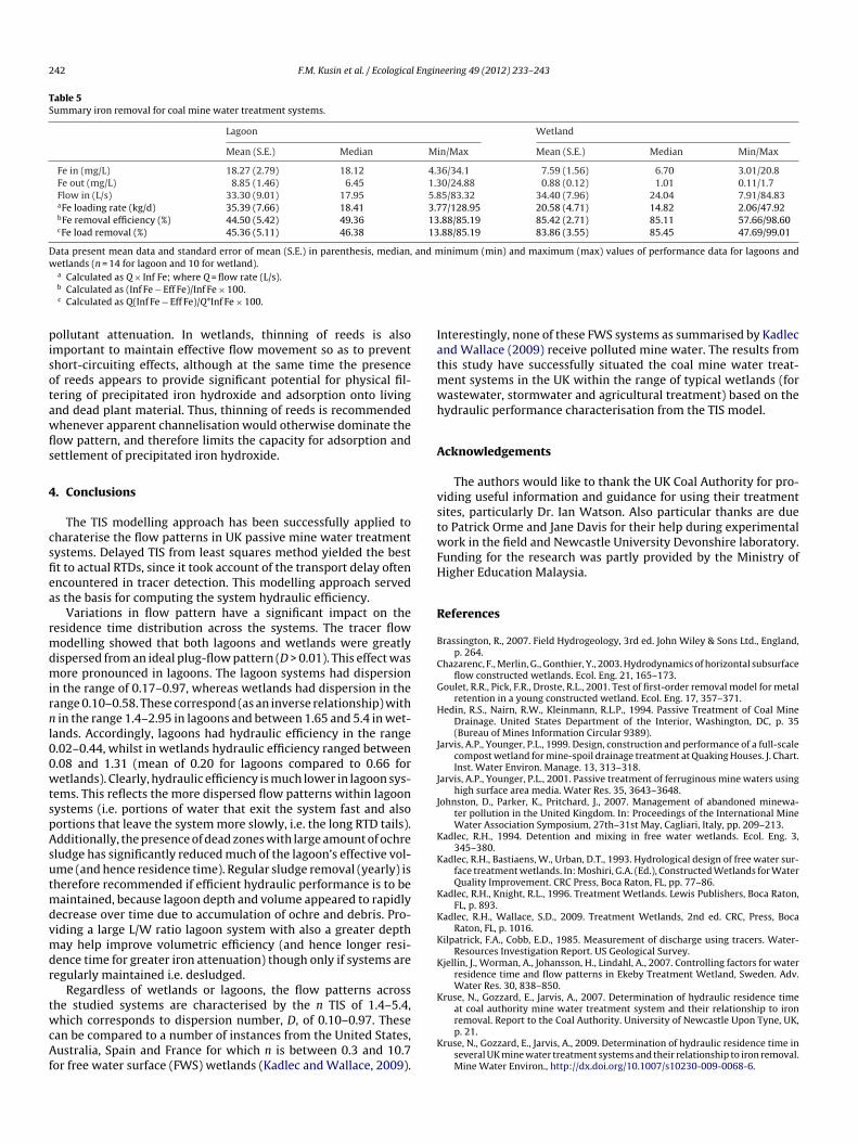
olumetric efficiency in the wetland systems, which thus resultsn a longer relative mean residence time for retention and attenu-tion of iron. On average, 83.86% of iron load is removed from thereatment wetlands compared to 45.36% in lagoons (Table 5).

Suwt

enc et al., 2003)).

For lagoons, residence time is an important variable for theesign of such systems. Current observations showed that lowctual residence time in the lagoons seems to be an impedimento further improvements in treatment performance. Therefore,erformance can be optimised by ensuring a greater volumetricfficiency (hence residence time). Based on the experiences of theracer tests, this appears to be achievable by providing a largeength-to-width ratio system (up to a ratio of 4.7), but also a greaterepth (i.e. maximum of 3.0 m), though only if systems are regularlyaintained i.e. dredged. Greater L/W was found to significantly cor-

elate to greater depth, although this may imply a coincidence ofngineering design rather than any sort of cause and effect. Foretlands, the use of area-adjusted removal rate formula appears toork well for the design of aerobic wetlands, despite the observed

oncentration-dependence of iron removal processes. This washown by the hydraulic performance and treatment efficiency ofhe wetland systems which is far better than lagoon systems.

Nevertheless, first-order removal formula (TIS basis) wouldppear to be a more appropriate approach to the design of mineater treatment systems since it takes account of the flow pattern

ffect on pollutant removal processes, in addition to the first-orderinetics (concentration-dependence) of iron removal. For the sys-ems studied, it has been showed that it is appropriate to takeccount of both the flow pattern effect and first-order kinetics inesigning lagoons and wetlands. However, there is no evidencerom actual systems to show whether such criteria (residence timend treatment area) estimated from a TIS first-order approachould enhance removal efficiency and hydraulic performance.

Regular sludge removal (yearly), particularly from lagoons, isery important because of rapid depth reduction due to build upf ochre and debris (7–49% effective depth reduction per year).

uch ochre accumulation significantly reduces the effective vol-me of the systems (which is especially pronounced in lagoons),hereby apparent streaming effects result in very short residence

imes in the systems, and hence reduce the time available for

242 F.M. Kusin et al. / Ecological Engineering 49 (2012) 233– 243

Table 5Summary iron removal for coal mine water treatment systems.

Lagoon Wetland

Mean (S.E.) Median Min/Max Mean (S.E.) Median Min/Max

Fe in (mg/L) 18.27 (2.79) 18.12 4.36/34.1 7.59 (1.56) 6.70 3.01/20.8Fe out (mg/L) 8.85 (1.46) 6.45 1.30/24.88 0.88 (0.12) 1.01 0.11/1.7Flow in (L/s) 33.30 (9.01) 17.95 5.85/83.32 34.40 (7.96) 24.04 7.91/84.83aFe loading rate (kg/d) 35.39 (7.66) 18.41 3.77/128.95 20.58 (4.71) 14.82 2.06/47.92bFe removal efficiency (%) 44.50 (5.42) 49.36 13.88/85.19 85.42 (2.71) 85.11 57.66/98.60cFe load removal (%) 45.36 (5.11) 46.38 13.88/85.19 83.86 (3.55) 85.45 47.69/99.01

Data present mean data and standard error of mean (S.E.) in parenthesis, median, and minimum (min) and maximum (max) values of performance data for lagoons andwetlands (n = 14 for lagoon and 10 for wetland).

pisotawfls

4

csfiea

rmdmirnl00wtspAsutmdvmdr

twcAf

Iatmwh

A

vstwFH

R

B

C

G

H

J

J

J

K

K

K

K

K

K

K

a Calculated as Q × Inf Fe; where Q = flow rate (L/s).b Calculated as (Inf Fe − Eff Fe)/Inf Fe × 100.c Calculated as Q(Inf Fe − Eff Fe)/Q*Inf Fe × 100.

ollutant attenuation. In wetlands, thinning of reeds is alsomportant to maintain effective flow movement so as to preventhort-circuiting effects, although at the same time the presencef reeds appears to provide significant potential for physical fil-ering of precipitated iron hydroxide and adsorption onto livingnd dead plant material. Thus, thinning of reeds is recommendedhenever apparent channelisation would otherwise dominate theow pattern, and therefore limits the capacity for adsorption andettlement of precipitated iron hydroxide.

. Conclusions

The TIS modelling approach has been successfully applied toharaterise the flow patterns in UK passive mine water treatmentystems. Delayed TIS from least squares method yielded the bestt to actual RTDs, since it took account of the transport delay oftenncountered in tracer detection. This modelling approach serveds the basis for computing the system hydraulic efficiency.

Variations in flow pattern have a significant impact on theesidence time distribution across the systems. The tracer flowodelling showed that both lagoons and wetlands were greatly

ispersed from an ideal plug-flow pattern (D > 0.01). This effect wasore pronounced in lagoons. The lagoon systems had dispersion

n the range of 0.17–0.97, whereas wetlands had dispersion in theange 0.10–0.58. These correspond (as an inverse relationship) with

in the range 1.4–2.95 in lagoons and between 1.65 and 5.4 in wet-ands. Accordingly, lagoons had hydraulic efficiency in the range.02–0.44, whilst in wetlands hydraulic efficiency ranged between.08 and 1.31 (mean of 0.20 for lagoons compared to 0.66 foretlands). Clearly, hydraulic efficiency is much lower in lagoon sys-

ems. This reflects the more dispersed flow patterns within lagoonystems (i.e. portions of water that exit the system fast and alsoortions that leave the system more slowly, i.e. the long RTD tails).dditionally, the presence of dead zones with large amount of ochreludge has significantly reduced much of the lagoon’s effective vol-me (and hence residence time). Regular sludge removal (yearly) isherefore recommended if efficient hydraulic performance is to be

aintained, because lagoon depth and volume appeared to rapidlyecrease over time due to accumulation of ochre and debris. Pro-iding a large L/W ratio lagoon system with also a greater depthay help improve volumetric efficiency (and hence longer resi-

ence time for greater iron attenuation) though only if systems areegularly maintained i.e. desludged.

Regardless of wetlands or lagoons, the flow patterns acrosshe studied systems are characterised by the n TIS of 1.4–5.4,

hich corresponds to dispersion number, D, of 0.10–0.97. These

an be compared to a number of instances from the United States,ustralia, Spain and France for which n is between 0.3 and 10.7

or free water surface (FWS) wetlands (Kadlec and Wallace, 2009).

K

nterestingly, none of these FWS systems as summarised by Kadlecnd Wallace (2009) receive polluted mine water. The results fromhis study have successfully situated the coal mine water treat-

ent systems in the UK within the range of typical wetlands (forastewater, stormwater and agricultural treatment) based on theydraulic performance characterisation from the TIS model.

cknowledgements

The authors would like to thank the UK Coal Authority for pro-iding useful information and guidance for using their treatmentites, particularly Dr. Ian Watson. Also particular thanks are dueo Patrick Orme and Jane Davis for their help during experimentalork in the field and Newcastle University Devonshire laboratory.

unding for the research was partly provided by the Ministry ofigher Education Malaysia.

eferences

rassington, R., 2007. Field Hydrogeology, 3rd ed. John Wiley & Sons Ltd., England,p. 264.

hazarenc, F., Merlin, G., Gonthier, Y., 2003. Hydrodynamics of horizontal subsurfaceflow constructed wetlands. Ecol. Eng. 21, 165–173.

oulet, R.R., Pick, F.R., Droste, R.L., 2001. Test of first-order removal model for metalretention in a young constructed wetland. Ecol. Eng. 17, 357–371.

edin, R.S., Nairn, R.W., Kleinmann, R.L.P., 1994. Passive Treatment of Coal MineDrainage. United States Department of the Interior, Washington, DC, p. 35(Bureau of Mines Information Circular 9389).

arvis, A.P., Younger, P.L., 1999. Design, construction and performance of a full-scalecompost wetland for mine-spoil drainage treatment at Quaking Houses. J. Chart.Inst. Water Environ. Manage. 13, 313–318.

arvis, A.P., Younger, P.L., 2001. Passive treatment of ferruginous mine waters usinghigh surface area media. Water Res. 35, 3643–3648.

ohnston, D., Parker, K., Pritchard, J., 2007. Management of abandoned minewa-ter pollution in the United Kingdom. In: Proceedings of the International MineWater Association Symposium, 27th–31st May, Cagliari, Italy, pp. 209–213.

adlec, R.H., 1994. Detention and mixing in free water wetlands. Ecol. Eng. 3,345–380.

adlec, R.H., Bastiaens, W., Urban, D.T., 1993. Hydrological design of free water sur-face treatment wetlands. In: Moshiri, G.A. (Ed.), Constructed Wetlands for WaterQuality Improvement. CRC Press, Boca Raton, FL, pp. 77–86.

adlec, R.H., Knight, R.L., 1996. Treatment Wetlands. Lewis Publishers, Boca Raton,FL, p. 893.

adlec, R.H., Wallace, S.D., 2009. Treatment Wetlands, 2nd ed. CRC, Press, BocaRaton, FL, p. 1016.

ilpatrick, F.A., Cobb, E.D., 1985. Measurement of discharge using tracers. Water-Resources Investigation Report. US Geological Survey.

jellin, J., Worman, A., Johansson, H., Lindahl, A., 2007. Controlling factors for waterresidence time and flow patterns in Ekeby Treatment Wetland, Sweden. Adv.Water Res. 30, 838–850.

ruse, N., Gozzard, E., Jarvis, A., 2007. Determination of hydraulic residence timeat coal authority mine water treatment system and their relationship to iron

removal. Report to the Coal Authority. University of Newcastle Upon Tyne, UK,p. 21.

ruse, N., Gozzard, E., Jarvis, A., 2009. Determination of hydraulic residence time inseveral UK mine water treatment systems and their relationship to iron removal.Mine Water Environ., http://dx.doi.org/10.1007/s10230-009-0068-6.

Engin

K

K

L

L

M

L

P

P

C

T

T

S

S

S

W

W

Y

Y

F.M. Kusin et al. / Ecological

usin, F.M., Kruse, N., Mayes, W.M., Jarvis, A.P., 2009. A comparative study ofhydraulic residence time using a multi-tracer approach at a coal mine watertreatment wetland, Lambley, Northumberland UK. In: Proceedings of the 8thICARD, 22–26 June 2009, Skellefteå, Sweden.

usin, F.M., Jarvis, A.P., Gandy, C.J., 2010. Hydraulic residence time and iron removalin a wetland receiving ferruginous mine water over a 4 year period from com-missioning. Water Sci. Technol. 62 (8), 1937–1946.

evenspiel, O., 1972. Chemical Reaction Engineering, 1st ed. John Wiley & Sons, NewYork.

evenspiel, O., 1999. Chemical Reaction Engineering, 3rd ed. John Wiley & Sons, NewYork, p. 664.

artinez, C.J., Wise, W.R., 2003. Hydraulic analysis of Orlando easterly wetland. J.Environ. Eng. 129, 553–559.

in, A.Y.C., Debroux, J.F., Cunningham, J.A., Reinhard, M., 2003. Comparison of rho-damine WT and bromide in the determination of hydraulic characteristics ofconstructed wetlands. Ecol. Eng. 20, 75–88.

ersson, J., 2000. The hydraulic performance of ponds of various layouts. UrbanWater 2, 243–250.

ersson, J., Somes, N.L.G., Wong, Y.H.F., 1999. Hydraulics efficiency ofconstructed wetlands and ponds. Water Sci. Technol. 40 (3), 291–300.

onsortium, PIRAMID., 2003. Engineering guidelines for the passive remediation ofacidic and/or metalliferous mine drainage and similar wastewaters. In: Euro-pean Commission 5th Framework Programme Passive In Situ Remediation ofAcid Mine/Industrial Drainage (PIRAMID). University of Newcastle Upon Tyne,UK, p. 166.

Y

eering 49 (2012) 233– 243 243

arutis, W.J., Stark, L.R., Williams, F.M., 1999. Sizing and performance estimation ofcoal mine drainage wetlands. Ecol. Eng. 12 (3–4), 353–372.

hackston, E.L., Shields F.D.Jr., Schroeder, P.R., 1987. Residence time distributions ofshallow basins. J. Environ. Eng. (ASCE) 113 (6), 1319–1332.

apsford, D.J., Watson, I., 2011. A process-orientated design and performance assess-ment methodology for passive mine water treatment systems. Ecol. Eng. 37 (6),970–975.

haw, E.M., Beven, K.J., Chappell, N.A., Lamb, R., 2011. Hydrology in Practice, 4th ed.Taylor & Francis, London, p. 560.

herman, B.S., Trefry, M.G., Davey, P., 2009. Hydraulic characterisation of aconstructed wetland used for nitrogen removal via a dual-tracer test. In: Pro-ceedings of the International Mine Water Association Conference, 19th–23rdOctober, Pretoria, South Africa, pp. 548–556.

erner, T.M., Kadlec, R.H., 1996. Application of residence time distributions tostormwater treatment systems. Ecol. Eng. 7, 213–234.

olkersdorfer, C., Hasche, A., Gobel, J., Younger, P.L., 2005. Tracer test in the BowdenClose passive treatment system (UK)-preliminary results. WissenschaftlicheMitteilungen 28, 87–92.

ounger, P.L., 2000. The adoption and adaptation of passive treatment technologiesfor mine waters in the United Kingdom. Mine Water Environ. 19, 84–97.

ounger, P.L., Banwart, S.A., Hedin, R.S., 2002. Mine Water: Hydrology, Pollution

Remediation. Kluwer Academic Publishers, Dordrecht, Netherlands, p. 442.

ounger, P.L., Jayaweera, A., Wood, R., 2004. A full-scale reducing and alkalinity-producing system (RAPS) for the passive treatment of acidic, aluminium-richmine site drainage at Bowden Close, County Durham. In: Proceedings of theCL:AIRE Annual Project Conference, April 2004, London.