HAL Id: tel-02940092https://pastel.archives-ouvertes.fr/tel-02940092

Submitted on 16 Sep 2020

HAL is a multi-disciplinary open accessarchive for the deposit and dissemination of sci-entific research documents, whether they are pub-lished or not. The documents may come fromteaching and research institutions in France orabroad, or from public or private research centers.

L’archive ouverte pluridisciplinaire HAL, estdestinée au dépôt et à la diffusion de documentsscientifiques de niveau recherche, publiés ou non,émanant des établissements d’enseignement et derecherche français ou étrangers, des laboratoirespublics ou privés.

Hybrid refrigeration system with a novel membraneexchanger

Rasha Mustapha

To cite this version:Rasha Mustapha. Hybrid refrigeration system with a novel membrane exchanger. Chemical andProcess Engineering. Université Paris sciences et lettres, 2019. English. �NNT : 2019PSLEM073�.�tel-02940092�

Composition du jury :

Laurence, FOURNAISON

Directrice de Recherche, Irstea Président

Predrag, HRNJAK

Professeur, Université d’Illinois Rapporteur

Vincent, LEMORT

Professeur, Université de Liège Rapporteur

Khalil, EL KHOURY

Professeur, Université Libanaise Examinateur

Kamel, GHALI

Professeur, Université Américaine de Beyrouth Examinateur

Assaad, ZOUGHAIB

Professeur, PSL-Mines ParisTech Directeur de

thèse

Préparée à MINES ParisTech

Hybrid Refrigeration System with a Novel Membrane

Exchanger

Système de Réfrigération Hybride Comportant un

Echangeur Membranaire Innovant

Soutenue par

Rasha MUSTAPHA Le 15 Novembre 2019

Ecole doctorale n° 621

Ingénierie des Systèmes,

Matériaux, Mécanique,

Énergetique

Spécialité

Énergétique et Procédés

To the Memory of my Dad

2

ACKNOWLEDGMENT

This thesis would never have been realized without some great people who contributed with their

expertise and precious help.

I am absolutely thankful to my thesis advisor Dr. Assaad ZOUGHAIB for his continuous support

and insightful comments. His encouragement, friendly attitude and one-of-a-kind sense of humor

were the main sources of motivation during these three years.

Besides my adviser, I wish to thank the members of my dissertation committee: Dr. Predrag

HRNJAK, Dr. Vincent LEMORT, Dr. Laurence FOURNAISON, Dr. Kamel GHALI and Dr.

Khalil EL KHOURY for generously offering their time, support, guidance and good will

throughout the preparation and review of this thesis. I feel proud and honored that you have

accepted to be on my committee.

I would like to gratefully acknowledge the financial support of ERANETMED project Sol-Cool-

Dry, ID number: ERANETMED_ENERG-11-138 under ERA-MET Initiative “EURO-

MEDITERRANEAN Cooperation through ERANET joint activities of FP7 INITIATIVE

ERANETMED.

Throughout the ERANETMED project, I had the chance to participate in international academic

discussions. I am indebted to those who contributed to the rich exchange of ideas and information

especially Dr. Nesreen GHADDAR and Dr. Kamel GHALI. This research process was greatly

supported by their valuable insights. I would like to thank them as well for supplying us with

some membrane materials manufactured in the laboratories of the American University of Beirut.

I wish to record my gratitude to Dr. Khalil EL KHOURY for his help and constructive advices

throughout these years and who has always generously made his broad international relationships

available for his students.

My debts go to my colleagues for providing a stimulating environment for learning and growing

and even far beyond to those who read the manuscript and those who have accompanied me from

one moment to another during this period of research life.

Finally, nobody has been more important for me in the completion of this work than my family

members, Daad, Samer, Nathalie, Reem, Roni, Rayn and last but least Rami. I would like to

thank them all for their endless love and support providing me the necessary faith and strength to

pursue my goals. Without them life would have been much harder.

3

4

Table of Contents

ACKNOWLEDGMENT .................................................................................................................. 2

Table of Contents ............................................................................................................................ 4

List of Figures ................................................................................................................................ 8

List of Tables ............................................................................................................................... 10

Nomenclature ............................................................................................................................... 12

General Introduction ...................................................................................................................... 16

Chapitre 1 Contexte, Etat de l’art et la Problématique (résume) .............................................................. 18

Chapter 1 Context, State of the Art and Problem Statement ................................................................... 28

1.1 Context ............................................................................................................................ 28

1.1.1 The energy and environmental context ..................................................................................... 28

1.1.2 The refrigeration and cooling context ....................................................................................... 32

1.1.3 The humidity control issue..................................................................................................... 34

1.1.4 Conclusion ......................................................................................................................... 36

1.2 Desiccant Systems Review ............................................................................................... 36

1.2.1 Types of Desiccant ............................................................................................................... 37

1.2.2 Hybrid desiccant/vapor compression systems ............................................................................ 39

1.2.3 Heat and mass exchangers ..................................................................................................... 43

1.3 Thesis Problem Statement ............................................................................................... 53

Chapitre 2 Méthode Modifiée de la coupe pour Tester la Perméabilité de la Vapeur D'eau dans les Membranes

Poreuses (résumé) ......................................................................................................................... 54

Chapter 2 Modified Upright Cup Method for Testing Water Vapor Permeability in Porous Membranes ......... 62

2.1 Introduction ....................................................................................................................... 62

2.2 ASTM E96 Upright Cup Method .......................................................................................... 63

2.2.1 Procedure ...................................................................................................................... 63

2.2.2 Assumptions .................................................................................................................. 64

2.2.3 Discussion ..................................................................................................................... 64

2.3 Modified Upright Cup Method ............................................................................................. 65

2.3.1 Experimental Conditions Assessment ...................................................................................... 66

2.3.2 Tested Membranes ............................................................................................................... 66

5

2.3.3 Experimental Data and Measurements ..................................................................................... 66

2.3.4 Deduction of Water Vapor Permeability ................................................................................... 68

2.3.5 Results ............................................................................................................................... 72

2.3.6 Uncertainty Analysis ............................................................................................................ 73

2.4 Conclusion ......................................................................................................................... 79

Chapitre 3 Modélisation de l'échangeur de chaleur et de masse et validation expérimentale (résumé) .... 82

Chapter 3 Modeling the Heat and Mass Exchanger and Experimental Validation ............................. 100

3.1 Introduction ..................................................................................................................... 100

3.2 Test bench description ....................................................................................................... 101

3.2.1 Layout and components ...................................................................................................... 102

3.2.2 Description of the exchanger ................................................................................................ 102

3.2.3 Testing Procedure .............................................................................................................. 104

3.3 Experiments ..................................................................................................................... 105

3.4 Proposed heat and mass membrane exchanger model ........................................................... 106

3.4.1 Assumptions ..................................................................................................................... 107

3.4.2 Definitions, properties and basic relations ............................................................................... 108

3.4.3 Mathematical and discretized model ...................................................................................... 114

3.4.4 Numerical implementation of the model ................................................................................. 117

3.5 Application done on the prototype ...................................................................................... 129

3.5.1 Selection of water side heat transfer coefficient correlation ........................................................ 130

3.5.2 Comparison of the three computations schemes ....................................................................... 131

3.5.3 Model verification and validation .......................................................................................... 133

3.5.4 Uncertainty analysis ........................................................................................................... 141

3.5.5 Air side heat transfer coefficient correction ............................................................................. 150

3.6 Conclusion .................................................................................................................... 153

Chapitre 4 Étude de Cas : Une Conception Flexible d'un Système de Climatisation Hybride dans un

Bureau (résumé) ........................................................................................................................ 156

Chapter 4 Case Study: Flexible Design of a Hybrid Air Conditioning System in an Office .................. 168

4.1 Introduction .................................................................................................................. 168

4.2 Case study ..................................................................................................................... 169

4.2.1 Building description ........................................................................................................... 169

4.2.2 Cooling and dehumidification in the base case configuration ...................................................... 170

6

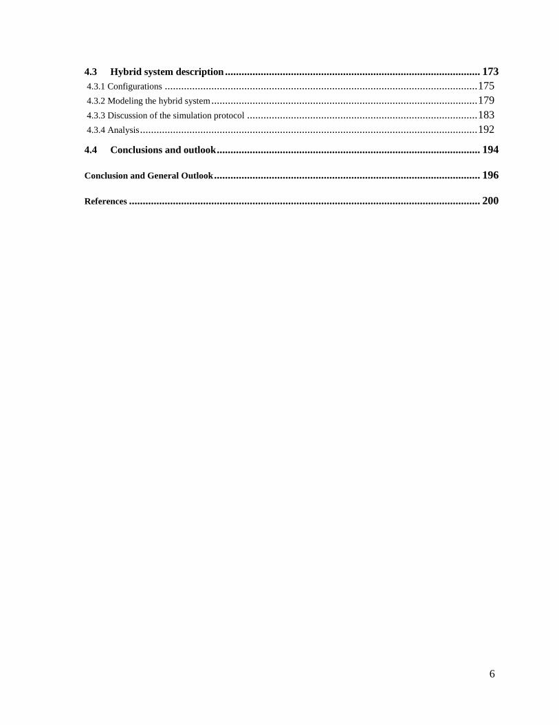
4.3 Hybrid system description ............................................................................................. 173

4.3.1 Configurations .................................................................................................................. 175

4.3.2 Modeling the hybrid system ................................................................................................. 179

4.3.3 Discussion of the simulation protocol .................................................................................... 183

4.3.4 Analysis ........................................................................................................................... 192

4.4 Conclusions and outlook ................................................................................................ 194

Conclusion and General Outlook ................................................................................................. 196

References ................................................................................................................................ 200

7

8

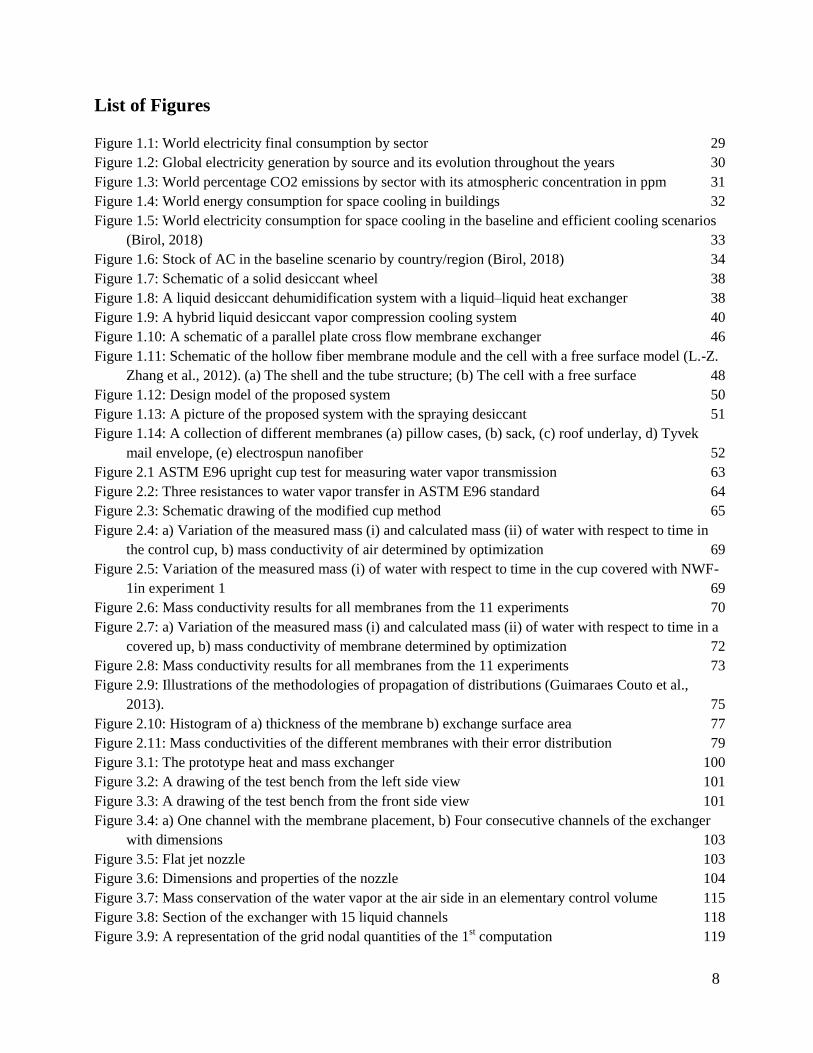
List of Figures

Figure 1.1: World electricity final consumption by sector 29

Figure 1.2: Global electricity generation by source and its evolution throughout the years 30

Figure 1.3: World percentage CO2 emissions by sector with its atmospheric concentration in ppm 31

Figure 1.4: World energy consumption for space cooling in buildings 32

Figure 1.5: World electricity consumption for space cooling in the baseline and efficient cooling scenarios

(Birol, 2018) 33

Figure 1.6: Stock of AC in the baseline scenario by country/region (Birol, 2018) 34

Figure 1.7: Schematic of a solid desiccant wheel 38

Figure 1.8: A liquid desiccant dehumidification system with a liquid–liquid heat exchanger 38

Figure 1.9: A hybrid liquid desiccant vapor compression cooling system 40

Figure 1.10: A schematic of a parallel plate cross flow membrane exchanger 46

Figure 1.11: Schematic of the hollow fiber membrane module and the cell with a free surface model (L.-Z.

Zhang et al., 2012). (a) The shell and the tube structure; (b) The cell with a free surface 48

Figure 1.12: Design model of the proposed system 50

Figure 1.13: A picture of the proposed system with the spraying desiccant 51

Figure 1.14: A collection of different membranes (a) pillow cases, (b) sack, (c) roof underlay, d) Tyvek

mail envelope, (e) electrospun nanofiber 52

Figure 2.1 ASTM E96 upright cup test for measuring water vapor transmission 63

Figure 2.2: Three resistances to water vapor transfer in ASTM E96 standard 64

Figure 2.3: Schematic drawing of the modified cup method 65

Figure 2.4: a) Variation of the measured mass (i) and calculated mass (ii) of water with respect to time in

the control cup, b) mass conductivity of air determined by optimization 69

Figure 2.5: Variation of the measured mass (i) of water with respect to time in the cup covered with NWF-

1in experiment 1 69

Figure 2.6: Mass conductivity results for all membranes from the 11 experiments 70

Figure 2.7: a) Variation of the measured mass (i) and calculated mass (ii) of water with respect to time in a

covered up, b) mass conductivity of membrane determined by optimization 72

Figure 2.8: Mass conductivity results for all membranes from the 11 experiments 73

Figure 2.9: Illustrations of the methodologies of propagation of distributions (Guimaraes Couto et al.,

2013). 75

Figure 2.10: Histogram of a) thickness of the membrane b) exchange surface area 77

Figure 2.11: Mass conductivities of the different membranes with their error distribution 79

Figure 3.1: The prototype heat and mass exchanger 100

Figure 3.2: A drawing of the test bench from the left side view 101

Figure 3.3: A drawing of the test bench from the front side view 101

Figure 3.4: a) One channel with the membrane placement, b) Four consecutive channels of the exchanger

with dimensions 103

Figure 3.5: Flat jet nozzle 103

Figure 3.6: Dimensions and properties of the nozzle 104

Figure 3.7: Mass conservation of the water vapor at the air side in an elementary control volume 115

Figure 3.8: Section of the exchanger with 15 liquid channels 118

Figure 3.9: A representation of the grid nodal quantities of the 1st computation 119

9

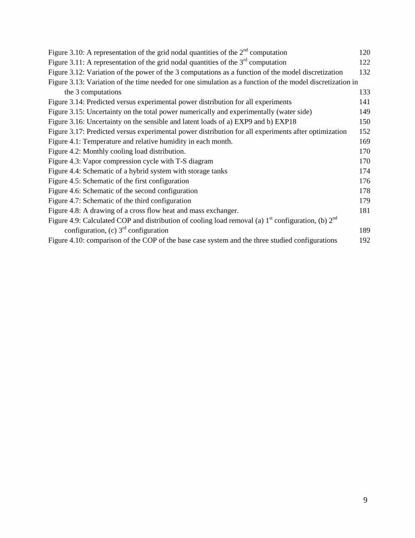
Figure 3.10: A representation of the grid nodal quantities of the 2nd

computation 120

Figure 3.11: A representation of the grid nodal quantities of the 3rd

computation 122

Figure 3.12: Variation of the power of the 3 computations as a function of the model discretization 132

Figure 3.13: Variation of the time needed for one simulation as a function of the model discretization in

the 3 computations 133

Figure 3.14: Predicted versus experimental power distribution for all experiments 141

Figure 3.15: Uncertainty on the total power numerically and experimentally (water side) 149

Figure 3.16: Uncertainty on the sensible and latent loads of a) EXP9 and b) EXP18 150

Figure 3.17: Predicted versus experimental power distribution for all experiments after optimization 152

Figure 4.1: Temperature and relative humidity in each month. 169

Figure 4.2: Monthly cooling load distribution. 170

Figure 4.3: Vapor compression cycle with T-S diagram 170

Figure 4.4: Schematic of a hybrid system with storage tanks 174

Figure 4.5: Schematic of the first configuration 176

Figure 4.6: Schematic of the second configuration 178

Figure 4.7: Schematic of the third configuration 179

Figure 4.8: A drawing of a cross flow heat and mass exchanger. 181

Figure 4.9: Calculated COP and distribution of cooling load removal (a) 1st configuration, (b) 2

nd

configuration, (c) 3rd

configuration 189

Figure 4.10: comparison of the COP of the base case system and the three studied configurations 192

10

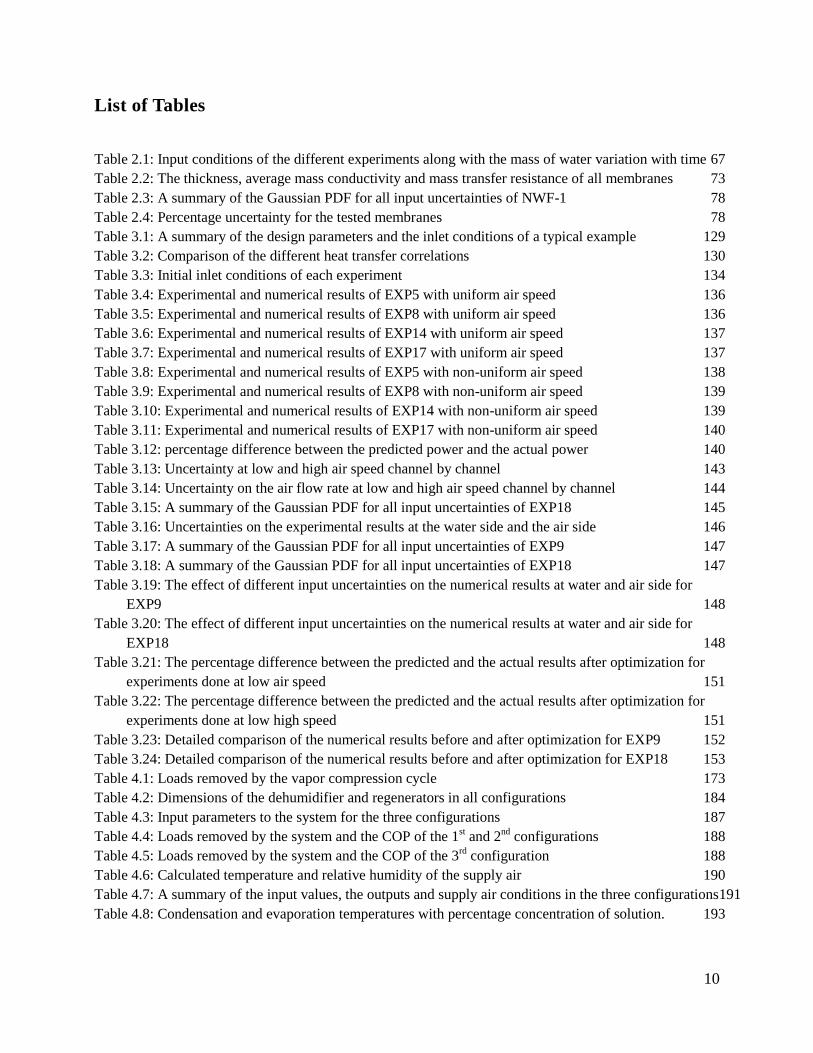
List of Tables

Table ‎2.1: Input conditions of the different experiments along with the mass of water variation with time 67

Table ‎2.2: The thickness, average mass conductivity and mass transfer resistance of all membranes 73

Table ‎2.3: A summary of the Gaussian PDF for all input uncertainties of NWF-1 78

Table ‎2.4: Percentage uncertainty for the tested membranes 78

Table ‎3.1: A summary of the design parameters and the inlet conditions of a typical example 129

Table ‎3.2: Comparison of the different heat transfer correlations 130

Table ‎3.3: Initial inlet conditions of each experiment 134

Table ‎3.4: Experimental and numerical results of EXP5 with uniform air speed 136

Table ‎3.5: Experimental and numerical results of EXP8 with uniform air speed 136

Table ‎3.6: Experimental and numerical results of EXP14 with uniform air speed 137

Table ‎3.7: Experimental and numerical results of EXP17 with uniform air speed 137

Table ‎3.8: Experimental and numerical results of EXP5 with non-uniform air speed 138

Table ‎3.9: Experimental and numerical results of EXP8 with non-uniform air speed 139

Table ‎3.10: Experimental and numerical results of EXP14 with non-uniform air speed 139

Table ‎3.11: Experimental and numerical results of EXP17 with non-uniform air speed 140

Table ‎3.12: percentage difference between the predicted power and the actual power 140

Table ‎3.13: Uncertainty at low and high air speed channel by channel 143

Table ‎3.14: Uncertainty on the air flow rate at low and high air speed channel by channel 144

Table ‎3.15: A summary of the Gaussian PDF for all input uncertainties of EXP18 145

Table ‎3.16: Uncertainties on the experimental results at the water side and the air side 146

Table ‎3.17: A summary of the Gaussian PDF for all input uncertainties of EXP9 147

Table ‎3.18: A summary of the Gaussian PDF for all input uncertainties of EXP18 147

Table ‎3.19: The effect of different input uncertainties on the numerical results at water and air side for

EXP9 148

Table ‎3.20: The effect of different input uncertainties on the numerical results at water and air side for

EXP18 148

Table ‎3.21: The percentage difference between the predicted and the actual results after optimization for

experiments done at low air speed 151

Table ‎3.22: The percentage difference between the predicted and the actual results after optimization for

experiments done at low high speed 151

Table ‎3.23: Detailed comparison of the numerical results before and after optimization for EXP9 152

Table ‎3.24: Detailed comparison of the numerical results before and after optimization for EXP18 153

Table ‎4.1: Loads removed by the vapor compression cycle 173

Table ‎4.2: Dimensions of the dehumidifier and regenerators in all configurations 184

Table ‎4.3: Input parameters to the system for the three configurations 187

Table ‎4.4: Loads removed by the system and the COP of the 1st and 2

nd configurations 188

Table ‎4.5: Loads removed by the system and the COP of the 3rd

configuration 188

Table ‎4.6: Calculated temperature and relative humidity of the supply air 190

Table ‎4.7: A summary of the input values, the outputs and supply air conditions in the three configurations191

Table ‎4.8: Condensation and evaporation temperatures with percentage concentration of solution. 193

11

12

Nomenclature

Latin letters

A Area

[m2]

C Concentration

[kg/kg] unless indicated otherwise

Specific heat at constant pressure [J/kg.K]

Mass diffusion coefficient [m2/s]

D Hydraulic diameter [m]

g Gravitational acceleration,

[m/s2]

h Specific enthalpy [J/kg]

H Enthalpy [J]

H Height [m]

Fan static pressure [m]

Latent heat of vaporization of water [J/kg]

Pump head [m]

Mass transfer coefficient [kg/m2.s]

Heat transfer coefficient [W/m2.K]

Heat transfer coefficient in the confined space [W/m2.K]

Thermal conductivity [W/m.K]

km Mass conductivity of the membrane [kg/m.s]

L Length [m]

Lc Characteristic length for convection correlations [m]

m Mass [kg]

Mass flow rate [kg/s] unless indicated otherwise

Ni Number of discretization in the direction of x-axis [-]

Nj Number of discretization in the direction of z-axis [-]

P Pressure [Pa]

Q Load or heat transfer [W]

Resistance to heat and mass transfer [m2s/kg] unless indicated

otherwise

R’ Ratio of latent to sensible load [%]

RH Relative humidity [%]

t Time [s]

T Temperature [K] unless indicated otherwise

u Uncertainty [%]

UM Overall mass exchange coefficient [kg/m2.s]

W Width [m]

X Mass of water per mass of dry desiccant [kgw/kgd]

Y Mass of water vapor per mass of dry air [kgv/kgda]

13

Z Height of the dehumidifier [m]

Dimensionless Numbers

Gr Grashof number [-]

Le Lewis number [-]

Nu Nusselt number [-]

Pr Prandtl number [-]

Ra Rayleigh number [-]

Re Raynold number [-]

Greek symbols

Correction factor at low air speed [-]

β Coefficient of volume expansion [1/K]

Correction factor at low air speed [-]

Thickness

[m]

η Efficiency [%]

Reduced temperature [-]

Kinematic viscosity of the fluid [m2/s]

Dynamic viscosity [N.s/m2]

Concentration of desiccant in the solution [kg/kg]

Density

[Kg/m3]

Subscripts

a Humid air

avg Average

b Boundary layer

c Cavity

C Celsius

cf Cold fluid

comp Compressor

cond Condenser

d Dry desiccant

da Dry air

dp Dew point

evap Evaporator

f Fan

f Falling film

hf Hot fluid

i Inlet

is Isentropic

14

L Latent

m Membrane

ma Membrane-air

ms Membrane-solution

mw Membrane-water

o Outlet

or Outlet return

p Pump

r Return

ref Refrigerant

reg Regenerator

s Desiccant solution

S Sensible

T Total

v Vapor

w Liquid water

Abbreviations and Acronyms

AC Air Conditioner

ACH Air Changes per Hour

ASTM American Society for Testing and Materials

CaCl2 Calcium Chloride

CO Carbon Monoxide

CO2 Carbon Dioxide

COP Coefficient of Performance

ESA European Space Agency

GHG Green House Gases

HVAC Heating, Ventilation and Air Conditioning

hx Heat Exchanger

IEA International Energy Agency

IPCC Intergovernmental Panel on Climate Change

ISO International Organization for Standardization

LAMEE Liquid to Air Membrane Energy Exchanger

LiBr Lithium Bromide

LiCl Lithium Chloride

MAE Mean Absolute Error

NOAA National Oceanic and Atmospheric Administration

NOx Nitrogen Oxides

NTU Number of Transfer Units

NWF Non Woven Fabric

15

PCM Phase Change Material

PDF Probability Density Function

PE Poly-Ethylene

PP Poly-Propylene

PTFE Poly-Tetra-Fluoro-Ethylene

RMSE Root Mean Square Error

SHGC Solar Heat Gain Coefficient

SOx Sulfur Oxides

std Standard Deviation

VCC Vapor Compression Cycle

16

General Introduction

The drastic impact of high energy consumption on the environment and on human’s health is

raising a critical alert which requires global strategic plans to overcome its destructive

consequences. Energy consumption has been remarkably increasing during the last few decades

and is likely to rise further in light of the developing global economy. In particular, higher

electricity demands are forecasted mainly for heating and cooling in some cities of the world.

Amidst the universal growth in the energy demand and its significant environmental impacts, it is

of great importance to find techniques that provide the energy needs of the economies and

simultaneously reduce the GHG emissions. Fundamental changes in the energy sector is evolving

worldwide primarily driven by the integration of renewable energy sources and more energy

efficient technologies.

Our work starts by describing the energy and environmental context related to the world

electricity final consumption and percentage of CO2 emissions by sector. It is shown that

buildings play a dominant role accounting to 36% of global final energy consumption and having

the largest share of the energy-related CO2 emissions. Electricity use in buildings has had the

largest growth of 15% between 2010 and 2017 with the space cooling leading this growth by

more than 20% (International Energy Agency and the United Nations Environment

Program, 2018). Space cooling is usually performed through vapor compression cycles that have

low Coefficients of Performance (COP) and show deficiencies in handling latent loads. They

consume excessive energy to remove humidity through cooling the air below its dew point

temperature and then they reheat it to the desired indoor temperature. Therefore, realizing the

potential of the buildings sector in contributing to the electricity consumption triggers the

initiation of energy efficient building measures aiming to improve applications related mainly to

space cooling.

Hybrid liquid desiccant vapor compression systems showed to be reliable alternatives for the

conventional cooling systems by which the control of latent and sensible load is done separately.

In these systems, a liquid desiccant cycle dehumidifies the air prior to its cooling by the vapor

compression cycle. In some cases, the desiccant cycle could contribute simultaneously to both

dehumidifying and partially cooling the air. This is accomplished through passing the desiccant

solution by the evaporator of the vapor compression cycle to decrease its temperature. After

absorbing water vapor from the air, the concentration of the desiccant solution decreases. Thus, it

needs to be reactivated through a regeneration cycle that exchanges the solution with high

temperature air heated by the free energy provided by the condenser of the vapor compression

cycle. The movement of water vapor to or from the solution depends on the difference of vapor

pressure between the solution and the surrounding air. A literature review of such hybrid systems

is investigated in the first chapter focusing on the dehumidifier and the regenerator which are

membrane based heat and mass exchangers. Their existing designs are then subjected to deep

analysis and their drawbacks are inspected. In a way to solve their drawbacks, an innovative

membrane based heat and mass exchanger is described and analyzed. It addresses a new

17

technique based on vertically spraying the liquid desiccant to increase the indirect contact surface

area between the air and the liquid. Moreover, it questions the possibility of using certain low

cost materials with convenient enduring characteristics as membranes for these exchangers. Yet,

the challenge remains to find the physical properties of these materials that were originally

fabricated for uses other than heat and mass exchange.

One major property of these materials, the mass conductivity, is determined in the second

chapter. It is the ability to transmit water vapor and it greatly affects the transfer of heat and mass

within the material. Aiming to infer the water vapor permeability of these materials, a collection

of different fabrics is tested by a modified upright cup method, based on the ASTM E96 standard,

but using a new methodology. The results of this test are subjected to an uncertainty analysis to

assess the accuracy of our measurements. From the tested materials, the fabric with the best

cost/quality compromise is then adopted and employed as a membrane to cover the channels of a

prototype of a cross flow heat and mass exchanger.

The prototype is tested on a dedicated test bench allowing evaluating its performance. Validation

experiments are performed at different operating conditions and data is collected from the

different sensors inserted in the system. Next, in order to numerically predict the behavior of such

an exchanger, a detailed mathematical model is developed using conjugate heat and mass transfer

based on fitted algebraic equations and specific correlations. Simulations are performed and the

validity of the suggested model is analyzed by comparing the simulation results to the

experimental data mainly related to the power of the exchanger at the water side.

Finally, in the last chapter a complete evaluation of a hybrid liquid desiccant system is conducted

to assess the seasonal air conditioning operation of an office located in a Mediterranean climate

in the south of France. Several flexible configurations of such a hybrid system are suggested by

adding heat exchangers and changing their location for different applications. Our developed

model is used to estimate the performance of the dehumidifier and regenerator of the hybrid

system. This study sheds the light on the importance of the system’s flexibility and on the effect

of the indoor latent to sensible load ratio (R’) on the system’s performance. As a final point, the

simulation results of the three configurations are then compared to that of a conventional air

conditioning system to evaluate their potential savings.

18

Chapitre 1 Contexte, Etat de l’art et la Problématique

(résume)

1.1 Contexte

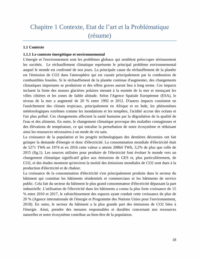
1.1.1 Le contexte énergétique et environnemental

L'énergie et l'environnement sont les problèmes globaux qui semblent préoccuper sérieusement

les sociétés. Le réchauffement climatique représente le principal problème environnemental

auquel le monde est confronté de nos jours. La principale cause du réchauffement de la planète

est l'émission de CO2 dans l'atmosphère qui est causée principalement par la combustion de

combustibles fossiles. Si le réchauffement de la planète continue d'augmenter, des changements

climatiques importants se produiront et des effets graves auront lieu à long terme. Ces impacts

incluent la fonte des masses glacières polaires menant à la montée de la mer et menaçant les

villes côtières et les zones de faible altitude. Selon l'Agence Spatiale Européenne (ESA), le

niveau de la mer a augmenté de 20 % entre 1992 et 2012. D'autres impacts consistent en

l'assèchement des climats tropicaux, principalement en Afrique et en Inde, les phénomènes

météorologiques extrêmes comme les inondations et les tempêtes, l'acidité accrue des océans et

l'air plus pollué. Ces changements affectent la santé humaine par la dégradation de la qualité de

l'eau et des aliments. En outre, le changement climatique provoque des maladies contagieuses et

des élévations de température, ce qui entraîne la perturbation de notre écosystème et réduisant

ainsi les ressources nécessaires à un mode de vie sain.

La croissance de la population et les progrès technologiques des dernières décennies ont fait

grimper la demande d'énergie et donc d'électricité. La consommation mondiale d'électricité était

de 5271 TWh en 1974 et en 2016 cette valeur a atteint 20864 TWh, 3,2% de plus que celle de

2015 (fig.1). Les sources utilisées pour produire de l'électricité font évoluer le monde vers un

changement climatique significatif grâce aux émissions de GES et, plus particulièrement, de

CO2, et des études montrent qu'environ la moitié des émissions mondiales de CO2 sont dues à la

production d'électricité et de chaleur.

La croissance de la consommation d'électricité s'est principalement produite dans le secteur du

bâtiment qui constitue les bâtiments résidentiels et commerciaux et les bâtiments de service

public. Cela fait du secteur du bâtiment le plus grand consommateur d'électricité dépassant la part

industrielle. L'utilisation de l'électricité dans les bâtiments a connu la plus forte croissance de 15

% entre 2010 et 2017, le rafraichissement des espaces ayant conduit cette croissance de plus de

20 % (Agence internationale de l'énergie et Programme des Nations Unies pour l'environnement,

2018). En outre, le secteur du bâtiment a la plus grande part des émissions de CO2 liées à

l'énergie. Ainsi, prendre des mesures responsables et durables concernant nos ressources

naturelles et notre écosystème contribue au bien-être de la population.

19

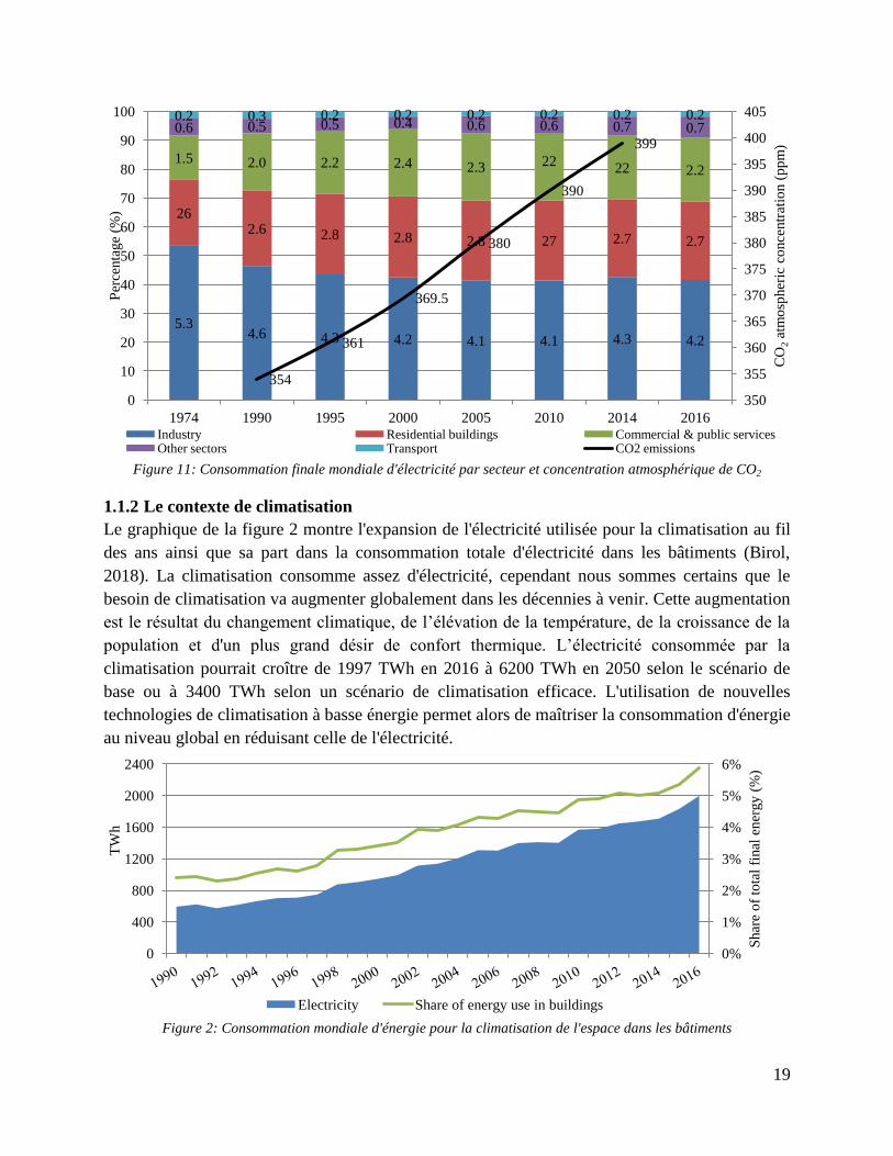
Figure 11: Consommation finale mondiale d'électricité par secteur et concentration atmosphérique de CO2

1.1.2 Le contexte de climatisation

Le graphique de la figure 2 montre l'expansion de l'électricité utilisée pour la climatisation au fil

des ans ainsi que sa part dans la consommation totale d'électricité dans les bâtiments (Birol,

2018). La climatisation consomme assez d'électricité, cependant nous sommes certains que le

besoin de climatisation va augmenter globalement dans les décennies à venir. Cette augmentation

est le résultat du changement climatique, de l’élévation de la température, de la croissance de la

population et d'un plus grand désir de confort thermique. L’électricité consommée par la

climatisation pourrait croître de 1997 TWh en 2016 à 6200 TWh en 2050 selon le scénario de

base ou à 3400 TWh selon un scénario de climatisation efficace. L'utilisation de nouvelles

technologies de climatisation à basse énergie permet alors de maîtriser la consommation d'énergie

au niveau global en réduisant celle de l'électricité.

Figure 2: Consommation mondiale d'énergie pour la climatisation de l'espace dans les bâtiments

5.3 4.6 4.3 4.2 4.1 4.1 4.3 4.2

26 2.6 2.8 2.8 2.8 27 2.7 2.7

1.5 2.0 2.2 2.4 2.3 22 22 2.2

0.6 0.5 0.5 0.4 0.6 0.6 0.7 0.7 0.2 0.3 0.2 0.2 0.2 0.2 0.2 0.2

354

361

369.5

380

390

399

350

355

360

365

370

375

380

385

390

395

400

405

0

10

20

30

40

50

60

70

80

90

100

1974 1990 1995 2000 2005 2010 2014 2016

CO

2 a

tmo

spher

ic c

once

ntr

atio

n (

pp

m)

Per

centa

ge

(%)

Industry Residential buildings Commercial & public services Other sectors Transport CO2 emissions

0%

1%

2%

3%

4%

5%

6%

0

400

800

1200

1600

2000

2400 S

har

e o

f to

tal

final

ener

gy (

%)

TW

h

Electricity Share of energy use in buildings

20

Les climatiseurs (AC) souvent utilisés sont généralement basés sur une technologie à cycle de

compression de vapeur. Il n'est pas surprenant que le nombre d'unités de l’AC augmente

rapidement en raison de l'augmentation de la température mondiale et des capacités d’achat dans

les pays en développement, ce qui peut justifier le stock mondial de ces unités : En 2000, le

nombre d'unités stockées était de 815 millions et a doublé en 2016 pour atteindre 1622 millions.

La croissance prévue du marché de l’AC d’ici à 2050 montre que la majorité des unités AC

mondiales sera concentrée dans les pays du sud les plus touchés par l’augmentation de la

température, d’où le besoin le plus crucial pour la climatisation.

Les systèmes de climatisation à compression de vapeur AC peuvent gérer efficacement la

température, mais ils présentent certaines lacunes lorsqu'il s'agit de contrôler l'humidité

intérieure.

1.1.3 Problème de contrôle de l'humidité

Afin d'extraire l'humidité, les cycles à compression de vapeur abaissent la température de l'air en

dessous de celle du point de rosée afin d'éliminer l'humidité par le processus de condensation, et

de réchauffer l’air ensuite pour atteindre la température de confort intérieure désirée. Ce

processus consomme environ 20 à 40 % de l’énergie totale et augmente la demande d’électricité

(Zhang et al., 2010). Un autre inconvénient est la faible qualité de l'air généré qui cause des

problèmes de santé et qui affecte le bien-être humain.

1.1.4 Conclusion

Vue la relation directe entre la climatisation et la consommation d'électricité, et tenant compte de

tous les problèmes environnementaux liés à l’exploitation des ressources fossiles pour produire

de l'électricité, il est désormais prioritaire de développer de nouveaux systèmes de réfrigération

économes en énergie. Ces systèmes innovants devraient réduire la consommation d'énergie et

répondre à l'augmentation de la demande pour le confort en termes de bien-être thermo

hygrométrique et de la qualité de l'air.

L'une de ces solutions alternatives est l'utilisation de la technique de desiccation pour réaliser la

déshumidification avant le refroidissement de l'air d'alimentation. Cela sépare le contrôle de

l'humidité de celui de la température dans les systèmes traditionnels de climatisation, ce qui

améliore leur efficacité énergétique globale et réduit les coûts énergétiques qui en résultent.

1.2 Système de dessiccation

1.2.1 Types de dessiccants

Un dessiccant a la propriété d'absorber une grande quantité de vapeur d'eau et de la désorber

facilement en étant réactivé à une température de régénération relativement basse. Il peut être de

type solide sous forme de roue tournante (fig.3) (Jani et al., 2016, p. 20; Rambhad et al., 2016) ou

liquide comme solution d'eau et de sel (fig.4) (Abdel-Salam et Simonson, 2016). L'objectif

principal du dessiccant est d'absorber l'humidité de l'air à travers la différence de pression de

vapeur entre la surface du desiccant et l'air qui agit comme force motrice pour le transfert de

masse ou d'humidité (Mohammad et al., 2016). Lorsque la pression de vapeur à la surface du

desiccant est inférieure à celle de l'air, la déshumidification se produit et vice versa. Le processus

21

de déshumidification se poursuit jusqu'à ce que les pressions de vapeur soient égales. Après ce

point, la vapeur d'eau commencera à se déplacer dans le sens opposé qui va du dessiccant à l'air.

Afin de réactiver le desiccant, sa pression de vapeur de surface doit être augmentée par

préchauffage après avoir quitté l'unité de déshumidification. La régénération se fait généralement

à basse température, de 30 à 80 °C environ.

Figure 3: Schéma d'une roue de dessiccation solide

Figure 4: Système de déshumidification par dessiccation liquide avec échangeur de chaleur liquide-liquide

1.2.2 Systèmes hybrides de compression des déformations/vapeurs

Les systèmes hybrides basés sur des desiccants liquides sont donc de bons candidats pour

permettre le contrôle séparé de la charge latente et sensible. La figure ci-dessous (fig.

5) montre le principe de cette technologie. Dans ces systèmes, un cycle de dessiccation liquide

déshumidifie l'air et le refroidissement et réalisé par le cycle de compression de vapeur. Dans

certains cas, le cycle desiccant pourrait contribuer simultanément à la déshumidification et au

refroidissement partiel de l'air. Pour ce faire, la solution desiccante est traverse par l’évaporateur

du cycle de compression de vapeur pour réduire sa température. Après avoir absorbé la vapeur

d'eau de l'air, la concentration de la solution dessiccante diminue. Ainsi, il doit être réactivé par

22

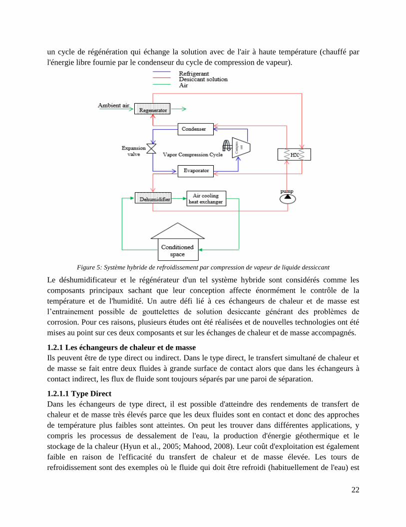
un cycle de régénération qui échange la solution avec de l'air à haute température (chauffé par

l'énergie libre fournie par le condenseur du cycle de compression de vapeur).

Figure 5: Système hybride de refroidissement par compression de vapeur de liquide dessiccant

Le déshumidificateur et le régénérateur d'un tel système hybride sont considérés comme les

composants principaux sachant que leur conception affecte énormément le contrôle de la

température et de l'humidité. Un autre défi lié à ces échangeurs de chaleur et de masse est

l’entrainement possible de gouttelettes de solution desiccante générant des problèmes de

corrosion. Pour ces raisons, plusieurs études ont été réalisées et de nouvelles technologies ont été

mises au point sur ces deux composants et sur les échanges de chaleur et de masse accompagnés.

1.2.1 Les échangeurs de chaleur et de masse

Ils peuvent être de type direct ou indirect. Dans le type direct, le transfert simultané de chaleur et

de masse se fait entre deux fluides à grande surface de contact alors que dans les échangeurs à

contact indirect, les flux de fluide sont toujours séparés par une paroi de séparation.

1.2.1.1 Type Direct

Dans les échangeurs de type direct, il est possible d'atteindre des rendements de transfert de

chaleur et de masse très élevés parce que les deux fluides sont en contact et donc des approches

de température plus faibles sont atteintes. On peut les trouver dans différentes applications, y

compris les processus de dessalement de l'eau, la production d'énergie géothermique et le

stockage de la chaleur (Hyun et al., 2005; Mahood, 2008). Leur coût d'exploitation est également

faible en raison de l'efficacité du transfert de chaleur et de masse élevée. Les tours de

refroidissement sont des exemples où le fluide qui doit être refroidi (habituellement de l'eau) est

23

dispersé sur un courant d'air et le contact direct permet à l'air de refroidir l'eau par évaporation et

convection (Evans, 2016). Le processus d’entrainement de gouttes dû au transfert du fluide

refroidi par l'air représente un inconvénient majeur de ces dispositifs. Dans le cas où une solution

de dessiccation doit être refroidie, l’entrainement de fines gouttelettes transportées par l'air

contiendra du sel qui se dépose dans les zones avoisinantes et dans le processus. Le dépôt de sel

est nocif pour le procédé et l'équipement en raison de son caractère corrosif.

1.2.1.2 Type indirect

Les échangeurs de type indirect sont utilisés lorsque le contact direct entre les deux fluides est

indésirable, comme dans le cas de l'air et de la solution dessiccante. Ici, le contact direct entre les

deux fluides qui s’écoulent est complètement évité par une paroi de séparation, mais le transfert

de la chaleur et de la masse se font à travers la paroi. Le transfert se produit lorsqu'une force

motrice est appliquée et qui est généralement une différence de pression ou de concentration

entre les fluides des deux côtés de la paroi. Les parois (aussi appelées membranes) ont la capacité

d'empêcher la solution liquide de se diriger vers l'air humide, mais ils permettent le transport de

vapeur d'eau et de chaleur de la solution dessiccante vers l'air et vice versa. Ils peuvent être

constitués de polypropylène (PP), de polyéthylène (PE) ou de polytétra-fluoro-éthylène (PTFE)

recouvertes d'une couche dense de silicium ou de téflon amorphe (Huang et Zhang, 2013).

De nombreuses études ont porté sur la performance des échangeurs de chaleur et de masse,

soulignant par exemple l'importance des propriétés de la membrane dans les types indirects ou

l'avantage de certains arrangements utilisant des techniques de pulvérisation dans les types

directs. Toutefois, après avoir décrit les dessins ou modèles existants de ces échangeurs, on peut

remarquer qu'ils présentent encore certains inconvénients.

1.2.1.3 Inconvénients des échangeurs existants et des solutions possibles

La technologie de pulvérisation d'eau dans les tours de refroidissement a prouvé son importance e

t sa bonne performance mais le problème d’entrainement conduit à de graves complications en pa

rticulier lorsque les gouttelettes de solution de sel sont transportées par l'air. (Ruiz et al., 2016).

En outre, en ce qui concerne les échangeurs membranaires de chaleur et de masse, il y a des défis

à relever. Premièrement, ces systèmes sont généralement sophistiqués en raison de l'installation et

de la distribution de canaux avec différentes configurations. Deuxièmement, elles sont coûteuses

en raison du prix élevé des membranes qui sont faites de structures complexes et sont difficiles à

traiter. Concernant les membranes, l'un des inconvénients est qu'elles devraient pouvoir résister à

une pression liquide sans être endommagées ou mouillées, de sorte qu'elles doivent être assez

rigides pour résister à la différence de pression (X Zhao et al., 2008). L'imperméabilité à l'eau

liquide constitue également un autre défi important pour les membranes par lesquelles l'eau

liquide ne devrait jamais pénétrer de l'autre côté de la membrane chaque fois qu'une pression

d'eau est appliquée. Cependant, la vapeur d'eau devrait toujours pouvoir se déplacer d'un côté de

la membrane à l'autre. Toutes ces caractéristiques exigent des propriétés spécifiques qui devraient

être présentes dans la membrane, telles que des conductivités thermiques et massiques

acceptables, la tension de surface et la résistance à l'usure (Onsekizoglu, 2012). Ainsi, la

résistance au transfert de chaleur et de masse de la membrane devrait être aussi basse que

24

possible et la conductivité thermique devrait être suffisamment petite pour réduire la perte de

chaleur entre les côtés de la membrane. La conductivité thermique de la membrane est liée à ses

caractéristiques physiques et à sa géométrie, ainsi qu'à sa capacité de conduire la chaleur. Une

autre limite des membranes proposées dans la littérature est leur coût et leur faible performance,

car les membranes doivent être renforcées mécaniquement, ce qui conduit à une faible

conductivité de masse.

Afin d'obtenir un système performant, des propriétés membranaires pratiques devraient être

disponibles et les défis susmentionnés devraient être surmontés. Dans tous les systèmes existants,

ces propriétés sont en contradiction les unes avec les autres. Chaque fois que la membrane est

capable de résister à une pression liquide, sa perméabilité à la vapeur d'eau diminue en réduisant

sa conductivité de masse. Ces contradictions dans le système, ainsi que le coût élevé de

fabrication et la complexité du système dans son ensemble, favorisent le développement d'un

nouveau système innovant capable de répondre à tous les besoins et défis susmentionnés.

1.3 Conception nouvelle de l'échangeur de chaleur et de masse à membrane

Une nouvelle technologie brevetée par "Armines" est proposée. Cette technologie fait un usage

positif de la présence de la membrane pour résoudre le problème de l’entrainement et les

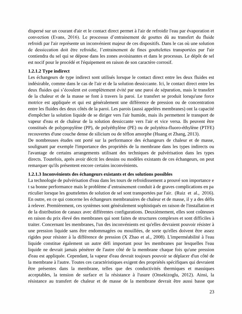
inconvénients des technologies membranaires réelles. La figure 6 représente notre système

proposé consistant en un échangeur à flux croisé où la solution dessiccante est projetée

verticalement vers le bas entre les membranes, représentées par les couches vertes, et où l'air

s’écoule dans un flux perpendiculaire. La solution dessiccante avec une faible concentration est

ensuite collectée au bas de l'échangeur et renvoyée à un régénérateur pour être réactivée.

Figure 6: Modèle de conception du système proposé

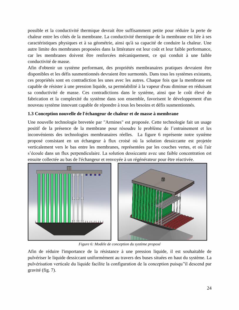
Afin de réduire l'importance de la résistance à une pression liquide, il est souhaitable de

pulvériser le liquide dessiccant uniformément au travers des buses situées en haut du système. La

pulvérisation verticale du liquide facilite la configuration de la conception puisqu’'il descend par

gravité (fig. 7).

25

Figure 7: Le système proposé avec le dessiccant pulvérisateur

La pulvérisation du liquide non seulement diminue la pression de l'eau sur la membrane, mais

elle disperse aussi l'eau en petites gouttelettes augmentant la surface de contact indirect entre l'air

et le liquide (Gluesenkamp et Radermacher, 2011). Cela conduit à une plus grande turbulence du

côté de l'air près de la membrane, ce qui augmente à son tour le transfert de chaleur et de masse

dans cette zone et minimise sa résistance interne. La pulvérisation du liquide induit une pression

identique des petites gouttelettes liquides pulvérisées et de l'air par lequel les propriétés

mécaniques de la membrane ainsi que son imperméabilité ne seront plus de fortes contraintes. Par

conséquent, les contradictions qui ont été présentées dans la section précédente sont maintenant

évitées en adoptant cette conception.

En ce qui concerne le coût relativement élevé associé au processus de fabrication des membranes,

notre objectif est d'utiliser des matériaux à faible coût qui sont fabriqués à l'origine pour des

utilisations autres que l'échange de la chaleur et de masse. Certains de ces matériaux qui semblent

être une excellente alternative aux membranes traditionnelles à coût élevé peuvent être des tissus

non tissés (NWF) qui sont des toiles ou des structures de toile de fibres liées ensemble de

différentes façons. D'autres candidats se trouvent également dans différentes industries comme

des membranes de sous toiture. Les propriétés intrinsèques des tissus non tissés sont déterminées

par les propriétés individuelles des fibres qui les composent; leur diamètre, leur porosité et leur

orientation (Chen et al., 2019). Certains de ces tissus non tissés ont une excellente résistance à

l’humidité ou ou une excellente répulsion, ils n’absorbent pas l’eau, mais ils sont perméables à

l’air. De plus, ces tissus sont souples, légers, poreux, lavables, jetables, bon marché et faciles à

fabriquer. Ainsi, la nouvelle conception d’échangeur proposée peut être réalisée en choisissant

des tissus non tissés pour servir de membranes en raison de leurs avantages importants,

principalement en ce qui concerne leur perméabilité à la vapeur, leur résistance au liquide et leur

faible coût de fabrication. Le choix principal de ces matériaux dépend principalement de la

capacité de la membrane à transmettre de la vapeur d'eau de manière à maximiser la chaleur et le

transfert de masse.

La figure 8 montre certaine des membranes en tissus non tissés et autres matériaux.

26

(a) (b)

(c) (d)

(e)

Figure 8: Une collection de différentes membranes a) caisses d'oreillers, b) sac, c) sous-toiture, d) enveloppe de

courrier Tyvek, e) nano-fibres électrofilées

Toutefois, l’utilisation de tissus non tissés qui sont initialement fabriqués pour des raisons autres

que l’utilisation à des fins de transfert de chaleur et de masse élargit la portée à de nouvelles

perspectives ainsi qu’à de nouveaux défis scientifiques et technologiques. Les défis concernant

ces matériaux sont le manque de caractéristiques scientifiques et d'informations sur leurs

propriétés. Afin de déterminer leur perméabilité à la vapeur d'eau, ces matériaux ont été testés

expérimentalement à l'aide d'un essai à la coupe modifiée et la méthodologie utilisée sera discutée

dans le prochain chapitre.

27

1.4 La problématique de la thèse

Les systèmes hybrides de compression de vapeur à base de desiccant liquide semblent des

candidats fiables qui permettent un contrôle adéquat de l'humidité dans les applications de

climatisation et un fonctionnement sans givre dans le cas de la réfrigération, avec un COP

potentiellement accrue. Comme le dessiccant solide présente l'inconvénient des températures de

régénération élevées et de la complexité de leur intégration dans les systèmes, les dessiccants

liquides sont plus attrayants en montrant des températures de régénération basses et des capacités

de déshumidification remarquables. D'après les recherches il a été déterminé que la configuration

du système hybride et son architecture offrent une grande efficacité dans toute une gamme de

conditions d'exploitation avec différents rapports de charge latent à sensible. Cette gamme de

conditions d'exploitation varie d'une architecture à l'autre; il est clair que le maintien d'un système

hybride à haute performance ne pourrait être réalisé que par une conception flexible fonctionnant

tout au long d'une saison de manière efficace sur le plan énergétique. Ceci définit l'objectif final

de cette thèse de concevoir des systèmes hybrides de climatisation à haute performance,

abordables et flexibles, ainsi qu'une méthodologie de conception et des outils de modélisation.

Le déshumidificateur et le régénérateur d'un tel système hybride sont considérés comme les

principaux éléments et leur conception propre a une incidence considérable sur le contrôle de la

température et de l'humidité. Comme nous l'avons vu, l'un des défis liés à ces échangeurs est leur

capacité d'empêcher l’entrainement des gouttelettes de solution dessiccante vers l'air en évitant

les problèmes de corrosion tout en les gardant simples à construire et à faible coût. Les

échangeurs membranaires à constituent une réponse technologique à ces problèmes, mais les

technologies existantes présentent de nombreux inconvénients, comme nous l'avons expliqué.

Dans cette thèse, la nouvelle technologie présentée dans la section précédente sera soigneusement

étudiée. Elle utilise de nouveaux matériaux membranaires et une nouvelle conception liée à la

distribution de liquide. Les défis concernant ces matériaux sont le manque de caractéristiques

scientifiques et d'informations concernant leurs propriétés, principalement leur perméabilité de la

vapeur d'eau. Pour découvrir cette propriété, ces matériaux sont testés expérimentalement à l'aide

d'une méthode modifiée de coupe verticale et la méthodologie utilisée sera discutée dans le

prochain chapitre.

Le troisième chapitre de cette thèse vise à comprendre profondément le comportement et la

performance de ce nouvel échangeur. La bonne compréhension et la modélisation des transferts

couplés de chaleur et de masse au sein de cet échangeur innovante sont des facteurs clés pour les

intégrer efficacement dans les processus et pour bénéficier de leurs avantages par rapport aux

technologies conventionnelles existantes. Une approche de modélisation des phénomènes de

transfert de chaleur et de masse est développée en modélisant les échangeurs conçus et est

soutenue par une caractérisation expérimentale.

Ce modèle est utilisé dans le dernier chapitre pour étudier l'intérêt énergétique de l'intégration de

ces échangeurs dans les applications de climatisation et pour concevoir une architecture flexible

capable de faire face à la variation saisonnière du rapport de charge thermique.

28

Chapter 1 Context, State of the Art and Problem

Statement

1.1 Context

1.1.1 The energy and environmental context

Energy and environment are the most trending worldwide issues that seem to be of a serious

concern for societies. Global warming represents the major environmental problem that the world

is facing nowadays. The principal cause of global warming is the emission of CO2 in the

atmosphere which is caused mainly by the burning of fossil fuels. Burning fossil fuels such as oil,

coal and natural gas does not only generate CO2 (the main greenhouse gas) but also generates

other pollutant gases like SOx, NOx, CO and fine particles (Bose, 2010). These greenhouse gases

(GHG) trap the solar heat in the atmosphere and raise the earth’s temperature causing harmful

impacts on the environment. Across the globe, the past five years have been recorded as the

hottest years (e.g. year 2018 was considered to have very high unusual temperatures and ranked

as the fourth hottest year on record). Further increase in temperature is estimated by the United

Nations IPCC (Climate Change 2014 Summary for Policymakers, 2014). As mentioned in their

report an increase in the global mean surface temperature is expected by the end of this century

under three possible scenarios. The most optimistic one would be through applying stringent

mitigation measures whereas the worst one would be through maintaining the same rate of GHG

emissions. In the first scenario the increase would be from 0.3°C to 1.7°C, while in the baseline

scenario the increase can reach higher values from 2.6°C to 4.8°C.

This increase triggers the usage of more electricity for cooling purposes. Likewise, the climate

change in some cold countries such as North America and due to colder-than-average

temperature in winters, an additional increment in heating requirements is expected. In 2018, a

rise by 4% was recognized in the global energy demand presenting the fastest pace since 2010

after the recovery of the global economy from the financial crisis. Studies indicate that about one

fifth of the increase in energy demands was directly related to the change in weather conditions

(IEA, 2018, p. 2). In addition to the increase in the heating and cooling demands, some other

factors affect the electricity consumption. It is interesting to mention that the United States and

China together account for around 70% of the global demand growth reflecting by that the high

standards of living in the first country and the rapid growth in the industrial sector in the second.

The graph in figure 1.1 shows the continuous growth in the electricity consumption over the past

few decades.

29

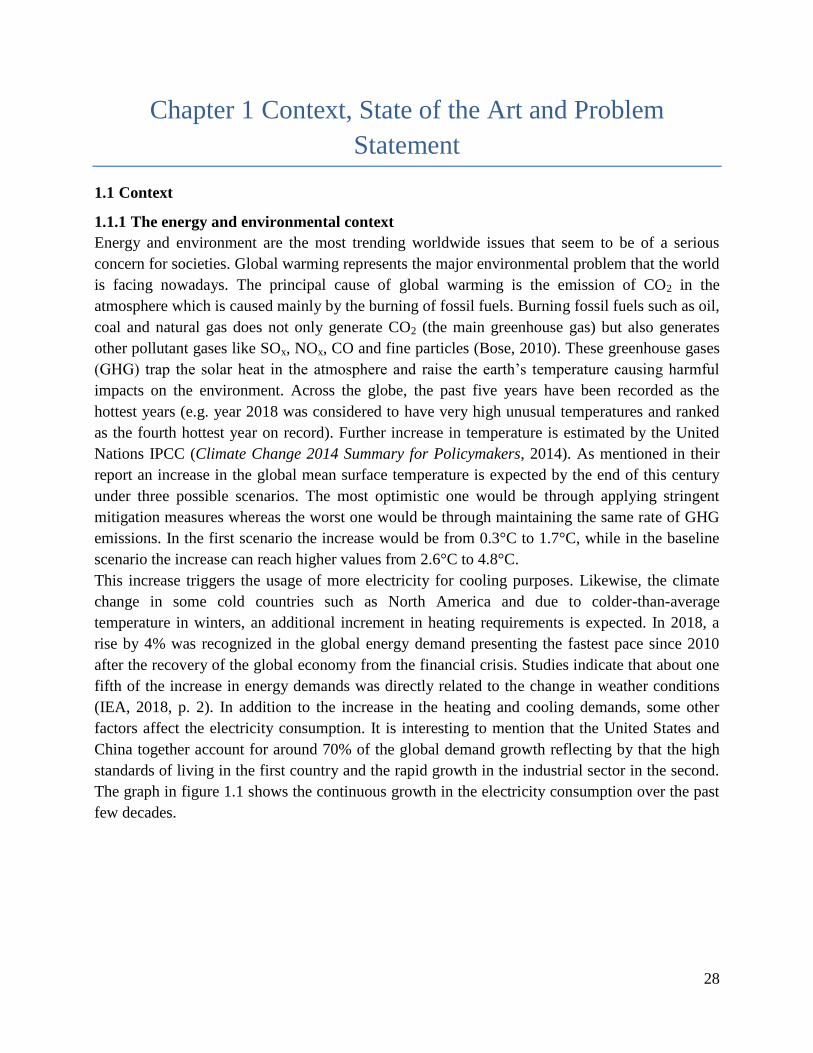
Figure 1.1: World electricity final consumption by sector

In year 1990 the world electricity consumption was 9699 TWh and in 2016 this value has reached

20864 TWh, 3.2% above that of 2015. The growth in the electricity consumption mainly took

place in the building sector that constitutes the residential as well as the commercial and public

service buildings as observed in the graph of fig. 1.1. The share of residential combined with the

commercial and public service sectors increased from 46% in 1990 to 49.3% in 2016. This makes

the building sector the highest electricity consumer surpassing the industrial share. Although the

electricity consumed by the industries has incremented throughout the years yet its share has

fallen from 46.5% in year 1990 to 41.6% in year 2016, yielding the share mostly towards the

commercial and service sector. Thus, It can be clearly noticed that the building sector contributes

to around half of the global electricity consumption. This is due to the excessive use of electronic

and telecommunication equipment and to the employment of heating and cooling systems that

consume lots of electricity.

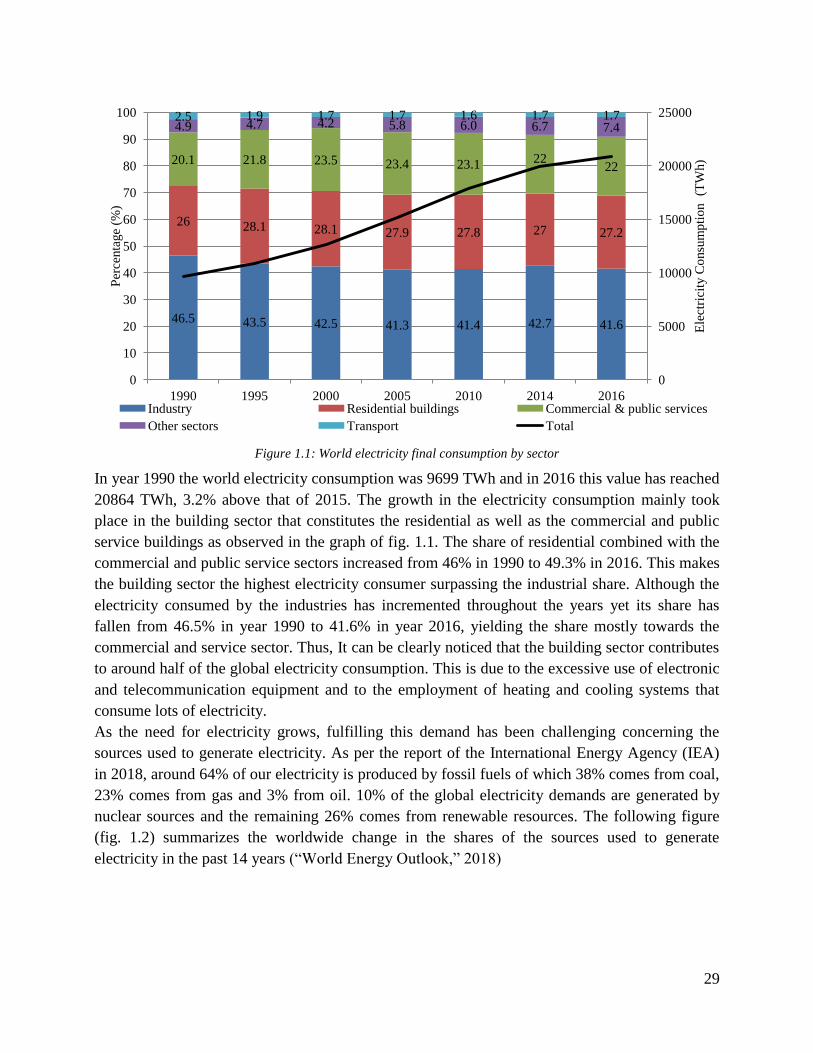
As the need for electricity grows, fulfilling this demand has been challenging concerning the

sources used to generate electricity. As per the report of the International Energy Agency (IEA)

in 2018, around 64% of our electricity is produced by fossil fuels of which 38% comes from coal,

23% comes from gas and 3% from oil. 10% of the global electricity demands are generated by

nuclear sources and the remaining 26% comes from renewable resources. The following figure

(fig. 1.2) summarizes the worldwide change in the shares of the sources used to generate

electricity in the past 14 years (“World Energy Outlook,” 2018)

46.5 43.5 42.5 41.3 41.4 42.7 41.6

26 28.1 28.1 27.9 27.8 27 27.2

20.1 21.8 23.5 23.4 23.1 22 22

4.9 4.7 4.2 5.8 6.0 6.7 7.4 2.5 1.9 1.7 1.7 1.6 1.7 1.7

0

5000

10000

15000

20000

25000

0

10

20

30

40

50

60

70

80

90

100

1990 1995 2000 2005 2010 2014 2016

Ele

ctri

city

Co

nsu

mp

tio

n

(TW

h)

Per

centa

ge

(%)

Industry Residential buildings Commercial & public services

Other sectors Transport Total

30

Figure 1.2: Global electricity generation by source and its evolution throughout the years

Different policies are already established by governments all over the world including the

Nationally Determined Contributions achieved in Paris agreement in 2016 to reduce emissions

and energy consumption. If these policies are adopted the share of coal will decrease from 38% to

25% in year 2040 according to the IEA. This is in favor for a significant development in the

renewable energy shares including solar, wind, hydro and marine sources that could reach 40%.

Whilst if more strict approaches are followed under a sustainable development scenario, the

coal’s share would decrease to 5% in 2040 and that of renewable energy would reach 66%

(“Sustainable Development Scenario,” 2018).

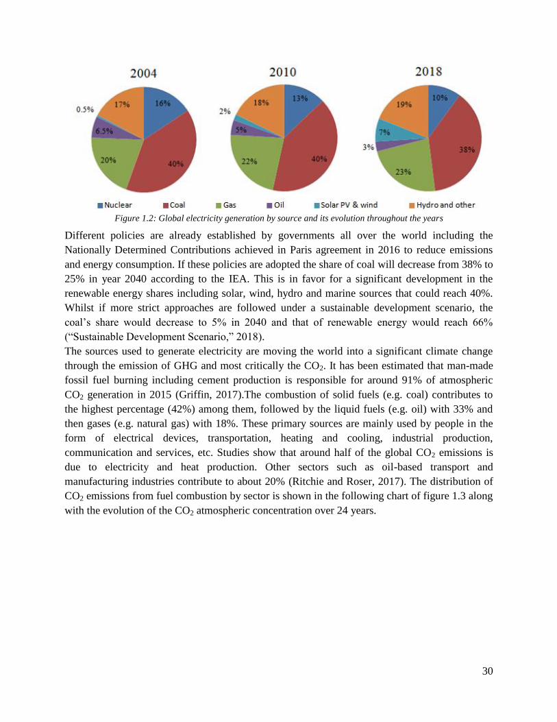
The sources used to generate electricity are moving the world into a significant climate change

through the emission of GHG and most critically the CO2. It has been estimated that man-made

fossil fuel burning including cement production is responsible for around 91% of atmospheric

CO2 generation in 2015 (Griffin, 2017).The combustion of solid fuels (e.g. coal) contributes to

the highest percentage (42%) among them, followed by the liquid fuels (e.g. oil) with 33% and

then gases (e.g. natural gas) with 18%. These primary sources are mainly used by people in the

form of electrical devices, transportation, heating and cooling, industrial production,

communication and services, etc. Studies show that around half of the global CO2 emissions is

due to electricity and heat production. Other sectors such as oil-based transport and

manufacturing industries contribute to about 20% (Ritchie and Roser, 2017). The distribution of

CO2 emissions from fuel combustion by sector is shown in the following chart of figure 1.3 along

with the evolution of the CO2 atmospheric concentration over 24 years.

31

Figure 1.3: World percentage CO2 emissions by sector with its atmospheric concentration in ppm

Over the course of few decades, the global concentration of CO2 in the atmosphere in particles

per million (ppm) was observed and studied by scientists. According to NOAA the particles of

CO2 per million molecules of dry air increased significantly (NOAA, 2019). The CO2

atmospheric concentration shown in figure 1.3 is based on data records through the direct

measurements of CO2 in the atmosphere at Muana Loa Observatory in Hawaii. The data reveals

that the global atmospheric carbon dioxide concentration was 354 ppm in year 1990 and reached

around 399 ppm in year 2014.

The curve of the CO2 data is widely recognized to have a possible exponential nature and thus its

future behavior could be predictable. By introducing the measured values in a model and

applying several corrections related to oil shocks, population increase and other factors that might

affect CO2 production, extrapolation would give a future evolution of CO2 concentration in the

atmosphere (“Concentrations de CO2 dans l’Atmosphere. Elements de Prospective,” 2015).

According to the model prediction of the CO2 levels if the worldwide emissions continue with a

similar pace following the same trend the numbers might reach 510 ppm in the year 2050.

The trend of other GHG is similar to that of CO2 and the consequences of the continuous growth

in the emissions are undesirable and potentially harmful. If global warming keeps increasing,

significant climate change will occur and severe long term effects will take place. These impacts

involve higher sea levels due to the melting of the ice mass at the poles threatening coastal cities

and low-lying areas. According to the European space agency (ESA) there had been a rise in 20%

of the sea levels between 1992 and 2012 (ESA, 2018). Other impacts include severe dryness in

tropical climates mainly in Africa and India, extreme weather events like floods and storms,

increased acidity of oceans and more polluted air (Wilkinson et al., 2007). These changes are

most likely to affect humans’ health through the deterioration in water and food security.

43.3 44.8 47.1 48.2 48.8 49

20 20.9 22 21.1 20 20.5

20 19.1 17.4 18.3 20 20

13.1 12.4 11.4 10.3 9.2 8.5 3.7 2.8 2.2 2.2 2.1 2

330

340

350

360

370

380

390

400

410

0

10

20

30

40

50

60

70

80

90

100

1990 1995 2000 2005 2010 2014

Co

nce

ntr

atio

n o

f C

O2 i

n t

he

atm

osp

her

e (p

pm

)

Per

centa

ge

(%)

Electricity & heat production Transport

Manufacturing industries & construction Residential buildings, commercial & public services

Other sectors Concentration of CO2

32

Moreover, climate change induces the spread of infectious diseases and higher-than-normal

temperatures result in the disruption of our ecosystem reducing the resources needed for a healthy

lifestyle (Kovats and Butler, 2012).

Furthermore, climate change induces damaging effects on the global economic development.

According to the International Labor Organization (“World Employment and Social Outlook

2018 – Greening with jobs,” 2018), the agricultural crops are expected to decline affected by the

global increase in temperature and dryness threatening about 1.2 billion jobs directly dependent

on ecosystem services. These might include employments in agriculture, fisheries and forestry

especially in developing countries like India and Brazil that are directly affected by global

warming. In addition to the unemployment, agricultural deterioration raises the food prices

enhancing malnutrition and poverty.

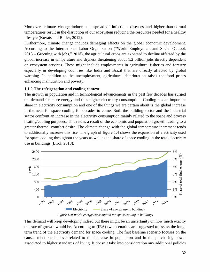
1.1.2 The refrigeration and cooling context

The growth in population and in technological advancements in the past few decades has surged

the demand for more energy and thus higher electricity consumption. Cooling has an important

share in electricity consumption and one of the things we are certain about is the global increase

in the need for space cooling for decades to come. Both the building sector and the industrial

sector confront an increase in the electricity consumption mainly related to the space and process

heating/cooling purposes. This rise is a result of the economic and population growth leading to a

greater thermal comfort desire. The climate change with the global temperature increment tends

to additionally increase this rise. The graph of figure 1.4 shows the expansion of electricity used

for space cooling throughout the years as well as the share of space cooling in the total electricity

use in buildings (Birol, 2018);

Figure 1.4: World energy consumption for space cooling in buildings

This demand will keep developing indeed but there might be an uncertainty on how much exactly

the rate of growth would be. According to (IEA) two scenarios are suggested to assess the long-

term trend of the electricity demand for space cooling. The first baseline scenario focuses on the

causes mentioned above related to the increase in population and in the purchasing power

associated to higher standards of living. It doesn’t take into consideration any additional policies

0%

1%

2%

3%

4%

5%

6%

0

400

800

1200

1600

2000

2400

Shar

e o

f to

tal

final

ener

gy (

%)

TW

h

Electricity Share of energy use in buildings

33

beyond the ones that have already been announced around the world. The second scenario favors

a more optimistic trend considering the adoption of further rigorous policies with more efficient

cooling measures in the aim of reducing the amount of energy needed. According to the baseline

scenario the electricity consumed by space cooling is expected to increase from 1997 TWh in

2016 to 6200 TWh in 2050 while this value would be 3400 TWh if an efficient cooling scenario

is followed (45% lower than the baseline projection) as shown in figure 1.5 (Birol, 2018). Hence

employing new energy efficient technologies in space cooling contributes to the global energy

savings through reducing electricity consumption.

Figure 1.5: World electricity consumption for space cooling in the baseline and efficient cooling scenarios (Birol,

2018)

In order to perform space cooling, air conditioners (ACs) are the most common used appliances

worldwide. Very few of them are powered by natural gas and the rest by electricity. The AC

systems include split units that are usually used in houses and residential entities and water

chillers that are mainly used in commercial buildings. Relying mostly on electricity for the power

generation, space cooling contributes to the growth of the overall energy demand.

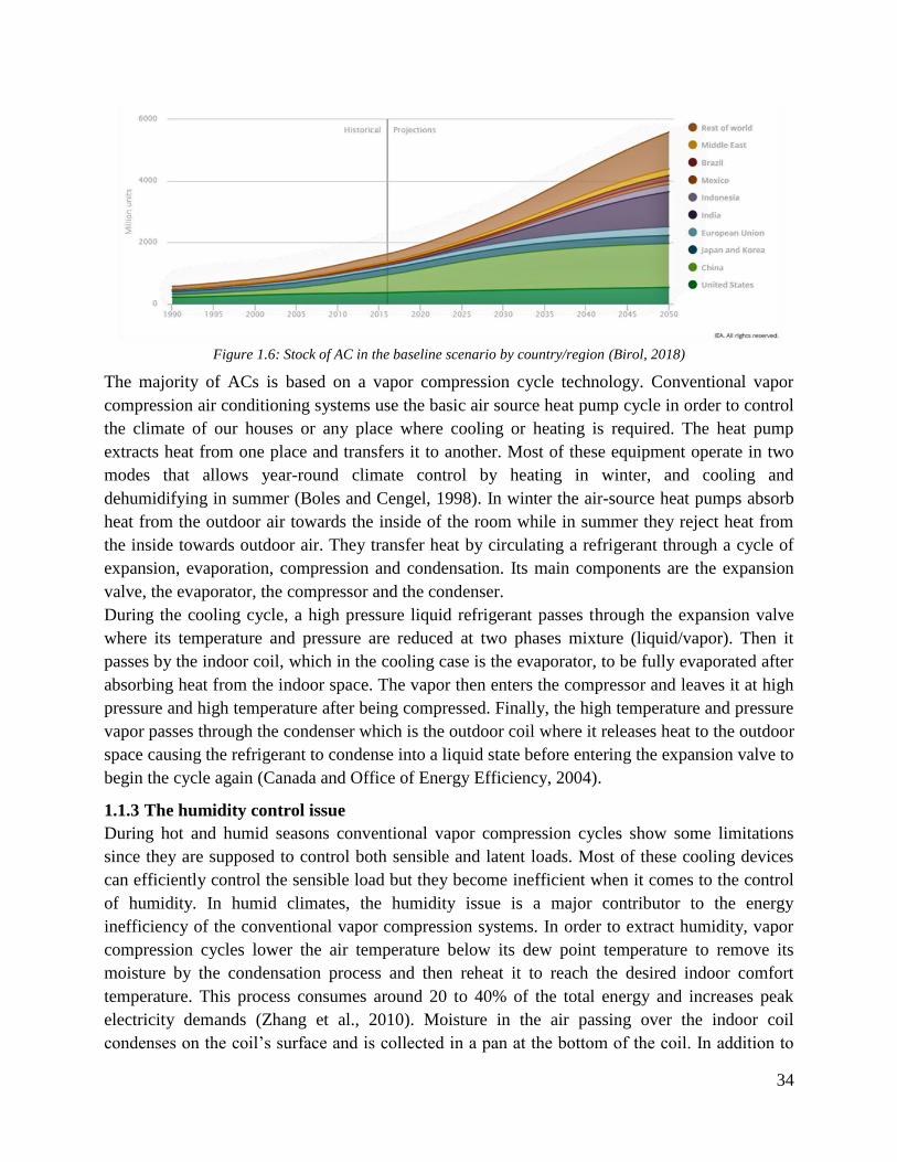
Unsurprisingly, the number of AC units is also expanding as a result of the global increase in

temperature and this can be significant from the global stock of these units. As shown in figure

1.6, in year 2000, the number of stocked units of ACs was 815 million and it doubled in 2016 to

reach 1622 million. The projected growth in the AC market shows that the lion’s share of the

global AC units will be concentrated in the southern countries which are confronting the highest

economic development leading to an increased standard of living. These countries are also being

the most affected by the increase in the global earth temperature and thus the need for cooling

becomes more crucial. The graph indicates that the expectations are at their highest in India,

Indonesia and China with just the three of them contributing to half of the total growth in the

number of AC units (Birol, 2018)

34

Figure 1.6: Stock of AC in the baseline scenario by country/region (Birol, 2018)

The majority of ACs is based on a vapor compression cycle technology. Conventional vapor

compression air conditioning systems use the basic air source heat pump cycle in order to control

the climate of our houses or any place where cooling or heating is required. The heat pump

extracts heat from one place and transfers it to another. Most of these equipment operate in two

modes that allows year-round climate control by heating in winter, and cooling and

dehumidifying in summer (Boles and Cengel, 1998). In winter the air-source heat pumps absorb

heat from the outdoor air towards the inside of the room while in summer they reject heat from

the inside towards outdoor air. They transfer heat by circulating a refrigerant through a cycle of

expansion, evaporation, compression and condensation. Its main components are the expansion

valve, the evaporator, the compressor and the condenser.

During the cooling cycle, a high pressure liquid refrigerant passes through the expansion valve

where its temperature and pressure are reduced at two phases mixture (liquid/vapor). Then it

passes by the indoor coil, which in the cooling case is the evaporator, to be fully evaporated after

absorbing heat from the indoor space. The vapor then enters the compressor and leaves it at high

pressure and high temperature after being compressed. Finally, the high temperature and pressure

vapor passes through the condenser which is the outdoor coil where it releases heat to the outdoor

space causing the refrigerant to condense into a liquid state before entering the expansion valve to

begin the cycle again (Canada and Office of Energy Efficiency, 2004).

1.1.3 The humidity control issue

During hot and humid seasons conventional vapor compression cycles show some limitations

since they are supposed to control both sensible and latent loads. Most of these cooling devices

can efficiently control the sensible load but they become inefficient when it comes to the control

of humidity. In humid climates, the humidity issue is a major contributor to the energy

inefficiency of the conventional vapor compression systems. In order to extract humidity, vapor

compression cycles lower the air temperature below its dew point temperature to remove its

moisture by the condensation process and then reheat it to reach the desired indoor comfort

temperature. This process consumes around 20 to 40% of the total energy and increases peak

electricity demands (Zhang et al., 2010). Moisture in the air passing over the indoor coil

condenses on the coil’s surface and is collected in a pan at the bottom of the coil. In addition to

35

wasting energy, the condensation of air leads to the growth of molds and different fungi viruses

on the air ducts and on the tubes of the exchanger. These impurities would be carried by the air to

the indoor space causing poor indoor air quality and serious problems for human health.

In other cases where refrigeration applications are needed in industrial storage rooms for

example, indoor air temperatures close to zero (positive temperature) or inferior to zero (freezers)

with very low levels of absolute humidity are required. To be able to cool the air to the required

temperature, the evaporating temperature of the cooling coil should be significantly low and this

requires adequate choice of the refrigerant circulating in the cycle. These spaces are usually

constructed with extreme tightness and proper sealing to maximize the efficiency of the cooling

system. However, due to infiltration through doorways from nearby warmer areas and due to the

absence of ventilation systems, undesired warm humid air may enter the storage room and in

other cases internal sources of humidity may be present (respiration, cleaning processes, etc.).

The moisture present in the air condenses on the walls and ceilings of the room causing the

formation of molds and bacteria nests that may damage the stored items; moreover, in case of

freezers, this condensation leads to frost that makes some areas slippery and dangerous to

workers. In these spaces, usually the vapor compression cycle that is used to control the

temperature is also designed to control the humidity level. In this case when air passes through

the cooling coil, it condenses on the fins causing ice buildup and frost formation and the amount

of frost depends on the moisture in the air. Frost normally accumulates when the space

temperature is below 5°C with a relative humidity over 60% (Byrne et al., 2011). When a large

amount of frost is present over the cooling coil, the air flow rate would be reduced due to the

blocked air passages which in turn lowers the heat transfer (Byrne et al., 2011; Staffell et al.,

2012). In order to avoid the blockage of the heat exchangers by frost buildup three different

methods are available and widely adopted these days. One of these methods is reversing the cycle

(Ding et al., 2004; Shen et al., 2019). In this way the inside unit will act as the condenser and the

passing hot refrigerant will melt the frost. But the disadvantage of this approach is that by

reversing the cycle, the evaporator inside the room will be heated up and will consume a great

part of the cooling capacity to be re-cooled after the defrost cycle. Another method is by the

addition of an electric resistance heater to melt the ice that is formed on the cooling coil (Yin et

al., 2012). This approach is also unfavorable because it increases the equipment cost due to the

addition of auxiliary heating elements and this will lead to supplementary electrical consumption.

Bansal et al. (Bansal et al., 2010) analyzed a defrost cycle using an electric heater in a domestic

freezer. They concluded that this defrost method increased the power consumption of the freezer

by 17.7% and that the efficiency of the heater that is used for defrosting is only 30.3% while the

rest of the heat is dissipated to the surrounding. The third method is by using hot gas refrigerant

by-pass where the superheated refrigerant from the compressor directly flows to the

evaporator bypassing the condenser and the expansion device (Byun et al., 2008;

Hoffenbecker et al., 2005; Wenju et al., 2011). This is also considered a costly process with

some limitations since the amount of heat in the hot gases might not last enough to do all the

needed defrost if a large amount of ice was compiled on the coil. In addition to the direct

energy penalty of defrost, defrosting the evaporator may increase the room temperature

36

creating a constraint in the case where the temperature of the products should not fluctuate

much.

1.1.4 Conclusion

In the absence of determined preventive means, excessive energy consumption threatens

economic structures and causes serious environmental, social and health disorders. Therefore,

efforts should be doubled for the aim of protecting future human health and preserving our

natural ecosystem. This can be done by promoting environmental policy programs encouraging

renewable energy alternatives such as solar, biomass, etc. and by supporting energy efficient

measures to ameliorate both health and environmental conditions.

Due to the direct relation between refrigeration along with space heating/cooling and electricity

consumption and in the light of all the mentioned environmental concerns associated with

burning fossil fuels for electricity generation, it is now a priority to develop new energy-efficient

refrigeration systems. Indeed, consuming lots of electricity for performing dehumidification

of air in hot and humid conditions and wasting energy to carry out defrosting cycle in near

zero and sub zero refrigeration conditions are of the major causes why conventional vapor

compression cycles are not an energy efficient technology. This is to be added to the fact that the

low quality air delivered by the vapor compression cycles causes health problems and affects

human well-being.

Innovative refrigeration and space air conditioning systems should involve novel solutions that

can reduce energy consumption and respond to the increase in the occupant comfort demand in

terms of both thermo-hygrometric well-being and air quality. One of these alternatives is the use

of desiccant techniques for the dehumidification process prior to the cooling of supply air. This

separates humidity control from temperature control in the traditional air conditioning systems

thus improving their overall energy efficiency and reducing their resultant energy costs. The next

section is a review of the desiccant systems aiming to introduce the concept that is developed in

this thesis.

1.2 Desiccant Systems Review

Desiccants are not only environmentally friendly because of the absence of refrigerants that

contribute to global warming, but at the same time they take use of recovered or renewable

heating sources like solar energy or waste heat gases or biomass (Yu et al., 2009). A desiccant

material has the property to absorb a large amount of water vapor and desorb easily by being

reactivated at relatively low regeneration temperature. It can be of a solid type in the form of a

rotating wheel (Jani et al., 2016, p. 20; Rambhad et al., 2016) or a liquid type as a solution of

water and a salt (Abdel-Salam and Simonson, 2016). The main purpose of the desiccant is to

absorb moisture from air through the difference in vapor pressure between the surface of the

desiccant material and the air which acts as the driving force for mass or moisture transfer

(Mohammad et al., 2016). When the vapor pressure at the surface of the desiccant solution is

lower than that of the process air, dehumidification occurs and vice versa. Dehumidification

process continues until the vapor pressures are equal. After that point, the moist or water vapor

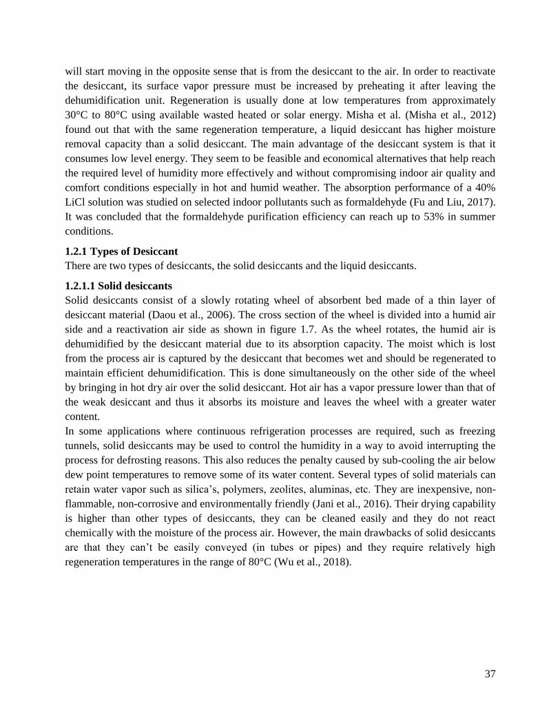
37

will start moving in the opposite sense that is from the desiccant to the air. In order to reactivate

the desiccant, its surface vapor pressure must be increased by preheating it after leaving the

dehumidification unit. Regeneration is usually done at low temperatures from approximately

30°C to 80°C using available wasted heated or solar energy. Misha et al. (Misha et al., 2012)

found out that with the same regeneration temperature, a liquid desiccant has higher moisture

removal capacity than a solid desiccant. The main advantage of the desiccant system is that it

consumes low level energy. They seem to be feasible and economical alternatives that help reach

the required level of humidity more effectively and without compromising indoor air quality and

comfort conditions especially in hot and humid weather. The absorption performance of a 40%

LiCl solution was studied on selected indoor pollutants such as formaldehyde (Fu and Liu, 2017).

It was concluded that the formaldehyde purification efficiency can reach up to 53% in summer

conditions.

1.2.1 Types of Desiccant

There are two types of desiccants, the solid desiccants and the liquid desiccants.

1.2.1.1 Solid desiccants

Solid desiccants consist of a slowly rotating wheel of absorbent bed made of a thin layer of

desiccant material (Daou et al., 2006). The cross section of the wheel is divided into a humid air

side and a reactivation air side as shown in figure 1.7. As the wheel rotates, the humid air is

dehumidified by the desiccant material due to its absorption capacity. The moist which is lost

from the process air is captured by the desiccant that becomes wet and should be regenerated to

maintain efficient dehumidification. This is done simultaneously on the other side of the wheel

by bringing in hot dry air over the solid desiccant. Hot air has a vapor pressure lower than that of

the weak desiccant and thus it absorbs its moisture and leaves the wheel with a greater water

content.

In some applications where continuous refrigeration processes are required, such as freezing

tunnels, solid desiccants may be used to control the humidity in a way to avoid interrupting the

process for defrosting reasons. This also reduces the penalty caused by sub-cooling the air below

dew point temperatures to remove some of its water content. Several types of solid materials can

retain water vapor such as silica’s, polymers, zeolites, aluminas, etc. They are inexpensive, non-

flammable, non-corrosive and environmentally friendly (Jani et al., 2016). Their drying capability

is higher than other types of desiccants, they can be cleaned easily and they do not react

chemically with the moisture of the process air. However, the main drawbacks of solid desiccants

are that they can’t be easily conveyed (in tubes or pipes) and they require relatively high

regeneration temperatures in the range of 80°C (Wu et al., 2018).

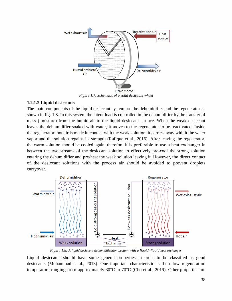
38

Figure 1.7: Schematic of a solid desiccant wheel

1.2.1.2 Liquid desiccants

The main components of the liquid desiccant system are the dehumidifier and the regenerator as

shown in fig. 1.8. In this system the latent load is controlled in the dehumidifier by the transfer of

mass (moisture) from the humid air to the liquid desiccant surface. When the weak desiccant

leaves the dehumidifier soaked with water, it moves to the regenerator to be reactivated. Inside

the regenerator, hot air is made in contact with the weak solution, it carries away with it the water

vapor and the solution regains its strength (Rafique et al., 2016). After leaving the regenerator,

the warm solution should be cooled again, therefore it is preferable to use a heat exchanger in

between the two streams of the desiccant solution to effectively pre-cool the strong solution

entering the dehumidifier and pre-heat the weak solution leaving it. However, the direct contact

of the desiccant solutions with the process air should be avoided to prevent droplets

carryover.

Figure 1.8: A liquid desiccant dehumidification system with a liquid–liquid heat exchanger

Liquid desiccants should have some general properties in order to be classified as good

desiccants (Mohammad et al., 2013). One important characteristic is their low regeneration

temperature ranging from approximately 30°C to 70°C (Cho et al., 2019). Other properties are

39

also essential even if it is hard to find them all together in a single desiccant. These properties

include being non-volatile, non-corrosive, non-toxic, non-flammable, inexpensive. They should

also have low viscosity, high rates of heat and mass transfer, low vapor pressure, large saturation

absorption capacity, low crystallization point and high density. Liquid desiccants should as

well possess certain characteristics to be considered of high performance. These characteristics

may include a limited liquid side resistance to moisture diffusion, a large surface contact area per

unit volume, a good capacity of energy storage and a large availability in nature.

Some commonly used liquid desiccants are glycols and solutions of halide salts including

calcium chloride (CaCl2), lithium chloride (LiCl), lithium bromide (LiBr), tri-ethylene glycol, or

a mixture of any of these salts. It is essential to adequately select the desiccant because of its

direct effect on the system design and dehumidification capacity. Glycols are of limited use

because of their high viscosity. They are also highly volatile that they might evaporate with air

into the indoor space and may be considered as undesirable impurities. CaCl2 is the cheapest

desiccant and it is readily available in nature, however, its stability is dependent on its

concentration in the solution and on the inlet air conditions which contributes to its reduced use.

LiCl is considered to be a highly performing desiccant because of its significant stability

and its extremely low vapor pressure. In addition, at ambient conditions it doesn’t vaporize and

it requires a reduced pumping power due to its low viscosity. Yet, this desiccant is

considered corrosive and is expensive compared to others such as CaCl2 (Bouzenada et al., 2016).

1.2.2 Hybrid desiccant/vapor compression systems

The use of desiccant technique prior to cooling process of the supply air can improve humidity

control independent of temperature control in air conditioning systems enhancing the overall

energy efficiency and reducing energy costs. In this way, the dew point temperature of air

entering the cooling coil decreases which is, in the case of near/subzero applications, the key

for frost free operations. Therefore, the combination of desiccants with conventional

refrigeration systems avoids evaporating below the dew point temperature to handle

dehumidification. As a consequence, this avoids frost formation in refrigeration applications by

separating the treatment of latent and sensible loads. The figure below (fig. 1.9) shows the

principle of this technology where first the hot and humid ambient air passes by the dehumidifier

which is a heat and mass exchanger operating either with a solid or a liquid desiccant (Daou et

al., 2006). If the temperature of the desiccant is less than that of the temperature of air, the

desiccant would as well engage slightly in the cooling of the air. For further cooling, the dry air is

then transferred to the cooling system which can be a chiller or a heat pump. Thus the air leaving

dry and cool is now ready to be delivered to the indoor space.

40

Figure 1.9: A hybrid liquid desiccant vapor compression cooling system

Several studies have been done on hybrid systems to study their behavior and performance. Nei

et al. (Nie et al., 2017) modeled and tested a heat pump assisted with a solid desiccant wheel in

hot and humid conditions. In their system, the desiccant rotor was regenerated by the waste heat

produced by the condenser of the cooling system. Their system showed efficient energy

performance with high air purification potential and it was concluded that its performance was

sensitive to the outdoor humidity. Another study was conducted by Qin et al. (Qin and Schmitz,

2006) on an energy driven hybrid solid desiccant air conditioning system. Their experimental

results suggested that by regenerating the desiccant using recovered waste heat, more than 30%

savings in operational cost could be attained. The solid desiccant rotor was used as well with a

heat pump operating in heating and cooling mode (Ge et al., 2011). It was found that the energy

requirement can be reduced by around 8% in the cooling mode and 14% in the heating mode. For

the cooling operations in industrial fields one of the applications was mentioned by Capozzoli et

al. (Capozzoli et al., 2006) which was the insertion of a solid desiccant wheel and a sensible heat

exchanger to an air conditioning system of a supermarket. In this study the desiccant wheel was

regenerated by air heated with gas fired heater and the results showed operating cost savings by

about 5-13% compared to traditional systems. In a way to improve the performance of solid

desiccant hybrid systems in commercial buildings a study was conducted by Fong et al. (Fong et

al., 2011). They proposed the use of a silica gel desiccant wheel with its regeneration heat coming

mainly from solar collectors by transforming solar radiation into heat energy. It was shown that

41

their system could lower the annual primary energy consumption by more than 49% in a hot and

humid climate in a Chinese restaurant.

However, using solid desiccants requires high regeneration temperatures which is considered as a

penalty because heat at temperatures higher than 80°C is not always available and it becomes

costly when investing in solar collectors. In many cases, electrical resistances or gas combustion

were used for this reason increasing the overall energy consumption of the system. Thus further

energy reduction can be done by regenerating the desiccant through waste heat produced by

nearby sources or heat generated by the condenser of the conventional cycle but this is usually

incompatible with solid desiccants.

Liquid desiccants present a real advantage compared to solid desiccants thanks to their lower

regeneration temperature and to the flexibility of their integration into other systems, being in

liquid state. Liquid desiccants hence allow higher efficiency due to flexible architecture and may

valorize renewable heating sources like solar energy or low temperature waste heat. Considering

their availability and inexpensiveness, their relative low regeneration temperature, their strong

ability to control humidity and to provide high indoor air quality, liquid desiccant cooling

technology is being extensively spread and research on this field is arising. Specifically, this

technology has been widely implanted in the air conditioning industry and embedded within the

vapor compression cycles in different applications. Zhang et al. (T. Zhang et al., 2012) carried

out a performance optimization on a heat pump driven liquid desiccant system with condenser’s

dissipated heat enough to regenerate the desiccant. They compared different types of condensers

to find out which configuration is the most efficient. This integration generates a hybrid liquid

desiccant based vapor compression system which has received much attention as a viable

alternative for the conventional air conditioning systems. Likewise, the research of Rafique et al.

(Rafique et al., 2016) presented the different configurations available for liquid desiccant cooling

technologies. They compared desiccant cooling to conventional cooling in terms of the system’s

efficiency, energy savings, CO2 emissions and indoor air quality. Seenivasan et al. (Seenivasan et

al., 2014) tested experimentally the effects of some parameters on the efficiency of

dehumidification using CaCl2 as a desiccant material. These parameters included the desiccant

temperature, concentration and flow rate as well as the air temperature, relative humidity and

flow rate. Their investigations came out with the conclusion that the mass flow rate of the

solution was the most influencing parameter. In his work Khalil (Khalil, 2012) used a hybrid

liquid desiccant integrated with a small capacity vapor compression air conditioning system. It

was shown that the COP of such a system was 3.8 meaning 68% higher than that of a

conventional VCC. In their work, Cheng et al. (Cheng and Zhang, 2013) identified that the

regeneration process is the most energy consuming in hybrid liquid desiccant air conditioning

systems. Thus they compared different regeneration methods using solar energy. Qi et al. (Qi and

Lu, 2014) carried out a research on LiCl desiccant solution heated by a solar collector and cooled

by a cooling tower. The modeling of such a system revealed energy savings of about 11-35%

however these savings reached 22-47% when a cooling coil was added aiming to adjust the inlet

temperature of the desiccant solution. Zhang et al. (L. Zhang et al., 2012) outlined the use of

liquid desiccant technique for frost free applications to increase the efficiency of such systems.

42

They designed and tested a hybrid frost free air source heat pump under low temperatures and

high relative humidity conditions. The COP of the proposed system varied between 2.6 and 2.9

and these values seemed to be 30-40% higher than that of a heat pump integrated with an electric

heater for defrosting purpose. In some studies (Lin et al., 2018), the desiccant solution in the

dehumidifier was used to do the humidity control contributing at the same time to the

temperature reduction of the process air. In other studies (Niu et al., 2010), the liquid desiccant

was used only to remove the latent load and in order to treat the sensible load, the air was passed

by the cooling coil of the vapor compression cycle. Bergero and Chiari (Bergero and Chiari,

2011) suggested the addition of a storage tank between the regenerator and the dehumidifier of

the liquid desiccant cycle so that the change in concentration and temperature inside the tank was

always compensated from both cycles. Also, in a way to improve the flexibility of the system Dai

et al. (Dai et al., 2001) added an evaporative cooler after the dehumidifier. Its role was to cool the

dehumidified air in the form of direct or indirect evaporative cooling according to the desired

comfort level. In their work the outlet air temperature and absolute humidity were assumed

constant in the simulations of a traditional hybrid system since it was difficult to change the

dehumidification capacity through changing the design of the dehumidifier and the regenerator.

Another investigation was performed by Wang et al. (Wang et al., 2017) on the coupled heat and

mass transfer process in a counter flow adiabatic packed tower. It was realized that in extremely

high humidity conditions the dehumidification was highly influenced by liquid to air mass flow

rate ratio and slightly influenced by the desiccant temperature and concentration compared to a

low humidity condition. Fumo and Goswami experimentally studied an aqueous lithium chloride

liquid desiccant dehumidification hybrid system. Their findings indicated that the effectiveness as

well as the rates of the dehumidification and regeneration processes were not much affected by

the desiccant flow rate. Instead the desiccant’s temperature and concentration in addition to the

inlet air conditions had significant effects on dehumidification and regeneration abilities. By

limiting the number of parameters that could affect the dehumidification and regeneration

abilities the degrees of freedom decrease leading to less flexible systems.

From the literature review above, it was shown that liquid desiccant based hybrid systems are an

interesting technology for reducing the energy consumption while providing a good control of

both sensible and latent load. Many authors discussed different architectures of such systems

aiming to study the impact of the hybridization on the flexibility of these systems and their ability

to keep a high performance level while facing variable operating conditions. However, whatever

the considered architecture is, the dehumidifier and the regenerator of such a hybrid system are

considered the main challenging components and their proper designs greatly affect the

temperature and humidity control. Another challenge related to these heat and mass exchangers is

their ability to prevent the escarpment of the desiccant solution droplets towards the air avoiding

corrosion problems. For these reasons, several studies have been made and new technologies

appeared focusing on these two components and on the accompanied heat and mass exchanges.

In the next section, a state of the art of these components is discussed in details showing the

existing technologies, their properties, advantages and drawbacks.

43

1.2.3 Heat and mass exchangers

Heat and mass exchangers are present in many applications such as cooling towers, humidifiers

and dehumidifiers. Heat and mass exchanger technology is used to transfer energy in the form of

both heat and moisture between two fluid streams flowing in different configurations (cross-flow,

counter flow, etc.), at different temperatures, concentrations, and flow rates. Therefore it can be

used as both sensible and latent load exchanger where the heat and mass transfers are coupled.

The heat transfer is driven by thermal non-equilibrium and occurs as a function of the

temperature gradient between the fluids. The thermal performance is mainly affected by the

exchanger’s geometry and by the flow configuration of the streams. As for the moisture transfer,

it takes place due to the difference in the vapor pressure or in the concentration of these two

fluids. It also depends on the exchanger’s geometry as well as on the kind of fluids passing, on

their densities, viscosities and concentrations. The heat and mass exchangers can be of direct type

or of indirect type. In the direct type, simultaneous heat and mass transfer takes place between

two fluids with a large surface of contact whereas in indirect contact exchangers the fluid streams

are always separated by a dividing wall.

1.2.3.1 Direct type

In the direct type heat and mass exchangers it is possible to reach very high heat and mass

transfer efficiencies because the two fluids are in contact and thus closer temperature approaches

are attained. For example in such devices the temperature difference between the circulating

fluids can reach as low as 1°C. They can be found in different applications including water

desalination processes, geothermal power generation, heat storage, and in solar and low grade

energy production (Hyun et al., 2005; Mahood, 2008). Common applications usually engage both

heat and mass transfer (such as in evaporative cooling) and those involving only heat transfer are

very rare. The enthalpy that is due to the phase change -which constitutes the mass transfer-

represents a significant amount of the total energy transferred and this enthalpy enhances heat

transfer. Adiabatic type dehumidifiers are examples of direct contact exchangers that are widely

used for residential and commercial cooling applications. Direct contact exchangers have simple

configurations, they are easily constructed from cheap materials and reduced amount of metals

thus they have low capital cost (Baqir et al., 2016). Their operational cost is also low due to the

high heat and mass transfer efficiency and to the large surface of contact between the flowing

fluids compared to indirect types. Another advantage of direct contact exchangers is the absence

of fouling problems due to the absence of a heat transfer surface or a wall between the fluids

(Zohuri, 2017). Several research was performed on hybrid liquid desiccant systems using direct

contact dehumidifiers and regenerators. An internally cooled direct contact dehumidifier was

studied by Khan et al. (Khan and Sulsona, 1998) where a solution of lithium chloride was

sprayed uniformly over the air. The dehumidifier had a cross flow configuration where the

desiccant solution was sprayed vertically at the top of the exchanger and then recollected in a

sump. Profiles of the temperature and humidity ratio of the process air, of the temperature and

concentration of the desiccant and of the quality of the refrigerant in the cooling coil were

analyzed and presented in their work. Dai et al. (Dai et al., 2001) investigated the use of direct

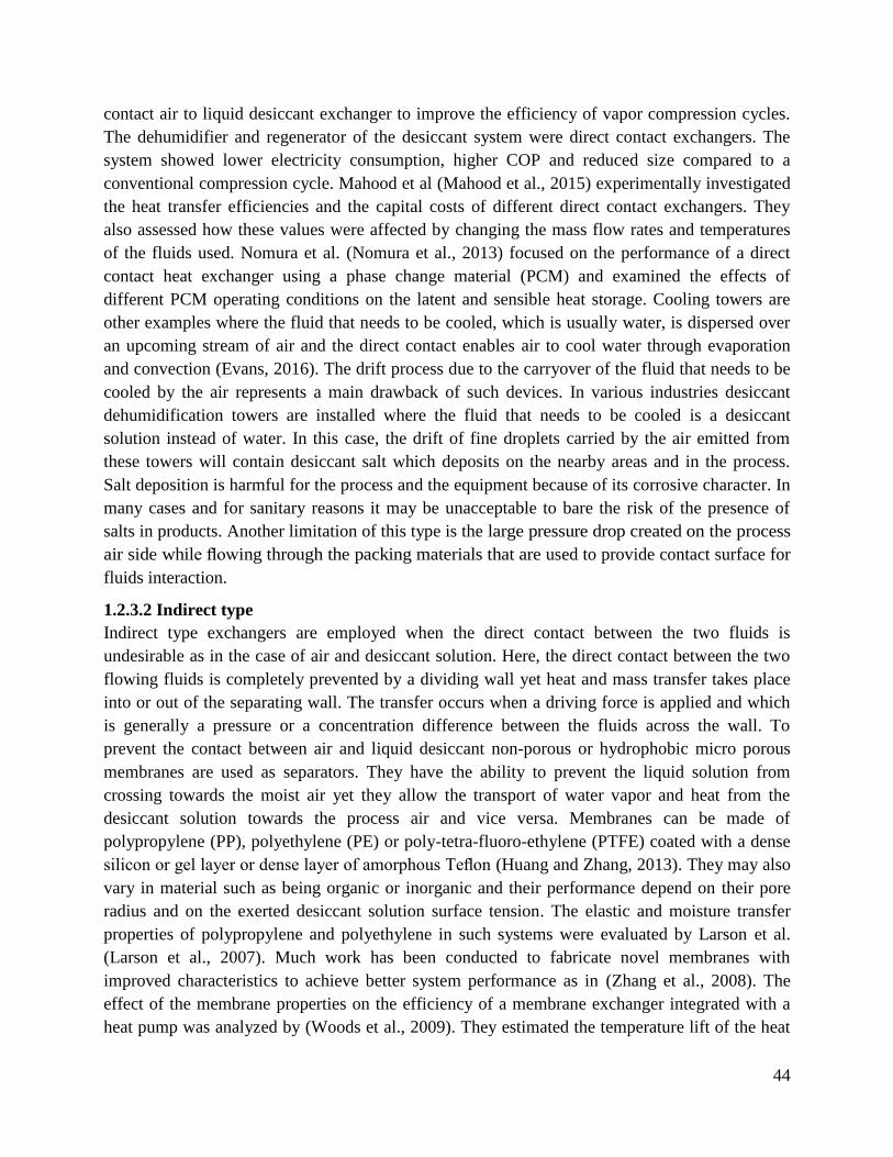
44

contact air to liquid desiccant exchanger to improve the efficiency of vapor compression cycles.

The dehumidifier and regenerator of the desiccant system were direct contact exchangers. The

system showed lower electricity consumption, higher COP and reduced size compared to a

conventional compression cycle. Mahood et al (Mahood et al., 2015) experimentally investigated

the heat transfer efficiencies and the capital costs of different direct contact exchangers. They

also assessed how these values were affected by changing the mass flow rates and temperatures

of the fluids used. Nomura et al. (Nomura et al., 2013) focused on the performance of a direct

contact heat exchanger using a phase change material (PCM) and examined the effects of

different PCM operating conditions on the latent and sensible heat storage. Cooling towers are

other examples where the fluid that needs to be cooled, which is usually water, is dispersed over

an upcoming stream of air and the direct contact enables air to cool water through evaporation

and convection (Evans, 2016). The drift process due to the carryover of the fluid that needs to be

cooled by the air represents a main drawback of such devices. In various industries desiccant

dehumidification towers are installed where the fluid that needs to be cooled is a desiccant

solution instead of water. In this case, the drift of fine droplets carried by the air emitted from

these towers will contain desiccant salt which deposits on the nearby areas and in the process.

Salt deposition is harmful for the process and the equipment because of its corrosive character. In

many cases and for sanitary reasons it may be unacceptable to bare the risk of the presence of

salts in products. Another limitation of this type is the large pressure drop created on the process

air side while flowing through the packing materials that are used to provide contact surface for

fluids interaction.

1.2.3.2 Indirect type

Indirect type exchangers are employed when the direct contact between the two fluids is

undesirable as in the case of air and desiccant solution. Here, the direct contact between the two

flowing fluids is completely prevented by a dividing wall yet heat and mass transfer takes place

into or out of the separating wall. The transfer occurs when a driving force is applied and which

is generally a pressure or a concentration difference between the fluids across the wall. To

prevent the contact between air and liquid desiccant non-porous or hydrophobic micro porous

membranes are used as separators. They have the ability to prevent the liquid solution from

crossing towards the moist air yet they allow the transport of water vapor and heat from the

desiccant solution towards the process air and vice versa. Membranes can be made of

polypropylene (PP), polyethylene (PE) or poly-tetra-fluoro-ethylene (PTFE) coated with a dense

silicon or gel layer or dense layer of amorphous Teflon (Huang and Zhang, 2013). They may also

vary in material such as being organic or inorganic and their performance depend on their pore

radius and on the exerted desiccant solution surface tension. The elastic and moisture transfer

properties of polypropylene and polyethylene in such systems were evaluated by Larson et al.

(Larson et al., 2007). Much work has been conducted to fabricate novel membranes with

improved characteristics to achieve better system performance as in (Zhang et al., 2008). The

effect of the membrane properties on the efficiency of a membrane exchanger integrated with a

heat pump was analyzed by (Woods et al., 2009). They estimated the temperature lift of the heat

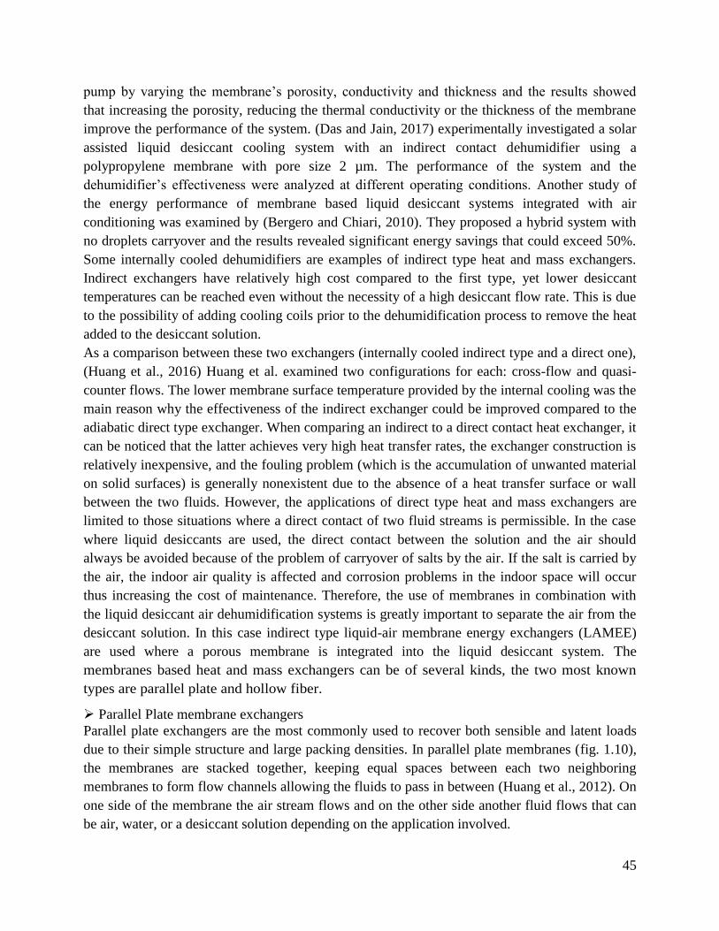
45

pump by varying the membrane’s porosity, conductivity and thickness and the results showed

that increasing the porosity, reducing the thermal conductivity or the thickness of the membrane

improve the performance of the system. (Das and Jain, 2017) experimentally investigated a solar

assisted liquid desiccant cooling system with an indirect contact dehumidifier using a

polypropylene membrane with pore size 2 µm. The performance of the system and the

dehumidifier’s effectiveness were analyzed at different operating conditions. Another study of

the energy performance of membrane based liquid desiccant systems integrated with air

conditioning was examined by (Bergero and Chiari, 2010). They proposed a hybrid system with

no droplets carryover and the results revealed significant energy savings that could exceed 50%.

Some internally cooled dehumidifiers are examples of indirect type heat and mass exchangers.

Indirect exchangers have relatively high cost compared to the first type, yet lower desiccant

temperatures can be reached even without the necessity of a high desiccant flow rate. This is due

to the possibility of adding cooling coils prior to the dehumidification process to remove the heat

added to the desiccant solution.

As a comparison between these two exchangers (internally cooled indirect type and a direct one),

(Huang et al., 2016) Huang et al. examined two configurations for each: cross-flow and quasi-

counter flows. The lower membrane surface temperature provided by the internal cooling was the

main reason why the effectiveness of the indirect exchanger could be improved compared to the

adiabatic direct type exchanger. When comparing an indirect to a direct contact heat exchanger, it

can be noticed that the latter achieves very high heat transfer rates, the exchanger construction is

relatively inexpensive, and the fouling problem (which is the accumulation of unwanted material

on solid surfaces) is generally nonexistent due to the absence of a heat transfer surface or wall

between the two fluids. However, the applications of direct type heat and mass exchangers are

limited to those situations where a direct contact of two fluid streams is permissible. In the case

where liquid desiccants are used, the direct contact between the solution and the air should

always be avoided because of the problem of carryover of salts by the air. If the salt is carried by

the air, the indoor air quality is affected and corrosion problems in the indoor space will occur

thus increasing the cost of maintenance. Therefore, the use of membranes in combination with

the liquid desiccant air dehumidification systems is greatly important to separate the air from the

desiccant solution. In this case indirect type liquid-air membrane energy exchangers (LAMEE)

are used where a porous membrane is integrated into the liquid desiccant system. The

membranes based heat and mass exchangers can be of several kinds, the two most known

types are parallel plate and hollow fiber.

Parallel Plate membrane exchangers

Parallel plate exchangers are the most commonly used to recover both sensible and latent loads

due to their simple structure and large packing densities. In parallel plate membranes (fig. 1.10),

the membranes are stacked together, keeping equal spaces between each two neighboring

membranes to form flow channels allowing the fluids to pass in between (Huang et al., 2012). On

one side of the membrane the air stream flows and on the other side another fluid flows that can

be air, water, or a desiccant solution depending on the application involved.

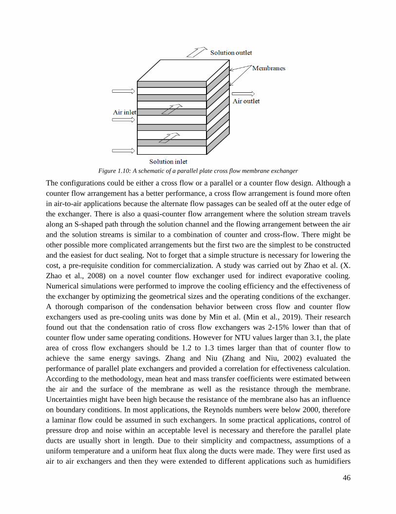
46

Figure 1.10: A schematic of a parallel plate cross flow membrane exchanger

The configurations could be either a cross flow or a parallel or a counter flow design. Although a

counter flow arrangement has a better performance, a cross flow arrangement is found more often

in air-to-air applications because the alternate flow passages can be sealed off at the outer edge of

the exchanger. There is also a quasi-counter flow arrangement where the solution stream travels

along an S-shaped path through the solution channel and the flowing arrangement between the air

and the solution streams is similar to a combination of counter and cross-flow. There might be

other possible more complicated arrangements but the first two are the simplest to be constructed

and the easiest for duct sealing. Not to forget that a simple structure is necessary for lowering the

cost, a pre-requisite condition for commercialization. A study was carried out by Zhao et al. (X.

Zhao et al., 2008) on a novel counter flow exchanger used for indirect evaporative cooling.

Numerical simulations were performed to improve the cooling efficiency and the effectiveness of

the exchanger by optimizing the geometrical sizes and the operating conditions of the exchanger.

A thorough comparison of the condensation behavior between cross flow and counter flow

exchangers used as pre-cooling units was done by Min et al. (Min et al., 2019). Their research

found out that the condensation ratio of cross flow exchangers was 2-15% lower than that of

counter flow under same operating conditions. However for NTU values larger than 3.1, the plate

area of cross flow exchangers should be 1.2 to 1.3 times larger than that of counter flow to

achieve the same energy savings. Zhang and Niu (Zhang and Niu, 2002) evaluated the

performance of parallel plate exchangers and provided a correlation for effectiveness calculation.

According to the methodology, mean heat and mass transfer coefficients were estimated between

the air and the surface of the membrane as well as the resistance through the membrane.

Uncertainties might have been high because the resistance of the membrane also has an influence

on boundary conditions. In most applications, the Reynolds numbers were below 2000, therefore

a laminar flow could be assumed in such exchangers. In some practical applications, control of

pressure drop and noise within an acceptable level is necessary and therefore the parallel plate

ducts are usually short in length. Due to their simplicity and compactness, assumptions of a

uniform temperature and a uniform heat flux along the ducts were made. They were first used as

air to air exchangers and then they were extended to different applications such as humidifiers

47

and dehumidifiers used as LAMEE as it is the case here (Huang et al., 2014; Vali et al., 2009).

The performance of a cross flow flat plate membrane based heat and mass exchanger for

regeneration (Bai et al., 2018) and dehumidification processes was evaluated in several studies.

They experimentally and numerically assessed the effects of the main operating parameters on

the regeneration and dehumidification by varying the inlet properties of the solution and the air.

(Abdel-Salam et al., 2013) studied a system where two LAMEEs were used, one in the

dehumidifier for drying the process air and the other in the regenerator for the reactivation of the

desiccant. An analysis of a LAMEE using LiCl desiccant solution for both dehumidification and

regeneration was conducted by Ge et al. (Ge et al., 2014). They experimentally tested the effect

of changing the inlet conditions of the solution and the air (including concentration, flow rates

and temperatures) on the performances of the exchanger in both devices and they compared them

to those of direct contact liquid desiccant devices. Another application for the LAMEE was in the

energy recovery ventilators where they could be placed in the supply and exhaust air streams (Al-

Waked et al., 2018). Effectiveness and moisture removal rate were the most common indices that

determine their performance. The configuration of the liquid-air flow within the exchanger was

one of the essential design parameters that can affect the performance of a LAMEE. A quasi

counter flow parallel plate membrane heat pump was proposed by (Huang, 2015; Huang et al.,

2014). A numerical calculation was done to show the effects of the channels structure on the

solution temperature lift and efficiency. (Liang, 2014) Liang tested experimentally the sensible,

latent and total energy transfer in a parallel plate enthalpy exchanger under various operating

conditions. The results showed that the sensible, latent and total heat effectiveness decrease with

the increase in the air mass flow rate and increase with the increase of the air temperature.

Another study done by Nielsen et al. (Nielsen et al., 2013) focused on the influence of the fluid

flow maldistribution on the performance of non-homogenous parallel plate exchangers. Their

model showed that the flow maldistribution reduced greatly the performance of non-homogenous

stacks of parallel plates compared to uniform plate stacks.

Hollow Fiber

Similar to parallel plate membrane exchangers, in the hollow fiber types the air stream and the

liquid stream do not mix together; each will be flowing on one side of the membrane (fig. 1.11).

It is like a shell and tube heat exchanger where the tube side is formed by a bundle of hollow

fiber membranes placed inside a shell. The shell side flow is formed in the cavities between the

shell and the fibers. The best performance can be expected by transverse flow configurations with

well-defined fiber spacing leading to a low pressure drop and a sufficient mass transfer (Yang et

al., 2013). Two possible configurations can be done; the first one is to allow the desiccant

solution to flow outside the tubes while the airstream inside the tubes. However, in most

engineering applications, the solution flows in the tube side while the air moves in the shell side

in a counter flow arrangement. The benefit of this flowing configuration is that the pressure drop

for the air flow in the shell side is less and the performance is better (Bruining, 1989).

48

Figure 1.11: Schematic of the hollow fiber membrane module and the cell with a free surface model (L.-Z. Zhang et

al., 2012). (a) The shell and the tube structure; (b) The cell with a free surface

The hollow fiber membranes are gaining more attraction from researchers because they have a

higher packing density and a larger heat and mass transfer capability. A general review of hollow

fiber contactors was given by (Gabelman and Hwang, 1999) including their field of applications,

their design considerations and their operating principles. Pabby et al. (Pabby and Sastre, 2013)

examined the most recent developments concerning the hollow fiber membrane contractors

estimating their potential success and proposing possible future applications in which they might

have promising role in industrial production cycles. Hollow fiber contractors were also

investigated in air dehumidification processes as presented by Zhang and Huang (Zhang and

Huang, 2011). They investigated, experimentally and analytically, the heat and mass transfer in a

counter flow hollow fiber membrane module that showed very high performance and it was

found that the membrane properties greatly affected the mass transfer of the exchanger. Further

studies were done by Zhao et al. (Zhao et al., 2015) who evaluated experimentally a hollow fiber

membrane exchanger performance during vacuum dehumidification. After running the test bench

for 150 hours they found that the potential reduction in energy consumption of such a system

could reach up to 26% compared to a conventional vapor compression cycle. Similar to

dehumidifiers, regenerators were also made of hollow fiber membrane contractors. Zhang (Zhang

and Zhang, 2014) integrated these contractors with a heat pump system to perform

dehumidification prior to air cooling and regeneration of the liquid desiccant. The system was

experimentally assessed under different operating conditions and the numerical results showed

that the system performed properly even under very hot and humid weather. Research on the role

of hollow fiber exchangers in gas separation applications was widely published throughout the

years. Feron and Jason (Feron and Jansen, 2002) employed a hollow fiber membrane contractor

for CO2 separation with a porous polypropylene membrane. The aqueous solution used as

absorbent was “Coral”, a novel absorption liquid based on mixtures of salts and amino acids.

49

Due to the numerous amounts of fibers in the shell, a direct modeling of the whole module is

difficult. The mathematical models of the heat and mass transfer in the gas-liquid hollow fiber

membrane contactors were established in several references and there have been many researches

on this kind of exchangers. Zhang et al. (L.-Z. Zhang et al., 2012) investigated a laminar fluid

flow heat and mass transfer in a hollow fiber membrane contactor for liquid desiccant air

dehumidification. A cross flow arrangement was used where the solution flowed inside the fiber

tubes while the air in the shell side. Their study resulted in obtaining the total drag coefficient,

and the Nusselt and Sherwood numbers for a certain range of Reynolds number. Kistler and

Cussler (Kistler and Cussler, 2002) also investigated the feasibility of using hollow fiber

polymer membranes to recover heat and mass from ventilation air. Johnson et al. (Johnson et

al., 2003) experimentally studied the influence of the membrane and the operating parameters on

achievable mass and heat flux in order to be able to assess the efficiency of hollow fiber

exchangers in evaporative cooling. They showed that reasonable numbers of fibers and

membrane surface area could provide more cooling effectiveness comparable to conventional

evaporative cooling equipment.

1.2.3.3 Drawbacks of the existing heat and mass exchangers and possible solutions

In the previous paragraphs, many of the mentioned studies focused on the performance of heat

and mass exchangers highlighting for instance the importance of the properties of the membrane

in indirect types or the advantage of some arrangements using spraying techniques in direct

contact ones. However, after describing the existing designs where these exchangers are applied,

it could be noticed that they still have certain drawbacks.

Regarding the direct contact water spraying in cooling towers, this technology proved its

importance and good performance yet the problem of drift lead to serious complications

especially when salt solution droplets were carried by the air and could ruin nearby spaces (Ruiz

et al., 2016). Moreover, concerning the actual membrane based heat and mass exchangers, there

exist some challenges that need to be enhanced and much research is being conducted concerning

the amelioration of their effectiveness. First, these systems are usually sophisticated due to the

installation and distribution of channels with different configurations. Second, they are costly due

to the high price of the membranes that are of made of complex structures and are difficult to

process. Concerning the membranes, one of the drawbacks is that they should be able to

withstand a liquid pressure without being damaged or wetted thus they must be stiff enough to

withstand the pressure difference and limit the surface warping under both dry and wet conditions

(X Zhao et al., 2008). The impermeability to liquid water is also another important challenge for

the membranes by which liquid water should never penetrate or permeate to the other side of the

membrane whenever a water pressure is applied. However, water vapor should always be able to

move from one side of the membrane to the other. All these characteristics require specific

properties that should be present within the membrane such as acceptable thermal and mass

conductivities, surface tension and elasticity, wear-resistant and high strength in order to promote

the heat and moisture transfer (Onsekizoglu, 2012). Thus the heat and mass transfer resistance of

the membrane should be as low as possible and the thermal conductivity should be small enough

50

to reduce the heat loss between the sides of the membrane. The thermal conductivity of the

membrane is related to its physical characteristics and geometry and to its ability to conduct heat.

Another limitation of the proposed membranes in the literature is their expensiveness and low

performance since the membranes need to be mechanically reinforced which leads to a low mass

conductivity.

In order to get a high performing system, convenient membrane properties should be available

and the above mentioned challenges should be overcome. In all the existing systems these

properties are found to be in contradiction with each other. Whenever the membrane is capable to

withstand a liquid pressure its permeability to water vapor decreases reducing its mass

conductivity. These contradictions in the system along with the challenging leak tightness

feature, the high manufacturing cost and the complexity of the system as a whole, promote the

development of a new competent system capable of responding to all the above mentioned needs

and challenges.

1.2.3.4 Novel design of membrane based heat and mass exchanger

A novel technology patented by “Armines” is proposed. This technology makes a positive use of

the presence of the membrane to solve the drift problem and the drawbacks of the actual

membrane based technologies.

Figure 1.12 represents our proposed system consisting of a cross flow heat and mass exchanger

where the desiccant solution is sprayed vertically downwards in between the membranes,

represented by the green layers, and the air flows in a perpendicular stream. The weakened

desiccant solution is then collected in the sump at the bottom of the exchanger and sent back to a

regenerator in order to be reactivated.

Figure 1.12: Design model of the proposed system

In a way to decrease the importance of withstanding a liquid pressure, spraying the liquid

desiccant evenly through nozzles at the top of the system represents a desirable alternative. The

vertical spraying of the liquid facilitates the design configuration as it flows downward by gravity

(fig. 1.13).

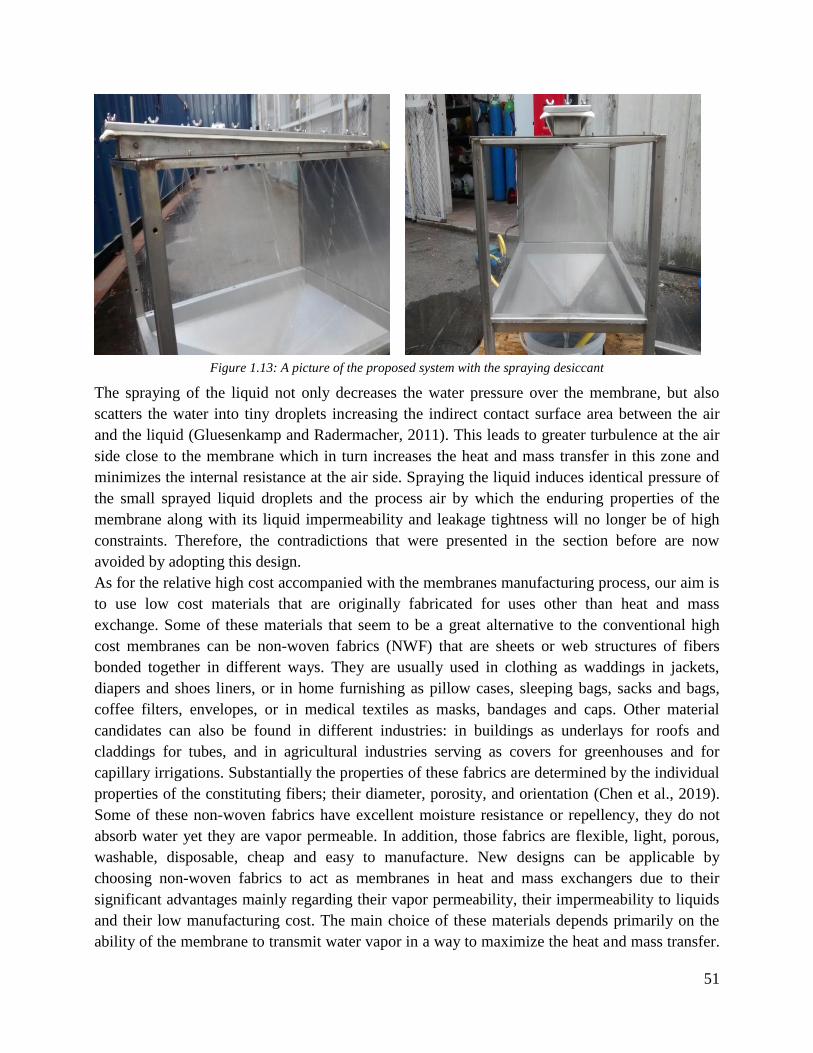
51

Figure 1.13: A picture of the proposed system with the spraying desiccant

The spraying of the liquid not only decreases the water pressure over the membrane, but also

scatters the water into tiny droplets increasing the indirect contact surface area between the air

and the liquid (Gluesenkamp and Radermacher, 2011). This leads to greater turbulence at the air

side close to the membrane which in turn increases the heat and mass transfer in this zone and

minimizes the internal resistance at the air side. Spraying the liquid induces identical pressure of

the small sprayed liquid droplets and the process air by which the enduring properties of the

membrane along with its liquid impermeability and leakage tightness will no longer be of high

constraints. Therefore, the contradictions that were presented in the section before are now

avoided by adopting this design.

As for the relative high cost accompanied with the membranes manufacturing process, our aim is

to use low cost materials that are originally fabricated for uses other than heat and mass

exchange. Some of these materials that seem to be a great alternative to the conventional high

cost membranes can be non-woven fabrics (NWF) that are sheets or web structures of fibers

bonded together in different ways. They are usually used in clothing as waddings in jackets,

diapers and shoes liners, or in home furnishing as pillow cases, sleeping bags, sacks and bags,

coffee filters, envelopes, or in medical textiles as masks, bandages and caps. Other material

candidates can also be found in different industries: in buildings as underlays for roofs and

claddings for tubes, and in agricultural industries serving as covers for greenhouses and for

capillary irrigations. Substantially the properties of these fabrics are determined by the individual

properties of the constituting fibers; their diameter, porosity, and orientation (Chen et al., 2019).

Some of these non-woven fabrics have excellent moisture resistance or repellency, they do not

absorb water yet they are vapor permeable. In addition, those fabrics are flexible, light, porous,

washable, disposable, cheap and easy to manufacture. New designs can be applicable by

choosing non-woven fabrics to act as membranes in heat and mass exchangers due to their

significant advantages mainly regarding their vapor permeability, their impermeability to liquids

and their low manufacturing cost. The main choice of these materials depends primarily on the

ability of the membrane to transmit water vapor in a way to maximize the heat and mass transfer.

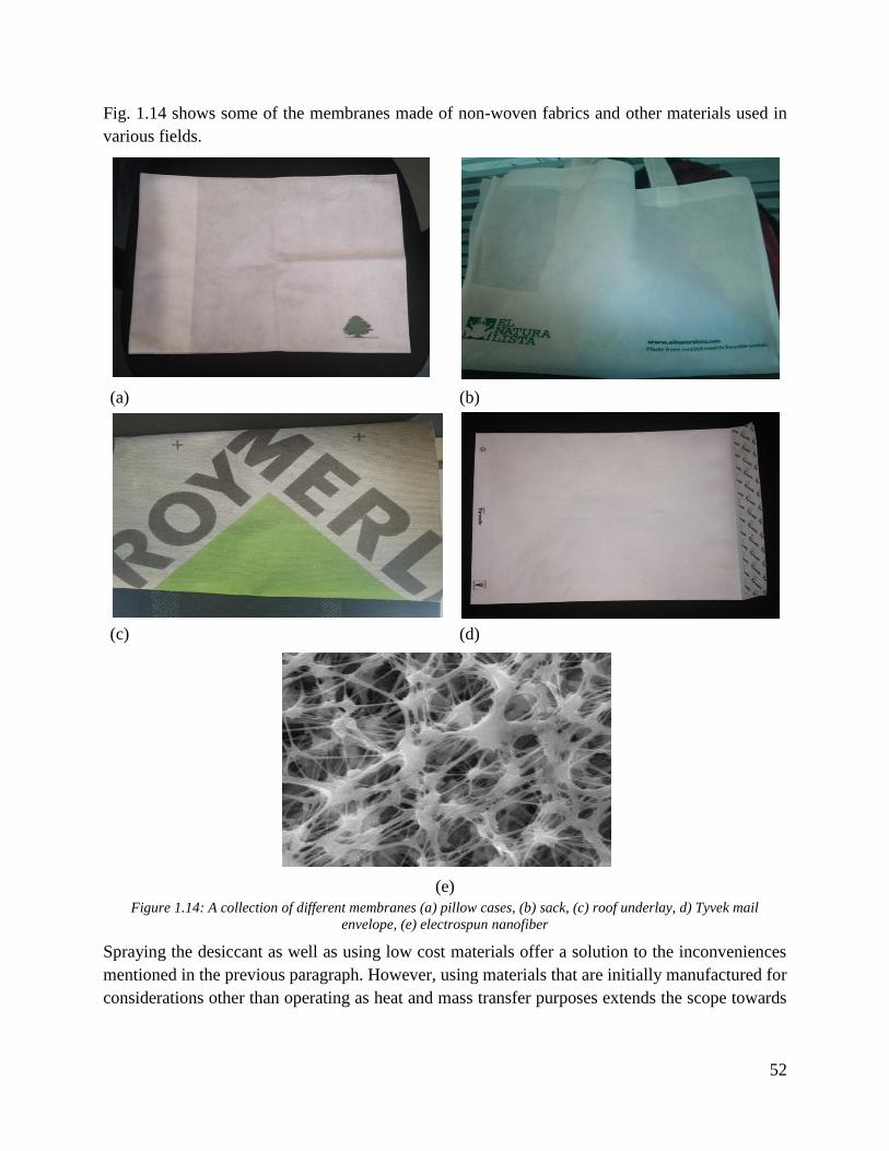
52

Fig. 1.14 shows some of the membranes made of non-woven fabrics and other materials used in

various fields.

(a) (b)

(c) (d)

(e)

Figure 1.14: A collection of different membranes (a) pillow cases, (b) sack, (c) roof underlay, d) Tyvek mail

envelope, (e) electrospun nanofiber

Spraying the desiccant as well as using low cost materials offer a solution to the inconveniences

mentioned in the previous paragraph. However, using materials that are initially manufactured for

considerations other than operating as heat and mass transfer purposes extends the scope towards

53

new perspectives as well as new scientific and technological burdens that will be explained and

solved in the next chapter.

1.3 Thesis Problem Statement

Hybrid systems based on coupling desiccant cycle and vapor compression cycle seem reliable

candidates that allow proper humidity control in air conditioning applications and a frost free

operation in the case of refrigeration, with a potentially increased COP. Since solid desiccant

present the drawback of high regeneration temperatures and complexity in their integration

in systems, liquid desiccants are more attractive showing low regeneration temperatures and

remarkable dehumidification capacities. From the previous cited research, it was determined

that the configuration of the hybrid system and its architecture offer high efficiency over a range

of operating conditions with different latent to sensible load ratio. This range of operating

conditions varies from one architecture to another; it is clear that maintaining a high performing

hybrid system could only be accomplished by a flexible design operating through a whole season

in an energy efficient way. This defines the final objective of this thesis to design high

performance, affordable and flexible hybrid refrigeration and air conditioning systems along with

a design methodology and modeling tools.

The dehumidifier and the regenerator of such a hybrid system are considered the main

challenging components and their proper designs greatly affect the temperature and humidity

control. As discussed, one challenge related to these heat and mass exchangers is their ability to

prevent the escarpment of the desiccant solution droplets towards the air avoiding corrosion

problems while keeping them simple to build and low in cost. The membrane heat and mass

exchangers constitute a technological response for such issues but the state of the art technologies

present many drawbacks as explained earlier. In this thesis, the novel technology presented in the

preceding section will be thoroughly studied. It uses original membrane materials and new design

related to liquid distribution. The challenges concerning these materials are the lack of scientific

characteristics and information concerning their properties mainly their water vapor permeability.

To find out this property, these materials are tested experimentally using a modified cup test and

the used methodology will be discussed in the coming chapter.

The third chapter of this thesis aims to deeply understand the behavior and the performance of

this novel indirect contact heat and mass exchanger. The proper understanding and modeling of

coupled heat and mass transfers within this novel exchanger are key factors to efficiently

integrate them into processes and to benefit from their advantages over the existing conventional

technologies. A modeling approach of the heat and mass transfer phenomena is developed by

modeling the designed membrane exchangers and is supported by experimental characterization.

This model is used in the last chapter to study the energy interest of the integration of these

exchangers in air conditioning applications and to design a flexible architecture able to cope with

the seasonal variation of the load ratio.

54

Chapitre 2 Méthode Modifiée de la coupe pour Tester la

Perméabilité de la Vapeur D'eau dans les Membranes

Poreuses (résumé)

2.1 Introduction

Comme indiqué dans le chapitre précédent, les systèmes hybrides de climatisation (dessiccant

liquide avec cycle de compression de vapeur) utilisant des échangeurs membranaires de chaleur

et de masse peuvent être des alternatives prometteuses aux systèmes traditionnels de climatisation

(Abdel-Salam et al., 2013); Huang et al., 2013; Zhang et Zhang, 2014). Certaines propriétés

d’une membrane, comme son épaisseur, sa porosité, sa conductivité thermique et celle de masse,

affectent l’efficacité des échangeurs. La conductivité de masse, aussi appelée perméabilité à la

vapeur d'eau, a un impact majeur sur le transfert de la vapeur d'eau à l'intérieur de la membrane et

donc sur la performance globale des échangeurs (Zhang, 2006). Il s'agit de la mesure de la

quantité de vapeur d'eau qui passe d'un milieu à un autre à travers un matériau d'une épaisseur et

d'une surface données et à une unité de temps définie. La transmission de la vapeur d'eau est

induite par la différence de pression de vapeur entre les deux milieux causée par la différence de

température et de concentration (Gurubalan et al., 2017). Si la perméabilité de la membrane est

très faible la vapeur d'eau serait piégée dans le matériau qui provoque la condensation (si sa

température atteint la saturation). Par conséquent, l'humidité interne augmente, ce qui bloque le

transfert massique de l'échangeur. Le taux de transmission de la vapeur d'eau des matériaux

poreux dépend fortement des propriétés physiques de la membrane, comme les dimensions de ses

pores (Mukhopadhyaya et al., 2005). Afin de pouvoir comparer cette grandeur dans différentes

membranes, il est important de s'assurer que ces membranes sont analysées et testées selon la

même méthode et procédure d'essai (Li et Yao, 2018). Diverses techniques existent pour mesurer

la perméabilité à la vapeur d'eau dans les membranes de différents types et caractéristiques. La

méthode la plus couramment utilisée est le test de la coupe basé sur les normes publiées par la

ASTM E96. La méthode de la coupe décrite dans la norme ASTM E96 est principalement utilisée

pour prédire le taux de transmission de la vapeur d'eau dans des matériaux poreux ayant une

perméabilité faible à modérée. L'une des hypothèses principales des normes ASTM est que la

valeur de la résistance de l’air n'est pas indépendamment calculée. Par contre, on l'estime en

supposant en même temps que la résistance de la membrane étant considérablement plus élevée.

Pourtant, cette supposition n’est plus valide lorsque les matériaux testés ont une grande

perméabilité à la vapeur d'eau. La perméabilité élevée implique une faible résistance au transfert

de masse et donc la résistance à l'air ne serait plus négligeable par rapport à celle du matériau.

Dans notre étude, nous sommes intéressés par les matériaux qui permettent une transmission de

vapeur d'eau élevée et donc la résistance à l'air devrait être calculée séparément. Le test ASTM

E96 ne fournit pas de données sur la façon de calculer cette résistance ; par conséquent, ce

chapitre décrit brièvement l'essai de coupe et introduit une technique modifiée pour estimer la

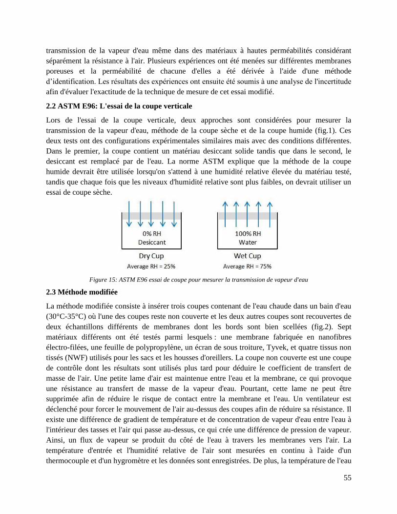
55

transmission de la vapeur d'eau même dans des matériaux à hautes perméabilités considérant

séparément la résistance à l'air. Plusieurs expériences ont été menées sur différentes membranes

poreuses et la perméabilité de chacune d'elles a été dérivée à l'aide d'une méthode

d’identification. Les résultats des expériences ont ensuite été soumis à une analyse de l'incertitude

afin d'évaluer l'exactitude de la technique de mesure de cet essai modifié.

2.2 ASTM E96: L'essai de la coupe verticale

Lors de l'essai de la coupe verticale, deux approches sont considérées pour mesurer la

transmission de la vapeur d'eau, méthode de la coupe sèche et de la coupe humide (fig.1). Ces

deux tests ont des configurations expérimentales similaires mais avec des conditions différentes.

Dans le premier, la coupe contient un matériau desiccant solide tandis que dans le second, le

desiccant est remplacé par de l'eau. La norme ASTM explique que la méthode de la coupe

humide devrait être utilisée lorsqu'on s'attend à une humidité relative élevée du matériau testé,

tandis que chaque fois que les niveaux d'humidité relative sont plus faibles, on devrait utiliser un

essai de coupe sèche.

Figure 15: ASTM E96 essai de coupe pour mesurer la transmission de vapeur d'eau

2.3 Méthode modifiée

La méthode modifiée consiste à insérer trois coupes contenant de l'eau chaude dans un bain d'eau

(30°C-35°C) où l'une des coupes reste non couverte et les deux autres coupes sont recouvertes de

deux échantillons différents de membranes dont les bords sont bien scellées (fig.2). Sept

matériaux différents ont été testés parmi lesquels : une membrane fabriquée en nanofibres

électro-filées, une feuille de polypropylène, un écran de sous troiture, Tyvek, et quatre tissus non

tissés (NWF) utilisés pour les sacs et les housses d'oreillers. La coupe non couverte est une coupe

de contrôle dont les résultats sont utilisés plus tard pour déduire le coefficient de transfert de

masse de l'air. Une petite lame d'air est maintenue entre l'eau et la membrane, ce qui provoque

une résistance au transfert de masse de la vapeur d'eau. Pourtant, cette lame ne peut être

supprimée afin de réduire le risque de contact entre la membrane et l'eau. Un ventilateur est

déclenché pour forcer le mouvement de l'air au-dessus des coupes afin de réduire sa résistance. Il

existe une différence de gradient de température et de concentration de vapeur d'eau entre l'eau à

l'intérieur des tasses et l'air qui passe au-dessus, ce qui crée une différence de pression de vapeur.

Ainsi, un flux de vapeur se produit du côté de l'eau à travers les membranes vers l'air. La

température d'entrée et l'humidité relative de l'air sont mesurées en continu à l'aide d'un

thermocouple et d'un hygromètre et les données sont enregistrées. De plus, la température de l'eau

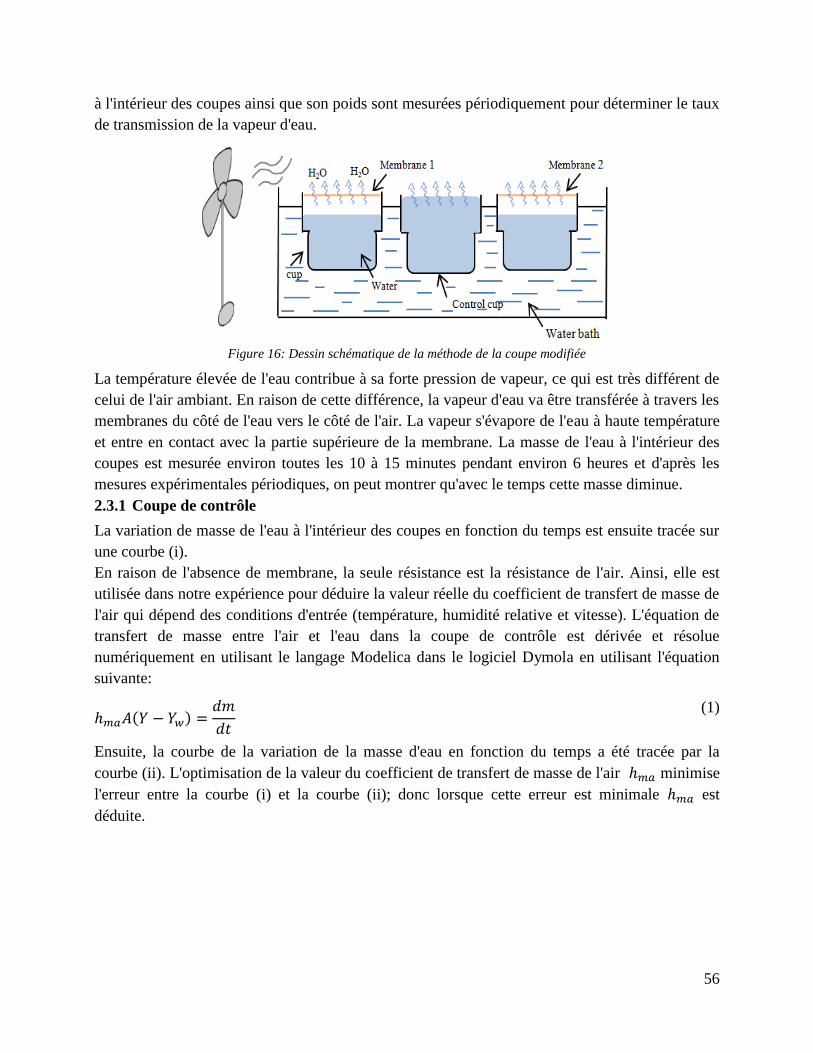
56

à l'intérieur des coupes ainsi que son poids sont mesurées périodiquement pour déterminer le taux

de transmission de la vapeur d'eau.

Figure 16: Dessin schématique de la méthode de la coupe modifiée

La température élevée de l'eau contribue à sa forte pression de vapeur, ce qui est très différent de

celui de l'air ambiant. En raison de cette différence, la vapeur d'eau va être transférée à travers les

membranes du côté de l'eau vers le côté de l'air. La vapeur s'évapore de l'eau à haute température

et entre en contact avec la partie supérieure de la membrane. La masse de l'eau à l'intérieur des

coupes est mesurée environ toutes les 10 à 15 minutes pendant environ 6 heures et d'après les

mesures expérimentales périodiques, on peut montrer qu'avec le temps cette masse diminue. 2.3.1 Coupe de contrôle

La variation de masse de l'eau à l'intérieur des coupes en fonction du temps est ensuite tracée sur

une courbe (i).

En raison de l'absence de membrane, la seule résistance est la résistance de l'air. Ainsi, elle est

utilisée dans notre expérience pour déduire la valeur réelle du coefficient de transfert de masse de

l'air qui dépend des conditions d'entrée (température, humidité relative et vitesse). L'équation de

transfert de masse entre l'air et l'eau dans la coupe de contrôle est dérivée et résolue

numériquement en utilisant le langage Modelica dans le logiciel Dymola en utilisant l'équation

suivante:

(1)

Ensuite, la courbe de la variation de la masse d'eau en fonction du temps a été tracée par la

courbe (ii). L'optimisation de la valeur du coefficient de transfert de masse de l'air minimise

l'erreur entre la courbe (i) et la courbe (ii); donc lorsque cette erreur est minimale est

déduite.

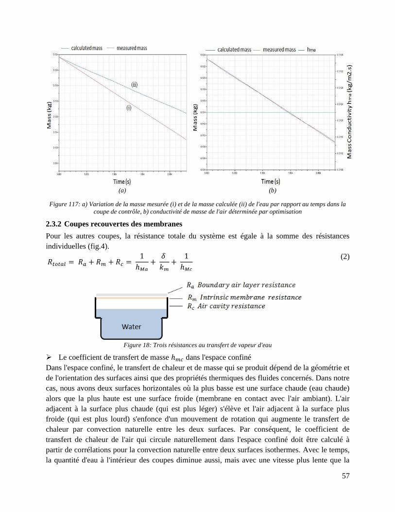
57

(a) (b)

Figure 117: a) Variation de la masse mesurée (i) et de la masse calculée (ii) de l'eau par rapport au temps dans la

coupe de contrôle, b) conductivité de masse de l'air déterminée par optimisation

2.3.2 Coupes recouvertes des membranes

Pour les autres coupes, la résistance totale du système est égale à la somme des résistances

individuelles (fig.4).

(2)

Figure 18: Trois résistances au transfert de vapeur d'eau

Le coefficient de transfert de masse dans l'espace confiné

Dans l'espace confiné, le transfert de chaleur et de masse qui se produit dépend de la géométrie et

de l'orientation des surfaces ainsi que des propriétés thermiques des fluides concernés. Dans notre

cas, nous avons deux surfaces horizontales où la plus basse est une surface chaude (eau chaude)

alors que la plus haute est une surface froide (membrane en contact avec l'air ambiant). L'air

adjacent à la surface plus chaude (qui est plus léger) s'élève et l'air adjacent à la surface plus

froide (qui est plus lourd) s'enfonce d'un mouvement de rotation qui augmente le transfert de

chaleur par convection naturelle entre les deux surfaces. Par conséquent, le coefficient de

transfert de chaleur de l'air qui circule naturellement dans l'espace confiné doit être calculé à

partir de corrélations pour la convection naturelle entre deux surfaces isothermes. Avec le temps,

la quantité d'eau à l'intérieur des coupes diminue aussi, mais avec une vitesse plus lente que la

58

coupe de contrôle. Ainsi, l'espace confiné entre l'eau et la membrane augmente, ce qui entraîne

une diminution de sa conductivité de masse et donc une augmentation de sa résistance. Le

nombre de Nusselt est exprimé dans le cas d'une cavité horizontale chauffée par le bas, par :

(3)

Et donc le coefficient de transfert de masse est déduit en utilisant l'analogie de Lewis

(4)

Avec

(5)

Déduction de

Les équations de transfert de masse d'une coupe recouverte d'une membrane peuvent être écrites

comme suit:

(6)

(7)

(8)

Ce système est utilisé pour déterminer les inconnues et en substituant la valeur de la

conductivité de masse déduite précédemment de l'air et de la cavité . La solution du

système d'équation de transfert de masse dans les coupes couvertes permet de tracer la courbe de

la variation de masse calculée en fonction du temps (ii). Minimiser l'erreur entre ces deux

courbes nous permet de trouver la conductivité de la masse de la membrane (fig.5).

(a) (b) Figure 19: a) Variation de la masse mesurée (i) et de la masse calculée (ii) de l'eau par rapport au temps dans la

coupe recouverte d’une membrane, b) conductivité de masse de la membrane déterminée par optimisation

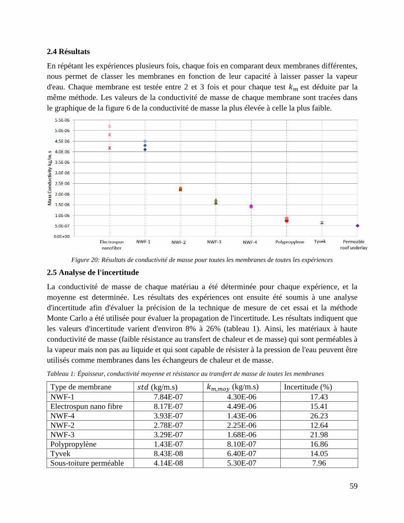
59

2.4 Résultats

En répétant les expériences plusieurs fois, chaque fois en comparant deux membranes différentes,

nous permet de classer les membranes en fonction de leur capacité à laisser passer la vapeur

d'eau. Chaque membrane est testée entre 2 et 3 fois et pour chaque test est déduite par la

même méthode. Les valeurs de la conductivité de masse de chaque membrane sont tracées dans

le graphique de la figure 6 de la conductivité de masse la plus élevée à celle la plus faible.

Figure 20: Résultats de conductivité de masse pour toutes les membranes de toutes les expériences

2.5 Analyse de l'incertitude

La conductivité de masse de chaque matériau a été déterminée pour chaque expérience, et la

moyenne est determinée. Les résultats des expériences ont ensuite été soumis à une analyse

d'incertitude afin d'évaluer la précision de la technique de mesure de cet essai et la méthode

Monte Carlo a été utilisée pour évaluer la propagation de l'incertitude. Les résultats indiquent que

les valeurs d'incertitude varient d'environ 8% à 26% (tableau 1). Ainsi, les matériaux à haute

conductivité de masse (faible résistance au transfert de chaleur et de masse) qui sont perméables à

la vapeur mais non pas au liquide et qui sont capable de résister à la pression de l'eau peuvent être

utilisés comme membranes dans les échangeurs de chaleur et de masse.

Tableau 1: Épaisseur, conductivité moyenne et résistance au transfert de masse de toutes les membranes

Type de membrane (kg/m.s) (kg/m.s) Incertitude (%)

NWF-1 7.84E-07 4.30E-06 17.43

Electrospun nano fibre 8.17E-07 4.49E-06 15.41

NWF-4 3.93E-07 1.43E-06 26.23

NWF-2 2.78E-07 2.25E-06 12.64

NWF-3 3.29E-07 1.68E-06 21.98

Polypropylène 1.43E-07 8.10E-07 16.86

Tyvek 8.43E-08 6.40E-07 14.05

Sous-toiture perméable 4.14E-08 5.30E-07 7.96

60

2.6 Conclusion

La perméabilité à la vapeur d'eau est la propriété principale des membranes qui influence sa

capacité de transfert de masse. Dans ce chapitre, on a identifié différents matériaux à faible coût

qui sont initialement fabriqués pour des usages autres que l'utilisation comme membranes. Ces

matériaux ont été testés expérimentalement à l'aide d'un essai de coupe modifié et d’une méthode

d’identification afin de déterminer leur perméabilité à la vapeur d'eau. Dans cette méthodologie,

nous avons réussi à déduire explicitement la valeur des résistances de l'air au-dessus des coupes

et de l'air coincé entre l'eau et la membrane. En substituant ces valeurs dans le système

d'équations de conservation de masse, on a déterminé la conductivité de masse des membranes.

Ces valeurs allaient de 5,3 x 10-7 à 4,49 x 10-6 kg/m.s. Ainsi, la mesure, l'analyse et

l'interprétation des résultats pour les différents matériaux nous permettent de classer et de

comparer la capacité de transfert de masse de chacun. Une analyse de l'incertitude a ensuite été

effectuée pour évaluer l'exactitude de cette approche et la méthode Monte Carlo a été utilisée

pour évaluer la propagation de l'incertitude. L'utilisation pratique des simulations de Monte-Carlo

pour l'estimation des incertitudes est un outil fondamental dans ce domaine, capable de résoudre

des problèmes de mesure complexes. Les résultats ont montré que les valeurs d'incertitude

variaient d'environ 8 % à 26 %. Ces chiffres, bien qu’ils n’aient pas été jugés suffisamment bas,

n’ont pas permis de modifier la classification des tissus testés par ordre de perméabilité de la

vapeur d’eau. Par la suite, une analyse de l'impact de l'incertitude de la conductivité de masse sur

la puissance totale de l'échangeur de chaleur et de masse sera effectuée. Cela donnerait une idée

si ces grandes valeurs d'incertitude sur ont un grand effet sur les résultats numériques de la

performance de l'échangeur ou non. Dans ce chapitre, nous avons pu classer les matériaux à haute

conductivité de masse (faible résistance à la chaleur et transfert de masse) et possédant les

caractéristiques d'être perméable à la vapeur, imperméable au liquide et capable de résister à la

pression d'eau peuvent être utilisés comme membranes dans les échangeurs de chaleur et de

masse. Selon nos résultats, la membrane composée de nanofibres électrospun semblait avoir la

conductivité de masse la plus élevée parmi les membranes testées; c’est un bon candidat potentiel

pour notre échangeur. Cependant, elle est produite par une nouvelle technique de fabrication alors

que les tissus non tissés sont largement disponibles. Ainsi, dans le chapitre à venir, la NWF-1, qui

présente la plus faible résistance au transfert de masse et qui possède les propriétés durables

requises, est utilisée comme membrane dans notre prototype d'un échangeur de chaleur et de

masse.

61

62

Chapter 2 Modified Upright Cup Method for Testing

Water Vapor Permeability in Porous Membranes

2.1 Introduction

As discussed in the previous chapter, hybrid air conditioning systems (liquid desiccant with vapor

compression cycle) using porous membrane based heat and mass exchangers may be ideal

alternatives to traditional air conditioning systems (Abdel-Salam et al., 2013; Huang et al., 2013;

Zhang and Zhang, 2014). Some of the properties of a membrane such as its thickness, porosity,

thermal conductivity, and mass conductivity affect the efficiency of the heat and mass exchangers

(Sabek et al., 2016). Mass conductivity, also known as water vapor permeability, has a main

impact on the transport of water vapor within the membrane and thus on the overall performance

of the membrane based exchangers (Zhang, 2006). It is the measure of the amount of water vapor

that passes from one medium to another through a material of a given thickness and surface area

and at a defined unit of time. The water vapor transmission is induced by the difference in vapor

pressure between the two different media caused by the difference in temperature and

concentration (Gurubalan et al., 2017). If the membrane is not permeable or has a very low

permeability, water vapor would be trapped within the material causing condensation to occur if

its temperature reaches the saturation one. Consequently, internal moisture increases which

blocks the mass transfer of the membrane exchanger. The water vapor transmission rate of porous

materials highly depends on the physical properties of the membrane such as its material and the

dimensions of its pores (Mukhopadhyaya et al., 2005). In order to be able to compare this

magnitude in different membranes, it is important to be sure that these membranes are analyzed

and tested to the same test method and procedure (Li and Yao, 2018). This property has often

been determined by standard methods such as the ISO 2528 (ISO 2528 Sheet materials –

Determination of water vapour transmission rate – Gravimetric (dish) method., 1995) and ASTM

E96 (ASTM E 96 Standard Test Methods for Water Vapor Transmission of Materials., 2013). The

most commonly used method is the cup test based on the standards published by The American

Society for Testing and Materials (ASTM). The upright cup test described in the ASTM E96

standard is mainly used to predict the values of low to moderate permeable materials where the

air resistance above the cup is assumed to be relatively small. This chapter briefly describes the

basic cup test and introduces a modified technique that infers the water vapor transmission even

in highly permeable materials by considering explicitly the resistance of the air. Several

experiments were conducted on different porous membranes and the permeability of each was

derived using an inverse method. The results of the experiments were then subjected to an

uncertainty analysis in order to assess the accuracy of the measuring technique of this modified

cup test.

63

2.2 ASTM E96 Upright Cup Method

In the upright cup test, two approaches can be done to measure the water vapor transmission, a

dry cup and a wet cup method. These two tests have similar experimental setups but with

different conditions. In the former the cup contains a solid desiccant material while in the latter

the desiccant is replaced with liquid water (Seng et al., 2018). The ASTM standard explains that

the wet cup method should be used whenever a high relative humidity is expected in the vicinity

of the tested material while whenever relative humidity levels are lower a dry cup test should be

used (Murphy, 2010). In the dry test the desiccant absorbs the water vapor which migrates from

the air in the environmental chamber through the porous material and then into the cup. While in

the wet cup method water molecules move from the water side to the air side crossing the

membrane (Joseph W. Lstiburek, 2017) as shown in figure 2.1.

Figure 2.1 ASTM E96 upright cup test for measuring water vapor transmission

Procedure

The procedure for both tests is similar. A cup is filled either with a solid desiccant material or

with distilled water leaving a small air space between them and the membrane. The sample of the

porous material that needs to be tested is properly sealed to the edge of the cup to prevent side

diffusion (Richter and Staněk, 2016). The initial weight of the cup is taken and then the cup is

placed in an environmental chamber where the air temperature and relative humidity are

continuously measured. The test cup is then weighed periodically to provide enough number of

data points throughout the test. For the dry test weight is gained inside the cup due to the transfer

of the water vapor from the chamber (high humidity) to the desiccant (low humidity). As for the

wet test, it marks weight loss where the water vapor is transmitted from the cup (high humidity)

to the atmosphere inside the chamber (low humidity).

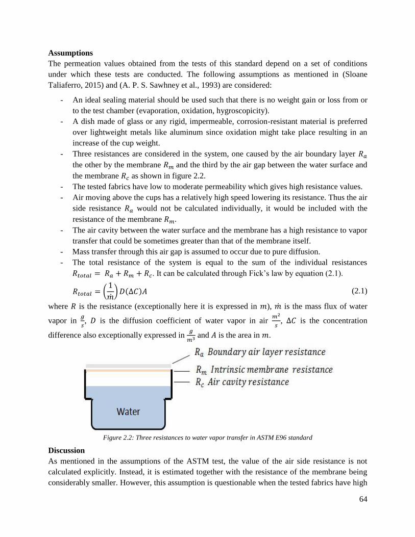
64

Assumptions

The permeation values obtained from the tests of this standard depend on a set of conditions

under which these tests are conducted. The following assumptions as mentioned in (Sloane

Taliaferro, 2015) and (A. P. S. Sawhney et al., 1993) are considered:

- An ideal sealing material should be used such that there is no weight gain or loss from or

to the test chamber (evaporation, oxidation, hygroscopicity).

- A dish made of glass or any rigid, impermeable, corrosion-resistant material is preferred

over lightweight metals like aluminum since oxidation might take place resulting in an

increase of the cup weight.

- Three resistances are considered in the system, one caused by the air boundary layer

the other by the membrane and the third by the air gap between the water surface and

the membrane as shown in figure 2.2.

- The tested fabrics have low to moderate permeability which gives high resistance values.

- Air moving above the cups has a relatively high speed lowering its resistance. Thus the air

side resistance would not be calculated individually, it would be included with the

resistance of the membrane

- The air cavity between the water surface and the membrane has a high resistance to vapor

transfer that could be sometimes greater than that of the membrane itself.

- Mass transfer through this air gap is assumed to occur due to pure diffusion.

- The total resistance of the system is equal to the sum of the individual resistances

. It can be calculated through Fick’s law by equation (2.1).

(2.1)

where is the resistance (exceptionally here it is expressed in ), is the mass flux of water

vapor in

, is the diffusion coefficient of water vapor in air

, is the concentration

difference also exceptionally expressed in

and is the area in .

Figure 2.2: Three resistances to water vapor transfer in ASTM E96 standard

Discussion

As mentioned in the assumptions of the ASTM test, the value of the air side resistance is not

calculated explicitly. Instead, it is estimated together with the resistance of the membrane being

considerably smaller. However, this assumption is questionable when the tested fabrics have high

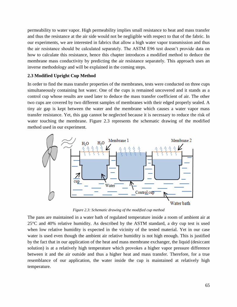
65

permeability to water vapor. High permeability implies small resistance to heat and mass transfer

and thus the resistance at the air side would not be negligible with respect to that of the fabric. In

our experiments, we are interested in fabrics that allow a high water vapor transmission and thus

the air resistance should be calculated separately. The ASTM E96 test doesn’t provide data on

how to calculate this resistance, hence this chapter introduces a modified method to deduce the

membrane mass conductivity by predicting the air resistance separately. This approach uses an

inverse methodology and will be explained in the coming steps.

2.3 Modified Upright Cup Method

In order to find the mass transfer properties of the membranes, tests were conducted on three cups

simultaneously containing hot water. One of the cups is remained uncovered and it stands as a

control cup whose results are used later to deduce the mass transfer coefficient of air. The other

two cups are covered by two different samples of membranes with their edged properly sealed. A

tiny air gap is kept between the water and the membrane which causes a water vapor mass

transfer resistance. Yet, this gap cannot be neglected because it is necessary to reduce the risk of

water touching the membrane. Figure 2.3 represents the schematic drawing of the modified

method used in our experiment.

Figure 2.3: Schematic drawing of the modified cup method

The pans are maintained in a water bath of regulated temperature inside a room of ambient air at

25°C and 40% relative humidity. As described by the ASTM standard, a dry cup test is used

when low relative humidity is expected in the vicinity of the tested material. Yet in our case

water is used even though the ambient air relative humidity is not high enough. This is justified

by the fact that in our application of the heat and mass membrane exchanger, the liquid (desiccant

solution) is at a relatively high temperature which provokes a higher vapor pressure difference

between it and the air outside and thus a higher heat and mass transfer. Therefore, for a true

resemblance of our application, the water inside the cup is maintained at relatively high

temperature.

66

A fan is turned on to force the air movement above the pans in order to decrease the air side mass

transfer resistance. A temperature and water vapor concentration gradient difference exists

between the water inside the pans and the air passing above them which creates a difference in

the vapor pressure. Thus a vapor flow occurs from the water side through the permeable

membranes towards the air side. The inlet temperature and the relative humidity of the air are

continuously measured using a digital thermocouple and a hygrometer and the data is recorded.

In addition, the temperature of the water inside the cups is repeatedly measured and periodic

weighing of the test pans is made to determine the rate of water vapor transmission.

2.3.1 Experimental Conditions Assessment

The high temperature of water contributes to its high vapor pressure with a significant difference

from that of the ambient air. Due to this difference the water vapor is going to be transferred

through the membranes from the water side to the air side. The vapor is evaporated from the

water at high temperature and comes in contact with the cool upper side of the membrane which

has a temperature . However, if the temperature of the water inside the cups is greatly higher

than that of air, a condensation process takes place by which the condensed water deposits on the

membrane. When these droplets pile up on the lower surface of the membrane they fall back in

the pan. In this case, the model representing the heat and mass transfer in the air gap between the

liquid level and the membrane fails to be accurate and the results in term of membrane vapor

permeability are not reliable. So in a way to be able to avoid the condensation problem, the

temperature of the water should be kept just slightly greater than that of the air. Water vapor

continues to be transmitted from the water to the air as long as the vapor pressure of the water is

higher than that of air. The experiments are done with a water temperature between 30°C and

35˚C and the mass of the water inside the pans is measured approximately every 10 to 15 minutes

for around 6 hours.

2.3.2 Tested Membranes

Seven different materials were tested including a membrane fabricated from electro-spun

nanofiber, a sheet of polypropylene, a permeable roof underlay material, Tyvek, and four non-

woven fabrics used for pillow cases and sacs. The main choice of these materials depends firstly

on their prevention to liquid water permeation and secondly on their allowance to water vapor

transfer. This makes them good candidates for being used as membranes in a heat and mass

exchanger.

2.3.3 Experimental Data and Measurements

A total of 11 experiments were done, such that for every material the test is repeated 2 or 3 times.

The conditions upon which the 11 experiments were performed are summarized in table 2.1 along

with the results of the decrease in the water content in each cup.

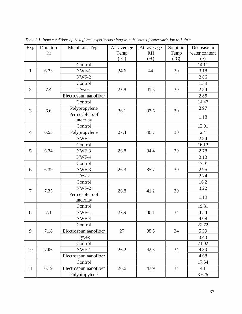
67

Table 2.1: Input conditions of the different experiments along with the mass of water variation with time

Exp Duration

(h)

Membrane Type Air average

Temp

(°C)

Air average

RH

(%)

Solution

Temp

(°C)

Decrease in

water content

(g)

1 6.23

Control

24.6 44 30

14.11

NWF-1 3.18

NWF-2 2.86

2 7.4

Control

27.8 41.3 30

15.9

Tyvek 2.34

Electrospun nanofiber 2.85

3 6.6

Control

26.1 37.6 30

14.47

Polypropylene 2.97

Permeable roof

underlay 1.18

4 6.55

Control

27.4 46.7 30

12.01

Polypropylene 2.4

NWF-1 2.84

5 6.34

Control

26.8 34.4 30

16.12

NWF-3 2.78

NWF-4 3.13

6 6.39

Control

26.3 35.7 30

17.01

NWF-3 2.95

Tyvek 2.24

7 7.35

Control

26.8 41.2 30

16.2

NWF-2 3.22

Permeable roof

underlay 1.19

8 7.1

Control

27.9 36.1 34

19.81

NWF-1 4.54

NWF-4 4.08

9 7.18

Control

27 38.5 34

22.72

Electrospun nanofiber 5.39

Tyvek 3.43

10 7.06

Control

26.2 42.5 34

21.02

NWF-1 4.89

Electrospun nanofiber 4.68

11 6.19

Control

26.6 47.9 34

17.54

Electrospun nanofiber 4.1

Polypropylene 3.625

68

2.3.4 Deduction of Water Vapor Permeability

In the following section the methodology used to infer the water vapor permeability of the tested

materials is discussed. The control cup is used to deduce the air side resistance as it is explained

in the next paragraph.

2.3.4.1 Control Cup

Measurements

From the periodic experimental measurements, it can be shown that with time there is a decrease

in the mass of water inside the cup. The mass variation of water inside the cups as a function of

time can be plotted as curve (i) in figure 2.4a. This curve illustrates an example for the evolution

of the water content in the control cup of experiment 1.

Numerical model

In the case of the control cup, due to the absence of a membrane, the only resistance is the air

resistance. Thus it is used in our experiment to deduce the real value of the mass transfer

coefficient of the air which is dependent on the inlet air conditions (temperature, relative

humidity and velocity). The mass transfer equation between the air and the water in the control

cup is derived and expressed in equation (2.2).

(2.2)

Where is the mass transfer coefficient of air in

, is the exchange area between the air

and the water in , is the absolute humidity in

and

is the variation of the mass of

water as a function of time in

.

By solving equation (2.2) numerically using Modelica language in Dymola software, the curve of

the variation of the mass of water as a function of time in experiment 1 is shown by curve (ii) in

figure 2.4a.

Deduction of the mass transfer coefficient

The optimization of the value of minimizes the error between curve (i) and curve (ii). Then

when this error is minimal, this would give the value of the mass transfer coefficient of air as

shown in figure 2.4b.

69

(a) (b)

Figure 2.4: a) Variation of the measured mass (i) and calculated mass (ii) of water with respect to time in the control

cup, b) mass conductivity of air determined by optimization

2.3.4.2 Cups Covered with Membranes

Measurements

From the periodic experimental measurements, the curve of the mass variation of water as a

function of time inside the cup covered with a membrane was plotted. This curve shows a

decrease in the water mass inside the cups which is less than the decrease in the control cup. The

curve (i) of the change in the water content of the cup covered with NWF-1 in experiment 1 is

plotted in figure 2.5.

Figure 2.5: Variation of the measured mass (i) of water with respect to time in the cup covered with NWF-1in

experiment 1

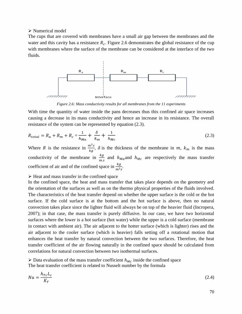
70

Numerical model

The cups that are covered with membranes have a small air gap between the membranes and the

water and this cavity has a resistance . Figure 2.6 demonstrates the global resistance of the cup

with membranes where the surface of the membrane can be considered at the interface of the two

fluids.

Figure 2.6: Mass conductivity results for all membranes from the 11 experiments

With time the quantity of water inside the pans decreases thus this confined air space increases

causing a decrease in its mass conductivity and hence an increase in its resistance. The overall

resistance of the system can be represented by equation (2.3).

=

(2.3)

Where is the resistance in

, is the thickness of the membrane in , is the mass

conductivity of the membrane in

and and are respectively the mass transfer

coefficient of air and of the confined space in

.

Heat and mass transfer in the confined space

In the confined space, the heat and mass transfer that takes place depends on the geometry and

the orientation of the surfaces as well as on the thermo physical properties of the fluids involved.

The characteristics of the heat transfer depend on whether the upper surface is the cold or the hot

surface. If the cold surface is at the bottom and the hot surface is above, then no natural

convection takes place since the lighter fluid will always be on top of the heavier fluid (Incropera,

2007); in that case, the mass transfer is purely diffusive. In our case, we have two horizontal

surfaces where the lower is a hot surface (hot water) while the upper is a cold surface (membrane

in contact with ambient air). The air adjacent to the hotter surface (which is lighter) rises and the

air adjacent to the cooler surface (which is heavier) falls setting off a rotational motion that

enhances the heat transfer by natural convection between the two surfaces. Therefore, the heat

transfer coefficient of the air flowing naturally in the confined space should be calculated from

correlations for natural convection between two isothermal surfaces.

Data evaluation of the mass transfer coefficient inside the confined space

The heat transfer coefficient is related to Nusselt number by the formula

(2.4)

71

where is the heat transfer coefficient of the cavity, is its thermal conductivity and is its

characteristic length considered between the membrane and the water given by eq. (2.5)

(2.5)

With being the total length of the cup (4.3 cm), the mass of water inside cup at every

measurement and the total mass of water in the cup.

The mass transfer coefficient is deduced by using the Lewis analogy

(2.6)

with being the specific heat capacity and the Lewis number.

The Nusselt number is expressed as a function of Rayleigh number which in turn is expressed as

a function of Grashof and Prandtl numbers. For a horizontal plate that represents an upper surface

of a hot plate or a lower surface of a cold plate, the correlation for the Nusselt number is the

following (Incropera, 2007):

Ra<10

8 (2.7)

Ra<5832 (2.8)

Ra<1708 (2.9)

Where

and

is the coefficient of volume expansion

in

, is the gravitational acceleration in

, and are the temperatures of the surface of

the hot and cold fluids in (in our case they are the temperature of water and air respectively)

and is the kinematic viscosity of the fluid inside the cavity in

.

In our case, the temperature of the hot surface is considered to be equal to the temperature of the

water . While the temperature of the cold surface, for more precision, it is considered to be

equal to the temperature of the upper side of the membrane which is in contact with the air

(and not the temperature of air itself). In order to find the energy or heat conservation equation

of the system must be derived and it is expressed in eq. (2.10) with being the heat transfer

coefficient of air.

(2.10)

Therefore, by calculating Rayleigh and Nusselt numbers, the convective heat and mass transfer

coefficients in the confined space between the hot water and the membrane can be deduced.

Deduction of

The mass transfer equations of a cup covered with a membrane can be written as:

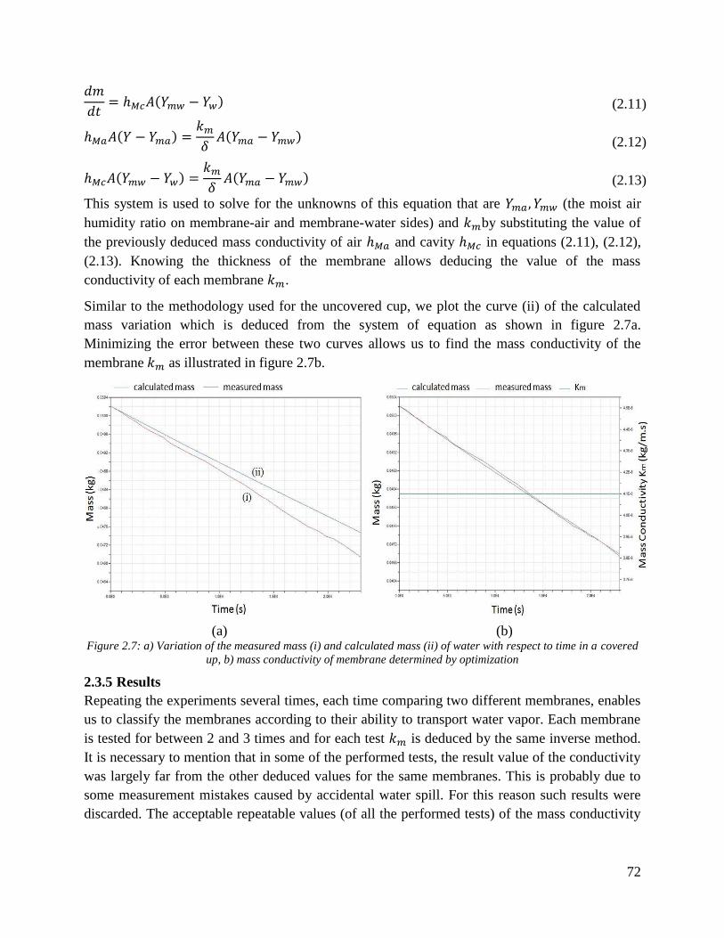
72

(2.11)

(2.12)

(2.13)

This system is used to solve for the unknowns of this equation that are (the moist air

humidity ratio on membrane-air and membrane-water sides) and by substituting the value of

the previously deduced mass conductivity of air and cavity in equations (2.11), (2.12),

(2.13). Knowing the thickness of the membrane allows deducing the value of the mass

conductivity of each membrane .

Similar to the methodology used for the uncovered cup, we plot the curve (ii) of the calculated

mass variation which is deduced from the system of equation as shown in figure 2.7a.

Minimizing the error between these two curves allows us to find the mass conductivity of the

membrane as illustrated in figure 2.7b.

(a) (b) Figure 2.7: a) Variation of the measured mass (i) and calculated mass (ii) of water with respect to time in a covered

up, b) mass conductivity of membrane determined by optimization

2.3.5 Results

Repeating the experiments several times, each time comparing two different membranes, enables

us to classify the membranes according to their ability to transport water vapor. Each membrane

is tested for between 2 and 3 times and for each test is deduced by the same inverse method.

It is necessary to mention that in some of the performed tests, the result value of the conductivity

was largely far from the other deduced values for the same membranes. This is probably due to

some measurement mistakes caused by accidental water spill. For this reason such results were

discarded. The acceptable repeatable values (of all the performed tests) of the mass conductivity

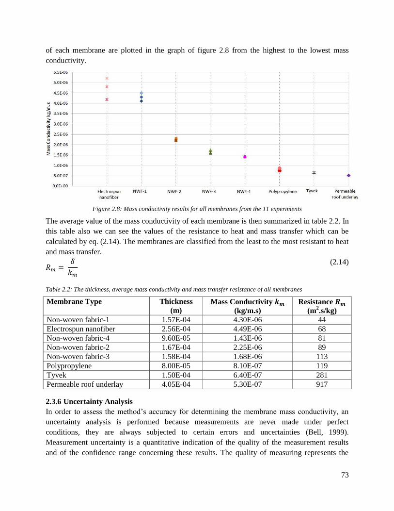
73

of each membrane are plotted in the graph of figure 2.8 from the highest to the lowest mass

conductivity.

Figure 2.8: Mass conductivity results for all membranes from the 11 experiments

The average value of the mass conductivity of each membrane is then summarized in table 2.2. In

this table also we can see the values of the resistance to heat and mass transfer which can be

calculated by eq. (2.14). The membranes are classified from the least to the most resistant to heat

and mass transfer.

(2.14)

Table 2.2: The thickness, average mass conductivity and mass transfer resistance of all membranes

Membrane Type Thickness

(m)

Mass Conductivity

(kg/m.s)

Resistance

(m2.s/kg)

Non-woven fabric-1 1.57E-04 4.30E-06 44

Electrospun nanofiber 2.56E-04 4.49E-06 68

Non-woven fabric-4 9.60E-05 1.43E-06 81

Non-woven fabric-2 1.67E-04 2.25E-06 89

Non-woven fabric-3 1.58E-04 1.68E-06 113

Polypropylene 8.00E-05 8.10E-07 119

Tyvek 1.50E-04 6.40E-07 281

Permeable roof underlay 4.05E-04 5.30E-07 917

2.3.6 Uncertainty Analysis

In order to assess the method’s accuracy for determining the membrane mass conductivity, an

uncertainty analysis is performed because measurements are never made under perfect

conditions, they are always subjected to certain errors and uncertainties (Bell, 1999).

Measurement uncertainty is a quantitative indication of the quality of the measurement results

and of the confidence range concerning these results. The quality of measuring represents the

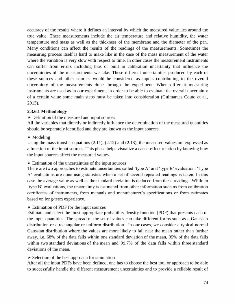
74

accuracy of the results where it defines an interval by which the measured value lies around the

true value. These measurements include the air temperature and relative humidity, the water

temperature and mass as well as the thickness of the membrane and the diameter of the pan.

Many conditions can affect the results of the readings of the measurements. Sometimes the

measuring process itself is hard to make like in the case of the mass measurement of the water

where the variation is very slow with respect to time. In other cases the measurement instruments

can suffer from errors including bias or built in calibration uncertainty that influence the

uncertainties of the measurements we take. These different uncertainties produced by each of

these sources and other sources would be considered as inputs contributing to the overall

uncertainty of the measurements done through the experiment. When different measuring

instruments are used as in our experiment, in order to be able to evaluate the overall uncertainty

of a certain value some main steps must be taken into consideration (Guimaraes Couto et al.,

2013).

2.3.6.1 Methodology

Definition of the measured and input sources

All the variables that directly or indirectly influence the determination of the measured quantities

should be separately identified and they are known as the input sources.

Modeling

Using the mass transfer equations (2.11), (2.12) and (2.13), the measured values are expressed as

a function of the input sources. This phase helps visualize a cause-effect relation by knowing how

the input sources affect the measured values.

Estimation of the uncertainties of the input sources

There are two approaches to estimate uncertainties called ‘type A’ and ‘type B’ evaluation. ‘Type

A’ evaluations are done using statistics when a set of several repeated readings is taken. In this

case the average value as well as the standard deviation is deduced from these readings. While in

‘type B’ evaluations, the uncertainty is estimated from other information such as from calibration

certificates of instruments, from manuals and manufacturer’s specifications or from estimates

based on long-term experience.

Estimation of PDF for the input sources

Estimate and select the most appropriate probability density function (PDF) that presents each of

the input quantities. The spread of the set of values can take different forms such as a Gaussian

distribution or a rectangular or uniform distribution. In our cases, we consider a typical normal

Gaussian distribution where the values are more likely to fall near the mean rather than further

away, i.e. 68% of the data falls within one standard deviation of the mean, 95% of the data falls

within two standard deviations of the mean and 99.7% of the data falls within three standard

deviations of the mean.

Selection of the best approach for simulation

After all the input PDFs have been defined, one has to choose the best tool or approach to be able

to successfully handle the different measurement uncertainties and to provide a reliable result of

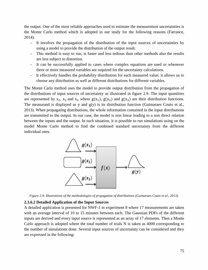
75

the output. One of the most reliable approaches used to estimate the measurement uncertainties is

the Monte Carlo method which is adopted in our study for the following reasons (Farrance,

2014):

- It involves the propagation of the distribution of the input sources of uncertainties by

using a model to provide the distribution of the output result.

- This method is easy to run, is faster and less tedious than other methods also the results

are less subject to distortion.

- It can be successfully applied to cases where complex equations are used or whenever

three or more measured variables are required for the uncertainty calculations.

- It effectively handles the probability distribution for each measured value; it allows us to

choose any distribution as well as different distributions for different variables.

The Monte Carlo method uses the model to provide output distribution from the propagation of

the distributions of input sources of uncertainty as illustrated in figure 2.9. The input quantities

are represented by and where and are their distribution functions.

The measurand is displayed as and g(y) is its distribution function (Guimaraes Couto et al.,

2013). When propagating distributions, the whole information contained in the input distributions

are transmitted to the output. In our case, the model is non linear leading to a non direct relation

between the inputs and the output. In such situation, it is possible to run simulations using on the

model Monte Carlo method to find the combined standard uncertainty from the different

individual ones.

Figure 2.9: Illustrations of the methodologies of propagation of distributions (Guimaraes Couto et al., 2013).

2.3.6.2 Detailed Application of the Input Sources

A detailed application is presented for NWF-1 in experiment 8 where 17 measurements are taken

with an average interval of 10 to 15 minutes between each. The Gaussian PDFs of the different

inputs are derived and every input source is represented as an array of 17 elements. Then a Monte

Carlo approach is adopted where the total number of trials N is taken as 4000 corresponding to

the number of simulations done. Several input sources of uncertainty can be considered and they

are expressed in the following:

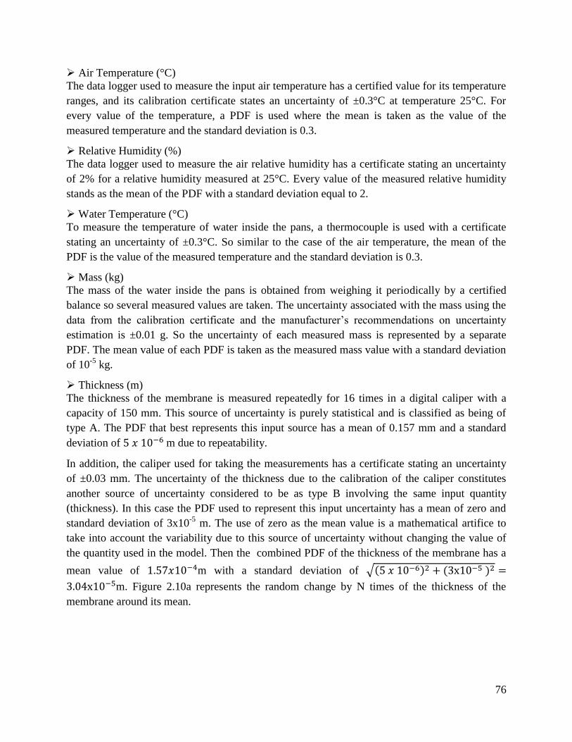
76

Air Temperature (°C)

The data logger used to measure the input air temperature has a certified value for its temperature

ranges, and its calibration certificate states an uncertainty of ±0.3°C at temperature 25°C. For

every value of the temperature, a PDF is used where the mean is taken as the value of the

measured temperature and the standard deviation is 0.3.

Relative Humidity (%)

The data logger used to measure the air relative humidity has a certificate stating an uncertainty

of 2% for a relative humidity measured at 25°C. Every value of the measured relative humidity

stands as the mean of the PDF with a standard deviation equal to 2.

Water Temperature (°C)

To measure the temperature of water inside the pans, a thermocouple is used with a certificate

stating an uncertainty of ±0.3°C. So similar to the case of the air temperature, the mean of the

PDF is the value of the measured temperature and the standard deviation is 0.3.

Mass (kg)

The mass of the water inside the pans is obtained from weighing it periodically by a certified

balance so several measured values are taken. The uncertainty associated with the mass using the

data from the calibration certificate and the manufacturer’s recommendations on uncertainty

estimation is ±0.01 g. So the uncertainty of each measured mass is represented by a separate

PDF. The mean value of each PDF is taken as the measured mass value with a standard deviation

of 10-5

kg.

Thickness (m)

The thickness of the membrane is measured repeatedly for 16 times in a digital caliper with a

capacity of 150 mm. This source of uncertainty is purely statistical and is classified as being of

type A. The PDF that best represents this input source has a mean of 0.157 mm and a standard

deviation of m due to repeatability.

In addition, the caliper used for taking the measurements has a certificate stating an uncertainty

of ±0.03 mm. The uncertainty of the thickness due to the calibration of the caliper constitutes

another source of uncertainty considered to be as type B involving the same input quantity

(thickness). In this case the PDF used to represent this input uncertainty has a mean of zero and

standard deviation of 3x10-5

m. The use of zero as the mean value is a mathematical artifice to

take into account the variability due to this source of uncertainty without changing the value of

the quantity used in the model. Then the combined PDF of the thickness of the membrane has a

mean value of m with a standard deviation of

m. Figure 2.10a represents the random change by N times of the thickness of the

membrane around its mean.

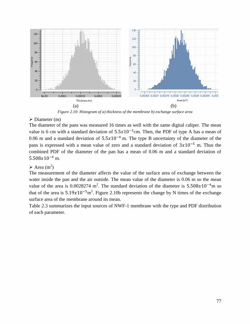
77

(a) (b)

Figure 2.10: Histogram of a) thickness of the membrane b) exchange surface area

Diameter (m)

The diameter of the pans was measured 16 times as well with the same digital caliper. The mean

value is 6 cm with a standard deviation of cm. Then, the PDF of type A has a mean of

0.06 m and a standard deviation of m. The type B uncertainty of the diameter of the

pans is expressed with a mean value of zero and a standard deviation of m. Thus the

combined PDF of the diameter of the pan has a mean of 0.06 m and a standard deviation of

m.

Area (m2)

The measurement of the diameter affects the value of the surface area of exchange between the

water inside the pan and the air outside. The mean value of the diameter is 0.06 m so the mean

value of the area is 0.0028274 m2. The standard deviation of the diameter is m so

that of the area is m2. Figure 2.10b represents the change by N times of the exchange

surface area of the membrane around its mean.

Table 2.3 summarizes the input sources of NWF-1 membrane with the type and PDF distribution

of each parameter.

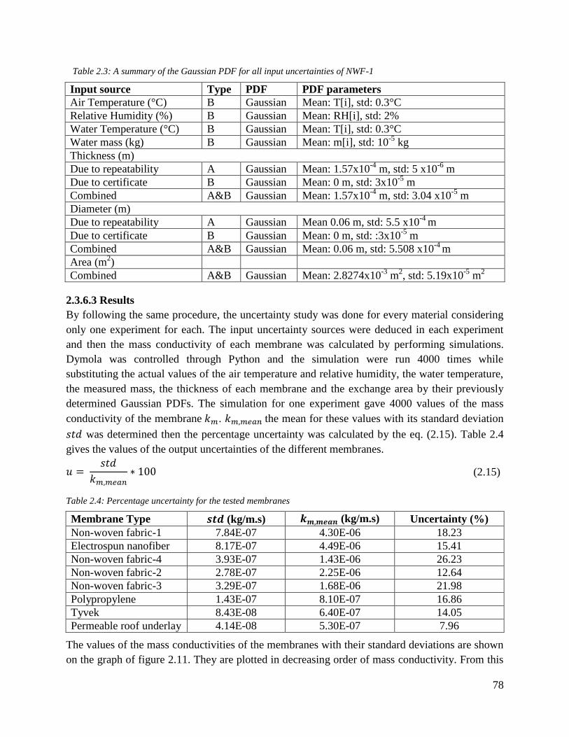
78

Table 2.3: A summary of the Gaussian PDF for all input uncertainties of NWF-1

Input source Type PDF PDF parameters

Air Temperature (°C) B Gaussian Mean: T[i], std: 0.3°C

Relative Humidity (%) B Gaussian Mean: RH[i], std: 2%

Water Temperature (°C) B Gaussian Mean: T[i], std: 0.3°C

Water mass (kg) B Gaussian Mean: m[i], std: 10-5

kg

Thickness (m)

Due to repeatability A Gaussian Mean: 1.57x10-4

m, std: 5 x10-6

m

Due to certificate B Gaussian Mean: 0 m, std: 3x10-5

m

Combined A&B Gaussian Mean: 1.57x10-4

m, std: 3.04 x10-5

m

Diameter (m)

Due to repeatability A Gaussian Mean 0.06 m, std: 5.5 x10-4

m

Due to certificate B Gaussian Mean: 0 m, std: :3x10-5

m

Combined A&B Gaussian Mean: 0.06 m, std: 5.508 x10-4

m

Area (m2)

Combined A&B Gaussian Mean: 2.8274x10-3

m2, std: 5.19x10

-5 m

2

2.3.6.3 Results

By following the same procedure, the uncertainty study was done for every material considering

only one experiment for each. The input uncertainty sources were deduced in each experiment

and then the mass conductivity of each membrane was calculated by performing simulations.

Dymola was controlled through Python and the simulation were run 4000 times while

substituting the actual values of the air temperature and relative humidity, the water temperature,

the measured mass, the thickness of each membrane and the exchange area by their previously

determined Gaussian PDFs. The simulation for one experiment gave 4000 values of the mass

conductivity of the membrane . the mean for these values with its standard deviation

was determined then the percentage uncertainty was calculated by the eq. (2.15). Table 2.4

gives the values of the output uncertainties of the different membranes.

(2.15)

Table 2.4: Percentage uncertainty for the tested membranes

Membrane Type (kg/m.s) (kg/m.s) Uncertainty (%)

Non-woven fabric-1 7.84E-07 4.30E-06 18.23

Electrospun nanofiber 8.17E-07 4.49E-06 15.41

Non-woven fabric-4 3.93E-07 1.43E-06 26.23

Non-woven fabric-2 2.78E-07 2.25E-06 12.64

Non-woven fabric-3 3.29E-07 1.68E-06 21.98

Polypropylene 1.43E-07 8.10E-07 16.86

Tyvek 8.43E-08 6.40E-07 14.05

Permeable roof underlay 4.14E-08 5.30E-07 7.96

The values of the mass conductivities of the membranes with their standard deviations are shown

on the graph of figure 2.11. They are plotted in decreasing order of mass conductivity. From this

79

graph we can observe that even if the uncertainty on the mass conductivity is relatively high, yet

the classification of the membranes by decreasing order of permeability would not change

remarkably.

Figure 2.11: Mass conductivities of the different membranes with their error distribution

2.4 Conclusion

Water vapor permeability is the main property of membranes that influences its capacity of mass

transfer. In this chapter different possible low cost materials that are initially manufactured for

considerations other than operating as membranes were identified. These materials were tested

experimentally using a modified cup test and an inverse methodology in order to find out their

water vapor permeability. In this methodology we succeeded to deduce explicitly the value of

the resistances at the air above the cups and of the air trapped between the water and the fabric.

By substituting these values in the system of mass equations, the mass conductivities of the

materials were determined. These values ranged from 5.3x10-7

to 4.49x10-6

kg/m.s. Thus

measuring, analyzing and then interpreting the results for the different materials allow us to

classify and compare the mass transfer capacity of each. Then an uncertainty analysis was

performed to assess the accuracy of this approach and Monte Carlo method was used to evaluate

the uncertainty propagation. The practical use of Monte Carlo simulations on the estimation of

uncertainties has proved to be a fundamental tool in this area, being able to address complex

measurement problems. The results showed that the uncertainty values varied from around 8% to

26%. These figures, although not considered low enough, yet, didn’t bring a change to the

classification of the tested fabrics by order of the water vapor permeability. In later steps, an

analysis of the impact of the uncertainty of the mass conductivity on the total power of the heat

and mass exchanger is going to be performed. This would give an idea whether these large

uncertainty values on have a great effect on the numerical results of the performance of the

exchanger or not. In this chapter we were able to classify highly permeable materials and the ones

80

with a high mass conductivity (low resistance to heat and mass transfer) and possessing the

characteristics of being permeable to vapor, impermeable to liquid and capable to withstand

water pressure can be employed as membranes in heat and mass exchangers. As per our results,

the membrane made of electrospun nanofiber seemed to have the highest mass conductivity

among the tested membranes; it is a potential good candidate for our exchanger. However, it is

produced by a novel fabrication technique whereas the non-woven fabrics are widely available.

Thus in the coming chapter, NWF-1, having the lowest resistance to mass transfer and possessing

the required enduring properties, is employed as a membrane in our prototype of a liquid to air

cross flow heat and mass exchanger.

81

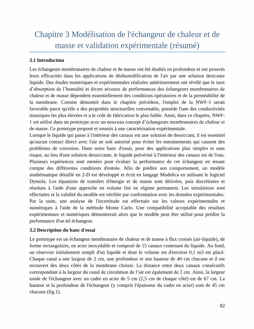
82

Chapitre 3 Modélisation de l'échangeur de chaleur et de

masse et validation expérimentale (résumé)

3.1 Introduction

Les échangeurs membranaires de chaleur et de masse ont été étudiés en profondeur et ont prouvés

leurs efficacités dans les applications de déshumidification de l'air par une solution desicante

liquide. Des études numériques et expérimentales réalisées antérieurement ont révélé que le taux

d’absorption de l’humidité et divers niveaux de performances des échangeurs membranaires de

chaleur et de masse dépendent essentiellement des conditions opératoires et de la perméabilité de

la membrane. Comme démontré dans le chapitre précédent, l'emploi de la NWF-1 serait

favorable parce qu'elle a des propriétés structurelles convenable, possède l'une des conductivités

massiques les plus élevées et a le coût de fabrication le plus faible. Ainsi, dans ce chapitre, NWF-

1 est utilisé dans un prototype avec un nouveau concept d’échangeurs membranaires de chaleur et

de masse. Ce prototype proposé et soumis à une caractérisation expérimentale.

Lorsque le liquide qui passe à l'intérieur des canaux est une solution de dessiccant, il est essentiel

qu'aucun contact direct avec l'air ne soit autorisé pour éviter les entrainements qui causent des

problèmes de corrosion. Dans notre banc d'essai, pour des applications plus simples et sans

risque, au lieu d'une solution dessiccante, le liquide pulvérisé à l'intérieur des canaux est de l'eau.

Plusieurs expériences sont menées pour évaluer la performance de cet échangeur en tenant

compte des différentes conditions d'entrée. Afin de prédire son comportement, un modèle

mathématique détaillé en 2-D est développé et écrit en langage Modelica en utilisant le logiciel

Dymola. Les équations de transfert d'énergie et de masse sont dérivées, puis discrétisées et

résolues à l'aide d'une approche en volume fini en régime permanent. Les simulations sont

effectuées et la validité du modèle est vérifiée par confrontation avec les données expérimentales.

Par la suite, une analyse de l'incertitude est effectuée sur les valeurs expérimentales et

numériques à l'aide de la méthode Monte Carlo. Une compatibilité acceptable des résultats

expérimentaux et numériques démontrerait alors que le modèle peut être utilisé pour prédire la

performance d'un tel échangeur.

3.2 Description du banc d'essai

Le prototype est un échangeur membranaire de chaleur et de masse à flux croisés (air-liquide), de

forme rectangulaire, en acier inoxydable et composé de 15 canaux contenant du liquide. Au fond,

un réservoir initialement rempli d'un liquide et dont le volume est d'environ 0,1 m3 est placé.

Chaque canal a une largeur de 2 cm, une profondeur et une hauteur de 40 cm chacune et il est

recouvert des deux côtés de la membrane choisie. La distance entre deux canaux consécutifs

correspondant à la largeur du canal de circulation de l’air est également de 2 cm. Ainsi, la largeur

totale de l'échangeur avec un cadre en acier de 5 cm (2,5 cm de chaque côté) est de 67 cm. La

hauteur et la profondeur de l'échangeur (y compris l'épaisseur du cadre en acier) sont de 45 cm

chacune (fig.1).

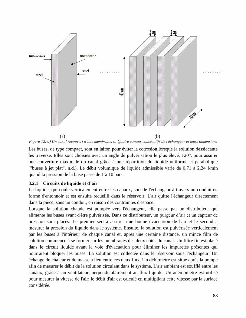
83

(a) (b) Figure 12: a) Un canal recouvert d’une membrane, b) Quatre canaux consécutifs de l'échangeur et leurs dimensions

Les buses, de type compact, sont en laiton pour éviter la corrosion lorsque la solution dessiccante

les traverse. Elles sont choisies avec un angle de pulvérisation le plus élevé, 120°, pour assurer

une couverture maximale du canal grâce à une répartition du liquide uniforme et parabolique

("buses à jet plat", n.d.). Le débit volumique de liquide admissible varie de 0,71 à 2,24 l/min

quand la pression de la buse passe de 1 à 10 bars.

3.2.1 Circuits‎de‎liquide‎et‎d’air

Le liquide, qui coule verticalement entre les canaux, sort de l'échangeur à travers un conduit en

forme d'entonnoir et est ensuite recueilli dans le réservoir. L'air quitte l'échangeur directement

dans la pièce, sans un conduit, en raison des contraintes d'espace.

Lorsque la solution chaude est pompée vers l'échangeur, elle passe par un distributeur qui

alimente les buses avant d'être pulvérisée. Dans ce distributeur, un purgeur d’air et un capteur de

pression sont placés. Le premier sert à assurer une bonne évacuation de l'air et le second à

mesurer la pression du liquide dans le système. Ensuite, la solution est pulvérisée verticalement

par les buses à l'intérieur de chaque canal et, après une certaine distance, un mince film de

solution commence à se former sur les membranes des deux côtés du canal. Un filtre fin est placé

dans le circuit liquide avant la voie d'évacuation pour éliminer les impuretés présentes qui

pourraient bloquer les buses. La solution est collectée dans le réservoir sous l'échangeur. Un

échange de chaleur et de masse a lieu entre ces deux flux. Un débitmètre est situé après la pompe

afin de mesurer le débit de la solution circulant dans le système. L'air ambiant est soufflé entre les

canaux, grâce à un ventilateur, perpendiculairement au flux liquide. Un anémomètre est utilisé

pour mesurer la vitesse de l'air; le débit d'air est calculé en multipliant cette vitesse par la surface

considérée.

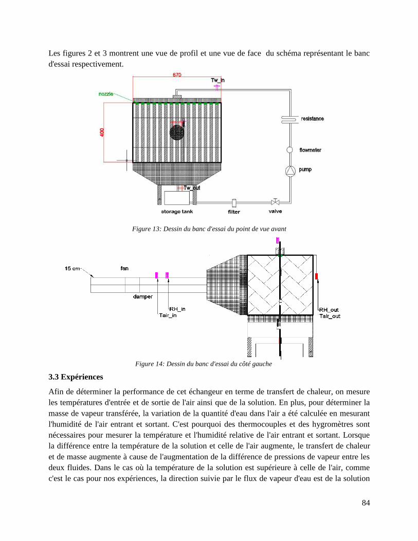
84

Les figures 2 et 3 montrent une vue de profil et une vue de face du schéma représentant le banc

d'essai respectivement.

Figure 13: Dessin du banc d'essai du point de vue avant

Figure 14: Dessin du banc d'essai du côté gauche

3.3 Expériences

Afin de déterminer la performance de cet échangeur en terme de transfert de chaleur, on mesure

les températures d'entrée et de sortie de l'air ainsi que de la solution. En plus, pour déterminer la

masse de vapeur transférée, la variation de la quantité d'eau dans l'air a été calculée en mesurant

l'humidité de l'air entrant et sortant. C'est pourquoi des thermocouples et des hygromètres sont

nécessaires pour mesurer la température et l'humidité relative de l'air entrant et sortant. Lorsque

la différence entre la température de la solution et celle de l'air augmente, le transfert de chaleur

et de masse augmente à cause de l'augmentation de la différence de pressions de vapeur entre les

deux fluides. Dans le cas où la température de la solution est supérieure à celle de l'air, comme

c'est le cas pour nos expériences, la direction suivie par le flux de vapeur d'eau est de la solution

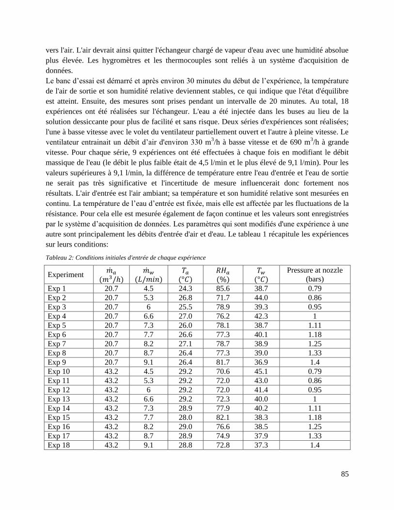
85

vers l'air. L'air devrait ainsi quitter l'échangeur chargé de vapeur d'eau avec une humidité absolue

plus élevée. Les hygromètres et les thermocouples sont reliés à un système d'acquisition de

données.

Le banc d’essai est démarré et après environ 30 minutes du début de l’expérience, la température

de l'air de sortie et son humidité relative deviennent stables, ce qui indique que l'état d'équilibre

est atteint. Ensuite, des mesures sont prises pendant un intervalle de 20 minutes. Au total, 18

expériences ont été réalisées sur l'échangeur. L'eau a été injectée dans les buses au lieu de la

solution dessiccante pour plus de facilité et sans risque. Deux séries d'expériences sont réalisées;

l'une à basse vitesse avec le volet du ventilateur partiellement ouvert et l'autre à pleine vitesse. Le

ventilateur entrainait un débit d’air d'environ 330 m3/h à basse vitesse et de 690 m

3/h à grande

vitesse. Pour chaque série, 9 expériences ont été effectuées à chaque fois en modifiant le débit

massique de l'eau (le débit le plus faible était de 4,5 l/min et le plus élevé de 9,1 l/min). Pour les

valeurs supérieures à 9,1 l/min, la différence de température entre l'eau d'entrée et l'eau de sortie

ne serait pas très significative et l'incertitude de mesure influencerait donc fortement nos

résultats. L'air d'entrée est l'air ambiant; sa température et son humidité relative sont mesurées en

continu. La température de l’eau d’entrée est fixée, mais elle est affectée par les fluctuations de la

résistance. Pour cela elle est mesurée également de façon continue et les valeurs sont enregistrées

par le système d’acquisition de données. Les paramètres qui sont modifiés d'une expérience à une

autre sont principalement les débits d'entrée d'air et d'eau. Le tableau 1 récapitule les expériences

sur leurs conditions:

Tableau 2: Conditions initiales d'entrée de chaque expérience

Experiment

Pressure at nozzle

(bars)

Exp 1 20.7 4.5 24.3 85.6 38.7 0.79

Exp 2 20.7 5.3 26.8 71.7 44.0 0.86

Exp 3 20.7 6 25.5 78.9 39.3 0.95

Exp 4 20.7 6.6 27.0 76.2 42.3 1

Exp 5 20.7 7.3 26.0 78.1 38.7 1.11

Exp 6 20.7 7.7 26.6 77.3 40.1 1.18

Exp 7 20.7 8.2 27.1 78.7 38.9 1.25

Exp 8 20.7 8.7 26.4 77.3 39.0 1.33

Exp 9 20.7 9.1 26.4 81.7 36.9 1.4

Exp 10 43.2 4.5 29.2 70.6 45.1 0.79

Exp 11 43.2 5.3 29.2 72.0 43.0 0.86

Exp 12 43.2 6 29.2 72.0 41.4 0.95

Exp 13 43.2 6.6 29.2 72.3 40.0 1

Exp 14 43.2 7.3 28.9 77.9 40.2 1.11

Exp 15 43.2 7.7 28.0 82.1 38.3 1.18

Exp 16 43.2 8.2 29.0 76.6 38.5 1.25

Exp 17 43.2 8.7 28.9 74.9 37.9 1.33

Exp 18 43.2 9.1 28.8 72.8 37.3 1.4

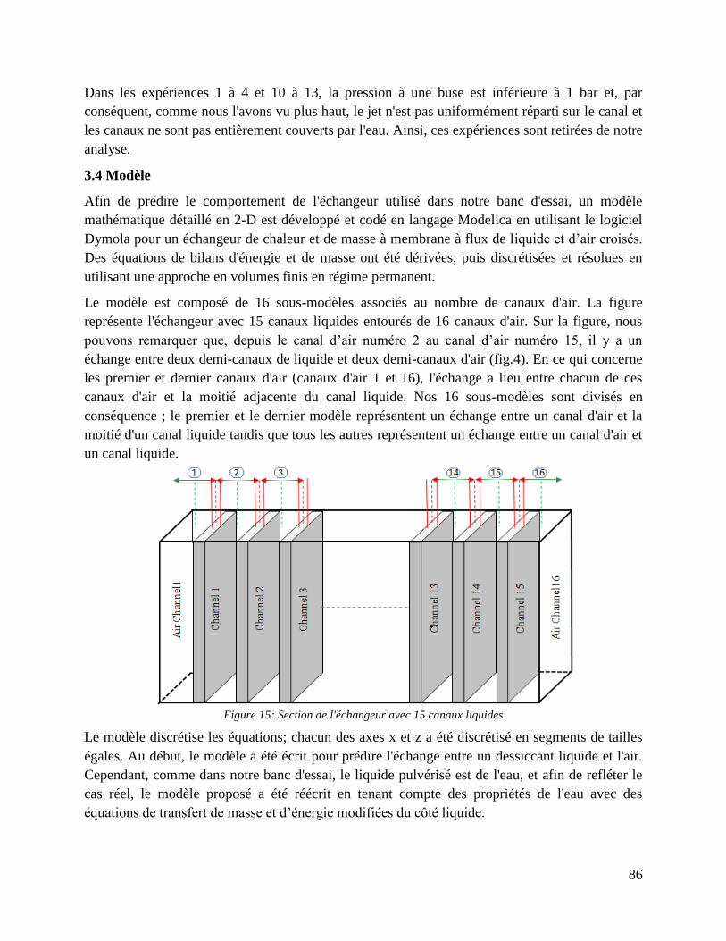
86

Dans les expériences 1 à 4 et 10 à 13, la pression à une buse est inférieure à 1 bar et, par

conséquent, comme nous l'avons vu plus haut, le jet n'est pas uniformément réparti sur le canal et

les canaux ne sont pas entièrement couverts par l'eau. Ainsi, ces expériences sont retirées de notre

analyse.

3.4 Modèle

Afin de prédire le comportement de l'échangeur utilisé dans notre banc d'essai, un modèle

mathématique détaillé en 2-D est développé et codé en langage Modelica en utilisant le logiciel

Dymola pour un échangeur de chaleur et de masse à membrane à flux de liquide et d’air croisés.

Des équations de bilans d'énergie et de masse ont été dérivées, puis discrétisées et résolues en

utilisant une approche en volumes finis en régime permanent.

Le modèle est composé de 16 sous-modèles associés au nombre de canaux d'air. La figure

représente l'échangeur avec 15 canaux liquides entourés de 16 canaux d'air. Sur la figure, nous

pouvons remarquer que, depuis le canal d’air numéro 2 au canal d’air numéro 15, il y a un

échange entre deux demi-canaux de liquide et deux demi-canaux d'air (fig.4). En ce qui concerne

les premier et dernier canaux d'air (canaux d'air 1 et 16), l'échange a lieu entre chacun de ces

canaux d'air et la moitié adjacente du canal liquide. Nos 16 sous-modèles sont divisés en

conséquence ; le premier et le dernier modèle représentent un échange entre un canal d'air et la

moitié d'un canal liquide tandis que tous les autres représentent un échange entre un canal d'air et

un canal liquide.

Figure 15: Section de l'échangeur avec 15 canaux liquides

Le modèle discrétise les équations; chacun des axes x et z a été discrétisé en segments de tailles

égales. Au début, le modèle a été écrit pour prédire l'échange entre un dessiccant liquide et l'air.

Cependant, comme dans notre banc d'essai, le liquide pulvérisé est de l'eau, et afin de refléter le

cas réel, le modèle proposé a été réécrit en tenant compte des propriétés de l'eau avec des

équations de transfert de masse et d’énergie modifiées du côté liquide.

87

La surface de la membrane était représentée par une série de points du maillage et son domaine

est discrétisé en cellules de mailles égales. Nos volumes de contrôle sont choisis pour être

identiques aux cellules du maillage et des points nodaux sont utilisés à l’intérieur de ces volumes

de contrôle pour interpoler les variables de la zone. Trois méthodes de calcul sont proposées pour

approximer les valeurs de ces quantités nodales.

1ere

méthode

Dans la première méthode, les valeurs des quantités nodales liées aux paramètres de l'air sont

calculées compte tenu de l'interface de surface ouest d'un volume de contrôle général (i,j) et

celles liées à la solution sont calculées compte tenu de l'interface de surface nord (fig.5).

Figure 16: Représentation des quantités nodales de la grille de la première méthode

2ème

méthode

Dans le deuxième méthode, les valeurs des quantités nodales liées aux paramètres de l'air sont

calculées en tenant compte de l'interface de surface est d'un volume de contrôle général (i,j) et

celles liées à la solution sont calculées en tenant compte de l'interface de surface sud (fig.6).

Figure 17: Représentation des quantités nodales de la grille de la deuxième méthode

3ème

méthode

Quant à la troisième méthode, pour une modélisation plus précise, les valeurs des quantités

nodales sont considérées comme des valeurs moyennes des deux premières configurations. Les

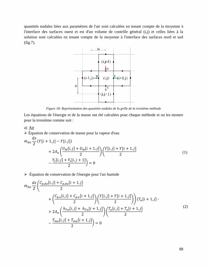
88

quantités nodales liées aux paramètres de l'air sont calculées en tenant compte de la moyenne à

l'interface des surfaces ouest et est d'un volume de contrôle général (i,j) et celles liées à la

solution sont calculées en tenant compte de la moyenne à l'interface des surfaces nord et sud

(fig.7).

Figure 18: Représentation des quantités nodales de la grille de la troisième méthode

Les équations de l'énergie et de la masse ont été calculées pour chaque méthode et on les montre

pour la troisième comme suit :

a) Air

Équation de conservation de masse pour la vapeur d'eau

(1)

Équation de conservation de l'énergie pour l'air humide

(2)

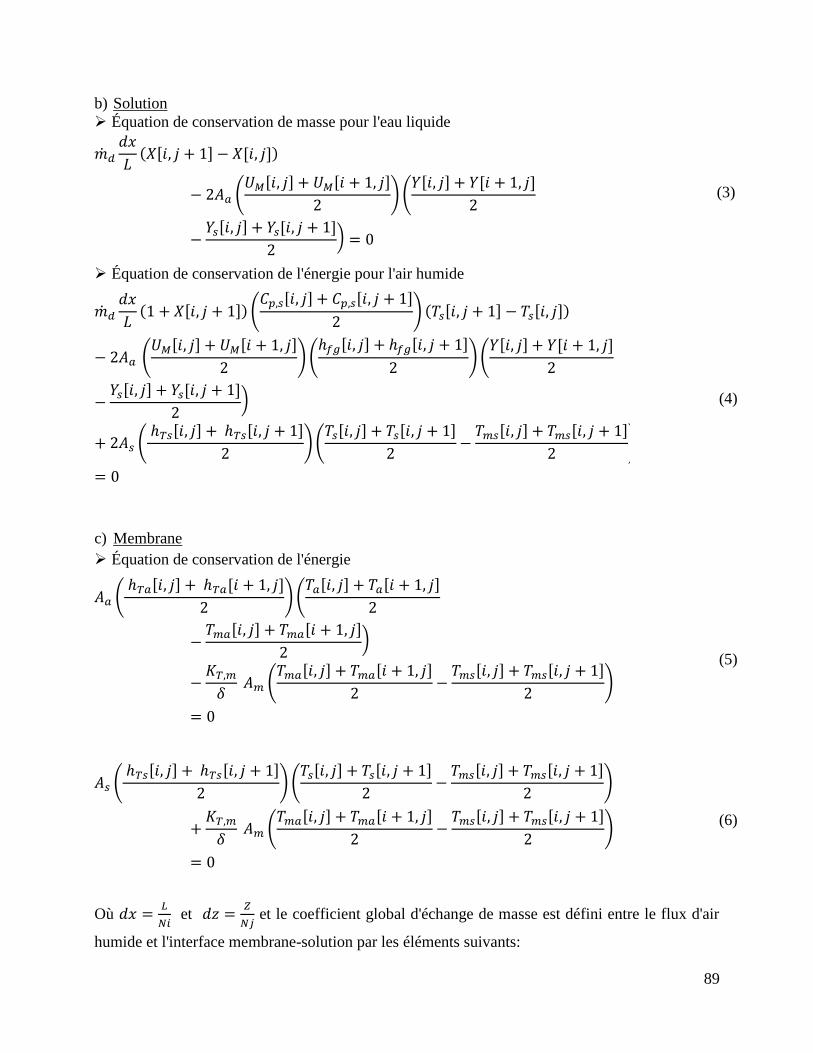
89

b) Solution

Équation de conservation de masse pour l'eau liquide

(3)

Équation de conservation de l'énergie pour l'air humide

(4)

c) Membrane

Équation de conservation de l'énergie

(5)

(6)

Où

et

et le coefficient global d'échange de masse est défini entre le flux d'air

humide et l'interface membrane-solution par les éléments suivants:

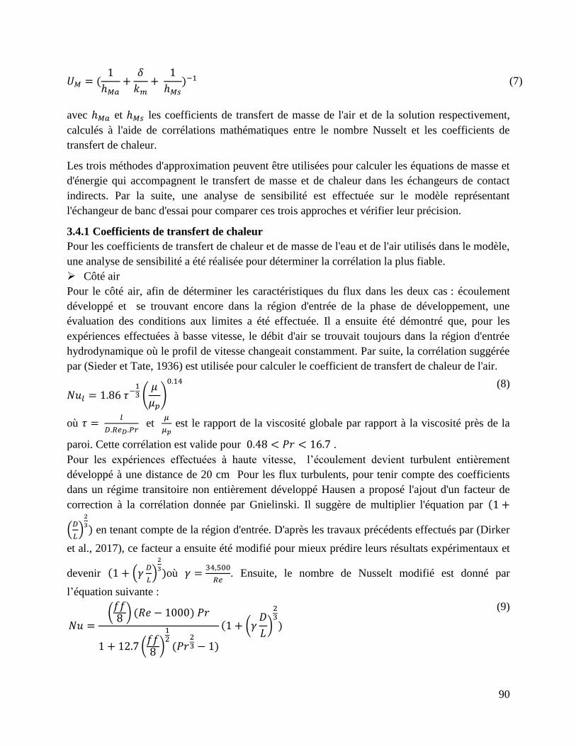
90

(7)

avec et les coefficients de transfert de masse de l'air et de la solution respectivement,

calculés à l'aide de corrélations mathématiques entre le nombre Nusselt et les coefficients de

transfert de chaleur.

Les trois méthodes d'approximation peuvent être utilisées pour calculer les équations de masse et

d'énergie qui accompagnent le transfert de masse et de chaleur dans les échangeurs de contact

indirects. Par la suite, une analyse de sensibilité est effectuée sur le modèle représentant

l'échangeur de banc d'essai pour comparer ces trois approches et vérifier leur précision.

3.4.1 Coefficients de transfert de chaleur

Pour les coefficients de transfert de chaleur et de masse de l'eau et de l'air utilisés dans le modèle,

une analyse de sensibilité a été réalisée pour déterminer la corrélation la plus fiable.

Côté air

Pour le côté air, afin de déterminer les caractéristiques du flux dans les deux cas : écoulement

développé et se trouvant encore dans la région d'entrée de la phase de développement, une

évaluation des conditions aux limites a été effectuée. Il a ensuite été démontré que, pour les

expériences effectuées à basse vitesse, le débit d'air se trouvait toujours dans la région d'entrée

hydrodynamique où le profil de vitesse changeait constamment. Par suite, la corrélation suggérée

par (Sieder et Tate, 1936) est utilisée pour calculer le coefficient de transfert de chaleur de l'air.

(8)

où

et

est le rapport de la viscosité globale par rapport à la viscosité près de la

paroi. Cette corrélation est valide pour .

Pour les expériences effectuées à haute vitesse, l’écoulement devient turbulent entièrement

développé à une distance de 20 cm Pour les flux turbulents, pour tenir compte des coefficients

dans un régime transitoire non entièrement développé Hausen a proposé l'ajout d'un facteur de

correction à la corrélation donnée par Gnielinski. Il suggère de multiplier l'équation par

en tenant compte de la région d'entrée. D'après les travaux précédents effectués par (Dirker

et al., 2017), ce facteur a ensuite été modifié pour mieux prédire leurs résultats expérimentaux et

devenir

où

. Ensuite, le nombre de Nusselt modifié est donné par

l’équation suivante :

(9)

91

Côté liquide

Différentes corrélations ont aussi été discutées pour le coefficient de transfert de chaleur coté eau.

Toutefois, aucune d'entre elles n’a pu vraiment refléter le cas présenté dans notre banc d'essai.

Les corrélations disponibles relatives aux jets considèrent que le jet est perpendiculaire à une

surface horizontale alors que, dans notre cas, le jet est plat et parallèle à la surface des

membranes. Ainsi, notre recherche a été étendue pour examiner les corrélations des films

tombants. Cependant, en réalité, même un film tombant ne représente pas totalement

l’écoulement dans notre échangeur. En effet, chaque fois qu'une buse fonctionne dans une plage

de pression inférieure à la plage optimale, l’eau ne serait pas entièrement distribuée avec un angle

de 120°, ce qui résulte en une configuration de pulvérisation indésirable. Dans ce cas, le flux ne

doit pas être considéré comme un film puisqu’il est encore divergent et que le canal n’est pas

complètement couvert par la pulvérisation. Par conséquent, une comparaison de l'ordre de

grandeur entre les corrélations liées aux jets et celles liées aux films tombants a été effectuée afin

de vérifier les différences entre elles et de décider laquelle choisir et utiliser dans notre modèle.

L'étude de l'effet des valeurs du coefficient de transfert de chaleur du coté eau sur la puissance

totale de l'échangeur a montré que les corrélations sont du même ordre de grandeur. La

corrélation donnée par (Zhu, 2013) a été choisie vu qu’elle a fourni une valeur moyenne parmi les

corrélations examinées.

(10)

où

et étant le diamètre latéral équivalent en .

3.4.2 Comparaison‎des‎trois‎méthodes‎d’estimation‎des‎propriétés

Après avoir trouvé les paramètres nécessaires pour résoudre les équations d'énergie et de masse,

les trois méthodes sont comparées par leur précision, le temps nécessaire pour une simulation et

la façon dont ils sont affectés par certains paramètres de modélisation. Pour cette comparaison, la

puissance de sortie est calculée pour chaque méthode en modifiant la discrétisation du modèle.

La création et la sélection de la taille de la discrétisation dans le modèle est une étape importante,

car pendant les simulations, le maillage est considéré comme le facteur le plus consommateur de

mémoire. Ainsi, le choix d'un nombre commode de maillage peut contribuer à réduire les besoins

en mémoire et à réduire le temps de calcul nécessaire à une simulation. D'autre part,

l'abaissement du nombre de maillages peut affecter la précision des résultats numériques de notre

modèle. Un maillage pratique garantit un résultat numérique plus précis, tandis qu'un maillage

insuffisant affecte la convergence de la solution. Afin de trouver un nombre acceptable de

maillages par lesquels il existe un compromis entre la précision du modèle et les restrictions de

mémoire et de temps, une analyse de sensibilité est effectuée. Cela se fait en simulant plusieurs

fois les modèles des trois méthodes, en ne modifiant que le nombre de maillages Ni et Nj dans

chacun des modèles. L'étude se concentre sur la puissance totale de l'échangeur et examine sa

variation avec l'augmentation de Ni et Nj de 5 à 40 par pas de 5 à chaque fois. Cette étude donne

une idée de l'effet de la modification de la taille du maillage sur les résultats numériques

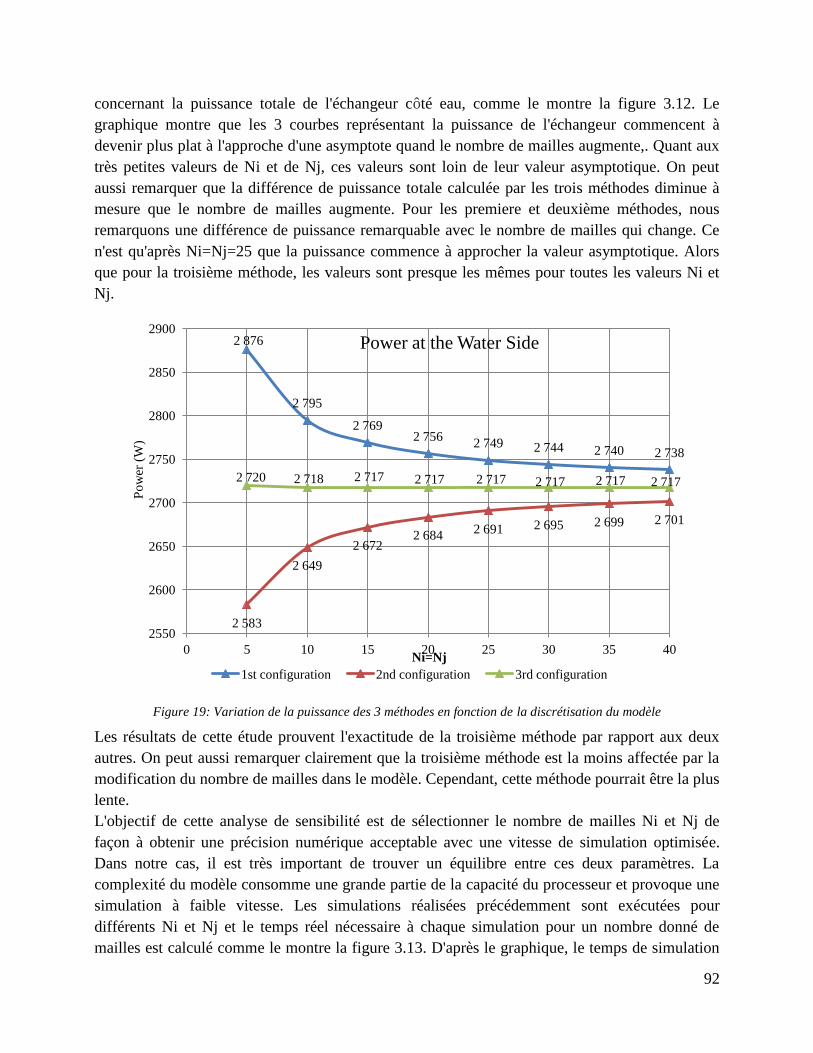
92

concernant la puissance totale de l'échangeur côté eau, comme le montre la figure 3.12. Le

graphique montre que les 3 courbes représentant la puissance de l'échangeur commencent à

devenir plus plat à l'approche d'une asymptote quand le nombre de mailles augmente,. Quant aux

très petites valeurs de Ni et de Nj, ces valeurs sont loin de leur valeur asymptotique. On peut

aussi remarquer que la différence de puissance totale calculée par les trois méthodes diminue à

mesure que le nombre de mailles augmente. Pour les premiere et deuxième méthodes, nous

remarquons une différence de puissance remarquable avec le nombre de mailles qui change. Ce

n'est qu'après Ni=Nj=25 que la puissance commence à approcher la valeur asymptotique. Alors

que pour la troisième méthode, les valeurs sont presque les mêmes pour toutes les valeurs Ni et

Nj.

Figure 19: Variation de la puissance des 3 méthodes en fonction de la discrétisation du modèle

Les résultats de cette étude prouvent l'exactitude de la troisième méthode par rapport aux deux

autres. On peut aussi remarquer clairement que la troisième méthode est la moins affectée par la

modification du nombre de mailles dans le modèle. Cependant, cette méthode pourrait être la plus

lente.

L'objectif de cette analyse de sensibilité est de sélectionner le nombre de mailles Ni et Nj de

façon à obtenir une précision numérique acceptable avec une vitesse de simulation optimisée.

Dans notre cas, il est très important de trouver un équilibre entre ces deux paramètres. La

complexité du modèle consomme une grande partie de la capacité du processeur et provoque une

simulation à faible vitesse. Les simulations réalisées précédemment sont exécutées pour

différents Ni et Nj et le temps réel nécessaire à chaque simulation pour un nombre donné de

mailles est calculé comme le montre la figure 3.13. D'après le graphique, le temps de simulation

2 876

2 795

2 769 2 756

2 749 2 744 2 740 2 738

2 583

2 649

2 672 2 684

2 691 2 695 2 699 2 701

2 720 2 718 2 717 2 717 2 717 2 717 2 717 2 717

2550

2600

2650

2700

2750

2800

2850

2900

0 5 10 15 20 25 30 35 40

Po

wer

(W

)

Ni=Nj

Power at the Water Side

1st configuration 2nd configuration 3rd configuration

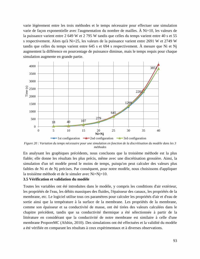
93

varie légèrement entre les trois méthodes et le temps nécessaire pour effectuer une simulation

varie de façon exponentielle avec l'augmentation du nombre de mailles. À Ni=10, les valeurs de

la puissance varient entre 2 649 W et 2 795 W tandis que celles du temps varient entre 40 s et 55

s respectivement. Alors qu'à Ni=25, les valeurs de la puissance varient entre 2691 W et 2749 W

tandis que celles du temps varient entre 645 s et 694 s respectivement. À mesure que Ni et Nj

augmentent la différence en pourcentage de puissance diminue, mais le temps requis pour chaque

simulation augmente en grande partie.

Figure 20 : Variation du temps nécessaire pour une simulation en fonction de la discrétisation du modèle dans les 3

méthodes

En analysant les graphiques précédents, nous concluons que la troisième méthode est la plus

fiable; elle donne les résultats les plus précis, même avec une discrétisation grossière. Ainsi, la

simulation d'un tel modèle prend le moins de temps, puisqu'on peut calculer des valeurs plus

faibles de Ni et de Nj précises. Par conséquent, pour notre modèle, nous choisissons d'appliquer

la troisième méthode et de le simuler avec Ni=Nj=10.

3.5 Vérification et validation du modèle

Toutes les variables ont été introduites dans le modèle, y compris les conditions d'air extérieur,

les propriétés de l'eau, les débits massiques des fluides, l'épaisseur des canaux, les propriétés de la

membrane, etc. Le logiciel utilise tous ces paramètres pour calculer les propriétés d'air et d'eau de

sortie ainsi que la température à la surface de la membrane. Les propriétés de la membrane,

comme son épaisseur et sa conductivité de masse, ont été tirées des valeurs calculées dans le

chapitre précédent, tandis que sa conductivité thermique a été sélectionnée à partir de la

littérature en considérant que la conductivité de notre membrane est similaire à celle d'une

membrane ProporeMC (Afshin, 2010). Des simulations ont été effectuées et la validité du modèle

a été vérifiée en comparant les résultats à ceux expérimentaux et à diverses observations.

18 40 107 279

645

1299

2281

3851

0

500

1000

1500

2000

2500

3000

3500

4000

0 5 10 15 20 25 30 35 40

Tim

e (s

)

Ni=Nj

1st configuration 2nd configuration 3rd configuration

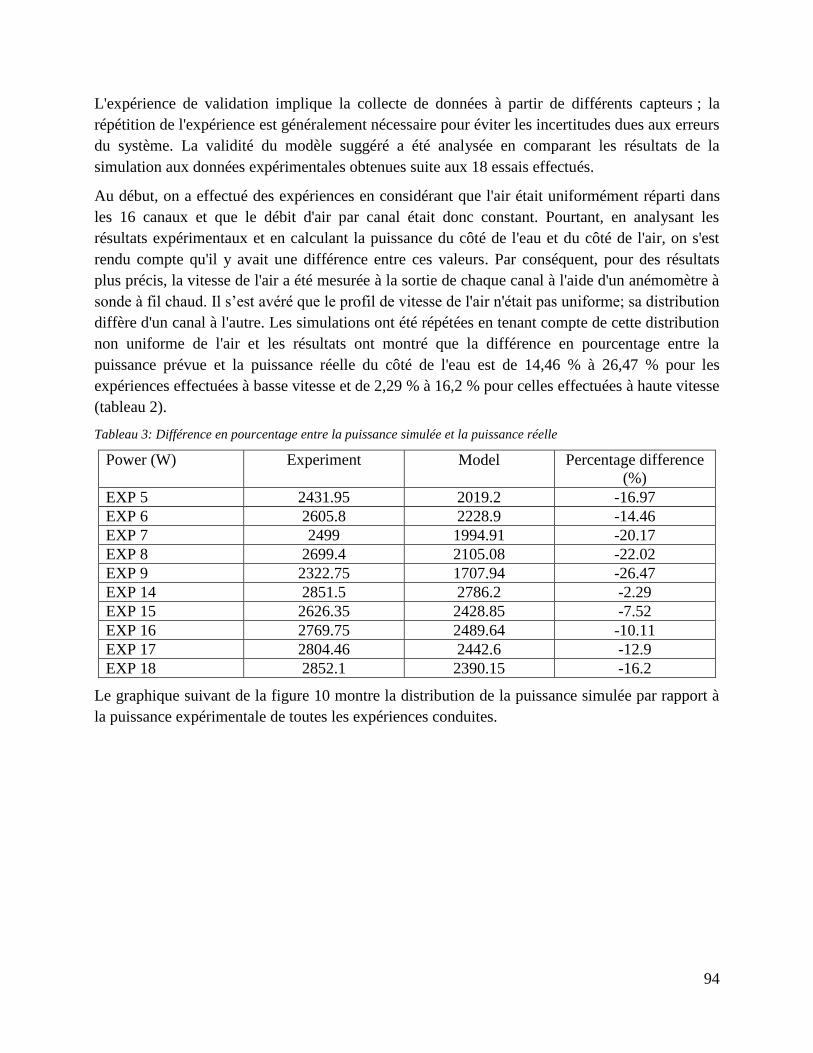
94

L'expérience de validation implique la collecte de données à partir de différents capteurs ; la

répétition de l'expérience est généralement nécessaire pour éviter les incertitudes dues aux erreurs

du système. La validité du modèle suggéré a été analysée en comparant les résultats de la

simulation aux données expérimentales obtenues suite aux 18 essais effectués.

Au début, on a effectué des expériences en considérant que l'air était uniformément réparti dans

les 16 canaux et que le débit d'air par canal était donc constant. Pourtant, en analysant les

résultats expérimentaux et en calculant la puissance du côté de l'eau et du côté de l'air, on s'est

rendu compte qu'il y avait une différence entre ces valeurs. Par conséquent, pour des résultats

plus précis, la vitesse de l'air a été mesurée à la sortie de chaque canal à l'aide d'un anémomètre à

sonde à fil chaud. Il s’est avéré que le profil de vitesse de l'air n'était pas uniforme; sa distribution

diffère d'un canal à l'autre. Les simulations ont été répétées en tenant compte de cette distribution

non uniforme de l'air et les résultats ont montré que la différence en pourcentage entre la

puissance prévue et la puissance réelle du côté de l'eau est de 14,46 % à 26,47 % pour les

expériences effectuées à basse vitesse et de 2,29 % à 16,2 % pour celles effectuées à haute vitesse

(tableau 2).

Tableau 3: Différence en pourcentage entre la puissance simulée et la puissance réelle

Power (W) Experiment Model Percentage difference

(%)

EXP 5 2431.95 2019.2 -16.97

EXP 6 2605.8 2228.9 -14.46

EXP 7 2499 1994.91 -20.17

EXP 8 2699.4 2105.08 -22.02

EXP 9 2322.75 1707.94 -26.47

EXP 14 2851.5 2786.2 -2.29

EXP 15 2626.35 2428.85 -7.52

EXP 16 2769.75 2489.64 -10.11

EXP 17 2804.46 2442.6 -12.9

EXP 18 2852.1 2390.15 -16.2

Le graphique suivant de la figure 10 montre la distribution de la puissance simulée par rapport à

la puissance expérimentale de toutes les expériences conduites.

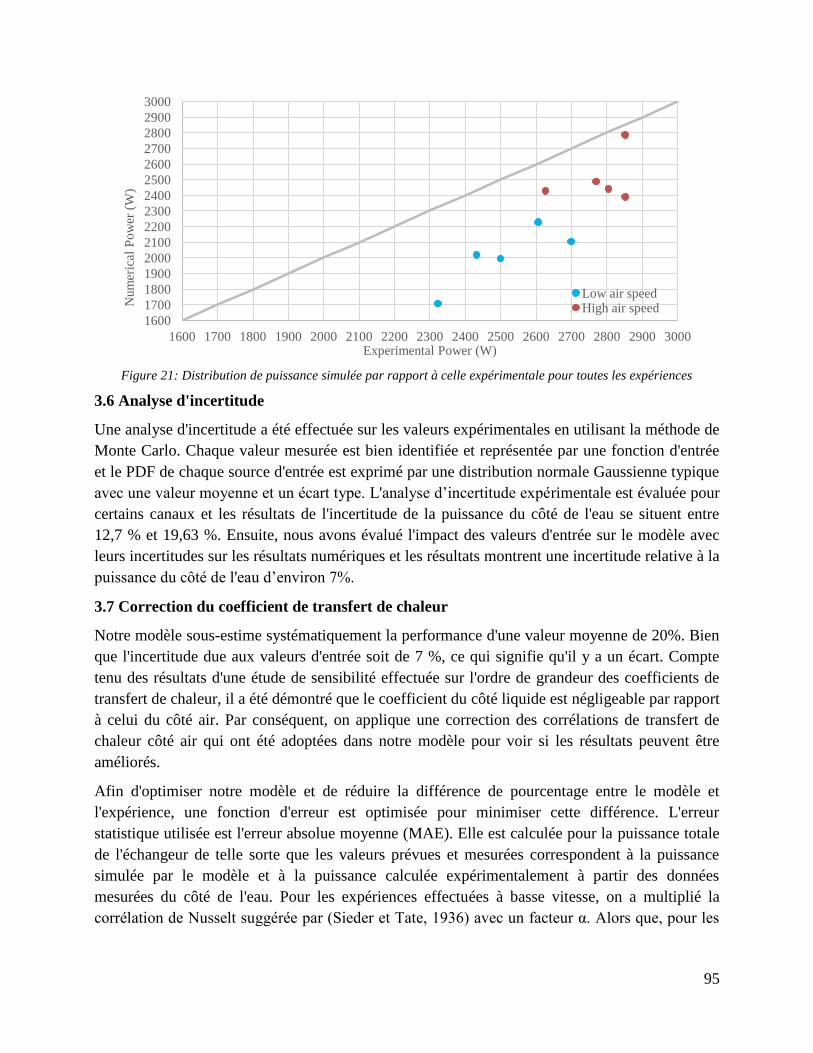
95

Figure 21: Distribution de puissance simulée par rapport à celle expérimentale pour toutes les expériences

3.6 Analyse d'incertitude

Une analyse d'incertitude a été effectuée sur les valeurs expérimentales en utilisant la méthode de

Monte Carlo. Chaque valeur mesurée est bien identifiée et représentée par une fonction d'entrée

et le PDF de chaque source d'entrée est exprimé par une distribution normale Gaussienne typique

avec une valeur moyenne et un écart type. L'analyse d’incertitude expérimentale est évaluée pour

certains canaux et les résultats de l'incertitude de la puissance du côté de l'eau se situent entre

12,7 % et 19,63 %. Ensuite, nous avons évalué l'impact des valeurs d'entrée sur le modèle avec

leurs incertitudes sur les résultats numériques et les résultats montrent une incertitude relative à la

puissance du côté de l'eau d’environ 7%.

3.7 Correction du coefficient de transfert de chaleur

Notre modèle sous-estime systématiquement la performance d'une valeur moyenne de 20%. Bien

que l'incertitude due aux valeurs d'entrée soit de 7 %, ce qui signifie qu'il y a un écart. Compte

tenu des résultats d'une étude de sensibilité effectuée sur l'ordre de grandeur des coefficients de

transfert de chaleur, il a été démontré que le coefficient du côté liquide est négligeable par rapport

à celui du côté air. Par conséquent, on applique une correction des corrélations de transfert de

chaleur côté air qui ont été adoptées dans notre modèle pour voir si les résultats peuvent être

améliorés.

Afin d'optimiser notre modèle et de réduire la différence de pourcentage entre le modèle et

l'expérience, une fonction d'erreur est optimisée pour minimiser cette différence. L'erreur

statistique utilisée est l'erreur absolue moyenne (MAE). Elle est calculée pour la puissance totale

de l'échangeur de telle sorte que les valeurs prévues et mesurées correspondent à la puissance

simulée par le modèle et à la puissance calculée expérimentalement à partir des données

mesurées du côté de l'eau. Pour les expériences effectuées à basse vitesse, on a multiplié la

corrélation de Nusselt suggérée par (Sieder et Tate, 1936) avec un facteur α. Alors que, pour les

1600

1700

1800

1900

2000

2100

2200

2300

2400

2500

2600

2700

2800

2900

3000

1600 1700 1800 1900 2000 2100 2200 2300 2400 2500 2600 2700 2800 2900 3000

Num

eric

al P

ow

er (

W)

Experimental Power (W)

Low air speed High air speed

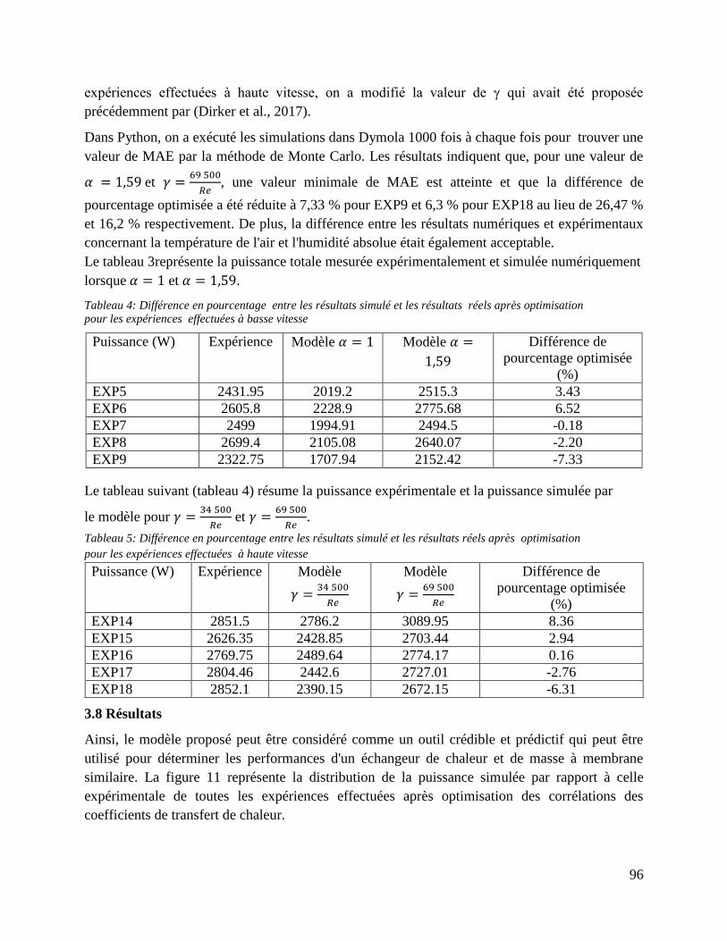
96

expériences effectuées à haute vitesse, on a modifié la valeur de γ qui avait été proposée

précédemment par (Dirker et al., 2017).

Dans Python, on a exécuté les simulations dans Dymola 1000 fois à chaque fois pour trouver une

valeur de MAE par la méthode de Monte Carlo. Les résultats indiquent que, pour une valeur de

et

, une valeur minimale de MAE est atteinte et que la différence de

pourcentage optimisée a été réduite à 7,33 % pour EXP9 et 6,3 % pour EXP18 au lieu de 26,47 %

et 16,2 % respectivement. De plus, la différence entre les résultats numériques et expérimentaux

concernant la température de l'air et l'humidité absolue était également acceptable.

Le tableau 3représente la puissance totale mesurée expérimentalement et simulée numériquement

lorsque et .

Tableau 4: Différence en pourcentage entre les résultats simulé et les résultats réels après optimisation

pour les expériences effectuées à basse vitesse

Puissance (W) Expérience Modèle Modèle

Différence de

pourcentage optimisée

(%)

EXP5 2431.95 2019.2 2515.3 3.43

EXP6 2605.8 2228.9 2775.68 6.52

EXP7 2499 1994.91 2494.5 -0.18

EXP8 2699.4 2105.08 2640.07 -2.20

EXP9 2322.75 1707.94 2152.42 -7.33

Le tableau suivant (tableau 4) résume la puissance expérimentale et la puissance simulée par

le modèle pour

et

.

Tableau 5: Différence en pourcentage entre les résultats simulé et les résultats réels après optimisation

pour les expériences effectuées à haute vitesse

Puissance (W) Expérience Modèle

Modèle

Différence de

pourcentage optimisée

(%)

EXP14 2851.5 2786.2 3089.95 8.36

EXP15 2626.35 2428.85 2703.44 2.94

EXP16 2769.75 2489.64 2774.17 0.16

EXP17 2804.46 2442.6 2727.01 -2.76

EXP18 2852.1 2390.15 2672.15 -6.31

3.8 Résultats

Ainsi, le modèle proposé peut être considéré comme un outil crédible et prédictif qui peut être

utilisé pour déterminer les performances d'un échangeur de chaleur et de masse à membrane

similaire. La figure 11 représente la distribution de la puissance simulée par rapport à celle

expérimentale de toutes les expériences effectuées après optimisation des corrélations des

coefficients de transfert de chaleur.

97

Figure 22: Distribution de puissance simulée par rapport à celle expérimentale pour toutes les expériences après

optimisation

3.9 Conclusion

En conclusion, la différence entre la puissance prévue par le modèle et celle calculée

expérimentalement atteint ses valeurs maximales de 26,5 % pour EXP9 et de 16,2 % pour

EXP18. Incluses dans ces différences, les incertitudes intrinsèques représentent environ 6 à 7 %

de l'incertitude totale. Afin de réduire cette différence, on a modifié les corrélations liées au

coefficient de transfert de chaleur de l'air (étant le plus influent sur le coefficient global de

transfert de chaleur) et on a cherché à trouver une valeur optimisée de MAE. Les résultats

indiquent qu'après l'optimisation, la différence de pourcentage a été réduite à 7,33 % pour EXP9

et 6,3 % pour EXP18. De plus, la différence entre les résultats des simulations et ceux

expérimentaux concernant la température et l'humidité absolue de l'air est également acceptable.

Par conséquent, comme les résultats numériques et expérimentaux présentent des tendances de

variation similaires, une conformité satisfaisante est déduites entre les deux, ce qui indique que le

modèle développé évalue la performance d’un échangeur de masse et de chaleur à membrane à

flux croisés de façon assez précise et réussit à simuler les caractéristiques opérationnelles de cet

échangeur. Cependant, les expériences menées ne suffisent pas à généraliser cette conclusion

pour tous les scénarios possibles et, par conséquent, il faudrait faire davantage d'expériences pour

valider le modèle et prouver son exactitude dans plusieurs autres cas. Dans les étapes suivantes,

certains paramètres pourraient être modifiés, comme par exemple élargir la plage du débit d'eau

dont la limite supérieure est affectée par la puissance de la résistance (mentionnée

précédemment) et la limite inférieure est influencée par la plage de pression de fonctionnement

des buses. De plus, d'autres paramètres de conception peuvent être modifiés, comme le nombre

de canaux ou la largeur d'un canal de l'échangeur. Pour des mesures plus précises, d'autres

expériences peuvent être réalisées avec des capteurs plus précis ou en installant un conduit d'air

2300

2400

2500

2600

2700

2800

2900

3000

2300 2400 2500 2600 2700 2800 2900 3000

Num

eric

al P

ow

er (

W)

Experimental Power (W)

Low air speed

High air speed

98

de sortie pour obtenir de meilleures lectures du côté de l'air. Dans ce chapitre, nous avons pu

établir un modèle 2D pour évaluer la performance énergétique d’un échangeur de masse et de

chaleur à membrane à flux croisés. Les résultats ont prouvé qu'il peut être considéré comme un

outil crédible et prédictif qui pourrait s'appliquer à des échangeurs similaires. Par conséquent, le

modèle proposé prédit l'efficacité du déshumidificateur et du régénérateur qui est un échangeur

de membranes à flux croisé. Dans le chapitre suivant, ce modèle est utilisé dans l'évaluation de la

performance d'un système hybride de compression de vapeur/ dessiccant liquide dans le cadre

d’une climatisation saisonnière d'un bureau dans un immeuble du sud de la France.

99

100

Chapter 3 Modeling the Heat and Mass Exchanger and

Experimental Validation

3.1 Introduction

Membrane based heat and mass exchangers have been studied extensively and proved to be

effective tools for liquid desiccant air dehumidification applications. Previously accomplished

numerical and experimental investigations revealed that the moisture removal rate and various

performance of membrane based heat and mass exchangers depend significantly on its operating

conditions and on the membrane’s permeability. As demonstrated in the previous chapter,

employing NWF-1 would be favorable because it has enduring structural properties, possesses

one of the highest mass conductivities and has the lowest manufacturing cost. Thus in this

chapter NWF-1 is used in a prototype with a novel concept of membrane based heat and mass

exchanger as indicated in chapter 1. The proposed prototype is a liquid to air cross flow

exchanger constructed and subjected to experimental testing on a dedicated test bench. NWF-1 is

used to cover the channels, in which liquid is supposed to flow inside separating the air flow from

the liquid flow (see figure 3.1). When the liquid passing inside the channels is a desiccant

solution, it is essential that no direct contact is allowed with the air to avoid corrosion problems.

In our test bench, for easier and riskless applications, instead of a desiccant solution, the liquid

sprayed inside the channels is water. Several experiments are conducted to evaluate the

performance of this exchanger considering different input conditions. In a way to predict its

behavior, a detailed 2-D mathematical model is developed and written in Modelica language

using Dymola software. Conjugate energy and mass transfer equations are derived and then

discretized and solved using a finite volume approach at steady state. Simulations are performed

accordingly and the validity of the model is checked by experimental verifications and

observations. Later, an uncertainty analysis is performed on the experimental and numerical

values through Monte Carlo method. An acceptable compatibility of the experimental and

numerical outcomes would then prove that the model can be used for the prediction of the

performance of such an exchanger.

Figure 3.1: The prototype heat and mass exchanger

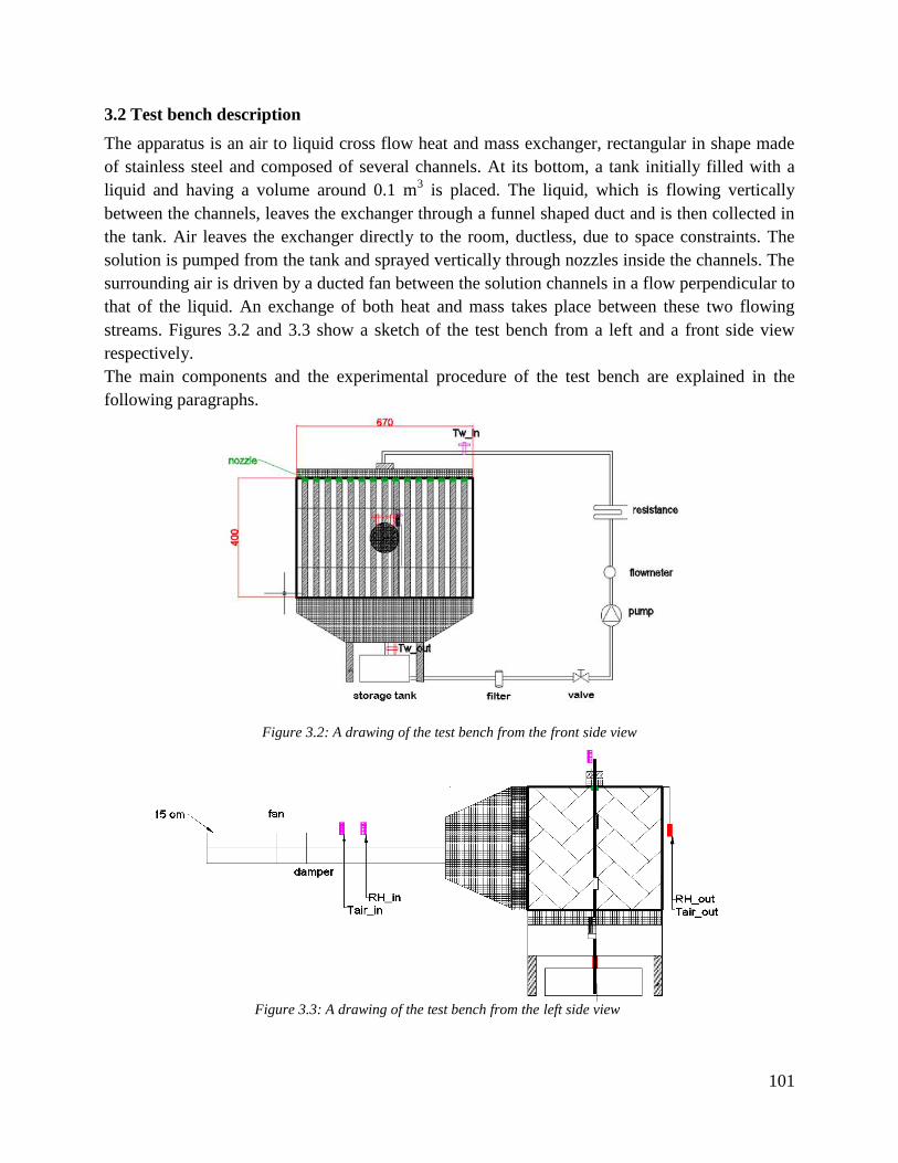
101

3.2 Test bench description

The apparatus is an air to liquid cross flow heat and mass exchanger, rectangular in shape made

of stainless steel and composed of several channels. At its bottom, a tank initially filled with a

liquid and having a volume around 0.1 m3 is placed. The liquid, which is flowing vertically

between the channels, leaves the exchanger through a funnel shaped duct and is then collected in

the tank. Air leaves the exchanger directly to the room, ductless, due to space constraints. The

solution is pumped from the tank and sprayed vertically through nozzles inside the channels. The

surrounding air is driven by a ducted fan between the solution channels in a flow perpendicular to

that of the liquid. An exchange of both heat and mass takes place between these two flowing

streams. Figures 3.2 and 3.3 show a sketch of the test bench from a left and a front side view

respectively.

The main components and the experimental procedure of the test bench are explained in the

following paragraphs.

Figure 3.2: A drawing of the test bench from the front side view

Figure 3.3: A drawing of the test bench from the left side view

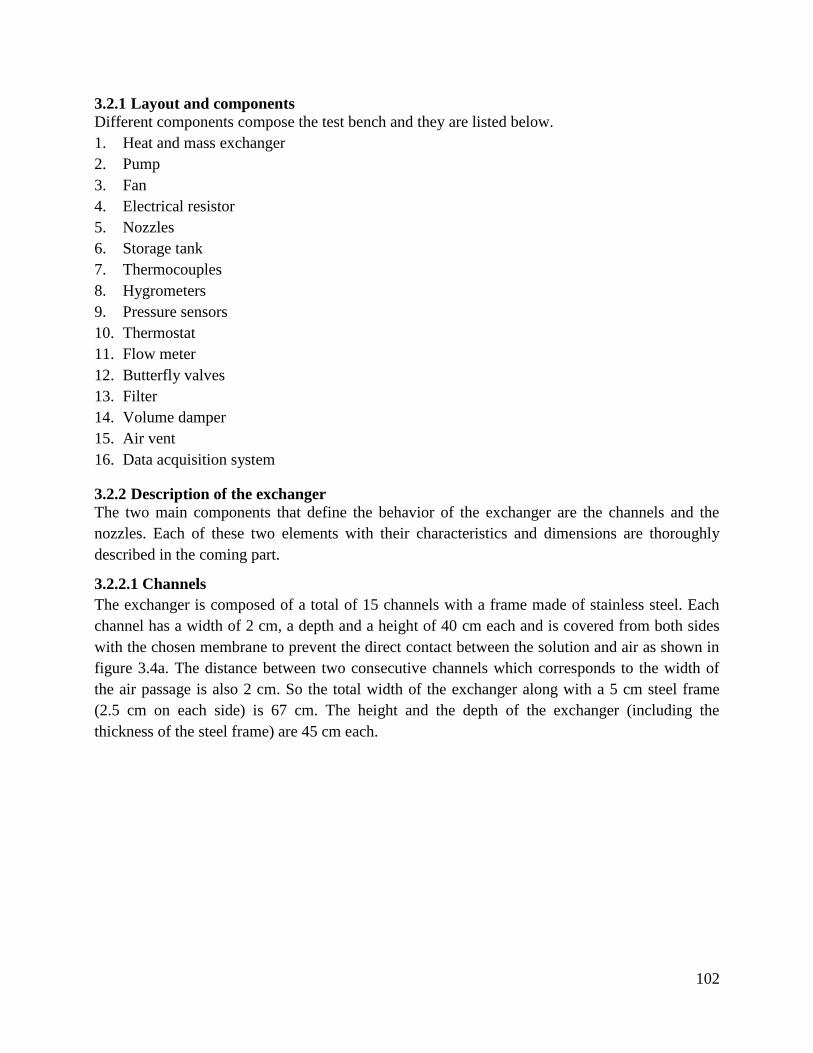
102

3.2.1 Layout and components

Different components compose the test bench and they are listed below.

1. Heat and mass exchanger

2. Pump

3. Fan

4. Electrical resistor

5. Nozzles

6. Storage tank

7. Thermocouples

8. Hygrometers

9. Pressure sensors

10. Thermostat

11. Flow meter

12. Butterfly valves

13. Filter

14. Volume damper

15. Air vent

16. Data acquisition system

3.2.2 Description of the exchanger

The two main components that define the behavior of the exchanger are the channels and the

nozzles. Each of these two elements with their characteristics and dimensions are thoroughly

described in the coming part.

3.2.2.1 Channels

The exchanger is composed of a total of 15 channels with a frame made of stainless steel. Each

channel has a width of 2 cm, a depth and a height of 40 cm each and is covered from both sides

with the chosen membrane to prevent the direct contact between the solution and air as shown in

figure 3.4a. The distance between two consecutive channels which corresponds to the width of

the air passage is also 2 cm. So the total width of the exchanger along with a 5 cm steel frame

(2.5 cm on each side) is 67 cm. The height and the depth of the exchanger (including the

thickness of the steel frame) are 45 cm each.

103

(a) (b) Figure 3.4: a) One channel with the membrane placement, b) Four consecutive channels of the exchanger with

dimensions

3.2.2.2 Nozzles

The nozzles are of compact type made of brass to avoid corrosion when the desiccant solution

passes through them. They are chosen with the highest spray angle, 120°, to ensure maximum

solution coverage where the repartition of the liquid is uniform and parabolic (“Flat fan nozzles,”

n.d.) (fig. 3.5 and 3.6). The chosen nozzle has a minimum passage diameter of 0.6 mm and with

an allowable liquid volume flow rate varying from 0.71 to 2.24 l/min as the pressure difference

across it changes from 1 to 10 bar. If the nozzles function at a different pressure range this would

result in an undesired spray pattern. As mentioned in the data sheet, at a pressure of 2 bar and a

vertical height of 250 mm, the width of the jet is 660 mm.

Figure 3.5: Flat jet nozzle

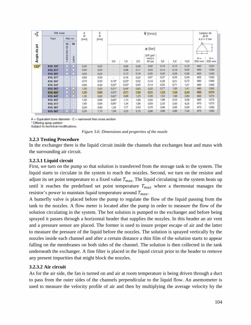
104

Figure 3.6: Dimensions and properties of the nozzle

3.2.3 Testing Procedure

In the exchanger there is the liquid circuit inside the channels that exchanges heat and mass with

the surrounding air circuit.

3.2.3.1 Liquid circuit

First, we turn on the pump so that solution is transferred from the storage tank to the system. The

liquid starts to circulate in the system to reach the nozzles. Second, we turn on the resistor and

adjust its set point temperature to a fixed value . The liquid circulating in the system heats up

until it reaches the predefined set point temperature where a thermostat manages the

resistor’s power to maintain liquid temperature around .

A butterfly valve is placed before the pump to regulate the flow of the liquid passing from the

tank to the nozzles. A flow meter is located after the pump in order to measure the flow of the

solution circulating in the system. The hot solution is pumped to the exchanger and before being

sprayed it passes through a horizontal header that supplies the nozzles. In this header an air vent

and a pressure sensor are placed. The former is used to insure proper escape of air and the latter

to measure the pressure of the liquid before the nozzles. The solution is sprayed vertically by the

nozzles inside each channel and after a certain distance a thin film of the solution starts to appear

falling on the membranes on both sides of the channel. The solution is then collected in the tank

underneath the exchanger. A fine filter is placed in the liquid circuit prior to the header to remove

any present impurities that might block the nozzles.

3.2.3.2 Air circuit

As for the air side, the fan is turned on and air at room temperature is being driven through a duct

to pass from the outer sides of the channels perpendicular to the liquid flow. An anemometer is

used to measure the velocity profile of air and then by multiplying the average velocity by the

105

considered area the air flow is deduced. At full speed, the fan gives an air flow of 690 m3/h and a

volume damper placed before the fan is used to reduce this flow sequentially.

3.2.3.3 Performance determination

In order to measure the performance of this exchanger in terms of heat transfer, the inlet and

outlet temperatures of both air and the solution entering and leaving the exchanger are measured.

In addition, to determine the amount of mass transfer, the change in the water vapor

concentration in air is computed through measuring the difference in the relative humidity of air

entering and air leaving. That is why a thermocouple and a hygrometer are placed in the air duct

at about 20 cm before the exchanger to measure the temperature and the relative humidity of the

inlet air. Due to the absence of an exit air duct, a thermocouple and a hygrometer are placed

directly at the outlets of some air channels of the exchanger to measure the temperature and the

relative humidity of the air leaving the exchanger. Two thermocouples are placed in the liquid

pipe directly before entering the nozzles header and the temperature of the inlet solution is

measured before being sprayed. Two thermocouples are also placed at the collection point of the

liquid before falling into the tank to measure its outlet temperature. The average temperature at

each side is considered to be the actual inlet and outlet solution temperature respectively.

The hygrometers and the thermocouples are connected to a data acquisition system by which

their readings are plotted and saved continuously for further analysis. As the difference between

the temperature of the solution and air gets bigger, the heat and mass transfer rises due to the

increase in the difference between the vapor pressure of the two fluids. In case where the

temperature of the solution is higher than that of air, as it is in the case of our experiments, the

direction of flow of water vapor is from the solution to air. Hence the air should be leaving the

exchanger loaded with water and thus with a higher absolute humidity.

3.3 Experiments

To test its performance a total of 18 experiments are done on the heat and mass exchanger.

Instead of liquid desiccant solution, water is injected through the nozzles for easier and riskless

applications. The apparatus is turned on and when the outlet air temperature and relative humidity

become stable indicating that the steady state is reached (time to reach steady state is around 30

min); then, measurements are taken for an interval of 20 minutes. The measurement of the outlet

air conditions is done using a hygrometer placed at the exit of three channels where the outlet air

temperature and relative humidity are taken every minute. The inlet and outlet water temperature

as well as the inlet and outlet air temperature and relative humidity are measured continuously

and they will be shown for some experiments in later sections. The velocity of air passing in the

exchanger is measured at the inlet duct before the fan using an anemometer with a telescopic

vane probe at the inlet of the exchanger. Multiplying the mean speed by the cross section area of

the duct gives the overall mass flow rate of air traversing the exchanger. The results of the inlet

and outlet conditions are later used for the calculations of the performance of the exchanger.

Two sets of experiments are performed; one at low air speed and the other at full air speed. The

first set of experiments is done with the volume damper partially opened so the fan was driving

106

air at a flow rate of around 330 m3/h. In the second set of experiments the volume damper is fully

opened and the full delivered air flow is around 690 m3/h. In each set, 9 experiments are

performed each time by changing the mass flow rate of water, the lowest flow rate was 4.5 lpm

and the highest was 9.1 lpm. For values greater than 9.1 lpm the temperature difference between

the inlet and outlet water would not be very significant and thus the measurement uncertainty

would highly affect our results. The electrical resistor's maximum power is 3000 W and it is

always working at full power having set at very high limits. Thus the inlet water

temperature changes from one experiment to another influenced by the variation of the flow rate.

The parameters that are changed from one experiment to another are mainly the inlet air and

water flow rates. The inlet air is the room air; its temperature and relative humidity are

continuously measured. The inlet water temperature is set but it is affected by the resistor’s

fluctuations so it is continuously measured as well and stored by the data acquisition system.

3.4 Proposed heat and mass membrane exchanger model

A fundamental evaluation of the performance of heat and mass exchangers requires modeling

tools. Several researchers have examined coupled heat and mass transfer in energy exchangers

such as Moghaddam et al. (Ghadiri Moghaddam et al., 2013) who experimentally and

numerically assessed the performance of a counter-flow liquid to air membrane energy exchanger

(LAMEE). They investigated as well the effects of the air convective heat transfer coefficient and

the resistance of the membrane on the performance of the LAMEE. Among the developed

models, some were established as one dimensional used to predict analytical solutions of packed

bed dehumidifiers and regenerators at steady state (Chengqin et al., 2005; Ren et al., 2007).

Chengqin et al. used a solution with CaCl2 as a desiccant and studied the effect of changing the

inlet conditions such as the liquid concentration, temperature and flow rate as well as the air

temperature, humidity and flow rate on the heat and mass transfer performance. Two-dimensional

models were as well developed and examined in various studies (Khan, 1998; Vali et al., 2015).

Vali et al. used a two dimensional numerical model to solve for a steady state flow in a counter

cross flow parallel plate membrane exchanger and their model was validated later by

experimental data. With a similar model Bergero et al. (Bergero et al., 2000) investigated a cross

flow exchanger and justified his numerical results by performing experiments at different test

conditions. Huang (Huang, 2015) also used a two dimensional steady state model to compare the

performance of a quasi-counter flow parallel plate membrane contractor to a cross flow one. He

concluded that compared to a cross flow contractor the sensible cooling and dehumidification

effectiveness deteriorated by approximately 5-29% and 2-13% respectively under various air and

solution flow rates and temperatures. A transient 2-D model was used by Namvar et al. (Namvar

et al., 2013) to predict the performance of a counter cross liquid to air membrane based

exchanger under summer and winter operating conditions and their model was then validated

using experimental data.

The three main kinds of theoretical modeling approaches are the effectiveness-NTU (Stevens et

al., 1989), the finite difference (Factor and Grossman, 1980), and the conjugate heat and mass

transfer based on fitted algebraic equations (Y. Khan, 1994). The method is less widely

107

spread in literature compared to the other two methods (Huang et al., 2018). Xie et al. (Xie et al.,

2016) developed an model for a counter-current dehumidifier and proved its reliability

by experimental data. The method is a simple method with a fast computation time yet

its results are less accurate compared to the other methods especially when fluids properties may

change through the exchanger. Finite difference methods are commonly applied for the modeling

of membrane based liquid desiccant energy exchangers mainly for performance analysis and

optimization. However, their application is limited when it comes to control design due to their

complex model development and to the intensive iterations that are performed during the

simulations to converge the results. Consequently, this method is much more time consuming

relative to the others. Fumo and Goswami adopted a finite difference model in their work to

evaluate the impact of varying operating conditions on air dehumidification and desiccant

regeneration using LiCl desiccant solution. Their model showed satisfactory agreement with the

experimental findings. In the finite difference method, the heat and mass transfer equations are

derived from correlations of fundamental data such as Nusselt and Sherwood (Holman, 1989;

Incropera and DeWitt, 1996). However, one main drawback of this method is that the obtained

data is considered under uniform temperature (heat flux) or concentration (mass flux) boundary

conditions the conception that does not precisely reflect the truly existing heat and mass

properties at the boundary conditions of the membrane surface. The third method is used to avoid

the drawback presented by the finite difference method. It determines the real boundary

conditions at the surface of the membrane through separate mass and energy equations and thus

provides better accuracy (Jafarian et al., 2019). Huang et al. (Huang et al., 2012) developed and

validated a model using conjugate method for a cross flow parallel plate channels for liquid

desiccant air dehumidification. The results of their numerical model was compared to

experimental data and showed very good agreement with the findings.

Inspired by the literature results and since the proposed design in this work is novel and not

studied before, the next sections present the developed numerical model.

3.4.1 Assumptions

In a way to predict the performance of the exchanger proposed in this thesis, a detailed 2-D

numerical model is written in Modelica language using Dymola software for a liquid to air cross

flow membrane heat and mass exchanger. Conjugate energy and mass transfer equations are

derived and then discretized and solved by using a finite volume approach at steady state. Our

model is generated considering the liquid as a desiccant solution of LiCl which is later tailored to

water in order to reflect the real experimental case study of our test bench.

The liquid desiccant solution is sprayed in the nozzles and is supplied vertically inside the

channels in the direction of z axis. While air is supplied outside the channels perpendicular to the

liquid flow in direction of x axis with the two flows being completely separated by the chosen

semi permeable membrane. All the parameters and boundary conditions are introduced into the

model including the outdoor air conditions, the properties of the introduced desiccant solution,

the mass flow rates, the thickness of the channels, the properties of the membrane, etc. The model

uses all these parameters to calculate the output air and desiccant conditions and the temperature

108

at the surfaces of the membrane. The properties of the membrane including its thickness and

mass conductivity are taken from the values determined in the previous chapter while its thermal

conductivity was adopted from literature review by considering that the conductivity of our

membrane is similar to that of ProporeTM

membrane (Afshin, 2010). The properties of the humid

air are taken from (McPherson, 1993) and the properties of LiCl solution in water are given by

Conde (Conde, 2014, 2004).

In order to reduce the complexity of the model, several assumptions were made. These

assumptions help in solving some physical problems without significantly affecting the results

and accuracy of the calculations. The validity of the majority of these assumptions is discussed

by Vali et al (Vali et al., 2009) and these assumptions can be stated as follows:

1. Both the air and the liquid desiccant flows are assumed to be at steady state.

2. All variables have 1-D variations in space, in the direction of flow.

3. The fluid flows are independent of the heat and mass transfer and the mass flow rates of

dry air and dry desiccant are considered constant.

4. Only the transport of water vapor is permitted by the membrane while the transport of

liquid water is not allowed and the membrane properties are independent of the

temperature and humidity of the fluids.

5. The heat and mass transfer between the two adjacent fluids only occurs in the direction

that is perpendicular to the membrane. The heat conduction and moisture diffusion in the

direction of the fluid flows are neglected.

6. Water transfers from or to moist air as vapor. Latent heat of vaporization is always taken

from the liquid solution or dissipated into it.

7. The exchanger’s casing, the connecting pipes and other system components are

considered to be adiabatic. Therefore, there is no heat transfer with the surrounding.

8. The salt solution is assumed to contain no other chemicals and impurities and it is

considered to be well mixed before entering the exchanger.

9. The air and the desiccant solution are assumed to be in equilibrium at the solution-air

interface which is located at the liquid-membrane interface.

Other assumptions and approximations will be stated later in the model development.

3.4.2 Definitions, properties and basic relations

In the following sections, the properties of the moist air and the desiccant solution are discussed

with the ranges of variables.

3.4.2.1 Moist air

The mixture of air with water vapor may be characterized by the molar fraction of vapor, , that

is the ratio of the number of water moles to the total number of moles. But the main variable used

for the characterization of the moist air flow is the humidity ratio defined as the mass of vapor

per of dry air. It is related to the molar fraction of vapor by:

(3.1)

109

The constant is in fact the ratio of the molar mass of water ( ) to that of

dry air ( ). Inverting equation (3.1) gives :

(3.2)

If the total pressure of a mixture is (normally = 101325 Pa), then that of water vapor is:

(3.3)

Then we have the following relations:

(3.4)

(3.5)

If the air relative humidity and the temperature are known at some point of the system, then the

partial pressure of vapor may be determined using:

(3.6)

For the calculation of the saturation pressure of water vapor, a formula adapted from (Bolton,

1980) is used. Compared to the tables found in (Ameen et al., 1993), it gives an error that is less

than in the range of temperature from to .

(3.7)

where is the temperature in .

When the side of the membrane that is in contact with the air has a temperature that is less than

the dew point temperature of the air, the absorbed water vapor condenses and thus the droplets of

water might stick to the surface of the membrane. Therefore, it is important during the modeling

phase to pay attention that the surface of the membrane that is in contact with the air must always

have a temperature greater than the dew point temperature of the air at the specified conditions.

Also note that the temperature of the membrane changes with time and with the direction of the

flow, so at both the entrance and the exit of the membrane the difference in temperature between

the surface of the membrane and the dew point of the air should always be positive.

Therefore, the calculation of the dew point temperature is very important, because it allows

determining whether there is condensation or not on the membrane according to its surface

temperature. The formula used is also adapted from (Bolton, 1980) and has a good accuracy

compared to the tables given by Çengel and Boles (Çengel and Boles, 2015), with a maximum

error that is less than for ranging between and . The dew point

temperature in is given by:

110

(3.8)

Dry air is considered as an ideal gas having a molar mass of . Its density at

atmospheric pressure ( ) is then:

(3.9)

As for the other properties of moist air, they are mainly taken from (Tsilingiris, 2008) and

adapted with some simplifications. They are expressed in terms of the temperature, given in ,

and the molar fraction of vapor in air, .

The dynamic viscosity and the thermal conductivity of moist air are important for the calculation

of the convective heat transfer coefficients. First, for the calculation of the dynamic viscosity:

(3.10)

with:

(3.11)

and

(3.12)

And for the thermal conductivity:

(3.13)

ith:

(3.14)

and

(3.15)

Regarding the specific heat of air and vapor, taking the constant values below shows that the

maximum error is around for air and for water vapor, for temperatures ranging from

to .

(3.16)

and

(3.17)

Last, the diffusion coefficient of water vapor in air at atmospheric pressure is important for the

calculation of the convective mass exchange coefficient. According to (Mills, 1995), it is:

111

(3.18)

where is the temperature in .

3.4.2.1 Desiccant solution

The desiccant solution differs from the moist air by the fact that it is a solution of LiCl solid

salt in liquid water and not a simple mixture of two ideal gases:

(3.19)

In these conditions, properties like density and specific heat may not be calculated using simple

mixing formulas. On one hand, the volumes occupied by each substance cannot be estimated as

in the case of gases; the calculation of the density is then impossible. On the other hand, the

reaction described by eq. (3.19) is exothermal. Its enthalpy, the enthalpy of solution, , is

known only at and at low concentrations (Apelblat et al., 1984; Wolf et al., 1987) , which

removes the possibility to deduce the specific heat of the solution using those of the substances in

the mixing formula.

In these conditions, the properties of the desiccant solution as a whole have to be considered.

The desiccant solution may be characterized by the concentration of salt in the solution, that is:

(3.20)

But the main variable used for the characterization of the solution is the water ratio, , defined as

the ratio of the mass of water to that of dry desiccant, or the mass of water per of dry

desiccant in the solution:

(3.21)

It can be easily shown that:

(3.22)

and:

(3.23)

The properties of LiCl solution in water are given by Conde (Conde, 2014, 2004). First, the

equivalent pressure of water vapor in the solution is given by:

(3.24)

112

where:

(3.25)

(3.26)

(3.27)

(3.28)

Knowing , the equivalent humidity ratio in the solution may be determined by:

(3.29)

Determining is important for the modeling of the vapor mass transfer flow rate between the

moist air and the desiccant solution, since the driving potential of that transfer is .

The expression of the solution density is adapted from (Conde, 2004) in a simplified form and

gives very accurate results, with a relative error of less than for a big range of variation for

:

(3.30)

Considering the density of water as constant gives a relative error

of less than for temperatures ranging between and .

The dynamic viscosity of the solution is given by:

(3.31)

Where is the same as defined by eq. (3.25), and:

(3.32)

As for the viscosity of liquid water, it is adapted from (Furukawa, 1991) with a relative error less

than :

(3.33)

The thermal conductivity of the solution is given by (Conde, 2004) as:

113

(3.34)

where:

(3.35)

(3.36)

While the thermal conductivity of water is expressed, after simplification with still a high

accuracy, as:

(3.37)

The conductivity of water at ( ) is taken from (Ramires et al., 1995).

The specific heat of the solution is taken from (Conde, 2004) with some simplifications:

(3.38)

where:

(3.39)

(3.40)

with:

(3.41)

The specific heat of water is considered constant, .

When water is added to the solution or rejected from it, due to the mass transfer of water vapor

taking place across the membrane there is the enthalpy of water phase change (latent heat). It

may be calculated by the formula given in (Furukawa, 1991):

(3.42)

Last, the diffusion coefficient of water in the solution is found in (Conde, 2014):

(3.43)

Here, is the self diffusion coefficient of water. Its expression is found in (Holtz et al., 2000):

(3.44)

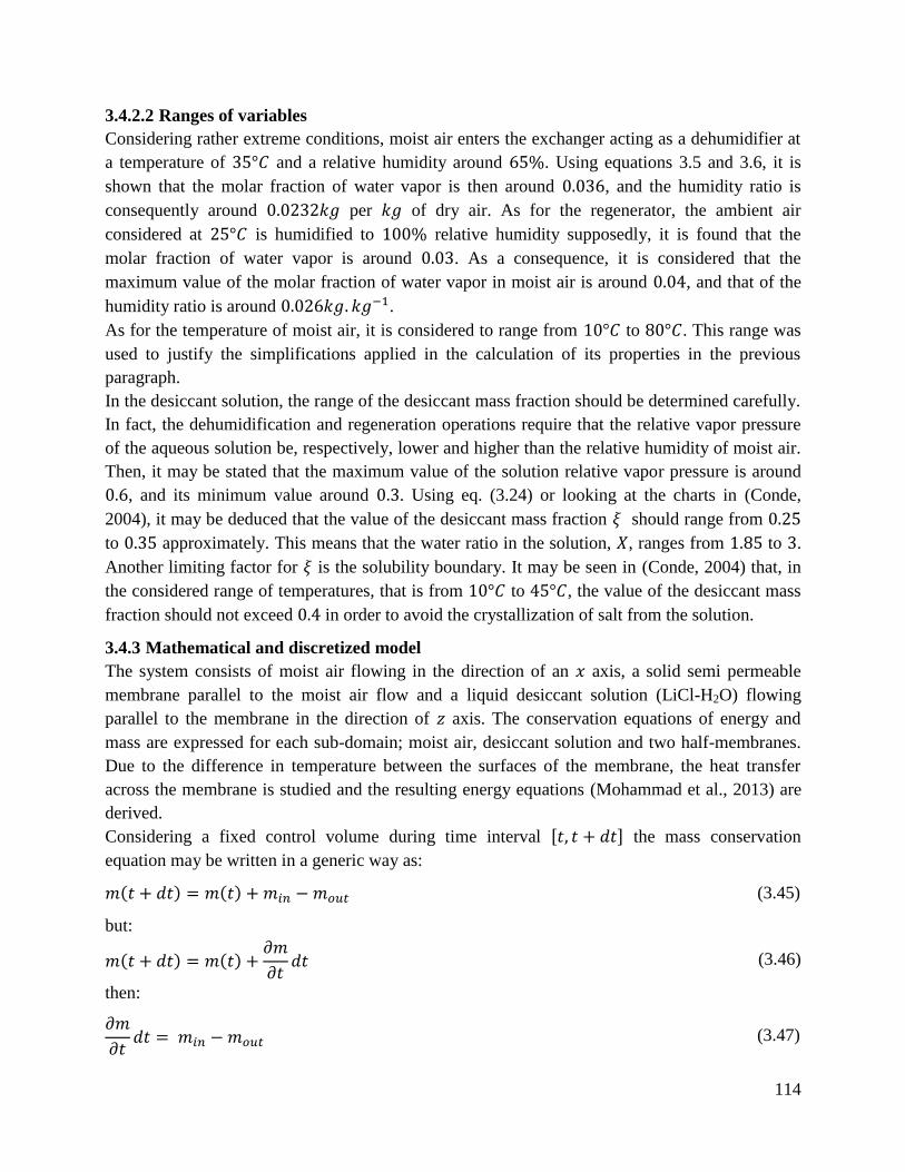
114

3.4.2.2 Ranges of variables

Considering rather extreme conditions, moist air enters the exchanger acting as a dehumidifier at

a temperature of and a relative humidity around . Using equations 3.5 and 3.6, it is

shown that the molar fraction of water vapor is then around , and the humidity ratio is

consequently around per of dry air. As for the regenerator, the ambient air

considered at is humidified to relative humidity supposedly, it is found that the

molar fraction of water vapor is around . As a consequence, it is considered that the

maximum value of the molar fraction of water vapor in moist air is around , and that of the

humidity ratio is around .

As for the temperature of moist air, it is considered to range from to . This range was

used to justify the simplifications applied in the calculation of its properties in the previous

paragraph.

In the desiccant solution, the range of the desiccant mass fraction should be determined carefully.

In fact, the dehumidification and regeneration operations require that the relative vapor pressure

of the aqueous solution be, respectively, lower and higher than the relative humidity of moist air.

Then, it may be stated that the maximum value of the solution relative vapor pressure is around

, and its minimum value around . Using eq. (3.24) or looking at the charts in (Conde,

2004), it may be deduced that the value of the desiccant mass fraction should range from

to approximately. This means that the water ratio in the solution, , ranges from to .

Another limiting factor for is the solubility boundary. It may be seen in (Conde, 2004) that, in

the considered range of temperatures, that is from to , the value of the desiccant mass

fraction should not exceed in order to avoid the crystallization of salt from the solution.

3.4.3 Mathematical and discretized model

The system consists of moist air flowing in the direction of an axis, a solid semi permeable

membrane parallel to the moist air flow and a liquid desiccant solution (LiCl-H2O) flowing

parallel to the membrane in the direction of axis. The conservation equations of energy and

mass are expressed for each sub-domain; moist air, desiccant solution and two half-membranes.

Due to the difference in temperature between the surfaces of the membrane, the heat transfer

across the membrane is studied and the resulting energy equations (Mohammad et al., 2013) are

derived.

Considering a fixed control volume during time interval the mass conservation

equation may be written in a generic way as:

(3.45)

but:

(3.46)

then:

(3.47)

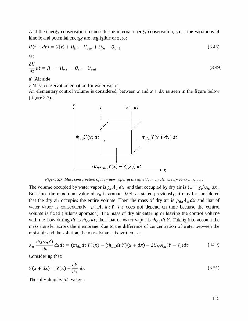
115

And the energy conservation reduces to the internal energy conservation, since the variations of

kinetic and potential energy are negligible or zero:

(3.48)

or:

(3.49)

a) Air side

Mass conservation equation for water vapor

An elementary control volume is considered, between and as seen in the figure below

(figure 3.7).

Figure 3.7: Mass conservation of the water vapor at the air side in an elementary control volume

The volume occupied by water vapor is and that occupied by dry air is .

But since the maximum value of is around , as stated previously, it may be considered

that the dry air occupies the entire volume. Then the mass of dry air is and that of

water vapor is consequently . does not depend on time because the control

volume is fixed (Euler’s approach). The mass of dry air entering or leaving the control volume

with the flow during is , then that of water vapor is . Taking into account the

mass transfer across the membrane, due to the difference of concentration of water between the

moist air and the solution, the mass balance is written as:

(3.50)

Considering that:

(3.51)

Then dividing by , we get:

116

(3.52)

But the density of dry air depends only on temperature, and the variations of the latter in time are

rather slow. It is then assumed that is independent of time:

(3.53)

In all cases, in steady state:

(3.54)

Energy conservation equation for moist air

The enthalpy entering or leaving the control volume with the flow during is

. As for the mass transfer across the membrane, it carries the enthalpy of vapor as

stated in the assumptions. Last, a thermal convective exchange takes place between the

membrane and the moist air stream. Considering the same assumption about neglecting the

variations of and a steady state, the enthalpy balance is then after simplification and

replacement of with :

(3.55)

a) Solution side

Mass conservation equation for liquid water

An elemental control volume is considered, between and . Here it is not at all possible to

consider that the dry desiccant occupies the whole volume. In fact:

(3.56)

then:

(3.57)

Now, applying the same approach as for water vapor leads toat steady state:

(3.58)

Energy conservation equation for the desiccant solution

The enthalpy entering or leaving the control volume with the flow is . As for the

mass transfer across the membrane, it transports the enthalpy of vapor, as stated in the

assumptions. Last, a thermal convective exchange takes place between the membrane and the

desiccant solution flow.

In these conditions, the energy balance under steady state on an elemental control volume may be

written as:

117

(3.59)

Comparing with , that is , for values of the temperature and the water

ratio in the solution covering the entire ranges defined previously, it is observed that the

maximum relative difference is around . With being the enthalpy of vaporization

defined as a function of temperature then finally:

(3.60)

b) Membrane

Energy conservation equations in the membrane

The enthalpy balance in each half-membrane accounts for the conduction in the direction of the

flow, the transversal conduction with the other half-membrane, considered instantaneous, with

the temperatures and taken on the interfaces with the fluids, and the convective heat

exchange with the neighboring fluid flow. As stated in the assumptions, the mass transfer across

the membrane is considered instantaneous and does not affect its energy balance. In these

conditions, under steady state, the energy conservation equations for the membrane are:

(3.61)

(3.62)

where: is in

, in

, in , in

, in

.

3.4.4 Numerical implementation of the model

The model is written using discretization method; each of the x axis and the z axis was

discretized into segments of equal sizes. The number of discretization is noted by Ni and Nj in

the horizontal and vertical directions respectively. The choice of the number of discretization is

based on an analysis that is discussed in further steps. It studies the effect of the number of mesh

on the precision of the numerical results maintaining a compromise between them and the

computational time needed to finish a simulation. The discretized model represents one channel

of the exchanger and thus modeling the whole exchanger is done by assembling several channels.

Hence, the model of the prototype exchanger is composed of 16 sub models associated to the

number of air channels. Figure 3.8 represents the exchanger with 15 liquid channels surrounded

by 16 air channels. In the figure we can notice that from air channel number 2 till air channel

number 15 there is an exchange between two half channels of liquid and two half channels of air.

As for the first and last air channels (air channels 1 and 16) the exchange takes place between

each of these air channels and the adjacent one half of the liquid channel. Therefore our 16 sub-

models are divided accordingly; the first and last model represent an exchange between one air

channel and half a liquid channel while all the others represent an exchange between an air

channel and a liquid channel.

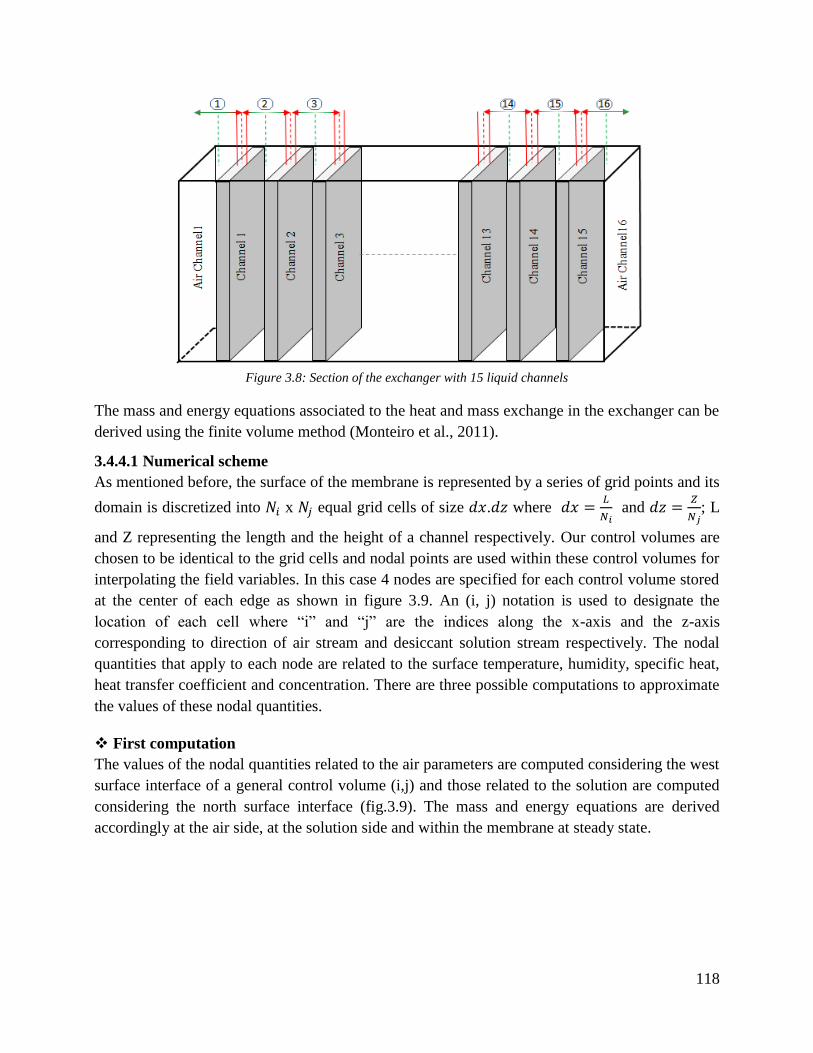
118

Figure 3.8: Section of the exchanger with 15 liquid channels

The mass and energy equations associated to the heat and mass exchange in the exchanger can be

derived using the finite volume method (Monteiro et al., 2011).

3.4.4.1 Numerical scheme

As mentioned before, the surface of the membrane is represented by a series of grid points and its

domain is discretized into x equal grid cells of size . where

and

; L

and Z representing the length and the height of a channel respectively. Our control volumes are

chosen to be identical to the grid cells and nodal points are used within these control volumes for

interpolating the field variables. In this case 4 nodes are specified for each control volume stored

at the center of each edge as shown in figure 3.9. An (i, j) notation is used to designate the

location of each cell where “i” and “j” are the indices along the x-axis and the z-axis

corresponding to direction of air stream and desiccant solution stream respectively. The nodal

quantities that apply to each node are related to the surface temperature, humidity, specific heat,

heat transfer coefficient and concentration. There are three possible computations to approximate

the values of these nodal quantities.

First computation

The values of the nodal quantities related to the air parameters are computed considering the west

surface interface of a general control volume (i,j) and those related to the solution are computed

considering the north surface interface (fig.3.9). The mass and energy equations are derived

accordingly at the air side, at the solution side and within the membrane at steady state.

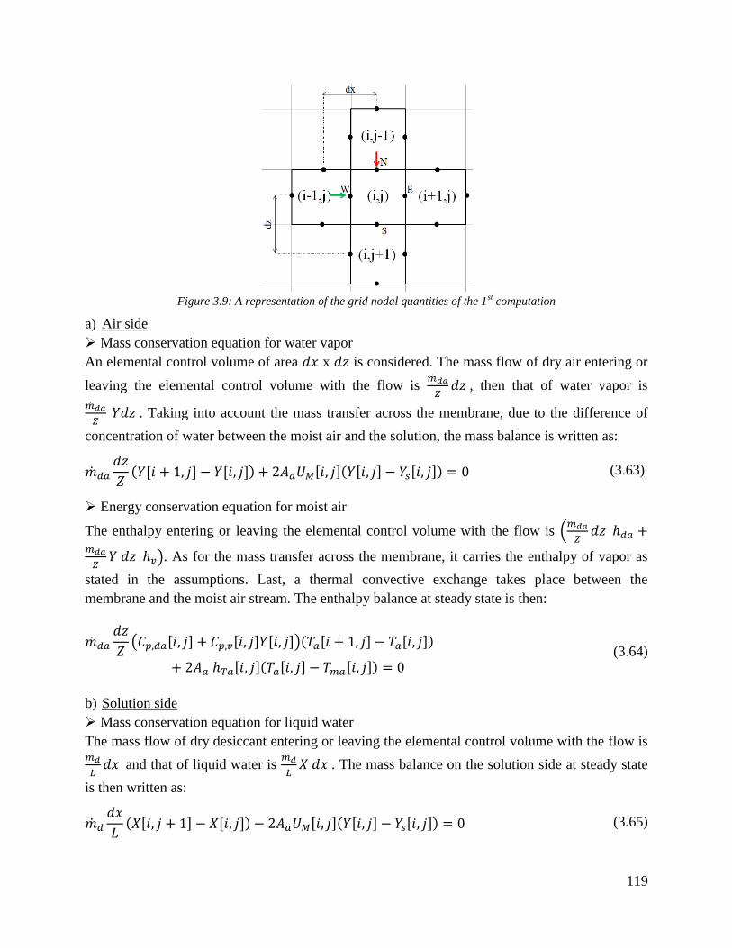
119

Figure 3.9: A representation of the grid nodal quantities of the 1

st computation

a) Air side

Mass conservation equation for water vapor

An elemental control volume of area x is considered. The mass flow of dry air entering or

leaving the elemental control volume with the flow is

, then that of water vapor is

. Taking into account the mass transfer across the membrane, due to the difference of

concentration of water between the moist air and the solution, the mass balance is written as:

(3.63)

Energy conservation equation for moist air

The enthalpy entering or leaving the elemental control volume with the flow is

. As for the mass transfer across the membrane, it carries the enthalpy of vapor as

stated in the assumptions. Last, a thermal convective exchange takes place between the

membrane and the moist air stream. The enthalpy balance at steady state is then:

(3.64)

b) Solution side

Mass conservation equation for liquid water

The mass flow of dry desiccant entering or leaving the elemental control volume with the flow is

and that of liquid water is

. The mass balance on the solution side at steady state

is then written as:

(3.65)

120

Energy conservation equation for the desiccant solution

The total mass flow of the solution is . The enthalpy entering or

leaving the elemental control volume with the flow is

. As for the mass transfer

across the membrane, it transports the enthalpy of vapor, as stated in the assumptions. Last, a

thermal convective exchange takes place between the membrane and the desiccant solution flow.

(3.66)

c) Membrane

Energy conservation equations

(3.67)

(3.68)

Second computation

Here, the values of the nodal quantities related to the air parameters are computed considering the

east surface interface of a general control volume (i,j) and those related to the solution are

computed considering the south surface interface (fig.3.10). Similarly, the mass and energy

equations are derived accordingly at the air side, at the solution side and within the membrane.

Figure 3.10: A representation of the grid nodal quantities of the 2

nd computation

a) Air side

Mass conservation equation for water vapor

(3.69)

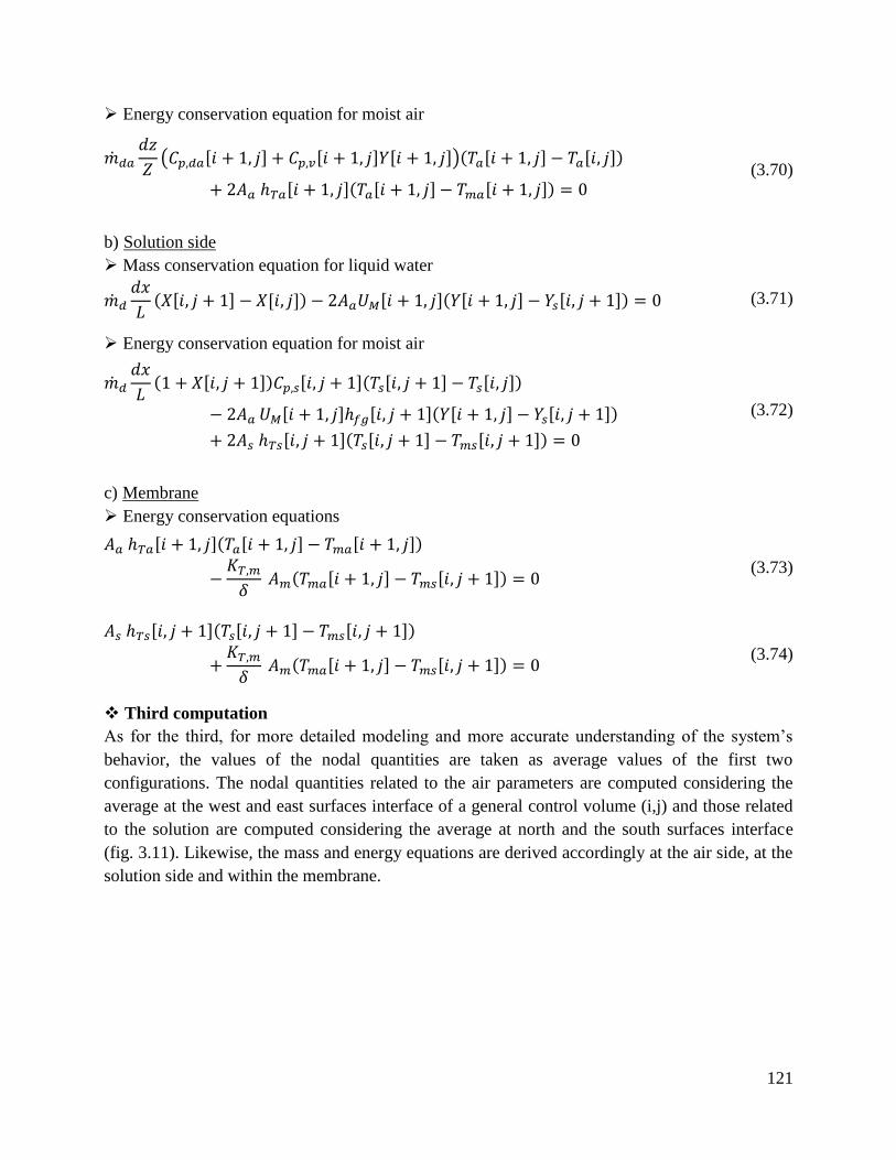
121

Energy conservation equation for moist air

(3.70)

b) Solution side

Mass conservation equation for liquid water

(3.71)

Energy conservation equation for moist air

(3.72)

c) Membrane

Energy conservation equations

(3.73)

(3.74)

Third computation

As for the third, for more detailed modeling and more accurate understanding of the system’s

behavior, the values of the nodal quantities are taken as average values of the first two

configurations. The nodal quantities related to the air parameters are computed considering the

average at the west and east surfaces interface of a general control volume (i,j) and those related

to the solution are computed considering the average at north and the south surfaces interface

(fig. 3.11). Likewise, the mass and energy equations are derived accordingly at the air side, at the

solution side and within the membrane.

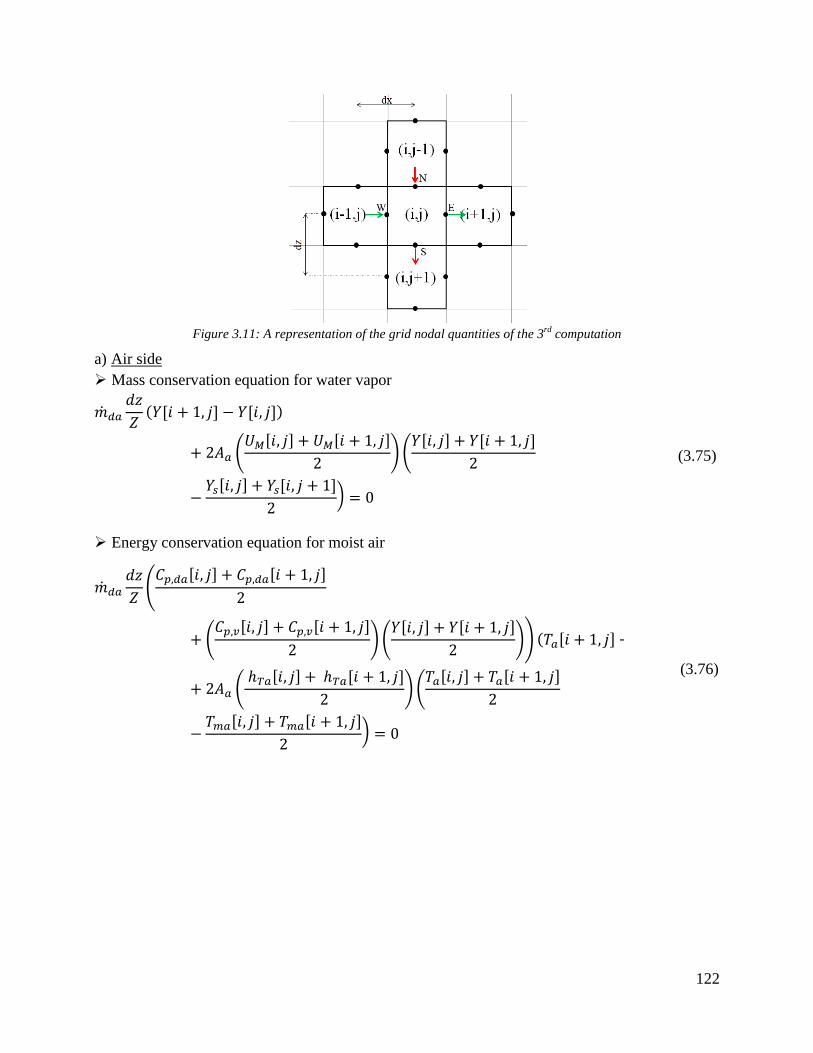
122

Figure 3.11: A representation of the grid nodal quantities of the 3

rd computation

a) Air side

Mass conservation equation for water vapor

(3.75)

Energy conservation equation for moist air

(3.76)

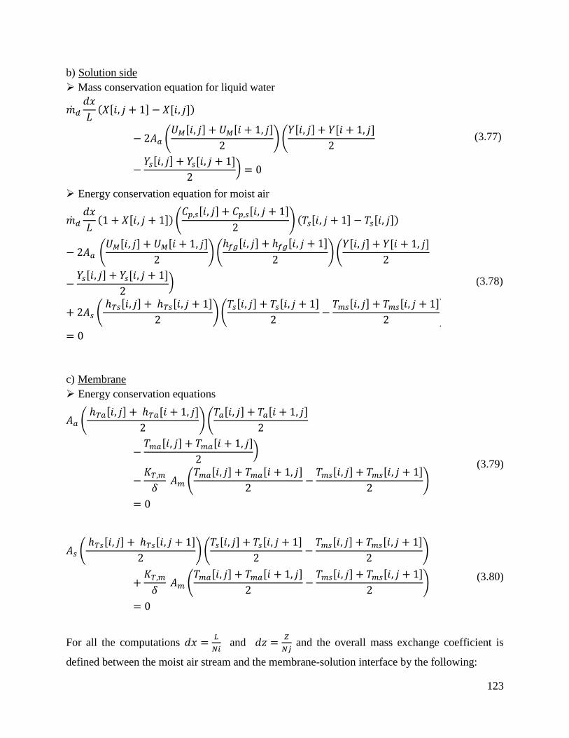
123

b) Solution side

Mass conservation equation for liquid water

(3.77)

Energy conservation equation for moist air

(3.78)

c) Membrane

Energy conservation equations

(3.79)

(3.80)

For all the computations

and

and the overall mass exchange coefficient is

defined between the moist air stream and the membrane-solution interface by the following:

124

(3.81)

With and being the mass transfer coefficients of air and the solution respectively

computed through mathematical correlations relating the Nusselt number and the heat transfer

coefficients.

The three approximation methods can be used to derive the mass and energy equations that

accompany the mass and heat transfer in indirect contact exchangers. In later steps, a sensitivity

analysis is done on the model representing the test bench exchanger to compare these three

approaches and to check their precision.

3.4.4.2 Convective heat and mass transfer coefficients

a) Air side

Heat transfer coefficient

The heat exchange coefficient used in the modeling equations can be deduced from correlations

relating Nusselt number to Reynolds number and Prandtl number .

(3.82)

These correlations are influenced by the thermal properties of the medium, the channel’s

geometry and the flow characteristics mainly temperature, viscosity and thermal conductivity.

Their applicability is affected as well by the hydrodynamic and thermal boundary conditions.

Different correlations exist for the various applications, inside or outside tubes, between two

parallel plates, in falling films, etc. for laminar, turbulent and transitional flows (Incropera et al.,

2007).

For laminar flow in circular tubes, the local Nusselt number is a constant throughout the fully

developed region depending on the surface thermal conditions:

For a uniform surface heat flux:

(3.83)

For a uniform surface temperature:

(3.84)

For a smooth surface and fully developed turbulent conditions valid for , Dittus-

Boelter equation may be used:

(3.85)

For turbulent flow in tubes with and the correlation of

Gnielinski defined for fully developed flows cited by (Incropera et al., 2007) may be used:

125

(3.86)

where for smooth tubes the friction factor is given by Darcy as in eq. (3.87).

(3.87)

Reynolds and Prandtl numbers are given by eq. (3.88) and eq. (3.89).

(3.88)

(3.89)

And the heat transfer coefficient is related to Nusselt number by eq. (3.90)

(3.90)

Then to calculate the heat transfer coefficient use eq. (3.91)

(3.91)

Where is the dynamic viscosity of air at the given inlet conditions in or equivalently

,

is the thermal conductivity in

is the velocity air in

, is the hydraulic diameter of a

channel in given by:

(3.92)

with and being the length and the width of a channel respectively.

Reynolds number is mainly used to determine the type of the flow. For a fluid moving between

two plane parallel surfaces, a flow is considered to be laminar if its Reynolds number is less than

2000. Yet, the Nusselt number differs along the flow, for instance in the entrance region of a

pipe or a duct is usually greater than that in the fully developed region. Thus to find out the

characteristics of the flow; whether it is fully developed or still in the entrance region of the

developing phase, an assessment of the boundary conditions should be performed. Therefore, to

choose which correlation to adopt for each flow one essential element to be inspected is the

growth of the boundary layer thickness.

Boundary layer thickness

For flow over any surface, there always exists a velocity boundary layer and hence surface

friction. The boundary layer thickness is the distance across a boundary layer from the walls to a

point where the flow velocity has essentially reached the 'free stream' velocity (“Boundary layer

126

thickness,” 2019). Boundary layers may be either laminar or turbulent depending on Reynolds

number associated to the fluid. In practice, the critical values of this number, which characterizes

the transition from laminar flow to turbulence, are given for each geometric configuration. For

low values of Reynolds the boundary layer has laminar characteristics where the fluid’s velocity

changes uniformly as we move away from the wall (Hall, 2015). For higher values of Reynolds

number this layer becomes turbulent where the velocity is disordered and the flow becomes

unsteady with time. For laminar and turbulent flows the boundary layer thickness over a flat plate

is given by (Schlichting, 1960) respectively in eq. (3.93) and eq. (3.94):

(3.93)

(3.94)

with being the overall thickness of the boundary layer, being the distance at a point of the

wall where we need to find , and being the Reynolds number at .

If the flow is still in a transitional regime other heat transfer correlations exist. For a developing

laminar flow at a length , correlations reported by (Sieder and Tate, 1936) are used to calculate

the Nusselt number:

(3.95)

where

and

is the ratio of the bulk viscosity over the viscosity near the wall. This

correlation is valid for .

For turbulent flows, to account for the coefficients in a non-fully developed transitional flow

regimes Hausen proposed the addition of a correction factor to the correlation given by

Gnielinski in eq. (3.101). He suggested to multiply the equation by

taking into

account the entrance region as cited by (Dirker et al., 2017) . According to previous work

performed by (Dirker et al., 2017) this factor was then modified to better predict their

experimental results to become

where

. Then the modified Nusselt

number is given by eq. (3.96):

(3.96)

where and are respectively the hydraulic diameter and the length of a channel in m.

127

Mass transfer coefficient

The convective mass transfer coefficient may be determined using specific correlations relating

Sherwood number to Reynolds number and Schmidt number (Incropera et al., 2007) as

in the following:

(3.97)

(3.98)

(3.99)

Then:

(3.100)

The Chilton-Colburn analogy (Incropera et al., 2007) may also be used to deduce these

coefficients from the heat convection ones by:

(3.101)

Where is the Lewis number defined as:

(3.102)

Where is the density of air and is the diffusivity of vapor in air.

b) Water side

Heat transfer coefficient

Correlations related to jet

On the other side of the membrane, water is sprayed through nozzles with a flat jet angle in a

direction parallel to the membranes. Different researchers have investigated the heat transfer

mechanism occurring in spraying process in several domains. In most of these processes it was

ensured that the nozzle axis was always normal to the target surface and sometimes the

impingement was over an inclined surface. In spray and jet cooling techniques coolants are

sprayed through nozzles over a hot surface provoking phase change when the sprayed liquid

heats up (Wang et al., 2011; Wu et al., 2019; Xia et al., 2006). The heat transfer rate showed a

great dependence on different parameters including the nozzle’s geometry and the flow pattern

after jet impingement. It is also influenced by the behavior of the jet depending on its angle, on

the nozzle orifice dimensions and other parameters (Royne and Dey, 2006; Vinze et al., 2016).

Several correlations were developed relating the Nusselt number to the spray Reynolds number

and in the following some of them are stated and discussed.

128

An experimentally derived correlation deduced by Specht (Specht, 2014) provided the following

average function for a single circular nozzle being determined for air application (as the flow

moves from laminar to turbulent the exponent of increases)

(3.103)

where

, being the diameter of the nozzle in , the speed at which the flow exits the

nozzle in

and the kinematic viscosity of the fluid in

.

Other experimental studies were performed by Scholtz and Trass for parabolic velocity profile

circular jets normally impinging a surface with a laminar boundary layer condition. They

proposed the following Nusselt correlation valid for and and cited by

(Lienhard, 2005):

(3.104)

where

, being the diameter of the jet in , the speed of the coming jet in

The heat transfer coefficient is then deduced from the Nusselt correlation by eq. (3.91).

Correlations related to falling films

The above mentioned correlations consider that the jet is impinged normal to a horizontal surface

and as a matter of fact none of these correlations reflects the real case. In our case water is

sprayed through flat jet nozzles in a direction parallel to the surface of the membranes. Thus our

search is extended to examine the correlations of falling films.

In falling films, heat transfer takes place between a thin liquid film and a surface that absorbs or

emits heat and the film falls over this surface because of the gravitational force. Coefficients of

heat and mass transfer for falling films have been widely studied and Nusselt correlations were

determined theoretically and experimentally in different applications. For shell and tube heat

exchangers Kern’s correlation is used to estimate the shell side Nusselt equation (Zhu, 2013):

(3.105)

where

and being the equivalent shell side diameter .

Another equation for heat transfer in falling films is discussed by Schnabel and Schlünder where

three correlations are given for laminar, transition and turbulent flows as cited in (Åkesjö et al.,

2018).

(Laminar )

(Transition ) (3.106)

(Turbulent )

where

and

is the mass flow rate of the fluid per unit width in

129

In this correlation the heat transfer coefficient is related to the Nussselt number by the following

equation eq. (3.107)

(3.107)

where is the film thickness in (Yoshioka and Hasegawa, 2012).

Mass transfer coefficient

The mass transfer coefficient at the water side is calculated by the Chilton-Colburn analogy

mentioned in eq. (3.100).

However, in reality even a falling film does not totally represent the flow pattern of our

exchanger. This is because whenever the spray is not fully distributed with an angle of 120°, the

flow isn’t considered as a film since it would be still diverging and the channel would not be

completely within the spray coverage. Therefore, a comparison of the order of magnitude

between the correlations related to jets and those related to falling films is performed in order to

check the differences and to decide which of them to select and to employ in our model. For this

reason a typical example is considered for our case study taking typical input air and water

conditions and analyzing the output results based on the different discussed correlations.

3.5 Application done on the prototype

In our test bench the liquid sprayed inside the channels is water and thus the properties of water

instead of desiccant are used in our model. Therefore the mass conservation equation at the liquid

side is not applicable anymore and the mass flow rate of the desiccant solution

is replaced by that of water .

Table 3.1: A summary of the design parameters and the inlet conditions of a typical example

Exchanger

Length (m) 0.4

Height (m) 0.4

Number of water channels 15

Wa (m) 0.02

Ws (m) 0.02

Ni 20

Nj 20

Membrane

δ (m) 1.57 x 10-4

m (m2/s) 4.3 x 10

-6

(W/m.K) 0.334

Air conditions

T (°C) 20

RH (%) 70

Velocity per channel (m/s) 1.2

Flow per channel (m3/h) 34.56

Water conditions

T (°C) 35

Total flow (lpm) 8

Flow per channel (kg/s) 8.89 x 10-3

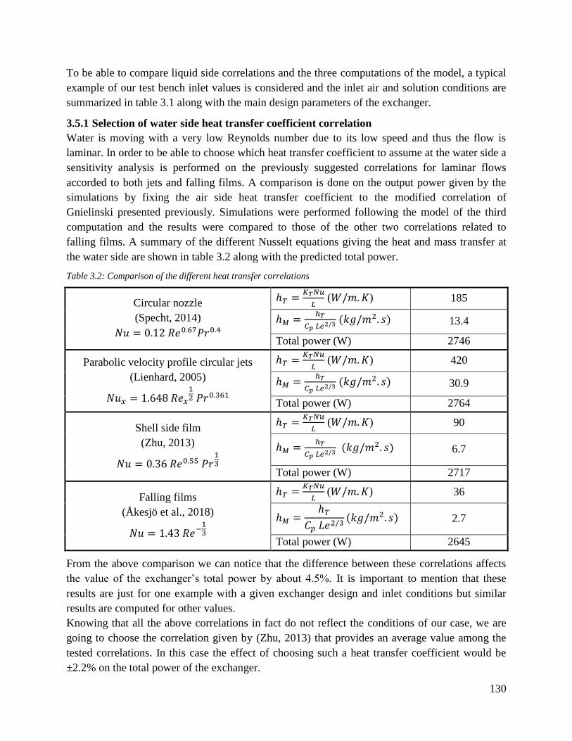
130

To be able to compare liquid side correlations and the three computations of the model, a typical

example of our test bench inlet values is considered and the inlet air and solution conditions are

summarized in table 3.1 along with the main design parameters of the exchanger.

3.5.1 Selection of water side heat transfer coefficient correlation

Water is moving with a very low Reynolds number due to its low speed and thus the flow is

laminar. In order to be able to choose which heat transfer coefficient to assume at the water side a

sensitivity analysis is performed on the previously suggested correlations for laminar flows

accorded to both jets and falling films. A comparison is done on the output power given by the

simulations by fixing the air side heat transfer coefficient to the modified correlation of

Gnielinski presented previously. Simulations were performed following the model of the third

computation and the results were compared to those of the other two correlations related to

falling films. A summary of the different Nusselt equations giving the heat and mass transfer at

the water side are shown in table 3.2 along with the predicted total power.

Table 3.2: Comparison of the different heat transfer correlations

Circular nozzle

(Specht, 2014)

( ) 185

13.4

Total power (W) 2746

Parabolic velocity profile circular jets

(Lienhard, 2005)

( ) 420

30.9

Total power (W) 2764

Shell side film

(Zhu, 2013)

( ) 90

6.7

Total power (W) 2717

Falling films

(Åkesjö et al., 2018)

( ) 36

2.7

Total power (W) 2645

From the above comparison we can notice that the difference between these correlations affects

the value of the exchanger’s total power by about 4.5%. It is important to mention that these

results are just for one example with a given exchanger design and inlet conditions but similar

results are computed for other values.

Knowing that all the above correlations in fact do not reflect the conditions of our case, we are

going to choose the correlation given by (Zhu, 2013) that provides an average value among the

tested correlations. In this case the effect of choosing such a heat transfer coefficient would be

±2.2% on the total power of the exchanger.

131

For the coming steps of the model validation the modified Nusselt correlation provided by

Gnielinski (eq. (3.96)) and that provided by Kern (eq. (3.105)) are adopted for the air side and

water side respectively.

3.5.2 Comparison of the three computations schemes

As discussed before, the third computation is the average of the other two and it should provide

more accurate results. In the coming step these three computations are compared by their

accuracy, the time needed to finish a simulation and how they are affected by some modeling

parameters. For this comparison, the output power is calculated for each computation by varying

the model discretization.

The creation and selection of discretization size in the model is an important step since during

simulations meshing is considered to be the most memory intensive measure. Thus choosing a

convenient number of mesh can help reduce memory requirements decreasing the computational

time needed for a simulation. On the other hand, lowering the number of mesh can affect the

accuracy of the numerical results of our model. A convenient mesh size guarantees a more

accurate numerical outcome while a poor mesh size affects the convergence of the solution. In

order to find an acceptable number of mesh by which there is a compromise between the

accuracy of the model and the restrictions of memory and time, a sensitivity analysis is

performed. This is done by simulating the models of the three computations’ schemes several

times modifying only the number of mesh Ni and Nj in each. The study concentrates on the total

power of the exchanger and examines its variation with the increase of Ni and Nj from 5 to 40 by

a step of 5 every time. This study gives an idea about the effect of changing the mesh size on the

numerical results regarding the total water power of the exchanger as shown in figure 3.12. From

the graph it can be observed that as the number of mesh increases the 3 curves representing the

power of the exchanger start to get flatter approaching an asymptote. As for very small values of

Ni and Nj these values are far from this asymptotic value. It can be noticed as well that the

difference of the total power calculated by the 3 computations decreases as the number of mesh

increases. For the first and second computations we notice that there is a remarkable difference in

the power as the number of mesh changes. It is not until Ni=Nj=25 that the power starts

approaching the asymptotic value. While for the third configuration, the power values are almost

the same for whatever values of Ni and Nj.

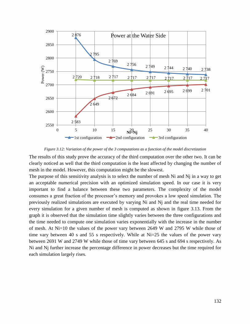
132

Figure 3.12: Variation of the power of the 3 computations as a function of the model discretization

The results of this study prove the accuracy of the third computation over the other two. It can be

clearly noticed as well that the third computation is the least affected by changing the number of

mesh in the model. However, this computation might be the slowest.

The purpose of this sensitivity analysis is to select the number of mesh Ni and Nj in a way to get

an acceptable numerical precision with an optimized simulation speed. In our case it is very

important to find a balance between these two parameters. The complexity of the model

consumes a great fraction of the processor’s memory and provokes a low speed simulation. The

previously realized simulations are executed by varying Ni and Nj and the real time needed for

every simulation for a given number of mesh is computed as shown in figure 3.13. From the

graph it is observed that the simulation time slightly varies between the three configurations and

the time needed to compute one simulation varies exponentially with the increase in the number

of mesh. At Ni=10 the values of the power vary between 2649 W and 2795 W while those of

time vary between 40 s and 55 s respectively. While at Ni=25 the values of the power vary

between 2691 W and 2749 W while those of time vary between 645 s and 694 s respectively. As

Ni and Nj further increase the percentage difference in power decreases but the time required for

each simulation largely rises.

2 876

2 795

2 769 2 756

2 749 2 744 2 740 2 738

2 583

2 649

2 672 2 684

2 691 2 695 2 699 2 701

2 720 2 718 2 717 2 717 2 717 2 717 2 717 2 717

2550

2600

2650

2700

2750

2800

2850

2900

0 5 10 15 20 25 30 35 40

Po

wer

(W

)

Ni=Nj

Power at the Water Side

1st configuration 2nd configuration 3rd configuration

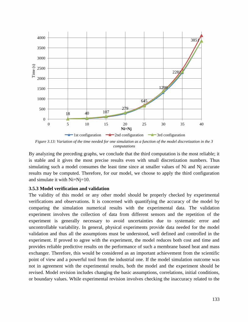
133

Figure 3.13: Variation of the time needed for one simulation as a function of the model discretization in the 3

computations

By analyzing the preceding graphs, we conclude that the third computation is the most reliable; it

is stable and it gives the most precise results even with small discretization numbers. Thus

simulating such a model consumes the least time since at smaller values of Ni and Nj accurate

results may be computed. Therefore, for our model, we choose to apply the third configuration

and simulate it with Ni=Nj=10.

3.5.3 Model verification and validation

The validity of this model or any other model should be properly checked by experimental

verifications and observations. It is concerned with quantifying the accuracy of the model by

comparing the simulation numerical results with the experimental data. The validation

experiment involves the collection of data from different sensors and the repetition of the

experiment is generally necessary to avoid uncertainties due to systematic error and

uncontrollable variability. In general, physical experiments provide data needed for the model

validation and thus all the assumptions must be understood, well defined and controlled in the

experiment. If proved to agree with the experiment, the model reduces both cost and time and

provides reliable predictive results on the performance of such a membrane based heat and mass

exchanger. Therefore, this would be considered as an important achievement from the scientific

point of view and a powerful tool from the industrial one. If the model simulation outcome was

not in agreement with the experimental results, both the model and the experiment should be

revised. Model revision includes changing the basic assumptions, correlations, initial conditions,

or boundary values. While experimental revision involves checking the inaccuracy related to the

18 40 107 279

645

1299

2281

3851

0

500

1000

1500

2000

2500

3000

3500

4000

0 5 10 15 20 25 30 35 40

Tim

e (s

)

Ni=Nj

1st configuration 2nd configuration 3rd configuration

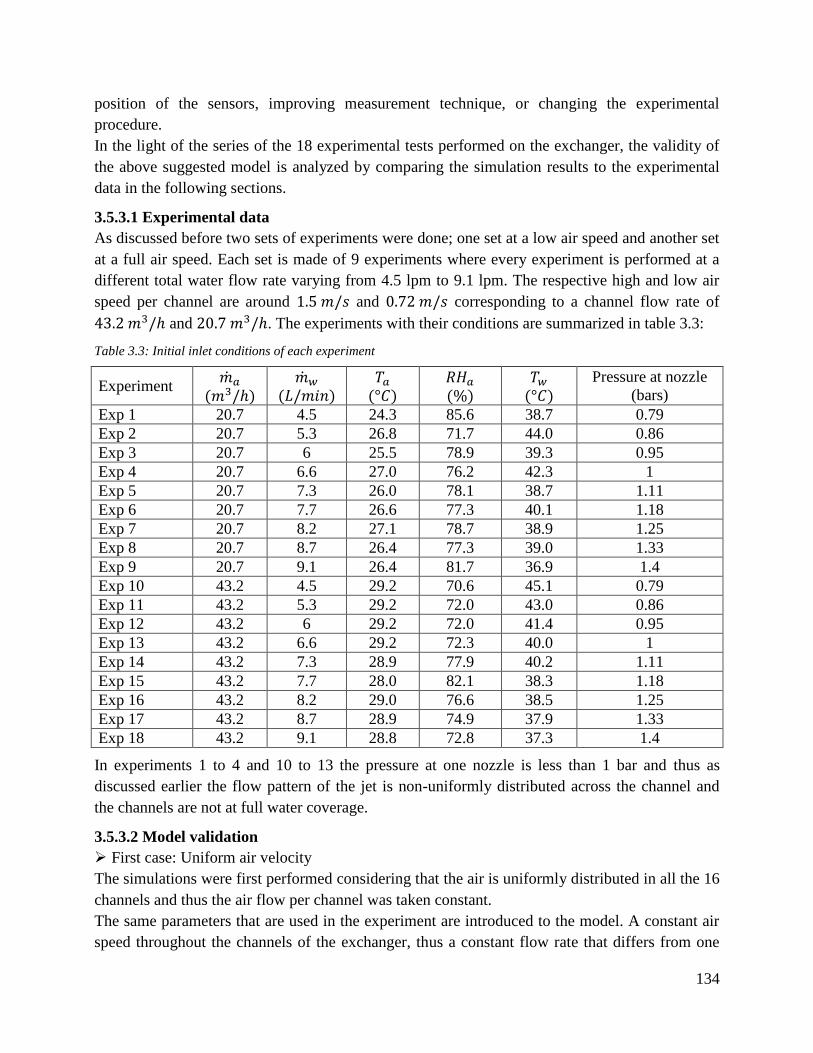
134

position of the sensors, improving measurement technique, or changing the experimental

procedure.

In the light of the series of the 18 experimental tests performed on the exchanger, the validity of

the above suggested model is analyzed by comparing the simulation results to the experimental

data in the following sections.

3.5.3.1 Experimental data

As discussed before two sets of experiments were done; one set at a low air speed and another set

at a full air speed. Each set is made of 9 experiments where every experiment is performed at a

different total water flow rate varying from 4.5 lpm to 9.1 lpm. The respective high and low air

speed per channel are around and corresponding to a channel flow rate of

and . The experiments with their conditions are summarized in table 3.3:

Table 3.3: Initial inlet conditions of each experiment

Experiment

Pressure at nozzle

(bars)

Exp 1 20.7 4.5 24.3 85.6 38.7 0.79

Exp 2 20.7 5.3 26.8 71.7 44.0 0.86

Exp 3 20.7 6 25.5 78.9 39.3 0.95

Exp 4 20.7 6.6 27.0 76.2 42.3 1

Exp 5 20.7 7.3 26.0 78.1 38.7 1.11

Exp 6 20.7 7.7 26.6 77.3 40.1 1.18

Exp 7 20.7 8.2 27.1 78.7 38.9 1.25

Exp 8 20.7 8.7 26.4 77.3 39.0 1.33

Exp 9 20.7 9.1 26.4 81.7 36.9 1.4

Exp 10 43.2 4.5 29.2 70.6 45.1 0.79

Exp 11 43.2 5.3 29.2 72.0 43.0 0.86

Exp 12 43.2 6 29.2 72.0 41.4 0.95

Exp 13 43.2 6.6 29.2 72.3 40.0 1

Exp 14 43.2 7.3 28.9 77.9 40.2 1.11

Exp 15 43.2 7.7 28.0 82.1 38.3 1.18

Exp 16 43.2 8.2 29.0 76.6 38.5 1.25

Exp 17 43.2 8.7 28.9 74.9 37.9 1.33

Exp 18 43.2 9.1 28.8 72.8 37.3 1.4

In experiments 1 to 4 and 10 to 13 the pressure at one nozzle is less than 1 bar and thus as

discussed earlier the flow pattern of the jet is non-uniformly distributed across the channel and

the channels are not at full water coverage.

3.5.3.2 Model validation

First case: Uniform air velocity

The simulations were first performed considering that the air is uniformly distributed in all the 16

channels and thus the air flow per channel was taken constant.

The same parameters that are used in the experiment are introduced to the model. A constant air

speed throughout the channels of the exchanger, thus a constant flow rate that differs from one

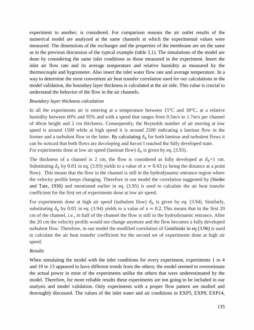
135

experiment to another, is considered. For comparison reasons the air outlet results of the

numerical model are analyzed at the same channels at which the experimental values were

measured. The dimensions of the exchanger and the properties of the membrane are set the same

as in the previous discussion of the typical example (table 3.1). The simulations of the model are

done by considering the same inlet conditions as those measured in the experiment. Insert the

inlet air flow rate and its average temperature and relative humidity as measured by the

thermocouple and hygrometer. Also insert the inlet water flow rate and average temperature. In a

way to determine the most convenient air heat transfer correlation used for our calculations in the

model validation, the boundary layer thickness is calculated at the air side. This value is crucial to

understand the behavior of the flow in the air channels.

Boundary layer thickness calculation

In all the experiments air is entering at a temperature between 15°C and 30°C, at a relative

humidity between 60% and 95% and with a speed that ranges from 0.5m/s to 1.7m/s per channel

of 40cm height and 2 cm thickness. Consequently, the Reynolds number of air moving at low

speed is around 1500 while at high speed it is around 2500 indicating a laminar flow in the

former and a turbulent flow in the latter. By calculating for both laminar and turbulent flows it

can be noticed that both flows are developing and haven’t reached the fully developed state.

For experiments done at low air speed (laminar flow) is given by eq. (3.93).

The thickness of a channel is 2 cm, the flow is considered as fully developed at =1 cm.

Substituting by in eq. (3.93) yields to a value of ( being the distance at a point

flow). This means that the flow in the channel is still in the hydrodynamic entrance region where

the velocity profile keeps changing. Therefore in our model the correlation suggested by (Sieder

and Tate, 1936) and mentioned earlier in eq. (3.95) is used to calculate the air heat transfer

coefficient for the first set of experiments done at low air speed.

For experiments done at high air speed (turbulent flow) is given by eq. (3.94). Similarly,

substituting by in eq. (3.94) yields to a value of This means that in the first 20

cm of the channel, i.e., in half of the channel the flow is still in the hydrodynamic entrance. After

the 20 cm the velocity profile would not change anymore and the flow becomes a fully developed

turbulent flow. Therefore, in our model the modified correlation of Gnielinski in eq (3.96) is used

to calculate the air heat transfer coefficient for the second set of experiments done at high air

speed.

Results

When simulating the model with the inlet conditions for every experiment, experiments 1 to 4

and 10 to 13 appeared to have different trends from the others; the model seemed to overestimate

the actual power in most of the experiments unlike the others that were underestimated by the

model. Therefore, for more reliable results these experiments are not going to be included in our

analysis and model validation. Only experiments with a proper flow pattern are studied and

thoroughly discussed. The values of the inlet water and air conditions in EXP5, EXP8, EXP14,

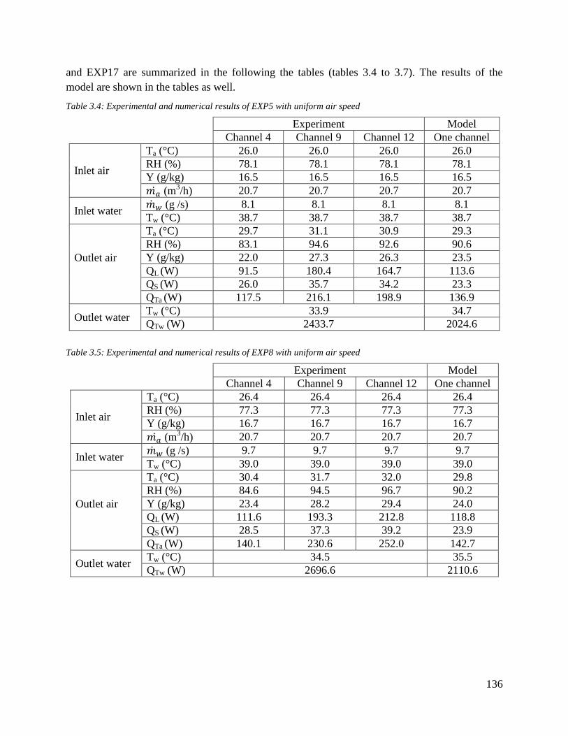
136

and EXP17 are summarized in the following the tables (tables 3.4 to 3.7). The results of the

model are shown in the tables as well.

Table 3.4: Experimental and numerical results of EXP5 with uniform air speed

Experiment Model

Channel 4 Channel 9 Channel 12 One channel

Inlet air

Ta (°C) 26.0 26.0 26.0 26.0 RH (%) 78.1 78.1 78.1 78.1

Y (g/kg) 16.5 16.5 16.5 16.5

(m3/h) 20.7 20.7 20.7 20.7

Inlet water (g /s) 8.1 8.1 8.1 8.1

Tw (°C) 38.7 38.7 38.7 38.7

Outlet air

Ta (°C) 29.7 31.1 30.9 29.3

RH (%) 83.1 94.6 92.6 90.6

Y (g/kg) 22.0 27.3 26.3 23.5

QL (W) 91.5 180.4 164.7 113.6

QS (W) 26.0 35.7 34.2 23.3

QTa (W) 117.5 216.1 198.9 136.9

Outlet water Tw (°C) 33.9 34.7

QTw (W) 2433.7 2024.6

Table 3.5: Experimental and numerical results of EXP8 with uniform air speed

Experiment Model

Channel 4 Channel 9 Channel 12 One channel

Inlet air

Ta (°C) 26.4 26.4 26.4 26.4

RH (%) 77.3 77.3 77.3 77.3

Y (g/kg) 16.7 16.7 16.7 16.7

(m3/h) 20.7 20.7 20.7 20.7

Inlet water (g /s) 9.7 9.7 9.7 9.7

Tw (°C) 39.0 39.0 39.0 39.0

Outlet air

Ta (°C) 30.4 31.7 32.0 29.8

RH (%) 84.6 94.5 96.7 90.2

Y (g/kg) 23.4 28.2 29.4 24.0

QL (W) 111.6 193.3 212.8 118.8

QS (W) 28.5 37.3 39.2 23.9

QTa (W) 140.1 230.6 252.0 142.7

Outlet water Tw (°C) 34.5 35.5

QTw (W) 2696.6 2110.6

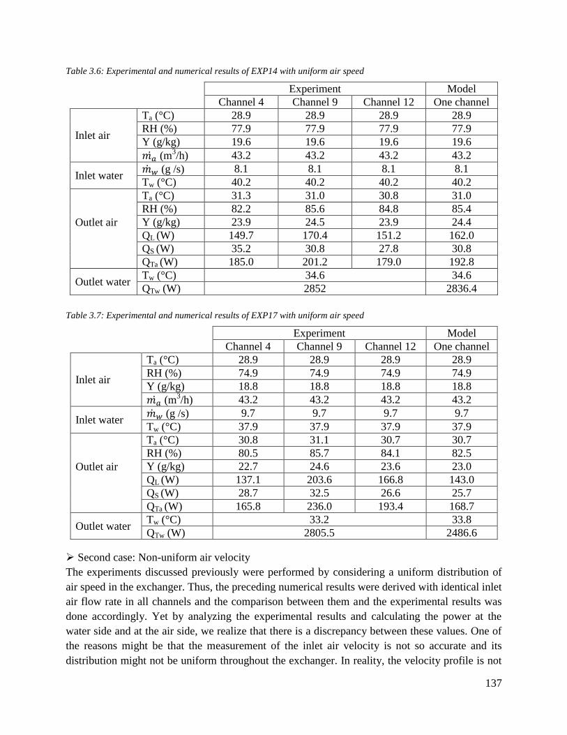
137

Table 3.6: Experimental and numerical results of EXP14 with uniform air speed

Experiment Model

Channel 4 Channel 9 Channel 12 One channel

Inlet air

Ta (°C) 28.9 28.9 28.9 28.9

RH (%) 77.9 77.9 77.9 77.9

Y (g/kg) 19.6 19.6 19.6 19.6

(m3/h) 43.2 43.2 43.2 43.2

Inlet water (g /s) 8.1 8.1 8.1 8.1

Tw (°C) 40.2 40.2 40.2 40.2

Outlet air

Ta (°C) 31.3 31.0 30.8 31.0

RH (%) 82.2 85.6 84.8 85.4

Y (g/kg) 23.9 24.5 23.9 24.4

QL (W) 149.7 170.4 151.2 162.0

QS (W) 35.2 30.8 27.8 30.8

QTa (W) 185.0 201.2 179.0 192.8

Outlet water Tw (°C) 34.6 34.6

QTw (W) 2852 2836.4

Table 3.7: Experimental and numerical results of EXP17 with uniform air speed

Experiment Model

Channel 4 Channel 9 Channel 12 One channel

Inlet air

Ta (°C) 28.9 28.9 28.9 28.9

RH (%) 74.9 74.9 74.9 74.9

Y (g/kg) 18.8 18.8 18.8 18.8

(m3/h) 43.2 43.2 43.2 43.2

Inlet water (g /s) 9.7 9.7 9.7 9.7

Tw (°C) 37.9 37.9 37.9 37.9

Outlet air

Ta (°C) 30.8 31.1 30.7 30.7

RH (%) 80.5 85.7 84.1 82.5

Y (g/kg) 22.7 24.6 23.6 23.0

QL (W) 137.1 203.6 166.8 143.0

QS (W) 28.7 32.5 26.6 25.7

QTa (W) 165.8 236.0 193.4 168.7

Outlet water Tw (°C) 33.2 33.8

QTw (W) 2805.5 2486.6

Second case: Non-uniform air velocity

The experiments discussed previously were performed by considering a uniform distribution of

air speed in the exchanger. Thus, the preceding numerical results were derived with identical inlet

air flow rate in all channels and the comparison between them and the experimental results was

done accordingly. Yet by analyzing the experimental results and calculating the power at the

water side and at the air side, we realize that there is a discrepancy between these values. One of

the reasons might be that the measurement of the inlet air velocity is not so accurate and its

distribution might not be uniform throughout the exchanger. In reality, the velocity profile is not

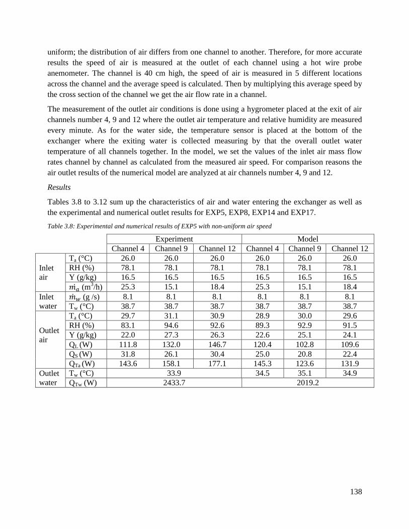
138

uniform; the distribution of air differs from one channel to another. Therefore, for more accurate

results the speed of air is measured at the outlet of each channel using a hot wire probe

anemometer. The channel is 40 cm high, the speed of air is measured in 5 different locations

across the channel and the average speed is calculated. Then by multiplying this average speed by

the cross section of the channel we get the air flow rate in a channel.

The measurement of the outlet air conditions is done using a hygrometer placed at the exit of air

channels number 4, 9 and 12 where the outlet air temperature and relative humidity are measured

every minute. As for the water side, the temperature sensor is placed at the bottom of the

exchanger where the exiting water is collected measuring by that the overall outlet water

temperature of all channels together. In the model, we set the values of the inlet air mass flow

rates channel by channel as calculated from the measured air speed. For comparison reasons the

air outlet results of the numerical model are analyzed at air channels number 4, 9 and 12.

Results

Tables 3.8 to 3.12 sum up the characteristics of air and water entering the exchanger as well as

the experimental and numerical outlet results for EXP5, EXP8, EXP14 and EXP17.

Table 3.8: Experimental and numerical results of EXP5 with non-uniform air speed

Experiment Model

Channel 4 Channel 9 Channel 12 Channel 4 Channel 9 Channel 12

Inlet

air

Ta (°C) 26.0 26.0 26.0 26.0 26.0 26.0

RH (%) 78.1 78.1 78.1 78.1 78.1 78.1

Y (g/kg) 16.5 16.5 16.5 16.5 16.5 16.5

(m3/h) 25.3 15.1 18.4 25.3 15.1 18.4

Inlet

water

(g /s) 8.1 8.1 8.1 8.1 8.1 8.1

Tw (°C) 38.7 38.7 38.7 38.7 38.7 38.7

Outlet

air

Ta (°C) 29.7 31.1 30.9 28.9 30.0 29.6

RH (%) 83.1 94.6 92.6 89.3 92.9 91.5

Y (g/kg) 22.0 27.3 26.3 22.6 25.1 24.1

QL (W) 111.8 132.0 146.7 120.4 102.8 109.6

QS (W) 31.8 26.1 30.4 25.0 20.8 22.4

QTa (W) 143.6 158.1 177.1 145.3 123.6 131.9

Outlet

water

Tw (°C) 33.9 34.5 35.1 34.9

QTw (W) 2433.7 2019.2

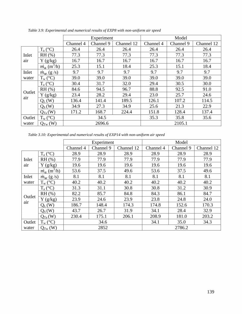
139

Table 3.9: Experimental and numerical results of EXP8 with non-uniform air speed

Experiment Model

Channel 4 Channel 9 Channel 12 Channel 4 Channel 9 Channel 12

Inlet

air

Ta (°C) 26.4 26.4 26.4 26.4 26.4 26.4

RH (%) 77.3 77.3 77.3 77.3 77.3 77.3

Y (g/kg) 16.7 16.7 16.7 16.7 16.7 16.7

(m3/h) 25.3 15.1 18.4 25.3 15.1 18.4

Inlet

water

(g /s) 9.7 9.7 9.7 9.7 9.7 9.7

Tw (°C) 39.0 39.0 39.0 39.0 39.0 39.0

Outlet

air

Ta (°C) 30.4 31.7 32.0 29.4 30.5 30.0

RH (%) 84.6 94.5 96.7 88.8 92.5 91.0

Y (g/kg) 23.4 28.2 29.4 23.0 25.7 24.6

QL (W) 136.4 141.4 189.5 126.1 107.2 114.5

QS (W) 34.9 27.3 34.9 25.6 21.3 22.9

QTa (W) 171.2 168.7 224.4 151.8 128.4 137.4

Outlet

water

Tw (°C) 34.5 35.3 35.8 35.6

QTw (W) 2696.6 2105.1

Table 3.10: Experimental and numerical results of EXP14 with non-uniform air speed

Experiment Model

Channel 4 Channel 9 Channel 12 Channel 4 Channel 9 Channel 12

Inlet

air

Ta (°C) 28.9 28.9 28.9 28.9 28.9 28.9

RH (%) 77.9 77.9 77.9 77.9 77.9 77.9

Y (g/kg) 19.6 19.6 19.6 19.6 19.6 19.6

(m3/h) 53.6 37.5 49.6 53.6 37.5 49.6

Inlet

water

(g /s) 8.1 8.1 8.1 8.1 8.1 8.1

Tw (°C) 40.2 40.2 40.2 40.2 40.2 40.2

Outlet

air

Ta (°C) 31.3 31.1 30.8 30.8 31.2 30.9

RH (%) 82.2 85.7 84.8 84.3 86.1 84.7

Y (g/kg) 23.9 24.6 23.9 23.8 24.8 24.0

QL (W) 186.7 148.4 174.3 174.8 152.6 170.3

QS (W) 43.7 26.7 31.9 34.1 28.4 32.9

QTa (W) 230.4 175.1 206.1 208.9 181.0 203.2

Outlet

water

Tw (°C) 34.6 34.1 35.0 34.3

QTw (W) 2852 2786.2

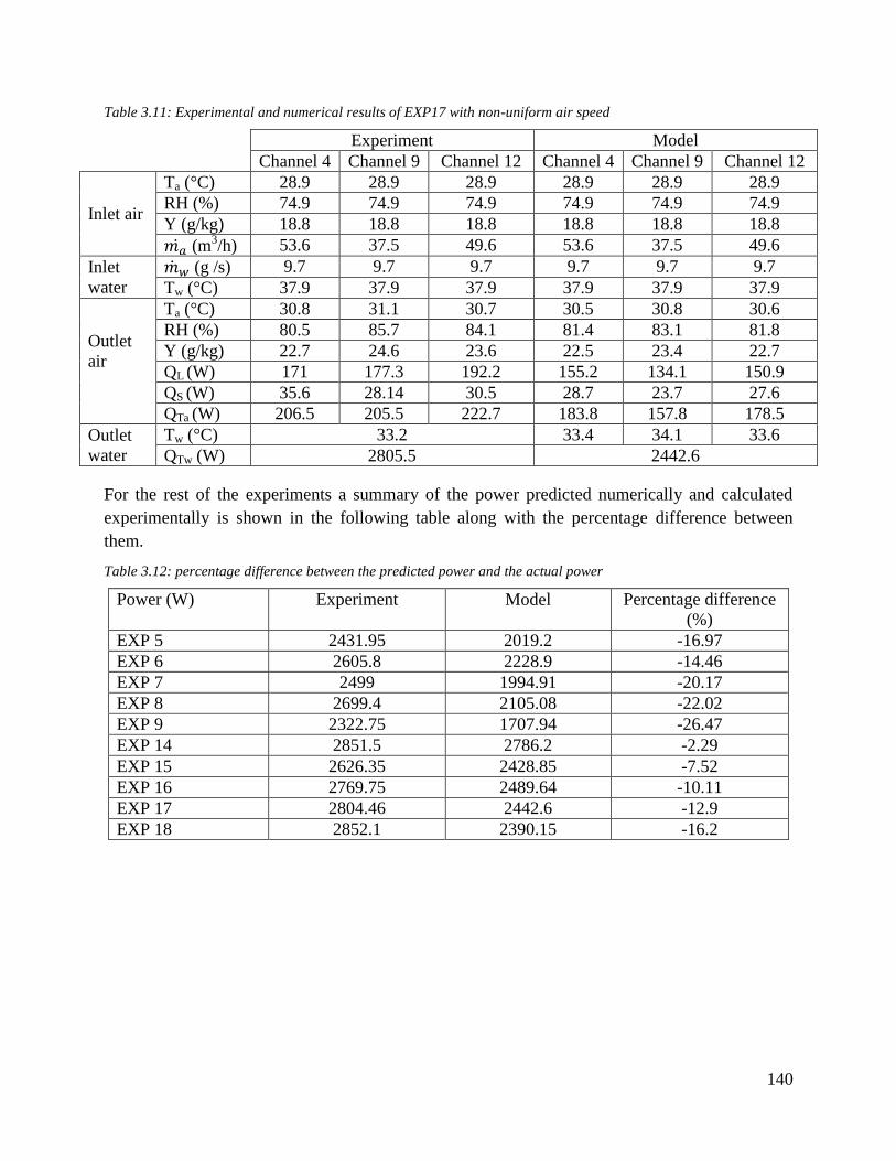
140

Table 3.11: Experimental and numerical results of EXP17 with non-uniform air speed

Experiment Model

Channel 4 Channel 9 Channel 12 Channel 4 Channel 9 Channel 12

Inlet air

Ta (°C) 28.9 28.9 28.9 28.9 28.9 28.9

RH (%) 74.9 74.9 74.9 74.9 74.9 74.9

Y (g/kg) 18.8 18.8 18.8 18.8 18.8 18.8

(m3/h) 53.6 37.5 49.6 53.6 37.5 49.6

Inlet

water

(g /s) 9.7 9.7 9.7 9.7 9.7 9.7

Tw (°C) 37.9 37.9 37.9 37.9 37.9 37.9

Outlet

air

Ta (°C) 30.8 31.1 30.7 30.5 30.8 30.6

RH (%) 80.5 85.7 84.1 81.4 83.1 81.8

Y (g/kg) 22.7 24.6 23.6 22.5 23.4 22.7

QL (W) 171 177.3 192.2 155.2 134.1 150.9

QS (W) 35.6 28.14 30.5 28.7 23.7 27.6

QTa (W) 206.5 205.5 222.7 183.8 157.8 178.5

Outlet

water

Tw (°C) 33.2 33.4 34.1 33.6

QTw (W) 2805.5 2442.6

For the rest of the experiments a summary of the power predicted numerically and calculated

experimentally is shown in the following table along with the percentage difference between

them.

Table 3.12: percentage difference between the predicted power and the actual power

Power (W) Experiment Model Percentage difference

(%)

EXP 5 2431.95 2019.2 -16.97

EXP 6 2605.8 2228.9 -14.46

EXP 7 2499 1994.91 -20.17

EXP 8 2699.4 2105.08 -22.02

EXP 9 2322.75 1707.94 -26.47

EXP 14 2851.5 2786.2 -2.29

EXP 15 2626.35 2428.85 -7.52

EXP 16 2769.75 2489.64 -10.11

EXP 17 2804.46 2442.6 -12.9

EXP 18 2852.1 2390.15 -16.2

141

The following graph in fig. 3.14 shows the distribution of the predicted power versus the

experimental power of all the conducted experiments.

Figure 3.14: Predicted versus experimental power distribution for all experiments

3.5.3.3 Mean Absolute Error (MAE)

To validate the performance and the accuracy of a model qualitatively, some standard methods

that use statistical error tests are generally applied mainly the Mean Absolute Error (MAE) and

the Root Mean Square Error (RMSE). During the evaluation of the model, a lower value of MAE

or RMSE indicates a better performance and improved predicted values. MAE method is adopted

in our study to compare the value predicted by the model to that calculated experimentally. It is

the average of the total sum of the absolute prediction errors between the model and experiment

and is calculated by the following formula (Lee and Jeong, 2019).

(3.108)

where is the actual value from the experiment, is the predicted value by the model,

and is the number of experimental data.

MAE is calculated for the total power of the exchanger such that the predicted and measured

values are the total power simulated by the model and the power calculated experimentally from

the measured data at the water side. Two separate MAE were determined; one for all experiments

done at high air speed and another for those performed at low air speed and the calculated MAE

was 0.098 and 0.199 respectively.

3.5.4 Uncertainty analysis

The uncertainty of the readings taken in our experiments for the measured values of some input

parameters affect the output results. The overall power of the exchanger is determined at the

1600

1700

1800

1900

2000

2100

2200

2300

2400

2500

2600

2700

2800

2900

3000

1600 1700 1800 1900 2000 2100 2200 2300 2400 2500 2600 2700 2800 2900 3000

Num

eric

al P

ow

er (

W)

Experimental Power (W)

Low air speed

High air speed

142

water side by multiplying the water mass flow rate by its specific heat and the difference in

temperature of the inlet and outlet water. At the air side, the power is determined by multiplying

the air mass flow rate by the difference in its enthalpy at the inlet and the outlet. All these

parameters are inferred from our measured values and thus evaluating the accuracy of our

measurements and the quality of our readings is essential to better determine the performance of

our exchanger. Consequently, an uncertainty analysis is performed similar to the one explained

previously in chapter 2. Every measured value is well identified and represented by an input

function and the PDF of every input source is expressed by a typical normal Gaussian

distribution with a mean value and a standard deviation. Later, an uncertainty analysis is done on

the model taking into account the uncertainties on the numerical input sources.

3.5.4.1 Experimental uncertainties

The experimental uncertainties are those related to the input parameters mainly to the

measurements taken at the air and water side.

Measured values

Air speed (m/s)

One measurement uncertainty that affects the results of our simulations is the one related to the

speed of air which directly impacts the air flow rate. The speed of air inside each channel is

measured for 5 times. Thus the PDF of type A uncertainty is represented by the mean of these 5

measurements and the standard deviation due to the repeatability noted by .

A hot wire anemometer is used with a certified uncertainty of ±3% of 0.05m/s for ranges of speed

between 0.15 and 3m/s. Therefore the mean of type B uncertainty is zero and its standard

deviation is 0.03*0.05= 0.015 m/s noted by .

As for the combined uncertainty, the mean is the average value for each channel and the

standard deviation

.

The air speed uncertainties are represented for each channel in table 3.13:

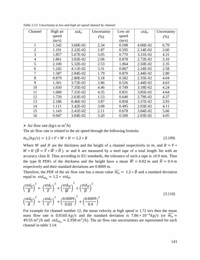
143

Table 3.13: Uncertainty at low and high air speed channel by channel

Channel High air

speed

(m/s)

Uncertainty

(%)

Low air

speed

(m/s)

Uncertainty

(%)

1 1.542 3.60E-02 2.34 0.598 4.06E-02 6.79

2 1.191 2.22E-02 1.87 0.595 2.14E-02 3.60

3 1.857 5.67E-02 3.05 0.770 3.31E-02 4.31

4 1.861 3.83E-02 2.06 0.878 2.72E-02 3.10

5 2.100 5.32E-02 2.53 1.064 2.50E-02 2.35

6 1.242 4.11E-02 3.31 0.867 2.24E-02 2.58

7 1.587 2.84E-02 1.79 0.870 2.44E-02 2.80

8 0.879 2.80E-02 3.18 0.582 2.35E-02 4.04

9 1.301 3.72E-02 2.86 0.526 2.44E-02 4.63

10 1.650 7.35E-02 4.46 0.749 3.18E-02 4.24

11 1.680 7.31E-02 4.35 0.831 3.85E-02 4.64

12 1.720 2.63E-02 1.53 0.640 2.79E-02 4.37

13 2.186 8.46E-02 3.87 0.858 3.37E-02 3.93

14 1.111 3.42E-02 3.08 0.495 2.03E-02 4.11

15 1.143 2.41E-02 2.11 0.678 3.84E-02 5.66

16 0.947 3.04E-02 3.20 0.500 2.03E-02 4.05

Air flow rate (kg/s or m3/h)

The air flow rate is related to the air speed through the following formula:

(3.109)

Where and are the thickness and the height of a channel respectively in , and

( . and are measured by a steel tape of a total length 3m with an

accuracy class Ⅱ. Thus according to EU standards, the tolerance of such a tape is ±0.9 mm. Thus

the type B PDFs of the thickness and the height have a mean and

respectively and their standard deviations are 0.0009 m.

Therefore, the PDF of the air flow rate has a mean value and a standard deviation

equal to .

(3.110)

For example for channel number 12, the mean velocity at high speed is 1.72 m/s then the mean

mass flow rate is and the standard deviation is (or and The air flow rate uncertainties are represented for each

channel in table 3.14:

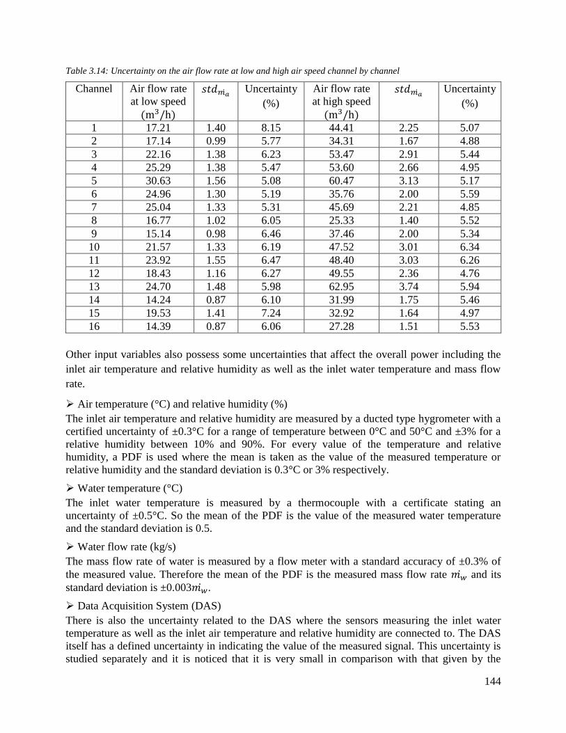
144

Table 3.14: Uncertainty on the air flow rate at low and high air speed channel by channel

Channel Air flow rate

at low speed

Uncertainty

(%)

Air flow rate

at high speed

Uncertainty

(%)

1 17.21 1.40 8.15 44.41 2.25 5.07

2 17.14 0.99 5.77 34.31 1.67 4.88

3 22.16 1.38 6.23 53.47 2.91 5.44

4 25.29 1.38 5.47 53.60 2.66 4.95

5 30.63 1.56 5.08 60.47 3.13 5.17

6 24.96 1.30 5.19 35.76 2.00 5.59

7 25.04 1.33 5.31 45.69 2.21 4.85

8 16.77 1.02 6.05 25.33 1.40 5.52

9 15.14 0.98 6.46 37.46 2.00 5.34

10 21.57 1.33 6.19 47.52 3.01 6.34

11 23.92 1.55 6.47 48.40 3.03 6.26

12 18.43 1.16 6.27 49.55 2.36 4.76

13 24.70 1.48 5.98 62.95 3.74 5.94

14 14.24 0.87 6.10 31.99 1.75 5.46

15 19.53 1.41 7.24 32.92 1.64 4.97

16 14.39 0.87 6.06 27.28 1.51 5.53

Other input variables also possess some uncertainties that affect the overall power including the

inlet air temperature and relative humidity as well as the inlet water temperature and mass flow

rate.

Air temperature (°C) and relative humidity (%)

The inlet air temperature and relative humidity are measured by a ducted type hygrometer with a

certified uncertainty of ±0.3°C for a range of temperature between 0°C and 50°C and ±3% for a

relative humidity between 10% and 90%. For every value of the temperature and relative

humidity, a PDF is used where the mean is taken as the value of the measured temperature or

relative humidity and the standard deviation is 0.3°C or 3% respectively.

Water temperature (°C)

The inlet water temperature is measured by a thermocouple with a certificate stating an

uncertainty of ±0.5°C. So the mean of the PDF is the value of the measured water temperature

and the standard deviation is 0.5.

Water flow rate (kg/s)

The mass flow rate of water is measured by a flow meter with a standard accuracy of ±0.3% of

the measured value. Therefore the mean of the PDF is the measured mass flow rate and its

standard deviation is ±0.003 .

Data Acquisition System (DAS)

There is also the uncertainty related to the DAS where the sensors measuring the inlet water

temperature as well as the inlet air temperature and relative humidity are connected to. The DAS

itself has a defined uncertainty in indicating the value of the measured signal. This uncertainty is

studied separately and it is noticed that it is very small in comparison with that given by the

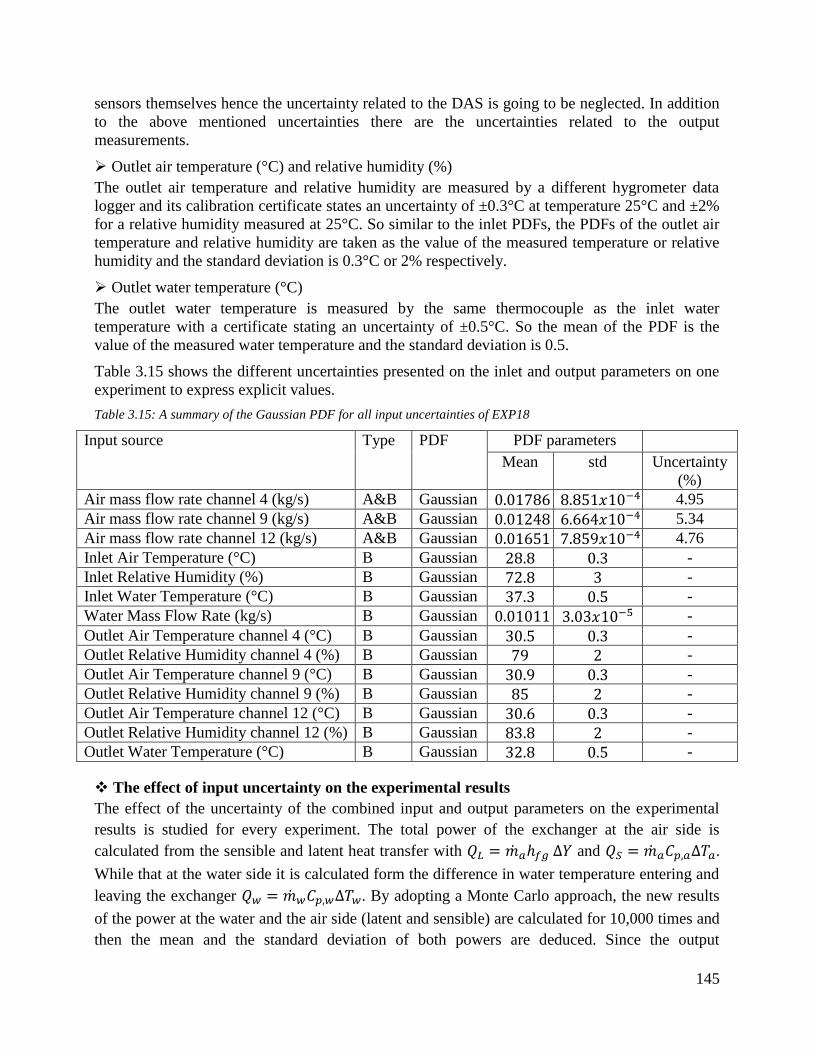
145

sensors themselves hence the uncertainty related to the DAS is going to be neglected. In addition

to the above mentioned uncertainties there are the uncertainties related to the output

measurements.

Outlet air temperature (°C) and relative humidity (%)

The outlet air temperature and relative humidity are measured by a different hygrometer data

logger and its calibration certificate states an uncertainty of ±0.3°C at temperature 25°C and ±2%

for a relative humidity measured at 25°C. So similar to the inlet PDFs, the PDFs of the outlet air

temperature and relative humidity are taken as the value of the measured temperature or relative

humidity and the standard deviation is 0.3°C or 2% respectively.

Outlet water temperature (°C)

The outlet water temperature is measured by the same thermocouple as the inlet water

temperature with a certificate stating an uncertainty of ±0.5°C. So the mean of the PDF is the

value of the measured water temperature and the standard deviation is 0.5.

Table 3.15 shows the different uncertainties presented on the inlet and output parameters on one

experiment to express explicit values.

Table 3.15: A summary of the Gaussian PDF for all input uncertainties of EXP18

Input source Type PDF PDF parameters

Mean std Uncertainty

(%)

Air mass flow rate channel 4 (kg/s) A&B Gaussian 4.95

Air mass flow rate channel 9 (kg/s) A&B Gaussian 5.34

Air mass flow rate channel 12 (kg/s) A&B Gaussian 4.76

Inlet Air Temperature (°C) B Gaussian -

Inlet Relative Humidity (%) B Gaussian -

Inlet Water Temperature (°C) B Gaussian -

Water Mass Flow Rate (kg/s) B Gaussian -

Outlet Air Temperature channel 4 (°C) B Gaussian -

Outlet Relative Humidity channel 4 (%) B Gaussian -

Outlet Air Temperature channel 9 (°C) B Gaussian -

Outlet Relative Humidity channel 9 (%) B Gaussian -

Outlet Air Temperature channel 12 (°C) B Gaussian -

Outlet Relative Humidity channel 12 (%) B Gaussian -

Outlet Water Temperature (°C) B Gaussian -

The effect of input uncertainty on the experimental results

The effect of the uncertainty of the combined input and output parameters on the experimental

results is studied for every experiment. The total power of the exchanger at the air side is

calculated from the sensible and latent heat transfer with and .

While that at the water side it is calculated form the difference in water temperature entering and

leaving the exchanger . By adopting a Monte Carlo approach, the new results

of the power at the water and the air side (latent and sensible) are calculated for 10,000 times and

then the mean and the standard deviation of both powers are deduced. Since the output

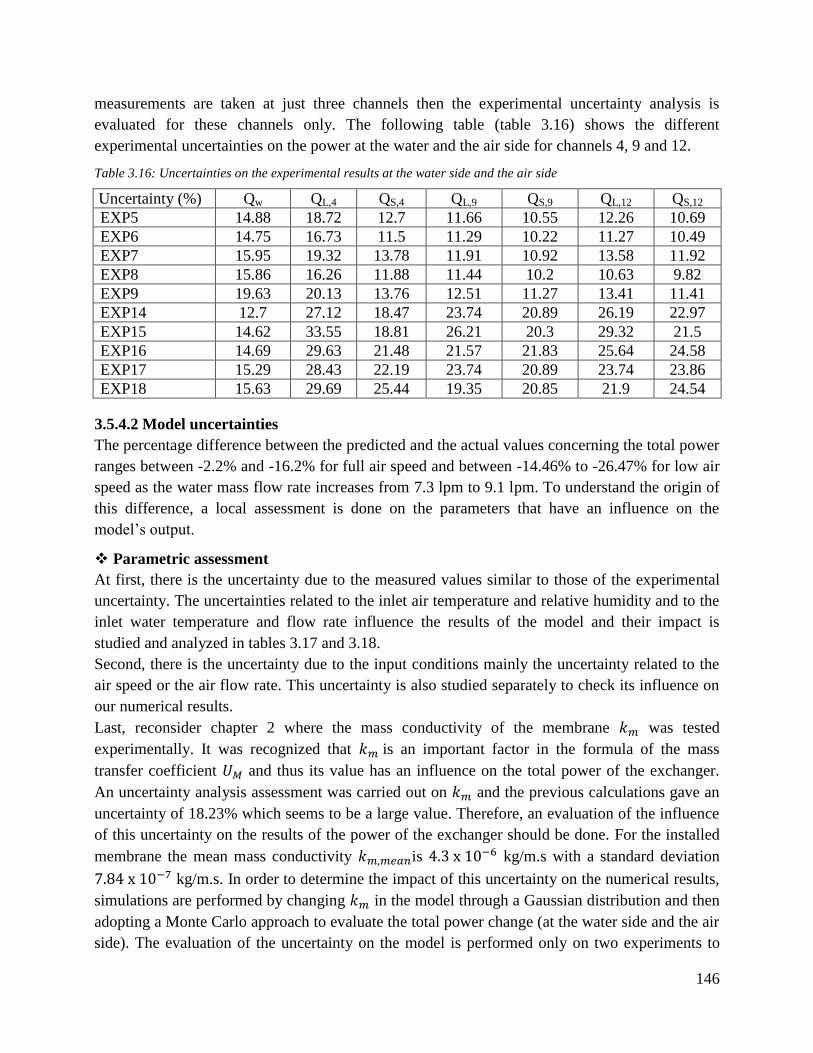
146

measurements are taken at just three channels then the experimental uncertainty analysis is

evaluated for these channels only. The following table (table 3.16) shows the different

experimental uncertainties on the power at the water and the air side for channels 4, 9 and 12.

Table 3.16: Uncertainties on the experimental results at the water side and the air side

Uncertainty (%) Qw QL,4 QS,4 QL,9 QS,9 QL,12 QS,12

EXP5 14.88 18.72 12.7 11.66 10.55 12.26 10.69

EXP6 14.75 16.73 11.5 11.29 10.22 11.27 10.49

EXP7 15.95 19.32 13.78 11.91 10.92 13.58 11.92

EXP8 15.86 16.26 11.88 11.44 10.2 10.63 9.82

EXP9 19.63 20.13 13.76 12.51 11.27 13.41 11.41

EXP14 12.7 27.12 18.47 23.74 20.89 26.19 22.97

EXP15 14.62 33.55 18.81 26.21 20.3 29.32 21.5

EXP16 14.69 29.63 21.48 21.57 21.83 25.64 24.58

EXP17 15.29 28.43 22.19 23.74 20.89 23.74 23.86

EXP18 15.63 29.69 25.44 19.35 20.85 21.9 24.54

3.5.4.2 Model uncertainties

The percentage difference between the predicted and the actual values concerning the total power

ranges between -2.2% and -16.2% for full air speed and between -14.46% to -26.47% for low air

speed as the water mass flow rate increases from 7.3 lpm to 9.1 lpm. To understand the origin of

this difference, a local assessment is done on the parameters that have an influence on the

model’s output.

Parametric assessment

At first, there is the uncertainty due to the measured values similar to those of the experimental

uncertainty. The uncertainties related to the inlet air temperature and relative humidity and to the

inlet water temperature and flow rate influence the results of the model and their impact is

studied and analyzed in tables 3.17 and 3.18.

Second, there is the uncertainty due to the input conditions mainly the uncertainty related to the

air speed or the air flow rate. This uncertainty is also studied separately to check its influence on

our numerical results.

Last, reconsider chapter 2 where the mass conductivity of the membrane was tested

experimentally. It was recognized that is an important factor in the formula of the mass

transfer coefficient and thus its value has an influence on the total power of the exchanger.

An uncertainty analysis assessment was carried out on and the previous calculations gave an

uncertainty of 18.23% which seems to be a large value. Therefore, an evaluation of the influence

of this uncertainty on the results of the power of the exchanger should be done. For the installed

membrane the mean mass conductivity is kg/m.s with a standard deviation

kg/m.s. In order to determine the impact of this uncertainty on the numerical results,

simulations are performed by changing in the model through a Gaussian distribution and then

adopting a Monte Carlo approach to evaluate the total power change (at the water side and the air

side). The evaluation of the uncertainty on the model is performed only on two experiments to

147

have an idea about the order of magnitude of the effect of the different uncertainties on the

numerical forecasted results. These two experiments are EXP9 and EXP18 having a water mass

flow rate of 9.1 lpm at low and high air speed respectively. They were chosen to be thoroughly

studied because as seen previously these two experiments possess the highest percentage

difference between the model predictions and the experimental results when comparing the total

power given by the exchanger.

All the input parameters of EXP9 and EXP18 are represented by their Gaussian PDF’s in the

following tables. The uncertainty on the air mass flow rate for every channel was mentioned

earlier in table 3.14 for the experiments performed at low and high air speed and thus in the

following tables (tables 3.17 and 3.18) it is only indicated for one channel.

Table 3.17: A summary of the Gaussian PDF for all input uncertainties of EXP9

Input source Type PDF PDF parameters

Mean std Uncertainty

(%)

Membrane Mass conductivity (kg/m.s) A Gaussian 18.23

Air mass flow rate channel 1 (m3/h) A&B Gaussian 17.21 1.40 8.15

Air Inlet Temperature (°C) B Gaussian

Inlet Relative Humidity (%) B Gaussian

Water Temperature (°C) B Gaussian

Water Mass Flow Rate (kg/s) B Gaussian 0.3

Table 3.18: A summary of the Gaussian PDF for all input uncertainties of EXP18

Input source Type PDF PDF parameters

Mean std Uncertainty

(%)

Membrane Mass conductivity (kg/m.s) A Gaussian 18.23

Air mass flow rate channel 1 (m3/h) A&B Gaussian 44.41 2.25 5.07

Air Inlet Temperature (°C) B Gaussian

Inlet Relative Humidity (%) B Gaussian

Water Temperature (°C) B Gaussian

Water Mass Flow Rate (kg/s) B Gaussian 0.3

Effect of input uncertainty on the numerical results

The effects of the uncertainty of the measured values, of the input conditions and of on the

total power of the exchanger as predicted by the model are analyzed separately in tables 3.19 and

3.20.

At first, we introduce the PDF’s of the measured values in the model through Python and run the

simulations in Dymola for 10,000 times. Each simulation computes a value of the total load at the

water side as well as the latent and sensible loads for channels 4, 9 and 12.

Then, we keep the measured values constant and change the air mass flow rate according to its

deduced PDF and repeat the same procedure. Finally, we set the measured values and the input

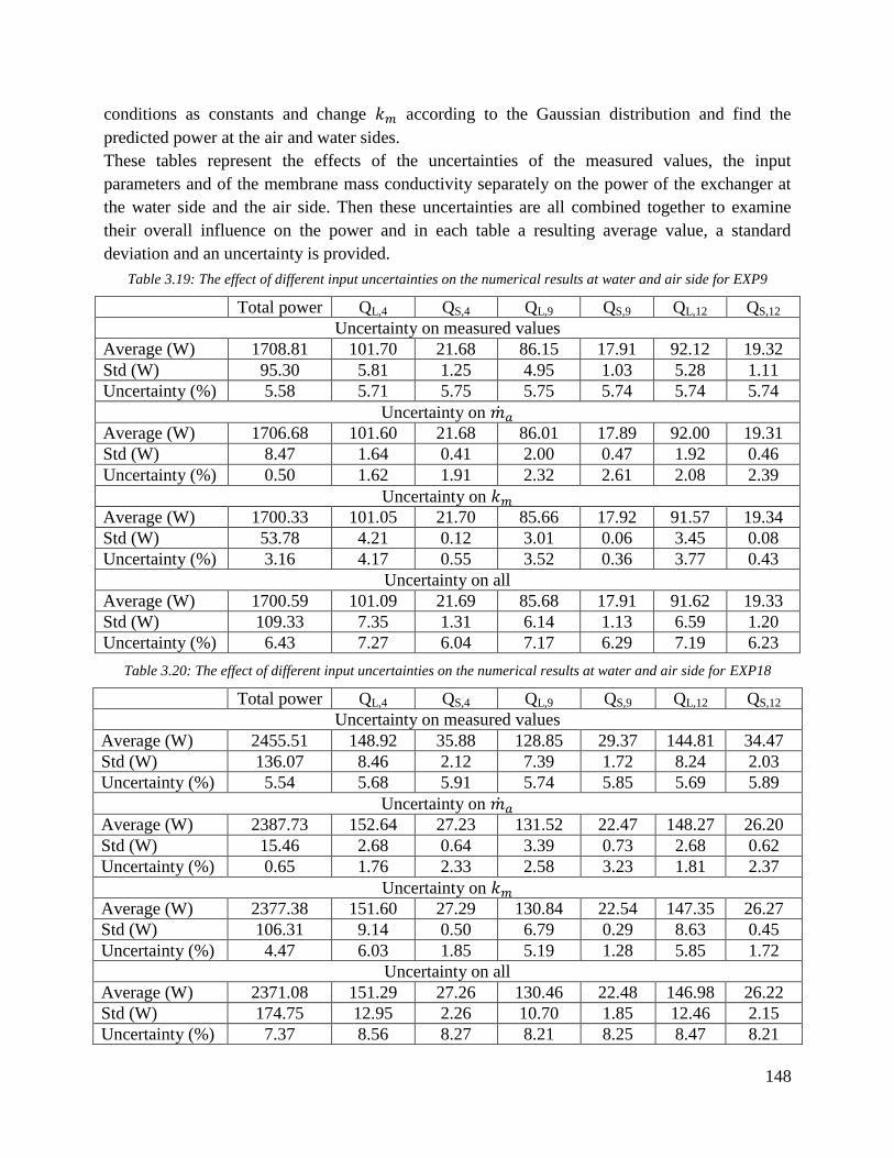
148

conditions as constants and change according to the Gaussian distribution and find the

predicted power at the air and water sides.

These tables represent the effects of the uncertainties of the measured values, the input

parameters and of the membrane mass conductivity separately on the power of the exchanger at

the water side and the air side. Then these uncertainties are all combined together to examine

their overall influence on the power and in each table a resulting average value, a standard

deviation and an uncertainty is provided.

Table 3.19: The effect of different input uncertainties on the numerical results at water and air side for EXP9

Total power QL,4 QS,4 QL,9 QS,9 QL,12 QS,12

Uncertainty on measured values

Average (W) 1708.81 101.70 21.68 86.15 17.91 92.12 19.32

Std (W) 95.30 5.81 1.25 4.95 1.03 5.28 1.11

Uncertainty (%) 5.58 5.71 5.75 5.75 5.74 5.74 5.74

Uncertainty on

Average (W) 1706.68 101.60 21.68 86.01 17.89 92.00 19.31

Std (W) 8.47 1.64 0.41 2.00 0.47 1.92 0.46

Uncertainty (%) 0.50 1.62 1.91 2.32 2.61 2.08 2.39

Uncertainty on

Average (W) 1700.33 101.05 21.70 85.66 17.92 91.57 19.34

Std (W) 53.78 4.21 0.12 3.01 0.06 3.45 0.08

Uncertainty (%) 3.16 4.17 0.55 3.52 0.36 3.77 0.43

Uncertainty on all

Average (W) 1700.59 101.09 21.69 85.68 17.91 91.62 19.33

Std (W) 109.33 7.35 1.31 6.14 1.13 6.59 1.20

Uncertainty (%) 6.43 7.27 6.04 7.17 6.29 7.19 6.23

Table 3.20: The effect of different input uncertainties on the numerical results at water and air side for EXP18

Total power QL,4 QS,4 QL,9 QS,9 QL,12 QS,12

Uncertainty on measured values

Average (W) 2455.51 148.92 35.88 128.85 29.37 144.81 34.47

Std (W) 136.07 8.46 2.12 7.39 1.72 8.24 2.03

Uncertainty (%) 5.54 5.68 5.91 5.74 5.85 5.69 5.89

Uncertainty on

Average (W) 2387.73 152.64 27.23 131.52 22.47 148.27 26.20

Std (W) 15.46 2.68 0.64 3.39 0.73 2.68 0.62

Uncertainty (%) 0.65 1.76 2.33 2.58 3.23 1.81 2.37

Uncertainty on

Average (W) 2377.38 151.60 27.29 130.84 22.54 147.35 26.27

Std (W) 106.31 9.14 0.50 6.79 0.29 8.63 0.45

Uncertainty (%) 4.47 6.03 1.85 5.19 1.28 5.85 1.72

Uncertainty on all

Average (W) 2371.08 151.29 27.26 130.46 22.48 146.98 26.22

Std (W) 174.75 12.95 2.26 10.70 1.85 12.46 2.15

Uncertainty (%) 7.37 8.56 8.27 8.21 8.25 8.47 8.21

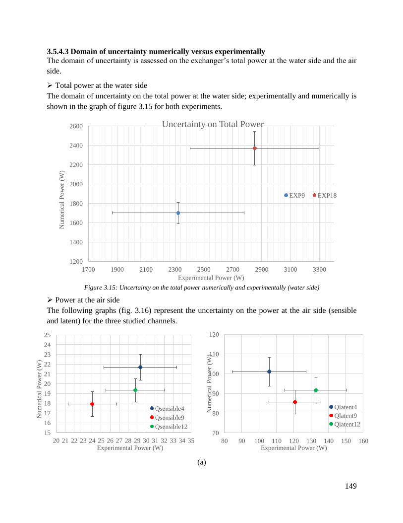
149

3.5.4.3 Domain of uncertainty numerically versus experimentally

The domain of uncertainty is assessed on the exchanger’s total power at the water side and the air

side.

Total power at the water side

The domain of uncertainty on the total power at the water side; experimentally and numerically is

shown in the graph of figure 3.15 for both experiments.

Figure 3.15: Uncertainty on the total power numerically and experimentally (water side)

Power at the air side

The following graphs (fig. 3.16) represent the uncertainty on the power at the air side (sensible

and latent) for the three studied channels.

(a)

1200

1400

1600

1800

2000

2200

2400

2600

1700 1900 2100 2300 2500 2700 2900 3100 3300

Num

eric

al P

ow

er (

W)

Experimental Power (W)

Uncertainty on Total Power

EXP9 EXP18

15

16

17

18

19

20

21

22

23

24

25

20 21 22 23 24 25 26 27 28 29 30 31 32 33 34 35

Num

eric

al P

ow

er (

W)

Experimental Power (W)

Qsensible4

Qsensible9

Qsensible12 70

80

90

100

110

120

80 90 100 110 120 130 140 150 160

Num

eric

al P

ow

er (

W)

Experimental Power (W)

Qlatent4

Qlatent9

Qlatent12

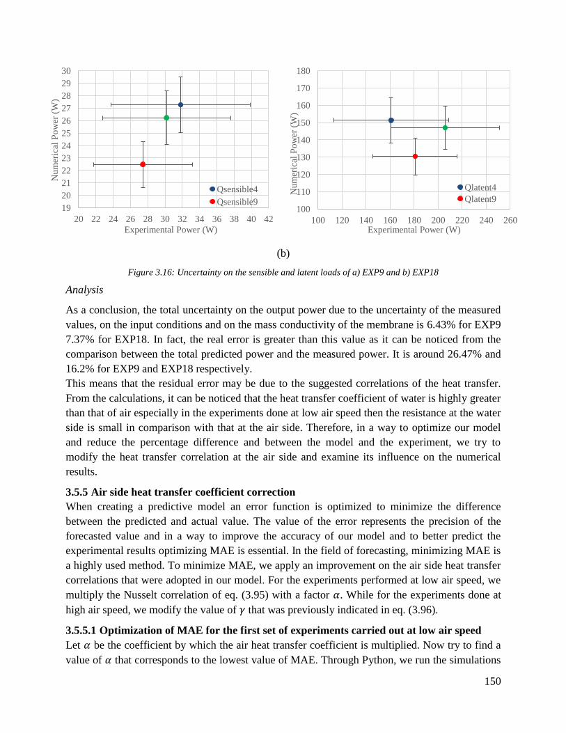
150

(b)

Figure 3.16: Uncertainty on the sensible and latent loads of a) EXP9 and b) EXP18

Analysis

As a conclusion, the total uncertainty on the output power due to the uncertainty of the measured

values, on the input conditions and on the mass conductivity of the membrane is 6.43% for EXP9

7.37% for EXP18. In fact, the real error is greater than this value as it can be noticed from the

comparison between the total predicted power and the measured power. It is around 26.47% and

16.2% for EXP9 and EXP18 respectively.

This means that the residual error may be due to the suggested correlations of the heat transfer.

From the calculations, it can be noticed that the heat transfer coefficient of water is highly greater

than that of air especially in the experiments done at low air speed then the resistance at the water

side is small in comparison with that at the air side. Therefore, in a way to optimize our model

and reduce the percentage difference and between the model and the experiment, we try to

modify the heat transfer correlation at the air side and examine its influence on the numerical

results.

3.5.5 Air side heat transfer coefficient correction

When creating a predictive model an error function is optimized to minimize the difference

between the predicted and actual value. The value of the error represents the precision of the

forecasted value and in a way to improve the accuracy of our model and to better predict the

experimental results optimizing MAE is essential. In the field of forecasting, minimizing MAE is

a highly used method. To minimize MAE, we apply an improvement on the air side heat transfer

correlations that were adopted in our model. For the experiments performed at low air speed, we

multiply the Nusselt correlation of eq. (3.95) with a factor . While for the experiments done at

high air speed, we modify the value of that was previously indicated in eq. (3.96).

3.5.5.1 Optimization of MAE for the first set of experiments carried out at low air speed

Let be the coefficient by which the air heat transfer coefficient is multiplied. Now try to find a

value of that corresponds to the lowest value of MAE. Through Python, we run the simulations

19

20

21

22

23

24

25

26

27

28

29

30

20 22 24 26 28 30 32 34 36 38 40 42

Num

eric

al P

ow

er (

W)

Experimental Power (W)

Qsensible4

Qsensible9 100

110

120

130

140

150

160

170

180

100 120 140 160 180 200 220 240 260

Num

eric

al P

ow

er (

W)

Experimental Power (W)

Qlatent4

Qlatent9

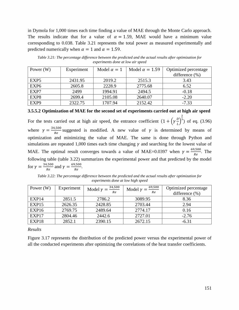
151

in Dymola for 1,000 times each time finding a value of MAE through the Monte Carlo approach.

The results indicate that for a value of .59, MAE would have a minimum value

corresponding to 0.038. Table 3.21 represents the total power as measured experimentally and

predicted numerically when and .

Table 3.21: The percentage difference between the predicted and the actual results after optimization for

experiments done at low air speed

Power (W) Experiment Model Model Optimized percentage

difference (%)

EXP5 2431.95 2019.2 2515.3 3.43

EXP6 2605.8 2228.9 2775.68 6.52

EXP7 2499 1994.91 2494.5 -0.18

EXP8 2699.4 2105.08 2640.07 -2.20

EXP9 2322.75 1707.94 2152.42 -7.33

3.5.5.2 Optimization of MAE for the second set of experiments carried out at high air speed

For the tests carried out at high air speed, the entrance coefficient

of eq. (3.96)

where

suggested is modified. A new value of is determined by means of

optimization and minimizing the value of MAE. The same is done through Python and

simulations are repeated 1,000 times each time changing and searching for the lowest value of

MAE. The optimal result converges towards a value of MAE=0.0397 when

. The

following table (table 3.22) summarizes the experimental power and that predicted by the model

for

and

.

Table 3.22: The percentage difference between the predicted and the actual results after optimization for

experiments done at low high speed

Power (W) Experiment Model

Model

Optimized percentage

difference (%)

EXP14 2851.5 2786.2 3089.95 8.36

EXP15 2626.35 2428.85 2703.44 2.94

EXP16 2769.75 2489.64 2774.17 0.16

EXP17 2804.46 2442.6 2727.01 -2.76

EXP18 2852.1 2390.15 2672.15 -6.31

Results

Figure 3.17 represents the distribution of the predicted power versus the experimental power of

all the conducted experiments after optimizing the correlations of the heat transfer coefficients.

152

Figure 3.17: Predicted versus experimental power distribution for all experiments after optimization

For a detailed comparison at the air side as well, EXP9 and EXP18 are studied. Table 3.23

summarizes the outlet air and water conditions as measured experimentally and numerically for

and in EXP9 while table 3.24 summarizes them for

and

in

EXP18.

Table 3.23: Detailed comparison of the numerical results before and after optimization for EXP9

Experiment Model Model

Ch 4 Ch 9 Ch 12 Ch 4 Ch 9 Ch 12 Ch 4 Ch 9 Ch 12

Inlet

air

Ta (°C) 26.4 26.4 26.4 26.4 26.4 26.4 26.4 26.4 26.4

RH (%) 81.7 81.7 81.7 81.7 81.7 81.7 81.7 81.7 81.7

Y (g/kg) 17.6 17.6 17.6 17.6 17.6 17.6 17.6 17.6 17.6

(g/s) 8.4 5.1 6.0 8.4 5.1 6.0 8.4 5.1 6.0

Inlet

water

(g /s) 10.1 10.1 10.1 10.1 10.1 10.1 10.1 10.1 10.1

Tw (°C) 36.9 36.9 36.9 36.9 36.9 36.9 36.9 36.9 36.9

Outlet

air

Ta (°C) 29.7 30.9 30.9 28.9 29.9 29.5 29.7 30.9 30.5

RH (%) 86.4 96.5 93.6 90.4 93.3 92.1 90.5 93.4 92.3

Y (g/kg) 22.9 27.6 26.6 22.9 25.0 24.1 24.0 26.7 25.6

QL (W) 105.8 120.6 132.7 103.2 87.6 93.6 126.4 107.1 114.6

QS (W) 29.4 24.0 28.8 22.0 18.2 19.6 28.9 23.6 25.6

QTa (W) 135.2 144.6 161.5 125.2 105.8 113.2 155.3 130.7 140.2

Outlet

water

Tw (°C) 33.2 34.0 34.4 34.2 33.3 33.8 33.6

QTw (W) 2322.8 1734.6 2152.4

2300

2400

2500

2600

2700

2800

2900

3000

3100

2300 2400 2500 2600 2700 2800 2900 3000 3100

Num

eric

al P

ow

er (

W)

Experimental Power (W)

Low air speed

High air speed

153

Table 3.24: Detailed comparison of the numerical results before and after optimization for EXP18

Experiment Model Model

Ch 4 Ch 9 Ch 12 Ch 4 Ch 9 Ch 12 Ch 4 Ch 9 Ch 12

Inlet

air

Ta (°C) 28.8 28.8 28.8 28.8 28.8 28.8 28.8 28.8 28.8

RH (%) 72.8 72.8 72.8 72.8 72.8 72.8 72.8 72.8 72.8

Y (g/kg) 18.1 18.1 18.1 18.1 18.1 18.1 18.1 18.1 18.1

(g/s) 17.9 12.5 16.5 17.9 12.5 16.5 17.9 12.5 16.5

Inlet

water

(g /s) 10.1 10.1 10.1 10.1 10.1 10.1 10.1 10.1 10.1

Tw (°C) 36.9 36.9 36.9 36.9 36.9 36.9 36.9 36.9 36.9

Outlet

air

Ta (°C) 30.5 30.9 30.6 30.3 30.6 30.4 30.5 30.9 30.6

RH (%) 79 .04 85.0 83.8 79.7 81.4 80.1 80.0 81.9 80.4

Y (g/kg) 21.9 24.1 23.3 21.8 22.6 22.0 22.1 23.2 22.4

QL (W) 160.8 180.8 205.8 152.7 131.7 148.4 167.2 147.6 163.3

QS (W) 31.8 27.4 30.2 27.2 22.5 26.2 31.0 26.2 30.0

QTa (W) 192.6 208.3 235.9 179.9 154.2 174.6 198.2 173.9 193.3

Outlet

water

Tw (°C) 32.8 33.1 33.7 33.2 32.7 33.2 32.8

QTw (W) 2852.1 2390.2 2672.2

3.6 Conclusion

In this chapter, a numerical model of the novel exchanger is developed and a prototype is built

and tested. The tests performed with water demonstrated the feasibility of the new design and

allowed to determine its performance. Measured data were also used to validate and tune the

numerical model.

As a conclusion, the percentage difference between the power predicted by the model and that

calculated experimentally, is at its maximum values of 26.47% for EXP9 and 16.2% for EXP18.

Among this difference, the intrinsic uncertainties constitute around 6 to 7% of the total

uncertainty. In a way to reduce this difference, we proposed a modification of the correlations

related to the heat transfer coefficient at the air side (being the most influencing on the overall

heat transfer coefficient) and we solved for an optimized value of MAE. The results indicate that

after the optimization the percentage difference was reduced to 7.33% for EXP9 and 6.3% for

EXP18. Moreover, the difference between the numerical and experimental outcomes concerning

the air temperature and absolute humidity are also acceptable. Thus the suggested model can be

considered as a credible and predictive tool that might be applicable to determine the

performance of a similar membrane based heat and mass exchanger. Yet, the performed

experiments are insufficient to generalize this conclusion for all possible scenarios and hence

more experiments should be carried out to validate the model and prove its accuracy for several

other cases. In further steps, some parameters might be changed such as expanding the range of

the water flow rate where the upper limit is affected by the power of the resistor as mentioned

before and the lower limit is influenced by the range of the working pressure of the nozzles.

Moreover, other design parameters can be changed such as the number of channels or the width

of a channel of the exchanger. For more accurate measurements, other experiments can be done

154

with more precise sensors or with the presence of an outlet air duct to obtain better readings on

the air side. Finally, the prototype should be operated with a desiccant solution instead of water to

check its operation with the salt.

In the following chapter, the validated model is used to build a hybrid system model and study its

performance in an air conditioning application.

155

156

Chapitre 4 Étude de Cas : Une Conception Flexible d'un

Système de Climatisation Hybride dans un Bureau

(résumé)

4.1 Introduction

Dans les bâtiments, la climatisation est principalement assurée par des systèmes de compression

de vapeur avec un nombre croissant d’unités de climatisation installées, comme indiqué au

chapitre 1. Pourtant, ces systèmes sont inefficaces pour contrôler l'humidité à l'intérieur des

bâtiments. D'autres systèmes, tels que les systèmes hybrides, ont été étudiés dans le but

d'améliorer la performance énergétique en intégrant les échangeurs membranaires de chaleur et

de masse dans les systèmes traditionnels de climatisation. Ces systèmes hybrides ont gagné un

intérêt croissant en raison de leur refroidissement efficace en contrôlant séparément les charges

latentes et sensibles, et donc de leur consommation réduite d'électricité. Toutefois, la

performance de ces systèmes dépend radicalement des conditions opératoires dans lesquelles le

rapport entre la charge latente et la charge sensible à l'intérieur du bâtiment change en

conséquence, comme indiqué au chapitre 1. Ainsi, dans les applications où un rapport de charge

latente-sensible non constant est requis, ces systèmes font preuve d'un manque de flexibilité.

Dans ce cas, il pourrait être possible d'utiliser la configuration du système hybride citée dans les

recherches de Bergero et Chiari (Bergero et Chiari, 2011) qui offre une performance très efficace

sur une gamme des conditions opératoires en fonction du rapport entre la charge latente et la

charge sensible mais cette gamme reste insuffisante.

Dans ce chapitre, un système hybride est utilisé pour effectuer la climatisation saisonnière d'un

bureau dans un immeuble du sud de la France. Ce système est composé d'un cycle de desiccant

liquide et d’un cycle de compression de vapeur. Le modèle précédemment suggéré et validé dans

le chapitre 4 est utilisé pour évaluer la performance des échangeurs de chaleur et de masse du

cycle du desiccant. Le présent chapitre a pour but d'analyser le comportement des différentes

architectures en régime permanent et de comparer leur performance par une simulation

saisonnière d'un bureau situé à Nice (43,3°N, 5,4°E). Plusieurs architectures sont proposées et

les résultats sont comparés à ceux d'un cycle de compression de vapeur classique. Ce chapitre

décrit chaque composant du cycle de compression de vapeur ainsi que ses équations de

modélisation. Ensuite, un modèle complet est utilisé pour évaluer la performance de chaque

architecture du système hybride dans les différents mois de l'année où le refroidissement est

nécessaire. Les conclusions de ce chapitre donneraient un aperçu de la contribution des systèmes

hybrides à la réduction du coût de l'énergie lorsqu'ils sont convenablement appliqués dans les

bâtiments.

4.2 Description du bâtiment

Le bureau est situé au troisième étage dans un immeuble de 5 étages à Nice d’un climat

méditerranéen : les températures étant élevées en été et modérées au printemps et en automne.

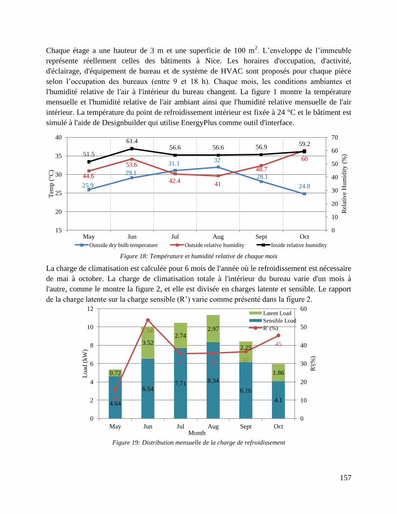
157

Chaque étage a une hauteur de 3 m et une superficie de 100 m2. L’enveloppe de l’immeuble

représente réellement celles des bâtiments à Nice. Les horaires d'occupation, d'activité,

d'éclairage, d'équipement de bureau et de système de HVAC sont proposés pour chaque pièce

selon l’occupation des bureaux (entre 9 et 18 h). Chaque mois, les conditions ambiantes et

l'humidité relative de l'air à l'intérieur du bureau changent. La figure 1 montre la température

mensuelle et l'humidité relative de l'air ambiant ainsi que l'humidité relative mensuelle de l'air

intérieur. La température du point de refroidissement intérieur est fixée à 24 °C et le bâtiment est

simulé à l'aide de Designbuilder qui utilise EnergyPlus comme outil d'interface.

Figure 18: Température et humidité relative de chaque mois

La charge de climatisation est calculée pour 6 mois de l'année où le refroidissement est nécessaire

de mai à octobre. La charge de climatisation totale à l'intérieur du bureau varie d'un mois à

l'autre, comme le montre la figure 2, et elle est divisée en charges latente et sensible. Le rapport

de la charge latente sur la charge sensible (R’) varie comme présenté dans la figure 2.

Figure 19: Distribution mensuelle de la charge de refroidissement

25.9

29.1

31.1 32

28.1

24.8

44.6

53.6

42.4 41

48.7

60 51.5

61.4 56.6 56.6 56.9

59.2

0

10

20

30

40

50

60

70

15

20

25

30

35

40

May Jun Jul Aug Sept Oct

Rel

ativ

e H

um

idit

y (

%)

Tem

p (

°C)

Outside dry bulb temperature Outside relative humidity Inside relative humidity

4.64

6.54 7.71 8.34

6.16

4.1

0.72

3.52 2.74

2.97

2.25

1.86

16

54

36 36 37

45

0

10

20

30

40

50

60

0

2

4

6

8

10

12

May Jun Jul Aug Sept Oct

R'(

%)

Lo

ad (

kW

)

Month

Latent Load

Sensible Load

R' (%)

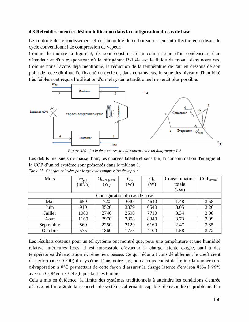
158

4.3 Refroidissement et déshumidification dans la configuration du cas de base

Le contrôle du refroidissement et de l'humidité de ce bureau est en fait effectué en utilisant le

cycle conventionnel de compression de vapeur.

Comme le montre la figure 3, ils sont constitués d'un compresseur, d'un condenseur, d'un

détendeur et d'un évaporateur où le réfrigérant R-134a est le fluide de travail dans notre cas.

Comme nous l'avons déjà mentionné, la réduction de la température de l'air en dessous de son

point de rosée diminue l'efficacité du cycle et, dans certains cas, lorsque des niveaux d'humidité

très faibles sont requis l’utilisation d'un tel système traditionnel ne serait plus possible.

Figure 320: Cycle de compression de vapeur avec un diagramme T-S

Les débits mensuels de masse d’air, les charges latente et sensible, la consommation d'énergie et

la COP d’un tel système sont présentés dans le tableau 1.

Table 25: Charges enlevées par le cycle de compression de vapeur

Mois (m

3/h)

QL, required

(W)

QL

(W)

QS

(W)

Consommation

totale

(kW)

COPoverall

Configuration du cas de base

Mai 650 720 640 4640 1.48 3.58

Juin 910 3520 3379 6540 3.05 3.26

Juillet 1080 2740 2590 7710 3.34 3.08

Aout 1160 2970 2808 8340 3.73 2.99

Septembre 860 2250 2129 6160 2.47 3.35

Octobre 575 1860 1775 4100 1.58 3.72

Les résultats obtenus pour un tel système ont montré que, pour une température et une humidité

relative intérieures fixes, il est impossible d’évacuer la charge latente exigée, sauf à des

températures d'évaporation extrêmement basses. Ce qui réduirait considérablement le coefficient

de performance (COP) du système. Dans notre cas, nous avons choisi de limiter la température

d'évaporation à 0°C permettant de cette façon d’assurer la charge latente d'environ 88% à 96%

avec un COP entre 3 et 3,6 pendant les 6 mois.

Cela a mis en évidence la limite des systèmes traditionnels à atteindre les conditions d'entrée

désirées et l’intérêt de la recherche de systèmes alternatifs capables de résoudre ce problème. Par

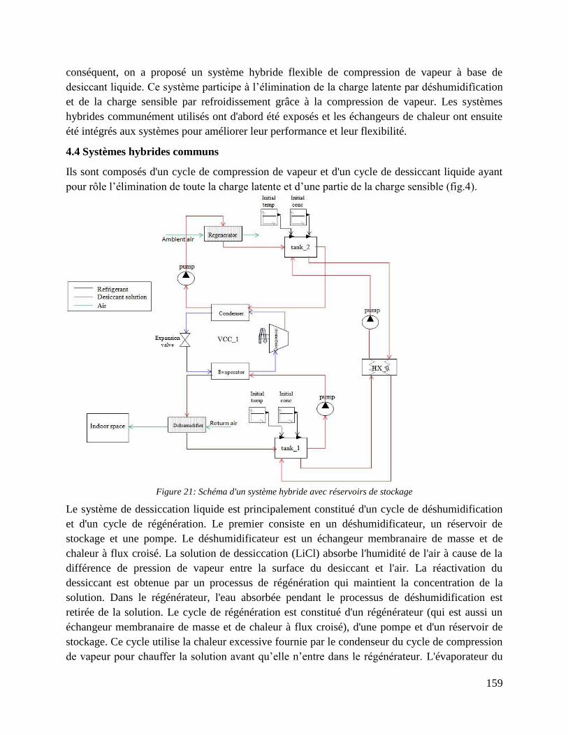
159

conséquent, on a proposé un système hybride flexible de compression de vapeur à base de

desiccant liquide. Ce système participe à l’élimination de la charge latente par déshumidification

et de la charge sensible par refroidissement grâce à la compression de vapeur. Les systèmes

hybrides communément utilisés ont d'abord été exposés et les échangeurs de chaleur ont ensuite

été intégrés aux systèmes pour améliorer leur performance et leur flexibilité.

4.4 Systèmes hybrides communs

Ils sont composés d'un cycle de compression de vapeur et d'un cycle de dessiccant liquide ayant

pour rôle l’élimination de toute la charge latente et d’une partie de la charge sensible (fig.4).

Figure 21: Schéma d'un système hybride avec réservoirs de stockage

Le système de dessiccation liquide est principalement constitué d'un cycle de déshumidification

et d'un cycle de régénération. Le premier consiste en un déshumidificateur, un réservoir de

stockage et une pompe. Le déshumidificateur est un échangeur membranaire de masse et de

chaleur à flux croisé. La solution de dessiccation (LiCl) absorbe l'humidité de l'air à cause de la

différence de pression de vapeur entre la surface du desiccant et l'air. La réactivation du

dessiccant est obtenue par un processus de régénération qui maintient la concentration de la

solution. Dans le régénérateur, l'eau absorbée pendant le processus de déshumidification est

retirée de la solution. Le cycle de régénération est constitué d'un régénérateur (qui est aussi un

échangeur membranaire de masse et de chaleur à flux croisé), d'une pompe et d'un réservoir de

stockage. Ce cycle utilise la chaleur excessive fournie par le condenseur du cycle de compression

de vapeur pour chauffer la solution avant qu’elle n’entre dans le régénérateur. L'évaporateur du

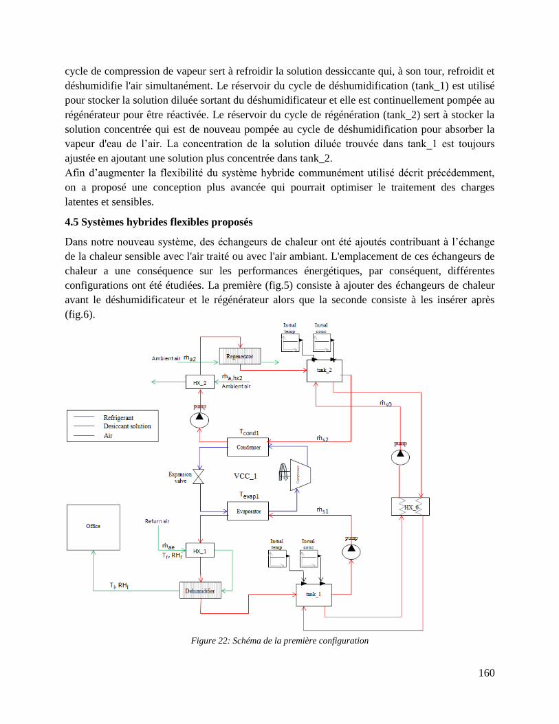
160

cycle de compression de vapeur sert à refroidir la solution dessiccante qui, à son tour, refroidit et

déshumidifie l'air simultanément. Le réservoir du cycle de déshumidification (tank_1) est utilisé

pour stocker la solution diluée sortant du déshumidificateur et elle est continuellement pompée au

régénérateur pour être réactivée. Le réservoir du cycle de régénération (tank_2) sert à stocker la

solution concentrée qui est de nouveau pompée au cycle de déshumidification pour absorber la

vapeur d'eau de l’air. La concentration de la solution diluée trouvée dans tank_1 est toujours

ajustée en ajoutant une solution plus concentrée dans tank_2.

Afin d’augmenter la flexibilité du système hybride communément utilisé décrit précédemment,

on a proposé une conception plus avancée qui pourrait optimiser le traitement des charges

latentes et sensibles.

4.5 Systèmes hybrides flexibles proposés

Dans notre nouveau système, des échangeurs de chaleur ont été ajoutés contribuant à l’échange

de la chaleur sensible avec l'air traité ou avec l'air ambiant. L'emplacement de ces échangeurs de

chaleur a une conséquence sur les performances énergétiques, par conséquent, différentes

configurations ont été étudiées. La première (fig.5) consiste à ajouter des échangeurs de chaleur

avant le déshumidificateur et le régénérateur alors que la seconde consiste à les insérer après

(fig.6).

Figure 22: Schéma de la première configuration

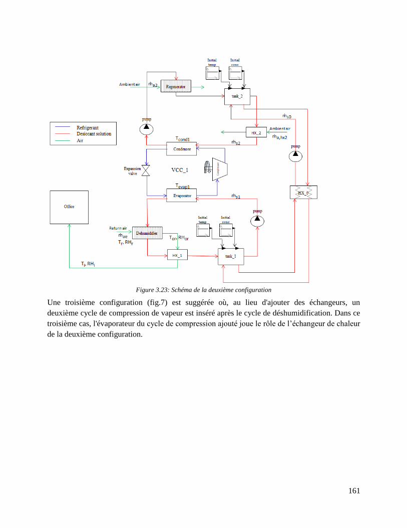
161

Figure 3.23: Schéma de la deuxième configuration

Une troisième configuration (fig.7) est suggérée où, au lieu d'ajouter des échangeurs, un

deuxième cycle de compression de vapeur est inséré après le cycle de déshumidification. Dans ce

troisième cas, l'évaporateur du cycle de compression ajouté joue le rôle de l’échangeur de chaleur

de la deuxième configuration.

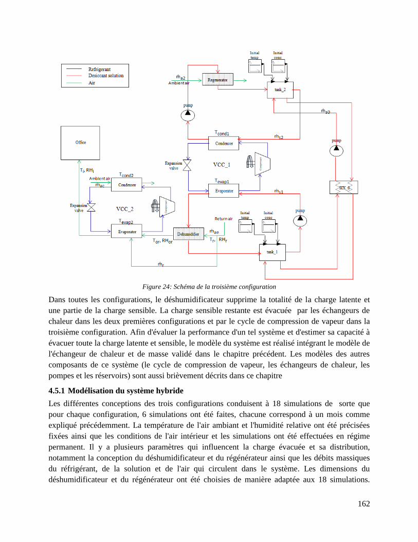
162

Figure 24: Schéma de la troisième configuration

Dans toutes les configurations, le déshumidificateur supprime la totalité de la charge latente et

une partie de la charge sensible. La charge sensible restante est évacuée par les échangeurs de

chaleur dans les deux premières configurations et par le cycle de compression de vapeur dans la

troisième configuration. Afin d'évaluer la performance d'un tel système et d'estimer sa capacité à

évacuer toute la charge latente et sensible, le modèle du système est réalisé intégrant le modèle de

l'échangeur de chaleur et de masse validé dans le chapitre précédent. Les modèles des autres

composants de ce système (le cycle de compression de vapeur, les échangeurs de chaleur, les

pompes et les réservoirs) sont aussi brièvement décrits dans ce chapitre

4.5.1 Modélisation du système hybride

Les différentes conceptions des trois configurations conduisent à 18 simulations de sorte que

pour chaque configuration, 6 simulations ont été faites, chacune correspond à un mois comme

expliqué précédemment. La température de l'air ambiant et l'humidité relative ont été précisées

fixées ainsi que les conditions de l'air intérieur et les simulations ont été effectuées en régime

permanent. Il y a plusieurs paramètres qui influencent la charge évacuée et sa distribution,

notamment la conception du déshumidificateur et du régénérateur ainsi que les débits massiques

du réfrigérant, de la solution et de l'air qui circulent dans le système. Les dimensions du

déshumidificateur et du régénérateur ont été choisies de manière adaptée aux 18 simulations.

163

Nous avons fait le choix d’utiliser la même géométrie pour l’ensemble des configurations, vu que

l'objectif de cette étude est de montrer la flexibilité relative de chaque conception et le domaine

dans lequel son application est la plus efficace. Ces dimensions sont présentées dans le tableau 1.

Tableau 6: Dimensions du déshumidificateur et des régénérateurs dans toutes les configurations

Nombre de canaux L Z

Régénérateur 20 0.4 0.4

déshumidificateur 48 0.5 0.5

4.6 Résultats

Étant donné que le système est complexe avec plusieurs éléments reliés entre eux, des

simulations ont été effectuées par le biais d'un logiciel externe, Python. Les simulations ont été

réalisées pour chacun des 6 mois des trois configurations et 10 000 itérations ont été opérées. À

chaque itération, les paramètres d'entrée qui influent directement ou indirectement les grandeurs

d’interêt ont été modifiées jusqu'à ce que les charges mensuelles latentes et sensibles soient

totalement retirées du bureau. Parmi les 10 000 résultats obtenus, de nombreuses valeurs ne

répondaient pas aux charges sensibles et latentes requises, alors que le reste présente une solution

pour notre système proposé. Pour chaque solution acceptable, le COP du système a été calculé,

les résultats ont été ordonnés et la combinaison des sources d’entrée correspondant au COP le

plus élevé a été choisi.

Le tableau 2 récapitule pour les trois configurations, les valeurs optimales des paramètres d'entrée

qui donnent le COP le plus élevé. Il donne également les résultats de sortie, y compris les

charges, la consommation d'énergie et le COP. Les conditions de l’air d’alimentation sont

également indiquées.

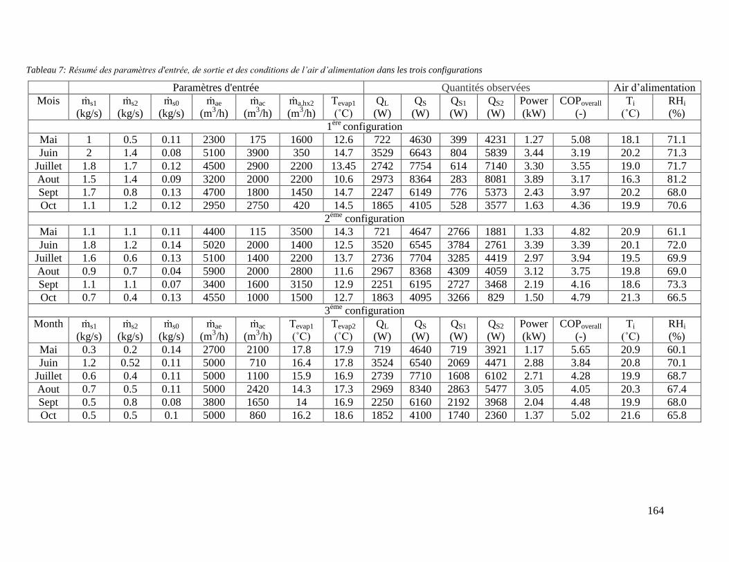
164

Tableau 7: Résumé des paramètres d'entrée, de sortie et des conditions de l’air d’alimentation dans les trois configurations

Paramètres d'entrée Quantités observées Air d’alimentation

Mois ṁs1

(kg/s)

ṁs2

(kg/s)

ṁs0

(kg/s)

ṁae

(m3/h)

ṁac

(m3/h)

ṁa,hx2

(m3/h)

Tevap1

(˚C)

QL

(W)

QS

(W)

QS1

(W)

QS2

(W)

Power

(kW)

COPoverall

(-)

Ti

(˚C)

RHi

(%)

1ère

configuration

Mai 1 0.5 0.11 2300 175 1600 12.6 722 4630 399 4231 1.27 5.08 18.1 71.1

Juin 2 1.4 0.08 5100 3900 350 14.7 3529 6643 804 5839 3.44 3.19 20.2 71.3

Juillet 1.8 1.7 0.12 4500 2900 2200 13.45 2742 7754 614 7140 3.30 3.55 19.0 71.7

Aout 1.5 1.4 0.09 3200 2000 2200 10.6 2973 8364 283 8081 3.89 3.17 16.3 81.2

Sept 1.7 0.8 0.13 4700 1800 1450 14.7 2247 6149 776 5373 2.43 3.97 20.2 68.0

Oct 1.1 1.2 0.12 2950 2750 420 14.5 1865 4105 528 3577 1.63 4.36 19.9 70.6

2ème

configuration

Mai 1.1 1.1 0.11 4400 115 3500 14.3 721 4647 2766 1881 1.33 4.82 20.9 61.1

Juin 1.8 1.2 0.14 5020 2000 1400 12.5 3520 6545 3784 2761 3.39 3.39 20.1 72.0

Juillet 1.6 0.6 0.13 5100 1400 2200 13.7 2736 7704 3285 4419 2.97 3.94 19.5 69.9

Aout 0.9 0.7 0.04 5900 2000 2800 11.6 2967 8368 4309 4059 3.12 3.75 19.8 69.0

Sept 1.1 1.1 0.07 3400 1600 3150 12.9 2251 6195 2727 3468 2.19 4.16 18.6 73.3

Oct 0.7 0.4 0.13 4550 1000 1500 12.7 1863 4095 3266 829 1.50 4.79 21.3 66.5

3ème

configuration

Month ṁs1

(kg/s)

ṁs2

(kg/s)

ṁs0

(kg/s)

ṁae

(m3/h)

ṁac

(m3/h)

Tevap1

(˚C)

Tevap2

(˚C)

QL

(W)

QS

(W)

QS1

(W)

QS2

(W)

Power

(kW)

COPoverall

(-)

Ti

(˚C)

RHi

(%)

Mai 0.3 0.2 0.14 2700 2100 17.8 17.9 719 4640 719 3921 1.17 5.65 20.9 60.1

Juin 1.2 0.52 0.11 5000 710 16.4 17.8 3524 6540 2069 4471 2.88 3.84 20.8 70.1

Juillet 0.6 0.4 0.11 5000 1100 15.9 16.9 2739 7710 1608 6102 2.71 4.28 19.9 68.7

Aout 0.7 0.5 0.11 5000 2420 14.3 17.3 2969 8340 2863 5477 3.05 4.05 20.3 67.4

Sept 0.5 0.8 0.08 3800 1650 14 16.9 2250 6160 2192 3968 2.04 4.48 19.9 68.0

Oct 0.5 0.5 0.1 5000 860 16.2 18.6 1852 4100 1740 2360 1.37 5.02 21.6 65.8

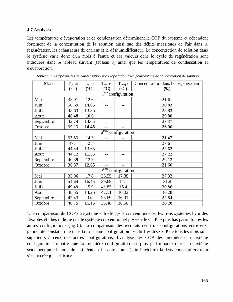
165

4.7 Analyses

Les températures d'évaporation et de condensation déterminent le COP du système et dépendent

fortement de la concentration de la solution ainsi que des débits massiques de l'air dans le

régénérateur, les échangeurs de chaleur et le déshumidificateur. La concentration de solution dans

le système varie donc d'un mois à l'autre et ses valeurs dans le cycle de régénération sont

indiquées dans le tableau suivant (tableau 3) ainsi que les températures de condensation et

d'évaporation.

Tableau 8: Températures de condensation et d'évaporation avec pourcentage de concentration de solution

Mois Tcond1

(°C)

Tevap1

(°C)

Tcond2

(°C)

Tevap2

(°C)

Concentration dans le régénérateur

(%)

1ère

configuration

Mai 35.01 12.6 -- -- 21.61

Juin 50.69 14.65 -- -- 30.83

Juillet 45.63 13.35 28.83

Aout 48.48 10.6 29.80

Septembre 43.74 14.65 -- -- 27.37

Octobre 39.13 14.45 -- -- 26.00

2ème

configuration

Mai 33.83 14.3 -- -- 21.47

Juin 47.1 12.5 27.61

Juillet 44.44 13.65 27.62

Aout 44.12 11.55 -- -- 27.22

Septembre 40.39 12.9 -- -- 26.12

Octobre 36.87 12.65 -- -- 21.60

3ème

configuration

Mai 33.06 17.8 36.55 17.88 27.32

Juin 54.64 16.45 39.68 17.1 31.8

Juillet 49.49 15.9 41.83 16.4 30.86

Aout 48.55 14.25 42.51 16.02 30.28

Septembre 42.43 14 38.69 16.91 27.84

Octobre 40.75 16.15 35.48 18.56 26.28

Une comparaison du COP du système entre le cycle conventionnel et les trois systèmes hybrides

flexibles étudiés indique que le système conventionnel possède le COP le plus bas parmi toutes les

autres configurations (fig 8). La comparaison des résultats des trois configurations entre eux,

permet de constater que dans la troisième configuration les chiffres des COP de tous les mois sont

supérieurs à ceux des autres configurations. L'analyse des COP des première et deuxième

configurations montre que la première configuration est plus performante que la deuxième

seulement pour le mois de mai. Pendant les autres mois (juin à octobre), la deuxième configuration

s'est avérée plus efficace.

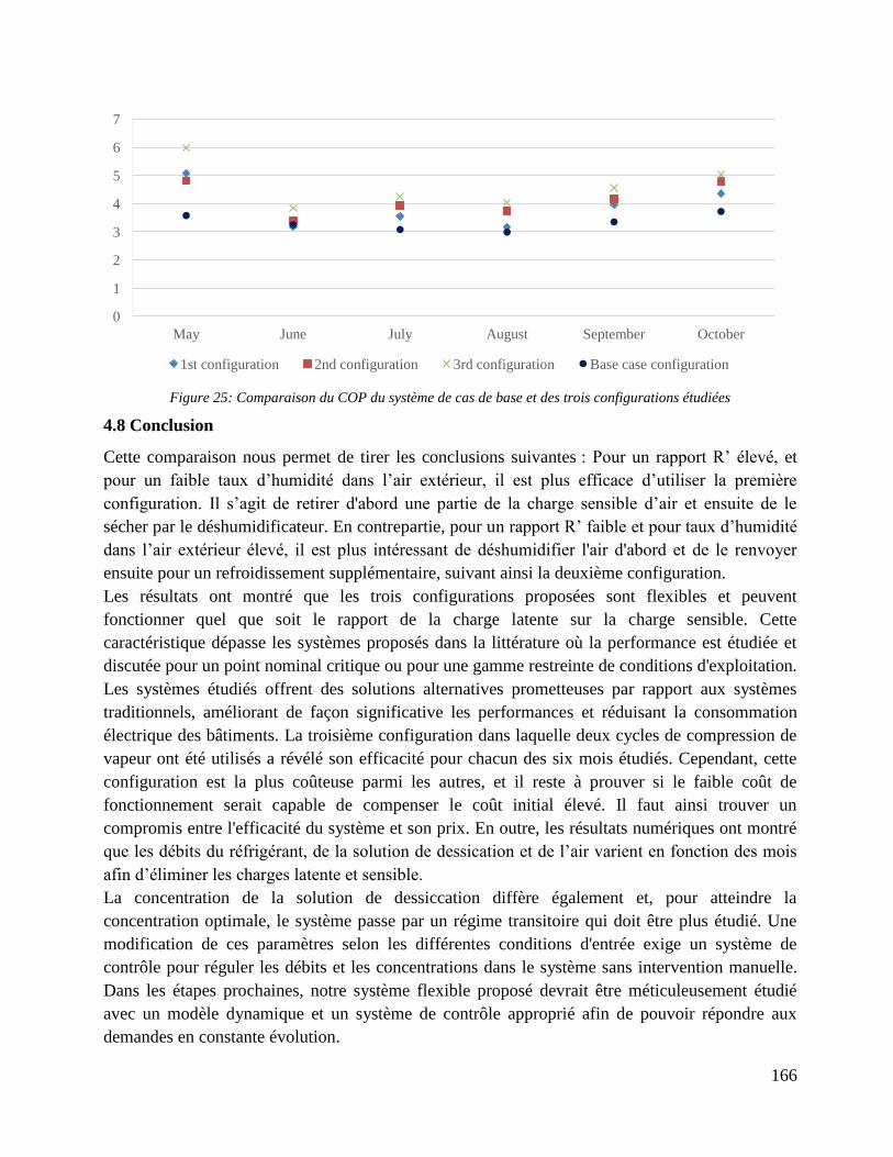
166

Figure 25: Comparaison du COP du système de cas de base et des trois configurations étudiées

4.8 Conclusion

Cette comparaison nous permet de tirer les conclusions suivantes : Pour un rapport R’ élevé, et

pour un faible taux d’humidité dans l’air extérieur, il est plus efficace d’utiliser la première

configuration. Il s’agit de retirer d'abord une partie de la charge sensible d’air et ensuite de le

sécher par le déshumidificateur. En contrepartie, pour un rapport R’ faible et pour taux d’humidité

dans l’air extérieur élevé, il est plus intéressant de déshumidifier l'air d'abord et de le renvoyer

ensuite pour un refroidissement supplémentaire, suivant ainsi la deuxième configuration.

Les résultats ont montré que les trois configurations proposées sont flexibles et peuvent

fonctionner quel que soit le rapport de la charge latente sur la charge sensible. Cette

caractéristique dépasse les systèmes proposés dans la littérature où la performance est étudiée et

discutée pour un point nominal critique ou pour une gamme restreinte de conditions d'exploitation.

Les systèmes étudiés offrent des solutions alternatives prometteuses par rapport aux systèmes

traditionnels, améliorant de façon significative les performances et réduisant la consommation

électrique des bâtiments. La troisième configuration dans laquelle deux cycles de compression de

vapeur ont été utilisés a révélé son efficacité pour chacun des six mois étudiés. Cependant, cette

configuration est la plus coûteuse parmi les autres, et il reste à prouver si le faible coût de

fonctionnement serait capable de compenser le coût initial élevé. Il faut ainsi trouver un

compromis entre l'efficacité du système et son prix. En outre, les résultats numériques ont montré

que les débits du réfrigérant, de la solution de dessication et de l’air varient en fonction des mois

afin d’éliminer les charges latente et sensible.

La concentration de la solution de dessiccation diffère également et, pour atteindre la

concentration optimale, le système passe par un régime transitoire qui doit être plus étudié. Une

modification de ces paramètres selon les différentes conditions d'entrée exige un système de

contrôle pour réguler les débits et les concentrations dans le système sans intervention manuelle.

Dans les étapes prochaines, notre système flexible proposé devrait être méticuleusement étudié

avec un modèle dynamique et un système de contrôle approprié afin de pouvoir répondre aux

demandes en constante évolution.

0

1

2

3

4

5

6

7

May June July August September October

1st configuration 2nd configuration 3rd configuration Base case configuration

167

168

Chapter 4 Case Study: Flexible Design of a Hybrid Air

Conditioning System in an Office

4.1 Introduction

Air conditioning in buildings is mostly performed using vapor compression systems with an

increasing amount of installed AC units as mentioned in chapter 1. Yet these systems waste

energy when it comes to humidity control inside buildings. Alternative systems, such as hybrid

systems, have been studied with the aim of improving the energy performance consisting of the

integration of membrane based heat and mass exchangers within the traditional air conditioning

systems. These hybrid systems have gained an increasing interest due to their efficient cooling

through controlling latent and sensible loads separately and thus their reduced electricity

consumption. In addition, they have shown a great competence in maintaining thermal comfort

with proper indoor air quality. However, the performance of these systems radically depends on

the outside operating conditions where the ratio of latent to sensible load inside the building

changes accordingly as presented in the state of the art in chapter 1. Thus in applications where a

non-constant latent to sensible load ratio is required these systems show a lack of flexibility. In

this case it might be feasible to use the configuration of the hybrid system cited earlier in the

research of Bergero and Chiari (Bergero and Chiari, 2011) that offers a highly efficient

performance over a range of operating conditions depending on the ratio of the latent to sensible

load.

In this chapter a hybrid system, including the novel design of membrane exchanger studied in

chapter 3, is assessed. This system is considered to perform the seasonal air conditioning of an

office in a mid-rise building in Nice in the south of France. The main objective of this case study

is to understand the flexibility issues in these hybrid systems. Accordingly, several architectures of

such a hybrid system are proposed and the results are compared to that of a conventional vapor

compression cycle. This chapter describes each component of the vapor compression cycle along

with its modeling equations. The model validated in chapter 3 is used to assess the performance of

the heat and mass exchangers of the liquid desiccant system. Then a complete model is used to

assess the performance of each architecture of the hybrid system in the different months of the

year where cooling is required. The findings of this chapter would provide insight about the

contribution of hybrid systems in reducing the energy cost when cleverly implemented in

buildings.

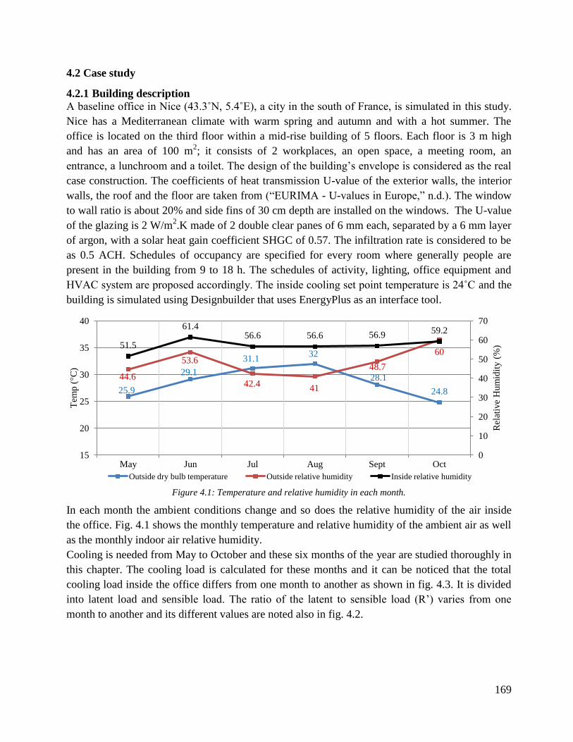
169

4.2 Case study

4.2.1 Building description

A baseline office in Nice (43.3˚N, 5.4˚E), a city in the south of France, is simulated in this study.

Nice has a Mediterranean climate with warm spring and autumn and with a hot summer. The

office is located on the third floor within a mid-rise building of 5 floors. Each floor is 3 m high

and has an area of 100 m2; it consists of 2 workplaces, an open space, a meeting room, an

entrance, a lunchroom and a toilet. The design of the building’s envelope is considered as the real

case construction. The coefficients of heat transmission U-value of the exterior walls, the interior

walls, the roof and the floor are taken from (“EURIMA - U-values in Europe,” n.d.). The window

to wall ratio is about 20% and side fins of 30 cm depth are installed on the windows. The U-value

of the glazing is 2 W/m2.K made of 2 double clear panes of 6 mm each, separated by a 6 mm layer

of argon, with a solar heat gain coefficient SHGC of 0.57. The infiltration rate is considered to be

as 0.5 ACH. Schedules of occupancy are specified for every room where generally people are

present in the building from 9 to 18 h. The schedules of activity, lighting, office equipment and

HVAC system are proposed accordingly. The inside cooling set point temperature is 24˚C and the

building is simulated using Designbuilder that uses EnergyPlus as an interface tool.

Figure 4.1: Temperature and relative humidity in each month.

In each month the ambient conditions change and so does the relative humidity of the air inside

the office. Fig. 4.1 shows the monthly temperature and relative humidity of the ambient air as well

as the monthly indoor air relative humidity.

Cooling is needed from May to October and these six months of the year are studied thoroughly in

this chapter. The cooling load is calculated for these months and it can be noticed that the total

cooling load inside the office differs from one month to another as shown in fig. 4.3. It is divided

into latent load and sensible load. The ratio of the latent to sensible load (R’) varies from one

month to another and its different values are noted also in fig. 4.2.

25.9

29.1

31.1 32

28.1

24.8

44.6

53.6

42.4 41

48.7

60 51.5

61.4 56.6 56.6 56.9

59.2

0

10

20

30

40

50

60

70

15

20

25

30

35

40

May Jun Jul Aug Sept Oct

Rel

ativ

e H

um

idit

y (

%)

Tem

p (

°C)

Outside dry bulb temperature Outside relative humidity Inside relative humidity

170

Figure 4.2: Monthly cooling load distribution.

4.2.2 Cooling and dehumidification in the base case configuration

Conventional vapor compression cycles are the most commonly used to perform the cooling of

such an office. As shown in figure 4.3, they consist of a compressor, a condenser, an expansion

valve and an evaporator where refrigerant R-134a is considered to be the working fluid in our

case. As mentioned before, reducing the air temperature below its dew point decreases the

efficiency of the cycle and in some cases where very low humidity levels are required using such a

traditional system would be no more feasible.

Figure 4.3: Vapor compression cycle with T-S diagram

4.2.2.1 Simplified model of the vapor compression system

To examine the performance of a vapor compression system the heat transfer and energy

conservation equations are briefly described for every component.

Compressor (process 1-2): Compression

A simplified model for a volumetric compressor is developed. The geometrical parameters are

taken constant with a swept volume of m3. The model calculates the power of the

compressor by the following equation (4.1):

4.64

6.54 7.71 8.34

6.16

4.1

0.72

3.52 2.74

2.97

2.25

1.86

16

54

36 36 37

45

0

10

20

30

40

50

60

0

2

4

6

8

10

12

May Jun Jul Aug Sept Oct

R'(

%)

Lo

ad (

kW

)

Month

Latent Load

Sensible Load

R' (%)

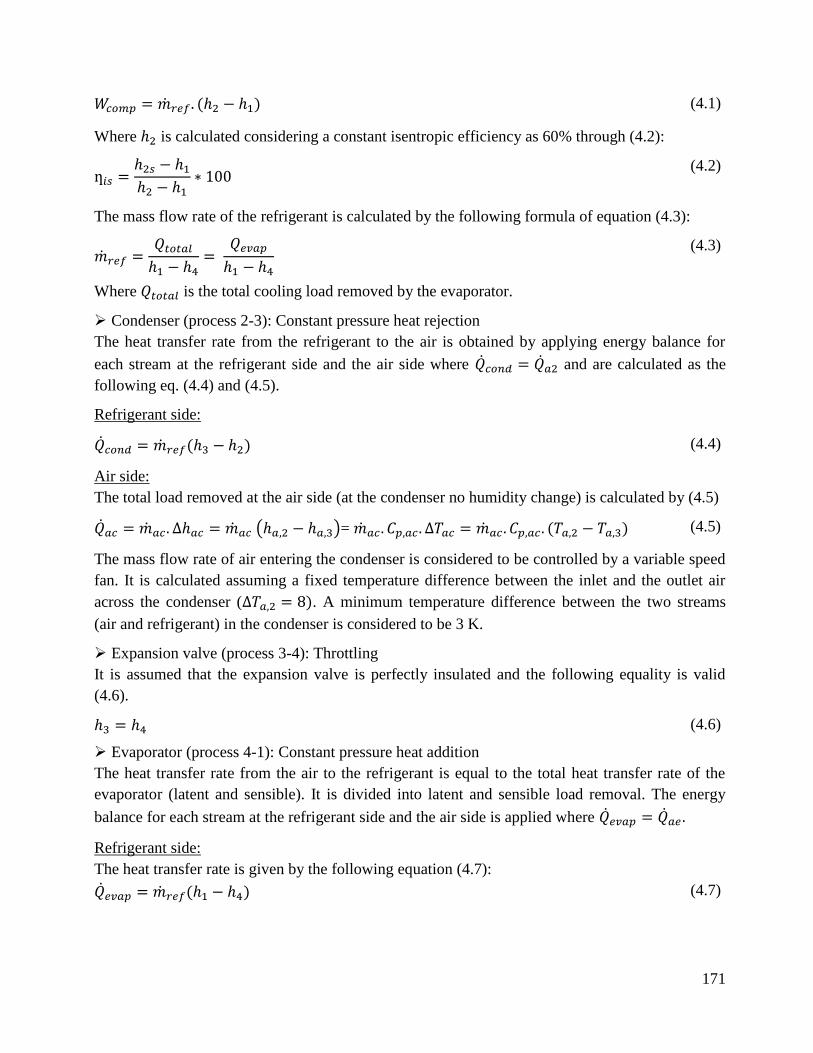
171

(4.1)

Where is calculated considering a constant isentropic efficiency as 60% through (4.2):

(4.2)

The mass flow rate of the refrigerant is calculated by the following formula of equation (4.3):

(4.3)

Where is the total cooling load removed by the evaporator.

Condenser (process 2-3): Constant pressure heat rejection

The heat transfer rate from the refrigerant to the air is obtained by applying energy balance for

each stream at the refrigerant side and the air side where and are calculated as the

following eq. (4.4) and (4.5).

Refrigerant side:

(4.4)

Air side:

The total load removed at the air side (at the condenser no humidity change) is calculated by (4.5)

= (4.5)

The mass flow rate of air entering the condenser is considered to be controlled by a variable speed

fan. It is calculated assuming a fixed temperature difference between the inlet and the outlet air

across the condenser ( . A minimum temperature difference between the two streams

(air and refrigerant) in the condenser is considered to be 3 K.

Expansion valve (process 3-4): Throttling

It is assumed that the expansion valve is perfectly insulated and the following equality is valid

(4.6).

(4.6)

Evaporator (process 4-1): Constant pressure heat addition

The heat transfer rate from the air to the refrigerant is equal to the total heat transfer rate of the

evaporator (latent and sensible). It is divided into latent and sensible load removal. The energy

balance for each stream at the refrigerant side and the air side is applied where

Refrigerant side:

The heat transfer rate is given by the following equation (4.7):

(4.7)

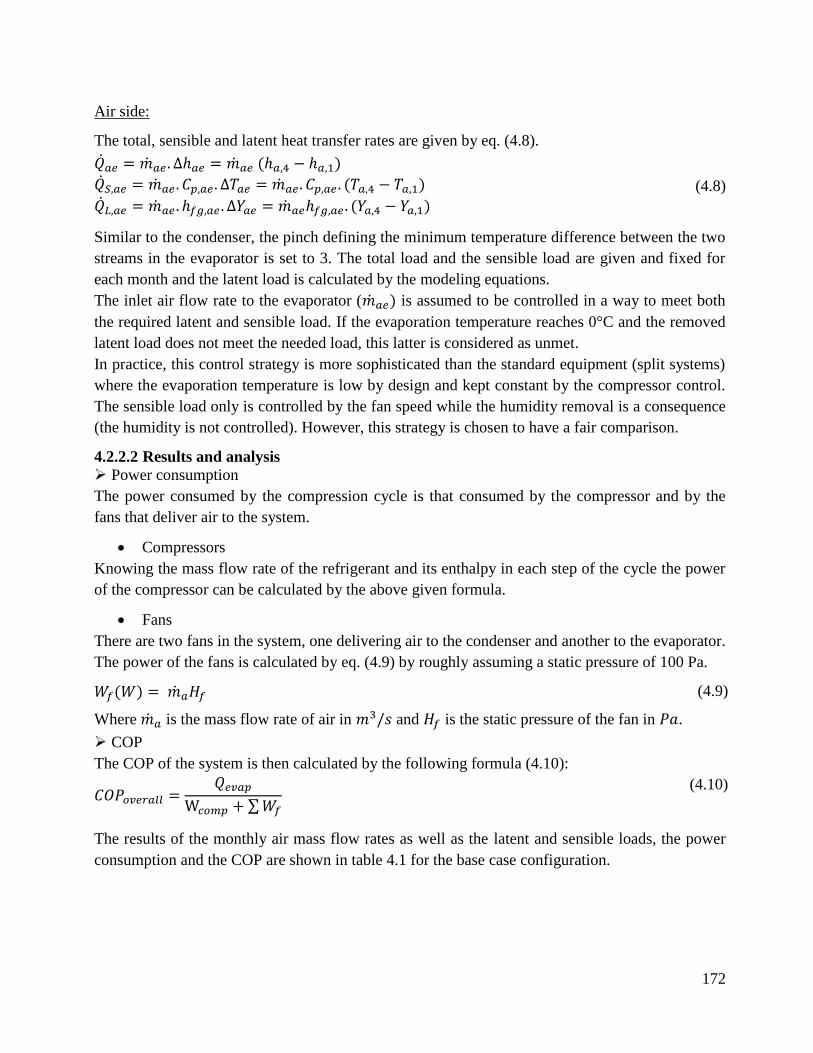
172

Air side:

The total, sensible and latent heat transfer rates are given by eq. (4.8).

(4.8)

Similar to the condenser, the pinch defining the minimum temperature difference between the two

streams in the evaporator is set to 3. The total load and the sensible load are given and fixed for

each month and the latent load is calculated by the modeling equations.

The inlet air flow rate to the evaporator ( is assumed to be controlled in a way to meet both

the required latent and sensible load. If the evaporation temperature reaches 0°C and the removed

latent load does not meet the needed load, this latter is considered as unmet.

In practice, this control strategy is more sophisticated than the standard equipment (split systems)

where the evaporation temperature is low by design and kept constant by the compressor control.

The sensible load only is controlled by the fan speed while the humidity removal is a consequence

(the humidity is not controlled). However, this strategy is chosen to have a fair comparison.

4.2.2.2 Results and analysis

Power consumption

The power consumed by the compression cycle is that consumed by the compressor and by the

fans that deliver air to the system.

Compressors

Knowing the mass flow rate of the refrigerant and its enthalpy in each step of the cycle the power

of the compressor can be calculated by the above given formula.

Fans

There are two fans in the system, one delivering air to the condenser and another to the evaporator.

The power of the fans is calculated by eq. (4.9) by roughly assuming a static pressure of 100 Pa.

(4.9)

Where is the mass flow rate of air in and is the static pressure of the fan in .

COP

The COP of the system is then calculated by the following formula (4.10):

(4.10)

The results of the monthly air mass flow rates as well as the latent and sensible loads, the power

consumption and the COP are shown in table 4.1 for the base case configuration.

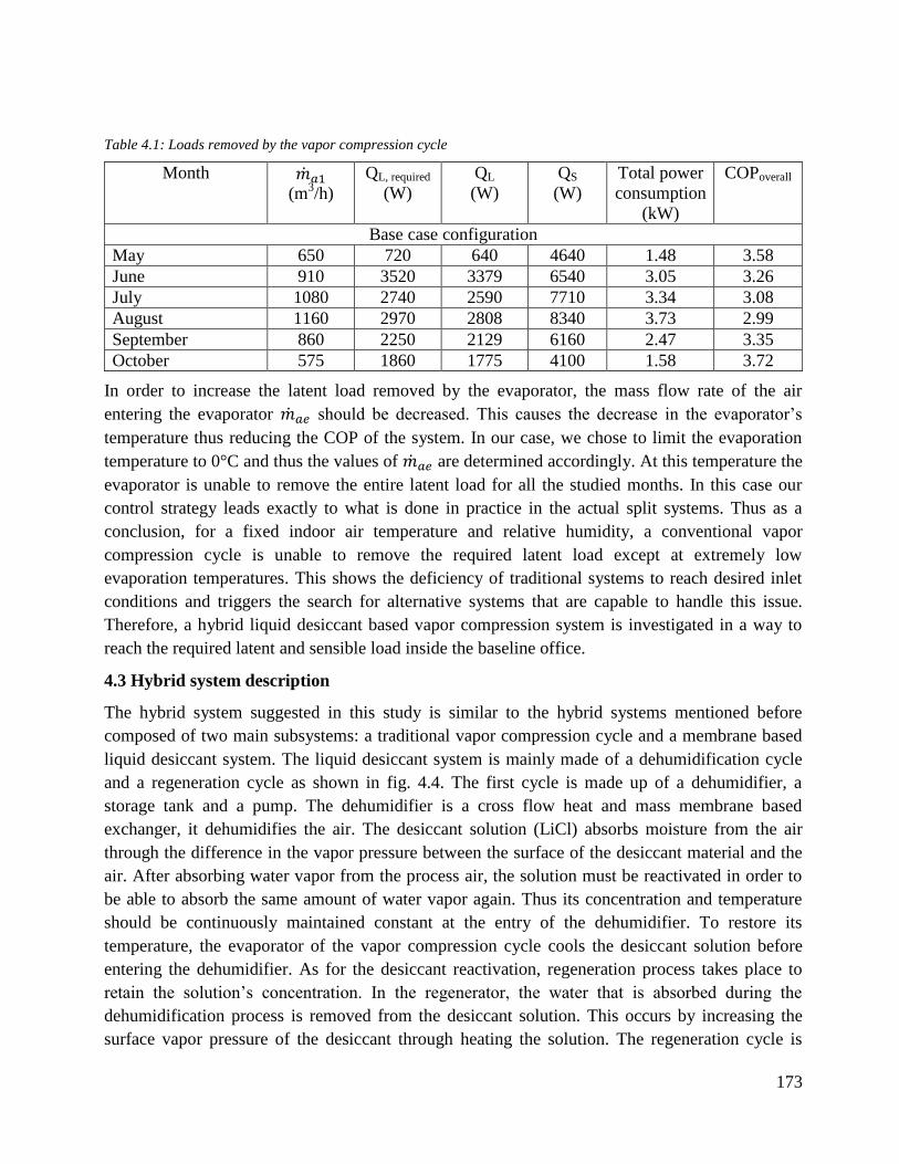
173

Table 4.1: Loads removed by the vapor compression cycle

Month (m

3/h)

QL, required

(W)

QL

(W)

QS

(W)

Total power

consumption

(kW)

COPoverall

Base case configuration

May 650 720 640 4640 1.48 3.58

June 910 3520 3379 6540 3.05 3.26

July 1080 2740 2590 7710 3.34 3.08

August 1160 2970 2808 8340 3.73 2.99

September 860 2250 2129 6160 2.47 3.35

October 575 1860 1775 4100 1.58 3.72

In order to increase the latent load removed by the evaporator, the mass flow rate of the air

entering the evaporator should be decreased. This causes the decrease in the evaporator’s

temperature thus reducing the COP of the system. In our case, we chose to limit the evaporation

temperature to 0°C and thus the values of are determined accordingly. At this temperature the

evaporator is unable to remove the entire latent load for all the studied months. In this case our

control strategy leads exactly to what is done in practice in the actual split systems. Thus as a

conclusion, for a fixed indoor air temperature and relative humidity, a conventional vapor

compression cycle is unable to remove the required latent load except at extremely low

evaporation temperatures. This shows the deficiency of traditional systems to reach desired inlet

conditions and triggers the search for alternative systems that are capable to handle this issue.

Therefore, a hybrid liquid desiccant based vapor compression system is investigated in a way to

reach the required latent and sensible load inside the baseline office.

4.3 Hybrid system description

The hybrid system suggested in this study is similar to the hybrid systems mentioned before

composed of two main subsystems: a traditional vapor compression cycle and a membrane based

liquid desiccant system. The liquid desiccant system is mainly made of a dehumidification cycle

and a regeneration cycle as shown in fig. 4.4. The first cycle is made up of a dehumidifier, a

storage tank and a pump. The dehumidifier is a cross flow heat and mass membrane based

exchanger, it dehumidifies the air. The desiccant solution (LiCl) absorbs moisture from the air

through the difference in the vapor pressure between the surface of the desiccant material and the

air. After absorbing water vapor from the process air, the solution must be reactivated in order to

be able to absorb the same amount of water vapor again. Thus its concentration and temperature

should be continuously maintained constant at the entry of the dehumidifier. To restore its

temperature, the evaporator of the vapor compression cycle cools the desiccant solution before

entering the dehumidifier. As for the desiccant reactivation, regeneration process takes place to

retain the solution’s concentration. In the regenerator, the water that is absorbed during the

dehumidification process is removed from the desiccant solution. This occurs by increasing the

surface vapor pressure of the desiccant through heating the solution. The regeneration cycle is

174

made of a regenerator (which is also a cross flow membrane heat and mass exchanger), a pump

and a storage tank and it uses the excess heat given by the condenser of the vapor compression

cycle to heat the solution before entering the regenerator. It should be noted that at steady state the

mass flow rate of the water vapor removed by the dehumidifier is transferred to the regenerator

where it is released to the driven ambient air.

Figure 4.4: Schematic of a hybrid system with storage tanks

The storage tank in the dehumidification cycle (tank_1) is used to store the diluted solution

leaving the dehumidifier which is continuously pumped to the regenerator for reactivation. The

tank in the regeneration cycle (tank_2) is for storing the concentrated solution which is again

pumped to the first cycle to absorb the water vapor from the return air and so on. Before reaching

a steady state the concentration of the solution inside the tank of the first cycle decreases with time

while that of the second cycle increases. The concentration of the diluted solution found in tank_1

is always adjusted by adding more concentrated solution from tank_2. The starting temperature

and concentration of the solution are specified as initial conditions inside the tanks which are not

necessarily equal in both tanks.

The action of preheating the solution before entering the condenser and pre-cooling it before

entering the evaporator is very important. It intends to save some of the energy required in the

process of regeneration and dehumidification respectively. Thus also a new cycle exists which

consists of the two storage tanks: tank_1 and tank_2, a heat exchanger hx_0 and a pump. As the

desiccant solution flows from one tank to the other, it passes through a heat exchanger where heat

is transferred to or from the solution. The heat exchanger is used to increase the solution’s

175

temperature before entering the regeneration cycle and to reduce its temperature before entering

the dehumidification cycle. This circuit adds flexibility to the system by allowing us to assign

different solution concentrations and flow rates in the two cycles. The pumps are used to define

the mass flow rates of the solution in each cycle.

The desiccant cycle is able to play the role of both dehumidifying and cooling the air at the same

time. The evaporator of VCC_1 is used to cool the desiccant solution which in turn cools and

dehumidifies the air simultaneously. A previous study was done by (Mustapha et al., 2017) where

different architectures were analyzed to find the most efficient one among them. The

configurations were proposed according to whether the solution removes the latent and sensible

loads entirely, or the whole latent load and part of the sensible load or only the latent load without

interfering with the sensible load. In the case where part of the sensible load is removed by the

solution, air would pass by another vapor compression cycle in order to reach the desired

temperature before entering the indoor conditioned space. The results showed that optimizing the

amount of the sensible load removed by the liquid desiccant solution led to an increase in the COP

of the system and a decrease in the overall power consumption by around 30%.

4.3.1 Configurations

The above described system represents a good alternative for conventional cycles, yet, such a

system might also lack some flexibility when the latent to sensible ratio varies in an important

range. Aiming to properly handle the latent and sensible loads of the previously described baseline

office a more developed system is proposed. It consists of the addition of heat exchangers that

transfer sensible heat from the air in the dehumidification cycle and to the ambient air in the

regenerator cycle increasing the flexibility of the system. The placement of the heat exchangers is

a critical issue and thus different configurations are studied. The first one consists of adding heat

exchangers before the dehumidifier and the regenerator and the second involves inserting them

after the dehumidifier and the regenerator. A third configuration is suggested where instead of

adding heat exchangers, a second vapor compression cycle is inserted after the dehumidification

cycle. In this case the evaporator of this added compression cycle plays the role of a heat

exchanger of the second configuration. In all configurations the dehumidifier of the desiccant

system removes the entire latent load and part of the sensible load. The remaining sensible load is

removed by the heat exchangers in the first two configurations and by the vapor compression

cycle in the third configuration. Another configuration exists where both, latent and sensible loads,

are entirely removed by the desiccant system without the help of additional equipment. This

configuration has a poor flexibility outside the months with high latent to sensible load ratio and

failed to prove any seasonal effectiveness because the desiccant system shows high performance

in removing latent loads rather than sensible loads. Thus when the dimensions of the dehumidifier

are chosen to be able to remove the entire latent load, the sensible load removal would be small.

Consequently, the mass flow rate of the air in the dehumidifier should be greatly increased in

order to increase the sensible load removal. This leads to the increase of the solution’s

concentration leading to an increase in the condensation temperature and hence the COP of the

system decreases. So due to its very low COP, this configuration is eliminated from our study. A

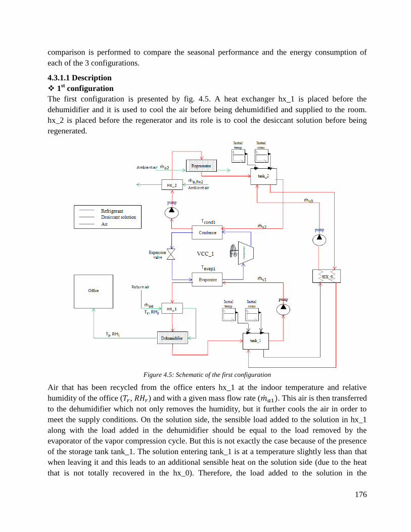
176

comparison is performed to compare the seasonal performance and the energy consumption of

each of the 3 configurations.

4.3.1.1 Description

1st configuration

The first configuration is presented by fig. 4.5. A heat exchanger hx_1 is placed before the

dehumidifier and it is used to cool the air before being dehumidified and supplied to the room.

hx_2 is placed before the regenerator and its role is to cool the desiccant solution before being

regenerated.

Figure 4.5: Schematic of the first configuration

Air that has been recycled from the office enters hx_1 at the indoor temperature and relative

humidity of the office ( , ) and with a given mass flow rate ( . This air is then transferred

to the dehumidifier which not only removes the humidity, but it further cools the air in order to

meet the supply conditions. On the solution side, the sensible load added to the solution in hx_1

along with the load added in the dehumidifier should be equal to the load removed by the

evaporator of the vapor compression cycle. But this is not exactly the case because of the presence

of the storage tank tank_1. The solution entering tank_1 is at a temperature slightly less than that

when leaving it and this leads to an additional sensible heat on the solution side (due to the heat

that is not totally recovered in the hx_0). Therefore, the load added to the solution in the

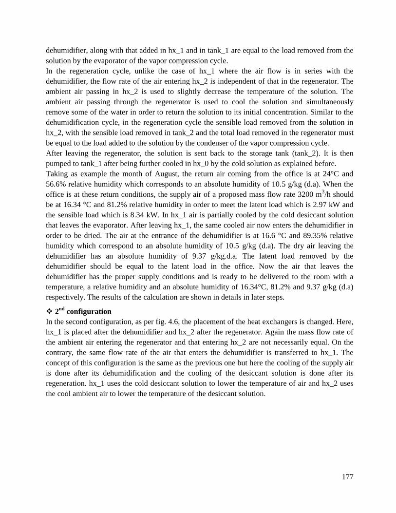
177

dehumidifier, along with that added in hx_1 and in tank_1 are equal to the load removed from the

solution by the evaporator of the vapor compression cycle.

In the regeneration cycle, unlike the case of hx_1 where the air flow is in series with the

dehumidifier, the flow rate of the air entering hx_2 is independent of that in the regenerator. The

ambient air passing in hx_2 is used to slightly decrease the temperature of the solution. The

ambient air passing through the regenerator is used to cool the solution and simultaneously

remove some of the water in order to return the solution to its initial concentration. Similar to the

dehumidification cycle, in the regeneration cycle the sensible load removed from the solution in

hx_2, with the sensible load removed in tank_2 and the total load removed in the regenerator must

be equal to the load added to the solution by the condenser of the vapor compression cycle.

After leaving the regenerator, the solution is sent back to the storage tank (tank_2). It is then

pumped to tank_1 after being further cooled in hx_0 by the cold solution as explained before.

Taking as example the month of August, the return air coming from the office is at 24°C and

56.6% relative humidity which corresponds to an absolute humidity of 10.5 g/kg (d.a). When the

office is at these return conditions, the supply air of a proposed mass flow rate 3200 m3/h should

be at 16.34 °C and 81.2% relative humidity in order to meet the latent load which is 2.97 kW and

the sensible load which is 8.34 kW. In hx_1 air is partially cooled by the cold desiccant solution

that leaves the evaporator. After leaving hx_1, the same cooled air now enters the dehumidifier in

order to be dried. The air at the entrance of the dehumidifier is at 16.6 °C and 89.35% relative

humidity which correspond to an absolute humidity of 10.5 g/kg (d.a). The dry air leaving the

dehumidifier has an absolute humidity of 9.37 g/kg.d.a. The latent load removed by the

dehumidifier should be equal to the latent load in the office. Now the air that leaves the

dehumidifier has the proper supply conditions and is ready to be delivered to the room with a

temperature, a relative humidity and an absolute humidity of 16.34°C, 81.2% and 9.37 g/kg (d.a)

respectively. The results of the calculation are shown in details in later steps.

2nd configuration

In the second configuration, as per fig. 4.6, the placement of the heat exchangers is changed. Here,

hx_1 is placed after the dehumidifier and hx_2 after the regenerator. Again the mass flow rate of

the ambient air entering the regenerator and that entering hx_2 are not necessarily equal. On the

contrary, the same flow rate of the air that enters the dehumidifier is transferred to hx_1. The

concept of this configuration is the same as the previous one but here the cooling of the supply air

is done after its dehumidification and the cooling of the desiccant solution is done after its

regeneration. hx_1 uses the cold desiccant solution to lower the temperature of air and hx_2 uses

the cool ambient air to lower the temperature of the desiccant solution.

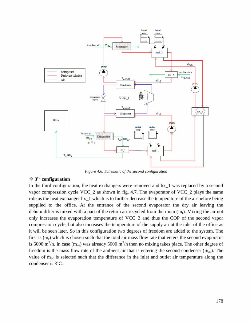
178

Figure 4.6: Schematic of the second configuration

3rd configuration

In the third configuration, the heat exchangers were removed and hx_1 was replaced by a second

vapor compression cycle VCC_2 as shown in fig. 4.7. The evaporator of VCC_2 plays the same

role as the heat exchanger hx_1 which is to further decrease the temperature of the air before being

supplied to the office. At the entrance of the second evaporator the dry air leaving the

dehumidifier is mixed with a part of the return air recycled from the room (ṁr). Mixing the air not

only increases the evaporation temperature of VCC_2 and thus the COP of the second vapor

compression cycle, but also increases the temperature of the supply air at the inlet of the office as

it will be seen later. So in this configuration two degrees of freedom are added to the system. The

first is (ṁr) which is chosen such that the total air mass flow rate that enters the second evaporator

is 5000 m3/h. In case (ṁae) was already 5000 m

3/h then no mixing takes place. The other degree of

freedom is the mass flow rate of the ambient air that is entering the second condenser (ṁac). The

value of ṁac is selected such that the difference in the inlet and outlet air temperature along the

condenser is 8˚C.

179

Figure 4.7: Schematic of the third configuration

4.3.2 Modeling the hybrid system

For the modeling of such a system, a mathematical model for each component is written in

Modelica language using Dymola software and is described in the following steps.

4.3.2.1 Vapor compression cycles

For VCC_1 and VCC_2 the modeling is the same as described for the base case but the only

difference is that in VCC_1 the exchange is between the refrigerant and the desiccant solution

instead of air. Same assumptions are taken regarding the compressor’s design and efficiency, the

temperature difference across the condenser, the perfectly insulated expansion valve and the fixed

pinch in the condenser and evaporator.

4.3.2.2 Desiccant cycle

Heat exchangers

Heat transfer takes place between the desiccant solution on one side and air on the other side. It is

worth noting that the total heat transfer rate leaving the hot fluid must be equal to the total heat

transfer rate absorbed by the cold fluid. Hence according to eq. (4.11).

(4.11)

180

In hx_0, the solution coming from the regenerator is the hot fluid and that coming from the

dehumidifier is the cold one. In hx_2 the solution is the hot fluid and the air is the cold one; for the

heat exchanger of the dehumidification cycle (hx_1) the cold stream is represented by the

desiccant solution and the hot one is represented by the air that needs to be processed.

The pinch defining the minimum temperature difference between the two streams in the heat

exchangers is set to 3.

Storage tanks

The solution entering the storage tank has a temperature and concentration different from that

leaving it due to the connection between tank_1 and tank_2. These values change with time and

thus the new outlet solution conditions are calculated by equations (4.12) and (4.13)

(4.12)

(4.13)

Where is the height of the tank and is its area, and are the average specific

heat of the solution that is coming from the dehumidifier (or regenerator) and hx_0 respectively

and they are calculated by eq. (4.14). is the outlet specific heat of the solution at temperature

and concentration .

(4.14)

and being the specific heat of the solution that is coming from the dehumidifier (or

regenerator) and hx_0 respectively.

Pumps

The role of the pumps in the system is to move a certain mass flow rate of the desiccant solution

within a cycle or from one cycle to another. The pumps are used to control the mass flow rates of

the solution in each cycle. The power needed to drive a pump is calculated by the following

equation (4.15):

(4.15)

Where is the mass flow rate of the solution in

and is the head of the pump in .

Fans

The fans are used to deliver air to the components where an exchange is needed between air and

the desiccant solution or between air and the refrigerant. The power produced by a fan is

calculated by (4.9) as stated previously.

Dehumidifier and regenerator

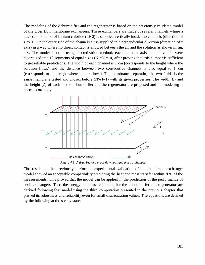
181

The modeling of the dehumidifier and the regenerator is based on the previously validated model

of the cross flow membrane exchangers. These exchangers are made of several channels where a

desiccant solution of lithium chloride (LiCl) is supplied vertically inside the channels (direction of

z axis). On the outer side of the channels air is supplied in a perpendicular direction (direction of x

axis) in a way where no direct contact is allowed between the air and the solution as shown in fig.

4.8. The model is done using discretization method; each of the x axis and the z axis were

discretized into 10 segments of equal sizes (Ni=Nj=10) after proving that this number is sufficient

to get reliable predictions. The width of each channel is 1 cm (corresponds to the height where the

solution flows) and the distance between two consecutive channels is also equal to 1 cm

(corresponds to the height where the air flows). The membranes separating the two fluids is the

same membrane tested and chosen before (NWF-1) with its given properties. The width (L) and

the height (Z) of each of the dehumidifier and the regenerator are proposed and the modeling is

done accordingly.

Figure 4.8: A drawing of a cross flow heat and mass exchanger.

The results of the previously performed experimental validation of the membrane exchanger

model showed an acceptable compatibility predicting the heat and mass transfer within 20% of the

measurements. This proved that the model can be applied in the prediction of the performance of

such exchangers. Thus the energy and mass equations for the dehumidifier and regenerator are

derived following that model using the third computation presented in the previous chapter that

proved its robustness and reliability even for small discretization values. The equations are defined

by the following at the steady state:

182

a) Air side

Mass conservation equation for water vapor

(4.16)

Energy conservation equation for moist air

(4.17)

b) Solution side

Mass conservation equation for liquid water

(4.18)

Energy conservation equation for moist air

(4.19)

183

c) Membrane

Energy conservation equations

(4.20)

(4.21)

Where

(4.22)

4.3.3 Discussion of the simulation protocol

The different designs of the three configurations allow simulating 18 models such that for every

configuration 6 simulations are done corresponding to each month as explained before. The

ambient air temperature and relative humidity are given to the system as well as the indoor air

conditions and the simulations are performed at steady state.

4.3.3.1 Design strategy

Our system has several related elements that affect the quantity and distribution of load removal.

They include the design of the dehumidifier and regenerator as well as the mass flow rates of the

solution and air circulating in the system. When the system is complex with several interacting

elements and related parameters, the simulations can be done through an external software that

determines the values of the design and control variables while maximizing the system COP. This

separate control avoids redundancy and provides less time consuming operations through

bypassing mesh construction and configuration reading at each solver call in Dymola. For this

purpose, Python is used to perform the simulations where for each month of the three

configurations optimization iterations are conducted. In each iteration the input sources that

directly or indirectly influence the determination of the measured quantities are changed until the

required monthly latent and sensible loads are removed from the office. Such input sources are

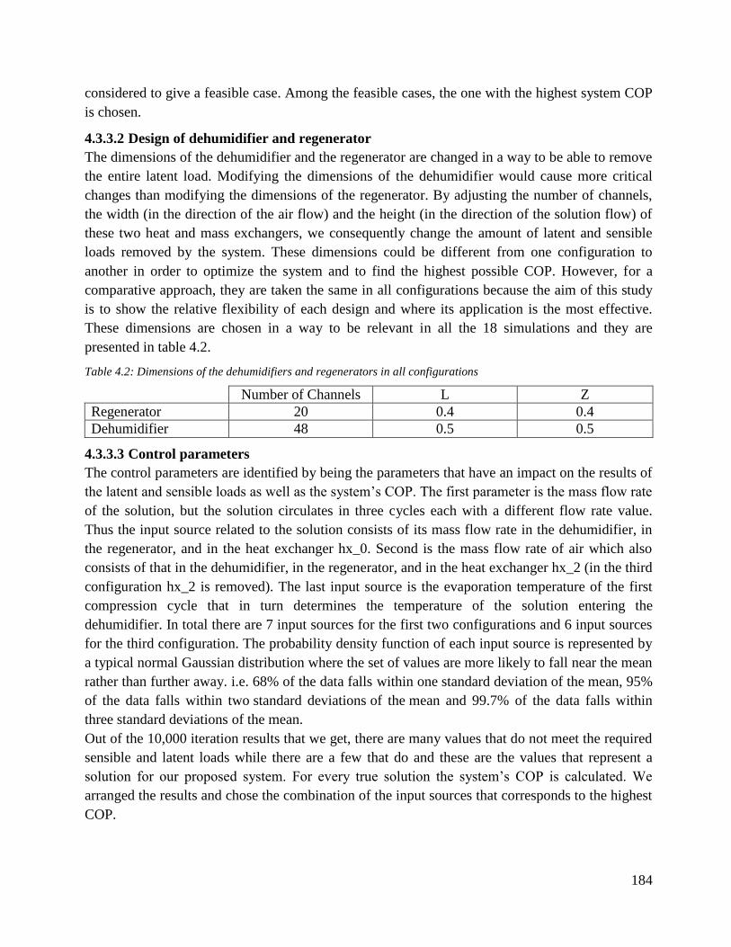
184

considered to give a feasible case. Among the feasible cases, the one with the highest system COP

is chosen.

4.3.3.2 Design of dehumidifier and regenerator

The dimensions of the dehumidifier and the regenerator are changed in a way to be able to remove

the entire latent load. Modifying the dimensions of the dehumidifier would cause more critical

changes than modifying the dimensions of the regenerator. By adjusting the number of channels,

the width (in the direction of the air flow) and the height (in the direction of the solution flow) of

these two heat and mass exchangers, we consequently change the amount of latent and sensible

loads removed by the system. These dimensions could be different from one configuration to

another in order to optimize the system and to find the highest possible COP. However, for a

comparative approach, they are taken the same in all configurations because the aim of this study

is to show the relative flexibility of each design and where its application is the most effective.

These dimensions are chosen in a way to be relevant in all the 18 simulations and they are

presented in table 4.2.

Table 4.2: Dimensions of the dehumidifiers and regenerators in all configurations

Number of Channels L Z

Regenerator 20 0.4 0.4

Dehumidifier 48 0.5 0.5

4.3.3.3 Control parameters

The control parameters are identified by being the parameters that have an impact on the results of

the latent and sensible loads as well as the system’s COP. The first parameter is the mass flow rate

of the solution, but the solution circulates in three cycles each with a different flow rate value.

Thus the input source related to the solution consists of its mass flow rate in the dehumidifier, in

the regenerator, and in the heat exchanger hx_0. Second is the mass flow rate of air which also

consists of that in the dehumidifier, in the regenerator, and in the heat exchanger hx_2 (in the third

configuration hx_2 is removed). The last input source is the evaporation temperature of the first

compression cycle that in turn determines the temperature of the solution entering the

dehumidifier. In total there are 7 input sources for the first two configurations and 6 input sources

for the third configuration. The probability density function of each input source is represented by

a typical normal Gaussian distribution where the set of values are more likely to fall near the mean

rather than further away. i.e. 68% of the data falls within one standard deviation of the mean, 95%

of the data falls within two standard deviations of the mean and 99.7% of the data falls within

three standard deviations of the mean.

Out of the 10,000 iteration results that we get, there are many values that do not meet the required

sensible and latent loads while there are a few that do and these are the values that represent a

solution for our proposed system. For every true solution the system’s COP is calculated. We

arranged the results and chose the combination of the input sources that corresponds to the highest

COP.

185

4.3.3.4 Observed quantities

The measured quantities in our case are the latent and sensible loads removed by the system, as

well as the total power consumed and the overall system COP.

Latent load

The latent load is totally removed by the dehumidifier and is calculated by eq. (4.23).

(4.23)

where = for the first two configurations.

Sensible load

The sensible load that needs to be removed from the system is given for every month. A part of

this load is removed by the dehumidifier ( and the remaining share ( is extracted by the

heat exchangers hx_1 in the first two configurations and by the evaporator of the second vapor

compression cycle in the third configuration.

(4.24)

For the first configuration:

(4.25)

For the second configuration:

(4.26)

And for the third configuration the power of the second evaporator is calculated by fixing the total

sensible load and then subtracting the sensible load removed by the dehumidifier.

(4.27)

Power consumption

The total power consumption is the summation of that consumed by the compressors, the fans and

the pumps.

Compressors

In the first and second configuration, the power consumption of the vapor compression cycle is

that used by the compressor. As for the third configuration it is the summation of that used by the

two compressors.

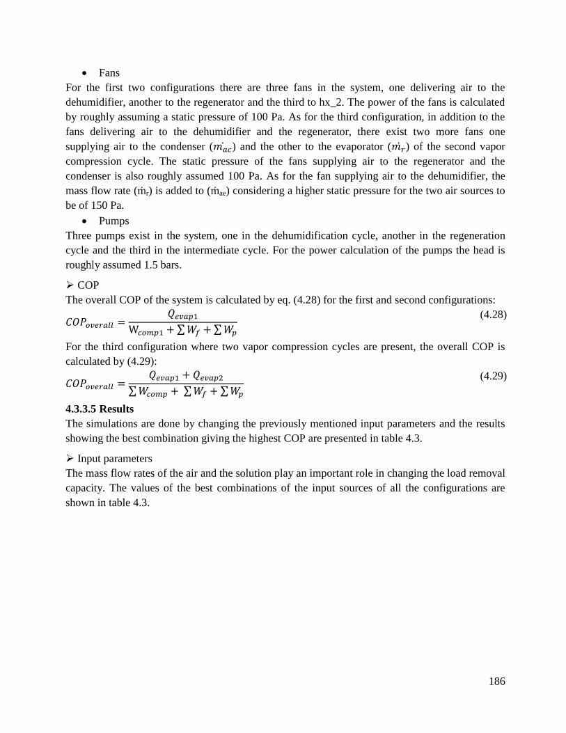
186

Fans

For the first two configurations there are three fans in the system, one delivering air to the

dehumidifier, another to the regenerator and the third to hx_2. The power of the fans is calculated

by roughly assuming a static pressure of 100 Pa. As for the third configuration, in addition to the

fans delivering air to the dehumidifier and the regenerator, there exist two more fans one

supplying air to the condenser ( ) and the other to the evaporator ( ) of the second vapor

compression cycle. The static pressure of the fans supplying air to the regenerator and the

condenser is also roughly assumed 100 Pa. As for the fan supplying air to the dehumidifier, the

mass flow rate (ṁr) is added to (ṁae) considering a higher static pressure for the two air sources to

be of 150 Pa.

Pumps

Three pumps exist in the system, one in the dehumidification cycle, another in the regeneration

cycle and the third in the intermediate cycle. For the power calculation of the pumps the head is

roughly assumed 1.5 bars.

COP

The overall COP of the system is calculated by eq. (4.28) for the first and second configurations:

(4.28)

For the third configuration where two vapor compression cycles are present, the overall COP is

calculated by (4.29):

(4.29)

4.3.3.5 Results

The simulations are done by changing the previously mentioned input parameters and the results

showing the best combination giving the highest COP are presented in table 4.3.

Input parameters

The mass flow rates of the air and the solution play an important role in changing the load removal

capacity. The values of the best combinations of the input sources of all the configurations are

shown in table 4.3.

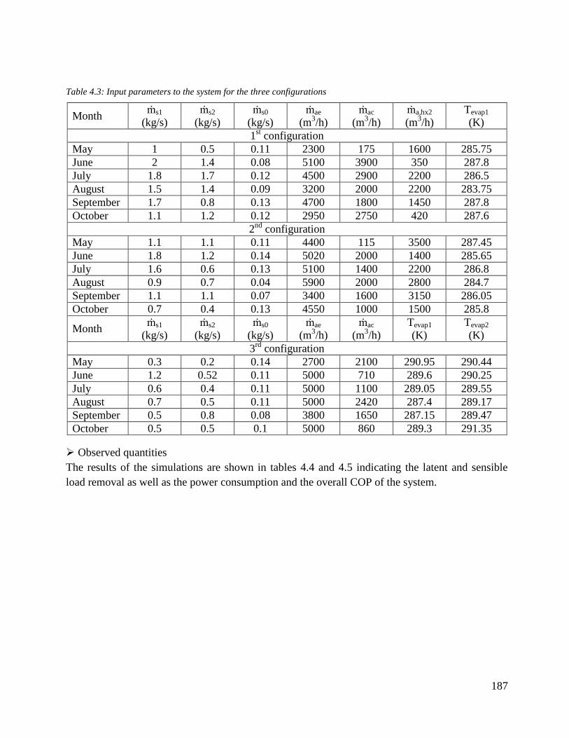
187

Table 4.3: Input parameters to the system for the three configurations

Month ṁs1

(kg/s)

ṁs2

(kg/s)

ṁs0

(kg/s)

ṁae

(m3/h)

ṁac

(m3/h)

ṁa,hx2

(m3/h)

Tevap1

(K)

1st configuration

May 1 0.5 0.11 2300 175 1600 285.75

June 2 1.4 0.08 5100 3900 350 287.8

July 1.8 1.7 0.12 4500 2900 2200 286.5

August 1.5 1.4 0.09 3200 2000 2200 283.75

September 1.7 0.8 0.13 4700 1800 1450 287.8

October 1.1 1.2 0.12 2950 2750 420 287.6

2nd

configuration

May 1.1 1.1 0.11 4400 115 3500 287.45

June 1.8 1.2 0.14 5020 2000 1400 285.65

July 1.6 0.6 0.13 5100 1400 2200 286.8

August 0.9 0.7 0.04 5900 2000 2800 284.7

September 1.1 1.1 0.07 3400 1600 3150 286.05

October 0.7 0.4 0.13 4550 1000 1500 285.8

Month ṁs1

(kg/s)

ṁs2

(kg/s)

ṁs0

(kg/s)

ṁae

(m3/h)

ṁac

(m3/h)

Tevap1

(K)

Tevap2

(K)

3rd

configuration

May 0.3 0.2 0.14 2700 2100 290.95 290.44

June 1.2 0.52 0.11 5000 710 289.6 290.25

July 0.6 0.4 0.11 5000 1100 289.05 289.55

August 0.7 0.5 0.11 5000 2420 287.4 289.17

September 0.5 0.8 0.08 3800 1650 287.15 289.47

October 0.5 0.5 0.1 5000 860 289.3 291.35

Observed quantities

The results of the simulations are shown in tables 4.4 and 4.5 indicating the latent and sensible

load removal as well as the power consumption and the overall COP of the system.

188

Table 4.4: Loads removed by the system and the COP of the 1st and 2

nd configurations

Month QL

(W)

QS1

(W)

QS2

(W)

QS

(W)

Power

(kW)

COPoverall

1st configuration

May 722 399 4231 4630 1.27 5.08

June 3529 804 5839 6643 3.44 3.19

July 2742 614 7140 7754 3.30 3.55

August 2973 283 8081 8364 3.89 3.17

September 2247 776 5373 6149 2.43 3.97

October 1865 528 3577 4105 1.63 4.36

2nd

configuration

May 721 2766 1881 4647 1.33 4.82

June 3520 3784 2761 6545 3.39 3.39

July 2736 3285 4419 7704 2.97 3.94

August 2967 4309 4059 8368 3.12 3.75

September 2251 2727 3468 6195 2.19 4.16

October 1863 3266 829 4095 1.50 4.79

Table 4.5: Loads removed by the system and the COP of the 3rd

configuration

Month QL

(W)

QS1

(W)

QS2

(W)

QS

(W)

Power

(kW)

COP1 COP2 COPoverall

3rd

configuration

May 719 719 3921 4640 1.17 5.19 6.91 5.65

June 3524 2069 4471 6540 2.88 3.45 6.62 3.84

July 2739 1608 6102 7710 2.71 3.58 5.76 4.28

August 2969 2863 5477 8340 3.05 3.58 5.7 4.05

September 2250 2192 3968 6160 2.04 4.21 6.3 4.48

October 1852 1740 2360 4100 1.37 4.75 8.61 5.02

Load removal distribution by equipment

Figures 4.9(a) and 4.9(b) show the distribution of the sensible load removal by the dehumidifier

and by the heat exchanger in the first and second configurations respectively as well as the latent

load removed by the dehumidifier and the COP of the system. Figure 4.9(c) presents the load

removed by the dehumidifier (latent and sensible) and by the evaporator (sensible) of the second

vapor compression cycle as well as the overall COP in the third configuration.

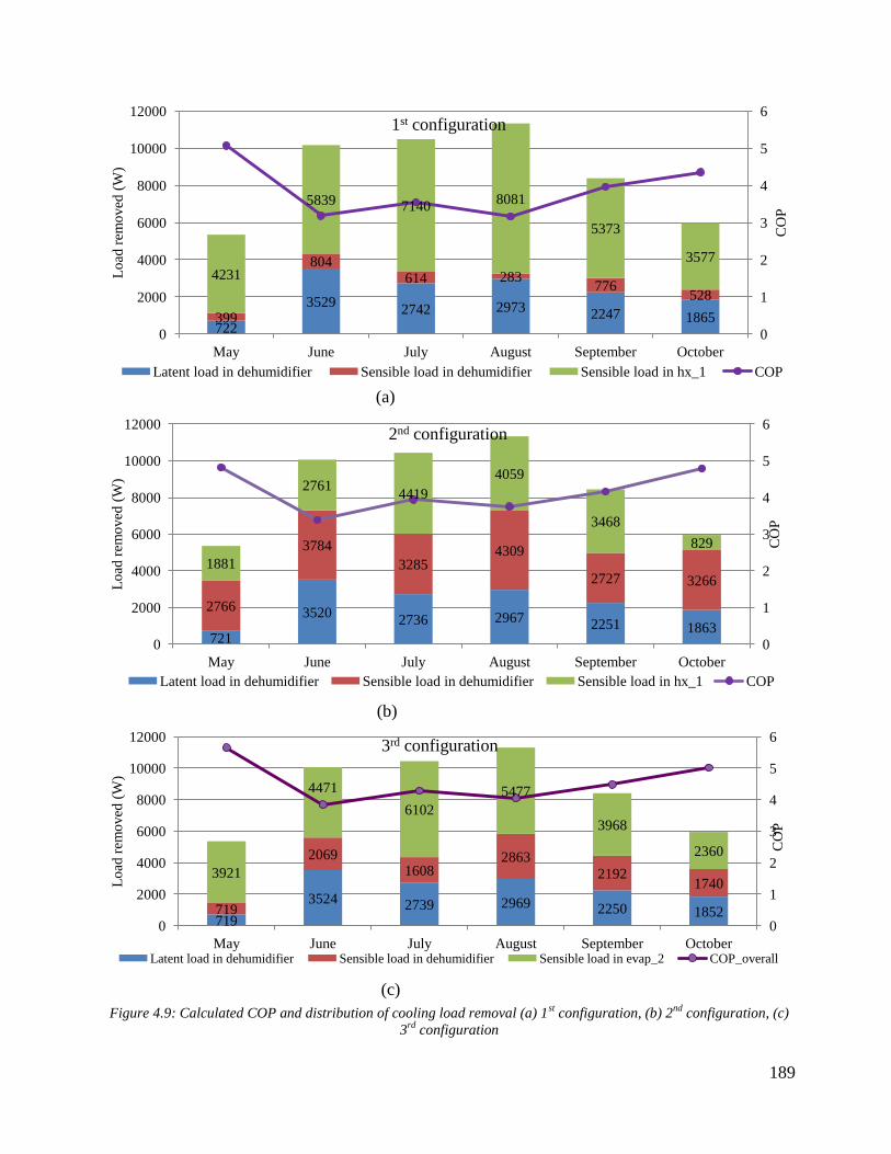
189

(a)

(b)

(c)

Figure 4.9: Calculated COP and distribution of cooling load removal (a) 1st configuration, (b) 2

nd configuration, (c)

3rd

configuration

722

3529 2742 2973

2247 1865 399

804 614 283

776 528

4231

5839 7140 8081

5373

3577

0

1

2

3

4

5

6

0

2000

4000

6000

8000

10000

12000

May June July August September October

CO

P

Lo

ad r

emo

ved

(W

) 1st configuration

Latent load in dehumidifier Sensible load in dehumidifier Sensible load in hx_1 COP

721

3520 2736 2967 2251 1863

2766

3784

3285 4309

2727 3266

1881

2761 4419

4059

3468

829

0

1

2

3

4

5

6

0

2000

4000

6000

8000

10000

12000

May June July August September October

CO

P

Lo

ad r

emo

ved

(W

)

2nd configuration

Latent load in dehumidifier Sensible load in dehumidifier Sensible load in hx_1 COP

719

3524 2739 2969 2250 1852 719

2069 1608

2863

2192 1740

3921

4471

6102

5477

3968

2360

0

1

2

3

4

5

6

0

2000

4000

6000

8000

10000

12000

May June July August September October

CO

P

Lo

ad r

emo

ved

(W

)

3rd configuration

Latent load in dehumidifier Sensible load in dehumidifier Sensible load in evap_2 COP_overall

190

Supply indoor air conditions

Unlike traditional systems, the air supplied to the office in these hybrid systems could have higher

temperatures. Generally, in vapor compression cycles, the larger the air mass flow rate that enters

the evaporator, the lower is the difference in temperature between the inlet and the outlet air across

the evaporator. This is considered a limitation for the conventional systems because if large air

mass flow rate is supplied, the temperature would not be sufficiently decreased to reach values

below the dew point and thus the humidity that would be removed from the air would not be

enough. This problem is avoided by using the desiccant system that allows the proper control of

humidity even at higher air mass flow rates and temperatures. The values of the temperature and

relative humidity of the supply air ( , ) for the 3 configurations are shown in table 4.6.

Table 4.6: Calculated temperature and relative humidity of the supply air

1st configuration 2

nd configuration 3

rd configuration

Month Ti

(˚C)

RHi

(%)

Yi

(g/kg)

Ti

(˚C)

RHi

(%)

Yi

(g/kg)

Ti

(˚C)

RHi

(%)

Yi

(g/kg)

May 18.1 71.1 9.16 20.9 61.1 9.34 20.9 60.1 9.21

June 20.2 71.3 10.49 20.1 72.0 10.54 20.8 70.1 10.68

July 19.0 71.7 9.76 19.5 69.9 9.84 19.9 68.7 9.89

August 16.3 81.2 9.37 19.8 69.0 9.88 20.3 67.4 9.95

September 20.2 68.0 9.98 18.6 73.3 9.74 19.9 68.0 9.82

October 19.9 70.6 10.22 21.3 66.5 10.49 21.56 65.81 10.53

191

4.3.3.6 Summary

The following table 4.7 summarizes for the three configurations the optimal values of the input parameters that gave the highest COP.

It also gives the results of the outputs including the loads, the power consumption and the COP. The supply indoor air conditions are as

well indicated.

Table 4.7: A summary of the input values, the outputs and supply air conditions in the three configurations

Input parameters Observed quantities Supply indoor air

Month ṁs1

(kg/s)

ṁs2

(kg/s)

ṁs0

(kg/s)

ṁae

(m3/h)

ṁac

(m3/h)

ṁa,hx2

(m3/h)

Tevap1

(˚C)

QL

(W)

QS

(W)

QS1

(W)

QS2

(W)

Power

(kW)

COPoverall

(-)

Ti

(˚C)

RHi

(%)

1st configuration

May 1 0.5 0.11 2300 175 1600 12.6 722 4630 399 4231 1.27 5.08 18.1 71.1

Jun 2 1.4 0.08 5100 3900 350 14.7 3529 6643 804 5839 3.44 3.19 20.2 71.3

Jul 1.8 1.7 0.12 4500 2900 2200 13.45 2742 7754 614 7140 3.30 3.55 19.0 71.7

Aug 1.5 1.4 0.09 3200 2000 2200 10.6 2973 8364 283 8081 3.89 3.17 16.3 81.2

Sept 1.7 0.8 0.13 4700 1800 1450 14.7 2247 6149 776 5373 2.43 3.97 20.2 68.0

Oct 1.1 1.2 0.12 2950 2750 420 14.5 1865 4105 528 3577 1.63 4.36 19.9 70.6

2nd

configuration

May 1.1 1.1 0.11 4400 115 3500 14.3 721 4647 2766 1881 1.33 4.82 20.9 61.1

Jun 1.8 1.2 0.14 5020 2000 1400 12.5 3520 6545 3784 2761 3.39 3.39 20.1 72.0

Jul 1.6 0.6 0.13 5100 1400 2200 13.7 2736 7704 3285 4419 2.97 3.94 19.5 69.9

Aug 0.9 0.7 0.04 5900 2000 2800 11.6 2967 8368 4309 4059 3.12 3.75 19.8 69.0

Sept 1.1 1.1 0.07 3400 1600 3150 12.9 2251 6195 2727 3468 2.19 4.16 18.6 73.3

Oct 0.7 0.4 0.13 4550 1000 1500 12.7 1863 4095 3266 829 1.50 4.79 21.3 66.5

3rd

configuration

Month ṁs1

(kg/s)

ṁs2

(kg/s)

ṁs0

(kg/s)

ṁae

(m3/h)

ṁac

(m3/h)

Tevap1

(˚C)

Tevap2

(˚C)

QL

(W)

QS

(W)

QS1

(W)

QS2

(W)

Power

(kW)

COPoverall

(-)

Ti

(˚C)

RHi

(%)

May 0.3 0.2 0.14 2700 2100 17.8 17.9 719 4640 719 3921 1.17 5.65 20.9 60.1

Jun 1.2 0.52 0.11 5000 710 16.4 17.8 3524 6540 2069 4471 2.88 3.84 20.8 70.1

Jul 0.6 0.4 0.11 5000 1100 15.9 16.9 2739 7710 1608 6102 2.71 4.28 19.9 68.7

Aug 0.7 0.5 0.11 5000 2420 14.3 17.3 2969 8340 2863 5477 3.05 4.05 20.3 67.4

Sept 0.5 0.8 0.08 3800 1650 14 16.9 2250 6160 2192 3968 2.04 4.48 19.9 68.0

Oct 0.5 0.5 0.1 5000 860 16.2 18.6 1852 4100 1740 2360 1.37 5.02 21.6 65.8

192

4.3.4 Analysis

Figure 11 shows a comparison of the system’s COP between the base case and the three

studied flexible hybrid systems.

Figure 4.10: comparison of the COP of the base case system and the three studied configurations

It is observed that the base case system consisting of a conventional vapor compression cycle

possesses the lowest COP among all the other configurations. It can be clearly observed by

comparing the results of the three configurations that in the third configuration the figures of

the COPs of all the months are higher than the other configurations. Analyzing the COPs of

the 6 months simulated by the first and second configurations shows that the first

configuration is more performing than the second only for the month of May. While for the

other months from June to October, the second configuration has proved to be more efficient.

We may say that whenever the ratio of latent to sensible load is low, it is more favorable to

reduce the temperature of air prior to dehumidifying it. Comparing the results of the second

configuration in the months where it is more favorable shows a contradiction with the fact that

as the ambient air temperature decreases as the COP of the system increases. We can

recognize that even though the ambient temperature in August is higher than that in June, still

the COP of the system in August is greater than that of June. The same can be noticed if we

compare June with July. This is because whenever the latent load is, higher which is the case

of June, in order to increase the latent load removal in the dehumidifier, the evaporation

temperature decreases causing the COP to decrease.

The evaporation and the condensation temperatures determine the COP of the system and they

are highly dependent on the concentration of the solution as well as on the mass flow rates of

air in the regenerator, in the heat exchangers, and in the dehumidifier. The solution

concentration in the regenerator as well as the condensation and evaporation temperatures of

the vapor compression cycles are shown in table 4.8.

0

1

2

3

4

5

6

May June July August September October

1st configuration 2nd configuration 3rd configuration Base case configuration

193

Table 4.8: Condensation and evaporation temperatures with percentage concentration of solution.

Month Tcond1

(°C)

Tevap1

(°C)

Tcond2

(°C)

Tevap2

(°C)

(kg/kg)

1st configuration

May 35.01 12.6 -- -- 0.216

June 50.69 14.65 -- -- 0.308

July 45.63 13.35 0.288

August 48.48 10.6 0.298

September 43.74 14.65 -- -- 0.274

October 39.13 14.45 -- -- 0.260

2nd

configuration

May 33.83 14.3 -- -- 0.215

June 47.1 12.5 0.276

July 44.44 13.65 0.276

August 44.12 11.55 -- -- 0.272

September 40.39 12.9 -- -- 0.261

October 36.87 12.65 -- -- 0.216

3rd

configuration

May 33.06 17.8 36.55 17.88 0.273

June 52.5 16.35 39.7 17.75 0.310

July 50 15.85 41.84 16.85 0.311

August 47.3 14.25 42.54 17.25 0.297

September 42.43 14 38.69 16.91 0.278

October 40.75 16.15 35.48 18.56 0.263

When comparing the behavior of the first two configurations in October, we observe that by

passing from the first configuration to the second, the amount of latent and sensible loads

removed increases if no changes are proposed to the input parameters. The mass flow rate of

the regeneration air if decreased, the latent load removal decreases while the sensible load

removal is not affected. In order to decrease the sensible load control, the mass flow rate of

the air in the dehumidifier should be increased which in turn greatly decreases the latent load

control. These changes cause the concentration of the solution to increase, thus increasing the

condensation temperature and reducing the COP of the system. But again to slightly increase

the latent load removal, the air mass flow rate in hx_2 should be increased and the solution

mass flow rate in the dehumidifier should be decreased which in turn lowers the concentration

of the solution reducing the condensation temperature and increasing the COP. Thus the COP

in the second configuration is higher than that in the first due to the difference in the

condensation temperature (affected by the higher regeneration air mass flow rate).

As mentioned before, the third configuration shows the highest values of COP in each of the

six studied months. Yet, the chosen input values could be optimized by changing the mass

flow rates of the air entering the condenser on one side and of the recycled air entering the

evaporator on another side.

More globally, the three proposed configurations are flexible and can operate in a wide range

of latent to sensible load ratio. This feature surpasses the proposed systems in literature where

194

the performance is studied and discussed for a critical nominal point or for a tight range of

operating conditions.

4.4 Conclusions and outlook

Three different configurations of a flexible hybrid liquid desiccant membrane based system

have been proposed and studied in six months of a year where cooling is needed in an office

located in a Mediterranean climate. Energy and mass equations were used to do the modeling

and the results showed that the ratio of latent to sensible load plays an important role in

determining the most relevant application of a certain configuration. The following

conclusions can be drawn:

(1) Compared to a vapor compression system, hybrid systems allow using a higher air

mass flow rate to achieve higher supply air temperatures and thus higher evaporation

temperatures.

(2) The installation of storage tanks in the system increases its flexibility where the

concentration of the desiccant solution could be varied between the dehumidification

cycle and the regeneration cycle.

(3) Whenever the ratio of latent to sensible load inside the room is of a low value, it is

more efficient to remove part of its sensible load first and then to dry it by the

dehumidifier.

(4) When the ratio of latent to sensible load inside the room is high, it is favorable to

dehumidify the air first and then send it for further cooling.

(5) Using two vapor compression cycles showed to be the highest performing system for

the studied months where cooling is needed.

The results show that the studied systems present promising alternatives for traditional

systems where they can significantly improve the performance and decrease the consumption

of electricity in buildings. The third configuration where two vapor compression cycles were

used revealed its effectiveness in each of the six studied months. However, this configuration

is the most costly among the others, and still it should be proved whether the low running cost

would be able to compensate for the high initial cost. Thus a compromise should be reached

between the effectiveness of the system and its price. Moreover, the numerical results showed

that in every month the flow rates of the refrigerant, the desiccant solution and the air are

changed for proper latent and sensible load removal. The concentration of the desiccant

solution also differs and in order to reach the optimal concentration, the system passes

through a transient regime changing from one month to another that needs to be further

examined. Such a change in these parameters between different inlet conditions recommends

a control system to regulate the flows and the concentrations in the system without any

manual intervention. In further steps our proposed flexible system should be thoroughly

studied with a dynamic model and a proper control system to be able to respond to the

continuously changing demands.

195

196

Conclusion and General Outlook

The primary objective of this work was to deeply understand the hybrid refrigeration system

technology for highly efficient coupled heat and mass transfers to be able to integrate such a

system in different applications.

The first section of the thesis described the global energy situation with its serious

environmental concerns causing significant climate change with long term effects on people’s

health and well-being. Statistical analysis showed a rise in energy demand and thus in

electricity consumption as a result of climate change, global temperature increment,

population growth and a greater thermal comfort desire. The building sector appeared to be

the highest electricity consumer contributing to around 50%; with space cooling occupying

the lion’s share. Conventional vapor compression cycles are the commonly used systems for

air conditioning despite their drawbacks. They consume excessive energy trying to lower the

moisture content in air, they deliver low indoor air quality and they bring damage to the

environment through the used refrigerants. For these reasons providing healthy indoor

environment with low energy demand is a considerable engineering challenge and the search

for innovative technologies that could respond to it has risen. Thus, a literature review was

then done on hybrid liquid desiccant systems that are environmentally friendly, feasible and

cost effective alternatives. They help reach the required levels of humidity more effectively

and without compromising indoor air quality and comfort conditions especially in hot and

humid weather. In these systems, humidity control was separated from temperature control

systems improving their overall energy efficiency and reducing their resultant energy costs.

The dehumidifier and the regenerator of such hybrid systems were considered the main

challenging components since their design could greatly affect the control of both temperature

and humidity. Therefore, heat and mass exchangers were thoroughly investigated mainly the

indirect type using membranes as separators between the desiccant solution and air preventing

corrosion problems. However, after describing the existing designs of these exchangers it

could be noticed that they still have certain drawbacks regarding the system flexibility and the

membrane properties and price. These drawbacks were deeply examined and overcome by a

novel proposed design defined by spraying the desiccant vertically inside the channels of the

exchanger. Another improvement was by suggesting the use of non-woven fabrics to act as

membranes in heat and mass exchangers due to their significant advantages mainly regarding

their vapor permeability, their moisture resistance and their low cost. The proper

understanding and modeling of coupled heat and mass transfers within the porous membranes

are considered key factors to efficiently integrate them into processes and to benefit from the

advantages of these systems compared to existing conventional technologies.

In a later chapter, the non-woven fabrics along with other materials were tested

experimentally using a modified cup method in order to find out their water vapor

permeability also known as mass conductivity. The modified method, unlike the upright cup

method described in ASTM E96 standard, was able to predict the water vapor transmission

rate in highly permeable porous materials using a detailed inverse methodology. The

experiments were capable of determining the mass conductivities of the tested membranes

and the results were later subjected to an uncertainty analysis to assess the accuracy of this

197

technique using Monte Carlo method. According to the results, the non-woven fabric NWF-1

possessed the best compromise between the mass conductivity ( ),

the required enduring properties and a low price. This fabric is then employed as a membrane

in a prototype of a liquid to air cross flow heat and mass exchanger. It was used to cover the

channels, in which liquid flows inside, separating the two fluids. Experiments were conducted

to evaluate the performance of the exchanger considering different input conditions. They

involved the collection of data from different sensors inserted in the test bench and

experiments were repeated to avoid uncertainties due to systematic error and uncontrollable

variability. Then, in a way to predict the behavior of this exchanger, a detailed 2-D

mathematical model was developed and written in Modelica language using Dymola

software. Conjugate energy and mass transfer equations were derived and then discretized and

solved using a finite volume approach at steady state. Simulations were performed and the

validity of the model was checked by experimental verifications and observations. An

acceptable compatibility of the experimental and numerical outcomes proved that the model

could be used for the prediction of the performance of such an exchanger. Later, an

uncertainty analysis was performed on the results by Monte Carlo method. Then in a way to

optimize our model, an error function was optimized to minimize the difference between the

power predicted numerically and calculated experimentally.

In the last chapter a hybrid system was used to perform the seasonal air conditioning of an

office in Nice having a Mediterranean climate where the indoor ratio of the latent to sensible

load was always changing. The previously validated model was used to assess the

performance of the heat and mass exchangers of the liquid desiccant system. Each component

of the vapor compression cycle was described along with its modeling equations. Then a

complete model was used to assess the performance of the hybrid system in the different

months of the year where cooling is required. To increase the flexibility of the system heat

exchangers were added. The placement of the heat exchangers is a critical issue and thus

different configurations were studied. The first one consisted of adding heat exchangers

before the dehumidifier and the regenerator while the second involved inserting them right

after. A third configuration was suggested where instead of adding heat exchangers, a second

vapor compression cycle was inserted after the dehumidification cycle. The simulation results

of each configuration were compared to those of a conventional vapor compression cycle and

they provided insight about the contribution of hybrid systems in reducing the energy cost

when cleverly implemented in buildings. The findings claimed that whenever the ratio of

latent to sensible load inside the room (R’) is of a high value it was more efficient to remove

part of its sensible load first and then to dry it by the dehumidifier. For low values of (R’), it

was favorable to dehumidify the air first and then cool it.

The investigations within this study not only revealed the optimization potential of membrane

heat and mass exchangers but also provoked future work. From this study it was shown that

the properties of the membrane are key factors that affect the performance of the exchangers.

The proposed non-woven fabric membrane tested in chapter 2 was chosen for its high mass

conductivity and low manufacturing cost. Yet, the performance and functionality of the tested

membranes might be adversely affected over time. Thus it would be interesting to check the

durability and the lifetime of these kinds of membranes and try to find practical guidelines to

198

optimize them if needed. It is also beneficial to examine the pollution transfer across the

membranes to decide if they are suitable to be used in residential buildings or in food storage

rooms. In addition, the exchanger should also be functioned with a liquid desiccant instead of

water to check for compatibility of the non-woven fabrics with chemicals and to insure long

term performance.

The findings of the last chapter gave an idea about the best operating parameters that would

remove the load for every typical outdoor condition. The numerical results indicated that for

each month the flow rates of the refrigerant, of the desiccant solution and of the air were

changed for proper latent and sensible load removal. The concentration of the desiccant

solution varied as well and in order to reach the optimal concentration, the system passed

through a transient regime. In later research the transient behavior of the system should be

examined to check the time needed to reach equilibrium while moving from one condition to

another through a dynamic model. The model should be helpful in studying the effect of the

changing mass flow rates, temperatures and concentrations on the transient performance.

Moreover, such a change in these target parameters at different inlet conditions recommends a

control system to regulate the flows and the concentrations in the system without any manual

intervention. These findings open up some perspectives focusing on investigating a control

strategy for the system performance improvement upon varying operation conditions. The

strategy aims to control the target parameters to successfully converge them to the desired

values towards a steady state in reduced transient time.

Another recommendation for a future work would include the reconstruction of the exchanger

prototype with an increased number of channels and larger dimensions to be tested with

increased air and water temperatures and mass flow rates. Furthermore, it could be beneficial

to build the entire hybrid liquid desiccant air conditioning system described in the last chapter.

The system would be fully assessed in the prospect of manufacturing and testing within

timeframe, cost and potential technical constraints. Additionally, experimental tests could be

performed directly on the full system discovering and technically understanding unexpected

phenomena, and improving the accuracy in interpreting the system functionality. Then the

results estimated numerically would be compared to the experimental data aiming to closely

examine the precision and the robustness of the suggested model that can be used later to

predict large scale operations.

199

200

References

A. P. S. Sawhney, Kimmel, L.B., Ruppenicker, G.F., Thibodeaux, D.P., 1993. A Unique

Polyester Staple-Core / Cotton-Wrap Yarn Made on a Tandem Spinning System.

Abdel-Salam, A.H., Ge, G., Simonson, C.J., 2013. Performance analysis of a membrane

liquid desiccant air-conditioning system. Energy and Buildings 62, 559–569.

https://doi.org/10.1016/j.enbuild.2013.03.028

Abdel-Salam, A.H., Simonson, C.J., 2016. State-of-the-art in liquid desiccant air conditioning

equipment and systems. Renewable and Sustainable Energy Reviews 58, 1152–1183.

https://doi.org/10.1016/j.rser.2015.12.042

Afshin, M., 2010. Selection of the liquid desiccant in a run-around membrane energy

exchanger.

Åkesjö, A., Vamling, L., Sasic, S., Olausson, L., Innings, F., Gourdon, M., 2018. On the

measuring of film thickness profiles and local heat transfer coefficients in falling

films. Experimental Thermal and Fluid Science 99, 287–296.

https://doi.org/10.1016/j.expthermflusci.2018.07.028

Al-Waked, R., Nasif, M.S., Mostafa, D.B., 2018. Enhancing the performance of energy

recovery ventilators. Energy Conversion and Management 171, 196–210.

https://doi.org/10.1016/j.enconman.2018.05.105

Ameen, F.R., Coney, J.E.R., Sheppard, C.G.W., 1993. Experimental study of warm-air

defrosting of heat-pump evaporators. International Journal of Refrigeration 16, 13–18.

https://doi.org/10.1016/0140-7007(93)90015-Z

Apelblat, A., Weintraub, R., Tamir, A., 1984. Enthalpy of solution of lithium chloride and of

lithium chloride monohydrate in water. The Journal of Chemical Thermodynamics 16,

935–941. https://doi.org/10.1016/0021-9614(84)90161-7

ASTM E 96 Standard Test Methods for Water Vapor Transmission of Materials., 2013. .

ASTM International, West Conshohocken, PA.

Bai, H., Zhu, J., Chen, Z., Chu, J., Liu, Y., 2018. Performance evaluation of a membrane-

based flat-plate heat and mass exchanger used for liquid desiccant regeneration.

Applied Thermal Engineering 139, 569–584.

https://doi.org/10.1016/j.applthermaleng.2018.05.011

Bansal, P., Fothergill, D., Fernandes, R., 2010. Thermal analysis of the defrost cycle in a

domestic freezer. International Journal of Refrigeration 33, 589–599.

https://doi.org/10.1016/j.ijrefrig.2009.11.012

Baqir, A.Sh., Mahood, H.B., Hameed, M.S., Campbell, A.N., 2016. Heat transfer

measurement in a three-phase spray column direct contact heat exchanger for

utilisation in energy recovery from low-grade sources. Energy Conversion and

Management 126, 342–351. https://doi.org/10.1016/j.enconman.2016.08.013

Bell, S., 1999. Measurement Good Practice Guide No. 11 (Issue 2) 41.

Bergero, S., Chiari, A., 2011. On the performances of a hybrid air-conditioning system in

different climatic conditions. Energy, PRES 2010 36, 5261–5273.

https://doi.org/10.1016/j.energy.2011.06.030

Bergero, S., Chiari, A., 2010. Performance analysis of a liquid desiccant and membrane

contactor hybrid air-conditioning system. Energy and Buildings 42, 1976–1986.

https://doi.org/10.1016/j.enbuild.2010.06.003

Bergero, S., Chiari, A., Isetti, C., 2000. On the performance of a plane plate membrane

contactor for air dehumidification.

Birol, D.F., 2018. The Future of Cooling.

Boles, M.A., Cengel, Y.A., 1998. Chapter 10: Refrigeration Cycles, in: Thermodynamics: An

Engineering Approach. p. 15.

201

Bolton, D., 1980. The Computation of Equivalent Potential Temperature. Mon. Wea. Rev.

108, 1046–1053. https://doi.org/10.1175/1520-

0493(1980)108<1046:TCOEPT>2.0.CO;2

Bose, B.K., 2010. Global Warming: Energy, Environmental Pollution, and the Impact of

Power Electronics. IEEE Industrial Electronics Magazine 4, 6–17.

https://doi.org/10.1109/MIE.2010.935860

Boundary layer thickness, 2019. . Wikipedia.

Bouzenada, S., Kaabi, A.N., Frainkin, L., Salmon, T., Léonard, A., 2016. Experimental

Comparative Study on Lithium Chloride and Calcium Chloride Desiccants. Procedia

Computer Science, The 7th International Conference on Ambient Systems, Networks

and Technologies (ANT 2016) / The 6th International Conference on Sustainable

Energy Information Technology (SEIT-2016) / Affiliated Workshops 83, 718–725.

https://doi.org/10.1016/j.procs.2016.04.159

Bruining, W.J., 1989. A general description of flows and pressures in hollow fiber membrane

modules. Chemical Engineering Science 44, 1441–1447. https://doi.org/10.1016/0009-

2509(89)85016-X

Byrne, P., Miriel, J., Lénat, Y., 2011. Experimental study of an air-source heat pump for

simultaneous heating and cooling - Part 2: Dynamic behaviour and two-phase

thermosiphon defrosting technique. Applied Energy 88, 3072–3078.

https://doi.org/10.1016/j.apenergy.2011.03.002

Byun, J.-S., Lee, J., Jeon, C.-D., 2008. Frost retardation of an air-source heat pump by the hot

gas bypass method. International Journal of Refrigeration 31, 328–334.

https://doi.org/10.1016/j.ijrefrig.2007.05.006

Canada, Office of Energy Efficiency, 2004. Heating and cooling with a heat pump. Office of

Energy Efficiency, Ottawa.

Capozzoli, A., Mazzei, P., Minichiello, F., Palma, D., 2006. Hybrid HVAC systems with

chemical dehumidification for supermarket applications. Applied Thermal

Engineering 26, 795–805. https://doi.org/10.1016/j.applthermaleng.2005.10.014

Çengel, Y.A., Boles, M.A., 2015. Thermodynamics an engineering approach ED8 - StuDocu

[WWW Document]. URL https://www.studocu.com/en/document/cavite-state-

university/bachelor-of-science-in-industrial-engineering/book-

solutions/thermodynamics-an-engineering-approach-ed8/2684204/view (accessed

5.16.19).

Chen, Y., Deng, N., Xin, B.-J., Xing, W.-Y., Zhang, Z.-Y., 2019. Structural characterization

and measurement of nonwoven fabrics based on multi-focus image fusion.

Measurement 141, 356–363. https://doi.org/10.1016/j.measurement.2019.04.034

Cheng, Q., Zhang, X., 2013. Review of solar regeneration methods for liquid desiccant air-

conditioning system. Energy and Buildings 67, 426–433.

https://doi.org/10.1016/j.enbuild.2013.08.053

Chengqin, R., Yi, J., Guangfa, T., Yianpin, Z., 2005. A characteristic study of liquid desiccant

dehumidification/regeneration processes. Solar Energy 79, 483–494.

https://doi.org/10.1016/j.solener.2004.12.010

Cho, H.-J., Cheon, S.-Y., Jeong, J.-W., 2019. Experimental analysis of dehumidification

performance of counter and cross-flow liquid desiccant dehumidifiers. Applied

Thermal Engineering 150, 210–223.

https://doi.org/10.1016/j.applthermaleng.2019.01.006

Climate Change 2014 Summary for Policymakers (Synthesis Report), 2014.

Concentrations de CO2 dans l’Atmosphere. Elements de Prospective, 2015.

Conde, M.R., 2014. Aqueous solutions of lithium and calcium chlorides: property

formulations for use in air conditioning equipment design.

202

Conde, M.R., 2004. Properties of aqueous solutions of lithium and calcium chlorides:

formulations for use in air conditioning equipment design. International Journal of

Thermal Sciences 43, 367–382. https://doi.org/10.1016/j.ijthermalsci.2003.09.003

Dai, Y.J., Wang, R.Z., Zhang, H.F., Yu, J.D., 2001. Use of liquid desiccant cooling to

improve the performance of vapor compression air conditioning. Applied Thermal

Engineering 21, 1185–1202. https://doi.org/10.1016/S1359-4311(01)00002-3

Daou, K., Wang, R.Z., Xia, Z.Z., 2006. Desiccant cooling air conditioning: a review.

Renewable and Sustainable Energy Reviews 10, 55–77.

https://doi.org/10.1016/j.rser.2004.09.010

Das, R.S., Jain, S., 2017. Experimental investigations on a solar assisted liquid desiccant

cooling system with indirect contact dehumidifier. Solar Energy 153, 289–300.

https://doi.org/10.1016/j.solener.2017.05.071

Ding, Y., Ma, G., Chai, Q., Jiang, Y., 2004. Experiment investigation of reverse cycle

defrosting methods on air source heat pump with TXV as the throttle regulator.

International Journal of Refrigeration 27, 671–678.

https://doi.org/10.1016/j.ijrefrig.2004.01.008

Dirker, J., Meyer, J.P., Kohlmeyer, B.W., 2017. Local heat transfer coefficients at the inlet of

an annular flow passage. International Journal of Heat and Mass Transfer 113, 268–

280. https://doi.org/10.1016/j.ijheatmasstransfer.2017.05.044

ESA, 2018. Spotlight on sea-level rise [WWW Document]. European Space Agency. URL

https://www.esa.int/Our_Activities/Observing_the_Earth/Spotlight_on_sea-level_rise

(accessed 9.28.19).

EURIMA - U-values in Europe [WWW Document], n.d. URL https://www.eurima.org/u-

values-in-europe/ (accessed 5.14.18).

Evans, P., 2016. How Cooling Towers work. The Engineering Mindset. URL

http://theengineeringmindset.com/how-cooling-towers-work/ (accessed 6.15.18).

Factor, H.M., Grossman, G., 1980. A packed bed dehumidifier/regenerator for solar air

conditioning with liquid desiccants. Solar Energy 24, 541–550.

https://doi.org/10.1016/0038-092X(80)90353-9

Farrance, I., 2014. Uncertainty in Measurement: A Review of Monte Carlo Simulation Using

Microsoft Excel for the Calculation of Uncertainties Through Functional

Relationships, Including Uncertainties in Empirically Derived Constants. The Clinical

biochemist. Reviews / Australian Association of Clinical Biochemists 35, 37.

Feron, P.H.M., Jansen, A.E., 2002. CO2 separation with polyolefin membrane contactors and

dedicated absorption liquids: performances and prospects. Separation and Purification

Technology 27, 231–242. https://doi.org/10.1016/S1383-5866(01)00207-6

Flat fan nozzles, n.d.

Fong, K.F., Lee, C.K., Chow, T.T., Fong, A.M.L., 2011. Investigation on solar hybrid

desiccant cooling system for commercial premises with high latent cooling load in

subtropical Hong Kong. Applied Thermal Engineering 31, 3393–3401.

https://doi.org/10.1016/j.applthermaleng.2011.06.024

Fu, H.-X., Liu, X.-H., 2017. Review of the impact of liquid desiccant dehumidification on

indoor air quality. Building and Environment 116, 158–172.

https://doi.org/10.1016/j.buildenv.2017.02.014

Furukawa, M., 1991. Practical expressions for thermodynamic and transport properties of

commonly used fluids | Journal of Thermophysics and Heat Transfer [WWW

Document]. URL https://arc.aiaa.org/doi/10.2514/3.296 (accessed 5.17.19).

Gabelman, A., Hwang, S.-T., 1999. Hollow fiber membrane contactors. Journal of Membrane

Science 159, 61–106. https://doi.org/10.1016/S0376-7388(99)00040-X

203

Ge, F., Guo, X., Hu, Z., Chu, Y., 2011. Energy savings potential of a desiccant assisted hybrid

air source heat pump system for residential building in hot summer and cold winter

zone in China. Energy and Buildings 43, 3521–3527.

https://doi.org/10.1016/j.enbuild.2011.09.021

Ge, G., Ghadiri Moghaddam, D., Abdel-Salam, A.H., Besant, R.W., Simonson, C.J., 2014.

Comparison of experimental data and a model for heat and mass transfer performance

of a liquid-to-air membrane energy exchanger (LAMEE) when used for air

dehumidification and salt solution regeneration. International Journal of Heat and

Mass Transfer 68, 119–131. https://doi.org/10.1016/j.ijheatmasstransfer.2013.09.016

Ghadiri Moghaddam, D., Oghabi, A., Ge, G., Besant, R.W., Simonson, C.J., 2013. Numerical

model of a small-scale liquid-to-air membrane energy exchanger: Parametric study of

membrane resistance and air side convective heat transfer coefficient. Applied

Thermal Engineering 61, 245–258.

https://doi.org/10.1016/j.applthermaleng.2013.07.017

Gluesenkamp, K., Radermacher, R., 2011. 11 - Heat-activated cooling technologies for small

and micro combined heat and power (CHP) applications, in: Beith, R. (Ed.), Small and

Micro Combined Heat and Power (CHP) Systems, Woodhead Publishing Series in

Energy. Woodhead Publishing, pp. 262–306.

https://doi.org/10.1533/9780857092755.2.262

Griffin, D.P., 2017. CDP Carbon Majors Report 2017 16.

Guimaraes Couto, P.R., Carreteiro, J., de Oliveir, S.P., 2013. Monte Carlo Simulations

Applied to Uncertainty in Measurement, in: Chan, W.K.V. (Ed.), Theory and

Applications of Monte Carlo Simulations. InTech. https://doi.org/10.5772/53014

Gurubalan, A., Maiya, M.P., Tiwari, S., 2017. Performance characterization of membrane

dehumidifier with desiccants in flat-plate arrangement. Energy and Buildings 156,

151–162. https://doi.org/10.1016/j.enbuild.2017.09.040

Hall, N., 2015. Boundary Layer [WWW Document]. URL

https://www.grc.nasa.gov/WWW/k-12/airplane/boundlay.html (accessed 5.27.19).

Hoffenbecker, N., Klein, S.A., Reindl, D.T., 2005. Hot gas defrost model development and

validation. International Journal of Refrigeration 28, 605–615.

https://doi.org/10.1016/j.ijrefrig.2004.08.016

Holman, J.P., 1989. Heat transfer. McGraw-Hill.

Holtz, M., Heil, S.R., Sacco, A., 2000. Temperature-dependent self-diffusion coefficients of

water and six selected molecular liquids for calibration in accurate 1H NMR PFG

measurements - Physical Chemistry Chemical Physics (RSC Publishing) [WWW

Document]. URL

https://pubs.rsc.org/en/content/articlelanding/2000/cp/b005319h#!divAbstract

(accessed 5.17.19).

Huang, S.-M., 2015. Heat and mass transfer in a quasi-counter flow parallel-plate membrane-

based absorption heat pump (QPMAHP). Journal of Membrane Science 496, 39–47.

https://doi.org/10.1016/j.memsci.2015.08.027

Huang, S.-M., Yang, M., Hong, Y., Ye, W.-B., 2018. Performance correlations of an

adjacently internally-cooled membrane contactor applied for liquid desiccant air

dehumidification. Applied Thermal Engineering 129, 1660–1669.

https://doi.org/10.1016/j.applthermaleng.2017.10.154

Huang, S.-M., Yang, M., Yang, X., 2014. Performance analysis of a quasi-counter flow

parallel-plate membrane contactor used for liquid desiccant air dehumidification.

Applied Thermal Engineering 63, 323–332.

https://doi.org/10.1016/j.applthermaleng.2013.11.027

204

Huang, S.-M., Zhang, L.-Z., 2013. Researches and trends in membrane-based liquid desiccant

air dehumidification. Renewable and Sustainable Energy Reviews 28, 425–440.

https://doi.org/10.1016/j.rser.2013.08.005

Huang, S.-M., Zhang, L.-Z., Tang, K., Pei, L.-X., 2012. Fluid flow and heat mass transfer in

membrane parallel-plates channels used for liquid desiccant air dehumidification.

International Journal of Heat and Mass Transfer 55, 2571–2580.

https://doi.org/10.1016/j.ijheatmasstransfer.2012.01.003

Huang, S.-M., Zhang, L.-Z., Yang, M., 2013. Conjugate heat and mass transfer in membrane

parallel-plates ducts for liquid desiccant air dehumidification: Effects of the

developing entrances. Journal of Membrane Science 437, 82–89.

https://doi.org/10.1016/j.memsci.2013.02.048

Huang, S.-M., Zhong, Z., Yang, M., 2016. Conjugate heat and mass transfer in an internally-

cooled membrane-based liquid desiccant dehumidifier (IMLDD). Journal of

Membrane Science 508, 73–83. https://doi.org/10.1016/j.memsci.2016.02.026

Hyun, Y.J., Hyun, J.H., Chun, W.G., Kang, Y.H., 2005. An experimental investigation into

the operation of a direct contact heat exchanger for solar exploitation. International

Communications in Heat and Mass Transfer 32, 425–434.

https://doi.org/10.1016/j.icheatmasstransfer.2004.06.003

IEA, 2018. Global Energy and CO2 Status Report 2018. Energy Demand.

Incropera, F.P., 2007. Natural Convection, in: Fundementals of Heat and Mass Transfer. John

Wiley, Hoboken, NJ.

Incropera, F.P., DeWitt, D.P., 1996. Introduction to Heat Transfer, third ed. ed. John Wiley &

Sons, New York.

Incropera, F.P., DeWitt, D.P., Bergman, T.L., Lavine, A.S., 2007. Fundamentals of Heat and

Mass Transfer - 6th Edition.

International Energy Agency and the United Nations Environment Program, 2018. 2018

Global Status Report - Towards a zero-emission, efficient and resilient buildings and

construction sector.

ISO 2528 Sheet materials – Determination of water vapour transmission rate – Gravimetric

(dish) method., 1995. . International Organization for Standardization, Geneva.

Jafarian, H., Sayyaadi, H., Torabi, F., 2019. Numerical modeling and comparative study of

different membrane-based liquid desiccant dehumidifiers. Energy Conversion and

Management 184, 735–747. https://doi.org/10.1016/j.enconman.2019.01.099

Jani, D.B., Mishra, M., Sahoo, P.K., 2016. Solid desiccant air conditioning – A state of the art

review. Renewable and Sustainable Energy Reviews 60.

https://doi.org/10.1016/j.rser.2016.03.031

Johnson, D.W., Yavuzturk, C., Pruis, J., 2003. Analysis of heat and mass transfer phenomena

in hollow fiber membranes used for evaporative cooling. Journal of Membrane

Science 227, 159–171. https://doi.org/10.1016/j.memsci.2003.08.023

Joseph W. Lstiburek, 2017. It’s All Relative. Magic and Mystery of the Water Molecule.

ASHRAE Journal.

Khalil, A., 2012. An experimental study on multi‐purpose desiccant integrated

vapor‐compression air‐conditioning system. https://doi.org/10.1002/er.1767

Khan, A.Y., 1998. Cooling and dehumidification performance analysis of internally-cooled

liquid desiccant absorbers. Applied Thermal Engineering 18, 265–281.

https://doi.org/10.1016/S1359-4311(97)00074-4

Khan, A.Y., Sulsona, F.J., 1998. Modelling and parametric analysis of heat and mass transfer

performance of refrigerant cooled liquid desiccant absorbers. International Journal of

Energy Research 22, 813–832. https://doi.org/10.1002/(SICI)1099-

114X(199807)22:9<813::AID-ER403>3.0.CO;2-M

205

Kistler, K.R., Cussler, E.L., 2002. Membrane Modules for Building Ventilation. Chemical

Engineering Research and Design, Process and Product Development 80, 53–64.

https://doi.org/10.1205/026387602753393367

Kovats, R., Butler, C., 2012. Global health and environmental change: linking research and

policy. Current Opinion in Environmental Sustainability 7.

Larson, M., Simonson, C., Besant, R., Gibson, P., 2007. The elastic and moisture transfer

properties of polyethylene and polypropylene membranes for use in liquid-to-air

energy exchangers. Journal of Membrane Science 302, 136–149.

https://doi.org/10.1016/j.memsci.2007.06.050

Lee, W.-J., Jeong, J.H., 2019. Development of a numerical analysis model for a multi-port

mini-channel heat exchanger considering a two-phase flow distribution in the header.

Part I: Numerical modeling. International Journal of Heat and Mass Transfer 138,

1264–1280. https://doi.org/10.1016/j.ijheatmasstransfer.2019.04.100

Li, W., Yao, Y., 2018. Study on the method for testing the water vapor diffusion resistance of

membranes. Polymer Testing 69, 80–90.

https://doi.org/10.1016/j.polymertesting.2018.04.030

Liang, C.H., 2014. Experiments Investigation of the Parallel-plates Enthalpy Exchangers.

Energy Procedia, International Conference on Applied Energy, ICAE2014 61, 2699–

2703. https://doi.org/10.1016/j.egypro.2014.12.281

Lienhard, J.H., 2005. Heat Transfer by Impingement of Circular Free-Surface Liquid Jets.

Lin, J., Huang, S.-M., Wang, R., Chua, K.J., 2018. Thermodynamic analysis of a hybrid

membrane liquid desiccant dehumidification and dew point evaporative cooling

system. Energy Conversion and Management 156, 440–458.

https://doi.org/10.1016/j.enconman.2017.11.057

Liu, X., Gabour, L.A., Lienhard, V., J.H., 1993. Stagnation-Point Heat Transfer During

Impingement of Laminar Liquid Jets: Analysis Including Surface Tension. J. Heat

Transfer 115, 99–105. https://doi.org/10.1115/1.2910677

Mahood, H.B., 2008. Direct-contact heat transfer of a single volatile liquid drop evaporation

in an immiscible liquid. Desalination, European Desalination Society and Center for

Research and Technology Hellas (CERTH), Sani Resort 22 –25 April 2007, Halkidiki,

Greece 222, 656–665. https://doi.org/10.1016/j.desal.2007.01.188

Mahood, H.B., Campbell, A.N., Thorpe, R.B., Sharif, A.O., 2015. Heat transfer efficiency and

capital cost evaluation of a three-phase direct contact heat exchanger for the utilisation

of low-grade energy sources. Energy Conversion and Management 106, 101–109.

https://doi.org/10.1016/j.enconman.2015.09.023

McPherson, M.J., 1993. Subsurface Ventilation and Environmental Engineering, in:

Subsurface Ventilation Engineering. p. 834.

Mills, A.F., 1995. Heat and Mass Transfer. Chicago, Ill: Irwin.

Min, Y., Chen, Y., Yang, H., 2019. Numerical study on indirect evaporative coolers

considering condensation: A thorough comparison between cross flow and counter

flow. International Journal of Heat and Mass Transfer 131, 472–486.

https://doi.org/10.1016/j.ijheatmasstransfer.2018.11.082

Misha, S., Mat, S., Ruslan, M.H., Sopian, K., 2012. Review of solid/liquid desiccant in the

drying applications and its regeneration methods. Renewable and Sustainable Energy

Reviews 16, 4686–4707. https://doi.org/10.1016/j.rser.2012.04.041

Mohammad, A.Th., Mat, S.B., Sopian, K., Al-abidi, A.A., 2016. Review: Survey of the

control strategy of liquid desiccant systems. Renewable and Sustainable Energy

Reviews 58, 250–258. https://doi.org/10.1016/j.rser.2015.12.333

Mohammad, A.Th., Mat, S.B., Sulaiman, M.Y., Sopian, K., Al-abidi, A.A., 2013. Survey of

liquid desiccant dehumidification system based on integrated vapor compression

206

technology for building applications. Energy and Buildings 62, 1–14.

https://doi.org/10.1016/j.enbuild.2013.03.001

Monteiro, E., Almeida, R., Rouboa, A., 2011. Finite Volume Method Analysis of Heat

Transfer in Multiblock Grid during Solidification. Heat Transfer - Mathematical

Modelling, Numerical Methods and Information Technology.

https://doi.org/10.5772/14443

Mukhopadhyaya, P., Kumaran, M.K., Lackey, J., 2005. Use of the modified cup method to

determine temperature dependency of water vapor transmission properties of building

materials. Journal of Testing and Evaluation 33, 316–322.

Murphy, B., 2010. Terms of Confusion Part 2 Permeability Test Methods. Sherwin-Williams

Waterblog. URL https://sherwinblogs.com/2010/02/01/terms-of-confusion-part-2-

permeability-test-methods/ (accessed 11.2.18).

Mustapha, R., Khoury, K.E., Zoughaib, A., 2017. A Hybrid no Frost Refrigeration System

Using a Membrane Based Desiccant System. Presented at the 30th International

Conference on Efficiency, Cost, Optimisation, Simulation and Environmental Impact

of Energy Systems (ECOS 2017).

Namvar, R., Ge, G., Simonson, C.J., Besant, R.W., 2013. Transient heat and moisture transfer

characteristics of a liquid-to-air membrane energy exchanger (LAMEE) model

verification and extrapolation. International Journal of Heat and Mass Transfer 66,

757–771. https://doi.org/10.1016/j.ijheatmasstransfer.2013.07.068

Nie, J., Li, Z., Hu, W., Fang, L., Zhang, Q., 2017. Theoretical modelling and experimental

study of air thermal conditioning process of a heat pump assisted solid desiccant

cooling system. Energy and Buildings 153, 31–40.

https://doi.org/10.1016/j.enbuild.2017.07.075

Nielsen, K.K., Engelbrecht, K., Bahl, C.R.H., 2013. The influence of flow maldistribution on

the performance of inhomogeneous parallel plate heat exchangers. International

Journal of Heat and Mass Transfer 60, 432–439.

https://doi.org/10.1016/j.ijheatmasstransfer.2013.01.018

Niu, X., Xiao, F., Ge, G., 2010. Performance analysis of liquid desiccant based air-

conditioning system under variable fresh air ratios. Energy and Buildings 42, 2457–

2464. https://doi.org/10.1016/j.enbuild.2010.08.027

NOAA, U.D. of C., 2019. ESRL Global Monitoring Division - Global Greenhouse Gas

Reference Network [WWW Document]. URL

https://www.esrl.noaa.gov/gmd/ccgg/trends/gl_full.html (accessed 3.25.19).

Nomura, T., Tsubota, M., Sagara, A., Okinaka, N., Akiyama, T., 2013. Performance analysis

of heat storage of direct-contact heat exchanger with phase-change material. Applied

Thermal Engineering 58, 108–113.

https://doi.org/10.1016/j.applthermaleng.2013.03.041

Onsekizoglu, P., 2012. Membrane Distillation: Principle, Advances, Limitations and Future

Prospects in Food Industry. https://doi.org/10.5772/37625

Pabby, A.K., Sastre, A.M., 2013. State-of-the-art review on hollow fibre contactor technology

and membrane-based extraction processes. Journal of Membrane Science 430, 263–

303. https://doi.org/10.1016/j.memsci.2012.11.060

Qi, R., Lu, L., 2014. Energy consumption and optimization of internally cooled/heated liquid

desiccant air-conditioning system: A case study in Hong Kong. Energy 73, 801–808.

https://doi.org/10.1016/j.energy.2014.06.086

Qin, C.K., Schmitz, G., 2006. Engine-driven desiccant-assisted hybrid air-conditioning

system.

207

Rafique, M.M., Gandhidasan, P., Bahaidarah, H.M.S., 2016. Liquid desiccant materials and

dehumidifiers – A review. Renewable and Sustainable Energy Reviews 56, 179–195.

https://doi.org/10.1016/j.rser.2015.11.061

Rambhad, K.S., Walke, P.V., Tidke, D.J., 2016. Solid desiccant dehumidification and

regeneration methods—A review. Renewable and Sustainable Energy Reviews 59,

73–83. https://doi.org/10.1016/j.rser.2015.12.264

Ramires, M.L.V., Nieto de Castro, C.A., Nagasaka, Y., Nagashima, A., Assael, M.J.,

Wakeham, W.A., 1995. Standard Reference Data for the Thermal Conductivity of

Water [WWW Document]. URL

https://keio.pure.elsevier.com/en/publications/standard-reference-data-for-the-thermal-

conductivity-of-water (accessed 5.17.19).

Ren, C.Q., Tu, M., Wang, H.H., 2007. An analytical model for heat and mass transfer

processes in internally cooled or heated liquid desiccant–air contact units.

International Journal of Heat and Mass Transfer 50, 3545–3555.

https://doi.org/10.1016/j.ijheatmasstransfer.2006.12.034

Richter, J., Staněk, K., 2016. Measurements of Water Vapour Permeability – Tightness of

Fibreglass Cups and Different Sealants and Comparison of μ-value of Gypsum Plaster

Boards. Procedia Engineering 151, 277–283.

https://doi.org/10.1016/j.proeng.2016.07.377

Ritchie, H., Roser, M., 2017. CO₂ and other Greenhouse Gas Emissions. Our World in Data.

Royne, A., Dey, C.J., 2006. Effect of nozzle geometry on pressure drop and heat transfer in

submerged jet arrays. International Journal of Heat and Mass Transfer 49, 800–804.

Ruiz, J., Cutillas, C.G., Kaiser, A.S., Ballesta, M., Zamora, B., Lucas, M., 2016. Experimental

study of drift deposition from mechanical draft cooling towers in urban environments.

Energy and Buildings 125, 181–195. https://doi.org/10.1016/j.enbuild.2016.04.076

Sabek, S., Tiss, F., Chouikh, R., Guizani, A., 2016. Experimental investigation and numerical

validation of total heat exchanger and membrane phenomena. Energy and Buildings

133, 131–140. https://doi.org/10.1016/j.enbuild.2016.09.045

Schlichting, H., 1960. Boundary Layer Theory BY: DR.Hermann Schlichting. McGraw-Hill.

Seenivasan, D., Selladurai, V., Senthil, P., 2014. Optimization of Liquid Desiccant

Dehumidifier Performance Using Taguchi Method. Advances in Mechanical

Engineering 6, 506487. https://doi.org/10.1155/2014/506487

Seng, B., Magniont, C., Lorente, S., 2018. Characterization of a precast hemp concrete block.

Part II: Hygric properties. Journal of Building Engineering.

https://doi.org/10.1016/j.jobe.2018.09.007

Shen, J., Qian, Z., Xing, Z., Yu, Y., Ge, M., 2019. A review of the defrosting methods of air

source heat pumps using heat exchanger with phase change material. Energy Procedia,

2nd International Conference on Energy and Power, ICEP2018, 13–15 December

2018, Sydney, Australia 160, 491–498. https://doi.org/10.1016/j.egypro.2019.02.197

Sieder, E.N., Tate, G.E., 1936. Heat Transfer and Pressure Drop of Liquids in Tubes. Ind.

Eng. Chem. 28, 1429–1435. https://doi.org/10.1021/ie50324a027

Sloane Taliaferro, 2015. Documentation and testing of nineteenth-century lime wash recipes

in the united states.

Specht, E., 2014. Impinging Jet Drying, in: Modern Drying Technology. pp. 1–26.

https://doi.org/10.1002/9783527631704.ch01

Staffell, I., Brett, D., Brandon, N., Hawkes, A., 2012. A review of domestic heat pumps.

Energy & Environmental Science.

Stevens, D.I., Braun, J.E., Klein, S.A., 1989. An effectiveness model of liquid-desiccant

system heat/mass exchangers. Solar Energy 42, 449–455.

https://doi.org/10.1016/0038-092X(89)90045-5

208

Sustainable Development Scenario [WWW Document], 2018. URL

https://www.iea.org/weo/weomodel/sds/ (accessed 3.30.19).

Tsilingiris, P.T., 2008. Thermophysical and transport properties of humid air at temperature

range between 0 and 100 °C - ScienceDirect [WWW Document]. URL

https://www.sciencedirect.com/science/article/pii/S0196890407003329 (accessed

5.16.19).

Vali, A., Ge, G., Besant, R.W., Simonson, C.J., 2015. Numerical modeling of fluid flow and

coupled heat and mass transfer in a counter-cross-flow parallel-plate liquid-to-air

membrane energy exchanger. International Journal of Heat and Mass Transfer 89,

1258–1276. https://doi.org/10.1016/j.ijheatmasstransfer.2015.06.043

Vali, A., Simonson, C.J., Besant, R.W., Mahmood, G., 2009. Numerical model and

effectiveness correlations for a run-around heat recovery system with combined

counter and cross flow exchangers. International Journal of Heat and Mass Transfer

52, 5827–5840. https://doi.org/10.1016/j.ijheatmasstransfer.2009.07.020

Vinze, R., Chandel, S., Limaye, M.D., Prabhu, S.V., 2016. Influence of jet temperature and

nozzle shape on the heat transfer distribution between a smooth plate and impinging

air jets. International Journal of Thermal Sciences 99, 136–151.

https://doi.org/10.1016/j.ijthermalsci.2015.08.009

Wang, Y., Liu, M., Liu, D., Xu, K., 2011. Heat Flux Correlation for Spray Cooling in the

Nonboiling Regime. Heat Transfer Engineering 32, 1075–1081.

https://doi.org/10.1080/01457632.2011.556505

Wang, Z., Zhang, X., Li, Z., 2017. Investigation on the coupled heat and mass transfer process

between extremely high humidity air and liquid desiccant in the counter-flow adiabatic

packed tower - ScienceDirect [WWW Document]. URL

https://www.sciencedirect.com/science/article/pii/S001793101632419X (accessed

5.2.19).

Wenju, H., Yiqiang, J., Minglu, Q., Long, N., Yang, Y., Shiming, D., 2011. An experimental

study on the operating performance of a novel reverse-cycle hot gas defrosting method

for air source heat pumps. Applied Thermal Engineering 31, 363–369.

https://doi.org/10.1016/j.applthermaleng.2010.09.024

Wilkinson, D.P., Smith, P.K., Joffe, M., Haines, P.A., 2007. A global perspective on energy:

health effects and injustices. THE LANCET 370, 965–978.

Wolf, G., Jahn, H., Pekarek, V., Vacek, V., 1987. Enthalpy of dissolution of lici and

LiCl·H2O in water at 25° C at low concentrations [WWW Document]. URL

https://www.sciencedirect.com/science/article/pii/004060318788190X (accessed

5.17.19).

Woods, J., Pellegrino, J., Kozubal, E., Slayzak, S., Burch, J., 2009. Modeling of a membrane-

based absorption heat pump. Journal of Membrane Science 337, 113–124.

https://doi.org/10.1016/j.memsci.2009.03.039

World Employment and Social Outlook 2018 – Greening with jobs, 2018. . World

Employment and Social Outlook 28.

World Energy Outlook [WWW Document], 2018. URL https://www.iea.org/weo/ (accessed

3.26.19).

Wu, R., Hong, T., Cheng, Q., Zou, H., Fan, Y., Luo, X., 2019. Thermal modeling and

comparative analysis of jet impingement liquid cooling for high power electronics.

International Journal of Heat and Mass Transfer 137, 42–51.

https://doi.org/10.1016/j.ijheatmasstransfer.2019.03.112

Wu, X.N., Ge, T.S., Dai, Y.J., Wang, R.Z., 2018. Review on substrate of solid desiccant

dehumidification system. Renewable and Sustainable Energy Reviews 82, 3236–3249.

https://doi.org/10.1016/j.rser.2017.10.021

209

Xia, J.L., Järvi, J., Nurminen, E., Peuraniemi, E., Gasik, M., 2006. COOLING OF GAS BY A

WATER SPRAY IN A STRAIGHT DUCT – CROSS FLOW 9.

Xie, Y., Xu, Z., Mei, N., 2016. Evaluation of the effectiveness-NTU method for

countercurrent humidifier. Applied Thermal Engineering 99, 1270–1276.

https://doi.org/10.1016/j.applthermaleng.2016.01.112

Y. Khan, A., 1994. Sensitivity analysis and component modelling of a packed‐type liquid

desiccant system at partial load operating conditions.

https://doi.org/10.1002/er.4440180703

Yang, L., Yan, Y., Ma, J., Liu, B., 2013. Effects of inter-fiber spacing and thermal residual

stress on transverse failure of fiber-reinforced polymer–matrix composites.

Computational Materials Science 68, 255–262.

https://doi.org/10.1016/j.commatsci.2012.09.027

Yin, H.-J., Yang, Z., Chen, A.-Q., Zhang, N., 2012. Experimental research on a novel cold

storage defrost method based on air bypass circulation and electric heater. Energy, 7th

Biennial International Workshop “Advances in Energy Studies” 37, 623–631.

https://doi.org/10.1016/j.energy.2011.10.040

Yoshioka, K., Hasegawa, S., 2012. Heat Transfer to Falling Water Film on a Vertical Surface.

Journal of Nuclear Science and Technology 12, 618–625.

https://doi.org/10.1080/18811248.1975.9733162

Yu, B.F., Hu, Z.B., Liu, M., Yang, H.L., Kong, Q.X., Liu, Y.H., 2009. Review of research on

air-conditioning systems and indoor air quality control for human health. International

Journal of Refrigeration 32, 3–20. https://doi.org/10.1016/j.ijrefrig.2008.05.004

Zhang, L., Hihara, E., Saikawa, M., 2012. Combination of air-source heat pumps with liquid

desiccant dehumidification of air. Energy Conversion and Management 57, 107–116.

https://doi.org/10.1016/j.enconman.2011.12.023

Zhang, L.-Z., 2006. Investigation of moisture transfer effectiveness through a hydrophilic

polymer membrane with a field and laboratory emission cell. International Journal of

Heat and Mass Transfer 49, 1176–1184.

https://doi.org/10.1016/j.ijheatmasstransfer.2005.08.029

Zhang, L.-Z., Huang, S.-M., 2011. Coupled heat and mass transfer in a counter flow hollow

fiber membrane module for air humidification. International Journal of Heat and Mass

Transfer 54, 1055–1063. https://doi.org/10.1016/j.ijheatmasstransfer.2010.11.025

Zhang, L.-Z., Huang, S.-M., Chi, J.-H., Pei, L.-X., 2012. Conjugate heat and mass transfer in

a hollow fiber membrane module for liquid desiccant air dehumidification: A free

surface model approach. International Journal of Heat and Mass Transfer 55, 3789–

3799. https://doi.org/10.1016/j.ijheatmasstransfer.2012.03.034

Zhang, L.-Z., Liang, C.-H., Pei, L.-X., 2010. Conjugate heat and mass transfer in membrane-

formed channels in all entry regions. International Journal of Heat and Mass Transfer

53, 815–824. https://doi.org/10.1016/j.ijheatmasstransfer.2009.11.043

Zhang, L.Z., Niu, J.L., 2002. Effectiveness Correlations for Heat and Moisture Transfer

Processes in an Enthalpy Exchanger With Membrane Cores. Journal of Heat Transfer

124, 922. https://doi.org/10.1115/1.1469524

Zhang, L.-Z., Wang, Y.-Y., Wang, C.-L., Xiang, H., 2008. Synthesis and characterization of a

PVA/LiCl blend membrane for air dehumidification. Journal of Membrane Science

308, 198–206. https://doi.org/10.1016/j.memsci.2007.09.056

Zhang, L.-Z., Zhang, N., 2014. A heat pump driven and hollow fiber membrane-based liquid

desiccant air dehumidification system: Modeling and experimental validation. Energy

65, 441–451. https://doi.org/10.1016/j.energy.2013.10.014

210

Zhang, T., Liu, X., Jiang, Y., 2012. Performance optimization of heat pump driven liquid

desiccant dehumidification systems. Energy and Buildings 52, 132–144.

https://doi.org/10.1016/j.enbuild.2012.06.002

Zhao, B., Peng, N., Liang, C., Yong, W.F., Chung, T.-S., 2015. Hollow Fiber Membrane

Dehumidification Device for Air Conditioning System. Membranes 5, 722–738.

https://doi.org/10.3390/membranes5040722

Zhao, X., Li, J.M., Riffat, S.B., 2008. Numerical study of a novel counter-flow heat and mass

exchanger for dew point evaporative cooling. Applied Thermal Engineering 28, 1942–

1951. https://doi.org/10.1016/j.applthermaleng.2007.12.006

Zhao, X, Liu, S., Riffat, S.B., 2008. Comparative study of heat and mass exchanging

materials for indirect evaporative cooling systems. Building and Environment 43,

1902–1911. https://doi.org/10.1016/j.buildenv.2007.11.009

Zhu, F. (Xin X.), 2013. Energy and Process Optimization for the Process Industries. John

Wiley & Sons.

Zohuri, B., 2017. Heat Exchanger Types and Classifications, in: Compact Heat Exchangers.

Springer International Publishing, Cham, pp. 19–56. https://doi.org/10.1007/978-3-

319-29835-1_2

211

212

RÉSUMÉ

L'objectif principal de cette thèse est de proposer une méthodologie et un outil de

modélisation pour concevoir des systèmes hybrides de réfrigération et de climatisation à

haute performance, abordables et flexibles. Il se concentre sur des systèmes hybrides basés

sur le couplage d'un cycle de dessiccation et un cycle de compression de vapeur permettant

un contrôle efficace de l'humidité dans les applications de climatisation et un fonctionnement

sans givre dans les applications de réfrigération. Le travail a été développé pour étudier une

nouvelle conception d'un échangeur membranaire de chaleur et de masse à l'aide de

membranes originales et d'une nouvelle conception liée à la distribution de liquide. La

conception tire parti des matériaux à faible coût qui sont testés expérimentalement à l'aide

d'une nouvelle méthodologie pour déduire leur perméabilité de la vapeur d'eau qui affecte

significativement le transfert de masse. Un prototype de l'échangeur membranaire proposé

est alors construit et une approche de modélisation des phénomènes de transfert de chaleur

et de masse est développée et appuyée par des caractérisations expérimentales. Ce modèle

est ensuite utilisé pour étudier l'intérêt énergétique de l'intégration de ces échangeurs dans

les applications de climatisation et pour concevoir une architecture flexible capable de faire

face à la variation saisonnière du rapport de charge latente à sensible. Les résultats montrent

que le système hybride étudié présente des solutions alternatives prometteuses comparé aux

cycles conventionnels, où ils peuvent améliorer de façon significative les performances et

réduire la consommation d'électricité.

MOTS CLÉS

Systèmes hybrides, échangeurs de chaleur et de masse, membranes, desiccant liquide,

performances saisonnières, efficacité de l’énergie.

ABSTRACT

The major objective of this thesis is to propose a methodology and a modeling tool to design

high performance, affordable and flexible hybrid refrigeration and air conditioning systems. It

focuses on hybrid systems based on coupling a desiccant cycle with a vapor compression

cycle allowing an efficient humidity control in air conditioning applications and a frost free

operation in refrigeration applications. The work was developed to investigate a novel design

of a membrane based heat and mass exchanger using original membrane materials and new

design related to liquid distribution. The design takes advantage of materials with low cost

that are experimentally tested using a new methodology to infer their water vapor

permeability that greatly affects the mass transfer. A prototype of the designed membrane

exchanger is then built and a modeling approach of the heat and mass transfer phenomena is

developed and is supported by experimental characterization. This model is then used to

study the energy interest of the integration of these exchangers in air conditioning

applications and to design a flexible architecture able to cope with the seasonal variation of

the latent to sensible load ratio. The results show that the studied hybrid systems present

promising alternatives for conventional cycles where they can significantly improve the

performance and decrease the consumption of electricity.

KEYWORDS

Hybrid systems, heat and mass exchangers, membranes, liquid desiccant, seasonal

performance, energy efficiency.