Integrated Cryogenic Refrigeration System ... - DSpace@MIT

Integrated Cryogenic Refrigeration System DesignFor Superconducting Magnetic Energy Storage Systems

by

Brian J. Bowers

B.S., Mechanical EngineeringUniversity of Wisconsin-Platteville, 1994

Submitted to the Department of Mechanical Engineeringin Partial Fulfillment of the Requirements for the Degree of

Master of Science in Mechanical Engineering

at theMassachusetts Institute of Technology

June 1997

@ 1997 Massachusetts Institute of TechnologyAll rights reserved

Signature of Author ,__Department of Mechanical Engineering

May 9, 1997

Certified byS/ " Joseph L. Smith, Jr.

Collins Professor of Mechanical EngineeringThesis Supervisor

Accepted byAin A. Sonin

Chairman of Departmental Graduate CommitteeDepartment of Mechanical Engineering

JUL 2 . 1997

Integrated Cryogenic Refrigeration System DesignFor Superconducting Magnetic Energy Storage Systems

by

Brian J. Bowers

Submitted To the Department of Mechanical Engineering on May 9, 1997in Partial Fulfillment of the Requirements for the Degree of

Master of Science in Mechanical Engineering

ABSTRACT

The cryogenic refrigeration system is a significant part of any superconductingmagnetic energy storage (SMES) system. Matching the designs of the magnet andrefrigeration system could reduce the required cooling power and lead to a smaller, lessexpensive refrigeration system.

This study looked at the magnet/refrigerator interactions in the lowest temperaturearea of the SMES system since this area affects the performance of the entire refrigerator.Magnets made with cable-in-conduit conductors (CICCs) were considered.

Computer models were used to study the flow of helium through the flow passageof a cable-in-conduit conductor. A similarity relation was found, which can estimate themaximum amount of heat that can be removed for flow passages of different sizes understeady state conditions.

The transient response of a recirculator-loop cooling configuration was modeled.This scheme cools the magnet by circulating helium in a closed loop and rejecting heat to abuffer tank, which is cooled by the refrigerator. The buffer is a closed tank with two-phase helium that absorbs heat during magnet discharges to "average" the load on therefrigerator. Characteristics of the pump, heat exchangers, and buffer tank were includedin the model. Several buffers were compared.

The modeling showed that the pumping power required for forced-flow coolingcan significantly increase the refrigeration load. The pumping power can be reduced byre-cooling the helium before it enters the pump and by using a lower pressure in thesystem. High efficiency pumps and parallel flow cooling configurations can also decreasethe pumping power and allow a smaller refrigerator to be used. Future SMES modelsshould include pump characteristics to better estimate the system response and the size ofthe required refrigeration system.

Thesis Supervisor: Professor Joseph L. Smith, Jr.Collins Professor of Mechanical EngineeringDepartment of Mechanical Engineering

Acknowledgments

I thank my advisor, Professor Joseph L. Smith, for his patient guidance and forgiving me the opportunity to do graduate work at MIT. I also thank Westinghouse andthe U. S. Navy for sponsoring this project and providing financial support.

I thank Dr. Joseph Minervini for filling in as my advisor last summer whileProfessor Smith took advantage of a research opportunity in Japan.

I express my sincere appreciation for Greg Nellis (now Dr. Nellis), a fellowgraduate student who answered my numerous questions about thermodynamics and taughtme computational techniques that I used throughout this project.

I thank Ashok Patel and Professor John Brisson for allowing me to use theircomputer.

I acknowledge Dr. Edward Ognibene, who started this project and passed it on tome.

I recognize Joel Schultz and Pei Wen Wang, of the MIT Plasma fusion center forproviding me with memos and computer software.

I thank my friends in Ashdown House for supporting me and I thank myroommate, Li Ju, for putting up with the noisy fan on my computer as it ran night and dayto perform the simulations. I thank Tom Burbine and Dhaya Lakshminarayanan forproofreading and for bringing excitement into the otherwise boring social life of agraduate dorm.

And I especially thank Doris Elsemiller, for her reminders and advice, for mailingmy monthly reports, for giving me candy, and for her caring personality.

Table of Contents

A bstract ........................................................................................................................... 3Acknow ledgm ents...................................................................................................5.........List of Figures.................................................... ........................................................ 9List of Tables................................................................................................................. 11N om enclature................................................................................................................. 12

1. Introduction............................................................................................................... 151.1 Background and Motivation Behind this Project................................. 151.2 Cooling of SMES Systems with Helium Refrigeration......................... 17

1.2.1 Magnet/Refrigerator Interactions........................... ......... 171.2.2 Typical Helium Refrigeration System................................... 18

1.3 Focus of Study......................................... ................................................ 20

2. Steady State Modeling of Helium Flow in a Cable-in-Conduit Conductor................212.1 Motivation Behind the Steady State Modeling.............................. ............ 212.2 Development of Governing Equations for Fluid Flow Though a Passage.........222.3 Finite Difference Approximation of Governing Equations............................ 272.4 Sample Results of a Specific Helium Flow Passage............................... 292.5 Similarity Between Flow Passages and Generalization of Results................. 352.6 Conclusions.................................................... .......................................... 43

3. Pum ping Issues.......................................................................................................... 453.1 Motivation Behind the Study of Pumping Issues.................................. 453.2 Effect of Pump Efficiency on the Total Refrigeration Load....................... 46

3.2.1 Effect of Pumping Power on Refrigerator Load.......................... 463.2.2 Simple Model of Steady State Recirculator Loop............................. 473.2.3 Steady State Recirculator Loop Model Using CICC Characteristics. 50

3.3 Cold Pum ping .......................................... ................................................ 523.4 C onclusions.................................................... .......................................... 56

4. Buffer System s........................................................ ............................................. 574.1 Motivation Behind the Study of Buffer Systems.............................. ... 574.2 Results of Buffer System Modeling.........................................584.3 Comparison of Possible Buffering Systems............................... ....... 59

4.3.1 Boiling at 1 atm with an Expandable External Tank to Hold Vapor.. 594.3.2 Compressed Liquid in a Closed Container........................... . 604.3.3 Two-Phase Helium in a Closed Container. .............................. 604.3.4 Two-Phase Helium with a Rigid External Tank to Hold Vapor.........604.3.5 Evacuated Closed Container.............................. ........... 624.3.6 Divided Tank with Energy Transfer to Environment......................62

4.4 C onclusions .................................................................................................... 65

5. Transient Modeling of a SMES Refrigerator Cold End ............................................... 675.1 Motivation Behind the Transient Modeling............................ ........ 675.2 Description of a Possible Cooling Configuration.......................... ............. 685.3 Development of Governing Equations............................... ........... 70

5.3.1 Magnet and Recirculator Loop Heat Exchangers..............................705.3.2 Buffer Tank................................................... 73

5.4 Finite Difference Approximation of Governing Equations............................. 745.5 Pump Characteristics and Operating Point.................................. ...... 765.6 Description of Computer Program......................................... 775.7 Input Parameters....................................................................................... 795.8 R esults........................................................................................................... 815.9 Discussion of Results................................................. ..................... 855.10 Conclusions .................................................................................................... 87

6. Conclusions and Recommendations.......................................... ................... 896.1 Project Conclusions................................................. ........................ 896.2 Recommendations................................................ 91

7. R eferences................................................................................................................. 93

Appendix A: Expressing Property Derivatives in Terms of Those inthe Available Property Routine................................. ............ 95

Appendix B: Listing of Steady State CICC Computer Program (CICC.EXE).................97

Appendix C: Listing of Pumping Analysis Computer Program (CICC4.EXE)...............101

Appendix D:

Appendix E:

Listing of Computer Programs Regarding Buffer Issues........................ 111D.1: RIGID2.FOR................................................................................... 111D.2: RIGID4.FOR.......................................................................... 113D.3: DOUBLE3.FOR.................................................................. 115D .4: FLOAT.FOR ............................................................. ................ 120

Transient Recirculator Loop Computer Program (TRANS6.EXE)............ 123E.1: Flow Chart and Description.......................... 123E.2: Sample Input File...................................................................126E.3: Main Module TRANS6............................... 127E.4: Subroutine BUFFER.................. ................ 133E.5: Subroutine INIT................................. 135E.6: Subroutine STEADY............................... 139E.7: Subroutine PUMP................................. 147E.8: Subroutine QLOAD............................. 148E.9: Subroutine POOL............ .................. 149E.10: Subroutine UNSTEADY............................. 151

List of Figures

Figure 1.1: A Possible SMES Refrigeration System................................................. 19

Figure 2.1:Figure 2.2:Figure 2.3:Figure 2.4:Figure 2.5:Figure 2.6:Figure 2.7:Figure 2.8:Figure 2.9:Figure 2.10:Figure 2.11:Figure 2.12:

Figure 3.1:Figure 3.2:Figure 3.3:

Figure 3.4:Figure 3.5:Figure 3.6:Figure 3.7:Figure 3.8a:Figure 3.8b:Figure 3.9:Figure 3.10

Figure 4. 1:Figure 4.2:Figure 4.3:Figure 4.4:

Figure 5.1:Figure 5.2:Figure 5.3:Figure 5.4:

Energy Flux for a Differential Element of Helium Flow.........................23Maximum Heat Load that Can Be Removed versus. Inlet Pressure ........ 30Maximum Heat Load that Can Be Removed versus Mass Flow Rate.........32Pressure-Enthalpy Diagram for Steady State Helium Flow, Pin = 20 atm...34Pressure-Enthalpy Diagram for Steady State Helium Flow, Pin = 8 atm.... 34Flow Constant at Maximum Heat Load - 2D Plot................................. 38Flow Constant at Maximum Heat Load - 3D Plot................................. 38Pressure-Enthalpy Diagram with Paths for Maximum Heat Load........... 39Temperature versus Distance at Maximum Steady State Heat Load.......... 40Pressure versus Distance at Maximum Steady State Heat Load........... 41Temperature versus Pressure at Maximum Steady State Heat Load..........41Steady State Entropy Generation in Magnet............................... . 42

A Possible SMES Cooling Configuration........................ ......... 46Energy Balance on Recirculator Loop....................................47Ratio of Refrigerator Heat Load to Magnet Heat Load versusPressure Drop in Recirculator Loop.....................................48Entropy Flow Diagram of Recirculator Loop................................49Entropy Generation in Recirculator Loop............................... ..... 50Ratio of Refrigerator Load to Heat Removed from Magnet...................... 51Effect Fluid Temperature on Ideal Pump Work................................. 52W arm Pumping................................................... ........... ........... 53Cold Pumping with Re-Cool.................................. ........ 53Ratio of Warm to Cold Pumping Power at Maximum Heat Load........... 54Ratio of Pumping Power to Heat Removed from the Magnet atMaximum Heat Load................................................. 55

Boiling at 1 atm With an Expandable External Tank to Hold Vapor ......... 59Heating Two-Phase Helium with a Rigid External Tank.........................61Energy Storage per Volume for Two-Tank Buffer System..................... 61Divided Tank With Energy Transfer to Environment.......................... 63

A Possible SMES Cooling Configuration........................... ..... 68Energy Flow Through Recirculator Loop Segment.............................. 70Location of Operating Point on Pressure Change versus Mass Flow Plot...76Recirculator Loop Cooling Configuration.......................... ....... 77

Figure 5.5:Figure 5.6:Figure 5.7:Figure 5.8:Figure 5.9:Figure 5.10:Figure 5.11:

Assumed Magnet Heat Load Profile................................ ......... 80Buffer Tank Heat Loads and Pumping Power versus Time......................81Temperature at Magnet Exit versus Time................................. ........... 82Buffer Tank Temperature versus Time...................................................... 82Pressures at Pump Inlet and Exit versus Time....................................... 83Mass Flow Rate at Magnet Inlet versus Time..........................................84Mass Flow Rate at Magnet Exit versus Time...................................... 84

Figure E.1: Flow Chart of TRANS6.EXE............................. 124

List of Tables

Table 2.1: CICC Flow Passage Dimensions and Constraints That Were Used ......... 29

Table 4.1: Comparison of Energy Storage Methods........................................ 58

Table 5.1: Iteration Criteria.....................................................78Table 5.2: Component Characteristics Used in the Simulation............................ 79Table 5.3: Pump Characteristics Used in the Simulation........................... .... 80Table 5.4: Initial (Steady State) Conditions in the Recirculator Loop................... 80Table 5.5: Steady State Values Found by Computer Iteration....................................81

Table E.1: FORTRAN Files Needed for TRANS6.EXE........................... 123

Nomenclature

A cross sectional area of flowC flow constantCp specific heatDh hydraulic diameterE' change of energy per time of the control volumef friction factorg gravitational accelerationh specific enthalpyhfg heat of vaporizationL length of flow passagem massm' mass flow raten number of nodesP absolute pressurePmm, minimum allowable pressure in conductor flow passagesq` rate of heat addition per unit lengthQ energy transferQ' heat transfer per timeQ' o. total rate of heat addition to buffer tank per timeQ'mat total rate of heat removal from the magnet per timeQ'., steady state cooling power provided by refrigeratorRH. gas constant of heliums specific entropySgen entropy generationT temperatureT. maximum allowable helium temperature in conductor flow passagesTBuffr temperature of buffer tanku specific internal energyua overall heat transfer coefficient per length of heat exchangerw work per unit massWAB total work done by A on Bw' work transfer per time per length of conductorW' power (work transfer per time)W'p.mp pumping powerv velocityV volumex distance from inlet of flow passagexint initial quality of helium in buffer tankX dimensionless distance from inlet of flow passage (x/L)z elevation

F ratio of initial cold volume to initial warm volume in divided tank buffer conceptTI isentropic efficiency of pump8 dimensionless temperature (T/Tre)v specific volumeI dimensionless pressure (P/Pref)

p density6 ratio of change in cold volume to original cold volume in divided tank buffer

At time stepAV change in volumeAx length of control volume segment

da derivative of a with respect to b while holding c constantdb l

Subscripts

1, 2 first and second conductors being compared for similarityOR initial and final conditions in divided buffer tank

A-D locations in recirculator loopA, B compartments in divided tank buffer schemeambient surrounding environmentBuffer buffer tankfinal ending conditionHX heat exchangerin inlet of magnet / amount that enters control volumeinitial starting conditionload heat transfer between recirculator loop and buffer tankout outlet of magnet / amount that exits control volumeref reference conditions exit of pump if the pump were isentropict current time stept-At previous time stepv vaporx node at location xx+Ax next node after node at location xx-Ax node immediately before node at location x

1. INTRODUCTION

This chapter is divided into three sections. Section 1 contains a general descriptionof a superconducting magnetic energy storage (SMES) system and the motivation behindthis project. Section 2 describes the various interactions between the SMES magnet andrefrigeration system. Section 3 describes the areas of the SMES system on which thisstudy has focused.

1.1 BACKGROUND AND MOTIVATION BEHIND THIS PROJECT

Superconducting magnetic energy storage (SMES) systems offer a way to directlystore electrical energy. An electromagnet made of superconducting material hasessentially no electrical resistance at low temperatures. By connecting the two ends of themagnet together, a continuous loop can be made. Electrical energy put into this loop willcirculate nearly indefinitely. Therefore, energy can be stored in the magnet to beimmediately available for later use.

SMES systems are most suited for applications where a large amount of energymust be available on short notice. Applications for the power industry include helping tocontrol frequency variations in power grids and providing extra energy to the grid duringpeak load times. Naval applications include electromagnetic aircraft launching (EMAL),electrodynamic arresting gear, auxiliary power units, and emergency power units.

SMES systems contain two major subsystems: the magnet and the refrigerationsystem. As mentioned, the magnet is used for storing the electrical energy. Therefrigeration system is needed to ensure that the magnet remains cold enough tosuperconduct. In a very small system, the magnet could be cooled using liquid heliumbrought in from elsewhere and replenished as needed. However, the size of most real-lifesystems makes it both impractical and inefficient to cool in this manner. Therefore, mostSMES systems include a cryogenic refrigerator to continuously supply cold helium to themagnet and re-cool the warm helium that exits from the magnet.

By considering the interaction of the magnet and refrigeration system, the overallperformance of the SMES system may be improved. The SMES system could possibly bemade smaller, more efficient, and more cost effective.

The interaction between the magnet and the refrigeration system has not been fullystudied and is not completely understood. Previous SMES magnets were designedwithout full consideration of how the magnet design could be altered to better match therefrigeration system. Likewise, only a small emphasis has been placed on the task ofdevising a refrigeration system specifically matched to a SMES system.

This project was undertaken to study the interactions between SMES magnets andtheir refrigeration systems. The goals that were set for the project are:

1. To develop a methodology for the design of refrigeration systems for SMES thatare fully integrated with the design of the complete SMES system

2. To define refrigeration system configurations that are most suitable for integrationinto various SMES magnet systems.

3. To identify refrigeration system components that offer the largest payoff in systemperformance for an investment in additional component development.

4. To develop ideas for improving refrigeration system components that offer largepayoff for a SMES system.

1.2 COOLING OF SMES SYSTEMS WITH HELIUMREFRIGERATION

1.2.1 MAGNET/REFRIGERATOR INTERACTIONS

A SMES refrigeration system interacts with the magnet in several ways. Theseinteractions are designed to keep the magnet cold while using a minimal amount ofrefrigeration power. The primary interaction is the direct cooling of the magnet'ssuperconducting coils. This cooling can be done in several ways, but usually involves coldhelium in direct contact with the superconductor. The secondary magnet/refrigeratorinteractions minimize the heat that leaks in from the outside environment. Thesesecondary loads include cooling for current leads, heat shields, and structural supports.

The direct cooling of the superconductor in the magnet can be done using eitherpool cooling or forced flow. A pool cooled magnet is entirely submerged in a pool ofliquid helium. Heat that is generated inside the magnet or that leaks in from theenvironment is rejected to the pool and causes the liquid helium to boil. The vapor that isproduced is sent to the refrigeration system to be re-liquefied and is then returned to thepool. Forced flow cooling is typically used with magnets made from cable in conduitconductors (CICC). The superconducting cable is made of many strands ofsuperconductor placed inside a conduit. Cold helium is forced through the conduit, whereit flows in direct contact with the numerous superconducting strands.

Cooling of the current leads, heat shields, and structural supports are important tominimize the heat leak into the magnet. The current leads between the cold magnet andthe room temperature electronics can be a source for a large heat leak. The high thermalconductivity of the metal in the current leads can create a large heat leak if the leads arenot cooled. The most common lead cooling method uses some of the liquid heliumproduced by the refrigerator. The liquid is forced into the leads at the magnet side andexits toward the room temperature side, where it is returned to the refrigerator. Coolingof the heat shields is done to intercept some of the radiation heat leak into the magnet.One or more shields are used to provide intermediate temperature surfaces between roomtemperature and the magnet temperature. These shields can be cooled by the boil-offvapor or can be specifically matched to intermediate temperature stages in therefrigeration system. Like the current leads, the structural supports are cooled tominimize heat conduction into the magnet. However, they are usually cooled at severaldiscrete locations in a manner similar to the heat shields.

1.2.2 TYPICAL HELIUM REFRIGERATION SYSTEM

Figure 1.1 shows a possible refrigeration system for cooling a SMES magnet. Thesystem produces low temperature helium to provide the cooling. At the top of the figureis the compressor, which is used to circulate helium throughout the refrigeration system.High pressure helium exits the compressor and is cooled through a series of regenerativeheat exchangers until it is about 5 K at the exit of the last heat exchanger. The helium isthen expanded to atmospheric pressure to produce liquid helium for cooling the magnet.Some of the liquid can be taken out to cool the current leads and then returned to thecompressor. The remaining helium is sent back through the heat exchangers where itcools the high pressure stream.

This particular refrigerator is broken up into several modules. The three types ofmodules are the compressor, the expansion loop modules, and the lowest temperaturemodule. The compressor provides the power to circulate the helium. In each expansionloop module, some of the high pressure stream is diverted to the low pressure sidethrough an expander. This extra mass increases the heat capacity of the low pressure sideto better balance the temperature changes in the heat exchangers. This diverted heliumcan also be used for cooling the secondary loads such as the heat shields and structuralsupports (heat loads Q'1, Q'2, and Q'3). The lowest temperature module or "cold end" iswhere the refrigerator interacts with the magnet. This section of the refrigeration systemis crucial for determining the overall performance of the system.

From a refrigeration standpoint, the lowest temperature areas of the system can bethe most important. A refrigerator can be thought of as a device for removing entropyfrom a cold system and rejecting it to a warm environment. The inefficiencies of poorlydesigned systems will generate extra entropy which must also be removed. Any extraentropy generated at the cold end of the refrigerator must be processed through the entirerefrigerator before being rejected to the environment [Smith]. A refrigerator with a poorlydesigned low temperature section will require larger components and more powerconsumption. Therefore, improving the cold end can reduce the size and operating cost ofthe entire refrigeration system.

Q'comp \

MAINCOMPRESSOR

PHI

EXPANSIONLOOPMODULE 3



LOWESTTEMPERATUREMODULE("COLD END")

Q magnet

Figure 1.1: A Possible SMES Refrigeration System

Q leads

-dddll--

w "

1.3 FOCUS OF STUDY

The remaining chapters address issues related to the cold end of SMESrefrigeration systems. Due to the interest in CICC magnets, the study focuses on systemsusing forced flow cooling. Chapter 2 models the steady state flow of cold helium througha CICC. Chapter 3 looks at ways to reduce the pumping power that is required for forcedflow cooling. Chapter 4 compares various buffer systems, which are used to temporarilystore the extra energy dissipated during magnet discharges. Chapter 5 describes a possiblecold end cooling configuration and presents an analysis of its transient behavior. Chapter6 lists the major conclusions and recommendations.

2. STEADY STATE MODELING OF HELIUM FLOWIN A CABLE-IN-CONDUIT CONDUCTOR

This chapter contains seven sections. Section 1 presents reasons for studying thesteady state flow of helium through a cable-in-conduit conductor (CICC). Section 2shows the derivation of the governing equations. Section 3 explains the finite differencemodeling technique that was used to obtain results. Section 4 presents and discussessample results from a particular CICC passage. Section 5 develops similarity relations togeneralize the results and then plots the generalized results. Section 6 containsconclusions.

2.1 MOTIVATION BEHIND THE STEADY STATE MODELING

During the operation of a typical SMES system, a significant portion of the time isspent in a steady state mode. This mode occurs when the magnet is fully charged and isstoring energy until needed. To reduce the operating cost, the refrigeration powerrequired during these periods of steady state operation should be minimized. Therefore itis important to understand the parameters which affect the steady state cooling of themagnet.

In a CICC magnet, the flow passages of the magnet are located in the lowtemperature area of the refrigeration system. Since this is a critical area for determiningthe refrigerator performance, the flow passages themselves are important to study. Anyextra entropy generated in the passages will increase the required size of the entirerefrigeration system [Smith]. Therefore, this chapter looks at the steady state flow of coldhelium through a long passage.

2.2 DEVELOPMENT OF GOVERNING EQUATIONS FOR FLUIDFLOW THOUGH A PASSAGE

The flow of helium through cable in conduit conductors has been studied bynumerous people [Long, var der Linde, Wang]. Sophisticated models can include theelectrical properties of the conductor and effects that are specific to particular flowpassage geometries [Long]. However, a model which focuses on the thermodynamicbehavior of the helium is valuable for studying the behavior of the entire refrigerationsystem. This section develops the differential equations governing flow through a generalpassage of a given cross sectional area and hydraulic diameter.

Previous studies have also examined the optimum operating conditions of a generalCICC flow passage [Katheder, Hale]. However, these studies were done using averagedfluid properties and pressure drop parameters. This study differs by using a differentialmodel of the CICC and recalculating fluid properties along the length of the conductor.Since the properties of helium vary significantly around the range of interest, thedifferential model could be more accurate than a model with averaged properties.

The governing equations of flow through a long passage are easily found. Thestarting point is the first law of thermodynamics, which is written for an open systemcontrol volume as:

E' = Q'- W' + mmhm - Ymouthot (2.1)

where E' is the rate of change of the energy in the control volume, Q' is the rate of heataddition, W' is the rate of work removal, m' is the mass flow rate, and h is the specificenthalpy.

Figure 2.1 shows the steady state energy fluxes for a differential element of heliumflowing in a long passage. The element has length Ax. It is in steady state, so there is nochange in energy per time (E--0). Therefore the energy balance equation is given by:

0 = q'.Ax - w'-Ax- m'. h+--+g.z )Ax (2.2)

where q' is the rate of heat addition per unit length and w' is the rate of work removal perunit length. The mass flow rate (m') is constant due to the steady state assumption. Theenergy change of the fluid includes terms for enthalpy (h), velocity (v) and elevation (z).For this study, the heat load q' was assumed to be uniform and constant throughout theconductor.

Figure 2.1: Energy Flux for a Differential Element of Helium Flow

Ignoring the gravitational potential energy and noting that there is no work transferto the control volume, equation 2.2 reduces to:

0 = q' - m'. + 1 (2.3)dx dx 2

The next step is to express the change in enthalpy per unit length in terms of thechanges of pressure and temperature per unit length. A useful equation for this is thedifferential substitution rule [Cravalho, 289], which relates the change in a variable to thechanges in other variables it depends on. Here c is considered to depend on the twovariables a and b:

dc= da + ac db (2.4a)daab a

ORdc ac da ac db

dx aalb dx abl, d (2.4b)

where the subscript on the vertical bar indicates that the subscripted variable is heldconstant while the partial derivative is taken.

Any thermodynamic property can be considered to be a function of two otherproperties. Since temperature and pressure are of the most interest, all property changes

+ x i(h +- -+g-z)Ax

'Ax

m'. (h+ +g- z)

f V 2 d v22

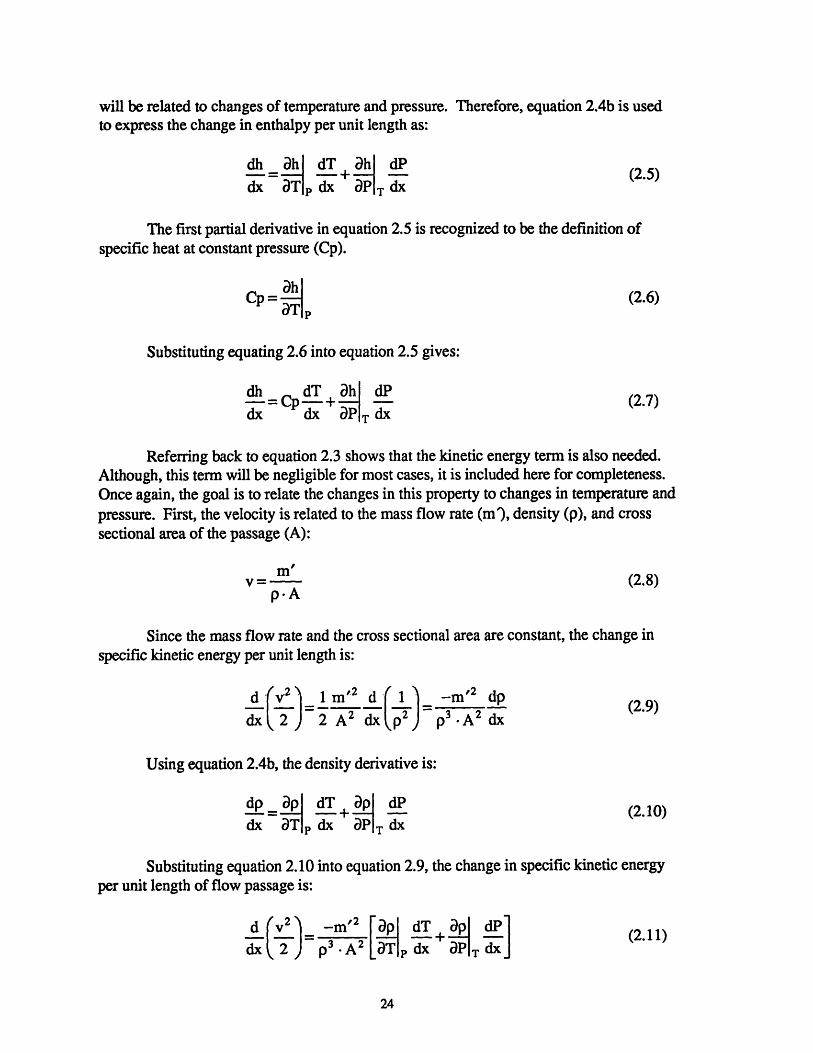
will be related to changes of temperature and pressure. Therefore, equation 2.4b is usedto express the change in enthalpy per unit length as:

dh Dh I dT ah dP-= - + d(2.5)dx aTjp dx aPT dx

The first partial derivative in equation 2.5 is recognized to be the definition ofspecific heat at constant pressure (Cp).

Cp = - (2.6)DTIp

Substituting equating 2.6 into equation 2.5 gives:

dh dT + ah dP-=Cp-+ • (2.7)

dx dx aPT dx

Referring back to equation 2.3 shows that the kinetic energy term is also needed.Although, this term will be negligible for most cases, it is included here for completeness.Once again, the goal is to relate the changes in this property to changes in temperature andpressure. First, the velocity is related to the mass flow rate (m), density (p), and crosssectional area of the passage (A):

m'v = (2.8)p-A

Since the mass flow rate and the cross sectional area are constant, the change inspecific kinetic energy per unit length is:

dlv2 1r m' 2 d( =1 -m'2 dp (2.9)dx 2 2 A2 dxp2) p3 .A2 dx

Using equation 2.4b, the density derivative is:

dp ~p dT+ dP (2.10)dx paT dx aPT, d

Substituting equation 2.10 into equation 2.9, the change in specific kinetic energyper unit length of flow passage is:

d(v 2 3- -m'2 ap _TdT ap dP- d , LaT p dg+(2.11)dx 2 p'3 ['g2 p' ax iTdx

Substituting equations 2.7 and 2.11 in equation 2.3 and rearranging gives thechange in temperature per unit length to be:

q m ap - h dP

dT m' p3 -A 2 TdxdT = p 2 (2.12a)dx m ap

CP -3A2 aT p

In cases where the kinetic energy term in equation 2.3 can be neglected, thetemperature change can be further simplified to be:

dT= q' L-a h dP (2.12b)dx m'. CCp Cp ap T dx

Equations 2.12 show that the change in pressure per unit length is needed.Assuming the flow can be represented by flow through a pipe, the pressure change alongthe passage is given by:

dP -f-p.v 2 -f -m' 2S= = (2.13)

dx 2 .Dh 2.Dh -p-A2

where f is the friction factor, p is the fluid density, Dh is the hydraulic diameter, and A isthe cross sectional area of the flow passage.

Substituting equation 2.13 into equations 2.12, the change in temperature per unitlength is:

q' 2 aph 1 f .m'2

dT m' p- d 2 D h -p AdT -PT PT 2 (2.14a)dx CP- m." p

And if the change in kinetic energy is negligible, equation 2.12b becomes:

dT q' f m' 2 hdT= +. (2.14b)dx m'-Cp 2-Dh 'p-A2"CP a1T

Therefore, the governing equations for steady state flow in a passage are:

q_ in' 2 a p f . M._ 2

dT m' P, p3 A P2 2-Dh-p-A

dx Cp m ap2 PCp - *A- aTp3 -A aT p

dP -f -m' 2

dx 2.Dh p-A 2

(2.15)

where equation 2.14b can be used in place of this dT/dx equation if the change in specifickinetic energy per length is small compared to the change in enthalpy per unit length.

Equations 2.15 can be used to create a finite difference model for finding theconditions throughout a flow passage. Appendix A shows how the property derivativescan be expressed in terms of the derivatives in the available computer software[HEPROP]. These relations allow equations 2.15 to be rewritten as:

(2.16)

And in cases where the change in kinetic energy per unit length is negligible, dT/dxcan be written as:

DPdT q' f. m' 2 1 T DTp

dx m'.Cp p pA2 apT

apI

(2.17)

dTdx

dP -f -m ' 2

dx 2.Dh -.pA 2

2.3 FINITE DIFFERENCE APPROXIMATION OF GOVERNINGEQUATIONS FOR USE IN COMPUTER SIMULATION

Using the equations for dP/dx and dT/dx, a finite difference model can be created.This model looks at the conditions throughout the flow passage at many locations. Eachlocation is considered to be a "node". As the nodes are placed closer and closer together,the derivatives of pressure and temperature can be approximated by the forward Eulerfinite difference equations [Strang, 562]:

dT Tx+ax - Txdx Ax

(2.18)

dP PX+Ax - P,dx Ax

where the subscript x denotes the node at location x and the subscript x+Ax denotes thenext node, which is a distance Ax away from the first node. Note that these equations canbe formally obtained by expanding T,+a and P+a& into Taylor series and ignoring theterms of 2nd order or higher:

(dT Cd2 T Ax 2 +dnT Ax n

+ T Ax + (-+....+ T nTx+ = Tx+---x + --x 2! " n!

(dx 2! )X n!

dp Ax 2 . p AX (2.19)

Px+A = Px + Ax ++..... + t "

For small values of Ax, higher order terms become negligible and equations 2.19 reduce toequations 2.18.

If the pressure and temperature at a given node are known, all properties at thatnode can be found. The derivatives dT/dx and dP/dx can then be found using equations2.16. Rearranging equations 2.18 shows a way to find the temperature and pressure at thenext node:

Tx+ax = T. + dT Axdx

(2.20)dP

Px+ax = P + dPAxdx

Using equations 2.20, the temperature and pressure throughout a flow passage canbe found for a given heat load and mass flow rate. The conductor is first divided up toplace nodes from inlet to outlet. Starting with a known inlet temperature and pressure,equations 2.16 and 2.20 are used to find the temperature and pressure at the second node.All properties can then be found at the second node. Similarly, the conditions are foundfor the third node and all remaining nodes. Along the way, checks are made to ensure thatthe temperature never rises above the maximum allowable temperature and that thepressure remains above 3 atm. The value of the temperature constraint is chosen based onstability requirements. The 3 atm pressure constraint is chosen to ensure that there is notwo-phase helium in the conductor. If either condition is violated, the mass flow rate orthe heat load can be varied until a valid combination is found.

Using the procedure described above, a computer program was written to find theconditions throughout a flow passage. The program was written in FORTRAN and isnamed CICC.EXE. A listing of the program is included in Appendix B.

2.4 SAMPLE RESULTS OF A SPECIFIC HELIUM FLOW PASSAGE

Using the program CICC.EXE, the conditions in a particular flow passage wereevaluated. The following assumptions were used:

* The heat addition to the helium (q') is constant throughout the flow passage.* A constant friction factor is assumed due to scatter of experimental data

[Katheder]. This represents an average value over most flow conditions.* No thermodynamic interaction between flow passages in adjacent turns of the

magnet is considered.* The heat transfer coefficient between the helium and the superconductor is

assumed to be large due to the large contact area. Therefore, the conductor isassumed to be at the same temperature as the surrounding fluid.

In addition, the dimensions and constraints listed in Table 2.1 were used. Thesevalues were also used in a study that performed a similar analysis using averaged fluidproperties [Hale]. The same values were used to allow a comparison and a check of theresults.

A brief note on the friction factor is appropriate. Studies of flow in CICC flowpassages have measured the friction factor for certain conductors [Katheder]. Whilecorrelations between the friction factor and the Reynolds number have been found, theyare not particularly accurate. Due to the large fluctuation in the measured friction factorand the uncertainty of the correlations, an average value of 0.15 is suggested by Kathederfor 6000 < Re < 15000. Therefore, this study assumes a constant friction factorthroughout the conductor flow passage.

Table 2.1: CICC Flow Passage Dimensions and Constraints That Were Used

Using the assumptions stated above and the values of Table 2.1, the programCICC.EXE was used to study the helium flow through the passage. The program searchesfor the maximum heat load that can be removed for given inlet conditions. To start,relatively low values are chosen for the heat load (q' and the mass flow rate (m). Theconditions are then found throughout the conductor. If the temperature at any location istoo high, the mass flow rate is increased until the temperatures are acceptable. The heatload is then increased slightly and the new mass flow rate is found. This procedure isrepeated until the heat load cannot be increased without violating either the maximum

temperature or minimum pressure constraint. Figure 2.2 shows the results of this studyby plotting the maximum allowable heat load for various inlet pressures and maximumallowable temperatures.

Figure 2.2 shows that the maximum heat removal occurs at a distinct inlet pressurefor each maximum allowable temperature. In addition, each curve has a "kink" at higherinlet pressures. These kinks mark the point where the flow switches from being able tofully use both the temperature and pressure constraints to a point where only thetemperature constraint can be fully used. However, this feature is irrelevant since it isundesirable to operate to the right side of the peak heat flux.

The lowest inlet pressure that can safely remove the heat load should be used.For example if 20 W must be removed with a maximum temperature of 6.0 K, it would bebetter to use an inlet pressure of 4.5 atm even though 11.5 atm would also work. Thereason to use the lower inlet pressure is that the higher inlet pressure will have a higherpressure drop (assuming the same minimum pressure is occurring at the outlet). Thehigher pressure drop implies a larger mass flow rate and larger pumping power. It thenmakes sense to use the lower inlet pressure since it would have a lower pumping powerrequirement.

.15

10

5

0

Maximum Heat Load vs Inlet Pressure and Maximum Allowable TemperatureL = 1140 m, Dh = 0.00054 m, A = 0.000116 m2, f = 0.15

T14.5KTxTmax= 6.0 K I mn3atm

.... ... .. .... i:~.... .... ... ... ... .... ..... ........-- 0-5.0

---- 5.1

-b-- 5.2

-e-5.4

--- 5.5

-W- 5.6---i--5.7

+--5.8-4-5.8

--1--6.0

3 4 5 6 7 8 9 10 11 12 13 14 15 16 17 18 19 20

Inlet Pressure (atm)

FIGURE 2.2: Maximum Heat Load that Can Be Removed versus Inlet Pressure

25-

20-T

Figure 2.2 summarizes the most important results for the modeling of thisparticular conductor. However, a more detailed investigation can give further insight intothe processes which control the amount of heat that the helium can remove. Therefore, astudy was done to examine what happens as the mass flow rate through the conductor isvaried. This study looked at the amount of heat that can be removed for different massflow rates instead of only looking at the point of maximum heat removal.

Once again, the dimensions and constraints listed in Table 2.1 were used. Theprogram CICC.EXE was used to find the heat load that can be removed for a range ofmass flow rates. Figure 2.3 plots the results. Curves are provided for several inletpressures. For all the curves shown, the maximum allowable temperature was set at6.0 K. Note that the peak value for each of the curves is the one that was shown inFigure 2.2.

Figure 2.3 shows that Figure 2.2 is slightly misleading. Figure 2.2 suggests thatyou would always want to run at an inlet pressure of about 7 or 8 atmospheres for amaximum allowable temperature of 6.0 K. While it is true that this would allow themaximum possible removal of heat, it is not necessary if a smaller amount of heat is beingremoved. Figure 2.3 shows that the lowest inlet pressure that can safely remove the heatshould be used. For example, consider a situation where 10 W must be removed from theconductor. By running at an inlet pressure of 4 atm, the heat can be removed with a massflow rate of about 0.6 g/s. Using an inlet pressure of 8 atm would require a mass flow rateof 1.5 g/s, which is nearly 3 times as much. It would be inefficient to run at an inletpressure of 8 atm due to the larger pumping power required to provide the higher massflow rate.

Even though low inlet pressures should be used, a word of caution is required.The sharp drop-off of the curves in Figure 2.3 indicates a possible danger of running tooclose to the peak heat flux. For example, Figure 2.3 shows an inlet pressure of 4 atmcould be used to remove 15 W from the conductor, However, if unforeseencircumstances cause the heat load to rise to 18 W, the 4 atm system could not remove theheat without violating the temperature or pressure constraints. Therefore, it is importantto consider the maximum steady state flux that might have to be removed when choosingthe steady state inlet pressure.

Figure 2.3: Maximum Heat Load that Can Be Removed versus Mass Flow Rate

The curves of Figure 2.3 all show a sudden drop. This drop can be explained byconsidering a pressure-enthalpy diagram. Figure 2.4 shows the conditions throughout theflow passage for several mass flow rates with inlet conditions of 4.5 K and 20 atm. Figure2.5 shows similar data for an inlet pressure of 8 atm. For each case, the maximumallowable temperature is 6.0 K and the minimum allowable pressure is 3 atm. On theseP-h diagrams, the lines of constant temperature bend due to the Joule-Thomson effect.The particular way that these lines bend is what limits the amount of heat that can beremoved from the flow passage.

For example, consider the curves for the 20 atm inlet condition of Figure 2.4. Atlow mass flow rates (curve a), the pressure drop is relatively low. Therefore, the limitingconstraint is the maximum temperature. For this case, the heat load can be adjusted untilthe outlet temperature is exactly on the 6.0 K line. As the mass flow rate is increased(curves b through d), the pressure drop becomes larger and the outlet condition movesdown the 6.0 K line. However, the slope of the 6.0 K line causes the outlet enthalpy tobecome closer to the inlet enthalpy. Integration of equation 2.3 shows that the heatremoved from the passage is:

Q' = q'-L = m'.(hout -hm) (2.21)

Q'= m' Ah

where the kinetic energy term of equation 2.3 was found to be negligible and is omitted.

Maximum Heat Load of Magnet vs Mass Flow Rate

Tin =4.5 K6 atm A 8atm Tmax =6.0K

20Vccl0-J 15

CD

0Elio

E0CI 5

02

0 0.5 1 1.5 2 2.5 3 3.5 4 4.5

Mass Flow Rate (g/s)

Pmin = 3 atm

15 atm

.... 20 atm.......... ....................20 arm

As the mass flow rate is increased, the Ah term decreases. So a tradeoff develops to findthe maximum value of the product m'-Ah. For this particular case, curve (a) has a large Ahbut a low m'. Curve (b) has a smaller Ah but a larger m' that allows a larger heat removal.Curve (c) has such a small Ah that even its large m' cannot make the product m'-Ah largerthan that of curve (b). Finally curve (d) has the largest mass flow rate but is incapable ofremoving any heat due a Ah of zero.

Figure 2.5 shows results for inlet conditions of 8 atm and 4.5 K. The importantdifference between this inlet condition and the 20 atm case is that the bend in the 6.0 Kline is now used for an advantage. Like curve (a) of Figure 2.4, curve (e) has a relativelylow mass flow rate. But this time the Ah is larger due to the divergence of the constanttemperature lines. Increasing the mass flow rate slightly would allow the exit condition tomove down the 6.0 K line. However, the sharp turn in the 6.0 K line allows curve (f) tobarely touch the 6.0 K line and then continue on until it hits the 3 atm minimum pressureconstraint. This allows a much larger Ah along with the increased mass flow rate.Attempting to further increase the mass flow rate without lowering the heat load wouldcause the pressure drop to be too large. Therefore, curve (g) has a large mass flow rate,but a reduced Ah since the pressure constraint is now the limiting constraint. Thistransition from simultaneously satisfying the temperature and pressure constraints (curvef) to only being able to use the pressure constraint (curves g and h) is the reason for thesharp drop-offs shown back in Figure 2.3.

The paths shown on Figures 2.3 and 2.5 are very similar to those shown byKatheder. In that study, the paths of maximum heat load were taken as straight lines. Thelines were drawn from the inlet condition to a point on the minimum pressure line along apath that just barely touches the maximum temperature (similar to curve f on Figure 2.5).Figure 2.5 shows that the paths are not always straight lines, but that the straight-line-method would give similar results.

Figure 2.4: Pressure-Enthalpy Diagram for Steady State Helium Flow - Pin = 20 atm

19-18s

17s16

15s1413

E 12-S11,

9.

7.6-

5.4.37

2100

Pressure vs Enthalpy:Effect of Increasing Mass Flow Rate on Available Enthalpy Rise of Fluid Stream

I40 K II I............. . .. ..... ........ . .................... . ......... ... ........ .. .... . ............... ..................... • ..................... :. ....................,

4.0 K. / /

..................... .......... . ..... . .. .................................... .. . .. /

S/5.0 K

of 8 atm, 4.5 K ......................... . 4.. K.... ... ....." ".. .... "..................... ..............................

.... .............................. .. ....... Tmax=0 ............... .... 1..0 ......... 2 ..... .. 3 3 0

0 5000 10000 15000 20000 25000 30000 35000 40000 45000Enthalpy (J/kg)

Figure 2.5: Pressure-Enthalpy Diagram for Steady State Helium Flow - Pin = 8 atm

Pressure vs Enthalpy:Effect of Increasing Mass Flow Rate on Available Enthalpy Rise of Fluid Stream

S.................................. ........... Flow Passage Inlet . ..... ... ..

..---...-..-...-.-.... .of 20 atm, 4.5K K ........ ..r• ••' - Flow Passage Outlet for Qmax20am

.....Y....Y.. .... Y.... .....................:..... .......... ... Y.. ...... ........4 .................................. I .................... ...................

INCREASING MASS FLOW RATE .....

II I"............................. r ....... ........................... .... ........................ ....................../ 1 1............" ..... .... .. ... .... .. .. ....L...... .......

4.5 K

;J ............... ......... .I............../ / /. .5 K. . ........ ..

555. KI

S5.5 K d 6.0 KPmin 3atmn I

.. .......... ..................... .................... ............ ........ ....... . . . ....................../.. ,. - , .k..- . ---" --. ..Tmax = 6.0 Ki I 1

30000 35000 40000 450000 5000 10000 15000 20000 25000Enthalpy (J/kg)

2.5 SIMILARITY BETWEEN FLOW PASSAGES ANDGENERALIZATION OF RESULTS

Although section 2.4 showed many useful results, they are limited to a specificflow passage. A more useful set of results would generalize the information for use with aflow passage of any size. Therefore, this section develops a method for determining whatconditions make flow passages behave similarly. In this way, the results obtained insection 2.4 can be scaled for use with passages of different sizes.

The first step to finding a scaling method is to notice what makes two differentflow passages behave in a similar way. The most obvious answer is that thethermodynamic conditions at the inlet, outlet, and all corresponding points in-between aresame in each passage. In other words, the inlet temperature and pressure will be the samein each passage, as will the temperature and pressure half-way through each passage,three-quarters of the way through, at the exit, etc. Therefore, the governing equations arereformulated to use the fraction of the distance along the conductor rather than anabsolute length. The dimensionless distance from the conductor inlet (X) is defined as:

X = - (2.22)L

where x is the distance from the CICC inlet and L is the total length of the conductor.

In addition, a dimensionless temperature (8) and dimensionless pressure (H) canbe defined by using a suitable reference temperature and pressure:

T PE=- , I = (2.23)Tef Pef

Next, equations 2.23 are substituted into equations 2.15 to find the dimensionlesschanges in pressure and temperature per unit length. Equation 2.12b is used to expressdT/dx since the results of section 2.4 indicate that the kinetic energy terms are negligible.Therefore, the dimensionless changes in temperature and pressure per unit length at agiven location (X) are:

dO q' L Pref (X) p 1 d() (2.24)([ 2 (X) - ( - - -(X) (2.24)dX m' Cp(X). Tf Cp(X).Taf p(X) IP p an le p(X) dX

-d () = 2 (2.25)

dX 2.p(X).Dh .A Pref

where f is the friction factor, Dh is the hydraulic diameter, A is the cross-sectional area, m"is the mass flow rate, and q' is the rate of heat transfer per unit length. Note that all fluid

properties, including the specific heat (Cp), density (p), and property derivatives arefunctions of the position in the passage (X).

As mentioned, two flow passages will have similar behavior if at each point (X),the two passages have the same dimensionless temperature (0) and pressure (Il). Toequate the temperature and pressure, equations 2.24 and 2.25 would have to be integratedfor each passage. However, we can avoid the integration by noticing that the slopes mustalso be the same since the distance has been normalized. Thus, for two conductors tohave the same temperature-pressure profile it must be true that at any location X:

dO dO dil dlIdX(X)= -- (X) and (X)= (X) (2.26)dX dX dX dX

where 1 denotes the first conductor flow passage and 2 denotes the second flow passage.

Combining equations 2.25 and 2.26 gives:

f -L, -m' 2 f2 L2 m;2= (2.27)

2.p(X)Dhi Al 2 .Pref 2. p(X).Dh2 A22 . Pef

Similarly, equations 2.24 and 2.26 are combined to show:

q' -Ll Pref 8(X) ( aX 1 1 1di+ [I(X -(X IM(X)

mi Cp(X). Tref Cp(X).Te p(X) " p a e( p(X) dX

1 .M(X• (2.28)q2 L2 Pref (X) anp ( 1 dH 2+ 2-(X) -(X(X)m2 C (X).T f Cp(X) Tf p(X)2 p n p(X) d

It was assumed that the temperature and pressure of each passage are the same atthe same value of X. Therefore, all other properties must also be the same. Since thebracketed term on each side of equation 2.28 involves fluid properties, it must be the samefor each passage. In addition, equation 2.26 states that the dimensionless pressure drop isthe same for each. Therefore, the second term on each side of equation 2.28 is the sameand equation 2.28 reduces to:

( (2.29)m; Cp(X)- Tf m; -Cp(X)- Trf

To find an expression which does not include the mass flow rate, equation 2.29 is squaredand multiplied by equation 2.27 to obtain:

f, L, q' -L, 1

2 Dhl A1 ) p(X) -C,(X)2 Tre2 f (2.30)(2.30)

f2 L2 (q 2 L 2 1

2 Dh2 , A2 p(X) C, (X)2 Tref2 'Pf

Since the density and specific heat will be the same in each conductor, those termscan be canceled. In addition the same reference conditions will be chosen for eachconductor and can also be canceled. Finally, the equation that allows scaling betweensimilar conductors is:

( \2L , q A-L 2 L g 2q_.L 2

f, I = f2 (2.31)

DhI A Dh2 A2

Note that this equation is independent of fluid properties and position. Therefore,the dimensional group of equation 2.31 must be a constant throughout the entireconductor. Conductors with the same inlet conditions and the same temperature andpressure constraints will be related by equation 2.31. A more convenient form of thisrelationship is to note that this value is a constant (C) which depends on the inletconditions and the constraints:

f = C(P, Tin, Pmin, Tmax) (2.32)

The most significant result of this relationship is that only one CICC geometrymust be evaluated in detail. Once the value of the flow constant C is found for all inletpressures and constraints of interest, any other geometry can be quickly evaluated. Ofcourse, the value of C could be found for any valid heat load, but the value at themaximum heat load is of the most interest. Using the data from section 2.4, the value ofthe flow constant at the maximum heat load was found for an inlet temperature of 4.5 Kand various inlet pressures. The results are shown graphically in Figures 2.6 and 2.7.

Flow Constant vs Inlet Pressure and Maxlumum Allowable Temperature4 A Ct" ,.... .. ...... .. ........ .............. ...... ......... .

3 4 5 6 7 8 9 10 11 12 13 14 15 16 17 18 19 20Inlet Pressure (atm)

Figure 2.6: Flow Constant at Maximum Heat Load - 2D Plot

Figure 2.7: Flow Constant at Maximum Heat Load - 3D Plot

1.4+1 I

4'1.2E+16E1E+16

* 8E+15

6E+15

S4E+158i" 2E+15

0

-*-5.0

---- 5.1

-6-5.2

-e-5.3

-o--5.4

-G-5.5

-i--5.6

-- 5.7--5.8

-4-5.9

--- 6.0

Flow Constant vs Inlet Pressure and Maximum Allowable TemperatureInlet Temperature = 4.5 K, Minimum Pressure = 3 atm

FlowConstantat Max

Heat Load(W2 m)

6.05.86Tm (K)

Tmax (K)


Equation 2.32 can be rearranged to make several important points. Equation 2.33shows how the flow passage dimensions affect the amount of heat that the helium canremove per unit length. A larger heat load can be removed by increasing the flow area andhydraulic diameter, and by decreasing the friction factor and length of the conductor. Thelength has a greater influence than that area or hydraulic diameter since it is raised to thenegative 1.5 power. For example, reducing the length by 50% will increase the possibleheat load per unit length by a factor of 2.8.

A IlDhf=A Dh C(Pi.Ti..'m m mT ..)q f (2.33)

Each point on Figures 2.6 and 2.7 represent a passage with a specificdimensionless temperature and pressure profile. Passages with the same flow constant willhave the same fluid properties at the same dimensionless distance through the passage.Therefore, the paths on a pressure-enthalpy diagram will be the same for conductors withthe same flow constant. Figure 2.8 shows the paths which allow the maximum heat loadfor several inlet pressures. Once again, an inlet temperature of 4.5 K, a maximumallowable temperature of 6.0 K, and a minimum allowable pressure of 3 atm are used.Notice that most of the maximum heat load paths are able to fully use both thetemperature and pressure constraint.

Pressure vs Enthalpy:Paths of Maximum Heat Load for Tin = 4.5 K and Various Inlet Pressures

................... ... ... .. .... . . . .. . . .. . .. . . . . .. . .. . .. . . .. . .. . .. . .. . .. . .. . . .. . .. . .. . .. . .. . .. . .

.2 oam = 0.1138*1016 W2An 44/./.0 K / .. I".... .................................

'.0 5 K K

.................... 0.................................78 6...... ..... .. ......................... ................ . .......... ... ........... . ...... .............. 0....................:. .... ...1 W. •: ................. ...... .................. .................. j........... ................... . ..5 =... .. .. .. .. ............ ......... ... . ........................5.5 K I Tmax =6.0K

............ ................. .... n =........... 3 atm.. 2 4 .. I ... I ......... . ........................................Cloatm= 1.127*10 / 4

... ......................... ......... ................... .. . .. . ... ...... 6. K ............ ..................

Cs atm = 1.236*1016 4W2Irrl4 / *1

6= W~/ 4 IC4 atm 0.634*1016 .2. ..I • ". .

................ .... ...... ............. ... ....... ..... .. .. -........................ ................................I............... ... .... ................ .. .......... .. ... .............................. ... ....... .... ........ ....... ..........

0 5000 10000 15000 20000 25000Enthalpy (J/kg)

Figure 2.8: Pressure-Enthalpy Diagram with Paths for Maximum Heat Load

30000 35000 40000 45000

------------------------..............

I3

The results show that the maximum temperature may not occur at the exit. Thisphenomenon is shown by plotting the same data shown in Figure 2.8 on the temperatureversus distance plot of Figure 2.9. This effect is related to the Joule-Thomson coefficient(defined as dT/dPIh). For positive values of the Joule-Thomson coefficient, a decrease inpressure will cause the temperature to decrease. In pipe flow, friction causes the pressureto decrease in the direction of flow. So, if the Joule-Thomson coefficient becomes largeenough, the temperature can show a net decrease in the flow direction even while heat isbeing added. Hale and Katheder show similar results. This effect should be consideredwhen estimating the maximum steady state temperature.

Figure 2.9: Temperature vs. Distance at Maximum Steady State Heat Load

The data can also be shown on the pressure versus distance plot of Figure 2.10 andthe temperature versus pressure plot of Figure 2.11. The pressure shows a nearly lineardrop through the passage with only slight curves due to the changing density. Thetemperature-pressure plot shows useful information, but it requires a brief explanation tobe understood. The passage inlet is at the bottom right of each curve. As the flowproceeds through the conductor, the pressure drops and the temperature rises. At acertain point, most of the curves show a decrease in temperature from Joule-Thomsoneffects. Once again, these curves are applicable to any regular passage under theconditions of the maximum allowable heat load with the same inlet conditions andconstraints as shown.

Temperature vs. Distance at Maximum Heat Load

5.8 C 1 .236*10' W'm

5.7 ".

5.6 - PP, = 20 atm

.55.3...... .. .... ....... 0.47 10 W m ........ ...........

i l D10 m = 4.5 KTmu = 6.0 K

9 Pin = 3 atm4.8.

4.60 0.1 0.2 0.3 0.4 0.5 0.6 0.7 0.8 0.9 1

Dimensionless Distance Through Flow Passage (x / L)

-~-- -

Pressure vs. Distance at Maximum Heat Load

0 0.1 0.2 0.3 0.4 0.5 0.6 0.7 0.8 0.9

Dimensionless Distance Through Flow Passage (x / L)

Figure 2.10: Pressure vs. Distance at Maximum Steady State Heat Load

Temperature vs. Pressure at Maximum Heat Load

3 4 5 6 7 8 9 10 11 12 13 14 15 16 17 18 19 20

Pressure (atm)

Figure 2.11: Temperature vs. Pressure at Maximum Steady State Heat Load

41

20-19-

18-

17-

16-15-

E 14-

V) 10-C.0. 9-

8-

7-

6-

5-

4-

3

, ........... ... ............................... .................. .................. ............ .. , 8 1 ~ w,....................................... ..... .................

· · · ·· · · Pk 20 atm

C= 0.478"10 W'/m........... .. .. .. . .... ... . .. .. .. ..... .. .. .................. . . . . . .. . ... ............ .. .. ....................I T ..5... .. .. .. .................... ....... ... ....................... ........... .......... ........ ................... ..... ............... .. .... J ..... ...... .. ...............................................................................................................=..0 .K ..................... •.................. -................ i.. ................ . ....................... .. . . . .. . . . . .........................tm..... : .................. ... . . .... ..TC0 =84.5'K....... ...... ... i ................. i ................. .. . . . . ..i.................. i.................. ...... . . . . .. . .. . . . . . .i......................................C= 0 6= 6.0 K

........I. .......... ...............................................PTin = 3.atm10 a=6.0mC. 1.127*10 lW2/m4

.. . . . . . . . . .i.• = v.• .............. ... ;;.. .......... . .................... .... ... ........... .. . .. ................. . .... .... ............... .......... ..... ..... ..... .................

...................................... . ....... ............ . ... .....- --. -........... ..... .............. ....................C.1.1W ........ ......... ............. .............. .... ..............

Pi 4 atmC -0.6346*10------

6-

5.9

5.8-

5.7-

5.6-

5.5-

a 5.4

5.3-

s 5.2-

a) S 5.1

4.9-

4.8-

4.7 -

4.6 -

4.5

T5 =94.5K

Tmax = 6.0 KPmi= 3 atm co 101 wmC -C 0••. 478 10 W/m

di.......................ion...................... ..........

S ..................................... f f... ..............

E i .id irection................ . . . . . . . . .... ..... .............. " .......... . .. .......... . .... ......... ........ .iC-1 1. 1 6 '(

' " " of flowo

....... ........ ..... ....... ........ ........... in le t ..........

C4 -C 0.634 101C W.m47

The generalized data can also show how efficiently the heat is removed from thepassage. The entropy generated in the passage is used to measure this efficiency. A lowerentropy generation signifies a higher heat removal efficiency. Figure 2.12 shows the ratioof the entropy generated in the flow passages to the entropy removed from the walls ofthe passage. Once again, the data at the maximum heat load was used for each curve.The results show that the entropy generation is lower at lower inlet pressures for a fixedallowable temperature. The results also show that allowing higher temperatures reducesthe entropy generation for a given inlet pressure.

The curves are drawn to the point where the flow goes from being able to matchboth the temperature and pressure constraints to only matching the temperature constraintat the maximum heat load. Due to this sharp change, no results should be extrapolatedbeyond the curves shown.

Figure 2.12: Steady State Entropy Generation in Magnet

Ratio of Entropy Generation in Magnet to Entropy Removed from Magnet atMaximum Heat load vs Inlet Pressure and Maximum Allowable Temperature

I-

ITin4.5 K6

5

4

3

2

1

03 4 5 6 7 8 9 10 11 12 13 14 15 16 17 18 19 20


2.6 CONCLUSIONS

The steady state modeling of helium flow through a passage resulted in thefollowing conclusions:

* A finite difference model can be used to study the steady state heat removalcapability of helium flowing through a passage.

* Computer programs using the finite difference technique found the maximumamount of heat that can be removed from a passage for given inlet conditionsand constraints.

* The results can be generalized for use with passages of different sizes.

* Passages with the same temperature and pressure profile along the normalizeddistance through the passage (X) will have the same value of the flowconstant (C) presented in equation 2.32.

* The flow constant is a function of the inlet conditions.

* The flow constant at maximum heat load is also a function of the temperatureand pressure constraints.

* Equation 2.33 can be used along with Figure 2.6 to estimate the maximumamount of heat that can be removed from a given flow passage.

* In practice, passages should include a safety margin by being designed tooperate below the maximum heat load as calculated by equation 2.33.

* To reduce steady state pumping power, cooling systems should use the lowestinlet pressure that will allow the heat load to be safely removed.

* The steady state entropy generation in the flow passage can be reduced byrunning at lower inlet pressures and allowing higher temperatures in the flowpassage.

* When operating at high heat loads or in lower pressure regions, the maximumtemperature in the flow passage may not occur at the passage outlet due tothe temperature drop associated with Joule-Thomson effects.

3. PUMPING ISSUES

This chapter contains three sections. Section 1 describes the reasons for studyingpumping issues related to the cooling of cable-in-conduit conductor SMES magnets.Section 2 examines the effect of the pump efficiency on the total refrigeration heat load.Section 3 looks at the effect of placing the pump at a location where it can pump colder,denser helium. Section 4 summarizes the conclusions.

3.1 MOTIVATION BEHIND THE STUDY OF PUMPING ISSUES

A cable-in-conduit conductor (CICC) is cooled by forcing cold helium through theconduit. The helium picks up heat energy as it flows in contact with the numeroussuperconducting strands. The pump (or compressor) that produces this flow of heliumalso adds energy to the helium. In a continuously operating magnet system, the energyfrom both the magnet conductor and the pump must be removed so that the helium can bereused to cool the conductor. Therefore, the refrigeration system must be designed toremove the combined heat load of the magnet and the pump.

Most studies concentrate on magnet issues and neglect the pump needed to coolthe magnet. However, the pumping power can be the dominant load on the refrigerationsystem. A poorly designed refrigeration system could require a large pumping power tocool the magnet. The system would require a larger and more expensive refrigerator thanif it were properly optimized to reduce the pumping power.

To minimize the size of the refrigeration system, it is important to consider thefactors which affect the pumping power. This chapter looks at two of these factors.First, the isentropic efficiency of the pump is considered. Second, the location of thepump in the cooling loop is examined.

3.2 EFFECT OF PUMP EFFICIENCY ON THE TOTALREFRIGERATION LOAD

The isentropic efficiency of a pump affects the power required for the pump toincrease the pressure of a fluid. An inefficient pump requires more energy than an idealpump. In a SMES system, any extra pumping power will increase the refrigeration load.Therefore, an inefficient pump can increase the size of the refrigerator needed. Thissection looks at how the pump adds to the refrigeration load and how the pump efficiencydetermines the amount the load is increased.

3.2.1 EFFECT OF PUMPING POWER ON REFRIGERATOR LOAD

Figure 3.1 shows a possible configuration for cooling a SMES magnet. Highpressure helium circulates in a closed loop (ABCD). Helium exits the pump at location Aand is then cooled in a heat exchanger that is inside a pool of liquid helium. The heliumenters the magnet at B and then absorbs heat from the magnet. After leaving the magnetat C, the helium returns to the pump to be recirculated. This configuration is called arecirculator loop.

rator

pump Q magnet

D C

Figure 3.1: A Possible SMES Cooling Configuration

%teadv otate heat Inad

I] Q'magnet

W'pump

ID C I

Figure 3.2: Energy Balance on Recirculator Loop

Figure 3.2 shows the recirculator loop with a control volume drawn around it.The steady state energy balance is given by:

Q'oad =Q'magnet +Wplump (3.1)

It is apparent that the refrigerator must remove the heat load of both the magnetand the recirculating pump. A low efficiency pump will require a large power input andwill increase the heat load on the refrigerator. To study this effect, steady state models ofthe recirculator loop were made.

3.2.2 SIMPLE MODEL OF STEADY STATE RECIRCULATOR LOOP

To illustrate the effect of the pump efficiency on the refrigerator load, a simplemodel can be used. The three equations which determine the heat flows in the recirculatorloop are:

Q'magnet=(h e - h g).m' (3.2)

Wump = (hA -hD )m' (3.3)

Q'lo`= (hA - ha)" m' (3.4)

where m' is the mass flow rate and h is the specific enthalpy.

The equation which relates the enthalpy at the pump inlet and outlet is:

1hA =hD +--.(hA -hD) (3.5)

where ri is the pump's isentropic efficiency and h As is the ideal exit enthalpy of the pump.

To analyze the system performance, the conditions in the loop are needed. First,the conditions at locations B and C are chosen. Assuming there are no losses between themagnet exit and the pump, the conditions at D are the same as at C. Assuming that thepressure drop across the pool heat exchanger is small, the pressure at A is nearly the sameas at B (PA = PB). Using the pressure at A and the conditions at D, the ideal (isentropic)enthalpy at A is found. Using equation 3.5, the actual conditions at A can then found.Once, all conditions are known, equations 3.2 through 3.4 are used to evaluate the heatloads.

For this study, the magnet inlet temperature (TB) was taken to be 4.3 K, themagnet exit temperature (Tc) was 5.0 K, and the pressure at the pump exit (PA) was10 atm.

The pressure drop across the magnet was varied to simulate different frictionalcharacteristics of the magnet. Figure 3.3 shows the ratio of the refrigerator heat load tothe magnet heat load. As expected, the pump's isentropic efficiency affects therefrigerator's heat load. For example, a system with a 50% efficient pump has arefrigerator load that is about 30% larger than a system with a 70% efficient pump.

Figure 3.3 also shows how the refrigerator heat load increases as the pressure dropincreases. For example, if the pressure drop across the magnet is 0.5 atm, the refrigeratorheat load is about 30 to 40 % larger than the heat load removed from the magnet. But fora 2 atm drop, the refrigerator heat load is 200 to 300 % larger than the cooling supplied tothe magnet. Therefore, the pressure drop across the magnet should be kept to a minimumto reduce the size of the refrigerator required.

0.0 0.5 1.0 1.5 2.0 2.5 3.0Pressure Drop in Recirculating Loop: PA " PD (atm)

Figure 3.3: Ratio of Refrigerator Heat Load to Magnet Heat Load versusPressure Drop in Recirculator Loop

Ratio of Refrigerator Refrigerator Heat Load to Magnet Heat Load vs.Pressure Drop Around the Recirculator Loop

5.5 -

5.

c 4.5

E 43.5-

23-

2-1.5-

1

PA = PB = 10 atmTB = 4.3 K

T. = TD = 5.0 KT pool = 4.2 K.. ...

.... 100%.. . . . . .. .. . . ..." . . .. . . . .. . . . . ... . . . .. . . . . .. . . .. . . . . .. . . . . .. . . . . .. . . . .. . . .. .. . . . .

00

Another way to measure the impact of the recirculator loop is to look at theentropy generated in the loop. Entropy generated in the magnet, in the pump, and in thepool heat exchanger will increase the entropy load on the refrigerator. Figure 3.4 showsan entropy flow diagram. Entropy is removed from the magnet (Smagn) and put into therecirculator loop where it passes through the pump and finally into the helium pool of therefrigerator. The entropy generated along the way must also be removed. Therefore, theentropy load of the refrigerator pool (Sod) is larger than the entropy removed from themagnet (Smanet):

Sioa = Smagnet + Sgen (3.6)

Where the total entropy generation (Sgen) is the sum of the entropy generated in themagnet, pump, and heat exchanger:

Sgen = Sgenmagne,+ Sgenpmp + SgenHx (3.7)

For this model, no entropy generation was considered inside the magnet (i.e.Sgenm.agne= 0, Sin = Smet). Only the entropy generated in the pump and in the heattransfer of the pool heat exchanger were included. However, these two components alonecan add a significant amount of entropy to the system. Figure 3.5 shows the influence ofthe pump's isentropic efficiency. A system with a perfect pump would increase theentropy load by about 10% while a 50% efficient pump could create 80% more entropyload on the refrigerator. It should be noted that most magnets are designed for a pressuredrop under 1 or 2 atm. However, Figure 3.5 shows the dramatic influence of largerpressure drops on a low efficiency pump.

POOL HEATEXCHANGER

RECIRCULATORPUMP

MAGNET TORECIRCULATOR

HEAT EXCHANGE

d by refrigerator pool

from recirculating loop

y recirculating loop

ved from magnet

Figure 3.4: Entropy Flow Diagram of Recirculator Loop

Ratio of Entropy Generated in Recirculator Loop to Entropy ReceivedFrom Magnet vs. Pressure Drop Around the Recirculator Loop1

0.9

0.8-

0.7-

0.65-

e o.0.4 -

0.3-

0.2-

0.11

00.0 0.5 1.0 1.5 2.0 2.5 3.0

Pressure Drop in Recirculating Loop (atm)

NOTE: No entropygeneration was consideredin the magnet itself. (Sgenin pump and pool HX only).

Also, no pressure dropwas considered in poolheat exchanger. (dP inmagnet only).

Figure 3.5: Entropy Generation in Recirculator Loop

3.2.3 STEADY STATE RECIRCULATOR LOOP MODEL USING CICCCHARACTERISTICS

The simple model illustrated how the recirculator pump increases the load on therefrigerator. That model assumed that the conditions at the magnet inlet and outlet can bechosen arbitrarily. A more detailed model would find these conditions by including thecharacteristics of the conductor in the magnet. This section illustrates how the conductormodel of Chapter 2 can be used as a part of a larger model of the entire recirculator loop.In Chapter 5, the model will be further enhanced to include more detailed characteristicsof the pump and heat exchangers.

The magnet was modeled using the finite-difference technique of Section 2.3. Themagnet inlet and outlet conditions were taken from the example in Section 2.4.1Equations 3.2 to 3.5 were then used to evaluate the recirculator loop performance. Aprogram' was written to solve the equations.

Figure 3.6 shows the ratio of the refrigerator heat load to the heat removed fromthe magnet. This ratio is the multiplying factor by which the recirculator loop increasesthe load on the refrigerator pool. In a perfect system, no pump power would be requiredand the ratio would be 1.0. However, a real system requires pumping power to force the

This example found the maximum amount of heat that could be removed from the conductor for variousmass flow rates. Data from this example is also plotted in Figure 2.3.

2 program named CICC4.EXE. see appendix for listing

P. = 10 atm Isentropic Efficiency = 50%0.....TB = 4.3 K . ....................... ................ ..............i........• •. ...Tc = ToD 5.0 KTpool= 4.2 K ......................

.... 100% ."". .i.

helium through the magnet. The pump power adds to the refrigerator load, making theQ'lo" / Q'mag•,• ratio greater than 1.0.

Figure 3.6 shows three trends. First, as the heat load on the magnet is increased,the recirculator loop has a larger multiplying effect on the refrigerator load. This is causedby the additional pumping power required to supply more mass flow at higher heat loads.Second, a low efficiency pump requires more pumping power and further increases theload on the refrigerator. Finally, a lower magnet inlet pressure can reduce the refrigeratorload due a lower pumping power requirement. However, this assumes that a pump can befound to match the pressure drop and mass flow rate calculated by the model.

This example shows that cooling system models should include the effect of thepump on the refrigeration load. It also shows how the model for any conductor can beused as a part of the overall system model.

The curves of Figure 3.6 are drawn to the point where the flow goes from beingable to match both the temperature and pressure constraints to only matching thetemperature constraint at the maximum heat load (see section 2.4). Due to this sharpchange, no results should be extrapolated beyond the curves shown.

Figure 3.6: Ratio of Refrigerator Load to Heat Removed from Magnet

Ratio of Total Refrigerator Heat Load (Q'load) to Heat Removed fromMagnet (Q'magnet) vs. Heat Removed from Magnet (Q'magnet)

Z.Z

2-

1.86

1.6

1.4

S 1.2-

1

0 5 10 15 20 25Heat Load Removed From Magnet: Q'magnet (W)

PA = 8 atmIsentropic Eff. = 50%Isentropic Eff. = 70%

.................................... Isentropic Eff. = 100% ...............................Tmax = 6.0 K

...] r a in -- 0 C ,, , I 'I ........................... ........... .... .. .............. ...... ..... ....... ...... .. ...... ............... ............. ................. I.......... ....... ................ ........ .... ......... ....... .P'Iminr = atmlL = 1140 mD h = 0.54 m m ....................... ......... ......................... .........PA=4 atmA= 116 mm 2 = aimS= 0.15 ~50% Isentropic Eff.

.If = 0.015e tri' ...... .... .... ......... ....................... ........ • -. '- ...7. .. n - _ - -. ... ". E ., __ •-- -" -- -- .; ' 1700%/ Isentropic Eff.

4bt a E '100% Isentropic Eff.

3.3 COLD PUMPING

Another way to reduce the refrigeration load is to place the recirculator pump at thecoldest part of the recirculator loop. Pumping colder, denser helium will reduce the pumppower. This reduction can be explained by looking at the equation which determinespump work for an ideal, steady state pump [Jones, 33]:

w=Jv.dP (3.8)

where w is the pump work per unit mass, P is the pressure, and v is the specific volume.

Equation 3.8 shows that the ideal pump work is proportional to the specific volumeof the fluid flowing through the pump. The work required to produce a given pressurerise can be reduced by pumping a cold, high density (low v) fluid. This concept can beillustrated by comparing two ideal pumps.

Figure 3.7 compares ideal pumps operating between 3 atm and 5 atm. One pumphas a fluid inlet temperature of 4.5 K while the other is one degree warmer at 5.5 KThe paths for ideal pumps are shown as a dark line. The area under this line is equal tothe required pump work (equation 3.8). The area under the 4.5 K curve (diagonalpattern) is 29% less than the area under the 5.5 K curve (horizontal pattern). Thus, a1.0 K reduction in inlet temperature can significantly decrease the required pump work.

Figure 3.7: Effect Fluid Temperature on Ideal Pump Work

Figure 3.8a shows a recirculator loop that places the pump immediately after themagnet. The helium entering the pump is relatively warm from the energy it gained in themagnet. A better design would recool the helium before it enters the pump. Figure 3.8bshows a cold-pumping configuration. An additional heat exchanger is added to the loopso that the pump receives cold helium at D. In this system, the temperatures at B and Dshould be as cold as possible and approximately equal. Therefore, heat exchanger 2(HX2) is designed to remove the magnet load and heat exchanger 1 (HX1) is designed toremove the pump power.

Liquid Pool

Figure 3.8a: Warm Pumping Figure 3.8b: Cold Pumping with Re-Cool

The two cooling configurations can be compared by using the generalized conductordata of section 2.5 to model the magnet. This data can be used to obtain the conditions atB and C. The conditions at D are found by either assuming that they are the same as at Cfor the warm pumping system, or by assuming HX2 is sized to re-cool the helium to thesame temperature as at B. Equations 3.2 to 3.5 are then used to evaluate the systemperformance.

Once the data from section 2.5 is used to find the conditions at B and C, theconditions at A and D are fixed by the assumptions stated above. Since all conditions arefixed, the ratio of pumping power to rate of heat removal from the magnet will be constantfor a given magnet operating condition:

Wpump (hA -hD) ' m' (hA-hD)Q•agnet (hc -h ).m' (hc -hB)

The data that was used to find the properties at B and C is for the maximumallowable heat removal in the magnet. Therefore, the W',.p / Qma., ratio will be afunction of the magnet inlet conditions and the constraints. This ratio also depend on thecooling configuration, which sets the conditions at A and D. Therefore, the ratio is a

I -u *.A•au ntm hmat ,A I-

D C

t

|

constant for a given cooling configuration and a given set of magnet inlet conditions andconstraints:

Wpu = S(P jin, ,,Pmin,Tmax,configuration)magnet

(3.10)

For a given set of conditions at B and C, the warm pumping power and coldpumping power can be compared by using equation 3.10:

(hA -hd)warm

(Wpump)cold (hA-hbd)cld

(hc - hB)

(WP•MP)wan

uragnp cold

magnet

3(Pin,Tim,PminTmax,warm)

3(Pin, Tin, Pmin, Tmax, cold) (3.11)

Figure 3.9 shows the ratio of warm pumping to cold pumping. Figure 3.10 showsthe ratio of pumping power to the rate of heat removal from the magnet for both the coldand warm pumping configurations. For each case, the magnet inlet temperature is 4.5 Kand the minimum allowable pressure is 3 atm.

3 3.5 4

Ratio of Warm Pumping Power to Cold Pumping Powerat Maximum Heat Load

7 7.5 84.5 5 5.5 6 6.5Loop Inlet Pressure: PA = PB (atm)

Figure 3.9: Ratio of Warm to Cold Pumping Power at Maximum Heat Load

5.5 K 4.5 K

S5.0 K

5 . ............... .................. ........... ........ ......... ......... ......... ........I I I

Figure 3.10 Ratio of Pumping Power to Heat Removedfrom the Magnet at Maximum Heat Load

Figure 3.9 shows that pumping the helium at a colder temperature will reduce theamount of pump work. The difference between warm and cold pumping becomes greateras the maximum helium temperature in the magnet is increased. This occurs since thewarm pumping is done at approximately Tm,, while the cold pumping is always done at4.5 K. Therefore, the difference between warm and cold pumping becomes greater asTm. is raised.

Figure 3.10 shows that the refrigerator load decreases when cold pumping is used.Therefore, cold pumping can reduce the size of the refrigerator required.

The plot also shows that allowing higher temperatures can significantly reduce thepumping power due to the lower mass flow requirement.

Section 2.4 showed that, when the temperature is constrained, there is a practicallimit to the conductor inlet pressure. Above this limiting inlet pressure, no more heat canbe removed. Therefore the curves of Figures 3.9 and 3.10 are only drawn up to thelimiting inlet pressure. Results should not be interpolated beyond the curves shown.

1.8.

1.6

1.4-

S1.2E

1C

E1 0.8-

0.6

0.4.

0.2-

0

Ratio of Pumping Power to Heat Removed From Magnet atMaximum Heat Load, Pump Isentropic Efficiency = 70 %

Warm Pump A = 4.5 K........... o d P m .. ........ ...... ............................ .. .. .. .. .. .. ........ ........... ..................................... ......................... ...................... ........: ~ " = 3 a m ...ColdPup - I ip i P = 3 atm

... .. ............. ........ ........ .... ...... .. ... .............. ............. ...... ........ ..... . ... ..... .... .... ... ..... ........ ....... .................. .. ................ ........ .... ..STmax = 5.0 K i

................. •................. •................. ..... • ......... ................. .................-- - -] ........ :............ ...i................. •................................. ......... .......... ....... ...... .....K

....................

.... . ... 5.5 K

................................... .................. ................. ................... ................ ........ ....... ...... ... .. ... . ,, ......................... ..... .. ... . ...... .... ... .. • .. ... :.... ....... ........ .. ................ ............. ... ... ... .... . .................. . ...: ......................

.......... ... .. ... .. ... .. . - ... ..... .. ............. ............................................ ...................... .i. ............. 6 . K ............. --.." 7 .- .. .... .... ... ........ ... ........ .... ............ ............ .................... . . 0 .....

3 3.5 4 4.5 5 5.5 6 6.5 7 7.5 8 8.5


3.4 CONCLUSIONS

The study of SMES pumping issues resulted in the following conclusions:

* In a recirculator loop cooling configuration, the refrigerator must remove theheat load of both the magnet and pump.

* The recirculator loop acts as a heat load multiplier by rejecting more heat tothe refrigerator than it removes from the magnet.

* Low efficiency pumps will increase the load on the refrigerator.

* The pump power can be reduced by re-cooling the helium before entering thepump.

* The pressure drop across the magnet should be minimized to reduce thepumping power required.

* The CICC model of Chapter 2 can be used as a part of a larger recirculatorloop model which includes the pump and heat exchanger(s).

* Lower magnet heat loads will require less helium flow and less pump power.

* To reduce pumping power, systems should be designed to run at much lessthan the maximum allowable heat load.

4. BUFFER SYSTEMS

This chapter contains 4 sections. Section 1 describes reasons for using a bufferin a SMES refrigeration system. Section 2 lists the results of the buffer system models.Section 3 discusses the buffering schemes that were analyzed and the thermodynamicmodels that were used. Section 4 summarizes the conclusions.

4.1 MOTIVATION BEHIND THE STUDY OF BUFFER SYSTEMS

When a SMES magnet is charged or discharged, AC losses deposit heat energyin the conductor. The refrigeration system must remove this energy to keep theconductor cold. However, this heat is deposited at a much higher rate than the steadystate refrigerator load. Only a high power refrigerator could remove this energy "pulse"at the same rate as it is deposited. This refrigerator would be expensive and oversizedfor most times of operation.

A buffer system temporarily stores the pulse energy in some material or fluid(usually helium). After the pulse, the refrigerator can slowly remove the stored energy.Therefore, the refrigerator can be smaller than if it had to remove the energy at the fullpower level of the pulse. In effect, a buffer system "averages" the transient loads over along period of time so that a smaller refrigerator can be used.

While there are many possible buffer systems, some must be much larger thanothers to store a given amount of energy. In most applications, the space for a buffer islimited. Therefore, this chapter looks at which systems can store the most energy pervolume.

4.2 RESULTS OF BUFFER SYSTEM MODELING

Several buffer systems were considered. The results are summarized in Table4.1. The evacuated tank concept can store the most energy per volume, but could bedifficult to carry out in a real system. The divided tank allows the second most energystorage, but an actual system may not perform as well as the ideal system that wasmodeled. The closed container with two-phase helium is probably the most practicalsystem. Each of the systems are described in the next section.

Table 4.1: Comparison of Energy Storage Methods

METHOD SPECS ENERGY STORAGE PUMP PROS CONSPER VOLUME (J/m3') WORK

1. Boiling At 1 Start with none Simple. Poor Q/Vatm With An saturated liquid, ratio dueExpandable end with saturated 344,000 Constant to largeExternal Tank vapor. (No Temp of vaporTo Hold Vapor superheat allowed 4.2 K volume.

to keep at 4.2 K)2. Heat Start with . 285,000 (Tm, = 5 K) pressurize Simple Pressure

Compressed compressed liquid (22 to 27 atm) once when vesselLiquid In at 4.2 K. 659,000 (T. = 6 K) filling required.Closed Optimum Pma (28 to 39 atm) tank RequiresContainer varies with Tu, temp rise.

3. Heat 2-Phase Start at 4.2 K, two 424,000 (T,, = 5 K) none Simple. RequiresHelium In phase liquid (xlit = 0.37) temp rise.Closed 720,000 (T. =6 K)Container (xlwt = 0.07)

4. Heating Two- Start at 4.2 K. none -- MorePhase Helium Two phase in main complexWith A Rigid tank, saturated 727,000 (Tm = 6K) than 3, butExternal Tank vapor in external (V2/V1=0.36) no gain.To Hold Vapor tank.

5. Heat Liquid Start with Pump Very Hard toHelium in saturated liquid at 806,000 (Tn = 5 K) enough to Good maintainEvacuated 0.1 atm.(T=2.5 K). 1,15.8,000 (T,. = 6 K) remove Q/V ratio 2.5 K.Closed Close and add heat boil-off RequiresContainer at constant density. vapor vacuum

pump.6. Divided Tank Insulated float 795,400 (T,=, = 6 K) none Good Requires

With Energy divides tank into a pm = 125 kg/m3, xa1 = 0.0 Q/V ratio temp rise.Transfer To section at 4.2 K P2 = 4atm, r = 0.66, d = 0.5Environment and a section at (assumed no conduction

300 K. Pi= 1 atm losses)

4.3 COMPARISON OF POSSIBLE BUFFERING SYSTEMS

A buffer system stores thermal energy by either increasing the temperature orchanging the phase of a substance. Helium is the best substance for storing energy in thetemperature range of interest (~ 4.2 to 6 K) since it changes phase and has a highspecific heat.

Several options for storing energy in helium were looked at. They may beclassified as either boiling or heating in a closed container. Boiling maintains a constanttemperature, but requires a large volume to hold the vapor that is produced. The closedcontainer uses a smaller volume, but requires a temperature rise. Table 4.1 summarizesthe results of the study. The remainder of this section describes the buffer systems thatwere studied and the thermodynamic models that were used.

4.3.1 BOILING AT 1 atm WITH AN EXPANDABLE EXTERNAL TANK TOHOLD VAPOR

Figure 4.1 shows a buffer system that absorbs heat by boiling helium at 1 atm.The advantage of this system is that the temperature remains constant at 4.2 K.Therefore, there is little danger of the magnet temperature rising. However, thedisadvantage is that the vapor takes up much more volume than the liquid. Therefore, alarge external tank is required to hold the vapor being produced. The model for thissystem assumes that the external tank can expand to always keep the pressure at 1 atm.This leads to a large final volume V2nnal and a relatively small energy storage per totaltank volume.

The model also assumes that the rigid tank starts with saturated liquid and theexpandable tank starts at zero volume. At the final state, saturated vapor exists in bothtanks. Therefore, the energy storage per volume is the product of the vapor density andthe heat of vaporization:

QS -hfg (4.1)V1 + V2rml

Figure 4.1: Boiling at 1 atm With an Expandable External Tank to Hold Vapor

4.3.2 HEATING COMPRESSED LIQUID IN A CLOSED CONTAINER

The large tank to hold vapor can be eliminated if the helium container is notvented and the temperature is allowed to rise slightly. The tank can be initiallypressurized to fit more mass in the container. As heat is added, the pressure andtemperature will rise. Since the tank volume and mass are fixed, this is a constantdensity process and the final conditions are easily found. The energy storage per volumeis given by the overall density times the change in specific internal energy:

Sp (U Tal - U iial,Tinitial) (4.2)

A program' was written to find the optimum starting pressure for a startingtemperature of 4.2 K and different final temperatures. These values are listed in Table4.1 along with the heat stored per volume. This process could allow more heat to bestored per unit volume than the boiling of method 1. However the temperature risecould create problems for the magnet stability if the tank is in direct contact with thefluid flowing through the magnet.

4.3.3 HEATING TWO-PHASE HELIUM IN A CLOSED CONTAINER

Another closed container concept uses two-phase helium that starts at 4.2 K and1 atm. This is a constant density process, which can be evaluated using Equation 4.2.A program2 was written to search for the optimum initial density (which fixes the initialquality). The program showed that this method can store more heat per unit volumethan the compressed liquid of method 2. Although the 1 atm helium is less dense thanthe compressed liquid, the latent heat allows more energy to be stored per volume ofcontainer. However, as in method 2, a temperature rise is required.

4.3.4 HEATING TWO-PHASE HELIUM WITH A RIGID EXTERNAL TANKTO HOLD VAPOR

Instead of confining the helium to a closed tank, a rigid external tank can be usedas an "overflow" for some of the vapor produced. This system would be easier todesign and require less volume than the expandable tank system of method 1.

Figure 4.2 shows the setup of the tanks. Heat is added to tank 1, which startswith two-phase helium at 4.2 K. As heat is added, the liquid and vapor change density.However, the densities change at different rates, causing vapor to move from tank 1 totank 2. This vapor removes energy from tank 1 since it has a higher enthalpy than theliquid. Removing this energy could allow more heat to be added for a given temperature

1 The program is named rigid2.for. See appendix for listing.2 The program is named rigid4.for. See appendix for listing.

change in tank 1. A program3 was written to evaluate this system for various volumeratios. The program uses a differential model to tabulate the amount of heat absorbed asthe temperature in tank 1 increases by tiny amounts.

Figure 4.3 shows that, if the ratio of the tank volumes is 0.36, this system canstore about 1% more energy than a single closed tank (V2/V1 = 0). However, thisanalysis neglected heat leaks. In a real system, the extra surface area of the second tankwould add to the heat leak and probably eliminate this small advantage. Therefore, thismethod does not seem to be any better than using one closed tank (method 3).

Tank 1

Tank 2

Figure 4.2: Heating Two-Phase Helium with a Rigid External Tank

Energy Absorbed per Volume vs Volume Ratio of Tank 1 to Tank 2

Figure 4.3: Energy Storage per Volume for Two-Tank Buffer System

3 The program is named double3.for. See appendix for listing.

720

. 710

700

. 690-680

+ 670T-

> 660

0 650

640

6300.00 0.20 0.40 0.60 0.80 1.00 1.20 1.40

V2 / V1

4.3.5 EVACUATED CLOSED CONTAINER

Another way of storing energy in a closed container is to start with liquid heliumat a pressure much lower than 1 atm. This would decrease the initial temperature in thetank and allow more energy to be absorbed than if the tank started at 1 atm. Using avacuum pump, a container with saturated liquid helium could be kept at a low pressure.Just before the pulse load, the container would be closed. Heat could then be added tothe container in a constant density process. As shown in Table 1, this method allows arather large amount of heat to be absorbed per unit volume. However, cooling andmaintaining saturated liquid at low pressures (and temperatures) could be difficult. Andonce again, the temperature rise could create stability problems for the magnet.

4.3.6 DIVIDED TANK WITH ENERGY TRANSFER TO ENVIRONMENT

The size of the storage system could be reduced if the ambient environment isused to store some of the energy. A direct heat transfer to the environment would warmthe system undesirably. However, the system can be kept cold if the heat is transferredto the environment via a work transfer. A theoretical sketch of such a system is shownin Figure 4.4.

The system uses a rigid container that is divided by an insulated float into 2compartments. Compartment A holds cold helium and is where the magnet energy isrejected to. Compartment B holds warm helium that is in thermal contact with theambient environment. As heat is added to A, the helium in A expands and increases inpressure. This expansion causes the float to rise upward and compress the warm heliumin B. Since B is held at a constant temperature via contact with the ambient, thecompressive work done on B will be rejected to the atmosphere through the ideal gasrelation:

Qout = WAB = mBRHeTambient n(VBnital (4.3)

As compartment A is re-cooled, the float will move back down. Heat will betransferred back from the ambient to compartment B and then to A through a worktransfer. In effect, the system uses the ambient environment to temporarily store someof the energy that the refrigerator cannot immediately absorb.

A program4 was written to evaluate the performance of this system. The programsearches for the optimum initial and final volume ratios of the two compartments. Theresults are shown in Table 4.1. The model showed that this system can absorb 10%more heat per total volume (32% more per cold mass) than an undivided closedcontainer. However, the analysis neglected conduction losses, which would decrease theperformance. A more detailed model could determine if the advantage can be realized.

4 The program is namedfloat.for. See appendix for listing.

Figure 4.4: Divided Tank With Energy Transfer to Environment

Since this is a novel storage concept, the governing equations are developedbelow.

The energy balance for the entire system is:

AE= mA(UA 2 -UAI)+mB(UB 2 -UB1 ) = Qin - Qout (4.4)

where m is mass, u is specific internal energy, 1 denotes the initial state, and 2 denotesthe final state.

Modeling B as an ideal gas, its internal energy depends only on temperature.Since it is always at 300 K, its internal energy does not change and equation 4.4becomes:

mA(UA 2 - UAI) = Q - Qout (4.5)

The energy balance for compartment B is

AE = 0= Qot +WAB =out + mBR HeTbient ln B(4.6)

where WAB is the work done by compartment A on compartment B.

Top in ContWith Ambie

RigidContainer

InsulatedBottom End

Combining equations 4.5 and 4.6, the heat input to the system is:

Qin =mA (UA2 - UA1 )+ mBRHeTbient ln( VBi

The total volume of compartments A and B is constant:

vtot = VAI + VB1= VA2+ VB2

(4.7)

(4.8)

Defining the increase in volume of compartment A as AVA, using the ideal gaslaw, and rearranging equations 4.7 and 4.8 , the energy received per total volume ofhelium is:

Q PAl= (UA2 - uVtot +1

V.

A1+ VA AVIVBJ VBJ

where P1 is the initial pressure in both compartments.

To simplify the equations, F is defined as the initial ratio of volume B to volumeA, and & is defined as the ratio of the change in volume A to the initial volume of A:

VBVB117 -V

=AVAVA1

Finally, the energy stored per total volume is

n + (uA2 -. UA1)+ In{1t ( 1+U 1-A

(4.10)

(4.11)

To evaluate equation 4.11, the initial conditions in compartment A are chosenalong with the volume ratios F and *. The final conditions in A are found by using theideal gas equation and mass conservation to obtain:

P2= , '

11--

PA1P 1+0 UA2 UP2,PA 2

(4.12)

The computer program4 sweeps through a wide range of F, a, and PAl for an

initial pressure of 1 atm and a given maximum temperature in A. The optimum valuesfound for T,, = 6.0 K are F = 0.66 and 1 = 0.5 with PAl = 135 kg/m3 (XA1 = 0.0).

(4.9)

I'

I

4.4 CONCLUSIONS

The modeling of buffer systems resulted in the following conclusions:

* A buffer system can temporarily store the energy deposited in a SMESmagnet during charging and discharging.

* The buffer system allows a smaller refrigerator to be used by "averaging"the transient heat loads over a long period of time.

* Helium is the best buffer material since it changes phase and has a highspecific heat in the temp range of interest (- 4.2 to 6 K).

* Boiling helium at 1 atm retains a constant temperature but requires a largevolume to store the vapor that is produced.

* Heating two-phase helium in a closed container requires a temperature rise,but is a simple, practical buffer system.

* An evacuated tank of low pressure helium was found to absorb the mostheat, but may be difficult to implement.

* A novel buffer concept was proposed. The system uses the ambientenvironment to store some of the energy.

* An idealized model of the proposed buffer showed a 10% increase in theenergy stored per total volume (32% per cold mass) over a closed container,but the concept should be further studied to see if a real system would bepractical.

5. TRANSIENT MODELING OF A SMESREFRIGERATOR COLD END

This chapter contains ten sections. Section 1 gives the reasons for modeling thetransient behavior of a SMES refrigeration system. Section 2 describes the system thatwas modeled. Section 3 develops the governing equations. Section 4 gives the finitedifference approximation to the governing equations. Section 5 shows that iteration isnecessary for the solution to be consistent with the pump characteristics. Section 6describes the computer program. Section 7 lists the input parameters that were used.Section 8 presents results. Section 9 discusses the results. Section 10 summarizes theconclusions.

5.1 MOTIVATION BEHIND THE TRANSIENT MODELING

When a SMES magnet is charged or discharged, AC losses deposit heat energy inthe conductor. The energy is deposited much faster than the refrigeration system canreact. Therefore, the refrigerator will experience a transient period while it adjusts to theextra heat load.

During the transient period, the temperature of the helium in the magnet will rise.If the system is not properly designed, the rising temperature could jeopardize the magnetstability or push the refrigerator off its design point and reduce the cooling power at thetime it is most needed. If the transient load is large, liquid helium in the system couldvaporize so quickly that it must be vented to prevent over-pressurization. Losing thishelium is undesirable, especially on shipboard applications where it is difficult to replenish.

The transient cooling of SMES magnets is not completely understood. Thecomplexity of the refrigerator makes it difficult to predict the transient performance.Systems which require multiple discharges in a short time are even less understood sincethe system may not have fully recovered between discharges.

Although transient models of SMES magnets have been made [van der Linden,Wang], the models do not usually include other components in the refrigeration system. Amodel which includes characteristics of the pump and buffer could help to betterunderstand the factors that are important to cooling.

This chapter discusses a transient model that includes characteristics of the pump,heat exchangers, and buffer. The model simulates a specific SMES cooling configurationbut also yields results that apply to general cooling systems.

5.2 DESCRIPTION OF A POSSIBLE COOLING CONFIGURATION

Figure 5.1 shows the cooling configuration that was modeled. The system containshelium in three separate sub-systems: the recirculator loop, the buffer tank, and therefrigerator pool.

The recirculator loop (ABCD) contains pressurized helium that circulates through themagnet. The helium removes heat from the magnet (Q,'mapc) and rejects heat to the buffertank through two heat exchangers (Q'.d).

The buffer tank is a closed tank containing two-phase helium. It accepts the heatfrom the recirculator loop (Q';I) while allowing the refrigerator to remove heat (Q',).During steady state operation, these heat loads are equal. However, during transientoperation, Q'Ioad is greater than Q'. and the buffer absorbs the excess heat that therefrigerator cannot immediately absorb.

The refrigerator pool contains two-phase helium that is produced by the refrigerator.Liquid from this tank runs through a heat exchanger inside the buffer tank. The liquidabsorbs heat from the buffer (Q',) and then returns to the refrigerator to be re-cooled.This model assumes that the refrigerator is sized to remove the steady state load.Therefore, a larger Q', will require, a larger refrigerator.

Figure 5.1: A Possible SMES Cooling Configuration

This cooling configuration has several desirable features:

* First, the buffer tank decouples the magnet and refrigerator. The refrigeratorcan operate at a constant cooling power while the magnet heat loadfluctuates.

* Second, a large transient heat load can be absorbed in the buffer tank withoutheating the refrigerator pool. Heating the pool would push the refrigeratoroff its design point and decrease the amount of cooling that could beprovided.

* Third, the fixed-volume buffer tank can absorb heat without vaporizing heliumand requiring large storage tanks to hold the vapor.

* Finally, the separate volumes of helium can be isolated from each other if themagnet quenches. Normally, a quench will add so much heat to the systemthat helium must be vented to prevent over-pressurization. In this system, therecirculator loop could be vented while the helium in the buffer and therefrigerator is preserved. In a case where the buffer tank also overheats, thehelium in the refrigerator could still be saved by stopping the flow from thepool to the buffer tank.

5.3 DEVELOPMENT OF GOVERNING EQUATIONS

5.3.1 MAGNET AND RECIRCULATOR LOOP HEAT EXCHANGERS

This section develops the equations for transient conditions in both the CICCmagnet and the recirculator loop heat exchangers. Like the steady state equations, thetransient equations are developed using a differential element of the recirculator loop.

Figure 5.2 shows a generalized segment of the loop between nodes at a point x andthe next node at point x + Ax. At each node, the temperature and pressure are required tofix the thermodynamic state. In addition, the mass flow rate is required since the segmentcould gain or lose mass (unlike the steady state case). Therefore, each node has threevariables associated with it: T, P and m'. For each segment, three equations are neededto relate these three unknown variables. For a small segment size (Ax), the entire segmentcan be assumed to have the same fluid properties as those at node x. Neglecting the heatcapacity of the conductor material, the energy balance for the helium in the segment is:

dE 1 df v 'dE = q-w'- dm'h+-+g- z (5.1)dt Ax dx , 2

where E is the total energy contained in the control volume, q' is the heat load per unitlength, w' is the work transfer per unit length, m' is the mass flow rate, h is the specificenthalpy, v is the velocity, and z is the elevation.

Figure 5.2: Energy Flow Through Recirculator Loop Segment

in'.(h +-a + a - I.+ -fm' (h +! -.- zYlAXx 2

m.(h + 2 + g II I

Noting there is no work transfer to the control volume, neglecting the changes inkinetic and potential energy, and substituting for the energy stored in the conductor,equation 5.1 becomes:

1 {Mc • u}=q'- m'. h} (5.2)Ax at ax

where Mcv is the total mass inside the control volume and u is it's specific internal energy.Noting that Mcv = (density)-(cross sectional area)-(Ax) = p-A-Ax and taking derivatives,equation 5.2 becomes:

aMc 1 au a, m' aT •h DPu v +A.p.-= q-h - m' Cp - m'. (5.3)at Ax at ax ax aP T ax

where the cross-sectional area A is assumed to be constant for the segment.

The mass conservation equation for the segment is:

aMcy am'- = (-) Ax (5.4)at ax

Substituting for Mcv = p-A-Ax:

ap am'A + -+-+ = 0 (5.5)at ax

ap aT ap P amA t +A ++ =0 (5.6)PT p Tt ap , t ax

Once again, the pressure drop in the control volume is assumed to follow the relationship:

aP -f.m'2S - 2 (5.7)ax 2-p-Dh.A2

Finally, after substituting equation 5.4 into equation 5.3, and rewriting equations5.6 and 5.7, the three equations in T, P, and m' are:

P am' Au T au IaP CT a , _ah- +A -.+m'Cp-+mp ax aTp at aPIT at ax aPIT

Pap aT p aP a am'aT at aPT, at ax

_P f-m'2

a+ =2.ax 2.p.Dh-A 2

ap-ax '=0ax

Equations 5.8 apply to both the conductor passage and the heat exchangers. Theheat load per unit length (q') is assumed to be known for the conductor. However, theheat load in the heat exchangers can be expressed as

q'nx = ua -(Tuffer - T) (5.9)

where ua is the overall heat transfer coefficient per unit length of heat exchanger andTBuff.r is the temperature of the buffer tank.

Therefore, the equations that govern the helium flow in the heat exchangers are:

P am'" au DT auS---+A P • ' - + A " Tp x ap at Tp_P aT ,ahl aP-+ m'Cp- +m -- + ua(T- Tewff.r) = 0at ax apT, ax

S aT +A ap a- + amaTp att atat ax

aP f m'2ax+ 2pDhA 2ax 2 -p -Dh -AZ

(5.8)

(5.10)

---I

---

5.3.2 BUFFER TANK

The buffer tank is modeled as an insulated closed container with helium inside. Thehelium temperature will rise if the tank receives heat from the recirculator loop faster thanthe refrigerator removes heat. It is important to track the temperature rise since the heatexchanger performance depends on the tank temperature (equation 5.8).

The temperature of the tank can be found by first relating the net energy added to thechange of internal energy.

dQnet = mBuffer du (5.11)

where mBuffe, is the mass of helium in the buffer tank.

If the initial condition is known, the density and the initial specific internal energy canbe found. The final specific internal energy can then be found:

1urinal = Uinitial + - . dQnet (5.12)

mBuffer

Since the tank volume and the mass in the tank are constant, the overall density isconstant. Using the density and the final internal energy, the new temperature in the tankcan be found: Tfian = T(ufinal, p).

5.4 FINITE DIFFERENCE APPROXIMATION OF GOVERNINGEQUATIONS

The transient equations contain both space and time derivatives. As in the steadystate model of Chapter 2, the derivatives are approximated using a finite differencemethod. However, the transient model uses the more stable backward Eulerapproximation instead of a forward Euler approximation [Strang, 563]. These derivativesare estimated as:

8T Txt - Tx-ax,tax Ax

P P~,t - x-Ax.t8x Axam' mit -max Ax

aT Txt - Tx.t-,tat At8P Px,t - Pxt-Atat Atm' mx,t - mx,t-Atat At

where x denotes the node location, t denotes the time, Ax is the distance between nodesand At is the time step. The subscript x - Ax denotes the node immediately before x, andt - At denotes the previous time step.

Using equations 5.13 and 5.8, the finite difference approximations of the governingequations for the CICC magnet are:

(5.14)

(5.13)

m'. Cp p.A alu m' ahl p. A aI [ P m,Ax At T t LAX PT At aPIT] p. A xX'

[+ (-)m'. Cp ]-T [.(-)m' ah F(-)P mxTx-"x, " x-t+ + -.- x-j x, .

PA lta -x, [ x, t x '- .+ qt aT Txp- t TaPIT , -

[E A'p1 -f[A'mmTP Jx,t + PAP, 2+- Hx h Axl I-xJ h

Ax Ax +x-Ax, 2-p-Dh -A2

--

The equations for the recirculator loop heat exchangers are found by substitutingfor the heat load (q') using Equation 5.9:

If the conditions in the heat exchangers are known, they can be used to find theamount of heat being added to the buffer tank. Each segment of the heat exchanger addsheat to the buffer at a different rate:

Aqx = ua -(Tx - TBuffer) -Ax (5.16)

The total rate of heat rejection to the buffer is the sum over all segments of bothheat exchangers:

Qoad = uaHx(Tx -TBuffer)X + -uaHx(T -TBuffer)AHX2 (5.17)HX1 HX2

The net heat addition to the buffer tank during the time step At is:

Qnet = (Q'oad - Q:, ) -At (5.18)

The new buffer tank temperature can be found by using the density and the newspecific internal energy: Tt = T(p, ut). Using equation 5.12, the new internal energy is:

ut = utt +Qn (5.19)m Buffer

m.p .A +ua Tx + + AtPt + mAx At aTI p X x Tr At _TPx

+ ,-m'x Cp.Th (-)m PT (- ) .P ,

AIx-Ax I t-x -Ax.t + -' mx-axt

At PT+ p T AxIT

A ap A apfTx. t xm + +X m xt + m x-ax.tA+[ap ATxtP aP

-_ A[A p 1[A d TAt t AT T tAtx T

[1.•1. [ 1._ -f .m'.lmPt + Px-Ax,t p A2

•Axx 2-p -Dh -A

(5.15)

5.5 PUMP CHARACTERISTICS AND OPERATING POINT

The model includes characteristics of the recirculator pump. The pump not onlyinfluences the refrigerator heat load (Chapter 3), it also determines the boundaryconditions of the recirculator loop. The model must find the mass flow rate that matchesthe pressure drop around the loop with the pressure rise supplied by the pump. It mustalso find pump inlet and outlet temperatures that match the isentropic efficiency of thepump.

Figure 5.3 shows the pressure drop of the system and the pressure rise of the pumpversus the mass flow rate. As the mass flow rate increases, the pressure drop of thesystem increases while the pressure rise of the pump decreases. The point where thesecurves intersect is where the system will operate.

While the pump curve is usually well known, the system curve can depend onseveral factors. Since the properties of helium vary widely at low temperatures, thesystem curve is dependent on the conditions in the system. Changing the heat input fromthe magnet can alter the AP versus m' behavior of the system. Therefore, an iteration isrequired to find the operating point each time the conditions change.

The computer model iterates to find the operating point. A mass flow rate ischosen and the pressure drop around the loop is calculated (location 1). This pressuredrop is used to find the mass flow rate that is required for the pump to provide the samepressure rise (la). A weighted average of these two mass flow rates (2) is used as thenext guess. Once again, the pressure drop around the loop is calculated and thecorresponding pump mass flow rate is found (2a). The weighted average of these massflow rates (3) becomes the next guess and the iteration continues until the operating pointis found.

Figure 5.3: Location of Operating Point on Pressure Change versus Mass Flow Plot

AP ~tn

system curve

m

I llm nf llrllck

'ating

5.6 DESCRIPTION OF COMPUTER PROGRAM

Figure 5.4 shows a simplified diagram of the system that the computer programsimulates. The recirculator loop (ABCD) contains the high pressure helium that cools themagnet and rejects heat to the buffer tank. The refrigerator removes heat from the tank atthe steady state rate. The model breaks the loop into segments by placing nodesthroughout the magnet and the two heat exchangers. Equations 5.14 and 5.15 are used,along with an iteration routine, to find the conditions in the loop as the magnet heat loadchanges.

Q'S1 heat removal by refrigeratorat steady state rate

CQmagnet

B

HX2

HXoad

HX1

W'pump

AXI

Buffer Tank (Pool) Tim, in, min

Figure 5.4: Recirculator Loop Cooling Configuration

The core of the computer program is a routine that solves equations 5.14 and 5.15for given loop inlet conditions (Tm, Pin, m'm). This routine puts the equations into matrixform: A x = b. The A matrix contains the terms in the square brackets on the left side ofequations 5.14 and 5.15. The b vector contains all terms on the right side of the equalssigns. The fluid properties in A and .b are found using guesses for the conditions in theloop. The program then solves for the x vector, which contains the temperature, pressure,and mass flow rate at all nodes. Once x is found, it is used to update the fluid propertiesin A and b. A new x vector is then found. These corrections continue until the solutionconverges.

The routine can be used to find the conditions throughout the loop for a given setof inlet conditions. The "trick" is to vary the inlet conditions until the solution isconsistent with the pump characteristics. The iteration is described below.

The program assumes that the system starts in steady state before any transientloads are applied. For steady operation, one of the three variables at location A (Tin, Pn,m'mi) can be chosen while the other two are found by iteration. A value is chosen for the

pressure since it can be independently set by the amount of helium that is put in the fixed-volume, closed loop.

To start the steady state iteration, Pi. is chosen and guesses are made for Tm andm'm. The conditions in the loop are then found. Using the iteration scheme described insection 5.5, m'. is varied until the pressure drop around the loop is the same as thepressure rise provided by the pump. At the same time, the conditions at D are used to findthe temperature at A that matches the isentropic efficiency of the pump. This newtemperature is used for the next guess of T, in successive iterations. Since the m'. andTm iterations are relatively stable, they can be done at the same time to speed theconvergence.

For transient operation, Pi, must also be found by iteration. The same iteration asin the steady state case is used to find m'm and Tin. An outer loop is added to vary Pmuntil the mass flow rates at A and D are equal. These mass flow rates should be equalsince the pump is assumed to have such a small internal volume that it cannot store mass.

Table 5.1 summarizes the iteration methods used to find the Tin, Pin, and m'm thatgive a solution consistent with the pump characteristics. A flow chart and description ofthe computer subroutines are included in Appendix E along with a listing of the program(TRANS6.EXE).

Parameter Criteria for Iterationm'm, i vary until APsys, =AP,,,,Tm consistent with isentropic efficiency and conditions at location DPin I vary until m', = m'D

Table 5.1: Iteration Criteria

5.7 INPUT PARAMETERS

Computer simulations were run to investigate two effects. The first effect is theinfluence of parallel or series flow through the magnet. The second effect is the influenceof the initial pressure in the recirculator loop.

To study the effect of parallel or series flow, two flow configurations weresimulated. The first simulation was taken to be the "series flow" case by considering it toconsist of one pass through a magnet in which all conductors are connected end-to-end.A "parallel flow" case was simulated by considering the same conductors to be split intotwo parallel paths, each half of the total length. For the computer to simulate the parallelflow, three parameters were changed. The passage length was cut in half, the effectivecross sectional area was doubled, and the heat load per unit length was doubled. Table5.2 summarizes the component characteristics that were used. Note that the same heatexchangers and buffer tank were used in each simulation.

To study the effect of the initial pressure in the recirculator loop, the parallel flowconfiguration was re-run using a lower initial loop pressure. The two pressures used were8 atm and 5 atm.

Table 5.3 shows the pump characteristics used for all three simulations. Table 5.4lists the initial conditions. Figure 5.6 shows how the total heat load in the magnet wasvaried to simulate a series of five magnet discharges. This heat load was assumed to beuniformly distributed over the passage length. A recovery period was included after thefive discharges.

Magnet(mag)

SERIES20 m

0.1 x 10"3 m20.4 x 10-3 m

0.15

31 nodes

where: LADhfuanVtapxiwJt

PARALLEL10 m

0.2 x 1.0" m2

0.4 x 10-3 m0.15

31 nodes

Heat Exchanger 1(HX1)

5m3.9 x 1073 m210 x 10-3 m

0.155 W/m

11 nodes---

---

Heat Exchanger 2(HX2)

10 m3.9 x 10-3 m2

10 x 10 3 m0.15

5 W/ m11 nodes

= Length of Each Passage= Total Cross Sectional Area of the Flow= Hydraulic Diameter= Friction Factor= Overall Heat Transfer Coefficient Per Unit Length= Number of Nodes Used in Simulation= Volume of Buffer Tank= Initial Quality of Buffer Tank

Table 5.2: Component Characteristics Used in the Simulation

LADhf

uan

VtX k

xeia

BufferTank

0.01 m3

0.09

--- T

isentropic efficiency * mass flow rate (g/s) vs. pressure rise (atm) **60% m = -1.29AP 2 + 0.61AP + 6

* actual system would have efficiency that varies with the operating condition** rough fit of data from a helium pump at 100 rpm. [Lue]

Table 5.3: Pump Characteristics Used in the Simulation

Initial Magnet Heat Load (qInitial Pressure at Pump Exit (Pinitial)

Initial Temperature of Buffer Tank (TBuffer initial)Initial Quality of Buffer Tank (xi.it)

SERIESFLOW

0.03 W/m8 atm4.3 K0.09

PARALLELFLOW

0.06 W/m8 atm and 5 atm

4.3 K0.09

Table 5.4: Initial (Steady State) Conditions in the Recirculator Loop

Magnet Heat Load vs. Time120

Q'pulse= 100 WE 100s ............... .................. .. . ........... ....... ......... ...................... .. ..s.o 80 4 sec. pulses

O 45 sec. recoveries6 so ................ . . .. ............ . ................ ..... 300 sec. final recovery

820

IQ'offpulse= 0.6 W Q'recowy = 0.6 W

0 50 100 150 200 250 300 350 400 450 500 550Time (seconds)

Figure 5.5: Assumed Magnet Heat Load Profile

80

5.8 RESULTS

Table 5.5 shows the steady state values of the system, which existed immediatelybefore the transient heat load was applied. Figure 5.6 shows the heat load on the buffertank and the pump power for the three simulations. Figure 5.7 plots the temperature atthe magnet exit. Figure 5.8 plots the buffer tank temperature. Figure 5.9 shows thepressure at the pump inlet and outlet. Figures 5.10 and 5.11 show the mass flow rate atthe magnet inlet and exit.

Initial Pressure at Pump Exit (Pi. ini.ial)

Steady State Mass Flow Rate (m')Steady State Magnet Heat Load (Q'",,•rt)

Steady State Pumping Power (W',.P)Steady State Refrigerator Heat Load (Q'.)Steady State Refrigerator Heat Load as a

Percentage of the Heat Removed From the Magnet

SERIESFLOW8 atm

5.64 g/s0.6 W

5.34 W5.93 W983 %

PARALLELFLOW8 atm

6.05 g/s0.6 W

0.89 W1.49 W248 %

Table 5.5: Steady State Values Found by Computer Iteration

Energy Flows vs. Time

•. .............................................................................................................. .. .. . ..... .........................

PARALLELFLOW5 atm

6.06 g/s0.6 W0.81 W1.41 W235 %

- - - - - -- - --.... ...... ...... ....... .............W'pump

parallel flow, Pininial = 8 atm -0 5 100. 150I 200 250 300 350 400 450 500.. 550..

0 50 100 150 200 250 300 350 400 450 500 550Time (seconds)

Figure 5.6: Buffer Tank Heat Loads and Pumping Power versus Time

3

2

1-

0*

................................... "................ .................................. •................. ............. *............... •..... f ............... 1 .......... •...... •'...............

.Q

7-i--~--- ~oad

57-. ................ •................ • ............. ................ W p p .............................. !................ i................ ................S ... . ........ -------.. ......... .. ..oa

4 parallel flow, Pininitil 5 atm4 ...., P. .i... .=.5.a i..................... ............ ......... .IL

I I

.................. ........

I I

Temperature at Magnet Exit vs Time

Figure 5.7: Temperature at Magnet Exit versus Time

arae.. flo.... ........... .................

parallel flow, PI Ra =

series flow, Pinlntkg = 8 atm

.............. ....... . .............. .... ........ ........................

Temperature of Pool vs. Time

4.38

4.37

4.36

4.35

4.34

4.33-

,A .

4.31

4.3450 500150 200 250 300

Time (seconds)0 50 100

Tank Volume = 0.01 mInital Quality = 0.09

S.. .... i....Figure 5.8: Buffer Tank Temperature versus Time

Flow with Pinminia = 8 atm

aii Flow with Pin inaw = 8 atm

al Flow with Piininia = 5 atm

g-

.. ....... .....I ....... I...... ... ... .. .

0 50 100 150 200 250 300 350 400 450 500 550Time (seconds)

I-.

ceprtuea age-ft sTr

.... ...................

.. .... ....~~"

1............. .... .. ................

: ··-·-·- ····- ········ 1·-···-···· ··---- ·.................;··-·--

.. .. ... .. ... .. ... .. ... .. ... .. ...

.. ... .... .... ... .... .... ... .. ..... ... .... .... ..

............................... ..... ....... .... ....... ........-~-·- ·· ·-·--··· · ·

0 50 100 150 200 250 300 350 400 450 500 550Time (seconds)

· ·· · · ·- ·· · · ·· ·-

............................ ·..... ·..

Pressure vs Time

850000

800000

750000o

700000-

£ 650000

600000

550000O

500000

450000-0 50 100 150 200 250 300 350 400 450 500 550

Time (seconds)

Figure 5.9: Pressures at Pump Inlet and Exit versus Time

83

................. !............... "................ r.............. T.............. T ............... T ............... rT............... r ..............................................

Pump Exit, Pinintawl = 8 atm....................; ...............;........ .... --- ... ..."• i Pump Inlet for parallel flow, Pnw_ = 8 atm.............. ............... ............... ................ ............... .............. ............... •. .............. +. .............. ...............................

...... ............. ump I nlet for series flow, Pin nwl = 8atm

............... ;................................. ............... ............................... ............................... ................ •................• ...............

Pump Exit for parallel flow, Pininitial = 5 atn

." .. • ... .. , .. .. t .. t .. ' .. ,

Pump Inlet for parallel flow, Pin int•an = 5 atm I. " • i .. .i .. .i i, • ; ; ; I I "'1 ... ... .. ,' , "'...

0.00800

0.00750 -

0.00700-

0.00650-

0.00600o

U-

* 0.00550 -a

Mass Flow Rate at Magnet Inlet vsTime

..

0.00500-

0.00450

SOOAln -

400 450 500 55050 100

parallel flow (both curves overlap in this region)

series flow, Piri = 8 atm

parallel flow, Pi~a = 8 atmparallel flow, Pinn~ a = 5 atm

.. .... n .a . ... O newr: - uiuase irs W, Finw, ik l w= avuii

........ ....... ...... ....................... .......................

200 250 300Time (seconds)

Figure 5.10: Mass Flow Rate at Magnet Inlet versus Time

Mass Flow Rate at Magnet Exit vs.Tiie

series..........sie slow, Pino•.........l. 8 a

.. ...................... i............... ............... .. ...................................... ............... .. .............. • ..............

......

...... .. . . ... . . . ... .. .. . . .i .. . . . .. .i . .. . . . ... . . . . ... .-. .. . .. . ..4 . . . .. . . . * . .. . .. . . . .. .. . . .

0 o50 100 150 200 250 300 350 400 450 500 550Time (seconds)

Figure 5.11: Mass Flow Rate at Magnet Exit versus Time

0.00800-

0.00750

0.00700-

0.00650

0.00600-

So.00550o-

0.00500-

0.00450 -

0.00400--

Darallel flow. Pin inal = 5 atmparallel flow, Pininal = 8 atm

series flow, Pi_•ial= 8 atm............... cu...............................................re g io n ............... .

_ _ _ e . .Ii ~ ,.-

.. .... ...... ...........

------ -- - ~e

............................................................................................................................................................................

................................ ...................................................... ...............·. ·.· ··-

........... .......... .......... .......... ......... .... .......... .......... .........................

.. .... ...

................................

L.......................... .............. .... .................................

i f v I I I

.............

U.UWq V | |-

P1

... ......... .... ...... ....... .

................................... ..... ... .. .....

R .... ............. .. ......................................

F1.. .............

... ... ... ...

a • • A ' flr li i, • • _ = - R 1t . .. ............... I

.0 50 100 1 50 200 250 300 350 400 450 500 550

Tlmo (m©onds)

Figure 5.11: Mass Flow Rate at Magnet Exit versus Time

5.9 DISCUSSION OF RESULTS

The input parameters that were used are not necessarily values that would befound in an actual SMES system. The simulations were run only to demonstrate a methodfor modeling a cooling system that includes the characteristics of the pump, heatexchangers, and buffer. The results can be used to make generalizations about forced flowcooling of SMES magnets.

Table 5.5 shows that the flow configuration strongly influences the steady staterefrigerator load. The series flow configuration requires a refrigerator that is 4 timeslarger than for the parallel flow configurations. The pumping power accounts for thisdifference. A larger pumping power is required to force the helium through the longer,narrower passage of the series system. Since the refrigerator is assumed to be sized forthe steady state load, the series configuration will require a larger, more expensiverefrigerator.

Figure 5.6 shows that the transient heat load on the buffer tank (Q'load) is related tothe steady state heat load (Q'"). The shape of the heat load curve is similar for the parallelflow and series flow systems. The curves are just offset by the difference in their steadystate heat load, which is caused by a difference in steady state pumping power.

Figure 5.6 also shows that the initial pressure in the recirculator loop can influencethe buffer tank heat load (Q'o•d). For the same parallel flow configuration, an 8 atm initialpressure results in a slightly lower heat load than a 5 atm initial pressure. Once again, thisdifference is due to a difference in pumping power. The 8 atm helium requires slightlyless pumping power since it has a higher density than the 5 atm helium.

Figure 5.7 shows that the series configuration has a higher magnet-exittemperature than either of the parallel configurations The higher frictional losses in theseries configuration can account for this difference. These frictional losses act as an extraheat addition to the passage and can therefore increase the temperature.

The initial loop pressure also affects the temperature. For the same parallel flowsystem, the 5 atm system shows slightly lower temperatures than the 8 atm system. Thisdifference occurs because helium has a higher specific heat at 5 atm than at 8 atm. Thehigher specific heat means that the temperature will rise less for the same heat input.Therefore, lower pressure systems may allow a greater temperature margin in the magnet.

Figure 5.8 shows that the pool temperature is nearly the same for all threeconfigurations. The values differ by less than 0.005 K, which is probably beyond theaccuracy of the model. It may seem that the series configuration should have a higherpool temperature since it's recirculator loop rejects the most heat to the pool. However,it's refrigerator is sized to remove a larger steady state heat load. Therefore, the net heatload on the pool (Q'load - Q'.) and the pool temperature are nearly the same for eachsystem.

For this system, the buffer tank was probably oversized. The temperatureincreased by less than 0.1 K after 5 discharges. However, a system requiring 20 magnetdischarges would see an increase of about 0.5 K, which could affect the magnet stability.

Figure 5.9 shows that the pressure in the system rises during the transient period.This pressure rise means that energy is stored in the recirculator loop. For this example,there is actually more energy stored in the loop than in the buffer tank:

The extra energy that the magnet adds to the system over the steady state heatload is:

(100 W - 0.6 W)(4 sec/pulse)(5 pulses) = 1998 J.

From Figure 5.6, the energy added to the buffer tank is approximately:(QIoad - Qss)At = (1 W)(300 sec) = 300 J.

Therefore, about 1698 J are stored in the pressure change in the loop. This shows that theloop can store a significant amount of energy in addition to the energy stored in the buffertank. Part of the buffer mass could actually be placed inside the loop instead of in thebuffer tank. This example uses large heat exchangers, which add extra volume to the loopand allow the energy storage. This energy storage technique should be further studied tolook at optimum ratios of loop and buffer volumes.

This simulation is unique in that the system was not allowed to fully recover afterthe last discharge. The buffer tank temperature and the loop pressure never return to theoriginal steady state values. The reason that the values don't return is that the refrigeratoris assumed to only remove heat at the non-discharge, steady-state rate. When the magnetheat load is increased, more energy is being added to the system than is being removed.However, the system never removes more heat than is being added. Therefore, the extraenergy from the magnet discharge is never removed. It is eventually stored in the buffertank and recirculator loop as a new equilibrium is established. A real system would eitherincrease the refrigeration power during the discharge or set the steady refrigeration powerto be the average of all heat loads, not just the lowest load.

Figures 5.10 and 5.11 show that the mass flow rates in the magnet change whenthe heat load changes. When the heat load is suddenly increased, the pressure in themagnet increases and mass is driven from the magnet. As the mass leaves, the mass flowrate at the exit becomes higher than at the inlet. The exit mass flow increases while theinlet mass flow rate decreases. This effect explains the sudden dip in the inlet mass flowrate and the sudden rise in the exit mass flow rate during each discharge. After thedischarge, mass re-accumulates in the magnet as the mass flow rate becomes higher at theinlet than at the exit.

_ _____ ______

5.10 CONCLUSIONS

The transient modeling of a recirculator loop SMES cooling configuration resultedin the following conclusions:

* A finite difference technique can be used to model the forced flow cooling ofa SMES magnet.

* A cooling scheme that uses a recirculator loop and a buffer tank can decouplethe refrigerator cooling load from the transient variations in the magnet heatload.

* Models of the cooling system should include characteristics of the pump, heatexchangers, and buffer tank.

* An iteration technique can be used to find solutions to the governingequations that are consistent with the characteristics of the pump, heatexchangers, and buffer tank.

* The pumping power required to cool the magnet can be reduced by usingflow configurations with short passages and large cross-sectional areas. (i.e.,parallel flow).

* The reduced pumping power means that a smaller refrigerator can be usedwith a parallel flow configuration than with a series flow configuration.

* The transient heat load on the buffer tank has a similar shape for each of theconfigurations simulated. The curves are offset by the difference in steadystate pumping power.

* The pumping power during transient conditions shows only a small increaseover the steady state pumping power.

* The steady state pumping power could be used as means of determining theaverage cooling power needed for different cooling schemes withoutperforming a transient simulation.

* The maximum temperature in the magnet during transient conditions can bereduced by using a parallel flow configuration and a lower initial pressure inthe recirculator loop.

* A higher pressure in the recirculator loop can reduce the pump power slightlybut it will allow a larger temperature increase in the magnet during discharges.

* The helium in the recirculator loop increases in pressure to store some of thetransient heat load energy. This effect should be studied further.

___~I__ _~ __~_I_ _·· ·

6. CONCLUSIONS AND RECOMMENDATIONS

This chapter summarizes the overall conclusions of the project and makesrecommendations for areas of further study.

6.1 PROJECT CONCLUSIONS

The project conclusions can be summarized by topic:

Steady State Modeling Of Helium Flow Passages

* A finite difference model can be used to estimate the amount of heat thathelium can remove from the flow passage of a cable-in-conduit conductor.

* The results can be generalized for use with passages of different sizes.

* Equation 2.33 can be used along with Figure 2.6 to estimate the maximumamount of heat that can be removed from a given flow passage.

* The steady state entropy generation in the passage can be reduced by usinglower inlet pressures and allowing higher temperatures.

Pumping Concerns

* In a recirculator loop cooling configuration, the refrigerator must remove theheat load of both the magnet and pump.

* The pump power can be reduced by using higher efficiency pumps and by re-cooling the helium before it enters the pump.

* The pressure drop across the magnet should be minimized to reduce thepumping power required.

* Lower magnet heat loads will require less helium flow and less pump power.

* To reduce pumping power, systems should be designed to run at much lessthan the maximum allowable heat load.

Buffer Systems

* A buffer system can temporarily store the energy deposited in a SMESmagnet during charging and discharging.

* The buffer system allows a smaller refrigerator to be used by "averaging" thetransient heat loads over a long period of time.

* The most practical buffer is probably a closed container containing two-phasehelium.

* A novel buffer concept, which uses the.ambient environment to store some ofthe energy, was proposed. An idealized model of this buffer showed that itcould store more energy per volume than a closed container, but the conceptshould be further studied to see if a real system would be practical.

Transient Modeling Of Entire Refrigerator Cold End

* Models of SMES cooling systems should include techniques to make thesolution consistent with the characteristics of the pump, heat exchangers, andbuffer tank.

* A cooling scheme that uses a recirculator loop and a buffer tank can decouplethe refrigerator cooling load from the transient variations in the magnet heatload.

* Due to the reduced pumping power, a smaller refrigerator can be used withparallel flow cooling configuration than a series flow configuration.

* The maximum temperature in the magnet during transient conditions can bereduced by using a parallel flow configuration and a lower initial pressure inthe recirculator loop.

* A higher pressure in the recirculator loop can reduce the pump power slightlybut it will allow a larger temperature increase in the magnet during discharges.

* The helium in the recirculator loop increases in pressure to store some of thetransient heat load energy.

* The steady state pumping power could be used as means of determining theaverage cooling power needed for different cooling schemes withoutperforming a transient simulation.

__1

6.2 RECOMMENDATIONS

* Since the pumping power can dominate the refrigeration load, future studiesshould look at ways to cool SMES magnets using low pumping powerconfigurations such as parallel flow or externally forced flow.

* Sophisticated models of SMES magnets currently include electricalproperties, material properties, and geometry effects. These models may beimproved by adding refrigerator components such as the pump, heatexchangers, and buffer.

* The ability of recirculator loop cooling configurations to store transient loadsshould be further studied to determine the optimum ratio of loop and buffertank volumes.

* A more detailed model of the divided-tank buffering system should be madeto determine if the advantages shown in the ideal model can be realized.

7. REFERENCES

Cravalho, Ernest G., and Smith, Joseph L., Jr., Engineering Thermodynamics.Reprinted by Authors, 1992.

Hale, J. R., Cooling Capacity of Flowing Supercritical Helium in GEM CICCConductor. Internal Memorandum of the MIT Plasma Fusion Center - June 22,1992, MIT-GEM-CR-001.

HEPROP by Cryodata. Fortran subroutine version of HEPAK, a computer programfor calculating the thermophysical properties of helium. Version 3.30, October1994.

Jones, J. B, and Hawkins, G. A., Engineering Thermodynamics. 2nd Ed. John Wiley &Sons, Inc., New York, 1986.

Katheder, H., Thermodynamic considerations of helium flow in cable and conduitsuperconductors, Memorandum of The NET team at Garching - February 20,1991, N/R/3511/1/A.

Long, Alexander E., "Transverse Heat Transfer in a Cable-in-Conduit Conductor withCentral Cooling Channel". Masters thesis, Massachusetts Institute ofTechnology, June 1995.

Lue, J.W., et al Test of a Cryogenic Helium Pump. Advances in CryogenicEngineering, Vol. 27, Plenum Press, New York, 1982.

Press, et al. Numerical Recipes: The Art of Scientific Computing. 2nd Ed. FortranVersion. Cambridge University Press. Cambridge, 1989.

Schoettler, R. M., Cooling of a small SMES system with forced flow supercriticalhelium. Cryogenics, Vol 34. No. 10. 1994

Smith, Joseph L., Jr., Entropy Flow and Generation in Energy Conversion Systems.AES-Vol.30/HTD-Vol. 266, Thermodynamics and the Design, Analysis andImprovement of Energy Systems. ASME 1993.

Strang, Gilbert, Introduction to Applied Mathematics. Wellesley-Cambridge Press,Wellesley, MA, 1986.

var der Linden, R.J. and Hoogendoorn, C.J., Transient cooling of an internally cooledsuperconducting magnet. Cryogenics, Vol. 29. March 1989.

Wang, P. W., Steady-state heat removal of the SMES 0.1 MWhr conductor.Memorandum of the MIT Plasma Fusion Center, May 13, 1996,NAVSEASMES-MIT-PWang-96-0801-16.

Wang, P. W., Transient heat removal of the SMES 0.1 MWhr conductor.Memorandum of the MIT Plasma Fusion Center, August 1, 1996,NAVSEASMES-MIT-PWang-96-0801-16.

__ ·_

APPENDIX A:

EXPRESSING PROPERTY DERIVATIVES IN TERMS OFTHOSE IN THE AVAILABLE PROPERTY ROUTINE

To create a finite difference model of helium flow through a long passage,equations 2.15 are used. A computer program by Cryodata [HEPROP] is used to find thefluid properties of helium. However, not all of the property derivatives that are inequations 2.15 are directly available in the program. The derivatives that are available inthis software are 8P/8TI, and 8P/SpiT. Therefore, this section rewrites the needed propertyderivatives in terms of the two that are available in HEPROP.

Three property derivatives are needed for equations 2.15. The easiest one torewrite in terms of the available derivatives is 8P/8plT. Using the reciprocal relation forpartial derivatives [Cravalho, 289], this derivative can rewritten as:

T 1=_ (A.1)

aPIT

The second property derivative that is required is 8h/WPIT. Maxwell relations areused to express this derivative in terms of derivatives that are included in the availablesoftware. First, the equation which defines enthalpy is written:

1dh = T -ds +- .dP (A.2)

Next, the change in entropy is rewritten in terms of temperature and pressure usingequation 2.4a:

ds= as dT+ as dP (A.3)aTIp aPIT

Combining equations A.2 and A.3 gives:

dh - dT+T T dP (A.4)

which is of the form:

ah ahIdh= -T dT + - dP (A.5)aTIp aPIT

By matching terms in equations A.4 and A.5, the partial derivative of enthalpy withrespect to pressure at constant temperature can be written as:

ah 1 asl=-+T.-a (A.6)aP T p dPI,

Next, the following Maxwell relation is needed [Cravalho, 282]:

aPTT aT P P 2 PaTIp

Applying the cyclical relation for partial derivatives [Cravalho, 289]:

= (-) - (A.8)PaT aTpaPIT

Combining equations A.6, A.7, and A.8 gives:

dah 1 T aP apTah T . T (A.9)p p Td

Substituting equation A.1 into equation A.9, the partial derivative of enthalpy withrespect to pressure at constant temperature is written in terms of the derivatives availablein the computer software:

aPT

The last derivative needed for equations 2.15 is 8p/6TIp. Once again we are tryingto express it in terms of the derivatives in the available computer software ( 8P/jTIp and8P/5piT ). Therefore the cyclical relation [Cravahlo, 289] is used to express this derivativeas:

(-) ,TP3d P1A. = P (A.11)PaT a I

aP T

_ ~I ·_ _~·~·~__ ··_· ___~

APPENDIX B

LISTING OF STEADY-STATE CICC COMPUTER PROGRAMNAMED CICC.EXE* CICC.FOR

* Program to evaluate the temperature profile in a Cable in Conduit* Conductor.

* The program asks for the inlet conditions, the maximum allowable* temperature, and the minimum allowable pressure in the passage.* It also asks for starting values for the heat load per unit length (q)* and the mass flow rate (m).

* The core of the program uses a finite difference method. It takes theconditions at one location, calculates dT/dx and dP/dx, and uses these

* to get the conditions at the next node:* T(n+l) - T(n) + (dT/dx) * (dx)* P(n+l) - P(n) + (dP/dx) * (dx)

* Once the inlet conditions are specified the conditionsat the rest of the nodes can be found.

* The program starts with a low mass flow rate (m) and heat flux (q) and* calculates the conditions throughout the passage. If at any point the* temperature is higher than the maximum allowable, the mass* flow rate is increased and the program starts over. When a mass flow* rate is found that gives acceptable temperatures, the values of q and m* are saved. Then q is increased and the process starts over. Eventually* a point is reached where the mass flow rate (m) becomes so high that the* exit pressure is too low due to the frictional pressure drop At this point,* the conditions for the highest valid heat load (q) are written to the

output file named CABLE.OUT

* This program must be linked with HEPROP.OBJ a property routineprogram by CRYODATA

* Brian Bowers* original version started on* 6-14-96

* last modified 6-14-96

* VARIABLES USED

* ANS - Character variable for a Y/N answer from the user* A - Area of flow passage (m2)a Cp - Specific heat at current location (J/kg-K)

Dh - Hydraulic diameter of flow passage (m)* dPdR - dP/dRho at constant temperature at current location (Pa-m3/kg)* dPdT - dP/dT at constant density at current location (Pa/K)* dPdx - dP/dx - Pressure change due to friction at current location (Pa/m)* dx - Distance between nodes (m)* dTdx - dT/dx Temperature change per length at current location (K/m)* f - Fricton factor* h - Specific enthalpy of helium at current location (J/kg)* IERR - Flag variable used to determine whether you are trying to* write to an output file that already exits. (used to prevent* accidental overwriting)

L - Length of flow passage (m)* *m - Mass flow rate (-kg/s)* mlast - Last sucessful value of m

NumSteps- Number of divisions in the meshOUTFILE - Name of output fileOUTPUT - Flag that determines whether to write an output fileP - Pressure at current location (Pa)

* Pin - Inlet pressure (Pa)* Pout - Minimum Allowable Outlet pressure (Pa)* q - Heat flow rate into passage per unit length (W/m)

S qlast - Last successful value of q* Rho - Density at current location (kg/m3)* s - Specific entropy at current location (J/kg-K)

S T - Temperature at current location (K)Tin - Inlet temperature (K)Tmax - Maximum allowable temperature at any location(K)Ttop - Highest acutal temperature in the conductor

* x - Current location

a My Variable assignmentsreal A, Dh, f, L, NumStepsreal m, qreal Pin, Pout, Tin, Tmaxreal Cp, dPdR, dPdT, h, Rho, areal P, Treal mlast, qlastreal RhoPrev, sPrev, hPrev, Tprevreal Sin, Sgen, SgenTotreal dPdx, dTdxreal x, dxcharacter*10 OUTFILEcharacter*l ANSinteger IERR, OUTPUT

97

Variable assignments needed for HEPROP

DOUBLE PRECISION VALU1, VALU2, PROP(0:41,0:21CHARACTER MESSAG*60INTEGER IDID, NUNITS, NPRCIS, JIN1, JIN2, JOUT

* Defining variable values for using HEPROP property routine

* Precision (moderate)NPRCIS-2

* Units (SI units)NUNITS-1

* Which properties to calculate (state varriables and derivatives)JOUT-11000

* Given conditions

print *, * Inlet pressure (atm) - ?'read(*,*) PinPin - Pin *101325

print *,'Inlet temperature (K) - ?'read(*,*) Tin

print *,'Minimum allowable pressure (atm) - ?'read(*,*) PoutPout - Pout *101325

print *,'Maximum allowable temperature (K) - V'read(*,*) Tmax

PRINT *,*Starting q 7'read(*,*) q

PRINT *,'Starting m 2'read(*,*) m

* flow passage dimensions and number of nodesA - 0.000116Dh -0.00054f - 0.15L - 1140NumSteps- 1140

* Length Stepdx - L/NumSteps

* name of output fileOUTFILE - 'CABLE.OUT'

* set variable OUTPUT equal to 0 so that the program knows* that the maximum heat load has not been found yet* (OUTPUT is set to 1 once the maximum q has been found)

OUTPUT- 0

* control is sent back here when the program has found qmax400 CONTINUE

* Opening an output file if the maximum heat load has been* found (OUTPUT-1)

IF (OUTPUT.EQ.1) THENOPEN (Unit-10, FILE-OUTFILE, status-'new', IOSTAT-IERR)

IF (IERR.NE.0) THENPRINT *, ' The output file ', OUTFILE,' already exists.'PRINT *,* Do you wish to overwrite it?'PRINT *,' (Y to overwrite, N or <RETURN> to not overwrite)'READ (*,1) ANSFORMAT (Al)IF (ANS.NE.*Y'.and.ANS.NE.'y') STOP

ENDIFENDIF

IF (OUTPUT.EQ.1) THENOPEN (Unit-10,FILE-OUTFILE, status-'old')write(10,50)'q - *,qwrite(10,60)'m - *,mwrite(10,70)'Ttop - ',TtopLastwrite(10,80)'Pexit - ',Poutlastwrite(10,90)'SinTot - ',SinLastwrite(10,100)*SgenTot - ',SgenLastwrite(10,110)'Sgen/Sin - ',SgenLast/SinLastWRITE(10,*)* IWRITE(10,10)' x T dtDx P dPdx

S * h Cp Rho dPdT dPdRho& q Sin Sgen SgenTot'

WRITE(10,10)' (m) (K) (K/m) (Pa) (Pa/m) (J-kg-K)*,; I (J/kg) (J/kg-K) (kg/m3) (Pa/K) (Pa-m3/kg) ',

I (W/m) (J/K) (J/K) (J/K)

ENDIF

10 FORMAT(A48,A47,A30)

500 CONTINUEs*·ta*******tt** t***·*********** ****************** ********************

* Assigning the values at the first location

T - TinP - Pinx - 0.0000000000000000000

* Starting the loop to march through the length of the conductor

1000 CONTINUE* print *, x,T,P,m

* Save the conditions of the previous locationRhoPrev - RhosPrev - ahPrev - hTPrev - T

************************************************************************

* Finding the conditions at the current locationJIN1-1VALU1-PJIN2-2VALU2-T

CALL CALC (IDID, PROP, JOUT, JIN1, VALU1, JIN2, VALU2,+ NPRCIS, NUNITS)

IF ((IDID .EQ. 1) .OR. (IDID .EQ. 3)) THENRho - PROP(3,0)3 - PROP(8,0)h - PROP(9,0)Cp - PROP(14,0)dPdR - PROP(22,0)dPdT - PROP(23,0)

IF (IDID .EQ. 3) THENThis code not used in this case

ENDIFELSE

CALL ERRMSG (MESSAG, IDID)WRITE (*, *(1X,A60)') MESSAGSTOP

ENDIF

*tt* tt*** ******************************t*********t*********

Heat Input, Entropy Input, and Entropy Generation

IF (x.ne.0) THENqin - m*( h-hPrev +0.5*(m/A)**2*(1/Rho**2 - 1/RhoPrev**2))/dxSin - qin/l( (T+TPrev)/2)*dxSinTot - SinTot + SinSgen - m*(s-sPrev) - SinSgenTot - SgenTot + Sgen

ELSEqin - 0.0Sin - 0.0Sgen - 0.0SgenTot - 0.0SinTot - 0.0

ENDIF

****t*** t****************t************************************

* Slopes of temerature and pressure change per length

dTdx - ( q/m + ( 1/Rho - T*dPdT/(Rho**2 * dPdR) -m**2/(Rho**3 * A**2 * dPdR) ) * f*m**2/(2*Rho* A**2 *Dh) ) /( Cp + m**2*dPDT/(Rho**3 * A**2 * dPdR) )

dPdx - -f* m**2 /(2* Rho * A**2 * Dh)

t*tt* t***********t*********************************************

* OUTPUT

IF(OUTPUT.EQ.1) THENWRITE(10,20) x, T, dTdx, P, dPdx, s, h, Cp, Rho, dPdT, dPdR,

; qin, Sin, Sgen, SgenTot

20 FORMAT (F8.3,2x, F5.3,1x, F7.5,2x, F8.0,1x, F6.1,2x, F7.1,3x, F7.1,lx, F7.1,2x, F6.1,1x, F9.1,lx, F8.1,3x,F6.5,1x, F6.5,1x, F7.6,2x, F6.5)

ENDIF

t**t*t* ** * ***************t***********************************

* Finding the conditions at the NEXT location

IF (x.LT.L) THENT - T + dTdx*dxP - P + dPdx*dx

ENDIFx-x+dx

*********** ****** *** **********************************************

* CHECK TO MAKE SURE THAT THE TEMPERATURE DOES NOT EXCEED THE* MAXIMUM ALLOWABLE TEMPERATUE. IF IT DOES, INCREASE THE MASS FLOW

IF (T.GT.Tmax) THEN* CLOSE(10)

Ttop - TM - M + .00001PRINT *,'******MAX TEMP EXCEEDED -- MASS FLOW INCREASED'WRITE(*,40)' Pexit - ',P,. Ttop - ',Ttop,' q - ',q,' m - ',mTtop-0.0GOTO 500

ENDIF

** * ***********************************************

* CHECK TO SEE IF THE PRESSURE GETS BELOW THE MINIMUM ALLOWABLE* TEMPERATURE. IF IT DOES, THEN THE MASS FLOW RATE IS TOO LARGE.* WE ASSUME THIS MEANS THAT THE LAST CONDITION EVALUATED IS THE* MAXIUMUM HEAT LOAD CONDTION. THEREFORE RESET THE CONDITIONS TO* THE LAST VALID HEAT LOAD AND SET OUTPUT - 1 SO THAT THE VALUES* ARE SAVED TO THE OUTPUT FILE

IF (P.LT.Pout) THEN* CLOSE(10)

PRINT *,' 'PRINT *, ' ***************** *********************PRINT *,' * PRESSURE BELOW MINIMUM ALLOWABLE PRESSURE *8PRINT *, * THE CABLE CANNOT REMOVE THIS *PRINT *,' * LARGE OF OF A HEAT LOAD WITH THE *6PRINT *,' * GIVEN MAXIMUM ALLOWED TEMPERATURE *PRINT *,' ******************************************PRINT *, *SOUTPUT - I1q - qlastm - mlastTtop - 0.0GOTO 400

* STOPENDIF

* RECORD THE MAXIMUM TEMPERATURE IN THE PASSAGE

IF (T.GT.Ttop.and.x.LE.L) THENTtop - T

ENDIF

**********************************************

* IF NO ERRORS WERE FOUND, THEN FIND CONDITIONS AT NEXT POINT* (UNLESS WE ARE AT THE EXIT -- THEN CHECK TO SEE IF THE* EXIT PRESSURE IS GREATER THAN NEEDED---IF IT IS INCREASE MASS* FLOW RATE OR THE HEAT LOAD)

IF (x.LE.L) ThenGO TO 1000

ELSECLOSE (10)IF (P.GT.Pout.and.OUTPUT.EQ.0) THENprint *,'EXIT PRESSURE HIGHER THAN REQUIRED - INCREASING q'WRITE(*,40)' Pexit - ',P,' Ttop - ',Ttop, q - ,q,' m - ',m

40 FORMAT(A8,F8.0,AS,F6.4,A5,F6.5,A5,F6.5)* m - 1.01 *m

qlast - qmlast - mTtopLast - TtopPoutLast - PSinLast - SinTotSqenLast - SgenTotq - q + 0.0001Ttop-0.0GOTO 500

ENDIFENDIF

write(*,*) 'CONDITIONS AT MAXIMUM HEAT LOAD"write(*,50)'q - ',qwrite(*,60)'m - 6,mwrite(*,70)'Ttop - ',Ttopwrite(*,80)'Pexit - *,Pwrite(*,90)'SinTt - ,SinTotwrite(*,100)'SgenTot - ',SgenTotwrite(*,110) 'Sgen/Sin - ',SgenTOT/SinTOT

50 format(lx,a4,f6.5)60 format(Ix, a4,f6.5)70 format(Ix, a7, f5.3)80 format(lx,a8,f8.0)90 format(lx,a9,f6.4)100 format(lx,al0,f5.4)110 format(lx,all,f6.3)

END

100

APPENDIX C

LISTING OF PUMPING ANALYSIS COMPUTERPROGRAM (CICC4.EXE)

* CICC4.FOR

* Program to evaluate the temperature profile in a Cable in Conduit* Conductor. This version is very similar to CICC.EXE but it also* calculates the required pump work for cold pumping and warm pumping* for 3 pump isentropic efficiencies. (see chapter 2 of the thesis for

a sketch of the system)

The core of the program uses a finite difference method. It takes the* conditions at one location, calculates dT/dx and dP/dx, and uses these* to get the conditions at the next node:* T(n+l) - T(n) + (dT/dx) * (dx)* P(n+l) - P(n) + (dP/dx) * (dx)

* The inlet conditions are specified and then the conditions* at the rest of the nodes are found.

* The program starts with a low mass flow rate (m) and heat flux (q) andcalculates the conditions throughout the passage. If at any point the

* temperature is higher than the maximum allowable, the massflow rate is increased and the program starts over. When a mass flowrate is found that gives acceptable temperatures, the values of q and m

* are saved. Then q is increased and the process starts over. Eventually* a point is reached where the mass flow rate (m) becomes so high that the* exit pressure is too low due to the frictional pressure drop At this point,* the conditions for the highest q that was ok are used to find the pump* power required for a simple loop model (section 3.2.2).

* Since it can take quite a while to search for the highest q, the programa asks for initial guesses for q and m. (which are good if you have already* run the program once and know approximately what the maximum vales will be.)

You can save a lot of time by guessing close, but slightly less than* the maximum values. I did this so many times that I made an input

file of guesses for each maximum temperature. The file has values* for inlet pressure Pin, and guesses for q and m that are close to the maximum* values. The files were named for the maximum allowable temperature: ex 52.dat* for 5.2 K, 58.dat for 5.8 K, etc. I then made a file called infile.dat that contains

the names of each of these files so that the program could call themone after the other. If you are running the program for the first timeyou can remove the lines that read Pin, m and q from the input file and

a uncomment the lines that prompt the user to enter the values. The input filesare listed at the end of the program.

* I realize that the looping structure I used is not the best sinceI used GOTO statements, but the program is not too complicated and

* it works.

* This program must be linked with HEPROP.OBJ a property routine* program by CRYODATA

* Brian Bowersoriginal version started on

* 6-14-96


* VARIABLES USED

* ANS - Character variable for a Y/N answer from the usera A - Area of flow passage (m2)

Cp - Specific heat at current location (J/kg-K)* CpIN - Specific heat at inlet (J/kg-K)* Dh - Hydraulic diameter of flow passage (m)

dPdR - dP/dRho at constant temperature at current location (Pa-m3/kg)dPdT - dP/dT at constant density at current location (Pa/K)dPdx - dP/dx - Pressure drop due to friction at current location (Pa/m)dx - Increment of length (m)

* dTdx - dT/dx Temperature change per length at current location (K/m)f - Friction factorS h - Specific enthalpy of helium at current location (J/kg)

* Hinlet - Specific enthalpy of helium at CICC inlet (J/kg-K)* IERR - Flag variable used to determine whether you are trying to* write to an output file that already exits. (used to prevent* accidental overwriting)

L - Length of flow passage (m)* m - Mass flow rate (kg/s)

mlast - Last successful value of mNumSteps- Number of divisions in the mesh

* OUTFILE - Name of output fileOUTPUT - Flag the determines whether to write and output fileP - Pressure at current location (Pa)

* Pin - Inlet pressure (Pa)* Pout - Outlet pressure (Pa)

q - Heat flow rate per unit length (W/m)* qlast - Last successful value of q* Rho - Density at current location (kg/m3)

RhoIN - Density at inlet (kg/m3)* s - Specific entropy at current location (J/kg-K)

101

* Sgen - Total entropy generation in the current segment of CICCSgenTOT - Cumulative total entropy generation from CICC inlet to outlet

* Sin - Entropy gained by helium in the CICC (J/K)* Sinlet - Specific entropy of helium at CICC inlet (J/kg-K)

SoutLast- Specific entropy at CICC exit for the last valid solution (J/kg-K)* Sout - Total entropy rejected from recirculator loop to pool (J/K)* spool - Total entropy received by the 4.2 K pool (J/K)

T - Temperature at current location (K)Tin - Inlet temperature (K)

* Tmax - Maximum allowable temperature at any location(K)a Ttop - Highest actual temperature in the conductor* W - Pumping power: WI: warm pump - 100% efficient* W2: warm, 70%, W3: warm, 50%,

W4: cold, 100%, WS: cold 70%, W6: warm 50%x - Current location

* My Variable assignmentsreal A, Dh, f, L, NumStepsreal m, qreal Pin, Pout, Tin, Tmaxreal Cp, dPdR, dPdT, h, hs, Rho, areal P, Treal mlast, qlast, TtopLast, PoutLastreal Sinlast, SgenLast, SoutLast, houtLastreal hl,h2,h3,h4,hS,h6real RhoIN, CpINreal RhoPrev, sPrev, hPrev, Tprevreal Sin, Sgen, SgenTotreal dPdx, dTdxreal x, dxreal Soutl,Sout2,Sout3,Sout4,Sout5,Sout6real Spooll, Spool

2, Spool3, Spool4, Spool5, Spool6

real SgenPmpl,SgenPmp2, SgenPmp3,SgenPmp4, Sg enPmp6real s2, s3, s5, s6real wl, w2, w3, w4, w5, w6character*10 OUTFILE, INFILEcharacter*l ANSinteger IERR, OUTPUT


DOUBLE PRECISION VALU1, VALU2, PROP(0:41,0:2)CHARACTER MESSAG*60INTEGER IDID, NUNITS, NPRCIS, JIN1, JIN2, JOUT




* Which properties to calculate (state variables and derivatives)JOUT-11000

* OPENING AN OUTPUT FILEOUTFILE - 'CABLE.OUT'OPEN (Unit-10,FILE-OUTFILE, status-'new', IOSTAT-IERR)

IF (IERR.NE.0) THENPRINT *,' The output file ', OUTFILE,' already exists.'PRINT *,' Do you wish to overwrite it?'PRINT *, (Y to overwrite, N or <RETURN> to not overwrite)'READ (*,1) ANS

1 FORMAT (Al)IF (ANS.NE.'Y'.and.ANS.NE.'y') STOPOPEN (Unit-lO,FILE-OUTFILE, status-'old',IOSTAT-IERR)

ENDIF

OPENING INPUT FILE

* read the name of the file that has the guess values for m and qopen(unit-99, file-"infile.dat",status-'old')

200 close(unit-5)read(99,55) infile

55 format(A10)

OPEN(UNIT-5,FILE-infile,STATUS- OLD')

* FIRST LINE OF INPUT FILE HAS THE MAXIMUM ALLOWABLE TEMPERATURERead (5, *)Tmaxwrite(10,*)'write(10,44)' Tmax - ',Tmax

* WRITE HEADING TO THE OUTPUT FILE44 format(aS, f5.2)

WRITE(10,2) '

* n-1.0

: 'n-0.7 n-0.5 n-l1.0 n-0.7 n-0.5 n-1.0',S n-0.7 n-0.5 n-1.0 n-0.7 n-0.5',

; J n-0.7 n-0.5 n-0.7 n-0.5 n-1.0 ',; ' n-0.7 n-0.5 n-1.0 n-0.7 n-0.5',; 'n-1.0 n-0.7 n-0.5 n-1.0 n-0.7 n-0.5'WRITE(10,2)' Tin RhoIN CpIN ',

* Pin Pout Pin Pout qmax Qmax ,; m m Sin Sgen Sgen/Sin Wpl

: ' Wp2 Wp3 Qloadl Qload2 Qload3 Wp4 ',

102

_ _ C_ ____ __ __~_·

SWp5 Wp6 Qload4 Qload5 Qload6',* SgenPmp2 SqenPmp3 SqenPmp5 SqenPmp6 SoutlS ' Sout2 Sout3 Sout4 Sout5 Sout6 ',

* 'Spooll Spool2 Spool3 Spool4 Spools Spool6'Write(10,2)' (K) (kg/m3) (J/kg-K)'.

: (Pa) (Pa) (atm) (atm) (W/m) (W) ()* (kg/s) (g/s) (J/K) (J/K) (W)

* ' (W) (W) (W) (w) (W) (W)* (W) (W) (W) (W) (W) 1,; ' (J/K) (J/K) (J/K) (J/K) (J/K)* (J/K) (J/K) (J/K) (J/K) (J/K)* ' (J/K) (J/K) (J/K) (J/K) (J/K) (J/K)1

2 format(A24,A46,A53,A53,A45,A46,ASO,A58)

300 CONTINUE

* READ THE INLET PRESSURE, HEAT FLUX PER LENGTH AND MASS FLOW RATEREAD(5,fmt-*,Err-200) Pin, q, mmLast- m

* Given conditions

* these line are commented out - they are used if the user enters Pin,* m, and q instead of reading from a file.* print *,'Inlet pressure (atm) - 7'

read(*,*) Pin

* Pin - 1519875* q - 0.00* PRINT *,'Starting q 2'* read(

*,*) q

S m - 0.0001* PRINT *,'Starting m 2'* read(*,*) m

Tin - 4.5Pin - Pin *101325

A - 0.000116Dh -0.00054f - 0.15L - 1140Tmax - 6.0

Pout - 303975NumSteps- 1140OUTFILE - 'CABLE.OUT'OUTPUT- 0

* Length Stepdx - L/NumSteps

**** ***** *********************************************

* Finding the conditions at the inletJIN1-1VALU1-PinJIN2-2VALU2-Tin

CALL CALC (IDID, PROP, JOUT, JINi, VALU1, JIN2, VALU2,+ NPRCIS, NUNITS)

IF ((IDID .EQ. 1) .OR. (IDID .EQ. 3)) THENRhoIN - PROP(3,0)CpIN - PROP(14,0)dPdR - PROP(22,0)dPdT - PROP(23,0)


ENDIFELSE

CALL ERRMSG (MESSAG, IDID)WRITE (*, '(1X,A60)') MESSAGSTOP

ENDIF

********************* **** *************

* Opening an output file* THIS SECTION IS USED IF YOU WANT TO SAVE THE TEMPERATURE AND

PRESSURE VALUES ALL ALONG THE CONDUCTOR INSTEAD OF JUST THE OVERALLHEAT LOAD, PUMP WORK, ETC. THESE LINES ARE COMMENTED OUT, BUT I

* DIDN'T DELETE THEM IN CASE SOMEONE WANTS TO GET THIS TYPE OF DATA LATER.* (THERE ARE ALSO A FEW LINES BELOW -in an "IF (OUTPUT.EQ.1)" section -* THAT SHOULD BE UNCOMMENTED TO GET THIS OUTPUT)

400 CONTINUE

IF (OUTPUT.EQ.1) THENOPEN (Unit-10,FILE-OUTFILE, status-'new',IOSTAT-IERR)

* IF (IERR.NE.0) THENPRINT *,' The output file ', OUTFILE,' already exists.'

* PRINT *,' Do you wish to overwrite it?'* PRINT *, (Y to overwrite, N or <RETURN> to not overwrite)'* READ (*,1) ANS* IF (ANS.NE.'Y'.and.ANS.NE.'y') STOP* ENDIF* ENDIF

500 CONTINUE

103

* IF (OUTPUT.EQ.1) THEN* OPEN (Unit-10,FILE-OUTFILE,status-'old')* write(10,50)'q - ',q* write(10,60)'m - ',m

write(10,70)'Ttop - ',TtopLast* write(10,80)'Pexit - ',Poutlast* write(10,90)'SinTot - ',SinLast* write(10,100)*SgenTot - *,SgenLast* write(10,110)'Sgen/Sin - ',SgenLast/SinLast* WRITE(10,*)* '

S WRITE(10,10)' x T dtDx P dPdx a ,* : ' h Cp Rho dPdT dPdRho

* q Sin Sgen SgenTot'WRITE(10,10) (mn) (K) (K/m) (Pa) (Pa/m) (J-kg-K)',

* (J/kg) (J/kg-K) (kg/m3) (Pa/K) (Pa-m3/kg) ',S(W/m) (J/K) (J/K) (J/K) I

* ENDIF

*10 FORMAT(A48,A47,A30)

* Assigning the values at the first location

T - TinP - Pinx - 0.000

* Starting the loop to march through the length of the conductor

1000 CONTINUE* print *, x,T,P,m

* Save the conditions of the previous locationRhoPrev - RhosPrev - shPrev - hTPrev - T

***********************************************************************

* Finding the conditions at the current locationJIN1-1VALU1-PJIN2-2VALU2-T

CALL CALC (IDID, PROP, JOUT, JINI, VALUI, JIN2, VALU2,+ NPRCIS, NUNITS)

IF ((IDID .EQ. 1) .OR. (IDID .EQ. 3)) THENRho - PROP(3, 0)s - PROP(8,0)h - PROP(9,0)Cp - PROP(14,0)dPdR - PROP(22,0)dPdT - PROP(23,0)


ENDIFELSE

CALL ERRMSG (MESSAG, IDID)WRITE (*, '(1X,A60)') MESSAGSTOP

ENDIF

* Heat Input, .Entrxpy Input, and Entropy Generation

IF (x.ne.0) THENqin - m*( h-hPrev +0.5*(m/A)**2*(1/Rho**2 - 1/RhoPrev**2))/dxSin - qin/( (T+TPrev)/2)*dxSinTot - SinTot + SinSgen - m*(s-sPrev) - SinSgenTot - SgenTot + Sgen

ELSEqin - 0.0Sin - 0.0Sgen - 0.0SgenTot - 0.0SinTot - 0.0

ENDIF

* Slopes of temerature and pressure change per length

dTdx - ( q/m + ( 1/Rho - T*dPdT/(Rho**2 * dPdR) -; m**2/(Rho**3 * A**2 * dPdR) ) * f*m**2/(2*Rho* A**2 *Dh) ) /; ( Cp + m**2*dPDT/(Rho**3 * A**2 * dPdR) )

dPdx - --f* m**2 /(2* Rho * A**2 * Dh)

* OUTPUT

* IF(OUTPUT.EQ.1) THEN* WRITE(10,20) x, T, dTdx, P, dPdx, s, h, Cp, Rho, dPdT, dPdR,* . qin, Sin, Sgen, SgenTot

*20 FORMAT (F8.3,2x, F5.3,1x, F7.5,2x, F8.0,1x, F6.1,2x, F7.1,

104

_LI_ · _ · __ I^

* ; 3x, F7.1,lx, F7.1,2x, F6.1,1x, F9.1,1x, F8.1,3x,* * F6.5,1x, F6.5,1x, F7.6,2x, F6.5)

ENDIF

* Finding the conditions at the NEXT location

IF (x.LT.L) THENT - T + dTdx*dxP - P + dPdx*dx

ENDIFx - x + dx

**********************************************************************

* CHECK TO MAKE SURE THAT THE TEMPERATURE DOES NOT EXCEED THEMAXIMUM ALLOWABLE TEMPERATUE. IF IT IS, INCREASE THE MASS FLOW

IF (T.GT.Tmax) THEN* CLOSE (10)

Ttop-0.0M - M + .00001PRINT *, MAX TEMP EXCEEDED -- MASS FLOW INCREASED'GOTO 500

ENDIF

**** * **** ***********************************************

* CHECK TO SEE IF THE PRESSURE GETS BELOW THE MINIMUM ALLOWABLE* TEMPERATURE. IF IT DOES, THEN THE HEAT LOAD IS TOO LARGE.* USE VALUES FROM THE LAST VALID HEAT LOAD TO FIND PUMPING* POWER AND THEN WRITE DATA TO OUTPUT FILE

* IF (P.LT.Pout) THENIF (P.LT.Pout.or.m.GT.mLast+.0002) THEN

CLOSE (10)PRINT *,PRINT *, * ************************** *************PRINT *, * PRESSURE BELOW MINIMUM ALLOWABLE PRESSURE *'PRINT *, * HEAT LOAD TOO LARGE *3PRINT *, * WRITING LAST VALID HEAT LOAD DATA TO FILE *3PRINT *, *********************************** ******PRINT *,PRINT W,,q - ',q,' W/m'PRINT *,'Ttop - ', Ttop

CONDTIONS AT INLET OF CICCJIN1-1VALUl-PinJIN2-2VALU2-Tin


IF ((IDID .EQ. 1) .OR. (IDID .EQ. 3)) THENSinlet - PROP(8,0)Hinlet - PROP(9,0)IF (IDID .EQ. 3) THEN

This code not used in this caseENDIF

ELSECALL ERRMSG (MESSAG, IDID)WRITE (*, '(1X,A60)') MESSAGSTOP

ENDIF

* ********** WARM SIDE PUMPING ********

* Isentropic pump exit conditionsJIm1-1VALU1-PinJIN2-5VALU2-SoutLast

CALL CALC (IDID, PROP, JOUT, JINI, VALU1, JIN2, VALU2,+ NPRCIS, NUNITS)

IF ((IDID .EQ. 1) .OR. (IDID .EQ. 3)) THENha - PROP(9,0)IF (IDID .EQ. 3) THEN



ENDIF

Actual exit enthalpy of compressor if it was adiabatic

hi - hsh2 - ( hs - houtLast )/0.7 + houtLasth3 - ( hs - houtLast )/0.5 + houtLast

Warm Pump power

Wl - mlast*( hl - houtLast)W2 - mlast*( h2 - houtLast)W3 - mlast*( h3 - houtLast)

Finding the exit entropy of the pump - Eta - 70%JIN1-1

105

VALUl-PinJIN2-6VALU2-h2


IF ((IDID .EQ. 1) .OR. (IDID .EQ. 3)) THENs2-PROP(8,0)IF (IDID .EO. 3) THEN



ENDIF

Finding the exit entropy of the pump - Eta - 50%JIN1-1VALUl-PinJIN2-6VALU2-h3


IF ((IDID .EQ. 1) .OR. (IDID .EQ. 3)) THENs3-PROP (8, 0)IF (IDID .EQ. 3) THEN



ENDIF

Entropy Generated in PumpSgenPmpl - 0SgenPmp2 - mlast*(s2 - SoutLast)Sgenpmp3 - mlast*(s3 - SoutLast)

Entropy rejected by recirculator loop to poolSout1 - mlast*(SoutLast - Sinlet)Sout2 - mlast*(s2 - Sinlet)Sout3 - mlast*(s3 - Sinlet)

Entropy received by PoolSpooll - (qlast * L + W1)/4.2Spool2 - (qlast * L + W2)/4.2Spool3 - (qlast * L + W3)/4.2

******** COLD SIDE PUMPING - PpumpIN - Pexit, TpumpIN - 4.5 K

Conditions at pump inletJIN1-1VALU1-PoutLastJIN2-2VALU2-4.5


IF ((IDID .EQ. 1) .OR. (IDID .EQ. 3)) THEN5 - PROP(8,0)h - PROP(9,0)IF (IDID .EQ. 3) THEN



ENDIF

Isentropic pump exit conditionsJIN1-1VALUl-PinJIN2-5VALU2-s

CALL CALC (IDID, PROP, JOUT, JIN1, VALUI, JIN2, VALU2,+ NPRCIS, NUNITS)

IF ((IDID .EQ. 1) .OR. (IDID .EQ. 3)) THENhs - PROP(9,0)IF (IDID .EQ. 3) THEN


ELSECALL ERRMSG (MESSAG, IDID)WRITE (*, '(lX,A60)') MESSAGSTOP

ENDIF

Actual exit enthalpy of compressor if it was adiabatic

h4 - hsh5 - ( hs - h )/0.7 + hh6 - ( hs - h )/0.5 + h

Cold Pump power

W4 - mlast*( h4 - h)W5 - mlast*( h5 - h)W6 - mlast*( h6 - h)

Finding the exit entropy of the pump - Eta - 70%

106

_ __~~_~_~__

JIN1-1VALUl-PinJIN2-6VALU2-h5


IF ((IDID .EQ. 1) .OR. (IDID .EQ. 3)) THENs5-PROP (8,0)IF (IDID .EQ. 3) THEN



ENDIF

Finding the exit entropy of the pump - Eta - 50%JIN1-1VALU1-PinJIN2-6VALU2-h6


IF ((IDID .EQ. 1) .OR. (IDID .EQ. 3)) THENs6-PROP(8,0)IF (IDID .EQ. 3) THEN



ENDIF

Entropy Generated in PumpSgenPmp4 - 0SgenPmp5 - mlast*(s5 - s)Sgenpmp6 - mlast*(s6 - s)

Entropy rejected by recirculator loop to the poolSout4 - mlast*( (SoutLast - s) + (s - sinlet) )Sout5 - mlast'( (SoutLast - s) + (s5 - sinlet) )Sout6 - mlast*( (SoutLast - s) + (s6 - sinlet) )

Entropy received by PoolSpool4 - (qlast * L + W4)/4.2Spool5 - (qlast * L + W5)/4.2Spool6 - (qlast * L + W6)/4.2

WRITE(10,30) Tin, Rholn, CpIN,; Pin, PoutLast,Pin/101325,PoutLast/101325,* qlast,qlast*L,mlast,mlast*1000,: Sinlast,SgenLast,SgenLast/Sinlast,W1,W2,W3,

Wl+qlast*L,W2+qlast*L,W3+qlast*L,W4,W5,W6,* W4+qlast*L,W5+qlast*L,W6+qlast*L,

SgenPmp2, SgenPmp3, SgenPmp5, SgenPmp6,; Soutl,Sout2, Sout3, Sout4,SoutS,sout6,

Spooll,Spool2,Spool3,Spoold,SpoolS,Spool630 format(lx,F5.2,2x,F6.1,2x,F7.1,2x,

; f8.0,1lx,f8.0,1x,FS.2,lx,f5.2,lx,f6.5,2x,f7.3,lx,f6.5,2x,f4.2,2x,

; F7.4,2x,f7.4,3x,f6.4,3x,f8.4,1x,fS.4,1x,fS.4,2x,Sf7.3,2xf7.3,2xf7x, f8.4,1x, f8.4,1x, f8.4,2x,* f7.3,2x,f7.3,2x,f7.3,lx,; f7.5,2x,f7.5,2x,f7.5,4x,f7.5,1x,; f8.4,2x,f8.4,2x,fS.4,2x,fS.4,2x,fS.4,2x,fS.4,2x,* f8.4,2x,f8.4,2x,f8.4,2x,f8.4,2x,f8.4,2x,fS.4)

goto 300

* OUTPUT - I* q - qlast* m - mlasta Ttop - 0.0a GOTO 400* STOP

ENDIF

RECORD THE MAXIMUM TEMPERATURE IN THE PIPE

IF (T.GT.Ttop.and.x.LE.L) THENTtop - T

ENDIF

* IF NO ERRORS WERE FOUND, THEN FIND CONDITIONS AT NEXT POINTa (UNLESS WE ARE AT THE EXIT -- THEN CHECK TO SEE IF THE5 EXIT PRESSURE IS GREATER THAN NEEDED---IF IT IS INCREASE MASS

FLOW RATE OR THE HEAT LOAD AND SAVE THESE CONDITIONS AS THELAST VALID SOLUTION FOUND.)

IF (x.LE.L) Thena if (x-L.LT.dx) then

GO TO 1000ELSE

CLOSE (10)a IF ((P-Pout)/Pout.GT.O.01) THEN

IF (P.GT.Pout.and.OUTPUT.EQ.0) THENprint *,'EXIT PRESSURE HIGHER THAN REQUIRED - INCREASING q'WRITE(*,40)'Pexit - 1,P,' Ttop - ',Ttop,' q - ',q,' m - ',m

40 FORMAT(lx,A$,F8.0,A8,F7.4,AS,F6.5,A5,F6.5)

107

m - 1.01 *mqlast - qmlast - mTtopLast - TtopPoutLast - PSinLast - SinTotSgenLast - SqenTotSoutLast - ShoutLAst - hq - q + 0.0001Ttop-0.0GOTO 500

ENDIFENDIF

* write(*,50) q - l,qwrite(*,60) 'm - *,m

* write(*,70)'Ttop - ',Ttop* write(*,80)'Pexit - ',PS write(*,90)'SinTot - *,SinTot

write(*,100) SgenTot - ',SgenTot* write(*,110)'Sgen/Sin - ',SqenTOT/SinTOT

*50 format(lx,a4,f6.5)*60 format(lx,a4,f6.5)*70 format(Ix, a7, 5.3)*80 format(lx,a8,f8.0)*90 format(1lx,a9,f6.4)*100 format(lx,al0, f5.4)*110 format(lx,all,f6.3)

END

INPUT FILES

INFILE.DAT:5.in51.in52.in525.in53.in54.in55.in56.in57.in575.in58.in59.in6.in7.in8.in10.in15.in20.in

5.IN: 52.IN:5 5.23.05 0.0005 0.00021 3.05 0.0008 0.000223.5 0.0016 0.00071 3.5 0.0026 0.000724 0.0022 0.00104 4 0.0035 0.001024.5 0.0025 0.00128 4.5 0.0041 0.001255 0.0026 0.00147 5 0.0045 0.001455.5 0.0026 0.00164 5.5 0.0048 0.001646 0.0025 0.0018 6 0.0049 0.00186.5 0.0024 0.00198 6.5 0.0049 0.001957 0.0021 0.00211 7 0.0048 0.002097.5 0.0018 0.00225 7.5 0.0046 0.002237.7 0.0016 0.00228 8 0.0043 0.002367.8 0.0015 0.00122 8.5 0.0039 0.002488 0.0015 0.00129 9 0.0034 0.002588.5 0.0014 0.00116 9.5 0.0029 0.002719 0.0013 0.00104 9.7 0.0027 0.0027610 0.0013 0.00119 9.8 0.0025 0.0027512 0.0011 0.00094 9.9 0.0024 0.0027815 0.001 0.00091 10 0.0023 0.0014418 0.001 0.00105 12 0.002 0.0012520 0.0009 0.00088 15 0.0018 0.00119

18 0.0017 0.0012220 0.0016 0.00114

51.IN:5.13.05 0.0006 0.0002 53.IN:3.5 0.002 0.0007 5.34 0.0028 0.00102 3.05 0.001 0.000224.5 0.0032 0.00125 3.5 0.0031 0.00075 0.0035 0.00146 4 0.0043 0.0015.5 0.0036 0.00164 4.5 0.0052 0.001256 0.0036 0.0018 5 0.0058 0.001456.5 0.0036 0.00197 5.5 0.0061 0.001627 0.0034 0.0021 6 0.0064 0.001797.5 0.0031 0.00223 6.5 0.0064 0.001948 0.0028 0.00237 7 0.0064 0.002088.5 0.0023 0.00247 7.5 0.0062 0.002218.8 0.002 0.00254 8 0.0059 0.002348.9 0.0019 0.00136 8.5 0.0056 0.002479 0.0019 0.0014 9 0.0051 0.0025710 0.0017 0.00119 10 0.0041 0.002812 0.0016 0.00127 11 0.0028 0.0030115 0.0014 0.0011 11.5 0.0027 0.001618 0.0013 0.00107 12 0.0026 0.0014920 0.0013 0.0012 15 0.0023 0.00137

18 0.0021 0.0012920 0.002 0.00125

108

_ _

Oar4

f- r4r4

mw

N

w

4m

A

: 4N

a 1

4

.WaN

V9

4 NV

0

eO

W

-mo

Nw

eq

m-

N

m 0

O

1m

.0

NO

N

1=

N

co r-N

eqeq M

4

hm

4.1

" N

mo1=

qm

=4.W

00w

w

wo

...

Ne q

r-r

qM

m

oo aw

oNw

(no M..

N V

eq

4

a N

4.e o a

mO

NV

Imm

004m

VW

OW

OO

•

aN

0ooooo~

~n

~~

~B

~c ooooo

ooooo

ooooooooo

ooo

~ ~o~ronro

oooo~

N00C

4

n-

a n

NN

Nq

r4

aaar4

00

Oaar4

a

0

-N

N

N

NN

ci

M M

mm

mm

N

N

04

oC

.-

a

Nr

4

, N

N

N

qfm

C

4M

m

.m.4

V4

VN

N4

0000a0

0000000000000000

000000o00C

00000000000000

00o00000

000000000000000

00000000000000000000000

000000000000000000000000

00000000000000000000000

0000000000000000

0000000

000000000000000000000000

ooooooooooooooooooooooo

ooooooooooooooooo~oooooo

oooooooooooo

00fto

-4

4.0

V

m

%n

N

VV

ON

r.N..V fooo0

oNm

Nomr- m

m m

V0 0oooo-4o

o-4 ro

ooooooo

a 0

00000000000000

Ca000

0000000a0000000000000000

OW

W

me-N

N

OW

~fN

WO

1

=4

00000o

00

m000000

0N

0w

0m

..

..

..

..

..

... .

..

..

..

..

ooocoo~ooooooooooo400ooooooo

4.0

n.4

.4N

ON

.fmr-

4.N

-m

a4

S041=

000%

000000

0%

mN

W

oooooooooooooo4-4

0

o000o

000000000000000000000000

000000000000000000000000

Z

2

0

o

m

a

m:

r: m

2:

w

mC

,*O

o

m

m

m

mm

Vw

o%

%D

• m

.

a m

m

m

m

m

r-

-.-

•

C

% w

M (v

Iw4

,*.

..

..

.O

mW

I-w

O

0%

. .

..

.O

NIf4

.m

1=

rwO

.

..

..

.O~

m

=r--.....w

r4 cqq,4r ljD

mor P

Non o

0c

0aa

a

VNN

N

Vqaa

S0000000000000

00

0000

00000000000000000000

N w

ON

~ m

C

-4

aV

4n

.m

V

r.

m W

%D

m

mn

0D

0 0

aaa14

1

a

N

N N

N

M

N

N n

i m 1

a.-faaa4000000000000000000000

000000000000000000000

S...

..00000000000000000000.00o0ooo00oo0o0o000000

Wm

: w

' aw

WN

Nw

elwaem

W

~q~

4~

O

eq

.wq

m

w

en

V

0%

V

4.N

O

w

w1

Nooo

qM

0 N

=4 0m

1a m

I

Ow

eqm

w

Ow

q r)ae

r -

-ooo

.r

..

r-.0.0.oa..

..

...

NN

NN

NM

Me.-4a

00 o0

mm

mN

NN

NN

4 ........

0000000000000009000000

00

00

00

00

00

00

00

00

00

00

00

.... ...

.,.

, .

9

9

9

,9..

..

.9

..9

,9,9

.9

9...

..

.9

.9999.

0000000000000000000000

00

00

00

00

00

00

00

o0

00

00

00

oo

o0

00

00

00

00

00

00

00

00

00

00

0

OO

OO

OO

OO

OO

OO

OO

OO

QO

oo

aa

0 N rý

-4 4m

r- w

r n '4 4D

o A

ný I

%N

O4m

N1

a

01=

4.

faW

m

-4

N

N

em

M

qo

o

Wm

mm

mm

4N

ooooooooooew

ooo

oooo

00000000000000000000

000

0000c0000000000000

00000000000000000000

0000

0000000000000000

.00000000000..0

0000000

.00000000000

000

.0

....

oooooooooooooooooooo

0oooooooooooooooooooo

Ww

aw

n

-eg-m

m

Wa

ma

w

otin

00

aaa.a

a.m

fa

aam

a

00000000

000..4

0000000000000000

0000000000000000003000

........

...9..

.9

.9

.. .

.9

-:Vgo

0 in

o 0

0 11090

In 0

o 0

0 L

i·~u, u

u, vl l

uan

m;

m4

a4V

4

o

V

0k

-9

a

m

0m

ac

.C

4

0 4

0 ý,

' m

m

. 1

4.

..

..

OaN

~N

mo

m.

..

..

..

··

ON

eqam

i-w

W

.. .o

~m

eq44.

-oo

m~

me

qe

q4

4.m

mW

c-,-e

O

a.-a

aae

~mm

eqe4.4

.mW

~tr-w

O

.-fa

aaa

N

mm

eqe4.4

.mW

~rr-0

wo

aaaaaaa.-

N

.10

0 4

V.W

O

0O

N

b4

O

w -w

ina

rN

O

Nm

00

NN

e

qe

q

qe

qN

0

0W

4

.44

.4.4

0

oa

aa

aa

aMMaN

00000000

00

00

00

00

00

00

00

00

00

00

00

00

00

00

00

00

00

00

00

00

00

00

29

m!

m!a

t V

W

ý0

m

.... .

a.

.O

eq.

o

rqm

m4

r-m

m

eq q

44

. m

W

-i=

00

a

aa

a

aa

~4

APPENDIX D

LISTING OF COMPUTER PROGRAMS REGARDINGBUFFER ISSUES

D.1: RIGID2.FOR

* RIGID2.FOR

* PROGRAM TO LOOK AT ABSORBING A HEAT PULSE AT 4.2 K BY* ADDING HEAT TO A RIGID CONTAINER WITH COMPRESSED LIQUID

* BRIAN BOWERS* CREATED 8-20-96

* VARIABLES USED

* hl - Initial enthalpy of helium tank (J/kg)* h2 - Final enthalpy of helium in tank (J/kg)* P1 - Initial pressure of tank (Pa)* Plbest - Best initial pressure found (Pa)* P2 - Final pressure of tank (Pa)* Plbest - Final pressure at best condition (Pa)* OV - Heat absorbed per unit volume of tank* QVbest - Best QV found (J/m3)* rhol - Initial density of helium in tank (kg/m3)* rho2 - Final density of helium in tank (kg/m3)* Ti - Initial temperature of tank (K))* Tmax - Maximum allowable temperature of tank (K)* ul - Initial internal energy of helium tank (J/kg)

u2 - Final internal energy of helium in tank (J/kg)

* MY VARIABLE DECLARATIONS

REAL hl, h2REAL P1, P2, PlbestREAL rhol, rho2REAL QV, QvbestREAL Ti, TmaxREAL ul, u2

* Variable assignments needed for HEPROP

DOUBLE PRECISION VALU1, VALU2, PROP(0:41,0:2)CHARACTER MESSAG*60INTEGER IDID, NUNITS, NPRCIS, JINI, JIN2, JOUT

********* ******************************** ***************





* Given Values

print *,' Enter Tmax 'read (*,*) TmaxT1 - 4.2

* First Value to use in the iteration for the Starting PressureP1 - 101325

100 continue

* FIND CONDITIONS AT START

JIN1-1VALUl-P1JIN2-2VALU2-Tl


IF ((IDID .EQ. 1) .OR. (IDID .EQ. 3)) THENrhol - PROP(3,0)sl - PROP(8,0)

111

hi - PROP(9,0)ul - PROP(11,0)IF (IDID .EQ. 3) THEN


ELSECALL ERRMSG (MESSAG, IDID)WRITE (*, '(1X,A603') MESSAGSTOP

ENDIF

* DENSITY IS CONSTANT IN THE RIGID CONTAINERrho2 - rhol

* FIND FINAL CONDITIONSJIN1-3VALUi-rho2JIN2-2VALU2-Tmax


IF ((IDID .EQ. 1) .OR. (IDID .EQ. 3)) THENP2 - PROP(1,0)s2 - PROP(S,0)h2 - PROP(9,0)u2 - PROP(11,0)IF (IDID .EQ. 3) THEN



ENDIF

* FIND HEAT ABSORBED PER UNIT VOLUME

QV - rhol*(u2-ul)write(*,5)'P1 -',P1/101325,' QV - ',QV

5 format(lx,a5,f6.2,a6,fl0.1)

IF (QV.gt.QVbest) ThenOvbest - QVPlbest - P1P2best - P2

ENDIF

P1 - P1 + 101325

IF (P1.LE .101325*30) thengoto 100

ENDIF

print , 'WRITE(*, 10) OQVbest - ',Qvbest,' J/m3'

10 FORMAT(lx, alO, flO.1,A5)

WRITE(*,15)' 100% PULSE VOLUME *,1800E6/OVbest,' m3'WRITE(*,15)' 50% PULSE VOLUME ',900E6/QVbest,' m3'WRITE(*, 15) 10% PULSE VOLUME ',180E6/QVbest,' m3'

15 FORMAT(1X,A19,F7. 1,A3)

WRITE(*,20)' P1 - ',Plbest/101324, T1 - ',Tl,' P2 -; P2best/101325,' T2 - ',Tmax

20 FORMAT(IX,A6,F5.2,A7,F6.3,A6,F5.2,A6, f5.2)

end

112

V_ __ _ I·_ I_·

D2: RIGID4.FOR

* RIGID4.FOR

* PROGRAM TO LOOK AT ABSORBING A HEAT PULSE BY* ADDING HEAT TO A RIGID CONTAINER HELIUM STARTING AT 4.2 K

* BRIAN BOWERS* CREATED 8-20-96

* VARIABLES USED

P1 - Initial pressure of tank (Pa)* Plbest - Best initial pressure found (Pa)* P2 - Final pressure of tank (Pa)

P2best - Final pressure at best condition (Pa)* QV - Heat absorbed per unit volume of tank* QVbest - Best QV found (J/m3)* rho - Density of helium in tank (kg/m3)* rhoBest - Final density of helium in tank (kg/m3)

T1 - Initial temperature of tank (K)* Tmax - Maximum allowable temperature of tank (K)* ul - Initial internal energy of helium tank (J/kg)

u2 - Final internal energy of helium in tank (J/kg)xl - Initial quality

* xlBest - Best initial quality


REAL P1,REAL QV,REAL rhoREAL T1,REAL ul,REAL xl,

P2, Plbest, P2bestQVbest, rhobestTmaxu2xlBest

V* ariable assignments needed for HEPROP




Units (SI units)NUNITS-1


tttt ***t*******************************************t**t********************t******************

***** * ** *t************************************************

* Given Values

print *,' Enter Tmax 'read (*,*) TmaxT1 - 4.22

* First Value to use in the iteration for the densityrho - 5

100 continue

s*e****te******** t********t*** *********** ******* *******

* FIND CONDITIONS AT START

JIN1-3VALUl-rhoJIN2-2VALU2-T1


IF ((IDID .EQ. 1) .OR. (IDID .EQ. 3)) THENP1 - PROP(1,0)xl - PROP (0, 0)ul - PROP(11,0)IF (IDID .EQ. 3) THEN



ENDIF

* FIND FINAL CONDITIONSJIN1-3VALU1-rhoJIN2-2VALU2-Tmax

113


IF ((IDID .EQ. 1) .OR. (IDID .EQ. 3)) THENP2 - PROP(1,0)u2 - PROP(11,0)IF (IDID .EQ. 3) THEN


ELSECALL ERRMSG (MESSAG, IDID)WRITE (*, I(IX,A60)') MESSAGSTOP

ENDIF

FIND HEAT ABSORBED PER UNIT VOLUME

QV - rho*(u2-ul)

IF (QV.gt.QVbest) ThenQvbest - QVPlbest - PlP2best - P2rhoBest - rhoxlBest - xl

ENDIF

QM - (u2-ul)IF (QM.gt.QMbest) Then

QMbest - QMP1mbest - P1P2mbest - P2rhomBest - rhoxlmBest - xl

ENDIF

write( *,5)'rho -6,rho, QV - ,QV, M am- ,QM

5 format(lx,a5,f6.2,a6,f10.1,AS,fl0.1)rho - rho + 1

IF (rho.LE.110) thengoto 100

ENDIF

print *,WRITE(

*,11)' QVbest - ',Qvbest,' J/m3 rhoQVbest - ',rhoBest,

; ' QM - ',QVbest/rhoBest,' J/kg'WRITE(*,11)' QMbest - ',QMbest,' J/kg rhoQMbest - ',rhomBest,

; QV - ',Qmbest*rhomBest, J/m3'11 FORMAT(1x,alO,f10.1,A20,fS.1,A7,fl10.,a5)

WRITE(*,15)' 100% PULSE VOLUME ',1800E6/QVbest,' m3'WRITE(

*,15)' 50% PULSE VOLUME ',900E6/QVbest,' m3'

WRITE(*,15)8 10% PULSE VOLUME ',180E6/QVbest,' m3'

15 FORMAT(1X,A19,F7.1,A3)

WRITE(*,20)' rhoBest - *,rhoBest,l P1 - ',Plbest/101324,

: ' P2 - ', P2best/101325,' xl - ',xlBest,; T2 - ',Tmax

20 FORMAT(1X,A11,F5.1,A7,F5.2,A7,F.22,A7, f6.3,A7, f5.2)

end

114

__

D3: DOUBLE3.FOR

* DOUBLE3.FOR

* PROGRAM TO LOOK AT ABSORBING A HEAT PULSE BY ADDING HEAT TO A* TWO PHASE TANK WITH AN AUXILIARY TANK TO HOLD SOME OF THE VAPOR.* THIS PROGRAM USES T AS THE INDEPENDENT VARIABLE AND ITERATES ON THE* MASS THAT MOVES BETWEEN THE TANKS.

* BRIAN BOWERS* CREATED 10-8-96********************* ****************************f***************

* VARIABLES USED

* DIR - Direction of flow of mass between tanks (1 - intotank 1, 2 - into tank 2)

DIRFLAG - Flag variable that tells if you have already switched* directions (1 if you have switched, 0 if you have not)* dm - Increment of mass vented moving between the tanks (kg)* dO - Heat absorbed as dm moves (J)* dqinit - Initial dO (J)

hlv - Current enthalpy of vapor in tank 1 (J/kg-K)* hlvold - Previous enthalpy of tank 1 (J/kg-K)

hV - Enthalpy of vapor at starth2 - Current enthalpy of tank 2 (J/kg-K)

* h2old - Previous enthalpy of tank 1 (J/kg-K)* ml - Current mass in tank 1 (kg)* mlold - Previous mass in tank 1 (kg)* mlfinal - Final mass in tank 1 at best QV condition (kg)* mlstart - Initial mass in tank I (kg)* m2 - Current mass in tank 2 (kg)* m2old - Previous mass in tank 1 (kg)* m2final - Final mass in tank 2 at best QV condition (kg)* m2start - Initial mass in tank 2 (kg)* P - Current pressure of tanks (Pa)* Pold - Previous pressure of tanks (Pa)* Pstart - Initial pressure of tanks I and 2 (Pa)* Pfinal - Final pressure of both tanks at QVbest conditions (Pa)* Q - Total heat absorbed (J)* Obest - Total heat absorbed at QVbest conditions (J)* QV - Heat absorbed per unit volume of tank (J/m3)* QVbest - Best QV found (J/m3)* rhoStart- Initial overall density of tanks 1 and 2 (kg/m3)* rhoBest - Best initial density(kg/m3)* rhoL - Initial density of liquid (kg/m3)

rhoV - Initial density of vapor (kg/m3)* rhol - Current density of helium in tank 1 (kg/m3)* rholold - Previous density of helium in tank 1 (kg/m3)* rho2 - Current density of helium in tank 2 (kg/m3)* rho2old - Previous density of helium in tank 1 (kg/m3)

* - Current entropy in tank 1 (J/kg-K)* slold - Previous entropy in tank 1 (J/kg-K)* slstart - Initial value of entropy in tank 1 (J/kg-K)

* 2 - Current entropy in tank 2 (J/kg-K)s2old - Previous entropy in tank 2 (J/kg-K)

* s2start - Initial value of entropy in tank 2 (J/kg-K)* sV - Initial entropy of vapor (J/kg-K), T1 - Current temperature of tank 1 (K)* Tlmax - Maximum allowable temp of tank 1 (K)

Tlold - Previous temp of tank 1 (K)* T2 - Current temperature of tank 2 (K)

T2old - Previous temp of tank 2 (K)Tstart - Starting temp of tanks 1 and 2 (K)ul - Current internal energy of tank 1 (J/kg)ulold - Previous internal energy (J/kg)

* ulstart - Starting internal energy of tank 1 (J/kg)* u2 - Current internal energy of tank 2(J/kg)

u2old - Previous internal energy in tank 2 (J/kg)u2start - Starting internial energy of 'taik 2 ~J/kg)uV - Internal energy of vapor in tank 1

* V1 - Volume of tank 1 (m3)* Vlbest - Volume of tank 1 at best OV condition (m3)

V2 - Volume of tank 2 (m3)* V2best - Volume of tank 2 at best OV condition (m3)

V2V1 - Ratio of V2 to V1* V2Vlbest- Ratio of V2 to V1 at best QV

xStart - Initial qualityxSbest - Best initial x


REAL dm, dQREAL hlv, h1vold, h2, hVREAL ml, mlold. mlfinal, mlstartREAL m2, m2old, m2final, m2startREAL P, Pold, Pstart, PfinalREAL Q, QbestREAL QV, QVbestdouble precision rhoStart, rhoL, rhoVdouble precision rhol , rholold, rho2, rho2oldREAL sl, slold, s1start, s2, s2old, s2start, SvREAL TI, T1max, Tlold, T2, T2old, Tstartdouble precision ul, ulold, ulstart, u2, u2old, u2start, uVREAL VI, Vlbest, V2, V2bestREAL V2V1, V2VlbestREAL xlStart, x1sbest


115

DOUBLE PRECISION VALU1, VALU2, PROP(0:41,0:2)CHARACTER MESSAG*60INTEGER IDID, NUNITS, NPRCIS, JINI, JIN2, JOUT





* Given Values

print *,' Enter Tmax in tank 1'read(*,*) Tlmax

Tstart - 4.22V1 - 1000

Choosing a ratio of V2 to VI

* V2V1 - 0.01print *,' Enter ratio of V2 to Vi'read(*,*) V2V1

V2 - V1 * V2VI

* CHOOSING AN INCREMENT IN TEMPERATURE AS A FRACTION OF* THE TOTAL ALLOWABLE CHANGE IN TEMPERATURE

NT - 50dT - (Tlmax - Tstart) / NT

INITIAL QUALITY IN TANK 1print *,' enter starting quality in tank 1'read(

*,*) xlStart

Opening and output file

* OPEN(UNIT - 10, FILE - 'DOUBLE.OUT',STATUS -'UNKNOWN')

* STARTING POINT FOR CALCULATION

100 Continue

* Setting current stateT1 - TstartT2 - Tstartxl - xlStartQ - 0.0

* FIND INITIAL VAPOR AND LIQUID DENSITY AND CONDITIONS IN TANK 1

JINI-2VALU1-T1JIN2-9VALU2-xl

CALL CALC (IDID, PROP, JOUT, JINI, VALU1, JIN2, VALU2,+ NPRCIS, NUNITS)

IF ((IDID .EQ. 1) .OR. (IDID .EQ. 3)) THENP - PROP(I,0)T1 - PROP(2,0)rhol - PROP(3,0)sl - PROP(8,0)ul - PROP(11,0)IF (IDID .EQ. 3) THEN

hlV - PROP(9,2)ELSE

hlV - PROP(9,0)ENDIF

rhoL - PROP(3,1)rhoV - PROP(3,2)sV - PROP(8,2)hV - PROP(9,2)uV - PROP(11,2)IF (IDID .EO. 3) THEN


ELSECALL ERRMSG (MESSAG, IDID)WRITE (*, *(1X,A60)') MESSAGSTOP

ENDIF

IF (rhoL.eq.0.OR.rhoV.eq.0) THEN

116

print *,' Error! Not 2 phase start'stop

ENDIF

* FIND INITIAL MASS AND DENSITY IN TANK 1 AND TANK 2

rho2 - rhoV

m2 - rho2 * V2ml - rhol * V1

* OVERALL STARTING DENSITY

rhoStart - (ml+m2)/(V1+V2)

* CONDITIONS IN TANK 2 ARE THE SAME AS THE VAPOR

u2 - uVh2 - hVs2 - sV

if(Tl.LT.4.2) thenprint *,'error notstop

endif

* Save starting conditions

mlstart - mlm2start - m2slstart - sls2start - s2Pstart - Pulstart - ulu2start - u2

write(10,24) 'write(10,25) 'write(10,25) 'write(10,25) '

rhoI -V1 -V2 -Vt -

2 phase start - Temp below 4.2 K'

',rhoStart',V1',V2',VI+V2

write(10,20) ' P ml sl1I m2 s2

ml/mlinit Si/Slinit S2/SlinitO Q/Vtot '

format (a40,a24,a58,al0)format (lx,a10,f6.2)format (lx,al0,f7.1)

printprintprintprintprintprintprintprintprint

T1T2',

do/dOinit',

ml - ',ml,' m2 - ',m2dm - ',dmV2 - ',Vl,' V2 - ',V2ul - ',ul,' u2 - ',u2T1 - ',Tl,' T2 - ',T2P - ',PhlV - ',hlV,' h2 - ',h2rhoStart - ',rhostartrhol - ',rhol,' rho2 - ',rho2

* GUESSING AN INCREMENT IN MASS

dm - m2 /1000

* BEGINNING THE ITERATION LOOP

DO 200, I - 1,NT

* SAVING PREVIOUS CONDITIONS OF TANK 1 and TANK 2Pold - Pmlold - mlm2old - m2ulold - ulu2old - u2hlVold - hlVh2old - h2rholold - rholrho2old - rho2slold - 81s2old - s2Tlold - T1T2old - T2

n-0

250 continue* USING THE TEMP CHANGE AND THE ASSUMED MASS FLOW TO FIND THE NEW CONDITIONS IN TANK 1

T1 - T1 + dTrhol - rhol - dm/V1

JIN1-2VALUl-T1JIN2-3VALU2-rhol

CALL CALC (IDID, PROP, JOUT, JINI, VALU1, JIN2, VALU2,NPRCIS, NUNITS)

117

IF ((IDID .EQ. 1) .OR. (IDID .EQ. 3)) THENxl - PROP(0,0)P - PROP(1,0)sl - PROP(8,O)ul - PROP(11,0)IF (IDID .EQ. 3) THEN

hlV - PROP(9,2)ELSE

hlV - PROP(9,0)ENDIF

ELSEprint *,'rhol error rho 1 - ',rholCALL ERRMSG (MESSAG, IDID)WRITE (*, '(1X,A60)') MESSAGSTOP

ENDIF

* NEW CONDITIONS IN TANK 2

rho2 - rho2 +dm/V2

JIN1-3VALUl-rho2JIN2-1VALU2-P

CALL CALC (IDID, PROP, JOUT, JIN1, VALU1, JIN2, VALU2,NPRCIS, NUNITS)

IF ((IDID .EQ. 1) .OR. (IDID .EQ. 3)) THENT2 - PROP(2,0)s2 - PROP(8,0)h2 - PROP(9,0)u2 - PROP(11,0)IF (IDID .EQ. 3) THEN


ELSEprint *,'rho2 error rho2 - ', rho2CALL ERRMSG (MESSAG, IDID)WRITE (*, '(lX,A60)') MESSAGSTOP

ENDIF

* dq USING TANK 1 ENERGY BALANCE

if(dm.gt.0) thendq - (ml-dm)*ul - ml*ulold + dm*hlVold

elsedq - (ml+dm)*ul - ml*mlold - dm*h2old

endif

* dm USING OVERALL ENERGY BALANCE

dm2 - ( ml*(ulold - ul) + m2*(u2old-u2) + dq ) / (u2-ul)

* COMPARING GUESSED dm and dm2

* print *,' dm - ',dmprint *,' dm2 - ',dm2read(*,*)

if (abs((dm-dm2)/dm).lt.0.01) thenprint *,'Ti - ',Ti

ml - ml - dmm2 - m2 + dmQ - + dq

n-0

else* if same sign then average, otherwise take negative of dm2

if(abs(dm+dm2).gt.abs(dm-dm2) ) then

dm - dm + (dm-dm2)/20

if (dm.gt.ml.or.dm.gt.m2) thendm - dm/2

endif

n-n+lif (n.gt.3000) then

print *,'not converging'print *,' dm - ',dmprint *, ' dm2- ',dm2read(*,*)

stopendif

elsedm - dm + (dm-dm2)/2

endifP - Poldul - uloldu2 - u2oldhlV - hlVoldh2 - h2oldrhol - rhololdrho2 - rho2olds1 - slold

118

s2 - s2oldT1 - TloldT2 - T2oldgoto 250

endif

200 continue

write(10,30) P/101325,ml,sl,T1,m2,s2,T2,* ml/mlstart,

, ; ml*sl/(mlstart*slstart), m2*s2/(mlstart*slstart),* P/101325, dq/dqinit, Q/(V1+V2)

*30 format (ix,f6.4,2x,flO.0,2x,f8.1,2x,f6.3,2x,* ; fl0.0,2x,f8.1,lx,f6.3,3x,

* f7.6,4x,f8.5,3x,f8.5,5x,f6.3,2x,f6.3,* ;4x,f9.1)* print *,' P - ',P,' Ti - ',Tl,' ml - ',ml* read(*,*)

E* GOTO 200* ELSE

QV - Q/(VI+V2)OM - Q/(ml+m2)WRITE(*,4)' QV - ',QV,' J/M3 V2 / V1 -',V2/V1,

I xlstart - ',xlstart,' OH - ',OM4 format(a7,f9.l,al7,f5.2,all,f4.3,a6,f10.1)

IF (QV.GT.QVbest) thenQVbest - QVQbest - 0V2Vlbest - V2/V1Pfinal - Pmlfinal - mlm2final - m2Vlbest - V1V2best - V2T1final - T1T2final - T2xlSbest - xlStart

ENDIF

if (xlstart-.01.gt.0) thenxlstart - x1start - .01goto 100

endif

* print *, 'rhoStart - ',rhostart* rhoStart - rhoStart + 5* if (rhoStart.1t.130) then* goto 100* endif

ENDIF

********** ******************** ***************

* OUTPUT

print *,' 'WRITE(*.5) * Tstart - ',Tstart,' rhoStart - 1,rhostart

5 FORMAT(1X,A11,F5.2,2x,al3,f5.1)WRITE(*,6) ' Pfinal - ',P/101325, atm '

6 FORMAT(lX,All,F5.2,A4)WRITE(*,7) * Tlfinal - ',Tlfinal,' K T2final - ',T2final,' K'

7 FORMAT(lX,A12,F5.2,A15,f5.2,a2)

WRITE(*,10)' QVbest - ',Qvbest,' J/m3'10 FORMAT(1x, all,f f10.1,A5)

WRITE(*,11)' V2 / V1 best - ', V2Vlbest11 FORMAT(IX,A16,F6.3)

WRITE(*,12)' xlstartBest - ',xlsBest12 FORMAT(1X,A15,FS.3)

* WRITE(*,15)' 100% PULSE VOLUME ',1800E6/QVbest,' m3'WRITE(*,15) 50% PULSE VOLUME ',900E6/QVbest, m3'

1 WRITE(*,15) 10% PULSE VOLUME ',180E6/QVbest, m3'*15 FORMAT(1X,A19,F7.1,A3)

end

119

D4: FLOAT.FOR

* FLOAT.FOR

Program for finding the energy that can be absorbed per totalhelium volume when adding heat to a container with liquid helium inthe bottom and room temp helium in the top (separated by an insulated float)

This program must be linked with HEPROP.OBJ a property routineprogram by CRYODATA

Brian Bowers* original version started on* 11-7-96

last modified 11-7-96

VARIABLES USED

* P1 - Initial pressure in both sections (Pa)* P2 - Final pressure in both sections (Pa)

QVtot - Ratio of heat entering system to total helium volume (J/m3)R - Ratio of initial warm volume to cold volume

* rhol - Initial density in the liquid section (kg/m3)* S - Change in volume of liquid per initial unit volume

T2 - Final temp in cold end (K)ul - Initial specific internal energy in the liquid section (J/kg)

* u2 - Final specific internal energy in the liquid section (J/kg)

* My Variable assignmentsreal Pl, P2, Qvtot, R, rhol, a, T2, ul, u2







print *,'Enter initial liquid density'read (*,*) rhol

print *,'Enter final liquid temp'read (*,*) T2

* print *,'Enter change in liquid volume ',r* e 'per initial unit volume (S)'

* read (*,*) S

rhol - 10

* looping through rho terns

do while (rhol.le.180)

a - 0.01print *,'rhol - 1,rhol

* Finding the liquid conditions at the start

JIN1-2VALU1-4.22JIN2-3VALU2-rhol


IF ((IDID .EQ. 1) .OR. (IDID .EQ. 3)) THENP1 - PROP(1,0)ul - PROP(11,0)IF (IDID .EQ. 3) THEN

* This code not used in this caseENDIF


ENDIF

* looping through a termsdo while (s.lt.3)

120

____ _1

* Finding the liquid conditions at the end

JIN1-2VALU1-T2JIN2-3VALU2-rhol/ (1+S)


IF ((IDID .EQ. 1) .OR. (IDID .EQ. 3)) THENP2 - PROP(1,0)u2 - PROP(11,0)IF (IDID .EQ. 3) THEN



ENDIF

R - S / (1-Pl/P2)

QVtot - rhol*(u2-ul)/(l+R) + Pl*log( 1/(1-S/R) ) / (1+1/R)

if (Qvtot.gt.QVbest.and.R.gt.0) thenQvbest - QvtotPlbest - P1P2best - P2Rbest - RRholbest - RholSbest - S

endif

s- s+0.01

enddo

rhol - rhol + 1

enddo

write(*,10)' QVbest - ',QVbest,' J/m3 Rholbest- ,: Rholbest,' kg/m3',l Plbest - ',Plbest,

I P2best - ,,P2best,; Rbest - ',Rbest,' Sbest -',Sbest

10 format(all,f12.1,a25, f5.1,a6,/a14,f12.1,a14,f2.1/; all,f5.3,a12, f5.3)

END

APPENDIX E:

COMPUTER PROGRAM FOR TRANSIENT MODELINGOF RECIRCULATOR LOOP (TRANS6.EXE)

E.1: Flow Chart and Description

A flow chart of the computer program is shown in Figure E.1. The programconsists of a main module and 7 subroutines that were written for this project. Inaddition, a subroutine called HEPROP by Cryodata is used to find properties of heliumand several subroutines from Numerical Recipes by Press, et al. are used to solve matrixequations (these are not shown in Figure E. 1). Collectively, the main module andsubroutines are called TRANS6.EXE. The main module, called TRANS6, is used to callthe subroutines.

The program TRANS6.EXE was written in FORTRAN and compiled usingMicrosoft FORTRAN 5.00. The competeneeded is given in Table E.1.

list of source codes and object codes that are

NAME AUTHOR DESCRIPTIONTRANS6.FOR B. Bowers Main moduleBUFFER3.FOR B. Bowers Finds initial conditions in buffer tankINIT7.FOR B. Bowers Finds initial (steady state) conditions in

recirculator loopSTEADY5.FOR B. Bowers Solves for steady conditions in loop for

given inlet conditions (m's, Tin, Pin)PUMP2.FOR B. Bowers Uses pump curve to find mass flow rate that

matches a given pressure changeQLOAD3.FOR B. Bowers Finds heat rejected to the buffer tank from

the recirculator loopUNSTEAD10.FOR B. Bowers Performs iteration to find transient solution

consistent with the pump characteristicsPOOL.3FOR B. Bowers Finds current conditions in buffer tankHEPROP.OBJ Cryodata Finds properties of heliumLINBCG.FOR Numerical Recipes Part of sparse matrix solverATIMES.FOR Numerical Recipes Part of sparse matrix solverASOLVE.FOR Numerical Recipes Part of sparse matrix solverDSPRSAX.FOR Numerical Recipes Part of sparse matrix solverDSPRSTX.FOR Numerical Recipes Part of sparse matrix solverSRNM.FOR Numerical Recipes Part of sparse matrix solver

Table E.1: FORTRAN Files Needed for TRANS6.EXE

123

L ~..I I.

------------------11--------,---I--------------steady state initilization transient loop

Figure E.1: Flow Chart of TRANS6.EXE

124

11 II~~I__~I~ ~----L----L---ill- ·-CI -··~^--~IIII._XI---

I

I

I

I

I

I

I

I

I

I

I

I

I

I

I

I

I

I

I

I

I

I

I

I

I

I

I

I

I

I

The first part of the program finds the initial (steady state) conditions of therecirculator loop and buffer tank. TRANS6 reads the input file and then calls subroutineBUFFER to find the initial conditions in the buffer tank. Subroutine INIT is then calledto find the initial steady state conditions in the recirculator loop. The conditions are foundfor a given inlet pressure (P,). The correct inlet temperature and mass flow rate (Tm,m'i.) are eventually found, but must be guessed to start the solution. INIT uses a forwardEuler method (similar to CICC.EXE) to estimate the conditions in the recirculator loop.INIT then calls subroutine STEADY, which uses the values from INIT as a starting pointfor an iteration that finds conditions consistent with a Backward Euler method. Theconditions are then checked against the pump curve using subroutine PUMP. Thissubroutine finds the mass flow rate that is required for the pressure rise of the pump tomatch the system pressure drop that was calculated in STEADY. If the current guess forthe mass flow rate does not agree with the one found in PUMP, or the inlet and outletconditions of the pump do not agree with the isentropic efficiency, the inlet conditions(Tm, m'n) are changed and the loop is repeated until they do agree. INIT then returnscontrol to TRANS6. Subroutine QLOAD is then called to find the steady staterefrigeration load.

The transient portion of the program finds the conditions as the magnet heat loadis changed. For each time step, the heat load is set based on the discharge profile that ischosen. The subroutine UNSTEADY is then called to find the new conditions in therecirculator loop. UNSTEADY uses an iteration routine that varies the inlet conditions(Pin, m'- , and Tin) until the solution 1) is consistent with the pump curve, 2) is consistentwith the pump isentropic efficiency, and 3) has the same mass flow rate at the pump inletand outlet. Subroutine QLOAD is then called to find the rate of heat rejection to thebuffer tank. Subroutine POOL is called to find the new conditions in the buffer tank. Thedata for the current time step is then written to an output file. Finally, the time isincremented to prepare for the next time step. This transient loop is repeated until all timesteps have been evaluated.

The program was found to work well for many flow passages. However, it wassometimes unstable with very long or very narrow flow passages. In addition, theprogram was often unstable when using time steps of less than 0.1 sec. Part of thisinstability may be caused by using an iteration criteria that is too strict. However, some ofthe instability is probably due to the finite difference method that was used. This stabilityproblem should be addressed if the code is to ever be used on a regular basis as a SMESdesign tool.

125

E.2: Sample Input File

MAGNET FLOW PASSAGETotal Area of Magnet Flow Passages (m2)0.0001Total Hydraulic Diameter of Magnet Flow Passages (m)0.0004Length of Magnet Flow Passages20Friction Factor of Magnet Flow Passages0.15

FIRST HEAT EXCHANGERTotal Flow Area of Heat Exchanger 1 (m2)0.0039Total Hydraulic Diameter of Heat Exchanger 1 (m)0.01Length of heat exchanger 1 (m)5Friction Factor of Heat Exchanger 10.15Overall heat transfer coefficient per unit length of hxl (W/m-K)5

SECOND HEAT EXCHANGERTotal Flow Area of Heat Exchanger 2 (m2)0.0039Total Hydraulic Diameter of Heat Exchanger 2 (m)0.01Length of heat exchanger 2 (m)10Friction Factor of Heat Exchanger 20.15Overall heat transfer coefficient per unit length of hx2 (W/m-K)5

RECIRCULATOR PUMPIsentropic efficiency of pump0.6

BUFFER TANK (POOL)Volume of buffer tank (m3)0.1Initial quality of tank0.09

INITIAL CONDITIONSInitial temperature of the pool4.3Temperature (K) at HXl inlet (pump exit) before pulse'5.0Pressure (atm) at HX1 inlet (pump exit) before pulse'8Initial heat rejection in magnet(W/m)'0.03Initial mass flow rate (kg/s)'0.004

HEAT LOAD PROFILEHeat rejection in magnet during pulse (W/m)'5.0Heat rejection in magnet during non-pulse times(W/m)'0.03Heat rejection in magnet during recovery period (W/m)0.03

NUMBER OF NODES BEING CONSIDEREDNumber of nodes in the magnet31Number of nodes in heat exchanger 111Number of nodes in heat exchanger 211

TIME INFORMATIONTime step during cycling (seconds)0.1Time step during recovery after cycling (seconds)0.1Number ot time steps of pulsed load per cycle (sec)40Number of time steps of non-pulse load per cycle (sec)450Total number of pulse/non-pulse cycles (sec)5Number of time steps of recovery after cycling (sec)2000

126

__~ __~_

E.3: Main Module TRANS6

* TRANS6.FOR

* Main module for evaluating transient load in recirculator loop.

Note the x vector is used to hold the values of T, P, and m forall nodes in the loop. Where the T's, P's and m's for aparticular node n in the conductor are found by:

T(n) - x(3*n-2)P(n) - x(3*n-1)m(n) - x(3*n)


Brian Bowersoriginal version started on10-31-96


* VARIABLES USED

* AcMag - Cross sectional area of magnet flow passage (m2)AcHxl - Cross sectional area of heat exchanger 1 flow

* passage (m2)* AcHx2 - Cross sectional area of heat exchanger 2 flow* passage (m2)* Allo - Flag to determine whether A, b, fm , fP, and fT arrays* Cp(n) - Specific heat at node n (J/kg-K)* DhHxl - Hydraulic diameter of heat exchanger 1 (m)* DhHx2 - Hydraulic diameter of heat exchanger 2 (m)* DhMag - Hydraulic diameter of flow passage (m)s* dt - Time step between calculations during pulsing (sec)* dtRecov - Time step between calculations during recovery (sec)* dPdR(n) - dP/dRho at constant temperature at node n (Pa-m3/kg)* dPdT(n) - dP/dT at constant density at node n (Pa/K)* dxHxl - Distance between nodes in heat exchanger 1* dxHx2 - Distance between nodes in heat exchanger 2* dxMag - Distance between nodes in magnet (m)* eta - Isentropic efficiency of recirculator pump* fhxl - Friction factor in heat exchanger 1* fhx2 - Friction factor in heat exchanger 2* fmag - Friction factor in magnet* Lhxl - Length of heat exchanger 1 (m)* Lhx2 - Length of heat exchanger 2 (m)* Lmag - Length of magnet flow passage (m)

h(n) - Specific enthalpy of helium at node n (J/kg)* Line - Variable used to read past a comment line in input file* m - Mass flow rate at node n (kg/s)S min - Inlet mass flow rate to the loop (kg/s)

* minit - Steady state mass flow rate through loop (kg/s)* mtank - Mass of helium in the buffer tank (kg)a nCycle - Current cycle being evaluated* nCycTot - Total number of pulse/non-pulse cycles in simulation* Nin - Value of node number n for the conductor inlet* Nout - Value of node number n for the conductor outlet* nPulse - Number of time steps that the pulse lasts* nNoPulse- Number of time steps that the non-pulse load lasts* nRecover- Number of time steps in the recovery period* nTime - Counter to tell where in the pulse/non-pulse cycle* you are at* Ntot - Total number of nodes in system (1/3 of the size of x )* P(n) - Pressure at node n (Pa)* Pin - Initial magnet inlet pressure (Pa)* Pmin - Minimum allowable pressure in conductor (Pa)* Ptank - Pressure in the buffer tank (Pa)* q - Current heat flow rate per unit length in magnet(W/m)* qPulse - Heat rejection in magnet per unit length during pulse (W/m)* qNoPulse- Heat rejection in magnet rate per unit length during* non-pulse times (W/m)* qRecover- Heat rejection in magnet per unit length during recovery (W/m)* Ohxl - Heat load being rejected to the buffer tank from hxl (W)* Ohx2 - Heat load being rejected to the buffer tank from hx2 (W)* Qpool - Current heat load being rejected to the buffer tank (W)* Oss - Steady state heat load passing through the buffer* tank (W)* Rho(n) - Density at node n (kg/m3)* s(n) - Specific entropy at node n (J/kg-K)a T(n) - Temperature at node n (K)* Tin - Initial magnet inlet temperature (K)* Tpool - Temperature in the pool (K)* time - Current time in the magnet cycle (sec)* Tmax - Maximum allowable temperature at any location(K)* uaHxl - Overall heat transfer coefficient PER UNIT LENGTH* of HX1 (W/m-K)

127

uaHx2 - Overall heat transfer coefficient PER UNIT LENGTHof HX1 (W/m-K)

Vtank - Volume of buffer tank pool (m3)x(n) - Vector containing T, P, and m data for all nodesxp(n) - Vector containing previous x(n)

* My Variable assignmentsreal AcHxl, AcHx2, AcMaginteger alloDOUBLE PRECISION Cp[allocatable](:)real DhHxl, DhHx2, DhMagdouble precision dtDOUBLE PRECISION dPdR[allocatable](:), dPdT[allocatable](:)DOUBLE PRECISION dxHxl, dxHx2, dxMagreal etareal fhxl, fhx2, fmagreal Lhxl, Lhx2, LmagCHARACTER*80 LINEREAL h[allocatable](:)DIMENSION m[allocatable](:)double precision minit, minreal mtankInteger nCycle,nCycTot,nNoPulse, nPulse, nRecover, nTimeInteger Nin, Nout, NtotDOUBLE PRECISION P[allocatableJ (:)DOUBLE PRECISION Pin, PminREAL Ptankreal q, qPulse, qNoPulse, qRecover, Qpool, Qss, Qhxl, Qhx2DOUBLE PRECISION Rho(allocatable](:), s[allocatable](:)DIMENSION T[allocatable](:)double precision Tindouble precision Tmax, Tpooldouble precision timereal uaHxl, uaHx2real VtankDOUBLE PRECISION x[allocatable](:) , xp[allocatable](:)

* OPENING AN INPUT FILE

OPEN(UNIT-10,FILE-'TRANS.IN',STATUS-'OLD')

* Reading Initial Conditions and Physical Description of Loop

80 format(a80)

*MAGNET FLOW PASSAGE* Total Area of Magnet Flow Passages (m2)

read (10,80) LINEread (10,80) LINEread (10,*) AcMag

* Total Hydraulic Diameter of Magnet Flow Passages (m)read (10,80) LINEread (10,*) DhMag

* Length of Magnet Flow Passagesread (10,80) LINEread (10, *) Lmag

* Friction Factor of Magnet Flow Passagesread (10,80) LINEread (10,*) fmag

*FIRST HEAT EXCHANGER* Total Area of Heat Exchanger 1 (m2)

read (10,80) LINEread (10,80) LINEread (10,*) AcHxl

* Total Hydraulic Diameter of Heat Exchanger 1 (m)read (10,80) LINEread (10,*) DhHxl

* Length of heat exchanger 1 (m)read (10,80) LINEread (10,*) Lhxl

* Friction Factor of Heat Exchanger 1read (10,80) LINEread (10,*) fhxl

* Overall heat transfer coefficient per unit length of hxl (W/m-K)read (10,80) LINEread (10,*) uaHxl

*SECOND HEAT EXCHANGER* Total Area of Heat Exchanger 2 (m2)

read (10,80) LINEread (10,80) LINEread (10,*) AcHx2

* Total Hydraulic Diameter of Heat Exchanger 2 (m)read (10,80) LINEread (10,*) DhHx2

* Length of heat exchanger 2 (m)

128

__· ·

read (10,80) LINEread (10,*) Lhx2

* Friction Factor of Heat Exchangerread (10,80) LINEread (10,*) fhx2

* Overall heat transfer coefficientread (10,80) LINEread (10,*) uaHx2

per unit length of hx2 (W/m-K)

*RECIRCULATOR PUMP* Isentropic efficiency of pump

read (10,80) LINEread (10,80) LINEread (10,*) eta

*BUFFER TANK (POOL)* Volume of buffer tank (m3)

read (10,80) LINEread (10,80) LINEread (10,*) Vtank

*Initial quality of tankread (10,80) LINEread (10,*) xtank

*INITIAL CONDITIONS* Initial temperature in pool

read (10,80) LINEread (10,80) LINEread (10,*) Tpool

* temperature (K) at magnet inlet before pulse'read (10,80) LINEread (10,*) Tin

* Pressure (atm) at magnet inlet before pulse'read (10,80) LINEread (10,*) PinPin - Pin *101325

* Initial heat rejection in magnet (W/m)'read (10,80) LINEread (10,*) q

* Initial mass flow rate (g/s)*read (10,80) LINEread (10,*) minit

*HEAT LOAD PROFILE* Heat rejection in magnet

read (10,80) LINEread (10,80) LINEread (10,*) qPulse

* Heat rejection in magnetread (10,80) LINEread (10,*) qNoPulse

* Heat rejection in magnetread (10,80) LINEread (10,*) qRecover

during pulse (W/m)'

during non-pulse times (W/m)l

during recovery period (W/m)

*NUMBER OF NODES BEING CONSIDERED* Magnet

read (10,80) LINEread (10,80) LINEread (10,*) Nmag

* First HXread (10,80) LINEread (10,*) Nhxl

* Second HXread (10,80) LINEread (10,*) Nhx2

*TIME INFORMATION* Time step during cycling (sec)

read (10,80) LINEread (10,80) LINEread (10,*) dt

' Time step during recoveryread (10,80) LINEread (10,*) dtRecov

Number of time steps of pulsed load petread (10,80) LINEread (10,*) nPulse

* Number of time steps of non-pulse loadread (10,80) LINEread (10,*) nNoPulse

' Total number of cycles (sec)read (10,80) LINEread (10,*) nCycTot

' Number of time steps of recovery afterread (10,80) LINEread (10,*) nRecover

r cycle (sec)

per cycle (sec)

cycling (sec)

CLOSE (10)

STotal number of nodes in systemNtot - Nmag + Nhxl + Nhx2

129

* Dimension vectors

allocate ( x(3*Ntot),xp(3*Ntot),Cp(Ntot), dPdR(Ntot), dPdT(Ntot),: h(Ntot), m(Ntot), P(Ntot), Rho(Ntot), s(Ntot), T(Ntot))

* Temperature and pressure constraints

* Maximum Temp allowed in magnetTmax - 6.0

* Minimum Pressure allowed anywhere in loopPmin - 101325*3

*e**tw*e****te e*s****** ·***e***··***************************

* Node numbers of magnet inlet and outlet

Nin - Nhxl + 1Nout- Nin + Nmag-1

print *, 'nin - ',nin,' nout - ',nout

****s*tt**te****te*t****t******t **********@************************

* Initial conditions buffer tank

CALL BUFFER(Vtank, Tpool, xtank, mtank, Ptank, utank)PRINT *,'OUT OF BUFFER'print *,'Tpool - ',Tpool,' mtank - ', mtank

*tt*ttst*t*t*ttta*t****t**tt***·************************************

* Initial conditions in loop

CALL INIT(Pin, Tin, minit, q, Nin, Nout, Ntot,; AcMaq, DhMag, Lmag, fmag,

AcHxl, DhHxl, Lhxl, fhxl, uaHxl,; AcHx2, DhHx2, Lhx2, fhx2, uaHx2,* Pmin, Tmax, Tpool, eta,: Cp, Rho, s, h, dPdR, dPdT, x, dxMag, dxhxl, dxhx2)

PRINT *,'OUT OF INIT'print *,'Tpool - ',Tpool

*t*t*********************·tata·eetattt*L*L*******************t*******

* Steady State Heat Load

CALL QLOAD(x, uahxl, uahx2, dxhxl, dxhx2, Tpool, Nout,; Nin, Ntot, Qss, Ohxl, Qhx2)

print *, 'Qss - ',Qss, * qmag*tmag - ',q*Lmag

ettst**t*****tt** **t*te ***tt*tt tee*t*·*te*eke*****************

* Opening and Writing Headings to the Output Files

open(unit - 4, file - 'T.out', status - 'unknowo')open(unit - 5,file - 'P.out', status - 'unknown')open(unit - 6,file - 'm.out', status - 'unknown')open(unit - 7,file - 's.out', status - 'unknown')open(unit - $,file - 'q.out', status - 'unknown')

time - 0.0write(4,40) 'location',

* (xLOCAT(Nin,Nout, dxHxl,dxHx2,dxMag, j), j-1,Ntot)write(4,41) time, (x(3*J-2), J-l,Ntot)

40 format(AS,250F8.3)41 format(F8.3,250F8.5)

write(5,50) 'location',* (xLOCAT(Nin, Nout, dxHxl,dxHx2,dxMag, j), j-1,Ntot)

write(5,51) time, (x(3*j-1), j~-1,Ntot)50 format(AB,250F9.3)51 format(FS.3,250F9.0)

write(6,60) 'location',* (xLOCAT(Nin, Nout, dxHxl,dxHx2, dxMag, j), j-1,Ntot)

write(6,61) time, (x(3*j), J-1,Ntot)60 format(A8,250F11.3)61 format(FS.3,250F11.6)

write(7,70) 'location',(xLOCAT(Nin, Nout, dxHxl,dxHx2,dxMag, j), j-1,Ntot)

write(7,71) time, (x(3*j)*s(j), j-1,Ntot)70 format(AS,250F10.3)71 format(F8.3,250F10.4)

130

___.__ ___

write(8,81) 'qss - ', qsswrite(8,*)' time Omag Qhxl Ohx2 Opool Wp*,

: Tpool'write(8,82) time, q*Lmag, Ohxl, Ohx2, Qss,

; x(3*ntot)*(h(1)-h(Ntot)),Tpool81 format(aS,lx,f8.5)82 format(fS.3,lx, f.2,lx,fS.5,lx,f8.5, lx,fS.5,lx, F.5,1x,F8.6)

****************************************************************seeke

* Initializing the time to the first time step and the cycle number* the first cycle

nTime - 1time - dtnCycle - 1

*·e·t***t**t** *************·**sta *************** *******************

* Initializing the inlet mass flow to be the steady state mess* flow rate

min - minit

et**st***··***************·*****************************************

* Transient loop

Do 100 While (nCycle.le.nCycTot+l)

******************t*t********te******te*s*ta*t**te*******

* Setting the heat load by checking to see where in the cycle you are

write(*,90)' q - ', q

if(nCycle.le.nCycTot) thenif (nTime.le.nPulse) thenq - qPulse

elseq - QNoPulse

endifelse

q - qRecoverendif

write(*,90)' q - ', q

write(*,90)' t - ', time90 format(a5,F7.3)

*t****t***********tt**********t*************

* Saving the current values of the x vector into the xp vector

DO 200 i - 1, 3*nTotxp(i) - x(i)

200 continue

**t******** *************************************tt******

* Calling subroutine UNSTEADY to evaluate the T, P and m at* each node for the current time step

250 continue

* print *, ' dxMag - ',dxMag,' DhMag - *,DhMag,' AcMag - ',AcMag

CALL UNSTEADY(x, xp, q, Nin, Nout, Ntot,* AcMag, DhMag, fmag, dxMag,* AAcHxl, DhHxl, fhxl, uaHxl, dxHxl,* AcHx2, DhHx2, fhx2, uaHx2, dxHx2,; eta,* Cp, Rho, S, h, dPdR, dPdT, dt,: Pin, Tin, min, Tpool, Pmin, Tmax, Allo)

*s****t*t**** * ****e********************************* *

* FINDING THE HEAT LOAD BEING ADDED TO THE POOL (BUFFER TANK)

CALL QLOAD(x, uahxl, uahx2, dxhxl, dxhx2, Tpool, Nout, Nin,Ntot, Opool, Qhxl, Qhx2)

PRINT *,'OUT OF QLOAD'print *,'Tpool - ',Tpool

* FINDING THE NEW CONDITIONS IN THE POOL (BUFFER TANK)

CALL POOL(Qss, Opool, Vtank, mtank, utank, Tpool, Ptank,dt)PRINT *,'OUT OF POOL'print *, 'Opool - ',Opool, ' Qss - ',Qss,' Tpool - ',Tpool

write(4,41) time, (x(3*j-2), j-1,Ntot)write(5,51) time, (x(3*j-1), j-1,Ntot)write(6,61) time, (x(3*j), J-1,Ntot)write(7,71) time, (x(3*j)*s(j), j-1,Ntot)write(8,82) time, q*Lmag,Qhxl, Qhx2, Opool,

Sx x(3*ntot)* (h(1)-h(Ntot)), Tpool

* Updating time and nTime

if(nCycle.le.nCycTot) thenif (nTime.eq.nPulse+nNoPulse) then

nTime - 1nCycle - nCycle +1if(nCycle.eq.nCycTot+1) then

dt - dtRecovendif

elsenTime - nTime + 1

endifelse

if(nTime.eq.nRecover+l) thennCycle - nCycle + 1

elsenTime - nTime + 1

endifendif

time - time + dt

100 continue

close(5)close(6)close(7)close (8)

* OUTPUT USED IF YOU WANT TO CHECK THE CONDITIONS AT EACH NODE* FOR A PARTICULAR TIME STEP - THIS IS USUALLY DISABLED AND* COMMENTED OUT USING THE ASTERISKS

* OPEN(UNIT-20,FILE-'MAG.OUT', STATUS-'UNKNOWN')

* WRITE(20,5)' x T P m* WRITE(20,5)' m K atm g/s*5 FORMAT(A30)

* DO 400 n - 1, Ntot* WRITE(20,10.) (n-Nin)*Lmag/(Nmag-1), xj3*n-?.),* x(3*n-1)/101325,x(3*n)*1000*10 format(lx,f7.2,lx,f6.3,1x,f6.3,x, f5.3)*400 CONTINUE

END

* FUNCTION FOR DETERMINING DISTANCE FROM PUMP EXIT* (used for placing distances in output files)

REAL FUNCTION xLOCAT(Nin,Nout, dxHxl,dxHx2, dxMag, i)double precision dxHxl, dxRx2, dxMAg

if (i.LT.Nin) THENxLOCAT - (i-l)*dxHxl

elseif (i.GT.Nout) thenxLOCAT - (Nin-2)*dxHxl + (Nout-Nin)*dxMag +

(i-Nout-1)*dxHx2else

xLOCAT - (Nin-2)*dxHxl + (i-Nin)*dxMagendifreturnend

132

E4: Subroutine Buffer

SUBROUTINE BUFFER(Vtank, Tpool, xtank, mtank, Ptank, utank)

* BUFFER3.FOR

* Subroutine for evaluating the initial conditions of the* buffer tank.



* last modified 5-19-97***t·****tw******tt······estn*******************************@*********

* VARIABLES USED

* mtank - Total helium mass in the buffer tank (kg)* Ptank - Pressure in buffer tank (Pa)* rho - Overall density of helium in buffer tank* Tpool - Temperature of buffer tank/pool (K)* utank - Specific internal energy of buffer tank (J/kg-K)* Vtank - Volume of buffer tank (m3)* xtank - Quality of buffer tank

My Variable assignmentsreal mtankreal Ptankdouble precision Tpoolreal utankreal Vtankreal xtank



Defining variable values for using HEPROP property routine




PRINT *, IN BUFFER'

*** t***** ** ********************************************e

* Finding the condition of the tank

JIN1 - 2VALU1 - TpoolJIN2 - 9VALU 2- xtank


IF ((IDID .EQ. 1) .OR. (IDID .EQ. 3)) THENPtank - PROP(1,0)rho - PROP(3,0)utank - PROP(11,0)IF (IDID .EQ. 3) THEN


ELSECALL ERRMSG (MESSAG, IDID)WRITE (*, *(1X,A60) ) MESSAGSTOP

ENDIF

133

* Mass in the tank

mtank - rho*Vtank

print *,'mtank - ',mtank,' ptank - ',ptank,' rho - ',rho

RETURNEND

134

___

E5: Subroutine INIT

SUBROUTINE INIT(Pin, Tin, m, q, Nin, Nout, Ntot,AcMag, DhMag, Lmag, fmag,

* AcHxl, DhHxl, Lhxl, fhxl, uaHxl,* AcHx2, DhHx2, Lhx2, fhx2, uaHx2,; Pmin, Tmax, Tpool, eta,; Cp, Rho, s, h, dPdR, dPdT, x, dxMag, dxhxl, dxhx2)

* INIT7.FOR

Subroutine for evaluating the temperature and pressure profilein a recirculator loop under steady state conditions.(Used to find initial values before a transient load is applied)This version has 2 pool-cooled heat exchangers and a cable inconduit conductor between them.

* This version allows for negative mass flows.*

Note the x vector is used to hold the values of T, P, and m forthe length of the conductor. Where T's, P's and m's for aparticular node n in the conductor are found by:

T(n) - x(3*n-2)P(n) - x(3*n-1)m(n) - x(3*n)


Brian Bowersoriginal version started on10-31-96


* VARIABLES USED

* AcHxl - Cross sectional area of heat exchanger 1 flow passage (m2)* AcHx2 - Cross sectional area of heat exchanger 2 flow passage (m2)* AcMag - Cross sectional area of flow passage (m2)* Cp(n) - Specific heat at node n (J/kg-K)

DhHxl - Hydraulic diameter of heat exchanger 1 (m)DhHx2 - Hydraulic diameter of heat exchanger 2 (m)

* DhMag - Hydraulic diameter of flow passage (m)* dP - Total pressure drop around loop (atm)

dPdR(n) - dP/dRho at constant temperature at node n (Pa-m3/kg)* dPdT(n) - dP/dT at constant density at node n (Pa/K)

dPdx - dP/dx - Pressure drop due to friction at currentlocation (Pa/m) (m)

* dTdx - dT/dx Temperature change per length at current location (K/m)dxHxl - Distance between nodes in heat exchanger 1

* dxHx2 - Distance between nodes in heat exchanger 2* dxMag - Distance between nodes in magnet* fmag - Friction factor in magnet* fhxl - Friction factor in heat exchanger 1* fhx2 - Friction factor in heat exchanger 2* Lhxl - Length of heat exchanger 1 flow passage (m)* Lhx2 - Length of heat exchanger 2 flow passage (m* Lmag - Length of magnet flow passage (m))* h(n) - Specific enthalpy of helium at node n (J/kg)* m - Mass flow rate through conductor (kg/s)* mpump - Value of m that corresponds to current dP (kg/s)* n - Current node being evaluated* Nin - Value of node number n for the conductor inlet* Nout - Value of node number n for the conductor outlet* Ntot - Total number of nodes in system include those that are* not in the conductor (ie 1/3 of the size of x )* P - Pressure at current node(Pa)* Pin - Inlet pressure (Pa)* Pmin - Minimum allowable pressure in conductor (Pa)* q - Heat flow rate per unit length (W/m)

Rho(n) - Density at node n (kg/m3)* s(n) - Specific entropy at node n (J/kg-K)* T - Temperature at current node (K)* Tin - Inlet temperature (K)* Tmax - Maximum allowable temperature at any location(K)* uaHxl - Overall heat transfer coefficient PER UNIT LENGTH of HX1 (W/m-K)* uaHx2 - Overall heat transfer coefficient PER UNIT LENGTH of HX1 (W/m-K)* x(n) - Vector containing T, P, and m data for all nodes

* My Variable assignmentsreal AcHxl, AcHx2, AcMagDOUBLE PRECISION Cp(Ntot)real DhHxl, DhHx2, DhMaq

135

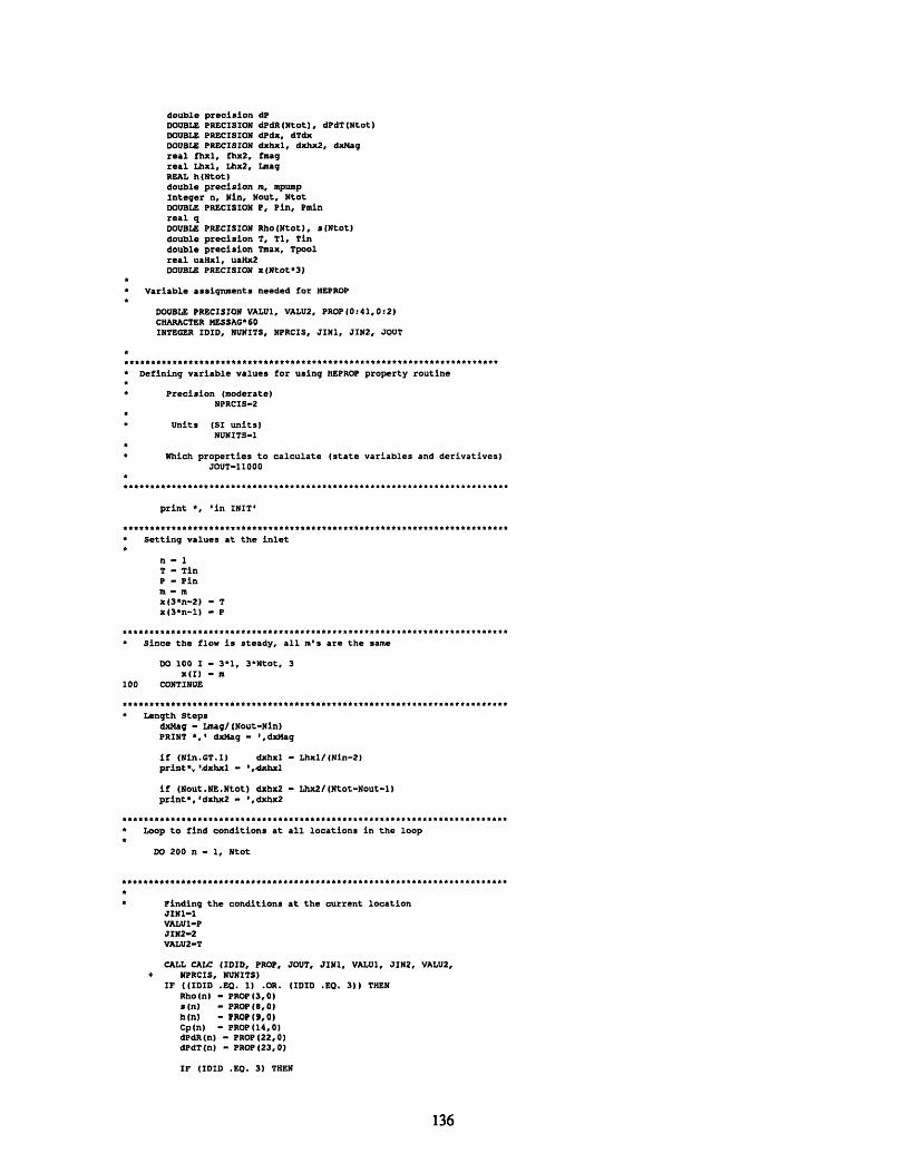
double precision dPDOUBLE PRECISION dPdR(Ntot), dPdT(Ntot)DOUBLE PRECISION dPdx, dTdxDOUBLE PRECISION dxhxl, dxhx2, dxMagreal fhxl, fhx2, fmagreal Lhxl, Lhx2, LmagREAL h(Ntot)double precision m, mpumpInteger n, Nin, Nout, NtotDOUBLE PRECISION P, Pin, Pminreal qDOUBLE PRECISION Rho(Ntot), s(Ntot)double precision T, T1, Tindouble precision Tmax, Tpoolreal uaHxl, uaHx2DOUBLE PRECISION x(Ntot*3)







print *, 'in INIT'

* Setting values at the inlet

n-IT - TinP - Pin

x(3*n-2) - Tx(3*n-1) - P

* Since the flow is steady, all m's are the same

DO 100 I - 3*1, 3*Ntot, 3x(I) - m

100 CONTINUE

* Length StepsdxNag - Lmag/(Nout-Nin)PRINT *,' dxMag - ',dxMag

if (Nin.GT.1) dxhxl - Lhxl/(Nin-2)print*, '.d*hxl - ',dKhxl

if (Nout.NE.Ntot) dxhx2 - Lhx2/(Ntot-Nout-1)print', dxhx2 - ',dxhx2

* Loop to find conditions at all locations in the loop

DO 200 n - i, Ntot

* Finding the conditions at the current locationJIN1-1VALUI-PJIN2-2VALU2-T


IF ((IDID .EQ. 1) .OR. (IDID .EQ. 3)) THENRho(n) - PROP(3,0)s(n) - PROP(8,0)h(n) - PROP(9,0)Cp(n) - PROP(14,0)dPdR(n) - PROP(22,0)dPdT(n) - PROP(23,0)

IF (IDID .EQ. 3) THEN

136


ELSECALL ERRMSG (MESSAG, IDID)WRITE (', (1lX,A60)') MESSAGSTOP

ENDIF

***Slopes of temperature and pressure change per length*********

* Slopes of temperature and pressure change per length

IF (n.LT.Nin-1) THENdPdx - -fhx1* m* abs(m) /(2* Rho(n)dTdx - uaHx1*(Tpool-T)/(m*Cp(n))

- ( 1/Rho(n) - T*dPdT(n)/(Rho(n)**2ELSEIF (n.EQ.Nin-1) THEN

dPdx - 0.0dTdx - 0.0

ELSEIF (n.LT.Nout) THENdPdx - -fmag* m* abs(m) /(2* Rho(n) *dTdx - q/(m*Cp(n))

- ( 1/Rho(n) - T*dPdT(n)/(Rho(n)**2ELSEIF (n.EQ.Nout) THEN

dPdx - 0.0dTdx - 0.0

ELSEdPdx - -fhx2* m* abs(m) /(2* Rho(n) *dTdx - uaHx2*(Tpool-T)/(m*Cp(n))

- ( 1/Rho(n) - T*dPdT(n)/(Rho(n)**2ENDIF

AcHxl**2 * DhHxl)

* dPdR(n)) )*dPdx/Cp(n)

AcMag**2 * DhMag)


AcHx2**2 * DhHx2)


Finding the conditions at the NEXT locationnote that this is only done if n is less than Ntot since ifn - Ntot there is not another node to calculate T and P at.(but the whole loop was needed to calculate the properties ofthe last node--which is done at the top of the loop)

IF (n.LT.NtoT) THENIF (n.LT.Nin-1) THEN

T - T + dTdx*dxHxlP - P + dPdx*dxHxl

ELSEIF (n.EQ.Nin) THENT - T + dTdx*dxHxlP - P + dPdx*dxHxl

ELSEIF (n.LT.Nout) THENT - T + dTx*xdxMagP - P + dPdx*dxMag

ELSEIF (n.EQ.Nout) THENT - T + dTdx*dxMagP - P + dPdx*dxMag

ELSET - T + dTdx*dxHx2P - P + dPdx*dxHx2

ENDIFx(3*(n+l)-2) - Tx(3*(n+l)-l) - P

ENLTF

ttt** * *te *** ******tt*t***************************************

CHECK TO MAKE SURE THAT THE TEMPERATURE DOES NOT EXCEED THEMAXIMUM ALLOWABLE TEMPERATE AND THAT THE PRESSURE IS ABOVE MINIMUM

IF (T.GT.Tmax) THENprint *, ' Temp greater than max allowed temp before pulse'stop

ENDIF

IF (P.LT.Pmin) THENprint *, ' Pressure below minimum allowable before pulse'stop

ENDIF

200 Continue

t***s*teeke**·tetw*teen***t***t******************************************

CALLING THE SUBROUTINE STEADY TO MAKE VALUES CONSISTENT WITH A* BACKWARD EULER METHOD

CALL STEADY(x, q, m, Nin, Nout, Ntot,: AcMag, DhMag, fmag, dxMag,* AcHxl, DhHxl, fhxl, uaHxl, dxHxl,; AcHx2, DhHx2, fhx2, uaHx2, dxHx2,

137

*****te****t tt***********tw***************************************k****

Cp, Rho, s, h, dPdR, dPdT,Pin, Tin, Tpool)

USING THE PUMP CHARACTERISTIC EQN TO FIND THE MASS FLOW RATE THAT THEPUMP SHOULD HAVE TO GIVE THE CURRENT TOTAL PRESSURE DROP AROUND THE LOOP

* Converting the pressure drop around the loop to atmospheres

dP - ( x(2)-x(3*Ntot-1) ) / 101325* PRINT *,'dp - ',dp

* Calling the subroutine PUMP to find the mass flow rate that the pump* would need to give the same pressure drop as calculated.

CALL PUMP(dP,mPump)

* CHECKING FOR CONSISTENCY WITH THE PUMP ISENTROPIC EFFICIENCY

* ISENTROPIC EXIT ENTHALPY OF PUMPJIN1-1VALUi-x(2)JIN2-5VALU2-s (Ntot)


IF ((IDID .EQ. 1) .OR. (IDID .EQ. 3)) THENhs - PROP(9,0)IF (IDID .EQ. 3) THEN


ELSECALL ERRMSG (MESSAG, IDID)WRITE (*, '(IX,A60)') MESSAGSTOP

ENDIF

hl- h(Ntot) + ( hs - h(Ntot) )/Etaprint *,'hl - ',hl

a TEMPERATURE AT EXIT OF PUMPJIN1-1VALUI-x(2)JIN2-6VALU2-hl


IF ((IDID .EQ. 1) .OR. (IDID .EQ. 3)) THENT1 - PROP(2,0)IF (IDID .EQ. 3) THEN


ELSECALL ERRMSG (MESSAG, IDID)WRITE (*, '(IX,A60)') MESSAGSTOP

ENDIF

COMPARING THE CALCULATED TEMPERATURE AT NODE 1 (pump exit) WITHTHE CURRENT VALUE IF THEY DISAGREE, THEN ADJUST Tin USING AWEIGHTED AVERAGE OF THE TWO VALUES.ALSO COMPARE THE PRESSURE DROP AND ADJUST m AS NEEDED TO ZERO INON THE CORRECT OPERATING POINT.

if (abs( (Ti-Tin) /Tin ) .gt. le-7 .OR.* abs( (mpump-m)/m ) .GT. 1E-6) THEN

print *,'m - ',m,' Tin - ',TinTin - Tin*0.1 + T1*0.9m - (mpump + m)/2print *, m - ',m,' Tin - ',Tingoto 200

endif

END

138

E.6: Subroutine STEADY

SUBROUTINE STEADY(x, q, m, Nin, Nout, Ntot,; AcMag, DhMag, fmag, dxMag,* AcHxl, DhHxl, fhxl, uaHxl, dxHxl,; AcHx2, DhHx2, fhx2, uaHx2, dxHx2,; Cp, Rho, s, h, dPdR, dPdT,SPin, Tin, Tpool)

*··**t**ttetta*te··****e**tt*t*****************************************

* STEADY5.FOR - sparse matrix version

* Subroutine for evaluating the temperature and pressure profile* in a recirculator loop under STEADY STATE conditions. This routine* uses the T, P and m values that are found in subroutine INIT as a* starting point. It then iterates to make sure that the values are* all consistent with a BACKWARD EULER estimation for spatial* derivatives.* (INIT uses a FORWARD EULER technique that will give very similar* results, but will be slightly different.)

* Note the x vector is used to hold the values of T, P, and m for* the length of the conductor. Where T's, P's and m's for a* particular node n in the conductor are found by:

ST(n) - x(3*n-2)SP(n) - x(3*n-1)m(n) - x(3*n)

* Note that the program originally used an LU decompostion method* of solution that put the coefficients into an A matrix. This* method was slow and memory intensive so a sparse matrix method* was used. However, the sparse matrix solution compacts the* A matrix into two vector: SA to store the diagonal and non-zero* elements, and IJA to store the indices. Since the locations in* these vectors are very difficult to interpret, the original A matrix* assignments were left in, but commented out, to show where in the* A matrix the values are being assigned.

* The routines needed to solve the sparse matrix are all from* Numerical Recipes: the Art of Scientific Computing, version 2.* The routines that were used are:* linbcg* atimes* asolve* dsprsax* dsprstx* snrm



* last modified 5-19-97*** ** *********************************************

* VARIABLES USED

A - Matrix containing derivatives - used for Newton's methodAcHxl - Cross sectional area of heat exchanger 1 flow

passage (m2)AcHx2 - Cross sectional area of heat exchanger 2 flow

passage (m2)* AcMag - Cross sectional area of flow passage (m2)* b - Vector used for solving using Newton's method* Cp(n) - Specific heat at node n (J/kg-K)* D - Flag used by program LUDCMP and LUBKSB* DhHxl - Hydraulic diameter of heat exchanger 1 (m)* DhHx2 - Hydraulic diameter of heat exchanger 2 (m)* DhMag - Hydraulic diameter of flow passage (m)* dhdP(n) - dh/dP at constant temperature at node n (m3/kg)* dPdR(n) - dP/dRho at constant temperature at node n (Pa-m3/kg)* dPdT(n) - dP/dT at constant density at node n (Pa/K)* dRdT(n) - dRho/dT at constant pressure at node n (kg /m3-K)* dRdP(n) - dRho/dP at constant temperature at node n ( kg/m3-Pa)* dudT(n) - du/dT at constant pressure at node n (J/kg-K)* dudP(n) - du/dP at constant temperature at node n (J/kg-Pa)* or (m3/kg)* dxHxl - Distance between nodes in heat exchanger 1* dxHx2 - Distance between nodes in heat exchanger 2* dxMag - Distance between nodes in magnet (m)* Em - Total error in m equations* EP - Total error in P equations* ET - Total error in T equations* err - Error value returned from sparse matrix solver (linbcg)* fhxl - Friction factor in heat exchanger 1* fhx2 - Friction factor in heat exchanger 2

139

fmagija

iteritmaxitolindxLenSAh(n)mNinNoutNtot

PinPminqRho (n)a(n)SATinTmaxtolTpooluaHxl

uaHx2

x(n)xt (n)

- Friction factor in magnet- Vector used to store column information for sparseversion of the A matrix (called SA)

- Number of iterations used by linbcg- Maximum allowable number of iterations in linbcg- Type of convergence check being used in linbcg- Vector used by program LUDCMP and LUBKSB- Length of SA and ija (vectors used to store sparse matrix)- Specific enthalpy of helium at node n (J/kg)- Mass flow rate at all locations (kg/s)- Value of node number n for the conductor inlet- Value of node number n for the conductor outlet- Total number of nodes in system include those that are

not in the conductor (ie 1/3 of the size of x )- Inlet pressure (Pa)- Minimum allowable pressure in conductor (Pa)- Heat flow rate per unit length (W/m)- Density at node n (kg/m3)- Specific entropy at node n (J/kg-K)- Sparse version of A matrix (stored in a vector)- Inlet temperature (K)- Maximum allowable temperature at any location(K)- Tolerance variable required for sparse matrix solver- Temperature of pool (K)- Overall heat transfer coefficient PER UNIT LENGTH

of HX1 (W/m-K)- Overall heat transfer coefficient PER UNIT LENGTH

of HX1 (W/m-K)- Vector containing T, P, and m data for all nodes- Values of x at last iteration

* My Variable assignments* DOUBLE PRECISION A[allocatable](:,:)

real AcHxl, AcHx2, AcMagDOUBLE PRECISION b[allocatable](:)DOUBLE PRECISION Cp(Ntot)REAL Dreal DhHxl, DhHx2, DhMagDOUBLE PRECISION dPdR(Ntot), dPdT(Ntot)DOUBLE PRECISION dRdT[allocatable](:)DOUBLE PRECISION dRdP[allocatable] (:)DOUBLE PRECISION dhdP[allocatable](:)DOUBLE PRECISION dudT[allocatable](:)DOUBLE PRECISION dudP[allocatablel(:)DOUBLE PRECISION dxHxl, dxHx2, dxMagreal Em, ET, EPreal fhxl, fhx2, fmagreal h(Ntot)integer ija[allocatable](:)INTEGER indx(allocatable](:)

DOUBLE PRECISION mInteger Nin, Nout, NtotDOUBLE PRECISION Pinreal qDOUBLE PRECISION Rho(Ntot), s(Ntot)DOUBLE PRECISION SA[allocatable) (:)double precision Tindouble precision Tpoolreal uaHxl, uaHx2DOUBLE PRECISION x(Ntot*3)DOUBLE PRECISION xt[allocatable](:)

Variable assignments needed for sparse matrix solver linbcg

integer itmax, itol, iterdouble precision tol, err


DOUBLE PRECISION VALU1, VALU2, PROP(0:41,0:2)CHARACTER NESSAG*60INTEGER IDID, NUNITS, NPRCIS, JIN1, JIN2, JOUT

....*** ..... **.......*........*...********..************************ *



S Units (SI units)NUNITS-1

Which properties to calculate (state variables and derivatives)JOUT-11000

print *, 'in STEADY'

140

k

* Length of SA and ija (vectors used to store sparse matrix)* (there are 3*Ntot diagonal elements, 1 blank space, 4 off diagonal* elements for each of the Ntot-3 "elements", and 3 off diagonal* elements from continuity at both the HX1-Mag and Mag-HX2 interfaces.)

LenSA - 3*Ntot + 1 + 4*(Ntot-3) + 3 * 2

* Allocating memory to the variables not being* passed back to main routine

* allocate(A(3*Ntot,3*nTot), b(3*Ntot), SA(LenSA), ija(LenSA),allocate(b(3*Ntot), SA(LenSA), ija(LenSA),

; dRdT(Ntot), dRdP(Ntot), dhdP(Ntot), dudT(Ntot), dudP(Ntot),; xt(3*Ntot))

* indx(3*Ntot),xt(3*Ntot))

·ese***************t***************************************************

* Specifying ija vector for sparse matrix storage

* PATTERN IS:

* FROM HX1:first 3 rows : no off diagonalsNext 3*(Nin-2) rows have pattern [rows 4 to 3*(Nin-1)

row 3*n-2 : off diagonals at columns3*n-53*n-43*n-1

row 3*n-1 : off diagonal at column 3*n-4

FROM MAGNET:row 3*Nin-2 : off diagonal at column 3*(Nin-1)-2row 3*Nin-1 : off diagonal at column 3*(Nin-1)-lrow 3*Nin : off diagonal at column 3*(Nin-1)Next 3*(Nout-Nin) rows [ rows 3*Nin+l to 3*Nout ]



FROM HX2:row 3*Nout+l : off diagonal at column 3*Nout-2row 3*Nout+2 : off diagonal at column 3*Nout-1row 3*Nout+3 : off diagonal at column 3*NoutNext 3*(Ntot-Nout-l) rows [rows 3*Nout+4 to 3*Ntot]

row 3*n-2 : off diagonals at columns3*n-5S3n-4S3n-1


* Setting up the first 3*Ntot+l elements of ija (from diagonal components)

ija(1) - 3*Ntot+2ija(2) - 3*Ntot+2ija(3) - 3*Ntot+2ija(4) - 3*Ntot+2

do i - 5, 5 + 3*(Nin-3), 3ija(i) - ija(i-1) + 3ija(i+1) - ija(i) + 1ija(i+2) - ija(i+l)

enddo

ija(3*Nin-1) - ija(3*Nin-2)+lija(3*Nin) - ija(3*Nin-1)+lija(3*Nin+l) - ija(3*Nin) +1

do i - 3*Nin+2, 3*Nin+2 + 3*(Nout-Nin-1), 3ija(i) - ija(i-1) + 3ija(i+l) - ija(1) + 1ija(i+2) - ija(i+1)

enddo

ija(3*Nout+2) - ija(3*Nout+l)+lija(3*Nout+3) - ija(3*Nout+2)+lija(3*Nout+4) - ija(3*Nout+3)+l

do i - 3*Nout+5, 3*Nout+5 + 3*(Ntot-Nout-2), 3ija(i) - ija(i-1) + 3ija(i+l) - ija(i) + 1ija(i+2) - ija(i+l)

141

enddo

* setting up the off diagonal components of ija

ija(3*Ntot+2) - 1ija(3*Ntot+3) - 2ija(3*Ntot+4) - 5ija(3*Ntot+5) - 2

do i - 3*Ntot+6, 3*Ntot+6 + 4*(Nin-3) - 1ija(i) - ija(i-4) + 3

enddo

ija(3*Ntot+6 + 4*(Nin-3) ) - 3*Nin-5ija(3*Ntot+6 + 4*(Nin-3)+1) - 3*Nin-4ija(3*Ntot+6 + 4*(Nin-3)+2) - 3*Nin-3

ija(3*Ntot+6 + 4*(Nin-3)+3) - 3*Nin-2ija(3*Ntot+6 + 4*(Nin-3)+4) - 3*Nin-1ija(3*Ntot+6 + 4*(Nin-3)+5) - 3*Nin+2ija(3*Ntot+6 + 4*(Nin-3)+6) - 3*Nin-1

do i - 3*Ntot+6 + 4*(Nin-3)+7, 3*Ntot+4*(Nout-3)+8ija(i) - ija(i-4) + 3

enddo

ija(3*Ntot+4*(Nout-3) +9) - 3*Nout-2ija(3*Ntot+4*(Nout-3)+10) - 3*Nout-1ija(3*Ntot+4*(Nout-3)+11) - 3*Nout

ija(3*Ntot+4*(Nout-3)+12) - 3*Nout+lija(3*Ntot+4*(Nout-3)+13) - 3*Nout+2ija(3*Ntot+4*(Nout-3)+14) - 3*Nout+5ija(3*Ntot+4*(Nout-3)+15) - 3*Nout+2

do i - 3*Ntot+4*(Nout-3)+16, LenSAija(i) - ija(i-4) + 3

enddo

* print *,' ija(1) - ',ija(1), ' 3*Ntot - ',3*Ntotprint *,' LenSA - ',LenSA

a k-0* do - 1, LenSASk - k+l*print *,'i - ',i, ' ija - ',ija(i)* if (k.eq.20) then

pause ' <RETURN> for more'* k-0* endif* enddo* pause ' <RETURN> to continue '

* DERIVATIVES

DO 30 n - 1, NtotdRdT(n) - -dPdT(n) / dPdR(n)dRdP(n) - 1/dPdR(n)dhdP(n) - 1/Rho(n) - x(3*n-2)*dPdT(n) /( dPdR(n)*(Rho(n))**2 )dudT-(n) -- Cp(n4 - -x.(3*n-1) *dPdT(n) /( .dPdR4n) * (Rho(a) **2 )dudP(n) - ( x(3*n-1) - x(3*n-2)*dPdT(n) ) /

( dPdR(n)*(Rho(n))**2 )30 CONTINUE

t*n**t**t*******· ···· ****·*·e* e**·************************************

* CLEARING THE A MATRIX AND THE b VECTOR TO START THE SOLUTION* (A matrix was commented out when the sparse matrix solution was added)

50 CONTINUEDO 200 i - 1, 3*Ntot

b(i) - 0* DO 300 j - 1, 3*Ntot* A(i,j) - 0*300 CONTINUE200 CONTINUE

* SETTING UP THE A and b COMPONENTS DUE TO THE FIRST HEAT EXCHANGER* (note the A matrix assignments are commented out since the sparse* matrix method of solution is being used. But these original A matrix* statements are left in for it to be easier to see where the values* are being assigned to since the sparse matrix vector is difficult* to understand.)

142

* SETTING UP THE FIRST THREE EQNS IN THE MATRIX* NODE 1 IS SAME AS PUMP* ASSUMING P1 - Pin and T1 - Tin and ml - msteady

A(l, l) - 1SA(1) - 1

b(l) - Tin

A(2,2) - 1SA(2) - 1b(2) - Pin

A(3,3) - 1SA(3) - 1

b(3) - m

* starting a counter for* end of the SA matrix:

k - 3*Ntot + 2

filling in the off diagonal elements at the

* REMAINING HX1 EQUATIONS

DO 400 n - 2, Nin-i

* First Law equationsA(3*n-2,3*n-5)

SA(k)k - k+l

A(3*n-2,3*n-4)SA(k)k - k+l

A(3*n-2,3*n-2)SA(3*n-2)

S A(3*n-2,3*n-1)SA(k)k - k+l

b(3*n-2)

- -m*Cp(n) /dxHxl- -m*Cp(n) /dxHxl

- -m*dhdP(n)/dxHxl- -m*dhdP(n)/dxHxl

- m*Cp(n)/dxHxl + uaHxl- m*Cp(n)/dxHxl + uaHxl- m*dhdP(n)/dxHxl- m*dhdP(n)/dxHxl

- uaHxl*Tpool

* Momentum (pressure drop) equationsA(3*n-1,3*n-4) - -1/dxHxl

SA(k) - -1/dxHxlk - k+l

A(3*n-1,3*n-1) - 1/dxHxlSA(3*n-1) - i/dxHxl

b(3*n-1) - -fHxl*m**2/(2*Rho(n)*DhHxl*AcHxl**2)

Mass Conservation equationsS A(3*n,3*n) - 1

SA(3*n) - 1b(3*n) - m

400 ENDDO

SETTING UP THE A and b COMPONENTS DUE TO THE CICC MAGNET CABLE

ASSUMING CONTINUITY OF m, P and T BETWEEN THE !XI1 AND THE MAGNET INLETTHE FIRST 3 EQUATION FOR THE MAGNET ARE THEN

* temperature continuityA(3*Nin-2,3*(Nin-1)-2)

SA(k)k - k+l

* A(3*Nin-2,3*Nin-2)SA(3*Nin-2)

* pressure continuity* A(3*Nin-1,3*(Nin-l)-1)

SA(k)k - k+l

* A(3*Nin-1,3*Nin-1)SA(3*Nin-1)

* mass continuityA(3*Nin,3*(Nin-1))

SA(k)k - k+l

A(3*Nin,3*Nin)SA(3*Nin)

- -1-- 1

-1-1

-- 1

-1

-1

S-1

- -1

-1

-1

* REMAINING MAGNET EQUATIONSDO 600 n - Nin+l, Nout

* First Law equationsA(3*n-2,3*n-5) - -m*Cp(n) /dxMag

SA(k) - -m*Cp(n) /dxMag

143

k - k+lA(3*n-2,3*n-4)

SA(k)k - k+1l

A(3*n-2,3*n-2)SA(3*n-2)

A(3*n-2, 3*n-1)SA(k)k - k+l

b(3*n-2)

- -m*dhdP(n)/dxMag- -m*dhdP(n)/dxMag

- m*Cp(n)/dxMaq- m*Cp(n)/dxMaq

- m*dhdP(n)/dxMag- m*dhdP(n)/dxMag

- q

* Momentum (pressure drop) equations* A(3*n-1,3*n-4) - -1/dxMag

SA(k) - -l/dxMagk - k+l

* A(3*n-1,3*n-1) - 1/dxMaqSA(3*n-1) - 1/dxMag

b(3*n-1) - -fmag*m**2 / (2*Rho(n)*DhMag*AcMag**2)

Mass Conservation equations (allA(3*n,3*n) - 1

SA(3*n) - 1b(3*n) -m

600 ENDDO

nodes have same mass flow)

* SETTING UP THE A and b COMPONENTS DUE TO THE SECOND HEAT EXCHANGER

* ASSUMING CONTINUITY OF m, P and T BETWEEN THE MAGNET EXIT AND HX2 INI* THE FIRST 3 EQUATION FOR HX2 ARE THEN

* temperature continuity* A(3*Nout+1,3*Nout-2) - -1

SA(k) - -1k - k+l

* A(3*Nout+1,3*(Nout+1)-2) - 1SA(3*Nout+l) - 1

* pressure continuity* A(3*Nout+2,3*Nout-1) - -1

SA(k) - -1k - k+l

* A(3*Nout+2,3*(Nout+1)-1) - 1SA(3*Nout+2) - 1

* mass continuity* A(3*Nout+3,3*Nout)

SA(k)k - k+l

* A(3*Nout+3,3*(Nout+1))SA(3*Nout+3)


DO 700 n - Nout+2, Ntot

-- 1- -1

- 1-1

* First Law equations* A(3*n-2,3*n-5)

SA(k)k - k+l

* A(3*n-2,3*n-4)SA(k)k - k+l

* A(3*n-2,3*n-2)SA(3*n-2)

A(3*n-2,3*n-1)SA(k)k - k+l

- -m*Cp(n) /dxHx2- -m*Cp(n) /dxHx2

- -m*dhdP(n)/dxHx2- -m*dhdP(n)/dxHx2

- m*Cp(n)/dxHx2 + uaHx2- m*Cp(n)/dxHx2 + uaHx2

- m*dhdP(n)/dxHx2- m*dhdP(n)/dxHx2

b(3*n-2) - uaHx2*Tpool* Momentum (pressure drop) equations* A(3*n-1,3*n-4) - -1/dxHx2

SA(k) - -1/dxHx2k - k+l

* A(3*n-1,3*n-1) - 1/dxHx2SA(3*n-1) - 1/dxHx2

b(3*n-1) - -fHx2*m**2/(2*Rho(n)*DhHx2*AcHx2**2)

* Mass Conservation equations* A(3*n,3*n) - 1

SA(3*n) - 1

b(3*n) - m

144

LET

__ __L

700 ENDDO

* Before Solving, save the previous values of the x vector in xt

DO 800 i - 1, 3*Ntotxt(i) - x(i)

800 CONTINUE

*****************************************************************

* Solving for the new x vector - the sparse matrix solver LINBCG* from Numerical Recipes is used. The LU decomposition matrix solver* (LUDCMP and LUBKSB also from Numerical Recipes) that was originally* used is shown, but is commented out.* tolerance and maximum number of iteration needed for LINBCG

itol - 1tol - le-7itmax - 200

call linbcg(SA,ija,3*Ntot,b,x, itoltoltol,itmax,iter,err)

CALL LUDCMP(A,3*Ntot,3*Ntot, INDX, D)CALL LUBKSB(A, 3*Ntot,3*Ntot, INDX,b)

*11*750

DO 750 n - 1, Ntotwrite(*,*) ' n - ',nwrite(*,11)1 T(n) - ',x(3*n-2), * P(n) - ',x(3*n-1),

* m(n) - ', b(3*n)write(*,11)' Tt(n) - ',xt(3*n-2),' Pt(n) - ',xt(3*n-1),

* mt(n) - ', xt(3*n)read(*,*)format(A10,f9.3,a9,f10.0,al0,f7.5)CONTINUE

* Saving the previous values of the x vector in xt and* Assigning the new values to the x vector* (this section is currently commented out- it is used if the solution* is unstable and a relaxation method is needed. The new values* are averaged with the old to let the solution converge slower)

S DO 800 i - 1, 3*Ntotxt(i) - x(i)x(i) - (b(i)*.5 + x(i)*.5)

*800 CONTINUE

* CHECKING THE ERROREm-0EP - 0ET - 0

DO 900 n - 1, NtotEm - Em + abs( x(3*n) - xt(3*n) )

EP - EP + abs( x(3*n-1) - xt(3*n-1) )

ET - ET + abs( x(3*n-2) - xt(3*n-2) )

900 CONTINUE

* IF ERROR IS GOOD, THEN RETURN, OTHERWISE GET THE PROPERTIES AT* ALL NODES USING THE NEW X VECTOR

IF (Em.GT.0.0000001*Ntot. or. EP.GT.Ntot/10 .or .ET.GT.0.0000005*Ntot) THEN

print *,'em - ',em,' ep - ',eP,' eT - ',eTDO 1000 n - 1, Ntot

Finding the conditionsJIN1-1VALU1-x(3*n-1)JIN2-2VALU2-x(3*n-2)

CALL CALC (IDID, PROP,+ NPRCIS, NUNITS)

IF ((IDID .EQ. 1) .OR.Rho(n) - PROP (3,0)s(n) - PROP(8,0)h(n) - PROP(9,0)Cp(n) - PROP(14,0)

It the current location

JOUT, JIN1, VALU1, JIN2, VALU2,

(IDID .EQ. 3)) THEN

145

dPdR(n) - PROP(22,0)dPdT(n) - PROP(23,0)

dRdT(n) - -dPdT(n) / dPdR(n)dRdP(n) - 1/dPdR(n)dhdP(n) - 1/Rho(n) - x(3*n-2)*dPdT(n) /

( dPdR(n)*(Rho(n))**2)dudT(n) - Cp(n) - x(3*n-1)*dPdT(n) /

( dPdR(n)*(Rho(n))**2 )dudP(n) - ( x(3*n-1) - x(3*n-2)*dPdT(n) ) /

( dPdR(n)*(Rho(n))**2 )

IF (IDID .EQ. 3) THEN* This code not used in this case

ENDIFELSE

CALL ERRMSG (MESSAG, IDID)WRITE (*, '(IX,A60)') MESSAGprint *,nSTOP

ENDIF1000 CONTINUE

GOTO 50

ELSEprint *,' error good'print *,lem - %,em,' ep - ',eP,1 eT - 1,eT

ENDIF

* Deallocating the memory of the variables not being* passed back to main routine

* this line commented out when program was switched from using full A matrix* to only using the SA and IJA vectors of the sparse matrix method* deallocate(A, b, SA, ija, dRdT, dRdP, dhdP, dudT, dudP, indx, xt)

deallocate(b, SA, ija, dRdT, dRdP, dhdP, dudT, dudP, xt)

END

146

E.7 Subroutine PUMP

SUBROUTINE PUMP(dP, mPump)

******t*te**t****t****t*t****·t***************************************

* PUMP2.FOR

* Subroutine that uses the pump curve of a given pump to give the* mass flow for a given pressure change.



* VARIABLES USED

* dP - Total pressure drop around loop (atm)* mPump - Value of m that corresponds to current dP (kg/s)

* My Variable assignmentsdouble precision dPdouble precision mPump

* Using the pump curve to find mPump* this curve is a very rough fit of data from* Lue, J.W., et al. Test of a Cryogenic Helium Pump.* Advances in Cryogenic Engineering, Vol. 27,* Plenum Press, New York, 1982.

* 200 rpm curve* mpump - (-1.4 * dp**2 + 1.2 * dp + 10.1) / 1000

* 100 rpm curvempump - (-1.29 * dp**2 + 0.61 * dp + 6) / 1000

RETURNEND

147

E.8 Subroutine QLOADSUBROUTINE Qload(x, uahxl, uahx2, dxhxl, dxhx2, Tpool, Nout, Nin,

; Ntot, Qpool, Qhxl, Qhx2)

* Qload3.FOR

* Subroutine for finding the heat being rejected to the buffer tank


ST(n) - x(3*n-2)* P(n) - x(3*n-1)a m(n) - x(3*n)


* last modified 2-16-97*·*se*e****+tenetateette********·*+t*********************************

* VARIABLES USED

* DhHxl - Hydraulic diameter of heat exchanger 1 (m)* DhHx2 - Hydraulic diameter of heat exchanger 2 (m)* Nin - Node number of magnet inlet* Nout - Node number of magnet outlet* Ntot - Total number of nodes in loopS OQhxl - Heat load being rejected to the buffer tank from hxl (W)* Qhx2 - Heat load being rejected to the buffer tank from hx2 (W)* Qpool - Total heat load being rejected to the buffer tank (W)* Tpool - Current temperature of buffer tank (K)* uaHxl - Overall heat transfer coefficient PER UNIT LENGTH* of HX1 (W/m-K)* uaHx2 - Overall heat transfer coefficient PER UNIT LENGTH* of HX1 (W/m-K)* x(n) - Vector containing T, P, and m data for all nodes

* My Variable assignments

double precision dxhxl, dxhx2integer Nin, Nout, Ntotreal Qhxl, Qhx2real Opooldouble precision Tpoolreal uahxl, uahx2double precision x(*)

* print *, 'uahxl - ',uahxl,'uahx2 - ',uahx2* print *, 'dxhxl - *,dxhxl,'dxhx2 - ',dxhx2

* print *, 'T*pool - ',tpool

PRINT *,'IN QLOAD'

* HEAT LOAD DUE TO HEAT EXCHANGER 1

Ohxl - 0.0000000do 100 n - 2, Nin-l

Ohxl - Qhxl + uahxl*(x(3*n-2)-Tpool)*dxhxl100 enddo

* HEAT LOAD DUE TO HEAT EXCHANGER 2

Qhx2 - 0.0000000do 200 n - Nout+2, Ntot

Qhx2 - Qhx2 + uahx2*(x(3*n-2)-Tpool)*dxhx2200 enddo

Opool - Qhxl + Qhx2

returnend

148

E.9 Subroutine POOL

SUBROUTINE POOL(Qss, Qpool, Vtank, mtank, utank, Tpool, Ptank,dt)

*********************************************************************

* POOL3.FOR

* Subroutine for evaluating the current temperature of the* buffer tank




* VARIABLES USED

* dt - time step* mtank - Total helium mass in the buffer tank (kg)* Ptank - Current pressure in buffer tank (Pa)* Qpool - Current heat load being rejected to buffer tank (W)* Qss - Steady state heat load passing through buffer tank (W)* Tpool - Temperature of buffer tank/pool (K)* utank - Specific internal energy of buffer tank (J/kg-K)* Vtank - Volume of buffer tank (m3)

My Variable assignmentsdouble precision dtreal mtankreal Ptankreal Opool, Qssdouble precision Tpoolreal utankreal Vtank


DOUBLE PRECISION VALUI, VALU2, PROP(0:41,0:2)CHARACTER MESSAG*60INTEGER IDID, NUNITS, NPRCIS, JINI, JIN2, JOUT





PRINT *,'IN POOL'print *, mtank - ',mtank

tee*t**e*teetwee****·t*****t*****************************************

Finding the new specific internal energy of the tank

* print *,'qpool - ',qpool,' Oss - *,Qss* print *,'Vtank - ',Vtank,' Tpool - ',Tpool,' Ptank - ',Ptank* print *, utank - ',utank

utank - utank + (Opool - Qss)*dt/mtank* print *,'utank - ',utank

* Finding the new temperature of the tank

JIN1-3VALU1- mtank/VtankJIN2- 7VALU2- utank


149

IF ((IDID .EQ. 1) .OR. (IDID .EQ. 3)) THENPtank - PROP(1,0)Tpool - PROP(2,O)IF (IDID .EQ. 3) THEN



ENDIF

RETURNEND

150

E.10 Subroutine UNSTEADYSUBROUTINE UNSTEADY(x, xp, q, Nin, Nout, Ntot,: AcMag, DhMag, fmag, dxMag,; AcHxl, DhHxl, fhxl, uaHxl, dxHxl,* AcHx2, DhHx2, fhx2, uaHx2, dxHx2,

eta,; Cp, Rho, s, h, dPdR, dPdT, dt,; Pin, Tin, min, Tpool, Pmin, Tmax, Allo)

* UnsteadlO.FOR - spare matrix version

* Subroutine for evaluating the temperature and pressure profile* in a recirculator loop under transient conditions.* (Used to for pulsed load cycling from a discharging cycle)* This version has 2 pool-cooled heat exchangers and a cable in* conduit conductor between them.

* This version estimates spatial derivatives using the current node* and the previous node instead of the current node and next node.


ST(n) - x(3*n-2)SP(n) - x(3*n-1)m(n) - x(3*n)

* Note that the program originally used an LU decompostion method* of solution that put the coefficients into an A matrix. This* method was slow and memory intensive so a sparse matrix method* was used. However, the sparse matrix solution compacts the* A matrix into two vector: SA to store the diagonal and non-zero* elements, and IJA to store the indices. Since the locations in* these vectors are very difficult to interpret, the original A matrix* assignments were left in, but commented out, to show where in the

A matrix the values are being assigned.

* The routines needed to solve the sparse matrix are all from* Numerical Recipes: the Art of Scientific Computing, version 2.* The routines that were used are:* linbcg* atimes* asolve* dsprsax* dsprstx

snrm



* last modified 5-19-97*a ** aa* aa*******a* *********************a********aaaaaaaaaaaaa****

* VARIABLES USED

* A - Matrix containing .derimatives - used for Newton's method* AcHx1 - Cross sectional area of heat exchanger 1 flow* passage (m2)* AcHx2 - Cross sectional area of heat exchanger 2 flow* passage (m2)* AcMag - Cross sectional area of flow passage (m2)* Allo - Flag to determine whether A, b, fm , fP, and fT arrays* have already been allocated* b - Vector used for solving using Newton's method* Cp(n) - Specific heat at node n (J/kg-K)* D - Flag used by program LUDCMP and LUBKSB* DhHxl - Hydraulic diameter of heat exchanger 1 (m)* DhHx2 - Hydraulic diameter of heat exchanger 2 (m)* DhMag - Hydraulic diameter of flow passage (m)* dhdP(n) - dh/dP at constant temperature at node n (m3/kg)* dP - Pressure change across pump (Pa)*** dPin - Amount to change the guess value of Pin in next iteration (Pa)* dPdR(n) - dP/dRho at constant temperature at node n (Pa-m3/kg)* dPdT(n) - dP/dT at constant density at node n (Pa/K)* dRdT(n) - dRho/dT at constant pressure at node n (kg /m3-K)* dRdP(n) - dRho/dP at constant temperature at node n ( kg/m3-Pa)* dudT(n) - du/dT at constant pressure at node n (J/kg-K)

dudP(n) - du/dP at constant temperature at node n (J/kg-Pa)* or (m3/kg)* dxHxl - Distance between nodes in heat exchanger 1* dxHx2 - Distance between nodes in heat exchanger 2* dxMag - Distance between nodes in magnet (m)* dt - Time step between calculations (sec)* Em - Total error in m equations

151

* EP - Total error in P equations* ET - Total error in T equations* err - Error value returned from sparse matrix solver (linbcg)* eta - Isentropic efficiency of recirculator pump* fhxl - Friction factor in heat exchanger 1* fhx2 - Friction factor in heat exchanger 2* fmaq - Friction factor* indx - Vector used by program LUDCMP and LUBKSB* h(n) - Specific enthalpy of helium at node n (J/kg)* ija - Vector used to store column information for sparse* version of the A matrix (called SA)* iter - Number of iterations used by linbcg* itmax - Maximum allowable number of iterations in linbcg* itol - Type of convergence check being used in linbcg* LenSA - Length of SA and ija (vectors used to store sparse matrix)* mErr - Difference between outlet and inlet mass flow rates (kg/s)* mErrl - Value of mErr corresponding to Pinl* mErr2 - Value of mErr corresponding to Pin2****** mErrLast- Previous value of mErr (last iteration)

min - Inlet mass flow rate to the loop (kg/s)mpump - Value of m that corresponds to current dP (kg/s)Nin - Value of node number n for the conductor inletNout - Value of node number n for the conductor outletnRange - Flag used for bisection search of Pin:

1 - on first pick for Pin2 - on second pick for Pin3 - searching for range where merr2 C 0 < merrl

* -1 - range has been found* Ntot - Total number of nodes in system include those that are* not in the conductor (ie 1/3 of the size of x )* Pin - Inlet pressure (Pa)* Pinl - Used to store a value of Pin when iterating on Pin* if nRange - -1 then we know Pin is between Pinl and Pin2* Pin2 - Used to store a value of Pin when iterating on Pin* if nRange - -1 then we know Pin is between Pinl and Pin2* PinLast - Previous guess value for Pin (from last iteration)* Pmin - Minimum allowable pressure in conductor (Pa)* q - Heat flow rate per unit length (W/m)* Rho(n) - Density at node n (kg/m3)* s(n) - Specific entropy at node n (J/kg-K)* SA - Sparse version of A matrix (stored in a vector)* scale - Scaling factor used to search for range of Pin during* nRange - 3 mode* Tin - Inlet temperature (K)* Tmax - Maximum allowable temperature at any location(K)* tol - Tolerance variable required for sparse matrix solver* Tpool - Temperature of pool (K)* uaHxl - Overall heat transfer coefficient PER UNIT LENGTH* of HXI (W/m-K)* uaHx2 - Overall heat transfer coefficient PER UNIT LENGTH* of HX1 (W/m-K)* x(n) - Vector containing T, P, and m data for all nodes* xp(n) - Vector containing T, P, and m data for previous* time step* xt(n) - Vector containing T, P, and m data for last iteration

* My Variable assignments* DOUBLE PRECISION A(allocatable](:,:)

real AcHxl, AcHx2, AcMaginteger alloDOUBLE PRECISION b[allocatable](:)DOUBLE PRECISION Cp(Ntot)

* REAL Dreal DhHxl, DhHx2, DhMagDOUBLE PRECISION dP

* DOUBLE PRECISION dPinDOUBLE PRECISION dPdR(Ntot), dPdT(Ntot)DOUBLE PRECISION dRdT[allocatablel(:)DOUBLE PRECISION dRdP[allocatable) (:)DOUBLE PRECISION dhdP[allocatable](:)DOUBLE PRECISION dudT(allocatable] (:)DOUBLE PRECISION dudP[allocatable](:)DOUBLE PRECISION dxHx1, dxHx2, dxMagDOUBLE PRECISION dtreal Em, ET, EPreal fhxl, fhx2, fmagreal h(Ntot)

* INTEGER indx[allocatable](:)INTEGER ija[allocatable](:)INTEGER LenSAdouble precision mErr, mErrl, mErr2

* double precision mErrLastdouble precision min, mpumpInteger Nin, Nout, Ntotinteger nRangeDOUBLE PRECISION Pin, Pinl, Pin2

* DOUBLE PRECISION PinLastDOUBLE PRECISION Pminreal qDOUBLE PRECISION Rho(Ntot), s(Ntot)DOUBLE PRECISION SA(allocatable](:)

152

real scaledouble precision Tindouble precision Tmax, Tpoolreal uaHxl, uaHx2DOUBLE PRECISION x(Ntot*3), xp(Ntot*3)DOUBLE PRECISION xt[allocatable](:)

* Variable assignments needed for sparse matrix solver linbcg

integer itmax, itol, iterdouble precision tol, err







print *, 'in UNSTEADY'

***********************************************************************

* Length of SA and ija (vectors used to store sparse matrix)* (there are 3*Ntot diagonal elements, 1 blank space, 7 off diagonal* elements for each of the Ntot-3 "elements", and 3 off diagonal* elements from continuity at both the HX1-Mag and Mag-HX2 interfaces.)

LenSA - 3*Ntot + 1 + 7*(Ntot-3) + 3 * 2

* Allocating memory to the variables not being* passed back to main routine

if (allo.eq.0) then* allocate(A(3*Ntot, b(3*Ntot), SA(LenSA), ija(LenSA),

allocate(b(3*Ntot), SA(LenSA), ija(LenSA),; dRdT(Ntot), dRdP(Ntot), dhdP(Ntot), dudT(Ntot), dudP(Ntot),; xt(3*Ntot) )

* ; indx(3*Ntot), xt(3*Ntot) )* allo - 1

endif

********66**************************************************************

* Setting the variable PinLast to zero so that the logic at the* end of the program will know that this is the first time through* the iteration

* PinLast - 0

min - min

****tt·***en*********·2e****·** ***************************************

* Setting the variable nRange to 1 so that the logic at thea end of the program will know that this is the first time through* the iteration. Also set scale variable for the bisection logic.

nRange - 1scale - 1.05

te**et**·*******e*··*******·**e********e****e****e****e*******n********

* Specifying ija vector

* PATTERN IS:

* FROM HXI:* first 3 rows : no off diagonals* Next 3*(Nin-2) rows have pattern (rows 4 to 3*(Nin-1) ]

153


row 3*n-1 : off diagonal at column 3*n-4row 3*n : off diagonals at columns

3*n-33*n-23*n-1

FROM MAGNET:row 3*Nin-2 : off diagonal at column 3*(Nin-1)-2row 3*Nin-i : off diagonal at column 3*(Nin-l)-1row 3*Nin : off diagonal at column 3*(Nin-1)Next 3*(Nout-Nin) rows [ rows 3*Nin+l to 3*Nout ]

row 3*n-2 : off diagonals at3*n-53*n-43*n-1


3*n-33'n-23*n-1

FROM HX2:row 3*Nout+l : off diagonal at column 3*Nout-2row 3*Nout+2 : off diagonal at column 3*Nout-1row 3*Nout+3 : off diagonal at column 3*NoutNext 3*(Ntot-Nout-1) rows [rows 3*Nout+4 to 3*Ntot]

row 3*n-2 : off diagonals at3'n-53'n-43*n-1


3*n-33*n-23*n-1

* Setting up the first 3*Ntot+l elements of ija (from diagonal components)

if (allo.eq.0) then

ija(l) - 3*Ntot+2ija(2) - 3*Ntot+2ija(3) - 3*Ntot+2ija(4) - 3*Ntot+2

do i - 5, 5 + 3*(Nin-3), 3ija(i) - ija(i-1) + 3ija(i+l) - ija(i) + 1ija(i+2) - ija(i+l) + 3

enddo

ija(3*Nin-l) - ija(3*Nin-2)+1ija(3*Nin) - ija(3*Nin-l)+lija(3*Nin+l) - ija(3*Nin) +1

do i - 3*Nin+2, 3*Nin+2 + 3*(Nout-Nin-1), 3ija(i) - ija(i-l) + 3ija(i+l) - ija(i) + 1ija(i+2) - ija(i+l) + 3

enddo

ija(3*Nout+2) - ija(3*Nout+1)+lija(3*Nout+3) - ija(3*Nout+2)+1ija(3*Nout+4) - ija(3*Nout+3)+1

do i - 3*Nout+5, 3*Nout+5 + 3*(Ntot-Nout-2), 3ija(i) - ija(i-1) + 3ija(i+l) - ija(i) + 1ija(i+2) - ija(i+l) + 3

enddo

setting up the off diagonal components of ija

ija(3*Ntot+2) - 1ija(3*Ntot+3) - 2ija(3*Ntot+4) - 5ija(3*Ntot+5) - 2ija(3*Ntot+6) - 3ija(3*Ntot+7) - 4ija(3*Ntot+8) - 5

do i - 3*Ntot+9, 3*Ntot+9 + 7*(Nin-3) - 1ija(i) - ija(i-7) + 3

enddo

ija(3*Ntot+9 + 7*(Nin-3) ) - 3*Nin-5ija(3*Ntot+9 + 7*(Nin-3)+1) - 3*Nin-4ija(3*Ntot+9 + 7*(Nin-3)+2) - 3*Nin-3

154

ija(3*Ntot+9 + 7*(Nin-3)+3) - 3*Nin-2ija(3*Ntot+9 + 7*(Nin-3)+4) - 3*Nin-1ija(3*Ntot+9 + 7*(Nin-3)+5) - 3*Nin+2ija(3*Ntot+9 + 7*(Nin-3)+6) - 3*Nin-1ija(3*Ntot+9 + 7*(Nin-3)+7) - 3*Ninija(3*Ntot+9 + 7*(Nin-3)+8) - 3*Nin+lija(3*Ntot+9 + 7*(Nin-3)+9) - 3*Nin+2

do i - 3*Ntot+9 + 7*(Nin-3)+10, 3*Ntot+7*(Nout-3)+11ija(i) - ija(i-7) + 3

enddo

ija(3*Ntot+7* (Nout-3)+12) - 3*Nout-2ija(3*Ntot+7*(Nout-3)+13) - 3*Nout-1ija(3*Ntot+7*(Nout-3)+14) - 3*Nout

ija(3*Ntot+7*(Nout-3)+15) - 3*Nout+lija(3*Ntot+7*(Nout-3)+16) - 3*Nout+2ija(3*Ntot+7*(Nout-3)+17) - 3*Nout+5ija(3*Ntot+7*(Nout-3)+18) - 3*Nout+2ija(3*Ntot+7*(Nout-3)+19) - 3*Nout+3ija(3*Ntot+7*(Nout-3)+20) - 3*Nout+4ija(3*Ntot+7*(Nout-3)+21) - 3*Nout+5

do i - 3*Ntot+7*(Nout-3)+22, LenSAija(i) - ija(i-7) + 3

enddoallo - 1

endif

* print *,' ijail) - ',ijal(), ' 3*Ntot - ',3*Ntot* print *,' LenSA - ',LenSA* k-0

do i - 1, LenSAk - k+l

* print *,i - ',i, * ija - ,ija(i)if (k.eq.20) then

pause ' <RETURN> for more'k-0

endifenddopause * <RETURN> to continue 'stop

* DERIVATIVES

DO 30 n - 1, NtotdRdT(n) - -dPdT(n) / dPdR(n)dRdP(n) - 1/dPdR(n)dhdP(n) - 1/Rho(n) - x(3*n-2)*dPdT(n) /( dPdR(n)*(Rho(n))**2 )dudT(n) - Cp(n) - x(3*n-1)*dPdT(n) /( dPdR(n)*(Rho(n))**2 )dudP4m) - (.x(3*n-1) - x.(3*n-Z)*dPdT(n) ) /

( dPdR(n)*(Rho(n))**2 )

30 CONTINUE

* DO 40 n - 1, Ntot* write(*,*) ' n - ',n* write(*,11)* T(n) - ',x(3*n-2), ' P(n) - ',x(3*n-1),* ; m(n) - ', x(3*n)* write(*,11)' Tp(n) - ',xp(3*n-2),' Pp(n) - ',xp(3*n-1),

* ; ' mp(n) - ', xp(3*n)* read(*,*)*40 CONTINUE

*********************************************************************

* CLEARING THE A MATRIX AND THE b VECTOR TO START THE SOLUTION

50 CONTINUEDO 200 i - 1, 3*Ntot

b(i) - 0.0* DO 300 j - 1, 3*Ntot* A(i,j) - 0*300 CONTINUE200 CONTINUE

155

DO 300 i - 1, LenSASA(i) - 0.0

300 CONTINUE

* SETTING UP THE A and b COMPONENTS DUE TO THE FIRST HEAT EXCHANGER* (the A matrix was commented out when the sparse matrix solution was added)

SETTING UP THE FIRST THREE EQNS IN THE MATRIXNODE 1 IS SAME AS PUMPASSUMING P1 - Pin and T1 - Tin and ml - msteady

A(1, 1) - 1SA(1) - 1bil) - Tin

A(2,2) - 1SA(2) - 1b(2) - Pin

A(3,3) - 1SA(3) - 1b(3) - min

* starting a counter for filling in the off diagonal elements at the* end of the SA matrix:

k - 3*Ntot + 2

* REMAINING HX1 EQUATIONSDO 400 n - 2, Nin -1

* First Law equations* A(3*n-2,3*n-5) - -x(3*n)*Cp(n) /dxHxl

SA(k) - -x(3*n)*Cp(n) /dxHxlk - k+l

* A(3*n-2,3*n-4) - -x(3*n)*dhdP(n)/dxHxlSA(k) - -x(3*n)*dhdP(n)/dxHxlk - k+l

** A(3*n-2,3*n-3) - -x(3*n-1) / (Rho(n)*dxHxl)* A(3*n-2,3*n-2) - x(3*n)*Cp(n)/dxHxl + Rho(n)*AcHxl*dudT(n)/dt** ; + uaHxl

* -AcHxl*x(3*n-1)*dRdT(n)/(Rho(n)*dt) + uaHxlSA(3*n-2)- x(3*n)*Cp(n)/dxHxl + Rho(n)*AcHxl*dudT(n)/dt

-AcHxl*x(3*n-1)*dRdT(n)/(Rho(n)*dt) + uaHxlA(3*n-2,3*n-1) - x(3*n)*dhdP(n)/dxHxl + Rho(n)*AcHxl*dudP(n)/dt

a -AcHxl*x(3*n-1)*dRdP(n)/(Rho(n)*dt)SA(k) - x(3*n)*dhdP(n)/dxHxl + Rho(n)*AcHxl*dudP(n)/dt

-AcHxl*x(3*n-l)*dRdP(n)/(Rho(n)*dt)k - k+l

A(3*n-2,3*n) - x(3*n-1)/(Rho(n)*dxHxl)

b(3*n-2) - Rho(n)*AcHxl*dudT(n)*xp(3*n-2)/dt +* Rho(n)*AcHxl*dudP(n)*xp(3*n-l)/dt + uaHxl*Tpool; -AcHxl*x(3*n-1)*dRdT(n)*xp(3*n-2)/(Rho(n)*dt)* -AcHxl*x(3*n-1)*dRdP(n)*xp(3*n-1)/(Rho(n)*dt)

* Momentum (presrure drop) equations* A(3*n-1,3*n-4) - -1/dxHxl


A(3*n-1,3*n-1) - l/dxHxlSA(3*n-1) - 1/dxHxl

b(3*n-1) - -fHx1*x(3*n)*abs(x(3*n))/(2*Rho(n)*DhHxl*AcHxl**2)

* Mass Conservation equationsA(3*n,3*n-3) - -1/dxHxl


A(3*n,3*n-2) - AcHxl*dRdT(n) / dtSA(k) - AcHxl*dRdT(n) / dtk - k+1l

A(3*n,3*n-1) - AcHxl*dRdP(n) / dtSA(k) - AcHxl*dRdP(n) / dtk - k+l

A(3*n,3*n) - 1/dxHxlSA(3*n) - 1/dxHxl

b(3*n) - (AcHxl*dRdT(n)/dt)*xp(3*n-2)+; (AcHx1*dRdP(n)/dt)*xp(3*n-1)

400 ENDDO

156

* SETTING UP THE A and b COMPONENTS DUE TO THE CICC MAGNET CABLE* (the A matrix was commented out when the sparse matrix solution was added)

* ASSUMING CONTINUITY OF m, P and T BETWEEN THE HX1 AND THE MAGNET INLET* THE FIRST 3 EQUATION FOR THE MAGNET ARE THEN

* temperature continuity* A(3*Nin-2,3*(Nin-1)-2) - -1

SA(k) - -1k - k+l

A(3*Nin-2,3*Nin-2) - 1SA(3*Nin-2) - 1

* pressure continuity* A(3*Nin-1,3*(Nin-l)-1) - -1

SA(k) - -1k - k+1

* A(3*Nin-1,3*Nin-1) - 1SA(3*Nin-1) - 1

* mass continuity* A(3*Nin,3*(Nin-1)) - -1

SA(k) - -1k - k+1

* A(3*Nin,3*Nin) - 1SA(3*Nin) - 1

* REMAINING MAGNET EQUATIONSDO 600 n - Nin+1, Nout

* First Law equations* A(3*n-2,3*n-5) - -x(3*n)*Cp(n) /dxMag

SA(k) - -x(3*n)*Cp(n) /dxMaqk - k+l

* A(3*n-2,3*n-4) - -x(3*n)*dhdP(n)/dxMagSA(k) - -x(3*n)*dhdP(n)/dxMagk - k+l

** A(3*n,3*n-3) - -x(3*n-1) / (Rho(n)*dxMaq)* A(3*n-2,3*n-2) - x(3*n)*Cp(n)IdxMag + Rho(n)*AcMag*dudT(n)/dt* : - AcMag*x(3*n-1)*dRdT(n)/ (Rho(n)*dt)

SA(3*n-2) - x(3*n)*Cp(n)/dxMag + Rho(n)*AcMag*dudT(n)/dt- AcMag*x(3*n-1)*dRdT(n)/(Rho(n)*dt)

* A(3*n-2,3*n-1) - x(3*n)*dhdP(n)/dxMag + Rho(n)*AcMag*dudP(n)/dt* ; - AcMag*x(3*n-1)*dRdP(n)/(Rho(n)*dt)

SA(k) -x(3*n)*dhdP(n)/dxMag + Rho(n)*AcMag*dudP(n)/dt- AcMaq*x(3*n-1)*dRdP(n)/(Rho(n)*dt)

k - k+l

** A(3*n,3*n) - x(3*n-1)/(Rho(n)*dxMag)b(3*n-2) - Rho(n)*AcMaq*dudT(n)*xp(3*n-2)/dt +

Rho (n) *AcMag*dudP(n) *xp(3*n-1)/dt + q- AcMag*x(3*n-1)*dRdT(n)*xp(3*n-2)/(Rho(n)*dt)- AcMag*x(3*n-1)*dRdP(n)*xp(3*n-1)/(Rho(n)*dt)

* Momentum (pressure drop) equations* A(3*n-1,3*n-4) - -1/dxMaq

SA(k) - -1/dxMagk - k+l

* A(3*n-1,3*n-1) - 1/dxMagSA(3*n-1) - 1/dxMaq

b(3*n-1) - -fmag*x(3*n)*abs (x(3*n)) /(2*Rho(n) *DhMag*Acag**2)

* Mass Conservation equations* A(3*n,3*n-3) - -1/dxMAg

SA(k) - -1/dxMagk - k+1

* A(3*n,3*n-2) - AcMag*dRdT(n) / dtSA(k) - AcMag*dRdT(n) / dtk - k+l

A(3*n,3*n-1) - AcMaq*dRdP(n) / dtSA(k) - AcMaq*dRdP(n) / dtk - k+1

* A(3*n,3*n) - l/dxMagSA(3*n) - 1/dxMaq

b(3*n) - (AcMag*dRdT(n)/dt) *xp(3*n-2)+; (AcMag*dRdP(n)/dt) *xp(3*n-1)

600 ENDDO

* SETTING UP THE A and b COMPONENTS DUE TO THE SECOND HEAT EXCHANGER

* ASSUMING CONTINUITY OF m, P and T BETWEEN THE MAGNET EXIT AND HX2 INLET* THE FIRST 3 EQUATION FOR HX2 ARE THEN

* temperature continuity

157

A(3*Nout+1,3*Nout-2) - -1SA(k) - -1k - k+l

A(3*Nout+1,3*(Nout+1)-2) - 1SA(3*Nout+1) - 1

* pressure continuity* A(3*Nout+2,3*Nout-1) - -1

SA(k) - -1k - k+1

* A(3*Nout+2,3*(Nout+l)-1) - 1SA(3*Nout+2) - 1

* mass continuity* A(3*Nout+3,3*Nout) - -1

SA(k) - -1k - k+l

* A(3*Nout+3,3*(Nout+l)) - 1SA(3*Nout+3) - 1


DO 700 n - Nout+2, Ntot

* First Law equations* A(3*n-2,3*n-5) - -x(3*n)*Cp(n) /dxHx2

SA(k) - -x(3*n)*Cp(n) /dxHx2k - k+l

* A(3*n-2,3*n-4) - -x(3*n)*dhdP(n)/dxHx2SA(k) - -x(3*n)*dhdP(n)/dxHx2k - k+l

** A(3*n-2,3*n-3) - -x(3*n-1) / (Rho(n)*dxHx2)* A(3*n-2,3*n-2) - x(3*n)*Cp(n)/dxHx2 + Rho(n)*AcHx2*dudT(n)/dt** + uaHx2* I -AcHx2*x(3*n-1)*dRdT(n)/(Rho(n)*dt) + uaHX2

SA(3*n-2) - x(3*n)*Cp(n)/dxHx2 + Rho(n)*AcHx2*dudT(n)/dt; ~-AcHx2*x(3*n-1)*dRdT(n)/(Rho(n)*dt) + uaHX2

* A(3*n-2,3*n-1) - x(3*n)*dhdP(n)/dxHx2 + Rho(n)*AcHx2*dudP(n)/dt* ; -AcHx2*x(3*n-1)*dRdP(n)/(Rho(n)*dt)

SA(k) - x(3*n)*dhdP(n)/dxHx2 + Rho(n)*AcHx2*dudP(n)/dt;* -AcHx2*x(3*n-1)*dRdP(n)/(Rho(n)*dt)

k - k+1

** A(3*n-2,3*n) - x(3*n-1)/(Rho(n)*dxHx2)

b(3*n-2) - Rho(n)*AcHx2*dudT(n)*xp(3*n-2)/dt +; Rho(n)*AcHx2*dudP(n)*xp(3*n-1)/dt + uaHx2*Tpool; -AcHx2*x(3*n-1)*dRdT(n)*xp(3*n-2)/(Rho(n)*dt)

-AcHx2*x(3*n-1)*dRdP(n)*xp(3*n-1)/(Rho(n)*dt)

* Momentum (pressure drop) equations* A(3*n-1,3*n-4) - -1/dxHx2

SA(k) - -l/dxHx2k - k+l

* A(3*n-1,3*n-1) - 1/dxHx2SA(3*n-1) - 1/dxHx2

b(3*n-1) - -fHx2*x(3*n)*abs(x(3*n))/(2*Rho(n)*DhHx2*AcHx2**2)

* Mass Conservation equationsS A(3*n,3*n-3) - -1/dxHx2

SA(k) - -1/dxHx2k - k+l

A(3*n,3*n-2) - AcHx2*dRdT(n) / dtSA(k) - AcHx2*dRdT(n) / dtk - k+l

A(3*n,3*n-1) - AcHx2*dRdP(n) / dtSA(k) - AcHx2*dRdP(n) / dtk - k+l

A(3*n,3*n) - 1/dxHx2SA(3*n) - 1/dxHx2

b(3*n) - (AcHx2*dRdT(n)/dt)*xp(3*n-2)+(AcHx2*dRdP(n)/dt)*xp(3*n-1)

700 ENDDO

* logic used if you ever want to check the A or b matrix* open (unit - 8, file - 'A.out', status - 'unknown')* open (unit - 9, file - 'A.prn', status - 'unknown')* open (unit - 10, file - 'b.prn', status - 'unknown')* write(8,87)' dt - ',dt,' dx - ',dxMag,' q - ',q,* ; AcMag -',AcMag, DhMag - ',DhMaq,' fmag - ',fmag*87 format(a8, f5.3,a8,f6.2,a8, f6.5,a8, f7.6,a8,f6.5,a8, f5.4)

* do i - 1, 3*Ntot* write(8,88) (A(i,j), j-1,3*Ntot)* write(9,88) (A(i,j), J-1,3*Ntot)*88 format(15E10.4)* enddo

* do i - 1, 3*Ntot* write(8,89) b(i)

158

write(10,89) b(i)format (E9.3)

enddo

write(8,*)' TI

P mdPDdR dPdT'

Cp rho',

do n - 1,Ntotwrite(8,90) x(3*n-2),x(3*n-1),x(3*n),cp(n),rho(n),

dPdR(n), dPdT(n)format(lx,f5.2,2x,f7.0,1x,f6.5,2x,f6.0,2x,fS.1,2x,

fS.1,2x, f8.1)enddoclose (8)close (9)close (10)

***t** * **t*tessentat ·· · ens**** *********@

* Before Solving, save the previous values of the x vector in xt

DO 750 i - 1, 3*Ntotxt(i) - x(i)

750 CONTINUE

****************************************L**********************

Solving for the new x vector -- the sparse matrix solver LINBCGfrom Numerical Recipes is used. The LU decomposition matrix solver(LUDCHP and LUBKSB also from Numerical Recipes) that was originallyused is shown, but is commented out.

* tolerance and maximum number of iteration needed for LINBCG

itol - 1tol - le-10itmax - 200

call linbcg(SA, ija,3*Ntot,b,x, itol,tol, itmax,iter,err)

CALL LUDCMP(A, 3*Ntot, 3*Ntot, INDX,D)CALL LUBKSB(A, 3*Ntot,3*Ntot, INDX, b)

* lines used if you wan to watch values as the solution progresses* DO 760 n - 1, Ntot* write(*, *) n - ',n* write(*,11)' T(n) - ',b(3*n-2), ' P(n) - ',b(3*n-1),

S ; ' m(n) - ', b(3*n)* write(*,ll)' Ts(n) - ',x(3*n-2),' Ps(n) - ',x(3*n-1),* ; ' ms(n) - ', x(3*n)* read(*,*)*11 format(Al0,f9.3,a9,fl0.0,al0,f7.5)*760 CONTINUE

** Saving the previous values of the x vector in xt and* Assigning the new values to the x vector

* this section uses a weighted average of the new solution and* the old values (A relaxation technique) to improve stability

DO 800 i - 1, 3*Ntotx(i) - (x(i)*.9 + xt(i)*.l)

0tD CODTZNUE

DO 850 n - 1, Ntotwrite(*,*) ' n - ',nwrite(*,11)S T(n) - %,x(3*n-2), '

I m(n) - ', x(3*n)write(*,11)' Tp(n) - ',xp(3*n-2),'

I mp(n) - ', xp(3*n)read(*,*)format(A10,f9.3,a9,fl0.0,al0,f7.5)CONTINUE

P(n) - %aI3*n-1).

Ppn) - ,ap(3*n-1),

* CHECKING THE ERROREm-0EP - 0ET - 0

DO 900 n - 1, NTOTif ( abs( (x(3*n)-xt(3*n)) / x(3*n) ).GT.Em ) then

Em - abs( (x(3*n)-xt(3*n)) / x(3*n) )endif

159

*11*850

if ( abs( (x(3*n-1)-xt(3*n-1)) / x(3*n-1) ).GT.EP ) thenEP - abs( (x(3*n-1)-xt(3*n-1)) / x(3*n-1)

endifIf ( abs( (x(3*n-2)-xt(3*n-2)) / x(3*n-2) ).GT.ET ) then

ET - abs( (x(3*n-2)-xt(3*n-2)) / x(3*n-2) )endif

900 CONTINUE

IF (Em.GT.5E-5. or. EP.GT.1E-5 .or .ET.GT.1E-5) THEN

print *,'em - ',em,' ep - ',eP,' eT - ',eT

* CHECK FOR NEGATIVE PRESSURES* if pressure is negative then mass flow rate is too high* lower min, reset x vector and return to top* otherwise, continue finding the new properties

do n - 2, 3*Ntot-1,3

if ( x(n).lt.0) thenprint *,'negative pressure found - lowering min'

min - 0.8*mindo i - 1, 3*Ntot

x(i) - xp(i)enddogoto 50

endifenddo

t~*********** ********* ********

* CHECK FOR EXTRA LOW TEMPERATURES* if temperature is below 0.8 K then inlet temp is too low* raise Tin, reset x vector and return to top* otherwise, continue finding the new properties

do n - 1, 3*Ntot-2,3

if ( x(n).lt.0.8) thenprint *,'temperature below 0.8 K - raising Pin'print *,'n -',(n+2)/3print *,'Pin - ',Pin,' Tin - ',Tinwrite(*,l11) Tin - ',Tin, ' Pin - ',Pin,; min - ', min

11 format(A10,f9.5,a9,f10.0,al0,f8.6)Pin - Pin+50min - min*1.125write(*,11)' Tin - ',Tin, ' Pin - ',Pin,

; ' min - ', min

* print *,'Pin - ',Pin,' Tin - ',Tin

do i - 1, 3*Ntotx(i) - xp(i)

enddogoto 50

endifenddo

********* *********************************************

* CALCULATING THE PROPERTIES AT ALL NODES USING THE NEW X VECTORDO 1000 n - 1, Ntot

Finding the conditions at the current locationJIN1-1VALU1-x(3*n-1)JIN2-2VALU2-x(3*n-2)


IF ((IDID .EQ. 1) .OR. (IDID .EQ. 3)) THENRho(n) - PROP(3,0)s(n) - PROP(8,0)h(n) - PROP(9,0)Cp(n) - PROP(14,0)dPdR(n) - PROP(22,0)dPdT(n) - PROP(23,0)

dRdT(n) - -dPdT(n) / dPdR(n)dRdP(n) - 1/dPdR(n)

dhdP(n) - 1/Rho(n) - x(3*n-2)*dPdT(n) /( dPdR(n)*(Rho(n))**2)dudT(n) - Cp(n) - x(3*n-1)*dPdT(n) /( dPdR(n)*(Rho(n))**2 )dudP(n) - ( x(3*n-1) - x(3*n-2)*dPdT(n) ) /

( dPdR(n)*(Rho(n))**2 )

160


ENDIFELSE

CALL ERRMSG (MESSAG, IDID)WRITE (*, '(1X,A60)') MESSAGprint *,n,x(3*n-1),x(3*n-2)STOP

ENDIF

1000 CONTINUE

GOTO 50else

print *,' error good'print *,'em - ',em,' ep - ',eP,' eT - ',eT

* DO 950 n - 1, Ntot* write(*,*) ' n - ',n* write(*,11)' T(n) - I,x(3*n-2), ' P(n) - ',x(3*n-1),

* ; m(n) - ', x(3*n)* write(*,11)' Tp(n) - ',xp(3*n-2),' Pp(n) - ',xp(3*n-1),S ; mp(n) - ', xp(3*n)

* iwrite(*,*) ' dRdT - ',dRdT(n) ,' dRdP - ',dRdP(n)* write(*,*) ' rho - ',rho(n),' cp - ',cp(n)* write(*,*) ' energy equation:',* ; x(3*n)*Cp(n) * ( x(3*n-2) - x(3*n-5) ) / dxMag+* x(3*n)*dhdP(n)*( x(3*n-1) - x(3*n-4) ) / dxMag+* : x(3*n-1)*( x(3*n)-x(3*n-3) )/Rho(n)/dxMag+* Rho(n)*AcMag*dudT(n)*( x(3*n-2) - xp(3*n-2) )I /dt+* Rho(n) *AcMag*dudP(n)*( x(3*n-1) - xp(3*n-1) ) /dt - q

* read(*,*)*11 format(A10,f9.5,a9,flO.0,al0,f8.6)950 CONTINUE

ENDIF

* USING THE PUMP CHARACTERISTIC EON TO FIND THE MASS FLOW RATE THAT THE* PUMP SHOULD HAVE TO GIVE THE CURRENT TOTAL PRESSURE DROP AROUND THE LOOP

dP - ( x(2)-x(3*Ntot-1) ) / 101325PRINT *,'dp - ',dp

CALL PUMP (dP,mPump)print *,'mpump- ',mpump

* CHECKING FOR CONSISTENCY WITH THE PUMP ISENTROPIC EFFICIENCY

* ISENTROPIC EXIT ENTHALPY OF PUMPJINI-1VALU1-x(2)JIN2-5VALU2-s (Ntot)


IF ((IDID .EQ. 1) .OR. (IDID .EQ. 3)) THENha - PROP(9,0)IF (IDID .EQ. 3) THEN


ELSECALL ERRMSG (MESSAG, IDID)WRITE (*, '(1X,A60)') MESSAGprint *, 'failure from pump lookup: 1'STOP

ENDIF

hl- h(Ntot) + ( hs - h(Ntot) )/Etaprint *,'hl - ',hl

* TEMPERATURE AT EXIT OF PUMPJIN1-1VALU1-x(2)JIN2-6VALU2-hl


IF ((IDID .EQ. 1) .OR. (IDID .EQ. 3)) THEN

161

T1 - PROP(2,O)IF (IDID .EO. 3) THEN


ELSECALL ERRMSG (MESSAG, IDID)WRITE (*, '(1X,A60)') MESSAGprint *,'failure from pump lookup: 2'STOP

ENDIF

* Double iteration logicCOMPARING THE CALCULATED TEMPERATURE AT NODE 1 WITH THE CURRENT VALUEIF THEY DISAGREE, THEN ADJUST Tin.ALSO COMPARE THE PRESSURE DROP AND ADJUST m AS NEEDED

if (abs( (TI-Tin) /Tin ) .gt. 5e-4 .OR.abs( (mpump-min)/min ) .GT. SE-4) THEN

print *,'min - ',min,' Tin - ',TinTin - Tin*O.l + T1*0.9

if ( 0.3*mpump + 0.7*min .lt. 0.5*min) thenmin - min * 0.9

elsemin - 0.3*mpump + 0.7*min

endifprint *,'min - ',min,' Tin - ',Tingoto 50

endif

Comparing the inlet and outlet mass flow ratesIf they disagree, adjust Pin using a bisection method

mErr - x(3*Ntot) - minprint *,'mErr/min - ',mErr/minPrint *,'Pin - ',Pinprint *,'nRange - ',nRange

IF ( abs( mErr/min ).gt.5e-3) THENif (nRange.ne.-l) thenfinding a range for Pin

IF (nRange.ne.3) THENgetting and storing Pin and mErr values for 2 guesses of Pinif(nRange.eq.1) thennRange - 1 : first guessPin1 - PinmErrl - mErrPin - Pin + 20nRange - 2

elsenRange must be - 2 : second guessPin2 - Pinmerr2 - mErrPin - Pin2 + (Pinl-Pin2)*merr2/(merr2-mErrl)*scalerange is found if merrl and merr2 have opposite signstherefore start bisection on next iteration (nRange - -1)

* .otherwise need to search using nRange -3 logicIF (merr2*merrl.lt.0) THENnRange - -1

ELSEnRange- 3

ENDIFendif

ELSEnRange - 3 : searching for range of Pin where merr changes signif ( mErr*mErrl.GT.0) then

* mErr and mErrl must have same sign - increase rangescale - scale *1.5Pin - Pin2 + (Pinl-Pin2)*merr2/(merr2-mErrl)*scale

elsemErr and mErrl must have opposite sign - Range foundstore value with merr < 0 as Pin2 and mErr2nRange - -1IF (mErr.lt.0) then

mErr2 - mErrPin2 - Pin

ELSEmErr2 - mErrlPin2 - Pin1mErrl - mErrPinl - Pin

ENDIFPin - Pin2 + (Pinl-Pin2)*merr2/(merr2-mErrl)

endifENDIF

else

162

nrange - -1 : bisection routineIF (mErr.gt.0) THEN

Pin1 - PinmErrl - mErr

ELSEPin2 - PinmErr2 - mErr

ENDIFeither use pure bisection or do and interopolation(comment out the one you not using)

Pin - (Pinl+Pin2)/2Pin - Pin1 + (Pinl-Pin2)*mErrl/(mErr2-mErr1)

endifPrint *,'Pin 1 - ',Pin1, * Pin2 - ',Pin2

Print *,'Pin - ',PinRead(

*,*)

GOTO 50

ENDIF

* note there is no need to deallocate the vectors and matrices since this is the* last thing being done in the program. There is no reason to try to free up* the memory for something else since nothing else is being done.

END

163

Integrated Cryogenic Refrigeration System ... - DSpace@MIT

Documents

Transcript of Integrated Cryogenic Refrigeration System ... - DSpace@MIT