Hurricane Directional Wave Spectrum Spatial Variation at Landfall

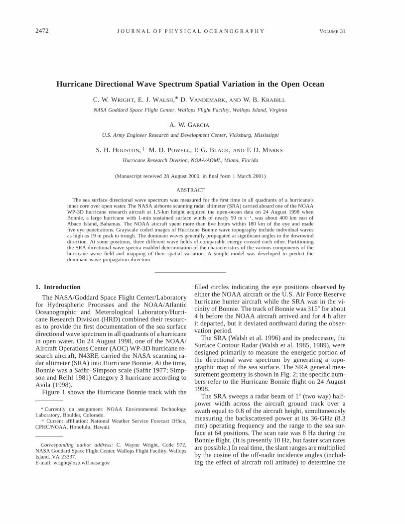
2472 VOLUME 31J O U R N A L O F P H Y S I C A L O C E A N O G R A P H Y

Hurricane Directional Wave Spectrum Spatial Variation in the Open Ocean

C. W. WRIGHT, E. J. WALSH,* D. VANDEMARK, AND W. B. KRABILL

NASA Goddard Space Flight Center, Wallops Flight Facility, Wallops Island, Virginia

A. W. GARCIA

U.S. Army Engineer Research and Development Center, Vicksburg, Mississippi

S. H. HOUSTON,1 M. D. POWELL, P. G. BLACK, AND F. D. MARKS

Hurricane Research Division, NOAA/AOML, Miami, Florida

(Manuscript received 28 August 2000, in final form 1 March 2001)

ABSTRACT

The sea surface directional wave spectrum was measured for the first time in all quadrants of a hurricane’sinner core over open water. The NASA airborne scanning radar altimeter (SRA) carried aboard one of the NOAAWP-3D hurricane research aircraft at 1.5-km height acquired the open-ocean data on 24 August 1998 whenBonnie, a large hurricane with 1-min sustained surface winds of nearly 50 m s21, was about 400 km east ofAbaco Island, Bahamas. The NOAA aircraft spent more than five hours within 180 km of the eye and madefive eye penetrations. Grayscale coded images of Hurricane Bonnie wave topography include individual wavesas high as 19 m peak to trough. The dominant waves generally propagated at significant angles to the downwinddirection. At some positions, three different wave fields of comparable energy crossed each other. Partitioningthe SRA directional wave spectra enabled determination of the characteristics of the various components of thehurricane wave field and mapping of their spatial variation. A simple model was developed to predict thedominant wave propagation direction.

1. Introduction

The NASA/Goddard Space Flight Center/Laboratoryfor Hydrospheric Processes and the NOAA/AtlanticOceanographic and Meterological Laboratory/Hurri-cane Research Division (HRD) combined their resourc-es to provide the first documentation of the sea surfacedirectional wave spectrum in all quadrants of a hurricanein open water. On 24 August 1998, one of the NOAA/Aircraft Operations Center (AOC) WP-3D hurricane re-search aircraft, N43RF, carried the NASA scanning ra-dar altimeter (SRA) into Hurricane Bonnie. At the time,Bonnie was a Saffir–Simpson scale (Saffir 1977; Simp-son and Reihl 1981) Category 3 hurricane according toAvila (1998).

Figure 1 shows the Hurricane Bonnie track with the

* Currently on assignment: NOAA Environmental TechnologyLaboratory, Boulder, Colorado.

1 Current affiliation: National Weather Service Forecast Office,CPHC/NOAA, Honolulu, Hawaii.

Corresponding author address: C. Wayne Wright, Code 972,NASA Goddard Space Flight Center, Wallops Flight Facility, WallopsIsland, VA 23337.E-mail: [email protected]

filled circles indicating the eye positions observed byeither the NOAA aircraft or the U.S. Air Force Reservehurricane hunter aircraft while the SRA was in the vi-cinity of Bonnie. The track of Bonnie was 3158 for about4 h before the NOAA aircraft arrived and for 4 h afterit departed, but it deviated northward during the obser-vation period.

The SRA (Walsh et al. 1996) and its predecessor, theSurface Contour Radar (Walsh et al. 1985, 1989), weredesigned primarily to measure the energetic portion ofthe directional wave spectrum by generating a topo-graphic map of the sea surface. The SRA general mea-surement geometry is shown in Fig. 2; the specific num-bers refer to the Hurricane Bonnie flight on 24 August1998.

The SRA sweeps a radar beam of 18 (two way) half-power width across the aircraft ground track over aswath equal to 0.8 of the aircraft height, simultaneouslymeasuring the backscattered power at its 36-GHz (8.3mm) operating frequency and the range to the sea sur-face at 64 positions. The scan rate was 8 Hz during theBonnie flight. (It is presently 10 Hz, but faster scan ratesare possible.) In real time, the slant ranges are multipliedby the cosine of the off-nadir incidence angles (includ-ing the effect of aircraft roll attitude) to determine the

AUGUST 2001 2473W R I G H T E T A L .

FIG. 1. Eye positions of Hurricane Bonnie observed by the NOAAresearch aircraft or the U.S. Air Force Reserve hurricane hunter air-craft. The filled circles indicate the eye positions observed duringthe SRA data-collection interval. The observation times beside theeye locations are UTC on 24 Aug 1998, with 24 h added to theobservation times on 25 Aug. The NOAA aircraft ground track isshown, except that two loops it made at 27.38N, 74.18W and 26.358N,73.18W have been deleted so they would not be mistaken for eyelocations.

FIG. 2. Measurement geometry of the SRA. The specific numbersrefer to the Hurricane Bonnie flight on 24 Aug 1998.

vertical distances from the aircraft to the sea surface.These distances are subtracted from the aircraft heightto produce a sea-surface elevation map, which is dis-played on a monitor in the aircraft to enable real-timeassessments of data quality and wave properties.

Because the SRA directional wave spectra are rep-resented in terms of ocean wave propagation vectors inwavenumber space, the wind is referenced to the direc-tion toward which it is blowing, rather than the mete-orological convention, to make it easier to assess dif-ferences in the wind and wave directions on the plots.

Observation-based surface wind analyses for hurri-canes are produced routinely by HRD (Powell et al.1996). These wind fields are provided in real time foroperational use by forecasters at the National HurricaneCenter. A real-time storm-centered analysis was per-formed at HRD for Hurricane Bonnie at 0130 UTC 25August 1998, which incorporated the NOAA flight-levelwinds adjusted to 10-m height above the surface, someCooperative Institute for Meteorological Satellite Stud-ies geostationary low-level visible satellite cloud-tracked winds adjusted to the surface (Dunion et al.2001, manuscript submitted to Mon. Wea. Rev.), and afew ship and buoy reports. The surface wind vectors

used throughout this paper were extracted from that sur-face wind analysis.

2. Wave topography

Figure 3 shows three examples of SRA wave topog-raphy maps using the same grayscale coding (darktroughs and light crests). The time sequence of the dataprogresses upward for the three 8-km segments, inde-pendent of the actual flight-line orientation. At the flightlevel of 1.5 km, the SRA swath width was 1.2 km andthe images are in proportion. The topography for theleft-hand image was obtained while the aircraft was trav-eling northward about 150 km north of Hurricane Bon-nie’s eye. The waves were predominantly swell prop-agating toward 3308, and the periodic oscillation in theheight of the waves associated with the narrow spectralwidth is apparent in the image. The significant waveheight (HS, 4 times rms surface elevation) was about 10m, and the dominant wavelength was about 300 m.

The HRD surface wind at this location was directedtoward the west at about 40 m s21. A secondary, shorterwavelength system generated by this wind can be seenpropagating from right to left across the image, whichwas parallel to the wind direction.

The wave topography in the middle image of Fig. 3was obtained while the aircraft was traveling south-eastward about 30 km south and 40 km east of the eye.Here HS was over 6 m, and the wave field was bimodalwith approximately the same energy in the two com-ponents. The sea surface topography for the image onthe right was acquired traveling northward about 120km east and 90 km south of the eye, where HS was over7 m and the wave field was trimodal.

To emphasize that the images of Fig. 3 represent wave


FIG. 3. Wave topography maps produced by the SRA displayedwith the same grayscale coding (dark troughs and light crests). Theisolated white speckles and the white line at 3700 m alongtrack and200 m cross-track are data dropouts. The left-hand and middle imagesinvolve about 550 crosstrack scan lines acquired over 71 s. The right-hand image involves only about 400 scan lines acquired over 51 sbecause the aircraft ground speed was faster.

FIG. 4. Surface elevation profile from cross-track positions 30 and37 (of 64 starting from the left-hand side of the SRA swath) for theinterval between 5 and 8 km on the left-hand image in Fig. 3.

topography, Fig. 4 shows the surface elevation profilesfrom cross-track positions 30 and 37 (of 64 starting fromthe left-hand side of the SRA swath) for the intervalbetween 5 and 8 km on the left-hand image in Fig. 3.Cross-track position 30 goes through the highest posi-tion on the crest of the large wave, 11 m above sealevel. It misses the deepest part of the trough, which islined up directly behind the highest part of the crest inthe direction of wave propagation. Cross-track position37, which is about 100 m to the right of position 30,profiles the deepest part of the trough, which is 8 mbelow sea level. The crest-to-trough height was 19 mwith a 178-m separation, which corresponds to a 356-m wavelength.

Figure 5 shows contours of the smoothed HS spatialvariation measured by the SRA during the 5 h it wasin the vicinity of Hurricane Bonnie on 24 August 1998.The smallest waves are in the vicinity of the radius ofmaximum wind in the southwest quadrant, and the larg-est waves are in a similar position in the northeast quad-

rant. While accurate and valuable, Fig. 5 should be con-sidered a simple characterization of the wave fieldwhose complexities are evident in Fig. 3.

3. Directional wave spectra

The sea-surface topography measured by the SRA isinterpolated to a uniform grid and transformed by a two-dimensional FFT. The artifact spectral lobes are deleted,and the real lobes are Doppler corrected. The appendixdescribes these processes in detail.

Figures 6–9 show wavenumber directional wavespectra generated from SRA topography measured inHurricane Bonnie on 24 August 1998. The time se-quence progresses from left to right and top to bottom.The map in the upper left-hand panel superimposes thestorm-centered track of the NOAA aircraft on the HRDsurface wind field. The wind radials extend downwind.This is opposite to the convention used in meteorology,but it is useful for comparison with the wave spectrapresented here. A speed of 30 m s21 corresponds to alength of 10 km. The spacing between adjacent windvector locations is 20 km. The circles on the map show


FIG. 5. Spatial variation in HS measured by the SRA in Hurricane Bonnie on 24 Aug 1998.Contours for integer values of wave height (in meters) are solid and contours for integer valuesplus 0.5 m are dashed.

the locations of the 15 spectra with the circle corre-sponding to the first spectrum in the sequence filled.

The SRA spectral observations presented in this paperspanned from 2030 UTC 24 August to 0144 UTC 25August. The 60 spectra in Figs. 6–9 have been selectedto show the significant features of the wave-field spatialvariation and provide detailed information on the spec-tral shapes.

The spectra are in a north, east (kn, ke) linear wave-number coordinate system with direction being towardwhich the waves are propagating. Each spectrum con-tains nine contours, linearly spaced from 10% to 90%of the peak spectral density of that spectrum, which in(rad m21)2 equals the number in the lower right-handcorner times 81 342. The half-power contour is thicker.

The thick radials in Figs. 6–9 indicate the orientationsof the boundaries of the half-planes used to eliminatethe spectral artifact lobes. To be able to deal with com-plex situations (such as real spectral lobes in oppositehalf-planes), there are separate boundaries for wave-lengths less than 150 m and greater than 150 m, althoughthey frequently have the same orientation. All spectralenergy is deleted on the artifact side of the boundary,

but subsequent Doppler corrections sometimes push thecontours past the boundaries.

Two dashed radials are used to partition each spec-trum into one to three components. The three pairs ofnumbers separated by a slash in the header of eachspectrum are the wave height (in meters, equal to fourtimes the square root of the spectral variance within thepartition) and the dominant wavelength (in meters, de-termined from kn and ke at the highest spectral valuewithin the partition). The sequence of the three sets ofnumbers is in clockwise (CW) order around the spec-trum. When only two wave components are identified,the two dashed radials are placed coincident betweenthem, so the middle elements in the header are zero.When only one component is identified, the two dashedradials are placed coincident at one of the half-planeboundaries, but, in this case, some spurious numbersstill show up in the third header entry.

The location north and east of the eye (in kilometers)is indicated in the upper left-hand corner of each spec-trum. The total HS is shown in the upper right-handcorner. In the lower left-hand corner are the flight seg-ment (1–10) and spectrum number, separated by a hy-


FIG. 6. SRA directional wave spectra acquired between 2030 and 2115 UTC 24 Aug 1998. The map in the upper left-hand panel superimposesthe NOAA aircraft track on the HRD surface wind field with radials extending downwind. A speed of 30 m s 21 corresponds to a length of10 km. The 15 circles indicate the locations of the 15 spectra, and the circle corresponding to the first spectrum in the sequence is filled.Wave direction is toward that in which the waves are propagating.

phen, and the second of the day (with 86 400 addedafter midnight).

The outer solid circle on each spectrum indicates awavelength of 100 m, and the inner circles correspond

to wavelengths of 200 and 300 m. The three dashedcircles correspond to wavelengths of 150, 250, and350 m.

The arrow superimposed on each spectrum points in


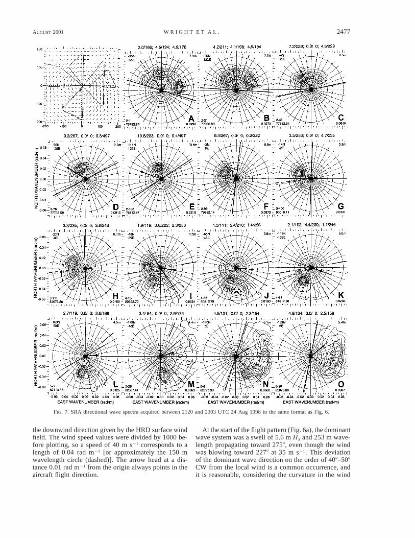
FIG. 7. SRA directional wave spectra acquired between 2120 and 2303 UTC 24 Aug 1998 in the same format as Fig. 6.

the downwind direction given by the HRD surface windfield. The wind speed values were divided by 1000 be-fore plotting, so a speed of 40 m s21 corresponds to alength of 0.04 rad m21 [or approximately the 150 mwavelength circle (dashed)]. The arrow head at a dis-tance 0.01 rad m21 from the origin always points in theaircraft flight direction.

At the start of the flight pattern (Fig. 6a), the dominantwave system was a swell of 5.6 m HS and 253 m wave-length propagating toward 2758, even though the windwas blowing toward 2278 at 35 m s21. This deviationof the dominant wave direction on the order of 408–508CW from the local wind is a common occurrence, andit is reasonable, considering the curvature in the wind


FIG. 8. SRA directional wave spectra acquired between 2307 UTC 24 Aug and 0016 UTC 25 Aug 1998 in the same format as Fig. 6.

field. The dashed partition radials are both oriented at2308. Even though no contours extend into the southernpartition, the energy it contains corresponds to a waveheight of 2.4 m, and the wavelength at the spectral peakwas 133 m. It was decided not to use log instead oflinear contours to extend below the 10% level because

it made many of the spectra busy and difficult to inter-pret.

In Figs. 6b–d the wind-driven waves appear as a tailon the westward propagating swell, extending towardshorter wavelengths. This points up a limitation of thepartitioning scheme used here. When the swell and


FIG. 9. SRA directional wave spectra acquired between 0024 and 0144 UTC 25 Aug 1998 in the same format as Fig. 6.

wind-driven wave components are not disjointed, the‘‘windsea’’ wavelength and direction of propagationwill sometimes be determined at the partition boundarywhen the spectral density is highest there.

Since even this simple scheme required four anglesto be determined for each spectrum (two for the half-planes, two for the partitions), a more complex parti-

tioning was considered too burdensome for the presentanalysis. The numbers in the headers should be usedwith caution, but they can provide quantitative infor-mation on the wave-field components.

The spectrum shown in Fig. 6e was near the eye, andthe situation was not very different from that shown inFig. 6d except that the wind was almost zero. The se-


FIG. 10. Wind-weighting patterns overlaid on six spectra from various parts of Hurricane Bonnie.

quence in Figs. 6f–l shows spectra from contiguous 8-km data spans approaching the radius of maximumwind. The spectra in Figs. 6h–l show the wind-drivencomponent growing with increasing wind from 2.8 mHS and 107 m wavelength to 5.8 m HS and 166 m wave-length. The swell component maintained about 4 m HS

during this sequence. As the end of the Fig. 6 flightsegment was approached, the northwestward propagat-ing swell bifurcated, and the wave field as a whole ro-tated CW as the wind rotated counterclockwise (CCW).

The aircraft turned northward when it was about 120km east and 100 km south of the eye. Fifty kilometerssouth of the eye the wave field became strongly trimodal(Fig. 7b), with each of the three components havingabout 200 m wavelength and over 4 m HS. The spectralpeaks were spread over 1008 and the span of the half-power spectral width was about 1458. This would likelybe a particularly dangerous location for a boat, sincethe total HS was 7.7 m and it was not possible to keepthe bow pointed into the approaching waves.

Due east of the eye, the north and northwest wavecomponents had coalesced (Fig. 7c), and by 56 km northof the eye (and 125 km east) only a broad northwestwardpropagating swell of 9.2 m HS remained (Fig. 7d). Theswell spectrum narrowed and rotated CW as the distance

north of the eye increased (Fig. 7e). The HS increasedalong this flight segment from about 7 m to more than10 m.

As the aircraft proceeded back to the eye, the swellsystem rotated CCW. About 40 km northeast of the eye,a CCW extrusion of the spectrum toward shorter wave-lengths began that became pronounced in the eye (Figs.7f,g). By 20 km south of the eye (Fig. 7h) the two wavefields were comparable and opposed to the local wind.Between 80 and 160 km southwest of the eye (Figs.7j,k) the dominant waves propagated at right angles tothe 35–25 m s21 local wind.

At 160 km due south of the eye (Fig. 7n), the wavefield was quite broad with highly correlated trends inspectral density, wavelength, and propagation direction.The longest waves propagated toward the southeast, andthe shortest toward the northeast. Proceeding north, thebroad eastward propagating wave field consolidated androtated CCW without much increase in HS (Figs. 7o,8a).

Between 96 and 39 km south of the eye (Figs. 8a–h), the wave-field composition changed radically withonly a small decrease in HS. A northwestward propa-gating swell appeared and increased to 4.3 m HS and246 m wavelength as it rotated CCW. During the same


FIG. 11. Wind-weighting patterns overlaid on six spectra from one 40-km flight segment in Hurricane Bonnie. The solid patterns considerthe hurricane motion over the 10 h prior to the observations, and the dashed patterns held the wind field fixed to that at the observationtimes.

interval, the eastward propagating system diminishedfrom 5.8 to 2.6 m HS as it also rotated CCW.

The spectrum had essentially the same shape betweenthe eye (Fig. 8i) and 40 km north of the eye, but HS

increased from 7 to 10 m. At 66 km north of the eye(Fig. 8j), the spectrum was quite narrow and it rotatedCW as the distance from the eye increased (Fig. 8k).

The header indicates that the swell system in the spec-trum shown in Fig. 8k had 8.8 m HS and 307 m dominantwavelength. The secondary wave system seen propa-gating toward the west in the left-hand image of Fig. 3is not apparent in the spectrum (Fig. 8k) because itspeak energy density was less than 10% of the swellpeak. Even though the energy density for the wind-driven sea was below the lowest contour in the spectrumshown in Fig. 8k, the numbers in the header indicatethat HS associated with the wind direction was 3.1 m.The windsea spectrum would have been much broaderthan the narrow swell spectrum. The wind-driven waveheight was probably higher since the partition boundarywas only 128 CW of the wind vector, but, for simplicity,the partitioning process was restricted to two radials forboundaries. The 422 m dominant wavelength for thewind-driven sea partition suggests that there was some

unseen noise contamination near the origin that washigher than the wind-driven sea peak.

Figure 9 is included for completeness so that the de-tails of the spectral shapes and spatial variations can becompared with those of the other flight lines. All thesignificant variations in spectral shape are displayed inFigs. 6–9. They can be used in interpreting the planviews of the spatial variation of the wave-field com-ponents discussed later in this paper.

4. A simple model for predicting wave dominance

When the dominant waves were observed propagat-ing orthogonal to a 30 m s21 local wind, a simple modelwas developed to check on the reasonableness of theobserved spectra. To study differential wave growth inLake St. Clair, Donelan et al. (1992) used the root-mean-square (rms) wind along the propagation path rather thana linear average because wave energy scales roughlywith the square of wind speed (Hasselmann et al. 1973).This analysis uses a modification of that approach.

The goal was to develop a function that would suggestthe direction toward which the dominant waves wouldpropagate at each location where a directional wave


FIG. 12. Hurricane Bonnie primary wave field. The circles indicatethe data locations and the radials extend in the wave propagationdirection a length proportional to the wavelength. The width of theradials is proportional to the HS, so the aspect ratio is an indicationof wave steepness. The short, narrow lines indicate the HRD surfacewind analysis.

FIG. 13. Hurricane Bonnie secondary wave field in same format asFig. 12.

FIG. 14. Hurricane Bonnie tertiary wave field in same format asFig. 12.

spectrum was determined. At each location, for every108 azimuth, the wind effect over a 300-km fetch wassummed in 10-km increments. At the 31 positions alongeach radial direction, the wind vector from the HRDsurface wind analysis was used to determine f, the anglebetween it and the radial direction. An ‘‘effective’’ windat that position for generating waves propagating towardthe observation point was calculated as U cosf1.63,where U is the wind speed.

The term U cosf is the component of the wind speedalong the radial, but Walsh et al. (1989) found that windcomponents needed to be less effective in generatingwaves in slant-fetch geometries than a wind of the com-ponent magnitude blowing in that direction. In partic-ular, the wind components needed to be degraded byraising the cosine to the 1.63 power. When f is small,there is little difference, but when f is 558, the effectivewind is reduced to 0.7 of the wind component alongthe radial.

To keep the model simple, but still acknowledge themotion of the hurricane and the travel time of the waves,an 8.8 m s21 group velocity (corresponding to waves of200 m wavelength) was used to determine how muchearlier the time would have been at each position alongthe radial for the effect of the wind at that position tohave reached the point of observation. (Group velocitiesfor 100 m and 300 m wavelengths are 6.2 m s21 and10.2 m s21, respectively.)

The wind computation was not done in the storm-relative coordinates used elsewhere in this paper, but inan earth-relative absolute reference frame. A time offset

determined by the distance along the radial directionand the 8.8 m s21 group velocity was subtracted fromthe observation time of the spectrum to determine aneffective time for the wind observation. The absolutelocation along the radial direction and the hurricane-eyeposition at the effective time were then used to deter-mine the position relative to the eye for extracting thewind vector from the storm-relative HRD surface-windfield. Using an 8.8 m s21 group velocity meant that theeffective wind at 300 km from the observation pointcorresponded to the hurricane position 9.4 h earlier.


Only effective winds blowing toward the observationpoint were considered. Their values were squared andsummed over the 300 km, following Donelan et al.(1992). This was taken to be a crude measure of thetotal ability of the wind along each 300 km radial di-rection to generate waves propagating toward the ob-servation point.

Figure 10 shows the results of the wind computationoverlaid on six spectra from various parts of HurricaneBonnie. The sums of the squares of the effective windvalues for the 36 radial directions were normalized bytheir peak value, multiplied by 0.07, and plotted as anindication of the cumulative relative strength of the windfield. In all six cases the maximum of the pattern agreedvery well with the observed propagation direction ofthe dominant waves, whether they were in the winddirection (Fig. 10a), or off the wind direction by 508(Figs. 10b and 10c), 908 (Fig. 10d), 1108 (Fig. 10e), oreven 1808 (Fig. 10f).

All the wind-weighting patterns in Fig. 10 were fairlynarrow and the spectra were relatively simple. Figure11 shows the predictive ability of the wind-weightingpattern in a complex situation. As the aircraft travelednorthward through the radius of maximum wind southof the eye, the composition of the wave field totallychanged with little change in wave height (Fig. 8). Thewind-weighting patterns in Fig. 11 predict the rapidchange in the composition of the wave field over this40-km interval, even though the local wind was alwaysdirected toward 508 and was never less than about 25m s21.

This accomplishment is remarkable if one looks atthe storm-centered wind field in Fig. 8. The wind to thesoutheast of the segment for the spectra of Fig. 11 isalmost orthogonal to the northwest swell propagationdirection evident in Fig. 11. The hurricane had beenmoving toward the northwest, but turned nearly duenorth just as the research flight entered the storm (Fig.1), cutting across northwestward propagating wavesgenerated at an earlier time. The simple model was ableto predict the transition in the wave field because itaccounted for the hurricane motion over the 10 h priorto the observations. The dashed wind-weighting patternin Fig. 11 shows the result of holding the wind fieldfixed in the position it occupied at the observation time.

This simple model does not predict the dominantwavelength and is not intended to compete with eventhe crudest wind wave generation model. But the com-putation is fast enough that it can be performed at thelocation of every spectrum. It is of great benefit in de-termining which components in the encounter spectrumof a complex wave field are real.

5. Spatial variation of wave components

Even though the previous section showed the limi-tations of a storm-centered analysis of a hurricane, somecautious observations can be made in that reference

frame. For each of the three partitions in each spectrum,HS, the wavelength, and the direction of propagation atthe peak spectral density were determined and desig-nated as primary, secondary, or tertiary wave fieldsbased on the wave height.

Figure 12 is a plan view of the Hurricane Bonnieprimary wave field. The circles indicate the data loca-tions, and the radials extend in the wave propagationdirection a length proportional to the wavelength. Thewidth of the radials is proportional to the HS, so theaspect ratio is an indication of wave steepness. A widerectangle indicates steep waves, and a narrow rectangleindicates shallow waves.

The northeast quadrant of Bonnie had the most heavyrain, which resulted in data gaps caused by completeattenuation of the SRA signal. The dominance of the300 m wavelength, 10-m high swell propagating towardthe northwest is apparent. Its propagation direction isroughly aligned with the track Bonnie had for the 4-hperiod just prior to the observations. The northwestswell was the result of two effects. First, the wind isgenerally higher in the direction of motion of the hur-ricane because, in most cases, the forward translationof the storm adds to the wind speed in the right half ofthe storm (and subtracts from it on the opposite side).Second, there is a partial resonance that increases theeffective fetch and duration of the wave-growth processin the direction of the motion of the storm (Shemdin1980; Young 1988; MacAfee and Bowyer 2000a,b;Bowyer 2000). The high curvature of the wind fieldlimits the fetch, but the waves that propagate in thedirection of the motion of the storm remain under theinfluence of an aligned wind for a longer time and dis-tance. This is not a new concept since the general rulethat the largest waves in a hurricane are in the rightforward quadrant is well known (Cline 1920; Tannehill1936), but Fig. 12 is an impressive demonstration of it.

Also apparent in Fig. 12 is the frequent propagationof the dominant waves at a large angle to the local wind,sometimes even opposite it. Stress formulations that donot consider this phenomenon might be subject to con-siderable error.

Figure 13 shows a plan view of the secondary wavefield. The plot should be interpreted in conjunction withthe spectral shapes and the partition orientations shownin Figs. 6–9. In contrast to the primary wave field, thesecondary wave field is more symmetrical spatially, andit frequently propagates near the downwind direction.

Figure 14 shows the tertiary wave field. No tertiarywave components were identifiable north of the eye be-cause of the dominance of the northwestward propa-gating swell.

Figures 12, 13, and 14 indicate three directions ofpropagating wave fields for the northbound flight seg-ment 120 km east of the eye: northwest, north, andnortheast. At the south end of the flight segment, thenorthwestward propagating wave field is tertiary, but 40


FIG. A1. Grayscale-coded topography for 180-line segment measured with the SRA when the aircraft was about75 km north and 125 km east of the eye and traveling toward the southwest. The outline of the uniform grid the dataare interpolated to is indicated by the square box.

FIG. A2. Expanded region around the origin of Fig. A1. Circlesindicate locations of SRA elevation measurements; dots indicatepoints of the uniform grid to which the data are linearly interpolated.

km to the north it becomes secondary, and in another30 km it is primary.

If only the northwest propagating wave componentsfrom Figs. 12–14 were plotted on a single figure and

traced backward, they would appear to originate froma broad region in the right rear quadrant of the storm.

In 1976 there were pioneering hurricane observationswith comparable coverage and resolution to that of theSRA that need to be acknowledged. They were aquiredusing a Jet Propulsion Laboratory synthetic aperture ra-dar (SAR) onboard a NASA CV-990 research aircraftat 8 to 13 km altitude. Two flights were made in Hur-ricane Emmy, one in Hurricane Francis, and two in Hur-ricane Gloria. Elachi et al. (1977) and King and Shemdin(1979) essentially treated the SAR high-resolutionocean wave imagery as microwave photographs fromwhich they could determine the direction and the wave-length of the waves. They made no attempt to use amodulation transfer function to relate the radar signatureto the wave directional energy spectrum. But even with-out the quantitative formation of the present analysis,they were still able to point out many of the same qual-itative properties of the wave field presented here.

6. Conclusions

The SRA has provided the first sea-surface directionalwave spectrum measurements in all quadrants of theinner core of a hurricane over open water. The highestHS in Hurricane Bonnie on 24 August 1998 was almost11 m and individual waves up to 19 m peak to troughwere observed. The highest waves and the longest wave-


FIG. A3. Doppler-corrected spectra resulting from a northward flight line 156 km north and 10 km east of the eye(a) and a southwestward flight line about 167 km north and 9 km west of the eye (b).

lengths were observed in the right forward quadrant ofthe hurricane, as is commonly assumed. They are dueto the typically higher wind speed resulting from theforward motion of the storm and a partial resonancebetween the forward motion of the storm and the groupvelocity of the waves propagating in that direction.

The lowest HS, about 5.5 m, was observed in thevicinity of the radius of maximum wind in the left rearquadrant of the hurricane. A trimodal wave system ex-isted in the right rear quadrant of Hurricane Bonnie witha total HS of almost 8 m. Each of the three componentshad a dominant wavelength of about 200 m and an HS

of more than 4 m.The dominant waves generally do not propagate in

the downwind direction of the local wind, but a simplemodel for the effective wind-weighting pattern pre-dicted their propagation direction, even in complex sit-uations, when the time history of the hurricane trackover the previous 10 h was considered.

An animation of the Hurricane Bonnie wave spectracan be seen online (http://lidar.wff.nasa.gov/sra/chs2000.shtml).

Acknowledgments. Donald E. Hines of EG&G Inc.maintained the SRA and Gerald S. McIntire of CSCinstalled it in NOAA aircraft N43RF. The authors thankthe flight crew and staff of the NOAA/AOC for theirhelp in ensuring the success of this experiment. TheScience and Engineering Division deserves special rec-ognition for work in installing the SRA on N43RF anddeveloping the needed interfaces with the other aircraftsystems. This work was supported by the NASA SolidEarth/Natural Hazards Program, the NASA PhysicalOceanography Program, and the Office of Naval Re-search (Document N00014-98-F-0209).

APPENDIX

Generating and Correcting Directional WaveSpectra

Figure A1 shows a 180-line segment of grayscale-coded topography measured with the SRA when theaircraft was about 75 km north and 125 km east ofBonnie’s eye and traveling toward the southwest. TheSRA topographic data are processed in 180-line seg-ments with the measured elevation points interpolatedto a uniform orthogonal grid that is centered on themidpoint of the data. The axes are oriented north andeast, and the outline of the uniform grid is indicated bythe square box. The axes of the uniform grid each con-tain 256 points spaced at 7 m for a nominal spectralresolution of 0.0035 rad m21. Figure A1 demonstratesthat the actual crosstrack spectral resolution is onlyabout 0.0052 rad m21, determined by the nominal 1200-m swath width. Since the data do not fill the box, thespectral variances are multiplied by the ratio of the totalarea of the box to the area containing nonzero surfaceelevation values.

Figure A2 expands the region around the origin ofFig. A1. The circles indicate the locations of the SRAelevation measurements, and the dots indicate the pointsof the uniform grid to which the data are linearly in-terpolated. The interpolation automatically compensatesfor variations in ground speed and track and aircraftdrift angle, which causes the SRA scan plane to deviatefrom the normal to the ground track.

The interpolated data are transformed by a two-di-mensional FFT to obtain the directional wave spectrumin wavenumber space. The line count is advanced 100for each new spectrum. The amount of overlap in the


FIG. A4. Wave spectra corresponding to Fig. 6o (left side, panels a and c) and Fig. 7a (right side, panels b and d)before (top panels, a and b) and after (bottom panels, c and d) Doppler correction.

wave topography input into adjacent spectra depends onthe aircraft ground track and ground speed, which variedbetween 86 and 169 m s21 with a mean of 119 m s21.At the average ground speed, the overlap would be about13%. At the lowest ground speed, the overlap would beabout 40%.

Output spectra are obtained by averaging five con-secutive spectra. The output spectra are additionallysmoothed by using uniform weighting on a 3 3 3 arrayof points in wavenumber space. If the input topographyto the individual spectra were nonoverlapping and theuniform grid were filled, the smoothed output spectrawould have 90 degrees of freedom. The actual spectrahave fewer.

Each spectrum contains an ambiguity of 1808 in thedirection of propagation of the waves, which is commonto all transformations from topographic maps. The FFTdoes not determine the actual direction of propagation

and puts half the spectral energy into the real lobe andhalf into an artifact lobe that is perfectly symmetric withthe real lobe. The SRA processing doubles the energyeverywhere in the FFT output spectrum and then deletesthe energy in the half-plane containing the artifacts.

The spectra must be corrected for Doppler effectscaused by ocean wave propagation. The proper Dopplercorrections can be applied without any a priori infor-mation on the wave field. All wave components arecorrected as if they were real. Waves propagating in theaircraft flight direction appear to be too long, and theymust be shifted to higher wavenumbers (shorter wave-lengths). Waves propagating opposite the aircraft flightdirection appear too short, and they must be shifted tolower wavenumbers (longer wavelengths). Waves prop-agating at right angles to the aircraft flight track appearto have a different propagation direction. In general,corrections to both the wavelength and direction of


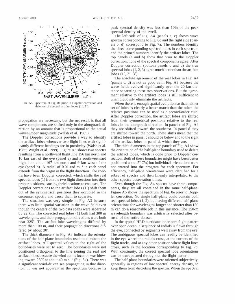
FIG. A5. Spectrum of Fig. 8e prior to Doppler correction anddeletion of spectral artifact lobes (19, 29).

propagation are necessary, but the net result is that allwave components are shifted only in the alongtrack di-rection by an amount that is proportional to the actualwavenumber magnitude (Walsh et al. 1985).

The Doppler corrections provide a way to identifythe artifact lobes whenever two flight lines with signif-icantly different headings are in proximity (Walsh et al.1985; Wright et al. 1999). Figure A3 shows two spectraresulting from a northward flight line 156 km north and10 km east of the eye (panel a) and a southwestwardflight line about 167 km north and 9 km west of theeye (panel b). A radial of 0.01 rad m21 in each panelextends from the origin in the flight direction. The spec-tra have been Doppler corrected, which shifts the realspectral lobes (1) from the two flight directions into theirproper positions, causing their locations to coalesce. TheDoppler corrections to the artifact lobes (19) shift themout of the symmetrical positions they occupied in theencounter spectra and cause them to separate.

The situation was very simple in Fig. A3 becausethere was little spatial variation in the wave field eventhough the centers of the two data spans were separatedby 22 km. The corrected real lobes (1) both had 300 mwavelengths, and their propagation directions were bothnear 3258. The artifact-lobe wavelengths differed bymore than 100 m, and their propagation directions dif-fered by about 308.

The thick diameters in Fig. A3 indicate the orienta-tions of the half-plane boundaries used to eliminate theartifact lobes. All spectral values to the right of theboundaries were set to zero. The boundaries were notpositioned orthogonal to the line joining the real andartifact lobes because the wind at this location was blow-ing toward 2608 at about 40 m s21 (Fig. 8k). There wasa significant wind-driven sea propagating in that direc-tion. It was not apparent in the spectrum because its

peak spectral density was less than 10% of the peakspectral density of the swell.

The left side of Fig. A4 (panels a, c) shows wavespectra corresponding to Fig. 6o and the right side (pan-els b, d) correspond to Fig. 7a. The numbers identifythe three corresponding spectral lobes in each spectrumand the primed numbers identify the artifact lobes. Thetop panels (a and b) show that prior to the Dopplercorrection, none of the spectral components agree. AfterDoppler correction (bottom panels c and d) the truespectral lobes (1, 2, 3) agree much better than the artifactlobes (19, 29, 39).

The absolute agreement of the real lobes in Fig. A4(panels c, d) is not as good as in Fig. A3 because thewave fields evolved significantly over the 20-km dis-tance separating these two observations. But the agree-ment relative to the artifact lobes is still sufficient tounambiguously eliminate the artifacts.

When there is enough spatial evolution so that neitherset of lobes is clearly a better match than the other, therelative positions can be used as a second-order clue.After Doppler correction, the artifact lobes are shiftedfrom their symmetrical positions relative to the reallobes in the alongtrack direction. In panel c of Fig. A4they are shifted toward the southeast. In panel d theyare shifted toward the north. These shifts mean that theartifact lobes in panel c should be below and to the rightof the artifact lobes in panel d, which they are.

The thick diameters in the top panels of Fig. A4 showthe orientation of the half-plane boundary used to deletethe artifact lobes, which is done prior to Doppler cor-rection. Both of these boundaries might have been betterpositioned about 58 CW, but individual orientations werenot entered into the program for each spectrum. Forefficiency, half-plane orientations were identified for asubset of spectra and then linearly interpolated to theother spectra observation times.

Even though the Fig. A4 spectra have three compo-nents, they are all contained in the same half-plane.Figure A5 shows the spectrum of Fig. 8e prior to Dopp-ler correction. No single half-plane could contain bothreal spectral lobes (1, 2), but having different half-planeorientations for wavelengths longer and shorter than 150m can do a reasonable job in this instance. The 150-mwavelength boundary was arbitrarily selected after pe-rusal of the entire dataset.

In the typical HRD hurricane inner core flight patternover open ocean, a sequence of radials is flown throughthe eye, connected by segments well away from the eye.The ambiguous spectral lobes can readily be identifiedin the eye where the radials cross, at the corners of theflight tracks, and at any other position where flight linescross, such as the location corresponding to Fig. 7c.With continuity, the correct spectral lobe orientationscan be extrapolated throughout the flight pattern.

The half-plane boundaries were oriented subjectively,generally in regions of low spectral energy density, tokeep them from distorting the spectra. When the spectral


azimuthal variation permitted, the high-wavenumberhalf-plane boundary was oriented nearly orthogonal tothe wind direction.

REFERENCES

Avila, L. A., 1998: Preliminary report: Hurricane Bonnie 19–30 Au-gust 1998. NOAA National Hurricane Center/Tropical PredictionCenter, 16 pp. [Available online at http://www.nhc.noaa.gov.]

Bowyer, P. J., 2000: Phenomenal waves with a transitioning tropicalcyclone (Luis, the Queen, and the buoys). Preprints, 24th Conf.on Hurricanes and Tropical Meteorology, Ft. Lauderdale, FL,Amer. Meteor. Soc., 294–295.

Cline, I. M., 1920: Relation of changes in storm tides on the coastof the Gulf of Mexico to the center and movement of hurricanes.Mon. Wea. Rev., 48, 127–146.

Donelan, M., M. Skafel, H. Graber, P. Liu, D. Schwab, and S. Ven-katesh, 1992: On the growth of wind-generated waves. Atmos.–Ocean, 30, 457–478.

Elachi, C., T. W. Thompson, and D. King, 1977: Ocean wave patternsunder Hurricane Gloria: Observation with an airborne synthetic-aperture radar. Science, 198, 609–610.

Hasselmann, K., and Coauthors,1973: Measurements of wind–wavegrowth and swell decay during the Joint North Sea Wave Project(JONSWAP). Dtsch. Hydrogr. Z., A8 (12) (Suppl.), 95 pp.

King, D. B., and O. H. Shemdin, 1979: Radar observations of hur-ricane wave directions. Proc. 16th Int. Conf. Coastal Eng., Ham-burg, Germany, ASCE, 209–226.

MacAfee, A. W., and P. J. Bowyer, 2000a: Trapped-fetch waves in atransitioning tropical cyclone (Part I—The need and the theory).Preprints, 24th Conf. on Hurricanes and Tropical Meteorology,Ft. Lauderdale, FL, Amer. Meteor. Soc., 292–293.

——, and ——, 2000b: Trapped-fetch waves in a transitioning trop-

ical cyclone (Part II—Analytical and predictive model). Pre-prints, 24th Conf. on Hurricanes and Tropical Meteorology, Ft.Lauderdale, FL, Amer. Meteor. Soc., 165–166.

Powell, M. D., S. H. Houston, and T. A. Reinhold, 1996: HurricaneAndrew’s landfall in south Florida. Part I: Standardizing mea-surements for documentation of surface wind fields. Wea. Fore-casting, 11, 304–328.

Saffir, H. S., 1977: Design and construction requirements for hurri-cane resistant construction. ASCE Preprint No. 2830, AmericanSociety of Civil Engineers, New York, 20 pp.

Shemdin, O. H., 1980: Prediction of dominant wave properties aheadof hurricanes. Proc. 17th Int. Coastal Engineering Conf., Syd-ney, Australia, ASCE, 600–609.

Simpson, R. H., and H. Riehl, 1981: The Hurricane and its Impact.Louisiana State University Press, 398 pp.

Tannehill, I. R., 1936: Sea swells in relation to movement and in-tensity of tropical storms. Mon. Wea. Rev., 64, 231–238.

Walsh, E. J., D. W. Hancock, D. E. Hines, R. N. Swift, and J. F. Scott,1985: Directional wave spectra measured with the surface con-tour radar. J. Phys. Oceanogr., 15, 566–592.

——, ——, ——, ——, and ——,1989: An observation of the di-rectional wave spectrum evolution from shoreline to fully de-veloped. J. Phys. Oceanogr., 19, 670–690.

——, L. K. Shay, H. C. Graber, A. Guillaume, D. Vandemark, D. E.Hines, R. N. Swift, and J. F. Scott, 1996: Observations of surfacewave–current interaction during SWADE. Global Atmos. OceanSyst., 5, 99–124.

Wright, C. W., E. J. Walsh, D. Vandemark, W. B. Krabill, and A.Garcia, 1999: Hurricane directional wave spectrum measurementwith a scanning radar altimeter. Proceedings of the Third Inter-national Workshop on Very Large Floating Structures(VLFS’99), R. C. Ertekin and W. J. Kim, Eds., Vol. 1, U.S. Officeof Naval Research, 37–41.

Young, I. R., 1988: Parametric hurricane wave prediction model. J.Waterway, Port, Coastal Ocean Eng., 114, 637–652.

Hurricane Directional Wave Spectrum Spatial Variation at Landfall

Documents

Transcript of Hurricane Directional Wave Spectrum Spatial Variation at Landfall