1

Human-induced changes in Wind,

Temperature and Relative Humidity during

Santa Ana events

Mimi Hughes1, Alex Hall

2, and Jinwon Kim

2

1 National Research Council/National Oceanic and Atmospheric Administration,

Earth System Research Laboratory, Physical Sciences Division, 325 Broadway,

Boulder CO 80305

(303)497-4865

Mimi.hughes@noaa.gov

2 University of California, Los Angeles, Department of Atmospheric and Oceanic

Sciences, Box 951565, Los Angeles, CA 90095

Abstract: The frequency and character of Southern California’s Santa Ana wind events are

investigated within a 12-km-resolution downscaling of late-20th

and mid-21st century time periods

of the National Center for Atmospheric Research Community Climate System Model global

climate change scenario run. The number of Santa Ana days per winter season is approximately

20% fewer in the mid-21st century compared to the late-20

th century. Since the only systematic

and sustained difference between these two periods is the level of anthropogenic forcing, this

effect is anthropogenic in origin. In both time periods, Santa Ana winds are partly katabatically-

driven by a temperature difference between the cold wintertime air pooling in the desert against

coastal mountains and the adjacent warm air over the ocean. However, this katabatic mechanism

is significantly weaker during the mid-21st century time period. This occurs because of the well-

documented differential warming associated with transient climate change, with more warming in

the desert interior than over the ocean. Thus the mechanism responsible for the decrease in Santa

Ana frequency originates from a well-known aspect of the climate response to increasing

greenhouse gases, but cannot be understood or simulated without mesoscale atmospheric

dynamics. In addition to the change in Santa Ana frequency, we investigate changes during Santa

Anas in two other meteorological variables known to be relevant to fire weather conditions --

relative humidity and temperature. We find a decrease in the relative humidity and an increase in

temperature. Both these changes would favor fire. A fire behavior model accounting for changes

in wind, temperature, and relative humidity simultaneously is necessary to draw firm conclusions

about future fire risk and growth associated with Santa Ana events.

Keywords: regional climate, climate change, downslope winds, fire weather

Abbreviations:

2

1.0 Introduction

The cool, relatively moist fall and winter climate of Southern California is

often disrupted by dry, hot days with strong winds, known as Santa Anas, blowing

out of the desert. The Santa Ana winds are a dominant feature of the fall and

wintertime climate of Southern California (Conil and Hall 2006), and they have

important ecological impacts. The most familiar is their influence on wildfires:

Following the hot, dry Southern California summer, the extremely low relative

humidities and strong, gusty winds associated with Santa Anas introduce extreme

fire risk, often culminating in wildfires with large economic loss (Westerling et al.

2004). Less widely-known but just as important is their impact on coastal-ocean

ecosystems: The strong winds induce cold filaments in sea-surface temperature

(SST) with an associated increase in biological activity (Castro et al. 2006;

Trasvina et al. 2003). This decrease in SST and increase in biological activity is

likely due in part to increased mixing in the oceanic boundary layer, although an

increase in dust deposition on the ocean surface during these events could also

increase biological activity (Hu and Liu 2003; Jickells et al. 2005).

A recent investigation of the dynamics of Santa Ana winds (Hughes and

Hall 2009) found that both local and synoptic conditions control their formation.

When strong synoptically-forced offshore flow impinges on Southern California’s

topography, offshore momentum can be transported to the surface, causing Santa

Ana conditions. However, Hughes and Hall (2009) found that there are many days

with Santa Ana conditions that are not associated with this type of strong synoptic

forcing. Rather, for a large fraction of the Santa Ana days, offshore winds are

forced by a local temperature gradient between the cold desert and warmer air

over the ocean at the same altitude. The temperature gradient induces a

hydrostatic pressure gradient pointing from the desert to the ocean, which is

reinforced by the negative buoyancy of the cold air as it flows down the sloped

surface of the major topographical gaps.

This study investigates the response of the frequency and intensity of

Santa Ana events and associated meteorological conditions to anthropogenic

forcing. Santa Ana wind events cannot be simulated without resolving the coastal

mountain ranges separating the Mojave desert from the Southern California Bight.

This requires resolution higher than roughly 10-15km. Hughes and Hall (2009)

3

showed that even the relatively high-resolution North American Regional

Reanalysis (NARR, 32 km horizontal resolution) has unrealistically weak Santa

Ana winds. Because its coarse resolution does not adequately resolve the coastal

topography, it cannot develop the tight desert-ocean temperature gradient often

driving Santa Anas. However, when the NARR data are dynamically downscaled

with a much higher resolution regional atmospheric model, Santa Ana events are

well-reproduced. This indicates that conditions leading to Santa Anas are implicit

in the coarser resolution NARR data set, even if the reanalysis model itself is

incapable of generating them realistically. This dynamical downscaling technique

has also been proven numerous times to give a more realistic view of local climate

conditions in other contexts (e.g., Diffenbaugh et al. 2005; Leung and Ghan 1999;

Kim and Lee 2003).

It follows that global models even coarser in resolution than the NARR

product, such as those used for global climate change simulations, likely have

almost no signature of these strong offshore winds, even if they do contain

information highly relevant for Santa Ana formation. In our case, we are

examining changes in Santa Anas implicit in the National Center for Atmospheric

Research (NCAR) Community Climate System Model (CCSM) global climate

change scenario run. This model has a grid-point equivalent resolution of roughly

1.4 degrees, obviously much too coarse to resolve Southern California’s coastal

ranges. To resolve the topography and draw out the simulation’s implications for

Santa Anas, we therefore must downscale it with a regional atmospheric model.

As we demonstrate, the regional simulation and the dynamical framework

describing Santa Ana wind development of Hughes and Hall (2009) together

allow us to identify how large-scale changes in the simulated future climate of the

CCSM simulation affect the frequency and intensity of Santa Ana events. Our

results indicate that as the climate adjusts to anthropogenic forcing, the frequency

of Santa Ana days is reduced. Although the reduction in Santa Ana events could

suggest a reduction in fire occurrence as the climate responds to anthropogenic

forcing, we further investigate two other meteorological variables known to affect

fire in the region, temperature and relative humidity (Moritz et. al. 2010). In both

cases, these meteorological variables change in ways favorable for fire

occurrence, with relative humidity decreasing on days with Santa Ana conditions,

4

and temperature increasing. Thus the implications of anthropogenic climate

change for fire conditions in the region are ambiguous.

2.0 Weather Research and Forecast (WRF)

Simulation

The climate change experiment is carried out by downscaling late 20th

century and mid 21st century time slices from a climate change scenario

simulation done with the NCAR Community Climate System Model 3 (CCSM3).

This dynamical downscaling was performed with the Weather Research and

Forecast (WRF) model, version 2.2.1 (Skamarock et al. 2005). The model solves a

non-hydrostatic momentum equation in conjunction with the thermodynamic

energy equation. The model features multiple options for advection and

parameterized atmospheric physical processes. The physics options selected in

this experiment include the NOAH land-surface scheme (Chang et al. 1999), the

simplified Arakawa Schubert (SAS) convection scheme (Hong and Pan 1998), the

Rapid Radiative Transfer Model (RRTM) longwave radiation scheme (Mlawer et

al. 1997), Dudhia (1989) shortwave radiation, and the WRF Single-Moment

(WSM) 3-class with simple ice cloud microphysics scheme. For more details on

the physics options, readers are referred to the website http://wrf-model.org. The

model domain covers the western United States at a 36-km horizontal resolution,

with the inner 12-km nest spanning the entire state of California and adjacent

coastal zone. Both domains have 28 atmospheric and 4 soil layers in the vertical.

WRF was driven by the global climate data generated when the Special

Report on Emissions Scenarios (SRES) A1B emission scenario is imposed on

CCSM3 (Nakicenovic and Swart 2000). The emission scenario assumes balanced

energy generation between fossil and non-fossil fuel; the resulting carbon dioxide

(CO2) emissions are located near the averages of all SRES emission scenarios.

The CO2 concentrations in the WRF simulations were fixed at 330 parts per

million, volume (ppmv) and 430 ppmv during the late 20th

century and mid-

twenty-first century periods, respectively.

Regional climate for the late 20th

century and mid-21st century periods is

calculated from a total of 20 cold season (October–March) WRF simulations

spanning two time periods: 1971–1981 and 2045–2055. Individual WRF runs

were initialized at 00UTC October 1 of the corresponding years using the CCSM3

5

output data. All simulations continued for the remaining six-month period without

re-initialization by updating the large-scale forcing along the lateral boundaries at

three-hour intervals. The focus on the cold season simulations is appropriate in

this case because Santa Ana winds have a very strong seasonality, with peak

occurrence in December, and no strong offshore winds from April to September.

3.0 Santa Ana response to a changing climate

The first step in quantifying anthropogenic changes in Santa Ana (SA)

wind occurrence and characteristics is to create a SA index (SAt). As in Hughes

and Hall (2009), our SA index is simply the offshore wind strength at the exit of

the largest gap in southern California (blue box, Figure 1). The advantage of this

index, in contrast to previously-defined SA indices (e.g. Miller and Schlegel 2006;

Raphael 2003; Sommers 1978; D. Danielson, personal communication), is that it

provides information about SA occurrence and intensity, but does not introduce

assumptions about mechanisms possibly causing Santa Anas, whether local or

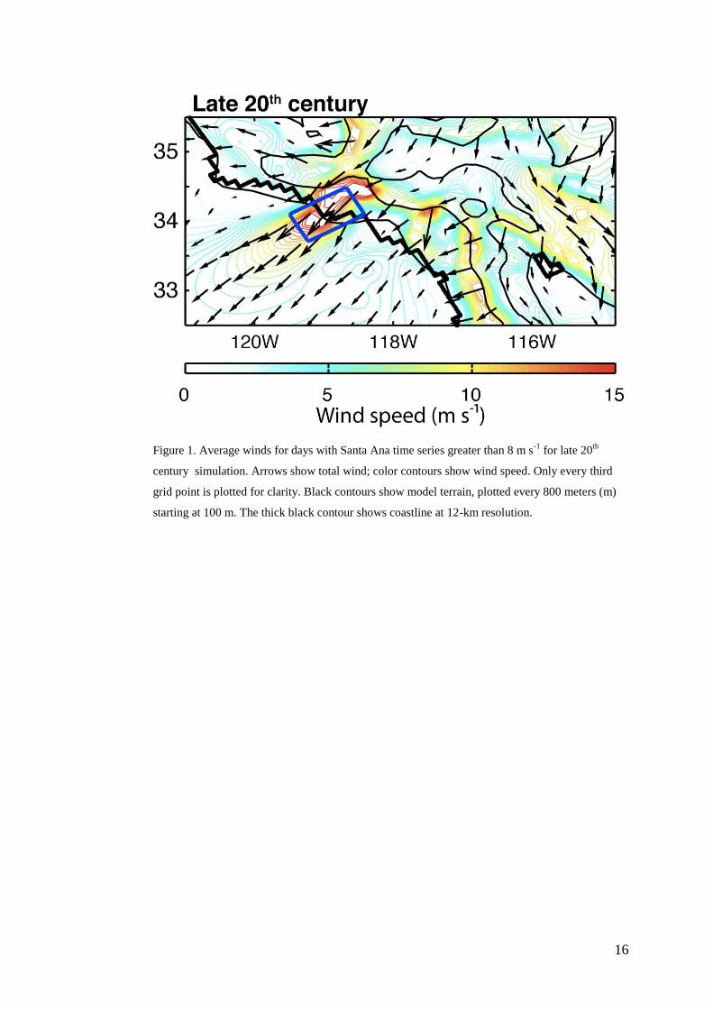
synoptic. Figure 1 shows the composite surface winds for days with SAt greater

than 8 m s-1

for the 10 cold season WRF simulations corresponding to the late

20th century time slice (1971-1981). The composite SA wind field exhibits

characteristics we expect for SA events: strong offshore (that is, roughly

northeasterly) winds throughout most of Southern California, with the strongest

winds on the leeward slopes of the mountains and through the gaps in the

topography, most notably across the Santa Monica mountains.

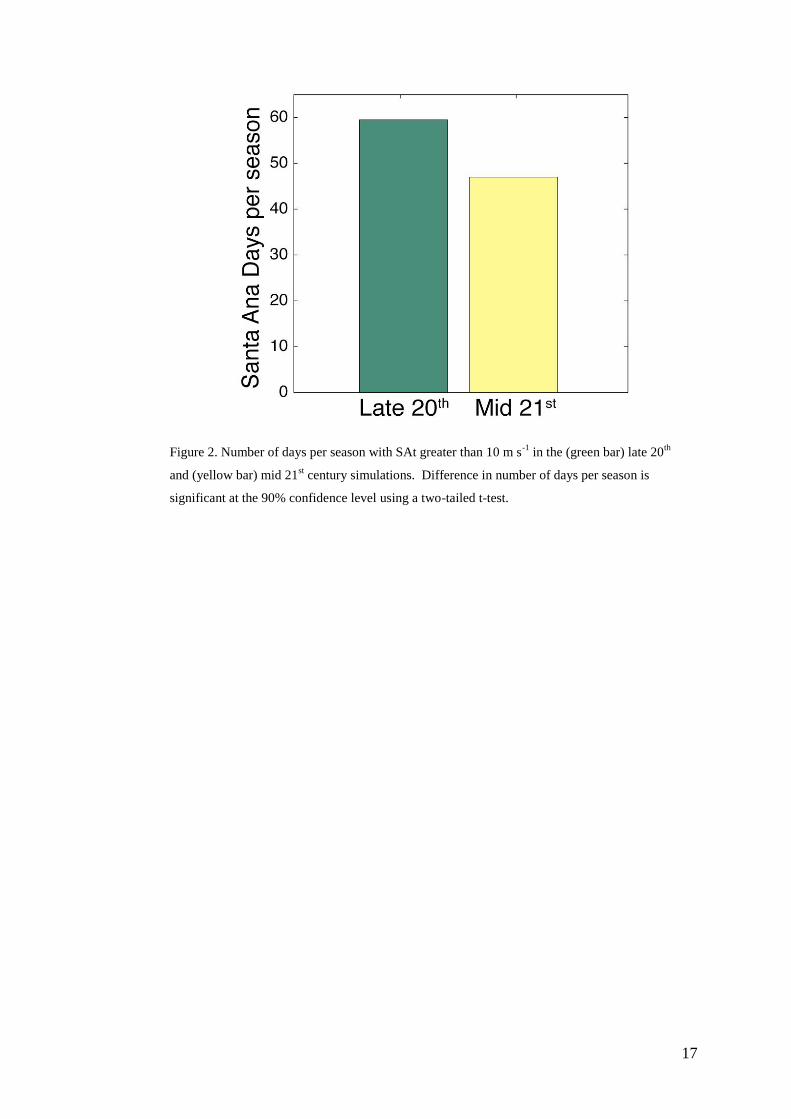
Is there any change in the number of SA days due to anthropogenic

forcing? To answer this question, we quantify the number of SA days per season

in the WRF downscaling of CCSM. To the extent that there is a difference in

climate between the two WRF simulations, we know it is due to the effect of

anthropogenic forcing, since that is the only sustained and systematic difference

between the two simulations. Figure 2 shows the average number of days with

SAt greater than 10 m s-1

for the late-20th and mid-21st century WRF simulations.

There is nearly a 20% reduction in the total number of SA days per year in the

mid-21st century run. In the following sections, we explore the mechanism by

which the frequency of SA wind events is reduced to lend more credibility to this

result.

6

4.0 Understanding Reduced Santa Ana Frequency

The atmospheric dynamics associated with SA winds were recently

investigated by Hughes and Hall (2009). They validated and analyzed SA events

in a 6-km resolution Southern California climate reconstruction. The

reconstruction was accomplished by downscaling reanalysis data corresponding to

the years 1995-2006 using WRF’s predecessor, the NCAR/Pennsylvania State

University Mesoscale Model, Version 5 (MM5, Grell et. al. 1994). They found

that SAs arise from a combination of two mechanisms – one with a synoptic

extent covering much of the western U.S., and another more local process

confined to Southern California. Here we briefly review important results from

this study, as they are relevant to our explanation of reduced SA frequency

resulting from anthropogenic forcing.

Previous studies identified large-scale mid-tropospheric conditions as the

driver of SAs (e.g., Sommers, 1978). If there is a large synoptic-scale pressure

gradient causing strong offshore winds over Southern California at mountain-top

level, this causes surface flow as the offshore momentum is transferred to the

surface in a stably stratified atmosphere. This often occurs when a high surface

pressure anomaly is located over the Great Basin, with a corresponding high

geopotential height anomaly at 700 hPa centered over Oregon. Though this

synoptic mechanism contributes to offshore flow in Southern California, Hughes

and Hall (2009) also found that if a large temperature gradient exists between the

cold desert surface and the warm ocean air at the same altitude (approximately 1.2

km), it causes a localized offshore pressure gradient near the surface. This

generates katabatic offshore flow in a thin layer near the surface, as the negatively

buoyant, cold desert air flows down the sloped surface of the gaps. The negative

buoyancy can be written as a pressure gradient force (Parish and Cassano, 2003):

g

0

sin Eq. 1

where g=9.8 m s-1

is gravitational acceleration, ’ is the temperature deficit of the

cold layer, 0 is the average temperature in the cold layer, and is the slope of the

topography. To calculate , Hughes and Hall (2009) used the average desert

surface temperature for 0, the average slope of the topography through the largest

gap for (approximately 1 degree, or 1 km drop over 50 km; see Figure 1) and

7

the temperature difference between the air over the cold desert surface (i.e., the

cold layer) and air over the ocean at the same altitude (representative of the

ambient atmosphere) for ’.

These two mechanisms can act independently (and often do), causing mild

SA winds, or combine to force the largest magnitude offshore winds. Their joint

contribution to SAt can be modeled statistically by a bivariate regression model to

predict SAt based on two parameters representative of each mechanism

S ˆ A t(u,) A * u B * C Eq. 2

where u, the offshore (and mainly geostrophic) wind speed at 2 km, represents the

synoptic forcing and represents the local thermodynamic forcing. In the MM5

reconstruction, this regression model captured almost all variability in SAt

(correlation between SAt and SÂt was 0.93), with about 1/8 of the variability

accounted for by the synoptic mechanism, more than half by the local mechanism,

and the remainder by in-phase variability of the two mechanisms impossible to

unambiguously ascribe to one or the other.

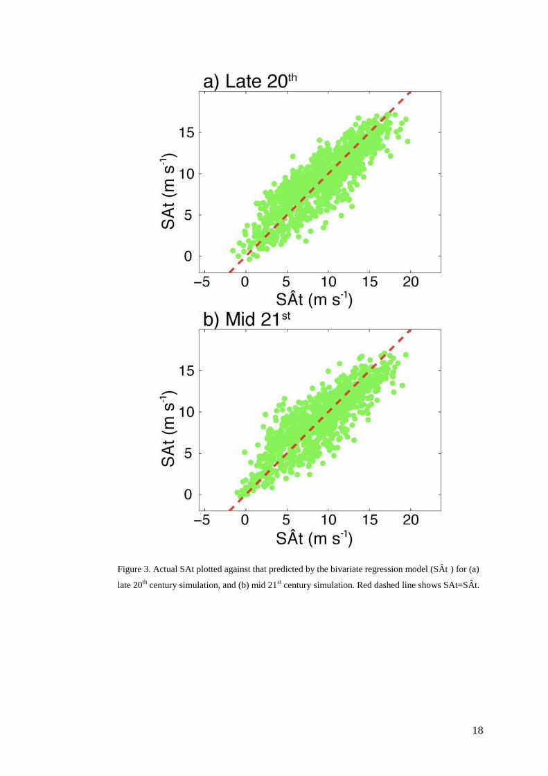
Figure 3 shows the regression model’s representation of SAt, SÂt, plotted

against SAt for the WRF late 20th century and mid 21st century cold season

simulations. The high degree of correspondence (correlation coefficient = 0.88,

and 0.86 for the late 20th and mid 21st simulations, respectively) confirms that, as

with the MM5 reconstruction, the two mechanisms are primarily responsible for

determining SAt in the WRF simulations forced by CCSM3 data. The regression

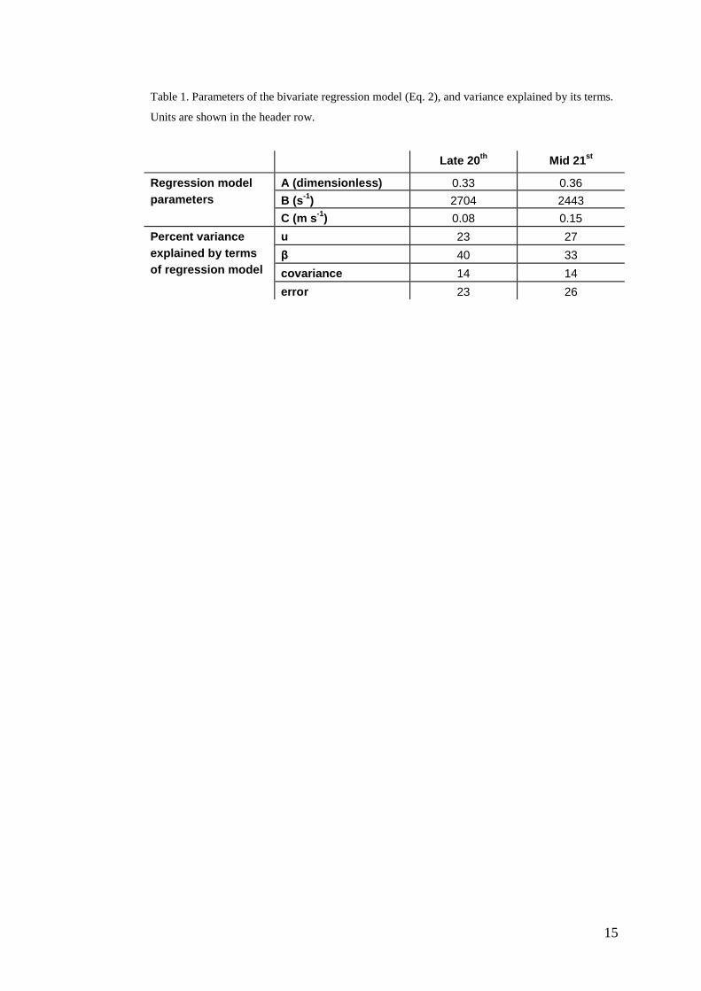
model coefficients are shown in Table 1 for both decades. Parameters A and B are

within 10% of one another, and C is close to zero for both decades. Table 1 also

shows the variance explained by each of the terms of the regression model.

Similar to Hughes and Hall (2009), more variance is explained by the local

mechanism than by the synoptic mechanism, although in the case of the current

WRF downscaling of CCSM data, the variance is more equally partitioned.

Because the terms within it correspond to distinct physical processes, the

regression model allows us to identify the changes in forcing responsible for the

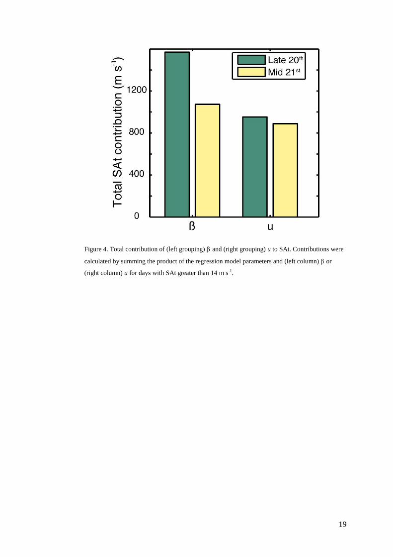
reduction in SAt. To understand which term of the regression model is causing

reduced SÂt, we calculate the total contribution of and u to SÂt separately and

then sum over days with SÂt greater than 14 m s-1

for the two time periods

(Figure 4).

8

Turning our attention first to the synoptic forcing represented by u in Eq. 1

and the second column grouping in Figure 4, we see that the WRF simulation

shows almost no change between the present and future simulations. Thus the

reduction in SAt between present and future simulations is not primarily due to a

systematic change in the low-to-mid-troposphere geostrophic wind and associated

synoptic-scale pressure gradients when offshore winds blow. Focusing instead on

the katabatic forcing of in Eq. 1 and the first column grouping in Figure 4, we

see that the 21st century time period shows over 1/3 less contribution to SÂt from

than the present day scenario. This is likely because land masses warm more

quickly in response to increased radiative forcing than the oceans (e.g. Trenberth

et al. 2007), reducing the temperature gradient between the cold desert and warm

ocean.

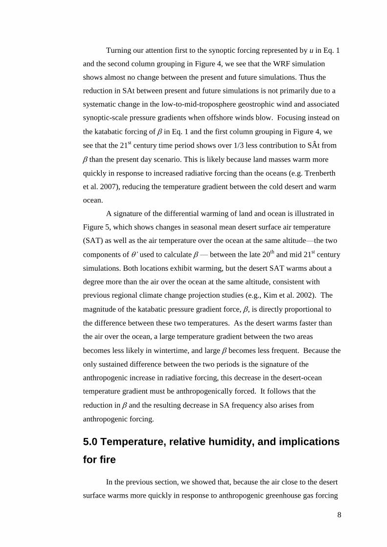
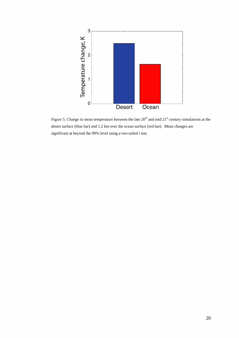
A signature of the differential warming of land and ocean is illustrated in

Figure 5, which shows changes in seasonal mean desert surface air temperature

(SAT) as well as the air temperature over the ocean at the same altitude—the two

components of ’ used to calculate — between the late 20th

and mid 21st century

simulations. Both locations exhibit warming, but the desert SAT warms about a

degree more than the air over the ocean at the same altitude, consistent with

previous regional climate change projection studies (e.g., Kim et al. 2002). The

magnitude of the katabatic pressure gradient force, , is directly proportional to

the difference between these two temperatures. As the desert warms faster than

the air over the ocean, a large temperature gradient between the two areas

becomes less likely in wintertime, and large becomes less frequent. Because the

only sustained difference between the two periods is the signature of the

anthropogenic increase in radiative forcing, this decrease in the desert-ocean

temperature gradient must be anthropogenically forced. It follows that the

reduction in and the resulting decrease in SA frequency also arises from

anthropogenic forcing.

5.0 Temperature, relative humidity, and implications

for fire

In the previous section, we showed that, because the air close to the desert

surface warms more quickly in response to anthropogenic greenhouse gas forcing

9

than the air 1.2 km above the ocean, the number of strong offshore wind events

per year will likely decline over the following decades. Because wildfire activity

in this region is strongly tied to the occurrence of SA winds (e.g., Moritz et. al.

2010; Westerling 2004; Keeley 2004), it is tempting to conclude that this

reduction could lead to a reduction in wildfire activity. However, this may be a

misleading conclusion because the reduction in SAs is accompanied by changes in

other meteorological variables also determining fire risk. For example, fire

severity tends to increase as temperature increases (Moritz et. al. 2010).

Therefore, the local increases in simulated temperature (Fig. 5) should also favor

more severe wildfire outbreaks.

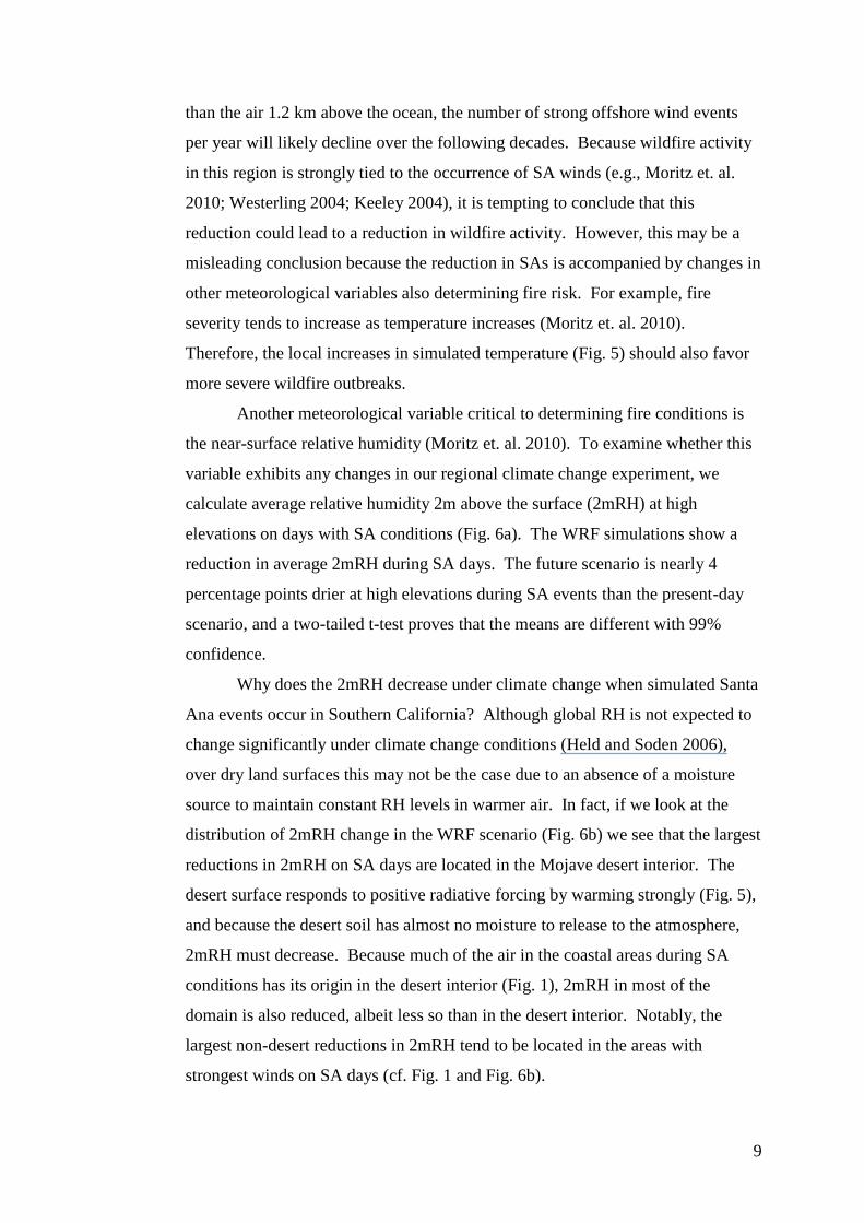
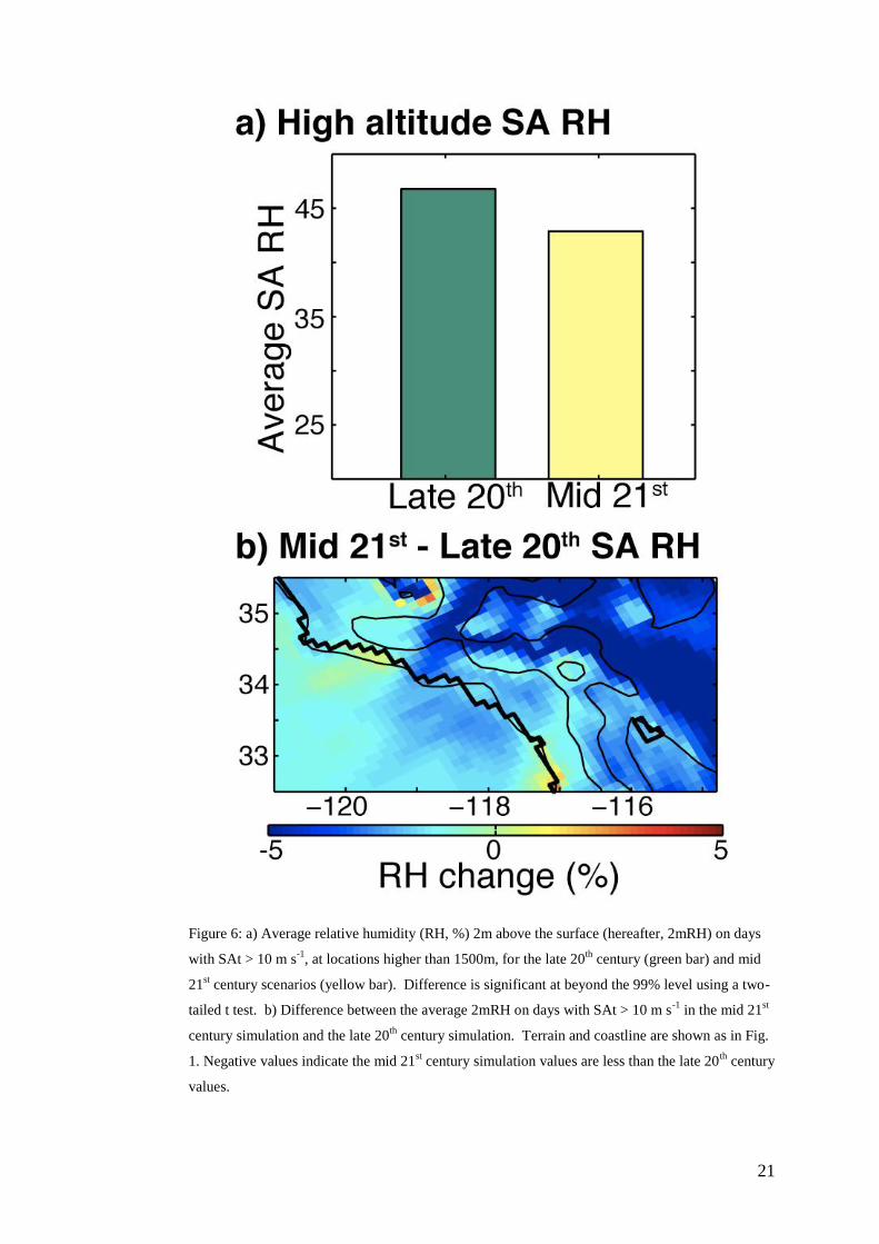
Another meteorological variable critical to determining fire conditions is

the near-surface relative humidity (Moritz et. al. 2010). To examine whether this

variable exhibits any changes in our regional climate change experiment, we

calculate average relative humidity 2m above the surface (2mRH) at high

elevations on days with SA conditions (Fig. 6a). The WRF simulations show a

reduction in average 2mRH during SA days. The future scenario is nearly 4

percentage points drier at high elevations during SA events than the present-day

scenario, and a two-tailed t-test proves that the means are different with 99%

confidence.

Why does the 2mRH decrease under climate change when simulated Santa

Ana events occur in Southern California? Although global RH is not expected to

change significantly under climate change conditions (Held and Soden 2006),

over dry land surfaces this may not be the case due to an absence of a moisture

source to maintain constant RH levels in warmer air. In fact, if we look at the

distribution of 2mRH change in the WRF scenario (Fig. 6b) we see that the largest

reductions in 2mRH on SA days are located in the Mojave desert interior. The

desert surface responds to positive radiative forcing by warming strongly (Fig. 5),

and because the desert soil has almost no moisture to release to the atmosphere,

2mRH must decrease. Because much of the air in the coastal areas during SA

conditions has its origin in the desert interior (Fig. 1), 2mRH in most of the

domain is also reduced, albeit less so than in the desert interior. Notably, the

largest non-desert reductions in 2mRH tend to be located in the areas with

strongest winds on SA days (cf. Fig. 1 and Fig. 6b).

10

The resulting implications for fire incidence of the combination of these

three meteorological variables (wind, RH, and temperature) are ambiguous, since

strong offshore wind frequency decreases while RH decreases and temperature

increases. To get quantitative estimates on the meteorological implications for

fire incidence, a fire behavior model would be necessary to untangle the

respective roles these three variables will play in the future. Westerling et. al.

(2006) recently showed that wildfire activity has increased in Southern California

over the past three decades. If the RH and temperature effects dominate the wind

speed effects, wildfire activity may well continue to increase as climate change

accelerates.

6.0 Conclusions

This study investigates the frequency of Southern California’s SA wind

events within a high-resolution dynamical downscaling of two time slices of the

NCAR CCSM3 climate change scenario simulation. One time slice corresponds

to the late-20th

century, the other to the mid-21st century. This particular CCSM

simulation imposes the SRES-A1B emission scenario. In the high resolution

simulation the SA events per year are reduced approximately 20% in the mid-21st

compared with the late-20th

century. Because the only difference between the two

time slices is the level of anthropogenic forcing, the change in SA events is

caused by anthropogenic forcing. The reduction in the frequency of SAs is also

associated with a reduction in their mean intensity.

We use a bivariate regression model to reproduce the Santa Ana time

series, where two known forcing mechanisms as used as independent (predictor)

variables: (1) synoptically-forced strong offshore winds at the mountain tops

whose momentum is transported to the surface, and (2) local thermodynamically

forced winds caused by a katabatic pressure gradient that arises from the thermal

contrast between cold desert air and warmer air over the adjacent ocean. The

regression model reproduces approximately 80% of the variability in the Santa

Ana time index and also reproduces the significant reduction in SA events

between the two time slices. We use the regression model to partition the

anthropogenic change in SA events into contributions from synoptic and katabatic

components. We find a large reduction in katabatic forcing. This is caused by the

larger transient warming of the desert surface than the air over the ocean at the

11

same altitude. This reduces the likelihood of a large temperature deficit

developing in the desert in wintertime and therefore reduces the likelihood of

large katabatic forcing. We see no change in the likelihood of synoptically forced

SAs.

These results are not inconsistent with previous results: While Miller and

Schlegel (2006) did identify an anthropogenically-forced change in large-scale

pressure patterns associated with SAs, the change they detected was a seasonal

shift, which would not appear in our annual-total analysis. Moreover, these

investigators did not examine the katabatic forcing mechanism, which we found to

be of primary importance in creating anthropogenic change in SAs.

The role SA winds play in spreading wildfire in the region (e.g.,

Westerling 2004; Keeley 2004) suggests their reduction in frequency could lead to

reduced wildfire in Southern California. However, we find that two other

meteorological variables important to fire risk and growth, RH and temperature,

also change significantly and systematically in the region during SA events. RH

on SA days is reduced, and temperature increases; both of these changes would

favor fire development. Also, this study does not address changes in other

parameters critical to fire behavior, such as available fuel. Moreover, ignition

events (i.e., humans lighting matches in the coastal chaparral shrubland), another

major factor affecting fire frequency, will probably increase with population

(Syphard et al. 2007). Therefore, a fire behavior model is needed to predict how

fire incidence will change under anthropogenic climate change conditions, and no

conclusions can be drawn from this study alone about future wildfire occurrence

associated with SA events.

There are other societal implications of this anthropogenic reduction of SA

wind events that could be significant and should be explored further. A reduction

in the frequency and intensity of SA winds has implications for coastal marine

ecosystems, which respond favorably to SA conditions, and to the air quality in

the Los Angeles basin, which is better during SA events. The ecological effects of

nutrient loss for the Southern California Bight and the decline in air quality during

winter could be quantified with regional simulations of oceanic biogeochemistry

and atmospheric chemistry.

To the extent that the smaller temperature increase in the atmosphere over

the ocean is due to the larger oceanic heat capacity, the reduction in

12

thermodynamic forcing of SAs might be a feature of the transient climate change

that will return to pre-industrial levels once the climate equilibrates. Nevertheless,

the reduction in SA wind events due to anthropogenic climate change is

significant because it illustrates an observed and explainable regional change in

climate due to plausible mesoscale processes. Further, despite the fact that surface

temperature changes are due to a well-known response of the climate system to an

increase in greenhouse gases, the resultant change in SA wind events cannot be

simulated or understood without mesoscale atmospheric processes, thus requiring

a high spatial resolution atmospheric model for its detection.

Acknowledgements

Mimi Hughes is supported by a National Research Council Postdoctoral

Associateship and National Science Foundation ATM-0735056, which also

supports Alex Hall. Part of this work was performed using the National Center for

Atmospheric Research supercomputer allocation 35681070. The research

described in this paper was performed as an activity of the Joint Institute for

Regional Earth System Science and Engineering, through an agreement between

the University of California, Los Angeles, and the Jet Propulsion Laboratory,

California Institute of Technology, and was sponsored by the National

Aeronautics and Space Administration. Preprocessing of the Community Climate

System Model data was also partially funded by the "National Comprehensive

Measures against Climate Change" Program by Ministry of Environment, Korea

(Grant No. 1600-1637-301-210-13) National Institute of Environmental Research,

Korea. Computational resources for this study have been provided by Jet

Propulsion Laboratory’s Supercomputing and Visualization Facility and the

National Aeronautics and Space Administration’s Advanced Supercomputing

Division.

References

Castro, R., A. Mascarenhas, A. Martinez-Diaz-de Leon, R. Durazo, and E. Gil-Silva. 2006.

―Spatial influence and oceanic thermal response to Santa Ana events along the Baja California

peninsula.‖ Atmosfera 19(3): 195–211.

Chang, S., D. Hahn, C. Yang, D. Norquist, and M. Ek. 1999. ―Validation study of the CAPS

model and land surface scheme using the 1987 Cabauw/PILPS dataset.‖ J. Appl. Meteor. 38: 405–

422.

13

Conil, S., and A. Hall. 2006. ―Local regimes of atmospheric variability: A case study of Southern

California.‖ J. Clim. 19(17): 4308–4325.

Diffenbaugh, N., J. Pal, R. Trapp, and F. Giorgi. 2005. ―Fine-scale processes regulate the response

of extreme events to global climate change.‖ PNAS 102(44): 15 774–15 778.

Dudhia, J. 1989. ―Numerical study of convection observed during the winter monsoon experiment

using a mesoscale two-dimensional model.‖ J. Atmos. Sci. 46(20): 3077–3107.

Grell, G., J. Dudhia, and D. Stauffer. 1994. A description of the fifth-generation Penn State/NCAR

Mesoscale Model (MM5). Tech. rep., NCAR Tech. Note NCAR/TN-398+STR.

Held, I.M., and B.J. Soden, 2006: Robust Responses of the Hydrological Cycle to Global

Warming. J. Climate, 19, 5686–5699.

Hong, S., and H. Pan. 1998. ―Convective trigger function for a mass flux cumulus

parameterization scheme.‖ Mon. Wea. Rev. 126: 2599–2620.

Hu, H., and W. Liu. 2003. ―Oceanic thermal and biological responses in Santa Ana winds.‖

Geophys. Res. Lett. 30(11): 1596. DOI:10.1029/2003GL017208.

Hughes, M., and A. Hall. 2009. Local and synoptic mechanisms causing Southern California’s

Santa Ana winds. Clim. Dyn., DOI: 10.1007/s00382-009-0650-4

Jickells, T., Z. S. An, K. K. Andersen, A. R. Baker, G. Bergametti, N. Brooks, J. J. Cao, P. W.

Boyd, R. A. Duce, K. A. Hunter, H. Kawahata, N. Kubilay, J. laRoche, P. S. Liss, N. Mahowald, J.

M. Prospero, A. J. Ridgwell, I. Tegen, and R. Torres. 2005. ―Global iron connections between

desert dust, ocean biogeochemistry, and climate.‖ Science 308: 67–71. DOI:

10.1126/science.1105959.

Kim, J., T.-K. Kim, R.W. Arritt, and N. Miller. 2002. ―Impacts of increased atmospheric CO2 on

the hydroclimate of the western United States. J. Clim. 15: 1926-1942.

Kim, J., and J.-E. Lee. 2003. ―A multi-year regional climate hindcast for the western United States

using the Mesoscale Atmospheric Simulation Model.‖ J. Hydrometeor. 4: 878-890.

Leung, L., and S. Ghan. 1999. ―Pacific Northwest climate sensitivity simulated by a regional

climate model driven by a GCM. Part I: Control simulations.‖ J. Clim. 12: 2010–2030.

Miller, N. L., and N. J. Schlegel. 2006. ―Climate change projected fire weather sensitivity:

California Santa Ana wind occurrence.‖ Geophys. Res. Lett. 33. doi:10.1029/2006GL025 808.

Mlawer, E., S. Taubman, P. Brown, M. Iacono, and S. Clough. 1997. ―Radiative transfer for

inhomogeneous atmosphere: RRTM, a validated correlated-k model for the longwave.‖ J.

Geophys. Res. 102(D14): 16663–16682.

Moritz, M., Moody, T. J., Krawchuk M. A., Hughes, M. and A. Hall. 2010. ―Spatial Variation in

Extreme Winds Predicts Large Wildfire Locations in Chaparral Ecosystems.‖ GRL. Submitted.

Nakicenovic, N., and R. Swart. 2000. Special Report on Emissions Scenarios. Edited by Nebojsa

Nakicenovic and Robert Swart, pp. 612. ISBN 0521804930. Cambridge, UK: Cambridge

University Press, July 2000.

Parish, T., and J. Cassano. 2003. ―Diagnosis of the katabatic wind influence on the wintertime

Antarctic surface wind field from numerical simulations.‖ Mon. Wea. Rev. 131: 1128–1139.

Raphael, M. N. 2003. ―The Santa Ana winds of California.‖ Earth Interactions 7: 1–13.

14

Skamarock, W., J. Klemp, J. Dudhia, D. Gill, D. Baker, W. Wang, and J. Powers. 2005. A

description of the advanced research WRF version 2. Tech. rep., NCAR Tech. Note,

NCAR/TN468+STR.

Sommers, W. T. 1978. ―LFM forecast variables related to Santa Ana wind occurences.‖ Mon.

Wea. Rev. 106: 1307–1316.

Syphard, A., V. Radeloff, J. Keeley, T. Hawbaker, M. Clayton, S. Stewart, and R. Hammer. 2007.

―Human influence on California fire regimes.‖ Ecological Applications 17: 1388–1402.

Trasvina, A., M. Ortiz-Figueroa, H. Herrera, M. A. Coso, and E. Gonzlez. 2003. ―Santa Ana winds

and upwelling filaments off northern Baja California.‖ Dynamics of Atmospheres and Oceans

37(2): 113–129.

Trenberth, K., P. Jones, P. Ambenje, R. Bojariu, D. Easterling, A. Klein Tank, D. Parker, F.

Rahimzadeh, J. Renwick, M. Rusticucci, B. Soden, and P. Zhai. 2007. Observations: Surface and

atmospheric climate change. Climate Change 2007: The Physical Science Basis. Contribution of

Working Group I to the Fourth Assessment Report of the Intergovernmental Panel on Climate

Change. Solomon, S., D. Qin, M. Manning, Z. Chen, M. Marquis, K. Averyt, M. Tignor, and H.

Miller, Eds. Cambridge, United Kingdom and New York, NY, USA: Cambridge University Press.

Westerling, A. L., D. R. Cayan, T. J. Brown, B. L. Hall, and L. G. Riddle. 2004. ―Climate, Santa

Ana winds and autumn wildfires in Southern California.‖ EOS 85(31): 289–296.

Westerling, A.L., H.G. Hidalgo, D.R. Cayan, T.W. Swetnam 2006: "Warming and Earlier Spring

Increases Western U.S. Forest Wildfire Activity" Science, 313: 940-943.

DOI:10.1126/science.1128834

15

Table 1. Parameters of the bivariate regression model (Eq. 2), and variance explained by its terms.

Units are shown in the header row.

Late 20th

Mid 21st

Regression model

parameters

A (dimensionless) 0.33 0.36

B (s-1

) 2704 2443

C (m s-1

) 0.08 0.15

Percent variance

explained by terms

of regression model

u 23 27

β 40 33

covariance 14 14

error 23 26

16

Figure 1. Average winds for days with Santa Ana time series greater than 8 m s-1

for late 20th

century simulation. Arrows show total wind; color contours show wind speed. Only every third

grid point is plotted for clarity. Black contours show model terrain, plotted every 800 meters (m)

starting at 100 m. The thick black contour shows coastline at 12-km resolution.

17

Figure 2. Number of days per season with SAt greater than 10 m s-1

in the (green bar) late 20th

and (yellow bar) mid 21st century simulations. Difference in number of days per season is

significant at the 90% confidence level using a two-tailed t-test.

18

Figure 3. Actual SAt plotted against that predicted by the bivariate regression model (SÂt ) for (a)

late 20th

century simulation, and (b) mid 21st century simulation. Red dashed line shows SAt=SÂt.

19

Figure 4. Total contribution of (left grouping) and (right grouping) u to SAt. Contributions were

calculated by summing the product of the regression model parameters and (left column) or

(right column) u for days with SAt greater than 14 m s-1

.

20

Figure 5. Change in mean temperature between the late 20th

and mid 21st century simulations at the

desert surface (blue bar) and 1.2 km over the ocean surface (red bar). Mean changes are

significant at beyond the 99% level using a two-tailed t test.

21

Figure 6: a) Average relative humidity (RH, %) 2m above the surface (hereafter, 2mRH) on days

with SAt > 10 m s-1

, at locations higher than 1500m, for the late 20th

century (green bar) and mid

21st century scenarios (yellow bar). Difference is significant at beyond the 99% level using a two-

tailed t test. b) Difference between the average 2mRH on days with SAt > 10 m s-1

in the mid 21st

century simulation and the late 20th

century simulation. Terrain and coastline are shown as in Fig.

1. Negative values indicate the mid 21st century simulation values are less than the late 20

th century

values.