hsdpa system simulation - DiVA-Portal

Thesis Number: MEE05:30

HSDPA SYSTEM SIMULATION

Nguyen Kim Cuong Khan Muhammad Sohaib

This thesis is presented as part of Degree of Master of Science in Electrical Engineering

Blekinge Institute of Technology September 2005

School of Engineering Department of Applied Signal Processing Examiner: Dr. Jörgen Nordberg

This page is intentionally left blank

ii

Abstract

This thesis provides a background of the high speed downlink packet access (HSDPA) concept; a new feature which has been introduced in the Release 5 specifications of the 3GPP WCDMA/UTRA-FDD standards. In order to emphasize the theoretical analysis, a simulation of a HSDPA system shall also be performed. To support an evolution towards more sophisticated network and multimedia services, the main target of HSDPA is to increase user peak data rates, quality of service, and to generally improve spectral efficiency for downlink asymmetrical and bursty packet data services. This is accomplished by introducing a fast and complex channel control mechanism based on a short and fixed packet transmission time interval (TTI), adaptive modulation and coding (AMC), and fast physical layer (L1) hybrid ARQ. To facilitate fast scheduling with a per-TTI resolution in coherence with the instantaneous air interface load, the HSDPA-related MAC functionality is moved to the Node-B. The HSDPA concept facilitates peak data rates exceeding 2 Mbps (theoretically up to and exceeding 14 Mbps), and the cell throughput gain over previous UTRA-FDD releases has been evaluated to be in the order of 50-100% or even more, highly dependent on factors such as the radio environment and the service provision strategy of the network operator. The former part of the thesis provides the trends of mobile services, drawbacks of 3G systems and the fundamental knowledge of HSDPA. The later part focuses on the simulation of a HSDPA system and its results compared to those in other publications. Key words: High Speed Downlink Packet Access (HSDPA), Adaptive Modulation and Coding (AMC), Packet Scheduling (PS), Hybrid Automatic Retransmit reQuest (ARQ), Node B, Radio Network Controller (RNC), High-speed Downlink Shared Channel (HS-DSCH), Transmission Time Interval (TTI), link adaptation.

iii


iv

Acknowledgment

Firstly, we would like to express our most sincere appreciation to our supervisor, Doctor Jörgen Nordberg for his great input to this thesis, which would not be completed without his patient guidance, continuous inspiration and in-depth expertise in the field of cellular communications. His expertise together with his documentation experience is a great asset for us.

Secondly, we would like to acknowledge turbo codes matlab code written by Mr. Yufei Wu, MPRG laboratory, Virginia Tech. which is used in our simulation program.

Finally, we thank all the BTH library staff who were very helpful and enthusiasm. Thank you all for your efforts and patience in helping us find the books that were even not available in the library. We also thank all the staff in IT department who permitted us to run our simulation in several computers simultaneously over nights. This has significantly shortened our simulation time.

Khan Muhammad Sohaib – Nguyen Kim Cuong

Blekinge Institute of Technology (BTH) Karlskrona, Sweden – September 2005

v


vi

Table of Contents

List of Figures List of Tables

1. Introduction . . . . . . . . . .. . . . . . . .. . . . . . . . . . . . . . .. . . . . . . . ... . . . . . .. . . . . . .. . 1 1.1 Motivation. . . . . . .. . . . . . . .. . . . . . . . . . . . . . .. . . . . . . .. . . . . . .. . . . . …. . . 1

1.2 Benefits o the new system – HSDPA. . . . . . .. . . . . . . .. . . . . . . . . . . . . . .. . . ... 2 1.3 Thesis Objective. . . . . . .. . . . . . . .. . . . . . . . . . . . . . .. . . . . . . . .. . . . . . ... . . . . . . 3 1.4 Thesis outline . . . . . .. . . . . . . .. . . . . . . . . . . . . . .. . . . . . . . .. . . . . . .. . . . . . . . . . 3 2. Evolution of 3G CDMA. . . . . .. . . . . . . .. . . . . . . . . . . . . .. . . .. . . . . . .. . . . . . . . 4

2.1 Objective of 3G systems. . . . . .. . . . . . . .. . . . . . . . . . . . . .. . . . . . .. . . .. . .. . . . 4

2.2 Evolution of wireless cellular systems. . . . . .. . . . . . . .. . . . . . . . . . .. . . . . .. . . .. 4 2.3 Alternative interfaces in CDMA. . . . . .. . . . . . . .. . . . . . . . . . .. . .. . . . . . . .. . . .. 6 2.4 CDMA design considerations . . .. . . . . . . .. . . . . . . . . . . . . .. . .. . . . . . .. . . .. . . 7 2.5 Wideband CDMA. . .. . . . . . . .. . . . . . . . . . . . . .. . .. . . . . . .. . . .. . . . . . . .. . . .. . 9 2.5.1 Carrier spacing and deployment scenario. .. . .. . . . . . . .. . . .. . . . . . . . . 10 2.5.2 WCDMA logical channels. .. . . . . . . .. . . . . . . . . . . . . .. . .. . . . . . . . . . . . 10 2.5.3 WCDMA physical channels. .. . . . . . . .. . . . . . . . . . . . . .. . .. . . . . .. .. . . 11 2.5.4 Spreading. .. . . . . . . .. . . . . . . . . . . . . .. . .. . . . . .. .. . . .. . . . . .. .. . . .. . . . 12 2.5.5 Multirate. .. . . . . . . .. . . . . . . . . . . . . .. . .. . . . . .. .. . . .. . . . . .. .. . . .. . . . . 13 2.5.6 Packet data.. . . . . . . .. . . . . . . . . . . . . .. . .. . . . . .. .. . . .. . . . . .. .. . . .. . . . 14 2.5.7 Handover. . . . . . . .. . . . . . . . . . . . . .. . .. . . . . .. .. . . .. . . . . .. .. . . .. . . . . 15 2.5.8 Inter-frequency handover. . . . . . . . . .. . .. . . . . .. .. . . .. . . . . .. .. . . . . . . . 15 2.5.9 Power Control . . . . . . . . .. . .. . . . . .. .. . . .. . . . . .. .. . . .. . . . . . .. . . .. . . 16

3. HSDPA . . . . . . . . .. . .. . . . . .. .. . . .. . . . . .. .. . . .. …………...……...........…… 18

3.1 Comparisons of R99 and HSDPA. .. . . . . .. .. .…………...…… ..........……… 18 3.2 Adaptive modulation and coding (AMC) . .. . . . . .. .. .…………. .......... ..……… 20

3.2.1 Link quality feedback .. . . . . .. .. .…………...…………… ...........……… 21 3.2.2 Different modulation and coding combinations.. .……… .........………. 21 3.2.3 HSDPA System Model.…………...…………… …….............................. 22 3.2.4 Threshold decision making for MCS and multicode selection... ............... 23 3.2.5 Markov’s model of MCS selection.. .…………...……………… ..…… 27 3.2.6 Comparison between Markov and Threshold Models.…………… ..…… 28

vii


viii

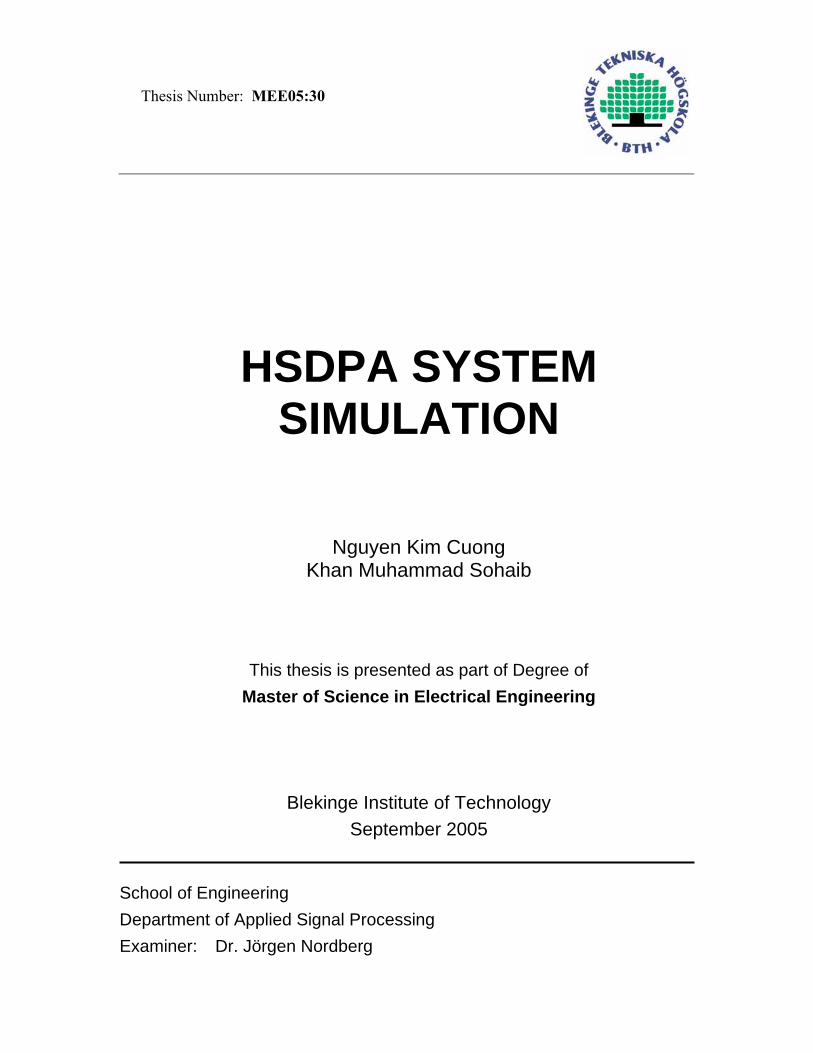
3.3 Adaptive hybrid ARQ.……………………… .……………………… …..……… 28

3.3.1 Incremental rearrangement .……………………… .……………… ..……. 29 3.3.2 16QAM constellation rearrangement…………………… .………… .… 30 3.3.3 Candidate H-ARQ schemes…………………… .………………… ..…….... 32

3.4 Packet scheduling…………………… .……………………...................... ............ 33 3.4.1 QoS classes………………… .……………………....................... ............ 34 3.4.2 Input parameters for packet scheduler………………................................. 36 3.4.3 Packet scheduling principles……………….............................................. 38 3.4.4 Packet scheduling algorithms………………............................................. 39

3.4.5 Performance analysis of packet scheduling algorithms and rommendation…………….................................................................. 42

3.5 Turbo Codes……………….................................................................................... 43

3.5.1 Performance of Turbo Codes........................................................ ............. 44 3.5.2 The UMTS turbo code......................................................... ...................... 45 3.5.3 The CDMA2000 turbo codes.......................................... .......................... 46 3.5.4 Turbo code interleaver........................................................ ...................... 47 3.5.5 Turbo codes decoding.................................... ............................................ 47 3.5.6 Practical issues..................................................... ...................................... 49

3.6 Conclusion....................................................................... ............ .......................... 51

4. Simulation....................................................................................... ................................ 52

4.1 Simulation Program.................................................................. .............. ............... 52

4.2 Simulation Results............................................................................ .... ................ 53 4.2.1 Five Iterations.................................................................. .......................... 53 4.2.2 Ten Iterations................................................................ ................ ............. 55 4.3 Conclusion............................................................................... ............................... 58

5. Future Works............................................................................... ................................. 60

ix


x

List of Figures

2.1 Evolution of Cellular Wireless Systems . . . . .. . . . . . . .. . . . . . . . . . . . .. . . . . 5 2.2 IMT-2000 Terrestrial Interfaces . . . . . . . . . . . .. . . . . . . .. . . . . . . .. . . . . . . . . . . 7 2.3 Time and Code Multiplexing Principles . . . . . . . . . . .. . . . . . . .. . . . . . . . . . . . . 8 2.4 Frequency utilization with WCDMA . . . . . . .. . . . . . . .. . . . . . . .. . . . . . . . . . 10 2.5 Different Level Channels . . . . . . . .. . . . . . . .. . . . . . . .. . . . . . . . . . . . . . . . . . . 11 2.6 IQ/code multiplexing with complex spreading circuit . . . . . .. . . . . . . .. . . . . . . . 12 2.7 Signal constellation for IQ/code multiplexed control channel

with complex spreading . . . . . . . . . . . . . . . . . . .. . . . . . . .. . . . . . . .. . . . .. . . . . . 13 2.8 Service multiplexing in WCDMA . . . . . . . . . . . . . . . .. . . . . . . .. . . . . . . .. . . . . 13 2.9 Packet transmission on the common channel . . . . . . . .. . . . . . . .. . . . . . .. . . . . . 15 2.10 Slotted mode structure . . . . . . . . . . . . . . . . . . . . . .. . . . . . . .. . . . . . . .. . . . .. . . . 16 3.1 WCDMA/HSDPA components and interfaces . . . . . .. . . . . . . . . .. . . . . . . . . .. . 19 3.2 Adaptive Modulation and Coding . . . . . . . . . . .. . . . . . . . . .. . . . . . . . . . . . . . . . 22 3.3 AMCS system model . . . . . . . . . . . . . . .... . . . . . . . . .. . . . . . . . . . . . . . . . . . . . . 23

3.4 Different code allocations to different users on TTI basis Example for 3 users sharing 5 codes. . . . .. . . . . . . . . .. . . . . . … . . . . . . . 23 3.5 Illustration of the link performance in changing channel conditions .. . . . . . . . . 25 3.6 The algorithm to select the number of multicodes and the

Adaptive Modulation and Coding scheme . . . . . . . . . .. . . . . . . . . .. . . . . . . . . . . 26 3.7 Incremental redundancy . . . . . . . . . . . . . . . . .. . . . . . . . . .. . . . . . . . . . . . . . . . . . 30 3.8 16-QAM symbol constellation . . . . . . . . . . . . . . . . . . . .. . . . . . . . . .. . . . . . . . . . 31 3.9 Node B packet scheduler operation procedure……………….. . . . . . .. . . . . .. . . 38 3.10 Operation principles of HSDPA packet scheduling algorithms . . . . . . .. . . .. . . . 41 3.11 Operation principles of HSDPA packet scheduling algorithms . . . . . .. . .. . . .. 42 3.12 Serial Concatenated Encoding . . . . . . . . . .. . . . . . . . . .. . . . . . . . . . . . . . . . . . . . 44 3.13 A generic turbo encoder . . . . . . . . . . . . . . . . . .. . . . . . . . . .. . . . . . . . . . . . . . . . . 45 3.14 The UMTS turbo encoder . . . . . . . . . . . . . . . . . . . . . . .. . . . . . . . . .. . . . . . . .. . . 46 3.15 The rate 1/3 RSC encoder used by the CDMA2000 turbo code . . . . . .. . . . . . . . 46

xi


xii

3.16 An architecture for decoding UMTS Turbo codes . . . . . . . . . .. . . .. . . . . . .. . . . 48 4.1 HSDPA simulated system model . . . . . . . . . . . . .. . . . . . . . . .. . . . . . . . . . . . . . . 52 4.2 Bit-error performance of the HSDPA turbo code as the number

of decoder iterations varies from one to five, TFRC=2 (QPSK & FEC1/2) . . . . . . . . . . . . . . . . . . . . . . . . . . .. . . . . . . . . .. . . . . . . . . .. . . . . . . . . 53

4.3 Frame-error performance of the HSDPA turbo code as the number of decoder iterations varies from one to five, TFRC=2 (QPSK & FEC1/2) . . . . . . . . . . . . . . .. . . . . . . . . .. . . . . . . . . . . . . . . . . . . . . . . . 54

4.4 Bit-error performance of the HSDPA turbo code as the number of decoder iterations varies from one to five, TFRC=4 (16QAM & FEC1/2) . . . . . . . . . . . . . . . . . . . . . .. . . . . . . . . .. . . . . . . . .. . . . . . . 54

4.5 Frame-error performance of the HSDPA turbo code as the number of decoder iterations varies from one to five, TFRC=4 (16QAM & FEC1/2) . . . . . . . . . . . . . . .. . . . . . . . . .. . . . . . . . . . . . . . . . . . . . . . 55

4.6 Bit-error performance of the HSDPA turbo code as the number of decoder iterations varies from one to ten, TFRC=2 (QPSK & FEC1/2) . . . . . . . . . . . . . .. . . . . . . . . .. . . . . . . . . .. . . . . . . . . . . . . . . . . . . . . . 56

4.7 Frame-error performance of the HSDPA turbo code as the number of decoder iterations varies from one to ten, TFRC=2 (QPSK & FEC1/2) . . . . . . . . . .. . . . . . . . . .. . . . . . . . . . . . . . . . . . . . . . . . . . . . . 56

4.8 Bit-error performance of the HSDPA turbo code as the number of decoder iterations varies from one to ten, TFRC=4 (16QAM & FEC1/2) . . . . . . . . . . . . . .. . . . . . . . . .. . . . . . . . . .. . . . . . . . . . . . . . . . . . . . . 57

4.9 Frame-error performance of the HSDPA turbo code as the number of decoder iterations varies from one to ten, TFRC=4 (16QAM & FEC1/2) . . . . . . . . . . . . . . . . . . . . . . . .. . . . . . . . . .. . . . . . . . .. . . . . 57

4.10 Bit-error performance of the UMTS turbo code as the number of decoder iterations varies from one to ten, Modulation is BPSK . . . . . . . . . . . 59

xiii


xiv

List of Tables

2.1 IS-95 Parameter Summary . . . . . . . . . . . . . .. . . . . . . . . .. . . . . . .. . . . . . . . . . . 5 2.2 CDMA2000 Parameters Summary . . . . . . . . . . . . . . . .. . . . . . . . . .. . . .. . . . . . . .. 6 2.3 WCDMA Parameters . . . . . . . . . . . . .. . . . . . . . . .. . . . . . . . . . . . . . . . . . . . . . . . .. 9 2.4 Transport and Physical Channels in WCDMA . . . . . . . . . . .. . . . . . . . . .. . . . . . 11 3.1 Comparisons between Rel-99/4 and HSDPA . . . . . . . . . . . . . . .. . . . . . . . . .. . . 20 3.2 Different Modulation and Coding Schemes and their Information

carrying capacity . . . . . . . . . . . . . . . . . . . . . .. . . . . . . . . .. . . . . . . . . .. . . . . . 22 3.3 Values of Ni . . . . . . . . . . . . . . . . . . . . . . . . . . . .. . . . . . . . . .. . . . . . . . . . . . . . . . 27 3.4 Encoding of redundancy version parameters for 16QAM . . . . . . . . .. . . . . . . . . 29 3.5 Constellation rearrangement for 16QAM . . . . . . . . . . . . . . .. . . . . . . . . .. . . .. . . 31 3.6 UMTS QoS classes . . . . . . . . . . . . . . . . . . . . .. . . . . . . . . .. . . . . . . . .. . . . . . . . . 36 3.7 Summary of packet scheduling algorithms . . . . . . . . . . . . . .. . . . . . . . . .. . . . . . 41

xv


xvi

Chapter 1

Introduction

This chapter provides an introduction of the thesis, its objective and the topics that will be discussed in the thesis. At the end of this chapter, the major issues that shall be discussed in each chapter shall be outlined. 1.1 Motivation Of all the tremendous advances in data communications and telecommunications, perhaps the most revolutionary is the development of cellar networks. Since the introduction of its First Generation in 1980s, mobile communication technology has developed a long way over three decades. In each generation, transmission rate and services, among other things, were improved. Nowadays, data services are anticipated to have an enormous rate of growth over the next years (the so-called data tornado) and will likely become the dominating source of traffic load in 3G mobile cellular networks. Example applications to supplement speech services include multiplayer games, instant messaging, online shopping, face-to-face videoconferences, movies, music, as well as personal/public database access. As more sophisticated services evolve, a major challenge of cellular systems design is to achieve a high system capacity and simultaneously facilitate a mixture of diverse services with very different quality of service (QoS) requirements. Various traffic classes exhibit very different traffic symmetry and bandwidth requirements. For example, two-way speech services (conversational class) require strict channel symmetry and very tight latency, while Internet download services (background class) are often asymmetrical and are tolerant to latency. The streaming class, on the other hand, typically exhibits tight latency requirements with most of the traffic carried in the downlink direction. In Release 99 of the WCDMA/UTRA specifications, there exist several types of downlink radio bearers to facilitate efficient transportation of the different service classes. The forward access channel (FACH) is a common channel offering low latency. However, as it does not apply fast closed loop power control it exhibits limited spectral efficiency and is in practice limited to carrying only small data amounts. The dedicated channel (DCH) is the “basic” radio- bearer in WCDMA/UTRA and supports all traffic classes due to high parameter flexibility. The data rate is updated by means of variable spreading factor (VSF) while the block error rate (BLER) is controlled by inner and outer loop power control mechanisms. However, the power and hardware efficiency of the DCH is limited for bursty and high data rate services since channel reconfiguration is a rather slow process (in the range of 500 ms).

Page 1 of 61

Hence, for certain Internet services with high maximum bit rate allocation the DCH channel utilization can be rather low. To enhance trunking efficiency, the downlink shared channel (DSCH) provides the possibility to time-multiplex different users (as opposed to code multiplexing). The benefit of the DSCH over the DCH is a fast channel reconfiguration time and packet scheduling procedure (in the order of 10 ms intervals). The efficiency of the DSCH can be significantly higher than for the DCH for bursty high data rate traffic. The HSDPA concept can be seen as a continued evolution of the DSCH and the radio bearer is thus denoted the high speed DSCH (HS-DSCH). As will be explained in the following chapters, HSDPA introduces several adaptation and control mechanisms in order to enhance peak data rates, spectral efficiency, as well as QoS control for bursty and downlink asymmetrical packet data. The key idea of the HSDPA concept is to increase packet data throughput with methods known already from Global System for Mobile Communications (GSM)/Enhanced Data rates for Global Evolution (EDGE) standards, including link adaptation and fast physical layer (L1) retransmission combining. The physical layer retransmission handling has large delays of the existing Radio Network Controller (RNC)-based Automatic Repeat reQuest ARQ architecture would result in unrealistic amounts of memory on the terminal side. Thus, architectural changes are needed to arrive at feasible memory requirements, as well as to bring the control for link adaptation closer to the air interface. The transport channel carrying the user data with HSDPA operation is denoted as the High-speed Downlink Shared Channel (HS-DSCH). 1.2 Benefits of the new system - HSDPA HSDPA provides impressive enhancements over WCDMA R’99 for the downlink. It offers peak data rates of up to 14Mbps, resulting in a better end-user experience for downlink data applications, with shorter connection and response times. More importantly, HSDPA offers three- to five-fold sector throughput increase, which translates into significantly more data users on a single frequency (or carrier). The substantial increase in data rate and throughput is achieved by implementing a fast and complex channel control mechanism based upon short physical layer frames, Adaptive Modulation and Coding (AMC), fast Hybrid-ARQ and fast scheduling. HSDPA higher throughputs and peak data rates will help stimulate and drive consumption of data-intensive applications that cannot be supported by Release 99. In fact, HSDPA allows a more efficient implementation of interactive and background Quality of Service (QoS) classes, as standardized by 3GPP. HSDPA high data rates improve the use of streaming applications, while lower roundtrip delays will benefit web browsing applications. Another important benefit of HSDPA is its backwards compatibility with Release 99. This makes its deployment very smooth and gradual on an as-needed basis. The deployment of HSDPA is very cost effective since the incremental cost is mainly due to Node Bs (or BTS – Base Transceiver System) and RNC (Radio Network Controller) software/hardware upgrades. In fact, in a capacity-limited environment (high subscriber density and/or data-traffic volume per subscriber), the network cost to deliver a megabyte of data traffic is about three cents for a typical dense urban environment, as opposed to seven cents for Release 99 assuming an incremental cost of 20 percent. The ability to offer higher peak rates for an increasingly performance-demanding end user at a substantially lower cost will create a significant competitive advantage for HSDPA operators. Supporting rich multimedia

Page 2 of 61

applications and content and more compelling devices at lower user costs will enable early adopters to differentiate themselves with advanced services, resulting in higher traffic per user and increased subscriber growth, data market share and profitability 1.3 Thesis objective The objective of the thesis is to identify and analyze different capacity enhancement in the downlink of HSDPA as compared to WCDMA systems. The overall study includes the general capacity enhancing schemes for the downlink of WCDMA. All the new concepts in HSDPA including a new downlink time shared channel that supports a 2-ms transmission time interval (TTI), adaptive modulation and coding (AMC), multi-code transmission, and fast physical layer hybrid ARQ (H-ARQ). The migration of the link adaptation and packet scheduling functionalities are executed directly from the Node B will be analyzed and discussed throughout in the thesis together with turbo codes channel coding which is used in HSDPA. To sum up, our investigation aims at evaluating the system level performance of the aforementioned capacity enhancing methods in HSDPA for the downlink of WCDMA. The results included in this thesis are based on theoretical analyses as well as dynamic computer simulations. The system level simulations include investigation of system performance in term of Bit Error Rate with different level of channel qualifications represented by Signal to Noise Ratio. In each case, several iterations of turbo codes encoding and decoding are performed. The results also show how the performance is improved in each iteration. The main focus of the present Master thesis is the HSDPA technology and the simulation of a part of an HSDPA system. 1.4 Thesis outlines This thesis report is organized as follows: Chapter 1, Introduction, gives a short introduction and outlines the objectives of this Master thesis. Chapter 2, Evolutions of 3G, provides an overview of the evolution of the evolution in Wireless technology and different schemes to migrate from 2G to 3G networks. Chapter 3, HSDPA, discusses in detail HSDPA technology and its major improvement. The background knowledge of HSDPA is given in this chapter. Chapter 4, Simulation, presents our simulation program and results. Chapter 5, Simulation results and Conclusions, concludes all the works that have been done in our thesis and gives some possible research directions for future development.

Page 3 of 61

Chapter 2

Evolution of 3G CDMA

Third generation (3G) is a wireless industry term for a collection of international standards and technologies aimed at increasing efficiency and improving the performance of mobile wireless networks. 3G wireless services offer enhancements to current applications, including greater data speeds, increased capacity for voice and data and the advent of packet data networks as compared to previous wireless networks. 2.1 Objective of 3G Systems The objective of the third-generation (3G) of wireless communications is to provide fairly high speed wireless communications to support multimedia, data, and video in addition to voice. The ITU’s International Mobile Telecommunications for the year 2000 (IMT-2000) initially defined third-generation capabilities as [1]: • Voice quality comparable to public switched telephone network • 144 kbps data rate available to users in high-speed motor vehicles over large areas • 384 kbps available to pedestrians standing or moving slowly over small areas • Support for 2.048 Mbps for office use • Symmetrical / asymmetrical data transmission rates • Support for both packet switched and circuit switched data services • An adaptive interface to the Internet to reflect efficiently the common asymmetry

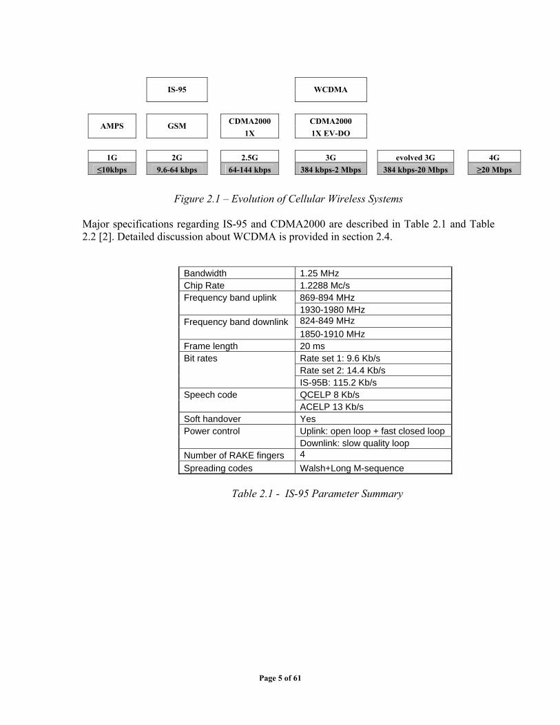
between inbound and outbound traffic • More efficient use of the available spectrum in general • Support for a wide variety of mobile equipment • Flexibility to allow the introduction of new services and technologies 2.2 Evolution of Wireless Cellular Systems The following Figure 2.1 [1] shows the evolution of wireless cellular systems. As the figure suggests, although 3G systems are in early stages of commercial deployment, work on fourth generation is underway. Objectives of 4G systems include greater data rates and more flexible quality of service (QoS) capabilities.

Page 4 of 61

IS-95

WCDMA

CDMA2000 CDMA2000 AMPS

GSM 1X 1X EV-DO

1G 2G 2.5G 3G evolved 3G 4G

≤10kbps 9.6-64 kbps 64-144 kbps 384 kbps-2 Mbps 384 kbps-20 Mbps ≥20 Mbps

Figure 2.1 – Evolution of Cellular Wireless Systems Major specifications regarding IS-95 and CDMA2000 are described in Table 2.1 and Table 2.2 [2]. Detailed discussion about WCDMA is provided in section 2.4.

Bandwidth 1.25 MHz Chip Rate 1.2288 Mc/s Frequency band uplink 869-894 MHz 1930-1980 MHz Frequency band downlink 824-849 MHz 1850-1910 MHz Frame length 20 ms Bit rates Rate set 1: 9.6 Kb/s Rate set 2: 14.4 Kb/s IS-95B: 115.2 Kb/s Speech code QCELP 8 Kb/s ACELP 13 Kb/s Soft handover Yes Power control Uplink: open loop + fast closed loop Downlink: slow quality loop Number of RAKE fingers 4 Spreading codes Walsh+Long M-sequence

Table 2.1 - IS-95 Parameter Summary

Page 5 of 61

Channel bandwidth 1.25, 5, 10, 15, 20 MHz Downlink RF channel structure

Direct spread or multicarrier

Chip rate 1.2288/3.6864/7.3728/11.0593/14.7456 Mc/s for direct spread

n x 1.2288 Mc/s (n = 1, 3, 6, 9, 12) for multicarrier Roll-off factor Similar to IS-95 Frame length

20 ms for data and control/5 ms for control information on the fundamental and dedicated control channel

Spreading modulation Balanced QPSK (downlink) Dual-channel QPSK (uplink) Complex spreading circuit Data modulation QPSK (downlink) BPSK (uplink) Coherent detection Pilot time multiplexed with PC and EIB (uplink)

Common continuous pilot channel and auxiliary pilot (downlink)

Channel multiplexing in uplink

Control, pilot, fundamental, and supplemental code multiplexed

I&Q multiplexing for data and control channels Multirate Variable spreading and multicode Spreading factors 4-256

Power control Open loop and fast closed loop (800 Hz, higher rates under study)

Spreading (downlink)

Variable length Walsh sequences for channel separation, M-sequence 215 (same sequence with time shift utilized in different cells, different sequence in I&Q channel)

Spreading (uplink)

Variable length orthogonal sequences for channel separation, M-sequence 215 (same sequence for all users, different sequences in I&Q channels);M-sequence 2411 for user separation (different time shifts for different users)

Handover Soft handover Interfrequency handover

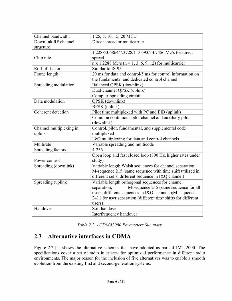
Table 2.2 - CDMA2000 Parameters Summary

2.3 Alternative interfaces in CDMA Figure 2.2 [1] shows the alternative schemes that have adopted as part of IMT-2000. The specifications cover a set of radio interfaces for optimized performance in different radio environments. The major reason for the inclusion of five alternatives was to enable a smooth evolution from the existing first and second-generation systems.

Page 6 of 61

Radio Interface

IMT-DS IMT-MC IMT-TC IMT-SC IMT-FT Direct Spread Multicarrier Time Code Single Carrier Frequency-Time (W-CDMA (CDMA2000) (TD-CDMA (TDD) (DECT+)

CDMA-based TDMA-based FDMA-based networks networks networks

Figure 2.2 - TMT-2000 Terrestrial Interfaces

The five alternatives [1] reflect the evolution from the second-generation. Two of the specifications grow out of the work at the European Telecommunications Standards Institute (ETSI) to develop a UMTS (universal mobile telecommunication system) as Europe’s 3G wireless standard. UMTS includes two standards. One is known as Wideband CDMA, or W-CDMA. This scheme fully exploits CDMA technology to provide high data rates with efficient use of bandwidth. The other European effort under UMTS is known as IMT-TC, or TD-CDMA. This approach is a combination of W-CDMA and TDMA technology. IMT-TC is intended to provide an upgrade path for the TDMA-based GSM systems. Another CDMA-based system, known as CDMA2000 [1], has a North American origin. This scheme is similar to, but incompatible with W-CDMA in part because the two standards use different chip rates. Also, CDMA2000 uses a technique known as muticarrier, which is not used in W-CDMA. Other two interface specifications shown in the figure are IMT-SC is primarily designed for TDMA-only networks. IMT-FT can be used by both TDMA and FDMA carriers to provide some 3G services. It is an outgrowth of the Digital European Cordless Telecommunications (DECT) standard. In the remainder of this chapter, we will provide some general considerations of CDMA technology for 3G systems and then an overview of a specific 3G system namely W-CDMA.

Page 7 of 61

2.4 CDMA Design Consideration: The dominant technology for 3G systems is CDMA. Although three different CDMA schemes have been adopted, they share some common design issues, given as following [1]: Bandwidth: An important design goal for all 3G systems is to limit channel usage to 5MHz. There are several reasons for this goal. On one hand, a larger bandwidth improves the receiver’s ability to resolve multipath when compared to narrower bandwidths. On the other hand, available spectrum is limited by competing needs, and 5 MHz is a reasonable upper limit on what can be allocated for 3G. Finally, 5 MHz is adequate for supporting data rates of 144 and 384 kHz, the main targets for 3G services. Chip rate: Given the bandwidth, the chip rate depends on desired data rate, the need for error control and bandwidth limitations. A chip rate of 3 Mcps (mega-chips per second) or more is reasonable given these design parameters.

Time Outer Coding mux

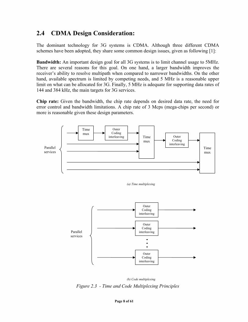
Figure 2.3 - Time and Code Multiplexing Principles

interleaving Time mux

Outer Coding

interleaving

Time mux

Outer Coding

interleaving

Outer Coding

interleaving

Outer Coding

interleaving

(a) Time multiplexing

Parallel

Parallel services

services

(b) Code multiplexing

Page 8 of 61

Mutirate: The term multirate refers to the provision of multiple fixed-data-rate logical channels to a given user, in which different data rate are provided on different logical channels. The advantage of multirate is that the system can flexibly support multiple simultaneous applications form a given user and can efficiently use available capacity by only providing the capacity required for each service. Further the traffic on each logical channel can be switched independently through the wireless and fixed networks to different destinations. Multirate can be achieved with a TDMA scheme with a single CDMA channel, in which a different number of slots per frame are assigned to achieve different data rates. All the subchannels at the given data rate would be protected by error correction and interleaving techniques as in Figure 2.3a [1]. An alternative is to use multiple CDMA codes, with separate coding and interleaving, and map them to separate CDMA channels (Figure 2.3b) [1] 2.5 Wideband CDMA (WCDMA) The WCDMA scheme was developed as a joint effort between ETSI and ARIB during the second half of 1997. The ETSI WCDMA scheme has been developed from the FMA2 scheme in Europe [3339] and the ARIB WCDMA from the Core-A scheme in Japan. The uplink of the WCDMA scheme is based mainly on the FMA2 scheme, and the downlink on the Core-A scheme. In this section, we present the chief technical features of the ARIB/ETSI WCDMA scheme. Table 2.3 lists the main parameters of WCDMA [2]. In the ARIB WCDMA proposal a chip rate of 1.024 Mc/s has been specified, whereas in the ETSI WCDMA is has not.

Channel bandwidth 1.25, 5, 10, 20 MHz Downlink RF channel structure Direct spread Chip rate (1.024)a/4.096/8.192/16.384 Mc/s Roll-off factor for chip shaping 0.22 Frame length 10 ms/20 ms (optional) Spreading modulation Balanced QPSK (downlink) Dual channel QPSK (uplink) Complex spreading circuit Data modulation QPSK (downlink) BPSK (uplink) Coherent detection

User dedicated time multiplexed pilot (downlink and uplink); no common pilot in downlink

Channel multiplexing in uplink Control and pilot channel time multiplexed I&Q multiplexing for data and control channel Multirate Variable spreading and multicode Spreading factors 4256 Power control Open and fast closed loop (1.6 kHz) Spreading (downlink)

Variable length orthogonal sequences for channel separation Gold sequences 218 for cell and user separation (truncated cycle 10 ms)

Spreading (uplink)

Variable length orthogonal sequences for channel separation, Gold sequence 241 for user separation (different time shifts in I and Q channel, truncated cycle 10 ms)

Handover Soft handover Interfrequency handover Table 2.3 - WCDMA Parameters

Page 9 of 61

2.5.1 Carrier Spacing and Deployment Scenarios The carrier spacing has a raster of 200 kHz and can vary from 4.2 to 5.4 MHz. The different carrier spacing can be used to obtain suitable adjacent channel protections depending on the interference scenario. Figure 2.4 shows an example for the operator bandwidth of 15 MHz with three cell layers [3]. Larger carrier spacing can be applied between operators than within one operator's band in order to avoid inter-operator interference. Inter-frequency measurements and handovers are supported by WCDMA to utilize several cell layers and carriers.

Figure 2.4 - Frequency utilization with WCDMA 2.5.2. WCDMA Logical Channels WCDMA basically follows the ITU Recommendation M.1035 in the definition of logical channels. The following logical channels are defined for WCDMA. The three available common control channels are:

• Broadcast control channel (BCCH) carries system and cell specific information • Paging channel (PCH) for messages to the mobiles in the paging area • Forward access channel (FACH) for massages from the base station to the mobile in

one cell.

In addition, there are two dedicated channels:

• Dedicated control channel (DCCH) covers the two dedicated control channel stand-alone dedicated channel (SDCCH) and associated control channel (ACCH)

• Dedicated traffic channel (DTCH) for point-to-point data transmission in the uplink and downlink

Page 10 of 61

2.5.3. WCDMA Physical Channels

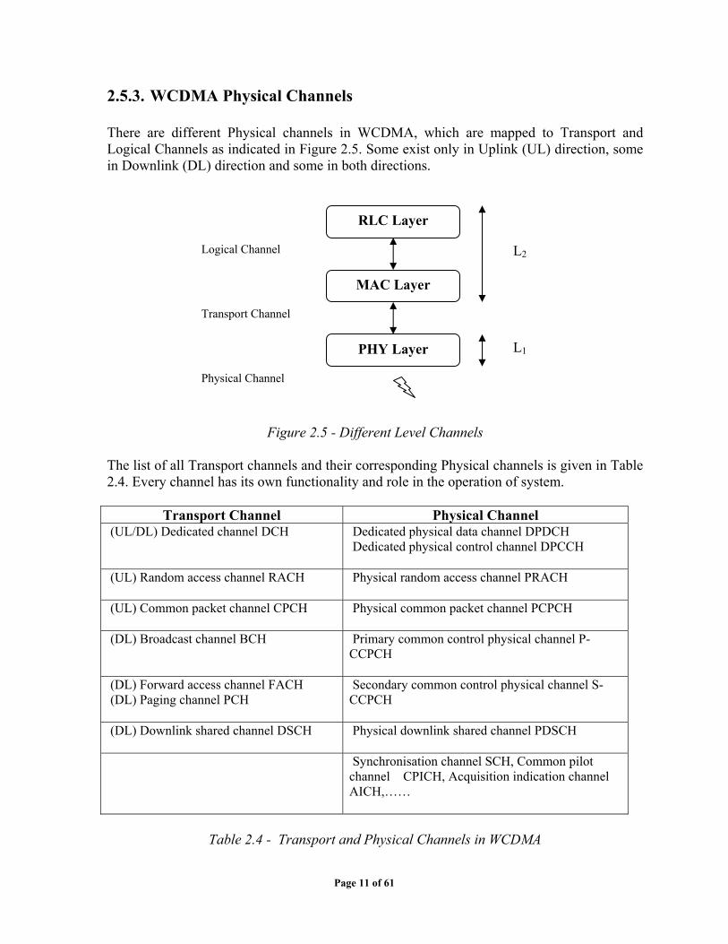
There are different Physical channels in WCDMA, which are mapped to Transport and Logical Channels as indicated in Figure 2.5. Some exist only in Uplink (UL) direction, some in Downlink (DL) direction and some in both directions.

RLC Layer

Figure 2.5 - Different Level Channels The list of all Transport channels and their corresponding Physical channels is given in Table 2.4. Every channel has its own functionality and role in the operation of system.

Transport Channel Physical Channel (UL/DL) Dedicated channel DCH Dedicated physical data channel DPDCH

Dedicated physical control channel DPCCH

(UL) Random access channel RACH

Physical random access channel PRACH

(UL) Common packet channel CPCH Physical common packet channel PCPCH

(DL) Broadcast channel BCH Primary common control physical channel P-CCPCH

(DL) Forward access channel FACH (DL) Paging channel PCH

Secondary common control physical channel S- CCPCH

(DL) Downlink shared channel DSCH Physical downlink shared channel PDSCH

Synchronisation channel SCH, Common pilot channel CPICH, Acquisition indication channel AICH,……

Table 2.4 - Transport and Physical Channels in WCDMA

Logical Channel

MAC Layer

L2

PHY Layer

Transport Channel

L1

Physical Channel

Page 11 of 61

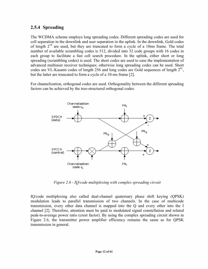
2.5.4 Spreading The WCDMA scheme employs long spreading codes. Different spreading codes are used for cell separation in the downlink and user separation in the uplink. In the downlink, Gold codes of length 218 are used, but they are truncated to form a cycle of a 10ms frame. The total number of available scrambling codes is 512, divided into 32 code groups with 16 codes in each group to facilitate a fast cell search procedure. In the uplink, either short or long spreading (scrambling codes) is used. The short codes are used to ease the implementation of advanced multiuser receiver techniques; otherwise long spreading codes can be used. Short codes are VL-Kasami codes of length 256 and long codes are Gold sequences of length 241, but the latter are truncated to form a cycle of a 10-ms frame [2]. For channelization, orthogonal codes are used. Orthogonality between the different spreading factors can be achieved by the tree-structured orthogonal codes.

Figure 2.6 - IQ/code multiplexing with complex spreading circuit IQ/code multiplexing also called dual-channel quaternary phase shift keying (QPSK) modulation leads to parallel transmission of two channels. In the case of multicode transmission, every other data channel is mapped into the Q and every other into the I channel [2]. Therefore, attention must be paid to modulated signal constellation and related peak-to-average power ratio (crest factor). By using the complex spreading circuit shown in Figure 2.6, the transmitter power amplifier efficiency remains the same as for QPSK transmission in general.

Page 12 of 61

Figure 2.7 - Signal constellation for IQ/code multiplexed control channel with complex spreading

Moreover, the efficiency remains constant irrespective of the power difference G between DPDCH and DPCCH. This can be explained by Figure 2.7, which shows the signal constellation for IQ/code multiplexed control channel with complex spreading. In the middle constellation with G = 0.5 all eight constellation points are at the same distance from the origin. The same is true for all values of G. Thus, signal envelope variations are very similar to the QPSK transmission for all values of G. The IQ/code multiplexing solution with complex scrambling results in power amplifier output backoff requirements that remain constant as a function of power difference. Furthermore, the achieved output backoff is the same as for one QPSK signal. 2.5.5 Multirate Multiple services of the same connection are multiplexed on one DPDCH.

Figure 2.8 - Service multiplexing in WCDMA Multiplexing may take place either before or after the inner or outer coding, as illustrated in Figure 2.8. After service multiplexing and channel coding, the multiservice data stream is

Page 13 of 61

mapped to one DPDCH. If the total rate exceeds the upper limit for single code transmission, several DPDCHs can be allocated. A second alternative for service multiplexing would be to map parallel services to different DPDCHs in a multicode fashion with separate channel coding/interleaving. With this alternative scheme, the power and consequently the quality of each service can be separately and independently controlled. The disadvantage is the need for multicode transmission which will have an impact on mobile station complexity. Multicode transmission sets higher requirements for the power amplifier linearity in transmission and more correlators are needed in reception. For BER = 103 services, convolutional coding of 1/3 is used. For high bit rates a code rate of 1/2 can be applied. For higher quality service classes outer Reed-Solomon coding is used to reach the 106 BER level. Retransmissions can be utilized to guarantee service quality for non real-time packet data services. After channel coding and service multiplexing, the total bit rate can be almost arbitrary. The rate matching adapts this rate to the limited set of possible bit rates of a DPDCH. Repetition or puncturing is used to match the coded bit stream to the channel gross rate. The rate matching for uplink and downlink are introduced below: For the uplink, rate matching to the closest uplink DPDCH bit rate is always based on unequal repetition (a subset of the bits repeated) or code puncturing. In general, code puncturing is chosen for bit rates less than 20 percent above the closest lower DPDCH bit rate. For all other cases, unequal repetition is performed to the closest higher DPDCH bit rate. The repetition/puncturing patterns follow a regular predefined rule (i.e., only the amount of repetition/puncturing needs to be agreed on). The correct repetition/puncturing pattern can then be directly derived by both the transmitter and receiver side. For the downlink, rate matching to the closest DPDCH bit rate, using either unequal repetition or code puncturing, is only made for the highest rate (after channel coding and service multiplexing) of a variable rate connection and for fixed-rate connections. For lower rates of a variable rate connection, the same repetition/puncturing pattern as for the highest rate is used, and the remaining rate matching is based on discontinuous transmission where only a part of each slot is used for transmission. This approach is used in order to simplify the implementation of blind rate detection in the mobile station. 2.5.6 Packet Data WCDMA has two different types of packet data transmission possibilities. Short data packets can be appended directly to a random access burst. This method, called common channel packet transmission, is used for short infrequent packets, where the link maintenance needed for a dedicated channel would lead to an unacceptable overhead [2]. When using the uplink common channel, a packet is appended directly to a random access burst. Also, the delay associated with a transfer to a dedicated channel is avoided. Note that for common channel packet transmission only open loop power control is in operation.

Page 14 of 61

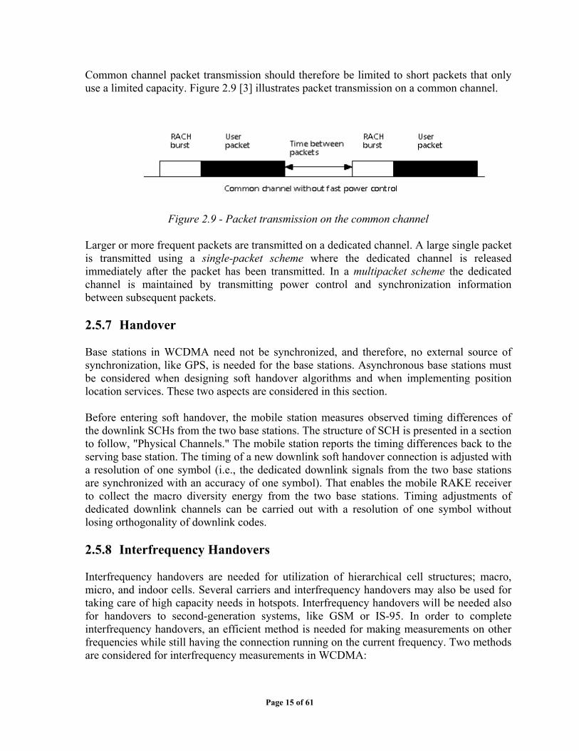
Common channel packet transmission should therefore be limited to short packets that only use a limited capacity. Figure 2.9 [3] illustrates packet transmission on a common channel.

Figure 2.9 - Packet transmission on the common channel Larger or more frequent packets are transmitted on a dedicated channel. A large single packet is transmitted using a single-packet scheme where the dedicated channel is released immediately after the packet has been transmitted. In a multipacket scheme the dedicated channel is maintained by transmitting power control and synchronization information between subsequent packets. 2.5.7 Handover Base stations in WCDMA need not be synchronized, and therefore, no external source of synchronization, like GPS, is needed for the base stations. Asynchronous base stations must be considered when designing soft handover algorithms and when implementing position location services. These two aspects are considered in this section. Before entering soft handover, the mobile station measures observed timing differences of the downlink SCHs from the two base stations. The structure of SCH is presented in a section to follow, "Physical Channels." The mobile station reports the timing differences back to the serving base station. The timing of a new downlink soft handover connection is adjusted with a resolution of one symbol (i.e., the dedicated downlink signals from the two base stations are synchronized with an accuracy of one symbol). That enables the mobile RAKE receiver to collect the macro diversity energy from the two base stations. Timing adjustments of dedicated downlink channels can be carried out with a resolution of one symbol without losing orthogonality of downlink codes. 2.5.8 Interfrequency Handovers Interfrequency handovers are needed for utilization of hierarchical cell structures; macro, micro, and indoor cells. Several carriers and interfrequency handovers may also be used for taking care of high capacity needs in hotspots. Interfrequency handovers will be needed also for handovers to second-generation systems, like GSM or IS-95. In order to complete interfrequency handovers, an efficient method is needed for making measurements on other frequencies while still having the connection running on the current frequency. Two methods are considered for interfrequency measurements in WCDMA:

Page 15 of 61

• Dual receiver • Slotted mode

1. Dual Receiver Approach: The dual receiver approach is considered suitable especially if the mobile terminal employs antenna diversity. During the interfrequency measurements, one receiver branch is switched to another frequency for measurements, while the other keeps receiving from the current frequency. The loss of diversity gain during measurements needs to be compensated for with higher downlink transmission power. The advantage of the dual receiver approach is that there is no break in the current frequency connection. Fast closed loop power loop is running all the time.

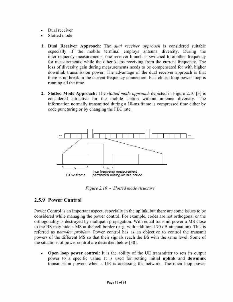
2. Slotted Mode Approach: The slotted mode approach depicted in Figure 2.10 [3] is

considered attractive for the mobile station without antenna diversity. The information normally transmitted during a 10-ms frame is compressed time either by code puncturing or by changing the FEC rate.

Figure 2.10 - Slotted mode structure 2.5.9 Power Control Power Control is an important aspect, especially in the uplink, but there are some issues to be considered while managing the power control. For example, codes are not orthogonal or the orthogonality is destroyed by multipath propagation. With equal transmit power a MS close to the BS may hide a MS at the cell border (e. g. with additional 70 dB attenuation). This is referred as near-far problem. Power control has as an objective to control the transmit powers of the different MS so that their signals reach the BS with the same level. Some of the situations of power control are described below [30].

• Open loop power control: It is the ability of the UE transmitter to sets its output power to a specific value. It is used for setting initial uplink and downlink transmission powers when a UE is accessing the network. The open loop power

Page 16 of 61

control tolerance is ± 9 dB (normal conditions) or ± 12 dB (extreme conditions)

• Inner loop power control: Also called fast closed loop power control, in the uplink is the ability of the UE transmitter to adjust its output power in accordance with one or more Transmit Power Control (TPC) commands received in the downlink, in order to keep the received uplink Signal-to-Interference Ratio (SIR) at a given SIR target. The UE transmitter is capable of changing the output power with a step size of 1, 2 and 3 dB, in the slot immediately after the TPC_cmd can be derived. Inner loop power control frequency is 1500Hz. The transmit power of the downlink channels is determined by the network. The power control step size can take four values: 0.5, 1, 1.5 or 2 dB. It is mandatory for UTRAN to support step size of 1dB, while support of other step sizes is optional. The UE generates TPC commands to control the network transmit power and send them in the TPC field of the uplink DPCCH. Upon receiving the TPC commands UTRAN adjusts its downlink DPCCH/DPDCH power accordingly.

• Outer loop power control: It is used to maintain the quality of communication at the

level of bearer service quality requirement, while using as low power as possible. The uplink outer loop power control is responsible for setting a target SIR in the Node B for each individual uplink inner loop power control. This target SIR is updated for each UE according to the estimated uplink quality (BLock Error Ration, Bit Error Ratio) for each Radio Resource Control connection. The downlink outer loop power control is the ability of the UE receiver to converge to required link quality (BLER) set by the network (RNC) in downlink.

• Power control of the downlink common channels: Power control of the downlink

common channels, are determined by the network. In general the ratio of the transmit power between different downlink channels is not specified in 3GPP specifications and may change with time, even dynamically.

Additional special situations of power control are Power control in compressed mode and Downlink power during handover, which are not explained over here have various proposed algorithms.

Page 17 of 61

Chapter 3

HSDPA

As discussed in the previous chapter, recent 3G standardization and related technology development reflect the need of the high-speed packet data of wireless internet. The race of the high-speed packet data in CDMA started roughly in late 1999. Before then, WCDMA and CDMA2000 systems supported the packet data but the design philosophy was still old in the sense that the system resources such as power, code and data rate are optimized to voice like applications. There was a change since late 1999 when system designers realized that 1) the main wireless data applications will be Internet protocol (IP) related, thus 2) optimum packet data performance is the primary goal for the system designers to accomplish. With the design philosophy change, some new technologies have appeared such as adaptive modulation and coding, hybrid ARQ, fast scheduling etc. which are all in cooperated in Release 5 of WCDMA named as High Speed Downlink Packet Access (HSDPA) which will be discussed in detail in this thesis. 3.1 Comparisons of Release 99 and HSDPA Various methods for packet data transmission in WCDMA downlink already exist in Release 99 (R99). The standard provides two different channels for high data rate packet services in the downlink dedicated channel (DCH) and downlink shared channel (DSCH). Both can provide variable bit rate. The DCH is the basic radio bearer in WCDMA and supports all traffic classes due to high parameter flexibility. The data rate is updated by means of variable spreading factor while the block error rate (BLER) is controlled by inner and outer loop power control mechanisms. However, in the dedicated channel spreading factor and spreading code are reserved from the OVSF (orthogonal variable spreading factor) code tree based on the highest data rate. This easily leads to shortage of downlink codes. Therefore, the DSCH is more appropriate for high data rate packet services. The benefit of the DSCH over the DCH is a fast channel reconfiguration time and packet scheduling procedure. With the introduction of Release 5 (R5) of the specifications in the spring of 2002, WCDMA packet data support is further enhanced to peak data rates in the order of 10 Mbps together with lower round-trip delays and increased capacity provide a further boost for wireless data access. WCDMA R5 contains a new set of features known collectively as HSDPA (High Speed Downlink Packet Access). The HSDPA concept can be seen as a continued evolution of the DSCH and a new transport channel targeting packet data transmissions, the high speed DSCH (HS-DSCH), is introduced. The HS-DSCH supports three basic principles: fast link adaptation, fast Hybrid ARQ (HARQ), and fast scheduling. These three principles rely on

Page 18 of 61

rapid adaptation to changing radio conditions and the corresponding functionality is therefore placed in the Node B instead of the RNC. Similar to the R99 DSCH, each UE to which data can be transmitted on the HS-DSCH has an associated DCH. This DCH is used to carry power control commands and the necessary control information in the uplink namely ARQ acknowledgement (ACKMACK) and channel quality indicator (CQI). To implement the HSDPA feature, a new channel called High Speed Shared Control Channel (HS-SCCH) is introduced in the physical layer specifications. The HS-SCCH carries the control information that is only relevant for the UE for which there is data on the HS-DSCH. The system level diagram is shown in Figure 3.1.

Figure 3.1 - WCDMA/HSDPA components and interfaces The fundamental characteristics of the HS-DSCH and the DSCH are compared in Table 3.1 [5]. While being more complicated, the replacement of fast power control with fast AMC yields a power efficiency gain due to an elimination of the inherent power control overhead. Specifically, the spreading factor of the assigned channelization code is fixed to 16 and up to 15 out of 16 orthogonal codes can be allocated for the HS-DSCH. The HS-DSCH uses AMC for fast link adaptation. A terminal experiencing good link conditions will be served with a higher data rate than a terminal in a less favorable situation. To support the different data rates, a wide range of channel coding rates and different modulation formats, namely QPSK and 16QAM, are supported. In order to increase the link adaptation rate and efficiency of the AMC, the packet duration has been reduced from normally 10 or 20 ms down to a fixed 2 ms. To achieve low delays in the link control, the MAC functionality for the HS-DSCH has been moved from RNC to the Node-B. It will enhance the packet data characteristics by reducing the round-trip delay.

Page 19 of 61

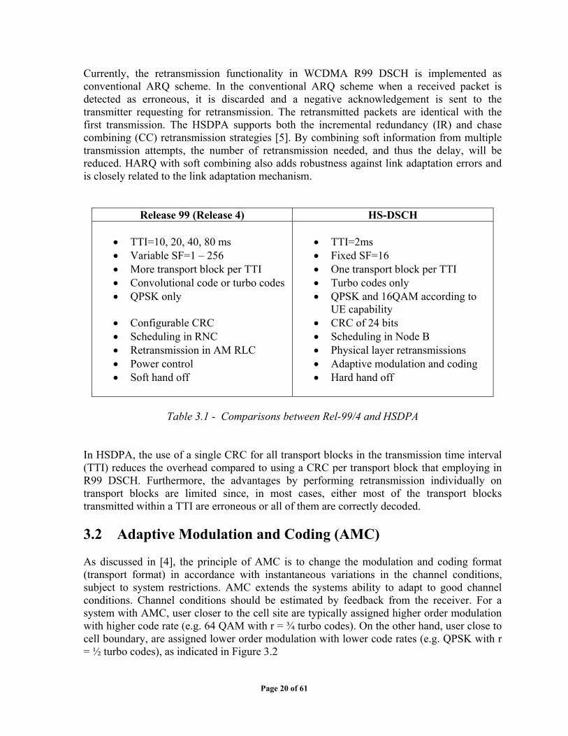
Currently, the retransmission functionality in WCDMA R99 DSCH is implemented as conventional ARQ scheme. In the conventional ARQ scheme when a received packet is detected as erroneous, it is discarded and a negative acknowledgement is sent to the transmitter requesting for retransmission. The retransmitted packets are identical with the first transmission. The HSDPA supports both the incremental redundancy (IR) and chase combining (CC) retransmission strategies [5]. By combining soft information from multiple transmission attempts, the number of retransmission needed, and thus the delay, will be reduced. HARQ with soft combining also adds robustness against link adaptation errors and is closely related to the link adaptation mechanism.

Release 99 (Release 4) HS-DSCH • TTI=10, 20, 40, 80 ms • Variable SF=1 – 256 • More transport block per TTI • Convolutional code or turbo codes • QPSK only

• Configurable CRC • Scheduling in RNC • Retransmission in AM RLC • Power control • Soft hand off

• TTI=2ms • Fixed SF=16 • One transport block per TTI • Turbo codes only • QPSK and 16QAM according to

UE capability • CRC of 24 bits • Scheduling in Node B • Physical layer retransmissions • Adaptive modulation and coding • Hard hand off

Table 3.1 - Comparisons between Rel-99/4 and HSDPA

In HSDPA, the use of a single CRC for all transport blocks in the transmission time interval (TTI) reduces the overhead compared to using a CRC per transport block that employing in R99 DSCH. Furthermore, the advantages by performing retransmission individually on transport blocks are limited since, in most cases, either most of the transport blocks transmitted within a TTI are erroneous or all of them are correctly decoded. 3.2 Adaptive Modulation and Coding (AMC) As discussed in [4], the principle of AMC is to change the modulation and coding format (transport format) in accordance with instantaneous variations in the channel conditions, subject to system restrictions. AMC extends the systems ability to adapt to good channel conditions. Channel conditions should be estimated by feedback from the receiver. For a system with AMC, user closer to the cell site are typically assigned higher order modulation with higher code rate (e.g. 64 QAM with r = ¾ turbo codes). On the other hand, user close to cell boundary, are assigned lower order modulation with lower code rates (e.g. QPSK with r = ½ turbo codes), as indicated in Figure 3.2

Page 20 of 61

Adapting the transmission parameters in a wireless system to changing channel conditions can bring benefits. In case of the fast power control, the transmission power is adjusted based on the channel fading. Thus, a good channel condition requires lower transmission power to maintain the targeted signal quality at the receiver. The process of changing transmission parameters to compensate the variation in the channel conditions is known as link adaptation. Besides power control, adaptive modulation and coding is another type of link adaptation [10]. The core idea of AMC is to dynamically change the Modulation and Coding Scheme (MCS) in subsequent frames with the objective of adapting the overall spectral efficiency to the channel condition. The decision about selecting the appropriate MCS is performed at the receiver side according to the observed channel condition with the information fed back to the transmitter in each frame [11]. 3.2.1 Link Quality Feedback A key factor determining the performance of an AMC scheme is the method used at the receiver to estimate the channel condition and thereby deciding for the appropriate MCS to be used in the next frame [11]. Different control channels are used to communicate channel quality information between user equipment (UE) and Node-B and an appropriate AMCS is selected for the specific UE based on this information. As mentioned in [9], the sequence of Link Quality Feedback could be: • UE measures channel quality by evaluation of CPICH (Common Pilot Channel). • UE reports channel quality to BS by choosing a transport format (modulation, code rate,

and transmit power offset) such that a 10% FER target is met. • BS determines the transport format based on the recommended transport format and

possibly on power control commands of associated dedicated physical channel (DPCH). • Transport format update rate: every TTI= 3 slots • Measurement report rate: every TTI= 3 slots 3.2.2 Different Modulation and Coding Combinations The goal of the AMC is to change the modulation and channel coding according to the varying channel conditions. In this scheme, a terminal with favourable channel conditions can be assigned a higher order modulation with a higher channel coding rate, and a lower order modulation with a lower channel coding rate, when the terminal has unfavourable channel conditions. The benefits of the AMC enable higher bit rates on the transport channel, when the terminal is in good channel conditions [10]. That means the users near to the Base Station (BS) are allocated higher order modulation and coding with respect to users far from BS as can be seen in Figure 3-2 [12]

Page 21 of 61

Figure 3.2 - Adaptive Modulation and Coding Scheme is changed with respect to users

Table 3.2, shows different Modulation and Coding combinations proposed in [9] and the respective data rates could be achieved at user level when one code out of 15 is allocated to it.

TFRC’s Modulation Code rate # of info bits per code

Info bit rate per code

1 QPSK 1/4 240 120 kbps 2 QPSK 1/2 480 240 kbps 3 QPSK 3/4 720 360 kbps 4 16-QAM 1/2 960 480 kbps 5 16-QAM 3/4 1440 720 kbps

1 TTI = 3 slots = 2ms = 7680 chips = 480 symbols @ SF = 16 480 symbols = 960 bits @ QPSK, 480 symbols = 1920 bits @ 16-QAM

Table 3.2 - Different Modulation and Coding Schemes and

their information carrying capacity

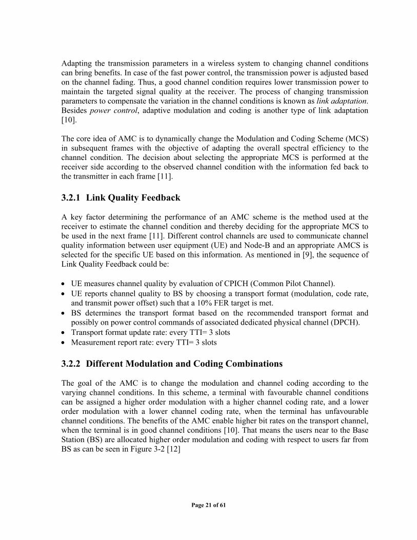
We have assigned single code of SF=16, to each user in Table 3.2. But if we give one user all 15 possible codes then we can achieve 10.8 Mbps (720 kbps x 15) while using highest TFRC (Transport Format & Resource Combination). Also note that higher TFRC’s are proposed in different papers which would provide more data rates than those mentioned in Table 3.2 3.2.3 HSDPA System Model The system model for AMCS is shown in Figure 3-3 [9]. The model also describes the Multiplexer-Demultiplexer which could be used to assign/separate more than one code to a user. The selection criteria and method have already been discussed in previous sections 3.2.1 and 3.2.2.

Page 22 of 61

Figure 3.3 - AMCS system model The decision regarding allocation 15 codes to one or more users is taken on TTI basis that is time multiplexed as depicted in Figure 3-4 [9].

Figure 3.4 - Different code allocations to different users on TTI basis. Example for 3 users sharing 5 codes

From the discussion presented in previous sections we can conclude that correct selection of MCS is quite important in order to increase the system throughput, increase spectral efficiency and avoid prediction of turbo codes. There are no standard methods for MCS selection used in HSDPA as it is in experimental phase. The following two methods have been tested and widely acclaimed and hence will be mentioned in this thesis.

3.2.4 Threshold decision making for MCS and multicode selection It is well known that higher order modulations may give better spectral efficiency in the expense of worse bit error performance. A lower channel coding rate has a better error correction capability than the same type of coding with a higher coding rate. Thus, with a proper combination of the modulation order and channel coding rate, it is possible to design a

D E M U X

QPSK/ 16-QAM Interleaver Rate

Matching

Turbo Encoder

Tail Bits

AMCS W1SF

WMSF

Data to UE #1 Data to UE #2 Data to UE #3

Page 23 of 61

definite set of modulation and coding schemes (MCS), from which an adaptive selection is made per TTI such that an increased spectral efficiency can be achieved in good channel conditions. At each selection of the MCS, the criteria should be such that the probability of correct decoding of the Transmission Block is close to the threshold value. It is also possible to increase the bit rate further by the use of the multicodes for a given

ρi, j= fi, j-1 (εthreshold ) (3-1)

The change of this channel state is in every TTI, which is defined to be 2 ms, in practice.

f i ,j (ρ)= f i ,1 (ρ-10 . log10 (j)) (3-2)

where ρ is in dB. The bit rate associated with the state (i, j) is given by ri, j = j . ri ,where ri is

MCS, when the channel conditions allow. Of course, when multicode-transmission is used, the available power resource would have to be shared among the parallel channelization codes. The algorithm presented in [10] selects the number of multicodes and the MCS per each TTI such that the increase in the number of multicodes is prioritised over the increase in the higher order modulation and coding scheme. Together with the AMC, multicode transmission provides an additional dimension and increased granularity for the link adaptation. While AMC provides a coarse adaptation to the channel, the use of multicode brings the “fine tuning” to the selected MCS. Obviously, an algorithm is needed to select the MCS and the number of multicodes. The objective is to maximize the bit rate by selecting the right combination for the number of multicodes j (maximum value = j max=3 in [10]) and the MCS i, given a channel condition ρ= Eb / No , where Eb is the energy per bit and No is the two-sided power spectral density. Let f i ,j (ρ) = f i,j be the frame error rate (FER) associated with the state (i, j) as a function of ρ, and g (ρ) be the probability density function of ρ. Also, let threshold εthreshold be the frame error threshold which defines the maximum tolerable error (considered as 50% in [10]). The minimum channel condition which is required for state (i, j) such that εthreshold is not exceeded is shown in Figure 3-5, and is given by

Such a short transmission period allows the scheduling to adapt to the fast changing channel conditions. Since the power is shared among the multicodes, the error curves are typically given by

the single-code bit rate associated with the MCSi.

Page 24 of 61

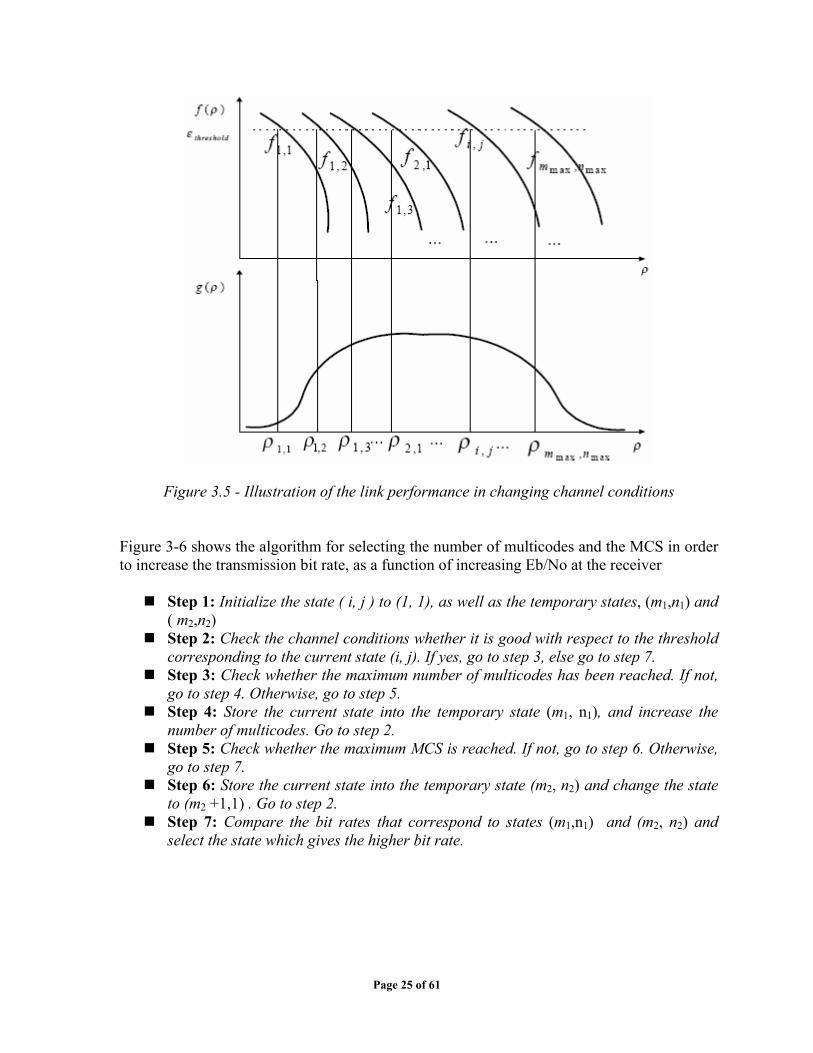
Figure 3.5 - Illustration of the link performance in changing channel conditions

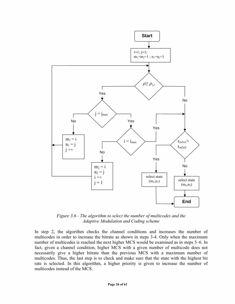
Figure 3-6 shows the algorithm for selecting the number of multicodes and the MCS in order to increase the transmission bit rate, as a function of increasing Eb/No at the receiver

Step 1: Initialize the state ( i, j ) to (1, 1), as well as the temporary states, (m1,n1) and ( m2,n2)

Step 2: Check the channel conditions whether it is good with respect to the threshold corresponding to the current state (i, j). If yes, go to step 3, else go to step 7.

Step 3: Check whether the maximum number of multicodes has been reached. If not, go to step 4. Otherwise, go to step 5.

Step 4: Store the current state into the temporary state (m1, n1), and increase the number of multicodes. Go to step 2.

Step 5: Check whether the maximum MCS is reached. If not, go to step 6. Otherwise, go to step 7.

Step 6: Store the current state into the temporary state (m2, n2) and change the state to (m2 +1,1) . Go to step 2.

Step 7: Compare the bit rates that correspond to states (m1,n1) and (m2, n2) and select the state which gives the higher bit rate.

Page 25 of 61

i=1; j=1; m1=m2=1 ; n1=n2=1

ρ≥ ρi,j

i = imax rm1n1> rm2n2

j = jmax

m2 = i n2 = j i ++ j = 1

m1 = i n1 = j j ++

select state (m1,n1) select state

(m2,n2)

End

No

No

Yes

Yes

Yes

No

No

Yes

Start

Figure 3.6 - The algorithm to select the number of multicodes and the Adaptive Modulation and Coding scheme

In step 2, the algorithm checks the channel conditions and increases the number of multicodes in order to increase the bitrate as shown in steps 3-4. Only when the maximum number of multicodes is reached the next higher MCS would be examined as in steps 5–6. In fact, given a channel condition, higher MCS with a given number of multicode does not necessarily give a higher bitrate than the previous MCS with a maximum number of multicodes. Thus, the last step is to check and make sure that the state with the highest bit rate is selected. In this algorithm, a higher priority is given to increase the number of multicodes instead of the MCS.

Page 26 of 61

3.2.5 Markov’s Model of MCS selection It is assumed in the “threshold” method that the fading is slow enough such that the average channel SNR remains in the same region from the current frame to the next, the estimated channel SNR of the current frame is simply taken as the predicted channel SNR for the next frame. This simplifying assumption, however, is often not true in a mobile environment. In such case, an error in the estimation of average channel SNR can cause inappropriate selection of MCS, resulting in degradation in FER performance. For packet data in the 3G standards, turbo codes are specified as the channel coding technique. One of the main characteristics of turbo codes is that they operate close to the channel capacity and the corresponding FER vs. SNR curves have a steep slope. This means that even a small prediction error in channel SNR can result in a large degradation in FER. Therefore, it is essential to take into account the possible prediction errors when designing an AMC system where turbo codes are employed. In [11], the authors have considered a first-order finite-state Markov model to represent the time variations in the average channel SNR. The states in this model represent the average channel SNR of a frame uniformly quantized in dB scale with a given step size ∆, and they form a set S={S0, . . ., Sm−1} of m states. As in the “threshold” method, assume that there are n MCS’s. We denote Ni as the number of information bits in a frame of 384 coded symbols that uses ith MCS, namely Mi. Table 3.3 shows the values of Ni for the three MCS’s used in this [11]. In the paper [11] Fij is defined as the FER of Mi in state j, and Tij as the expected throughput of Mi in state j. Please refer to section 3.2.2, which describes the calculation of information bits in each modulation scheme.

Modulation scheme (Mi)

Turbo codes rate (Rc)

Ni (bits)

16QAM 8PSK BPSK

1/2 1/2 1/3

768 576 128

Table 3.3 - Values of Ni

Two sub-models are presented in [11] for selecting appropriate MCS based on the states of a first-order Markov model, and evaluate its expected throughput. These are:

• Full Scale Markov Model • Simplified Markov Model

The basic strategy is to assign an MCS to each state such that the expected throughput is maximized in that state. Each sub-model has their own advantages and disadvantages in terms of efficiency and throughput as discussed in [11].

Page 27 of 61

3.2.6 Comparison between Markov and Threshold Models From the discussion in Sections 3.2.4 and 3.2.5 and results from [11], we can conclude that Markov Model which takes statistical decision making approach for selecting the appropriate Modulation and Coding Scheme (MCS) is better, when considering the issue caused by the sensitivity of turbo code to the errors in predicting the channel SNR. Numerical results presented in [11] showing that Markov method substantially outperforms the conventional techniques that use a “threshold-based” decision making approach. Simplified Model proposed in [11] has fewer parameters, suitable to systems where changes in the fading characteristics need to be accounted for in an adaptive manner. It is shown in [11] that the Simplified Model only results in negligible loss in the expected throughput. Also we would like to emphasize that, these are not only the two solution algorithms for the AMC module, but there exist many more which are under evaluation and considerations. 3.3 Hybrid Automatic Retransmit Request (HARQ) H-ARQ is described in [6] and consists of the following three techniques: i) Chase combining (CC): If the received block doesn't have the correct Circular Redundancy Check (CRC) sequence, it is retransmitted and new values of soft bits are added to those of the first transmission to form a good set of data. ii) Incremental redundancy (IR): Incorrect block is retransmitted with different redundancy version parameters (different systematic over parity bits priority and/or rate matching parameters). iii) 16QAM constellation rearrangement (CoRe): Different mapping of blocks of bits to symbols. Chase combining was originally proposed in [7]. It provides a considerable gain in transmission power (3 dB in Gaussian environment) at the cost of slightly increased processing complexity and a buffer in the UE that is required to store the received values. Chase combining can be used at both bit and symbol levels. However, the improvement of performance is not sufficient to obtain target rates. Incremental redundancy provides yet another improvement by allowing senders to send additional information in case retransmission is needed. In other words, bits which are punctured at the rate matching step of the first transmission can be sent at the second one. More precisely, one can prioritize sending systematic or parity bits, and at the same time, vary rate matching parameters, thus choosing not to puncture the same bits as at previous transmissions. This technique greatly improves Turbo decoder's performance. The disadvantage is that the buffer size in the UE has to increase considerably, as well as processing complexity.

Page 28 of 61

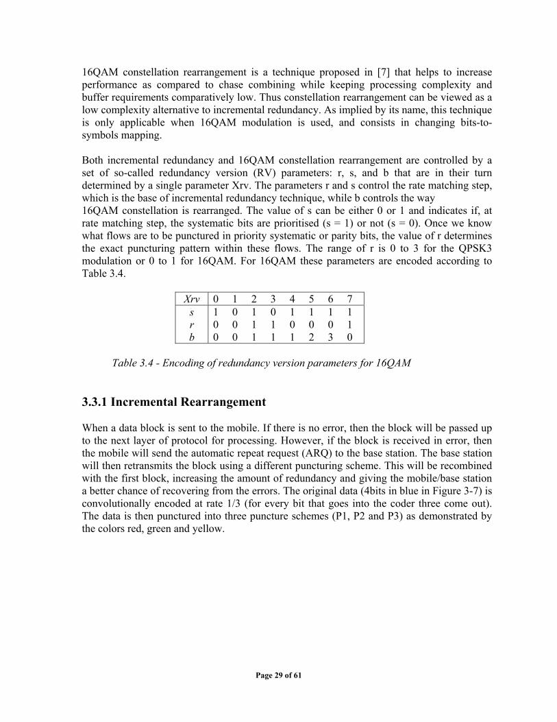
16QAM constellation rearrangement is a technique proposed in [7] that helps to increase performance as compared to chase combining while keeping processing complexity and buffer requirements comparatively low. Thus constellation rearrangement can be viewed as a low complexity alternative to incremental redundancy. As implied by its name, this technique is only applicable when 16QAM modulation is used, and consists in changing bits-to-symbols mapping. Both incremental redundancy and 16QAM constellation rearrangement are controlled by a set of so-called redundancy version (RV) parameters: r, s, and b that are in their turn determined by a single parameter Xrv. The parameters r and s control the rate matching step, which is the base of incremental redundancy technique, while b controls the way 16QAM constellation is rearranged. The value of s can be either 0 or 1 and indicates if, at rate matching step, the systematic bits are prioritised (s = 1) or not (s = 0). Once we know what flows are to be punctured in priority systematic or parity bits, the value of r determines the exact puncturing pattern within these flows. The range of r is 0 to 3 for the QPSK3 modulation or 0 to 1 for 16QAM. For 16QAM these parameters are encoded according to Table 3.4.

Xrv 0 1 2 3 4 5 6 7 s r b

1 0 1 0 1 1 1 1 0 0 1 1 0 0 0 1 0 0 1 1 1 2 3 0

Table 3.4 - Encoding of redundancy version parameters for 16QAM 3.3.1 Incremental Rearrangement When a data block is sent to the mobile. If there is no error, then the block will be passed up to the next layer of protocol for processing. However, if the block is received in error, then the mobile will send the automatic repeat request (ARQ) to the base station. The base station will then retransmits the block using a different puncturing scheme. This will be recombined with the first block, increasing the amount of redundancy and giving the mobile/base station a better chance of recovering from the errors. The original data (4bits in blue in Figure 3-7) is convolutionally encoded at rate 1/3 (for every bit that goes into the coder three come out). The data is then punctured into three puncture schemes (P1, P2 and P3) as demonstrated by the colors red, green and yellow.

Page 29 of 61

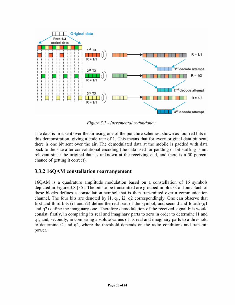
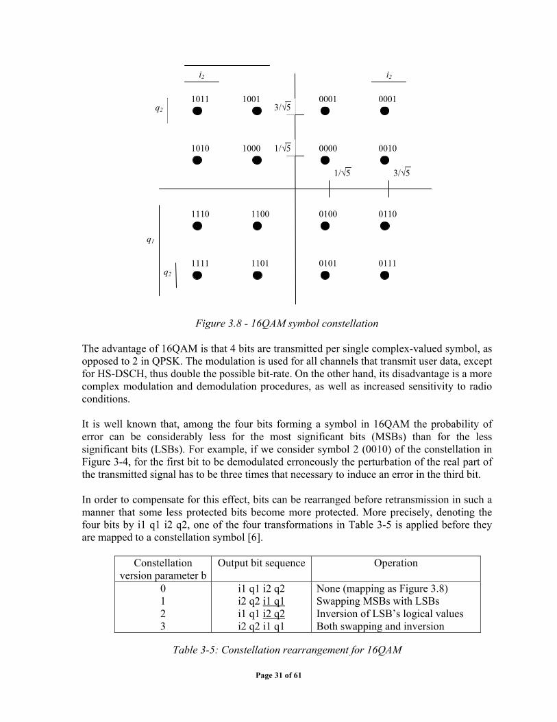
Figure 3.7 - Incremental redundancy The data is first sent over the air using one of the puncture schemes, shown as four red bits in this demonstration, giving a code rate of 1. This means that for every original data bit sent, there is one bit sent over the air. The demodulated data at the mobile is padded with data back to the size after convolutional encoding (the data used for padding or bit stuffing is not relevant since the original data is unknown at the receiving end, and there is a 50 percent chance of getting it correct). 3.3.2 16QAM constellation rearrangement 16QAM is a quadrature amplitude modulation based on a constellation of 16 symbols depicted in Figure 3.8 [35]. The bits to be transmitted are grouped in blocks of four. Each of these blocks defines a constellation symbol that is then transmitted over a communication channel. The four bits are denoted by i1, q1, i2, q2 correspondingly. One can observe that first and third bits (i1 and i2) define the real part of the symbol, and second and fourth (q1 and q2) define the imaginary one. Therefore demodulation of the received signal bits would consist, firstly, in comparing its real and imaginary parts to zero in order to determine i1 and q1, and, secondly, in comparing absolute values of its real and imaginary parts to a threshold to determine i2 and q2, where the threshold depends on the radio conditions and transmit power.

Page 30 of 61

i2 i2

1011 1001 0001 0001 3/√5q2

1010 1000 1/√5 0000 0010

1/√5 3/√5

Figure 3.8 - 16QAM symbol constellation The advantage of 16QAM is that 4 bits are transmitted per single complex-valued symbol, as opposed to 2 in QPSK. The modulation is used for all channels that transmit user data, except for HS-DSCH, thus double the possible bit-rate. On the other hand, its disadvantage is a more complex modulation and demodulation procedures, as well as increased sensitivity to radio conditions. It is well known that, among the four bits forming a symbol in 16QAM the probability of error can be considerably less for the most significant bits (MSBs) than for the less significant bits (LSBs). For example, if we consider symbol 2 (0010) of the constellation in Figure 3-4, for the first bit to be demodulated erroneously the perturbation of the real part of the transmitted signal has to be three times that necessary to induce an error in the third bit. In order to compensate for this effect, bits can be rearranged before retransmission in such a manner that some less protected bits become more protected. More precisely, denoting the four bits by i1 q1 i2 q2, one of the four transformations in Table 3-5 is applied before they are mapped to a constellation symbol [6].

Constellation version parameter b

Output bit sequence Operation

0 1 2 3

i1 q1 i2 q2 i2 q2 i1 q1i1 q1 i2 q2i2 q2 i1 q1

None (mapping as Figure 3.8) Swapping MSBs with LSBs Inversion of LSB’s logical values Both swapping and inversion

Table 3-5: Constellation rearrangement for 16QAM

1110 1100

1111 1101

0100 0110

0101 0111 q2

q1

Page 31 of 61

Averaging of error p veraging it over the

he following observations can be made regarding constellation rearrangement. E. The only

• four constellation rearrangement

Maximum benefit from

.3.3 Candidate H-ARQ schemes

question arises naturally: what H-ARQ control scheme is optimal in terms of the quality of

s mentioned above, the maximum benefit from constellation rearrangement can be obtained

robability over a long chain of bits is equivalent to asymbol constellation. Thus, in order to better understand the principle of constellation rearrangement, we can consider a transmission where each constellation symbol is sent exactly once over an ideal channel (no fading, no noise). Suppose we use standard bits-to-symbols mapping, i.e. b = 0. We then have a chain of 64 bits, out of which 16 are better protected than the other 48. These 16 bits are the two MSBs of each of four symbols in the corners of the constellation, and one of the MSBs for the eight other symbols on the constellation's exterior. Each of the four transformations in Table 3-5 provides better protection for a different set of 16 bits. Thus consequent retransmissions with different constellation arrangements would considerably improve turbo decoder's performance. T

• Constellation rearrangement does not require additional buffer in the Uspace required is that, necessary to store three additional tables for bits-to symbols mapping, and it is negligible compared to the size of buffer used to store transmitted bits. There is no additional processing to be done. When only one transmission is performed, all techniques are equivalent. Similarly, if several retransmissions are needed, whatever is the rearrangement sequence, there is always an equivalent one with first transmission using standard mapping (b =0). constellation rearrangement can be obtained with four retransmissions using different rearrangement techniques.

3 Aservice (QoS) and complexity (UE buffer and processing)? Awith four retransmissions. The same can be said about incremental redundancy in 16QAM as there are four different redundancy versions: systematic or parity bits, and two rate matching patterns for each of them. Some simulations have been proposed and according to [8], CC provides us with reference performances. IR being the scheme that ensures most diversity (different redundancy versions plus some use of constellation rearrangement), is the candidate for best performance, however it also requires the largest UE buffer. The goal of CoRe and IR is to enable a comparison between the two techniques, as well as to verify if sufficiently good results can be obtained using only one of them.

Page 32 of 61

3.4 Packet Scheduling Packet Scheduling is the mechanism determining which user to transmit to in a given time interval. It is a key element in the design of packet-data system as it to a large extent determines the overall behaviour of the system. Maximum system throughput is obtained by assigning all available radio resources to the user with the currently best radio-channel conditions, while a practical scheduler should include some degree of fairness. By selecting different scheduling algorithms, the operators can tailor the behaviour of the system to suite their needs. In HSDPA, scheduling of the transmission of data packets over the air interface is performed in the base station based on information about the channel quality, terminal capability, QoS class and power/code availability. Scheduling is fast because it is performed as close to the air interface as possible and because a short frame length is used. Recall that in HSDPA packet scheduling is performed in Node B instead of RNC and the TTI is 2ms instead of 10ms as that in WCDMA. HSDPA represents a new Radio Access Network concept that introduces new adaptation and control mechanisms to enhance downlink peak data rates, spectral efficiency and the user’s QoS. Packet Scheduling functionality plays a key role in HSDPA. The HSDPA enhancing features and the location of the scheduler in the Node B open a new space of possibilities for the design of this functionality for the evolution of WCDMA/UTRAN. The goal of the Packet Scheduling is to maximize the network throughput while satisfying the QoS requirement from the users. With the purpose of enhancing the cell throughput, the HSDPA scheduling algorithms take advantage of the instantaneous channel variations and temporarily increase priorities of the favorable users. Since the user’s channel quality varies asynchronously, the time-shared nature of HS-DSCH introduces a form of selection diversity with important benefits for the spectral efficiency. The QoS requirements of the interactive and background services are the least demanding of the four UMTS QoS classes, and have been widely regarded as best effort traffic where no service guarantees are provided. The UMTS bearers do not set any absolute quality guarantees in terms of data rate for interactive and background traffic classes. However, the interactive users still expect the message within a certain time, which could not be satisfied if any of those users were denied access to the network resources. Moreover, the starvation of NRT users could have negative effects on the performance of higher layer protocols, as such TCP. Hence, the introduction of minimum service guarantees for NRT users is a relevant factor, and it will be taken into consideration in the performance evaluation of the Packet Scheduler in this chapter. The service guarantees interact with the notion of fairness and the level of satisfaction among users. Very unfair scheduling mechanisms can lead to the starvation of the least favourable users in highly loaded networks. These concepts and their effect on the HSDPA performance are to be investigated in this chapter.

Page 33 of 61

3.4.1 QoS classes There are many ways to categorize services depending on the classification criterion, such as the directionality (unidirectional or bi-directional), symmetry of communications (symmetric or asymmetric), etc. The 3GPP defined a traffic classification attending to their general QoS requirements. The QoS refers to the collective effect of service performances that determine the degree of satisfaction of the end-user of the service. The four classes are [13]:

• Conversational class • Streaming class • Interactive class • Background class

The main distinguishing factor between the classes is how delay sensitive the traffic is conversational class is meant for traffic very delay sensitive whereas background class is the most delay insensitive. Conversational class The most well known use of this scheme is telephony speech (e.g. GSM). However, with Internet and multimedia, a number of new applications will require this scheme, for example voice over IP and video conferencing tools. Real time conversation is always performed between peers (or groups) of live (human) end-users. This is the only scheme where the required characteristics are strictly given by human perception. Real time conversation scheme is characterised by that the transfer time shall be low because of the conversational nature of the scheme and at the same time that the time relation (variation) between information entities of the stream shall be preserved in the same way as for real time streams. The maximum transfer delay is given by the human perception of video and audio conversation. Therefore the limit for acceptable transfer delay is very strict, as failure to provide low enough transfer delay will result in unacceptable lack of quality. The transfer delay requirement is therefore both significantly lower and more stringent than the round trip delay of the interactive traffic case. In real time conversation the fundamental characteristics for QoS is to preserve time relation (variation) between information entities of the stream and conversational pattern (stringent and low delay). Streaming class When the user is looking at (listening to) real time video (audio) the scheme of real time streams applies. The real time data flow is always aiming at a live (human) destination. It is a one way transport. This scheme is one of the newcomers in data communication, raising a number of new requirements in both telecommunication and data communication systems. It is characterised by that the time relations (variation) between information entities (i.e. samples, packets) within a flow shall be preserved, although it does not have any requirements on low transfer delay.

Page 34 of 61

The delay variation of the end-to-end flow shall be limited, to preserve the time relation (variation) between information entities of the stream. But as the stream normally is time aligned at the receiving end (in the user equipment), the highest acceptable delay variation over the transmission media is given by the capability of the time alignment function of the application. Acceptable delay variation is thus much greater than the delay variation given by the limits of human perception. In real time streams the fundamental characteristics for QoS is to preserve time relation (variation) between information entities of the stream. Interactive class When the end-user, that is either a machine or a human, is on line requesting data from remote equipment (e.g. a server), this scheme applies. Examples of human interaction with the remote equipment are: web browsing, data base retrieval, server access. Examples of machines interaction with remote equipment are: polling for measurement records and automatic data base enquiries (tele-machines). Interactive traffic is the other classical data communication scheme that on an overall level is characterised by the request response pattern of the end-user. At the message destination there is an entity expecting the message (response) within a certain time. Round trip delay time is therefore one of the key attributes. Another characteristic is that the content of the packets shall be transparently transferred (with low bit error rate). Interactive traffic, the fundamental characteristics for QoS is request response pattern and preserve payload content.

Background class When the end-user, that typically is a computer, sends and receives data-files in the background, this scheme applies. Examples are background delivery of E-mails, SMS, download of databases and reception of measurement records. Background traffic is one of the classical data communication schemes that on an overall level is characterised by that the destination is not expecting the data within a certain time. The scheme is thus more or less delivery time insensitive. Another characteristic is that the content of the packets shall be transparently transferred (with low bit error rate). In background traffic, the fundamental characteristic for QoS is that the destination is not expecting the data within a certain time and preserve payload content.

Page 35 of 61

Traffic class Conversational class

conversational RT

Streaming class streaming RT

Interactive class Interactive best

effort

Background Background best effort

Fundamental characteristics

- Preserve time relation (variation) between information entities of the stream -Conversational pattern (stringent and low delay)

-Preserve time relation (variation) between information entities of the stream

-Request response pattern -Preserve payload content

-Destination is not expecting the data within a certain time -Preserve payload content

Example of the application

-voice -streaming video -Web browsing -background download of emails

Table 3.6 - UMTS QoS classes

The traffic corresponding to the conversational class refers to real time conversation where the time relation between information entities of the stream must be preserved. The conversational pattern of this type of communication requires a low end-to-end delay to satisfy the stringent requirements of human perception. A service example is telephony speech, voice over IP or video conferencing. According to [14], HSDPA focuses on streaming, interactive, and background traffic classes but not on conversational traffic. However, only the two NRT traffic classes (interactive, and background) will be covered in packet scheduling of this thesis. Table 3.6 summarizes the all discussion. 3.4.2 Input parameters for packet scheduler One of the main differences between the Release 99 WCDMA architecture and the Release 5 is that the location of the Packet Scheduler for HS-DSCH is in Node B while the location for packet scheduler in Release 99 is in RNC [15]. The scheduler has available diverse input information to serve the users in the cell. The input parameters can be classified in resource allocation, UE feedback measurements, and QoS related parameters. The relevant parameters for this investigation regarding NRT services are described below for each category. Resource Allocation • HS-PDSCH and HS-SCCH Total Power: Indicates the maximum power to be used for

both HS-PDSCH and HS-SCCH channels. This amount of power is reserved by the RNC to HSDPA. Optionally, the Node B might also add unused amount of power (up to the maximum base station transmission power). Note that the HS-SCCH represents an overhead power (i.e. it is designated for signaling purposes), which could be non negligible when signaling users with poor radio propagation conditions.

Page 36 of 61

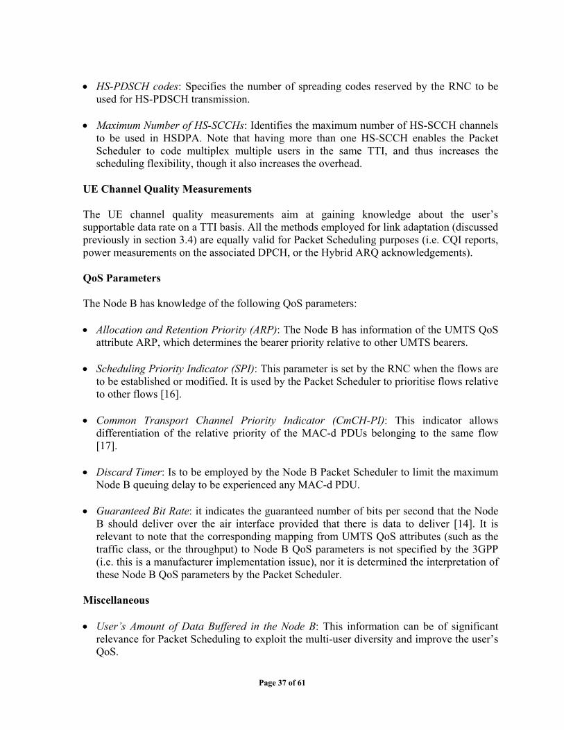
• HS-PDSCH codes: Specifies the number of spreading codes reserved by the RNC to be

used for HS-PDSCH transmission. • Maximum Number of HS-SCCHs: Identifies the maximum number of HS-SCCH channels

to be used in HSDPA. Note that having more than one HS-SCCH enables the Packet Scheduler to code multiplex multiple users in the same TTI, and thus increases the scheduling flexibility, though it also increases the overhead.

UE Channel Quality Measurements The UE channel quality measurements aim at gaining knowledge about the user’s supportable data rate on a TTI basis. All the methods employed for link adaptation (discussed previously in section 3.4) are equally valid for Packet Scheduling purposes (i.e. CQI reports, power measurements on the associated DPCH, or the Hybrid ARQ acknowledgements). QoS Parameters The Node B has knowledge of the following QoS parameters: • Allocation and Retention Priority (ARP): The Node B has information of the UMTS QoS

attribute ARP, which determines the bearer priority relative to other UMTS bearers. • Scheduling Priority Indicator (SPI): This parameter is set by the RNC when the flows are

to be established or modified. It is used by the Packet Scheduler to prioritise flows relative to other flows [16].

• Common Transport Channel Priority Indicator (CmCH-PI): This indicator allows

differentiation of the relative priority of the MAC-d PDUs belonging to the same flow [17].

• Discard Timer: Is to be employed by the Node B Packet Scheduler to limit the maximum

Node B queuing delay to be experienced any MAC-d PDU. • Guaranteed Bit Rate: it indicates the guaranteed number of bits per second that the Node

B should deliver over the air interface provided that there is data to deliver [14]. It is relevant to note that the corresponding mapping from UMTS QoS attributes (such as the traffic class, or the throughput) to Node B QoS parameters is not specified by the 3GPP (i.e. this is a manufacturer implementation issue), nor it is determined the interpretation of these Node B QoS parameters by the Packet Scheduler.

Miscellaneous • User’s Amount of Data Buffered in the Node B: This information can be of significant

relevance for Packet Scheduling to exploit the multi-user diversity and improve the user’s QoS.

Page 37 of 61

• UE Capabilities: They may limit factors like the maximum number of HS-PDSCH codes

to be supported by the terminal, the minimum period between consecutive UE receptions, or the maximum number of soft channel bits the terminal is capable to store.

• HARQ Manager: This entity is to indicate to the Packet Scheduler when a certain Hybrid

ARQ retransmission is required. 3.4.3 Packet scheduling principles Let us define the operation goal of the Packet Scheduler as to maximize the cell throughput while satisfying the QoS attributes belonging to the UMTS QoS classes of the cell bearers. Figure 3.9 depicts the procedure by which the Node B Packet Scheduler selects the user to be served.The operation of the Packet scheduler is constrained by the satisfaction of the QoS attributes of the users. Users belonging to dissimilar traffic classes require different scheduling treatment. Even within the same traffic class, the ARP

Figure 3.9 - Node B packet scheduler operation procedure (Source: Nokia) attribute differentiates the service priority between the cell bearers. In the interactive class, the throughput parameter further adds another dimension for bearer prioritisation. In the present assessment of the Packet Scheduler functionality, the scope will be narrowed down to NRT users without any specific QoS prioritisation between them. The Packet Scheduler rules the distribution of the radio resources among the users in the cell. In [18], Elliot describes that the scheduling algorithms that reach the highest system throughput tend to cause the starvation of the least favourable users (low G factor users). This behaviour interacts with the fairness in the allocation of the cell resources, which

Page 38 of 61

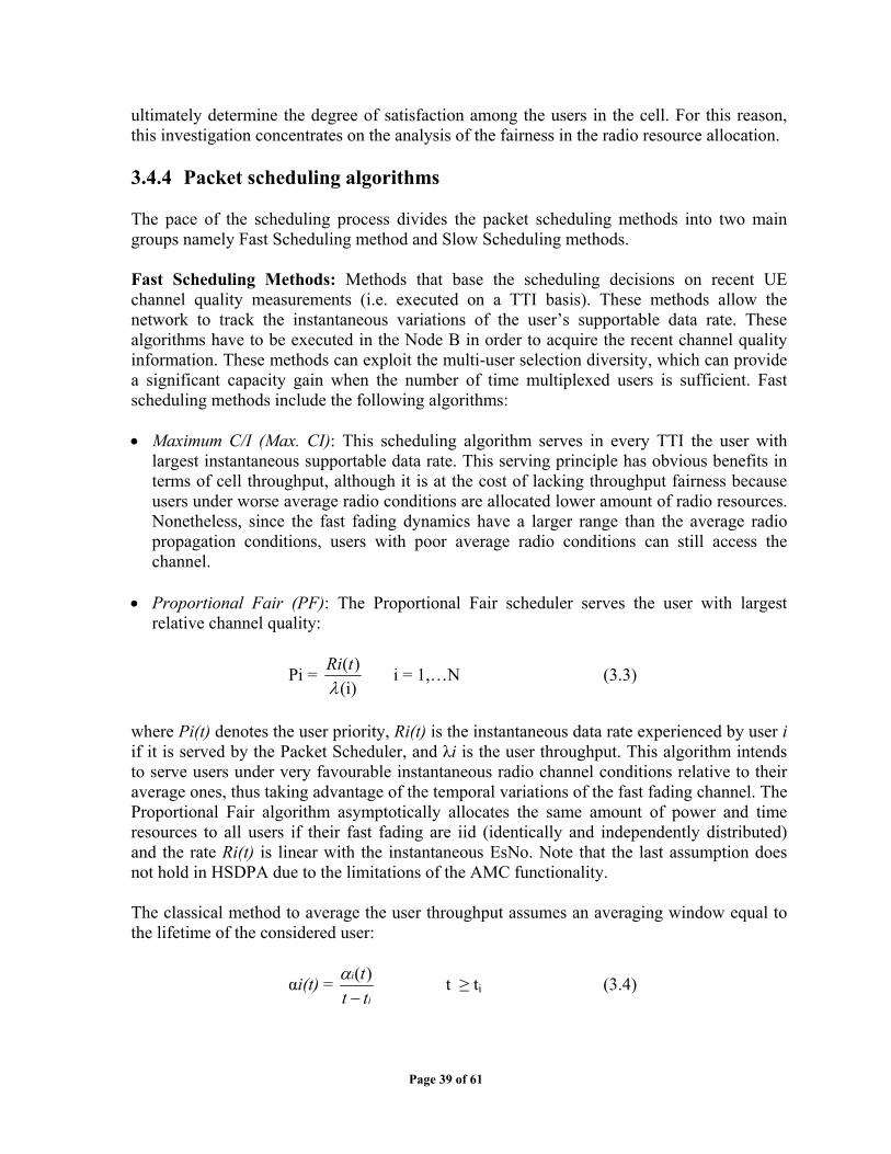
ultimately determine the degree of satisfaction among the users in the cell. For this reason, this investigation concentrates on the analysis of the fairness in the radio resource allocation. 3.4.4 Packet scheduling algorithms The pace of the scheduling process divides the packet scheduling methods into two main groups namely Fast Scheduling method and Slow Scheduling methods. Fast Scheduling Methods: Methods that base the scheduling decisions on recent UE channel quality measurements (i.e. executed on a TTI basis). These methods allow the network to track the instantaneous variations of the user’s supportable data rate. These algorithms have to be executed in the Node B in order to acquire the recent channel quality information. These methods can exploit the multi-user selection diversity, which can provide a significant capacity gain when the number of time multiplexed users is sufficient. Fast scheduling methods include the following algorithms: • Maximum C/I (Max. CI): This scheduling algorithm serves in every TTI the user with

largest instantaneous supportable data rate. This serving principle has obvious benefits in terms of cell throughput, although it is at the cost of lacking throughput fairness because users under worse average radio conditions are allocated lower amount of radio resources. Nonetheless, since the fast fading dynamics have a larger range than the average radio propagation conditions, users with poor average radio conditions can still access the channel.

• Proportional Fair (PF): The Proportional Fair scheduler serves the user with largest

relative channel quality:

Pi = (i)

)(λ

tRi i = 1,…N (3.3)

where Pi(t) denotes the user priority, Ri(t) is the instantaneous data rate experienced by user i if it is served by the Packet Scheduler, and λi is the user throughput. This algorithm intends to serve users under very favourable instantaneous radio channel conditions relative to their average ones, thus taking advantage of the temporal variations of the fast fading channel. The Proportional Fair algorithm asymptotically allocates the same amount of power and time resources to all users if their fast fading are iid (identically and independently distributed) and the rate Ri(t) is linear with the instantaneous EsNo. Note that the last assumption does not hold in HSDPA due to the limitations of the AMC functionality. The classical method to average the user throughput assumes an averaging window equal to the lifetime of the considered user:

αi(t) = i

i

ttt−

)(α t ≥ ti (3.4)

Page 39 of 61

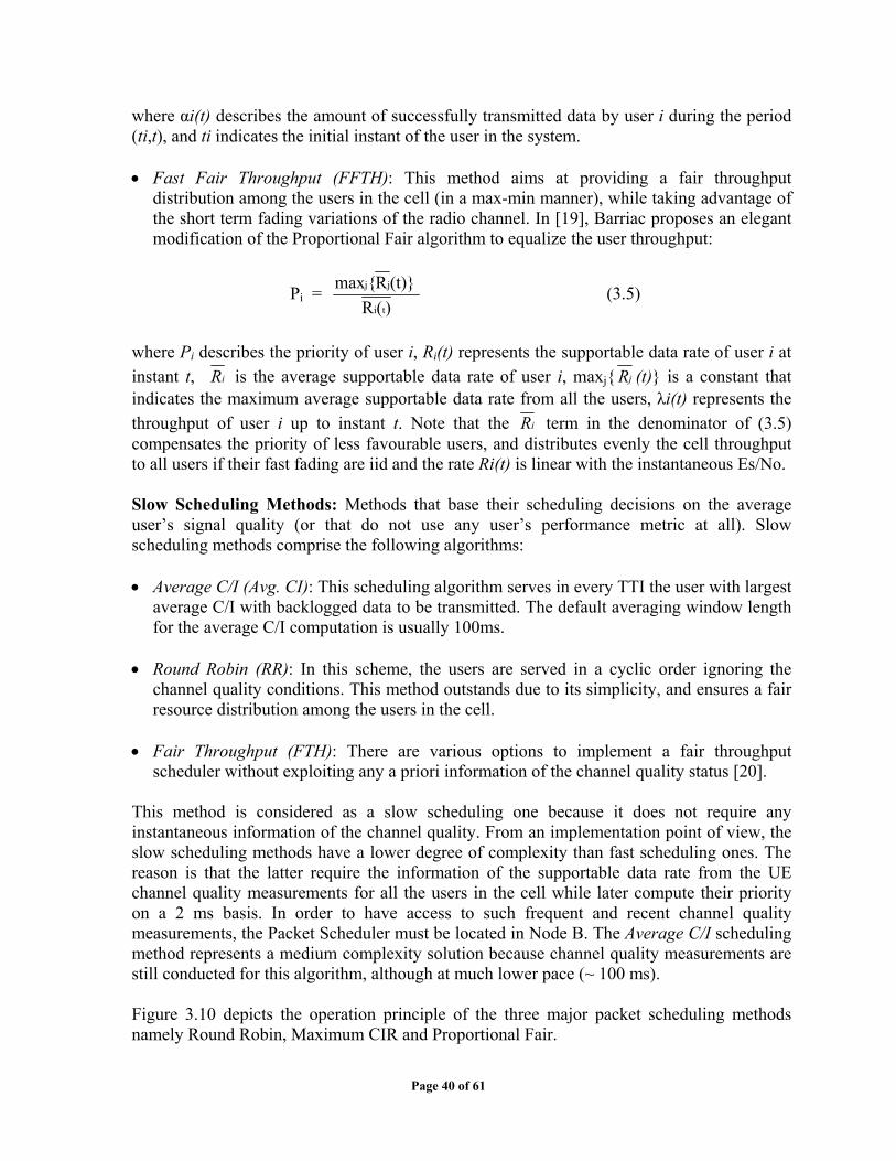
where αi(t) describes the amount of successfully transmitted data by user i during the period (ti,t), and ti indicates the initial instant of the user in the system. • Fast Fair Throughput (FFTH): This method aims at providing a fair throughput

distribution among the users in the cell (in a max-min manner), while taking advantage of the short term fading variations of the radio channel. In [19], Barriac proposes an elegant modification of the Proportional Fair algorithm to equalize the user throughput:

Pi = )(R

(t)}R{maxti

jj (3.5)

where Pi describes the priority of user i, Ri(t) represents the supportable data rate of user i at instant t, iR is the average supportable data rate of user i, maxj{ jR (t)} is a constant that indicates the maximum average supportable data rate from all the users, λi(t) represents the throughput of user i up to instant t. Note that the iR term in the denominator of (3.5) compensates the priority of less favourable users, and distributes evenly the cell throughput to all users if their fast fading are iid and the rate Ri(t) is linear with the instantaneous Es/No. Slow Scheduling Methods: Methods that base their scheduling decisions on the average user’s signal quality (or that do not use any user’s performance metric at all). Slow scheduling methods comprise the following algorithms: • Average C/I (Avg. CI): This scheduling algorithm serves in every TTI the user with largest

average C/I with backlogged data to be transmitted. The default averaging window length for the average C/I computation is usually 100ms.

• Round Robin (RR): In this scheme, the users are served in a cyclic order ignoring the

channel quality conditions. This method outstands due to its simplicity, and ensures a fair resource distribution among the users in the cell.

• Fair Throughput (FTH): There are various options to implement a fair throughput

scheduler without exploiting any a priori information of the channel quality status [20]. This method is considered as a slow scheduling one because it does not require any instantaneous information of the channel quality. From an implementation point of view, the slow scheduling methods have a lower degree of complexity than fast scheduling ones. The reason is that the latter require the information of the supportable data rate from the UE channel quality measurements for all the users in the cell while later compute their priority on a 2 ms basis. In order to have access to such frequent and recent channel quality measurements, the Packet Scheduler must be located in Node B. The Average C/I scheduling method represents a medium complexity solution because channel quality measurements are still conducted for this algorithm, although at much lower pace (~ 100 ms). Figure 3.10 depicts the operation principle of the three major packet scheduling methods namely Round Robin, Maximum CIR and Proportional Fair.

Page 40 of 61

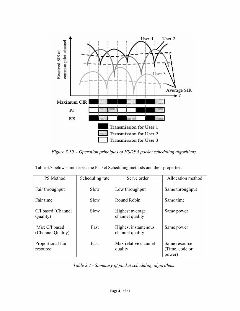
Figure 3.10 - Operation principles of HSDPA packet scheduling algorithms Table 3.7 below summarizes the Packet Scheduling methods and their properties.

PS Method Scheduling rate Serve order Allocation method Fair throughput

Slow

Low throughput

Same throughput

Fair time

Slow

Round Robin

Same time

C/I based (Channel Quality)

Slow Highest average channel quality

Same power

Max C/I based (Channel Quality)

Fast Highest instantenous channel quality

Same power

Proportional fair resource

Fast Max relative channel quality

Same resource (Time, code or power)

Table 3.7 - Summary of packet scheduling algorithms

Page 41 of 61

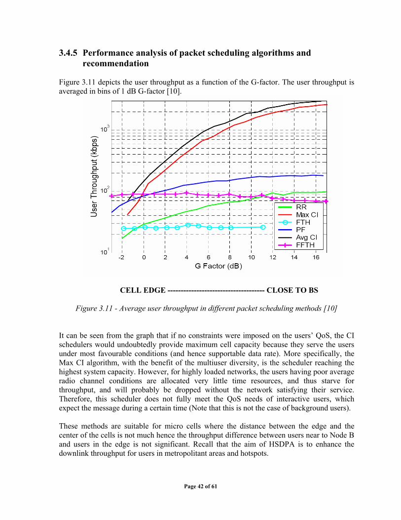
3.4.5 Performance analysis of packet scheduling algorithms and recommendation

Figure 3.11 depicts the user throughput as a function of the G-factor. The user throughput is averaged in bins of 1 dB G-factor [10].

CELL EDGE ------------------------------------- CLOSE TO BS

Figure 3.11 - Average user throughput in different packet scheduling methods [10] It can be seen from the graph that if no constraints were imposed on the users’ QoS, the CI schedulers would undoubtedly provide maximum cell capacity because they serve the users under most favourable conditions (and hence supportable data rate). More specifically, the Max CI algorithm, with the benefit of the multiuser diversity, is the scheduler reaching the highest system capacity. However, for highly loaded networks, the users having poor average radio channel conditions are allocated very little time resources, and thus starve for throughput, and will probably be dropped without the network satisfying their service. Therefore, this scheduler does not fully meet the QoS needs of interactive users, which expect the message during a certain time (Note that this is not the case of background users). These methods are suitable for micro cells where the distance between the edge and the center of the cells is not much hence the throughput difference between users near to Node B and users in the edge is not significant. Recall that the aim of HSDPA is to enhance the downlink throughput for users in metropolitant areas and hotspots.

Page 42 of 61

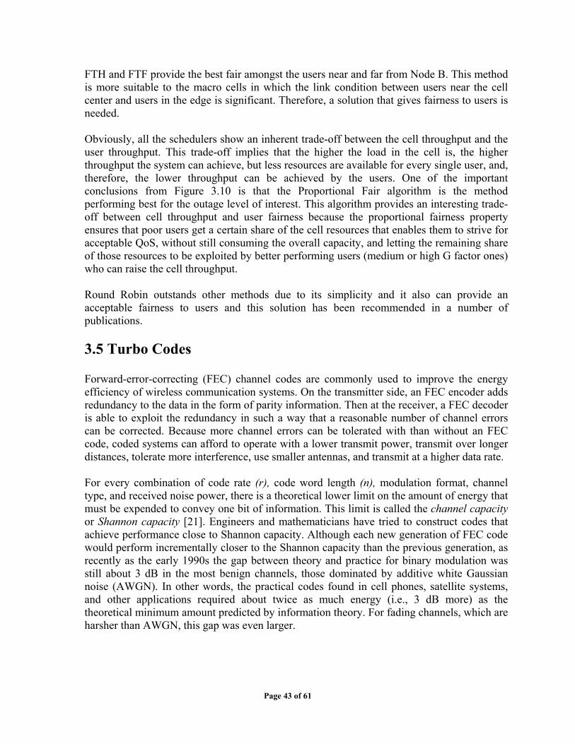
FTH and FTF provide the best fair amongst the users near and far from Node B. This method is more suitable to the macro cells in which the link condition between users near the cell center and users in the edge is significant. Therefore, a solution that gives fairness to users is needed. Obviously, all the schedulers show an inherent trade-off between the cell throughput and the user throughput. This trade-off implies that the higher the load in the cell is, the higher throughput the system can achieve, but less resources are available for every single user, and, therefore, the lower throughput can be achieved by the users. One of the important conclusions from Figure 3.10 is that the Proportional Fair algorithm is the method performing best for the outage level of interest. This algorithm provides an interesting trade-off between cell throughput and user fairness because the proportional fairness property ensures that poor users get a certain share of the cell resources that enables them to strive for acceptable QoS, without still consuming the overall capacity, and letting the remaining share of those resources to be exploited by better performing users (medium or high G factor ones) who can raise the cell throughput. Round Robin outstands other methods due to its simplicity and it also can provide an acceptable fairness to users and this solution has been recommended in a number of publications. 3.5 Turbo Codes Forward-error-correcting (FEC) channel codes are commonly used to improve the energy efficiency of wireless communication systems. On the transmitter side, an FEC encoder adds redundancy to the data in the form of parity information. Then at the receiver, a FEC decoder is able to exploit the redundancy in such a way that a reasonable number of channel errors can be corrected. Because more channel errors can be tolerated with than without an FEC code, coded systems can afford to operate with a lower transmit power, transmit over longer distances, tolerate more interference, use smaller antennas, and transmit at a higher data rate. For every combination of code rate (r), code word length (n), modulation format, channel type, and received noise power, there is a theoretical lower limit on the amount of energy that must be expended to convey one bit of information. This limit is called the channel capacity or Shannon capacity [21]. Engineers and mathematicians have tried to construct codes that achieve performance close to Shannon capacity. Although each new generation of FEC code would perform incrementally closer to the Shannon capacity than the previous generation, as recently as the early 1990s the gap between theory and practice for binary modulation was still about 3 dB in the most benign channels, those dominated by additive white Gaussian noise (AWGN). In other words, the practical codes found in cell phones, satellite systems, and other applications required about twice as much energy (i.e., 3 dB more) as the theoretical minimum amount predicted by information theory. For fading channels, which are harsher than AWGN, this gap was even larger.

Page 43 of 61

3.5.1 Performance of Turbo Codes Turbo Codes are regarded as an essential part of a HSDPA system and the only code supported by HSDPA. In contrast, it is optional to use either convolutional or turbo codes in 3G systems. Turbo codes were proposed by Berrou and Glavieux in the 1993 International Conference in Communications [21]. The initial results showed that turbo codes could achieve energy efficiencies within only a half decibel of the Shannon capacity. Further research carried out after its invention proved further benefits and applications of turbo codes. By the end of the 1990s, the virtues of turbo codes were well known, and they began to be adopted in various systems. Now they are incorporated into standards used by NASA for deep space communications (CCSDS), digital video broadcasting (DVB-T), and both third-generation cellular standards (UMTS and CDMA2000). Different features of turbo codes are parallel concatenated coding, recursive convolutional encoders, pseudo-random interleaving and iterative decoding. The name turbo comes from the iterative decoding which is similar to “turbo engine” in which feedback mechanism enhances the engine performance. A single error correction code does not always provide enough error protection with reasonable complexity. Solution provided by concatenating two (or more) codes. As shown in Figure 3.12 the concatenation of inner codes and outer codes creates a much more powerful code.

Outer Encoder

Block Interleaver

Inner Encoder

Outer Decoder

De-Interleaver

Channel

Inner Decoder

Figure 3.12 - Serial Concatenated Encoding

Turbo code is formed from the parallel concatenation of two constituent codes separated by an interleaver. Each constituent Encoder may be different, in practice they are identical. A generic structure of turbo codes is shown in Figure 3.13. As can be seen, the turbo code consists of two identical constituent encoders. The output of each encoder is systematic, that means we can separate parity and information. The input data stream and the parity outputs of the two parallel encoders are then serialized into a single turbo code word. The interleaver is a critical part of the turbo code. It is a simple device that rearranges the order of the data bits in a prescribed, but in an irregular manner (details will be discussed later on).

Page 44 of 61

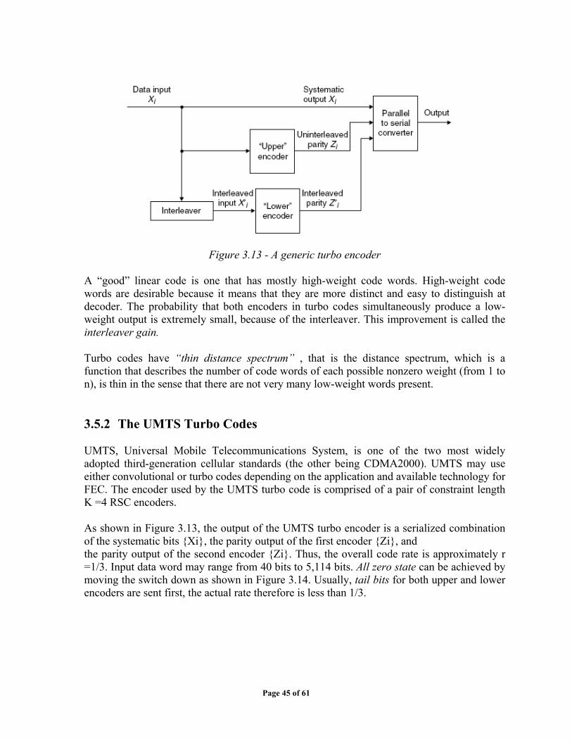
Figure 3.13 - A generic turbo encoder A “good” linear code is one that has mostly high-weight code words. High-weight code words are desirable because it means that they are more distinct and easy to distinguish at decoder. The probability that both encoders in turbo codes simultaneously produce a low-weight output is extremely small, because of the interleaver. This improvement is called the interleaver gain. Turbo codes have “thin distance spectrum” , that is the distance spectrum, which is a function that describes the number of code words of each possible nonzero weight (from 1 to n), is thin in the sense that there are not very many low-weight words present. 3.5.2 The UMTS Turbo Codes UMTS, Universal Mobile Telecommunications System, is one of the two most widely adopted third-generation cellular standards (the other being CDMA2000). UMTS may use either convolutional or turbo codes depending on the application and available technology for FEC. The encoder used by the UMTS turbo code is comprised of a pair of constraint length K =4 RSC encoders. As shown in Figure 3.13, the output of the UMTS turbo encoder is a serialized combination of the systematic bits {Xi}, the parity output of the first encoder {Zi}, and the parity output of the second encoder {Zi}. Thus, the overall code rate is approximately r =1/3. Input data word may range from 40 bits to 5,114 bits. All zero state can be achieved by moving the switch down as shown in Figure 3.14. Usually, tail bits for both upper and lower encoders are sent first, the actual rate therefore is less than 1/3.

Page 45 of 61

Zi

Xi

D D D

Z'i

D D D

Interleaver

X’i

Xi

Figure 3.14 - The UMTS turbo encoder 3.5.3 The CDMA2000 Turbo Codes As in UMTS, CDMA2000 uses either convolutional or turbo codes for FEC. While the turbo codes used by these two systems are very similar, the differences lie major in following:

• Algorithm of interleaver • Input data size (specific values): 378, 570, 762, 1146, 1530, 2398, 3066, 4602, 6138,

9210, 12282, or 20730 bits. • Rate of constituent RSC encoders (r=1/3): so overall rate=1/5

First parity output Z1j

Second parity output Z2j

Data input Xj D D D

Systematic output Xj

Figure 3.15 - The rate 1/3 RSC encoder used by the CDMA2000 turbo code

Page 46 of 61

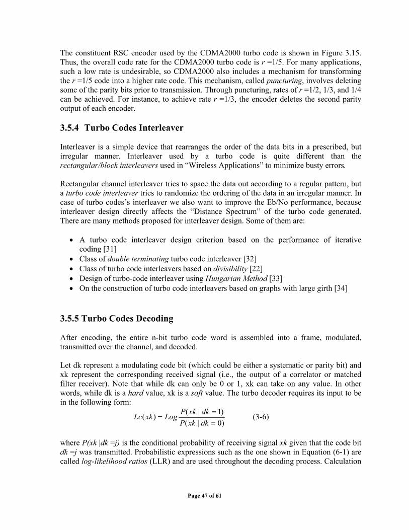
The constituent RSC encoder used by the CDMA2000 turbo code is shown in Figure 3.15. Thus, the overall code rate for the CDMA2000 turbo code is r =1/5. For many applications, such a low rate is undesirable, so CDMA2000 also includes a mechanism for transforming the r =1/5 code into a higher rate code. This mechanism, called puncturing, involves deleting some of the parity bits prior to transmission. Through puncturing, rates of r =1/2, 1/3, and 1/4 can be achieved. For instance, to achieve rate r =1/3, the encoder deletes the second parity output of each encoder. 3.5.4 Turbo Codes Interleaver Interleaver is a simple device that rearranges the order of the data bits in a prescribed, but irregular manner. Interleaver used by a turbo code is quite different than the rectangular/block interleavers used in “Wireless Applications” to minimize busty errors. Rectangular channel interleaver tries to space the data out according to a regular pattern, but a turbo code interleaver tries to randomize the ordering of the data in an irregular manner. In case of turbo codes’s interleaver we also want to improve the Eb/No performance, because interleaver design directly affects the “Distance Spectrum” of the turbo code generated. There are many methods proposed for interleaver design. Some of them are:

• A turbo code interleaver design criterion based on the performance of iterative coding [31]

• Class of double terminating turbo code interleaver [32] • Class of turbo code interleavers based on divisibility [22] • Design of turbo-code interleaver using Hungarian Method [33] • On the construction of turbo code interleavers based on graphs with large girth [34]

3.5.5 Turbo Codes Decoding After encoding, the entire n-bit turbo code word is assembled into a frame, modulated, transmitted over the channel, and decoded. Let dk represent a modulating code bit (which could be either a systematic or parity bit) and xk represent the corresponding received signal (i.e., the output of a correlator or matched filter receiver). Note that while dk can only be 0 or 1, xk can take on any value. In other words, while dk is a hard value, xk is a soft value. The turbo decoder requires its input to be in the following form:

)0|()1|()(

==

=dkxkPdkxkPLogxkLc (3-6)

where P(xk |dk =j) is the conditional probability of receiving signal xk given that the code bit dk =j was transmitted. Probabilistic expressions such as the one shown in Equation (6-1) are called log-likelihood ratios (LLR) and are used throughout the decoding process. Calculation

Page 47 of 61

of equation (3-6) requires not only the received signal sample xk , but also some knowledge of the statistics of the channel. For instance, if binary phase-shift keying (BPSK) modulation is used over an AWGN channel with noise variance σ2, then the corresponding decoder input in LLR form would be: Lc(xk) = 2xk/σ2 [23].

Deinterleaver

APP

APPInterleaver

SISO SISO #2 #1

Figure 3.16 - An architecture for decoding UMTS Turbo codes

The received values for the systematic and parity bits are put into LLR form and fed into the input of the turbo decoder shown in Figure 3.16. For each data bit dk, the turbo decoder must compute the following LLR:

)0|()1|()(

==

=∧dkxkPdkxkPLogdk (3-7)

This LLR compares the probability that the particular data bit was a one versus the probability that it was a zero, given the entire received code word (x1 . . . xn). Once this LLR is computed, a hard decision on dk can be performed by simply comparing the LLR to zero, that is, when Λ(dk)>0 the hard bit estimate is d’k = 1 and when Λ(dk)< 0, d’k = 0. The turbo decoder uses the received code word along with knowledge of the code structure to compute Λ(dk). However, because the interleaver greatly complicates the structure of the code, it is not feasible to compute Λ(dk) simply by using a single probabilistic processor. Instead, the turbo decoder breaks the job of achieving a global LLR estimate Λ(dk) into two estimation steps. In the first step, the decoder attempts to compute Equation (3-7) using only the structure of the upper encoder, while during the second step, the decoder computes it using just the structure of the lower encoder. The LLR estimate computed using the structure of the upper encoder is denoted Λ1(dk) and that computed using the structure of the lower encoder is denoted Λ2(dk). Each of these two LLR estimates is computed using a soft-input soft-output (SISO) processor.

DeMUX

Deinterleaver

Parity data

Hard bit decisions

Page 48 of 61

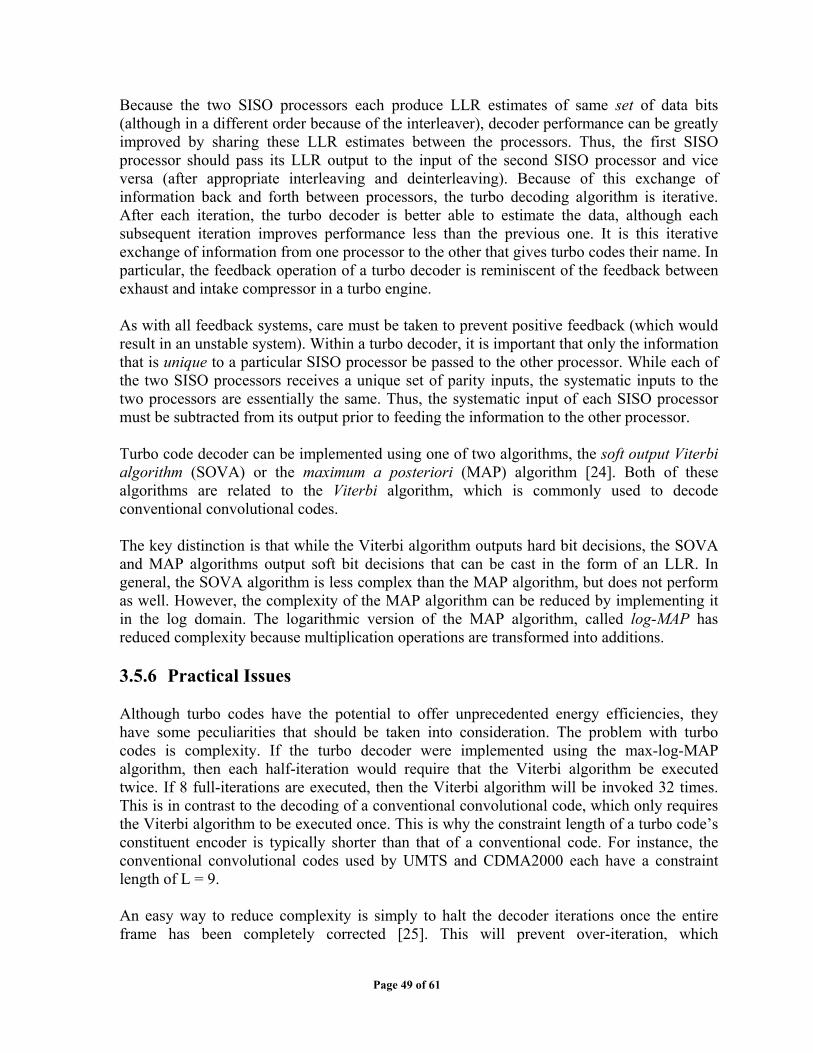
Because the two SISO processors each produce LLR estimates of same set of data bits (although in a different order because of the interleaver), decoder performance can be greatly improved by sharing these LLR estimates between the processors. Thus, the first SISO processor should pass its LLR output to the input of the second SISO processor and vice versa (after appropriate interleaving and deinterleaving). Because of this exchange of information back and forth between processors, the turbo decoding algorithm is iterative. After each iteration, the turbo decoder is better able to estimate the data, although each subsequent iteration improves performance less than the previous one. It is this iterative exchange of information from one processor to the other that gives turbo codes their name. In particular, the feedback operation of a turbo decoder is reminiscent of the feedback between exhaust and intake compressor in a turbo engine. As with all feedback systems, care must be taken to prevent positive feedback (which would result in an unstable system). Within a turbo decoder, it is important that only the information that is unique to a particular SISO processor be passed to the other processor. While each of the two SISO processors receives a unique set of parity inputs, the systematic inputs to the two processors are essentially the same. Thus, the systematic input of each SISO processor must be subtracted from its output prior to feeding the information to the other processor. Turbo code decoder can be implemented using one of two algorithms, the soft output Viterbi algorithm (SOVA) or the maximum a posteriori (MAP) algorithm [24]. Both of these algorithms are related to the Viterbi algorithm, which is commonly used to decode conventional convolutional codes. The key distinction is that while the Viterbi algorithm outputs hard bit decisions, the SOVA and MAP algorithms output soft bit decisions that can be cast in the form of an LLR. In general, the SOVA algorithm is less complex than the MAP algorithm, but does not perform as well. However, the complexity of the MAP algorithm can be reduced by implementing it in the log domain. The logarithmic version of the MAP algorithm, called log-MAP has reduced complexity because multiplication operations are transformed into additions. 3.5.6 Practical Issues Although turbo codes have the potential to offer unprecedented energy efficiencies, they have some peculiarities that should be taken into consideration. The problem with turbo codes is complexity. If the turbo decoder were implemented using the max-log-MAP algorithm, then each half-iteration would require that the Viterbi algorithm be executed twice. If 8 full-iterations are executed, then the Viterbi algorithm will be invoked 32 times. This is in contrast to the decoding of a conventional convolutional code, which only requires the Viterbi algorithm to be executed once. This is why the constraint length of a turbo code’s constituent encoder is typically shorter than that of a conventional code. For instance, the conventional convolutional codes used by UMTS and CDMA2000 each have a constraint length of L = 9. An easy way to reduce complexity is simply to halt the decoder iterations once the entire frame has been completely corrected [25]. This will prevent over-iteration, which

Page 49 of 61

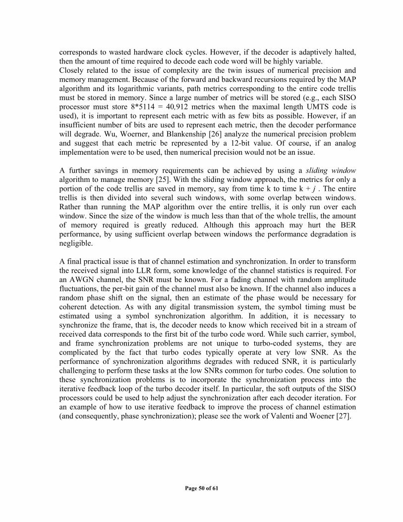
corresponds to wasted hardware clock cycles. However, if the decoder is adaptively halted, then the amount of time required to decode each code word will be highly variable. Closely related to the issue of complexity are the twin issues of numerical precision and memory management. Because of the forward and backward recursions required by the MAP algorithm and its logarithmic variants, path metrics corresponding to the entire code trellis must be stored in memory. Since a large number of metrics will be stored (e.g., each SISO processor must store 8*5114 = 40,912 metrics when the maximal length UMTS code is used), it is important to represent each metric with as few bits as possible. However, if an insufficient number of bits are used to represent each metric, then the decoder performance will degrade. Wu, Woerner, and Blankenship [26] analyze the numerical precision problem and suggest that each metric be represented by a 12-bit value. Of course, if an analog implementation were to be used, then numerical precision would not be an issue. A further savings in memory requirements can be achieved by using a sliding window algorithm to manage memory [25]. With the sliding window approach, the metrics for only a portion of the code trellis are saved in memory, say from time k to time k + j . The entire trellis is then divided into several such windows, with some overlap between windows. Rather than running the MAP algorithm over the entire trellis, it is only run over each window. Since the size of the window is much less than that of the whole trellis, the amount of memory required is greatly reduced. Although this approach may hurt the BER performance, by using sufficient overlap between windows the performance degradation is negligible. A final practical issue is that of channel estimation and synchronization. In order to transform the received signal into LLR form, some knowledge of the channel statistics is required. For an AWGN channel, the SNR must be known. For a fading channel with random amplitude fluctuations, the per-bit gain of the channel must also be known. If the channel also induces a random phase shift on the signal, then an estimate of the phase would be necessary for coherent detection. As with any digital transmission system, the symbol timing must be estimated using a symbol synchronization algorithm. In addition, it is necessary to synchronize the frame, that is, the decoder needs to know which received bit in a stream of received data corresponds to the first bit of the turbo code word. While such carrier, symbol, and frame synchronization problems are not unique to turbo-coded systems, they are complicated by the fact that turbo codes typically operate at very low SNR. As the performance of synchronization algorithms degrades with reduced SNR, it is particularly challenging to perform these tasks at the low SNRs common for turbo codes. One solution to these synchronization problems is to incorporate the synchronization process into the iterative feedback loop of the turbo decoder itself. In particular, the soft outputs of the SISO processors could be used to help adjust the synchronization after each decoder iteration. For an example of how to use iterative feedback to improve the process of channel estimation (and consequently, phase synchronization); please see the work of Valenti and Woener [27].

Page 50 of 61

3.6 Conclusion This chapter has discussed the most fundamental features of HSDPA. The chapter begins with a brief comparison between Release 99 (Release 4) and HSDPA (Release 5). The improvement of HSDPA toward 3G systems includes the introduction of AMC, Hybrid ARQ, Fast Packet Scheduling and the mandatory use of turbo codes. The chapter has been developed by the analysis of each feature above. AMC uses link quality feed back from physical channel to adjust the modulation types and code rate to provide users with the most reliable transmission. The combination of modulation type and code rate is referred as TFRC. Hybrid ARQ inherits the ARQ used in TCP/IP networks. In ARQ, when data is lost the receiver discards the erroneous data and requests for retransmission, the sender then simply retransmits the lost data hoping that the data will arrive without error. The retransmission process in HARQ is much more complicated. The sender rearranges the data each time it is retransmitted depending upon its predefined algorithm: Chase Combining, Incremental Redundancy or Constellation Rearrangement. Instead of dropping erroneous data, the receiver keeps all the data it receives and then combines them together to form a good set of data. With this data combination ability, users can receive integrity data even in the case that no single transmission is error-free. The number of retransmission is also significantly reduced. Packet Scheduling in HSDPA is called Fast Scheduling because the TTI has been decreased from 10ms as in Release 99 down to 2ms. Packet scheduler is also moved from MAC layer of RNC to in physical layer of Node B hence improves the scheduling speed. Besides the Fast scheduling methods in which the scheduling decision is made based on the instantaneous value, slow scheduling methods decide the transmitted user and rate based on the average values. There is a tradeoff between cell throughput and user fairness amongst the scheduling methods. The selection of packet scheduling algorithm depends upon the specific situation where either throughput or fairness is biased. Unlike 3G system where either convolutional codes or turbo codes can be used, HSDPA only support turbo codes. Even though turbo codes are not a new channel coding, operation principles for both Encoder and Encoder were given. Turbo codes are an improvement of convolutional codes where Recursive Systematic Code (RSC) is used. The recursive nature enables turbo codes performance to be improved after each iteration. Together with RSC, interleaving technique considerably contributes to the high performance and robust of Turbo codes. One drawback of Turbo codes is the complexity; however, this disadvantage is reduced thanks to the introduction of log-MAP in Viterbi algorithm.

Page 51 of 61

Chapter 4

Simulation

The previous chapters have discussed theoretical background of the HSDPA. This chapter will introduce our simulation program and analysis of the simulated results by comparing them with those results that have been published. 4.1 Simulation Program Figure 4.1 represents the simulation model used in our program. Within the scope of a Master thesis, we have simplified the system and just include the most fundamental component only. For details of the component excluded, please refer to Chapter 5 “Conclusion and Future works” On the transmitter side, the generated user data is spreaded with spreading factor of 16. This sequence of chipped data is then encoded by a turbo codes Encoder operating with either FEC 1/2 or FEC 1/3. Before propagating though a Gaussian-noise channel, the encoded signal is modulated with either QPSK or 16QAM, the only two modulation schemes supported by HSDPA [35].

Spreading Codes AWGN

Figure 4.1: HSDPA simulated system model

Decoded data

User data

Spreader Modulator

QPSK/16QAM

Noisy Channel

Channel Encoder

Spreading Codes

Despreader

Detector Channel Decoder

Turbocodes

Turbocode QPSK/16QAM

BER FER

Page 52 of 61

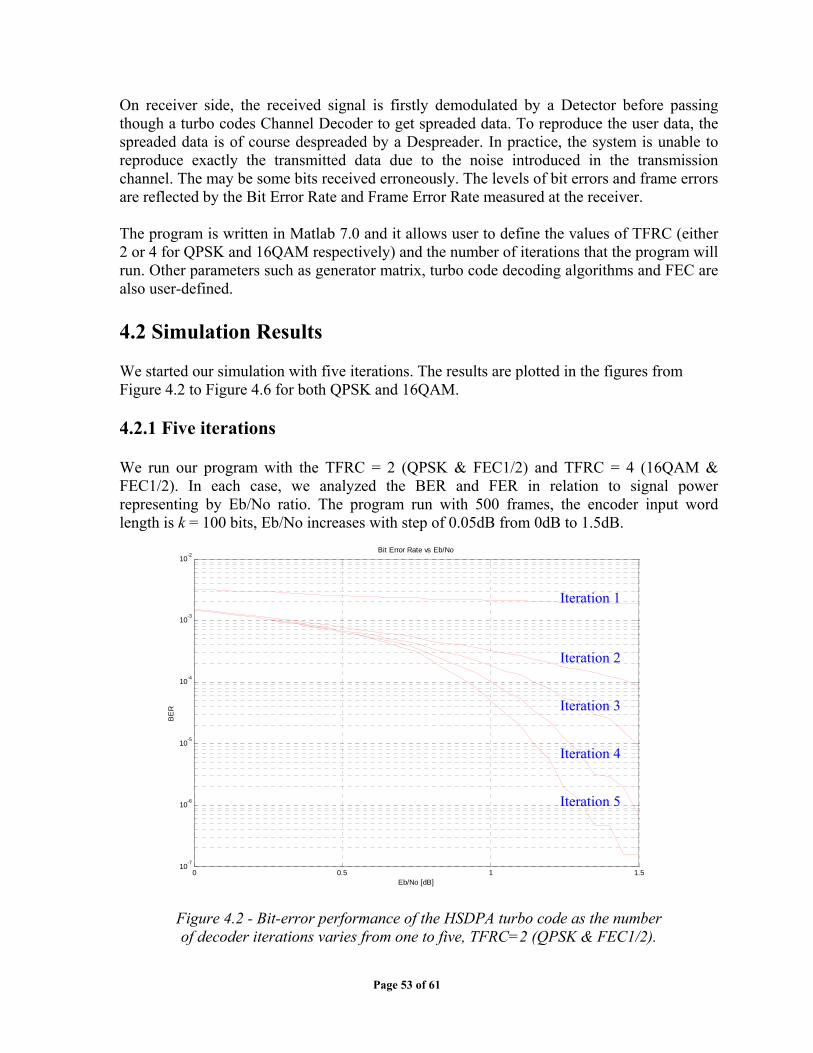
On receiver side, the received signal is firstly demodulated by a Detector before passing though a turbo codes Channel Decoder to get spreaded data. To reproduce the user data, the spreaded data is of course despreaded by a Despreader. In practice, the system is unable to reproduce exactly the transmitted data due to the noise introduced in the transmission channel. The may be some bits received erroneously. The levels of bit errors and frame errors are reflected by the Bit Error Rate and Frame Error Rate measured at the receiver. The program is written in Matlab 7.0 and it allows user to define the values of TFRC (either 2 or 4 for QPSK and 16QAM respectively) and the number of iterations that the program will run. Other parameters such as generator matrix, turbo code decoding algorithms and FEC are also user-defined. 4.2 Simulation Results We started our simulation with five iterations. The results are plotted in the figures from Figure 4.2 to Figure 4.6 for both QPSK and 16QAM. 4.2.1 Five iterations We run our program with the TFRC = 2 (QPSK & FEC1/2) and TFRC = 4 (16QAM & FEC1/2). In each case, we analyzed the BER and FER in relation to signal power representing by Eb/No ratio. The program run with 500 frames, the encoder input word length is k = 100 bits, Eb/No increases with step of 0.05dB from 0dB to 1.5dB.

0 0.5 1 1.510-7

10-6

10-5

10-4

10-3

10-2

Eb/No [dB]

BE

R

Bit Error Rate vs Eb/No

Iteration 1

Iteration 2

Iteration 3

Iteration 4

Iteration 5

Figure 4.2 - Bit-error performance of the HSDPA turbo code as the number of decoder iterations varies from one to five, TFRC=2 (QPSK & FEC1/2).

Page 53 of 61

0 0.5 1 1.510-4

10-3

10-2

10-1

Eb/No [dB]

FER

Frame Error Rate vs Eb/No

Iteration 1

Iteration 2

Iteration 3

Iteration 4

Iteration 5

Figure 4.3 - Frame-error performance of the HSDPA turbo code as the number of decoder iterations varies from one to five, TFRC=2 (QPSK & FEC1/2).

0 0.5 1 1.510-7

10-6

10-5

10-4

10-3

10-2

Eb/No [dB]

BE

R

Bit Error Rate vs Eb/No

Iteration 1

Iteration 2

Iteration 3

Iteration 4

Iteration 5

Figure 4.4: Bit-error performance of the HSDPA turbo code as the number of decoder iterations varies from one to five, TFRC=4 (16QAM & FEC1/2).

Page 54 of 61

0 0.5 1 1.510-4

10-3

10-2

10-1

Eb/No [dB]

FER

Frame Error Rate vs Eb/No

Iteration 1 Iteration 2

Iteration 3

Iteration 4

Iteration 5

Figure 4.5 - Frame-error performance of the HSDPA turbo code as the number of decoder iterations varies from one to five, TFRC=4 (16QAM & FEC1/2)

In both cases QPSK and 16QAM, the error rates at high power (Eb/No from 1.25dB to 1.5dB) are less than 10-6. However, the error rates are quite high (more than 10-4) in case of low power (Eb/No is less than 1dB). We will now run the program with ten iterations to observe how the error rates are improved in later iterations. 4.2.2 Ten iterations With ten iteration, we run our program with the TFRC = 2 (QPSK & FEC1/2) and TFRC = 4 (16QAM & FEC1/2). In each case, we analyzed the BER and FER in relation to signal power representing by Eb/No ratio. The program run with 500 frames, the encoder input word length is k = 100 bits, Eb/No increases with step of 0.02dB from 0dB to 1.3dB. Figure 4.6 depicts the relation between the BER and Eb/No in case of TFRC=2. With extremely small value of Eb/No, the BER is about 10-3. When Eb/No increases up to 0.75dB BER slightly decreases. However, if Eb/No is further improved, BER drops very quickly. In the 10th iteration, the BER is extremely low when Eb/No>=1.2dB. The FER in case of TFRC=2 is shown in the Figure 4.7. The FER is of course higher than BER with the same Eb/No. This is understandable because each frame comprises many bits and even if only one bit in the frame has error, then the frame is counted as an erroneous frame. On the interval of Eb/No between 0dB and 0.75dB, FER is almost unchanged. However, after this point, FER rapidly decreases, especially from 6th to 10th iterations. The

Page 55 of 61

FERs in iteration 1 and iteration 2 are very close, this can be interpreted that in the first two iterations, the FERs are not much improved.

0 0.2 0.4 0.6 0.8 1 1.210-8

10-7

10-6

10-5

10-4

10-3

10-2

Eb/No [dB]

BE

R

Iteration 1

Iteration 2

Iteration 10

Figure 4.6: Bit-error performance of the HSDPA turbo code as the number of decoder iterations varies from one to ten, TFRC=2 (QPSK & FEC1/2)

0 0.2 0.4 0.6 0.8 1 1.210

-5

10-4

10-3

10-2

10-1

Eb/No [dB]

FER


Iteration 10

Figure 4.7: Frame-error performance of the HSDPA turbo code as the number of decoder iterations varies from one to ten, TFRC=2 (QPSK & FEC1/2)

Page 56 of 61

Similar to the case of TFRC=2, we can see in Figure 4.8 which represents the relation between BER and Eb/No with TFRC=4, that the BER is improved after each iteration. In the first few iterations, the BER declines very slowly but with high iterations, BERs considerably fall down. At the 9th and 10th iterations, BERs go to extremely small values at around the point of Eb/No=1.25dB.

0 0.2 0.4 0.6 0.8 1 1.210-7

10-6

10-5

10-4

10-3

10-2

Eb/No [dB]

BE

R

Iteration 1

Iteration 2

Iteration 10

Figure 4.8: Bit-error performance of the HSDPA turbo code as the number of decoder iterations varies from one to ten, TFRC=4 (16QAM & FEC1/2)

0 0.2 0.4 0.6 0.8 1 1.210-4

10-3

10-2

10-1

Eb/No [dB]

FER


Iteration 10

Figure 4.9 - Frame-error performance of the HSDPA turbo code as the number of decoder iterations varies from one to ten, TFRC=4 (16QAM & FEC1/2)

Page 57 of 61

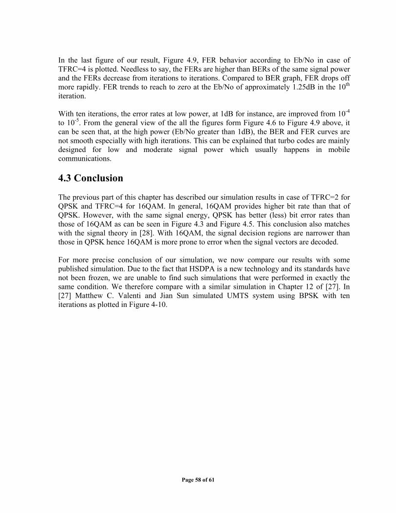
In the last figure of our result, Figure 4.9, FER behavior according to Eb/No in case of TFRC=4 is plotted. Needless to say, the FERs are higher than BERs of the same signal power and the FERs decrease from iterations to iterations. Compared to BER graph, FER drops off more rapidly. FER trends to reach to zero at the Eb/No of approximately 1.25dB in the 10th iteration. With ten iterations, the error rates at low power, at 1dB for instance, are improved from 10-4 to 10-5. From the general view of the all the figures form Figure 4.6 to Figure 4.9 above, it can be seen that, at the high power (Eb/No greater than 1dB), the BER and FER curves are not smooth especially with high iterations. This can be explained that turbo codes are mainly designed for low and moderate signal power which usually happens in mobile communications. 4.3 Conclusion The previous part of this chapter has described our simulation results in case of TFRC=2 for QPSK and TFRC=4 for 16QAM. In general, 16QAM provides higher bit rate than that of QPSK. However, with the same signal energy, QPSK has better (less) bit error rates than those of 16QAM as can be seen in Figure 4.3 and Figure 4.5. This conclusion also matches with the signal theory in [28]. With 16QAM, the signal decision regions are narrower than those in QPSK hence 16QAM is more prone to error when the signal vectors are decoded. For more precise conclusion of our simulation, we now compare our results with some published simulation. Due to the fact that HSDPA is a new technology and its standards have not been frozen, we are unable to find such simulations that were performed in exactly the same condition. We therefore compare with a similar simulation in Chapter 12 of [27]. In [27] Matthew C. Valenti and Jian Sun simulated UMTS system using BPSK with ten iterations as plotted in Figure 4-10.

Page 58 of 61

Figure 4.10 - Bit-error performance of the UMTS turbo code as the number

of decoder iterations varies from one to ten, Modulation is BPSK.

It is obvious that the behavior of BER in relation to Eb/No in this simulation is very similar to our results in terms of the shapes of the curves and their values. Similar to our results, in the first four iterations, the BERs decrease a little. However, from the 5th to the 10th iterations BERs are significantly improved.

Page 59 of 61

Chapter 5

Future Works

In this Master thesis, we have introduced a new technology - HSDPA in theory and also simulated the system performance. The performance is evaluated by the bit error rates and frame error rates as depicted in the figures from Figure 4.2 to Figure 4.9. One may raise a question of when HSDPA can be deployed. Even though the original road map envisaged HSDPA being commercialized in the 2006-2007 timeframe, this process has been accelerated. Many leading telecommunication companies have announced to launch HSDPA end-to-end to the market in the near future. Nokia will be making the first commercial release of its HSDPA at the end of this year. Vodacom plans to launch HSDPA by December 2005. DoCoMo is going to introduce HSDPA network technology sometime during its 2006 fiscal year. Due to its dominant advantages, in the coming years, there will be a lot of new researches and deployment of HSDPA introduced by the telecom operators and manufacturers. With this thesis, we would like to provide the readers the most fundamental theoretical knowledge of the technology and, together with our simulation, we want to confirm the benefits of HSDPA that have been introduced throughout the document.

It is obvious that HDSPA is a broad and complicated topic. With five months timeframe allocated for a Master thesis, we are unable to cover all the aspects of the technology. Our thesis therefore is limited to the following:

• The program supports both SOVA and MAP turbo codes decoding algorithms but our simulation was tested with MAP only, which in theory, provides better performance.

• In practice, the TFRC is chosen according to the link quality feedback from downlink direction. However, in our simulated environment, TFRC value is predefined by user.

• Due to the complexity of HARQ, AMC and Packet Scheduling, these functions are not included in our program.

To overcome the aforementioned limitations, further work is required. A simulation can be run with SOVA decoding algorithm to confirm the conclusion in some papers that MAP is better than SOVA. One can also write AMC and Packet Scheduling modules and then integrate to our program to provide a full system model of HSDPA. With the present of AMC and Packet Scheduling, the system performance will of course be improved. More combinations of TFRC as in Table 4-1 will need to be simulated rather than just two values of TFRC as in our program.

Page 60 of 61

Many researchers nowadays mention about the cousin of HSDPA namely HSUPA (High Speed Uplink Packet Access). Another potential research is about HSUPA which should be interested to telecom operators. A combination of HSDPA and HSUPA is also possible. According to [30], Nokia is working around the objection to limited uplink speeds by referring to HSPA (High Speed Packet Access), rather than HSDPA, or HSUPA separately.

Page 61 of 61

Bibliography

[1] William Stallings

Wireless Communications & Networks Second Edition, ISBN: 0-13-191835-4 Publisher: Prentice Hall, Copyright: 2005

[2] Ojanpera, T.; Prasad, R. An overview of air interface multiple access for IMT-2000/UMTS Communications Magazine, IEEE Volume 36, Issue 9, Sept. 1998 Page(s):82 - 86, 91-5

[3] http://www.comsoc.org/livepubs/surveys/public/4q98issue/prasad.html [4] Qiu R.C; Wenwu Zhu; Ya-Qin Zhang

Third-Generation and beyond (3.5G) wireless networks and its applications Journal: Circuits and Systems, 2002 ; ISCAS 2002; IEEE International Symposium , year: 2002 , vol: 1 , pages: I-41-I-44 publisher:IEEE , provider:IEEE , doc type: Conference proceedings

[5] Che-Sheng Chiu; Chen-Chiu Lin

Comparative downlink shared channel performance evaluation of WCDMA release 99 and HSDPA Journal: Networking, Sensing and Control, 2004; IEEE International Conference; year: 2004 , vol: 2 , pages: 1165-1170 publisher: IEEE , provider: IEEE , doc type: Conference proceedings

[6] Project(3GPP) Technical Specification TS 25.212,Rev. 5.9.0,June 2004

D. Chase, Code combining: A maximum-likelihood decoding approach for combining an arbitrary number of noisy packets IEEE Transport Communication, vol. 33, pp. 593.607, May 1985.

[7] 3GPP Technical Specification TSGR1#19(01)0237, Mar. 2001

Enhanced HARQ Method with Signal Constellation Rearrangement [8] Simon Bliudze

On optimal Hybrid ARQ control schemes for HSDPA with 16QAM

- i -

[9] Dr. Alexander Seeger High Speed Downlink Packet Access ICM NPGR HAS, Siemens, Mobile Business

[10] Kwan R. ; Chong P. ; Rinne M.

Analysis of the Adaptive Modulation and Coding Algorithm with the Multicode Transmission Journal: Vehicular Technology Conference, 2002; year: 2002; vol: 4; pages: 2007-2011; publisher: IEEE; doc type: Conference proceedings

[11] Yang J. ; Tin N. ; Khandani A.K.

Adaptive Modulation and Coding in 3G Wireless Systems Journal: Vehicular Technology Conference, 2002; year: 2002; vol: 1 pages: 544-548; publisher: IEEE; doc type: Conference proceedings

[12] Intel, Adaptive Modulation developer

http://www.intel.com/netcomms/technologies/wimax/303788.pdf [13] 3GPP Technical Specification Group Services and System Aspects

QoS Concept and Architecture (3GPP TS 23.107 version 5.9.0)

[14 3GPP Technical Specification Group Radio Access Network

High Speed Downlink Packet Access; Overall UTRAN Description (3GPP TR 25.855 version 5.0.0)

[15] 3GPP Technical Specification Group Radio Access Network

High Speed Downlink Packet Access (HSDPA); Overall Description (3GPP TS 25.308 version 5.4.0)


UTRAN Iub Interface NBAP signaling (3GPP TR 25.433 version 5.5.0)


UTRAN Iub Interface User Plane Protocols for Common Transport Channel Data Streams (3GPP TS 25.435 version 5.4.0)

[18] Elliott R.C.

Scheduling Algorithms for the CDMA2000 Packet Data Evolution Vehicular Technology Conference, 2002; VTC 2002 Fall; Volume 1; pp. 304-310

[19] Barriac G.

Introducing Delay Sensitivity into the Proportional Fair Algorithm for CDMA Downlink Scheduling 2002 IEEE Seventh International Symposium; Volume 3; pp. 652-656

- ii -

[20] Kolding T. Performance Aspects of WCDMA Systems with High Speed Downlink Packet Access (HSDPA) Vehicular Technology Conference 2002; VTC 2002 Fall; Volume 1; pp. 477-481

[21] Berrou C.; Glavieux A.; Thitimajshima P.

Near Shannon limit error-correcting coding and decoding: Turbo-codes Journal: Communications, 1993. ICC ’93 Geneva. Year: 1993 Volume: 2 Pages: 1064-1070 vol.2 Provider: IEEE Journal: IEEE Communications Letters year: 2004 vol: 8 pages: 529-531, publisher: IEE/IEEE provider: IEEE doc type: Journal Paper

[22] Qi F.: Wang M.Z.; Sheikh A.U.H.; Shao D.R.

Class of turbo code interleavers based on divisibility Journal: Electronic Letters year: 2000 vol: 36 pages: 46-48 publisher: IEE/IEEE provider: IEEE doc type: Journal paper

[23] Bernard Sklar

Turbo code concepts made easy, or how I learned to concatenate and reiterate [24] L. R. Bahl, J. Cocke, F. Jelink, and J. Raviv

Optimal Decoding of Linear Codes for Minimizing Symbol Error Rate IEEE Transactions on Information Theory 20 (March 1974): 284-7

[25] Matthew C. Valenti and Jian Sun Handbook of RF and Wireless Technologies

[26] H. Loeliger, F.Tarkoy, F. Lustenberger, and M. Helfenstein

Decoding in Analog VLSI IEEE Communications Magazine (April 1999): 99-101

[27] M. C. Valenti and B. D. Woerner

Iterative Channel Estimation and Decoding of Pilot Symbol Assisted Turbo Codes over Flat-Fading Channels IEEE Journal on Selected Areas of Communications 19 (Sep-2001): 1697-1705

[28] Simon Haykin

Digital Communications [29] Telecom Magazine http://www.telecommagazine.com [30] http://www.umtsworld.com/technology.power.htm

- iii -

[31] Johan Hokfelt, Ove Edfors and Torleiv Maseng Interleaver Design for Turbo Codes Based on the Performance of Iterative Decoding ICC '99, Vancouver, Canada

[32] M. Breiling, S. Peeters, and J. Huber

The Class of Double Terminating Turbo Code Interleavers

[33] A.K. Khandani Design of turbo-code interleaver using Hungarian method Electronics Letters, 8th January 7998 Vol. 34

[34] Pascal O. Vontobe

On the Construction of Turbo Code Interleavers based on Graphs with large girth

[35] Simon Bliudze et al. On Optimum Hybrid ARQ control schemes for HSDPA with 16QAM

- iv -

Appendix A

Abbreviations

3G Third Generation 3GPP Third Generation Partnership Project AICH Acquisition Indication Channel AMC Adaptive Modulation and Coding ARIB Association of Radio Industries and Businesses ARP Address Resolution Protocol ARQ Automatic Retransmit reQuest AWGN Additive White Gaussian Noise BCH Broadcast Channel BLER Block Error Rate BPSK Binary Phase Shift Keying BTS Base Transceiver System CC Chase Combining CmCH-PI Common Channel Priority Indicator CoRe Constellation Rearrangement CPCH Common Packet Channel CPICH Common Pilot Channel CQI Channel Quality Indicator CRC Cyclic Redundancy Check DCH Dedicated Channel DECT Digital European Cordless Telecommunications DL Downlink DPCCH Dedicated Physical Control Channel DPDCH Dedicated Physical Data Channel DSCH Downlink Shared Channel EDGE Enhanced Data rates for Global Evolution ETSI European Telecommunications Standards Institute FACH Forward Access Channel FDD Frequency Division Duplex FDMA Frequency Division Multiple Access FEC Forward Error Correction FER Frame Error Rate FFTH Fast Fair Throughput FTH Fair Throughput

- v -


- vi -

G-factor Geographical Factor GSM Global System for Mobile Communications HARQ Hybrid Automatic Retransmission reQuest HSDPA High Speed Downlink Packet Access HS-DSCH High Speed Downlink Shared Channel HSPA High Speed Packet Access HSUPA High Speed Uplink Packet Access IR Incremental Redundancy ITU International Mobile Telecommunications LLR Log-Likelihood Ratios LSB Less Significant Bit MAC Media Access Control. MAP Maximum A Posteriori MCS Modulation and Coding Scheme MSB Most Significant Bit P-CCPCH Primary Common Control Physical Channel PCH Paging Channel PCN Personal communication networks PCPCH Physical Common Packet Channel PCS Personal communication services PDSCH Physical Downlink Shared Channel PDU Protocol Data Unit PF Proportional Fair PRACH Physical Random Access Channel PS Packet Scheduling QAM Quadrature Amplitude Modulation QoS Quality of Service QPSK Quadrature Phase Shift Keying RACH Random Access Channel RLC Radio Link Control RNC Radio Network Controller RR Round Robin RSC Recursive Systematic Code RV Redundancy Version S-CCPCH Secondary Common Control Physical Channel SCH Synchronisation Channel SF Spreading Factor SISO Soft-Input Soft-Output SNR Signal to Noise Ratio SOVA Soft Output Viterbi Algorithm SPI Scheduling Priority Indicator TDMA Time Division Multiple Access TFRC Transport Format & Resource Combination TTI Transmission Time Interval UE User Equipment UL Uplink

- vii -


- viii -

UMTS Universal Mobile Telecommunication System UTRA Universal Terrestrial Radio Access UTRAN UMTS Terestrial Radio Access Network VSF Variable Spreading Factor WCDMA Wideband Code Division Multiple Access

- ix -

hsdpa system simulation - DiVA-Portal

Documents

Transcript of hsdpa system simulation - DiVA-Portal