HPCView: A Tool for Top-down Analysis of Node Performance

John Mellor-Crummey Robert Fowler Gabriel Marin

Department of Computer Science, MS 132Rice University

6100 Main Street, Houston, TX 77005-1892.{johnmc,rjf,mgabi}@cs.rice.edu

Abstract

Although it is increasingly difficult for large scientific programs to attain a significant fraction ofpeak performance on systems based on microprocessors with substantial instruction level parallelism andwith deep memory hierarchies, performance analysis and tuning tools are still not used on a day-to-daybasis by algorithm and application designers. We present HPCView—a toolkit for combining multiplesets of program profile data, correlating the data with source code, and generating a database thatcan be analyzed portably and collaboratively with commodity Web browsers. We argue that HPCViewaddresses many of the issues that have limited the usability and the utility of most existing tools. Weoriginally built HPCView to facilitate our own work on data layout and optimizing compilers. Now, inaddition to daily use within our group, HPCView is being used by several code development teams inDoD and DoE laboratories as well as at NCSA.

1 Introduction

The peak performance of microprocessor CPUs has been growing at a dramatic rate due to architecturalinnovations and improvements in semiconductor technology. Unfortunately, other performance measures,such as memory latency, have not kept pace, so it has become increasingly difficult for applications toachieve substantial fractions of peak performance.

Despite the increasing recognition of this problem, and a thirty-year history of papers advocating the useof profiling tools [12] or describing their implementation[13], the everyday use of performance instrumen-tation and analysis tools to tune real applications is surprisingly rare. Our own research on program anddata transformation methods in optimizing compilers has provided us with ample motivation to analyze,explain, and tune many codes, but we found that existing tools were not enhancing our productivity in theseinvestigations. We therefore wrote our own tools to address what we concluded were the impediments to ourown work.1 In this paper we describe HPCView, a performance analysis toolkit that combines generalizedprofile data captured from diverse sources, correlates that data with source code, and writes a hyperlinkeddatabase that can be browsed collaboratively. In addition to describing the key components of the toolkit,we discuss some of the issues that motivated us to begin this project and some of the lessons we have learned.

We believe that the common characteristic of all of the impediments to the effective and widespread useof performance tools is that the tools do not do nearly enough to improve the productivity of the applicationdevelopers and performance analysts that use them, especially when working on complex problems thatrequire multiple iterations of a measurement, analysis, and code-modification cycle. Specifically, manualtasks perceived as annoying inconveniences when a tool is applied once in a small demonstration becomeunbearable costs when done repetitively in an analysis and tuning cycle for a big program. In addition toproblems that complicate the mechanical process of getting tools to provide useful results, the main causesof excess user effort are shortcomings in the tools’ explanatory power. That is, the tools fail to present theinformation needed to identify and solve a problem, or they fail to present that information in a form thatmakes it easy to focus on the problem and its solution. In either case, the developer/analyst must make upfor the deficiencies of the tool(s) with manual effort.

1As of this writing, these tools are also being used to improve production applications by several groups at DoD and DoElaboratories as well as at NCSA.

1

1.1 Key Issues

For performance tools to be widely useful, they must address issues that can be placed in three majorcategories.

1.1.1 Usability issues related to tool interfaces

Language independence and portability are important. Tools restricted to a narrow set of systems andapplications have limited utility. Language- or compiler-based systems have limited applicability for largeproblems since a large scientific program may have a numerical core written in some modern dialect ofFortran, while using a combination of frameworks and communication libraries written in C or C++.Architecture and location independent analysis are important. Vendor-supplied tools usuall work only

on that vendor’s systems. This usually means that the analysis must be done on a machine in the samearchitecture family as the target machine. This can be problematic when analysts are using a heterogeneouscollection of desktop machines and servers. Furthermore, cross-platform performance studies are extremelyuseful, but are very difficult to do with vendor tools, each tied to a specific hardware/OS/compiler suite.Manual intervention for recompilation and instrumentation are costly. Recompiling an application to

insert instrumentation is labor intensive. Worse, inserting instrumentation manually requires performingconsistent modifications to source code. While tolerable for small examples, it is prohibitive for large appli-cations, especially in a tuning cycle. Inserting instrumentation before compilation must inhibit optimizationacross instrumentation points or the instrumentation will not measure what was intended. Neither case isacceptable. Inserting instrumentation in aggressively optimized object code is prohibitively difficult.Tools need to present compelling cases. Performance tools should identify problems explicitly and prior-

itize what look like important problems, or provide enabling mechanisms that allow the user to search forthe problem in a browser. It is unreasonable to require users to hunt through mountains of printouts ormany screens full of data in multiple windows to identify important problems. Tools need to assist the userby ranking potential problem areas and presenting a top down view.

1.1.2 Breadth and extensibility of the space of performance metrics

Any one performance measure produces a myopic view. The measurement of time, or of one species of systemevent, seldom identifies or diagnoses a correctable performance problem. Some metrics measure potentialcauses of performance problems and other events measure the effects on execution time. The analyst needs tounderstand the relationships among these different kinds of measurement. For example, while Amdahl’s lawwould have us focus on program units that consume large amounts of time, there is a performance problemonly if the time is spent inefficiently. Further, one set of data may be necessary to identify a problem, andanother set may be necessary to diagnose its causes. A common example is that measures such as cachemiss count indicate problems only if both the miss rate is high and the latency of the misses is not hidden.Data needs to come from diverse sources. Hardware performance counters are valuable, but so are other

measures such as “ideal cycles”, which can be produced by combining output from a code analysis tool thatuses a model of the processor with an execution time profiling tool [6]. Other code analysis and simulationtools generate information that is not otherwise available. If a code must run on several architectures, itshould be easy to use data collected on those systems to do cross-system comparisons; either tools willsupport data combination and comparison, or the analyst will have to do the assembly manually.Raw event counts are seldom the real measures of interest. Derived measures such as cache miss ratios,

cycles per floating point operation, or differences between actual and predicted costs are far more usefuland interesting for performance analysis. While doing the mental arithmetic to estimate such metrics cansometimes be an enjoyable exercise, it eventually becomes annoying. Furthermore, a tool that computessuch measures explicitly can then use them as keys for for sorting or searching.

1.1.3 Data attribution and aggregation issues

Data collection tools provide only approximate attribution. In modern multi-issue microprocessors withmultiple functional units, out of order execution, and non-blocking caches, the amount of instruction levelparallelism is such that it is very difficult or expensive to associate particular events with specific instructions.

2

On such systems, line level (or finer) information can be misleading. For example, on a MIPS R10K processor,the counter monitoring L2 cache misses is not incremented until the cycle after the second quadword of datahas been moved into the cache from the bus. If an instruction using the data occurs immediately after theload, the system will stall until the data is available and the delay will probably be charged to some instruction“related” to the load. As long as the two instructions are from the same statement, there’s little chancefor confusion. However, if the compiler has optimized the code to exploit non-blocking loads by schedulingload instructions from multiple statements in clusters, misses may be attributed to unrelated instructionsfrom other parts of the loop. This occurs all too often for inner loops that have been unrolled and softwarepipelined. The nonsensical fine-grain attribution of costs confuses users. On the other hand, at high levels ofoptimization, such performance problems are really loop-level issues, and the loop-level information is stillsensible. For out-of-order machines with non-blocking caches, per-line and/or per-reference information canonly be accurate or useful if some sophisticated instrumentation such as ProfileMe [5] on the Compaq AlphaEV67 processors and successors is used.Compiler transformations introduce problems with cost attribution. Many of the things that compilers

do to improve performance confound both performance tools and users. Some optimizations, e.g. commonsub-expression elimination, combine fragments from two or more places in the source program. Otheroptimizations (e.g. tiling) introduce new control constructs. Still other optimizations (e.g. loop unrolling andsoftware pipelining) replicate and interleave computations from multiple statements. Finally, “unoptimizing”transformations such as forward substitution of scalar values, or loop re-rolling, may be introduced to reduceregister pressure and to facilitate downstream analysis and optimizations.2 Such transformations, combinedwith imperfect attribution mechanisms, may move memory references into statements that were carefullydesigned to touch only values in registers.With instruction-level parallelism, aggregated properties are vital. Even if profiling instrumentation could

provide perfect attribution of costs to executable instructions and if compilers could provide perfect mappingfrom executable instructions to source code, a program’s performance on machines with extensive instruction-level parallelism is less a function of the properties of individual source lines, and more of a function of thedependences and balance among the statements in larger program units such as loops or loop nests[3].

For example, the balance of floating point operations to memory references within one line is not partic-ularly relevant to performance as long as the innermost loop containing that statement has the appropriatebalance between the two types of operations, a good instruction schedule that keeps the pipelines full, andmemory operations can be scheduled to most of the cache miss latency.

We have thus found that aggregated information is often much more useful than the information gatheredon a per-line and/or per-reference basis. In particular, derived metrics are more useful at the loop level ratherthan a line level. A key to performance is matching the number and type of issued operations in a loop,known as the loop balance [2], with the hardware capabilities, known as the machine balance. Balancemetrics (FLOPS per cycle issued versus the peak rate, bytes of data loadef from memory per instructionversus peak memory bandwidth per cycle) are especially useful for suggesting how one might tune a loop.The relevant level of aggregation for reporting performance data is often not known a priori. Typical

performance tools report information only for a small, fixed number program constructs, typically proceduresand/or source lines (statements). As we argued above, for most performance problems, these are usually notthe right levels of granularity.

In other cases, understanding interactions among individual memory references may be necessary. Ifperformance metrics are reported at the wrong granularity, either the analyst has to interpolate or aggregateinformation by hand to draw the right conclusions. Data must be available at a fine enough level, butaggressive compiler optimization combined with instruction level parallelism and out-of-order execution puta lower bound on the size of the program unit to which a particular unit of cost can be unambiguouslycharged. To compensate, tools must flexibly aggregate data at multiple levels.

1.2 Our Approach

The focus of our effort has been to develop tools that are easy to use and that provide useful information,rather than on inventing new performance measures or new ways to collect measurements.

2However, if the downstream analysis/optimization stumbles, the resulting executable may run slower than code compiledwith less aggressive optimization.

3

The observations in the previous section should not be construed to be a set of a priori design principles,rather they are the product of our experiences. Before starting work on HPCView, we developed MHSim, amulti-level memory hierarchy simulator to help analyze the effects of code and data transformations on cachebehavior. Analyzing conventional reports fromMHSim by hand was too tedious, so we modified the simulatorto correlate its results with source code and produce hyper-linked HTML documents that can be exploredinteractively. While MHSim proved to be extremely useful, it had three shortcomings: (1) memory hierarchyevent counts alone offer a myopic viewpoint — what is important is whether these misses cause stalls ornot, (2) in many cases the simulator was overkill because similar, though less detailed, information can beobtained at far less expense using hardware performance counters, and (3) many performance problems arenot simple matters of memory hierarchy issues. We began work on HPCView to broaden the applicabilityof the ideas behind the MHSim interface.

A principal design objective of HPCView was to correlate source code with data from multiple, diverseinstrumentation sources and present the information in an easily understood, interactively-browsable formthat facilitates top-down performance analysis. Like MHSim, HPCView produces a hyper-linked HTMLdocument for interactive exploration with commodity browsers. Our use of a commodity browser interfacehas three key advantages. First, it provides users with a familiar interface that gets them started quickly.Second, it eliminates the need to develop a custom user interface. Third, commodity browsers provide arich interface that includes the ability to search, scroll, navigate hyper-links, and update several panes ofa browser window in a coordinated fashion. Each of these capabilities facilitates exploration of the web ofinformation in the program performance dataset.

2 HPCView

The HPCView performance analysis toolkit is a collection of scripts and programs designed to facilitateperformance analysis and program tuning by correlating performance measurements from diverse sourceswith program source code. A program called hpcview is at the toolkit’s center.

Performance data manipulated by hpcview can come from any source, as long as a filter program canconvert it to a standard, profile-like input format. To date, the principal sources of input data for hpcviewhave been hardware performance counter profiles. Such profiles are generated by setting up a counter of tocount events of interest (e.g., primary cache misses), to generate a trap when the counter overflows, and thento histogram the program counter values at which these traps occur. SGI’s ssrun and Compaq’s uprofileutilities collect profiles this way on MIPS and Alpha platforms, respectively. Any information source thatgenerates profile-like output can be used as an hpcview data source. Currently, we use vendor-suppliedversions of prof to turn PC histograms collected by ssrun or uprofile into line-level statistics. Scriptsin the HPCView toolkit transform these profiles from their platform-specific formats into our architecture-independent XML-based profile format.

To direct the correlation of performance data with program source test, hpcview is driven by a configu-ration file that contains paths to directories that contain source code, specifications for a set of performancemetrics, and parameters that control the appearance of the display. The performance metric specificationseither point to a file containing measured profile data, or describe a computed metric using an expressionin terms of other measured or computed metrics. Optionally, the configuration file can also name a filethat describes a hierarchical decomposition of the program, either the loop nesting structure, or some otherpartitioning.

Hpcview reads the specified performance data files and attributes the metrics to the nodes of a treerepresenting the hierarchical program structure known to the tool, typically files, procedures, nests of loops,and lines. Next, it uses these measures as operands for computing the derived metrics at each node of thetree. Finally, hpcview associates the performance metric data with individual lines in the source text andproduces a hierarchical hyper-linked database of HTML files and JavaScript routines that define a multi-panehypertext document. In this document, hyper-links cross-reference source code lines and their associatedperformance data. This HTML database can be interactively explored using Netscape Navigator 4.x orInternet Explorer 4+.

To help new users on SGI and Compaq machines get started, a generic script called hpcquick canorchestrate the whole process from a single command line. As a side effect, hpcquick leaves behind the an

4

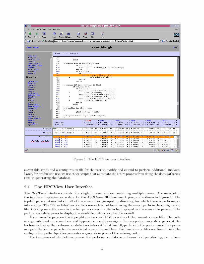
Figure 1: The HPCView user interface.

executable script and a configuration file for the user to modify and extend to perform additional analyses.Later, for production use, we use other scripts that automate the entire process from doing the data-gatheringruns to generating the database.

2.1 The HPCView User Interface

The HPCView interface consists of a single browser window containing multiple panes. A screenshot ofthe interface displaying some data for the ASCI Sweep3D benchmark program is shown in Figure 1. Thetop-left pane contains links to all of the source files, grouped by directory, for which there is performanceinformation. The “Other Files” section lists source files not found using the search paths in the configurationfile. Clicking on a file name in the left pane causes the file to be displayed in the source file pane and theperformance data panes to display the available metrics for that file as well.

The source-file pane on the top-right displays an HTML version of the current source file. The codeis augmented with line numbers and hyper-links used to navigate the two performance data panes at thebottom to display the performance data associates with that line. Hyperlinks in the performance data panesnavigate the source pane to the associated source file and line. For functions or files not found using theconfiguration paths, hpcview generates a synopsis in place of the missing code.

The two panes at the bottom present the performance data as a hierarchical partitioning, i.e. a tree.

5

At the top of the hierarchy is the program. Using a typical structural decomposition, the nodes below theprogram are files and then procedures. Below a procedure in the hierarchy may be one or more levels ofloops. The leaves of the tree are individual source lines for which at least one non-zero performance measuredata has been found. Thus, the leaves of the tree are sparse. Not all lines will have values for all metrics.For instance, floating point operations and cache misses often are associated with different lines. Missingdata is indicated with a blank.

The tables of data presented in the performance panes are sorted in decreasing order according to thecurrently selected performance metric. Initially, the leftmost metric in the display is the one selected.Clicking on the ‘sort’ link of a different metric’s column header will display the data sorted by that metric.

When a browser first reads an HPCView database, the current scope is the entire program and the sourcefiles are shown as its children. Navigation through the hierarchy is done by clicking on the up- and down-arrow icons at the left of each line. The selected scope is moved to the “Current” pane with its ancestor anddescendants shown above and below it, respectively.

To the left of the hierarchical display of the scope tree are iconic links that are used to to adjust the viewof the scope hierarchy by “flattening” or “unflattening” the descendants of the current scope. Flatteningthe current scope replaces each non-leaf scope shown in the descendants pane with its children. Leaf scopescannot be flattened further, so they are retained as is. Progressive unflattening reverses the process until thedescendants pane shows only children of the current scope. Interactive, incremental flattening was addedto the current version (2.0) of HPCView, and a completely flat line-level pane was removed, specificallyto support and encourage top-down performance analysis. When tuning the performance of a scientificprogram, the most important question often to identify the most costly loop in the program. At the toplevel, files are initially displayed as the children of the program. After one round of flattening, the program’sdescendants become the set of procedures. However, knowing the cost of each procedure still doesn’t tell uswhich contains the most costly loop. By flattening one more level, all top-level loops are viewed as peerswith the most costly one at the top of the display. Without the ability to flatten a profile in this way, onewould be forced to navigate into each procedure to look for the one containing the highest cost loop.

The combination of panes of sorted performance data, the hierarchical structure of the data in the tree,the ability to look at all of the peers at each level of the tree, and simple navigation back and forth betweensource code and the performance data are the keys to the effectiveness of the HPCView interface.

2.2 Computed Metrics

Identifying performance problems and opportunities for tuning may require computed performance met-rics that, for instance, compare the instruction mix in a program’s loop nests (loop balance) to the idealinstruction mix supported by the target architecture.

When attempting to tune the performance of a floating-point intensive scientific code, it is often less usefulto know where the majority of the floating-point operations are than where floating-point performance is low.For instance, knowing where the most cycles are spent doing things other than floating-point computation isuseful for tuning scientific codes. This can be directly computed by taking the difference between the cyclecount and FLOP count divided by a target FLOPs per cycle number, and displaying this measure at loopand procedure level. Our experiences with using multiple computed metrics such as miss ratios, instructionbalance, and “lost cycles” using HPCView underscore the power of this approach.

To support the computation of derived metrics, the configuration file assigns an internal name to eachmetric as part of its definition. The definition of each computed metric is a MathML [7] expression thatrefers to previously-defined metrics, either read from a file or computed.

2.3 Program Structure

A program’s performance is less a function of the properties of individual source lines than of the dependenciesand balance among the statements in larger program units such as loops or loop nests. For example, thebalance of floating point operations to memory references within any one line is not particularly relevant toperformance as long as the innermost loop containing that statement has the appropriate balance betweenthe two types of operations and a good instruction schedule.

6

As HPCView processes its performance profile inputs, it incrementally builds a scope tree that reflectsthe structure is either read in explicitly or that can be inferred from information reported. The root ofthe tree represents the entire program. Below the root are nodes representing the files containing sourcecode. Below the files are procedures and, using typical profile data without any additional informantion,below the procedures are nodes representing lines. Some compilers (e.g. SGI) use lines as surrogates forentire statements, while other compilers (e.g. Compaq) provide attribution of costs to individual lines (andcolumns within lines) within multi-line statements.

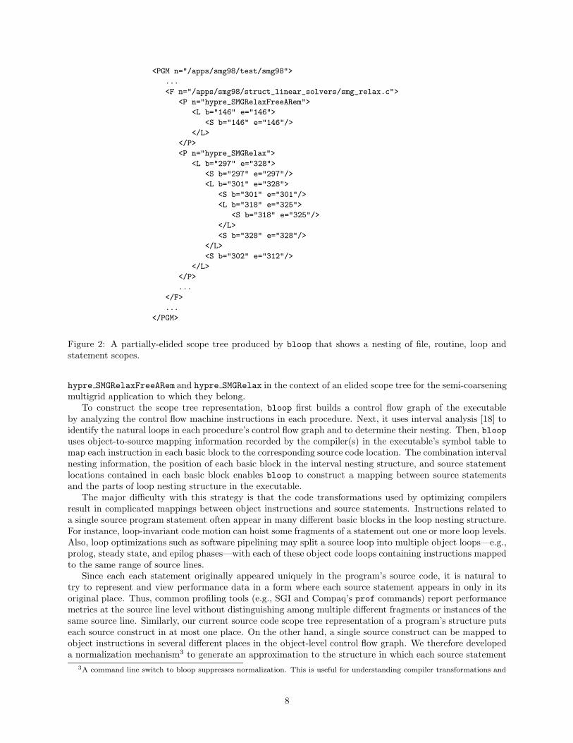
To better organize the information available from the performance data, hpcview (the program) canalso be instructed to initialize the scope tree with information from one or more XML “structure” files (SeeFigure 2.) that contain a tree representation of a hierarchical decomposition of the program as defined bysome external source. The program structure description that we use is extremely general. Here is a list ofthe possible scopes and the relationships among them.

• Program scope – is the root of the tree and can include files and groups.

• File scope – can contain procedures, statements, loops, and groups.

• Procedure scope – can contain loops, statements, and groups.

• Loop scope – may include zero or more loops, statements, and groups.

• Statement scope – specifies a contiguous range of source lines.• Group scope – is a catch-all scope that can include zero or more files, procedures, loops, statements,or other groups.

The group scope is not bound to any conventional syntactic program unit, but it can include any set ofscopes and it can be included in any other scope. The motivation for this virtual unit is to support arbitrary,non-syntactic partitionings. The simplest use is to aggregate non-adjacent statement ranges into a singleunit. It can also be used to represent a semantic partitioning of the program in which program units withrelated function are aggregated for reporting purposes.

Structure files can be generated in several ways:

• They can be emitted by a compiler to reflect the program structure discovered in the source file.

• Structure can be derived from static or dynamic analysis of the executable object code.

• They can be defined explicitly. For example, annotations applied to the code of a library could be toinduce a hierarchically partitioning by semantic category.

We initially used a compiler-based structure generator [10] to emit loop informantion. This was limited toFortran77 programs and required explicitly applying the tool to each source file. We are currently using staticanalysis of binary executables to extract a control flow graph and to approximate syntactic loop nesting.This is described in the next section. Explicit construction of structure files from program annotationsis someting we intend to support in the near future to provide the flexibility to define abstractions thataggregate program units by functional characteristics, or other semantic criteria.

3 Extracting Structure from Executables

The principal disadvantage of analyzing source files to determine a program’s structure is that it requiresseparate handling for each source language. Other issues include the need to analyze many source files inmany directories, unavailable source files, and the discrepancies between the structure of source code andthe structure of the highly-optimized object code. To address all of these problems, we developed bloop,a tool that leverages the Executable Editing Library (EEL) [9] infrastructure to construct a hierarchicalrepresentation of an application’s loop nesting structure based on an analysis of the executable code.

Figure 2 shows an example of an XML document constructed by bloop containing an hpcview scopetree encoding an application’s structure. The XML document includes scope trees for the procedures

7

<PGM n="/apps/smg98/test/smg98">

...

<F n="/apps/smg98/struct_linear_solvers/smg_relax.c">

<P n="hypre_SMGRelaxFreeARem">

<L b="146" e="146">

<S b="146" e="146"/>

</L>

</P>

<P n="hypre_SMGRelax">

<L b="297" e="328">

<S b="297" e="297"/>

<L b="301" e="328">

<S b="301" e="301"/>

<L b="318" e="325">

<S b="318" e="325"/>

</L>

<S b="328" e="328"/>

</L>

<S b="302" e="312"/>

</L>

</P>

...

</F>

...

</PGM>

Figure 2: A partially-elided scope tree produced by bloop that shows a nesting of file, routine, loop andstatement scopes.

hypre SMGRelaxFreeARem and hypre SMGRelax in the context of an elided scope tree for the semi-coarseningmultigrid application to which they belong.

To construct the scope tree representation, bloop first builds a control flow graph of the executableby analyzing the control flow machine instructions in each procedure. Next, it uses interval analysis [18] toidentify the natural loops in each procedure’s control flow graph and to determine their nesting. Then, bloopuses object-to-source mapping information recorded by the compiler(s) in the executable’s symbol table tomap each instruction in each basic block to the corresponding source code location. The combination intervalnesting information, the position of each basic block in the interval nesting structure, and source statementlocations contained in each basic block enables bloop to construct a mapping between source statementsand the parts of loop nesting structure in the executable.

The major difficulty with this strategy is that the code transformations used by optimizing compilersresult in complicated mappings between object instructions and source statements. Instructions related toa single source program statement often appear in many different basic blocks in the loop nesting structure.For instance, loop-invariant code motion can hoist some fragments of a statement out one or more loop levels.Also, loop optimizations such as software pipelining may split a source loop into multiple object loops—e.g.,prolog, steady state, and epilog phases—with each of these object code loops containing instructions mappedto the same range of source lines.

Since each each statement originally appeared uniquely in the program’s source code, it is natural totry to represent and view performance data in a form where each source statement appears in only in itsoriginal place. Thus, common profiling tools (e.g., SGI and Compaq’s prof commands) report performancemetrics at the source line level without distinguishing among multiple different fragments or instances of thesame source line. Similarly, our current source code scope tree representation of a program’s structure putseach source construct in at most one place. On the other hand, a single source construct can be mapped toobject instructions in several different places in the object-level control flow graph. We therefore developeda normalization mechanism3 to generate an approximation to the structure in which each source statement

3A command line switch to bloop suppresses normalization. This is useful for understanding compiler transformations and

8

is reported in at most one position. The fragment shown in Figure 2 is an example of this normalizedrepresentation.

To normalize the scope tree representation, bloop repeatedly applies the following rules until a fixedpoint is reached.

• Whenever instances of one statement appear in two or more disjoint loop nests, the normalizer recur-sively fuses their ancestors from the level of the outermost of the statement instances out to the levelof their lowest common ancestor. Rationale: loop transformations often split a loop nest into severalpieces; to restore the representation to a source-like nesting requires fusing these back together.

• When a statement appears at multiple distinct loop levels within the same loop nest, all instancesof the statement other than the innermost are elided from the mapping. Rationale: the statementprobably incurs the greatest cost in the innermost loop; moving the costs incurred in outer loops inwardwill produce an acceptable level of distortion.

Finally, since the structure produced by bloop is intended only to organize the presentation of performancemetrics, all of the loops in each perfect loop nest are collapsed into the outermost loop of the nest. Thismakes it less tedious to explore the scope hierarchy since it avoids presenting exactly the same informationfor each of the loops in the perfect nest.

One unfortunate consequence of our current reliance on vendor tools for gathering performance profilesis that the reporting of performance metrics at the source line level by these tools can make it impossible insome case to correctly attribute performance metrics. In particular, if a program contains multiple loop nestson the same line (Such a case arises when a macro expands into multiple loop nests.), one cannot distinguishthe performance of the individual loop nests. The normalized representation produced by bloop for suchcases dutifully fuses such loop nests so these aggregate statistics can be reported sensibly. To avoid theinherent inaccuracy when SGI and Compaq’s prof commands aggregate information to source lines ratherthan reporting separate information for line instances or fragments, our future plans include writing newdata collection tools that distinguish among distinct line instances.

A substantial benefit of using a binary analyzer such as bloop to discover program structure is that theresults of compiler transformations such as loop fusion and distribution are exposed to the programmer. Forexample, when loops are fused in the executable, the normalized representation reported by bloop will showstatements in the fused loop as belonging to a common loop nest.

It is worth noting that any inaccuracy by a compiler in mapping object instructions to source constructsdegrades the accuracy with which bloop can generate a reasonable normalized scope tree. While mappinginformation seems to be accurate for the SUN and Alpha compilers, the SGI C compiler sometimes associatesincorrect source line numbers with instructions performing loop condition tests and adjusting the values ofloop induction variable. We have not yet found a reliable method to compensate for this bug. It affects thereported line numbers of the loop scopes and it sometimes distorts the structure of the normalized tree.

3.1 Research Issues

In its current incarnation, HPCView does not provide any facilities for aggregating performance metrics upthe dynamic call chain. We are exploring methods for capturing dynamic call chain information throughbinary instrumentation. Such experiments are using binary rewriting features of EEL [9].

Another extension for the future is to collect and report performance information for line instances.Combined with the un-normalized control structure information recovered by bloop, this would enablemore detailed analysis of the effectiveness of aggressive loop transformations. As developers of compileroptimization algorithms, we expect this will be useful to ourselves. We alst believe that this will be useful forapplication tuning, especially for understanding the relationships among performance, source-level programstructure, and and the detailed structure of the code generated at each level of optimization.

will be used in a future version of HPCView to display transformed code.

9

4 Using the Tools

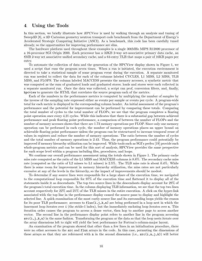
In this section, we briefly illustrate how HPCView is used by walking through an analysis and tuning ofSweep3D [8], a 3D Cartesian geometry neutron transport code benchmark from the Department of Energy’sAccelerated Strategic Computing Initiative (ASCI). As a benchmark, this code has been carefully tunedalready, so the opportunities for improving performance are slim.

The hardware platform used throughout these examples is a single 300MHz MIPS R12000 processor ofa 16-processor SGI Origin 2000. Each processor has a 32KB 2-way set-associative primary data cache, an8MB 2-way set associative unified secondary cache, and a 64-entry TLB that maps a pair of 16KB pages perentry.

To automate the collection of data and the generation of the HPCView display shown in Figure 1, weused a script that runs the program seven times. When a run is initiated, the execution environment isdirected to take a statistical sample of some program event during the execution. A separate monitoredrun was needed to collect the data for each of the columns labeled CYCLES, L1 MISS, L2 MISS, TLBMISS, and FLOPS. The column labeled MACCESS presents the memory accesses, a synthetic metric thatwas computed as the sum of graduated loads and graduated stores; loads and stores were each collected ina separate monitored run. Once the data was collected, a script ran prof, conversion filters, and, finally,hpcview to generate the HTML that correlates the source program each of the metrics.

Each of the numbers in the performance metrics is computed by multiplying the number of samples bythe inverse of the sampling rate expressed either as events per sample or events per cycle. A program-widetotal for each metric is displayed in the corresponding column header. An initial assessment of the program’sperformance and the potential for improvement can be performed by comparing these totals. Comparingthe total number of cycles to the total number of FLOPs, we see that the program completes a floatingpoint operation once every 4.21 cycles. While this indicates that there is a substantial gap between achievedperformance and peak floating point performance, a comparison of between the number of FLOPs and thenumber of memory accesses shows that there are 1.73 memory operations per FLOP. Since only one memoryoperation can be performed in each cycle, the number of memory operations places an upper bound onachievable floating point performance unless the program can be restructured to increase temporal reuse ofvalues in registers and reduce the number of memory operations. The ratio between the number of cyclesand the total number of memory operations is 2.43. Thus, the program performance could potentially beimproved if memory hierarchy utilization can be improved. While tools such as SGI’s perfex [19] provide suchwhole-program metrics and can be used for this sort of analysis, HPCView provides the same perspectivefor each scope level within a program including files, procedures, and loops.

We continue our overall performance assessment using the totals shown in Figure 1. The primary cachemiss rate computed as the ratio of the L1 MISS and MACCESS columns is 8.8%. The secondary cache missrate (computed as the ratio of L2 misses to L1 misses) is 2.5%. The TLB miss rate is about 0.4%. Whilethere is some room for improvement in memory hierarchy utilization, the miss rates are not particularlyexcessive at any of the levels in the hierarchy, so the impact of improvements should be modest.

To determine if any source lines were responsible for a large share of the execution time, we navigatedto the computational loop responsible for 97% of the execution time and flattened it to display all of thestatements inside it as descendants. The top two source lines in the descendants display account for 29% ofthe program’s total execution time. In the column displaying TLB information, we see that the top two linesaccount respectively for 22% and 21% of the TLB misses in the entire execution. A click on the hyper-linkassociated with the top line in the performance display caused the source pane to display and highlight theselected line. A quick examination of the most costly source line and its surrounding loops yields the reasonfor its poor TLB performance: accesses to flux(i,j,k,n) are being performed in a loop nest in which theinnermost loop iterates over i (the stride-1 index), but the immediately enclosing loop iterates over n. Thisiteration order causes the program to access a dense vector, then hop to another page to access anothervector. The second line in the performance display point refers to another line in the program accessingsrc(i,j,k,n) in the same fashion. Transforming the program or the data so that the loop nests iterate overthe array dimensions left to right will yield the best performance for Fortran’s column-major layout.

An examination of the program showed that other than a few lines in an initialization procedure, therewere no other accesses to the src and flux arrays in the code. In this case, permuting the dimensions ofthese arrays so that they are referenced with n in the second dimension (i.e., src(i,n,j,k)) will better

10

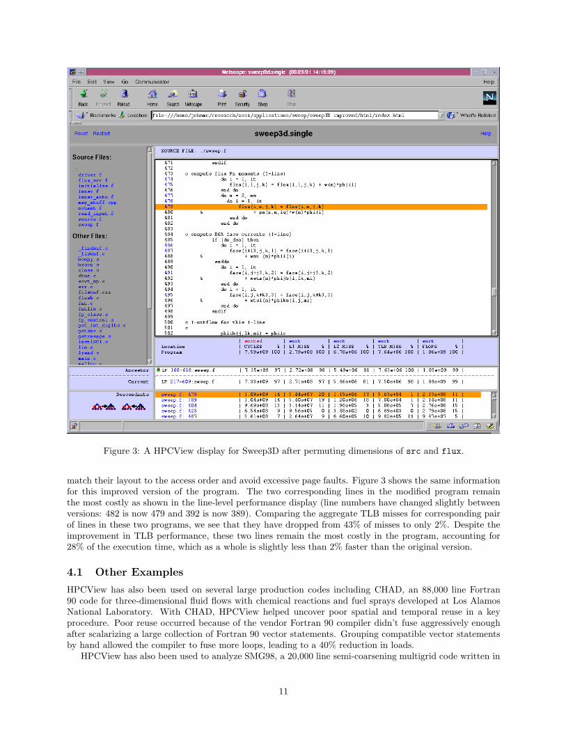
Figure 3: A HPCView display for Sweep3D after permuting dimensions of src and flux.

match their layout to the access order and avoid excessive page faults. Figure 3 shows the same informationfor this improved version of the program. The two corresponding lines in the modified program remainthe most costly as shown in the line-level performance display (line numbers have changed slightly betweenversions: 482 is now 479 and 392 is now 389). Comparing the aggregate TLB misses for corresponding pairof lines in these two programs, we see that they have dropped from 43% of misses to only 2%. Despite theimprovement in TLB performance, these two lines remain the most costly in the program, accounting for28% of the execution time, which as a whole is slightly less than 2% faster than the original version.

4.1 Other Examples

HPCView has also been used on several large production codes including CHAD, an 88,000 line Fortran90 code for three-dimensional fluid flows with chemical reactions and fuel sprays developed at Los AlamosNational Laboratory. With CHAD, HPCView helped uncover poor spatial and temporal reuse in a keyprocedure. Poor reuse occurred because of the vendor Fortran 90 compiler didn’t fuse aggressively enoughafter scalarizing a large collection of Fortran 90 vector statements. Grouping compatible vector statementsby hand allowed the compiler to fuse more loops, leading to a 40% reduction in loads.

HPCView has also been used to analyze SMG98, a 20,000 line semi-coarsening multigrid code written in

11

C that was developed at Lawrence Livermore National Laboratory. Using HPCView it was straightforwardto determine that the biggest problem with the code was several of its key computational loops were memorybound. Node performance tuning efforts focused on this problem have led to improvements of 20%.

<HPCVIEW>

<TITLE name="heat.single" />

<PATH name="." />

<METRIC name="fcy_hwc" displayName="CYCLES">

<FILE name="heat.single.fcy_hwc.pxml" />

</METRIC>

<METRIC name="ideal" displayName="ICYCLES">

<FILE name="heat.single.ideal.pxml" />

</METRIC>

<METRIC name="stall" displayName="STALL">

<COMPUTE>

<math>

<apply><max/>

<apply><minus/>

<ci>fcy_hwc</ci> <ci>ideal</ci>

</apply>

<cn>0</cn>

</apply>

</math>

</COMPUTE>

</METRIC>

<METRIC name="gfp_hwc" displayName="FLOPS">

<FILE name="heat.single.gfp_hwc.pxml" />

</METRIC>

</HPCVIEW>

Figure 4: The HPCView configuration file showing the specification of metrics displayed in Figure 5.

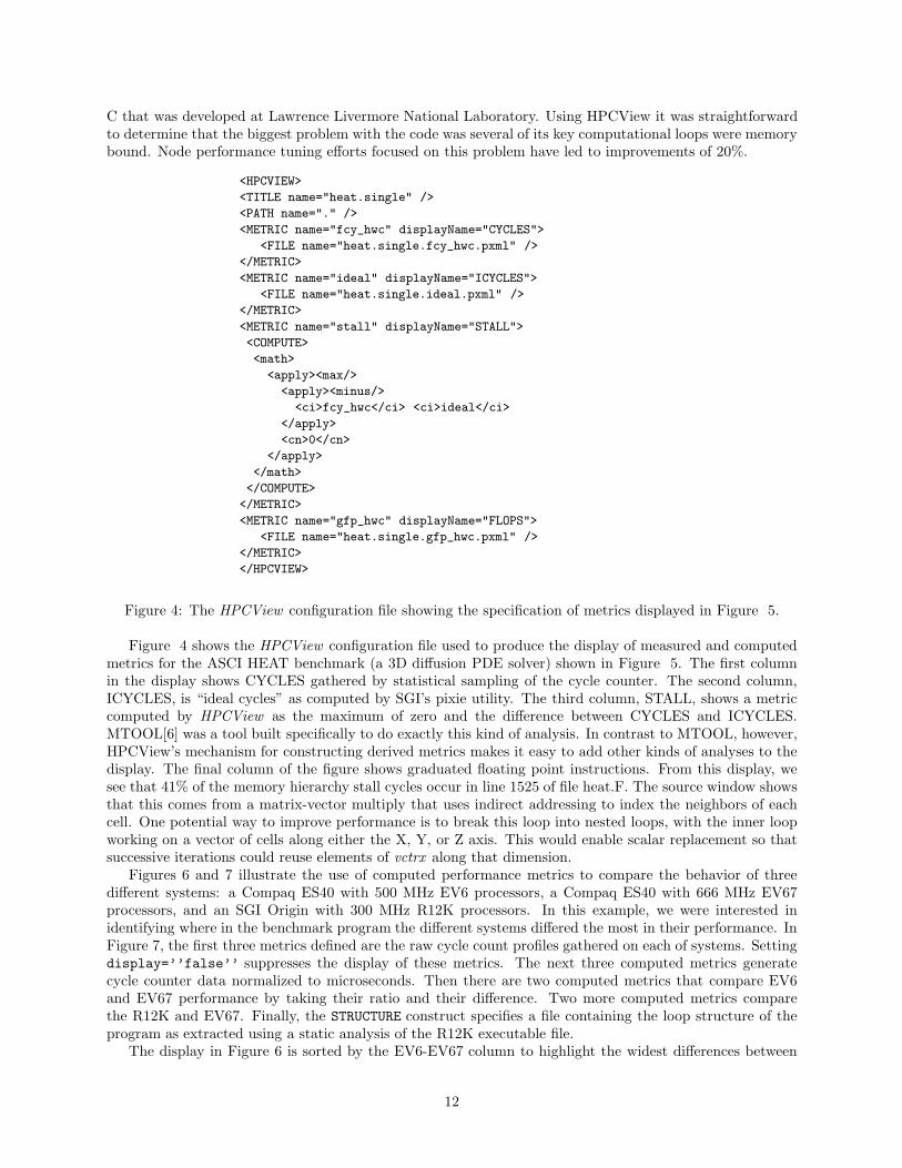
Figure 4 shows the HPCView configuration file used to produce the display of measured and computedmetrics for the ASCI HEAT benchmark (a 3D diffusion PDE solver) shown in Figure 5. The first columnin the display shows CYCLES gathered by statistical sampling of the cycle counter. The second column,ICYCLES, is “ideal cycles” as computed by SGI’s pixie utility. The third column, STALL, shows a metriccomputed by HPCView as the maximum of zero and the difference between CYCLES and ICYCLES.MTOOL[6] was a tool built specifically to do exactly this kind of analysis. In contrast to MTOOL, however,HPCView’s mechanism for constructing derived metrics makes it easy to add other kinds of analyses to thedisplay. The final column of the figure shows graduated floating point instructions. From this display, wesee that 41% of the memory hierarchy stall cycles occur in line 1525 of file heat.F. The source window showsthat this comes from a matrix-vector multiply that uses indirect addressing to index the neighbors of eachcell. One potential way to improve performance is to break this loop into nested loops, with the inner loopworking on a vector of cells along either the X, Y, or Z axis. This would enable scalar replacement so thatsuccessive iterations could reuse elements of vctrx along that dimension.

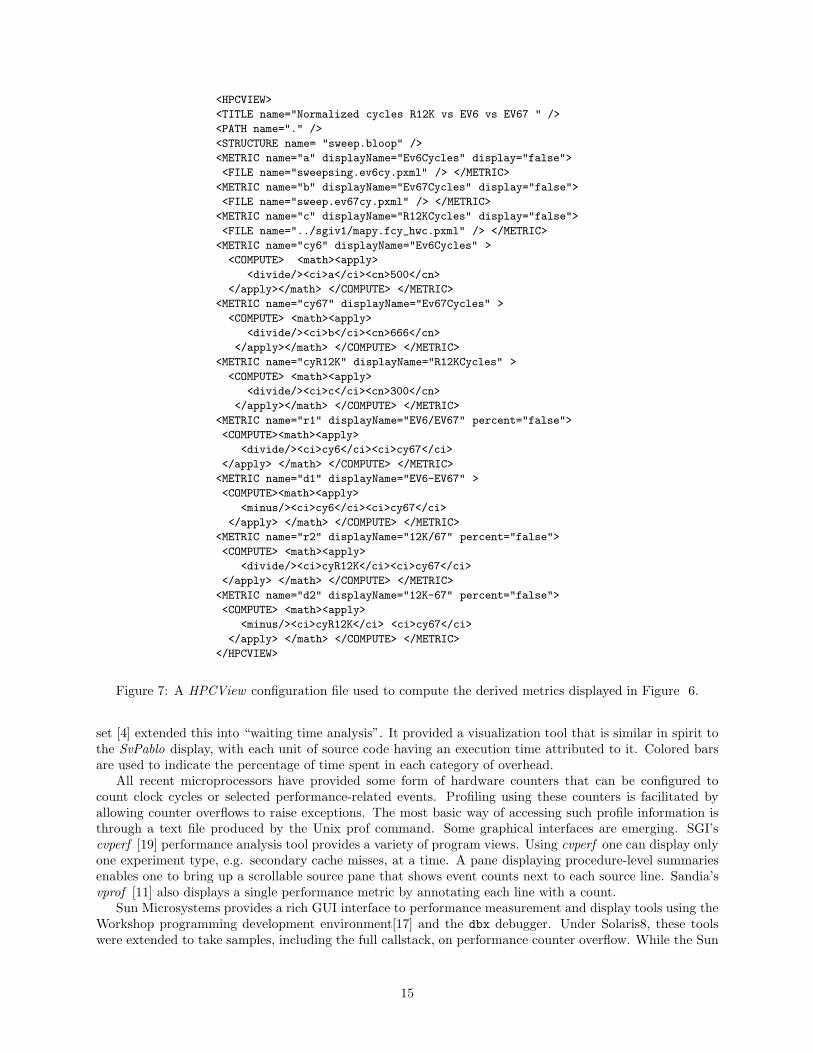
Figures 6 and 7 illustrate the use of computed performance metrics to compare the behavior of threedifferent systems: a Compaq ES40 with 500 MHz EV6 processors, a Compaq ES40 with 666 MHz EV67processors, and an SGI Origin with 300 MHz R12K processors. In this example, we were interested inidentifying where in the benchmark program the different systems differed the most in their performance. InFigure 7, the first three metrics defined are the raw cycle count profiles gathered on each of systems. Settingdisplay=’’false’’ suppresses the display of these metrics. The next three computed metrics generatecycle counter data normalized to microseconds. Then there are two computed metrics that compare EV6and EV67 performance by taking their ratio and their difference. Two more computed metrics comparethe R12K and EV67. Finally, the STRUCTURE construct specifies a file containing the loop structure of theprogram as extracted using a static analysis of the R12K executable file.

The display in Figure 6 is sorted by the EV6-EV67 column to highlight the widest differences between

12

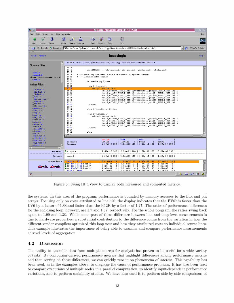
Figure 5: Using HPCView to display both measured and computed metrics.

the systems. In this area of the program, performance is bounded by memory accesses to the flux and phiarrays. Focusing only on costs attributed to line 520, the display indicates that the EV67 is faster than theEV6 by a factor of 1.88 and faster than the R12K by a factor of 1.27. The ratios of performance differencesfor the enclosing loop, however, are 1.7 and 1.57, respectively. For the whole program, the ratios swing backagain to 1.99 and 1.38. While some part of these difference between line and loop level measurements isdue to hardware properties, a substantial contribution to the difference comes from the variation in how thedifferent vendor compilers optimized this loop nest and how they attributed costs to individual source lines.This example illustrates the importance of being able to examine and compare performance measurementsat sevel levels of aggregation.

4.2 Discussion

The ability to assemble data from multiple sources for analysis has proven to be useful for a wide varietyof tasks. By computing derived performance metrics that highlight differences among performance metricsand then sorting on those differences, we can quickly zero in on phenomena of interest. This capability hasbeen used, as in the examples above, to diagnose the cause of performance problems. It has also been usedto compare executions of multiple nodes in a parallel computation, to identify input-dependent performancevariations, and to perform scalability studies. We have also used it to perform side-by-side comparisons of

13

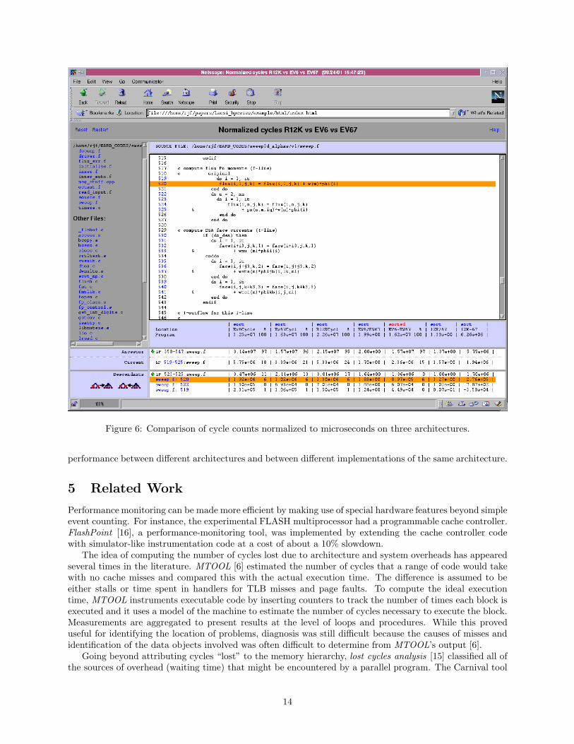
Figure 6: Comparison of cycle counts normalized to microseconds on three architectures.

performance between different architectures and between different implementations of the same architecture.

5 Related Work

Performance monitoring can be made more efficient by making use of special hardware features beyond simpleevent counting. For instance, the experimental FLASH multiprocessor had a programmable cache controller.FlashPoint [16], a performance-monitoring tool, was implemented by extending the cache controller codewith simulator-like instrumentation code at a cost of about a 10% slowdown.

The idea of computing the number of cycles lost due to architecture and system overheads has appearedseveral times in the literature. MTOOL [6] estimated the number of cycles that a range of code would takewith no cache misses and compared this with the actual execution time. The difference is assumed to beeither stalls or time spent in handlers for TLB misses and page faults. To compute the ideal executiontime, MTOOL instruments executable code by inserting counters to track the number of times each block isexecuted and it uses a model of the machine to estimate the number of cycles necessary to execute the block.Measurements are aggregated to present results at the level of loops and procedures. While this proveduseful for identifying the location of problems, diagnosis was still difficult because the causes of misses andidentification of the data objects involved was often difficult to determine from MTOOL’s output [6].

Going beyond attributing cycles “lost” to the memory hierarchy, lost cycles analysis [15] classified all ofthe sources of overhead (waiting time) that might be encountered by a parallel program. The Carnival tool

14

<HPCVIEW>

<TITLE name="Normalized cycles R12K vs EV6 vs EV67 " />

<PATH name="." />

<STRUCTURE name= "sweep.bloop" />

<METRIC name="a" displayName="Ev6Cycles" display="false">

<FILE name="sweepsing.ev6cy.pxml" /> </METRIC>

<METRIC name="b" displayName="Ev67Cycles" display="false">

<FILE name="sweep.ev67cy.pxml" /> </METRIC>

<METRIC name="c" displayName="R12KCycles" display="false">

<FILE name="../sgiv1/mapy.fcy_hwc.pxml" /> </METRIC>

<METRIC name="cy6" displayName="Ev6Cycles" >

<COMPUTE> <math><apply>

<divide/><ci>a</ci><cn>500</cn>

</apply></math> </COMPUTE> </METRIC>

<METRIC name="cy67" displayName="Ev67Cycles" >

<COMPUTE> <math><apply>

<divide/><ci>b</ci><cn>666</cn>

</apply></math> </COMPUTE> </METRIC>

<METRIC name="cyR12K" displayName="R12KCycles" >

<COMPUTE> <math><apply>

<divide/><ci>c</ci><cn>300</cn>

</apply></math> </COMPUTE> </METRIC>

<METRIC name="r1" displayName="EV6/EV67" percent="false">

<COMPUTE><math><apply>

<divide/><ci>cy6</ci><ci>cy67</ci>

</apply> </math> </COMPUTE> </METRIC>

<METRIC name="d1" displayName="EV6-EV67" >

<COMPUTE><math><apply>

<minus/><ci>cy6</ci><ci>cy67</ci>

</apply> </math> </COMPUTE> </METRIC>

<METRIC name="r2" displayName="12K/67" percent="false">

<COMPUTE> <math><apply>

<divide/><ci>cyR12K</ci><ci>cy67</ci>

</apply> </math> </COMPUTE> </METRIC>

<METRIC name="d2" displayName="12K-67" percent="false">

<COMPUTE> <math><apply>

<minus/><ci>cyR12K</ci> <ci>cy67</ci>

</apply> </math> </COMPUTE> </METRIC>

</HPCVIEW>

Figure 7: A HPCView configuration file used to compute the derived metrics displayed in Figure 6.

set [4] extended this into “waiting time analysis”. It provided a visualization tool that is similar in spirit tothe SvPablo display, with each unit of source code having an execution time attributed to it. Colored barsare used to indicate the percentage of time spent in each category of overhead.

All recent microprocessors have provided some form of hardware counters that can be configured tocount clock cycles or selected performance-related events. Profiling using these counters is facilitated byallowing counter overflows to raise exceptions. The most basic way of accessing such profile information isthrough a text file produced by the Unix prof command. Some graphical interfaces are emerging. SGI’scvperf [19] performance analysis tool provides a variety of program views. Using cvperf one can display onlyone experiment type, e.g. secondary cache misses, at a time. A pane displaying procedure-level summariesenables one to bring up a scrollable source pane that shows event counts next to each source line. Sandia’svprof [11] also displays a single performance metric by annotating each line with a count.

Sun Microsystems provides a rich GUI interface to performance measurement and display tools using theWorkshop programming development environment[17] and the dbx debugger. Under Solaris8, these toolswere extended to take samples, including the full callstack, on performance counter overflow. While the Sun

15

tools provide a generic set of basic profiling and analysis tools, the advanced features are largely orthogonalto the concerns addressed by HPCView. The Sun tools can display multiple metrics, but there is no provisionfor computing derived metrics. While data can be aggregated inclusively, and exclusively up the call chain,there is no way of aggregating metrics at scopes below the procedure level.

Both the Sun analyzer tool and the programs for displaying information from Compaq’s Dynamic Con-tinuous Profiling Infrastructure have options for displaying performance histogram data in a listing of disas-sembled object code annotated with source code. While this makes it possible to analyze highly-optimizedcode where a single source line may map into multiple instances in the executable, it is a difficult and timeconsuming exercise. Adve et al. [1] demonstrated a performance browser that uses compiler-derived mappinginformation to interactively correlate HPF source code with the compiler’s parallelized, optimized F77+MPIoutput, which is instrumented with SvPablo (See below.). This combination can present MPI performancedata in terms of both the transformed and original code. Vendor compilers are increasingly able to generateannotated listings that attempt to explain both what optimizations have been performed and what aspectsof the program inhibit optimization. To our knowledge, performance data has not been integrated with thisinformation for presentation.SvPablo (source view Pablo) is a graphical environment for instrumenting application source code and

browsing dynamic performance data from a diverse set of performance instrumentation mechanisms, whichinclude hardware performance counters [14]. Rather than using overflow-driven profiling, SvPablo librarycalls are inserted in the program, either by hand, or by a preprocessor that can instrument proceduresand loops. The library routines query the hardware performance counters during program execution. Afterprogram execution is complete, the library records a summary file of its statistical analysis for each executingprocess. Like, HPCView, the SvPablo GUI correlates performance metrics with the program source andprovides access to detailed information at the routine and source-line level. Next to each source line in thedisplay is a row of color-coded squares, where each column is associated with a performance metric andeach color indicates the importance that source line has on the overall performance of that metric. However,SvPablo’s displays do not provide sorted or hierarchical displays to facilitate top-down analysis.

6 Concluding Remarks

In this paper we described some of the design issues and lessons learned in the construction and use ofHPCView, a performance analysis toolkit intended specifically to increase programmer productivity in per-formance engineering by being easier to use, while providing powerful more analytic capabilities than existingtools.

As described in previous sections, we have used HPCView on several whole applications. Notably, thishas included a 20,000 line semi-coarsening multigrid code written in C, an 88,000 line Fortran 90 codefor three-dimensional fluid flows, and a multi-lingual 200,000 line cosmology application. In each of thesecodes the tools enabled us to quickly identify significant opportunities for performance improvement. Forlarge codes, however, the HTML database size grows large when many metrics are measured or computed.Currently, we precompute static HTML for the entire set of potential displays. For example, instead ofdynamically sorting the performance metric panes, we write a separate copy of the data for each sort order.These separate copies are written for the data in each of the program scopes. We have seen HTML databasesrelating several performance metrics to a 150,000 line application occupy 30 megabytes in slightly over 6000files4. These databases correlate performance metrics to all of the application sources. To reduce the size ofperformance databases, we are prototyping a stand-alone performance browser written in Java that createsviews on demand.

Acknowledgments

Monika Mevencamp and Xuesong Yuan were the principal implementers of the first version of HPCView.Nathan Tallent and Gabriel Marin have been the principal implementers of the bloop binary analyzer foridentifying loops. We thank Jim Larus for letting us use the EEL binary editing toolkit as the basis for

4The amount of wasted and redundant space is illustrated by the fact that the gzip’ed tar file is less than 1.5 megabytes,most of which represents compressed source code.

16

constructing bloop. This research was supported in part by NSF grants EIA-9806525, CCR-9904943, andEIA-0072043, the DOE ASCI Program under research subcontract B347884, and the Los Alamos NationalLaboratory Computer Science Institute (LACSI) through LANL contract number 03891-99-23 as part of theprime contract (W-7405-ENG-36) between the DOE and the Regents of the University of California.

References

[1] V. Adve, J.-C. Wang, J. Mellor-Crummey, D. Reed, M. Anderson, and K. Kennedy. An Integrated Compilationand Performance Analysis Environment for Data Parallel Programs. In Proceedings of Supercomputing ’95, SanDiego, CA, December 1995.

[2] D. Callahan, J. Cocke, and K. Kennedy. Estimating interlock and improving balance for pipelined machines.Journal of Parallel and Distributed Computing, 5(4):334–358, August 1988.

[3] Kirk W. Cameron, Yong Luo, and Janes Scharmeier. Instruction-levle microprocessor modeling of scientificapplications. In ISHPC 1999, pages 29 – 40, Japan, May 1999.

[4] Carnival Web Site. http://www.cs.rochester.edu/u/leblanc/prediction.html.

[5] Jeffrey Dean, James E. Hicks, Carl A. Waldspurger, William E. Weihl, and George Chrysos. ProfileMe: Hardwaresupport for instruction-level profiling on out-of-order processors. In Proceedings of the 30th Annual InternationalSymposium on Microarchitecture (Micro ’97), December 1997.

[6] A. J. Goldberg and J. Hennessy. MTOOL: A Method for Isolating Memory Bottlenecks in Shared MemoryMultiprocessor Programs. In Proceedings of the International Conference on Parallel Processing, pages 251–257,August 1991.

[7] W3C Math Working Group. Mathematical markup language (mathml) 1.01 specification, July 1999.http://www.w3.org/TR/REC-MathML.

[8] Sweep3D Benchmark Code. DOE Accelerated Strategic Computing Initiative.http://www.llnl.gov/asci benchmarks/asci/limited/sweep3d/asci sweep3d.html.

[9] E. Schnarr J. Larus. EEL: Machine-Independent Executable Editing. In Proceedings of the ACM SIGPLANConference on Programming Language Design and Implementation, pages 291–300, June 1995.

[10] K. Kennedy J. Mellor-Crummey, D. Whalley. Improving Memory Hierarchy Performance for Irregular Ap-plications. In Proceedings of the ACM International Conference on Supercomputing ’94, pages 425–433, June1999.

[11] C. Janssen. The Visual Profiler. http://aros.ca.sandia.gov/~cljanss/perf/vprof/doc/README.html.

[12] T.Y. Johnston and R. H. Johnson. Program performance measurement. Technical Report SLAC User Note 33,Rev. 1, SLAC, Stanford University, California, 1970.

[13] D. E. Knuth and F. R. Stevenson. Optimal measurement points for program frequency counts. BIT, 13(3):313–322, 1973.

[14] D. Reed L. DeRose, Y. Zhang. SvPablo: A Multi-Language Performance Analysis System. In 10th InternationalConference on Performance Tools, pages 352–355, September 1998.

[15] T. LeBlanc M. Crovella. Parallel Performance Prediction Using Lost Cycles. In Proceedings Supercomputing ’94,pages 600–610, November 1994.

[16] D. Ofelt M. Martonosi and M. Heinrich. Integrating Performance Monitoring and Communication in ParallelComputers. In ACM SIGMETRICS International Conference on Measurement and Modeling of ComputerSystems, pages 138–147, May 1996.

[17] Sun Microsystems. Analyzing Program Performance With Sun WorkShop, 2001.http://docs.sun.com/htmlcoll/coll.36.7/iso-8859-1/SWKSHPPERF/AnalyzingTOC.html.

[18] R. E. Tarjan. Testing flow graph reducibility. Journal of Computer and System Sciences, 9:355–365, 1974.

[19] M. Zagha, B. Larson, S. Turner, and M. Itzkowitz. Performance Analysis Using the MIPS R10000 PerformanceCounters. In Proceedings Supercomputing ’96, November 1996.

17