Howard Lee, (2007) Essentials of Behavioral Science Research.
225
Essentials of Behavioral Science Research. A First Course in Research Methodology Howard Lee California State University Distributed by WWW.LULU.COM Morrisville, NC 27560 Essentials of Behavioral Science Research: A First Course in Research Methodology Copyright © 2007 by Howard Lee. All rights reserved. Published and Distributed by WWW.LULU.COM 3131 RDU Center Drive, Suite 210 Morrisville, NC 27560 Printed in the United States of America
Transcript of Howard Lee, (2007) Essentials of Behavioral Science Research.

Essentials of Behavioral Science Research.A First Course in Research MethodologyHoward LeeCalifornia State UniversityDistributed by WWW.LULU.COM Morrisville, NC 27560Essentials of Behavioral Science Research: A FirstCourse in Research MethodologyCopyright © 2007 by Howard Lee. All rights reserved.Published and Distributed by WWW.LULU.COM 3131 RDUCenter Drive, Suite 210 Morrisville, NC 27560Printed in the United States of America
Chapter Summary109Chapter 10 111
Table of ContentsChapter 1 1Science and the Scientific Approach 1Science and Common Sense 1Four Methods of Knowing 3Science and Its Functions 4The Aims of Science, Scientific Explanation, andTheory 5Scientific Research a Definition 7 The Scientific Approach 8 Problem-Obstacle-Idea 8 Hypothesis 8 Reasoning-Deduction 8 Observation-Test-Experiment 10 Chapter Outline-Summary 12Chapter 2 13Problems and Hypotheses 13Criteria of Problems and Problem Statements 14Hypotheses 14The Importance of Problems and Hypotheses 15 Virtues of Problems andHypotheses 15 Problems, Values, and Definitions 17 Generality andSpecificity of Problems and Hypotheses 17Concluding Remarks-the Special Power of Hypotheses 19 Chapter Summary 21Chapter 3 23Constructs, Variables and Definitions 23 Concepts and Constructs 23Constitutive and Operational Definitions of Constructs and Variables 24Types of Variables 28 Independent and Dependent Variables 28 Active andAttribute Variables 30 Continuous and Categorical Variables 32 Constructs,Observables, and Latent Variables 33 Examples of Variables and OperationalDefinitions 34Chapter 4 39Calculation of Means and Variances 39Kinds of Variance 40Population and Sample Variances 41Between-Groups (Experimental) Variance 41Error Variance 43Components of Variance 48Covariance 49Study Suggestions 50Chapter Summary 51Chapter 5 53Sampling and Randomness 53 Sampling, Random Sampling, andRepresentativeness 53 randomness 55An Example of Random Sampling 55Randomization 56Sample Size 60Kinds of Samples 62Some books on sampling. 67Chapter Summary 68Chapter 6 69
Ethical Considerations in Conducting BehavioralScience Research 69A Beginning? 70General Considerations 72Deception 73Freedom from Coercion 73Debriefing 73Protection of Participants 73 Confidentiality 73 Ethics of Animal Research74 Study Suggestions 74 th Chapter Summary 75Chapter 7 77Research Design: Purpose and Principles 77 Purposes of Research Design 77
Chapter Summary109Chapter 10 111
A Stronger Design 78 Research Design As Variance Control 80 A ControversialExample 81 Maximization of Experimental Variance 82 Control of ExtraneousVariables 83 Minimization of Error Variance 85 Chapter Summary 86Chapter 8 87Inadequate Designs and Design Criteria 87 Experimental and NonexperimentalApproaches 87Symbolism and Definitions 88 Faulty Designs 89Measurement, History, Maturation 90The Regression Effect 90Criteria of Research Design 91Answer Research Questions? 91Control of Extraneous Independent Variables 92Generalizability 93Internal and External Validity 93Chapter 9 97General Designs of Research 97 Conceptual Foundations of Research Design 97A Preliminary Note: Experimental Designs and Analysis Of Variance 99 TheDesigns 99The Notion of the Control Group and Extensions of Design 9.1 100Matching versus Randomization 102 Some ways of matching groups. 102Matching by Equating Participants 102 The Frequency Distribution MatchingMethod 103Matching by Holding Variables Constant 104 Matching by incorporating theNuisance Variable into the Research Design 104 Participant as Own Control104 Additional Design Extensions: Design 9.3 using a Pretest 105Difference Scores 106 Concluding Remarks 108 Study Suggestions 108Research Design Applications: 111 simple Randomized Subjects Design 111Factorial Designs 113Factorial Designs with More than Two Variables 114Research Examples of Factorial Designs 114Flowers: Groupthink 114Correlated Groups 120the General Paradigm 120One group Repeated Trials Design 121Two group, Experimental Group-Control GroupDesigns 122Research Examples of Correlated-groups Designs 122Multigroup Correlated-groups Designs 125 Units Variance 125 FactorialCorrelated Groups 125 Analysis of Covariance 127 Chapter Summary 133Chapter 11 135Quasi Experimental and N = 1 Designs of Research 135Variants of Basic Designs 135Compromise Designs a.k.a. Quasi ExperimentalDesigns 135Nonequivalent Control Group Design 135 No-treatment Control Group Design136 Time Designs 140

Chapter 1: Science and the Scientific Approach 1Chapter 1Science and the Scientific ApproachTO UNDERSTAND any complex human activity one must grasp the language andapproach of the individuals who pursue it. So it is with understandingscience and scientific research. One must know and understand, at least inpart, scientific language and the scientific approach to problem-solving.
One of the most confusing things to the student of science is the specialway scientists use ordinary words. To make matters worse, they invent newwords. There are good reasons for this specialized use of language; theywill become evident later. For now, suffice it to say that we mustunderstand and learn the language of social scientists. When investigatorstell us about their independent and dependent variables, we must know whatthey mean. When they tell us that they have randomized their experimentalprocedures, we must not only know what they mean-we must understand whythey do as they do.
Similarly, the scientist's approach to problems must be clearlyunderstood. It is not so much that this approach is different from thelayperson. It is different, of course, but it is not strange and esoteric.This is quite the contrary. When understood, it will seem natural andalmost inevitable what the scientist does. Indeed, we will probably wonderwhy much more human thinking and problem-solving are not consciouslystructured along such lines.
The purpose of Chapters 1 and 2 of this book is to help the student learnand understand the language and approach of science and research. In thechapters of this part many of the basic constructs of the social,behavioral and educational scientist will be studied. In some cases it willnot be possible to give complete and satisfactory definitions. This is dueto the lack of background at this early point in our development. In suchcases an attempt will be made to formulate and use reasonably accuratefirst approximations to later, more satisfactory definitions. Let us beginour study by considering how the scientist approaches problems and how thisapproach differs from what might be called a common sense approach.SCIENCE AND COMMON SENSE
Whitehead (1911/1992, p. 157) at the beginning of the 20th Centurypointed out that in creative thought common sense is a bad master. “Itssole criterion for judgment is that the new ideas shall look like the oldones.” This is well said. Common sense may often be a bad master for theevaluation of knowledge. But how are science and common sense alike and howare they different? From one viewpoint, science and common sense are alike.This view would say that science is a systematic and controlled extensionof common sense. James Bryant Conant (1951) states that common sense is aseries ofconcepts and conceptual schemes1 satisfactory for thepractical uses of humanity. However, these concepts and conceptual schemesmay be seriously misleading in modern science-and particularly inpsychology and education. To many educators in the 1800’s, it was commonsense to use punishment as a basic tool of pedagogy. However, in the mid1900’s evidence emerged to show that this older commonsense view ofmotivation may be quite erroneous. Reward seems more effective thanpunishment in aiding learning. However, recent findings suggest thatdifferent forms of punishment are useful in classroom learning (Tingstrom,et al., 1997; Marlow, et al., 1997).
Science and common sense differ sharply in five ways. These disagreements
Chapter Summary109Chapter 10 111
revolve around the words "systematic" and “controlled.” First, the uses ofconceptual schemes and theoretical structures are strikingly different. Thecommon person may use "theories" and concepts, but usually does so in aloose fashion. This person often blandly accepts fanciful explanations ofnatural and human phenomena. An 1
1 A CONCEPT is a word that expresses an abstraction formed by generalization from particulars. "Aggression" is a concept, an abstraction that expresses a number of particular actions having the similar characteristic of hurting people or objects. A CONCEPTUAL SCHEME is a set of concepts interrelated by hypothetical and theoretical propositions. A construct is a concept with the additional meaning of having been created or appropriated for special scientific purposes. "Mass," "energy," "hostility," "introversion," and "achievement" are constructs. They might more accurately be called "constructed types" or "constructed classes," classes or sets of objects or events bound together by the possession of common characteristics defined by the scientist. The term "variable" will be defined in a later chapter. For now let it mean a symbol or name of a characteristic that takes on different numerical values.
2 Chapter 1: Science and the Scientific Approach
illness, for instance, may be thought to be a punishment for sinfulness(Klonoff & Landrine, 1994). Jolliness is due to being overweight.Scientists, on the other hand, systematically build theoretical structures,test them for internal consistency, and put aspects of them to empiricaltest. Furthermore, they realize that the concepts they use are man-madeterms that may or may not exhibit a close relation to reality.
Second, scientists systematically and empirically test their theories andhypotheses. Nonscientists test "hypotheses," too, but they test them in aselective fashion. They often "select" evidence simply because it isconsistent with the hypotheses. Take the stereotype: Asians are science andmath oriented. If people believe this, they can easily "verify" the beliefby noting that many Asians are engineers and scientists (see Tang, 1993).Exceptions to the stereotype, the non-science Asian or the mathematicallychallenged Asian, for example, are not perceived. Sophisticated social andbehavioral scientists knowing this "selection tendency" to be a commonpsychological phenomenon, carefully guard their research against their ownpreconceptions and predilections and against selective support ofhypotheses. For one thing, they are not content with armchair or fiatexploration of relations; they must test the relations in the laboratory orin the field. They are not content, for example, with the presumed relationsbetween methods of teaching and achievement, between intelligence andcreativity, between values and administrative decisions. They insist uponsystematic, controlled, and empirical testing of these relations.
A third difference lies in the notion of control. In scientific research,control means several things. For the present, let it mean that thescientist tries systematically to rule out variables that are possible"causes" of the effects under study other than the variables hypothesized tobe the "causes." Laypeople seldom bother to control systematically theirexplanations of observed phenomena. They ordinarily make little effort tocontrol extraneous sources of influence. They tend to accept thoseexplanations that are in accord with their preconceptions and biases. Ifthey believe that slum conditions produce delinquency, they tend todisregard delinquency in nonslum neighborhoods. The scientist, on the otherhand, seeks out and "controls" delinquency incidence in different kinds ofneighborhoods. The difference, of course, is profound.
Another difference between science and common sense is perhaps not sosharp. It was said earlier that the scientist is constantly preoccupied withrelations among phenomena. The layperson also does this by using commonsense for explanations of phenomena. But the scientist consciously andsystematically pursues relations. The layperson’s preoccupation withrelations is loose, unsystematic, and uncontrolled. The layperson oftenseizes, for example, on the fortuitous occurrence of two phenomena andimmediately links them indissolubly as cause and effect.
Take the relation tested in the classic study done many years ago byHurlock (1925). In more recent terminology, this relation may be expressed:Positive reinforcement (reward) produces greater increments of learning thandoes punishment. The relation is between reinforcement (or reward andpunishment) and learning. Educators and parents of the nineteenth centuryoften assumed that punishment was the more effective agent in learning.Educators and parents of the present often assume that positivereinforcement (reward) is more effective. Both may say that their viewpointsare "only common sense." It is obvious, they may say, that if you reward (orpunish) a child, he or she will learn better. The scientist, on the otherhand, while personally espousing one or the other or neither of these

Chapter 1: Science and the Scientific Approach 3
viewpoints, would probably insist on systematic and controlled testing ofboth (and other) relations, as Hurlock did. Using the scientific methodHurlock found incentive to be substantially related to arithmeticachievement. The group receiving praise scored higher than the reproof orignored groups.
A final difference between common sense and science lies in differentexplanations of observed phenomena. The scientist, when attempting toexplain the relations among observed phenomena, carefully rules out whathave been called "metaphysical explanations." A metaphysical explanation issimply a proposition that cannot be tested. To say, for example, that peopleare poor and starving because God wills it, or that it is wrong to beauthoritarian, is to talk metaphysically.
None of these propositions can be tested; thus they are metaphysical. Assuch, science is not concerned with them. This does not mean that scientistswould necessarily spurn such statements, say they are not true, or claimthey are meaningless. It simply means that as scientists they are not concernedwith them. In short, science is concerned with things that can be publiclyobserved and tested. If propositions or questions do not containimplications for such public observation and testing, they are notscientific propositions or questions.FOUR METHODS OF KNOWINGCharles Sanders Peirce as reported in Buchler (1955) said that there arefour general ways of knowing or, as he put it, fixing belief. In the ensuingdiscussion, the authors are taking some liberties with Peirce's originalformulation in an attempt to clarify the ideas and to make them more germaneto the present discussion. The first is the method of tenacity. Here people holdfirmly to the truth, the truth that they know to be true because they holdfirmly to it, because they have always known it to be true. Frequentrepetition of such "truths" seems to enhance their validity. People oftencling to their beliefs in the face of clearly conflicting facts. And theywill also infer "new" knowledge from propositions that may be false.
A second method of knowing or fixing belief is the method of authority. Thisis the method of established belief. If the Bible says it, it is so. If anoted physicist says there is a God, it is so. If an idea has the weight oftradition and public sanction behind it, it is so. As Peirce points out,this method is superior to the method of tenacity, because human progress,although slow, can be achieved using this method. Actually, life could notgo on without the method of authority. Dawes (1994) states that asindividuals, we cannot know everything. We accept the authority of the U.S.Drug and Food Administration in determining what we eat and drink are safe.Dawes states that the completely open mind that questions all authority doesnot exist. We must take a large body of facts and information on the basisof authority. Thus, it should not be concluded that the method of authorityis unsound; it is unsound only under certain circumstances.
The a priori method is the third way of knowing or fixing belief. Graziano andRaulin (1993) call it the method of intuition. It rests its case for superiorityon the assumption that the propositions accepted by the "a priorist" areself-evident. Note that a priori propositions "agree with reason" and notnecessarily with experience. The idea seems to be that people, through freecommunication and intercourse, can reach the truth because their naturalinclinations tend toward truth. The difficulty with this position lies inthe expression “agree with reason.” Whose reason? Suppose two honest andwell-meaning individuals, using rational processes, reach differentconclusions, as they often do. Which one is right? Is it a matter of taste,

4 Chapter 1: Science and the Scientific Approachas Peirce puts it? If something is self-evident to many people-for instance,that learning hard subjects trains the mind and builds moral character, thatAmerican education is inferior to Asian and European education-does thismean it is so? According to the a priori method, it does-it just "stands toreason."
The fourth method is the method of science. Peirce says:“To satisfy our doubts, . . . therefore, it is necessary that a methodshould be found by which our beliefs may be determined by nothing human, butby some external permanency-by something upon which our thinking has noeffect. . . . The method must be such that the ultimate conclusion of everyman shall be the same. Such is the method of science. Its fundamentalhypothesis. . . is this: “There are real things, whose characters areentirely independent of our opinions about them. . . ” (Buchler 1955, p.18)
The scientific approach has a characteristic that no other method ofattaining knowledge has: self correction. There are built-in checks allalong the way to scientific knowledge. These checks are so conceived andused that they control and verify scientific activities and conclusions tothe end of attaining dependable knowledge. Even if a hypothesis seems to besupported in an experiment, the scientist will test alternative plausiblehypotheses that, if also supported, may cast doubt on the first hypothesis.Scientists do not accept statements as true, even though the evidence atfirst looks promising. They insist upon testing them. They also insist thatany testing procedure be open to public inspection. One interpretation of thescientific method and scientific method is that there is no one scientificmethod as such. Rather, there are a number of methods that scientists canand do use, but it can probably be said that there is one scientificapproach.
As Peirce says, the checks used in scientific research are anchored asmuch as possible in reality lying outside the scientist's personal beliefs,perceptions, biases, values, attitudes, and emotions. Perhaps the bestsingle word to express this is "objectivity." Objectivity is agreement among"expert" judges on what is observed or what is to be done or has been donein research (see Kerlinger, 1979 for a discussion of objectivity, itsmeaning and its controversial character.). According to Sampson(1991, p.12) objectivity “ refers to those statements about the world thatwe currently can justify and defend using the standards of argument andproof employed within the community to which we belong - for example, thecommunity of scientists.” But, as we shall see later, the scientificapproach involves more than both of these statements. The point is that moredependable knowledge is attained because science ultimately appeals toevidence: propositions are subjected to empirical test. An objection may beraised: Theory, which scientists use and exalt, comes from people, thescientists themselves. But, as Polanyi (1958/1974, p. 4) points out, "Atheory is something other than myself.” Thus a theory helps the scientist toattain greater objectivity. In short, scientists systematically andconsciously use the self-corrective aspect of the scientific approach.SCIENCE AND ITS FUNCTIONS
What is science? The question is not easy to answer. Indeed, nodefinition of science will be directly attempted. We shall, instead, talkabout notions and views of science and then try to explain the functions ofscience.
Science is a badly misunderstood word. There seem to be three popularstereotypes that impede understanding of scientific activity. One is thewhite coat-stethoscope-laboratory stereotype. Scientists are perceived as

Chapter 1: Science and the Scientific Approach 5
individuals who work with facts in laboratories. They use complicatedequipment, do innumerable experiments, and pile up facts for the ultimatepurpose of improving the lot of humanity. Thus, while somewhat unimaginativegrubbers after facts, they are redeemed by noble motives. You can believethem when, for example, they tell you that such-and-such toothpaste is goodfor you or that you should not smoke cigarettes.
The second stereotype of scientists is that they are brilliantindividuals who think, spin complex theories, and spend their time in ivorytowers aloof from the world and its problems. They are impracticaltheorists, even though their thinking and theory occasionally lead toresults of practical significance like atomic energy.
The third stereotype equates science with engineering and technology. Thebuilding of bridges, the improvement of automobiles and missiles, theautomation of industry, the invention of teaching machines, and the likesare thought to be science. The scientist's job, in this conception, is towork at the improvement of inventions and artifacts. The scientist isconceived to be a sort of highly skilled engineer working to make lifesmooth and efficient.
These notions impede student understanding of science, the activities andthinking of the scientist, and scientific research in general. In short,they make the student's task harder than it would otherwise be. Thus theyshould be cleared away to make room for more adequate notions.
There are two broad views of science: the static and the dynamic.According to Conant (1951, pp. 23-27) the static view, the view that seems toinfluence most laypeople and students, is that science is an activity thatcontributes systematized information to the world. The scientist's job is todiscover new facts and to add them to the already existing body ofinformation. Science is even conceived to be a body of facts. In this view,science is also a way of explaining observed phenomena. The emphasis, then,is on the present state of knowledge and adding to it and on the present set of laws,theories, hypotheses, and principles.
The dynamic view, on the other hand, regards science more as an activity,what scientists do. The present state of knowledge is important, of course.But it is important mainly because it is a base for further scientifictheory and research. This has been called a heuristic view. The word“heuristic,” meaning serving to discover or reveal, now has the notion ofselfdiscovery connected with it. A heuristic method of teaching, forinstance, emphasizes students' discovering things for themselves. Theheuristic view in science emphasizes theory and interconnected conceptualschemata that are fruitful for further research. A heuristic emphasis is adiscovery emphasis.
It is the heuristic aspect of science that distinguishes it in good partfrom engineering and technology. On the basis of a heuristic hunch, thescientist takes a risky leap. As Polanyi (1958/1974, p. 123) says, “It isthe plunge by which we gain a foothold at another shore of reality. On suchplunges the scientist has to stake bit by bit his entire professional life.”Michel (1991, p. 23) adds “anyone who fears being mistaken and for thisreason study a “safe” or “certain” scientific method, should never enterupon any scientific enquiry.” Heuristic may also be called problem-solving,but the emphasis is on imaginative and not routine problem-solving. Theheuristic view in science stresses problem-solving rather than facts andbodies of information. Alleged established facts and bodies of information
6 Chapter 1: Science and the Scientific Approachare important to the heuristic scientist because they help lead to furthertheory, further discovery, and further investigation.
Still avoiding a direct definition of science-but certainly implying one-we now look at the function of science. Here we find two distinct views. Thepractical person, the nonscientist generally, thinks of science as adiscipline or activity aimed at improving things, at making progress. Somescientists, too, take this position. The function of science, in this viewis to make discoveries, to learn facts, to advance knowledge in order toimprove things. Branches of science that are clearly of this characterreceive wide and strong support. Witness the continuing generous support ofmedical and meteorological research. The criteria of practicality and"payoff" are preeminent in this view, especially in educational research(see Kerlinger, 1977; Bruno, 1972).
A very different view of the function of science is well expressed byBraithwaite (1953/1996, p. 1):"The function of science. . . is to establish general laws covering thebehaviors of the empirical events or objects with which the science inquestion is concerned, and thereby to enable us to connect together ourknowledge of the separately known events, and to make reliable predictionsof events as yet unknown. “ The connection between this view of the functionof science and the dynamic-heuristic view discussed earlier is obvious,except that an important element is added: the establishment of generallaws-or theory, if you will. If we are to understand modern behavioralresearch and its strengths and weaknesses, we must explore the elements ofBraithwaite's statement. We do so by considering the aims of science,scientific explanation, and the role and importance of theory.
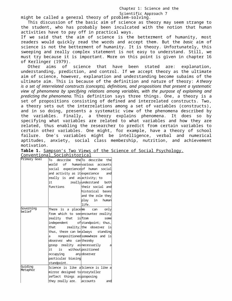
Sampson (1991) discusses two opposing views of science. There is theconventional or traditional perspective and then there is thesociohistorical perspective. The conventional view perceives science as amirror of nature or a windowpane of clear glass that presents nature withoutbias or distortion. The goal here is to describe with the highest degree ofaccuracy what the world really looks like. Here Sampson states that scienceis an objective referee. Its job is to “resolve disagreements anddistinguish what is true and correct from what is not.” When theconventional view of science is unable to resolve the dispute, it only meansthat there is insufficient data or information to do so. Conventionalists,however, feel it is only a matter of time before the truth is apparent.
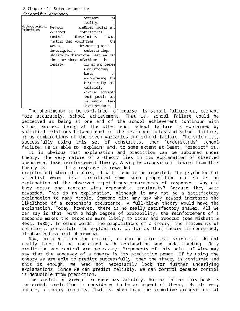
The sociohistorical view sees science as a story. The scientists arestorytellers. Here the idea is that reality can only be discovered by thestories that can be told about it. Here, this approach is unlike theconventional view in that there is no neutral arbitrator. Every story willbe flavored by the storyteller’s orientation. As a result there is no singletrue story. Sampson’s table comparing these two are reproduced in Table 1.
Even though Sampson gives these two views of science in light of socialpsychology, his presentation has applicability in all areas of thebehavioral science.THE AIMS OF SCIENCE, SCIENTIFIC EXPLANATION, AND THEORYThe basic aim of science is theory. Perhaps less cryptically, the basic aimof science is to explain natural phenomena. Such explanations are calledtheories. Instead of trying to explain each and every separate behavior ofchildren, the scientific psychologist seeks general explanations thatencompass and link together many different behaviors. Rather than try toexplain children's methods of solving arithmetic problems, for example, thescientist seeks general explanations of all kinds of problem-solving. It
Chapter 1: Science and the Scientific Approach 7
might be called a general theory of problem-solving.This discussion of the basic aim of science as theory may seem strange to
the student, who has probably been inculcated with the notion that humanactivities have to pay off in practical ways.If we said that the aim of science is the betterment of humanity, mostreaders would quickly read the words and accept them. But the basic aim ofscience is not the betterment of humanity. It is theory. Unfortunately, thissweeping and really complex statement is not easy to understand. Still, wemust try because it is important. More on this point is given in chapter 16of Kerlinger (1979).
Other aims of science that have been stated are: explanation,understanding, prediction, and control. If we accept theory as the ultimateaim of science, however, explanation and understanding become subaims of theultimate aim. This is because of the definition and nature of theory: A theoryis a set of interrelated constructs (concepts), definitions, and propositions that present a systematicview of phenomena by specifying relations among variables, with the purpose of explaining andpredicting the phenomena. This definition says three things. One, a theory is aset of propositions consisting of defined and interrelated constructs. Two,a theory sets out the interrelations among a set of variables (constructs),and in so doing, presents a systematic view of the phenomena described bythe variables. Finally, a theory explains phenomena. It does so byspecifying what variables are related to what variables and how they arerelated, thus enabling the researcher to predict from certain variables tocertain other variables. One might, for example, have a theory of schoolfailure. One's variables might be intelligence, verbal and numericalaptitudes, anxiety, social class membership, nutrition, and achievementmotivation.Table 1. Sampson’s Two Views of the Science of Social Psychology.Conventional __ Sociohistorical Primary Goal To describe the
world of humansocial experienceand activity as itreally is and asit reallyfunctions
To describe thevarious accountsof human socialexperience andactivity; tounderstand boththeir social andhistorical basesand the role theyplay in humanlife.
Governingbelief There is a place
from which to seereality that isindependent ofthat reality;thus, there can bea nonpositionedobserver who cangrasp reality asit is withoutoccupying anyparticular biasingstandpoint.
We can onlyencounter realityfrom somestandpoint; thus,the observer isalways standingsomewhere and istherebynecessarily apositionedobserver
GuidingMetaphor Science is like a
mirror designed toreflect things asthey really are.
Science is like astorytellerproposingaccounts and
8 Chapter 1: Science and the Scientific Approach
versions ofreality.
MethodologicalPriorities Methods are
designed tocontrol thosefactors that wouldweaken theinvestigator’sability to discernthe true shape ofreality.
Broad social andhistoricalfactors alwaysframe theinvestigator’sunderstanding;the best we canachieve is aricher and deeperunderstandingbased onencountering thehistorically andculturallydiverse accountsthat people usein making theirlives sensible.
The phenomenon to be explained, of course, is school failure or, perhapsmore accurately, school achievement. That is, school failure could beperceived as being at one end of the school achievement continuum withschool success being at the other end. School failure is explained byspecified relations between each of the seven variables and school failure,or by combinations of the seven variables and school failure. The scientist,successfully using this set of constructs, then "understands" schoolfailure. He is able to "explain" and, to some extent at least, "predict" it.
It is obvious that explanation and prediction can be subsumed undertheory. The very nature of a theory lies in its explanation of observedphenomena. Take reinforcement theory. A simple proposition flowing from thistheory is: If a response is rewarded(reinforced) when it occurs, it will tend to be repeated. The psychologicalscientist whom first formulated some such proposition did so as anexplanation of the observed repetitious occurrences of responses. Why didthey occur and reoccur with dependable regularity? Because they wererewarded. This is an explanation, although it may not be a satisfactoryexplanation to many people. Someone else may ask why reward increases thelikelihood of a response's occurrence. A full-blown theory would have theexplanation. Today, however, there is no really satisfactory answer. All wecan say is that, with a high degree of probability, the reinforcement of aresponse makes the response more likely to occur and reoccur (see Nisbett &Ross, 1980). In other words, the propositions of a theory, the statements ofrelations, constitute the explanation, as far as that theory is concerned,of observed natural phenomena.
Now, on prediction and control, it can be said that scientists do notreally have to be concerned with explanation and understanding. Onlyprediction and control are necessary. Proponents of this point of view maysay that the adequacy of a theory is its predictive power. If by using thetheory we are able to predict successfully, then the theory is confirmed andthis is enough. We need not necessarily look for further underlyingexplanations. Since we can predict reliably, we can control because controlis deducible from prediction.
The prediction view of science has validity. But as far as this book isconcerned, prediction is considered to be an aspect of theory. By its verynature, a theory predicts. That is, when from the primitive propositions of

Chapter 1: Science and the Scientific Approach 9
a theory we deduce more complex ones, we are in essence "predicting." Whenwe explain observed phenomena, we are always stating a relation between,say, the class A and the class B. Scientific explanation inheres inspecifying the relations between one class of empirical events and another,under certain conditions. We say: If A, then B, A and B referring to classesof objects or events.2 But this is prediction, prediction from A to B. Thusa theoretical explanation implies prediction. And we come back to the ideathat theory is the ultimate aim of science. All else flows from theory.
There is no intention here to discredit or denigrate research that is notspecifically and consciously theory-oriented. Much valuable socialscientific and educational research is preoccupied with the shorter- rangegoal of finding specific relations; that is, merely to discover a relationis part of science. The ultimately most usable and satisfying relations,however, are those that are the most generalized, those that are tied toother relations in a theory.
The notion of generality is important. Theories, because they aregeneral, apply to many phenomena and to many people in many places. Aspecific relation, of course, is less widely applicable. If, for example,one finds that test anxiety is related to test performance. This finding,though interesting and important, is less widely applicable and lessunderstood than finding a relation in a network of interrelated variablesthat are parts of a theory. Modest, limited, and specific research aims,then, are good. Theoretical research aims are better because, among otherreasons, they are more general and can be applied to a wide range ofsituations. Additionally, when both a simple theory and a complex one existand both account for the facts equally well, the simple explanation ispreferred. Hence in the discussion of generalizability, a good theory isalso parsimonious. However, a number of incorrect theories concerning mentalillness persist because of this parsimony feature. Some still believe thatindividuals are possessed with demons. Such an explanation is simple whencompared to psychological and/or medical explanations.
Theories are tentative explanations. Each theory is evaluated empiricallyto determine how well it predicts new findings. Theories can be used toguide one’s research plan by generating testable hypotheses and to organizefacts obtained from the testing of the hypotheses. A good theory is one thatcannot fit all observations. One should be able to find an occurrence thatwould contradict it. Blondlot’s theory of N-Rays is an example of a poortheory. Blondlot claimed that all matter emitted N-Rays (Weber, 1973).Although N-Rays was later demonstrated to be nonexistent, Barber (1976)reported that nearly 100 papers were published in a single year on N-Rays inFrance. Blondlot even developed elaborate equipment for the viewing of N-Rays. Scientists claiming they 1 saw N-Rays only added support to Blondlot’stheory and findings. However, when a person did not see N- Rays, Blondlotclaimed that the person’s eyes were not sensitive enough or the person didnot set up the instrument correctly. No possible outcome was taken asevidence against the theory. In more recent times, another faulty theorythat took over 75 years to debunk concerned the origin of peptic ulcers. In1910 Schwartz (as reported in Blaser, 1996) had claimed that he had firmlyestablished the cause of ulcers. He stated that peptic ulcers were due to2 Statements of the form "If p, then q," called conditional statements in logic,
are the core of scientific inquiry. They and the concepts or variables that go into them are the central ingredient of theories. The logical foundation of scientific inquiry that underlies much of the reasoning in this book is outlinedin Kerlinger(1977).
10 Chapter 1: Science and the Scientific Approachstomach acids. In the years that followed, medical researchers devoted theirtime and energy toward treating these ulcers by developing medication toeither neutralize the acids or block them. These treatments were nevertotally successful and they were expensive. However in 1985, J. Robin Warrenand Barry Marshall (as reported in Blaser, 1996) discovered that the heliocbacter pylori was the real culprit for stomach ulcers. Almost all cases ofthis type of ulcers were successfully treated with antibiotics and for aconsiderably lower. For 75 years no possible outcome was taken as evidenceagainst this stress-acid theory of ulcers.SCIENTIFIC RESEARCH A DEFINITION
It is easier to define scientific research than it is to define science.It would not be easy, however, to get scientists and researchers to agree onsuch a definition. Even so, we attempt one here:
Scientific research is systematic, controlled, empirical, amoral, publicand critical investigation of natural phenomena. It is guided by theory andhypotheses about the presumed relations among such phenomena.
This definition requires little explanation since it is mostly acondensed and formalized statement of much that was said earlier or thatwill be said soon. Two points need emphasis, however. First, when we saythat scientific research is systematic and controlled, we mean, in effect,that scientific investigation is so ordered that investigators can havecritical confidence in research outcomes. As we shall see later, scientificresearch observations are tightly disciplined. Moreover, among the manyalternative explanations of a phenomenon, all but one are systematicallyruled out. One can thus have greater confidence that a tested relation is asit is than if one had not controlled the observations and ruled outalternative possibilities. In some instances a cause-and-effect relationshipcan be established.
Second, scientific investigation is empirical. If the scientist believessomething is so, that belief must somehow or other put to an outsideindependent test. Subjective belief, in other words, must be checked againstobjective reality. Scientists must always subject their notions to the courtof empirical inquiry and test. Scientists are hypercritical of the resultsof their own and others' research. Every scientist writing a research reporthas other scientists reading what one writes while he or she writes it.Though it is easy to err, to exaggerate, to overgeneralize when writing upone's own work, it is not easy to escape the feeling of scientific eyesconstantly peering over one's shoulder.
In science there is peer review. This means that others of equal trainingand knowledge are called upon to evaluate another scientists work before itis published in scientific journals. There are both positive and negativepoints concerning this. It is through peer review that fraudulent studieshave been exposed. The essay written by R. W. Wood (1973) on his experienceswith Professor Blondlot of France concerning the nonexistence of N-raysgives a clear demonstration of peer review. Peer review works very well forscience and it promotes quality research. The system however is not perfect.There are occasions where peer review worked against science. This isdocumented throughout history with people such as Kepler, Galileo,Copernicus, Jenner, and Semelweiss. The ideas of these individuals were justnot popular with their peers. More recently in psychology, the works of JohnGarcia on the biological constraints on learning went contrary to his peers.Garcia managed to publish his findings in a journal (Bulletin of thePsychonomic Society) that did not have peer review. Others who read Garcia’swork and replicated it found Garcia’s work to be valuable. In the large
Chapter 1: Science and the Scientific Approach 11
majority of cases, peer review of science is beneficial.Thirdly, knowledge obtained scientifically is not subject to moral
evaluation. The results are neither considered “bad” or “good,” but in termsof its validity and reliability. The scientific method is however subject toissues of morality. That is, scientists are held responsible for the methodsused in obtaining scientific knowledge. In psychology, codes of ethics areenforced to protect those under study. Science is a cooperative venture.Information obtained from science is available to all. Plus the scientificmethod is well known and available to all that chooses to use it.THE SCIENTIFIC APPROACHThe scientific approach is a special systematized form of all-reflectivethinking and inquiry. Dewey (1933/ 1991), in his influential How We Think,outlined ageneral paradigm of inquiry. The present discussion of the scientificapproach is based largely on Dewey's analysis.Problem-Obstacle-IdeaThe scientist will usually experience an obstacle to understanding, a vagueunrest about observed and unobserved phenomena, a curiosity as to whysomething is as it is. The first and most important step is to get the ideaout in the open, to express the problem in some reasonably manageable form.Rarely or never will the problem spring full-blown at this stage. Thescientist must struggle with it, try it out, and live with it. Dewey(1933/1991, p. 108) says, "There is a troubled, perplexed, trying situation,where the difficulty is, as it were, spread throughout the entiresituation, infecting it as a whole." Sooner or later, explicitly orimplicitly, the scientist states the problem, even if the expression of itis inchoate and tentative. Here the scientist intellectualizes, as (1933/1991 p. 109) puts it, "what at first is merely anemotional quality of the whole situation."' In some respects, this is themost difficult and most important part of the whole process. Without somesort of statement of the problem, the scientist can rarely go further andexpect the work to be fruitful. With some researchers, the idea may comefrom speaking to a colleague or observing a curious phenomenon. The ideahere is that the problem usually begins with vague and/or unscientificthoughts or unsystematic hunches. It then goes through a step of refinement.HypothesisAfter intellectualizing the problem, after referring to past experiences forpossible solutions, after observing relevant phenomena, the scientist mayformulate a hypothesis. A hypothesis is a conjectural statement, a tentativeproposition about the relation between two or more phenomena or variables.Our scientist will say, "If such-and-such occurs, then so-and-so results."Reasoning-Deduction
This step or activity is frequently overlooked or underemphasized. It isperhaps the most important part of Dewey's analysis of reflective thinking.The scientist deduces the consequences of the hypothesis he has formulated.Conant (1951), in talking about the rise of modern science, said that thenew element added in the seventeenth century was the use ofdeductive reasoning. Here is where experience, knowledge, and perspicacityare important.
Often the scientist, when deducing the consequences of a formulatedhypothesis, will arrive at a problem quite different from the one startedwith. On the other hand, the deductions may lead to the belief that theproblem cannot be solved with present technical tools. For example, beforemodern statistics was developed, certain behavioral research problems were
12 Chapter 1: Science and the Scientific Approachinsoluble. It was difficult, if not impossible, to test two or threeinterdependent hypotheses at one time. It was next to impossible to test theinteractive effect of variables. And we now have reason to believe thatcertain problems are insoluble unless they are tackled in a multivariatemanner. An example of this is teaching methods and their relation toachievement and other variables. It is likely that teaching methods, per se,do not differ much if we study only their simple effects. Teaching methodsprobably work differently under different conditions, with differentteachers, and with different pupils. It is said that the methods "interact"with the conditions and with the characteristics of teachers and of pupils.Simon (1987) stated another example of this. Simon (1987) pointed out that aresearch on pilot training proposed by Williams and Adelson in 1954 couldnot be carried out using traditional experimental research methods. Thestudy proposed to study 34 variables and their influence on pilot training.Using traditional research methods, the number of variables under study wastoo overwhelming. Over 20 years later, Simon (1976, 1984) showed that suchstudies could be effectively studied using economical multifactor designs.
An example may help us understand this reasoning-deduction step. Supposean investigator becomes intrigued with aggressive behavior. The investigatorwonders why people are often aggressive in situations where aggressivenessmay not be appropriate. Personal observation leads to the notion thataggressive behavior seems to occur when people have experienced difficultiesof one kind or another. (Note the vagueness of the problem here.) Afterthinking for some time, reading the literature for clues, and making furtherobservations, the hypothesis is formulated: Frustration leads to aggression."Frustration" is defined as prevention from reaching a goal and "aggression"as behavior characterized by physical or verbal attack on other persons orobjects.
What follows from this is a statement like: If frustration leads toaggression, then we should find a great deal of aggression among childrenwho are in schools that are restrictive, schools that do not permit childrenmuch freedom and self-expression. Similarly, in difficult social situationsassuming such situations are frustrating, we should expect more aggressionthan is "usual." Reasoning further, if we give experimental subjectsinteresting problems to solve and then prevent them from solving them, wecan predict some kind of aggressive behavior. In a nutshell, this process ofmoving from a broader picture to a more specific one is called deductivereasoning.
Reasoning may, as indicated above, change the problem. We may realizethat the initial problem was only a special case of a broader, morefundamental and important problem. We may, for example startwith a narrower hypothesis: Restrictive school situations lead to negativismin children. Then we can generalize the problem to the form: Frustrationleads to aggression. While this is a different form of thinking from thatdiscussed earlier, it is important because of what could almost be calledits heuristic quality. Reasoning can help lead to wider, more basic, andthus more significant problems, as well as provide operational (testable)implications of the original hypothesis. This type of reasoning is calledinductive reasoning. It starts from particular facts and moves to a generalstatement or hypothesis. If one is not careful, this method could lead tofaulty reasoning. This is due to the method’s natural tendency to excludeother data that do not fit the hypothesis. The inductive reasoning method isinclined to look for supporting data rather than refuting evidence.
Consider the classical study by Peter Wason (Wason and Johnson-Laird,
Chapter 1: Science and the Scientific Approach 13
1972) that has been a topic of much interest (Hoch, 1986; Klayman and Ha,1987). In this study, students were asked to discover a rule theexperimenter had in mind that generated a sequence of numbers. One examplewas to generate a rule for the following sequence of numbers: “3, 5, 7.”Students were told that they could ask about other sequences. Students wouldreceive feedback on each sequence proposed as to whether it fits or does notfit the rule the experimenter had in mind. When the students felt confident,they could put forth the rule. Some students would offer “9, 11, 13.” Theyare told that this sequence fits the rule. They may then follow with “15,17, 19.” And again they are told that this sequence fits. The students thenmay offer as their answer: “The rule is three consecutive odd numbers.” Theywould be told that this is not the rule. Others that would be offered aftersome more proposed sequences are “increasing numbers in increments of two,or odd numbers in increments of two.” In each of these, they are told thatit is not the rule that the experimenter was thinking of. The actual rule inmind was “any three increasing positive numbers.” Had the students’ proposedthe sequences “8, 9, 10” or “1, 15, 4500” they would have been told thatthese also fit the rule. Where the students made their error was in testingonly the cases that fitted their first proposed sequence that confirmedtheir hypothesis.
Although oversimplified, the Wason study demonstrated what could happenin actual scientific investigations. A scientist could easily be locked intorepeating the same type of experiment that always supports the hypothesis.Observation-Test-Experiment
It should be clear by now that the observation-test- experiment phase isonly part of the scientific enterprise. If the problem has been well stated,the hypothesis or hypotheses adequately formulated, and the implications ofthe hypotheses carefully deduced, this step is almost automatic-assumingthat the investigator is technically competent.
The essence of testing a hypothesis is to test the relation expressed bythe hypothesis. We do not test variables, as such; we test the relationbetween the variables. Observation, testing, and experimentation are for onelarge purpose: putting the problem relation to empirical test. To testwithout knowing at least fairly well what and why one is testing is toblunder. Simply to state a vague problem, like ‘ How does Open Educationaffect learning?’ and then to test pupils in schools presumed to differ in"openness," or to ask: What are the effects of cognitive dissonance? andthen, after experimental manipulations to create dissonance, to search forpresumed effects could lead only to questionable information. Similarly, tosay one is going to study attribution processes without really knowing whyone is doing it or without stating relations between variables is researchnonsense.
Another point about testing hypotheses is that we usually do not testhypotheses directly. As indicated in the previous step on reasoning, we testdeduced implications of hypotheses. Our test hypothesis may be: "Subjectstold to suppress unwanted thoughts will be more preoccupied with them thansubjects who are given a distraction." This was deduced from a broader andmore general hypothesis: “Greater efforts to suppress an idea leads togreater preoccupation with the idea." We do not test "suppression of ideas"nor "preoccupation." We test the relation between them, in this case therelation between suppression of unwanted thoughts and the level ofpreoccupation. (see Wegner, Schneider, Carter and White, 1987; Wegner, 1989)
Dewey emphasized that the temporal sequence of reflective thinking orinquiry is not fixed. We can repeat and reemphasize what he says in our own

14 Chapter 1: Science and the Scientific Approachframework. The steps of the scientific approach are not neatly fixed. Thefirst step is not neatly completed before the second step begins. Further,we may test before adequately deducing the implications of the hypothesis.The hypothesis itself may seem to need elaboration or refinement as a resultof deducingimplications from it. Hypotheses and their expression will often be foundinadequate when implications are deduced from them. A frequent difficultyoccurs when a hypothesis is so vague that one deduction is as good asanother-that is, the hypothesis may not yield to precise test.
Feedback to the problem, the hypotheses, and, finally, the theory of theresults of research is highly important. Learning theorists and researchers,for example, have frequently altered their theories andresearch as a result of experimental findings (see Malone, 1991; Schunk,1996; Hergenhahn, 1996). Theorists and researchers have been studying theeffects of early environment and training on later development. Kagan andZentner (1996) reviewed the results of 70 studies concerned with therelation between early life experiences and psychopathology in adulthood.They found that juvenile delinquency could be predicted by the amount ofimpulsivity detected at preschool age. Lynch, Short and Chua (1995) foundthat musical processing was influenced by perceptual stimulation an infantexperienced at age 6 months to 1 year. These and other research have yieldedvaried evidence converging on this extremelyimportant theoretical and practical problem. Part of the essential core ofscientific research is the constant effort to replicate and check findings,to correct theory on the basis of empirical evidence, and to find betterexplanations of natural phenomena. One can even go so far as to say thatscience has a cyclic aspect. A researcher finds, say, that A is related to Bin such- and-such a way. Then more research is conducted to determine underwhat other conditions A is similarly related to B. Other researcherschallenge this theory and this research, offering explanations and evidenceof their own. The original researcher, it is hoped, alters one’s work in thelight of new data. The process never ends.
Let us summarize the so-called scientific approach to inquiry. Firstthere is doubt, a barrier, an indeterminate situation crying out to be madedeterminate. The scientist experiences vague doubts, emotional disturbance,and inchoate ideas. There is a struggle to formulate the problem, even ifinadequately. The scientist then studies the literature, scans one’s ownexperience and the experience of others. Often the researcher simply has towait for an inventive leap of the mind. Maybe it will occur; maybe not. Withthe problem formulated, with the basic question or questions properly asked,the rest is much easier. Then the hypothesis is constructed, after which itsempirical implications are deduced. In this process the original problem,and of course the original hypothesis, may be changed. It may be broadenedor narrowed. It may even be abandoned. Last, but not finally, the relationexpressed by the hypothesis is tested by observation and experimentation. Onthe basis of the research evidence, the hypothesis is supported or rejected.This information is then fed back to the original problem, and the problemis kept or altered as dictated by the evidence. Dewey pointed out that onephase of the process may be expanded and be of great importance, another maybe skimped, and there may be fewer or more steps involved. Research israrely an orderly business anyway. Indeed, it is much more disorderly thanthe above discussion may imply. Order and disorder, however, are not ofprimary importance. What is much more important is the controlledrationality of scientific research as a process of reflective inquiry, the
Chapter 1: Science and the Scientific Approach 15
interdependent nature of the parts of the process, and the paramountimportance of the problem and its statement.Study SuggestionSome of the content of this chapter is highly controversial. The viewsexpressed are accepted by some thinkers and rejected by others. Readers canenhance understanding of science and its purpose, the relation betweenscience and technology, and basic and applied research by selective readingof the literature. Such reading can be the basis for class discussions.Extended treatment of the controversial aspects of science, especiallybehavioral science, is given in the first author’s book, Behavioral Research: AConceptual Approach. New York: Holt, Rinehart and Winston, 1979, chaps. 1, 15,and 16. Many fine articles on science and research have been published inscience journals and philosophy of science books. Here are some of them.Included is also a special report in Scientific American. All are pertinent tothis chapter's substance.Barinaga, M. (1993). Philosophy of science: Feminists find gender everywhere
in science. Science, 260, 392-393. Discusses the difficulty of separatingcultural views of women and science. Talks about science as apredominantly male field.
Editors of Scientific American. Science versus antiscience. (Special report).January 1997, 96101. Presents three different anti-science movements:creationist, feminist, and media.
Hausheer, J. & Harris, J. (1994). In search of a brief definition ofscience. The Physics
Teacher, 32(5), 318. Mentions that any definition of science must includeguidelines for evaluating theory and hypotheses as either science ornonscience.Holton, G. (1996). The controversy over the end of science. Scientific American,
273(10), 191. This is an article concerned with the development of twocamps of thought: the
linearists and the cyclists. The Linearists take a more conventionalperspective of science. The cyclists see science as degenerating withinitself.Horgan, J. (1994). Anti-omniscience: Aneclectic gang of thinkers pushes at knowledge’s limits. Scientific American,271, 20-22.Discusses the limits of science. Also see Horgan, J. (1997). The end of science.New York: Broadway Books.Miller, J. A (1994). Postmodern attitude toward science. Bioscience, 41(6), 395.
Discuses the reasons some educators and scholars in the humanities haveadopted a hostile attitude toward science.Smith, B. (1995). Formal ontology, common sense and cognitive science.
International Journal of Human-Computer Studies, 43(5-6), 641-667. An article examiningcommon sense and cognitive science.
Timpane, J. (1995). How to convince a reluctant scientist. Scientific American,272, 104. This article warns that too much originality in science wouldlead to non-acceptance and difficulty of understanding. It also discusseshow scientific acceptance is governed by both old and new data and thereputation of the scientist.
Chapter Outline-Summary1. To understand complex human behavior, one must understand the scientific

16 Chapter 1: Science and the Scientific Approachlanguage and approach.2. Science is a systematic and controlled extension of common sense. There
are 5 differences between science and common sensea) science uses conceptual schemes and theoretical structuresb) science systematically and empirically tests theories and hypothesesc) science attempts to control possible extraneous causesd) science consciously and systematically pursues relationse) science rules out metaphysical (untestable) explanations
3. Peirce’s Four Methods of Knowinga) method of tenacity -- influenced by established past beliefsb) method of authority -- influenced by the weight of tradition or public
sanctionc) a priori method -- also known as the method of intuition. Natural
inclination toward the truth.d) method of science - self-correcting. Notions are testable and
objective4. The stereotype of science has hindered understanding of science by thepublic5. Views, functions of science
a) static view sees science contributing scientific information to world.Science adds to the body of information and present state of knowledge.
b) dynamic view is concerned with the activity of science. Whatscientists do. With this comes the heuristic view of science. This is one ofselfdiscovery. Science takes risks and solves problems.6. Aims of science
a) develop theory and explain natural phenomenonb) promote understanding and develop predictions7. A theory has 3 elements
a) set of properties consisting of defined and interrelated constructsb) systematically sets the interrelations among a set of variables.
c) explains phenomenon8. Scientific research is systematic, controlled, empirical and critical
investigation of natural phenomenon. It is guided by theory andhypotheses about presumed relations among such phenomenon. It is alsopublic and amoral.
9. The scientific approach according to Dewey is made up of the following:a) Problem-Obstacle-Idea -- formulate the research problem or questionto be solved.b) Hypothesis -- formulate a conjectural statement about the relationbetween phenomenon or variablesc) Reasoning-Deduction -- scientist deduces the consequences of thehypothesis. This can lead to a more significant problem and provide ideas onhow the hypothesis can be tested in observable terms.d) Observation-Test-Experiment- this is the data collection and analysisphase. The results of the research conducted are related back to theproblem.
Chapter 2: Problems and Hypothese 17Chapter 2
Problems and HypothesesMANY PEOPLE think that science is basically a factgathering activity. It isnot. As M. R. Cohen (1956/ 1997, p. 148) says:There is.. no genuine progress in scientific insightthrough the Baconian method of accumulatingempirical facts without hypotheses or anticipation of nature. Without someguiding idea we do not know what facts to gather... we cannot determine whatis relevant and what is irrelevant.The scientifically uninformed person often has the idea that the scientistis a highly objective individual who gathers data without preconceivedideas. Poincare (1952/1996, p. 143) long ago pointed out how wrong this ideais. He said: “It is often said that experiments should be made withoutpreconceived ideas. That is impossible. Not only would it make everyexperiment fruitless, but even if we wished to doso, it could not be done.PROBLEMSIt is not always possible for a researcher to formulate the problem simply,clearly, and completely. The research may often have only a rather general,diffuse, even confused notion of the problem. This is in the nature of thecomplexity of scientific research. It may even take an investigator years ofexploration, thought, and research before the researcher can clearly statethe questions. Nevertheless, adequate statement of the research problem isone of the most important parts of research. The difficulty of stating aresearch problem satisfactorily at a given time should not allow us to losesight of the ultimate desirability and necessity of doing so.
Bearing this difficulty in mind, a fundamental principle can be stated:If one wants to solve a problem, one must generally know what the problemis. It can be said that a large part of the solution lies in knowing what itis one is trying to do. Another part lies in knowing what a problem is andespecially what a scientific problem is.
What is a good problem statement? Although research problems differgreatly and there is no one "right" way to state a problem, certaincharacteristics of problems and problem statements can be learned and usedto good advantage. To start, let us take two or three examples of publishedresearch problems and study their characteristics. First, take the problemof the study by Hurlock (1925)3 mentioned in Chapter 1: What is the effectson pupil performance of different types of incentives? Note that the problemis stated in question form. The simplest way is here the best way. Also notethat the problem states a relation between variables, in this case betweenthe variables incentives and pupil performance (achievement). ("Variable"will be formally defined in Chapter 3. For now, a variable is the name of aphenomenon, or a construct, that takes a set of different numerical values.)
A problem, then, is an interrogative sentence or statement that asks: Whatrelation exists between two or more variables? The answer is what is beingsought in the research. A problem in most cases will have two or morevariables. In the Hurlock example, the problem statement relates incentiveto pupil performance. Another problem, studied in an influential experimentby Bahrick (1984, 1992), is associated with the age-old questions: How much
3 When citing problems and hypotheses from the literature, we have not always used the words of the authors. In fact, the statements of many of the problems are ours and not those of the cited authors. Some authors use only problem statements; some use only hypotheses; others use both.
18 Chapter 2: Problems andHypothesesof what you are studying now will you remember 10 years from now? How muchof it will you remember 50 years from today? How much of it will youremember later if you never used it? Formally Bahrick asks: Does semanticmemory involve separate processes? One variable is the amount of time sincethe material was first learned, a second would be the quality of originallearning and the other variable is remembering (or forgetting). Stillanother problem, by Little, Sterling and Tingstrom (1996), is quitedifferent: Does geographic and racial cues influence attribution (perceivedblame)? One variable geographical cues, a second would be racial informationand the other is attribution. Not all research problems clearly have two ormore variables. For example, in experimental psychology, the research focusis often on psychological processes like memory andcategorization. In her justifiably well known and influential study ofperceptual categories, Rosch(1973) in effect asked the question: Are therenonarbitrary ("natural") categories of color and form? Although the relationbetween two or more variables is not apparent in this problem statement, inthe actual research the categories were related to learning.Toward the end of this book we will see that factor analytic researchproblems also lack the relation form discussed above. In most behavioralresearch problems, however, the relations among two or more variables arestudied, and we will therefore emphasize such relation statements.Criteria of Problems and Problem Statements
There are three criteria of good problems and problem statements. One,the problem should express a relation between two or more variables. Itasks, in effect, questions like: Is A related to B? How are A and B relatedto C? How is A related to B under conditions C and D? The exceptions to thisdictum occur mostly in taxonomic or methodological research.
Two, the problem should be stated clearly and unambiguously in questionform. Instead of saying, for instance, "The problem is...” or "The purposeof this study is... “, ask a question. Questions have the virtue of posingproblems directly. The purpose of a study is not necessarily the same as theproblem of a study. The purpose of the Hurlock study, for instance, was tothrow light on the use of incentives in school situations. The problem wasthe question about the relation between incentives and performance. Again,the simplest way is the best way: ask a question.
The third criterion is often difficult to satisfy. It demands that theproblem and the problem statement should be such as to imply possibilities ofempirical testing. A problem that does not contain implications for testingits stated relation or relations is not a scientific problem. This means notonly that an actual relation is stated, but also that the variables of therelation can somehow be measured. Many interesting and important questionsare not scientific questions simply because they are not amenable totesting. Certain philosophic and theological questions, while perhapsimportant to the individuals who consider them, cannot be tested empiricallyand are thus of no interest to the scientist as a scientist. Theepistemological question, "How do we know?," is such a question. Educationhas many interesting but nonscientific questions, such as, "Does democraticeducation improve the learning of youngsters?" "Are group processes good forchildren?" These questions can be called metaphysical in the sense that theyare, at least as stated, beyond empirical testing possibilities. The keydifficulties are that some of them are not relations, and most of theirconstructs are very difficult or impossible to so define that they can bemeasured.HYPOTHESES
Chapter 2: Problems and Hypothese 19
A hypothesis is a conjectural statement of the relation between two or morevariables. Hypotheses are always in declarative sentence form, and theyrelate, either generally or specifically, variables to variables. There aretwo criteria for "good" hypotheses and hypothesis statements. They are thesame as two of those for problems and problem statements. One, hypothesesare statements about the relations between variables. Two, hypotheses carryclear implications for testing the stated relations. These criteria mean,then, that hypothesis statements contain two or more variables that aremeasurable or potentiallymeasurable and that they specify how the variables are related.
Let us take three hypotheses from the literature and apply the criteriato them. The first hypothesis from a study by Wegner, et al (1987). seems todefy common sense: The greater the suppression of unwanted thoughts, thegreater the preoccupation with those unwanted thoughts (suppress now; obsesslater). Here a relation is stated between one variable, suppression of anidea or thought, and another variable, preoccupation or obsession. Since thetwo variables are readily defined and measured, implications for testing thehypothesis, too, are readily conceived. The criteria are satisfied. In theWegner, et al study, subjects were asked to not think about a “white bear.”Each time they did think of the white bear, they would ring a bell. Thenumber of bell rings indicated the level of preoccupation. A secondhypothesis is from a study by Ayres and Hughes (1986). This study’shypothesis is unusual. It states a relation in the so-called null form:Levels of noise ormusic has no effect on visual functioning. The relation is stated clearly:one variable, loudness of sound (like music), is related to anothervariable, visual functioning, by the words "has no effect on." On thecriterion of potential testability, however, we meet with difficulty. We arefaced with the problem of defining "visual functioning" and “loudness" sothey can be are measured. If we can solve this problem satisfactorily, thenwe definitely have a hypothesis. Ayres and Hughes did solve this by definingloudness as 107 decibels and visual functioning in terms of a score on avisual acuity task. And this hypothesis did lead to answering a questionthat people often ask: “Why do we turn down the volume of the car stereowhen we are looking for a street address?” Ayres and Hughes found a definitedrop in perceptual functioning when the level of music was at 107 decibels.
The third hypothesis represents a numerous and important class. Here therelation is indirect, concealed, as it were. It customarily comes in theform of a statement that Groups A and B will differ on some characteristic.For example: Women more often than men believe they should lose weight eventhough their weight is well within normal bounds (Fallon & Rozin, 1985).That is, women differ from men in terms of their perceived body shape. Notethat this statement is one step removed from the actual hypothesis, whichmay be stated: Perceived body shape is in part a function of gender. If thelatter statements were the hypothesis stated, then the first might be calleda subhypothesis, or a specific prediction based on the original hypothesis.
Let us consider another hypothesis of this type but removed one stepfurther. Individuals having the same or similar characteristics will holdsimilar attitudes toward cognitive objects significantly related to theoccupational role (Saal and Moore, 1993). ("Cognitive objects" are anyconcrete or abstract things perceived and "known" by individuals. People,groups, job or grade promotion, the government, and education are examples.)The relation in this case, of course, is between personal characteristicsand attitudes (toward a cognitive object related to the personal
20 Chapter 2: Problems andHypothesescharacteristic, for example, gender and attitudes toward others receiving apromotion). In order to test this hypothesis, it would be necessary to haveat least two groups, each with a different characteristic, and then tocompare the attitudes of the groups. For instance, as in the case of theSaal and Moore study, the comparison would be between men and women. Theywould be compared on their assessment of fairness toward a promotion givento a co-worker of the opposite or same sex. In this example, the criteriaare satisfied.THE IMPORTANCE OF PROBLEMS AND HYPOTHESES
There is little doubt that hypotheses are important and indispensabletools of scientific research. There are three main reasons for this belief.One, they are, so to speak, the working instruments of theory. Hypothesescan be deduced from theory and from other hypotheses. If, for instance, weare working on a theory of aggression, we are presumably looking for causesand effects of aggressive behavior. We might have observed cases ofaggressive behavior occurring after frustrating circumstances. The theory,then, might include the proposition: Frustration produces aggression(Dollard, Doob, Miller, Mowrer & Sears, 1939; Berkowitz, 1983; Dill &Anderson, 1995). From this broad hypothesis we may deduce more specifichypotheses, such as: To prevent children from reaching desired goals(frustration) will result in their fighting each other (aggression); ifchildren are deprived of parental love (frustration), they will react inpart with aggressive behavior.
The second reason is that hypotheses can be tested and shown to beprobably true or probably false. Isolated facts are not tested, as we saidbefore; only relations are tested. Since hypotheses are relationalpropositions, this is probably the main reason they are used in scientificinquiry. They are, in essence, predictions of the form, "If A, then B,"which we set up to test the relation between A and B. We let the facts havea chance to establish the probable truth or falsity of the hypothesis.
Three, hypotheses are powerful tools for the advancement of knowledgebecause they enable scientists to get outside themselves. Though constructedby humans, hypotheses exist, can be tested, and can be shown to be probablycorrect or incorrect apart from person's values and opinions. This is soimportant that we venture to say that there would be no science in anycomplete sense without hypotheses.
Just as important as hypotheses are the problems behind the hypotheses.As Dewey (1938/1982, pp. 105-107) has well pointed out, research usuallystarts with a problem. He says that there is first an indeterminatesituation in which ideas are vague, doubts are raised, and the thinker isperplexed. Dewey further points out that the problem is not enunciated,indeed cannot be enunciated, until one has experienced such an indeterminatesituation.
The indeterminacy, however, must ultimately be removed. Though it istrue, as stated earlier, that a researcher may often have only a general anddiffuse notion of the problem, sooner or later he or she has to have afairly clear idea of what the problem is. Though this statement seems self-evident, one of the most difficult things to do is to state one's researchproblem clearly and completely. In other words, you must know what you aretrying to find out. When you finally do know, the problem is a long waytoward solution.VIRTUES OF PROBLEMS AND HYPOTHESESProblems and hypotheses, then, have important virtues. One, they directinvestigation. The relations
Chapter 2: Problems and Hypothese 21
expressed in the hypotheses tell the investigator what to do. Two, problemsand hypotheses, because they are ordinarily generalized relationalstatements, enable the researcher to deduce specific empiricalmanifestations implied by the problems and hypotheses. We may say, followingGuida and Ludlow (1989): If it is indeed true that children in one type ofculture (Chile) have higher test anxiety than children of another type ofculture (White- Americans), then it follows that children in the Chileanculture should do more poorly in academics than children in the Americanculture. They should perhaps also have a lower self-esteem or more externallocus-of-control when it comes to school and academics.
There are important differences between problems and hypotheses.Hypotheses, if properly stated, can be tested. While a given hypothesis maybe too broad to be tested directly, if it is a "good" hypothesis, then othertestable hypotheses can be deduced from it. Facts or variables are nottested as such. The relations stated by the hypotheses are tested. And aproblem cannot be scientifically solved unless it is reduced to hypothesisform, because a problem is a question, usually of a broad nature, and is notdirectly testable. One does not test the questions: Does the presence orabsence of a person in a public restroom alter personalhygiene (Pedersen, Keithly and Brady, 1986)? Does group counseling sessionsreduce the level of psychiatric morbidity in police officers? (Doctor,Cutris and Issacs, 1994)? Instead, one tests one or more hypotheses impliedby these questions. For example, to study the latter problem, one mayhypothesize that police officers who attend stress reduction counselingsessions will take fewer sick days off than those police officers who didnot attend counseling sessions. The hypothesis in the former problem couldstate that the presence of a person in a public restroom will cause theother person to wash their hands.
Problems and hypotheses advance scientific knowledge by helping theinvestigator confirm or disconfirm theory. Suppose a psychologicalinvestigator gives a number of subjects three or four tests, among which isa test of anxiety and an arithmetic test. Routinely computing theintercorrelations between the three or four tests, one finds that thecorrelation between anxiety and arithmetic is negative. One concludes,therefore that the greater the anxiety the lower the arithmetic score. Butit is quite conceivable that the relation is fortuitous or even spurious.If, however, the investigator had hypothesized the relation on the basis oftheory, the investigator could have greater confidence in the results.Investigators who do not hypothesize relations in advance, in short, do notgive the facts a chance to prove or disprove anything. The words "prove" and"disprove" are not to be taken here in their usual literal sense. Ahypothesis is never really proved or disproved. To be more accurate weshould probably say something like: The weight of evidence is on the side ofthe hypothesis, or the weight of the evidence casts doubt on the hypothesis.Braithwaite(1953/1996 p. 14) says:“Thus the empirical evidence of its instance never proves the hypothesis: insuitable cases we may say that it establishes the hypothesis, meaning by thisthat the evidence makes it reasonable to accept the hypothesis; but it neverproves the hypothesis in the sense that the hypothesis is a logicalconsequence of the evidence."This use of the hypothesis is similar to playing a game of chance. The rulesof the game are set up in advance, and bets are made in advance. One cannotchange the rules after an outcome, nor can one change one's bets after

22 Chapter 2: Problems andHypothesesmaking them. That would not be "fair." One cannot throw the dice first andthen bet. Similarly, if one gathers data first and then selects a datum andcomes to a conclusion on the basis of the datum, one has violated the rulesof the scientific game. The game is not "fair" because the investigator caneasily capitalize on, say, two significant relations out of five tested.What happens to the other three? They are usually forgotten. But in a fairgame every throw of the dice is counted, in the sense that one either winsor does not win on the basis of the outcome of each throw.
Hypotheses direct inquiry. As Darwin pointed out over a hundred yearsago, observations have to be for or against some view if they are to be ofany use. Hypotheses incorporate aspects of the theory under test in testableor near-testable form. Earlier, an example of reinforcement theory was givenin which testable hypotheses were deduced from the general problem. Theimportance of recognizing this function of hypotheses may be shown by goingthrough the back door and using a theory that is very difficult, or perhapsimpossible, to test. Freud's theory of anxiety includes the construct ofrepression. Now, by repression Freud meant the forcing of unacceptable ideasdeep into the unconscious. In order to test the Freudian theory of anxietyit is necessary to deduce relations suggested by the theory. Thesedeductions will, of course, have to include the repression notion, whichincludes the construct of the unconscious. Hypotheses can be formulatedusing these constructs; in order to test the theory, they have to be soformulated. But testing them is another, more difficult matter because ofthe extreme difficulty of so defining terms such as "repression" and"unconscious" that they can be measured. To the present, no one hassucceeded in defining these two constructs without seriously departing fromthe original Freudian meaning and usage. Hypotheses, then, are importantbridges between theory and empirical inquiry.PROBLEMS, VALUES, AND DEFINITIONSTo clarify further the nature of problems and hypotheses, two or threecommon errors will now be discussed. First, scientific problems are notmoral and ethical questions. Are punitive disciplinary measures bad forchildren? Should an organization's leadership be democratic? What is thebest way to teach college students? To ask these questions is to ask valueand judgmental questions that science cannot answer. Many so-calledhypotheses are not hypotheses at all. For instance: The small-group methodof teaching is better than the lecture method. This is a value statement; itis an article of faith and not a hypothesis. If it was possible to state arelation between the variables, and if it was possible to define thevariables so as to permit testing the relation, then we might have ahypothesis. But there is no way to test value questions scientifically.
A quick and relatively easy way to detect value questions and statementsis to look for words such as "should," "ought," "better than" (instead of"greater than"). Also one can look for similar words that indicate culturalor personal judgments or preferences. Value statements, however, are tricky.While a "should" statement is obviously a value statement, certain otherkinds of statements are not so obvious. Take the statement: Authoritarianmethods of teaching lead to poor learning. Here there is a relation. But thestatement fails as a scientific hypothesis because it uses two valueexpressions or words, "authoritarian methods of teaching" and "poorlearning." Neither of which can be defined for measurement purposes withoutdeleting the words "authoritarian" and"poor."4
4 An almost classic case of the use of the word "authoritarian" is the statement
Chapter 2: Problems and Hypothese 23
Other kinds of statements that are not hypotheses or are poor ones arefrequently formulated, especially in education. Consider, for instance: Thecore curriculum is an enriching experience. Another type, too frequent, isthe vague generalization: Reading skills can be identified in the secondgrade; the goal of the unique individual is self-realization; Prejudice isrelated to certain personality traits.
Another common defect of problem statements often occurs in doctoraltheses: the listing of methodological points or "problems" as subproblems.These methodological points have two characteristics that make them easy todetect: (1) they are not substantive problems that spring from the basicproblem; and (2) they relate to techniques or methods of sampling,measuring, or analyzing. They are usually not in question form, but rathercontain the words "test," "determine," "measure," and the like. "Todetermine the reliability of the instruments used in this research," "Totest the significance of the differences between the means," and "To assignpupils at random to the experimental groups" are examples of this mistakennotion of problems and subproblems.GENERALITY AND SPECIFICITY OF PROBLEMS AND HYPOTHESES
One difficulty that the research worker usually encounters and thatalmost all students working on a thesis find annoying is the generality andspecificity of problems and hypotheses. If the problem is too general, it isusually too vague to be tested. Thus, it is scientifically useless, thoughit may be interesting to read. Problems and hypotheses that are too generalor too vague are common. For example: Creativity is a function of the self-actualization of the individual; Democratic education enhances sociallearning and citizenship; Authoritarianism in the college classroom inhibitsthe creative imagination of students. These are interesting problems. But,in their present form, they are worse than useless scientifically, becausethey cannot be tested and because they give one the spurious assurance thatthey are hypotheses that can "some day" be tested.
Terms such as "creativity," "self-actualization," "democracy,""authoritarianism," and the like have, at the present time at least, noadequate empirical 2referents. Now, it is quite true that we can define "creativity," say, in alimited way by specifying one or two creativity tests. This may be alegitimate procedure. Still, in so doing, we run the risk of getting faraway from the original term and its meaning. This is particularly true whenwe speak of artistic creativity. We are often willing to accept the risk inorder to be able to investigate important problems, of course. Yet termslike "democracy" are almost hopeless to define. Even when we do define it,we often find we have destroyed the original meaning ofthe term. An outstanding exception to this statement is Bollen's (1980)definition and measurement of "democracy." We will examine both insubsequent chapters.
The other extreme is too great specificity. Every student has heard thatit is necessary to narrow problems down to workable size. This is true. But,unfortunately, we can also narrow the problem out of existence. In general,the more specific the problem or hypothesis the clearer are its testingimplications. But triviality may be the price we pay. Researchers cannothandle problems that are too broad because they tend to be too vague for
sometimes heard among educators: The lecture method is authoritarian. This seems tomean that the speaker does not like the lecture method and is telling us that it isbad. Similarly, one of the most effective ways to criticize a teacher is to say that teacher is authoritarian.
24 Chapter 2: Problems andHypothesesadequate research operations. On the other hand, in their zeal to cut theproblems down to workable size or to find a workable problem, they may cutthe life out of it. They may make it trivial or inconsequential. A thesisfor instance, on the simple relation between the speed of reading and sizeof type, while important and maybe even interesting, is too thin by itselffor doctoral study. The doctoral student would need to expand on the topicby also recommending a comparison between genders and considering variablessuch as culture and family background. The researcher could possibly expandthe study to look at levels of illumination and font types. Too greatspecificity is perhaps a worse danger than too great generality. Theresearcher may be able to answer the specific question but will not be ableto generalize the finding to other situations or groups of people. At anyrate, some kind of compromise must be made between generality andspecificity. The ability effectively to make such compromises is a functionpartly of experience and partly of critical study of research problems.
Here are a few examples contrasting research problems stated as toogeneral or too specific:2. Although many studies of authoritarianism have been done with considerablesuccess, it is doubtful that we know what authoritarianism in the classroom means.For instance, an action of a teacher that is authoritarian in one classroom may notbe authoritarian in another classroom. The alleged democratic behavior exhibited byone teacher may even be called authoritarian if exhibited by another teacher. Suchelasticity is not the stuff of science.1.Too General: There are gender differences in game playing.
Too Specific: Tommy’s score will be 10 points higher than Carol’s onTetris Professional Gold.
About Right: Video game playing will result in a higher transfer oflearning for boys than girls.2. Too General: People can read large size lettersfaster than small size letters.Too Specific: Seniors at Duarte High School can read 24 point fonts faster
than 12 point fonts.About Right: A comparison of three different font sizes and visual acuity on
reading speed and comprehension.THE MULTIVARIABLE NATURE OF BEHAVIORAL RESEARCH AND PROBLEMS
Until now the discussion of problems and hypotheses has been pretty muchlimited to two variables, x and y. We must hasten to correct any impressionthat such problems and hypotheses are the norm in behavioral research.Researchers in psychology, sociology, education, and other behavioralsciences have become keenly aware of the multivariable nature of behavioralresearch. Instead of saying: Ifp, then q, it is often more appropriate tosay: If p1, p2,..., Pk, then q; or: If p then q, under conditions r, s, andt.
An example may clarify the point. Instead of simply stating thehypothesis: If frustration, then aggression, it is more realistic torecognize the multivariable nature of the determinants and influences ofaggression. This can be done by saying, for example: If high intelligence,middle class, male, and frustrated, then aggression. Or: If frustration,then aggression, under the conditions of high intelligence, middle class,and male. Instead of one x, we now have four x's. Although one phenomenonmay be the most important in determining or influencing another phenomenon,it is unlikely that most of the phenomena of interest to behavioralscientists are determined simply. It is much more likely that they aredetermined multiply. It is much more likely that aggression is the result of
Chapter 2: Problems and Hypothese 25
several influences working in complex ways. Moreover, aggression itself hasmultiple aspects. After all, there are different kinds of aggression.
Problems and hypotheses thus have to reflect the multivariable complexityof psychological, sociological, and educational reality. We will talk of onex and one y, especially in the early part of the book. However, it must beunderstood that behavioral research, which used to be almost exclusivelyunivariate in its approach, has become more and more multivariable. We havepurposely used the word “multivariable” instead of “multivariate” for animportant reason. Traditionally, “multivariate” studies are those that havemore than one y variable and one or more x variables. When we speak of one yand more than one x variable, we use the more appropriate term“multivariable” to make the distinction. For now, we will use "univariate"to indicate one x and one y. "Univariate," strictly speaking, also appliesto y. We will soon encounter multivariate conceptions and problems. Andlater parts of the book will be especially concerned with a multivariateapproach and emphasis. For a clear explanation on the differences betweenmultivariable and multivariate see Kleinbaum, Kupper, Muller and Nizam(1997).CONCLUDING REMARKS-THE SPECIAL POWER OF HYPOTHESES
One will sometimes hear that hypotheses are unnecessary in research. Somefeel that they unnecessarily restrict the investigative imagination, andthat the job of science and scientific investigation is to find out thingsand not to belabor the obvious. Some feel that hypotheses are obsolete, andthe like. Such statements are quite misleading. They misconstrue the purposeof hypotheses.
It can almost be said that the hypothesis is one of the most powerfultools yet invented to achieve dependable knowledge. We observe a phenomenon.We speculate on possible causes. Naturally, our culture has answers toaccount for most phenomena, many correct, many incorrect, many a mixture offact and superstition, many pure superstition. It is the business ofscientists to doubt most explanations of phenomena. Such doubts aresystematic. Scientists insist upon subjecting explanations of phenomena tocontrolled empirical test. In order to do this, they formulate theexplanations in the form of theories and hypotheses. In fact, theexplanations are hypotheses. Scientists simply discipline the business bywriting systematic and testable hypotheses. If an explanation cannot beformulated in the form of a testable hypothesis, then it can be consideredto be a metaphysical explanation and thus not amenable to scientificinvestigation. As such, it is dismissed by scientists as being of nointerest.
The power of hypotheses goes further than this, however. A hypothesis isa prediction. It says that if x occurs, y will also occur. That is, y ispredicted from x. If, then, x is made to occur (vary), and it is observedthat y also occurs (varies concomitantly), then the hypothesis is confirmed.This is more powerful evidence than simply observing, without prediction,the covarying of x and y. It is more powerful in the betting-game sensediscussed earlier. The scientist makes a bet that x leads to y. If, in anexperiment, x does lead to y, then one has won the bet. A person cannot justenter the game at any point and pick a perhaps fortuitous common occurrenceof x and y. Games are not played this way (at least in our culture). Thisperson must play according to the rules, and the rules in science are madeto minimize error and fallibility. Hypotheses are part of the rules of thescience game.
Even when hypotheses are not confirmed, they have power. Even when y does
26 Chapter 2: Problems andHypothesesnot covary with x, knowledge is advanced. Negative findings are sometimes asimportant as positive ones, since they cut down the total universe ofignorance and sometimes point up fruitful further hypotheses and lines ofinvestigation. But the scientist cannot tell positive from negative evidence unless one useshypotheses. It is possible to conduct research without hypotheses, of course,particularly in exploratory investigations. But it is hard to conceivemodern science in all its rigorous and disciplined fertility without theguiding power of hypotheses.Study Suggestions
1. Use the following variable names to writeresearch problems and hypotheses: frustration,academic achievement, intelligence, verbal ability, race, social class(socioeconomic status), sex, reinforcement, teaching methods occupationalchoice, conservatism, education, income, authority, need for achievement,group cohesiveness, obedience, social prestige, permissiveness.
2. Ten problems from the research literature are given below. Study themcarefully, choose two or three, and construct hypotheses based on them.
(a) Do children of different ethnic groups have different levels of testanxiety? (Guida and Ludlow, 1989).
(b) Does cooperative social situations lead to higher levels ofintrinsic motivation? (Hom, Berger, et al., 1994).
(c) Are affective responses influenced by people’s facial activity?(Strack, Martin and Stepper, 1988).
(d) Will jurors follow prohibitive judicial instructions andinformation? (Shaw and Skolnick, 1995).(e) What are the positive effects of using alternating pressure pads to
prevent pressure sores in homebound hospice patients? (Stoneberg,Pitcock, and Myton, 1986).
(f) What are the effects of early Pavlovian conditioning on later Pavlovianconditioning? (Lariviere and Spear, 1996).
(g) Does the efficacy of encoding information into long-term memory dependon the novelty of the information? (Tulving and Kroll, 1995).
(h) What is the effect of alcohol consumption on the likelihood of condomuse during causal sex? (MacDonald, Zanna and Fong, 1996).
(I) Are there gender differences in predicting retirement decisions? (Talagaand Beehr, 1995).
(j) Is the Good Behavior Game a viable intervention strategy for children ina classroom that require behavior change procedures? (Tingstrom, 1994).3.Ten hypotheses are given below. Discuss possibilities of testing them.
Then read two or three of the studies to see how the authors tested them.(a) Job applicants who claim a great deal of experience at nonexistent
tasks overstate their ability on real tasks. (Anderson, Warner andSpencer, 1984).
(b) In social situations, men misread women’s intended friendliness as asign of sexual interest. (Saal, Johnson and Weber, 1989)
(c) The greater the team success, the greater the attribution of each teammember toward one’s ability and luck. (Chambers and Abrami, 1991).
(d) Increasing interest in a task will increase compliance. (Rind, 1997).(e) Extracts from men’s perspiration can affect women’s menstrual cycle.
(Cutler, Preti, Kreiger and Huggins, 1986).(f) Physically attractive people are viewed with higher intelligence than
Chapter 2: Problems and Hypothese 27
non-attractive people. (Moran and McCullers, 1984).(g) One can receive help from a stranger if that stranger is similar to
oneself, or if the request is made at a certain distance. (Glick,DeMorest and Hotze, 1988).
(h) Cigarette smoking (nicotine) improves mental performance. (Spilich,June, and Remer, 1992).
(i) People stowing valuable items in unusual locations will have bettermemory of that location than
stowing valuable items in usual locations. (Winograd and Soloway, 1986).(j)Gay men with symptomatic HIV disease aresignificantly more distressed than gay men whoseHIV status is unknown. (Cochran and Mays, 1994).
4.Multivariate (for now, more than two dependent variables) problems andhypotheses have become common in behavioral research. To give the student apreliminary feeling for such problems, we here append several of them. Tryto imagine how you would do research to study them.(a) Do men and women differ in their perceptions of their genitals, sexual
enjoyment, oral sex and masturbation? (Reinholtz and Muehlenhard, 1995).(b) Are youthful smokers more extroverted while older smokers are more
depressed and withdrawn (Stein, Newcomb and Bentler, 1996)?(c) How much do teacher’s ratings of social skills for popular students
different from rejected students? (Stuart, Gresham and Elliot, 1991);(Frentz, Gresham, and Elliot, 1991).
(d) Do counselor-client matching on ethnicity, gender and languageinfluence treatment outcomes of school aged children? (Hall, Kaplan andLee, 1994).
(e) Are there any differences in the cognitive and functional abilities ofAlzheimer’s patients who reside at a special care unit versus thoseresiding at a traditional care unit? (Swanson, Maas, and Buckwalter,1994).
(f) Do hyperactive children with attention deficit differ fromnonhyperactive children with attention deficit on reading, spelling andwritten language achievement? (Elbert, 1993).
(g) Will perceivers see women who prefer the courtesy title of Ms. as beinghigher on instrumental qualities and lower on expressiveness qualitiesthan women who prefer traditional courtesy titles? (Dion and Cota, 1991).
(h) Will an empowering style of leadership increase team membersatisfaction and perceptions of team efficacy to increase teameffectiveness? (Kumpfer,Turner, Hopkins, and Librett, 1993)
(i) How do ethnicity, gender and socioeconomic background influencepsychosis-proneness: perceptual aberration, magical ideation andschizotypal personality (Porch, Ross, Hanks and Whitman, 1995).
(j) Does stimulus exposure have two effects, one cognitive and oneaffective, which in turn affect liking, familiarity, and recognitionconfidence and accuracy (Zajonc, 1980)?The Last two problems and studies are quite complex because the relations
stated are complex. The other problems and studies, though also complex,have only one phenomenon presumably affected by other phenomena, whereas thelast two problems have several phenomena influencing two or more other
28 Chapter 2: Problems andHypothesesphenomena. Readers should not be discouraged if they find these problems abit difficult. By the end of the book they should appear interesting andnatural.Chapter Summary1.Formulating the research problem is not an easytask. Researcher starts with a general, diffused and vague notion and thengradually refines it. Research problems differ greatly and there is no oneright way to state the problem.2. Three criteria of a good problem and problemstatement
a) The problem should be expressed as a relation between two or morevariables.
b) The problem should be put in the form of a question.c) The problem statement should imply the possibilities of empirical
testing.3. A hypothesis is a conjectural statement of therelation between two or more variables. It is put in the form of adeclarative statement. A criteria for a good hypothesis is the same as a)and b) in criteria of a good problem.4. Importance of problems and hypotheses.
a) It is a working instrument of science. It is a specific workingstatement of theory.b) Hypotheses can be tested and be predictive.c) Advances knowledge.5. Virtues of problems and hypothesesa) Directs investigation and inquiry
b) Enables research to deduce specific empirical manifestationsc) Serves as the bridge between theory and empirical inquiry.
6.Scientific problems are not moral or ethical questions. Science cannotanswer value or judgmental questions.
7.Detection of value questions: Look for words suchas “better than”, “should”, or “ought.”8.Another common defect of problem statements isthe listing of methodological points as subproblems.
a) they are not substantive problems that come directly from the basicproblem
b) they relate to techniques or methods of sampling, measuring, oranalyzing. Not in question form.9.On problems, there is a need to compromise between being too general and
too specific. The ability to do this comes with experience.10. Problems and hypotheses need to reflect the multivariate complexity of
behavioral science reality.11. The hypothesis is one of the most powerful tools invented to achieve
dependable knowledge. It has the power of prediction. Negative findingfor a hypothesis can serve to eliminate one possible explanation and openup other hypotheses and lines of investigation.

22 Chapter 2: Problems and Hypotheses

Chapter 3: Constructs, Variables and Definitions 23
Chapter 3Constructs, Variables and DefinitionsSCIENTISTS operate on two levels: theory- hypothesis-construct and observation.More accurately, they shuttle back and forth between these levels. Apsychological scientist may say, "Early deprivation produces learningdeficiency." This statement is a hypothesis consisting of two concepts, "earlydeprivation" and "learning deficiency," joined by a relation word, "produces."It is on the theory hypothesis-construct level. Whenever scientists utterrelational statements and whenever they use concepts, or constructs as we shallcall them, they are operating at this level.
Scientists must also operate at the level of observation. They must gatherdata to test hypotheses. To do this, they must somehow get from the constructlevel to the observation level. They cannot simply make observations of "earlydeprivation" and "learning deficiency." They must so define these constructsthat observations are possible. The problem of this chapter is to examine andclarify the nature of scientific concepts or constructs. Also, this chapterwill examine and clarify the way in which behavioral scientists get from theconstruct level to the observation level, how they shuttle from one to theother.CONCEPTS AND CONSTRUCTSThe terms "concept" and "construct" have similar meanings. Yet there is animportant distinction. A concept expresses an abstraction formed bygeneralization from particulars. "Weight" is a concept. It expresses numerousobservations of things that are “more or less” and “heavy or light.” “Mass,”“energy,” and “force” are concepts used by physical scientists. They are, ofcourse, much more abstract than concepts such as “weight,” “height,“ and“length.”
A concept of more interest to readers of this book is "achievement." It isan abstraction formed from the observation of certain behaviors of children.These behaviors are associated with the mastery or "learning" of school tasks-reading words, doing arithmetic problems, drawing pictures, and so on. Thevarious observed behaviors are put together and expressed in a word."Achievement," "intelligence," "aggressiveness," "conformity," and "honesty"are all concepts used to express varieties of human behavior.
A construct is a concept. It has the added meaning, however, of having beendeliberately and consciously invented or adopted for a special scientificpurpose. "Intelligence" is a concept, an abstraction from the observation ofpresumably intelligent and nonintelligent behaviors. But as a scientificconstruct, "intelligence" means both more and less than it may mean as aconcept. It means that scientists consciously and systematically use it in twoways. One, it enters into theoretical schemes and is related in various ways toother constructs. We may say, for example, that school achievement is in part afunction of intelligence and motivation. Two, "intelligence" is so defined andspecified that it can be observed and measured. We can make observations of theintelligence of children by administering an intelligence test to them, or wecan ask teachers to tell us the relative degrees of intelligence of theirpupils.VARIABLESScientists somewhat loosely call the constructs or properties they study"variables." Examples of important variables in sociology, psychology,
24 Chapter 3: Construct, Variables and Definitions
political science and education are gender, income, education, social class,organizational productivity, occupational mobility, level of aspiration, verbalaptitude, anxiety, religious affiliation, political preference, politicaldevelopment (of nations), task orientation, racial and ethnic prejudices,conformity, recall memory, recognition memory, achievement. It can be said thata variable is a property that takes on different values. Putting itredundantly, a variable is something that varies. While this way of speakinggives us an intuitive notion of what variables are, we need a more general andyet more precise definition.
A variable is a symbol to which numerals or values are assigned. For instance,x is a variable: it is a symbol to which we assign numerical values.The variable x may take on any justifiable set of values, for example, scoreson an intelligence test or an attitude scale. In the case of intelligence weassign to x a set of numerical values yielded by the procedure designated in aspecified test of intelligence. This set of values ranges from low to high,from, say, 50 to 150.
A variable, x, however, may have only two values. If gender is the constructunder study, then x can be assigned 1 and 0, where 1 standing for one of thegenders and 0 standing for the other. It is still a variable. Other examples oftwo-valued variables are in-out, correct-incorrect, old-young, citizen-noncitizen, middle class-working class, teacher- nonteacher, Republican-Democrat, and so on. Such variables are called dichotomies, dichotomous, orbinary variables.
Some of the variables used in behavioral research are true dichotomies, thatis, they are characterized by the presence or absence of a property: male-female, home-homeless, employed- unemployed. Some variables are polytomies. Agood example is religious preference: Protestant, Catholic, Muslim, Jew,Buddhist, Other. Such dichotomies and polytomies have been called "qualitativevariables." The nature of this designation will be discussed later. Mostvariables, however, are theoretically capable of taking on continuous values.It has been common practice in behavioral research to convert continuousvariables to dichotomies or polytomies. For example, intelligence, a continuousvariable, has been broken down into high and low intelligence, or into high,medium, and low intelligence. Variables such as anxiety, introversion, andauthoritarianism have been treated similarly. While it is not possible toconvert a truly dichotomous variable such as gender to a continuous variable,it is always possible to convert a continuous variable to a dichotomy or apolytomy. As we will see later, such conversion can serve a useful conceptualpurpose, but is poor practice in the analysis of data because it throws awayinformation.CONSTITUTIVE AND OPERATIONAL DEFINITIONS OF CONSTRUCTS AND VARIABLES
The distinction made earlier between "concept" and "construct" leadsnaturally to another important distinction between kinds of definitions ofconstructs and variables. Words or constructs can be defined in two generalways. First, we can define a word by using other words, which is what adictionary usually does. We can define "intelligence" by saying it is"operating intellect," "mental acuity," or "the ability to think abstractly."Such definitions use other concepts or conceptual expressions in lieu of theexpression being defined.

Chapter 3: Constructs, Variables and Definitions 25
Second, we can define a word by telling what actions or behaviors itexpresses or implies. Defining "intelligence" this way requires that we specifywhat behaviors of children are "intelligent" and what behaviors are "notintelligent." We may say that a seven-year-old child who successfully reads astory is "intelligent.” If the child cannot read the story, we may say thechild is "not intelligent." In other words, this kind of definition can becalled a behavioral or observational definition. Both "other word" and "observational"definitions are used constantly in everyday living.
There is a disturbing looseness about this discussion. Although scientistsuse the types of definition just described they do so in a more precise manner.We express this usage by defining and explaining Margenau’s (1950/1977)distinction between constitutive and operational definitions. A constitutive definitiondefines a construct with other constructs. For instance, we can define "weight"by saying that it is the "heaviness" of objects. Or we can define "anxiety" as"subjectified fear." In both cases we have substituted one concept for another.Some of the constructs of a scientific theory may be defined constitutively.Torgerson (1958/1985), borrowing from Margenau, says that all constructs, inorder to be scientifically useful, must possess constitutive meaning. Thismeans that they must be capable of being used in theories.
An operational definition assigns meaning to a construct or a variable byspecifying the activities or “operations” necessary to measure it and evaluatethe measurement. Alternatively, an operational definition is a specification ofthe activities of the researcher in measuring a variable or in manipulating it.An operational definition is a sort of manual of instructions to theinvestigator.It says, in effect, "Do such-and-such in so-and-so a manner." In short, itdefines or gives meaning to a variable by spelling out what the investigatormust do to measure it and evaluate that measurement.
Michel (1990) gives an excellent historical account on how operationaldefinitions became popular in the social and behavioral sciences. Michel citesP. W. Bridgeman, a Nobel laureate, for creating the operation definition in1927. Bridgeman as quoted in Michel (1990, p. 15) states: “In general we meanby any conceptnothing more than a set of operations; the concept is synonymous with the corresponding setof operations'” Each different operation woulddefine a different concept.
A well-known, if extreme, example of an operational definition is:Intelligence (anxiety, achievement, and so forth) is scores on X intelligencetest, or intelligence is what X intelligence test measures. Also high scoresindicate a greater level of intelligence than lower scores. This definitiontells us what to do to measure intelligence. It says nothing about how wellintelligence is measured by the specified instrument. (Presumably the adequacyof the test was ascertained prior to the investigator’s use of it.). In thisusage, an operational definition is an equation where we say, "Let intelligenceequal the scores on X test of intelligence and higher scores indicate a higherdegree of intelligence than lower scores." We also seem to be saying, "Themeaning of intelligence (in this research) is expressed by the scores on Xintelligence test."
There are, in general, two kinds of operational definitions: (1) measured and
26 Chapter 3: Construct, Variables and Definitions
(2) experimental. The definition given above is more closely tied to measured thanto experimental definitions. A measured operational definition describes how avariable will be measured. For example, achievement may be defined by astandardized achievement test, by a teacher-made achievement test, or bygrades. Doctor, Cutris and Isaacs (1994), studying the effects of stresscounseling on police officers, operationally defined psychiatric morbidity asscores on the General Health Questionnaire and the number of sick leave daystaken. Higher scores and large number of daysindicated elevated levels of morbidity. Little,Sterling and Tingstrom (1996) studied the effects of race and geographic originon attribution. Attribution was operationally defined as a score on theAttributional Style Questionnaire. A study may include the variable consideration.It can be defined operationally by listing behaviors of children that arepresumably considerate behaviors and then requiring teachers to rate thechildren on a five-point scale. Such behaviors might be when the children sayto each other, "I’m sorry," or "Excuse me." Or when one child yields a toy toanother on request (but not on threat of aggression), or when one child helpsanother with a school task. It can also be defined as counting the number ofconsiderate behaviors. The greater the number, the higher the level ofconsideration.
An experimental operational definition spells out the details (operations) ofthe investigator’s manipulation of a variable. Reinforcement can beoperationally defined by giving the details of how subjects are to bereinforced (rewarded) and not reinforced (not rewarded) for specifiedbehaviors. Hom, Berger, Miller, & Belvin (1994) defined reinforcementexperimentally in operational terms. In this study, children were assigned toone of four groups. Two of the groups received a cooperative reward conditionwhile the other two groups got an individualistic reward condition. Bahrick(1984) defines long-term memory in terms of at least two processes when incomes to the retention of academically oriented information. One process called“permastore” selectively chooses some information to be stored permanently andis highly resistant to decay (forgetting). The other process seems to selectcertain information that is apparently less significant and hence is lessresistant to forgetting. This definition contains clear implications forexperimental manipulation. Strack, Martin, and Stepper (1988) operationallydefined smiling as the activation of the muscles associated with the humansmile. This was done by having a person hold a pen in a person’s mouth in acertain way. This was unobtrusive in that the subjects in the study were notasked to pose in asmiling face. Other examples of both kinds of operational definitions will begiven later.
Scientific investigators must sooner or later face the necessity ofmeasuring the variables of the relations they are studying. Sometimesmeasurement is easy, sometimes difficult. To measure gender or social class iseasy; to measure creativity, conservatism, or organizational effectiveness isdifficult. The importance of operational definitions cannot be overemphasized.They are indispensable ingredients of scientific research because they enableresearchers to measure variables and because they are bridges between thetheory-hypothesis-construct level and the level of observation. There can be noscientific research without observations, and observations are impossible

Chapter 3: Constructs, Variables and Definitions 27
without clear and specific instructions on what and how to observe. Operationaldefinitions are such instructions.
Though indispensable, operational definitions yield only limited meanings ofconstructs. No operational definition can ever express all of a variable. Nooperational definition can ever express the rich and diverse aspects of humanprejudice, for example. This means that the variables measured by scientistsare always limited and specific in meaning. The "creativity" studied bypsychologists is not the "creativity" referred to by artists, though there willof course be common elements. A person who thinks of a creative solution for amath problem may show little creativity as a poet (Barron and Harrington,1981). Some psychologists have operationally defined creativity as performanceon the Torrance Test of Creative Thinking (Torrance, 1982). Children who scorehigh on this test are more likely to make creative achievements as adults.
Some scientists say that such limited operational meanings are the onlymeanings that "mean" anything, that all other definitions are metaphysicalnonsense. They say that discussions of anxiety are metaphysical nonsense,unless adequate operational definitions of anxiety are available and are used.This view is extreme, though it has healthy aspects. To insist that every termwe use in scientific discourse be operationally defined would be too narrowing,too restrictive, and, as we shall see, scientificallyunsound. Northrop (1947/1983 p. 130) says, for example, "The importance ofoperational definitions is that they make verification possible and enrichmeaning. They do not, however, exhaust scientific meaning.” Margenau (1950/1977, p. 232) makes the same point in his extended discussion of scientificconstructs.
Despite the dangers of extreme operationism, it can be safely said thatoperationism has been and still is a healthy influence. As Skinner (1945, p.274) puts it, “The operational attitude, in spite of its shortcomings, is agood thing in any science but especially in psychology because of the presencethere of a vast vocabulary of ancient andnonscientific origin." When the terms used in education are considered, clearlyeducation, too, has a vast vocabulary of ancient and nonscientific terms.Consider these: the whole child, horizontal and vertical enrichment, meetingthe needs of the learner, core curriculum, emotional adjustment, and curricularenrichment. This is also true in the field of geriatric nursing. Here nursesdeal with such terms as the aging process, self-image, attention-span andunilateral neglect (Eliopoulos, 1993; Smeltzer and Bare, 1992).
To clarify constitutive and operational definitions (and theory too) look atFigure 3.1, which has been adapted after Margenau (1950/1977)and Torgerson (1958/1985). The diagram is supposed to illustrate a well-developed theory. The single lines represent theoretical connections orrelations between constructs. These constructs, labeled with lower-caseletters, are defined constitutively; that is, c4 is defined somehow by c3, orvice versa. The double lines represent operational definitions. The Cconstructs are directly linked to observable data; they are indispensable linksto empirical reality. However, not all constructs in a scientific theory aredefined operationally. Indeed, it is a rather thin theory that has all itsconstructs so defined.
Let us build a "small theory" of underachievement to illustrate these
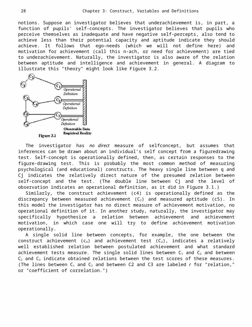
28 Chapter 3: Construct, Variables and Definitions
notions. Suppose an investigator believes that underachievement is, in part, afunction of pupils' self-concepts. The investigator believes that pupils whoperceive themselves as inadequate and have negative self-percepts, also tend toachieve less than their potential capacity and aptitude indicate they shouldachieve. It follows that ego-needs (which we will not define here) andmotivation for achievement (call this n-ach, or need for achievement) are tiedto underachievement. Naturally, the investigator is also aware of the relationbetween aptitude and intelligence and achievement in general. A diagram toillustrate this "theory" might look like Figure 3.2.
The investigator has no direct measure of selfconcept, but assumes thatinferences can be drawn about an individual’s self concept from a figuredrawingtest. Self-concept is operationally defined, then, as certain responses to thefigure-drawing test. This is probably the most common method of measuringpsychological (and educational) constructs. The heavy single line between q andCj indicates the relatively direct nature of the presumed relation betweenself-concept and the test. (The double line between Cj and the level ofobservation indicates an operational definition, as it did in Figure 3.1.)
Similarly, the construct achievement (c4) is operationally defined as thediscrepancy between measured achievement (C2) and measured aptitude (c5). Inthis model the investigator has no direct measure of achievement motivation, nooperational definition of it. In another study, naturally, the investigator mayspecifically hypothesize a relation between achievement and achievementmotivation, in which case one will try to define achievement motivationoperationally.
A single solid line between concepts, for example, the one between theconstruct achievement (c4) and achievement test (C2), indicates a relativelywell established relation between postulated achievement and what standardachievement tests measure. The single solid lines between C1 and C2 and betweenC2 and C3 indicate obtained relations between the test scores of these measures.(The lines between C1 and C2 and between C2 and C3 are labeled r for "relation,"or "coefficient of correlation.")
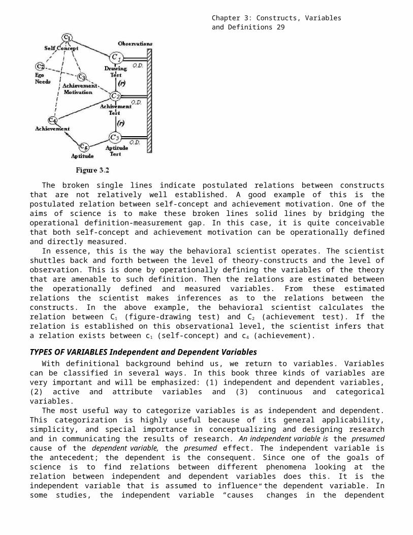
Chapter 3: Constructs, Variables and Definitions 29
The broken single lines indicate postulated relations between constructsthat are not relatively well established. A good example of this is thepostulated relation between self-concept and achievement motivation. One of theaims of science is to make these broken lines solid lines by bridging theoperational definition-measurement gap. In this case, it is quite conceivablethat both self-concept and achievement motivation can be operationally definedand directly measured.
In essence, this is the way the behavioral scientist operates. The scientistshuttles back and forth between the level of theory-constructs and the level ofobservation. This is done by operationally defining the variables of the theorythat are amenable to such definition. Then the relations are estimated betweenthe operationally defined and measured variables. From these estimatedrelations the scientist makes inferences as to the relations between theconstructs. In the above example, the behavioral scientist calculates therelation between C1 (figure-drawing test) and C2 (achievement test). If therelation is established on this observational level, the scientist infers thata relation exists between c1 (self-concept) and c4 (achievement).
TYPES OF VARIABLES Independent and Dependent VariablesWith definitional background behind us, we return to variables. Variables
can be classified in several ways. In this book three kinds of variables arevery important and will be emphasized: (1) independent and dependent variables,(2) active and attribute variables and (3) continuous and categoricalvariables.
The most useful way to categorize variables is as independent and dependent.This categorization is highly useful because of its general applicability,simplicity, and special importance in conceptualizing and designing researchand in communicating the results of research. An independent variable is the presumedcause of the dependent variable, the presumed effect. The independent variable isthe antecedent; the dependent is the consequent. Since one of the goals ofscience is to find relations between different phenomena looking at therelation between independent and dependent variables does this. It is theindependent variable that is assumed to influence the dependent variable. Insome studies, the independent variable “causes” changes in the dependent
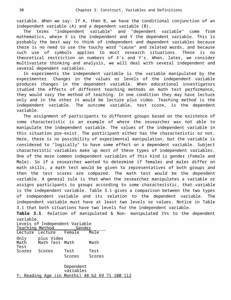
30 Chapter 3: Construct, Variables and Definitions
variable. When we say: If A, then B, we have the conditional conjunction of anindependent variable (A) and a dependent variable (B).
The terms "independent variable" and "dependent variable" come frommathematics, where X is the independent and Y the dependent variable. This isprobably the best way to think of independent and dependent variables becausethere is no need to use the touchy word "cause" and related words, and becausesuch use of symbols applies to most research situations. There is notheoretical restriction on numbers of X’s and Y’s. When, later, we considermultivariate thinking and analysis, we will deal with several independent andseveral dependent variables.
In experiments the independent variable is the variable manipulated by theexperimenter. Changes in the values or levels of the independent variableproduces changes in the dependent variable. When educational investigatorsstudied the effects of different teaching methods on math test performance,they would vary the method of teaching. In one condition they may have lectureonly and in the other it would be lecture plus video. Teaching method is theindependent variable. The outcome variable, test score, is the dependentvariable.
The assignment of participants to different groups based on the existence ofsome characteristic is an example of where the researcher was not able tomanipulate the independent variable. The values of the independent variable inthis situation pre-exist. The participant either has the characteristic or not.Here, there is no possibility of experimental manipulation, but the variable isconsidered to "logically" to have some effect on a dependent variable. Subjectcharacteristic variables make up most of these types of independent variables.One of the more common independent variables of this kind is gender (Female andMale). So if a researcher wanted to determine if females and males differ onmath skills, a math test would be given to representatives of both groups andthen the test scores are compared. The math test would be the dependentvariable. A general rule is that when the researcher manipulates a variable orassigns participants to groups according to some characteristic, that variableis the independent variable. Table 3.1 gives a comparison between the two typesof independent variable and its relation to the dependent variable. Theindependent variable must have at least two levels or values. Notice in Table3.1 that both situations have two levels for the independent variable.Table 3.1. Relation of manipulated & Non- manipulated IVs to the dependentvariable.Levels of Independent VariableTeaching Method _________ Gender Lecture Lecture Female MaleOnly plus VideoMathTest
Math Test Math MathScores Scores Test Test
Scores Scores
Dependentvariables
Y: Reading Age (in Months) 48 62 69 71 100 112
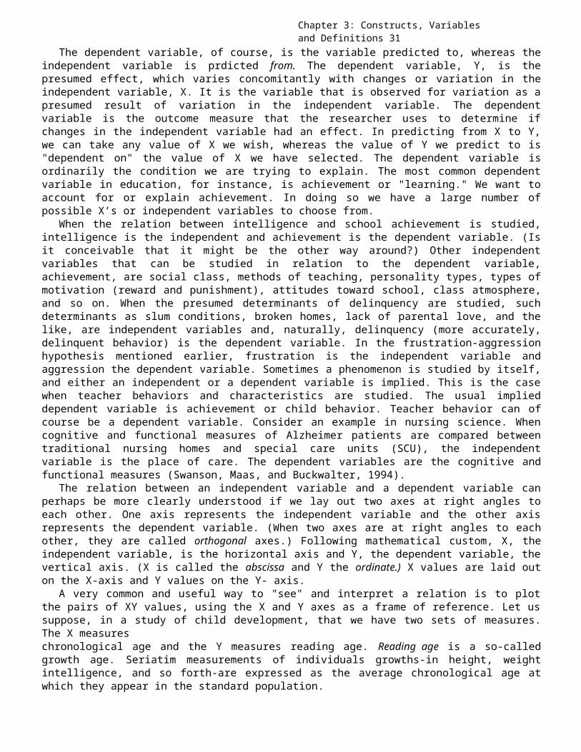
Chapter 3: Constructs, Variables and Definitions 31
The dependent variable, of course, is the variable predicted to, whereas theindependent variable is prdicted from. The dependent variable, Y, is thepresumed effect, which varies concomitantly with changes or variation in theindependent variable, X. It is the variable that is observed for variation as apresumed result of variation in the independent variable. The dependentvariable is the outcome measure that the researcher uses to determine ifchanges in the independent variable had an effect. In predicting from X to Y,we can take any value of X we wish, whereas the value of Y we predict to is"dependent on" the value of X we have selected. The dependent variable isordinarily the condition we are trying to explain. The most common dependentvariable in education, for instance, is achievement or "learning." We want toaccount for or explain achievement. In doing so we have a large number ofpossible X’s or independent variables to choose from.
When the relation between intelligence and school achievement is studied,intelligence is the independent and achievement is the dependent variable. (Isit conceivable that it might be the other way around?) Other independentvariables that can be studied in relation to the dependent variable,achievement, are social class, methods of teaching, personality types, types ofmotivation (reward and punishment), attitudes toward school, class atmosphere,and so on. When the presumed determinants of delinquency are studied, suchdeterminants as slum conditions, broken homes, lack of parental love, and thelike, are independent variables and, naturally, delinquency (more accurately,delinquent behavior) is the dependent variable. In the frustration-aggressionhypothesis mentioned earlier, frustration is the independent variable andaggression the dependent variable. Sometimes a phenomenon is studied by itself,and either an independent or a dependent variable is implied. This is the casewhen teacher behaviors and characteristics are studied. The usual implieddependent variable is achievement or child behavior. Teacher behavior can ofcourse be a dependent variable. Consider an example in nursing science. Whencognitive and functional measures of Alzheimer patients are compared betweentraditional nursing homes and special care units (SCU), the independentvariable is the place of care. The dependent variables are the cognitive andfunctional measures (Swanson, Maas, and Buckwalter, 1994).
The relation between an independent variable and a dependent variable canperhaps be more clearly understood if we lay out two axes at right angles toeach other. One axis represents the independent variable and the other axisrepresents the dependent variable. (When two axes are at right angles to eachother, they are called orthogonal axes.) Following mathematical custom, X, theindependent variable, is the horizontal axis and Y, the dependent variable, thevertical axis. (X is called the abscissa and Y the ordinate.) X values are laid outon the X-axis and Y values on the Y- axis.
A very common and useful way to "see" and interpret a relation is to plotthe pairs of XY values, using the X and Y axes as a frame of reference. Let ussuppose, in a study of child development, that we have two sets of measures.The X measureschronological age and the Y measures reading age. Reading age is a so-calledgrowth age. Seriatim measurements of individuals growths-in height, weightintelligence, and so forth-are expressed as the average chronological age atwhich they appear in the standard population.
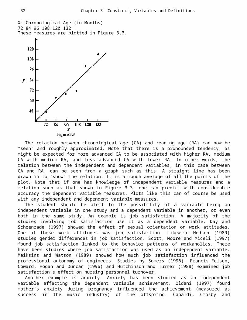
32 Chapter 3: Construct, Variables and Definitions
X: Chronological Age (in Months)72 84 96 108 120 132These measures are plotted in Figure 3.3.
The relation between chronological age (CA) and reading age (RA) can now be"seen" and roughly approximated. Note that there is a pronounced tendency, asmight be expected for more advanced CA to be associated with higher RA, mediumCA with medium RA, and less advanced CA with lower RA. In other words, therelation between the independent and dependent variables, in this case betweenCA and RA, can be seen from a graph such as this. A straight line has beendrawn in to "show" the relation. It is a rough average of all the points of theplot. Note that if one has knowledge of independent variable measures and arelation such as that shown in Figure 3.3, one can predict with considerableaccuracy the dependent variable measures. Plots like this can of course be usedwith any independent and dependent variable measures.
The student should be alert to the possibility of a variable being anindependent variable in one study and a dependent variable in another, or evenboth in the same study. An example is job satisfaction. A majority of thestudies involving job satisfaction use it as a dependent variable. Day andSchoenrade (1997) showed the effect of sexual orientation on work attitudes.One of those work attitudes was job satisfaction. Likewise Hodson (1989)studies gender differences in job satisfaction. Scott, Moore and Miceli (1997)found job satisfaction linked to the behavior patterns of workaholics. Therehave been studies where job satisfaction was used as an independent variable.Meiksins and Watson (1989) showed how much job satisfaction influenced theprofessional autonomy of engineers. Studies by Somers (1996), Francis-Felsen,Coward, Hogan and Duncan (1996) and Hutchinson and Turner (1988) examined jobsatisfaction’s effect on nursing personnel turnover.
Another example is anxiety. Anxiety has been studied as an independentvariable affecting the dependent variable achievement. Oldani (1997) foundmother’s anxiety during pregnancy influenced the achievement (measured assuccess in the music industry) of the offspring. Capaldi, Crosby and
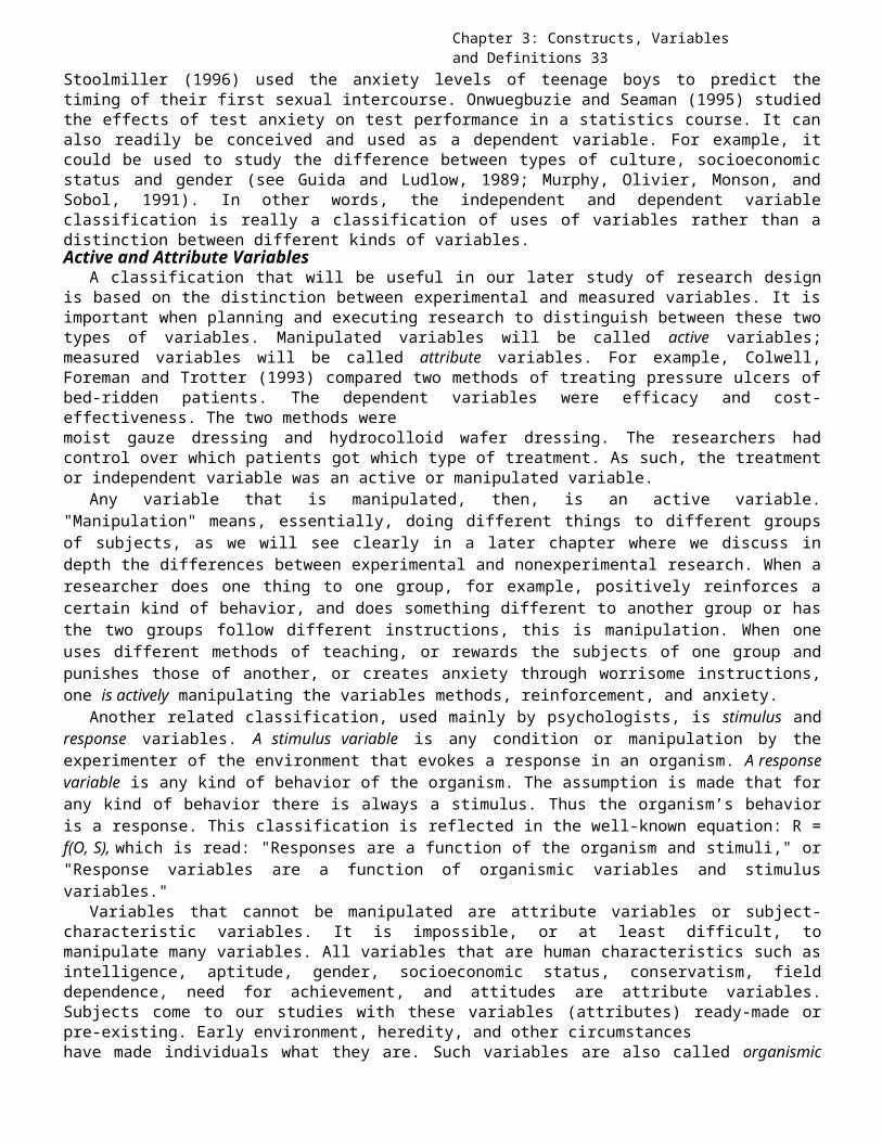
Chapter 3: Constructs, Variables and Definitions 33
Stoolmiller (1996) used the anxiety levels of teenage boys to predict thetiming of their first sexual intercourse. Onwuegbuzie and Seaman (1995) studiedthe effects of test anxiety on test performance in a statistics course. It canalso readily be conceived and used as a dependent variable. For example, itcould be used to study the difference between types of culture, socioeconomicstatus and gender (see Guida and Ludlow, 1989; Murphy, Olivier, Monson, andSobol, 1991). In other words, the independent and dependent variableclassification is really a classification of uses of variables rather than adistinction between different kinds of variables.Active and Attribute Variables
A classification that will be useful in our later study of research designis based on the distinction between experimental and measured variables. It isimportant when planning and executing research to distinguish between these twotypes of variables. Manipulated variables will be called active variables;measured variables will be called attribute variables. For example, Colwell,Foreman and Trotter (1993) compared two methods of treating pressure ulcers ofbed-ridden patients. The dependent variables were efficacy and cost-effectiveness. The two methods weremoist gauze dressing and hydrocolloid wafer dressing. The researchers hadcontrol over which patients got which type of treatment. As such, the treatmentor independent variable was an active or manipulated variable.
Any variable that is manipulated, then, is an active variable."Manipulation" means, essentially, doing different things to different groupsof subjects, as we will see clearly in a later chapter where we discuss indepth the differences between experimental and nonexperimental research. When aresearcher does one thing to one group, for example, positively reinforces acertain kind of behavior, and does something different to another group or hasthe two groups follow different instructions, this is manipulation. When oneuses different methods of teaching, or rewards the subjects of one group andpunishes those of another, or creates anxiety through worrisome instructions,one is actively manipulating the variables methods, reinforcement, and anxiety.
Another related classification, used mainly by psychologists, is stimulus andresponse variables. A stimulus variable is any condition or manipulation by theexperimenter of the environment that evokes a response in an organism. A responsevariable is any kind of behavior of the organism. The assumption is made that forany kind of behavior there is always a stimulus. Thus the organism’s behavioris a response. This classification is reflected in the well-known equation: R =f(O, S), which is read: "Responses are a function of the organism and stimuli," or"Response variables are a function of organismic variables and stimulusvariables."
Variables that cannot be manipulated are attribute variables or subject-characteristic variables. It is impossible, or at least difficult, tomanipulate many variables. All variables that are human characteristics such asintelligence, aptitude, gender, socioeconomic status, conservatism, fielddependence, need for achievement, and attitudes are attribute variables.Subjects come to our studies with these variables (attributes) ready-made orpre-existing. Early environment, heredity, and other circumstanceshave made individuals what they are. Such variables are also called organismic
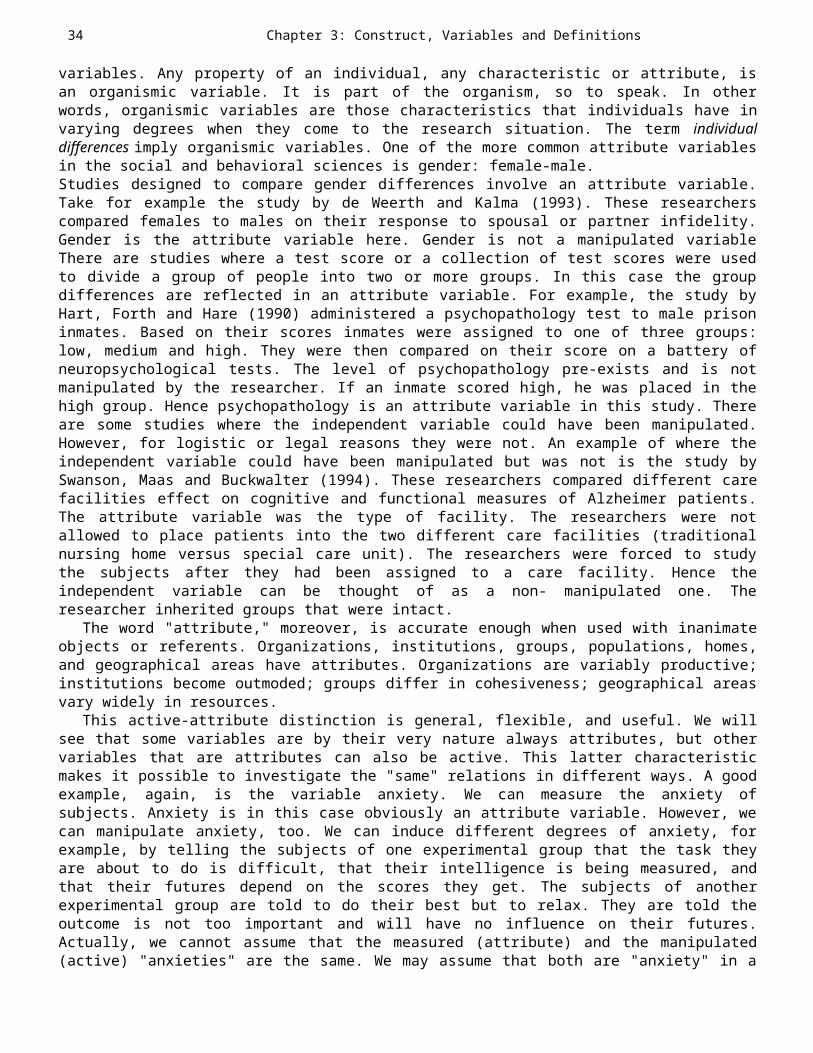
34 Chapter 3: Construct, Variables and Definitions
variables. Any property of an individual, any characteristic or attribute, isan organismic variable. It is part of the organism, so to speak. In otherwords, organismic variables are those characteristics that individuals have invarying degrees when they come to the research situation. The term individualdifferences imply organismic variables. One of the more common attribute variablesin the social and behavioral sciences is gender: female-male.Studies designed to compare gender differences involve an attribute variable.Take for example the study by de Weerth and Kalma (1993). These researcherscompared females to males on their response to spousal or partner infidelity.Gender is the attribute variable here. Gender is not a manipulated variableThere are studies where a test score or a collection of test scores were usedto divide a group of people into two or more groups. In this case the groupdifferences are reflected in an attribute variable. For example, the study byHart, Forth and Hare (1990) administered a psychopathology test to male prisoninmates. Based on their scores inmates were assigned to one of three groups:low, medium and high. They were then compared on their score on a battery ofneuropsychological tests. The level of psychopathology pre-exists and is notmanipulated by the researcher. If an inmate scored high, he was placed in thehigh group. Hence psychopathology is an attribute variable in this study. Thereare some studies where the independent variable could have been manipulated.However, for logistic or legal reasons they were not. An example of where theindependent variable could have been manipulated but was not is the study bySwanson, Maas and Buckwalter (1994). These researchers compared different carefacilities effect on cognitive and functional measures of Alzheimer patients.The attribute variable was the type of facility. The researchers were notallowed to place patients into the two different care facilities (traditionalnursing home versus special care unit). The researchers were forced to studythe subjects after they had been assigned to a care facility. Hence theindependent variable can be thought of as a non- manipulated one. Theresearcher inherited groups that were intact.
The word "attribute," moreover, is accurate enough when used with inanimateobjects or referents. Organizations, institutions, groups, populations, homes,and geographical areas have attributes. Organizations are variably productive;institutions become outmoded; groups differ in cohesiveness; geographical areasvary widely in resources.
This active-attribute distinction is general, flexible, and useful. We willsee that some variables are by their very nature always attributes, but othervariables that are attributes can also be active. This latter characteristicmakes it possible to investigate the "same" relations in different ways. A goodexample, again, is the variable anxiety. We can measure the anxiety ofsubjects. Anxiety is in this case obviously an attribute variable. However, wecan manipulate anxiety, too. We can induce different degrees of anxiety, forexample, by telling the subjects of one experimental group that the task theyare about to do is difficult, that their intelligence is being measured, andthat their futures depend on the scores they get. The subjects of anotherexperimental group are told to do their best but to relax. They are told theoutcome is not too important and will have no influence on their futures.Actually, we cannot assume that the measured (attribute) and the manipulated(active) "anxieties" are the same. We may assume that both are "anxiety" in a
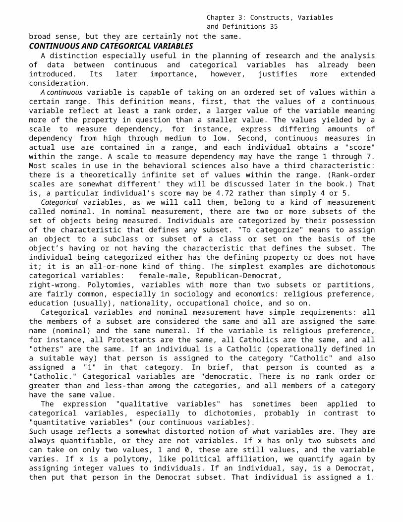
Chapter 3: Constructs, Variables and Definitions 35
broad sense, but they are certainly not the same.CONTINUOUS AND CATEGORICAL VARIABLES
A distinction especially useful in the planning of research and the analysisof data between continuous and categorical variables has already beenintroduced. Its later importance, however, justifies more extendedconsideration.
A continuous variable is capable of taking on an ordered set of values within acertain range. This definition means, first, that the values of a continuousvariable reflect at least a rank order, a larger value of the variable meaningmore of the property in question than a smaller value. The values yielded by ascale to measure dependency, for instance, express differing amounts ofdependency from high through medium to low. Second, continuous measures inactual use are contained in a range, and each individual obtains a "score"within the range. A scale to measure dependency may have the range 1 through 7.Most scales in use in the behavioral sciences also have a third characteristic:there is a theoretically infinite set of values within the range. (Rank-orderscales are somewhat different' they will be discussed later in the book.) Thatis, a particular individual’s score may be 4.72 rather than simply 4 or 5.
Categorical variables, as we will call them, belong to a kind of measurementcalled nominal. In nominal measurement, there are two or more subsets of theset of objects being measured. Individuals are categorized by their possessionof the characteristic that defines any subset. "To categorize" means to assignan object to a subclass or subset of a class or set on the basis of theobject’s having or not having the characteristic that defines the subset. Theindividual being categorized either has the defining property or does not haveit; it is an all-or-none kind of thing. The simplest examples are dichotomouscategorical variables: female-male, Republican-Democrat,right-wrong. Polytomies, variables with more than two subsets or partitions,are fairly common, especially in sociology and economics: religious preference,education (usually), nationality, occupational choice, and so on.
Categorical variables and nominal measurement have simple requirements: allthe members of a subset are considered the same and all are assigned the samename (nominal) and the same numeral. If the variable is religious preference,for instance, all Protestants are the same, all Catholics are the same, and all"others" are the same. If an individual is a Catholic (operationally defined ina suitable way) that person is assigned to the category "Catholic" and alsoassigned a "1" in that category. In brief, that person is counted as a"Catholic." Categorical variables are "democratic. There is no rank order orgreater than and less-than among the categories, and all members of a categoryhave the same value.
The expression "qualitative variables" has sometimes been applied tocategorical variables, especially to dichotomies, probably in contrast to"quantitative variables" (our continuous variables).Such usage reflects a somewhat distorted notion of what variables are. They arealways quantifiable, or they are not variables. If x has only two subsets andcan take on only two values, 1 and 0, these are still values, and the variablevaries. If x is a polytomy, like political affiliation, we quantify again byassigning integer values to individuals. If an individual, say, is a Democrat,then put that person in the Democrat subset. That individual is assigned a 1.
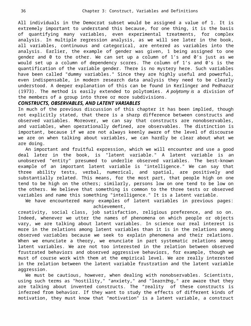
36 Chapter 3: Construct, Variables and Definitions
All individuals in the Democrat subset would be assigned a value of 1. It isextremely important to understand this because, for one thing, it is the basisof quantifying many variables, even experimental treatments, for complexanalysis. In multiple regression analysis, as we will see later in the book,all variables, continuous and categorical, are entered as variables into theanalysis. Earlier, the example of gender was given, 1 being assigned to onegender and 0 to the other. We can set up a column of 1’s and 0’s just as wewould set up a column of dependency scores. The column of 1’s and 0’s is thequantification of the variable gender. There is no mystery here. Such variableshave been called "dummy variables." Since they are highly useful and powerful,even indispensable, in modern research data analysis they need to be clearlyunderstood. A deeper explanation of this can be found in Kerlinger and Pedhazur(1973). The method is easily extended to polytomies. A polytomy is a division ofthe members of a group into three or more subdivisions.CONSTRUCTS, OBSERVABLES, AND LATENT VARIABLESIn much of the previous discussion of this chapter it has been implied, thoughnot explicitly stated, that there is a sharp difference between constructs andobserved variables. Moreover, we can say that constructs are nonobservables,and variables, when operationally defined, are observables. The distinction isimportant, because if we are not always keenly aware of the level of discoursewe are on when talking about variables, we can hardly be clear about what weare doing.
An important and fruitful expression, which we will encounter and use a gooddeal later in the book, is "latent variable." A latent variable is anunobserved "entity" presumed to underlie observed variables. The best-knownexample of an important latent variable is "intelligence." We can say thatthree ability tests, verbal, numerical, and spatial, are positively andsubstantially related. This means, for the most part, that people high on onetend to be high on the others; similarly, persons low on one tend to be low onthe others. We believe that something is common to the three tests or observedvariables and name this something "intelligence." It is a latent variable.
We have encountered many examples of latent variables in previous pages:achievement,
creativity, social class, job satisfaction, religious preference, and so on.Indeed, whenever we utter the names of phenomena on which people or objectsvary, we are talking about latent variables. In science our real interest ismore in the relations among latent variables than it is in the relations amongobserved variables because we seek to explain phenomena and their relations.When we enunciate a theory, we enunciate in part systematic relations amonglatent variables. We are not too interested in the relation between observedfrustrated behaviors and observed aggressive behaviors, for example, though wemust of course work with them at the empirical level. We are really interestedin the relation between the latent variable frustration and the latent variableaggression.
We must be cautious, however, when dealing with nonobservables. Scientists,using such terms as "hostility," "anxiety," and "learning," are aware that theyare talking about invented constructs. The “reality” of these constructs isinferred from behavior. If they want to study the effects of different kinds ofmotivation, they must know that "motivation" is a latent variable, a construct
Chapter 3: Constructs, Variables and Definitions 37
invented to account for presumably "motivated" behavior. They must know thatits "reality" is only a postulated reality. They can only judge that youngstersare motivated or not motivated by observing their behavior. Still, in order tostudy motivation, they must measure it or manipulate it. But they cannotmeasure it directly because it is an "in-the-head" variable, an unobservableentity, a latent variable, in short. The construct was invented for "something"presumed to be inside individuals, "something" prompting them to behave in such-and-such manners. This means that researchers must always measure presumedindicators of motivation and not motivation itself. They must, in other words,always measure some kind of behavior, be it marks on paper, spoken words, ormeaningful gestures, and then make inferences about presumed characteristics-orlatent variables.
Other terms have been used to express more or less the same ideas. Forexample, Tolman (1951 pp. 115-129.) calls constructs intervening variables.Intervening variable is a term invented to account for internal, unobservablepsychological processes that in turn account for behavior. An interveningvariable is an "in-the-head" variable. It cannot be seen, heard, or felt. It isinferred from behavior. "Hostility" is inferred from presumably hostile oraggressive acts. "Anxiety" is inferred from test scores, skin responses, heartbeat, and certain experimental manipulations. Another term is "hypotheticalconstruct." Since this expression means much the same as latent variable withsomewhat less generality, we need not pause over it. We should mention,however, that "latent variable" appears to be a more general and applicableexpression than "intervening variable" and "hypothetical construct." This isbecause it can be used for virtually any phenomena that presumably influence orare influenced by other phenomena. In other words, "latent variable" can beused with psychological, sociological, and other phenomena. "Latent variable"seems to be the preferable term because of its generality. Also, because it isnow possible in the analysis of covariance structures approach to assess theeffects of latent variables on each other and on so-called manifest or observedvariables. This rather abstract discussion will later be made more concreteand, it is hoped, meaningful. We will then see that the idea of latentvariables and the relations between them is an extremely important, fruitful,and useful one that is helping to change fundamental approaches to researchproblems.EXAMPLES OF VARIABLES AND OPERATIONAL DEFINITIONS
A number of constructs and operational definitions have already been given.To illustrate and clarify the preceding discussion, especially that in whichthe distinction was made between experimental and measured variables andbetween constructs and operationally defined variables, several examples ofconstructs or variables and operational definitions are given below. If adefinition is experimental, it is labeled (E); if it is measured, it is labeled(M).
Operational definitions differ in degree of specificity. Some are quiteclosely tied to observations. "Test" definitions, like "Intelligence is definedas a score on X intelligence test " are very specific. A definition like"Frustration is prevention from reaching a goal" is more general and requiresfurther specification to be measurable.
Social Class “. . . two or more orders of people who are believed to be, and are

38 Chapter 3: Construct, Variables and Definitions
accordingly ranked by the members of a community, in socially superior andinferior positions." (M) Warner and Lunt, 1941 p. 82). To be operational, thisdefinition has to be specified by questions aimed at people’s beliefs aboutother people’s positions. This is a subjective definition of social class.Social class, or social status, is also defined more objectively by using suchindices as occupation, income, and education, or by combinations of suchindices. For example, ". . . we converted information about the education,occupation and income of the parents of the NLSY youths into an index ofsocioeconomic status (SES) in which the highest scores indicate advancededucation, affluence and prestigious occupations. Lowest scores indicatepoverty, meager education and the most menial jobs." (M) (Herrnstein andMurray, 1996, p. 131).
Achievement (School, Arithmetic, and Spelling) Achievement is customarily definedoperationally by citing a standardized test of achievement (for example, IowaTests of Basic Skills, Elementary or the Achievement Test of the KaufmanAssessment Battery for Children (K-ABC), by grade-point averages, or by teacherjudgments. “Student achievement was measured by the combined test scores ofreading and mathematics.” (M) (Peng and Wright, 1994). Occasionally achievementis in the form of a performance test. Silverman (1993) examined students on twoskills in volleyball: The serve test and the forearm passing test. In the servetest, students received a score between 0 and 4 depending on where the servedball dropped. The forearm passing test involved bouncing the ball off of one’sforearm. The criteria used was to count the number of times the student canpass the ball above a 8 foot line against the wall within a 1 minute period.(M) Also used in some educational studies is an operational definition of theconcept student achievement perception. Here the students are asked to evaluatethemselves. The question used by Shoffner (1990) was “What kind of student doyou think you are?” The response choices available were “A student,” “Bstudent,” and “C student.” (M)
Achievement (Academic Performance) “As a result, grades for all students in allsections were obtained and used to determine the section-rank for each studentparticipating in the study. Section percentile rank was computed for each ofthese students and was used as the dependent measure of achievement in thefinal data analysis.” (M) (Strom, Hocevar, and Zimmer, 1990).
Hom, Berger, et al (1994) operationally define intrinsic Motivation as “The cumulative amountof time that each student played with the pattern blocks with the reward systemabsent.” (M).
Popularity. Popularity is often defined operationally by the number ofsociometric choices an individual receives from other individuals (in hisclass, play group, and so on). Individuals are asked: "With whom would you liketo work?," "With whom would you like to play?,” and the like. Each individualis required to choose one, two, or more individuals from his group on the basisof such criterion questions. (M)
Task Involvement ". . . each child’s behavior during a lesson was coded every 6sec as being appropriately involved, or deviant. The task involvement scoresfor a lesson was the percentage of 6-sec units in which the children were codedas appropriately involved.” (M) (Kounin and Doyle, 1975).
Reinforcement. Reinforcement definitions come in a number of forms. Most ofthem involve, in one way or another, the principle of reward. However, both
Chapter 3: Constructs, Variables and Definitions 39
positive and negative reinforcement may be used. The author gives specificexperimental definitions of "reinforcement. " For example,In the second 10 minutes, every opinion statement S made was recorded by E andreinforced. For two groups, E agreed with every opinion statement by saying:"Yes, you’re right," "That’s so," or the like, or by nodding and smilingaffirmation if he could not interrupt. (E) the model and the child wereadministered alternately 12 different sets of story items. To each of the 12items, the model consistently expressed judgmental responses in opposition tothe child’s moral orientation. . . and the experimenter reinforced the modelsbehavior with verbal approval responses such as "Very good," "That’s fine," and"That’s good." The child was similarly reinforced whenever he adopted themodels class of moral judgments in response to his own set of items. (E) [Thisis called "social reinforcement."] (Bandura and MacDonald, 1994).
Another example: The teacher gives verbal praise each time the childexhibits the target behavior. The target behaviors are attending toinstruction, school work, and responding aloud. The recording is done every 15seconds. (E) (Martens, Hiralall, and Bradley, 1997).
Attitudes Toward AIDS is defined by an 18-item scale. Each item consisted of aLikert-type format reflecting different attitudes toward AIDS patients. Somesample items are “People with AIDS should not be permitted to use publictoilets,” and “There should be mandatory testing of all Americans for AIDS.”(M) (Lester, 1989).
Comrey (1993) defines borderline Personality as having low scores on three scales of theComrey Personality Scales. The three scales are Trust versus Defensiveness,Social Conformity versus Rebelliousness and Emotional Stability versusNeuroticism.
Employee delinquency is operationally defined as a combination of threevariables. The variables are the number of chargeable accidents, the number ofwarning letters and the number of suspensions. (M) (Hogan and Hogan, 1989).
Religiosity is defined as a score on the Francis Scale of Attitudes towardChristianity. This scale consists of 24 items. Each item has a Likert-typeresponse scale. Sample items include: “Saying my prayers helps me a lot.” and“God helps me to lead a better life.” (M) (Gillings and Joseph, 1996).Religiosity should not be confused with religious preference. Here religiosityrefers to the strength of devotion to one’s chosen religion.
Self Esteem. Self-Esteem is a manipulated independent variable in the study bySteele, Spencer and Lynch (1993). Here subjects are given a self-esteem test,but when they are given feedback, the information on the official lookingfeedback report was bogus. Subjects of the same measured level of self-esteemare divided into 3 feedback groups: positive, negative and none. In thepositive feedback condition (positive selfesteem), subjects are described withstatements such as “clear thinking.” Those in the negative group (negativeself-esteem) are given adjectives like “passive in action.” The no feedbackgroup are told that their personality profile (self-esteem) were not ready dueto a backlog in scoring and interpretation. (E). Most studies on self-esteemuse a measured operational definition. In the above example, Steele, Spencerand Lynch used the Janis- Field Feelings of Inadequacy Self-Esteem scale. (M)In another example, Luhtanen and Crocker (1992) defines collective self-esteemas a score on a scale containing 16 Likert-type items. These items ask

40 Chapter 3: Construct, Variables and Definitions
respondents to think about a variety of social groups and membership such asgender, religion, race and ethnicity. (M).
Race. Race is usually a measured variable. However, in a study by Annis andCorenblum, (1986), 83 Canadian Indian kindergartners and first graders wereasked questions on racial preferences and self-identity by either a White orIndian experimenter. (E). The interest here was on whether the race of theexperimenter influenced responses.
Loneliness. One definition of this is a score on the UCLA Loneliness Scale.This scale includes items such as “No one really knows me well,” or “I lackcompanionship.” There is also theLoneliness Deprivation Scale that has items such as “I experience a sense ofemptiness,” or “There is no one who shows a particular interest in me.” (M)(Oshagan and Allen, 1992).
Halo. There have been many operationaldefinitions of the halo effect. Balzer and Sulsky (1992) summarize them. Theyfound 108 definitions that fit into 6 categories. One of the definitions statesthat halo is “ . . . the average within-ratee variance or standard deviation ofratings.” Another would be “comparing obtained ratings with true ratingsprovided by expert raters.” (M).
Memory: Recall and Recognition ". . . recall, is to ask the subject to recite what heremembers of the items shown him, giving him a point for each item that matchesone on the stimulus list. (M) (Norman, 1976 p. 97.). “The recognition testconsisted of 62 sentences presented to all subjects. .. . . subjects were instructed to rate each sentence on their degree ofconfidence that the sentence had been presented in the acquisition set.” (M)(Richter and Seay, 1987).
Social Skills. This can be operationally defined as a score on the Social SkillsRating Scale (Gresham and Elliot, 1990). There is the possibility of input fromthe student, parent and teacher. Social behaviors are rated in terms offrequency of occurrence and also on the level of importance. Some social skillitems include: “Gets along with people who are different, (Teacher),”“Volunteers to help family members with tasks, (Parent)” and “I politelyquestion rules that may be unfair. (Student)” (M).
Ingratiation. One of many impressionmanagement techniques (see Orpen, 1996 and Gordon, 1996). Ingratiation isoperationallydefined as a score on the Kumar and Beyerlein (1991) scale. This scaleconsisted of 25 Likert-type items and designed to measure the frequency thatsubordinates in a superior-subordinate relationship use ingratiatory tactics.(M). Strutton, Pelton and Lumpkin (1995) modified the Kumar-Beyerlein scale.Instead of measuring ingratiation between and employee and employer-supervisor,it measured ingratiation behavior between a salesperson and a customer. (M).
Feminism. This is defined by a score on the Attitudes Toward WomenQuestionnaire. This instrument consists of 18 statements to which therespondent registers agreement on a 5-point scale. Items include ‘Men have heldpower for too long’; ‘Beauty contests are degrading to women,' ‘Children ofworking mothers are bound to suffer.’ “ (Wilson and Reading, 1989).
Values. "Rank the ten goals in the order of their importance to you. (1) financialsuccess; (2) being liked; (3) success in family life; (4) being intellectually
Chapter 3: Constructs, Variables and Definitions 41
capable; (5) living by religious principles; (6) helping others; (7) beingnormal,reading ability needs interests delinquency need for affiliation conformitymarital satisfactionwell-adjusted; (8) cooperating with others; (9)doing a thorough job; (10) occupational success." (M) (Newcomb, 1978).
Democracy (Political Democracy) "The index [of political democracy] consists ofthree indicators of popular sovereignty and three of political liberties. Thethree measures of popular sovereignty are: (1) fairness of elections, (2)effective executive selection, and (3) legislative selection. The indicators ofpolitical liberties are: (4) freedom of the press, (5) freedom of groupopposition, and (6) government sanctions." (M). Bollen (1979) gives operationaldetails of the six social indicators in an appendix (pp. 585-586). This is aparticularly good example of the operational definition of a complex concept.Moreover, it is an excellent description of the ingredients of democracy.
The benefits of operational thinking have been great. Indeed, operationismhas been and is one of the most significant and important movements of ourtimes. Extreme operationism, of course, can be dangerous because it cloudsrecognition of the importance of constructs and constitutive definitions inbehavioral science, and because it can also restrict research to trivialproblems. There can be little doubt, however, that it is a healthy influence.It is the indispensable key to achieving objectivity (without which there is noscience) because its demand that observations must be public and replicablehelps to put research activities outside of and apart from researchers andtheir predilections. And, as Underwood (1957 p. 53) has said in his classicaltext on psychological research:
. . . I would say that operational thinking makes better scientists. Theoperationist is forced toremove the fuzz from his empirical concepts. operationism facilitates communication among scientists because the meaningof concepts so defined is not easily subject to misinterpretation. StudySuggestions1. Write operational definitions for five or six of the following constructs.
When possible, write two such definitions: an experimental one and ameasured one.
reinforcement punitivenessachievement underachievement leadership transfer of training level ofaspiration organizational conflict political preference
Some of these concepts or variables-for example, needs and transfer oftraining-may be difficult to define operationally. Why?2.Can any of the variables in 1, above, be bothindependent and dependent variables? Which ones?3.It is instructive and broadening for specialists to read outside their
fields. This is particularly true for students of behavioral research. It issuggested that the student of a particular field read two or three researchstudies in one of the best journals of another field. If you are inpsychology, read a sociology journal, say the American Sociological Review. If youare in education or sociology, read a psychology journal say the Journal! ofPersonality and Social Psychology or the Journal of Experimental Psychology. Students not in
42 Chapter 3: Construct, Variables and Definitions
education can sample the Journal of Educational Psychology or the American EducationalResearch Journal. When you read, jot down the names of the variables and comparethem to the variables in your own field. Are they primarily active orattribute variables? Note, for instance, that psychology’s variables aremore "active" than sociology’s. What implications do the variables of afield have for its research?
4.Reading the following articles is useful in learning and developingoperational definitions.Kinnier, R. T. (1995). A reconceptualization of values clarification: Values
conflict resolution.Journal of Counseling and Development, 74(1), 1824.Lego, S. (1988). Multiple disorder: An interpersonal approach to etiology,
treatment and nursing care. Archives of Psychiatric Nursing, 2(4), 231-235.Lobel, M. (1994). Conceptualizations, measurement, and effects of prenatal
maternal stress on birth outcomes. Journal of Behavioral Medicine, 17(3), 225-272.Navathe, P. D. & Singh, B. (1994). An operational definition for spatial
disorientation.Aviation, Space & Environmental Medicine, 65(12), 1153-1155.Sun, K.(1995). The definition of race. American Psychologist, 50(1), 43-44.Talaga, J. A. & Beehr, T. A. (1995). Are there gender differences in predictingretirement decisions? Journal of Applied Psychology, 80(1), 16-28. Woods, D. W.,Miltenberger, R. G. & Flach, A. D. (1996). Habits, tics, and stuttering:Prevalence and relation to anxiety an somatic awareness. Behavior Modification, 20(2),216-225.Chapter Summary1. A concept is an expression of an abstraction formed from generalization of
particulars, e.g., weight. This expression is from observations of certainbehaviors or actions.
2.A construct is a concept that has been formulated sothat it can be used in science. It is used in theoretical schemes. It isdefined so that it can be observed and measured.3.A variable is defined as a property that can take ondifferent values. It is a symbol to which values are assigned.4.Constructs and words can be defined bya) other words or concepts
b) description of an implicit or explicit action or behavior5.A constitutive definition is one where constructs are defined by other constructs.6.An operational definition is one where meaning isassigned by specifying the activities or operations necessary to measure andevaluate the construct. Operational definitions can give only limited meaningof constructs. They cannot completely describe a construct or variable. Thereare two types of operational definitions:
a) measured - tells us how the variable or construct will be measuredb) experimental - lays out the details of how the variable (construct) is
manipulated by the experimenter.7.Types of variables
a) The independent variable is a variable that is varied and has a presumedcause on another variable, the dependent variable. In an experiment, it is themanipulated variable. It is the variable under the control of the experimenter.
Chapter 3: Constructs, Variables and Definitions 43
In a non-experimental study, it is the variable that has a logical effect onthe dependent variable.
b) dependent variable is a variable whose effect varies concomitantly withchanges or variations in the independent variable.
c) An active variable is a variable that is manipulated. Manipulation meansthat the experimenter has control over how the values change.
d) An attributive variable is one that is measured and cannot be manipulated. Avariable that cannot be manipulated is one where the experimenter has nocontrol over the values of the variable.
e) A continuous variable is one capable of taking on an ordered set of valueswithin a certain range. These variables reflect at least a rank order.
f) Categorical variables belong to a kind of measurement where objects areassigned to a subclass or subset The subclasses are distinct and non-overlapping. All objects put into the same category are considered to have thesame characteristic.
g) Latent variables are unobservable entities. They are assumed to underlieobserved variables.
h) Intervening variables are constructs that account for internal unobservablepsychological processes that account for behavior. It is a variable that cannotbe seen but inferred from behavior.
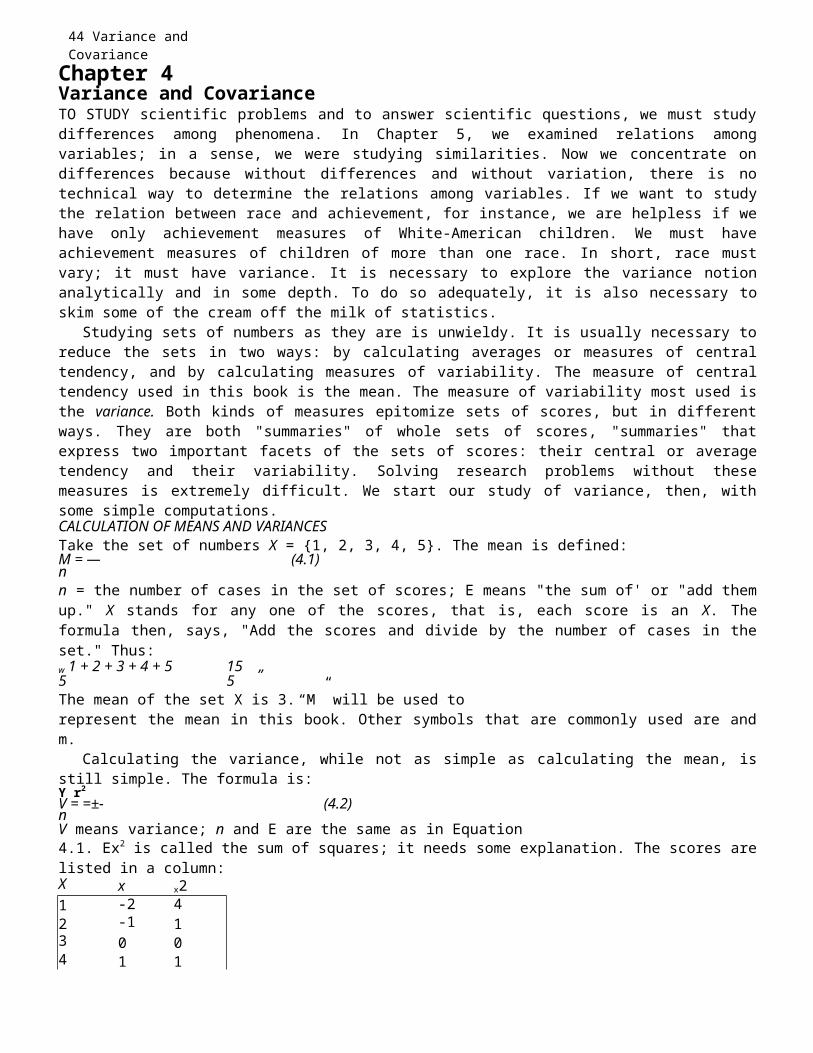
44 Variance and CovarianceChapter 4Variance and CovarianceTO STUDY scientific problems and to answer scientific questions, we must studydifferences among phenomena. In Chapter 5, we examined relations amongvariables; in a sense, we were studying similarities. Now we concentrate ondifferences because without differences and without variation, there is notechnical way to determine the relations among variables. If we want to studythe relation between race and achievement, for instance, we are helpless if wehave only achievement measures of White-American children. We must haveachievement measures of children of more than one race. In short, race mustvary; it must have variance. It is necessary to explore the variance notionanalytically and in some depth. To do so adequately, it is also necessary toskim some of the cream off the milk of statistics.
Studying sets of numbers as they are is unwieldy. It is usually necessary toreduce the sets in two ways: by calculating averages or measures of centraltendency, and by calculating measures of variability. The measure of centraltendency used in this book is the mean. The measure of variability most used isthe variance. Both kinds of measures epitomize sets of scores, but in differentways. They are both "summaries" of whole sets of scores, "summaries" thatexpress two important facets of the sets of scores: their central or averagetendency and their variability. Solving research problems without thesemeasures is extremely difficult. We start our study of variance, then, withsome simple computations.CALCULATION OF MEANS AND VARIANCESTake the set of numbers X = {1, 2, 3, 4, 5}. The mean is defined:M = — (4.1)nn = the number of cases in the set of scores; E means "the sum of' or "add themup." X stands for any one of the scores, that is, each score is an X. Theformula then, says, "Add the scores and divide by the number of cases in theset." Thus:w 1 + 2 + 3 + 4 + 5 15 „5 5The mean of the set X is 3.“M” will be used torepresent the mean in this book. Other symbols that are commonly used are andm.
Calculating the variance, while not as simple as calculating the mean, isstill simple. The formula is:Y r2V = =±- (4.2)nV means variance; n and E are the same as in Equation4.1. Ex2 is called the sum of squares; it needs some explanation. The scores arelisted in a column:X x x21 -2 42 -1 13 0 04 1 1
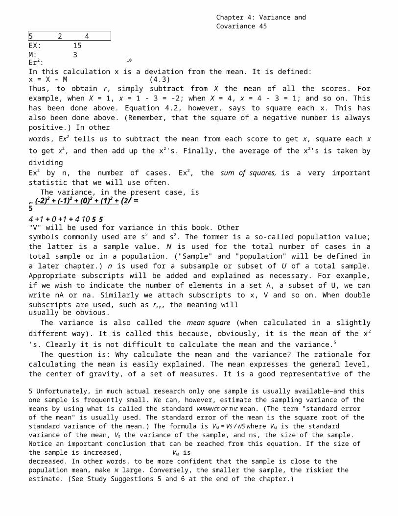
Chapter 4: Variance and Covariance 45
5 2 4EX: 15M: 3Er2: 10
In this calculation x is a deviation from the mean. It is defined:x = X - M (4.3)Thus, to obtain r, simply subtract from X the mean of all the scores. Forexample, when X = 1, x = 1 - 3 = -2; when X = 4, x = 4 - 3 = 1; and so on. Thishas been done above. Equation 4.2, however, says to square each x. This hasalso been done above. (Remember, that the square of a negative number is alwayspositive.) In otherwords, Ex2 tells us to subtract the mean from each score to get x, square each xto get x2, and then add up the x2's. Finally, the average of the x2's is taken bydividingEx2 by n, the number of cases. Ex2, the sum of squares, is a very importantstatistic that we will use often.
The variance, in the present case, isv= (- 2) 2 + (- 1) 2 + ( 0) 2 + ( 1) 2 + (2/ =54 +1 + 0 +1 + 4 10 5 5"V" will be used for variance in this book. Othersymbols commonly used are s2 and s2. The former is a so-called population value;the latter is a sample value. N is used for the total number of cases in atotal sample or in a population. ("Sample" and "population" will be defined ina later chapter.) n is used for a subsample or subset of U of a total sample.Appropriate subscripts will be added and explained as necessary. For example,if we wish to indicate the number of elements in a set A, a subset of U, we canwrite nA or na. Similarly we attach subscripts to x, V and so on. When doublesubscripts are used, such as rxy, the meaning willusually be obvious.
The variance is also called the mean square (when calculated in a slightlydifferent way). It is called this because, obviously, it is the mean of the x2
's. Clearly it is not difficult to calculate the mean and the variance.5
The question is: Why calculate the mean and the variance? The rationale forcalculating the mean is easily explained. The mean expresses the general level,the center of gravity, of a set of measures. It is a good representative of the
5 Unfortunately, in much actual research only one sample is usually available—and this one sample is frequently small. We can, however, estimate the sampling variance of the means by using what is called the standard VARIANCE OF THE mean. (The term "standard error of the mean" is usually used. The standard error of the mean is the square root of the standard variance of the mean.) The formula is VM = VS / NS where VM is the standard variance of the mean, VS the variance of the sample, and ns, the size of the sample. Notice an important conclusion that can be reached from this equation. If the size of the sample is increased, VM isdecreased. In other words, to be more confident that the sample is close to the population mean, make N large. Conversely, the smaller the sample, the riskier the estimate. (See Study Suggestions 5 and 6 at the end of the chapter.)
46 Variance and Covariance
level of a group's characteristics or performance. It also has certaindesirable statistical properties, and is the most ubiquitous statistic of thebehavioral sciences. In much behavioral research, for example, means ofdifferent experimental groups are 6 compared to study relations, as pointed outin Chapter 5. We may be testing the relation between organizational climatesand productivity, for instance. We may have used three kinds of climates andmay be interested in the question of which climate has the greatest effect onproductivity. In such cases means are customarily compared. For instance, ofthree groups, each operating under one of three climates, Ai, A2, and A3, whichhasthe greatest mean on, say, a measure of productivity?
The rationale for computing and using the variance in research is moredifficult to explain. In the usual case of ordinary scores the variance is ameasure of the dispersion of the set of scores. It tells us how much the scoresare spread out. If a group of pupils is very heterogeneous in readingachievement, then the variance of their reading scores will be large comparedto the variance of a group that is homogeneous in reading achievement. Thevariance, then, is a measure of the spread of the scores; it describes theextent towhich the scores differ from each other. Fordescriptive purposes, the square root of the variance is ordinarily used. It iscalled the standard deviation. Certain mathematical properties, however, make thevariance more useful in research. It is suggested that the student supplementthis topic of study with the appropriate sections of an elementary statisticstext (see Comrey and Lee, 1995). It will not be possible in this book todiscuss all the facets of meaning and interpretation of means, variances, andstandard deviations. The remainder of this chapter and later parts of the bookwill explore other aspects of the use of the variance statistic.KINDS OF VARIANCEVariances come in a number of forms. When you read the research and technicalliterature, you will frequently come across the term, sometimes with aqualifying adjective, sometimes not. To understand the literature, it isnecessary to have a good idea of the characteristics and purposes of thesedifferent variances. And to design and do research, one must have a ratherthorough understanding of the variance concept as well as considerable masteryof statistical variance notions and manipulations.Population and Sample VariancesThe population variance is the variance of U, a universe or population of measures.Greek symbols are usually used to represent population parameters or measures.For the population variance the symbol s2 (sigma squared) is used. The symbol sis used for the population standard deviation. The population mean is m (mu).If all the measures of a defined universal set, U, are known, then the variance
6 The method of calculating the variance used in this chapter differs from the methods ordinarily used. In fact, the method given above is impracticable in most situations. Our purpose is not to learn statistics, as such. Rather, we are pursuing basic ideas. Methods of computation, examples, and demonstrations have been constructedto aid this pursuit of basic ideas.
Chapter 4: Variance and Covariance 47
is known. More likely, however, all the measures of U are not available. Insuch cases the variance is estimated by calculating the variance of one or moresamples of U. A good deal of statistical energy goes into this importantactivity. A question may arise: How variable is the intelligence of thecitizens of the United States? This is a U or population question. If therewere a complete list of all the millions of people in the United States—andthere were also a complete list of intelligence test scores of these people—thevariance could be simply if wearily computed. No such list exists. So samples,representative samples, of Americans are tested and means and variancescomputed. The samples are used to estimate the mean and variance of the wholepopulation. These estimated values are called statistics (in the populationthey are called parameters). The sample mean is denoted by the symbol M and thesample variance is denoted by S.D. or s . A number ofstatistics textbooks use the X(X-bar) to represent the sample mean.
Sampling variance is the variance of statistics computed from samples. The meansof four random samples drawn from a population will differ. If the sampling israndom and the samples are large enough, the means should not vary too much.That is, the
variance of the means should be relatively small. Systematic VariancePerhaps the most general way to classify variance is as systematic variance and errorvariance. Systematic variance is the variation in measures due to some known orunknown influences that "cause" the scores to lean in one direction more thananother. Any natural or man-made influences that cause events to happen in acertain predictable way are systematic influences. The achievement test scoresof the children in a wealthy suburban school will tend to be systematicallyhigher than the scores of the children in a city slum area school. Adeptteaching may systematically influence the achievement of children, as comparedto the achievement of children who are ineptly taught.
There are many, many causes of systematic variance. Scientists seek toseparate those in which they are interested from those in which they are notinterested. They also try to separate from systematic variance, variance thatis random. Indeed, research may narrowly and technically be defined as thecontrolled study of variances.Between-Groups (Experimental) Variance
One important type of systematic variance in research is between-groups orexperimental variance. Between-groups or experimental variance, as the name indicates,is the variance that reflects systematic differences between groups of measures.The variance discussed previously as score variance reflects the differencesbetween individuals in a group. We can say, for instance, that, on the basis ofpresent evidence and current tests, the variance in intelligence of a randomsample of eleven-year-old children is about 225 points. (This is obtained bysquaring the standard deviation reported in a test manual. The standarddeviation of the California Test of Mental Maturity for 11-year-old children,for instance, is about 15, and 152 = 225.) This figure is a statistic that tellsus how much the 1 individuals differ from each other. Between-groups variance,on the other hand, is the variance due to the differences between groups ofindividuals. If the achievement of northern region and southern region childrenin comparable schools is measured, there would be differences between the
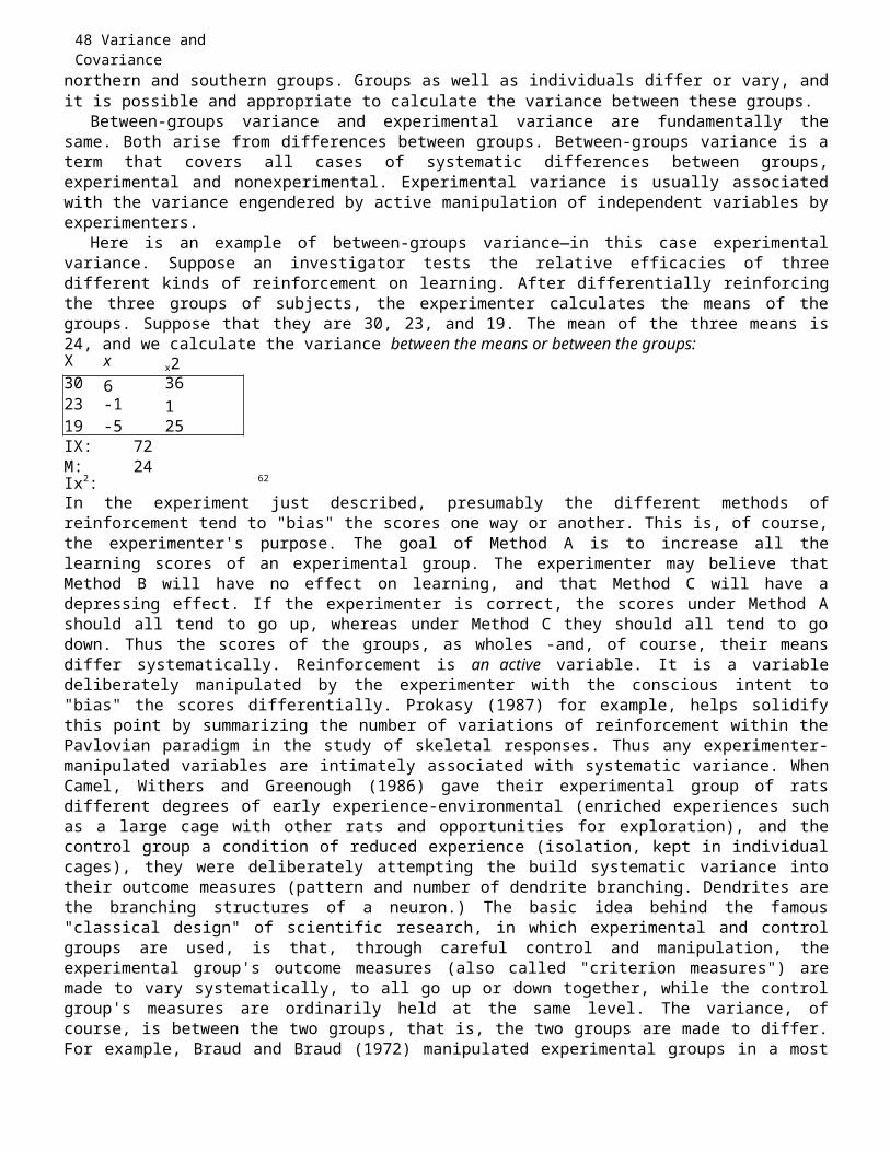
48 Variance and Covariance
northern and southern groups. Groups as well as individuals differ or vary, andit is possible and appropriate to calculate the variance between these groups.
Between-groups variance and experimental variance are fundamentally thesame. Both arise from differences between groups. Between-groups variance is aterm that covers all cases of systematic differences between groups,experimental and nonexperimental. Experimental variance is usually associatedwith the variance engendered by active manipulation of independent variables byexperimenters.
Here is an example of between-groups variance—in this case experimentalvariance. Suppose an investigator tests the relative efficacies of threedifferent kinds of reinforcement on learning. After differentially reinforcingthe three groups of subjects, the experimenter calculates the means of thegroups. Suppose that they are 30, 23, and 19. The mean of the three means is24, and we calculate the variance between the means or between the groups:X x x230 6 3623 -1 119 -5 25IX: 72M: 24Ix2: 62
In the experiment just described, presumably the different methods ofreinforcement tend to "bias" the scores one way or another. This is, of course,the experimenter's purpose. The goal of Method A is to increase all thelearning scores of an experimental group. The experimenter may believe thatMethod B will have no effect on learning, and that Method C will have adepressing effect. If the experimenter is correct, the scores under Method Ashould all tend to go up, whereas under Method C they should all tend to godown. Thus the scores of the groups, as wholes -and, of course, their meansdiffer systematically. Reinforcement is an active variable. It is a variabledeliberately manipulated by the experimenter with the conscious intent to"bias" the scores differentially. Prokasy (1987) for example, helps solidifythis point by summarizing the number of variations of reinforcement within thePavlovian paradigm in the study of skeletal responses. Thus any experimenter-manipulated variables are intimately associated with systematic variance. WhenCamel, Withers and Greenough (1986) gave their experimental group of ratsdifferent degrees of early experience-environmental (enriched experiences suchas a large cage with other rats and opportunities for exploration), and thecontrol group a condition of reduced experience (isolation, kept in individualcages), they were deliberately attempting the build systematic variance intotheir outcome measures (pattern and number of dendrite branching. Dendrites arethe branching structures of a neuron.) The basic idea behind the famous"classical design" of scientific research, in which experimental and controlgroups are used, is that, through careful control and manipulation, theexperimental group's outcome measures (also called "criterion measures") aremade to vary systematically, to all go up or down together, while the controlgroup's measures are ordinarily held at the same level. The variance, ofcourse, is between the two groups, that is, the two groups are made to differ.For example, Braud and Braud (1972) manipulated experimental groups in a most
Chapter 4: Variance and Covariance 49
unusual way. They trained the rats of an experimental group to choose thelarger of two circles in a choice task; the control group rats received notraining. Extracts from the brains of the animals of both groups were injectedinto the brains of two new groups of rats. Statistically speaking, they weretrying to increase the between-groups variance. They succeeded: the new"experimental group" animals exceeded the new "control group" animals inchoosing the larger circle in the same choice task!
This is clear and easy to see in experiments. In research that is notexperimental, in research where already existing differences between groups arestudied, it is not always so clear and easy to see that one is studyingbetween-groups variance. But the idea is the same. The principle may be statedin a somewhat different way: The greater the differences between groups, themore an independent variable or variables can be presumed to have operated. Ifthere is little difference between groups, on the other hand, then thepresumption must be that an independent variable or variables have notoperated. That is, their effects are too weak to be noticed, or that differentinfluences have canceled each other out. We judge the effects of independentvariables that have been manipulated or that have worked in the past, then, bybetween-groups variance. Whether the independent variables have or have notbeen manipulated, the principle is the same.
To illustrate the principle, we use the well-studied problem of the effectof anxiety on school achievement. It is possible to manipulate anxiety byhaving two experimental groups and inducing anxiety in one and not in theother. This can be done by giving each group the same test with differentinstructions. We tell the members of one group that their grades depend whollyon the test. We tell the members of the other group that the test does notmatter particularly, that its outcome will not affect grades. On the otherhand, the relation between anxiety and achievement may also be studied bycomparing groups of individuals on whom it can be assumed that differentenvironmental and psychological circumstances have acted to produce anxiety.(Of course, the experimentally induced anxiety and thealready existing anxiety the stimulus variable andthe organismic variable, are not assumed to be the same.) A study to test thehypothesis that different environmental and psychological circumstances act toproduce different levels test anxiety was done by Guidaand Ludlow (1989). These investigators hypothesized that students in the UnitedStates culture would show a lower level of test anxiety than students from theChilean culture. Using the language of this chapter, the investigatorshypothesized a larger between-groups variance than could be expected by chancebecause of the difference between Chilean and American environmental,educational and psychological conditions. (The hypothesis was supported.Chilean students exhibited a higher level of test anxiety than students fromthe United States. However, when considering only the lower socio-economicgroups of each culture, the United States students had higher test anxiety thanthe Chilean students.)Error VarianceError variance is the fluctuation or varying of measures that is unaccounted for.The fluctuations of the measurements in the dependent variable in a researchstudy where all participants were treated equally is considered error variance.
50 Variance and Covariance
Some of these fluctuations are due to chance. In this case, error variance israndom variance. It is the variation in measures due to the usually small andself-compensating fluctuations of measures-now here, now there; now up, nowdown. The sampling variance discussed earlier in the chapter, for example, israndom or error variance.
To digress briefly before continuing, it is necessary in this chapter andthe next to use the notion of "random" or "randomness." Ideas of randomness andrandomization will be discussed in considerable more detail in a ;ater chapter.For the present, however, randomness means that there is no known way that canbe expressed in language of correctly describing or explaining events and theiroutcomes. In different words, random events cannot be predicted. A randomsample is a subset of a universe. Its members are so drawn that each member ofthe universe has an equal chance of being selected. This is another way ofsaying that, if members are randomly selected, there is no way to predict whichmember will be selected on any one selection-other things equal.
However, one should not think that random variance is the only possiblesource of error variance. Error variance can be also consist of othercomponents as pointed out by Barber (1976). What gets “pooled” into the termcalled error variance can include measurement errors within the measuringinstrument, procedural errors by the researcher, misrecording of responses, andthe researcher’s outcome expectancy. It is possible that “equal” subjectsdiffer on the dependent variable because one may be experiencing a differentphysiological and psychological functioning at the time the measurements weretaken.
Returning to our main discussion, it can be said that error variance is thevariance in measurements due to ignorance. Imagine a great dictionary in whicheverything in the world—every occurrence, every event, every little thing,every great thing—is given in complete detail. To understand any event that hasoccurred, that is now occurring, or that will occur, all one needs to do islook it up in the dictionary. With this dictionary there are obviously norandom or chance occurrences. Everything is accounted for. In brief, there isno error variance; all is systematic variance. Unfortunately, (or more likely,fortunately) we do not have such a dictionary. Many, many events andoccurrences cannot be explained. Much variance eludes2x x3 1.5 2.256 1.5 2.25identification and control. This is error variance as long as identificationand control elude us.
While seemingly strange and even a bit bizarre, this mode of reasoning isuseful, provided we remember that some of the error variance of today may notbe the error variance of tomorrow. Suppose that we do an experiment on teachingproblem solving in which we assign pupils to three groups at random. After wefinish the experiment, we study the differences between the three groups to seeif the teaching has had an effect. We know that the scores and the means of thegroups will always show minor fluctuations, now plus a point or two or three,now minus a point or two or three, which we can probably never control.Something or other makes the scores and the means fluctuate in this fashion.According to the view under discussion, they do not just fluctuate for any
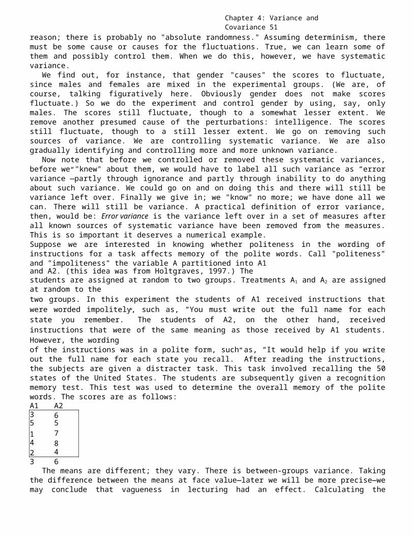
Chapter 4: Variance and Covariance 51
reason; there is probably no "absolute randomness." Assuming determinism, theremust be some cause or causes for the fluctuations. True, we can learn some ofthem and possibly control them. When we do this, however, we have systematicvariance.
We find out, for instance, that gender "causes" the scores to fluctuate,since males and females are mixed in the experimental groups. (We are, ofcourse, talking figuratively here. Obviously gender does not make scoresfluctuate.) So we do the experiment and control gender by using, say, onlymales. The scores still fluctuate, though to a somewhat lesser extent. Weremove another presumed cause of the perturbations: intelligence. The scoresstill fluctuate, though to a still lesser extent. We go on removing suchsources of variance. We are controlling systematic variance. We are alsogradually identifying and controlling more and more unknown variance.
Now note that before we controlled or removed these systematic variances,before we "knew" about them, we would have to label all such variance as “errorvariance”—partly through ignorance and partly through inability to do anythingabout such variance. We could go on and on doing this and there will still bevariance left over. Finally we give in; we "know" no more; we have done all wecan. There will still be variance. A practical definition of error variance,then, would be: Error variance is the variance left over in a set of measures afterall known sources of systematic variance have been removed from the measures.This is so important it deserves a numerical example.Suppose we are interested in knowing whether politeness in the wording ofinstructions for a task affects memory of the polite words. Call "politeness"and "impoliteness" the variable A partitioned into A1and A2. (this idea was from Holtgraves, 1997.) Thestudents are assigned at random to two groups. Treatments A1 and A2 are assignedat random to thetwo groups. In this experiment the students of A1 received instructions thatwere worded impolitely, such as, “You must write out the full name for eachstate you remember.” The students of A2, on the other hand, receivedinstructions that were of the same meaning as those received by A1 students.However, the wordingof the instructions was in a polite form, such as, “It would help if you writeout the full name for each state you recall.” After reading the instructions,the subjects are given a distracter task. This task involved recalling the 50states of the United States. The students are subsequently given a recognitionmemory test. This test was used to determine the overall memory of the politewords. The scores are as follows:A1 A23 65 51 74 82 43 6
The means are different; they vary. There is between-groups variance. Takingthe difference between the means at face value—later we will be more precise—wemay conclude that vagueness in lecturing had an effect. Calculating the
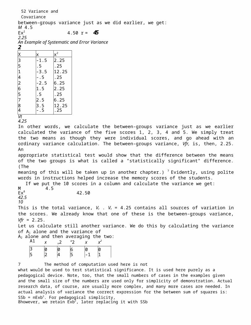
52 Variance and Covariance
between-groups variance just as we did earlier, we get:M 4.5Ex2 4.50 r = 452.25An Example of Systematic and Error Variance2X x x2
3 -1.5 2.255 .5 .251 -3.5 12.254 -.5 .252 -2.5 6.256 1.5 2.255 .5 .257 2.5 6.258 3.5 12.254 -.5 .25Vt4.25In other words, we calculate the between-groups variance just as we earliercalculated the variance of the five scores 1, 2, 3, 4 and 5. We simply treatthe two means as though they were individual scores, and go ahead with anordinary variance calculation. The between-groups variance, Vfr, is, then, 2.25.Anappropriate statistical test would show that the difference between the meansof the two groups is what is called a "statistically significant" difference.(Themeaning of this will be taken up in another chapter.) 7 Evidently, using politewords in instructions helped increase the memory scores of the students.
If we put the 10 scores in a column and calculate the variance we get:M 4.5Ex8 42.5042.510This is the total variance, Vt . Vt = 4.25 contains all sources of variation inthe scores. We already know that one of these is the between-groups variance,Vfr = 2.25.Let us calculate still another variance. We do this by calculating the varianceof A1 alone and the variance ofA2 alone and then averaging the two:
A1 x x2 a2 x x2
3 0 0 6 0 05 2 4 5 -1 1
7 The method of computation used here is notwhat would be used to test statistical significance. It is used here purely as a pedagogical device. Note, too, that the small numbers of cases in the examples given and the small size of the numbers are used only for simplicity of demonstration. Actualresearch data, of course, are usually more complex, and many more cases are needed. In actual analysis of variance the correct expression for the between sum of squares is: SSb = nExb2. For pedagogical simplicity,8however, we retain Exb2, later replacing it with SSb
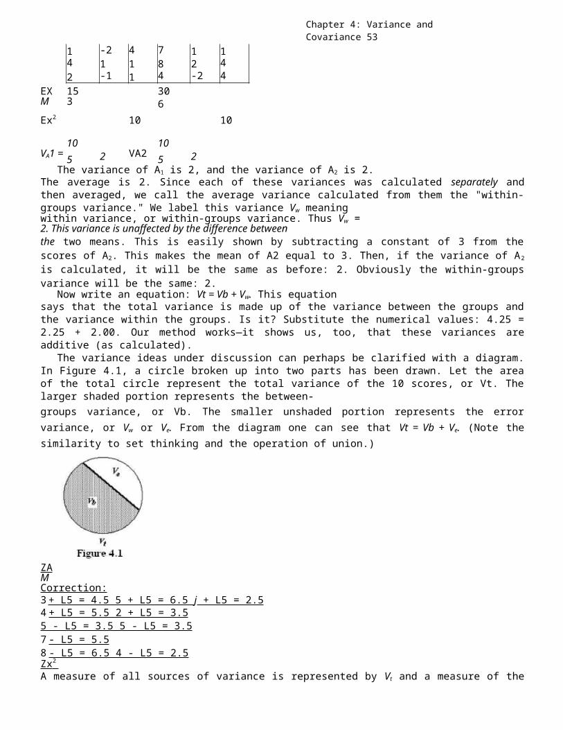
Chapter 4: Variance and Covariance 53
1 -2 4 7 1 14 1 1 8 2 42 -1 1 4 -2 4
EX 15 30M 3 6Ex2 10 10
10 10VA1 = 5 2 VA2 5 2
The variance of A1 is 2, and the variance of A2 is 2.The average is 2. Since each of these variances was calculated separately andthen averaged, we call the average variance calculated from them the "within-groups variance." We label this variance Vw meaningwithin variance, or within-groups variance. Thus Vw =2. This variance is unaffected by the difference betweenthe two means. This is easily shown by subtracting a constant of 3 from thescores of A2. This makes the mean of A2 equal to 3. Then, if the variance of A2
is calculated, it will be the same as before: 2. Obviously the within-groupsvariance will be the same: 2.
Now write an equation: Vt = Vb + Vw. This equationsays that the total variance is made up of the variance between the groups andthe variance within the groups. Is it? Substitute the numerical values: 4.25 =2.25 + 2.00. Our method works—it shows us, too, that these variances areadditive (as calculated).
The variance ideas under discussion can perhaps be clarified with a diagram.In Figure 4.1, a circle broken up into two parts has been drawn. Let the areaof the total circle represent the total variance of the 10 scores, or Vt. Thelarger shaded portion represents the between-groups variance, or Vb. The smaller unshaded portion represents the errorvariance, or Vw or Ve. From the diagram one can see that Vt = Vb + Ve. (Note thesimilarity to set thinking and the operation of union.)
ZAMCorrection:3 + L5 = 4.5 5 + L5 = 6.5 j + L5 = 2.54 + L5 = 5.5 2 + L5 = 3.5 5 - L5 = 3.5 5 - L5 = 3.57 - L5 = 5.5 8 - L5 = 6.5 4 - L5 = 2.5 Zx 2 A measure of all sources of variance is represented by Vt and a measure of the
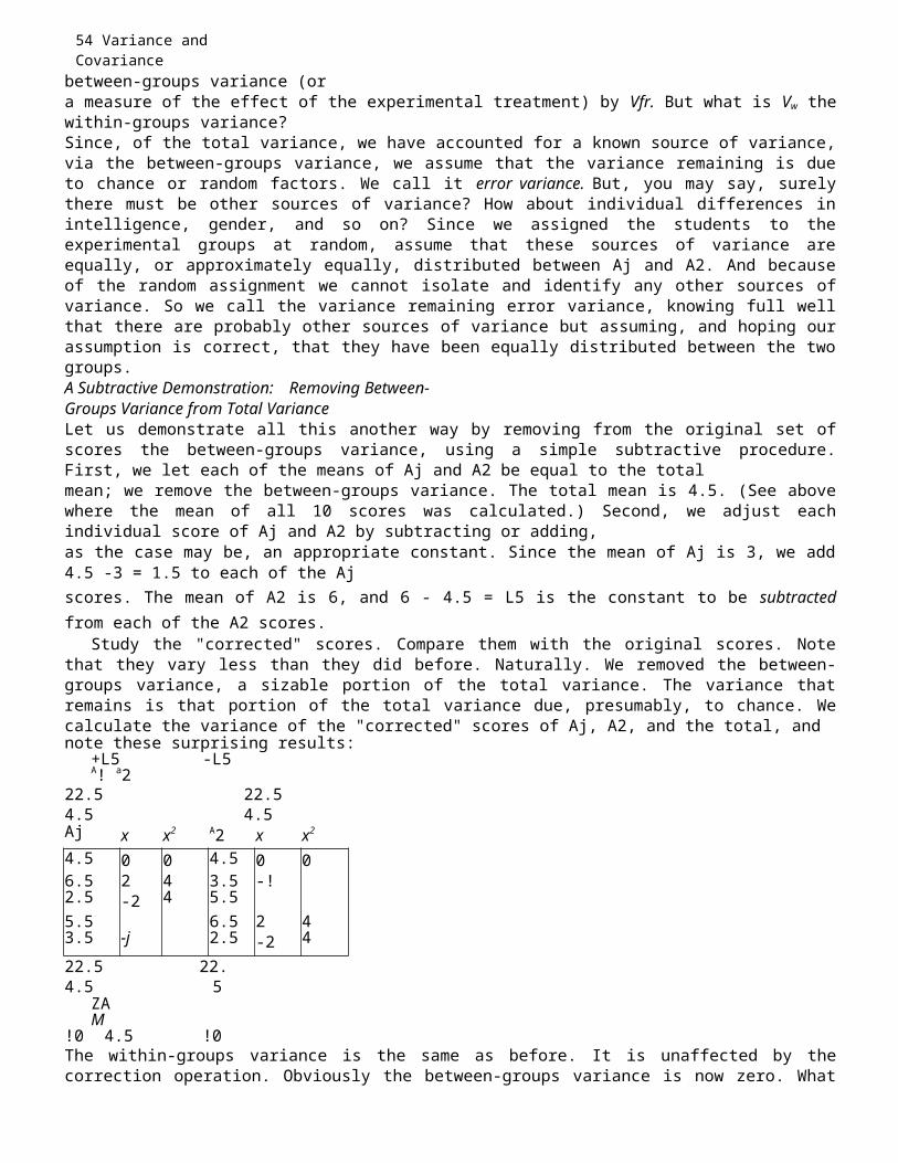
54 Variance and Covariance
between-groups variance (ora measure of the effect of the experimental treatment) by Vfr. But what is Vw thewithin-groups variance?Since, of the total variance, we have accounted for a known source of variance,via the between-groups variance, we assume that the variance remaining is dueto chance or random factors. We call it error variance. But, you may say, surelythere must be other sources of variance? How about individual differences inintelligence, gender, and so on? Since we assigned the students to theexperimental groups at random, assume that these sources of variance areequally, or approximately equally, distributed between Aj and A2. And becauseof the random assignment we cannot isolate and identify any other sources ofvariance. So we call the variance remaining error variance, knowing full wellthat there are probably other sources of variance but assuming, and hoping ourassumption is correct, that they have been equally distributed between the twogroups.A Subtractive Demonstration: Removing Between-Groups Variance from Total VarianceLet us demonstrate all this another way by removing from the original set ofscores the between-groups variance, using a simple subtractive procedure.First, we let each of the means of Aj and A2 be equal to the totalmean; we remove the between-groups variance. The total mean is 4.5. (See abovewhere the mean of all 10 scores was calculated.) Second, we adjust eachindividual score of Aj and A2 by subtracting or adding,as the case may be, an appropriate constant. Since the mean of Aj is 3, we add4.5 -3 = 1.5 to each of the Ajscores. The mean of A2 is 6, and 6 - 4.5 = L5 is the constant to be subtractedfrom each of the A2 scores.
Study the "corrected" scores. Compare them with the original scores. Notethat they vary less than they did before. Naturally. We removed the between-groups variance, a sizable portion of the total variance. The variance thatremains is that portion of the total variance due, presumably, to chance. Wecalculate the variance of the "corrected" scores of Aj, A2, and the total, andnote these surprising results:
+L5 -L5A! a2
22.5 22.54.5 4.5Aj x x2 A2 x x2
4.5 0 0 4.5 0 06.5 2 4 3.5 -!2.5 -2 4 5.55.5 6.5 2 43.5 -j 2.5 -2 422.5 22.4.5 5
ZAM
!0 4.5 !0The within-groups variance is the same as before. It is unaffected by thecorrection operation. Obviously the between-groups variance is now zero. What
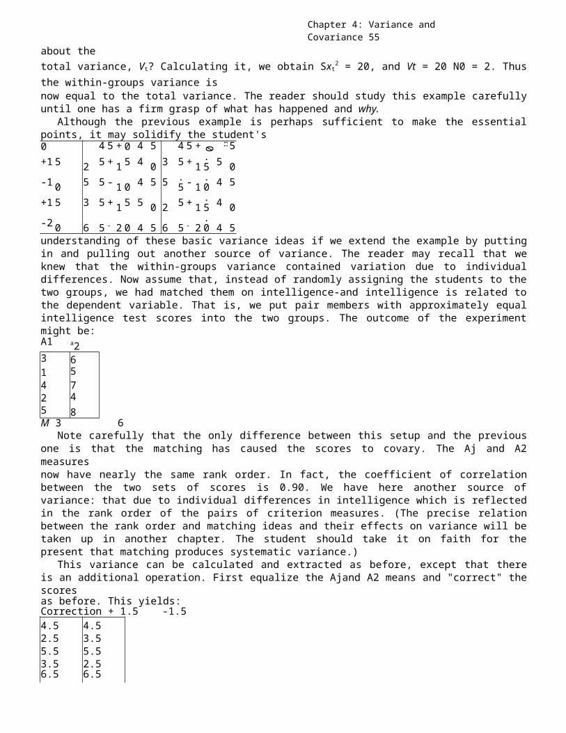
Chapter 4: Variance and Covariance 55
about thetotal variance, Vt? Calculating it, we obtain Sxt2 = 20, and Vt = 20 N0 = 2. Thusthe within-groups variance isnow equal to the total variance. The reader should study this example carefullyuntil one has a firm grasp of what has happened and why.
Although the previous example is perhaps sufficient to make the essentialpoints, it may solidify the student's0 4 5 + 0 4 5 4 5 + 0
II 5+1 5 2 5 + 1 5 4 0 3 5 + 1
.5 5 0
-1 0 5 5 - 1 0 4 5 5 .5 - 1
.0 4 5
+1 5 3 5 + 1 5 5 0 2 5 + 1.5 4 0
-2 0 6 5 - 2 0 4 5 6 5 - 2.0 4 5
understanding of these basic variance ideas if we extend the example by puttingin and pulling out another source of variance. The reader may recall that weknew that the within-groups variance contained variation due to individualdifferences. Now assume that, instead of randomly assigning the students to thetwo groups, we had matched them on intelligence-and intelligence is related tothe dependent variable. That is, we put pair members with approximately equalintelligence test scores into the two groups. The outcome of the experimentmight be:A1 a23 61 54 72 45 8M 3 6
Note carefully that the only difference between this setup and the previousone is that the matching has caused the scores to covary. The Aj and A2measuresnow have nearly the same rank order. In fact, the coefficient of correlationbetween the two sets of scores is 0.90. We have here another source ofvariance: that due to individual differences in intelligence which is reflectedin the rank order of the pairs of criterion measures. (The precise relationbetween the rank order and matching ideas and their effects on variance will betaken up in another chapter. The student should take it on faith for thepresent that matching produces systematic variance.)
This variance can be calculated and extracted as before, except that thereis an additional operation. First equalize the Ajand A2 means and "correct" thescoresas before. This yields:Correction + 1.5 -1.54.5 4.52.5 3.55.5 5.53.5 2.56.5 6.5
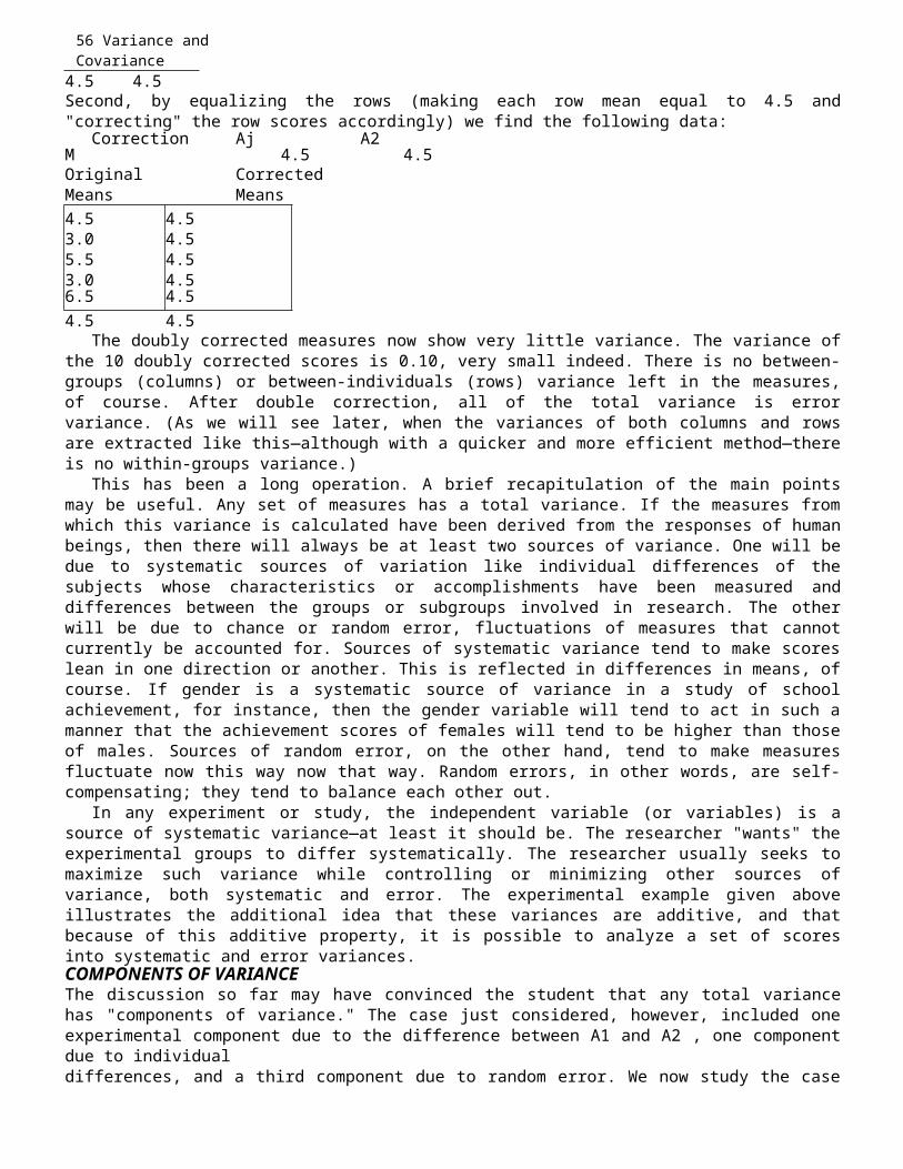
56 Variance and Covariance
4.5 4.5Second, by equalizing the rows (making each row mean equal to 4.5 and"correcting" the row scores accordingly) we find the following data:
Correction Aj A2M 4.5 4.5Original CorrectedMeans Means4.5 4.53.0 4.55.5 4.53.0 4.56.5 4.54.5 4.5
The doubly corrected measures now show very little variance. The variance ofthe 10 doubly corrected scores is 0.10, very small indeed. There is no between-groups (columns) or between-individuals (rows) variance left in the measures,of course. After double correction, all of the total variance is errorvariance. (As we will see later, when the variances of both columns and rowsare extracted like this—although with a quicker and more efficient method—thereis no within-groups variance.)
This has been a long operation. A brief recapitulation of the main pointsmay be useful. Any set of measures has a total variance. If the measures fromwhich this variance is calculated have been derived from the responses of humanbeings, then there will always be at least two sources of variance. One will bedue to systematic sources of variation like individual differences of thesubjects whose characteristics or accomplishments have been measured anddifferences between the groups or subgroups involved in research. The otherwill be due to chance or random error, fluctuations of measures that cannotcurrently be accounted for. Sources of systematic variance tend to make scoreslean in one direction or another. This is reflected in differences in means, ofcourse. If gender is a systematic source of variance in a study of schoolachievement, for instance, then the gender variable will tend to act in such amanner that the achievement scores of females will tend to be higher than thoseof males. Sources of random error, on the other hand, tend to make measuresfluctuate now this way now that way. Random errors, in other words, are self-compensating; they tend to balance each other out.
In any experiment or study, the independent variable (or variables) is asource of systematic variance—at least it should be. The researcher "wants" theexperimental groups to differ systematically. The researcher usually seeks tomaximize such variance while controlling or minimizing other sources ofvariance, both systematic and error. The experimental example given aboveillustrates the additional idea that these variances are additive, and thatbecause of this additive property, it is possible to analyze a set of scoresinto systematic and error variances.COMPONENTS OF VARIANCEThe discussion so far may have convinced the student that any total variancehas "components of variance." The case just considered, however, included oneexperimental component due to the difference between A1 and A2 , one componentdue to individualdifferences, and a third component due to random error. We now study the case
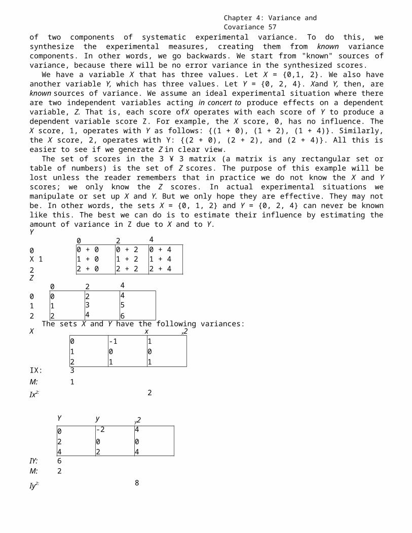
Chapter 4: Variance and Covariance 57
of two components of systematic experimental variance. To do this, wesynthesize the experimental measures, creating them from known variancecomponents. In other words, we go backwards. We start from "known" sources ofvariance, because there will be no error variance in the synthesized scores.
We have a variable X that has three values. Let X = {0,1, 2}. We also haveanother variable Y, which has three values. Let Y = {0, 2, 4}. Xand Y, then, areknown sources of variance. We assume an ideal experimental situation where thereare two independent variables acting in concert to produce effects on a dependentvariable, Z. That is, each score ofX operates with each score of Y to produce adependent variable score Z. For example, the X score, 0, has no influence. TheX score, 1, operates with Y as follows: {(1 + 0), (1 + 2), (1 + 4)}. Similarly,the X score, 2, operates with Y: {(2 + 0), (2 + 2), and (2 + 4)}. All this iseasier to see if we generate Z in clear view.
The set of scores in the 3 ¥ 3 matrix (a matrix is any rectangular set ortable of numbers) is the set of Z scores. The purpose of this example will belost unless the reader remembers that in practice we do not know the X and Yscores; we only know the Z scores. In actual experimental situations wemanipulate or set up X and Y. But we only hope they are effective. They may notbe. In other words, the sets X = {0, 1, 2} and Y = {0, 2, 4} can never be knownlike this. The best we can do is to estimate their influence by estimating theamount of variance in Z due to X and to Y.Y
0 2 40 0 + 0 0 + 2 0 + 4X 1 1 + 0 1 + 2 1 + 42 2 + 0 2 + 2 2 + 4Z
0 2 40 0 2 41 1 3 52 2 4 6
The sets X and Y have the following variances:X x x2
012
-101
101
IX: 3M: 1Ix2: 2
Y y y20 -2 42 0 04 2 4
IY: 6M: 2Iy2: 8
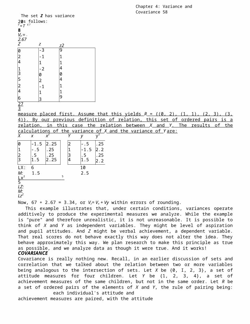
The set Z has varianceas follows:
Chapter 4: Variance and Covariance 58
20V = T 6 7
8Vy = -2.67Z z z20 -3 92 -1 14 1 11 -2 43 0 05 2 42 -1 14 1 16 3 9273measure placed first. Assume that this yields R = {(0, 2), (1, 1), (2, 3), (3,4)}. By our previous definition of relation, this set of ordered pairs is arelation, in this case the relation between X and Y. The results of thecalculations of the variance of X and the variance of Y are:X x x2 Y y y2
0 -1.5 2.25 2 -.5 .251 -.5 .25 1 -1.5 2.22 .5 .25 3 .5 .253 1.5 2.25 4 1.5 2.2LX: 6 10M: 1.5 2.5Lx 2 5 5LZ:M:Lz2
Now, 67 + 2.67 = 3.34, or Vz= Vx + Vy within errors of rounding.This example illustrates that, under certain conditions, variances operate
additively to produce the experimental measures we analyze. While the exampleis "pure" and therefore unrealistic, it is not unreasonable. It is possible tothink of X and Y as independent variables. They might be level of aspirationand pupil attitudes. And Z might be verbal achievement, a dependent variable.That real scores do not behave exactly this way does not alter the idea. Theybehave approximately this way. We plan research to make this principle as trueas possible, and we analyze data as though it were true. And it works!COVARIANCECovariance is really nothing new. Recall, in an earlier discussion of sets andcorrelation that we talked about the relation between two or more variablesbeing analogous to the intersection of sets. Let X be {0, I, 2, 3}, a set ofattitude measures for four children. Let Y be {1, 2, 3, 4}, a set ofachievement measures of the same children, but not in the same order. Let R bea set of ordered pairs of the elements of X and Y, the rule of pairing being:
each individual's attitude andachievement measures are paired, with the attitude
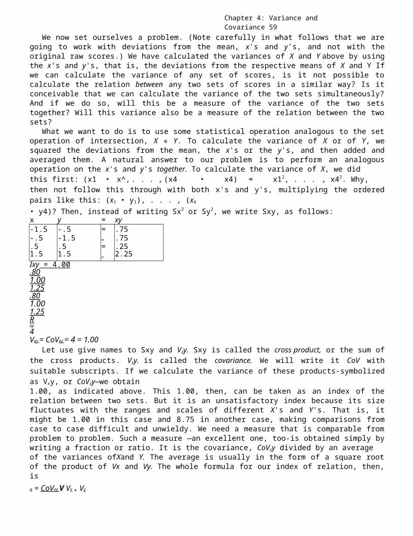
Chapter 4: Variance and Covariance 59
We now set ourselves a problem. (Note carefully in what follows that we aregoing to work with deviations from the mean, x's and y's, and not with theoriginal raw scores.) We have calculated the variances of X and Y above by usingthe x's and y's, that is, the deviations from the respective means of X and Y Ifwe can calculate the variance of any set of scores, is it not possible tocalculate the relation between any two sets of scores in a similar way? Is itconceivable that we can calculate the variance of the two sets simultaneously?And if we do so, will this be a measure of the variance of the two setstogether? Will this variance also be a measure of the relation between the twosets?
What we want to do is to use some statistical operation analogous to the setoperation of intersection, X « Y. To calculate the variance of X or of Y, wesquared the deviations from the mean, the x's or the y's, and then added andaveraged them. A natural answer to our problem is to perform an analogousoperation on the x's and y's together. To calculate the variance of X, we didthis first: (x1 • x^,. . . , (x4 • x4) = x12, . . . , x42. Why,then not follow this through with both x's and y's, multiplying the orderedpairs like this: (x1 • y1), . . . , (x4• y4)? Then, instead of writing Sx2 or Sy2, we write Sxy, as follows:x y = xy-1.5 -.5 = .75-.5 -1.5 = .75.5 .5 = .251.5 1.5 = 2.25Ixy = 4.00.801.001.25.801.001.25Rxy4Vxy = CoVxy = 4 = 1.00
Let use give names to Sxy and Vxy. Sxy is called the cross product, or the sum ofthe cross products. Vxy. is called the covariance. We will write it CoV withsuitable subscripts. If we calculate the variance of these products-symbolizedas Vxy, or CoVxy—we obtain1.00, as indicated above. This 1.00, then, can be taken as an index of therelation between two sets. But it is an unsatisfactory index because its sizefluctuates with the ranges and scales of different X's and Y's. That is, itmight be 1.00 in this case and 8.75 in another case, making comparisons fromcase to case difficult and unwieldy. We need a measure that is comparable fromproblem to problem. Such a measure —an excellent one, too-is obtained simply bywriting a fraction or ratio. It is the covariance, CoVxy divided by an averageof the variances ofXand Y. The average is usually in the form of a square rootof the product of Vx and Vy. The whole formula for our index of relation, then,isR = CoV xy V Vx . Vy
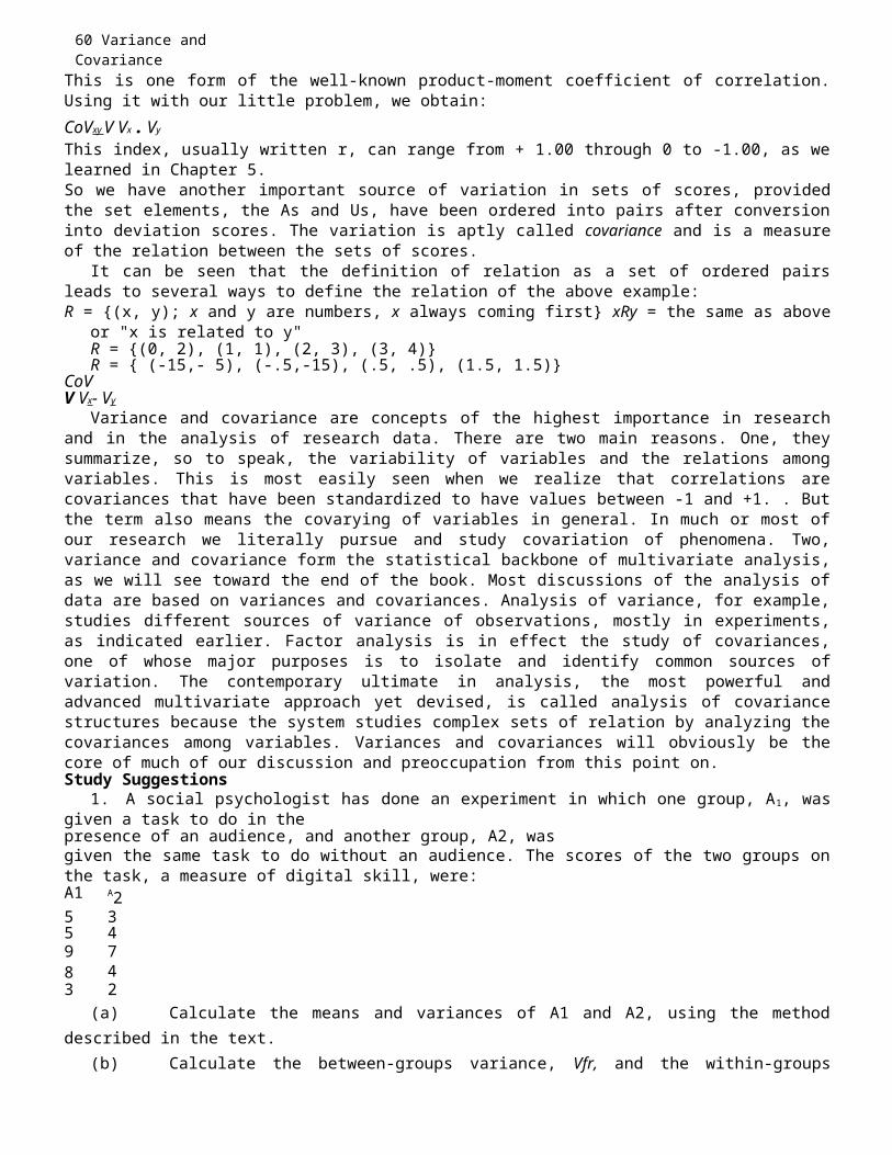
60 Variance and Covariance
This is one form of the well-known product-moment coefficient of correlation.Using it with our little problem, we obtain:CoVxy V Vx . Vy
This index, usually written r, can range from + 1.00 through 0 to -1.00, as welearned in Chapter 5.So we have another important source of variation in sets of scores, providedthe set elements, the As and Us, have been ordered into pairs after conversioninto deviation scores. The variation is aptly called covariance and is a measureof the relation between the sets of scores.
It can be seen that the definition of relation as a set of ordered pairsleads to several ways to define the relation of the above example:R = {(x, y); x and y are numbers, x always coming first} xRy = the same as above
or "x is related to y"R = {(0, 2), (1, 1), (2, 3), (3, 4)}R = { (-15,- 5), (-.5,-15), (.5, .5), (1.5, 1.5)}
CoVV Vx- Vy
Variance and covariance are concepts of the highest importance in researchand in the analysis of research data. There are two main reasons. One, theysummarize, so to speak, the variability of variables and the relations amongvariables. This is most easily seen when we realize that correlations arecovariances that have been standardized to have values between -1 and +1. . Butthe term also means the covarying of variables in general. In much or most ofour research we literally pursue and study covariation of phenomena. Two,variance and covariance form the statistical backbone of multivariate analysis,as we will see toward the end of the book. Most discussions of the analysis ofdata are based on variances and covariances. Analysis of variance, for example,studies different sources of variance of observations, mostly in experiments,as indicated earlier. Factor analysis is in effect the study of covariances,one of whose major purposes is to isolate and identify common sources ofvariation. The contemporary ultimate in analysis, the most powerful andadvanced multivariate approach yet devised, is called analysis of covariancestructures because the system studies complex sets of relation by analyzing thecovariances among variables. Variances and covariances will obviously be thecore of much of our discussion and preoccupation from this point on.Study Suggestions
1. A social psychologist has done an experiment in which one group, A1, wasgiven a task to do in thepresence of an audience, and another group, A2, wasgiven the same task to do without an audience. The scores of the two groups onthe task, a measure of digital skill, were:A1 A25 35 49 78 43 2
(a) Calculate the means and variances of A1 and A2, using the methoddescribed in the text.
(b) Calculate the between-groups variance, Vfr, and the within-groups
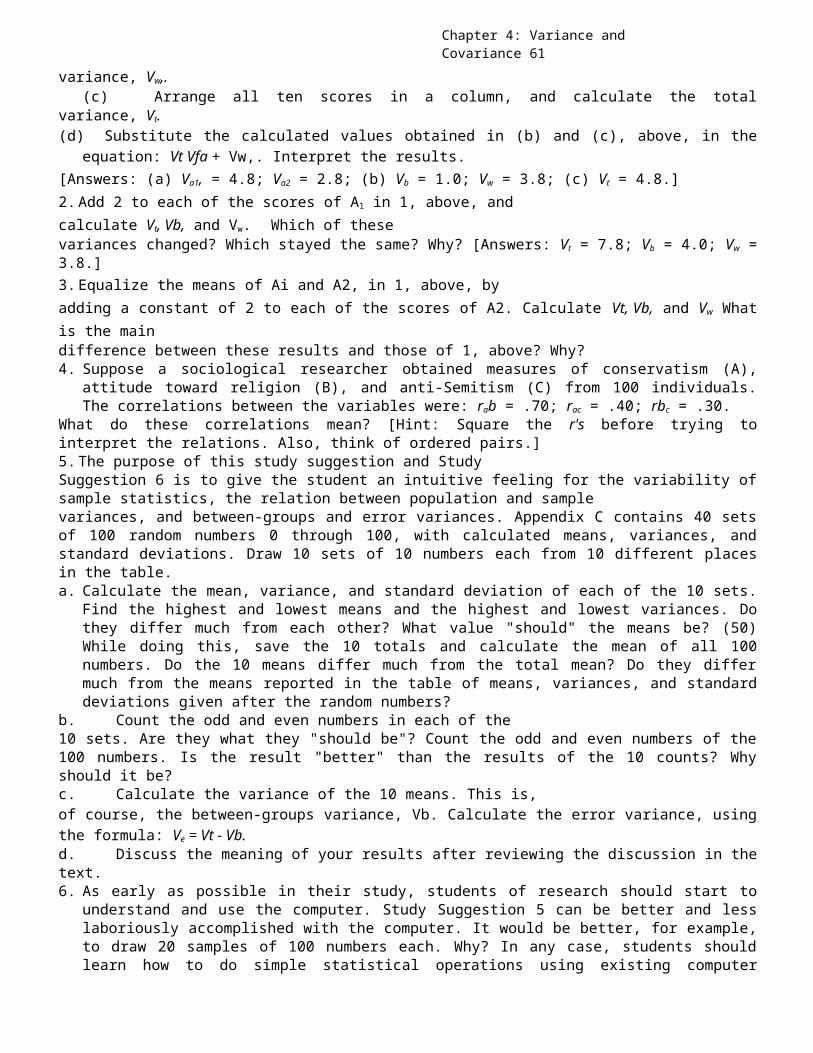
Chapter 4: Variance and Covariance 61
variance, Vw,.(c) Arrange all ten scores in a column, and calculate the total
variance, Vt.(d) Substitute the calculated values obtained in (b) and (c), above, in the
equation: Vt Vfa + Vw,. Interpret the results.[Answers: (a) Va1, = 4.8; Va2 = 2.8; (b) Vb = 1.0; Vw = 3.8; (c) Vt = 4.8.]2.Add 2 to each of the scores of A1 in 1, above, andcalculate Vt, Vb, and Vw. Which of thesevariances changed? Which stayed the same? Why? [Answers: Vt = 7.8; Vb = 4.0; Vw =3.8.]3.Equalize the means of Ai and A2, in 1, above, byadding a constant of 2 to each of the scores of A2. Calculate Vt, Vb, and Vw Whatis the maindifference between these results and those of 1, above? Why?4. Suppose a sociological researcher obtained measures of conservatism (A),
attitude toward religion (B), and anti-Semitism (C) from 100 individuals.The correlations between the variables were: rab = .70; rac = .40; rbc = .30.
What do these correlations mean? [Hint: Square the r's before trying tointerpret the relations. Also, think of ordered pairs.]5.The purpose of this study suggestion and StudySuggestion 6 is to give the student an intuitive feeling for the variability ofsample statistics, the relation between population and samplevariances, and between-groups and error variances. Appendix C contains 40 setsof 100 random numbers 0 through 100, with calculated means, variances, andstandard deviations. Draw 10 sets of 10 numbers each from 10 different placesin the table.a. Calculate the mean, variance, and standard deviation of each of the 10 sets.
Find the highest and lowest means and the highest and lowest variances. Dothey differ much from each other? What value "should" the means be? (50)While doing this, save the 10 totals and calculate the mean of all 100numbers. Do the 10 means differ much from the total mean? Do they differmuch from the means reported in the table of means, variances, and standarddeviations given after the random numbers?
b. Count the odd and even numbers in each of the10 sets. Are they what they "should be"? Count the odd and even numbers of the100 numbers. Is the result "better" than the results of the 10 counts? Whyshould it be?c. Calculate the variance of the 10 means. This is,of course, the between-groups variance, Vb. Calculate the error variance, usingthe formula: Ve = Vt - Vb.d. Discuss the meaning of your results after reviewing the discussion in thetext.6. As early as possible in their study, students of research should start to
understand and use the computer. Study Suggestion 5 can be better and lesslaboriously accomplished with the computer. It would be better, for example,to draw 20 samples of 100 numbers each. Why? In any case, students shouldlearn how to do simple statistical operations using existing computer
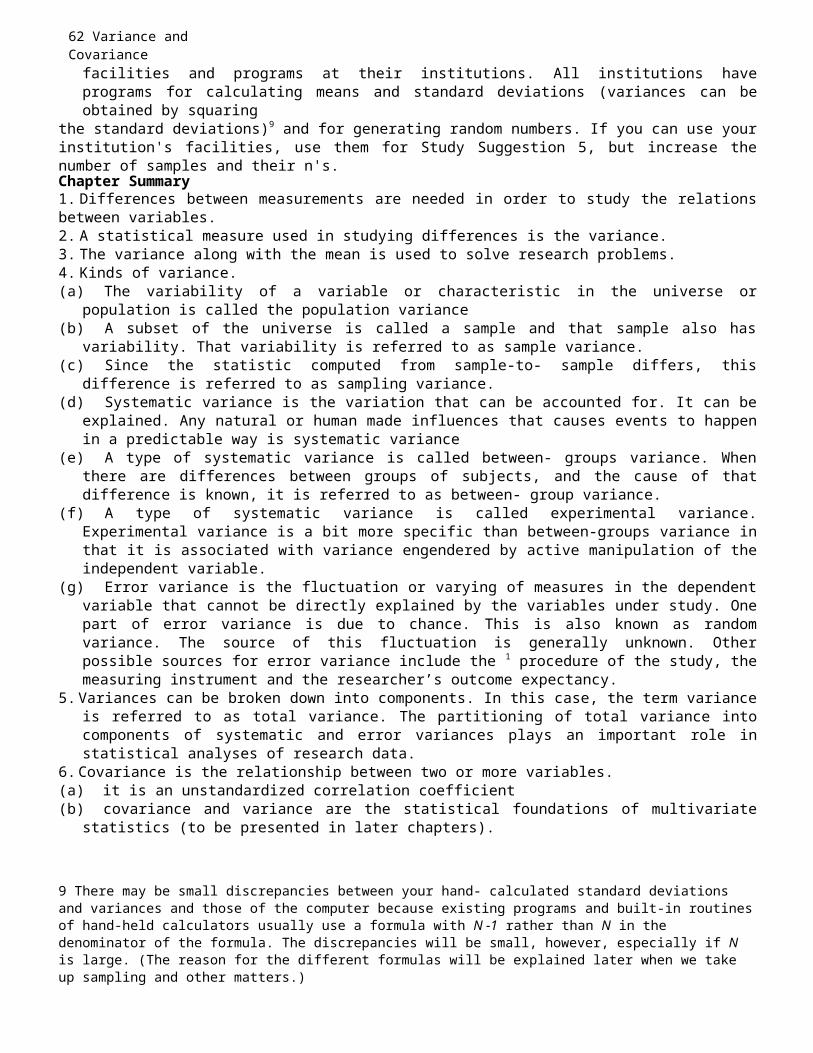
62 Variance and Covariancefacilities and programs at their institutions. All institutions haveprograms for calculating means and standard deviations (variances can beobtained by squaring
the standard deviations)9 and for generating random numbers. If you can use yourinstitution's facilities, use them for Study Suggestion 5, but increase thenumber of samples and their n's.Chapter Summary1. Differences between measurements are needed in order to study the relationsbetween variables.2. A statistical measure used in studying differences is the variance.3. The variance along with the mean is used to solve research problems.4. Kinds of variance.(a) The variability of a variable or characteristic in the universe or
population is called the population variance(b) A subset of the universe is called a sample and that sample also has
variability. That variability is referred to as sample variance.(c) Since the statistic computed from sample-to- sample differs, this
difference is referred to as sampling variance.(d) Systematic variance is the variation that can be accounted for. It can be
explained. Any natural or human made influences that causes events to happenin a predictable way is systematic variance
(e) A type of systematic variance is called between- groups variance. Whenthere are differences between groups of subjects, and the cause of thatdifference is known, it is referred to as between- group variance.
(f) A type of systematic variance is called experimental variance.Experimental variance is a bit more specific than between-groups variance inthat it is associated with variance engendered by active manipulation of theindependent variable.
(g) Error variance is the fluctuation or varying of measures in the dependentvariable that cannot be directly explained by the variables under study. Onepart of error variance is due to chance. This is also known as randomvariance. The source of this fluctuation is generally unknown. Otherpossible sources for error variance include the 1 procedure of the study, themeasuring instrument and the researcher’s outcome expectancy.
5.Variances can be broken down into components. In this case, the term varianceis referred to as total variance. The partitioning of total variance intocomponents of systematic and error variances plays an important role instatistical analyses of research data.
6.Covariance is the relationship between two or more variables.(a) it is an unstandardized correlation coefficient(b) covariance and variance are the statistical foundations of multivariate
statistics (to be presented in later chapters).
9 There may be small discrepancies between your hand- calculated standard deviations and variances and those of the computer because existing programs and built-in routinesof hand-held calculators usually use a formula with N -1 rather than N in the denominator of the formula. The discrepancies will be small, however, especially if N is large. (The reason for the different formulas will be explained later when we take up sampling and other matters.)
Chapter 5 Sampling and Randomness 63
Chapter 5Sampling and Randomness
IMAGINE the many situations in which we want to know something about people,about events, about things. To learn something about people, for instance, wetake some few people whom we know—or do not know—and study them. After our"study," we come to certain conclusions, often about people in general. Somesuch method is behind much folk wisdom. Commonsensical observations aboutpeople, their motives, and their behaviors derive, for the most part, fromobservations and experiences with relatively few people. We make suchstatements as: "People nowadays have no sense of moral values"; "Politiciansare corrupt"; and "Public school pupils are not learning the three R's." Thebasis for making such statements is simple. People, mostly through theirlimited experiences, come to certain conclusions about other people and abouttheir environment. In order to come to such conclusions, they must sample their"experiences" of other people. Actually, they take relatively small samples ofall possible experiences. The term "experiences" here has to be taken in abroad sense. It can mean direct experience with other people—for example,first-hand interaction with, say, Moslems or Asians. Or it can mean indirectexperience: hearing about Moslems or Asians from friends, acquaintances,parents, and others. Whether experience is direct or indirect, however, doesnot concern us too much at this point. Let us assume that all such experienceis direct. An individual claim to "know" something about Asians and says “ I‘know’ they are clannish because I have had direct experience with a number ofAsians.” Or, "Some of my best friends are Asians, and I know that. . . " Thepoint is that this person’s conclusions are based on a sample of Asians, or asample of the behaviors of Asians, or both. This individual can never "know"all Asians; and must depend, in the last analysis, on samples. Indeed, most ofthe world's knowledge is based on samples, most often on inadequate samples.SAMPLING, RANDOM SAMPLING, AND REPRESENTATIVENESSSampling refers to taking a portion of a population or universe as representative ofthat population or universe. This definition does not say that the sampletaken-or drawn, as researchers say—is representative. It says, rather, taking aportion of the population and considering it to be representative. When a schooladministrator visits certain classrooms in the school system "to get the feelof the system," that administrator is sampling classes from all the classes inthe system. This person might assume that by visiting, say, eight to tenclasses out of forty "at random," he or she will get a fair notion of thequality of teaching going on in the system. Or another way would be to visitone teacher's class two or three times to sample teaching performance. By doingthis, the administrator is now sampling behaviors, in this case teachingbehaviors, from the universe of all possible behaviors of the teacher. Suchsampling is necessary and legitimate. However, you can come up with somesituations where the entire universe could be measured. So why bother withsamples? Why not just measure every element of the universe? Take a census? Onemajor reason is one of economics. The second author (HBL) worked in a marketingresearch department of a large grocery chain in southern California. This chainconsisted of 100 stores. Research on customers and products occasionally takethe form of a controlled-store test. These are studies conducted in a real day-to-day grocery store operation. Perhaps one might be interested in testing anew dog food. Certain stores would be chosen to receive the new product whileanother set of stores will not carry the new product. Secrecy is very importantin such studies. If a competing manufacture of dog food received informationthat a marketing test was being done at such-and-such store, they can
64 Chapter 5 Sampling and Randomness
contaminate the results. To conduct controlled stored tests of cents-offcoupons, or new products, or shelf allocation space, a research study could beconducted with two groups of 50 stores each. However, the labor andadministrative costs alone would be prohibitive. It would make a lot more senseto use samples that are representative of the population. Choosing 10 stores ineach group to conduct the research would cut down the costs of doing the study.Smaller studies are more manageable and controllable. The study using samplescan be completed on a timely manner. In some disciplines, such as qualitycontrol and education-instructional evaluation, sampling is essential. Inquality control there is a procedure called destructive testing. One way todetermine whether a product meets specification is to put it through an actualperformance test. When the product is destroyed (fails), the product can beevaluated. In testing tires, for example, it would make little sense to destroyevery tire just to determine if the manufacturer has adequate quality control.Likewise the teacher who wants to determine if the child has learned thematerial will give an examination. It would be difficult to write anexamination that covers every aspect of instruction and knowledge retention ofthe child.
Random sampling is that method of drawing a portion (or sample) of apopulation or universe so that each member of the population or universe has anequal chance of being selected. This definition has the virtue of being easilyunderstood. Unfortunately, it is not entirely satisfactory because it islimited. A better definition is by Kirk (1990, p. 8).The method of drawing samples from a population such that every possible sampleof a particular size has an equal chance of being selected is called randomsampling, and the resulting samples are random samples.This definition is general and thus more satisfactory than the earlierdefinition.
Define a universe to be studied as all fourth-grade children in X schoolsystem. Suppose there are 200 such children. They comprise the population (oruniverse). We select one child at random from the population. His (or her)chance of being selected is 1/ 200, if the sampling procedure is random.Likewise, a number of other children are similarly selected. Let us assume thatafter selecting a child, the child is returned (or the symbol assigned to thechild) to the population. Then the chance of selecting any second child is also1/200. (If we do not return this child to the population, then the chance eachof the remaining children has, of course, is 1/199. This is called samplingwithout replacement. When the sample elements are returned to the population afterbeing drawn, the procedure is called sampling with replacement.)
Suppose from the population of the 200 fourth- grade children in X schoolsystem we decide to draw a random sample of 50 children. This means, if thesample is random, that all possible samples of 50 have the same probability ofbeing selected—a very large number of possible samples. To make the ideasinvolved comprehensible, suppose a population consists of four children, a, b,c, and d, and we draw a random sample of two children. Then the list of all thepossibilities, or the sample space, is: (a, b), (a, c), (a, d), (b, c), (b, d),(c, d). There are six possibilities. If the sample of two is drawn at random,then its probability is 1/6. Each of the pairs has the same probability ofbeing drawn. This sort of reasoning is needed to solve many research problems,but we will usually confine ourselves to the simpler idea of sampling connectedwith the first definition. The first definition, then, is a special case of thesecond general definition-the special case in which n = 1.
Unfortunately, we can never be sure that a random sample is representative
Chapter 5 Sampling and Randomness 65
of the population from which it is drawn. Remember that any particular sampleof size n has the same probability of being selected as any other sample of thesame size. Thus, a particular sample may not be representative at all. Weshould know what "representative" means. Ordinarily, "representative" means tobe typical of a population, that is, to exemplify the characteristics of thepopulation. From a research point of view, "representative" must be moreprecisely defined, though it is often difficult to be precise. We must ask:What characteristics are we talking about? So, in research, a "representativesample" means that the sample has approximately the characteristics of thepopulation relevant to the research in question. If sex and socioeconomic classare variables (characteristics) relevant to the research, a representativesample will have approximately the same proportions of men and women andmiddle-class and working class individuals as the population. When we draw arandom sample, we hope that it will be representative. We hope that the relevantcharacteristics of the population will be present in the sample inapproximately the same way they are present in the population. But we can neverbe sure. There is no guarantee.
What we rely on is the fact, as Stilson (1966) points out, that thecharacteristics typical of a population are those that are the most frequentand therefore most likely to be present in any particularrandom sample. When sampling is random, the sampling variability ispredictable. We learned in Chapter 7, for example, that if we throw two dice anumber of times, the probability of a 7 turning up is greater than that of a 12turning up. (See Table 7.1.)
A sample drawn at random is unbiased in the sense that no member of thepopulation has any more chance of being selected than any other member. We havehere a democracy in which all members are equal before the bar of selection.Rather than using coins or dice, let's use a research example. Suppose we havea population of 100 children. The children differ in intelligence, a variablerelevant to our research. We want to know the mean intelligence score of thepopulation, but for some reason we can only sample 30 of the 100 children. Ifwe sample randomly, there are a large number of possible samples of 30 each.The samples have equal probabilities of being selected.The means of most of the samples will be relatively close to the mean of thepopulation. A few will not be close. If the sampling has been random, theprobability of selecting a sample with a mean close to the population mean isgreater than the probability of selecting a sample with a mean not close to thepopulation mean.
If we do not draw our sample at random, however, some factor or factorsunknown to us may predispose us to select a biased sample. In this case perhapsone of the samples with a mean not close to the population mean. The meanintelligence of this sample will then be a biased estimate of the populationmean. If we knew the 100 children, we might unconsciously tend to select themore intelligent children. It is not so much that we would do so; it is that ourmethod allows us to do so. Random methods of selection do not allow our ownbiases or any other systematic selection factors to operate. The procedure isobjective, divorced from our own predilections and biases.
The reader may be experiencing a vague and disquieting sense of uneasiness.If we can't be sure that random samples are representative, how can we haveconfidence in our research results and their applicability to the populationsfrom which we draw our samples? Why not select samples systematically so thatthey are representative? The answer is complex. First—and again—we cannot ever
66 Chapter 5 Sampling and Randomness
be sure. Second, random samples are more likely to include the characteristicstypical of the population if the characteristics are frequent in thepopulation. In actual research, we draw random samples whenever we can and hopeand assume that the samples are representative. We learn to live withuncertainty. We try to cut it down whenever we can—just as we do in ordinaryday-to-day living but more systematically and with considerable knowledge ofand experience with random sampling and random outcomes. Fortunately, our lackof certainty does not impair our research functioning.RANDOMNESSThe notion of randomness is at the core of modern probabilistic methods in thenatural and behavioral sciences. But it is difficult to define "random." Thedictionary notion of haphazard, accidental, without aim or direction, does nothelp us much. In fact, scientists are quite systematic about randomness; theycarefully select random samples and plan random procedures.
The position can be taken that nothing happens at random, that for any eventthere is a cause. The only reason, this position might say, that one uses theword random is that human beings do not know enough. To omniscience nothing israndom. Suppose an omniscient being has an omniscient newspaper. It is agigantic newspaper in which every event down to the last detail—for tomorrow,the next day, and the next day, and on and on into indefinite time—is carefullyinscribed. (see Kemeny, 1959, p. 39). There is nothing unknown. And, of course,there is no randomness. Randomness is, as it were, ignorance, in this view.
Taking a cue from this argument, we define randomness in a backhand way. Wesay events are random if we cannot predict their outcomes. For instance, thereis no known way to win a pennytossing game. Whenever there is no system forplaying a game that ensures our winning (or losing), then the event-outcomes ofthe game are random. More formally put, randomness means that there is no knownlaw, capable of being expressed in language that correctly describes orexplains events and their outcomes. In a word, when events are random we cannotpredict them individually. Strange to say, however, we can predict them quitesuccessfully in the aggregate. That is, we can predict the outcomes of largenumbers of events. We cannot predict whether a coin tossed will be heads ortails. But, if we toss the coin 1000 times, we can predict, with considerableaccuracy, the total numbers of heads and tails.An Example of Random SamplingTo give the reader a feeling for randomness and random samples, we now do ademonstration using a table of random numbers. A table of random numberscontains numbers generated mechanically so that there is no discernible orderor system in them. It was said above that if events are random they cannot bepredicted. But now we are going to predict the general nature of the outcomes ofour experiment. We select, from a table of random digits, 10 samples of 10digits each. Since the numbers are random, each sample "should" berepresentative of the universe of digits. The universe can be variouslydefined. We simply define it as the complete set of digits in the RandCorporation table of random digits. We now draw samples from the table. Themeans of the 10 samples will, of course, be different. However, they shouldfluctuate within a relatively narrow range, with most of them fairly close tothe mean of all 100 numbers and to the theoretical mean of the whole populationof random numbers. The number of even numbers in each sample of 10 should beapproximately equal to the number of odd numbers—though. There will befluctuations, some of them perhaps extreme but most of them comparativelymodest. The samples are given in Table 5. l.TABLE 5.1 Ten Samples of Random Numbersm m 1 3 PH rn HP 1 7 PP PP PP
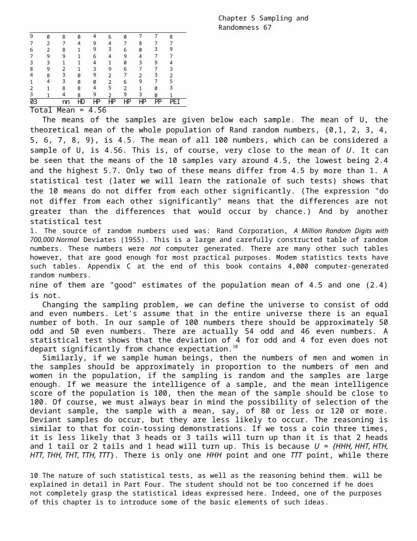
Chapter 5 Sampling and Randomness 67
9 0 8 0 4 6 0 7 7 87 2 7 4 9 4 7 8 7 76 2 8 1 9 3 6 0 3 97 9 9 1 6 4 9 4 7 73 3 1 1 4 1 0 3 9 48 9 2 1 3 9 6 7 7 34 8 3 0 9 2 7 2 3 21 4 3 0 0 2 6 9 7 52 1 8 8 4 5 2 1 0 33 1 4 8 9 2 9 3 0 103 nn HD HP HP HP HP PP PEITotal Mean = 4.56
The means of the samples are given below each sample. The mean of U, thetheoretical mean of the whole population of Rand random numbers, {0,1, 2, 3, 4,5, 6, 7, 8, 9}, is 4.5. The mean of all 100 numbers, which can be considered asample of U, is 4.56. This is, of course, very close to the mean of U. It canbe seen that the means of the 10 samples vary around 4.5, the lowest being 2.4and the highest 5.7. Only two of these means differ from 4.5 by more than 1. Astatistical test (later we will learn the rationale of such tests) shows thatthe 10 means do not differ from each other significantly. (The expression "donot differ from each other significantly" means that the differences are notgreater than the differences that would occur by chance.) And by anotherstatistical test1. The source of random numbers used was: Rand Corporation, A Million Random Digits with700,000 Normal Deviates (1955). This is a large and carefully constructed table of randomnumbers. These numbers were not computer generated. There are many other such tableshowever, that are good enough for most practical purposes. Modem statistics texts havesuch tables. Appendix C at the end of this book contains 4,000 computer-generatedrandom numbers.nine of them are "good" estimates of the population mean of 4.5 and one (2.4)is not.
Changing the sampling problem, we can define the universe to consist of oddand even numbers. Let's assume that in the entire universe there is an equalnumber of both. In our sample of 100 numbers there should be approximately 50odd and 50 even numbers. There are actually 54 odd and 46 even numbers. Astatistical test shows that the deviation of 4 for odd and 4 for even does notdepart significantly from chance expectation.10
Similarly, if we sample human beings, then the numbers of men and women inthe samples should be approximately in proportion to the numbers of men andwomen in the population, if the sampling is random and the samples are largeenough. If we measure the intelligence of a sample, and the mean intelligencescore of the population is 100, then the mean of the sample should be close to100. Of course, we must always bear in mind the possibility of selection of thedeviant sample, the sample with a mean, say, of 80 or less or 120 or more.Deviant samples do occur, but they are less likely to occur. The reasoning issimilar to that for coin-tossing demonstrations. If we toss a coin three times,it is less likely that 3 heads or 3 tails will turn up than it is that 2 headsand 1 tail or 2 tails and 1 head will turn up. This is because U = {HHH, HHT, HTH,HTT, THH, THT, TTH, TTT}. There is only one HHH point and one TTT point, while there
10 The nature of such statistical tests, as well as the reasoning behind them. will be explained in detail in Part Four. The student should not be too concerned if he does not completely grasp the statistical ideas expressed here. Indeed, one of the purposes of this chapter is to introduce some of the basic elements of such ideas.

68 Chapter 5 Sampling and Randomness
are three points with two H's and three with two T's.RANDOMIZATIONSuppose an investigator wishes to test the hypothesis that counseling helpsunderachievers. The test involves using two groups of underachievers, one to becounseled, one not to be counseled. Naturally, the wish is to have the twogroups equal in other independent variables that may have a possible effect onachievement. One way this can be done is to assign the children to both groupsat random by, say, tossing a coin for each child. The child is assigned to onegroup if the toss is heads and to the other group if the toss is tails. (Notethat if there were three experimental groups coin tossing would probably not beused. A 6sided die may be used. Outcomes of 1 or 2 would assign that child togroup 1. Outcomes of 3 and 4 would put the child in group 2 and the outcomes 5and 6 would designate the child to be in group 3. Or a table of random numberscan be used to assign the children to groups. If an odd number turns up, assigna child to one group, and if an even number turns up, assign the child to theother group. The investigator can now assume that the groups are approximatelyequal in all possible independent variables. The larger the groups, the saferthe assumption. Just as there is no guarantee, however, of not drawing adeviant sample, as discussed earlier, there is no guarantee that the groups areequal or even approximately equal in all possible independent variables.Nevertheless, it can be said that the investigator has used randomization toequalize the groups, or, as it is said, to control influences on the dependentvariable other than that of the manipulated independent variable. Although wewill use the term “randomization.” a number of researchers prefer to use thewords “random assignment.” The procedure calls for assigning participants toexperimental conditions on a random basis. While some believe that randomassignment removes variation, in reality it only distributes it.
An "ideal" experiment is one in which all the factors or variables likely toaffect the experimental outcome are controlled. If we knew all these factors,in the first place, and could make efforts to control them, in the second place,then we might have an ideal experiment. However, the sad case is that we cannever know all the pertinent variables nor could we control them even if we didknow them. Randomization, however, comes to our aid.
Randomization is the assignment to experimental treatments of members of auniverse in such a way that, for any given assignment to a treatment, everymember of the universe has an equal probability of being chosen for thatassignment. The basic purpose of random assignment, as indicated earlier, is toapportion subjects (objects, groups) to treatments. Individuals with varyingcharacteristics are spread approximately equally among the treatments so thatvariables that might affect the dependent variable other than the experimentalvariables have "equal" effects in the different treatments. There is noguarantee that this desirable state of affairs will be attained, but it is morelikely to be attained with randomization than otherwise. Randomization also hasa statistical rationale and purpose. If random assignment has been used, thenit is possible to distinguish between systematic or experimental variance anderror variance. Biasing variables are distributed to experimental groupsaccording to chance. The tests of statistical significance that we will discusslater logically depend on random assignment. These tests are used to determinewhether the observed phenomenon is statistically different from chance. Withoutrandom assignment the significance tests lack logical foundation. The idea ofrandomization seems to have been discovered or invented by Sir Ronald Fisher(see Cowles, 1989). It was Fisher who virtually revolutionized statistical andexperimental design thinking and methods using random notions as part of his
Chapter 5 Sampling and Randomness 69
leverage. He has been referred to as “the father of analysis-of-variance.” Inany case, randomization and what can be called the principle of randomizationis one of the great intellectual achievements of our time. It is not possibleto overrate the importance of both the idea and the practical measures thatcome from it to improve experimentation and inference.
Randomization can perhaps be clarified in two or three ways: by stating theprinciple of randomization, by describing how one uses it in practice, and bydemonstrating how it works with objects and numbers. The importance of the ideadeserves all three.
The principle of randomization may be stated as the following. Since, in randomprocedures, every member of a population has an equal chance of being selected,members with certain distinguishing characteristics—male or female, high or lowintelligence, conservative or liberal, and so on and on—will, if selected,probably be offset in the long run by the selection of other members of thepopulation with counterbalancing quantities or qualities of thecharacteristics. We can say that this is a practical principle of what usuallyhappens; we cannot say that it is a law of nature. It is simply a statement ofwhat most often happens when random procedures are used.
We say that subjects are assigned at random to experimental groups, and thatexperimental treatments are assigned at random to groups. For instance, in theexample cited above of an experiment to test the effectiveness of counseling onachievement, subjects can be assigned to two groups at random by using randomnumbers or by tossing a coin. When the subjects have been so assigned, thegroups can be randomly designated as experimental and control groups using asimilar procedure. We will encounter a number of examples of randomization aswe go along.
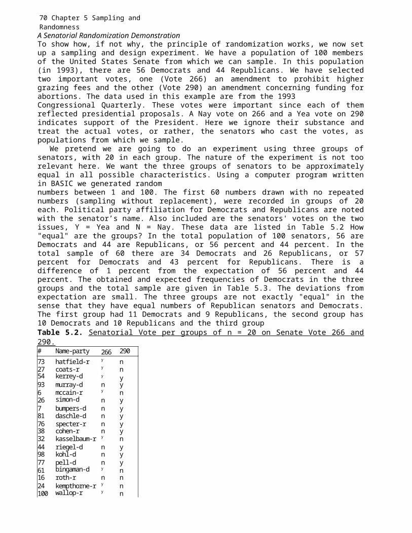
70 Chapter 5 Sampling and RandomnessA Senatorial Randomization DemonstrationTo show how, if not why, the principle of randomization works, we now setup a sampling and design experiment. We have a population of 100 membersof the United States Senate from which we can sample. In this population(in 1993), there are 56 Democrats and 44 Republicans. We have selectedtwo important votes, one (Vote 266) an amendment to prohibit highergrazing fees and the other (Vote 290) an amendment concerning funding forabortions. The data used in this example are from the 1993Congressional Quarterly. These votes were important since each of themreflected presidential proposals. A Nay vote on 266 and a Yea vote on 290indicates support of the President. Here we ignore their substance andtreat the actual votes, or rather, the senators who cast the votes, aspopulations from which we sample.
We pretend we are going to do an experiment using three groups ofsenators, with 20 in each group. The nature of the experiment is not toorelevant here. We want the three groups of senators to be approximatelyequal in all possible characteristics. Using a computer program writtenin BASIC we generated randomnumbers between 1 and 100. The first 60 numbers drawn with no repeatednumbers (sampling without replacement), were recorded in groups of 20each. Political party affiliation for Democrats and Republicans are notedwith the senator’s name. Also included are the senators' votes on the twoissues, Y = Yea and N = Nay. These data are listed in Table 5.2 How"equal" are the groups? In the total population of 100 senators, 56 areDemocrats and 44 are Republicans, or 56 percent and 44 percent. In thetotal sample of 60 there are 34 Democrats and 26 Republicans, or 57percent for Democrats and 43 percent for Republicans. There is adifference of 1 percent from the expectation of 56 percent and 44percent. The obtained and expected frequencies of Democrats in the threegroups and the total sample are given in Table 5.3. The deviations fromexpectation are small. The three groups are not exactly "equal" in thesense that they have equal numbers of Republican senators and Democrats.The first group had 11 Democrats and 9 Republicans, the second group has10 Democrats and 10 Republicans and the third groupTable 5.2. Senatorial Vote per groups of n = 20 on Senate Vote 266 and290.# Name-party 266 29073 hatfield-r y n27 coats-r y n54 kerrey-d y y93 murray-d n y6 mccain-r y n26 simon-d n y7 bumpers-d n y81 daschle-d n y76 specter-r n y38 cohen-r n y32 kasselbaum-r y n44 riegel-d n y98 kohl-d n y77 pell-d n y61 bingaman-d y n16 roth-r n n24 kempthorne-r y n100 wallop-r y n
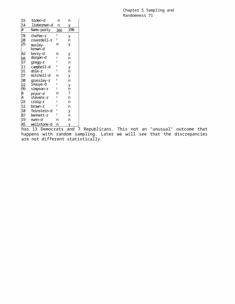
Chapter 5 Sampling and Randomness 71
15 biden-d n n14 lieberman-d n y# Name-party 266 29078 chafee-r y y20 coverdell-r y n25 mosley-
brown-dn y
42 kerry-d n y68 dorgan-d y n57 gregg-r y n11 campbell-d y y31 dole-r y n37 mitchell-d n y30 grassley-r y n22 inouye-d y y99 simpson-r y n8 pryor-d n ?4 stevens-r y n23 craig-r y n12 brown-r y n10 feinstein-d y y87 bennett-r y n19 nunn-d n n45 wellstone-d n yhas 13 Democrats and 7 Republicans. This not an "unusual" outcome thathappens with random sampling. Later we will see that the discrepanciesare not different statistically.
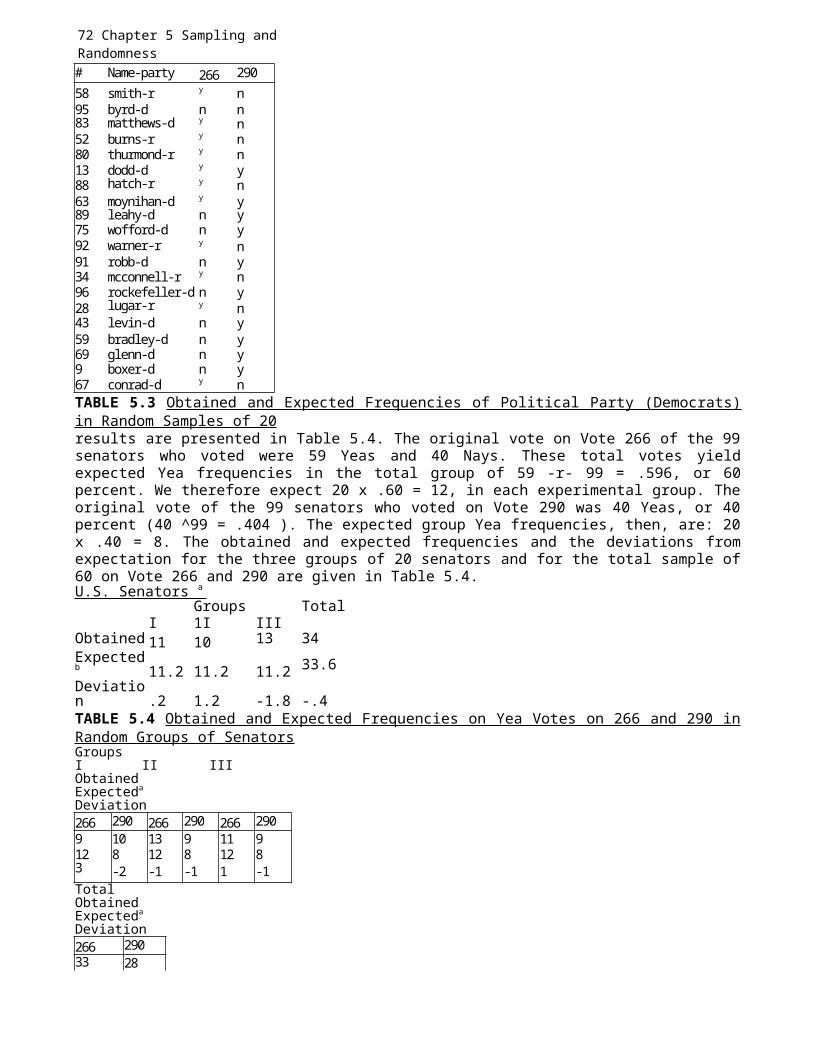
72 Chapter 5 Sampling and Randomness# Name-party 266 29058 smith-r y n95 byrd-d n n83 matthews-d y n52 burns-r y n80 thurmond-r y n13 dodd-d y y88 hatch-r y n63 moynihan-d y y89 leahy-d n y75 wofford-d n y92 warner-r y n91 robb-d n y34 mcconnell-r y n96 rockefeller-d n y28 lugar-r y n43 levin-d n y59 bradley-d n y69 glenn-d n y9 boxer-d n y67 conrad-d y nTABLE 5.3 Obtained and Expected Frequencies of Political Party (Democrats)in Random Samples of 20results are presented in Table 5.4. The original vote on Vote 266 of the 99senators who voted were 59 Yeas and 40 Nays. These total votes yieldexpected Yea frequencies in the total group of 59 -r- 99 = .596, or 60percent. We therefore expect 20 x .60 = 12, in each experimental group. Theoriginal vote of the 99 senators who voted on Vote 290 was 40 Yeas, or 40percent (40 ^99 = .404 ). The expected group Yea frequencies, then, are: 20x .40 = 8. The obtained and expected frequencies and the deviations fromexpectation for the three groups of 20 senators and for the total sample of60 on Vote 266 and 290 are given in Table 5.4.U.S. Senators a
Groups TotalI 1I III
Obtained 11 10 13 34Expectedb 11.2 11.2 11.2 33.6Deviation .2 1.2 -1.8 -.4TABLE 5.4 Obtained and Expected Frequencies on Yea Votes on 266 and 290 inRandom Groups of SenatorsGroupsI II IIIObtainedExpecteda
Deviation266 290 266 290 266 2909 10 13 9 11 912 8 12 8 12 83 -2 -1 -1 1 -1TotalObtainedExpecteda
Deviation266 29033 28
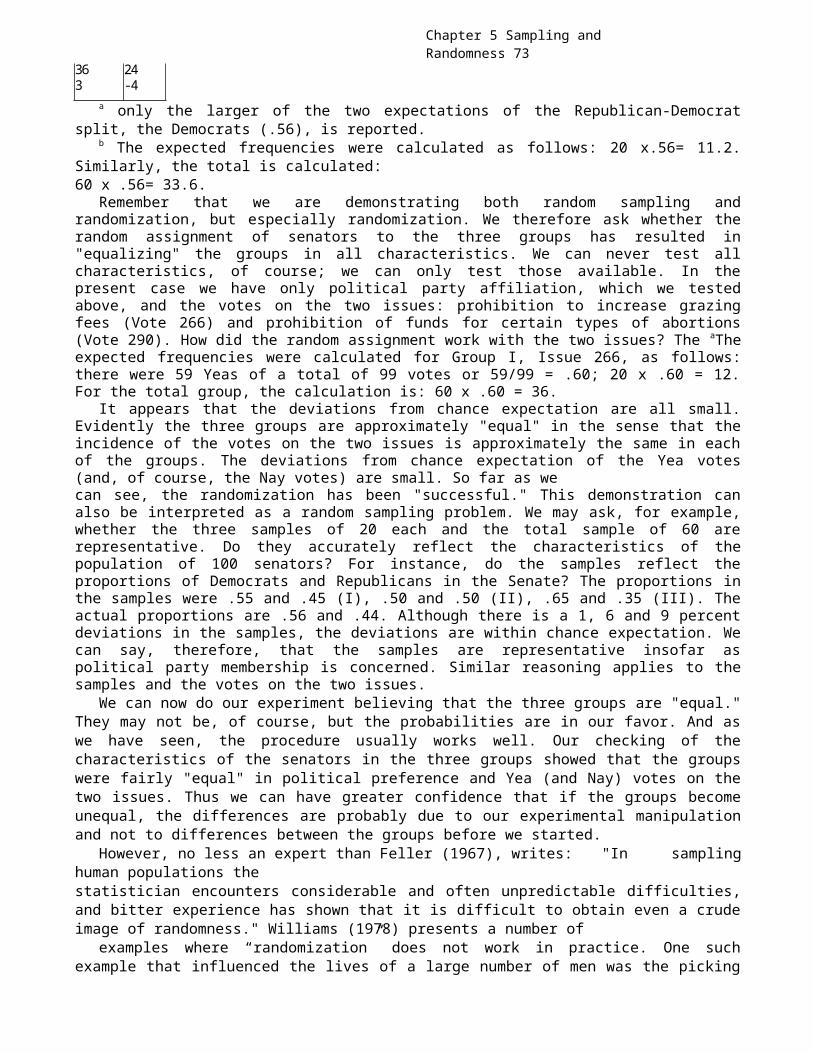
Chapter 5 Sampling and Randomness 73
36 243 -4
a only the larger of the two expectations of the Republican-Democratsplit, the Democrats (.56), is reported.
b The expected frequencies were calculated as follows: 20 x.56= 11.2.Similarly, the total is calculated:60 x .56= 33.6.
Remember that we are demonstrating both random sampling andrandomization, but especially randomization. We therefore ask whether therandom assignment of senators to the three groups has resulted in"equalizing" the groups in all characteristics. We can never test allcharacteristics, of course; we can only test those available. In thepresent case we have only political party affiliation, which we testedabove, and the votes on the two issues: prohibition to increase grazingfees (Vote 266) and prohibition of funds for certain types of abortions(Vote 290). How did the random assignment work with the two issues? The aTheexpected frequencies were calculated for Group I, Issue 266, as follows:there were 59 Yeas of a total of 99 votes or 59/99 = .60; 20 x .60 = 12.For the total group, the calculation is: 60 x .60 = 36.
It appears that the deviations from chance expectation are all small.Evidently the three groups are approximately "equal" in the sense that theincidence of the votes on the two issues is approximately the same in eachof the groups. The deviations from chance expectation of the Yea votes(and, of course, the Nay votes) are small. So far as wecan see, the randomization has been "successful." This demonstration canalso be interpreted as a random sampling problem. We may ask, for example,whether the three samples of 20 each and the total sample of 60 arerepresentative. Do they accurately reflect the characteristics of thepopulation of 100 senators? For instance, do the samples reflect theproportions of Democrats and Republicans in the Senate? The proportions inthe samples were .55 and .45 (I), .50 and .50 (II), .65 and .35 (III). Theactual proportions are .56 and .44. Although there is a 1, 6 and 9 percentdeviations in the samples, the deviations are within chance expectation. Wecan say, therefore, that the samples are representative insofar aspolitical party membership is concerned. Similar reasoning applies to thesamples and the votes on the two issues.
We can now do our experiment believing that the three groups are "equal."They may not be, of course, but the probabilities are in our favor. And aswe have seen, the procedure usually works well. Our checking of thecharacteristics of the senators in the three groups showed that the groupswere fairly "equal" in political preference and Yea (and Nay) votes on thetwo issues. Thus we can have greater confidence that if the groups becomeunequal, the differences are probably due to our experimental manipulationand not to differences between the groups before we started.
However, no less an expert than Feller (1967), writes: "In samplinghuman populations thestatistician encounters considerable and often unpredictable difficulties,and bitter experience has shown that it is difficult to obtain even a crudeimage of randomness." Williams (1978) presents a number of
examples where “randomization” does not work in practice. One suchexample that influenced the lives of a large number of men was the picking
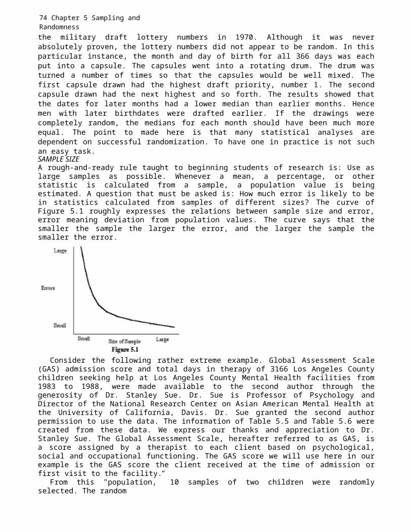
74 Chapter 5 Sampling and Randomnessthe military draft lottery numbers in 1970. Although it was neverabsolutely proven, the lottery numbers did not appear to be random. In thisparticular instance, the month and day of birth for all 366 days was eachput into a capsule. The capsules went into a rotating drum. The drum wasturned a number of times so that the capsules would be well mixed. Thefirst capsule drawn had the highest draft priority, number 1. The secondcapsule drawn had the next highest and so forth. The results showed thatthe dates for later months had a lower median than earlier months. Hencemen with later birthdates were drafted earlier. If the drawings werecompletely random, the medians for each month should have been much moreequal. The point to made here is that many statistical analyses aredependent on successful randomization. To have one in practice is not suchan easy task.SAMPLE SIZEA rough-and-ready rule taught to beginning students of research is: Use aslarge samples as possible. Whenever a mean, a percentage, or otherstatistic is calculated from a sample, a population value is beingestimated. A question that must be asked is: How much error is likely to bein statistics calculated from samples of different sizes? The curve ofFigure 5.1 roughly expresses the relations between sample size and error,error meaning deviation from population values. The curve says that thesmaller the sample the larger the error, and the larger the sample thesmaller the error.
Consider the following rather extreme example. Global Assessment Scale(GAS) admission score and total days in therapy of 3166 Los Angeles Countychildren seeking help at Los Angeles County Mental Health facilities from1983 to 1988, were made available to the second author through thegenerosity of Dr. Stanley Sue. Dr. Sue is Professor of Psychology andDirector of the National Research Center on Asian American Mental Health atthe University of California, Davis. Dr. Sue granted the second authorpermission to use the data. The information of Table 5.5 and Table 5.6 werecreated from these data. We express our thanks and appreciation to Dr.Stanley Sue. The Global Assessment Scale, hereafter referred to as GAS, isa score assigned by a therapist to each client based on psychological,social and occupational functioning. The GAS score we will use here in ourexample is the GAS score the client received at the time of admission orfirst visit to the facility.
From this "population,” 10 samples of two children were randomlyselected. The random
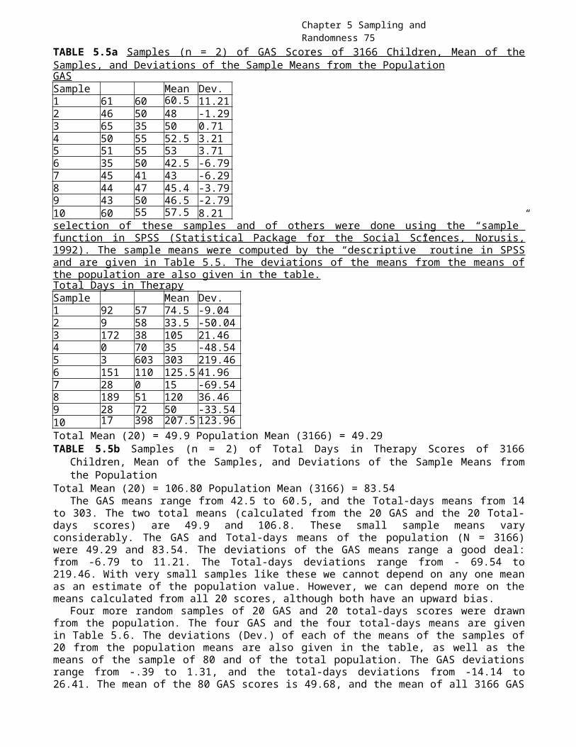
Chapter 5 Sampling and Randomness 75
TABLE 5.5a Samples (n = 2) of GAS Scores of 3166 Children, Mean of theSamples, and Deviations of the Sample Means from the PopulationGASSample Mean Dev.1 61 60 60.5 11.212 46 50 48 -1.293 65 35 50 0.714 50 55 52.5 3.215 51 55 53 3.716 35 50 42.5 -6.797 45 41 43 -6.298 44 47 45.4 -3.799 43 50 46.5 -2.7910 60 55 57.5 8.21selection of these samples and of others were done using the “sample”function in SPSS (Statistical Package for the Social Sciences, Norusis,1992). The sample means were computed by the “descriptive” routine in SPSSand are given in Table 5.5. The deviations of the means from the means ofthe population are also given in the table.Total Days in TherapySample Mean Dev.1 92 57 74.5 -9.042 9 58 33.5 -50.043 172 38 105 21.464 0 70 35 -48.545 3 603 303 219.466 151 110 125.5 41.967 28 0 15 -69.548 189 51 120 36.469 28 72 50 -33.5410 17 398 207.5 123.96Total Mean (20) = 49.9 Population Mean (3166) = 49.29TABLE 5.5b Samples (n = 2) of Total Days in Therapy Scores of 3166
Children, Mean of the Samples, and Deviations of the Sample Means fromthe Population
Total Mean (20) = 106.80 Population Mean (3166) = 83.54The GAS means range from 42.5 to 60.5, and the Total-days means from 14
to 303. The two total means (calculated from the 20 GAS and the 20 Total-days scores) are 49.9 and 106.8. These small sample means varyconsiderably. The GAS and Total-days means of the population (N = 3166)were 49.29 and 83.54. The deviations of the GAS means range a good deal:from -6.79 to 11.21. The Total-days deviations range from - 69.54 to219.46. With very small samples like these we cannot depend on any one meanas an estimate of the population value. However, we can depend more on themeans calculated from all 20 scores, although both have an upward bias.
Four more random samples of 20 GAS and 20 total-days scores were drawnfrom the population. The four GAS and the four total-days means are givenin Table 5.6. The deviations (Dev.) of each of the means of the samples of20 from the population means are also given in the table, as well as themeans of the sample of 80 and of the total population. The GAS deviationsrange from -.39 to 1.31, and the total-days deviations from -14.14 to26.41. The mean of the 80 GAS scores is 49.68, and the mean of all 3166 GAS
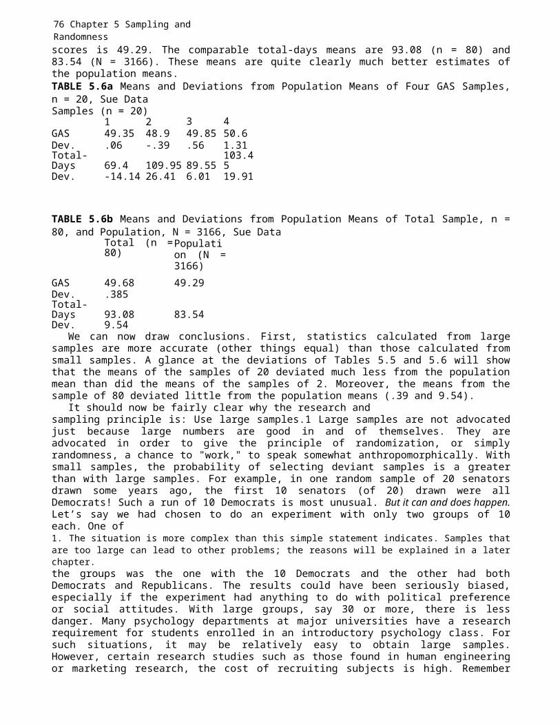
76 Chapter 5 Sampling and Randomnessscores is 49.29. The comparable total-days means are 93.08 (n = 80) and83.54 (N = 3166). These means are quite clearly much better estimates ofthe population means.TABLE 5.6a Means and Deviations from Population Means of Four GAS Samples,n = 20, Sue DataSamples (n = 20)
1 2 3 4GAS 49.35 48.9 49.85 50.6Dev. .06 -.39 .56 1.31Total-Days 69.4 109.95 89.55
103.45
Dev. -14.14 26.41 6.01 19.91
TABLE 5.6b Means and Deviations from Population Means of Total Sample, n =80, and Population, N = 3166, Sue Data
Total (n =80)
Population (N =3166)
GAS 49.68 49.29Dev. .385Total-Days 93.08 83.54Dev. 9.54
We can now draw conclusions. First, statistics calculated from largesamples are more accurate (other things equal) than those calculated fromsmall samples. A glance at the deviations of Tables 5.5 and 5.6 will showthat the means of the samples of 20 deviated much less from the populationmean than did the means of the samples of 2. Moreover, the means from thesample of 80 deviated little from the population means (.39 and 9.54).
It should now be fairly clear why the research andsampling principle is: Use large samples.1 Large samples are not advocatedjust because large numbers are good in and of themselves. They areadvocated in order to give the principle of randomization, or simplyrandomness, a chance to "work," to speak somewhat anthropomorphically. Withsmall samples, the probability of selecting deviant samples is a greaterthan with large samples. For example, in one random sample of 20 senatorsdrawn some years ago, the first 10 senators (of 20) drawn were allDemocrats! Such a run of 10 Democrats is most unusual. But it can and does happen.Let’s say we had chosen to do an experiment with only two groups of 10each. One of1. The situation is more complex than this simple statement indicates. Samples thatare too large can lead to other problems; the reasons will be explained in a laterchapter.the groups was the one with the 10 Democrats and the other had bothDemocrats and Republicans. The results could have been seriously biased,especially if the experiment had anything to do with political preferenceor social attitudes. With large groups, say 30 or more, there is lessdanger. Many psychology departments at major universities have a researchrequirement for students enrolled in an introductory psychology class. Forsuch situations, it may be relatively easy to obtain large samples.However, certain research studies such as those found in human engineeringor marketing research, the cost of recruiting subjects is high. Remember
Chapter 5 Sampling and Randomness 77
the Williams and Adelson study discussed by Simon (1987) in Chapter 1? Sothe rule of getting large samples may not be appropriate for all researchsituations. In some studies, 30 or more elements, participants or subjectsmay be too little. This is especially true in studies that are multivariatein nature. Comrey and Lee (1992) for example states that samples of size 50or less give very inadequate reliability of correlation coefficients.Hence, it may be more appropriate to obtain an approximation to the samplesize needed. The statistical determination of sample size will be discussedin Chapter 12 for the various kinds of samples.KINDS OF SAMPLESThe discussion of sampling has until now been confined to simple randomsampling. The purpose is to help the student understand fundamentalprinciples; thus the idea of simple random sampling, which is behind muchof the thinking and procedures of modern research, is emphasized. Thestudent should realize, however, that simple random sampling is not theonly kind of sampling used in behavioral research. Indeed, it is relativelyuncommon, at least for describing characteristics of populations and therelations between such characteristics. It is, nevertheless, the model onwhich all scientific sampling is based.
Other kinds of samples can be broadly classified into probability andnonprobability samples (and certain mixed forms). Probability samples use someform of random sampling in one or more of their stages. Nonprobability samplesdo not use random sampling; they thus lack the virtues being discussed.Still, they are often necessary and unavoidable. Their weakness can to someextent be mitigated by using knowledge, expertise, and care in selectingsamples and by replicating studies with different samples. It is importantfor the student to know that probability sampling is not necessarilysuperior to nonprobability sampling for all possible situations. Also,probability sampling does not guarantee samples that are morerepresentative of the universe under study. In probability sampling theemphasis is placed in the method and the theory behind it. Withnonprobability sampling the emphasis relies on the person doing thesampling and that can bring with it entirely new and complicated batch ofconcerns. The person doing the sampling must be knowledgeable of thepopulation to be studied and the phenomena under study.
One form of nonprobability sampling is quota sampling. Here the knowledge ofthe strata of the population—sex, race, region, and so on—is used to selectsample members that are representative, "typical," and suitable for certainresearch purposes. A strata is the partitioning of the universe or populationinto two or more non-overlapping (mutually exclusive) groups. From eachpartition a sample is taken. Quota sampling derives its name from thepractice of assigning quotas, or proportions of kinds of people, tointerviewers. Such sampling has been used a good deal in public opinionpolls. To perform this sampling correctly, the researcher would need tohave a very complete set of characteristics for the population. Next, theresearcher must know the proportions for each quota. After knowing this,the next step is to collect the data. Since the proportions might beunequal from quota to quota, the sample elements are assigned a weight.Quota sampling is difficult to accomplish because it requires accurateinformation on the proportions for each quota and such information israrely available.
Another form of nonprobability sampling is purposive sampling, which ischaracterized by the use of judgment and a deliberate effort to obtain
78 Chapter 5 Sampling and Randomnessrepresentative samples by including presumably typical areas or groups inthe sample. Purposive sampling is used a lot in marketing research. To testthe reaction of consumers to a new product, the researcher may give out thenew product to people that fits the researcher’s notion of what theuniverse looks like. Political polls are another example where purposivesampling is used. On the basis of past voting results and existingpolitical party registration, in a given region, the researcher purposivelyselects a group of voting precincts. The researcher feels that thisselection will match the characteristics of the entire electorate. A veryinteresting presentation of how this information was used to help elect aU.S. Senator in California is given in Barkan and Bruno (1972).
So-called “accidental" sampling, the weakest form of sampling, is probablyalso the most frequent. In effect, one takes available samples at hand;classes of seniors in high school, sophomores in college, a convenient PTA,and the like. This practice is hard to defend. Yet, used with reasonableknowledge and care, it is probably not as bad as it has been said to be.The most sensible advice seems to be: Avoid accidental samples unless youcan get no others (random samples are usually expensive and in somesituations, hard to come by). If you do use them, use extremecircumspection in analysis and interpretation of data.
Probability sampling includes a variety of forms. When we discussed simplerandom sampling, we were talking about one version of probability sampling.Some of the other common forms of probability sampling are stratifiedsampling, cluster sampling, two-stage cluster sampling, and systematicsampling. Some more unconventional methods would include the Bayesianapproach or the sequential approach. The superiority of one method ofsampling over another is usually evaluated in terms of the amount ofreduced variability in parameters estimated and in terms of cost. Cost issometimes interpreted as the amount of labor in data collection and dataanalysis.
In stratified sampling, the population is first divided into strata such as menand women, African- American and Mexican-American, and the like. Thenrandom samples are drawn from each strata. If the population consists of 52percent women and 48 percent men, a stratified sample of 100 participantswould consist of 52 women and 48 men. The 52 women would be randomly chosenfrom the available group of women and the 48 men would be randomly selectedfrom the group of men. This is also called proportional allocation. Whenthis procedure is performed correctly it is superior to simple randomsampling. When compared to simple random sampling, stratified samplingusually reduces the amount of variability and reduces the cost in datacollection and analyses. Stratified sampling capitalizes on the between-strata differences. Figure 5.2 conveys the basic idea of stratifiedsampling. Stratified sampling adds control to the sampling process bydecreasing the amount of sampling error. This design is recommended whenthe population is composed of sets of dissimilar groups. Randomizedstratified sampling allows us to study the stratum differences. It allowsus to give special attention to certain groups that would otherwise beignored because of their size. Stratified random sampling is oftenaccomplished through proportional allocation procedures (PAP). When usingsuch procedures, the sample’s proportional partitioning resembles that ofthe population. The major advantage in using PAP is that it provides a“self-weighted” sample.
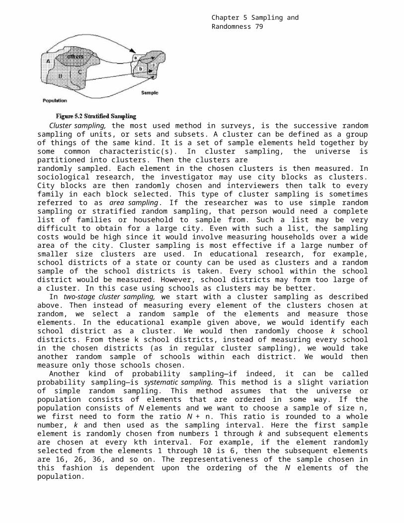
Chapter 5 Sampling and Randomness 79
Cluster sampling, the most used method in surveys, is the successive randomsampling of units, or sets and subsets. A cluster can be defined as a groupof things of the same kind. It is a set of sample elements held together bysome common characteristic(s). In cluster sampling, the universe ispartitioned into clusters. Then the clusters arerandomly sampled. Each element in the chosen clusters is then measured. Insociological research, the investigator may use city blocks as clusters.City blocks are then randomly chosen and interviewers then talk to everyfamily in each block selected. This type of cluster sampling is sometimesreferred to as area sampling. If the researcher was to use simple randomsampling or stratified random sampling, that person would need a completelist of families or household to sample from. Such a list may be verydifficult to obtain for a large city. Even with such a list, the samplingcosts would be high since it would involve measuring households over a widearea of the city. Cluster sampling is most effective if a large number ofsmaller size clusters are used. In educational research, for example,school districts of a state or county can be used as clusters and a randomsample of the school districts is taken. Every school within the schooldistrict would be measured. However, school districts may form too large ofa cluster. In this case using schools as clusters may be better.
In two-stage cluster sampling, we start with a cluster sampling as describedabove. Then instead of measuring every element of the clusters chosen atrandom, we select a random sample of the elements and measure thoseelements. In the educational example given above, we would identify eachschool district as a cluster. We would then randomly choose k schooldistricts. From these k school districts, instead of measuring every schoolin the chosen districts (as in regular cluster sampling), we would takeanother random sample of schools within each district. We would thenmeasure only those schools chosen.
Another kind of probability sampling—if indeed, it can be calledprobability sampling—is systematic sampling. This method is a slight variationof simple random sampling. This method assumes that the universe orpopulation consists of elements that are ordered in some way. If thepopulation consists of N elements and we want to choose a sample of size n,we first need to form the ratio N + n. This ratio is rounded to a wholenumber, k and then used as the sampling interval. Here the first sampleelement is randomly chosen from numbers 1 through k and subsequent elementsare chosen at every kth interval. For example, if the element randomlyselected from the elements 1 through 10 is 6, then the subsequent elementsare 16, 26, 36, and so on. The representativeness of the sample chosen inthis fashion is dependent upon the ordering of the N elements of thepopulation.
80 Chapter 5 Sampling and Randomness
The student who will pursue research further should, of course, know muchmore about these methods. The student is encouraged to consult one or moreof the excellent references on the subject presented at the end of thischapter. Williams (1978) gives an interesting presentation anddemonstration of each sampling method using artificial data.
Another related topic to randomness and sampling is randomization orpermutation tests. We will give this topic more extensive treatment when wediscuss the data analysis for quasi-experimental designs. The proponent ofthis method in psychology and the behavioral sciences has been Eugene S.Edgington. Edgington (1980,1996) advocates the use ofapproximate randomization tests to handle statistical analyses of data fromnon-random samples and single subject research designs. We can brieflymention here how this procedure works. Take Edgington’s example of thecorrelating the IQ scores of foster parents and their adopted children. Ifthe sample was not randomly selected, the sample may be biased in favor ofparents who want to have their IQ and the IQ of their adopted childmeasured. It is likely that some foster parents will intentionally lowertheir scores to match those of their adopted child. One way of handlingnon-random data like this is to first compute the correlation between theparents and child. Then one would randomly pair the parents’’ scores withthe child’s’. That is, parent 1 may in a random pairing get matched up withthe child from parent number 10. After such a random pairing, thecorrelation is again computed. If the researcher performs 100 suchrandomization pairings and computed the correlation each time, one can thencompare the original correlation to the 100 created from random pairings.If the original correlation is the best (highest) the researcher would havea better idea that the correlation obtained may be credible. Theserandomizations or permutation tests have been quite useful in certainresearch and data analysis situations. It has been used to evaluateclusters obtained in a cluster analysis (see Lee and MacQueen, 1980). Ithas been proposed as a solution to analyzing self-efficacy data that arenot independent (see Cervone, 1987).
Randomness, randomization, and random sampling are among the great ideasof science, as indicated earlier. While research can, of course, be donewithout using ideas of randomness, it is difficult to conceive how it canhave viability and validity, at least in most aspects of behavioralscientific research. Modern notions of research design, sampling, andinference, for example, are literally inconceivable without the idea ofrandomness. One of the most remarkable of paradoxes is that throughrandomness, or "disorder," we are able to achieve control over the often-obstreperous complexities of psychological sociological and educationalphenomena. We impose order, in short, by exploiting the known behavior ofsets of random events. One is perpetually awed by what can be called thestructural beauty of probability, sampling, and design theory and by itsgreat usefulness in solving difficult problems of research design andplanning and the analysis and interpretation of data.
Before leaving the subject, let's return to a view of randomnessmentioned earlier. To an omniscient being, there is no randomness. Bydefinition such a being would "know" the occurrence of any event withcomplete certainty. As Poincare (1952/1996) points out, to gamble with sucha being would be a losing venture. Indeed, it would not be gambling. When acoin was tossed ten times, he or she would predict heads and tails withcomplete certainty and accuracy. When dice were thrown, this being would
Chapter 5 Sampling and Randomness 81
know infallibly what the outcomes will be. Every number in a table ofrandom numbers would be correctly predicted! And certainly this being wouldhave no need for research and science. What we seem to be saying is thatrandomness is a term for ignorance. If we, like the omniscient being, knewall the contributing causes of events, then there would be no randomness.The beauty of it, as indicated above, is that we use this "ignorance" andturn it to knowledge. How we do this should become more and more apparentas we go on with our study.Study SuggestionsA variety of experiments with chance phenomena are recommended: games usingcoins, dice, cards, roulette wheels, and tables of random numbers. Suchgames, properly approached, can help one learn a great deal aboutfundamental notions of modern scientific research, statistics, probability,and, of course, randomness. Try the problems given in the suggestionsbelow. Do not become discouraged by the seeming laboriousness of suchexercises here and later on in the book. It is evidently necessary and,indeed, helpful occasionally to go through the routine involved in certainproblems. After working the problems given, devise some of your own. If youcan devise intelligent problems, you are probably well on your way tounderstanding.
1.From a table of random numbers draw 50 numbers, 0 through 9. (Use therandom numbers of Appendix C, if you wish.) List them in columns of 10each.(a) Count the total number of odd numbers; count the total number of even
numbers. What would you expect to get by chance? Compare the obtainedtotals with the expected totals.
(b) Count the total number of numbers 0, 1, 2, 3,4. Similarly count 5, 6, 7, 8, 9. How many of the first group should youget? The second group? Compare what you do get with these chanceexpectations. Are you far off?(c) Count the odd and even numbers in each group of 10. Count the two
groups of numbers 0, 1, 2, 3, 4 and 5, 6, 7, 8, 9 in each group of 10. Dothe totals differ greatly from chance expectations?
(d) Add the columns of the five groups of 10 numbers each. Divide eachsum by 10. (Simply move the decimal point one place to the left.) Whatwould you expect to get as the mean of each group if only chance were"operating"? What did you get? Add the five sums and divide by 50. Isthis mean close to the chance expectation? [Hint: To obtain the chanceexpectation, remember the population limits.]
2.This is a class exercise and demonstration. Assign numbers arbitrarily toall the members of the class from 1 through N, N being the total numberof members of the class. Take a table of random numbers and start withany page. Have a student wave a pencil in the air and blindly stab at thepage of the table. Starting with the number the pencil indicates, choosen two-digit numbers between 1 and N (ignoring numbers greater than N andrepeated numbers) by, say, going down columns (or any other specifiedway). n is the numerator of the fraction n/N, which is decided by thesize of the class. If N = 30, for instance, let n = 10. Repeat theprocess twice on different pages of the random numbers table. You nowhave three equal groups (if N is not divisible by 3, drop one or two

82 Chapter 5 Sampling and Randomness
persons at random). Write the random numbers on the blackboard in thethree groups. Have each class member call out his height in inches. Writethese values on the blackboard separate from the numbers, but in the samethree groups. Add the three sets of numbers in each of the sets on theblackboard, the random numbers and the heights. Calculate the means ofthe six sets of numbers. Also calculate the means of the total sets.
(a) How close are the means in each of the sets of numbers? How close arethe means of the groups to the mean of the total group?
(b) Count the number of men and women in each of the groups. Are thesexes spread fairly evenly among the three groups?
(c) Discuss this demonstration. What do you think is its meaning forresearch?
3.In Chapter 6, it was suggested that the student generate 20 sets of 100random numbers between 0 and 100 and calculate means and variances. Ifyou did this, use the numbers and statistics in this exercise. If you didnot, use the numbers and statistics of Appendix C at the end of the book.
(a) How close to the population mean are the means of the 20 samples? Areany of the means "deviant"? (You might judge this by calculating thestandard deviation of the means and adding and subtracting two standarddeviations to the total mean.)
(b) On the basis of (a), above, and your judgment, are the samples"representative"? What does "representative" mean?
(c) Pick out the third, fifth, and ninth group means. Suppose that 300subjects had been assigned at random to the three groups and that thesewere scores on some measure of importance to a study you wanted to do.What can you conclude from the three means, do you think?
4. Most published studies in the behavioral sciences and education have notused random samples, especially random samples of large populations.Occasionally, however, studies based on random samples are done. One suchstudy is:
Osgood, D. W., Wilson, J. K., O’Malley, P. M., Bachman, J. G. & Johnston,L. D. (1996). Routine activities and individual deviant behavior. AmericanSociological Review, 61, 635-655.This study is worth careful reading, even though its level of
methodological sophistication puts a number of its details beyond ourpresent grasp. Try not to be discouraged by this sophistication. Get whatyou can out of it, especially its sampling of a large population of youngmen. Later in the book we will return to the interesting problem pursued.At that time, perhaps the methodology will no longer appear so formidable.(In studying research, it is sometimes helpful to read beyond our presentcapacity-provided we don't do too much of it!)Another study random samples from a large population is byVoelkl, K. F. (1995). School warmth, student participation and achievement.Journal of Experimental Education, 63, 127-138.In this study the researcher gives some detail about using a two-stagestratified random samplingplan to measure student’s perception of school warmth.5.Random assignment of subjects to experimental groups is much more common
than random sampling of subjects. A particularly good, even excellent,
Chapter 5 Sampling and Randomness 83
example of research in which subjects were assigned at random to twoexperimental groups, is:
Thompson, S. (1980). Do individualized mastery and traditionalinstructional systems yield different course effects in college calculus?American Educational Research Journal, 17, 361-375.Again, don't be daunted by the methodological details of this study. Getwhat you can out of it. Note at this time how the subjects were classifiedinto aptitude groups and then assigned at random to experimentaltreatments. We will also return to this study later. At that time, weshould be able to understand its purpose and design and be intrigued by itscarefully controlled experimental pursuit of a difficult substantiveeducational problem: the comparative merits of so-called individualizedmastery instruction and conventional lecture- discussion-recitationinstruction.6. Another noteworthy example of random assignment is done in a study byGlick, P., DeMorest, J. A., & Hotze, C. A. (1988). Keeping your distance:
Group membership,personal space, and requests for small favors. Journal of Applied SocialPsychology, 18, 315-330.This study is noteworthy because the study takes place in a real settingoutside the laboratories of the university. Also the participants are notnecessarily university students. Participants in this study are people in apublic eating area within a large indoor shopping mall. Participants werechosen and then assigned to one of six experimental conditions. Thisarticle is easy to read and the statistics analysis is not much beyond thelevel of elementary statistics.7. Another interesting study that uses yet another variation of random
sampling isMoran, J. D. & McCullers, J. C. (1984). A comparison of achievement scoresin physically attractive and unattractive students. Home Economics ResearchJournal, 13, 36-40.
In this study, the researchers randomly selected photographs from schoolyearbooks. These photographs were then randomly grouped into 10 sets of 16pictures. Students who were not familiar with the students in the photoswere then asked to rate each person in the photo in terms ofattractiveness.
Special Note. In some of the above study suggestions and in those of Chapter6, instructions were given to draw numbers from tables of random numbers orto generate sets of random numbers using a computer. If you have amicrocomputer or have access to one, you may well prefer to generate therandom numbers using the built-in random number generator (function) of themicrocomputer. An outstanding and fun book to read and learn how to do thisis Walter’s (1997) “The Secret Guide to Computers.” Walter shows you how towrite a simple computer program using the BASIC language, the languagecommon to most microcomputers. How "good" are the random numbers generated?("How good?" means "How random?") Since they are produced in line with thebest contemporary theory and practice, they should be satisfactory,although they might not meet the exacting requirements of some experts. Inour experience, they are quite satisfactory, and we recommend their use to
84 Chapter 5 Sampling and Randomnessteachers and students.Some books on sampling.Babbie, E. R. (1990). Survey research methods. (2nd Ed.). Belmont, CA: Wadsworth.Babbie, E. R. (1995). The practice of social research, 7th ed. Belmont, CA: Wadsworth.Cowles, M. (1989). Statistics in psychology: A historical perspective. Hillsdale, NJ:
Lawrence Erlbaum Associates.Deming, W. E. (1966). Some theory of sampling.
New York: Dover.Deming, W. E. (1990). Sampling design in business research. New York: Wiley.Kish, L. (1953). Selection of the sample. InFestinger, L. & Katz, D. Eds., Research methods in the behavioral sciences. New York:Holt, Rinehart and Winston.Kish, L. (1995). Survey sampling. New York: John Wiley.Snedecor, G. & Cochran, W. (1989). Statistical Methods. (8th Ed). Ames, IA: Iowa
State University Press. .Stephan, F. & McCarthy, P. (1974). Sampling opinions. Westport, CT: Greenwood.Sudman, S. (1976). Applied sampling. New York: Academic Press.Warwick, D. & Lininger, D. (1975). The sample survey: Theory and practice. New York:
McGraw- Hill.Williams, B. (1978). A sampler on sampling. New York: John Wiley.Chapter Summary1. Sampling refers to taking a portion of a population or universe as
representative of that population or universe.2. Studies using samples are economical, manageable and controllable.3. One of the more popular methods of sampling israndom sampling.4. Random sampling is that method of drawing a portion (or sample) of a
population or universe so that each member of the population or universehas an equal chance of being selected
5. The researcher defines the population or universe. A sample is a subsetof the population.
6. We can never be sure that a random sampling is representative of thepopulation.
7. With a random sampling, the probability of selecting a sample with a meanclose to the population mean is greater than the probability of selectinga sample with a mean not close to the population mean.
8. Nonrandom sampling may be biased and the chances increase that the samplemean will not be close to the population mean.
9. We say events are random if we cannot predicttheir outcomes.10. Random assignment is another term forrandomization. This is where participants are assigned to research groupsrandomly. It is used to control unwanted variances.11. There are two types of samples: nonprobability andprobability samples.12. Nonprobability samples do not use randomassignment, while probability samples do use random sampling.13.Simple random sampling, stratified random sampling, cluster sampling andsystematic sampling are four types of probability sampling. 14.Quota

Chapter 5 Sampling and Randomness 85
sampling, purposive sampling and accidental sampling are three types ofnonprobability sampling.
86 Chapter 6: Ethical Considerations in Conducting Behavioral Science ResearchChapter 6Ethical Considerations in Conducting Behavioral ScienceResearchFiction and Reality
In the previous chapters we have discussed science and the variablesinvolved in social and behavioral sciences. We have also introduced some ofthe basic statistical methods used to analyze the data gathered from suchresearch studies. In the chapters following this one, we will be discussingthe actual conduct of the research process. Before doing this, we must presenta very important topic. This topic involves the issue of research ethics. Somebooks have placed this topic in the latter part of the book after the researchplan and designs have been discussed. We feel that such a topic should bepresented earlier. The student of research needs this information in order todesign an ethically sound study using the methods given in chapters after thisone. It would be ideal if the researcher read this chapter, then read thechapters on research design and then return to re-read the points made in thischapter.
What is research ethics? What is research? These are two terms that aredifficult to define. Shrader- Frechette (1994) provides a definition bycontrasting “research” from “practice.” As we saw in an earlier chapter,research is an activity done to test theories, make inferences and add orupdate information on a base of knowledge. Professional practice does notusually involve testing theories or hypotheses but rather enhance the welfareof clients using actions and information that have been demonstrated to besuccessful. Some of these actions were established through earlier scientificresearch. Even though both “research” and “practice” have ethics, the ethicsinvolved with the research process is directed toward the individuals who doresearch and their conduct of the research process. . Shrader-Frechette statesthat research ethics specifies the behavior researchers ought to show duringthe entire process of their investigation. Keith- Spiegel & Koocher (1985)discusses the ethics of psychological practice. Dawes (1994) gives a verycritical view of the practice of psychology and psychotherapy. Part of Dawes’discussion concerns ethics of practice.
The discussion, emphasis and practice of research ethics are relativelyrecent events. Before the 20th century, those scientists who were caughtexperimenting on people without proper consent were punished. However, therewere instances in history where the violations of research ethics yieldfruitful results. When one thinks about the ethics of doing research on humansor animals one can not avoid mixed feelings. In examining history, there werethose brave individuals like Edward Jenner who injected a child with a weakerform of the smallpox virus and in doing so developed a vaccine for small pox.History has it that Edward Jenner did not get permission from anyone beforedoing this. Or how about Dr. Barry Marshall who in order to show that thepeptic ulcer was caused by bacteria and not acids swallowed the culture ofbacteria himself and them successfully treated himself with dosages of anti-biotic drugs. Yet there are documented cases of tragic consequences forresearchers who failed to follow proper ethical principles of research andthose committing scientific fraud in science. Some of these are noted anddiscussed in Shrader-Frechette (1994). This is an excellent book worth readingas well as Miller & Hersen (1992) and Erwin, Gendin & Kleiman (1994). Evidenceof known or suspected fraud can be traced to research done in ancient Greece.
In conducting research, the sensitive researcher is often confronted with
Chapter 6: Ethical Considerations in Conducting Behavioral Science Research 87
ethical dilemmas. Prior to the 1960’s researchers from all fields of sciencewere left to their own conscious in terms of research ethics. The scholarlypublications on the appropriate behavior of scientists provided some guidance,but none or few of the guidelines were mandated. An example exemplifying anethical dilemma can be found in the fictional story of Martin Arrowsmith, theprotagonist in Sinclair Lewis’ novel Arrowsmith. In this novel, Dr. MartinArrowsmith in a laboratory study discovers by accident a principle that waseffective in destroying bacteria. Arrowsmith called it a “phage.” When thebubonic plague breaks out in a third world country, Arrowsmith is sent to thatcountry to help the afflicted and to test his phage. Arrowsmith was taughtthat the true effectiveness of the phage can be determined by giving it tohalf of the infected population. The other half would be given a placebo or notreatment at all. However, Arrowsmith upon seeing the alarming death rate,including the death of his wife and close friend decides to give the phage tothe entire population. If he had followed his experimental plan and his phagewas truly effective, the people receiving the phage would survive and thosereceiving the placebo would not. Arrowsmith’s conscience would not allow himto deceive half of the population and let them die in the name of scientificresearch. He administered the phage to everyone. The plague did end after thenatives were inoculated, but Arrowsmith never really knew whether his phagewas effective. Although this was fiction, actual research scientists are attimes faced with similar dilemmas.A Beginning?
It was studies done in the 1960’s and 1970’s where there was evidence ofresearch fraud and deception of research participants that led to a demand forspecific mandated rules for the conduct of research. In 1974, the UnitedStates Congress called for the creation of institutional review boards. Thepurpose of these boards was to review the ethical conduct of those researchstudies that had received federal research grants. Later in the 1980’sfederally funded research involving humans and animals were reviewed for bothethical acceptability and research design. By the 1980’s many of the majoruniversities in the United States had guidelines for dealing with misconductin research. Other countries also began to put forth guidelines and rules. Thegovernments of Sweden and the Netherlands required that independent reviewcommittees evaluate all biomedical studies. Shrader-Frechette (1994) describestwo broad categories in terms of ethical problems in scientific research. Thetwo major categories are (1) processes and (2) products. The research processis deemed harmful if participants do not give informed consent to theprocedures used on them. The research process is also considered harmful ifthe participants were deceived or recruited using deceptive methods. Theresearch product is harmful if the conduct of that research results in aharmful environment for anyone who comes into contact with it. Shrader-Frechette refers to this as “downwinders.” The case of radiation poisoning dueto scientific tests of nuclear weapons is an example of a research productthat is harmful. Shrader-Frechette briefly describes this research and theconsequences. Saffer & Kelly (1983) give a more complete account in aninformative book titled “Countdown Zero.” Saffer and Kelly describe how theatmospheric tests of the atomic bomb in the desert of Nevada in the late1940’s carried over into other parts of the desert. The crew, staff and actorsin the movie The Conqueror were all exposed to radioactive sand during thefilming of the movie in the desert. All of these people developed cancer andlater died from cancer related illnesses. Some of the well- known actors andactresses included John Wayne, Susan Hayward and Dick Powell. Saffer and Kellyalso describes how the United States military’s research on how to fight anuclear war in the 1950’s led to the exposure of many military personnel toradiation fallout. Saffer himself was one of the soldiers who participated insuch studies. He noticed after a number of years after leaving the service
88 Chapter 6: Ethical Considerations in Conducting Behavioral Science Researchthat fellow soldiers developed cancer.
One of the most infamous case on the unethical use of deception was theTuskegee Study (see Brandt,1978) . In 1932 the U.S. Public Health Service did an experiment on 399 poor,semiliterate African-American males who had contracted syphilis. One purposeof this study was to examine the effects of syphilis on untreated individuals.In order to get afflicted African- American males to participate in the study,they were told they were being treated when in fact they were not. Symptoms ofsyphilis were periodically measured and recorded. Autopsies were performed oneach individual after each death. It would be forty years later before thepublic became aware of this research. At the time of disclosure, the study wasstill in progress. The research was clearly unethical; one reason was becausetreatment was still being withheld from the survivors as late as 1972. Theycould have been effectively treated with penicillin that became available inthe 1940s. One of the major outcries of unethical research behavior has beenfocused on the use of deception.
Deception is still used in some research studies today. However, theresearch is critically evaluated before it can be done. All major universitiesin the United States have a research ethics and human usage committee thatscreens and evaluates studies for potential deceptions and harmful effects. Itis their task to make sure no harm is inflicted on any of the participants.
One of the most noted studies in psychology that used deception wasconducted by social psychologist Stanley Milgram, who recruited participantsin a "learning" experiment (see Milgrim, 1963). Those who volunteered weretold that some would be teachers and the others would be learners. Theteachers were in charge of teaching lists of words to the learners. Theteachers were told to administer increasingly painful shocks every time thelearners made an error. The real purpose of the experiment, however, was notto study learning but to study obedience to authority. Milgrim wasparticularly interested in whether there was any truth to the claims of Naziwar criminals who said they did the atrocious acts because they were “ordered”by their superiors to do so. Unknown to the participants, all participantsserved as "teachers." That is, all participants were told that they wereteachers. None of the participants served as “learners.” The learners wereconfederates of the experimenter. They pretended to be participants who wererandomly chosen to serve as learners. Furthermore, there were actually noshocks administered at anytime. The teachers were tricked into believing thatthe learners’ cries of pain and requests for assistance was real. Wheninstructed to increase the severity of the shocks, some of the participantshesitated. However, when they were instructed by the experimenter to continue,they did so. They even continued "shocking' the learners beyond the pointwhere the learners "begged" to be released from the experiment. The resultswere, to Milgram as well to others, almost beyond belief. A great manysubjects (the "teachers") unhesitatingly obeyed the experimenter's "Pleasecontinue" or "You have no choice, you must go on" and continued to increasethe level of the shocks no matter how much the learner pleaded with the"teacher" to stop. What particularly surprised Milgram was that no one everwalked out of the laboratory in disgust or protest. This remarkable obediencewas seen time and time again in several universities where the experiment wasrepeated. Public anger over this experiment centered on the deception thatmight have caused psychological discomforts and harm to the participants. Morethan that, some people overgeneralized and thought that many suchpsychological experiments were being conducted.
For years following the famous study, critics of his study repeatedlydogged Milgrim. There was very little publicity surrounding the fact thatMilgrim did a number of follow-up studies on the participants and found thatthere were no negative effects. In fact, at the conclusion of each

Chapter 6: Ethical Considerations in Conducting Behavioral Science Research 89
experimental session, the participants were debriefed and introduced to the“learner” to show that no dangerous electrical shocks were administered.
Another sensitive area has been one directed at fraud. This includessituations where the researcher altered data from a research study in order toshow that a certain hypothesis or theory was true. Other cases of fraudinvolved the reporting of research findings for research studies that nevertook place. History shows that there have been a number of prominentindividuals who have been involved in fraud (see Erwin, Gendin & Kleiman,1994). One of the more sensational cases of alleged fraud comes frompsychology. The person involved was Sir Cyril Burt, a prominent Britishpsychologist who received knighthood for his work on statistics and theheritability of intelligence. His work was marked by the use of identicaltwins whose genetic composition was the most alike. Burt supposedlydemonstrated that there was a strong genetic component to intelligence byexamining the intelligence of twins who were raised together versus those whowere separated at birth and hence were reared apart. The intention was todetermine how much influence the environment or heredity had on intelligence.In the mid 1970’s after the death of Burt, Leon Kamin (1974) reported that anumber of the correlations that Burt reported were identical to the thirddecimal place. By chance alone this was highly improbable. Later it wasdiscovered that a few of Burt’s co-authors on research articles publishedaround the Second World War could not be found. Many of Burt’s critics feltthat Burt created these co-authors in order to mislead the scientificcommunity. Even Leslie Hearnshaw, who was commissioned by Burt’s family towrite a biography of Burt, claimed to have found evidence of fraud. Thisparticular view of Burt’s fraud is detailed in Gould (1981). However, Jensen(1992) presents a different socio-historical view of Burt. Jensen states thatthe charges against Burt were never adequately proven. Jensen also givesinformation concerning Burt that was never mentioned in Gould’s book or inother publications that were critical of Burt.
Such events as the Tuskegee, Milgram and Burt brought about the creation oflaws and regulations to restrict or stop unethical research behavior in themedical, behavioral and social sciences. Professional organizations, such asthe American Psychological Association and the American Physiological Societydeveloped commissions to investigate and recommend action on reported cases ofunethical research behavior. However, the reported incidence of unethicalresearch by scientists has been minimal. Amongst the cases that have receivedthe most negative publicity in behavioral science research involved StevenBreuning of the University of Pittsburgh. Breuning was convicted in 1988 offabricating scientific data about drug tests (Ritalin and Dexedrine) onhyperactive children. Breuning’s falsified results were widely cited andinfluenced several states to change their regulations on the treatment ofthese children. The Breuning case illustrates how dangerous the fraudulentbehavior of a scientist can be.
In the physical sciences and medicine, Maurice Buchbinder, a cardiologist,was broached for research problems associated with his testing of theRotablator. This device is a coronary vessel-cleaning device. Investigationrevealed that the device was manufactured by a company where Buchbinder ownedmillions of dollars in stock. Amongst his ethical violations were (1) thefailure to conduct follow-up examinations on about 280 patients, (2) theimproper use of the device on patients with severe heart disease, and (3) notproperly reporting some of the problems experienced by patients.
Douglas Richman was another research physician who received notoriety inhis study of a new hepatitis treatment drug. Richman was cited for failing toreport the death of the patients in the study, failing to inform the drug’smanufacturer about the serious side effects, and failing to properly explain
90 Chapter 6: Ethical Considerations in Conducting Behavioral Science Researchrisks to patients in the study. Even though the reported incidence of fraudand unethical behavior by scientists is scarce, Shrader- Frechette (1994) haspointed out that many unethical behaviors go unnoticed or unreported. Evenresearch journals do not mention anything about requiring the author topresent information that the study was done ethically (e.g. with informedconsent). It is possible that when a researcher studies the behavior ofhumans, that those humans are put at risk through coercion, deception,violation of privacy, breaches of confidentiality, stress, social injury andfailure to obtain free informed consent.Some General GuidelinesThe following guidelines are summaries taken from Shrader-Frechette’sexcellent book. Shrader-Frechette lays down the codes that should be followedby researchers in all areas of study where animals and humans are used asparticipants. One of the topics centers on situations where the researchershould not perform the research study. There are five general rules to followwhen determining that the research should not be done.• Scientists should not do research that puts people at risk• Scientists should not do research that violates the norms of free informed
consent.• Scientists should not do research that converts public resources to private
gains.• Scientists should not do research that could seriously damage the
environment.• Scientists ought not do biased research.In the fifth and last point made by Shrader-Frechette, the implication istoward racial and sexual biases only. One should realize that in all researchstudies there are biases inherent in the research design itself.
However, one of the major criterion in deciding the execution of a researchstudy is the consequences from that study. Shrader-Frechette states that thereare studies that will put humans and animals at risk, but the non-execution ofthat research may lead to even greater risks to humans and animals. Indifferent words, not all potentially dangerous research should be condemned.Shrader-Frechette states:“Just as scientists have a duty to do research but to avoid ethicallyquestionable research, so also they have a responsibility not to become soethically scrupulous about their work that they threaten the societal endsresearch should serve.” (p. 37).Hence, the researcher must exercise some degree of common sense when decidingto do or not do the research study involving human and animal participants.Guidelines from the American Psychological Association.
In 1973 the American Psychological Association published ethical guidelinesfor psychologists. The original guidelines went through a number of revisionssince then. The latest guidelines and principles were published in the AmericanPsychologist in the March 1990 issue. The Ethical Principles of Psychologists and Code ofConduct can be found in the 1994 edition of the Publication Manual of the AmericanPsychological Association. The following section will give a brief discussion of theethical principles and codes that are relevant of behavioral science research.These guidelines are directed toward both human and animal research. Allpersons working on a research project are bounded by the ethic codesregardless if they are a professional psychologist or a member of the AmericanPsychological Association.General Considerations
The decision to undertake a research project lies solely with theresearcher. The first question that the researcher needs to ask oneself iswhether or not the research is worth doing. Will the information obtained fromthe study be valuable and useful for science and human welfare? Will it help
Chapter 6: Ethical Considerations in Conducting Behavioral Science Research 91
improve the human health and welfare? If the researcher feels that theresearch is worthwhile, then the research is to be conducted with respect andconcern for the welfare and dignity of the participants.The Participant at Minimal Risk.One of the major consideration on whether the study should be conducted or notis the decision as to whether the participant will be a "subject at risk" or a"subject at minimal risk." If there is the possibility of serious risk for theparticipant, the possible outcome of the research should indeed be ofconsiderable value before proceeding. Researchers in this category shouldconsult with colleagues before continuing. At most universities, there is aspecial committee that reviews research proposals to determine if the value ofthe research is worth placing participants at risk. At all times, theresearcher must take steps to prevent harm to the participant. Studentresearch projects should be conducted with the minimum amount of risk on theparticipants.Fairness, Responsibility and Informed Consent.Prior to participation, the researcher and the participant should enter intoan agreement that clarifies the obligation and responsibilities. With certainstudies this involves informed consent. Here the participant agreesto tolerate deception, discomfort, and boredom for the good of science. Inreturn, the experimenter guarantees the safety and well being of theparticipant. Psychological research differs from medical research in thisregard. Medical research ethics requires the researcher to inform theparticipant what will be done to them and for what purpose. Most behavioraland social science research is not this restrictive. The behavioral scienceresearcher needs to tell only those aspects of the study that may influencethe participant’s willingness to participate. Informed consent is notrequired inminimal-risk research. Still, it is a good idea for the investigator in allresearch to establish a clear and fair agreement with research participantsprior to their participation.DeceptionDemand characteristics exists with many behavioral science studies.Participants volunteer to participate with the knowledge that something notharmful will be done to them. Their expectations and their desire to “do whatthe researcher wants” could influence the outcome of the study. Hence validityof the study would be compromised. The famous Hawthorne study is a case inpoint. In the Hawthorne study, the factory workers were told ahead of timethat some people will be coming to the factory to do a study on workerproductivity. The workers knowing that they will be studied for theirproductivity behaved in ways that they would not normal behave, i.e. punctual,working harder, shorter breaks, etc. As a result the investigators in thestudy were unable to get a true measure of worker productivity. Hence, entersdeception. Like a magic show, the participants’ attentions are misdirected. Ifthe investigators had entered the factory as “ordinary” workers, they couldhave obtained a clearer picture of worker productivity.
If the researcher can justify that deception is of value, and ifalternative procedures are not available, then the participant must beprovided with a sufficient explanation as soon as possible after the end ofthe experiment. This explanation is called debriefing. Any deceptive procedurethat presents the participants with a negative perception of themselves mustbe avoided.Freedom from CoercionParticipants must always be made to feel that they can withdraw from the studyat any time without penalty or repercussions. Participants need to be informedof this prior to the beginning of the experimental session. The researcher ata university that uses introductory psychology students as participants should
92 Chapter 6: Ethical Considerations in Conducting Behavioral Science Researchmake it clear that their participation is voluntary. At some universities, theintroductory psychology course has a graded research component. This componentcannot be based solely on participation in research studies. For those thatwish so, the research component can be satisfied through other means such as aresearch paper. Giving extra credit points for participation can be conceivedas coercion.DebriefingAfter collecting the data from the participant the nature of the research iscarefully explained to the participant. Debriefing is an attempt to remove anymisconceptions the participant may have about the study. This is an extremelyimportant element in conducting a research study. Even the explanation of thestudy should not be aversive. It needs to be worded in such a way so thatthose that have just been deceived would not feel foolish or stupid orembarrassed. In the event of student researchers, it would be beneficial forboth the researcher and participant to review the data. The debriefing sessioncould be used as a learning experience so that the student participant canbecome more knowledgeable about behavioral science research. Showing a studentaround the laboratory and explaining the apparatus is also advised if timepermits.
For those studies where an immediate debriefing would compromise thevalidity of the study, the researcher may delay debriefing. However, theresearcher must make all possible attempts to contact the participant once theentire study (data collection) is completed.Protection of ParticipantsThe researcher must inform the participant of all risks and dangers inherentin the study. The researcher should realize that the participant is doing theresearcher a favor by participating. Participation in any research may produceat least some degree of stress. Additionally, the researcher is obligated toremove any undesirable consequences of participation. This is relevant in thecase where participant were placed in a “do nothing” or control group. Itwould be unethical in a study that examines pain-management programs to placepeople who are in chronic pain into a control group where they received notreatment.ConfidentialityThe issue of keeping the participant from harm includes confidentiality. Theresearcher must assure the participant that the data collected from them willbe safeguarded. That is, the information collected from the participant willnot be disclosed to the public in a way that could identify the participant.With sensitive data, the researcher must inform the participant how the datawill be handled. In one study dealing with sexual behavior and AIDs,participants were asked to fill out the questionnaire, place the questionnairein an unmarked envelope and deposit the envelope in a sealed box. Theresearcher assured the participants that the questionnaire would only be seenby data entry people who don’t know who they are and cannot guess who theyare. Smith & Garner (1976) for example took extra precautions to assure theanonymity of participants in their study of homosexual behavior among malecollege athletes.ETHICS OF ANIMAL RESEARCHTo some people, the use of animals in research is inhumane and not necessary.However, research studies using animals have provided a number of worthwhileadvancements for both animals and human. Neal Miller (1985) has noted themajor contributions that animal research has provided for society. Unlikehuman participants, animals do not volunteer. Contrary to the belief of animalright activists, very few studies of today involve inflicting animals withpain. Experiments using animals as participants are generally permissible solong as the animals are treated humanely. APA provides guidelines on the useof animals for behavioral research and also logistic guidelines for their
Chapter 6: Ethical Considerations in Conducting Behavioral Science Research 93
housing and care. There are eleven major points covered in APA’s guidelines.They will be listed here:1. General.: This involved the code behind theacquisition, maintenance and disposal of animals. The emphasis is on thefamiliarity with the code.2. Personnel: This point involves the people whowill be caring for the animals. This includes the availability of aveterinarian and supervisor of the facility.3. Facilities: The housing of the animals mustconform to the standard set by National Institute of Health (NIH) for the careand use of laboratory animals.4. Acquisition of Animals: This point deals with how the animals are acquired.
Covered are the rules for breeding and/or purchasing of animals.5. Care and Housing of Animals: This deals with the condition of the
facilities where the animals are kept.6. Justification of Research: The purpose of theresearch using animals must be stated clearly.7. Experimental Design: The research design of the study should include humane
considerations. This would include the type of animal and how many animals.8. Experimental Procedure. All experimental procedures must take into
consideration the animal’s well being. Procedures must involve no inflictedpain. Any amount of induced pain must be justified by the value of thestudy. Any aversive stimuli should be set at the lowest level possible.
9. Field Research. Researchers doing field research should disturb thepopulation as little as possible. There must be respect for property andprivacy of inhabitants
10. Educational Use of Animals. Alternative nonanimal studies should beconsidered. Classroom demonstrations using animals should be used wheneducational objectives can not be made through the use of media.Psychologists need to include a presentation on the ethics of using animalsin research.
11. Disposition of Animals. This point deals with what to do with the animalonce the study is finished.These guidelines (available from the American Psychological Association)
should be made known to all personnel involved in the research andconspicuously posted wherever animals are maintained and used.
In assessing the research, the possibility of increasing knowledge aboutbehavior, including benefit for health or welfare of humans and animals,should be sufficient to outweigh any harm or distress to the animals. Humaneconsideration for the well being of the animals should thus always be keptuppermost in mind. If the animal is likely to be subjected to distress orpain, the experimental procedures specified in the guidelines of the AmericanPsychological Association should be carefully followed, especially forsurgical procedures. No animal should be discarded until its death isverified, and it should be disposed of in a manner that is legal andconsistent with health, environmental, and aesthetic concerns.
A recent book by Shapiro (1998) presents the history and current status onthe use of animals in scientific research. This book contains articles thatdeal with ethics and situations when animal research is necessary and when itis not.Study Suggestions1. Some feel that society have placed too many restrictions of scientists on
how to conduct their research. List the strong and weak points behind theseregulations.
2. What is the purpose of debriefing? Why is it necessary?
94 Chapter 6: Ethical Considerations in Conducting Behavioral Science Research3. A student who is a fan of daytime talk shows, wanted to determine if the
way a woman dresses influences men’s behavior. She plans to attend two barsat night. In one bar she will be dressed provocatively and in the other shewill be dressed in a business suit. Her dependent variable is the number ofmen who would approach and talk to her. Can you find some ethical problemswith this study?
4. Go to your library and find other incidences of fraud and unethicalbehavior of behavioral and medical scientists. How many of these can youfind?
5. In the novel Arrowsmith, can you propose an alternative method that wouldhave enabled Martin Arrowsmith to fully test his phage?
6. Locate and read one of the following articles:Braunwald, E. (1987). On analyzing scientific fraud.Nature, 325, 215-216.Brody, R. G. & Bowman, L. (1998). Accounting and psychology students'
perceptions of whistle blowing. College Student Journal. 32, 162-166. Does thecollege curriculum need to include ethics?
Broad, W. J. & Wade, N. (1982). Betrayers of the truth. New York: Touchstone.Fontes, L. A. (1998). Ethics in family violence research: Cross-cultural
issues. Family Relations: Interdisciplinary Journal of Applied Family Studies, 47, 53-61.Herrmann, D. & Yoder, C. (1998). The potential effects of the implanted memory
paradigm on child subjects. Applied Cognitive Psychology, 12, 198-206.(Discusses the danger of implanted memory.)Knight, J. A. (1984). Exploring the compromise of ethical principles in
science. Perspectives in Biology and Medicine, 27, 432-442. (Explores the reasons forfraud and dishonesty in science.)
Stark, C. (1998). Ethics in the research context: Misinterpretations andmisplaced misgivings. Canadian Psychology. 39,.202-211. (A look at the ethiccodes for the Canadian Psychological Association.)
tChapter Summary1. The Tuskegee and Milgrim studies used a form of deception and are often
cited as reasons why scientific research with humans and animals need to beregulated.
2. Fraud is also an issue of concern, since the work of individuals such asBurt and Breuning had a lot of influence on legislation and how peopleperceived themselves and others.
3. Organizations such as the American Psychological Association have set upguidelines on the ethics of doing research. Also they have set up reviewboards to evaluate and take action on claims of ethical misconduct.
4. Researchers are obligated to do no physical or psychological harm toresearch participants.
5. Researchers must do research in a way that will produce useful information.6. The ten ethical standards set up by the American Psychological Association
include provisions for planning the research, protection of participants,confidentiality, debriefing, deception, informed consent, and freedom fromcoercion
7. Guidelines are also provided for the use of animals in research. Theseprovide guidelines on the care, feeding and housing of animals and what todo with animals after the end of the study.

76 Chapter 6: Ethical Considerations in Conducting Behavioral Science Research
Chapter 7: Research Design: Purpose and Principles 77
Chapter 7Research Design: Purpose and PrinciplesResearch Design is the plan and structure of investigation so conceived as toobtain answers to research questions. The plan is the overall scheme orprogram of the research. It includes an outline of what the investigator willdo from writing the hypotheses and their operational implications to the finalanalysis of data. The structure of research is harder to explain because"structure" is difficult to define clearly and unambiguously. Since it is aconcept that becomes increasingly important as we continue our study, we herebreak off and attempt a definition and a brief explanation. The discourse willnecessarily be somewhat abstract at this point. Later examples, however, willbe more concrete. More important, we will find the concept powerful, useful,even indispensable, especially in our later study of multivariate analysiswhere "structure" is a key concept whose understanding is essential tounderstanding much contemporary research methodology.
A structure is the framework, organization, or configuration of elements ofthe structure related in specified ways. The best way to specify a structureis to write a mathematical equation that relates the parts of the structure toeach other. Such a mathematical equation, since its terms are defined andspecifically related by the equation (or set of equations), is unambiguous. Inshort, a structure is a paradigm or model of the relations among the variablesof a study. The words "structure," "model” and "paradigm" are troublesomebecause they are hard to define clearly and unambiguously. A "paradigm" is amodel, an example. Diagrams, graphs, and verbal outlines are paradigms. We use"paradigm" here rather than "model" because "model" has another importantmeaning in science,'
A research design expresses both the structure of the research problem andthe plan of investigation used to obtain empirical evidence on the relationsof the problem. We will soon encounter examples of both design and structurethat will perhaps enliven this abstract discussion.PURPOSES OF RESEARCH DESIGNResearch design has two basic purposes: ( 1 ) to provide answers to research questionsand (2) to control variance. Design helps investigators obtain answers to thequestions of research and also helps them to control the experimental,extraneous, and error variances of the particular research problem understudy. Since all research activity can be said to have the purpose ofproviding answers to research questions, it is possible to omit this purposefrom the discussion and to say that research design has one grand purpose: tocontrol variance. Such a delimitation of the purpose of design, however, isdangerous. Without strong stress on the research questions and on the use ofdesign to help provide answers to these questions, the study of design candegenerate into an interesting, but sterile, technical exercise.
Research designs are invented to enable researchers to answer researchquestions as validly, objectively accurately, and economically as possible.Research plans are deliberately and specifically conceived and executed tobring empirical evidence to bear on the research problem. Research problemscan be and are stated in the form of hypotheses. At some point in the researchthey are stated so that they can be empirically tested. Designs are carefullyworked out to yield dependable and valid answers to the research questionsepitomized by the hypotheses. We can make one observation and infer that thehypothesized relation exists on the basis of this one observation, but it isobvious that we cannot accept the inference so made. On the other hand, it is
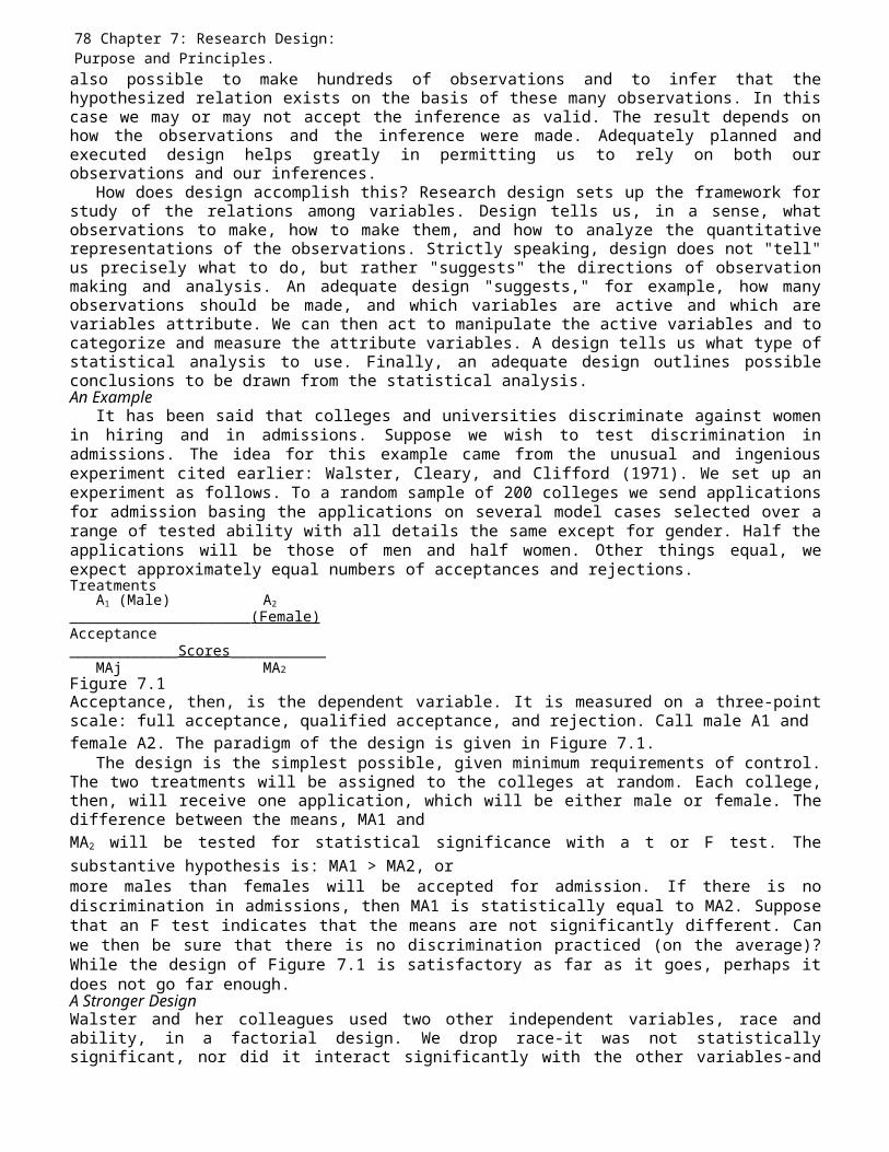
78 Chapter 7: Research Design: Purpose and Principles.also possible to make hundreds of observations and to infer that thehypothesized relation exists on the basis of these many observations. In thiscase we may or may not accept the inference as valid. The result depends onhow the observations and the inference were made. Adequately planned andexecuted design helps greatly in permitting us to rely on both ourobservations and our inferences.
How does design accomplish this? Research design sets up the framework forstudy of the relations among variables. Design tells us, in a sense, whatobservations to make, how to make them, and how to analyze the quantitativerepresentations of the observations. Strictly speaking, design does not "tell"us precisely what to do, but rather "suggests" the directions of observationmaking and analysis. An adequate design "suggests," for example, how manyobservations should be made, and which variables are active and which arevariables attribute. We can then act to manipulate the active variables and tocategorize and measure the attribute variables. A design tells us what type ofstatistical analysis to use. Finally, an adequate design outlines possibleconclusions to be drawn from the statistical analysis.An Example
It has been said that colleges and universities discriminate against womenin hiring and in admissions. Suppose we wish to test discrimination inadmissions. The idea for this example came from the unusual and ingeniousexperiment cited earlier: Walster, Cleary, and Clifford (1971). We set up anexperiment as follows. To a random sample of 200 colleges we send applicationsfor admission basing the applications on several model cases selected over arange of tested ability with all details the same except for gender. Half theapplications will be those of men and half women. Other things equal, weexpect approximately equal numbers of acceptances and rejections.Treatments
A1 (Male) A2_____________________(Female)Acceptance_____________Scores___________
MAj MA2Figure 7.1Acceptance, then, is the dependent variable. It is measured on a three-pointscale: full acceptance, qualified acceptance, and rejection. Call male A1 andfemale A2. The paradigm of the design is given in Figure 7.1.
The design is the simplest possible, given minimum requirements of control.The two treatments will be assigned to the colleges at random. Each college,then, will receive one application, which will be either male or female. Thedifference between the means, MA1 andMA2 will be tested for statistical significance with a t or F test. Thesubstantive hypothesis is: MA1 > MA2, ormore males than females will be accepted for admission. If there is nodiscrimination in admissions, then MA1 is statistically equal to MA2. Supposethat an F test indicates that the means are not significantly different. Canwe then be sure that there is no discrimination practiced (on the average)?While the design of Figure 7.1 is satisfactory as far as it goes, perhaps itdoes not go far enough.A Stronger DesignWalster and her colleagues used two other independent variables, race andability, in a factorial design. We drop race-it was not statisticallysignificant, nor did it interact significantly with the other variables-and

Chapter 7: Research Design: Purpose and Principles 79
concentrate on gender and ability. If a college bases its selection ofincoming students strictly on ability, there is no discrimination (unless, ofcourse, ability selection is called discrimination). Add ability to the designof Figure 7.1; use three levels. That is, in addition to the applicationsbeing designated male and female, they are also designated as high, medium,and low ability. For example, three of the applications may be: male, mediumability; female, high ability; female, low ability. Now, if there is nosignificant difference between genders and the interaction between gender andability is not significant, this would be considerably stronger evidence forno discrimination than that yielded by the design and statistical test ofFigure 7.1. We now use the expanded design to explain this statement and todiscuss a number of points about research design. The expanded design is givenin Figure7.2.
The design is a 2 x 3 factorial. One independent variable, A, is gender,the same as in Figure 7.1. The second independent variable, B, is ability,which is manipulated by indicating in several ways what the ability levels ofthe students are. It is important not to be confused by the names of thevariables. Gender and ability are ordinarily attribute variables and thusnonexperimental. In this case, however, they are manipulated. The studentrecords sent to the colleges were systematically adjusted to fit the six cellsof Figure7.2. A case in the A1B2 cell, for instance, would be therecord of a male of medium ability. It is this record that the college judgesfor admission.
Let's assume that we believe discrimination against women takes a moresubtle form than simply across-the board exclusion: that it is the women oflower ability who are discriminated against (compared to men). This is aninteraction hypothesis. At any rate, we use this problem and the paradigm ofFigure 7.2 as a basis for discussing some elements of research design.
Research problems suggest research designs. Since the hypothesis justdiscussed is one of interaction, a factorial design is evidently appropriate.A is gender; B is ability. A is partitioned into A1 and A2, and B intoB1, B2, and B3.
The paradigm of Figure 7.2 suggests a number of things. First and mostobvious, a fairly large number of subjects is needed.Bj (High)Ability B2(Medium)B3 (Low)GenderAj (Male)A2(Female)
Acceptance Scores
MBjMB
2MB3
MAj MA2Figure 7.2
Specifically, 6n subjects are necessary (n = number of S's in each cell).If we decide that n should be 20, then we must have 120 S's for theexperiment. Note the "wisdom" of the design here. If we were only testing thetreatments and ignoring ability, only 2n S's would beneeded. Please note that some such as Simon (1976, 1987), Simon & Roscoe
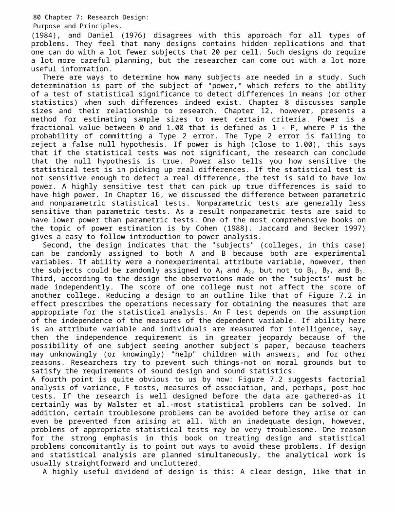
80 Chapter 7: Research Design: Purpose and Principles.(1984), and Daniel (1976) disagrees with this approach for all types ofproblems. They feel that many designs contains hidden replications and thatone can do with a lot fewer subjects that 20 per cell. Such designs do requirea lot more careful planning, but the researcher can come out with a lot moreuseful information.
There are ways to determine how many subjects are needed in a study. Suchdetermination is part of the subject of "power," which refers to the abilityof a test of statistical significance to detect differences in means (or otherstatistics) when such differences indeed exist. Chapter 8 discusses samplesizes and their relationship to research. Chapter 12, however, presents amethod for estimating sample sizes to meet certain criteria. Power is afractional value between 0 and 1.00 that is defined as 1 - P, where P is theprobability of committing a Type 2 error. The Type 2 error is failing toreject a false null hypothesis. If power is high (close to 1.00), this saysthat if the statistical tests was not significant, the research can concludethat the null hypothesis is true. Power also tells you how sensitive thestatistical test is in picking up real differences. If the statistical test isnot sensitive enough to detect a real difference, the test is said to have lowpower. A highly sensitive test that can pick up true differences is said tohave high power. In Chapter 16, we discussed the difference between parametricand nonparametric statistical tests. Nonparametric tests are generally lesssensitive than parametric tests. As a result nonparametric tests are said tohave lower power than parametric tests. One of the most comprehensive books onthe topic of power estimation is by Cohen (1988). Jaccard and Becker 1997)gives a easy to follow introduction to power analysis.
Second, the design indicates that the "subjects" (colleges, in this case)can be randomly assigned to both A and B because both are experimentalvariables. If ability were a nonexperimental attribute variable, however, thenthe subjects could be randomly assigned to A1 and A2, but not to B1, B2, and B3.Third, according to the design the observations made on the "subjects" must bemade independently. The score of one college must not affect the score ofanother college. Reducing a design to an outline like that of Figure 7.2 ineffect prescribes the operations necessary for obtaining the measures that areappropriate for the statistical analysis. An F test depends on the assumptionof the independence of the measures of the dependent variable. If ability hereis an attribute variable and individuals are measured for intelligence, say,then the independence requirement is in greater jeopardy because of thepossibility of one subject seeing another subject's paper, because teachersmay unknowingly (or knowingly) "help" children with answers, and for otherreasons. Researchers try to prevent such things-not on moral grounds but tosatisfy the requirements of sound design and sound statistics.A fourth point is quite obvious to us by now: Figure 7.2 suggests factorialanalysis of variance, F tests, measures of association, and, perhaps, post hoctests. If the research is well designed before the data are gathered-as itcertainly was by Walster et al.-most statistical problems can be solved. Inaddition, certain troublesome problems can be avoided before they arise or caneven be prevented from arising at all. With an inadequate design, however,problems of appropriate statistical tests may be very troublesome. One reasonfor the strong emphasis in this book on treating design and statisticalproblems concomitantly is to point out ways to avoid these problems. If designand statistical analysis are planned simultaneously, the analytical work isusually straightforward and uncluttered.
A highly useful dividend of design is this: A clear design, like that in
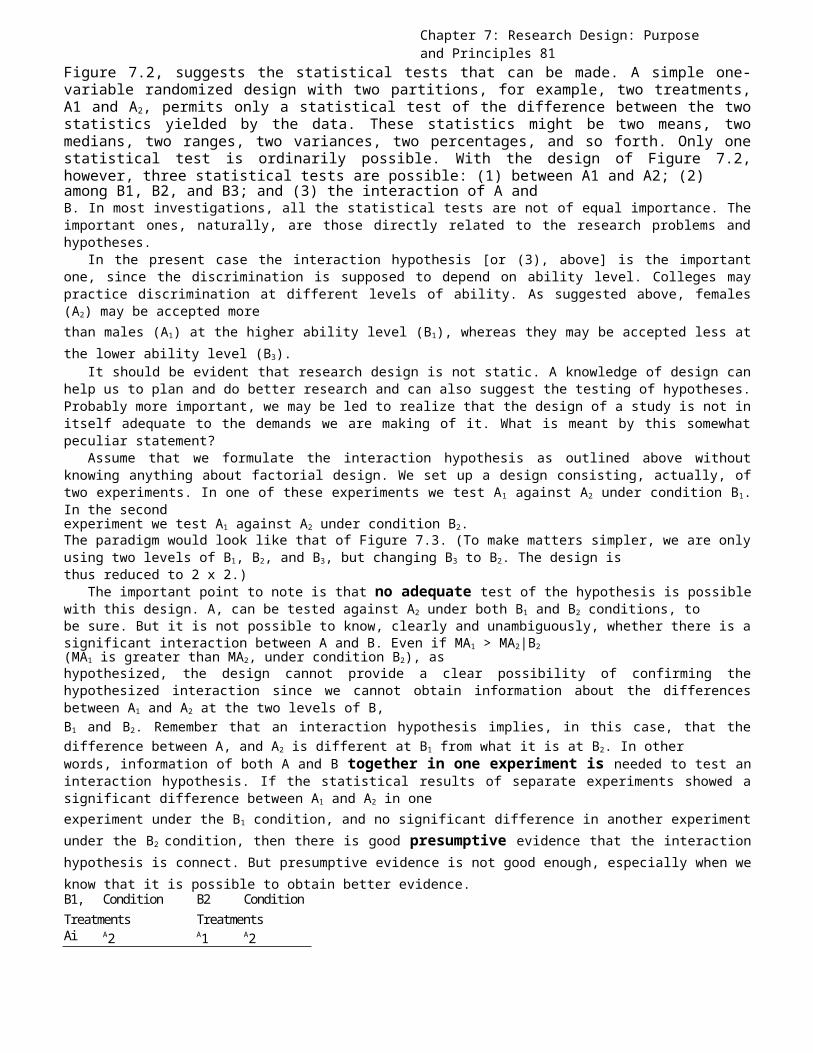
Chapter 7: Research Design: Purpose and Principles 81
Figure 7.2, suggests the statistical tests that can be made. A simple one-variable randomized design with two partitions, for example, two treatments,A1 and A2, permits only a statistical test of the difference between the twostatistics yielded by the data. These statistics might be two means, twomedians, two ranges, two variances, two percentages, and so forth. Only onestatistical test is ordinarily possible. With the design of Figure 7.2,however, three statistical tests are possible: (1) between A1 and A2; (2)among B1, B2, and B3; and (3) the interaction of A andB. In most investigations, all the statistical tests are not of equal importance. Theimportant ones, naturally, are those directly related to the research problems andhypotheses.
In the present case the interaction hypothesis [or (3), above] is the importantone, since the discrimination is supposed to depend on ability level. Colleges maypractice discrimination at different levels of ability. As suggested above, females(A2) may be accepted morethan males (A1) at the higher ability level (B1), whereas they may be accepted less atthe lower ability level (B3).
It should be evident that research design is not static. A knowledge of design canhelp us to plan and do better research and can also suggest the testing of hypotheses.Probably more important, we may be led to realize that the design of a study is not initself adequate to the demands we are making of it. What is meant by this somewhatpeculiar statement?
Assume that we formulate the interaction hypothesis as outlined above withoutknowing anything about factorial design. We set up a design consisting, actually, oftwo experiments. In one of these experiments we test A1 against A2 under condition B1.In the secondexperiment we test A1 against A2 under condition B2.The paradigm would look like that of Figure 7.3. (To make matters simpler, we are onlyusing two levels of B1, B2, and B3, but changing B3 to B2. The design isthus reduced to 2 x 2.)
The important point to note is that no adequate test of the hypothesis is possiblewith this design. A, can be tested against A2 under both B1 and B2 conditions, tobe sure. But it is not possible to know, clearly and unambiguously, whether there is asignificant interaction between A and B. Even if MA1 > MA2|B2(MA1 is greater than MA2, under condition B2), ashypothesized, the design cannot provide a clear possibility of confirming thehypothesized interaction since we cannot obtain information about the differencesbetween A1 and A2 at the two levels of B,B1 and B2. Remember that an interaction hypothesis implies, in this case, that thedifference between A, and A2 is different at B1 from what it is at B2. In otherwords, information of both A and B together in one experiment is needed to test aninteraction hypothesis. If the statistical results of separate experiments showed asignificant difference between A1 and A2 in oneexperiment under the B1 condition, and no significant difference in another experimentunder the B2 condition, then there is good presumptive evidence that the interactionhypothesis is connect. But presumptive evidence is not good enough, especially when weknow that it is possible to obtain better evidence.B1, Condition B2 ConditionTreatments TreatmentsAi A2 A1 A2
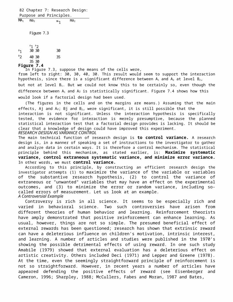
82 Chapter 7: Research Design: Purpose and Principles.MA1 ma2 MA1 ma2
Figure 7.3
A1 A2B1 30 30 30B2 40 30 35
35 30Figure 7.4
In Figure 7.3, suppose the means of the cells were,from left to right: 30, 30, 40, 30. This result would seem to support the interactionhypothesis, since there is a significant difference between A1 and A2 at level B2,but not at level B1. But we could not know this to be certainly so, even though thedifference between A1 and A2 is statistically significant. Figure 7.4 shows how thiswould look if a factorial design had been used.
(The figures in the cells and on the margins are means.) Assuming that the maineffects, Aj and A2; Bj and B2, were significant, it is still possible that theinteraction is not significant. Unless the interaction hypothesis is specificallytested, the evidence for interaction is merely presumptive, because the plannedstatistical interaction test that a factorial design provides is lacking. It should beclear that a knowledge of design could have improved this experiment.RESEARCH DESIGN AS VARIANCE CONTROLThe main technical function of research design is to control variance. A researchdesign is, in a manner of speaking a set of instructions to the investigator to gatherand analyze data in certain ways. It is therefore a control mechanism. The statisticalprinciple behind this mechanism, as stated earlier, is: Maximize systematicvariance, control extraneous systematic variance, and minimize error variance.In other words, we must control variance.
According to this principle, by constructing an efficient research design theinvestigator attempts (1) to maximize the variance of the variable or variablesof the substantive research hypothesis, (2) to control the variance ofextraneous or "unwanted" variables that may have an effect on the experimentaloutcomes, and (3) to minimize the error or random variance, including so-called errors of measurement. Let us look at an example.A Controversial Example
Controversy is rich in all science. It seems to be especially rich andvaried in behavioral science. Two such controversies have arisen fromdifferent theories of human behavior and learning. Reinforcement theoristshave amply demonstrated that positive reinforcement can enhance learning. Asusual, however, things are not so simple. The presumed beneficial effect ofexternal rewards has been questioned; research has shown that extrinsic rewardcan have a deleterious influence on children's motivation, intrinsic interest,and learning. A number of articles and studies were published in the 1970’sshowing the possible detrimental effects of using reward. In one such studyAmabile (1979) showed that external evaluation has a deleterious effect onartistic creativity. Others included Deci (1971) and Lepper and Greene (1978).At the time, even the seemingly straightforward principle of reinforcement isnot so straightforward. However, in recent years a number of articles haveappeared defending the positive effects of reward (see Eisenberger andCameron, 1996; Sharpley, 1988; McCullers, Fabes and Moran, 1987 and Bates,

Chapter 7: Research Design: Purpose and Principles 83
1979) .There is a substantial body of belief and research that indicates that
college students learn well under a regime of what has been called masterylearning. Very briefly "mastery learning" means a system of pedagogy based onpersonalized instruction and requiring students tolearn curriculum units to a mastery criterion. (see Abbott and Falstrom, 1975;Ross and McBean, 1995; Senemoglu and Fogelman, 1995; Bergin, 1995). Althoughthere appears to be some research supporting the efficacy of mastery learning.there is at least one study-and a fine study it is by Thompson (1980) whoseresults indicate that students taught through the mastery learning approach dono better than students taught with a conventional approach of lecture,discussion, and recitation. This is an exemplary study, done with carefulcontrols over an extended time period. The example given below was inspired bythe Thompson study. The design and controls in the example, however, are muchsimpler than Thompson's. Note, too, that Thompson had an enormous advantage:He did his experiment in a military establishment. This means, of course, thatmany control problems, usually recalcitrant in educational research, areeasily solved.
Controversy enters the picture because mastery learning adherents seem sostrongly convinced of its virtues, while its doubters are almost equallyskeptical. Will research decide the matter? Hardly. But let's see how onemight approach a relatively modest study capable of yielding at least apartial empirical answer.
An educational investigator decides to test the hypothesis that achievementin science is enhanced more by a mastery learning method (ML) than by atraditional method (T). We ignore the details of the methods and concentrateon the design of the research. Call the mastery learning method A1 and thetraditionalmethod A2. As investigators, we know that otherpossible independent variables influence achievement: intelligence, gender,social class background, previous experience with science, motivation, and soon. We would have reason to believe that the two methods work differently withdifferent kinds of students. They may work differently, for example, withstudents of different scholastic aptitudes. The traditional approach iseffective, perhaps, with students of high aptitude, whereas mastery learningis more effective with students of low aptitude. Call aptitude B: highaptitude is B1 and low aptitude B2. In this example, the variableaptitude was dichotomous into high and low groups. This is not the best way tohandle the aptitude variable. When a continuous measure is dichotomized ortrichotomized, variance is lost. In a later chapter when we will see thatleaving a continuous measure and using multiple regression is a better method.What kind of design should be set up? To answer this question it is importantto label the variables and to know clearly what questions are being asked. Thevariables are:Independent VariablesMethods AptitudeMastery Learning, A1 High Aptitude, B1
Traditional, A2 Low Aptitude, B2
Dependent Variable Science Achievement Test scores in ScienceWe may as investigators also have included other variables in the design,
especially variables potentially influential on achievement: generalintelligence, social class, gender, high school average, for example. We also
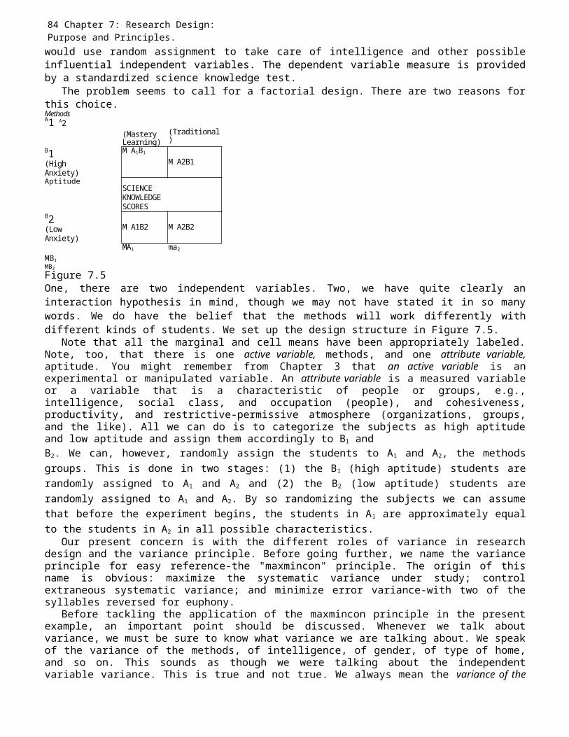
84 Chapter 7: Research Design: Purpose and Principles.would use random assignment to take care of intelligence and other possibleinfluential independent variables. The dependent variable measure is providedby a standardized science knowledge test.
The problem seems to call for a factorial design. There are two reasons forthis choice.MethodsA1 A2
(MasteryLearning)
(Traditional)
B1(HighAnxiety)
M A1B1
M A2B1
AptitudeSCIENCEKNOWLEDGESCORES
B2(LowAnxiety)
M A1B2 M A2B2
MA1 ma2
MB1MB2Figure 7.5One, there are two independent variables. Two, we have quite clearly aninteraction hypothesis in mind, though we may not have stated it in so manywords. We do have the belief that the methods will work differently withdifferent kinds of students. We set up the design structure in Figure 7.5.
Note that all the marginal and cell means have been appropriately labeled.Note, too, that there is one active variable, methods, and one attribute variable,aptitude. You might remember from Chapter 3 that an active variable is anexperimental or manipulated variable. An attribute variable is a measured variableor a variable that is a characteristic of people or groups, e.g.,intelligence, social class, and occupation (people), and cohesiveness,productivity, and restrictive-permissive atmosphere (organizations, groups,and the like). All we can do is to categorize the subjects as high aptitudeand low aptitude and assign them accordingly to B1 andB2. We can, however, randomly assign the students to A1 and A2, the methodsgroups. This is done in two stages: (1) the B1 (high aptitude) students arerandomly assigned to A1 and A2 and (2) the B2 (low aptitude) students arerandomly assigned to A1 and A2. By so randomizing the subjects we can assumethat before the experiment begins, the students in A1 are approximately equalto the students in A2 in all possible characteristics.
Our present concern is with the different roles of variance in researchdesign and the variance principle. Before going further, we name the varianceprinciple for easy reference-the "maxmincon" principle. The origin of thisname is obvious: maximize the systematic variance under study; controlextraneous systematic variance; and minimize error variance-with two of thesyllables reversed for euphony.
Before tackling the application of the maxmincon principle in the presentexample, an important point should be discussed. Whenever we talk aboutvariance, we must be sure to know what variance we are talking about. We speakof the variance of the methods, of intelligence, of gender, of type of home,and so on. This sounds as though we were talking about the independentvariable variance. This is true and not true. We always mean the variance of the
Chapter 7: Research Design: Purpose and Principles 85
dependent variable the variance of the dependent variable measures, after the experiment hasbeen done. This is not true in so-called correlational studies where, when wesay "the variance of the independent variable," we mean just that. Whencorrelating two variables, we study the variances of the independent anddependent variables "directly." Our way of saying "independent variablevariance" stems from the fact that, by manipulation and control of independentvariables, we influence, presumably, the variance of the dependent variable.Somewhat inaccurately put we "make" the measures of the dependent variablebehave or vary as a presumed result of our manipulation and control of theindependent variables. In an experiment, it is the dependent variable measuresthat are analyzed. Then, from the analysis we infer that the variances presentin the total variance of the dependent variable measures are due to themanipulation and control of the independent variables and to error. Now, backto our principle.MAXIMIZATION OF EXPERIMENTAL VARIANCEThe experimenter's most obvious, but not necessarily most important, concernis to maximize what we will call the experimental variance. This term is introducedto facilitate subsequent discussions and, in general, simply refers to thevariance of the dependent variable influenced by the independent variable orvariables of the substantive hypothesis. In this particular case, theexperimental variance is the variance in the dependent variable presumably dueto methods, A1 and A2, and aptitude, B1 and B2. Although experimental variancecan be taken to mean only the variance due to a manipulated or active variable,like methods, we shall also consider attribute variables, like intelligence,gender, and, in this case, aptitude, experimental variables. One of the maintasks of an experimenter is to maximize this variance. The methods must be“pulled” apart as much as possible to make A1 and A2 (and A3,A4, and so on, if they are in the design) as unlike as possible.
If the independent variable does not vary substantially, there is littlechance of separating its effect from the total variance of the dependentvariable. It is necessary to give the variance of a relation a chance to showitself, to separate itself, so to speak, from the total variance, which is acomposite of variances due to numerous sources and chance. Remembering thissubprinciple of the maxmincon principle, we can write a research precept:Design, plan, and conduct research so that the experimental conditions are as different aspossible. There are, of course, exceptions to this subprinciple, but they areprobably rare. An investigator might want to study the effects of smallgradations of, say, motivational incentives on the learning of some subjectmatter. Here one would not make the experimental conditions as different aspossible. Still, they would have to be made to vary somewhat or there would beno discernible resulting variance in the dependent variable.
In the present research example, this subprinciple means that theinvestigator must take pains to make A1 and A2, the mastery learning andtraditional methods, as different as possible. Next, B1 and B2 must also bemade as different as possible on the aptitude dimension. This latter problemis essentially one of measurement, as we will see in a later chapter. In anexperiment, the investigator is like a puppeteer making the independentvariable puppets do what he or she wants. The strings of the A1 and A2 puppetsare held on the right hand andthe strings of the B1 and B2 puppets in the left hand.(We assume there is no influence of one hand on the other, that is, the handsmust be independent.) The A1

86 Chapter 7: Research Design: Purpose and Principles.and A2 puppets are made to dance apart just as the B1 and B2 puppets are madeto dance apart. Theinvestigator then watches the audience (the dependent variable) to see andmeasure the effect of the manipulations. If one is successful in making A1 andA2 dance apart, and if there is a relation between A and the dependentvariable, the audience reaction-if separating A1 and A2 is funny, for instance-should belaughter. The investigator may even observe that he or she only gets laughterwhen A1 and A2 dance apart and, at the same time, B1 or B2 dance apart(interaction again).CONTROL OF EXTRANEOUS VARIABLES The control of extraneous variables means thatthe influences of independent variables extraneous to the purposes of thestudy are minimized, nullified, or isolated. There are three ways to controlextraneous variables. The first is the easiest, if it is possible: toeliminate the variable as a variable. If we are worried about intelligence asa possible contributing factor in studies of achievement, its effect on thedependent variable can be virtually eliminated by using subjects of only oneintelligence level, say intelligence scores within the range of 90 to 110. Ifwe are studying achievement, and racial membership is a possible contributingfactor to the variance of achievement, it can be eliminated by using onlymembers of one race. The principle is: To eliminate the effect of a possible influentialindependent variable on a dependent variable, choose subjects so that they are as homogeneous aspossible on that independent variable.
This method of controlling unwanted or extraneous variance is veryeffective. If we select only one gender for an experiment, then we can be surethat gender cannot be a contributing independent variable. But then we losegeneralization power; for instance we can say nothing about the relation understudy with girls if we use only boys in the experiment. If the range ofintelligence is restricted, then we can discuss only this restricted range. Isit possible that the relation, if discovered, is nonexistent or quitedifferent with children of high intelligence or children of low intelligence?We simply do not know; we can only surmise or guess.
The second way to control extraneous variance is through randomization.This is the best way, in the sense that you can have your cake and eat some ofit, too. Theoretically, randomization is the only method of controlling allpossible extraneous variables. Another way to phrase it is: if randomizationhas been accomplished, then the experimental groups can be consideredstatistically equal in all possible ways. This does not mean, of course, thatthe groups are equal in all the possible variables. We already know that bychance the groups can be unequal, but the probability of their being equal isgreater, with proper randomization, than the probability of their not beingequal. For this reason control of the extraneous variance by randomization isa powerful method of control. All other methods leave many possibilities ofinequality. If we match for intelligence, we may successfully achievestatistical equality in intelligence (at least in those aspects ofintelligence measured), but we may suffer from inequality in othersignificantly influential independent variables like aptitude, motivation, andsocial class. A precept that springs from this equalizing power ofrandomization, then, is: Whenever it is possible to do so, randomly assign subjects toexperimental groups and conditions, and randomly assign conditions and other factors to experimentalgroups.
The third means of controlling an extraneous variable is to build it rightinto the design as an independent variable. For example, assume that gender
Chapter 7: Research Design: Purpose and Principles 87
was to be controlled in the experiment discussed earlier and it was consideredinexpedient or unwise to eliminate it. One could add a third independentvariable, gender, to the design. Unless one were interested in the actualdifference between the genders on the dependent variable or wanted to studythe interaction between one or two of the other variables and gender, however,it is unlikely that this form of control would be used. One might wantinformation of the kind just mentioned and also want to control gender, too.In such a case, adding it to the design as a variable might be desirable. Thepoint is that building a variable into an experimental design "controls" thevariable, since it then becomes possible to extract from the total variance ofthe dependent variable the variance due to the variable. (In the above case,this would be the "between-genders" variance.)
These considerations lead to another principle: An extraneous variable can be controlled by building itinto the research design as an attribute variable, thus achieving control and yielding additional researchinformation about the effect of the variable on the dependent variable and about its possible interactionwith other independent variables.
The fourth way to control extraneous variance is to match subjects. Thecontrol principle behind matching is the same as that for any other kind ofcontrol, the control of variance. Matching is similar-in fact, it might becalled a corollary-to the principle of controlling the variance of anextraneous variable by building it into the design. The basic principle is tosplit a variable into two or more parts, say into high and low intelligence ina factorial design, and then randomize within each level as described above.Matching is a special case of this principle. Instead of splitting thesubjects into two, three, or four parts, however, they are split into N/2parts, N being the number of subjects used; thus the control of variance isbuilt into the design.
In using the matching method several problems may be encountered. To beginwith, the variable on which the subjects are matched must be substantiallyrelated to the dependent variable or the matching is a waste of time. Evenworse, it can be misleading. In addition, matching has severe limitations. Ifwe try to match, say, on more than two variables, or even more than one, welose subjects. It is difficult to find matched subjects on more than twovariables. For instance, if one decides to match intelligence, gender, andsocial class, one may be fairly successful in matching the first two variablesbut not in finding pairs that are fairly equal on all three variables. Add afourth variable and the problem becomes difficult, often impossible to solve.
Let us not throw the baby out with the bath, however. When there is asubstantial correlation between the matching variable or variables and thedependent variable (>.50 or .60), then matching reduces the error term andthus increases the precision of an experiment, a desirable outcome. If thesame subjects are used with different experimental treatments-called repeatedmeasures or randomized blocks design-we have powerful control of variance. Howmatch better on all possible variables than by matching a subject withoneself? Unfortunately, other negative considerations usually rule out thispossibility. It should be forcefully emphasized that matching of any kind isno substitute for randomization. If subjects are matched, they should then beassigned to experimental groups at random. Through a random procedure, like tossing acoin or using odd and even random numbers, the members of the matched pairsare assigned to experimental and control groups. If the same subjects undergoall treatments, then the order of the treatments should be assigned randomly.This adds randomization control to the matching, or repeated measures,control.
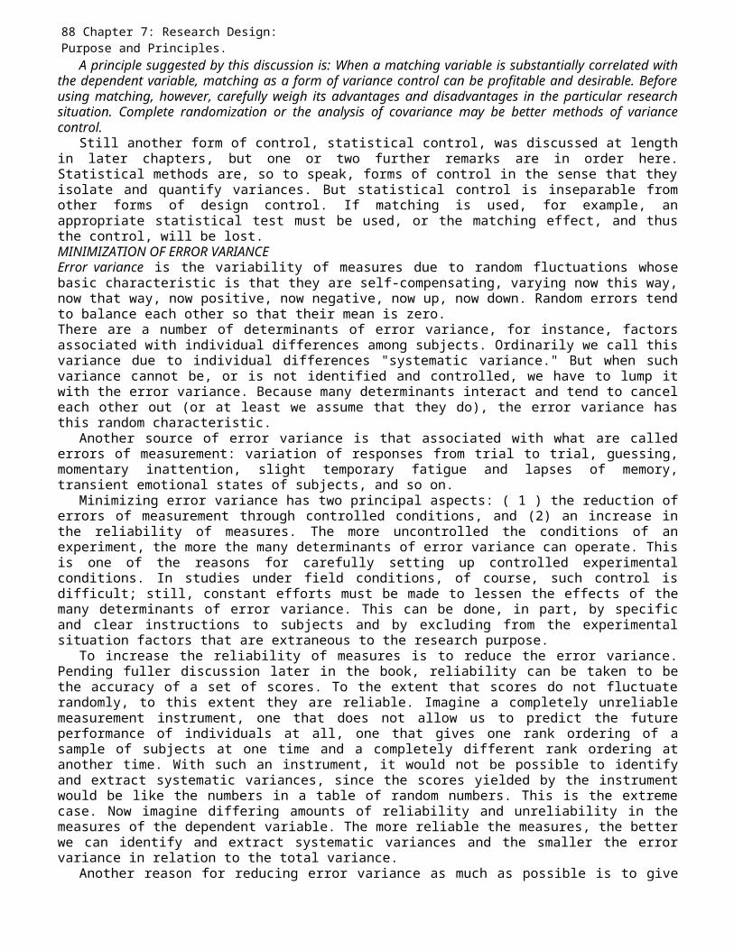
88 Chapter 7: Research Design: Purpose and Principles.
A principle suggested by this discussion is: When a matching variable is substantially correlated withthe dependent variable, matching as a form of variance control can be profitable and desirable. Beforeusing matching, however, carefully weigh its advantages and disadvantages in the particular researchsituation. Complete randomization or the analysis of covariance may be better methods of variancecontrol.
Still another form of control, statistical control, was discussed at lengthin later chapters, but one or two further remarks are in order here.Statistical methods are, so to speak, forms of control in the sense that theyisolate and quantify variances. But statistical control is inseparable fromother forms of design control. If matching is used, for example, anappropriate statistical test must be used, or the matching effect, and thusthe control, will be lost.MINIMIZATION OF ERROR VARIANCEError variance is the variability of measures due to random fluctuations whosebasic characteristic is that they are self-compensating, varying now this way,now that way, now positive, now negative, now up, now down. Random errors tendto balance each other so that their mean is zero.There are a number of determinants of error variance, for instance, factorsassociated with individual differences among subjects. Ordinarily we call thisvariance due to individual differences "systematic variance." But when suchvariance cannot be, or is not identified and controlled, we have to lump itwith the error variance. Because many determinants interact and tend to canceleach other out (or at least we assume that they do), the error variance hasthis random characteristic.
Another source of error variance is that associated with what are callederrors of measurement: variation of responses from trial to trial, guessing,momentary inattention, slight temporary fatigue and lapses of memory,transient emotional states of subjects, and so on.
Minimizing error variance has two principal aspects: ( 1 ) the reduction oferrors of measurement through controlled conditions, and (2) an increase inthe reliability of measures. The more uncontrolled the conditions of anexperiment, the more the many determinants of error variance can operate. Thisis one of the reasons for carefully setting up controlled experimentalconditions. In studies under field conditions, of course, such control isdifficult; still, constant efforts must be made to lessen the effects of themany determinants of error variance. This can be done, in part, by specificand clear instructions to subjects and by excluding from the experimentalsituation factors that are extraneous to the research purpose.
To increase the reliability of measures is to reduce the error variance.Pending fuller discussion later in the book, reliability can be taken to bethe accuracy of a set of scores. To the extent that scores do not fluctuaterandomly, to this extent they are reliable. Imagine a completely unreliablemeasurement instrument, one that does not allow us to predict the futureperformance of individuals at all, one that gives one rank ordering of asample of subjects at one time and a completely different rank ordering atanother time. With such an instrument, it would not be possible to identifyand extract systematic variances, since the scores yielded by the instrumentwould be like the numbers in a table of random numbers. This is the extremecase. Now imagine differing amounts of reliability and unreliability in themeasures of the dependent variable. The more reliable the measures, the betterwe can identify and extract systematic variances and the smaller the errorvariance in relation to the total variance.
Another reason for reducing error variance as much as possible is to give
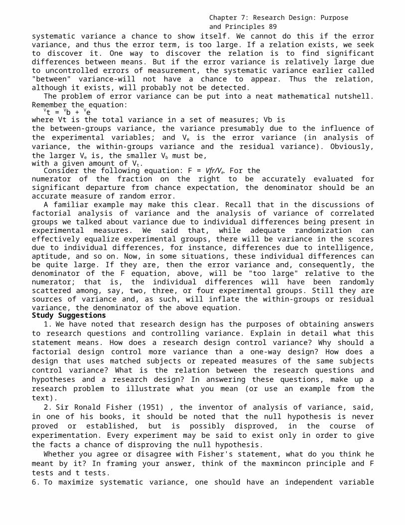
Chapter 7: Research Design: Purpose and Principles 89
systematic variance a chance to show itself. We cannot do this if the errorvariance, and thus the error term, is too large. If a relation exists, we seekto discover it. One way to discover the relation is to find significantdifferences between means. But if the error variance is relatively large dueto uncontrolled errors of measurement, the systematic variance earlier called"between" variance-will not have a chance to appear. Thus the relation,although it exists, will probably not be detected.
The problem of error variance can be put into a neat mathematical nutshell.Remember the equation:
Vt = Vb + Vewhere Vt is the total variance in a set of measures; Vb isthe between-groups variance, the variance presumably due to the influence ofthe experimental variables; and Ve is the error variance (in analysis ofvariance, the within-groups variance and the residual variance). Obviously,the larger Ve is, the smaller Vb must be,with a given amount of Vt.
Consider the following equation: F = Vfr/Ve. For thenumerator of the fraction on the right to be accurately evaluated forsignificant departure from chance expectation, the denominator should be anaccurate measure of random error.
A familiar example may make this clear. Recall that in the discussions offactorial analysis of variance and the analysis of variance of correlatedgroups we talked about variance due to individual differences being present inexperimental measures. We said that, while adequate randomization caneffectively equalize experimental groups, there will be variance in the scoresdue to individual differences, for instance, differences due to intelligence,aptitude, and so on. Now, in some situations, these individual differences canbe quite large. If they are, then the error variance and, consequently, thedenominator of the F equation, above, will be "too large" relative to thenumerator; that is, the individual differences will have been randomlyscattered among, say, two, three, or four experimental groups. Still they aresources of variance and, as such, will inflate the within-groups or residualvariance, the denominator of the above equation.Study Suggestions
1. We have noted that research design has the purposes of obtaining answersto research questions and controlling variance. Explain in detail what thisstatement means. How does a research design control variance? Why should afactorial design control more variance than a one-way design? How does adesign that uses matched subjects or repeated measures of the same subjectscontrol variance? What is the relation between the research questions andhypotheses and a research design? In answering these questions, make up aresearch problem to illustrate what you mean (or use an example from thetext).
2. Sir Ronald Fisher (1951) , the inventor of analysis of variance, said,in one of his books, it should be noted that the null hypothesis is neverproved or established, but is possibly disproved, in the course ofexperimentation. Every experiment may be said to exist only in order to givethe facts a chance of disproving the null hypothesis.
Whether you agree or disagree with Fisher's statement, what do you think hemeant by it? In framing your answer, think of the maxmincon principle and Ftests and t tests.6. To maximize systematic variance, one should have an independent variable
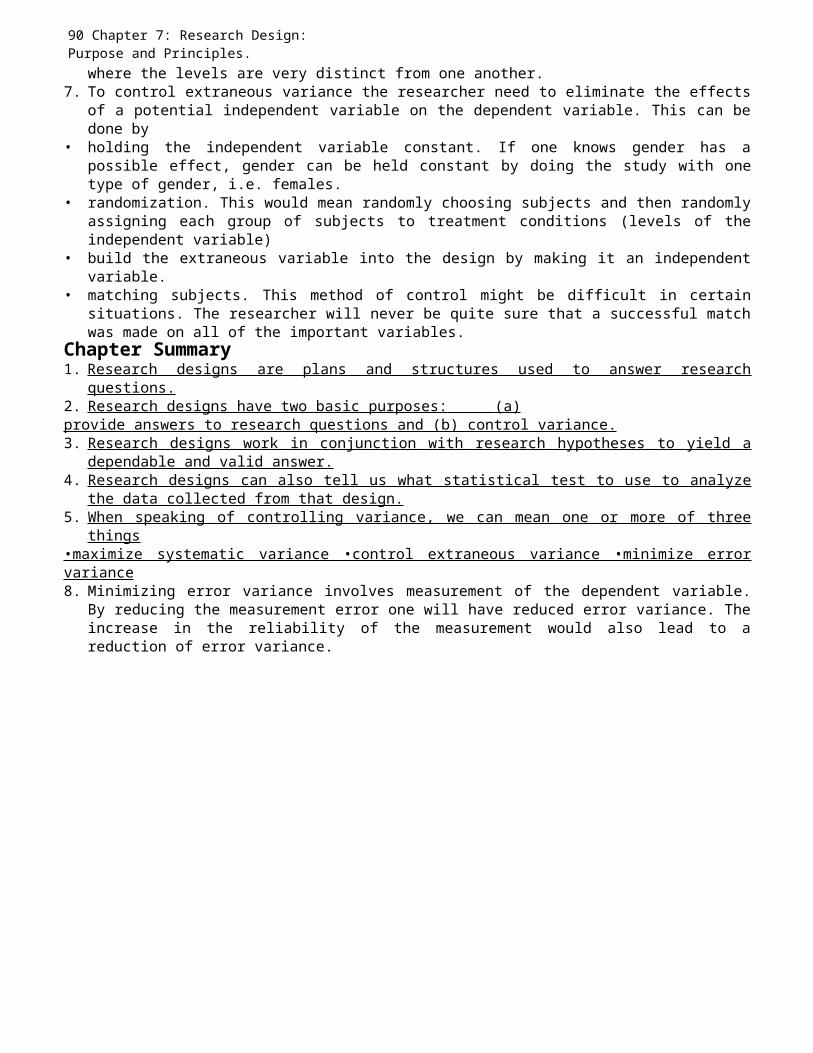
90 Chapter 7: Research Design: Purpose and Principles.
where the levels are very distinct from one another.7. To control extraneous variance the researcher need to eliminate the effects
of a potential independent variable on the dependent variable. This can bedone by
• holding the independent variable constant. If one knows gender has apossible effect, gender can be held constant by doing the study with onetype of gender, i.e. females.
• randomization. This would mean randomly choosing subjects and then randomlyassigning each group of subjects to treatment conditions (levels of theindependent variable)
• build the extraneous variable into the design by making it an independentvariable.
• matching subjects. This method of control might be difficult in certainsituations. The researcher will never be quite sure that a successful matchwas made on all of the important variables.
Chapter Summary1. Research designs are plans and structures used to answer research
questions.2. Research designs have two basic purposes: (a) provide answers to research questions and (b) control variance.3. Research designs work in conjunction with research hypotheses to yield a
dependable and valid answer.4. Research designs can also tell us what statistical test to use to analyze
the data collected from that design.5. When speaking of controlling variance, we can mean one or more of three
things•maximize systematic variance •control extraneous variance •minimize errorvariance8. Minimizing error variance involves measurement of the dependent variable.
By reducing the measurement error one will have reduced error variance. Theincrease in the reliability of the measurement would also lead to areduction of error variance.
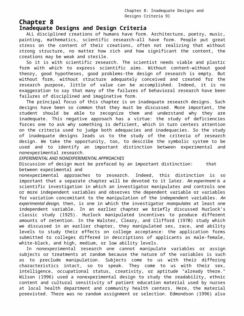
Chapter 8: Inadequate Designs and Designs Criteria 91
Chapter 8Inadequate Designs and Design Criteria
ALL disciplined creations of humans have form. Architecture, poetry, music,painting, mathematics, scientific research-all have form. People put greatstress on the content of their creations, often not realizing that withoutstrong structure, no matter how rich and how significant the content, thecreations may be weak and sterile.
So it is with scientific research. The scientist needs viable and plasticform with which to express scientific aims. Without content-without goodtheory, good hypotheses, good problems-the design of research is empty. Butwithout form, without structure adequately conceived and created for theresearch purpose, little of value can be accomplished. Indeed, it is noexaggeration to say that many of the failures of behavioral research have beenfailures of disciplined and imaginative form.
The principal focus of this chapter is on inadequate research designs. Suchdesigns have been so common that they must be discussed. More important, thestudent should be able to recognize them and understand why they areinadequate. This negative approach has a virtue: the study of deficienciesforces one to ask why something is deficient, which in turn centers attentionon the criteria used to judge both adequacies and inadequacies. So the studyof inadequate designs leads us to the study of the criteria of researchdesign. We take the opportunity, too, to describe the symbolic system to beused and to identify an important distinction between experimental andnonexperimental research.EXPERIMENTAL AND NONEXPERIMENTAL APPROACHESDiscussion of design must be prefaced by an important distinction: thatbetween experimental andnonexperimental approaches to research. Indeed, this distinction is soimportant that a separate chapter will be devoted to it later. An experiment is ascientific investigation in which an investigator manipulates and controls oneor more independent variables and observes the dependent variable or variablesfor variation concomitant to the manipulation of the independent variables. Anexperimental design, then, is one in which the investigator manipulates at least oneindependent variable. In an earlier chapter we briefly discussed Hurlock’sclassic study (1925). Hurlock manipulated incentives to produce differentamounts of retention. In the Walster, Cleary, and Clifford (1970) study whichwe discussed in an earlier chapter, they manipulated sex, race, and abilitylevels to study their effects on college acceptance: the application formssubmitted to colleges differed in descriptions of applicants as male-female,white-black, and high, medium, or low ability levels.
In nonexperimental research one cannot manipulate variables or assignsubjects or treatments at random because the nature of the variables is suchas to preclude manipulation. Subjects come to us with their differingcharacteristics intact, so to speak. They come to us with their sex,intelligence, occupational status, creativity, or aptitude "already there."Wilson (1996) used a nonexperimental design to study the readability, ethniccontent and cultural sensitivity of patient education material used by nursesat local health department and community health centers. Here, the materialpreexisted. There was no random assignment or selection. Edmondson (1996) also
92 Chapter 8: Inadequate Designs and Designs Criteria.used a nonexperimental design to compare the number of medication errors bynurses, physicians, and pharmacists in 8 hospital units at two urban teachinghospitals. Edmondson did not choose these units or hospitals at random norwere the medical professionals chosen at random. In many areas of research,likewise, random assignment is unfortunately not possible, as we will seelater. Although experimental and nonexperimental research differ in thesecrucial respects, they share structural and design features that will bepointed out in this and subsequent chapters. In addition, their basic purposeis the same: to study relations among phenomena. Their scientific logic isalso the same: to bring empirical evidence to bear on conditional statementsof the form If p, then q. In some fields of behavioral and social sciences thenonexperimental framework is unavoidable. Keith (1988) states that a lot ofstudies conducted by school psychologists are of the nonexperimental nature.School psychology researchers as well as many in educational psychology mustwork within a practical framework. Many times, schools, classrooms or evenstudents are given to the researcher “as-is.” Stone- Romero, Weaver & Glenar(1995) have summarized nearly 20 years of articles from the Journal of AppliedPsychology concerning the use of experimental and nonexperimental researchdesigns.
The ideal of science is the controlled experiment. Except, perhaps, intaxonomic research-research with the purpose of discovering, classifying, andmeasuring natural phenomena and the factors behind such phenomena-thecontrolled experiment is the desired model of science. It may be difficult formany students to accept this rather categorical statement since its logic isnot readily apparent. Earlier it was said that the main goal of science was todiscover relations among phenomena. Why, then, assign a priority to thecontrolled experiment? Do not other methods of discovering relations exist?Yes, of course they do. The main reason for the preeminence of the controlledexperiment, however, is that researchers can have more confidence that therelations they study are the relations they think they are. The reason is nothard to see: they study the relations under the most carefully controlledconditions of inquiry known. The unique and overwhelmingly important virtue ofexperimental inquiry, then, is control. In a perfectly controlled experimentalstudy, the experimenter can be confident that the manipulation of theindependent variable affected the dependent variable and nothing else. Inshort, a perfectly conducted experimental study is more trustworthy than aperfectly conducted nonexperimental study. Why this is so should become moreand more apparent as we advance in our study of research design.SYMBOLISM AND DEFINITIONSBefore discussing inadequate designs, explanation of the symbolism to be usedin these chapters is necessary. X means an experimentally manipulated independentvariable (or variables). X1 X2, X3, etc. meanindependent variables 1, 2, 3, and so on, though we usually use X alone, evenwhen it can mean more than one independent variable. (We also use X1 X2, etc.tomean partitions of an independent variable, but the difference will always beclear.) The symbol (X) indicates that the independent variable is notmanipulated-is not under the direct control of the investigator, but is measuredor imagined. The dependent variable is Y: Yb is the dependent variable before the
Chapter 8: Inadequate Designs and Designs Criteria 93
manipulation of X, and Ya the dependent variable after the manipulation of X.With ~X, we borrow the negation sign of set theory; ~X ("not-X") means thatthe experimental variable, the independent variable X, is not manipulated.(Note: (X) is a nonmanipulable variable and ~X is a manipulable variable thatis not manipulated.) The symbol (R) will be used for the random assignment ofsubjects to experimental groups and the random assignment of experimentaltreatments to experimental groups.
The explanation of ~X, just given, is not quite accurate, because in somecases ~X can mean a different aspect of the treatment X rather than merely theabsence of X. In an older language, the experimental group was the group thatwas given the so- called experimental treatment, X, while the control groupdid not receive it, ~X. For our purposes, however, ~X will do well enough,especially if we understand the generalized meaning of "control" discussedbelow. An experimental group, then, is a group of subjects receiving some aspector treatment of X. In testing the frustration-aggression hypothesis, theexperimental group is the group whose subjects are systematically frustrated.In contrast, the control group is one that is given "no" treatment.
In modern multivariate research, it is necessary to expand these notions.They are not changed basically; they are only expanded. It is quite possibleto have more than one experimental group, as we have seen. Different degreesof manipulation of the independent variable are not only possible; they areoften also desirable or even imperative. Furthermore, it is possible to havemore than one control group, a statement that at first seems like nonsense.How can one have different degrees of "no" experimental treatment?-because thenotion of control is generalized. When there are more than two groups, and whenany two of them are treated differently, one or more groups serve as"controls" on the others. Recall that control is always control of variance.With two or more groups treated differently, variance is engendered by theexperimental manipulation. So the traditional notion of X and ~X, treatmentand no treatment, is generalized to X1 X2,X3, . . ., Xk, different forms or degrees of treatment.
If X is circled, (X), this means that the investigator “imagines" themanipulation of X, or assumes that X occurred and that it is the X of thehypothesis. It may also mean that X is measured and not manipulated.Actually, we are saying the same thing here in different ways. The context ofthe discussion should make the distinction clear. Suppose a sociologist isstudying delinquency and the frustration-aggression hypothesis. Thesociologist observes delinquency, Y, and imagines that the delinquent subjectswere frustrated in their earlier years, or (X). All nonexperimental designswill have (X). Generally, then, (X) means an independent variable not underthe experimental control of the investigator.
One more point-each design in this chapter will ordinarily have an a and ab form. The a form will be the experimental form, or that in which X ismanipulated. The b form will be the nonexperimental form, that in which X isnot under the control of the investigator, or (X). Obviously, (~X) is alsopossible.
FAULTY DESIGNSThere are four (or more) inadequate designs of research that have often
been used-and are occasionally still used-in behavioral research. The
94 Chapter 8: Inadequate Designs and Designs Criteria.inadequacies of the designs lead to poor control of independent variables. Wenumber each such design, give it a name, sketch its structure, and thendiscuss it.Design 8.1: One-Group(a)X Y (Experimental)(b)(X)Y(Nonexperimental)
Design 8.1 (a) has been called the "One-Shot Case Study," an apropos namegiven by Campbell and Stanley (1963). The (a) form is experimental, the (b)form nonexperimental. An example of the (a) form: a school faculty institutesa new curriculum and wishes to evaluate its effects. After one year, Y,
studentachievement, is measured. It is concluded, say, that achievement has improvedunder the new program. With such a design the conclusion is weak. Design 8.1(b) is the nonexperimental form of the one-groupdesign. Y, the outcome, is studied, and X is assumed or imagined. An examplewould be to study delinquency by searching the past of a group of juveniledelinquents for factors that may have led to antisocial behavior. The methodis problematic because the factors (variables) may be confounded. When theeffect of two or more factors (variables) cannot be separated, the results aredifficult to interpret. Any number of possible explanations might beplausible.
Scientifically, Design 8.1 is worthless. There is virtually no control ofother possible influences on outcome. As Campbell (1957) long ago pointed out,the minimum of useful scientific information requires at least one formalcomparison. The curriculum example requires, at the least, comparison of the groupthat experienced the new curriculum with a group that did not experience it.The presumed effect of the new curriculum, say such and-such achievement,might well have been about the same under any kind of curriculum. The point isnot that the new curriculum did or did not have an effect. It was that withoutany formal, controlled comparison of the performance of the members of the"experimental" group with the performance of the members of some other groupnot experiencing the new curriculum, little can be said about its effect.
An important distinction should be made. It is not that the method isentirely worthless, but that it is scientifically worthless. In everyday life, ofcourse, we depend on such scientifically questionable evidence; we have to. Weact, we say, on the basis of our experience. We hope that we use ourexperience rationally. The everyday-thinking paradigm implied by Design 8.1 isnot being criticized. Only when such a paradigm is used and said or believedto be scientific do difficulties arise. Even in high intellectual pursuits,the thinking implied by this design is used. Freud's careful observations andbrilliant and creative analysis of neurotic behavior seem to fall into thiscategory. The quarrel is not with Freud, then, but rather with assertions thathis conclusions are "scientifically established. "Design 8.2: One-Group, before-after (Pretest Posttest)(a) Yb X Ya (Experimental)(b) Yb (X) Ya (Nonexperimental)
Design 8.2 is only a small improvement on Design 8.1. The essentialcharacteristic of this mode of research is that a group is compared withitself. Theoretically, there is no better choice since all possibleindependent variables associated with the subjects' characteristics are
Chapter 8: Inadequate Designs and Designs Criteria 95
controlled. The procedure dictated by such a design is as follows. A group ismeasured on the dependent variable, Y, before experimental manipulation. Thisis usually called a pretest. Assume that the attitudes toward women of a group ofsubjects are measured. An experimental manipulation designed to change theseattitudes is used. An experimenter might expose the group to expert opinion onwomen's rights, for example. After the interposition of this X, the attitudesof the subjects are again measured. The difference scores, or Ya - Yb, areexamined for change in attitudes.
At face value, this would seem a good way to accomplish the experimentalpurpose. After all, if the difference scores are statistically significant,does this not indicate a change in attitudes? The situation is not so simple.There are a number of other factors that may have contributed to the change inscores. Hence, the factors are confounded. Campbell (1957) gives an excellentdetailed discussion of these factors, only a brief outline of which can begiven here.Measurement, History, MaturationFirst is the possible effect of the measurement procedure: measuring subjectschanges them. Can it be that the post-X measures were influenced not by themanipulation of X but by increased sensitization due to the pretest? Campbell(1957) calls such measures reactive measures, because they themselves cause thesubject to react. Controversial attitudes, for example, seem to be especiallysusceptible to such sensitization. Achievement measures, though probably lessreactive, are still affected. Measures involving memory are susceptible. Ifyou take a test now, you are more likely to remember later things that wereincluded in the test. In short, observed changes may be due to reactiveeffects.
Two other important sources of extraneous variance are history and maturation.Between the Yb and Ya
testings, many things can occur other than X. The longer the period of time,the greater the chance of extraneous variables affecting the subjects and thusthe Ya measures. This is what Campbell (1957) calls history. These variables orevents are specific to the particular experimental situation. Maturation, on theother hand, covers events that are general, not specific to any particularsituation. They reflect change or growth in the organism studied. Mental ageincreases with time, an increase that can easily affect achievement, memory,and attitudes. People can learn in any given time interval and the learningmay affect dependent variable measures. This is one of the exasperatingdifficulties of research that extends over considerable time periods. Thelonger the time interval, the greater the possibility that extraneous,unwanted sources of systematic variance will influence dependent variablemeasures.The Regression EffectA statistical phenomenon that has misled researchers is the so-called regressioneffect. Test scores change as a statistical fact of life: on retest, on theaverage, they regress toward the mean. The regression effect operates becauseof the imperfect correlation between the pretest and posttest scores. If rab =1.00, then there is noregression effect; if rab = .00, the effect is at amaximum in the sense that the best prediction of any posttest score from
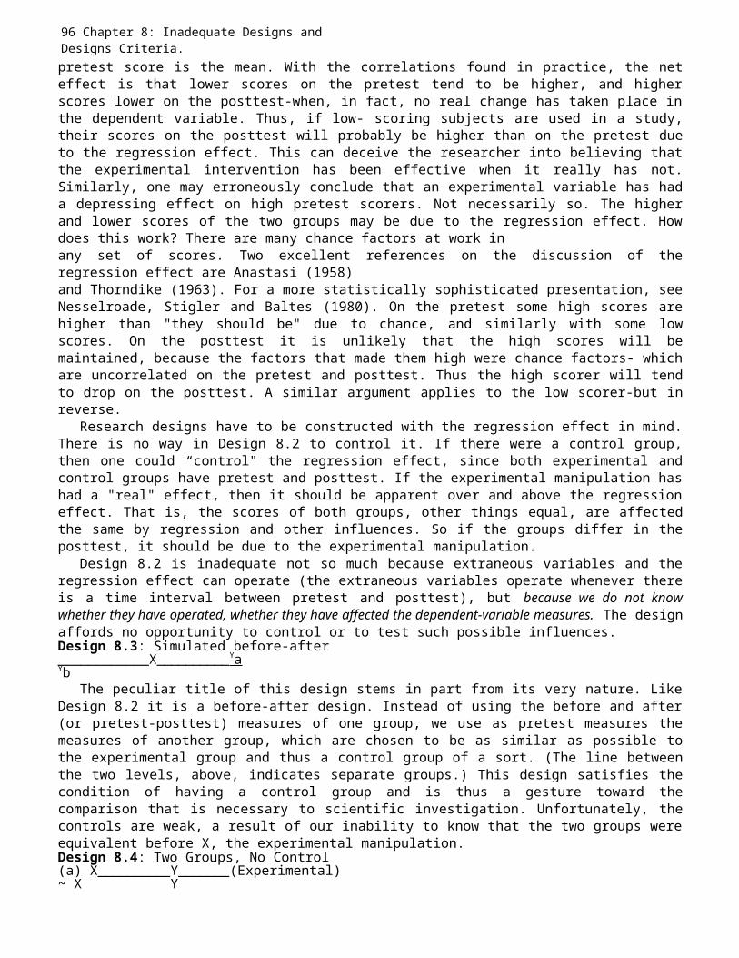
96 Chapter 8: Inadequate Designs and Designs Criteria.pretest score is the mean. With the correlations found in practice, the neteffect is that lower scores on the pretest tend to be higher, and higherscores lower on the posttest-when, in fact, no real change has taken place inthe dependent variable. Thus, if low- scoring subjects are used in a study,their scores on the posttest will probably be higher than on the pretest dueto the regression effect. This can deceive the researcher into believing thatthe experimental intervention has been effective when it really has not.Similarly, one may erroneously conclude that an experimental variable has hada depressing effect on high pretest scorers. Not necessarily so. The higherand lower scores of the two groups may be due to the regression effect. Howdoes this work? There are many chance factors at work inany set of scores. Two excellent references on the discussion of theregression effect are Anastasi (1958)and Thorndike (1963). For a more statistically sophisticated presentation, seeNesselroade, Stigler and Baltes (1980). On the pretest some high scores arehigher than "they should be" due to chance, and similarly with some lowscores. On the posttest it is unlikely that the high scores will bemaintained, because the factors that made them high were chance factors- whichare uncorrelated on the pretest and posttest. Thus the high scorer will tendto drop on the posttest. A similar argument applies to the low scorer-but inreverse.
Research designs have to be constructed with the regression effect in mind.There is no way in Design 8.2 to control it. If there were a control group,then one could “control" the regression effect, since both experimental andcontrol groups have pretest and posttest. If the experimental manipulation hashad a "real" effect, then it should be apparent over and above the regressioneffect. That is, the scores of both groups, other things equal, are affectedthe same by regression and other influences. So if the groups differ in theposttest, it should be due to the experimental manipulation.
Design 8.2 is inadequate not so much because extraneous variables and theregression effect can operate (the extraneous variables operate whenever thereis a time interval between pretest and posttest), but because we do not knowwhether they have operated, whether they have affected the dependent-variable measures. The designaffords no opportunity to control or to test such possible influences.Design 8.3: Simulated before-after____________X__________Y a Yb
The peculiar title of this design stems in part from its very nature. LikeDesign 8.2 it is a before-after design. Instead of using the before and after(or pretest-posttest) measures of one group, we use as pretest measures themeasures of another group, which are chosen to be as similar as possible tothe experimental group and thus a control group of a sort. (The line betweenthe two levels, above, indicates separate groups.) This design satisfies thecondition of having a control group and is thus a gesture toward thecomparison that is necessary to scientific investigation. Unfortunately, thecontrols are weak, a result of our inability to know that the two groups wereequivalent before X, the experimental manipulation.Design 8.4: Two Groups, No Control(a) X__________Y_______(Experimental)~ X Y
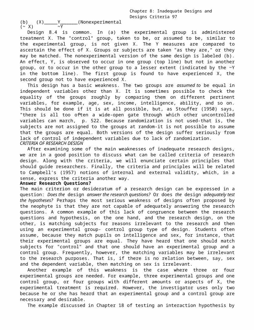
Chapter 8: Inadequate Designs and Designs Criteria 97
(b) (X)_____Y_______(Nonexperimental(~ X) ~Y
Design 8.4 is common. In (a) the experimental group is administeredtreatment X. The "control" group, taken to be, or assumed to be, similar tothe experimental group, is not given X. The Y measures are compared toascertain the effect of X. Groups or subjects are taken "as they are," or theymay be matched. The nonexperimental version of the same design is labeled (b).An effect, Y, is observed to occur in one group (top line) but not in anothergroup, or to occur in the other group to a lesser extent (indicated by the ~Yin the bottom line). The first group is found to have experienced X, thesecond group not to have experienced X.
This design has a basic weakness. The two groups are assumed to be equal inindependent variables other than X. It is sometimes possible to check theequality of the groups roughly by comparing them on different pertinentvariables, for example, age, sex, income, intelligence, ability, and so on.This should be done if it is at all possible, but, as Stouffer (1950) says,"there is all too often a wide-open gate through which other uncontrolledvariables can march,” p. 522. Because randomization is not used-that is, thesubjects are not assigned to the groups at random-it is not possible to assumethat the groups are equal. Both versions of the design suffer seriously fromlack of control of independent variables due to lack of randomization.CRITERIA OF RESEARCH DESIGN
After examining some of the main weaknesses of inadequate research designs,we are in a good position to discuss what can be called criteria of researchdesign. Along with the criteria, we will enunciate certain principles thatshould guide researchers. Finally, the criteria and principles will be relatedto Campbell's (1957) notions of internal and external validity, which, in asense, express the criteria another way.Answer Research Questions?The main criterion or desideratum of a research design can be expressed in aquestion: Does the design answer the research questions? Or does the design adequately testthe hypotheses? Perhaps the most serious weakness of designs often proposed bythe neophyte is that they are not capable of adequately answering the researchquestions. A common example of this lack of congruence between the researchquestions and hypothesis, on the one hand, and the research design, on theother, is matching subjects for reasons irrelevant to the research and thenusing an experimental group- control group type of design. Students oftenassume, because they match pupils on intelligence and sex, for instance, thattheir experimental groups are equal. They have heard that one should matchsubjects for "control" and that one should have an experimental group and acontrol group. Frequently, however, the matching variables may be irrelevantto the research purposes. That is, if there is no relation between, say, sexand the dependent variable, then matching on sex is irrelevant.
Another example of this weakness is the case where three or fourexperimental groups are needed. For example, three experimental groups and onecontrol group, or four groups with different amounts or aspects of X, theexperimental treatment is required. However, the investigator uses only twobecause he or she has heard that an experimental group and a control group arenecessary and desirable.
The example discussed in Chapter 18 of testing an interaction hypothesis by
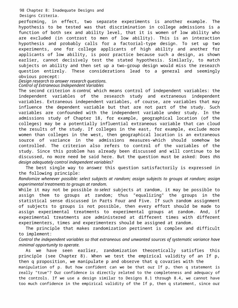
98 Chapter 8: Inadequate Designs and Designs Criteria.performing, in effect, two separate experiments is another example. Thehypothesis to be tested was that discrimination in college admissions is afunction of both sex and ability level, that it is women of low ability whoare excluded (in contrast to men of low ability). This is an interactionhypothesis and probably calls for a factorial-type design. To set up twoexperiments, one for college applicants of high ability and another forapplicants of low ability, is poor practice because such a design, as shownearlier, cannot decisively test the stated hypothesis. Similarly, to matchsubjects on ability and then set up a two-group design would miss the researchquestion entirely. These considerations lead to a general and seeminglyobvious precept:Design research to answer research questions.Control of Extraneous Independent VariablesThe second criterion is control, which means control of independent variables: theindependent variables of the research study and extraneous independentvariables. Extraneous independent variables, of course, are variables that mayinfluence the dependent variable but that are not part of the study. Suchvariables are confounded with the independent variable under study. In theadmissions study of Chapter 18, for example, geographical location (of thecolleges) may be a potentially influential extraneous variable that can cloudthe results of the study. If colleges in the east, for example, exclude morewomen than colleges in the west, then geographical location is an extraneoussource of variance in the admissions measures-which should somehow becontrolled. The criterion also refers to control of the variables of thestudy. Since this problem has already been discussed and will continue to bediscussed, no more need be said here. But the question must be asked: Does thisdesign adequately control independent variables?
The best single way to answer this question satisfactorily is expressed inthe following principle:Randomize whenever possible: select subjects at random; assign subjects to groups at random; assignexperimental treatments to groups at random.While it may not be possible to select subjects at random, it may be possible toassign them to groups at random; thus "equalizing" the groups in thestatistical sense discussed in Parts Four and Five. If such random assignmentof subjects to groups is not possible, then every effort should be made toassign experimental treatments to experimental groups at random. And, ifexperimental treatments are administered at different times with differentexperimenters, times and experimenters should be assigned at random.
The principle that makes randomization pertinent is complex and difficultto implement:Control the independent variables so that extraneous and unwanted sources of systematic variance haveminimal opportunity to operate.
As we have seen earlier, randomization theoretically satisfies thisprinciple (see Chapter 8). When we test the empirical validity of an If p,then q proposition, we manipulate p and observe that q covaries with themanipulation of p. But how confident can we be that our If p, then q statement isreally "true"? Our confidence is directly related to the completeness and adequacy ofthe controls. If we use a design similar to Designs 8.1 through 8.4, we cannot havetoo much confidence in the empirical validity of the If p, then q statement, since our
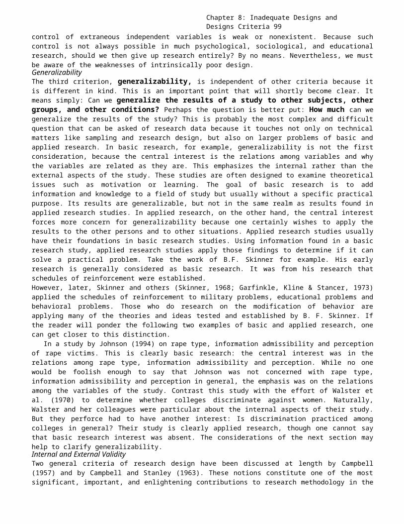
Chapter 8: Inadequate Designs and Designs Criteria 99
control of extraneous independent variables is weak or nonexistent. Because suchcontrol is not always possible in much psychological, sociological, and educationalresearch, should we then give up research entirely? By no means. Nevertheless, we mustbe aware of the weaknesses of intrinsically poor design.GeneralizabilityThe third criterion, generalizability, is independent of other criteria because itis different in kind. This is an important point that will shortly become clear. Itmeans simply: Can we generalize the results of a study to other subjects, othergroups, and other conditions? Perhaps the question is better put: How much can wegeneralize the results of the study? This is probably the most complex and difficultquestion that can be asked of research data because it touches not only on technicalmatters like sampling and research design, but also on larger problems of basic andapplied research. In basic research, for example, generalizability is not the firstconsideration, because the central interest is the relations among variables and whythe variables are related as they are. This emphasizes the internal rather than theexternal aspects of the study. These studies are often designed to examine theoreticalissues such as motivation or learning. The goal of basic research is to addinformation and knowledge to a field of study but usually without a specific practicalpurpose. Its results are generalizable, but not in the same realm as results found inapplied research studies. In applied research, on the other hand, the central interestforces more concern for generalizability because one certainly wishes to apply theresults to the other persons and to other situations. Applied research studies usuallyhave their foundations in basic research studies. Using information found in a basicresearch study, applied research studies apply those findings to determine if it cansolve a practical problem. Take the work of B.F. Skinner for example. His earlyresearch is generally considered as basic research. It was from his research thatschedules of reinforcement were established.However, later, Skinner and others (Skinner, 1968; Garfinkle, Kline & Stancer, 1973)applied the schedules of reinforcement to military problems, educational problems andbehavioral problems. Those who do research on the modification of behavior areapplying many of the theories and ideas tested and established by B. F. Skinner. Ifthe reader will ponder the following two examples of basic and applied research, onecan get closer to this distinction.
In a study by Johnson (1994) on rape type, information admissibility and perceptionof rape victims. This is clearly basic research: the central interest was in therelations among rape type, information admissibility and perception. While no onewould be foolish enough to say that Johnson was not concerned with rape type,information admissibility and perception in general, the emphasis was on the relationsamong the variables of the study. Contrast this study with the effort of Walster etal. (1970) to determine whether colleges discriminate against women. Naturally,Walster and her colleagues were particular about the internal aspects of their study.But they perforce had to have another interest: Is discrimination practiced amongcolleges in general? Their study is clearly applied research, though one cannot saythat basic research interest was absent. The considerations of the next section mayhelp to clarify generalizability.Internal and External ValidityTwo general criteria of research design have been discussed at length by Campbell(1957) and by Campbell and Stanley (1963). These notions constitute one of the mostsignificant, important, and enlightening contributions to research methodology in the
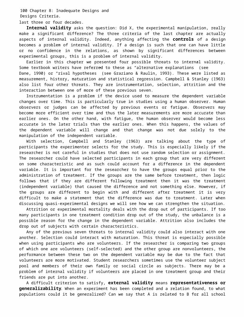
100 Chapter 8: Inadequate Designs andDesigns Criteria.last three or four decades.
Internal validity asks the question: Did X, the experimental manipulation, reallymake a significant difference? The three criteria of the last chapter are actuallyaspects of internal validity. Indeed, anything affecting the controls of a designbecomes a problem of internal validity. If a design is such that one can have littleor no confidence in the relations, as shown by significant differences betweenexperimental groups, this is a problem of internal validity.
Earlier in this chapter we presented four possible threats to internal validity.Some textbook writers have referred to these as “alternative explanations” (seeDane, 1990) or “rival hypotheses” (see Graziano & Raulin, 1993). These were listed asmeasurement, history, maturation and statistical regression. Campbell & Stanley (1963)also list four other threats. They are instrumentation, selection, attrition and theinteraction between one of more of these previous seven.
Instrumentation is a problem if the device used to measure the dependent variablechanges over time. This is particularly true in studies using a human observer. Humanobservers or judges can be affected by previous events or fatigue. Observers maybecome more efficient over time and thus the later measurements are more accurate thanearlier ones. On the other hand, with fatigue, the human observer would become lessaccurate in the later trials than the earlier ones. When this happens, the values ofthe dependent variable will change and that change was not due solely to themanipulation of the independent variable.
With selection, Campbell and Stanley (1963) are talking about the type ofparticipants the experimenter selects for the study. This is especially likely if theresearcher is not careful in studies that does not use random selection or assignment.The researcher could have selected participants in each group that are very differenton some characteristic and as such could account for a difference in the dependentvariable. It is important for the researcher to have the groups equal prior to theadministration of treatment. If the groups are the same before treatment, then logicfollows that if they are different following treatment then it was the treatment(independent variable) that caused the difference and not something else. However, ifthe groups are different to begin with and different after treatment it is verydifficult to make a statement that the difference was due to treatment. Later whendiscussing quasi-experimental designs we will see how we can strengthen the situation.
Attrition or experimental mortality deals with the drop out of participants. If toomany participants in one treatment condition drop out of the study, the unbalance is apossible reason for the change in the dependent variable. Attrition also includes thedrop out of subjects with certain characteristics.
Any of the previous seven threats to internal validity could also interact with oneanother. Selection could interact with maturation. This threat is especially possiblewhen using participants who are volunteers. If the researcher is comparing two groupsof which one are volunteers (self-selected) and the other group are nonvolunteers, theperformance between these two on the dependent variable may be due to the fact thatvolunteers are more motivated. Student researchers sometimes use the volunteer subjectpool and members of their own family or social circle as subjects. There may be aproblem of internal validity if volunteers are placed in one treatment group and theirfriends are put into another.
A difficult criterion to satisfy, external validity means representativeness orgeneralizability. When an experiment has been completed and a relation found, to whatpopulations could it be generalized? Can we say that A is related to B for all school
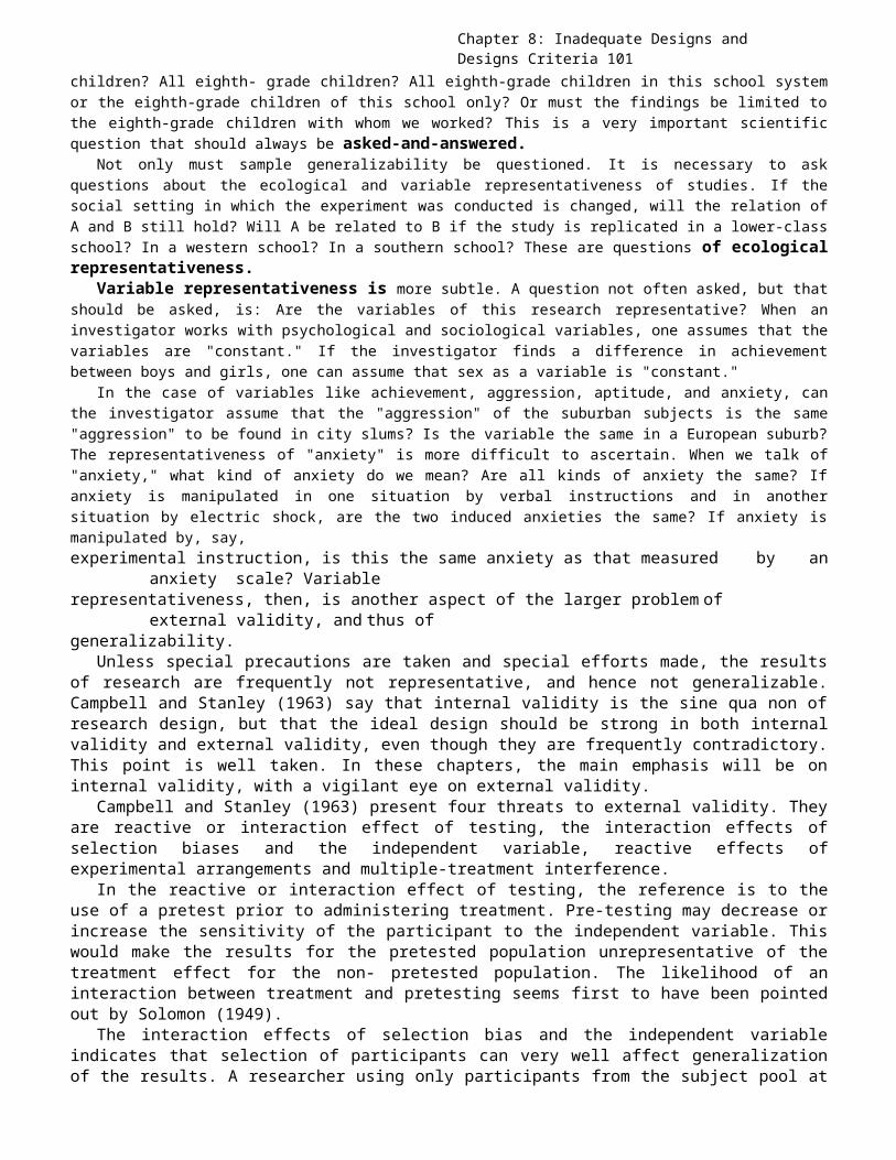
Chapter 8: Inadequate Designs and Designs Criteria 101
children? All eighth- grade children? All eighth-grade children in this school systemor the eighth-grade children of this school only? Or must the findings be limited tothe eighth-grade children with whom we worked? This is a very important scientificquestion that should always be asked-and-answered.
Not only must sample generalizability be questioned. It is necessary to askquestions about the ecological and variable representativeness of studies. If thesocial setting in which the experiment was conducted is changed, will the relation ofA and B still hold? Will A be related to B if the study is replicated in a lower-classschool? In a western school? In a southern school? These are questions of ecologicalrepresentativeness.
Variable representativeness is more subtle. A question not often asked, but thatshould be asked, is: Are the variables of this research representative? When aninvestigator works with psychological and sociological variables, one assumes that thevariables are "constant." If the investigator finds a difference in achievementbetween boys and girls, one can assume that sex as a variable is "constant."
In the case of variables like achievement, aggression, aptitude, and anxiety, canthe investigator assume that the "aggression" of the suburban subjects is the same"aggression" to be found in city slums? Is the variable the same in a European suburb?The representativeness of "anxiety" is more difficult to ascertain. When we talk of"anxiety," what kind of anxiety do we mean? Are all kinds of anxiety the same? Ifanxiety is manipulated in one situation by verbal instructions and in anothersituation by electric shock, are the two induced anxieties the same? If anxiety ismanipulated by, say,experimental instruction, is this the same anxiety as that measured by an
anxiety scale? Variablerepresentativeness, then, is another aspect of the larger problem of
external validity, and thus ofgeneralizability.
Unless special precautions are taken and special efforts made, the resultsof research are frequently not representative, and hence not generalizable.Campbell and Stanley (1963) say that internal validity is the sine qua non ofresearch design, but that the ideal design should be strong in both internalvalidity and external validity, even though they are frequently contradictory.This point is well taken. In these chapters, the main emphasis will be oninternal validity, with a vigilant eye on external validity.
Campbell and Stanley (1963) present four threats to external validity. Theyare reactive or interaction effect of testing, the interaction effects ofselection biases and the independent variable, reactive effects ofexperimental arrangements and multiple-treatment interference.
In the reactive or interaction effect of testing, the reference is to theuse of a pretest prior to administering treatment. Pre-testing may decrease orincrease the sensitivity of the participant to the independent variable. Thiswould make the results for the pretested population unrepresentative of thetreatment effect for the non- pretested population. The likelihood of aninteraction between treatment and pretesting seems first to have been pointedout by Solomon (1949).
The interaction effects of selection bias and the independent variableindicates that selection of participants can very well affect generalizationof the results. A researcher using only participants from the subject pool at
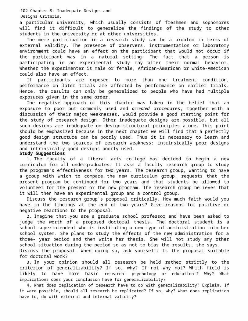
102 Chapter 8: Inadequate Designs andDesigns Criteria.a particular university, which usually consists of freshmen and sophomoreswill find it difficult to generalize the findings of the study to otherstudents in the university or at other universities.
The mere participation in a research study can be a problem in terms ofexternal validity. The presence of observers, instrumentation or laboratoryenvironment could have an effect on the participant that would not occur ifthe participant was in a natural setting. The fact that a person isparticipating in an experimental study may alter their normal behavior.Whether the experimenter is male or female, African-American or white-Americancould also have an effect.
If participants are exposed to more than one treatment condition,performance on later trials are affected by performance on earlier trials.Hence, the results can only be generalized to people who have had multipleexposures given in the same order.
The negative approach of this chapter was taken in the belief that anexposure to poor but commonly used and accepted procedures, together with adiscussion of their major weaknesses, would provide a good starting point forthe study of research design. Other inadequate designs are possible, but allsuch designs are inadequate on design-structural principles alone. This pointshould be emphasized because in the next chapter we will find that a perfectlygood design structure can be poorly used. Thus it is necessary to learn andunderstand the two sources of research weakness: intrinsically poor designsand intrinsically good designs poorly used.Study Suggestions
1. The faculty of a liberal arts college has decided to begin a newcurriculum for all undergraduates. It asks a faculty research group to studythe program's effectiveness for two years. The research group, wanting to havea group with which to compare the new curriculum group, requests that thepresent program be continued for two years and that students be allowed tovolunteer for the present or the new program. The research group believes thatit will then have an experimental group and a control group.
Discuss the research group's proposal critically. How much faith would youhave in the findings at the end of two years? Give reasons for positive ornegative reactions to the proposal.
2. Imagine that you are a graduate school professor and have been asked tojudge the worth of a proposed doctoral thesis. The doctoral student is aschool superintendent who is instituting a new type of administration into herschool system. She plans to study the effects of the new administration for athree- year period and then write her thesis. She will not study any otherschool situation during the period so as not to bias the results, she says.Discuss the proposal. When doing so, ask yourself: Is the proposal suitablefor doctoral work?
3. In your opinion should all research be held rather strictly to thecriterion of generalizability? If so, why? If not why not? Which field islikely to have more basic research: psychology or education'? Why? Whatimplications does your conclusion have for generalizability?
4. What does replication of research have to do with generalizability? Explain. Ifit were possible, should all research be replicated? If so, why? What does replicationhave to, do with external and internal validity?
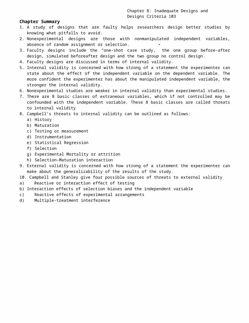
Chapter 8: Inadequate Designs and Designs Criteria 103
Chapter Summary1. A study of designs that are faulty helps researchers design better studies by
knowing what pitfalls to avoid.2. Nonexperimental designs are those with nonmanipulated independent variables,
absence of random assignment or selection.3. Faculty designs include the “one-shot case study,” the one group before-after
design, simulated beforeafter design and the two group no control design.4. Faculty designs are discussed in terms of internal validity.5. Internal validity is concerned with how strong of a statement the experimenter can
state about the effect of the independent variable on the dependent variable. Themore confident the experimenter has about the manipulated independent variable, thestronger the internal validity.
6. Nonexperimental studies are weaker in internal validity than experimental studies.7. There are 8 basic classes of extraneous variables, which if not controlled may be
confounded with the independent variable. These 8 basic classes are called threatsto internal validity
8. Campbell’s threats to internal validity can be outlined as follows:a) Historyb) Maturationc) Testing or measurementd) Instrumentatione) Statistical Regressionf) Selectiong) Experimental Mortality or attritionh) Selection-Maturation interaction
9. External validity is concerned with how strong of a statement the experimenter canmake about the generalizability of the results of the study.
10. Campbell and Stanley give four possible sources of threats to external validitya) Reactive or interaction effect of testingb) Interaction effects of selection biases and the independent variablec) Reactive effects of experimental arrangementsd) Multiple-treatment interference
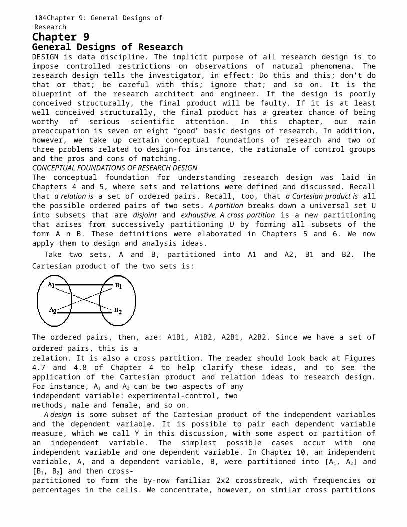
104Chapter 9: General Designs of ResearchChapter 9General Designs of ResearchDESIGN is data discipline. The implicit purpose of all research design is toimpose controlled restrictions on observations of natural phenomena. Theresearch design tells the investigator, in effect: Do this and this; don't dothat or that; be careful with this; ignore that; and so on. It is theblueprint of the research architect and engineer. If the design is poorlyconceived structurally, the final product will be faulty. If it is at leastwell conceived structurally, the final product has a greater chance of beingworthy of serious scientific attention. In this chapter, our mainpreoccupation is seven or eight “good" basic designs of research. In addition,however, we take up certain conceptual foundations of research and two orthree problems related to design-for instance, the rationale of control groupsand the pros and cons of matching.CONCEPTUAL FOUNDATIONS OF RESEARCH DESIGNThe conceptual foundation for understanding research design was laid inChapters 4 and 5, where sets and relations were defined and discussed. Recallthat a relation is a set of ordered pairs. Recall, too, that a Cartesian product is allthe possible ordered pairs of two sets. A partition breaks down a universal set Uinto subsets that are disjoint and exhaustive. A cross partition is a new partitioningthat arises from successively partitioning U by forming all subsets of theform A n B. These definitions were elaborated in Chapters 5 and 6. We nowapply them to design and analysis ideas.
Take two sets, A and B, partitioned into A1 and A2, B1 and B2. TheCartesian product of the two sets is:
The ordered pairs, then, are: A1B1, A1B2, A2B1, A2B2. Since we have a set ofordered pairs, this is arelation. It is also a cross partition. The reader should look back at Figures4.7 and 4.8 of Chapter 4 to help clarify these ideas, and to see theapplication of the Cartesian product and relation ideas to research design.For instance, A1 and A2 can be two aspects of anyindependent variable: experimental-control, twomethods, male and female, and so on.
A design is some subset of the Cartesian product of the independent variablesand the dependent variable. It is possible to pair each dependent variablemeasure, which we call Y in this discussion, with some aspect or partition ofan independent variable. The simplest possible cases occur with oneindependent variable and one dependent variable. In Chapter 10, an independentvariable, A, and a dependent variable, B, were partitioned into [A1, A2] and[B1, B2] and then cross-partitioned to form the by-now familiar 2x2 crossbreak, with frequencies orpercentages in the cells. We concentrate, however, on similar cross partitions
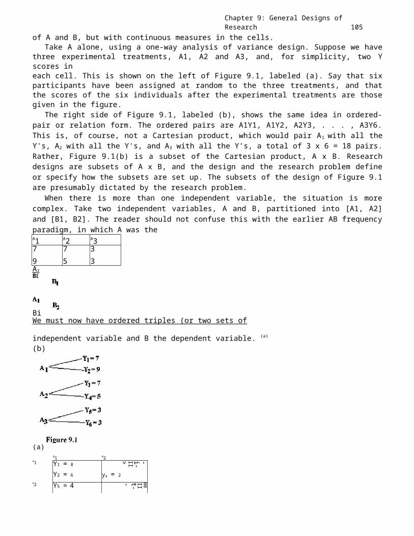
Chapter 9: General Designs of Research 105
of A and B, but with continuous measures in the cells.Take A alone, using a one-way analysis of variance design. Suppose we have
three experimental treatments, A1, A2 and A3, and, for simplicity, two Yscores ineach cell. This is shown on the left of Figure 9.1, labeled (a). Say that sixparticipants have been assigned at random to the three treatments, and thatthe scores of the six individuals after the experimental treatments are thosegiven in the figure.
The right side of Figure 9.1, labeled (b), shows the same idea in ordered-pair or relation form. The ordered pairs are A1Y1, A1Y2, A2Y3, . . . , A3Y6.This is, of course, not a Cartesian product, which would pair A1 with all theY's, A2 with all the Y's, and A3 with all the Y's, a total of 3 x 6 = 18 pairs.Rather, Figure 9.1(b) is a subset of the Cartesian product, A x B. Researchdesigns are subsets of A x B, and the design and the research problem defineor specify how the subsets are set up. The subsets of the design of Figure 9.1are presumably dictated by the research problem.
When there is more than one independent variable, the situation is morecomplex. Take two independent variables, A and B, partitioned into [A1, A2]and [B1, B2]. The reader should not confuse this with the earlier AB frequencyparadigm, in which A was theA1 A2 A37 7 39 5 3A2BI
BiWe must now have ordered triples (or two sets of
independent variable and B the dependent variable. (a)
(b)
(a)B1 B2
A1 Y1 = 8 -i-II>
Y2 = 6 y4 = 2A2 Y5 = 4 00IIt--
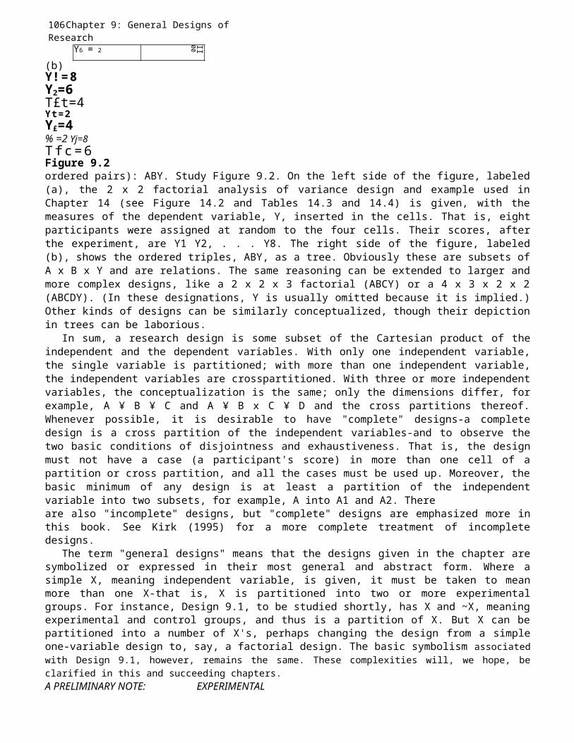
106Chapter 9: General Designs of Research
Y6 = 2 II00
(b)Y!=8Y2=6T£t=4Yt=2Y£=4% =2 Yj=8Tfc=6Figure 9.2ordered pairs): ABY. Study Figure 9.2. On the left side of the figure, labeled(a), the 2 x 2 factorial analysis of variance design and example used inChapter 14 (see Figure 14.2 and Tables 14.3 and 14.4) is given, with themeasures of the dependent variable, Y, inserted in the cells. That is, eightparticipants were assigned at random to the four cells. Their scores, afterthe experiment, are Y1 Y2, . . . Y8. The right side of the figure, labeled(b), shows the ordered triples, ABY, as a tree. Obviously these are subsets ofA x B x Y and are relations. The same reasoning can be extended to larger andmore complex designs, like a 2 x 2 x 3 factorial (ABCY) or a 4 x 3 x 2 x 2(ABCDY). (In these designations, Y is usually omitted because it is implied.)Other kinds of designs can be similarly conceptualized, though their depictionin trees can be laborious.
In sum, a research design is some subset of the Cartesian product of theindependent and the dependent variables. With only one independent variable,the single variable is partitioned; with more than one independent variable,the independent variables are crosspartitioned. With three or more independentvariables, the conceptualization is the same; only the dimensions differ, forexample, A ¥ B ¥ C and A ¥ B x C ¥ D and the cross partitions thereof.Whenever possible, it is desirable to have "complete" designs-a completedesign is a cross partition of the independent variables-and to observe thetwo basic conditions of disjointness and exhaustiveness. That is, the designmust not have a case (a participant's score) in more than one cell of apartition or cross partition, and all the cases must be used up. Moreover, thebasic minimum of any design is at least a partition of the independentvariable into two subsets, for example, A into A1 and A2. Thereare also "incomplete" designs, but "complete" designs are emphasized more inthis book. See Kirk (1995) for a more complete treatment of incompletedesigns.
The term "general designs" means that the designs given in the chapter aresymbolized or expressed in their most general and abstract form. Where asimple X, meaning independent variable, is given, it must be taken to meanmore than one X-that is, X is partitioned into two or more experimentalgroups. For instance, Design 9.1, to be studied shortly, has X and ~X, meaningexperimental and control groups, and thus is a partition of X. But X can bepartitioned into a number of X's, perhaps changing the design from a simpleone-variable design to, say, a factorial design. The basic symbolism associatedwith Design 9.1, however, remains the same. These complexities will, we hope, beclarified in this and succeeding chapters.A PRELIMINARY NOTE: EXPERIMENTAL
Chapter 9: General Designs of Research 107
DESIGNS AND ANALYSIS OF VARIANCEBefore taking up the designs of this chapter, we need to clarify one or two confusingand potentially controversial points not usually considered in the literature. Most ofthe designs we consider are experimental. As usually conceived, the rationale ofresearch design is based on experimental ideas and conditions. They are alsointimately linked to analysis of variance paradigms. This is of course no accident.Modern conceptions of design, especially factorial designs, were born when analysis ofvariance was invented. Although there is no hard law that says that analysis ofvariance is applicable only in experimental situations-indeed, it has been used manytimes in nonexperimental research-it is in general true that it ismost appropriate for the data of experiments. This is especially so for factorialdesigns where there are equal numbers of cases in the design paradigm cells, and wherethe participants are assigned to the experimental conditions (or cells) at random.
When it is not possible to assign participants at random, and when, for one reasonor another, there are unequal numbers of cases in the cells of a factorial design, theuse of analysis of variance is questionable, even inappropriate. It can also be clumsyand inelegant. This is because the use of analysis of variance assumes that thecorrelations between or among the independent variables of a factorial design arezero. Random assignment makes this assumption tenable since such assignment presumablyapportions sources of variance equally among the cells. But random assignment can onlybe accomplished in experiments. In nonexperimental research, the independent variablesare more or less fixed characteristics of the participants, e.g., intelligence, sex,social class, and the like. They are usually systematically correlated. Take twoindependent manipulated variables, say reinforcement and anxiety. Because participantswith varying amounts of characteristics correlated with these variables are randomlydistributed in the cells, the correlations between aspects of reinforcement andanxiety are assumed to be zero. If, on the other hand, the two independent variablesare intelligence and social class, both ordinarily nonmanipulable and correlated, theassumption of zero correlation between them necessary for analysis of variance cannotbe made. Some method of analysis that takes account of the correlation between themshould be used. We will see later in the book that such a method is readily available:multiple regression.
We have not yet reached a state of research maturity to appreciate the profounddifference between the two situations. For now, however, let us accept the differenceand the statement that analysis of variance is basically an experimental conceptionand form of analysis. Strictly speaking, if our independent variables arenonexperimental, then analysis of variance is not the appropriate mode of analysis.There are exceptions to this statement. For instance, if one independent variable isexperimental and one nonexperimental, analysis of variance is appropriate. In one-wayanalysis of variance, moreover, since there is only one independent variable, analysisof variance can be used with a nonexperimental independent variable, though regressionanalysis would probably be more appropriate. In Study Suggestion 5 at the end of thechapter, an interesting use of analysis of variance with nonexperimental data iscited.
Similarly, if for some reason the numbers of cases in the cells are unequal (anddisproportionate), then there will be correlation between the independent variables,and the assumption of zero correlation is not tenable. This rather abstract andabstruse digression from our main design theme may seem a bit confusing at this stageof our study. The problems involved should become clear after we have studied
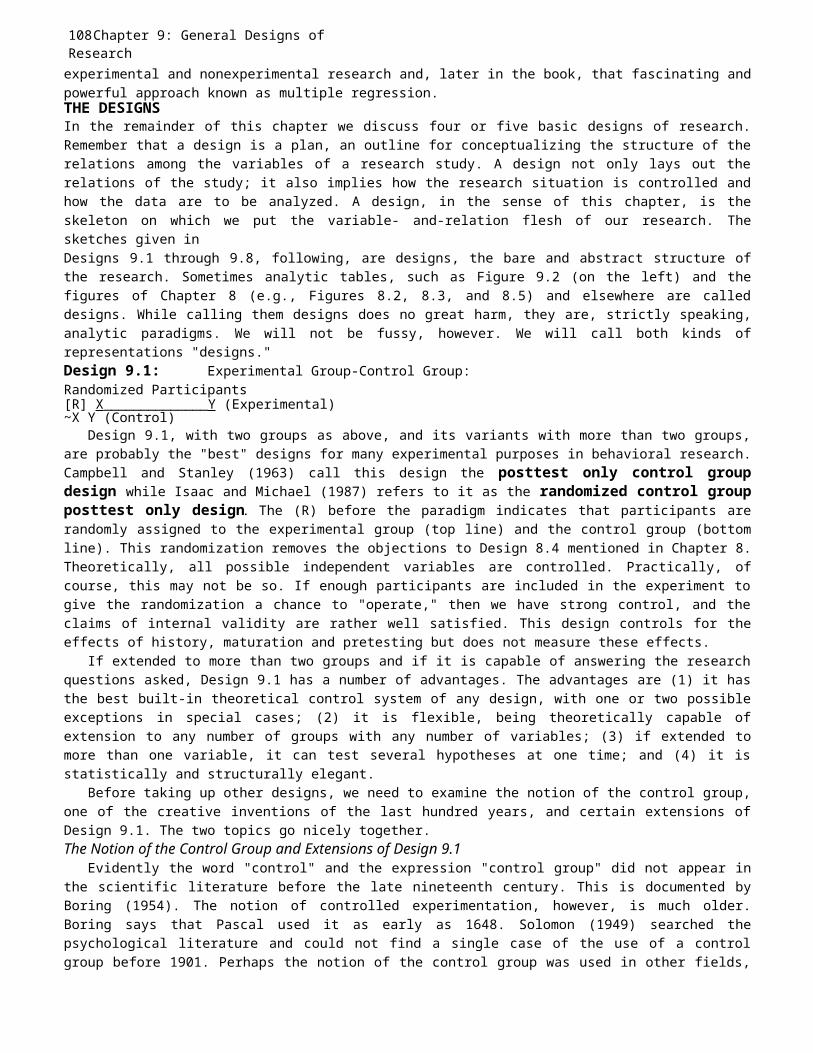
108Chapter 9: General Designs of Researchexperimental and nonexperimental research and, later in the book, that fascinating andpowerful approach known as multiple regression.THE DESIGNSIn the remainder of this chapter we discuss four or five basic designs of research.Remember that a design is a plan, an outline for conceptualizing the structure of therelations among the variables of a research study. A design not only lays out therelations of the study; it also implies how the research situation is controlled andhow the data are to be analyzed. A design, in the sense of this chapter, is theskeleton on which we put the variable- and-relation flesh of our research. Thesketches given inDesigns 9.1 through 9.8, following, are designs, the bare and abstract structure ofthe research. Sometimes analytic tables, such as Figure 9.2 (on the left) and thefigures of Chapter 8 (e.g., Figures 8.2, 8.3, and 8.5) and elsewhere are calleddesigns. While calling them designs does no great harm, they are, strictly speaking,analytic paradigms. We will not be fussy, however. We will call both kinds ofrepresentations "designs."Design 9.1: Experimental Group-Control Group:Randomized Participants[R] X______________Y (Experimental)~X Y (Control)
Design 9.1, with two groups as above, and its variants with more than two groups,are probably the "best" designs for many experimental purposes in behavioral research.Campbell and Stanley (1963) call this design the posttest only control groupdesign while Isaac and Michael (1987) refers to it as the randomized control groupposttest only design. The (R) before the paradigm indicates that participants arerandomly assigned to the experimental group (top line) and the control group (bottomline). This randomization removes the objections to Design 8.4 mentioned in Chapter 8.Theoretically, all possible independent variables are controlled. Practically, ofcourse, this may not be so. If enough participants are included in the experiment togive the randomization a chance to "operate," then we have strong control, and theclaims of internal validity are rather well satisfied. This design controls for theeffects of history, maturation and pretesting but does not measure these effects.
If extended to more than two groups and if it is capable of answering the researchquestions asked, Design 9.1 has a number of advantages. The advantages are (1) it hasthe best built-in theoretical control system of any design, with one or two possibleexceptions in special cases; (2) it is flexible, being theoretically capable ofextension to any number of groups with any number of variables; (3) if extended tomore than one variable, it can test several hypotheses at one time; and (4) it isstatistically and structurally elegant.
Before taking up other designs, we need to examine the notion of the control group,one of the creative inventions of the last hundred years, and certain extensions ofDesign 9.1. The two topics go nicely together.The Notion of the Control Group and Extensions of Design 9.1
Evidently the word "control" and the expression "control group" did not appear inthe scientific literature before the late nineteenth century. This is documented byBoring (1954). The notion of controlled experimentation, however, is much older.Boring says that Pascal used it as early as 1648. Solomon (1949) searched thepsychological literature and could not find a single case of the use of a controlgroup before 1901. Perhaps the notion of the control group was used in other fields,

Chapter 9: General Designs of Research 109
though it is doubtful that the idea was well developed. Solomon (p.175) also says thatthe Peterson and Thurstone study of attitudes in 1933 was the first serious attempt touse control groups in the evaluation of the effects of educational procedures. Onecannot find the expression "control group" in the famous eleventh edition (1911) ofthe Encyclopedia Britannica, even though experimental method is discussed. Solomonalso says that control-group design apparently had to await statistical developmentsand the development of statistical sophistication among psychologists.
Perhaps the first use of control groups in psychology and education occurred in1901 with the publication of Thorndike and Woodworth (1901). One of the two men whodid this research, E. L. Thorndike, extended the basic and revolutionary ideas of thisfirst research series to education (Thorndike, 1924). Thorndike's controls, in thisgigantic study of 8564 pupils in many schools in a number of cities, were independenteducational groups. Among other comparisons, he contrasted the gains in intelligencetest scores presumably engendered by the study of English, history, geometry, andLatin with the gains presumably engendered by the study of English, history, geometry,and shopwork. He tried, in effect, to compare the influence of Latin and shopwork. Healso made other comparisons of a similar nature. Despite the weaknesses of design andcontrol, Thorndike's experiments and those he stimulated others to perform wereremarkable for their insight. Thorndike even berated colleagues for not admittingstudents of stenography and typing who had not studied Latin, because he claimed tohave shown that the influence of various participants onX1X 1a 11 121b Y Measures intelligence was similar. It is interesting that he thought huge numbers ofparticipants were necessary-he called for 18,000 more cases. He was also quiteaware, in 1924, of the need for random samples.
The notion of the control group needs generalization. Assume that in aneducational experiment we have four experimental groups as follows. A, isreinforcement of every response, As reinforcement at regular time intervals,
11X2 X2a122b Figure 9.3The structure of Design 9.2 is the same as that of Design 9.1. The only
difference is that participants are matched on one or more attributes. For thedesign to take its place as an "adequate" design, however, randomization must enter the picture, as noted by the small r attached to the M (for "matched"). It is not enough that matched participants are used. The members of each pair must be assigned to the two groups at random. Ideally, too, whether a group isto be an experimental or a control group is also decided at random. In either case, each decision can be made by flipping a coin or by using a table of random numbers, letting odd numbers mean one group and even numbers the other group. If there are more than two groups, naturally, a random number system must be used.Design 9.2 : Experimental Group-Control Group: Matched Participants[Mr] X Y (Experimental)~X Y (Control)
As in Design 9.1, it is possible, though often not easy, to use more than two groups. (The difficulty of matching more than two groups was discussed earlier.)
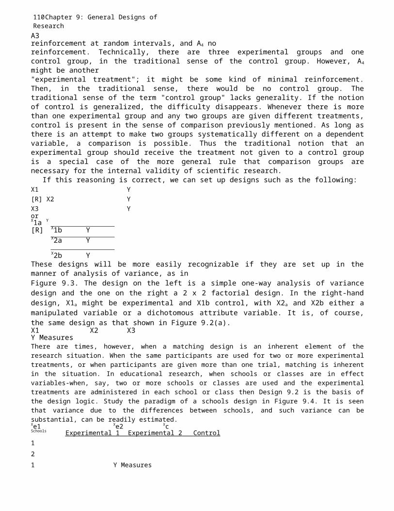
110Chapter 9: General Designs of ResearchA3reinforcement at random intervals, and A4 noreinforcement. Technically, there are three experimental groups and onecontrol group, in the traditional sense of the control group. However, A4might be another"experimental treatment"; it might be some kind of minimal reinforcement.Then, in the traditional sense, there would be no control group. Thetraditional sense of the term "control group" lacks generality. If the notionof control is generalized, the difficulty disappears. Whenever there is morethan one experimental group and any two groups are given different treatments,control is present in the sense of comparison previously mentioned. As long asthere is an attempt to make two groups systematically different on a dependentvariable, a comparison is possible. Thus the traditional notion that anexperimental group should receive the treatment not given to a control groupis a special case of the more general rule that comparison groups arenecessary for the internal validity of scientific research.
If this reasoning is correct, we can set up designs such as the following:X1 Y[R] X2 YX3 YorX1a Y
[R] X1b YX2a YX2b Y
These designs will be more easily recognizable if they are set up in themanner of analysis of variance, as inFigure 9.3. The design on the left is a simple one-way analysis of variancedesign and the one on the right a 2 x 2 factorial design. In the right-handdesign, X1a might be experimental and X1b control, with X2a and X2b either amanipulated variable or a dichotomous attribute variable. It is, of course,the same design as that shown in Figure 9.2(a).X1 X2 X3Y MeasuresThere are times, however, when a matching design is an inherent element of theresearch situation. When the same participants are used for two or more experimentaltreatments, or when participants are given more than one trial, matching is inherentin the situation. In educational research, when schools or classes are in effectvariables-when, say, two or more schools or classes are used and the experimentaltreatments are administered in each school or class then Design 9.2 is the basis ofthe design logic. Study the paradigm of a schools design in Figure 9.4. It is seenthat variance due to the differences between schools, and such variance can besubstantial, can be readily estimated.Xe1 Xe2 XcSchools Experimental 1 Experimental 2 Control 121 Y Measures
Chapter 9: General Designs of Research 111
45Figure 9.4Matching versus RandomizationAlthough randomization, which includes randomselection and random assignment, is the preferred method for controlling extraneousvariance, there is merit to the use of matching. In a number of situations outsideacademic circles, the behavioral scientist will not be able to use randomization inachieving constancy between groups prior to the administration of treatment. Usuallyin a university a participant pool is available to draw from. Researchers in thissituation can afford to use randomization procedures. In business-marketing research,however, this may not be the case. Popular among market researchers is the controlled-store test. The controlled store test is an experiment that is done in the field. Thesecond author has conducted such studies for a number of market research firms and agrocery chain in southern California. One of the goals of the controlled store test isto be very discreet. If a manufacturer of soap products wants to determine the effectsof a cents-off coupon on consumer purchasing behavior, that manufacturer does not wantthe competing manufacturer of the same product to know about it. Why? Well if acompetitor knew that a research study was going on in a store, they could go in andbuy up their own products and hence contaminate the study.
To return to our discussion of randomization versus matching often times a grocerychain or a chain of department stores has a finite number of stores to use in a study.Location and clientele have a lot of influence on sales. Sales are usually thedependent variable in such studies. With a limited number of stores to choose from inorder to perform the research, random assignment often does not work in equatinggroups of stores. One store in the chain might do 3 to 4 times the volume of businessas another. If it is chosen at random, the group in falls into will create a greatdeal of unbalance especially if the other group does not have one to balance it. Inshort, the groups will no longer be equal. Hence, the solution here is to match thestores on an individual basis. One half of the matched pair is randomly assigned toone experimental condition and the other half gets the other condition. With more than2 conditions, more stores would have to be matched and then assigned to treatmentconditions.
In some human factors engineering studies using simulators, the use ofrandomization is sometimes not economically or practically feasible. Consider thetesting of two test configurations for a simulator. Researcher may want to know whichone leads to fewer perceptual errors. Processes of randomization would say that theexperimenter should randomly assigned participants to conditions as they enter thestudy. However, when it requires 3 to 6 months to change the configuration of thesimulator from one to the other, it is no longer feasible to do it the “usual” way.
However, an important point to remember is that randomization when it can be donecorrectly and appropriately is better than matching. It is perhaps the only method forcontrolling unknown sources of variances. One of the major shortcomings of matching isthat one can never be sure that an exact match has been made. Without that exactness,the inexactness can be an alternative explanation on why the dependent variable isdifferent between the treatment conditions after treatment.Some ways of matching groups.Matching by Equating ParticipantsThe most common method of matching is to equate participants on one or more

112Chapter 9: General Designs of Researchvariables to be controlled. Christensen (1996) refers to this method as theprecision control method and Matheson, Bruce and Beauchamp (1978) calls it thematched-by-correlated criterion design. To control for the influence of intelligence onthe dependent variable, for example, the researcher must make sure that theparticipants in each of the treatment groups are of the same intelligencelevel. The goal here is to create equivalent groups of participants. Using ourexample of intelligence, if we had only two treatment conditions, we wouldselect pairs of participants with identical or near identical intelligencetest scores. Half of each pair would be assigned at random to one treatmentcondition and the other half is assigned to the other treatment condition. Ina controlled stored test, where location is an important variable to becontrolled for, we would find two stores of similar locale and call them amatch. After we have built up, lets say 10 of such pairs, we can then take onehalf of each pair and assign them to one test environment and the other halfto the other. If we had required matching for three conditions, we would thenhave to find three people with the same intelligence score or three stores inthe same locale.
The major advantage in using this method is that it is able to detect smalldifferences (increase in sensitivity) by ensuring that the participants in thevarious groups are equal on at least the paired variables. However animportant requirement is that the variables on which participants are matchedmust be correlated significantly with the dependent variable. We had shown inan earlier chapter that matching is most useful when the variables on whichparticipants are matched correlate greater than 0.5 or 0.6 with the dependentvariable.
This method of matching has two major flaws or disadvantages. First, it isdifficult to know which are the most important variables to match. In mostinstances, there are many potentially relevant variables. In a study theresearcher might match on age, sex, race, marital status and intelligence.However, the researcher could have selected many other variables. Theresearcher should select those variables that show the lowest correlation witheach other but the highest correlation with the dependent variable.
A second problem is the decrease in finding eligible matched participantsas the number of variables used for matching increases. To choose 3 or 4variables to match on and then find enough participants that meets thematching criteria requires a lot of participants to choose from. Theresearcher would need a large pool of available participants in order toobtain a just a few that are matched on all of the relevant variables.Matching affects the generalizability of the study. The researcher can onlygeneralize the results to other individuals having the same characteristics.The Frequency Distribution Matching MethodThe individual-by-individual technique of matching presented above is a verygood for developing equal groups, but many participants must be eliminatedbecause they cannot be matched. Frequency distribution method attempts toovercome this disadvantage while retaining some of the advantages of matching.This technique, as the name implies, matches groups of participants in termsof overall distribution of the selected variable or variables rather than onan individual-by-individual basis. Let us say that we want to have two or moregroups matched on intelligence. Let’s further say we want to use the frequency

Chapter 9: General Designs of Research 113
distribution method of matching. First we would need an intelligence testscore on each child. We then need to create the two or more groups in such away that the groups of participants would have to have the same averageintelligence test score, as well as the same standard deviation and skewnessof the scores. Here, each group would be statistically equal. The mean,standard deviation and skewness between each group would be statisticallyequivalent. A statistical test of hypotheses could be utilized, but theresearcher needs to be aware that both types of errors should be considered.If more than one variable was considered to be relevant on which to matchparticipants, each group of participants would be required to have the samestatistical measures on all of these variables. The number of participantslost using this technique would not be as great as the number lost using theindividual- by-individual method, because each additional participant wouldmerely have to contribute to producing the appropriate statistical measuresrather than be identical to another participant on the relevant variables.Hence, this technique is more flexible in terms of being able to use aparticular participant.The major disadvantage of matching by the frequency distribution method occursonly when there ismatching on more than one variable. Here the combinations of variables may bemismatched in the various groups. If age and reaction time were to be matched, onegroup might include older participants with slower reaction times and youngerparticipants with quicker reaction times, where the other group has the oppositecombination. The mean and distribution of the two variables would be equivalent butthe participants in each group would be completely different. This difference mayaffect the dependent variable.Matching by Holding Variables Constant
Holding the adventitious variable constant for all experimental groups is anothertechnique that can be used to create equal groups of participants. All participants ineach experimental group will have the same degree or type of extraneous variable. Ifwe need to control the variation caused by gender differences, we can hold sexconstant by using only males or only females in the study. This has the effect ofmatching all participants in terms of the sex variable. This matching procedurecreates a more homogeneous participant sample, because only participants with acertain type or amount of the fortuitous variable are used. A number of studentresearch projects at universities use this method especially when the participant poolhas a majority of male or female participants. This technique of holding variablesconstant has at least two problems that could affect the validity of the study. Theseverity of the problem increases if too many variables are held constant. The firstdisadvantage is that the technique restricts the size of the participant population.Consequently, in some cases, it may be difficult to find enough participants toparticipate in the study. The early split-brain research of Roger Sperry has oftenbeen criticized by the restriction of the participants used in the study. His earlystudies used only epileptic patients. So a study using this method could be criticizedof a selection bias.
The second drawback is more critical in that the results of the study onlygeneralizable to the type of participant used in the study. The results obtained fromthe epileptic patients study could only be generalized to other epileptic patients. Ifsomeone wanted to know whether non-epileptic patients would experience the same
114Chapter 9: General Designs of Researchperceptual changes the researcher would have to conduct a similar study using non-epileptic patients.Conclusions from such a study might indeed be the same as those obtained from theepileptic patient study but separate studies have to be conducted. The only way we canfind out if the results of one study can be generalized to the population is toreplicate the study using the participants with different characteristics.Matching by incorporating the Nuisance Variable into the Research Design
Another way of trying to develop equal groups is to use the nuisance or extraneousvariable as an independent variable in the research design. Assume that we wereconducting a learning experiment on rats and wanted to control for the effects ofweight. The thought here is that the animal with the greater weight will need toconsume more food after a period of deprivation and hence is more motivated. If we hadused the method of holding weight constant, we would have a lot fewer participants. Byusing weight as an independent variable, we can use a lot more participants in thestudy. In statistical terms, the increase in the number of participants means anincrease in power and sensitivity. By using an extraneous variable as an independentvariable in the design we can isolate a source of systematic variance and alsodetermine if the extraneous variable has an effect on the dependent variable.
However, building an extraneous variable into the design should not be doneindiscriminately. Making the extraneous variable a part of the research design seemslike an excellent control method. However, this method is best used when there is aninterest in the differences produced by the extraneous variable or in the interactionbetween the extraneous variable and other independent variables. For a variablemeasured on a continuous scale, a researcher can still incorporate it into the design.The difference between a discrete and continuous extraneous variable would lie in thedata analysis part of the research process. With a continuous variable regression oranalysis of covariance would be preferable over analysis of variance.Participant as Own ControlSince each individual is quite unique it is very difficult if not impossible to findanother individual that would be a perfect match. However, a single person is aperfect match to oneself. One of the more powerful techniques for achieving equalityor constancy of experimental groups prior to the administration of treatment is to usethat person in every condition of the experiment. Some refers to this as using theparticipants as their own control. Other than the reactivity of the experiment itself,the possibility of extraneous variation due to individual-to-individual differences isdrastically minimized. This method of achieving constancy is common in some areas ofthe behavioral sciences. In psychology, the study of the interface of humans andmachines (human factors or human engineering) utilizes this method. Dr. Charles W.Simon (1976) has presented a number of interesting experimental designs, which usesthe participant over many treatment conditions. However, this method does not fit allapplications. Some studies involved with learning are not suitable because a personcannot unlearn a problem so that he or she can now apply a different method. The useof this method also requires a lot more planning than others.Additional Design Extensions: Design 9.3 using a PretestDesign 9.3 has many advantages and is frequently used. Its structure is similar tothat of Design 8.2, with two important differences: Design 8.2 lacks a control groupand randomization. Design 9.3 is similar to Designs 9.1 and 9.2, except that the"before" or pretest feature has been added. It is used frequently to study change.Like Designs 9.1 and 9.2, it can be expanded to more than two groups.
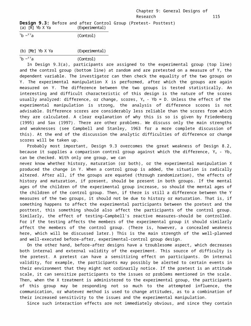
Chapter 9: General Designs of Research 115
Design 9.3: Before and after Control Group (Pretest- Posttest)(a) [R] Yb X Ya (Experimental)Yb ~X Ya (Control)
(b) [Mr] Yb X Ya (Experimental)Yb ~X Ya (Control)
In Design 9.3(a), participants are assigned to the experimental group (top line)and the control group (bottom line) at random and are pretested on a measure of Y, thedependent variable. The investigator can then check the equality of the two groups onY. The experimental manipulation X is performed, after which the groups are againmeasured on Y. The difference between the two groups is tested statistically. Aninteresting and difficult characteristic of this design is the nature of the scoresusually analyzed: difference, or change, scores, Ya - Yb = D. Unless the effect of theexperimental manipulation is strong, the analysis of difference scores is notadvisable. Difference scores are considerably less reliable than the scores from whichthey are calculated. A clear explanation of why this is so is given by Friedenberg(1995) and Sax (1997). There are other problems. We discuss only the main strengthsand weaknesses (see Campbell and Stanley, 1963 for a more complete discussion ofthis). At the end of the discussion the analytic difficulties of difference or changescores will be taken up.
Probably most important, Design 9.3 overcomes the great weakness of Design 8.2,because it supplies a comparison control group against which the difference, Ya - Yb,can be checked. With only one group, we cannever know whether history, maturation (or both), or the experimental manipulation Xproduced the change in Y. When a control group is added, the situation is radicallyaltered. After all, if the groups are equated (through randomization), the effects ofhistory and maturation, if present, should be present in both groups. If the mentalages of the children of the experimental group increase, so should the mental ages ofthe children of the control group. Then, if there is still a difference between the Ymeasures of the two groups, it should not be due to history or maturation. That is, ifsomething happens to affect the experimental participants between the pretest and theposttest, this something should also affect the participants of the control group.Similarly, the effect of testing-Campbell's reactive measures-should be controlled.For if the testing affects the members of the experimental group it should similarlyaffect the members of the control group. (There is, however, a concealed weaknesshere, which will be discussed later.) This is the main strength of the well-plannedand well-executed before-after, experimental-control group design.
On the other hand, before-after designs have a troublesome aspect, which decreasesboth internal and external validity of the experiment. This source of difficulty isthe pretest. A pretest can have a sensitizing effect on participants. On internalvalidity, for example, the participants may possibly be alerted to certain events intheir environment that they might not ordinarily notice. If the pretest is an attitudescale, it can sensitize participants to the issues or problems mentioned in the scale.Then, when the X treatment is administered to the experimental group, the participantsof this group may be responding not so much to the attempted influence, thecommunication, or whatever method is used to change attitudes, as to a combination oftheir increased sensitivity to the issues and the experimental manipulation.
Since such interaction effects are not immediately obvious, and since they contain
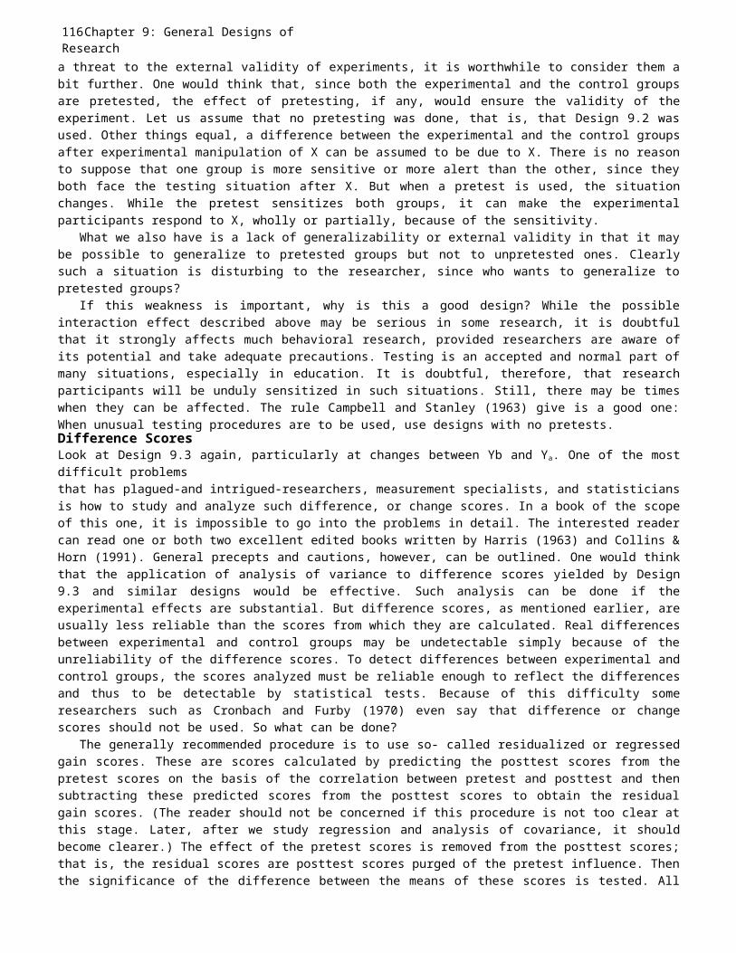
116Chapter 9: General Designs of Researcha threat to the external validity of experiments, it is worthwhile to consider them abit further. One would think that, since both the experimental and the control groupsare pretested, the effect of pretesting, if any, would ensure the validity of theexperiment. Let us assume that no pretesting was done, that is, that Design 9.2 wasused. Other things equal, a difference between the experimental and the control groupsafter experimental manipulation of X can be assumed to be due to X. There is no reasonto suppose that one group is more sensitive or more alert than the other, since theyboth face the testing situation after X. But when a pretest is used, the situationchanges. While the pretest sensitizes both groups, it can make the experimentalparticipants respond to X, wholly or partially, because of the sensitivity.
What we also have is a lack of generalizability or external validity in that it maybe possible to generalize to pretested groups but not to unpretested ones. Clearlysuch a situation is disturbing to the researcher, since who wants to generalize topretested groups?
If this weakness is important, why is this a good design? While the possibleinteraction effect described above may be serious in some research, it is doubtfulthat it strongly affects much behavioral research, provided researchers are aware ofits potential and take adequate precautions. Testing is an accepted and normal part ofmany situations, especially in education. It is doubtful, therefore, that researchparticipants will be unduly sensitized in such situations. Still, there may be timeswhen they can be affected. The rule Campbell and Stanley (1963) give is a good one:When unusual testing procedures are to be used, use designs with no pretests.Difference ScoresLook at Design 9.3 again, particularly at changes between Yb and Ya. One of the mostdifficult problemsthat has plagued-and intrigued-researchers, measurement specialists, and statisticiansis how to study and analyze such difference, or change scores. In a book of the scopeof this one, it is impossible to go into the problems in detail. The interested readercan read one or both two excellent edited books written by Harris (1963) and Collins &Horn (1991). General precepts and cautions, however, can be outlined. One would thinkthat the application of analysis of variance to difference scores yielded by Design9.3 and similar designs would be effective. Such analysis can be done if theexperimental effects are substantial. But difference scores, as mentioned earlier, areusually less reliable than the scores from which they are calculated. Real differencesbetween experimental and control groups may be undetectable simply because of theunreliability of the difference scores. To detect differences between experimental andcontrol groups, the scores analyzed must be reliable enough to reflect the differencesand thus to be detectable by statistical tests. Because of this difficulty someresearchers such as Cronbach and Furby (1970) even say that difference or changescores should not be used. So what can be done?
The generally recommended procedure is to use so- called residualized or regressedgain scores. These are scores calculated by predicting the posttest scores from thepretest scores on the basis of the correlation between pretest and posttest and thensubtracting these predicted scores from the posttest scores to obtain the residualgain scores. (The reader should not be concerned if this procedure is not too clear atthis stage. Later, after we study regression and analysis of covariance, it shouldbecome clearer.) The effect of the pretest scores is removed from the posttest scores;that is, the residual scores are posttest scores purged of the pretest influence. Thenthe significance of the difference between the means of these scores is tested. All
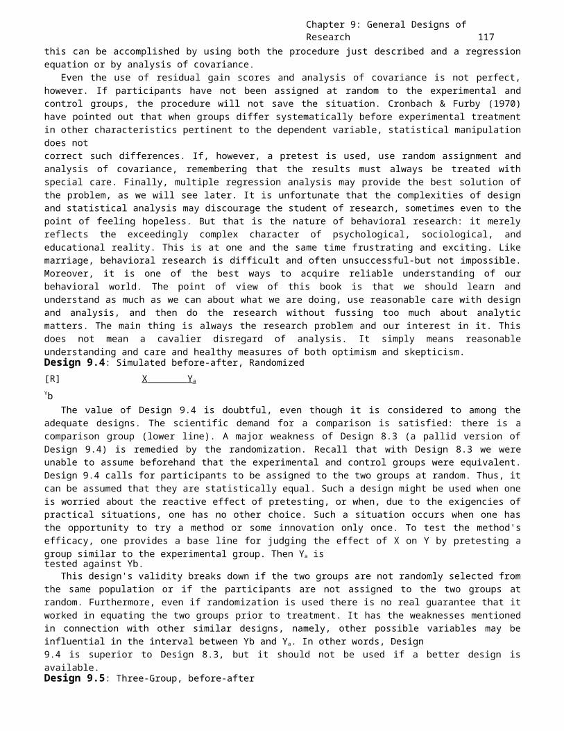
Chapter 9: General Designs of Research 117
this can be accomplished by using both the procedure just described and a regressionequation or by analysis of covariance.
Even the use of residual gain scores and analysis of covariance is not perfect,however. If participants have not been assigned at random to the experimental andcontrol groups, the procedure will not save the situation. Cronbach & Furby (1970)have pointed out that when groups differ systematically before experimental treatmentin other characteristics pertinent to the dependent variable, statistical manipulationdoes notcorrect such differences. If, however, a pretest is used, use random assignment andanalysis of covariance, remembering that the results must always be treated withspecial care. Finally, multiple regression analysis may provide the best solution ofthe problem, as we will see later. It is unfortunate that the complexities of designand statistical analysis may discourage the student of research, sometimes even to thepoint of feeling hopeless. But that is the nature of behavioral research: it merelyreflects the exceedingly complex character of psychological, sociological, andeducational reality. This is at one and the same time frustrating and exciting. Likemarriage, behavioral research is difficult and often unsuccessful-but not impossible.Moreover, it is one of the best ways to acquire reliable understanding of ourbehavioral world. The point of view of this book is that we should learn andunderstand as much as we can about what we are doing, use reasonable care with designand analysis, and then do the research without fussing too much about analyticmatters. The main thing is always the research problem and our interest in it. Thisdoes not mean a cavalier disregard of analysis. It simply means reasonableunderstanding and care and healthy measures of both optimism and skepticism.Design 9.4: Simulated before-after, Randomized[R] X Y a
YbThe value of Design 9.4 is doubtful, even though it is considered to among the
adequate designs. The scientific demand for a comparison is satisfied: there is acomparison group (lower line). A major weakness of Design 8.3 (a pallid version ofDesign 9.4) is remedied by the randomization. Recall that with Design 8.3 we wereunable to assume beforehand that the experimental and control groups were equivalent.Design 9.4 calls for participants to be assigned to the two groups at random. Thus, itcan be assumed that they are statistically equal. Such a design might be used when oneis worried about the reactive effect of pretesting, or when, due to the exigencies ofpractical situations, one has no other choice. Such a situation occurs when one hasthe opportunity to try a method or some innovation only once. To test the method'sefficacy, one provides a base line for judging the effect of X on Y by pretesting agroup similar to the experimental group. Then Ya istested against Yb.
This design's validity breaks down if the two groups are not randomly selected fromthe same population or if the participants are not assigned to the two groups atrandom. Furthermore, even if randomization is used there is no real guarantee that itworked in equating the two groups prior to treatment. It has the weaknesses mentionedin connection with other similar designs, namely, other possible variables may beinfluential in the interval between Yb and Ya. In other words, Design9.4 is superior to Design 8.3, but it should not be used if a better design isavailable.Design 9.5: Three-Group, before-after
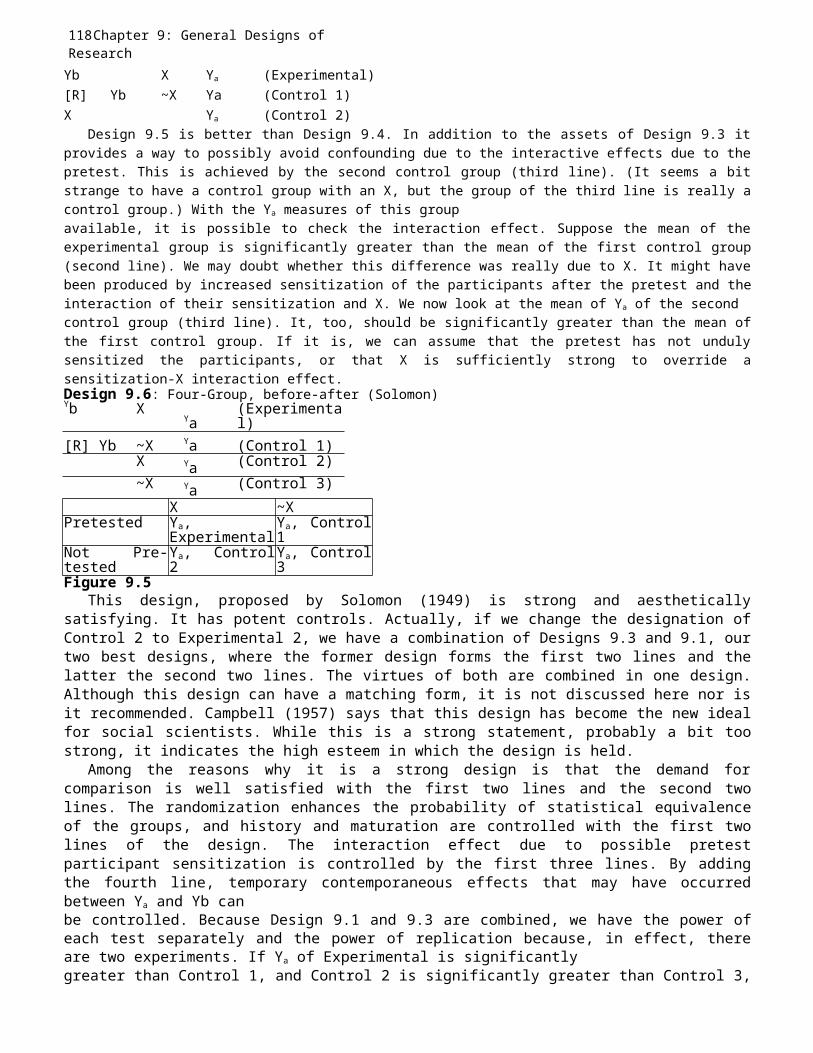
118Chapter 9: General Designs of ResearchYb X Ya (Experimental)[R] Yb ~X Ya (Control 1)X Ya (Control 2)
Design 9.5 is better than Design 9.4. In addition to the assets of Design 9.3 itprovides a way to possibly avoid confounding due to the interactive effects due to thepretest. This is achieved by the second control group (third line). (It seems a bitstrange to have a control group with an X, but the group of the third line is really acontrol group.) With the Ya measures of this groupavailable, it is possible to check the interaction effect. Suppose the mean of theexperimental group is significantly greater than the mean of the first control group(second line). We may doubt whether this difference was really due to X. It might havebeen produced by increased sensitization of the participants after the pretest and theinteraction of their sensitization and X. We now look at the mean of Ya of the secondcontrol group (third line). It, too, should be significantly greater than the mean ofthe first control group. If it is, we can assume that the pretest has not undulysensitized the participants, or that X is sufficiently strong to override asensitization-X interaction effect.Design 9.6: Four-Group, before-after (Solomon)Yb X
Ya(Experimental)
[R] Yb ~X Ya (Control 1)X Ya (Control 2)~X Ya (Control 3)
X ~XPretested Ya,
ExperimentalYa, Control1
Not Pre-tested
Ya, Control2
Ya, Control3
Figure 9.5This design, proposed by Solomon (1949) is strong and aesthetically
satisfying. It has potent controls. Actually, if we change the designation ofControl 2 to Experimental 2, we have a combination of Designs 9.3 and 9.1, ourtwo best designs, where the former design forms the first two lines and thelatter the second two lines. The virtues of both are combined in one design.Although this design can have a matching form, it is not discussed here nor isit recommended. Campbell (1957) says that this design has become the new idealfor social scientists. While this is a strong statement, probably a bit toostrong, it indicates the high esteem in which the design is held.
Among the reasons why it is a strong design is that the demand forcomparison is well satisfied with the first two lines and the second twolines. The randomization enhances the probability of statistical equivalenceof the groups, and history and maturation are controlled with the first twolines of the design. The interaction effect due to possible pretestparticipant sensitization is controlled by the first three lines. By addingthe fourth line, temporary contemporaneous effects that may have occurredbetween Ya and Yb canbe controlled. Because Design 9.1 and 9.3 are combined, we have the power ofeach test separately and the power of replication because, in effect, thereare two experiments. If Ya of Experimental is significantlygreater than Control 1, and Control 2 is significantly greater than Control 3,
Chapter 9: General Designs of Research 119
together with a consistency of results between the two experiments, this isstrong evidence, indeed, of the validity of our research hypothesis.
What is wrong with this paragon of designs? It certainly looks fine onpaper. There seem to be only two sources of weakness. One is practicability-itis harder to run two simultaneous experiments than one and the researcherencounters the difficulty of locating more participants of the same kind.
The other difficulty is statistical. Note that there is a lack of balanceof groups. There are four actual groups, but not four complete sets ofmeasures. Using the first two lines, that is, with Design 9.3, one cansubtract Yb from Ya or do an analysis of covariance. With the two lines, onecan test the Ya 's against each other with a ttest or F test, but the problem is how to obtain one overall statisticalapproach. One solution is to test the Ya 's of Controls 2 and 3 against theaverage of the twoYb's (the first two lines), as well as to test the significance of thedifference of the Ya 's of the first twolines. In addition, Solomon originally suggested a 2 x 2 factorial analysis ofvariance, using the four Ya sets ofmeasures. Solomon's suggestion is outlined in Figure 9.5. A careful study willreveal that this is a fine example of research thinking, a nice blending ofdesign and analysis. With this analysis we can study the main effects, X and~X, and Pretested and Not Pretested. What is more interesting, we can test theinteraction of pretesting and X and get a clear answer to the previousproblem.
While this and other complex designs have decided strengths, it is doubtfulthat they can be used routinely. In fact, they should probably be saved forvery important experiments in which, perhaps, hypotheses already tested withsimpler designs are again tested with greater rigor and control. Indeed, it isrecommended that designs like 9.5 and 9.6 and certain variants of Designs 9.6,to be discussed later, be reserved for definitive tests of research hypothesesafter a certain amount of preliminary experimentation has been done.Concluding RemarksThe designs of this chapter are general: they are stripped down to bareessentials to show underlying structure. Having the underlying structures wellin mind-cognitive psychologists say that such structures are important inremembering and thinking-the student is in a position to use the more specificdesigns of analysis of variance and related paradigms. Knowing andunderstanding the general designs may enhance mental flexibility and theability to cope conceptually and practically with research problems and thedesign means of solving the problems.Study Suggestions
1. The first sentence of this chapter is "Design is data discipline." What doesthis sentence mean? Justify it.
2. Suppose you are an educational psychologist and plan to test the hypothesis thatfeeding back psychological information to teachers effectively enhances the children'slearning by increasing the teachers' understanding of the children. Outline an idealresearch design to test this hypothesis, assuming that you have complete command ofthe situation and plenty of money and help. (These are important conditions, which areincluded to free the reader from the practical limitations that so often compromise
120Chapter 9: General Designs of Researchgood research designs.) Set up two designs, each with complete randomization, bothfollowing the paradigm of Design 9.1. In one of these use only one independentvariable and one-way analysis of variance. In the second, use two independentvariables and a simple factorial design. How do these two designs compare in theircontrol powers and in the information they yield? Which one tests the hypothesisbetter? Why?
3. Design research to test the hypothesis of Study Suggestion 2, above, but thistime compromise the design by not having randomization. Compare the relativeefficacies of the two approaches. In which of them would you put greater faith? Why?Explain in detail.
4. Suppose that a team of sociologists, psychologists, and educators believed thatcompetent and insightful counseling can change the predominantly negative attitudes ofjuvenile offenders for the better. They took 30 juvenile offenders-found to be so bythe courts-who had been referred for counseling in the previous year and matched eachof them to another nonoffender youngster on sex and intelligence. They compared theattitudes of the two groups at the beginning and the end of the year (the duration ofthe counseling), and found a significant difference at the beginning of the year butno significant difference at the end. They concluded that counseling had a salutaryeffect on the juvenile offenders' attitudes. Criticize the research. Bring out itsstrengths and weaknesses. Keep the following in mind: sampling, randomization, groupcomparability, matching, and control. Is the conclusion of the researchers empiricallyvalid, do you think? If not, outline a study that will yield valid conclusions.
5. The advice in the text not to use analysis of variance in nonexperimentalresearch does not apply so much to one-way analysis of variance as it does tofactorial analysis. Nor does the problem of equal numbers of cases in the cells apply(within reason). In a number of nonexperimental studies, in fact, one-way analysis ofvariance has been profitably used. One such study is: Jones & Cook (1975). Theindependent variable was attitude toward African-Americans, obviously not manipulated.The dependent variable was preference for social policy affecting African- Americans:remedial action involving social change or action involving self-improvement ofAfrican- Americans. One-way analysis of variance was used with social policypreference scores of four groups differing in attitudes toward African-Americans.(Attitudes toward African-Americans were also measured with an attitude scale.)It is suggested that students read and digest this excellent and provocative study. Itwill be time and effort well-spent. You may also want to do an analysis of variance ofthe data of the authors' Table 1, using the method outlined earlier of analysis ofvariance using n's, means, and standard deviations (see Addendum, Chapter 13).Chapter Summary1. The design of a study is its blueprint or plan for the investigation.2. A design is a subset of a Cartesian cross-product of levels of the independent
variable.3. The experimental design is the one where at least one of the independent variables
for the study is manipulated.4. Non experimental designs are those where there is no randomization to equate the
groups prior to administering treatment.5. For experimental designs, usually the most appropriate statistical method is
analysis of variance.6. The assumptions of the analysis of variance are usually violated for non-
experimental designs. Multiple regression may be a more appropriate method of

Chapter 9: General Designs of Research 121
analyzing data from non-experimental

122Chapter 9: General Designs of Researchdesigns.7. The experimental group-control group design with randomized participants
(Design 9.1) is the best design for many experimental behavioral researchstudies.
8. The Solomon four group design (Design 9.6) is a design that handles many ofthe concerns of behavioral research. However, it uses the resources of twostudies and may not be economically efficient.
9. Design 9.2 is like Design 9.1 except it uses matched participants.10.The use of matched participants is useful in some situations where
randomization will not work properly.11.There is several way of matching participants. The most popular is the
individual-by-individual method.12.Matching has problems in that the researcher is never sure that all the
important variables have been used in the match. Additionally, if too manyvariables are used to match, it becomes more difficult to get participantsthat match.
13.Design 9.3 uses a pretest. Pretesting is one way of determining if the groupsare equal or whether randomization has worked. However, pretesting alsosensitizes the participants to the experiment.
14.Difference scores are often used in designs using a pretest. However, thereare some problems with doing this. Namely, difference scores can beunreliable.
15.Design 9.4 is a simulated before after design using randomized participants.The second (control) group is only measured on a pretest. The experimentalgroup receives treatment and the posttest.
16.Design 9.5 is a 3 group before-after design. It is just like design 9.3 excepta third group receiving treatment and no pretest is used.
Chapter 10: Research Design Applications: Randomized Groups and Correlated Groups 123
Chapter 10Research Design Applications: Randomized Groups andCorrelated GroupsIT is difficult to tell anyone how to do research. Perhaps the best thing todo is to make sure that the beginner has a grasp of principles andpossibilities. In addition, approaches and tactics can be suggested. Intackling a research problem, the investigator should let one’s mind roam,speculate about possibilities, even guess the pattern of results. Once thepossibilities are known, intuitions can be followed and explored. Intuitionand imagination, however, are not much help if we know little or nothing oftechnical resources. On the other hand, good research is not just methodologyand technique. Intuitive thinking is essential because it helps researchersarrive at solutions that are not merely conventional and routine. It shouldnever be forgotten, however, that analytic thinking and creative intuitivethinking both depend on knowledge, understanding, and experience.
The main purposes of this chapter are to enrich and illustrate our designand statistical discussion with actual research examples and to suggest basicpossibilities for designing research so that the student can ultimately solveresearch problems. Our summary purpose, then, is to supplement and enrichearlier, more abstract design and statistical discussions.SIMPLE RANDOMIZED SUBJECTS DESIGNIn Chapters 13 and 14 the statistics of simple one-way and factorial analysisof variance were discussed and illustrated. The design behind the earlierdiscussions is called randomized subjects design. The general design paradigm isDesign 9.1:X Y (Experimental)
[R]~X Y (Control)Research ExamplesThe simplest form of Design 9.1 is a one-way analysis of variance paradigm inwhich k groups are given k experimental treatments and the k means arecompared with analysis of variance or separate tests of significance. A glanceat Figure 9.3, left side, shows this simple form of 9.1 with k = 3. Strange tosay, it is not used too often. Researchers more often prefer the factorialform of Design 9.1. Two one-way examples are given below. Both used randomassignment. Unfortunately, some researchers do not report how participantswere assigned to groups or treatments. The need to report the method ofparticipant selection and assignment to experimental groups should by now beobvious.Dolinski & Nawrat: Fear-then-Relief andCompliance.Studies on compliance have been of great interest to social psychologists. InChapter 17 where we discussed ethics of doing behavioral science research wementioned the influence of the Milgrim study on how we now do behavioralresearch. Milgrim, if you recall was interested in why the Nazis during WorldWar 2 complied to commit unspeakable acts of brutality to other humans. In astudy by Dolinski and Nawrat (1998), they explored another method that wasused to induce compliance. This was a method used by Nazis and Stalinists toget Polish prisoners to testify against themselves, their friends and/or their
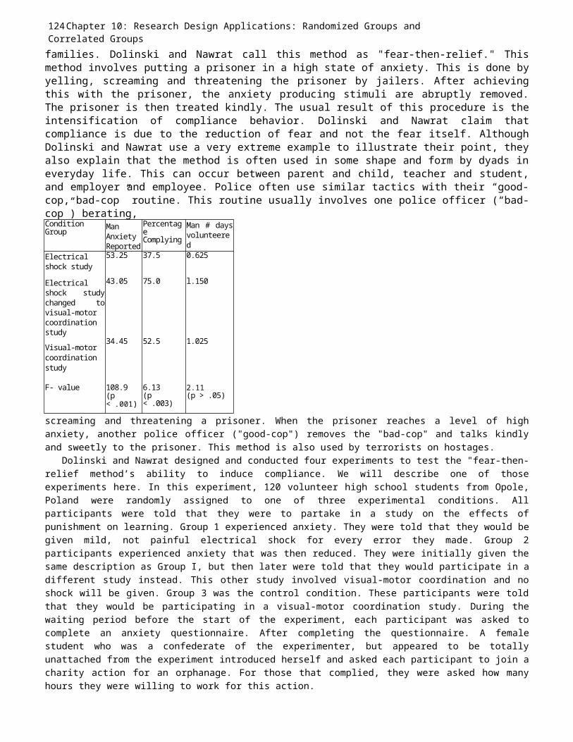
124Chapter 10: Research Design Applications: Randomized Groups andCorrelated Groupsfamilies. Dolinski and Nawrat call this method as "fear-then-relief." Thismethod involves putting a prisoner in a high state of anxiety. This is done byyelling, screaming and threatening the prisoner by jailers. After achievingthis with the prisoner, the anxiety producing stimuli are abruptly removed.The prisoner is then treated kindly. The usual result of this procedure is theintensification of compliance behavior. Dolinski and Nawrat claim thatcompliance is due to the reduction of fear and not the fear itself. AlthoughDolinski and Nawrat use a very extreme example to illustrate their point, theyalso explain that the method is often used in some shape and form by dyads ineveryday life. This can occur between parent and child, teacher and student,and employer and employee. Police often use similar tactics with their “good-cop, bad-cop” routine. This routine usually involves one police officer (“bad-cop”) berating,ConditionGroup Man
AnxietyReported
PercentageComplying
Man # daysvolunteered
Electricalshock study
53.25 37.5 0.625
Electricalshock studychanged tovisual-motorcoordinationstudy
43.05 75.0 l.150
Visual-motorcoordinationstudy
34.45 52.5 1.025
F- value 108.9 6.13 2.11(p< .001)
(p< .003)
(p > .05)
screaming and threatening a prisoner. When the prisoner reaches a level of highanxiety, another police officer ("good-cop") removes the "bad-cop" and talks kindlyand sweetly to the prisoner. This method is also used by terrorists on hostages.
Dolinski and Nawrat designed and conducted four experiments to test the "fear-then-relief method’s ability to induce compliance. We will describe one of thoseexperiments here. In this experiment, 120 volunteer high school students from Opole,Poland were randomly assigned to one of three experimental conditions. Allparticipants were told that they were to partake in a study on the effects ofpunishment on learning. Group 1 experienced anxiety. They were told that they would begiven mild, not painful electrical shock for every error they made. Group 2participants experienced anxiety that was then reduced. They were initially given thesame description as Group I, but then later were told that they would participate in adifferent study instead. This other study involved visual-motor coordination and noshock will be given. Group 3 was the control condition. These participants were toldthat they would be participating in a visual-motor coordination study. During thewaiting period before the start of the experiment, each participant was asked tocomplete an anxiety questionnaire. After completing the questionnaire. A femalestudent who was a confederate of the experimenter, but appeared to be totallyunattached from the experiment introduced herself and asked each participant to join acharity action for an orphanage. For those that complied, they were asked how manyhours they were willing to work for this action.
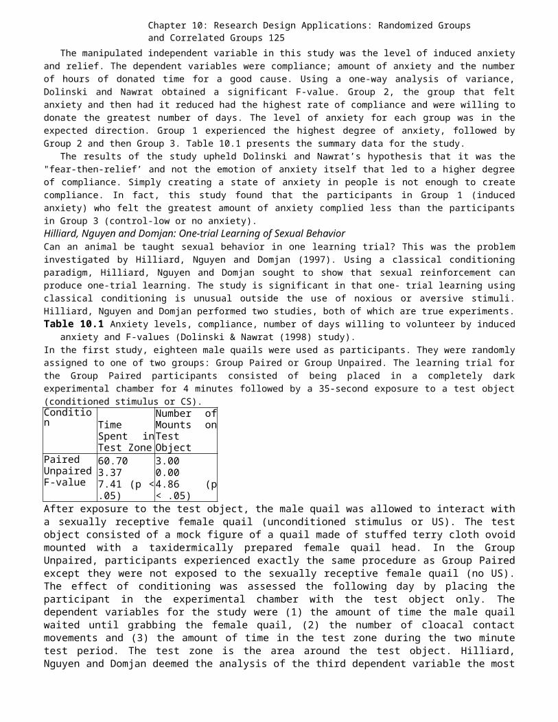
Chapter 10: Research Design Applications: Randomized Groups and Correlated Groups 125
The manipulated independent variable in this study was the level of induced anxietyand relief. The dependent variables were compliance; amount of anxiety and the numberof hours of donated time for a good cause. Using a one-way analysis of variance,Dolinski and Nawrat obtained a significant F-value. Group 2, the group that feltanxiety and then had it reduced had the highest rate of compliance and were willing todonate the greatest number of days. The level of anxiety for each group was in theexpected direction. Group 1 experienced the highest degree of anxiety, followed byGroup 2 and then Group 3. Table 10.1 presents the summary data for the study.
The results of the study upheld Dolinski and Nawrat’s hypothesis that it was the"fear-then-relief’ and not the emotion of anxiety itself that led to a higher degreeof compliance. Simply creating a state of anxiety in people is not enough to createcompliance. In fact, this study found that the participants in Group 1 (inducedanxiety) who felt the greatest amount of anxiety complied less than the participantsin Group 3 (control-low or no anxiety).Hilliard, Nguyen and Domjan: One-trial Learning of Sexual BehaviorCan an animal be taught sexual behavior in one learning trial? This was the probleminvestigated by Hilliard, Nguyen and Domjan (1997). Using a classical conditioningparadigm, Hilliard, Nguyen and Domjan sought to show that sexual reinforcement canproduce one-trial learning. The study is significant in that one- trial learning usingclassical conditioning is unusual outside the use of noxious or aversive stimuli.Hilliard, Nguyen and Domjan performed two studies, both of which are true experiments.Table 10.1 Anxiety levels, compliance, number of days willing to volunteer by induced
anxiety and F-values (Dolinski & Nawrat (1998) study).In the first study, eighteen male quails were used as participants. They were randomlyassigned to one of two groups: Group Paired or Group Unpaired. The learning trial forthe Group Paired participants consisted of being placed in a completely darkexperimental chamber for 4 minutes followed by a 35-second exposure to a test object(conditioned stimulus or CS).Condition Time
Spent inTest Zone
Number ofMounts onTestObject
PairedUnpairedF-value
60.703.377.41 (p <.05)
3.000.004.86 (p< .05)
After exposure to the test object, the male quail was allowed to interact witha sexually receptive female quail (unconditioned stimulus or US). The testobject consisted of a mock figure of a quail made of stuffed terry cloth ovoidmounted with a taxidermically prepared female quail head. In the GroupUnpaired, participants experienced exactly the same procedure as Group Pairedexcept they were not exposed to the sexually receptive female quail (no US).The effect of conditioning was assessed the following day by placing theparticipant in the experimental chamber with the test object only. Thedependent variables for the study were (1) the amount of time the male quailwaited until grabbing the female quail, (2) the number of cloacal contactmovements and (3) the amount of time in the test zone during the two minutetest period. The test zone is the area around the test object. Hilliard,Nguyen and Domjan deemed the analysis of the third dependent variable the most
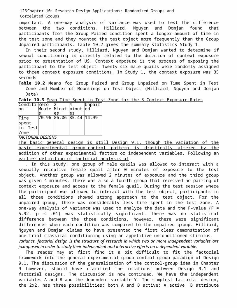
126Chapter 10: Research Design Applications: Randomized Groups andCorrelated Groupsimportant. A one-way analysis of variance was used to test the differencebetween the two conditions. Hilliard, Nguyen and Domjan found thatparticipants from the Group Paired condition spent a longer amount of time inthe test zone and they mounted the test object more frequently than the GroupUnpaired participants. Table 10.2 gives the summary statistics Study 1.
In their second study, Hilliard, Nguyen and Domjan wanted to determine ifsexual conditioning is directly related to the duration of context exposureprior to presentation of US. Context exposure is the process of exposing theparticipant to the test object. Twenty-six male quails were randomly assignedto three context exposure conditions. In Study 1, the context exposure was 35secondsTable 10.2 Means for Group Paired and Group Unpaired on Time Spent in Test
Zone and Number of Mountings on Test Object (Hilliard, Nguyen and DomjanData)
Table 10.3 Mean Time Spent in Test Zone for the 3 Context Exposure RatesCondition
ZeroMnutes
2Minutes
4minutes
Unpaired
Timespentin TestZone
70.96 86.06 85.44 14.99
FACTORIAL DESIGNSThe basic general design is still Design 9.1, though the variation of thebasic experimental group-control pattern is drastically altered by theaddition of other experimental factors or independent variables. Following anearlier definition of factorial analysis of
. In this study, one group of male quails was allowed to interact with asexually receptive female quail after 0 minutes of exposure to the testobject. Another group was allowed 2 minutes of exposure and the third groupwas given 4 minutes. There was also a fourth group that received no pairing ofcontext exposure and access to the female quail. During the test session wherethe participant was allowed to interact with the test object, participants inall three conditions showed strong approach to the test object. For theunpaired group, there was considerably less time spent in the test zone. Aone-way analysis of variance was used to analyze the data and the F-value (F =5.92, p < .01) was statistically significant. There was no statisticaldifference between the three conditions, however, there were significantdifferences when each condition was compared to the unpaired group. Hilliard,Nguyen and Domjan claims to have presented the first clear demonstration ofone-trial classical conditioning using an appetitive unconditioned stimulus.variance, factorial design is the structure of research in which two or more independent variables arejuxtaposed in order to study their independent and interactive effects on a dependent variable.
The reader may at first find it a bit difficult to fit the factorialframework into the general experimental group-control group paradigm of Design9.1. The discussion of the generalization of the control-group idea in Chapter9 however, should have clarified the relations between Design 9.1 andfactorial designs. The discussion is now continued. We have the independentvariables A and B and the dependent variable Y. The simplest factorial design,the 2x2, has three possibilities: both A and B active; A active, B attribute
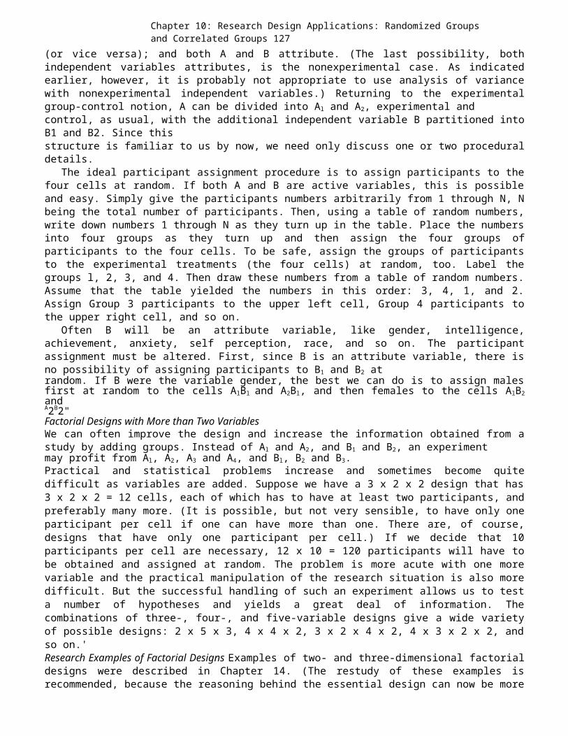
Chapter 10: Research Design Applications: Randomized Groups and Correlated Groups 127
(or vice versa); and both A and B attribute. (The last possibility, bothindependent variables attributes, is the nonexperimental case. As indicatedearlier, however, it is probably not appropriate to use analysis of variancewith nonexperimental independent variables.) Returning to the experimentalgroup-control notion, A can be divided into Al and A2, experimental andcontrol, as usual, with the additional independent variable B partitioned intoB1 and B2. Since thisstructure is familiar to us by now, we need only discuss one or two proceduraldetails.
The ideal participant assignment procedure is to assign participants to thefour cells at random. If both A and B are active variables, this is possibleand easy. Simply give the participants numbers arbitrarily from 1 through N, Nbeing the total number of participants. Then, using a table of random numbers,write down numbers 1 through N as they turn up in the table. Place the numbersinto four groups as they turn up and then assign the four groups ofparticipants to the four cells. To be safe, assign the groups of participantsto the experimental treatments (the four cells) at random, too. Label thegroups l, 2, 3, and 4. Then draw these numbers from a table of random numbers.Assume that the table yielded the numbers in this order: 3, 4, 1, and 2.Assign Group 3 participants to the upper left cell, Group 4 participants tothe upper right cell, and so on.
Often B will be an attribute variable, like gender, intelligence,achievement, anxiety, self perception, race, and so on. The participantassignment must be altered. First, since B is an attribute variable, there isno possibility of assigning participants to B1 and B2 atrandom. If B were the variable gender, the best we can do is to assign malesfirst at random to the cells AlBl and A2Bl, and then females to the cells AlB2andA2B2"Factorial Designs with More than Two VariablesWe can often improve the design and increase the information obtained from astudy by adding groups. Instead of Al and A2, and B1 and B2, an experimentmay profit from Al, A2, A3 and A4, and Bl, B2 and B3.Practical and statistical problems increase and sometimes become quitedifficult as variables are added. Suppose we have a 3 x 2 x 2 design that has3 x 2 x 2 = 12 cells, each of which has to have at least two participants, andpreferably many more. (It is possible, but not very sensible, to have only oneparticipant per cell if one can have more than one. There are, of course,designs that have only one participant per cell.) If we decide that 10participants per cell are necessary, 12 x 10 = 120 participants will have tobe obtained and assigned at random. The problem is more acute with one morevariable and the practical manipulation of the research situation is also moredifficult. But the successful handling of such an experiment allows us to testa number of hypotheses and yields a great deal of information. Thecombinations of three-, four-, and five-variable designs give a wide varietyof possible designs: 2 x 5 x 3, 4 x 4 x 2, 3 x 2 x 4 x 2, 4 x 3 x 2 x 2, andso on.'Research Examples of Factorial Designs Examples of two- and three-dimensional factorialdesigns were described in Chapter 14. (The restudy of these examples isrecommended, because the reasoning behind the essential design can now be more
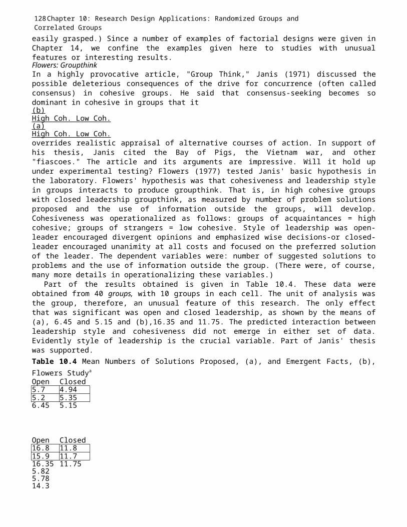
128Chapter 10: Research Design Applications: Randomized Groups andCorrelated Groupseasily grasped.) Since a number of examples of factorial designs were given inChapter 14, we confine the examples given here to studies with unusualfeatures or interesting results.Flowers: GroupthinkIn a highly provocative article, "Group Think," Janis (1971) discussed thepossible deleterious consequences of the drive for concurrence (often calledconsensus) in cohesive groups. He said that consensus-seeking becomes sodominant in cohesive in groups that it(b)High Coh. Low Coh.(a)High Coh. Low Coh.overrides realistic appraisal of alternative courses of action. In support ofhis thesis, Janis cited the Bay of Pigs, the Vietnam war, and other"fiascoes." The article and its arguments are impressive. Will it hold upunder experimental testing? Flowers (1977) tested Janis' basic hypothesis inthe laboratory. Flowers' hypothesis was that cohesiveness and leadership stylein groups interacts to produce groupthink. That is, in high cohesive groupswith closed leadership groupthink, as measured by number of problem solutionsproposed and the use of information outside the groups, will develop.Cohesiveness was operationalized as follows: groups of acquaintances = highcohesive; groups of strangers = low cohesive. Style of leadership was open-leader encouraged divergent opinions and emphasized wise decisions-or closed-leader encouraged unanimity at all costs and focused on the preferred solutionof the leader. The dependent variables were: number of suggested solutions toproblems and the use of information outside the group. (There were, of course,many more details in operationalizing these variables.)
Part of the results obtained is given in Table 10.4. These data wereobtained from 40 groups, with 10 groups in each cell. The unit of analysis wasthe group, therefore, an unusual feature of this research. The only effectthat was significant was open and closed leadership, as shown by the means of(a), 6.45 and 5.15 and (b),16.35 and 11.75. The predicted interaction betweenleadership style and cohesiveness did not emerge in either set of data.Evidently style of leadership is the crucial variable. Part of Janis' thesiswas supported.Table 10.4 Mean Numbers of Solutions Proposed, (a), and Emergent Facts, (b),Flowers Studya
Open Closed5.7 4.945.2 5.356.45 5.15
Open Closed16.8 11.815.9 11.716.35 11.755.825.7814.3
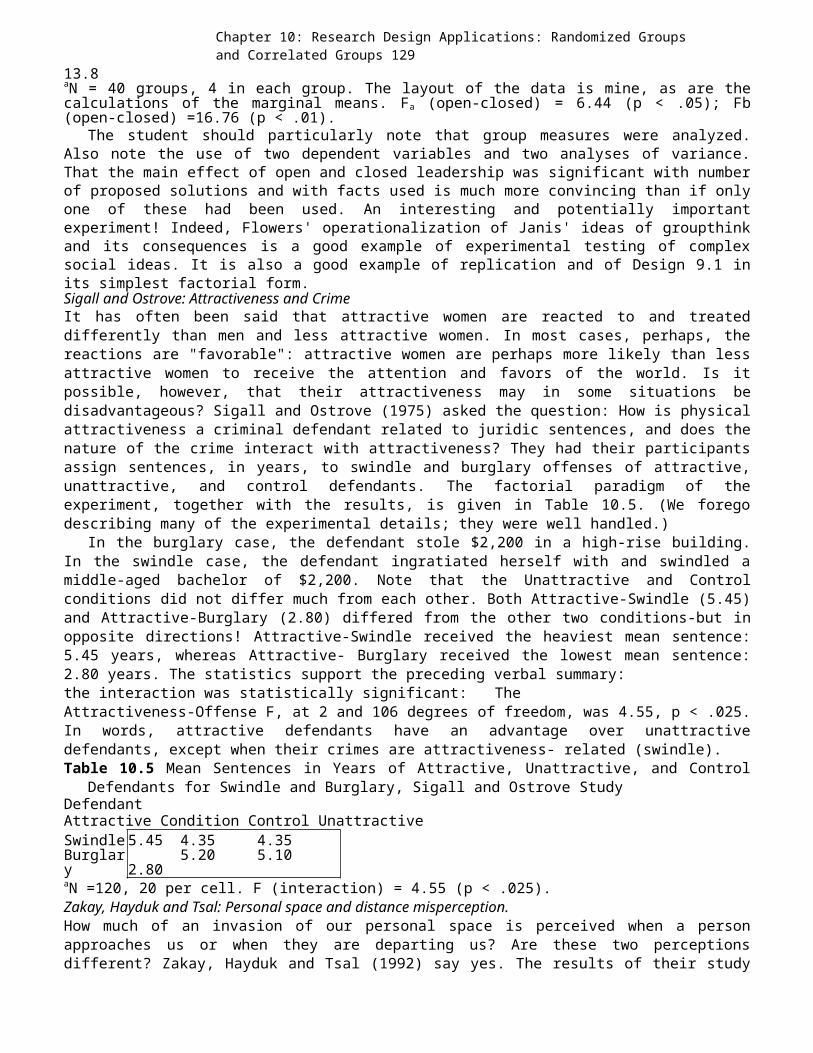
Chapter 10: Research Design Applications: Randomized Groups and Correlated Groups 129
13.8aN = 40 groups, 4 in each group. The layout of the data is mine, as are thecalculations of the marginal means. Fa (open-closed) = 6.44 (p < .05); Fb(open-closed) =16.76 (p < .01).
The student should particularly note that group measures were analyzed.Also note the use of two dependent variables and two analyses of variance.That the main effect of open and closed leadership was significant with numberof proposed solutions and with facts used is much more convincing than if onlyone of these had been used. An interesting and potentially importantexperiment! Indeed, Flowers' operationalization of Janis' ideas of groupthinkand its consequences is a good example of experimental testing of complexsocial ideas. It is also a good example of replication and of Design 9.1 inits simplest factorial form.Sigall and Ostrove: Attractiveness and CrimeIt has often been said that attractive women are reacted to and treateddifferently than men and less attractive women. In most cases, perhaps, thereactions are "favorable": attractive women are perhaps more likely than lessattractive women to receive the attention and favors of the world. Is itpossible, however, that their attractiveness may in some situations bedisadvantageous? Sigall and Ostrove (1975) asked the question: How is physicalattractiveness a criminal defendant related to juridic sentences, and does thenature of the crime interact with attractiveness? They had their participantsassign sentences, in years, to swindle and burglary offenses of attractive,unattractive, and control defendants. The factorial paradigm of theexperiment, together with the results, is given in Table 10.5. (We foregodescribing many of the experimental details; they were well handled.)
In the burglary case, the defendant stole $2,200 in a high-rise building.In the swindle case, the defendant ingratiated herself with and swindled amiddle-aged bachelor of $2,200. Note that the Unattractive and Controlconditions did not differ much from each other. Both Attractive-Swindle (5.45)and Attractive-Burglary (2.80) differed from the other two conditions-but inopposite directions! Attractive-Swindle received the heaviest mean sentence:5.45 years, whereas Attractive- Burglary received the lowest mean sentence:2.80 years. The statistics support the preceding verbal summary:the interaction was statistically significant: TheAttractiveness-Offense F, at 2 and 106 degrees of freedom, was 4.55, p < .025.In words, attractive defendants have an advantage over unattractivedefendants, except when their crimes are attractiveness- related (swindle).Table 10.5 Mean Sentences in Years of Attractive, Unattractive, and Control
Defendants for Swindle and Burglary, Sigall and Ostrove StudyDefendantAttractive Condition Control UnattractiveSwindle 5.45 4.35 4.35Burglary 2.80
5.20 5.10aN =120, 20 per cell. F (interaction) = 4.55 (p < .025).Zakay, Hayduk and Tsal: Personal space and distance misperception.How much of an invasion of our personal space is perceived when a personapproaches us or when they are departing us? Are these two perceptionsdifferent? Zakay, Hayduk and Tsal (1992) say yes. The results of their study
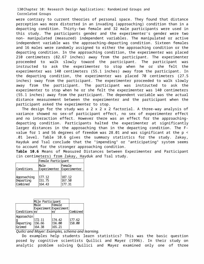
130Chapter 10: Research Design Applications: Randomized Groups andCorrelated Groupswere contrary to current theories of personal space. They found that distanceperception was more distorted in an invading (approaching) condition than in adeparting condition. Thirty-two female and 32 male participants were used inthis study. The participants gender and the experimenter's gender were twonon- manipulated (measured) independent variables. The manipulated or activeindependent variable was the approaching-departing condition. Sixteen femalesand 16 males were randomly assigned to either the approaching condition or thedeparting condition. In the approaching condition, the experimenter was placed210 centimeters (82.67 inches) away from the participant. The experimenterproceeded to walk slowly toward the participant. The participant wasinstructed to ask the experimenter to stop when he or she felt theexperimenter was 140 centimeters (55.1 inches) away from the participant. Inthe departing condition, the experimenter was placed 70 centimeters (27.5inches) sway from the participant. The experimenter proceeded to walk slowlyaway from the participant. The participant was instructed to ask theexperimenter to stop when he or she felt the experimenter was 140 centimeters(55.1 inches) away from the participant. The dependent variable was the actualdistance measurement between the experimenter and the participant when theparticipant asked the experimenter to stop.
The design for the study was a 2 x 2 x 2 factorial. A three-way analysis ofvariance showed no sex-of participant effect, no sex of experimenter effectand no interaction effect. However there was an effect for the approaching-departing condition. Participants halted the experimenter at significantlylarger distances in the approaching than in the departing condition. The F-value for 1 and 56 degrees of freedom was 28.01 and was significant at the p <.01 level. Table 10.6 gives the summary statistics for the study. Zakay,Hayduk and Tsal conclude that the "impending" or "anticipating" system seemsto account for the stronger approaching condition.Table 10.6 Means of Measured Distances between Experimenter and Participant(in centimeters) from Zakay, Hayduk and Tsal study.
Female Participant
ConditionsMaleExperimenter
FemaleExperimenter
Approaching 177.12 187.12Departing 151.75 167.50Combined 164.43 177.31
Mile Participant
ConditionsMaleExperimenter
FemaleExperimenter Combined
Approaching 172.11 174.42 177.62Departing 156.66 156.00 158.00Grimed 164.38 165.21Quilici and Mayer: Examples, schema and learning.
Do examples help students learn statistics? This was the basic questionposed by cognitive scientists Quilici and Mayer (1996). In their study onanalytic problem solving Quilici and Mayer examined only one of three

Chapter 10: Research Design Applications: Randomized Groups and Correlated Groups 131
processes that define analogical thinking. These researchers were concernedonly with the recognition process that involves two techniques: (1} focus onthe surface similarities between the example and actual problem to be solvedor (2) focus on the structural similarities. Surface similarities deal withthe shared attributes of objects in the problem cover story. With structuralsimilarity, the concern is with the shared relations between objects in bothexample and problem. To study this phenomena, Quilici and Mayer used learninghow to solve word problems in statistics. Quilici and Mayer felt that studentswho learn the structure of statistical word problems will be better able tosolve other problems they encounter in the future by properly classifying theminto the correct statistical method of analysis, e.g. t-test, correlation,etc. A few examples are given below to illustrate the difference betweensurface and structural similarities.Example 1: A personnel expert wishes to determine whether experienced typistsare able to type faster than inexperienced typists. Twenty experienced typistsand 20 inexperienced typists are given a typing test. Each typist's averagenumber of words typed per minute is recorded.Example 2: A personnel expert wishes to determine whether typing experience goeswith faster typing speeds. Forty typists are asked to report how many yearsthey have worked as typists and are given a typing test to determine theiraverage number of words typed per minute.Example 3: After examining weather data for the last 50 years, a meteorologistclaims that the annual precipitation varies with average temperature. For eachof 50 years, she notes the annual rainfall and average temperature.Example 4: A college dean claims that good readers earn better grades than poorreaders. The grade point average is recorded for 50 first-year students whoscored high on the reading comprehension test and for 50 first year studentswho scored low on a reading comprehension test.Example 2 would have the same surface features. Both deal with typists andtyping. To solve Example 1 a t- test would be used to compare experienced withinexperienced typists. However, to solve Example 2, one would use acorrelation since the question asks for a relation between typing experienceand average number of words typed per minute. Hence Example 1 and Example twowould be different structurally. Example 3 also looks at the relation betweentwo variables: amount of rainfall and temperature. It would have the samestructure as Example 2 but a different surface. They have the same structurebecause both require the use of correlation to solve the problem. Example 4and Example 1 have the same structure but a different surface.
Quilici and Mayer (1996) designed a study to determine if experience withexamples foster structural schema construction. One of their hypotheses statedthat students who are exposed to statistical word problem examples are morelikely to sort future problems on the basis of structure and less likely tosort on the basis of surface features. Students who are not exposed tostatistical word problem examples will not exhibit such behavior. They alsohypothesized that those exposed to three examples will be able to exhibit thebehavior to a higher degree than those exposed to only one example. Theseresearchers used a 3 x 4 factorial design. The first independent variable wasstructural characteristics (t- test, chi-square and correlation). The second
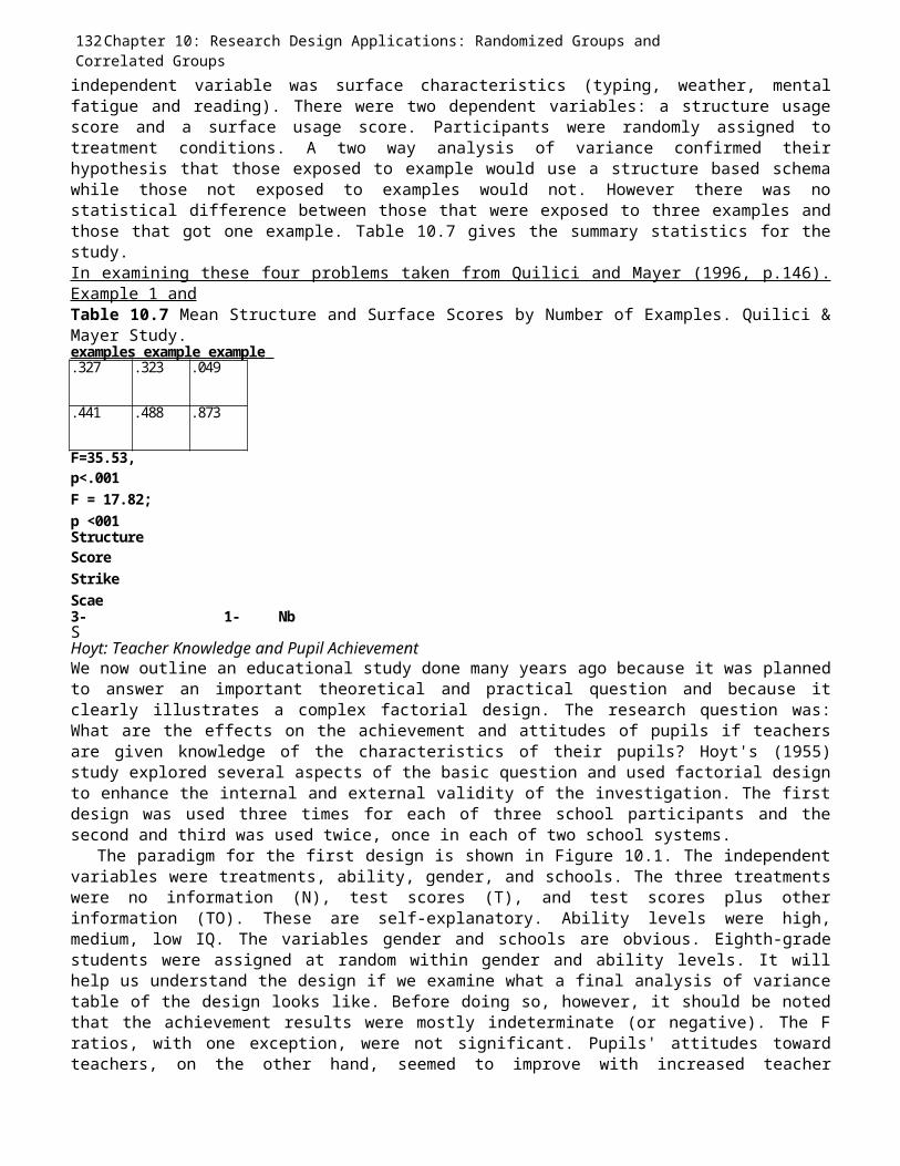
132Chapter 10: Research Design Applications: Randomized Groups andCorrelated Groupsindependent variable was surface characteristics (typing, weather, mentalfatigue and reading). There were two dependent variables: a structure usagescore and a surface usage score. Participants were randomly assigned totreatment conditions. A two way analysis of variance confirmed theirhypothesis that those exposed to example would use a structure based schemawhile those not exposed to examples would not. However there was nostatistical difference between those that were exposed to three examples andthose that got one example. Table 10.7 gives the summary statistics for thestudy.In examining these four problems taken from Quilici and Mayer (1996, p.146).Example 1 andTable 10.7 Mean Structure and Surface Scores by Number of Examples. Quilici &Mayer Study.examples example example .327 .323 .049
.441 .488 .873
F=35.53,p<.001F = 17.82;p <001StructureScoreStrikeScae3- 1- NbSHoyt: Teacher Knowledge and Pupil AchievementWe now outline an educational study done many years ago because it was plannedto answer an important theoretical and practical question and because itclearly illustrates a complex factorial design. The research question was:What are the effects on the achievement and attitudes of pupils if teachersare given knowledge of the characteristics of their pupils? Hoyt's (1955)study explored several aspects of the basic question and used factorial designto enhance the internal and external validity of the investigation. The firstdesign was used three times for each of three school participants and thesecond and third was used twice, once in each of two school systems.
The paradigm for the first design is shown in Figure 10.1. The independentvariables were treatments, ability, gender, and schools. The three treatmentswere no information (N), test scores (T), and test scores plus otherinformation (TO). These are self-explanatory. Ability levels were high,medium, low IQ. The variables gender and schools are obvious. Eighth-gradestudents were assigned at random within gender and ability levels. It willhelp us understand the design if we examine what a final analysis of variancetable of the design looks like. Before doing so, however, it should be notedthat the achievement results were mostly indeterminate (or negative). The Fratios, with one exception, were not significant. Pupils' attitudes towardteachers, on the other hand, seemed to improve with increased teacher
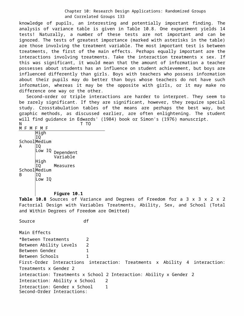
Chapter 10: Research Design Applications: Randomized Groups and Correlated Groups 133
knowledge of pupils, an interesting and potentially important finding. Theanalysis of variance table is given in Table 10.8. One experiment yields 14tests! Naturally, a number of these tests are not important and can beignored. The tests of greatest importance (marked with asterisks in the table)are those involving the treatment variable. The most important test is betweentreatments, the first of the main effects. Perhaps equally important are theinteractions involving treatments. Take the interaction treatments x sex. Ifthis was significant, it would mean that the amount of information a teacherpossesses about students has an influence on student achievement, but boys areinfluenced differently than girls. Boys with teachers who possess informationabout their pupils may do better than boys whose teachers do not have suchinformation, whereas it may be the opposite with girls, or it may make nodifference one way or the other.
Second-order or triple interactions are harder to interpret. They seem tobe rarely significant. If they are significant, however, they require specialstudy. Crosstabulation tables of the means are perhaps the best way, butgraphic methods, as discussed earlier, are often enlightening. The studentwill find guidance in Edwards' (1984) book or Simon's (1976) manuscript.N T TOM F M F M F
HighIQ
SchoolMediumA IQ
Low IQ DependentVariable
HighIQ Measures
SchoolMediumB IQ
Low IQ
Figure 10.1Table 10.8 Sources of Variance and Degrees of Freedom for a 3 x 3 x 2 x 2Factorial Design with Variables Treatments, Ability, Sex, and School (Totaland Within Degrees of Freedom are Omitted)
Source df
Main Effects*Between Treatments 2Between Ability Levels 2Between Gender 1Between Schools 1First-Order Interactions interaction: Treatments x Ability 4 interaction:Treatments x Gender 2interaction: Treatments x School 2 Interaction: Ability x Gender 2Interaction: Ability x School 2Interaction: Gender x School 1Second-Order Interactions:

134Chapter 10: Research Design Applications: Randomized Groups andCorrelated Groupsinteraction: Treatments x Ability x Gender 4 interaction: Treatments x Abilityx School 4 Interaction: Ability x Gender x School 2Third-Order Interactions:Interaction: Treatments x Ability x Gender x School 4Within or ResidualTotalEVALUATION OF RANDOMIZED SUBJECTS DESIGNSRandomized subjects designs are all variants or extensions of Design 9.1, thebasic experimental group- control group design in which participants areassigned to the experimental and control groups at random. As such they havethe strengths of the basic design, the most important of which is therandomization feature and the consequent ability to assume the preexperimentalapproximate equality of the experimental groups in all possible independentvariables. History and maturation are controlled because very little timeelapses between the manipulation of X and the observation and measurement ofY. There is no possible contamination due to pretesting.
Two other strengths of these designs, springing from the many variationspossible, are flexibility and applicability. They can be used to help solvemany behavioral research problems, since they seem to be peculiarly wellsuited to the types of design problems that arise from social scientific andeducational problems and hypotheses. The one-way designs, for example, canincorporate any number of methods, and the testing of methods is a majoreducational need. The variables that constantly need control in behavioralresearch-gender intelligence, aptitude, social class, schools, and manyothers-can be incorporated into factorial designs and thus controlled. Withfactorial designs, too, it is possible to have mixtures of active andattribute variables another important need.
There are also weaknesses. One criticism has been that randomized subjectsdesigns do not permit tests of the equality of groups, as do before-afterdesigns. Actually, this is not a valid criticism for two reasons: with enoughparticipants and randomization, it can be assumed that the groups are equal,as we have seen; and it is possible to check the groups for equality onvariables other than Y, the dependent variable. For educational research, dataon intelligence, aptitude, and achievement, for example, are available inschool records. Pertinent data for sociology and political science studies canoften be found in county and election district records.
Another difficulty is statistical. One should have equal numbers of casesin the cells of factorial designs. (It is possible to work with unequal n's,but it is both clumsy and a threat to interpretation. Dropping out cases atrandom or the use of missing data methods (see Dear, 1959; Gleason & Staelin,1975 for two excellent references on estimating missing data.) can cure smalldiscrepancies.) This imposes a limitation on the use of such designs; becauseit is often not possible to have equal numbers in each cell. One-wayrandomized designs are not so delicate: unequal numbers are not a difficultproblem. How to adjust and analyze data for unequal n's is a complex, thorny,and much-argue problem. For a discussion in the context mostly of analysis ofvariance, see Snedecor and Cochran (1989). Discussion in the context ofmultiple regression, which is actually a better solution of the problem, canbe found in Kerlinger and Pedhazur (1973) and Pedhazur (1996). Pedhazur's
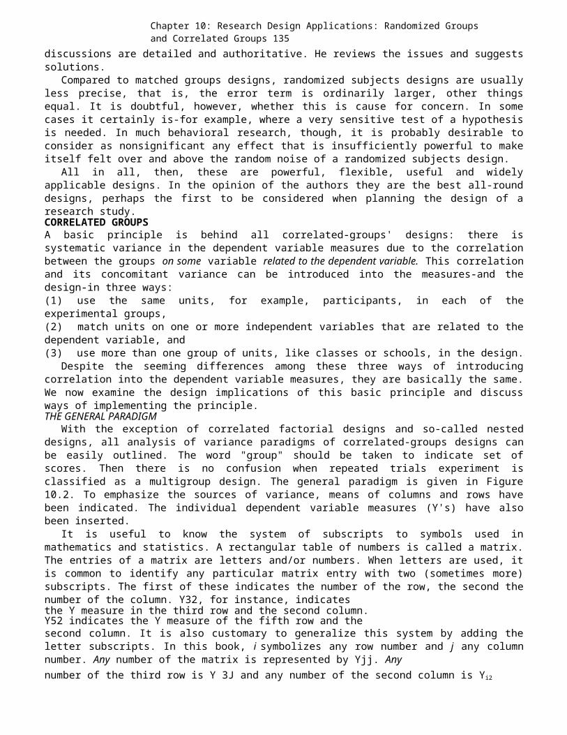
Chapter 10: Research Design Applications: Randomized Groups and Correlated Groups 135
discussions are detailed and authoritative. He reviews the issues and suggestssolutions.
Compared to matched groups designs, randomized subjects designs are usuallyless precise, that is, the error term is ordinarily larger, other thingsequal. It is doubtful, however, whether this is cause for concern. In somecases it certainly is-for example, where a very sensitive test of a hypothesisis needed. In much behavioral research, though, it is probably desirable toconsider as nonsignificant any effect that is insufficiently powerful to makeitself felt over and above the random noise of a randomized subjects design.
All in all, then, these are powerful, flexible, useful and widelyapplicable designs. In the opinion of the authors they are the best all-rounddesigns, perhaps the first to be considered when planning the design of aresearch study.CORRELATED GROUPSA basic principle is behind all correlated-groups' designs: there issystematic variance in the dependent variable measures due to the correlationbetween the groups on some variable related to the dependent variable. This correlationand its concomitant variance can be introduced into the measures-and thedesign-in three ways:(1) use the same units, for example, participants, in each of theexperimental groups,(2) match units on one or more independent variables that are related to thedependent variable, and(3) use more than one group of units, like classes or schools, in the design.
Despite the seeming differences among these three ways of introducingcorrelation into the dependent variable measures, they are basically the same.We now examine the design implications of this basic principle and discussways of implementing the principle.THE GENERAL PARADIGM
With the exception of correlated factorial designs and so-called nesteddesigns, all analysis of variance paradigms of correlated-groups designs canbe easily outlined. The word "group" should be taken to indicate set ofscores. Then there is no confusion when repeated trials experiment isclassified as a multigroup design. The general paradigm is given in Figure10.2. To emphasize the sources of variance, means of columns and rows havebeen indicated. The individual dependent variable measures (Y's) have alsobeen inserted.
It is useful to know the system of subscripts to symbols used inmathematics and statistics. A rectangular table of numbers is called a matrix.The entries of a matrix are letters and/or numbers. When letters are used, itis common to identify any particular matrix entry with two (sometimes more)subscripts. The first of these indicates the number of the row, the second thenumber of the column. Y32, for instance, indicatesthe Y measure in the third row and the second column.Y52 indicates the Y measure of the fifth row and thesecond column. It is also customary to generalize this system by adding theletter subscripts. In this book, i symbolizes any row number and j any columnnumber. Any number of the matrix is represented by Yjj. Anynumber of the third row is Y 3J and any number of the second column is Yi2
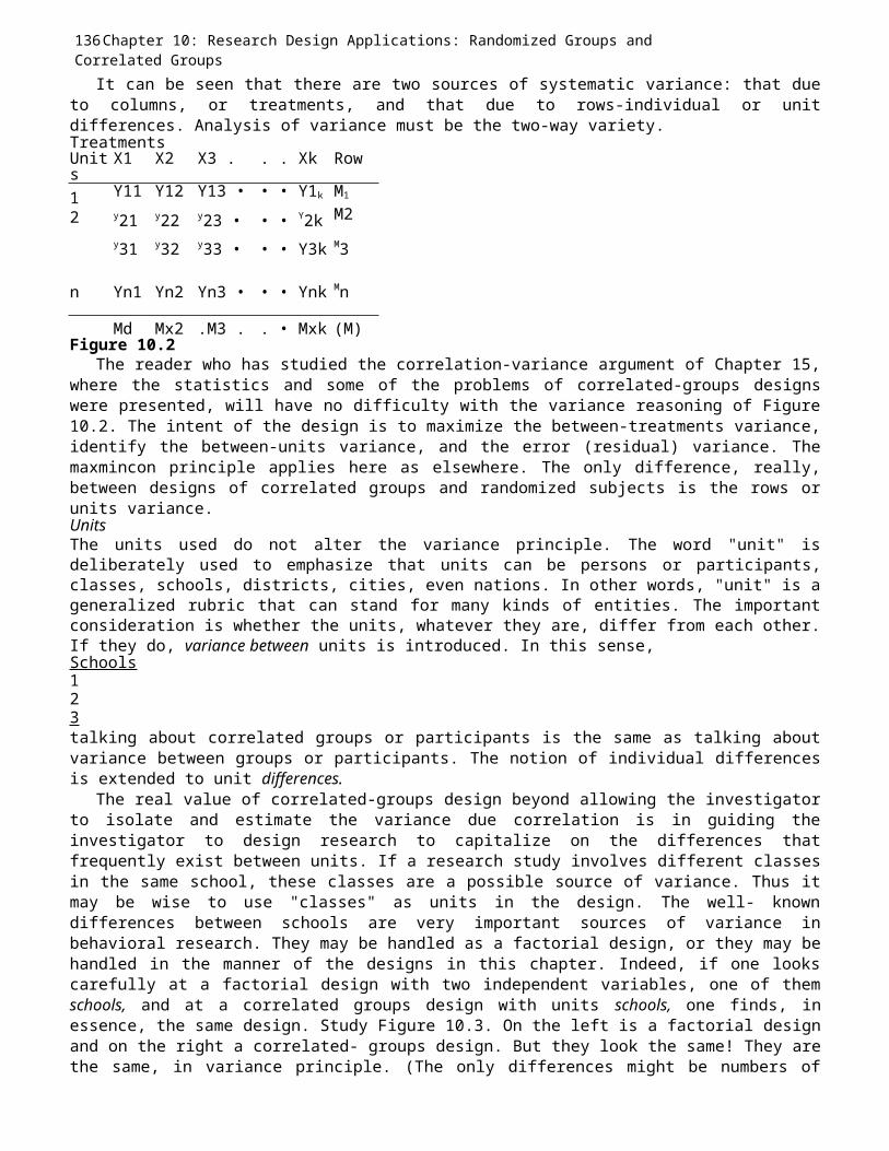
136Chapter 10: Research Design Applications: Randomized Groups andCorrelated Groups
It can be seen that there are two sources of systematic variance: that dueto columns, or treatments, and that due to rows-individual or unitdifferences. Analysis of variance must be the two-way variety.TreatmentsUnits
X1 X2 X3 . . . Xk Row
1 Y11 Y12 Y13 • • • Y1k M1
2 y21 y22 y23 • • • Y2k M2y31 y32 y33 • • • Y3k M3
n Yn1 Yn2 Yn3 • • • Ynk Mn
Md Mx2 .M3 . . • Mxk (M)Figure 10.2
The reader who has studied the correlation-variance argument of Chapter 15,where the statistics and some of the problems of correlated-groups designswere presented, will have no difficulty with the variance reasoning of Figure10.2. The intent of the design is to maximize the between-treatments variance,identify the between-units variance, and the error (residual) variance. Themaxmincon principle applies here as elsewhere. The only difference, really,between designs of correlated groups and randomized subjects is the rows orunits variance.UnitsThe units used do not alter the variance principle. The word "unit" isdeliberately used to emphasize that units can be persons or participants,classes, schools, districts, cities, even nations. In other words, "unit" is ageneralized rubric that can stand for many kinds of entities. The importantconsideration is whether the units, whatever they are, differ from each other.If they do, variance between units is introduced. In this sense,Schools123talking about correlated groups or participants is the same as talking aboutvariance between groups or participants. The notion of individual differencesis extended to unit differences.
The real value of correlated-groups design beyond allowing the investigatorto isolate and estimate the variance due correlation is in guiding theinvestigator to design research to capitalize on the differences thatfrequently exist between units. If a research study involves different classesin the same school, these classes are a possible source of variance. Thus itmay be wise to use "classes" as units in the design. The well- knowndifferences between schools are very important sources of variance inbehavioral research. They may be handled as a factorial design, or they may behandled in the manner of the designs in this chapter. Indeed, if one lookscarefully at a factorial design with two independent variables, one of themschools, and at a correlated groups design with units schools, one finds, inessence, the same design. Study Figure 10.3. On the left is a factorial designand on the right a correlated- groups design. But they look the same! They arethe same, in variance principle. (The only differences might be numbers of
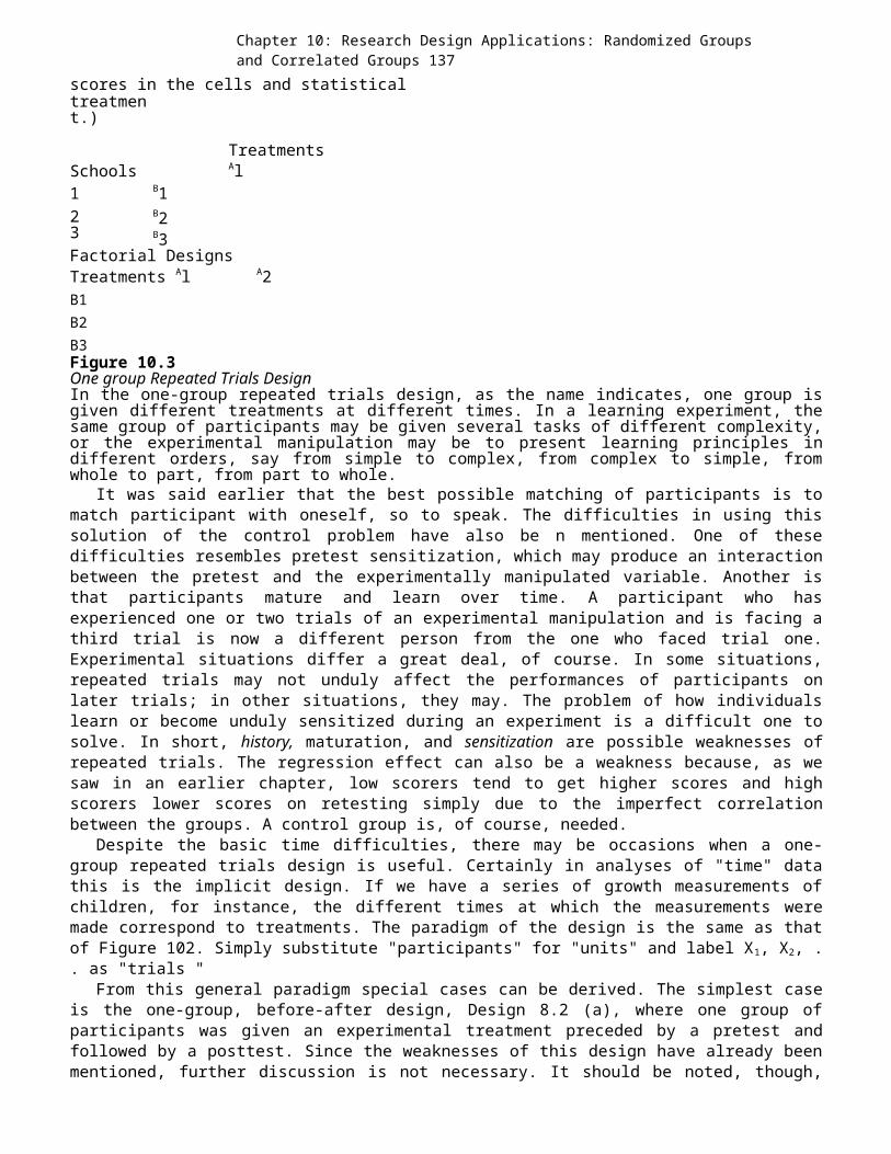
Chapter 10: Research Design Applications: Randomized Groups and Correlated Groups 137
scores in the cells and statisticaltreatment.)
TreatmentsSchools Al1 B123
B2B3
Factorial DesignsTreatments Al A2B1B2B3Figure 10.3One group Repeated Trials DesignIn the one-group repeated trials design, as the name indicates, one group isgiven different treatments at different times. In a learning experiment, thesame group of participants may be given several tasks of different complexity,or the experimental manipulation may be to present learning principles indifferent orders, say from simple to complex, from complex to simple, fromwhole to part, from part to whole.
It was said earlier that the best possible matching of participants is tomatch participant with oneself, so to speak. The difficulties in using thissolution of the control problem have also be n mentioned. One of thesedifficulties resembles pretest sensitization, which may produce an interactionbetween the pretest and the experimentally manipulated variable. Another isthat participants mature and learn over time. A participant who hasexperienced one or two trials of an experimental manipulation and is facing athird trial is now a different person from the one who faced trial one.Experimental situations differ a great deal, of course. In some situations,repeated trials may not unduly affect the performances of participants onlater trials; in other situations, they may. The problem of how individualslearn or become unduly sensitized during an experiment is a difficult one tosolve. In short, history, maturation, and sensitization are possible weaknesses ofrepeated trials. The regression effect can also be a weakness because, as wesaw in an earlier chapter, low scorers tend to get higher scores and highscorers lower scores on retesting simply due to the imperfect correlationbetween the groups. A control group is, of course, needed.
Despite the basic time difficulties, there may be occasions when a one-group repeated trials design is useful. Certainly in analyses of "time" datathis is the implicit design. If we have a series of growth measurements ofchildren, for instance, the different times at which the measurements weremade correspond to treatments. The paradigm of the design is the same as thatof Figure 102. Simply substitute "participants" for "units" and label X1, X2, .. as "trials "
From this general paradigm special cases can be derived. The simplest caseis the one-group, before-after design, Design 8.2 (a), where one group ofparticipants was given an experimental treatment preceded by a pretest andfollowed by a posttest. Since the weaknesses of this design have already beenmentioned, further discussion is not necessary. It should be noted, though,
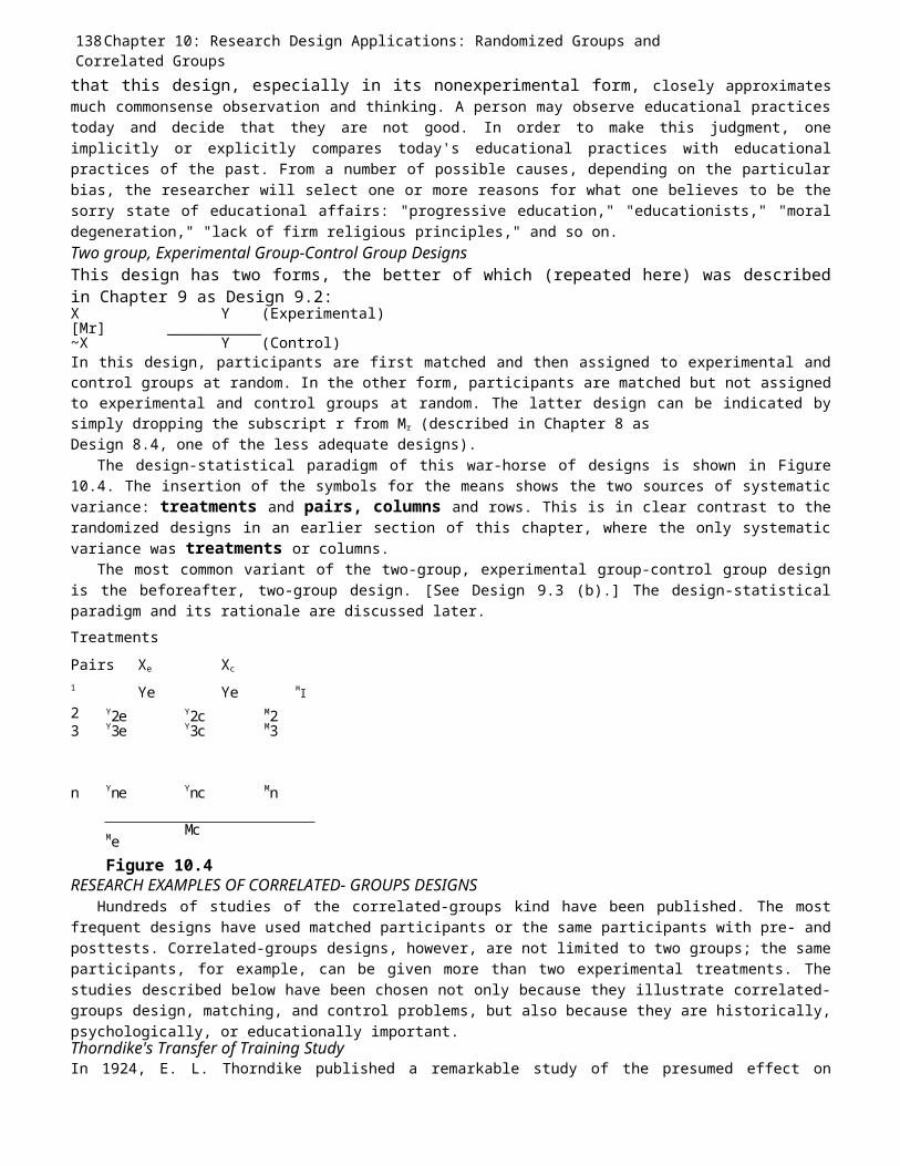
138Chapter 10: Research Design Applications: Randomized Groups andCorrelated Groupsthat this design, especially in its nonexperimental form, closely approximatesmuch commonsense observation and thinking. A person may observe educational practicestoday and decide that they are not good. In order to make this judgment, oneimplicitly or explicitly compares today's educational practices with educationalpractices of the past. From a number of possible causes, depending on the particularbias, the researcher will select one or more reasons for what one believes to be thesorry state of educational affairs: "progressive education," "educationists," "moraldegeneration," "lack of firm religious principles," and so on.Two group, Experimental Group-Control Group DesignsThis design has two forms, the better of which (repeated here) was describedin Chapter 9 as Design 9.2:X Y (Experimental)[Mr] ___________~X Y (Control)In this design, participants are first matched and then assigned to experimental andcontrol groups at random. In the other form, participants are matched but not assignedto experimental and control groups at random. The latter design can be indicated bysimply dropping the subscript r from Mr (described in Chapter 8 asDesign 8.4, one of the less adequate designs).
The design-statistical paradigm of this war-horse of designs is shown in Figure10.4. The insertion of the symbols for the means shows the two sources of systematicvariance: treatments and pairs, columns and rows. This is in clear contrast to therandomized designs in an earlier section of this chapter, where the only systematicvariance was treatments or columns.
The most common variant of the two-group, experimental group-control group designis the beforeafter, two-group design. [See Design 9.3 (b).] The design-statisticalparadigm and its rationale are discussed later.TreatmentsPairs Xe Xc
1 Ye Ye MI2 Y2e Y2c M23 Y3e Y3c M3
n Yne Ync Mn
MeMc
Figure 10.4RESEARCH EXAMPLES OF CORRELATED- GROUPS DESIGNS
Hundreds of studies of the correlated-groups kind have been published. The mostfrequent designs have used matched participants or the same participants with pre- andposttests. Correlated-groups designs, however, are not limited to two groups; the sameparticipants, for example, can be given more than two experimental treatments. Thestudies described below have been chosen not only because they illustrate correlated-groups design, matching, and control problems, but also because they are historically,psychologically, or educationally important.Thorndike's Transfer of Training StudyIn 1924, E. L. Thorndike published a remarkable study of the presumed effect on

Chapter 10: Research Design Applications: Randomized Groups and Correlated Groups 139
intelligence of certain school participants. Students were matched according to scoreson Form A of the measure of the dependent variable, intelligence. This test alsoserved as a pretest. The independent variable was One Year's Study of Participants,such as history, mathematics, and Latin. A posttest, Form B of the intelligence test,was given at the end of the year. Thorndike (1924) used an ingenious device toseparate the differential effect of each school subject. He did this by matching onForm A of the intelligence test those pupils who studied, for instance, English,history, geometry, and Latin with those pupils who studied English, history,geometry, and shopwork. Thus, for these two groups, he was comparing the differentialeffects of Latin and shopwork. Gains in final intelligence scores were considered ajoint effect of growth plus the academic subjects studied.
Despite its weaknesses, this was a colossal study. Thorndike was aware of the lackof adequate controls, as revealed in the following passage on the effects ofselection:The chief reason why good thinkers seem superficially to have been made suchby having taken certain school studies, is that good thinkers have taken suchstudies. . . .When the good thinkers studied Greek and Latin, these studies seemed to makegood thinkers. Now that the good thinkers study Physics and Trigonometry,these seem to make good thinkers. If the abler pupils should all studyPhysical Education and Dramatic Art these subjects would seem to make goodthinkers. (p. 98)Thorndike pointed the way to controlled educational research, which has led tothe decrease of metaphysical and dogmatic explanations in education. His workstruck a blow against the razor-strop theory of mental training, the theorythat likened the mind to a razor that could be sharpened by stropping it on"hard" subjects.
It is not easy to evaluate a study such as this, the scope and ingenuity ofwhich is impressive. One wonders, however, about the adequacy of the dependentvariable, "intelligence" or "intellectual ability." Can school subjectsstudied for one year have much effect on intelligence? Moreover, the study wasnot experimental. Thorndike measured the intelligence of students and let theindependent variables, school subjects, operate. No randomization, of course,was possible. As mentioned above, he was aware of this control weakness in hisstudy, which is still a classic that deserves respect and careful studydespite its weaknesses in history and selection (maturation was controlled).Miller and DiCara: Learning of Autonomic FunctionsIn a previous chapter we presented data from one of the set of remarkablestudies of the learning of autonomic functioning done by Miller and hiscolleagues. (Miller, 1971; Miller & DiCara, 1968). Experts and non-expertsbelieve that it is not possible to learn and control responses of theautonomic nervous system. That is, glandular and visceral responses-heartbeat, urine secretion, arid blood pressure, for example-were supposed to bebeyond the "control" of the individual. Miller believed otherwise. Hedemonstrated experimentally that such responses are subject to instrumentallearning. The crucial part of his method consisted of rewarding visceralresponses when they occurred. In the study whose data were cited in an earlierchapter of this book for example, rats were rewarded when they increased ordecreased the secretion of urine. Fourteen rats were assigned at random to two
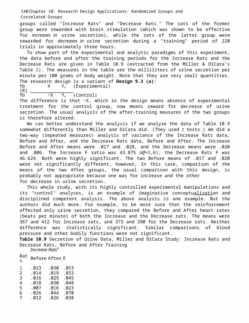
140Chapter 10: Research Design Applications: Randomized Groups andCorrelated Groupsgroups called "Increase Rats" and "Decrease Rats." The rats of the formergroup were rewarded with brain stimulation (which was shown to be effectivefor increases in urine secretion), while the rats of the latter group wererewarded for decreases in urine secretion during a "training" period of 220trials in approximately three hours.
To show part of the experimental and analytic paradigms of this experiment,the data before and after the training periods for the Increase Rats and theDecrease Rats are given in Table 10.9 (extracted from the Miller & DiCara’sTable 1). The measures in the table are the milliliters of urine secretion perminute per 100 grams of body weight. Note that they are very small quantities.The research design is a variant of Design 9.3 (a):Yb X Ya (Experimental)[R] ________________Yb ~X Ya (Control)The difference is that ~X, which in the design means absence of experimentaltreatment for the control group, now means reward for decrease of urinesecretion. The usual analysis of the after-training measures of the two groupsis therefore altered.
We can better understand the analysis if we analyze the data of Table 10.9somewhat differently than Miller and DiCara did. (They used t tests.) We did atwo-way (repeated measures) analysis of variance of the Increase Rats data,Before and After, and the Decrease Rats data, Before and After. The IncreaseBefore and After means were .017 and .028, and the Decrease means were .020and .006. The Increase F ratio was 43.875 (df=1,6); the Decrease Rats F was46.624. Both were highly significant. The two Before means of .017 and .020were not significantly different, however, In this case, comparison of themeans of the two After groups, the usual comparison with this design, isprobably not appropriate because one was for increase and the otherfor decrease in urine secretion.
This whole study, with its highly controlled experimental manipulations andits "control" analyses, is an example of imaginative conceptualization anddisciplined competent analysis. The above analysis is one example. But theauthors did much more. For example, to be more sure that the reinforcementaffected only urine secretion, they compared the Before and After heart rates(beats per minute) of both the Increase and the Decrease rats. The means were367 and 412 for Increase rats, and 373 and 390 for the Decrease rats. Neitherdifference was statistically significant. Similar comparisons of bloodpressure and other bodily functions were not significant.Table 10.9 Secretion of Urine Data, Miller and DiCara Study: Increase Rats andDecrease Rats, Before and After Training
Increase Rats&
Rats Before After E
1 .023 .030 .0532 .014 .019 .0333 .016 .029 .0454 .018 .030 .0485 .007 .016 .0236 .026 .044 .0707 .012 .026 .038
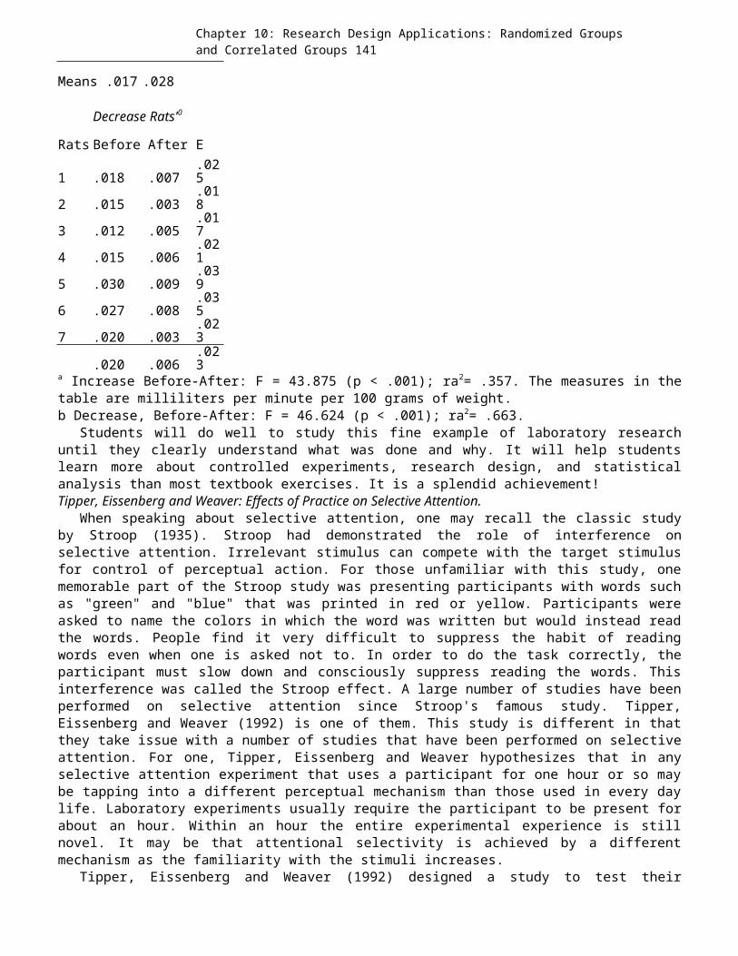
Chapter 10: Research Design Applications: Randomized Groups and Correlated Groups 141
Means .017 .028
Decrease Rats'0
Rats Before After E
1 .018 .007.025
2 .015 .003.018
3 .012 .005.017
4 .015 .006.021
5 .030 .009.039
6 .027 .008.035
7 .020 .003.023
.020 .006.023
a Increase Before-After: F = 43.875 (p < .001); ra2= .357. The measures in thetable are milliliters per minute per 100 grams of weight.b Decrease, Before-After: F = 46.624 (p < .001); ra2= .663.
Students will do well to study this fine example of laboratory researchuntil they clearly understand what was done and why. It will help studentslearn more about controlled experiments, research design, and statisticalanalysis than most textbook exercises. It is a splendid achievement!Tipper, Eissenberg and Weaver: Effects of Practice on Selective Attention.
When speaking about selective attention, one may recall the classic studyby Stroop (1935). Stroop had demonstrated the role of interference onselective attention. Irrelevant stimulus can compete with the target stimulusfor control of perceptual action. For those unfamiliar with this study, onememorable part of the Stroop study was presenting participants with words suchas "green" and "blue" that was printed in red or yellow. Participants wereasked to name the colors in which the word was written but would instead readthe words. People find it very difficult to suppress the habit of readingwords even when one is asked not to. In order to do the task correctly, theparticipant must slow down and consciously suppress reading the words. Thisinterference was called the Stroop effect. A large number of studies have beenperformed on selective attention since Stroop's famous study. Tipper,Eissenberg and Weaver (1992) is one of them. This study is different in thatthey take issue with a number of studies that have been performed on selectiveattention. For one, Tipper, Eissenberg and Weaver hypothesizes that in anyselective attention experiment that uses a participant for one hour or so maybe tapping into a different perceptual mechanism than those used in every daylife. Laboratory experiments usually require the participant to be present forabout an hour. Within an hour the entire experimental experience is stillnovel. It may be that attentional selectivity is achieved by a differentmechanism as the familiarity with the stimuli increases.
Tipper, Eissenberg and Weaver (1992) designed a study to test their

142Chapter 10: Research Design Applications: Randomized Groups andCorrelated Groupshypotheses concerning selective attention using a completely within subjectsdesign. All of the participants experienced all of the treatment conditions.They looked at the effect of interference on reaction time and errors. Theyhad each participant experience both levels of interference: negative primingand response inhibition across 11 blocks or trials taken over 4 days (practiceeffect). Their results showed that there was an interference effect (F =35.15, p < .001) when using reaction time as the dependent variable. Thereaction times were longer when the distraction was present. They also found apractice effect (blocks) {F = 9.62, p< .0001 ) and no interaction effect. Thepractice effect indicated that the reaction time of participants became fasterwith the increase in practice. The fact that the interaction effect was notsignificant indicates that the interfering effects of the irrelevant stimulusremained constant even after extended practice. The findings of Tipper,Eissenberg and Weaver (1992) does suggest that other mechanisms for selectionattention exist and operate with different levels of experience.MULTIGROUP CORRELATED-GRO UPS DESIGNSUnits VarianceWhile it is difficult to match three and four sets of participants, and whileit is ordinarily not feasible or desirable in behavioral research to use thesame participants in each of the groups, there are natural situations in whichcorrelated groups exist. These situations are particularly important ineducational research. Until recently, the variances due to differences betweenclasses, schools, school systems, and other "natural" units have not been wellcontrolled or often used in the analysis of data. Perhaps the first indicationof the importance of this kind of variance was given in Lindquist's (1940)fine book on statistical analysis in educational research. In this book,Lindquist placed considerable emphasis on schools variance. Schools, classes,and other educational units tend to differ significantly in achievement,intelligence, aptitudes, and other variables. The educational investigator hasto be alert to these unit differences, as well as to individual differences.
Consider an obvious example. Suppose an investigator chooses a sample offive schools for their variety and homogeneity. The goal of course is externalvalidity: representativeness. The investigator uses pupils from all fiveschools and combines the measures from the five schools to test the meandifferences in some dependent variable. In so doing, the investigator isignoring the variance due to the differences among schools. It isunderstandable that the means do not differ significantly; the schoolsvariance is mixed in with the error variance.
Gross errors can arise from ignoring the variance of units such as schoolsand classes. One such error is to select a number of schools and to designatecertain schools as experimental schools and others as control schools. Herethe between-schools variance gets entangled with the variance of theexperimental variable. Similarly, classes, school districts, and othereducational units differ and thus engender variance. The variances must beidentified and controlled, whether it be by experimental or statisticalcontrol, or both.FACTORIAL CORRELATED GROUPSFactorial models can be combined with the units notion to yield a valuabledesign: factorial correlated groups design. Such a design is appropriate when units
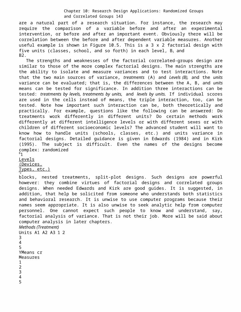
Chapter 10: Research Design Applications: Randomized Groups and Correlated Groups 143
are a natural part of a research situation. For instance, the research mayrequire the comparison of a variable before and after an experimentalintervention, or before and after an important event. Obviously there will becorrelation between the before and after dependent variable measures. Anotheruseful example is shown in Figure 10.5. This is a 3 x 2 factorial design withfive units (classes, school, and so forth) in each level, B1 andB2.
The strengths and weaknesses of the factorial correlated-groups design aresimilar to those of the more complex factorial designs. The main strengths arethe ability to isolate and measure variances and to test interactions. Notethat the two main sources of variance, treatments (A) and Levels (B), and the unitsvariance can be evaluated; that is, the differences between the A, B, and unitsmeans can be tested for significance. In addition three interactions can betested: treatments by levels, treatments by units, and levels by units. If individual scoresare used in the cells instead of means, the triple interaction, too, can betested. Note how important such interaction can be, both theoretically andpractically. For example, questions like the following can be answered: Dotreatments work differently in different units? Do certain methods workdifferently at different intelligence levels or with different sexes or withchildren of different socioeconomic levels? The advanced student will want toknow how to handle units (schools, classes, etc.) and units variance infactorial designs. Detailed guidance is given in Edwards (1984) and in Kirk(1995). The subject is difficult. Even the names of the designs becomecomplex: randomizedB1Levels(Devices,Types, etc.)B2blocks, nested treatments, split-plot designs. Such designs are powerfulhowever: they combine virtues of factorial designs and correlated groupsdesigns. When needed Edwards and Kirk are good guides. It is suggested, inaddition, that help be solicited from someone who understands both statisticsand behavioral research. It is unwise to use computer programs because theirnames seem appropriate. It is also unwise to seek analytic help from computerpersonnel. One cannot expect such people to know and understand, say,factorial analysis of variance. That is not their job. More will be said aboutcomputer analysis in later chapters.Methods (Treatment)Units A1 A2 A3 1 2345YMeans crMeasures12345
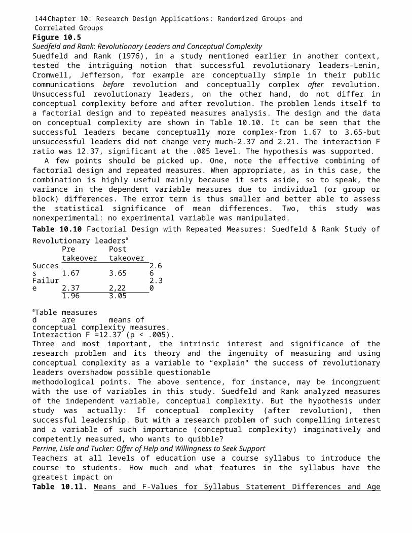
144Chapter 10: Research Design Applications: Randomized Groups andCorrelated GroupsFigure 10.5Suedfeld and Rank: Revolutionary Leaders and Conceptual ComplexitySuedfeld and Rank (1976), in a study mentioned earlier in another context,tested the intriguing notion that successful revolutionary leaders-Lenin,Cromwell, Jefferson, for example are conceptually simple in their publiccommunications before revolution and conceptually complex after revolution.Unsuccessful revolutionary leaders, on the other hand, do not differ inconceptual complexity before and after revolution. The problem lends itself toa factorial design and to repeated measures analysis. The design and the dataon conceptual complexity are shown in Table 10.10. It can be seen that thesuccessful leaders became conceptually more complex-from 1.67 to 3.65-butunsuccessful leaders did not change very much-2.37 and 2.21. The interaction Fratio was 12.37, significant at the .005 level. The hypothesis was supported.
A few points should be picked up. One, note the effective combining offactorial design and repeated measures. When appropriate, as in this case, thecombination is highly useful mainly because it sets aside, so to speak, thevariance in the dependent variable measures due to individual (or group orblock) differences. The error term is thus smaller and better able to assessthe statistical significance of mean differences. Two, this study wasnonexperimental: no experimental variable was manipulated.Table 10.10 Factorial Design with Repeated Measures: Suedfeld & Rank Study ofRevolutionary leadersa
Pre Posttakeover takeover
Success 1.67 3.65
2.66
Failure 2.37 2,22
2.30
1.96 3.05aTabled
measuresare means of
conceptual complexity measures.Interaction F =12.37 (p < .005).Three and most important, the intrinsic interest and significance of theresearch problem and its theory and the ingenuity of measuring and usingconceptual complexity as a variable to “explain" the success of revolutionaryleaders overshadow possible questionablemethodological points. The above sentence, for instance, may be incongruentwith the use of variables in this study. Suedfeld and Rank analyzed measuresof the independent variable, conceptual complexity. But the hypothesis understudy was actually: If conceptual complexity (after revolution), thensuccessful leadership. But with a research problem of such compelling interestand a variable of such importance (conceptual complexity) imaginatively andcompetently measured, who wants to quibble?Perrine, Lisle and Tucker: Offer of Help and Willingness to Seek SupportTeachers at all levels of education use a course syllabus to introduce thecourse to students. How much and what features in the syllabus have thegreatest impact onTable 10.1l. Means and F-Values for Syllabus Statement Differences and Age
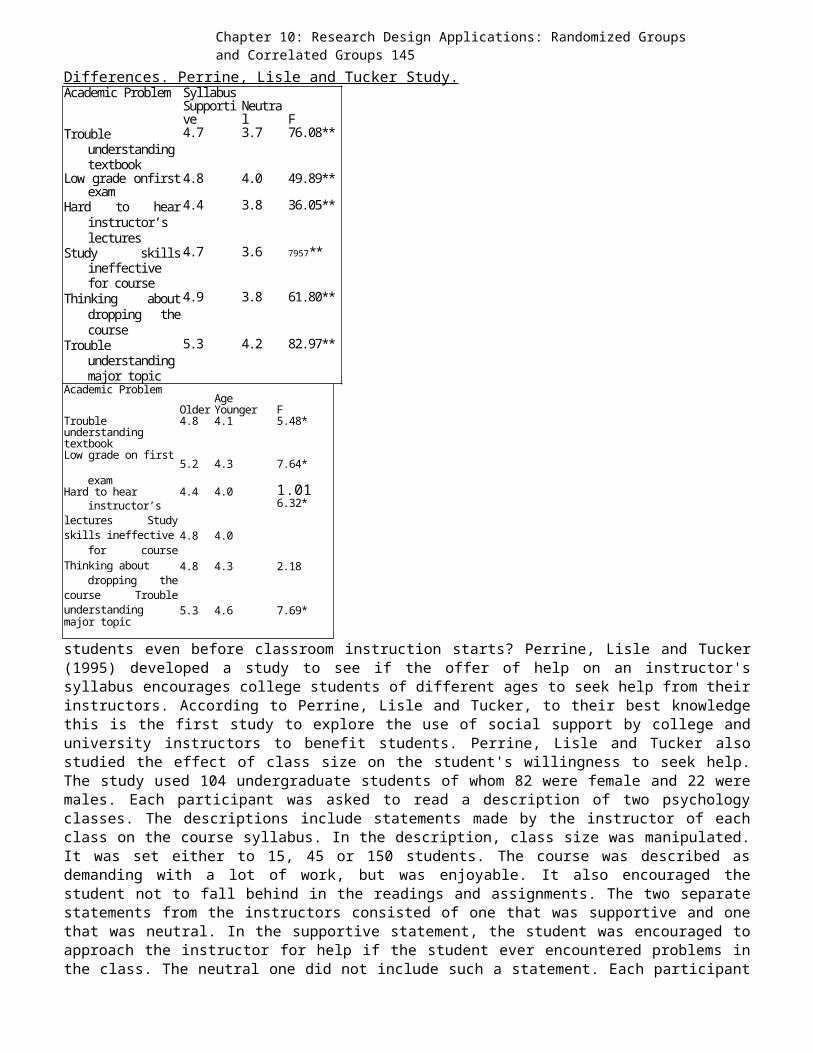
Chapter 10: Research Design Applications: Randomized Groups and Correlated Groups 145
Differences. Perrine, Lisle and Tucker Study.Academic Problem Syllabus
Supportive
Neutral F
Troubleunderstandingtextbook
4.7 3.7 76.08**
Low grade onfirstexam
4.8 4.0 49.89**
Hard to hearinstructor’slectures
4.4 3.8 36.05**
Study skillsineffectivefor course
4.7 3.6 7957**
Thinking aboutdropping thecourse
4.9 3.8 61.80**
Troubleunderstandingmajor topic
5.3 4.2 82.97**
Academic ProblemOlder
AgeYounger F
Troubleunderstanding
4.8 4.1 5.48*textbookLow grade on first 5.2 4.3 7.64*
examHard to hear 4.4 4.0 1.01
instructor’slectures Studyskills ineffective 4.8 4.0
6.32*
for courseThinking about 4.8 4.3 2.18
dropping thecourse Troubleunderstanding 5.3 4.6 7.69*major topic
students even before classroom instruction starts? Perrine, Lisle and Tucker(1995) developed a study to see if the offer of help on an instructor'ssyllabus encourages college students of different ages to seek help from theirinstructors. According to Perrine, Lisle and Tucker, to their best knowledgethis is the first study to explore the use of social support by college anduniversity instructors to benefit students. Perrine, Lisle and Tucker alsostudied the effect of class size on the student's willingness to seek help.The study used 104 undergraduate students of whom 82 were female and 22 weremales. Each participant was asked to read a description of two psychologyclasses. The descriptions include statements made by the instructor of eachclass on the course syllabus. In the description, class size was manipulated.It was set either to 15, 45 or 150 students. The course was described asdemanding with a lot of work, but was enjoyable. It also encouraged thestudent not to fall behind in the readings and assignments. The two separatestatements from the instructors consisted of one that was supportive and onethat was neutral. In the supportive statement, the student was encouraged toapproach the instructor for help if the student ever encountered problems inthe class. The neutral one did not include such a statement. Each participant
146Chapter 10: Research Design Applications: Randomized Groups andCorrelated Groupsread both descriptions. After reading the descriptions, the participantresponded to questions about their willingness to seek help from theinstructor for six possible academic problems encountered in the class. Thesix problems were (1) trouble understanding textbook, (2) low grade on firstexam, (3) hard to hear instructor’s lectures, (4) study skills ineffective forcourse, (5) thinking of dropping the course and (6) trouble understandingmajor topic. The participant used a 6 point rating scale: 0 = definitely no to6 = definitely yes.
The design was a 3 x 2 x 2 (class size x syllabus statement x student age)factorial design. The design contained one manipulated (active) independentvariable, one measured (attribute) independent variable and one within-subjects (correlated) independent variable. Class size was the randomized andmanipulated dependent variable. Student age was the measured independentvariable and syllabus statement was the correlated independent variable. Usingthe appropriate analysis of variance (usually referred to as mixed anova whenat least one independent variable is between subjects and at least one otheris within- subjects) participants expressed significantly more willingness toseek help from the instructor when the supportive statement appeared on thecourse syllabus than when only the neutral statement appeared.*p<.05, **p<.01
Younger students under the age of 25) expressed less willingness than olderstudents. There was also an age x syllabus interaction (F = 4.85, p < .05)that was significant. The response to the offer of help was different betweenage groups. The statements affected younger students less than older students.Class size did not appear to be a significant factor on whether students werewilling to seek help or not. Table 10.11 presents the summary statistics forthe study.ANALYSIS OF COVARIANCEThe invention of the analysis of covariance by Ronald Fisher was an importantevent in behavioral research methodology. Here is a creative use of thevariance principles common to experimental design and to correlation andregression theory-which we study later in the book-to help solve a long-standing control problem.
Analysis of covariance is a form of analysis of variance that tests thesignificance of the differences among means of experimental groups aftertaking into account initial differences among the groups and the correlationof the initial measures and the dependent variable measures. That is, analysisof covariance analyzes the differences between experimental groups on Y, thedependent variable, after taking into account either initial differencesbetween the groups on Y (pretest), or differences between the groups in somepotential independent variable or variables, X, substantially correlated withY, the dependent variable. The measure used as a control variable-the pretestor pertinent variable is called a covariate.
The reader should be cautious when using the analysis of covariance. It isparticularly sensitive to violations of its assumptions. The potential misuseof this method was of such concern that the journal of Biometrics in 1957devoted an entire issue to it. Elashoff (1969) wrote an important article foreducational researchers on the use of this method. The consensus is that it isgenerally not a good idea to use this method for nonexperimental research
Chapter 10: Research Design Applications: Randomized Groups and Correlated Groups 147
designs.Clark and Walberg: Massive Reinforcement and Reading AchievementThere is little point to describing the statistical procedures andcalculations of analysis of covariance. First, in their conventional form,they are complex and hard to follow. Second, we wish here only to convey themeaning and purpose of the approach. Third and most important, there is a mucheasier way to do what analysis of covariance does. Later in the book we willsee that analysis of covariance is a special case of multiple regression andis much easier to do with multiple regression. To give the reader a feelingfor what analysis of covariance accomplishes, let us look at an effective useof the procedure in educational and psychological studies
Clark and Walberg (1968) thought that their participants, potential schooldropouts doing poorly in school, needed far more reinforcement (encouragement,reward, etc.) than participants doing well in school. So they used massivereinforcement with their experimental group participants and moderatereinforcement with their control group participants. Since their dependentvariable, reading achievement, is substantially correlated with intelligence,they also needed to control intelligence. A one-way analysis of variance ofthe reading achievement means of the experimental and control groups yieldedan F of 9.52, significant at the .01 level, supporting their belief. It isconceivable, however, that the difference between the experimental and controlgroups was due to intelligence rather than to reinforcement. That is, eventhough the S's were assigned at random to the experimental groups, an initialdifference in intelligence in favor of the experimental group may have beenenough to make the experimental group reading mean significantly greater thanthe control group reading mean, since intelligence is substantially correlatedwith reading. With random assignment, it is unlikely to happen, but it canhappen. To control this possibility, Clark and Walberg used analysis ofcovariance.Table 10.12 Analysis of Covariance Paradigm, Clark and Walberg StudyExperimental (Massive Reinforcement)X Y(Intelligence) (Reading) Means 92.05 31.62Control
(Moderate Reinforcement)XY(Intelligenc (Reading)e)___________________90.73 26.86
Study Table 10.4, which shows in outline the design and analysis. The meansof the X and Y scores, as reported by Clark and Walberg, are given at thebottom of the table. The Y means are the main concern. Theywere significantly different. Although it is doubtful thatthe analysis of covariance will change this result, it is possible that thedifference between the X means, 92.05 and 90.73, may have tipped thestatistical scales, in the test of the difference between the Y means, infavor of the experimental group. The analysis of covariance F test, which usesY sums of squares and mean squares purged of the influence of X, wassignificant at the .01 level: F = 7.90. Thus the mean reading scores of theexperimental and control groups differed significantly, after adjusting or
148Chapter 10: Research Design Applications: Randomized Groups andCorrelated Groupscontrolling for intelligence.Taris: Locus of Control, Situations and Driving Behavior.This study by Taris (1997) uses a rather unusual design. This is a 2 x 2 x 2 x2 factorial with two covariates. All four of the independent variables in thisstudy were within-subject factors. Taris' study examines the extentsituational and personality factors influences driving behavior of youngadults. The study's four within factors are (1) desirability {2)verifiability, (3} scenario and (4) controllability. The covariates are locusof control and annual mileage. Annual mileage was used as a measure of drivingexperience. Locus of control is a personality measure. Each participantreceived descriptions of four situations in which Controllability andVerifiability were systematically manipulated. High controllability wasgenerally in the form of a statement where the participant was at ease, "withplenty of time." Low controllability meant a situational statement where theparticipant is in a hurry to get somewhere. High verifiability generally meantsomeone was watching,i. e. "an area heavily patrolled by police," or "passenger in the car." Ineach situation there are two scenarios. One scenario asked for a decision onthe speed at which one was driving and the other involved a decision to eitherstop or not stop for a red traffic light. In each scenario there is adesirable and an undesirable course of action. Taris presented the situations,scenarios and actions in random order.
An example of a low controllability, high verifiability condition createdby Taris is
"You are driving home after work. The traffic israther dense. You are aware that the police often
patrol the area. The meeting at your job took more time than you expected. Nowyou will be late for the home match of your volleyball team in which you aredrafted. Your team counts on you." (p. 990).An example of high controllability and low verifiability would read:"You are driving home after work. The traffic is rather dense. You are awarethat the police seldom patrol the area. You left your job at the usual time.Tonight you will play a home match with your volleyball team in which you aredrafted. Your team counts on you " (p. 990}.As mentioned previously, there are two scenarios. One scenario deals withobeying speed laws and the other deals with stopping at a red light. For eachscenario there is a desirable or undesirable action. From Taris' example, thiswould be a statement such as "You drive on. At times you exceed the speedlimit," versus " You drive on. Nowhere do you exceed the speed limit."
The dependent variable is a probability judgment regarding the likelihoodthat one would engage in that particular action. Results showed a DesirabilityEffect (F = 532.21, p < .001). Desirable actions were considered more likelythan undesirable ones. This shows that youthful drivers are not likely to actin an undesirable way. The significant interaction between Desirability andVerifiability (F = 4.22, p < .05) states that undesirable actions were morelikely if verifiability was low. The interaction between Controllability andDesirability was not significant. So Taris was unable to state thatundesirable behavior would be more likely to occur when controllability waslow. The interaction between Verifiability and Locus of Control (F = 8.42, p <
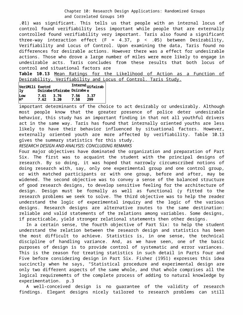
Chapter 10: Research Design Applications: Randomized Groups and Correlated Groups 149
.01) was significant. This tells us that people with an internal locus ofcontrol found verifiability less important while people that are externallycontrolled found verifiability very important. Taris also found a significantthree-way interaction effect (F = 4.37, p < .05) between Desirability,Verifiability and Locus of Control. Upon examining the data, Taris found nodifferences for desirable actions. However there was a effect for undesirableactions. Those who drove a large number of miles were more likely to engage inundesirable acts. Taris concludes from these results that both locus ofcontrol and situational factors areTable 10.13 Mean Ratings for the Likelihood of Action as a Function ofDesirability, Verifiability and Locus of Control. Taris Study.VeriMilily
ExetrdDsirabeUfairabe
InterndDsirabe
Uifairabe
Low 7.61 3.76 7.56 3.37H* 7.62 3.20 7.58 299important determinants of the choice to act desirably or undesirably. Althoughmost people know that the greater presence of police deter undesirablebehavior, this study has an important finding in that not all youthful driversact in the same way. Taris has found that internally oriented youths are lesslikely to have their behavior influenced by situational factors. However,externally oriented youth are more affected by verifiability. Table 10.13gives the summary statistics for this study.RESEARCH DESIGN AND ANALYSIS: CONCLUDING REMARKSFour major objectives have dominated the organization and preparation of PartSix. The first was to acquaint the student with the principal designs ofresearch. By so doing, it was hoped that narrowly circumscribed notions ofdoing research with, say, only one experimental group and one control group,or with matched participants or with one group, before and after, may bewidened. The second objective was to convey a sense of the balanced structureof good research designs, to develop sensitive feeling for the architecture ofdesign. Design must be formally as well as functional (y fitted to theresearch problems we seek to solve. The third objective was to help the readerunderstand the logic of experimental inquiry and the logic of the variousdesigns. Research designs are alternative routes to the same destination:reliable and valid statements of the relations among variables. Some designs,if practicable, yield stronger relational statements then other designs.
In a certain sense, the fourth objective of Part Six: to help the studentunderstand the relation between the research design and statistics has beenthe most difficult to achieve. Statistics is, in one sense, the technicaldiscipline of handling variance. And, as we have seen, one of the basicpurposes of design is to provide control of systematic and error variances.This is the reason for treating statistics in such detail in Parts Four andFive before considering design in Part Six. Fisher (1951) expresses this ideasuccinctly when he says, "Statistical procedure and experimental design areonly two different aspects of the same whole, and that whole comprises all thelogical requirements of the complete process of adding to natural knowledge byexperimentation.” p.3
A well-conceived design is no guarantee of the validity of researchfindings. Elegant designs nicely tailored to research problems can still
150Chapter 10: Research Design Applications: Randomized Groups andCorrelated Groupsresult in wrong or distorted conclusions. Nevertheless, the chances ofarriving at accurate and valid conclusions are better with sound designs thanwith unsound ones. This is relatively sure: if design is faulty, one can cometo no clear conclusions. If, for instance, one uses a two-group, matched-subjects design when the research problem logically demands a factorialdesign, or if one uses a factorial design when the nature of the researchsituation calls for a correlated-groups design, no amount of interpretative orstatistical manipulation can increase confidence in the conclusions of suchresearch.
It is fitting that. Fisher (1951) should have the last word on thissubject. In the first chapter of his book, The Design of Experiments, he said:If the design of an experiment is faulty, any method of interpretation thatmakes it out to be decisive must be faulty too. It is true that there are agreat many experimental procedures which are well designed that may lead todecisive conclusions? However, on other occasions they may fail to do so. Insuch cases, if decisive conclusions are in fact drawn when they areunjustified, we may say that the fault is wholly in the interpretation, not inthe design. But the fault of interpretation. . . lies in overlooking thecharacteristic features of the design which lead to the result being sometimesinconclusive, or conclusive on some questions but not on all. To understandcorrectly the one aspect of the problem is to understand the other. (p. 3)Study SuggestionsRandomized Groups
1.In studying research design, it is useful to do analyses of variance-asmany as possible: simple oneway analyses and two-variable factorial analyses.Try even a three-variable analysis. By means of this statistical work you canget a better understanding of the designs. You may well attach variable namesto your "data," rather than work with numbers alone. Some useful suggestionsfor projects with random numbers follow.
(a} Draw three groups of random numbers 0 through 9. Name the independentand dependent variables. Express a hypothesis and translate it into design-statistical language. Do a one-way analysis of variance. Interpret.
(b) Repeat 1 (a) with five groups of numbers.(c) Now increase the numbers of one of your groups by 2, and decrease
those of another group by 2. Repeat the statistical analysis.(d) Draw four groups of random numbers, 10 in each group. Set them up,
at random, in a 2x2 factorial design. Do a factorial analysis of variance.(e) Bias the numbers of the two right-hand cells by adding 3 to each
number. Repeat the analysis. Compare with the results of 1(d).(f) Bias the numbers of the data of 1 (d}, as follows: add 2 to each of
the numbers in the upper left and lower right cells. Repeat the analysis.Interpret.
2.Look up Study Suggestion 2 and 3, Chapter 14. Work through both examplesagain. (Are they easier for you now?)
3. Suppose that you are the principal of an elementary school. Some of thefourth- and fifth grade teachers want to dispense with workbooks. Thesuperintendent does not like the idea, but is willing to let you test thenotion that workbooks do not make much difference. (One of the teachers evensuggests that workbooks may have bad effects on both teachers and pupils.) Set
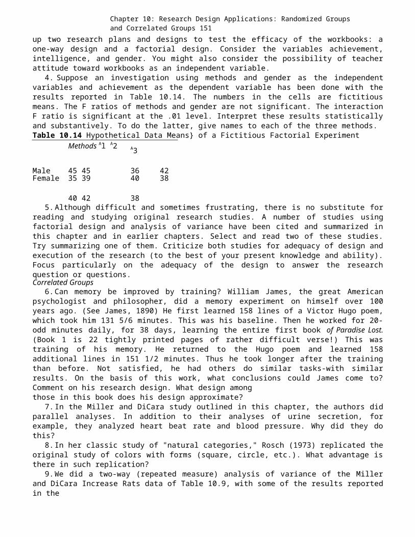
Chapter 10: Research Design Applications: Randomized Groups and Correlated Groups 151
up two research plans and designs to test the efficacy of the workbooks: aone-way design and a factorial design. Consider the variables achievement,intelligence, and gender. You might also consider the possibility of teacherattitude toward workbooks as an independent variable.
4. Suppose an investigation using methods and gender as the independentvariables and achievement as the dependent variable has been done with theresults reported in Table 10.14. The numbers in the cells are fictitiousmeans. The F ratios of methods and gender are not significant. The interactionF ratio is significant at the .01 level. Interpret these results statisticallyand substantively. To do the latter, give names to each of the three methods.Table 10.14 Hypothetical Data Means} of a Fictitious Factorial Experiment
Methods Al A2 A3
Male 45 45 36 42Female 35 39 40 38
40 42 385.Although difficult and sometimes frustrating, there is no substitute for
reading and studying original research studies. A number of studies usingfactorial design and analysis of variance have been cited and summarized inthis chapter and in earlier chapters. Select and read two of these studies.Try summarizing one of them. Criticize both studies for adequacy of design andexecution of the research (to the best of your present knowledge and ability).Focus particularly on the adequacy of the design to answer the researchquestion or questions.Correlated Groups
6.Can memory be improved by training? William James, the great Americanpsychologist and philosopher, did a memory experiment on himself over 100years ago. (See James, 1890) He first learned 158 lines of a Victor Hugo poem,which took him 131 5/6 minutes. This was his baseline. Then he worked for 20-odd minutes daily, for 38 days, learning the entire first book of Paradise Lost.(Book 1 is 22 tightly printed pages of rather difficult verse!) This wastraining of his memory. He returned to the Hugo poem and learned 158additional lines in 151 1/2 minutes. Thus he took longer after the trainingthan before. Not satisfied, he had others do similar tasks-with similarresults. On the basis of this work, what conclusions could James come to?Comment on his research design. What design amongthose in this book does his design approximate?
7.In the Miller and DiCara study outlined in this chapter, the authors didparallel analyses. In addition to their analyses of urine secretion, forexample, they analyzed heart beat rate and blood pressure. Why did they dothis?
8.In her classic study of "natural categories," Rosch (1973) replicated theoriginal study of colors with forms (square, circle, etc.). What advantage isthere in such replication?
9.We did a two-way (repeated measure) analysis of variance of the Millerand DiCara Increase Rats data of Table 10.9, with some of the results reportedin the
152Chapter 10: Research Design Applications: Randomized Groups andCorrelated Groupstable. (a2 (Hays omega-squared) was .357 a2 for the Decrease Rats datawas .663. What do these coefficients mean? Why calculate them?
10.Kolb (1965), basing his work on the outstanding work of McClelland onachievement motivation, did a fascinating experiment with underachieving highschool boys of high intelligence. Of 57 boys, he assigned 20 at random to atraining program in which, through various means; the boys were "taught"achievement motivation (an attempt to build a need to achieve into the boys).The boys were given a pretest of achievement motivation in the summer, andgiven the test again six months later. The mean change scores were, forexperimental and control groups, 6.72 and -. 34, respectively. These weresignificant at the .005 level.
(a) Comment on the use of change scores. Does their use lessen our faith inthe statistical significance of the results?(b) Might factors other than the experimental training have induced the
change?11. Lest the student believe that only continuous measures are analyzed and
that analysis of variance alone is used in psychological and educationalexperiments, read the study by Freedman, Wallington and Bless (1967) onguilt and compliance. There was an experimental group (S's induced to lie)and a control group. The dependent variable was measured by whether aparticipant did or did not comply with a request for help. The results werereported in crosstabulation frequency tables. Read the study, and, afterstudying the authors' design and results, design one of the threeexperiments another way. Bring in another independent variable, forinstance. Suppose that it was known that there were wide individualdifferences in compliance. How can this be controlled? Name and describetwo kinds of design to do it.
12. One useful means of control by matching is to use pairs of identicaltwins. Why is this method a useful means of control? If you were setting upan experiment to test the effect of environment on measured intelligenceand you had 20 pairs of identical twins and complete experimental freedom,how would you set up the experiment?
13. In a study in which training on the complexities of art stimuli affectedattitude toward music, among other things, Renner (1970 used analysis ofcovariance, with the covariate being measures from a
scale designed to measure attitude toward music. This was a pretest. Therewere three experimental groups. Sketch the design from this brief description.Why did Renner use the music attitude scale as a pretest? Why did she useanalysis of covariance? (Note: The original report is well worth reading. Thestudy, in part a study of creativity, is itself creative.)14. In a significant study of the effect of liberal arts education on
complex concept formation, inter and McClelland (1978) found the differencebetween senior and freshmen of a liberal arts college on measure of complexconcept formation to be statistically significant (Ms = 2.00, Mf = 1.22; t =
3.76 (p < .001). Realizing that a comparison was needed, they also testedsimilar mean differences in a teachers college and in a community college.Neither of these differences was statistically significant. Why did Winter andMcClelland test the relation in the teachers college and in the communitycollege? It is suggested that students look up the original report-it is well
Chapter 10: Research Design Applications: Randomized Groups and Correlated Groups 153
worth study-and do analysis of variance from the reported n's, means, andstandard deviations, using the method outlined in Chapter 13 (Addendum).15. One virtue of analysis of covariance seldom mentioned in texts is that
three estimates of the correlation between X and Y can be calculated. Thethree are the total r over all the scores, the between- groups r, which isthe r between the X and Y means, and the within-groups r, the r calculatedfrom an average of the r's between X and Y within the k groups. The within-groups r is the "best" estimate of
the "true" r between X and Y. Why is this so?[Hint: Can a total r, the one usually calculated in practice, be inflated or
deflated by between-groups variance?]16. The 2 x 2 x 2 factorial design is used a good deal by social
psychologists. Here are two unusual, excellent, even creative studies inwhich it was used:
Aronson, E. & Gerard E. (1966). Beyond Parkinson's law: The effect of excesstime on subsequent performance. Journal of Personality and Social Psychology, 3, 336-339.
Carlsmith, J. & Gross, A (1969). Some effects of guilt on compliance. Journal ofPersonality and Social Psychology, 11, 232-239.
The following article of Martin's uses a 2 x 3 x 5 and a 2 x 2 x 5 designs.Martin, R. {1998). Majority and minority influence using the afterimage
paradigm: A series of attempted replications. Journal of Experimental SocialPsychology, 34, 1-26.
Read one of these studies.Chapter Summary1. Randomized subjects designs are the preferred designs of behavioral
research.2. Randomized subjects designs are true experiments with active, manipulated
independent variables.3. The usual statistical method to analyze data from randomized subjects
designs is analysis of variance.4. Randomized subject designs usually require a large number of participants
to achieve the desired precision.5. Correlated subjects designs usually involvea) using the same participants in each treatment conditionb) matching participants on one or more independent variables related tothe dependent variablec) using more than one group of participants, i.e., classrooms.6. Units can be different kinds of entities. In psychological research, unitsare usually people or animals7. Correlated subjects designs include the one group repeated trials(measures) design.8. Design 9.2 is the better design to use when participants are matched andrandomly assigned totreatment groups.9. A covariate is a potential independent variable used to adjust for the
individual differences between groups that are not due to the treatment.Pretests are the most common covariates.
10.Analysis of covariance is a correlated subjects method of statistical

154Chapter 10: Research Design Applications: Randomized Groups andCorrelated Groups
analysis. A covariate adjusts the dependent variable, then the adjustedvalues are used in an analysis of variance. Multiple regression is anotherstatistical method one can use for this purpose.

134Chapter 10: Research Design Applications: Randomized Groups and CorrelatedGroups
Chapter 11: Quasi Experimental and N = 1 Designs of Research 135
Chapter 11Quasi Experimental and N = 1 Designs of ResearchVARIANTS OF BASIC DESIGNSDesigns 9.1 through 9.6 are the basic experimental designs. Some variants ofthese designs have already been indicated. Additional experimental and controlgroups can be added as needed, but the core ideas remain the same. It isalways wise to consider the possibility of adding experimental and controlgroups. Within reason, the addition of such groups provides more validatingevidence for the study’s hypotheses. This design was a combination of twoother basic designs. It combined the strengths of both and adding replicationpower, as well as further controls. Such advantages lead to the principlethat, whenever we consider a research design, we should consider thepossibility of adding experimental groups as replications or variants ofexperimental and control groups. One of the major goals of science is to findcausal relations. The true experiment (“true here is taken to mean amanipulated independent variable where a causal statement is possible) ifarranged and executed correctly can provide the researcher with a causalstatement concerning the relation between X and Y. This is generallyconsidered the highest form of experimentation. The weakening of thecomponents of the true experiment is what we will discuss in this chapter.Compromise Designs a.k.a. Quasi Experimental Designs
It is possible, indeed necessary, to use designs that are compromises withtrue experimentation. Recall that true experimentation requires at least twogroups, one receiving an experimental treatment and one not receiving thetreatment or receiving it in different form. The true experiment requires themanipulation of at least one independent variable, the random assignment ofparticipants to groups, and the random assignment of treatments to groups.When one or more of these prerequisites is missing for one reason or another,we have a compromise design. Compromise designs are popularly known as quasi-experimental designs. They are called quasi because quasi means “almost” or“sort of.” Cook and Campbell (1979) presented two major classifications ofquasi-experimental design. The first is called the “non-equivalent controlgroup designs” and the second is the “interrupted time series designs.” Anumber of research studies performed outside of the laboratory could fall intothis category. Many marketing research studies are in the form ofquasiexperimental designs. Often a researcher is asked to “design” and analyzethe data from a study that was unplanned. For example, a grocery buyer decidesto stock a different brand of baby food. Her superiors may later ask if such amove was profitable. This buyer would then consult with a market researcher todetermine what can be done to show whether her decision was a profitable oneor not. Such analyses would not have the niceties of random selection andassignment and it would consist of data taken over time. Additionally, otherads or the season of the year could influence the baby food sales. The onlycomponent resembling a true experiment is the fact that the independentvariable was manipulated. Not all stores received the different baby foodproduct. With such problems, the researcher would turn to the use ofquasiexperimental or compromise research designs.Nonequivalent Control Group Design

136 Chapter 11: Quasi Experimental and N = 1 Designs of ResearchPerhaps the most commonly used quasi-experimental design is the experimentalgroup-control pattern in which one has no clear assurance that theexperimental and control groups are equivalent. Some such as Cook and Campbell(1979), Christensen (1996), Ray (1997) and Graziano & Raulin (1993) refer toit as the nonequivalent control group design. Cook and Campbell present eightvariations of this design that they state are “interpretable.” The eight are•no-treatment control group designs •nonequivalent dependent variables designs•removed treatment group designs •repeated treatment designs•reversed treatment nonequivalent control group design•cohort designs•posttest only designs •regression continuity designsIn this book we will discuss in detail only one of these. This one is the most likelyone to occur in the research literature in some shape and form. For a thoroughdiscussion of these eight types of non-equivalent control group designs one shouldread Cook and Campbell (1979).No-treatment Control Group DesignThe structure of the no-treatment control group design has already been considered inDesign 9.3. Cook and Campbell (1979) refers to this design as the untreated controlgroup design with pretest and posttest. The compromise form is as follows:Design 11.1: No-treatment Control Group DesignYb X Ya (Experimental)Yb ~X Ya (Control)The difference between Designs 9.3 and 11.1 is sharp. In Design 11.1, there is norandomized assignment of participants to groups, as in 9.3(a), and no matching ofparticipants and then random assignment, as in 9.3(b). Design 11.1, therefore, issubject to the weaknesses due to the possible lack of equivalence between the groupsin variables other than X. Researchers commonly take pains to establish equivalenceby other means, and to the extent they are successful in doing so, to this extent thedesign is valid. This is done in ways discussed below.
It is often difficult or impossible to equate groups by random selection or randomassignment, or by matching. Should one then give up doing the research? By no means.Every effort should be made, first, to select and to assign at random. If both ofthese are not possible, perhaps matching and random assignment can be accomplished.If they are not, an effort should be made at least to use samples from the samepopulation or to use samples as alike as possible. The experimental treatments shouldbe assigned at random. Then the similarity of the groups should be checked using anyinformation available sex, age, social class, and so on.The equivalence of the groups could be verified using the means and standarddeviations of the pretests: t tests and F tests will do. The distributions shouldalso be checked. Although one cannot have the assurance that randomization gives, ifthese items all check out satisfactorily, one can go ahead with the study knowing atleast that there is no known evidence against the equivalence assumption.
These precautions increase the possibilities of attaining internal validity. Thereare still difficulties, all of which are subordinate to one main difficulty, calledselection. (These other difficulties will not be discussed here. For detaileddiscussion, see the Campbell and Stanley, 1963 or Cook & Campbell, 1979).
Selection is one of the difficult and troublesome problems of behavioral research.Since its aspects will be discussed in detail in Chapter 23 on nonexperimentalresearch, only a brief description will be given here. One of the important reasons
137 Chapter 11: Quasi Experimental and N = 1 Designs of Researchfor the emphasis on random selection and assignment is to avoid the difficulties ofselection. When participants are selected into groups on bases extraneous to theresearch purposes, we call this "selection," or alternatively, "selfselection." Takea common example: let us assume that volunteers are used in the experimental groupand other participants are used as controls. If the volunteers differ in acharacteristic related to Y, the dependent variable, the ultimate difference betweenthe experimental and control groups may be due to this characteristic rather than toX, the independent variable. Volunteers, for instance, may be more intelligent (orless intelligent) than nonvolunteers. If we were doing an experiment with some kindof learning as the dependent variable, obviously the volunteers might perform betteron Y because of superior intelligence, despite the initial likeness of the two groupson the pretest. Note that, if we had used only volunteers and had assigned them toexperimental and control groups at random, the selection difficulty is lessened.External validity or representativeness, however, would be decreased.
Cook and Campbell (1979) claim that even in very extreme cases, it is stillpossible to draw strong conclusions if all the threats to validity are considered andaccounted for. Without the benefit of random assignment, attempts should be madethrough other means to eliminate rival hypotheses. We consider only the design thatuses the pretest because the pretest could provide useful information concerning theeffectiveness
Chapter 11: Quasi Experimental and N = 1 Designs of Researchof the independent variable on the dependent variable. The pretest could provide data
on how equal the groups are to each other prior to administering treatment to theexperimental group.
Another more frequent example in educational research is to take some schoolclasses for the experimental group and others for the control group. If a fairlylarge number of classes are selected and assigned at random to experimental andcontrol groups, there is no great problem. But if they are not assigned at random,certain ones may select themselves into the experimental groups, and these classesmay have characteristics that predispose them to have higher mean Y scores than theother classes. For example, their teachers may be more alert, more intelligent, andmore aggressive. These characteristics interact with the selection to produce,irrespective of X, higher experimental group than control group Y scores. In otherwords, something that influences the selection processes, as do the volunteerparticipants, also influences the dependent variable measures. This happens eventhough the pretest may show the groups to be the same on the dependent variable. TheX manipulation is "effective," but it is not effective in and of itself. It iseffective because of selection, or selfselection. Additionally, an educationalresearcher may have to receive the school district’s approval for research. At times,the district will assign the school and the classroom that a research may use.
A classic study by Sanford and Hemphill (1952) reported in Campbell and Stanley(1963) used this design. This study was conducted at the United States Naval Academyat Annapolis. This study was done to see if a psychology course in the curriculumincreased the students’ (midshipmen) confidence in social situations. The second-yearclass took the psychology course. The second-year midshipmen were the first group ofstudents to take the psychology course. The comparison or control group was thethird-year class. The third year students did not take the course in their secondyear. A social situation questionnaire was administered to both classes at thebeginning of the academic year and at the end of the year. The results showed anincrease in confidence scores for the second year class from 43.26 to 51.42. Thethird-year class also showed an increase. However, their increase was considerablysmaller changing from 55.80 to 56.78. One might conclude from these data that takingthe137psychology course did have an effect of increasing confidence in social situations.However, other explanations are also possible. One could explain that the greatergains made by the second-year class were the result of some maturational developmentthat has its largest growth in the second year with a smaller growth in the thirdyear. If such a process exists, the larger score increase for the second-year classwould have occurred even if the midshipmen had not taken the psychology class. Thefact that the second year class started with a lower score than the third year classmight indicate that these students had not yet reached an equivalent level to thethird year class. Plus, the end-of- year scores of the second year class were notequivalent to the beginning scores for the third year class. A better and strongerdesign would be to create two equivalent groups from the second-year class throughrandom selection and give at random the psychology class to one of them.Possible outcomes from this design are given in Figure 11.1. There is the possibilityof a different interpretation on causality depending on which outcome the researcherobtains. In almost all of the cases the most likely threat to internal validity wouldbe the selection-maturation interaction. You might recall that this interactionoccurs when the two groups are different to begin with as measured by the posttest.Then one of the groups experience greater differential changes such as getting moreexperienced, more accurate, more tired, etc. than the other group. The difference
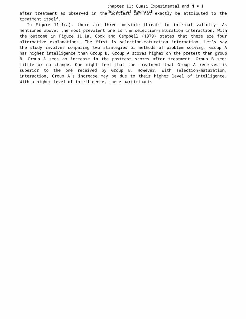
Chapter 11: Quasi Experimental and N = 1 Designs of Researchafter treatment as observed in the posttest can not exactly be attributed to the
treatment itself.In Figure 11.1(a), there are three possible threats to internal validity. As
mentioned above, the most prevalent one is the selection-maturation interaction. Withthe outcome in Figure 11.1a, Cook and Campbell (1979) states that there are fouralternative explanations. The first is selection-maturation interaction. Let’s saythe study involves comparing two strategies or methods of problem solving. Group Ahas higher intelligence than Group B. Group A scores higher on the pretest than groupB. Group A sees an increase in the posttest scores after treatment. Group B seeslittle or no change. One might feel that the treatment that Group A receives issuperior to the one received by Group B. However, with selection-maturation,interaction, Group A’s increase may be due to their higher level of intelligence.With a higher level of intelligence, these participants
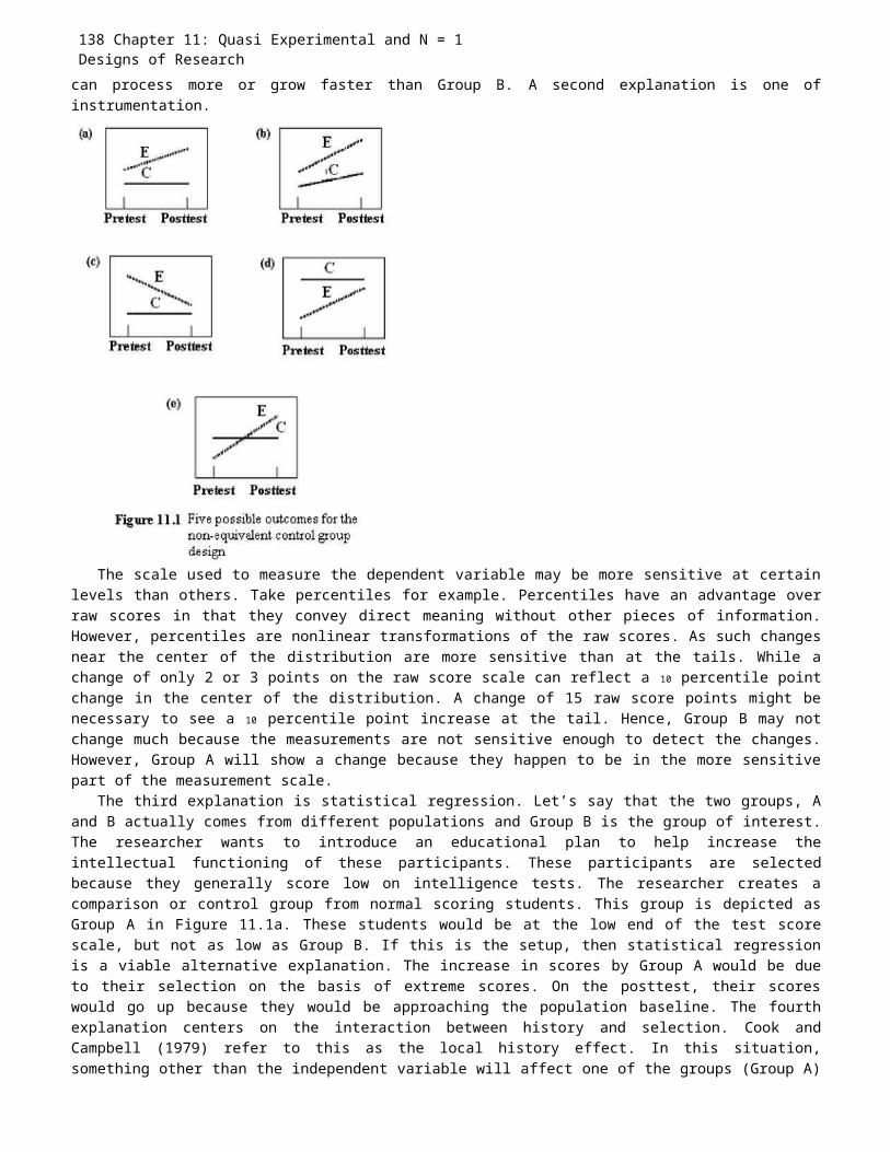
138 Chapter 11: Quasi Experimental and N = 1 Designs of Researchcan process more or grow faster than Group B. A second explanation is one ofinstrumentation.
The scale used to measure the dependent variable may be more sensitive at certainlevels than others. Take percentiles for example. Percentiles have an advantage overraw scores in that they convey direct meaning without other pieces of information.However, percentiles are nonlinear transformations of the raw scores. As such changesnear the center of the distribution are more sensitive than at the tails. While achange of only 2 or 3 points on the raw score scale can reflect a 10 percentile pointchange in the center of the distribution. A change of 15 raw score points might benecessary to see a 10 percentile point increase at the tail. Hence, Group B may notchange much because the measurements are not sensitive enough to detect the changes.However, Group A will show a change because they happen to be in the more sensitivepart of the measurement scale.
The third explanation is statistical regression. Let’s say that the two groups, Aand B actually comes from different populations and Group B is the group of interest.The researcher wants to introduce an educational plan to help increase theintellectual functioning of these participants. These participants are selectedbecause they generally score low on intelligence tests. The researcher creates acomparison or control group from normal scoring students. This group is depicted asGroup A in Figure 11.1a. These students would be at the low end of the test scorescale, but not as low as Group B. If this is the setup, then statistical regressionis a viable alternative explanation. The increase in scores by Group A would be dueto their selection on the basis of extreme scores. On the posttest, their scoreswould go up because they would be approaching the population baseline. The fourthexplanation centers on the interaction between history and selection. Cook andCampbell (1979) refer to this as the local history effect. In this situation,something other than the independent variable will affect one of the groups (Group A)
139 Chapter 11: Quasi Experimental and N = 1 Designs of Researchand not the other (Group B). Let’s say a market researcher wanted to determine theeffectiveness of an ad for soup starters. Sales data are gathered before and afterintroducing the ad. If two groups are used where they are from different regions ofthe country, the growth in sales seen by one of the groups (A) may not be necessarilydue to the ad. Let us say one group is from southern California and the other is inthe Midwestern United States. Both groups may have similar purchasing behavior duringthe spring and summer, i.e., not a great deal of need for soup starters. However, asthe fall season approaches, the sale of soup starters may increase for the group inthe Midwest. In southern California, where the temperatures are considerably warmerall year around, the demand for soup starters would remain fairly constant. So herethe explanation would be the season of the year and not the ad.
All of the threats mentioned for Figure 11.1a is also true for Figure 11.1b. Whilein Figure 11.1a one of the groups (Group B) remains constant, in Figure 11.1b, bothgroups experience an increase from pretest to posttest. Selection-maturation is stilla possibility since by definition the groups are growing (or declining) at adifferent rate where the lower scoring group (Group C) progresses at a lower ratethan the high scoring group (Group T). To determine if selection-maturation isplaying a main role for the results, Cook and Campbell (1979) recommends two methods.The first involves looking at only the data for the experimental group (Group T). Ifthe within group variance for the posttest is considerably greater than the within-group variance of the pre-test, then there is evidence of a selection- maturationinteraction. The second method is to
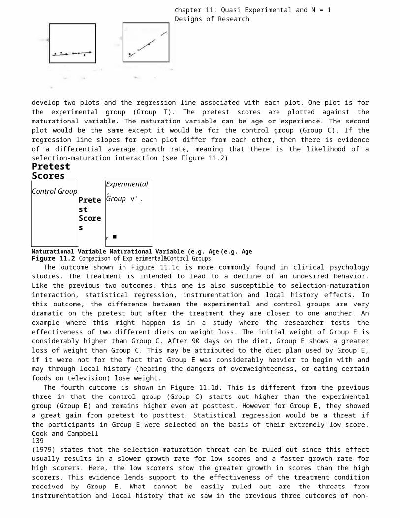
Chapter 11: Quasi Experimental and N = 1 Designs of Research
develop two plots and the regression line associated with each plot. One plot is forthe experimental group (Group T). The pretest scores are plotted against thematurational variable. The maturation variable can be age or experience. The secondplot would be the same except it would be for the control group (Group C). If theregression line slopes for each plot differ from each other, then there is evidenceof a differential average growth rate, meaning that there is the likelihood of aselection-maturation interaction (see Figure 11.2)PretestScoresControl Group
Experimental,
Pretest
Group v'.
Scores
Jr ■Maturational Variable Maturational Variable (e.g. Age (e.g. AgeFigure 11.2 Comparison of Exp erimental&Control Groups
The outcome shown in Figure 11.1c is more commonly found in clinical psychologystudies. The treatment is intended to lead to a decline of an undesired behavior.Like the previous two outcomes, this one is also susceptible to selection-maturationinteraction, statistical regression, instrumentation and local history effects. Inthis outcome, the difference between the experimental and control groups are verydramatic on the pretest but after the treatment they are closer to one another. Anexample where this might happen is in a study where the researcher tests theeffectiveness of two different diets on weight loss. The initial weight of Group E isconsiderably higher than Group C. After 90 days on the diet, Group E shows a greaterloss of weight than Group C. This may be attributed to the diet plan used by Group E,if it were not for the fact that Group E was considerably heavier to begin with andmay through local history (hearing the dangers of overweightedness, or eating certainfoods on television) lose weight.
The fourth outcome is shown in Figure 11.1d. This is different from the previousthree in that the control group (Group C) starts out higher than the experimentalgroup (Group E) and remains higher even at posttest. However for Group E, they showeda great gain from pretest to posttest. Statistical regression would be a threat ifthe participants in Group E were selected on the basis of their extremely low score.Cook and Campbell139(1979) states that the selection-maturation threat can be ruled out since this effectusually results in a slower growth rate for low scores and a faster growth rate forhigh scorers. Here, the low scorers show the greater growth in scores than the highscorers. This evidence lends support to the effectiveness of the treatment conditionreceived by Group E. What cannot be easily ruled out are the threats frominstrumentation and local history that we saw in the previous three outcomes of non-
Chapter 11: Quasi Experimental and N = 1 Designs of Researchequivalent control group designs.
With the final outcome shown in Figure 11.1e, the means of the experimental (GroupE) and control (Group C) groups are significantly different from one another at bothpretest and posttest. However, the differences are in the reverse direction in theposttest than in the pretest. The trend lines cross over one another. Group Einitially starts low but then overtakes Group C who initially scored high. Cook andCampbell (1979) found this outcome to be more interpretable than the previous four.Instrumentation or scaling is ruled out because no transformation of the scores couldremove or reduce this cross-over or interaction effect. Statistical regressionbecomes untenable because it is extremely rare that a low score can regress enough toovertake an initially high score. Other than a very complicated selection-maturationinteraction effect, this pattern is not akin to selection-maturation threats.Maturation for example does not generally start off different, meet and then growsapart in the opposite direction. Hence, outcome 11.1e seems to be the strongest onethat would enable the researcher to make a causal statement concerning treatment.Cook and Campbell, however, warn that researchers should not plan on developingquasi-experimental research in the hopes of obtaining this outcome. Definitely, thedesigning of a nonequivalent control group study should be done with care andcaution.Research ExamplesNelson, Hall and Walsh-Bowers: Non-Equivalent Control Group Design.The research study by Nelson, Hall and Walsh-Bowers (1997) specifically state thatthey used a non equivalent control group design to compare the long term effects ofsupportive apartments (SA), group homes (GH) and board-and-care homes (BCH) forpsychiatric residents.
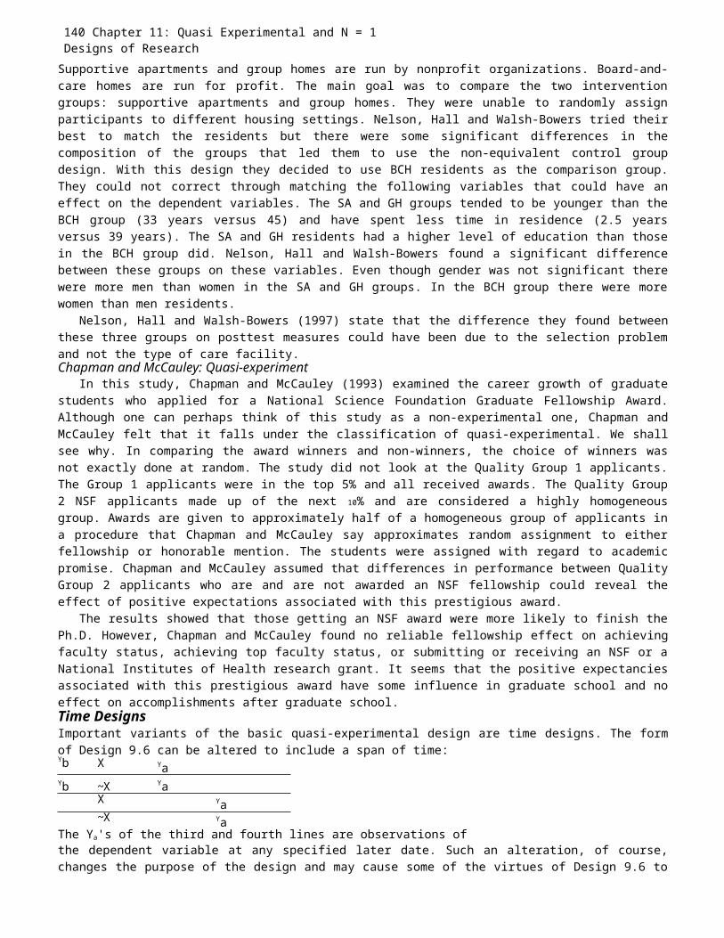
140 Chapter 11: Quasi Experimental and N = 1 Designs of ResearchSupportive apartments and group homes are run by nonprofit organizations. Board-and-care homes are run for profit. The main goal was to compare the two interventiongroups: supportive apartments and group homes. They were unable to randomly assignparticipants to different housing settings. Nelson, Hall and Walsh-Bowers tried theirbest to match the residents but there were some significant differences in thecomposition of the groups that led them to use the non-equivalent control groupdesign. With this design they decided to use BCH residents as the comparison group.They could not correct through matching the following variables that could have aneffect on the dependent variables. The SA and GH groups tended to be younger than theBCH group (33 years versus 45) and have spent less time in residence (2.5 yearsversus 39 years). The SA and GH residents had a higher level of education than thosein the BCH group did. Nelson, Hall and Walsh-Bowers found a significant differencebetween these groups on these variables. Even though gender was not significant therewere more men than women in the SA and GH groups. In the BCH group there were morewomen than men residents.
Nelson, Hall and Walsh-Bowers (1997) state that the difference they found betweenthese three groups on posttest measures could have been due to the selection problemand not the type of care facility.Chapman and McCauley: Quasi-experiment
In this study, Chapman and McCauley (1993) examined the career growth of graduatestudents who applied for a National Science Foundation Graduate Fellowship Award.Although one can perhaps think of this study as a non-experimental one, Chapman andMcCauley felt that it falls under the classification of quasi-experimental. We shallsee why. In comparing the award winners and non-winners, the choice of winners wasnot exactly done at random. The study did not look at the Quality Group 1 applicants.The Group 1 applicants were in the top 5% and all received awards. The Quality Group2 NSF applicants made up of the next 10% and are considered a highly homogeneousgroup. Awards are given to approximately half of a homogeneous group of applicants ina procedure that Chapman and McCauley say approximates random assignment to eitherfellowship or honorable mention. The students were assigned with regard to academicpromise. Chapman and McCauley assumed that differences in performance between QualityGroup 2 applicants who are and are not awarded an NSF fellowship could reveal theeffect of positive expectations associated with this prestigious award.
The results showed that those getting an NSF award were more likely to finish thePh.D. However, Chapman and McCauley found no reliable fellowship effect on achievingfaculty status, achieving top faculty status, or submitting or receiving an NSF or aNational Institutes of Health research grant. It seems that the positive expectanciesassociated with this prestigious award have some influence in graduate school and noeffect on accomplishments after graduate school.Time DesignsImportant variants of the basic quasi-experimental design are time designs. The formof Design 9.6 can be altered to include a span of time:Yb X YaYb ~X Ya
X Ya~X Ya
The Ya's of the third and fourth lines are observations ofthe dependent variable at any specified later date. Such an alteration, of course,changes the purpose of the design and may cause some of the virtues of Design 9.6 to

141 Chapter 11: Quasi Experimental and N = 1 Designs of Researchbe lost. We might, if we had the time, the patience, and the resources, retain allthe former benefits and still extend in time by adding two more groups to Design 9.6itself.
A common research problem, especially in studies of the development and growth ofchildren, involves the study of individuals and groups using time as a variable. Suchstudies are longitudinal studies of participants, often children, at different pointsin time. One such design among many might be:Y1 y2 Y3 Y4 X Y5 Y6 Y7 00
Design 11.2: A Longitudinal Time Design (a.k.a. Interrupted Time Series Design)
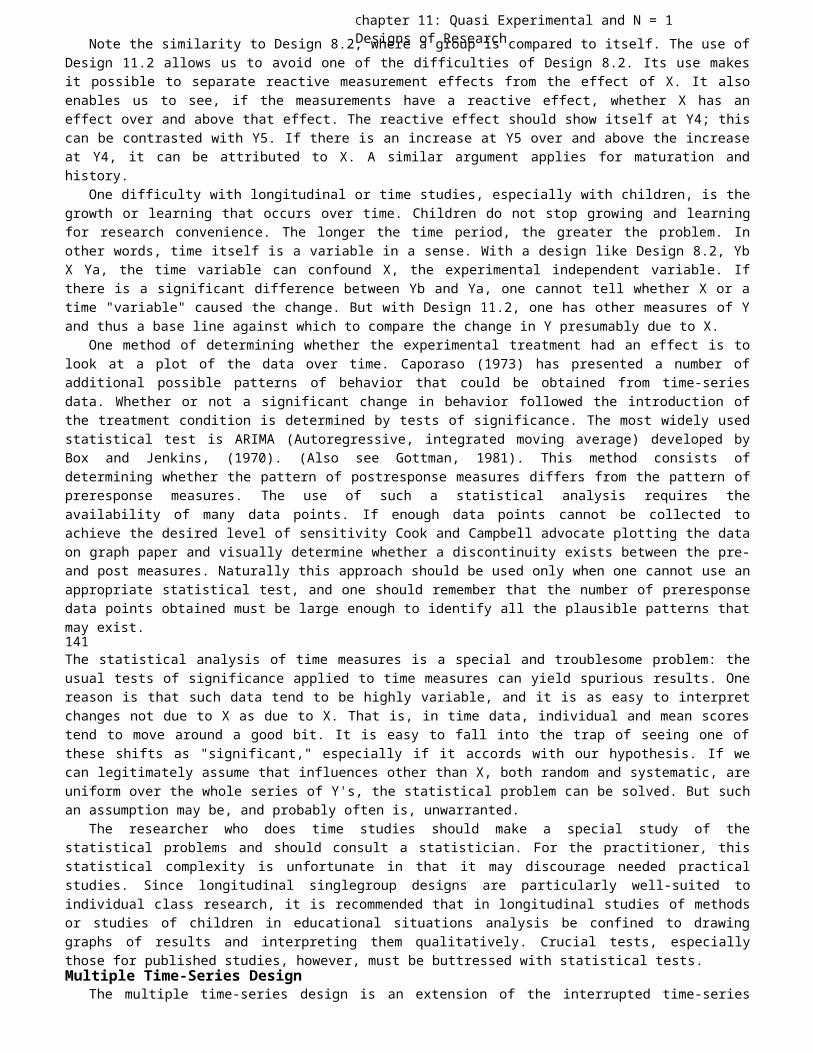
Chapter 11: Quasi Experimental and N = 1 Designs of ResearchNote the similarity to Design 8.2, where a group is compared to itself. The use of
Design 11.2 allows us to avoid one of the difficulties of Design 8.2. Its use makesit possible to separate reactive measurement effects from the effect of X. It alsoenables us to see, if the measurements have a reactive effect, whether X has aneffect over and above that effect. The reactive effect should show itself at Y4; thiscan be contrasted with Y5. If there is an increase at Y5 over and above the increaseat Y4, it can be attributed to X. A similar argument applies for maturation andhistory.
One difficulty with longitudinal or time studies, especially with children, is thegrowth or learning that occurs over time. Children do not stop growing and learningfor research convenience. The longer the time period, the greater the problem. Inother words, time itself is a variable in a sense. With a design like Design 8.2, YbX Ya, the time variable can confound X, the experimental independent variable. Ifthere is a significant difference between Yb and Ya, one cannot tell whether X or atime "variable" caused the change. But with Design 11.2, one has other measures of Yand thus a base line against which to compare the change in Y presumably due to X.
One method of determining whether the experimental treatment had an effect is tolook at a plot of the data over time. Caporaso (1973) has presented a number ofadditional possible patterns of behavior that could be obtained from time-seriesdata. Whether or not a significant change in behavior followed the introduction ofthe treatment condition is determined by tests of significance. The most widely usedstatistical test is ARIMA (Autoregressive, integrated moving average) developed byBox and Jenkins, (1970). (Also see Gottman, 1981). This method consists ofdetermining whether the pattern of postresponse measures differs from the pattern ofpreresponse measures. The use of such a statistical analysis requires theavailability of many data points. If enough data points cannot be collected toachieve the desired level of sensitivity Cook and Campbell advocate plotting the dataon graph paper and visually determine whether a discontinuity exists between the pre-and post measures. Naturally this approach should be used only when one cannot use anappropriate statistical test, and one should remember that the number of preresponsedata points obtained must be large enough to identify all the plausible patterns thatmay exist.141The statistical analysis of time measures is a special and troublesome problem: theusual tests of significance applied to time measures can yield spurious results. Onereason is that such data tend to be highly variable, and it is as easy to interpretchanges not due to X as due to X. That is, in time data, individual and mean scorestend to move around a good bit. It is easy to fall into the trap of seeing one ofthese shifts as "significant," especially if it accords with our hypothesis. If wecan legitimately assume that influences other than X, both random and systematic, areuniform over the whole series of Y's, the statistical problem can be solved. But suchan assumption may be, and probably often is, unwarranted.
The researcher who does time studies should make a special study of thestatistical problems and should consult a statistician. For the practitioner, thisstatistical complexity is unfortunate in that it may discourage needed practicalstudies. Since longitudinal singlegroup designs are particularly well-suited toindividual class research, it is recommended that in longitudinal studies of methodsor studies of children in educational situations analysis be confined to drawinggraphs of results and interpreting them qualitatively. Crucial tests, especiallythose for published studies, however, must be buttressed with statistical tests.Multiple Time-Series Design
The multiple time-series design is an extension of the interrupted time-series

Chapter 11: Quasi Experimental and N = 1 Designs of Researchdesign. With the interrupted time series design, only one group of participants was
used. As a result, alternative explanations can come from a history effect. Themultiple time-series design has the advantage of eliminating the history effect byincluding a control group comprised of an equivalent-or at least comparable-group ofparticipants that does not receive the treatment condition. This is shown in Design11.3. In this design one experimental group receives the treatment condition and thecontrol group does not. Consequently, the design offers a greater degree of controlover sources of alternative explanations or rival hypotheses. The history effects,for example, are controlled because they would influence the experimental and controlgroups equally.

142 Chapter 11: Quasi Experimental and N = 1 Designs of ResearchDesign 113: AMitipe Tine-Series DesignY1 y2 y3 y4 X y5 y6 y7 y8
Experimental
Y1 y2y3 y4 y5 y6
y7 y8 CentralNaturally, there are other possible variations of Design 11.2 besides Design 11.3.
One important variation is to add one or more control groups; another is to add moretime observations. Still another is to add more X's, more experimental interventions.(see Gottman, 1981; Gottman, McFall & Barnett, 1969; Campbell & Stanley, 1963).Single Subject Experimental Designs
The majority of today’s behavioral research involves using groups of participants.However, there are other approaches. In this section we deal with strategies forachieving control in experiments using one or a few participants. These singlesubject designs are sometimes referred to as the N = 1 design. Single subject designsare an extension of the interrupted time- series design. Where the interrupted timeseries generally looks at a group of individuals over time, e.g. children, the singlesubject study uses only one participant or at most a few participants. Even when afew participants are used, each is studied individually and extensively. These willalso be called single subject designs or studies. . Although they have differentnames, they all share the following characteristics:Only one or a few participants are used in the studyEach subject participates in a number of trials (repeated measures). This is similar
to the within- participants designs described in Chapter 10.Randomization (i.e., random assignment and/or random selection) procedures are hardly
ever used. The repeated measurements or time intervals are instead assigned atrandom to the different treatment conditions.
These designs observe the organism's behavior before the experimental treatment andused as a baseline measure. The observations after the treatment are then comparedwith these baseline observations. The participant serves as his or her owncontrol. These designs are usually applied in school, clinical, andcounseling research. They are used to evaluate the effects of behavioral
interventions. This mode of research is popular among those that do operant learningexperiments or behavior modification. Research using single participants is not new.There were some such as Gustav Fechner, who developed the discipline of psychophysicsin the 1860s using only two participants: himself and his brother-inlaw. Fechner iscredited with inventing the basic psychophysical methods that are still used today tomeasure sensory thresholds. Fechner heavily influenced Hermann Ebbinghaus, who isknown for his experimental work on memory. He also used himself as his own subject.Wilhelm Wundt, who is credited with founding the first psychological laboratory in1879, conducted experiments measuring various psychological and behavioral responsesin individual participants. Finally, I. P. Pavlov did his pioneering work oninstrumental conditioning using individual dogs. The list of psychologists usingsingle participants is extensive with most of them occurring before 1930 and theadvent of R.A. Fisher and William Sealy Gossett’s work in modern statistics
Behavioral scientists doing research before the development of modern statisticsattempted to solve the problem of reliability and validity by making extensiveobservations and frequent replication of results. This is a traditional procedureused by researchers doing single-subject experiments. The assumption is thatindividual participants are essentially equivalent and that one should studyadditional participants only to make certain that the original subject was within thenorm.

143 Chapter 11: Quasi Experimental and N = 1 Designs of Research
The popularity of Fisher’s work on analysis of variance and Gossett’s work on theStudent’s t-test led the way for group oriented research methodology. Some claim thatthese works were so popular that the single-subject tradition nearly became extinct.In fact, even in today’s world, there are hiring practices at major universities thatdepend on whether the candidate is a group-oriented research scientist or a single-participants design oriented researcher. Despite the popularity of Fisher’s methodsand group oriented research, certain psychologists continued to work in the singlesubject tradition The most notable of these was Burrus Frederick Skinner. Skinnerrefrained from using inferential statistics. He does not advocate the use of complexof inferential statistics. Skinner feels that one
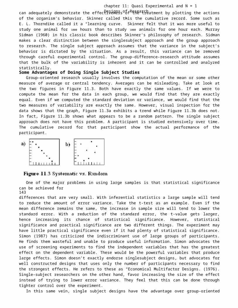
Chapter 11: Quasi Experimental and N = 1 Designs of Researchcan adequately demonstrate the effectiveness of the treatment by plotting the actions
of the organism's behavior. Skinner called this the cumulative record. Some such asE. L. Thorndike called it a “learning curve.” Skinner felt that it was more useful tostudy one animal for 1000 hours than to study 1000 animals for one hour each. MurraySidman (1960) in his classic book describes Skinner's philosophy of research. Sidmanmakes a clear distinction between the singlesubject approach and the group approachto research. The single subject approach assumes that the variance in the subject’sbehavior is dictated by the situation. As a result, this variance can be removedthrough careful experimental control. The group-difference-research attitude assumesthat the bulk of the variability is inherent and it can be controlled and analyzedstatistically.Some Advantages of Doing Single Subject Studies
Group-oriented research usually involves the computation of the mean or some othermeasure of average or central tendency. Averages can be misleading. Take at look atthe two figures in Figure 11.3. Both have exactly the same values. If we were tocompute the mean for the data in each group, we would find that they are exactlyequal. Even if we computed the standard deviation or variance, we would find that thetwo measures of variability are exactly the same. However, visual inspection for thedata shows that the graph, Figure 11.3a exhibits a trend while Figure 11.3b does not.In fact, Figure 11.3b shows what appears to be a random pattern. The single subjectapproach does not have this problem. A participant is studied extensively over time.The cumulative record for that participant show the actual performance of theparticipant.
One of the major problems in using large samples is that statistical significancecan be achieved for143differences that are very small. With inferential statistics a large sample will tendto reduce the amount of error variance. Take the t-test as an example. Even if themean difference remains the same, the increase in sample size will tend to lower thestandard error. With a reduction of the standard error, the t-value gets larger,hence increasing its chance of statistical significance. However, statisticalsignificance and practical significance are two different things. The experiment mayhave little practical significance even if it had plenty of statistical significance.Simon (1987) has criticized the indiscriminant use of large groups of participants.He finds them wasteful and unable to produce useful information. Simon advocates theuse of screening experiments to find the independent variables that has the greatesteffect on the dependent variable. These would be the powerful variables that producelarge effects. Simon doesn’t exactly endorse singlesubject designs, but advocates forwell constructed designs that uses only the number of participants necessary to findthe strongest effects. He refers to these as “Economical Multifactor Designs. (1976).Single-subject researchers on the other hand, favor increasing the size of the effectinstead of trying to lower error variance. They feel that this can be done throughtighter control over the experiment.
In this same vein, single subject designs have the advantage over group-oriented
Chapter 11: Quasi Experimental and N = 1 Designs of Researchdesigns in that with only a few participants they can test different treatments. In
other words, they can determine the effectiveness or the ineffectiveness of atreatment intervention without employing a larger number of participants.
With single-subject studies, the researcher can avoid some of the ethical problemsthat face group- oriented researchers. One such ethical problems concerns the controlgroup. In some situations, the control group does not receive any real treatment.Although in most of the studies done today the participants in the control group arenot harmed in any way, there is still some ethical questions. Take for example thestudy by Gould and Clum (1995) to determine if self-help with minimal therapistcontact is effective in the treatment of panic disorder. All participants in thisstudy were sufferers of panic attacks. The participants were randomly assigned toeither an experimental or control group. The experimental group received self-helpmaterial. The control “did not receive treatment during the course of theexperiment.”
144 Chapter 11: Quasi Experimental and N = 1 Designs of Research(p. 536). Instead the control group was told that they were on the waiting list fortreatment.
In the study of certain type of individuals, the size of the population is smalland hence it would be difficult to do adequate sampling and obtain enoughparticipants for the study. In fact, the study by Strube (1991) shows that evenrandom sampling tends to fail when using small samples. If there are not enoughparticipants of a certain characteristic available for study, the researcher canconsider single-subject designs instead of abandoning the study. Simon (1987) citesthe attempted study by Adelson & Williams in 1954 concerning the important trainingparameters in pilot training. The study was abandoned because there were too manyvariables to consider and not enough participants. Simon pointed out that the studycould have been done, but not using the traditional group-oriented methodology.Some Disadvantages of using Single-Subject DesignsSingle-subject studies are not without their problems and limitations. Some of thesewill become more apparent when we actually discuss the types of single subjectdesigns. Some of the more general problems with the single subject paradigm areexternal validity. Some find it difficult to believe that the findings from one studyusing one subject (Or maybe three of four) can be generalized to an entirepopulation.
With repeated trial on one participant, one can question whether the treatmentwould be equally effective for a participant who has not experienced previoustreatments. If we are talking about a therapeutic treatment, it may be theaccumulation of sessions that is effective. The person going through the n-th trialcan be a very different person from the one in the first trial. It is here thatgroup-oriented research can eliminate this problem. Each person is given thetreatment once.
Single-subject studies are perhaps even more sensitive to aberrations on the partof the experimenter and participant. These studies are effective only if theresearcher can avoid biases and the participant is motivated and cooperative. Theresearcher can be prone to look only for certain effects and ignore others. Wediscussed earlier in this book about Blondlot. He was the only scientist able to see“N-Rays.” It wasn’t so much that he was a fraud, but that he was biased toward seeingsomething that was not there. A researcher doing single-subject research could beaffected more so than the group-oriented researcher and need to develop a system ofchecks and balances to avoid this pitfall.
A number of research studies are by nature required to follow group-orientedmethods and as such would be ill suited for single subject designs. For example, tostudy the behavior of jury members would require the use of groups and the influenceof group dynamics. In a previous chapter, we discussed the research surroundingJanis’ Groupthink. The study of this important phenomenon was best done with groups,since it was the group as a whole that displayed this phenomenon.SOME SINGLE-SUBJECT RESEARCH PARADIGMSThe Stable Baseline: An Important Goal.
In a group-oriented design one group of participants is compared to anotherdifferent group of participants. Or a group of participants receiving one conditionis compared to the same set of participants receiving a different condition. Weassume that the groups are equal prior to giving treatment so that if the dependentvariable differs after treatment, we can associate that difference to the treatment.The determination of an effective treatment is done by statistically comparing the
145 Chapter 11: Quasi Experimental and N = 1 Designs of Researchdifference between the two groups on some outcome variable. When we use only onesubject, however, a different tactic must be employed. In this one-subject situationwe need to compare the behavior that occurs before and after the introduction of theexperimental intervention. The behavior before the treatment intervention must bemeasured over a long enough time period so that we can obtain a stable baseline. Thisbaseline, or operant level is important because it is compared to later behavior. Ifthe baseline varies considerably, it could be more difficult to assess any reliablechange in behavior following intervention. The baseline problem with single subjectdesigns is an important one. For a complete description of the problems and possiblesolutions one should consult Barlow and Hersen (1976). Another excellent reference isKazdin (1982).
An example where baseline measures are very important is in the use of a polygraph(lie detector). Here, the operator gets physiological measurements of
Chapter 11: Quasi Experimental and N = 1 Designs of Researchthe person (defendant). The person is asked a number of questions where the
participant is asked to give factual information which are known to be true (name,eye color, place of birth, etc.). The responses emitted are recorded and taken as thebaseline measure for answering truthfully. Then another baseline is taken forresponses to untrue statements. These are statements where the participant is told tolie to the question asked. After establishing these two baselines, the question ofimportance (i.e., did you commit the crime?) is asked and compared to the twobaselines. If the physiological response resembles the lie baseline, the participantis told that they have lied.Designs that use the Withdrawal of TreatmentThe ABA Design.The ABA design involves three major steps. The first is to establish a stablebaseline (A). The experimental intervention is applied to the participant in thesecond step (B). If the treatment is effective, there will be a response differencefrom the baseline. In order to determine if the treatment intervention caused thechange in behavior, the researcher exercises step three: a return to baseline (A).The third is required because we don’t know what the response rate would have been ifthe participant received no treatment. We also would like to know whether theresponse change was due to the treatment intervention or something else.
A major problem with the ABA design is that the effect of the intervention may notbe fully reversible. If the treatment involved surgery, where the hypothalamus isremoved or the corpus callosum is severed, it would be impossible to reverse theseprocedures. A learning method that causes some permanent change in a participant’sbehavior would not be reversible.
There are also some ethical concerns about reverting the organism back to theoriginal state if that state was an undesirable behavior (Tingstrom, 1996).Experiments in behavior modification seldom return the participant back to baseline.This return to baseline is called the withdrawal condition. To benefit theparticipant, the treatment is re-introduced. The design that does this is the ABABdesign.Repeating Treatments (ABAB Designs)145There are two versions of the ABAB design. The first was briefly described in thelast section. It is the ABA design except that treatment is re-introduced to theparticipant and the participant leaves the study having achieved some beneficiallevel. Repeating the treatment also provides the experimenter with additionalinformation about the strength of the treatment intervention. By demonstrating thatthe treatment intervention can bring the participant back to the beneficial levelafter taking that person back to baseline lends strength to the statement thattreatment caused the change in behavior, i.e., evidence of internal validity. TheABAB design essentially produces the experimental effect twice.
The second variation of the ABAB design is called the alternating treatmentsdesign. In this variation there is no baseline taken. The A and B in this design aretwo different treatments that are alternated at random. The goal of this design is toevaluate the relative effectiveness of the two treatment interventions. The A and Bmay be two different methods of controlling overeating. The participant is given eachtreatment at different times. Over a period of time, one method might emerge as beingmore effective than the other. The advantage this design has over the first ABABdesign is that there is no baseline to be taken and the participant is not subjectedto withdraw procedures. Since this method involves comparing two sets of series ofdata, some have called it the between-series design.
There are some other interesting variations of the ABAB design where withdrawal ofthe treatment is not done. McGuigan (1996) calls it the ABCB design where in the
Chapter 11: Quasi Experimental and N = 1 Designs of Researchthird phase, the organism is given a “placebo” condition. This placebo condition is
essentially a different methodSingle subject designs are unlike group designs in that they only permit the
researcher to vary one variable at a time. The researcher would not be able todetermine which variable or which combination of variables caused the responsechanges if two or more variables are altered at the same time. The best that anyonecan do is to make a statement that the combination of variables led to the change.However, the researcher won’t be able to tell which one of how much of each. If thereare two variables, called B and C, and the baseline is A, then a possiblepresentation sequence of the conditions would be A-B-A-B-BC-B-BC. In this sequenceevery condition was preceded and proceeded by the same

146 Chapter 11: Quasi Experimental and N = 1 Designs of Researchcondition at least once with only one variable changing at a time.
The A-B-A-B-BC-B-BC design is often called an interaction design. Allpossible combinations of B and C, however, are not presented. Condition C isnever presented alone (A represents the absence of B and C). The interactionhere is different than the interaction discussed in the chapter on factorialdesigns. What is tested by this procedure is whether C adds to the effect ofB.
In a learning experiment using this design, we could examine the effect ofpraising a student for giving the correct answer (C) to a question ongeography along with a merit point (B). If we find that praise plus meritpoint has a greater effect than a merit point alone, we have information thatis useful in designing a learning situation for this and other students.However, we will not know the singular effect of praise. Praise used by itselfmay have been just as effective as the merit point plus praise. Yet, praise byitself may have little or no effect. We can however assess praise bylengthening the single subject design. The sequence would be A-B-A- B-BC-B-BC-C-BC. However, lengthening a single subject experiment of this kind comes withother problems. A subject may become fatigued or disinterested. As a result,too long of a session may not produce useful information even though thedesign looks sound.Some Research Examples.Powell and Nelson: Example of an ABAB design.
This study by Powell and Nelson (1997) involved one participant, Evan, a 7-year-old boy who had been diagnosed with attention deficit hyperactivitydisorder (ADHD). Evan was receiving 15 mg of Ritalin® per day. Most of Evan’sbehavior in the classroom was described as undesirable. Evan also had poorpeer relations and did not understand his schoolwork. The undesirablebehaviors included noncompliance, being away from his desk, disturbing others,staring off, and not doing work. Data were collected on the occurrence ofinteractions between Evan and his teacher.
The treatment intervention was letting Evan choose the class assignments hewanted to work on. There was choice and no-choice conditions. Baseline datawere collected during the no-choice phase. Evan was given the same assignmentas the rest of the class. During the choice phases, the teacher presented Evanwith three different assignments and he chose one to complete. The assignmentchoices were identical in length and difficulty and varied only in content.Evan was not given the same choice of assignments twice.
Powell and Nelson used an ABAB design to evaluate the effects of choicemaking on Evan's undesirable behavior. During the no-choice condition, Evanwas not given a choice of academic assignments. During the choice condition,he was allowed to choose his assignments.
The results showed that during the choice condition, the number ofundesirable behaviors decreased. This study supported the efficacy of choicemaking as an antecedent control technique. These results suggest thateducators attempting to manage the behaviors of students in classrooms may usechoice procedures.Rosenquist, Bodfish, & Thompson: Treating aMentally Retarded Person with Tourette Syndrome.
The treatment of people with Tourette syndrome with a drug called
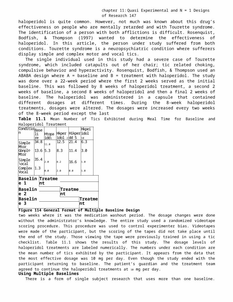
Chapter 11: Quasi Experimental and N = 1 Designs of Research 147
haloperidol is quite common. However, not much was known about this drug’seffectiveness on people who are mentally retarded and with Tourette syndrome.The identification of a person with both afflictions is difficult. Rosenquist,Bodfish, & Thompson (1997) wanted to determine the effectiveness ofhaloperidol. In this article, the person under study suffered from bothconditions. Tourette syndrome is a neuropsychiatric condition where sufferersdisplay simple and complex motor and vocal tics.
The single individual used in this study had a severe case of Tourettesyndrome, which included catapults out of her chair; tic related choking,compulsive behavior and hyperactivity. Rosenquist, Bodfish, & Thompson used anABABA design where A = baseline and B = treatment with haloperidol. The studywas done over a 22-week period where the first 2 weeks served as the initialbaseline. This was followed by 8 weeks of haloperidol treatment, a second 2weeks of baseline, a second 8 weeks of haloperidol and then a final 2 weeks ofbaseline. The haloperidol was administered in a capsule that containeddifferent dosages at different times. During the 8-week haloperidoltreatments, dosages were altered. The dosages were increased every two weeksof the 8-week period except the lastTable 11.1 Mean Number of Tics Exhibited during Meal Time for Baseline andHaloperidol TreatmentCondition Base
lire
Htopaidd1
Hkperidol 2
Hikperdd 5
Hkpeiidol10
SimpleMtor
34.811.0
12.5 21.4 6.3
Gbnpl©Mtor
13.6 5.3 8.3 11.4 3.0
Simple\ocal
35.42.0 8.2 16.6 1.0
ComplexVocal
1.30.0 2.0 0.0 1.0
Baseline 1
Treatment
Baseline 2
Treatment
Baseline 3
Treatment
Figure 114 General Format of Multiple Baseline Designtwo weeks where it was the medication washout period. The dosage changes were donewithout the administrator’s knowledge. The entire study used a randomized videotapescoring procedure. This procedure was used to control experimenter bias. Videotapeswere made of the participant, but the scoring of the tapes did not take place untilthe end of the study. Those viewing the tape were previously trained in using a ticchecklist. Table 11.1 shows the results of this study. The dosage levels ofhaloperidol treatments are labeled numerically. The numbers under each condition arethe mean number of tics exhibited by the participant. It appears from the data thatthe most effective dosage was 10 mg per day. Even though the study ended with theparticipant returning to baseline. The patient’s guardian and the treatment teamagreed to continue the haloperidol treatments at 10 mg per day.Using Multiple Baselines
There is a form of single subject research that uses more than one baseline.
148 Chapter 11: Quasi Experimental and N = 1 Designs of ResearchSeveral different baselines are established before treatment is given to theparticipant. These types of studies are called multiple baseline studies. There arethree classes of multiple baseline research designs.These are multiple baselines: across behaviors across participants across environments
The use of multiple baselines is another approach to demonstrate the effectivenessof a treatment on behavior change. There is a common pattern for implementing allthree classes of this design. That pattern is given in Figure 11.4.
With the multiple baselines across behaviors, the treatment intervention for eachdifferent behavior is introduced at different times. So looking in Figure 11.4, eachbaseline would be a baseline of a different behavior. In the case of an autisticchild, Baseline 1 might be banging one’s head against the wall. Baseline 2 would betalking constantly in different tones and noises and Baseline 3 would be hittingothers. This is done to see if the change in behavior coincides with the treatmentintervention. If one of the behaviors changes while the other behaviors remainconstant or stable at the baseline, the researcher could state that the treatment waseffective for that specific behavior. After a certain period of time has passed, thesame treatment is applied to the second undesirable behavior. Every following behavioris subjected to the treatment in the same stepwise procedure. If the treatmentintervention is effective in changing the response rate of each behavior, one canstate that the treatment is effective.
An important consideration with this particular class of multiple baseline designis that one assumes the responses for each behavior are independent of the responsesfor the other behaviors. The intervention can be considered effective if thisindependence exists. If the responses are in some way correlated, then theinterpretation of the results becomes more difficult.
In the multiple baseline design across participants, the same treatment is appliedin series to the same behavior of different individuals in the same environment. Whenlooking at Figure 11.4, each baseline is for a different participant. Each participantwill receive the same treatment for the same behavior in the same environment. Thestudy by Tingstrom, Marlow, Edwards, Kelshaw and Olmi (1997) is an example of amultiple baseline study across participants.Their compliance-training package is the treatment intervention. This interventionuses time-in (physical touch and verbal praise) and time-out (a coercive procedure) toincrease the rate of student compliance to teachers’ instructions. The behavior ofinterest here is compliance to teachers’ instructions. The environment is theclassroom. The participants of this study were three students: A, B and C, who havedemonstrated noncompliance behavior. All three students havearticulation and language disorders. The design of the study followed the followingintervention phases: baseline, time-in only, time-in/time-out combined and follow-up.Students B and C remained in the baseline phase while the time-in only phase wasimplemented for student A. When Student A showed a change in compliance, the time-inonly phase was implemented for student B while student C remained in baseline. Whenstudent B showed a change in compliance, time- in only was implemented for student C.Tingstrom, Marlow, Edwards, Kelshaw and Olmi was able to demonstrate the effectivenessof the combined time-in and time-out intervention in increasing compliance.
In the multiple baseline design across environments, the same treatment is given todifferent participants who are in different environments. In Figure 11.4, eachbaseline would be for a different participant in a different environment. The
Chapter 11: Quasi Experimental and N = 1 Designs of Research 149
treatment and behavior under study would be the same. Here we may have three differentpatients where each is a resident in a different type of psychiatric care facilitysuch as those studied by Nelson, Hall and Walsh- Bowers (1997) discussed earlier inthis chapter. In this study Nelson, Hall and Walsh-Bowers (1997) compared the long-term effects of supportive apartments (SA), group homes (GH) and board-and-care homes(BCH).Study Suggestions
Look up each of the following studies and determine which ones are quasi-experimental, nonequivalent control group and single subject designs.
Adkins, V. K. & Matthews, R. M. (1997). Prompted voiding to reduce incontinence incommunity-dwelling older adults. Journal of Applied Behavior Analysis, 30, 153-156.
Streufert, S., Satish, U., Pogash, R., Roache, J. & Severs, W. (1997). Excesscoffee consumption insimulated complex work settings: Detriment orfacilitation of performance? Journal of AppliedPsychology, 82, 774-782.
Lee, M. J. & Tingstrom, D. H. (1994). A group math intervention: The modificationof cover, copy, and compare for group application. Psychology in the Schools, 31,133-145.Why is a baseline measure necessary in single subject designs?Should the data from single subject designs be analyzed statistically? Why?Give an example of where a single subject design should be used. Also cite a research
situation where group designs is more appropriate.A university student wants to do a time-series study on the effects of the full moon
on psychiatric patients. What dependent variable should this student use? Whereshould this person look to locate the data for such a study?
Are single-subject studies applicable to medical research? Should medical schoolstudents be taught single subject designs? Read the following article:Bryson-Brockmann, W. and Roll, D. (1996). Single-case experimental designs in
medical education: An innovative research method. Academic Medicine, 71, 78-85.Chapter Summary
True experiments are those where the experimenter can randomly select theparticipants, randomly assign the participants to treatment conditions and control themanipulation of the independent variable. The quasiexperimental design lacks one ormore of these features.
Cook and Campbell (1979) covers 8 variations of the non-equivalent control groupdesign. The one covered here is the no-treatment control group design. Five differentresults are discussed in terms of internal validity.
Time -series designs are longitudinal designs. It involves repeated measurements ofthe same dependent variables at different fixed intervals of time. Usually at somepoint, treatment intervention is introduced.
Selection and selection-maturation interactions are two alternative explanationsthat plague the results obtained from quasi-experimental designs.

150 Chapter 11: Quasi Experimental and N = 1 Designs of Research
Experiments using single participants are not new. The first people inexperimental psychology used single subject designs
In single-subject researchers feel that with proper experimental controlvariability of the situation can be removed.
Group-oriented research feels variability be statistically analyzed.Single-subject research has several advantages over group research in terms of
flexibility and ethics. However it suffers from external validity credibility.Small but statistically significant effects found in group research may have
little clinical or practical significance and may have been artificially inducedby large sample sizes. In this case, the effect size would be small. Singlesubject research concentrates on effect size and not sample size.
The establishment of a stable baseline is one of the most important tasks insingle subject research.
The establishment of a baseline followed by administration of treatmentfollowed by a withdrawal of the treatment is called the ABA design.
A major problem with the design is that the treatment may be irreversible orleaving the participant in the improved state rather than return the person tothe original undesirable state.
A variation of the ABA design is the ABAB design where the participant isrestored to the improved state.
In a single-subject study only one variable can be varied at a time.The so-called interaction design does not permit the testing for an
interaction as defined earlier in factorial designs. It merely examines twovariables jointly.
There are three types of multiple-baseline designs. In each case, theintervention is introduced at different times for different behaviors,participants or environments. If behavior changes coincide with the introductionof treatment, this gives evidence that the treatment is effective.

ReferencesChapter 1Barber, T. X. (1976). Pitfalls in human research: Ten pivotal points. New York: Pergmon Blaser, M.J. (1996). The bacteria behind ulcers. Scientific American, 274, 104-107.Braithwaite, R. (1996). Scientific explanation. Herndon, VA: Books International. (Original work
published in 1953).Bruno, J. E. (1972) (Ed.). Emerging issues in education: Policy implications for the schools. Lexington, MA: Heath Buchler, J. (1955).Philosophical writings of Peirce. New York: Dover.Conant, J. B. (1951). Science and common sense. New Haven: Yale University Press.Dawes, R. M. (1994). House of cards: Psychology and psychotherapy built on myth. New York: The Free Press.Dewey, J. (1991). How we think. Amherst: Prometheus. (Original work published 1933).Graziano, A. M. & Raulin, M. L. (1993). Research methods: A process of inquiry. (2nd Ed.) New York:
Harper Collins.Hergenhahn, B. R. (1996). Introduction to theories of learning. (5th Ed.) Paramus, NJ: Prentice-HallHoch, S. J. (1986). Counterfactual reasoning and accuracy in predicting personal events. Journal
of Experimental Psychology: Learning, Memory, Cognition. 11, 719-731.Hurlock, E. (1925). An evaluation of certain incentives used in schoolwork. Journal of Educational
Psychology, 16, 145-159.Kagan, J. & Zentner, M. (1996). Early childhood predictors of adult psychopathology. HarvardReview of Psychiatry, 3, 341-350. Kerlinger, F. (1977). The influence of research on educationalpractice. Educational Researcher, 16, 5-12.Kerlinger, F. (1979). Behavioral research: A conceptual approach. New York: Holt, Rinehart and
Winston,Klayman, J. & Ha, Y.-W. (1987). Confirmation, disconfirmation and information in hypothesis
testing. Psychological Review, 94, 21-28.Klonoff, E. A. & Landrine, H. (1994). Culture and gender diversity in commonsense beliefs about
the causes of six illnesses. Journal of Behavioral Medicine, 17, 407-418.Lynch, M. P., Short, L. B., & Chua, R. (1995). Contributions of experience to the development of
musical processing in infancy. Developmental Psychobiology, 28, 377-398.Malone, J. C. (1991). Theories of learning: A historical approach. Pacific Grove: Brooks/Cole.Marlow, A. G., Tingstrom, D. H., Olmi, D. J., & Edwards, R. P. (1997). The effects of classroom-
based time-in/time-out on compliance rates in children with speech/language disabilities.Child and Family Behavior Therapy, 19, 1-15.
Michel, J. (1990). An introduction to the logic of psychological measurement. Hillsdale, NJ: Erlbaum.Nisbett, R. & Ross, L. (1980). Human inference: Strategies and shortcomings of social judgment.Englewood-Cliffs, NJ: Prentice Hall Polanyi, M. (1974). Personal knowledge: Toward a post criticalphilosophy. Chicago: University of Chicago Press. (Original work published in 1958).Sampson, E. E. (1991). Social worlds. Personal lives: An introduction to social psychology. Orlando: Harcourt Brace Jovanovich. Schunk,D. H. (1996). Learning theories: An educational perspective. Westerville, OH: Merrill.Simon, C. W. (1976). Economical multifactor designs for human factors engineering experiments. Culver City, CA: Hughes Aircraft
Company, 172 pp.Simon, C. W. (1987). Will egg-sucking ever become a science? Human Factors Society Bulletin, 30, 1-
4.Simon, C. W. & Roscoe, S. N. (1984). Application of a multifactor approach to transfer of
learning research. Human Factors, 26, 591612.Tang, J. (1993). Whites, Asians and Blacks in science and engineering: Reconsideration of their
economic prospects. Research in Social Stratification and Mobility, 12, 289-291.Tingstrom, D. H., Marlow, L. L. G, Edwards, R. P., Kelshaw, K. L., & Olmi, J. D. (1997, April).Evaluation of a compliance training package for children. In S. G. Little (Chair), Behavior schoolpsychology: Time-out revisited. Symposium conducted at the 29th Annual Convention, NationalAssociation of School Psychologists, Anaheim, California Wason, P C., & Johnson-Laird, P N.(1972). Psychology of reasoning: Structure and content. Cambridge, MA: Harvard University Press.Weber, R. L. (1973). A random walk in science: An anthology. New York: Crane Rusak.Wegner, D. M. (1989). White bears and other unwanted thoughts: Suppression, obsession and the psychology of mental control. New York:
Penguin Books.Wegner, D. M., Schneider, D. J., Carter, S. R., & White, T. L. (1987). Paradoxical effects of
thought suppression. Journal of Personality and Social Psychology, 53(1), 5-13.
152
Whitehead, A. N. (1992). An introduction to mathematics. New York: Oxford University Press.(Original work published in 1911).
Wood, R. W. (1973). N rays. In R. L. Weber’s (Ed.) A random walk in science: An anthology. London:Institute of Physics.
Chapter 2Anderson, C. D., Warner, J. L., & Spencer, C. C. (1984). Inflation bias in self-assessment
examinations: Implications for valid employee selection. Journal of Applied Psychology, 69, 574-580.
Ayres, T. & Hughes, P. (1986). Visual acuity with noise and music at 107 dbA. Journal of AuditoryResearch, 26, 65-74.
Bahrick, H. P. (1984). Semantic memory content in permastore: Fifty years of memory for Spanishlearned in school. Journal of Experimental Psychology: General, 113, 1-26.
Bahrick, H. P. (1992). Stabilized memory of unrehearsed knowledge. Journal of ExperimentalPsychology: General, 121, 112-113.
Berkowitz, L (1983).Aversively stimulated aggression: Some parallels and differences in researchwith humans and animals. American Psychologist, 38,1135-1144.
Bollen, K. (1980). Issues in the comparative measurement of political democracy. AmericanSociological Review, 45, 370-390.
Braithwaite, R. (1996). Scientific explanation. Herndon, VA: Books International. (Original workpublished in 1953).
Chamber, B. & Abrami, P. C. (1991). The relationship between student team learning outcomes andachievement, causal attributions and affect. Journal of Educational Psychology, 83, 140-146.
Cochran, S. D. & Mays, V. M. (1994). Depressive distress among homosexually active African-American men and women. American Journal of Psychiatry, 15, 524-529.
Cohen, M. R. (1997). A Preface to logic. New York: Meridian. (Original work published in 1956).Cutler, W. B., Preti, G., Krieger, A. & Huggins, G R. (1986). Human axilliary secretions
influence women’s menstrual cycles: The role of donor extract from men. Hormones and Behavior,20, 463-473.
Dewey, J. (1982). Logic: The theory of inquiry.. New York: Irvington Publishers. (Original workpublished in 1938).
Dill, J.C. & Anderson, C.A. (1995). Effects of frustration justification in hostile aggression.Aggressive-Behavior, 21(5), 359-369.
Dion, K. L. & Cota, A. A. (1991). The Ms. stereotype: Its domain and its role of explicitness intitle preference. Psychology of Women Quarterly, 15, 403-410.
Doctor, R. S., Cutris, D. & Isaacs, G (1994). Psychiatric morbidity in policemen and the effectof brief psychotherapeutic intervention:
A pilot study. Stress Medicine, 10, 151-157.Dollard, J., Doob, L. Miller, N., Mowrer, O. & Sears, R. (1939). Frustration and aggression. New
Haven:Yale University Press.Elbert, J. C. (1993). Occurrence and pattern of impaired reading and written language in children
with ADDS. Annals of Dyslexia, 43, 2643.Fallon, A. & Rozin, P. (1985). Sex differences in perception of desirable body shape. Journal of
Abnormal Psychology, 94, 102-105.Frentz, C., Gresham, F. M. & Elliot, S. N. (1991). Popular, controversial, neglected and rejected
adolescents: Contrasts of social competence and achievement differences. Journal of SchoolPsychology, 29, 109-120.
Glick, P., DeMorest, J. A., & Hotze, C.A. (1988). Keeping your distance. Group membership,personal space and request for small favors. Journal of Applied Social Psychology, 18, 315-330.
Guida, F. V. & Ludlow, L. H. (1989). A cross-cultural study of test anxiety. Journal of Cross-Cultural Psychology, 20, 178-190.
Hall, J. , Kaplan, D. & Lee, H. B. (October, 1994). Counselor-Client matching on ethnic, gender andlanguage: Implications for school psychology. Paper presented at the Annual convention for theAssociation for the Advancement of Behavioral Therapy, San Diego, CA,
Hom, H. L. , Berger, M., Duncan, M. K., Miller, A. & Belvin, A. (1994). The effects ofcooperative and individualistic reward on intrinsic motivation. Journal of Genetic Psychology,155, 87-97.
Hurlock, E. (1925). An evaluation of certain incentives used in schoolwork, Journal of EducationalPsychology. 16, 145-149.
Kleinbaum, D. G., Kupper, L. L., Muller, K. E. & Nizam, A. (1997). Applied regression analysis andother multivariable methods. (3rd ed.) Belmont, CA: Duxbury.
Kumpfer, K. L., Turner, C., Hopkins, R. & Librett, J. (1993). Leadership and team effectivenessin community coalitions for the prevention of alcohol and other drug abuse. Health EducationResearch, 8, 359-374.
Langer, E. & Imber, L. (1980). When practice makes imperfect: Debilitating effects ofoverlearning,
Journal of Personality and Social Psychology, 37, 2014-2024.Lariviere, N. A. & Spear, N. E. (1996). Early Pavlovian conditioning impairs later Pavlovian
conditioning. Developmental Psychobiology, 29, 613-635.Little, S. G, Sterling, R. C., Tingstrom, D. H. (1996). The influence of geographic and racial
cues on evaluation of blame. Journal of Social Psychology, 136, 373-379.MacDonald, T. K., Zanna, M. P. & Fong, G. T. (1996). Why common sense goes out the window:
Effects of alcohol on intentions to use condoms. Personality and Social Psychology Bulletin, 22,763-775.
Moran, J. D., & McCullers, J. C. (1984). A comparison of achievement scores in physicallyattractive and unattractive students. Home Economics Research Journal, 13, 36-40.
Pedersen, D., Keithly, S. & Brady, M. (1986). Effects of an observer on comformity to handwashingnorm. Perceptual and Motor Skills, 62, 169-170.
Poincare, H. (1996). Science and method. Herndon, VA: Books International. (Original work publishedin 1952).
Porch, A. M., Ross, T. P., Hanks, R. & Whitman, D. R. (1995). Ethnicity, socioeconomic backgroundand psychosis-proneness in a diverse sample of college students. Current Psychology:Developmental, Learning, Personality, Social, 13, 365-370.
Reinholtz, R. K. & Muehlenhard, C. L. (1995). Genital perceptions and sexual activity in acollege population. Journal of Sex Research, 32, 155-165.
Rind, B. (1997). Effects of interest arousal on compliance with a request for help. Basic andApplied Social Psychology, 19, 49-59.
Rosch, E. H. (1973). On the internal structure of perceptual and semantic categories. In T. E.Moore (Ed.) Cognitive development and the acquisition of language. (pp. 111-144). New York:Academic Press.
Saal, F. K., Johnson, C. B., Weber, N. (1989). Friendly or sexy: It may depend on whom you ask.Psychology of Women Quarterly, 13, 263-276.
Saal, F. K. & Moore, S. C. (1993). Perceptions of promotion fairness and promotion candidates’qualifications. Journal of Applied Psychology, 78, 105-110.
Shaw, J. I. & Skolnick, P. (1995). Effects of prohibitive and informative judicial instructionson jury decision making. Social Behavior and Personality, 23, 319-325.
Spilich, G J., June, L. & Remer, J. (1992). Cigarette smoking and cognitive performance. BritishJournal of Addiction, 87, 1313-1326.
Stein, J. A., Newcomb, M. D., & Bentler, P. M. (1996). Initiation and maintenance of tobaccosmoking: Changing personality correlates in adolescence and young adulthood. Journal of AppliedSocial Psychology, 26, 160-187.
Stoneberg, C., Pitcock, N. & Myton, C. (1986). Pressure sores in the homebound: One solution ,alternating pressure pads. American Journal of Nursing, 86, 426-428.
Stuart, D. L., Gresham, F. M. & Elliot, S. N. (1991). Teacher rating of social skills in popularand rejected males and females. School Psychology Quarterly, 6, 16-26.
Swanson, E. A., Maas, M. L., & Buckwalter, K. C. (1994). Alzheimer’s residents’ cognitive andfunctional measures: Special and traditional care unit comparison. Clinical Nursing Research, 3,27-41.
Talaga, J. A. & Beehr, T. A. (1995). Are there gender differences in predicting retirementdecisions? Journal of Applied Psychology, 80, 16-28.
Tingstrom, D. H. (1994). The Good Behavior Game: An investigation of teachers’ acceptance.Psychology in the Schools, 31, 57-65.
Tulving, E. & Kroll, N. (1995). Novelty assessment in the brain and long-term memory encoding.
154
Psychonomic Bulletin and Review, 2, 387-390.Wegner, D. M., Schneider, D. J., Carter, S. R., & White, T. L. (1987). Paradoxical effects of
thought suppression. Journal of Personality and Social Psychology, 53, 5-13.Winograd, E. & Soloway, R. (1986). On forgetting the locations of things stored in special
places. Journal of Experimental Psychology: General, 115, 366-372.Zajonc, R. (1980). Feeling and thinking: Preferences need no inferences. American Psychologist, 35,15l-175.Chapter 3.Annis, R. C. & Corenblum, B. (1986). Effect of test language and experimenter race on Canadian
Indian children’s racial and selfidentity. Journal of Social Psychology, 126, 761-773.Bahrick, H. P. (1984). Semantic memory content in permastore: Fifty years of memory for Spanish
learned in school. Journal of Experimental Psychology: General, 113, 1-26.Balzer, W. K. & Sulsky, L. M. (1992). Halo and performance appraisal research: A critical
examination. Journal of Applied Psychology, 77, 975-985.Bandura, A. & MacDonald, F. (1994). Influence of social reinforcement and the behavior of models
in shaping children’s moraljudgments. In B. Paka (Ed.) Defining perspectives in moral development. Moral development: Acompendium, Vol. 1. (pp. 136143). New York: Garland Publications.. (Original work published in1963).Barron, F. & Harrington, D. M. (1981). Creativity, intelligence and personality. Annual Review of
Psychology, 32, 439-476.Bollen, K. (1979). Political democracy and the timing of development. American Sociological
Review, 44, 572-587Capaldi, D. H., Crosby, L. & Stoolmiller, M. (1996). Predicting the timing of first sexual
intercourse for at-risk adolescent males. Child Development, 67, 344-359.Colwell, J. C., Foreman, M. D., & Trotter, J. P. (1993). A comparison of the efficacy and cost-
effectiveness of two methods of managing pressure ulcers. Debubitus, 6(4), 28-36.Comrey, A. L. (1993). EdITS Manual for the Comrey Personality Scales. San Diego, CA: Educational and
Industrial Testing Service.Day, N. E. & Schoenrode, P. (1997). Staying in the closet versus coming out: Relationship between
communication about sexual orientation and work attitudes. Personnel Psychology, 50, 147-163.de Weerth, C. & Kalma, A. F. (1993). Female aggression as a response to sexual jealousy: A sex
role reversal? Aggressive Behavior, 19, 265-279.Doctor, R. S., Cutris, D. & Isaacs, G (1994). Psychiatric morbidity in policemen and the effect
of brief therapeutic intervention. Stress Medicine, 10, 151-157.Eliopoulos, C. (1993). Gerontological nursing, 3rd. Ed. Philadelphia: J. B. Lippincott.Francis-Felsen, L. C., Coward, R. T., Hogan, T. L., & Duncan, R. P. (1996). Factors influencing
intentions of nursing personnel to leave employment in long-term care settings. Journal ofApplied Gerontology, 15, 450-470.
Gillings, V. & Joseph, S. (1996). Religiosity and social desirability: Impression management andself-deceptive positivity. Personality and Individual Differences, 21, 1047-1050.
Gordon, R. A. (1996). Impact of ingratiation on judgment and evaluations: A meta-analyticinvestigation. Journal of Personality and Social Psychology, 71, 54-70.
Gresham, F. M. & Elliot, S. N. (1990). Social skills rating system manual. Circle Pines, MN:American Guidance Service.
Guida, F. V. & Ludlow, L. H. (1989). A cross-cultural study of test anxiety. Journal of Cross-Cultural Psychology, 20, 178-190.
Hart, S. D., Forth, A. E. & Hare, R. D. (1990). Performance of criminal psychopaths on selectedneuropsychological tests. Journal of Abnormal Psychology, 99, 374-379.
Hernstein, R. J. & Murray, C. (1996). The bell curve: Intelligence and class structure in American life. New York: The Free Press.Hodson, R. (1989). Gender differences in job satisfaction: Why women aren’t more dissatisfied.
Sociological Quarterly, 30, 385-399.Hogan, J. & Hogan, R. (1989). How to measure employee reliability. Journal of Applied Psychology,
74, 273-279.Hom, H. L. , Berger, M., Duncan, M. K., Miller, A. & Belvin, A. (1994). The effects of
cooperative and individualistic reward on intrinsic motivation. Journal of Genetic Psychology,155, 87-97.

Hutchinson, S. J. & Turner, J. A. (1988). Developing a multidimensional turnover preventionprogram. Archives of Psychiatric Nursing, 2, 373-378.
Kerlinger, F. N. & Pedhazur, E. (1973). Multiple regression analysis in behavioral research. NewYork: Holt, Rinehart and Winston.
Kounin, J. & Doyle, P (1975). Degree of continuity of a lesson’s signal system and the taskinvolvement of children. Journal of Educational Psychology, 67, 159-164.
Kumar, K. & Beyerlein, M. (1991). Construction and validation of an instrument for measuringingratiatory behaviors in organizational settings. Journal of Applied Psychology, 76, 619-627.
Lester, D. (1989). Attitudes toward AIDS. Personality and Individual Differences, 10, 693-694.Little, S. G., Sterling, R. C. & Tingstrom, D. H. (1996). The influence of geographical and
racial cues on evaluation of blame. Journal of Social Psychology, 136, 373-379.Luhtanen, R. & Crocker, J. (1992). A collective self-esteem scale: Self evaluation of ones’
social identity. Personality and Social Psychology Bulletin, 18, 302-318.Margenau, H. (1977). The nature of physical reality.. Woodbridge, CT : Ox Bow Press. (Original work
published in 1950).Martens, B. K., Hiralall, A. S., & Bradley, T. A. (1997). Improving student behavior through goal
setting and feedback. School Psychology Quarterly, 12, 33-41.Meiksin, P. F. & Watson, J. M. (1989). Professional autonomy and organizational constraint: The
case of engineers. Sociological Quarterly, 30, 561-585.Michel, J. (1990). An introduction to the logic of psychological measurement. Hillsdale, NJ: Erlbaum.Murphy, J. M., Olivier, D. C., Monson, R. R., Sobol, A.M. (1991). Depression and anxiety in
relation to social status: A prospective epidemiological study. Archives of General Psychiatry,48(3), 223-229.
Newcomb, T. (1978). The acquaintance process: Looking mostly backwards. Journal of Personality andSocial Psychology, 36, 10751083.
Norman, D. (1976). Memory and attention: An introduction to human information processing. (2nd Ed.)New York: Wiley.
Northrop, F. (1983). The logic of the sciences and the humanities. Woodbridge, CT: Ox Bow Press.(Original work published in 1947).
Oldani, R. (1997). Causes of increases in achievement motivation: Is the personality influencedby prenatal environment? Personality and Individual Differences, 22, 403-410.
Onwuegbuzie, A. J. & Seaman, M. A. (1995). The effect of two constraints and statistics testanxiety on test performance in a statistics course. Journal of Experimental Education, 63, 115-124.
Orpen, C. (1996). Construct validation of a measure of ingratiatory behavior in organizationalsettings. Current Psychology: Developmental, Learning, Personality, Social, 15(1), 38-41
Oshagan, H. & Allen, R. L. (1992). Three loneliness scales: An assessment of their measurement.Journal of Personality Assessment, 59, 380-409.
Peng, S. S. & Wright, D. (1994). Explanation of academic achievement of Asian-American students.Journal of Educational Research, 87, 346-352.
Richter, M. L. & Seay, M. B. (1987). Anova designs with subjects and stimuli as random effects:Application to prototype effects in recognition memory. Journal of Personality and SocialPsychology, 53, 470-480.
Scott, K. S., Moore, K. S. & Miceli, M. P. (1997). An exploration of the meaning and consequencesof workaholics. Human Relations, 50, 287-314.
Shoffner, L. B. (1990). The effects of home environment on achievement and attitudes towardcomputer literacy. Educational Research Quarterly, 14(1), 6-14.
Silverman, S. (1993). Student characteristics, practice and achievement in physical education.Journal of Educational Research, 87, 5461.
Skinner, B.F. (1945). The operational analysis of psychological terms. Psychological Review, 52,270-277.
Smeltzer, S. C. & Bare, B. G (1992). Brunner and Suddarth’s textbook of medical surgical nursing, 7thed. Philadelphia: J. B. Lippincott.
Somers, M. J. (1996). Modeling employees withdrawal behavior over time: A study of turnover usingsurvival analysis. Journal of Occupational and Organizational Psychology, 69, 315-326.
Steele, C. M., Spencer, S. J. & Lynch, M. (1993). Self-image resilience and dissonance: The role
156
of affirmational resources. Journal of Personality and Social Psychology, 64, 885-896.Strack, F., Martin, L. L., & Stepper, S. (1988). Inhibiting and facilitating conditions of the
human smile: A nonobtrusive test of facial feedback hypothesis. Journal of Personality andSocial Psychology, 54, 768-777.
Strom, B., Hocevar, D. & Zimmer, J. (1990). Satisfaction and achievement antagonists in ATIresearch on student-oriented instruction. Educational Research Quarterly, 14(4), 15-21.
Strutton, D., Pelton, L. E. & Lumpkin, J. R. (1995). Sex differences in ingratiatory behavior: Aninvestigation of influence tactics in the salesperson-customer dyad. Journal of BusinessResearch, 34, 35-45.
Swanson, E. L., Maas, M. L. & Buckwalter, K. C. (1994). Alzheimer’s residents’ cognitive andfunctional measures: Special and traditional care unit comparison. Clinical Nursing Research,3(1), 27-41.
Tolman, E. (1951). Behavior and psychological man. Berkeley, CA: University of California Press.Torgerson, W. (1985). Theory and methods of scaling. Melbourne, FL: Krieger. (Original work
published in 1958).Torrance, E. P. (1982). “Sounds and Images” production of elementary school pupils as predictors
of creative achievements of young adults. Creative Child and Adult Quarterly, 7, 8-14.Underwood, B. (1957). Psychological research. New York: Appleton.Warner, W. & Lunt, P. (1941). The social life of a modern community. New Haven: Yale University
Press.Wilson, G. D. & Reading, A. E. (1989). Pelvic shape, gender role conformity and sexual
satisfaction. Personality and Individual Differences, 10, 577-579.Chapter 4.Barber, T. X. (1976). Pitfalls of human research: Ten pivotal points. New York: Pergamon.Braud, L. & Braud, W. (1972) Biochemical transfer of relational responding. Science, 176, 942-
944.Camel, J. E., Withers, G. S. & Greenough, W. T. (1986). Persistence of visual cortex dendritic
alterations induced by post weaning exposure to a “superenriched” environment in rats.Behavioral Neuroscience, 100, 810-813.
Comrey, A. L. & Lee, H. B. (1995). Elementary statistics: A problem-solving approach. 3rd Ed.Dubuque, IA: Kendall-Hunt.
Guida, F. V. & Ludlow, L. H. (1989). A cross-cultural study of test anxiety. Journal of Cross-Cultural Psychology, 20, 178-190.
Holtgraves, T. (1997). Politeness and memory for wording of remarks. Memory and Cognition, 25, 106-116.
Prokasy, W. F. (1987). A perspective on the acquisition of skeletal responses employing thePavlovian paradigm. . In I. Gormezano, W. F. Prokasy, & R. Thompson (Eds.), Classicalconditioning, 3rd. Ed. Hillsdale, NJ: Lawrence Erlbaum.
Chapter 5Barkan, J. D. & Bruno, J. B. (1972). Operations research in planning political campaign
strategies. Operations research, 20, 926-936.Cervone, D. (1987). Chi-square analysis of self-efficacy data: A cautionary note. Cognitive
Therapy and Research, 11, 709-714.Comrey, A. L. & Lee, H. B. (1992). A first course in factor analysis, 2nd ed., Hillsdale, NJ:
Lawrence Erlbaum Associates.Congressional Quarterly, (1993) Volume 51, pp. 3497 (No. 266) and (No. 290).Edgington, E. S. (1980). Randomization tests. New York: Marcel Dekker.Edgington, E. S. (1996). Randomized single-subject experimental designs. Behaviour Research and
Therapy, 34, 567-574.Feller, W. (1967). An introduction to probability theory and its applications. (3rd. Ed.) New York: WileyKemeny, J. (1959). A philosopher looks at science. New York: Van Nostrand Reinhold.Kirk, R. E., (1990). Statistics: An introduction, 3d. ed. Fort Worth, TX: Holt, Rinehart and
Winston.Lee, H. B. & MacQueen, J. B. (1980). A k-means cluster analysis computer program with cross-
tabulations and next-nearest neighbor analysis. Educational and Psychological Measurement, 40,133-138.
Norusis, M. J. (1992). SPSS/PC+ base system user’s guide. Version 5.0. Chicago: SPSS, Inc.

Poincare, H. (1996). Science and method. Herndon, VA: Books International. (Original workpublished in 1952).
Rand Corporation (1955). A million random digits with 700,000 normal deviates. New York: Free Press.Simon, C. W. (1987). Will egg-sucking ever become a science? Human Factors Society Bulletin, 30, 1-
4.Stilson, D. W. (1966). Probability and statistics in psychological research and theory. SanFrancisco: Holden-Day Walter, R. (1998). The secret guide to computers. (24th Ed.) Somerville, MA:Russ Walter.Williams, B. (1978). A sampler on sampling. New York: John Wiley.Chapter 6Brandt, A. M. (1978). Racism and research: The case of the Tuskegee Syphilis study. Hastings
Center Report, 8, 21-29.Dawes, R. M. (1994). House of cards. Psychology and psychotherapy built on myth. New York: Free Press.Erwin, E., Gendin, S. & Kleiman, L. (1994). Ethical issues in scientific research: An anthology. New
York: Garland.Ethical principles of psychologists. (1990, March). American Psychologist, p. 395.Gould, S. J. (1981) The mismeasure of man. Norton: New York.Jensen, A. R. (1992). Scientific fraud or false accusations? The case of Cyril Burt. In D. J.
Miller & M. Hersen (Eds.). Research fraud in the behavioral and biomedical sciences (pp. 97-124).New York: Wiley.
Kamin, L. J. (1974). The science and politics of IQ. New York: Wiley.Keith-Spiegel, P. & Koocher, G P. (1985). Ethics in psychology: Professional Standards in Cases.
Hillsdale, NJ: Erlbaum.Milgrim, S. (1963). Behavioral study of obedience. Journal of Abnormal and Social Psychology, 67,
371-378.Miller, N. E. (1985). The value of behavioral research on animals. American Psychologist, 40, 423-
440.Saffer, T. H. & Kelly, O. E. (1983). Countdown zero. New York: Putnam.Shapiro, K. J. (1998). Animal models of human psychology: Critique of science, ethics, and policy. Seattle, WA: Hogrefe & Huber Publishers.Shrader-Frechette, K. (1994). Ethics of scientific research. New York: Rowman & Littlefield
Publishers.Smith, R. W. & Garner, B. (1976, June). Are there really any gay male athletes? Paper presented at
the Society for the Scientific Study of Sex Convention, San Diego, California.Chapter 7Abbott, R. D. & Falstrom, P. M. (1975). Design of a Keller plan course in elementary statistics.Psychological Reports, 36, 171-174. Amabile, T. (1979). Effects of external evaluation on artisticcreativity. Journal of Personality and Social Psychology. 37, 221-233. Bates, J. A. (1979).Extrinsic reward and intrinsic motivation: A review with implications for the classroom.Review of Educational Research, 49, 557-576.Bergin, D. A. (1995). Effects of a mastery versus competitive motivation situation on learning.
Journal of Experimental Education, 63, 303-314.Cohen, J. (1988). Statistical power analysis for the behavioral sciences, 2nd. Ed. Hillsdale, NJ: Lawrence Erlbaum Associates.Daniel, C. (1975). Applications of statistics to industrial experiments. New York: Wiley.Deci, E. (1971). Effects of externally mediated rewards on intrinsic motivation. Journal of
Personality and Social Psychology, 18, 105115,Eisenberger, R. & Cameron, J. (1996).Detrimental effects of reward: Reality or myth? American
Psychologist, 51, 1153-1166.Fisher, R. (1951). The Design of Experiments, 4th ed. New York: HafnerJaccard, J. & Becker, M. A. (1997). Statistics for the behavioral sciences, 3rd Ed. Pacific Grove,
CA: Brooks-Cole.Lepper, M. & Greene, D. (Eds.), (1978). The Hidden Costs of Reward. Hillsdale, N.J.: Erlbaum.McCullers, J. C., Fabes, R. A. & Moran, J. D. (1987). Does intrinsic motivation theory explain
the adverse effects of rewards on immediate task performance? Journal of Personality & SocialPsychology, 52, 1027-1033.
Ross, L. L. & McBean, D. (1995). A comparison of pacing contingencies in class using apersonalized system of instruction. Journal of Applied Behavior Analysis, 28, 87-88.
Senemoglu, N. & Fogelman, K. (1995). Effects of enhancing behavior of students and use of
158
feedback-corrective procedures. Journal of Educational Research, 89, 59-63.Sharpley, C. F. (1988). Effects of varying contingency and directness of rewards upon children's
performance under implicit reward conditions. Journal of Experimental Child Psychology, 45, 422-437.
Simon, C. W. (1976). Economical multifactor designs for human factors engineering experiments. Culver City, CA: Hughes AircraftCompany, 172 pp.
Simon, C. W. (1987). Will egg-sucking ever become a science? Human Factors Society Bulletin, 30(6),1-4.
Simon, C. W. & Roscoe, S. N. (1984). Application of a multifactor approach to transfer oflearning research. Human Factors, 26, 591612.
Thompson, S. (1980). Do individualized mastery and traditional instruction systems yielddifferent course effects in college calculus? American Educational Research Journal, 17, 361-375.
Walster, E., Cleary, T. & Clifford, M. (1971). The effect of race and sex on college admission.
Sociology of Education, 44, 237-244. Chapter 8
Anastasi, A. (1958). Differential psychology, 3d Ed. New York: Macmillan, pp. 203-205.Campbell, D. (1957). Factors relevant to the validity of experiments in social settings.
Psychological Bulletin, 54, 297-312.Campbell, D. & Stanley, J. (1963). Experimental and quasi-experimental designs for research. Chicago:
Rand McNally.Dane, F. C. (1990). Research methods. Pacific Grove, CA: Brooks-Cole.Edmondson, A. C. (1996). Learning from mistakes is easier said than done: Group and
organizational influences on the detection and correction of human error. Journal of AppliedBehavioral Science, 32, 5-28.
Garfinkle, P. E., Kline, S. A. & Stancer, H. C. (1973). Treatment of anorexia nervosa usingoperant conditioning techniques. Journal of Nervous and Mental Disease, 157, 428-433.
Graziano, A. M. & Raulin, M. I. (1993). Research methods: A process of inquiry, 2nd Ed. New York, NY:Harper Collins.
Hurlock, E. (1925). An evaluation of certain incentives used in schoolwork. Journal of EducationalPsychology, 16, 145-159.
Johnson, J. D. (1994). The effect of rape type and information admissibility on perception ofrape victims. Sex Roles, 30, 781-792.
Keith, T.Z. (1988). Research methods in school psychology: An overview. School Psychology Review,17, 502-520.
Skinner, B. F. (1968). The technology of teaching. New York: Appleton-Century-Crofts.Solomon, R. (1949). An extension of control group design. Psychological Bulletin, 46, 137-150.Stone-Romero, E. F., Weaver, A. E. and Glenar, J. L. (1995). Trends in research design and data
analytic strategies in organizational research. Journal of Management, 21, 141-157.Stouffer, S. (1950). Some observations on study design. American Journal of Sociology, 55, 355-361.Thorndike, R. (1963). Concepts of over- and underachievement. New York: Teachers College Press, pp.
11-15.Nesselroade, J., Stigler, S. & Baltes, P. (1980). Regression toward the mean and the study ofchange. Psychological Bulletin, 88, 622-637. Walster, E., Cleary, T. & Clifford, M. (1970). Theeffect of race and sex on college admissions. Journal of Educational Sociology, 44, 237-244.
Wilson, F. L. (1996). Patient education materials nurses use in community health. Western Journal
of Nursing Research, 18, 195-205. Chapter 9Boring E. (1954). The nature and history of experimental control. American Journal of Psychology,67, 573-589 Campbell, D. (1957). Factors relevant to the validity of experiments in socialsettings. Psychological Bulletin, 54, 297-312.Campbell, D. & Stanley, J. (1963). Experimental and quasi-experimental designs for research. Chicago:
Rand McNally.

Christensen, L. B. (1996). Experimental methodology. 6th. Ed. Needham Heights, MA: Allyn & Bacon.Collins, L. M & Horn, J. L. (Eds.) (1991). Best methods for the analysis of change: Recent advances, unanswered questions, future directions.
Washington, DC: American Psychological Association.Cronbach, L. & Furby, L. (1970). How should we measure 'change'-or should we? Psychological
Bulletin, 74, 68-80.Friedenberg, L. (1995). Psychological testing: Design, analysis and use. Boston, MA: Allyn & Bacon.Harris, C. W. (Ed.) (1963). Problems in measuring change. Madison, WI: University of Wisconsin
Press.Isaac, S. & Michael, W. B. Handbook in research and evaluation. 2nd Ed. San Diego, CA: EDITSJones, S. & Cook, S. (1975). The influence of attitude on judgments of the effectiveness of
alternative social policies. Journal of Personality and Social Psychology, 32, 767-773.Kirk, R. E. (1995). Experimental designs: Procedures for the behavioral sciences (3rd. ed.). PacificGrove, CA: Brooks/Cole. Matheson, D. W., Bruce, R. L. & Beauchamp, K. L. (1978). Experimentalpsychology: Research design and analysis. 3rd. Ed. New York: Holt, Rinehart & Winston.Sax, G (1997). Principles of educational and psychological measurement and evaluation, 4th Ed. Belmont, CA: Wadsworth.Simon, C. W. (1976). Economical multifactor designs for human factors engineering experiments. Culver City, CA: Hughes Aircraft
Company, 172 pp.Solomon, R. (1949). An extension of control group design. Psychological Bulletin, 46, 137-150.Underwood, B. (1957). Psychological research. New York, NY: Appleton.Thorndike, E. (1924). Mental discipline in high school subjects. Journal of Educational Psychology,
15, 1-22, 83-98.Thorndike, E. & Woodworth, R. (1901). The influence of improvement in one mental function upon
the efficiency of other functions. Psychological Review, 8,, 247-261, 384-395, 553-564.Chapter 10Clark, C. & Walberg, H. (1968). The influence of massive rewards on reading achievement in
potential school dropouts. American Educational Research Journal, 5, 305-310.Dear, R. E. (1959). A principal-component missing data method for multiple regression models.
Technical Report SP-86. Santa Monica, CA: Systems Development Corporation.Dolinski, D. & Nawrat, R. (1998). "Fear-then-relief" procedure for producing compliance: Beware
when the danger is over. Journal of Experimental Social Psychology, 34, 27-50.Edwards, A L. (1984). Experimental design in psychological research (5th. Ed.). Reading, MA:
Addison-Wesley.Elashoff, J. (1969). Analysis of covariance: A delicate instrument. American Educational Research
Journal, 6, 383-401.Fisher, R. A (1951). The design of experiments. {6th Ed.) New York, NY: HafnerFlowers, M. (1977). A laboratory test of some implications of Janis' groupthink hypothesis.
Journal of Personality and Social Psychology, 35, 888-896.Freedman, J., Wallington, S. & Bless, E. (1967). Compliance without pressure: The effect of
guilt. Journal of Personality and Social Psychology, 7,117-124.Gleason, T. L. & Staelin, R. (1975). A proposal for handling missing data. Psychometrika, 40, 229-
252.Hilliard, S., Nguyen, M. & Domjan, M. (1997). One-trial appetitive conditioning in the sexual
behavior system. Psychonomic Bulletin & Review, 4, 237- 241.Hoyt, K. (1955). A study of the effects of teacher knowledge of pupil characteristics on pupil
achievement and attitudes towards classwork. Journal of Educational Psychology, 46, 302-310.James, W. (1890). The principles of psychology. New York: Holt, pp. 666-667Janis, I. (1971). Groupthink. Psychology Today, 43-46, 74-86.Kerlinger, F. N. & Pedhazur, E. (1973). Multiple regression in behavioral research. New York, NY:
Holt, Rinehart and WinstonKirk, R. E. (1995}. Experimental designs: Procedures for the behavioral sciences (3rd. ed.}. Pacific
Grove, CA: Brooks/Cole.Kolb, D. (1965). Achievement motivation training for underachieving high-school boys. Journal of
Personality and Social Psychology, 2, 783-792.Lindquist, E. (1940). Statistical analysis in educational research. Boston, MA Houghton Mifflin.Miller, N, (1971}. Selected papers. New York, NY: AldineMiller, N. & DiCara, L. (1968). Instrumental learning of urine formation by rats: Changes in
160
renal blood flow. American Journal of Physiology, 215, 677-683.Pedhazur, E. (1996). Multiple regression in behavioral research: Explanation and prediction. (3rd Ed.) Orlando, FL: Harcourt Brace.Perrine, R. M., Lisle, J. & Tucker, D. L. (1995). Effect of a syllabus offer of help, student age
and class size on college students' willingness to seek support from faculty. Journal ofExperimental Education, 64, 41-52.
Quilici, J. L. & Mayer, R. E. (1996). Role of examples in how students learn to categorizestatistics word problems. Journal of Educational Psychology, 88,144-161.
Renner, V. (1970). Effects of modification of cognitive style on creative behavior. Journal ofPersonality and Social Psychology, 14 4, 257-262.
Rosch, E. (1973). Natural categories. Cognitive Psychology, 4, 328-350.Sigall, H. & Ostrove, N. (1975}. Beautiful but dangerous: Effects of offender attractiveness and
nature of the crime on juridic judgment. Journal of Personality and Social Psychology, 31, 410-414
Simon, C. W. (1976}. Economical multifactor designs for human factors engineering experiments. CulverCity, CA Hughes Aircraft Company, 172 pp.
Snedecor, G & Cochran, W. (1989}. Statistical Methods, 8th ed. Ames, Iowa: Iowa State UniversityPress.
Stroop, J. R. (1935). Studies of interference in serial verbal reactions. Journal of ExperimentalPsychology, 18, 643-662.
Suedfeld, P. & Rank, A (1976). Revolutionary leaders: Long-term success as a function of changesin conceptual complexity. Journal of Personality and Social Psychology, 34,169-I78.
Taris, T. W. (1997). Reckless driving behaviour of youth: Does locus of control influenceperceptions of situational characteristics and driving behavior? Personality and IndividualDifferences, 23, 987-995.
Thorndike, E. (1924). Mental Discipline in High School Studies. Journal of Educational Psychology,15, 1-22, 83-98.
Tipper, S. P., Eissenberg, T. & Weaver, B. (1992}. The effects of practice on mechanisms ofattention. Bulletin of the Psychonomic Society, 30, 77-80.
Winter, D. & McClelland, D. (1978). Thematic analysis: An empirically derived measure of theeffects of liberal arts education. Journal of Educational Psychology, 70, 8-16.
Zakay, D., Hayduk, L. A & Tsal, Y (1992). Personal space and distance misperception: Implicationsof a novel observation. Bulletin of the Psychonomic Society, 30, 33-35.
Chapter 11Barlow, D. & Hersen, M. (1984). Single case experimental designs: Strategies for studying behavior change (2nd. Ed.). New York:
Pergamon Press.Box, G. E. P. & Jenkins, G. M. (1970). Time-series analysis: forecasting and control. San Francisco.
CA: Holden-Day.Campbell, D. (1957). Factors relevant to the validity of experiments in social settings.
Psychological Bulletin, 54, 297-312.Campbell, D. & Stanley, J. (1963). Experimental and quasi-experimental designs for research. Chicago:
Rand McNally.Caporaso, J. A. (1973). Quasi-experimental approaches to social sciences. In J. A. Caporaso & L.
L. Ross (Eds.), Quasi-experimental approaches. Evanston, IL: Northwestern University Press.Chapman, G. B. & McCauley, C. (1993). Early career achievements of National Science Foundation
(NSF) Graduate Applicants: Looking for Pygmalion and Galatea effects on NSF winners. Journal ofApplied Psychology, 78, 815-820.
Gottman, J. M. (1981). Time-series analysis: A comprehensive introduction for social scientists. New York, NY: Cambridge University Press.Gottman, J. M., McFall, R. & Barnett, J. (1969). Design and analysis of research using time
series. Psychological Bulletin, 72, 299-306Gould, R. A. & Clum, G. A. (1995). Self-help plus minimal therapist contact in the treatment of
panic disorder: A replication and extension. Behavior Therapy, 26, 533-546.Graziano, A. M. & Raulin, M. L. (1993). Research methods: A process of inquiry. 2nd Ed. New York:
Harper Collins.Isaac, S. & Michael, W. B. (1987). Handbook in research and evaluation. 2nd Ed. San Diego, CA: EDITSKazdin, A. E. (1982). Single-case research designs: Methods for clinical and applied settings. New York, NY: Oxford University Press.Kirk, R. E. (1995). Experimental designs: Procedures for the behavioral sciences (3rd. ed.).
Pacific Grove, CA: Brooks/Cole.
Nelson, G, Hall, G B., & Walsh-Bowers, R. (1997). A comparative evaluation of supportiveapartments, group homes and board-and- care homes for psychiatric consumer/survivors. JournalofCommunity Psychology, 25, 167-188.
Powell, S. & Nelson, B. (1997). Effects of choosing academic assignments on a student withattention deficit hyperactivity disorder. Journal of Applied Behavior Analysis, 30, 181-183.
Ray, W. J. (1997). Methods: Toward a science of behavior and experience. (5th Ed.) Pacific Grove, CA:Brooks-Cole.
Rosenquist, P. B., Bodfish, J. W. & Thompson, R. (1997). Tourette syndrome associated with mentalretardation: A single-subject treatment study with haloperidol. American Journal of MentalRetardation, 101, 497-504.
Sanford, F. H. & Hemphill, J. K. (1952). An evaluation of a brief course in psychology at theU.S. Naval Academy. Educational and Psychological Measurement, 12, 194-216.
Sidman, M. (1960). Tactics of scientific research. New York, NY: Basic Books.Simon, C. W. (1976). Economical multifactor designs for human factors engineering experiments. Culver City, CA: Hughes Aircraft
Company, 172 pp.Strube, M. J. (1991). Small sample failure of random assignment: A further examination. Journal of
Consulting and Clinical Psychology, 59, 346-350.Tingstrom, D. H (1996). ABAB designs and experimental designs. In T. K. Fagan & P. G. Warden
(Eds.), Historical encyclopedia of school psychology. Westport, CN: Greenwood Press.Tingstrom, D. H., Marlow, L. L. G., Edwards, R. P., Kelshaw, K. L., and Olmi, J. D. (April,
1997). Evaluation of a compliance training package for children. In S. G. Little (Chair),Behavior school psychology: Time-out revisited. Symposium conducted at the 29th
Annual Convention, National Association of School Psychologists, Anaheim, California
IndexDesign 9.1 100 Design 9.2 102 Design 9.3 105 Design 9.4 107 Design 9.5 107 Design 9.6 107 Dewey 8difference between common sense and science 2difference scores 106Dr. Stanley Sue 60dynamic view 4Eecological representativeness 94 error variance 43ethical guidelines for psychologists 72 ETHICS OF ANIMAL RESEARCH 74 Eugene S. Edgington 64experimental and nonexperimental approaches 87 experimental mortality 94 experimental operationaldefinition 25 experimental variance 41experimentally manipulated independent variable 88 external validity 94 FFACTORIAL CORRELATED GROUPS 125 factorial design 80, 114Factorial Designs with More than Two Variables 114 four general ways of knowing 3 FrequencyDistribution Matching Method 103 Ggenerality 7generality and specificity of problems and hypotheses 17generalizability, 93Global Assessment Scale 60good problem statement 13HHawthorne study 73 heuristic view 4highest form of experimentation 135history 90Hurlock 2Hypothesis 8hypothesis 14Iinadequate research designs 87incomplete" designs 98independent and dependent variables 28Instrumentation 94interaction design 146interaction hypothesis 80internal validity 93interrupted time series designs 135
162
JJ. Robin Warren 7 Kkinds of samples 62AABA design 145ABAB design 145A-B-A-B-BC-B-BC design 146accidental samples 63active and attribute variables 28American Psychological Association 72analysis of covariance 128analysis of variance 99approach of science 1ARIMA (Autoregressive, integrated moving average) 141 Attrition 94 BBahrick 13Barry Marshall 7, 69basic aim of science 5Bayesian approach 63behavioral or observational definition 24between-groups or experimental variance 41Blondlot 7CCampbell and Stanley 89Cartesian product of the independent variables and the dependentvariable 97change scores 106Cluster sampling, 64common sense 1complete" designs 98components of variance 48compromise design 135Comrey 40concept 1concepts 23conceptual foundation for understanding research 97 construct 23continuous and categorical variables 28 contro 78 control group 100Control of Extraneous Independent Variables 92 CONTROL OF EXTRANEOUS VARIABLES 83 Cook andCampbell 136 correlated-groups' designs 120 Covariance 49Criteria of Problems and Problem Statements 14 criteria of research design. 91 cross product, 50DDebriefing 73 Deception 70 Design 8.1 89 Design 8.2 89 Design 8.3 91 Design 8.4 91Lrandom variance 43 RANDOMIZATION 56 Randomization 57 randomization 136 randomized subjects design111 randomized subjects designs 119 randomness 43, 55 reactive measures 90 Reasoning-Deduction 8Reasoning-Deduction 8 regression effect 90 Research Design 77Research design has two basic purposes 77research ethics 69research problem 13response variable 31SSafer & Kelly 70 SAMPLE SIZE 60 Sampling variance 41 sampling without replacement 54 Sampson 3Sampson’s Two Views of the Science 6 science and common sense 1 SCIENCE AND ITS FUNCTIONS 4SCIENTIFIC APPROACH 8 scientific research 7 Second-order 118 Selection 136 selection 94selection-maturation interaction 138 Shrader-Frechette 69 Simon 9Single subject designs 142 Sir Cyril Burt 71 Solomon four group design 109 standard deviations 40Stanley Milgram 70 stereotype of scientists 4 stratified sampling 63 structure of research 77 Ttable of random numbers 55 time designs 140 triple interactions 118 true experiment 135 TuskegeeStudy 70 Uunethical research behavior 70 VVariable representativeness 94 variables 23 variance 39 WWhitehead 1latent variable, 33 longitudinal or time studies 141 M
MacQueen, 64 Manipulated variables 30 matching 103Matching by Equating Participants 102Matching by Holding Variables Constant 104Matching by incorporating the Nuisance Variable into the ResearchDesign 104Matching versus Randomization 102 maturation 90MAXIMIZATION OF EXPERIMENTAL VARIANCE 82mean 40mean square 40measured variables 30method of authority 3method of intuition 3method of science 3method of tenacity. 3MINIMIZATION OF ERROR VARIANCE 85MULTIGROUP CORRELATED-GROUPS DESIGNS 125multiple baseline research designs 147multiple regression 99multiple time-series design 141multivariable nature of behavioral research 18Nnature of theory 5non-equivalent control group designs 135 nonexperimental research 87 nonobservables 33no-treatment control group design 136 N-Rays 7 Oobservation 23observation-test-experiment phase 10 One-Shot Case Study 89 one-way analysis of variance design97 onprobability samples 62 operational definition 24 PParticipant as Own Control 104Peirce 3peptic ulcers 7plan of investigation 77population variance 41posttest only control group design 100power analysis 79pretest 89Probability samples 62 Problems and hypotheses 16 Q
quasi-experimental designs 135 RRand Corporation, A Million Random Digits 56 Random sampling 54