Housing location in a Philadelphia metro watershed: Can profitable be green?

This article appeared in a journal published by Elsevier. The attachedcopy is furnished to the author for internal non-commercial researchand education use, including for instruction at the authors institution

and sharing with colleagues.

Other uses, including reproduction and distribution, or selling orlicensing copies, or posting to personal, institutional or third party

websites are prohibited.

In most cases authors are permitted to post their version of thearticle (e.g. in Word or Tex form) to their personal website orinstitutional repository. Authors requiring further information

regarding Elsevier’s archiving and manuscript policies areencouraged to visit:

http://www.elsevier.com/authorsrights

http://www.elsevier.com/authorsrights

Author's personal copy

Landscape and Urban Planning 125 (2014) 188–206

Contents lists available at ScienceDirect

Landscape and Urban Planning

j o ur na l ho me pag e: www.elsev ier .com/ locate / landurbplan

Research Paper

Housing location in a Philadelphia metro watershed: Can profitable begreen?

John A. Sorrentinoa,∗, Mahbubur R. Meenarb, Alice J. Lambertc, Donald T. Wargod

a Department of Economics, Center for Sustainable Communities, Temple University, 580 Meetinghouse Road, Ambler, PA 19002, United Statesb Center for Sustainable Communities, Department of Community & Regional Planning, Temple University, United Statesc Formerly at the Bucks County (PA) Planning Commission, United Statesd Department of Economics, Temple University, United States

h i g h l i g h t s

• Housing is placed in a Philadelphia-area watershed according to profitability and sustainability under two different zoning schemes.• Profit, energy use, air pollution, greenhouse gases, water quality and biological integrity are assessed for each scenario-zoning combination and compared.• Implications of the results are used for policy recommendations.

a r t i c l e i n f o

Article history:Received 12 March 2013Received in revised form 31 January 2014Accepted 1 February 2014

Keywords:HousingLocationProfitabilitySustainabilityWatershed planning

a b s t r a c t

The objective of this paper was to examine the profit levels, energy use and environmental impactsof two residential development scenarios in a watershed in the Philadelphia region under two zoningassumptions. The two scenarios were based on economic suitability and environmental suitability. A keyquestion was whether these occurred together in the Pennypack Creek Watershed. Suitability analysesin ArcGIS using criteria for profit and for local sustainability parsed out two sets of developable areas.Buildouts to satisfy 2035 population projections in these areas using CommunityViz software were basedon actual municipal zoning ordinances. In a unified zoning scheme created by the authors, a density-adjusted number of housing units are placed watershed-wide without municipal restrictions. Profit datafor buildings in each zip code were used to compute a Weighted Profit per Square Meter. Householdunits were associated with a particular type of automobile and average Vehicle Kilometers Traveled inthe relevant census tracts. The GREET program was used to compute energy use, air pollution emissionsand greenhouse gas emissions. A Weighted Water Quality Index and Index of Biological Integrity wereused to assess water-related impacts based on recent monitoring data supplied by the Philadelphia WaterDepartment. It was no surprise that ECON-UNI and ECON-MUNI generated higher profit than ENV-MUNIand ENV-UNI. ENV-UNI had lower energy use and environmental impacts than all others. That ECON-MUNI had the second lowest energy use and environmental impacts, and the highest water quality, wasunexpected. Some policy proposals and conclusions end the paper.

© 2014 Elsevier B.V. All rights reserved.

1. Introduction

Land use change is considered by some analysts to be themost important human-induced environmental transformation(Wolman & Fournier, 1987). Suburbanization in the US has been apredominant form of land use change that has become increasinglyautomobile-dependent and has lost ties with central cities. New

∗ Corresponding author. Tel.: +1 267 468 8370.E-mail addresses: [email protected] (J.A. Sorrentino), [email protected]

(M.R. Meenar), [email protected] (A.J. Lambert), [email protected](D.T. Wargo).

development has extended into prime agricultural and woodedlands, and other environmentally sensitive areas (Batty & Xie, 2005;Cervero, 2003; Cullingworth & Caves, 2003; Galster et al., 2001;Walker, 2004). Environmental degradation at the suburban fringeincludes an increase in the release of greenhouse gases, degradationof lakes and streams and loss of biodiversity (Walker, 2004). Suchgrowth is also thought to cause many socioeconomic ills (Adams,Bartelt, Elesh, & Goldstein, 2008). That some of this can be avoidedis the thrust of the present work.

Watershed planning, conducted within watershed boundaries,and land use planning, usually focused on municipal boundaries,are often two different planning processes. A watershed-basedplanning approach is a “coordinating framework for environmental

0169-2046/$ – see front matter © 2014 Elsevier B.V. All rights reserved.http://dx.doi.org/10.1016/j.landurbplan.2014.02.005


J.A. Sorrentino et al. / Landscape and Urban Planning 125 (2014) 188–206 189

management that focuses public and private sector efforts toaddress the highest priority problems within hydrologically-defined geographic areas” (Browner, 1996). A multi-municipalprogram, with governments and watershed associations workingtogether to establish and apply regulations, offers a comprehen-sive way to manage the natural and built environment. This studyexamines such an approach, despite the difficulties that exist instates such as Pennsylvania where fundamental land use decisionsare made by municipalities (Hershberg, 2003; Kenney, 1997).

Although the integration of local planning processes is increas-ingly being seen as a critical public policy challenge (Carter,Kreutzwiser, & de Loë, 2005; Mitchell, 2005; Plummer, de Grosbois,de Loe, & Velaniskis, 2011), few studies have analyzed the processof using a watershed-based planning approach to locate residen-tial development. Steiner, McSherry, and Cohen (2000) performeda suitability analysis for four land uses, including housing devel-opment, within a large, rural watershed in the western US. Theauthors found areas suitable for housing, but did not focus on theimpacts of development in the areas they found suitable. Tang,Engel, Pijanowski, and Lim (2005) also studied a large watershedin an already urbanized and industrialized area in the US Mid-west. They concentrated on the environmental impacts of previousdevelopment, but made very general recommendations for futurewatershed decision making. Brown (2000) proposed using housingdensity as a water quality indicator in another large US Midwestwatershed, but did not estimate the impacts of new residentialdevelopment. The present study uses suitability analyses to locateareas for housing buildouts in a small watershed in the easternUS, examines the energy use and environmental impacts of fourscenario-zoning combinations and makes some policy recommen-dations based on the results. By comparing economic impacts andenergy/environmental impacts of housing location schemes, thepresent work aims to determine whether profitable and greendevelopment can happen together. It is thought that this approachcan add a new dimension to planning at the watershed level.

Using a mix of regulations and incentives, municipalities canimplement watershed-level plans within their boundaries bychanneling development in agreed-upon directions. As Danielsand Daniels (2003, p. 3) write, “Land use planning . . . needsto emphasize redevelopment and infill within cities and sub-urbs, maintaining quality built environments, preserving valuablenatural areas and working landscapes, and carefully designinggreenfield developments.” While the work for this paper is focusedon the former objectives, there was no attempt to implement designat the subdivision level.

The next section describes the study area and discusses how thedata were used to generate suitable areas for development, to locatebuildings in those areas, and to measure the impacts of such loca-tion. The third section presents and discusses the empirical results.Policy implications and conclusions follow.

2. Data and methods

The logical sequence by which the analysis proceeds is asfollows: After setting the geo-political context, the elements ofresidential development that comprise economic suitability andenvironmental suitability are discussed. These elements wereoperationalized in Geographic Information Systems (GIS) software,ArcGIS from the Environmental Science and Research Institute(ESRI), to create suitable areas for the economically suitable andenvironmentally suitable scenarios. CommunityViz was used toperform buildouts for the two scenarios under actual and “unified”zoning. The means are described by which profit, energy use, airpollution, greenhouse gases, water quality and biological integrityresulting from the housing location patterns were computed.

2.1. The study area

Located in the Delaware River Basin (Kaufman, Homsey, Belden,& Ritter-Sanchez, 2011), the 90 km2 Pennypack Creek Watershed(PCW) crosses through 12 municipalities within three counties insoutheastern Pennsylvania on its way to the Delaware River. About328,000 people live within its boundaries according to the 2010 USCensus. The Creek is a public amenity, contributing to the publicwater supply and used extensively for recreation.

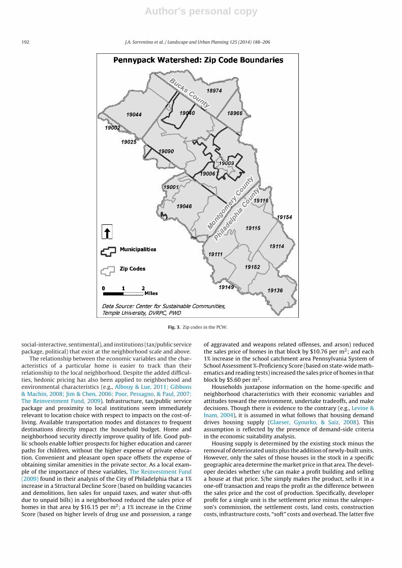
From 1950 to 1980 the watershed outside the City of Philadel-phia limits experienced significant development. As of 2012,single-family homes made up 38% and multi-family homes 12% ofthe watershed (Fromuth, 2012). Over the last decade, the PCW hasbeen estimated to be about 30% impervious (PWD, 2003, 2009). ThePCW is serviced by public water suppliers, and it is estimated thatstormwater collection systems are installed in 65% of it. Many ofthese systems were designed only to collect runoff and discharge itoffsite. This has resulted in increased flooding, destabilized streamchannels, severe erosion and sedimentation. A municipal treatmentplant contributes a large portion of the base flow in the Creek,resulting in additional nutrients. In the midst of the urbanizationwithin the PCW, there has been significant effort by conservationgroups and government agencies to preserve land as open space(Fig. 1) (DVRPC, 2010), Figs. 2 and 3 are intended to give the readerspatial views of the watershed.

Local political independence is evident in Pennsylvania, andplays into land use considerations significantly. In the mid-1970s,the state legislature adopted the Home Rule Charter stating, “Amunicipality . . . may exercise any function not denied by this Con-stitution, by its home rule charter or by the General Assembly at anytime” (PA DCED, 2003). The Pennsylvania Municipalities PlanningCode Act of 1968 permits municipalities to make land use decisions.In the PCW, there are 12 different zoning codes regulating landuse and (in most codes) dwelling density. Though most municipal-ities have their own protective measures to conserve floodplainsand preserve open space, the end result is often a disconnectedset of preserved parcels throughout the watershed. The potentialsynergies of joint measures across municipalities are thereby notrealized.

Section 303(d) of the US Clean Water Act describes the natureof an impaired stream. The Act requires that: “The states identifyall waters where required pollution controls are not sufficient toattain or maintain applicable water quality standards, and estab-lish priorities for development of Total Maximum Daily Loads basedon the severity of the pollution and the sensitivity of the usesto be made of the waters, among other factors” (US EPA, 2014).The Pennypack Creek is listed by the Pennsylvania Department ofEnvironmental Protection (PA DEP) as an impaired stream for twodesignated uses, aquatic life and recreation. Total Maximum DailyLoads have been assigned by the PA DEP for a number of pollutants.They include quantifiable reductions for trichoroethylene, fecal col-iform, dissolved oxygen-consuming pollutants, phosphorous, andsuspended solids. The responsibility to implement the reductionslies with either wastewater treatment operators or local municipal-ities. Both must apply to the US Environmental Protection Agency(EPA) for a National Pollution Discharge Elimination System Permitfor permission to discharge pollutants. Wastewater operators andmunicipalities have to pay for and administer additional controlsto reduce the amount of pollutants in their wastewater or stormsewer systems. These efforts are not done in coordination, reducingpollutants in a piecemeal fashion.

In 1978, the Pennsylvania legislature recognized that floodingand water quality problems existed because regulations were notstandardized throughout watersheds. It enacted the StormwaterManagement Act (SMA), requiring the PA DEP to designate water-sheds, and establish guidelines for the preparation of Stormwater


190 J.A. Sorrentino et al. / Landscape and Urban Planning 125 (2014) 188–206

Fig. 1. Land uses in the PCW.

Management Plans (SMP). These plans encourage comprehensiveplanning and management of stormwater by requiring counties toprepare the plans and to develop ordinance language for munici-palities. Within the SMP planning process, counties are responsiblefor establishing a Watershed Planning Advisory Committee. Eachmunicipality is required to adopt stormwater management ordi-nances that are consistent with the standards and criteria of theplan. Although these stormwater runoff performance standards arerequired to be consistent throughout the watershed, municipalitiesstill have the freedom to structure and enforce ordinances as theysee fit.

The only legislation which requires multi-municipal plan-ning for watersheds is the SMA. Municipal officials have limitedresources. They are generally not eager to commit to voluntaryactivities. Often municipal officials want to know how combinedplanning efforts will benefit their jurisdictions directly before theycommit. Multi-municipal planning for watersheds tends to bemost successful when incentives are offered, or local governmentneeds besides watershed conservation are met (Barletta, Dahme, &Maimone, 2007).

The present study developed a unified zoning scheme for thePCW to investigate whether consistent classification would resultin more profit and/or less environmental degradation. To arrive atthe unified residential zoning scheme, the residential zoning cate-gories and codes of the suburban municipalities with portions thatlie in the PCW, and those of the City of Philadelphia, were gathered

and recorded. Using key words from the actual categories, the eightgeneric categories listed vertically in Table 1 were created. The keyzoning parameters used in the CommunityViz buildouts are listedhorizontally in Table 1. The homogenized values were derived bydifferent methods based on the amount of variation in the actualcodes. Dwelling Units per Building and Floors per Building werechosen by straight frequency. A spatially-weighted average was cal-culated for Building Separation, Building Density and Road Setback.The weights contained the percentages of the relevant municipal-ities that were zoned with each code, and the percentages of thePCW land area that the portions of these municipalities occupied.

2.2. Residential development: economic suitability

In general, housing demand is largely a function of the price ofhousing as altered by the fact that mortgage interest is federal tax-deductible in the US. The effective price of a housing unit (H) is theafter-tax user-cost (ATUCH) as shown in Eq. (1).

ATUCH = PH ∗ (L ∗ MC + M + RET) + U − PH ∗ (L ∗ MR + RET) ∗ ATR

(1)

The variables are designated as follows:

PH – the price of a housing unitL – loan-to-value ratio



Fig. 2. Counties and municipalities in the PCW.

MC – mortgage constant that multiplies the loan amount to getthe annual principal plus interest paymentM – maintenance costs as a percent of PHU – utility costsMR – mortgage interest rateRET – real estate taxes as a percent of PHATR – average income tax rate

Studies of US housing markets broadly agree on the price ofhousing as ATUC (e.g., Gill & Haurin, 1991; Gillen, 2005). Thesestudies are also in agreement on the percentages used for main-tenance cost, real estate taxes and average income tax rate. Theloan-to-value ratio is the amount of the purchase price that abank will finance. The mortgage constant is a statistic that, when

multiplied by the loan amount, yields the annual payment of prin-cipal and interest on a home loan. Utility costs have been estimatedfrom actual values for a sample of 75 homes randomly chosenwithin the PCW zip codes on www.trulia.com (Trulia.com, 2011).Finally, deducted from the ATUC is tax savings.

Current and anticipated household income/wealth, and thehedonic characteristics of a particular home and its neighborhood,are the other major determinants of housing choice. Since the objectof the present study is location, the characteristics of a buyer’starget house are not directly relevant. Galster et al. (2001) posita taxonomy of neighborhood characteristics that depict an inter-active relationship between the individual households and thenatural (environmental) and built (structural, infrastructural, prox-imity) environments, the community (demographic, class status,

Table 1Unified zoning classifications and requirements.

District Zoning code Dwelling units per building Floors per building Building separation (m) Building density (per ha) Road setback (m)

Low L 1 3 7.62 2.69 15.24Low–medium LM 1 3 7.62 5.66 12.19Medium M 1 3 4.57 10.13 9.14High H 2 3 4.72 14.43 9.14Multi-family MF 8 3 7.62 19.62 9.14High urban HU 1 3 2.44 43.32 3.51High urban duplex HUD 2 3 2.44 63.01 3.84Multi-family urban MFU 25 10 0 7.17 0



Fig. 3. Zip codes in the PCW.

social-interactive, sentimental), and institutions (tax/public servicepackage, political) that exist at the neighborhood scale and above.

The relationship between the economic variables and the char-acteristics of a particular home is easier to track than theirrelationship to the local neighborhood. Despite the added difficul-ties, hedonic pricing has also been applied to neighborhood andenvironmental characteristics (e.g., Albouy & Lue, 2011; Gibbons& Machin, 2008; Jim & Chen, 2006; Poor, Pessagno, & Paul, 2007;The Reinvestment Fund, 2009). Infrastructure, tax/public servicepackage and proximity to local institutions seem immediatelyrelevant to location choice with respect to impacts on the cost-of-living. Available transportation modes and distances to frequentdestinations directly impact the household budget. Home andneighborhood security directly improve quality of life. Good pub-lic schools enable loftier prospects for higher education and careerpaths for children, without the higher expense of private educa-tion. Convenient and pleasant open space offsets the expense ofobtaining similar amenities in the private sector. As a local exam-ple of the importance of these variables, The Reinvestment Fund(2009) found in their analysis of the City of Philadelphia that a 1%increase in a Structural Decline Score (based on building vacanciesand demolitions, lien sales for unpaid taxes, and water shut-offsdue to unpaid bills) in a neighborhood reduced the sales price ofhomes in that area by $16.15 per m2; a 1% increase in the CrimeScore (based on higher levels of drug use and possession, a range

of aggravated and weapons related offenses, and arson) reducedthe sales price of homes in that block by $10.76 per m2; and each1% increase in the school catchment area Pennsylvania System ofSchool Assessment %-Proficiency Score (based on state-wide math-ematics and reading tests) increased the sales price of homes in thatblock by $5.60 per m2.

Households juxtapose information on the home-specific andneighborhood characteristics with their economic variables andattitudes toward the environment, undertake tradeoffs, and makedecisions. Though there is evidence to the contrary (e.g., Levine &Inam, 2004), it is assumed in what follows that housing demanddrives housing supply (Glaeser, Gyourko, & Saiz, 2008). Thisassumption is reflected by the presence of demand-side criteriain the economic suitability analysis.

Housing supply is determined by the existing stock minus theremoval of deteriorated units plus the addition of newly-built units.However, only the sales of those houses in the stock in a specificgeographic area determine the market price in that area. The devel-oper decides whether s/he can make a profit building and sellinga house at that price. S/he simply makes the product, sells it in aone-off transaction and reaps the profit as the difference betweenthe sales price and the cost of production. Specifically, developerprofit for a single unit is the settlement price minus the salesper-son’s commission, the settlement costs, land costs, constructioncosts, infrastructure costs, “soft” costs and overhead. The latter five



Table 2Housing unit projections.*

Municipality 2010 census householdsize (persons peroccupied housing unit)

Vacancy rate (2% ofoccupancy rate)

Occupancyrate + vacancy rate(persons per unit)

Change in populationin watershed2010–2035

2035 housingunits needed

Upper Southampton Township 2.569 0.051 2.620 410 156Warminster Township 2.539 0.051 2.590 2465 952Abington Township 2.587 0.052 2.639 457 173Bryn Athyn Borough 3.213 0.064 3.277 58 18Hatboro Borough 2.419 0.048 2.467 283 115Horsham Township 2.732 0.055 2.787 1709 613Jenkintown Borough 2.196 0.044 2.240 4 2Rockledge Borough 2.420 0.048 2.468 31 13Upper Dublin Township 2.721 0.054 2.775 164 59Upper Moreland Township 2.417 0.048 2.465 1492 605

Total 2706

* Lower Moreland and Philadelphia were excluded due to non-positive population projections.

costs sum to the overhead-adjusted total cost of providing the unit.The soft costs include items such as appraisal, permit application,review and inspection fees. Overhead is generally computed as astandard percentage of the sum of the other costs.

Well-accepted formulas and sources for housing supply andconstruction costs have been used. Whereas most models estimatea national or metro-region-wide housing supply (Blackley, 1999;Glaeser, Gyourko, & Saiz, 2008; Kinsey, 1992; Mayer & Somerville,2000; Somerville, 1999), prices and costs by zip codes within thePCW have been examined for this analysis. This disaggregatedapproach is thought to be somewhat unique in the housingliterature.

2.3. Residential development: environmental suitability

The goals of simultaneously seeking positive economic, envi-ronmental and social justice outcomes from development havebeen pursued at the international, national and local levels fordecades. From Maclaren (1996), Berke and Manta-Conroy (2000)and Wheeler (2000), the following goals of local sustainability werechosen: (1) protection of the natural environment, (2) minimal useof nonrenewable resources and (3) responsible regional cooper-ation by local governments. In this paper, goals (1) and (2) aredirectly sought via criteria that are imposed in the environmen-tal suitability analysis below. Regional cooperation in our studymeans multi-municipal collaboration within the watershed region.The unified zoning scheme described above represents such col-laboration in the analysis. The PCW municipalities are thought tocomply with the hypothetical unified scheme. It is incorporated intwo suitability analyses and two buildouts below. Some policy rec-ommendations based on the housing location are also made in thesequel to encourage such regional cooperation.

The notion of environmentally sustainable land developmentis not alien to the land development industry. Of particular inter-est to this study, the US Green Building Council (2011) promotesstandards and sponsors education and training programs to fostersustainability.1 A rather spirited enunciation of the need for devel-opment to involve people, the planet, and profit is given as part ofthe Sustainable Land Development Initiative (SLDI):

Today’s reality is that the ‘people’ are driving demand for prac-tices that steward the ‘planet.’ There are many sound landdevelopment practices . . . which not only reduce developmentcosts, but add sales premium potential and provide additional

1 The Council has headquarters in Washington, DC, and a Certification Institute inPhiladelphia. Its mission is “To transform the way buildings and communities aredesigned, built and operated, enabling an environmentally and socially responsible,healthy, and prosperous environment that improves the quality of life.”

environmental benefits. Such practices require a more holis-tic and sophisticated approach than that which is typicallyemployed today, but nevertheless, offer significant cost savingopportunities (TriplePundit, 2010).

An implication of the three-pronged approach is that the environ-ment and less-advantaged citizens need not suffer when there arepositive economic outcomes for developers. This scenario will con-centrate only on environmental criteria.

2.4. Two hypothetical scenarios and their impacts

The Delaware Regional Planning Commission (DVRPC) is themetropolitan planning organization for the nine-county Philadel-phia region. As part of its portfolio of projects, it makes projectionsabout population and employment growth for counties and munic-ipalities within the region with their collaboration. The PCWcontains all or part of 12 municipalities in Bucks, Montgomeryand Philadelphia Counties. The 2035 projected percentage popu-lation growth for Bucks County is 21%. It is 15% for MontgomeryCounty, and 0% for Philadelphia County (DVRPC, 2007). The actual-zoning scenarios presented below hypothetically placed in the zipcodes the buildings required to house the DVRPC population fore-casts, given zip code-specific household sizes. These projectionsappear in Table 2, with those municipalities (Lower Moreland andPhiladelphia) with negative or zero projected growth omitted.

As noted by Church (1999, chap. 20) and Murray (2010), mod-ern GIS have evolved to include sophisticated analytical tools thathelp organize location problems. Two suitability models weredeveloped using the ArcGIS 10.2 (ESRI, 2013), one for economicsuitability and one for environmental suitability. The GIS base lay-ers contained data reflecting development desirability. Table A.1lists the data sets needed to produce the suitability layers. To buildthe models, each vector layer was converted to a grid-formattedraster layer using values for a single suitability criterion. Each rasterlayer was then reclassified with an assigned scale value rangingfrom 2 to 10 (most suitable). Additionally, the model required layer-influence percentages for each layer that sum to 100.

Housing data representative of the zip codes in the PCW arelisted in Table 3. Because the housing data representative of thezip codes in the PCW show that single detached homes makeup the majority of new housing supply, prices and costs of sin-gle homes have been listed. Adjustments made in the buildoutsreflect the presence of multi-household supply. Together withthe values in Table 4, these data were used to provide econom-ically suitable areas for development. While most criteria reflectdemand-side desirability, it is thought that developers benefitfrom higher asset prices for homes sold as demand factors makethem more desirable. The median house price data were taken



Table 3Housing price-related data (2012 $).

Zip code Median house price ($) ATUC ($) Common Level Ratio Price per m2 ($) Build cost per m2 ($) Profit per m2 ($)

18966 278,800 23,796 0.1273 1571.53 1140.22 431.3118974 271,000 23,231 0.1273 1528.48 1140.22 388.2519001 203,200 18,320 0.7512 1485.42 1221.17 264.2519002 392,500 32,033 0.8153 1722.23 1221.17 501.0619006 237,000 20,768 0.7354 1614.59 1221.17 393.4219009 290,000 24,608 0.7108 1334.73 1221.17 113.5619025 326,000 27,215 0.8153 1506.95 1221.17 285.7819040 223,000 19,754 0.7188 2174.31 1221.17 953.1419044 225,000 19,899 0.7188 1302.43 1221.17 81.2719046 247,500 21,529 0.7401 1194.79 1221.17 −26.3719090 182,000 16,784 0.7401 1474.66 1221.17 253.4919111 151,500 14,575 0.2846 1259.38 1002.01 257.3719114 131,500 13,126 0.2846 1173.27 1002.01 171.2519115 179,000 16,567 0.2846 1334.73 1002.01 332.7119116 205,000 18,450 0.2846 1442.36 1002.01 440.3519136 98,950 10,768 0.2846 968.75 1002.01 −33.2619149 105,000 11,206 0.2846 893.40 1002.01 −108.6119152 155,000 14,828 0.2846 1227.09 1002.01 225.07

Table 4Neighborhood criteria for economic suitability.

Zip code Educational attainment Index of household income Crime index School district name School district rating

18966 14.051 1.176 2.33 Centennial 0.89318974 13.19 0.931 3.77 Centennial 0.89319001 13.704 0.939 4.99 Upper Moreland 0.76719002 14.609 1.4 1.76 Upper Dublin 0.87819006 14.4 1.413 3.5 Lower Moreland 0.98519009 16.122 1.757 0.15 Bryn Athyn 0.98519025 15.629 1.623 3.08 Upper Dublin 0.87819040 13.374 0.833 2.38 Hatboro/Horsham 0.85119044 13.731 0.912 3.79 Hatboro/Horsham 0.85119046 14.497 1.255 4.99 Abington 0.69719090 13.37 0.858 4.48 Abington 0.69719111 12.571 0.643 5.27 Philadelphia 0.17819114 12.661 0.699 5.79 Philadelphia 0.17819115 12.879 0.698 4.08 Philadelphia 0.17819116 13.115 0.737 3.85 Philadelphia 0.17819136 11.954 0.599 5.7 Philadelphia 0.17819149 12.281 0.618 7.17 Philadelphia 0.17819152 12.369 0.645 6.7 Philadelphia 0.178

from actual house sales in the “Real Estate Trends” section ofwww.trulia.com (Trulia.com, 2011) for houses sold between thedates 1 October and 31 December 2012. It is important to notethat sales prices for settled homes are the only appropriate datato use for the asset price of a house. There was a wide range ofhousing prices, with the non-Philadelphia zip codes commandingmuch higher prices. Therefore, those zip codes had much higheruser costs of housing. As a suitability criterion, a higher medianprice was valued more highly from the supply side. The ATUC asgiven in Eq. (1) is the annual cost of carrying the house. For suit-ability, a lower ATUC was given a higher value from the demandside.

In general, housing quality is important to potential home buy-ers. A reasonable proxy for the quality of a house is average price persquare meter (m2). The average price per m2 came from Trulia.com(2011). The costs of construction per m2 came from R.S. Means(2011) and were updated using the 2% increase in the Producer PriceIndex for Materials and Supply Inputs to Residential Constructionfor December 2012 (US BLS, 2012). The land component cost wasset at 25% of the total sales price. The overhead and profit figurescame from interviews with local Philadelphia metro area housingdevelopers. The overhead was set at 10% and the profit 17% of con-struction costs. In the suitability analysis, the higher the averageprofit, the more suitable is the area from the supply-side.

From among the elements in Galster et al. (2001), those inTable 4 have been chosen to represent neighborhood. Each zipcode in the PCW is associated with a public school district.

SchoolDigger.com (2011) ranks schools at elementary, middle, andhigh school levels by percentile rank. It ranks districts using thearithmetic average of the percentile ranks of the schools in the dis-trict. Column six in Table 4 lists these scores. A higher school districtrating implies higher suitability from the demand side.

Educational attainment was found using American FactFinder(US Census Bureau, 2011). Years of school attained were multipliedby the frequency of each category in the zip code population to getthe frequency-weighted average years of school. Column two inTable 4 displays a range from slightly below 12 to slightly above16. The higher the educational attainment, the higher the suit-ability of that zip code from the demand and supply sides. Meanhousehold income was also gotten from American FactFinder (USCensus Bureau, 2011). The arithmetic average of the mean incomesof the zip code populations was computed. The index of house-hold income was calculated for each zip code by dividing the meanincome of that zip code by the average over all zip codes. Columnthree in Table 4 shows these values. The higher the index of house-hold income, the higher the suitability from the supply side, butperhaps also the demand side. Computing the crime index was abit more involved. Data on the number of robberies, aggravatedassaults, burglaries and thefts were found and divided by thousandsof people. The four types of crimes were given “severity weights”of 0.3, 0.3, 0.2 and 0.2 and a weighted sum of the four crime rateswas calculated. These numbers populate the crime index column inTable 4. The lower the crime index, the higher the suitability fromthe demand and supply sides.



Fig. 4. Economically suitable areas.

Table A.2 shows five (all but profit based on natural breaks)reclassified values for each economic suitability criterion rasterlayer ranging from 2 to 10 (most suitable). The land use classeswere assigned values based on estimated likelihood of conversioninto residential development with modern construction technol-ogy. The layer influences were ascertained through interviews withthree developers, one of whom is Mr. Thomas Bentley, Presidentof Bentley Homes, Paoli, PA (personal communication, 8 January2014), a highly involved member of the American Association ofHome Builders. Mr. Bentley shared national data on home buildersand the determinants of housing supply. Table A.3 shows the val-ues chosen. Fig. 4 shows the most economically suitable areas forresidential development in the PCW.

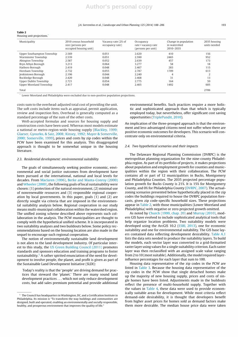
The criteria used to determine the areas for residential devel-opment consistent with local sustainability are listed vertically inTable A.4. Some of the layers were merged for processing conve-nience. The assigned scale values for each suitability layer rangingfrom 2 to 10 (most suitable). The layer influences were solicited inan online survey developed in Qualtrics (2012) of municipal Envi-ronmental Advisory Council members in the watershed throughoutthe months of March and April in 2011. The six question surveyasked for inputs in choosing suitability layers and their influencesin the model, and was distributed to the municipal managersand chairpersons of the Environmental Advisory Councils of eachmunicipality with land area in the PCW. Overall, the survey reached

52 people. Of the 43 responses recorded, 36 were complete andused.2 Fig. 5 contains the environmentally suitable areas.

Each municipality was clipped to the watershed boundaries.As noted, the zoning classifications for residential developmentwithin the watershed vary among municipalities. Each zoning classincludes information on lot size requirements, height restrictions,and setback distances. The zoning classifications were used as thebase layer to run the buildout analyses.3

The software chosen to conduct the buildouts for this study wasCommunityViz 4.1 Scenario 360 (Placeways, 2009). The BuildoutWizard requires a GIS base layer, such as a zoning layer, to providedensity allowances for each zoning class. The software promptsuser input on zoning classifications, existing buildings, minimumlot sizes, minimum setback distances for front, back and side yards,height restrictions, and other data. Using this information, the Wiz-ard then calculates and spatially allocates the maximum number ofbuildings that could be built on the developable land. The choicewas made in the Wizard to “follow roads.”

2 This survey of public-spirited individuals was performed as part of another studyby one of the present authors. It contrasts with the small number of developers askedto divulge proprietary information on commercial activities.

3 More detailed information on the areas that the zoning classes cover is availablefrom the authors.



Fig. 5. Environmentally suitable areas.

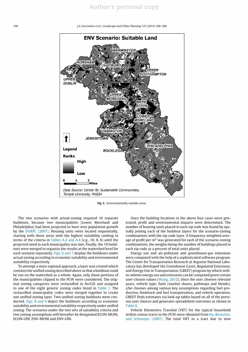
The two scenarios with actual-zoning required 10 separatebuildouts, because two municipalities (Lower Moreland andPhiladelphia) had been projected to have zero population growthby the DVRPC (2007). Housing units were located sequentially,starting with those areas with the highest suitability ranking interms of the criteria in Tables A.2 and A.4 (e.g., 10, 8, 6) until theprojected need in each municipality was met. Finally, the 10 build-outs were merged to organize the results at the watershed level foreach scenario separately. Figs. 6 and 7 display the buildouts underactual zoning according to economic suitability and environmentalsuitability respectively.

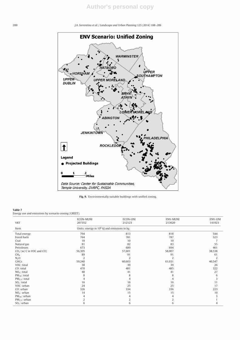
To attempt a more regional approach, a layer was created whichcontains the unified zoning described above so that a buildout couldbe run on the watershed as a whole. Again, only those portions ofthe municipalities clipped to the PCW were considered. The orig-inal zoning categories were reclassified in ArcGIS and assignedto one of the eight generic zoning codes listed in Table 1. Thereclassified municipality codes were merged together to createone unified zoning layer. Two unified-zoning buildouts were con-ducted. Figs. 8 and 9 depict the buildouts according to economicsuitability and environmental suitability respectively under unifiedzoning. The scenarios under the two sets of suitability criteria andtwo zoning assumptions will hereafter be designated ECON-MUNI,ECON-UNI, ENV-MUNI and ENV-UNI.

Once the building locations in the above four cases were gen-erated, profit and environmental impacts were determined. Thenumber of housing units placed in each zip code was found by spa-tially joining each of the buildout layers for the scenario-zoningcombinations with the zip code layer. A frequency-weighted aver-age of profit per m2 was generated for each of the scenario-zoningcombinations, the weights being the number of buildings placed ineach zip code as a percent of total units placed.

Energy use and air-pollutant and greenhouse-gas emissionswere computed with the help of a sophisticated software program.The Center for Transportation Research at Argonne National Labo-ratory has developed the Greenhouse Gases, Regulated Emissions,and Energy Use in Transportation (GREET) program by which well-to-wheels energy use and emissions can be computed given certainuser-chosen values (Wang, 2012). Once the user chooses relevantyears, vehicle type, fuels (market shares, pathways and blends),s/he chooses among various key assumptions regarding fuel pro-duction, feedstock and fuel transportation, and vehicle operation.GREET finds estimates via look-up tables based on all of the previ-ous user choices and generates spreadsheet outcomes as shown inTable 6.

Vehicle Kilometers Traveled (VKT) for the typical householdwithin census tracts in the PCW were obtained from Hu, Reuscher,and Schmoyer (2007). The total VKT in a tract due to new



Fig. 6. Economically suitable buildings with actual zoning.

households was obtained by multiplying the VKT per householdby the number of new households. The total VKT per tract was thenmultiplied by the per-kilometer energy use and emissions param-eters from GREET to get the total energy use and emissions for thetract.

The water-related impacts on the Pennypack Creek wereassessed with monitoring data provided by Mr. Jason Cruz of thePhiladelphia Water Department (PWD; personal communication,10 January 2013), a Water Quality Index derived from chemicalanalyses, and a standard biological analysis.

The water chemistry parameters that were deemed important(Bordalo, Teixeira, & Wiebe, 2006; Brown, McClelland, Deininger,& Tozer, 1970; SDD, 1976; Sorrentino, Meenar, & Flamm, 2008) areAmmonia, Biochemical Oxygen Demand (BOD), Dissolved Oxygen(DO), E. coli, Nitrate, Orthophosphate, pH, Suspended Solids andTemperature. Readings of these parameters were taken at fixedPWD monitoring stations along the Creek over particular timeperiods. Sorrentino et al. (2008) had used readings from 13 chem-ical, 10 fish and 13 macroinvertebrate monitoring stations. Sincethen, monitoring in the Creek has been reduced. The chemical dataused in this work came from 12 stations for Ammonia, BOD, E. coli,Nitrate, Orthophosphate and Suspended Solids and four stations forDO, pH and Temperature (see Fig. 10).

In previous studies (Meenar, 2006; Sorrentino, Featherstone, &Meenar, 2007), the PCW had been divided into various levels of

sub-basins as shown in Fig. 10. Each of these sub-basins drains intoan area on the main Creek with a unique monitoring station belowthe confluence. The value of the Water Quality Index (WQI) at thatmonitoring station was attributed to that sub-basin. The overallWeighted Water Quality Index (WWQI) values were computed bymultiplying the sub-basin WQI values by the percent of buildingsplaced in that sub-basin by ECON-MUNI, ECON-UNI, ENV-MUNI andENV-UNI respectively.

The numbers of fish and/or macroinvertebrates found at a setof stations were given Index of Biological Integrity (IBI; Karr, 1991)values by the PWD. At the stations where either fish or macroin-vertebrates were measured (see Fig. 10), the IBI was based on theone that was measured. At the stations where both were measured,the arithmetic average of the IBI scores was used. Once each stationhad an IBI score, the Weighted IBI (WIBI) score was gotten in thesame manner as the WWQI.

3. Empirical results and discussion

In each scenario-zoning combination, the numbers of buildingsplaced in each zip-code area (Table 5) depended on the relativedensities allowed. As noted above, the building counts were alsodetermined for census tracts and watershed sub-basins. Countswere determined via spatial joining. Any necessary spatial unitconversions were done with overlays.



Fig. 7. Environmentally suitable buildings with actual zoning.

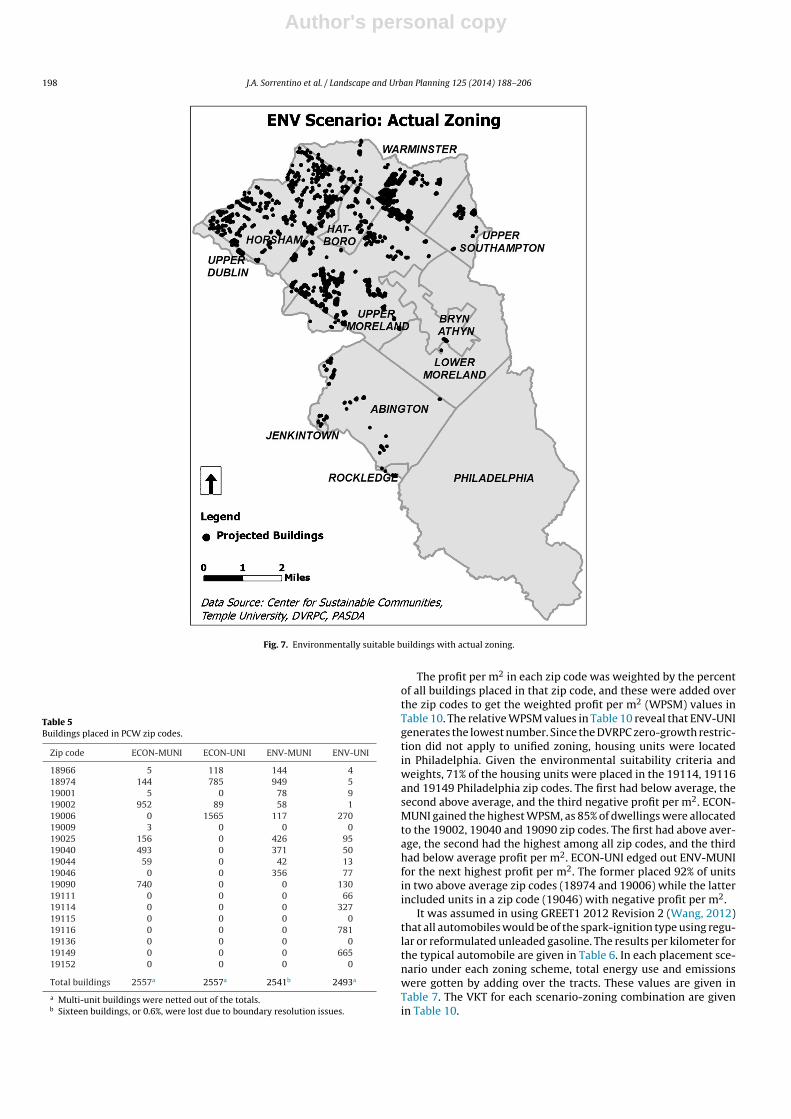
Table 5Buildings placed in PCW zip codes.

Zip code ECON-MUNI ECON-UNI ENV-MUNI ENV-UNI

18966 5 118 144 418974 144 785 949 519001 5 0 78 919002 952 89 58 119006 0 1565 117 27019009 3 0 0 019025 156 0 426 9519040 493 0 371 5019044 59 0 42 1319046 0 0 356 7719090 740 0 0 13019111 0 0 0 6619114 0 0 0 32719115 0 0 0 019116 0 0 0 78119136 0 0 0 019149 0 0 0 66519152 0 0 0 0

Total buildings 2557a 2557a 2541b 2493a

a Multi-unit buildings were netted out of the totals.b Sixteen buildings, or 0.6%, were lost due to boundary resolution issues.

The profit per m2 in each zip code was weighted by the percentof all buildings placed in that zip code, and these were added overthe zip codes to get the weighted profit per m2 (WPSM) values inTable 10. The relative WPSM values in Table 10 reveal that ENV-UNIgenerates the lowest number. Since the DVRPC zero-growth restric-tion did not apply to unified zoning, housing units were locatedin Philadelphia. Given the environmental suitability criteria andweights, 71% of the housing units were placed in the 19114, 19116and 19149 Philadelphia zip codes. The first had below average, thesecond above average, and the third negative profit per m2. ECON-MUNI gained the highest WPSM, as 85% of dwellings were allocatedto the 19002, 19040 and 19090 zip codes. The first had above aver-age, the second had the highest among all zip codes, and the thirdhad below average profit per m2. ECON-UNI edged out ENV-MUNIfor the next highest profit per m2. The former placed 92% of unitsin two above average zip codes (18974 and 19006) while the latterincluded units in a zip code (19046) with negative profit per m2.

It was assumed in using GREET1 2012 Revision 2 (Wang, 2012)that all automobiles would be of the spark-ignition type using regu-lar or reformulated unleaded gasoline. The results per kilometer forthe typical automobile are given in Table 6. In each placement sce-nario under each zoning scheme, total energy use and emissionswere gotten by adding over the tracts. These values are given inTable 7. The VKT for each scenario-zoning combination are givenin Table 10.



Fig. 8. Economically suitable buildings with unified zoning.

Table 6Well-to-wheels energy use and emissions per km (GREET).

Item J/km or g/km

Feedstock Fuel Vehicle operation Total

Total energy 209,594 520,930 3,100,861 3,831,385Fossil fuels 204,695 454,492 3,024,609 3,683,796Coal 20,421 27,233 0 47,654Natural gas 142,201 246,453 0 388,654Petroleum 42,074 180,805 3,024,609 3,247,488CO2 (w/ C in VOC and CO) 10.850 34.938 225.755 271.544CH4 0.298 0.123 0.007 0.428N2O 0.000 0.004 0.007 0.012GHGs 18.363 39.169 228.164 285.696VOC: total 0.010 0.070 0.101 0.182CO: total 0.016 0.019 2.233 2.269NOx: total 0.076 0.056 0.061 0.194PM10: total 0.008 0.014 0.018 0.039PM2.5: total 0.005 0.007 0.009 0.021SOx: total 0.033 0.040 0.004 0.077VOC: urban 0.002 0.045 0.071 0.118CO: urban 0.001 0.009 1.563 1.573NOx: urban 0.004 0.022 0.043 0.069PM10: urban 0.000 0.005 0.013 0.018PM2.5: urban 0.000 0.003 0.007 0.010SOx: urban 0.004 0.020 0.003 0.027



Fig. 9. Environmentally suitable buildings with unified zoning.

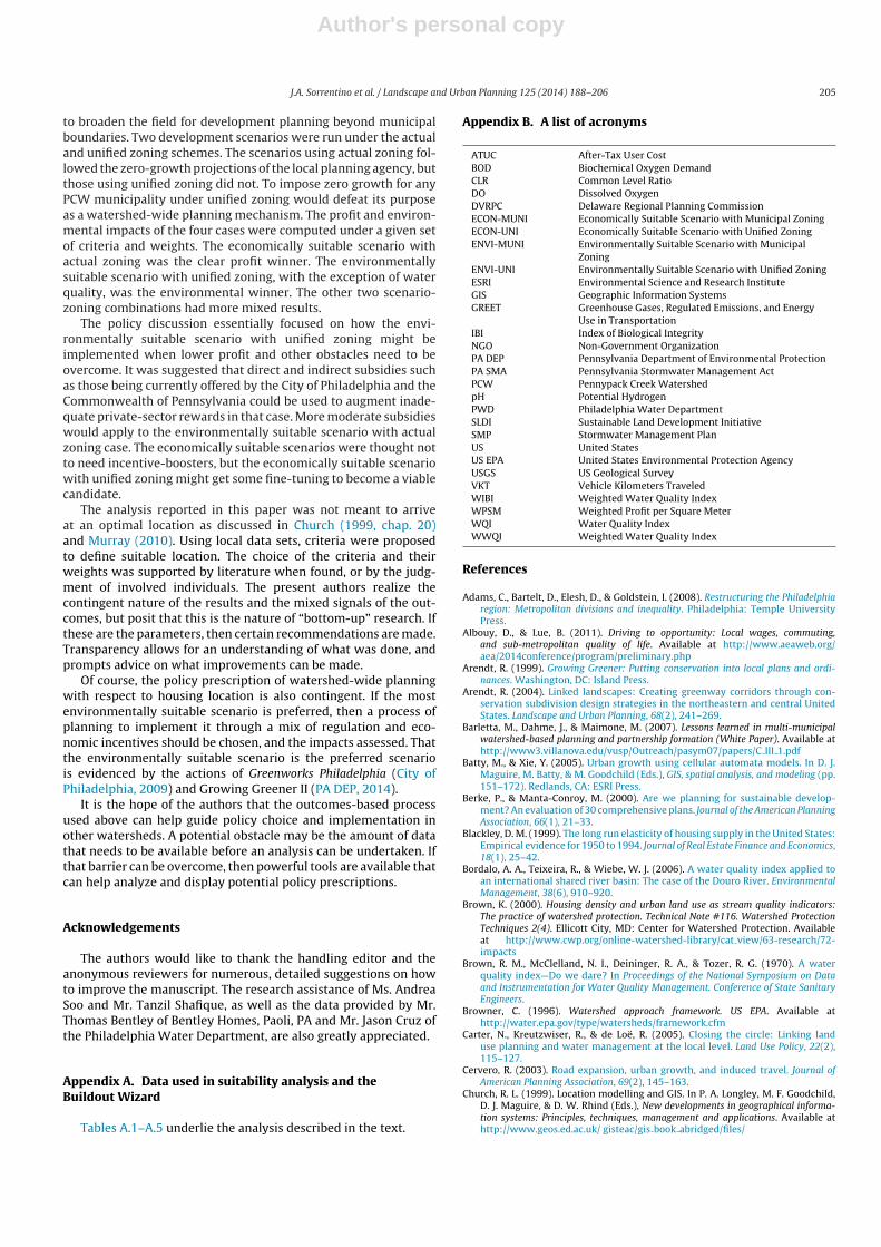
Table 7Energy use and emissions by scenario-zoning (GREET).

ECON-MUNI ECON-UNI ENV-MUNI ENV-UNIVKT 207352 212123 213620 141923

Item Units: energy in 106 kJ and emissions in kg

Total energy 794 813 818 544Fossil fuels 764 781 787 523Coal 10 10 10 7Natural gas 81 82 83 55Petroleum 673 689 694 461CO2 (w/ C in VOC and CO) 56,305 57,601 58,007 38,538CH4 89 91 91 61N2O 2 2 2 2GHGs 59,240 60,603 61,031 40,547VOC: total 38 39 39 26CO: total 470 481 485 322NOx: total 40 41 41 27PM10: total 8 8 8 6PM2.5: total 4 4 4 3SOx: total 16 16 16 11VOC: urban 24 25 25 17CO: urban 326 334 336 223NOx: urban 14 15 15 10PM10: urban 4 4 4 3PM2.5: urban 2 2 2 1SOx: urban 6 6 6 4



Fig. 10. Sub-basins in the PCW.

Table 7 reveals that ENV-UNI had lower energy use and airpollution and greenhouse gas emissions than any of the othercombinations. Locating buildings in environmentally suitable areaswith the unified zoning scheme places many within easy accessto public transportation and other built-environment amenities inPhiladelphia (see Fig. 9). Though based in part on not imposingthe DVRPC zero-growth restrictions on the unified zoning scheme,the results provide some evidence that a more regional approachto location may result in lower energy use and air and green-house emissions. ECON-MUNI generates the second lowest energyuse and emissions. Figs. 6–8 show that no buildings are placed inPhiladelphia in the ECON scenarios and in ENV-MUNI.

In calculating the WQI, chemical concentration levels were asso-ciated with “quality values.” (SDD, 1976) The following weightshad been attributed to these parameters by experts using the Del-phi Method (Bordalo et al., 2006; Brown, McClelland, Deininger, &Tozer, 1970; SDD, 1976; Sorrentino et al., 2008): Ammonia (0.12),BOD (0.15), DO (0.18), E. coli (0.12), Nitrate (0.09), Orthophosphate(0.09), pH (0.10), Suspended Solids (0.08) and Temperature (0.07).Table 8 contains values of the WQI for each chemical monitoringstation. The biological data involved readings from six fish and threemacroinvertibrate stations. The IBI levels are given in Table 9.

With respect to water-quality impacts, ECON-MUNI had ahigher WWQI than all the other scenario-zoning pairs largelybecause it placed slightly over 50% of its housing units in sub-basins

that drain into the PP180 monitoring station. The presence of the1300-acre Pennypack Park in this section of Philadelphia is a majorreason for the relatively high WQI of PP180. The ENV-UNI case wasassociated with the second highest WWQI. It can be seen in Table 8that PP2020 has the highest WQI. ENV-UNI placed about 9% and 28%of its units in basins that drain to PP2020 and PP180 respectively, soits overall WQI is relatively high. The other 63% of units, however,are placed in lower WQI basins. ECON-UNI and ENV-MUNI located98% and 92% of their units in lower-WQI basins draining to stationsbetween PP2220 and PP180.

ENV-UNI also had the winning WIBI, followed by ENV-MUNI,ECON-UNI and ECON-MUNI in that order. Table 9 shows that IBIin the southern-most stations (listed at the top) were among thehighest of those monitored. ENV-UNI placed many housing units inthe southern basins associated with higher IBI, while ENV-MUNI didalmost the same in the northern basins. ECON-UNI and ECON-MUNIplaced more units than the previous scenario-zoning combinationsin the lower-IBI basins.

With the criteria and weights chosen above, the orderings of theprofit and environmental impacts of the four scenario-zoning com-binations in Table 10 present several policy challenges. Profit andenvironmental suitability are starkly opposite in terms of WPSM.ENV-UNI generated more VKT than both of the ECON combina-tions, and ECON-MUNI dominated with respect to WWQI. Thesechallenges go to the heart of free-enterprise capitalism.



Table 8Water quality levels at PWD chemical monitoring stations.

Station Ammonia DO (%) BOD5 E. coli Nitrate Orthophosphate pH SS Temp WQI

PP110 82.1 73.00 81.94 99.50 83.69 76.72 92.00 99.8 19.00 80.17PP180 86.92 73.00 81.94 99.50 81.44 79.18 92.00 98.00 19.00 80.63PP340 75.24 73.00 56.55 93.00 82.11 71.36 92.00 20.00 19.00 67.75PP690 86.92 67.00 81.63 99.00 79.14 72.93 78.00 98.50 20.00 77.38PP970 86.92 67.00 81.28 98.00 78.84 71.08 78.00 98.75 20.00 77.04PP985 86.78 67.00 82.00 99.75 75.97 65.97 78.00 98.88 20.00 76.63PP993 78.59 67.00 72.91 96.00 78.78 60.72 78.00 40.00 20.00 68.90PP994 89.9 67.00 82.00 98.50 77.39 54.53 78.00 97.50 20.00 75.84PP1150 86.78 50.00 82.00 99.75 75.97 65.97 90.00 98.88 18.00 74.63PP1380 86.85 50.00 82.00 99.73 68.39 42.78 90.00 99.00 18.00 71.87PP1680 77.8 50.00 62.30 91.00 70.14 36.88 90.00 28.00 18.00 60.73PP1850 78.76 64.00 68.51 88.00 94.17 95.93 91.50 80.00 18.75 75.78PP2020 86.92 64.00 82.00 99.60 91.75 96 91.50 99.75 18.75 81.54

Table 9Index of Biological Integrity levels at PWD bio monitoring stations.

Station IBI

PP180 19.90PP340 25.30PP490 40.00PP690 30.00PP970 25.30PP1060 28.00PP1380 25.80PP1680 28.00PP2020 26.00

4. Policy implications

If environmentally suitable location saves buyers money, makessellers profit and avoids environmental degradation, the casewould be more compelling to let the housing market make it hap-pen. If the motives of private-sector agents cannot be relied upon toimplement ENV-UNI, what can governments and Non-GovernmentOrganizations (NGOs) do? Two sets of policy tools aimed at theclassic situation of environmental externalities, command-and-control regulation and economic incentives, could be considered.The former uses government intervention in the form of phys-ical prescriptions for development with legal prohibition and/orfinancial penalties for non-compliance. Candidates for command-and-control regulation at the local level include zoning restrictions,moratoria on non-environmentally suitable development, and theimposition of growth boundaries. However, prevention of develop-ment comes with various costs. Perhaps the most obvious, ceterisparibus, are higher land costs, higher housing prices and migrationof developers to more permissive jurisdictions.

Economic incentives are financial charges or subsidies on activ-ities that would not be chosen by self-interested, private decisionmakers, but are being discouraged or encouraged for the benefit ofsociety as a whole. An example of a financial charge is a municipal-ity charging homeowners for stormwater runoff pollution by taxing

units of impervious surface. A financial subsidy could be reduc-ing a homeowner’s property taxes for units of pervious surfaceinstalled. Without directly prohibiting certain activities, economicincentives can skew decisions by altering relative costs and/orprices. Of course, both policy approaches require economicresources for monitoring and enforcement to be effective.

If municipalities are free to choose any mix of regulations andeconomic incentives, what are the benefits to these individual juris-dictions of regional cooperation? The benefits can be institutionalor environmental. An example of the first is that migration from anyparticular restrictive municipality to a more permissive one willbe a less effective strategy by profit-seeking developers if there isregional cooperation on the restrictions. An example of the secondis the joint prevention of runoff pollution (degradation of the “com-mons”) to a lake that sits in several distinct municipalities. Thosepolitical units that allow the pollution cause external damage tothose who prevent it. Joint prevention can make the local societybetter off.

Precedent for collaboration among the municipalities and pri-vate partnerships in the PCW can inform the process of fosteringjoint decision making on the location of future housing develop-ment. As noted in Section 2.1, Pennsylvania legislators recognizedthat flooding and water-quality degradation were serious prob-lems. Human lives lost due to flooding, stream-bank erosion, anddead fish are highly visible. These problems that could not be solvedat the individual municipality level. Despite a Home Rule bias inthe state, the SMA recognized the ecological notion of watershed,and mandated that the next disaggregated geographically-basedadministrative units, counties, create comprehensive plans forflood control and stormwater management. While the countyplans were advisory and not legally enforceable, municipalitiesin each county were required to adopt stormwater managementordinances consistent with the county plans. The PennsylvaniaEnvironmental Council and Temple University’s Center for Sus-tainable Communities collaborated to create an “Act 167 Plan” forthe PCW at the behest of the counties (Fromuth, 2012). Meetingswere held with relevant stakeholders soliciting their input as tohow stormwater might be effectively managed and soliciting their

Table 10Summary of profit and environmental impacts.

Indicator ECON-MUNI ECON-UNI ENV-MUNI ENV-UNI Assessment

WPSMa 486.35 397.33 389.39 226.33 Higher is betterVKTb 207352 212123 213620 141923 Lower is betterWWQI 75.99 69.69 66.09 72.05 Higher is betterWIBI 23.77 25.73 27.07 31.17 Higher is better

a Weighted Profit per Square Meter in 2012 USD.b The VKT determine energy use and emissions with the GREET parameters.



buy-in. The process has generated legally-binding municipal ordi-nances and best management practices, even though there is anasymmetry in that upstream actions can affect those downstream,but generally not vice versa. The actions taken became more local-ized until they reached the municipality level.

A policy prescription for PCW housing location, therefore, canbe based on the precedent of stormwater mitigation. With orwithout a mandate from the state level, officials of Bucks, Mont-gomery and Philadelphia (the same area as the City) Counties canmeet to agree on considering each other’s actions when offer-ing guidance to their municipalities on housing location in theircomprehensive plans. The counties themselves, the Pennsylva-nia Environmental Council, and/or university and NGO affiliates,can arrange meetings with the relevant watershed-wide stakehol-ders. A set of agreed-upon principles and best practices can bedeveloped to guide PCW municipal officials in creating local ordi-nances relating to the location of housing development. Regardlessof whether command-and-control or economic incentives areused in local ordinances to motivate eco-sensitive housing loca-tion, the municipalities can agree on applying them in a uniformfashion.

Fortunately for the Philadelphia portion of the PCW, the cityhas been implementing a number of policies that subsidize localsustainability. In 2009, Mayor Michael Nutter unveiled GreenworksPhiladelphia (City of Philadelphia, 2009). Among the residentialinitiatives in the program are: (i) a 10 year forgiveness of prop-erty taxes for new residential houses in the city; (ii) increasedtree coverage citywide to 30% by year 2025; (iii) local food within10 minutes walking time of 75% of city residents by 2015; (iv)park and recreation resources within 10 minutes walking time of75% of city residents by 2025; (v) retrofit of 15% of existing hous-ing stock with insulation, air sealing and cool roofs immediatelyand (vi) 80% of the city’s infrastructure in good repair by year2015.

Fortunately for all PCW municipalities, the Commonwealth ofPennsylvania has taken steps in these directions. The GrowingGreener program was signed into law in 1999 and reauthorizedin 2002, and mandates that local governments include open spacepreservation as part of their comprehensive plans, with commensu-rate changes in ordinances (Arendt, 1999, 2004). Growing GreenerII became law in 2005 and continues to fund government activitiesfor watershed protection as well (PA DEP, 2014).

Besides being a precedent for watershed-wide cooperationin the PCW, stormwater management and housing location arerelated in more direct ways. Both can be easily incorporated alongwith open space preservation in comprehensive planning. Further-more, eco-sensitive housing location can obviate the need for manystormwater mitigation practices. That the location of housing is animportant cause of these problems, however, is more subtle for theaverage concerned citizen to understand. Once understood, it isnot certain that it will matter. Many home buyers and sellers pre-fer low-density, greenfield development almost regardless of thecosts. Many municipal officials find few problems with this. Someof the players are unaware of the costs, and this is where educationmay enter the picture (Arendt, 2004).

Can the results of our suitability and buildout analyses pro-vide justification for the imposition of local ordinances and theimplementation of best management practices with respect tohousing location from a watershed perspective? The answer ismixed.

Though ENV-UNI is the hands-down environmental winner, itis the least profitable. Home buyers may not demand sustainablehousing location that avoids greenfield destruction as suggestedby TriplePundit (2010) if school district quality is lower and crimehigher in those locations. Developers may not make enough profitfrom locally-sustainable placement. Municipalities may find it

difficult to foster environmentally suitable development if itreduces tax revenues. When private economic decisions conflictwith the broader goals of society, external intervention is thoughtnecessary. Penalties such as impacts fees for greenfield develop-ment and property tax relief for location in high-density urbansettings may alter the self-interested, private decisions.

The ENV-UNI case was singled out above because it appearsto have the least likelihood of happening through purely private-sector activity. The profit motive in ECON-MUNI, ECON-UNI is aliveand well in Figs. 6 and 7. Buildings were placed in the PCW suburbswith higher profit and neighborhood scores at the expense of localsustainability. The private sector should not have a problem caus-ing an ECON scenario to happen. Added environmental benefits arethat ECON-MUNI had the highest water quality and the second low-est VKT. This mix may cause suburban municipal officials to preferthem to ENV-UNI.

5. Conclusion

Land use change in a large metro region is a complex issue,even in the narrow slice called residential development. The inter-play of natural with economic, political and social processes cancause problems with few easy answers. The municipalities in thePennypack Creek Watershed, with their strong tendencies towardindependent decision making, are not defined by airsheds, drainagebasins or groundwater aquifers. Land use decisions by any town-ship or borough can, however, affect downwind or downstreampopulations.

One such decision by a municipality that can affect outsidepopulations is to allow residential development that does notfollow the criteria for local sustainability when private-sector profit

Table A.1Basic input data and sources.

Data layer Source Year of publication

Land use Del. Valley Reg.PlanningCommission

2010

Roads Penn. Dept. ofTransportation

2013

Municipal zoning 11 SuburbanMunicipalities inthe PCW

2011

City of Philadelphia 2011

Floodplain Center forSustainableCommunities (CSC)Temple UniversityAmbler

2010

Streams CSC 2010Slope CSC 2009Schools PASDA 2012Hospitals ESRI 2012Religious institutions ESRI 2000Employment centers DVRPC 2013Open space DVRPC, Andropogon

Associates2011

Wetlands CSC, DVRPC 2004Bus routes DVRPC 2013Rail stations S.E. Penn.

TransportationAuthority

2012

Zip codes PennsylvaniaSpatial DataAccess/U.S. Census

2009

School districts Pennsylvania Dept.of Transportation

2013

Existing buildings CSC/DCNR 2007



is not served by such criteria. Unless a developer is committed tolocal sustainability as espoused by Sustainable Land DevelopmentInitiative (TriplePundit, 2010) for her/his own sake, or in the beliefthat her/his customers are, s/he has virtually no economic incen-tive to achieve protection of the natural environment and minimaluse of nonrenewable resources. If there is little or no incentive for

Table A.2Layer reclassification values for economic suitability.

Layer Scale Reclass value

School district 0–0.18 20.18–0.77 40.77–0.85 60.85–0.89 80.89–0.99 10

Profit per square meter (10.09)a–13.02 213.02–36.14 436.14–59.25 659.25–82.36 882.36–105.48 10

Educational attainment 0–11.95 211.95–12.66 412.66–13.72 613.72–14.6 814.6–16.12 10

Index of income 0.6–0.64 20.64–0.74 40.74–0.94 60.94–1.25 81.25–1.76 10

Crime index 0.15–2.38 22.38–3.49 43.48–4.06 64.06–5.24 85.24–7.14 10

Land use Transportation, Utility,Community Service,Recreation and associatedParking; Wooded, Water

0

Light Manufacturing,Commercial and associatedParking

4

Multi-Family and RowHome Parking

5

Agriculture and associatedParking

8

Residential: Single-FamilyDetached, Multi-Family

10

Residential: Mobile Home,Row Home; Vacant

After-Tax User Cost 10,768–13,126 213,126–16,784 416,784–19,899 619,899–21,529 821,529–32,033 10

a ( ) designates a negative value.

Table A.3Influence percentages for economic suitability.

Layer Influence

School district 0.25Profit per square meter 0.15Educational attainment 0.08Income 0.05Crime 0.07Zoning 0.12Land use 0.13After-Tax User Cost 0.15

residential developers to achieve the goals of local sustainability,then local governments may provide regulatory and/or economicincentives for them to do so. If individual municipalities collaborateto do so, then responsible regional cooperation can be achieved.

The work in the previous sections operationalized criteria foreconomic and environmental suitability to find areas to locate res-idential development according to each. An alternative to actualmunicipal residential zoning was created by defining a common setof classifications that was applied watershed-wide. This was done

Table A.4Layer reclassification values for environmental suitability.

Layer Category Reclassifications

Slope (%) 23.18–80.3 213.16–23.18 47.28–13.16 63.35–7.28 80–3.35 10

Water-related areas Floodway, buffer (50’),wetlands, streams

0

100 year floodplain 2500 year floodplain 4Other areas 10

Large parcels Subdividable 10

Land use Transportation, Utility,Community Service,Recreation and associatedParking; Wooded, Water

0

Agriculture and associatedParking

4

Multi-Family and RowHome Parking

5

Light Manufacturing,Commercial and associatedParking

8

Residential: Single-FamilyDetached, Multi-Family

10

Residential: Mobile Home,Row Home; Vacant

Proximity (ma) to trainstations and bus stops

1832.0–3013.9 21181.9–1832.0 4697.34–1181.9 6295.49–697.34 80–295.49 10

Proximity (m) toschools, hospitals,religious centers andemployment centers

5674–9100 23712–5674 42248–3712 61035–2248 80–1035 10

Proximity (m) to openspace

6299–9755 24186–6299 42496–4186 61037–2496 80–1037 10

a Meters.

Table A.5Influence percentages for sustainability.

Layer Influence

Slope 0.14Water-related areas 0.14Large parcels 0.14Land use 0.13Proximity to train stations and bus stops 0.21Proximity to schools, hospitals, religious centers andemployment centers

0.1

Proximity to open space 0.14



to broaden the field for development planning beyond municipalboundaries. Two development scenarios were run under the actualand unified zoning schemes. The scenarios using actual zoning fol-lowed the zero-growth projections of the local planning agency, butthose using unified zoning did not. To impose zero growth for anyPCW municipality under unified zoning would defeat its purposeas a watershed-wide planning mechanism. The profit and environ-mental impacts of the four cases were computed under a given setof criteria and weights. The economically suitable scenario withactual zoning was the clear profit winner. The environmentallysuitable scenario with unified zoning, with the exception of waterquality, was the environmental winner. The other two scenario-zoning combinations had more mixed results.

The policy discussion essentially focused on how the envi-ronmentally suitable scenario with unified zoning might beimplemented when lower profit and other obstacles need to beovercome. It was suggested that direct and indirect subsidies suchas those being currently offered by the City of Philadelphia and theCommonwealth of Pennsylvania could be used to augment inade-quate private-sector rewards in that case. More moderate subsidieswould apply to the environmentally suitable scenario with actualzoning case. The economically suitable scenarios were thought notto need incentive-boosters, but the economically suitable scenariowith unified zoning might get some fine-tuning to become a viablecandidate.

The analysis reported in this paper was not meant to arriveat an optimal location as discussed in Church (1999, chap. 20)and Murray (2010). Using local data sets, criteria were proposedto define suitable location. The choice of the criteria and theirweights was supported by literature when found, or by the judg-ment of involved individuals. The present authors realize thecontingent nature of the results and the mixed signals of the out-comes, but posit that this is the nature of “bottom-up” research. Ifthese are the parameters, then certain recommendations are made.Transparency allows for an understanding of what was done, andprompts advice on what improvements can be made.

Of course, the policy prescription of watershed-wide planningwith respect to housing location is also contingent. If the mostenvironmentally suitable scenario is preferred, then a process ofplanning to implement it through a mix of regulation and eco-nomic incentives should be chosen, and the impacts assessed. Thatthe environmentally suitable scenario is the preferred scenariois evidenced by the actions of Greenworks Philadelphia (City ofPhiladelphia, 2009) and Growing Greener II (PA DEP, 2014).

It is the hope of the authors that the outcomes-based processused above can help guide policy choice and implementation inother watersheds. A potential obstacle may be the amount of datathat needs to be available before an analysis can be undertaken. Ifthat barrier can be overcome, then powerful tools are available thatcan help analyze and display potential policy prescriptions.

Acknowledgements

The authors would like to thank the handling editor and theanonymous reviewers for numerous, detailed suggestions on howto improve the manuscript. The research assistance of Ms. AndreaSoo and Mr. Tanzil Shafique, as well as the data provided by Mr.Thomas Bentley of Bentley Homes, Paoli, PA and Mr. Jason Cruz ofthe Philadelphia Water Department, are also greatly appreciated.

Appendix A. Data used in suitability analysis and theBuildout Wizard

Tables A.1–A.5 underlie the analysis described in the text.

Appendix B. A list of acronyms

ATUC After-Tax User CostBOD Biochemical Oxygen DemandCLR Common Level RatioDO Dissolved OxygenDVRPC Delaware Regional Planning CommissionECON-MUNI Economically Suitable Scenario with Municipal ZoningECON-UNI Economically Suitable Scenario with Unified ZoningENVI-MUNI Environmentally Suitable Scenario with Municipal

ZoningENVI-UNI Environmentally Suitable Scenario with Unified ZoningESRI Environmental Science and Research InstituteGIS Geographic Information SystemsGREET Greenhouse Gases, Regulated Emissions, and Energy

Use in TransportationIBI Index of Biological IntegrityNGO Non-Government OrganizationPA DEP Pennsylvania Department of Environmental ProtectionPA SMA Pennsylvania Stormwater Management ActPCW Pennypack Creek WatershedpH Potential HydrogenPWD Philadelphia Water DepartmentSLDI Sustainable Land Development InitiativeSMP Stormwater Management PlanUS United StatesUS EPA United States Environmental Protection AgencyUSGS US Geological SurveyVKT Vehicle Kilometers TraveledWIBI Weighted Water Quality IndexWPSM Weighted Profit per Square MeterWQI Water Quality IndexWWQI Weighted Water Quality Index

References

Adams, C., Bartelt, D., Elesh, D., & Goldstein, I. (2008). Restructuring the Philadelphiaregion: Metropolitan divisions and inequality. Philadelphia: Temple UniversityPress.

Albouy, D., & Lue, B. (2011). Driving to opportunity: Local wages, commuting,and sub-metropolitan quality of life. Available at http://www.aeaweb.org/aea/2014conference/program/preliminary.php

Arendt, R. (1999). Growing Greener: Putting conservation into local plans and ordi-nances. Washington, DC: Island Press.

Arendt, R. (2004). Linked landscapes: Creating greenway corridors through con-servation subdivision design strategies in the northeastern and central UnitedStates. Landscape and Urban Planning, 68(2), 241–269.

Barletta, M., Dahme, J., & Maimone, M. (2007). Lessons learned in multi-municipalwatershed-based planning and partnership formation (White Paper). Available athttp://www3.villanova.edu/vusp/Outreach/pasym07/papers/C III 1.pdf

Batty, M., & Xie, Y. (2005). Urban growth using cellular automata models. In D. J.Maguire, M. Batty, & M. Goodchild (Eds.), GIS, spatial analysis, and modeling (pp.151–172). Redlands, CA: ESRI Press.

Berke, P., & Manta-Conroy, M. (2000). Are we planning for sustainable develop-ment? An evaluation of 30 comprehensive plans. Journal of the American PlanningAssociation, 66(1), 21–33.

Blackley, D. M. (1999). The long run elasticity of housing supply in the United States:Empirical evidence for 1950 to 1994. Journal of Real Estate Finance and Economics,18(1), 25–42.

Bordalo, A. A., Teixeira, R., & Wiebe, W. J. (2006). A water quality index applied toan international shared river basin: The case of the Douro River. EnvironmentalManagement, 38(6), 910–920.

Brown, K. (2000). Housing density and urban land use as stream quality indicators:The practice of watershed protection. Technical Note #116. Watershed ProtectionTechniques 2(4). Ellicott City, MD: Center for Watershed Protection. Availableat http://www.cwp.org/online-watershed-library/cat view/63-research/72-impacts

Brown, R. M., McClelland, N. I., Deininger, R. A., & Tozer, R. G. (1970). A waterquality index—Do we dare? In Proceedings of the National Symposium on Dataand Instrumentation for Water Quality Management. Conference of State SanitaryEngineers.

Browner, C. (1996). Watershed approach framework. US EPA. Available athttp://water.epa.gov/type/watersheds/framework.cfm

Carter, N., Kreutzwiser, R., & de Loë, R. (2005). Closing the circle: Linking landuse planning and water management at the local level. Land Use Policy, 22(2),115–127.

Cervero, R. (2003). Road expansion, urban growth, and induced travel. Journal ofAmerican Planning Association, 69(2), 145–163.

Church, R. L. (1999). Location modelling and GIS. In P. A. Longley, M. F. Goodchild,D. J. Maguire, & D. W. Rhind (Eds.), New developments in geographical informa-tion systems: Principles, techniques, management and applications. Available athttp://www.geos.ed.ac.uk/ gisteac/gis book abridged/files/



City of Philadelphia, Mayor’s Office of Sustainability. (2009). GreenworksPhiladelphia. Available at http://www.phila.gov/green/greenworks/pdf/Greenworks OnlinePDF FINAL.pdf

Cullingworth, B., & Caves, R. W. (2003). Planning in the USA: Policies, issues andprocesses. London, UK: Routledge.

Daniels, T., & Daniels, K. (2003). The environmental planning handbook for sustain-able communities and regions. Chicago: American Planning Association PlannersPress.

Delaware Regional Planning Commission (DVRPC). (2007). Regional, county,and municipal population and employment forecasts, 2005–2035. Available athttp://www.dvrpc.org/reports/ADR14.pdf

Delaware Valley Regional Planning Commissions (DVRPC). (2010). Geospatial data –2010 land use. Available at http://www.dvrpc.org/mapping/data.htm

Environmental Protection Agency (US EPA). (2014). Clean Water Act Section 303.Available at http://water.epa.gov/lawsregs/guidance/303.cfm

Environmental Science and Research Institute (ESRI). (2013). ArcGIS 10.2.Fromuth, R. (Ed.). (2012). Pennypack Creek Watershed Act 167 Plan Revision. Ambler,

PA: Center for Sustainable Communities, Temple University. Available athttp://www.temple.edu/ambler/csc/research/documents/Act167 mainreportRevision-Dec2012.pdf

Galster, G., Hanson, R., Ratcliffe, M. R., Wolman, H., Coleman, S., & Freihage, J. (2001).Wrestling sprawl to the ground: Defining and measuring an elusive concept.Housing Policy Debate, 12(4), 681–717.

Gibbons, S., & Machin, S. (2008). Valuing school quality, better transport, and lowercrime: Evidence from house prices. Oxford Review of Economic Policy, 24(1),99–119.

Gill, H. L., & Haurin, D. R. (1991). User cost and the demand for housing attributes.American Real Estate and Urban Economics Journal, 19(3), 383–395.

Gillen, K. C. (2005). Philadelphia house price indexes: Technical FAQ and documentation.Philadelphia, PA: Econsult Corporation.

Glaeser, E. L., Gyourko, J., & Saiz, A. (2008). Housing supply and housing bubbles.Journal of Urban Economics, 64(2), 198–217.

Hershberg, T. (2003). In Kemp (Ed.), Making the case for regional cooperation in thegreater Philadelphia, Pennsylvania region (pp. 255–268).

Hu, P. S., Reuscher, T., & Schmoyer, R. L. (2007). Transferring 2001 National House-hold Travel Survey. Oak Ridge, TN: Oak Ridge National Laboratory. Available athttp://www.fmip.ornl.gov/nhts/TransferabilityReport.pdf

Jim, C. Y., & Chen, W. Y. (2006). Impacts of urban environmental elements on res-idential housing prices in Guangzhou (China). Landscape and Urban Planning,78(4), 422–434.

Karr, J. R. (1991). Biological integrity: A long-neglected aspect of water resourcemanagement. Ecological Applications, 1(1), 66–84.

Kaufman, G. J., Homsey, A. R., Belden, A. C., & Ritter-Sanchez, J. (2011). Water qualitytrends in the Delaware River Basin (USA) from 1980 to 2005. EnvironmentalMonitoring & Assessment, 177(1–4), 193–225.

Kenney, D. S. (1997). Resource management at the watershed level: An assess-ment of the changing federal role in the emerging era of community-basedwatershed management. Natural Resource Law Center, University of Col-orado School of Law. Available at http://bee.oregonstate.edu/Faculty/selker/Oregon%20Water%20Policy%20and%20Law%20Website/Report%20of%20the%20WWPRAC/RESOURCE.PDF

Kinsey, S. A. (1992). An analysis of the supply of housing characteristics by builderswithin the Rosen framework. Journal of Urban Economics, 32(1), 1–16.

Levine, J., & Inam, A. (2004). The market for transportation-land use integration: Dodevelopers want smarter growth than regulations allow? Transportation, 31(4),409–427.

Maclaren, V. W. (1996). Urban sustainability reporting. Journal of the American Plan-ning Association, 62(2), 184–202.

Mayer, C. J., & Somerville, C. T. (2000). Residential construction: Using the urbangrowth model to estimate housing supply. Journal of Urban Economics, 48(1),85–109.

Meenar, M. R. (Ed.). (2006). Pennypack Creek Watershed Study. Ambler, PA:Center for Sustainable Communities for the US Federal Emergency Man-agement Agency, Temple University. Available at http://www.csc.temple.edu/research/projects/PennypackCreekWatershed.htm

Mewis, B. (Ed.). (2011). RSMeans Residential Cost Data. Norwell, MA: Reed Construc-tion Data.

Mitchell, B. (2005). Integrated water resource management, institutional arrange-ments, and land-use planning. Environment and Planning A, 37(8), 1335–1352.

Murray, A. T. (2010). Advances in location modeling: GIS linkages and contributions.Journal of Geographical Systems, 12(3), 335–354.

Pennsylvania Department of Community and Economic Development (PA DCED).(2003). Home rule in Pennsylvania. Harrisburg, PA: Department of Communityand Economic Development, Governments Center for Local Government Ser-vices.

Pennsylvania Department of Environmental Protection (PA DEP). (1978). Stormwa-ter Management Act. Harrisburg, PA: Department of Environmental Protection,Office of Water Management.

Pennsylvania Department of Environmental Protection (PA DEP). (2014). Whatis Growing Greener II? Available at http://www.depweb.state.pa.us/portal/server.pt/community/growing greener/13958/what is growing greener ii /588900

Philadelphia Water Department (PWD). (2003). Baseline assessment of the Penny-pack Creek Watershed. Office of the Watersheds. Available at http://www.phillyriverinfo.org/WICLibrary/Baseline%20Assessment%20of%20the%20Pennypack%20Creek%20Watershed%20-%20PWD%202003.pdf

Philadelphia Water Department (PWD). (2009). Pennypack Creek Watershed Com-prehensive Characterization Report. Office of the Watersheds. Available at http://www.phillyriverinfo.org/WICLibrary/Pennypack%20Creek ComprehensiveCharacterization Report Entire.pdf

Placeways LLC. (2009). Working with the Build-out Wizard. Community Viz Version4.1. Boulder, CO.

Plummer, R., de Grosbois, D., de Loe, R., & Velaniskis, J. (2011). Probing the integra-tion of land use and watershed planning in a shifting governance regime. WaterResources Research, 47(1), 1–13.

Poor, P. J., Pessagno, K. L., & Paul, R. W. (2007). Exploring the hedonic value of ambi-ent water quality: A local watershed-based study. Ecological Economics, 60(4),797–806.

Qualtrics. (2012). Research Suite. Available at https://www.qualtrics.com/SchoolDigger.com. (2011). Retrieved from http://www.schooldigger.com/Scottish Development Department (SDD). (1976). Development of a water quality

index. Report ARD3. Edinburgh.Somerville, C. T. (1999). Residential construction costs and the supply of new hous-

ing: Endogeneity and bias in construction cost indexes. Journal of Real EstateFinance and Economics, 18(1), 43–62.

Sorrentino, J. A., Featherstone, J., & Meenar, M. R. (Eds.). (2007). Applying theEPA’s Regional Vulnerability Assessment (ReVA) approach to the PennypackCreek Watershed. Final report. Reston, VA: Office of Science Policy, Officeof Research and Development, US EPA. Available at http://www.epa.gov/reva/docs/Pennypack FinalReport.pdf

Sorrentino, J. A., Meenar, M. M., & Flamm, B. J. (2008). Suitable hous-ing placement: A GIS-based approach. Environmental Management, 42(5),803–820.

Steiner, F., McSherry, L., & Cohen, J. (2000). Land suitability analysis forthe upper Gila River watershed. Landscape and Urban Planning, 50(4),199–214.

Tang, Z., Engel, B. A., Pijanowski, B. C., & Lim, K. J. (2005). Forecasting land use changeand its environmental impact at a watershed scale. Journal of EnvironmentalManagement, 76(1), 35–45.

The Reinvestment Fund. (2009). Schools in the neighborhood: Are housingprices affected by school quality? Reinvestment Brief, Issue 6. Available athttp://www.trfund.com/tag/education/

TriplePundit. (2010). People planet & profit in land development. Available athttp://www.triplepundit.com/2010/08/people-planet-and-profit-in-land-development

Trulia.com. (2011). Real estate trends. Available at http://www.trulia.com/US Bureau of Labor Statistics (BLS). (December 2012). PPI Detailed Report.US Census Bureau. (2011). American FactFinder. Census Summary File 3, Matri-

ces P52, P53, P54, P79, P80, P81, PCT38, PCT40, and PCT41. Retrieved fromhttp://factfinder.census.gov/home/saff/main.html? lang=en

US Green Building Council. (2011). Available at http://www.usgbc.org/Walker, R. (2004). Theorizing land-cover and land-use change: The case

of tropical deforestation. International Regional Science Review, 27(3),247–270.

Wang, M. (2012). Greenhouse gases, regulated emissions, and energy use in trans-portation (GREET1 2012 Rev. 2). DuPage County, IL: Systems Assessment Section,Center for Transportation Research, Argonne National Laboratory.

Wheeler, S. M. (2000). Planning for metropolitan sustainability. Journal of PlanningEducation and Research, 20(2), 133–145.

Wolman, M. G., & Fournier, F. G. A. (Eds.). (1987). Land transformation in agriculture.Chichester, UK: John Wiley and Sons.

John A. Sorrentino received his M.S. and Ph.D. degrees from Purdue University.He has applied micro-economic theory to aircraft noise abatement and waste oilrecycling among other environmental issues. After taking courses in GeographicInformation Systems and working on a grant from the US Environmental Protec-tion Agency, he is continuing work on sustainable housing location in the majorPhiladelphia metro watersheds. Other research in his portfolio includes hunger-relief and “just sustainabilities.” Dr. Sorrentino has taught courses from principlesof economics to Ph.D. mathematical economics in-class and online, and currentlyteaches Energy, Ecology and Economy.

Mahbubur Meenar received a Ph.D. in Geography and Urban Studies from TempleUniversity and a Master’s in Urban and Regional Planning from the State Universityof New York at Buffalo. His research interests include: Food Justice and Food Sys-tems Planning; Urban Watershed Planning and Stormwater Green Infrastructure;GIS, Mixed-Methods, Visualization, and Environmental Modeling; E-Engagement,Digital Social Network, and Organizational Network, and Sustainable CommunityPlanning and Design. Dr. Meenar is an Assistant Director at the Center for SustainableCommunities, and he teaches several courses in Community and Regional Planningat Temple University.

Ms. Alice J. Lambert received an M.S. degree in Community and Regional Planning atTemple University. Upon graduation, she took a position as environmental plannerfor the Bucks County Planning Commission. Her areas of concern were watershedand stormwater planning and regulation. Ms. Lambert has changed geographic loca-tion and is no longer employed by the Commission.

Dr. Donald Wargo received a Ph.D. in economics from Temple University after anextended career in commercial real estate. Though he teaches a variety of economicscourses in-class and online at Temple University, he has a strong interest in teachingand research in the sub-discipline of behavioral economics. He is also very activewith the undergraduate economics student organization.

Housing location in a Philadelphia metro watershed: Can profitable be green?

Documents

Transcript of Housing location in a Philadelphia metro watershed: Can profitable be green?